Quantum counterpart of spontaneously broken classical PT symmetry

arX

iv:1

008.

0782

v1 [

quan

t-ph

] 4

Aug

201

0

Quantum counterpart of spontaneously broken classical PTsymmetry

Carl M. Bender1∗ and Hugh F. Jones2†

1Department of Physics, Washington University, St. Louis MO 63130, USA and

2Blackett Laboratory, Imperial College, London SW7 ABZ, UK

The classical trajectories of a particle governed by the PT -symmetric Hamiltonian

H = p2 + x2(ix)ǫ (ǫ ≥ 0) have been studied in depth. It is known that almost all

trajectories that begin at a classical turning point oscillate periodically between this

turning point and the corresponding PT -symmetric turning point. It is also known

that there are regions in ǫ for which the periods of these orbits vary rapidly as

functions of ǫ and that in these regions there are isolated values of ǫ for which the

classical trajectories exhibit spontaneously broken PT symmetry. The current paper

examines the corresponding quantum-mechanical systems. The eigenvalues of these

quantum systems exhibit characteristic behaviors that are correlated with those of

the associated classical system.

PACS numbers: 11.30.Er, 02.30.Fn, 03.65.-w

I. INTRODUCTION

This paper studies the eigenvalues of the non-Hermitian quantum systems defined by thePT -symmetric Hamiltonians

H = p2 + x2(ix)ǫ (ǫ ≥ 0). (1)

The Hamiltonians (1) can have many different spectra depending on the large-|x| bound-ary conditions that are imposed on the solutions to the corresponding time-independentSchrodinger eigenvalue equation

− ψ′′(x) + x2(ix)ǫψ(x) = Eψ(x). (2)

The boundary conditions on ψ(x) are imposed in Stokes’ wedges in the complex-x plane.At the edges of the Stokes wedges both linearly independent solutions to (2) are oscillatoryas |x| → ∞. However, in the interior of the wedges one solution decays exponentially andthe linearly independent solution grows exponentially. The eigenvalues E are determined byrequiring that the solution ψ(x) decay exponentially in two nonadjacent wedges. Ordinarily,the eigenvalues are complex. However, if the two wedges are PT -symmetric reflections of oneanother, then there is a possibility that all the eigenvalues will be real. (The PT reflectionof the complex number x is the number −x∗.)

∗Electronic address: [email protected]†Electronic address: [email protected]

2

If ǫ is not a rational number, there are infinitely many Stokes’ wedges, which we label bythe integer K. The center of the Kth Stokes wedge lies at the angle

θcenter =(4K + 2)π

4 + ǫ− π

2. (3)

The upper edge of the wedge lies at the angle

θupper =(4K + 3)π

4 + ǫ− π

2(4)

and the lower edge lies at the angle

θlower =(4K + 1)π

4 + ǫ− π

2. (5)

The opening angles of all wedges are the same:

opening angle =2π

4 + ǫ. (6)

The PT reflection of the wedge K is the wedge −K − 1.The PT -symmetric eigenvalue problem posed in the wedges K = 0 and K = −1 has been

studied in depth in [1–3]. The spectrum for this problem is real when ǫ ≥ 0, as illustratedin Fig. 1. For these boundary conditions the quantum theory specified by the Hamiltonianexhibits unitary time evolution [4].

The classical system corresponding to this quantum system has also been examined care-fully [2]. Without loss of generality, one can take the classical energy to be unity. Onecan then graph the classical trajectories by solving numerically the system of Hamilton’sdifferential equations

x =∂H

∂p= 2p, p = −∂H

∂x= −(2 + ǫ)x(ix)ǫ (7)

for an initial condition x(0); p(0) is determined from the equation H = E = 1. Since x(0)and p(0) are not necessarily real and the differential equations (7) are complex, the classicaltrajectories are curves in the complex-x plane. For ǫ ≥ 0 nearly all trajectories are closedcurves. (When ǫ is a positive integer, trajectories originating at some turning points canrun off to infinity, but these are special isolated cases. When ǫ < 0, all trajectories are opencurves.) If ǫ is noninteger, there is a branch cut in the complex-x plane, and to be consistentwith PT symmetry we take this cut to run from 0 to ∞ along the positive-imaginary axis.A closed trajectory may cross this branch cut and visit many sheets of the Riemann surfacebefore returning to its starting point.

As ǫ increases from 0, the harmonic-oscillator turning points at x = 1 (and at x = −1)rotate downward and clockwise (anticlockwise) into the complex-x plane. These turningpoints are solutions to the equation 1 + (ix)2+ǫ = 0. When ǫ > 0 is irrational, this equationhas infinitely many solutions; all solutions lie on the unit circle and have the form

x = eiθturning point, (8)

where

θturning point =(2K + 1)π

2 + ǫ− π

2. (9)

3

−1 0 1 2 3ε

1

3

5

7

9

11

13

15

17

19E

ne

rgy

FIG. 1: Eigenvalues of the Hamiltonian H in (1). These eigenvalues are found by solving the

Schrodinger equation (2) with boundary conditions imposed in the K = 0 and K = −1 wedges.

The eigenvalues are real, positive, and discrete when ǫ ≥ 0. When ǫ = 0 the spectrum consists of

the standard harmonic-oscillator eigenvalues En = 2n + 1 (n = 0, 1, 2, . . .). As ǫ increases, the

eigenvalues grow and become increasingly separated.

These turning points occur in PT -symmetric pairs (pairs that are symmetric when reflectedthrough the imaginary axis) corresponding to the K values (K = −1, K = 0), (K =−2, K = 1), (K = −3, K = 2), (K = −4, K = 3), and so on. When ǫ is rational, thereare only a finite number of turning points in the complex-x Riemann surface. For example,when ǫ = 12

5, the Riemann surface consists of five sheets and there are eleven pairs of turning

points.The period T of a classical orbit depends on the specific pairs of turning points that

are enclosed by the orbit and on the number of times that the orbit encircles each pair.As explained in Refs. [5, 6], any orbit can be deformed to a simpler orbit of exactly thesame period. This simpler orbit connects two turning points and oscillates between themrather than encircling them. For the elementary case of orbits that oscillate between theK = −1, K = 0 pair of turning points, the period of the closed orbit is a smoothly decreasing

4

function of ǫ:

T (ǫ) = 2√πΓ [(3 + ǫ)/(2 + ǫ)]

Γ [(4 + ǫ)/(4 + 2ǫ)]cos

(

ǫπ

4 + 2ǫ

)

. (10)

To derive (10) we evaluate the contour integral∮

dx/p along a closed trajectory in thecomplex-x plane. This trajectory encircles the square-root branch cut that joins the pair ofturning points. We deform the contour into a pair of rays that run from one turning point tothe origin and then from the origin to the other turning point. The integral along each rayis a beta function, which is a ratio of gamma functions. Equation (10) holds for all ǫ ≥ 0.

Complex trajectories that begin at turning points other than the K = 0 and K = −1turning points are more interesting. For these trajectories it was shown in Refs. [5] and [6]that there are three qualitatively distinct regions of ǫ. For the K > 0 turning point and thecorresponding −K−1 turning point, region I extends from ǫ = 0 to ǫ = 1/K. As ǫ increasesfrom 0 in region I, the period of the classical trajectory is a smooth monotone decreasingfunction of ǫ like that in (10). In region II, where ǫ ranges from 1/K up to 4K, the periodT (ǫ) of the classical trajectories is a noisy function of ǫ and the classical orbits in this regionare acutely sensitive to the value of ǫ. Small variations in ǫ can cause huge changes in thetopology and in the periods of the closed orbits. Depending on the value of ǫ, some orbitshave short periods and others have long and possibly even arbitrarily long periods. In thisregion there are isolated values of ǫ for which the orbits are not symmetric when reflectedthrough the imaginary axis, and thus these orbits are not PT symmetric; such orbits aresaid to have spontaneously broken classical PT symmetry. In region III, ǫ ranges from 4Kup to ∞ and the period of the orbits is again a smooth monotone decreasing function of ǫ.

The abrupt changes in the topology and the periods of the orbits for ǫ in region II areassociated with the appearance of orbits having spontaneously broken PT symmetry. Inregion II there are short patches where the period is a relatively small and slowly varyingfunction of ǫ. These patches are bounded by special values of ǫ for which the period ofthe orbit suddenly becomes extremely long. Numerical studies of the orbits connecting theKth pair of turning points have shown that there are only a finite number of these specialvalues of ǫ and that these values of ǫ are rational [5, 6]. Some special values of ǫ at whichspontaneously broken PT -symmetric orbits occur are indicated in Figs. 2 and 3 by shortvertical lines below the horizontal axis.

Refs. [5, 6] explain how very long-period orbits arise. In order for a classical particleto travel a great distance in the complex plane, its path must slip through the forest ofturning points. When the particle comes under the influence of a turning point, it usuallyexecutes a large number of nested U-turns and eventually returns back to its starting point.However, for some values of ǫ the complex trajectory may evade many turning points beforeit eventually encounters a turning point that takes control of the particle and flings it backto its starting point. Refs. [5, 6] conjectured that there may be special values of ǫ for whichthe classical path manages to avoid and sneak past all turning points. Such a path wouldhave an infinitely long period. We still do not know if such infinite-period orbits exist.

Ref. [5] did not explain why the period of a closed trajectory is such a wildly fluctuatingfunction of ǫ. However, in Ref. [6] it was shown that for special rational values of ǫ thetrajectory bumps directly into a turning point that is located at a point that is the complexconjugate of the point from which the trajectory was launched. This turning point reflectsthe trajectory back to its starting point and prevents the trajectory from being PT symmet-ric. Trajectories for values of ǫ near these special rational values have extremely different

5

FIG. 2: Period of a classical trajectory beginning at the K = 1 turning point in the complex-x

plane. The period is plotted as a function of ǫ. The period decreases smoothly for 0 ≤ ǫ < 1 (region

I). However, when 1 ≤ ǫ ≤ 4 (region II), the period is a rapidly varying and noisy function of ǫ. For

ǫ > 4 (region III) the period is once again a smoothly decaying function of ǫ. Region II contains

short subintervals where the period is a small and smoothly varying function of ǫ. At the edges of

these subintervals the period abruptly becomes extremely long. Detailed numerical analysis shows

that the edges of the subintervals lie at special rational values of ǫ that have the form p/q, where

p is a multiple of 4 and q is odd. Some of these rational values of ǫ are indicated by vertical line

segments that cross the horizontal axis. At these rational values the classical trajectory does not

reach the K = −2 turning point and the PT symmetry of the classical orbit is spontaneously

broken. The periods of the classical orbits are extremely long near these values of ǫ in region II,

so in this graph the period in regions I and III appears relatively small.

topologies and thus have periods that tend to be relatively long. This explains the noisyplots in Figs. 2 and 3.

We are not certain whether for each turning point there are a finite or an infinite numberof special rational values of ǫ for which the classical orbit has a broken PT symmetry. Thedata used to produce Figs. 2 and 3 is far from exhaustive and the bars underneath the

6

FIG. 3: Period of a classical trajectory joining (except when PT symmetry is broken) the K = 2

pair of turning points. The period is plotted as a function of ǫ. As in the K = 1 case shown in

Fig. 2, there are three regions. When 0 ≤ ǫ ≤ 12(region I), the period is a smooth decreasing

function of ǫ; when 12< ǫ ≤ 8 (region II), the period is a rapidly varying and choppy function of ǫ;

when 8 < ǫ (region III), the period is again a smooth and decreasing function of ǫ.

horizontal axes are only the known examples of broken PT symmetry. There are more suchspecial rational values of ǫ = p

q.

Having reviewed what is known about the classical situation, we come to the principalsubject of this paper, which is to study what happens at the quantum-mechanical level (thatis, how the eigenvalues behave) as ǫ increases through regions I, II, and III. In Sec. II wecompare the classical and quantum theories for two cases, K = 1 (and K = −2) and K = 2(and K = −3). Our numerical studies show that the eigenvalues exhibit characteristicchanges in behavior that correspond closely with the changes in behavior of the classicaltrajectories. In Sec. III we make some concluding remarks.

7

0

20

40

60

80

100

120

0 1 2 3 4 5 6 7

FIG. 4: Eigenvalues associated with the K = 1 and K = −2 pair of turning points plotted as

functions of ǫ. (The periods of the classical orbits that begin at the K = 1 turning point are shown

in Fig. 2 for regions I – III.) When ǫ = 0, the spectrum is that of the harmonic oscillator. As

soon as ǫ increases from 0, the eigenvalues begin to become complex, starting with the high-energy

part of the spectrum. When ǫ = 1, there are no more real eigenvalues. Real eigenvalues begin to

reappear at ǫ = 3, and at the isolated point ǫ = 4 all eigenvalues are real. The spectrum is once

again entirely real when ǫ is greater than about 5.5.

II. BEHAVIOR OF EIGENVALUES AS ǫ PASSES THROUGH REGIONS I – III

A. Eigenvalues corresponding with K = 1 and K = −2 turning points

In Refs. [5] and [6] the behavior of the classical trajectories was studied and the periodof the classical trajectories was found to have a remarkably complicated dependence on ǫ(see Fig. 2). In Fig. 4 we plot the eigenvalues for the corresponding eigenvalue problemfor 0 ≤ ǫ ≤ 7. (By the corresponding eigenvalue problem, we mean the eigenvalues forthe eigenvalue problem associated with the K = 1 and K = −2 Stokes wedges.) Theseeigenvalues were calculated by numerically integrating the Schrodinger equation from large|x| into the origin along the centers of the two Stokes wedges and then applying the appro-priate matching condition on ψ(x) and ψ′(x) at x = 0. At the origin ψ(x) is continuous,but the matching condition on ψ′(x) incorporates the angle of rotation between the twowedges. These matching conditions are reminiscent of the techniques used by M. Znojil inhis discussion of “quantum toboggans” [7].

The eigenvalues in Fig. 4 exhibit the following features: At ǫ = 0 the spectrum is that

8

of the harmonic oscillator, En = 2n + 1 (n = 0, 1, 2, . . .), and the entire spectrum is real,positive, and discrete. As soon as ǫ increases from 0, the eigenvalues begin to coalesce intocomplex conjugate pairs; the process of combining into complex-conjugate pairs starts atthe high-energy part of the spectrum. (This disappearance of real eigenvalues qualitativelyresembles that shown in Fig. 1 as ǫ decreases below 0.) When ǫ reaches the value 0.5, onlyone real eigenvalue (the ground-state eigenvalue) remains. This eigenvalue becomes infiniteat ǫ = 1. Between ǫ = 1 and ǫ = 3 there are no real eigenvalues at all. The real ground-stateeigenvalue reappears when ǫ increases past 3, and as ǫ approaches 4, more and more realeigenvalues appear. At the isolated point ǫ = 4 the spectrum is again entirely real and agreesexactly with the spectrum in Fig. 1 at ǫ = 4. At the isolated point ǫ = 5 the spectrum isonce again entirely real, but just above and below this value of ǫ the spectrum becomescomplex again. Finally, as ǫ reaches a value near ǫ = 5.5, the spectrum is again entirelyreal, positive, and discrete and it remains so for all larger values of ǫ.

Note that some of the qualitative changes in Figs. 2 and 4 occur at the same value of ǫ.For example, the noisy fluctuations in Fig. 2 begin at ǫ = 1, just as the real ground-stateeigenvalue blows up, and the fluctuations stop temporarily at ǫ = 3, just as the real ground-state eigenvalue reappears in Fig. 4. The noisy classical fluctuations cease completely atǫ = 4, just as the real eigenvalues begin to reappear in Fig. 4.

The most important qualitative changes in Fig. 4 appear to be caused by the classicalturning points entering and leaving the Stokes wedges inside of which the eigenvalue problemis specified (see Fig. 5). For the case K = 1 the upper and lower edges of the wedge aregiven by

θupper =7π

4 + ǫ− π

2and θlower =

5π

4 + ǫ− π

2. (11)

At ǫ = 0 the K = 1 classical turning point lies in the center of the wedge. However, as ǫincreases, the turning point rotates faster than the wedge rotates, and at ǫ = 1 this turningpoint leaves the wedge, as shown in Fig. 5(a). There are no turning points in the wedgebetween ǫ = 1 and ǫ = 3, which corresponds with the total nonexistence of real eigenvalues.At ǫ = 3 a turning point re-enters the wedge, as shown in Fig. 5(b), but this is the K = 2turning point and not the K = 1 turning point. The re-entry of a classical turning point isstrongly correlated with the reappearance of real eigenvalues.

When the turning point leaves the wedge, WKB quantization is no longer possible. Thus,the high-energy portion of the spectrum is no longer real. In fact, we believe that there areno eigenvalues at all, real or complex, when 1 < ǫ < 3.

B. Eigenvalues corresponding with K = 2 and K = −3 turning points

For a classical trajectory beginning at the K = 2 turning point, the period as a functionof ǫ again exhibits three types of behaviors. The period decreases smoothly for 0 ≤ ǫ < 1

2

(region I). When 1

2≤ ǫ ≤ 8 (region II), the period becomes a rapidly varying and noisy

function of ǫ. When ǫ > 8 (region III) the period is once again a smoothly decaying functionof ǫ. These behaviors are shown in Fig. 3. As in Fig. 2, the period in regions I and III isvery small compared with the period in region II. The classical trajectory that begins at theK = 2 turning point terminates at the K = −3 turning point except when PT symmetryis spontaneously broken. Broken-symmetry orbits occur at isolated points in region II.

Figure 6 displays the eigenvalues of the corresponding quantum problem. Observe thatthe eigenvalues are all real at ǫ = 0 (the harmonic oscillator spectrum), but they they begin

9

HaL HbL

FIG. 5: Turning points entering and leaving the K = 1 wedge as ǫ increases. As ǫ increases past

1, the K = 1 turning point, whose angle is indicated by a dotted line, leaves the wedge, as shown

by the arrow [panel (a)]. Then, as ǫ increases past 3, a new turning point enters the wedge [panel

(b)].

to become complex as ǫ increases from 0. There are no real eigenvalues when ǫ reaches thevalue 1/2, just at the onset of noisy fluctuations in Fig. 3. There are several isolated valuesof ǫ at 2, 4, 5, 7, 8, and 9, where the spectrum is entirely real. There are also two regions,1/2 ≤ ǫ ≤ 3/2 and 5 ≤ ǫ ≤ 7, where there are no real eigenvalues at all. Between 2 and 3there appears to be a patch where the eigenvalues are all (or almost all) real. (This patchcorresponds with a temporary disappearance of noise in Fig. 3). Real eigenvalues begin toreappear at ǫ = 9, and the spectrum appears to be completely real beyond ǫ = 21/2.

The regions in which there are no real eigenvalues are exactly correlated with turningpoints leaving the Stokes wedges. At ǫ = 1/2 the K = 2 classical turning point leaves thewedge at the angle θ = 3π/2. Then, at ǫ = 3/2 the K = 3 classical turning point entersthe wedge at the angle 3π/2. Again, at ǫ = 5 the K = 3 turning point leaves the wedge atthe angle π/2 and at ǫ = 7 the K = 4 classical turning point enters the wedge at the angleθ = π/2.

III. CONCLUDING REMARKS

Figures 2 and 3 for K = 1 and Figs. 4 and 6 for K = 2 illustrate a general pattern thatappears to hold for all K. For classical orbits that oscillate between the Kth pair of turningpoints, there are always three regions, region I for which 0 ≤ ǫ ≤ 1

K, region II for which

1

K< ǫ < 4K, and region III for which 4K < ǫ. When ǫ = 0, the turning points lie on the

real axis in the centers of the Stokes wedges. As ǫ increases, the turning points rotate fasterthan the wedges rotate and they rotate out of the wedges at ǫ = 1

K. At this point there is

a patch where there are no real eigenvalues. As ǫ continues to increase, the K + 1 turningpoint rotates into the Stokes wedge and the eigenvalues begin to become real. Eventually,this turning point leaves the wedge and there are again no real eigenvalues. In total, thereare K regions where there are no real eigenvalues. Eventually, the 2K turning point entersthe wedge at the end of region II, and the spectrum begins to become entirely real andremains entirely real in region III.

10

0

20

40

60

80

100

120

140

160

180

0 2 4 6 8 10

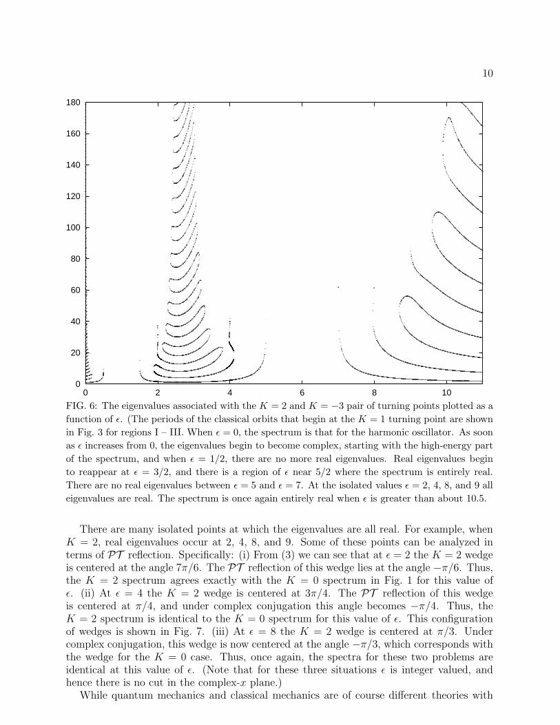
FIG. 6: The eigenvalues associated with the K = 2 and K = −3 pair of turning points plotted as a

function of ǫ. (The periods of the classical orbits that begin at the K = 1 turning point are shown

in Fig. 3 for regions I – III. When ǫ = 0, the spectrum is that for the harmonic oscillator. As soon

as ǫ increases from 0, the eigenvalues begin to become complex, starting with the high-energy part

of the spectrum, and when ǫ = 1/2, there are no more real eigenvalues. Real eigenvalues begin

to reappear at ǫ = 3/2, and there is a region of ǫ near 5/2 where the spectrum is entirely real.

There are no real eigenvalues between ǫ = 5 and ǫ = 7. At the isolated values ǫ = 2, 4, 8, and 9 all

eigenvalues are real. The spectrum is once again entirely real when ǫ is greater than about 10.5.

There are many isolated points at which the eigenvalues are all real. For example, whenK = 2, real eigenvalues occur at 2, 4, 8, and 9. Some of these points can be analyzed interms of PT reflection. Specifically: (i) From (3) we can see that at ǫ = 2 the K = 2 wedgeis centered at the angle 7π/6. The PT reflection of this wedge lies at the angle −π/6. Thus,the K = 2 spectrum agrees exactly with the K = 0 spectrum in Fig. 1 for this value ofǫ. (ii) At ǫ = 4 the K = 2 wedge is centered at 3π/4. The PT reflection of this wedgeis centered at π/4, and under complex conjugation this angle becomes −π/4. Thus, theK = 2 spectrum is identical to the K = 0 spectrum for this value of ǫ. This configurationof wedges is shown in Fig. 7. (iii) At ǫ = 8 the K = 2 wedge is centered at π/3. Undercomplex conjugation, this wedge is now centered at the angle −π/3, which corresponds withthe wedge for the K = 0 case. Thus, once again, the spectra for these two problems areidentical at this value of ǫ. (Note that for these three situations ǫ is integer valued, andhence there is no cut in the complex-x plane.)

While quantum mechanics and classical mechanics are of course different theories with

11

K=2K=2

K=0 K=0

Im x

Re x

FIG. 7: The Stokes wedges for ǫ = 4 for the cases K = 0 and K = 2. Because the wedges are

complex conjugate pairs the spectra are identical for this value of ǫ.

different regimes of applicability, our investigation has shown that there are nonethelesssome correlations between the two. Regular classical behavior seems to correspond to acompletely real quantum spectrum, while chaotic classical behavior in the complex plane isassociated with either a partially complex spectrum or a complete absence of eigenvalues. Inthe systems we have studied, the onset of rapid and irregular variation in the periods of theclassical trajectories correlates precisely with the disappearance of all quantum eigenvaluesas the ground-state energy goes to infinity, while the end of the noisy region is associatedwith the gradual reappearance of a completely real spectrum. Within the region of rapidvariation some correlations can be observed, but they are less clear-cut and merit furtheranalysis.

Acknowledgments

We thank D. Darg for helpful discussions and D. Hook for programming assistance. CMBis supported by a grant from the U.S. Department of Energy.

[1] C. M. Bender and S. Boettcher, Phys. Rev. Lett. 80, 5243 (1998).

[2] C. M. Bender, S. Boettcher, and P. N. Meisinger, J. Math. Phys. 40, 2201 (1999).

[3] P. Dorey, C. Dunning, and R. Tateo, J. Phys. A: Math. Gen. 34, L391 (2001) and 34, 5679

(2001).

[4] C. M. Bender, D. C. Brody, and H. F. Jones, Phys. Rev. Lett. 89, 270401 (2002).

[5] C. M. Bender, J.-H. Chen, D. W. Darg, and K. A. Milton, J. Phys. A: Math. Gen. 39, 4219

(2006).

[6] C. M. Bender and D. W. Darg, J. Math. Phys. 48, 042703 (2007).

[7] M. Znojil, J. Phys.: Conference Series 128, 012046 (2008).