QUANTUM COMPUTING UNDER REAL-WORLD CONSTRAINTS: EFFICIENCY OF AN ENSEMBLE QUANTUM ALGORITHM AND FIGHTING DECOHERENCE BY GATE DESIGN A DISSERTATION SUBMITTED TO THE DEPARTMENT OF ELECTRICAL ENGINEERING AND THE COMMITTEE ON GRADUATE STUDIES OF STANFORD UNIVERSITY IN PARTIAL FULFILLMENT OF THE REQUIREMENTS FOR THE DEGREE OF DOCTOR OF PHILOSOPHY Cyrus Phiroze Master September 2005

Welcome message from author
This document is posted to help you gain knowledge. Please leave a comment to let me know what you think about it! Share it to your friends and learn new things together.
Transcript
QUANTUM COMPUTING UNDER REAL-WORLD
CONSTRAINTS: EFFICIENCY OF AN ENSEMBLE QUANTUM
ALGORITHM AND FIGHTING DECOHERENCE BY GATE
DESIGN
A DISSERTATION
SUBMITTED TO THE DEPARTMENT OF ELECTRICAL
ENGINEERING
AND THE COMMITTEE ON GRADUATE STUDIES
OF STANFORD UNIVERSITY
IN PARTIAL FULFILLMENT OF THE REQUIREMENTS
FOR THE DEGREE OF
DOCTOR OF PHILOSOPHY
Cyrus Phiroze Master
September 2005
c© Copyright by Cyrus Phiroze Master 2005
All Rights Reserved
ii
I certify that I have read this dissertation and that, in my opinion, it
is fully adequate in scope and quality as a dissertation for the degree
of Doctor of Philosophy.
Yoshihisa Yamamoto Principal Adviser
I certify that I have read this dissertation and that, in my opinion, it
is fully adequate in scope and quality as a dissertation for the degree
of Doctor of Philosophy.
Jelena Vuckovic
I certify that I have read this dissertation and that, in my opinion, it
is fully adequate in scope and quality as a dissertation for the degree
of Doctor of Philosophy.
Colin Williams
Approved for the University Committee on Graduate Studies.
iii

Abstract
Quantum algorithms for problems such as integer factorization and database search
have spurred great interest in quantum computation. However, the construction
of scalable quantum computers has proved to be extremely difficult. Among the
challenging requirements that must be fulfilled in the “standard model” of quantum
computation, one must be able to initialize qubits into known pure states. In addition,
quantum computers must be protected from noise due to unwanted interactions with
their environment.
This work is concerned with two theoretical issues motivated by these difficulties.
First, I analyze the efficiency of an algorithm for an alternate model for quantum
computation that is motivated by bulk nuclear magnetic resonance. In such ensemble
systems, the initial state is not a fiducial pure state, but is instead a maximally-mixed
density operator. Although this constraint limits the power of such nuclear magnetic
resonance quantum computers, there still may exist algorithms that yield significant
computational speedup compared to “classical” computers. As one possibility, the
algorithm that I consider allows one to estimate the free energy of arbitrary spin-1/2
lattice models. To determine the efficiency of this algorithm, I calculate the compu-
tation time required to estimate the free energy to bounded error via the quantum
algorithm as a function of the lattice size. In the absence of stochastic fluctuations
in the measurement output, it is found that the algorithm is efficient. However, ev-
idence is presented that suggests that the algorithm becomes exponentially sensitive
to fluctuations as the lattice size increases.
iv
While rigorous techniques such as quantum error-correcting codes and decoherence-
free subsystem encodings have been devised to mitigate errors due to unwanted en-
vironmental couplings, these methods generally require many additional qubits or
complicated encodings. Here, I investigate a simple approach to reduce errors in
the quantum search algorithm due to a specific collective decoherence model. This
method takes advantage of the freedom inherent in compiling the search algorithm
into fundamental gates. Simple transition rate calculations and more rigorous quan-
tum master equation simulations are carried out for small-qubit instances to contrast
the performance of the original and modified algorithm. It is shown that the ex-
pected computational effort can be reduced by 22% for selected five-bit instances of
the quantum search algorithm. While this approach does not constitute a general
strategy for quantum error-correction, it illustrates the importance of judicious gate
design in mitigating decoherence.
v

Acknowledgments
I have been helped in so many ways by so many people over the past seven years
that an exhaustive list of acknowledgments would be, frankly, exhausting. I would of
course like to thank my family, my friends, and my colleagues for their support, their
advice, and the inspiration that they have given. However, I would like to single out
a few individuals who have had a special impact on my graduate career.
I am always amazed by the creativity and the scope of knowledge of my advi-
sor, Yoshi Yamamoto. I thank him most for his compassion, his support and his
encouragement during the difficult times in my graduate career.
I have been privileged to work with many bright and talented colleagues in the
Yamamoto group. I am most indebted to Fumiko Yamaguchi, Will Oliver and Thad-
deus Ladd. All three served as role models and mentors, and by watching them, I
learned how research should be done.
In my seven years at Stanford, I learned more about life than about physics, and
for this I am indebted to my parents, Jocelyn Plant and Chris and Raka Mitra.
Several of these names bear repeating for their efforts in reading through my
thesis and offering insightful comments. I am grateful to Thaddeus, Fumiko, Chris,
Raka and Patrik Recher for their help. I also thank my committee, Profs. Shanhui
Fan, Hari Manoharan, Jelena Vuckovic and Colin Williams for their comments and
questions.
Finally, I would like to thank the PACCAR Inc. Stanford Graduate Fellowship
for financial support during my first three years at Stanford.
vi

Contents
Abstract iv
Acknowledgments vi
1 Introduction 1
1.1 The big picture . . . . . . . . . . . . . . . . . . . . . . . . . . . . . . 1
1.2 Classical complexity theory . . . . . . . . . . . . . . . . . . . . . . . 6
1.2.1 Algorithms and Turing machines . . . . . . . . . . . . . . . . 6
1.2.2 Boolean circuits . . . . . . . . . . . . . . . . . . . . . . . . . . 10
1.3 Extrapolation to quantum circuits . . . . . . . . . . . . . . . . . . . . 12
1.4 Essential resources for quantum computation . . . . . . . . . . . . . . 16
1.5 Bulk nuclear magnetic resonance quantum computation . . . . . . . . 18
1.5.1 The density operator and mixed states . . . . . . . . . . . . . 18
1.5.2 Overview of NMR QC . . . . . . . . . . . . . . . . . . . . . . 21
1.6 Techniques to combat errors in the circuit model . . . . . . . . . . . . 27
1.6.1 Quantum error-correction . . . . . . . . . . . . . . . . . . . . 28
1.6.2 Decoherence-free subspaces . . . . . . . . . . . . . . . . . . . . 34
1.6.3 Dynamical decoupling . . . . . . . . . . . . . . . . . . . . . . 37
2 Quantum algorithms 39
2.1 Algorithms under the standard model . . . . . . . . . . . . . . . . . . 39
2.1.1 Deutsch-Jozsa problem . . . . . . . . . . . . . . . . . . . . . . 39
2.1.2 Quantum search and amplitude amplification . . . . . . . . . 43
2.1.3 Quantum Fourier transform . . . . . . . . . . . . . . . . . . . 48
vii
2.1.4 Phase-estimation algorithm . . . . . . . . . . . . . . . . . . . 50
2.1.5 Order finding and the factoring algorithm . . . . . . . . . . . 54
2.2 Ensemble Algorithms . . . . . . . . . . . . . . . . . . . . . . . . . . . 57
2.2.1 Models for Ensemble QC . . . . . . . . . . . . . . . . . . . . . 57
2.2.2 DQC1 algorithms . . . . . . . . . . . . . . . . . . . . . . . . . 62
3 Efficiency of free energy calculations in DQC1 71
3.1 Overview . . . . . . . . . . . . . . . . . . . . . . . . . . . . . . . . . . 71
3.2 Assumptions . . . . . . . . . . . . . . . . . . . . . . . . . . . . . . . . 75
3.3 Algorithm structure and discretization . . . . . . . . . . . . . . . . . 76
3.4 Error analysis: broadening . . . . . . . . . . . . . . . . . . . . . . . . 80
3.5 Error analysis: stochastic errors . . . . . . . . . . . . . . . . . . . . . 84
3.6 Summary and discussion of ensemble algorithms . . . . . . . . . . . . 88
4 Fighting decoherence by gate decomposition 90
4.1 Overview . . . . . . . . . . . . . . . . . . . . . . . . . . . . . . . . . . 90
4.2 Collective dissipation . . . . . . . . . . . . . . . . . . . . . . . . . . . 92
4.3 Modifying the quantum search algorithm . . . . . . . . . . . . . . . . 98
4.4 Simulation data for the collective enhancement factor . . . . . . . . . 101
4.5 Quantum master equation . . . . . . . . . . . . . . . . . . . . . . . . 109
4.6 Summary . . . . . . . . . . . . . . . . . . . . . . . . . . . . . . . . . 115
A Collective angular momentum states 117
B Elementary number theory 122
C Proof of broadening function lemmas 128
D Gray-code decomposition 133
E Fundamental-gate matrix elements 136
F Additional data 139
viii

List of Tables
4.1 The percent reduction in the number of expected iterations for the
modified five-bit search algorithm in comparison to the original algo-
rithm, as a function of the rate parameter ν0. The percentages are
averaged over all possible target states. . . . . . . . . . . . . . . . . . 114
F.1 The gate-averaged collective enhancement factor γ1 for selected in-
stances of the original and modified quantum search algorithm. . . . . 139
ix
List of Figures
1.1 A flowchart for Euclid’s algorithm. . . . . . . . . . . . . . . . . . . . 7
1.2 A simple example of a Boolean circuit using a set of primitive elements. 11
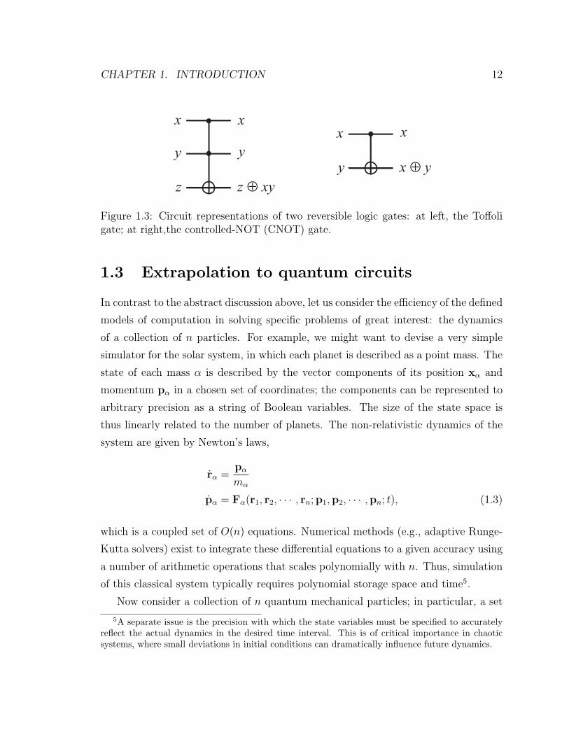
1.3 Circuit representations of two reversible logic gates. . . . . . . . . . . 12
1.4 Circuit to perform syndrome detection and recovery for the bit-flip code. 31
2.1 An n + 1 qubit circuit to show that a single invocation of Uq acts a
query of q(x). . . . . . . . . . . . . . . . . . . . . . . . . . . . . . . . 41
2.2 A circuit representation of the Deutsch-Josza algorithm. . . . . . . . 42
2.3 Quantum circuit for the n-qubit QFT. . . . . . . . . . . . . . . . . . 49
2.4 Circuit illustrating phase kickback. . . . . . . . . . . . . . . . . . . . 50
2.5 Phase-estimation algorithm. . . . . . . . . . . . . . . . . . . . . . . . 52
2.6 Parker-Plenio algorithm 1 . . . . . . . . . . . . . . . . . . . . . . . . 64
2.7 Parker-Plenio algorithm 2 . . . . . . . . . . . . . . . . . . . . . . . . 65
3.1 Schematic overview of the free-energy calculation by iterations of the
DQC1 algorithm. . . . . . . . . . . . . . . . . . . . . . . . . . . . . . 77
4.1 An example of two equivalent decompositions of the same overall uni-
tary operation. . . . . . . . . . . . . . . . . . . . . . . . . . . . . . . 91
4.2 The collective enhancement factor j(j + 1)−m(m− 1) for n = 8. . . 96
4.3 Probability weights∑
α |aj,m,α|2 for selected eight-qubit states. . . . . 97
4.4 A circuit to implement the U0 unitary operator on the n “data” qubits. 102
4.5 Collective enhancement for the original seven-bit search algorithm with
one ancillary qubit; the target state is |0000000〉. . . . . . . . . . . . . 105
x
4.6 Collective enhancement for the modified seven-bit search algorithm
with one ancillary qubit; the target state is again |0000000〉. . . . . . 106
4.7 Collective enhancement for the (a) original and (b) modified seven-bit
search algorithm with one ancillary qubit; the target state is |0001111〉. 108
4.8 Result of integration of the quantum master equation for the five-bit
search algorithm with target state |0〉 and ν0 = 5× 10⁻⁴. . . . . . . . 112
4.9 Result of integration of the quantum master equation for the five-bit
search algorithm with target state |31〉 and ν0 = 5× 10⁻⁴. . . . . . . 114
A.1 Collective angular momentum states for n = 2, 3, 4. . . . . . . . . . . 118
D.1 Gray-code circuit for the n-controlled-NOT for n = 3. . . . . . . . . 135
F.1 Comparison of quantum master equation calculations for the 5-bit
search algorithm, in which ν0 = 5× 10⁻⁴ inverse gate times. . . . . . 140
F.2 Similar to Fig. F.1, but in which ν0 = 2× 10⁻⁴ inverse gate times. . . 140
F.3 Similar to Fig. F.1, but in which ν0 = 1× 10⁻⁴ inverse gate times. . . 141
F.4 Similar to Fig. F.1, but in which ν0 = 5× 10⁻⁵ inverse gate times. . . 141
F.5 Similar to Fig. F.1, but in which ν0 = 2× 10⁻⁵ inverse gate times. . . 142
F.6 Similar to Fig. F.1, but in which ν0 = 1× 10⁻⁵ inverse gate times. . . 142
F.7 Similar to Fig. F.1, but in which ν0 = 5× 10⁻⁶ inverse gate times. . . 143
xi
Chapter 1
Introduction
1.1 The big picture
Measured on the canonical time-scale of a graduate-student lifetime, the field of quan-
tum computation (QC) has developed astoundingly quickly. The attention (and fund-
ing) focused on the field may be puzzling to the newcomer, as non-relativistic quan-
tum mechanics is hardly a new theory. Why, then, all the excitement? Among the
principal reasons are the following:
• Quantum computation is interdisciplinary. At the interface between physics,
computer science, mathematics and engineering, the field is accessible and in-
teresting to a wide range of researchers.
• Quantum computers might be powerful. Quantum computers offer a credible
challenge to the strong Church-Turing thesis, as there exist efficient algorithms
for which there are no classical counterparts. In addition, investigating the
power of quantum computers may even tell us something about the hierarchy
of “classical” computational complexity classes.
• Real experiments are plausible. Control and measurement of quantum systems
are possible in several contexts, including spin resonance and spintronics, atomic
physics involving ions and neutral atoms, optics and cavity quantum electrody-
namics, and superconductivity.
CHAPTER 1. INTRODUCTION 2
Nonetheless, engineering a physical system for scalable quantum computing has
proven to be extremely difficult. A ubiquitous problem is the need to limit sources
of error (i.e., noise) below levels that can be handled by error-correction techniques.
Error-correction demands a substantial increase in the amount of resources required to
implement a given algorithm, both in the number of qubits as well as the computation
time. The need to initialize, couple, and measure qubits implies the need for precise
experimental control of otherwise nearly-isolated quantum systems.
Although this thesis work is theoretical, it is motivated by such real-world diffi-
culties. The first of these is the problem of initializing nuclear-spin states, which is
an obstacle for the scalability of quantum computers based upon nuclear magnetic
resonance (NMR). Although spin-1/2 nuclei are attractive candidates for qubits due
to their relative isolation and their controllability by radio-frequency radiation, they
are not easily initialized to pure states due to the typically small energy splitting be-
tween spin states. Thus, it is of interest to consider models for quantum computation
that do not require such initialization, and to inquire whether useful algorithms can
be devised for such models. If so, they would be ideally applied to NMR quantum
computation.
The second motivating real-world problem is decoherence due to undesirable in-
teractions between a quantum computer and its environment. While techniques exist
to robustly identify and correct errors, these methods generally come at the cost of
additional required resources, such as ancillary qubits, or rapidly-applied measure-
ments or control pulses. These additional resources may be infeasible for a modest
“testbed” quantum computer, for which only a few two-level qubits are accessible. It
is of interest to inquire whether decoherence can be mitigated by simpler techniques.
The following is an overview of the structure of this thesis. The initial chapter
reviews the myriad topics required to discuss both of the above motivating issues in
further detail. Before delving into the subtleties of quantum computation, it is neces-
sary to formalize the notation of computation itself. To this end, this chapter reviews
salient results in classical complexity theory, including universal Turing machines,
complexity classes and reduction, and circuit models. An extension of the circuit
model is a natural formalism to define a quantum computer, and forms the basis of

CHAPTER 1. INTRODUCTION 3
the “standard model” for quantum computation. As part of this thesis work is moti-
vated by the restrictions of bulk liquid-state NMR quantum computers, this physical
system is described in Sec. 1.5. Finally, a review of error-correcting techniques is
presented in Sec. 1.6, including quantum error-correcting codes, decoherence-free
subspaces/subsystems, and dynamical decoupling.
The second chapter is concerned with quantum algorithms. The first part of the
chapter introduces quantum algorithms under the standard model of quantum com-
putation, where the quantum computer is initialized to a fiducial pure state. In the
second part, I discuss a computational model formalized by Knill and Laflamme for
ensemble quantum computation. A standard-model quantum computer differs from
this so-called “DQC1 model” in the description of the initial state. In the former
case, all qubits are initialized to a fiducial pure state. By contrast, for the latter
case, all qubits are initially in a maximally-mixed state, with the exception of a sin-
gle pure-state qubit. By virtue of the small energy splitting between spin states of
spin-1/2 nuclei, it is much easier for the experimentalist to satisfy the initialization
requirements of DQC1 than the standard model. Simply thermalizing a collection of
spin-1/2 to a “hot” reservoir suffices to create a maximally-mixed state1. By compar-
ison, the standard model demands that the qubits be “cooled” prior to computation,
which is a daunting task.
The problem with the DQC1 model is that it is distinctly weaker than the stan-
dard model; there are quantum algorithms for the standard model that cannot be
performed efficiently with only one initial pure-state qubit. However, this does not
forbid some applications for which the DQC1 model can outperform a classical com-
puter. Finding such examples of computational speedup for DQC1, aside from being
interesting in their own right, might help to quantify the resources necessary to dif-
ferentiate quantum computers from classical models of computing. At the end of
Chap. 2, I discuss examples of DQC1 algorithms from the literature, and comment
on their efficiency. One example discussed in Sec. 2.2.2 is an algorithm to investigate
quantum chaos that has no known efficient classical counterpart.
1How one may then “create” the single pure-state qubit is a topic to be explored in Sec. 1.5.

CHAPTER 1. INTRODUCTION 4
In Chap. 3, I propose a novel application of a DQC1 algorithm to compute the
free energy of arbitrary spin-lattice hamiltonians. An efficient means to compute
the free energy of such many-body systems would provide a computational tool to
investigate their thermodynamic properties and critical behavior. In this sense, the
quantum algorithm is a “simulator” that could be used to glean information about
a complicated many-body physical system. To determine the efficiency of the algo-
rithm, I quantify the computation time required as a function of the simulated-lattice
size. In doing so, I assume that we have available a somewhat-ideal DQC1 quantum
computer, in the sense that we may use error-correction techniques to eliminate errors
due to faulty gates or environmentally-induced decoherence. Interestingly, I find that
the efficiency of the algorithm is dependent upon the structure of the energy spec-
trum for a given spin-lattice model and the exponential character of the Boltzmann
distribution. By applying the algorithm to a few simple spin models that can also be
solved analytically, I show that the free-energy calculation is not efficient, in general.
Although this result does not allow us to reach a concrete conclusion regarding the
power of the DQC1 model, the relationship between the algorithm efficiency and the
functional form of the distribution function is intriguing.
Chap. 4 is concerned with the problem of decoherence due to unwanted cou-
plings of qubits with the environment. In the standard model, the unitary evolution
prescribed by an algorithm is carried out as a sequence of elementary gates. This
sequence is by no means unique; for a given algorithm, a continuum of possible de-
compositions (i.e., compilations) may exist. It is assumed that each elementary gate
is derived by external control of the hamiltonian that couples the qubits, allowing
time evolution of the system under the desired coupling. As the quantum computer
evolves in time, the collection of qubits traces out a path in its state space that de-
pends upon the sequence of gates. In the absence of decoherence, all trajectories lead
to the same final state. However, if there is undesired system-environment coupling,
the final state is erroneous. Furthermore, the error depends upon the chosen tra-
jectory, and thus the gate compilation. Given a particular algorithm, a set of basic
gates, and a model for the system-environment interaction, it is of interest to ask
whether the gate compilation can be altered to mitigate the impact of decoherence.
CHAPTER 1. INTRODUCTION 5
To be more precise, by modifying the gate sequence for a given algorithm, can we
improve the probability that the final measurement yields the correct answer? If so,
by increasing the probability of success, the number of times that the algorithm must
be repeated (and thus the expected computation time) decreases.
Clearly, the answer to this question depends intimately upon the particular deco-
herence model and the algorithm in question. As an illustration of the principle, in
Chap. 4, I examine the quantum search algorithm under a specific model of collec-
tive dissipation. This model is applicable if the dominant decoherence mechanism for
the qubits is the exchange of energy with a reservoir of long-wavelength boson (e.g.,
phonon) modes. I show by simulations for small-qubit systems that a small variation
in the compilation strategy can lead to a modest improvement in the success probabil-
ity of the algorithm. The intuition for this improvement arises from the geometrical
nature of the quantum search algorithm as a rotation in a specific two-dimensional
subspace. There is sufficient freedom in the gate compilation to allow us to choose
the specific two-dimensional subspace. For the selected form of system-environment
coupling, the rate at which energy is exchanged with the reservoir is highly state-
dependent, and the gate compilation can be chosen to steer us towards “subradiant”
states2.
It should be emphasized that this strategy cannot constitute a scalable method of
error-correction. However, it does emphasize the fact that the intrinsic physical in-
teractions coupling qubits to their environment should play a role in determining how
sequences of gates should be composed. Furthermore, we might envision a testbed
quantum computer, composed of a few tens of qubits, for which the overhead required
to implement error-correcting codes is steep. In other words, if we redundantly en-
code each qubit using five physical two-level systems, we may not have many logical
qubits to work with. In such a case, an alternative means to mitigate decoherence is
advisable, such as the scheme described in Chap. 4.
In this thesis, I have made an effort to present the body of the text in prose
and relegate detailed theorems to the appendices. Part of the reason that I chose this
2There is a close connection between this strategy and that of decoherence-free subspaces. Inthe former, we try to stay “near” the decoherence-free subspace without losing qubits by explicitencoding.

CHAPTER 1. INTRODUCTION 6
approach is to render the dissertation more accessible to students and researchers who
are not experts in the field. Also, it reflects my own historical approach to the subject
matter. As an electrical engineer who slowly evolved into a physicist, at first glance I
find a discussion of concepts to be more illuminating than mathematical exposition.
Nonetheless, at the end of the day, you can’t let the text write checks that your math
can’t cash, and as such, necessary details can be found in the appendices.
1.2 Classical complexity theory
Computation models, algorithms and complexity theory are large fields that are
treated here briefly. Excellent references for a more complete treatment include Pa-
padimitriou [1], Cormen et al. [2] and Knuth [3]; also see Nielsen and Chuang [4] and
Aharonov [5] for issues relevant to quantum computation.
1.2.1 Algorithms and Turing machines
An algorithm is a finite sequence of precisely-defined, simple tasks on a set of inputs
that yield the solution to an interesting problem as output. One classic example is
Euclid’s algorithm (Fig. 1.1), which computes the greatest common divisor of two
positive integers a and b. A sequence of arithmetic operations on the inputs a and b,
often conditional on the results of previous tasks in the sequence, yields the greatest
common divisor as output after a finite number of steps.
The utility of an algorithm is characterized by its complexity, which quantifies the
resources required to complete the sequence of tasks. In particular, how long does
an algorithm take to solve a problem as a function of the input size, and how much
workspace do we need to generate the answer? In the case of Euclid’s algorithm,
we might specify the input length by the number of digits n required to write down
both a and b. Algorithms for which the execution time is lower bounded by a polyno-
mial function of n [poly(n)] for asymptotically large n are labeled as efficient, while
problems for which no efficient algorithms are known are hard or intractable. In some
sense, this distinction is arbitrary; one may argue whether a running time of 10100n500

CHAPTER 1. INTRODUCTION 7
input a,b
a > b ?b = 0 ? a = 0 ?return a
compute a mod b
a mod b → a
return b
compute b mod a
b mod a → b
YES NOYES YES
NONO
Figure 1.1: A flowchart for Euclid’s algorithm, illustrating a sequence of tasks to findthe greatest common divisor of two positive integers a and b.
is preferable to 1.1n. However, this classification upholds two reasonable properties.
First, an arbitrary choice of how to write the input (e.g., binary versus decimal rep-
resentation of a and b) will not affect the tractability of a problem, as any reasonable
encoding of the input will only alter its size by a poly(n) factor. Second, the composi-
tion of efficient algorithms is itself efficient. For instance, Euclid’s algorithm requires
a number of arithmetic operations that is polynomial in n. If it is known that each
arithmetic operation requires poly(n) time, then the overall algorithm is efficient, as
polynomials are closed under composition. This property is very useful, as it allows
efficient complicated algorithms to be constructed from black-box subroutines.
To quantify how resources such as computation time scale with the problem size
n in the limit of large n, we adopt the following standard notation. Assume that
the computation time equals some function f(n). We characterize f(n) as O[g(n)]
(“order g of n”) if there exists a positive integer n0 and positive c such that
f(n) ≤ cg(n), ∀n > n0. (1.1)
The function g(n) gives us a leading-order upper bound for f(n). For example,
consider f(n) = 2n4 + 3n3 − 2n2 + 1 + log n. For large n, the first term dominates,
and f(n) = O(n4). To show that an algorithm is efficient, we must demonstrate that

CHAPTER 1. INTRODUCTION 8
its running time is is O[poly(n)].
Similarly, f(n) is denoted Ω[g(n)] if
f(n) ≥ cg(n), ∀n < n0. (1.2)
The Ω notation describes a lower bound on f(n). We denote f(n) = Θ[g(n)] if both
f(n) = O[g(n)] and f(n) = Ω[g(n)].
A discussion of algorithms is necessarily vague without a formal definition of a
“computer;” i.e., a model for the machine on which an algorithm is implemented.
Of seminal importance, both historically and also for its generality, is the Turing
machine [6] (also, see Ref. [1]). The Turing machine consists of an infinite tape, a
read-write head pointed to a particular location on the tape, a finite internal memory,
and a program; the last of these specifies a given algorithm. The tape is initialized
with a sequence of symbols from a finite-sized alphabet Σ; the initial configuration
of the tape is the machine’s input, and the final configuration yields the output. The
internal state of the machine is an element of a set Q, which includes a “start” state
qs and a “halt” state qh. The program is a function fT : Σ×Q→ Σ×Q× ←,→,in which the final set is an instruction for the read-write head to move either left
or right. Each Turing machine is characterized by its program fT ; we can uniquely
identify all functions, and thus the associated Turing machines, by an integer label
T . Operation of the Turing machine commences by initializing the internal memory
to qs and providing a tape with the input state. In successive time steps, the Turing
machine applies the function fT , stopping if the internal state is qh.
Turing machines would not be particularly interesting if a new one needed to be
created for every possible program fT of interest. Remarkably, one can construct a
universal Turing machine that can mimic the operation of any Turing machine. To be
precise, assume that we wish to compute the output that Turing machine T provides
for a given string s on its input tape. A universal Turing machine can be described
that, given both T and s as input, generates this output. In this sense, the universal
Turing machine is a general-purpose computer. It allows us to define a notion of
computability: any function that can be evaluated on a universal Turing machine is

CHAPTER 1. INTRODUCTION 9
computable. It is remarkably straightforward to show that uncomputable functions
exist. One such example is the so-called halting function h(T, s); h = 1 if machine T
ever halts given input s, and h = 0 if the program does not terminate.
Turing machines are by no means the only model for computation. However, the
Church-Turing thesis posits that a function that is computable by any “physically
reasonable” model is also computable by a Turing machine, and vice-versa. For
example, consider a probabilistic universal Turing machine, which has as an additional
resource an arbitrary number of random binary digits (bits). At a given time step, the
program may select a random bit and branch depending on the outcome. However,
the additional random bits confer no additional power, as a deterministic universal
Turing machine can compute all possible outcomes by running the program for all
possible branches. No counterexample of the Church-Turing thesis has been found
as yet. Indeed, such a discovery would be revolutionary, as it could yield solutions
to problems that are not only intractable, but completely incomputable by currently-
known means.
The original Church-Turing thesis only concerns itself with computability, and
does not make any claims regarding the time required for differing models to evaluate
a computable function. A more stringent claim is the modern or strong Church-Turing
thesis, which conjectures that the computation time required by any reasonable model
of computation is “polynomially equivalent” to a probabilistic universal Turing ma-
chine. In other words, it is conjectured that the number of time steps required by the
Turing machine is at most a polynomial function of the time required by any other
physically reasonable model. If true, the strong Church-Turing thesis implies that the
tractability of a problem is completely independent of the computation model used to
attack it. It is the strong Church-Turing thesis that quantum computation calls into
question, by yielding efficient algorithms for problems that are traditionally (though
not provably) thought to be hard on a probabilistic Turing machine.
There exists a large hierarchy of classes [1] to codify the complexity of various
problems3. Some important selections include P (polynomial), which includes all
3Scott Aaronson has compiled a staggering listing of complexity classes on the websitehttp://www.complexityzoo.com.
CHAPTER 1. INTRODUCTION 10
decision problems that can be solved in polynomial time by a Turing machine; NP
(non-deterministic polynomial), which roughly describes decision problems for which
a given solution can be verified to be correct efficiently, but not necessarily easy to
find that solution; and BPP4 (bounded-error probability polynomial), which includes
decision problems for which efficient solutions may be found by a universal Turing
machine with probability 2/3.
To contrast the power of quantum computers with their “classical” counterparts,
it is possible to define a quantum Turing machine [7, 8]. However, the formalism of
a quantum Turing machine is cumbersome, due in part to a formal description of
the infinite-length tape. It is decidedly more convenient to start from an alternative
model of computation that is described in the following section.
1.2.2 Boolean circuits
A Boolean circuit is a network of Boolean gates that performs logic operations on a
set of binary inputs. Formally, it is a directed acyclic graph, in which the number
of inputs to each node is at most two. Each edge (”wire”) encodes a binary value.
At each node (or ”gate”), the output edges are Boolean functions of the input edges.
The outputs of the circuit are each the binary values at the sinks of the graph. The
size of a circuit is given by the number of gates, or nodes.
Provided that the circuits are uniform (i.e., they can be constructed efficiently
by a universal Turing machine), there is an equivalence between the circuit model
and universal Turing machines. A problem in BPP can be solved by a polynomial-
sized family of circuits, and conversely, any polynomial-sized circuit can be simulated
efficiently on a universal Turing machine.
Part of the pedagogical appeal of the circuit model is that arbitrary computable
functions can be constructed out of a finite set of primitive circuit elements. One
common set [4] consists of wires, ancillary bits initialized to either logical state 0 or 1,
the FANOUT gate that copies one bit to two, a gate to exchange two input bits, and
4The factor 2/3 is somewhat arbitrary; if the probability of success is a constant larger than1/2 that does not diminish with problem size, by the Chernoff bound [1], a polynomial number ofrepetitions and a majority vote can amplify the success probability to 2/3.

CHAPTER 1. INTRODUCTION 11
FANOUT × 3
FANOUT × 3
x
y
x ⊕ y
Figure 1.2: A simple example of a Boolean circuit using a set of primitive elements;the output is the exclusive OR of the inputs x and y. The “D” shaped elements areNAND gates. Circuit elements are applied from left to right.
the NAND gate, which is the composition of the Boolean NOT and AND gates. By
convention, inputs enter from the left, and gates are applied in sequence to generate
the output at right. As an example, a circuit that computes the sum of two binary
inputs is shown in Fig. 1.2. The complexity of a quantum circuit can be assessed by
the number of gates or circuit depth.
Landauer [9] showed that there is an intimate connection between the erasure of
information and the dissipation of energy by a logic gate. For example, the NAND
gate, which eliminates one bit of information from its inputs, leads to a concomitant
minimum energy loss of kBT ln 2 to the environment. However, computation does
not have to be dissipative. A circuit can use only reversible gates with no loss in
computational power [10, 11] given poly(n) scratch bits. The ancillary bits store the
information required to undo the computation.
For instance, an AND gate, which is irreversible, can be performed reversibly
via a Toffoli gate (controlled-controlled-NOT gate), if an ancillary qubit in logical
state zero is used. The Toffoli gate (Fig. 1.3) maps the Boolean triplet (x, y, z)
to (x, y, z ⊕ xy), which can be undone by a second Toffoli gate; here, the symbol
⊕ denotes an exclusive-OR. The NOT and FANOUT gates can be constructed by
applying the Toffoli gate to (1, 1, x) and (1, x, 0). The reversible implementation of
each irreversible gate requires an ancillary qubit; this spatial requirement is reasonable
if the circuit is polynomial-sized.
CHAPTER 1. INTRODUCTION 12
x
y
z
x
y
z ⊕ xy
x
y
x
x ⊕ y
Figure 1.3: Circuit representations of two reversible logic gates: at left, the Toffoligate; at right,the controlled-NOT (CNOT) gate.
1.3 Extrapolation to quantum circuits
In contrast to the abstract discussion above, let us consider the efficiency of the defined
models of computation in solving specific problems of great interest: the dynamics
of a collection of n particles. For example, we might want to devise a very simple
simulator for the solar system, in which each planet is described as a point mass. The
state of each mass α is described by the vector components of its position xα and
momentum pα in a chosen set of coordinates; the components can be represented to
arbitrary precision as a string of Boolean variables. The size of the state space is
thus linearly related to the number of planets. The non-relativistic dynamics of the
system are given by Newton’s laws,
rα =pα
mα
pα = Fα(r1, r2, · · · , rn;p1,p2, · · · ,pn; t), (1.3)
which is a coupled set of O(n) equations. Numerical methods (e.g., adaptive Runge-
Kutta solvers) exist to integrate these differential equations to a given accuracy using
a number of arithmetic operations that scales polynomially with n. Thus, simulation
of this classical system typically requires polynomial storage space and time5.
Now consider a collection of n quantum mechanical particles; in particular, a set
5A separate issue is the precision with which the state variables must be specified to accuratelyreflect the actual dynamics in the desired time interval. This is of critical importance in chaoticsystems, where small deviations in initial conditions can dramatically influence future dynamics.

CHAPTER 1. INTRODUCTION 13
of n interacting spin-1/2 particles. Considering only the spin degree of freedom, the
state of the system can be described by the coefficients cα of a complex vector in
a 2n dimensional Hilbert space, each labeling a possible up or down spin configura-
tion along a given axis. The dynamics is the system are specified by Schrodinger’s
equation,
cα = −in∑
β=1
Hαβcβ, (1.4)
in which Hαβ are the matrix elements of the spin hamiltonian. Like Eq. 1.3, Eq. 1.4
is a coupled set of differential equations. Unlike Eq. 1.3, the number of equations
is exponential in n. No polynomial-sized circuit is known to solve this general set of
equations, and it seems unlikely that one could ever be found.
The simulation of quantum mechanics was an initial impetus for researchers to
propose using highly controllable quantum systems themselves as computers [12, 13].
Benioff [14] and Feynman [15] noted that unitary evolution of a quantum system
could perform reversible gate operations, and Deutsch [16] introduced a full quantum
circuit model of computation based on sequential unitary gates.
Each input to the circuit is a two-level quantum system (qubit), spanned by the
basis kets |0〉 and |1〉. Thus, the state of a collection of n qubits is a vector6 in a 2n
dimensional Hilbert space spanned by the basis states
|0〉 ⊗ |0〉 ⊗ · · · ⊗ |0〉 ⊗ |0〉 ⊗ |0〉 ,
|0〉 ⊗ |0〉 ⊗ · · · ⊗ |0〉 ⊗ |0〉 ⊗ |1〉 ,
|0〉 ⊗ |0〉 ⊗ · · · ⊗ |0〉 ⊗ |1〉 ⊗ |0〉 ,...
|1〉 ⊗ |1〉 ⊗ · · · ⊗ |1〉 ⊗ |1〉 ⊗ |1〉 . (1.5)
An example of these input basis states may be abbreviated as |00 · · · 011〉, or even
more compactly as |3〉, where the underline implies that the qubit state is given by
the binary expansion of the notated integer. Consider a subsystem of three qubits.
6At this point, we consider only pure states, and defer discussion of mixed states to Sec. 1.5.1.

CHAPTER 1. INTRODUCTION 14
If we can control the unitary dynamics of the subsystem by open-loop control of the
hamiltonian, we could implement a Toffoli gate via the unitary operator
1 0 0 0 0 0 0 0
0 1 0 0 0 0 0 0
0 0 1 0 0 0 0 0
0 0 0 1 0 0 0 0
0 0 0 0 1 0 0 0
0 0 0 0 0 1 0 0
0 0 0 0 0 0 0 1
0 0 0 0 0 0 1 0
; (1.6)
the matrix representation is written in the input basis. The output of the computation
must consist of the measurement of an observable; generally, this may be a projective
measurement in the input basis, which we then refer to as the computational basis.
Note that this quantum network model subsumes the reversible circuit model in
Sec. 1.2.2. If we initialize the qubits in a fixed computational basis state and apply
Toffoli gates, the output from projective measurement is equivalent. We therefore
expect the quantum circuit model to be at least as powerful as deterministic classical
models for computation. Random bits can be simulated in the former by initializing
work qubits in the (|0〉+ |1〉)/√
2 superposition state; projective measurement at the
output yields logical states 0 or 1 with equal probability. Therefore, the quantum
circuit model is at least as powerful as BPP.
To contrast the two circuit models, one may first view the classical circuit model
as a Markov process. The input to the circuit is set to binary state x with probability
px (which is zero or one if we provide the circuit with an input deterministically);
the state of the system is a 2n dimension, real, nonnegative vector p of probabilities.
Each logic gate can be represented as a stochastic matrix M that maps the vector
p to Mp. Note that the entries of M are nonnegative, and probability conservation
demands that the columns of M sum to 1.
By contrast, the state in the quantum circuit model is a 2n dimensional complex
vector |ψ〉 of probability amplitudes. Each logic gate may also be represented as a

CHAPTER 1. INTRODUCTION 15
matrix U that maps |ψ〉 to U |ψ〉. By probability conservation, U must be unitary.
Like the probabilistic classical circuit model, the state of the quantum circuit is
characterized by a vector that evolves by linear transformations. The distinction
between the two arises from the fact that while the elements of M are constrained
to be nonnegative, no such constraint7 applies to U . This implies that unlike the
classical state vector, the quantum state can undergo constructive and destructive
interference. This is a rather subtle distinction. Nonetheless, as we will see in Chap.
2, it enables the construction of quantum circuit families that yield efficient solutions
to problems for which no classical efficient algorithm is known8.
Analogous to classical circuits, quantum circuit families can be constructed from
a set of universal gates. A strict definition of a universal gate set S for quantum
circuits would demand that any unitary transformation on the 2n dimensional state
can be created by a sequence of elements of S. One such set is the controlled-NOT
(CNOT) gate, shown in Fig. 1.3, along with all possible two-dimensional SU(2)
transformations on single-qubit subsystems [16, 17]. Finite sets of universal gates
can be defined if a less stringent requirement of universality is adopted: the set S
is universal if any unitary operator U can be approximated by a sequence of gates
yielding the transformation U ′ such that |U − U ′| < ε for any nonnegative ε. By this
condition, virtually any two-qubit gate is universal [18, 19]. In either case, we will
refer interchangeably to the elements of a universal gate set as basic, fundamental or
elemental gates.
We assume that the time complexity of a quantum circuit is given by the number
of basic gates. In reality, the strength of physical interactions that generate the ele-
mental gates may vary with the number of qubits n; as qubits become more distantly
spaced, the time required to generate a two-qubit gate may increase. If the interaction
7One might argue that as the elements of U are complex, nonnegativity is ill-defined. However,we could just as easily describe the quantum state as a 2n+1 dimension real vector, composed of thereal and imaginary parts of the complex probability amplitudes. In this case, the logic gates areorthogonal matrices whose elements are real, and may be positive or negative.
8However, it is interesting that the BQP class of problems — those which can be solved tobounded error with probability at least 2/3 by uniform quantum circuits — has not been proved tobe strictly larger than BPP. Thus, there remains the possibility that BPP = BQP, which wouldimply that all quantum algorithms that exhibit exponential speedup have undiscovered classicalanalogues.

CHAPTER 1. INTRODUCTION 16
strength falls at most polynomially with n, this represents only a polynomial increase
in the running time, and will not impact the efficiency of a given algorithm.
Several useful theorems have been developed to decompose or compile many-qubit
gates into basic gates. DiVincenzo [20] has given a decomposition of the Toffoli gate
into six CNOT gates and eight single-qubit gates. Barenco et al. [17] have shown that
a single-qubit operation that is conditional on another control qubit can be expressed
as a sequence of at most two CNOT gates and three single-qubit gates. As a corollary
of these two results, if there exists an efficient gate representation for a many-qubit
gate U , there also exists an efficient decomposition of a controlled-U gate.
DiVincenzo [21] formalized an oft-referenced set of resources required for a func-
tional quantum computer; we will refer to a slightly-modified and more restrictive
version as the standard model of quantum computation. These resources are:
• A physical system with well-characterized two-level systems, or qubits.
• The ability to initialize the state of the qubits to a simple fiducial state, suchas |0〉.
• Long relevant decoherence times relative to the gate operation time (see Sec.1.6).
• A universal set of quantum gates.
• A qubit-specific measurement capacity; here considered to be projective in thecomputational basis.
1.4 Essential resources for quantum computation
If quantum computers do violate the strong Church-Turing thesis, it is natural to
inquire as to which resources are fundamental in distinguishing them from a universal
Turing machine. Can the requirements for the standard circuit model be relaxed or
revised, or are they all essential to achieve exponential speedup relative to a universal
Turing machine?

CHAPTER 1. INTRODUCTION 17
One means to answer this question is to show that in the absence of a given
resource, the computation can be simulated by a standard Turing machine. One
such example has been given by Jozsa and Linden [22], who showed that a pure-
state quantum algorithm with limited entanglement can be simulated classically9.
Interestingly, their result may not hold for mixed states.
A second, reductive approach is to show that a resource is either replaceable or
not required by demonstrating the equivalence of two computational models. Exam-
ples include measurement-based schemes for quantum computation. In such models,
some or all unitary gates can be replaced by projective measurement in conjunction
with additional entangled ancillary qubits10. In this sense, unitary evolution is not
essential, as a model for quantum computation that is equivalent to the standard
model can be devised in its absence (given additional resources).
Lastly, a constructive method is to find an algorithm for an alternative compu-
tational model, and determine whether the resources required to solve a difficult
problem scale efficiently with the problem size. This approach will be used in Chap.
3. In Sec. 2.2.1, I consider an ensemble quantum computation model that requires
a different initialization scheme than the standard model. Although the alternative
model is distinctly weaker than the standard model, it may still prove to be more pow-
erful than a standard Turing machine. The model is motivated by nuclear magnetic
resonance, which is described in the following section.
9It is perhaps ambiguous to characterize such multi-partite entanglement as a resource, butrather as a necessary characteristic of any quantum computation with pure states that outperformsa classical algorithm.
10Gottesman and Chuang [23] showed that a two-qubit controlled-NOT gate could be performed asa Bell-state measurement with one ancillary qubit from an Einstein-Podolsky-Rosen (EPR) entangledpair, followed by single-qubit gates; this approach generalizes the notion of quantum teleportation[24]. It was subsequently shown [25, 26, 27] that any unitary gate can be performed to boundederror by two-qubit projective measurements and EPR pairs, precluding the need for any unitaryevolution. Raussendorf and Briegel [28] introduced the idea of a one-way quantum computer wherethe qubits are initially entangled as a so-called cluster state with a large number of ancillary qubits.In contrast with the teleportation schemes, where EPR pairs must be introduced at each gate, theone-way computer initially prepares the cluster state, and performs subsequent gates by projectivemeasurements. In either case, it is apparent that the resource of universal unitary gates can bereplaced by a set of projective measurements and specially-prepared entangled ancillary bits withno loss in computational power.
CHAPTER 1. INTRODUCTION 18
1.5 Bulk nuclear magnetic resonance quantum com-
putation
Proposals for liquid-state nuclear magnetic resonance (NMR) quantum computation
were first presented by Cory et al. [29] and Gershenfeld and Chuang [30]. However,
these schemes are not readily scalable due to the difficulty of initializing nuclear spins
to a fiducial pure state. One solution has been to use labeling techniques to mimic the
evolution of an initially-pure state. However, these methods, described below, suffer
from exponential signal loss as the number of qubits is increased. It is thus relevant
to inquire whether algorithms can be found for an “uninitialized” NMR quantum
computer that significantly outperforms a universal Turing machine. In Sec. 2.2.1,
I will discuss an ensemble quantum computational model introduced by Knill and
Laflamme that is motivated by the physical constraints of NMR proposals. It is first
useful to present an overview of bulk NMR quantum computation, prefaced by a
discussion of mixed states and the density operator. A more thorough discussion can
be found in the review by Cory et al. [31] or in the Ph.D. thesis of Vandersypen [32].
The physics of nuclear spins and the principles of NMR spectroscopy are described by
the texts of Abragam [33] and Ernst et al. [34], while Vandersypen and Chuang [35]
provide a contemporary review of control techniques for NMR quantum computation.
1.5.1 The density operator and mixed states
The density operator formalism is useful for describing an ensemble of identical quan-
tum systems. For example, assume that we are given an N -dimensional system whose
state preparation is stochastic; we receive state |ψi〉 with probability pi. If we per-
form a measurement of observable M , its expectation value is conditioned on the
probability distribution of the ensemble.
⟨M⟩
=∑
i
pi 〈ψi| m |ψi〉 = tr
(∑i
pi |ψi〉 〈ψi|
)= tr
(ρM), (1.7)
CHAPTER 1. INTRODUCTION 19
where we have defined the density operator
ρ =∑
i
pi |ψi〉 〈ψi| . (1.8)
We refer to ρ as a pure state if pi = 1 for any i, in which case the ensemble consists
of only one member. Otherwise, the state is mixed. Note that ρ is nonnegative,
hermitian, and has unity trace.
The ensemble generating ρ is not unique; as a result, different ensembles are
indistinguishable under the measurement of any observable. For example, consider
a complete basis set |φj〉, where j ∈ 1, 2, · · · , N. The resolution of the identity
operator I is given by a sum of projectors, so the maximally-mixed state can be
expressed as
ρ =I
N=
1
N
∑i
|φi〉 〈φi| ; (1.9)
the 1/N factor ensures that tr ρ = 1. As this result holds for any basis set, the
maximally-mixed state can be interpreted as any equiprobable mixture of complete
basis states.
The state of a closed system in thermodynamic equilibrium with a heat bath can
be compactly described by a density operator. Under the Boltzmann distribution,
each eigenstate |ψ`〉 of the hamiltonian H with eigenvalue E` occurs with relative
probability e−βE` ; here, β is the inverse temperature. Thus,
ρthermal =
∑` e
−βE` |ψ`〉 〈ψ`|
tr(e−βH
) =
∑` e
−βH |ψ`〉 〈ψ`|
tr(e−βH
) =e−βH
tr(e−βH
) . (1.10)
The denominator guarantees that the density operator has unity trace.
The time evolution of the density operator is found by differentiating Eq. 1.8 and
applying the Schrodinger equation, yielding the Liouville-von Neumann equation of
motiond
dtρ = − i
~
[H, ρ
], (1.11)
where H is the hamiltonian. Equivalently, if U is the unitary time evolution operator,

CHAPTER 1. INTRODUCTION 20
then
ρ 7→ U ρU †, (1.12)
where
id
dtU = HU (1.13)
The density operator has a more general application when we consider states
that are partitioned into subsystems. Consider a bipartite system consisting of two
subsystems A and B, each spanned by the basis sets |φα〉 and |θβ〉, where α ∈1, 2, · · · , NA and β ∈ 1, 2, · · · , NB. The density operator of the total system is
denoted ρAB. If we confine ourselves to observations of subsystem A alone (either
willingly, or if B is inaccessible), all measurements are dependent on the partial trace
of ρAB over system B. To be precise, consider the expectation value of the operator
MA ⊗ IB. ⟨MA ⊗ IB
⟩= tr
[(MA ⊗ IB
)ρAB
](1.14)
=
NA∑α=1
NB∑β=1
〈φα| 〈θβ|(MA ⊗ IB
)ρAB |φα〉 |θβ〉
=
NA∑α=1
〈φα| MA
(NB∑β=1
〈θβ| ρAB |θB〉
)|θα〉
= trA
(MAρA
), (1.15)
where
ρA ≡ trB (ρAB) ≡NB∑β=1
〈θβ| ρAB |θβ〉 . (1.16)
The reduced density operator ρA is a nonnegative, hermitian operator of unity trace,
and is thus a valid density operator for subsystem A.
Note that although the composite system may be a pure state, the reduced density
operator for a single subsystem may be mixed. This can be explained by noting that

CHAPTER 1. INTRODUCTION 21
any state vector in a bipartite system can be written as
|ψ〉 =N∑
`=1
λ` |`〉A |`〉B . (1.17)
by the Schmidt decomposition [4]. Here, N = min(N1, N2). A measurement solely
on subsystem B cannot affect the measurement statistics11 on subsystem A. Thus,
a projective measurement of B in the Schmidt basis yields ` with probability |λ`|2.After the measurement, system A is characterized by an ensemble of states |`〉A with
probability weights |λ`|2. The reduced density operator for A is then
ρA =N∑
`=1
|λ`|2 |`〉 〈`| . (1.18)
Thus, in discarding subsystem B, the state of subsystem A is generally mixed.
1.5.2 Overview of NMR QC
The qubits in a liquid-state bulk NMR quantum computer consist of n spin-1/2 nuclei
— such as 1H, 13C and 19F — in a macroscopic number of identical molecules dissolved
in a solvent. The sample is subject to a large, homogeneous DC magnetic field B0 (on
the order of 10 T) along the z-axis, to which the magnetic moments of the spins couple
by a hamiltonian of the form −µ ·B0. This is equivalently the Zeeman interaction
H0 = −∑
ε
∑j
1
2γjB0σ
zε,j. (1.19)
The first sum is carried out over all molecules, while index j labels the individual spins
in each molecule. The spins precess around the DC field at the Larmor frequency
ω0,j = γjB0, where γj is the gyromagnetic ratio; for example, at 11.74T, the Larmor
frequencies for protons and 13C are 500 MHz and 126 MHz [35]. The field seen by
each nucleus varies depending on its local environment, leading to chemical shifts
11If this argument did not hold, we could spatially separate A and B, and use measurements onone to communicate instantaneously with the other.
CHAPTER 1. INTRODUCTION 22
that allow homonuclear spins to have distinct, resolvable Larmor frequencies.
Radio-frequency radiation is used to selectively excite individual spin species, and
create arbitrary single-qubit gates. An RF pulse may be generated that yields a
magnetic field B1(t) cos[ωt+φ(t)] at the sample along an axis orthogonal to B0. The
carrier frequency ω selects the spin species that is manipulated; the spin is rotated by
an angle proportional to the pulse area along an axis determined by the phase φ(t).
To ensure selectivity, the pulse duration must be long compared to the inverse Larmor
frequency. Rotations along two axes suffice to allow general single-qubit gates.
It is assumed that the solution is sufficiently dilute such that the interaction
between molecules is negligible; residual couplings between molecules are averaged
out by their random relative motion (i.e., motional narrowing). Thus, each molecule
consists of an independent n-qubit quantum computer.
In a selected molecule, spins may couple amongst themselves by magnetic dipolar
interactions and indirect couplings that are mediated by bonding electrons. However,
as the molecules rapidly tumble about in solution, the time-average of the dipolar
interactions is zero. In contrast, the indirect coupling hamiltonian can contain com-
ponents of the form ~σεj ·~σεj′ that are invariant under collective rotations. The strength
of these residual couplings is typically a few hundred hertz or less [35]. To create a
two-qubit gate (e.g., a controlled-NOT) between any two particular spins j and j′, it
is necessary to somehow decouple all other pairwise interactions between spins. This
can be accomplished using refocusing techniques [30, 36].
A simple method to initialize qubits is by thermalization to a cold reservoir. Re-
laxation can occur by coupling to vibrational modes, paramagnetic ions, higher-spin
species (which themselves couple to stray fields by electric quadrupole interactions),
or via chemical reactions that exchange ions with the solvent [35]; ideally, these in-
teractions are slow on the timescale of any desired computation. As spins in different
molecules are uncoupled, the equilibrium density operator is separable as a tensor
product over all molecules. The Zeeman interaction is orders of magnitude stronger
CHAPTER 1. INTRODUCTION 23
than interspin couplings, which justifies neglecting the latter to determine the equi-
librium state. By Eq. 1.10,
ρthermal =⊗
ε
exp(∑
j12β~ωjσ
zεj
)tr[exp
(∑j
12β~ωjσz
εj
)] (1.20a)
=⊗ε,j
1
eβ~ωj/2 + e−β~ωj/2
[eβ~ωj/2 0
0 e−β~ωj/2
], (1.20b)
=⊗ε,j
[12
+ εj 0
0 12− εj
], (1.20c)
where the matrix representation is in the basis of eigenvectors of σzεj and εj ≡
2 tanh(β~ωj/2). The symbol ⊗ denotes a tensor direct product or matrix direct
product. The diagonal elements of Eqs. 1.20b and 1.20c represent the probability
of spin j in molecule ε being aligned with or against the field. Using the Larmor
frequency for 1H listed above,
1
2β~ωj ≈
1
83× (temperature in K). (1.21)
At temperatures where liquid solvents are practical, the Zeeman splitting relative to
the thermal energy is diminishingly small. Thus, the population difference between
the spin up and down states is
p↑ − p↓ = tanh(β~ωj/2) ≈ β~ωj/2, (1.22)
which is less than 10−4 at room temperature. Thus, the thermal density matrix is
a good approximation to a maximally mixed state, as opposed to the fiducial pure
state required for the standard model of quantum computation.
An effective initial pure state may be created by the techniques of logical labeling
[29, 30] or temporal/spatial labeling [37]. In logical labeling, one performs permuta-
tion operations on the computational basis states to create an effective pure state in
a subsystem of qubits. The general idea is illustrated by an example: consider two

CHAPTER 1. INTRODUCTION 24
spins with equal Larmor frequency on a single molecule in the ensemble; the com-
putational basis states are |↑1↑2〉, |↑1↓2〉, |↓1↑2〉, and |↓1↓2〉. In the high-temperature
limit, the diagonal elements of the density matrix are
ρthermal =
1/4 + 2ε
1/4
1/4
1/4− 2ε
=I
4+ 2ε
1
0
0
−1
. (1.23)
The term containing the identity operator is unchanged by time evolution (Eq. 1.11),
and as we will see below, does not influence the measurement result. The matrix in
the second term, which we denote the residual contribution to the density matrix,
can be rewritten in terms of projectors as |↑1↑2〉 〈↑1↑2| − |↓1↓2〉 〈↓1↓2|. Now, imagine
that we use the first spin as a qubit, and leave the second spin untouched. The final
measurements can be manipulated to only yield a contribution from the “up” state
of the second qubit (i.e., a measurement conditional on the second qubit state), and
thus depend only on the “up” pure state for the first qubit.
Generalization to a larger number of qubits n generally requires some permutation
of the diagonal elements of the density operator; this is done to form blocks that can
be interpreted as pure states in a restricted subsystem. These permutations can be
accomplished by initially applying a sequence of controlled-NOT and NOT gates.
The number of distillable qubits is given by the logarithm of the dimension of a given
block. It is interesting that in the limit of large n, the number of distillable qubits
approaches n itself. To see this, note that a block can be formed out of spin states
where as many spins are up as down (which all have residual diagonal matrix elements
of zero) and the state where all spins are up (which has a nonzero residual matrix
element). The number of such states is N !/[(N/2)!]2 + 1, which is O[poly(n)2n] by
Stirling’s formula. Thus, the number of distilled qubits is n−O(log n).
Unfortunately, the cost of logical labeling is an exponential loss in the measure-
ment signal. The diagonal elements of the n-spin density matrix consist of the product
of n terms of the form (1/2 ± ε), where terms linear in ε form the residual density
matrix. The linear term in the binomial product is O(n2−n). The measurement

CHAPTER 1. INTRODUCTION 25
signal is linear in the residual density matrix, leading to an exponential loss in the
signal strength with increasing number of qubits. For the NMR quantum computer
to be scalable, we expect that the signal-to-noise ratio remain constant as the num-
ber of qubits increases. To do so using logical labeling, the fluctuations due to noise
must diminish exponentially with n, implying exponentially-long integration times or
exponentially-large ensemble sizes (i.e., number of molecules).
An alternate initialization scheme is temporal labeling [37] (also referred to as
temporal averaging). Unlike logical labeling, temporal averaging does not restrict the
effective pure states to a smaller-dimensional subsystem. However, the total compu-
tation time increases exponentially with the number of spins. The idea leverages the
fact that all quantum gates and final measurement on the spins are linear functions of
the density operator. Thus, measurements averaged over multiple experiments with
initial density operators chosen from a set R are equivalent to a single experiment
with an initial density operator equal to the arithmetic average over all elements of
R.
To illustrate the principle (using a modified example of Nielsen and Chuang [4]),
assume that the unaltered residual density matrix isa0
a1
. . .
a2n−1
. (1.24)
Now consider a second experiment, where CNOT and NOT gates are used to cyclically
permute all diagonal elements except for a0:
a0
a2n−1
a2
. . .
a2n−2
. (1.25)

CHAPTER 1. INTRODUCTION 26
If 2n − 1 experiments are performed, in which the initial residual density operator is
one of the cyclic permutations, then the average initial state is given bya0 ∑2n−1
j=1 aj
2n−1. . . ∑2n−1
j=1 aj
2n−1
=
a0
1−a0
2n−1. . .
1−a0
2n−1
(1.26)
=1− a0
2n − 1I +
2na0 − 1
2n − 1
1
0. . .
(1.27)
The residual created by exhaustive averaging is precisely the pure state where all spins
are the spin-up state. However, O(2n) experiments are needed. The signal-to-noise
ratio also diminishes exponentially with n, as discussed in Knill et al. [37].
To perform a measurement of the final spin state, the spins are allowed to pre-
cess around the DC magnetic field. The sample is inside a pickup coil whose axis is
perpendicular to B0; as a spin precesses, it generates a magnetic field whose com-
ponent along the coil axis varies at the Larmor frequency. A large number of spins
are required to generate an appreciable emf across the pickup coil; a free induction
measurement is inherently an ensemble measurement over all of the molecules. The
observed signal at the Larmor frequency is proportional to the ensemble-averaged
magnetization of the spins in the plane perpendicular to B0. If the Larmor frequen-
cies of differing spins on each molecule are sufficiently far apart, then the contribution
due to a spin with Larmor frequency ωj can be resolved by Fourier transformation of
the signal. Thus, free induction gives an estimate of the expectation value
⟨σx
j + iσyj
⟩= tr
[ρ(σx
j + iσyj
)](1.28)
for each j. The expectation value of arbitrary spin operators can be computed by
applying unitary gates prior to measurement. For example, if we apply the unitary
CHAPTER 1. INTRODUCTION 27
operator
Xπ = e−iσyj π/2 =
[0 −ii 0
](1.29)
before measurement, then we obtain
tr[XπρX
†π
(σx
j + iσyj
)]= tr
[ρX†
π
(σx
j + iσyj
)Xπ
]= tr
[ρ(σx
j − iσyj
)]. (1.30)
The measurements in Eqs. 1.28 and 1.30 can be combined to yield⟨σx
j
⟩. Similarly,
we can generate expectation values of other spin operators such as⟨σz
j
⟩.
1.6 Techniques to combat errors in the circuit model
In the quantum circuit model, one uses a sequence of unitary operations to manipu-
late a delicate superposition of computational basis states, where the amplitude and
phase of each component determine the final measurement results. However, there
inevitably exist unwanted couplings of qubits to their “environment” — i.e., degrees
of freedom apart from logical states of our quantum computer. These undesired in-
teractions can lead to errors in the output of a given quantum algorithm, by causing
deviations between the ideal and actual reduced density matrix for the collection of
qubits.
As a simple example, consider a single qubit S in an arbitrary state c0 |0〉S+c1 |1〉S,
equivalently written as the density matrix
ρS =
[|c0|2 c0c
∗1
c∗0c1 |c1|2
]. (1.31)
Now assume that the qubit is coupled with environmental degrees of freedom, initially
in state |e〉E. The collective system state may evolve to c0 |0〉S |e0〉E + c1 |1〉S |e1〉E,
CHAPTER 1. INTRODUCTION 28
where |e0〉E and |e1〉E are unnormalized states of the environment, and are not nec-
essarily orthogonal. The reduced density matrix of the qubit is then
ρ′S =
[|c0|2 〈e0| e0〉 c0c
∗1 〈e1| e0〉
c∗0c1 〈e0| e1〉 |c1|2 〈e1| e1〉
]. (1.32)
“Observation” of the qubit by the environment can lead to variations in both the
off-diagonal elements (coherences) and diagonal elements (populations) of the density
matrix (see, for example, Zurek [38]). The impact of such quantum noise12 depends
on the nature of the qubit-environment interaction.
In this section, I review techniques devised to mitigate unwanted qubit-environment
couplings.
1.6.1 Quantum error-correction
Classical circuits can be protected against random errors by redundant encoding. For
instance, a single bit 0 (1) can be encoded as the three bits 000 (111) in a repetition
code. If independent bit-flip errors occur in a given time interval with probability p,
a single error can be identified and corrected by a majority vote. The code fails only
if two or more errors occur in a time interval, which occurs with probability O(p2).
It is not obvious that error correction schemes can be extended to qubits, as errors
are not discrete; continuous errors in the magnitude and phase of the density ma-
trix components are possible. Furthermore, syndrome detection — i.e., identification
of errors — must be performed without projective measurements that destroy the
information stored in the quantum state.
Shor [39] and Steane [40] were the first to demonstrate quantum error-correcting
codes that protect against independent error models. Here, we will illustrate the
principle by discussing the Shor code, using a discussion adapted from Nielsen and
Chuang [4].
12The terminology relating to decoherence varies amongst authors. Here, I will refer to system-environment interactions that modify populations (coherences) as dissipation (dephasing). Both willbe referred to as quantum noise or decoherence.

CHAPTER 1. INTRODUCTION 29
Operator-Sum Repesentation
It is possible to discuss quantum error correcting codes using the state vector for-
malism, but it is more convenient to use the operator-sum representation of general
quantum operations. Assume that the state of a collection of qubits and their envi-
ronment is described by the density operator ρ⊗ ρe at some time t1. The environment
density operator may be expressed as a pure state |e0〉 〈e0| with no loss of generality;
let |ek〉 be a complete basis set for the environment. After evolution under the
time-evolution operator U , which may couple the qubits and environmental degrees
of freedom, the reduced density operator for the qubit subsystem is
ρ′ = tre
(U ρ⊗ |e0〉 〈e0| U †
)=∑
k
EkρE†k, (1.33)
where Ek = 〈ek| U |e0〉. Ensuring that ρ′ has unity trace implies∑
k E†kEk = I. A
general quantum operation that acts on the qubits — either unitary or non-unitary —
can be described by the operator-sum representation. Although the operator elements
Ek can be derived from the hamiltonian for a specific physical system, it is convenient
to use quantum operations as descriptions of abstract quantum channels. Below, we
will discuss simple error-correcting codes for two restricted quantum channels, and
then show that concatenating these schemes by the Shor code can protect against
general independent error models.
Bit-flip code
A rather limited error model is a bit-flip channel, which flips a qubit j with probability
pj:
ρ 7→ Ej(ρ) = (1− pj) ρ+ pjσxj ρσ
xj . (1.34)
An uncorrelated bit-flip channel for all n qubits is given by the mapping
ρ′ = E1 · · · En (ρ) (1.35)

CHAPTER 1. INTRODUCTION 30
Such errors can be corrected if we redundantly encode a single logical qubit as three
physical qubits13
|0〉 → |000〉 , |1〉 → |111〉 . (1.36)
Note that a bit flip on the first qubit transforms the encoded states to |100〉 and |011〉,which are orthogonal to the initial codewords. Similarly, bit flips on the second or
third qubit map the encoded states to mutually orthogonal subspaces. A projective
measurement can carry out syndrome detection by projecting the state onto one of
these orthogonal subspaces. These projectors are
P0 = |000〉 〈000|+ |111〉 〈111| (1.37)
P1 = |100〉 〈100|+ |011〉 〈011| (1.38)
P2 = |010〉 〈010|+ |101〉 〈101| (1.39)
P3 = |001〉 〈001|+ |110〉 〈110| . (1.40)
Syndrome detection can be carried out simply by using two ancillary or “work” qubits
and performing projective measurement in the computational basis, as explained
in Fig. 1.4; the work qubits can be recycled for reuse. The recovery operation is
conditional on the outcome of the measurement; e.g., if we project onto P3, a unitary
bit flip of the third qubit restores the original state.
Phase-flip code
A channel that leads to uncorrelated phase-flip errors in the computational basis is
ρ′ = (1− pj) ρ+ pjσzj ρσ
zj . (1.41)
13The no-cloning theorem [41, 42] shows that an arbitrary qubit state cannot be copied withperfect fidelity, which at first glance does not bode well for the idea of redundant encoding. However,such encoding in quantum error-correction occurs immediately after initialization, which presumablyplaces the qubit in a fiducial |0〉 state. A known qubit state (and its orthogonal complement) canbe copied by a simple sequence of elementary gates; the no-cloning theorem only forbids a unitaryoperation that allows perfect duplication of arbitrary superpositions.

CHAPTER 1. INTRODUCTION 31
encodedqubits workqubits
|0 > syndrome detection
recovery
|0 >
Figure 1.4: Circuit to perform syndrome detection and recovery for the bit-flip code.The arrow symbols denote projective measurement in the computational basis. Re-covery consists of conditional bit flips dependent on the measurement results. Thedouble line indicates that the recovery operations are conditional on the “classical”information obtained from the projective measurement. Filled (hollow) circles onconditional bits imply that the bit flip is dependent on the conditional bit being log-ical one (zero). For instance, the first recovery operation carries out a unitary NOTgate on the first qubit in the encoded triplet if the two work qubits are projected intothe 1 and 0 states respectively. The work qubits can be reused after the recoveryoperation, as they are disentangled from the encoded qubit.
CHAPTER 1. INTRODUCTION 32
Define |+〉 = (|0〉+ |1〉)/√
2 and |−〉 = (|0〉− |1〉)/√
2. Note that σz |±〉 = |∓〉. Thus,
the phase-flip channel acts as a bit-flip channel in the |±〉 basis. Thus, to protect
against phase-flip errors, a single qubit of information is encoded as three physical
qubits:
|0〉 → |+ + +〉 , |1〉 → |− −−〉 . (1.42)
Syndrome detection and error recovery are identical to the bit-flip case, with the
exception that all operations are conjugated by single-qubit gates to instantiate a
change of basis from the computational basis to the |±〉 basis.
Shor code
Remarkably, concatenation of the bit-flip and phase-flip code can protect against
general independent-error models. Consider the nine-qubit code
|0〉 → (|000〉+ |111〉) (|000〉+ |111〉) (|000〉+ |111〉)2√
2
|1〉 → (|000〉 − |111〉) (|000〉 − |111〉) (|000〉 − |111〉)2√
2. (1.43)
The syndrome detection and error recovery procedure of the bit-flip code can be ap-
plied to each triplet. Random phase flips can be detected by projective measurements
on pairs of triplets that distinguish whether both three-qubit blocks have the same
or differing sign. Thus, the Shor code can correct bit-flip and phase-flip errors (or
both).
Now consider a more general independent error channel for a single qubit j
E (ρ) =∑
`
E`ρE†` , (1.44)
and
E` = cI` I + cx` σx` + cy` σ
y` + cz` σ
z` (1.45)
Ej is a weighted sum of operations that do nothing, cause a bit flip, a combination of
a bit flip and a phase flip (as σy = iσxσz), or just a phase flip. Syndrome detection in

CHAPTER 1. INTRODUCTION 33
the Shor code is a projective measurement onto a subspace corresponding to a single
error syndrome, and identifies the recovery operation required to restore a legitimate
encoded state. Thus, the ability to correct a finite set of discrete errors suffices to
engender correction of arbitrary uncorrelated errors.
Projective measurement is not a necessary resource for quantum error-correction,
provided that fresh ancillary qubits are available at every syndrome-detection step.
For example, referring to Fig. 1.4, the measurement steps on the work qubits can be
commuted with all the gates required for recovery14. The recovery gates that were
dependent on the measurement outcomes are instead conditioned directly on the
ancillary qubits. The reduced density matrix for the encoded qubits is unchanged by
this modification. The clear disadvantage to the omission of projective measurement
is the need for new ancillary qubits at each error correction step.
Beyond the Shor code
The Shor code is only the tip of the iceberg in the rich theory of error-correcting
codes. Calderbank-Shor-Steane codes [43, 44] leverage classical linear codes to gener-
ate quantum error-correcting codes. The stabilizer formalism introduced by Gottes-
man [45, 46] provides an elegant method to understand and construct quantum error-
correcting codes.
In the above discussion, we have considered gate operations and measurements
to be ideal. However, in practice, the precision with which gates can be constructed
is limited; for example, the rotation of a nucleus via a radio-frequency pulse may be
inaccurate due to an imprecise calibration of the pulse area. Furthermore, external
classical noise sources (e.g., thermal Johnson noise) may create errors in the recorded
measurement results.
Remarkably, a theory of fault-tolerant quantum computation (see, for example,
Refs. [46, 47, 48, 49] and references therein) has been developed that allows computa-
tion to arbitrary bounded error provided that the error per gate operation falls below
a threshold value. This result is based upon the concatenation of error-correcting
14This commutation is referred to as the principle of deferred measurement.
CHAPTER 1. INTRODUCTION 34
codes. Although this topic is admittedly of great pragmatic importance in the im-
plementation of quantum computers, we shall not address the issue of faulty gate
operations in this work, and generally assume gate operations to be ideal unless oth-
erwise mentioned.
1.6.2 Decoherence-free subspaces
If the interaction between a collection of qubits and the environment exhibits a high
level of dynamical symmetry, then logical states can be encoded in a subspace that is
immune to the influence of the system-environment coupling. Palma et al. [50] and
Duan and Guo [51, 52] first noted that pairs of qubits collectively coupled to a bosonic
reservoir could be prepared in states that do not decohere. A general mathematical
framework for the description of decoherence-free subspaces was subsequently con-
structed by several authors, using a hamiltonian formalism [53, 54], quantum master
equations in Lindblad form [55, 56] and an operator-sum formalism [57]. A compre-
hensive review of decoherence-free subspaces is given by Lidar and Whaley [58]. In
this section, I introduce the decoherence-free subspace condition under the hamilto-
nian formalism using the notation and argument of [57], and present a simple example
using spins coupled to a reservoir of bosons.
A general hamiltonian for a system S and environmental degrees of freedom E is
H = HS ⊗ IE + IS ⊗ HE + HI , (1.46)
where I is the identity operator on the respective subsystems. The first and second
terms correspond to the internal hamiltonians for the system and environment, and
the third term dictates their coupling. The latter may be expanded as
HI =∑
α
Sα ⊗ Eα, (1.47)
where Sα and Eα are operators on the system and environment.
Assume there exists a set of system states |k〉S that satisfy the degeneracy
CHAPTER 1. INTRODUCTION 35
criterion
Sα |k〉S = cα |k〉S . (1.48)
Furthermore, assume that HS leaves invariant the subspace spanned by |k〉S. The
action of the hamiltonian on the overall state |k〉S |φ〉E is then
H |k〉S |φ〉E =(HS |k〉S
)|φ〉E + |k〉S
(HE |φ〉E
)+∑
α
cα |k〉S(Eα |φ〉E
)= HS |k〉S |φ〉E + |k〉S
(HE +
∑α
cαEα
)|φ〉E
=
[HS ⊗ IE + IS ⊗
(HE +
∑α
cαEα
)]|k〉S |φ〉E . (1.49)
Tracing over the environmental degrees of freedom, we find that the evolution of
system is unitary; the subspace spanned by |k〉S is decoupled from interaction
with the environment. Equation 1.48 is a sufficient condition for the existence of a
decoherence-free subspace; the necessity of Eq. 1.48 is proved in [54].
As an example [53], consider n spin-1/2 particles (i.e., qubits) coupled to a set of
boson modes by the interaction
HI =1
2
n∑i=1
∑k
[g∗i,kσ
+i ⊗ ak + gi,kσ
−i ⊗ a
†k + gz
i,kσzi ⊗
(ak + a†k
)], (1.50)
where i is an index for spins and k is a label for reservoir modes. The first two
Jaynes-Cummings-like terms allow spin flips by energy exchange with the reservoir,
while the final term contributes to dephasing. Now, assume that the interaction
is permutation-invariant in the spin label such that gi,k = gk. Physically, all spins
interact collectively with the reservoir, which is a reasonable assumption if spins
are closely-spaced relative to the wavelength of the reservoir modes15. Defining the
collective spin operators Sµ = 12
∑ni=1 σ
µ, where µ ∈ +,−, z,
HI =∑
k
[g∗kS
+ ⊗ ak + gkS− ⊗ a†k + gz
kSz ⊗
(a†k + ak
)]. (1.51)
15A more rigorous criterion will be discussed in Chap. 4.

CHAPTER 1. INTRODUCTION 36
By Eq. 1.48, degenerate simultaneous eigenstates of S+, S− and Sz constitute a
decoherence-free subspace. These are a subset of the collective angular momentum
states or Dicke states [59] |j;m;α〉. The collective angular momentum states are
simultaneous eigenstates of S2 = (Sx)2 + (Sy)2 + (Sz)2 and Sz with associated eigen-
values characterized by half-integral 0 ≤ j ≤ n/2 and m ∈ −j,−j + 1, · · · , j. The
label α distinguishes degenerate states for a given j and m. Appendix A derives the
allowed values of j and m, the degeneracy of each state, and the states’ representation
in an alternate basis for small n.
It is straightforward to confirm that for even n, the singlet states |j = 0,m = 0, α〉satisfy Eq. 1.48, as Sµ |j = 0,m = 0, α〉 = 0. For n = 4, the two-fold degenerate
singlet states (Eq. A.17) can be used to encode one decoherence-free qubit. If general,
if there are dα degenerate singlet states, log2 dα qubits can be encoded in this subspace.
In the limit of large n, the collective angular momentum states are predominantly
singlets, and the ratio of encodable qubits to physical spin-1/2 particles approaches
unity [54] (cf. A.19):log2 dα
n= 1−O
(log n
n
). (1.52)
Decoherence-free subspaces are a powerful “error-avoiding” construct in systems
where it is known that the undesired coupling to the environment exhibits a high
degree of symmetry. Lidar et al. [57, 55] have shown how a concatenated quantum
error-correction code can be embedded in a decoherence-free subspace, and protect
against independent errors in addition to fully collective noise.
Decoherence-free subsystems [60] are a generalization of decoherence-free sub-
spaces. For example, in the spin-boson model of Eq. 1.51, the operators Sµ only
couple states in the same j manifold; Sµ is reducible as a direct sum of linear trans-
formations on each of the j manifolds. In each manifold, Sµ acts as Sµj ⊗ I
µj which is a
tensor product of operators acting on |m〉⊗|α〉. Note that this operation does not cou-
ple states with different degeneracy labels α. The decoherence-free subspaces for this
example corresponded to the states for which Sµj has a one-dimensional matrix rep-
resentation; decoherence-free subsystems are a generalization to higher-dimensional
representations. For example, whereas the smallest n for which a decoherence-free

CHAPTER 1. INTRODUCTION 37
qubit can be encoded in the collective spin-boson model is n = 4, a decoherence-free
subsystem qubit exists for n = 3 [60, 61, 62]. The logical states in the latter case are
[58]
|0L〉 ← c− |j = 1/2,m = −1/2, α = 1〉+ c+ |j = 1/2,m = 1/2, α = 1〉
|1L〉 ← c− |j = 1/2,m = −1/2, α = 2〉+ c+ |j = 1/2,m = 1/2, α = 2〉 , (1.53)
where |c+|2 + |c−|2 = 1. Under interaction with the environment, the values of c+
and c− will evolve over time, modifying the logical state. However, the amplitude
and relative phase in a linear superposition of |0L〉 and |1L〉 are preserved, implying
no decoherence.
1.6.3 Dynamical decoupling
Inspired by decoupling pulse techniques from nuclear magnetic resonance, Viola, Knill
and Lloyd [63, 64] showed that open-loop control applied on a timescale shorter
than the system-environment interaction strength can dynamically eliminate such
couplings. Further, they demonstrated that universal control could be applied in the
presence of these decoupling sequences, and qubits can be encoded in a dynamically
generated decoherence-free subspace [65, 66].
The basic idea is as follows [64]. Assume a hamiltonian of the form of Eq. 1.46,
to which we add a periodic control hamiltonian H1(t)⊗ IE with period TC . Consider
the interaction picture generated by the coordinate transformation
|ψ〉int = U1(t)† |ψ〉 , (1.54)
where
U1(t) = T exp
[−i∫ t
0
H1(τ)dτ
](1.55)
and T denotes the time-ordering operator. In this reference frame, the hamiltonian
is transformed to
Hint = U1(t)†H(t)U1(t). (1.56)

CHAPTER 1. INTRODUCTION 38
The control hamiltonian is chosen such that U1(t+Tc) = U1(t). In this case, U1(`Tc) =
1S for ` ∈ Z, which by Eq. 1.54 implies that the state in the interaction picture is
identical to the lab frame at integer multiples of Tc. The interaction picture suffices
to describe the dynamics provided that we limit observations to these discrete times.
Define a hermitian generator of U1(Tc) as F :
U1(Tc) = exp(−iF Tc). (1.57)
It is assumed that the period TC is small compared to the time scale of the system-
environment coupling Hint. F can then be expanded in powers of TC by the Magnus
expansion [34]. To first order,
F =1
TC
∫ TC
0
dτH(τ). (1.58)
If the cycle time is arbitrarily short, then the operators Sα in Eq. 1.48 can be replaced
by their average over one cycle in the rotating frame. Viola, Knill and Lloyd [64] give
a group-theoretic proof that arbitrary system-environment coupling can be canceled
to first order. As a simple example, they consider the case where Sα are the collective
spin operators. Decoupling can be performed by four equally-spaced, instantaneous
π pulses along two orthogonal axes. Qubits can be encoded in subspaces that are left
invariant by the decoupling operations. For a system-environment coupling involving
collective spin operators, n−2 logical qubits can be encoded in n physical qubits [66].
While “bang-bang” control sequences — where the applied pulses are instanta-
neous — are simplest to analyze, Viola and Knill later extended dynamical decoupling
to allow control hamiltonians of bounded strength [67].

Chapter 2
Quantum algorithms
In the first section of this chapter, I present several algorithms within the standard
model of quantum computation. In addition to the cited references, the reader is
referred to the excellent text by Nielsen and Chuang [4] for further discussion. In the
second section, I discuss models for ensemble-based quantum computation, and define
the deterministic model of quantum computation with a single pure-state qubit [68],
referred to as DQC1. Three algorithms for DQC1 from the literature are reviewed in
this chapter, and I discuss salient issues regarding scalability.
2.1 Algorithms under the standard model
The standard algorithms that I will discuss are quantum search, Deutsch-Jozsa, par-
ity, phase-estimation or phase kickback, and order-finding. The presentation of these
algorithms is not meant to be historical nor a comprehensive survey, but rather pro-
vides the background required for discussions of scalability in later sections.
2.1.1 Deutsch-Jozsa problem
The Deutsch-Jozsa algorithm [69, 70, 71] is a generalization of a previous algorithm
by Deutsch [7]. We are given a Boolean function q : 0, 1n → 0, 1, and are asked
to determine whether q is constant (i.e., q equal for all inputs) or balanced (i.e.,
CHAPTER 2. QUANTUM ALGORITHMS 40
q = 0 for exactly half of its inputs) given the promise that it is one of these. The
function q can be considered to be a black box or oracle; if we provide it a value
x ∈ 0, 1n, it yields q(x). We want to distinguish constant from balanced functions
with a minimum number of queries. Note that a brute force search requires 2n−1 + 1
function evaluations in the worst-case to determine whether q is constant or balanced
with certainty.
How can this problem be solved on an n-qubit quantum computer? Consider as
an oracle the unitary operator Uq, defined as:
Uq =2n−1∑x=0
(−1)q(x) |x〉 〈x| . (2.1)
The compact notation |x〉 is used for convenience; for |x〉, the logical state of each of
the n qubits is given by the binary digits of x. More precisely, as x can be expressed
as
x =n−1∑j=0
xj2j, (2.2)
where each xj ∈ 0, 1, then |x〉 = |xn−1〉⊗|xn−2〉⊗· · ·⊗|x0〉. Uq applies a phase shift
of π to a basis state |x〉 if q(x) = 1. For the Deutsch-Jozsa problem, we are concerned
with the query complexity (i.e., the number of times Uq must be invoked to discern
constant functions from balanced ones with certainty); we assume that Uq is invoked
as a black box, and do not concern ourselves with how it might be implemented as
basic gates.
First, let us assure ourselves that Uq represents a black box for q(x); that is,
a quantum circuit with a single invocation of Uq can be used to generate a single
function evaluation of q(x). Consider the circuit in Fig. 2.1, which uses a single work
qubit (labeled A) initialized to |0〉A, in addition to an n-qubit register R, initialized
to |x〉R. The operators HA are single-qubit Hadamard gates, defined by
HA :
|0〉A 7→ (|0〉A + |1〉A) /
√2
|1〉A 7→ (|0〉A − |1〉A) /√
2. (2.3)
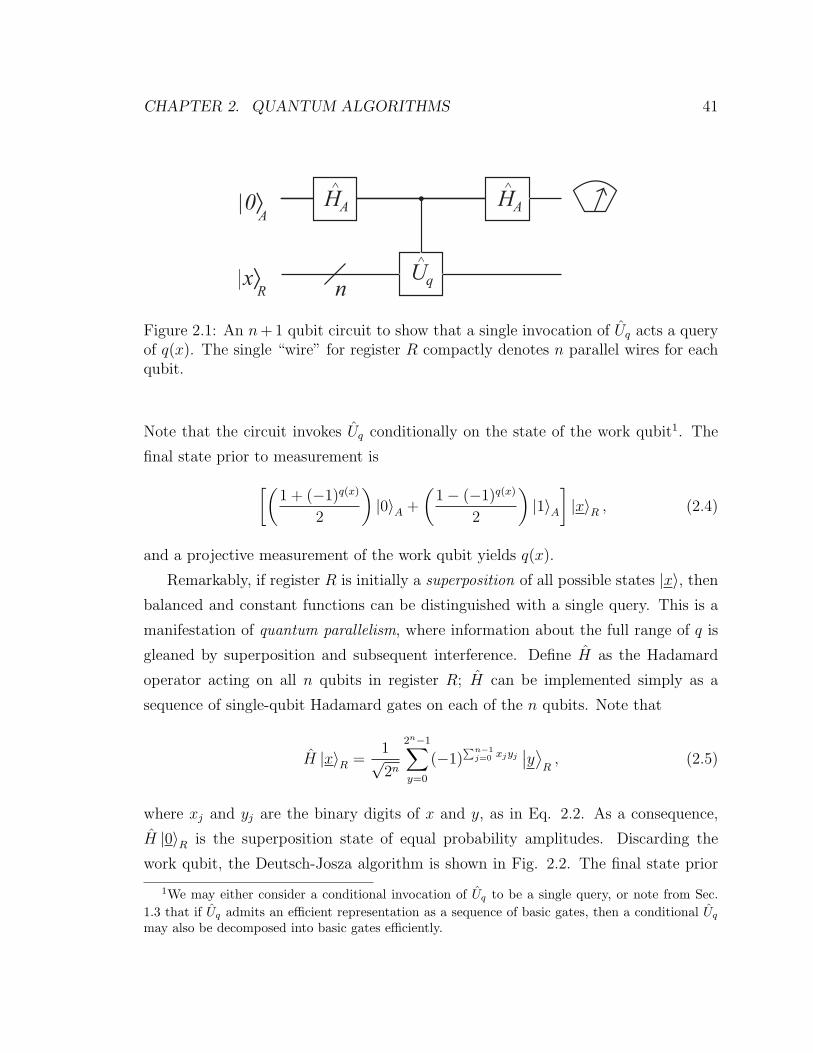
CHAPTER 2. QUANTUM ALGORITHMS 41
n
|0⟩
|x⟩
HA HA
Uq
A
R
^^
^
Figure 2.1: An n+ 1 qubit circuit to show that a single invocation of Uq acts a queryof q(x). The single “wire” for register R compactly denotes n parallel wires for eachqubit.
Note that the circuit invokes Uq conditionally on the state of the work qubit1. The
final state prior to measurement is[(1 + (−1)q(x)
2
)|0〉A +
(1− (−1)q(x)
2
)|1〉A
]|x〉R , (2.4)
and a projective measurement of the work qubit yields q(x).
Remarkably, if register R is initially a superposition of all possible states |x〉, then
balanced and constant functions can be distinguished with a single query. This is a
manifestation of quantum parallelism, where information about the full range of q is
gleaned by superposition and subsequent interference. Define H as the Hadamard
operator acting on all n qubits in register R; H can be implemented simply as a
sequence of single-qubit Hadamard gates on each of the n qubits. Note that
H |x〉R =1√2n
2n−1∑y=0
(−1)∑n−1
j=0 xjyj∣∣y⟩
R, (2.5)
where xj and yj are the binary digits of x and y, as in Eq. 2.2. As a consequence,
H |0〉R is the superposition state of equal probability amplitudes. Discarding the
work qubit, the Deutsch-Josza algorithm is shown in Fig. 2.2. The final state prior
1We may either consider a conditional invocation of Uq to be a single query, or note from Sec.1.3 that if Uq admits an efficient representation as a sequence of basic gates, then a conditional Uq
may also be decomposed into basic gates efficiently.

CHAPTER 2. QUANTUM ALGORITHMS 42
n|0⟩
RH^H^ Uq
^
Figure 2.2: A circuit representation of the Deutsch-Josza algorithm.
to measurement is1
2n
2n−1∑y=0
2n−1∑x=0
(−1)f(x)+∑n−1
j=0 xjyj∣∣y⟩
R. (2.6)
If f1is constant, the state is identically |0〉R, whereas the probability amplitude of
the |0〉R state is zero if q is balanced. Thus, a projective measurement of the qubits
allow constant and balanced functions to be distinguished with a single invocation of
Uq.
While it is a simple and elegant example of quantum parallelism, the Deutsch-
Jozsa algorithm is perhaps not the best example of exponential speedup in a quantum
algorithm. First, the efficiency of the algorithm is measured by the number of queries,
and is not an absolute gate count or total evolution time required to complete the
algorithm; the time required to actually implement Uq is not considered. Second, the
quantum algorithm exhibits exponential speedup only if we demand that constant
and balanced functions must be distinguished with zero probability of error. If we
relax this requirement, and demand that the answer be obtained with a probability
of error less than some ε > 0, then an efficient classical heuristic exists. Evaluate
q(x) for K random values of x; if any of the values of q(x) differ, we guess that q is
balanced, and is constant otherwise. K = O[log(1/ε)] values of q(x) are required to
upper bound the probability of error by ε. K is independent of n, and thus a constant
number of queries is sufficient, like the quantum algorithm.

CHAPTER 2. QUANTUM ALGORITHMS 43
2.1.2 Quantum search and amplitude amplification
Grover’s unstructured database search algorithm [72, 73] is one of several algorithms
discovered in the mid-nineties that spurred great interest in the potential computa-
tional power of quantum computers relative to their classical counterparts. Although
the utility of the algorithm lies in its application as a building block in other prob-
lems, it is easiest for us to start with the algorithm in its original form, with a slight
modification [74] to allow for multiple target states.
We are given a function f : ZN → 0, 1 that maps the integers 0 through N − 1,
where N = 2n, to a single Boolean output. We are told there exists a nonempty set
for which the function yields output 1:
X = x|f(x) = 1, |X| ≡ r, 0 < r < N. (2.7)
Given a black box that can be queried for function evaluations of f(x), we seek an
element of X with a minimum expected number of queries over all f . The function
f(x) can be thought of as a database with unknown structure for which the subset
X of inputs are desired records, or targets. An obvious heuristic is to guess values
of x at random; O(N/r) evaluations will find a solution with a minimum guaranteed
probability of success.
A quantum algorithm in the standard model can solve an equivalent problem with
O(√N) invocations of an oracle UX , which encodes the function f(x) as a unitary
operator. UX is defined on an n-qubit Hilbert space:
UX =N−1∑x=0
(−1)f(x) |x〉 〈x| = I − 2∑x∈X
|x〉 〈x| , (2.8)
where I is the identity operator, and the second summation includes computational
basis states |0〉 , |1〉 , · · · , |N − 1〉 that are targets. Acting on a general n-qubit
state, UX shifts the phase of target components by π, and does nothing to remaining
components.
As in the Deutsch-Jozsa problem, UX can be applied in a quantum circuit to
CHAPTER 2. QUANTUM ALGORITHMS 44
evaluate a single value of f(x). However, a significant improvement results when
the input to the oracle is a superposition of computational basis states. Consider
the operator Q = −HU0HUX acting on an N -dimensional Hilbert space; H is the
Hadamard operator on all n qubits, and U0 flips the phase of the |0〉 state:
U0 = I − 2 |0〉 〈0| . (2.9)
Note that H is self-inverse, so H = H†. Define the equal superposition state |σ〉 and
the superposition state over all targets∣∣X⟩:
|σ〉 = H |0〉 =1√N
N−1∑x=0
|x〉 (2.10a)
∣∣X⟩ =1√r
∑x∈X
|x〉 (2.10b)
Q leaves invariant the two-dimensional subspace Q0 spanned by |σ〉 and∣∣X⟩; i.e.,
Q = Q0 ⊕ Q⊥0 . This is easily verified, as
Q |σ〉 = −H(I − 2 |0〉 〈0|
)H
(1− 2
∑x∈X
|x〉 〈x|
)|σ〉 (2.11a)
= − (1− 2 |σ〉 〈σ|)
(1− 2
∑x∈X
|x〉 〈x|
)|σ〉 (2.11b)
=
(1− 4r
N
)|σ〉+ 2
√r
N
∣∣X⟩ , (2.11c)
and
Q∣∣X⟩ =
∣∣X⟩− 2
√r
N|σ〉 . (2.12)
Let∣∣X⊥⟩ be a vector in the invariant subspace such that
∣∣X⊥⟩ is orthogonal to∣∣X⟩:
∣∣X⊥⟩ =
√N
N − r|σ〉 −
√r
N − r∣∣X⟩ . (2.13)
The matrix representation of Q on the two-dimensional subspace spanned by∣∣X⟩

CHAPTER 2. QUANTUM ALGORITHMS 45
and∣∣X⊥⟩ is then
Q =
1− 2rN
−2√
r(N−r)
N
2√
r(N−r)
N1− 2r
N
. (2.14)
As the determinant of the matrix is 1, each invocation of Q0 is a rotation by an angle
θ, where
θ = sin−1
(2√r(N − r)N
), (2.15)
which approaches 2/√N for N r. Note that the angle between |σ〉 and
∣∣X⟩ is
cos−1∣∣〈σ| X⟩∣∣ = cos−1
(1√N
), (2.16)
which approaches π/2 if N r. Thus, the number of iterations K of Q required to
rotate |σ〉 to the state∣∣X⟩ is
K =cos−1
(1/√N)
θ≈ π√N
4. (2.17)
To find a target state with near unity probability, the system is initialized in the
|σ〉 = H |0〉 state, K iterations of Q are performed, requiring O(√N) oracle calls, and
projective measurement in the computational basis is carried out. The measurement
of the n qubits yields the n-bit representation of a target state in set X with near
certainty.
Brassard and Høyer [75] and Grover [76] showed that the search algorithm can
be generalized, in that there is freedom to modify the initial state and Hadamard
operations. To be precise, consider the operator
Q′ = −V UγV†UX , (2.18)
where V is any unitary operator on all n qubits, Uγ is defined by
Uγ = I − 2 |γ〉 〈γ| , (2.19)

CHAPTER 2. QUANTUM ALGORITHMS 46
and |γ〉 is the initial state. A little algebra shows that the two-dimensional subspace
spanned by V |γ〉 and∑
x∈X Vxγ |x〉 are invariant under Q′, where
Vxγ = 〈x| V |γ〉 . (2.20)
V causes a rotation in the invariant subspace by an angle
sin−1
2
√√√√∑x∈X
|Vxγ|2 −
(∑x∈X
|Vxγ|2)2 (2.21)
The generalized algorithm can be useful in a couple ways. First, if the problem
that we wish to solve is a search problem with a known structure, it may hold that
V can be chosen to reduce the number of required calls to the oracle. For example,
Grover [77] showed that if it is known that the target states are a fixed Hamming
distance k from a known n-bit string y, then the number of required iterations can
be reduced by selecting |γ〉 =∣∣y⟩ and defining the single-qubit operator V as
V =
[ √1− k/n
√k/n√
k/n −√
1− k/n
]. (2.22)
Second, as we will discuss in Sec. 4.3, replacement of Hadamard gates in the un-
structured search algorithm with other single qubit gates that preserve Vxγ = 1/√N
can be advantageous in reducing the impact of decoherence. Such modifications do
not modify the gate count of the unstructured search algorithm, but could be bene-
ficial if unwanted interactions are present between the system and the environment.
Quadratic speedup [that is, O(√N) = O(1.414n)] may also be accomplished for
problems in NP such as 3-SAT, where f(x) encodes an n-variable Boolean expression
whose satisfying assignment is sought. However, the structure of such problems can
often be exploited by classical heuristics that outperform the quadratic speedup of
the quantum search. Averaged over all problem instances, the expected number of
function evaluations for such heuristics scales as O(αn), where α may be smaller than√
2.
CHAPTER 2. QUANTUM ALGORITHMS 47
The powerful principle of amplitude amplification [74, 78], reviewed succinctly
by Ambainis [79], generalizes quantum search and addresses this issue. A classical
heuristic can be mapped to a quantum algorithm, in which guessing via random
numbers is replaced by quantum search. The resultant quadratic speedup leads to
an expected O(αn/2) oracle calls, improving on any classical heuristic. Thus, the
applications of quantum search are far more general than the simple database search
algorithm suggests.
In the above discussion, I did not comment on the number of elementary gates
required to construct both U0 and UX . The former can be implemented simply by
placing an ancillary qubit in the (|0〉 − |1〉) /√
2 state, and applying a NOT gate to
the ancillary qubit conditional on all other qubits being in the logical zero state.
Such a controlled-NOT gate with multiple control bits can be implemented using
O(n) elementary gates with an additional work bit [17]. The oracle for UX can be
decomposed in a similar fashion, with O(n) additional NOT gates. If our metric for
the efficiency of the algorithm is the query complexity (i.e., the asymptotic scaling of
the number of invocations of UX), then the internal implementation of the black box
UX is not relevant in any case.
Interestingly, tight bounds have been derived for the quantum search algorithm
that preclude the existence of any quantum algorithm leading to less than Θ(√N)
oracle calls. Bennett et al. [80], Boyer et al. [74] and Zalka [81], have provided
lower bounds in the event that a target state is to be obtained with near certainty
at the end of one invocation of the search algorithm. Gingrich et al. [82] have shown
that the expected number of calls to UX improves by a constant factor if the search
algorithm is terminated before a full π/2 rotation is carried out, and repeated from
the beginning until a solution is found.
If the number of satisfying solutions r to the search problem are not known in
advance, they can either be determined by repeating the search algorithm with an
exponentially increasing number of iterations of Q [74, 78], or by the elegant quantum
counting algorithm [78].

CHAPTER 2. QUANTUM ALGORITHMS 48
2.1.3 Quantum Fourier transform
The quantum Fourier transform (QFT) [83] is the analogue of the discrete Fourier
transform, applied to the probability amplitude in the computational basis. It is a
subroutine used by subsequent algorithms discussed in this chapter.
The QFT maps the n-qubit basis state |x〉 to
|x〉 → |ψx〉 =1√N
N−1∑y=0
e2πixy/N∣∣y⟩ , (2.23)
where N = 2n. It is remarkable that the QFT can be implemented using only
O(n2) gates, which can be seen from the following product representation of the QFT
[70, 84]. Expanding the integers x and y as
x` =n−1∑`=0
x`2`, yj =
n−1∑j=0
yj2j, (2.24)
then
|ψx〉 =1√N
∑yn−1,··· ,y0∈0,1
n−1∏j=0
e2πixyj/2n−j |yn−1〉 ⊗ · · · ⊗ |y0〉 (2.25a)
=1√N
∑yn−1,··· ,y0∈0,1
n−1⊗j=0
e2πixyj/2n−j |yj〉 (2.25b)
=1√N
n−1⊗j=0
(|0〉j + e2πix/2n−j |1〉j
)(2.25c)
=1√N
n−1⊗j=0
(|0〉j + e
∑` 2πix`2
`+j−n |1〉j)
(2.25d)
Any terms of the exponent for which `+j−n ≥ 0 can be discarded, as they contribute
an integer multiple of 2πi. Using the binary fraction notation
K∑k=1
ak2−k ≡ 0.a1a2 · · · aK , (2.26)

CHAPTER 2. QUANTUM ALGORITHMS 49
n-1 Hn-1
Hn-2
H1
H0
R2
R2
R2
R3
Rn-1
Rn-2Rn-1
Rn
n-2
n-3
1
0^ ^
^
^
^
^
^
^
^
^
^
^
Figure 2.3: Quantum circuit for the n-qubit QFT. Qubit labels are at left. Adaptedfrom [70].
then
|ψx〉 =1√2n
(|0〉0 + e2πi0.xn−1xn−2···x0 |1〉0
)⊗(|0〉1 + e2πi0.xn−2···x0 |1〉1
)· · ·
⊗(|0〉n−1 + e2πi0.x0 |1〉n−1
). (2.27)
Note that the state [|0〉+exp(2πi0.xn−1) |1〉]/√
2 can be created by a Hadamard gate
on input bit n − 1. The first term’s exponential on the righthand side of Eq. (2.27)
also has contributions from the remaining input bits. These can be performed by the
controlled-phase gates Rα, which apply the following phase shift to the target qubit
j = 0
|0〉0 → |0〉0 , |1〉0 → e2πiπ/2α |1〉0 , (2.28)
conditioned on the control qubit. Note that Rα is congruent to a controlled z-rotation
by an angle −π/2α+1 within a global phase factor. Similar constructions for the
remaining terms of Eq. (2.27) lead to the tiered gate construction of Fig. 2.3. The
output qubits are bit-reversed from the input. This construction requires n(n− 1)/2
controlled phase gates and n Hadamard gates.
By observing that the control and target bits of the controlled-phase gates are
symmetrical, Griffiths and Niu [84] proposed a semiclassical implementation of the
QFT, where each qubit is measured in the computational basis after the Hadamard

CHAPTER 2. QUANTUM ALGORITHMS 50
n
|0⟩
|α⟩
HA HA
U
A
R
^ ^
^
Figure 2.4: Circuit illustrating phase kickback.
gate, and the measurement result is classically fed forward to the successive phase
gates. Furthermore, an approximate QFT, where controlled-phase gates with angles
below a given polynomial threshold are omitted, gives rise to at most polynomial
error in the output state [83, 4].
2.1.4 Phase-estimation algorithm
The phase-estimation algorithm [85, 70, 86] uses the phase kickback principle and
the QFT to estimate the phase accrued by the application of a unitary operator.
This problem is analogous to solving for eigenvalues of a hermitian operator, and can
thus be used to deduce spectral information about a hamiltonian. It is also the core
principle behind the order-finding and factoring algorithms.
Consider the quantum circuit in Fig. 2.4, which acts on a single ancillary qubit
A and a register R of n qubits. The work qubit is prepared in the fiducial |0〉A state,
while register R is prepared in an eigenstate |α〉R of a unitary operator U :
U |α〉R = e2πiφα |α〉R . (2.29)
Note that the phase has been normalized such that 0 ≤ φα < 1. After the application
of all three operators, the output is
|ψf〉 =
[(1 + e2πiφα
2
)|0〉A +
(1− e2πiφα
2
)|1〉A
]|α〉R . (2.30)

CHAPTER 2. QUANTUM ALGORITHMS 51
Information about the phase φα has been encoded in the ancillary qubit, which,
remaining separable from the register R, can be measured to discern some knowledge
about φα. For instance, if it is known that φα is either 0 or 1/2, then the one bit of
information yielded from a projective measurement of the work qubit is sufficient to
determine the value. This is a simple example of the principle of phase kickback.
This example could be used, in theory, to yield information about the global
spectrum of U , and thus, the hermitian operator that generates U . If we can prepare
register R in an equal superposition of eigenstates, such that the initial state is
|ψi〉 =1√N
N−1∑α=0
|0〉A |α〉R , (2.31)
where N = 2n, then the final state is
|ψf〉 =1√N
N−1∑α=0
[(1 + e2πiφα
2
)|0〉A +
(1− e2πiφα
2
)|1〉A
]|α〉R . (2.32)
If the ancillary qubit is measured in the computational basis, the expectation value
is
〈σz〉 =1
N
N−1∑α=0
(∣∣∣∣1 + e2πiφα
2
∣∣∣∣2 − ∣∣∣∣1− e2πiφα
2
∣∣∣∣2)
(2.33a)
=1
NRe
(N−1∑α=0
e2πiφα
)(2.33b)
=1
NRe
∫dφ e2πiφ
N−1∑α=0
δ (φ− φα) , (2.33c)
which, to a constant factor, is the real part of the continuous Fourier transform of
the global spectral density function∑N−1
α=0 δ(φ − φα). The imaginary part could be
obtained by repeating the algorithm with the second Hadamard operator replaced by
an x-axis rotation.
This approach to determining information about the spectral density function

CHAPTER 2. QUANTUM ALGORITHMS 52
n
F F
U2m-1U2m-2
U2 U
†m qubits
...
|0⟩A
|α⟩R
^ ^
^ ^ ^ ^
Figure 2.5: Phase-estimation algorithm.
suffers from two problems. First, register R requires complicated initial state prepa-
ration with advance knowledge of the eigenvectors of U . Second, multiple projective
measurements of the ancillary qubit must be performed to estimate the desired ex-
pected value. We will address both of these concerns using mixed states and ensemble
measurements in Sec. 2.2.1.
Multiple ancillary qubits allow one to generate a bitwise estimate of individual
eigenvalues of U . Consider the quantum circuit in Fig. 2.5, where register A has been
expanded from a single qubit to m work qubits; its computational basis states are
|x〉A ∈ |0〉A , · · · |M − 1〉A, where M = 2m. The operation F is the QFT, and F †
its inverse. It is convenient to rescale the phase applied by U such that 0 ≤ φα < M :
U |α〉R = e2πiφα/M |α〉R . (2.34)
The succession of controlled-U2jgates performs the mapping
|x〉A |α〉R → e2πiφαx/M |x〉A |α〉R . (2.35)
If the initial state is |ψi〉 = |0〉A |α〉R, then the circuit yields the output
|ψf〉 =M−1∑y=0
eiπ(φx−y)(M−1)/M sin [π(φα − y)]M sin [π(φα − y)/M ]
∣∣y⟩A|α〉R . (2.36)

CHAPTER 2. QUANTUM ALGORITHMS 53
A projective measurement in the computational basis is now made on register A.
Consider the probability p(y0) of finding the state y0 that is closest to φα; i.e., |∆φ| ≡|φ − y0| ≤ 1/2 modulo M . Note that y0 gives the best m-bit approximation to φα.
As 2|x|/π ≤ | sin x| ≤ |x| for |x| ≤ π/2,
p(y0) =sin2 [π(φα − y0)]
M2 sin2 [π(φα − y0)/M ]≥ 4
π2. (2.37)
The probability of obtaining the best `-bit approximation for φα can be amplified by
increasing the number of ancillary bits. We obtain the best `-bit approximation if
the measured value of y obeys |δ| < 2m−`, where δ ≡ y0 − y. Thus, the probability ε
of obtaining a value of y outside of this bound is
ε =−2m−`∑
δ=−M/2
p(y0 − δ) +
M/2−1∑δ=2m−`
p(y0 − δ). (2.38)
These summations can be bounded by an integral [86] to yield
ε ≤ 1
2m−`+1 − 2. (2.39)
To ensure that ε ≤ ε0 for some constant ε0, it is sufficient that
m ≥ `+ 1 + log2
(1 +
1
4ε0
). (2.40)
Several authors have discussed the issue of initial state generation for register R.
To calculate the energy eigenvalues of many-body hamiltonians such as many-electron
atoms, Abrams and Lloyd [87] discussed the possibility of using mean-field estimates
to create |φα〉 . To scale efficiently with the problem size, the overlap of the initial state
with |φα〉 must diminish at most polynomially with the number of qubits n. Hillery
and Buzek [88] have proposed a clever scheme in which N registers R0, · · · , RN−1 of
n qubits are initialized as a singlet state in U(N). To be precise, the singlet state
consists of the superposition of the state |0〉R0⊗ |1〉R1
⊗ · · · |N − 1〉RN−1with all per-
mutations of the state labels such that the linear combination is antisymmetric. N
CHAPTER 2. QUANTUM ALGORITHMS 54
ancillary registers of m qubits are chosen, and initialized in the |0〉 state. The key
point is that the singlet state is invariant of the choice of basis; registers R0 through
RN−1 can be considered to be a fully antisymmetric superposition of the eigenstates
of U⊗N . Independent phase-estimation algorithms are run on each register Rj. With
arbitrarily high probability, each eigenvalue and corresponding eigenvector is found
in the ancillary and Rj registers by projective measurement. Though pedagogically
interesting, this scheme is not particularly useful, as it requires exponentially-large
resources. Travaglione and Milburn [89] have bounded the success probability of gen-
erating eigenstates for arbitrary initial states of register R. Jaksch and Papageorgiou
[90] have analyzed the error probability if an eigenstate for a smaller problem instance
is appended to additional qubits.
These results notwithstanding, the phase-estimation algorithm with multiple an-
cillary qubits is not easily modified to yield global information about the energy
spectrum of U . We will return to this topic in Sec. 2.2.1.
2.1.5 Order finding and the factoring algorithm
In 1994, Shor presented a quantum algorithm to efficiently solve the integer factor-
ization and discrete logarithm problems [91, 92]. As the supposed difficulty of integer
factorization is the cornerstone of the RSA public-key encryption algorithm [93, 2],
the practical impact of this discovery is profound.
Shor’s algorithm in fact solves the order-finding problem, which I define and dis-
cuss first; I closely follow the interpretation of Cleve et al. [70] and Mosca [86] of
order-finding as an application of phase estimation. Subsequently, we will comment
on the reduction of the factorization problem to order-finding. The derivations in this
section leverage several results in elementary number theory, the proofs of which the
reader may consult in Appendix B.
Order finding
Given a finite group G, the order of an element a ∈ G is the smallest positive
integer r such that ar = e, where e is the identity element. Consider, for example,

CHAPTER 2. QUANTUM ALGORITHMS 55
the set generated by multiplication modulo N of an integer a < N : 1, amod N, a2
mod N, · · · , ar−1 mod N. Given a and N , we seek the order of the group. Note that
for any x ∈ ZN , the mapping x 7→ axmod N is invertible provided that a and N are
coprime, by Corollary B.2 of Theorem B.1. Thus, we can define a unitary operator
Ua on an N -dimensional space spanned by |0〉 , |1〉 , · · · , |N − 1〉:
Ua |x〉 = |ax mod N〉 . (2.41)
This modular multiplication operation can be constructed efficiently from fundamen-
tal gates [94, 95, 96].
By applying phase-estimation to Ua, we can estimate the order r. Note that U ra
equals the identity operator, as
U ra |x〉 = |arx mod N〉 = |x〉 , (2.42)
by Theorem B.4. Thus, Ua has r eigenvectors
|φk〉 =1√r
r−1∑`=0
e−i2πk`/r∣∣a` mod N
⟩, k ∈ Zr (2.43)
with corresponding eigenvalues ei2πk/r. Phase estimation requires us to prepare a
good estimate of the corresponding eigenstate, which appears to be difficult without
a priori knowledge of the order r. However, a superposition of the eigenvectors is
trivial, as
|1〉 =1√r
r−1∑k=0
|φk〉 . (2.44)
Consider performing the phase-estimation algorithm with ` ≥ m+ 1 + log2(1 + 1/4ε)
qubits in register A, and n qubits in the |1〉 state in register R. Prior to the final
measurement, register A will be “close to” a superposition of the best m-bit approx-
imations to the fractions k/r, for k ∈ ZN . To be precise, measurement of register A
yields the best m-bit approximation to k/r for a random k ∈ 0, 1, · · · , r − 1, with
probability 1− ε.

CHAPTER 2. QUANTUM ALGORITHMS 56
Given a sufficiently close m-bit estimate k/r of k/r, the method of continued
fractions can be used to extract k and r. By Theorem B.8, if |k/r − k/r| ≤ 1/2r2 ≤1/2N2, then k/r must be a convergent of the continued fraction for k/r. Corollary
B.6 states that the number of convergents that must be evaluated is only O(log r) =
O(logN). An m-bit estimate of k/r is accurate to within 2−m−1 of the actual value,
so |k/r − k/r| ≤ 1/2N2 implies that m ≥ 2 log(N). Thus, the phase estimation
algorithm with ` = d2 log(N) + 1 + log(1 + 1/4ε)e ancilla qubits allows us to evaluate
the numerator and denominator of k/r for a random k ∈ Zr with probability 1− ε.The algorithm succeeds in finding the order r if k and r are coprime; if the
numerator and denominator of k/r share a common factor, then the order-finding
algorithm will yield a factor of r instead of r itself. However, by the prime number
theorem, the number of prime numbers less than r approaches r/ log(r) as r → ∞,
and the probability of obtaining k coprime with r is always Ω(1/ log r). Thus, by
repeating the algorithm O(log r) = O(logN) times, the order r is obtained with
probability arbitrarily close to unity.
Integer Factorization
The order-finding algorithm determines the smallest positive integer r such that xr = 1
mod N , where N is the integer that we wish to factor and x is chosen coprime to
N . Assume the order is even. Then, (xr/2 − 1)(xr/2 + 1) = 0 mod N . Note that
the first term cannot be equal to 0 mod N , or else r/2 would be the order. Thus, if
xr/2 6= −1 mod N , then neither bracketed term is a multiple of N , and gcd(xr/2−1, N)
or gcd(xr/2 + 1, N) must yield a factor of N . The greatest common divisor can be
computed efficiently by Euclid’s algorithm.
How likely is it that for a given N and a randomly chosen x coprime to N , the
order r is even and xr/2 6= −1 mod N? By Corollary B.14 to Theorem B.13, this
probability is at least 1/2 provided that N is not the integer power of an odd prime;
the factorization algorithm is successful with arbitrarily high probability with O(1)
repetitions of the order-finding algorithm, using different values of x. Note that if N
is the integer power of an odd prime, its prime factorization can be found trivially by
classical means.

CHAPTER 2. QUANTUM ALGORITHMS 57
Thus, the order-finding algorithm for the standard model yields an efficient solu-
tion to the integer factoring problem.
2.2 Ensemble Algorithms
In the previous section, I discussed algorithms that require initialization of the qubits
to a fiducial pure state. Initialization is performed, in principle, by projective mea-
surement of all qubits onto the computational basis, or thermalization to a reservoir
with a temperature much smaller than the energy spacing between logical qubit levels.
But what of quantum information processors such as liquid-state magnetic resonance
of nuclear spins (Sec. 1.5), where direct projective measurements of qubits are inac-
cessible, and the Zeeman splitting H0 is far smaller than the thermal energy? In this
case, the initial state is described by a highly-mixed density matrix. In addition, in
such an ensemble quantum computing scheme, the final measurement yields an expec-
tation value averaged over an ensemble of identically-prepared quantum computers,
as opposed to a single projective measurement.
Such ensemble quantum computers can be reduced to the standard model by the
preparation of pseudopure states or logical labeling. However, the prohibitive scaling
of such schemes motivates the search for quantum algorithms that yield exponential
speedup while mitigating the need for initialization. In this section, I will first review
models for ensemble quantum computation, using terminology introduced by Knill
and Laflamme [68]. I will then examine ensemble algorithms from the literature for
the so-called DQC1 model, in which all input qubits are highly mixed, except for one.
These examples will contextualize and lay the foundation for the following chapter, in
which I propose and analyze a novel application of a DQC1 algorithm to determining
the thermodynamic properties of a many-body system.
2.2.1 Models for Ensemble QC
The deterministic quantum computation with pure states model (DQCp) [68] func-
tionally differs from the standard model only in measurement. We are given a register
CHAPTER 2. QUANTUM ALGORITHMS 58
of n qubits that can be initialized to a fiducial pure state, and on which we can apply
any uniform acyclic circuit family formed from elements of a universal gate set. Treat-
ing the qubit as a pseudospin, measurement yields a random variable αj with a mean
equal to the expectation value⟨σz
j
⟩for a single qubit j, and a variance s2 that is inde-
pendent of n. For example, consider an ensemble of K quantum computers (e.g., each
a molecule of n addressable spins, with no intermolecule interactions). The ensemble
is probabilistic, such that the final state of a given ensemble member is |φj〉 with
probability qj; equivalently, the density matrix representing the state of the ensemble
prior to measurement is ρf =∑
j qj |φj〉 〈φj|. A projective measurement of qubit j
in the computational basis (i.e., a measurement of the observable σzj ) would yield an
eigenvalue of +1 or −1 with probabilities p1 = tr(|0〉j 〈0| ρf ) and p−1 = 1 − p1. The
result of a projective measurement of a single ensemble member is a Bernoulli random
variable βj that takes values ±1 with expected value 〈βj〉 = p1 − p−1 and variance
s2βj
= 1 − (p1 − p−1)2. Now, assume that due to experimental limitations, measure-
ments of a given qubit are averaged over all ensemble members. The measurement
result αj is then the average of K independent random variables with distributions
identical to βj; 〈αj〉 = 〈βj〉 and
s2βj
= [1− (p1 − p−1)2]/K ≤ 1/K. (2.45)
By the Chebyshev inequality, for any ε > 0,
Prob[∣∣αj −
⟨σz
j
⟩∣∣ ≥ ε]≤ 1
Kε2. (2.46)
Thus, with O(1/ε2p0) ensemble members2,⟨σz
j
⟩can be determined by DQCp within
error ε with probability at least p0.
This measurement model can be used to describe a noisy free induction measure-
ment over an ensemble of spins. Thus, DQCp is an appropriate model for an NMR
quantum computer, provided that a pseudopure initial state or logical labeling is
2As this bound is based on the Chebyshev inequality, it is rather weak. As the sum of K Bernoullirandom variables with fixed pj approaches a Gaussian, a tighter bound of O(log(1/p0)/ε2) can beinferred by the central limit theorem. However, note that the dependence on the error ε is unchanged.
CHAPTER 2. QUANTUM ALGORITHMS 59
utilized, and time evolution is unitary.
Consider weakening the initialization requirement. Note that no computation can
be performed if the n qubits (labeled 0 through n− 1) are in a fully mixed state, as
the system density matrix is the identity:
ρ0 =n−1⊗j=0
Ij2, (2.47)
where Ij is the identity operator on the two-dimensional subsystem for qubit j. Any
unitary operation U maps the state from ρ0 to Uρ0U† = ρ0, leaving the system state
unchanged. Now, consider the case where only the first qubit is initialized to logical
zero, and the remainder are fully mixed:
ρ1 = |0〉 〈0| ⊗n−1⊗j=1
Ij2
(2.48)
The deterministic quantum computation with one pure qubit model (DQC1) is defined
as an ensemble quantum computation scheme equivalent to DQCp, but with the initial
state restricted to ρ1.
The utility of the DQC1 scheme seems dubious at first inspection. Knill and
Laflamme [68] provided a clever proof that DQC1 requires exponentially more re-
sources to solve black-box problems such as quantum search. Furthermore, assume
that we want to use our n-qubit DQC1 machine to simulate an arbitrary algorithm for
an x-qubit standard model quantum computer. Ambainis et al. [97] have shown that
this is only possible if x = O[1 + lg(n)], which is no better than a classical computer
can accomplish. However, although these results show that DQC1 is weaker than the
standard model, neither result precludes specific tasks at which the DQC1 quantum
computer could outperform a classical computer.
Trace of a Unitary Operator by DQC1
One calculation that can be efficiently performed by a DQC1 machine, and which
forms the kernel of all algorithms to be discussed, is finding the trace of a unitary

CHAPTER 2. QUANTUM ALGORITHMS 60
operator U defined on an 2n-dimensional Hilbert space3 [68, 98]. The trace of U can
be calculated on a classical computer by summing the diagonal elements of its matrix
representation; this procedure requires O[poly(2n)] elementary arithmetic operations.
No efficient classical algorithm to compute tr(U) with O[poly(n)] resources is known
for a general U .
I first review how the DQC1 model can estimate the trace of U efficiently. In the
following section, I will draw upon the literature to summarize how this result can
be applied to solve various problems, such as Deutsch-Jozsa, integer factoring and an
additional problem known as fidelity decay. In the following chapter, I propose using
estimations of tr(U) to estimate the free energy of spin lattice models.
Assume that we have a DQC1 machine with one pure-state qubit and n fully-
mixed-state qubits. U is an operator on an N = 2n dimensional Hilbert space that
acts on the n mixed-state qubits. The initial state is
ρ1 = |0〉 〈0| ⊗I(N)
N, (2.49)
where I(N) is the N -dimensional identity operator describing the n maximally-mixed
qubits. Note that I(N) can be expressed as a sum of projectors (i.e., the resolution
of the identity). These projectors can be chosen from any complete basis set. As U
is unitary, and thus normal, its eigenstates form a complete orthonormal set. Define
the eigenstates and associated eigenvalues by
U |α〉 = eiφα |α〉 . (2.50)
The initial state can be expressed as
ρ1 = |0〉 〈0| ⊗N−1∑α=0
1
N|α〉 〈α| . (2.51)
Consider the sequence of operations HpU(p)Hp, where Hp are Hadamard gates
acting on the initially pure qubit, and U(p) is the application of U on the mixed
3Subject to the constraint that U can be represented by a uniform family of quantum gates.
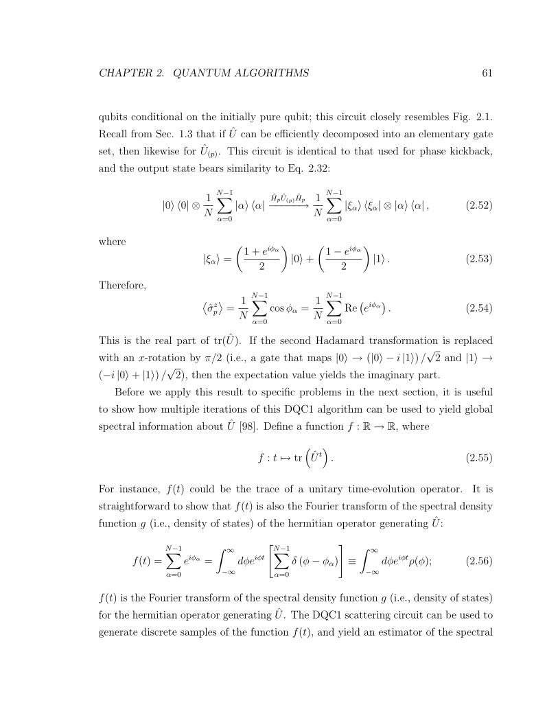
CHAPTER 2. QUANTUM ALGORITHMS 61
qubits conditional on the initially pure qubit; this circuit closely resembles Fig. 2.1.
Recall from Sec. 1.3 that if U can be efficiently decomposed into an elementary gate
set, then likewise for U(p). This circuit is identical to that used for phase kickback,
and the output state bears similarity to Eq. 2.32:
|0〉 〈0| ⊗ 1
N
N−1∑α=0
|α〉 〈α|HpU(p)Hp−−−−−→ 1
N
N−1∑α=0
|ξα〉 〈ξα| ⊗ |α〉 〈α| , (2.52)
where
|ξα〉 =
(1 + eiφα
2
)|0〉+
(1− eiφα
2
)|1〉 . (2.53)
Therefore, ⟨σz
p
⟩=
1
N
N−1∑α=0
cosφα =1
N
N−1∑α=0
Re(eiφα
). (2.54)
This is the real part of tr(U). If the second Hadamard transformation is replaced
with an x-rotation by π/2 (i.e., a gate that maps |0〉 → (|0〉 − i |1〉) /√
2 and |1〉 →(−i |0〉+ |1〉) /
√2), then the expectation value yields the imaginary part.
Before we apply this result to specific problems in the next section, it is useful
to show how multiple iterations of this DQC1 algorithm can be used to yield global
spectral information about U [98]. Define a function f : R→ R, where
f : t 7→ tr(U t). (2.55)
For instance, f(t) could be the trace of a unitary time-evolution operator. It is
straightforward to show that f(t) is also the Fourier transform of the spectral density
function g (i.e., density of states) of the hermitian operator generating U :
f(t) =N−1∑α=0
eiφα =
∫ ∞
−∞dφeiφt
[N−1∑α=0
δ (φ− φα)
]≡∫ ∞
−∞dφeiφtρ(φ); (2.56)
f(t) is the Fourier transform of the spectral density function g (i.e., density of states)
for the hermitian operator generating U . The DQC1 scattering circuit can be used to
generate discrete samples of the function f(t), and yield an estimator of the spectral

CHAPTER 2. QUANTUM ALGORITHMS 62
density function.
2.2.2 DQC1 algorithms
The following are applications from the literature that make use of the DQC1 algo-
rithm to compute the trace of a unitary operator U .
Deutsch-Jozsa algorithm
A DQC1 implementation of the Deutsch-Jozsa algorithm — for which we want to
determine if a Boolean function q is constant or balanced — is straightforward [99,
100]. The function q is encoded in the black box Uq, which is defined in Eq. 2.1.
Note that Uq is diagonal in the computational basis. If the function is constant, then
all the diagonal matrix elements are 1. Otherwise, if q is balanced, then half of the
matrix elements are 1, and the other half −1. Thus, the trace of Uq distinguishes the
two function types. By Eq. 2.54, the measured expectation value of the pure-state
qubit is ⟨σz
p
⟩=
±1 if q is constant,
0 if q is balanced.(2.57)
This measurement unambiguously distinguishes constant functions from balanced
ones with a single function evaluation.
Factoring
Parker and Plenio realized a clever modification that could allow restricted instances
of the order-finding problem to be addressed by a quantum computer with a single
pure-state qubit and the remaining qubits maximally-mixed [101]. However, their
scheme, described below, requires projective measurement and feed-forwarding of the
results, thus falling outside the domain of DQC1. In this subsection, I will first
describe the algorithm of Parker and Plenio, and show how it is applicable to a wider
range of factoring problems than they originally considered. To contrast, I will then
consider a DQC1 method for attacking the order-finding problem based on finding
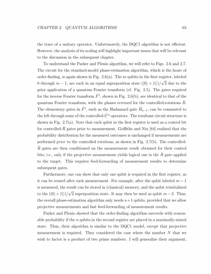
CHAPTER 2. QUANTUM ALGORITHMS 63
the trace of a unitary operator. Unfortunately, the DQC1 algorithm is not efficient.
However, the analysis of its scaling will highlight important issues that will be relevant
to the discussion in the subsequent chapter.
To understand the Parker and Plenio algorithm, we will refer to Figs. 2.6 and 2.7.
The circuit for the standard-model phase-estimation algorithm, which is the heart of
order-finding, is again shown in Fig. 2.6(a). The m qubits in the first register, labeled
0 through m − 1, are each in an equal superposition state (|0〉 + |1〉)/√
2 due to the
prior application of a quantum Fourier transform (cf. Fig. 2.5). The gates required
for the inverse Fourier transform F †, shown in Fig. 2.6(b), are identical to that of the
quantum Fourier transform, with the phases reversed for the controlled-rotations R.
The elementary gates in F †, such as the Hadamard gate Hn−1, can be commuted to
the left through some of the controlled-Uα operators. The resultant circuit structure is
shown in Fig. 2.7(a). Note that each qubit in the first register is used as a control bit
for controlled-R gates prior to measurement. Griffiths and Niu [84] realized that the
probability distribution for the measured outcomes is unchanged if measurements are
performed prior to the controlled rotations, as shown in Fig. 2.7(b). The controlled-
R gates are then conditioned on the measurement result obtained for their control
bits; i.e., only if the projective measurement yields logical one is the R gate applied
to the target. This requires feed-forwarding of measurement results to determine
subsequent gates.
Furthermore, one can show that only one qubit is required in the first register, as
it can be reused after each measurement. For example, after the qubit labeled m− 1
is measured, the result can be stored in (classical) memory, and the qubit reinitialized
to the (|0〉+ |1〉)/√
2 superposition state. It may then be used as qubit m− 2. Thus,
the overall phase-estimation algorithm only needs n+1 qubits, provided that we allow
projective measurements and fast feed-forwarding of measurement results.
Parker and Plenio showed that the order-finding algorithm succeeds with reason-
able probability if the n qubits in the second register are placed in a maximally-mixed
state. Thus, their algorithm is similar to the DQC1 model, except that projective
measurement is required. They considered the case where the number N that we
wish to factor is a product of two prime numbers. I will generalize their argument,

CHAPTER 2. QUANTUM ALGORITHMS 64
m-1 Hn-1
Hn-2
H1
H0
R2
R2
R2
R3
Rn-1
Rn-2Rn-1
Rn
m-2
m-3
1
0^ ^
^
^
^
^
^
^
^
^
^
^
†
†
†
†
†
†
† †
nU2m-1
U2m-2U2 U...
F†^
^ ^ ^ ^
|0>+|1>
|0>+|1>
|0>+|1>
|0>+|1>
m-1m-2
0
(a)
(b)
m-3
...
m-3
Figure 2.6: (a) Phase-estimation algorithm. Similar to Fig. 2.5, but noting that eachof the m qubits in the first register is in an equal superposition of |0〉 and |1〉 after thequantum Fourier transform. (b) Gate decomposition for the inverse quantum Fouriertransform F †.
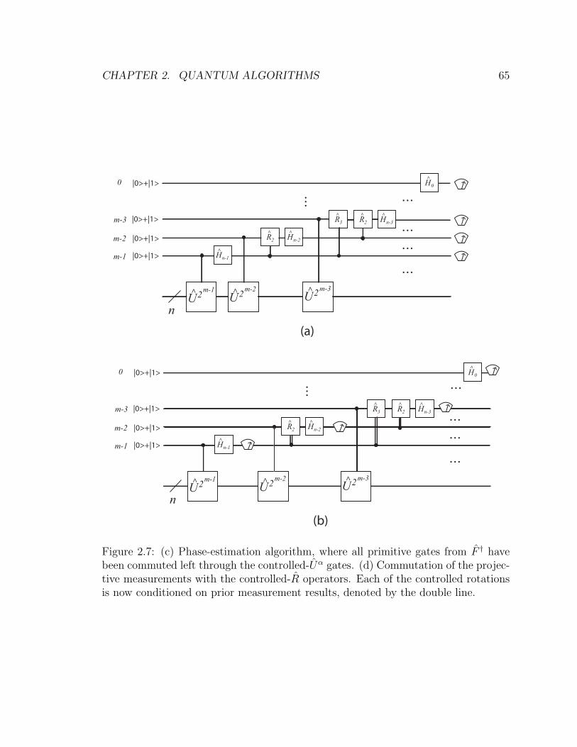
CHAPTER 2. QUANTUM ALGORITHMS 65
nU2m-1
U2m-2U2
...
^ ^ ^
(a)
Hn-1^
R2^
Hn-2^
m-3
R3^
R2^
Hn-3^
...
H0^
...
...
...|0>+|1>
|0>+|1>
|0>+|1>
|0>+|1>
m-1
m-2
0
m-3
n
(b)
Hn-1^
Hn-2^
Hn-3^
U2m-1^
...
H0^
...
...
...|0>+|1>
|0>+|1>
|0>+|1>
|0>+|1>
m-1
m-2
0
m-3
U2m-2^
R2^
U2^ m-3
R3^
...R2^
Figure 2.7: (c) Phase-estimation algorithm, where all primitive gates from F † havebeen commuted left through the controlled-Uα gates. (d) Commutation of the projec-tive measurements with the controlled-R operators. Each of the controlled rotationsis now conditioned on prior measurement results, denoted by the double line.

CHAPTER 2. QUANTUM ALGORITHMS 66
by allowing N to be an arbitrary product of powers of primes.
Recall that in the standard-model order-finding problem (Sec. 2.1.5), we construct
a unitary operator Ua (defined in Eq. 2.41) that acts on an N -dimensional space
and performs modular multiplication by an integer a coprime with N . The smallest
nonnegative r such that U ra = 1 is defined as the order. In the original order-finding
algorithm, the second register (with n qubits) is prepared as an equal superposition
of r selected eigenstates of Ua, where the phases of the associated eigenvalues are
multiples of 2π/r; the order is then deduced from phase estimation. However, Parker
and Plenio realized that a large fraction of all of the eigenvalues of Ua are multiples
of 2π/r. Thus, initializing register R as an equal superposition of all eigenstates, or
even as an incoherent mixture, suffices in the phase-estimation procedure.
To be precise, note that Ua = ⊕dUa,(d), where each Ua,(d) acts on an invariant rd-
dimensional subspace; equivalently, repeated multiplication by a modulo N partitions
the integers in ZN into sequences (labeled d) of length rd, and permutes the sequences
amongst themselves. This statement is best illustrated by an example provided by
Parker and Plenio. For a = 2 and N = 15, successive applications of the operator
Ua=2 lead to the mappings
|1〉 7→ |2〉 7→ |4〉 7→ |8〉 7→ |1〉
|3〉 7→ |6〉 7→ |12〉 7→ |9〉 7→ |3〉
|5〉 7→ |10〉 7→ |5〉
|7〉 7→ |14〉 7→ |13〉 7→ |11〉 7→ |7〉 (2.58)
Thus, Ua=2 is reducible, and acts on four invariant subspaces. Each subspace can be
labeled with a unique integer d, and can be characterized by a sequence of rd integers.
The first sequence, for which d = 1, is 1, 2, 4, 8, and thus r1 = 4. As U ra is the identity,
it is clear that rd must divide the order r. For this example, r = 4, and the sequence
lengths are either 2 or 4.
Parker and Plenio’s main observation was that most of the sequence elements fall
into sequences for which rd = r. I now state a minor generalization of their result as
the following theorem.
CHAPTER 2. QUANTUM ALGORITHMS 67
Theorem 2.1. Assume that N can be expressed as a product of powers of primes
pα11 p
α22 · · · pαs
s , where each α is a nonnegative integer. A random x ∈ ZN is an element
of a sequence d with length rd = r with probability at least P ≡∏s
j=1(pj − 1)/pj.
Proof. Let x be an element of sequence d with length rd, implying xard = xmod N ,
so x(ard − 1) = 0 mod N . If gcd(x,N) = 1, then ard = 1 mod N and r|rd. But, by
Theorem B.4 in Appendix B, rd|r, so rd = r. There are∏s
j=1 pαj−1j (pj−1) integers in
ZN that are coprime to N . Thus, selecting one at random, there is a probability at
least∏s
j=1(pj − 1)/pj that it is coprime to N , and therefore an element of a sequence
of length r.
It is straightforward to find the eigenstates of Ua,(d). Let gd be any element of of
sequence d; e.g., the first element of each sequence in Eq. 2.58. The complete set of
eigenstates of Ua,(d) are
|φk,d〉 =1√rd
rd−1∑`=0
e−i2πk`/rd∣∣gda
` mod N⟩, k ∈ 0, 1, · · · , rd − 1, (2.59)
with corresponding eigenvalues ei2πk/rd . In other words, the eigenstates are formed
by a linear combination of the kets in one sequence, with phase factors as their
coefficients. As the eigenstates of Ua form a complete set, a maximally-mixed state
can be expressed as
|I〉 =∑
d
rd∑k=1
|φk,d〉 〈φk,d| . (2.60)
This resolution of the identity represents an equally-weighted, incoherent mixture of
eigenstates of Ua, each with eigenvalue ei2πk/rd .
Recall that in the standard-model order-finding algorithm, the initial state (Eq.
2.44) is a superposition of eigenstates of Ua, with eigenvalues ei2πk/r, where k ∈0, 1, · · · , r − 1. By Theorem 2.1, the maximally-mixed state is an incoherent en-
semble of all eigenstates of Ua, a fraction P of which also have eigenvalues ei2πk/r.
The mixed-state implementation succeeds if our measurement selects an ensemble
member where rd = r. Thus, with probability P , Parker and Plenio’s mixed-state
implementation is as successful as the standard-model order-finding algorithm.
CHAPTER 2. QUANTUM ALGORITHMS 68
The following lemma establishes a lower bound for the success probability. As a
consequence, a reasonable number of repetitions of the mixed-state algorithm ampli-
fies the success probability to a value arbitrarily close to unity.
Lemma 2.2. If N is odd, then P =∏s
β=1(pβ − 1)/pβ ≥√π/ (2 log3N + 1).
Proof. Assume that the sequence of primes p1, p2, · · · , ps is in increasing order. As
N is even, p1 ≥ 3 and pβ+1 ≥ pβ + 2, so pβ ≥ (2β + 1). Therefore,
P =s∏
β=1
(1− 1
pβ
)≥
s∏β=1
(1− 1
2β + 1
)=
s∏β=1
2β
2β + 1=
(2s)!!
(2s+ 1)!!. (2.61)
(2s)!! = 2sΓ(s + 1), and from Abramowitz and Stegun [102, p. 255], (2s + 1)!! =
2s+1Γ(s+ 3/2)/√π. Thus,
(2s)!!
(2s+ 1)!!=
√π
2
Γ (s+ 1)
Γ (s+ 3/2)≥√π
2
Γ (s+ 1/2)
Γ (s+ 3/2)=
√π
2s+ 1. (2.62)
Now, N = pα11 p
α22 · · · pαs
s ≥ p1p2 · · · ps ≥ 3s, so s ≤ log3N . It follows that P ≥√π/(2 log3N + 1).
How many repetitions k of the algorithm are required to boost the probability of
success to 1− ε? The algorithm succeeds if any single repetition is successful, which
occurs with probability 1− (1− P )k > 1− ε. Thus,
k = O
[log(1/ε)
P
]= O[log(1/ε) log(N)], (2.63)
completing the proof of efficiency.
As mentioned above, the Parker-Plenio algorithm does not fall under the DQC1
model, as it requires repeated projective measurements. However, using insight from
Theorem 2.1, a DQC1 algorithm can be proposed to try to solve the order-finding
problem. By Eq. 2.56, multiple iterations of the phase kickback circuit can be used

CHAPTER 2. QUANTUM ALGORITHMS 69
to generate discrete values of f(t), and thus estimate the spectral density g. Here,
g(φ) =∑
d
rd∑k=1
δ(φ− 2πk/rd). (2.64)
By Theorem 2.1, most terms in Eq. 2.64 contribute to a sequence of delta functions
that is 2π/r-periodic over the finite support φ ∈ (0, 2π]. This period can be estimated
by a (classical) fast-Fourier transform of the measured values of f(t).
The efficiency of the algorithm is determined by the number of samples of f(t)
we need to calculate to obtain the order. As only a discrete number of samples K
of f(t) can be calculated, the estimated spectral density function will be broadened,
even in the presence of perfect measurements. A rough argument for the minimum
required number of samples follows. The Nyquist sampling theorem [103] implies that
the interval between samples must be O(1) to avoid aliasing. On the other hand, the
spectral broadening linewidth is inversely proportional to the number of samples, or
1/K. This matches our intuition, which suggests that more samples lead to a better
estimate. To unambiguously determine the order from g(φ), the linewidth should
be much smaller than 1/r, and thus K r. As r = O(N), this indicates that the
number of samples will increase in the worst case exponentially with the number of
bits. As a consequence, we do not expect this DQC1 algorithm to be efficient.
The problem with the non-projective version of the algorithm is that we are at-
tempting to use the pure-state qubit as a meter to distinguish amongst an exponen-
tially large range of values for the order r ∈ 1, 2, · · · , N. Consider, by contrast, the
operator UX for the Deutsch-Jozsa algorithm. It has only two distinct eigenvalues ±1;
the spectral density function consists of only two peaks whose spacing is independent
of the problem size. The resolution with which the spectral density function must be
measured is of direct impact on the efficiency of the DQC1 algorithm. The analysis
in the subsequent chapter is a more rigorous application of this principle.
Note that this argument does not preclude the existence of another DQC1 algo-
rithm that efficiently yields the order. This is an open question of great interest.

CHAPTER 2. QUANTUM ALGORITHMS 70
Fidelity decay
Poulin et al. [104] described an algorithm that gives strong evidence that the DQC1
model is indeed more powerful than classical computation. They showed how a quan-
tity conjectured to be a marker of quantum chaos can be determined by a measure-
ment of the trace of a unitary operator. This quantity is not efficiently calculated by
any known classical algorithm. Their result strongly motivates the search for other
DQC1 algorithms that exhibit computational speedup.
Summarizing their results, consider two unitary operators U and Up defined on
an N -dimensional Hilbert space, where Up = UeiV and V is a Hermitian operator of
small norm. Thus, Up is a slight perturbation of the correspondence U . The deviation
of an initial state |ψ〉 after m applications of each map can be quantified by the fidelity
Fm(ψ) =∣∣〈ψ| (Um)†Um
p |ψ〉∣∣2 . (2.65)
The fidelity is a measure of the distance between the states Ump |ψ〉 and Um |ψ〉. The
decay of the fidelity with Fm is conjectured to depend only on |V 2| for chaotic maps U ,
whereas the fidelity decay is conjectured to depend on the structure of V for regular
U [105].
Define Fm(ψ) =∫Fm(ψ)dψ as the average of Fm over all states ψ, where dψ is a
uniform measure invariant under unitary transformations. Poulin et al. showed that
Fm(ψ) =
∣∣tr [(Um)†Ump
]∣∣2 +N
N2 +N. (2.66)
There is no efficient classical algorithm to efficiently compute Fm(ψ) for general
U . However, if U and Up admit efficient decompositions as fundamental gates, then
Fm(ψ) can be computed by the DQC1 phase kickback algorithm in Sec. 2.2.1. If
measurements of the real and imaginary parts of tr[(Um)†Um
p
]/N are independent
Gaussian random variables with variance s2, then the variance of the estimated value
of∣∣tr [(Um)†Um
p
]/N∣∣2 is 4s4. O[log(1/p)/ε2] repetitions of the algorithm suffice to
determine Fm(ψ) to error at most ε with probability p.

Chapter 3
Efficiency of free energy
calculations in DQC1
3.1 Overview
As discussed in Sec. 1.3, simulation of the time-evolution of a quantum many-body
system on a conventional computer is computationally difficult, as the dimension of
the Hilbert space scales exponentially with the number of constituent particles. For
example, a pure state of a collection of n two-level systems (e.g., spin-1/2 particles or
pseudospins) is described by a complex vector of dimension N = 2n. Thus, both the
space required to store the state vector and the number of elementary arithmetic op-
erations needed to update the state vector at each time step both scale exponentially
with n. Similarly, it is difficult to enumerate by conventional means the eigenvalues
of a hermitian operator acting on this vector space; one must diagonalize a matrix
representation of the operator to find the spectral density function ρ.
An algorithm that could efficiently estimate the spectral density of a hermitian
operator would be of great utility in the study of quantum many-body systems.
Consider, for example, a collection of n two-level systems in a lattice of d spatial

CHAPTER 3. FREE ENERGY CALCULATIONS IN DQC1 72
dimensions, interacting via the general spin hamiltonian
H =∑
γ∈x,y,z
n∑j=1
εjγσ(γ)j +
∑γ,γ′
∑<j,j′>
εjj′γγ′σ(γ)j σ
(γ′)j′ . (3.1)
Such hamiltonians are ubiquitous in the study of magnetic ordering of nuclei or elec-
trons in periodic lattices. Spin lattice models can be derived as limiting cases of more
complicated interactions involving both spatial and spin degrees of freedom; e.g., the
equivalence of the antiferromagnetic Heisenberg model to the Hubbard model in the
limit of strong coupling and half-filling [see, for example, Ref. 106]. Alternatively, spin
lattice hamiltonians may be proposed as a posteriori models for magnetic ordering,
lattice gases or binary alloys [refer to Refs. 107, 108].
Although spin lattice models can be compactly described by such spin hamilto-
nians, it is often difficult to analytically compute thermodynamic functions. These
functions are encapsulated in the dependence of the Helmholtz free energy per spin,
F , on external parameters such as the temperature or applied magnetic field; partial
derivatives of F yield the thermodynamic functions. For example, the specific-heat
capacity at constant volume is cV = −θ(∂2F/∂θ2), where θ is the temperature. In
the thermodynamic limit, first or second-order phase transitions may be inferred by
discontinuities in the derivatives of the free energy with respect to external param-
eters such as temperature or applied field. Thus, an efficient method to determine
the free energy could be a powerful tool to study the thermodynamic properties of
quantum many-body systems.
Aside from brute-force diagonalization of H, a variety of quantum Monte Carlo
methods exist to estimate the free energy, including thermodynamic integration [109,
110], histogram methods [111, 112], and cumulant expansion techniques [113, 114].
However, the “sign problem” prevents their application to arbitrary lattice hamilto-
nians [see, for example, 115]. This problem arises in path integral quantum Monte
Carlo methods, where the partition function of a quantum system in d spatial di-
mensions may be shown to be equivalent to a d+ 1 dimension classical spin system.
In some cases, thermodynamic functions can be estimated by standard Monte Carlo
procedures, such as the Metropolis algorithm [116]; this algorithm is essentially a
CHAPTER 3. FREE ENERGY CALCULATIONS IN DQC1 73
Markov process amongst spin configurations of the transformed lattice, with transi-
tion rates related to the Boltzmann factor for each configuration. However, for many
cases of interest involving fermions (e.g., the Hubbard model) or lattice frustration,
simulation by standard Monte Carlo techniques is not possible.
Note that the free energy is determined entirely by the temperature and eigenvalue
spectrum of the underlying hamiltonian. Thus, if the eigenvalues Em of a given lattice
model H are known, then the free energy per spin can be calculated via
F = −kBθ lnZ
n= −
kBθ ln(∑
m e−βEm
)n
, (3.2)
where kBθ = β−1 is the thermal energy and Z is the partition function.
In Sec. 2.2.1, we discussed a DQC1 algorithm that efficiently generates an estimate
of the spectral density function g for the generator of a unitary operator U . Here, we
consider U = e−iH , so U t is the time-evolution operator for the spin-lattice hamilto-
nian1. The spectral density function consists of delta-functions at each eigenenergy,
and can be written g(E) =∑
m δ(E − Em). The quantum algorithm yields finite
samples of f` ≡ f(t`) = tr(U t`), which can be inverse Fourier transformed (by classi-
cal post-processing) to yield an estimate g′(E). This algorithm can then be used to
generate an estimate F ′ of the free energy per spin:
F ′ = −kBθ ln
(∫∞−∞ g′(E)e−βEdE
)n
. (3.3)
In this chapter, we will examine the computational resources required by this
DQC1 algorithm to compute the free energy to bounded error. For the calculation
to be deemed efficient, it must be shown that the computation time – and, thus, the
number of Fourier components – required to calculate an estimate F ′ to bounded
error scales polynomially with n. The bounded-error criterion that we adopt is
Prob(∣∣∣F ′ − F
∣∣∣ < γkBθ)> 1− ε, (3.4)
1To simplify notation, I have chosen H to be unitless, and t to be given in units of ~.
CHAPTER 3. FREE ENERGY CALCULATIONS IN DQC1 74
where γ and ε are arbitrarily small positive numbers. Thus, the absolute error in the
estimated free energy per spin must be smaller than a fraction of the thermal energy
with probability arbitrarily close to one.
We rigorously examine two primary sources of error involved in the calculation
of F ′. First, as only a finite number of Fourier components of the spectral density
function are calculated, the estimated function is broadened relative to the actual
function. This deterministic source of error (i.e., it is unchanged if the calculation
is repeated) is reduced by increasing the number of components M , and thus the
computation time. We denote an estimate of the free energy per spin subject to
this broadening error by F ′. Second, there is an inherent stochastic source of error
reflected in deviations of the estimated f` from their actual values; these fluctuations
may arise from external noise sources or more fundamentally as intrinstic fluctuations
in the initial ensemble. Subject to both deterministic and stochastic error, an estimate
of the free energy per spin is labeled F ′.
In this chapter, we will show that if the f` are known exactly, the bound in
Eq. 3.4 may be met with a number of Fourier components that scales polynomially
with n. Thus, the deterministic error due to the broadening of the spectral density
function does not prevent efficient estimation of the free energy per spin. However,
the free energy becomes increasingly sensitive to random errors in each of the f` as
the number of spins is increased. We will show that the required precision of the
measured expectation value in the quantum algorithm must improve exponentially
with n in order to sustain the condition in Eq. 3.4 for selected spin models. Therefore,
in presence of stochastic fluctuations, there exist spin models for which the algorithm
requires exponentially large resources.
Our analysis neglects the deleterious impact of decoherence and faulty logic-gate
construction, and thus represents the algorithm’s performance under ideal conditions.
Nonetheless, the sources of error that we consider are more fundamental than consid-
erations of unwanted noise, the latter of which can be mitigated in principle by the
techniques of Sec. 1.6.
In the following section, we outline basic assumptions required in our analysis.
Next, we will discuss how discretization of f(t) qualitatively impacts the estimated
CHAPTER 3. FREE ENERGY CALCULATIONS IN DQC1 75
spectral density function. Subsequently, we analyze the impact of error due to broad-
ening, initially assuming the stochastic error to be zero. This assumption is then
relaxed, and the impact of measurement fluctuations is analyzed. Finally, we end
this chapter with a general discussion of scaling and required ensemble sizes in DQC1
algorithms.
3.2 Assumptions
Three physically reasonable assumptions are required in our analysis. First, it is
assumed that the energy bandwidth ∆E — the energy difference between the ground
state of H and the highest excited state — is bounded by a polynomial function of n.
This assumption is likely to be valid for models of physical interest. As an example,
consider a lattice of particles interacting by a nearest-neighbor XXZ interaction:
H =∑
<j,j′>
[Jx
(σ
(x)j σ
(x)j′ + σ
(y)j σ
(y)j′
)+ Jzσ
(z)j σ
(z)j′
]. (3.5)
The expectation value of the summand in Eq. 3.5 must lie between −(2|Jx|+|Jz|) and
2|Jx|+|Jz|. The energy bandwidth is bounded by the product of this constant and the
number of interacting pairs in the lattice, which is a linear function of n. By similar
reasoning, for any hamiltonian involving only pairwise interactions between spins (of
n-independent interaction strength), the energy bandwidth is O(n2). Although the
hamiltonian that we consider in Eq. 3.1 only contains pairwise interactions, we can
generalize to include any k-local interactions, where the hamiltonian contains multi-
linear tensor products of Pauli operators of degree at most k. The energy bandwidth
then scales as O(nk).
Second, we assume that the time-evolution operator U t can be implemented as
a sequence of elementary single and two-qubit gates, where the number of gates is
a polynomial function of n. (Recall, as shown in Sec. 1.3, that an efficient gate
decomposition for U t implies an efficient sequence of gates for controlled-U t). In
cases where the hamiltonian consists of commuting pairwise interactions (e.g., the
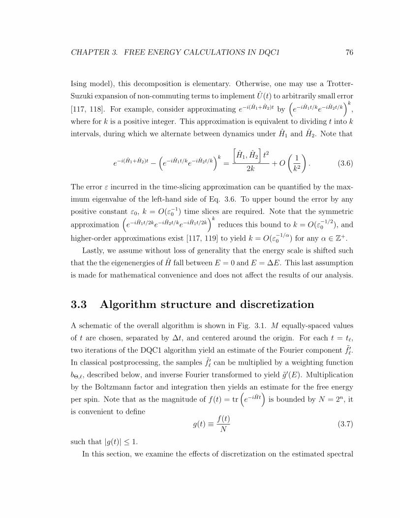
CHAPTER 3. FREE ENERGY CALCULATIONS IN DQC1 76
Ising model), this decomposition is elementary. Otherwise, one may use a Trotter-
Suzuki expansion of non-commuting terms to implement U(t) to arbitrarily small error
[117, 118]. For example, consider approximating e−i(H1+H2)t by(e−iH1t/ke−iH2t/k
)k
,
where for k is a positive integer. This approximation is equivalent to dividing t into k
intervals, during which we alternate between dynamics under H1 and H2. Note that
e−i(H1+H2)t −(e−iH1t/ke−iH2t/k
)k
=
[H1, H2
]t2
2k+O
(1
k2
). (3.6)
The error ε incurred in the time-slicing approximation can be quantified by the max-
imum eigenvalue of the left-hand side of Eq. 3.6. To upper bound the error by any
positive constant ε0, k = O(ε−10 ) time slices are required. Note that the symmetric
approximation(e−iH1t/2ke−iH2t/ke−iH1t/2k
)k
reduces this bound to k = O(ε−1/20 ), and
higher-order approximations exist [117, 119] to yield k = O(ε−1/α0 ) for any α ∈ Z+.
Lastly, we assume without loss of generality that the energy scale is shifted such
that the the eigenenergies of H fall between E = 0 and E = ∆E. This last assumption
is made for mathematical convenience and does not affect the results of our analysis.
3.3 Algorithm structure and discretization
A schematic of the overall algorithm is shown in Fig. 3.1. M equally-spaced values
of t are chosen, separated by ∆t, and centered around the origin. For each t = t`,
two iterations of the DQC1 algorithm yield an estimate of the Fourier component f ′`.
In classical postprocessing, the samples f ′` can be multiplied by a weighting function
bΘ,`, described below, and inverse Fourier transformed to yield g′(E). Multiplication
by the Boltzmann factor and integration then yields an estimate for the free energy
per spin. Note that as the magnitude of f(t) = tr(e−iHt
)is bounded by N = 2n, it
is convenient to define
g(t) ≡ f(t)
N(3.7)
such that |g(t)| ≤ 1.
In this section, we examine the effects of discretization on the estimated spectral
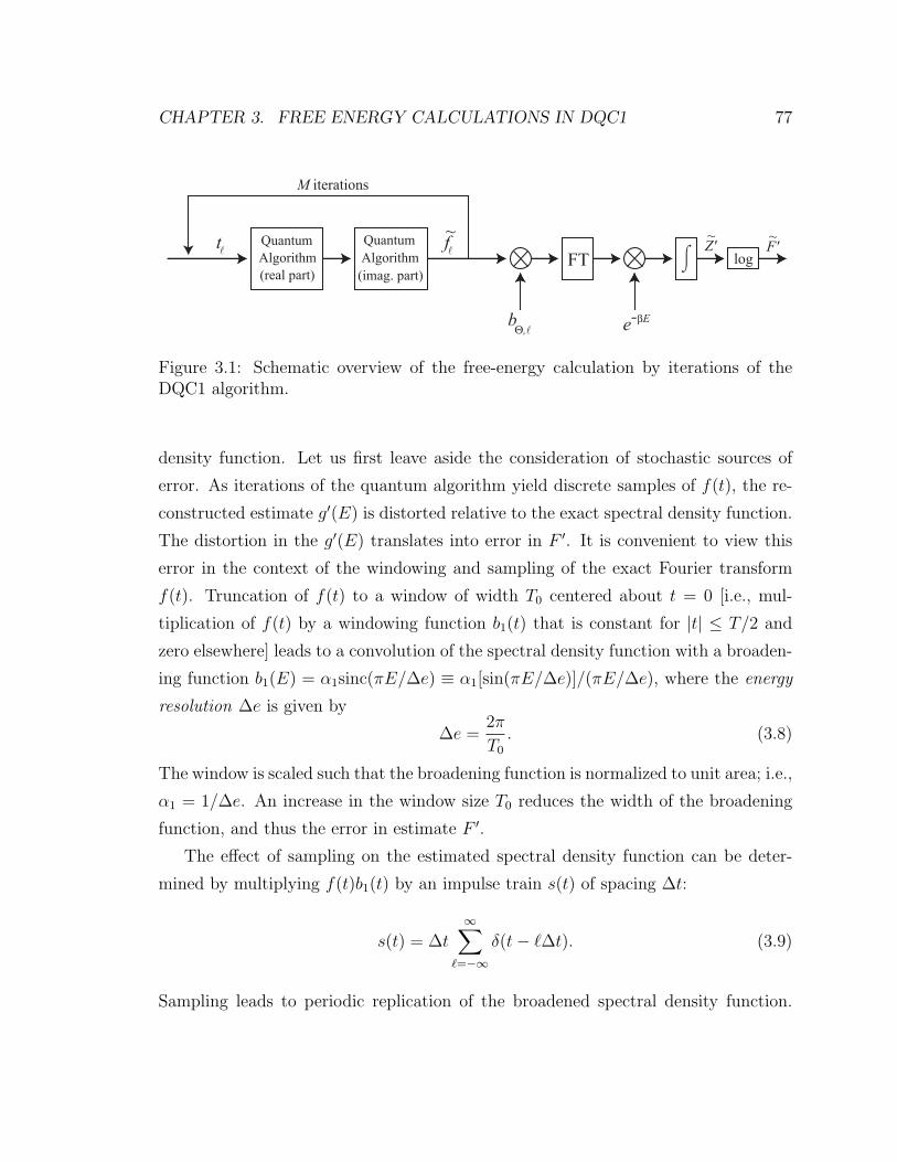
CHAPTER 3. FREE ENERGY CALCULATIONS IN DQC1 77
QuantumAlgorithm(real part)
QuantumAlgorithm(imag. part)
FTtl fl
~
bΘ,l e-βE
⌠⌡ log
Z'~
F'~
M iterations
Figure 3.1: Schematic overview of the free-energy calculation by iterations of theDQC1 algorithm.
density function. Let us first leave aside the consideration of stochastic sources of
error. As iterations of the quantum algorithm yield discrete samples of f(t), the re-
constructed estimate g′(E) is distorted relative to the exact spectral density function.
The distortion in the g′(E) translates into error in F ′. It is convenient to view this
error in the context of the windowing and sampling of the exact Fourier transform
f(t). Truncation of f(t) to a window of width T0 centered about t = 0 [i.e., mul-
tiplication of f(t) by a windowing function b1(t) that is constant for |t| ≤ T/2 and
zero elsewhere] leads to a convolution of the spectral density function with a broaden-
ing function b1(E) = α1sinc(πE/∆e) ≡ α1[sin(πE/∆e)]/(πE/∆e), where the energy
resolution ∆e is given by
∆e =2π
T0
. (3.8)
The window is scaled such that the broadening function is normalized to unit area; i.e.,
α1 = 1/∆e. An increase in the window size T0 reduces the width of the broadening
function, and thus the error in estimate F ′.
The effect of sampling on the estimated spectral density function can be deter-
mined by multiplying f(t)b1(t) by an impulse train s(t) of spacing ∆t:
s(t) = ∆t∞∑
`=−∞
δ(t− `∆t). (3.9)
Sampling leads to periodic replication of the broadened spectral density function.

CHAPTER 3. FREE ENERGY CALCULATIONS IN DQC1 78
The resultant function is given by the Fourier transform of f(t)b1(t)s(t):
g′(E) = g(E) ∗ b1(E) ∗∞∑
k=−∞
δ
(E +
2πk
∆t
), (3.10)
where the asterisks denote convolution.
To avoid aliasing in the estimated spectral density function, the Nyquist sampling
condition requires that
∆t ≤ 2π
∆E. (3.11)
Note that the spacing between samples of f(t) is determined solely by the estimate
of the energy bandwidth, ∆E. We assume that sampling is performed at the Nyquist
rate, in which case the equality in Eq. 3.11 holds.
As the number of samples is equal to the ratio of the windowing function width
T0 to the sampling time, one can determine the minimum value of T0 required to
satisfy Eq. 3.4 as a function of n. However, the rectangular windowing function
leads to poor results. The broadening function b1(E) is a sinc function that falls off
weakly with 1/E; in the calculation of the free energy in Eq. 3.3, the oscillating
side lobes are amplified at low energies by the Boltzmann factor. The window width
required to mitigate the resultant error scales poorly with n. In contrast to using
wider rectangular windows, one may adopt more elaborate window shapes, whose
corresponding broadening functions exhibit envelopes that are more sharply peaked.
We consider the functions bΘ(t), formed by the successive convolution of Θ rectangular
windows, each of width T0. Θ is referred to as the degree of the windowing function.
For Θ = 2, the window is triangular and of width 2T0. With increasing degree, the
window approaches a Gaussian shape, and is of width ΘT0. The resulting broadening
function is then
bΘ(E) = αΘ
[sinc
(πE
∆e
)]Θ
, (3.12)
which exhibits a 1/EΘ envelope. The value of αΘ is determined by constraining the
area under bΘ(E) to equal 1. In practice, a given window shape would be constructed
by obtaining samples f` only within the window width ΘT0 centered at t = 0, and

CHAPTER 3. FREE ENERGY CALCULATIONS IN DQC1 79
weighting each sample by bΘ,` ≡ bΘ(t`).
As the envelope of the side lobes of bΘ(E) falls off exponentially with Θ, windowing
functions of large degree significantly reduce the error in the calculated free energy.
However, the trade-off is a wider window, leading to more Fourier components, and
thus more iterations of the quantum algorithm:
M =ΘT0
∆T. (3.13)
Therefore, the question of how M scales with the number of spins n translates into
the determination of the minimum values of Θ and T0 required to satisfy Eq. 3.4.
An estimate Z ′ for the partition function can be calculated directly from the
estimated Fourier components without intermediate calculation of the spectral density
function. To see this, first evaluate the Fourier transform of f(t)bΘ(t)s(t) via Eq. 3.9
to give an intermediate estimate of the broadened, periodically replicated g′(E) in
terms of the components f`:
g′(E) =1
2π
∫ ∞
−∞f(t)bΘ(t)
[∆t
∞∑`=−∞
δ(t− `∆t)
]eiEtdt (3.14a)
=∆t
2π
∑`
f`bΘ,`eiEt` , (3.14b)
where the sum is performed over all ` within the window described by bΘ,`. Integrating
Eq. 3.14b over the energy bandwidth, using Eqs. 3.7 and 3.11, and labeling quantities
with a tilde to acknowledge stochastic errors, one finds
Z ′ =
∫ ∆E
0
g′(E)e−βEdE (3.15a)
=2n∆t
2πβ
(1− e−β∆E
)bΘ,0 + 2
M/2∑`>0
bΘ,`
×[
1
1 + (t`/β)2Re(g`)−
t`/β
1 + (t`/β)2Im(g`)
]. (3.15b)
Note that the real and imaginary parts of g` are precisely the quantities obtained at

CHAPTER 3. FREE ENERGY CALCULATIONS IN DQC1 80
each iteration of the DQC1 algorithm.
3.4 Error analysis: broadening
In this section, we determine an upper bound on the number of samples M of g(t)
required to calculate the free energy to the tolerance prescribed by Eq. 3.4. At this
point, we consider the individual samples of g` to be known exactly (allowing us to
omit the tilde over all quantities), and only consider the error in F ′ due to the finite
number of Fourier components – i.e., due only to the broadening of the density of
states. With this restriction, we will show that M is a polynomial function of the
number of spins n.
As it is more convenient to work with the partition function than the free energy,
we use a more stringent bound based upon the relative error in the calculated partition
function Z ′. First, note that |F ′ − F | < γkBθ is equivalent to the inequalities
e−γn − 1 <Z ′ − ZZ
< eγn − 1. (3.16)
It is sufficient to demand that
Prob
(r ≡
∣∣∣∣Z ′ − ZZ
∣∣∣∣ < ξ
)> 1− ε, (3.17)
where ξ ≡ 1 − exp(−γn). In other words, satisfaction of Eq. (3.17) automatically
implies Eq. (3.4).
From Eqs. 3.8, 3.11, and 3.13, if the Nyquist sampling condition is satisfied, then
M =Θ∆E
∆e. (3.18)
It has been asserted that ∆E is a polynomial function of n. In the remainder of this
section, we examine the dependence of Θ and ∆e on n such that Eq. 3.4 is satisfied.
We require a pair of intermediate results:
Lemma 3.1. The parameter αΘ is defined in Eq. 3.12, and is determined by the
CHAPTER 3. FREE ENERGY CALCULATIONS IN DQC1 81
constraint that the area under the broadening function bΘ(E) is 1, implying that αΘ =(∫∞−∞ sincΘ(πE/∆E)dE
)−1
. An upper bound on αΘ is then
αΘ <cπ
∆e
√Θ
6π, (3.19)
where c ≈ 2.0367.
Lemma 3.2. Define Aside as the area under the broadening function that is outside
of the main lobe; i.e., Aside ≡ 1 −∫ ∆e
−∆ebΘ(E)dE. If Θ is even, then an upper bound
on Aside is
Aside <c
πΘ−3
√Θ
6π. (3.20)
Lemma 1 places an upper bound on αΘ such that bΘ(E) is normalized. Lemma 2
defines an upper bound on the area of bΘ(E) that is outside of the interval [−∆e,∆e]
(i.e., outside the main lobe of the broadening function); this bound decreases expo-
nentially with Θ. Both lemmas are proved in Appendix C.
One can relate the relative error r in the calculated partition function to the
parameters Θ and ∆e via Lemma 2. As the exact spectral density function g(E) may
be expressed as a sum of delta-functions for each eigenenergy Em, Eqs. 3.10 and 3.11
evaluated at the Nyquist condition yield
Z ′ =
∫ ∆E
0
g′(E)e−βEdE
=∑m
∞∑k=−∞
∫ ∆E
0
bΘ(E − Em + k∆E)e−βEdE
=∑m
[∞∑
k=−∞
∫ (k+1)∆E
k∆E
bΘ(E − Em)e−β(E−k∆E)dE
]≡∑m
Z ′m. (3.21)
The change of variables allows one to view Z ′m as an integral of the broadening
function, centered at Em, and weighted by periodically replicated segments of an

CHAPTER 3. FREE ENERGY CALCULATIONS IN DQC1 82
exponential function. Z ′ is found by summing over all eigenenergies.
One can show that the maximum relative error r in the partition function is
bounded by the largest contribution from any single eigenenergy, which we define as
rm ≡ maxm |Z ′m − Zm/Zm|, where Zm ≡ e−βEm . Defining γm = Z ′
m/Zm, it follows
that
r =
∣∣∣∣Z ′ − ZZ
∣∣∣∣ =|∑
m (Z ′m − Zm)|∑
m Zm
=|∑
m(γm − 1)Zm|∑m Zm
≤ maxm|γm − 1| = max
m
∣∣∣∣Z ′m − Zm
Zm
∣∣∣∣ = rm. (3.22)
This argument shows that one may consider a simplified system with just one
eigenstate at an energy Em somewhere in the energy bandwidth. An upper bound on
the error rm for this simplified system at any Em suffices to bound the error for an
arbitrary energy spectrum over the same bandwidth.
Lower and upper bounds on Z ′m (Z ′
m,min and Z ′m,max, respectively) are now derived
to bound rm, since
rm < max
(∣∣∣∣Z ′m,min − Zm
Zm
∣∣∣∣ , ∣∣∣∣Z ′m,max − Zm
Zm
∣∣∣∣) . (3.23)
In the main lobe, the minimum value of the Boltzmann factor is e−β(Em+∆e). Outside
of the main lobe, the minimum value is e−β∆E. Thus,
Z ′m =
∞∑k=−∞
∫ (k+1)∆E
k∆E
bΘ(E − Em)e−β(E−k∆E)dE
≥ (1− Aside)e−β(Em+∆e) + Asidee
−β∆E ≡ Z ′m,min. (3.24)
Similarly, as the maximum value of the Boltzmann factor is e−β(Em−∆e) inside the
main lobe and 1 outside,
Z ′m ≤ (1− Aside)e
−β(Em−∆e) + Aside ≡ Z ′m,max. (3.25)

CHAPTER 3. FREE ENERGY CALCULATIONS IN DQC1 83
Substituting Eqs. (3.24) and (3.25) into Eq. (3.23), we see that
rm < max[1− (1− Aside)e−β∆e − Asidee
−β(∆E−Em),
(1− Aside)eβ∆e + Asidee
βEm − 1]. (3.26)
It is difficult to invert Eq. (3.26) explicitly to find optimal conditions on Aside(Θ) and
∆e which ensure that rm < ξ. However, one can show that the following conditions
are sufficient:
β∆e = ln(1 + ξ/2), (3.27a)
Aside <ξ
2e−β∆E. (3.27b)
As proof of their sufficiency, note that
1− (1− Aside)e−β∆e − Asidee
−β(∆E−Em) <ξ
2+ξ
2e−β∆E
(1− ξ
2
)< ξ (3.28)
and
(1− Aside)eβ∆e + Asidee
βEm − 1 <ξ
2+ξ
2e−β(∆E−Em) < ξ. (3.29)
Therefore, the conditions in Eqs. 3.27a and 3.27b guarantee that r < rm < ξ, as
desired.
Using Lemma 3.2, one can manipulate Eqs. 3.27a and 3.27b to show that M
scales polynomially with n.
∆e =ln(1 + ξ/2)
β, (3.30a)
Θ− ln Θ
2 ln π>β∆E
ln π+
ln(1/ξ)
ln π+ κ, (3.30b)
where κ = 5/2 + ln(2c/√
6)/ ln π ≈ 2.9443 . As ln Θ < Θ, a sufficient condition to
satisfy Eq. 3.30b is
Θ/2 = dµβ∆E + µ ln(1/ξ) + κ′e, (3.31)

CHAPTER 3. FREE ENERGY CALCULATIONS IN DQC1 84
where µ ≡ 1/(2 ln π − 1) and κ′ ≡ µκ ln π.
In summary, the error bound on the partition function is satisfied if the energy
resolution scales linearly with temperature, and if Θ scales linearly with β∆E.
As a final step, we substitute the conditions in Eqs. 3.30a and 3.31 into Eq. 3.18,
disregarding the weak logarithmic dependence of Θ and ∆e on n.
M =Θ∆E
∆e∝ (β∆E)(∆E)
1/β= β2(∆E)2 ∝ poly(n), (3.32)
by the assertion that the energy bandwidth is a polynomial function of the number
of spins in our system. This result shows that in the absence of fluctuations in the
calculated Fourier components of the spectral density, the free energy per spin can
be determined efficiently to bounded error.
A qualitative argument can help to understand this result. Note that shifting the
eigenvalue spectrum by γkBθ increases the free energy by the same amount. There-
fore, to satisfy Eq. 3.4, one expects that the broadening width ∆e of each eigenvalue
should be less than γkBθ. As M ∝ ∆E/∆e, we surmise that M = Ω(∆E/kBθ).
Why, then, is M = O[(∆E/kBθ)2] in Eq. 3.32? First, this simple argument neglects
the error due to the long tails of the broadening function bΘ(E), and thus should
be treated with some skepticism. Second, the bound in Eq. 3.32 is not tight, as
we derived a sufficient but non-optimal solution to Eq. 3.26. There may exist other
values that improve the upper bound on M . Nonetheless, as we have shown that
M = O[poly(n)], the bound is sufficient to show that the algorithm is efficient in the
absence of stochastic errors.
3.5 Error analysis: stochastic errors
In the preceding section, it was assumed that values of g` are generated with arbitrary
precision, implying noiseless measurement of the expectation value of σz for a single
qubit. However, stochastic fluctuations may be introduced either by undesired inter-
action of our measurement apparatus with the environmental degrees of freedom, or,
more fundamentally, due to fluctuations in the initial ensemble, as discussed in Sec.
CHAPTER 3. FREE ENERGY CALCULATIONS IN DQC1 85
2.2.1. To model the effect of random noise, we assume that the real and imaginary
part of each estimated g` is an independent Gaussian random variable with variance
s2. In this section, we determine an upper bound on s such that Eq. 3.4 is satisfied.
Recall that Z ′ represents an estimate of the partition function calculated from
discrete and imprecise Fourier components of the density of states. From Eq. 3.15,
Z ′ is a linear combination of the independent random variables Re(g`) and Im(g`).
Thus, Z ′ is also Gaussian-distributed, with a variance
σ2Z′ =
[2n∆t
πβ
(1− e−β∆E
)]2 M/2∑`>0
b2Θ,`
[1
1 + (t`/β)2
]2
s2 +
[t`/β
1 + (t`/β)2
]2
s2
(3.33a)
=4ns2∆t2
(1− e−β∆E
)2π2β2
M/2∑`=1
b2Θ,`
1 + (t`/β)2. (3.33b)
As the functions 1/(1 + t2/β2) and bΘ(t) monotonically decrease with t, the sum can
be lower bounded by an integral
1
∆t
∫ (M/2+1)∆t
∆t
b2Θ(t)
1 + (t/β)2dt. (3.34)
Note that the temperature is an intensive quantity, whereas the energy bandwidth
∆E is extensive, and depends polynomially on the number of spins n. Thus, the
relevant limit as the system size increases is β∆E 1.
Recall that bΘ(t) is the convolution of Θ rectangular windows of width T0. By
the central limit theorem2, bΘ(t) approaches a Gaussian of second central moment
ν2 = ΘT 20 /12 as Θ → ∞. Consider the approximation bΘ(t) = e−t2/2ν2
. Even
for modest finite Θ, the approximation is reasonable; for Θ = 20, the relative error
incurred in Eq. 3.34 is less than 0.002. The following lemma then bounds the variance
of the estimated partition function; it is proved in Appendix C.
2Imagine that b1(t) is a probability distribution function for a random variable uniformly dis-tributed between −T0 and T0; q has a second moment of T0/12. bΘ(t) is then the distributionfunction for the sum of Θ such independent random variables.

CHAPTER 3. FREE ENERGY CALCULATIONS IN DQC1 86
Lemma 3.3.
1
∆t
∫ (M/2+1)∆t
∆t
e−t2/ν2
1 + (t/β)2dt >
β∆E
4
[1−O
(1√β∆E
)]
Applying Lemma 3.3 to Eqs. 3.11 and 3.33b, to lowest order in 1/β∆E,
σ2Z′ >
4ns2
β∆E
[1−O
(1√β∆E
)]. (3.35)
Eq. 3.35 indicates that the standard deviation of Z ′ scales exponentially with n;
i.e., as 2n. The above result can be used to derive a condition on s such that the error
bound on the free energy is fulfilled. By Eq. 3.16, the condition
Ze−γn < Z ′ < Zeγn (3.36)
is equivalent to Eq. 3.4. As Z ′ is Gaussian-distributed, the probability ε0 that Eq.
3.36 is violated is
ε0 = 1− Prob(Ze−γn < Z ′ < Zeγn) (3.37a)
=1
2
erfc
[Z(eγn − 1)√
2σZ′
]+ erfc
[Z(1− e−γn)√
2σZ′
](3.37b)
≤ erfc
[Zγn√2σZ
]. (3.37c)
Substituting Eq. 3.35 and isolating s, we find
s ≤ Z
2n
poly(n)[erfc−1(ε0)
] . (3.38)
It is an interesting consequence of Eq. 3.38 that the allowed variance in the mea-
surement depends on the ratio of the actual partition function to 2n. Let us examine
this ratio for some simple cases. First, consider the admittedly non-physical yet sim-
ple example of a spectral density function gconst(E) that is constant and continuous
CHAPTER 3. FREE ENERGY CALCULATIONS IN DQC1 87
over the interval [0,∆E]. As 2n =∫ ∆E
0g(E)dE, it holds that g(E) = 2n/∆E. The
partition function is
Zconst =2n(1− e−β∆E)
β∆E. (3.39)
In this case, as Zconst is O [2n/poly(n)], it is possible to meet the criterion specified
in Eq. 3.38.
Now, let us consider three simple spin models that admit analytic solutions. First,
for n noninteracting (free) spins in a magnetic field,
Hfree = −h2
n∑`=1
(σz` − 1) (3.40)
where h is the Zeeman splitting between levels. The constant offset ensures that the
the support of g(E) is [0, nh]. The partition function is trivial to evaluate:
Zfree = (1 + e−βh)n. (3.41)
Second, we examine the Ising model in zero magnetic field for one and two dimensions,
using periodic boundary conditions.
HIsing = −ε∑〈ij〉
(σz
i σzj − 1
)(3.42)
The partition function for the one-dimensional model is [107]
ZIsing,1D =(1 + e−4βε
)n. (3.43)
The two-dimensional model was solved by Onsager [120], and yields [107]
ZIsing,2D =[2 cosh (2βε) e−2βε+f/2π
]n, (3.44)
CHAPTER 3. FREE ENERGY CALCULATIONS IN DQC1 88
where
f =
∫ π
0
dφ ln
[1
2
(1 +
√1− 4 sin2 φ
cosh2(2φ) coth2(2φ)
)]≈ −0.059547. (3.45)
The two-dimensional Ising model undergoes a phase transition from no net alignment
of spins to spontaneous magnetization at βε =[tanh−1(1/
√2)]/2 ≈ 0.440687; we
might wish to investigate the thermodynamic functions near the point of spontaneous
magnetization. The corresponding partition function is
ZIsing,2D ≈ (1.161)n. (3.46)
We see that in all three of these physical models, the partition function scales
as an exponential function ζn where ζ < 2. By Eq. 3.38, the standard deviation
of the measured Fourier components must decrease as (ζ/2)n. This is ensured by
Eq. 2.45 only if the number of ensemble members, and thus the system size, is an
exponential function of n. Thus, to find the free energy for bounded error for these
physically-motivated models requires an inefficient amount of spatial resources in the
presence of stochastic fluctuations. While this argument does not constitute a proof of
inefficiency for all spin models, it illustrates the importance of stochastic fluctuations
as a determining factor.
3.6 Summary and discussion of ensemble algorithms
Arvind and Collins [121] have argued that the DQC1 variant of the Deutsch-Jozsa
algorithm yields no advantage over a classical heuristic. As noted in Sec. 2.1.1, we can
evaluate f(x) at O[log(1/ε)] random inputs x, and distinguish constant and balanced
functions with a probability of error at most ε. As the number of function inquiries
for a given error is independent of n, the heuristic is efficient.
Does this criticism also apply to other DQC1 algorithms that depend upon cal-
culation of the trace of a unitary operator? In other words, does there exist a gen-
eral heuristic to generate K random eigenvalues eiφ` of a unitary operator U (for

CHAPTER 3. FREE ENERGY CALCULATIONS IN DQC1 89
` ∈ 1, 2, · · · , K), and then estimate the trace as N∑
` eiφ`/K? The answer seems
to be “no.” Note that the Deutsch-Jozsa case is special, as the eigenvalues are con-
strained by the inherent structure of the problem to be ±1, and can be generated effi-
ciently by a classical black box that computes f(x) for any x. By contrast, there is no
efficient heuristic known to generate random eigenvalues of a general N -dimensional
unitary operator. Thus, it is possible that DQC1 algorithms could yield exponential
speedup for selected problems.
The application of the DQC1 algorithm to free energy calculation fails for some
spin models as the partition function diminishes exponentially faster than the fluctua-
tions induced by the stochastic input state. Interestingly, this failure is a consequence
of the exponential dependence of the Boltzmann factor on energy. It is an open ques-
tion whether error criteria differing from Eq. 3.4 may be less stringent, and yield
an efficient algorithm. For instance, an alternative criterion depending directly on
bounding an order parameter such as specific heat capacity might be more physically
relevant and yield different scaling results, if less analytically tractable than Eq. 3.4.
Finally, note that other ensemble quantum computing models with highly-mixed
states hold promise. Zhou et al. [122] have considered an alternate scenario where all
qubits are highly mixed; each qubit state can be described by the high-temperature
density matrix (1/2 + p) |0〉 〈0|+ (1/2− p) |1〉 〈1|, where p 1. They show that the
Deutsch-Jozsa and parity algorithms can be solved efficiently without the need for
further initialization.
In summary, in this chapter, I proposed the usage of a DQC1 algorithm to com-
pute the free energy of spin lattice models. The algorithm yields individual Fourier
coefficients of the spectral density function, from which an estimate of the free en-
ergy can be constructed. The computational effort required to satisfy a bound on
the absolute error in the free energy was determined. Primary sources of error in-
cluded broadening due to the calculation of a finite number of Fourier coefficients,
and stochastic errors due to ensemble fluctuations. In the former case, a number
of Fourier coefficients that is polynomial in the number of spins n was found to be
sufficient to satisfy the error bound. However, it was shown for simple spin lattice
models that the stochastic fluctuations must diminish exponentially with n.

Chapter 4
Fighting decoherence by gate
decomposition
4.1 Overview
In this chapter, we are concerned with methods to mitigate the deleterious effect
of decoherence due to unwanted system-environment interactions. In contrast to the
previous two chapters, our subsequent discussion will be in the context of the standard
model of quantum computation, where fiducial pure-state initialization and projective
measurements are permitted.
Given the variety and sophistication of the error-correcting or error-avoiding tech-
niques reviewed in Sec. 1.6, one might inquire why an alternative approach to re-
ducing decoherence would be beneficial. However, each of the methods in Sec. 1.6 is
accompanied by disadvantages, either in additional resources, or in the difficulty of
implementation. For quantum error-correcting codes, several two-level systems are
required to encode a single logical qubit. In addition, many projective measurements1
and conditional unitary gates are required to detect and correct errors.
In decoherence-free subspaces, logical states are typically complicated superposi-
tions of “physical” two-level basis states. For example, the decoherence-free subspace
1As noted in Sec. 1.6.1, ancillary qubits can be substituted for projective measurements. However,the work qubits are then entangled and cannot be reused.
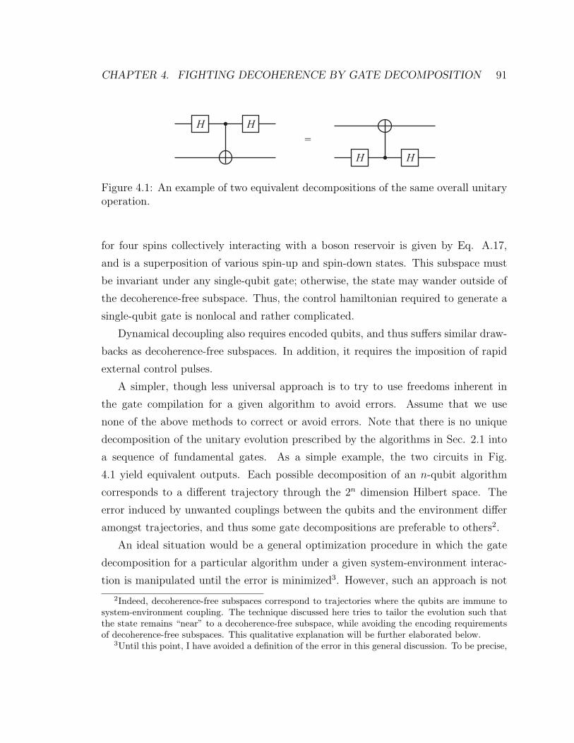
CHAPTER 4. FIGHTING DECOHERENCE BY GATE DECOMPOSITION 91
H H
H H=
Figure 4.1: An example of two equivalent decompositions of the same overall unitaryoperation.
for four spins collectively interacting with a boson reservoir is given by Eq. A.17,
and is a superposition of various spin-up and spin-down states. This subspace must
be invariant under any single-qubit gate; otherwise, the state may wander outside of
the decoherence-free subspace. Thus, the control hamiltonian required to generate a
single-qubit gate is nonlocal and rather complicated.
Dynamical decoupling also requires encoded qubits, and thus suffers similar draw-
backs as decoherence-free subspaces. In addition, it requires the imposition of rapid
external control pulses.
A simpler, though less universal approach is to try to use freedoms inherent in
the gate compilation for a given algorithm to avoid errors. Assume that we use
none of the above methods to correct or avoid errors. Note that there is no unique
decomposition of the unitary evolution prescribed by the algorithms in Sec. 2.1 into
a sequence of fundamental gates. As a simple example, the two circuits in Fig.
4.1 yield equivalent outputs. Each possible decomposition of an n-qubit algorithm
corresponds to a different trajectory through the 2n dimension Hilbert space. The
error induced by unwanted couplings between the qubits and the environment differ
amongst trajectories, and thus some gate decompositions are preferable to others2.
An ideal situation would be a general optimization procedure in which the gate
decomposition for a particular algorithm under a given system-environment interac-
tion is manipulated until the error is minimized3. However, such an approach is not
2Indeed, decoherence-free subspaces correspond to trajectories where the qubits are immune tosystem-environment coupling. The technique discussed here tries to tailor the evolution such thatthe state remains “near” to a decoherence-free subspace, while avoiding the encoding requirementsof decoherence-free subspaces. This qualitative explanation will be further elaborated below.
3Until this point, I have avoided a definition of the error in this general discussion. To be precise,

CHAPTER 4. FIGHTING DECOHERENCE BY GATE DECOMPOSITION 92
feasible, as each gate decomposition circuit must be explicitly simulated on a classi-
cal computer to compute the error. Simulation of a quantum circuit on a classical
computer is generally inefficient due to the exponential size of the Hilbert space.
The approach of mitigating decoherence by gate design is only useful if both the
algorithm and decoherence model possess a structure that immediately suggests an
advantageous gate decomposition. In this chapter, I will investigate the database-
search quantum algorithm (cf. 2.1.2) as such an example, in the presence of a collec-
tive, dissipative system-environment interaction. At first, I will present a very crude
argument based on first-order transition rates to substantiate why a simple change in
selected fundamental gates for the search algorithm could lead to diminished error.
This argument hinges on the interpretation of the database search algorithm as a
sequence of rotations in a two-dimensional substance. Calculations of the averaged
transition rate are carried out for the search algorithm for up to nine qubits, and
are presented in 4.4. A more rigorous computation of the error is carried out in Sec.
4.5 using a quantum master equation approach, which computes the evolution of
the reduced density matrix for the qubits in the presence of the system-environment
coupling. Due to the computational overhead of these simulations, only six-qubit
instances of the search algorithm were simulated. The modified search algorithm
gives rise to a modest improvement in performance for specific ranges of system-
environment coupling strengths, as is discussed in Sec. 4.5.
4.2 Collective dissipation
A general hamiltonian for the system and environment (cf. Eq. 1.46) is
H = HS ⊗ IE + IS ⊗ HE + HSE. (4.1)
the outcomes of the final measurement can be characterized by a probability distribution functionfor the computational basis states. The error can be quantified by a distance measure between theideal probability distribution function, and also the function in the presence of system-environmentcouplings.
CHAPTER 4. FIGHTING DECOHERENCE BY GATE DECOMPOSITION 93
We consider the environment to be composed of a reservoir of boson modes, such that
HE =∑
k
ωk
(a†kak + 1/2
). (4.2)
The following model for the system-reservoir interaction is assumed. The n qubits
are coupled to the environment by a Jaynes-Cummings-like interaction
HSE =1
2
n∑i=1
∑k
(g∗i,kσ
+i ⊗ ak + gi,kσ
−i ⊗ a
†k
). (4.3)
This interaction leads to energy exchange between the qubits and the reservoir, as
the σ+ and σ− operators lead to bit-flips.
We assume that the n qubits interact collectively with the reservoir, such that
gi,k = gk. Defining the total spin operator Sα = 12
∑ni=1 σ
αi , this implies that
HSE =∑
k
(g∗kS
+ ⊗ ak + gkS− ⊗ a†k
). (4.4)
Furthermore, we assume that the reservoir is at zero temperature, so that each envi-
ronment mode is in the vacuum state, which we denote as |0〉E. We notate as |k〉E the
reservoir state where all modes are in the ground state except for mode k, which has
one excitation (e.g., a single phonon in mode k for vibrational modes in a solid-state
system). Consideration of the single-excitation manifold will be sufficient to derive a
first-order transition rate.
This collective interaction corresponds to the physical scenario in which the qubits
are closely spaced relative to the wavelength of the cold reservoir. This might be rele-
vant for solid-state implementations, where qubits are two-level systems (e.g., selected
ionic or atomic levels) that couple to long-wavelength modes of a cold phonon bath.
The electric-dipole coupling of closely-spaced atoms to a fluctuating electromagnetic
field is another such example.
In the interaction picture associated with IS ⊗ HE, the hamiltonian is
H int = HS ⊗ IE +(g∗ke
−iωktS+ ⊗ ak + gkeiωktS− ⊗ a†k
). (4.5)
CHAPTER 4. FIGHTING DECOHERENCE BY GATE DECOMPOSITION 94
The hamiltonian H int leads to transitions between the collective angular momen-
tum states |j,m, α〉S, introduced in Sec. 1.6.2 and discussed in detail4 in App. A.
These transitions can be explained by a simple first-order perturbation theory ar-
gument [123, 124]. Assume that at time t = 0, the system and environment are in
the state |j,m, α〉S ⊗ |0〉E, which we compactly notate as |j,m, α; 0〉. A general state
(limited to the single-excitation manifold) is
|ψ〉SE =∑j,m,α
(cj,m,α;0 |j,m, α; 0〉+
∑k
cj,m,α;k |j,m, α; k〉
). (4.6)
The coefficients evolve under the Schrodinger equation
icj′,m′,α′;k′(t) =∑
j′′,m′′,α′′,k′′
cj′′,m′′,α′′;k′′(t) 〈j′,m′, α′; k′| H int |j′′,m′′, α′′; k′′〉 . (4.7)
Near t = 0,
cj′′,m′′,α′′,k′′(t) = δj,j′′δm,m′′δα,α′′δk,0, (4.8)
implying
cj′,m′,α′;k′(t) = −i 〈j′,m′, α′; k′| H int |j,m, α; 0〉 . (4.9)
Now, assume that no control hamiltonian is applied, so HS is zero. Then, from Eq.
4.5,
cj′,m′,α′;k′(t) = −i∑
k
gkeiωkt 〈j′,m′, α′; k′| S− ⊗ a†k |j,m, α; 0〉
= −i∑
k
gkeiωkt 〈j′,m′, α′| S− |j,m, α〉 〈k′| a†k |0〉 (4.10)
where we have noted that ak acting on the vacuum state is zero. The first matrix
element is obtained from Eq. A.10a,
〈j′,m′, α′| S− |j,m, α〉 =√j(j + 1)−m(m− 1)δj,j′δm−1,m′δα,α′ , (4.11)
4As a brief reminder, each qubit is viewed as a pseudospin, and the labels j and m refer to theeigenvalues of the total squared angular momentum operator and its z-component. The label αsubsumes all other quantum numbers.
CHAPTER 4. FIGHTING DECOHERENCE BY GATE DECOMPOSITION 95
while the second matrix element is simply δk,k′ . Substituting Eq. 4.11 into Eq. 4.10
and integrating from 0 to t,
|cj,m−1,α,k′|2 =[j(j + 1)−m(m− 1)] |gk′|2 sin2 (ωk′t)
ω2k′
. (4.12)
By probability conservation, the population of the original qubit state |j,m, α〉 decays
as
|cj,m,α,0|2 = 1− E(j,m)∑k′
|gk′|2 sin2 (ωk′t)
ω2k′
, (4.13)
where
E(j,m) ≡ j(j + 1)−m(m− 1). (4.14)
E(j,m) is a collective enhancement factor that can augment or reduce the transition
rate; it is the source of “superradiance” in quantum optics [59]. Note that for a
single qubit (i.e., pseudospin) in the excited state |j = 1/2,m = 1/2〉, the collective
enhancement factor is 1. Thus, E(j,m) represents the enhancement in the transition
rate compared to a single spin.
The collective enhancement factors are depicted in Fig. 4.2 for n = 8. The
states |j;m = −j;α〉 have E(j,m) = 0; no transitions can occur in these “subra-
diant” or “dark” states as S− |j;m = −j;α〉 = 0. Indeed, these states form the
decoherence-free subspace for the hamiltonian in Eq. 4.3. By contrast, the states
|j = n/2;m = 0 or ± 1/2;α〉 are superradiant and have significantly higher dissipa-
tion rates than independent spins.
This analysis suggests a crude estimate of the instantaneous dissipation rate for
a given n-qubit pure state. The collective angular momentum or Dicke-states form a
complete basis, so an arbitrary n-qubit pure state can be expanded as
|ψ〉S =∑j,m,α
aj,m,α |j,m, α〉 . (4.15)

CHAPTER 4. FIGHTING DECOHERENCE BY GATE DECOMPOSITION 96
43
21
0−4 −3 −2 −1 0 1 2 3 4
0
2
4
6
8
10
12
14
16
18
20
mj
j(j+
1)−
m(m
−1)
Figure 4.2: The collective enhancement factor j(j + 1)−m(m− 1) for n = 8. Super-radiant states are shown in red, while subradiant states are in blue.
Define the state-averaged collective enhancement factor
γ1 =∑j,m,α
E(j,m) |aj,m,α|2 =∑j,m
E(j,m)∑
α
|aj,m,α|2
=∑j,m
E(j,m)∑
α
|〈j,m, α| ψ〉S|2 . (4.16)
A state with a large probability amplitude in the subradiant (superradiant) states will
yield a small (large) value of γ1. This suggests that states with large state-averaged
collective enhancement factors interact strongly with the environment. Note that γ1
is entirely determined by the probability weights for each (j,m) value,∑
α |aj,m,α|2.These probability weights and the corresponding values of γ1 are plotted for selected
states |ψ〉S in Fig. 4.3.
For a given algorithm, in the absence of noise, the state evolves from an initial
fiducial state |ψ(0)〉 to a final state |ψ(T )〉 according to the hamiltonian that generates
the sequence of fundamental unitary gates. If we simulate the algorithm on a classical

CHAPTER 4. FIGHTING DECOHERENCE BY GATE DECOMPOSITION 97
(a)
(b)
(c)
43
21
0
4 3 2 1 0 1 2 3 4
0
0.1
0.2
0.3
0.4
0.5
0.6
0.7
0.8
0.9
1
mj
Pro
bab
ility
43
21
0
4 3 2 1 0 1 2 3 4
0
0.05
0.1
0.15
0.2
0.25
0.3
mj
Pro
bab
ility
43
21
0
4 3 2 1 0 1 2 3 4
0
0.05
0.1
0.15
0.2
0.25
0.3
mj
Pro
bab
ility
γ = 01
γ = 181
γ = 21
Figure 4.3: Bar plots of the probability weights∑
α |aj,m,α|2 for selected eight-qubitstates, and the associated value of γ1. Subradiant (DFS) states are dark blue, whilesuperradiant states are bright red. (a) State |j = 4,m = −4〉 = |00000000〉. (b)Equal superposition state |σ〉 ≡ (|0〉+ |1〉)⊗8 /
√256. (c) Singlet-like superposition
state |σ′〉 ≡ [(|0〉+ |1〉)⊗ (|0〉 − |1〉)]⊗4 /√
256.

CHAPTER 4. FIGHTING DECOHERENCE BY GATE DECOMPOSITION 98
computer, the state-averaged collective enhancement factor γ1(t) can be calculated
at each time in the interval [0, T ]. This parameter is then proposed as an estimate of
the instantaneous enhancement in the dissipation rate.
I emphasize that γ1 provides a qualitative estimate of the impact of collective
decoherence, and does not necessarily correlate to a true physical dissipation rate.
The reason for this is threefold. First, I have neglected the system hamiltonian HS in
the above discussion of transition rates. We know from the discussion of dynamical
decoupling that the control hamiltonian can influence and even eliminate the impact
of system-environment coupling. Second, the state-averaged collective enhancement
factor ignores phase information, as it averages over probabilities as opposed to prob-
ability amplitudes. Third, γ1 is computed from the ideal trajectory of the state ket
through the Hilbert space (i.e., the state in the absence of system-environment in-
teraction). However, the system-environment coupling entangles the qubits with the
reservoir, and the qubit state is correctly described by a reduced density matrix,
tracing over the environmental degrees of freedom. As time progresses, we expect the
reduced density matrix to be poorly approximated by the ideal state vector.
In Sec. 4.5, a more rigorous calculation of the evolution of the reduced density
matrix by integration of a quantum-master equation is performed. However, to justify
the intuition behind the gate decomposition for the quantum search algorithm in the
next section, we commence by using γ1 as a measure of the dissipation rate.
4.3 Modifying the quantum search algorithm
The quantum search algorithm was discussed in Sec. 2.1.2. In the underlying problem,
we are given a function f : ZN → 0, 1, and are asked to find a value x ∈ ZN such
that f(x) = 1. Let X be the subset of all x for which f(x) = 1. If there are r
such elements, the simplest heuristic is to evaluate f for random values of x until a
solution is found; O(N/r) guesses are required. The quantum search algorithm solves
this problem with a square-root speedup in the number of function evaluations.
Recall that to perform the quantum search algorithm, one first applies a Hadamard

CHAPTER 4. FIGHTING DECOHERENCE BY GATE DECOMPOSITION 99
transformation H to all of n qubits to create the equally-weighted superposition state
|σ〉 =1√N
N−1∑x=0
|x〉 . (4.17)
Then, one repeatedly applies the operator Q = −HU0HUX , where UX and U0 are
defined as
UX = I − 2∑x∈X
|x〉 〈x| (4.18a)
U0 = I − 2 |0〉 〈0| . (4.18b)
In the subspace spanned by |σ〉 and the state∣∣X⟩, defined as
∣∣X⟩ =1√r
∑x∈X
|x〉 , (4.19)
Q can be interpreted as a rotation by a fixed angle θ, given in Eq. 2.15. After a given
number of applications of Q, the superposition state |σ〉 is rotated near∣∣X⟩, and a
projective measurement yields one of the solutions to the search problem with near
certainty. The number of required rotations is O(√N/r).
Note in Fig. 4.3(b) that the equal superposition state |σ〉 has a large state-averaged
collective enhancement factor γ1, as it exhibits a high probability weighting near the
superradiant states5. Thus, in the initial part of the quantum search algorithm, as
we start to rotate from |σ〉 towards∣∣X⟩, we expect the dissipation rate to be high. It
would be preferable if the algorithm could be carried out as a rotation in a different
two-dimensional subspace, spanned by a subradiant state and∣∣X⟩.
5As |σ〉 is symmetric under qubit permutations, only the maximal j = n/2 components havenon-zero probability amplitudes.
CHAPTER 4. FIGHTING DECOHERENCE BY GATE DECOMPOSITION 100
For example, consider replacing |σ〉 by the superposition state
|σ′〉 =
(|0〉+ |1〉√
2
)⊗(|0〉 − |1〉√
2
)⊗(|0〉+ |1〉√
2
)⊗(|0〉 − |1〉√
2
)⊗ · · ·
=1√N
N−1∑x=0
m(x) |x〉 , (4.20)
in which m(x) keeps track of the minus signs inherent in expanding out the first line,
and thus takes value ±1. The state-average collective enhancement factor of |σ′〉 is
given in Fig. 4.3(c) for n = 8. The parameter γ1 is substantially improved compared
to |σ〉, due to the significant probability amplitude in subradiant states6.
The modification required to change the invariant two-dimensional subspace is
simple. Replace the Hadamard transformations in Q by the operator Vmod, whose
matrix representation in the computational basis is defined as
Vmod =1√2
[1 1
1 −1
]⊗ 1√
2
[−1 1
1 1
]⊗ 1√
2
[1 1
1 −1
]⊗ 1√
2
[−1 1
1 1
]⊗ · · ·
(4.21)
Like the n-qubit Hadamard operator, V is a sequence of simple single-qubit gates on
all n qubits. They differ only in the diagonal elements of the operators on alternating
qubits.
To show that the operator Qmod ≡ VmodU0VmodUX yields a rotation in the desired
subspace, we recall the discussion of the generalized search algorithm [75, 76] in Sec.
2.1.2. By Eqs. 2.18 through 2.21, the invariant subspace is spanned by
Vmod |0〉 = |σ′〉 (4.22)
and √N
r
∑x∈X
|x〉 〈x| Vmod |0〉 =
√N
r
∑x∈X
|x〉 〈x| σ′〉 =1√r
∑x∈X
m(x) |x〉 . (4.23)
6The small value of γ1 for |σ′〉 can be understood by noting that (|0〉+ |1〉) ⊗ (|0〉 − |1〉) =|00〉− |11〉+ |10〉− |01〉. The states |00〉 and |10〉− |01〉 are the subradiant triplet and singlet states.

CHAPTER 4. FIGHTING DECOHERENCE BY GATE DECOMPOSITION 101
The rotation angle, given by Eq. 2.21, is
θ = sin−1
2
√√√√∑x∈X
∣∣∣〈x| Vmod |0〉∣∣∣2 −(∑
x∈X
∣∣∣〈x| Vmod |0〉∣∣∣2)2
= sin−1
[2√r(N − r)N
], (4.24)
where we have noted that∣∣∣〈x| Vmod |0〉
∣∣∣2 =[h(x)/
√N]2
= 1/N . The angle in Eq.
4.24 is identical to that of the original algorithm (cf. Eq. 2.15).
In summary, the “modified algorithm” commences by applying Vmod to the initial
state |0〉, leading to |σ′〉. Successive applications of Qmod rotate |σ′〉 towards the1√r
∑x∈X m(x) |x〉 state. After O(
√N/r) rotations, projective measurement yields
one of the solutions in X with near-unity probability.
As the probability amplitudes of |σ′〉 in the collective angular momentum basis
are large near the subradiant states, we intuit that the error induced by dissipation
in the modified algorithm would be less than in the original algorithm. In the next
chapter, I present simulation data of γ1 for various instances of the search algorithm
to bolster this claim.
4.4 Simulation data for the collective enhancement
factor
In this section, I present simulation data of the state-averaged collective enhancement
factor γ1(t) for instances of the original and modified quantum search algorithms. In
Sec. 4.2, I conjectured that γ1(t), plotted over the evolution time of a quantum
algorithm, gives a crude estimate of the dissipation rate. The simulations described
in this section decompose a given instance of the search algorithm into a sequence
of elementary gates, and then evaluate γ1 after each gate. I first show how this
decomposition is carried out for the original and modified algorithms. I then argue
why it is reasonable to discretize the continuous function γ1 after each fundamental
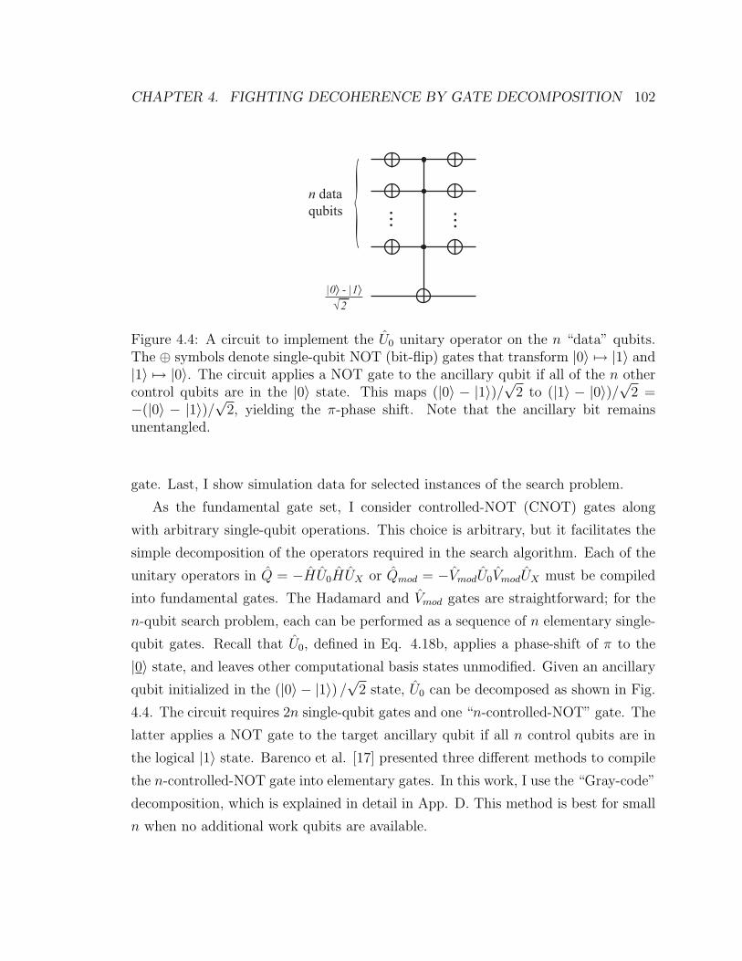
CHAPTER 4. FIGHTING DECOHERENCE BY GATE DECOMPOSITION 102
... ...
|0⟩ - |1⟩√2
n dataqubits
Figure 4.4: A circuit to implement the U0 unitary operator on the n “data” qubits.The ⊕ symbols denote single-qubit NOT (bit-flip) gates that transform |0〉 7→ |1〉 and|1〉 7→ |0〉. The circuit applies a NOT gate to the ancillary qubit if all of the n othercontrol qubits are in the |0〉 state. This maps (|0〉 − |1〉)/
√2 to (|1〉 − |0〉)/
√2 =
−(|0〉 − |1〉)/√
2, yielding the π-phase shift. Note that the ancillary bit remainsunentangled.
gate. Last, I show simulation data for selected instances of the search problem.
As the fundamental gate set, I consider controlled-NOT (CNOT) gates along
with arbitrary single-qubit operations. This choice is arbitrary, but it facilitates the
simple decomposition of the operators required in the search algorithm. Each of the
unitary operators in Q = −HU0HUX or Qmod = −VmodU0VmodUX must be compiled
into fundamental gates. The Hadamard and Vmod gates are straightforward; for the
n-qubit search problem, each can be performed as a sequence of n elementary single-
qubit gates. Recall that U0, defined in Eq. 4.18b, applies a phase-shift of π to the
|0〉 state, and leaves other computational basis states unmodified. Given an ancillary
qubit initialized in the (|0〉 − |1〉) /√
2 state, U0 can be decomposed as shown in Fig.
4.4. The circuit requires 2n single-qubit gates and one “n-controlled-NOT” gate. The
latter applies a NOT gate to the target ancillary qubit if all n control qubits are in
the logical |1〉 state. Barenco et al. [17] presented three different methods to compile
the n-controlled-NOT gate into elementary gates. In this work, I use the “Gray-code”
decomposition, which is explained in detail in App. D. This method is best for small
n when no additional work qubits are available.

CHAPTER 4. FIGHTING DECOHERENCE BY GATE DECOMPOSITION 103
For simplicity, I only consider instances of the quantum search algorithm where
there is a single target state (i.e., f(x) = 1 for only a single input). The oracle UX is
then implemented in an identical fashion to U0; the only difference lies in the NOT
gates that conjugate the n-controlled-NOT operator.
The simulation data were generated as follows. The n-qubit state vector consists
of 2n complex components, which are initialized to the |0〉 state. The compiler breaks
down the unitary operations required for the given instance of the search algorithm
into fundamental gates. Each unitary elementary gate is applied to the state vector
in sequence. After each gate, the state is projected on the Dicke-state basis and
the state-averaged enhancement factor γ1 is calculated. I implicitly assume that the
evolution times for all single-qubit and CNOT gates are equal.
Note that this procedure computes γ1 only at discrete times. However, one can
argue that the variation of γ1 over a gate time is small; solving for γ1 after each
fundamental gate is a reasonable approximation to the continuous function. To justify
this assertion, note that a general n-qubit state can be expanded in the Dicke-state
basis as Eq. 4.15. A unitary transformation U due to a single-qubit or CNOT gate
maps |ψ〉S to
U |ψ〉S =∑
j′,m′,α′
bj′,m′,α′ |j′,m′, α′〉 (4.25)
where
bj′,m′,α′ =∑j,m,α
aj,m,α 〈j′,m′, α′| U |j,m, α〉 . (4.26)
In App. E, it is shown that as a consequence of the Wigner-Eckart theorem [125, 126,
127], the matrix element in Eq. 4.26 is nonzero only for restricted values of |j′ − j|and |m′ −m|. For a single qubit gate, 〈j′,m′, α′| U |j,m, α〉 is zero unless both
|j′ − j| ≤ 1,
|m′ −m| ≤ 1. (4.27)
To understand the consequence of this restriction, consider how a single-qubit gate can
transform the the graph of probability weights∑
α |aj,m,α|2 for the |σ〉 state, shown
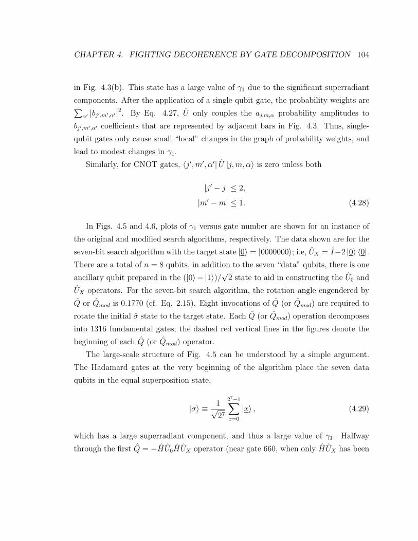
CHAPTER 4. FIGHTING DECOHERENCE BY GATE DECOMPOSITION 104
in Fig. 4.3(b). This state has a large value of γ1 due to the significant superradiant
components. After the application of a single-qubit gate, the probability weights are∑α′ |bj′,m′,α′|2. By Eq. 4.27, U only couples the aj,m,α probability amplitudes to
bj′,m′,α′ coefficients that are represented by adjacent bars in Fig. 4.3. Thus, single-
qubit gates only cause small “local” changes in the graph of probability weights, and
lead to modest changes in γ1.
Similarly, for CNOT gates, 〈j′,m′, α′| U |j,m, α〉 is zero unless both
|j′ − j| ≤ 2,
|m′ −m| ≤ 1. (4.28)
In Figs. 4.5 and 4.6, plots of γ1 versus gate number are shown for an instance of
the original and modified search algorithms, respectively. The data shown are for the
seven-bit search algorithm with the target state |0〉 = |0000000〉; i.e, UX = I−2 |0〉 〈0|.There are a total of n = 8 qubits, in addition to the seven “data” qubits, there is one
ancillary qubit prepared in the (|0〉− |1〉)/√
2 state to aid in constructing the U0 and
UX operators. For the seven-bit search algorithm, the rotation angle engendered by
Q or Qmod is 0.1770 (cf. Eq. 2.15). Eight invocations of Q (or Qmod) are required to
rotate the initial σ state to the target state. Each Q (or Qmod) operation decomposes
into 1316 fundamental gates; the dashed red vertical lines in the figures denote the
beginning of each Q (or Qmod) operator.
The large-scale structure of Fig. 4.5 can be understood by a simple argument.
The Hadamard gates at the very beginning of the algorithm place the seven data
qubits in the equal superposition state,
|σ〉 ≡ 1√27
27−1∑x=0
|x〉 , (4.29)
which has a large superradiant component, and thus a large value of γ1. Halfway
through the first Q = −HU0HUX operator (near gate 660, when only HUX has been
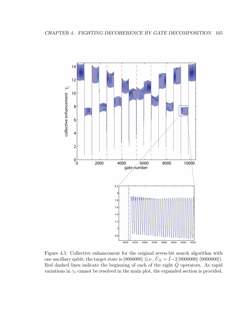
CHAPTER 4. FIGHTING DECOHERENCE BY GATE DECOMPOSITION 105
0 2000 4000 6000 8000 100000
2
4
6
8
10
12
14
gate number
colle
ctiv
e en
han
cem
ent
γ 1
9200 9250 9300 9350 9400 9450 9500 9550
6.8
7
7.2
7.4
7.6
7.8
8
8.2
Figure 4.5: Collective enhancement for the original seven-bit search algorithm withone ancillary qubit; the target state is |0000000〉 (i.e., UX = I−2 |0000000〉 〈0000000|).Red dashed lines indicate the beginning of each of the eight Q operators. As rapidvariations in γ1 cannot be resolved in the main plot, the expanded section is provided.

CHAPTER 4. FIGHTING DECOHERENCE BY GATE DECOMPOSITION 106
0 2000 4000 6000 8000 100000
1
2
3
4
5
6
7
8
9
10
gate number
colle
ctiv
e en
han
cem
ent
γ 1
Figure 4.6: Collective enhancement for the modified seven-bit search algorithm withone ancillary qubit; the target state is again |0000000〉.
CHAPTER 4. FIGHTING DECOHERENCE BY GATE DECOMPOSITION 107
applied), the value of γ1 drops significantly. Note that
HUX |σ〉 = H(I − 2 |0〉 〈0|
)|σ〉
= H
(|σ〉 − 2√
27|0〉)
= |0〉 − 2√27|σ〉 . (4.30)
The probability amplitude of the subradiant |0〉 component is large, and it is not
surprising that γ1 decreases markedly. Now, consider γ1 immediately after each invo-
cation of Q; i.e., to the right of each vertical red line. Each application of Q rotates
the initial |σ〉 state towards the target |0〉 state, and γ1 steadily decreases.
Comparison of Figs. 4.5(a) and 4.5(b) show that the collective enhancement
parameter γ1 is significantly smaller for the modified algorithm compared to the
initial algorithm, in accordance with the discussion in Sec. 4.3. Let γ1 represent the
average of γ1 over all gates. For the original algorithm, γ1 = 10.28, while γ1 = 4.74
for the modified case.
As a further typical example, the collective enhancement factor is shown for the
original and modified seven-bit search algorithm with target state |31〉 = |0011111〉in Fig. 4.7.
These two examples demonstrate the principle; further data is recorded in App.
F. Table F.1 presents the gate-averaged γ1 for several search problems with differing
number of bits and target states. In all simulations, the modified algorithm yielded
a smaller gate-averaged collective enhancement factor.
While these data are suggestive, I reiterate that γ1 is only a qualitative indicator
of the dissipation rate. In the following section, I discuss more rigorous quantum
master equation calculations to quantify the error due to collective decoherence for
the original and modified algorithm.

CHAPTER 4. FIGHTING DECOHERENCE BY GATE DECOMPOSITION 108
0 2000 4000 6000 8000 100000
2
4
6
8
10
12
14
gate number
colle
ctiv
e en
han
cem
ent
γ 1
0 2000 4000 6000 8000 100000
2
4
6
8
10
12
14
gate number
colle
ctiv
e en
han
cem
ent
γ 1
(a)
(b)
Figure 4.7: Collective enhancement for the (a) original and (b) modified seven-bitsearch algorithm with one ancillary qubit; the target state is |0001111〉. The averagecollective enhancement factor γ1 is 8.00 for the original algorithm and 4.91 for themodified case.

CHAPTER 4. FIGHTING DECOHERENCE BY GATE DECOMPOSITION 109
4.5 Quantum master equation
A rigorous simulation of the impact of system-environment coupling might proceed
as follows. The system state is the reduced density operator ρS, which can be ob-
tained by a partial trace over the full density operator ρ for the combined system and
environment. The density operator evolves over time according to the Liouville-von
Neumann equationd
dtρ(t) = −i
[H(t), ρ(t)
], (4.31)
in which the hamiltonian H is given by Eq. 4.2. Thus, the equation of motion for
the reduced density operator is
d
dtρS(t) = −itrE
[H(t), ρ(t)
]. (4.32)
Note that the qubits are coupled to a large (possibly infinite) number of degrees
of freedom in the environment, and direct integration of Eq. 4.32 is generally not
feasible. However, under a set of assumptions, the equation of motion for the reduced
density operator can be expressed as a quantum master equation in Lindblad form
[128, 129, 130]. In brief, these assumptions are
• The system-environment coupling is weak. Consider the dynamics in the inter-
action picture associated with HS ⊗ IE + IS ⊗ HE. Eq. 4.31 can be integrated
from 0 to t, and the expression for ρ(t) substituted in the right-hand side to
yield
d
dtρ(t) = −i
[HSE, ρ(0)
]−∫ t
0
dτ[HSE(t),
[HSE(τ), ρ(τ)
]]. (4.33)
This process can be iterated (cf. Dyson series) to yield an expansion in products
of HSE. It is assumed that the system-environment coupling is weak, and the
expansion is truncated to second-order.
• Born approximation. The environment is far larger than the system, and its
state is changed negligibly by interaction with the qubits. Thus, it is assumed

CHAPTER 4. FIGHTING DECOHERENCE BY GATE DECOMPOSITION 110
that the system-environment state is instantaneously separable, and the reser-
voir state is constant:
ρ(t) = ρS(t)⊗ ρE. (4.34)
For the zero-temperature boson reservoir, the environment density operator
consists of all modes in the vacuum state.
• Markov approximation. The two-time correlation functions for the reservoir
decay quickly compared to any other time scales. In this sense, the environment
is “memoryless.”
Derivations of the quantum master equation under these assumptions can be found
in Gardiner and Zoller [129] and Breuer and Petruccione [130]. For example, the latter
provides a detailed derivation of the equation of motion for a chain of two-level atoms
coupled to electromagnetic-field spontaneous-emission modes by an electric-dipole
interaction. If the energy difference between atomic levels is ω, the two-level systems
interact collectively with the field modes when the distance between atoms is small
compared with c/ω, where c is the field phase velocity. In this case, the resultant
quantum master equation is
d
dtρS(t) = −i
[HS(t), ρS(t)
]+ ν0
(S−ρS(t)S+ − 1
2S+S−ρS(t)− 1
2ρS(t)S+S−
).
(4.35)
Equation 4.35 can be interpreted as a general equation of motion for collective dissi-
pation due to interaction with a large memoryless boson reservoir.
In the absence of the bracketed second term on the right-hand side of Eq. 4.35,
the evolution is wholly unitary, and is dictated by the system hamiltonian7 HS. For a
given quantum algorithm, HS can be considered as the hamiltonian that generates the
sequence of fundamental unitary gates. The second term, referred to as the dissipator,
leads to non-unitary evolution. The decay rate ν0 parameterizes the strength of the
system-environment interaction.
7The system-environment interaction does lead to a modification of the unitary evolution throughHS (cf. the Lamb and Stark shifts). We neglect this shift, assuming that it can be compensated inprinciple by subtracting by altering the control hamiltonian HS .

CHAPTER 4. FIGHTING DECOHERENCE BY GATE DECOMPOSITION 111
Simulations were carried out for instances of the quantum search algorithm by
integration of the master equation Eq. 4.35. As in Sec. 4.4, the operators for the
original or modified algorithms were decomposed into fundamental unitary gates.
The evolution time required for all fundamental gates was assumed to be equal. The
hermitian generator HS for each unitary gate U was then calculated, such that8
U = e−iHS . (4.36)
HS is then the control hamiltonian applied to generate gate U . For a given ν0, the
quantum master equation was integrated by an adaptive fifth-order Runge-Kutta
solver to relative error less than 10−7. The simulations yielded the reduced density
operator ρS(t) over an entire algorithm.
The error induced by the system-environment coupling can be quantified by the fi-
delity. Recall that in the absence of any system-environment interaction, the qubits re-
main uncoupled from the reservoir, and the system evolves unitarily. Thus, the “ideal”
density operator for the system can be described by the pure state |ψS(t)〉 〈ψS(t)|.The fidelity of ρS(t) with respect to the ideal state is defined as
F (t) ≡ 〈ψS(t)| ρS(t) |ψS(t)〉 . (4.37)
If F (t) = 1, then if ρS(t) is equal to the ideal state at time t. If F (t) < 1, then there
is a discrepancy between the actual and ideal states.
The calculated fidelity of the final state |ψS(tf )〉 in the quantum search algorithm
has a simple interpretation. If the target state for the search problem is the compu-
tational basis state |x〉, then |ψS(tf )〉 ≈ |x〉. Thus,
F (tf ) ≈ 〈x| ρS(t) |x〉 , (4.38)
which is the probability that a projective measurement in the computational basis
yields the bit string x. Thus, the fidelity is a measure of the success probability of
8In regards to units, I have assumed ~ = 1, and have accepted the gate time as the elementaryunit of time. Thus, ν0 is specified in units of inverse gate times.

CHAPTER 4. FIGHTING DECOHERENCE BY GATE DECOMPOSITION 112
0 200 400 600 800 1000 1200 1400
0.4
0.5
0.6
0.7
0.8
0.9
1
Gate number
Fid
elit
y
Figure 4.8: Result of integration of the quantum master equation for the five-bitsearch algorithm with target state |0〉 and ν0 = 5 × 10⁻⁴. The dashed (black) linedenotes the original algorithm, whereas the solid (red) line represents the modifiedalgorithm.
the algorithm in the presence of noise due to system-environment coupling.
Two examples for the five-qubit search algorithm are presented here; data for a
range of ν0 and differing target states is presented in App. F.
First, the fidelity versus gate number for the five-bit search algorithm with target
state |0〉 is shown in Fig. 4.8. The rate ν0 is 5 × 10⁻⁴ in units of inverse gate time.
The modified algorithm shows a 24% improvement in final-state fidelity compared to
the original algorithm.
An alternative means to compare the performance of the original and modified
algorithms is to contrast the number of expected iterations required to find the target
state with probability greater than 1 − ε; the fidelity is interpreted as the success
CHAPTER 4. FIGHTING DECOHERENCE BY GATE DECOMPOSITION 113
probability for a single iteration. If the algorithm is repeated k times, the probability
that it succeeds at least once is 1− [1− F (tf )]k. For this probability to equal 1− ε,
it must hold that
k =log(
1ε
)log(
11−F (tf )
) . (4.39)
Therefore,kmodified
koriginal
=log [1− Foriginal(tf )]
log [1− Fmodified(tf )]. (4.40)
For this example, the ratio is 0.75, implying a 25% improvement in the number of
iterations required to obtain the solution to bounded error.
An additional example for the five-bit search algorithm is shown in Fig. 4.9. Here,
the improvement in the number of iterations is 15%.
The data in App. F present the final-state fidelities for a range of ν0 between
5 × 10⁻⁴ and 5 × 10⁻⁶ for all possible target states in the five-bit search algorithm.
While the modified algorithm outperforms the original algorithm in the vast majority
of cases, the largest percentage improvements are observed when the product of ν0
and the total number of gates is of order unity. When this product is larger (i.e., the
limit of a large dissipation rate), the final fidelity is diminishingly small, such that
the classical heuristic of guessing solutions to the search problem out-performs both
the original and modified algorithms. If the product of ν0 and the number of gates
is much smaller than unity, then the impact of dissipation on the fidelity is small
even for the original algorithm, and the modified algorithm negligibly improves the
number of iterations expected for success. To be precise, consider the improvement
in the number of iterations for a given value of ν0, averaged over all target states.
These values are shown in Table 4.5. Thus, we expect the modified algorithm to be
most applicable when the dissipation time is on the order of the total evolution time.
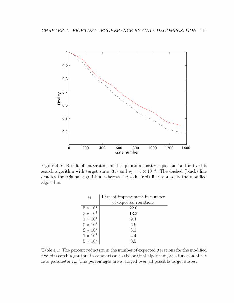
CHAPTER 4. FIGHTING DECOHERENCE BY GATE DECOMPOSITION 114
0 200 400 600 800 1000 1200 1400
0.4
0.5
0.6
0.7
0.8
0.9
1
Gate number
Fid
elit
y
Figure 4.9: Result of integration of the quantum master equation for the five-bitsearch algorithm with target state |31〉 and ν0 = 5 × 10⁻⁴. The dashed (black) linedenotes the original algorithm, whereas the solid (red) line represents the modifiedalgorithm.
ν0 Percent improvement in numberof expected iterations
5× 10⁴ 22.02× 10⁴ 13.31× 10⁴ 9.45× 10⁵ 6.92× 10⁵ 5.11× 10⁵ 4.45× 10⁶ 0.5
Table 4.1: The percent reduction in the number of expected iterations for the modifiedfive-bit search algorithm in comparison to the original algorithm, as a function of therate parameter ν0. The percentages are averaged over all possible target states.

CHAPTER 4. FIGHTING DECOHERENCE BY GATE DECOMPOSITION 115
4.6 Summary
In this chapter, I investigated whether the ordering of fundamental gates could miti-
gate the impact of decoherence in a standard-model quantum algorithm. I examined
the specific example of the quantum database search algorithm in the presence of
collective dissipation due to the coupling of qubits to a cold boson reservoir. A mod-
ification to the algorithm was proposed based upon a geometrical understanding of
the search algorithm, and the interpretation of the system-environment interaction
as an inducer of transitions in the Dicke-state basis. The original and modified algo-
rithm were compared by two approaches. First, a crude metric based on transition
rates was proposed. Simulations for quantum search instances between five and eight
bits showed a significantly reduced average transition rate in the modified algorithm.
Next, more rigorous calculations for instances of the five-bit search algorithm were
performed based on integration of a quantum master equation. When the decay time
is on the order of the total evolution time, the expected number of iterations required
for success is reduced by 22%. Although simulations were performed for small-qubit
problems, the geometric argument in Sec. 4.3 for the modified algorithm applies for
all problem sizes.
It should be noted that this chapter does not propose a general strategy for man-
aging decoherence, as the problem considered is very specific. In particular, I have
made the following limiting assumptions:
• The algorithm of interest is the quantum database search.
• The noise model is a permutation-invariant, collective dissipation process. No
other noise sources are present.
• The environment is a cold, memoryless reservoir of bosons.
• The fundamental gate set consists of CNOT and all single-qubit gates.
• All fundamental gates require equal time.
• Gates are not performed in parallel.
CHAPTER 4. FIGHTING DECOHERENCE BY GATE DECOMPOSITION 116
• The physical hamiltonians that generate the fundamental gates are specified by
Eq. 4.36.
Some of these assumptions could be readily relaxed in future work. For instance,
the dissipator in the quantum master equation can be modified to reflect a reservoir
at finite temperature, or additional system-environment interactions that break the
permutation symmetry. Simulations could be performed that allow simultaneous
operation of commuting gates, or vary the time required for different fundamental
gates.
It is an open question whether gate compilation can be leveraged to improve
the performance of other algorithms under more general noise models. However,
in conjunction with dynamical decoupling, this work illustrates the importance of
judicious design of control hamiltonians in implementing quantum algorithms and
their logic gates.
Appendix A
Collective angular momentum
states
In this appendix, I review some basic properties of collective angular momentum
states, or Dicke states [59]. Consider a collection of n spin-1/2 particles. One complete
set of basis states consists of the tensor product of σzi eigenstates for all spins i;
these are the individual “spin-up” states |↑〉 or “spin-down” states |↓〉 for each two-
level system. Alternatively, we can consider the simultaneous eigenstates of the total
squared angular momentum operator and the total z-component angular operator.
To be precise, define
Jγ =1
2
n∑i=1
σγi (A.1)
for γ ∈ x, y, z,J2 =
(Jx)2
+(Jy)2
+(Jz)2
, (A.2)
and J± = Jx + iJy. The Cartesian operators satisfy the commutation relations[Jα, Jβ
]= iεαβγ Jγ, (A.3)
where εαβγ is the antisymmetric Levi-Cevita tensor. Recognizing Eq. A.3 as the
fundamental commutation relations for angular momentum, we immediately know

APPENDIX A. COLLECTIVE ANGULAR MOMENTUM STATES 118
m = 1
m = 0
m = -1
m = 1
m = 0
m = -1
m = -2
m = 2
m = 1/2
m = -1/2
m = -3/2
m = 3/2
j = 1 j = 0 j = 3/2 j = 1/2 j = 2 j = 1 j = 0
n = 2 n = 3 n = 4
1
1
1
1
1
1
1
1
2
2
1
1
1
1
1
3
3
3
2
Figure A.1: Collective angular momentum states for n = 2, 3, 4. The degeneracy ofeach state is indicated in bold.
that there exist simultaneous eigenstates |j,m, α〉 of J2 and Jz such that
J2 |j,m, α〉 = j(j + 1) |j,m, α〉
Jz |j,m, α〉 = m |j,m, α〉 (A.4)
for half-integral j and m ∈ −j,−j+1, · · · , j. The label α distinguishes degenerate
states, and will be labeled by positive integers.
The allowed states and their degeneracies can be computed by the theory of ad-
dition of angular momentum. For the case of n spin-1/2 particles, the calculation
is particularly simple. First, note that the tensor product of n spin-up/spin-down
states is an eigenstate of J2 with eigenvalue m in the set −n/2,−n/2+1, · · · , n/2.Thus, j ∈ n/2, n/2 − 1, · · · , 0 (1/2); the minimum value of j depends on whether
n is even or odd. The allowed values of j and m can be represented graphically, as
in Fig. A.1
Before examining simple examples, first note that the fundamental commutation
relations imply that[Jz, J+
]= J+. Thus,
Jz(J+ |j,m, α〉
)=(J+Jz + J+
)|j,m, α〉 = (m+ 1)J+ |j,m, α〉 , (A.5)

APPENDIX A. COLLECTIVE ANGULAR MOMENTUM STATES 119
implying that J+ |j,m, α〉 is also an eigenstate of J2 and Jz, unless J+ |j,m, α〉 = 0.
The eigenvalue j is unmodified, and m→ m+ 1. Similarly,
J− |j,m, α〉 = c |j,m− 1, α〉 (A.6)
where c is an as-yet undetermined constant. As |j,m− 1, α〉 is normalized,
|c| =√〈j,m, α| J+J− |j,m, α〉. (A.7)
From Eq. A.2 and the commutation relations in Eq. A.3, it can be shown that
J+J− = J2 −(Jz)2
+ Jz. (A.8)
Thus,
|c| =√j(j + 1)−m2 +m =
√j(j + 1)−m(m− 1). (A.9)
A similar derivation for J+ yields
J− |j,m, α〉 =√j(j + 1)−m(m− 1) |j,m− 1, α〉 (A.10a)
J+ |j,m, α〉 =√j(j + 1)−m(m+ 1) |j,m+ 1, α〉 , (A.10b)
Consider the simplest example, where n = 2. Amongst all four possible tensor
products of spin-up/spin-down states, there only exists one for which m = −1, so
|j = 1;m = −1;α = 1〉 = |↓↓〉 . (A.11)
Successively applying J+ = 12(σ+
1 + σ+2 ), we find
|j = 1;m = 0;α = 1〉 =|↓↑〉+ |↑↓〉√
2
|j = 1;m = 1;α = 1〉 = |↑↑〉 . (A.12)

APPENDIX A. COLLECTIVE ANGULAR MOMENTUM STATES 120
The |j = 0;m = 0〉 states consist of all independent spin states with as many spins up
as down that are orthogonal to |j = 1;m = 0;α = 1〉. There is only one such state,
which is the singlet
|j = 0;m = 0;α = 1〉 =|↓↑〉 − |↑↓〉√
2. (A.13)
For n = 3, we again deduce that the only state for which m = −3/2 has all spins
down. The j = 3/2 manifold is then computed by successive applications of J+,
|j = 3/2;m = −3/2;α = 1〉 = |↓↓↓〉
|j = 3/2;m = −1/2;α = 1〉 =|↓↓↑〉+ |↓↑↓〉+ |↑↓↓〉√
3
|j = 3/2;m = 1/2;α = 1〉 =|↓↑↑〉+ |↑↓↑〉+ |↑↑↓〉√
3
|j = 3/2;m = 3/2;α = 1〉 = |↑↑↑〉 . (A.14)
There are three configurations where a single spin points down, and thus three degen-
erate states for m = −1/2. The j = 1/2, m = −1/2 subspace is two-fold degenerate,
and spanned by kets orthogonal to the j = 3/2, m = −1/2 subspace. Thus,
|j = 1/2;m = −1/2;α = 1〉 =2 |↓↓↑〉+ |↓↑↓〉 − |↑↓↓〉√
6
|j = 1/2;m = −1/2;α = 2〉 =|↓↑↓〉 − |↑↓↓〉√
2(A.15)
|j = 1/2;m = 1/2;α = 1〉 =−2 |↑↑↓〉+ |↑↓↑〉+ |↓↑↑〉√
6
|j = 1/2;m = 1/2;α = 2〉 =− |↑↓↑〉+ |↓↑↑〉√
2. (A.16)
This procedure can be continued in a similar fashion for larger n. For n = 4, I list
APPENDIX A. COLLECTIVE ANGULAR MOMENTUM STATES 121
only the two-fold degenerate j = 0, m = 0 singlet states:
|j = 0;m = 0;α = 1〉 =|↑↓↑↓〉 − |↑↓↓↑〉 − |↓↑↑↓〉+ |↓↑↓↑〉
2
|j = 0;m = 0;α = 2〉 =2 |↑↑↓↓〉+ 2 |↓↓↑↑〉 − |↑↓↑↓〉 − |↓↑↓↑〉 − |↑↓↓↑〉 − |↓↑↑↓〉√
12
(A.17)
It is evident that the degeneracies of all states in a given j manifold are equal.
The degeneracy of j = n/2− ε subspace is(n
ε
)−
(n
ε− 1
). (A.18)
Amazingly, for even n, the degeneracy of the j = 0, m = 0 subspace is [54](n
n/2
)−
(n
n/2− 1
)=
1
n/2 + 1
(n
n/2
)=
2n
O[poly(n)]. (A.19)
Thus, the j = 0, m = 0 subspace is highly degenerate for large n.
Appendix B
Elementary number theory
In this appendix, we prove a few elementary results of number theory.
Theorem B.1. Let x, y ∈ Z. The greatest common divisor g of x and y is the
smallest positive integer that satisfies g = mx+ ny for all integers m,n.
Proof. If g is the smallest positive integer such that g = mx + ny, then gcd(x, y)|g,so gcd(x, y) ≤ g. Assume that g - x. Then g = αx+ β, where α ∈ Z and 0 ≤ β < x.
Thus, β = (m − α)x + ny. This implies that β is the smallest positive integer that
is an integral linear combination of x and y, in contradiction to the initial assertion.
Thus, g|x, and similarly, g|y. As g is a common divisor of x and y, g ≤ gcd(x, y).
Combining this result with the above inequality, we find g = gcd(x, y).
Corollary B.2. Define the correspondence f : ZN → ZN where f : x 7→ gxmod N .
If g and N are coprime, then f is invertible.
Proof. Let x1, x2 ∈ ZN . Then, f(x1) = f(x2) implies that g(x1 − x2) = 0mod(N).
As g and N are coprime, from Theorem B.1 there exist integers m,n such that
1 = ag + bN . Thus, (1 − bN)(x1 − x2) = 0mod(N) and x1 − x2 = 0modN , showing
that the correspondence f is injective. As f maps ZN onto itself, it must also be
bijective, and thus invertible.
Corollary B.3. If the positive integers g and N are coprime, then there exists a
positive integer r such that gr = 1 mod N . The smallest such value of r, called the
order of g modulo N , is less than or equal to N .
APPENDIX B. ELEMENTARY NUMBER THEORY 123
Proof. Consider the ordered set of positive integers Q = q0, q1, q2, · · · , where qj = gj
mod N . Define the first repeated element of the sequences as qα = qβ, where β < α.
By Corollary B.2, the mapping f : x 7→ gxmod N is invertible. Thus, if β > 0,
f−1 (qα) = f−1 (qβ), so qα−1 = qβ−1. By iteration, we find that the first repeated
element of the sequence is q0 = 1. As the number of distinct elements of Q is less
than or equal to N , there exists an r ≤ N , r ∈ Z+ such that gr = 1 mod N .
Theorem B.4. Let a, g,N ∈ Z be nonnegative integers, where g and N are coprime
and 0 ≤ a < N . Define ra as the smallest positive integer such that agra = amod N .
Then, ra|r, where r is the order of g modulo N .
Proof. As gr = 1 mod N , then agr = amod N . Define b = gcd(r, ra) ≤ ra, so
∃x, y ∈ Z such that b = xr + yra by Theorem B.1. Therefore, agb = a(gr)x(gra)y = a
mod N . By assertion, ra is the smallest integer that obeys agra = amod N , showing
that ra ≥ b. Thus, the strict equality ra = b = gcd(ra, r) holds, and ra|r.
Any rational number p/q can be expressed as a continued fraction
p
q= a0 +
1
a1 + 1a2+ 1
···+ 1aN
that we denote as [a0, a1, · · · , aN ] where a ∈ Z+. The following proofs regarding
continued fractions are from [4].
Theorem B.5. Define pn/qn as the rational number represented by the continued
fraction [a0, a1, · · · , an]. Then, p0 = a0, p1 = 1 + a0a1, q0 = 1, q1 = a1, and
pn = anpn−1 + pn−2
qn = anqn−1 + qn−2
for n ≥ 2.

APPENDIX B. ELEMENTARY NUMBER THEORY 124
Proof. By induction. Assume the recursion relations apply for n = m− 1. Then
pm
qm= [a0, · · · , am−2, am−1, am] = [a0, · · · , am−2, am−1 + 1/am]
=(am−1 + 1/am)pm−2 + pm−3
(am−1 + 1/am)qm−2 + qm−3
=pm−1 + pm−2/am
qm−1 + qm−2/am
=ampm−1 + pm−2
amqm−1 + qm−2
Corollary B.6. A rational number p/q > 1 can be represented by a continued fraction
[a0, a1, · · · , aN ] where N = O(log p).
Proof. A continued fraction for p/q can be constructed by successively splitting and
inverting the fraction. To be precise, if p = a0q + r, where r is the remainder of q
dividing p, thenp
q= a0 +
r
q= a0 +
1(qr
) .Now, we can express q as q = a1r + r′, where r′ is the remainder of r dividing q.
Then,p
q= a0 +
1
a1 + r′
r
.
Clearly, this process must terminate after a finite number of steps, as the denominator
of the residual fraction decreases at each step. The continued fraction [a0, a1, · · · , an]
obtained after n + 1 split-and-invert steps is referred to as a convergent of p/q, and
will be denoted pn/qn.
By Theorem B.5, the sequences pn and qn are monotonically increasing. As qn =
anqn−1 + qn−2 ≥ qn−1 + qn−2 > 2qn−2, pn > qn > 2bn/2c. If the final element in the
continued fraction for p/q is aN , then p > 2bN/2c, and N = O(log p).
Corollary B.7. For n ≥ 1, qnpn−1 − pnqn−1 = (−1)n.
APPENDIX B. ELEMENTARY NUMBER THEORY 125
Proof. By induction. Trivial to verify for n = 1. Furthermore,
qnpn−1 − pnqn−1 = (anqn−1 − qn−2)pn−1 − (anpn−1 + pn−2)qn−1
= qn−2pn−1 − pn−2qn−1 = −(−1)n−1.
Theorem B.8. Let x and p/q be rational numbers such that |p/q−x| ≤ 1/2q2. Then,
p/q is a convergent of the continued fraction of x.
Proof. Let the continued fraction expansion for p/q be [a0, a1, · · · , an]. Then, x can
be expressed as
x =pn
qn+
δ
2q2n
,
where |δ| < 1. Define the parameter
λ = 2
(qnpn−1 − pnqn−1
δ
)− qn−1
qn,
which implies that x = (λpn + pn−1)/(λqn + qn−1). Thus, x can be expressed as the
continued fraction [a0, a1, · · · , an, λ], where we must take care to note that λ is not
necessarily an integer. However, if n is even, then
λ =2
δ− qn−1
qn> 1.
Therefore, λ has a continued fraction representation [b0, b1, · · · ], and x can be ex-
pressed as [a0, a1, · · · , an, b0, b1, · · · ]. Clearly, p/q is a convergent of the continued
fraction representation of x. Note that n can always be chosen to be even by ambi-
guity in the final split-and-invert step of the continued fraction expansion.
The multiplicative group Z∗pα consists of all elements in Zpα that are coprime to
pα. Its binary operation consists of multiplication modulo pα.
Lemma B.9. Z∗pα is cyclic.
Proof. Knuth, pp. 19-20 [131].
APPENDIX B. ELEMENTARY NUMBER THEORY 126
Lemma B.10. The order of the group Z∗pα is pα−1(p− 1).
Proof. The integers in Zpα that share a factor with pα are p, 2p, 3p, · · · , (pα−1 − 1)p.
Eliminating these integers as well as zero, there remain pα− (pα−1−1)−1 = pα−1(p−1).
Some definitions are in order. Let pα11 p
α22 · · · p
αkk be the decomposition of the odd
positive integer N as a product of integer powers of distinct primes. Select any
x ∈ ZN such that gcd(x,N) = 1. Define rj as the order of xmod pαj
j and r the order
of xmod N . The largest power of 2 dividing rj is labeled 2dj .
Lemma B.11. Consider the correspondence
f :Zpα11× Zp
α22× · · ·Zp
αkk→ ZN
f :a1, a2, · · · , ak 7→ x : x = aj mod pαj
j ∀j.
The correspondence f is a bijection.
Proof. All elements of the domain have an image under f , by the Chinese remain-
der theorem (Knuth [131], p. 286). Label the sequences A = a1, · · · , ak, A′ =
a′1, · · · , a′k, and let x = f(A), x′ = f(A′). If x = x′, then aj = a′j mod pαj
j . As
aj ∈ Zp
αjj
, aj = a′j. Thus, f is injective. As aj = xmod pαj
j , f is surjective. Therefore,
f is a bijection.
Corollary B.12. Randomly selecting an integer in ZN is equivalent to randomly
selecting a sequence of integers in Zpα11× Zp
α22× · · ·Zp
αkk
.
Proof. Consequence of the bijection in Theorem B.11.
Theorem B.13. The probability that all dj are equal is at most 1/2k.
Proof. Follows Nielsen and Chuang [4]. Let a1, · · · , an = f−1(x), so x = aj mod pαj
j .
As gcd(x,N) = 1, gcd(x, pαj
j ) = 1 as well. Note that aj cannot be a power of the
prime pj; if this were true, then x would be a multiple of pj, and not coprime to pαj
j .
Thus, the only possible values of aj are those coprime with pαj
j , which are the elements
APPENDIX B. ELEMENTARY NUMBER THEORY 127
of the multiplicative group Z∗p
αjj
. By Lemmas B.9 and B.10, this group is cyclic with
order Pj ≡ pαj−1j (pj − 1). Note that Pj is even, but not divisible by a higher power of
two. Let g be a generator of Z∗p
αjj
, so aj can be written gk mod pαj
j for some k ∈ ZPj.
Consider the order of element gk: the value of ρ such that gkρ = 1 mod pαj
j . Note
that Pj|kρ. If k is odd, then ρ must be even. If k is even, then gkPj/2 = 1 mod pαj
j ,
implying ρ|Pj/2. Thus, ρ must be odd. By Lemma B.12, choosing an x at random is
equivalent to choosing an aj at random. Thus, with probability of 1/2, the order of
aj is odd, and dj = 0. The probability that all k values of dj are the same is strictly
bounded by 1/2m−1.
Corollary B.14. The probability that r is either odd or xr/2 = −1 mod N is at most
1/2m.
Proof. First, note that rj|r, as xr = 1 mod pαj
j . Thus, for r to be odd, all the rj must
be equal. If xr/2 = −1 mod N , then xr/2 = −1 mod pαj
j , and rj - r/2. But, as rj|r,each rj must divide the highest power of two that divides r. In either case, all dj
must be equal, which occurs with probability at most 1/2m−1 by Theorem B.13.

Appendix C
Proof of broadening function
lemmas
Lemma 3.1. If bΘ(E) (as defined in Eq. 3.12) is subject to the normalization con-
dition 1 =∫∞−∞ bΘ(E)dE, then
αΘ <cπ
∆e
√Θ
6π, (C.1)
where c ≈ 2.0367.
Proof. A lower bound is first derived for
I ≡∫ ∞
−∞[sinc(x)]Θ =
∫ ∞
−∞eΘ ln[sinc(x)]dx. (C.2)
We exclude infinitesimal regions around x = mπ, x ∈ Z from the integral to avoid
divergence of the logarithm; as sinc(x) approaches a finite value in these regions, the
contribution of these regions to the integral can be made arbitrarily small. As the
integrand is positive over the entire domain of x, I can be lower bounded by reducing
the limits of integration to any finite interval, such as |x| <√
6/Θ.

APPENDIX C. PROOF OF BROADENING FUNCTION LEMMAS 129
Using a series expansion for ln[sinc(x)] [132, see p.38 and p.123],
ln [sinc(x)] = −x2
6−
∞∑k=2
x2k
kπ2k
(∞∑
n=1
1
n2k
)(C.3a)
> −x2
6−(π2
6
) ∞∑k=2
x2k
kπ2k, (C.3b)
which converges for 0 < |x| < π. Thus, for Θ ∈ Z+,
I >
∫ 6/Θ
−√
6/Θ
e−Θx2/6 exp
(−Θπ2
6
∞∑k=2
x2k
kπ2k
)dx. (C.4)
The second exponent monotonically decreases with |x|, so
I > exp
(−Θπ2
6
∞∑k=2
(6/Θ)k
kπ2k
)∫ √6/Θ
−√
6/Θ
e−Θx2/6dx. (C.5)
The integral is√
6π/Θ erf(1). The summation can be performed explicitly to yield
I > e1+π2Θ ln(1−6/π2Θ)/6
√6π
Θerf(1) (C.6a)
= e
(1− 6
Θπ2
)Θπ2/6
erf(1)
√6π
Θ(C.6b)
> e
(1− 6
π2
)π2/6
erf(1)
√6π
Θ, (C.6c)
where we make use of the fact that (1− 1/x)x is a monotonically increasing function
for x > 1.
This lower bound for I is used to establish an upper bound for αΘ.
αΘ =1∫∞
−∞
[sinc
(πE∆e
)]ΘdE
=π
∆e I<
π
∆e
(c
√Θ
6π
),

APPENDIX C. PROOF OF BROADENING FUNCTION LEMMAS 130
where c is defined as
c ≡ 1
e
(1
1− 6/π2
)π2/61
erf(1)≈ 2.0367. (C.7)
Lemma 3.2. If Θ is even,
Aside ≡ 1−∫ ∆e
−∆e
bΘ(E)dE <c
πΘ−3
√Θ
6π. (C.8)
Proof. As bΘ(E) is nonnegative over its domain, and∫∞−∞ bΘ(E) = 1, we can apply a
variant of the Markov inequality. For even m,∫ ∞
−∞EmbΘ(E)dE ≥
∫ −∆e
−∞EmbΘ(E)dE +
∫ ∞
∆e
EmbΘ(E)dE (C.9a)
≥ ∆em
[∫ −∆e
−∞bΘ(E)dE +
∫ ∞
∆e
bΘ(E)dE
](C.9b)
= ∆emAside. (C.9c)
Using Eq. 3.12 for m = Θ− 2,
Aside ≤1
∆eΘ−2
∫ ∞
−∞EΘ−2αΘsincΘ
(πE
∆e
)dE =
αΘ∆e
πΘ−1
∫ ∞
−∞
sinΘ x
x2(C.10a)
≤ αΘ∆e
πΘ−1
∫ ∞
−∞
sin2 x
x2(C.10b)
=αΘ∆e
πΘ−2(C.10c)
The proof is completed by using the bound on αΘ from Lemma 3.1.
Lemma 3.3.
1
∆t
∫ (M/2+1)∆t
∆t
e−t2/ν2
1 + (t/β)2dt >
β∆E
4
[1−O
(1√β∆E
)]Proof. Define the left-hand side of the inequality as Q. Recall that ν2 = ΘT 2
0 /12 =
APPENDIX C. PROOF OF BROADENING FUNCTION LEMMAS 131
π2Θ/3(∆e)2 and ∆t = 2π/∆E by Eqs. 3.8 and 3.11. Defining x = t/β,
Q =
∫ (M2
+1)∆tβ
∆tβ
β∆E
2π·exp
(−3β2∆e2x2
π2Θ
)1 + x2
dx. (C.11)
I will show that the leading-order error incurred by extending the limits to 0 and ∞are negligible. Define
Q = Q1 −Q2 −Q3
=
(∫ ∞
0
−∫ ∆t
β
0
−∫ ∞
(M2
+1)∆tβ
)β∆E
2π·exp
(−3β2∆e2x2
π2Θ
)1 + x2
dx. (C.12)
Q1 can be integrated exactly to
Q1 =β∆E
4exp
[3(β∆e)2
π2Θ
]erfc
(3√Θ
β∆e
π
). (C.13)
From Eqs. 3.30a and 3.31, it is known that β∆e is independent of n, while Θ =
O(β∆E) = O[poly(n)]. Thus, if are interested in the asymptotic behavior in the
limit of large n, it suffices to expand Q1 to leading order in 1/β∆E. Noting that
erfc(x) = 1− 2x√π
+O(x2),
Q1 =β∆E
4
[1 +O
(1
β∆E
)][1−O
(1√β∆E
)]=β∆E
4
[1−O
(1√β∆E
)]. (C.14)
As for Q2, we can upper bound the integral by noting that the integrand is always
less than β∆E/2π. Thus,
Q2 ≤(
∆t
β
)(β∆E
2π
)≤ 1, (C.15)
where we have made use of Eq. 3.11. Q2 is smaller than the leading two terms of Q1,
and can be neglected.

APPENDIX C. PROOF OF BROADENING FUNCTION LEMMAS 132
Finally, let us examine Q3.
Q3 =
∫ ∞
(M2
+1)∆tβ
β∆E
2π·exp
(−3β2∆e2x2
π2Θ
)1 + x2
dx<β∆E
2π
∫ ∞
M∆t/2β
exp
(−3β2∆e2x2
π2Θ
)dx
(C.16)
From Eqs. 3.8 and 3.13, M∆t/2β = πΘ/β∆E. Therefore,
Q3 <∆E
4∆e
√πΘ
3erfc
(√3Θ). (C.17)
Q3 becomes exponentially small with increasing n. A series expansion for the com-
plementary error function yields
erfc(√
3Θ)
=e−3Θ
√3πΘ
[1−O
(1
3Θ
)]. (C.18)
Recall that Θ = O[poly(n)]. Thus, it suffices to neglect Q2 and Q3 in the large-n
expansion of Q.
Appendix D
Gray-code decomposition
This appendix explains the Gray-code decomposition of an n-controlled-NOT gate,
as shown by Barenco et al. [17]. We start with a lemma. Consider the n Boolean
variables x1, x2, · · · , xn; denote the Boolean AND operation as ∧ and the exclusive-
OR operation as ⊕.
Lemma D.1.
2n−1 (x1 ∧ x2 ∧ · · · ∧ xn) =n∑
i=1
xi −∑i<j
xi ⊕ xj +∑
i<j<k
xi ⊕ xj ⊕ xk − · · · (D.1)
Proof. By induction. The base case for n = 1 is trivial. Assume that D.1 holds for n
Boolean variables. Define the right-hand side of D.1 as Yn. Then,
Yn+1 = Yn +xn+1−n∑
i=1
xi⊕xn+1 +∑i<j
xi⊕xj⊕xn+1−∑
i<j<k
xi⊕xj⊕xk⊕xn+1 + · · · .
(D.2)
As q ⊕ 0 = q, Yn+1 = 0 if xn+1 = 0. Now, if xn+1 = 1, we note that q ⊕ 1 = 1− q to
find
Yn+1 = Yn + 1−n∑
i=1
(1− xi) +∑i<j
(1− xi ⊕ xj)−∑
i<j<k
(1− xi ⊕ xj ⊕ xk). (D.3)
The constants sum to∑n
`=0(−1)`(
n`
)= 0. Therefore, Yn+1 = 2Yn if xn+1 = 1.
APPENDIX D. GRAY-CODE DECOMPOSITION 134
Combining with the case that xn=1 = 0, we find that
Yn+1 = 2Yn ∧ xn+1 = 2n (x1 ∧ x2 ∧ · · · ∧ xn+1) . (D.4)
Note that each of the terms on the right-hand side of Eq. D.1 can be represented
by an n-bit string. For example, for n = 3, the string x1 ⊕ x3 could be denoted 101,
where the presence of the variables x1 and x3 are indicated by the ones. All possible
strings can be listed as a Gray code, a sequence in which the Hamming distance
between adjacent strings is exactly one; for example:
001, 011, 010, 110, 111, 101, 100. (D.5)
These strings correspond to the terms x3, x2 ⊕ x3, x2, x1 ⊕ x2, x1 ⊕ x2 ⊕ x3, x1 ⊕ x3,
and x1. As we move from element to element in the Gray code sequence, the signs of
the corresponding terms in Eq. D.1 alternate.
Now consider a quantum circuit with three control qubits and one target qubit.
If the first string (x3) is true, a unitary gate V is applied to the target qubit. Next,
if the second string (x2 ⊕ x3) is true, V −1 = V † acts on the target. Subsequently,
the operators V and V † are alternatingly applied, successively conditioned on each
string in the Gray-code sequence. As a net result, by Lemma D.1, V 4 is applied to
the target if x1 ∧ x2 ∧ x3 is true.
The n-controlled-NOT gate enacts the σx bit-flip operation to the target qubit
if all n control qubits are logical one. Thus, by selecting V such that V 4 = σx,
the Gray-code scheme described above can implement the n-controlled-NOT gate for
n = 3. The corresponding quantum circuit is shown in Fig. D.1. The Gray-code
ordering is convenient, as it necessitates only a single controlled-NOT gate between
controlled-V gates.
Each controlled-V gate can be decomposed into two fundamental controlled-NOT
gates and two single-qubit gates [17]. The compiler can reduce the total gate count

APPENDIX D. GRAY-CODE DECOMPOSITION 135
V 4 V V V V V† † V† V
=
Figure D.1: Gray-code circuit for the n-controlled-NOT for n = 3.
significantly by concatenating single-qubit gates and eliminating adjacent controlled-
NOT gates, which are self-inverse.
The generalization for any n > 3 is straightforward. The operator V must be
chosen such that V 2n−1 = σx, and either the V or V † operator is applied for each of
the strings in the 2n − 1 element Gray-code sequence.
It should be noted that the number of fundamental gates required to implement the
Gray code decomposition increases exponentially with n, and is clearly not preferable
for asymptotically large n. Barenco et al. describe an alternative method to imple-
ment the n-controlled-NOT gate with O(n2) gates. However, for n < 9, the Gray
code method leads to a smaller gate count, and is thus used in my simulations.
Appendix E
Fundamental-gate matrix elements
A spherical tensor T(k)q of rank k can be defined as an operator that upholds the
commutation relations [127]:[Jz, T (k)
q
]= qT (k)
q[J±, T (k)
q
]=√
(k ∓ q)(k ± q + 1)T(k)q±1 (E.1)
The parameter q takes integral values between −k and k. Thus, there is one spherical
tensor of rank zero, three spherical tensors of rank one, and five spherical tensors of
rank two.
The Wigner-Eckart theorem [125, 126, 127] implies that the matrix element (over
collective angular momentum states) 〈j′,m′, α′| T (k)q |j,m, α〉 is zero unless the trian-
gular relation
|j − k| ≤ j′ ≤ j + k (E.2)
and the m-selection rule
m′ = m+ q (E.3)
are upheld.
Any single-qubit unitary operator U1 can be represented as a rotation on the Bloch
APPENDIX E. FUNDAMENTAL-GATE MATRIX ELEMENTS 137
sphere around the unit-vector ~n by an angle θ.
U1 = exp(−i~σ · ~nθ/2
)= cos(θ/2)I − i sin(θ/2)~σ · ~n (E.4)
Note that the Pauli operators σ+, σ− and σz are all spherical tensors of rank one,
while the identity operator I is of rank zero. Thus,
U1 = c0,0T(0)0 + c1,−1T
(1)−1 + c1,0T
(1)0 + c1,1T
(1)1 . (E.5)
where ci,j are constants dependent on ~n and θ. By Eqs. E.2 and E.3, the matrix
element 〈j′,m′, α′| U1 |j,m, α〉 is nonzero only if
|j′ − j| ≤ 1,
|m′ −m| ≤ 1. (E.6)
Now consider a CNOT gate U2 acting on control qubit a and target qubit b. U2
can be expanded in terms of the Cartesian Pauli operators as
U2 =1
2
(Ia ⊗ Ib + Ia ⊗ σx
b + σza ⊗ Ib − σz
a ⊗ σxb
). (E.7)
The first three terms are clearly a linear combination of spherical tensors of rank zero
or one. The fourth term is a tensor product of two Cartesian Pauli operators. Note
that there are nine such products: σxa σ
xb , σx
a σyb , σ
xa σ
zb , σ
yaσ
xb , σy
aσyb , σ
yaσ
zb σ
zaσ
xb , σz
aσyb ,
and σzaσ
zb . An invertible linear transformation can express each such product as a
combination of nine spherical tensors of rank two or less; the exact definition of each
spherical tensor can be found in Sakurai [127, p. 236]. The key point is that all terms
in Eq. E.7 can be expressed as a linear combination of spherical tensors of rank two
or less. Thus, 〈j′,m′, α′| U2 |j,m, α〉 is nonzero only if
|j′ − j| ≤ 2
|m′ −m| ≤ 2. (E.8)
APPENDIX E. FUNDAMENTAL-GATE MATRIX ELEMENTS 138
In fact, Eq. E.8 can be made more stringent. Recall that the CNOT gate causes
at most one bit flip on the target qubit. Thus, |m′ −m| ≤ 1. This conclusion can be
confirmed rigorously by showing that the expansion of Eq. E.7 in terms of spherical
tensors only involves operators with q = 0 or q = 1.
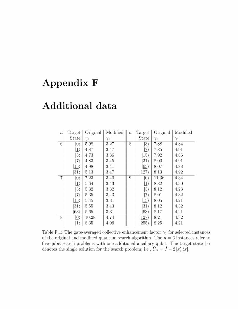
Appendix F
Additional data
n Target Original Modified n Target Original ModifiedState γ1 γ1 State γ1 γ1
6 |0〉 5.98 3.27 8 |3〉 7.88 4.84|1〉 4.87 3.47 |7〉 7.85 4.91|3〉 4.73 3.36 |15〉 7.92 4.86|7〉 4.83 3.45 |31〉 8.00 4.91|15〉 4.98 3.41 |63〉 8.07 4.88|31〉 5.13 3.47 |127〉 8.13 4.92
7 |0〉 7.23 3.40 9 |0〉 11.36 4.34|1〉 5.64 3.43 |1〉 8.82 4.30|3〉 5.32 3.32 |3〉 8.12 4.23|7〉 5.35 3.43 |7〉 8.01 4.32|15〉 5.45 3.31 |15〉 8.05 4.21|31〉 5.55 3.43 |31〉 8.12 4.32|63〉 5.65 3.31 |63〉 8.17 4.21
8 |0〉 10.28 4.74 |127〉 8.21 4.32|1〉 8.35 4.96 |255〉 8.25 4.21
Table F.1: The gate-averaged collective enhancement factor γ1 for selected instancesof the original and modified quantum search algorithm. The n = 6 instances refer tofive-qubit search problems with one additional ancillary qubit. The target state |x〉denotes the single solution for the search problem; i.e., UX = I − 2 |x〉 〈x|.

APPENDIX F. ADDITIONAL DATA 140
0 5 10 15 20 25 30 35
0.090
0.095
0.100
0.105
0.110
0.115
0.120
0.125
0.130
0.135
0.140
0.145
Fina
l-sta
te fi
delit
y
Search target state x
Original Modified
Figure F.1: Comparison of quantum master equation calculations for the 5-bit searchalgorithm, in which ν0 = 5 × 10⁻⁴ inverse gate times. Each point on the horizontalaxis is a different instance of the search algorithm, in which the target state is |x〉;i.e., UX = I − 2 |x〉 〈x|. The vertical axis denotes the fidelity of the final state. Datafor the original and modified algorithms are overlaid.
0 5 10 15 20 25 30 35
0.355
0.360
0.365
0.370
0.375
0.380
0.385
0.390
0.395
0.400
0.405
0.410
0.415
0.420
0.425
0.430
0.435
0.440
0.445
0.450
Fina
l-sta
te fi
delit
y
Search target state x
Original Modified
Figure F.2: Similar to Fig. F.1, but in which ν0 = 2× 10⁻⁴ inverse gate times.

APPENDIX F. ADDITIONAL DATA 141
0 5 10 15 20 25 30 35
0.590
0.595
0.600
0.605
0.610
0.615
0.620
0.625
0.630
0.635
0.640
0.645
0.650
0.655
0.660
0.665
0.670
Fina
l-sta
te fi
delit
y
Search target state x
Original Modified
Figure F.3: Similar to Fig. F.1, but in which ν0 = 1× 10⁻⁴ inverse gate times.
0 5 10 15 20 25 30 35
0.765
0.770
0.775
0.780
0.785
0.790
0.795
0.800
0.805
0.810
0.815
0.820
Fina
l-sta
te fi
delit
y
Search target state x
Original Modified
Figure F.4: Similar to Fig. F.1, but in which ν0 = 5× 10⁻⁵ inverse gate times.
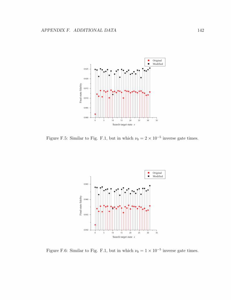
APPENDIX F. ADDITIONAL DATA 142
0 5 10 15 20 25 30 35
0.900
0.905
0.910
0.915
0.920
0.925
Fina
l-sta
te fi
delit
y
Search target state x
Original Modified
Figure F.5: Similar to Fig. F.1, but in which ν0 = 2× 10⁻⁵ inverse gate times.
0 5 10 15 20 25 30 35
0.950
0.955
0.960
0.965
Fina
l-sta
te fi
delit
y
Search target state x
Original Modified
Figure F.6: Similar to Fig. F.1, but in which ν0 = 1× 10⁻⁵ inverse gate times.

APPENDIX F. ADDITIONAL DATA 143
0 5 10 15 20 25 30 35
0.975
0.980
0.985
Fina
l-sta
te fi
delit
y
Search target state x
Original Modified
Figure F.7: Similar to Fig. F.1, but in which ν0 = 5× 10⁻⁶ inverse gate times.
References
[1] C. H. Papadimitriou, Computational Complexity (Addison-Wesley, U.S.A.,
1994).
[2] T. H. Cormen, C. E. Leiserson, R. L. Rivest, and C. Stein, Introduction to
Algorithms (MIT Press, Cambridge, U.S.A., 2001), 2nd ed.
[3] D. E. Knuth, The Art of Computer Programming v. 1. Fundamental Algorithms
(Addison-Wesley, 1997), 3rd ed.
[4] M. A. Nielsen and I. L. Chuang, Quantum Computation and Quantum Infor-
mation (Cambridge University Press, U.K., 2000).
[5] D. Aharonov, Quantum Computation (1998), e-print quant-ph/9812037.
[6] A. M. Turing, On computable numbers, with an application to the Entschei-
dungsproblem, Proc. London. Math. Soc. 2, 230 (1936).
[7] D. Deutsch, Quantum theory, the Church-Turing Principle and the universal
quantum computer, Proc. R. Soc. London A 400, 97 (1985).
[8] E. Bernstein and U. Vazirani, Quantum complexity theory, SIAM J. Comput.
26, 1411 (1997).
[9] R. Landauer, Irreversibility and heat generation in the computing process, IBM
J. Res. Dev. 5, 183 (1961).
[10] C. H. Bennett, Logical reversibility of computation, IBM J. Res. Dev. 17, 525
(1973).
144
REFERENCES 145
[11] E. Fredkin and T. Toffoli, Conservative Logic, Int. J. Theor. Phys. 21, 219
(1982).
[12] Y. Manin, Computable and Uncomputable (Russian) (1980).
[13] R. P. Feynman, Simulating Physics with Computers, Int. J. Theor. Phys. 21,
467 (1982).
[14] P. Benioff, Quantum mechanical Hamiltonian models of Turing machines, J.
Stat. Phys. 29, 515 (1982).
[15] R. P. Feynman, Quantum Mechanical Computers, Found. Phys. 16, 507 (1986).
[16] D. Deutsch, Quantum computational networks, Proc. R. Soc. London A 425,
73 (1989).
[17] A. Barenco, C. H. Bennett, R. Cleve, D. P. DiVincenzo, N. Margolus, P. Shor,
T. Sleator, J. Smolin, and H. Weinfurter, Elementary gates for quantum com-
putation, Phys. Rev. A 52, 3457 (1995).
[18] D. Deutsch, A. Barenco, and A. Ekert, Universality in quantum computation,
Proc. R. Soc. London A 669, 669 (1995).
[19] S. Lloyd, Almost any quantum logic gate is universal, Phys. Rev. Lett. 75, 346
(1995).
[20] D. P. DiVincenzo, Quantum gates and circuits, Proc. R. Soc. London A 454,
261 (1998).
[21] D. P. DiVincenzo, The Physical Implementation of Quantum Computation,
Fortschr. Phys. 9-11, 771 (2000).
[22] R. Jozsa and N. Linden, On the role of entanglement in quantum-computational
speed-up, Proc. R. Soc. Lond. A 459, 2011 (2003).
[23] D. Gottesman, Demonstrating the viability of universal quantum computation
using teleportation and single-qubit operations, Nature 402, 390 (1999).

REFERENCES 146
[24] C. H. Bennett, G. Brassard, C. Crepeau, R. Jozsa, A. Peres, and W. K. Woot-
ters, Teleporting and unknown quantum state via dual classical and Einstein-
Podolsky-Rosen channels, Phys. Rev. Lett. 70, 1895 (1993).
[25] M. A. Nielsen, Quantum computation by measurement and quantum memory,
Phys. Lett. A 308, 96 (2003).
[26] S. A. Fenner and Y. Zhang, Universal quantum computation with two- and
three-qubit projective measurements (2001), e-print quant-ph/9812049.
[27] D. W. Leung, Two-qubit Projective Measurements are Universal for Quantum
Computation (2001), e-print quant-ph/0111122.
[28] R. Raussendorf and H. J. Briegel, A One-Way Quantum Computer, Phys. Rev.
Lett. 86, 5188 (2001).
[29] D. G. Cory, A. F. Fahmy, and T. F. Havel, Ensemble quantum computing by
NMR spectroscopy, Proc. Natl. Acad. Sci. U.S.A. 94, 1634 (1997).
[30] N. Gershenfeld and I. L. Chuang, Bulk Spin-Resonance Quantum Computation,
Science 275, 350 (1997).
[31] D. G. Cory, R. Laflamme, E. Knill, L. Viola, T. F. Havel, N. Boulant, G. Boutis,
E. Fortunato, S. Lloyd, R. Martinez, et al., NMR Based Quantum Information
Processing: Achievements and Prospects, Fortschr. Phys. 48, 875 (2000).
[32] L. M. K. Vandersypen, Ph.D. thesis, Experimental Quantum Computation with
Nuclear Spins in Liquid Solution, Stanford University (2001).
[33] A. Abragram, Principles of Nuclear Magnetism (Oxford Science, New York,
1961).
[34] R. R. Ernst, G. Bodenhausen, and A. Wokaun, Principles of Nuclear Magnetic
Resonance in One and Two Dimensions (Oxford Science, New York, 1990).
[35] L. M. K. Vandersypen and I. L. Chuang, NMR techniques for quantum control
and computation, Rev. Mod. Phys. 76, 1037 (2004).
REFERENCES 147
[36] D. W. Leung, I. L. Chuang, F. Yamaguchi, and Y. Yamamoto, Efficient imple-
mentation of coupled logic gates for quantum computation, Phys. Rev. A 61,
042310 (2000).
[37] E. Knill, I. L. Chuang, and R. Laflamme, Effective pure states for bulk quantum
computation, Phys. Rev. A 57, 3348 (1998).
[38] W. H. Zurek, Decoherence and the transition from quantum to classical, Phys.
Today 44, 36 (1991).
[39] P. W. Shor, Scheme for reducing decoherence in quantum computer memory,
Phys. Rev. A 52, 2493 (1995).
[40] A. M. Steane, Error correcting codes in quantum theory, Phys. Rev. Lett. 77,
793 (1996).
[41] D. Dieks, Communication by EPR devices, Phys. Lett.A 92, 271 (1982).
[42] W. K. Wooters and W. H. Zurek, A single quantum cannot be cloned, Nature
299, 802 (1982).
[43] A. R. Calderbank and P. W. Shor, Good quantum error-correcting codes exist,
Phys. Rev. A 54, 1098 (1996).
[44] A. M. Steane, Multiple particle interference and quantum error correction, Proc.
R. Soc. London A 452, 2551 (1996).
[45] D. Gottesman, Class of quantum error-correcting codes saturating the quantum
Hamming bound, Phys. Rev. A 54, 1862 (1996).
[46] D. Gottesman, Ph.D. thesis, Stabilizer Codes and Quantum Error Correction,
California Institute of Technology (1997).
[47] D. Aharonov, Ph.D. thesis, Noisy Quantum Computation, The Hebrew Univer-
sity (1999).
REFERENCES 148
[48] E. Knill, R. Laflamme, and W. H. Zurek, Resilient Quantum Computation,
Science 279, 342 (1998).
[49] J. Preskill, Reliable quantum computers, Proc. R. Soc. London A 454, 385
(1998).
[50] G. M. Palma, K.-A. Suominen, and A. K. Ekert, Quantum computers and dis-
sipation, Proc. R. Soc. London.A 452, 567 (1996).
[51] L.-M. Duan and G.-C. Guo, Reducing decoherence in quantum-computer mem-
ory with all quantum bits coupling to the same environment, Phys. Rev. A 57,
737 (1998).
[52] L.-M. Duan and G.-C. Guo, Preserving Coherence in Quantum Computation
by Pairing Quantum Bits, Phys. Rev. Lett. 79, 1953 (1997).
[53] P. Zanardi, Noiseless Quantum Codes, Phys. Rev. Lett. 79, 3306 (1997).
[54] P. Zanardi and M. Rasetti, Error-avoiding codes, Mod. Phys. Lett. B 11, 1085
(1997).
[55] D. A. Lidar, I. L. Chuang, and K. B. Whaley, Decoherence-Free Subspaces for
Quantum Computation, Phys. Rev. Lett. 81, 2594 (1998).
[56] P. Zanardi, Dissipation and decoherence in a quantum register, Phys. Rev. A
57, 3276 (1998).
[57] D. A. Lidar, D. Bacon, and K. B. Whaley, Concatenating Decoherence-Free
Subspaces with Quantum Error Correcting Codes, Phys. Rev. Lett. 82, 4556
(1999).
[58] D. A. Lidar and K. B. Whaley, Decoherence-Free Subspaces and Subsystems,
in Irreversible Quantum Dynamics, edited by F. Benatti and R. Floreanini
(Springer-Verlag, Trieste, Italy, 2003), p. 83.
[59] R. H. Dicke, Coherence in spontaneous radiation processes, Phys. Rev. 93, 99
(1954).

REFERENCES 149
[60] E. Knill, R. Laflamme, and L. Viola, Theory of Quantum Error Correction for
General Noise, Phys. Rev. Lett. 84, 2525 (2000).
[61] S. D. Filippo, Quantum computation using decoherence-free states of the phys-
ical operator algebra, Phys. Rev. A 62, 022311 (2001).
[62] C.-P. Yang and J. Gea-Banacloche, Three-qubit quantum error-correction
scheme for collective decoherence, Phys. Rev. A 63, 022301 (2001).
[63] L. Viola and S. Lloyd, Dynamical suppresion of decoherence in two-state quan-
tum systems, Phys. Rev. A 58, 2733 (1998).
[64] L. Viola, E. Knill, and S. Lloyd, Dynamical Decoupling of Open Quantum Sys-
tems, Phys. Rev. Lett. 82, 2417 (1999).
[65] L. Viola, S. Lloyd, and E. Knill, Universal Control of Decoupled Quantum Sys-
tems, Phys. Rev. Lett. 83, 4888 (1999).
[66] L. Viola, E. Knill, and S. Lloyd, Dynamical Generation of Noiseless Quantum
Subsystems, Phys. Rev. Lett. 85, 3520 (2000).
[67] L. Viola and E. Knill, Robust Dynamical Decoupling of Quantum Systems with
Bounded Controls, Phys. Rev. Lett. 90, 037901 (2003).
[68] E. Knill and R. Laflamme, Power of One Bit of Quantum Information, Phys.
Rev. Lett. 81, 5672 (1998).
[69] D. Deutsch and R. Jozsa, Rapid solution of problems by quantum computation,
Proc. R. Soc. London A 439, 553 (1992).
[70] R. Cleve, A. Ekert, C. Macchiavello, and M. Mosca, Quantum Algorithms Re-
visited, Proc. R. Soc. London A 454, 339 (1998).
[71] D. Collins, K. W. Kim, and W. Holton, Deutsch-Jozsa algorithm as a test of
quantum computation, Phys. Rev. A 58 (1998).
REFERENCES 150
[72] L. K. Grover, A fast quantum mechanical algorithm for database search, in Pro-
ceedings of the Twenty-Eighth Annual Symposium on the Theory of Computing
(ACM Press, New York, 1996), pp. 212–218.
[73] L. K. Grover, Quantum Mechanics Helps in Searching for a Needle in a
Haystack, Phys. Rev. Lett. 79, 325 (1997).
[74] M. Boyer, G. Brassard, P. Høyer, and A. Tapp, Tight bounds on quantum
searching (1996), e-print quant-ph/9605034.
[75] G. Brassard and P. Høyer, An Exact Quantum Polynomial-Time Algorithm for
Simon’s Problem, in Proceedings of the Fifth Israeli Symposium on the Theory
of Computing and Systems (IEEE Computer Society Press, 1997), p. 12.
[76] L. K. Grover, Quantum Computers Can Search Rapidly by Using Almost Any
Transformation, Phys. Rev. Lett. 80, 4329 (1998).
[77] L. K. Grover, A fast quantum mechanical algorithm for database search, in
Proceedings of the Thirtieth Annual Symposium on the Theory of Computing
(ACM Press, New York, 1998), pp. 53–62.
[78] G. Brassard, P. Høyer, M. Mosca, and A. Tapp, Quantum Amplitude Amplifi-
cation and Estimation (2000), e-print quant-ph/0005055.
[79] A. Ambainis, Quantum Search Algorithms (2005), e-print quant-ph/0504012.
[80] C. H. Bennett, E. Bernstein, G. Brassard, and U. Vazirani, Strengths and Weak-
nesses of Quantum Computing, SIAM J. Comput. 26, 1510 (1997).
[81] C. Zalka, Grover’s quantum searching algorithm is optimal, Phys. Rev. Lett.
60, 2746 (1999).
[82] R. M. Gingrich, C. P. Williams, and N. J. Cerf, Generalized quantum search
with parallelism, Phys. Rev. A 61, 052313 (2000).
[83] D. Coppersmith, An approximate Fourier transform useful in quantum factor-
ing, IBM Research Report RC 19642 (1994).
REFERENCES 151
[84] R. B. Griffiths and C.-S. Niu, Semiclassical Fourier Transform for Quantum
Computation, Phys. Rev. Lett. 76, 3228 (1996).
[85] A. Y. Kitaev, Quantum measurements and the Abelian Stabilizer Problem
(1995), e-print quant-ph/9511026.
[86] M. Mosca, Ph.D. thesis, Quantum Computer Algorithms, University of Oxford
(1999).
[87] D. S. Abrams and S. Lloyd, Quantum Algorithm Providing Exponential Speed
Increase for Finding Eigenvalues and Eigenvectors, Phys. Rev. Lett. 83, 5162
(1999).
[88] M. Hillary and M. Buzek, Singlet states and the estimation of eigenstates and
eigenvalues of an unknown controlled-U gate, Phys. Rev. A 64, 042303 (1999).
[89] B. C. Travaglione and G. J. Milburn, Generation of eigenstates using the phase-
estimation algorithm, Phys. Rev. A 63, 032301 (2001).
[90] P. Jaksch and A. Papageorgiou, Eigenvector Approximation Leading to Expo-
nential Speedup of Quantum eigenvalue Calculation, Phys. Rev. Lett. 91, 257902
(2003).
[91] P. W. Shor, Polynomial-Time Algorithms for Prime Factorization and Discrete
Logarithms on a Quantum Computer, in Proceedings of the 35th Annual Sym-
posium on Foundations of Computer Science (IEEE Computer Society Press,
Santa Fe, NM, 1994), pp. 124–134.
[92] P. W. Shor, Polynomial-time algorithms for prime factorization and discrete
logarithms on a quantum computer, SIAM J. Comput. 26, 1484 (1997).
[93] R. L. Rivest, A. Shamir, and L. M. Adleman, A method for obtaining digital
signatures and public-key cryptosystems, Communications of the ACM 21, 120
(1978).

REFERENCES 152
[94] V. Vedral, A. Barenco, and A. Ekert, Quantum networks for elementary arith-
metic operations, Phys. Rev. A 54, 147 (1996).
[95] D. Beckman, A. N. Chari, S. Devabhaktuni, and J. Preskill, Efficient networks
for quantum factoring, Phys. Rev. A 54, 1034 (1996).
[96] R. V. Meter and K. Itoh, Fast quantum modular exponentiation, Phys. Rev. A
71, 52320 (2005).
[97] A. Ambainis, L. J. Schulman, and U. V. Vazirani, Computing with Highly Mixed
States, in 32nd Annual ACM Symposium on Theory of Computing (ACM Press,
Portland, OR, 2000), p. 697, see also e-print quant-ph/0003136.
[98] C. Miquel, J. P. Paz, M. Saraceno, E. Knill, R. Laflamme, and C. Negrevergne,
Interpretation of tomography and spectroscopy as dual forms of quantum com-
putation, Nature 418, 59 (2002).
[99] F. M. Woodward and R. Bruschweiler, Solution of the Deutsch-Josza Problem by
NMR Ensemble Computing Without Sensitivity Scaling (2001), e-print quant-
ph/0006024.
[100] J. M. Myers, A. F. Fahmy, S. J. Glaser, and R. Marx, Rapid solution of problems
by nuclear-magnetic-resonance quantum computation, Phys. Rev. A 63, 032302
(2001).
[101] S. Parker and M. B. Plenio, Efficient factorization with a Single Pure Qubit and
log N Mixed Qubits, Phys. Rev. Lett. 85, 3049 (2000).
[102] M. Abramowitz and I. A. Stegun, Handbook of Mathematical Functions (Dover
Publications, New York, 1972).
[103] A. V. Oppenheim and R. W. Schafer, Discrete-Time Signal Processing (Prentice
Hall, U.S.A., 1989).
[104] D. Poulin, R. Blume-Kohout, R. Laflamme, and H. Ollivier, Exponential
Speedup with a Single Bit of Quantum Information: Measuring the Average
Fidelity Decay, Phys. Rev. Lett. 92, 177906 (2004).

REFERENCES 153
[105] J. Emerson, Y. S. Weinstein, S. Lloyd, and D. G. Cory, Fidelity Decay as an
Efficient Indicator of Quantum Chaos, Phys. Rev. Lett. 89, 284102 (2002).
[106] M. W. Long, in The Hubbard Model - Recent Results, edited by M. Rasetti
(World Scientific, 1991), p. 1.
[107] K. Huang, Statistical Mechanics (Wiley, New York, 1987).
[108] D. A. Lavis and G. M. Bell, Statistical Mechanics of Lattice Systems (Springer,
New York, 1999).
[109] D. Frenkel and A. J. C. Ladd, New Monte Carlo method to compute the free
energy of arbitrary solids. Application to the FCC and HCP phases of hard
spheres., J. Chem. Phys. 81, 3188 (1984).
[110] M. de Koning, A. Antonelli, and S. Yip, Optimized free-energy evaluation using
a single reversible-scaling simulation, Phys. Rev. Lett. 83 (1999).
[111] A. M. Ferrenberg and R. H. Swendsen, New Monte Carlo technique for studying
phase transitions, Phys. Rev. Lett. 61, 2635 (1988).
[112] N. A. Alves, B. A. Berg, and R. Villanova, Ising-model Monte Carlo simulations:
Density of states and mass gap, Phys. Rev. B 41, 383 (1990).
[113] J. M. Rickman and S. R. Phillpot, Temperature dependence of thermodynamic
quantities from simulations at a single temperature, Phys. Rev. Lett. 66, 349
(1991).
[114] S. R. Phillpot and J. M. Rickman, Calculation of the free energy of solids from
the energy distribution function, J. Chem. Phys 94, 1454 (1991).
[115] D. P. Landau and K. Binder, A Guide to Monte Carlo Simulations in Statistical
Physics (Cambridge Univ. Press, Cambridge, UK, 2000).
[116] N. Metropolis, A. W. Rosenbluth, M. N. Rosenbluth, A. H. Teller, and E. Teller,
Equation of state calculations by fast computing machines, J. Chem. Phys. 21,
1087 (1953).
REFERENCES 154
[117] M. Suzuki, Quantum Monte Carlo Methods in Condensed Matter Physics
(World Scientific, Singapore, 1993), pp. 13–48.
[118] S. Lloyd, Universal Quantum Simulators, Science 273, 1073 (1996).
[119] A. T. Sornborger and E. D. Stewart, Higher-order methods for simulations on
quantum computers, Phys. Rev. A 60, 1956 (1999).
[120] L. Onsager, Crystal Statistics. I. A Two-Dimensional Model with an Order-
Disorder Transition, Phys. Rev. p. 117 (1944).
[121] Arvind and D. Collins, Scaling issues in ensemble implementations of the
Deutsch-Jozsa algorithm, Phys. Rev. A 68, 052301 (2003).
[122] X. Zhou, D. W. Leung, and I. L. Chuang, Quantum algorithms with hot qubit
inputs (1999), e-print quant-ph/990611.
[123] D. F. Walls and G. J. Milburn, Quantum Optics (Springer-Verlag, Berlin, 1994).
[124] Y. Yamamoto and A. Imamoglu, Mesoscopic Quantum Optics (Wiley, New
York, 1999).
[125] C. Eckart, The application of group theory to the quantum dynamics of
monatomic systems, Rev. Mod. Phys. 2, 305 (1930).
[126] E. P. Wigner, Gruppentheorie (Vieweg, 1931).
[127] J. J. Sakurai, Modern Quantum Mechanics (Addison-Wesley, U.S.A., 1994).
[128] G. Lindblad, On the generator of quantum dynamical semigroups, Commun.
Math. Phys. 48, 119 (1976).
[129] C. W. Gardiner and P. Zoller, Quantum Noise (Springer-Verlag, Berlin, ????),
2nd ed.
[130] H.-P. Breuer and F. Petruccione, The Theory of Open Quantum Systems (Ox-
ford Univ. Press, Oxford, 2002).

REFERENCES 155
[131] D. E. Knuth, The Art of Computer Programming v. 2. Seminumerical Algo-
rithms (Addison-Wesley, 1998), 3rd ed.
[132] A. Jeffrey, Handbook of Mathematical Formulas and Integrals (Acadamic Press,
London, 1995).
Related Documents