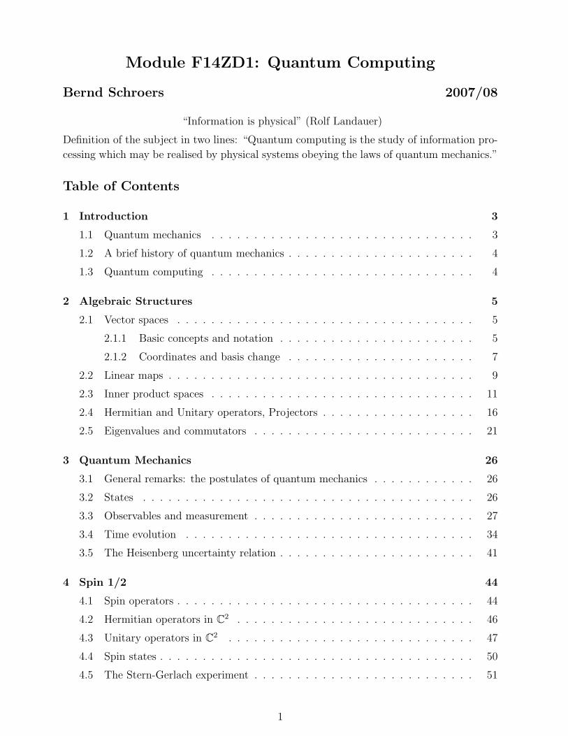
Module F14ZD1: Quantum Computing Bernd Schroers 2007/08 “Information is physical” (Rolf Landauer) Definition of the subject in two lines: “Quantum computing is the study of information pro- cessing which may be realised by physical systems obeying the laws of quantum mechanics.” Table of Contents 1 Introduction 3 1.1 Quantum mechanics ............................... 3 1.2 A brief history of quantum mechanics ...................... 4 1.3 Quantum computing ............................... 4 2 Algebraic Structures 5 2.1 Vector spaces ................................... 5 2.1.1 Basic concepts and notation ....................... 5 2.1.2 Coordinates and basis change ...................... 7 2.2 Linear maps .................................... 9 2.3 Inner product spaces ............................... 11 2.4 Hermitian and Unitary operators, Projectors .................. 16 2.5 Eigenvalues and commutators .......................... 21 3 Quantum Mechanics 26 3.1 General remarks: the postulates of quantum mechanics ............ 26 3.2 States ....................................... 26 3.3 Observables and measurement .......................... 27 3.4 Time evolution .................................. 34 3.5 The Heisenberg uncertainty relation ....................... 41 4 Spin 1/2 44 4.1 Spin operators ................................... 44 4.2 Hermitian operators in C 2 ............................ 46 4.3 Unitary operators in C 2 ............................. 47 4.4 Spin states ..................................... 50 4.5 The Stern-Gerlach experiment .......................... 51 1

Welcome message from author
This document is posted to help you gain knowledge. Please leave a comment to let me know what you think about it! Share it to your friends and learn new things together.
Transcript
Module F14ZD1: Quantum Computing
Bernd Schroers 2007/08
“Information is physical” (Rolf Landauer)
Definition of the subject in two lines: “Quantum computing is the study of information pro-
cessing which may be realised by physical systems obeying the laws of quantum mechanics.”
Table of Contents
1 Introduction 3
1.1 Quantum mechanics . . . . . . . . . . . . . . . . . . . . . . . . . . . . . . . 3
1.2 A brief history of quantum mechanics . . . . . . . . . . . . . . . . . . . . . . 4
1.3 Quantum computing . . . . . . . . . . . . . . . . . . . . . . . . . . . . . . . 4
2 Algebraic Structures 5
2.1 Vector spaces . . . . . . . . . . . . . . . . . . . . . . . . . . . . . . . . . . . 5
2.1.1 Basic concepts and notation . . . . . . . . . . . . . . . . . . . . . . . 5
2.1.2 Coordinates and basis change . . . . . . . . . . . . . . . . . . . . . . 7
2.2 Linear maps . . . . . . . . . . . . . . . . . . . . . . . . . . . . . . . . . . . . 9
2.3 Inner product spaces . . . . . . . . . . . . . . . . . . . . . . . . . . . . . . . 11
2.4 Hermitian and Unitary operators, Projectors . . . . . . . . . . . . . . . . . . 16
2.5 Eigenvalues and commutators . . . . . . . . . . . . . . . . . . . . . . . . . . 21
3 Quantum Mechanics 26
3.1 General remarks: the postulates of quantum mechanics . . . . . . . . . . . . 26
3.2 States . . . . . . . . . . . . . . . . . . . . . . . . . . . . . . . . . . . . . . . 26
3.3 Observables and measurement . . . . . . . . . . . . . . . . . . . . . . . . . . 27
3.4 Time evolution . . . . . . . . . . . . . . . . . . . . . . . . . . . . . . . . . . 34
3.5 The Heisenberg uncertainty relation . . . . . . . . . . . . . . . . . . . . . . . 41
4 Spin 1/2 44
4.1 Spin operators . . . . . . . . . . . . . . . . . . . . . . . . . . . . . . . . . . . 44
4.2 Hermitian operators in C2 . . . . . . . . . . . . . . . . . . . . . . . . . . . . 46
4.3 Unitary operators in C2 . . . . . . . . . . . . . . . . . . . . . . . . . . . . . 47
4.4 Spin states . . . . . . . . . . . . . . . . . . . . . . . . . . . . . . . . . . . . . 50
4.5 The Stern-Gerlach experiment . . . . . . . . . . . . . . . . . . . . . . . . . . 51
1

5 The density operator 54
5.1 Ensembles of states . . . . . . . . . . . . . . . . . . . . . . . . . . . . . . . . 54
5.2 The postulates of quantum mechanics in terms of density operators . . . . . 60
6 Composite systems 65
6.1 Tensor products . . . . . . . . . . . . . . . . . . . . . . . . . . . . . . . . . . 65
6.1.1 Basic definitions, notation . . . . . . . . . . . . . . . . . . . . . . . . 65
6.1.2 Inner products . . . . . . . . . . . . . . . . . . . . . . . . . . . . . . 67
6.1.3 Linear operators . . . . . . . . . . . . . . . . . . . . . . . . . . . . . 67
6.2 Quantum mechanics of composite systems . . . . . . . . . . . . . . . . . . . 72
6.3 Schmidt decomposition and purification . . . . . . . . . . . . . . . . . . . . . 75
6.4 The EPR (thought) experiment . . . . . . . . . . . . . . . . . . . . . . . . . 81
6.5 Bell’s inequality . . . . . . . . . . . . . . . . . . . . . . . . . . . . . . . . . 85
7 Quantum circuits and quantum algorithms 88
7.1 Classical versus quantum circuits . . . . . . . . . . . . . . . . . . . . . . . . 88
7.2 Unitary quantum gates . . . . . . . . . . . . . . . . . . . . . . . . . . . . . . 89
7.3 Measurement: the circuit for quantum teleportation . . . . . . . . . . . . . . 92
7.4 The Deutsch algorithm . . . . . . . . . . . . . . . . . . . . . . . . . . . . . . 94
2

1 Introduction
The following subsections are modified excerpts form articles on quantum mechanics and
quantum computing in the the on-line encyclopedia Wikipedia, http://www.wikipedia.org.
1.1 Quantum mechanics
Quantum mechanics is the framework in which most fundamental physical theories are for-
mulated. There exist quantum versions of most classical theories, including mechanics and
electromagnetism (but not general relativity), which provide accurate descriptions for many
previously unexplained phenomena such as black body radiation and stable electron orbits.
The effects of quantum mechanics are typically not observable on macroscopic scales, but
become evident at the atomic and subatomic level. The term quantum (Latin, ”how much”)
refers to the discrete units that the theory assigns to certain physical quantities, such as the
energy of an atom at rest.
Quantum mechanics has had enormous success in explaining many of the features of our
world. The individual behaviour of the microscopic particles that make up all forms of
matter, such as electrons, protons or neutrons, can often only be satisfactorily described
using quantum mechanics. The application of quantum mechanics to chemistry - known
as quantum chemistry - can provide quantitative insight into chemical bonding processes
by explicitly showing which molecules are energetically favourable to which others, and by
approximately how much. Most of the calculations performed in computational chemistry
rely on quantum mechanics.
Much of modern technology operates at a scale where quantum effects are significant. Ex-
amples include the laser, the transistor, the electron microscope, and magnetic resonance
imaging. The study of semiconductors led to the invention of the diode and the transistor,
which are indispensable for modern electronics.
In the formalism of quantum mechanics, the state of a system at a given time is described
by an element of a complex vector space. This abstract mathematical object allows for the
calculation of probabilities of outcomes of concrete experiments. For example, it allows one
to compute the probability of finding an electron in a particular region around the nucleus
at a particular time. Contrary to classical mechanics, one can never make simultaneous
predictions of conjugate quantities, such as position and momentum, with arbitrary accu-
racy. Heisenberg’s uncertainty principle quantifies the inability to precisely specify conjugate
quantities.
Quantum mechanics remains the subject of intense research, both concerning applications
and the foundations of the subject. One important challenge is to find robust methods for
directly manipulating quantum states. Efforts are being made to develop quantum cryptog-
raphy, which will allow guaranteed secure transmission of information. A long-term goal is
the development of quantum computers, which are expected to perform certain computa-
tional tasks exponentially faster than classical computers. Another active research topic is
quantum teleportation, which deals with techniques to transmit quantum states over arbi-
trary distances.
3

1.2 A brief history of quantum mechanics
The foundations of quantum mechanics were established during the first half of the 20th
century by Max Planck (1858-1947), Albert Einstein (1879-1955), Niels Bohr 1885-1962),
Werner Heisenberg (1901-1976), Erwin Schrodinger (1887-1961), Max Born (1882-1970),
John von Neumann (1903-1957), Paul Dirac (1902-1984), Wolfgang Pauli (1900-1958) and
others.
In 1900, Max Planck introduced the idea that energy is quantised, in order to derive a
formula for the observed frequency dependence of the energy emitted by a black body. In
1905, Einstein explained the photoelectric effect by postulating that light energy comes in
quanta called photons. In 1913, Bohr explained the spectral lines of the hydrogen atom,
again by using quantisation. In 1924, Louis de Broglie put forward his theory of matter
waves.
These theories, though successful, were strictly phenomenological: there was no rigorous
justification for quantisation. They are collectively known as the old quantum theory.
Modern quantum mechanics was born in 1925, when Heisenberg developed matrix mechan-
ics and Schrodinger invented wave mechanics and the Schrodinger equation. Schrodinger
subsequently showed that the two approaches were equivalent.
Heisenberg formulated his uncertainty principle in 1927, and the Copenhagen interpretation
took shape at about the same time. Starting around 1927, Paul Dirac unified quantum
mechanics with special relativity. He also pioneered the use of operator theory, including
the influential bra-ket notation, as described in his famous 1930 textbook. During the
same period, John von Neumann formulated the rigorous mathematical basis for quantum
mechanics as the theory of linear operators on Hilbert spaces, as described in his likewise
famous 1932 textbook. These, like many other works from the founding period still stand,
and remain widely used.
1.3 Quantum computing
A quantum computer is any device for computation that makes direct use of distinctively
quantum mechanical phenomena, such as superposition and entanglement, to perform oper-
ations on data. In a classical (or conventional) computer, the amount of data is measured
by bits; in a quantum computer, it is measured by qubits. The basic principle of quantum
computation is that the quantum properties of particles can be used to represent and struc-
ture data, and that devised quantum mechanisms can be used to perform operations with
these data.
Experiments have already been carried out in which quantum computational operations
were executed on a very small number of qubits. Research in both theoretical and practical
areas continues at a frantic pace. Many national government and military funding agencies
support quantum computing research, to develop quantum computers for both civilian and
national security purposes, such as cryptanalysis.
It is widely believed that if large-scale quantum computers can be built, they will be able to
4

solve certain problems faster than any classical computer. Quantum computers are different
from classical computers based on transistors, even though these may ultimately use some
kind of quantum mechanical effect. Some computing architectures such as optical comput-
ers may use classical superposition of electromagnetic waves, but without some specifically
quantum mechanical resource such as entanglement, they do not share the potential for
computational speed-up of quantum computers.
2 Algebraic Structures
In this section we review some algebraic structures which you studied in the second year
module on linear algebra, and introduce some algebraic concepts which you have not yet
come across. I will not give formal definitions and proofs of concepts and results which you
studied in second year, but will remind you of the basic ideas. Please refer to your notes on
linear algebra for further details. All new concepts will be carefully defined and I will give
plenty of examples for both old and new material.
2.1 Vector spaces
2.1.1 Basic concepts and notation
A vector space is a set whose elements one can add together and multiply by a number,
often called a scalar, and which contains a special element 0, the zero vector. The scalar
will generally be a complex number in this course. Vector spaces with complex numbers as
scalars are called complex vector spaces. In quantum mechanics, the vectorial nature of
a quantity v is usually expressed by enclosing it between a vertical line and a right bracket
|v〉. We will adopt this convention here, which goes back to Paul Dirac, who also introduced
the name “ket” for a vector. As we shall see later, this name is motivated by thinking of a
vector as “half a brac-ket”.
Example 2.1.1 The set C2 of column vectors made up of two complex numbers is a complex
vector space. Find the vector obtained by adding the vectors
|v1〉 =
(i−4
), |v2〉 =
(6− i5 + i
),
and multiplying the result by the scalar α = 3eiπ2 .
Since 3eiπ2 = 3i we have
α(|v1〉+ |v2〉) = 3i
(6
1 + i
)=
(18i
−3 + 3i
).
�
Recall that a vector |v〉 is called a linear combination of vectors |v1〉 and |v2〉 if it can be
written
|v〉 = α1|v1〉+ α2|v2〉
5

for two complex numbers α1 and α2. The span of a subset S = {|v1〉, . . . , |vn〉} is the set of
all linear combinations of the vectors |v1〉, . . . , |vn〉 and denoted [|v1〉, . . . , |vn〉]. We say that
the subset S = {|v1〉, . . . , |vn〉} of a vector space V is a spanning set if any vector can be
written as a linear combination of the vectors |v1〉, . . . , |vn〉 i.e. if [|v1〉, . . . , |vn〉] = V . The
vectors |v1〉, . . . , |vn〉 are called linearly independent if
n∑i=1
αi|vi〉 = 0 ⇒ αi = 0, i = 1, . . . , n. (2.1)
Conversely, the vectors |v1〉, . . . , |vn〉 are linearly dependent if we can find complex num-
bers α1, . . . , αn, not all zero, so that
n∑i=1
αi|vi〉 = 0 (2.2)
Example 2.1.2 Show that the vectors |v1〉 =
(1− i
1
)and |v2〉 =
(1
12
+ i2
)in C2 are linearly
dependent.
Since (1 + i)|v1〉 = 2|v2〉 we have (1 + i)|v1〉+ (−2)|v2〉 = 0. �
Example 2.1.3 Suppose that the vectors |v1〉, . . . , |vn〉 are linearly independent. Show that
a vector |v〉 in V can be written as linear combinations of |v1〉, . . . , |vn〉 in at most one way.
Suppose that there are two ways of writing |v〉 as a linear combination, i.e.
v =n∑i=1
αi|vi〉 (2.3)
and
v =n∑i=1
βi|vi〉. (2.4)
Then, taking the difference, we deduce that
n∑i=1
(αi − βi)|vi〉 = 0.
But since the |vi〉 are linearly independent we deduce that αi = βi for i = 1, . . . , n, so that
the two linear combinations (2.3) and (2.4) are in fact the same. �.
A set S = {|v1〉, . . . |vn〉} is called a basis of the vector space V if S is both spanning and
linearly independent. One can show that every vector space has a basis. The basis is not
unique - in fact there are infinitely many different bases as we shall see below - but the
number of elements in any basis is the same; that number is called the dimension of the
vector space. The dimension may be finite or infinite. In this course we only deal with finite
6

dimensional vector spaces. For a vector space of finite dimension n one can show that any
set of n linearly independent vectors is automatically spanning, i.e. a basis. In order to
check if a given set containing n vectors constitutes a basis we therefore only need to check
for linear independence. There are simple tests for this, one of which we give below.
The vector space Cn has a canonical basis consisting of the column vectors
|b1 〉 =
10...
0
, |b2 〉 =
01...
0
, . . . , |bn 〉 =
00...
1
. (2.5)
The space C2 plays a particularly important role in quantum computing and it is conventional
to denote the canonical basis as
|0〉 =
(10
)|1〉 =
(01
). (2.6)
The notation anticipates the role of the space C2 as a quantum bit or qubit. Whereas a
classical bit can be in one of two states “0” or “1”, quantum bit can be in the basis states
|0〉 or |1〉 or in any linear combination of the basis states. Any two vectors
|x 〉 =
(x1
x2
), |y 〉 =
(y1
y2
)in C2 are independent (and hence constitute a basis) if the matrix made from the the column
vectors has a non-vanishing determinant:
det
(x1 y1
x2 y2
)6= 0. (2.7)
2.1.2 Coordinates and basis change
Suppose that V is a complex vector space of dimension n and that B = {|b1〉, . . . |bn〉} is a
basis of V . Then a vector |x〉 has a unique expansion
|x〉 =n∑i=1
xi|bi〉 (2.8)
in terms of this basis. The complex numbers x1, . . . , xn are called the coordinates of the
vector |x〉 with respect to the basis B.
A vector can be expanded in any basis, and its coordinates with respect to different bases
differ. We are interested in the change of coordinates under a change of basis. Suppose
the basis B′ = {|b′1〉, . . . , |b′n〉} of an n-dimensional vector space is obtained from the basis
B = {|b1〉, . . . , |bn〉} via
|b′i〉 =n∑j=1
Mji|bj〉, for i = 1, . . . n, (2.9)
7

where Mij are the matrix elements of an invertible n× n-matrix of complex numbers. Now
we have the two expansions
|x〉 =n∑j=1
xj|bj〉 (2.10)
and
|x〉 =n∑i=1
x′i|b′i〉. (2.11)
Inserting the relation (2.9) into the expansion (2.11) we have
|x〉 =n∑
i,j=1
x′iMji|bj〉. (2.12)
Comparing with (2.10) and using the uniqueness of expansions in a basis we deduce
xj =n∑i=1
Mjix′i. (2.13)
Collecting the coordinates xi and x′j into column vectors this can be writtenx1
x2...
xn
=
M11 M12 . . . M1n
M21 M22 . . . M2n...
Mn1 Mn2 . . . Mnn
x′1x′2...
x′n
(2.14)
or, denoting the matrix with matrix entries Mij by M ,x1
x2...
xn
= M
x′1x′2...
x′n
(2.15)
so that x′1x′2...
x′n
= M−1
x1
x2...
xn
. (2.16)
Performing the inversion explicitly in the case n = 2(x1
x2
)=
(M11 M12
M21 M22
)(x′1x′2
)(2.17)
we find (x′1x′2
)=
1
M11M22 −M12M21
(M22 −M12
−M21 M11
)(x1
x2
). (2.18)
8

Example 2.1.4 Give the coordinates of the vector |x〉 = i|0〉 − |1〉 in C2 in the basis with
basis vectors |v1〉 = 1√2(|0〉+ |1〉) and |v2〉 = 1√
2(−|0〉+ |1〉)
With
M =1√2
(1 −11 1
)and
M−1 =1√2
(1 1−1 1
)we have the coordinates(
x′1x′2
)=
1√2
(1 1−1 1
)(i−1
)=
1√2
(i− 1−i− 1
)so that |x〉 = i−1√
2|v1〉 − i+1√
2|v2〉.
2.2 Linear maps
Recall that a linear map from a vector space V to a vector space W is a map A : V → W
which satisfies A(α|u〉 + β|v〉) = αA(|u〉) + βA(|v〉) for any complex numbers α and β and
any two elements |u〉 and |v〉 in V . In quantum mechanics it is customary to call linear maps
linear operators, though mathematicians tend to reserve this term for situations where
both V and W are infinite dimensional. We will mostly be concerned with the situation
V = W in the following. It is not difficult to show (check you linear algebra notes) that a
linear map is completely determined by its action on basis of V . This leads to the matrix
representation of a linear map as follows.
Consider a linear map A : V → V in a complex vector space of dimension n, and let
B = {|b1, . . . , |bn〉} be a basis of V . We consider the action of A on each of the basis
elements, and expand the images in the basis B:
A(|bi〉) =n∑j=1
Aji|bj〉. (2.19)
The matrix made up of the n×n numbers Aij, i, j = 1, . . . , n is the matrix representation
of A with respect to the basis B. The action of A on a general element |x〉 ∈ V can be written
conveniently in terms of the matrix representation. With the expansion |x〉 =∑n
i=1 xi|bi〉we have
A(|x〉) =n∑j=1
Ajixi|bj〉. (2.20)
so that the coordinates of the image A(|x〉) with respect to the basis B are obtained from the
coordinates of |x〉 with respect to B by putting them into a column vector and multiplying
them with the matrix representation of A.
Important notational convention: In the following we will often fix one basis for a given
vector space V and work with coordinates and matrix representations relative to that basis.
9

In particular when working with V = Cn we use the canonical basis (2.5). In that case we do
not distinguish notationally between the operator A and its matrix representation relative
to the canonical basis.
Example 2.2.1 The linear map A : C2 → C2 satisfies A(|0〉) = 3i|0〉 + 4|1〉 and A(|1〉) =
3|0〉 − 4i|1〉. Give its matrix representation with respect to the canonical basis, and give the
image of the vector |x〉 = |0〉 − |1〉 under the action of A.
The matrix representation is
A =
(3i 34 −4i
)so the image of the vector with coordinates
(1−1
)has coordinates(
3i 34 −4i
)(1−1
)=
(−3 + 3i4 + 4i
).
�
Before leaving linear operators we need to understand how the matrix representation of an
operator A changes when we change the basis of V . Consider again a complex vector space
V with two distinct bases B and B′. The basis B′ = {|b′1〉, . . . , |b′n〉} is obtained from the
basis B = {|b1〉, . . . , |bn〉} via
|b′i〉 =n∑j=1
Mji|bj〉, for i = 1, . . . n. (2.21)
Suppose we are given the matrix representation of A relative to the basis B via (2.19) and
would like to know its matrix representation with respect to the basis B′. Defining
A(|b′i〉) =n∑j=1
A′ji|b′j〉. (2.22)
we replace |b′i 〉 by the expression in (2.21) and use the linearity of A to deduce
n∑k=1
MkiA(|bk〉) =n∑
j,l=1
A′jiMlj|bl〉. (2.23)
Expanding the left-hand side according to (2.19) we have
n∑k,l=1
MkiAlk(|bl〉) =n∑
j,l=1
A′jiMlj|bl〉 (2.24)
Comparing coefficients of basis elements |bl〉 we deduce that the matrices M,A,A′ satisfy
AM = MA′ (2.25)
or
A′ = M−1AM (2.26)
10

Example 2.2.2 See problem sheet 1!
In the linear algebra course in second year you came across the definition of the determinant
and the trace of a matrix. Using the relation (2.26) we can now define the determinant and
trace of a linear map. Although one requires a matrix representation to compute both, the
result is independent of the basis to which the matrix representation refers. To see this,
recall that for any two n× n matrices A and B
det(AB) = det(A)det(B), (2.27)
which implies in particular det(A−1) = (detA)−1. Recall also that the definition
tr(A) =n∑i=1
Aii, (2.28)
which implies
tr(AB) =n∑
i,j=1
AijBji = tr(BA). (2.29)
It follows that for the two matrices A′ and A related by conjugation with M as in (2.26)
that
det(A′) = (det(M))−1det(A)det(M) = det(A) (2.30)
and
tr(A′) = tr(M−1AM) = tr(MM−1A) = tr(A). (2.31)
2.3 Inner product spaces
For vector spaces to be of use in quantum mechanics they need to be equipped with an
addition structural feature: an inner product or scalar product. For complex vector spaces
this is defined as follows.
Definition 2.3.1 (Inner product) An inner product on a complex vector space V is a map
( , ) : V × V → C (2.32)
which satisfies
1. (|v〉, α1|w1〉+ α2|w2〉) = α1(|v〉, |w1〉) + α2(|v〉, |w2〉)(Linearity in the second argument)
2. (|v〉, |w〉) = (|w〉, |v〉), (Symmetry)
3. |v〉 6= 0 ⇒ (|v〉, |v〉) > 0 (Positivity)
11

Note that the last condition makes sense since (|v〉, |v〉) is real, which follows directly from
condition 2.
Before we study examples we note an important property.
Lemma 2.3.2 (Conjugate linearity) The inner product (·, ·) is conjugate-linear in the
first argument, i.e.
(α1|v1 〉+ α2|v2 〉, |w〉) = α1(|v 〉1, |w〉) + α2(|v2 〉, w〉) (2.33)
Proof: Using the properties of the inner product we compute
(α1|v1 〉+ α2|v2 〉, |w〉) = (|w 〉, α1|v1 〉+ α2|v2 〉) (Property 2)
= α1(|w 〉, |v1 〉) + α2(|w 〉, |v2 〉) (Property 1)
= α1(|v1 〉, |w 〉) + α2(|v2 〉, |w 〉) (Property 2). (2.34)
�
Example 2.3.3 Define an inner product on C2 via
(
(x1
x2
),
(y1
y2
)) = x1y1 + x2y2. (2.35)
Show that it satisfies all the properties of the definition 2.3.1.
Checking linearity and symmetry of (2.35) is left as a simple exercise. For positivity note
that
(
(z1
z2
),
(z1
z2
)) = |z1|2 + |z2|2,
which is a sum of positive terms and non-vanishing if z1 and z2 are not both zero. �
In quantum mechanics it is customary to write
(|v〉, |w〉) = 〈v|w〉 (2.36)
The mathematical motivation for this notation is that in an inner product space every vector
|v〉 defines a linear map
〈v| : V → C via
|w〉 7→ 〈v|w〉. (2.37)
The inner product 〈v|w〉 can thus be thought of as the the map 〈v| evaluated on the vector
|w〉. In quantum mechanics the map 〈v| is called a bra: the “left half” of the “bra-ket”.
Example 2.3.4 Suppose that B = {|b1 〉, . . . , |b2 〉} is an orthogonal basis of V and |x 〉 =∑ni=1 xi|bi 〉. Find the matrix representation of the linear map 〈x|.
12

We have only considered matrix representations of maps V → V in this course so far, but
it is not difficult to extend this notion to the situation 〈x| : V → C. The idea is again to
apply the map to each of the basis vectors |bi 〉. We find
〈x|bi 〉 = 〈 bi|x 〉 = xi (2.38)
There is no need to expand the result in a basis since the target space C is one-dimensional.
Comparing with (2.19) and noting that the index i labels the columns of the matrix rep-
resentation we conclude that the matrix representation of the map 〈x| is the row vector
(x1, . . . , xn). �
The inner product allows one to define the norm of a vector and the notion of orthogonality.
Definition 2.3.5 Let V be a vector space with inner product.
1. The norm of a vector |v〉 is
||v〉| =√〈v|v〉. (2.39)
2. Two vectors |v〉 and |w〉 are orthogonal if 〈v|w〉 = 0.
3. A basis B = {|b1〉, . . . , |bn〉} of V is called orthonormal if
〈bi|bj〉 = δij, i, j = 1, . . . , n (2.40)
In the last part of the definition we use the Kronecker delta symbol: δij is 1 when i = j
and zero otherwise. Any basis of a vector space V with inner product can be turned into
an orthonormal basis by the Gram-Schmidt process, which you studied in second year
and which I will not review here. Since every vector space has a basis it follows from the
Gram-Schmidt procedure that every vector space with an inner product has an orthonormal
basis.
Example 2.3.6 Show that |b1〉 = (cos θ|0〉 + sin θ|1〉) and |b2〉 = i(cos θ|1〉 − sin θ|0〉) form
an orthonormal basis of C2 with the canonical inner product defined in (2.35) for any value
of the parameter θ ∈ [0, 2π).
It is easy to check that {|0〉, |1〉} form an orthonormal basis. Hence 〈b1|b1〉 = cos2 θ+sin2 θ = 1
and similarly 〈b2|b2〉 = 1. Moreover 〈b1|b2〉 = −i cos θ sin θ + i cos θ sin θ = 0. �.
Example 2.3.7 For the case V = Cn, a canonical inner product is defined via
(
x1
x2...
xn
,
y1
y2...
yn
) =n∑i=1
xiyi. (2.41)
Check that the canonical basis (2.5) is an orthonormal basis with respect to this inner product.
13

Inserting the coordinate given in (2.5) one finds 〈bi|bj 〉 = δij �
The inner product allows one to define the orthogonality not only of vectors but of entire
subspaces. For later use we note
Definition 2.3.8 (Orthogonal complement) If W is a subspace of a vector space V with
inner product we define the orthogonal complement to be the space
W⊥ = {|v 〉 ∈ V |〈v|w 〉 = 0 for all |w 〉 ∈W} (2.42)
It is not difficult to check that W⊥ is indeed a vector space (see problem sheet).
Example 2.3.9 Let V = C3 and W be the linear span of
100
. Find the orthogonal com-
plement of W .
Elements |v 〉 =
z1
z2
z3
in v are orthogonal to
100
iff z1 = 0. Thus
W⊥ = {
0z2
z3
|z2, z3 ∈ C}.
�
We have already seen in (2.8) that any element |x〉 of a vector space can be expanded
in a given basis. However, in the previous subsection we did not give an algorithm for
computing the expansion coefficients xi. If the vector space V is equipped with an inner
product, the computation of the expansion coefficients is considerably simplified. Suppose
that B = {|b1〉, . . . , |bn〉} is an orthonormal basis of V and we want to find the coordinates
of |x〉 in this basis:
|x〉 =n∑i=1
xi|bi〉. (2.43)
Acting on both sides of the equation with the bra’s 〈bj|, j = 1, . . . , n we find
〈bj|x〉 =n∑i=1
xiδij = xj, (2.44)
thus giving us an explicit formula for the coordinates xj.
We can similarly give an explicit formula for the matrix representation of a linear operator
A on the vector space V with inner product. We consider the action of A on each of the
basis elements in B:
A|bi〉 =n∑k=1
Aki|bj〉. (2.45)
14

Acting on both sides of the equation with the bra’s 〈bj|, k = 1, . . . , n we find
〈bj|A|bi〉 =n∑k=1
Ajiδjk = Aji, (2.46)
The inner product structure even helps in explicitly reconstructing the linear operator A
from its matrix representation. For this purpose we introduce the maps
|bi〉〈bj| : V → V
|x〉 7→ |bi〉〈bj|x〉 (2.47)
associated to the elementary bras and kets 〈bj| and |bi〉. We claim
Lemma 2.3.10 For any linear operator A in a vector space V with inner product and or-
thonormal basis B we have the representation
A =n∑
i,j=1
Aij|bi〉〈bj|, (2.48)
where Aij = 〈 bi|A|bj 〉.
To prove this claim we show the left and the right hand side have the same action on each
of the basis vectors |bk〉:
A|bk〉 =n∑
i,j=1
Aij|bi〉〈bj|bk〉 =n∑i=1
Aik|bi〉, (2.49)
which is true by the definition of the matrix elements Aik. �
We note in particular
Corollary 2.3.11 (Resolution of the identity) The identity operator I : V 7→ V has the
representation
I =∑i=1
|bi〉〈bi| (2.50)
This representation of identity is often useful in calculations. As an example we give a quick
proof of the
Theorem 2.3.12 (Cauchy-Schwarz inequality) For any two vectors |ϕ〉 and |ψ〉 in the
vector space V with inner product we have
〈ϕ|ψ〉〈ψ|ϕ〉 ≤ 〈ϕ|ϕ〉〈ψ|ψ〉 (2.51)
15

Proof: We may assume without loss of generality that the vector |ψ〉 is normalised i.e.
〈ψ|ψ〉 = 1; otherwise we divide left and right-hand side of the inequality by the real, positive
number 〈ψ|ψ〉. We need to show that
〈ϕ|ψ〉〈ψ|ϕ〉 ≤ 〈ϕ|ϕ〉. (2.52)
To see this, complete |ψ〉 to an orthonormal basis B = {|ψ〉, |b2〉, . . . , |bn〉} and write the
identity as
I = |ψ〉〈ψ|+n∑i=2
|bi〉〈bi|. (2.53)
Now consider the inner product 〈ϕ|ϕ〉 and insert the identity:
〈ϕ|ϕ〉 = 〈ϕ|I|ϕ〉 = 〈ϕ|ψ〉〈ψ|ϕ〉+n∑i=2
〈ϕ|bi〉〈bi|ϕ〉
≥ 〈ϕ|ψ〉〈ψ|ϕ〉 (2.54)
where we used that 〈ϕ|bi〉〈bi|ϕ〉 = 〈ϕ|bi〉〈ϕ|bi〉 = |〈ϕ|bi〉|2 ≥ 0. �
2.4 Hermitian and Unitary operators, Projectors
Having defined inner product spaces, we now consider operators in such spaces in some
detail. We begin with the fundamental
Definition 2.4.1 (Adjoint operator) Let A be a linear operator in a complex vector space
V with inner product (·, ·). Then we define the adjoint operator A† by the condition
(|ϕ 〉, A|ψ 〉) = (A†|ϕ 〉, |ψ 〉) for all |ϕ 〉, |ψ 〉 ∈ V (2.55)
or, using bra-ket notation,
〈ϕ|A|ψ 〉 = 〈ψ|A†|ϕ 〉. (2.56)
Let B = {|b1 〉, . . . , |bn 〉} be an orthonormal basis of V and Aij be the matrix elements of
the matrix representation of A i.e.
〈 bi|A|bj 〉 = Aij (2.57)
Then, we can read off the matrix representation of A† with respect to the same basis from
(2.56):
〈 bi|A†|bj 〉 = 〈 bj|A|bi 〉 = Aji. (2.58)
Thus the matrix representing A† is obtained from the matrix representing A by transposition
and complex conjugation. Using the same symbols for the matrices as for the operators which
they represent, we write
A† = At. (2.59)
16

Example 2.4.2 The matrix representing the operator A : C2 → C2 relative to a fixed or-
thonormal basis of C2 is
A =
(2− i 3 + 2i1− i 1 + i
).
Find the matrix representing the adjoint A†.
Transposing and complex conjugating we obtain
A† =
(2 + i 1 + i3− 2i 1− i
).
We note the following general properties of adjoints:
Lemma 2.4.3 Let A and B be linear operators in a vector space V with inner product and
α, β ∈ C. Then
1. (A†)† = A
2. (αA+ βB)† = αA† + βB†
3. (AB)† = B†A†
The proof is straightforward - and left as an exercise.
Example 2.4.4 Let B = {|b1 〉, . . . , |bn 〉} be an orthonormal basis of the inner product space
V . Find the adjoint of the map
|bi〉〈bj| : V → V |x〉 7→ |bi〉〈bj|x〉
considered in (2.47)
For arbitrary elements |ϕ 〉, |ψ 〉 ∈ V we have
(|ϕ 〉, |bi〉〈bj|ψ 〉) = 〈ϕ, |bi 〉〈bj, |ψ 〉= 〈bi|ϕ 〉〈bj, |ψ 〉= (|bj 〉〈bi|ϕ 〉, |ψ 〉) (2.60)
Comparing with the definition (2.55) we conclude
(|bi〉〈bj|)† = |bj〉〈bi|. (2.61)
�
One can extend the definition of an adjoint to maps A : V → W , where V and W are two
different inner product spaces. In that case A† is a map W → V . The matrix representation
of A† is still obtained from the matrix representation of A be transposition (turning rows
into columns) and complex conjugation. We will not need this definition in full generality,
17
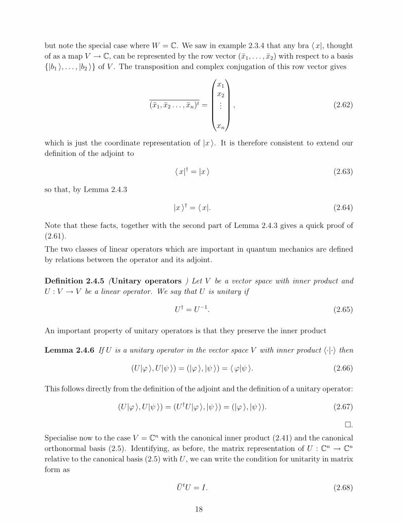
but note the special case where W = C. We saw in example 2.3.4 that any bra 〈x|, thought
of as a map V → C, can be represented by the row vector (x1, . . . , x2) with respect to a basis
{|b1 〉, . . . , |b2 〉} of V . The transposition and complex conjugation of this row vector gives
(x1, x2 . . . , xn)t =
x1
x2...
xn
, (2.62)
which is just the coordinate representation of |x 〉. It is therefore consistent to extend our
definition of the adjoint to
〈x|† = |x 〉 (2.63)
so that, by Lemma 2.4.3
|x 〉† = 〈x|. (2.64)
Note that these facts, together with the second part of Lemma 2.4.3 gives a quick proof of
(2.61).
The two classes of linear operators which are important in quantum mechanics are defined
by relations between the operator and its adjoint.
Definition 2.4.5 (Unitary operators ) Let V be a vector space with inner product and
U : V → V be a linear operator. We say that U is unitary if
U † = U−1. (2.65)
An important property of unitary operators is that they preserve the inner product
Lemma 2.4.6 If U is a unitary operator in the vector space V with inner product 〈·|·〉 then
(U |ϕ 〉, U |ψ 〉) = (|ϕ 〉, |ψ 〉) = 〈ϕ|ψ 〉. (2.66)
This follows directly from the definition of the adjoint and the definition of a unitary operator:
(U |ϕ 〉, U |ψ 〉) = (U †U |ϕ 〉, |ψ 〉) = (|ϕ 〉, |ψ 〉). (2.67)
�.
Specialise now to the case V = Cn with the canonical inner product (2.41) and the canonical
orthonormal basis (2.5). Identifying, as before, the matrix representation of U : Cn → Cn
relative to the canonical basis (2.5) with U , we can write the condition for unitarity in matrix
form as
U tU = I. (2.68)
18

Example 2.4.7 Show that the matrix
U =
(eiφ cos( θ
2) − sin( θ
2)
sin( θ2) e−iφ cos( θ
2)
)is unitary for θ ∈ (0, 2π) and φ ∈ [0, 2π)
Using cos2( θ2) + sin2( θ
2) = 1 we find
U tU =
(e−iφ cos( θ
2) sin( θ
2)
− sin( θ2) eiφ cos( θ
2)
)(eiφ cos( θ
2) − sin( θ
2)
sin( θ2) e−iφ cos( θ
2)
)=
(1 00 1
)�.
Definition 2.4.8 (Hermitian operators ) Let V be a vector space with inner product and
A : V → V be a linear operator. We say that A is Hermitian if
A† = A (2.69)
Example 2.4.9 (Pauli matrices The following three matrices are called the Pauli matrices
σ1 =
(0 11 0
), σ2 =
(0 −ii 0
), σ3 =
(1 00 −1
)(2.70)
Show that they are both Hermitian and unitary.
This is an elementary calculation �
We collect some properties of unitary and Hermitian operators in the following lemma.
Lemma 2.4.10 In the following V is a complex vector space with inner product. Then
1. A†A is Hermitian for any operator A : V → V .
2. If B : V → V is Hermitian, then so is B−1.
3. If W : V → V is unitary, then so is W−1.
4. If B is Hermitian and U unitary, then U−1BU is Hermitian
5. If W and U are unitary, then U−1WU is unitary
Proof:
1. Applying the rules 1 and 3 in Lemma 2.4.3, we have (A†A)† = A†(A†)† = A†A, thus
establishing the first claim.
2. Taking the adjoint of the equation B−1B = I we find B†(B−1)† = I since the identity
is Hermitian. Now use Hermiticity of B to deduce B(B−1)† = I so that (B−1)† = B−1,
establishing the Hermiticity of B−1.
19

3. Taking the adjoint of the equation W−1 = W † we find (W−1)† = W . Hence (W−1)† =
(W−1)−1, showing the W−1 is unitary.
4. (U−1BU)† = U †(U−1B)† = U †B†(U−1)† = U−1BU .
5. (U−1WU)† = U †W †(U−1)† = U−1W−1U = (U−1WU)−1 �.
Finally we turn to a class of operators called projectors or projection operators
Definition 2.4.11 (Projection operator) An operator P : V → V is called projection
operator if P 2 = P . If V is equipped with an inner product and P is Hermitian with respect
to that inner product, P is called an orthogonal projection operator
Example 2.4.12 Consider the vector space R2 (“the xy-plane”) with its canonical inner
product and canonical basis |0 〉, |1 〉. Write down the matrix representation, with respect to
the canonical basis, of
1. The projection along the y-axis onto the x-axis.
2. The projection along the line x+ y = 0 onto the x-axis
You can visualise the examples in terms of shining light along the y-axis for 1. and along
the line x + y = 0 for 2. Working out the projection operator is equivalent to determining
the shadow cast on the x-axis. Which of the projections is (are) orthogonal?
In order to determine any linear map, it is enough to determine its action on a basis. In the
first example we have
P |0 〉 = |0 〉, P |1 〉 = 0.
Hence the matrix representing P is
P =
(1 00 0
).
In the second example we have
P |0 〉 = |0 〉, P |1 〉 = |0 〉
leading to the matrix representation
P =
(1 10 0
).
It is clear geometrically that the first projection operator is orthogonal and the second is
not. This is also reflected in the matrix representation: the first projection is represented by
a Hermitian matrix, but the matrix representing the second projection is not Hermitian.
Generally, given anm-dimensional subspaceW of an inner product space V , we can construct
an orthogonal project operator onto W by picking an orthonormal basis {|b1 〉, . . . |bm 〉} of
W . We claim
20
Lemma 2.4.13 The operator PW defined via
PW =m∑i=1
|bi 〉〈 bi|. (2.71)
is an orthogonal projection operator
Proof: In order to check that PW is a projection we compute
P 2W =
m∑i=1
|bi 〉〈 bi|m∑j=1
|bj 〉〈 bj|
=m∑
i,j=1
|bi 〉〈bi|bj 〉〈 bj|
=m∑
i,j=1
δij|bi 〉〈 bj|
=m∑i
|bi 〉〈 bi| = PW (2.72)
The orthogonality
P †W = PW (2.73)
follows from (|bi 〉〈 bi|)† = |bi 〉〈 bi|, which is a special case of (2.61). �
Note that if P is a projection operator, then so is I−P since (I−P )2 = I−2P +P = I−P .
Similarly, if P is an orthogonal projection operator, then so is I − P . Geometrically, if
P is the orthogonal projection onto a subspace W , then I − P is the projection onto the
orthogonal complement W⊥ defined in (2.3.8) .
2.5 Eigenvalues and commutators
An important part of solving problems in quantum mechanics involves finding eigenvalues
and eigenvectors of linear operators. Recall that if A : V → V is a linear operator, we call
λ ∈ C an eigenvalue of A if there exists a non-zero vector |v 〉 ∈ V such that
A|v 〉 = λ|v 〉. (2.74)
Any such vector |v 〉 is called an eigenvector of A with eigenvalue λ. More generally, there
may be several linearly dependent eigenvectors for a given eigenvalue λ. The space of all
eigenvectors is called the eigenspace for the eigenvalue λ and denoted
Eigλ = {|v 〉 ∈ V |A|v 〉 = λ|v 〉}. (2.75)
It is not difficult to check that Eigλ is indeed a vector space (do it!)
The eigenvalues of A are most easily determined by solving the characteristic equation
det(A− λI) = 0. (2.76)
21
This is a polynomial equation in λ of degree n = dimV . By the fundamental theorem of
algebra such an equation has at least one solution (“root”) in the complex numbers, and this
fact considerably simplifies the eigenvalue problem in complex vector spaces compared to
real vector spaces. It follows that every operator in a complex vector spaces has at least one
eigenvalue. For some operators one can find an entire basis of V consisting of eigenvectors.
Such operators are called diagonalisable. Remarkably, the Hermitian and unitary operators
which are important in quantum mechanics are always diagonalisable. The key reason for
their diagonalisability lies in the following
Lemma 2.5.1 Suppose |v 〉 ∈ V is an eigenvector of the Hermitian operator A with eigen-
value λ. Then A maps the orthogonal complement of [|v 〉] into itself, i.e. if |w 〉 ⊥ |v 〉 then
also A|w 〉 ⊥ |v 〉.
Proof: Suppose 〈 v|w 〉 = 0. Then 〈 v|A|w 〉 = 〈w|A|v 〉 = λ〈 v|w 〉 = 0 �.
Theorem 2.5.2 Suppose V is a (complex) vector space with inner product. If A : V → V is
a Hermitian operator, all eigenvalues are real and eigenvectors for different eigenvalues are
necessarily orthogonal. Moreover, there exists an orthonormal basis of eigenvectors of A.
Proof: To see that any eigenvalue of a Hermitian operator has to be real, suppose λ is an
eigenvalue of the Hermitian operator A, with associated eigenvector |v 〉, which we assume
to be normalised. Then
〈 v|A|v 〉 = λ. (2.77)
On the other hand
〈 v|A|v 〉 = 〈 v|A†|v 〉 = 〈 v|A|v 〉 = λ. (2.78)
Comparing (2.77) with (2.78) we conclude that
λ = λ (2.79)
so that λ is real. Now suppose that |v1 〉 and |v2 〉 are eigenvectors associated to distinct
eigenvalues λ1 and λ2. Then 〈 v1|A|v2 〉 = λ2〈 v1|v2 〉 but also, by Hermiticity, 〈 v1|A|v2 〉 =
λ1〈 v1|v2 〉. Hence (λ1 − λ2)〈 v1|v2 〉 = 0. Since λ1 6= λ2 this implies 〈 v1|v2 〉 = 0.
In order to prove the existence of an orthonormal basis we proceed by induction over the
dimension of V . If the dimension is 1 there is nothing to prove. Suppose we have proved
the theorem for vector spaces of dimension n− 1, and let V be a vector space of dimension
n. A is a Hermitian operator in V and has at least one eigenvalue with eigenspace W . Pick
one eigenvector |v 〉 and consider the orthogonal complement [|v 〉]⊥. It has dimension n− 1
and by Lemma 2.5.1 is mapped into itself by A. Hence the restriction of A to [|v 〉]⊥ is
a Hermitian operator in a vector space of dimension n − 1. By the induction assumption
it is diagonalisable and has an orthonormal basis {|v1 〉, . . . , |vn−1 〉} of eigenvectors. Then
B = {|v 〉, |v1 〉, . . . , |vn−1 〉} is an orthonormal basis of eigenvectors for A.
22

�
We can rephrase the results of this theorem by collecting all eigenvectors which have the
same eigenvalue into eigenspaces, thus obtaining the following
Corollary 2.5.3 Suppose V is a n-dimensional (complex) vector space with inner product.
and A : V → V is a Hermitian operator with m ≤ n distinct eigenvalues λ1, . . . , λm. Then
there is a unique decomposition of V into mutually orthogonal eigenspaces of V , i.e.
V = Eigλ1⊕ . . .⊕ Eigλm
(2.80)
Example 2.5.4 A Hermitian operator A : C2 → C2 has the matrix representation
A =
(0 11 0
)(2.81)
with respect to the canonical basis {|0 〉, |1 〉}. Find the eigenvalues λ1 and λ2 and corre-
sponding orthonormal eigenvectors |v1 〉, |v2 〉 of A. Give the matrix representation A′ of A
relative to the basis {|v1 〉, |v2 〉} and find the 2× 2 matrix M so that
A′ = M−1AM (2.82)
The characteristic equation
det(A− λ) = 0 ⇔ λ2 − 1 = 0
has solutions λ1 = 1 and λ2 = −1. To find an eigenvector
(xy
)for the eigenvalue −1 we
need to solve
y = x, x = y,
yielding the (normalised) eigenvector
|v1 〉 =1√2
(11
).
Similarly one finds the eigenvector for the eigenvalue λ2 = −1 to be
|v2 〉 =1√2
(1−1
).
Thus, the matrix representation of A relative to the basis {|v1 〉, |v2 〉} is
A′ =
(1 00 −1
).
We read off the transformation matrix M from the expansion
|v1 〉 =1√2(|0 〉+ |1 〉), |v2 〉 =
1√2(|0 〉 − |1 〉)
according to (2.21) and find
M =1√2
(1 11 −1
).
it is now easy to verify that (2.82) holds. �.
23

Theorem 2.5.5 Suppose V is a (complex) vector space with inner product. If U : V → V
is a unitary operator, there exists an orthonormal basis of eigenvectors of U . Moreover, all
eigenvalues λ of U have modulus 1, i.e. can be written in the form eiα for some α ∈ [0, 2π).
Eigenvectors corresponding to different eigenvalues are necessarily orthogonal.
We will not prove this here, since the proof is analogous to the that of the corresponding
statement for Hermitian operators. We only show that any eigenvalue of a unitary operator
has to have modulus 1. Suppose λ is an eigenvalue of the unitary operator U , with associated
normalised eigenvector |v 〉. Then
〈 v|U |v 〉 = λ. (2.83)
On the other hand
〈 v|U |v 〉 = 〈 v|U †|v 〉 = 〈 v|U−1|v 〉 =1
λ. (2.84)
Comparing (2.83) with (2.84) we conclude that
λλ = 1 (2.85)
so that |λ| = 1. �.
Example 2.5.6 Find the eigenvalues and normalised eigenvectors of the unitary matrix
A =
(cos γ sin γ− sin γ cos γ
)(2.86)
The method is as for example 2.5.4. This time we find eigenvalues λ1 = eiγ and λ2 = e−iγ
with eigenvectors
|v1 〉 =1√2
(1i
)|v1 〉 =
1√2
(1−i
).
�.
Example 2.5.7 Show that any eigenvalue of a projection operator is either 0 or 1.
Suppose λ is an eigenvalues of a projection operator P i.e., there exists a non-zero |v 〉 so
that
P |v 〉 = λ|v 〉
Applying P again to both sides of the equation and using P 2 = P we find
λ|v 〉 = λ2|v 〉
Since |v 〉 is non-zero by assumption we have λ = λ2 which is solved by λ = 0 and λ = 1. �
In quantum mechanics it is often necessary to consider several operators and to find a basis
of eigenvectors for both. It is not always possible to find such a basis, even if each of the
operators is diagonalisable. However, there is a simple test for simultaneous diagonalisation.
In order to state it succinctly, we define
24

Definition 2.5.8 (Commutator) The commutator of two operators A,B : V → V is
defined as
[A,B] = AB −BA (2.87)
Theorem 2.5.9 Let A,B be two Hermitian or unitary operators in a vector space V . Then
A and B can be diagonalised simultaneously if and only if their commutator vanishes i.e. if
[A,B] = 0.
Proof: In the proof we assume for definiteness that A and B are Hermitian. The proof for
unitary operators is analogous.
Suppose there is a basis with respect to which both A and B are both diagonal, say
A =
λ1 0 . . . 00 λ2 . . . 0...
0 0 . . . λn
, B =
µ1 0 . . . 00 µ2 . . . 0...
0 0 . . . µn
, (2.88)
then clearly AB = BA, so the commutator of A and B vanishes.
Now suppose that the commutator [A,B] is zero. The operator A, being Hermitian, can be
diagonalised, producing the decomposition of V into m ≤ n eigenspaces given in corollary
2.5.3:
V = Eigλ1⊕ . . .⊕ Eigλm
(2.89)
Now pick one of the eigenvalues λi and let |v 〉 be in the eigenspace Eigλi. Then
A(B|v 〉) = BA|v 〉 = λi(B|v 〉)
so that B|v 〉 ∈ Eigλifor all |v 〉 ∈ Eigλi
. Hence we can restrict B to Eigλiand obtain a
Hermitian operator
B|Eigλi: Eigλi
→ Eigλi.
Since this operator is Hermitian, there exists an orthonormal basis Bi of eigenvectors which
are eigenvectors of A by construction. Repeating this process for every eigenvalue λi of A
we obtain the basis
m⋃i=1
Bi (2.90)
consisting of simultaneous eigenvectors of A and B. �.
25

3 Quantum Mechanics
3.1 General remarks: the postulates of quantum mechanics
In this section we state the basic postulates of quantum mechanics and illustrate with simple
examples. The postulates summarise how physics is mathematically described in quantum
mechanics. Like all good theories of physics, quantum mechanics allows one to make pre-
dictions about the outcomes of physical experiments. However, unlike the laws of classical
physics, which predict outcomes with certainty, quantum mechanics only singles out the
possible outcomes and predicts the probabilities with which they happen.
The quantum mechanical postulates emerged as a succinct summary of the quantum me-
chanical rules in the second half of the 1920’s. In contrast to other famous physical laws,
for example Newton’s laws in classical mechanics, they were not historically written down
in definitive form by one person. Instead they emerged from research activity lasting several
years and involving many physicists. As a result there is not one definitive version of the
postulates. Different books give slightly different versions - even the number and numbering
of the postulates is not standardised.
Inner product spaces play a key role in quantum mechanics, and for many applications of
quantum mechanics it is essential to consider infinite-dimensional vector spaces. We do not
need infinite dimensional vector spaces in this course, but nonetheless use notation and names
which are customary in the infinite dimensional context. An example of such terminology is
the word “linear operator” for linear maps. Another, very important term is “Hilbert space”
to describe an inner product space which is complete with respect to the norm derived from
the inner product. In finite dimensions all inner product spaces are complete, i.e. Hilbert
spaces and inner product spaces are the same thing in finite dimensions.
In this course all Hilbert spaces are assumed to be finite-dimensional!
3.2 States
The first postulate says how we describe the state of a physical system mathematically in
quantum mechanics.
Postulate 1: State space
Associated to every isolated physical system is a complex vector space V with inner product
(Hilbert space) called the state space of the system. At any give time the physical state of the
system is completely described by a state vector, which is a vector |v 〉 in V with norm 1.
Example 3.2.1 The vector |v 〉 = i√2(−|0 〉+|1 〉) describes a state of the system with Hilbert
space C2. We say that it is a superposition of the state vectors |0 〉 and |1 〉, and the coefficients
− i√2
and i√2
are sometimes called amplitudes.
Note that, while the state of the system is completely characterised by giving a state vector,
the postulate leaves open the possibility that different unit vectors may describe the same
state. In fact we shall see that in calculations of physical quantities it does not matter if we
26

use the state vector |v 〉 or |v′ 〉 = eiα|v 〉, α ∈ [0, 2π). The state vectors |v 〉 and |v′ 〉 may thus
be regarded as equivalent descriptions of the same physical state. There is a mathematical
formulation (using “projective Hilbert space”) which takes this equivalence into account,
but it is a little more complicated to handle, and we will not use it in this course. Strictly
speaking we should therefore distinguish between a state of a system and the state vector
used to describe this. However, since the phrase “the state vector describing the state..” is
much longer than “the state ..” we shall often use the latter as a shorthand.
3.3 Observables and measurement
The second postulate deals with possible outcomes of measurements and specifies how to
compute their probabilities.
Postulate 2: Observables and measurements
The physically observable quantities of a physical system, also called the observables, are
mathematically described by Hermitian operators acting on the state space V of the system.
The possible outcomes of measurements of an observable A are given by the eigenvalues
λ1, . . . λm of A. If the system is in the state with state vector |ψ 〉 at the time of the mea-
surement, the probability of obtaining the outcome λi is
pψ(λi) = 〈ψ|Pi|ψ 〉, (3.1)
where Pi is the orthogonal projection operator on the eigenspace of λi. Given that this
outcome occurred, the state of the system immediately after the measurement is described by
|ψ 〉 =Pi|ψ 〉√pψ(λi)
. (3.2)
(This is sometimes called the collapse of the wavefunction)
We need to check that the prescriptions given in Postulate 2 make sense:
1. Do the the numbers (3.1) lie between 0 and 1 and add up to 1, so that they can indeed
be interpreted as probabilities?
2. Is (3.2) really a state vector, i.e. does it have norm 1?
We postpone the discussion of both these question until a little later in this section. In
order to build up an understanding of the second postulate we first apply it in the following
example.
Example 3.3.1 Consider a system with Hilbert space V = C3, equipped with the canonical
inner product. The system is in the state described by |ψ 〉 =
100
when the observable
A =
1 1 01 1 00 0 2
(3.3)
27
is measured. Show that the possible outcomes of the measurement are 0 and 2 and compute the
probablity of each. For each of the possible outcomes, give the state of the system immediately
after the measurement.
From the characteristic equation det(A− λI) = 0 we find
(1− λ)2(2− λ)− (2− λ) = 0 ⇔ (2− λ)(λ2 − 2λ) = 0
which has solutions λ1 = 0 and λ2 = 2. The normalised eigenvector with eigenvalue λ1 = 0
is
|b1,1 〉 =1√2
1−10
(3.4)
but the eigenvalue λ2 = 2 has a two dimensional eigenspace with orthonormal basis given by
|b2,1 〉 =1√2
110
, |b2,2 〉 =
001
. (3.5)
Hence the projectors onto the eigenspaces are
P1 = |b1,1 〉〈 b1,1| and P1 = |b2,1 〉〈 b2,1|+ |b2,2 〉〈 b2,2|. (3.6)
The probability of measuring λ1 = 0 is
pψ(0) = 〈ψ|P1|ψ 〉 = 〈ψ|b1,1 〉〈b1,1|ψ 〉 = |〈b1,1|ψ 〉|2 =1
2(3.7)
and the probability of measuring λ2 = 2 is
pψ(2) = 〈ψ|P2|ψ 〉 = 〈ψ|b2,1 〉〈b2,1|ψ 〉+ 〈ψ|b2,2 〉〈b2,2|ψ 〉 = |〈b2,1|ψ 〉|2 + |〈b2,2|ψ 〉|2 =1
2(3.8)
If the measurement produces the result λ1 = 0, the state after the measurement is
|ϕ 〉 =P1|ψ 〉√pψ(λ1)
=√
2× 〈b1,1|ψ 〉|b1,1 〉 =1√2
1−10
(3.9)
If the measurement produces the result λ2 = 2, the state after the measurement is
|ϕ 〉 =P2|ψ 〉√pψ(λ1)
=√
2× (〈b2,1|ψ 〉|b2,1 〉+ 〈b2,2|ψ 〉|b2,2 〉) =1√2
110
(3.10)
�.
Note that the projection operators only play an intermediate role in the calculation. They are
useful in stating the measurement postulate, but in specific calculations we can go straight
from the calculation of the eigenvalues and eigenfunctions to the evaluation of probabilities
and final states. In particular, note that the state of the system after the measurement of the
non-degenerate eigenvalue λ1 = 0 is the eigenstate |b1,1 〉 associated to that eigenvalue. This
fact generalises: if a measurement outcome is an eigenvalue with one-dimensional
eigenspace spanned by the normalised eigenvector |v 〉, the state of the system
after the measurement is given by |v 〉 .
28

Example 3.3.2 (“Measurement of a state”) Consider the single qubit system with Hilbert
space C2. Consider the orthogonal projection operators associated to the canonical basis states
P = |0 〉〈 0|, Q = |1 〉〈 1| (3.11)
If the system is in the state |ψ 〉 = 12(√
3|0 〉 + |1 〉), what is the probability of obtaining the
eigenvalue 1 in a measurement of P . What is the probability of obtaining the eigenvalue 0?
What is the probability of obtaining the eigenvalue 0 in a measurement of Q?
The projection operator P has the eigenstate |0 〉 with eigenvalue 1 and the eigenstate |1 〉with eigenvalue 0. For Q the situation is the reverse: |0 〉 is eigenstate with eigenvalue 0 and
|1 〉 is eigenstate with eigenvalue 1. Hence the probability of measuring 1 in a measurement
of P is |〈ψ|0 〉|2 = 34. The probability of measuring 0 in a measurement of P is |〈ψ|1 〉|2 = 1
4.
The probability of measuring 0 in a measurement of Q is |〈ψ|0 〉|2 = 34. �
The example shows that measuring projection operators |ϕ 〉〈ϕ| associated to states |ϕ 〉amounts to asking for the probability of the system to be in the state |ϕ 〉. It is therefore
common practice in discussions of quantum mechanical systems to replace the long question
“What is the probability of obtaining the eigenvalue 1 in a measurement of the projection
operator |ϕ 〉〈ϕ| given that the system is in the state |ψ 〉?” with the shorter question “what
is the probability of finding the system in the state |ϕ 〉, given that it is in the state |ψ 〉? ”.
As we have seen, the answer to that question is
|〈ϕ|ψ 〉|2 (3.12)
The complex number 〈ϕ|ψ 〉 is often called the overlap of the states |ϕ 〉 and |ψ 〉. Note
that the probablity (3.12) can be non-zero even when the system’s state |ψ 〉 is different from
|ϕ 〉. It is zero if and only if |ϕ 〉 and |ψ 〉 are orthogonal.
We have yet to prove that the probabilities defined in (3.1) can consistently be interpreted
as probabilities. To show this we need the following lemma, which will be useful in other
applications as well.
Lemma 3.3.3 V is a Hilbert space and A a Hermitian operator in V with eigenvalues λi,
i = 1, . . . ,m and eigenspaces Eigλi. Let Pi be the orthogonal projector onto Eigλi
. Then
1. The orthogonality relations
PiPj = δijPi (3.13)
hold.
2. The completeness relations
m∑i=1
Pi = I (3.14)
hold.
29

3. Spectral decomposition of A: we can write A in terms of the orthogonal projection
operators Pi onto the eigenspaces Eigλias
A =m∑i=1
λiPi (3.15)
Proof: 1. If i = j, the claim reduces to P 2i = Pi, which is the defining property of any
projection operator. If i 6= j we need to show that PiPj = 0. To show this, consider arbitrary
states |ϕ 〉, |ψ 〉 ∈ V . Then, by the definition of the projection operators Pi, Pi|ψ 〉 ∈Eigλi.
Since Eigλiand Eigλj
are orthogonal for i 6= j, we conclude
0 = (Pi|ϕ 〉, Pj|ψ 〉) = 〈ϕ|PiPj|ψ 〉.
However, if the matrix element 〈ϕ|PiPj|ψ 〉 vanishes for all |ϕ 〉, |ψ 〉 ∈ V , then we have the
operator identity PiPj = 0.
2. Suppose the dimension of Eigλiis ki and Bi = {|bi,1 〉, . . . , |bi,ki
〉 is an orthonormal basis
of Eigλiso that B = ∪mi=1B
i is an orthonormal basis of eigenvectors of A. Then
Pi =
ki∑l=1
|bi,l 〉〈 bi,l| (3.16)
and hence
m∑i=1
Pi =m∑i=1
ki∑l=1
|bi,l 〉〈 bi,l| = I (3.17)
by the general formula (3.14) for the identity in terms of an orthonormal basis.
3. To show the equality of operators (3.15) we show their equality when acting on a basis
of V . Using
Pi|bj,l 〉 = δij|bj,l 〉, l = 1, . . . , kj (3.18)
we have
m∑i=1
λiPi|bj,l 〉 = λj|bj,l 〉 (3.19)
which agrees with the action of A on |bk,j 〉, as was to be shown. �.
Before we study examples we note
Corollary 3.3.4 With the assumptions of the previous theorem
(m∑i=1
λiPi)n =
m∑i=1
λni Pi (3.20)
30

Proof: We prove the corollary by induction. Clearly the claim holds for n = 1. Suppose it
holds for n− 1 i.e.
(m∑i=1
λiPi)n−1 =
m∑i=1
λn−1i Pi (3.21)
Using this identity, and applying (3.13) and (3.14) we compute
(m∑i=1
λiPi)n = (
m∑i=1
λiPi)(m∑j=1
λiPi)n−1
= (m∑i=1
λiPi)(m∑j=1
λn−1j Pj)
=m∑
i,j=1
λiλn−1j PiPj
=m∑i=1
λni Pi (3.22)
as was to be shown. �
Example 3.3.5 Consider again the Hermitian operator studied in example 2.5.4, whose
matrix representation relative to the canonical basis of C2 is
A =
(0 11 0
). (3.23)
Using the results of 2.5.4 write A in the form (3.15).
The eigenspaces for the eigenvalues λ1 = 1 and λ2 = −1 are both one dimensional, and
the projectors onto these eigenspaces can be written in terms of the eigenvectors found in
example 2.5.4:
P1 = |v1 〉〈 v1|, P2 = |v2 〉〈 v2|
Hence (3.15) takes the form
A = |v1 〉〈 v1| − |v2 〉〈 v2|.
It is instructive to check that this reproduces the matrix (3.23) when we insert the coordinates
of the eigenvectors |v1 〉 and |v2 〉 relative to the canonical basis
P1 =1
2
(11
)(1 1
)=
1
2
(1 11 1
)and
P2 =1
2
(1−1
)(1 −1
)=
1
2
(1 −1−1 1
)so that
P1 − P2 =
(0 11 0
)31

as required. �
We now come to the promised proof that the quantities pψ(λi) defined in Postulate 2 can
consistently be interpreted as probabilities.
Lemma 3.3.6 The probabilities defined in (3.1) satisfy
1. 0 ≤ pψ(λi) ≤ 1
2.m∑i=1
pψ(λi) = 1
Proof: 1. Starting from the definition pψ(λi) = 〈ψ|Pi|ψ 〉 we use the projection property
P 2i = Pi and the Hermiticity of Pi to write
pψ(λi) = (|ψ 〉, P 2i |ψ 〉) = (Pi|ψ 〉, Pi|ψ 〉) = |Pi|ψ 〉|2 (3.24)
showning that pψ(λi) is real and positive. To see that it is less than one note
(〈ψ|Pi|ψ 〉)2 ≤ ||ψ 〉|2|Pi|ψ 〉|2
by the Cauchy-Schwarz inequality. Since ||ψ 〉| = 1 we deduce
pψ(λi)2 ≤ pψ(λi)
or
pψ(λi) ≤ 1
2. Inserting the definition (3.1) and using the identity (3.14) we have
m∑i=1
pψ(λi) = 〈ψ|m∑i=1
Pi|ψ 〉 = 〈ψ|I|ψ 〉 = 1.
�
Corollary 3.3.7 The ket (3.2) is a state vector, i.e. has norm 1.
Proof: This follows from the calculation (3.24), which shows that the norm of Pi|ψ 〉 is√pψ(λi), so that Pi|ψ 〉/
√pψ(λi) has norm 1 �
The Postulate 2 discussed in this subsection selects the possible outcomes of measurements of
an observable A of a physical system and, given a state |ψ 〉 of the system, assigns probabilities
to each of these outcomes. Given such data we can compute the expectation value and
standard deviation for repeated measurements of the observable A, assuming that the system
is always prepared in the same state |ψ 〉 before the measurement. Using the usual definition
32

of expectation value as the average of the possible outcomes, weighted with their probabilities
we have
Eψ(A) =m∑i=1
λipψ(λi)
=m∑i=1
λi〈ψ|Pi|ψ 〉
= 〈ψ|m∑i=1
λiPi|ψ 〉
= 〈ψ|A|ψ 〉 (3.25)
Motivated by this calculation we define:
Definition 3.3.8 (Expectation value and standard deviation) Consider a system with
Hilbert space V . The quantum mechancial expectation value of an observable A in the state
|ψ 〉 is defined as
Eψ(A) = 〈ψ|A|ψ 〉. (3.26)
The standard deviation of A is defined via
∆ψ(A) =√Eψ(A2)− (Eψ(A))2 (3.27)
Note that
Eψ((A− Eψ(A)I)2
)= Eψ
((A2 − 2Eψ(A)A+ (Eψ(A))2 I
)= Eψ(A2)− (Eψ(A))2
so that the standard deviation is also given by
∆ψ(A) =√Eψ ((A− Eψ(A)I)2) (3.28)
Example 3.3.9 Suppose that |ψ 〉 is an eigenstate of the observable A with eigenvalue λ.
Show that then ∆ψ(A) = 0.
If A|ψ 〉 = λ|ψ 〉 we have 〈ψ|A|ψ 〉 = λ and 〈ψ|A2|ψ 〉 = λ2. Hence
∆2ψ(A) = Eψ(A2)− (Eψ(A))2 = 0.
�
Physical interpretation: The expectation value and standard deviation of an observable
play a crucial role in linking the formalism of quantum mechanics with experiment. The
expectation value 〈ψ|A|ψ 〉 of an observable is the prediction quantum mechanics makes for
the average over the results of a repeated measurement of the observable A, assuming that
the system is the state ψ at the time of the measurements. The standard deviation ∆ψ(A)
33

is the prediction quantum mechanics makes for the standard deviation of the experimen-
tal measurements. Note the contrast with classical physics, where an ideal experimental
confirmation of a theory would produce the predicted result every time, with vanishing stan-
dard deviation. A non-vanishing standard deviation in experimental results is interpreted
as a consequence of random errors and inaccurate measurements. In quantum mechanics
even an experiment free of errors and inaccuracies is predicted to produce results with a
non-vanishing standard deviation, except when the state of the system happens to be an
eigenstate of the observable to be measured.
Although we have motivated the definitions of expectation value and standard deviation by
the analogy with classiscal probablity theory, we will find some important differences between
quantum mechanical expectation values and expectation values in classical probability theory
in later sections, particularly in the discussion of Bell inequalities.
Example 3.3.10 Compute the expectation value and standard deviation of the observable
A in the state |ψ 〉 of example 3.3.1
〈ψ|A|ψ 〉 = (1, 0, 0)
1 1 01 1 00 0 2
100
= 1.
Since
A2 =
2 2 02 2 00 0 4
we have
〈ψ|A2|ψ 〉 = (1, 0, 0)
2 2 02 2 00 0 4
100
= 2
and therefore
∆ψ(A) =√
2− 1 = 1. (3.29)
3.4 Time evolution
An important part of any physical model is mathematical description of how the system
changes in time. In Newtonian mechanics this is achieved by Newton’s second law, which
states that the rate of change of the momentum of a particle is proportional to the force
exerted on it. Newton’s law does not specify the force but it postulates that there always
is a force responsible for a change in momentum. The time evolution postulate in quantum
mechanics is similar in this respect. It restricts the way in which the state of a quantum
mechanical system changes with time.
Postulate 3: Time evolution is unitary
The time evolution of a closed system is described by a unitary transformation. If the state
of the system is |ψ 〉 at time t and |ψ′ 〉 at time t′ then there is a unitary operator U so that
|ψ′ 〉 = U |ψ 〉 (3.30)
34

Before studying an example we note an important property of time evolution
Lemma 3.4.1 Quantum mechanical time evolution preserves the norm of a state. In par-
ticular, in the terminology of Postulate 1, it maps a state vector into a state vector
Proof: The preservation of the norm follows directly from the unitarity of U :
|U |ψ 〉|2 = (U |ψ 〉, U |ψ 〉) = (U †U |ψ 〉, |ψ 〉) = (|ψ 〉, |ψ 〉) = ||ψ 〉|2.
According to Postulate 1, state vectors are vectors of norm one. Since U perserves the norm,
it maps state vectors to state vectors. �.
Example 3.4.2 Suppose a single qubit system with Hilbert space V = C2 is in the state |0 〉at time t = 0 seconds. The time evolution operator from time t = 0 seconds to time t = 1
second has the matrix representation
U =1
2
(i√
3 −1
1 −i√
3
)(3.31)
relative to the canonical basis. Check that U is unitary and find the state of the system at time
t = 1 second. If a measurement in the canonical basis is carried out what is the probability of
finding the system in the state |0 〉 at time t = 1 seconds? What is the probability of finding
in the state |1 〉?
Checking unitary amounts to checking if U tU = I. This is a straightforward matrix cal-
culation. According to the time evolution postulate, the state of the system at time t = 1
seconds is
|ψ′ 〉 =1
2
(i√
3 −1
1 −i√
3
)(10
)=
1
2
(i√
31
)=i√
3
2|0 〉+
1
2|1 〉 (3.32)
According to the discussion preceding (3.12) the probability of finding the system in the the
state |0 〉 at time t = 1 seconds is therefore |〈ψ′|0 〉|2 = 34
and the probability of finding it in
the state |1 〉 at time t = 1 seconds is |〈ψ′|1 〉|2 = 14
�.
The time evolution postulate of quantum mechanics is often stated in terms of a differential
equation for the state vector. We give this alternative version here, and then show that it
implies our earlier version of the time evolution postulate.
Postulate 3’: Schrodinger equation The time evolution of a closed system with associated
Hilbert space V is governed by a differential equation for state vectors, called the Schrodinger
equation. It takes the form
i~d
dt|ψ 〉 = H|ψ 〉, (3.33)
where H : V → V is a Hermitian operator, called the Hamiltonian and 2π~ is a constant
called Planck’s constant.
35

It is instructive to consider the “trivial” case where V = C, so the time-dependent state
vector is just a map ψ : R → C, and a Hermitian operator H is a Hermitian 1×1 matrix,
i.e. a real number. Then the Schrodinger equation becomes
dψ
dt= −iH
~ψ, (3.34)
which is a first-order linear differential equation. The unique solution satisfying the initial
condition ψ(0) = ψ0 is
ψ(t) = e−i~ tHψ0. (3.35)
Thus we see that the state at time t is obtained from the state at time t = 0 by multiplication
with the phase exp(− i~tH) - which is a unitary operator C → C, as required by Postulate 3.
In order to generalise the derivation of Postulate 3 from Postulate 3’ to Hilbert spaces of
arbitrary (finite) dimension, we need to study the exponentiation of Hermitian operators.
We begin with the more general notion of a function of a Hermitian operator. The basic
idea is to use the spectral decomposition given in (3.15):
Definition 3.4.3 Let A : V → V be a Hermitian operator in the Hilbert space V , and
suppose the spectral decomposition of A is
A =m∑i=1
λiPi (3.36)
For a given function f : R → R we define the Hermitian operator f(A) via
f(A) =m∑i=1
f(λi)Pi (3.37)
The evaluation of the operator f(A) is cumbersome if we have to find the spectral decompo-
sition of A first. We can avoid this it the function f is analytic i.e. has a convergent power
series in some neighbourhood of 0.
f(λ) =∞∑n=0
anλn, (3.38)
for real numbers an. In that case we use the result (3.20) to compute
f(A) =m∑i=1
f(λi)Pi
=∞∑n=0
an
m∑i=1
λni Pi
=∞∑n=0
an(m∑i=1
λiPi)n
=∞∑n=0
anAn. (3.39)
36

Thus we see that we can compute f(A) by formally inserting the operator A into the power
series for f .
The following example shows that such power series of operators can sometimes be evaluated
explicitly.
Example 3.4.4 If H =
(0 11 0
)compute the matrix exp(itH) for t ∈ R.
We need to compute
exp(itH) =∞∑n=0
(it)n
n!(H)n. (3.40)
Noting that
H2 =
(1 00 1
)= I
and
H3 =
(0 11 0
)= H
etc. we have
exp(itH) =∑n even
(it)n
n!I +
∑n odd
(it)n
n!H.
But ∑n even
(it)n
n!= 1− t2
2+t4
4!. . . = cos(t)
and ∑n odd
(it)n
n!= it− i
t3
3!+ i
t5
5!. . . = i sin(t)
and therefore
exp(itH) = cos(t)I + i sin(t)H =
(cos t i sin ti sin t cos t
). (3.41)
�
In the example we could evaluate the power series explicitly and thereby show that it con-
verges. For a general operator A and a general analytic function f , the convergence of the
power series for f(A) needs to be checked. In general, the series will only have a finite radius
of convergence. However, it follows from the convergence of the power series
exp(x) =∞∑n=0
xn
n!
for all x that the operator exp(A) has a convergent power series for any operator A. We
combine this result with a result on the differentiation of power series in the following
37

Theorem 3.4.5 Let H be a Hermitian operator in a Hilbert space V . Then the power series
for exp(itH) converges for all t ∈ R. Moreover,
d
dtexp(itH) = iH exp(itH) = i exp(itH)H. (3.42)
Proof: The power series (3.40) for exp(itH) is absolutely and uniformly convergent and can
therefore be differentiated term by term. Thus we find
d
dtexp(itH) =
∞∑n=0
in(it)n−1
n!(H)n
= iH∞∑n=1
(it)n−1
(n− 1)!(H)n−1
= iH exp(itH) (3.43)
From the power series it is obvious that H commutes with exp(itH), so we also have
d
dtexp(itH) = i exp(itH)H
�.
This theorem is very useful for writing down solutions of the Schrodinger equation with given
initial conditions.
Corollary 3.4.6 (Time evolution operator) The unique solution of the Schrodinger
equation (3.33) satisfying the initial condition |ψ(t = 0) 〉 = |ψ0 〉 is given by
|ψ(t) 〉 = U(t)|ψ0 〉 (3.44)
where U(t) is the time evolution operator
U(t) = exp(−i t~H) (3.45)
Proof: Using the theorem 3.4.5 and the chain rule to differentiate (3.44) we find
d
dt|ψ(t) 〉 = − i
~H exp(−i t
~H)|ψ0 〉 = − i
~H|ψ(t) 〉
so that
i~d
dt|ψ(t) 〉 = H|ψ(t) 〉
and the Schrodinger equation is indeed satisfied. Moreover U(0) = 1 so |ψ(t) 〉 = |ψ0 〉 as
required. �
In order to make contact with our first version of the time evolution postulate we have to
show that the time evolution operator defined by (3.45) is unitary. To do this we need the
following lemma.
38
Lemma 3.4.7 If A and B are Hermitian operators in a Hilbert space V with vanishing
commutator [A,B] = 0 then
exp(A+B) = exp(A) exp(B) (3.46)
Proof: According to the theorem 2.5.9 there exists a basis of V such that both A and B are
diagonal with respect to that basis. Thus we can give spectral decompositions
A =m∑i=1
λiPi B =m∑i=1
µiPi (3.47)
with the same complete set of orthogonal projectors Pi. Hence
A+B =m∑i=1
(λi + µi)Pi (3.48)
and
exp(A+B) =m∑i=1
eλi+µiPi =m∑i=1
eλieµiPi. (3.49)
But by the same calculation as we carried out in the proof of (3.20) we find
exp(A) exp(B) = (m∑i=1
eλiPi)(m∑j=1
eµjPj)
=m∑i=1
eλieµiPi. (3.50)
�
We deduce
Theorem 3.4.8 If H is a Hermitian operator in the Hilbert space V , the time evolution
operator
U(t) = exp(−i t~H) (3.51)
is unitary for all t ∈ R.
Proof: It follows from the power series expression for U(t) that
U †(t) = exp(it
~H) (3.52)
since H is Hermitian, i.e. H† = H. Since H commutes with −H we can apply lemma 3.4.7
to conclude
U †U(t) = exp(it
~H − i
t
~H) = exp(0) = I, (3.53)
thus establishing the unitarity of U(t). �
39

Example 3.4.9 Consider the Hilbert space V = C2 with its canonical inner product and the
Hamiltonian with matrix representation
H = b
(1 00 −1
)(3.54)
relative to the canonical basis.
1. Find the time evolution operator and use it to solve the Schrodinger equation with
initial condition |ψ(t = 0) 〉 = 1√2(|0 〉+ |1 〉).
2. What is the probability of finding the system in the orthogonal state |ϕ 〉 = 1√2(|0 〉−|1 〉)
at time t?
3. Compute the expectation value at time t of the observable
A =
(0 11 0
).
1. Since the matrix representing the Hamiltonian is diagonal the time evolution operator is
U(t) = exp(−it~H) =
(e−
itb~ 0
0 eitb~
)(3.55)
Hence the state of the system at time t is
|ψ(t) 〉 = U(t)1√2
(11
)=
1√2
(e−
itb~
eitb~
)=
1√2e−
itb~ |0 〉+
1√2e
itb~ |1 〉. (3.56)
2. The probability of finding the system in the state |ϕ 〉 is
|〈ϕ||ψ(t) 〉|2 =1
2|e−
itb~ − e
itb~ |2 = sin2
(tb
~
). (3.57)
Note that the probability oscillates between 0 and 1.
3. To compute the expectation value of the observable A at time t we note
A|ψ(t) 〉 =1√2e−
itb~ |1 〉+
1√2e
itb~ |0 〉
and hence
〈ψ(t)|A|ψ(t) 〉 =
(1√2e−
itb~ |0 〉+
1√2e
itb~ |1 〉, 1√
2e−
itb~ |1 〉+
1√2e
itb~ |0 〉
)=
1
2(e
2itb~ + e
−2itb~ ) = cos(
2tb
~). (3.58)
�
40

Generally, in order to compute the expectation value of an observable in the state |ψ(t) 〉 =
U(t)|ψ(0) 〉 we need to evaluate
〈ψ(t)|A|ψ(t) 〉 = (ψ(t), Aψ(t)) = (U(t)ψ(0), AUψ(0)) =(ψ(0), U †AUψ(0)
)(3.59)
Writing the last expression in bra-ket notation and using the unitarity of U we have the
equality
〈ψ(t)|A|ψ(t) 〉 = 〈ψ(0)|U−1(t)AU(t)|ψ(t) 〉. (3.60)
This shows that the expectation value of the (time-independent) observable A in the time
dependent state |ψ(t) 〉 is the same as the expectation value of the time-dependent observable
A(t) = U−1(t)AU(t) (3.61)
in the time-independent state |ψ(0) 〉. The point of view where the observables obey the time
evolution law (3.61) and the states are time-independent is called the Heisenberg picture
of quantum mechancis. The point of view where states evolve according to the fundamental
equation (3.30) is called the Schrodinger picture. We will mostly stick to the Schrodinger
picture in this course.
3.5 The Heisenberg uncertainty relation
Heisenberg’s uncertainty relation is one of the best known results in quantum mechanics. It
sets an upper limit on the accuracy with which non-commuting observables can be measured.
More precisely, for a given state of a system it gives a lower bound on the product of the
standard deviations of two observables in terms of the expectation value of their commutator.
We already saw in the example 3.3.9 that the standard deviation of an observable A in a
state |ψ 〉 vanishes if the state |ψ 〉 is an eigenstate of A. On the other hand, we know from
theorem 2.5.9 that, given two observables, there is a basis of simultaneous eigenvectors if
and only if the observables commute. It therefore not surprising that the commutator of two
observables controls the extent to which the standard deviation of both can be minimised.
Mathematically, the uncertainty relation is not a very surprising or difficult result.
The fame of the uncertainty relation (also: uncertainty principle) is related to the role it
played in the disucssion about the physical interpretation of quantum mechanics. It clearly
points out a fundamental difference between quantum mechanics and classical physics, where
any two quantities can, in principle, be measured to arbitrary accuracy. It is named after its
discoverer, Werner Heisenberg, who, among the the inventors of quantum mechanics, is one
of the most colourful and certainly the most controversial. Heisenberg belonged to the young
generation of physicists who created quantum mechanics from the “old” quantum theory of
Einstein, Planck and Bohr. He was awarded the Nobel Prize in 1932, at the mere age of
31. During the second world war he lead the unsuccessful German nuclear bomb project.
His role there remains the source of much historical controversy. After the war, he played
an important role in rebuilding German physics as the head of the Max-Planck-Institute
of Physics in Gottingen (which later moved to Munich). If you want to read up about
Heisenberg and his life, you could have a look at the Wikipedia article about Heisenberg, or
read the wonderful play “Copenhagen” by Michael Frayn.
41

Theorem 3.5.1 (Heisenberg uncertainty relation) Let A and B be two Hermitian op-
erators in a Hilbert space V . Then, for any state |ψ 〉 ∈ V , the product of the standard
deviations of A and B is bounded below by half the modulus of the expectation value of the
commutator [A,B]; in symbols
∆ψ(A)∆ψ(B) ≥ 1
2|〈ψ|[A,B]|ψ 〉| (3.62)
Proof: Define the (|ψ 〉-dependent) operators
C = A− Eψ(A)I, D = B − Eψ(B)I (3.63)
so that, according to (3.28)
∆ψ(A) =√〈ψ|C2|ψ 〉, ∆ψ(B) =
√〈ψ|D2|ψ 〉. (3.64)
Now apply the Cauchy-Schwarz inequality to the expectation value of the product CD, using
the Hermiticity of C and D:
|〈ψ|CD|ψ 〉| ≤ |C|ψ 〉||D|ψ 〉| =√〈ψ|C2|ψ 〉
√〈ψ|D2|ψ 〉 (3.65)
Noting that
〈ψ|[C,D]|ψ 〉 = 〈ψ|CD|ψ 〉 − 〈ψ|DC|ψ 〉= 〈ψ|CD|ψ 〉 − 〈ψ|(CD)†|ψ 〉= 〈ψ|CD|ψ 〉 − 〈ψ|CD|ψ 〉= 2iIm(〈ψ|CD|ψ 〉) (3.66)
and that for any complex number w = a + ib we have |w| =√a2 + b2 ≥ |b| = |Im(w)| we
deduce
1
2|〈ψ|[C,D]|ψ 〉| ≤ |〈ψ|CD|ψ 〉| (3.67)
so that, together with (3.65) we have
1
2|〈ψ|[C,D]|ψ 〉| ≤
√〈ψ|C2|ψ 〉
√〈ψ|D2|ψ 〉 (3.68)
Now we note that [A,B] = [C,D] so that (3.68) is equivalent to the claimed inequality (3.62).
�
Example 3.5.2 Recall the definition of the Pauli matrices:
σ1 =
(0 11 0
), σ2 =
(0 −ii 0
), σ3 =
(1 00 −1
)(3.69)
Show that [σ1, σ2] = 2iσ3. Hence evaluate both sides of the Heisenberg uncertainty relation
(3.62) for A = σ1, B = σ2 and for a general state |ψ 〉 = α|0 〉 + β|1 〉 in C2 (i.e. α, β ∈ Cand |α|2 + |β|2 = 1). Find the condition on α and β for the equality to hold in (3.62).
42

Checking the commutation relation [σ1, σ2] = 2iσ3 is a simple matrix calculation. Now note
that σ21 = σ2
2 = I so that
∆2ψ(σ1) = 〈ψ|ψ 〉 − (〈ψ|σ1|ψ 〉)2 = |α|2 + |β|2 − (αβ + βα)2 = 1− (αβ + βα)2 (3.70)
and
∆2ψ(σ2) = 〈ψ|ψ 〉 − (〈ψ|σ2|ψ 〉)2 = |α|2 + |β|2 + (αβ − βα)2 = 1 + (αβ − βα)2 (3.71)
On the other hand
〈ψ|σ3|ψ 〉 = |α|2 − |β|2. (3.72)
Now define the real numbers
x = αβ + βα = 2Re(αβ)
y = −i(αβ − βα) = 2Im(αβ)
z = |α|2 − |β|2 (3.73)
and note that
x2 + y2 + z2 = (αβ + βα)2 − (αβ − βα)2 + (|α|2 − |β|2)2
= (|α|2 + |β|2)2 = 1 (3.74)
Therefore
∆2ψ(σ1)∆
2ψ(σ2) = (1− x2)(1− y2)
= 1− x2 − y2 + x2y2 = z2 + x2y2 (3.75)
Since z = 〈ψ|σ3|ψ 〉 = 12i〈ψ|[σ1, σ2]|ψ 〉 we have
∆2ψ(σ1)∆
2ψ(σ2) =
1
4|〈ψ|[σ1, σ2]|ψ 〉|2 + x2y2 (3.76)
so that the equality
∆2ψ(σ1)∆
2ψ(σ2) =
1
4|〈ψ|[σ1, σ2]|ψ 〉|2 (3.77)
holds iff x = 0 or y = 0. Comparing with (3.73) we conclude that this is equivalent to
Re(αβ) = 0 or Im(αβ) = 0 �
43

4 Spin 1/2
We have often used the Hilbert space V = C2 in example calculations in this course. His-
torically, the use of this Hilbert space in physics goes back to 1924 when Wolfgang Pauli
introduced what he called a ”two-valued quantum degree of freedom” associated with the
electron in the outermost shell of an atom. Pauli introduced these degrees of freedom to
account for certain properties of atomic spectra, and for the behaviour of atoms in magnetic
fields. It was subsequently pointed out by Uhlenbeck and Goudsmit that Pauli’s degrees of
freedom could be interpreted as describing a self-rotation or “spin” of the electron. Pauli
formalised the theory of spin in 1927, introducing the Hilbert space V = C2 for his ”two-
valued quantum degree of freedom” and also giving Hermitian operators which describe the
spin of the particles. As we shall explain, the spin of a particle with Hilbert space C2 is~2. Today we know that all experimentally observed elementary particles (electrons, muons,
quarks etc.) have spin ~2. It is common to drop the ~ and talk about “spin 1/2” particles.
In quantum computing the the Hilbert space V = C2 is the state space of a single qubit. This
is the fundamental constituent of any quantum computer, just like a bit is the fundamental
consituent of any classical computer. However, whereas there is little one can say about a
single bit, a surprising amount of theory is necessary fully to understand a single qubit.
Mathematically, the Hilbert space V = C2 is the simplest space in which to illustrate the
postulates of quantum mechanics. As we shall see, we can explicitly describe all Hermitian
and all unitary operators acting in this space, thus giving us a complete picture of all
observables and all possible time evolution operators. Moreover, we can interpret every
state in C2 as an eigenstate of a physically interesting observable, thus giving us a physical
interpretation of every state.
4.1 Spin operators
We begin by recalling the definition of the Pauli matrices,
σ1 =
(0 11 0
), σ2 =
(0 −ii 0
), σ3 =
(1 00 −1
), (4.1)
and noting the multiplication table
σ21 = σ2
2 = σ23 = I
σ1σ2 = −σ2σ1 = iσ3
σ2σ3 = −σ3σ2 = iσ1
σ3σ1 = −σ1σ3 = iσ2 (4.2)
which you should check as an exercise for sheet 5. The multiplication table (4.2) can be
summarised succinctly using the epsilon symbol, defined as follows
εabc =
1 if a, b, c are a cyclical permutation of 1,2,3−1 if a, b, c are an anti-cyclical permutation of 1,2,30 otherwise
(4.3)
44

Thus, for example, ε121 = 0 and ε213 = −1. The required multiplication law takes the form
σaσb = δabI + i
3∑c=1
εabcσc (4.4)
Definition 4.1.1 (Spin operators) The Hermitian operators
S1 =~2σ1, S2 =
~2σ2, S3 =
~2σ3 (4.5)
are called the spin operators.
The characteristic mathematical property of spin operators is expressed in the following
Theorem 4.1.2 (Commutation relations of spin operators)
[Sa, Sb] =3∑c=1
i~εabcSc. (4.6)
Proof: This follows directly from the rule (4.4). For example
S1S2 − S2S1 =~4(σ1σ2 − σ2σ1) =
2i~4σ3 = i~S3 (4.7)
etc. �
When the Hilbert space C2 describes the spin degrees of freedom of a particle, the Hermitian
operators S1,S2 and S3 represent the particle’s spin about the 1, 2 and 3 axis. Here spin
simply means angular momentum about an axis through the particle’s centre of mass. As
anticipated in the introductory remarks above, spin is therefore a measure of “self-rotation”
of the particle. It is obvious from the matrix representation
S3 = ~(
12
00 −1
2
)(4.8)
that the spin operator S3 has eigenvalues ±~2. According to the quantum theory of spin
these are the only possible outcomes in a measurement of spin along the 3-axis. Further
below we shall give a simple argument why the eigenvalues of S1 and S2 are also ±~2
(you
are welcome to check this by a direct calculation). This fact is the reason for associating the
internal Hilbert space C2 with “spin ~/2”. It is worth comparing the quantum mechanical
notion of spin with the description of spin in classical physics. When a top is spinning about
a fixed axis with an angular momentum j classical mechanics (and our intuition) predicts
that the projection of the angular momentum onto another axis can take any value in the
interval [−j, j] ⊂ R. According to quantum mechanics the measurement of the spin of a
spin s = 1/2 particle along any axis only every produces the result −~2
or ~2
- never any of
the real numbers inbetween those values. More generally, the allowed values for the total
spin in quantum mechanics are s = n~2
where n is an integer, and the allowed values for spin
along any axis are −n~2,−n~
2+ ~, . . . , n~
2− ~,−n~
2. Atomic and subatomic particles display
precisely this kind of behaviour. Their spin is quantised, and the difference between any two
allowed values of spin is an integer multiple of ~. In this sense, ~ is the “quantum of spin”.
45

4.2 Hermitian operators in C2
The spin operators are examples of Hermitian operators in C2, and the identity operator is
another obvious example. The next Lemma shows that all other Hermitian operators in C2
can be expressed as a linear combination of the identity matrix and the Pauli matrices.
Lemma 4.2.1 Any Hermitian 2× 2 matrix can be written as
A = a0I + a1σ1 + a2σ2 + a3σ3, (4.9)
where a0, a1, a2 and a3 are real numbers.
Proof: First we check that the matrix (4.9) is indeed Hermitian. However, this follows from
the fact that identity matrix I and the Pauli matrices σ1, σ2 and σ3 are all Hermitian, so
that
(a0I + a1σ1 + a2σ2 + a3σ3)† = a0I
† + a1σ†1 + a2σ
†2 + a3σ
†3
= a0I + a1σ1 + a2σ2 + a3σ3. (4.10)
Alternatively, we can check the Hermiticity by writing out the matrix
A =
(a0 + a3 a1 − ia2
a1 + ia2 a0 − a3
). (4.11)
Next we show that any Hermitian matrix can be written in the form (4.11). Thus consider
a general 2× 2 matrix with complex entries
A =
(a11 a12
a21 a22
). (4.12)
The requirement of Hermticity imposes the condition(a11 a12
a21 a22
)=
(a11 a21
a12 a22
). (4.13)
which implies that a11 and a22 are real and a12 and a21 each other’s complex conjugate.
Defining a1 and a2 to be the real and imaginary part of a21 and a0 = 12(a11 + a22) as well as
a3 = 12(a11 − a22) we recover the representation (4.11) �
Often we collect the real numbers a1, a2, a3 into one vector a = (a1, a2, a3) in R3 and similarly
collect the three Pauli matrices into a “vector of matrices”
σ = (σ1, σ2, σ3). (4.14)
Then we use the abbreviation
a·σ = a1σ1 + a2σ2 + a3σ3. (4.15)
As an illustration of the notation we study the following
Example 4.2.2 Use the identity (4.4) to show that, for any vectors p, q ∈ R3,
(p·σ)(q ·σ) = p·q I + i(p× q)·σ (4.16)
You can check the identity by writing out p·σ = p1σ1+p2σ2+p3σ3 and q·σ = q1σ1+q2σ2+q3σ3
and carrying out the multiplication term by term, using the rule (4.4). This is what you are
asked to on sheet 5! �
46

4.3 Unitary operators in C2
In order to construct a parametrisation of all unitary operators in C2 we need the following
Lemma 4.3.1 With the notation (4.15) we have, for a unit vector n ∈ R3,
exp(iφn·σ) = cosφ I + i sinφn·σ. (4.17)
Proof: This follows by the same calculation that we carried out in example 3.4.4. The key
fact is that n·σ, like the operator H in 3.4.4 squares to I, as follows from (4.16) by setting
p = q = n. Thus
exp(iφn·σ) =∑k even
(iφ)k
k!I +
∑k odd
(iφ)k
k!n·σ
= cosφ I + i sinφ n·σ, (4.18)
as was to be shown. �
Theorem 4.3.2 (Rotations) Suppose n and m are vectors in R3 of unit length, i.e. n2 =
m2 = 1. Then
exp(− i2αn·σ)m·σ exp(
i
2αn·σ) = k·σ, (4.19)
where
k = (n·m)n + cosα (m− (n·m)n) + sinα (n×m). (4.20)
Proof: Using the formula (4.17) on the left hand side (LHS), we need to evaluate
LHS = (cosα
2− i sin
α
2n·σ)m·σ(cos
α
2+ i sin
α
2n·σ) (4.21)
Now multiplying out using (4.16) we find
LHS = (cosα
2m·σ − i sin
α
2n·mI + sin
α
2(n×m)·σ)(cos
α
2+ i sin
α
2n·σ)
= cos2 α
2m·σ − i sin
α
2cos
α
2n·mI + sin
α
2cos
α
2(n×m)·σ
+ i sinα
2cos
α
2n·mI − sin
α
2cos
α
2(m× n)·σ
+ sin2 α
2(n·m)(n·σ)− sin2 α
2((n×m)× n)·σ, (4.22)
where we used (n×m)·n = 0 in the last step. Now use the identiy
(n×m)× n = m− (n·m)n
and collect terms to find
LHS = (cos2 α
2− sin2 α
2)m·σ + 2 sin
α
2cos
α
2(n×m)·σ + 2 sin2 α
2(n·m)(n·σ)
47

Finally use the trigonometric identities
cos2 α
2− sin2 α
2= cosα,
2 sinα
2cos
α
2= sinα
2 sin2 α
2= 1− cosα (4.23)
to rewrite the result as
LHS = cosα(m·σ) + sinα(n×m)·σ + (1− cosα)(n·m)(n·σ). (4.24)
Re-arranging the terms now yields the RHS of (4.19), thus proving the claim. �
The formula (4.20) has an important geometrical interpretation: The vector k in (4.20)
is obtained from the vector m applying a rotation by an angle α about the axis n. The
sense of the rotation is determined by the right-hand rule: point the thumb of your right
hand in the direction of the axis; your fingers then point in the direction of the rotation. To
illustrate this rule, we consider
Example 4.3.3 Let
Rn[α](m) = (n·m)n + cosα (m− (n·m)n) + sinα n×m (4.25)
and consider the canonical basis of R3
e1 =
100
, e2 =
010
, e3 =
001
.
Compute
Re3 [π/4]e1, Re2 [−π/2](e1), and Re1 [π/2]e2.
Applying the formula (4.25), or thinking geometrically about the effect of rotating the vector
e1 by π/4 (i.e. 45 degrees) about the axis e3 we find
Re3 [π/4]e1 =1√2e1 +
1√2e2. (4.26)
Similarly, rotating e1 by −90 degrees about e2 gives
Re2 [−π/2](e1) = e3. (4.27)
and rotating e2 about e1 by 90 degrees we obtain
Re1 [π/2]e2 = e3. (4.28)
�
As an immediate consquence we prove our earlier claim about the eigenvalues of the spin
operators S1 and S2.
48

Example 4.3.4 Show that the spin operators S1, S2 and S3 can be conjugated into each
other and therefore all have eigenvalues ±~2
Combining the result (4.27) from the previous example with the theorem 4.3.2 we deduce,
exp(iπ
4σ2)σ1 exp(−iπ
4σ2) = σ3 ⇒ exp(
iπ
4σ2)S1 exp(−iπ
4σ2) = S3 (4.29)
showing that S3 is the diagonal form of S1. Similarly, result (4.28) of the previous example
implies
exp(−iπ4σ1)σ2 exp(
iπ
4σ1) = σ3 ⇒ exp(−iπ
4σ1)S2 exp(
iπ
4σ1) = S3 (4.30)
showing how to diagonalise S2, and that the diagonal form of S2 is S3. Hence, S1, S2 and S3
all have eigenvalues ±~2. �
Corollary 4.3.5 Let θ ∈ [0, π] and φ ∈ [0, 2π) be angles parametrising unit vectors in R3
according to
k(θ, φ) =
sin θ cosφsin θ sinφ
cos θ
(4.31)
Then
e−i2φσ3e−
i2θσ2σ3e
i2θσ2e
i2φσ3 = k(θ, φ)·σ. (4.32)
Proof: This follows by consecutive applications of theorem (4.3.2). First we compute
e−i2θσ2σ3e
i2θσ2 = cos θ σ3 + sin θ σ1
as well as
e−i2φσ3σ3e
i2φσ3 = σ3, and e−
i2φσ3σ1e
i2φσ3 = cosφσ1 + sinφσ2.
Combining, we deduce
e−i2φσ3e−
i2θσ2σ3e
i2θσ2e
i2φσ3 = sin θ cosφσ1 + sin θ sinφσ2 + cos θ σ3, (4.33)
which was to be shown. �
We end this subsection by giving a parametrisation of a general unitary operator in C2. It
can be shown with the results proved in this subsection that our parametrisation captures
all unitary operators. The proof is a little technical and therefore omitted (but feel free to
give your own proof!)
Remark 4.3.6 Any unitary 2× 2 matrix can be written as
U = eiβ exp(iµk·σ) (4.34)
for angles β, µ ∈ [0, 2π) and a unit vector k ∈ R3.
49

4.4 Spin states
The spin operators S1, S2 and S3 are the Hermitian operators corresponding to spin along
the 1-, 2- and 3-axis. More generally we consider the operator
k·S = k1S1 + k2S2 + k3S3, (4.35)
where k = (k1, k2, k3) is a unit vector in R3. The operator (4.35) is the Hermitian operator
corresponding to spin along the axis k. According to the corollary 4.3.5 k·σ is conjugate to
σ3 and therefore has eigenvalues ±1; hence k·S has eigenvalues ±~2. In this section we find
the general form of the eigenstates of k ·S. Furthermore, we show that, conversely, every
state in C2 is in fact the eigenstate of k ·S with eigenvalue ~2
for some unit vector k ∈ R3.
This allows us to interpret an arbitrary state in C2 as the “spin up” state relative to some
axis k. In order to simplify the formula we consider the Pauli matrices σ1, σ2 and σ3 instead
of the corresponding spin operators here; to obtain the corresponding formulae for the spin
operators you simply need to rescale by ~2
at the appropriate places.
Lemma 4.4.1 (Spin eigenstates) The states
|(θ, φ)+〉 = e−i2φσ3e−
i2θσ2|0〉 (4.36)
and
|(θ, φ)−〉 = e−i2φσ3e−
i2θσ2|1〉 (4.37)
are eigenstates of the Hermitian operator k(θ, φ)·σ with eigenvalues respectively 1 and −1.
Proof: Using the parametrisation (4.32) of the Hermitian operator k(θ, φ)·σ we find
k(θ, φ)·σ|(θ, φ)+〉 = e−i2φσ3e−
i2θσ2σ3e
i2θσ2e
i2φσ3e−
i2φσ3e−
i2θσ3|0〉
= e−i2φσ3e−
i2θσ2|0〉 = |(θ, φ)+〉 (4.38)
where we used σ3|0 〉 = |0 〉. By an entirely analogous calculation, using σ3|1 〉 = −|1 〉, we
deduce
k(θ, φ)·σ|(θ, φ)−〉 = −|(θ, φ)−〉 (4.39)
�
Example 4.4.2 Find the components of the C2 vectors |(θ, φ)±〉
We expand
e−i2θσ2 = cos
(θ
2
)− i sin
(θ
2
)σ2 =
(cos( θ
2) − sin( θ
2)
sin( θ2) cos( θ
2)
)and
e−i2φσ3 =
(e−
i2φ 0
0 ei2φ
).
50

Carrying out the matrix mutliplication we find
|(θ, φ)+〉 = e−i2φσ3e−
i2θσ2
(10
)=
(e−
i2φ cos( θ
2)
ei2φ sin( θ
2)
)(4.40)
and
|(θ, φ)−〉 = e−i2φσ3e−
i2θσ2
(01
)=
(−e− i
2φ sin( θ
2)
ei2φ cos( θ
2)
). (4.41)
�
Corollary 4.4.3 Every vector |ψ 〉 ∈ C2 is eigenvector of k ·σ with eigenvalue 1 for some
unit vector k ∈ R3.
Given the state |ψ 〉 =
(αβ
)∈ C2, let us assume first that α 6= 0. Then consider the complex
number β/α. It has a unique paramerisation of the form
β
α= tan
(θ
2
)eiφ, (4.42)
where θ ∈ [0, π) and φ ∈ [0, 2π). Then the state |ψ 〉 must be of the form
|ψ 〉 = w
(e−
i2φ cos( θ
2)
ei2φ sin( θ
2)
)
for some complex number w and therefore proportional to (4.40). Hence it is an eigenstate
of k(θ, φ)·σ with eigenvalue 1, where k(θ, φ) given by (4.31). If α = 0 then
|ψ 〉 =
(0β
), (4.43)
and this state is an eigenstate of −σ3 with eigenvalue 1, i.e. an eigenstate of k ·σ if k =
(0, 0,−1). �
4.5 The Stern-Gerlach experiment
In the Stern-Gerlach experiment a beam of silver atoms (which are electrically neutral and
have spin 1/2) is sent through an inhomogeneous magnetic field. Each atom has a spin
magnetic moment which interacts with the magnetic field. In quantum mechanics, the
magnetic moment M = (M1,M2,M3) is a vector of Hermitian operators, proportional to
the spin vector S:
Ma = κSa, a = 1, 2, 3, (4.44)
where κ is a proportionality constant which dependes on various physical quantities like
the mass. Now let k be a unit vector which points from the north to the south pole of
51

the magnet used in the Stern-Gerlach experiment. Then the inhomogeneous magnetic field
causes the atom to be deflected either in the direction of k (“up”) or in the opposite direction
(“down”). A more detailed analysis shows that it effectively performs a measurement of the
operator k ·M . Up to a constant of proportionality, this is the operator k · σ which we
have studied in detail in this section. As we have seen, the eigenvalues of k ·σ are +1 and
−1; these eigenvalues correspond to the outcomes “deflected up” or “deflected down” in the
Stern-Gerlach experiment. If we parametrise k as in (4.31), the eigenstate with eigenvalue 1
is |(θ, φ)+ 〉 and the eigenstate with eigenvalue −1 is |(θ, φ)− 〉. The atoms which are deflected
up are therefore in the state |(θ, φ)+ 〉 and the atoms which are deflected down are in the
state |(θ, φ)− 〉.
incoming atoms
−
+(θ,φ)
(θ,φ)
.σk
Figure 1: Schematic representation of the Stern-Gerlach experiment
The Stern-Gerlach experiment was performed in Frankfurt in 1922 by Otto Stern and Walther
Gerlach with silver atoms. It played an important role in the genesis of quantum mechanics
because it could not be explained with the laws of classical physics. A classical analysis of
the experiment would go as follows. The electrically neutral but ”spinning” atoms enter an
inhomogneous magnetic field with their spin in some unknown direction. For some atoms,
the spin is approximately aligned with the direction k from north to south pole, for others
spin and k point in opposite directions, for most the angle between the spin and the k
takes some intermediate value. The force experienced by the atoms dependes on this angle.
It is such that atoms whose spin points in the direction of k (“up”) should be deflected
upwards and atoms whose spin points in the opposite direction of k ( “down”) should be
deflected downwards; atoms whose spin is at right angles to k should not to be deflected at
all. For intermediate angles we expect moderate deflections. However, in the Stern-Gerlach
experiment, we witness that all atoms are deflected either up or down by the same amount.
Quantum mechanics accounts for this, as we have seen. It allows only two outcomes of the
experiment since the observable k·M being measured has precisely two eigenvalues.
Example 4.5.1 (Cascaded Stern-Gerlach experiments) A beam of electrically neutral
spin 1/2 atoms is sent through a Stern-Gerlach apparatus with magnetic field direction k1 =010
. Subsequently the atoms which were deflected in the direction of k1 are sent through a
52

Stern-Gerlach apparatus with magnetic field direction k2 =
001
. What is the probability of
an atom being deflected “downwards” in the second apparatus, given that the initial state is
|ψ 〉 = |0 〉?
The first Stern-Gerlach apparatus measures the operator k1 ·σ = σ2 In the parametrisation
(4.31) this correponds to the angles θ = π2
and φ = π2. According to (4.40), the eigenstate
with eigenvalue +1 is therefore
|(π2,π
2)+ 〉 =
1
2
(1− i1 + i
). (4.45)
Thus, according to Postulate 2, the probability of measuring the eigenvalue 1 is
〈0|(π2,π
2)+ 〉〈(π
2,π
2)+|0 〉 =
1
4(1− i)(1 + i) =
1
2(4.46)
and the state after the measurement is |(π2, π
2)+ 〉. In the second Stern-Gerlach experiment,
the operator k2·σ = σ3 is measured. The outcome “downwards” corresponds to the eigenvalue
−1 being measured, for which the eigenstate is |1 〉. Given that the atom was in the state
|(π2, π
2)+ 〉 at the time of the measurement, the probability of this outcome is
〈(π2,π
2)+|1 〉〈1|(π
2,π
2)+ 〉 =
1
4(1 + i)(1− i) =
1
2, (4.47)
and the state of the atom after the measurement is |1 〉. Hence the probability of measuring
1 in the first and −1 in the second Stern-Gerlach experiment is 12× 1
2= 1
4. �
Note that in the example the state |1 〉 after the second measurement is orthogonal to the
initial state |0 〉. If we had sent the atom only through the second Stern-Gerlach apparatus,
the probability of measuring −1 would have been 〈0|1 〉〈1|0 〉 = 0.
53

5 The density operator
5.1 Ensembles of states
In this section we are going to generalise the notions of “state” and “expectation value”, and
formulate more general versions of the postulates of quantum mechanics. The drawback of
the description of the measurement process in 3.3 is that it requires a precises knowledge
of the state |ψ 〉 of the system before the measurement. However, since it is eigenvalues
of Hermitian operators and not the states which are the outcomes of measurements, we
can only prepare the system in a given state |ψ 〉 if that state is uniquely characterised by
being the eigenstate of one or several Hermitian operators. This is the case when |ψ 〉 is the
unique (up to phase) eigenstate corresponding to the eigenvalue λ of a Hermitian operator A,
or when |ψ 〉 is the unique (up to phase) eigenstate corresponding to eigenvalues λ, µ, . . . of
several commuting Hermitian operators A,B . . .. If, on the other hand, a Hermitian operator
A has an eigenvalue λ with a two- (or higher) dimensional eigenspace, the measurement
outcome λ by itself does not tell us the state of the system. We encountered this situation
in discussing the example 3.3.1, where the observable A had a two-dimensional eigenspace
for the eigenvalue λ2 = 2 spanned by |b2,1 〉, |b2,2 〉. If we had measured the eigenvalue λ2 = 2
of the observable A without knowledge of the state of the system before the measurement
we would only know that the state of the system after the measurement is |b2,1 〉 or |b2,2 〉 or
indeed any superposition of these two states. If we were to perform a further measurement
of a different observable, we would not be able to use Postulate 2 to calculate probabilities
and the state after the measurement since we do not know which initial state |ψ 〉 to use.
The usual way of parametrising ignorance in science is to ascribe probabilities to the var-
ious possibilities. Consider a generalisation of the example, where we have a collection of
orthonormal states |ψk 〉, k = 1, . . . , K. Suppose we know that the system is in of the states
|ψk 〉, but we do not know which. Instead we have probabilities pk, k = 1, . . . , K, for each of
the states |ψk 〉. The set
E = {(pk, |ψk 〉)}k=1,...,K (5.1)
is called a ensemble of states. Given an ensemble of states we reformulate Postulate 2
about the measurement of an observable A as follows.
Suppose the observable has the spectral decomposition
A =m∑i=1
λmPm. (5.2)
in terms of orthogonal projection operators Pi and eigenvalues λi, i = 1, . . . ,m. The possible
outcomes in a measurement of A are the eigenvalues λ1, . . . , λm. If the state of the system
is described by the ensemble (5.1) then we know that
Probability of system being in state |ψk 〉 = pk (5.3)
and
Probability of measuring λi given that system is in state |ψk 〉 = pψk(λi). (5.4)
54

Hence, using the standard “and” and “or” rules of classical probability, the probability of
measuring the eigenvalue λi is
pE(λi) =K∑k=1
pkpψk(λi), (5.5)
Using the formula (3.1) for pψk(λi) we have the equivalent expression
pE(λi) =N∑n=1
pk〈ψk|Pi|ψk 〉. (5.6)
In computing expectation values of the observable A we average the expectation values for
each of the states in the ensemble:
EE(A) =K∑k=1
pk〈ψk|A|ψk 〉. (5.7)
What is the ensemble after the measurement? Applying the projection rule (3.2) to each
of the states |ψn 〉 of the ensemble, the ensemble after the measurement contains the states
Pi|ψk 〉, k = 1, . . . , K. Again using standard probability theory for conditional probabilities
Probability of system being in state |ψk 〉 given that λi has been measured
=Probability of system being in state |ψk 〉 and measuring λi
Probability of measuring λi
=pkpψk
(λi)
pE(λi)(5.8)
Hence the ensemble after the measurement is
E = {
(pkpψk
(λi)
pE(λi),
1√pψk
(λi)Pi|ψk 〉
)}k=1,...,K (5.9)
Extending the measurement postulate by using the notion of an ensemble addresses our
original concern. If we only know that the state of a system is in some K-dimensional
subspace W of the full Hilbert space V , we might pick an orthonormal basis |ψk 〉 of W and,
based on our total ignorance, assign equal probabilities pk = 1K
to each of the basis states
|ψk 〉. Using the rules (5.5), (5.9) and (5.7) we can then analyse measurements and compute
expectation values
Example 5.1.1 Consider the Hilbert space C2 and the observable
A =
(1 11 1
). (5.10)
In order to see the difference between a superposition and an ensemble, consider the state
|ψ 〉 = α|0 〉+ β|1 〉,
55

where α and β are complex numbers satisfying |α|2 + |β|2 = 1, and the ensemble
E = {(|α|2, |0 〉), (|β|2, |1 〉)}
For both |ψ 〉 and E, compute the probability of measuring the eigenvalue 2 of the observable
A, and give the state, respectively the ensemble, after the measurement. Also compute the
expectation value of A for both the state |ψ 〉 and the ensemble E.
The eigenvector for the eigenvalue 2 of A is |v 〉 = 1√2(|0 〉+|1 〉). The probability of measuring
this eigenvalue, given that the system is in the state |ψ 〉, is
pψ(2) = 〈ψ|v 〉〈v|ψ 〉 =1
2(|α|2 + αβ + αβ + |β|2) =
1
2|α+ β|2,
and the state after the measurement is
1√pψ(2)
|v 〉〈v|ψ 〉 =α+ β
|α+ β||v 〉,
i.e. up to the phase eiδ := (α+ β)/|α+ β| the state after the measurement is the eigenstate
|v 〉 for the eigenvalue 2. For the expectation value we find
Eψ(A) = |α|2 + αβ + αβ + |β|2 = |α+ β|2.
In order to analyse the measurement from the point of view of the ensemble E we need the
probability of measuring the eigenvalue 2 given that the system was in the state |0 〉
p0(2) = 〈0|v 〉〈v|0 〉 =1
2
and the probability of measuring the eigenvalue 2 given that the system was in the state |1 〉
p1(2) = 〈1|v 〉〈v|1 〉 =1
2.
Hence the probability of measuring 2 if the system is described by the ensemble E is
pE(2) = |α|2p0(2) + |β|2p1(2) =1
2(|α|2 + |β|2) =
1
2.
To find the ensemble after the measurement we note that
1√p0(2)
|v 〉〈 v||0 〉 = |v 〉, 1√p1(2)
|v 〉〈 v||1 〉 = |v 〉
and therefore the ensemble after the measurement is
E ′ = {(|α|2, |v 〉), (|β|2, |v 〉)}; (5.11)
Since the state |v 〉 appears twice, with a total probability |α|2 + |β|2 = 1, the state of the
system after the measurement is |v 〉. Finally, the expectation value is
EE(A) = |α|2 + |β|2 = 1. �
56

The example shows that calculations with ensembles can be cumbersome, in particular the
determination of the ensemble after the measurement. The example also highlights a subtlety
in the notion of a state which we discussed after stating Postulate 1 in Sect. 3. The vectors
|v 〉 and eiδ|v 〉, where δ is an arbitrary real number, are eigenvectors of A with the same
eigenvalue 2 and they are both normalised to unit length. In quantum mechanics we can
identify |v 〉 and eiδ|v 〉, i.e. we can consider them to be the same state. We have not done
that in our formulation of Postulate 1 mainly for pedagogical reasons. However, we shall see
that the new formulation of the postulates in this section takes care of this problem. Our
new notion of states will not distinguish between |v 〉 and eiδ|v 〉.The key idea for the new formulation of the postulates is to associate to each normalised
vector ψ the projection operator
Pψ = |ψ 〉〈ψ|. (5.12)
Clearly, the projection operator is the same for |ψ 〉 and eiδ|ψ 〉, since the phase drops out in
(5.12). Furthermore we note
Lemma 5.1.2 For any Hermitian operator A acting in the Hilbert space V and any state
|ψ 〉 ∈ V
〈ψ|A|ψ 〉 = tr(PψA). (5.13)
Proof: Complete the |ψ 〉 to an orthonormal basis {|ψ 〉, |b2 〉, . . . |bn 〉} of V . Then
tr(PψA) = 〈ψ|PψA|ψ 〉+n∑j=2
〈 bj|PψA|bj 〉
= 〈ψ|ψ 〉〈ψ|A|ψ 〉+n∑j=2
〈bj|ψ 〉〈ψ|A|bj 〉
= 〈ψ|A|ψ 〉, (5.14)
where we used the orthonormality of the basis {|ψ 〉, |b2 〉, . . . |bn 〉} of V . �
Using this lemma we write the probability pψ(λi) as
pψ(λi) = tr(PψPi) (5.15)
and the expectation value Eψ(A) as
Eψ(A) = tr(PψA) (5.16)
Thus, if we associate the operator
ρE =K∑k=1
pk|ψk 〉〈ψk| (5.17)
to the ensemble E in (5.1), we can write the probability (5.5) as
pE(λi) = tr(ρEPi) (5.18)
57

and the expectation value (5.7) as
EE(A) = tr(ρEA). (5.19)
Operators like (5.17) are called density operators. We give a careful definition of such
operators below, and will rephrase our quantum mechanical postulates in terms of them. In
order to formulate all of the quantum mechanical postulates in terms of density operators
we need the following
Lemma 5.1.3 If 〈ψ| is the bra corresponding to the ket |ψ 〉 in a Hilbert space V and A is
an operator V → V then the bra corresponding to the ket A|ψ 〉 is 〈ψ|A†.
Proof: If you are happy with the extension of the definition of † to bra’s and ket’s in(2.63)
and (2.64) you will like the following one-line calculation of the bra corrsponding to A|ψ 〉:
(A|ψ 〉)† = |ψ 〉†A† = 〈ψ|A†. (5.20)
A proof starting from first principles goes as follows. Recall that, by definition, the bra 〈ψ|is the map
〈ψ| : V → V, |ϕ 〉 7→ 〈ψ|ϕ 〉 = (|ψ 〉, |ϕ 〉) (5.21)
Thus the bra associated to A|ψ 〉 is the map
|ϕ 〉 7→ (A|ψ 〉, ϕ) = (|ψ 〉, A†ϕ) (5.22)
which is the compositon of the maps
|ϕ 〉 7→ A†|ϕ 〉 7→ (|ψ 〉, A†ϕ), (5.23)
and this is precisely the definition of 〈ψ|A†. �
It follows in particular that if P is an orthogonal (i.e. Hermitian) projection operator then
the bra corresponding to P |ψ 〉 is 〈ψ|P . Hence the density operator constructed from the
ensemble (5.9) after the measurement is
ρE =K∑k=1
pkpE(λi)
Pi|ψk 〉〈ψk|Pi (5.24)
Note that the dependence on pψk(λi) drops out. Recalling the formula (5.18) we can write
the density operator after the measurement very elegantly in terms of the density operator
before the measurement and the projection operator Pi:
ρE =PiρEPitr(ρEPi)
. (5.25)
Finally we note that the time evoluation postulate can also be formulated very simply in
terms of the density operator. If the time evolution of the states |ψk 〉 in the ensemble E
58

from time t to time t′ is given by the unitary operator U , so that the states at t′ are given
by
|ψ′k 〉 = U |ψk 〉 (5.26)
then the corresponding density operator evolves to
ρE ′ =K∑k=1
Upk|ψk 〉〈ψk|U † = UρEU−1, (5.27)
where we used the unitarity of U .
Before we re-write the postulates of quantum mechanics in terms of density operators, we give
a general definition. The definition is motivated by two properties of the density operators
we have considered so far.
Definition 5.1.4 (Density operator) A density operator in a Hilbert space V is any Her-
mitian operator ρ : V → V satisfying the conditions
1. (Trace condition) tr(ρ) = 1
2. (Positivity) ρ is a positive operator, i.e. for any state |ψ 〉 ∈ V , 〈ψ|ρ|ψ 〉 ≥ 0.
It is not difficult to check that the density operator ρE (5.17) associated to the ensemble
E (5.1) satisfies the conditions. Complement the orthonormal set {|ψ1 〉, . . . , |ψK 〉} to an
orthonormal basis {|ψ1 〉, . . . , |ψK 〉, |bK+1 〉, . . . , |bn 〉} of the n-dimensional Hilbert space V .
Then, using the orthogonality of the basis,
tr(ρE) =K∑j=1
K∑k=1
pk〈ψj|ψk 〉〈ψk|ψj 〉+n∑
j=K+1
K∑k=1
pk〈bj|ψk 〉〈ψk|bj 〉
=K∑j=1
K∑k=1
pkδjk =K∑k=1
pk = 1 (5.28)
by the requirement that probabilities add up to 1. Furthermore, for any state |ψ 〉
〈ψ|ρ|ψ 〉 =K∑k=1
pk〈ψ|ψk 〉〈ψ|ψk 〉 =K∑k=1
pk|〈ψ|ψk 〉|2 ≥ 0 (5.29)
since each term in the sum is non-negative.
Perhaps more surprisingly, the reverse is also true:
Theorem 5.1.5 Let ρ be a density operator, i.e. an operator acting in a Hilbert space V
and satisfying the conditions in the definition 5.1.4. Then there exists an ensemble
E = {(pk, |ψk 〉)}k=1,...,K
with K ≤ n =dimV so that
ρ = ρE =K∑k=1
pk|ψk 〉〈ψk| (5.30)
59

Proof: By assumption, ρ is Hermitian and therefore has a spectral decomposition
ρ =n∑i=1
λi|bi 〉〈 bi| (5.31)
in terms of an orthonormal basis |b1 〉, . . . , |bn 〉 of V . By the positivity of ρ
〈 bi|ρ|bi 〉 = λi ≥ 0 (5.32)
for all i = 1, . . . , n. Computing the trace we also find
tr(ρ) =n∑i=1
λi = 1. (5.33)
However, if a sum of positive numbers is 1, each of the positive numbers must lie between 0
and 1. We can therefore interpret them as probabilities. After dropping the basis elements
|bi 〉 for which λi = 0 and renaming the remaining eigenvalues λk → pk and the the remaining
states |bk 〉 → |ψk 〉 we obtain the required ensemble. �
Motivated by our calculations with the density operator ρE we now reformulate the postulates
of quantum mechanics.
5.2 The postulates of quantum mechanics in terms of density operators
Postulate 1’: State space
Associated to every isolated physical system is a complex vector space V with inner product
(Hilbert space) called the state space of the system. At any give time the physical state of the
system is completely described by a density operator, which is Hermitian operator V → V
satisfying the conditions in the definition 5.1.4.
The density operators made from a single ket |ψ 〉 - our old notion of “state” - still play a
special role and are called pure states. They can be characterised as follows.
Definition 5.2.1 We say that a density operator ρ defines a pure state if it has precisely
one non-zero eigenvalue (which must then be equal to 1). Otherwise, the density operator is
said to characterise a mixed state
Lemma 5.2.2 (Criterion for pure states) Every density operator ρ satisfies
tr(ρ2) ≤ 1 (5.34)
The equality tr(ρ2) = 1 holds if and only if ρ describes a pure state.
Proof: Using the spectral decomposition
ρ =K∑k=1
pk|ψk 〉〈ψk| (5.35)
60

and (3.20) we compute
ρ2 =K∑k=1
p2k|ψk 〉〈ψk|. (5.36)
Since 0 ≤ pk ≤ 1 we have p2k ≤ pk. Hence
tr(ρ2) =K∑k=1
p2k ≤
K∑k=1
pk = 1. (5.37)
The equality p2k = pk holds iff pk is either 1 or 0. However, since
∑Kk=1 pk = 1 this can only
happen if precisely one of the pk is 1 and the others are 0 i.e. if ρ describes a pure state.
Hence the equality tr(ρ2) = 1 holds iff ρ describes a pure state. �
Example 5.2.3 For each of the following density operators decide if they describe pure or
mixed states. If they describe a pure state, find a ket |ψ 〉 so that ρ = |ψ 〉〈ψ|.
(i) ρ =1
4
(1 −13 3
)(ii) ρ =
1
2
(1 11 1
)(5.38)
(i) ρ2 has diagonal entries −216
and 616
(don’t bother working out all entries!) so tr(ρ2) = 14< 1
and ρ is a mixed state.
(ii) ρ2 = ρ in this case, so tr(ρ2) = 1 and the state is pure. The ket |b1 〉 = 1√2(|0 〉 − |1 〉) is
eigenvector with eigenvalue 0 and the ket |b2 〉 = 1√2(|0 〉+ |1 〉) is eigenvector with eigenvalue
1. Hence
ρ = |b2 〉〈 b2|
is the required representation of ρ. �
Example 5.2.4 Show that the most general density operator in C2 is of the form
ρ =1
2(I + r ·σ), (5.39)
where r is a vector in R3 of length at most 1.
Density operators are Hermitian, and we saw in Sect. 4 that any Hermitian operator can be
written as
ρ = a0I + a1σ1 + a2σ2 + a3σ3 (5.40)
in terms of real numbers a0, a1, a2, a3, see equation (4.9). The condition tr(ρ) = 1 for density
operators implies
tr(ρ) = 2a0 = 1 ⇒ a0 =1
2.
61

With the notation a =
a1
a2
a3
the requirement of positivity means that for any |ψ 〉 ∈ C2
with 〈ψ, |ψ 〉 = 1
〈ψ|ρ|ψ 〉 =1
2+ 〈ψ|a·σ|ψ 〉 ≥ 0 ⇒ 〈ψ|a·σ|ψ 〉 ≥ −1
2. (5.41)
Now write a = ak, where k is a unit vector and a = |a|. Then we know from Sect. 4 that
the operator k ·σ has eigenvalues ±1. Let us denote the eigenvectors by |+ 〉 and |− 〉 for
brevity. Expanding
|ψ 〉 = α|+ 〉+ β|− 〉
with |α|2 + |β|2 = 1 we deduce
〈ψ|a·σ|ψ 〉 = a(|α|2 − |β|2) ≥ −a.
Hence, comparing with (5.41) we obtain a positive operator if we pick a ≤ 12. Defining
r = 2a, the most general density operator is therefore of the form (5.39) with |r| ≤ 1. �.
Postulate 2’: Observables and measurements
The physically observable quantities of a physical system, also called the observables, are
mathematically described by Hermitian operators acting on the state space V of the system.
The possible outcomes of measurements of an observable A are given by the eigenvalues
λ1, . . . λm of A. If the system is in a state with density operator ρ at the time of the mea-
surement, the probability of obtaining the outcome λi is
pρ(λi) = tr(ρPi), (5.42)
where Pi is the orthogonal projection operator onto the eigenspace of λi. Given that this
outcome occurred, the state of the system immediately after the measurement has the density
operator
ρ =PiρPitr(ρPi)
. (5.43)
We compute expectation values of an observable A in a state with density operator ρ ac-
cording to the rule
Eρ(A) = tr(ρA) (5.44)
and standard deviations according to
∆2ρ(A) = tr(ρA2)− (tr(ρA))2. (5.45)
Example 5.2.5 In a system with Hilbert space V = C3 the observable A with matrix
A =
1 1 01 1 00 0 2
62

relative to the canonical basis is measured when the system is in the state with density operator
ρ. The matrix representing ρ relative to the canonical basis is
ρ =
12
0 00 1
40
0 0 14
What is the probability of measuring the eigenvalue 2 in a measurement of A? If the eigen-
value 2 is measured, what is the density operator of the system after the measurement? Find
the expectation value and standard deviation of A in the state described by ρ.
The observable A was studied in detail in example 3.3.1. There we saw that it has eigenvalues
λ1 = 0 and λ2 = 2, and gave the projectors onto both eigenspaces. Since the observable A
and the density operator ρ are given in terms of its matrix relative to the canonical basis, it
is easiest to do the entire calculation with matrices. The matrix representation for P2 is
P2 =
12
12
012
12
00 0 1
. (5.46)
Then
ρP2 =
14
14
018
18
00 0 1
4
. (5.47)
Hence the probability of measuring λ2 = 2 is
pρ(λ2) = tr(ρP2) =1
4+
1
8+
1
4=
5
8(5.48)
and the state after the measurement has the density matrix
ρ =8
5P2ρP2 =
8
5
316
316
0316
316
00 0 1
4
=
310
310
0310
310
00 0 2
5
. (5.49)
Finally the expectation value of A is
Eρ(A) = tr(ρA) =5
4, (5.50)
where we used the fact that A = 2ρ and the result (5.48). Since A2 = 2A we have
∆2ρ = Eρ(A
2)− (Eρ(A))2 =5
2− 25
16=
15
16. (5.51)
�
Postulate 3”: Time evolution is unitary
The time evolution of a closed system is described by a unitary transformation. If the state
of the system is given by the density operator ρ at time t and by the density operator ρ′ at
time t′ then there is a unitary operator U so that
ρ′ = UρU †. (5.52)
63

Example 5.2.6 The system with Hilbert space C2 is in the state with density operator
ρ =
(14
00 3
4
)at time t = 0 seconds. The time evolution operator from time t = 0 seconds to t = 1 second
is
U =
(0 11 0
).
Find the density operator of the system at time t = 1 second. If the observable
A =
(1 00 −1
)is measured at time t = 1 second, what is the probability of obtaining the eigenvalue −1?
The density operator at time t = 1 second is
ρ′ = UρU † =
(0 11 0
)(14
00 3
4
)(0 11 0
)=
(34
00 1
4
). (5.53)
The eigenstate with eigenvalue −1 of the observable A is |1 〉 =
(01
)so that the projector
onto this eigenspace has the matrix representation
P =
(01
)(0 1
)=
(0 00 1
). (5.54)
Therefore the probability of measuring −1 is at time t = 1 second is
pρ′ = tr(ρ′P ) =1
4. (5.55)
�
64
6 Composite systems
6.1 Tensor products
6.1.1 Basic definitions, notation
Given two vector spaces V and W one can construct a new vector space out of them in two
ways. One is called the direct sum and the other the tensor product. In quantum mechanics,
the composition of vector spaces via the tensor product plays an important role.
Definition 6.1.1 (Tensor product) Consider two complex vector spaces V and W . The
tensor product of V and W is a complex vector space consisting on all linear combinations
of elements of the form |v 〉 ⊗ |w 〉, where |v 〉 ∈ V and |w 〉 ∈ W . It satisfies the following
properties
1. α(|v 〉 ⊗ |w 〉) = (α|v 〉)⊗ |w 〉 = |v 〉 ⊗ (α|w 〉) for all α ∈ C, |v 〉 ∈ V, |w 〉 ∈W .
2. (|v1 〉+ |v2 〉)⊗ |w 〉 = |v1 〉 ⊗ |w 〉+ |v2 〉 ⊗ |w 〉 for all |v1 〉, |v2 〉 ∈ V, |w 〉 ∈W .
3. |v 〉 ⊗ (|w1 〉+ |w2 〉) = |v 〉 ⊗ |w1 〉+ |v 〉 ⊗ |w2 〉 for all |v 〉 ∈ V, |w1 〉, |w2 〉 ∈W .
Note that rules 1-3 in the definition are natural rules for a product: Rule 1 is similar to
the rule αAB = (αA)B = A(αB) for matrices A,B and a complex number α. Rules 2
and 3 are “distributive laws” which also hold for addition and multiplication of ordinary
numbers. Note however, that the product ⊗, unlike the product of ordinary numbers, is not
commutative
|v 〉 ⊗ |w 〉 6= |w 〉 ⊗ |v 〉. (6.1)
The following lemma, which we will not prove, summarises important properties of the tensor
product.
Lemma 6.1.2 (Bases of tensor products) Let V and W be vector spaces dimensions m
and n with bases D = {|d1 〉, . . . , |dm 〉} and E = {|e1 〉, . . . , |em 〉}. Then the tensor product
V ⊗W has dimension m× n and the set
P = {|di 〉 ⊗ |ej 〉}i=1,...,m, j=1,...,n (6.2)
is a basis of V ⊗W
When working with tensor products we often adopt a simplified notation, writing |v 〉|w 〉 or
even |vw 〉 for |v 〉 ⊗ |w 〉. The latter notation is particularly convenient for tensor products
of the basic qubit vector space C2.
Example 6.1.3 Write out the basis of tensor product C2⊗C2 constructed from the canonical
basis of C2. Also give the dimension and a basis for the triple tensor product C2 ⊗C2 ⊗C2.
65

Writing out all possible products of |0 〉 and |1 〉 we obtain
P = {|0 〉 ⊗ |0 〉, |0 〉 ⊗ |1 〉, |1 〉 ⊗ |0 〉, |1 〉 ⊗ |1 〉}
or, in simplified notation,
P = {|00 〉, |01 〉, |10 〉, |11 〉}. (6.3)
Note that there is a natural ordering of the basis elements by interpreting the labels 00, 01, 10, 11
as binary numbers.
The triple tensor product C2 ⊗C2 ⊗C2 can be thought of as the tensor product of C2 ⊗C2
with C2. Thus the product basis is
P = {|00 〉⊗|0 〉, |01 〉⊗|0 〉, |10 〉⊗|0 〉, |11 〉⊗|0 〉, |00 〉⊗|1 〉, |01 〉⊗|1 〉, |10 〉⊗|1 〉, |11 〉⊗|1 〉}
or, in simplified notation,
P = {|000 〉, |001 〉, |010 〉, |011 〉, |100 〉, |101 〉, |110 〉, |111 〉}, (6.4)
again ordered by interpreting the three digits as a binary representation of the numbers
0, . . . , 7. �
It is very important for the applications of tensor products in quantum computing that there
are elements in a tensor product space V ⊗W which cannot be written as the tensor product
|v 〉 ⊗ |w 〉 for |v 〉 ∈ V and |w 〉 ∈W .
Definition 6.1.4 (Factorisable and entangled states) Let V,W be vector spaces. A
state in |ψ 〉 ∈ V ⊗W is called a factorisable or product state if it can be written as
|ψ 〉 = |v 〉 ⊗ |w 〉 (6.5)
for |v 〉 ∈ V and |w 〉 ∈W . States which are not product states are called entangled states
Example 6.1.5 Consider V = W = C2. Show that the state |ϕ 〉 = 1√2(|01 〉 + |10 〉) is
entangled and that the state |ψ 〉 = 12(|00 〉+ |01 〉+ |10 〉+ |11 〉) is factorisable.
Suppose we could find |v 〉 = v0|0 〉+v1|1 〉 and |w 〉 = w0|0 〉+w1|1 〉 so that |ϕ 〉 = |v 〉⊗ |w 〉.Then we would have the equality
1√2(|01 〉+ |10 〉) = v0w0|00 〉+ v0w1|01 〉+ v1w0|10 〉+ v1w1|11 〉.
Comparing coefficients we deduce
v0w0 = 0, v0w1 =1√2, v1w0 =
1√2, v1w1 = 0.
These equations cannot be satisfied simultaneously. Suppose there was a solution. Then take
the product of the second and the third to deduce v0w1v1w0 = 12; on the other hand taking
66

the product of the first and the fourth we deduce v0w1v1w0 = 0, which is a contradiction. In
order to write |ψ 〉 as a product state we need to find v0, v1, w0, w1 so that
|ψ 〉 = v0w0|00 〉+ v0w1|01 〉+ v1w0|10 〉+ v1w1|11 〉.
Comparing with the expression for |ψ 〉 we find
|ψ 〉 =1√2(|0 〉+ |1 〉)⊗ 1√
2(|0 〉+ |1 〉).
�
6.1.2 Inner products
If both the space V and W are equipped with an inner product, the tensor product space
V ⊗W inherits an inner product as follows. If |v1 〉, |v2 〉 ∈ V and |w1 〉, |w2 〉 ∈W then define
(|v 〉 ⊗ |w 〉, |v′ 〉 ⊗ |w′ 〉) = (|v 〉, |v′ 〉)(|w 〉, |w′ 〉) = 〈v, |v′ 〉〈w, |w′ 〉 (6.6)
In order to compute the inner product of linear combinations
|ϕ 〉 =∑i
αi|vi 〉|wi 〉, |ψ 〉 =∑j
βj|v′j 〉|w′j 〉,
we extend the above definition linearly in the second argument and conjugate-linearly in the
first:
〈ϕ|ψ 〉 =∑i,j
αiβj〈vi, |v′j 〉〈wi, |w′j 〉. (6.7)
Example 6.1.6 Consider the two kets |ϕ 〉 = |00 〉+ |11 〉 and |ψ 〉 = i3(|00 〉+ |01 〉+ |10 〉).
Compute their norms and their inner product.
〈ϕ|ϕ 〉 = 1 + 1 = 2, so ||ϕ 〉| =√
2. 〈ψ|ψ 〉 = 39, so ||ϕ 〉| = 1√
3. Finally 〈ϕ|ψ 〉 = i
3. �
6.1.3 Linear operators
Suppose A : V1 → V2 is a linear operator from the vector space V1 to the vector space V2 and
B : W1 → W2 is a linear operator from the vector space W1 to the vector space W2. Then
we define a linear operator
A⊗B : V1 ⊗W1 → V2 ⊗W2 (6.8)
by the rule
A⊗B(|v 〉 ⊗ |w 〉) = A(|v 〉)⊗B(|w 〉) (6.9)
and the requirement of linearity i.e.
A⊗B(α|v 〉 ⊗ |w 〉+ β|v′ 〉 ⊗ |w′ 〉) = αA(|v 〉)⊗B(|w 〉) + βA(|v′ 〉)⊗B(|w′ 〉) (6.10)
67

Example 6.1.7 Linear operators A,B : C2 → C2 are defined via
A|0 〉 =1√2(|0 〉+ |1 〉), A|1 〉 =
1√2(|1 〉 − |0 〉)
and
B|0 〉 = |1 〉, B|1 〉 = |0 〉.
Find the images of A⊗B when acting on the ket |ϕ 〉 = |00 〉+ |11 〉.
A⊗B|ϕ 〉 =1√2(|0 〉+ |1 〉)⊗ |1 〉+
1√2(|1 〉 − |0 〉)⊗ |0 〉 =
1√2(|01 〉+ |11 〉+ |10 〉 − |00 〉)
�
The matrix representation of an operator of the form A ⊗ B is defined as for any linear
operator. It takes a particularly simple form in the tensor product basis (6.2). Let us
for simplicity consider the situation where V1 = V2 and W1 = W2 i.e. A : V → V and
B : W → W . Recall that the matrix representations of A and B relative to the bases D and
E are defined via
A(|di 〉) =m∑k=1
Aki|dk 〉, B(|ej 〉) =n∑l=1
Blj|el 〉 (6.11)
Then, acting on the elements of the basis (6.2) of V ⊗W we find
A⊗B|di 〉 ⊗ |ej 〉 = A(|di 〉)⊗B(|ej 〉)
= (m∑k=1
Aki|dk 〉)⊗ (n∑l=1
Blj|el 〉)
=m∑k=1
n∑l=1
AkiBlj|dk 〉 ⊗ |el 〉). (6.12)
This defines the matrix representation of A ⊗ B relative to the product basis B (6.2). Al-
though it looks complicated, it has a simple interpretation in terms of the matrix represen-
tations of A and B relative to the bases D and E (given before (6.2)). To see this consider
the special case V = W = C2 and recall the basis given in (6.3) and the ordering described
there. Suppose the linear maps A and B have the following actions on the basis elements
|0 〉 and |1 〉 of C2:
A|0 〉 = A00|0 〉+ A10|1 〉A|1 〉 = A01|0 〉+ A11|1 〉B|0 〉 = B00|0 〉+B10|1 〉B|1 〉 = B01|0 〉+B11|1 〉
(6.13)
68

so that the matrix representations relative to the canonical basis are
A =
(A00 A01
A10 A11
)B =
(B00 B01
B10 B11
). (6.14)
The 4× 4-matrix representing A⊗ B relative to the canonical basis {|00 〉, |01 〉, |10 〉, |11 〉}is then
A⊗B =
A00B00 A00B01 A01B00 A01B01
A00B10 A00B11 A01B10 A01B11
A10B00 A10B01 A11B00 A11B01
A10B10 A10B11 A11B10 A11B11
. (6.15)
We obtain this matrix by writing down the matrix A and multiplying every matrix element
of A with a copy of the matrix B:
A⊗B =
(A00B A01BA10B A11B
). (6.16)
Example 6.1.8 If
A =
(1 2−1 i
)and
B =
(3 45 6
)find A⊗B and B ⊗ A
Following the above rule, we find
A⊗B =
3 4 6 85 6 10 12−3 −4 3i 4i−5 −6 5i 6i
and
B ⊗ A =
3 6 4 8−3 3i −4 4i5 10 6 12−5 5i −6 6i
In particular A⊗B 6= B ⊗ A. �
Consider now a general linear map
C : V ⊗W → V ⊗W.
Its matrix representation relative to the product basis {|di 〉 ⊗ |ej 〉}i=1,...,m,j=1...,n is defined
via
C|dk 〉 ⊗ |el 〉 =m∑i=1
n∑j=1
Cikjl|di 〉 ⊗ |ej 〉. (6.17)
69

In the case of V = W being two dimensional we obtain the matrix
C =
C1111 C1112 C1211 C1212
C1121 C1122 C1221 C1222
C2111 C2112 C2211 C2212
C2121 C2122 C2221 C2222
. (6.18)
Such matrices need not be of the product form A⊗B - there are “entangled” matrices which
cannot be factorised, just like there are entangled states in V ⊗W . On sheet 4 you are asked
to show that a given matrix representation of a linear map cannot be a tensor product of
two matrices.
As for any pair of linear maps, we can compose two linear maps C,D : V ⊗W → V ⊗W .
The matrix of the product CD is
(CD)ikjl =m∑p=1
n∑q=1
CipjqDpkql. (6.19)
Finally we define the trace as for any matrix.
tr(C) =m∑i=1
n∑j=1
Ciijj (6.20)
If C is of the form A⊗B we have the useful formula
tr(A⊗B) = tr(A)tr(B). (6.21)
This follows directly from the definition
tr(A⊗B) =m∑i=1
n∑j=1
AiiBjj =m∑i=1
Aii
n∑j=1
Bjj = tr(A)tr(B). (6.22)
In addition, we can use the structure of the tensor product V ⊗W to define partial traces.
Definition 6.1.9 Let C : V ⊗W → V ⊗W be a linear map with matrix representation Cikjlrelative to the tensor product basis {|di 〉 ⊗ |ej 〉}i=1,...,m,j=1...,n. Then the partial trace of C
over V is the linear map CW = trV (C) : W → W with matrix elements
CWjl =
m∑i=1
Ciijl (6.23)
relative to the basis {|dj 〉}j=1,...,n of W . Similarly the partial trace of C over W is the linear
map CV = trW (C) : V → V with matrix elements
CVik =
n∑j=1
Cikjj (6.24)
relative to the basis {|ei 〉}i=1,...,m of V .
70

The following lemma is very useful for computing partial traces of tensor products.
Lemma 6.1.10 For any linear map of the product form A⊗B : V ⊗W → V ⊗W
(A⊗B)V = tr(B)A (A⊗B)W = tr(A)B. (6.25)
Proof: Using the bases D and E of V and W defined in (6.2) to define the matrix repre-
sentations of A and B we have
(A⊗B)Vik =n∑j=1
AikBjj = tr(B)Aik.
Since (A ⊗ B)V and tr(B)A have the same matrix representation with respect the basis D
of V , they are equal as linear maps. Similarly
(A⊗B)Wjl =m∑i=1
AiiBjl = tr(A)Bjl,
showing that (A⊗B)W and tr(A)B are the same linear map. �.
Example 6.1.11 (i) For the matrices A and B from example 6.1.8 compute tr(A), tr(B), tr(A⊗B) and tr(B ⊗ A), and check the formula (6.21).
(ii) Consider the operator C : V ⊗ W → V ⊗ W , where V = W = C2, with matrix
representation
C =
i 1 2 −11 −i 1 0−i 0 −i ii −1 i 1
relative to the canonical basis {|00 〉, |01 〉, |10 〉, |11 〉} of C2 ⊗ C2. Compute its partial trace
CW with respect to the first component V of the tensor product and its partial trace CV with
respect to the second component W of the tensor product. Also compute its full trace. Check
that trV (CV ) = trW (CW ) = trV⊗W (C)
(i) We find tr(A) = 1+ i, tr(B) = 9. Also tr(A⊗B) = 3+6+3i+6i = 9+9i = tr(B⊗A) =
tr(A)tr(B).
(ii) We find
CW =
(i 11 −i
)+
(−i ii 1
)=
(0 1 + i
1 + i 1− i
)and
CV =
(i− i 2− 0−i− 1 −i+ 1
)=
(0 2
−1− i 1− i
)so that trW (CW ) = 1− i = trV (CV ) = trV⊗W (C) �
71

Lemma 6.1.12 Consider two Hilbert spaces V and W and the tensor product V ⊗ W
equipped with its canonical inner product. Given two linear operators A : V → V and
B : W → W with adjoints A† and B†, the adjoint of the tensor product of A and B is
(A⊗B)† = A† ⊗B†. (6.26)
Proof: Let |v1 〉, |v2 〉 ∈ V and |w1 〉, |w2 〉 ∈W . Then
(|v1 〉 ⊗ |w1 〉, A⊗B|v2 〉 ⊗ |w2 〉) = (|v1 〉, A|w1 〉)(|v2 〉, B|w2 〉)= (A†|v1 〉, |w1 〉)(B†|v2 〉, |w2 〉)= (A† ⊗B†|v1 〉 ⊗ |w1 〉, |v2 〉 ⊗ |w2 〉) (6.27)
Since this holds for all product states |v1 〉⊗|w1 〉, |v2 〉⊗|w2 〉 ∈ V ⊗W , and since the product
states span V ⊗W , we deduce that the adjoint of A⊗B is A† ⊗B†. �.
Example 6.1.13 Suppose A : V → V and B : W → W are Hermitian operators. Since A
and B are Hermitian there exists a basis of eigenvectors{|di 〉}i=1,...m of A for V and a basis
of eigenvectors {|ej 〉}j=1,...n of B for W . Denote the corresponding eigenvalues by λi and µji.e.
A|di 〉 = λi|di 〉 B|ej 〉 = µj|ej 〉. (6.28)
Show that {|di 〉 ⊗ |ej 〉}i=1,...m,j=1,...n is a basis of eigenvectors of A⊗B for V ⊗W
Since
A⊗B |di 〉 ⊗ |ej 〉 = A|di 〉 ⊗B|ej 〉 = λiµj|di 〉 ⊗ |ej 〉the vectors {|di 〉⊗ |ej 〉} are eigenvectors with eigenvalues λiµj. They form a basis of V ⊗Wby Lemma 6.1.2. �
6.2 Quantum mechanics of composite systems
Postulate 4: Composite systems The state space of a composite physical system is
the tensor product of the component physical systems. If we have N systems with label
i = 1, . . . , N , then if the i-the system is prepared in the pure state |ψi 〉, the state of the total
system is the pure state |ψ1 〉 ⊗ . . . |ψN 〉.In order to investigate the properties of composite systems we apply postulate 2 (observables
and measurement) and postulate 3 (time evolution) to tensor product spaces.
Example 6.2.1 (Measurement in composite systems)
Consider the system made by composing two systems with Hilbert space C2. Suppose the
system is in the state
|ψ 〉 =1√2(|00 〉+ |11 〉) (6.29)
when the observable A = σ1 ⊗ σ3 is measured. Show that A has eigenvalues ±1 and find
the probability of measuring the eigenvalue 1. Find the state after the measurement and the
expectation value of A in the state |ψ 〉.
72
We know from Sect. 4 that σ3 has eigenvalues 1 and −1 with eigenvectors |0 〉 and |1 〉, and
that σ1 has eigenvalues 1 and −1 with eigenvectors 1√2(|0 〉+ |1 〉) and 1√
2(|0 〉 − |1 〉). Hence
|v 〉 =1√2(|0 〉+ |1 〉)⊗ |0 〉 =
1√2(|00 〉+ |10 〉),
|w 〉 =1√2(|0 〉 − |1 〉)⊗ |1 〉 =
1√2(|01 〉 − |11 〉) (6.30)
are eigenstates of σ1 ⊗ σ3 for the eigenvalue 1. The projector onto the eigenspace spanned
by |v 〉 and |w 〉 is
P1 = |v 〉〈 v|+ |w 〉〈w|
and therefore the probability of measuring the outcome 1, given that the system is in the
state |ψ 〉, is
pψ(1) = |〈ψ|v 〉|2 + |〈ψ|w 〉|2 =1
4+
1
4=
1
2
The state after the measurement is
1√pψ(1)
P1|ψ 〉 =√
2
(1
2√
2(|00 〉+ |10 〉)− 1
2√
2(|01 〉 − |11 〉)
)=
1
2(|00 〉+ |10 〉 − |01 〉+ |11 〉). (6.31)
The expectation value of A is
〈ψ|A|ψ 〉 =1√2(〈 00|+ 〈 11|)(|10 〉 − |01 〉) = 0 (6.32)
�
Example 6.2.2 (Partial measurement) Consider again the system made by composing
two systems with Hilbert space C2, and suppose the system is in the state
|ϕ 〉 =1√3(|00 〉+ |01 〉+ |10 〉). (6.33)
Give a precise mathematical formulation and then an answer for the question “what is the
probability that the first qubit is in the state |0 〉?”.
In order to answer this question in the formalism of quantum mechanics we need to give an
operator such that one of its eigenspaces contains all states of the form |0 〉⊗ |ψ 〉, where |ψ 〉is an arbitrary state of the second qubit. The operator
P = |0 〉〈 0| ⊗ I (6.34)
is a projection operator since P 2 = |0 〉〈0|0 〉〈 0| ⊗ I = P . According to example 6.1.13 its
eigenspace for eigenvalue 1 consists of all states of the form |0 〉⊗|v 〉, were |v 〉 is an arbitrary
state in C2 and its eigenspace for eigenvalue 0 consists of all states of the form |1 〉 ⊗ |v 〉,were |v 〉 is again an arbitrary state in C2. Hence we formulate the question “what is the
73

probability that the first qubit is in the state |0 〉?” as “what is the probability of measuring
the eigenvalue 1 of the operator P?”. The answer is
pϕ(P = 1) = 〈ϕ|P |ϕ 〉 =1
3(〈 00|+ 〈 01|+ 〈 10|)(|00 〉+ |01 〉) =
2
3
�
In studying composite systems we often need to adress questions which only concern one of
the subsystems that make the system, as illustrated by the previous example. There is a
systematic way of answering such questions which works as follows. Consider a system with
Hilbert space V ⊗W and the observable A : V → V of the subsystem with Hilbert space
V . We would like to compute the possible outcomes, probabilities and expectation values
in measurements of A, but we only have density operator of the total system ρ : V ⊗W →V ⊗W . In order to compute expectation values of A we “embed” the observable A into
the total system and compute with A = A ⊗ I. This is what we did in the example above.
However, using the bases D and E of V and W as before, and working with the matrix
representations of A and ρ we have
trV⊗W (ρA) =m∑
i,p=1
n∑j,q=1
ρipjqApiδqj
=m∑
i,p=1
n∑j
ρipjjApi
= trW (ρVA). (6.35)
In other words, the quantum mechanical predicitions for measurements of observables of the
subsystem V determined by the partial trace ρV of ρ.
Definition 6.2.3 (Reduced density operator) Let ρ be a density operator for the com-
posite system with Hilbert space V⊗W . Then the reduced density operators for the subsystems
V and W are given by the partial traces ρV and ρW of ρ as defined in 6.1.9.
Example 6.2.4 (Expectation values) The density operator of the two-qubit system with
Hilbert space C2 ⊗ C2 is given by
ρ =1
4(I + σ1)⊗ (I + σ2).
Find the expectation values of the observables
C = σ3 ⊗ σ3 + σ1 ⊗ I
and
D = σ2 ⊗ I.
Also find the reduced density operator for the first qubit and compute the expectation value
of σ2 in the first qubit.
74

Since
ρC =1
4(σ3 − iσ2)⊗ (σ3 + iσ1) +
1
4(σ1 + I)⊗ (I + σ2)
we have
tr(ρC) =1
4tr(I)tr(I) = 1,
where we used that all Pauli matrices are traceless. Similarly
tr(ρD) =1
4tr ((σ2 + iσ3)⊗ (I + σ2)) = 0
The partial trace of ρ over the second qubit gives
ρV =1
2(I + σ1)
and hence
tr(ρV σ2) =1
2tr(σ2 + iσ3) = 0,
which agrees with tr(ρD), as it should. �
Example 6.2.5 (Time evolution in composite systems) The time evolution of a state
|ψ(t) 〉 in C2 ⊗ C2 is given by the Schrodinger equation
i~d
dt|ψ 〉 = H|ψ 〉 (6.36)
where the Hamiltonian H is given by
H = σ1 ⊗ σ3. (6.37)
Find the time evolution operator. If the state of the system at time t = 0 is |ψ0 〉 = |11 〉 find
the state of the system at time t.
Since H satisfies H2 = I ⊗ I we can compute the time evolution operator as in(3.40):
U(t) = exp(−i t~H) = cos(
t
~)I ⊗ I − i sin(
t
~)σ1 ⊗ σ3.
Hence the the state at time t is
|ψ(t) 〉 = cos(t
~)I ⊗ I|11 〉 − i sin(
t
~)σ1 ⊗ σ3|11 〉 = cos(
t
~)|11 〉+ i sin(
t
~)|01 〉.
�
6.3 Schmidt decomposition and purification
We have seen that states in tensor product spaces V ⊗ W are either product states or
entangled. In this section we give an algorithm for determining if a state is a product state
or entangled, and introduce a measure for the degree of “entangledness” of entangled states.
We begin with a technical lemma. It generalises the representation of a Hermitian matrix
A = UDU−1 in terms of a real, diagonal matrix D and a unitary matrix U .
75

Lemma 6.3.1 (Singular value decomposition) Let S be a complex n× n matrix. Then
there exist unitary n×n matrices U and U and a diagonal matrix D with real, non-negative
diagonal entries such that
S = UDU. (6.38)
The eigenvalues of D (but not their ordering) are uniquely determined by S.
We omit the proof, which is a little technical but not difficult - see e.g. Nielsen and Chuang,
Quantum Computation and quantum Information, page 78 ff.
Theorem 6.3.2 (Schmidt decomposition) Suppose V and W are Hilbert spaces of di-
mension n and |ψ 〉 ∈ V ⊗W has norm 1. Then there exist orthonormal bases {|v1 〉, . . . , |vn 〉}and {|w1 〉, . . . , |wn 〉} of V and, respectively, W such that
|ψ 〉 =n∑k=1
λk|vk 〉 ⊗ |wk 〉, (6.39)
where the coefficients λi are non-negative real numbers satisfying
n∑k=1
λ2k = 1. (6.40)
Proof: Let D = {|d1 〉, . . . , |dn 〉} and E = {|e1 〉, . . . , |en 〉} be bases of V and W . Then a
given state |ψ 〉 can be expanded
|ψ 〉 =n∑
i,j=1
Sij|di 〉 ⊗ |ej 〉, (6.41)
with complex numbers Sij, i, j = 1, . . . , n. Now decompose the complex n × n matrix S
according to the singular value decomposition (6.38) so that
Sij =n∑
k,l=1
UikDklUlj
for unitary matrices U and U and a positive, diagonal matrixD. Writing the matrix elements
of D as
Dkl = δklλk
for non-negative numbers λk the expansion (6.41) becomes
|ψ 〉 =n∑
i,j,k=1
λkUik|di 〉 ⊗ Ukj|ej 〉. (6.42)
Now define the Schmidt basis
|vk 〉 =n∑i=1
Uik|di 〉, |wk 〉 =n∑j=1
Ukj|ej 〉. (6.43)
76
It follows from the unitarity of U and U that
〈vk|vl 〉 =n∑i=1
UikUil = δkl
and
〈wk|wl 〉 =n∑j=1
¯UkjUlj = δkl,
so that (6.42) gives the promised expansion (6.39) in terms of orthonormal states and non-
negative numbers λk. The condition (6.40) follows from the normalisation of |ψ 〉:
1 = 〈ψ|ψ 〉 =n∑
k,l=1
λkλl〈vl|vk 〉〈wl|wk 〉 =n∑k=1
λ2k. (6.44)
�
Definition 6.3.3 (Schmidt coefficients and Schmidt number) The real numbers in
the decomposition (6.39) are called the Schmidt coefficients of the state |ψ 〉. The number of
non-zero Schmidt coefficients is called the Schmidt number of the state |ψ 〉.
Lemma 6.3.4 The Schmidt number and the Schmidt coefficients of a state |ψ 〉 in the tensor
product V ⊗W are well-defined. Moreover, a pure state |ψ 〉 of a composite system is a product
state if and only if its Schmidt number is 1
Proof: If we had expanded the state |ψ 〉 in different bases D′ and E ′ of V and W we would
have obtained a matrix S ′ which is related to the matrix S in (6.41) via
S ′ = TSR
where T and R are unitary matrices. We thus obtain a singular value decomposition of
S ′ = U ′DU ′
where U ′ = TU and U ′ = UR, butD is unchanged. According to lemma 6.3.1 the eigenvalues
of D in any singular value decomposition are the same. In particular, the number of non-zero
eigenvalues in any Schmidt decomposition of a given state |ψ 〉 is therefore the same.
If |ψ 〉 is a product state then the formula
|ψ 〉 = |v 〉 ⊗ |w 〉 (6.45)
is a Schmidt decomposition of |ψ 〉 with one Schmidt coefficient equal to 1 and the others 0.
The Schmidt number of the state is therefore 1. Conversely, if we know that the Schmidt
number of a given state is 1 we deduce from (6.40) that the only non-zero Schmidt coefficient
is 1, and that the Schmidt decomposition takes the form (6.45).
77

When V = W and the matrix S with matrix elements Sij defined via the equation (6.41) is
Hermitian, we can find the Schmidt decomposition by diagonalising S. Suppose we have
S = UDU−1
where U is unitary and D is diagonal. Provided that the eigenvalues of D are non-negative,
we obtain a Schmidt basis (6.43) via
|vk 〉 =n∑i=1
Uik|di 〉, |wk 〉 =n∑j=1
Ujk|ej 〉. (6.46)
where we used that U−1 = U t for unitary matrices. If some of the eigenvalues λk of D are
negative, we multiply the corrsponding basis vectors wk by −1.
Example 6.3.5 Compute the Schmidt number of the state
|ψ 〉 =1
4(|00 〉 −
√3|01 〉 −
√3|10 〉+ 3|11 〉). (6.47)
Reading off the matrix S in the expansion
|ψ 〉 = S00|00 〉+ S01|01 〉+ S10|10 〉+ S11|11 〉 (6.48)
we find
S =1
4
(1 −
√3
−√
3 3
).
Since S is Hermitian, we find its singular value decomposition by diagonalising it. The
eigenvalues are 1 and 0, and therefore the Schmidt number is 1. The eigenvector for the
eigenvalue 1 is 12(|0 〉 −
√3|1 〉) and therefore the state factorises
|ψ 〉 =1
2(|0 〉 −
√3|1 〉)⊗ 1
2(|0 〉 −
√3|1 〉).
�.
The main application of the Schmidt decomposition is the following theorem, which links the
notion of factorisable states in a composite system with that of pure states in the constituent
systems.
Theorem 6.3.6 The state |ψ 〉 in the composite system with Hilbert space V ⊗ W is a
factorisable state if and only if the reduced density matrices ρV and ρW obtained form the
density operator ρ = |ψ 〉〈ψ| are pure states.
Note that, because of the formulation “if and only if” the theorem also says that the state
|ψ 〉 in the composite system is entangled if and only if the reduced density matrices ρV and
ρW obtained form ρ = |ψ 〉〈ψ| are mixed states.
78

Proof: Starting from the Schmidt decomposition of the state |ψ 〉
|ψ 〉 =n∑k=1
λk|vk 〉 ⊗ |wk 〉,
the density operator is
ρ = |ψ 〉〈ψ| =n∑
l,k=1
λkλl(|vk 〉〈 vl|)⊗ (|wk 〉〈wl|).
Hence
ρV = trW (ρ) =n∑i=1
n∑l,k=1
λkλl(|vk 〉〈 vl|)⊗ (〈wi|wk 〉〈wl|wi 〉) =n∑i=1
λ2i |vi 〉〈 vi|
and
ρW = trV (ρ) =n∑i=1
n∑l,k=1
λkλl(〈vi|vk 〉〈vl|vi 〉)⊗ (|wk 〉〈wl|) =n∑i=1
λ2i |wi 〉〈wi|,
where we used the orthonormality conditions
〈vi|vk 〉 = δik, 〈wl|wi 〉 = δli.
Thus the reduced density operators describe pure states if and only one of the λi is 1 and
all the others 0. This holds if and only if the state |ψ 〉 is a product state. �
Example 6.3.7 Consider the so-called Bell states in C2 ⊗ C2:
|Φ− 〉 =1√2(|00 〉 − |11 〉), |Ψ− 〉 =
1√2(|01 〉 − |10 〉).
Give their Schmidt decomposition and compute their reduced density operators for the first
and second qubit.
The state |Φ− 〉 is almost in the form required for Schmidt decomposition, except for the
minus sign in front of |11 〉. Factoring −1 = i× i we write
|Φ− 〉 =1√2|0 〉 ⊗ |0 〉+
1√2(i|1 〉)⊗ (i|1 〉).
Thus with |v1 〉 = |w1 〉 = |0 〉 and |v2 〉 = |w2 〉 = i|1 〉 we have a decomposition of the type
(6.39) with Schmidt coefficients 1√2
and 1√2. The reduced density operator for both qubits is
ρVΦ− = ρWΦ− =1
2|0 〉〈 0|+ 1
2|1 〉〈 1|
(note that the i drops out in the density operator!) so that the matrix representation with
respect to the canonical basis is
ρVΦ− = ρWΦ− =1
2
(1 00 1
).
79

To find the Schmidt decomposition of the state |Ψ+ 〉 we write it as
|Ψ− 〉 =1√2|0 〉 ⊗ |1 〉+
1√2(i|1 〉)⊗ (i|0 〉) (6.49)
Thus with |v1 〉 = |0 〉 and |v2 〉 = i|1 〉 but |w1 〉 = |1 〉 and |w2 〉 = i|0 〉 we have a decom-
position of the type (6.39) and the Schmidt coefficients are again 1√2
and 1√2. The reduced
density operators are
ρVΨ− =1
2|0 〉〈 0|+ 1
2|1 〉〈 1| = 1
2I
and
ρWΨ− =1
2|1 〉〈 1|+ 1
2|0 〉〈 0| = 1
2I,
where factors of i have again cancelled out. �
Both Bell states studied in the example have 2=dim(C2) Schmidt coefficients so that their
Schmidt number takes its largest possible value. Moreover, the Schmidt coefficients are all
the same. Hence both states are “maximally different” from a product state, whose Schmidt
coefficients would be 1 and 0, The Bell states are therefore also called “maximally entangled”.
The example shows that the reduced density operators constructed from pure but maximally
entangled states are “maximally mixed”: since the density operator is proportional to the
identity, all states are assigned the same probability in the ensemble interpretation of the
density operator. We will return to this point in the Sect. 6.4.
We have seen that reduced density operators obtained from entangled states in tensor product
are mixed states in each of the constituent spaces. It is possible to reverse this process i.e.
to start with a density operator in a system with Hilbert space V and to give a pure (but
entangled) state in a tensor product V ⊗W such that the reduced density operator gives
the original state. This process is called purification, and the Hilbert space W used for the
defining the composite system is called the auxiliary space.
Definition 6.3.8 (Purification) Suppose ρ is a density operator in the system with Hilbert
space V . A pure state |ψ 〉 in the tensor product V ⊗W , where W is called the auxiliary
Hilbert space, is called the purification of ρ if
ρ = ρVψ , where ρ = |ψ 〉〈ψ|. (6.50)
Example 6.3.9 Show that the state in C2 with density matrix
ρ =
(12
14
14
12
)relative to the canonical basis of C2 is a mixed state and find the purification of it in the
Hilbert space C2 ⊗ C2.
Since
tr(ρ2) =10
16< 1
80

the state is mixed. In order to find a purification, we diagonlise ρ. It has eigenvalues λ1 = 34
and λ2 = 14
with normalised eigenstates |v1 〉 = 1√2(|0 〉 + |1 〉) and |v2 〉 = 1√
2(|0 〉 − |1 〉).
Hence
ρ =3
4|v1 〉〈 v1|+
1
4|v2 〉〈 v2|
and the purification is given by ρψ where
|ψ 〉 =√λ1|v1 〉 ⊗ |v1 〉+
√λ2|v2 〉 ⊗ |v2 〉 =
√3
2|v1 〉 ⊗ |v1 〉+
1
2|v2 〉 ⊗ |v2 〉.
�
6.4 The EPR (thought) experiment
The EPR thought experiment demonstrates that the result of a measurement performed on
one part of a quantum system can have an instantaneous effect on the result of a measurement
performed on another part, regardless of the distance separating the two parts. This appears
to violate Einstein’s theory of special relativity, which states that information cannot be
transmitted faster than the speed of light. ”EPR” stands for Albert Einstein, Boris Podolsky,
and Nathan Rosen, who introduced the thought experiment in a 1935 paper to argue that
quantum mechanics is not a complete physical theory. The version of the thought experiment
we will discuss here is due to David Bohm.
The EPR thought experiment is often referred to as a paradox (not by the authors!). It is
a paradox in the following sense: if one takes quantum mechanics and adds some seemingly
reasonable conditions (referred to as ”locality”, ”realism”, and ”completeness”), then one
obtains a contradiction. However, quantum mechanics by itself does not appear to be in-
ternally inconsistent, nor does it contradict relativity. As a result of further theoretical and
experimental developments since the original EPR paper, most physicists today regard the
EPR paradox as an illustration of how quantum mechanics violates classical intuition, and
not as an indication that quantum mechanics is fundamentally flawed.
In Bohm’s version of the EPR thought experiments, two spin 1/2 particles with Hilbert space
are prepared in the state
|Ψ−〉 =1√2
(|01〉 − |10〉) . (6.51)
An important property of this state is that measurements of the particles’ spins along any
axis are correlated. If one particle is found to be in the “spin up” state along any axis k, the
other must be in the “spin down” state. Before we enter the discussion of the experiment,
we make this statement mathematically precise, and prove it.
Lemma 6.4.1 Let k be a unit vector in R3, and recall that ~2k·σ is the spin operator along
the axis k. Then the state |Ψ− 〉 satisfies
(k·σ ⊗ I + I ⊗ k·σ)|Ψ−〉 = 0. (6.52)
81

Proof: We first note that
σ3 ⊗ I(|01 〉 − |10 〉) = |01 〉+ |10 〉 (6.53)
and
I ⊗ σ3(|01 〉 − |10 〉) = −|01 〉 − |10 〉 (6.54)
so that
(σ3 ⊗ I + I ⊗ σ3)|Ψ−〉 = 0. (6.55)
Hence the claim holds for k = (0, 0, 1)t. Now recall from Eq. (4.32) that the operator for the
spin along an arbitrary axis
k(θ, φ) =
sin θ cosφsin θ sinφ
cos θ
, (6.56)
with θ ∈ [0, θ) and φ ∈ [0, 2π) is proportional to
k·σ = U(θ, φ)σ3U−1(θ, φ), (6.57)
where the unitary operator U(θ, φ) is
U(θ, φ) = e−i2φσ3e−
i2θσ2 . (6.58)
However, for any unitary operator
U =
(α βγ δ
)(6.59)
we have
U ⊗ U |01 〉 =
(αγ
)⊗(βδ
)= αβ|00 〉+ αδ|01 〉+ γβ|10 〉+ γδ|11 〉 (6.60)
and
U ⊗ U |10 〉 =
(βδ
)⊗(αγ
)= αβ|00 〉+ βγ|01 〉+ δα|10 〉+ γδ|11 〉 (6.61)
so that
U ⊗ U(|01 〉 − |10 〉) = (αδ − γβ)(|01 〉 − |10 〉) = det(U)(|01 〉 − |10 〉). (6.62)
we therefore have
(σ3 ⊗ I + I ⊗ σ3)|Ψ−〉 = 0
⇒ U ⊗ U(σ3 ⊗ I + I ⊗ σ3)(U−1 ⊗ U−1
)(U ⊗ U) |Ψ−〉 = 0
⇒ (k·σ ⊗ I + I ⊗ k·σ)det(U)|Ψ−〉 = 0
⇒ (k·σ ⊗ I + I ⊗ k·σ)|Ψ−〉 = 0, (6.63)
82

where we used that det(U) cannot be zero since unitary operators are invertible. �
Remark: For any unitary matrix
1 = det(UU−1) = det(UU †) = det(U)det(U †) = det(U)det(U) (6.64)
so that det(U) has unit modulus and can be written as det(U) = eiε for some real ε. However,
as explained in the paragraph preceding Eq. (5.12), we do not consider kets differing by a
phase eiε as different states in quantum mechanics. Hence the state |Ψ− 〉 is actually invariant
under transformations of the form U ⊗ U
U ⊗ U |Ψ− 〉 = |Ψ− 〉 up to a phase. (6.65)
�.
In the EPR thought experiment, two spin 1/2 particles are prepared in the state |Ψ− 〉 and
then separated. The particles’s spins are subsequently measured by two observers, tradi-
tionally called Alice and Bob, see Fig. 2. Both Alice and Bob only perform measurements
3σ
3σ −ψ
BobAlice
Figure 2: Schematic representation of Bohm’s version of the EPR thought experiment
on “their” particle, i.e. Alice measures observables of the form A ⊗ I and Bob measures
observables of the kind I ⊗ B. We saw in the previous section that we can calculate all
quantum mechanical predictions for measurements for such observables from the reduced
density matrices. Thus starting with the density operator
ρ = |Ψ− 〉〈Ψ−| (6.66)
we compute the reduced density operator for the first qubit (Alice’s) by tracing over the
second (Bob’s). Using our earlier calculation in Example 6.3.7 we have the following matrix
representation with respect to the canonical basis:
ρA = ρB =1
2I (6.67)
(A for Alice and B for Bob). Now suppose that Alice measures the spin along the 3-axis
of her particle, using, for example, a Stern-Gerlach apparatus. In the language of quantum
mechanics, she performs a measurement of the operator ~2σ3 ⊗ I. According to Sect. 4 the
only possible outcomes of the measurement are ±~2, corresponding to the spin pointing up
or down. Suppose Alice finds the outcome “spin up” i.e. ~2. The projection operator onto
this eigenspace is
P = |0 〉〈 0| ⊗ I (6.68)
83

and therefore the probability of the outcome “spin up” is
pΨ−
(~2
)= 〈Ψ−|P |Ψ− 〉 =
1√2〈Ψ−|01〉 =
1
2
and the state after the measurement is
|Ψ 〉 =√
2P |Ψ− 〉 = |01 〉. (6.69)
This is a product state, and the reduced density operators for both Alice and Bob after
Alice’s measurement are pure states:
ρA = |0 〉〈 0|, ρB = |1 〉〈 1|. (6.70)
Alice’s state has changed
ρA =1
2I 7→ ρB = |0 〉〈 0| (6.71)
as a result of her measurement in accordance with Postulate 2. However, Bob’s state has
also changed
ρB =1
2I 7→ ρA = |1 〉〈 1| (6.72)
as a result of Alice’s measurement. If we arrange for Alice and Bob to be well-separated
at the time of Alice’s measurement this result seems to imply that an event (Alice’s mea-
surement) can have an instantaneous effect in an arbitrarily far removed location (Bob).
However, according to the special theory of relativity, there is a maximal speed with which
information can be transmitted between two observers, namely the speed of light. Special
relativity rules out “action at a distance” and therefore appears to be inconsistent with
the quantum mechanical account of Bob’s measurement and its effect on Alice’s particle.
Einstein, Podolsky and Rosen concluded that the quantum mechanical description of the
situation in terms of the state |Ψ− 〉 is therefore incomplete. Recall that the knowledge of
|Ψ− 〉 allows us to deduce that the spins of the two particles must be equal and opposite, but
does not tell us anything about the direction of the spins. After Alice’s measurement, the
spin of Alice’s particle is known to be in the 3-direction and, due to the correlation imposed
by the state |Ψ− 〉, the spin of Bob’s particle has to point in the opposite direction. The
result of this argument is that at least one of three statements must be true:
1. The particles must be exchanging information instantaneously i.e. faster than light;
2. There are hidden variables, so the results of both Alice’s and Bob’s experiments are
pre-ordained;
3. Quantum theory is not exactly true in these rather special experiments.
The first possibility may be described as the renunciation of the principle of locality, whereby
signals cannot be passed from one particle to another faster than the speed of light. This
suggestion was anathema to Einstein. EPR therefore concluded that if quantum theory was
correct, i.e. if one ruled out possibility (3), then (2) must be true. In Einstein’s terms,
quantum theory was not complete but needed to be supplemented by hidden variables.
84

6.5 Bell’s inequality
The particle physicist John Bell (1928-1990) derived a testable prediction from the assump-
tion of local hidden variables, which has become known as Bell’s inequaltity. There are
several Bell inequalities, and we will consider one which is closely linked to our version of the
EPR thought experiment. We will show that the quantum mechanical analysis of the EPR
experiment shows that Bell’s inequality should be violated, whereas the inequality should
hold in any theory with local hidden variables. The different predictions can be and have
been put to experimental tests. All such tests confirm the violation of Bell’s inequalities,
precisely as predicted by quantum mechanics.
The key idea is to allow Alice and Bob to conduct several measurements of spin along
different axes, and to study the correlations between their findings. Consider spin operators
Q = q ·σ ⊗ I, R = r ·σ ⊗ I, S = I ⊗ s·σ, and T = I ⊗ t·σ. (6.73)
associated to unit vectors q, r, s and t in R3. Two pairs of spin 1/2 particles are prepared in
the state |Ψ− 〉 and separated. When Alice receives her particles, she picks two directions q
and r at random and performs measurements of Q and R. When Bob receives his particles he
picks two directions s and t at random and measures S and T , see Fig. 3. The experiment
Alice Bob
ψ−S , TQ , R
Figure 3: Schematic representation of the experimental set-up for the Bell inequality
is so arranged that Alice and Bob perform their measurements at the same time so that
no measurement which Alice performs can disturb Bob’ measurement and vice-versa. The
possible outcomes of each of the measurements are 1 or −1.
The assumption of local hidden variables is tantamount to the following two mathematical
assumptions
1. There is a probability space Λ and the observed outcomes by both Alice and Bob result
by random sampling of the (“hidden”) variable λ ∈ Λ.
2. The values observed by Alice or Bob are functions of the local detector settings and
the hidden variable only. Thus the value of the spin observed by Alice with detector
set to measure spin along the axis q is A(q, λ). Similarly, the value observed by Bob
with detector set to measure spin along the axis s is B(s, λ).
It is implicit in assumption 1. above that the hidden variable space Λ has a probability
measure ρ(λ)dλ (satisfying∫
Λρ(λ)dλ = 1). The expectation of a random variable X on Λ
85

with respect to λ is written as
E(X) =
∫Λ
X(λ)ρ(λ)dλ.
With the abbreviations
q(λ) = A(q, λ), r(λ) = A(r, λ)
s(λ) = B(s, λ), t(λ) = B(t, λ) (6.74)
we can compute the expectation values of Alice and Bob’s measurements according to
E(q) =
∫Λ
q(λ)ρ(λ)dλ, (6.75)
etc. and we can compute expectation values of products of Alice’s and Bob’s measurement
results according to
E(qs) =
∫Λ
q(λ)s(λ)ρ(λ)dλ =
∫Λ
A(q, λ)B(s, λ)ρ(λ)dλ, (6.76)
with corresponding formulae of E(rs), E(rt) and E(qt).
Now consider a fixed λ ∈ Λ. Since q(λ), r(λ) = ±1 we must have either (r(λ)+q(λ))s(λ) = 0
(in which case r(λ)− q(λ) = ±2) or (r(λ)− q(λ))t(λ) = 0 (in which case r(λ) + q(λ) = ±2).
In either case
qs+ rs+ rt− qt = (q + r)s+ (r − q)t = ±2, (6.77)
where all functions are evaluated at λ. Hence
E(qs+ rs+ rt− qt) ≤ E(2) = 2. (6.78)
Thus that we arrive a the Bell inequality
E(qs) + E(rs) + E(rt)− E(qt) ≤ 2. (6.79)
This particular version of the Bell inequality is called CHSH inequality, after its discoverers
Clauser, Horne, Shimony and Holt.
We now show that Bell’s inequality can be violated by quantum mechanical expectation
values. Choose
Q = σ3 ⊗ I , R = σ1 ⊗ I,
S = −I ⊗ 1√2(σ1 + σ3) , T = I ⊗ 1√
2(σ3 − σ1). (6.80)
Then
QS = − 1√2σ3 ⊗ (σ1 + σ3)
RS = − 1√2σ1 ⊗ (σ1 + σ3)
RT =1√2σ1 ⊗ (σ3 − σ1)
QT =1√2σ3 ⊗ (σ3 − σ1). (6.81)
86

It is straightforward to check that
〈Ψ−|σ3 ⊗ σ3|Ψ− 〉 = 〈Ψ−|σ1 ⊗ σ1|Ψ− 〉 = −1 (6.82)
and
〈Ψ−|σ1 ⊗ σ3|Ψ− 〉 = 〈Ψ−|σ3 ⊗ σ1|Ψ− 〉 = 0. (6.83)
It follows that
EΨ−(QS) =1√2, EΨ−(RS) =
1√2, EΨ−(RT ) =
1√2, EΨ−(QT ) = − 1√
2(6.84)
so that
EΨ−(QS) + EΨ−(RS) + EΨ−(RT )− EΨ−(QT ) = 2√
2 > 2. (6.85)
The calculation shows:
Theorem 6.5.1 (Bell’s theorem) No theory which uses local hidden variables can repro-
duce the predictions of quantum mechanics for all experiments.
Furthermore, as mentioned in the introductory remarks, experiments show that Bell’s in-
equality is indeed violated in precisely the way which quantum mechanics predicts, thus
ruling out local hidden variable theories and corroborating quantum mechanics.
87

7 Quantum circuits and quantum algorithms
7.1 Classical versus quantum circuits
A classical circuit is made up of wires, which carry information, and gates, which perform
simple computational tasks. It takes k input bits (i.e. a binary number with k digits) and
produces l output bits. Mathematically, a classical circuit is therefore a function
f : {0, 1}k → {0, 1}l. (7.1)
Each gate is itself a map of this type. The wires indicate how the maps for each gate are
to be composed to give the map for the entire circuit. The simplest non-trivial example of
Figure 4: The NOT gate
a gate (and hence of a circuit) is the NOT gate, graphically represented as shown in Fig. 4
and corresponding to the map
n : {0, 1} → {0, 1}, n(x) = x⊕ 1, (7.2)
where ⊕ denotes addition modulo 2, i.e.
0⊕ 1 = 1, 1⊕ 1 = 0, (7.3)
so that n(0) = 1 and n(1) = 0. If we interpret 1 as “true” and 0 as “false”, the NOT gate
negates, turning “true” into “false” and vice-versa.
Figure 5: The AND gate
Other elementary examples are the AND gate, shown in Fig. 5. It corresponds to the map
a : {0, 1}2 → {0, 1}, a(x, y) = xy. (7.4)
Again interpreting 0 as “false” and 1 as “true”, the AND gate takes “true” and “true” into
“true”, but gives the output “false” when either of the inputs is false. We can compose
the AND and NOT gates to construct the circuit for NAND, shown in Fig. 6 We obtain
88

Figure 6: The NAND circuit
the mathematical function describing this circuit by composing the functions for AND and
NOT, obtaining
na : {0, 1}2 → {0, 1}, n(x, y) = xy ⊕ 1. (7.5)
Quantum circuits take qubits as input and produce qubits as output. We introduce the
notation
k⊗C2 = C2 ⊗ . . .⊗ C2︸ ︷︷ ︸
k times
(7.6)
for the k-fold tensor product of the single qubit Hilbert space C2 with itself. Then quantum
circuits are mathematically presented by maps
F :k⊗
C2 →k⊗
C2. (7.7)
Note that, unlike in classical circuits, the number of input qubits is equal to the number of
output qubits. The basic reason for this lies in the nature of the two fundamental quantum
mechanical processes, time evolution and measurement, on which quantum computing rests.
As we have seen, for pure states both are mathematically represented by maps of the type
(7.7), preserving the number of qubits. Time evolution of a k-qubit system is given by a
unitary map
U :k⊗
C2 →k⊗
C2, (7.8)
and measurement is implemented by projection and rescaling
P :k⊗
C2 →k⊗
C2, |ψ 〉 7→ 1√〈ψ|P |ψ 〉
P |ψ 〉. (7.9)
(Note that, because of the division by√〈ψ|P |ψ 〉 this map is not linear). The gates used
in quantum computing makes use of these two types of operations and are correspondingly
called unitary gates and measurement gates.
7.2 Unitary quantum gates
The simplest unitary quantum gates perform an operation on one qubit only i.e. they are
unitary operators
U : C2 → C2. (7.10)
89

U
Figure 7: Circuit diagram for the unitary operator U
We studied all such operators in detail in Sect. 4, so we only introduce some additional
nomenclature here. The circuit diagram for the unitary operator U is shown in Fig. 7.
In particular there are gates correspoding to the three Pauli matrices. There is a special
σ1
Figure 8: Two representations of the quantum gate σ1
diagram for the Pauli gate σ1 since it is a quantum analogue of the classical NOT gate, see
Fig 8. We can write its action on the canonical basis states as
σ1 : |x 〉 7→ |x⊕ 1 〉 (7.11)
where x ∈ {0, 1} and ⊕ is the addition modulo 2 as before. The gate represented by the
operator with matrix representation
H =1√2
(1 11 −1
)(7.12)
relative to the canonical basis is called the Hadamard gate. Other simple gates which play
a role in quantum computing are the phase gate S with matrix representation
S =
(1 00 i
)(7.13)
and the so-called π/8 gate T with matrix representation
T =
(1 00 eiπ/4
). (7.14)
More interesting and useful gates involving two qubits are gates for controlled operations.
The first qubit plays the role of the controller, the other that of the target. If the control
qubit is in the state |0 〉, the target qubit is left unchanged. If the control qubit is in the state
|1 〉, a prescribed unitary transformation U is performed on the target qubit. We depict the
gate as shown in Fig. 9. An important example is U = σ1. The resulting gate is called the
CNOT gate, depicted in Fig. 10.It has the following action on the canonical basis of C2⊗C2:
|00 〉 7→ |00 〉, |01 〉 7→ |01 〉|10 〉 7→ |11 〉, |11 〉 7→ |10 〉 (7.15)
90

U
Figure 9: The gate for the controlled U operation
so that it is represented by the matrix1 0 0 00 1 0 00 0 0 10 0 1 0
. (7.16)
Figure 10: The gate for the controlled NOT operation
Composing the Hadamard gate on the control qubit with the CNOT gate we obtain our first
interesting quantum circuit, shown in Fig. 11. We work out its effect on the canonical basis
states by composing the operations
|00 〉 7→ 1√2(|00 〉+ |10 〉) 7→ 1√
2(|00 〉+ |11 〉)
|01 〉 7→ 1√2(|01 〉+ |11 〉) 7→ 1√
2(|01 〉+ |10 〉)
|10 〉 7→ 1√2(|00 〉 − |10 〉) 7→ 1√
2(|00 〉 − |11 〉)
|11 〉 7→ 1√2(|01 〉 − |11 〉) 7→ 1√
2(|01 〉 − |10 〉) (7.17)
so that the images of |00 〉, |01 〉, |10 〉, |11 〉 are the entangled Bell states, conventionally de-
noted |Φ+ 〉, |Ψ+ 〉, |Φ− 〉 and, respectively, |Ψ− 〉.
91

H
Figure 11: Quantum circuit to create Bell states
7.3 Measurement: the circuit for quantum teleportation
Measurement gates are depicted as shown inf Fig 12, with the outcome of the measurement
(a real number) denoted m. We now combine the unitary gates of the previous section with
m
Figure 12: Graphical representation of a measurement gate
measurement gates to understand something non-trivial and surprising: quantum teleporta-
tion. The task is to send a quantum state in C2 to a recipient by only transmitting classical
information without knowing the state. This can be achieved by using one of the Bell states
constructed in the previous section, and three qubits. Of these, the first two belong to the
sender (Alice) and the third to the recipient (Bob). Suppose that Alice and Bob generated
the Bell state |Φ+ 〉 sometime in the past and then each took one qubit when they separated,
Alice the first and Bob the second. The state to be teletransported is
|ψ 〉 = α|0 〉+ β|1 〉, (7.18)
where α and β are unknown complex numbers satisfying |α|2 + |β|2 = 1. The state
|ψ 〉 ⊗ |Φ+ 〉 =1√2[α(|000 〉+ |011 〉) + β(|100 〉+ |111 〉)] (7.19)
is then input into the quantum circuit shown in Fig. 13. Alice sends her two qubits through
a CNOT gate, resulting in the state
1√2[α(|000 〉+ |011 〉) + β(|110 〉+ |101 〉)]. (7.20)
She then sends the first qubit through a Hadamard gate, leading to
1
2[α(|000 〉+ |100 〉+ |011 〉+ |111 〉) + β(|010 〉 − |110 〉+ |001 〉 − |101 〉)]. (7.21)
92

σm21 σ3
m1
m2
Hm1
ψ
ψ
Φ+
Figure 13: Quantum circuit for teleporting a qubit
which can be written as
1
2[|00 〉(α|0 〉+ β|1 〉) + |01 〉(α|1 〉+ β|0 〉)
+ |10 〉(α|0 〉 − β|1 〉) + |11 〉(α|1 〉 − β|0 〉)]. (7.22)
Now Alice performs measurements on her two qubits. She measures the observable |1 〉〈 1| on
the first and then on the second on her qubit, i.e she measures the commuting observables
|1 〉〈 1| ⊗ I ⊗ I and I ⊗ |1 〉〈 1| ⊗ I. (7.23)
The possible outcomes of the measurements are (m1,m2) = (0, 0), (0, 1), (1, 0), (1, 1) and
correspondingly the state of her two qubits after the measurements are |00 〉, |01 〉, |10 〉, |11 〉.If her qubits are in the state |00 〉 she can tell Bob (by classical means - e.g. a phone call)
that his state is now |ψ 〉 i.e. she has successfully teleported her state. If her qubits are in
the state |01 〉, i.e. m2 = 1, then Bob can recover the state |ψ 〉 by passing his state through
a σ1-gate, which maps
(α|1 〉+ β|0 〉) 7→ (α|0 〉+ β|1 〉) = |ψ 〉 (7.24)
If Alice found the state |10 〉, i.e. m1 = 1, then Bob can recover the state |ψ 〉 by passing his
state through a σ3-gate:
(α|0 〉 − β|1 〉) 7→ (α|0 〉+ β|1 〉) = |ψ 〉. (7.25)
Finally, if Alice found the state |11 〉 she can tell Bob to recover the state |ψ 〉 by passing his
state through a σ1-gate and then a σ3 gate:
(α|1 〉 − β|0 〉) 7→ (α|0 〉 − β|1 〉) 7→ (α|0 〉+ β|1 〉) = |ψ 〉. (7.26)
Thus, in general Bob can recover the state |ψ 〉 by applying the transformations σm13 σm2
1 .
93

7.4 The Deutsch algorithm
In this final section we consider a quantum algorithm which “integrates” a function
f : {0, 1} → {0, 1} (7.27)
in a single evaluation of f . Classical computers would need to evaluate the function at
both arguments 0 and 1 and then add the results. The algorithm we are about to discuss,
called Deutsch algorithm after its inventor David Deutsch, therefore illustrates how quantum
algorithms can outperform classical algorithms.
fU
Figure 14: Quantum circuit implementing the unitrary transformation Uf
To construct the circuit, we first note that the linear operator Uf : C2 ⊗ C2 → C2 ⊗ C2
defined by its action on the canonical basis
Uf : |x, y 〉 7→ |x, y ⊕ f(x) 〉 (7.28)
is unitary. This can be checked explicitly by going through the four possibilities
f(0) = 0, f(1) = 0, f(0) = 0, f(1) = 1, f(0) = 1, f(1) = 0, f(0) = 1, f(1) = 1. (7.29)
H
H
H
fU
Figure 15: Quantum circuit implementing Deutsch’s algorithm
Let us assume that we have a two-qubit gate that implements this transformation, diagram-
matically shown in Fig. 14. The circuit diagram for the Deutsch algorithm is obtained by
composing this gate with Hadamard gates, see Fig. 15. Suppose we input the state |01 〉 into
this circuit. The state after passing through the two Hadamard gates is
|ψ1 〉 =1
2(|0 〉+ |1 〉)⊗ (|0 〉 − |1 〉). (7.30)
94

Now note that applying Uf to the state |x 〉 ⊗ (|0 〉 − |1 〉) gives |x 〉 ⊗ (|0 〉 − |1 〉) if f(x) = 0
and |x 〉 ⊗ (|1 〉 − |0 〉) if f(x) = 1. We can write this as
Uf (|x 〉 ⊗ (|0 〉 − |1 〉)) = (−1)f(x)|x 〉 ⊗ (|0 〉 − |1 〉). (7.31)
Hence, after passing through Uf the state |ψ1 〉 is
|ψ2 〉 =
{12(−1)f(0)(|0 〉+ |1 〉)⊗ (|0 〉 − |1 〉) if f(0) = f(1)
12(−1)f(0)(|0 〉 − |1 〉)⊗ (|0 〉 − |1 〉) if f(0) 6= f(1)
(7.32)
Applying the final Hadamard gate to the first qubit gives
|ψ3 〉 =
{(−1)f(0)|0 〉 ⊗ 1√
2(|0 〉 − |1 〉) if f(0) = f(1)
(−1)f(0)|1 〉 ⊗ 1√2(|0 〉 − |1 〉) if f(0) 6= f(1)
(7.33)
Now note that f(0) ⊕ f(1) = 0 if f(0) = f(1) and f(0) ⊕ f(1) = 1 if f(0) 6= f(1) to write
the final state as
|ψ3 〉 = (−1)f(0)|f(0) + f(1) 〉 ⊗ 1√2(|0 〉 − |1 〉). (7.34)
Hence by measuring the first qubit we obtain |f(0) + f(1)|, the promised “integral” of a
function f : {0, 1} → {0, 1}. Remarkably, this algorithm calculates a global property of the
function f by a single evaluation of the function in (single) use of the gate Uf .
95
Related Documents