Quantization Heejune AHN Embedded Communications Laboratory Seoul National Univ. of Technology Fall 2013 Last updated 2013. 9. 24

Quantization Heejune AHN Embedded Communications Laboratory Seoul National Univ. of Technology Fall 2013 Last updated 2013. 9. 24.
Dec 30, 2015
Welcome message from author
This document is posted to help you gain knowledge. Please leave a comment to let me know what you think about it! Share it to your friends and learn new things together.
Transcript
Quantization
Heejune AHNEmbedded Communications Laboratory
Seoul National Univ. of TechnologyFall 2013
Last updated 2013. 9. 24
Heejune AHN: Image and Video Compression p. 2
Outline
Quantization Concept Quantizer Design Quantizer in Video Coding Vector Quantizer Rate-distortion optimization Concept
Lagrangian Method
Appendix Detail for Lloyd-max Quantization Algorithm
Heejune AHN: Image and Video Compression p. 3
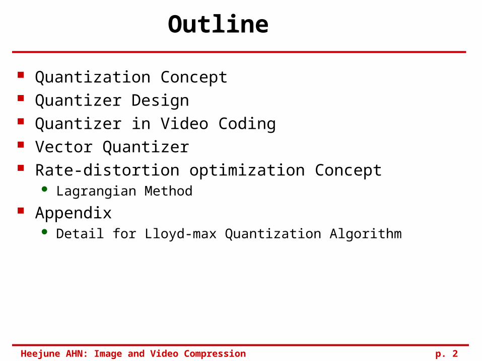
1. Quantization
Reduce representation set Nlarge points ([0 ~ Nlarge]) to Nsmall points ([0, … Nsmall]) Inevitable when Analog to Digital Conversion Not Reversible !
Original
(digital/analog)
ADC/Quant
Quanitzed
Levels
ReScale
Heejune AHN: Image and Video Compression p. 4
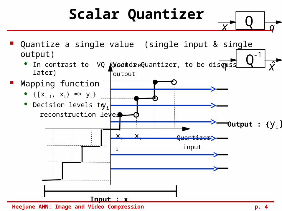
Scalar Quantizer
Quantize a single value (single input & single output) In contrast to VQ (Vector Quantizer, to be discussed later)
Mapping function {[xi-1, xi) => yi} Decision levels to
reconstruction level
Quantizer
input
Quantizer
output
xi-1 xi
yi
Output : {yi}
Input : x
Q q
Q-1
x
q x̂
Heejune AHN: Image and Video Compression p. 5
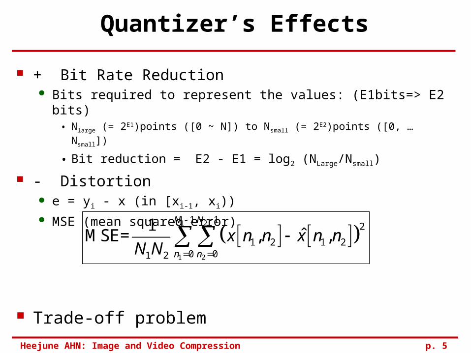
Quantizer’s Effects
+ Bit Rate Reduction Bits required to represent the values: (E1bits=> E2 bits)
• Nlarge (= 2E1)points ([0 ~ N]) to Nsmall (= 2E2)points ([0, … Nsmall])
• Bit reduction = E2 - E1 = log2 (NLarge/Nsmall)
- Distortion e = yi - x (in [xi-1, xi)) MSE (mean squared error)
Trade-off problem
1 2
1 2
1 12
1 2 1 20 01 2
1ˆMSE= , ,
N N
n n
x n n x n nN N
Heejune AHN: Image and Video Compression p. 6
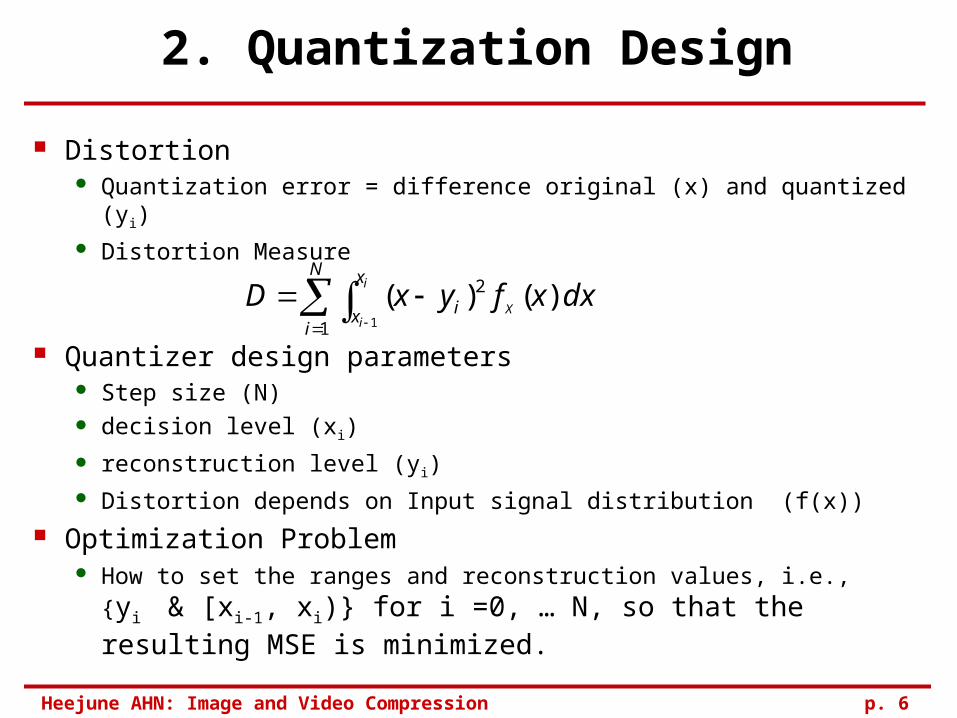
2. Quantization Design
Distortion Quantization error = difference original (x) and quantized (y i) Distortion Measure
Quantizer design parameters Step size (N) decision level (xi)
reconstruction level (yi) Distortion depends on Input signal distribution (f(x))
Optimization Problem How to set the ranges and reconstruction values, i.e., {yi & [xi-1,
xi)} for i =0, … N, so that the resulting MSE is minimized.
N
i
x
x i
i
iX
dxxfyxD1
2
1
)()(
Heejune AHN: Image and Video Compression p. 7
Optimal Quantizer
Solutions Note performance depends on the input statistics.
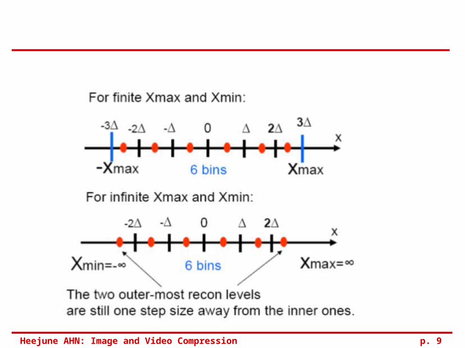
Simpler design • Uniform (Fixed quant step) quantizer • With/Without dead-zone near zero
Lloyd-Max algorithm• a optimal quantizer design algorithm• More levels for dense region, Less levels for sparse region.
(non-linear quantizer)
Heejune AHN: Image and Video Compression p. 8
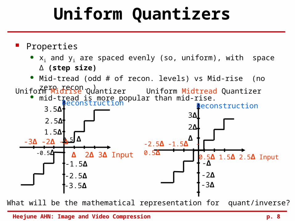
Uniform Quantizers
Properties xi and yi are spaced evenly (so, uniform), with space Δ (step size) Mid-tread (odd # of recon. levels) vs Mid-rise (no zero recon. ) mid-tread is more popular than mid-rise.
∆ 2∆ 3∆ Input
-3∆ -2∆ -∆
Reconstruction3.5∆
2.5∆
1.5∆0.5 ∆
-0.5∆
-1.5∆
-2.5∆-3.5∆
Uniform Midrise Quantizer
-2.5∆ -1.5∆ -0.5∆
Reconstruction3∆
2∆
∆
-∆
-2∆-3∆
Uniform Midtread Quantizer
0.5∆ 1.5∆ 2.5∆ Input
What will be the mathematical representation for quant/inverse?
Heejune AHN: Image and Video Compression p. 9
Heejune AHN: Image and Video Compression p. 10
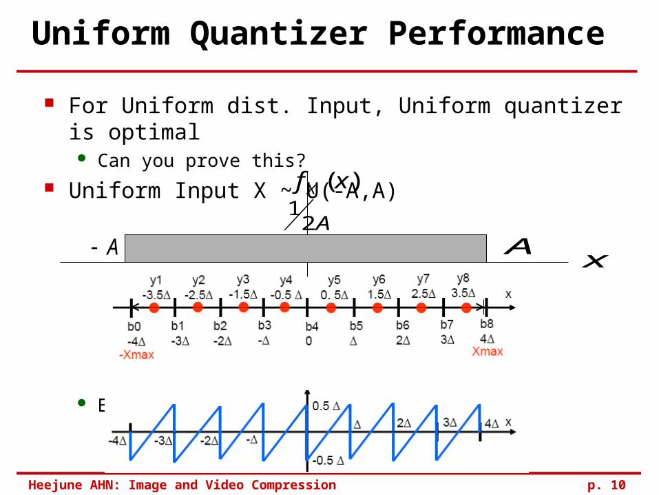
Uniform Quantizer Performance
xA A
A21
)(xf X
For Uniform dist. Input, Uniform quantizer is optimal Can you prove this?
Uniform Input X ~ U(-A,A)
Error signal e = y – x ~ U(-Δ/2, Δ/2)
Heejune AHN: Image and Video Compression p. 11
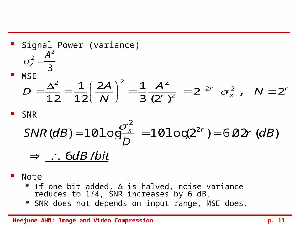
Signal Power (variance)
MSE
SNR
Note If one bit added, Δ is halved, noise variance reduces to 1/4, SNR
increases by 6 dB. SNR does not depends on input range, MSE does.
2 , 2 )2(3
12
12
1
1222
2
222r
xr
rN
A
N
AD
bitdB
dBrD
dBSNR rx
/6
)( 02.6 )2( log 10 log 10)( 22
3
22 Ax
Heejune AHN: Image and Video Compression p. 12
Non-uniform Quantizer
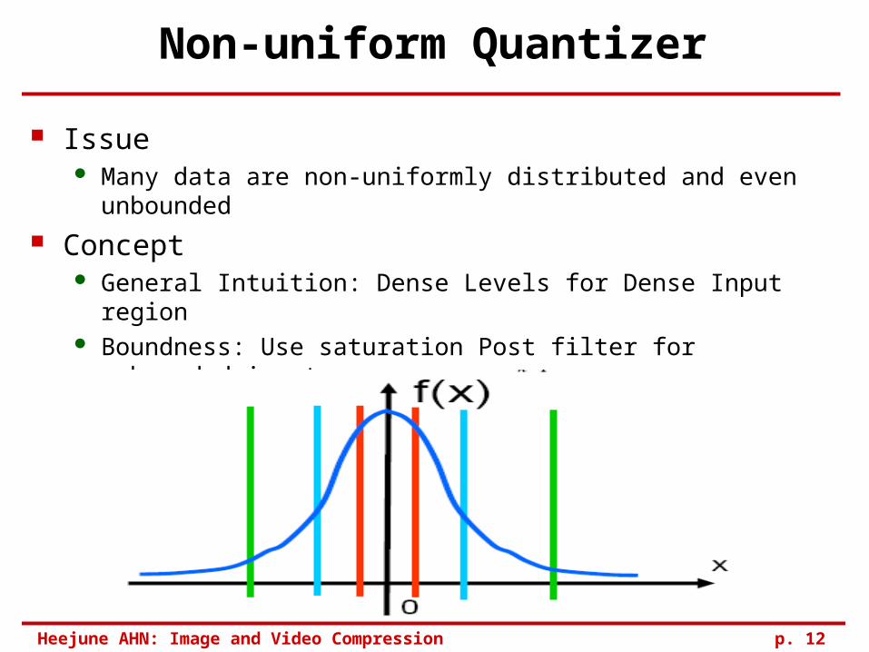
Issue Many data are non-uniformly distributed and even unbounded
Concept General Intuition: Dense Levels for Dense Input region Boundness: Use saturation Post filter for unbounded input Generally no closed-form expression for MSE.
• Range and Reconstruction Level is cross-related
Heejune AHN: Image and Video Compression p. 13
Lloyd-Max Algorithm
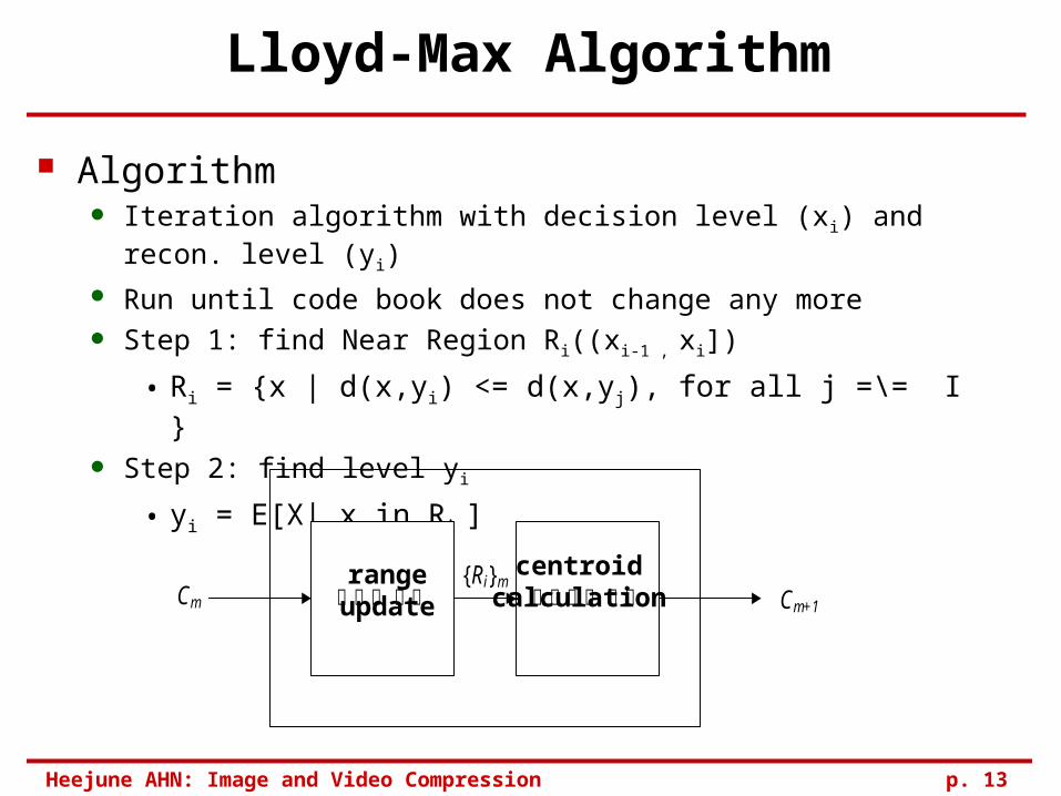
Algorithm Iteration algorithm with decision level (xi) and recon. level (yi) Run until code book does not change any more Step 1: find Near Region Ri((xi-1 , xi])
• Ri = {x | d(x,yi) <= d(x,yj), for all j =\= I }
Step 2: find level yi
• yi = E[X| x in Ri ]
최근린 분할 무게중심 계산Cm Cm+1
{Ri}mcentroid
calculation range
update
Heejune AHN: Image and Video Compression p. 14
L
k
t
t x
k
k
k dxxfyxyxE1
22 1
)()(])'[(
pdfinput on the depending ]|[)(
)(
2
)(
1
1
1
kt
t x
t
t x
k
kkk
xxEdxxf
dxuxfy
yyt
k
k
k
k
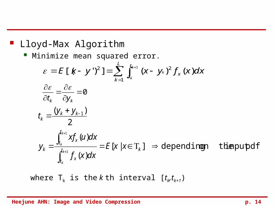
where Tk is the k th interval [tk,tk+1)
0
kk yt
Lloyd-Max Algorithm Minimize mean squared error.
Heejune AHN: Image and Video Compression p. 15
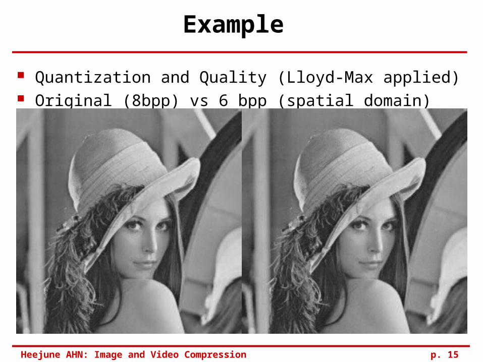
Example
Quantization and Quality (Lloyd-Max applied) Original (8bpp) vs 6 bpp (spatial domain)
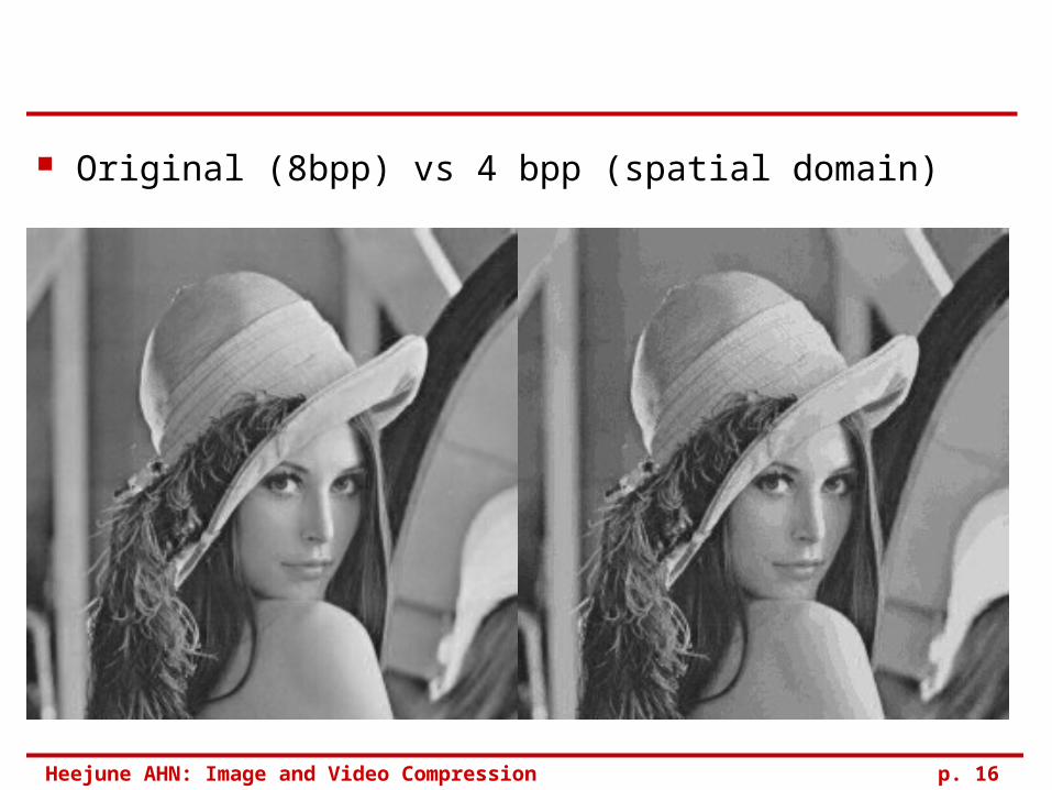
Heejune AHN: Image and Video Compression p. 16
Original (8bpp) vs 4 bpp (spatial domain)
Heejune AHN: Image and Video Compression p. 17
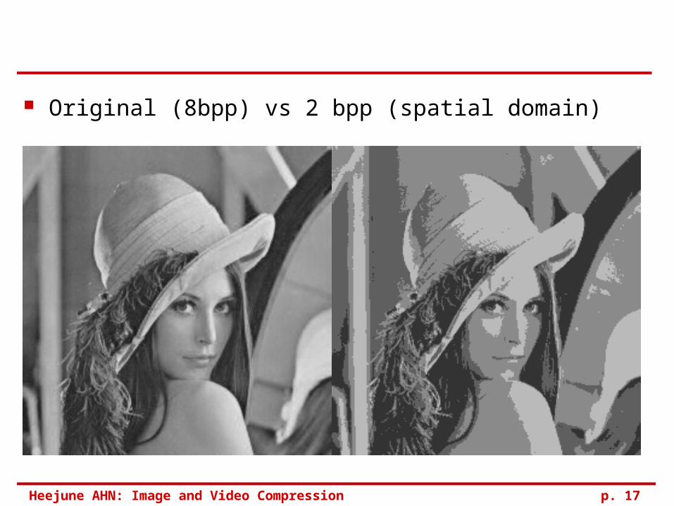
Original (8bpp) vs 2 bpp (spatial domain)
Heejune AHN: Image and Video Compression p. 18
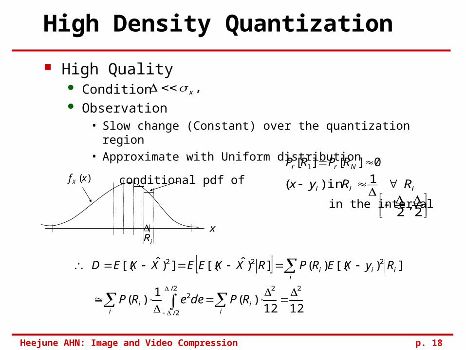
High Density Quantization
,x
iR
conditional pdf of
in the interval iii RRyx 1in )(
0][][ 1 Nrr RPRP
1212)(
1)(
])[()(])ˆ[(])ˆ[(
22/
2/
22
222
ii
ii
iiii
RPdeeRP
RyXERPRXXEEXXED
2,
2x
)(xf X
High Quality Condition Observation
• Slow change (Constant) over the quantization region
• Approximate with Uniform distribution
Heejune AHN: Image and Video Compression p. 19
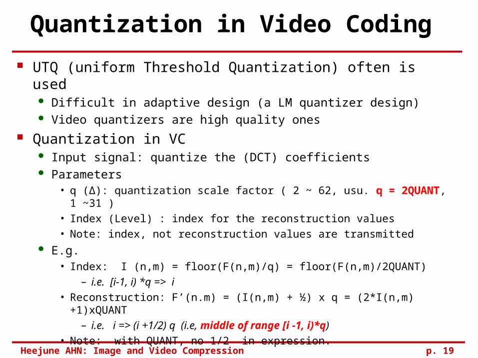
Quantization in Video Coding
UTQ (uniform Threshold Quantization) often is used Difficult in adaptive design (a LM quantizer design) Video quantizers are high quality ones
Quantization in VC Input signal: quantize the (DCT) coefficients Parameters
• q (Δ): quantization scale factor ( 2 ~ 62, usu. q = 2QUANT, 1 ~31 )
• Index (Level) : index for the reconstruction values
• Note: index, not reconstruction values are transmitted E.g.
• Index: I (n,m) = floor(F(n,m)/q) = floor(F(n,m)/2QUANT)– i.e. [i-1, i) *q => i
• Reconstruction: F’(n.m) = (I(n,m) + ½) x q = (2*I(n,m) +1)xQUANT – i.e. i => (i +1/2) q (i.e, middle of range [i -1, i)*q)
• Note: with QUANT, no 1/2 in expression.
Heejune AHN: Image and Video Compression p. 20
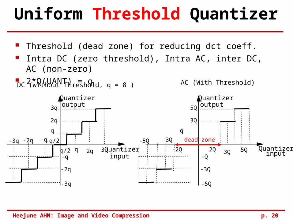
Uniform Threshold Quantizer
Threshold (dead zone) for reducing dct coeff. Intra DC (zero threshold), Intra AC, inter DC, AC (non-zero) 2*Q(UANT) = q
Quantizer input
Quantizer output
q/2
-q/2
q 2q
-q-2q
-q
-2q
-3q
2q
3q
q
3q
-3qQuantizer
input
Quantizer output
2Q 3Q-2Q
-3Q
-Q
-3Q
-5Q
3Q
5Q
q
5Q
-5Q
AC (With Threshold)DC (without Threshold, q = 8 )
dead zone
Heejune AHN: Image and Video Compression p. 21
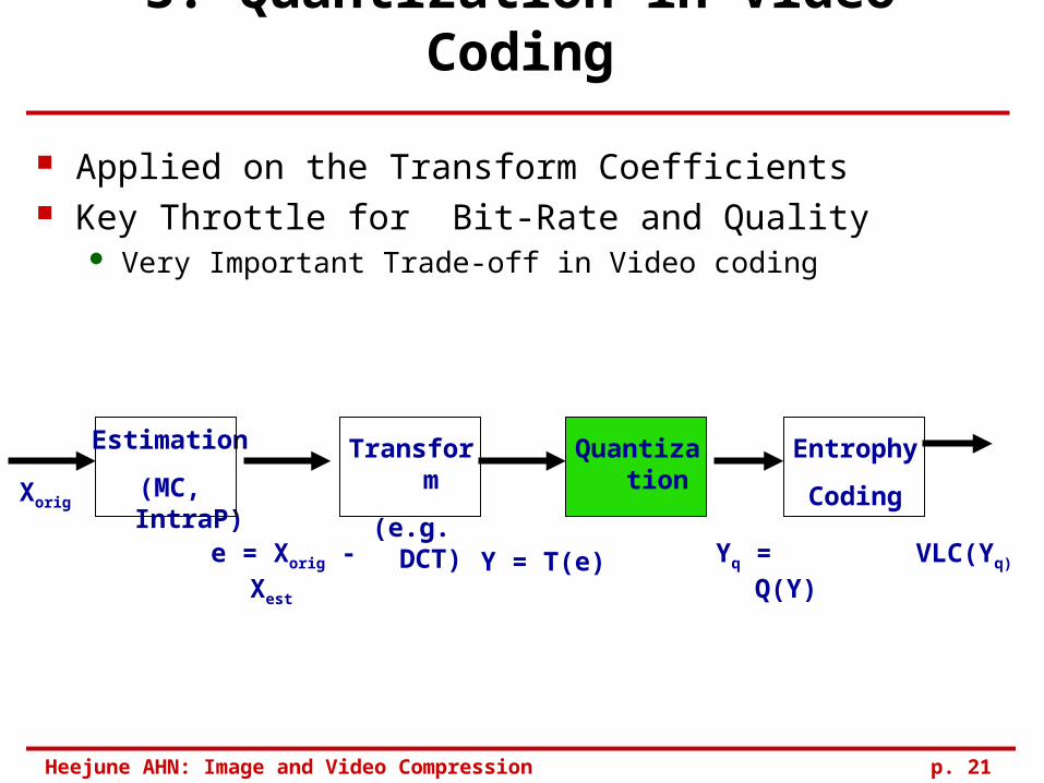
3. Quantization in Video Coding
Applied on the Transform Coefficients Key Throttle for Bit-Rate and Quality
Very Important Trade-off in Video coding
Estimation
(MC, IntraP)Xorig
Transform
(e.g. DCT)
e = Xorig - Xest Y = T(e)
Quantization
Entrophy
Coding
Yq = Q(Y) VLC(Yq)
Heejune AHN: Image and Video Compression p. 22
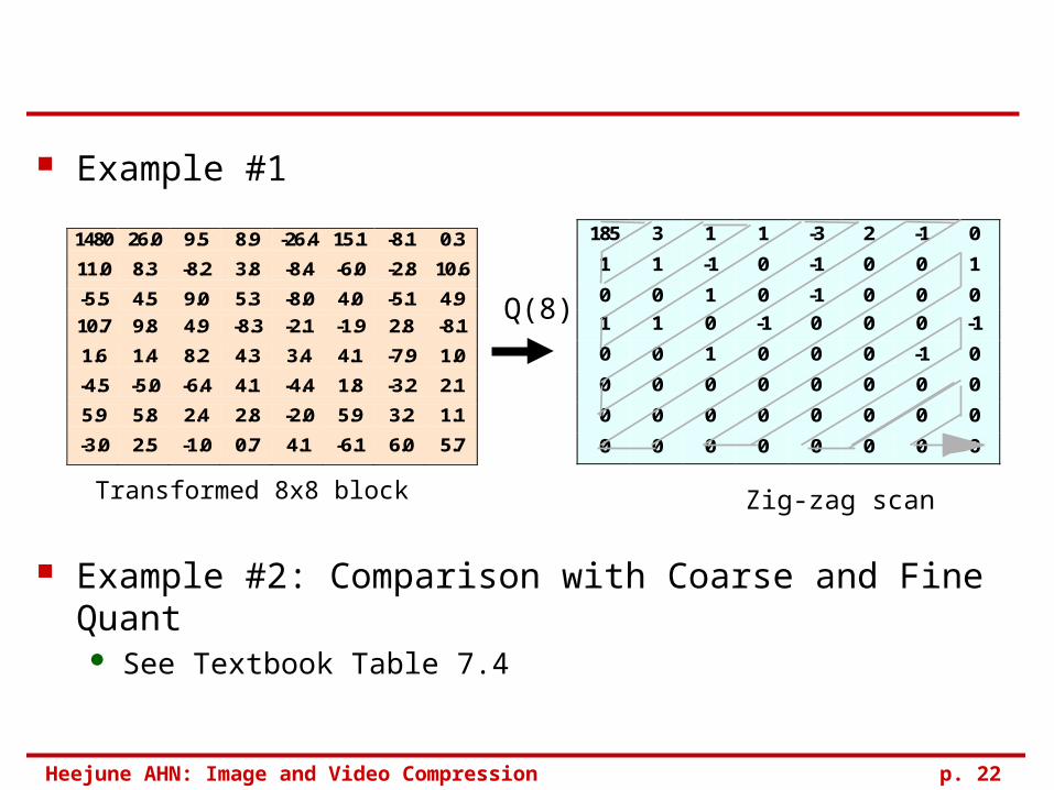
Example #1
Example #2: Comparison with Coarse and Fine Quant See Textbook Table 7.4
185 3 1 1 -3 2 -1 0
1 1 -1 0 -1 0 0 1
0 0 1 0 -1 0 0 0
1 1 0 -1 0 0 0 -1
0 0 1 0 0 0 -1 0
0 0 0 0 0 0 0 0
0 0 0 0 0 0 0 0
0 0 0 0 0 0 0 0
Q(8)
1480 26.0 9.5 8.9 -26.4 15.1 -8.1 0.3
11.0 8.3 -8.2 3.8 -8.4 -6.0 -2.8 10.6
-5.5 4.5 9.0 5.3 -8.0 4.0 -5.1 4.9
10.7 9.8 4.9 -8.3 -2.1 -1.9 2.8 -8.1
1.6 1.4 8.2 4.3 3.4 4.1 -7.9 1.0
-4.5 -5.0 -6.4 4.1 -4.4 1.8 -3.2 2.1
5.9 5.8 2.4 2.8 -2.0 5.9 3.2 1.1
-3.0 2.5 -1.0 0.7 4.1 -6.1 6.0 5.7
Zig-zag scanTransformed 8x8 block
Heejune AHN: Image and Video Compression p. 23
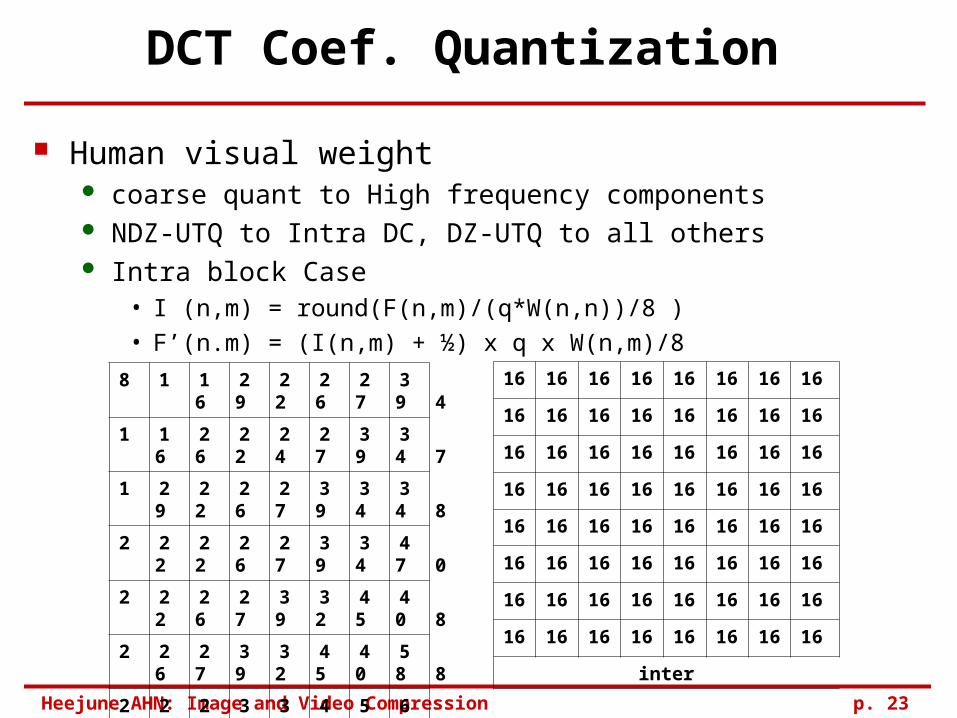
DCT Coef. Quantization
Human visual weight coarse quant to High frequency components NDZ-UTQ to Intra DC, DZ-UTQ to all others Intra block Case
• I (n,m) = round(F(n,m)/(q*W(n,n))/8 )
• F’(n.m) = (I(n,m) + ½) x q x W(n,m)/8
8 16 19 22 26 27 29 34
16 16 22 24 27 29 34 37
19 22 26 27 29 34 34 38
22 22 26 27 29 34 37 40
22 26 27 29 32 35 40 48
26 27 29 32 35 40 48 58
26 27 29 34 38 46 56 69
27 29 35 38 46 56 69 83
intra
16 16 16 16 16 16 16 16
16 16 16 16 16 16 16 16
16 16 16 16 16 16 16 16
16 16 16 16 16 16 16 16
16 16 16 16 16 16 16 16
16 16 16 16 16 16 16 16
16 16 16 16 16 16 16 16
16 16 16 16 16 16 16 16
inter
Heejune AHN: Image and Video Compression p. 24
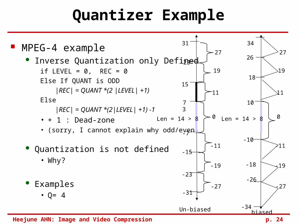
Quantizer Example
MPEG-4 example Inverse Quantization only Defined
if LEVEL = 0, REC = 0Else If QUANT is ODD
|REC| = QUANT *(2 |LEVEL| +1)Else
|REC| = QUANT *(2|LEVEL| +1) -1
• + 1 : Dead-zone • (sorry, I cannot explain why odd/even)
Quantization is not defined • Why?
Examples• Q= 4
31
23
15
7
-7
-15
-23
-31
27
19
11
0
-11
-19
-27
3
Len = 14 > 8
34
26
18
10
-10
-18
-26
-34
27
19
11
0
-11
-19
-27
Len = 14 > 8
Un-biased biased
Heejune AHN: Image and Video Compression p. 25
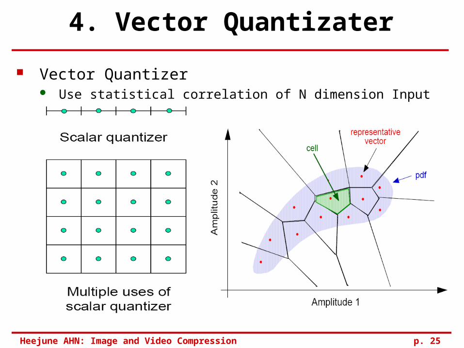
4. Vector Quantizater
Vector Quantizer Use statistical correlation of N dimension Input
Heejune AHN: Image and Video Compression p. 26
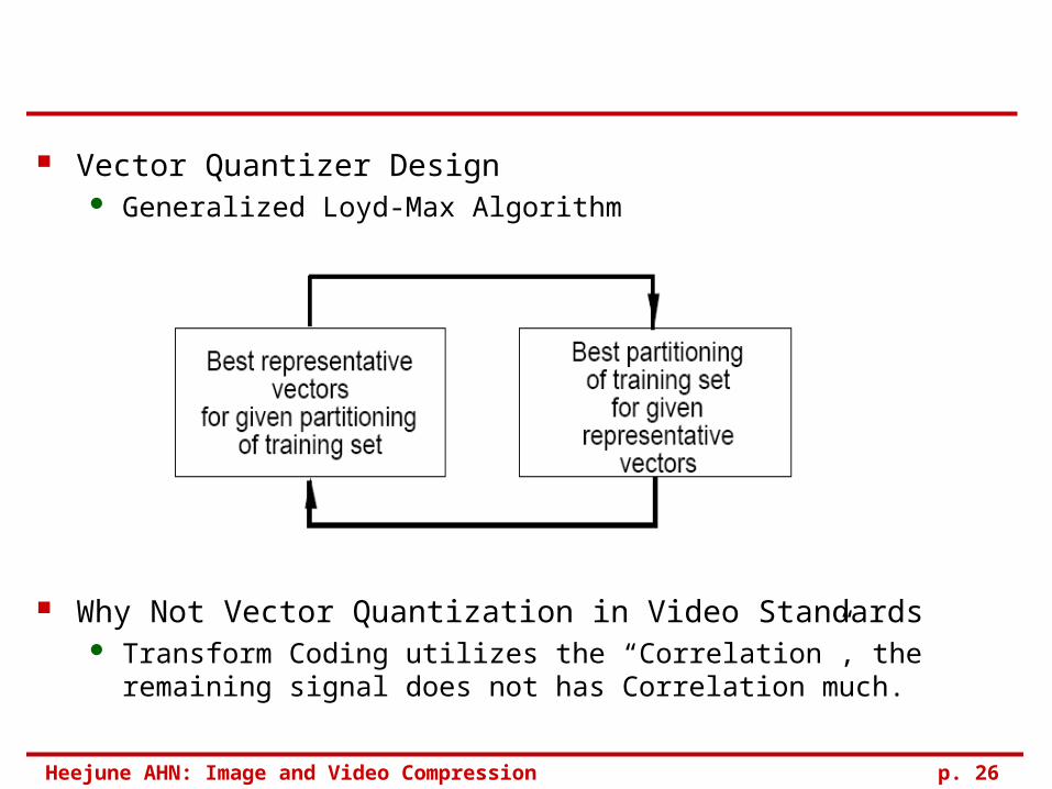
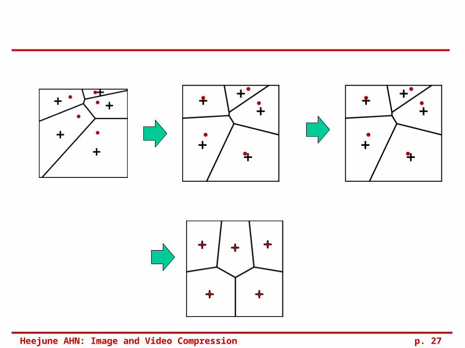
Vector Quantizer Design Generalized Loyd-Max Algorithm
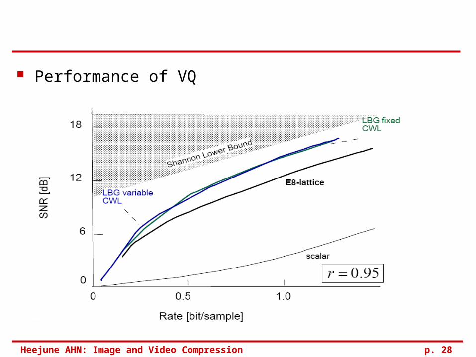
Why Not Vector Quantization in Video Standards Transform Coding utilizes the “Correlation”, the remaining signal does
not has Correlation much.
Heejune AHN: Image and Video Compression p. 27
Heejune AHN: Image and Video Compression p. 28
Performance of VQ
Heejune AHN: Image and Video Compression p. 29
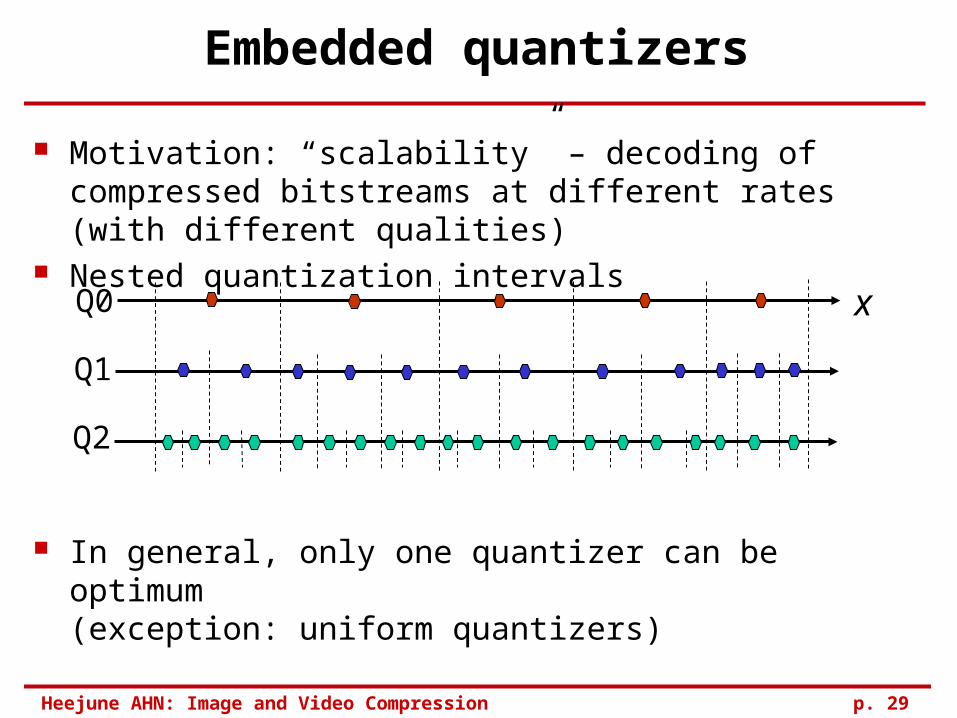
Embedded quantizers
Motivation: “scalability” – decoding of compressed bitstreams at different rates (with different qualities)
Nested quantization intervals
In general, only one quantizer can be optimum(exception: uniform quantizers)
Q0
Q1
Q2
x
Heejune AHN: Image and Video Compression p. 30
Rate Distortion Theory
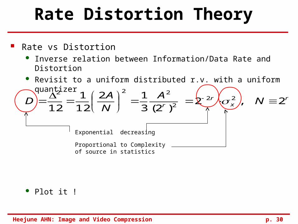
Rate vs Distortion Inverse relation between Information/Data Rate and Distortion Revisit to a uniform distributed r.v. with a uniform quantizer
Plot it !
2 , 2 )2(3
12
12
1
1222
2
222r
xr
rN
A
N
AD
Exponential decreasing
Proportional to Complexity of source in statistics
Heejune AHN: Image and Video Compression p. 31
Rate Distortion Theory
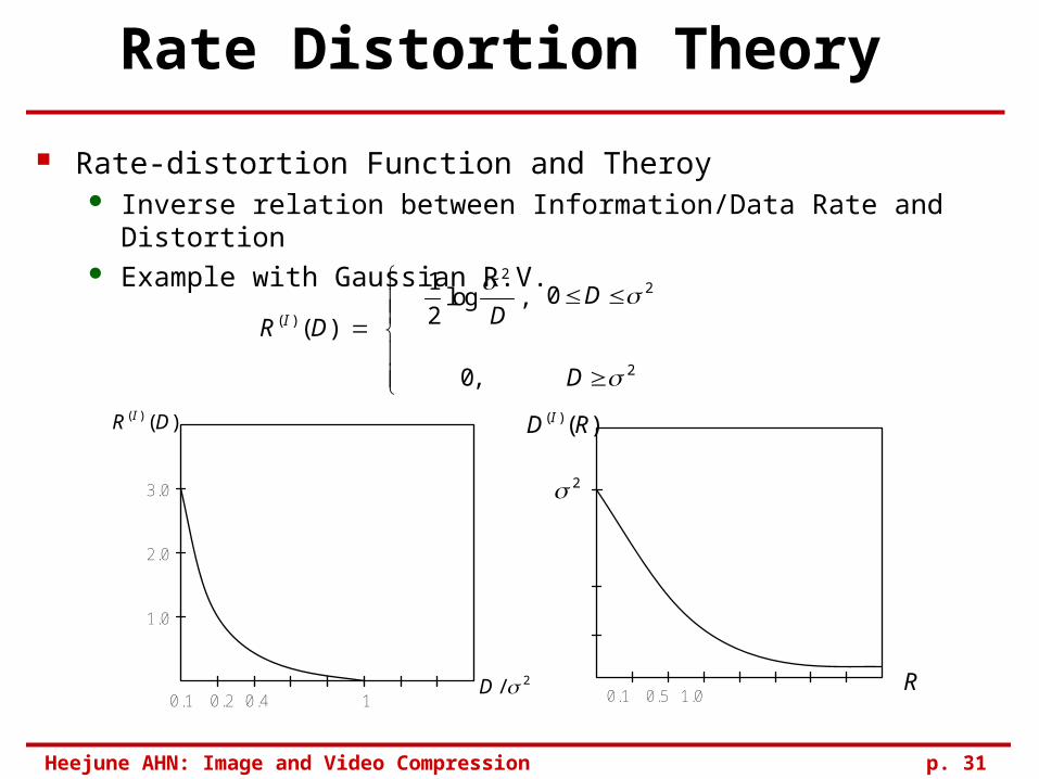
Rate-distortion Function and Theroy Inverse relation between Information/Data Rate and Distortion Example with Gaussian R.V.
3.0
2.0
1.0
0.1 0.2 0.4 1
R DI( ) ( )
D / 2
0.1 0.5 1.0
)()( RD I
R
2
R D DD
D
I( ) ( )log ,
,
1
20
0
22
2
Heejune AHN: Image and Video Compression p. 32
Rate-Distortion Optimization
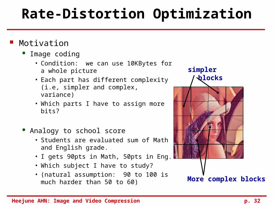
Motivation Image coding
• Condition: we can use 10KBytes for a whole picture
• Each part has different complexity (i.e, simpler and complex, variance)
• Which parts I have to assign more bits?
Analogy to school score • Students are evaluated sum of Math and
English grade.
• I gets 90pts in Math, 50pts in Eng.
• Which subject I have to study?
• (natural assumption: 90 to 100 is much harder than 50 to 60)
simpler blocks
More complex blocks
Heejune AHN: Image and Video Compression p. 33
Lagrange multiplier
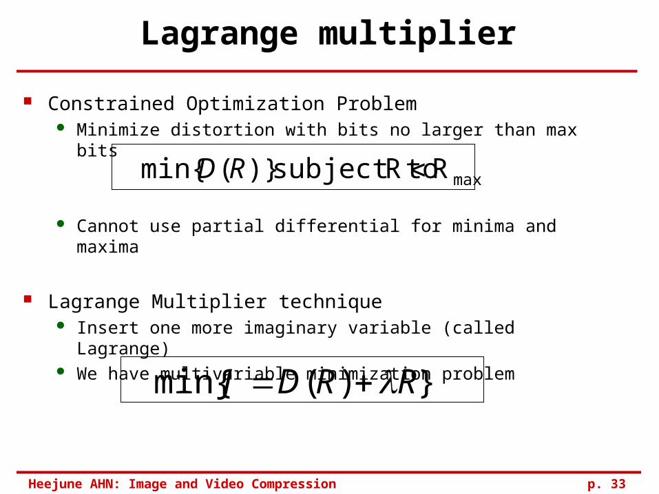
Constrained Optimization Problem Minimize distortion with bits no larger than max bits
Cannot use partial differential for minima and maxima
Lagrange Multiplier technique Insert one more imaginary variable (called Lagrange) We have multivariable minimization problem
maxR R subject to )}(min{ RD
})(min{ RRDJ
Heejune AHN: Image and Video Compression p. 34
Side note: why not partial differential
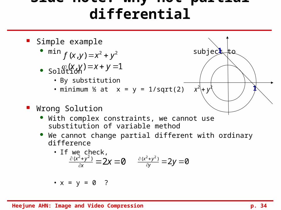
Simple example min subject to
Solution• By substitution• minimum ½ at x = y = 1/sqrt(2)
Wrong Solution With complex constraints, we cannot use substitution of variable
method We cannot change partial different with ordinary difference
• If we check,
• x = y = 0 ?
22 yx 1
122),( yxyxf 1),( yxyx
02)( 22
xx
yx 02)( 22
yy
yx
Heejune AHN: Image and Video Compression p. 35
An Example: Lagrange Multiplier
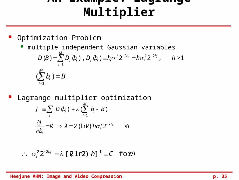
Optimization Problem multiple independent Gaussian variables
Lagrange multiplier optimization
BbM
ii
)(1
i hλb
J
B b b DJ
ibi
i
M
ii
ii
22
1
2)2ln( 2 0
)()(
1 ,22)( ),()( 2222
1
hhhbDbDBD ii b
ib
iiii
M
iii
iChibi for ])2 ln 2[( 2 122
Heejune AHN: Image and Video Compression p. 36
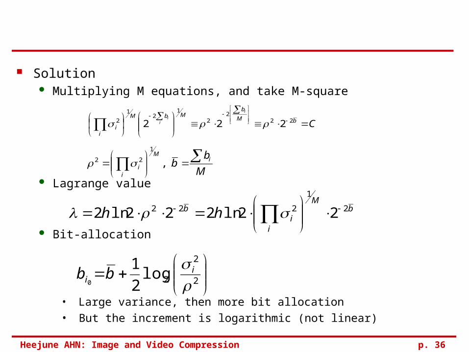
Solution Multiplying M equations, and take M-square
Lagrange value
Bit-allocation
• Large variance, then more bit allocation
• But the increment is logarithmic (not linear)
CbM
bMbM
ii
i
ii
222
2
12
1
2 222
M
bb i
M
ii
,
1
22
2
2
2 log2
1
0 i
i bb
bM
ii
b hh 2
1
222 22ln222ln2
Appendix
Lloyd-Max Algorithm Details
Heejune AHN: Image and Video Compression p. 38
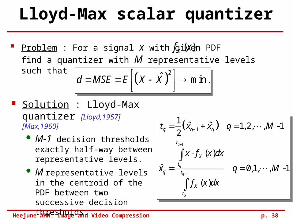
Lloyd-Max scalar quantizer
Problem : For a signal x with given PDF find a quantizer with
M representative levels such that
( )Xf x
Solution : Lloyd-Max quantizer [Lloyd,1957] [Max,1960]
M-1 decision thresholds exactly half-way between representative levels.
M representative levels in the centroid of the PDF between two successive decision thresholds.
Necessary (but not sufficient) conditions
1
1
1
1ˆ ˆ 1, 2, , -1
2
( )
ˆ 0,1, , -1
( )
q
q
q
q
q q q
t
X
t
q t
X
t
t x x q M
x f x dx
x q M
f x dx
1
1
1
1ˆ ˆ 1, 2, , -1
2
( )
ˆ 0,1, , -1
( )
q
q
q
q
q q q
t
X
t
q t
X
t
t x x q M
x f x dx
x q M
f x dx
2ˆ min .d MSE E X X 2ˆ min .d MSE E X X
Heejune AHN: Image and Video Compression p. 39
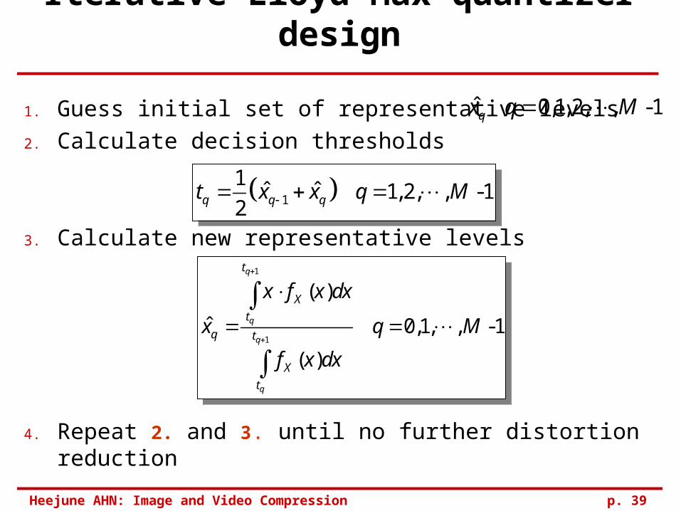
Iterative Lloyd-Max quantizer design
1. Guess initial set of representative levels
2. Calculate decision thresholds
3. Calculate new representative levels
4. Repeat 2. and 3. until no further distortion reduction
ˆ 0,1,2, , -1qx q M
1
1
( )
ˆ 0,1, , -1
( )
q
q
q
q
t
X
t
q t
X
t
x f x dx
x q M
f x dx
1
1
( )
ˆ 0,1, , -1
( )
q
q
q
q
t
X
t
q t
X
t
x f x dx
x q M
f x dx
1
1ˆ ˆ 1, 2, , -1
2q q qt x x q M 1
1ˆ ˆ 1, 2, , -1
2q q qt x x q M
Heejune AHN: Image and Video Compression p. 40
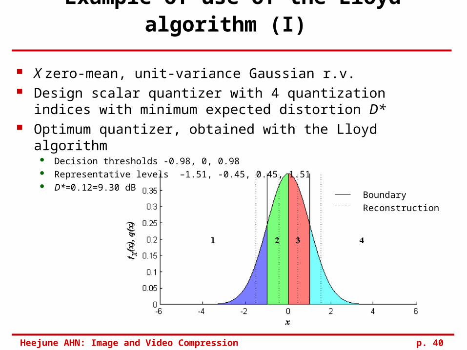
Example of use of the Lloyd algorithm (I)
X zero-mean, unit-variance Gaussian r.v. Design scalar quantizer with 4 quantization indices with
minimum expected distortion D* Optimum quantizer, obtained with the Lloyd algorithm
Decision thresholds -0.98, 0, 0.98 Representative levels –1.51, -0.45, 0.45, 1.51 D*=0.12=9.30 dB
Boundary
Reconstruction
Heejune AHN: Image and Video Compression p. 41
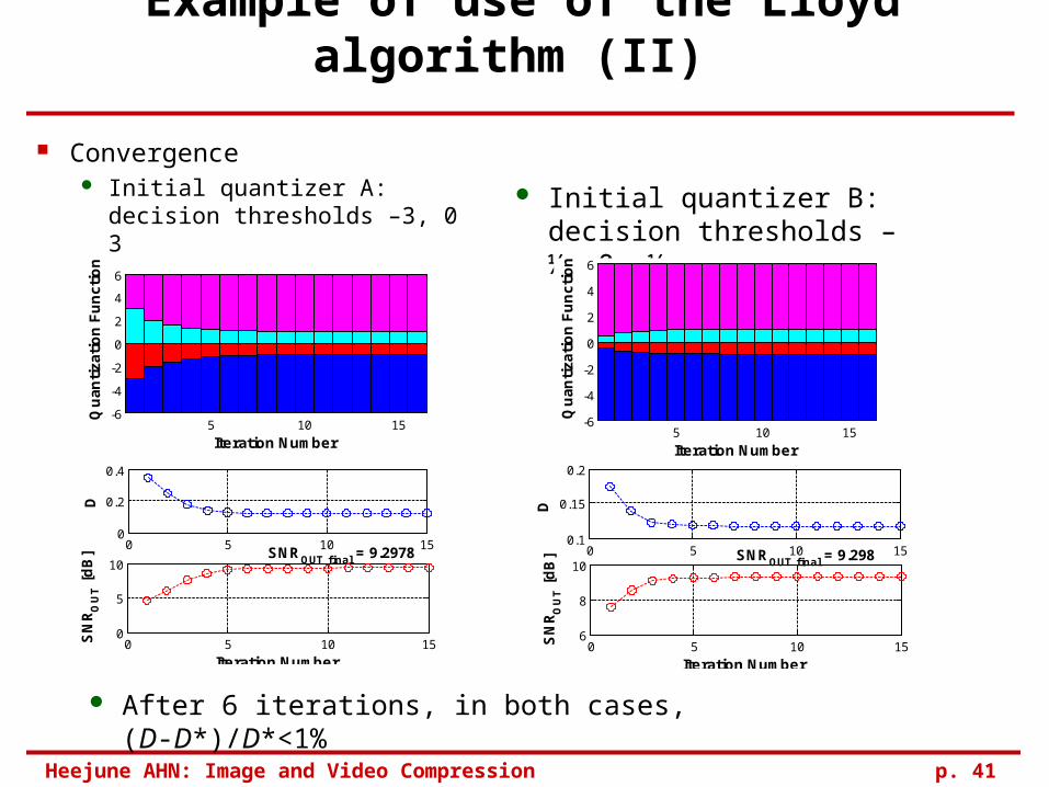
Example of use of the Lloyd algorithm (II)
Convergence Initial quantizer A:
decision thresholds –3, 0 3
Initial quantizer B:decision thresholds –½, 0, ½
After 6 iterations, in both cases, (D-D*)/D*<1%
5 10 15-6
-4
-2
0
2
4
6
Qu
an
tiz
ati
on
Fu
nc
tio
n
Iteration Number
0 5 10 150
0.2
0.4
D
0 5 10 150
5
10
SN
RO
UT
[dB
]
Iteration Number
SNROUT
final
= 9.2978
5 10 15-6
-4
-2
0
2
4
6
Qu
an
tiz
ati
on
Fu
nc
tio
n
Iteration Number
0 5 10 150.1
0.15
0.2
D
0 5 10 156
8
10S
NR
OU
T [d
B]
Iteration Number
SNROUT
final
= 9.298
Heejune AHN: Image and Video Compression p. 42
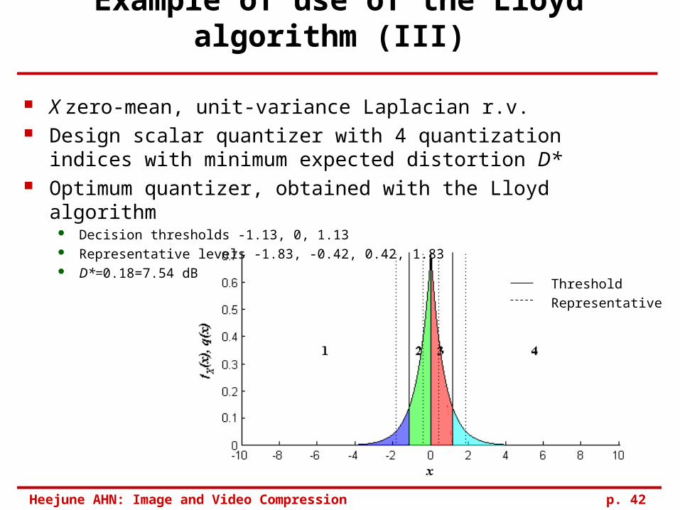
Example of use of the Lloyd algorithm (III)
X zero-mean, unit-variance Laplacian r.v. Design scalar quantizer with 4 quantization indices with
minimum expected distortion D* Optimum quantizer, obtained with the Lloyd algorithm
Decision thresholds -1.13, 0, 1.13 Representative levels -1.83, -0.42, 0.42, 1.83 D*=0.18=7.54 dB
Threshold
Representative
Heejune AHN: Image and Video Compression p. 43
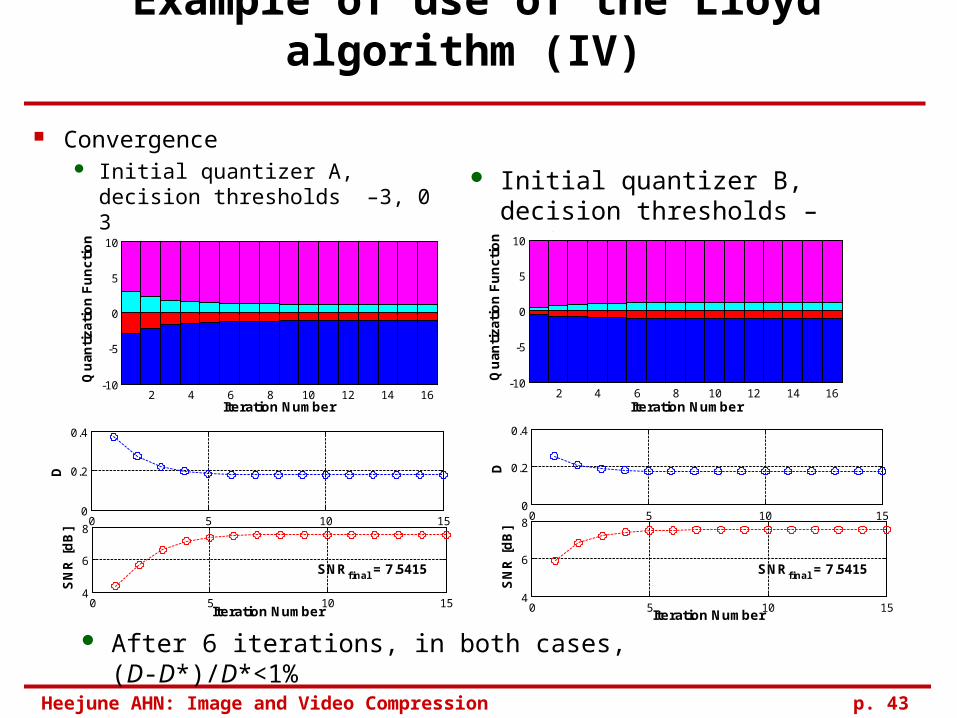
Example of use of the Lloyd algorithm (IV)
Convergence Initial quantizer A,
decision thresholds –3, 0 3
Initial quantizer B,decision thresholds –½, 0, ½
After 6 iterations, in both cases, (D-D*)/D*<1%
0 5 10 150
0.2
0.4
D
0 5 10 154
6
8
SN
R [
dB
]
Iteration Number
SNRfinal
= 7.5415
2 4 6 8 10 12 14 16-10
-5
0
5
10
Qu
an
tiz
ati
on
Fu
nc
tio
n
Iteration Number2 4 6 8 10 12 14 16
-10
-5
0
5
10
Qu
an
tiz
ati
on
Fu
nc
tio
n
Iteration Number
0 5 10 150
0.2
0.4
D
0 5 10 154
6
8S
NR
[d
B]
Iteration Number
SNRfinal
= 7.5415
Heejune AHN: Image and Video Compression p. 44
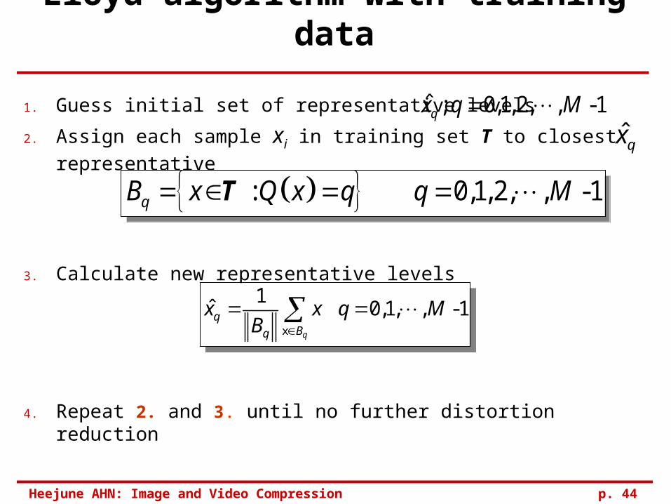
Lloyd algorithm with training data
1. Guess initial set of representative levels
2. Assign each sample xi in training set T to closest representative
3. Calculate new representative levels
4. Repeat 2. and 3. until no further distortion reduction
ˆ ; 0,1,2, , -1qx q M
x
1ˆ 0,1, , -1
q
qBq
x x q MB
x
1ˆ 0,1, , -1
q
qBq
x x q MB
ˆqx
: 0,1,2, , -1qB x Q x q q M T : 0,1,2, , -1qB x Q x q q M T
Heejune AHN: Image and Video Compression p. 45
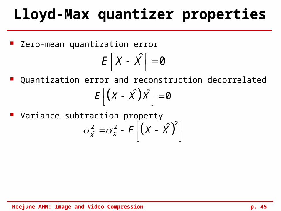
Lloyd-Max quantizer properties
Zero-mean quantization error
Quantization error and reconstruction decorrelated
Variance subtraction property
ˆ 0E X X
ˆ ˆ 0E X X X
22 2ˆ
ˆXX
E X X
Related Documents