Quantitative social dialectology: explaining linguistic variation geographically and socially

Quantitative Social Dialectology: Explaining LinguisticVariation Geographically and SociallyMartijn Wieling1*, John Nerbonne1, R. Harald Baayen2

1 Department of Humanities Computing, University of Groningen, Groningen, The Netherlands, 2 Department of Linguistics, University of Alberta, Edmonton, Canada

Abstract

In this study we examine linguistic variation and its dependence on both social and geographic factors. We followdialectometry in applying a quantitative methodology and focusing on dialect distances, and social dialectology in thechoice of factors we examine in building a model to predict word pronunciation distances from the standard Dutchlanguage to 424 Dutch dialects. We combine linear mixed-effects regression modeling with generalized additive modelingto predict the pronunciation distance of 559 words. Although geographical position is the dominant predictor, several otherfactors emerged as significant. The model predicts a greater distance from the standard for smaller communities, forcommunities with a higher average age, for nouns (as contrasted with verbs and adjectives), for more frequent words, andfor words with relatively many vowels. The impact of the demographic variables, however, varied from word to word. For amajority of words, larger, richer and younger communities are moving towards the standard. For a smaller minority ofwords, larger, richer and younger communities emerge as driving a change away from the standard. Similarly, the strengthof the effects of word frequency and word category varied geographically. The peripheral areas of the Netherlands showeda greater distance from the standard for nouns (as opposed to verbs and adjectives) as well as for high-frequency words,compared to the more central areas. Our findings indicate that changes in pronunciation have been spreading (in particularfor low-frequency words) from the Hollandic center of economic power to the peripheral areas of the country, meetingresistance that is stronger wherever, for well-documented historical reasons, the political influence of Holland was reduced.Our results are also consistent with the theory of lexical diffusion, in that distances from the Hollandic norm varysystematically and predictably on a word by word basis.

Citation: Wieling M, Nerbonne J, Baayen RH (2011) Quantitative Social Dialectology: Explaining Linguistic Variation Geographically and Socially. PLoS ONE 6(9):e23613. doi:10.1371/journal.pone.0023613

Editor: Matjaz Perc, University of Maribor, Slovenia

Received June 7, 2011; Accepted July 21, 2011; Published September 1, 2011

Copyright: � 2011 Wieling et al. This is an open-access article distributed under the terms of the Creative Commons Attribution License, which permitsunrestricted use, distribution, and reproduction in any medium, provided the original author and source are credited.

Funding: The authors have no support or funding to report.

Competing Interests: The authors have declared that no competing interests exist.

* E-mail: [email protected]

Introduction

In this study we integrate the approaches of two fields

addressing linguistic variation, dialectometry and (social) dialec-

tology. Dialectology is the older discipline, where researchers

focus on a single or small set of linguistic features in their

analysis. Initially the focus in this field was on dialect geography

[1, Ch. 2], where the distribution of these features was visualized

on a map. Later, dialectologists more and more realized the

importance of social variation. The work of Labov and later

Trudgill has been very influential in this regard [2,3]. Social

dialectologists have often examined both social and linguistic

influences on individual linguistic features, generally using

logistic regression designs [4], but more recently also using

mixed-effects regression modeling [5].

Dialectometry was pioneered by Jean Seguy, who calculated

aggregate dialect distances based on the number of mismatching

linguistic items between pairs of sites [6] and used a regression

design to examine the influence of geography on these aggregate

distances [7]. Since then other researchers, among others, Goebl,

Heeringa and Nerbonne, and Kretzschmar, have refined the

(computational and quantitative) techniques to measure and

interpret these aggregate dialect distances [8–10]. We follow

dialectometry in viewing linguistic distance for hundreds of

individual words as our primary dependent variable.

2While the social dimension is a very important aspect in

dialectology, it has been less important in dialectometry where the

main focus still lies on dialect geography [11]. Of course there are

some exceptions in which (for example) the diachronic perspective

is taken into account [12,13], or age and gender are considered as

covariates [14], but to our knowledge no dialectometric study has

attempted to model the effects of multiple geographic and social

variables simultaneously.

Dialectometry has also been criticized for focusing too much on

the aggregate level of linguistic differences [15,16], thereby

neglecting the level of linguistic structure where individual words

and linguistic properties are important. Acknowledging honorable

exceptions [11], we concede that the focus in dialectometry has

been on aggregate levels, but the strength of the present analysis is

that it focuses on individual words in addition to aggregate

distances predicted by geography.

This quantitative social dialectological study is the first to

investigate the effect of a range of social and lexical factors on a

large set of dialect distances. In the following we will focus on

building a model to explain the pronunciation distance between

dialectal pronunciations (in different locations) and standard

Dutch for a large set of distinct words. Of course, choosing

standard Dutch as the reference pronunciation is not historically

motivated, as standard Dutch is not the proto-language. However,

the standard language remains an important reference point for

PLoS ONE | www.plosone.org 1 September 2011 | Volume 6 | Issue 9 | e23613

two reasons. First, as noted by Kloeke, in the 16th and 17th

centuries individual sound changes have spread from the

Hollandic center of economic and political power to the more

peripheral areas of the Netherlands [17]. Furthermore, modern

Dutch dialects are known to be converging to the standard

language [13,18, pp. 355–356]. We therefore expect geographical

distance to reveal a pattern consistent with Kloeke’s ‘Hollandic

Expansion’, with greater geographical distance correlating with

greater distance from the Hollandic standard.

Kloeke also pointed out that sound changes may proceed on a

word-by-word basis [17]. The case for lexical diffusion was

championed by Wang and contrasts with the Neogrammarian

view that sound changes are exceptionless and apply to all words

of the appropriate form to undergo the change [19]. The Neo-

grammarian view is consistent with waves of sound changes

emanating from Holland to the outer provinces, but it predicts that

lexical properties such as a word’s frequency of occurrence and

its categorial status as a noun or verb should be irrelevant

for predicting a region’s pronunciation distance to the standard

language.

In order to clarify the extent to which variation at the lexical

level co-determines the dialect landscape in the Netherlands, we

combine generalized additive modeling (which allows us to

model complex non-linear surfaces) with mixed-effects regres-

sion models (which allow us to explore word-specific variation).

First, however, we introduce the materials and methods of our

study.

Materials and Methods

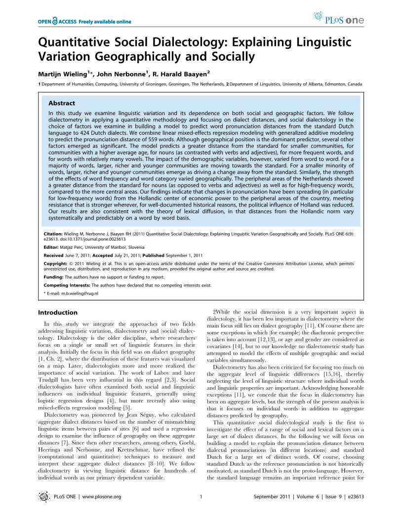
Pronunciation dataThe Dutch dialect data set contains phonetic transcriptions of

562 words in 424 locations in the Netherlands. Figure 1 shows the

distribution of the locations over the Netherlands together with the

province names. Wieling, Heeringa and Nerbonne selected

the words from the Goeman-Taeldeman-Van Reenen-Project

(GTRP; [20]) specifically for an analysis of pronunciation variation

in the Netherlands and Flanders [13]. The transcriptions in the

GTRP were made by several transcribers between 1980 and 1995,

making it currently the largest contemporary Dutch dialect data

set available. The word categories include mainly verbs (30.8%),

nouns (40.3%) and adjectives (20.8%). The complete list of words

is presented in [13]. For the present study, we excluded 3 words of

the original set (gaarne, geraken and ledig) as it turned out these words

also varied lexically. The standard Dutch pronunciation of all 559

words was transcribed by one of the authors based on [21].

Because the set of words included common words (e.g.,

‘walking’) as well as less frequent words (e.g., ‘oats’), we included

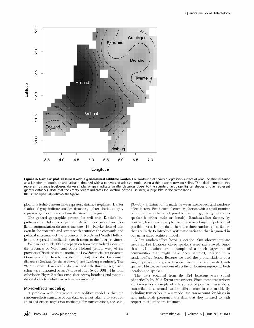
Figure 1. Distribution of locations in the GTRP including province names.doi:10.1371/journal.pone.0023613.g001

Quantitative Social Dialectology


word frequency information, extracted from the CELEX lexical

database [22], as an independent variable.

Social dataBesides the information about the speakers recorded by the

GTRP compilers, such as year of recording, gender and age of the

speaker, we extracted additional demographic information about

each of the 424 places from Statistics Netherlands [23]. We

obtained information about the average age, average income,

number of inhabitants (i.e. population size) and male-female ratio

in every location in the year 1995 (approximately coinciding with

the end of the GTRP data collection period). As Statistics

Netherlands uses three measurement levels (i.e. neighborhood,

district and municipality), we manually selected the appropriate

level for every location. For large cities (e.g., Rotterdam), the

corresponding municipality (generally having the same name) was

selected as it mainly consisted of the city itself. For smaller cities,

located in a municipality having multiple villages and/or cities, the

district was selected which consisted of the single city (e.g.,

Coevorden). Finally, for very small villages located in a district

having multiple small villages, the neighborhood was selected

which consisted of the single village (e.g., Barger-Oosterveld).

Obtaining pronunciation distancesFor all 424 locations, the pronunciation distance between

standard Dutch and the dialectal pronunciations was calculated by

using the Levenshtein distance [24]. The Levenshtein distance

minimizes the number of insertions, deletions and substitutions to

transform one pronunciation string into the other. For example,

the Levenshtein distance between two Dutch dialectal variants of

the word ‘two’, [tei] and [twa], is 3:

tei insert w 1

twei subst: a=e 1

twai delete i 1

twa

3

The corresponding alignment is:

t e i

t w a

1 1 1

Note that in the example above an alternative optimal alignment

substitutes [a] for [i] instead of [e].

The regular Levenshtein distance does not distinguish vowels

and consonants and therefore may align a vowel with a consonant.

To enforce linguistically sensible alignments, a syllabicity con-

straint is normally added such that vowels are not aligned with

(non-sonorant) consonants.

As shown in the example above, the Levenshtein distance

increases with one for every mismatch. Some sounds, however, are

phonetically closer to each other than other sounds, e.g., /a/

and /e/ are closer than /a/ and /i/. A distance measure for two

pronunciations should reflect this. Wieling, Prokic and Nerbonne

introduced a method which uses the relative alignment frequency

of sounds to determine their distance [25]. Pairs of sounds which

are aligned relatively frequently are assigned a low distance, while

sounds which co-occur relatively infrequently are assigned a high

distance. The method is based on calculating the Pointwise Mutual

Information score (PMI; [26]) between every pair of sounds and

was found to improve alignments compared to the Levenshtein

distance with (and without) the syllabicity constraint. In addition, a

recent study by Wieling, Margaretha and Nerbonne (submitted)

found that the automatically determined PMI distances between

vowels correspond well with acoustic vowel distances for several

languages. A detailed description about the PMI method can be

found in [27].

As an illustration of the PMI method, consider the alignment of

[tei] and [twa], now using the PMI-based costs:

t e i

t w a

0:031 0:030 0:027

In contrast to the previous example, the [a] can only be aligned

with [e], as the cost of aligning [a] and [i] is higher (and the cost of

deleting [e] is higher than deleting [i]).

In the following, the pronunciation distances are based on the

PMI-based Levenshtein distance. Because longer words will likely

have a greater pronunciation distance (as more sounds may

change) than shorter words, we normalize the PMI-based word

pronunciation distances by dividing by the alignment length.

Modeling the role of geography: generalized additivemodeling

Given a fine-grained measure capturing the distance between

two pronunciations, a key question from a dialectometric per-

spective is how to model pronunciation distance as a function of the

longitude and latitude of the pronunciation variants. The problem

is that for understanding how longitude and latitude predict pro-

nunciation distance, the standard linear regression model is not

flexible enough. The problem with standard regression is that it can

model pronunciation distance as a flat plane spanned by longitude

and latitude (by means of two simple main effects) or as a hyperbolic

plane (by means of a multiplicative interaction of longitude by

latitude). A hyperbolic plane, unfortunately, imposes a very limited

functional form on the regression surface that for dialect data will

often be totally inappropriate.

We therefore turned to generalized additive models (GAM), an

extension of multiple regression that provides flexible tools for

modeling complex interactions describing wiggly surfaces. For

isometric predictors such as longitude and latitude, thin plate

regression splines are an excellent choice. Thin plate regression

splines model a complex, wiggly surface as a weighted sum of

geometrically simpler, analytically well defined, surfaces [28]. The

details of the weights and smoothing basis functions are not of

interest for the user, they are estimated by the GAM algorithms

such that an optimal balance between undersmoothing and

oversmoothing is obtained, using either generalized cross-valida-

tion or relativized maximum likelihood (see [29] for a detailed

discussion). The significance of a thin plate regression spline is

assessed with an F-test evaluating whether the estimated degrees of

freedom invested in the spline yield an improved fit of the model to

the data. Generalized additive models have been used successfully

in modeling experimental data in psycholinguistics, see [30] for

evoked response potentials, and see [31–33] for chronometric

data. They are also widely used in biology, see, for instance, [34]

for spatial explicit modeling in ecology.

For our data, we use a generalized additive model to provide us

with a two-dimensional surface estimator (based on the combination

of longitude and latitude) of pronunciation distance using thin-plate

regression splines as implemented in the mgcv package for R [29].

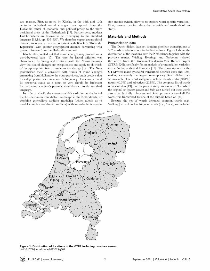
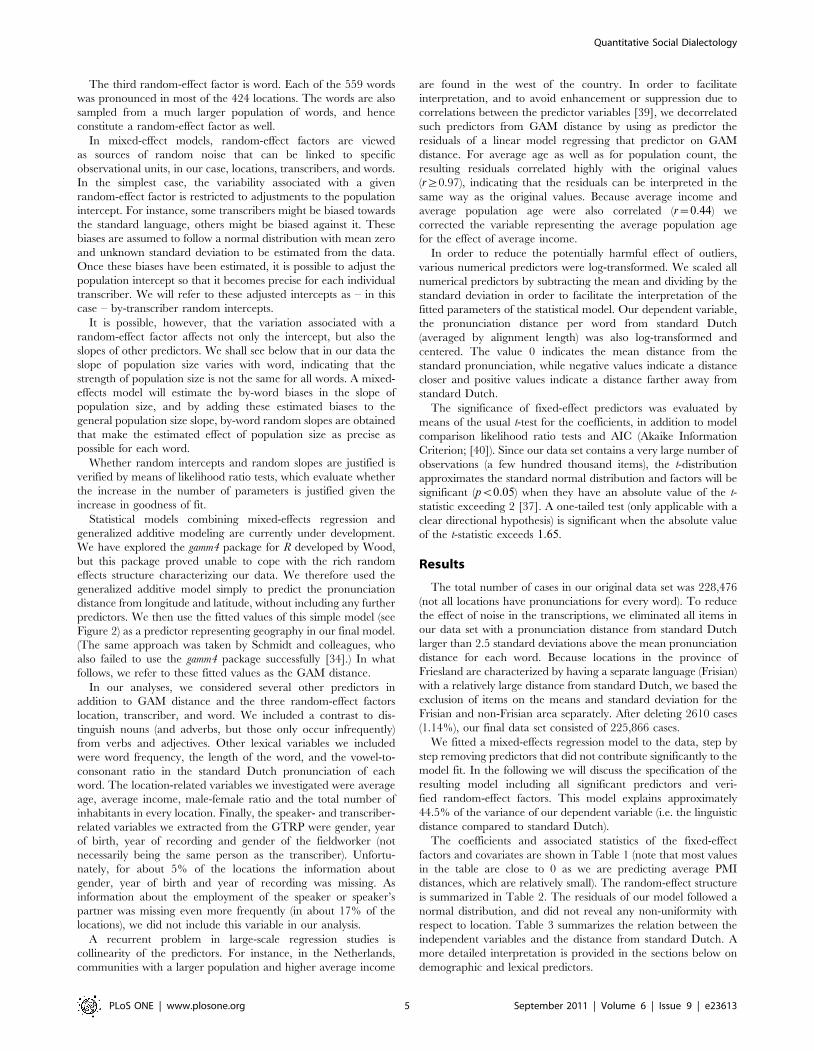
Figure 2 presents the resulting regression surface using a contour



plot. The (solid) contour lines represent distance isoglosses. Darker

shades of gray indicate smaller distances, lighter shades of gray

represent greater distances from the standard language.

The general geographic pattern fits well with Kloeke’s hy-

pothesis of a Hollandic expansion: As we move away from Ho-

lland, pronunciation distances increase [17]. Kloeke showed that

even in the sixteenth and seventeenth centuries the economic and

political supremacy of the provinces of North and South Holland

led to the spread of Hollandic speech norms to the outer provinces.

We can clearly identify the separation from the standard spoken in

the provinces of North and South Holland (central west) of the

province of Friesland (in the north), the Low Saxon dialects spoken in

Groningen and Drenthe (in the northeast), and the Franconian

dialects of Zeeland (in the southwest) and Limburg (southeast). The

28.69 estimated degrees of freedom invested in the thin plate regression

spline were supported by an F-value of 1051 (pv0:0001). The local

cohesion in Figure 2 makes sense, since nearby locations tend to speak

dialectal varieties which are relatively similar [35].

Mixed-effects modelingA problem with this generalized additive model is that the

random-effects structure of our data set is not taken into account.

In mixed-effects regression modeling (for introductions, see, e.g.,

[36–38]), a distinction is made between fixed-effect and random-

effect factors. Fixed-effect factors are factors with a small number

of levels that exhaust all possible levels (e.g., the gender of a

speaker is either male or female). Random-effect factors, by

contrast, have levels sampled from a much larger population of

possible levels. In our data, there are three random-effect factors

that are likely to introduce systematic variation that is ignored in

our generalized additive model.

A first random-effect factor is location. Our observations are

made at 424 locations where speakers were interviewed. Since

these 424 locations are a sample of a much larger set of

communities that might have been sampled, location is a

random-effect factor. Because we used the pronunciations of a

single speaker at a given location, location is confounded with

speaker. Hence, our random-effect factor location represents both

location and speaker.

The data obtained from the 424 locations were coded

phonetically by 30 different transcribers. Since these transcribers

are themselves a sample of a larger set of possible transcribers,

transcriber is a second random-effect factor in our model. By

including transcriber in our model, we can account for biases in

how individuals positioned the data that they listened to with

respect to the standard language.

Figure 2. Contour plot obtained with a generalized additive model. The contour plot shows a regression surface of pronunciation distanceas a function of longitude and latitude obtained with a generalized additive model using a thin plate regression spline. The (black) contour linesrepresent distance isoglosses, darker shades of gray indicate smaller distances closer to the standard language, lighter shades of gray representgreater distances. Note that the empty square indicates the location of the IJsselmeer, a large lake in the Netherlands.doi:10.1371/journal.pone.0023613.g002



The third random-effect factor is word. Each of the 559 words

was pronounced in most of the 424 locations. The words are also

sampled from a much larger population of words, and hence

constitute a random-effect factor as well.

In mixed-effect models, random-effect factors are viewed

as sources of random noise that can be linked to specific

observational units, in our case, locations, transcribers, and words.

In the simplest case, the variability associated with a given

random-effect factor is restricted to adjustments to the population

intercept. For instance, some transcribers might be biased towards

the standard language, others might be biased against it. These

biases are assumed to follow a normal distribution with mean zero

and unknown standard deviation to be estimated from the data.

Once these biases have been estimated, it is possible to adjust the

population intercept so that it becomes precise for each individual

transcriber. We will refer to these adjusted intercepts as – in this

case – by-transcriber random intercepts.

It is possible, however, that the variation associated with a

random-effect factor affects not only the intercept, but also the

slopes of other predictors. We shall see below that in our data the

slope of population size varies with word, indicating that the

strength of population size is not the same for all words. A mixed-

effects model will estimate the by-word biases in the slope of

population size, and by adding these estimated biases to the

general population size slope, by-word random slopes are obtained

that make the estimated effect of population size as precise as

possible for each word.

Whether random intercepts and random slopes are justified is

verified by means of likelihood ratio tests, which evaluate whether

the increase in the number of parameters is justified given the

increase in goodness of fit.

Statistical models combining mixed-effects regression and

generalized additive modeling are currently under development.

We have explored the gamm4 package for R developed by Wood,

but this package proved unable to cope with the rich random

effects structure characterizing our data. We therefore used the

generalized additive model simply to predict the pronunciation

distance from longitude and latitude, without including any further

predictors. We then use the fitted values of this simple model (see

Figure 2) as a predictor representing geography in our final model.

(The same approach was taken by Schmidt and colleagues, who

also failed to use the gamm4 package successfully [34].) In what

follows, we refer to these fitted values as the GAM distance.

In our analyses, we considered several other predictors in

addition to GAM distance and the three random-effect factors

location, transcriber, and word. We included a contrast to dis-

tinguish nouns (and adverbs, but those only occur infrequently)

from verbs and adjectives. Other lexical variables we included

were word frequency, the length of the word, and the vowel-to-

consonant ratio in the standard Dutch pronunciation of each

word. The location-related variables we investigated were average

age, average income, male-female ratio and the total number of

inhabitants in every location. Finally, the speaker- and transcriber-

related variables we extracted from the GTRP were gender, year

of birth, year of recording and gender of the fieldworker (not

necessarily being the same person as the transcriber). Unfortu-

nately, for about 5% of the locations the information about

gender, year of birth and year of recording was missing. As

information about the employment of the speaker or speaker’s

partner was missing even more frequently (in about 17% of the

locations), we did not include this variable in our analysis.

A recurrent problem in large-scale regression studies is

collinearity of the predictors. For instance, in the Netherlands,

communities with a larger population and higher average income

are found in the west of the country. In order to facilitate

interpretation, and to avoid enhancement or suppression due to

correlations between the predictor variables [39], we decorrelated

such predictors from GAM distance by using as predictor the

residuals of a linear model regressing that predictor on GAM

distance. For average age as well as for population count, the

resulting residuals correlated highly with the original values

(r§0.97), indicating that the residuals can be interpreted in the

same way as the original values. Because average income and

average population age were also correlated (r~0:44) we

corrected the variable representing the average population age

for the effect of average income.

In order to reduce the potentially harmful effect of outliers,

various numerical predictors were log-transformed. We scaled all

numerical predictors by subtracting the mean and dividing by the

standard deviation in order to facilitate the interpretation of the

fitted parameters of the statistical model. Our dependent variable,

the pronunciation distance per word from standard Dutch

(averaged by alignment length) was also log-transformed and

centered. The value 0 indicates the mean distance from the

standard pronunciation, while negative values indicate a distance

closer and positive values indicate a distance farther away from

standard Dutch.

The significance of fixed-effect predictors was evaluated by

means of the usual t-test for the coefficients, in addition to model

comparison likelihood ratio tests and AIC (Akaike Information

Criterion; [40]). Since our data set contains a very large number of

observations (a few hundred thousand items), the t-distribution

approximates the standard normal distribution and factors will be

significant (pv0:05) when they have an absolute value of the t-

statistic exceeding 2 [37]. A one-tailed test (only applicable with a

clear directional hypothesis) is significant when the absolute value

of the t-statistic exceeds 1:65.

Results

The total number of cases in our original data set was 228,476

(not all locations have pronunciations for every word). To reduce

the effect of noise in the transcriptions, we eliminated all items in

our data set with a pronunciation distance from standard Dutch

larger than 2.5 standard deviations above the mean pronunciation

distance for each word. Because locations in the province of

Friesland are characterized by having a separate language (Frisian)

with a relatively large distance from standard Dutch, we based the

exclusion of items on the means and standard deviation for the

Frisian and non-Frisian area separately. After deleting 2610 cases

(1.14%), our final data set consisted of 225,866 cases.

We fitted a mixed-effects regression model to the data, step by

step removing predictors that did not contribute significantly to the

model fit. In the following we will discuss the specification of the

resulting model including all significant predictors and veri-

fied random-effect factors. This model explains approximately

44.5% of the variance of our dependent variable (i.e. the linguistic

distance compared to standard Dutch).

The coefficients and associated statistics of the fixed-effect

factors and covariates are shown in Table 1 (note that most values

in the table are close to 0 as we are predicting average PMI

distances, which are relatively small). The random-effect structure

is summarized in Table 2. The residuals of our model followed a

normal distribution, and did not reveal any non-uniformity with

respect to location. Table 3 summarizes the relation between the

independent variables and the distance from standard Dutch. A

more detailed interpretation is provided in the sections below on

demographic and lexical predictors.



The inclusion of the fixed-effect factors (except average po-

pulation income) and random-effect factors shown in Table 1 and

2 was supported by likelihood ratio tests indicating that the

additional parameters significantly improved the goodness of fit of

the model. Tables 4 and 5 show the increase of the goodness of fit

for every additional factor measured by the increase of the log-

likelihood and the decrease of the Akaike Information Criterion

[40]. To assess the influence of each additional fixed-effect factor,

the random effects were held constant, including only the random

intercepts for word, location and transcriber. The baseline model,

to which the inclusion of the first fixed-effect factor (geography)

was compared, only consisted of the random intercepts for word,

location and transcriber. Subsequently, the next model (including

both geography and the vowel-to-consonant ratio per word), was

compared to the model including geography (and the random

intercepts) only. This is shown in Table 4 (sorted by decreasing

importance of the individual fixed-effect factors). Log-likelihood

ratio tests were carried out with maximum likelihood estimation,

as recommended in [36].

Similarly, the importance of additional random-effect factors

was assessed by restricting the fixed-effect predictors to those listed

in Table 1. The baseline model in Table 5, to which the inclusion

of the random intercept for word was compared, only consisted of

the fixed-effect factors listed in Table 1. The next model (also

including location as a random intercept) was compared to the

model with only word as a random intercept. In later steps random

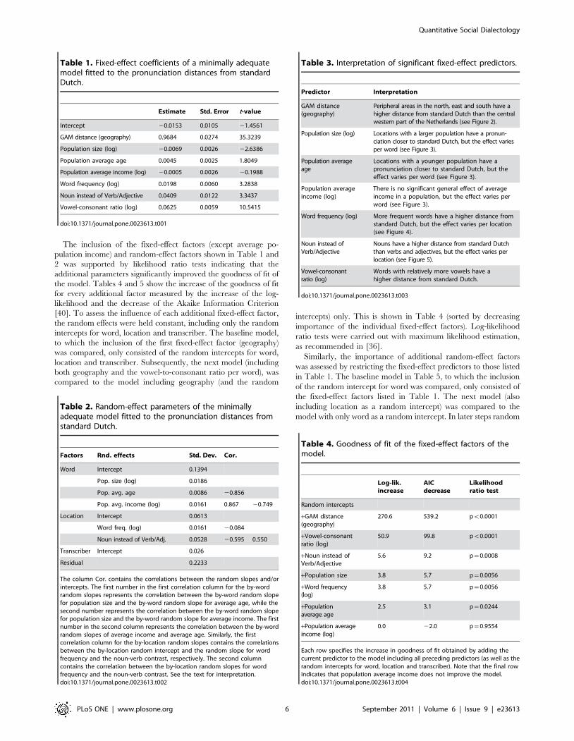
Table 1. Fixed-effect coefficients of a minimally adequatemodel fitted to the pronunciation distances from standardDutch.

Estimate Std. Error t-value

Intercept 20.0153 0.0105 21.4561

GAM distance (geography) 0.9684 0.0274 35.3239

Population size (log) 20.0069 0.0026 22.6386

Population average age 0.0045 0.0025 1.8049

Population average income (log) 20.0005 0.0026 20.1988

Word frequency (log) 0.0198 0.0060 3.2838

Noun instead of Verb/Adjective 0.0409 0.0122 3.3437

Vowel-consonant ratio (log) 0.0625 0.0059 10.5415

doi:10.1371/journal.pone.0023613.t001

Table 2. Random-effect parameters of the minimallyadequate model fitted to the pronunciation distances fromstandard Dutch.

Factors Rnd. effects Std. Dev. Cor.

Word Intercept 0.1394

Pop. size (log) 0.0186

Pop. avg. age 0.0086 20.856

Pop. avg. income (log) 0.0161 0.867 20.749

Location Intercept 0.0613

Word freq. (log) 0.0161 20.084

Noun instead of Verb/Adj. 0.0528 20.595 0.550

Transcriber Intercept 0.026

Residual 0.2233

The column Cor. contains the correlations between the random slopes and/orintercepts. The first number in the first correlation column for the by-wordrandom slopes represents the correlation between the by-word random slopefor population size and the by-word random slope for average age, while thesecond number represents the correlation between the by-word random slopefor population size and the by-word random slope for average income. The firstnumber in the second column represents the correlation between the by-wordrandom slopes of average income and average age. Similarly, the firstcorrelation column for the by-location random slopes contains the correlationsbetween the by-location random intercept and the random slope for wordfrequency and the noun-verb contrast, respectively. The second columncontains the correlation between the by-location random slopes for wordfrequency and the noun-verb contrast. See the text for interpretation.doi:10.1371/journal.pone.0023613.t002

Table 3. Interpretation of significant fixed-effect predictors.

Predictor Interpretation

GAM distance(geography)

Peripheral areas in the north, east and south have ahigher distance from standard Dutch than the centralwestern part of the Netherlands (see Figure 2).

Population size (log) Locations with a larger population have a pronun-ciation closer to standard Dutch, but the effect variesper word (see Figure 3).

Population averageage

Locations with a younger population have apronunciation closer to standard Dutch, but theeffect varies per word (see Figure 3).

Population averageincome (log)

There is no significant general effect of averageincome in a population, but the effect varies perword (see Figure 3).

Word frequency (log) More frequent words have a higher distance fromstandard Dutch, but the effect varies per location(see Figure 4).

Noun instead ofVerb/Adjective

Nouns have a higher distance from standard Dutchthan verbs and adjectives, but the effect varies perlocation (see Figure 5).

Vowel-consonantratio (log)

Words with relatively more vowels have ahigher distance from standard Dutch.

doi:10.1371/journal.pone.0023613.t003

Table 4. Goodness of fit of the fixed-effect factors of themodel.

Log-lik.increase

AICdecrease

Likelihoodratio test

Random intercepts

+GAM distance(geography)

270.6 539.2 pv0.0001

+Vowel-consonantratio (log)

50.9 99.8 pv0.0001

+Noun instead ofVerb/Adjective

5.6 9.2 p~0.0008

+Population size 3.8 5.7 p~0.0056

+Word frequency(log)

3.8 5.7 p~0.0056

+Populationaverage age

2.5 3.1 p~0.0244

+Population averageincome (log)

0.0 22.0 p~0.9554

Each row specifies the increase in goodness of fit obtained by adding thecurrent predictor to the model including all preceding predictors (as well as therandom intercepts for word, location and transcriber). Note that the final rowindicates that population average income does not improve the model.doi:10.1371/journal.pone.0023613.t004



slopes were added. For instance, the sixth model (including

random slopes for population size and average population age,

and their correlation) was compared to the fifth model which only

included population size as a random slope. Log-likelihood ratio

tests evaluating random-effects parameters were carried out with

relativized maximum likelihood estimation, again following [36].

Due to the large size of our data set, it proved to be com-

putationally infeasible to include all variables in our random-effects

structure (e.g., the vowel-to-consonant ratio was not included). As

further gains in goodness of fit are to be expected when more

parameters are invested in the random-effects structure, our

model does not show the complete (best) random-effects structure.

However, we have checked that the fixed-effect factors remained

significant when additional uncorrelated by-location or by-word

random slopes were included in the model specification. In other

words, we have verified that the t-values of the fixed-effect factors in

Table 1 are not anti-conservative and therefore our results remain

valid.

Demographic predictorsThe geographical predictor GAM distance (see Figure 2)

emerged as the predictor with the smallest uncertainty concerning

its slope, as indicated by the huge t-value. As GAM distance

represents the fitted values of a generalized additive model fitted to

pronunciation distance from standard Dutch (adjusted R2~0.12),

the strong statistical support for this predictor is unsurprising. Even

though GAM distance accounts for a substantial amount of

variance, location is also supported as a significant random-effect

factor, indicating that there are differences in pronunciation

distances from the standard language that cannot be reduced to

geographical location. The random-effect factor location, in other

words, represents systematic variability that can be traced to the

different locations (or speakers), but that resists explanation

through our demographic fixed-effect predictors. To what extent,

then, do these demographic predictors help explain pronunciation

distance from the standard language over and above longitude,

latitude, and the location (speaker) itself?

Table 1 lists two demographic predictors that reached

significance. First, locations with many inhabitants (a large

population size) tend to have a lower distance from the standard

language than locations with few inhabitants. A possible ex-

planation for this finding is that people tend to have weaker social

ties in urban populations, which causes dialect leveling [41]. Since

the standard Dutch language has an important position in the

Netherlands [18,42], and has been dominant for many centuries

[17], conversations between speakers of different dialects will

normally be held in standard Dutch and consequently leveling will

proceed in the direction of standard Dutch. The greater similarity

of varieties in settlements of larger size is also consistent with the

predictions of the gravity hypothesis which states that linguistic

innovation proceeds first from large settlements to other large

nearby settlements, after which smaller settlements adopt the

innovations from nearby larger settlements [43].

The second (one-tailed) significant demographic covariate is the

average age of the inhabitants of a given location. Since younger

people tend to speak less in their dialect and more in standard

Dutch than the older population [12,18, pp. 355–356], the

positive slope of average age is as expected.

Note that Table 1 also contains average income as a

demographic covariate. This variable is not significant in the

fixed-effect part of the model (as the absolute t-value is lower than

1.65), but is included as it is an important predictor in the random-

effects structure of the model.

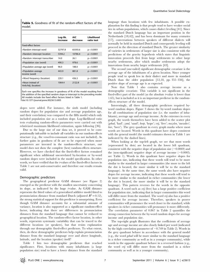
Interestingly, all three demographic predictors required by-

word random slopes. Figure 3 shows the by-word random slopes

for all combinations of population size (i.e. the number of inha-

bitants), average age and average income. At the extremes in every

graph, the words themselves have been added to the scatter plot

(gehad, ‘had’; zand, ‘sand’; hoop, ‘hope’; vrij, ‘free’; mazelen, ‘measles’;

bier, ‘beer’). The grey quadrant in every graph marks where most

words are located. Words in this quadrant have slopes consistent

with the general model (the model estimates shown in Table 1 are

indicated by the dashed lines).

When looking at the top-left graph, we see that most words

(represented by dots) are located in the lower left quadrant,

consistent with the negative slope of population size (20.0069) and

the (non-significant) negative slope of average income (20.0005;

see Table 1). Words in this quadrant have negative slopes for

population size, indicating that these words will tend to be more

similar to the standard in larger communities (the more to the left

the dot is located, the more similar it will be to the standard

language). At the same time, the same words also have negative

slopes for average income, indicating that these words will tend to

be more similar to the standard in richer communities (the lower

the dot is located, the more similar it will be to the standard

language). This pattern reverses for the words in the opposite

quadrant. A word such as vrij (free) has a large positive coefficient

for population size, indicating that in larger communities this word

will differ more from the standard. The word vrij also has a positive

coefficient for average income. Therefore, speakers in poorer

communities will pronounce the word closer to the standard, while

speakers in richer communities will pronounce it more differently.

The correlation parameter of 0.867 in Table 2 quantifies the

strong connection between the by-word random slopes for average

income and population size.

The top-right graph illustrates that the coefficients of average

age and average income are also closely linked per word (indicated

by the high correlation parameter of 20.749 in Table 2). Words in

the grey quadrant behave in accordance with the general model

(e.g., the word gehad will be more similar to the standard language

in a richer community as well as in a younger community), while

words in the opposite quadrant behave in a reversed fashion (e.g.,

the word vrij will differ more from the standard in a richer

community as well as in a younger community).

Table 5. Goodness of fit of the random-effect factors of themodel.

Log-lik.increase

AICdecrease

Likelihoodratio test

Fixed-effect factors

+Random intercept word 32797.8 65593.6 pv0.0001

+Random intercept location 5394.2 10786.4 pv0.0001

+Random intercept transcriber 14.0 26.1 pv0.0001

+Population size (word) 490.3 978.6 pv0.0001

+Population average age (word) 96.0 188.0 pv0.0001

+Population averageincome (word)

443.9 881.8 pv0.0001

+Word frequency (location) 220.1 436.3 pv0.0001

+Noun instead ofVerb/Adj. (location)

1064.4 2122.8 pv0.0001

Each row specifies the increase in goodness of fit of the model resulting fromthe addition of the specified random slope or intercept to the preceding model.All models include the fixed effect factors listed in Table 1.doi:10.1371/journal.pone.0023613.t005



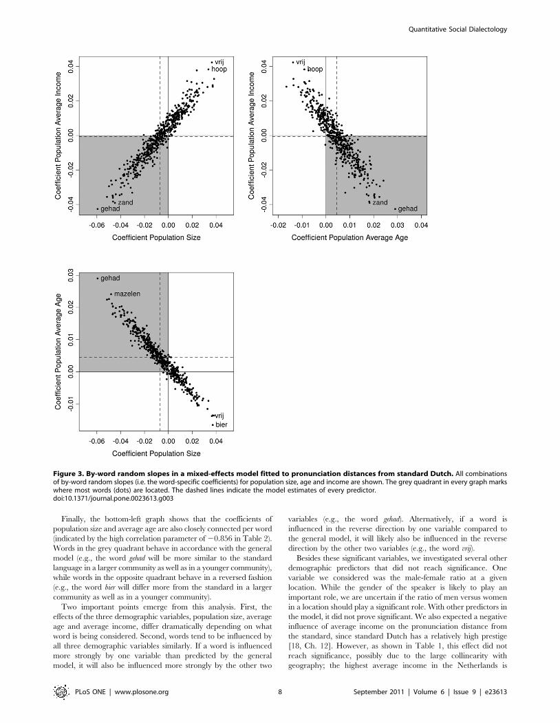
Finally, the bottom-left graph shows that the coefficients of

population size and average age are also closely connected per word

(indicated by the high correlation parameter of 20.856 in Table 2).

Words in the grey quadrant behave in accordance with the general

model (e.g., the word gehad will be more similar to the standard

language in a larger community as well as in a younger community),

while words in the opposite quadrant behave in a reversed fashion

(e.g., the word bier will differ more from the standard in a larger

community as well as in a younger community).

Two important points emerge from this analysis. First, the

effects of the three demographic variables, population size, average

age and average income, differ dramatically depending on what

word is being considered. Second, words tend to be influenced by

all three demographic variables similarly. If a word is influenced

more strongly by one variable than predicted by the general

model, it will also be influenced more strongly by the other two

variables (e.g., the word gehad). Alternatively, if a word is

influenced in the reverse direction by one variable compared to

the general model, it will likely also be influenced in the reverse

direction by the other two variables (e.g., the word vrij).

Besides these significant variables, we investigated several other

demographic predictors that did not reach significance. One

variable we considered was the male-female ratio at a given

location. While the gender of the speaker is likely to play an

important role, we are uncertain if the ratio of men versus women

in a location should play a significant role. With other predictors in

the model, it did not prove significant. We also expected a negative

influence of average income on the pronunciation distance from

the standard, since standard Dutch has a relatively high prestige

[18, Ch. 12]. However, as shown in Table 1, this effect did not

reach significance, possibly due to the large collinearity with

geography; the highest average income in the Netherlands is

Figure 3. By-word random slopes in a mixed-effects model fitted to pronunciation distances from standard Dutch. All combinationsof by-word random slopes (i.e. the word-specific coefficients) for population size, age and income are shown. The grey quadrant in every graph markswhere most words (dots) are located. The dashed lines indicate the model estimates of every predictor.doi:10.1371/journal.pone.0023613.g003



earned in the western part of the Netherlands [23], where dialects

are also most similar to standard Dutch [44, p. 274]. Average

income was highly significant when geography was excluded from

the model.

No speaker-related variables were included in the final model.

We were surprised that the gender of the speaker did not reach

significance, as the importance of this factor has been reported in

many sociolinguistic studies [45]. However, when women have a

limited social circle (e.g., the wife of a farmer living on the outskirts

of a small rural community), they actually tend to speak more

traditionally than men [18, p. 365]. Since such women are

certainly present in our data set, this may explain the absence of a

gender difference in our model. We also expected speaker age to

be a significant predictor, since dialects are leveling in the

Netherlands [12,18, pp. 355–356]. However, as the speakers were

relatively close in age (e.g., 74% of the speakers were born between

1910 and 1930) and we only used pronunciations of a single

speaker per location, this effect might have been too difficult to

detect in our data set.

The two fieldworker-related factors (gender of the fieldworker

and year of recording) were not very informative, because they

suffered from substantial geographic collinearity. With respect to

the year of recording, we found that locations in Friesland were

visited quite late in the project, while their distances from standard

Dutch were largest. Regarding the gender of the fieldworkers,

female fieldworkers mainly visited the central locations in the

Netherlands, while the male fieldworkers visited the more

peripheral areas (where the pronunciation distance from standard

Dutch is larger).

Lexical predictorsTable 1 lists three lexical predictors that reached significance:

the vowel-to-consonant ratio, word frequency and the contrast

between nouns and verbs. Unsurprisingly, the length of the word

was not a significant predictor, as we normalized pronunciation

distance by the alignment length.

The first significant lexical factor was the vowel-to-consonant

ratio. The general effect of the vowel-to-consonant ratio was

linear, with a greater ratio predicting a greater distance from the

standard. As vowels are much more variable than consonants (e.g.,

[46]), this is not a very surprising finding.

The second, more interesting, significant lexical factor was word

frequency. More frequent words tend to have a higher distance

from the standard. We remarked earlier that Dutch dialects tend

to converge to standard Dutch. A larger distance from the

standard likely indicates an increased resistance to standardization.

Indeed, given the recent study of Pagel and colleagues, where they

show that more frequent words are more resistant to change [47],

this seems quite sensible.

However, the effect of word frequency is not uniform across

locations, as indicated by the presence of by-location random

slopes for word frequency in our model (see Table 2). The

parameters for these random slopes (the standard deviation for the

random slopes and the correlation parameter for the random

slopes and intercepts) jointly increase the log-likelihood of the

model by no less than 220 units, compared to 3.8 log-likelihood

units for the fixed-effect (population) slope of frequency.

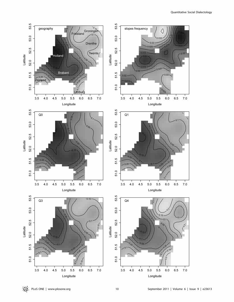
Interestingly, although the by-location random slopes for frequen-

cy properly follow a normal distribution, they are not uniformly

distributed across the different regions of the Netherlands, as

illustrated in the upper right panel of Figure 4. In this panel,

contour lines link locations for which the slope of the frequency

effect is the same. The two dark grey areas (central Holland and

Groningen and Drenthe) are characterized by slopes close to zero,

while the white area in Friesland indicates a large positive slope

(i.e. the Frisian pronunciations become more distinct from

standard Dutch for higher frequency words).

To clarify how geography (GAM distance) and frequency jointly

predict distance from the standard language, we first calculated the

fitted GAM distance for each location. We then estimated the

predicted distance from the standard language using GAM distance

and word frequency as predictors, weighted by the weights

estimated by our mixed-effects model. Because the fitted surfaces

vary with frequency, we selected the minimum frequency (Q0), first

(Q1) and third (Q3) quartiles as well as the maximum frequency

(Q4) for visualization (see the lower panels in Figure 4). Panel Q0

shows the surface for the words with the lowest frequency in our

data. As frequency increased, the surface gradually morphs into the

surface shown in the lower right panel (Q4). The first thing to note is

that as frequency increases, the shades of grey become lighter,

indicating greater differences from the standard. This is the main

effect of frequency: higher-frequency words are more likely to resist

assimilation to the standard language. The second thing to note is

that the distances between the contour lines decrease with

increasing frequency, indicating that the differences between

regions with respect to the frequency effect become increasingly

more pronounced. For instance, the Low Saxon dialect of Twente

on the central east border with Germany, and the Frisian varieties in

the north profile themselves more clearly as different from the

Hollandic standard for the higher-frequency words (Q4) than for the

lower-frequency words (Q0).

For the lowest-frequency words (panel Q0), the northeast

separates itself from the Hollandic sphere of influence, with

distance slowly increasing towards the very northeast of the

country. This area includes Friesland and the Low Saxon dialects.

As word frequency increases, the distance from standard Dutch

increases, and most clearly so in Friesland. For Friesland, this solid

resistance to the Hollandic norm, especially for high-frequency

words, can be attributed to Frisian being a different language that

is mutually unintelligible with standard Dutch.

Twente also stands out as highly resistant to the influence of the

standard language. In the 16th and 17th centuries, this region was

not under firm control of the Dutch Republic, and Roman

Catholicism remained stronger here than in the regions towards its

west and north. The resistance to protestantism in this region may

have contributed to its resistance to the Hollandic speech norms

(see also [48]).

In the southwest (Zeeland) and the southeast (Limburg), we find

Low Franconian dialects that show the same pattern across all

frequency quartiles, again with increased distance from Holland

predicting greater pronunciation distance. The province of

Limburg has never been under firm control of Holland for long,

and has a checkered history of being ruled by Spain, France,

Prussia, and Austria before becoming part of the kingdom of the

Netherlands. Outside of the Hollandic sphere of influence, it has

remained closer to dialects found in Germany and Belgium. The

province of Zeeland, in contrast, has retained many features of an

earlier linguistic expansion from Flanders – in the middle ages,

Flanders had strong political influence in Zeeland. Zeeland was

not affected by an expansion from Brabant (which is found in the

central south of the Netherlands as well as in Belgium), but that

expansion strongly influenced the dialects of Holland. This

Brabantic expansion, which took place in the late middle ages

up to the seventeenth century, clarifies why, across all frequency

quartiles, the Brabantic dialects are most similar to the Hollandic

dialects.

Our regression model appears to conflict with the view of

Kloeke (which was also adopted by Bloomfield) that high-





frequency words should be more likely to undergo change than

low-frequency words [17,49]. This position was already argued for

by Schuchardt, who discussed data suggesting that high-frequency

words are more profoundly affected by sound change than low-

frequency words [50]. Bybee called attention to language-internal

factors of change that are frequency-sensitive [51]. She argued that

changes affecting high-frequency words first would be a conse-

quence of the overlap and reduction of articulatory gestures that

comes with fluency. In contrast, low-frequency words would be

more likely to undergo analogical leveling or regularization.

Our method does not allow us to distinguish between pro-

cesses of articulatory simplification and processes of leveling or

regularization. Moreover, our method evaluates the joint effect of

many different sound changes for the geographical landscape. Our

results indicate that, in general, high-frequency words are most

different from the standard. However, high-frequency words can

differ from the standard for very different reasons. For instance,

they may represent older forms that have resisted changes that

affected the standard. Alternatively, they may have undergone

region-specific articulatory simplification. Furthermore, since

higher-frequency forms are better entrenched in memory [52,53],

they may be less susceptible to change. As a consequence, changes

towards the standard in high-frequency words may be more

salient, and more likely to negatively affect a speaker’s in-group

status as a member of a dialect community. Whatever the precise

causes underlying their resistance to accommodation to the

standard may be, our data do show that the net outcome of the

different forces involved in sound change is one in which it is the

high-frequency words that are most different from the standard

language.

The third lexical factor that reached significance was the

contrast between nouns as opposed to verbs and adjectives. Nouns

have a greater distance from the standard language than verbs and

adjectives. (Further analyses revealed that the effects of verbs and

adjectives did not differ significantly.) This finding harmonizes well

with the results of Pagel and colleagues, where they also observed

that nouns were most resistant to change, followed by verbs and

adjectives [47].

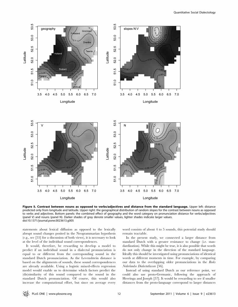
Similar to word frequency, we also observe a non-uniform effect

of the contrast between nouns as opposed to verbs and adjectives

across locations, indicated by the presence of the by-location

random slopes for the word category contrast in our model (see

Table 2). The parameters for these random slopes (the standard

deviation for the random slopes and the correlation parameter for

the random slopes and intercepts) jointly increase the log-

likelihood of the model by 1064 units, compared to 5.6 log-

likelihood units for the fixed-effect (population) slope of this

contrast. These by-location random slopes are not uniformly

distributed across the geographical area, as shown by the upper

right panel of Figure 5. This panel clearly shows that the word

category in the north-west of the Netherlands does not influence

the distance from the standard language (i.e. the slope is 0), while

in Friesland nouns have a much higher distance from the standard

than verbs or adjectives.

To clarify how geography (GAM distance) and the word

category contrast jointly predict distance from the standard

language, we first calculated the fitted GAM distance for each

location. We then estimated the predicted distance from the

standard language using GAM distance, a fixed (median) word

frequency, and the word category contrast as predictors, weighted

by the weights estimated by our mixed-effects model. Because the

fitted surfaces are different for nouns as opposed to verbs and

adjectives, we visualized both surfaces in the bottom panels in

Figure 5. The first thing to note is that in panel N the shades of

grey are lighter than in panel V, indicating greater differences

from the standard. This is the main effect of the word category

contrast: nouns are more likely to resist assimilation to the

standard language than verbs or adjectives. The second thing to

note is that the distances between the contour lines are smaller for

nouns, indicating that the differences between regions are more

pronounced for nouns than for verbs.

As the pattern of variation at the periphery of the Netherlands is

quite similar to the pattern reported for high-frequency words (i.e.

the peripheral areas are quite distinct from the standard), we will

not repeat its discussion here. The similarity between high-

frequency words and nouns (as opposed to verbs and adjectives) is

also indicated by the correlation parameter of 0.550 in Table 2.

Discussion

In this study we have illustrated that several factors play a

significant role in determining dialect distances from the standard

language. Besides the importance of geography, we found clear

support for three word-related variables (i.e. the contrast between

nouns as opposed to verbs and adjectives, word frequency and the

vowel-to-consonant ratio in the standard Dutch pronunciation) as

well as two variables relating to the social environment (i.e. the

number of inhabitants in a location and the average age of the

inhabitants in a population). These results clearly indicate the need

for variationists to consider explanatory quantitative models which

incorporate geographical, social and word-related variables as

independent variables.

We did not find support for the importance of speaker-related

variables such as gender and age. As we only had a single

pronunciation per location, we cannot exclude the possibility that

these speaker-related variables do play an important role. It would

be very informative to investigate dialect change in a data set with

speakers of various ages in the same location, using the apparent

time construct [54]. In addition, being able to compare male and

female speakers in a single location would give us more insight into

the effect of gender.

It is important to note that the contribution of the random-

effects structure to the goodness of fit of the model tends to be one

or two orders of magnitude larger than the contributions of the

fixed-effect predictors, with GAM distance (geography) as sole

exception. This indicates that the variation across speakers/

locations and across words is huge compared to the magnitude of

the effects of the socio-demographic and lexical predictors.

Our model also provides some insight into lexical diffusion.

While we did not focus on individual sound changes, it is clear that

the resistance to change at the word level is influenced by several

word-related factors, as well as a number of socio-demographic

factors of which the precise effect varies per word. Consequently, it

is sensible to presume that a sound in one word will change more

quickly than the same sound in another word (i.e. constituting

a lexically gradual change). However, to make more precise

Figure 4. Word frequency and distance from the standard language. Upper left: distance predicted only from longitude and latitude. Upperright: the geographical distribution of random slopes for word frequency. Lower four panels: the combined effect of geography and word frequencyon pronunciation distance for the minimum frequency (Q0), the first (Q1) and third quartile (Q3) and the maximum frequency (Q4). Darker shades ofgray denote smaller values, lighter shades indicate larger values.doi:10.1371/journal.pone.0023613.g004



statements about lexical diffusion as opposed to the lexically

abrupt sound changes posited in the Neogrammarian hypothesis

(e.g., see [55] for a discussion of both views), it is necessary to look

at the level of the individual sound correspondences.

It would, therefore, be rewarding to develop a model to

predict if an individual sound in a dialectal pronunciation is

equal to or different from the corresponding sound in the

standard Dutch pronunciation. As the Levenshtein distance is

based on the alignments of sounds, these sound correspondences

are already available. Using a logistic mixed-effects regression

model would enable us to determine which factors predict the

(dis)similarity of this sound compared to the sound in the

standard Dutch pronunciation. Of course, this would also

increase the computational effort, but since on average every

word consists of about 4 to 5 sounds, this potential study should

remain tractable.

In the present study, we connected a larger distance from

standard Dutch with a greater resistance to change (i.e. stan-

dardization). While this might be true, it is also possible that words

do not only change in the direction of the standard language.

Ideally this should be investigated using pronunciations of identical

words at different moments in time. For example, by comparing

our data to the overlapping older pronunciations in the Reeks

Nederlandse Dialectatlassen [56].

Instead of using standard Dutch as our reference point, we

could also use proto-Germanic, following the approach of

Heeringa and Joseph [57]. It would be rewarding to see if smaller

distances from the proto-language correspond to larger distances

Figure 5. Contrast between nouns as opposed to verbs/adjectives and distance from the standard language. Upper left: distancepredicted only from longitude and latitude. Upper right: the geographical distribution of random slopes for the contrast between nouns as opposedto verbs and adjectives. Bottom panels: the combined effect of geography and the word category on pronunciation distance for verbs/adjectives(panel V) and nouns (panel N). Darker shades of gray denote smaller values, lighter shades indicate larger values.doi:10.1371/journal.pone.0023613.g005



from the standard language. Alternatively, we might study the

dialectal landscape from another perspective, by selecting a

dialectal variety as our reference point. For example, dialect

distances could be calculated with respect to a specific Frisian or

Limburgian dialect.

In summary, our quantitative sociolinguistic analysis has found

support for lexical diffusion in Dutch dialects and has clearly

illustrated that convergence towards standard Dutch is most likely

in low-frequent words. Furthermore we have shown that mixed-

effects regression modeling in combination with a generalized

additive model representing geography is highly suitable for

investigating dialect distances and its determinants.

Author Contributions

Conceived and designed the experiments: MW RHB. Performed the

experiments: MW RHB. Analyzed the data: MW RHB. Contributed

reagents/materials/analysis tools: MW RHB. Wrote the paper: MW JN

RHB.

References

1. Chambers J, Trudgill P (1998) Dialectology. Cambridge University Press,Second edition.

2. Labov W (1963) The social motivation of a sound change. Word 19: 273–309.

3. Trudgill P (1986) Dialects in contact. Blackwell.

4. Paolillo JC (2002) Analyzing linguistic variation: Statistical models and methods.

StanfordCalifornia: Center for the Study of Language and Information.

5. Johnson DE (2009) Getting off the GoldVarb standard: Introducing Rbrul for

mixed-effects variable rule analysis. Language and Linguistics Compass 3:359–383.

6. Seguy J (1973) La dialectometrie dans l’atlas linguistique de Gascogne. Revue deLinguistique Romane 37: 1–24.

7. Seguy J (1971) La relation entre la distance spatiale et la distance lexicale. Revue

de Linguistique Romane 35: 335–357.

8. Goebl H (1993) Dialectometry: A short overview of the principles and practice of

quantitative classification of linguistic atlas data. In: Kohler R, Rieger B, eds.Contributions to Quantitative Linguistics. Dordrecht: Kluwer. pp 277–315.

9. Heeringa W, Nerbonne J (2001) Dialect areas and dialect continua. LanguageVariation and Change 13: 375–400.

10. Kretzschmar W, Jr. (1996) Quantitative areal analysis of dialect features.

Language Variation and Change 8: 13–39.

11. Nerbonne J, Prokic J, Wieling M, Gooskens C (2010) Some further

dialectometrical steps. In: Aurrekoetxea G, Ormaetxea JL, eds. Tools forLinguistic Variation, Supplements of the Anuario de Filologia Vasca ‘‘Julio

Urquijo’’, XIII. Bilbao: University of the Basque Country. pp 41–56.

12. Heeringa W, Nerbonne J (1999) Change, convergence and divergence among

Dutch and Frisian. In: Boersma P, Breuker PH, Jansma LG, van der Vaart J,

eds. Philologia Frisica Anno 1999. Lezingen fan it fyftjinde Frysk filologekongres,Fryske Akademy, Ljouwert. pp 88–109.

13. Wieling M, Heeringa W, Nerbonne J (2007) An aggregate analysis ofpronunciation in the Goeman-Taeldeman-Van Reenen-Project data. Taal en

Tongval 59: 84–116.

14. Leinonen T (2010) An acoustic analysis of vowel pronunciation in Swedish

dialects. Ph.D. thesis, University of Groningen.

15. Schneider E (1988) Qualitative vs. quantitative methods of area delimitation indialectology: A comparison based on lexical data from Georgia and Alabama.

Journal of English Linguistics 21: 175–212.

16. Woolhiser C (2005) Political borders and dialect divergence/convergence in

Europe. In: Peter Aurer FH, Kerswill P, eds. Dialect Change. Convergence andDivergence in European Languages. New York: Cambridge University Press. pp

236–262.

17. Kloeke GG (1927) De Hollandse expansie in de zestiende en zeventiende eeuwen haar weerspiegeling in de hedendaagsche Nederlandse dialecten (The

Hollandic expansion in the sixteenth and seventeenth centuries and herreflection in present-day Dutch dialects). The Hague: Martinus Nijhoff.

18. van der Wal M, van Bree C (2008) Geschiedenis van het Nederlands. Utrecht:

Spectrum, fifth edition.

19. Wang W (1969) Competing changes as a cause of residue. Language 45: 9–25.

20. Goeman T, Taeldeman J (1996) Fonologie en morfologie van de Nederlandsedialecten. Een nieuwe materiaalverzameling en twee nieuwe atlasprojecten. Taal

en Tongval 48: 38–59.

21. Gussenhoven C (1999) Illustrations of the IPA: Dutch. In: Handbook of the

International Phonetic Association. Cambridge: Cambridge University Press. pp

74–77.

22. Baayen RH, Piepenbrock R, Gulikers L (1996) CELEX2. Linguistic Data

Consortium, Philadelphia.

23. CBS Statline (2010) Kerncijfers wijken en buurten 1995. Available at http://

statline.cbs.nl. Accessed: August 9, 2010.

24. Levenshtein V (1965) Binary codes capable of correcting deletions, insertions

and reversals. Doklady Akademii Nauk SSSR 163: 845–848.

25. Wieling M, Prokic J, Nerbonne J (2009) Evaluating the pairwise alignment ofpronunciations. In: Borin L, Lendvai P, eds. Language Technology and

Resources for Cultural Heritage, Social Sciences, Humanities, and Education.pp 26–34.

26. Church K, Hanks P (1990) Word association norms, mutual information, andlexicography. Computational Linguistics 16: 22–29.

27. Wieling M, Nerbonne J (2011) Measuring linguistic variation commensurably.

Dialectologia Special Issue II: Production, Perception and Attitude. pp 141–162.

28. Wood S (2003) Thin plate regression splines. Journal of the Royal StatisticalSociety: Series B (Statistical Methodology) 65: 95–114.

29. Wood S (2006) Generalized additive models: an introduction with R. Chapman& Hall/CRC.

30. Tremblay A, Baayen RH (2010) Holistic processing of regular four-word

sequences: A behavioral and ERP study of the effects of structure, frequency,and probability on immediate free recall. In: Wood D, ed. Perspectives on

formulaic language: Acquisition and communication. London: The ContinuumInternational Publishing Group. pp 151–173.

31. Baayen RH, Kuperman V, Bertram R (2010) Frequency effects in compoundprocessing. In: Scalise S, Vogel I, eds. Compounding, Amsterdam/Philadelphia:

Benjamins. pp 257–270.

32. Baayen RH (2010) The directed compound graph of English. An exploration oflexical connectivity and its processing consequences. In: Olson S, ed. New

impulses in word-formation (Linguistische Berichte Sonderheft 17). Hamburg:Buske. pp 383–402.

33. Baayen RH, Milin P, Durdevic DF, Hendrix P, Marelli M (2011) An amorphous

model for morphological processing in visual comprehension based on naivediscriminative learning. Psychological Review 118: 438–481.

34. Schmidt M, Kiviste A, von Gadow K (2011) A spatially explicit height–diametermodel for Scots pine in Estonia. European Journal of Forest Research 130:

303–315.

35. Nerbonne J, Kleiweg P (2007) Toward a dialectological yardstick. Quantitative

Linguistics 14: 148–167.

36. Pinheiro JC, Bates DM (2000) Mixed-effects models in S and S-PLUS. Statisticsand Computing. New York: Springer.

37. Baayen RH, Davidson D, Bates D (2008) Mixed-effects modeling with crossedrandom effects for subjects and items. Journal of Memory and Language 59:

390–412.

38. Baayen RH (2008) Analyzing linguistic data: A practical introduction to statistics

using R. Cambridge University Press.

39. Friedman L, Wall M (2005) Graphical views of suppression and multicollinearityin multiple regression. The American Statistician 59: 127–136.

40. Akaike H (1974) A new look at the statistical identification model. IEEEtransactions on Automatic Control 19: 716–723.

41. Milroy L (2002) Social Networks. In: Chambers J, Trudgill P, Schilling-Estes N,eds. The Handbook of Language Variation and Change, Blackwell Publishing

Ltd. pp 549–572.

42. Smakman D (2006) Standard Dutch in the Netherlands. A sociolinguistic andphonetic description. Ph.D. thesis, Radboud Universiteit.

43. Trudgill P (1974) Linguistic change and diffusion: Description and explanationin sociolinguistic dialect geography. Language in Society 3: 215–246.

44. Heeringa W (2004) Measuring Dialect Pronunciation Differences usingLevenshtein Distance. Ph.D. thesis, Rijksuniversiteit Groningen.

45. Cheshire J (2002) Sex and gender in variationist research. In: Chambers J,

Trudgill P, Schilling-Estes N, eds. The Handbook of Language Variation andChange, Blackwell Publishing Ltd. pp 423–443.

46. Keating P, Lindblom B, Lubker J, Kreiman J (1994) Variability in jaw height forsegments in English and Swedish VCVs. Journal of Phonetics 22: 407–422.

47. Pagel M, Atkinson Q, Meade A (2007) Frequency of word-use predicts rates oflexical evolution throughout Indo-European history. Nature 449: 717–720.

48. van Reenen P (2006) In Holland staat een ‘Huis’. Kloekes expansietheorie met

speciale aandacht voor de dialecten van Overijssel (Kloeke’s expansion theorywith special attention to the dialects of Overijssel). Amsterdam & Munster:

Stichting Neerlandistiek VU & Nodus Publikationen.

49. Bloomfield L (1933) Language. London: Allen and Unwin.

50. Schuchardt H (1885) Uber die Lautgesetze: gegen die Junggrammatiker. Berlin:Oppenheim.

51. Bybee J (2002) Word frequency and context of use in the lexical diffusion of

phonetically conditioned sound change. Language Variation and Change 14:261–290.

52. Hasher L, Zacks RT (1984) Automatic processing of fundamental information.The case of frequency of occurrence. American Psychologist 39: 1372–1388.

53. Baayen RH (2007) Storage and computation in the mental lexicon. In: Jarema G,Libben G, eds. The Mental Lexicon: Core Perspectives, Elsevier. pp 81–104.

54. Bailey G, Wikle T, Tillery J, Sand L (1991) The apparent time construct.

Language Variation and Change 3: 241–264.



55. Labov W (1981) Resolving the Neogrammarian controversy. Language 57:

267–308.

56. Blancquaert E, Pee W (1925–1982) Reeks Nederlandse Dialectatlassen.

Antwerpen: De Sikkel.

57. Heeringa W, Joseph B (2007) The relative divergence of Dutch dialect

pronunciations from their common source: An exploratory study. In:Nerbonne J, Ellison TM, Kondrak G, eds. Proceedings of the Ninth Meeting

of the ACL Special Interest Group in Computational Morphology and

Phonology. Stroudsburg, PA: ACL. pp 31–39.



Quantitative social dialectology: explaining linguistic variation geographically and socially

Documents