Quantitative Modeling of Derivative Securities - Taylor ...

Quantitative Modeling of Derivative Securities

From Theory to Practice

Marco Avellaneda in collaboration with

Peter Laurence

CHAPMAN & HALLICRC Boca Raton London New York Washington, D.C.

Library of Congress Cataloging-in-Publication Data

Avellaneda, Marco 1955- Quantitative modeling of derivative securities from theory to practice / Marco Avellaneda in collaboration with Peter Laurence.

p. cm. Includes bibliographical references and index. ISBN 1-58488-031-7 (alk. paper) 1. Derivative securities. 2. Options (Finance). 3. Exotic options (Finance). I. Laurence,

Peter. TI. Title. P. 11. Rovatti, Riccardo. 111. Setti, Gianluca. 1V. Series.

HG6024.A3 A93 1999 332.63'228-dc21 99-047242

This book contains information obtained from authentic and highly regarded sources. Reprinted material is quoted with permission, and sources are indicated. A wide variety of references are listed. Reasonable efforts have been made to publish reliable data and information, but the authors and the publisher cannot assume responsibility for the validity of all materials or for the consequences of their use.

Neither this book nor any part may be reproduced or transmitted in any form or by any means, electronic or mechanical, including photocopying, microfilming, and recording, or by any information storage or retrieval system, without prior permission in writing from the publisher.

The consent of CRC Press LLC does not extend to copying for general distribution, for promotion, for creating new works, or for resale. Specific permission must be obtained in writing from CRC Press LLC for such copying.

Direct all inquiries to CRC Press LLC, 2000 N.W. Corporate Blvd., Boca Raton, Florida 33431

Trademark Notice: Product or corporate names may be trademarks or registered trademarks, and are used only for identification and explanation, without intent to infringe.

Visit the CRC Press Web site at www.crcpress.com

O 2000 by Chapman & Hall/CRC

No claim to original U.S. Government works International Standard Book Number 1-58488-031-7

Library of Congress Card Number 99-047242

Printed on acid-free paper

Contents

Introduction ix

1 Arbitrage Pricing Theory: The One-Period Model 1 . . . . . . . . . . . . . . . . . . . . . . . . . . . 1.1 The Arrow-Debreu Model 2

. . . . . 1.2 Security-Space Diagram: A Geometric Interpretation of Theorem 1.1 8 . . . . . . . . . . . . . . . . . . . . . . . . . . . . . . . . . . . 1.3 Replication 11

. . . . . . . . . . . . . . . . . . . . . . . . . . . . . . 1.4 The Binomial Model 13 . . . . . . . . . . . . . . . . . . . . . . . 1.5 Complete and Incomplete Markets 14 . . . . . . . . . . . . . . . . . . . . . . . 1.6 The One-Period Trinomial Model 16

. . . . . . . . . . . . . . . . . . . . . . . . . . . . . . . . . . . . 1.7 Exercises 18 . . . . . . . . . . . . . . . . . . . . . . . . . . . References and Further Reading 19

The Binomial Option Pricing Model 21 . . . . . . . . . . . . . . . 2.1 Recursion Relation for Pricing Contingent Claims 22

. . . . . . . . . . . . . . . . . . 2.2 Delta-Hedging and the Replicating Portfolio 24 . . . . . . . . . . . . . . . . . . . . . . . . 2.3 Pricing European Puts and Calls 26

. . . . . . . . . . . . . . . . . . . . . . . . . . . . . . . . . Portfolio Delta 27 . . . . . . . . . . . . . . . . . . . . . . . . . . . . Money-Market Account 27

. . . . . . . . . . . . . . . . . . . . . . . . . . . . . . . . . . . . . . Puts 28 2.4 Relation Between the Parameters of the Tree and the Stock

. . . . . . . . . . . . . . . . . . . . . . . . . . . . . . . Price Fluctuations 28 . . . . . . . . . . . . . . . . . . . . . Calibration of the Volatility Parameter 31

. . . . . . . . . . . . . . . . . . . . . . . . . . . . . Expected Growth Rate 32 . . . . . . . . . . . . . . . . . . . . . . . Implementation of Binomial Trees 33

. . . . . . . . . . . . . 2.5 The Limit for d t -+ 0: Log-Normal Approximation 34 . . . . . . . . . . . . . . . . . . . . . . . . . . 2.6 The Black-Scholes Formula 35

. . . . . . . . . . . . . . . . . . . . . . . . . . . References and Further Reading 39

3 Analysis of the Black-Scholes Formula 41 . . . . . . . . . . . . . . . . . . . . . . . . . . . . . . . . . . . . . . 3.1 Delta 42

. . . . . . . . . . . . . . . . . . . . . . . . . . . . . . . . . Option Deltas 44 . . . . . . . . . . . . . . . . . . . . . . . . . . . . 3.2 Practical Delta Hedging 45

. . . . . . . . . . . . . . . . . . . . . . . . 3.3 Gamma: The Convexity Factor 48 . . . . . . . . . . . . . . . . . . . . . . . . . 3.4 Theta: The Time-Decay Factor 51

3.5 The Binomial Model as a Finite-Difference Scheme for the . . . . . . . . . . . . . . . . . . . . . . . . . . . . Black-Scholes Equation 54


iv CONTENTS

4 Refinements of the Binomial Model 57 . . . . . . . . . . . . . . . . . . . . . . . . 4.1 Term-Structure of Interest Rates 57

4.2 Constructing a Risk-Neutral Measure with Time-Dependent Volatility . . . . . 63 . . . . . . . . 4.3 Deriving a Volatility Term-Structure from Option Market Data 66

. . . . . . . . . . . . . . . . . . . . . 4.4 Underlying Assets That Pay Dividends 70 . . . . . . . . . . . . . . . . . 4.5 Futures Contracts as the Underlying Security 73

. . . . . . . . . . . . . . . . 4.6 Valuation of a Stream of Uncertain Cash Flows 75 . . . . . . . . . . . . . . . . . . . . . . . . . . . References and Further Reading 76

5 American-Style Options. Early Exercise. and Time-Optionality . . . . . . . . . . . . . . . . . . . . . . . . . . . . 5.1 American-Style Options . . . . . . . . . . . . . . . . . . . . . . . . . . . . 5.2 Early-Exercise Premium

5.3 Pricing American Options Using the Binomial Model: The Dynamic . . . . . . . . . . . . . . . . . . . . . . . . . . . . . Programming Equation

. . . . . . . . . . . . . . . . . . . . . . . . . . . . . . . . . . . . 5.4 Hedging 5.5 Characterization of the Solution for dt << 1: Free-Boundary Problem for the

. . . . . . . . . . . . . . . . . . . . . . . . . . . . Black-Scholes Equation . . . . . . . . . . . . . . . . . . . . . . . . . . . References and Further Reading

. . . . . . . . . . . . . . A A PDE Approach to the Free-Boundary Condition . . . . . . . . . . . . . . . . . . . . A.l A Proof of the Free Boundary Condition

6 Trinomial Model and Finite-Difference Schemes 93 . . . . . . . . . . . . . . . . . . . . . . . . . . . . . . . . 6.1 Trinomial Model 93

. . . . . . . . . . . . . . . . . . . . . . . . . . . . . . . 6.2 Stability Analysis 95 . . . . . . . . . . . . . . . . . . . . . . . . . . . . 6.3 Calibration of the Mode1 96

. . . . . . . . . . . . . 6.4 "Tree-Trimming" and Far-Field Boundary Conditions 100 . . . . . . . . . . . . . . . . . . . . . . . . . . . . . . . . 6.5 Implicit Schemes 103


7 Brownian Motion and Ito Calculus 107 . . . . . . . . . . . . . . . . . . . . . . . . . . . . . . . 7.1 Brownian Motion 107

. . . . . . . . . . . . . . . . . . . 7.2 Elementary Properties of Brownian Paths 109 . . . . . . . . . . . . . . . . . . . . . . . . . . . . . . 7.3 Stochastic Integrals 111

. . . . . . . . . . . . . . . . . . . . . . . . . . . . . . . . . . 7.4 Ito's Lemma 117 . . . . . . . . . . . . . . . . . . . . . . . . . 7.5 Ito Processes and Ito Calculus 120

. . . . . . . . . . . . . . . . . . . . . . . . . . . References and Further Reading 122 . . . . . . . . . . . . . . . . . . . . . . . . . A Properties of the Ito Integral 123

8 Introduction to Exotic Options: Digital and Barrier Options 127 . . . . . . . . . . . . . . . . . . . . . . . . . . . . . . . . . 8.1 Digital Options 128

. . . . . . . . . . . . . . . . . . . . . . . . . . . . . . . European Digitals 128

. . . . . . . . . . . . . . . . . . . . . . . . . . . . . . . American Digitals 135 . . . . . . . . . . . . . . . . . . . . . . . . . . . . . . . . . 8.2 Barrier Options 139

. . . . . . . . . . . . . . . . Pricing Barrier Options Using Trees or Lattices 141 . . . . . . . . . . . . . . . . . . . . . . . . . . . . . Closed-Form Solutions 142

. . . . . . . . . . . . . . . . . . . . . . . . . . . . Hedging Barrier Options 145

. . . . . . . . . . . . . . . . . . . . . . . . . . . . 8.3 Double Barrier Options 146 . . . . . . . . . . . . . . . . . . . . . . . . . . . . . Range Discount Note 147

. . . . . . . . . . . . . . . . . . . . . . . . . . . . . . . . Range Accruals 148 . . . . . . . . . . . . . . . . . . . . . . . . . . . Double Knock-out Options 150 . . . . . . . . . . . . . . . . . . . . . . . . . . . References and Further Reading 150

CONTENTS v

A Proofs of Lemmas 8.1 and 8.2 . . . . . . . . . . . . . . . . . . . . . . . . 151 . . . A . 1 A Consequence of the Invariance of Brownian Motion Under Reflections 15 1

A.2 The Case p # 0 . . . . . . . . . . . . . . . . . . . . . . . . . . . . . . . . 153 . . . . . . . . . . . . . . B Closed-Form Solutions for Double-Barrier Options 155

. . . . B.l Exit Probabilities of a Brownian Trajectory from a Strip - B < Z < A 155 B.2 Applications to Pricing Barrier Options . . . . . . . . . . . . . . . . . . . . 158

9 Ito Processes. Continuous-Time Martingales. and Girsanov's Theorem 161 9.1 Martingales and Doob-Meyer Decomposition . . . . . . . . . . . . . . . . . 161 9.2 Exponential Martingales . . . . . . . . . . . . . . . . . . . . . . . . . . . . 163 9.3 Girsanov's Theorem . . . . . . . . . . . . . . . . . . . . . . . . . . . . . . 165 References and Further Reading . . . . . . . . . . . . . . . . . . . . . . . . . . . 168 A Proof of Equation (9.1 1) . . . . . . . . . . . . . . . . . . . . . . . . . . . 169

10 Continuous-Time Finance: An Introduction 171 10.1 The Basic Model . . . . . . . . . . . . . . . . . . . . . . . . . . . . . . . . 171 10.2 Trading Strategies . . . . . . . . . . . . . . . . . . . . . . . . . . . . . . . 173 10.3 Arbitrage Pricing Theory . . . . . . . . . . . . . . . . . . . . . . . . . . . . 176 References and Further Reading . . . . . . . . . . . . . . . . . . . . . . . . . . . 181

11 Valuation of Derivative Securities 183 11.1 The General Principle . . . . . . . . . . . . . . . . . . . . . . . . . . . . . 183 11.2 Black-Scholes Model . . . . . . . . . . . . . . . . . . . . . . . . . . . . . 185

. . . . . . . . . . . . . . . . 11.3 Dynamic Hedging and Dynamic Completeness 189 . . . . . . . . . 11.4 Fokker-Planck Theory: Computing Expectations Using PDEs 193

References and Further Reading . . . . . . . . . . . . . . . . . . . . . . . . . . . 196 A Proof of Proposition 11.5 . . . . . . . . . . . . . . . . . . . . . . . . . . . 197

12 Fixed-Income Securities and the Term-Structure of Interest Rates 199 12.1 Bonds . . . . . . . . . . . . . . . . . . . . . . . . . . . . . . . . . . . . . 199 12.2 Duration . . . . . . . . . . . . . . . . . . . . . . . . . . . . . . . . . . . . 206

. . . . . . . . . . . . 12.3 Term Rates, Forward Rates. and Futures-Implied Rates 209 12.4 Interest-Rate Swaps . . . . . . . . . . . . . . . . . . . . . . . . . . . . . . 212 12.5 Caps and Floors . . . . . . . . . . . . . . . . . . . . . . . . . . . . . . . . 217 12.6 Swaptions and Bond Options . . . . . . . . . . . . . . . . . . . . . . . . . . 218 12.7 Instantaneous Forward Rates: Definition . . . . . . . . . . . . . . . . . . . . 221

. . . . . . . . . . . . . . . . 12.8 Building an Instantaneous Forward-Rate Curve 224 References and Further Reading . . . . . . . . . . . . . . . . . . . . . . . . . . . 227

13 The Heath-Jarrow-Morton Theorem and Multidimensional Term-Structure Models 229

. . . . . . . . . . . . . . . . . . . . . . 13.1 The Heath-Jarrow-Morton Theorem 230 . . . . . . . . . . . . . . . . . . . . . . . . . . . . . . 13.2 The Ho-Lee Model 234

. . . . . . . . 13.3 Mean Reversion: The Modified Vasicek or Hull-White Model 237 13.4 Factor Analysis of the Term-Structure . . . . . . . . . . . . . . . . . . . . . 239 13.5 Example: Construction of a Two-Factor Model with

Parametric Components . . . . . . . . . . . . . . . . . . . . . . . . . . . . 245 . . . . . . . . . . 13.6 More General Volatility Specifications in the HJM Equation 248

References and Further Reading . . . . . . . . . . . . . . . . . . . . . . . . . . . 251

vi CONTENTS

14 Exponential-Affine Models 253 14.1 A Characterization of EA Models . . . . . . . . . . . . . . . . . . . . . . . 255 14.2 Gaussian State-Variables: General Formulas . . . . . . . . . . . . . . . . . . 258

. . . . . . . . . . . . . . . . . . . . . . 14.3 Gaussian Models: Explicit Formulas 261 14.4 Square-Root Processes and the Non-Central Chi-Squared Distribution . . . . 264 14.5 One-Factor Square-Root Model: Discount Factors and Forward Rates . . . . . 268

. . . . . . . . . . . . . . . . . . . . . . . . . . . References and Further Reading 272 A Behavior of Square-Root Processes for Large Times . . . . . . . . . . . . . 273 B Characterization of the Probability Density Function of

. . . . . . . . . . . . . . . . . . . . . . . . . . . . . Square-Root Processes 275 . . . . . . . . . . . . . . . . . . . . C The Square-Root Diffusion with v = 1 277

15 Interest-Rate Options 279 . . . . . . . . . . . . . . . . . . . . . . . . . . . . . . . 15.1 Forward Measures 279

. . . . . . . . . . . . . . . . . . . . . . . . . . . . Definition and Examples 279 . . . . . . . . . . . . . . . 15.2 Commodity Options with Stochastic Interest Rate 282

. . . . . . . . . . . . . . . . . . . . . . . . 15.3 Options on Zero-Coupon Bonds 283 . . . . . . . . . . . . . . . . . 15.4 Money-Market Deposits with Yield Protection 285

. . . . . . . . . . . . . . . . . . . . . Forward Rates and Forward Measures 286 . . . . . . . . . . . . . . . . . . . . . . . . . . . . . . . . . . 15.5 Pricing Caps 289

. . . . . . . . . . . . . . . . . . . . . . . . . . . . General Considerations 289 . . . . . . . . . . . . . . . . . . . . . . . Cap Pricing with Gaussian Models 292

. . . . . . . . . . . . . . . . . . . . . Cap Pricing with Square-Root Models 293 . . . . . . . . . . . . . . . . . . . . . . Cap Pricing and Implied Volatilities 297

. . . . . . . . . . . . . . . . . . . . . . . . . . 15.6 Bond Options and Swaptions 299 . . . . . . . . . . . . . . . . . . . . . . . . . . . General Pricing Relations 299

. . . . . . . . . . . . . . . . . . . . . . . . . . . . . Jamshidian's Theorem 301 . . . . . . . . . . . . . . . . . . . . . . . . . . . . . . . Volatility Analysis 303

. . . . . . . . . . . . . . . . . 15.7 Epilogue: The Brace-Gatarek-Musiela model 308 . . . . . . . . . . . . . . . . . . . . . . . . . . . References and Further Reading 312

Index 313

To Cassandra and Magda

http://taylorandfrancis.com

Introduction

This book originated in lecture notes for the courses Mathematics of Finance I and 11, which I have taught at the Courant Institute since the fall of 1993. As the material evolved and the possibility of writing a book became more real, I joined forces with Peter Laurence, of the University of Rome, who provided the scholarship and technical expertise needed to develop these notes and shape them into a coherent text. Quantitative Modeling ofDerivative Securities is the fruit of more than 2 years of close collaboration between us.

Our motivation for writing this book can be traced to the early 1990s when there was an increasing interest on the part of Wall Street firms in the so-called structured financial products or "second-generation derivatives." At that time, it had become commonplace for top-bracket investment banks to market new financial products with tailor-made payoffs.' The capability of designing these new financial derivatives, to bring them to the market and to manage their risk using financial engineering, is still seen as a competitive advantage. Another important aspect of quantitative analysis that developed strongly in the 1990s is the management of derivatives at the portfolio level using multifactor models. This "aggregate" approach to risk-management went far beyond the single-asset Black-Scholes model. For example, the 1990s saw U.S. dollar interest-rate derivatives markets reach their maturity. Quantitative models of the term-structure of interest rates-until then the realm of econometricians and Fed watchers--enabled Wall Street traders to warehouse and manage thousands of derivatives simultaneously. Asset pricing theory was a hammer that found its nail. This book is strongly influenced by the following two aspects of modeling derivatives: (1) pricing new financial products and measuring their market risk and (2) developing multifactor models that deal with several underlying securities-particularly in the realm of fixed-income derivatives.

This is a textbook on the theory behind modeling derivatives and their risk-management. The more theoretical portions of the book were drawn from several sources, among them Darrell Duffie's Dynamic Asset Pricing Theory, which provides a superb road map to the financial markets and asset-pricing, and the papers of Cox, Ingersoll, and Ross. Other sources included many readings in quantitative models, our own research on option volatility and risk-management and, last but not least, 2 years' experience in Wall Street: first at Banque Indosuez' foreign-exchange options department and later at Morgan Stanley Dean Witter's Derivative Products Group in the area of fixed-income derivatives.

Rather than attempting to write a "handbook" of derivatives with its mandatory list of mathematical formulas, we decided to focus on the valuation principles that are common to most derivative securities. This common thread is called Arbitrage Pricing Theory. We then focused on the analysis of the most widely traded structures and tried to link the theory with the practical aspects. This has the effect of showing the theory at work and, ultimately, of

'See, for instance, Mark Rubinstein, Exotic Options, working paper, Haas School o f Business, U.C. Berkeley, 1991.

x INTRODUCTION

revealing its scope and limitations. We occasionally point out instances in which the standard theory does not explain how market risk occurs. For example, we believe in developing intuition about synthetic and dynamic hedging under real market conditions. The concepts of "pin risk," "Gamma risk," "volatility risk," and problems related to discontinuous payoffs and barriers are very important. Quite remarkably, however, the effects of market imperfections on derivatives pricing and risk-management as perceived by traders are seldom presented in financial economics texts2 We believe that they give important clues for understanding derivatives, as opposed to being "nuisances" that do not fit the theory. Financial modeling is very different from modeling in the natural sciences. Unlike physics, where we deal with reproducible experiments with well-defined initial conditions, the models and ideas presented in this book deal with phenomena for which we have only limited information and that are not necessarily reproducible.

The mathematical style of the book is informal. We avoided using a "theorem-proof" style or giving complicated definitions of things that otherwise seem clear. Some of the key theoretical results deserve to be theorems and are stated as such (regardless of whether their proof is difficult or not). By and large, we treat mathematics as a language. We have not attempted to make this book self-contained. We have also not attempted to trivialize the mathematical level, since this would defeat our purpose of doing good theory and good application. Fortunately for us and for the reader, Quantitative Modeling of Derivative Securities does not exist in a literary vacuum, either on the mathematical or the financial side of the equation. In the first part of the book, the main tools are linear algebra and elementary probability. In the second part, we introduce the main ideas of stochastic calculus and apply them to develop continuous- time finance. Here, the mathematical level is more demanding, although we stay away from measure theory and other topics that are only tangentially related to the subject. We feel that continuous-time finance is beautiful and that it can be an excellent tool to develop derivative pricing models. However, we also believe that an overly technical mathematical treatment has no place in a book on derivatives. A candid introduction to the main mathematical ideas and some solid bibliographical references should suffice.

The book is essentially divided into two parts. The first part (Chapters 1 through 8) can be seen as dealing mostly with discrete lattice models. The first chapter discusses the no-arbitrage theorem in the context of a one-period securities market with uncertainty. The following chapters deal with the multiperiod binomial model, the Black-Scholes formula, generalizations of the Black-Scholes model, and option price sensitivities. The Black-Scholes formula is derived as an approximation, or rather as a limit of the binomial Cox-Ross-Rubinstein model. We then discuss American options and lattice schemes for pricing general derivative securities. These results use only random walks and discrete models. The first part ends with an introduction to Brownian motion and Ito calculus followed with a long chapter on digital options and barrier options. This chapter uses essentially all the theory discussed until then as well as specific aspects of hedging barrier options and examples.

The second part (Chapters 9 through 15) deals with continuous-time finance, modeling the term-structure of interest rates and pricing fixed-income derivatives. Here, we find it useful to discuss powerful mathematical concepts, such as Ito calculus and Girsanov's theorem, which link the notions of "subjective" probability with the risk-neutral, or risk-adjusted, probability used for pricing. The connection between the computation of expected values under diffusion measures and the solution of partial differential equations is established. We then present the main financial instruments traded in fixed-income markets, and the role of the yield curve for pricing instruments such as swaps and bonds. The following chapters deal with the Heath-

2 ~ n e major exception is the very informative book by Nassim Taleb, Dynamic Hedging, Wiley, New York, 1997.

INTRODUCTION xi

Jarrow-Morton no-arbitrage conditions and present the main fixed income models in use today. The book ends with a discussion of the pricing of interest-rate options.

Writing this book was a learning experience. It is a pleasure to thank those that provided valuable suggestions and insights along the way. I particularly thank Nassim Taleb, Raphael Douady, Zhifeng (Frank) Zhang, Lewis Scott, Paul Wilmott, and Nicole El Karoui for shar- ing many interesting ideas on modeling derivatives. I also thank traders and practitioners Howard Savery (Republic National Bank), Peter Tselepas (Banque Indosuez/Credot Agri- cole), Sergio Kostek (Morgan Stanley), Pablo Calderon (Goldman Sachs), Jay Janer (Banco Fonte CindamJBNP), Richard Pedde (Nomura Securitites), Carlos Korcarz (Banco Exprinter) Anna Raitcheva (Salomon Smith Barney), Thomas Artarit (CIBC), Philippe Burke (Morgan Stanley), Dino Buturovic (Bear Stearns), Adhil Reghai (Paribas), Marco Aurelio Teixeira (BM&F SBo Paulo), Gyorgy Varga (Financial Consultoria Economica), and Simon Altkorn Monti (MERVAL, Buenos Aires). I am grateful to my collaborators and former students Anto- nio Paras, Yingzi Zhu, Arnon Levy, Juan Carlos Porras, Dominick Samperi, Craig Friedman, Joshua Newman, Lucasz Kruk, Robert Buff, Nicolas Grandchamps, and to Joe Langsam and the fixed-income research team at Morgan Stanley. I also thank the attendants of the NYU Math Finance classes that worked through the material and honored me by attending the lectures. I am grateful to my colleagues at the Courant Institute of Mathematical Sciences for their support, to Tamar Arnon and Lisa Huntington, and especially to Dave McLaughlin. Finally, writing this book would not have been possible without the invaluable editorial assistance of Ms. Dawn Duffy.

Marco Avellaneda

New York

xii INTRODUCTION

My participation in this book is an outgrowth of a longstanding scientific collaboration and friendship with principal Marco Avellaneda. Marco first introduced me to the subject of mathematical finance in the mid-nineties. As my knowledge of the field has grown, I discovered that my favorite areas of expertise in applied mathematics, such as free boundary problems for partial differential equations, had many fascinating applications to derivative pricing in the presence of an early exercise feature.

I then tried presenting parts of Marco's lecture notes in a doctoral course on finance at the University of Rome in 1996. The reaction I received confirmed the need for a good textbook on mathematical finance in which the powerful language of probability was used in a way that the underlying beautiful financial ideas would be clarified rather than obscured. It was about this time that Marco gave me the opportunity to work with him to improve upon the existing lecture notes and add new material, with the objective of creating a book that would be of value to both theoreticians and practitioners.

I would like to thank Nicole El Karoui, who over the last two years generously shared with me many fine insights into the subject as well as some unforgettable couscous. Lastly I thank my wife Magda and my mother Steffi for their unconditional support over the years.

Peter Laurence

Chapter 1

Arbitrage Pricing Theory: The One- Period Model

This chapter describes the basic principles of derivative security valuation. The ideas presented here can be applied to most valuation problems-from the simplest ones, involving straightforward compound interest calculations, to the most complicated, such as the valuation of exotic options. For simplicity, we will discuss a model for a securities market with finitely many final states and with a single trading period. In this model, the main definitions and results can be formulated with elementary mathematics. The key idea behind asset pricing in markets with uncertainty is the notion of absence of arbitrage opportunities.

Suppose that an investor takes a "position in the marketplace," by buying and selling securities, that has zero net cost and guarantees (i) no losses in the future and (ii) some chance of making a profit. In this hypothetical situation, the investor has a positive probability of realizing a profit without taking risk. This situation is known as an arbitrage opportunity or simply an arbitrage. Although arbitrage opportunities may arise sporadically in financial markets, they cannot last long. In fact, an arbitrage can be viewed as a relative mispricing between correlated assets. If this mispricing becomes known to sufficiently many investors, the prices will be affected as they move to take advantage of such opportunity. As a consequence, prices will change and the arbitrage will disappear. This principle can be stated as follows: in an eficient market there are no permanent arbitrage opportunities.

Example 1.1 Suppose that the current (spot) price of an ounce gold is $398 and that the 3-month

forward price is $390. Furthermore, suppose that the annualized 3-month interest rate for borrowing gold (known as the "convenience yield") is 10% and that the interest rate on 3-month deposits is 4% (annualized). This situation gives rise to an arbitrage opportunity. In fact, an arbitrager can borrow 1 ounce of gold, sell it at its current price of $398 (go short 1 ounce), lend this money for 3 months, and enter into a 3-month forward contract to buy one ounce of gold at $390. Since the cost of borrowing the ounce of gold is $398 x 10%/4 = 398 x 2.5% = $9.95 and the interest on the 3-month deposit amounts to $398 x (.01) = $3.98, the total financing cost for this operation is $5.97. He will therefore have 398 - 5.97 = 392.03 dollars in his bank account after 3 months. By purchasing the ounce of gold in 3 months at the forward price of $390 and returning it, he will make a profit of $2.03. (This argument neglects transaction costs and assumes that interests are paid after the lending period.) 0

2 1. ARBITRAGE PRICING THEORY THE ONE-PERIOD MODEL

1.1 The Arrow-Debreu Model

We will consider the simplest possible model of a securities market with uncertainty, the Arrow-Debreu model. We assume that there are N securities, sl , s2, . . . , s ~ , that can be held long or short by any investor. Initially, an investor takes a position in the market by acquiring a portfolio of securities. He holds this position during a trading period (a specified period of time), which gives him the right to claimlowe the dividends paid by the securities (capital gainsllosses). He liquidates the position after the trading period and incurs a net profitlloss from the change in the market value of his holdings (market gainsllosses). The model is completely specified in terms of the price vector for the N securities

and the cash-jows matrix

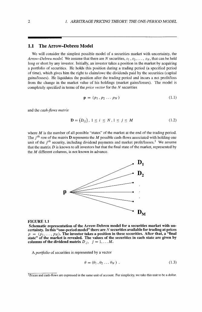
where M is the number of all possible "states" of the market at the end of the trading period. The j th row of the matrix D represents the M possible cash-flows associated with holding one unit of the j th security, including dividend payments and market profit/losses.l We assume that the matrix D is known to all investors but that the final state of the market, represented by the M different columns, is not known in advance.

FIGURE 1.1 Schematic representation of the Arrow-Debreu model for a securities market with un-

certainty. In this "one-period model" there are N securities available for trading at prices p = ( p i , . . . , pN) . The investor takes a position in these securities. After that, a "final state" of the market is revealed. The values of the securities in each state are given by columns of the dividend matrix D,, j , j = 1, . . . M.

A portfolio of securities is represented by a vector

lPrices and cash-flows are expressed in the same unit of account. For simplicity, we take this unit to be a dollar.

1 .l. THE ARROW-DEBREU MODEL 3

Here, represents the number of units of the i f h security held in the portfolio. If Oi is positive, the investor is long the security and hence has acquired the right to receive the corresponding cash-flow Oi Di,, at the end of the period. If Oi is negative, the investor is short the security and thus will have a liability at the end of the trading period. (Short positions are taken by borrowing securities and selling them at the market price.) It is assumed that all investors can take short and long positions in arbitrary amounts of securities. Transaction costs, commissions and tax implications associated with trading are neglected. For simplicity, we assume that the amounts Qi held long or short are not necessarily integers, but instead arbitrary real numbers.

The price of a portfolio 8 is N

Q . P = C ~ ~ P ~ , 1

and the cash-flow for this portfolio in the j th "state" of the market will be

We can express mathematically the concept of arbitrage opportunity within this simple model.

DEFINITION 1.1 An arbitrage portfolio is a portfolio 0 such that either ( i )

and 8 . D,,j > 0 for some 1 I j I M

and 0 . D,,, L 0 for all 1 5 j 5 M .

In plain words, an arbitrage portfolio is a position in the market that either (i) has zero initial cost, has no "down side" regardless of the market outcome, and offers a possibility of realizing a profit, or (ii) realizes an immediate profit for the investor and has no down side. We remark here that the distinction between the two cases is not really important: it is a consequence of the general form of the model, in which the nature of the "securities" is not specified. If it is possible to lend money (buy bonds), then the second case reduces to the first, because the investor can lend out the initial profit and then realize a positive cash-flow at the end of the trading period.

THEOREM 1.1 If there exists a vector of positive numbers

4

such that

1. ARBITRAGE PRICING THEORY: THE ONE-PERIOD MODEL

M

pi = C Dij ? j for all 1 5 i 5 N , I

there exist no arbitrage portfolios.2 Conversely, if there are no arbitrage portfolios, there exists a vector n with positive entries satisfying ( 1 . 5 ~ ) and (1.5b).

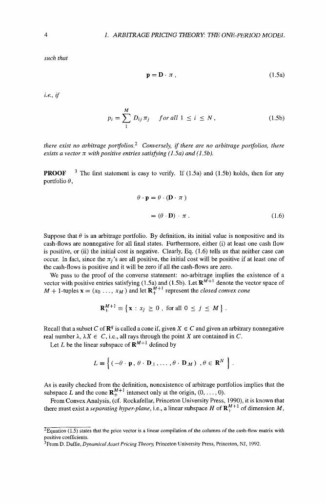
PROOF The first statement is easy to verify. If (1.5a) and (1.5b) holds, then for any portfolio 8,

Suppose that 8 is an arbitrage portfolio. By definition, its initial value is nonpositive and its cash-flows are nonnegative for all final states. Furthermore, either (i) at least one cash flow is positive, or (ii) the initial cost is negative. Clearly, Eq. (1.6) tells us that neither case can occur. In fact, since the nj's are all positive, the initial cost will be positive if at least one of the cash-flows is positive and it will be zero if all the cash-flows are zero.

We pass to the proof of the converse statement: no-arbitrage implies the existence of a vector with positive entries satisfying (1.5a) and (1.5b). Let R M f l denote the vector space of M + 1-tuples x = (xo . . . , X M ) and let R Y f l represent the closed convex cone

RY" = {x : xj >_ 0 , for all 0 5 j 5 M }

Recall that a subset C of R4 is called a cone if, given X E C and given an arbitrary nonnegative real number h, hX E C, i.e., all rays through the point X are contained in C.

Let L be the linear subspace of R M f l defined by

As is easily checked from the definition, nonexistence of arbitrage portfolios implies that the subspace L and the cone R Y f l intersect only at the origin, (0, . . . ,0) .

From Convex Analysis, (cf. Rockafellar, Princeton University Press, 1990), it is known that there must exist a separating hyper-plane, i.e., a linear subspace H of RY" of dimension M ,

2~quation (1.5) states that the price vector is a linear compilation of the columns of the cash-flow matrix with positive coefficients. 3 ~ r o m D. Duffie, Dynamical Asset Pricing Theory, Princeton University Press, Princeton, NJ, 1992.

1.1. THEARROW-DEBREUMODEL

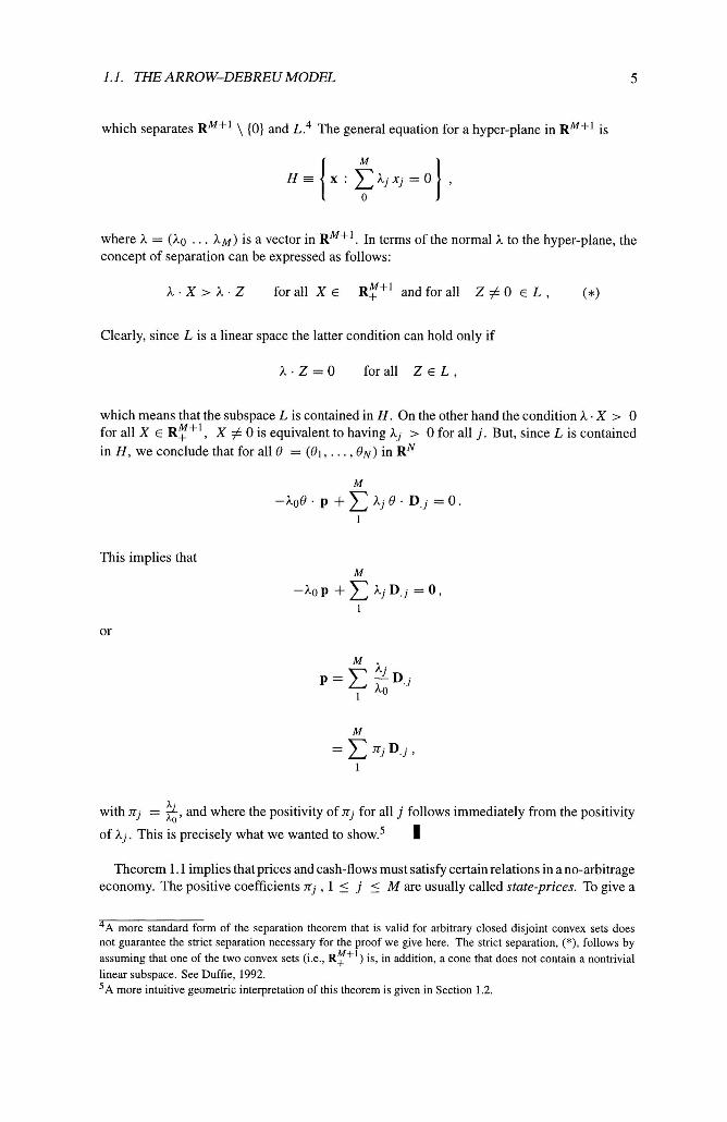
which separates RM+' \ (0) and L . ~ The general equation for a hyper-plane in RM+l is

where h = (Ao . . . AM) is a vector in RM". In terms of the normal h to the hyper-plane, the concept of separation can be expressed as follows:

h . X > h . Z for all X E ~7 ' ' and for all Z # 0 E L , (*)

Clearly, since L is a linear space the latter condition can hold only if

which means that the subspace L is contained in H. On the other hand the condition h . X > 0 for all X E R?", X # 0 is equivalent to having hj > 0 for all j. But, since L is contained in H, we conclude that for all 6' = (81, . . . , O N ) in R~

This implies that

or

h . with nj = *, and where the positivity of nj for all j follows immediately from the positivity

of hi. This is precisely what we wanted to show.5 1

Theorem 1.1 implies that prices and cash-flows must satisfy certain relations in a no-arbitrage economy. The positive coefficients nj , 1 5 j 5 M are usually called state-prices. To give a

4~ more standard form of the separation theorem that is valid for arbitrary closed disjoint convex sets does not guarantee the strict separation necessary for the proof we give here. The strict separation, (*), follows by assuming that one of the two convex sets (i.e., R:") is, in addition, a cone that does not contain a nontrivial linear subspace. See Duffie, 1992. 5~ more intuitive geometric interpretation of this theorem is given in Section 1.2.

6 1. ARBITRAGE PRICING 131EORY THE ONE-PERIOD MODEL

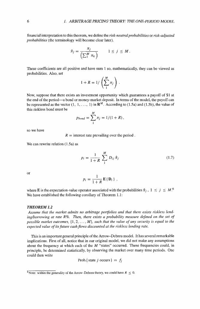
financial interpretation to this theorem, we define the risk-neutralprobabilities or risk-adjusted probabilities (the terminology will become clear later).

These coefficients are all positive and have sum 1 so, mathematically, they can be viewed as probabilities. Also, set

Now, suppose that there exists an investment opportunity which guarantees a payoff of $1 at the end of the period-a bond or money-market deposit. In terms of the model, the payoff can be represented as the vector (1, 1, . . . , 1) in R ~ . According to (1.5a) and (1.5b), the value of this riskless bond must be

M

Pbond = x~lj = 1/(1 + R) 1

so we have R = interest rate prevailing over the period .

We can rewrite relation (1.5a) as

where E is the expectation-value operator associated with the probabilities j?i , 1 5 j ( M . ~ We have established the following corollary of Theorem 1.1:

THEOREM 1.2 Assume that the market admits no arbitrage portfolios and that there exists riskless lend-

inghorrowing at rate R%. Then, there exists a probability measure dejned on the set of possible market outcomes, (1,2, . . . , M } , such that the value of any security is equal to the expected value of its future cash flows discounted at the riskless lending rate.

This is an important general principle of the Arrow-Debreu model. It has several remarkable implications. First of all, notice that in our original model, we did not make any assumptions about the frequency at which each of the M "states" occurred. These frequencies could, in principle, be determined statistically, by observing the market over many time periods. One could then write

Prob.{ state j occurs } = fi

6 ~ o t e : within the generality of the Arrow-Debreu theory, we could have R 5 0.

1. I . THE ARROW-DEBREU MODEL 7

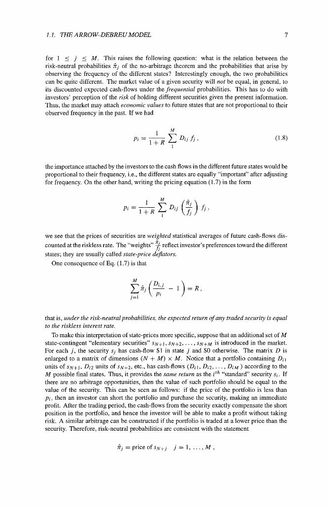
for 1 5 j ( M . This raises the following question: what is the relation between the risk-neutral probabilities $j of the no-arbitrage theorem and the probabilities that arise by observing the frequency of the different states? Interestingly enough, the two probabilities can be quite different. The market value of a given security will not be equal, in general, to its discounted expected cash-flows under the frequential probabilities. This has to do with investors' perception of the risk of holding different securities given the present information. Thus, the market may attach economic values to future states that are not proportional to their observed frequency in the past. If we had

the importance attached by the investors to the cash flows in the different future states would be proportional to their frequency, i.e., the different states are equally "important" after adjusting for frequency. On the other hand, writing the pricing equation (1.7) in the form

we see that the prices of securities are weighted statistical averages of future cash-flows dis-

counted at the riskless rate. The "weights" 9 reflect investor's preferences toward the different states; they are usually called state-price dejators.

One consequence of Eq. (1.7) is that

that is, under the risk-neutral probabilities, the expected return of any traded security is equal to the riskless interest rate.

To make this interpretation of state-prices more specific, suppose that an additional set of M state-contingent "elementary securities" s ~ + l , SN+2, . . . , SN+M is introduced in the market. For each j, the security sj has cash-flow $1 in state j and $0 otherwise. The matrix D is enlarged to a matrix of dimensions (N + M ) x M . Notice that a portfolio containing Dil units of s ~ + l , Di2 units of SN+2, etc., has cash-flows ( D i l , Di2, . . . , D ~ M ) according to the M possible final states. Thus, it provides the same return as the i th "standard" security si. If there are no arbitrage opportunities, then the value of such portfolio should be equal to the value of the security. This can be seen as follows: if the price of the portfolio is less than pi, then an investor can short the portfolio and purchase the security, making an immediate profit. After the trading period, the cash-flows from the security exactly compensate the short position in the portfolio, and hence the investor will be able to make a profit without taking risk. A similar arbitrage can be constructed if the portfolio is traded at a lower price than the security. Therefore, risk-neutral probabilities are consistent with the statement


in the sense that we must have M

for all i , which is precisely Eq. (1.5b). We conclude that state-prices can be interpreted as a set of market prices for "state-contingent claims" that pay $ 1 in state j and zero otherwise, for 1 5 j 5 M, supporting the notion that state-prices correspond to the prices of wealth in the different states. Notice then that the risk-neutral probabilities are those that "make the investor risk-neutral," given the prices of wealth of the different states.

Example 1.2 Let us assume a hypothetical presidential election with candidates from two political

parties, A and B. Historically, there have been equal numbers of presidents from either party. On the other hand, a well-known and reputable book-maker (English, of course) is giving the following odds for each candidate: candidate from party A: 3-5; candidate from Party B: 1-4 (i.e., a gambler wins $4 for every dollar he risks if Party B wins). Given the historical information, the frequential probabilities are, of course, fA = f B = .5. However, from the point of view of the bookie, the "odds-probabilities" are

5 n A = const. x - , n B = const. x 4 ,

3

which gives, after computing the unknown constant,

n~ = ,2942 , n~ = .7058 .

The latter can be interpreted as "risk-neutral" or "state-price" probabilities. Suppose, for instance, that an individual who is unaware of the bookmaker's odds offers you equal odds on candidate of Party B winning (you bet $1 and receive $2 if B wins and $0 if A wins). You can immediately create an "arbitrage" by betting $2 x ,2942 = $.5882 on candidate A with the book-maker. In this case, you have guaranteed payoff $2 regardless of who wins the election at a cost of $1.5882, or a net profit of $.4117. 0

In conclusion, the fj 's are probabilities in a statistical sense, whereas the risk-neutral probabilities ?j's are "mathematical probabilities" used to calculate the market values of all securities, including "state-contingent" claims (i.e., derivatives), from their cash-flows. These two notions of probability should not be confused. The correct market values of securities are determined from the risk-neutral probabilities.

1.2 Security-Space Diagram: A Geometric Interpretation of Theorem 1.1

The Arrow-Debreu model with N traded securities and M final states can be visualized geometrically. This interpretation is slightly different than the one presented in the proof of Theorem 1.1: let R~ represent N-dimensional Euclidean space. Since there are M final states,

1.2 SECURITY-SPACE DIAGRAM 9

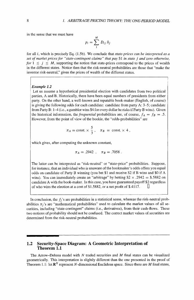
we can represent the final outcomes as M vectors D. 1, . . . , D. M , where the entries of each vector represent the final cash-flows of each traded security. (See Figure 1.2).

FIGURE 1.2

1 = D,, = D,,

The Arrow-Debreu model viewed geometrically. The "ambient space" has dimension N (the number of securities). The convex set K is the span of the M dividend (column) vectors which give the cash-flows of the securities in each of the M final states.

In addition, we can draw the price vector p as an element of this space. The absence of arbitrage corresponds to the price vector p lying in the interior of the convex cone K generated by the M cash-flow vectors, as shown in Figure 1.3.

In fact, if p would lie in the exterior or on the boundary of K, the separating hyper-plane theorem ensures that there exists linear subspace described by the equation

where n is an N-vector, which separates p from the interior of the convex cone generated by the D. ,'s. The separation property would imply (possibly after a change of the sign of n) the inequalities

p . n l O , D . , j . n > O

with at least one inner product positive for some j-i.e., an arbitrage. As in the discussion preceding Theorem 1.2, the existence of a bond or money-market

deposit can be used to pass from a convex cone to a bounded convex set in dimension N - 1. In fact, assume without loss of generality that the bond corresponds to the security with i = 1, so that all the D-vectors have the first entry equal to one (Dl j = 1). Denoting a generic vector in RN by

% = ( e l , e ) , e = ( ~ , , . . . 0,) ,

we can consider the intersection of the convex cone K with the hyper-plane in RN of vectors with first coordinate equal to p l , the price of the bond. This intersection is the convex set

1. ARBITRAGE PRICING THEORY: THE ONE-PERIOD MODEL

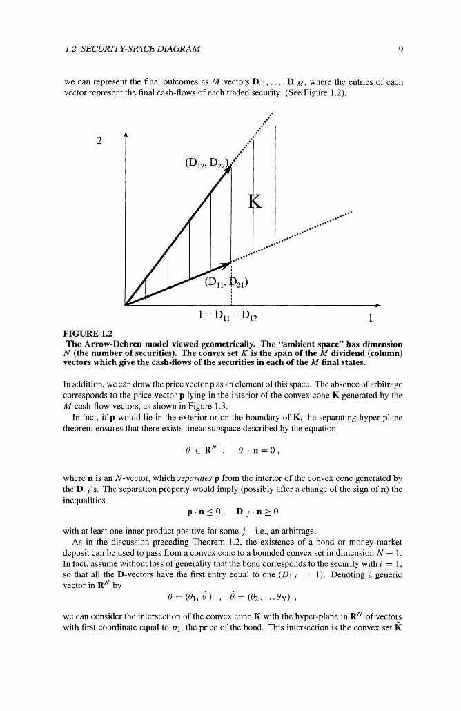
FIGURE 1.3 "No arbitrage" means that the price vector must lie in the convex cone K generated by the M cash-flow vectors corresponding the different final states. In the case M = 2, when one security is a riskless bond, the no-arbitrage condition means that the price of the stock, P2, satisfies * < P2 < A.

( I f R ) (1+R)

generated by the vectors

The no-arbitrage condition is then equivalent to stating that p lies in the interior of the convex set generated by these vectoq7 i.e.,

where the weights 2; are positive and sum to 1. (In the special case of Figure 1. l(b) the convex set K is a line segment.) Since, by definition, we have pl = &, the last formula is equivalent to Eq. (1.7).

' I~orne readers will recognize this result as a well-known result in game theory known as Farkas' lemma.

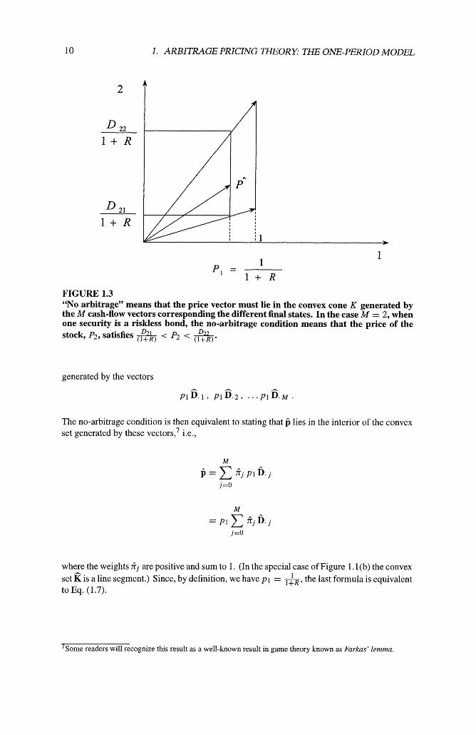
1.3. REPLICATION 11

1.3 Replication

The interpretation of state-prices as the values of elementary state-contingent claims is the basis for the valuation of derivative securities in a no-arbitrage market.

Given a security s , and a set of securities sl, sz, . . . , S K , we say that the portfolio (01, 02, . . . , OK), (representing holdings in each of the K securities) replicates s if the security and the portfolio have identical cash-flows. Under no-arbitrage conditions, the value of the security and of the replicating portfolio must be the same. Otherwise, an arbitrage could be realized either by shorting the portfolio and buying the security or, alternatively, by shorting the security and buying the portfolio. If the value of the portfolio is less than the value of the security, the first strategy is an arbitrage. If the portfolio is worth more than the security, the second strategy is an arbitrage. This argument gives rise to a simple but important valuation principle.

PROPOSITION 1.1 In a no-arbitrage market, i f a security admits a replicating portfolio of traded securities, its value is equal to the value of the replicating port$olio.

Here are some elementary applications of this principle.

Forward Prices. Suppose that a security has spot price P and that the yield for riskless lending over the trading period is R. Consider a forward contract, which consists of an agreement to purchase the security at the end of the trading period at price K . Assume that the security pays no dividends over the trading period. The no-arbitrage price of the forward contract is

To see this, consider a portfolio consisting of being long one unit of the security and short K l ( 1 + R) worth of riskless bonds. After the trading period, the holder of this portfolio will own the security and will owe $K. Therefore, if he receives K at the end of the final period he will be able to meet his cash obligation and deliver the security; he will have no profitJloss. The portfolio is equivalent to having long position in the forward contract. In practice, forward contracts are designed so that they have zero initial cost (Q = 0). The forwardprice, which is price for delivery of the security after the trading period, is

because K = F makes the initial cost zero.

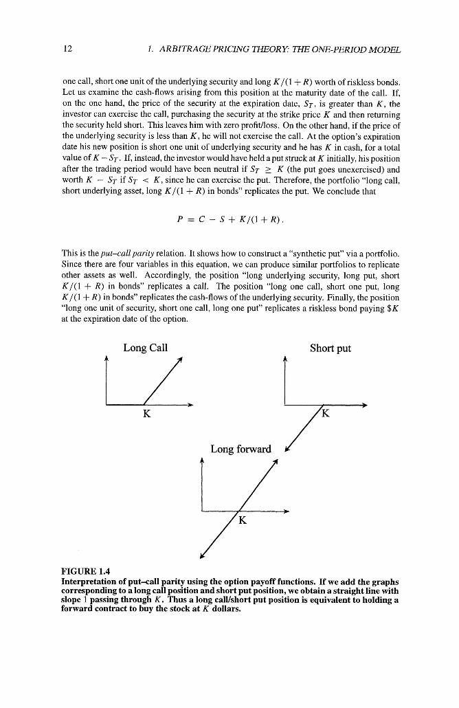
Put-Call Parity. This important example of replication involves options (see Figure 1.4). Suppose that a security with price S is traded as well as a call option and a put option with exercise price (strike price) K . Recall, from 1.1, that a call option is a contract that gives the holder the right, but not the obligation, to purchase (one unit of) the security at price K , at a stipulated date (expiration date). A put option gives the holder the right to sell the underlying security at price K at the maturity date. In this example, we assume that the call and the put have same strike prices and expiration dates. Denote the market prices of the call and the put by C and P, respectively. Let R be the interest paid for riskless lending over the duration of the option (compounded simply). Suppose that an investor has the following position: long


one call, short one unit of the underlying security and long K/(1+ R ) worth of riskless bonds. Let us examine the cash-flows arising from this position at the maturity date of the call. If, on the one hand, the price of the security at the expiration date, S T , is greater than K , the investor can exercise the call, purchasing the security at the strike price K and then returning the security held short. This leaves him with zero profit/loss. On the other hand, if the price of the underlying security is less than K, he will not exercise the call. At the option's expiration date his new position is short one unit of underlying security and he has K in cash, for a total value of K - ST . If, instead, the investor would have held a put struck at K initially, his position after the trading period would have been neutral if ST 2 K (the put goes unexercised) and worth K - ST if ST < K, since he can exercise the put. Therefore, the portfolio "long call, short underlying asset, long Kl (1 + R ) in bonds" replicates the put. We conclude that

This is relation. It shows how to construct a "synthetic put" via a portfolio. Since there are four variables in this equation, we can produce similar portfolios to replicate other assets as well. Accordingly, the position "long underlying security, long put, short Kl (1 + R ) in bonds" replicates a call. The position "long one call, short one put, long K/(1+ R) in bonds" replicates the cash-flows of the underlying security. Finally, the position "long one unit of security, short one call, long one put" replicates a riskless bond paying $K at the expiration date of the option.

Long Call Short put

FIGURE 1.4 Interpretation of put-call parity using the option payoff functions. If we add the graphs corresponding to a long call position and short put position, we obtain a straight line with slope 1 passing through K. Thus a long calYshort put position is equivalent to holding a forward contract to buy the stock at K dollars.

1.4. THE BINOMIAL MODEL 13

1.4 The Binomial Model

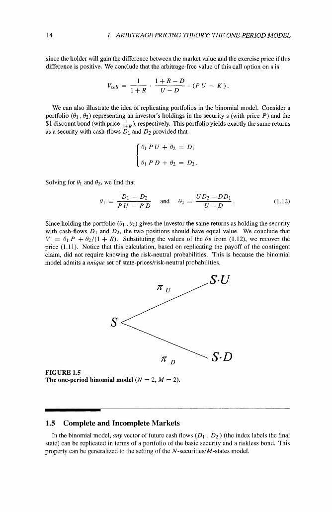
We present the simplest case of the Arrow-Debreu model (see Figure 1.5). Consider an ideal situation in which there are only two states (M = 2) and two securities: a bond with yield R% and a security (s) with price P. We assume that the cash-flows of this security in states 1 and 2 are P U and P D , respectively, where U and D are given numbers and D < U . If there are no arbitrage opportunities, we must have

where 721 and $2 are positive and + 722 = 1. Thus, the risk-neutral probabilities satisfy

It is easy to see that this system will have positive solutions if and only if

This is intuitively clear: if 1 + R 2 U , the return on riskless lending is greater than or equal to the return for investing in the risky security, regardless of the final state. An arbitrage could then be achieved by shorting the security and lending out the proceeds at the riskless rate. Similarly, if 1 + R I. D, the investor can make a riskless profit by borrowing at the riskless rate and purchasing the security. Suppose that (1.9) holds. The solution of the linear system is

A 1 + R - D A U - 1 - R nl = , 772 = (1.10)

U - D U - D

Thus, the risk-neutral probabilities are entirely determined from the parameters of the binomial model. The actual probabilities of occurrence of each state are irrelevant in the pricing process (as long as neither one is zero-we must assume that both states can occur).

This has interesting consequences. Suppose now that we augment the number of traded securities (the number of final states is still M = 2). Then, the price of any security is completely determined by future cash-flows because the risk-neutral probabilities are still given by (1.10). A "state-contingent" security which has cash-flows Dl in state 1 and D2 in state 2 must have value V, where

This idea can be applied to price any security contingent on the value of s. For instance, a "call option" on s with exercise price K (with P D < K < P U) has cash-flows

14 I. ARBITRAGE PRICING THEORY: THE ONE-PERIOD MODEL

since the holder will gain the difference between the market value and the exercise price if this difference is positive. We conclude that the arbitrage-free value of this call option on s is

1 1 + R - D Vcail = - . ( P U - K ) .

l + R U - D

We can also illustrate the idea of replicating portfolios in the binomial model. Consider a portfolio (01 , 02) representing an investor's holdings in the security s (with price P ) and the $1 discount bond (with price A), respectively. This portfolio yields exactly the same returns as a security with cash-flows Dl and D2 provided that

Solving for 01 and 02, we find that

Dl - D2 UD2 - DD1 Q1 = and e2 =

P U - P D U - D

Since holding the portfolio (81 , Q2) gives the investor the same returns as holding the security with cash-flows Dl and D2, the two positions should have equal value. We conclude that V = 01 P + 82/(1 + R). Substituting the values of the 0s from (1.12), we recover the price (1.11). Notice that this calculation, based on replicating the payoff of the contingent claim, did not require knowing the risk-neutral probabilities. This is because the binomial model admits a unique set of state-pricesfrisk-neutral probabilities.

FIGURE 1.5 The one-period binomial model (N = 2, M = 2).

1.5 Complete and Incomplete Markets

In the binomial model, any vector of future cash flows (Dl , D2 ) (the index labels the final state) can be replicated in terms of a portfolio of the basic security and a riskless bond. This property can be generalized to the setting of the N-securitieslM-states model.

1.5. COMPLETE AND INCOMPLETE MARKETS 15

DEFINITION 1.2 jow vector ( D l , D2, that has cash-$ow Dj

A securities market with M states is said to be complete 8 for any cash- . . . , DM), there exists a portfolio of traded securities (01, 62, . . . , QN) in state j , for all 1 5 j 5 M.

Market completeness is therefore equivalent to having a cash-flows matrix D = (DCj) with the property that the system of linear equations

has a solution 9 E R N for any E E RM. From Linear Algebra, we know that this property is satisfied if and only if

rank D = M ,

which is equivalent to saying that the column vectors of the matrix D span the entire space RM. Market completeness is a very strong assumption, which greatly simplifies the valuation of derivative securities. Derivative securities can be represented by general cash-flow vectors ( D l , D2, . . . , DM), as opposed to the N "standard securities" that have cash-flow vectors ( Di l , Di2, . . . , DiM), for 1 5 i 5 N. Since any derivative security is equivalent to a portfolio of standard traded assets, its price is fully determined from E in the absence of arbitrage. More formally, we have

PROPOSITION 1.2 Suppose that the market is complete and that there are no arbitrage opportunities. Then

there is a unique set of state-prices ( n l , n2, . . . , n M ) satisfying ( 1 . 5 ~ ) and (1.5b), and hence a unique set of risk-neutral probabilities (Sl , S2 , . . . , SM). Conversely, if there is a unique set of state-prices, then the market is complete.

PROOF The no arbitrage hypothesis implies the existence of a vector n such that p = Dn. If the market is complete the rank of Dt (the superscript "t" indicates the transposed matrix) is M . Therefore, the kernel of D is trivial and the equation p = Dn has a unique solution for a. This fact together with the interpretation that we gave below Theorem 1.2 of the state-price vector n as the price of the state-dependent contingent claims implies that the price of a state contingent claim that pays $1 in the j th state of the world and zero otherwise is completely determined for all j . Therefore, there can be at most one set of state-prices. If they exist, state-prices are unique.

To prove the converse statement, suppose that there exists a unique vector of state-prices n = (n l , n2, . . . , n~ ) (with strictly positive entries) such that (1.5a) and (1.5b) are satisfied. We will argue that the market is complete by contradiction. In fact, if the market is not complete, then rank D < M . From Linear Algebra, we know that the matrix D must have a nonempty right-null space, i.e., there exists h = (A], h2, . . . , hM ) such that


or, equivalently, M

Dij .Xi = 0 , for all 1 5 i 5 N 1

Using the no-arbitrage relation (1.5a) and (1.13), we conclude that

for all real numbers p. Since the entries of n are strictly positive, we can choose p sufficiently small so that Ti + p hi is positive for all j. Therefore, we have constructed a new state-price vector, contradicting our hypothesis. We conclude that, in a no-arbitrage market, uniqueness of state-prices implies that the market is complete. 1

The above argument can also be used to characterize the set of state-price vectors corresponding to an incomplete market with given price vector p and cash-flow matrix D. Let k = rank D. In an incomplete market, we have M - k > 0. Notice that k is the dimension of the right-null space of D. Given two state-price vectors n(') and n(2) and p such that 0 ( p 5 1, the convex combination p n(') + ( 1 - p) n(') is also a state-price vector. Hence, the set of all state-price vectors is convex. Moreover, in the proof of the Proposition, we showed that each state-price vector is contained in a (M - k)-dimensional neighborhood inside this cone. Consequently, the set of admissible state-price vectors is an open cone in an (M - k)-dimensional afine subspace of R ~ .

What is the financial meaning of a complete/incomplete market? In a complete market there is a unique set of state-prices. However, in real markets it is usually impossible to completely identify the set of final states or quantify the investors' preferences toward different states. Mar- ket completeness is a convenient idealization of the behavior of securities markets. Incomplete markets-with many possible price structures satisfying the no-arbitrage condition-are the rule rather than the exception.

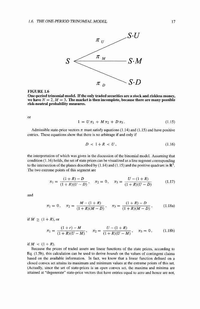
1.6 The One-Period Trinomial Model

We describe a simple example of an incomplete market (Figure 1.6). Assume that there are two securities-a riskless bond with yield R paying $1 at the end of the trading period and a security s. There are three states, which correspond to different cash-flows for s. We assume that the price of s is P and that the cash-flows of s are P U in state 1, P M in state 2, and P D in state 3, with

D < M < U .

Clearly, this market is incomplete, because the dimension of the cash-flows matrix is 3 x 2 (if there are more states than traded securities, the market is always incomplete). We can investigate the conditions for the existence of state-prices. Since we have assumed that there is riskless lending, we have

1 = nl +n2 +n3, (1.14)

1 + R

for any admissible set of state-prices. Since there is no arbitrage, we must have

1.6. THE ONE-PERIOD TRINOMIAL MODEL

FIGURE 1.6 One-period trinomial model. If the only traded securities are a stock and riskless money, we have N = 2, M = 3. The market is then incomplete, because there are many possible risk-neutral probability measures.

Admissible state-price vectors n must satisfy equations (1.14) and (1.15) and have positive entries. These equations show that there is no arbitrage if and only if

the interpretation of which was given in the discussion of the binomial model. Assuming that condition (1.16) holds, the set of state prices can be visualized as a line segment corresponding to the intersection of the planes described by (1.14) and (1.15) and the positive quadrant in R ~ . The two extreme points of this segment are

and

i f M < (1 + R). Because the prices of traded assets are linear functions of the state prices, according to

Eq. (1.5b), this calculation can be used to derive bounds on the values of contingent claims based on the available information. In fact, we know that a linear function defined on a closed convex set attains its maximum and minimum values at the extreme points of this set. (Actually, since the set of state-prices is an open convex set, the maxima and minima are attained at "degenerate" state-price vectors that have entries equal to zero and hence are not,


strictly speaking, state-prices.) To illustrate this, consider the case of a call option on the basic security s with strike price K . To fix ideas, assume that P M < K < P U . Then, the cash-flows for this option are P U - K in state 1 and 0 in states 2 and 3. Its no-arbitrage value is C = nl ( P U - K). Therefore, using (1.17), (1.18a) and (1.18b), we find that

is an upper bound for the price of the option. If M > (1 + R) the lower bound on the price is C- = 0 , and if M < (1 + R), the lower bound is

(Of course, the upper and the lower bounds coincide when M = D, and we recover the result of the binomial model.)

This example shows an important application of state prices as a tool for contingent claim valuation in incomplete markets. State prices are not unique but can nevertheless be used to obtain partial information about fair prices. This result can be interpreted financially in terms of risk-aversion of different agents. A market participant that does not want to incur any risk will bid (be willing to buy) the security at the price corresponding to the lower bound C- and will offer (be willing to sell) the security at the price corresponding to the upper bound C+. Since there is incomplete information about Arrow-Debreu prices, transactions made between the bounds imply a risk for the buyer as well as for the seller.

1.7 Exercises

1. Consider a hypothetical country where the government has declared a "currency band" policy, in which the exchange rate between the domestic currency, denoted by XYZ, and the U.S. dollar is guaranteed to fluctuate in a prescribed band, namely

U S D 0 . 9 5 5 X Y Z 5 U S D 1.05,

for at least 1 year. Suppose also that the government has issued 1-year notes denominated in the domestic currency that pay a simply compounded annualized rate of 30%. Assuming that the corresponding interest rate for U.S. deposits is 6%, show that this market is not arbitrage-free in the "pure" sense. Describe the situation in terms of the Arrow-Debreu model. Propose some realistic scenarios that could make this pure arbitrage disappear in practice.

2. (i) Show that the set of all probability measures on a finite state-space of M elements can be represented as a convex subset P of the Euclidean space RM. Given a security s defined by its price and its cash-flows, verify that the set of measures which are risk-neutral for this security corresponds to the intersection of the set P with a hyper-plane in RM. Similarly, show that the set of admissible risk-neutral measures for a securities market with N securities corresponds to the intersection of P with N hyper-planes.

1.7. EXERCISES 19

(ii) Apply this analysis to the trinomial model of Section 1.6-assuming that S = $100, U = 1.10, M = 1.00, D = .80, R = .05 and that a call option with strike $105 is trading at a premium of C = $3.80. Show that if, instead, C = $1.00, there is an arbitrage opportunity.

3. On the week of September 7, 1996, Ladbroke, a London bet-maker, gave the following odds regarding the upcoming U.S. presidential election: Clinton 1-6, Dole 7-2, Perot 1- 50. (For instance, Ladbroke pays £1 for every £6 bet on Clinton if he wins.) Calculate the corresponding risk-neutral probabilities for the victory of each candidate assuming that one of them will necessarily win.

References and Further Reading

[I] Arrow, K. (1952), Le Role des valeurs boursieres pour la r6partition des risques, Econometric, Colloque International C.N.R.S.

[2] Arrow, K. (1970), Essays in the Theory of Risk Bearing, North-Holland, London.

[3] Arrow, K. and Debreu, G. (1954), Existence of an Equilibrium for a Competitive Econ- omy, Econometrics 22, pp. 265-290.

[4] Debreu, G. (1959), Theory of Value: An Axiomatic Analysis of Economic Equilibrium, Yale University Press, New Haven, CT.

[5] Drbze, J. (Winter 1970-I), Market Allocation under Uncertainty, European Economic Review, pp. 133-165.

[6] Duffie, D. (1992), Dynamical Asset Pricing Theory, Princeton University Press, Prince- ton, NJ.

[7] Ross, S. (1978), A Simple Approach to the Valuation of Risky Streams, Journal of Business 5 1, pp. 453-475.

[8] Varian H.R. (1992), Microeconomic Analysis, W.W. Norton & Co., New York, 3rd ed.

http://taylorandfrancis.com

References

Copyright Page

Printed on acid-free paper

Contents

vi CONTENTS

Index313

Introduction

my wife Magda and my mother Steffi for their unconditionalsupport over the years.

Peter Laurence

1 Chapter 1. Arbitrage Pricing Theory:The One- Period Model

(ii) Apply this analysis to the trinomial model of Section1.6-assuming that S =$100, U=

1.10, M =1.00, D =.80, R =.05 and that a call option withstrike $105 is trading at a

premium of C =$3.80. Show that if, instead, C =$1.00,there is an arbitrage opportunity.

3. On the week of September 7, 1996, Ladbroke, a Londonbet-maker, gave the following

odds regarding the upcoming U.S. presidential election:Clinton 1-6, Dole 7-2, Perot 1-

50. (For instance, Ladbroke pays £1 for every £6 bet onClinton if he wins.) Calculate the

corresponding risk-neutral probabilities for the victory ofeach candidate assuming that one of

them will necessarily win.

[I] Arrow, K. (1952), Le Role desvaleursboursierespour lar6partitiond e s risques, Econometric, ColloqueInternational C.N.R.S.

[2] Arrow, K. (1970), EssaysintheTheoryofRiskBearing,North-Holland, London.

[3] Arrow, K. and Debreu, G. (1954), Existence of anEquilibrium for a Competitive Econ- omy, Econometrics22,pp. 265-290.

[4] Debreu, G. (1959), Theoryof Value: AnAxiomaticAnalysisof EconomicEquilibrium, Yale UniversityPress, New Haven, CT.

[5] Drbze, J. (Winter 1970-I), Market Allocation underUncertainty, EuropeanEconomic R e v i e w , pp. 133-165.

[6] Duffie, D. (1992), Dynamical AssetPricing T h e o r y, Princeton University Press, Prince- ton, NJ.

[7] Ross, S. (1978), A Simple Approach to the Valuation ofRisky Streams, Journalof Business 5 1, pp. 453-475.

[8] Varian H.R. (1992), MicroeconomicAnalysis,W.W. Norton&Co., New York, 3rd ed.

2 Chapter 2. The Binomial Option PricingModel

The next chapter analyzes in greater detail theBlack-Scholes formula and its implications.

FIGURE2.6

Value of a 6-month call option for different volatilityvalues. The strike price is $90, the

interest rate is 5%and the volatilities are 10 %, 20 %, 30%and 40 %. The value of the

call increases with the volatility.

2.6. T H E B L A C K S C H O L E S F O R M U L A 39

In particular, we will focus on the effect of volatility onthe value of an option and on the

composition of the equivalent portfolio.

[I] Black, F., and Scholes, M. (1973), The pricing ofoptions and corporate liabilities, JournalofPoliticalEconomy,8 1 , pp. 637-659.

[2] Cox, J. and Rubinstein, M. (1985), O p t i o nTheory,Prentice-Hall, Englewood Cliffs, NJ.

[3] Cox, J., Ross, S., and Rubinstein, M. (1979), Optionpricing: a simplified approach, JournalofFinancialEconomics,7 , pp. 229-264.

[4] Duffie, D. and Protter, P. (1988), From discrete tocontinuous time finance: Weak convergence of thefinancial gain process, MathematicalFinance,1 , pp. 1-16.

[5] Merton, R.C. (1973), Theory of rational optionpricing, BellJournalofE c o n o m i c s and ManagementS ci e n c e , 4 , pp. 141-183.

3 Chapter 3. Analysis of theBlack-Scholes Formula

and t varying from 0 to T ) gives rise to a function?A, defined on the binomial tree, which

can be regarded as an "approximate solution" of the basicbackward-induction Eq. ( 3 . 2 3 ) . The

point is that at each time step, the error is of order atmost d t 3 I 2 . We conclude that the total

discrepancy between V / and ?/ is of order d t 3 I 2 =0( d t 1 I 2 ) . This result is important,

since it shows that the binomial model can be viewed as anumerical scheme for solving the

Black-Scholes equation.

[ I ] Black, F. and Scholes, M. ( 1 9 7 3 ) , The Pricingof Options and Corporate Liabilities, JournalofPoliticalEconomy,8 1 , pp. 637-659.

[ 2 ] Figlewski, S., Silber, W., and Subrahmanyam, M. ( 1 99 0 ) , FinancialO p t i o n s : From T h e o r y t oPractice, Business One Irwin, Homewood, IL.

[ 3 ] Hull, J. ( 1 9 9 8 ) , Introductiont oFuturesandOptionsMarkets,Prentice-Hall, Upper SaddleRiver, NJ.

[ 4 ] Jarrow, R. ( 1 9 8 3 ) , O p t i o n Pricing,R.D.Irwin, Homewood, IL.

7 ~ o t i c e that this argument uses the fact that V ,is the derivative with respect to c a l e n d a r t i m eand V T =-Vt

is the derivative with respect to the time to maturity.Also, the error estimate of order d t 3 / * is derivedassuming

that higher-order derivatives of V(S, t) are bounded,which is true if F(S) is smooth. The extension to F(S) =

max(S -K, 0) requires a slightly more involved argumentnear t =T.

4 Chapter 4. Refinements of the BinomialModel

recursion relation that we seek follows from the followingobservation: at any given time,

the value of the derivative security is equal to thecurrent "coupon" value plus the discounted

expectation of future cash flows. Therefore, we have

Thus, solving a single recursive relation, we can computethe theoretical value of such contin-

gent claims.

[I] Boyle, P.P. (March 1988), A Lattice Framework forOption Pricing with Two State Variables, Journal ofFinancial and QuantitativeAnalysis,23, pp. 1-12.

[2] Cox, J., Ross, S., and Rubinstein, M. (October 1979),Option Pricing: A Simplified Approach, Journal ofFinancial Economics,7 , pp. 229-264.

ere, we assume that .f,(S) =0 if there are no cash flowsdue on a particular date. For example, a European

call with strike K and expiration date t n has ,fi (S) =0if j#nand fn (S) =max(S -K, 0).

5 Chapter 5. American-Style Options,Early Exercise, and Time- Optionality

date, then the hedger faces very little "slippage r i s kacross the exercise boundary. Of course,

the risk increases as t -+ 0 due to the fact that S ( t )-t K , which is a point of discontinuity

of A . (This is the usual "pin r i s k problem forat-the-money options near expiration.)

[I] Barone-Adesi, G. and Whaley, R. (June 1987), EfficientAnalytic Approximation of American Option Values, JournalofFinance, 42,pp. 301-20.

[2] Barone-Adesi, G. and Whaley, R. (1987), On theValuation of American Put Options on Dividend PayingStocks, AdvancesinFutures OptionsResearch,3 , pp. 1-14.

[3] Bensoussan, A. (1984), On the Theory of OptionPricing, ActaAppliedMathematics,2, pp. 139-158.

[4] Black, F. and Scholes, M. (MayIJune 1973), The Pricingof Options and Corporate Liabilities, Journal ofPolitical Economy,81,pp. 637-54.

[5] Brennan, M. and Schwartz, E. (1977), The Valuation ofAmerican Options, Journalof Finance, 32, pp. 449462.

[6] Cox, J., Ross, S., and Rubinstein, M. (1979), OptionPricing: A Simplified Approach, Journalof FinanceEconomics,7 , pp. 229-263.

[7] Geske, R. and Johnson, H.E. (December 1984), TheAmerican Put Option Valued Ana- lytically, Journal ofFinance, 39,pp. 151 1-24.

[8] Harrison, J.M. and Kreps, D. (1979), Martingales andArbitrage in Multiperiod Security Markets, Journal ofEconomicTheory,2 0 , pp. 381-408.

[9] Johnson, H. (1983), An Analytic Approximation of theAmerican Put Price, Journalof FinancialQuantitativeAnalysis, 18,pp. 141-148.

[lo] Karatzas, I. (1988), On the Pricing of AmericanOptions, AppliedMathand Optimization, 17,pp. 37-60.

[l 11 Lamberton, D. and Lapeyre, B. (1996), Introductiont

o StochasticCalculusAppliedto Finance, Chapman &Hall,London.

A P P E N D I X 89

[12] MacMillan, L. (1986), Analytic Valuation for theAmerican Put Option, A d v a n c e s Fut u r e s andO p ti o n s Research, 1,pp. 119-139.

[13] Omberg, E. (1987), The Valuation of American Putswith Exponential Exercise Policies, A d v a n c e s i nFuturesOptionsResearch,2,pp. 117-142.

[14] Parkinson, M. (January 1997), Option Pricing: TheAmerican Put, JournalofBusiness, 50,pp. 21-36.

[IS] Samuelson, P. and McKean, H.P. (Spring 1966), RationalTheory of Warrant Pricing: A Free Boundary Problem for theHeat Equation Arising from a Problem in MathematicalEconomics, IndustrialManagementReview,6, no. 2 .

[16] Van Moerbeke, P. (1976), On Optimal Stopping and FreeBoundary Problems, Archive f o r RationalMechanicsandA n al y s i s , 60,pp. 101-148.

[17] Wilmott, P., Dewynne, J.N., and Howison, S.D. (1995),O p t i o n Pricing:M a t h e m a t i c a l M e t h o d sandC o m p u t a t i o n , Oxford Financial Press.

Appendix: A PDE Approach tothe Free-Boundary Condition

Condition (5.3) at the beginning of this chapter relativeto an arbitrary initial time t , reads V,, =sup El { e "M a x ( ~ , -K , O ) } , O _ i r _ i T

or equivalently that V , , > E t { e " M a x ( ~ , -K ,~ ) } f o r a l l t : t 5t j T ('4.2)

where E t is the conditional expectation given theinformation at time t . This inequality can be

shown to be equivalent to the partial differentialinequality

where Pis the value of the put discounted to time t I j=e r f p

The equivalence of (A.3) and (A.2) is not surprising, sinceit is analogous to the equivalence,

demonstrated in Chapter 3, of relation (A.2) when there isequality and the Black-Scholes

equation, i.e., (A.3) with equality. For a more detaileddiscussion of this point we refer to the

article of ~ ~ e n i . ~

' ~ c t u a l l ~ a precise derivation of (A.3)establishes first that it holds in the sense ofdistributions or weak solutions.

90 5. AMERICAN-STYLE OPTIONS

A . l AProof of the Free Boundary Condition

In this appendix we show, in the case of an American put,the equivalence of the PDE (5.2)

with the free boundary condition (5.15). In this case thefree boundary condition a P lim -(S, t) =-1 S + S ~ ( ~) as

is satisfied.

Let C correspond to the operator

where we have replaced S by x for simplicity. In thisnotation (A.3) reads C[e-'l P(S, t)] 50 (S, t) E 8' x [0,TI. (A.4)

To facilitate the analysis, we introduce the new variable t=In S, whose effect is to transform

the differential (A.4) into one with constant coefficients.

We get o2 A < r k t F t + r F . ~ p c c -(T)

Also note that in the new variables the free boundarycondition P, =-1 reads =-ec .

Now we consider aregion ~ 2 " ~ that is a small strip ofwidth 6around the free boundary St =

a{(<, t ) :P ( x , t) LO}, which istheimage of the freeboundary S =a{(S, t) :P ( S , t) 20) in

the ( t , t) plane. We will integrate the expression (AS)over ~ 2 " ~ and derive the free boundary

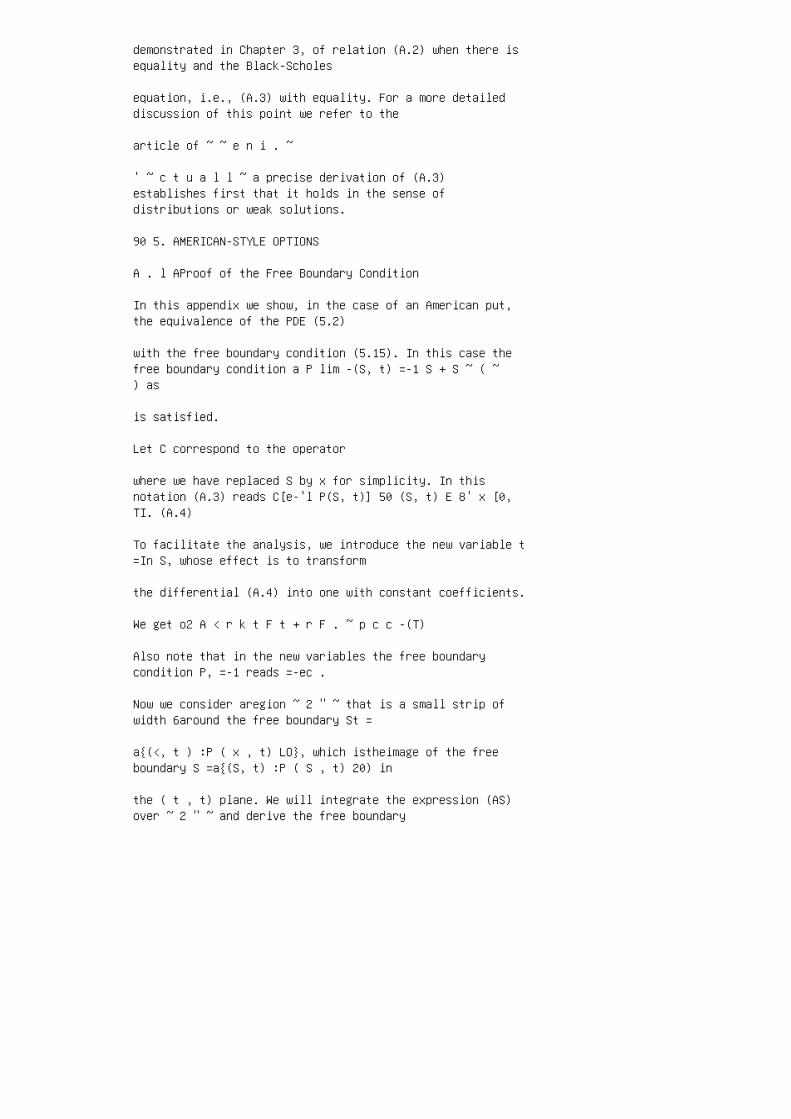
condition by passing to the limit as E--+ 0 and as t2 +ti.See Figure A.5. Indicating by

e*(t) a generic point on ~ 2 " ~ nS t , this gives

Now to deal with the integral over ~ 2 " ~ of Pt weexpress the latter as an iterated integral.

If we integrate Pt first with respect to t alonghorizontal strips Ct, denote the vertical strips

APPENDIX Astriparound the f r e e boundary 1t 2 t

FIGURE A.5

Striparoundthefree boundary used inthe derivation ofEquation (A.7).

by X I , and the intersection of a horizontal strip withthe free boundary by t * ( o (the inverse

function of 6 *(t)), we obtain

We have used that P =0 on the free boundary to cancel, foreach t , the contribution at t * ( t ) .

When rgets vanishingly small the vertical strips given bythe intersection E l i , i=1 , 2 are of

vanishingly small length. Thus rewriting the inequality(A.6) in the form

and letting rtend to zero, we see that the right-hand sideof (A.7) vanishes. Now since f6 is

9 2 5. A M E R I C A N S T Y L E O P T I O N S

identically equal to e t on the stopping region, theleft-hand side can be written

Now divide ( A . 8 ) by t2 -t l and let t2 +tlto recoverthe pointwise relation Ft 5e t *

which is equivalent to Psf5-1.

Also, since P ( S , t ) 2 ( K -S ) + , we clearly havethat P x ( S f ( t ) , t ) 2 1 and thus

P, ( S f ( t ) , t ) =-1. This establishes the"smooth-pasting" condition.

6 Chapter 6. Trinomial Model andFinite-Difference Schemes

accurately than if 8#112.The case 8=112 is theCrank-Nicholsons c h e m e . It gives

excellent approximations for the solutions of theBlack-Scholes PDE without need to enforce

the CFL condition.

106 6. T R I N O M I A L M O D E L A N D F I N I l E D EF E R E N C E S C H E M E S

[I] Avellaneda, M., Levy, A . , and ParBs, A. (1995),Pricing and Hedging Derivative Se- curities in Marketswith Uncertain Volatilities, AppliedMathematicalFinance,2,pp. 73-88.

[2] Avellaneda, M. and ParBs, A. (1996), Dynamic Hedgingwith Transaction Costs: Lattices Models, Non-LinearVolatility and Free-Boundary Problems, C o m m u n i c a ti o n s inPure andAppliedMath.

[3] Bellman, R. (1970), Introductiont oMatrixAnalysis,Mc-Graw Hill, New York.

[ 4 ] Dewynne, J., Howison, S. and Wilmott, P. (1993),OptionPricing:MathematicalModels andComputation,OxfordFinancial Press, Oxford.

[ 5 ] Park, A. and Avellaneda, M. (1996), Managing theVolatility Risk of Portfolios of Derivative Securities:The Lagrangian Uncertain Volatility Model,AppliedMathematicalFinance, 3 , pp. 21-52.

[6] Press, W. (1988), NumericalRecipesinC:T h e ArtofScientificC o m p u t i n g , University Press,Cambridge.

7 Chapter 7. Brownian Motion and ItoCalculus

In s u m m a r y , stochasticdifferentialc a l c u l u si s a n extensionofstandardc a l c u l u s i n w h i ch we

usetheItomultiplicationrule (7.26) t o a c c o u n t f or theeffectofnontrivialq u a d r a t i c variations.

T h e proofo f t h e GeneralizedItoL e m m a i s v e ry similart o t h e proofo f Proposition7 . 4 .

W e o m i t i t . T h e interestedreader shouldconsultIkedaand W a t a n a b e [ 6 ] , Varadhan[ 1 3 ] ,or

Karatzas and Shreve [ 8 ] .

[ I ] Bachelier,L . , ThCorie delaspCculation,Ann.EcoleNorm.Sup.,( S . 3 ) , 17,pp. 21-86.

[ 2 ] B r o w n , R.( J u n e and July 1 8 2 7 ) , AB ri e f Descriptiono f MicroscopicalObservations ( G e r ma n t r a n s l . ) , Ann.Phys.,1 4 , pp. 294-313.

[ 3 ] C h u n g , K.I.and W i l l i a m s , R.J. ( 1 9 90 ) , Introductiont o StochasticIntegration,2nd e d . ,Birkauser.

[ 4 ] C o o t n e r , P.H. TheR a n d o mCharacterofStockPrices,MITPress,C a m b r i d g e , M A .

[ 5 ] E i n s t e i n , A. ( 1 9 5 6 ) , Investigationson theT h e o r y ofBrownianM o v e m e n t ,DoverPublications,L o n d o n .

[ 6 ] I k e d a , N . and W a t a n a b e , S . ( 1 9 89 ) , StochasticDifferentialE q u a t i o n s a n dDiffusion Processes,2nd e d . , NorthHolland-Kodansha,A ms t e r d a m .

[ 7 ] I t o , K . ( 1 9 4 4 ) ,StochasticIntegral,Proc.Imp.Acad.Tokyo2 0 , pp. 648-665.

[ 8 ] Karatzas,I.and S h r e v e , S . ( 1 9 8 8 ) ,BrownianM o t i o n a n d StochasticC a l c u l u s ,SpringerV e r l a g , N e w Y o r k .

APPENDIX 123

[9] LCvy, P. (1948), Sur certains processus stochastiqueshomogknes, C o m p o s i t i o n Math.7, pp. 283-339.

[lo] LCvy, P. (1948), ProcessusStochastiqueset M o u v e me n t Brownien,Gauthier Villars, Paris.

[ l 11 Oksendaal, B. (1995), StochasticDifferentialE q u at i o n s , A n Introductionw i t h A p p l i c a t i on s , 4 t h ed., Springer Verlag, Berlin.

[12] Paley, R.E.A.C. and Wiener, N.Z.A. (1933), Notes onRandom Functions, Math.Z . , 37, pp. 47-668.

[13] Varadhan, S.R.S. (1980), D z ~ u s i o nProcessesandPartialDifferentialEquations,Tata InstituteLectures, Springer Verlag.

[14] Varadhan, S.R.S. (1980), Lectureso n BrownianM o t io n a n d S t o c h a s t i c DifferentialE q u a t i o ns , Tata Institute of Fundamental Research, Bombay.

Appendix: Properties of the Ito Integral

The aim of this appendix is to provide additional technicalelements to understand the basic

properties of the stochastic integral stated inPropositions 7.1 and 7.2.8

Let us consider Proposition 7.2. Notice that any"approximating sum"

has mean zero and uniformly bounded variance. In fact,since f ( t ) is nonanticipative, we have

where E {I Z ( s ) , s 5t i , }represents theconditional expectation operator given the his-

tory of the path up to time t j 1 . The conditionalexpectation of d Z j vanishes because the

increments of Z ( t ) are independent of their past. Weconclude that the sum in (A.l) has mean

zero. To compute its variance, we must evaluate the sum ofterms of the form

' ~ h e s e are in lieu of formal proofs, which would takeus too far from the subject of these chapters into Measure

precise hypotheses on f'(t),on the types of convergence ofrandom variables used in the proofs, etc.

124 7. B R O W N I A N MOTION A N D I T 0 CALCULUS

where 1 5j, k 5N. The key observation is that thisexpectation vanishes if j #k. In

fact, if j <k, we have

The variance on ( A . l ) is therefore equal to the sumof the "diagonal" terms

(This assumes implicitly that the sum can be approximatedby the integral, i.e., that

E ((f (t) ) 2 }is continuous.)

We have established that the random variables S N havebounded mean and variance. Next,

we show that the sums converge to a limitas the partitionsbecome finer and finer. Nu

Consider a sequence of partitions (t/v) } i = l ,where

and the corresponding sequence of sums S N , . We claimthat

Consider two such sums, S N , and s ~ , , ,corresponding to different partitions. The idea is to

"merge" the two partitions to form a finer one thatcombines the nodes of each of them. With

respect to this refined partition (which we call { t iI), both sums can be written in the form

and

Note that t; s and the ti** are times (of the originalpartitions) that satisfy ti* (t j ,ti**(t i

APPENDIX 125

Moreover, the differences ti**-ti*converge to zero as v+GO. The difference of the sums

can therefore be expressed in the form

Taking into account the fact that increments point to thefuture, it is easy to show that this sum

has mean zero and variance

I f f ( t ) satisfies suitable boundedness and continuityassumptions, e.g., i f f ( t ) is bounded and

the sum in ( A . 3 ) tends to zero with the mesh size.

This argument shows the existence of the Ito stochasticintegral. The properties stated in

Proposition 7.3 also follow from these calculations.

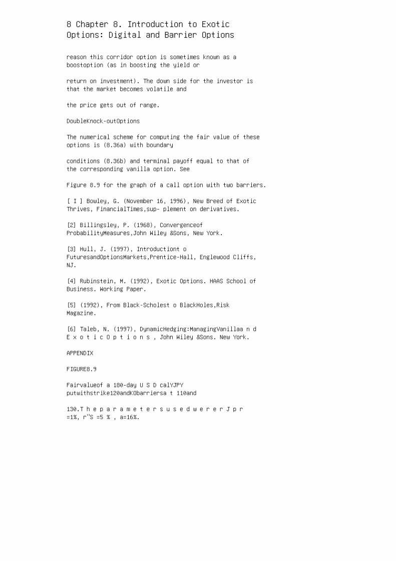
8 Chapter 8. Introduction to ExoticOptions: Digital and Barrier Options

reason this corridor option is sometimes known as aboostoption (as in boosting the yield or

return on investment). The down side for the investor isthat the market becomes volatile and

the price gets out of range.

DoubleKnock-outOptions

The numerical scheme for computing the fair value of theseoptions is (8.36a) with boundary

conditions (8.36b) and terminal payoff equal to that ofthe corresponding vanilla option. See

Figure 8.9 for the graph of a call option with two barriers.

[ I ] Bowley, G. (November 16, 1996), New Breed of ExoticThrives, FinancialTimes,sup- plement on derivatives.

[2] Billingsley, P. (1968), ConvergenceofProbabilityMeasures,John Wiley &Sons, New York.

[3] Hull, J. (1997), Introductiont oFuturesandOptionsMarkets,Prentice-Hall, Englewood Cliffs,NJ.

[4] Rubinstein, M. (1992), Exotic Options. HAAS School ofBusiness. Working Paper.

[5] (1992), From Black-Scholest o BlackHoles,RiskMagazine.

[6] Taleb, N. (1997), DynamicHedging:ManagingVanillaa n dE x o t i c O p t i o n s , John Wiley &Sons. New York.

APPENDIX

FIGURE8.9

Fairvalueof a 180-day U S D calYJPYputwithstrike120andKObarriersa t 110and

130.T h e p a r a m e t e r s u s e d w e r e r J p r=1%, r"S =5 % , a=16%.

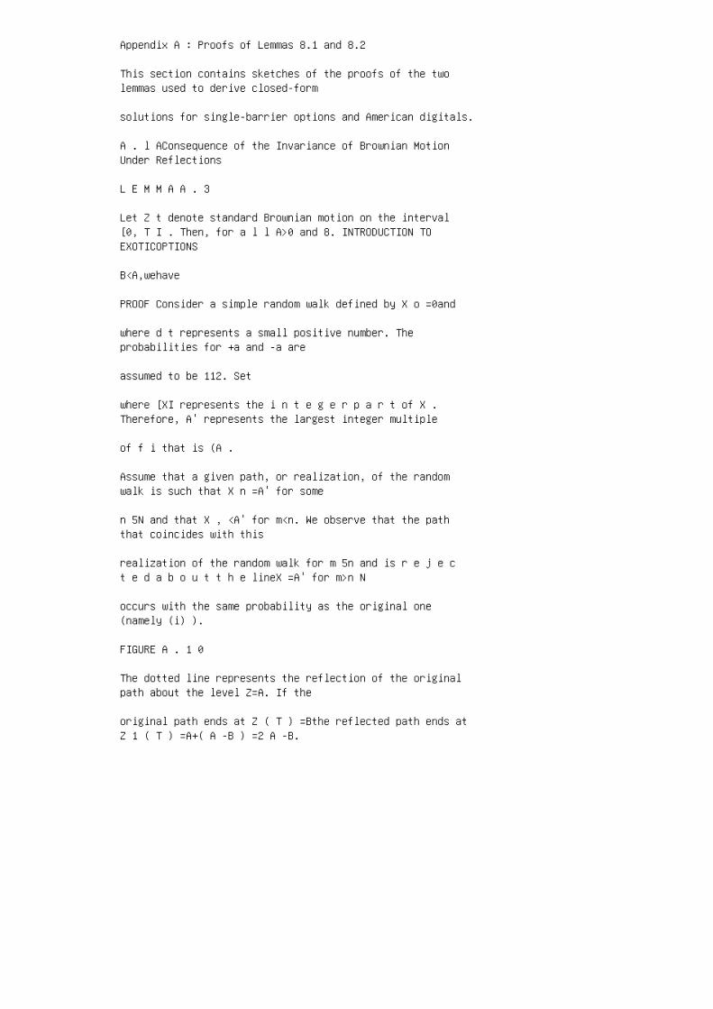
Appendix A : Proofs of Lemmas 8.1 and 8.2

This section contains sketches of the proofs of the twolemmas used to derive closed-form

solutions for single-barrier options and American digitals.

A . l AConsequence of the Invariance of Brownian MotionUnder Reflections

L E M M A A . 3

Let Z t denote standard Brownian motion on the interval[0, T I . Then, for a l l A>0 and 8. INTRODUCTION TOEXOTICOPTIONS

B<A,wehave

PROOF Consider a simple random walk defined by X o =0and

where d t represents a small positive number. Theprobabilities for +a and -a are

assumed to be 112. Set

where [XI represents the i n t e g e r p a r t of X .Therefore, A' represents the largest integer multiple

of f i that is (A .

Assume that a given path, or realization, of the randomwalk is such that X n =A' for some

n 5N and that X , <A' for m<n. We observe that the paththat coincides with this

realization of the random walk for m 5n and is r e j e ct e d a b o u t t h e lineX =A' for m>n N

occurs with the same probability as the original one(namely (i) ).

FIGURE A . 1 0

The dotted line represents the reflection of the originalpath about the level Z=A. If the

original path ends at Z ( T ) =Bthe reflected path ends atZ 1 ( T ) =A+( A -B ) =2 A -B.

Therefore, we conclude that for B<A ' , PI max X i 2A';X N =B max Xi 2A' ;X N =2A' -B I S j S N I S j s N I

APPENDIX

(This last equality holds because 2A' -B >A ' . )

Let T =N d t . By the Central Limit theorem, the jointdistribution of the random variables

X u approaches that of a Brownian motion as d t -t 0, N++o o . Therefore, if we replace

n

formally max15 jNX i by maxo5 TZ t ,X N by Z r , andA' by A , we conclude from (A.2)

that Eq. (A.l) holds. The lemma is proved.13 I

Notice that we have established the analogue of Lemma 8.2in the case p=0.

A . 2 The Case p80

To prove Lemma 8.2, we will need the following result aboutBrownian motion with drift:

THEOREM A . 1

(Cameron -Martin) Let F(zl , z 2 , ...,z,,)beacontinuousfunction.Then,

This result states that the expectation of a function ofBrownian motion with drift is equal to

the expectation of the same function of regular Brownianmultiplied by an exponential factor,

namely ew ZT -1w 2 T

Proof of theTheorem Define the increments of the Brownianpath

Also, set

Using the explicit form of the Gaussian distribution andthe fact that the increments Yj are

independent random variables with mean p(ti -tj-l) and

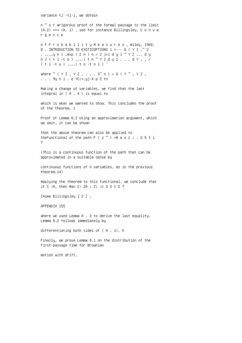
variance tj -ti-1, we obtain

n ~ o r arigorous proof of the formal passage to the limit(A.2) ==+ (A. l) , see for instance Billingsley, C o n v er g e n c e

o f P r o b a b i l i t y M e a s u r e s , Wiley, 1968.8 . INTRODUCTION TO EXOTICOPTIONS 1 =--- G ( Y I ,~ 2, ...,y n ) .exp ( 2 n ) n / 2 j=1 d y l ~ Y Z ... d yn J ( t l -t o ) ....( t n ~ Y I d y 2 . . . d Y , , /( t l -t o ) ....( t n -t n l ) '

where ~ ( Y I , Y Z , . . . 3~ n ) = G ( Y ~ , Y Z ,. . . 9y n 1 . e YC;=,yj-4 p 2 tn

Making a change of variables, we find that the lastintegral in ( A . 4 ) is equal to

which is what we wanted to show. This concludes the proofof the theorem. 1

Proof of Lemma 8.2 Using an approximation argument, whichwe omit, it can be shown

that the above theorem can also be applied tothefunctional of the path F ( z ~ ) =M a x z : . O 5 t iT

(This is a continuous function of the path that can beapproximated in a suitable sense by

continuous functions of n variables, as in the previoustheorem.14)

Applying the theorem to this functional, we conclude thatif C <A, then Max 2: 2A ; Z; <c O S t S T

I4see Billingsley [ 2 ] .

APPENDIX 155

where we used Lemma A . 3 to derive the last equality.Lemma 8.2 follows immediately by

differentiating both sides of ( A . 1). h

Finally, we prove Lemma 8.1 on the distribution of thefirst-passage time for Brownian

motion with drift.

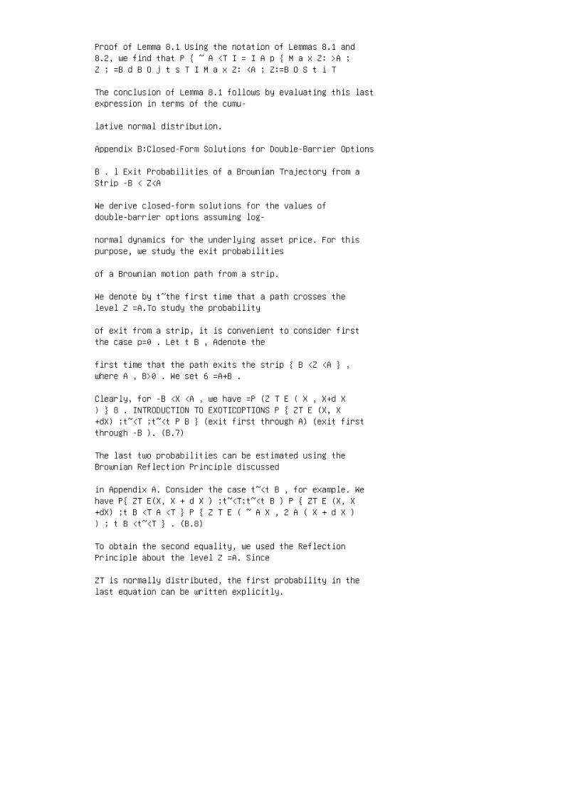
Proof of Lemma 8.1 Using the notation of Lemmas 8.1 and8.2, we find that P { ~ A <T I = I A p { M a x Z: >A ;Z ; =B d B O j t s T I M a x Z: <A ; Z:=B O S t i T

The conclusion of Lemma 8.1 follows by evaluating this lastexpression in terms of the cumu-

lative normal distribution.

Appendix B:Closed-Form Solutions for Double-Barrier Options

B . l Exit Probabilities of a Brownian Trajectory from aStrip -B < Z<A

We derive closed-form solutions for the values ofdouble-barrier options assuming log-

normal dynamics for the underlying asset price. For thispurpose, we study the exit probabilities

of a Brownian motion path from a strip.

We denote by t~the first time that a path crosses thelevel Z =A.To study the probability

of exit from a strip, it is convenient to consider firstthe case p=0 . Let t B , Adenote the

first time that the path exits the strip { B <Z <A } ,where A , B>0 . We set 6 =A+B .

Clearly, for -B <X <A , we have =P (Z T E ( X , X+d X) } 8 . INTRODUCTION TO EXOTICOPTIONS P { ZT E (X, X+dX) ;t~<T ;t~<t P B } (exit first through A) (exit firstthrough -B ). (B.7)

The last two probabilities can be estimated using theBrownian Reflection Principle discussed

in Appendix A. Consider the case t~<t B , for example. Wehave P{ ZT E(X, X + d X ) ;t~<T;t~<t B ) P { ZT E (X, X+dX) ;t B <T A <T } P { Z T E ( ~ A X , 2 A ( X + d X )) ; t B <t~<T } . (B.8)

To obtain the second equality, we used the ReflectionPrinciple about the level Z =A. Since

ZT is normally distributed, the first probability in thelast equation can be written explicitly.

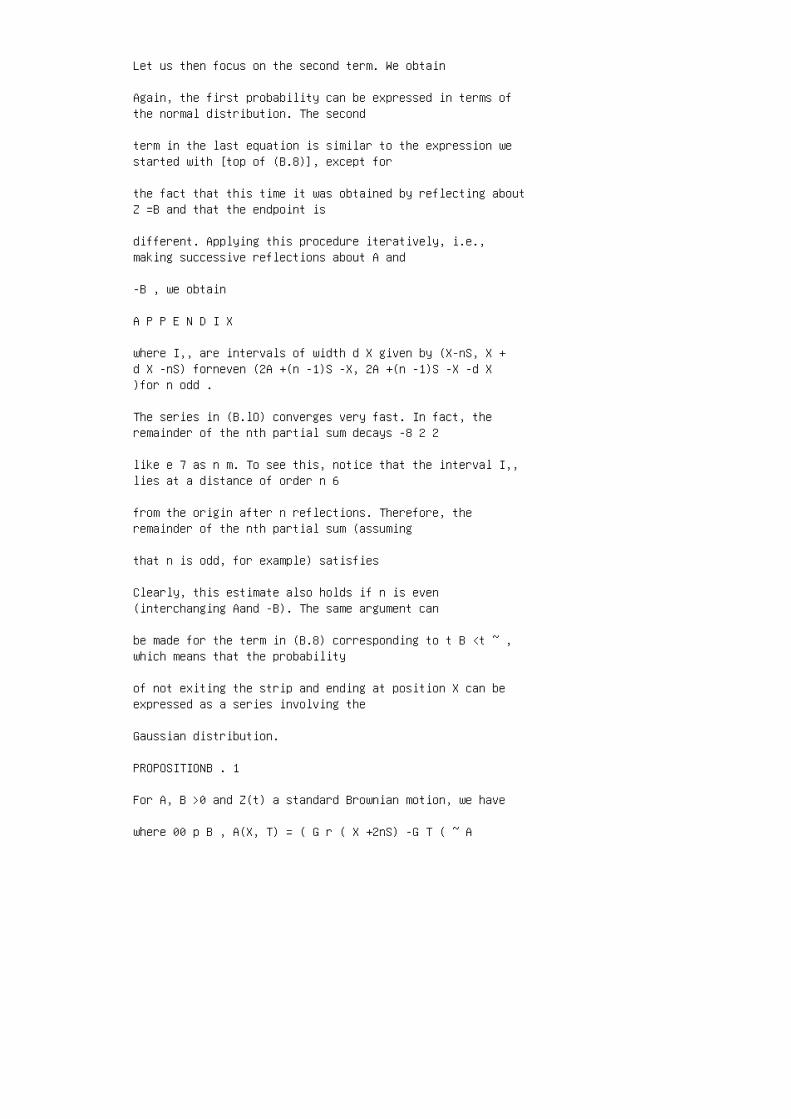
Let us then focus on the second term. We obtain

Again, the first probability can be expressed in terms ofthe normal distribution. The second

term in the last equation is similar to the expression westarted with [top of (B.8)], except for

the fact that this time it was obtained by reflecting aboutZ =B and that the endpoint is

different. Applying this procedure iteratively, i.e.,making successive reflections about A and

-B , we obtain

A P P E N D I X

where I,, are intervals of width d X given by (X-nS, X +d X -nS) forneven (2A +(n -1)S -X, 2A +(n -1)S -X -d X)for n odd .

The series in (B.lO) converges very fast. In fact, theremainder of the nth partial sum decays -8 2 2

like e 7 as n m. To see this, notice that the interval I,,lies at a distance of order n 6

from the origin after n reflections. Therefore, theremainder of the nth partial sum (assuming

that n is odd, for example) satisfies

Clearly, this estimate also holds if n is even(interchanging Aand -B). The same argument can

be made for the term in (B.8) corresponding to t B <t ~ ,which means that the probability

of not exiting the strip and ending at position X can beexpressed as a series involving the

Gaussian distribution.

PROPOSITIONB . 1

For A, B >0 and Z(t) a standard Brownian motion, we have

where 00 p B , A(X, T) = ( G r ( X +2nS) -G T ( ~ A

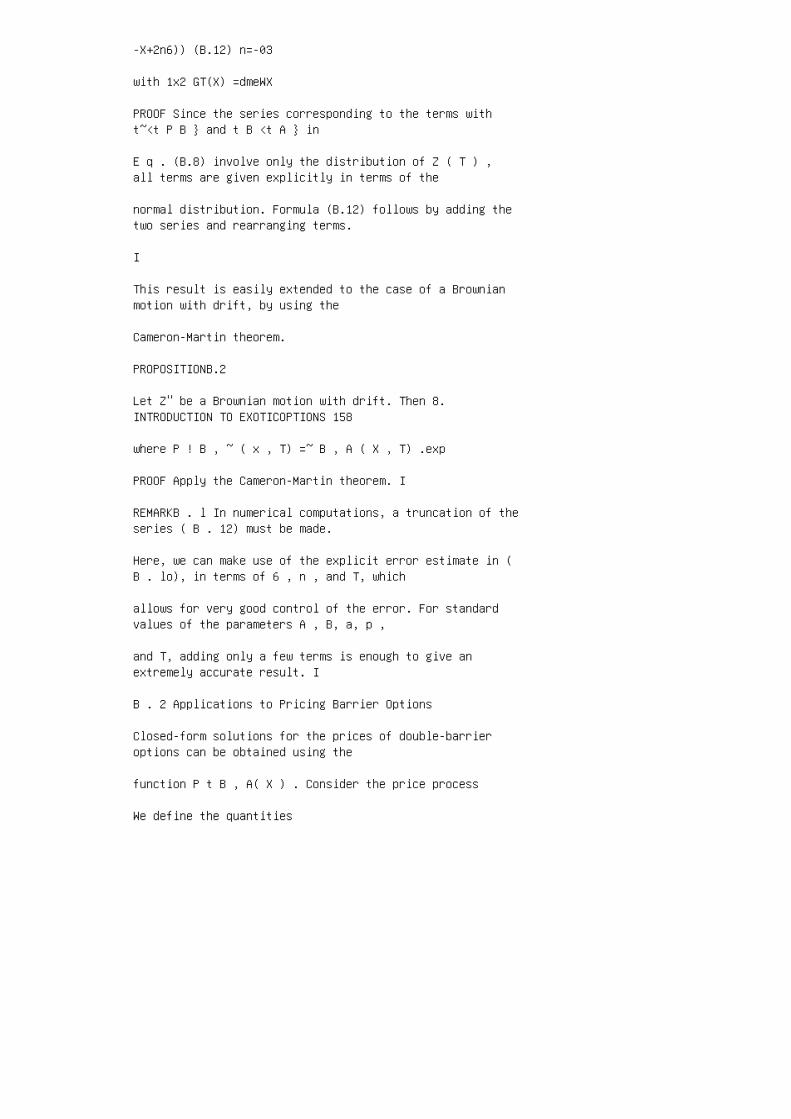
-X+2n6)) (B.12) n=-03

with 1x2 GT(X) =dmeWX

PROOF Since the series corresponding to the terms witht~<t P B } and t B <t A } in

E q . (B.8) involve only the distribution of Z ( T ) ,all terms are given explicitly in terms of the

normal distribution. Formula (B.12) follows by adding thetwo series and rearranging terms.

I

This result is easily extended to the case of a Brownianmotion with drift, by using the

Cameron-Martin theorem.

PROPOSITIONB.2

Let Z" be a Brownian motion with drift. Then 8.INTRODUCTION TO EXOTICOPTIONS 158

where P ! B , ~ ( x , T) =~ B , A ( X , T) .exp

PROOF Apply the Cameron-Martin theorem. I

REMARKB . l In numerical computations, a truncation of theseries ( B . 12) must be made.

Here, we can make use of the explicit error estimate in (B . lo), in terms of 6 , n , and T, which

allows for very good control of the error. For standardvalues of the parameters A , B, a, p ,

and T, adding only a few terms is enough to give anextremely accurate result. I

B . 2 Applications to Pricing Barrier Options

Closed-form solutions for the prices of double-barrieroptions can be obtained using the

function P t B , A( X ) . Consider the price process

We define the quantities

and

The following formulas for the prices of double-barrieroptions follow immediately.

a . RangeNotes

where N is the payoff.

b. AmericanRange AccrualNotes

A range accrual note paying p dollars every At units oftime with maturity T =N At can

be regarded as a portfolio of N range discount notes.Accordingly, we have

If payments are made frequently (for instance daily), wecan approximate the sum by an

integral, setting p =Q AT. In this case, the sum is wellapproximated by the integral " ( X , t ) d X d t .V=Qb T e-" l:" P A , , A ,

APPENDIX 159

Here Q can be interpreted as the payout that the holderwould receive in 1 year if the price did

not exit the range. (In the example given in Section 8.3,we had a daily payoff of 50K yen.

Assuming a 365-day year, this would give Q =360 x 50=18,250,000.

c . Double Knock-outOptions

For a call with strike K, we have

9 Chapter 9. Ito Processes,Continuous-Time Martingales, and Girsanov's Theorem

nian motion have probability zero for Brownian motion withdrift and vice-versa. The two

probability measure are said to be mutually absolutelycontinuous or equivalent.8

[I] Bickel, P. and Doksum (1991), Mathematical Statistics:Basic Ideas and Selected Topics, Prentice-Hall, EnglewoodCliffs, NJ.

[2] Breiman, L. (1968), Probability, Addison-Wesley,Reading, Massachusetts.

[3] Doob, J. (1953), Stochastic Processes, Wiley, New York.

[4] Girsanov, I. (1960), On Transforming a Certain Class ofStochastic Processes by Absolute Substitution of Measures,Theory of Probability and Applications, 5, pp. 285-301.

[5] Ikeda, N. and Watanabe, S. (1981), StochasticDifferential Equations and Dz~usion Processes, NorthHolland, Amsterdam.

[6] Karatzas, I. and Shreve, S.E. (1988), Brownian MotionandStochastic Calculus, Springer Verlag, Berlin.

his is true only for events that depend on values taken bypaths up to ajinite time-horizon T <co. For

instance, Brownian motion with positive drift convergeswith probability 1 to +cm as t++co and standard

Brownian motion does not.

A P P E N D I X 169

[ 7 ] Oksendaal, B. ( 1 9 9 5 ) , S t o c h a s t i cDifferentialE q u a t i o n s , A n I n t r o d u c t i on w i t h A p p l i c a t i o n s , 4th ed., SpringerVerlag, Berlin.

[ 8 ] Thorp, E . ( 1 9 6 9 ) , Optimal Gambling Systemsfor Favorable Games, Rev. I n t l . S t a t i s t i c a lI n s t i t u t e , 37,pp. 3.

[ 9 ] Varadhan, S.R.S. ( 1 9 8 0 ) , D i f f u s i o n P

r o c e s s e s a n d PartialDifferentialE q u a t i o ns , Tata Institute Lectures, Springer Verlag, New York.

Appendix: Proof of Equation (9.11)

We will use the elementary properties of conditionalexpectation operators with respect to

a given sub-0-algebra of event^.^ The conditionalexpectation operator with respect to the

history of paths up to time t , E t {. } , ischaracterized by the following property: let X be an

arbitrary random variable. Then E t {X }is the uniquerandom variable that is measurable with

respect to the past up to time tand satisfies E{ X Y }=E{ E t { X } Y } . ('4.1)

for all random variables Y that are measurable withrespect to the past up to time t .

Let us use this characterization to compute E& {X } ,where Qis defined in ( 9 . 8 ) . From the

definition of Q , we have

Here, we applied Eq. ( A . l ) and the martingaleproperty of M ( t ) to pass from the third to the

fourth equation.

5 ~ h e reader unfamiliar with these notions shouldconsult, for instance, Breiman [ 2 ] , or the firstchapter of Bickel

and Doksum [I].

170 9. I T 0 P R O C E S S E S , C O N T I N U O U S T IM E M A R T I N G A L E S

From the characterization of the conditional probabilityoperator, we conclude that

This is precisely what we wanted to show.

10 Chapter 10. Continuous-Time Finance:An Introduction

the "prior" statistical measure driving the economy, bymeans of the vector of marketprices

of risk hl( t ) , ...,hN(t). A detailed study of therelation between risk-neutral measures and

objective measures has been made in very few cases [3].This is an area of current research,

which is beyond the scope of this book.

Some concrete applications of Arbitrage Pricing Theory arepresented in the next chapter.

[I] Chatelain, G. and Stricker, C. (1994), OnComponentwise and Vector Stochastic Inte- gration,MathematicalFinance, 4, pp. 57-66.

[2] Chen, R.R. and Scott, L. (December 1993), MaximumLikelihood Estimation for a Multifactor Equilibrium Modelof the Term Structure of Interest Rates, Journalof FixedIncome, pp. 14-3 1.

[3] Chen, R.R. and Scott, L. (Winter 1995), Interest RateOptions in Multifactor Cox- Ingersoll-Ross Models of theTerm Structure, Journal of Fixed Income,pp. 53-72.

[4] Cox, J., Ingersoll, J., and Ross, S. (1985), AnInter-Temporal General Equilibrium Model of Asset Prices,Econometrics,5 3 .

[ 5 ] Delbaen, F. (1992), Representing Martingale MeasuresWhen the Asset Prices are Con- tinuous and Bounded,MathematicalFinance, 2 , pp. 107-130.

182 10. C O N T I N U O U S T I M E F I N A N C E : A NI N T R O D U C T I O N

[6] Delbaen, F. and Schachermayer, W. (1994), A GeneralVersion of the Fundamental Theorem of Asset Pricing, Math.Annalen,300, pp. 463-520.

[7] Duffie, D. (1992),DynamicalAssetPricingTheory,Princeton University Press,Prince- ton. NJ.

[8] Harrison, J.M. and Kreps, D. (1979), Martingales and

Arbitrage in Multi-Period Secu- rities Markets,JournalofEconomicTheory,20, pp. 38 1-3 16.

[9] Harrison, J.M. and Pliska, S.R. (1 98 I), Martingalesand Stochastic Integrals in the Theory of ContinuousTrading, StochasticProcess.Appl., 11,pp. 215-260.

[lo] Hull, J. (1993), Options,FuturesandOtherDerivativeSecurities,2nd ed., Prentice-Hall,Englewood Cliffs, NJ.

[I 11 Merton, R. (1991), ContinuousErne Finance,Blackwell,Oxford.

[I21 Muller, S. ArbitragePricingof ContingentClaims,LectureNotes in Economics and Mathematical Systems 254, SpringerVerlag, Berlin.

[13] Musiela, M. and Rutkowski, M. (1997),ArbitragePricingTheoryofDerivativeSecurities:TheoryandApplications,Springer Verlag,Berlin.

[14] Stricker, C. (1989), Arbitrage et Lois de Martingale,AnnalesInst.PoincarL, 26, pp. 451460.

11 Chapter 11. Valuation of DerivativeSecurities

a Dirac mass 6 (Y -X) from date t to date Tusing theforward Fokker-Planck equation.

functions can be computed by numerical quadrature using theformula

(Notice that, in contrast, the backward FP equation givesthe p as a function of the backward

variable X and hence cannot be used to compute theprobability density-only the expectation

value.)

A sketch of the proof of Proposition 11.5 is given as anappendix to this chapter.

[I] Dixit, A . and Pindyck, R. (1994), Investmentu n d e rUncertainty,Princeton University Press, Princeton, NJ.

[2] Duffie, D. (1992),DynamicalAssetPricingTheory,Princeton University Press,Prince- ton, NJ.

[3] Hull, J. (1998), Introductiont o FuturesandO p t i o ns M a r k e t s , Prentice-Hall, Upper Saddle River. NJ.

[4] Hull, J. and White, A. (1987), The Pricing of Optionson Assets with Stochastic Volatil- ities, JournalofFinance,4 2 , pp. 28 1-300.

APPENDIX197

[ 5 ] Scott, L.O. ( 1 9 8 6 ) , OptionPricingW h e n t he VarianceChangesRandomly:Theoryand Application.

[ 6 ] Wong, M.A. ( 1 9 9 1 ) , Trading andInvestinginBondOptions:RiskManagement,Arbitrage,andValue Investing, Wiley,New York.

[ 7 ] Zhu, Y. and Avellaneda, M. (August 1 9 9 7 ) , ARisk-Neutral Stochastic Volatility Model,AppliedMathematicalFinance.

Appendix: Proof of Proposition 11.5

We wish to show that p ( X , t ; Y , T ) satisfies the

forward Fokker-Plank equation in the

variables ( Y , T). For this, consider an intermediatetime 0such that t<0<T . It is clear

that the density function satisfies the following integralequation:

In fact, this equation just expresses the fact that thediffusion process that starts at Xat time

tand ends at Yat time Tmust be at somepoint Zat time 0 .The integral on the right-hand

side just sums over all possible positions at time 0 .

Notice also that the left-hand side of ( A . l ) isindependent of 0 . Differentiating both sides

of the equation with respect to 0 , we conclude that

Using the fact that in the second integral psatisfies thebackward FP equation in the variables

( Z , O ) , we have

where we used integration by parts in passing from thefirst line to the second. (Of course, we

are assuming here that the probabilities decay fast enoughfor a large IZI to preclude boundary

terms.) If we now let 0approach T , the function p ( Z ,0 ; Y , T ) approaches the Dirac mass

6 ( Z -Y ) . Therefore, as 0 +T , the last equationbecomes

1 9 8 11.VALUATIONOFD E R I V A T N E S E C U R I T l E S

or simply

This shows that p ( X , t ; Y, T ) satisfies theforward Fokker-Planck equation in (Y, T ) , as

desired.

12 Chapter 12. Fixed-Income Securitiesand the Term-Structure of Interest Rates

In summary, the construction of a forward-rate curve allowsus to generate a "continuum"

of discount factors and thus to price all "non-optionable"debt securities. Another important

application of forward-curve modeling is for hedging aportfolio in terms of the securities used

to build the curve. Hedge-ratios are derived by computingthe sensitivities of the value of the

portfolio to small changes in the bond prices (or the swaprates).

Which "cooking" method should we use in practice? Theanswer to this question ultimately

construction. At the time of this writing, one of the mostpopular methods in use by swap

traders is the bootstrapping approach with interpolatedswap rates.

[I] Fabozzi, F. (1997), Fixed Income Mathematics:Analytical and StatisticalTechniques, Irwin, Chicago.

Z 3 ~ e e , forexample,theWWW Courant Finance Server(http://marco-pc.cims.nyu.edu) for an on-lineyield

[2] Jarrow, R. (1995),ModellingFixed-IncomeSecuritiesandInterest-RateO p t i o ns , McGraw-Hill, New York.

[3] Jarrow, R. and Heath, D. (1998),Fixed-IncomeSecuritiesa n d InterestR a t e s , McGraw-Hill, New York.

[4] Kapner, K.R. and Marshall, J.F. (1994), UnderstandingSw a p s , Wiley, New York.

[5] Siegel, D.R. and Siegel D.F. (1990), T h eFuturesMarkets:Arbitrage,RiskM a n a g e m e n tandPortfolioStrategies, Probus, Chicago.

[6] Wong, M.A. (1991), Tradinga n d Investingi nBondOptions,John Wiley &Sons, New York.

13 Chapter 13. The Heath- Jarrow-MortonTheorem and MultidimensionalTerm-Structure Models

The Ho-Lee model and the modified Vasicek models areexamples of term-structure models

that admit reduced representations (with M =1). In theHo-Lee case, the underlying state

variable can be taken to be X(t) =W(t), and in themodified Vasicek model we can take

which is a diffusion process, since it satisfies thestochastic differential equation

The study of term-structure models that admit a reducedrepresentation, also known as

Markov term-structuremodels,will be carried out in the nextchapter.

[ I ] Black and Scholes (1973)

[2] Brace, A., Gatarek, D., and Musiela, M. (1997), TheMarket Model of Interest Rate Dynamics, MathematicalFinance, 7, pp. 127-154.

[3] Chen, R.R. and Scott, L. (December 1993), MaximumLikelihood Estimation for a Multifactor Equilibrium Modelof the Term Structure of Interest Rates, Journal of FixedIncome, pp. 53-72.

141 Cox, J., Ingersoll, J . , and Ross, S. (1985), ATheory of the Term Structure of Interest Rates,Econornetrica, 53, pp. 385-407.

252 13. T H E H E A T H J A R R O W M O R T O N THEOREM

[5] Heath, D., Jarrow R., and Morton, A. (1990a), BondPricing and the Term Structure of Interest Rates: ADiscrete Time Approximation, JournalofFinancialQ u a n t it a t i v e A n a l y s i s , 25,pp. 419-440.

[6] Heath, D., Jarrow, R., and Morton, A. (1990b),Contingent Claim Valuation with a Random Evolution ofInterest Rates, Rev. FuturesMarkets,9 , pp. 54-76.

[7] Heath, D., Jarrow, R., and Morton, A. (1992), BondPricing and the Term Structure of Interest Rates: A New

Methodology, Econometrics,6 0 , pp. 77-105.

[8] Ho, T. and Lee, S. (1986), Term Structure Movements andPricing Interest Rate Contin- gent Claims,JournalofFinance,4 2 , pp. 1129-1 142.

[9] Hull and White (1989)

[lo] Jamshidian, F. (1 997), LIBOR and Swap Market Modelsand Measures, FinanceS t o c h a s tic.

[ l 11 Judge, G.G., Griffiths, W.E., Hill, R.C.,Lutkepohl, H., andLee, T.C. (1988), Introduction t otheTheoryandPracticeof E c o n o m e t r i c s , 2nd ed.,John Wiley, New York.

[12] Litterman, R. and Scheinkman, J. (June 1980), CommonFactors Affecting Bond Returns, Journalof Fixed Income,pp.55-61.

[13] Longstaff, F. and Schwartz, E. (1992a), Interest RateVolatility and the Term Structure: A Two-Factor GeneralEquilibrium Model, Journalof Finance,4 7 , pp. 1259-1282.

1141 Longstaff, F. and Schwartz, E. (December 1992b), ATwo-Factor Interest Rate Model and Contingent ClaimsValuation, Journalof Fixed Income,3 , pp. 16-23.

[15] Merton, R.C. (Spring 1973), Theory of Rational OptionPricing, BellJournalof E c o n o m i c sandManagementScience, 4 , pp. 141-1 83.

[16] Morton, A.J. (1989), Arbitrage and Martingales.Doctoral dissertation, Cornell Univer- sity, Ithaca, NY.

[17] Vasicek, O.A. (1977), An Equilibrium Characterizationof the Term Structure, Journal of FinancialEconomics, 5 ,pp. 177-188.

14 Chapter 14. Exponential-Afine Models

a ( t ; T ) % 4a2 e a ( ~ t ) for T-t >> I . (K +a ) 2

This is in qualitative agreement with the Gaussian models,in which indexgaussian mod-

els@Gaussian modelsa is replaced by K. Thus, the standarddeviation of forward rates decays

exponentially with rate a as the maturity increases. Thefunctions in (14.49) correspond to the

exponentials e K i ( T t ) in the context of Gaussianmodels. They determine the shape of the

deformations of the forward-rate curve.

[ l ] Abramowitz, M. and Stegun, I. (1964), Handbook ofMathematicalFunctions,with Formulas, GraphsandMathematicalTables, National Bureau of Standards,Washington D.C.

[2] Chen, R.R., and Scott, L. (December 1993), MaximumLikelihood Estimation for a Multi-factor Equilibrium Modelof the Term Structure of Interest Rates, Journalof FixedIncome, pp. 14-3 1

[3] Chen, R.R. and Scott, L. (Winter 1995), Interest RateOptions in Multi-factor Cox- Ingersoll-Ross Models of theTerm Structure, Journalof Fixed Income,pp. 53-72.

[4] Cox, J., Ingersoll, J., and Ross, S. (1985), A Theoryof the Term Structure of Interest Rates,Econometrica,53(2), pp. 385-407.

[5] Duffie, D. and Kan, R. (1995), Multi-Factor InterestRate Models, PhilosophicalTransactionsof the RoyalSociety,SeriesA , 317, pp. 577-586.

[6] Feller, W. (1971), AnIntroductiontoProbabilityTheoryand ItsApplications,vol2 ,John Wiley &Sons, New York.

[7] Ikeda, N. and Watanabe, S. (1989),StochasticDifferentialEquationsand Diffusion Processes,North Holland-Kodansha, Amsterdam.

[8] Karatzas, I. and Shreve, S. (1988), BrownianMotionandStochasticC a l c u l u s , Springer, Berlin.

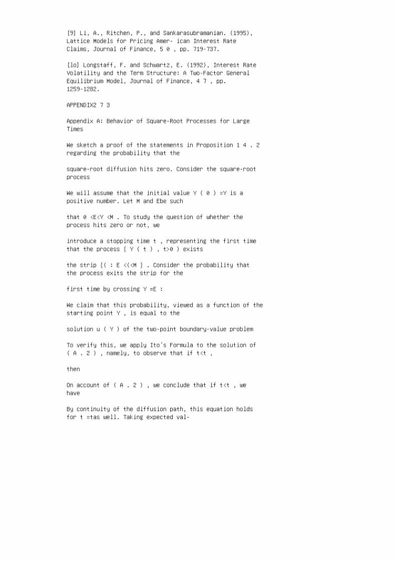
[9] Li, A., Ritchen, P., and Sankarasubramanian. (1995),Lattice Models for Pricing Amer- ican Interest RateClaims, Journal of Finance, 5 0 , pp. 719-737.

[lo] Longstaff, F. and Schwartz, E. (1992), Interest RateVolatility and the Term Structure: A Two-Factor GeneralEquilibrium Model, Journal of Finance, 4 7 , pp.1259-1282.

APPENDIX2 7 3

Appendix A: Behavior of Square-Root Processes for LargeTimes

We sketch a proof of the statements in Proposition 1 4 . 2regarding the probability that the

square-root diffusion hits zero. Consider the square-rootprocess

We will assume that the initial value Y ( 0 ) =Y is apositive number. Let M and Ebe such

that 0 <E<Y <M . To study the question of whether theprocess hits zero or not, we

introduce a stopping time t , representing the first timethat the process { Y ( t ) , t>0 ) exists

the strip {( : E <(<M } . Consider the probability thatthe process exits the strip for the

first time by crossing Y =E :

We claim that this probability, viewed as a function of thestarting point Y , is equal to the

solution u ( Y ) of the two-point boundary-value problem

To verify this, we apply Ito's Formula to the solution of( A . 2 ) , namely, to observe that if t<t ,

then

On account of ( A . 2 ) , we conclude that if t<t , wehave

By continuity of the diffusion path, this equation holdsfor t =tas well. Taking expected val-

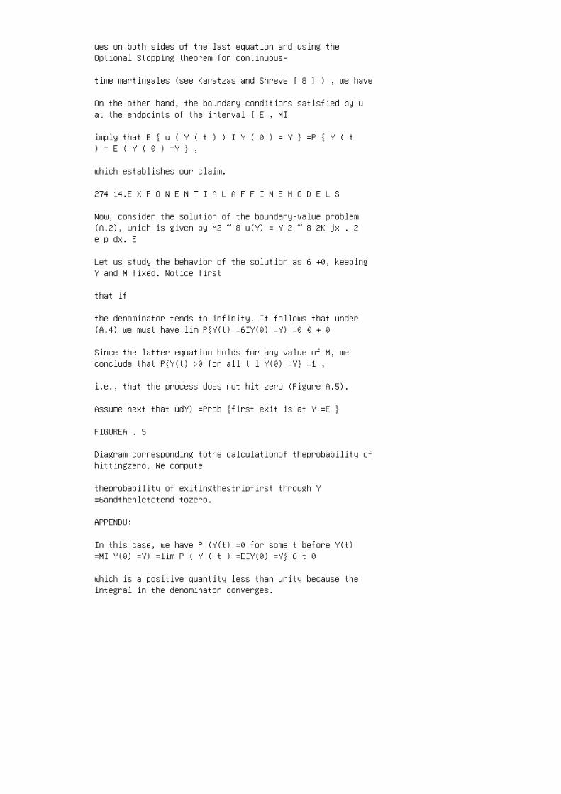
ues on both sides of the last equation and using theOptional Stopping theorem for continuous-

time martingales (see Karatzas and Shreve [ 8 ] ) , we have

On the other hand, the boundary conditions satisfied by uat the endpoints of the interval [ E , MI

imply that E { u ( Y ( t ) ) I Y ( 0 ) = Y } =P { Y ( t) = E ( Y ( 0 ) =Y } ,

which establishes our claim.

274 14.E X P O N E N T I A L A F F I N E M O D E L S

Now, consider the solution of the boundary-value problem(A.2), which is given by M2 ~ 8 u(Y) = Y 2 ~ 8 2K jx . 2e p dx. E

Let us study the behavior of the solution as 6 +0, keepingY and M fixed. Notice first

that if

the denominator tends to infinity. It follows that under(A.4) we must have lim P{Y(t) =6IY(0) =Y) =0 € + 0

Since the latter equation holds for any value of M, weconclude that P{Y(t) >0 for all t l Y(0) =Y} =1 ,

i.e., that the process does not hit zero (Figure A.5).

Assume next that udY) =Prob {first exit is at Y =E }

FIGUREA . 5

Diagram corresponding tothe calculationof theprobability ofhittingzero. We compute

theprobability of exitingthestripfirst through Y=6andthenletctend tozero.

APPENDU:

In this case, we have P (Y(t) =0 for some t before Y(t)=MI Y(0) =Y) =lim P ( Y ( t ) =EIY(0) =Y} 6 t 0

which is a positive quantity less than unity because theintegral in the denominator converges.

By letting M tend to infinity in both sides of the lastequation, the integrals will diverge at

infinity, and we can conclude that

The analysis of the behavior of Yt after the fist hittingtime of zero is more delicate. The

reader is referred to Feller 161 or Ikeda and Watanabe 171for a rigorous study of this question.

Appendix B:Characterization of the Probability DensityFunction of

Square-RootProcesses

As indicated before the statement of Proposition 14.3, itis convenient to analyze the moment-

generating function of the diffusion. Suppose first that KO >$, so that the process never

hits Y =0 . In this case, we can apply the standardtheory (cf. Chapter 12, section on

Fokker-Planck theory) or Ito calculus to the function

to conclude that it satisfies the partial differentialequation

A solution of this final-value problem can be sought in theform n(Y, t , T ; h) =exp (r ( t , T ; h) Y -s(t , T; h) ).

276 14. EXPONENTIAL-AFFINEMODELS

Substitution of this function into the PDE (B.l) shows thatthe functions r ( t , T ; h) and

s( t , T; h) satisfy the ordinary differential equations1 2 2 r-K r = g 2 s+~ e r = O ,

with boundary conditions

These Ricatti ordinary differential equations can be solvedin closed form (the transformation

y = is used to linearize the first equation). We find,after some calculation, that

and

Setting t =0 and T =t , this implies that themoment-generating function of Y (t) is given by

which corresponds to Eq. (14.33).

Notice that this moment-generating function, associatedwith the non-central distribution,

is well-defined for all parameter values such that 0 <5<0.5. It can also be shown

that Eq. (B.2) characterizes the statistics of square-rootprocesses even for the case where

KO <m2/2 (i.e., when the process hits zero).

The asymptotic distribution for large tassociated with theprocess Y(t) is obtained by taking

the limit t -+ cc in (B.2). The result is

It can be easily checked this is the moment-generatingfunction of the Gamma distribution of

Eq. (14.31).

APPENDIX277

Appendix C: TheSquare-RootDiffusion with V=1

According to the claim made in Proposition 1 4 . 2 ,square-root diffusions with K O <$

hit zero occasionally (actually, infinitely many times),but immediately reenter the half-line

( Y :Y >0). In Appendix 14.5of this chapter we did notdiscuss the behavior of such

processes after the first time that zero is hit. It turnsout that the case when

is simple to understand. It reveals the structure of thepaths of square-root diffusions that hit

zero but are not "absorbed."

Consider a Gauss-Markov process satisfying the stochasticdifferential equation

where a and b are positive constants.16 We have thoroughlyanalyzed this class of diffusions

in Sections 1 4 . 2 and 1 4 . 3 . Let us define a newprocess Ytby

Applying Ito's Formula to X ; and using (C. 1 ) ,we findthat d Y l =2 X f d X f +( d ~ , ) ~

To obtain the last equation, we introduced the notation

and defined the process r f

This process is a martingale that satisfies

1 6 ~ h i s process is usually called anOmstein-Uhlenbeckprocess.

278 14. EXPONENTIAL-AFFINEMODELS

Therefore, W t is a Brownian motion and, on account of(C.3), Y t is a square-root diffusion. It

is a special case of a square-root diffusion because thenumber of degrees of freedom is

This is perhaps the simplest example of a square-rootdiffusion that accesses the point

Y =0 but is not absorbed-falling under category (ii) ofProposition 14.2. The structure of

the process Ytis transparent: it is the square of aGaussian diffusion. This gives an independent

justification of why the v =1 square-root process has a x2distribution with one degree of

freedom.

Dynamically, the evolution of the process Ytis obtained bya mapping the dynamics of

X t via (C.2). This mapping idea can be generalized toarbitrary values of the ratio 5 by

introducing other processes X t , known as modified

Bessel processes.17

T 7 ~ o r moreinformationo n t h ecorrespondencebetweensquare-root d i f f u s i o n s andBesselprocesses,see

Feller [ 6 ] .

15 Chapter 15. Interest- Rate Options

prescribe the instantaneous volatilities of the forwardrates F,, we can easily match a series of

caplet volatilities. In fact, the relation between capletvolatilities and the instantaneous forward

rate volatilities is given by

The caplet volatilities are therefore obtained as integralsover the magnitudes of the vectors

a n ) ( t ) ,

3 1 2 15. I N T E R E S T R A T E OPTIONS

The BGM model can be used to price any contingent claimthat depends on a vector of

forward rates ( F 1 , ...F N 1 ) and has cash-flow datesT l , T 2 , ...T N . To be specific, let

represent a cash-flow determined at date T , and paid atdate T , , + l . The discounted cash-flow

along a path until date T2 is

Therefore, the fair value of the contingent claim withvalue ( 1 5 . 5 8 ) is Po" E " * T 2 {X 1

where the rates { F n ( t ) } evolve according to Eq. ( 15 . 5 7 ) . 1

[ I ] Brace, A., Gatarek, D., and Musiela, M. ( 1 9 9 7 ), The Market Model of Interest Rate Dynamics,MathematicalFinance,7, pp. 127-1 5 4 .

[ 2 ] Chen, R.R.( 1 9 9 6 ) ,UnderstandingandManagingInterestRateR i s k s , WorldScientific, Singapore.

[ 3 ] Ikeda, N. and Watanabe, S. ( 1 9 8 1 ) ,StochasticDifferentialE q u a t i o n s andDiffusionProcesses, North-Holland, Amsterdam.

[ 4 ] Jamshidian, F. ( 1 9 8 9 ) , An Exact Bond OptionPricing Formula, Journalof Finance,4 4 , pp. 2 0 5 2 0 9 .

[ 5 ] Jamshidian, F. ( 1 9 9 7 ) , LIBOR and Swap Market

Models and Measures, Financeand Stochastics, pp. 2 9 3 3 30 .

[ 6 ] Musiela, M. and Rutkowski, M. ( 1 9 9 7 ) ,Applicationof MartingaleM e t h o d s i n FinancialModelling, Applications of Mathematics, vol. 3 6 ,Springer-Verlag, Berlin.

[7] Sun, G. and Jagannathan, R. ( 1 9 9 8 ) , AnEvaluation of Multi-Factor CIR Models Using LIBOR, SwapsRates, and Cap and Swaptions Prices, Working paper.

[ 8 ] Wong, M.A. ( 1 9 9 1 ) , TradingandInvestingi nBondO p t i o n s , John Wiley &Sons, New York.

Index

zero-Gamma boundary condition, 102

Quantitative Modeling of Derivative Securities - Taylor ...

Documents