Quantitative Genomics and Geneticsmezeylab.cb.bscb.cornell.edu/labmembers/documents... · Lecture12: Continuing introduction to Quantitative Genomics Jason Mezey [email protected]

Lecture12: Continuing introduction to Quantitative Genomics

Jason [email protected]

March 5, 2020 (Th) 8:40-9:55

Quantitative Genomics and Genetics

BTRY 4830/6830; PBSB.5201.01

mailto:[email protected]

Announcements• IF YOU ARE SICK WITH FLU LIKE SYMPTOMS - we have now

official guidance yet but we will excuse you from computer lab without penalty + you may want to look at the video for lecture instead of attending (=up to you)

• More information on acceptable homework submission policies will be posted today or tomorrow via Piazza message

• Delay on grading homework #2 (= by next week) we will have a key up sooner

• We will try to post lecture #11 and #12 (today’s) by the end of the day today

• We will also post some supplemental materials on CMS (#1 - a useful stats textbook - Larsen and Marx; #2 “Matrix basics”)

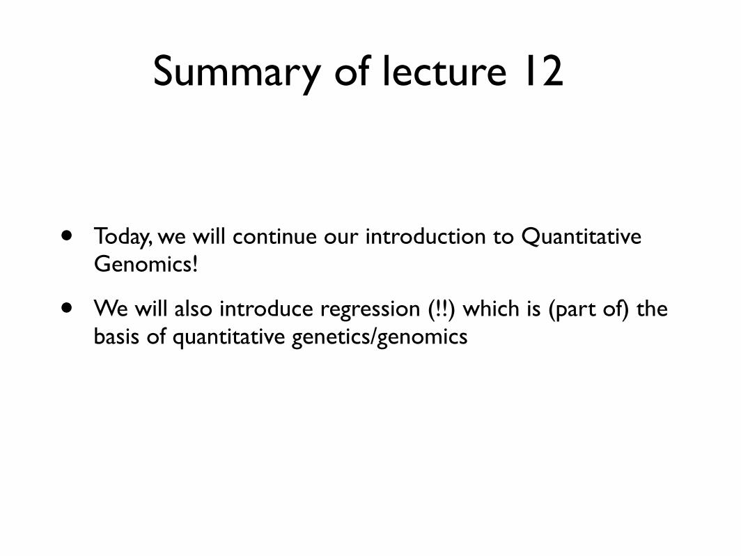
Summary of lecture 12

• Today, we will continue our introduction to Quantitative Genomics!

• We will also introduce regression (!!) which is (part of) the basis of quantitative genetics/genomics

Conceptual OverviewSystem

Questi

on

Experiment

Sample

Assumptions

InferencePr

ob. M

odels

Statistics

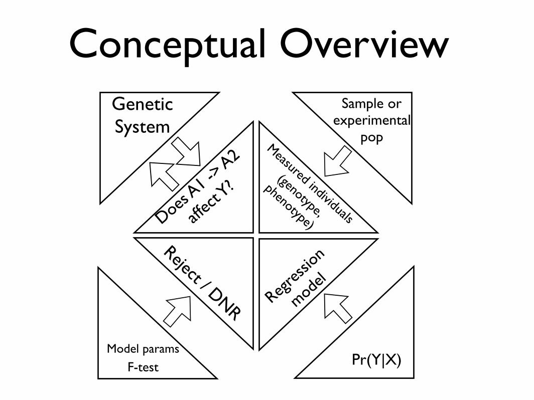
Conceptual OverviewGenetic System

Does A1 -

> A2

affec

t Y?

Sample or experimental

popMeasured individuals

(genotype,

phenotype)

Pr(Y|X)Model params

Reject / DNR Regres

sion

model

F-test

Review: Causal Mutation

• causal mutation - a position in the genome where an experimental manipulation of the DNA would produce an effect on the phenotype under specifiable conditions

• Formally, we may represent this as follows:

• Note: that this definition considers “under specifiable” conditions” so the change in genome need not cause a difference under every manipulation (just under broadly specifiable conditions)

• Also note the symmetry of the relationship

• Identifying these is the core of quantitative genetics/genomics (why do we want to do this!?)

• What is the perfect experiment?

• Our experiment will be a statistical experiment (sample and inference!)

Pr(X = x) = Pr(X1 = x1, X2 = x2, ..., Xn

= xn

) = PX(x) or fX(x)

MLE(p) =1

n

nX

i=1

xi

(8)

MLE(µ) = x =

1

n

nX

i=1

xi

(9)

A1 ! A2 ) �Y |Z (10)

4

Review: The statistical model I• As with any statistical experiment, we need to begin by defining our sample space

• In the most general sense, our sample space is:

• More specifically, each individual in our sample space can be quantified as a pair of sample outcomes so our sample space can be written as:

• Where is the genotype sample space at a locus and is the phenotype sample space

• Note that genotype is the set of possible genotypes, where for a diploid, with two alleles:

• For the phenotype, this can be any type of measurement (e.g. sick or healthy, height, etc.)

� or H0 : � = cPr(T (X) , Pr(T (X|�) , Pr(T (X|H0 : � = c)

L(�|x) =�

1↵2⇤

⇥n

ePn

i=1�(xi�µ)2

2 (3)

⇥ = { Possible Individuals }⇥ = {⇥g ⌥ ⇥P } (4)

F{g,P} (5)

Pr(F{g,P}) (6)

Pr{g, P} (7)

Pr(Y ⌥X) = Pr(Y,X) ⇧= Pr(Y )Pr(X) (8)

H0 : Pr(Y,X) = Pr(Y )Pr(X) (9)

LRT = � =

1

(2⇥)n2ePn

i=1�(xi�H0(µ))

2

2

1

(2⇥)n2ePn

i=1�(xi�MLE(µ))2

2

(10)

� =L(�0|x)L(�1|x)

(11)

Pr(LRT |H0 : � = c) ⇤ ⇧2d.f. (12)

LRT = �2ln(�) = �2ln

�L(�0|x)L(�1|x)

⇥(13)

L(�|x) (14)

�0 = argmax��0L(�|x) (15)

�1 = argmax��1L(�|x) (16)

H0 : µ = c (17)

[0,⌅) (18)

MLE(p) =1

n

n⇤

i=1

xi (19)

T (X = x) = X = µ ⇥ N(µ,⌅2/n) (20)

T (X = x) = � = p =1

n

n⇤

i=1

xi (21)

7


L(�|x) =�

1↵2⇤

⇥n

ePn

i=1�(xi�µ)2

2 (3)


F{g,P} (5)

Pr(F{g,P}) (6)

Pr{g, P} (7)

Pr(Y ⌥X) = Pr(Y,X) ⇧= Pr(Y )Pr(X) (8)

H0 : Pr(Y,X) = Pr(Y )Pr(X) (9)

LRT = � =

1

(2⇥)n2ePn

i=1�(xi�H0(µ))

2

2

1

(2⇥)n2ePn


2

(10)

� =L(�0|x)L(�1|x)

(11)

Pr(LRT |H0 : � = c) ⇤ ⇧2d.f. (12)

LRT = �2ln(�) = �2ln

�L(�0|x)L(�1|x)

⇥(13)

L(�|x) (14)

�0 = argmax��0L(�|x) (15)

�1 = argmax��1L(�|x) (16)

H0 : µ = c (17)

[0,⌅) (18)

MLE(p) =1

n

n⇤

i=1

xi (19)

T (X = x) = X = µ ⇥ N(µ,⌅2/n) (20)

T (X = x) = � = p =1

n

n⇤

i=1

xi (21)

7


L(�|x) =�

1⌦2⇤

⇥n

ePn

i=1�(xi�µ)2

2 (3)

⇥ = { Possible Individuals }⇥ = {⇥g ⌃ ⇥P } (4)

⇥g = {A1A1, A1A2, A2A2} (5)

⇥g (6)

⇥P (7)

F{g,P} (8)

Pr(F{g,P}) (9)

Pr{g, P} (10)

Pr(Y ⌃X) = Pr(Y,X) ⌅= Pr(Y )Pr(X) (11)

H0 : Pr(Y,X) = Pr(Y )Pr(X) (12)

LRT = � =

1

(2⇥)n2ePn

i=1�(xi�H0(µ))

2

2

1

(2⇥)n2ePn


2

(13)

� =L(�0|x)L(�1|x)

(14)

Pr(LRT |H0 : � = c) ⇥ ⌅2d.f. (15)

LRT = �2ln(�) = �2ln

�L(�0|x)L(�1|x)

⇥(16)

L(�|x) (17)

�0 = argmax��0L(�|x) (18)

�1 = argmax��1L(�|x) (19)

H0 : µ = c (20)

[0,⇤) (21)

MLE(p) =1

n

n⇤

i=1

xi (22)

7


L(�|x) =�

1⌦2⇤

⇥n

ePn

i=1�(xi�µ)2

2 (3)


⇥g = {A1A1, A1A2, A2A2} (5)

⇥g (6)

⇥P (7)

F{g,P} (8)

Pr(F{g,P}) (9)

Pr{g, P} (10)

Pr(Y ⌃X) = Pr(Y,X) ⌅= Pr(Y )Pr(X) (11)

H0 : Pr(Y,X) = Pr(Y )Pr(X) (12)

LRT = � =

1

(2⇥)n2ePn

i=1�(xi�H0(µ))

2

2

1

(2⇥)n2ePn


2

(13)

� =L(�0|x)L(�1|x)

(14)

Pr(LRT |H0 : � = c) ⇥ ⌅2d.f. (15)

LRT = �2ln(�) = �2ln

�L(�0|x)L(�1|x)

⇥(16)

L(�|x) (17)

�0 = argmax��0L(�|x) (18)

�1 = argmax��1L(�|x) (19)

H0 : µ = c (20)

[0,⇤) (21)

MLE(p) =1

n

n⇤

i=1

xi (22)

7


L(�|x) =�

1⌦2⇤

⇥n

ePn

i=1�(xi�µ)2

2 (3)


⇥g = {A1A1, A1A2, A2A2} (5)

⇥g (6)

⇥P (7)

F{g,P} (8)

Pr(F{g,P}) (9)

Pr{g, P} (10)

Pr(Y ⌃X) = Pr(Y,X) ⌅= Pr(Y )Pr(X) (11)

H0 : Pr(Y,X) = Pr(Y )Pr(X) (12)

LRT = � =

1

(2⇥)n2ePn

i=1�(xi�H0(µ))

2

2

1

(2⇥)n2ePn


2

(13)

� =L(�0|x)L(�1|x)

(14)

Pr(LRT |H0 : � = c) ⇥ ⌅2d.f. (15)

LRT = �2ln(�) = �2ln

�L(�0|x)L(�1|x)

⇥(16)

L(�|x) (17)

�0 = argmax��0L(�|x) (18)

�1 = argmax��1L(�|x) (19)

H0 : µ = c (20)

[0,⇤) (21)

MLE(p) =1

n

n⇤

i=1

xi (22)

7

Pr(X = x) = Pr(X1 = x1, X2 = x2, ..., Xn

= xn

) = PX(x) or fX(x)

MLE(p) =1

n

nX

i=1

xi

(8)

MLE(µ) = x =

1

n

nX

i=1

xi

(9)

A1 ! A2 ) �Y |Z (10)

gi

= Aj

Ak

(11)

2.1� 0.3 + (0)(�0.2) + (1)(1.1) + 0.7 (12)

4

Review: The statistical model II• Next, we need to define the probability model on the sigma

algebra of the sample space ( ):

• Which defines the probability of each possible genotype and phenotype pair:

• We will define two (types) or random variables (* = state does not matter):

• Note that the probability model induces a (joint) probability distribution on this random vector (these random variables):

For this sample space, we define a probability function (model):

Pr(S) = Pr(Sg, SP ) (5)

One could intuitively look at this as defining distinct probability functions for each ofthese sample spaces Sg and SP , although these probability functions would be related andwould actually define a single (joint) pdf for the sample space S = {Sg, SP }, S = {Sg\SP }.

We will define the following two (types) of random variables Y and X, where Y takesthe value of the phenotype to the reals (regardless of the genotype) and X takes the valueof the genotype to the reals (regardless of phenotype):

Y : (⇤, SP ) ! R (6)

X : (Sg, ⇤) ! R (7)

where ⇤ indicates the state of the given subset does not matter. Again, we could intuitivelythink of this as defining individual random variables for each sample space Sg and SP whereeach element of these random vectors is associated with only one probability function, i.e.a single random variable cannot be associated with more than one probability function.A more accurate way to think about this set-up is that we have defined a random vector[Y,X], where the probability function on S actually defines a joint probability functionover the random variables Y and X:

Pr(Y,X) (8)

and note we could have random vectors that include both discrete and continuous randomvariables, such that the joint probability distributions could combine discrete and contin-uous models.

As we discussed, regardless of the probability model describing our random variables /vectors, we can use expectations and variances to describe basic aspects of the models. Ifwe can take the expectation of the random vector [X,Y ] we obtain:

E [Y,X] = [EY,EX] (9)

and the variance of this random vector is:

V ar [Y,X] =

V ar(Y ) Cov(Y,X)

Cov(Y,X) V ar(X)

�

If X reflects a causal mutation (=causal allele =causal polymorphism), then Cov(Y,X) 6= 0(or Corr(Y,X) 6= 0). Our goal with quantitative genomic inference can therefore be broadlystated as determining whether Cov(Y,X) 6= 0 using a sample and we will do this using a

5


L(�|x) =�

1↵2⇤

⇥n

ePn

i=1�(xi�µ)2

2 (3)

⇤ = { Possible Individuals }⇤ = {⇤g ⌥ ⇤P } (4)

Pr{g, P} (5)

Pr(Y ⌥X) = Pr(Y,X) ⌃= Pr(Y )Pr(X) (6)

H0 : Pr(Y,X) = Pr(Y )Pr(X) (7)

LRT = ⇥ =

1

(2⇥)n2ePn

i=1�(xi�H0(µ))

2

2

1

(2⇥)n2ePn


2

(8)

⇥ =L(�0|x)L(�1|x)

(9)

Pr(LRT |H0 : � = c) ⇤ ⇧2d.f. (10)

LRT = �2ln(⇥) = �2ln

�L(�0|x)L(�1|x)

⇥(11)

L(�|x) (12)

�0 = argmax��0L(�|x) (13)

�1 = argmax��1L(�|x) (14)

H0 : µ = c (15)

[0,⌅) (16)

MLE(p) =1

n

n⇤

i=1

xi (17)

T (X = x) = X = µ ⇥ N(µ,⌅2/n) (18)

T (X = x) = � = p =1

n

n⇤

i=1

xi (19)

� ⇧ � (20)

� (21)

7


L(�|x) =�

1↵2⇤

⇥n

ePn

i=1�(xi�µ)2

2 (3)


F{g,P} (5)

Pr(Fg,P ) (6)

Pr{g, P} (7)

Pr(Y ⌥X) = Pr(Y,X) ⇧= Pr(Y )Pr(X) (8)

H0 : Pr(Y,X) = Pr(Y )Pr(X) (9)

LRT = � =

1

(2⇥)n2ePn

i=1�(xi�H0(µ))

2

2

1

(2⇥)n2ePn


2

(10)

� =L(�0|x)L(�1|x)

(11)

Pr(LRT |H0 : � = c) ⇤ ⇧2d.f. (12)

LRT = �2ln(�) = �2ln

�L(�0|x)L(�1|x)

⇥(13)

L(�|x) (14)

�0 = argmax��0L(�|x) (15)

�1 = argmax��1L(�|x) (16)

H0 : µ = c (17)

[0,⌅) (18)

MLE(p) =1

n

n⇤

i=1

xi (19)

T (X = x) = X = µ ⇥ N(µ,⌅2/n) (20)

T (X = x) = � = p =1

n

n⇤

i=1

xi (21)

7


L(�|x) =�

1↵2⇤

⇥n

ePn

i=1�(xi�µ)2

2 (3)


F{g,P} (5)

Pr(F{g,P}) (6)

Pr{g, P} (7)

Pr(Y ⌥X) = Pr(Y,X) ⇧= Pr(Y )Pr(X) (8)

H0 : Pr(Y,X) = Pr(Y )Pr(X) (9)

LRT = � =

1

(2⇥)n2ePn

i=1�(xi�H0(µ))

2

2

1

(2⇥)n2ePn


2

(10)

� =L(�0|x)L(�1|x)

(11)

Pr(LRT |H0 : � = c) ⇤ ⇧2d.f. (12)

LRT = �2ln(�) = �2ln

�L(�0|x)L(�1|x)

⇥(13)

L(�|x) (14)

�0 = argmax��0L(�|x) (15)

�1 = argmax��1L(�|x) (16)

H0 : µ = c (17)

[0,⌅) (18)

MLE(p) =1

n

n⇤

i=1

xi (19)

T (X = x) = X = µ ⇥ N(µ,⌅2/n) (20)

T (X = x) = � = p =1

n

n⇤

i=1

xi (21)

7


L(�|x) =�

1↵2⇤

⇥n

ePn

i=1�(xi�µ)2

2 (3)


⇥g = {A1A1, A1A2, A2A2} (5)

⇥g (6)

⇥P (7)

F{g,P} (8)

Pr(F{g,P}) (9)

Pr{g, P} (10)

Pr(Y ⌥X) = Pr(Y,X) ⇧= Pr(Y )Pr(X) (11)

H0 : Pr(Y,X) = Pr(Y )Pr(X) (12)

Y : (⇥,⇥P ) ⇤ R (13)

X : (⇥g, ⇥) ⇤ R (14)

LRT = � =

1

(2⇥)n2ePn

i=1�(xi�H0(µ))

2

2

1

(2⇥)n2ePn


2

(15)

� =L(�0|x)L(�1|x)

(16)

Pr(LRT |H0 : � = c) ⇤ ⌅2d.f. (17)

LRT = �2ln(�) = �2ln

�L(�0|x)L(�1|x)

⇥(18)

L(�|x) (19)

�0 = argmax��0L(�|x) (20)

�1 = argmax��1L(�|x) (21)

H0 : µ = c (22)

[0,⌅) (23)

7

Review: The statistical model III

• The goal of quantitative genomics and genetics is to identify cases of the following relationship:

• Remember that, regardless of the probability distribution of our random vector, we can define the expectation:

• and the variance:

• The goal of quantitative genomics can be rephrased as assessing the following relationship:


Pr(S) = Pr(Sg, SP ) (5)



Y : (⇤, SP ) ! R (6)

X : (Sg, ⇤) ! R (7)


Pr(Y,X) (8)



E [Y,X] = [EY,EX] (9)


V ar [Y,X] =

V ar(Y ) Cov(Y,X)

Cov(Y,X) V ar(X)

�


5


Pr(S) = Pr(Sg, SP ) (5)



Y : (⇤, SP ) ! R (6)

X : (Sg, ⇤) ! R (7)


Pr(Y,X) (8)



E [Y,X] = [EY,EX] (9)


V ar [Y,X] =

V ar(Y ) Cov(Y,X)

Cov(Y,X) V ar(X)

�


5


Pr(S) = Pr(Sg, SP ) (5)



Y : (⇤, SP ) ! R (6)

X : (Sg, ⇤) ! R (7)


Pr(Y,X) (8)



E [Y,X] = [EY,EX] (9)


V ar [Y,X] =

V ar(Y ) Cov(Y,X)

Cov(Y,X) V ar(X)

�


5

✓ or H0

: ✓ = cPr(T (X) , Pr(T (X|✓) , Pr(T (X|H

0

: ✓ = c)

L(✓|x) =

1p2⇡

!n

ePn

i=1

�(xi�µ)2

2 (3)

S = { Possible Individuals }S = {Sg \ SP } (4)

Pr(Y \X) = Pr(Y,X) 6= Pr(Y )Pr(X) (5)

LRT = ⇤ =

1

(2⇡)n2

ePn

i=1

�(xi�H0

(µ))2

2

1

(2⇡)n2

ePn

i=1

�(xi�MLE(µ))2

2

(6)

⇤ =L(✓

0

|x)L(✓

1

|x)(7)

Pr(LRT |H0

: ✓ = c) ! �2

d.f. (8)

LRT = �2ln(⇤) = �2ln

L(✓

0

|x)L(✓

1

|x)

!(9)

L(✓|x) (10)

✓0

= argmax✓2⇥0

L(✓|x) (11)

✓1

= argmax✓2⇥1

L(✓|x) (12)

H0

: µ = c (13)

[0,1) (14)

MLE(p) =1

n

nX

i=1

xi (15)

T (X = x) = X = µ ⇠ N(µ,�2/n) (16)

T (X = x) = ✓ = p =1

n

nX

i=1

xi (17)

✓ 2 ⇥ (18)

✓ (19)

N = {1, 2, 3, ...} (20)

Z = {...� 3,�2,�1, 0, 1, 2, 3, ...} (21)

7

The statistical model IV• We are going to consider a parameterized model to represent the

probability model of X and Y (that is the true statistical model of genetics!!!)

• Specifically, we will consider a regression model

• For the moment, let’s consider a regression model with normal error:

• Note that in this model, we consider Y to be the dependent or response variable and X to be the independent variable (what are the parameters!?)

• Also note implicitly assumes the following:

hypothesis testing framework. Note that while we are going to consider a specific prob-ability model as the basis for testing this hypothesis, any hypothesis test that assessesCov(Y,X) is a legitimate approach to the same goal (and many are used in quantitativegenomic analysis).

So far, we have not described the specific form of the probability model Pr(Y,X) thatwe are going to consider. While there are many ways of defining the probability modelthat will allow us to accomplish our purpose, we are going to consider the most versatileand widely used formulation. We will begin our introduction to this model by consider-ing a phenotype that we can model as continuous, and more specifically, with a normalprobability model, e.g. height (later we will introduce the broad class of models that canapply to continuous and discrete phentoypes). For such cases, we are going to consider alinear regression model. We are going to use a form of the same linear regression modelthat you likely learned about in your introductory statistics class. Recall that a linear re-gression mode assumes a similar set-up to the case we have considered, we have measureda dependent or response variable Y and an independent variable X for each individual ina sample. We can visualize this sample by plotting X versus Y (see your class notes for adiagram). We are going to define a probability model that has the following form:

Y = �0 +X�1 + ✏ (10)

✏ ⇠ N(0,�2✏ ) (11)

where Y and X are the values taken for each individual in the sample, �0 and �1 areparameters (constants) with some true value that we will estimate from the sample, ✏is the ‘error’ term and is a random variable with a normal distribution with parametersµ = 0 and �2 = �2

✏ which is unknown (which we generally do not estimate). Note that thisequation is a line (hence ‘linear regression’) and intuitively defines a line through the thepoints on the graph of X versus Y , with a slope defined by �1 and which intersects theY-axis at �0. Note that the sample points are more ‘scattered’ around this line the greaterthe �2

✏ , i.e. we assume that the true probability model is gaussian (normal) where the meanvalue of the normal distribution is the value X (the model depends on the value X of anindividual). This means that our probability model actually has the following form:

Pr(Y,X) = Pr(Y |X) (12)

i.e. we assume that X is fixed. This latter point is often not presented in introductorystatistics classes but it is implicit in all regression models.

We can write the value for single individual i in our sample as:

yi = �0 + xi�1 + ✏i (13)

6



Y = �0 +X�1 + ✏ (10)

✏ ⇠ N(0,�2✏ ) (11)




Pr(Y,X) = Pr(Y |X) (12)



yi = �0 + xi�1 + ✏i (13)

6

Linear regression is a bivariate distribution

• We’ve seen bivariate (multivariate) distributions before:

Linear regression I

• Let’s review the structure of a linear regression (not necessarily a genetic model):



Y = �0 +X�1 + ✏ (10)

✏ ⇠ N(0,�2✏ ) (11)




Pr(Y,X) = Pr(Y |X) (12)



yi = �0 + xi�1 + ✏i (13)

6



Y = �0 +X�1 + ✏ (10)

✏ ⇠ N(0,�2✏ ) (11)




Pr(Y,X) = Pr(Y |X) (12)



yi = �0 + xi�1 + ✏i (13)

6

X

Y

Linear regression I

Linear regression II

• The linear regression model allows calculation of the (interval) probability of observations (!!)



Y = �0 +X�1 + ✏ (10)

✏ ⇠ N(0,�2✏ ) (11)




Pr(Y,X) = Pr(Y |X) (12)



yi = �0 + xi�1 + ✏i (13)

6



Y = �0 +X�1 + ✏ (10)

✏ ⇠ N(0,�2✏ ) (11)




Pr(Y,X) = Pr(Y |X) (12)



yi = �0 + xi�1 + ✏i (13)

6

X

Y

Linear regression III• A multiple regression model has the same structure, with a

single dependent variable Y and more than one independent variable Xi, Xj, e.g.,

• The quantitative genetic model is a multiple regression model with the following independent (“dummy”) variables:

• and the following “multiple” regression equation:

where for an individual i in a sample we may write:

yi = �µ +Xi,a�a + xi,d�d + ✏ (23)

An intuitive way to consider this model, is to plot the phenotype Y on the Y-axis againstthe genotypes A1A1, A1A2, A2A2 on the X-axis for a sample (see class). We can repre-sent all the individuals in our sample as points that are grouped in the three categoriesA1A1, A1A2, A2A2 and note that the true model would include points distributed in threenormal distributions, with the means defined by the three classes A1A1, A1A2, A2A2. Ifwe were to then re-plot these points in two plots, Y versus Xa and Y versus Xd, the firstwould look like the original plot, and the second would put the points in two groups (seeclass). The multiple linear regression equation (20, 21) defines ‘two’ regression lines (ormore accurately a plane) for these latter two plots, where the slopes of the lines are �a and�d (see class). Note that �µ is where these two plots (the plane) intersect the Y-axis butwith the way we have coded Xa and Xd, this is actually an estimate of the overall meanof the population (hence the notation �µ).

To consider a ‘plane’ interpretation of the multiple regression model, let’s consider threeaxes, where on the x-axis we will plot Xa, on the y-axis we will plot Xd, and on the z-axis(which we will plot coming out towards you from the page) we will plot the phenotype Y .We can draw the x-axis and y-axis as follows:

1 A1A2

�1 A1A1 A2A2

-1 0 1

where the genotype are placed where they would map on the x- and y-axis. Now the phe-notypes would be plotted above each of these three genotypes in the z-plane and we couldthink of there being a plane that we would draw through these points where the slopeof the plane in the z-axis along the x-axis would be �a and the slope of the plane alongthe y-axis would be �d, i.e. the we are projecting the values of the phenotypes into threedimensions and the multiple regression defines a plane through the points in these threedimensions.

For this regression model (where we are assuming a probability model of the form Pr(Y |X))we have four parameters ✓ =

⇥�µ,�a,�d,�

2✏

⇤. We are interested in a case where in the true

probability model Cov(X,Y ) 6= 0, which corresponds to any case where �a 6= 0 or �d 6= 0(�µ and �2

✏ may be any value). As we will discuss, the way we are going to assess whether agenotype is a causal polymorphism, i.e. by performing a hypothesis test with the followingnull and alternative hypotheses:

H0 : �a = 0 \ �d = 0 (24)

8

and we can write the ‘predicted’ value of yi of an individual as:

yi = �0 + xi�1 (14)

which is the value we would expect yi to take if there is no error. Note that by conventionwe write the predicted value of y with a ‘hat’, which is the same terminology that we usefor parameter estimates. I consider this a bit confusing, since we only estimate parame-ters, but you can see where it comes from, i.e. the predicted value of yi is a function ofparameter estimates.

As an example, let’s consider the values all of the linear regression components wouldtake for a specific value yi. Let’s consider a system where:

Y = �0 +X�1 + ✏ = 0.5 +X(1) + ✏ (15)

✏ ⇠ N(0,�2✏ ) = N(0, 1) (16)

If we take a sample and obtain the value y1 = 3.8 for an individual in our sample, the truevalues of the equation for this individual are:

3.8 = 0.5 + 3(1) + 0.3 (17)

Let’s say we had estimated the parameters �0 and �1 from the sample to be �0 = 0.6 and�1 = 2.9. The predicted value of y1 in this case would be:

y1 = 3.5 = 0.6 + 2.9(1) (18)

Note that we have not yet discussed how we estimate the � parameters but we will get tothis next lecture.

To produce a linear regression model useful in quantitative genomics, we will define amultiple linear regression, which simply means that we have more than one independent(fixed random) variable X, each with their own associated �. Specifically, we will definethe two following independent (random) variables:

Xa(A1A1) = �1, Xa(A1A2) = 0, Xa(A2A2) = 1 (19)

Xd(A1A1) = �1, Xd(A1A2) = 1, Xd(A2A2) = �1 (20)

and the following regression equation:

Y = �µ +Xa�a +Xd�d + ✏ (21)

✏ ⇠ N(0,�2✏ ) (22)

7


yi = �0 + xi�1 (14)



Y = �0 +X�1 + ✏ = 0.5 +X(1) + ✏ (15)

✏ ⇠ N(0,�2✏ ) = N(0, 1) (16)


3.8 = 0.5 + 3(1) + 0.3 (17)


y1 = 3.5 = 0.6 + 2.9(1) (18)



Xa(A1A1) = �1, Xa(A1A2) = 0, Xa(A2A2) = 1 (19)

Xd(A1A1) = �1, Xd(A1A2) = 1, Xd(A2A2) = �1 (20)


Y = �µ +Xa�a +Xd�d + ✏ (21)

✏ ⇠ N(0,�2✏ ) (22)

7


yi = �0 + xi�1 (14)



Y = �0 +X�1 + ✏ = 0.5 +X(1) + ✏ (15)

✏ ⇠ N(0,�2✏ ) = N(0, 1) (16)


3.8 = 0.5 + 3(1) + 0.3 (17)


y1 = 3.5 = 0.6 + 2.9(1) (18)



Xa(A1A1) = �1, Xa(A1A2) = 0, Xa(A2A2) = 1 (19)

Xd(A1A1) = �1, Xd(A1A2) = 1, Xd(A2A2) = �1 (20)


Y = �µ +Xa�a +Xd�d + ✏ (21)

✏ ⇠ N(0,�2✏ ) (22)

7

The genetic probability model I

The genetic probability model II• The probability distribution of this model, is therefore:

• Which has four parameters:

• The three parameters are required to model the three separate genotypes (A1A1, A1A2, A2A2)

• The can be thought of as a random variable that describes the probability an individual will have a specific value of Y, conditional on the genotype AiAj, where the probability is normally distributed around the value determined by the X’s and ‘s

⇤ or H0 : ⇤ = cPr(T (X) , Pr(T (X|⇤) , Pr(T (X|H0 : ⇤ = c)

L(⇤|x) =�

1↵2⌅

⇥n

ePn

i=1�(xi�µ)2

2 (3)


⇥g = {A1A1, A1A2, A2A2} (5)

�µ = 0.3,�a = 0.2,�d = �1.1,⇧2� = 1.1 (6)

�µ,�a,�d,⇧2� (7)

Pr(Y |X) ⇤ N(�µ +Xa�a +Xd�d,⇧2� ) (8)

2.1 = 0.3 + (0)0.2, (�1)� 1.1 + 0.7 (9)

Xa(A1A2) = 0, Xd(A1A2) = �1 (10)

⇥i = 0.7 (11)

⇥g (12)

⇥P (13)

F{g,P} (14)

Pr(F{g,P}) (15)

Pr{g, P} (16)

Pr(Y ⌥X) = Pr(Y,X) ⇧= Pr(Y )Pr(X) (17)

H0 : Pr(Y,X) = Pr(Y )Pr(X) (18)

Y : (⇥,⇥P ) ⌅ R (19)

X : (⇥g, ⇥) ⌅ R (20)

LRT = � =

1

(2⇤)n2ePn

i=1�(xi�H0(µ))

2

2

1

(2⇤)n2ePn


2

(21)

� =L(⇤0|x)L(⇤1|x)

(22)

Pr(LRT |H0 : ⇤ = c) ⌅ ⌃2d.f. (23)

7


L(⇤|x) =�

1↵2⌅

⇥n

ePn

i=1�(xi�µ)2

2 (3)


⇥g = {A1A1, A1A2, A2A2} (5)

�µ = 0.3,�a = 0.2,�d = �1.1,⇧2� = 1.1 (6)

�µ,�a,�d,⇧2� (7)

� (8)

⇥ (9)

Pr(Y |X) ⇤ N(�µ +Xa�a +Xd�d,⇧2� ) (10)

2.1 = 0.3 + (0)0.2, (�1)� 1.1 + 0.7 (11)

Xa(A1A2) = 0, Xd(A1A2) = �1 (12)

⇥i = 0.7 (13)

⇥g (14)

⇥P (15)

F{g,P} (16)

Pr(F{g,P}) (17)

Pr{g, P} (18)

Pr(Y ⌥X) = Pr(Y,X) ⇧= Pr(Y )Pr(X) (19)

H0 : Pr(Y,X) = Pr(Y )Pr(X) (20)

Y : (⇥,⇥P ) ⌅ R (21)

X : (⇥g, ⇥) ⌅ R (22)

LRT = � =

1

(2⇤)n2ePn

i=1�(xi�H0(µ))

2

2

1

(2⇤)n2ePn


2

(23)

� =L(⇤0|x)L(⇤1|x)

(24)

7


L(⇤|x) =�

1↵2⌅

⇥n

ePn

i=1�(xi�µ)2

2 (3)


⇥g = {A1A1, A1A2, A2A2} (5)

�µ = 0.3,�a = 0.2,�d = �1.1,⇧2� = 1.1 (6)

�µ,�a,�d,⇧2� (7)

� (8)

⇥ (9)

Pr(Y |X) ⇤ N(�µ +Xa�a +Xd�d,⇧2� ) (10)

2.1 = 0.3 + (0)0.2, (�1)� 1.1 + 0.7 (11)

Xa(A1A2) = 0, Xd(A1A2) = �1 (12)

⇥i = 0.7 (13)

⇥g (14)

⇥P (15)

F{g,P} (16)

Pr(F{g,P}) (17)

Pr{g, P} (18)

Pr(Y ⌥X) = Pr(Y,X) ⇧= Pr(Y )Pr(X) (19)

H0 : Pr(Y,X) = Pr(Y )Pr(X) (20)

Y : (⇥,⇥P ) ⌅ R (21)

X : (⇥g, ⇥) ⌅ R (22)

LRT = � =

1

(2⇤)n2ePn

i=1�(xi�H0(µ))

2

2

1

(2⇤)n2ePn


2

(23)

� =L(⇤0|x)L(⇤1|x)

(24)

7


L(⇤|x) =�

1↵2⌅

⇥n

ePn

i=1�(xi�µ)2

2 (3)


⇥g = {A1A1, A1A2, A2A2} (5)

�µ = 0.3,�a = 0.2,�d = �1.1,⇧2� = 1.1 (6)

�µ,�a,�d,⇧2� (7)

� (8)

⇥ (9)

Pr(Y |X) ⇤ N(�µ +Xa�a +Xd�d,⇧2� ) (10)

2.1 = 0.3 + (0)0.2, (�1)� 1.1 + 0.7 (11)

Xa(A1A2) = 0, Xd(A1A2) = �1 (12)

⇥i = 0.7 (13)

⇥g (14)

⇥P (15)

F{g,P} (16)

Pr(F{g,P}) (17)

Pr{g, P} (18)

Pr(Y ⌥X) = Pr(Y,X) ⇧= Pr(Y )Pr(X) (19)

H0 : Pr(Y,X) = Pr(Y )Pr(X) (20)

Y : (⇥,⇥P ) ⌅ R (21)

X : (⇥g, ⇥) ⌅ R (22)

LRT = � =

1

(2⇤)n2ePn

i=1�(xi�H0(µ))

2

2

1

(2⇤)n2ePn


2

(23)

� =L(⇤0|x)L(⇤1|x)

(24)

7


yi = �0 + xi�1 (14)



Y = �0 +X�1 + ✏ = 0.5 +X(1) + ✏ (15)

✏ ⇠ N(0,�2✏ ) = N(0, 1) (16)


3.8 = 0.5 + 3(1) + 0.3 (17)


y1 = 3.5 = 0.6 + 2.9(1) (18)



Xa(A1A1) = �1, Xa(A1A2) = 0, Xa(A2A2) = 1 (19)

Xd(A1A1) = �1, Xd(A1A2) = 1, Xd(A2A2) = �1 (20)


Y = �µ +Xa�a +Xd�d + ✏ (21)

✏ ⇠ N(0,�2✏ ) (22)

7

Ski Ai = ⌦ and Ai \Aj = ; for all i 6= j

B ⇢ ⌦ (223)

Pr(Xcp|X, r) = Pr(g|r) (224)

Pr(Y |X) ⇠ N(�µ +Xa�a +Xd�d,�2

✏ ) (225)

25

The genetic probability model III• Let’s consider a specific example where we are interested modeling

the relationship between a genotype and a phenotype (such as height) where the latter is well approximated by a normal distribution

• For this case, the (unknown) conditions of the experiment define the true values of the parameters (unknown to us!), which we will say are the following (note these are the same for all individuals in the population since they are parameters of the probability distribution):

• Consider an individual i with gi = A1A2 such that we have:

• If this individual has a phenotype value yi = 2.1 then we have the epsilon value where the probability of this particular value (i.e. the interval surrounding this value) is defined by


yi = �0 + xi�1 (14)



Y = �0 +X�1 + ✏ = 0.5 +X(1) + ✏ (15)

✏ ⇠ N(0,�2✏ ) = N(0, 1) (16)


3.8 = 0.5 + 3(1) + 0.3 (17)


y1 = 3.5 = 0.6 + 2.9(1) (18)



Xa(A1A1) = �1, Xa(A1A2) = 0, Xa(A2A2) = 1 (19)

Xd(A1A1) = �1, Xd(A1A2) = 1, Xd(A2A2) = �1 (20)


Y = �µ +Xa�a +Xd�d + ✏ (21)

✏ ⇠ N(0,�2✏ ) (22)

7


L(⇤|x) =�

1⌦2⌅

⇥n

ePn

i=1�(xi�µ)2

2 (3)


⇥g = {A1A1, A1A2, A2A2} (5)

�0 = 0.3,�a = 0.2,�d = �1.1,⇧2� = 1.1 (6)

2.1 = 0.3 + (0)0.2, (�1)� 1.1 + 0.7 (7)

Xa(A1A2) = 0, Xd(A1A2) = �1 (8)

⇥i = 0.7 (9)

⇥g (10)

⇥P (11)

F{g,P} (12)

Pr(F{g,P}) (13)

Pr{g, P} (14)

Pr(Y ⌃X) = Pr(Y,X) ⌅= Pr(Y )Pr(X) (15)

H0 : Pr(Y,X) = Pr(Y )Pr(X) (16)

Y : (⇥,⇥P ) ⇤ R (17)

X : (⇥g, ⇥) ⇤ R (18)

LRT = � =

1

(2⇥)n2ePn

i=1�(xi�H0(µ))

2

2

1

(2⇥)n2ePn


2

(19)

� =L(⇤0|x)L(⇤1|x)

(20)

Pr(LRT |H0 : ⇤ = c) ⇤ ⌃2d.f. (21)

LRT = �2ln(�) = �2ln

�L(⇤0|x)L(⇤1|x)

⇥(22)

L(⇤|x) (23)

7


L(⇤|x) =�

1↵2⌅

⇥n

ePn

i=1�(xi�µ)2

2 (3)


⇥g = {A1A1, A1A2, A2A2} (5)

�µ = 0.3,�a = �0.2,�d = 1.1,⇧2� = 1.1 (6)

�µ,�a,�d,⇧2� (7)

� (8)

⇥ (9)

Pr(Y |X) ⇤ N(�µ +Xa�a +Xd�d,⇧2� ) (10)

2.1 = 0.3 + (0)0.2, (1)1.1 + 0.7 (11)

Xa(A1A2) = 0, Xd(A1A2) = 1 (12)

⇥i = 0.7 (13)

⇥g (14)

⇥P (15)

F{g,P} (16)

Pr(F{g,P}) (17)

Pr{g, P} (18)

Pr(Y ⌥X) = Pr(Y,X) ⇧= Pr(Y )Pr(X) (19)

H0 : Pr(Y,X) = Pr(Y )Pr(X) (20)

Y : (⇥,⇥P ) ⌅ R (21)

X : (⇥g, ⇥) ⌅ R (22)

LRT = � =

1

(2⇤)n2ePn

i=1�(xi�H0(µ))

2

2

1

(2⇤)n2ePn


2

(23)

� =L(⇤0|x)L(⇤1|x)

(24)

7


L(⇤|x) =�

1↵2⌅

⇥n

ePn

i=1�(xi�µ)2

2 (3)


⇥g = {A1A1, A1A2, A2A2} (5)

�µ = 0.3,�a = �0.2,�d = 1.1,⇧2� = 1.1 (6)

�µ,�a,�d,⇧2� (7)

� (8)

⇥ (9)

Pr(Y |X) ⇤ N(�µ +Xa�a +Xd�d,⇧2� ) (10)

2.1 = 0.3 + (0)0.2, (1)1.1 + 0.7 (11)

Xa(A1A2) = 0, Xd(A1A2) = 1 (12)

⇥i = 0.7 (13)

⇥g (14)

⇥P (15)

F{g,P} (16)

Pr(F{g,P}) (17)

Pr{g, P} (18)

Pr(Y ⌥X) = Pr(Y,X) ⇧= Pr(Y )Pr(X) (19)

H0 : Pr(Y,X) = Pr(Y )Pr(X) (20)

Y : (⇥,⇥P ) ⌅ R (21)

X : (⇥g, ⇥) ⌅ R (22)

LRT = � =

1

(2⇤)n2ePn

i=1�(xi�H0(µ))

2

2

1

(2⇤)n2ePn


2

(23)

� =L(⇤0|x)L(⇤1|x)

(24)

7

Pr(X = x) = Pr(X1 = x1, X2 = x2, ..., Xn

= xn

) = PX(x) or fX(x)

MLE(p) =1

n

nX

i=1

xi

(8)

MLE(µ) = x =

1

n

nX

i=1

xi

(9)

A1 ! A2 ) �Y |Z (10)

gi

= Aj

Ak

(11)

2.1� 0.3 + (0)(�0.2) + (1)(1.1) + 0.7 (12)

4

=

• Note that, while somewhat arbitrary, the advantage of the Xa and Xd coding is the parameters and map directly on to relationships between the genotype and phenotype that are important in genetics:

• If then this is a “purely” additive case

• If then this is only over- or under-dominance (homozygotes have equal effects on phenotype)

• If both are non-zero, there are both additive and dominance effects

• If both are zero, there is no effect of the genotype on the phenotype (the genotype is not causal!)

The genetic probability model IV

[X1 = x1, X2 = x2, ..., X10 = x10] ⇠ px1(1� p)1�x1px2(1� p)1�x2 ...px10(1� p)1�x10 (16)

T (X = x) = T (x) = X =1

10

10X

i=1

xi (17)

[Tmin, ..., Tmax] = [0, 0.1, ..., 1] ! [0, 1, ..., 10] (18)

Pr(T (x)) ⇠✓

n

nT (x)

◆pnT (x)(1� p)n�nT (x) (19)

T (x) = ✓ = p (20)

Pr(p) ⇠✓

n

nT (x)

◆pnT (x)(1� p)n�nT (x) (21)

Ep = p (22)

Pr(µ,�2|X = x) = L(µ,�2|X = x) =1p2⇡�2

e�(x�µ)2

2�2 (23)

l(p|X = x) = ln

✓n

x

◆+ xln(p) + (n� x)ln(1� p) (24)

MLE(µ) = X =1

n

nX

i=1

xi (25)

pval(T (x)) =

Z 1

T (x)Pr(T (x)|✓ = c)dT (x) (26)

pval(T (x)) =

Z �|T (x)�median(T (X)|

�1Pr(T (x)|✓ = c)dT (x)+

Z 1

|T (x)|�median(T (X)|Pr(T (x)|✓ = c)dT (x)

(27)

pval(T (x)) =

max(T (X))X

T (x)

Pr(T (x)|✓ = c) (28)

pval(T (x)) =

�|T (x)�median(T (X)|X

min(T (X))

Pr(T (x)|✓ = c) +

max(T (X))X

|T (x)�median(T (X)|

Pr(T (x)|✓ = c) (29)

�a (30)

�d (31)

�a 6= 0,�d = 0 (32)

�a = 0,�d 6= 0 (33)

H0 : Cov(Xa, Y ) = 0 \ Cov(Xd, Y ) = 0 (34)

13


T (X = x) = T (x) = X =1

10

10X

i=1

xi (17)

[Tmin, ..., Tmax] = [0, 0.1, ..., 1] ! [0, 1, ..., 10] (18)

Pr(T (x)) ⇠✓

n

nT (x)

◆pnT (x)(1� p)n�nT (x) (19)

T (x) = ✓ = p (20)

Pr(p) ⇠✓

n

nT (x)

◆pnT (x)(1� p)n�nT (x) (21)

Ep = p (22)

Pr(µ,�2|X = x) = L(µ,�2|X = x) =1p2⇡�2

e�(x�µ)2

2�2 (23)

l(p|X = x) = ln

✓n

x

◆+ xln(p) + (n� x)ln(1� p) (24)

MLE(µ) = X =1

n

nX

i=1

xi (25)

pval(T (x)) =

Z 1

T (x)Pr(T (x)|✓ = c)dT (x) (26)

pval(T (x)) =


�1Pr(T (x)|✓ = c)dT (x)+

Z 1


(27)

pval(T (x)) =

max(T (X))X

T (x)

Pr(T (x)|✓ = c) (28)

pval(T (x)) =


min(T (X))

Pr(T (x)|✓ = c) +

max(T (X))X


Pr(T (x)|✓ = c) (29)

�a (30)

�d (31)

�a 6= 0,�d = 0 (32)

�a = 0,�d 6= 0 (33)

H0 : Cov(Xa, Y ) = 0 \ Cov(Xd, Y ) = 0 (34)

13


T (X = x) = T (x) = X =1

10

10X

i=1

xi (17)

[Tmin, ..., Tmax] = [0, 0.1, ..., 1] ! [0, 1, ..., 10] (18)

Pr(T (x)) ⇠✓

n

nT (x)

◆pnT (x)(1� p)n�nT (x) (19)

T (x) = ✓ = p (20)

Pr(p) ⇠✓

n

nT (x)

◆pnT (x)(1� p)n�nT (x) (21)

Ep = p (22)

Pr(µ,�2|X = x) = L(µ,�2|X = x) =1p2⇡�2

e�(x�µ)2

2�2 (23)

l(p|X = x) = ln

✓n

x

◆+ xln(p) + (n� x)ln(1� p) (24)

MLE(µ) = X =1

n

nX

i=1

xi (25)

pval(T (x)) =

Z 1

T (x)Pr(T (x)|✓ = c)dT (x) (26)

pval(T (x)) =


�1Pr(T (x)|✓ = c)dT (x)+

Z 1


(27)

pval(T (x)) =

max(T (X))X

T (x)

Pr(T (x)|✓ = c) (28)

pval(T (x)) =


min(T (X))

Pr(T (x)|✓ = c) +

max(T (X))X


Pr(T (x)|✓ = c) (29)

�a (30)

�d (31)

�a 6= 0,�d = 0 (32)

�a = 0,�d 6= 0 (33)

H0 : Cov(Xa, Y ) = 0 \ Cov(Xd, Y ) = 0 (34)

13


T (X = x) = T (x) = X =1

10

10X

i=1

xi (17)

[Tmin, ..., Tmax] = [0, 0.1, ..., 1] ! [0, 1, ..., 10] (18)

Pr(T (x)) ⇠✓

n

nT (x)

◆pnT (x)(1� p)n�nT (x) (19)

T (x) = ✓ = p (20)

Pr(p) ⇠✓

n

nT (x)

◆pnT (x)(1� p)n�nT (x) (21)

Ep = p (22)

Pr(µ,�2|X = x) = L(µ,�2|X = x) =1p2⇡�2

e�(x�µ)2

2�2 (23)

l(p|X = x) = ln

✓n

x

◆+ xln(p) + (n� x)ln(1� p) (24)

MLE(µ) = X =1

n

nX

i=1

xi (25)

pval(T (x)) =

Z 1

T (x)Pr(T (x)|✓ = c)dT (x) (26)

pval(T (x)) =


�1Pr(T (x)|✓ = c)dT (x)+

Z 1


(27)

pval(T (x)) =

max(T (X))X

T (x)

Pr(T (x)|✓ = c) (28)

pval(T (x)) =


min(T (X))

Pr(T (x)|✓ = c) +

max(T (X))X


Pr(T (x)|✓ = c) (29)

�a (30)

�d (31)

�a 6= 0,�d = 0 (32)

�a = 0,�d 6= 0 (33)

H0 : Cov(Xa, Y ) = 0 \ Cov(Xd, Y ) = 0 (34)

13

Genetic example 1

• As an example, consider the following of a “purely additive” case (= no dominance):


yi = �µ +Xi,a�a + xi,d�d + ✏ (23)


�µ = 2,�a = 5,�d = 0,�2✏ = 1

�µ = 0,�a = 4,�d = �2,�2✏ = 1

�µ = 0,�a = 2,�d = 3,�2✏ = 1

�µ = 0,�a = 2,�d = 3,�2✏ = 1

�µ = 2,�a = 0,�d = 0,�2✏ = 1


1 A1A2

�1 A1A1 A2A2

-1 0 1

where the genotype are placed where they would map on the x- and y-axis. Now the phe-notypes would be plotted above each of these three genotypes in the z-plane and we could

8

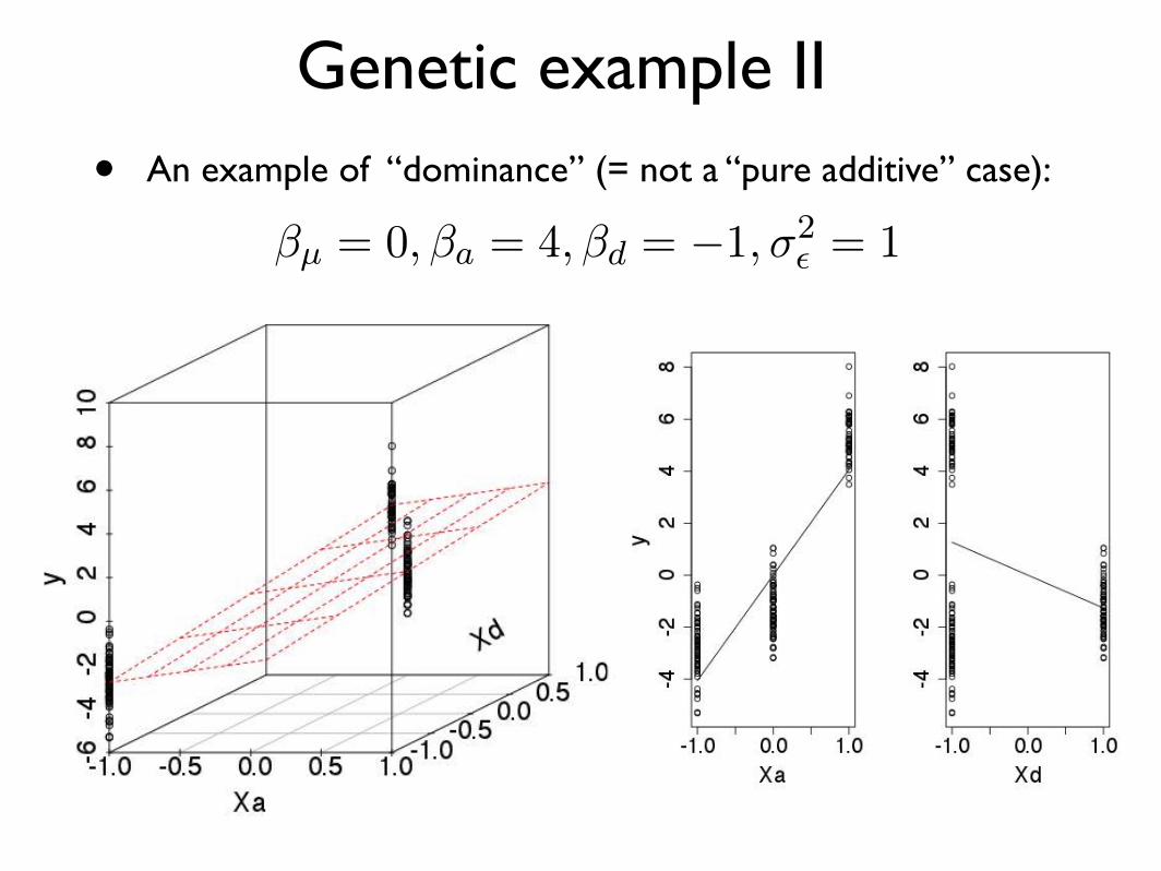
Genetic example II

• An example of “dominance” (= not a “pure additive” case):

H0 : Cov(Xa, Y ) = 0 \ Cov(Xd, Y ) = 0 (35)

HA : Cov(Xa, Y ) 6= 0 [ Cov(Xd, Y ) 6= 0 (36)

H0 : �a = 0 \ �d = 0 (37)

HA : �a 6= 0 [ �d 6= 0 (38)

F�statistic = f(⇤) (39)

�µ = 0,�a = 4,�d = �1,�2✏ = 1 (40)

14

Genetic example III• A case of NO genetic effect:


yi = �µ +Xi,a�a + xi,d�d + ✏ (23)


�µ = 2,�a = 5,�d = 0,�2✏ = 1

�µ = 0,�a = 4,�d = �2,�2✏ = 1

�µ = 0,�a = 2,�d = 3,�2✏ = 1

�µ = 0,�a = 2,�d = 3,�2✏ = 1

�µ = 2,�a = 0,�d = 0,�2✏ = 1


1 A1A2

�1 A1A1 A2A2

-1 0 1

where the genotype are placed where they would map on the x- and y-axis. Now the phe-notypes would be plotted above each of these three genotypes in the z-plane and we could

8

That’s it for today

• Next week: quantitative genomics II (estimation and hypothesis testing!)

Quantitative Genomics and Geneticsmezeylab.cb.bscb.cornell.edu/labmembers/documents... · Lecture12: Continuing introduction to Quantitative Genomics Jason Mezey [email protected]

Documents