Quantitative assessment of deep gas migration in ... - SKB · SKB may draw modified conclusions, based on additional literature sources and/or expert opinions. A pdf version of this

Svensk Kärnbränslehantering ABSwedish Nuclear Fueland Waste Management Co

Box 250, SE-101 24 Stockholm Phone +46 8 459 84 00

R-10-61

CM

Gru

ppen

AB

, Bro

mm

a, 2

010

Quantitative assessment of deep gas migration in Fennoscandian sites

Anne Delos, Paolo Trinchero, Laurent Richard, Jorge Molinero Amphos 21 Consulting S.L.

Marco Dentz IDAEA-CSIC Instituto de Diagnóstico Ambiental y Estudios del Agua

Petteri Pitkänen Posiva Oy

November 2010

R-10-61

Tänd ett lager: P, R eller TR.

Quantitative assessment of deep gas migration in Fennoscandian sites

Anne Delos, Paolo Trinchero, Laurent Richard, Jorge Molinero Amphos 21 Consulting S.L.

Marco Dentz IDAEA-CSIC Instituto de Diagnóstico Ambiental y Estudios del Agua

Petteri Pitkänen Posiva Oy

November 2010

ISSN 1402-3091

SKB R-10-61

This report concerns a study which was conducted for SKB. The conclusions and viewpoints presented in the report are those of the authors. SKB may draw modified conclusions, based on additional literature sources and/or expert opinions.

A pdf version of this document can be downloaded from www.skb.se.

R-10-61 3

Summary

The origin and migration of gases in the geosphere is of interest for performance assessment studies of deep geological repositories of nuclear waste. The presence of dissolved gases in groundwater relates with some safety issues linked to chemical processes. Noble gases, such as helium isotopes, are commonly used as a marker of the paleohydrogeological evolution, and are good tracers to give information on hydrogeological conditions and groundwater residence time. There are also reactive (non-inert) gases CH4, H2O, CO2, H2S, NH3, H2, and N2 dissolved in the groundwaters. CH4 and H2 are strong reducing agents that may consume oxygen and be involved in microbial sulphate reduction processes. The integrity of the copper canisters in the repository is one of the major issues to be analyzed in the framework of the Swedish program for geological disposal of spent nuclear fuel and dissolved oxygen and sulphide in groundwater are the most damaging components for copper corrosion. Therefore, quantification of flow rates of both, inert and reactive gases, such as helium, methane and hydrogen, in the bedrock would be important for performance assessment calculations.

Fluxes of Helium, Methane and Hydrogen at three Fennoscandian sites (Forsmark and Laxemar in Sweden, and Olkiluoto in Finland) have been modelled using Fick’s law and measured gradients of gas concentration. Under this hypothesis the concentration is a linear function of depth and hence the gradients can be easily inferred by linear regression. The uncertainty stemming from the scarcity of data and from the diffusivity value used in the analysis has been addressed by sensitivity analysis. Finally, estimates of steady-state gas fluxes of the three Fennoscandian sites are provided.

The same data-set has been modelled using the analytical solution provided by Andrews et al. (1989). This solution requires gas production to be constant throughout the domain (which, strictly speaking, is infinite). It turns out that its results cannot be reliably used to estimate gas fluxes. They can rather provide an estimate of the effective in situ gas production (i.e. radiogenic production) averaged over the model domain. Such effective in situ gas productions have been computed and discussed for the 3 sites.

Helium profiles have been modelled using two different approaches: calibrating the residence time or estimating the release fraction (i.e. the rate of Helium production actually released to the water). Methane and Hydrogen in situ productions have been then determined either setting time equal to the age of formation of the rock or using the value of residence time obtained from the analysis of the Helium profiles.

A new analytical solution that can take into account not only the radiogenic production but also the flux from a deep source of helium has been developed. This solution in companion with further field character ization (e.g. isotopic measurements of Helium) provides a powerful tool that allows accounting for the coupled effect of a (limited in space) in situ production and a source occurring at a large depth in the crust or mantle. It is thought that this new analytical solution could be used for future quantitative modelling of gas migration when more data were available.

R-10-61 5

List of notation

Note that throughout this report “L” stands for litre of water (either groundwater or porewater) and “m3” in general stands for a volume of geologic medium, that is, the rock and its porewater.

C(z, t) mol m–3 Gas concentration in the rock at depth z and time tC'(z, t) mol·L–1 Gas concentration in the water at depth z and time tDe

X m2y–1 Effective diffusion coefficient of XD0

X m2y–1 Diffusion coefficient of X in pure waterDp

X m2y–1 Pore diffusion coefficient of XG mol m–3y–1 Gas production rate in the rockJ mol m2y–1 Diffusive flux of the gas[U] ppm Uranium contents of the rock matrixSTP Standard Temperature and Pressuret y Timetf y Formation age[Th] ppm Thorium contents of the rock matrixVm m3·mol–1 Molar volumez m Depthδconst Constrictionρ kgm–3 Rock bulk densityφ – Porosityτ Tortuosity

R-10-61 7

Contents

1 Introduction 91.1 Background 91.2 Objectives of this report 91.3 Methodology and Scope 10

2 Site description and problem statement 112.1 Geological and hydrogeochemical settings 11

2.1.1 Olkiluoto site (Finland) 112.1.2 Forsmark site (Sweden) 112.1.3 Laxemar site (Sweden) 12

2.2 Sinks and sources of deep gases in the geosphere 122.2.1 Helium (He) 132.2.2 Methane (CH4) 132.2.3 Hydrogen (H2) 14

3 Observation of deep gas migration at the Fennoscandian sites 153.1 Gas transport mechanisms 153.2 Helium 163.3 Methane 173.4 Hydrogen 21

4 Quantitative interpretation of gas profiles at the Fennoscandian sites 234.1 Quantitative deep gas flux estimation 234.2 In situ gas production estimation 28

4.2.1 Implementation of the analytical model 284.2.2 Simulation of helium profile 284.2.3 Sensitivity analyses and calibration of helium profiles 304.2.4 Calculated results of CH4 and H2 33

5 Discussion and conclusions 41

6 References 43

Appendix A Derivation of gas production and diffusion into the Earth’s crust with a deep mantle contribution 47

Appendix B Application of new analytical solution to estimate deep gas flux and production 49

Appendix C Gas data used in this study 55

R-10-61 9

1 Introduction

1.1 BackgroundThe origin and migration of gases in the geosphere is of interest for performance assessment studies of deep geological repositories of nuclear waste. The presence of dissolved gases in groundwater relates to some safety issues linked to hydrogeology and to chemical processes which may be affected by their presence. Underground gases include inert and noble gases (mainly He, Ar and Rn). Noble gases, such as helium isotopes, are commonly used as markers of the paleohydrogeological evolution, and are good tracers of hydrogeological conditions and groundwater residence time. CH4 and H2 are reducing agents which may consume oxygen and/or be involved in microbial sulphate reduction processes. The integrity of the copper canisters in the repository is one of the major issues to be analyzed in the framework of the Swedish program for geological disposal of spent nuclear fuel. Puigdomenech and Taxen (2000) found that dissolved oxygen and sulphide in groundwater are the most critical components with respect to copper corrosion. Therefore, quantification of flow rates of reactive gases, such as methane and hydrogen, in the bedrock would be an important parameter for performance assessment calculations.

The construction of the repository will alter the undisturbed redox conditions. Initial redox conditions in a saturated HLW repository are expected to be determined by the presence of trapped atmospheric O2 in the pores of the buffer material. Yang et al. (2007) have recently applied a coupled hydrobiogeo-chemical model to evaluate geochemical and microbial consumption of dissolved oxygen trapped in the bentonite buffer after backfilling a potential HLW repository, in a granite formation with the typical characteristics found in the Fennoscandian shield. The results shown by Yang et al. (2007) can be used in the SR-Site exercise to estimate the time needed to consume the oxygen and, subsequently, to evaluate the risk of canister corrosion after the construction of the repository.

Once the trapped oxygen has been effectively consumed, the most important issue related to canister corrosion would be related to the presence of dissolved sulphide. Even though sulphide concentration is generally low in the groundwater of a potential repository site, sulphate reducing bacteria (SRB) can reduce sulphate to sulphide by anaerobic oxidation of organic carbon, hydrogen or other reductants such as methane (Liu and Neretnieks 2004). However, the use of CH4 as an energy source in SO4 reduction requires complex microbial consortia between SRB and anaerobic methane reducers (ANME) (Megonigal et al. 2005).

Methane is present in relatively high concentrations in some places of the Fennoscandian Shield (e.g. Äspö, Olkiluoto) and it is a gas that easily diffuses in groundwater. It can be geologically and/or microbially produced (Stevens and McKinley 1995). Then, the magnitude of the mass flow of methane through the geosphere becomes a key parameter for safety assessment of the repository. In case of glaciation, where organic matter from the surface is probably decreased, methane can become an important reductant for oxygen consumption.

1.2 Objectives of this reportThe main objective of this report is to perform a quantitative evaluation of the magnitude of the deep helium, methane and hydrogen fluxes using available field information from three Fennoscandian sites: Olkiluoto (Finland), Laxemar (Sweden) and Forsmark (Sweden). The gas data of Olkiluoto, Laxemar, and Forsmark used in this report are from Pitkänen and Partamies (2007), Hallbeck and Pedersen (2008a, b), respectively. A secondary objective of the project is to provide quantitative estimates of effective in situ production rates of such gases.

10 R-10-61

1.3 Methodology and ScopeFirst, a study of the background information about the three sites of interest is needed, including determination of geological, hydrogeological and hydrochemical data. Second, available data of dissolved gases have to be compiled and qualitatively analyzed. Then, flux and production of gases have to be quantitatively assessed separately based on the observation data. A simple 1D model is used to evaluate gas fluxes assuming that the source of gas occurs at large depths. A sensitivity analysis to both the parameters (i.e. effective diffusivity) and the gradients inferred from the field data allows accounting for the uncertainty associated with the results. The same model with different boundary conditions is used to infer the groundwater residence time or the release fraction of Helium (i.e. the rate of Helium production actually released to water) and Methane and Hydrogen in situ production rates. A new analytical solution is finally developed taking into account both (limited in space) in situ production and deep flux contributions. However, the limited amount of data available introduces large uncertainties in the computed results with the new analytical solution. This is why this solution is applied to perform a demonstrative exercise to calibrate helium and methane profiles at Olkiluoto. The computed results and the performance of the new analytical solution are presented and discussed in a separate appendix.

R-10-61 11

2 Site description and problem statement

2.1 Geological and hydrogeochemical settings2.1.1 Olkiluoto site (Finland)Olkiluoto is located on the coast of Gulf of Bothnia in southwestern Finland. The two main lithological units of the Olkiluoto site are 1) high grade metamorphic rocks including migmatitic gneisses, granitic gneisses, mica gneisses, mafic gneisses and quartzitic gneisses, and 2) igneous rocks consisting of granite pegmatites and few narrow diabase dykes. The host rock is strongly reducing which is character-ised by extensive hydrothermal sulphidisation and graphite in bedrock (Posiva 2009). Next to the east of Olkiluoto site occurs an anorogenic Rapakivi granite batholith, which has probably caused significant hydrothermal alteration at the site.

The majority of the transmissive fractures at depth could be located within three gently-dipping hydrogeological zones (HZ19 to HZ21). There are transmissive fractures between these zones, but their frequency is substantially lower than inside the HZs (Posiva 2009).

The groundwater chemistry to a depth of 1,000 m at Olkiluoto is characterised by a significant range in salinity (up to 85 g/L). Four groundwater types can be identified with increasing depth: fresh/brackish HCO3 type in the upper part, brackish SO4 type (100 m to 300 m depth), brackish Cl type (partly overlapping with SO4-type at 200 m to 400 m depth) and saline below 400 m. Interpretation of the chemical and isotopic data indicates that at least five initial water types from different origins have had an influence on the present-day groundwater types (Pitkänen et al. 1996, 1999, 2004, Posiva 2005, Pitkänen and Partamies 2007). Fresh, HCO3-rich groundwater of present day meteoric origin is present in the first 30 m, where the weathering of minerals by dissolved carbon dioxide and oxygen, such as calcite and silicate dissolution, are taking place. Oxygen is consumed along the first meters of infiltration paths. Down to 100 m depth, brackish-HCO3 groundwater results from the mixing between meteoric and former Littorina Sea derived waters, where organic matter oxidation, calcite precipitation, sulphate reduction, and pyrite precipitation have been reported to occur. Between 100 and 300 m depth, a sulphate-rich groundwater mainly originating from the Littorina Sea is encountered. Down to 400 m depth, mixing between saline and some ancient meteoric water(s) has resulted in a brackish-Cl water type, where methanogenesis occurs. A glacial water component dilutes slightly brackish SO4 and brackish-Cl water types. The main reactions take place at the interface between brackish-SO4 type and brackish-Cl type waters where anaerobic methane oxidation with sulphate reduction seems to be active. The saline groundwater below 400 m has probably been diluted from hydrothermal brine during geological history. Carbon dioxide reduction and methanogenesis are observed. Hydrogeochemical system is distributed in two systems: the old saline – brackish-Cl type groundwater system which dominates in the deep bedrock, is displaced by young post glacial fresh/brackish-HCO3 and brackish-SO4 type waters in the upper bedrock to 200–300 m depth (Posiva 2009).

2.1.2 Forsmark site (Sweden)According to Drake et al. (2006), the candidate area at the Forsmark site is dominated by a granitic to granodioritic rock (rock code 101057) that occupies about 84% of the candidate site volume.

The hydrogeology of the Forsmark site is determined by the presence of highly conductive gently-dipping fracture zones. Particularly, a fracture zone known as ZFMA2 plays a key role in the hydrogeological behaviour of the candidate area. The footwall of ZFMA2 is relatively disconnected from the hanging wall due to the high transmissivity of the gently dipping fractures that concentrate most of the groundwater flow. Then, water of meteoric origin infiltrating through the top boundary (surface) does not reach the foot wall. In addition, the foot wall is dominated by a bedrock containing very few conductive fractures (SKB 2008).

Groundwater composition in Forsmark (SKB 2008) shows that groundwaters in the uppermost parts of the rock (e.g. –150 m.a.s.l.) are mainly modern waters of meteoric origin. At depths between approx. 200 and 600 m, the salinity remains fairly constant, and M3 mixing models indicate significant input of Littorina (marine) waters at these depths. At greater depths up to 1,000 m, the salinity increases and

12 R-10-61

deep water signature are evident. There are indications that the salinity is higher at great depths in the rock in the northwestern part of the candidate area as compared to the southeastern part. The redox conditions of the groundwater are always reducing in the bedrock, after a few tens of meters of depth.

2.1.3 Laxemar site (Sweden)According to Drake et al. (2006), the candidate area at the Laxemar site is dominated by the Ävrö granite (rock code 501044), which occupies about 80% of the candidate site volume.

The influence of meteoric water is limited to the first 100 to 150 metres of the bedrock. Only part of the Laxemar sub-area was covered by the Littorina Sea water resulting in relatively little sea water influence, especially to the west and northwest. Littorina signatures are found to the southeast, in boreholes KLX10A, KLX15A and KLX01 at various depths between 200 and 680 m. Clear evidence of glacial water components are commonly present at 300 to 600 m depth, especially in the western and central parts of the area. These waters are usually lower in chloride (approx. 1,000–2,500 mg/L Cl). Decreasing hydraulic conductivities of the deformation zones with depth is reflected in different mixing/reaction environments, and increasing residence times of the groundwater. At depths > 1,200 m low flow to stagnant conditions are indicated.

The oxygen is consumed in the upper part (50–100 m) of the bedrock generally resulting in reducing conditions already at shallow depths. Iron and manganese are generally low in the groundwaters at Laxemar (below 1 mg/L Fe2+ and below 0.5 mg/L Mn2+) compared with the near-surface waters (up to 10 mg/L Fe2+ and below 2.0 mg/L Mn2+).

2.2 Sinks and sources of deep gases in the geosphereSubstantial quantities of dissolved gases are usually observed in many sites of the world. The upward migration of a large volume of gas through the fracture system of the Fennoscandian Shield has been considered (Söderberg and Flodén 1992, Sherwood Lollar et al. 1993a, b). Western Finland groundwater contains generally high volumes of 100 to 500 mL of dissolved gases per L of water over a depth range from 100 to 500 m (Pitkänen and Partamies 2007), whereas the Äspö groundwater has smaller volumes ranging from 20 to 60 mL of dissolved gases per L of water (Pedersen 2005).

Nitrogen is the main dissolved gas in Fennoscandian groundwaters (Pitkänen and Partamies 2007, Hallbeck and Pedersen 2008a, b). In the case of Olkiluoto, N2 is dominant in the upper 300 m whereas methane becomes the main dissolved gas below this depth (Pitkänen and Partamies 2007). Important information can be derived from the concentration of nitrogen. It is commonly found that the nitrogen concentration is up to 5 times higher than it would be in equilibrium with the atmosphere (Hallbeck et al. 2008a, b). The presence of noble gases such as Ar and He has also been observed. It is worth noting that due to the sampling method, which uses N2 and/or Ar as back-pressure gases, the samples may be contaminated by these gases. Therefore, it has been decided to neglect these gases and concentrate the current study on the behaviour of helium, methane and hydrogen.

The observation of gases in groundwater results from a balance between production, consumption and transport processes. Earth mantle could be a source of gas production and these gases diffuse through the crust to the atmosphere. In the crust, the gas concentration results from a complex balance between the deep mantle source input, the crustal production and consumption of the gas and the transport mechanisms of the gas such as diffusion and advection. Diffusion is the dominant transport at depth. Close to the ground surface, horizontal advective flow may be more significant making the problem more complex and invalidating any 1D analysis. Also, equilibrium with atmospheric air influences the concentration of gases in the upper parts of the crust. Furthermore, greater temperature and pressure with depth influence transport mechanisms such as the diffusion.

In this section, relevant sink and sources of gases of interest are described, whereas transport mechanisms of gases are detailed in the following section.

R-10-61 13

2.2.1 Helium (He)Noble gases are characterised by their low natural abundance and chemical inertness. The study of helium does not present any particular safety issue but can be quite useful in the characterisation of a repository site.

Helium originates mainly from three sources: the atmosphere, the mantle and as a result of radioactive decay processes taken place into the crust. Each source of helium is characterised by a particular 3He/4He ratio (Pepin and Porcelli 2002). The isotopic composition of helium in the atmosphere is characterised by a 3He/4He ratio of RA=1.4·10–6, which provides a reference. Radiogenic helium is primarily 4He, with a 3He/4He ratio in the terrestrial rocks closer to 10–8 (0.01RA), and primordial helium in the deep earth is enriched in 3He with a variable isotopic composition. 4He in the crust originates from the alpha decay of natural uranium and thorium series, whereas 3He is formed by thermal neutron capture by 6Li (Ballentine and Burnard 2002). No sink of helium is present in the bedrock.

Dissolved helium in groundwaters at Olkiluoto is considered to originate mainly from the bedrock either by in situ production and diffusion at shallow depth or by deep crustal degassing (Pitkänen and Partamies 2007).

2.2.2 Methane (CH4)CH4 may be either of organic or inorganic origin. Thermogenic breakdown of organic precursor in deep sediments dominates in large natural gas deposits. Microbial methanogenesis is well known process in near surface geological environments. At elevated temperatures, in geothermal or deep crustal environ-ments, CH4 may be formed by the reduction of dissolved CO2 in Fischer-Tropsch-type (FTT) reactions (e.g. Bougault et al. 1993, Schoell 1988, Whiticar 1990, Sherwood Lollar et al. 1993b, 2002), or may be directly released as a result of magma degassing.

At the Okiluoto site, high methane concentrations are observed below 300 m in brackish-Cl and saline waters (Table 2-1). Abiogenic sources such as diffusion or solid-state leakage of methane from fluid inclusions, deep production and diffusion from crustal inorganic carbon (Equation 2-3 and Equation 2-4) or degassing from a mantle source can be distinguished from biogenic sources such as thermogenic breakdown of organic precursors or methanogenesis (Equation 2-1 and Equation 2-2), which includes processes mediated by microbial activities. Analysis of stable isotopes of hydrocarbons can indicate the original source. Such analyses have only been performed in the investigations of Olkiluoto (Figure 2-1). Above 300 m depth, the main sinks of methane at the Olkiluoto site is probably anaerobic oxidation with sulphate reduction or aerobic oxidation near the surface which both are mediated by microbes (Equation 2-6 and Equation 2-8) at the temperature conditions prevailing at these depths.

Table 2-1. Potential sources and sinks of methane.

Reaction

SourcesCO2 + 4H2 → CH4 + 2 H2O Methanogenesis/carbonate reduction Equation 2-1CH3COOH → CH4 + CO2 Methanogenesis/fermentation Equation 2-2CO2 + 4 H2 → CH4 + 2 H2O Fischer-Tropsch synthesis Equation 2-3 C + 2 H2 → CH4 Low-grade metamorphism Equation 2-4SinksCH4 + 2 O2 → CO2 + 2 H2O Methanotrophy/ oxidation of methane Equation 2-5CH4 + SO4

2– → HCO3– + HS– + H2O Anaerobic oxidation with sulphate reduction Equation 2-6

8 Fe3+ + CH4 + 2 H2O = 8 Fe2+ + 8 H+ + CO2 Anaerobic oxidation with ferric iron reduction Equation 2-7

14 R-10-61

2.2.3 Hydrogen (H2)Besides being continuously released from the mantle, hydrogen is formed in the Earth´s crust as a product of the serpentinization of ultramafic rocks (Equation 2-9 – e.g. Neal and Stanger 1983, Charlou et al. 2002), by water radiolysis (Equation 2-7 – Dubessy 1983, Vovk 1987, Lin et al. 2005, Sherwood Lollar et al. 2007), as well as by thermophilic bacteria of the order Thermotogales (Huber et al. 1986). Hydrogen produced by serpentinization may reduce CO2 to methane in Fischer-Tropsch type reactions as reported for the hydrothermal fluids of the mid-Atlantic ridge (Charlou et al. 2002). Microbes may also use hydrogen as substrate to reduce oxygen and sulphate (Equation 2-9 and Equation 2-10), to perform methanogenesis (Equation 2-12) or for acetogenesis processes (Equation 2-13).

Figure 2-1. The variation of δ2H and δ13C of methane at Olkiluoto compared to empirically determined fields for thermogenic and bacterial methane produced either by fermentation or carbonate reduction pathway after Whiticar (1999). The arrows depict potential mixing of bacterial methane in potential thermal CH4 source at Olkiluoto, and the influence of bacterial oxidation on isotopic composition. The field of Kidd Creek represents isotopic compositions of methane sampled from Kidd Creek mine in Canadian Shield and postulated as typical abiogenic HC gases by Sherwood Lollar et al. (2002). (Pitkänen and Partamies 2007).

Table 2-2. Potential sources and sinks of hydrogen.

Reaction

SourcesH2O → 2 H· + O·2 H· → H2

Water radiolysis Equation 2-8

6 Mg1.8Fe0.2SiO4 + 8.2 H2O→ 1.8 Mg(OH)2 + 3 Mg3Si2O5(OH)4

+ 0.4 Fe3O4 + 0.4 H2

Serpentinization of olivine Equation 2-9

Sinks2 H2 + O2 → 2 H2O Hydrogen oxidation Equation 2-104 H2 + 2 H+ + SO4

2– → H2S + 4 H2O Sulphate reduction Equation 2-11CO2 + 4H2 → CH4 + 2 H2O Methanogenesis or Fischer-Tropsch synthesis Equation 2-122 CO2 + 4 H2 → CH3COOH + 2 H2O Acetogenesis/carbonate reduction Equation 2-13

R-10-61 15

3 Observation of deep gas migration at the Fennoscandian sites

3.1 Gas transport mechanismsThe amount of gas in a given volume of rock will depend on the magnitude and rate of gas production and accumulation, its chemical reactivity, its migration and possible degassing.

As a result, gas transport is submitted to driving forces, which depend on the physical-geological con-ditions that the gas encounters. Furthermore, gas transport may vary on a geological scale depending on factors such as temperature, pressure, mechanical stresses, chemical reactions and mineral precipitation reactions, which all affect the physical and chemical properties of geological formations. Two main mechanisms of gas transport are advection and diffusion. Gas can be transported as a gas-phase or dissolved in water, depending on the temperature and pressure conditions, as well as on the salinity of the groundwater (Gascoyne 2005). At Fennoscandian sites, temperature is probably a negligible factor, but salinity may be important for waters below 400 m. Methane solubility decreases up to 24% in a 1M NaCl solution compared to fresh water (Duan and Mao 2006).

At shallow depths pressure conditions can be an important factor affecting gas transport mechanisms. In particular, bubbles start forming when the pressure of the liquid falls below the gas pressure (i.e. fluid cavitation) leading to local circulating patterns which could also influence deeper regions.

From Figure 3-1 we see that Helium, Methane, and Hydrogen partial pressures are lower than the hydrostatic pressure everywhere throughout the domain. If we consider the sum of partial pressures of all measured gases (helium, methane, and hydrogen, plus carbon dioxide, argon, and nitrogen) we see that it can locally exceed the hydrostatic pressure only at very shallow depths (Figure 3-2).

-1000

-800

-600

-400

-200

01E-05 1E-04 1E-03 1E-02 1E-01 1E+00 1E+01 1E+02

Dep

th (m

)

Pressure (atm)

partial pressure of Hepartial pressure of CH4partial pressure of H2Hydrostatic pressure

-1000

-800

-600

-400

-200

01E-05 1E-04 1E-03 1E-02 1E-01 1E+00 1E+01 1E+02

Dep

th (m

)

partial pressure of He

partial pressure of H2Hydrostatic pressure

-1000

-800

-600

-400

-200

01E-05 1E-04 1E-03 1E-02 1E-01 1E+00 1E+01 1E+02

Dep

th (m

)

FORSMARK

LAXEMAR

OLKILUOTO

Figure 3-1. Comparison of He, CH4, and H2 partial pressures with the hydrostatic pressure at increasing depth in the Fennoscandian sites.

16 R-10-61

Hence, we can say that bubble formation may play a relevant role in gas transport only in the upper tens of meters of the rocks at the sites. As explained below, our conceptual model does not account for this very shallow region.

3.2 HeliumSink and source terms of He, CH4, and H2 have been previously identified. The trend of helium in groundwater at the three Fennoscandian sites is similar and increases with depth (Figure 3-3). He contents at Laxemar are systematically lower and about half of those in Olkiluoto and Forsmark. The amount of helium reflects radiogenic activity (which depends on the amount of uranium and thorium in the bedrock), the residence time of water (Andrews et al. 1989), and also possible deep sources in the Earth.

Figure 3-2. Comparison of the variation with depth of the sum of all measured gases partial pressures with the hydrostatic pressure at the Fennoscandian sites.

-1000

-800

-600

-400

-200

01.E-04 1.E-03 1.E-02 1.E-01 1.E+00 1.E+01 1.E+02

Dep

th (m

)Pressure (atm)

-1000

-800

-600

-400

-200

01.E-04 1.E-03 1.E-02 1.E-01 1.E+00 1.E+01 1.E+02

1.E+02

Dep

th (m

)

-1000

-800

-600

-400

-200

01E-04 1E-03 1E-02 1E-01 1E+00 1E+01

Dep

th (m

)

Hydrostatic pressure

Sum of gases partial pressure

FORSMARK

LAXEMAR

OLKILUOTO

R-10-61 17

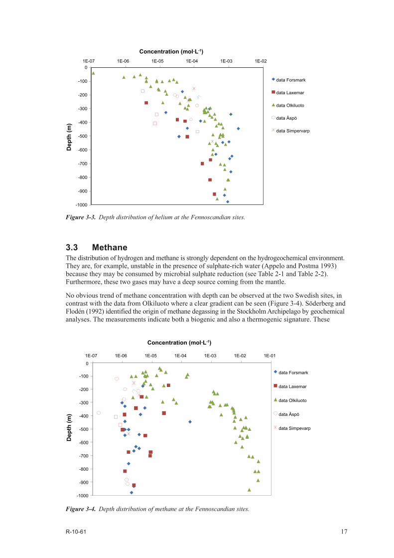
3.3 MethaneThe distribution of hydrogen and methane is strongly dependent on the hydrogeochemical environment. They are, for example, unstable in the presence of sulphate-rich water (Appelo and Postma 1993) because they may be consumed by microbial sulphate reduction (see Table 2-1 and Table 2-2). Furthermore, these two gases may have a deep source coming from the mantle.

No obvious trend of methane concentration with depth can be observed at the two Swedish sites, in contrast with the data from Olkiluoto where a clear gradient can be seen (Figure 3-4). Söderberg and Flodén (1992) identified the origin of methane degassing in the Stockholm Archipelago by geochemical analyses. The measurements indicate both a biogenic and also a thermogenic signature. These

Figure 3-3. Depth distribution of helium at the Fennoscandian sites.

Figure 3-4. Depth distribution of methane at the Fennoscandian sites.

-1000

-900

-800

-700

-600

-500

-400

-300

-200

-100

01E-07 1E-06 1E-05 1E-04 1E-03 1E-02

Dep

th (m

)

Concentration (mol·L-1)

data Forsmark

data Laxemar

data Olkiluoto

data Äspö

data Simpervarp

-1000

-900

-800

-700

-600

-500

-400

-300

-200

-100

0

1E-07 1E-06 1E-05 1E-04 1E-03 1E-02 1E-01

Dep

th (m

)


data Forsmark

data Laxemar

data Olkiluoto

data Äspö

data Simpevarp

18 R-10-61

observations are consistent with the analyses by Hallbeck and Pedersen (2008a, b) of gas samples from Forsmark and Laxemar. Hallbeck and Pedersen (2008a, b) calculate the ratio between methane and higher hydrocarbons to provide evidence regarding the origin of methane. This suggests that most of the samples are originated mainly from an abiogenic source, though some of the samples may have a biogenic signature. The carbon isotope signature of methane can reveal its source, but such type of data is not available for any of the Swedish sites. The isotopic analysis of methane performed at Olkiluoto indicates a potential mixing of bacterial and thermal (most probably abiogenic) origins contributing to the methane concentration of the samples (Figure 3-5).

A few data from the Swedish sites present methane concentrations which are one order of magnitude higher than the mean concentration of this gas (around 65μL·L–1 i.e. 2.6·10–6 mol·L–1) (Figure 3-4). Relatively high methane concentrations (> 4·10–6 mol·L–1) are observed in three samples at the Forsmark site (1.9·10–4 mol·L–1 in KFM01D at 445 m, 5.7·10–6 mol·L–1 in KFM01D at 341 m, and 4.9·10–6 mol·L–1 in KFM01A at 176 m). These samples also present higher concentrations of hydrocarbons other than methane. In this case, methane and the other hydrocarbons are believed to come from a deep abiogenic source through fractures, except for sample KFM01D at 445 m where a portion of methane seems biologically produced (Hallbeck and Pedersen 2008a).

Relatively high methane concentrations at Laxemar site are measured in samples KLX03 at 171 m (3.6·10–5 mol·L–1) and 380 m (2.5·10–5 mol·L–1). A portion of biologically produced methane has been identified in these two samples (Hallbeck and Pedersen 2008b). A third sample shows the same signature but presents a concentration in the mean range. The contribution of microbiological methanogenesis may be higher in the first two samples.

Figure 3-5. Molecular ratio between CH4 and higher hydrocarbons versus δ13C(CH4) of brackish-Cl and saline groundwater samples at Olkiluoto. The contours depict a conservative estimate of microbial CH4 fraction contributing to the samples (Pitkänen and Partamies 2007).

R-10-61 19

CH4/He ratios at the Swedish sites are similar and decrease with depth down to 600 m, becoming con-stant below this depth (Figure 3-6). No sink of helium exists in the bedrock and transport mechanisms are similar for all gases. Therefore, higher CH4/He ratio above 600 m at the Swedish sites could be taken as an indication of methane production at these depths or He production and accumulation in deeper groundwater where residence time are presumably longer.

The available information on methane at Olkiluoto shows a trend of a progressive increase of methane concentration with depth (Figure 3-6) with a rather constant CH4/He ratio in CH4-rich, old brackish Cl and saline groundwater system below 200 m depth (Figure 3-6). Similar trend as in the CH4 contents can be observed in the helium contents measured in the groundwater suggesting that both methane and helium share a deep origin and migrate slowly towards the surface or long term in situ production and accumulation in almost stagnant groundwater conditions (Figure 3-7).

Figure 3-7 confirms the similar tendency between helium and methane concentration distribution below 300 m. Figure 3-8 shows measured values of: (a) sulphate, (b) methane (notice that it is in linear scale, not logarithmic as in Figure 3-4) and sulphide in Olkiluoto groundwaters. On the basis of these data, a hypothesis could be established according to which:

1) Anaerobic methane oxidation, due to sulphate reduction, is probable in the first 300 m of the Olkiluoto bedrock.

2) The rate of sulphate reduction at 300 m is mainly limited by the mass flow rate of methane from the deep bedrock.

3) The rate of sulphate reduction is limited by mixing of SO4-rich (brackish SO4 type) and CH4-rich (brackish Cl and saline types) groundwaters.

In fact, the decreasing trends of methane and helium concentrations above 300 m are very similar (correlations shown in Figure 3-7), which indicates that hydrologic phenomena (such as mixing and dilution) are the most important for the concentration profiles of both gases and emphasizes the different evolution of the young upper and old deeper groundwater systems (Posiva 2009). The concentration of dissolved sulphide markedly increases up to 0.3 mmol/L at 300 m depth, while that of dissolved sulphate decreases about 4 mmol/L. This also suggests limited mixing of the groundwater systems at their interface. Additional data are obviously needed to clearly demonstrate the occurrence of microbial anaerobic CH4 oxidation with sulfate reduction at Olkiluoto.

Figure 3-6. Depth distribution of CH4/He concentration ratio at the Fennoscandian sites.

-1000

-900

-800

-700

-600

-500

-400

-300

-200

-100

01E-03 1E-02 1E-01 1E+00 1E+01 1E+02

Dep

th (m

)

CH4/He (-)

Forsmark

Laxemar

Olkiluoto

Äspö

Simpervarp

20 R-10-61

Figure 3-7. Depth distribution of methane and helium at Olkiluoto site.

Figure 3-8. Depth distribution measured at Olkiluoto of: A) sulphate, B) methane and, C) sulphide. (Pitkänen and Partamies 2007).

y = -106.06Ln(x) - 929.13

R2 = 0.8941

y = -84.467Ln(x) - 1038.1

R2 = 0.9678

-1000

-900

-800

-700

-600

-500

-400

-300

-200

1.E-05 1.E-04 1.E-03 1.E-02 1.E-01

Concentration (mol/l)D

epth

(m)

He in Brackish Cl water CH4 in Brackish Cl water

He in saline water CH4 in saline water

R-10-61 21

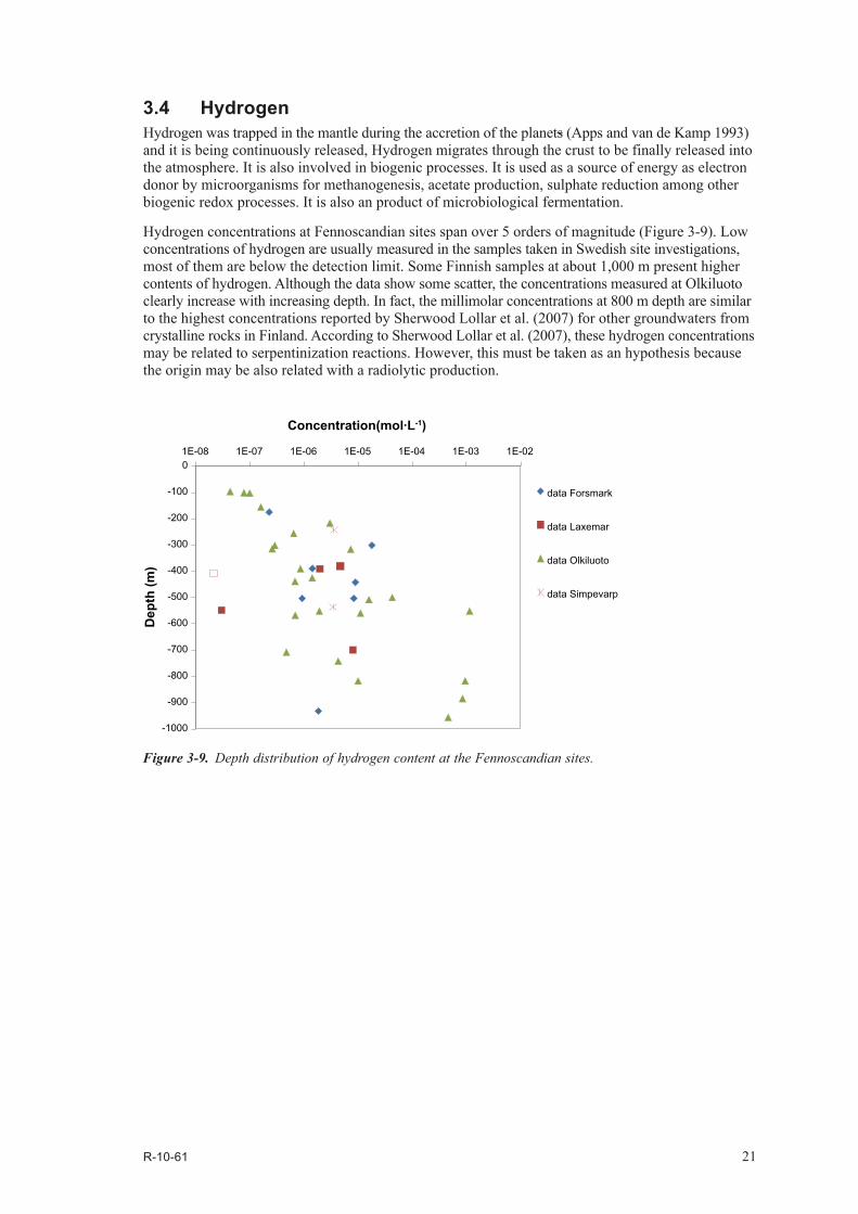
3.4 HydrogenHydrogen was trapped in the mantle during the accretion of the planets (Apps and van de Kamp 1993) and it is being continuously released, Hydrogen migrates through the crust to be finally released into the atmosphere. It is also involved in biogenic processes. It is used as a source of energy as electron donor by microorganisms for methanogenesis, acetate production, sulphate reduction among other biogenic redox processes. It is also an product of microbiological fermentation.

Hydrogen concentrations at Fennoscandian sites span over 5 orders of magnitude (Figure 3-9). Low concentrations of hydrogen are usually measured in the samples taken in Swedish site investigations, most of them are below the detection limit. Some Finnish samples at about 1,000 m present higher contents of hydrogen. Although the data show some scatter, the concentrations measured at Olkiluoto clearly increase with increasing depth. In fact, the millimolar concentrations at 800 m depth are similar to the highest concentrations reported by Sherwood Lollar et al. (2007) for other groundwaters from crystalline rocks in Finland. According to Sherwood Lollar et al. (2007), these hydrogen concentrations may be related to serpentinization reactions. However, this must be taken as an hypothesis because the origin may be also related with a radiolytic production.

Figure 3-9. Depth distribution of hydrogen content at the Fennoscandian sites.

-1000

-900

-800

-700

-600

-500

-400

-300

-200

-100

01E-08 1E-07 1E-06 1E-05 1E-04 1E-03 1E-02

Dep

th (m

)

Concentration(mol·L-1)

data Forsmark

data Laxemar

data Olkiluoto

data Simpevarp

R-10-61 23

4 Quantitative interpretation of gas profiles at the Fennoscandian sites

The aqueous concentration of gas at a certain depth is the result of a combination of different processes such as gas production, consumption, diffusion and advection. To interpret the gas profiles at the Fennoscandian sites, we consider each main source of gas separately: either in situ gas production or deep crustal/mantle flux of gas. The gas will diffuse vertically towards the surface (i.e. advection is neglected after a given depth, depending on the site). In each case, the contribution of the source is quantitatively estimated.

4.1 Quantitative deep gas flux estimationObservations on the helium distribution indicate that a deep source of helium is not negligible. We can quantitatively estimate the contribution of a deep gas flux coming from depth considering that gas production in the rock is negligible and gas profiles are only the result of the diffusion of a deep source.

If gas fluxes are mainly diffusive, then they can be evaluated from Fick’s law (Equation 4-1) using the effective diffusion coefficient of the gas in the dominant rock type of the site and the observed gradient of concentrations.

J = –De∇C(z,t) Equation 4-1

where C(z,t) (mol m–3 of rock) is the gas concentration in the rock at depth z and time t, De is its effec-tive diffusion coefficient (m2y–1), and J is the diffusive flux (mol m–2 y–1).

Equation 4-2 gives the relation between the diffusion coefficient of a reference ion in pure water (D0ref )

and the corresponding effective diffusion coefficient (Deref ) in the bedrock. The same relation can be

established to calculate the effective diffusion coefficient of gases (Equation 4-3).

2τδφ constrref

orefe DD = Equation 4-2

2τδφ constrgas

ogase DD = Equation 4-3

with φ, δconstr and τ the porosity, constriction and tortuosity of the bedrock, respectively.

Therefore, the effective diffusion coefficient of gas is calculated using Equation 4-4, considering a similar access of the reference ion and the different gases to the bedrock porosity and tortuosity.

refo

refe

gasogas

e DDDD = Equation 4-4

The diffusion coefficient in pure water of the major ions ranges between 1.0·10–9 and 2.0·10–9 m2s–1 at 25°C (Robinson and Stokes 1968). The calculation thereafter are performed considering the upper threshold value (i.e. D0

ref =2.0·10–9 m2s–1).

Jähne et al. (1987) performed some experiments to determine the diffusion coefficient (D0gas) of

soluble gases such as He, CH4 and H2 in water at different temperatures. The diffusion coefficients of gases into pure water presented into Table 4-1 are the ones measured at 25ºC.

A recommended value for the effective diffusion coefficient of cations and non-charged solutes in Forsmark is reported in the SR-Site Data report (SKB 2010) (De

ref =2.1·10–14 m2s–1). Furthermore, the same report suggests that the parameter is lognormally distributed with a standard deviation of the logarithm (base 10) equal to 0.25· m2s–1. Thus, following the three sigma rule, a sensitivity analysis has been carried out using the lower (De

ref_min

=3.5·10–15 m2s–1) and upper limit (Deref_max =1.1·10–13 m2s–1)

(see Table 4-1).

24 R-10-61

As an approximation the effective diffusion coefficient of the reference ion in Laxemar bedrock is taken to be equal to that of Forsmark.

The reference effective diffusion value for Olkiluoto has been obtained from the results reported by Eichinger et al. (2006) (De

ref =1.1·10–13 m2s–1 for chloride).

If the main source of gas production occurs deep in the mantle or crust, the concentration is a linear function of depth. Thus, the concentration gradient is constant with depth and can be easily evaluated by linear regression (Figure 4-1 to Figure 4-3). In the visual fit, some data have not been considered, such as values of samples considered affected by sampling artifact (for instance, some hydrogen data at Laxemar). Gas sampling is sensitive to disturbances due to slight pressure changes during sampling, which may particularly increase the fraction of light gases (Pitkänen and Partamies 2007). On the other hand open borehole effects of investigations may disturb gases and release them decreasing the contents. In all, uncertainties in gas contents are much higher than for other dissolved components. Also, the data presenting a very high concentration in comparison with samples at similar depth may be samples of upwelling gas through a fracture, and therefore have not been taken into account to determine the diffusive flux. Äspö and Simpevarp data are shown as indicative data, but have not been considered for the estimation of Laxemar gradient.

From Figure 3-3 we can see that Olkiluoto Helium concentration drops to very low values above 250 m depth. Consistently with previous geochemical studies (Pitkänen and Partamies 2007), this evidence can be explained by the fact that at different depths gas transport is affected by different mechanisms. While the “deep” part of the system is characterized by very high water residence times (i.e. molecular diffusion is the dominant transport process), at ‘shallow’ depths advection induced by relatively high horizontal flow rates plays a dominant role. Furthermore, as shown in Figure 3-2, above 100 m depth transport mechanisms are likely to be affected by bubble formation. A similar reasoning can be qualitatively extended to the Swedish sites, although a precise location of the boundary between the mobile and less mobile region is difficult due to uncertainty and scarcity of field data.

Table 4-1. Parameters of interest concerning helium, methane, and hydrogen.

Helium Methane Hydrogen

Henry´s Law constant (mol·L–1atm–1) (Sander 1999)

3.75·10–4 2.45·10–3 7.8·10–4

Molar volume (m3mol–1) 0.0224 0.0245 0.0238

D0gas (m2s–1) (Jähne et al. 1987) 7.50·10–9 1.70·10–9 4.50·10–9

Forsmark and Laxemar

Average value: Deref = 2.1·10–14 m2s–1 (from SR-Site Data report)

Degas (m2s–1)

calculated value following Equation 4-47.9·10–14 1.8·10–14 4.7·10–14

Lower limit (μ-3σ)*: Deref_min = 3.7·10–15 m2s–1 (from SR-Site Data report)

Degas_min (m2s–1)


Upper limit (μ+3σ)*: Deref_max = 1.1·10–13 m2s–1 (from SR-Site Data report)

Degas_max (m

2s–1)calculated value following Equation 4-4

4.4·10–13 1.0·10–13 2.7·10–13

Olkiluoto with = Deref 1.1·10–13 m2s–1 (Eichinger et al. 2006)

Degas (m2s–1)


* Note that μ and σ refers to the average and standard deviation of the base-10 logarithm of the effective diffusion coefficient reported in the SR-Site Data report (SKB 2010).

R-10-61 25

-1000

-800

-600

-400

-200

00.0E+00 5.0E-04 1.0E-03 1.5E-03 2.0E-03 2.5E-03

Dep

th (m

)


-1000

-800

-600

-400

-200

00.0E+00 5.0E-04 1.0E-03 1.5E-03 2.0E-03 2.5E-03

Dep

th (m

)

-1000

-800

-600

-400

-200

00.0E+00 5.0E-04 1.0E-03 1.5E-03 2.0E-03 2.5E-03

Dep

th (m

)FORSMARK

LAXEMAR

OLKILUOTO

Figure 4-1. Estimated helium gradient based on measurements. Open points are excluded data.

-1000

-800

-600

-400

-200

00.0E+00 5.0E-06 1.0E-05 1.5E-05 2.0E-05 2.5E-05 3.0E-05 3.5E-05 4.0E-05

Dep

th (m

)


-1000

-800

-600

-400

-200

00.0E+00 5.0E-06 1.0E-05 1.5E-05 2.0E-05 2.5E-05 3.0E-05 3.5E-05 4.0E-05

Dep

th (m

)

-1000

-800

-600

-400

-200

00.0E+00 5.0E-03 1.0E-02 1.5E-02 2.0E-02 2.5E-02 3.0E-02 3.5E-02 4.0E-02

Dep

th (m

)

FORSMARK

OLKILUOTO

LAXEMAR

Figure 4-2. Estimated minimum (dash line) and maximum (solid line) methane gradient based on measure-ments. Open points are excluded data. The horizontal scale for Olkiluoto is 1,000 times larger than for the two Swedish sites.

26 R-10-61

Based on the gradients described in Figure 4-1 to Figure 4-3 and the effective diffusion coefficients and molar volume listed in Table 4-1, deep fluxes of helium, methane and hydrogen in the Fenno scandian sites of interest can be calculated from Equation 4-1. It is worth mentioning that the quantitative estimations of the gradients are highly dependent of the number of available data and the judgement to determine them. Also, additional uncertainty stems from the value of effective diffusivity used in the analysis (Table 4-1 provides a range of values of effective diffusivity at Forsmark and Laxemar based on the information of the SR-Site Date report). Thus, to assess the uncertainty related with both the field data and the parameters, a range of fluxes is provided (Table 4-2).

From Table 4-1 one can see that the value of diffusivity of the reference ion at Forsmark and Laxemar spans one and a half orders of magnitudes. Due to the linear dependence of the results on this reference value (Equation 4-4), the fluxes obtained from the sensitivity analysis to the effective diffusivity show the same variability. A similar reasoning cannot be extended to Olkiluoto, since there is no information about the uncertainty associated to the effective diffusivity of Chloride.

The concentration gradients shown in Figure 4-1 to Figure 4-3 and reported in Table 4-1 are based on expert judgment. It is worth stressing that due to the scarcity of data these estimates are likely to be subject to bias. A few samples presenting high methane concentration due to microbiological methanogenesis (KFM01D at 445 m at Forsmark and KLX03 at 171 m and 380 m at Laxemar) or advective transport through fractures (KFM01D at 445 m, KFM01D at 341 m, and KFM01D at 176 m at Forsmark) have not been taken into account.

Figure 4-3. Estimated minimum (dash line) and maximum (plain line) hydrogen gradient based on measurements. Open points are excluded data. Note that four values of hydrogen content at the Olkiluoto site (between 4.5·10–4 and 1.2·10–3 mol·L–1) are not represented.

-1000

-800

-600

-400

-200

00.0E+00 2.0E-06 4.0E-06 6.0E-06 8.0E-06 1.0E-05 1.2E-05 1.4E-05 1.6E-05 1.8E-05 2.0E-05

Dep

th (m

)Concentration (mol·L-1)

-1000

-800

-600

-400

-200

00.0E+00 2.0E-06 4.0E-06 6.0E-06 8.0E-06 1.0E-05 1.2E-05 1.4E-05 1.6E-05 1.8E-05 2.0E-05

Dep

th (m

)

-1000

-800

-600

-400

-200

00.0E+00 2.0E-06 4.0E-06 6.0E-06 8.0E-06 1.0E-05 1.2E-05 1.4E-05 1.6E-05 1.8E-05 2.0E-05

Dep

th (m

)

FORSMARK

OLKILUOTO

LAXEMAR

R-10-61 27

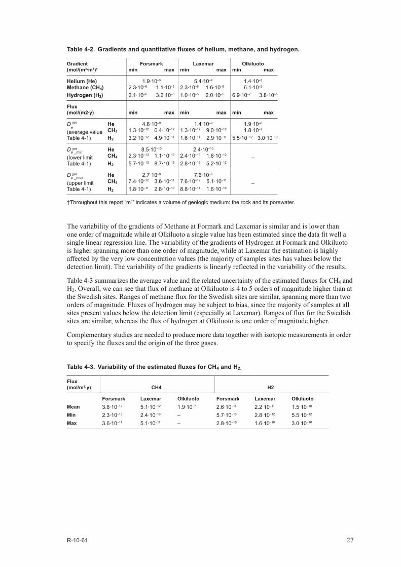
The variability of the gradients of Methane at Formark and Laxemar is similar and is lower than one order of magnitude while at Olkiluoto a single value has been estimated since the data fit well a single linear regression line. The variability of the gradients of Hydrogen at Formark and Olkiluoto is higher spanning more than one order of magnitude, while at Laxemar the estimation is highly affected by the very low concentration values (the majority of samples sites has values below the detection limit). The variability of the gradients is linearly reflected in the variability of the results.

Table 4-3 summarizes the average value and the related uncertainty of the estimated fluxes for CH4 and H2. Overall, we can see that flux of methane at Olkiluoto is 4 to 5 orders of magnitude higher than at the Swedish sites. Ranges of methane flux for the Swedish sites are similar, spanning more than two orders of magnitude. Fluxes of hydrogen may be subject to bias, since the majority of samples at all sites present values below the detection limit (especially at Laxemar). Ranges of flux for the Swedish sites are similar, whereas the flux of hydrogen at Olkiluoto is one order of magnitude higher.

Complementary studies are needed to produce more data together with isotopic measurements in order to specify the fluxes and the origin of the three gases.

Table 4-2. Gradients and quantitative fluxes of helium, methane, and hydrogen.

Gradient Forsmark Laxemar Olkiluoto(mol/(m3·m1)† min max min max min max

Helium (He) 1.9·10–3 5.4·10–4 1.4·10–3

Methane (CH4) 2.3·10–6 1.1·10–5 2.3·10–6 1.6·10–5 6.1·10–2

Hydrogen (H2) 2.1·10–6 3.2·10–5 1.0·10–5 2.0·10–5 6.9·10–7 3.8·10–5

Flux(mol/(m2·y) min max min max min max

Degas

(average value Table 4-1)

He 4.8·10–9 1.4·10–9 1.9·10–8

CH4 1.3·10–12 6.4·10–12 1.3·10–12 9.0·10–12 1.8·10–7

H2 3.2·10–12 4.9·10–11 1.6·10–11 2.9·10–11 5.5·10–12 3.0·10–10

Degas

_min(lower limit Table 4-1)

He 8.5·10–10 2.4·10–10

–CH4 2.3·10–13 1.1·10–12 2.4·10–13 1.6·10–12

H2 5.7·10–13 8.7·10–12 2.8·10–12 5.2·10–12

Degas

_max (upper limit Table 4-1)

He 2.7·10–8 7.6·10–9

–CH4 7.4·10–12 3.6·10–11 7.6·10–12 5.1·10–11

H2 1.8·10–11 2.8·10–10 8.8·10–11 1.6·10–10

†Throughout this report “m3” indicates a volume of geologic medium: the rock and its porewater.

Table 4-3. Variability of the estimated fluxes for CH4 and H2.

Flux (mol/m2·y)

CH4

H2

Forsmark Laxemar Olkiluoto Forsmark Laxemar OlkiluotoMean 3.8·10–12 5.1·10–12 1.9·10–7 2.6·10–11 2.2·10–11 1.5·10–10

Min 2.3·10–13 2.4·10–13 – 5.7·10–13 2.8·10–12 5.5·10–12

Max 3.6·10–11 5.1·10–11 – 2.8·10–10 1.6·10–10 3.0·10–10

28 R-10-61

4.2 In situ gas production estimation4.2.1 Implementation of the analytical modelHelium is dissolved in groundwater and its transport is therefore dependent on the behaviour of the fluid in the pore space. Furthermore, helium production in the crust is dominated by the alpha decay of the uranium and thorium decay chains, and therefore directly proportional to the concentration of 235,238U and 232Th in the crust.

Andrews et al. (1989) proposed an analytical formulation to model the production and diffusion of helium from the shallow granitic crust to the atmosphere. Considering a medium of infinite depth with a zero concentration boundary at the top boundary and zero concentration initial conditions, the produc-tion and migration of Helium can be described by the following partial differential equation, PDE:

( ) ( )2,

2,

dzC

DGt

C tzp

tz ∂+=

∂∂

Equation 4-5

where Dp is the pore diffusion coefficient and G (mol m–3 of rock per y) is the helium production rate in the rock, such as

[ ] [ ]( )ThUV

Gm

1716 10·88.210·19.1 −− += ρ Equation 4-6

where ρ is the rock bulk density (kg m–3), Vm the molar volume of the gas and [U] and [Th] are uranium and thorium contents of the rock matrix (ppm), respectively.

The solution of Equation 4-5 is

( )

−−=

fpftz tD

zGtC

f π2

exp1, Equation 4-7

where tf is the age (y) of the host rock.

The main limitations of this model are:

• The dissolved gas is transported only by diffusion.

• Constant diffusivity with depth considers that the diffusion does not vary with depth, i.e. it does not vary with increasing temperature and increasing pressure.

• Only steady state of helium production is considered. Helium storage in the matrix due to a very slow diffusion of the gas in the crystals is disregarded.

• Homogeneous contents of uranium and thorium (homogeneous formation) are assumed.

• The radiogenic production of helium is the only source of helium. This production source is assumed to be constant everywhere throughout the domain.

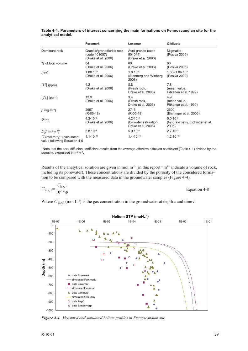
4.2.2 Simulation of helium profileTable 4-4 lists all parameters required for the analytical calculation of gas production and migration in the different rock types of the Fennoscadian sites. The calculated radiogenic production of helium has been considered to be similar for Forsmark and Olkiluoto sites, and slightly higher for Laxemar due to a higher content of uranium in Ävrö granite.

Using these parameters and based on Equation 4-5, the concentration of He is calculated to simulate Helium profile in Fennoscandian sites. The location of the upper boundary of the model (i.e. zero concentration boundary) is set to be the depth of the interface between the mobile and the less mobile region (250 m for Olkiluoto and 200 m for Forsmark and Laxemar).

R-10-61 29

Results of the analytical solution are given in mol m–3 (in this report “m3” indicate a volume of rock, including its porewater). These concentrations are divided by the porosity of the considered forma-tion to be compared with the measured data in the groundwater samples (Figure 4-4).

( )( )

φ*10' 3

,,

f

f

tztz

CC = Equation 4-8

Where C'(z,tf ) (mol L–1) is the gas concentration in the groundwater at depth z and time t.

Table 4-4. Parameters of interest concerning the main formations on Fennoscandian site for the analytical model.

Forsmark Laxemar Olkiluoto

Dominant rock Granitic/granodioritic rock (code 101057) (Drake et al. 2006)

Ävrö granite (code 501044) (Drake et al. 2006)

Migmatite (Posiva 2005)

% of total volume 84 (Drake et al. 2006)

80 (Drake et al. 2006)

80 (Posiva 2005)

tf (y) 1.88·109

(Drake et al. 2006)1.8·109

(Stenberg and Winberg 2008)

1.83–1.86·109

(Posiva 2009)

[U] (ppm) 4.2 (Drake et al. 2006)

8.8 (Fresh rock, Drake et al. 2006)

7.8 (mean value, Pitkänen et al. 1999)

[Th] (ppm) 13.9 (Drake et al. 2006)

3.4 (Fresh rock, Drake et al. 2006)

4.9 (mean value, Pitkänen et al. 1999)

ρ (kg·m–3) 2657 (R-05-18)

2716 (R-05-18)

2600 (Eichinger et al. 2006)

φ (–) 4.3·10–3 (Drake et al. 2006)

4.2·10–3 (by water saturation, Drake et al. 2006)

5.0·10–3 (by gravimetry, Eichinger et al. 2006)

DpHe (m2·y–1)* 5.8·10–4 5.9·10–4 2.7·10–3

G (mol·m–3y–1) calculated value following Equation 4-6

1.1·10–10 1.4·10–10 1.2·10–10

*Note that the pore diffusion coefficient results from the average effective diffusion coefficient (Table 4-1) divided by the porosity, expressed in m2·y–1.

Figure 4-4. Measured and simulated helium profiles in Fennoscandian site.

-1000

-900

-800

-700

-600

-500

-400

-300

-200

-100

01E-07 1E-06 1E-05 1E-04 1E-03 1E-02 1E-01

Helium STP (mol·L-1)

Dep

th (m

)

data Forsmarksimulated Forsmarkdata Laxemarsimulated Laxemardata Olkiluotosimulated Olkiluotodata Äspödata Simpervarp

30 R-10-61

The results in Figure 4-4 show that helium concentrations are overestimated by the analytical model when the simulation time corresponds to the estimated age of the rocks and the release fraction (i.e. the fraction oh Helium production that is actually released to water) is equal to 100%. Nevertheless, it can be noticed that the basic trend of helium production is reproduced: small gradient of helium concentrations below 400 m in logarithmic scale and a higher gradient above this depth.

4.2.3 Sensitivity analyses and calibration of helium profilesFirst, qualitative sensitivity analyses using Olkiluoto helium data are performed to understand the key parameters controlling the analytical solution. Then, a calibration of the helium profiles in the Fennoscandian sites is suggested and preliminary conclusions are drawn.

Sensitivity analysisTwo key parameters are controlling the results of the analytical solution: the production term, Gtf , and the pore diffusion coefficient, Dp.

Many uncertainties may arise from the production term. A number of previous studies (e.g. Rübel et al. 2002, Kulongoski et al. 2008, Roudil et al. 2008) assume that all produced helium goes into the water. Nonetheless, as recently shown by Neretnieks (2010) measurements of helium entrapped in crystals have been made in geologic materials (Martel et al. 1990). Furthermore, measurements of diffusion of helium in single crystals of rock forming minerals at different temperatures show that the diffusion coefficients in the solids are extremely low and even small crystals would tend to retain the formed helium over geologic times (Wolf et al. 1996, Bach et al. 1999, Roudil et al. 2008). However, recoil of the alpha-particles make them travel about ten micrometers in the solid and about 40 micrometers in water (Liu and Neretnieks 1996) which can release them from the crystals.

An additional uncertainty is the amount of uranium and thorium actually present in the rock, but the variability of this parameter is probably within a factor 2.

As expected, if we increase or decrease the production term by one order of magnitude, the curve is correspondingly shifted to one order of magnitude higher or lower helium concentrations (Figure 4-5).

Figure 4-5. Sensitivity analysis of the solution on the production term.

-1000

-900

-800

-700

-600

-500

-400

-300

-200

-100

01E-07 1E-06 1E-05 1E-04 1E-03 1E-02 1E-01 1E+00


Dep

th (m

)

data Olkiluoto

simulated with G radiogenic

simulated with G/10

simulated with G*10

R-10-61 31

To vary this production term, one can change the radiogenic production (e.g. uranium and thorium contents in the rock matrix) or the parameter tf (Equation 4-7), which is introduced as the formation age in Andrews et al. (1989). It is reasonable to assume that groundwater currently present in the bedrock has not been in contact with this formation the whole time of the formation age. So from now on in this work, we will consider that tf corresponds to the residence time of the present groundwater in the formation which can be a calibration parameter useful to estimate the residence time of the waters.

Helium concentration at depth is equal to the production term, Gtf, see Equation 4-9. This can be observed in Figure 4-5 for each simulated production term, implying that the depth of the simulated domain does not influence the results of the analytical solution.

C(z,t) ≈ Gtf for great depth Equation 4-9

The sensitivity analysis to the pore diffusion coefficient (Figure 4-6) shows that helium concentra-tions decrease and the gradient of concentrations is higher and deeper when the diffusion coefficient is increased.

The main uncertainties for the Olkiluoto formation concern uranium and thorium contents in the rock types and the formation porosity, affecting respectively the radiogenic production and the effective diffusion coefficient of the gas. The reported variation of the porosity does not exceed a factor of 3, which limits the uncertainties of the pore diffusion coefficient and as a consequence it also limits the influence on the helium concentration profiles. Thus, the main uncertainties occur in the radiogenic production term (Table 4-5). A variation of about half an order of magnitude can be observed depending on the rock type considered. So, based on expert judgment, it can be stated that the maximum uncertainty of helium production, which is related to the possible heterogeneity of uranium and thorium contents of the three Fennoscandian sites considered in this work, is about one order of magnitude.

Other sources of uncertainty stem from the ratio of Helium production that is actually released to the pore water, the variability of the diffusion coefficient (which depends on temperature which in turns increases with depth) and the increases of rock stresses with depth which may close the pores of the rock matrix.

Figure 4-6. Sensitivity analysis of the solution on the diffusion coefficient of helium.

-1000

-900

-800

-700

-600

-500

-400

-300

-200

-100

01E-07 1E-06 1E-05 1E-04 1E-03 1E-02 1E-01


Dep

th (m

)

data Olkiluotosimulated with D from Table4.3simulated with D/100

simulated with D*100simulated with D*1e4

32 R-10-61

This qualitative sensitivity analysis on key parameters puts in evidence the following:

• The production term of helium overestimates He accumulation when the whole age of the rock is considered and the release fraction is considered to be equal to 100%.

• The sensitivity of the helium profile with respect to the value of diffusion coefficient is not negligible in the range of the current uncertainty (Table 4-1).

• Uranium and thorium contents and porosity introduce a higher uncertainty on the radiogenic production factor that has been estimated to be one order of magnitude as maximum.

• The heterogeneity of the system should be taken into account to represent the variation of uranium and thorium contents in the different rock types.

• The analytical formulation used to model in situ gas production (Equation 4-5) is a function of three parameters: the production rate, G, the age of the host rock (thereafter assimilated with groundwater residence time), tf, and the pore diffusion coefficient of the gas, Dp. If we fix the value of Dp, Equation 4-7 has two degrees of freedom. Hence, the fitting between the calculated and measured data has to be carried out either by fixing G and calibrating tf or viceversa. If the parameter which is varied is G, then the calibration exercise would provide an estimation of the rate of Helium production that is actually released to the pore water.

• As explained in Section 4.2.2 the model is not valid in the upper part of the geosphere (from surface to 200 – 250 m depending on the site of study), which is clearly affected by a dynamic hydrogeologic system where advection, and bubble formation above 100 m depth, are the dominant processes. Therefore, the upper boundary of the domain (zero concentration boundary) has been placed at the interface between the mobile and the less mobile zone.(250 m for Olkiluoto and 200 m for Forsmark and Laxemar).

Calibration According to our current knowledge, isotopic data of helium in Fennoscandian sites have not been measured, which means that it is not possible to make any estimation of the possible mantle contribution to helium in the geosphere.

It is worth remembering that the main hypothesis needed at this point of the work is that all the helium present in the geosphere has a radiogenic (crustal) origin. This is in agreement with Ballentine and Burnard (2002) who compare measured and calculated isotopic ratios of helium based on the composi-tion of different granites. They state that granitic systems provide an example where mantle influences appear to be minimal.

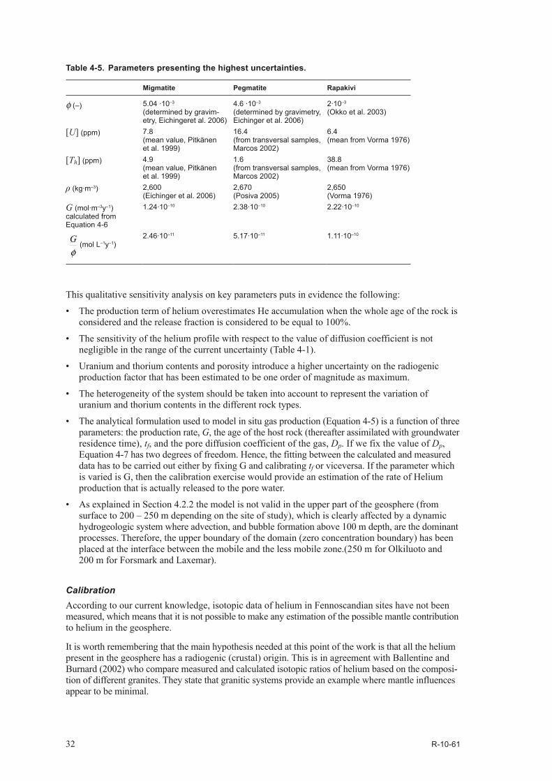
Table 4-5. Parameters presenting the highest uncertainties.

Migmatite Pegmatite Rapakivi

φ (–) 5.04 ·10–3 (determined by gravim-etry, Eichingeret al. 2006)

4.6 ·10–3 (determined by gravimetry, Eichinger et al. 2006)

2·10–3 (Okko et al. 2003)

[U] (ppm) 7.8 (mean value, Pitkänen et al. 1999)

16.4 (from transversal samples, Marcos 2002)

6.4 (mean from Vorma 1976)

[Th] (ppm) 4.9 (mean value, Pitkänen et al. 1999)

1.6 (from transversal samples, Marcos 2002)

38.8 (mean from Vorma 1976)

ρ (kg·m–3) 2,600 (Eichinger et al. 2006)

2,670 (Posiva 2005)

2,650 (Vorma 1976)

G (mol·m–3y–1) calculated from Equation 4-6

1.24·10–10 2.38·10–10 2.22·10–10

φG

(mol L–1y–1)2.46·10–11 5.17·10–11 1.11·10–10

R-10-61 33

Comparing the helium profiles measured at Olkiluoto, Forsmark and Laxemar (Figure 3-3), the data indicate similar profiles suggesting that the production and migration processes of helium are similar in the three Fennoscandian sites. Therefore, a similar fitting procedure is adopted for the three sites of study.

The fitting exercise has been carried out either considering that all the Helium production is released to the water and calibrating tf (Case A) or setting tf equal to the age of formation of the rock while calibrating the rate of Helium released to the pore water (Case B). The analytical solution (Equation 4-7) has been used to reproduce the data in the ‘deep zone’ where diffusive transport is expected to be dominant and where the main source of helium is the radiogenic production due to the uranium and thorium contents in the rocks. Thus, we place the top boundary (where c=0) at z = –250 m for Olkiluoto and z = –200 m for Forsmark and Laxemar. The input parameters of Equation 4-7 and Equation 4-8 are specified in Table 4-4. As an approximation, it is assumed that dissolved gas residence time is an indicator of the groundwater residence time.

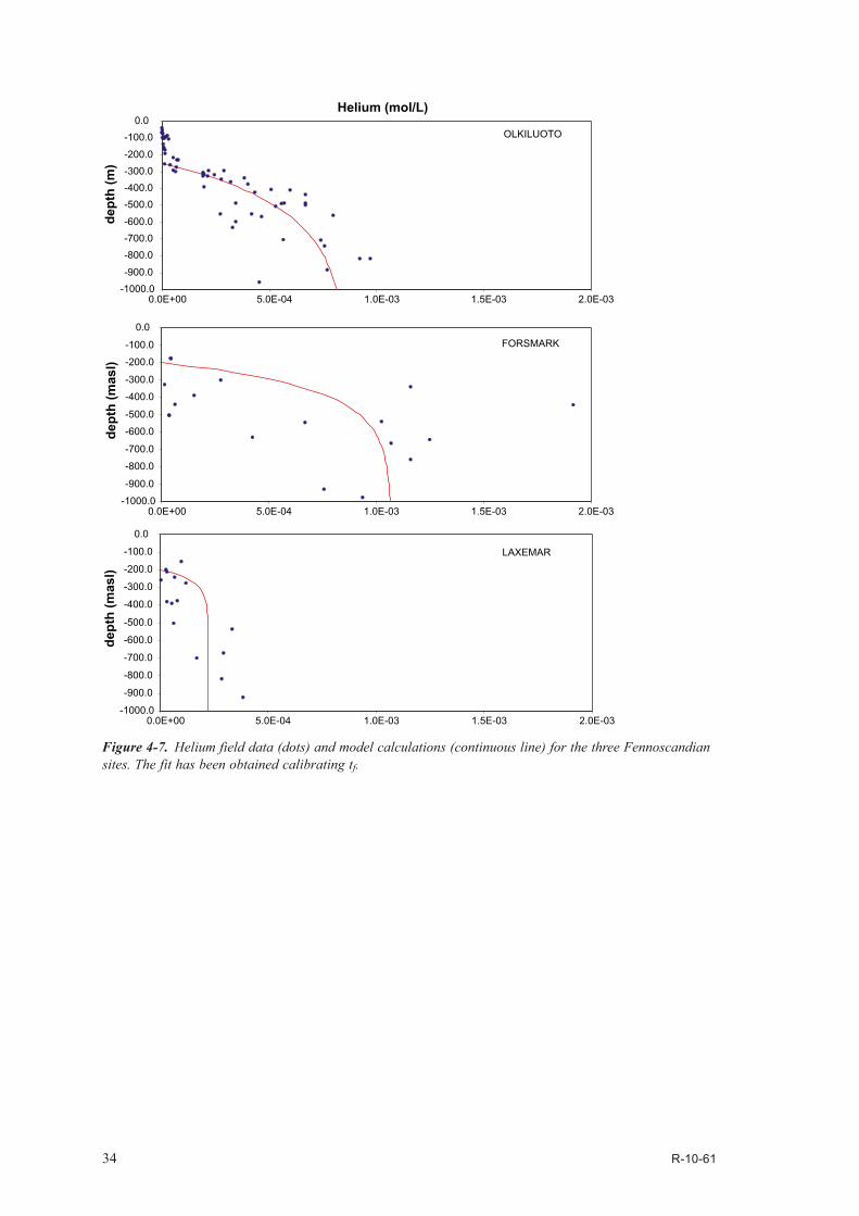
Figure 4-7 shows the comparison between measured and simulated (fitted) data for Case A and the three sites of study. If all produced Helium is released to the pore water, the fit procedure provides an estimation of the residence time (i.e. tf) that is between one and two orders of magnitude lower than the age of the rock formation (Table 4-6). The results would mean that Forsmark groundwater is the oldest with an estimated residence time of 50 My. The residence time of groundwaters in Laxemar and Olkiluoto is calculated to be 8 and 35 My respectively. These old groundwater “ages” would indicate that the deep zone of the three Fennoscandian sites behaves as a purely diffusive ‘compart-ment’ while advection processes with relatively high horizontal flow rates take part only in the first two/three hundred meters This is consistent with previous findings (Pitkänen and Partamies 2007).

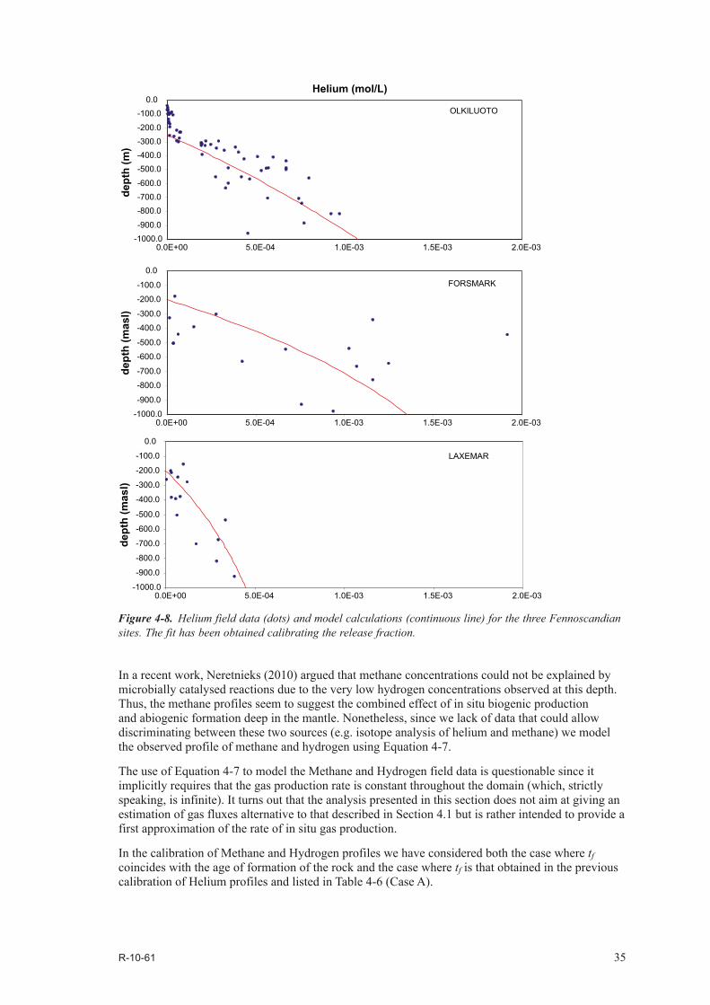
In a recent paper, Neretnieks (2010) argued that the assumption that all produced Helium is released to the pore water is not always justified. The author pointed out the fact that in a previous work (Martell et al. 1990) Helium entrapped in crystals was observed from measurements made in geological materials. To account for this, Figure 4-8 shows the results of the fitting exercise (Case B), where G (i.e. the release fraction) was used as fitting parameter. The estimated rate of Helium released to the pore water has been estimated as 6%, 2% and 7% out of the total generated Helium for Forsmark, Laxemar and Olkiluoto respectively.

It can be noticed that when the value of diffusivity is relatively small (Forsmark and Laxemar) and tf is smaller than the age of formation of the rock (Case A) the transition between the zero concentration and the plateau value (i.e. C=Gtf) occurs at shallow depths and with a steep profile (this evidence can be easily demonstrated by analysing the first derivative of Equation 4-7). Using the age of formation of the rock the concentration profile is smoother and fits better the distribution of the field data

It is worth noting that these results are affected by uncertainties related to incomplete knowledge of the phenomena to be modelled. An important source of uncertainty is related with uranium and thorium contents as well as with porosity values. For Case A, such uncertainty has been evaluated to one order of magnitude which means that even in the case of taking the extreme of the range of possible values, the residence time of the waters would be higher than 1 My.

Another important source of uncertainty stems from the deep mantle contribution. In fact, Equation 4-7 requires a constant production rate everywhere throughout the domain. Nonetheless, if the rate of mantle production was higher than the radiogenic production this could lead to an overestimation of either water residence time or in situ production rates. In Appendix 2 we present a new analytical solution that accompanied by a further field characterization (e.g. Isotope analysis of helium) would provide a powerful tool to decouple both effects thus reducing uncertainties.

4.2.4 Calculated results of CH4 and H2In this section, the analytical model for in situ production and diffusion of helium in groundwater has been used to simulate methane and hydrogen profiles in the three Fennoscandian sites in order to quantify the production rates (G) of these gases in the geosphere.

34 R-10-61

-1000.0-900.0

-800.0-700.0-600.0

-500.0-400.0-300.0-200.0

-100.00.0

0.0E+00 5.0E-04 1.0E-03 1.5E-03 2.0E-03

Helium (mol/L)de

pth

(m)

OLKILUOTO

-1000.0

-900.0

-800.0

-700.0

-600.0

-500.0

-400.0

-300.0

-200.0

-100.0

0.0

0.0E+00 5.0E-04 1.0E-03 1.5E-03 2.0E-03

dept

h (m

asl)

FORSMARK

-1000.0

-900.0

-800.0

-700.0

-600.0

-500.0

-400.0

-300.0

-200.0

-100.0

0.0

0.0E+00 5.0E-04 1.0E-03 1.5E-03 2.0E-03

dept

h (m

asl)

LAXEMAR

Figure 4-7. Helium field data (dots) and model calculations (continuous line) for the three Fennoscandian sites. The fit has been obtained calibrating tf.

R-10-61 35

Figure 4-8. Helium field data (dots) and model calculations (continuous line) for the three Fennoscandian sites. The fit has been obtained calibrating the release fraction.

-1000.0-900.0

-800.0-700.0-600.0

-500.0-400.0-300.0-200.0

-100.00.0

0.0E+00 5.0E-04 1.0E-03 1.5E-03 2.0E-03

Helium (mol/L)

dept

h (m

)OLKILUOTO

-1000.0

-900.0

-800.0

-700.0

-600.0

-500.0

-400.0

-300.0

-200.0

-100.0

0.0

0.0E+00 5.0E-04 1.0E-03 1.5E-03 2.0E-03

dept

h (m

asl)

FORSMARK

-1000.0

-900.0

-800.0

-700.0

-600.0

-500.0

-400.0

-300.0

-200.0

-100.0

0.0

0.0E+00 5.0E-04 1.0E-03 1.5E-03 2.0E-03

dept

h (m

asl)

LAXEMAR

In a recent work, Neretnieks (2010) argued that methane concentrations could not be explained by microbially catalysed reactions due to the very low hydrogen concentrations observed at this depth. Thus, the methane profiles seem to suggest the combined effect of in situ biogenic production and abiogenic formation deep in the mantle. Nonetheless, since we lack of data that could allow discriminating between these two sources (e.g. isotope analysis of helium and methane) we model the observed profile of methane and hydrogen using Equation 4-7.

The use of Equation 4-7 to model the Methane and Hydrogen field data is questionable since it implicitly requires that the gas production rate is constant throughout the domain (which, strictly speaking, is infinite). It turns out that the analysis presented in this section does not aim at giving an estimation of gas fluxes alternative to that described in Section 4.1 but is rather intended to provide a first approximation of the rate of in situ gas production.

In the calibration of Methane and Hydrogen profiles we have considered both the case where tf coincides with the age of formation of the rock and the case where tf is that obtained in the previous calibration of Helium profiles and listed in Table 4-6 (Case A).

36 R-10-61

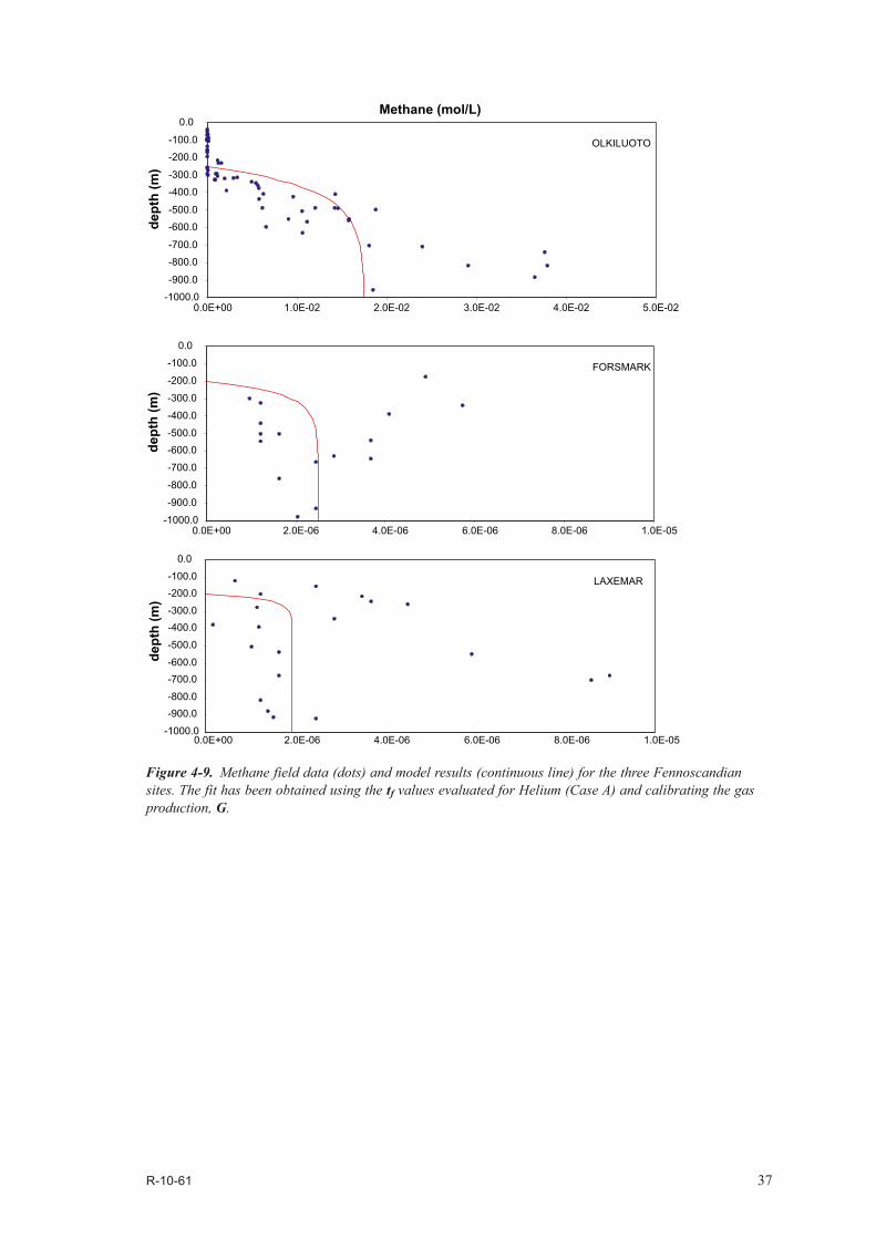
Methane Figure 4-9 and Figure 4-10 show the comparison between the measured and simulated (fitted) data for both the case where tf has been previously calibrated from the Helium analysis (Case A) (Figure 4-9) and the case where tf is set equal to the age of formation of the rock (Figure 4-10).

As in the case of Helium, low diffusivity values (Forsmark and Laxemar) in companion with tf smaller than the age of formation of the rock (Case A) produce steep profiles where the transition from the zero value to the maximum concentration occurs at shallow depths, thus giving poor fits between the measured and computed data. The agreement of the second approach (tf equal to the age of the rock) is much better. The implication of this is that, if we do not consider epistemic uncertainty (e.g. production rate variable with depth, microbial consumption, presence of a deep source with different rate of production, etc), the observed data are explained by a model where groundwater has been motionless since the age of formation of the rock (some thousands million years ago).

The fit between the model and the measurements of Forsmark and Laxemar is quite uncertain due to the scarcity of data and the fact that the measured concentrations are much lower that those observed at Olkiluoto. These low concentrations result in an estimated production term that is more than three orders of magnitude lower than for Olkiluoto. Also, it is worth noting that Laxemar field data clearly show two different trends with depth.

HydrogenThe fits between Hydrogen field data and the model are shown in Figure 4-11 and Figure 4-12 for the three sites of study and the two approaches described in Section 4.2.3.2. The scarcity of data and their high variability add additional uncertainty to this fitting exercise. In particular, it can be noticed that Olkiluoto data span four orders of magnitude with few samples at high depth showing very high hydrogen content.

Table 4-7 summarizes the results of the fitting exercise (i.e. production rates). It can be noticed that, consistently with field data, the estimated rate of Hydrogen production at Olkiluoto is between two and three orders of magnitude lower than the corresponding Methane production rate. Hydrogen production rates in Forsmark and Laxemar show approximately the same range of variation than Methane.

Table 4-6. Calibrated residence time of groundwater and calibrated Helium production released to the pore water (in parenthesis, percentage with respect to the total production).

tf (y) Forsmark Laxemar Olkiluoto

Age of formation 1.88·109

(Drake et al. 2006)1.8·109

(Stenberg and Winberg 2008)

1.83–1.86·109

(Posiva 2009)

Residence time (y) – Case A5.0·107 8.0·106 3.5·107

Production rate (mol/m3/y) – Case B6.4·10–12 (6%) 2.1·10–12 (2%) 9.2·10–12 (7%)

Table 4-7. Gas production at repository depth considering a residence time of groundwater of 50 My, 8 My, and 35 My for Forsmark, Laxemar, and Olkiluoto, respectively.

Production (mol/(m3·y) Forsmark Laxemar Olkiluoto

MethaneCalibrated tf (Helium, Case A)

2.5·10–13 1.2·10–12 2.5·10–9

Age formation 8.0·10–15 8.0·10–15 1.7·10–10

HydrogenCalibrated tf (Helium, Case A)

2.5·10–13 2.5·10–12 1.0·10–12

Age formation 3.0·10–14 3.5·10–14 1.0·10–13

R-10-61 37

Figure 4-9. Methane field data (dots) and model results (continuous line) for the three Fennoscandian sites. The fit has been obtained using the tf values evaluated for Helium (Case A) and calibrating the gas production, G.

Methane (mol/L)

-1000.0

-900.0

-800.0

-700.0

-600.0

-500.0

-400.0

-300.0

-200.0

-100.0

0.0

0.0E+00 1.0E-02 2.0E-02 3.0E-02 4.0E-02 5.0E-02

dept

h (m

)OLKILUOTO

-1000.0

-900.0

-800.0

-700.0

-600.0-500.0

-400.0

-300.0

-200.0

-100.0

0.0

0.0E+00 2.0E-06 4.0E-06 6.0E-06 8.0E-06 1.0E-05

dept

h (m

)

FORSMARK

-1000.0

-900.0-800.0

-700.0-600.0

-500.0

-400.0-300.0

-200.0-100.0

0.0

0.0E+00 2.0E-06 4.0E-06 6.0E-06 8.0E-06 1.0E-05

dept

h (m

)

LAXEMAR

38 R-10-61

Figure 4-10. Methane field data (dots) and model results (continuous line) for the three Fennoscandian sites. The fit has been obtained setting tf equal to the age of formation of the rock and calibrating the gas production, G.

Methane (mol/L)

-1000.0

-900.0

-800.0

-700.0

-600.0

-500.0

-400.0

-300.0

-200.0

-100.0

0.0

0.0E+00 1.0E-02 2.0E-02 3.0E-02 4.0E-02 5.0E-02

dept

h (m

)

-1000.0

-900.0

-800.0

-700.0

-600.0

-500.0

-400.0

-300.0

-200.0

-100.0

0.0

0.0E+00 2.0E-06 4.0E-06 6.0E-06 8.0E-06 1.0E-05

dept

h (m

)

-1000.0

-900.0

-800.0

-700.0

-600.0

-500.0

-400.0

-300.0

-200.0

-100.0

0.0

0.0E+00 2.0E-06 4.0E-06 6.0E-06 8.0E-06 1.0E-05

dept

h (m

asl)

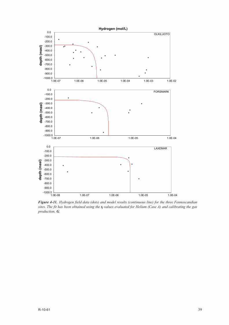
R-10-61 39

Figure 4-11. Hydrogen field data (dots) and model results (continuous line) for the three Fennoscandian sites. The fit has been obtained using the tf values evaluated for Helium (Case A) and calibrating the gas production, G.

Hydrogen (mol/L)

-1000.0

-900.0

-800.0

-700.0

-600.0

-500.0

-400.0

-300.0

-200.0

-100.0

0.0

1.0E-07 1.0E-06 1.0E-05 1.0E-04 1.0E-03 1.0E-02

dept

h (m

asl)

OLKILUOTO

-1000.0

-900.0

-800.0

-700.0

-600.0

-500.0

-400.0

-300.0

-200.0

-100.0

0.0

1.0E-07 1.0E-06 1.0E-05 1.0E-04

dept

h (m

asl)

FORSMARK

-1000.0

-900.0

-800.0

-700.0

-600.0

-500.0

-400.0

-300.0

-200.0

-100.0

0.0

1.0E-08 1.0E-07 1.0E-06 1.0E-05 1.0E-04

dept

h (m

asl)

LAXEMAR

40 R-10-61

Figure 4-12. Hydrogen field data (dots) and model results (continuous line) for the three Fennoscandian sites. The fit has been obtained setting tf equal to the age of formation of the rock and calibrating the gas production, G.

Hydrogen (mol/L)

-1000.0

-900.0

-800.0

-700.0

-600.0

-500.0

-400.0

-300.0

-200.0

-100.0

0.0

1.0E-07 1.0E-06 1.0E-05 1.0E-04 1.0E-03 1.0E-02

dept

h (m

asl)

OLKILUOTO

-1000-900-800-700-600-500-400-300-200-100

0

1.0E-07 1.0E-06 1.0E-05 1.0E-04

dept

h (m

asl)

FORSMARK

-1000.0-900.0-800.0-700.0-600.0-500.0-400.0-300.0-200.0-100.0

0.0

1.0E-08 1.0E-07 1.0E-06 1.0E-05 1.0E-04

dept

h (m

asl)

R-10-61 41

5 Discussion and conclusions

Fluxes and productions of helium, methane and hydrogen have been estimated for three Fennoscandian sites: Forsmark and Laxemar in Sweden, and Olkiluoto in Finland. Such estimations could be of impor-tance for the performance assessment of a deep geological repository, for the following main reasons:

• The chemically inert noble gases such as helium can be considered as conservative tracers to evaluate groundwater systems. For instance, they could be good indicators to evaluate groundwater residence time.

• The (bio)chemically active gases such as methane and hydrogen are involved in numerous redox processes, that must be quantified to define and understand accurately the chemical environment of the repository and the future evolution under different scenarios of interest.

Deep diffusive fluxes of Helium, Methane and Hydrogen at three Fennoscandian sites (Forsmark and Laxemar in Sweden, and Olkiluoto in Finland) have been estimated considering that gas production occurs at very large depths. Under these boundary conditions the concentration is a linear function of depth and hence the gradients have been inferred by linear regression. The uncertainty stemming from both the scarcity of data and the parameters used in the analysis (i.e. effective diffusivity) has been addressed by sensitivity analysis (see results summarized in Table 4-3) showing that the ranges of methane flux for the Swedish sites are similar, spanning more than two orders of magnitude. Flux of methane at Olkiluoto is 4 to 5 orders of magnitude higher than at the Swedish sites. Fluxes of hydrogen may be subject to bias, since the majority of samples at all sites present values near detection limit (especially at Laxemar). Ranges of flux for the Swedish sites are similar, whereas the flux of hydrogen at Olkiluoto is one order of magnitude higher.

It is worth stressing that the sensitivity analysis has been useful to address the uncertainty associated with the model parameters and the field data but it does not help to elucidate the effect of the simpli-fication assumptions introduced by the conceptual model (e.g. neglection of advective mixing, in situ production and microbial consumption, etc.)

Productions of helium, methane and hydrogen have been estimated for three sites of study. A residence time for the groundwaters has been estimated indicating that residence times are of the order of magni-tudes of millions years at repository depths. However these residence times require the assumption that helium production is only radiogenic and that all radiogenic helium is released to the groundwaters. There are indications that not all radiogenic helium is released to the water; part of the He produced remains enclosed in the mineral crystals. Furthermore, in a recent work Neretnieks (2010) argued that residence times of tens of millions of years are hardly justifiable since there is evidence of certain amounts of younger water (i.e. Littorina water) at the depths considered in this study. Because of these uncertainties the residence times of the groundwaters estimated by this method must be regarded as speculative.It is worth also noting that the apparent production rates of CH4 and H2 computed in this work, probably reflect the overall result of several processes such as deep sources, microbial consumption and production, etc.

A new analytical solution has been developed to account not only for the in situ production but also a flux with different rate from a deep source. This new model would allow performing more accurate estimation of mantle flux, crustal production and residence times when isotopic data become available and used to constrain the calibration procedure.

For all gases, isotopic data could complement conventional data on gas contents and composition giving valuable information on their origin. This information could allow improving the reliability of the model in the future, by defining more realistic boundary conditions.

R-10-61 43

6 References

SKB’s (Svensk Kärnbränslehantering AB) publications can be found at www.skb.se/publications.

Andrews J N, Hussain N, Youngman M J, 1989. Atmospheric and radiogenic gases in groundwaters from the Stripa granite. Geochimica et Cosmochimica Acta, 53, pp 1831–1841.

Appelo C, Postma D, 1993. Geochemistry, groundwater and pollution. Rotterdam: Balkema.

Apps J A, van de Kamp P C, 1993. Energy gases of abiogenic origin in the Earth’s crust. In: Howell D G (ed). The future of energy gases. Washington: United States Government Printing Office. (U.S. Geological Survey Professional Paper 1570), pp 81–132.

Bach W, Naumann D, Erzinger J, 1999. A helium, argon, and nitrogen record of the upper continental crust (KTB drill holes, Oberpfalz, Germany): implications for crustal degassing. Chemical Geology, 160, pp 81–101.

Ballentine C J, Burnard P G, 2002. Production, release and transport of noble gases in the continental crust. Reviews in Mineralogy and Geochemistry, 47, pp 481–538.

Beck J V, Cole K D, Haji-Sheikh A, Litkouhi B, 1992. Heat conduction using Green’s functions. Washington: Hemisphere.

Bougault H, Charlou J-L, Fouquet Y, Needham H D, Vaslet N, Appriou P, Jean Baptiste P, Rona P A, Dmitriev L, Silantiev S, 1993. Fast and slow spreading ridges: structure and hydrothermal activity, ultramafic topographic highs, and CH4 output. Journal of Geophysical Reserach, 98, pp 9643–9651.

Carslaw H S, Jaeger J C, 1959. Conduction of heat in solids. 2nd edition. Oxford: Clarendon.

Charlou J L, Donval J P, Fouquet Y, Jean-Baptiste P, Holm N, 2002. Geochemistry of high H2 and CH4 vent fluids issuing from ultramafic rocks at the Rainbow hydrothermal field (36°14’N, MAR). Chemical Geology, 191, pp 345–359.

Drake H, Sandström B, E Tullborg, 2006. Mineralogy and geochemistry of rocks and fracture fillings from Forsmark and Oskarshamn: Compilation of data for SR-Can. SKB R-06-109, Svensk Kärnbränslehantering AB.

Duan Z, Mao S, 2006. A thermodynamic model for calculating methane solubility, density and gas phase composition of methane-bearing aqueous fluids from 273 to 523 K and from 1 to 2000 bar. Geochimica et Cosmochimica Acta, 70, pp 3369–3386.

Dubessy J, 1983. Contribution à la connaissance des fluides ayant participé à la formation des gisements d’uranium. Revue Générale Nucléaire, 6, pp 472–474.

Eichinger F L, Waber H N, Smellie J A T, 2006. Characterisation of matrix pore water at the Okiluoto investigation site. Posiva Working Report 2006-103, Posiva Oy, Finland.

Gascoyne M, 2005. Dissolved gases in groundwaters at Olkiluoto. Posiva Working Report 2005-56, Posiva Oy, Finland.

Hallbeck L, Pedersen K, 2008a. Explorative analysis of microbes, colloids and gases. SDM-Site Forsmark. SKB R-08-85, Svensk Kärnbränslehantering AB.

Hallbeck L, Pedersen K, 2008b. Explorative analysis of microbes, colloids and gases together with microbial modelling. Site description model, SDM-Site Laxemar. SKB R-08-109, Svensk Kärnbränslehantering AB.

Huber R, Langworthy T A, König H, Thomm M, Woese C R, Sleytr U B, Stetter K O, 1986. Thermotoga maritima sp. nov. represents a new genus of unique extremely thermophilic eubacteria growing up to 90°C. Archives of Microbiology, 144, pp 324–333.

Jähne B, Heinz G, Dietrich W, 1987. Measurement of the diffusion coefficients of sparingly soluble gases in water. Journal of Geophysical Research, 92, pp 10767–10776.

44 R-10-61

Kulongoski J T, Hilton D R, Cresswell R G,Hostetler S, Jacobson G, 2008. Helium-4 characteristics of groundwaters from Central Australia: comparative chronology with chlorine-36 and carbon-14 dating techniques. Journal of Hydrology, 348, pp 176–194.

Lin L-H, Slater G F, Sherwood Lollar B, Lacrampe-Couloume G, Onstott T C, 2005. The yield and isotopic composition of radiolytic H2, a potential energy source for the deep subsurface biosphere. Geochimica et Cosmochemica Acta, 69, pp 893–903.

Liu J, Neretnieks I, 1996. A model for radiation energy deposition in natural uranium-bearing system and its consequences to water radiolysis. Journal of Nuclear Materials, 231, pp 103–112.

Liu J, Neretnieks I, 2004. Coupled transport/reaction modelling of copper canister corrosion aided by microbial processes. Radiochimica Acta, 92, pp 849–854.

Marcos N, 2002. Low-temperature mobility of rare earth elements (REE), U, and Th at the Okiluoto site, SW Finland. In: McGrail B P, Cragnolino G A (eds). Scientific Basis for Nuclear Waste Management XXV. Warrendale: Materials Research Society. (Materials Research Society Symposium Proceedings 713), pp 825–832.

Martel D J, O’Nions R K, Hilton D R, Oxburgh E R, 1990. The role of element distribution in production and release of radiogenic helium: the Carnmenellis Granite, southwest England. Chemical Geology, 88, pp 207–221.

Megonigal J P, Hines M E, Visscher P T, 2005. Anaerobic metabolism: linkages to trace gases and aerobic processes. In: Schlesinger W H (ed). Treatise on Geochemistry. Vol. 8, Biogeochemistry. Amsterdam: Elsevier, pp 317–392.

Neal C, Stanger G, 1983. Hydrogen generation from mantle source rocks in Oman. Earth and Planetary Science Letters, 66, pp 315–320.

Neretnieks I, 2010. Release and transport of gases in deep granitic rocks Applied Geochemistry (submitted).

Okko O, Front K, Anttila P, 2003. Low-angle fracture zones in rapakivi granite at Hästholmen, southern Finland. Engineering Geology, 69, pp 171–191.

Pedersen K, 2005. Äspö Hard Rock Laboratory. MICROBE. Analysis of microorganisms and gases in MICROBE groundwater over time during MINICAN drainage of the MICROBE water conducting zone. SKB IPR-05-29, Svensk Kärnbränslehantering AB.

Pepin R, Porcelli D, 2002. Origin of noble gases in the terrestrial planets. Reviews in Mineralogy and Geochemistry, 47, pp 191–246.

Pitkänen P, Partamies S, 2007. Origin and implications of dissolved gases in groundwater at Olkiluoto. Posiva 2007-04, Posiva Oy, Finland.

Pitkänen P, Snellman M, Vuorinen U, 1996. On the origin and chemical evolution of groundwater at the Olkiluoto site. Posiva 96-04, Posiva Oy, Finland.

Pitkänen P, Luukkonen A, Ruotsalainen P, Leino-Forsman H, Vuorinen U, 1999. Geochemical modelling of groundwater evolution and residence time at the Olkiluoto site. Posiva 98-10, Posiva Oy, Finland.

Pitkänen P, Partamies S, Luukkonen A, 2004. Hydrogeochemical interpretation of baseline groundwater conditions at the Olkiluoto site. Posiva 2003-07, Posiva Oy, Finland.

Posiva, 2005. Olkiluoto site description 2004. Posiva 2005-03, Posiva Oy, Finland.

Posiva, 2009. Olkiluoto site description 2008. Part 1. Posiva 2009-1, Posiva Oy, Finland.

Puigdomenech I, Taxén C, 2000. Thermodynamic data for copper. Implications for the corrosion of copper under repository conditions. SKB TR-00-13, Svensk Kärnbränslehantering AB.

Robinson R A, Stokes R H, 1968. Electrolyte solutions: the measurement and interpretation of conductance, chemical potential and diffusion in solutions of simple electrolytes. 2nd ed. London: Butterworths.

Roudil D, Bonhoure J, Pik R, Cuney M, Jégou C, Gauthier-Lafaye F, 2008. Diffusion of radiogenic helium in natural uranium oxides. Journal of Nuclear Materials, 378, pp 70–78.

R-10-61 45

Rübel A P, Sonntag C, Lippmann J, Pearson F J, Gautchi A, 2002. Solute transport in formations of very low permeability: profiles of stable isotope and dissolved noble gas contents of pore water in the Opalinus Clay, Mont Terri, Switzerland. Geochimica et Cosmochimica Acta, 66, pp 1311–1321.

Sander R, 1999. Compilation of Henry’s law constants for inorganic and organic species of potential importance in environmental chemistry. Version 3. [Online]. Available at: http://www.henrys-law.org.

Schoell M, 1988. Multiple origins of methane in the earth. Chemical Geology, 71, pp 1–10.

Sherwood Lollar B, Frape S K, Fritz P, Macko S A, Welham J A, Blomqvist R, Lahermo P W, 1993a. Evidence for bacterially generated hydrocarbon gas in Canadian Shield and Fennoscandian Shield rocks. Geochimica et Cosmochimica Acta, 57, pp 5073–5086.

Sherwood Lollar B, Frape S K, Weise S M, Fritz P, Macko S A, Welhan J A, 1993b. Abiogenic methanogenesis in crystalline rocks. Geochimica et Cosmochimica Acta, 57, pp 5087–5097.

Sherwood Lollar B, Westgate T D, Ward J A, Slater G F, Lacrampe-Couloume G, 2002. Abiogenic formation of alkanes in the Earth’s crust as a minor source for global hydrocarbon reservoirs. Nature, 416, pp 522–524.

Sherwood Lollar B, Voglesonger K, Lin L-H, Lacrampe-Couloume G, Telling J, Abrajano T A, Onstott T C, Pratt L M, 2007. Hydrogeologic controls on episodic H2 release from Precambrian fractured rocks – energy for deep subsurface life on Earth and Mars. Astrobiology, 7, pp 971–986.

SKB, 2008. Site description of Forsmark at completion of the site investigation phase. SDM-Site Forsmark. SKB TR-08-05, Svensk Kärnbränslehantering AB.

SKB, 2010. Data report for the safety assessment SR-Site. SKB TR-10-52, Svensk Kärnbränsle-hantering AB.

Stenberg L, Winberg A, 2008. Geoscientific understanding of the Laxemar-Simpevarp site. In: Ahlbom K, Stephens M (ed). Investigations of potential repository sites for spent nuclear fuel at Forsmark and Laxemar-Simpevarp, Sweden. Abstract, 33rd International Geological Congress, Oslo. SKB R-08-97, Svensk Kärnbränslehantering AB, p 9.

Stevens T O, McKinley J P, 1995. Lithoautotrophic microbial ecosystems in deep basalt aquifers. Science, 270, pp 450–455.

Söderberg P, Flodén T, 1992. Gas seepages, gas eruptions and degassing structures in the seafloor along the Strömma tectonic lineament in the crystalline Stockholm Archipelago, east Sweden. Continental Shelf Research, 12, pp 1157–1171.

Vorma A, 1976. On the petrochemistry of the rapakivi granites with special reference to the Laitila massif, southwestern Finland. Espoo: Geologinen Tutkimuslaitos. (Geological survey of Finland bulletin 285).

Vovk I F, 1987. Radiolytic salt enrichment and brines in the crystalline basement of the East European Platform. In: Fritz P, Frape S K (eds). Saline waters and gases in crystalline rocks. St. John’s, Nfld.: Geological Association of Canada. (Proceedings of the Geological Association of Canada 33), pp 197–210.

Whiticar M J, 1990. A geochemical perspective of natural gas and atmospheric methane. Organic Geochemistry, 16, pp 531–547.

Whiticar M J, 1999. Carbon and hydrogen isotope systematics of bacterial formation and oxidation of methane. Chemical Geology, 161, pp 291–314.

Wolf R A, Farley K A, Silver L T, 1996. Helium diffusion and low-temperature thermochronometry of apatite. Geochimica et Cosmochimica Acta, 60, pp 4231–4240.

Yang C, Samper, J Molinero J, Bonilla M, 2007. Modelling geochemical and microbial consumption of dissolved oxygen after backfilling a high level radiactive waste repository. Journal of Contaminant Hydrology, 93, pp 130–148.

R-10-61 47

Appendix A

Derivation of gas production and diffusion into the Earth’s crust with a deep mantle contribution

We consider the one dimensional diffusion problem:

( )tzzcD

tc ,2

2

ρ=∂∂−

∂∂ Equation A-1

With the initial conditions c(z,t = 0) = co (z) and the boundary conditions.

c(z = 0,t) = 0 ( )tjz

tzcDdz

0),( =

∂∂−

−=

Equation A-2

The source term ρ(z,t) has the units [(LT)–1], the boundary flux [T–1].

According to the Green theorem, the solution can be written in terms of the Green function g(z,t|z',t') as

( ) ( ) ( ) ( ) ( )

( ) ( )'',,'

','',','''0,',',

00

0

00

0

tjtdtzgdt

tztztzgdtdzzcztzgdztzc

td

t

d

∫

∫ ∫∫

−+

+=−−

ρ

Equation A-3

The first term accounts for the initial condition, the second for the source and the third term for the boundary conditions at z = –d. The Green function satisfies the diffusion equation.

0)',',()',',(

2

2

=∂

∂−

∂∂

ztztzg

Dt

tztzg Equation A-4

For the initial conditions g(z,t|z',t') = δ(z–z') and the boundary conditions.

g(z = 0,t|z’,t’) = 0 ( )

0',',

=∂

∂−

−= dzz

tztzgD Equation A-5

The solution for the Green function is obtained from Beck et al. (1992):

( )

−

+

+= ∑

∞

= Ddtt

ddz

ddz

dtztzg kk

kk /

'4

exp'2

cos2

cos2',', 2

22

1

παπαπα Equation A-6

where αk = (2k–1).

We now determine the solution of the above diffusion problem for zero initial conditions, c0(z) = 0, the source term

<<−−<<−−<<−

=00

0)(

2

210

1

zzzzzzzd

z ρρ Equation A-7

i.e., constant production in the interval [–z1, –z2], and the constant boundary flux j0(t) = j0.

According to Equation A-3 we obtain

48 R-10-61

( )

+

−−

−

×

−−

+= ∑

∞

=

20

3

012

2

22

12

2sin

2sin

2

/4exp1

2cos8,

kk

kk

kk

jd

dzd

dzd

Ddt

ddz

Ddtzc

k

απα

ρπαπα

παπαπ

Equation A-8

We can non-dimensionalize the solution in various ways. One possibility is to non-dimensionalize the solution as follows

z = zd, t = tτD, c(z,t) = ρ0τDc( zd, tτD) Equation A-9

where τD = d 2/D. Thus, we obtain for the dimensionless concentration

( ) ( )

( ) ( )

+

−−

−

×

−−

+= ∑

∞

=

23

12

22

12

ˆ12

sinˆ12

sin2

ˆ4

exp11ˆ2

cos8ˆ,ˆˆ

kk

kk

kk

zz

tztzck

αβ

πα

παπα

παπαπ

Equation A-10

where we defined the dimensionless group β = j0/(dp0), which compares the boundary and internal fluxes.

Another possibility is to define

z = zd, t = tτD, c(z,t) = (j0τD/d)c( zd, tτD) Equation A-11

Thus, we obtain for the dimensionless concentration

( ) ( )

( ) ( )

+

−−

−

×

−−

+= ∑

∞

=

23

12

22

12

1ˆ1

2sinˆ1

2sin

2

4exp11ˆ

2cos8ˆ,ˆˆ

kk

kk

kk

zz

t’ztzck

απα

παπαγ

παπαπ

Equation A-12

where we defined the dimensionless group γ = dρ0/j0, which compares the boundary and internal fluxes.

For comparison, the solution for a semi-infinite medium with zero boundary flux at infinity (here z > 0) is, according to Carslaw and Jaeger (1959, p 79).

( )

Dz

DtzDtz

DDtzerf

Dzttzc

24exp

22,

20

20

20

0ρ

πρρρ −

−+

+= Equation A-13

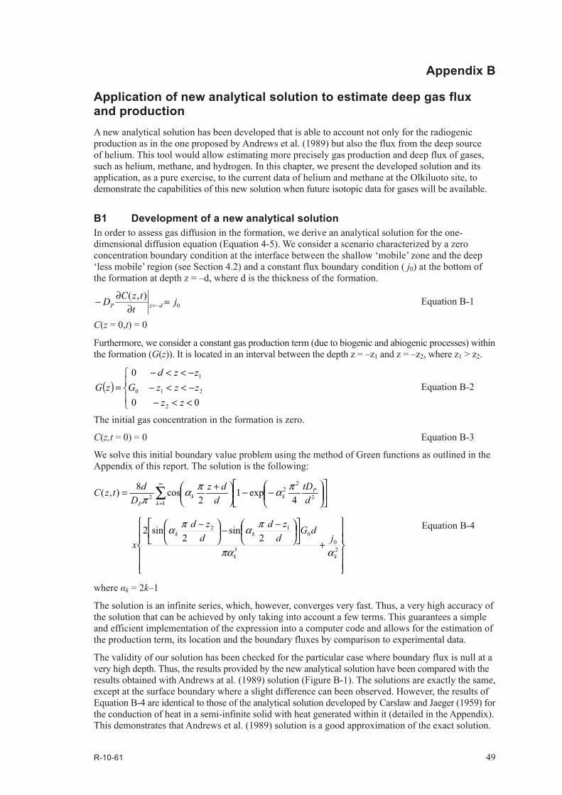
R-10-61 49

Appendix B

Application of new analytical solution to estimate deep gas flux and productionA new analytical solution has been developed that is able to account not only for the radiogenic production as in the one proposed by Andrews et al. (1989) but also the flux from the deep source of helium. This tool would allow estimating more precisely gas production and deep flux of gases, such as helium, methane, and hydrogen. In this chapter, we present the developed solution and its application, as a pure exercise, to the current data of helium and methane at the Olkiluoto site, to demonstrate the capabilities of this new solution when future isotopic data for gases will be available.

B1 Development of a new analytical solutionIn order to assess gas diffusion in the formation, we derive an analytical solution for the one-dimensional diffusion equation (Equation 4-5). We consider a scenario characterized by a zero concentration boundary condition at the interface between the shallow ‘mobile’ zone and the deep ‘less mobile’ region (see Section 4.2) and a constant flux boundary condition ( j0) at the bottom of the formation at depth z = –d, where d is the thickness of the formation.

0),( j

ttzCD dzP =

∂∂− −= Equation B-1

C(z = 0,t) = 0

Furthermore, we consider a constant gas production term (due to biogenic and abiogenic processes) within the formation (G(z)). It is located in an interval between the depth z = –z1 and z = –z2, where z1 > z2.

( )

<<−−<<−−<<−

=00

0

2

210

1

zzzzzGzzd

zG Equation B-2

The initial gas concentration in the formation is zero.

C(z,t = 0) = 0 Equation B-3

We solve this initial boundary value problem using the method of Green functions as outlined in the Appendix of this report. The solution is the following:

−−

+= ∑

∞

=2

22

12 4

exp12

cos8),(dtD

ddz

DdtzC P

kk

kP

παπαπ

+

−−

−

20

3

012

2sin

2sin2

kk

kk jdG

dzd

dzd

xαπα

παπα Equation B-4

where αk = 2k–1

The solution is an infinite series, which, however, converges very fast. Thus, a very high accuracy of the solution that can be achieved by only taking into account a few terms. This guarantees a simple and efficient implementation of the expression into a computer code and allows for the estimation of the production term, its location and the boundary fluxes by comparison to experimental data.

The validity of our solution has been checked for the particular case where boundary flux is null at a very high depth. Thus, the results provided by the new analytical solution have been compared with the results obtained with Andrews at al. (1989) solution (Figure B-1). The solutions are exactly the same, except at the surface boundary where a slight difference can been observed. However, the results of Equation B-4 are identical to those of the analytical solution developed by Carslaw and Jaeger (1959) for the conduction of heat in a semi-infinite solid with heat generated within it (detailed in the Appendix). This demonstrates that Andrews et al. (1989) solution is a good approximation of the exact solution.

50 R-10-61

B2 Application to helium and methane data at the Olkiluoto siteThe solution presented in Equation B-4 involves seven parameters, as many degrees of freedom. However, the exercise corresponds just to a pure calibration example to demonstrate the capabilities of the new analytical solution for the future.

To constrain our calibration procedure, we prescribed two parameters: the depth of the system (d=1,000 m) and the pore diffusion coefficient, which has a relatively low uncertainty (Pore diffu-sion coefficient is the result of the effective diffusion coefficient divided by the porosity taken from Table 4-1). The other five parameters (e.g. the gas production, G0, the zone of production, z1 and z2, the boundary flux, j0, and the diffusive time, t) have still to be calibrated.

To obtain the most meaningful set of calibrated parameters, the undertaken methodology to fit helium and methane profiles at the Olkiluoto site is the following:

• First the calibration of the 5 parameters to fit the most conservative gas (e.g. He) profile is performed. We consider that the obtained diffusive time, t, is the same for all gas species in the considered host rock.

• Then, the gas production, G0, the zone of production, z1 and z2, and the boundary flux, j0 are quantitatively estimated to fit methane concentrations profile.

Some qualitative information can be used to constrain more the calibration process for both gases. On one hand, the diffusive time (t) of gas into the host rock will be lower or equal to the formation age (1.86·109y, Table 4-4). On the other hand, the current profile of gas concentrations may indicate a deep contribution that has been diffused since the time t. Therefore, the boundary flux ( j0) is characterised by the observed gradient of concentrations (e.g. the deep flux of gas is the dominant source). We have performed one calibration based on j0 set to the calculated boundary flux based on the estimated gradient shown by concentrations profile. Then, the production term, the time of diffusion and the limits of the production zone are calibrated to fit the data. Also, the diffusion model has been applied below the first 300 m. As stated before, we suppose that above 300 m, the transport mechanism is probably sub-horizontal advective transport.

Figure B-1. Comparing analytical solutions for a production gas as unique source of helium at the Olkiluoto site.

-1000

-800

-600

-400

-200

03.5E-04 4.0E-04 4.5E-04 5.0E-04

Dep

th (m

)Helium (mol·L-1)

Andrews et al. (1989)

Carslaw and Jaeger (1959)

new analytical solution

R-10-61 51

B2.1 Helium profile at OlkiluotoThe first step of this exercise consists in calibrating the conservative gas profile. Figure B-2 compares the results of the calibration with the observed helium profile at Olkiluoto. The calibrated curve is a satisfying representation of the data in a normal and a log scale. Table B-1 lists all parameters fixed or obtained for the calibration. The set of parameters is meaningful according to the state of knowledge.

Figure B-2. Measured and calibrated helium profiles at Olkiluoto using the new analytical solution (B-4). Top: normal scale, bottom: log-normal scale.

-1000

-900

-800

-700

-600

-500

-400

-3000.0E+00 5.0E-04 1.0E-03 1.5E-03 2.0E-03 2.5E-03 3.0E-03

Dep

th (m

)

Helium (mol·L-1)

Olkiluoto data

calibration

-1000

-900

-800

-700

-600

-500

-400

-3001.0E-05 1.0E-04 1.0E-03 1.0E-02 1.0E-01

Dep

th (m

)

Helium (mol·L-1)

Olkiluoto data

calibration

52 R-10-61

Table B-1. Fixed or calibrated parameters to calibrate the helium profile at Olkiluoto.

Parameter Calibrated or fixed value

d (m) 1,000De

He (m2·s–1) 4.25·10–13 (Table 4-1)

φ (–) 5.04·10–3 (Table 4-4)

DpHe (m2·s–1) 8.43·10–11 (Table 4-4)

t (y) 1.9·107 (c)

j0 (mol/(m2·y) 1.92·10–8 (Table 4-2)

G0 (mol·m–3y–1) 2.11·10–10 (c)z1 (m) 1,000 (c)z2 (m) 400 (c)

*flux calculated based on Equation 4-1 considering a gradient between the deepest concentration of helium and a nil concentration at the surface.(c) indicates calibrated parameters.

Table B-2. Fixed or calibrated parameters to calibrate the methane profile at Olkiluoto.

Parameter Calibrated or fixed value

d (m) 1,000De

CH4 (m2·s–1) 8.58·10–13 (Table 4-1)

φ (–) 5.04·10–3 (Table 4-4)

DpCH4 (m2·s–1) 1.7·10–10

t (y) 1.9·107 (from He calibration)j0(m3/(m2·y) 1.86·10–7 (Table 4-2)

G0 (m3m–3y–1) 2.27·10–9 (c)z1 (m) 1,000 (c)z2 (m) 400 (c)

*flux calculated based on Equation 4-1 considering a gradient between the deepest concentration of methane and a nil concentration at the surface.(c) indicates calibrated parameters.

Calibrated gas production (2.11·10–10 mol m–3y–1) is similar to the radiogenic production (1.24·10–10 mol m–3y–1) used in the calibration based on Andrews et al. (1989) analytical solution. Calibrated diffusive times is lower (1.9·107 y) than the age of the host rock.

The exercise corresponds just to a pure calibration example to demonstrate the capabilities of the new analytical solution for the future. A meaningful calibration would be possible in the future if some information on the origin of the gas can be obtained by isotopic analysis.

B2.2 Methane profile at OlkiluotoThe second step of the exercise consists in fitting the methane gas profile at Olkiluoto. We remember that the diffusive time is a fixed parameter given by the calibration of the conservative gas profile. Figure B-3 compares the results of the calibration with the observed methane profile at Olkiluoto. The calibrated curve is a satisfactory representation of the data in a normal and a log scale. Table B-2 lists all parameters fixed or obtained for the calibration. As for helium, the sets of parameters are the most meaningful according to the state of knowledge.

As for helium, calibrated gas production (2.27·10–9 mol m–3y–1) is of the same order of magnitude but lower than the production (4.66·10–9 mol m–3y–1) resulting from the calibration based on Andrews et al. (1989) analytical solution. The calibrated production could count for all biogenic and abiogenic processes that release methane into the accessible pore water between 400 and 1,000 m.

R-10-61 53

Figure B-3. Measured and calibrated helium profiles at Olkiluoto using the new analytical solution (Equation 4-5). Top: normal scale, bottom: log-normal scale.

-1000

-900

-800

-700

-600

-500

-400

-3000.00E+00 5.00E-03 1.00E-02 1.50E-02 2.00E-02 2.50E-02 3.00E-02 3.50E-02 4.00E-02

Dep

th (m

)

Methane (mol·L-1)

Olkiluoto data

calibration

-1000

-900

-800

-700

-600

-500

-400

-3001.00E-06 1.00E-05 1.00E-04 1.00E-03 1.00E-02 1.00E-01 1.00E+00

Dep

th (m

)

Methane (mol·L-1)

Olkiluoto data

calibration

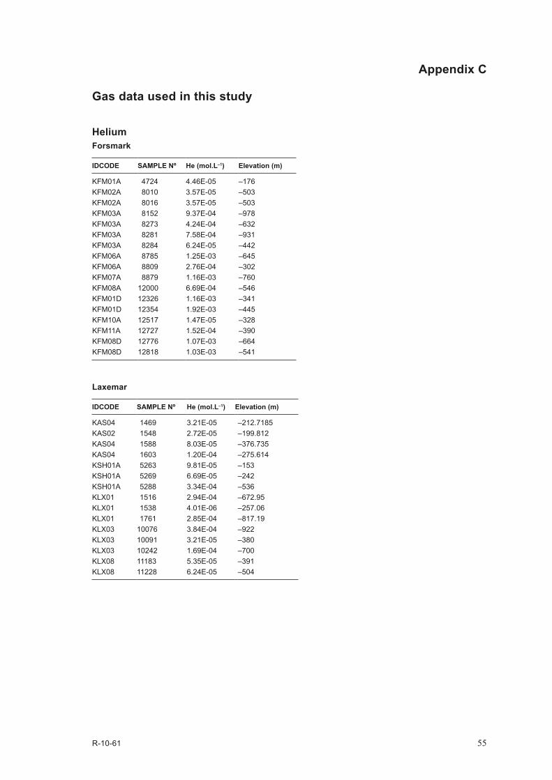
R-10-61 55

Appendix C

Gas data used in this study

HeliumForsmark

IDCODE SAMPLE Nº He (mol.L–1) Elevation (m)

KFM01A 4724 4.46E-05 –176KFM02A 8010 3.57E-05 –503KFM02A 8016 3.57E-05 –503KFM03A 8152 9.37E-04 –978KFM03A 8273 4.24E-04 –632KFM03A 8281 7.58E-04 –931KFM03A 8284 6.24E-05 –442KFM06A 8785 1.25E-03 –645KFM06A 8809 2.76E-04 –302KFM07A 8879 1.16E-03 –760KFM08A 12000 6.69E-04 –546KFM01D 12326 1.16E-03 –341KFM01D 12354 1.92E-03 –445KFM10A 12517 1.47E-05 –328KFM11A 12727 1.52E-04 –390KFM08D 12776 1.07E-03 –664KFM08D 12818 1.03E-03 –541

Laxemar

IDCODE SAMPLE Nº He (mol.L–1) Elevation (m)

KAS04 1469 3.21E-05 –212.7185KAS02 1548 2.72E-05 –199.812KAS04 1588 8.03E-05 –376.735KAS04 1603 1.20E-04 –275.614KSH01A 5263 9.81E-05 –153KSH01A 5269 6.69E-05 –242KSH01A 5288 3.34E-04 –536KLX01 1516 2.94E-04 –672.95KLX01 1538 4.01E-06 –257.06KLX01 1761 2.85E-04 –817.19KLX03 10076 3.84E-04 –922KLX03 10091 3.21E-05 –380KLX03 10242 1.69E-04 –700KLX08 11183 5.35E-05 –391KLX08 11228 6.24E-05 –504

56 R-10-61

Olkiluoto

SAMPLE Nº He (mol.L–1) Elevation (m)

KR30_50_1 1.16E-07 –39.5KR12_65_1 2.68E-06 –52.3KR14_79_1 1.78E-06 –65.9KR4_81_1 8.92E-07 –70.0KR6_98_6 4.01E-06 –73.7KR13_112_1 2.48E-05 –86.7KR6_125_4 8.03E-06 –94.1KR27_124_1 1.87E-05 –95.2KR8_120_1 4.01E-06 –96.1KR19_110_1 4.01E-06 –100.7KR6_135_6 8.03E-06 –101.8KR6_135_7 1.16E-05 –101.8KR10_115_1 3.08E-05 –106.0KR20_186_1 5.35E-06 –137.0KR23_192_1 8.92E-06 –155.1KR14_182_1 9.37E-06 –162.5KR13_214_1 1.43E-05 –170.7KR27_247_1 1.56E-05 –193.5KR3_243_1 5.35E-05 –216.1KR15_241_1 7.00E-05 –231.8KR15_241_2 7.58E-05 –231.8KR7_282_1 1.20E-05 –255.6KR8_302_1 3.79E-05 –260.7KR29_300_1 6.69E-05 –274.6KR29_320_1 5.35E-05 –293.4KR13_362_1 2.90E-04 –294.0KR13_362_2 2.19E-04 –294.0KR8_347_1 6.24E-05 –301.3KR2_329_1 1.92E-04 –306.2KR10_324_1 1.92E-04 –314.0KR10_326_1 1.96E-04 –316.0KR20_416_1 2.45E-04 –320.2KR6_422_2 2.14E-04 –328.4KR6_422_4 1.92E-04 –328.4KR12_365_1 3.84E-04 –339.1KR22_423_1 2.76E-04 –347.0KR20_465_1 3.21E-04 –360.7KR7_410_1 4.01E-04 –376.3KR3_438_1 1.96E-04 –390.1KR14_446_1 5.08E-04 –407.9KR6_525_1 5.98E-04 –410.9KR9_470_1 4.32E-04 –424.9KR15_449_1 6.69E-04 –438.1KR10_498_1 6.69E-04 –487.1KR10_498_2 5.71E-04 –487.1KR10_500_1 3.43E-04 –489.0KR8_556_1 5.57E-04 –490.2KR19_526_1 6.69E-04 –499.6KR9_563_1 5.31E-04 –508.0KR11_621_1 2.72E-04 –551.7KR11_621_2 4.19E-04 –551.7KR2_596_1 7.98E-04 –559.5KR1_612_3 4.64E-04 –567.7KR10_610_1 3.43E-04 –598.0KR12_664_1 3.30E-04 –632.5KR12_736_1 5.66E-04 –703.9KR12_741_1 7.40E-04 –708.3KR29_800_1 7.58E-04 –742.2KR2_876_2 9.72E-04 –817.7KR4_860_2 9.23E-04 –817.8KR2_950_1 7.72E-04 –884.8KR2_1030_1 4.55E-04 –956.6

R-10-61 57

MethaneForsmark

IDCODE Sample Nº CH4 (mol.L–1) Elevation (m)

KFM01A 4724 4.90E-06 –176KFM02A 8010 1.23E-06 –503KFM02A 8016 1.63E-06 –503KFM03A 8152 2.04E-06 –978KFM03A 8273 2.86E-06 –632KFM03A 8281 2.45E-06 –931KFM03A 8284 1.23E-06 –442KFM06A 8785 3.68E-06 –645KFM06A 8809 9.81E-07 –302KFM07A 8879 1.63E-06 –760KFM08A 12000 1.23E-06 –546KFM01D 12326 5.72E-06 –341KFM01D 12354 1.88E-04 –445KFM10A 12517 1.23E-06 –328KFM11A 12727 4.09E-06 –390KFM08D 12776 2.45E-06 –664KFM08D 12818 3.68E-06 –541

Laxemar

IDCODE Sample Nº CH4 (mol.L–1) Elevation (m)

KAS04 1469 3.47E-06 –212.7185KAS02 1548 1.23E-06 –199.812KAS02 1560 1.39E-06 –881.217KAS03 1569 6.54E-07 –121.782KAS03 1582 1.51E-06 –914.0105KAS04 1588 1.63E-07 –376.735KAS04 1603 1.14E-06 –275.614KSH01A 5263 2.45E-06 –153KSH01A 5269 3.68E-06 –242KSH01A 5288 1.63E-06 –536KLX01 1516 8.99E-06 –672.95KLX01 1538 4.50E-06 –257.06KLX01 1633 1.63E-06 –672.95KLX01 1761 1.23E-06 –817.19KLX03 7953 3.56E-05 –171KLX03 10076 2.45E-06 –922KLX03 10091 2.53E-05 –380KLX03 10242 8.58E-06 –700KLX08 11183 1.19E-06 –391KLX08 11228 1.02E-06 –504KLX17A 11692 5.93E-06 –548KLX17A 11810 2.86E-06 –342

58 R-10-61

Olkiluoto

Sample Nº CH4 (mol.L–1) Elevation (m)

KR30_50_1 1.80E-05 –39.5KR12_65_1 2.00E-05 –52.3KR14_79_1 6.13E-06 –65.9KR4_81_1 2.90E-05 –70.0KR6_98_6 4.90E-06 –73.7KR13_112_1 1.58E-04 –86.7KR6_125_4 1.43E-05 –94.1KR27_124_1 6.95E-06 –95.2KR8_120_1 5.72E-06 –96.1KR19_110_1 2.86E-06 –100.7KR6_135_6 2.04E-06 –101.8KR6_135_7 6.13E-06 –101.8KR10_115_1 1.43E-04 –106.0KR20_186_1 6.13E-06 –137.0KR23_192_1 5.31E-06 –155.1KR14_182_1 8.99E-06 –162.5KR13_214_1 2.49E-05 –170.7KR27_247_1 1.06E-05 –193.5KR3_243_1 1.17E-03 –216.1KR15_241_1 1.59E-03 –231.8KR15_241_2 1.26E-03 –231.8KR7_282_1 6.54E-06 –255.6KR8_302_1 2.29E-06 –260.7KR29_300_1 5.31E-05 –274.6KR29_320_1 2.29E-05 –293.4KR13_362_1 9.28E-04 –294.0KR13_362_2 1.06E-03 –294.0KR8_347_1 6.54E-05 –301.3KR2_329_1 1.14E-03 –306.2KR10_324_1 3.33E-03 –314.0KR10_326_1 2.90E-03 –316.0KR20_416_1 1.95E-03 –320.2KR6_422_2 8.30E-04 –328.4KR6_422_4 8.99E-04 –328.4KR12_365_1 4.93E-03 –339.1KR22_423_1 5.44E-03 –347.0KR20_465_1 5.60E-03 –360.7KR7_410_1 5.72E-03 –376.3KR3_438_1 2.12E-03 –390.1KR14_446_1 6.25E-03 –407.9KR6_525_1 1.43E-02 –410.9KR9_470_1 9.59E-03 –424.9KR15_449_1 5.76E-03 –438.1KR10_498_1 1.42E-02 –487.1KR10_498_2 1.20E-02 –487.1KR10_500_1 6.13E-03 –489.0KR8_556_1 1.46E-02 –490.2KR19_526_1 1.88E-02 –499.6KR9_563_1 1.05E-02 –508.0KR11_621_1 1.58E-02 –551.7KR11_621_2 9.07E-03 –551.7KR2_596_1 1.58E-02 –559.5KR1_612_3 1.11E-02 –567.7KR10_610_1 6.54E-03 –598.0KR12_664_1 1.06E-02 –632.5KR12_736_1 1.81E-02 –703.9KR12_741_1 2.40E-02 –708.3KR29_800_1 3.76E-02 –742.2KR2_876_2 2.91E-02 –817.7KR4_860_2 3.79E-02 –817.8KR2_950_1 3.65E-02 –884.8KR2_1030_1 1.85E-02 –956.6

R-10-61 59

HydrogenForsmark

IDCODE Sample Nº H2 (mol.L–1) Elevation (m)

KFM01A 4724 2.28E-07 –176KFM02A 8010 9.28E-07 –503KFM02A 8016 8.39E-06 –503KFM03A 8281 1.86E-06 –931KFM03A 8284 8.98E-06 –442KFM06A 8809 1.81E-05 –302KFM11A 12727 1.43E-06 –390

Laxemar

IDCODE Sample Nº H2 (mol.L–1) Elevation (m)

KSH01A 5269 3.58E-06 –242KSH01A 5288 3.42E-06 –536KLX03 10091 4.64E-06 –380KLX03 10242 8.01E-06 –700KLX08 11183 1.94E-06 –391KLX17A 11692 2.95E-08 –548KLX13A 11609 2.11E-08 –408

Olkiluoto

Sample Nº H2 (mol.L–1) Elevation (m)

KR8_120_1 4.22E-08 –96.1KR19_110_1 7.59E-08 –100.7KR6_135_7 9.70E-08 –101.8KR23_192_1 1.56E-07 –155.1KR3_243_1 2.95E-06 –216.1KR7_282_1 6.32E-07 –255.6KR8_347_1 2.82E-07 –301.3KR10_324_1 2.53E-07 –314.0KR10_326_1 7.17E-06 –316.0KR3_438_1 8.43E-07 –390.1KR9_470_1 1.39E-06 –424.9KR15_449_1 6.70E-07 –438.1KR19_526_1 4.22E-05 –499.6KR9_563_1 1.56E-05 –508.0KR11_621_1 1.14E-03 –551.7KR11_621_2 1.88E-06 –551.7KR2_596_1 1.09E-05 –559.5KR1_612_3 6.75E-07 –567.7KR12_741_1 4.64E-07 –708.3KR29_800_1 4.22E-06 –742.2KR2_876_2 9.42E-04 –817.7KR4_860_2 9.82E-06 –817.8KR2_950_1 8.43E-04 –884.8KR2_1030_1 4.56E-04 –956.6

Quantitative assessment of deep gas migration in ... - SKB · SKB may draw modified conclusions, based on additional literature sources and/or expert opinions. A pdf version of this

Documents