QUANTITATIVE ASSESSMENT OF CEREBRAL MICROVASCULATURE USING MACHINE LEARNING AND NETWORK ANALYSIS A Dissertation Presented to the Faculty of the Graduate School of Cornell University In Partial Fulfillment of the Requirements for the Degree of Doctor of Philosophy by Mohammad Haft Javaherian May 2019

Welcome message from author
This document is posted to help you gain knowledge. Please leave a comment to let me know what you think about it! Share it to your friends and learn new things together.
Transcript

QUANTITATIVE ASSESSMENT OF CEREBRAL
MICROVASCULATURE USING MACHINE LEARNING AND NETWORK
ANALYSIS
A Dissertation
Presented to the Faculty of the Graduate School
of Cornell University
In Partial Fulfillment of the Requirements for the Degree of
Doctor of Philosophy
by
Mohammad Haft Javaherian
May 2019

© 2019 Mohammad Haft Javaherian
iii
QUANTITATIVE ASSESSMENT OF CEREBRAL
MICROVASCULATURE USING MACHINE LEARNING AND NETWORK
ANALYSIS
Mohammad Haft Javaherian, Ph. D.
Cornell University 2019
Vasculature networks are responsible for providing reliable blood perfusion to
tissues in health or disease conditions. Volumetric imaging approaches, such as
multiphoton microscopy, can generate detailed 3D images of blood vessel networks
allowing researchers to investigate different aspects of vascular structures and networks
in normal physiology and disease mechanisms. Image processing tasks such as vessel
segmentation and centerline extraction impede research progress and have prevented the
systematic comparison of 3D vascular architecture across large experimental populations
in an objective fashion. The work presented in this dissertation provides complete a fully-
automated, open-source, and fast image processing pipeline that is transferable to other
research areas and practices with minimal interventions and fine-tuning. As a proof of
concept, the applications of the proposed pipeline are presented in the contexts of
different biomedical and biological research questions ranging from the stalling capillary
phenomenon in Alzheimer’s disease to the drought resistance of xylem networks in
various tree species and wood types.
iv
BIOGRAPHICAL SKETCH
Mohammad Haft Javaherian traveled around the world along a unique
interdisciplinary path to acquire computational mechanics and computer science skills,
which are ideal for addressing emerging biomedical problems. He has been eager to build
new bridges from artificial intelligence to biomedical science and medicine.
He decided to study civil engineering for his undergraduate program based on his
passion for learning about physical laws and their mathematical models that govern high-
rise buildings, dams, and bridges, which enable engineers to design those magnificent
structures. During his first semester at the University of Tehran, he noticed the possibility
of merging his high school computer programming interests with the knowledge of
physical laws and mathematical models within the field of computational mechanics. He
enhanced his knowledge by taking the system engineering course, which was his first
exposure to artificial intelligence.
During his master’s program, his main research project was the development of a
computer software package that synthesizes virtual microstructure of particle-reinforced
composites using generative models that mimics the geometrical and mechanical
characteristics of the real fabricated composite material. Subsequently, the synthetic
samples were tested using microstructure modeling to estimate the mechanical
characteristics of the anticipated material. This synthesized sample generation and testing
can potentially replace expensive and time-consuming laboratory fabrication and testing.

v
He adapted methods from the system engineering course to introduce new empirical and
stochastic models using image processing and Markov chain Monte Carlo simulations
that translate three-dimensional information of an asphalt mixture to its two-dimensional
counterpart.
After his master’s program, he realized that these quantitative tools could be used
to answer important life science questions, which were more compelling to him.
Therefore, he decided to pursue his Ph.D. study in the biomedical engineering field and
joined the Schaffer-Nishimura labs. His research interest turned to the microscopic-scale
understanding of normal and disease-state physiological processes in different organs and
systems such as the central nervous system.
His interdisciplinary education and training are strong foundations that support
him in introducing unique approaches to study life science questions in ways not
previously possible. His distinctive capability of adopting ideas from many, diverse,
research fields to answer a tough life science questions is enhanced with his programming
skills and mastery in computational methods in addition to the advanced novel optical
techniques developed in our research laboratory. He would like to invest his career in
investigating the application of machine learning in biomedical research and medicine in
addition to training the next generation of scientists.

vi
ACKNOWLEDGMENTS
It has been an absolute honor and a pleasure working with talented and affable
people in the course of my PhD studies at Cornell University. I would like to express my
sincere gratitude to my colleagues, friends, and family members for supporting me
through this journey.
First, I would like to thank my adviser and co-adviser, Prof. Nozomi Nishimura
and Prof. Chris Schaffer. I joined their labs after the tragic loss of my late PhD adviser,
Prof. Ephrahim Garcia. Nozomi and Chris flourished my scientific curiosity and
eagerness to investigate unknowns with allowing me thinking outside the box and
pursuing my passion in other research fields while advising me through the difficulties. I
am grateful that they took a chance on me. Beyond the academic settings and on a
personal level, their incredible support and kindness made my PhD studies a memorable
and pleasant experience that let me forget the difficulties happened prior to joining their
labs. I also thanks Prof. Andrew Ruina for his tremendous help and emotional support
during that difficult period.
I would also like to thank my committee members. Prof. Mert Sabuncu has been
a great resource since I started doing research and applying machine learning and
computer vision to biomedical problems. He was receptive in research and helped me to
obtain practical experience outside academia. Prof. Joseph Fetcho taught me many tips
that allowed me to navigate graduate school very smoothly in the past and academic

vii
career in future, in addition, to being a great resource when I felt lost in the Neuroscience
field.
I would like to thank the members of the Schaffer-Nishimura labs. In particular,
Dr. Jean Cruz Hernandez and Dr. Oliver Bracko for their experimental work presented in
this dissertation in addition to teaching me how to do the surgery myself and how the
behavioral test works. Their intellectual support and encouragements were essential.
Nancy Uribe Ruiz joined our lab in recently, and I am grateful for the experiments she
conducted for brain vasculature networks. I am also grateful to the Master’s,
undergraduate, and high school students who worked with me extensively and helped me
to grow while finishing the research projects together. Linjing Fang helped me with the
DeepVess and the Review chapter During her master’s program. Victorine Muse helped
me with DeepVess and Alzheimer’s project measurements. Nash Allan Rahill helped me
to investigate the application of DeepVess to the heart vasculature images. Muhammad
Ali, Iryna Ivasyk, Lawrence Cheng, Madisen Swallow, Nathaniel Pineda were a great
help while trying different prototypes for crowdsourcing and the Alzheimer’ project. Saif
Azam helped me with the speckle imaging. I wish all of them success in their future
endeavors.
Additionally, I thank Yu-Ting Cheng and Dr. David Small for teaching me details
of animal surgery and other experimental details as well as Dr. Mike Lamont for inhering
my responsibilities and projects in order to move them forward. Many thanks to B56
Weill Hall officemates and close friends who were great moral support during these years.
Dr. John Foo for sharing his graduate school experiences, Dr. Jason Jones and Mitch

viii
Pender for helping me to get established when I joined the lab, and Jeffrey Mulligan for
being available all the time to discuss scientific and non-scientific matters. Finally, thanks
to other Schaffer-Nishimura lab members for their supports: Daniel Rivera, Menansili
Mejooli, Dr. Amanda bares, Dr. Poornima Gadamsetty, Dr. Elizabeth Wayne, Silvia
Zhang, Dr. Sung Ji Ahn, Dr. Jiahn Choi, Seth Lieberman, Dr. SallyAnne DeNotta, Dr.
Chi-Yong Eom, Dr. Kawasi Lett, Dr. Laurie Bizimana, and many other undergraduate
students.
I would like to thank our collaborators from Cornell and other institutes around
the world. Prof. Sylvie Lorthois (Institut de Mecanique des Fluides de Toulouse in
France) was an excellent resource for my work within the Alzheimer’s project (allowing
me to have experience with human brain vasculature networks), DeepVess, and the fluid
simulation of xylem networks. I had a great collaboration with Dr. Amy Smith, Maxime
Berg, and Myriam Peyrounette from Sylvie’s lab. On the other hand, I had delightful and
joyful years of collaboration with Dr. Pietro Michelucci (Human Computation Institute)
and his colleagues Ieva Navikiene and Egle Marija Ramanauskaite for the development
of StallCatchers. Finally, I would like to thank Annika Huber and Prof. Taryn Bauerle
(School of Integrative Plant Science) for their extensive collaboration in the xylem
network project.
My gratitude extends to members of my family for their loving support throughout
my education. My parents are my long-standing role models and sources of support. Their
constant encouragements and continued love were the powerful fuels that allowed me to
finish this journey. I owe them a debt of gratitude that can never be repaid. I also thank

ix
my sister for her continued support at a different stage of my life. My gratitude also
extends to my wife for her support, friendship, and love. All these years, especially after
the birth of our son, she has often been the one holding up the pillars with her love,
encouragement, and intellectual depth. Without her support it was not possible to
conclude my PhD.
This work was supported by the European Research Council grant 615102
(Nozomi Nishimura), the National Institutes of Health grant AG049952 (Chris Schaffer),
the National Institutes of Health grants R01LM012719 and R01AG053949 (Mert
Sabuncu), the National Science Foundation Cornell NeuroNex Hub grant (1707312, Mert
Sabuncu and Chris Schaffer) and the National Science Foundation (1748377 to Mert
Sabuncu).
x
TABLE OF CONTENTS
Biographical sketch iv
Acknowledgments vi Table of contents x List of figures xiv List of tables xvii List of abbreviations xviii
CHAPTER 1 Introduction 1 References 6 CHAPTER 2 A review of three-dimensional vessel segmentation methods 8
2.1 Introduction 8 2.2 Image preprocessing 9
2.2.1 Smoothing and sharpening 10 2.2.2 Image artifact removal 11
2.2.3 Vesselness measurements 13 2.2.4 Frequency domain 14
2.3 Vascular segmentation methods 15 2.3.1 Region-based segmentation 15 2.3.2 Fuzzy clustering methods 17
2.3.3 Active contour models - Snakes 18 2.3.4 Geometric deformable models - Level set 20
2.3.5 Probabilistic graphical models 23 2.3.6 Artificial Deep Neural Networks 24
2.3.7 Centerline extraction Methods 26 2.3.8 Bifurcation detection 28
2.4 Vascular networks 29 2.4.1 Brain 29 2.4.2 Lung 32
2.4.3 Liver 34 2.5 Short segments 35
2.5.1 Heart 35
2.5.2 Coronary arteries 37 2.5.3 Carotid arteries 39 2.5.4 Abdominal aorta 40 2.5.5 Ascending aorta, aortic arch, and descending aorta 41
2.5.6 Aorta root 43 2.6 Disease state segmentation 45
2.6.1 Intracranial aneurysm and BAVM 45
2.6.2 Interstitial lung diseases 46 2.6.3 Carotid diseases 47 2.6.4 Coronary artery disease 48
2.7 Conclusion 49 References 51
xi
CHAPTER 3 Deep convolutional neural networks for segmenting 3D in
vivo multiphoton images of vasculature in Alzheimer disease mouse
models 82
3.1 Abstract 82 3.2 Introduction 83 3.3 Related work 85 3.4 Data and methods 87
3.4.1 Data 87
3.4.2 Preprocessing 90 3.4.3 Convolutional neural network architectures 91 3.4.4 Performance metrics 95 3.4.5 Training and implementation details 97 3.4.6 Post-processing 97
3.4.7 Analysis of vasculature centrelines 98 3.5 Results 99
3.6 Discussion 105 3.7 Application to Alzheimer’s mouse models 110
3.7.1 Capillary alteration caused by aging and Alzheimer’s disease 110 3.7.2 Aging and Alzheimer’s disease have little effect on capillary
characteristics 113
3.8 Conclusions 115 3.9 Data availability statement 116
3.10 Declarations of interest 116 3.11 Supplementary materials 116
3.11.1 Manual 3D segmentation protocol using ImageJ. 116
References 121
CHAPTER 4 Neutrophil adhesion in brain capillaries reduces cortical
blood flow and impairs memory function in Alzheimer’s disease mouse
models 128
4.1 List of Haft-Javaherian’s contributions 128 4.2 Abstract 129 4.3 Introduction 129
4.4 Results 131 4.5 Discussion 147 4.6 Acknowledgments 151 4.7 Author contributions: 151 4.8 Competing interests statement 152
4.9 Methods 152
4.9.1 Animals and surgical preparation 152
4.9.2 In vivo two-photon microscopy 154 4.9.3 Quantification of capillary network topology and capillary
segment stalling 156 4.9.4 Distinguishing causes of capillary stalls 158 4.9.5 Administration of antibodies against Ly6G or LFA-1 to interfere
with capillary stalling 159
xii
4.9.6 Behavior experiments 160 4.9.7 ELISA assay 163 4.9.8 Statistical analysis 164
4.9.9 Additional methodological details 165 4.9.10 Data availability 165 4.9.11 Code availability 165
References 166 4.10 Materials and methods 172
4.10.1 Animals and surgical preparation 172 4.10.2 In vivo two-photon microscopy 174 4.10.3 Awake imaging 177 4.10.4 Quantification of capillary network topology and capillary
segment stalling 178
4.10.5 Distinguishing causes of capillary stalls 180 4.10.6 Amyloid plaque segmentation and density analysis 181
4.10.7 Kinetics of capillary stalling 181 4.10.8 Administration of antibodies against Ly6G and impact on
neutrophil population 182 4.10.9 Measurement of volumetric blood flow in penetrating arterioles
184
4.10.10 Measurement of global blood flow using ASL-MRI 184 4.10.11 Multi-Exposure Laser Speckle Imaging 186
4.10.12 Extraction of network topology and vessel diameters from
mouse anatomical dataset 188 4.10.13 Extraction of network topology and vessel diameters from
human anatomical dataset 189
4.10.14 Synthetic network generation 190 4.10.15 Blood flow simulations 190 4.10.16 Behavior experiments 192
4.10.17 ELISA assay 196 4.10.18 Histopathology 197 4.10.19 Statistical analysis 198
4.10.20 Supplementary text on numerical simulations of cerebral blood
flow changes induced by capillary occlusions 199 4.10.21 Validation of simulations by comparison to in vivo
measurements in mouse: 199 4.11 Supplementary figures 203
4.12 Supplementary table 233
4.13 Supplementary movies 236
References 237 CHAPTER 5 Application of crowdsourcing citizen science in studying
brain capillaries in Alzheimer’s disease 245 5.1 Introduction 245 5.2 Method 248
5.2.1 General pipeline 248
xiii
5.2.2 Manual tracing and scoring 250 5.2.3 DeepVess 250 5.2.4 Vessel outlines and movie presentation for the StallCatchers user
251 5.2.5 Amazon AWS & Microsoft Azure 253
5.3 Results and discussions 255 5.3.1 Alpha test Discussions 255 5.3.2 Validation Study 256
5.3.3 High Fat Project 258 5.3.4 Post-hoc expert stall reconfirmation 260 5.3.5 Power of StallCatchers 261 5.3.6 Different stall-rate metrics 261 5.3.7 Comparison between StallCatchers and human manual
classifications 262 5.3.8 HFD results 265
5.3.9 Exceptional dataset 265 5.4 Conclusions 266
5.4.1 Future work 266 References 267 CHAPTER 6 Xylem vessel connectivity in the ring and diffuse porous trees
270 6.1 Introduction 270
6.2 Material and Methods 275 6.2.1 Plant material 275 6.2.2 Percent loss of hydraulic conductivity 275
6.2.3 Vessel length distribution 277
6.2.4 Laser ablation tomography 278 6.2.5 Selecting vessel length and cutting distance for analysis 281 6.2.6 Determining intervessel wall thickness 282
6.2.7 The study-design image processing pipeline 283 6.2.8 Motion artifact compensation 284 6.2.9 Segmentation 287
6.2.10 Computational fluid dynamics and embolism simulation 288 6.2.11 Statistics 290
6.3 Results and Discussions 290 6.3.1 Geometrical comparisons 295 6.3.2 Topological comparisons 298
6.3.3 Fluid simulations and P50 comparisons 308
6.4 Discussion 313
6.5 Supporting information 316 References 326 CHAPTER 7 Conclusions and future directions 329
xiv
LIST OF FIGURES
Figure 1.1. Three-dimensional structure of blood vessels in the brain of a mouse
model of Alzheimer’s ........................................................................................... 2 Figure 3.1. The optimal 3D CNN architecture. .............................................................. 94 Figure 3.2. In vivo MPM images of a capillary. ........................................................... 100 Figure 3.3. Slice-wise Dice index of DeepVess vs. manual annotation ....................... 102 Figure 3.4. Comparison of DeepVess and the state-of-the-art methods ....................... 104
Figure 3.5. 3D rendering of (A) the expert’s manual and (B) DeepVess
segmentation results. ......................................................................................... 106 Figure 3.6. Comparison of DeepVess and the gold standard human expert ................. 108
Figure 3.7. Comparison of capillaries between young and old mice with WT and
AD genotype (6 mice in each group). ............................................................... 112 Figure 4.1. 2PEF imaging of mouse cortical vasculature revealed a higher
fraction of plugged capillaries in APP/PS1 mice. ............................................ 133
Figure 4.2. Characterization of the cause, location, and dynamics of capillary
occlusions in APP/PS1 mice. ............................................................................ 135
Figure 4.3. Administration of antibodies against Ly6G reduced the number of
stalled capillaries and increased cCBF in APP/PS1 mice. ............................... 139 Figure 4.4. Administration of α-Ly6G improved short-term memory. ........................ 143
Figure 4.5. Administration of α-Ly6G for one month decreased the
concentration of Aβ1-40 in APP/PS1 mice. ..................................................... 145
Figure 4.6. Simulations predicted a similar CBF decrease in mouse and human
cortical capillary networks with increasing fraction of capillaries with
stalled flow. ....................................................................................................... 146 Figure 5.1. StallCatchers complete pipeline. Each row represents one of the
objectives (first column) and processes required to achieve it (other
columns). .......................................................................................................... 249 Figure 5.2. Example of frames from a StallCatchers movie showing a vessel that
traverses along the third dimension. ................................................................. 254 Figure 5.3. Alpha test results for the different numbers of annotations per vessel. ..... 256 Figure 5.4. Validation study results for the different numbers of annotations per
vessel based on the plaque proximity dataset. .................................................. 258 Figure 5.5. StallCatchers current user interface. ........................................................... 258 Figure 5.6. Comparison of image quality between a normal (A) and an HFD
image stack (B). ................................................................................................ 260
Figure 5.7. The stalled capillary phenomenon in AD and HFD. .................................. 263 Figure 5.8. Image Intensity normalization for two different datasets. .......................... 265 Figure 6.1. SEM images of a xylem intervessel connection. ........................................ 272
Figure 6.2. Samples of 3D LATscan images of tree branch cross-sections of
different species. ............................................................................................... 280 Figure 6.3. Examples of motion artifacts due to the residuals of last cross-section
(A) and the laser ablation signs in addition to the reflection (B). ..................... 285 Figure 6.4. Complete image processing pipeline.......................................................... 288
xv
Figure 6.5. Three graph representations of xylem networks. ....................................... 292 Figure 6.6. Anatomical characteristics based on the 3D segment representation. ....... 296 Figure 6.7. Anatomical characteristics based on the streamline representation. .......... 297
Figure 6.8. Network analysis based on the 3D segment representation. ...................... 301 Figure 6.9. Graph illustration based on the 3D segment representation. ...................... 303 Figure 6.10. Network analysis based on the streamline segment representation. ........ 305 Figure 6.11. Graph illustration based on the 3D segment representation. .................... 307 Figure 6.12. Computational fluid dynamics and embolism simulation: ....................... 310
Figure 6.13. Comparison between simulations and experientially measured P50. ...... 311 Figure 6.14. Percent loss of hydraulic conductivity (PLC). ......................................... 312
Figure S 3.1. Jaccard as a measure of the model accuracy. .......................................... 117 Figure S 3.2. The vessel diameters measured manually in comparison to the
DeepVess’s results. ........................................................................................... 118
Figure S 4.1. The fraction of capillaries with stalled blood flow did not increase
with increasing cortical amyloid plaque density in APP/PS1 mice. ................. 203 Figure S 4.2. Plot of the fraction of capillaries with stalled blood flow in mice
imaged while anesthetized and awake. ............................................................. 204 Figure S 4.3. α-Ly6G administration reduced the number of cortical capillary
stalls and increased penetrating arteriole blood flow in 5xFAD mice. ............. 205 Figure S 4.4. 2PEF imaging of cortical vasculature reveals a higher fraction of
stalled capillaries in TgCRND8 mice as compared to wt mice. ....................... 206
Figure S 4.5. Characterization of capillary stall dynamics in APP/PS1 mice. ............. 207 Figure S 4.6. Extended Data Figure 6. Number of stalled capillaries in APP/PS1
mice dropped rapidly after α-Ly6G administration. ......................................... 208 Figure S 4.7. Treatment with α-Ly6G leads to neutrophil depletion in both
APP/PS1 and wildtype control mice, beginning within three hours after
administration. .................................................................................................. 210 Figure S 4.8. Administration of antibodies against Ly6G increased the RBC
flow speed but did not alter the diameter of cortical penetrating arterioles
in APP/PS1 mice............................................................................................... 211
Figure S 4.9. Penetrating arterioles with slower initial flow tended to increase
flow speed more after α-Ly6G injection in APP/PS1 mice. ............................. 212 Figure S 4.10. Multi-exposure laser speckle imaging revealed CBF increased in
APP/PS1 mice within minutes of α-Ly6G administration. ............................... 214 Figure S 4.11. Treating APP/PS1 mice with α-LFA-1 reduced the number of
stalled capillaries and improved arterial blood flow after 24 hours. ................ 215 Figure S 4.12. Brain penetrating arteriole blood flow negatively correlates with
the number of capillaries stalled in underlying capillary beds in APP/PS1
mice. .................................................................................................................. 217 Figure S 4.13. Time spent at the replaced object in wild type controls and
APP/PS1 animals treated with α-Ly6G or isotype control antibodies. ............. 218 Figure S 4.14. Administration of α-Ly6G improves performance of 5xFAD mice
on object replacement and Y-maze tests of spatial and working memory. ...... 220 Figure S 4.15. Number of arm entries in the Y-maze for wild type controls and
APP/PS1 animals treated with α-Ly6G or isotype control antibodies. ............. 221
xvi
Figure S 4.16. Balance beam walk (BBW) to measure motor coordination in
wildtype controls and APP/PS1 animals treated with α-Ly6G or isotype
control antibodies. ............................................................................................. 223
Figure S 4.17.. Depression-like behavior measured as immobility time in a
forced swim test for wild type controls and APP/PS1 animals treated
with α-Ly6G or isotype control antibodies. ...................................................... 224 Figure S 4.18. Administration of α-LFA-1 improves performance of APP/PS1
mice on object replacement and Y-maze tests of spatial and working
memory. ............................................................................................................ 226 Figure S 4.19. Representative map of animal location and time spent at the novel
object in wild type controls and APP/PS1 animals treated with α-Ly6G
or isotype control antibodies. ............................................................................ 227 Figure S 4.20. Amyloid plaque density and concentration of amyloid-beta
oligomers were not changed in 11-month-old APP/PS1 animals treated
with α-Ly6G every three days for a month. ...................................................... 228
Figure S 4.21. Synthetic capillary network of order three. ........................................... 229 Figure S 4.22. Histogram of mouse capillary diameters from in vivo
measurements and post-mortem vascular casts. ............................................... 230 Figure S 4.23. Illustration of the pseudo-periodic boundary conditions. ..................... 230 Figure S 4.24. Validation of simulations. ..................................................................... 231
Figure S 4.25. Calculated blood flow decreases due to capillary stalls was robust
with respect to simulation parameters. ............................................................. 232
Figure S 6.1. Vessel length distribution of three diffuse porous (filled symbols)
and three ring-porous (unfilled symbols) tree species. ..................................... 316 Figure S 6.2. Characteristics of xylem vessels and their connections .......................... 319
Figure S 6.3. Characteristics of xylem vessels and their connections .......................... 320
Figure S 6.4. Relation between relative conductance of xylem networks .................... 321 Figure S 6.5. Network presentations ............................................................................. 322 Figure S 6.6. Network presentations ............................................................................. 324

xvii
LIST OF TABLES
Table 3-1. The comparison of our proposed CNN architecture (DeepVess), .............. 101
Table 3-2. Comparison between metrics distributions between different groups ........ 112 Table 3-3. Comparison of measured mouse capillary diameters from different
studies. .............................................................................................................. 115 Table 6-1. The geometrical characteristic of tree species samples. .............................. 282
xviii
LIST OF ABBREVIATIONS
3D-RA 3D Rotational Angiography
BAVM Brain Arteriovenous Malformation
BB-MRI Black-Blood Magnetic Resonance Image
CAD Coronary Artery Disease
CCA Conventional Catheter Angiography
CT Computed Tomography
CTA Computed Tomography Angiography
CTP Computed Tomography Perfusion
DSA Digital Subtraction Angiography
EM Expectation Maximization
FCM Fuzzy Clustering Methods
ILD Interstitial Lung Diseases
IPF Idiopathic Pulmonary Fibrosis
IVUS Intravascular
MAP Maximum A Posteriori Probability
Micro-CT Micro-Computed Tomography
MPM Multiphoton Microscopy
MRA Magnetic Resonance Angiographic
MRI Magnetic Resonance Image
OCT Optical Coherence Tomography
PC-CT Phase Contrast Computed Tomography
PC-MRA Phase Contrast Magnetic Resonance Angiographic
PD-MRI Proton-Density Magnetic Resonance Image
PSF Point Spread Function
SNR Signal-to-Noise Ratio
SRμCT Synchrotron Radiation-Based Micro-Computed
Tomography
SSFP-
MRA
Steady-State Free-Precession Magnetic Resonance
Angiography
TAVI Transcatheter Aortic Valve Implantation
TOF-MRA Time-Of-Flight Magnetic Resonance Angiographic
US Ultrasound
1
CHAPTER 1
INTRODUCTION
Current clinical evidence suggests that many cognitive disorders associated with
aging, such as dementia and Alzheimer’s disease, are correlated with microvascular
dysfunction and decreased blood flow (Iadecola, 2004). The underlying mechanisms are
unknown and the question of whether vascular dysfunction is a consequence of the
disease or one of its causes remains unanswered. Therefore, an understanding of the
linkage between Alzheimer’s disease and the properties of the brain vascular network is
essential (Hirsch, Reichold, Schneider, Székely, & Weber, 2012). However, the methods
to systematically and quantitatively describe and compare structures as complex as the
brain blood vessels are lacking. This shortage is hampering our ability to analyze the
relationship between the structure and function of blood vessels. For instance, we used
multiphoton microscopy (Kleinfeld, Mitra, Helmchen, & Denk, 1998; Santisakultarm et
al., 2012; Schaffer et al., 2006) to generate three-dimensional images of the brain
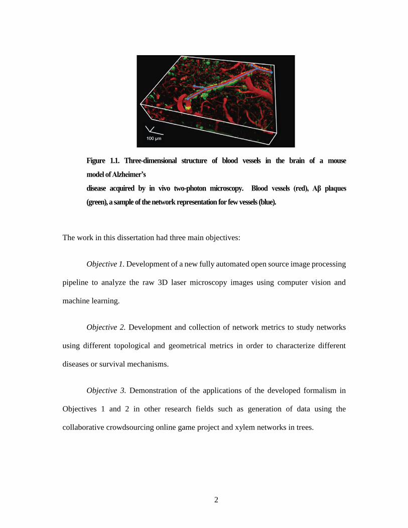
capillaries in mouse models of Alzheimer’s disease and normal mice (Figure 1.1). We
developed automated computer vision and machine learning solutions such as DeepVess
(Haft-Javaherian et al., 2019) to analyze such images and measure different geometrical
and topological metrics within the brain vasculature network. These solutions are now in
use in various research labs studying brain, heart, and even in trees. These methods are
also used in the data processing backbone for our citizen science crowdsourcing project
(StallCatchers.com).
2
Figure 1.1. Three-dimensional structure of blood vessels in the brain of a mouse
model of Alzheimer’s
disease acquired by in vivo two-photon microscopy. Blood vessels (red), Aβ plaques
(green), a sample of the network representation for few vessels (blue).
The work in this dissertation had three main objectives:
Objective 1. Development of a new fully automated open source image processing
pipeline to analyze the raw 3D laser microscopy images using computer vision and
machine learning.
Objective 2. Development and collection of network metrics to study networks
using different topological and geometrical metrics in order to characterize different
diseases or survival mechanisms.
Objective 3. Demonstration of the applications of the developed formalism in
Objectives 1 and 2 in other research fields such as generation of data using the
collaborative crowdsourcing online game project and xylem networks in trees.
3
Thesis structure
Chapter 2 is a review of the current literature of 3D vessel segmentation and
centerline extraction methods. This chapter is the draft of the paper that will be submitted.
Chapter 3 was published in PLoS One and has been reformatted for inclusion in
this dissertation. A fully-automated, open source pipeline was developed using the deep
convolutional neural networks to segment multiphoton microscopy images and extract
the vasculature centerlines. This method generated detailed analysis of the effects of
aging and Alzheimer genes on capillary network structure in mouse cortex. I
demonstrated the application of this formalism within two different research fields
described in Chapter 4, 5 and 6: the study of microvascular dysfunction in Alzheimer’s
disease and the study of the xylem networks in trees in response to drought and embolism.
Haft-Javaherian, M., Fang, L., Muse, V., Schaffer, C. B., Nishimura, N., &
Sabuncu, M. R. (2019). Deep convolutional neural networks for
segmenting 3D in vivo multiphoton images of vasculature in Alzheimer
disease mouse models. PLOS ONE, 14(3), e0213539.
https://doi.org/10.1371/journal.pone.0213539
Chapter 4 was published in Nature Neuroscience and has been reformatted for
inclusion in this dissertation. We discovered that leukocyte cells plug about two percent
of capillaries in the brains of Alzheimer’s disease mouse models. By blocking the
leukocyte adhesion, we showed the cerebral blood flow immediately increased, and
4
cognitive performance rapidly improved. The contribution section reads “MH., G.O. and
Y.K. developed custom software for data analysis. M.H. developed custom machine
learning algorithms for image segmentation.” I provided novel data analysis and original
algorithms which characterized the stalled vessels by several metrics including their
topology, relationships to amyloid-beta deposits and morphology.
Cruz Hernández, J. C., Bracko, O., Kersbergen, C. J., Muse, V., Haft-Javaherian,
…, Nishimura, N., Schaffer, C. B. (2019). Neutrophil adhesion in brain
capillaries reduces cortical blood flow and impairs memory function in
Alzheimer’s disease mouse models. Nature Neuroscience, 22(3), 413–
420. https://doi.org/10.1038/s41593-018-0329-4
Chapter 5 is on a crowdsourcing citizen science project, i.e., StallCatchers, that
utilizes the power of citizen science to perform the task of detecting stalled capillary from
images. This time-consuming task is a significant bottleneck for scientific research
progress. I developed the image processing pipeline, worked on the validation of the
crowd-source analysis, and contributed to generating the first scientific results from this
novel method. This chapter is the draft of the paper that will be submitted.
Chapter 6 explores drought resistance of trees with two different wood types and
in six species. Similar to blood vessel networks in the brain, tree xylem networks have
network structures that contribute to the tree’s resistance to drought and vulnerability to
air embolisms that block water flow. In this chapter, we utilized our formalism developed
in previous chapters to analyze images of the xylem networks and adapted these methods
for extremely large datasets. The 3D xylem images were more than a hundred times larger

5
than the brain vascular images acquired by multiphoton microscopy. Inspired by methods
used to study robustness in brain vascular networks, we also used fluid flow simulations
to compare different tree species. This chapter was done in collaboration with Ms. Annika
Huber and Prof. Taryn Bauerle at Cornell University in the School of Integrative Plant
Science. This is the draft of the paper that will be submitted.
6
REFERENCES
Cruz Hernández, J. C., Bracko, O., Kersbergen, C. J., Muse, V., Haft-Javaherian, M.,
Berg, M., … Schaffer, C. B. (2019). Neutrophil adhesion in brain capillaries
reduces cortical blood flow and impairs memory function in Alzheimer’s disease
mouse models. Nature Neuroscience, 22(3), 413–420.
https://doi.org/10.1038/s41593-018-0329-4
Haft-Javaherian, M., Fang, L., Muse, V., Schaffer, C. B., Nishimura, N., & Sabuncu, M.
R. (2019). Deep convolutional neural networks for segmenting 3D in vivo
multiphoton images of vasculature in Alzheimer disease mouse models. PLOS
ONE, 14(3), e0213539. https://doi.org/10.1371/journal.pone.0213539
Hirsch, S., Reichold, J., Schneider, M., Székely, G., & Weber, B. (2012). Topology and
hemodynamics of the cortical cerebrovascular system. Journal of Cerebral Blood
Flow & Metabolism, 32(6), 952–967.
Iadecola, C. (2004). Neurovascular regulation in the normal brain and in Alzheimer’s
disease. Nature Reviews Neuroscience, 5(5), 347–360.
https://doi.org/10.1038/nrn1387
Kleinfeld, D., Mitra, P. P., Helmchen, F., & Denk, W. (1998). Fluctuations and stimulus-
induced changes in blood flow observed in individual capillaries in layers 2
through 4 of rat neocortex. Proceedings of the National Academy of Sciences,
95(26), 15741–15746.
Santisakultarm, T. P., Cornelius, N. R., Nishimura, N., Schafer, A. I., Silver, R. T.,
Doerschuk, P. C., … Schaffer, C. B. (2012). In vivo two-photon excited
fluorescence microscopy reveals cardiac- and respiration-dependent pulsatile
blood flow in cortical blood vessels in mice. American Journal of Physiology -
Heart and Circulatory Physiology, 302(7), H1367–H1377.
https://doi.org/10.1152/ajpheart.00417.2011
Schaffer, C. B., Friedman, B., Nishimura, N., Schroeder, L. F., Tsai, P. S., Ebner, F. F.,
… Kleinfeld, D. (2006). Two-Photon Imaging of Cortical Surface Microvessels

7
Reveals a Robust Redistribution in Blood Flow after Vascular Occlusion. PLoS
Biol, 4(2), e22. https://doi.org/10.1371/journal.pbio.0040022
8
CHAPTER 2
A REVIEW OF THREE-DIMENSIONAL VESSEL SEGMENTATION METHODS
2.1 Introduction
The circulatory system provides oxygen and nutrients to the entire body and
collects the metabolic waste from cells through the vasculature network. Many medical
diagnoses and treatments depend heavily on different circulatory system examinations.
Likewise, many biomedical researchers are investigating different aspects of this system.
Imaging is one of the main methodological approaches used commonly in various
biomedical laboratories and medical settings. Extracting the substantial amount of
information embedded in cardiovascular images often costs an excessive amount of
valuable time of experts who analyze the images before it can be delivered in useful
formats to the downstream users ranging from physician and scientists to patients and
general public. Image segmentation is an essential image processing task, which is an
indispensable part of image analysis pipelines. The primary goal is to locate and label
pixels or voxels with different labels, deterministically or stochastically. From a machine
learning and data science point of view, this task can be done using supervised on
unsupervised approaches. Mainly, the vessel segmentation task is an essential tool for the
diagnosis, treatment, surgery planning, prognosis, and biomedical research.
To address the complexity and entanglement of multiple factors within medical
and biomedical image analysis, we focus on three different aspects of the 3D vessel
9
segmentation task. First, we focus on high-level image preprocessing (section 2) and
image segmentation methods (section 3) with an emphasis on vasculature images.
Second, we discuss organ- and tissue-based vessel segmentations into either vascular
networks (section 4) or short segments (section 5). Third, we discussed different
pathological vessel segmentation tasks (section 6). To best of our knowledge, currently,
Kirbas and Quek (Kirbas & Quek, 2004) and Lesage (Lesage, Angelini, Bloch, & Funka-
Lea, 2009) are the most general and extensive vascular segmentation reviews. Therefore,
we focused our review mostly on research papers published since 2008.
2.2 Image preprocessing
Preprocessing methods, as low-level pixel intensity operators and logic, filter the
unrelated information and enhance targeted image features before the application of main
image processing methods. Consequently, they reduce the information entropy to
facilitate the main image processing task. These methods may use prior information about
acquisition systems or estimate them based on the input image.
For example, pixel-wise intensity transformation can be designed using prior
information from neighboring pixels’ intensity statistics, the whole image intensity
statistics, or the imaging modality used to acquire the input image. Constant thresholding
uses no prior information, adaptive thresholding uses neighboring pixels, and the
histogram equalizer uses either the whole image data or subset of neighboring pixels. For
instance, the log-based intensity transform uses the prior information based on the
imaging modality and the segmentation task in order to enhance large vessels and supress
other structures in CTA or MRA (Freiman et al., 2009; Samet & Yildirim, 2016).
10
Prior knowledge of the imaged organs or tissues is a critical requirement for
developing effective segmentation methods. The organ-based segmentation and the prior
knowledge of the organ’s adjacencies produce a target mask that reduces the amount of
falsely detected objects and the computational time (Chi et al., 2011). For instance, the
skull-stripping algorithm facilitates cerebral tissues isolation (Forkert et al., 2009).
2.2.1 Smoothing and sharpening
Depending on the nature of the images and the main image processing task in
hand, different preprocessing techniques ranging from smoothing or sharpening to texture
measurements are common fundamental image preprocessing tasks used to prepare the
images for the future image procedures. The application of smoothing based on the
intensities of neighboring pixels reduces the salt-and-pepper noise and application of
methods such as Canny edge detection (Canny, 1987) or wavelet edge highlighting
(Korfiatis, Skiadopoulos, Sakellaropoulos, Kalogeropoulou, & Costaridou, 2007)
sharpen the image and facilitate edge detections.
The nonlinear smoothing techniques such as Gaussian filtering, Edge Enhancing
Diffusion, or Regularized Perona-Malik diffusion (Weickert, 2001) improve the
segmentation accuracy with application in CTA and 3D RA images (Firouzian et al.,
2011; Meijering, Niessen, Weickert, & Viergever, 2002). On the other hand, bi-Gaussian
functions with independent foreground and background scales apply an intra-region
smoothing based on the reduced adjacent objects interference (Xiao, Staring, Wang,
Shamonin, & Stoel, 2013).
11
The mathematical morphological filters applya logical operation to the image
using a structural element based on the set theory and logical operations. For example,
the hit-and-miss filter matches circular shapes along the perpendicular axis or stick shapes
along the other axes and leads to segmentation quality improvements (Kim, 2013).
Similarly, the morphological top-hat filter reduces the background by subtracting the
image from the morphological opening filter application on the image (Jin, Yang, Zhang,
& Ding, 2013).
In some cases, the combination of a few preprocessing tasks in addition to one
postprocessing algorithm results in a complete segmentation method. Läthén et al.
(Läthén, Jonasson, & Borga, 2010) combined line and edge detection using multi-scale
quadrature filters to detect distinct objects with lower intensity variation sensitivity.
Furthermore, they improved the vessel boundary precision using a min-cut/max-flow
algorithm (Marvasti & Acar, 2013)
2.2.2 Image artifact removal
Different imaging techniques may suffer from various artifacts with known or
unknown causes. The microscopy image artifacts due to the point spread function (PSF)
shape and size causes blurring which can be reduced by deconvolution with the PSF. If
there are no independent measures of the PSF, it can be estimated using different reverse-
engineering algorithms such as the Richardson-Lucy method and then used in
deconvolving the image (Seidel, Edelmann, & Sachse, 2016). The multi-slab acquisition
of time-of-flight (TOF) magnetic resonance angiography (MRA) contain inter- and intra-
slab boundary intensity variations caused by slab boundary artifacts and poor field
12
uniformity from the radio frequency coil, respectively. Histogram matching compensates
the inter-slice intensity variation artifacts (Kholmovski, Alexander, & Parker, 2002), and
the nonparametric methods such as N3 algorithm resolve the intra-slice intensity variation
artifacts (Sled, Zijdenbos, & Evans, 1998).
Image intensities in modalities such as PC-MRA fluctuate within the vessel
regions due to the blood flow velocity variation and different vessels size, which
consequently alter intensity gradients along the vessel centerlines and impair the gradient-
based segmentation methods. However, the dramatic signal loss in PC-MRA due to the
turbulent blood flows leads is partially recoverable using multiscale filters and local
variance (Law & Chung, 2013).
The 3D cerebral CTP scans at multiple time points are affected by severe motion
artifacts and the registration of 3D scans over time is the most crucial step in their
segmentation and other image analysis. After the motion artifact removal, segmentation
can be done simply using thresholding and image analyses such as arteries vs. veins
classification (arteriograms and venograms) can be done based on the time to peak
measurement of contrast enhancement curves (Mendrik et al., 2010).
Aylward et al. (Aylward, Jomier, Weeks, & Bullitt, 2003) repurposed a similar
registration strategy, which is a preprocessing solution for the motion artifact, for vessel
segmentation and centerline extraction techniques with less sensitivity to image noise and
without assumptions about the local shapes of vessels. They registered the designed
vessel templates with the image using both rigid and non-rigid registration methods to
segment the vessels and extract the centerlines.
13
2.2.3 Vesselness measurements
The vesselness filters measure local image texture and orientation to locate vessel-
like objects. The Hessian-based vesselness enhancement filters are based on simplified
cylindrical tube models and generate low values at bifurcations and boundaries. The strain
energy filters based on strain energy density theory from solid mechanics improves the
responses at those locations as well (Zhai, Staring, & Stoel, 2016).
Vesselness filters can be defined in the spherical polar coordinate system instead
of the Cartesian coordinate system to relax the simplified cylindrical tube model
assumption, which resolves the errors at the bifurcations and boundaries (Qian et al.,
2007). Similar to the Hessian-based filter, Gabor filtering can be applied in a multiscale
fashion to study the image textures based on high-frequency local directionality (Shoujun,
Jian, Yongtian, & Wufan, 2010).
The combination of lineness measures and line-direction vectors reduces the
partial volume effect in the analysis of small vessels in Hessian-based methods, which
happens if an small object smaller than the image resolution is surrounded with low
intensity objects and not detectable (Nimura, Kitasaka, & Mori, 2010). The computational
cost associated with the Hessian-based multi-scale vesselness measures can be reduced
by estimation of each Hessian matrix components using the fractional order differential
operators (Gong et al., 2016).
There are multi-scale filters such as the Frangi filter, which measures the
vesselness of the image at each voxel at different scales. The multi-scale line filters
14
applied at different orientations enhance cylindrical structures of vessels and improve
their segmentation and visualization (Sato et al., 1997). Similar to the Hessian-based local
measurement, the combination of the inward gradient flux through circular cross-sections
and non-linear penalizations of asymmetric flux contributions can reduce the false
positive rate (Lesage, Angelini, Bloch, & Funka-Lea, 2009). Likewise, filters based on
the medial-axis points, which pass a line through each point of the image intersecting the
edges of different tubes measuring the distance differences to the nearest edges to
facilitate the segmentation (Foruzan, Zoroofi, Sato, & Hori, 2012) with the option of
resolving the asymmetric cross-sections artifacts using the isotropic coefficient (Pock,
Thomas G, 2004).
2.2.4 Frequency domain
Note that some preprocessing methods are in the frequency domain due to the
nature of acquisition systems or image artifacts (Sonka, Hlavac, & Boyle, 2014). For
instance, the segmentation task for OCT images are either in the frequency (e.g., using
low-pass and high-pass filters) or the space domains. In the case of 1D segmentation in
the space domain, only the A-lines that captures the vessels are required to be analyzed
based on intensity criteria starting from the shallowest pixel. This intensity-based
preprocessing requires 2D or 3D smoothing in order to obtain segmentation continuity
(Ughi et al., 2012).
15
2.3 Vascular segmentation methods
In this section, we discuss the segmentation methods in the context of the vessel
segmentation task. The selection of segmentation methods for each task depends on the
imaged organ, imaging modality, method availability, and the state-of-the-art methods
for the particular task in hand.
2.3.1 Region-based segmentation
The main idea of the region-based segmentation methods is to divide the image
into regions that have the maximum homogeneity. The binary homogeneity function is
defined based on different characteristics of each voxel or super voxel such as intensity,
saliency, direction, and connectivity (Chi et al., 2011). For example, metrics such as
gradient vector flow field have high magnitudes at vessel boundaries and in directions
toward vessel centerlines (Chen, Sun, & Ong, 2014; Smistad, Elster, & Lindseth, 2014).
The regions should satisfy the following two criteria: homogeneity value of each region
should be true, and the homogeneity value of the union of each two adjacent regions
should be false (Sonka et al., 2014). The homogeneity criteria can have its internal voxel-
based inclusion criteria based on neighborhood homogeneity as well. In this scenario,
only voxels located in neighborhoods with homogeneity higher than the minimum
inclusion criteria are contributing to the homogeneity term of the cost function (Ogiela &
Hachaj, 2013). The growing process at different locations within the image can be done
simultaneously or can be done vessel branch by vessel branch sequentially (Eiho,
Sekiguchi, Sugimoto, Hanakawa, & Urayama, 2004). This method requires initial seed
16
points provided by experts or obtained from another method such as centerline extraction
(Smistad et al., 2014).
The variational region growing approaches utilize the intensity and vesselness
terms simultaneously to enforce the target intensity ranges and detect tubular shapes by
minimizing the region-descriptor energy function. The variational region growing
methods are similar to FCM (see next subsection). The initial seeds required for the
variational region growing approaches can be obtained using Hessian-based methods (Lo
et al., 2012; Pacureanu, Revol-Muller, Rose, Ruiz, & Peyrin, 2010; Rose, Rose, Revol-
Muller, Charpigny, & Odet, 2009). The region growing algorithms combined with noise
models can segment the 3D images of vessel laminae, which is the boundary between the
lumen and the rest of the tissue, instead of vessel luminal volume by utilizing the detected
high-confidence foreground voxels and then converting the detected foreground laminae
voxels into 3D isosurface meshes using the marching tetrahedra algorithm
(Narayanaswamy et al., 2010).
Researchers resolved some of the known shortcomings of these methods using
different techniques. The combination of slice marching and region growing algorithms
reduces the leakage and other false positive errors (Zhang, He, Dehmeshki, & Qanadli,
2010). Friman et al. (Friman, Hindennach, & Peitgen, 2008) utilized a vessel template
function based on radiuses, directions, and center points to improve the missing vessel
end segmentations at low SNR regions after the application of region growing methods.
Note that the inclusion criteria based on the formulated homogeneity function in
region-based methods are interchangeable with ensemble models such as the random
17
forest (Schwier, Hahn, Dahmen, & Dirsch, 2016). Fabijańska et al. (Fabijańska, 2012)
used the random walk within consecutive CT slices, slice-by-slice in addition to
considering images acquired from other acquisition series.
2.3.2 Fuzzy clustering methods
The segmentation FCM defines the relationship between different regions in the
image using fuzzy logic rules in order to include the uncertainties due to the image
variations and noise. For example, this statement is a fuzzy rule:
"if two sub-regions have similar pixel intensities and if they are
comparatively in close distance, there is a higher likelihood that
these two sub-regions belong to one region."
Therefore, the relationships between different sub-regions are considered for all
the possible pairs of sub-regions, which make this method very similar to the behavior of
a human observer. Hessian-based filtering and spatially-variant mathematical
morphology with low computation cost can enhance the fuzzy logic segmentation results
(Dufour et al., 2013). Similarly, the addition of line direction vectors of all voxels to the
vesselness information improves the FCM results (Wang, Xiong, Huang, Zhou, &
Venkatesh, 2012). The second order statistics of image voxels such as angular second
moment, contrast correlation, variance, and different inverse moment can be derived
using Gray level co-occurrence matrices at different directions and distances that are
suitable for the FCM feature extractions (Kumar & Jeyanthi, 2012). A computational cost
reduction by a factor of two is achievable by adopting look-up table strategies (Guo,
18
Huang, Fu, Wang, & Huang, 2015). Guo et al. (Guo et al., 2015) used watershed methods
to define the threshold for FCM binarization. The detection of crossing or bifurcation
simultaneously with FCM using the structural pattern detection algorithms reduces the
merging error (Shoujun et al., 2010).
The expectation maximization (EM) method is the probabilistic counterpart of
FCM that changes the segmentation problem into a missing data problem (Zhou et al.,
2007). EM defines class prior probabilities and probability density functions to determine
class associations. Given an image, EM solves an inverse problem to estimate the
parameters of density functions. In the expectation step, EM computes the expected
associate probabilities, and in the maximization step, EM estimates the parameters of
density functions using likelihood maximization. EM iterates between these two steps
until convergence. After convergence, the segmentation results can be acquired using
MAP. Analogous to FCM and EM, since the segmentation problems are interchangeable
with classification problems for each voxel or group of voxels between background and
one or multiple foreground classes, Zheng et al. (Zheng et al., 2011) extracted a set of
geometric and image features and used probabilistic boosting tree (Tu, 2005).
2.3.3 Active contour models - Snakes
Kass and colleagues initially introduced the active contour models or snakes for
image processing in the 1980s (Kass, Witkin, & Terzopoulos, 1988; Terzopoulos, Witkin,
& Kass, 1988; Witkin, Terzopoulos, & Kass, 1987). These models are defined in terms
of energy minimizing splines, which depend on the shape and the location of the spline
within the target image and tries to match a deformable model to that image. The prior

19
knowledge about the underlying structure of the image will be incorporated to find the
optimal solution. The 3D branching structures can be modeled using high order active
contours to define multiscale shapes and interactions between boundaries and from 3D
branches (Vazquez-Reina, Miller, Frisken, & Malek, 2008). Freiman et al. (Freiman,
Joskowicz, & Sosna, 2009) proposed an energy term based on the vessel surface property
to improve the segmentation results at the bifurcations and complex vascular structures.
Note that because the introduced evolution is a local process, it is possible to fall into
local minimum that result in errors (Reinbacher, Pock, Bauer, & Bischof, 2010).
On the other hand, Terzopoulos and Vasilescu (Terzopoulos & Vasilescu, 1991;
Vasilescu & Terzopoulos, 1992) developed a shape reconstruction algorithm based on a
deformable mesh using parameter fitting, which was later further improved by including
an attractive force derived from the 3D image. Since mesh initialization is critical for
precise segmentation, Huang and Goldgof (Huang & Goldgof, 1993) introduced a
tracking method for nonrigid structures by dynamically adding or subtracting mesh nodes
and correspondingly Delingette et al. (Delingette, Hebert, & Ikeuchi, 1992) developed a
dynamic model with both internal smoothness energy and forces derived from input
information. Cohen et al. (Cohen & Cohen, 1993) used balloon models to overcome
image noise as well as assist with better convergence. The inflating balloon models
decrease the computational cost by constructing surfaces from multi-scale images (Chen
& Medioni, 1995).
The intensity gradients within a local sphere region, called orientated flux, can be
symmetric or antisymmetric and are indicators of regions located at the centers or
20
boundaries of vessels, respectively. The active counter method evolves using the oriented
flux measured for a set of radii unaffected by intensity fluctuation along the vessel
centerlines (Law & Chung, 2008). The oriented flux is measured in the Fourier domain
in order to decrease computation time (Law & Chung, 2010). Likewise, the reformulation
of spherical flux based on divergence theorem, spherical step function, and the
convolution operation can be done in the Fourier domain (Law & Chung, 2009b). Since
the enforced antipodal-symmetry of the sphere is not appropriate for modeling the
bifurcations, cylindrical flux-based higher order tensors can be utilized to detect
vasculature and branching together (Cetin & Unal, 2015).
2.3.4 Geometric deformable models - Level set
Parametric methods are the basis of the active counter models (snakes), and partial
differential equations are the basis of the geometric deformable models (a.k.a. Level Set
(Malladi, Sethian, & Vemuri, 1995)). The main difference is that the optimized geometric
curves are non-parametric. The foreground and background are considered as fluid and
solid phases, respectively. Based on continuum mechanics, the three forces applied on
solid surfaces are the fluid pressure on the solid surfaces, the internal stresses in solid
surfaces to maintain the solid integrity, and the external bulk stresses on the surfaces of
solids. The fluid pressure deforms the surface along the centerline, the bulk force deforms
the surface along the cross-section, and the surface forces control the rate of deformation
changes along the surface. These forces can be defined using the second order intensity
statistics, and the surface geometry and the surfaces can be modeled using level set
functions.

21
On the other hand, to account for the vessel size variability, the second order
intensity statistics of images can be smoothed using Gaussian filters with multiple scale
kernels (Law & Chung, 2009a). The small vessels also can be captured using the minimal
curvature criteria (Lorigo et al., 2001). Similarly, the MAP of the intensity distribution
estimated as a finite mixture of statistical model distributions can be combined with the
intensity gradient to perform a fast level set segmentation (Gao et al., 2011).
Caselles et al. (Caselles, Kimmel, & Sapiro, 1997) proposed Geodesic Active
Contours to avoid trapping in the local minimum, which one can reformulate within the
level set framework. The energy function includes an edge detection function with a
common choice of exponential functions, which integrates the curve length and image
boundaries. Boykov and Kolmogorov (Boykov & Kolmogorov, 2003) combined a similar
energy function and minimized it using the graph cut method. In contrast to the active
counter models, this contour topology is changeable throughout its evolution. However,
there is still a low possibility to be trapped in a local minimum using these energy
functions.
Since the image intensity term of the level-set energy function causes higher
vessel segmentation errors within small vessels to compare to the larger vessel, its
relaxation improves the small vessel segmentation results (Ugurlu, Demirci, Navab, &
Celebi, 2011). Similarly, Zhu et al. (Zhu, Xiong, & Jiang, 2012) proposed to add a vessel
energy term to facilitate the distinction between tubular objects vs. spherical objects.
Alternatively, Ebrahimdoost et al. (Ebrahimdoost et al., 2011) proposed energy-based
stopping criteria for the vessel boundary evolution. Similarly, a vesselness-based
22
regularization can be added to the curvature term of the energy function to expedite the
evolution while maintaining the smoothness (Zhu, Xue, Gao, Zhu, & Wong, 2009).
Bresson (Bresson, 2005) and Reinbacher et al. (Reinbacher et al., 2010)
introduced the anisotropic weighted total variation energy with a global volumetric
constraint and assumed a continuous image domain instead of the formerly discrete
domain, which results in a convex energy function. The convex energy functions can be
globally optimized independently of the initial solution (Biesdorf, Wörz, Tengg-Kobligk,
Rohr, & Schnörr, 2015). Moreover, Unger et al. (Unger, Pock, Trobin, Cremers, &
Bischof, 2008) added an energy term based on the user-provided potential function with
regularizations to allow the user input incorporation throughout the segmentation process.
The second-order directional intensity tensors measured using the diffusion tensor image
modeling and tractography can be fed into the geodesic active contour energy function
based on the surface term in the Sobolev Space (Mohan, Sundaramoorthi, &
Tannenbaum, 2010) or fiber tracking tractography method (Cetin, Demir, Yezzi,
Degertekin, & Unal, 2013).
Segmentation methods based on the level-set and curve evolutions (Lorigo et al.,
2001) produce vessel wall leakages or under-segmentation in images acquired using
different modalities (e.g., intracranial TOF-MRA and cardiac CTA) due to the presence
of tissues with vessel-like intensity in the proximity of vessels (Law & Chung, 2009a,
2010). An external constraint term based on the standard deviation of the Gaussian filter
was used in Level Set to reduce the segmentation leakages of nonvascular structures (Jin
et al., 2013). Because the boundary and initial conditions have strong effects on the

23
accuracy, initialization methods such as colliding fronts (Piccinelli, Veneziani, Steinman,
Remuzzi, & Antiga, 2009) and cube search (Gong et al., 2014) improve the final results.
Instead of the devised gradient-based forces used for the level set method, the local phase
information filtered by multiscale quadrature can be used alternatively to detect the edges
and segment vessels of different diameter with less computational cost (Lathen, Jonasson,
& Borga, 2008).
2.3.5 Probabilistic graphical models
The graphical models typically consist of directed or undirected graphs with a set
of nodes and edges, in which nodes represent the image voxels classified with a particular
label and the edges represent the connection between nodes based on a set of
neighborhood criteria. Subsequently, the common graph algorithms such as minimum
spanning tree, shortest path, or graph-cuts can be adopted to solve the graph-based
segmentation problem.
FCM (Chen, 2012) or quick shift clustering (Chen et al., 2014) can be adapted to
obtain the initial segmentation, which is then represented based on the 6-connectivity
(when the connected voxels have a shared face) or 26-connectivity (when the connected
voxels have a shared face, edge, or corner). Then, graph analysis methods such as graph-
cuts coupled with an energy function based on the intensity and boundary penalty terms
improve the segmentation result.
Note that the surface smoothness constraint in the graph-cut energy functions
(Homann, Vesom, & Noble, 2008) may lead to the elimination of small or detailed
24
vessels, which can be resolved using submodular constraints (Kitrungrotsakul, Han,
Iwamoto, & Chen, 2017). Local graph-cut methods based on regional intensity
distributions can be applied iteratively until the minimal change of global results (B. Chen
et al., 2014). The sparse graph representation based on elimination of voxels with a very
high probability of being the background reduces the memory and computation
requirements (Zhai et al., 2016).
2.3.6 Artificial Deep Neural Networks
The artificial neural network (ANN) and specifically deep neural network (DNN)
are the most current popular segmentation methods, after the remarkable success of
AlexNet in the ImageNet challenge in 2012 (Krizhevsky, Sutskever, & Hinton, 2012),
which was the third reincarnation of ANN within the active area of research. ANN can
be used for solving any problem that can be reformulated as a classification problem by
modeling a black box classifier as a stack of Rosenblatt's Perceptrons (Rosenblatt, 1958)
with input nodes, output nodes and hidden nodes in between, which mimics the human
neural networks.
Feature extractions for ANN or other clustering and classification methods can be
done automatically using an extra set of initial ANN layers or manually. A set of features
can be manually engineered through utilizing the preprocessing methods such as Sato or
Frangi filters to enhance structures, the offset medialness filter to enhance topologies, and
strain energy filter to enhance bifurcations (Zeng et al., 2016). Similarly, k-means
methods are suitable for learning filter banks used for feature extraction.
25
In contrast to traditional ANN, DNN has a much greater number of layers
between input and output layers in comparison to the simple three-layer ANN. There are
four different common types of DNN: stacked auto-encoders (SAE), deep belief networks
(DBN), recurrent neural network (RNN), and convolutional neural network (CNN).
Currently, CNN is the most common method among these DNN for biomedical image
analysis (Litjens et al., 2017). The first successful CNN work was presented by Lecun et
al. (LeCun, Bottou, Bengio, & Haffner, 1998) in 1998 called LeNet-5 used for a digit
recognition task in handwritten zip code on mail envelopes.
Merkow et al. (Merkow, Marsden, Kriegman, & Tu, 2016) compared different
fully convolutional neural network models for 3D vessel boundary segmentation task.
Based on their results, the complete 3D U-Net architecture (i.e., encoding and decoding
layers with skip connections) outperforms both 2D and 3D fully convolutional encoder
architected adopted from a holistically-nested edge detection model (Xie & Tu, 2015),
which produced one of the top accuracy results on the BSDS500 dataset (Martin,
Fowlkes, & Malik, 2004). Conversely, Haft-Javaherian et al. (Haft-Javaherian et al.,
2019) showed the optimized patch-based CNN architecture with a customized cost
function segmentation outperforms 3D U-Net architecture.
Instead of 3D DNN networks, Kitrungrotsakul et al. (Kitrungrotsakul, Han,
Iwamoto, Foruzan, et al., 2017) uses three independent 2D sub-networks to process
sagittal, coronal, and transversal planes separately. The features extracted from these
three independent sub-networks are aggregated at the last layer of the network to produce
3D segmentation of the hepatic vessel in CT images, surpassing 3D CNN performance.
26
For a survey on deep learning in medical image analysis see the review by Litjens et al.
(Litjens et al., 2017).
2.3.7 Centerline extraction Methods
Many medical and biomedical tasks rely on a graph representation of the
vasculature network called vessel centerlines. The centerline can be extracted as the
primary task based on the raw image or can be a done as a secondary task by
skeletonization of the segmentation results. Although centerlines sometimes obtained as
a byproduct of segmentation, they can be also used as an initial seed for the segmentation
(Gülsün & Tek, 2010; Smistad et al., 2014). The skeletonization methods for the
centerline extraction do not perform well in the cases with irregularities and holes in the
vessels segmentation results, while the methods without a segmentation step, such as
parallel centerline extraction and ridge traversal, do not struggle in those cases (Smistad
et al., 2014).
The semi-automated centerline extraction methods often start with a seed point
defined by the user and then alternate between prediction and estimation steps to fit a
model such as a cylinder to the data (Friman, Hindennach, Kühnel, & Peitgen, 2010;
Kerrien et al., 2017; Yureidini, Kerrien, & Cotin, 2012) or solve an optimization problem
using a cost function based on the centerline path (Hachaj & Ogiela, 2012; Longair,
Baker, & Armstrong, 2011; Türetken, Benmansour, & Fua, 2012). Instead of searching
for the optimal path between two centerline seed points based on the 3D trajectory curves
of tubular structures, the 3D multi-branch tubular surfaces starting from one seed point
27
can be identified using 4D curve representation of the structure surfaces based on the 3D
sphere representation of points within the tubular structure (Li, Yezzi, & Cohen, 2009).
The crucial requirement for the centerline extraction of large 3D datasets is the
ability of local centerline extraction while preserving the global vasculature network
continuity (Cassot, Lauwers, Fouard, Prohaska, & Lauwers-Cances, 2006). The
segmentation results have different artifacts such as non-smooth boundaries, holes, side-
branch discontinuity, or side-branch inclusion. Techniques such as segmentation surface
postprocessing (Wala et al., 2011) and robust kernel regression (Schaap et al., 2009)
reduce these artifacts. The centerline extraction based on the segmented 3D images of
vessel laminae can be done using ray casting and vote accumulation (Narayanaswamy et
al., 2010) or cylindrical ellipsoids (Tyrrell et al., 2007). The orientation-based thinning
algorithms can be applied in parallel iteratively using different templates until no change
is observed (Hu & Cheng, 2015). The segmentation and centerline extraction computation
time can be reduced dramatically by utilizing the graphics processing unit (GPU) instead
of the central processing unit (CPU) (Bauer, Bischof, & Beichel, 2009; Bauer, Pock,
Bischof, & Beichel, 2009; Erdt, Raspe, & Suehling, 2008; Helmberger et al., 2013;
Narayanaswamy et al., 2010; Smistad et al., 2014).
The centerline errors such as center points ordering errors and filling inter- and
intra-vessel gaps can be resolved using different graph-based techniques such as the
shortest path search algorithms (Fetita, Brillet, & Prêteux, 2009; Helmberger et al., 2013)
and minimum spanning tree (Kitamura, Li, & Ito, 2012). There are different edge weights
that can be considered for finding the shortest path between two vertices including the
28
Euclidean distance and sum of voxel values along the path using raw intensities or
enhances intensities (Lo, Ginneken, & Bruijne, 2010) in addition to the surface
information from both the inner and outer walls of the vessel segments (Zhao et al., 2009).
Another postprocessing step to improve the centerline quality is simple point removal,
which removes the foreground voxels whose removal does not alter the centerline graph
representation (Dongen & Ginneken, 2010). Addotomally, a set of logical rules in
addition to multiple thinning and dilation applied iteratively improves the skeletonization
results (Haft-Javaherian et al., 2019). Algorithms such as 3D dynamic balloon tracking
(Zhou et al., 2012) produce more reasonable results compare to thinning algorithms when
the task is to extract the large vessels’ centerlines within a segmented image containing
both large and small vessel. The continuity and smoothness of the final centerline results
can be controlled using different techniques such as Laplacian filter and Kalman state
estimator (Valencia, Azencot, & Orkisz, 2010).
2.3.8 Bifurcation detection
The vessel bifurcations are detectable by clustering the pixels with high values of
a convexity metric measure based on the segmented image using one of the segmentation
methods such as k-mean clustering (Almasi & Miller, 2013), level set (Almasi et al.,
2015), kernel-based region growing (Almasi et al., 2017), and Bayesian tracking
estimation (Zheng, Carr, & Ge, 2013). This methodology may lead to a high rate of false
positive bifurcations that require rigorous postprocessing. Almasi et al. (Almasi et al.,
2015) reduced the false positive bifurcation candidates by solving an integer linear
programming problem with a utility function based on the intensity and structural
29
information of the graph representation of bifurcations. Pan et al. (Pan, Su, Lai, Liu, &
Wu, 2014) used all of the detected vessel bifurcations to construct a minimum spanning
tree based on the shortest distance bifurcations and combined it with a strategy that
connects the closest pairs of terminal bifurcations to resolve the network discontinuities.
The recursive application of the probabilistic sequential Monte Carlo method in addition
to the k-means clustering detects both vasculature and the junctions along the vessel tree
(Zhao & Bhotika, 2011). The bifurcations detection can be done using geometrical
model-based methods with different criteria such as the comparison between parent
vessel diameter and daughter vessels’ diameters as well as the angle and curvature of the
daughter vessels (Wala et al., 2011).
2.4 Vascular networks
2.4.1 Brain
2.4.1.1 Microscopic imaging
Imaging and automatic image analysis of 3D vascular microscopic images are
essential tools for researchers studying various biomedical science fields including stem
cells (Moore & Lemischka, 2006), neuroscience (Cruz Hernandez et al., 2017), brain
tumors (Calabrese et al., 2007), and angiogenesis (Tyrrell et al., 2005). Note that the
optimum image processing method should be selected with consideration of the different
types of labels and whether the labeling is of the lumen or laminae of vessels. Typical 3D
vascular microscopic images artifacts include:

30
• in vivo raster scanning induced motion artifact,
• low signal to noise ratio and multiscale vessel sizes,
• irregular or extra dense pathological vasculature networks,
• low sensitivity and specificity of labeling dyes,
• in complete labeling within the small vessels,
• large point spreads functions in comparison to the vessel sizes.
To study small vessels and cells with diameters ranges from 2 to 50 μm, an
imaging modality with one μm per pixel or smaller resolutions is required based on the
Nyquist–Shannon sampling theorem (Wu et al., 2014). On the other hand, the studies that
require large fields of views such as the barrel cortex local angiome project (Blinder et
al., 2013) need custom image processing toolboxes (Tsai et al., 2009) with large dataset
analysis capability.
Different geometrical and topological metrics such as diameter, length, tortuosity,
or betweenness centrality measured deterministically or stochastically on the
segmentation results can be used to assesses vasculature networks’ health and efficiency
under different conditions or disease models (Cruz Hernández et al., 2019; Haft-
Javaherian et al., 2019).
2.4.1.2 CTA and MRA
There are many different CTA and MRA sequences suitable for various medical
diagnosis and treatments. For instance, TOF-MRA has a high contrast between blood
serum and tissues that makes is suitable imaging modality for cerebral vascular network
imaging (Al-Kwifi, Emery, & Wilman, 2002). It is also possible to acquire more complete
31
brain vasculature networks using PD-MRI in comparison to PC-MRA and TOF-MRA
due to black-blood contrast phenomenon, i.e., low signal blood vessels (Descoteaux,
Collins, & Siddiqi, 2008). On the other hand, cerebral CTP scans acquired at a fixed time
interval for some time allow the cerebral tissue perfusion assessment for patients with
cerebrovascular diseases including acute stroke and subarachnoid hemorrhage (Mendrik
et al., 2010). However, repeated imaging over time induces severe motion artifacts
requiring registration processes. On the other hand, PC-CT as a non-invasive imaging
modality in comparison to the corrosion cast CT is very suitable for vascularization
studies because it is possible to perform microscopy imaging of the postmortem
histological slices of the same case (Lang et al., 2012). Also, the healthy and pathological
animal tissues such as mice and rats can be visualized using SRμCT in both absorption
and phase contrast modes (Lang et al., 2012).
For example, TOF-MRI images can be preprocessed (Forkert et al., 2013), and
multiscale line filtered (Sato et al., 1997) separately and then combined by a voxel-wise
fuzzy logic to weight the high-value intensity of each voxel in any of two images more
when the other image has a low intensity (Forkert et al., 2011). Afterward, two different
thresholds were applied to seed the level set method and the fuzzy value probability
estimation using the Parzen-Window technique (Schmidt-Richberg, Handels, &
Ehrhardt, 2009). Additionally, considering the local adaptive energy weights with
additional vesselness forces yields better small vessel detection results (Forkert et al.,
2013). The TOF-MRA intensity distribution can be models as a finite mixture of
statistical model distributions such as Linear Combination of Discrete Gaussians (El-Baz
et al., 2012) or a Gaussian distribution for cerebral vasculatures and a Rayleigh
32
distribution in addition to a set of Gaussian distributions for the surrounding tissues (Gao
et al., 2011). A mixture of finite statistical model distributions can be estimated using the
EM method and then using MAP to classify the image (Gao et al., 2011).
2.4.2 Lung
The accurate pulmonary vessel segmentation of lung images is required for
interventional lung disease diagnosis and treatments as a tool for pre-operation planning
and intraoperative assistance in order to avoid any significant vessel damage that has a
ubiquities role in the effective image-guided clinical intervention (Zhu et al., 2009).
Consequently, the VESSEL12 Challenge (Rudyanto et al., 2014) was hosted by Grand-
Challenges and organized in conjunction with the IEEE International Symposium on
Biomedical Imaging in 2012 was about lung vessel segmentation in thoracic CT images
with different phenotypes as well as characterization of segmentation difficulties in the
presence of anatomical abnormalities such as the presence of nodules and dense
consolidation.
The lung CT and MR images contain various anatomical information such as ribs,
spins, heart, and other vessel segments. Therefore, the vessel segmentation task in the
lung is entangled with segmentation of a few other tissues such as pulmonary lobes,
fissures, and bronchi (Lassen et al., 2013). For example, The lung field isolation as the
first preprocessing step can be performed using different methods such as the knowledge-
based segmentation using the prior information of lung intensity ranges (Heussel et al.,
2006) and tissue continuities (Lai, Huang, Wang, & Wang, 2016) and application of
morphological filters (Dongen & Ginneken, 2010) based on 2D slice-by-slice fashion
33
(Armato III & Sensakovic, 2004) or 3D volumes (Sun, Zhang, & Duan, 2006).
Correspondingly, it is required to exclude the airway walls within the lung a
preprocessing step using airway lumen segmentation (Fetita, Ortner, et al., 2009) or the
prior information of the wall thickness as a function of lumen diameter (Peters et al.,
2007). Then again, the automated detection methods identify the pathological-related
errors (Rikxoort, Hoop, Viergever, Prokop, & Ginneken, 2009) and the errors can be
reduced based on the abnormality types, e.g. juxtapleural nodules (Pu et al., 2008), prior
knowledge of lung regions with high attenuation due to various diseases, e.g. asthma,
scleroderma, and emphysema (Prasad et al., 2008), or presence of very dense pathologies
requiring atlas-based registrations (Sluimer, Prokop, & Ginneken, 2005).
The candidate seed points required for the semi-automated method can be refined
using special filtering based on the distance to the lung mask boundaries or applying
morphological erosion filter to the lung mask and utilize it to mask the seed points
(Rudyanto et al., 2014). Similarly, the image can be segmented into a fuzzy spherical
object representation of blood vessels and nodules and then a tracking algorithm to
connect the spheres into the vasculature network based on their connectivity and
collinearity (Wu, Agam, Roy, & Armato, 2004).
The Hessian matrix-based methods can detect strong responses based on the scale-
space particle sampling (Estépar et al., 2012), and the relevant scales of neighbor voxels
can be obtained using multi-label Markov Random Field models enabling the detection
of peripheral thin segments thick segments with better connectivity (Geng, Yang, Tan, &
Zhao, 2016). On the other hand, the nodules alongside the vessels or fibrosis tissue can
34
be eliminated as a postprocessing step using shape-based filters based on the medial axis
and diameter of vessels (Peters et al., 2007). Additionally, the log transformation based
on variance variations to reduces false positive.
2.4.3 Liver
The geometrical properties and territories of liver vasculature network in the
vicinity of a tumor facilitate the interventional procedure planning (Chi et al., 2011) or
about the liver parenchyma for the liver transplantations (Frericks et al., 2004).
Additionally, accurate anatomical dissection helps with avoiding portal osculation,
excessive blood loss, and healthy liver tissue injury (Kim, 2013). Accurate vessel
segmentation is essential for precise tumor growth estimation (Chen, 2012). Within the
liver, it is easier to detect the hepatic artery and bile duct in comparison to the portal vein
and hepatic vein due to similar intensity values and twisted structures, especially in cases
with abnormalities (Chi et al., 2011). Therefore, the vessel segmentation with inferior
vena cava and entrance of portal veins areas are challenging and requires the separation
of hepatic and portal veins (Wang, Hansen, Zidowitz, & Hahn, 2014), while it is possible
to merely segment the hepatic artery using Canny edge detection (Seo & Park, 2009),
dimension reduction using 2D projection (Huang, Wang, Cheng, Huang, & Ju, 2008), or
the combination of the vascular intensity Gaussian distribution and Hessian matrix
(Kawajiri et al., 2008; Wang et al., 2013).
The small vessels are very hard to detect and even occasionally are missing in the
manual segmentations (Chen et al., 2014). The small, precise branches at the liver
boundaries can be detected using the hyper-complex edge operator (Ma & Li, 2014),
35
which replaces the voxel intensity with an eight-dimension octonion containing the
neighbors’ intensities as well and circularly convoluted with the edge detection operates.
Oliveira et al. (Oliveira, Feitosa, & Correia, 2008) detected planes, which fit the hepatic
and portal veins, to define the eight distinct liver regions developed by Couinaud
facilitating the development of hepatectomies (Couinaud, 1954). The exploitation of the
anatomical information and post-order walks of the vessels’ graph representation in
addition to including 4D enhancement modeling and shape likelihoods improve the
segmentation and classification results (Yoshida, Sakas, & Linguraru, 2012).
In clinical practices, the 3D visualizations or information extractions of liver
images using common method are extremely beneficial (X. Gao et al., 2011). For
example, the maximum intensity projection reduces the 3D information to a 2D image by
illustrating the maximum value of voxels along the view angle at each pixel to show the
overall vasculature network (Johnson, Prince, & Chenevert, 1998).
2.5 Short segments
2.5.1 Heart
Alongside the importance of heart vessel segmentation in medical settings,
biomedical research projects and veterinary care also depend on the imaging the major
heart vessels for research studies, diagnosis, and prognosis in order to obtain geometrical
measurements, hemodynamics, autoregulation, and tissue oxygen delivery using different
imagining modalities such as MRA, Micro-CT, and multiphoton microscopy (Lee,
36
Beighley, Ritman, & Smith, 2007; Small et al., 2018). The motion of the beating heart
presents an additional challenge for vessel identification.
The segmentation methods benefit from prior information about the approximate
or precise location of the targeted organ within the image such as the heart in the thorax
CT. For example, the prior knowledge of the heart location significantly reduces the
computation time and search space because in this case, only the voxels in the proximity
of the heart surface require vessel segmentation. This prior information can be obtained
based on landmark detection (e.g., aorta, lungs, rib cage, plaques, and/or carina region),
mathematical morphology techniques (e.g. blur grey-level hit-or-miss transform)
(Bouraoui, Ronse, Baruthio, Passat, & Germain, 2010), adaptive thresholding (Zhou et
al., 2012), rigid registration of heart phantom, or estimating the elastic deformation of
heart atlas. Furthermore, the usage of several atlases in a multi-atlas fashion by
registration of all atlases and fusion of their results improves the segmentation results
(Isgum et al., 2009). In some cases, initially, the atlas can be registered rigidly, and then
non-rigid registration can be utilized (Isgum et al., 2009). Multi-label myocardium
segmentation (e.g., left and right atriums and ventricle, and valves) and heart movement
tracking can be done using different techniques such as 4D watershed-cut algorithm
(Cousty et al., 2010) or automatic model-based mesh adaptation method (Ecabert et al.,
2011).
Similar techniques can be utilized to the locate aorta or the coronary artery within
the prior detected heart (Bouraoui et al., 2010). The rib cage can be removed by intensity
thresholding and morphological closing (Wang & Smedby, 2010) or closing the anterior
37
or posterior mediastinum using 2D livewires with a cost function to attract the wire to the
interior edge of the sternum and the azygoesophageal recess (Wang & Smedby, 2008). In
cases that the heart atlas contains the major vessel segments as well, a vasculature model
can be obtained from the atlas and fed into a region growing or level set model to obtain
a precise vessel segmentation (Wang, Moreno, & Smedby, 2012).
The blood flow volume and pattern measurements required for diagnosis and
prognosis of cardiovascular diseases utilize semi-automated or fully-automated
segmentation of thoracic vessels at different cardiac phases based on 2D or 3D PC-MR
results in 3D or 4D flow tensors, respectively (Srichai, Lim, Wong, & Lee, 2009). Due to
the variation between segmentation results caused by the heart movement and
pathological issues, the atlas-based methods achieve reasonable results by registering an
atlas to each imaging time point (Bustamante et al., 2015). Rather than utilizing the
currently available atlases, atlases can be developed in a supervised fashion by learning
the cardiovascular structures and geometries from a set of images (Peters et al., 2008) and
then detecting the landmarks using methods such as simulated search (Peters, Ecabert, &
Weese, 2005).
2.5.2 Coronary arteries
Coronary arteries supply blood to the heart, and any complication may lead to
ischemia or heart attack. Many diagnosis and prognosis procedures depend heavily on the
geometrical characteristic of the coronary arteries.
38
In cases that the heart is detected and located in the image (Zambal, Hladuvka,
Kanitsar, & Bühler, 2008), searching algorithms such as cylindrical sampling and pattern
fitting can be used to extract the coronary artery vessel tree in addition to handing the
branching and terminations using by depth-first search and noise level estimation by
Bayesian tracking (Schaap, Smal, Metz, van Walsum, & Niessen, 2007).
The coronary artery images that capture both the lumen-intima and the external
elastic membrane of adventitia boundaries (e.g., IVUS) require multilabel segmentations
and can be done using the fast-marching method based on the textural gradients (Will,
Hermes, Buhmann, & Puzicha, 2000) or the gray level gradient (Destrempes, Roy
Cardinal, Allard, Tardif, & Cloutier, 2014). The front propagation of fast-marching
method along the local vessel orientation can be constrained using a minimum path cost
function (Garcia et al., 2013).
The sub-resolution segmentation is essential for applications that require precise
geometrical measurements such as vessel diameters or cross-section profiles for
diagnoses or follow-up analyses such as computational fluid mechanics with high
sensitivity to small geometrical variations. The methods based on coarse-to-fine fashion
initially obtain a rough vessel segmentation and then adapt to segment the image with
higher precision than the image resolution. For instance, non-linear regressions based on
the image intensity variations along the radial direction result in a sub-resolution
segmentation (Schaap et al., 2011).
39
2.5.3 Carotid arteries
Carotid arteries are located in the neck and supply blood to the head and neck,
mainly to the brain. Since the brain has a very low tolerance for blood flow disruption,
occlusion or narrowing of carotid arteries may lead to a stroke. MRI is the standard
method for the carotid atherosclerosis progression and regression visualization
(Underhill, Hatsukami, Fayad, Fuster, & Yuan, 2010). Since BB-MRA and PC-MRA
have higher SNR and are non-invasive compared to CTA and CE-MRA, and intensity
and gradient information are crucial for carotid lumen segmentation, BB-MRA or PC-
MRA are good candidates for quantifying the carotid bifurcation geometries such as
angle, area ratio, bulb size, and tortuosity that are correlated with the risk level of the
atherosclerosis development (Thomas et al., 2005).
Tang et al. (Tang et al., 2012) proposed utilizing Multispectral MRIs to accurately
detect and measure carotid centerlines and geometries, specifically in the pathological
conditions. Conversely, the use of local neighboring ray filtering in low-contrast images
facilitate the vessel segments’ surface detection (Xie, Padgett, Biancardi, & Reeves,
2014). Freiman et al. (Freiman et al., 2009) segmented the carotid arteries using graph
min-cut method by considering edge weights based on adaptively coupling of voxel
intensity, the intensity prior, and geometric vesselness shape prior. They applied a similar
methodology to remove tiny vessel segments and fill vessel discontinuities caused by
imaging artifacts.
In cases that the multi-label carotid vessel segmentation (e.g., vessel wall and
lumen vs. Background) is required, algorithms have utilized prior knowledge such as the
40
minimum and maximum separation between the wall and lumen, the segmentation
smoothness, and the minimum distribution-based distances such as Bhattacharyya
distance (Michailovich, Rathi, & Tannenbaum, 2007) between the label-based intensity
distribution models and the intensity distribution of the segmented object (Ukwatta et al.,
2013).
2.5.4 Abdominal aorta
There will be more than 15 thousand deaths in the United States due to abdominal
aortic aneurysm (Upchurch, Schaub, & others, 2006) and more than 3 million death
worldwide due to abdominal organs with malignant tumors between 2014 and 2030
(Maklad et al., 2017). Due to the asymptomatic nature of the abdominal aortic aneurysm,
they are not noticeable until the aneurysm ruptures (Cornuz, Sidoti Pinto, Tevaearai, &
Egger, 2004). Since the abdominal aorta is the largest human blood vessel, its rupture
causes massive internal bleeding with a 90% mortality rate in non-hospitalized cases
(Mozaffarian et al., 2016).
Surgical planning for vasculature disruption and reconnection as well as
percutaneous stent-graft deployment or medical diagnoses such as arterial occlusive
disease or thromboembolism requires accurate knowledge of localizations and
geometrical measurements of vasculature network and specifically abdominal aorta.
Preprocessing steps such as the segmentation of kidneys, liver, and the abdominal part of
the heart based on their morphological, textural, and geometrical information in addition
to various bone structures segmentations and lastly postprocessing steps such as 4D
curvature analysis (Maklad et al., 2017) facilitate the abdominal aorta segmentation task.
41
The 3D BB-MRI is the standard for the assessment and volumetric measurements
of the abdominal aortic aneurysm and vessel lumens and walls and is more predictive of
clinical outcomes (Zhu et al., 2014). Wang et al. (Wang et al., 2017) proposed the use of
both CE-MRI and BB-MRI to perform different segmentation based on the mutual
information and the geometric active contour using both image series and finally
superimposing the final result by their registration results using deformation-based
registration methods. Similarly, landmark-based registration methods based on the
fiducial markers facilitate the superimposing step (Wörz et al., 2016).
2.5.5 Ascending aorta, aortic arch, and descending aorta
The aorta, the largest artery, begins with the ascending aorta from the left
ventricle, reaches the aortic arch, and the continues to the descending aorta. The early
detection of congenital aortic disease and consequently the aortic aneurysms and
dissections are crucial. The SSFP-MRA (Potthast et al., 2010) has advantages compare
to CTA and MRA, which have high risks of renal dysfunction for patients with
forthcoming surgery, e.g., aortic endograft procedures, and with a high probability of
coexistent cardiovascular and renovascular disease due to repeated diagnostic and
prognostic imaging and exposure to ionizing radiation and nephrotoxic contrast agents
(Neschis & Fairman, 2004). Nevertheless, low SNR of SSFP-MRA makes the vessel
segmentation task more challenging, which can be tackled using the 3D model-based
segmentation approach (Müller-Eschner et al., 2014; Worz et al., 2010). Since the two
centerlines of ascending and descending aorta may not be spatially co-localized, post-
42
processing or adapted cost function is required to guarantee the continuity of the
centerlines (Zheng et al., 2013).
Due to the prominent intensity of blood within the ascending aorta in CTA and
MRA in addition to circular cross-section morphology, the segmentation task turns into
the detection of a circular object in each slice. The optimal set of circles consists of one
circle per slice and each circle has a high overlap with adjacent slices’ circles based on
the competing fuzzy connectedness tree (Wang & Smedby, 2008) or virtual contrast
injection method (Wang & Smedby, 2010). The precise perimeter of cross-sections can
be obtained using region growing or level-set techniques.
The outer aortic cross-sectional boundary can be segmented efficiently using a
piecewise constant curvature within a polar-based segmentation model by utilizing the
initial aortic centerline estimation to generate multiplanar reformatted image sequence
(Deserno, Handels, Meinzer, & Tolxdorff, 2014). Similarly, the initial centerline
estimation can be used as the seed points for the geodesic distance transformation and
then using each segmented slice as the segmentation seed for the next adjacent slice (Jang
et al., 2016). On the other hand, the prior knowledge of the ascending or descending aorta
shape and morphology can be used to generate an atlas-based segmentation model (Seada,
Hamad, & Mostafa, 2016). The temporal tracking of the centerline can be achieved using
the Kalman filter, 3D elliptic cylinder vessel models, and longitudinal intensity-based
motion determination (Biesdorf et al., 2011).

43
2.5.6 Aorta root
The vessel segment between the heart and ascending aorta with aortic valve and
the coronary arteries openings and its rupture lead to life-threatening internal bleeding.
The localization of lung and the carina tracheae facilitate the detection of the beginning
of the aorta root. Feuerstein et al. (Feuerstein, Kitasaka, & Mori, 2009) located a
confiding mediastinal bounding box centered at the carina on the mediolateral axis and at
the center of lungs bounding box on the anteroposterior and superior-inferior axes with
width equal to half of the lung bounding box dimension along the mediolateral axis and
the lung bounding box dimension along the anteroposterior and superior-inferior axes.
Due to mediastinal anatomy, the aortic arch centerline can be detected using a series of
circular Hough transforms (Dasgupta, Mukhopadhyay, Mehre, & Bhattacharyya, 2017;
Feuerstein et al., 2009; S. Gao et al., 2017) and the result can be used to segment the aorta
root precisely.
The intensity-based elastic image registrations of an image to an aorta root atlas
(Biesdorf et al., 2012) or a 3D parametric intensity model generated by convolving an
ideal sharp 3D cylinder with another 3D cylinder, which was already convoluted with a
3D Gaussian (Biesdorf, Worz, Tengg-Kobligk, & Rohr, 2009), facilitate the segmentation
task. In contrast to the atlas-based models, the parametric intensity models do not require
the prior knowledge of atlas and segmentation and produce the templates on-fly. The
artifacts caused by calcifications with high intensities can be masked to improve the
vascular segmentation accuracy (Elattar et al., 2014).
44
The severe aortic valve stenosis can be treated using the invasive transcatheter
aortic valve implantation (TAVI) procedure. TAVI requires geometrical and
morphological information extracted form C-arm CT images for surgery planning and
operational guidance such as providing 3-D valve measurements and determining a
proper C-arm angulation. Even though it has a lower image quality compared to CT and
MRI, C-arm CT captures both 2D and 3D images and overlay the 3D Left Atrium model
to the 2D fluoroscopy based on the intrinsic machine coordinate system, while it monitors
the physiological status of the patient simultaneously (Gessat et al., 2009; John et al.,
2010; Y. Zheng, Yang, John, & Comaniciu, 2014). Since the complete aorta segregation
is required (i.e., aortic root, ascending aorta, aortic arch, and descending aorta), Zheng et
al. (Zheng et al., 2012) proposed marginal space learning method to localize objects based
on their anatomical structures and estimates their scales and orientations.
On the other hand, the atrial fibrillation can be treated using a minimally invasive
catheter-based ablation surgery utilizing high radio-frequency energy to ablate the
potential sources of abnormal electrical activities (e.g., the ostia of pulmonary veins). An
overlay of electro-anatomical maps or real-time 2D fluoroscopic images on the
segmented result of left atrium chamber, appendage, and pulmonary veins in ECG-gated
MRI or CT images provide essential visual guidance during the surgery (Zheng et al.,
2014). In non-gated images, e.g., 3D US, users can define selecting end-diastolic and end-
systole in addition to some landmarks, e.g., mitral valve to segment both left atrium and
ventricle (Almeida et al., 2014).
45
2.6 Disease state segmentation
2.6.1 Intracranial aneurysm and BAVM
An intracranial aneurysm is a pathological dilation of a cerebral artery within the
Circle of Willis due to weakened vessel walls, and its rupture leads to subarachnoid
hemorrhage (Brisman, Song, & Newell, 2006). CTA and 3D-RA are widely-used
diagnoses and assessment imaging for intracranial aneurysm (Li et al., 2009). Also, non-
invasive modalities such as PC-MRA and TOF-MRA, which do not involve injections
and radiations, are preferred for diagnosis and screening (Bogunović et al., 2011).
For instance, CTA intracranial aneurysm images can be segmented using a level
set segmentation method such as geodesic active surfaces (Caselles et al., 1997) by
incorporating intensity, gradient magnitude, and intensity variance as different energy
terms and a single manual seed point within the aneurysm (Firouzian et al., 2011). There
are three ways to improve the geodesic active surfaces. First, the multiple-valued neuron
classifiers reduce the region-based probability map computation cost (Aizenberg,
Aizenberg, & Vandewalle, 2013). Second, utilizing the voxel-based feature scale
selection enable the processing of multiscale images (Bogunović et al., 2011). Third,
using image intensity standardization, the intensity dependency on the scanning machine
can be compensated (Nyúl, Udupa, & others, 1999). On the other hand, because 2D DSA
projections are the gold standard for geometrical measurements, Spiegel et al. (Spiegel,
Redel, Struffert, Hornegger, & Doerfler, 2011) proposed a snake-based segmentation
method for 3D DSA and validated their method by transforming their results into the 2D
DSA domain.
46
The brain arteriovenous malformation (BAVM) is an abnormal direct connection
and tangle, i.e., nidus, between arteries and veins without intermediate capillary bed
(Byrne, 2005). 2D catheter DSA was the gold standard for diagnostic aneurysm detection
(McKinney, Palmer, Truwit, Karagulle, & Teksam, 2008) before the introduction of 3D-
RA as the new gold standard (Rooij, Sprengers, Gast, Peluso, & Sluzewski, 2008). Even
though DSA and 3D-RA are the standard techniques for the diagnosis and prognosis of
BAVM (Friedlander, 2007), researchers explored various image sequences at different
stages for the same purpose such as CCA, CTA, TOF-MRA, and PC-MRA (Byrne, 2005;
Gauvrit et al., 2006; Remonda et al., 2002; Sanelli, Mifsud, & Stieg, 2004).
Microsurgery is the conventional treatment for BAVM with a diameter less than
3 cm and endovascular embolization (Pik & Morgan, 2000), which requires precise
location and geometry of BAVM. Sarieddeen et al. (Sarieddeen et al., 2013) compared
KM, FCM, and EM for the BAVM vascular segmentation. They reported similar
accuracy across the three methods and the lowest computation time for KM.
2.6.2 Interstitial lung diseases
Lung diseases are the third-leading cause of death in the United States. Interstitial
lung diseases (ILD) is a large group of parenchymal lung disorders with unpredictable
clinical courses and high mortality rates (Demedts et al., 2001). For instance, the five-
year survival-rate of idiopathic pulmonary fibrosis (IPF), major ILD diseases, is about
50% (Xu et al., 2006). The quantitative detection of pulmonary pathology based on
various segmentations facilitates the ILD diagnosis and prognosis (Korfiatis,
Kalogeropoulou, Karahaliou, Kazantzi, & Costaridou, 2011). The vessel segmentation
47
within the lung parenchyma field in the presence of abnormalities such as focal
abnormalities (Li, Sone, & Doi, 2003) and pulmonary embolism (Zhou et al., 2007) is
more challenging compared to healthy state (Shikata, McLennan, Hoffman, & Sonka,
2009). For example, the pattern similarity between reticular patterns and vessel tree
segments have similar patterns in lungs parenchyma affected by interstitial pneumonia
(Manivila, 2014).
2.6.3 Carotid diseases
Precise severity assessment of carotid diseases is crucial for therapy assignment,
which has been shown by the NASCET and ECST trials (European Carotid Surgery
Trialists’ Collaborative Group and others, 1991; North American Symptomatic Carotid
Endarterectomy Trial Collaborators, 1991). Accurate monitoring of carotid disease help
patients with managing the risk of stroke given the fact that surgical or non-surgical
treatment can prevent many strokes related to carotid atherosclerosis (Gorelick, 1994).
There are two classic ways to assess carotid disease severity and monitor atherosclerosis
progression: determine the degree of stenosis directly or assess the abnormalities in blood
flow velocity indirectly. DSA is the gold standard, but it is invasive and may cause emboli
formation during catheterization or adverse allergic reaction to the contrast agent. MRA
is an alternative to DSA, but it has the risk of overestimating stenosis due to intravoxel
phase dispersion.
Doppler ultrasonography has been increasingly used clinically due to its non-
invasive property, albeit it is not able to visualize the details of plaque or its surface and
has high intra- and inter-operator variabilities (Gill, Ladak, Steinman, & Fenster, 2000).
48
The development of 3D US with the ability to visualize plaque and its surface, as well as
measure volume of stenosis and the actual atheroma, can better evaluate carotid disease
severity and monitor stroke risk (Fenster & Downey, 1996). 3D US imaging is
noninvasive and gives 3D information of internal organs and vessels, whose structure can
be reconstructed by a 3D segmentation technique.
2.6.4 Coronary artery disease
Coronary artery disease (CAD) is one of the leading causes of death, and nearly
one-third of the patients experienced a coronary episode will die in the same year
(Mozaffarian et al., 2016). Even though the prevalence of CAD will increase by about
18% by 2030, its mortality rates are decreased since the 1970s in part due to
improvements in the clinical presentation patterns of acute myocardium infarction
(Mozaffarian et al., 2016). IVUS captures cross-sectional image sequences of vessel walls
and plaques by pulling-back a catheter inside arteries blood vessels, and it is the invasive
gold standard for studying atherosclerotic diseases (Nissen & Yock, 2001). Invasive
coronary angiography (ICA) in adjunction with fractional flow reserve (FFR)
measurement is the reference standard for lesion-specific diagnosis of canary artery
disease (CAD) (Min et al., 2012; Min, Shaw, & Berman, 2010). Even though coronary
CTA as noninvasive imaging method facilitate visualization of CAD and correlates with
ICA findings, it cannot capture the hemodynamic and consequently has low precision in
ischemia causing obstructive stenosis detection (Meijboom et al., 2008; Schuijf & Bax,
2008).
49
The narrowing or occlusion of the coronary artery (i.e., stenosis) due to the
accumulation of calcium, fat, or cholesterol plaques (i.e., atherosclerosis) compromises
the oxygen and nutrition delivery to the heart (i.e., ischemia). The atherosclerotic plaques
are divided into two categories of stable vs. unstable based on their rupture possibility,
and it may cause irreversible defects to the myocardium or myocardial infarction, (i.e.,
heart attack) (Kirişli et al., 2013). Therefore, the plaques and vessels identifications,
classifications (e.g., types of plaques and vessels), and characterizations (e.g.,
segmentation and geometrical measurements), especially in the early stage, is
indispensable.
Frequently, non-vascular objects such as plaques, stent struts, and guide-wire
require segmentation while causing artifacts on the vascular segmentation results. On the
other hand, since most of the plaques occur near a bifurcation in the pathological cases,
the plaque localization and identification can lead to landmark detections and allow an
automatic region of interest detections and image to image registrations (Hemmati,
Kamli-Asl, Talebpour, & Shirani, 2015). The external object localization (e.g., guide-
wire) is required to eliminate the caused shadow artifacts using different methods such as
convex hull approaches (Tung, Shi, Silva, Edwards, & Rueckert, 2011).
2.7 Conclusion
Many medical practices and biomedical research projects focusing on the
circulatory system depend profoundly on different imaging techniques and subsequently
requires efficient image processing procedures to analyze images time- and cost-
effectively. Image segmentation and centerline extraction methods play an essential role

50
in most of the image processing pipeline. In this review, we examined these important
tasks from different angles ranging from fundamental image segmentation methods to
organ- and tissue-level vascular segmentation methods divided into the segments and
networks in addition to the segmentation of pathological vasculatures.
51
REFERENCES
Aizenberg, I., Aizenberg, N. N., & Vandewalle, J. P. L. (2013). Multi-Valued and
Universal Binary Neurons: Theory, Learning and Applications. Springer Science
& Business Media.
Al-Kwifi, O., Emery, D. J., & Wilman, A. H. (2002). Vessel contrast at three Tesla in
time-of-flight magnetic resonance angiography of the intracranial and carotid
arteries. Magnetic Resonance Imaging, 20(2), 181–187.
https://doi.org/10.1016/S0730-725X(02)00486-1
Almasi, S., & Miller, E. L. (2013). Microvasculature network identification in 3-D
fluorescent microscopy images. 2013 IEEE 10th International Symposium on
Biomedical Imaging, 444–447. https://doi.org/10.1109/ISBI.2013.6556507
Almasi, Sepideh, Ben-Zvi, A., Lacoste, B., Gu, C., Miller, E. L., & Xu, X. (2017). Joint
volumetric extraction and enhancement of vasculature from low-SNR 3-D
fluorescence microscopy images. Pattern Recognition, 63, 710–718.
https://doi.org/10.1016/j.patcog.2016.09.031
Almasi, Sepideh, Xu, X., Ben-Zvi, A., Lacoste, B., Gu, C., & Miller, E. L. (2015). A
novel method for identifying a graph-based representation of 3-D microvascular
networks from fluorescence microscopy image stacks. Medical Image Analysis,
20(1), 208–223. https://doi.org/10.1016/j.media.2014.11.007
Almeida, N., Barbosa, D., Heyde, B., Mada, R. O., Friboulet, D., Bernard, O., …
D’hooge, J. (2014). Semi-automatic left-atrial segmentation from volumetric
ultrasound using B-spline explicit active surfaces. 2014 IEEE International
Ultrasonics Symposium, 612–615. https://doi.org/10.1109/ULTSYM.2014.0150
Armato III, S. G., & Sensakovic, W. F. (2004). Automated lung segmentation for thoracic
CT: Impact on computer-aided diagnosis. Academic Radiology, 11(9), 1011–
1021.
52
Aylward, S. R., Jomier, J., Weeks, S., & Bullitt, E. (2003). Registration and Analysis of
Vascular Images. International Journal of Computer Vision; New York, 55(2–3),
123–138. http://dx.doi.org.proxy.library.cornell.edu/10.1023/A:1026126900358
Bauer, C., Bischof, H., & Beichel, R. (2009). Segmentation of airways based on gradient
vector flow. International Workshop on Pulmonary Image Analysis, Medical
Image Computing and Computer Assisted Intervention, 191–201. Citeseer.
Bauer, C., Pock, T., Bischof, H., & Beichel, R. (2009). Airway tree reconstruction based
on tube detection. Proc. of Second International Workshop on Pulmonary Image
Analysis, 203–213.
Biesdorf, A., Worz, S., Tengg-Kobligk, H. von, & Rohr, K. (2009). Automatic detection
of supraaortic branches and model-based segmentation of the aortic arch froM 3D
CTA images. 2009 IEEE International Symposium on Biomedical Imaging: From
Nano to Macro, 486–489. https://doi.org/10.1109/ISBI.2009.5193090
Biesdorf, A., Wörz, S., Tengg-Kobligk, H. von, Rohr, K., & Schnörr, C. (2015). 3D
segmentation of vessels by incremental implicit polynomial fitting and convex
optimization. 2015 IEEE 12th International Symposium on Biomedical Imaging
(ISBI), 1540–1543. https://doi.org/10.1109/ISBI.2015.7164171
Biesdorf, Andreas, Rohr, K., Feng, D., von Tengg-Kobligk, H., Rengier, F., Böckler, D.,
… Wörz, S. (2012). Segmentation and quantification of the aortic arch using joint
3D model-based segmentation and elastic image registration. 16(6), 1187–1201.
https://doi.org/10.1016/j.media.2012.05.010
Biesdorf, Andreas, Wörz, S., Müller, T., Weber, T. F., Heye, T., Hosch, W., … Rohr, K.
(2011). Model-Based Segmentation and Motion Analysis of the Thoracic Aorta
from 4D ECG-Gated CTA Images. Medical Image Computing and Computer-
Assisted Intervention – MICCAI 2011, 589–596. https://doi.org/10.1007/978-3-
642-23623-5_74
Blinder, P., Tsai, P. S., Kaufhold, J. P., Knutsen, P. M., Suhl, H., & Kleinfeld, D. (2013).
The cortical angiome: an interconnected vascular network with noncolumnar
patterns of blood flow. Nature Neuroscience, 16(7), 889–897.
https://doi.org/10.1038/nn.3426
53
Bogunović, H., Pozo, J. M., Villa-Uriol, M. C., Majoie, C. B. L. M., van den Berg, R.,
Gratama van Andel, H. A. F., … Frangi, A. F. (2011). Automated segmentation
of cerebral vasculature with aneurysms in 3DRA and TOF-MRA using geodesic
active regions: An evaluation study. 38(1), 210–222.
https://doi.org/10.1118/1.3515749
Bouraoui, B., Ronse, C., Baruthio, J., Passat, N., & Germain, P. (2010). 3D segmentation
of coronary arteries based on advanced mathematical morphology techniques.
34(5), 377–387. https://doi.org/10.1016/j.compmedimag.2010.01.001
Boykov, Y., & Kolmogorov, V. (2003). Computing geodesics and minimal surfaces via
graph cuts. Proceedings Ninth IEEE International Conference on Computer
Vision, 26–33 vol.1. https://doi.org/10.1109/ICCV.2003.1238310
Bresson, X. (2005). Image segmentation with variational active contours (PhD Thesis).
Verlag nicht ermittelbar.
Brisman, J. L., Song, J. K., & Newell, D. W. (2006). Cerebral Aneurysms. New England
Journal of Medicine, 355(9), 928–939. https://doi.org/10.1056/NEJMra052760
Bustamante, M., Petersson, S., Eriksson, J., Alehagen, U., Dyverfeldt, P., Carlhäll, C.-J.,
& Ebbers, T. (2015). Atlas-based analysis of 4D flow CMR: Automated vessel
segmentation and flow quantification. 17, 87. https://doi.org/10.1186/s12968-
015-0190-5
Byrne, J. V. (2005). Cerebrovascular malformations. European Radiology, 15(3), 448–
452. https://doi.org/10.1007/s00330-004-2634-4
Calabrese, C., Poppleton, H., Kocak, M., Hogg, T. L., Fuller, C., Hamner, B., …
Gilbertson, R. J. (2007). A Perivascular Niche for Brain Tumor Stem Cells.
Cancer Cell, 11(1), 69–82. https://doi.org/10.1016/j.ccr.2006.11.020
Canny, J. (1987). A Computational Approach to Edge Detection. In Readings in
Computer Vision (pp. 184–203). https://doi.org/10.1016/B978-0-08-051581-
6.50024-6
Caselles, V., Kimmel, R., & Sapiro, G. (1997). Geodesic Active Contours. International
Journal of Computer Vision, 22(1), 61–79.
https://doi.org/10.1023/A:1007979827043
54
Cassot, F., Lauwers, F., Fouard, C., Prohaska, S., & Lauwers-Cances, V. (2006). A novel
three-dimensional computer-assisted method for a quantitative study of
microvascular networks of the human cerebral cortex. Microcirculation (New
York, N.Y.: 1994), 13(1), 1–18. https://doi.org/10.1080/10739680500383407
Cetin, S., Demir, A., Yezzi, A., Degertekin, M., & Unal, G. (2013). Vessel Tractography
Using an Intensity Based Tensor Model with Branch Detection. 32(2), 348–363.
https://doi.org/10.1109/TMI.2012.2227118
Cetin, S., & Unal, G. (2015). A Higher-Order Tensor Vessel Tractography for
Segmentation of Vascular Structures. 34(10), 2172–2185.
https://doi.org/10.1109/TMI.2015.2425535
Chen, B., Sun, Y., & Ong, S. H. (2014). Liver Vessel Segmentation Using Graph Cuts
with Quick Shift Initialization. In IFMBE Proceedings. The 15th International
Conference on Biomedical Engineering (pp. 188–191). Retrieved from
https://link.springer.com/chapter/10.1007/978-3-319-02913-9_48
Chen, X. (2012). Liver vessel tree segmentation based on a hybrid graph cut/fuzzy
connectedness method. Medical Imaging 2012: Image Processing, 8314, 83141K.
International Society for Optics and Photonics.
Chen, Y., & Medioni, G. (1995). Description of complex objects from multiple range
images using an inflating balloon model. Computer Vision and Image
Understanding, 61(3), 325–334.
Chi, Y., Liu, J., Venkatesh, S. K., Huang, S., Zhou, J., Tian, Q., & Nowinski, W. L.
(2011). Segmentation of Liver Vasculature from Contrast Enhanced CT Images
Using Context-Based Voting. 58(8), 2144–2153.
https://doi.org/10.1109/TBME.2010.2093523
Cohen, L. D., & Cohen, I. (1993). Finite-element methods for active contour models and
balloons for 2-D and 3-D images. IEEE Transactions on Pattern Analysis &
Machine Intelligence, (11), 1131–1147.
Cornuz, J., Sidoti Pinto, C., Tevaearai, H., & Egger, M. (2004). Risk factors for
asymptomatic abdominal aortic aneurysm: systematic review and meta-analysis
55
of population-based screening studies. The European Journal of Public Health,
14(4), 343–349.
Couinaud, C. (1954). Liver lobes and segments: notes on the anatomical architecture and
surgery of the liver. La Presse Médicale, 62(33), 709.
Cousty, J., Najman, L., Couprie, M., Clément-Guinaudeau, S., Goissen, T., & Garot, J.
(2010). Segmentation of 4D cardiac MRI: Automated method based on spatio-
temporal watershed cuts. 28(8), 1229–1243.
https://doi.org/10.1016/j.imavis.2010.01.001
Cruz Hernandez, J. C., Bracko, O., Kersbergen, C. J., Muse, V., Haft-Javaherian, M.,
Berg, M., … Schaffer, C. B. (2017). Neutrophil adhesion in brain capillaries
contributes to cortical blood flow decreases and impaired memory function in a
mouse model of Alzheimer’s disease. BioRxiv. https://doi.org/10.1101/226886
Cruz Hernández, J. C., Bracko, O., Kersbergen, C. J., Muse, V., Haft-Javaherian, M.,
Berg, M., … Schaffer, C. B. (2019). Neutrophil adhesion in brain capillaries
reduces cortical blood flow and impairs memory function in Alzheimer’s disease
mouse models. Nature Neuroscience, 22(3), 413–420.
https://doi.org/10.1038/s41593-018-0329-4
Dasgupta, A., Mukhopadhyay, S., Mehre, S. A., & Bhattacharyya, P. (2017).
Morphological Geodesic Active Contour Based Automatic Aorta Segmentation
in Thoracic CT Images. In Advances in Intelligent Systems and Computing.
Proceedings of International Conference on Computer Vision and Image
Processing (pp. 187–195). Retrieved from
https://link.springer.com/chapter/10.1007/978-981-10-2107-7_17
Delingette, H., Hebert, M., & Ikeuchi, K. (1992). Shape representation and image
segmentation using deformable surfaces. Image and Vision Computing, 10(3),
132–144.
Demedts, M., Wells, A. U., Antó, J. M., Costabel, U., Hubbard, R., Cullinan, P., …
Taylor, A. N. (2001). Interstitial lung diseases: an epidemiological overview.
European Respiratory Journal, 18(32 suppl), 2s–16s.
56
Descoteaux, M., Collins, D. L., & Siddiqi, K. (2008). A geometric flow for segmenting
vasculature in proton-density weighted MRI. 12(4), 497–513.
https://doi.org/10.1016/j.media.2008.02.003
Deserno, T. M., Handels, H., Meinzer, H.-P., & Tolxdorff, T. (2014). Polar-Based Aortic
Segmentation in 3D CTA Dissection Data Using a Piecewise Constant Curvature
Model. Springer-Verlag.
Destrempes, F., Roy Cardinal, M.-H., Allard, L., Tardif, J.-C., & Cloutier, G. (2014).
Segmentation method of intravascular ultrasound images of human coronary
arteries. 38(2), 91–103. https://doi.org/10.1016/j.compmedimag.2013.09.004
Dongen, E. van, & Ginneken, B. van. (2010). Automatic segmentation of pulmonary
vasculature in thoracic CT scans with local thresholding and airway wall removal.
2010 IEEE International Symposium on Biomedical Imaging: From Nano to
Macro, 668–671. https://doi.org/10.1109/ISBI.2010.5490088
Dufour, A., Tankyevych, O., Naegel, B., Talbot, H., Ronse, C., Baruthio, J., … Passat,
N. (2013). Filtering and segmentation of 3D angiographic data: Advances based
on mathematical morphology. 17(2), 147–164.
https://doi.org/10.1016/j.media.2012.08.004
Ebrahimdoost, Y., Qanadli, S. D., Nikravanshalmani, A., Ellis, T. J., Shojaee, Z. F., &
Dehmeshki, J. (2011). Automatic segmentation of Pulmonary Artery (PA) in 3D
pulmonary CTA images. 2011 17th International Conference on Digital Signal
Processing (DSP), 1–5. https://doi.org/10.1109/ICDSP.2011.6004964
Ecabert, O., Peters, J., Walker, M. J., Ivanc, T., Lorenz, C., von Berg, J., … Weese, J.
(2011). Segmentation of the heart and great vessels in CT images using a model-
based adaptation framework. 15(6), 863–876.
https://doi.org/10.1016/j.media.2011.06.004
Eiho, S., Sekiguchi, H., Sugimoto, N., Hanakawa, T., & Urayama, S. (2004). Branch-
based region growing method for blood vessel segmentation. Proceedings of
International Society for Photogrammetry and Remote Sensing Congress, 796–
801.
57
Elattar, M. A., Wiegerinck, E., Planken, R., van Assen, H., Baan, J., Marquering, H., &
others. (2014). Automatic segmentation of the aortic root in CT angiography of
candidate patients for transcatheter aortic valve implantation. Medical &
Biological Engineering & Computing, 52(7), 611–618.
El-Baz, A., Elnakib, A., Khalifa, F., El-Ghar, M. A., McClure, P., Soliman, A., &
Gimelrfarb, G. (2012). Precise Segmentation of 3-D Magnetic Resonance
Angiography. 59(7), 2019–2029. https://doi.org/10.1109/TBME.2012.2196434
Erdt, M., Raspe, M., & Suehling, M. (2008). Automatic Hepatic Vessel Segmentation
Using Graphics Hardware. Medical Imaging and Augmented Reality, 403–412.
https://doi.org/10.1007/978-3-540-79982-5_44
Estépar, R. S. J., Ross, J. C., Russian, K., Schultz, T., Washko, G. R., & Kindlmann, G.
L. (2012). Computational vascular morphometry for the assessment of pulmonary
vascular disease based on scale-space particles. 2012 9th IEEE International
Symposium on Biomedical Imaging (ISBI), 1479–1482. IEEE.
European Carotid Surgery Trialists’ Collaborative Group and others. (1991). MRC
European Carotid Surgery Trial: interim results for symptomatic patients with
severe (70-99%) or with mild (0-29%) carotid stenosis. Lancet, 337(8752), 1235–
43.
Fabijańska, A. (2012). Extraction of pulmonary vessels from MDCT thorax scans. 2012
IEEE International Conference on Imaging Systems and Techniques Proceedings,
63–67. https://doi.org/10.1109/IST.2012.6295486
Fenster, A., & Downey, D. B. (1996). 3-D ultrasound imaging: A review. IEEE
Engineering in Medicine and Biology Magazine, 15(6), 41–51.
Fetita, C., Brillet, P.-Y., & Prêteux, F. J. (2009). Morpho-geometrical approach for 3D
segmentation of pulmonary vascular tree in multi-slice CT. 7259, 72594F–
72594F–12. https://doi.org/10.1117/12.811637
Fetita, C., Ortner, M., Brillet, P.-Y., Prêteux, F., Grenier, P., & others. (2009). A
morphological-aggregative approach for 3D segmentation of pulmonary airways
from generic MSCT acquisitions. Proc. of Second International Workshop on
Pulmonary Image Analysis, 215–226.
58
Feuerstein, M., Kitasaka, T., & Mori, K. (2009). Automated anatomical likelihood driven
extraction and branching detection of aortic arch in 3-D chest CT. Second
International Workshop on Pulmonary Image Analysis, 49–60. Med. Image
Comput. Comput. Assist. Interv.(MICCAI).
Firouzian, A., Manniesing, R., Flach, Z. H., Risselada, R., van Kooten, F., Sturkenboom,
M. C. J. M., … Niessen, W. J. (2011). Intracranial aneurysm segmentation in 3D
CT angiography: Method and quantitative validation with and without prior noise
filtering. 79(2), 299–304. https://doi.org/10.1016/j.ejrad.2010.02.015
Forkert, N. D., Schmidt-Richberg, A., Fiehler, J., Illies, T., Möller, D., Handels, H., &
Säring, D. (2011). Fuzzy-based Vascular Structure Enhancement in Time-of-
Flight MRA Images for Improved Segmentation. 50(1), 74–83.
https://doi.org/10.3414/ME10-02-0003
Forkert, Nils Daniel, Säring, D., Fiehler, J., Illies, T., Möller, D., & Handels, H. (2009).
Automatic brain segmentation in Time-of-Flight MRA images. Methods of
Information in Medicine, 48(5), 399–407. https://doi.org/10.3414/ME9237
Forkert, Nils Daniel, Schmidt-Richberg, A., Fiehler, J., Illies, T., Möller, D., Säring, D.,
… Ehrhardt, J. (2013). 3D cerebrovascular segmentation combining fuzzy vessel
enhancement and level-sets with anisotropic energy weights. 31(2), 262–271.
https://doi.org/10.1016/j.mri.2012.07.008
Foruzan, A. H., Zoroofi, R. A., Sato, Y., & Hori, M. (2012). A Hessian-based filter for
vascular segmentation of noisy hepatic CT scans. 7(2), 199–205.
https://doi.org/10.1007/s11548-011-0640-y
Freiman, M., Joskowicz, L., & Sosna, J. (2009, February 1). A variational method for
vessels segmentation: algorithm and application to liver vessels visualization.
7261, 72610H. https://doi.org/10.1117/12.810611
Freiman, Moti, Broide, N., Natanzon, M., Nammer, E., Shilon, O., Weizman, L., …
Sosna, J. (2009). Vessels-Cut: A Graph Based Approach to Patient-Specific
Carotid Arteries Modeling. Modelling the Physiological Human, 1–12.
https://doi.org/10.1007/978-3-642-10470-1_1
59
Frericks, B. B., Caldarone, F. C., Nashan, B., Savellano, D. H., Stamm, G., Kirchhoff, T.
D., … Galanski, M. (2004). 3D CT modeling of hepatic vessel architecture and
volume calculation in living donated liver transplantation. 14(2), 326–333.
https://doi.org/10.1007/s00330-003-2161-8
Friedlander, R. M. (2007). Arteriovenous Malformations of the Brain. New England
Journal of Medicine, 356(26), 2704–2712.
https://doi.org/10.1056/NEJMcp067192
Friman, O., Hindennach, M., & Peitgen, H. O. (2008). Template-based multiple
hypotheses tracking of small vessels. 2008 5th IEEE International Symposium on
Biomedical Imaging: From Nano to Macro, 1047–1050.
https://doi.org/10.1109/ISBI.2008.4541179
Friman, Ola, Hindennach, M., Kühnel, C., & Peitgen, H.-O. (2010). Multiple hypothesis
template tracking of small 3D vessel structures. Medical Image Analysis, 14(2),
160–171. https://doi.org/10.1016/j.media.2009.12.003
Gao, S., van ’t Klooster, R., Brandts, A., Roes, S. D., Alizadeh Dehnavi, R., de Roos, A.,
… van der Geest, R. J. (2017). Quantification of common carotid artery and
descending aorta vessel wall thickness from MR vessel wall imaging using a fully
automated processing pipeline. 45(1), 215–228.
https://doi.org/10.1002/jmri.25332
Gao, X., Uchiyama, Y., Zhou, X., Hara, T., Asano, T., & Fujita, H. (2011). A Fast and
Fully Automatic Method for Cerebrovascular Segmentation on Time-of-Flight
(TOF) MRA Image. Journal of Digital Imaging, 24(4), 609–625.
https://doi.org/10.1007/s10278-010-9326-1
Garcia, M. P., Velut, J., Boulmier, D., Leclercq, C., Garreau, M., Haigron, P., &
Toumoulin, C. (2013). Coronary Vein Extraction in MSCT Volumes Using
Minimum Cost Path and Geometrical Moments. 17(2), 336–345.
https://doi.org/10.1109/JBHI.2013.2245420
Gauvrit, J.-Y., Oppenheim, C., Nataf, F., Naggara, O., Trystram, D., Munier, T., …
Meder, J.-F. (2006). Three-dimensional dynamic magnetic resonance
angiography for the evaluation of radiosurgically treated cerebral arteriovenous
60
malformations. European Radiology, 16(3), 583–591.
https://doi.org/10.1007/s00330-005-0011-6
Geng, H., Yang, J., Tan, W., & Zhao, D. (2016). 3D Multi-Scale Pulmonary Vascular
Segmentation Algorithm Based on Multi-Label MRF Optimization. 6(7), 1794–
1798. https://doi.org/10.1166/jmihi.2016.1892
Gessat, M., Merk, D. R., Falk, V., Walther, T., Jacobs, S., Nöttling, A., & Burgert, O.
(2009). A planning system for transapical aortic valve implantation. Medical
Imaging 2009: Visualization, Image-Guided Procedures, and Modeling, 7261,
72611E. International Society for Optics and Photonics.
Gill, J. D., Ladak, H. M., Steinman, D. A., & Fenster, A. (2000). Accuracy and variability
assessment of a semiautomatic technique for segmentation of the carotid arteries
from three-dimensional ultrasound images. 27(6), 1333–1342.
https://doi.org/10.1118/1.599014
Gong, Z.-X., Tan, W., Song, Y.-H., Geng, H., Ren, F.-L., Liang-Chen, ., … Zhang, J.
(2016). Segmentation of Pulmonary Blood Vessels Based on Fractional
Differentiation in 3D Chest CT Images. 6(7), 1746–1749.
https://doi.org/10.1166/jmihi.2016.1883
Gong, Z.-X., Tan, W.-J., Yang, J.-Z., Xu, M., Bian, Z., & Zhao, D.-Z. (2014). A Carotid
Vasculature Segmentation Method for Computed Tomography Angiography.
4(6), 912–915. https://doi.org/10.1166/jmihi.2014.1341
Gorelick, P. B. (1994). Stroke prevention. An opportunity for efficient utilization of
health care resources during the coming decade. Stroke, 25(1), 220–224.
Gülsün, M. A., & Tek, H. (2010, February 1). Segmentation of carotid arteries by graph-
cuts using centerline models. 7625, 762530. https://doi.org/10.1117/12.845638
Guo, X., Huang, S., Fu, X., Wang, B., & Huang, X. (2015). Vascular segmentation in
hepatic CT images using adaptive threshold fuzzy connectedness method. 14, 57.
https://doi.org/10.1186/s12938-015-0055-z
Hachaj, T., & Ogiela, M. R. (2012). Evaluation of Carotid Artery Segmentation with
Centerline Detection and Active Contours without Edges Algorithm.
61
Multidisciplinary Research and Practice for Information Systems, 468–478.
https://doi.org/10.1007/978-3-642-32498-7_35
Haft-Javaherian, M., Fang, L., Muse, V., Schaffer, C. B., Nishimura, N., & Sabuncu, M.
R. (2019). Deep convolutional neural networks for segmenting 3D in vivo
multiphoton images of vasculature in Alzheimer disease mouse models. PLOS
ONE, 14(3), e0213539. https://doi.org/10.1371/journal.pone.0213539
Helmberger, M., Urschler, M., Pienn, M., Balint, Z., Olschewski, A., & Bischof, H.
(2013). Pulmonary Vascular Tree Segmentation from Contrast-Enhanced CT
Images. Retrieved from http://arxiv.org/abs/1304.7140
Hemmati, H., Kamli-Asl, A., Talebpour, A., & Shirani, S. (2015). Semi-automatic 3D
segmentation of carotid lumen in contrast-enhanced computed tomography
angiography images. 31(8), 1098–1104.
https://doi.org/10.1016/j.ejmp.2015.08.002
Heussel, C. P., Achenbach, T., Buschsieweke, C., Kuhnigk, J., Weinheimer, O., Hammer,
G., … Kauczor, H. U. (2006). [Quantification of pulmonary emphysema in
multislice-CT using different software tools]. RoFo: Fortschritte auf dem Gebiete
der Rontgenstrahlen und der Nuklearmedizin, 178(10), 987–998.
https://doi.org/10.1055/s-2006-926823
Homann, H., Vesom, G., & Noble, J. A. (2008). Vasculature segmentation of CT liver
images using graph cuts and graph-based analysis. 2008 5th IEEE International
Symposium on Biomedical Imaging: From Nano to Macro, 53–56.
https://doi.org/10.1109/ISBI.2008.4540930
Hu, X., & Cheng, Y. (2015). Centerline-based vessel segmentation using graph cuts.
9443, 94432E–94432E–5. https://doi.org/10.1117/12.2179082
Huang, S., Wang, B., Cheng, M., Huang, X., & Ju, Y. (2008). The use of a projection
method to simplify portal and hepatic vein segmentation in liver anatomy. 92(3),
274–278. https://doi.org/10.1016/j.cmpb.2008.05.008
Huang, W.-C., & Goldgof, D. B. (1993). Adaptive-size meshes for rigid and nonrigid
shape analysis and synthesis. IEEE Transactions on Pattern Analysis and
Machine Intelligence, 15(6), 611–616.
62
Isgum, I., Staring, M., Rutten, A., Prokop, M., Viergever, M. A., & Ginneken, B. van.
(2009). Multi-Atlas-Based Segmentation with Local Decision Fusion—
Application to Cardiac and Aortic Segmentation in CT Scans. 28(7), 1000–1010.
https://doi.org/10.1109/TMI.2008.2011480
Jang, Y., Jung, H. Y., Hong, Y., Cho, I., Shim, H., & Chang, H.-J. (2016). Geodesic
Distance Algorithm for Extracting the Ascending Aorta from 3D CT Images
[Research article]. Retrieved July 3, 2017, from
https://www.hindawi.com/journals/cmmm/2016/4561979/abs/
Jin, J., Yang, L., Zhang, X., & Ding, M. (2013). Vascular Tree Segmentation in Medical
Images Using Hessian-Based Multiscale Filtering and Level Set Method. 2013,
e502013. https://doi.org/10.1155/2013/502013
John, M., Liao, R., Zheng, Y., Nöttling, A., Boese, J., Kirschstein, U., … Walther, T.
(2010). System to guide transcatheter aortic valve implantations based on
interventional C-arm CT imaging. International Conference on Medical Image
Computing and Computer-Assisted Intervention, 375–382. Springer.
Kass, M., Witkin, A., & Terzopoulos, D. (1988). Snakes: Active contour models.
International Journal of Computer Vision, 1(4), 321–331.
Kawajiri, S., Zhou, X., Zhang, X., Hara, T., Fujita, H., Yokoyama, R., … Hoshi, H.
(2008). Automated segmentation of hepatic vessels in non-contrast X-ray CT
images. 1(2), 214–222. https://doi.org/10.1007/s12194-008-0031-4
Kerrien, E., Yureidini, A., Dequidt, J., Duriez, C., Anxionnat, R., & Cotin, S. (2017).
Blood vessel modeling for interactive simulation of interventional neuroradiology
procedures. 35, 685–698. https://doi.org/10.1016/j.media.2016.10.003
Kholmovski Eugene G., Alexander Andrew L., & Parker Dennis L. (2002). Correction of
slab boundary artifact using histogram matching. Journal of Magnetic Resonance
Imaging, 15(5), 610–617. https://doi.org/10.1002/jmri.10094
Kim, D.-Y. (2013). Hepatic vessel segmentation on contrast enhanced CT image
sequence for liver transplantation planning. 2013.
https://doi.org/10.4236/jbise.2013.64063
63
Kirbas, C., & Quek, F. (2004). A Review of Vessel Extraction Techniques and
Algorithms. ACM Comput. Surv., 36(2), 81–121.
https://doi.org/10.1145/1031120.1031121
Kirişli, H. A., Schaap, M., Metz, C. T., Dharampal, A. S., Meijboom, W. B.,
Papadopoulou, S. L., … van Walsum, T. (2013). Standardized evaluation
framework for evaluating coronary artery stenosis detection, stenosis
quantification and lumen segmentation algorithms in computed tomography
angiography. 17(8), 859–876. https://doi.org/10.1016/j.media.2013.05.007
Kitamura, Y., Li, Y., & Ito, W. (2012). Automatic coronary extraction by supervised
detection and shape matching. 2012 9th IEEE International Symposium on
Biomedical Imaging (ISBI), 234–237.
https://doi.org/10.1109/ISBI.2012.6235527
Kitrungrotsakul, T., Han, X.-H., Iwamoto, Y., & Chen, Y.-W. (2017). Automatic and
Robust Vessel Segmentation in CT Volumes Using Submodular Constrained
Graph. Innovation in Medicine and Healthcare 2017, 57–66.
https://doi.org/10.1007/978-3-319-59397-5_7
Kitrungrotsakul, T., Han, X.-H., Iwamoto, Y., Foruzan, A. H., Lin, L., & Chen, Y.-W.
(2017). Robust hepatic vessel segmentation using multi deep convolution network.
10137, 1013711–1013711–6. https://doi.org/10.1117/12.2253811
Korfiatis, P. D., Kalogeropoulou, C., Karahaliou, A. N., Kazantzi, A. D., & Costaridou,
L. I. (2011). Vessel Tree Segmentation in Presence of Interstitial Lung Disease in
MDCT. 15(2), 214–220. https://doi.org/10.1109/TITB.2011.2112668
Korfiatis, P., Skiadopoulos, S., Sakellaropoulos, P., Kalogeropoulou, C., & Costaridou,
L. (2007). Combining 2D wavelet edge highlighting and 3D thresholding for lung
segmentation in thin-slice CT. The British Journal of Radiology, 80(960), 996–
1004. https://doi.org/10.1259/bjr/20861881
Krizhevsky, A., Sutskever, I., & Hinton, G. E. (2012). Imagenet classification with deep
convolutional neural networks. Advances in Neural Information Processing
Systems, 1097–1105.
64
Kumar, I. V., & Jeyanthi, S. (2012). Vascular segmentation of interstitial pneumonia
patterns in lung using MDCT. Vascular, 2(1).
Lai, J., Huang, Y., Wang, Y., & Wang, J. (2016). Three-Dimensions Segmentation of
Pulmonary Vascular Trees for Low Dose CT Scans. 1(17), 1–15.
https://doi.org/10.1007/s11220-016-0138-3
Lang, S., Müller, B., Dominietto, M. D., Cattin, P. C., Zanette, I., Weitkamp, T., &
Hieber, S. E. (2012). Three-dimensional quantification of capillary networks in
healthy and cancerous tissues of two mice. Microvascular Research, 84(3), 314–
322. https://doi.org/10.1016/j.mvr.2012.07.002
Lassen, B., Rikxoort, E. M. van, Schmidt, M., Kerkstra, S., Ginneken, B. van, & Kuhnigk,
J. M. (2013). Automatic Segmentation of the Pulmonary Lobes from Chest CT
Scans Based on Fissures, Vessels, and Bronchi. IEEE Transactions on Medical
Imaging, 32(2), 210–222. https://doi.org/10.1109/TMI.2012.2219881
Lathen, G., Jonasson, J., & Borga, M. (2008). Phase based level set segmentation of blood
vessels. 2008 19th International Conference on Pattern Recognition, 1–4.
https://doi.org/10.1109/ICPR.2008.4760970
Läthén, G., Jonasson, J., & Borga, M. (2010). Blood vessel segmentation using multi-
scale quadrature filtering. 31(8), 762–767.
https://doi.org/10.1016/j.patrec.2009.09.020
Law, M. W. K., & Chung, A. C. S. (2013). Segmentation of Intracranial Vessels and
Aneurysms in Phase Contrast Magnetic Resonance Angiography Using
Multirange Filters and Local Variances. 22(3), 845–859.
https://doi.org/10.1109/TIP.2012.2216274
Law, Max W. K., & Chung, A. C. S. (2008). Three-Dimensional Curvilinear Structure
Detection Using Optimally Oriented Flux. Computer Vision – ECCV 2008, 368–
382. https://doi.org/10.1007/978-3-540-88693-8_27
Law, Max W. K., & Chung, A. C. S. (2009a). A Deformable Surface Model for Vascular
Segmentation. Medical Image Computing and Computer-Assisted Intervention –
MICCAI 2009, 59–67. https://doi.org/10.1007/978-3-642-04271-3_8
65
Law, Max W. K., & Chung, A. C. S. (2009b). Efficient Implementation for Spherical Flux
Computation and Its Application to Vascular Segmentation. 18(3), 596–612.
https://doi.org/10.1109/TIP.2008.2010073
Law, Max W. K., & Chung, A. C. S. (2010). An Oriented Flux Symmetry Based Active
Contour Model for Three-Dimensional Vessel Segmentation. Computer Vision –
ECCV 2010, 720–734. https://doi.org/10.1007/978-3-642-15558-1_52
LeCun, Y., Bottou, L., Bengio, Y., & Haffner, P. (1998). Gradient-based learning applied
to document recognition. Proceedings of the IEEE, 86(11), 2278–2324.
Lee, J., Beighley, P., Ritman, E., & Smith, N. (2007). Automatic segmentation of 3D
micro-CT coronary vascular images. 11(6), 630–647.
https://doi.org/10.1016/j.media.2007.06.012
Lesage, D., Angelini, E. D., Bloch, I., & Funka-Lea, G. (2009). Design and study of flux-
based features for 3D vascular tracking. 2009 IEEE International Symposium on
Biomedical Imaging: From Nano to Macro, 286–289.
https://doi.org/10.1109/ISBI.2009.5193040
Lesage, David, Angelini, E. D., Bloch, I., & Funka-Lea, G. (2009). A review of 3D vessel
lumen segmentation techniques: Models, features and extraction schemes.
Medical Image Analysis, 13(6), 819–845.
https://doi.org/10.1016/j.media.2009.07.011
Li, H., Yezzi, A., & Cohen, L. (2009). 3D Multi-branch Tubular Surface and Centerline
Extraction with 4D Iterative Key Points. Medical Image Computing and
Computer-Assisted Intervention – MICCAI 2009, 1042–1050.
https://doi.org/10.1007/978-3-642-04271-3_126
Li, Qi, Lv, F., Li, Y., Li, K., Luo, T., & Xie, P. (2009). Subtraction CT angiography for
evaluation of intracranial aneurysms: comparison with conventional CT
angiography. European Radiology, 19(9), 2261–2267.
https://doi.org/10.1007/s00330-009-1416-4
Li, Qiang, Sone, S., & Doi, K. (2003). Selective enhancement filters for nodules, vessels,
and airway walls in two- and three-dimensional CT scans. Medical Physics, 30(8),
2040–2051. https://doi.org/10.1118/1.1581411
66
Litjens, G., Kooi, T., Bejnordi, B. E., Setio, A. A. A., Ciompi, F., Ghafoorian, M., …
Sánchez, C. I. (2017). A Survey on Deep Learning in Medical Image Analysis.
ArXiv:1702.05747 [Cs]. Retrieved from http://arxiv.org/abs/1702.05747
Lo, P., Ginneken, B. van, & Bruijne, M. de. (2010). Vessel tree extraction using locally
optimal paths. 2010 IEEE International Symposium on Biomedical Imaging:
From Nano to Macro, 680–683. https://doi.org/10.1109/ISBI.2010.5490083
Lo, Pechin, Van Ginneken, B., Reinhardt, J. M., Yavarna, T., De Jong, P. A., Irving, B.,
… others. (2012). Extraction of airways from CT (EXACT’09). IEEE
Transactions on Medical Imaging, 31(11), 2093–2107.
Longair, M. H., Baker, D. A., & Armstrong, J. D. (2011). Simple Neurite Tracer: open
source software for reconstruction, visualization and analysis of neuronal
processes. Bioinformatics, 27(17), 2453–2454.
https://doi.org/10.1093/bioinformatics/btr390
Lorigo, L. M., Faugeras, O. D., Grimson, W. E. L., Keriven, R., Kikinis, R., Nabavi, A.,
& Westin, C.-F. (2001). CURVES: Curve evolution for vessel segmentation.
Medical Image Analysis, 5(3), 195–206. https://doi.org/10.1016/S1361-
8415(01)00040-8
Ma, Y., & Li, X. (2014). Hepatic vessel segmentation from computed tomography using
three-dimensional hyper-complex edge detection operator. 9069, 90690K–
90690K–6. https://doi.org/10.1117/12.2050193
Maklad, A. S., Matsuhiro, M., Suzuki, H., Kawata, Y., Niki, N., Shimada, M., & Iinuma,
G. (2017). A hybrid 3D region growing and 4D curvature analysis-based
automatic abdominal blood vessel segmentation through contrast enhanced CT.
10134, 101344C–101344C–7. https://doi.org/10.1117/12.2254327
Malladi, R., Sethian, J. A., & Vemuri, B. C. (1995). Shape modeling with front
propagation: A level set approach. IEEE Transactions on Pattern Analysis and
Machine Intelligence, 17(2), 158–175.
Manivila, K. D. (2014). Automatic vessel segmentation of lung affected patterns in
MDCT using decision tree classification. Middle-East Journal of Scientific
Research, 22(11), 1679–1685.
67
Martin, D. R., Fowlkes, C. C., & Malik, J. (2004). Learning to detect natural image
boundaries using local brightness, color, and texture cues. IEEE Transactions on
Pattern Analysis & Machine Intelligence, (5), 530–549.
Marvasti, N. B., & Acar, B. (2013). Assessment of MRF based joint scale selection and
segmentation for 3D liver vessel segmentation task. 2013 21st Signal Processing
and Communications Applications Conference (SIU), 1–4.
https://doi.org/10.1109/SIU.2013.6531368
McKinney, A. M., Palmer, C. S., Truwit, C. L., Karagulle, A., & Teksam, M. (2008).
Detection of Aneurysms by 64-Section Multidetector CT Angiography in Patients
Acutely Suspected of Having an Intracranial Aneurysm and Comparison with
Digital Subtraction and 3D Rotational Angiography. American Journal of
Neuroradiology, 29(3), 594–602. https://doi.org/10.3174/ajnr.A0848
Meijboom, W. B., Mieghem, C. A. G. V., Pelt, N. van, Weustink, A., Pugliese, F., Mollet,
N. R., … Feyter, P. J. de. (2008). Comprehensive Assessment of Coronary Artery
Stenoses: Computed Tomography Coronary Angiography Versus Conventional
Coronary Angiography and Correlation with Fractional Flow Reserve in Patients
With Stable Angina. Journal of the American College of Cardiology, 52(8), 636–
643. https://doi.org/10.1016/j.jacc.2008.05.024
Meijering, E., Niessen, W., Weickert, J., & Viergever, M. (2002). Diffusion-enhanced
visualization and quantification of vascular anomalies in three-dimensional
rotational angiography: Results of an in-vitro evaluation. Medical Image Analysis,
6(3), 215–233. https://doi.org/10.1016/S1361-8415(02)00081-6
Mendrik, A., Vonken, E., van Ginneken, B., Smit, E., Waaijer, A., Bertolini, G., …
Prokop, M. (2010). Automatic segmentation of intracranial arteries and veins in
four-dimensional cerebral CT perfusion scans. 37(6), 2956–2966.
https://doi.org/10.1118/1.3397813
Merkow, J., Marsden, A., Kriegman, D., & Tu, Z. (2016). Dense Volume-to-Volume
Vascular Boundary Detection. Medical Image Computing and Computer-Assisted
Intervention – MICCAI 2016, 371–379. https://doi.org/10.1007/978-3-319-
46726-9_43
68
Michailovich, O., Rathi, Y., & Tannenbaum, A. (2007). Image Segmentation Using
Active Contours Driven by the Bhattacharyya Gradient Flow. Trans. Img. Proc.,
16(11), 2787–2801. https://doi.org/10.1109/TIP.2007.908073
Min, J. K., Leipsic, J., Pencina, M. J., Berman, D. S., Koo, B.-K., Mieghem, C. van, …
Mauri, L. (2012). Diagnostic Accuracy of Fractional Flow Reserve from
Anatomic CT Angiography. JAMA, 308(12), 1237–1245.
https://doi.org/10.1001/2012.jama.11274
Min, J. K., Shaw, L. J., & Berman, D. S. (2010). The Present State of Coronary Computed
Tomography Angiography: A Process in Evolution. Journal of the American
College of Cardiology, 55(10), 957–965.
https://doi.org/10.1016/j.jacc.2009.08.087
Mohan, V., Sundaramoorthi, G., & Tannenbaum, A. (2010). Tubular Surface
Segmentation for Extracting Anatomical Structures from Medical Imagery. IEEE
Transactions on Medical Imaging, 29(12), 1945–1958.
https://doi.org/10.1109/TMI.2010.2050896
Moore, K. A., & Lemischka, I. R. (2006). Stem Cells and Their Niches. Science,
311(5769), 1880–1885. https://doi.org/10.1126/science.1110542
Mozaffarian, D., Benjamin, E. J., Go, A. S., Arnett, D. K., Blaha, M. J., Cushman, M., …
Subcommittee, on behalf of the A. H. A. S. C. and S. S. (2016). Heart disease and
stroke statistics-2016 update a report from the American Heart Association.
Circulation, 133(4), e38–e48. https://doi.org/10.1161/CIR.0000000000000350
Müller-Eschner, M., Müller, T., Biesdorf, A., Wörz, S., Rengier, F., Böckler, D., … von
Tengg-Kobligk, H. (2014). 3D morphometry using automated aortic
segmentation in native MR angiography: an alternative to contrast enhanced
MRA? 4(2), 80–87. https://doi.org/10.3978/j.issn.2223-3652.2013.10.06
Narayanaswamy, A., Dwarakapuram, S., Bjornsson, C. S., Cutler, B. M., Shain, W., &
Roysam, B. (2010). Robust Adaptive 3-D Segmentation of Vessel Laminae from
Fluorescence Confocal Microscope Images and Parallel GPU Implementation.
29(3), 583–597. https://doi.org/10.1109/TMI.2009.2022086
69
Neschis, D. G., & Fairman, R. M. (2004). Magnetic resonance imaging for planning aortic
endograft procedures. Seminars in Vascular Surgery, 17, 135–143. Elsevier.
Nimura, Y., Kitasaka, T., & Mori, K. (2010). Blood vessel segmentation using line-
direction vector based on Hessian analysis. 7623, 76233Q–76233Q–9.
https://doi.org/10.1117/12.844672
Nissen, S. E., & Yock, P. (2001). Intravascular ultrasound: novel pathophysiological
insights and current clinical applications. Circulation, 103(4), 604–616.
North American Symptomatic Carotid Endarterectomy Trial Collaborators. (1991).
Beneficial effect of carotid endarterectomy in symptomatic patients with high-
grade carotid stenosis. New England Journal of Medicine, 325(7), 445–453.
Nyúl, L. G., Udupa, J. K., & others. (1999). On standardizing the MR image intensity
scale. Image, 1081.
Ogiela, M. R., & Hachaj, T. (2013). Automatic segmentation of the carotid artery
bifurcation region with a region-growing approach. 22(3), 033029–033029.
https://doi.org/10.1117/1.JEI.22.3.033029
Oliveira, D. A. B., Feitosa, R. Q., & Correia, M. M. (2008). Automatic Couinaud Liver
and Veins Segmentation from CT Images. BIOSIGNALS (1), 249–252.
Pacureanu, A., Revol-Muller, C., Rose, J.-L., Ruiz, M. S., & Peyrin, F. (2010).
Vesselness-guided variational segmentation of cellular networks from 3D micro-
CT. 2010 IEEE International Symposium on Biomedical Imaging: From Nano to
Macro, 912–915. IEEE.
Pan, X. C., Su, H. R., Lai, S. H., Liu, K. C., & Wu, H. S. (2014). 3D Liver Vessel
Reconstruction from CT Images. 2014 2nd International Conference on 3D
Vision, 2, 75–81. https://doi.org/10.1109/3DV.2014.96
Peters, J., Ecabert, O., Lorenz, C., von Berg, J., Walker, M. J., Ivanc, T. B., … Weese, J.
(2008). Segmentation of the heart and major vascular structures in
cardiovascular CT images. 6914, 691417–691417–12.
https://doi.org/10.1117/12.768494
70
Peters, Jochen, Ecabert, O., & Weese, J. (2005). Feature optimization via simulated
search for model-based heart segmentation. International Congress Series, 1281,
33–38. https://doi.org/10.1016/j.ics.2005.03.023
Peters, R. J., Marquering, H. A., Dogan, H., Hendriks, E. A., de Roos, A., Reiber, J. H.,
& Stoel, B. C. (2007). Labeling the pulmonary arterial tree in CT images for
automatic quantification of pulmonary embolism. Medical Imaging 2007:
Computer-Aided Diagnosis, 6514, 65143Q. International Society for Optics and
Photonics.
Piccinelli, M., Veneziani, A., Steinman, D. A., Remuzzi, A., & Antiga, L. (2009). A
Framework for Geometric Analysis of Vascular Structures: Application to
Cerebral Aneurysms. IEEE Transactions on Medical Imaging, 28(8), 1141–1155.
https://doi.org/10.1109/TMI.2009.2021652
Pik, J. H. T., & Morgan, M. K. (2000). Microsurgery for Small Arteriovenous
Malformations of the Brain: Results in 110 Consecutive Patients. Neurosurgery,
47(3), 571–577. https://doi.org/10.1097/00006123-200009000-00006
Pock, Thomas G. (2004). Robust segmentation of tubular structures in 3D volume data.
Technische Universit¨at Graz, Graz.
Potthast, S., Mitsumori, L., Stanescu, L. A., Richardson, M. L., Branch, K., Dubinsky, T.
J., & Maki, J. H. (2010). Measuring aortic diameter with different MR techniques:
Comparison of three-dimensional (3D) navigated steady-state free-precession
(SSFP), 3D contrast-enhanced magnetic resonance angiography (CE-MRA), 2D
T2 black blood, and 2D cine SSFP. Journal of Magnetic Resonance Imaging,
31(1), 177–184.
Prasad, M. N., Brown, M. S., Ahmad, S., Abtin, F., Allen, J., da Costa, I., … Goldin, J.
G. (2008). Automatic Segmentation of Lung Parenchyma in the Presence of
Diseases Based on Curvature of Ribs. Academic Radiology, 15(9), 1173–1180.
https://doi.org/10.1016/j.acra.2008.02.004
Pu, J., Roos, J., Yi, C. A., Napel, S., Rubin, G. D., & Paik, D. S. (2008). Adaptive border
marching algorithm: Automatic lung segmentation on chest CT images.
71
Computerized Medical Imaging and Graphics, 32(6), 452–462.
https://doi.org/10.1016/j.compmedimag.2008.04.005
Qian, X., Brennan, M. P., Dione, D. P., Dobrucki, W. L., Jackowski, M. P., Breuer, C.
K., … Papademetris, X. (2007). Detection of Complex Vascular Structures using
Polar Neighborhood Intensity Profile. 2007 IEEE 11th International Conference
on Computer Vision, 1–8. https://doi.org/10.1109/ICCV.2007.4409172
Reinbacher, C., Pock, T., Bauer, C., & Bischof, H. (2010). Variational segmentation of
elongated volumetric structures. 2010 IEEE Computer Society Conference on
Computer Vision and Pattern Recognition, 3177–3184.
https://doi.org/10.1109/CVPR.2010.5539771
Remonda, L., Senn, P., Barth, A., Arnold, M., Lövblad, K.-O., & Schroth, G. (2002).
Contrast-Enhanced 3D MR Angiography of the Carotid Artery: Comparison with
Conventional Digital Subtraction Angiography. American Journal of
Neuroradiology, 23(2), 213–219.
Rikxoort, E. M. van, Hoop, B. de, Viergever, M. A., Prokop, M., & Ginneken, B. van.
(2009). Automatic lung segmentation from thoracic computed tomography scans
using a hybrid approach with error detection. Medical Physics, 36(7), 2934–2947.
https://doi.org/10.1118/1.3147146
Rooij, W. J. van, Sprengers, M. E., Gast, A. N. de, Peluso, J. P. P., & Sluzewski, M.
(2008). 3D Rotational Angiography: The New Gold Standard in the Detection of
Additional Intracranial Aneurysms. American Journal of Neuroradiology, 29(5),
976–979. https://doi.org/10.3174/ajnr.A0964
Rose, J.-L., Rose, J.-L., Revol-Muller, C., Charpigny, D., & Odet, C. (2009). Shape prior
criterion based on Tchebichef moments in variational region growing. 2009 16th
IEEE International Conference on Image Processing (ICIP), 1081–1084. IEEE.
Rosenblatt, F. (1958). The perceptron: A probabilistic model for information storage and
organization in the brain. Psychological Review, 65(6), 386.
Rudyanto, R. D., Kerkstra, S., van Rikxoort, E. M., Fetita, C., Brillet, P.-Y., Lefevre, C.,
… van Ginneken, B. (2014). Comparing algorithms for automated vessel
segmentation in computed tomography scans of the lung: the VESSEL12 study.
72
Medical Image Analysis, 18(7), 1217–1232.
https://doi.org/10.1016/j.media.2014.07.003
Samet, R., & Yildirim, Z. (2016). A New Methodology for Blood Vessel Segmentation
on Lung CT Images. 2016 Nicograph International (NicoInt), 1–7.
https://doi.org/10.1109/NicoInt.2016.1
Sanelli, P. C., Mifsud, M. J., & Stieg, P. E. (2004). Role of CT Angiography in Guiding
Management Decisions of Newly Diagnosed and Residual Arteriovenous
Malformations. American Journal of Roentgenology, 183(4), 1123–1126.
https://doi.org/10.2214/ajr.183.4.1831123
Sarieddeen, F., El Berbari, R., Imad, S., Baki, J. A., Hamad, M., Blanc, R., … Chenoune,
Y. (2013). Image Clustering Framework for BAVM Segmentation in 3DRA
Images: Performance Analysis. World Academy of Science, Engineering and
Technology, International Journal of Computer, Electrical, Automation, Control
and Information Engineering, 7(1), 116–120.
Sato, Y., Nakajima, S., Atsumi, H., Koller, T., Gerig, G., Yoshida, S., & Kikinis, R.
(1997). 3D multi-scale line filter for segmentation and visualization of curvilinear
structures in medical images. In CVRMed-MRCAS’97 (pp. 213–222).
https://doi.org/10.1007/BFb0029240
Schaap, M., Walsum, T. van, Neefjes, L., Metz, C., Capuano, E., Bruijne, M. de, &
Niessen, W. (2011). Robust Shape Regression for Supervised Vessel
Segmentation and its Application to Coronary Segmentation in CTA. 30(11),
1974–1986. https://doi.org/10.1109/TMI.2011.2160556
Schaap, Michiel, Neefjes, L., Metz, C., Giessen, A. van der, Weustink, A., Mollet, N., …
Niessen, W. (2009). Coronary Lumen Segmentation Using Graph Cuts and
Robust Kernel Regression. Information Processing in Medical Imaging, 528–539.
https://doi.org/10.1007/978-3-642-02498-6_44
Schaap, Michiel, Smal, I., Metz, C., van Walsum, T., & Niessen, W. (2007). Bayesian
Tracking of Elongated Structures in 3D Images. In N. Karssemeijer & B.
Lelieveldt (Eds.), Information Processing in Medical Imaging (pp. 74–85).
Springer Berlin Heidelberg.
73
Schmidt-Richberg, A., Handels, H., & Ehrhardt, J. (2009). Integrated Segmentation and
Non-linear Registration for Organ Segmentation and Motion Field Estimation in
4D CT Data. Methods of Information in Medicine, 48(4), 344–349.
https://doi.org/10.3414/ME9234
Schuijf, J. D., & Bax, J. J. (2008). CT angiography: an alternative to nuclear perfusion
imaging? Heart, 94(3), 255–257. https://doi.org/10.1136/hrt.2006.105833
Schwier, M., Hahn, H. K., Dahmen, U., & Dirsch, O. (2016). Segmentation of vessel
structures in serial whole slide sections using region-based context features.
9791, 97910E–97910E–14. https://doi.org/10.1117/12.2216497
Seada, N. A., Hamad, S., & Mostafa, M. G. M. (2016). Automatically Seeded Region
Growing Approach for Automatic Segmentation of Ascending Aorta.
Proceedings of the 10th International Conference on Informatics and Systems,
127–132. https://doi.org/10.1145/2908446.2908479
Seidel, T., Edelmann, J.-C., & Sachse, F. B. (2016). Analyzing Remodeling of Cardiac
Tissue: A Comprehensive Approach Based on Confocal Microscopy and 3D
Reconstructions. 44(5), 1436–1448. https://doi.org/10.1007/s10439-015-1465-6
Seo, J. J., & Park, J. W. (2009). Automatic Segmentation of Hepatic Vessels in
Abdominal MDCT Image. 2009 Fourth International Conference on Computer
Sciences and Convergence Information Technology, 420–424.
https://doi.org/10.1109/ICCIT.2009.82
Shikata, H., McLennan, G., Hoffman, E. A., & Sonka, M. (2009). Segmentation of
Pulmonary Vascular Trees from Thoracic 3D CT Images. 2009, 24:1–24:11.
https://doi.org/10.1155/2009/636240
Shoujun, Z., Jian, Y., Yongtian, W., & Wufan, C. (2010). Automatic segmentation of
coronary angiograms based on fuzzy inferring and probabilistic tracking. 9, 40.
https://doi.org/10.1186/1475-925X-9-40
Sled, J. G., Zijdenbos, A. P., & Evans, A. C. (1998). A nonparametric method for
automatic correction of intensity nonuniformity in MRI data. IEEE Transactions
on Medical Imaging, 17(1), 87–97. https://doi.org/10.1109/42.668698
74
Sluimer, I., Prokop, M., & Ginneken, B. van. (2005). Toward automated segmentation of
the pathological lung in CT. IEEE Transactions on Medical Imaging, 24(8),
1025–1038. https://doi.org/10.1109/TMI.2005.851757
Small, D. M., Jones, J. S., Tendler, I. I., Miller, P. E., Ghetti, A., & Nishimura, N. (2018).
Label-free imaging of atherosclerotic plaques using third-harmonic generation
microscopy. Biomedical Optics Express, 9(1), 214–229.
https://doi.org/10.1364/BOE.9.000214
Smistad, E., Elster, A. C., & Lindseth, F. (2014). GPU accelerated segmentation and
centerline extraction of tubular structures from medical images. International
Journal of Computer Assisted Radiology and Surgery, 9(4), 561–575.
https://doi.org/10.1007/s11548-013-0956-x
Sonka, M., Hlavac, V., & Boyle, R. (2014). Image processing, analysis, and machine
vision. Cengage Learning.
Spiegel, M., Redel, T., Struffert, T., Hornegger, J., & Doerfler, A. (2011). A 2D driven
3D vessel segmentation algorithm for 3D digital subtraction angiography data.
56(19), 6401. https://doi.org/10.1088/0031-9155/56/19/015
Srichai, M. B., Lim, R. P., Wong, S., & Lee, V. S. (2009). Cardiovascular applications of
phase-contrast MRI. American Journal of Roentgenology, 192(3), 662–675.
Stafford Johnson, D. B., Prince, M. R., & Chenevert, T. L. (1998). Magnetic resonance
angiography: A review. Academic Radiology, 5(4), 289–305.
https://doi.org/10.1016/S1076-6332(98)80230-4
Sun, X., Zhang, H., & Duan, H. (2006). 3D Computerized Segmentation of Lung Volume
with Computed Tomography. Academic Radiology, 13(6), 670–677.
https://doi.org/10.1016/j.acra.2006.02.039
Tang, H., van Walsum, T., van Onkelen, R. S., Hameeteman, R., Klein, S., Schaap, M.,
… Niessen, W. J. (2012). Semiautomatic carotid lumen segmentation for
quantification of lumen geometry in multispectral MRI. 16(6), 1202–1215.
https://doi.org/10.1016/j.media.2012.05.014
75
Terzopoulos, D., & Vasilescu, M. (1991). Sampling and reconstruction with adaptive
mesh. Proceedings. 1991 IEEE Computer Society Conference on Computer
Vision and Pattern Recognition, 70–75. IEEE.
Terzopoulos, D., Witkin, A., & Kass, M. (1988). Symmetry-seeking models and 3D
object reconstruction. International Journal of Computer Vision, 1(3), 211–221.
Thomas Jonathan B., Antiga Luca, Che Susan L., Milner Jaques S., Hangan Steinman
Dolores A., Spence J. David, … Steinman David A. (2005). Variation in the
Carotid Bifurcation Geometry of Young Versus Older Adults. Stroke, 36(11),
2450–2456. https://doi.org/10.1161/01.STR.0000185679.62634.0a
Tsai, P. S., Kaufhold, J. P., Blinder, P., Friedman, B., Drew, P. J., Karten, H. J., …
Kleinfeld, D. (2009). Correlations of neuronal and microvascular densities in
murine cortex revealed by direct counting and colocalization of nuclei and
vessels. The Journal of Neuroscience: The Official Journal of the Society for
Neuroscience, 29(46), 14553–14570. https://doi.org/10.1523/JNEUROSCI.3287-
09.2009
Tu, Z. (2005). Probabilistic Boosting-Tree: Learning Discriminative Models for
Classification, Recognition, and Clustering. ICCV, 2, 2.
Tung, K. P., Shi, W. Z., Silva, R. D., Edwards, E., & Rueckert, D. (2011). Automatical
vessel wall detection in intravascular coronary OCT. 2011 IEEE International
Symposium on Biomedical Imaging: From Nano to Macro, 610–613.
https://doi.org/10.1109/ISBI.2011.5872481
Türetken, E., Benmansour, F., & Fua, P. (2012). Automated reconstruction of tree
structures using path classifiers and Mixed Integer Programming. 2012 IEEE
Conference on Computer Vision and Pattern Recognition, 566–573.
https://doi.org/10.1109/CVPR.2012.6247722
Tyrrell, J. A., Tomaso, E. di, Fuja, D., Tong, R., Kozak, K., Jain, R. K., & Roysam, B.
(2007). Robust 3-D Modeling of Vasculature Imagery Using Superellipsoids.
IEEE Transactions on Medical Imaging, 26(2), 223–237.
https://doi.org/10.1109/TMI.2006.889722
76
Tyrrell, James A., Mahadevan, V., Tong, R. T., Brown, E. B., Jain, R. K., & Roysam, B.
(2005). A 2-D/3-D model-based method to quantify the complexity of
microvasculature imaged by in vivo multiphoton microscopy. 70(3), 165–178.
https://doi.org/10.1016/j.mvr.2005.08.005
Ughi, G. J., Adriaenssens, T., Onsea, K., Kayaert, P., Dubois, C., Sinnaeve, P., …
D’hooge, J. (2012). Automatic segmentation of in-vivo intra-coronary optical
coherence tomography images to assess stent strut apposition and coverage.
28(2), 229–241. https://doi.org/10.1007/s10554-011-9824-3
Ugurlu, D., Demirci, S., Navab, N., & Celebi, M. S. (2011). A Vessel Segmentation
Method for MRA Images Based on Multi-scale Analysis and Level Set
Framework. 3rd International MICCAI-Workshop on Computation and
Visualization on (Intra) Vascular Imaging.
Ukwatta, E., Yuan, J., Rajchl, M., Qiu, W., Tessier, D., & Fenster, A. (2013). 3-D Carotid
Multi-Region MRI Segmentation by Globally Optimal Evolution of Coupled
Surfaces. IEEE Transactions on Medical Imaging, 32(4), 770–785.
https://doi.org/10.1109/TMI.2013.2237784
Underhill, H. R., Hatsukami, T. S., Fayad, Z. A., Fuster, V., & Yuan, C. (2010). MRI of
carotid atherosclerosis: clinical implications and future directions. Nature
Reviews Cardiology, 7(3), 165–173. https://doi.org/10.1038/nrcardio.2009.246
Unger, M., Pock, T., Trobin, W., Cremers, D., & Bischof, H. (2008). TVSeg-Interactive
Total Variation Based Image Segmentation. BMVC, 31, 44–46. Citeseer.
Upchurch, G. R., Schaub, T. A., & others. (2006). Abdominal aortic aneurysm. Am Fam
Physician, 73(7), 1198–204.
Valencia, L. F., Azencot, J., & Orkisz, M. (2010). Algorithm for Blood-Vessel
Segmentation in 3D Images Based on a Right Generalized Cylinder Model:
Application to Carotid Arteries. Computer Vision and Graphics, 27–34.
https://doi.org/10.1007/978-3-642-15910-7_4
Vasilescu, M., & Terzopoulos, D. (1992). Adaptive meshes and shells: Irregular
triangulation, discontinuities, and hierarchical subdivision. Proceedings 1992
77
IEEE Computer Society Conference on Computer Vision and Pattern
Recognition, 829–832. IEEE.
Vazquez-Reina, A., Miller, E., Frisken, S., & Malek, A. (2008). Multiscale Shape Priors
for 3D Branching Structures in Vasculature Segmentation.
Wala, J., Fotin, S., Lee, J., Jirapatnakul, A., Biancardi, A., & Reeves, A. (2011).
Automated segmentation of the pulmonary arteries in low-dose CT by vessel
tracking. Retrieved from http://arxiv.org/abs/1106.5460
Wang, C., Moreno, R., & Smedby, Ö. (2012). Vessel segmentation using implicit model-
guided level sets. MICCAI Workshop" 3D Cardiovascular Imaging: A MICCAI
Segmentation Challenge", Nice France, 1st of October 2012.
Wang, C., & Smedby, O. (2008). An automatic seeding method for coronary artery
segmentation and skeletonization in CTA. The Insight Journal, 43, 1–8.
Wang, C., & Smedby, Ö. (2010). Integrating automatic and interactive methods for
coronary artery segmentation: let the PACS workstation think ahead. 5(3), 275–
285. https://doi.org/10.1007/s11548-009-0393-z
Wang, L., Hansen, C., Zidowitz, S., & Hahn, H. K. (2014). Segmentation and separation
of venous vasculatures in liver CT images. 9035, 90350Q–90350Q–8.
https://doi.org/10.1117/12.2043406
Wang, Yan, Seguro, F., Kao, E., Zhang, Y., Faraji, F., Zhu, C., … Liu, J. (2017).
Segmentation of lumen and outer wall of abdominal aortic aneurysms from 3D
black-blood MRI with a registration based geodesic active contour model. 40, 1–
10. https://doi.org/10.1016/j.media.2017.05.005
Wang, Yi, Fang, B., Pi, J., Wu, L., Wang, P. S., & Wang, H. (2013). Automatic multi-
scale segmentation of intrahepatic vessel in CT images for liver surgery planning.
International Journal of Pattern Recognition and Artificial Intelligence, 27(01),
1357001.
Wang, Z., Xiong, W., Huang, W., Zhou, J., & Venkatesh, S. K. (2012). A fuzzy clustering
vessel segmentation method incorporating line-direction information. 8314,
83143I–83143I–8. https://doi.org/10.1117/12.919106
78
Weickert, J. (2001). Applications of nonlinear diffusion in image processing and
computer vision. Acta Math. Univ. Comenianae, 70(1), 33–50.
Will, S., Hermes, L., Buhmann, J. M., & Puzicha, J. (2000). On learning texture edge
detectors. Proceedings 2000 International Conference on Image Processing (Cat.
No. 00CH37101), 3, 877–880. IEEE.
Witkin, A., Terzopoulos, D., & Kass, M. (1987). Signal matching through scale space.
International Journal of Computer Vision, 1(2), 133–144.
Wörz, S., Hoegen, P., Liao, W., Müller-Eschner, M., Kauczor, H.-U., von Tengg-
Kobligk, H., & Rohr, K. (2016, March 1). Framework for quantitative evaluation
of 3D vessel segmentation approaches using vascular phantoms in conjunction
with 3D landmark localization and registration. 9784, 978419.
https://doi.org/10.1117/12.2216091
Worz, S., Tengg-Kobligk, H. v, Henninger, V., Rengier, F., Schumacher, H., Bockler, D.,
… Rohr, K. (2010). 3-D Quantification of the Aortic Arch Morphology in 3-D
CTA Data for Endovascular Aortic Repair. 57(10), 2359–2368.
https://doi.org/10.1109/TBME.2010.2053539
Wu, C., Agam, G., Roy, A. S., & Armato, S. G., III. (2004, May 1). Regulated
morphology approach to fuzzy shape analysis with application to blood vessel
extraction in thoracic CT scans. 5370, 1262–1270.
https://doi.org/10.1117/12.533175
Wu, J., He, Y., Yang, Z., Guo, C., Luo, Q., Zhou, W., … Gong, H. (2014). 3D BrainCV:
Simultaneous visualization and analysis of cells and capillaries in a whole mouse
brain with one-micron voxel resolution. NeuroImage, 87, 199–208.
https://doi.org/10.1016/j.neuroimage.2013.10.036
Xiao, C., Staring, M., Wang, Y., Shamonin, D. P., & Stoel, B. C. (2013). Multiscale Bi-
Gaussian Filter for Adjacent Curvilinear Structures Detection with Application to
Vasculature Images. IEEE Transactions on Image Processing, 22(1), 174–188.
https://doi.org/10.1109/TIP.2012.2216277
79
Xie, S., & Tu, Z. (2015). Holistically-Nested Edge Detection. 1395–1403. Retrieved from
http://openaccess.thecvf.com/content_iccv_2015/html/Xie_Holistically-
Nested_Edge_Detection_ICCV_2015_paper.html
Xie, Y., Padgett, J., Biancardi, A. M., & Reeves, A. P. (2014). Automated aorta
segmentation in low-dose chest CT images. 9(2), 211–219.
https://doi.org/10.1007/s11548-013-0924-5
Xu, Y., van Beek, E. J. R., Hwanjo, Y., Guo, J., McLennan, G., & Hoffman, E. A. (2006).
Computer-aided Classification of Interstitial Lung Diseases Via MDCT: 3D
Adaptive Multiple Feature Method (3D AMFM). Academic Radiology, 13(8),
969–978. https://doi.org/10.1016/j.acra.2006.04.017
Yoshida, H., Sakas, G., & Linguraru, M. G. (2012). Liver Segmental Anatomy and
Analysis from Vessel and Tumor Segmentation via Optimized Graph Cuts.
Springer.
Yureidini, A., Kerrien, E., & Cotin, S. (2012). Robust RANSAC-based blood vessel
segmentation. 8314, 83141M–83141M–8. https://doi.org/10.1117/12.911670
Zambal, S., Hladuvka, J., Kanitsar, A., & Bühler, K. (2008). Shape and appearance
models for automatic coronary artery tracking. The Insight Journal, 4.
Zeng, Y. Z., Zhao, Y. Q., Liao, M., Zou, B. J., Wang, X. F., & Wang, W. (2016). Liver
vessel segmentation based on extreme learning machine. 32(5), 709–716.
https://doi.org/10.1016/j.ejmp.2016.04.003
Zhai, Z., Staring, M., & Stoel, B. C. (2016). Lung vessel segmentation in CT images using
graph-cuts. 9784, 97842K–97842K–8. https://doi.org/10.1117/12.2216827
Zhang, J., He, Z., Dehmeshki, J., & Qanadli, S. D. (2010). Segmentation of pulmonary
artery based on ct angiography image. 2010 Chinese Conference on Pattern
Recognition (CCPR), 1–5. IEEE.
Zhao, F., & Bhotika, R. (2011). Coronary artery tree tracking with robust junction
detection in 3D CT Angiography. 2011 IEEE International Symposium on
Biomedical Imaging: From Nano to Macro, 2066–2071.
https://doi.org/10.1109/ISBI.2011.5872819
80
Zhao, Fei, Zhang, H., Wahle, A., Thomas, M. T., Stolpen, A. H., Scholz, T. D., & Sonka,
M. (2009). Congenital aortic disease: 4D magnetic resonance segmentation and
quantitative analysis. 13(3), 483–493.
https://doi.org/10.1016/j.media.2009.02.005
Zheng, M., Carr, J. J., & Ge, Y. (2013). Automatic Aorta Detection in Non-contrast 3D
Cardiac CT Images Using Bayesian Tracking Method. Medical Computer Vision.
Large Data in Medical Imaging, 130–137. https://doi.org/10.1007/978-3-319-
05530-5_13
Zheng, Y., John, M., Liao, R., Nottling, A., Boese, J., Kempfert, J., … Comaniciu, D.
(2012). Automatic Aorta Segmentation and Valve Landmark Detection in C-Arm
CT for Transcatheter Aortic Valve Implantation. 31(12), 2307–2321.
https://doi.org/10.1109/TMI.2012.2216541
Zheng, Y., Yang, D., John, M., & Comaniciu, D. (2014). Multi-Part Modeling and
Segmentation of Left Atrium in C-Arm CT for Image-Guided Ablation of Atrial
Fibrillation. 33(2), 318–331. https://doi.org/10.1109/TMI.2013.2284382
Zheng, Yefeng, Loziczonek, M., Georgescu, B., Zhou, S. K., Vega-Higuera, F., &
Comaniciu, D. (2011). Machine learning based vesselness measurement for
coronary artery segmentation in cardiac CT volumes. 7962, 79621K–79621K–
12. https://doi.org/10.1117/12.877233
Zhou, C., Chan, H.-P., Chughtai, A., Patel, S., Hadjiiski, L. M., Wei, J., & Kazerooni, E.
A. (2012). Automated coronary artery tree extraction in coronary CT
angiography using a multiscale enhancement and dynamic balloon tracking
(MSCAR-DBT) method. 36(1), 1–10.
https://doi.org/10.1016/j.compmedimag.2011.04.001
Zhou, C., Chan, H.-P., Sahiner, B., Hadjiiski, L. M., Chughtai, A., Patel, S., … Kazerooni,
E. A. (2007). Automatic multiscale enhancement and segmentation of pulmonary
vessels in CT pulmonary angiography images for CAD applications. Medical
Physics, 34(12), 4567–4577. https://doi.org/10.1118/1.2804558

81
Zhu, C., Sadat, U., Patterson, A. J., Teng, Z., Gillard, J. H., & Graves, M. J. (2014). 3D
high-resolution contrast enhanced MRI of carotid atheroma—a technical update.
Magnetic Resonance Imaging, 32(5), 594–597.
Zhu, Q., Xiong, H., & Jiang, X. (2012). Pulmonary Blood Vessels and Nodules
Segmentation via Vessel Energy Function and Radius-Variable Sphere Model.
2012 IEEE Second International Conference on Healthcare Informatics, Imaging
and Systems Biology, 121–121. https://doi.org/10.1109/HISB.2012.46
Zhu, X., Xue, Z., Gao, X., Zhu, Y., & Wong, S. T. C. (2009). VOLES: Vascularity-
Oriented LEvel Set algorithm for pulmonary vessel segmentation in image guided
intervention therapy. 2009 IEEE International Symposium on Biomedical
Imaging: From Nano to Macro, 1247–1250.
https://doi.org/10.1109/ISBI.2009.5193288

82
CHAPTER 3
DEEP CONVOLUTIONAL NEURAL NETWORKS FOR SEGMENTING 3D IN
VIVO MULTIPHOTON IMAGES OF VASCULATURE IN ALZHEIMER DISEASE
MOUSE MODELS
3.1 Abstract
The health and function of tissue rely on its vasculature network to provide
reliable blood perfusion. Volumetric imaging approaches, such as multiphoton
microscopy, are able to generate detailed 3D images of blood vessels that could contribute
to our understanding of the role of vascular structure in normal physiology and in disease
mechanisms. The segmentation of vessels, a core image analysis problem, is a bottleneck
that has prevented the systematic comparison of 3D vascular architecture across
experimental populations. We explored the use of convolutional neural networks to
segment 3D vessels within volumetric in vivo images acquired by multiphoton
microscopy. We evaluated different network architectures and machine learning
techniques in the context of this segmentation problem. We show that our optimized
convolutional neural network architecture with a customized loss function, which we call
DeepVess, yielded a segmentation accuracy that was better than state-of-the-art methods,
while also being orders of magnitude faster than the manual annotation. To explore the
effects of aging and Alzheimer’s disease on capillaries, we applied DeepVess to 3D
images of cortical blood vessels in young and old mouse models of Alzheimer’s disease
and wild type littermates. We found little difference in the distribution of capillary
83
diameter or tortuosity between these groups but did note a decrease in the number of
longer capillary segments (> 75µm) in aged animals as compared to young, in both wild
type and Alzheimer’s disease mouse models.
3.2 Introduction
The performance of organs and tissues depend critically on the delivery of nutrients
and removal of metabolic products by the vasculature. Blood flow deficits due to disease
related factors or aging often leads to functional impairment [1]. In particular, the brain
has essentially no energy reserve and relies on the vasculature to provide uninterrupted blood
perfusion [2].
Multiple image modalities can be used to study vascular structure and dynamics,
each offering tradeoffs between the smallest vessels that can be resolved and the volume of
tissue that can be imaged. Recent work with several modalities, including photoacoustic
microscopy [3], optical coherence tomography [4], and multiphoton microscopy (MPM)
[5], enable individual capillaries to be resolved in 3D over volumes approaching 1 mm3 in
living animals. The analysis of such images is one of the most critical and time-consuming
tasks of this research, especially when it has to be done manually.
For example, in our own work we investigated the mechanisms leading to reduced
brain blood flow in mouse models of Alzheimer’s disease (AD), which required extracting
topology from capillary networks each with ∼ 1, 000 vessels from dozens of animals. The
manual tracing of these networks required ∼ 40× the time required to acquire the images,
greatly slowing research progress [6]. The labor involved in such tasks limits our ability to
84
investigate the vital link between capillary function and many different diseases. Many
studies have shown anatomical and physiological differences in microvasculature associated
both with age and AD, such as changes in composition of large vessel walls’ smooth muscles
[7], increased collagen VI in microvascular basement membranes and their thickening in AD
[8], and age-associated reduction of microvascular plasticity and the ability of the vessels
to respond appropriately to changes in metabolic demand [9].
In this paper, we consider the segmentation of vessels, a core image analysis
problem that has received considerable attention [10, 11]. As in other segmentation and
computer vision problems, in recent years deep neural networks (DNNs) have offered
state-of-the-art performance [12]. DNN approaches often rely on formulating the problem
as supervised classification (or regression), where a neural network model is trained on
some (manually) labeled data. For a survey on deep learning in medical image analysis,
see a recent review by Litjens et al. [12].
Here, we explore the use of a convolutional neural network (CNN) to segment 3D
vessels within volumetric in vivo MPM images. In vivo MPM imaging of blood vessels
has the advantage that it captures the size and shape of vessels without introducing
artifacts from postmortem tissue processing. However, blood flow generates features
which must be accommodated in the vessel segmentation. We conduct a thorough study
of different network architectures and machine learning techniques in the context of this
segmentation problem. We apply the final model, which we call DeepVess, on image
stacks of cortical blood vessels in mouse models of AD and wild type (WT) littermates.
Our experimental results show that DeepVess yields segmentation accuracy that is better
85
than current state-of-the-art, while being orders of magnitude faster than the manual
annotation (20-30 hours manual work vs. 10 minutes computation time). The
segmentation method developed in this work provides robust and efficient analysis which
enabled us to quantify and compare capillary diameters and other vascular parameters
from in vivo cortex images across multiple animals, with varying age as well as across
WT mice and AD models.
3.3 Related work
Blood vessel segmentation is one of the most common and time-consuming tasks in
biomedical image analysis. This problem can either be approached in 2D or 3D, depending
on the specifics of the application and analytic technique. The most established blood vessel
segmentation methods are developed for 2D retinography [13] and 3D CT/MRI [11].
Among segmentation methods, region-based methods are well-known for their
simplicity and low computational cost [14]. For example, Yi et al. [15] developed a 3D
region growing vessel segmentation method based on local cube tracking. In related
work, Mille et al. [16] used a 3D parametric deformable model based on the explicit
representation of a vessel tree to generate centerlines. In recent years, these traditional
segmentation methods have become less popular and are considered to be limited in
comparison to deep learning methods, because they require handcrafted filters, features,
or logical rules and often yield lower accuracy.
Today, in problems that are closely related to ours, various deep learning
techniques dominate state-of-the-art. For instance, in a recent Kaggle challenge for

86
diabetic retinopathy detection within color fundus images, deep learning was used by
most of the 661 participant teams, including the top four teams. Interestingly, those top
four methods surpassed the average human accuracy. Subsequently, Gulshan et al. [17]
adopted the Google Inception V3 network [18] for this task and reached the accuracy of
seven ophthalmologists combined. For retinal blood vessel segmentation, Wu et al. [19]
used a CNN-based approach to extract the entire connected vessel tree. Fu et al. [20]
proposed to add a conditional random fields (CRF) to post-process the CNN segmentation
output. They further improved their method by replacing the CRF with a recurrent neural
network (RNN), which allows them to train the complete network in an end-to-end
fashion [21]. Further, Maninis et al. [22] addressed retinal vessel and optic disc
segmentation problems using one CNN network and could surpass the human expert.
There are 3D capillary image datasets in mice [14] and human [23] that were
segmented using traditional segmentation methods and have illustrated the scientific
value of such information, but few such datasets are available.
To the best of our knowledge, there are only two studies that used deep learning
for our problem: vascular image analysis of multi-photon microscopy (MPM) images.
The first one is by Teikari et al. [24] who proposed a hybrid 2D-3D CNN architecture to
produce state-of-the-art vessel segmentation results in 3D microscopy images. The main
limitation of their method was the use of 2D convolutions and 2D conditional random
fields (CRF)s, which restrict the full exploitation of the information along the third
dimension. The second study was conducted by Bates et al. [25], where the authors
applied a convolutional long short-term memory RNN to extract 3D vascular centerlines
87
of endothelial cells. Their approach was based on the U-net architecture [26], which is a
well-known fully convolutional network [27] widely used for biomedical image
segmentation. Bates and colleagues achieved state-of-the-art results in terms of centerline
extraction; nevertheless, they reported that certain vessels in the images were combined
in the automatic segmentation. Finally, we consider the 3D U-Net [28], which is the
volumetric version of the U-net architecture [26] and is regarded by many as state-of-the-
art for microscopy image segmentation problems.
3.4 Data and methods
The proposed vasculature segmentation method for 3D in vivo MPM images,
DeepVess, consists of (i) pre-processing to remove in vivo physiological motion artifacts
due to respiration and heartbeat, (ii) applying a 3D CNN for binary segmentation of the
vessel tree, and (iii) post-processing to remove artifacts such as network discontinuities
and holes.
3.4.1 Data
3.4.1.1 Animals
All animal procedures were approved by the Cornell University Institutional
Animal Care and Use Committee and were performed under the guidance of the Cornell
Center for Animal Resources and Education. We used double transgenic mice (B6.Cg-
Tg (APPswe, PSEN1dE9) 85Dbo/J, referred to as APP/PS1 mice) that express two human
proteins associated with early onset AD, a chimeric mouse/human amyloid precursor
protein (Mo/HuAPP695swe) and a mutant human presenilin1 (PS1-dE9), which is a
88
standard model of AD and typically develops amyloid-beta plaque deposition around 6
months of age [29]. Littermate WT mice (C57BL/6) served as controls. Animals were of
both sexes and ranged in age from 18 to 31 weeks for young mice and from 50 to 64
weeks for the old mice (6 WT and 6 AD at each age, for a total of 24 mice).
3.4.1.2 In vivo imaging of cortical vasculature
We use a locally-designed multiphoton microscope [30] for in vivo imaging of
the brain vasculature. Glass-covered craniotomies were prepared over parietal cortex, as
described previously [6, 31, 32]. For cranial window implantation and imaging, mice
were anesthetized with 3% isoflurane and then maintained on 1.5% isoflurane in 100%
oxygen. Mice were injected with 0.05 mg/100g of mouse weight glycopyrrolate (Baxter
Inc.) or 0.005 mg/100g atropine (intramuscular 54925-063-10, Med-Pharmex Inc.). At
time of surgery as well as 1 and 2 days after mice received 0.025 mg/100g dexamethasone
(subcutaneous 07-808-8194, Phoenix Pharm Inc.), and 0.5 mg/100g ketoprofen
(intramuscular, Zoetis Inc.). Bupivacaine (0.1 ml, 0.125%, Hospira Inc.) was
subcutaneously injected at the incision site. Animals were injected with 1 ml/100g mouse
5% (w/v) glucose in normal saline subcutaneously every hour during imaging and
surgery. Body temperature was maintained at 37oC with a feedback-controlled heating
blanket (40-90-8D DC, FHC). Mice were euthanized with pentobarbital overdose after
their last imaging session.
We waited at least three weeks after the surgery before imaging to give time for
the mild surgically-induced inflammation to subside. Windows typically remained clear
for as long as 20 weeks. This technique allows us to map the architecture of the
89
vasculature throughout the top 500 µm of the cortex. Briefly, the blood plasma of an
anesthetized mouse was labeled with an intravenous injection of Texas Red labeled
dextran (70 KDa, Life Technologies). The two-photon excited fluorescence intensity was
recorded while the position of the focus of a femtosecond laser pulse train was scanned
throughout the brain, providing a three-dimensional image of the vasculature [30].
Imaging was done using 800-nm or 830-nm, 75-fs pulses from a Ti:Sapphire laser
oscillator (MIRA HP, pumped by a Verdi-V18, or Vision S, Coherent). Lasers were
scanned by galvonometric scanners and focused into the sample using a 1.0 NA, 20X
water-immersion objective lens (Carl Zeiss, Inc.). Image stacks were acquired with
645/45 nm (center wavelength/bandwidth) bandpass filters. The ScanImage software
package [33] was used to control the whole system. Image stacks were taken with a range
of magnifications resulting in lateral voxel sizes from 0.45 to 1.71 µm/pixel, but always
1 µm in the axial direction.
3.4.1.3 Expert annotation
We implemented a protocol to facilitate the manual 3D segmentation task using
ImageJ, an open-source image processing software package [34] (supplementary
material). Two people, one expert and one less experienced, each manually segmented a
motion artifact corrected (see below), 256 × 256 × 200 voxels (292 × 292 × 200 µm3)
image from an AD mouse, independently, which took about 20 and 30 hours,
respectively. The second annotator was trained by the expert and then had several months
of practice prior to performing this task. These data were used to estimate inter-human
segmentation variation. We treated the expert labels as the “gold standard” segmentation
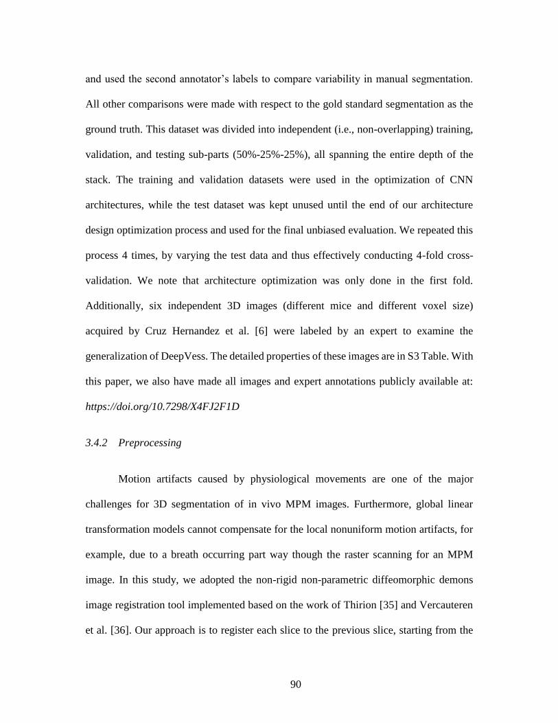
90
and used the second annotator’s labels to compare variability in manual segmentation.
All other comparisons were made with respect to the gold standard segmentation as the
ground truth. This dataset was divided into independent (i.e., non-overlapping) training,
validation, and testing sub-parts (50%-25%-25%), all spanning the entire depth of the
stack. The training and validation datasets were used in the optimization of CNN
architectures, while the test dataset was kept unused until the end of our architecture
design optimization process and used for the final unbiased evaluation. We repeated this
process 4 times, by varying the test data and thus effectively conducting 4-fold cross-
validation. We note that architecture optimization was only done in the first fold.
Additionally, six independent 3D images (different mice and different voxel size)
acquired by Cruz Hernandez et al. [6] were labeled by an expert to examine the
generalization of DeepVess. The detailed properties of these images are in S3 Table. With
this paper, we also have made all images and expert annotations publicly available at:
https://doi.org/10.7298/X4FJ2F1D
3.4.2 Preprocessing
Motion artifacts caused by physiological movements are one of the major
challenges for 3D segmentation of in vivo MPM images. Furthermore, global linear
transformation models cannot compensate for the local nonuniform motion artifacts, for
example, due to a breath occurring part way though the raster scanning for an MPM
image. In this study, we adopted the non-rigid non-parametric diffeomorphic demons
image registration tool implemented based on the work of Thirion [35] and Vercauteren
et al. [36]. Our approach is to register each slice to the previous slice, starting from the

91
first slice as the fixed reference. The diffeomorphic demons algorithm aims to match the
intensity values between the reference image and deformed image, where cost is
computed as the mean squared error. The smoothness prior on the deformation field is
implemented via an efficient Gaussian smoothing of gradient fields, and invertibility is
ensured via concatenation of small deformations. This kernel is effectively encouraging
the deformation field to be smooth, thus regularizing the ill-posed non-linear registration
problem. Based on our experiments, a Gaussian kernel with the standard deviation of 1.3
was chosen for the regularization of the registration algorithm. Next, in our pre-
processing steps, the 1-99% range of the image intensities in the input image patch were
linearly mapped between 0 and 1, and the extreme 1% of voxels were clipped at 0 and 1.
This step, we found, helps with generalizing the model to work well with images taken
from other MPM platforms by adapting normalization parameters to the acquisition
systems and image statistics utilizing most of the intensity rang. To facilitate comparison
between different datasets, image volumes were resampled to have 1 µm3 voxel for
comparisons.
3.4.3 Convolutional neural network architectures
Our aim in this work is to design a system that takes an input stack of images (in
3D) and produces a segmentation of vessels as a binary volume of the same size. For this
task, as we elaborate below, we explored different CNN architectures using validation
performance as our guiding metric. Our baseline CNN architecture starts with a 3D input
image patch (tile), which has 33 × 33 × 5 voxels (in x, y, and z directions). The first
convolution layer uses a 7 × 7 × 5 voxel kernel with 32 features to capture 3D structural
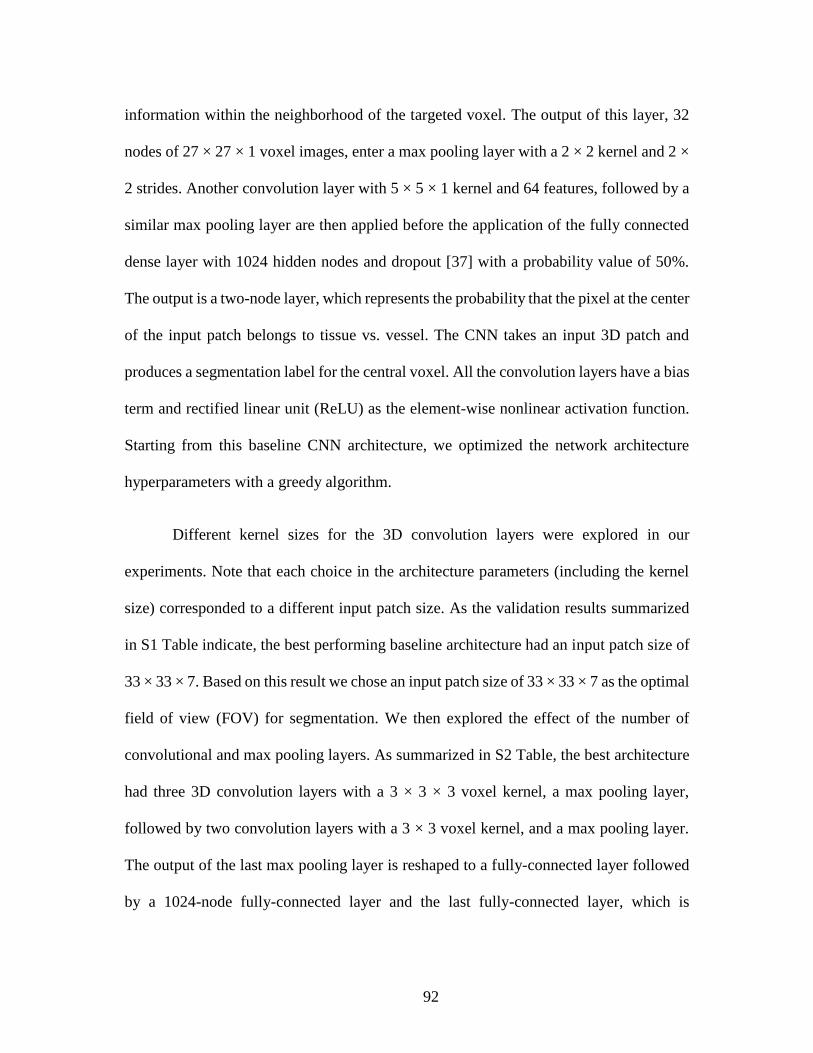
92
information within the neighborhood of the targeted voxel. The output of this layer, 32
nodes of 27 × 27 × 1 voxel images, enter a max pooling layer with a 2 × 2 kernel and 2 ×
2 strides. Another convolution layer with 5 × 5 × 1 kernel and 64 features, followed by a
similar max pooling layer are then applied before the application of the fully connected
dense layer with 1024 hidden nodes and dropout [37] with a probability value of 50%.
The output is a two-node layer, which represents the probability that the pixel at the center
of the input patch belongs to tissue vs. vessel. The CNN takes an input 3D patch and
produces a segmentation label for the central voxel. All the convolution layers have a bias
term and rectified linear unit (ReLU) as the element-wise nonlinear activation function.
Starting from this baseline CNN architecture, we optimized the network architecture
hyperparameters with a greedy algorithm.
Different kernel sizes for the 3D convolution layers were explored in our
experiments. Note that each choice in the architecture parameters (including the kernel
size) corresponded to a different input patch size. As the validation results summarized
in S1 Table indicate, the best performing baseline architecture had an input patch size of
33 × 33 × 7. Based on this result we chose an input patch size of 33 × 33 × 7 as the optimal
field of view (FOV) for segmentation. We then explored the effect of the number of
convolutional and max pooling layers. As summarized in S2 Table, the best architecture
had three 3D convolution layers with a 3 × 3 × 3 voxel kernel, a max pooling layer,
followed by two convolution layers with a 3 × 3 voxel kernel, and a max pooling layer.
The output of the last max pooling layer is reshaped to a fully-connected layer followed
by a 1024-node fully-connected layer and the last fully-connected layer, which is

93
reshaped to the output patch size. Note that there is no difference in spatial resolution
(i.e., voxel dimensions) between the input and output patches.
Finally, we investigated the performance for different output patch sizes, ranging
from 1 voxel to 5 × 5 × 5 voxels and found that performance was improved further when
the output is the segmentation of the central 5 × 5 × 1 patch and not just a single voxel.
A larger output area has the advantage of accounting for the structural relationship
between adjacent voxels in their segmentation. The optimal CNN architecture scheme is
shown in Figure 3.1.
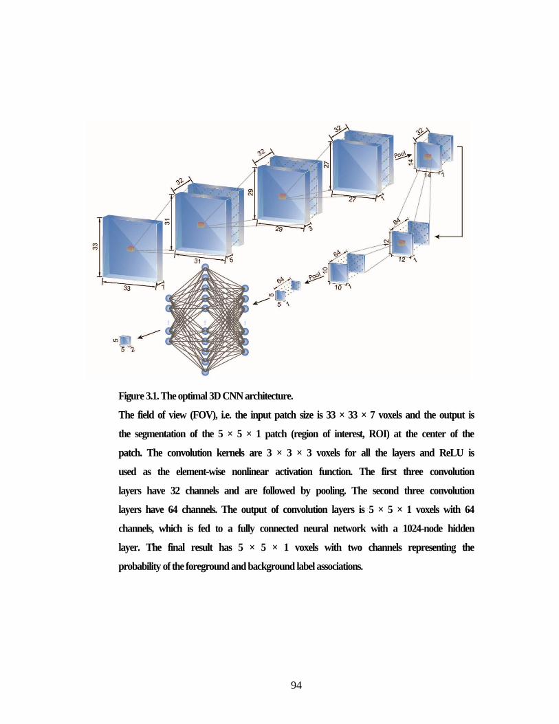
94
Figure 3.1. The optimal 3D CNN architecture.
The field of view (FOV), i.e. the input patch size is 33 × 33 × 7 voxels and the output is
the segmentation of the 5 × 5 × 1 patch (region of interest, ROI) at the center of the
patch. The convolution kernels are 3 × 3 × 3 voxels for all the layers and ReLU is
used as the element-wise nonlinear activation function. The first three convolution
layers have 32 channels and are followed by pooling. The second three convolution
layers have 64 channels. The output of convolution layers is 5 × 5 × 1 voxels with 64
channels, which is fed to a fully connected neural network with a 1024-node hidden
layer. The final result has 5 × 5 × 1 voxels with two channels representing the
probability of the foreground and background label associations.

95
3.4.4 Performance metrics
There are different performance metrics to compare agreement between an
automated segmentation method and a “ground truth” (GT) human annotation. In the
context of binary segmentation, the foreground (F) will be the positive class, and the
negative class will correspond to the background (B). Therefore, true positive (TP) can
be measured as the total number of voxels where both the automatic and human
segmentation labels are foreground. True Negative (TN), False Positive (FP) and False
Negative (FN) can be defined in a similar fashion.
Based on these, we can compute sensitivity and specificity. For example,
sensitivity is the percentage of GT foreground voxels that are labeled by the automatic
segmentation (ASeg) correctly. Mathematically, we have:
𝑠𝑒𝑛𝑠𝑖𝑡𝑖𝑣𝑖𝑡𝑦 = 𝑃(𝑦 = 𝑓|𝐺𝑇 = 𝐹) =𝑇𝑃
𝑇𝑃 + 𝐹𝑁 (1)
𝑠𝑝𝑒𝑐𝑖𝑓𝑖𝑐𝑖𝑡𝑦 = 𝑃(𝑦 = 𝐵|𝐺𝑇 = 𝐵) =𝑇𝑁
𝑇𝑁 + 𝐹𝑃 (2)
The Dice coefficient (DC), Jaccard index (JI), and modified Hausdorff distance
(MHD) are another set of commonly used segmentation performance metrics. JI is
defined as the ratio between the number of voxels labeled as foreground by both GT and
ASeg, to the total number of voxels that are called foreground by either GT and ASeg.
DC is very similar to JI, except it values TP twice as much as FP and FN. JI and DC are
useful metrics when the number of the foreground voxels is much less than background

96
and the detection accuracy of the foreground voxels is more important compared to
background voxel detection, which is the case for 3D imaging of vasculature.
𝐽𝐼 = 𝑃(𝑦 = 𝐹 ∩ 𝐹𝑇 = 𝐹|𝑦 = 𝐹 ∪ 𝐺𝑇 = 𝐹) =𝑇𝑃
𝑇𝑃 + 𝐹𝑃 + 𝐹𝑁 (3)
𝐷𝐶 =2 𝐽𝐼
1 + 𝐽𝐼=
2 𝑇𝑃
2 𝑇𝑃 + 𝐹𝑃 + 𝐹𝑁 (4)
On the other hand, MHD [38] quantifies accuracy in terms of distances between
boundaries, which might be appropriate when considering tubular structures. For each
boundary point in image A (a ∈ A), the closest Euclidean distance (d(a, b) = ||a − b||2) to
any boundary point inside image B (b ∈ B) is first calculated, d(a, B) = minb∈B ||a − b||2).
This is then averaged over all boundary points in A: 1
𝑁𝑎∑ 𝑑(𝑎, B)𝑎∈A [39]. MHD is then
defined as:
𝑀𝐻𝐷 = 𝑚𝑎𝑥 [∑ 𝑑(𝑎, B)
𝑎∈A
, ∑ 𝑑(𝑏, A)
𝑏∈B
] (5)
𝑑(𝑎, B) = 𝑚𝑖𝑛𝑏∈B‖𝑎 − 𝑏‖2 (6)
Note that in the segmentation setting, A and B can represent the foreground
boundaries in the automatic and GT segmentations, respectively. Finally, we can compute
the MHD on centerlines instead of boundaries, a metric we call MHD-CL.

97
3.4.5 Training and implementation details
In training our segmentation algorithms, we used a customized cross-entropy loss
function designed for our highly unbalanced datasets (where foreground voxels comprise
only a small fraction of the volume), measured over all voxels but TN (i ∈ {TP, FP, FN}),
defined as:
𝐿𝑜𝑠𝑠 = ∑ −|𝑦𝑖 log(𝑝𝑖) + (1 − 𝑦𝑖) log(1 − 𝑝𝑖)|
i ∈ {TP,FP,FN }
(7)
yi is the GT label and pi is the model’s output as the probability of the target
voxel i belonging to the foreground. Note that in Eq. (7), true negative voxels have no
contribution, effectively reducing the influence of the dominant background. We trained
our model using Adam stochastic optimization [40] with a learning rate of 10−4 for 100
epochs during architecture exploration and a learning rate of 10−6 for 30,000 epochs during
the fine tuning of model parameters for the proposed architecture with mini-batch size of
1000 samples (based on GPU memory constraints and results of our experiments with
smaller mini-batch size, which did not improve the optimization results). The fine tuning
took one month on one NVIDIA TITAN X GPU. We implemented our models in Python
using Tensorflow [41].
3.4.6 Post-processing
CNN segmentation results contain some segmentation artifact such as holes inside
the vessels, rough boundaries, or isolated small objects. In order to remove these artifacts,
the holes within the vessels were filled. This was followed by application of a 3D mean

98
filter with a 3 × 3 × 3 voxel kernel and the removal of small foreground objects, e.g.
smaller than 100 voxels. This result was used to compare to the gold standard.
3.4.7 Analysis of vasculature centrelines
To characterize the cortical vasculature of the experimental animals, we identified
capillary segments by calculating centerlines from the segmented image data. Our
centerline extraction method includes dilation and thinning operations, in addition to
some centerline artifact removal steps. The binary segmentation image was first thinned
using the algorithm developed by Lee et al. [42]. The result was then dilated using a
spherical kernel with a radius of 5-voxels to improve the vessel connectivity, which was
followed by mean filtering with a 3 × 3 × 3 voxel kernel and removing holes from each
cross section. Next, a thinning step was applied again to obtain the new centerline result.
The original segmented image was dilated using a spherical kernel with a radius of 1-
voxel to act as the mask for the centerlines with the goal of improving the centerline
connectivity. The following rules were applied to the resulting centerlines repeatedly until
no further changes could be done. A vessel is a segment between two bifurcations.
1) Remove any vessels with one end not connected to the network (i.e., dead end)
and with length smaller than 11 voxels.
2) Remove single voxels connected to a junction.
3) Remove single voxels with no connections.
4) Remove vessel loops with length of one or two voxels.
99
Finally, the centerline network representation (i.e. nodes, edges, and their
properties) was extracted. (The centerline extraction was applied on both manual and
automated segmentations.)
3.5 Results
We conducted a systematic evaluation of several network architecture parameters
in order to optimize segmentation accuracy of images of mouse cortex vasculature from
MPM. Features of in vivo MPM images include motion artifacts due to respiration and
heartbeat. Because vessels are visualized by an injection of dye that labels the blood
plasma, unlabeled red blood cells appear as dark spots and streaks moving through the
vessel lumen (arrows in Figure 3.2). Images are acquired by raster scanning through the
tissue and each vessel is captured in several images. The imaging speed has a significant
influence on these features and in in vivo experiments, imaging is often relatively slow,
such that these features become prominent [43]. We emphasize that our exploration was
based on performance on the validation dataset and the final results presented reflect the
model accuracy on an independent test dataset. The detailed performance results for some
of the tested architectures are reported in Table S 3.1 and Table S 3.2. The optimal
architecture, DeepVess, was trained on the training data until the model accuracy stopped
improving and no overfitting was observed (30,000 epochs). Figure S1 shows the JI
learning curve over 30,000 epochs, for training, validation, and test datasets. The constant
gap between JI of the training and validation datasets, which represent generalization
error, confirms that we are not strongly overfitting.
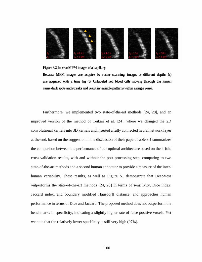
100
Figure 3.2. In vivo MPM images of a capillary.
Because MPM images are acquire by raster scanning, images at different depths (z)
are acquired with a time lag (t). Unlabeled red blood cells moving through the lumen
cause dark spots and streaks and result in variable patterns within a single vessel.
Furthermore, we implemented two state-of-the-art methods [24, 28], and an
improved version of the method of Teikari et al. [24], where we changed the 2D
convolutional kernels into 3D kernels and inserted a fully connected neural network layer
at the end, based on the suggestion in the discussion of their paper. Table 3.1 summarizes
the comparison between the performance of our optimal architecture based on the 4-fold
cross-validation results, with and without the post-processing step, comparing to two
state-of-the-art methods and a second human annotator to provide a measure of the inter-
human variability. These results, as well as Figure S1 demonstrate that DeepVess
outperforms the state-of-the-art methods [24, 28] in terms of sensitivity, Dice index,
Jaccard index, and boundary modified Hausdorff distance; and approaches human
performance in terms of Dice and Jaccard. The proposed method does not outperform the
benchmarks in specificity, indicating a slightly higher rate of false positive voxels. Yet
we note that the relatively lower specificity is still very high (97%).
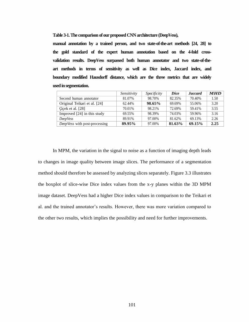
101
Table 3-1. The comparison of our proposed CNN architecture (DeepVess),
manual annotation by a trained person, and two state-of-the-art methods [24, 28] to
the gold standard of the expert human annotation based on the 4-fold cross-
validation results. DeepVess surpassed both human annotator and two state-of-the-
art methods in terms of sensitivity as well as Dice index, Jaccard index, and
boundary modified Hausdorff distance, which are the three metrics that are widely
used in segmentation.
Sensitivity Specificity Dice Jaccard MHD
Second human annotator 81.07% 98.70% 82.35% 70.40% 1.50
Original Teikari et al. [24] 62.44% 98.65% 69.69% 55.06% 3.20
C icek et al. [28] 70.01% 98.21% 72.69% 59.41% 3.55
Improved [24] in this study 69.55% 98.39% 74.03% 59.96% 3.16
DeepVess 89.91% 97.00% 81.62% 69.13% 2.26
DeepVess with post-processing 89.95% 97.00% 81.63% 69.15% 2.25
In MPM, the variation in the signal to noise as a function of imaging depth leads
to changes in image quality between image slices. The performance of a segmentation
method should therefore be assessed by analyzing slices separately. Figure 3.3 illustrates
the boxplot of slice-wise Dice index values from the x-y planes within the 3D MPM
image dataset. DeepVess had a higher Dice index values in comparison to the Teikari et
al. and the trained annotator’s results. However, there was more variation compared to
the other two results, which implies the possibility and need for further improvements.
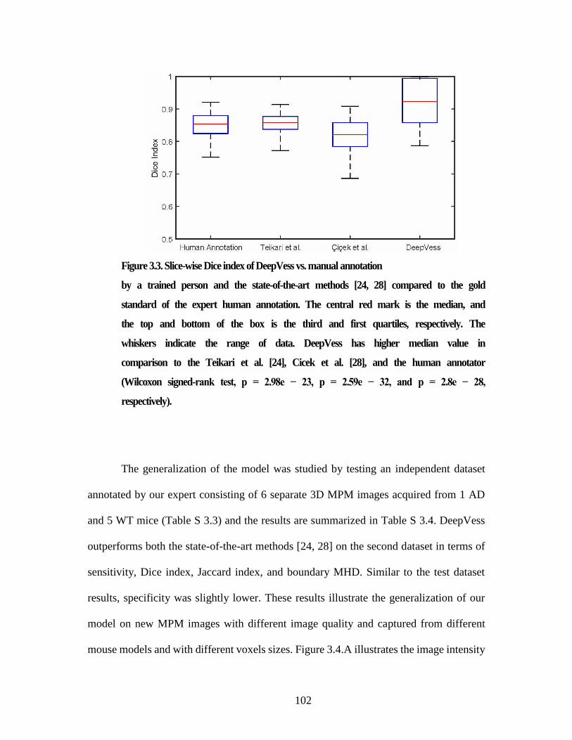
102
Figure 3.3. Slice-wise Dice index of DeepVess vs. manual annotation
by a trained person and the state-of-the-art methods [24, 28] compared to the gold
standard of the expert human annotation. The central red mark is the median, and
the top and bottom of the box is the third and first quartiles, respectively. The
whiskers indicate the range of data. DeepVess has higher median value in
comparison to the Teikari et al. [24], Cicek et al. [28], and the human annotator
(Wilcoxon signed-rank test, p = 2.98e − 23, p = 2.59e − 32, and p = 2.8e − 28,
respectively).
The generalization of the model was studied by testing an independent dataset
annotated by our expert consisting of 6 separate 3D MPM images acquired from 1 AD
and 5 WT mice (Table S 3.3) and the results are summarized in Table S 3.4. DeepVess
outperforms both the state-of-the-art methods [24, 28] on the second dataset in terms of
sensitivity, Dice index, Jaccard index, and boundary MHD. Similar to the test dataset
results, specificity was slightly lower. These results illustrate the generalization of our
model on new MPM images with different image quality and captured from different
mouse models and with different voxels sizes. Figure 3.4.A illustrates the image intensity

103
and three models overlaid on the image for a cross-section extracted from a 3D image
from the independent dataset (Table S 3.4 #1). Figure 3.4.B-E are magnified version of
three cases within Figure 3.4.A. The main sources of failure in the vessel segmentations
of 3D in vivo MPM images are low SNR at deeper cross-sections (Figure 3.4.C) and
unlabeled, moving red blood cells in the vessel lumen, which cause dark spots and streaks
(Figure 3.4.B and D). The patchy segmentations due to unlabeled red blood cells result
in unconnected and isolated vasculature centerlines and network. The DeepVess
architecture has fully connected layers and thus might be exploiting some spatially
varying properties of the signal (as in the variation of contrast as a function of depth) that
a fully convolutional architecture such as U-Net might not be able to exploit. Elsewhere,
in the absence of such difficulties, all three models segment the vessels largely accurately.
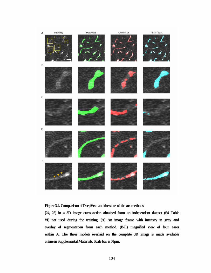
104
Figure 3.4. Comparison of DeepVess and the state-of-the-art methods
[24, 28] in a 3D image cross-section obtained from an independent dataset (S4 Table
#1) not used during the training. (A) An image frame with intensity in gray and
overlay of segmentation from each method. (B-E) magnified view of four cases
within A. The three models overlaid on the complete 3D image is made available
online in Supplemental Materials. Scale bar is 50µm.
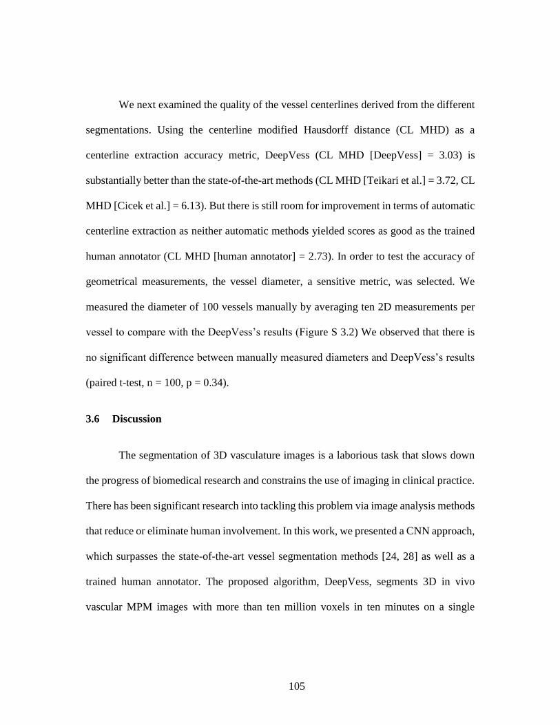
105
We next examined the quality of the vessel centerlines derived from the different
segmentations. Using the centerline modified Hausdorff distance (CL MHD) as a
centerline extraction accuracy metric, DeepVess (CL MHD [DeepVess] = 3.03) is
substantially better than the state-of-the-art methods (CL MHD [Teikari et al.] = 3.72, CL
MHD [Cicek et al.] = 6.13). But there is still room for improvement in terms of automatic
centerline extraction as neither automatic methods yielded scores as good as the trained
human annotator (CL MHD [human annotator] = 2.73). In order to test the accuracy of
geometrical measurements, the vessel diameter, a sensitive metric, was selected. We
measured the diameter of 100 vessels manually by averaging ten 2D measurements per
vessel to compare with the DeepVess’s results (Figure S 3.2) We observed that there is
no significant difference between manually measured diameters and DeepVess’s results
(paired t-test, n = 100, p = 0.34).
3.6 Discussion
The segmentation of 3D vasculature images is a laborious task that slows down
the progress of biomedical research and constrains the use of imaging in clinical practice.
There has been significant research into tackling this problem via image analysis methods
that reduce or eliminate human involvement. In this work, we presented a CNN approach,
which surpasses the state-of-the-art vessel segmentation methods [24, 28] as well as a
trained human annotator. The proposed algorithm, DeepVess, segments 3D in vivo
vascular MPM images with more than ten million voxels in ten minutes on a single
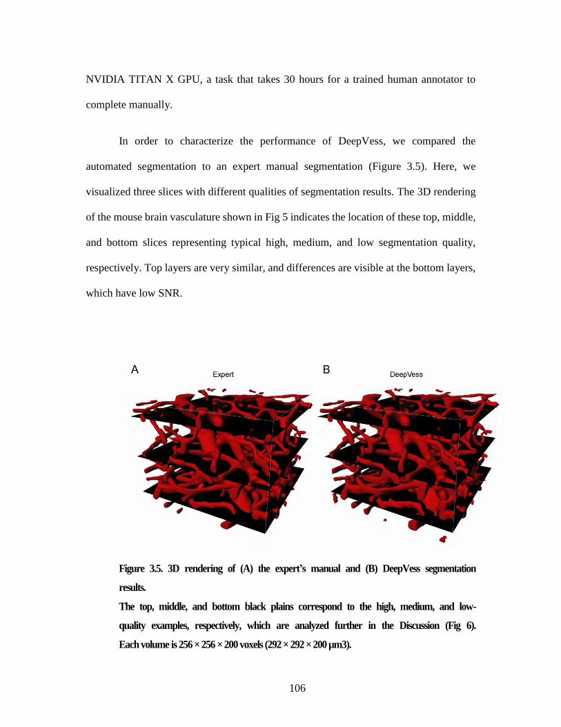
106
NVIDIA TITAN X GPU, a task that takes 30 hours for a trained human annotator to
complete manually.
In order to characterize the performance of DeepVess, we compared the
automated segmentation to an expert manual segmentation (Figure 3.5). Here, we
visualized three slices with different qualities of segmentation results. The 3D rendering
of the mouse brain vasculature shown in Fig 5 indicates the location of these top, middle,
and bottom slices representing typical high, medium, and low segmentation quality,
respectively. Top layers are very similar, and differences are visible at the bottom layers,
which have low SNR.
Figure 3.5. 3D rendering of (A) the expert’s manual and (B) DeepVess segmentation
results.
The top, middle, and bottom black plains correspond to the high, medium, and low-
quality examples, respectively, which are analyzed further in the Discussion (Fig 6).
Each volume is 256 × 256 × 200 voxels (292 × 292 × 200 µm3).
107
We used 50% dropout during test-time [44] and computed Shannon’s entropy for
the segmentation prediction at each voxel to quantify the uncertainty in the automated
segmentation. Higher entropy represents higher segmentation uncertainty at a particular
voxel. The entropy results together with the comparison between DeepVess and the
expert segmentations for those three planes are illustrated in Figure 3.6. The left column
contains the intensity gray-scale images of these examples. The segmentation results of
the DeepVess and the expert are superimposed on the original gray-scale image with red
(DeepVess) and green (the expert), as shown in the middle column. Yellow represents
agreement between DeepVess and the expert. The right column shows the entropy of each
example estimated via test time dropout. We observe that, in general, DeepVess has
higher uncertainty at the boundaries of vessels. The disagreement with ground truth is
also mostly concentrated at the boundaries. Images from deeper within the brain tissue
that often have lower image contrast and higher noise levels due to the nature of MPM,
suffer from more segmentation errors. These images can often be challenging even for
expert humans. Arrows in Figure 3.6.C highlight examples of these difficulties. The error
example 1 illustrates the case where the expert ignored bright pixels around the vessel
lumen based on their knowledge of the underlying physiology and experience with MPM
images of brain that postulate a rounded lumen instead of a jittery and rough lumen, despite
a very strong signal. The error example 2 illustrates a low intensity vessel junction that
was judged to be an artifact by humans based on experience or information from other
image planes. The error example 3 illustrates the case where a small vessel does not exhibit
a strong signal and it is not connected to another major vessel.
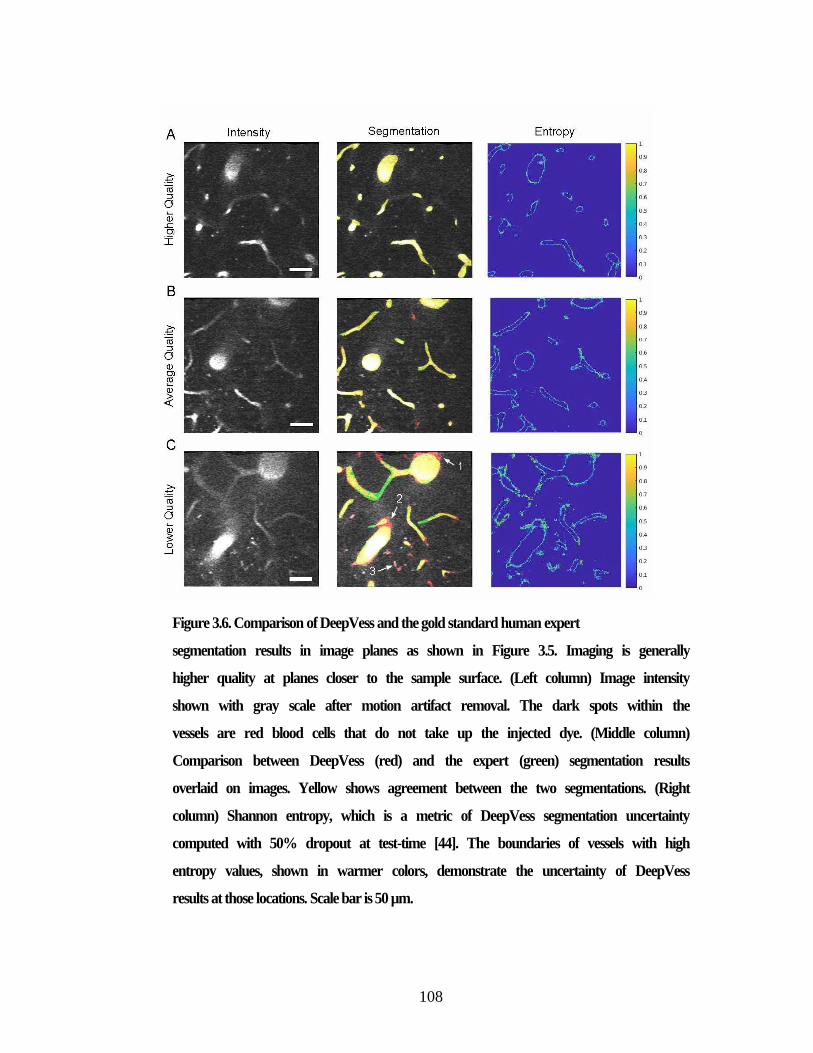
108
Figure 3.6. Comparison of DeepVess and the gold standard human expert
segmentation results in image planes as shown in Figure 3.5. Imaging is generally
higher quality at planes closer to the sample surface. (Left column) Image intensity
shown with gray scale after motion artifact removal. The dark spots within the
vessels are red blood cells that do not take up the injected dye. (Middle column)
Comparison between DeepVess (red) and the expert (green) segmentation results
overlaid on images. Yellow shows agreement between the two segmentations. (Right
column) Shannon entropy, which is a metric of DeepVess segmentation uncertainty
computed with 50% dropout at test-time [44]. The boundaries of vessels with high
entropy values, shown in warmer colors, demonstrate the uncertainty of DeepVess
results at those locations. Scale bar is 50 µm.
109
DeepVess implements pre- and post-processing tools to deal with in vivo MPM
images that suffer from different motion artifacts. DeepVess is freely available at
https://github.com/mhaft/DeepVess and can be used immediately by researchers who use
MPM for vasculature imaging. Also, our model can be fine-tuned further by adjusting the
intensity normalization step to utilize a different part of the intensity range and training
samples for other 3D vasiform structures or other imaging modalities. Similar to many
machine learning solutions, DeepVess’ performance depends on specific image features
and the performance will degrade in cases where the tissues are labeled differently (e.g.
vessel walls are labeled instead of blood serum) or the images intensities are concentrated
in a small portion of the intensity range.
Although in vivo measurements present unique challenges to image segmentation,
such as the red blood cell motion, in our case, we have shown that DeepVess successfully
handles these challenges. Postmortem techniques all change the vessel diameters in the
tissue processing. Hence, we believe that in vivo imaging is the best strategy to quantify
vessel diameters. While features such as topology and length might not be affected by
postmortem processing, in vivo imaging with MPM is important for capillary diameter
measurements. Two-photon microscopy has been used to validate histology in many
studies ([5, 14, 45–48]) and comparisons with other labeling techniques are quite
common.
While DeepVess offers very high accuracy in the problem we consider, there is
room for further improvement and validation, in particular in the application to other
vasiform structures and modalities. For example, other types of (e.g., non-convolutional)
110
architectures such as long short-term memory (LSTM) can be examined for this problem.
Likewise, a combined approach that treats segmentation and centerline extraction
methods together, such as the method proposed by Bates et al. [25] in a single complete
end-to-end learning framework might achieve higher centerline accuracy levels.
3.7 Application to Alzheimer’s mouse models
3.7.1 Capillary alteration caused by aging and Alzheimer’s disease
In vivo imaging with multiphoton microscopy of capillary beds is free of
distortions in vessel structure caused by postmortem tissue processing that can result in
artifacts such as altered diameters [5]. However, the images often suffer from poor signal
to noise and motion artifacts. An additional challenge is that unlabeled, moving red blood
cells in the vessel lumen cause dark spots and streaks that move over time. Disease models
are often especially challenging because inflammation and tissue damage can further
degrade imaging conditions.
Strong correlations between vascular health, brain blood flow and AD suggest
that mapping the microvascular network is critical to the understanding of cognitive
health in aging [49]. To explore this question, we imaged the cortical vascular networks
in young and old mouse models of AD (young AD and old AD) and their young and old
WT littermates (young WT and old WT). Imaged volumes ranged from 230 × 230 to 600
× 600 µm2 in x-y and 130 to 459 µm in the z direction. We imaged 6 animals per group,
with at least 3000 capillary segments analyzed for each group.
111
The resulting 3D stacks of images were preprocessed, segmented with DeepVess,
and post-processed as discussed in the previous sections. Centerlines were extracted, and
individual vessel segments were identified. To analyze capillaries while excluding
arterioles and venules, only vessel segments less than 10 µm in diameter were included
[6, 50, 51]. For the vascular parameters of segment length, diameter, and tortuosity
considered here, previous work has shown that AD mouse models have increased
tortuosity in cortical penetrating arterioles as compared to WT mice [52, 53]. Our analysis
of capillaries excluded these vessels. Three metrics were selected to characterize the
vascular network. For each capillary segment, we calculated the diameter averaged along
the length (Fig 7.A), the length (Figure 3.7.B), and the tortuosity, defined as the length
divided by the Euclidean distance between the two ends (Figure w.7.C). The distributions
of capillary diameter, length, and tortuosity varied little between young and old mice or
between WT and AD genotype (Table 3.2). There were subtle shifts (∼ 0.25 µm) in the
diameter distribution between groups, but no clear differences across old/young or
WT/AD and the differences in means were small compared to the standard deviation (6-
27% of SD). However, we observed a decrease in the number of longer length (> 75µm)
capillaries in older animals as compared to young in both WT and AD mice shown by a
rightward shift in the cumulative distribution function curve (Figure w.7.B and Table
3.2).
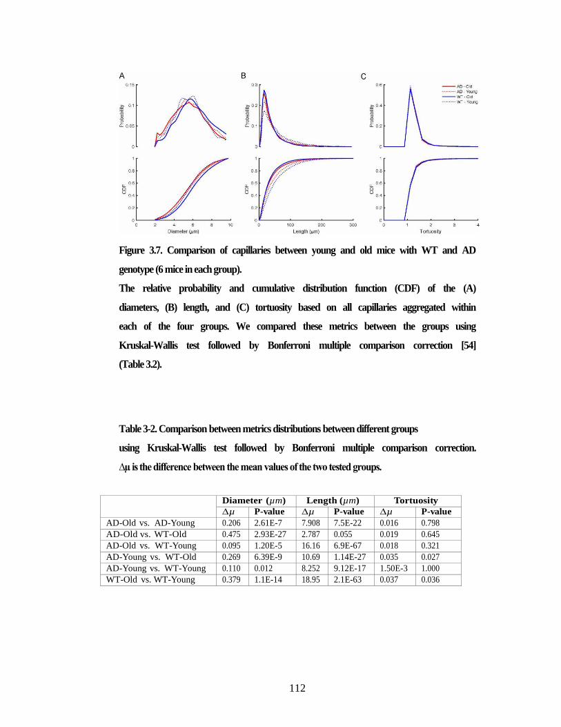
112
Figure 3.7. Comparison of capillaries between young and old mice with WT and AD
genotype (6 mice in each group).
The relative probability and cumulative distribution function (CDF) of the (A)
diameters, (B) length, and (C) tortuosity based on all capillaries aggregated within
each of the four groups. We compared these metrics between the groups using
Kruskal-Wallis test followed by Bonferroni multiple comparison correction [54]
(Table 3.2).
Table 3-2. Comparison between metrics distributions between different groups
using Kruskal-Wallis test followed by Bonferroni multiple comparison correction.
∆µ is the difference between the mean values of the two tested groups.
Diameter (µm) Length (µm) Tortuosity
∆µ P-value ∆µ P-value ∆µ P-value
AD-Old vs. AD-Young 0.206 2.61E-7 7.908 7.5E-22 0.016 0.798
AD-Old vs. WT-Old 0.475 2.93E-27 2.787 0.055 0.019 0.645
AD-Old vs. WT-Young 0.095 1.20E-5 16.16 6.9E-67 0.018 0.321
AD-Young vs. WT-Old 0.269 6.39E-9 10.69 1.14E-27 0.035 0.027
AD-Young vs. WT-Young 0.110 0.012 8.252 9.12E-17 1.50E-3 1.000
WT-Old vs. WT-Young 0.379 1.1E-14 18.95 2.1E-63 0.037 0.036
113
3.7.2 Aging and Alzheimer’s disease have little effect on capillary characteristics
Using a large database of vessel segments measured in three dimensions, we
surprisingly found only very small differences between groups that were dwarfed by the
variance in capillary diameter or tortuosity between young and old animals or between
WT and AD mouse models. The automation provided by DeepVess enabled the
evaluation across a very large number of vessels in a large group size. The strong
agreement between the measurements based on DeepVess and the manual measurements
by Cruz Hernandez et al. [6], confirms that the proposed pipeline yields unbiased and
accurate metrics to analyze capillary segments. There was a decrease in the number of
long capillary segments in the aged animals compared to young in both the WT and AD
groups. Note that the reported metrics only represent the parietal region of cortex and that
regional variability can affect our results. These finding may not generalize across all
ages and mouse models of AD and could be different in other regions of the brain.
Sonntag et al. [1] argue that changes in vasculature due to aging might be non-linear and
multi-phasic. For instance, two studies showed that the capillary density increases during
adulthood and then declines in more advanced age [55, 56]. As summarized in Table 3.3,
several previous studies have characterized the average diameters of cortical capillaries
in mice and showed high variability in results suggesting that methodological variations
make comparison between studies difficult. Other studies that compared AD models and
WT also found negligible or no difference in capillary diameters. Heinzer et al. compared
a different mouse model (APP23) using MRA and found no difference between WT and
114
AD mice [57]. The same group also compared the effects of “VEGF overexpression”
model and WT using SRµCT and also found little difference [58].
There are a wide range of imaging approaches used in these various studies and
data from both live animal and postmortem analysis is included. It is possible that some
of these differences emerge when tissues are processed rather than measured in vivo as
was done here. Studies based on sectioned tissue sample the 3D vascular architecture
differently so it is difficult to make direct comparisons between datasets. Measures of
capillaries depend on the definition of capillaries. Here it was based on a threshold
diameter of 10µm, which could explain some of the variability in the literature. Not
surprisingly given the differences in approach and sample preparation, there is significant
disagreement between reported average diameters. Some differences may, however,
reflect differences in vasculature across strains and ages of animals.
Therefore, the proposed fully automated objective segmentation of 3D in vivo
images of the vasculature can be used to reduce the variability due to sample preparation
and imaging/analysis approach, allowing such strain and age differences to be elucidated
clearly.
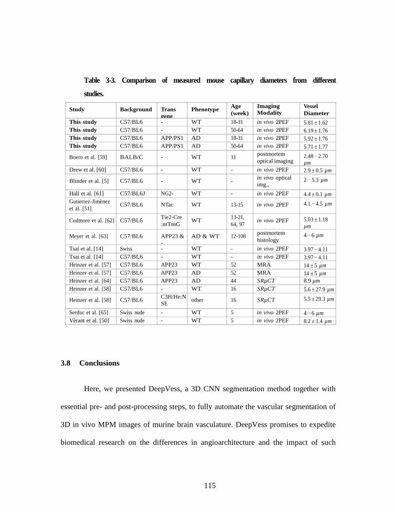
115
Table 3-3. Comparison of measured mouse capillary diameters from different
studies.
Study
Background
Trans
gene
Phenotype
Age
(week)
Imaging
Modality Vessel
Diameter
This study C57/BL6 - WT 18-31 in vivo 2PEF 5.81 ± 1.62
µm This study C57/BL6 - WT 50-64 in vivo 2PEF 6.19 ± 1.76
µm This study C57/BL6 APP/PS1 AD 18-31 in vivo 2PEF 5.92 ± 1.76
µm This study C57/BL6 APP/PS1 AD 50-64 in vivo 2PEF 5.71 ± 1.77
µm
Boero et al. [59]
BALB/C
-
WT
11 postmortem
optical imaging 2.48 − 2.70
µm
Drew et al. [60] C57/BL6 - WT - in vivo 2PEF 2.9 ± 0.5 µm
Blinder et al. [5]
C57/BL6
-
WT
- in vivo optical
img.,
postmortem 2PEF
2 − 5.3 µm
Hall et al. [61] C57/BL6J NG2-
DsRed
WT - in vivo 2PEF 4.4 ± 0.1 µm
Gutierrez-Jimenez
et al. [51]
C57/BL6
NTac
WT
13-15
in vivo 2PEF 4.1 − 4.5 µm
Cudmore et al. [62]
C57/BL6
Tie2-Cre
:mTmG
WT
13-21,
64, 97
in vivo 2PEF 5.03 ± 1.18
µm
Meyer et al. [63]
C57/BL6
APP23 &
-
AD & WT
12-108
postmortem
histology 4 − 6 µm
Tsai et al. [14] Swiss - WT - in vivo 2PEF 3.97 − 4.11
µm Tsai et al. [14] C57/BL6 - WT - in vivo 2PEF 3.97 − 4.11
µm Heinzer et al. [57] C57/BL6 APP23 WT 52 MRA 14 ± 5 µm
Heinzer et al. [57] C57/BL6 APP23 AD 52 MRA 14 ± 5 µm
Heinzer et al. [64] C57/BL6 APP23 AD 44 SRµCT 8.9 µm
Heinzer et al. [58] C57/BL6 - WT 16 SRµCT 5.6 ± 27.9 µm
Heinzer et al. [58]
C57/BL6 C3H/He:N
SE
-
VEGF165
1
other
16
SRµCT 5.5 ± 29.3 µm
Serduc et al. [65] Swiss nude - WT 5 in vivo 2PEF 4 − 6 µm
Verant et al. [50] Swiss nude - WT 5 in vivo 2PEF 8.2 ± 1.4 µm
3.8 Conclusions
Here, we presented DeepVess, a 3D CNN segmentation method together with
essential pre- and post-processing steps, to fully automate the vascular segmentation of
3D in vivo MPM images of murine brain vasculature. DeepVess promises to expedite
biomedical research on the differences in angioarchitecture and the impact of such
116
differences by removing the laborious, time consuming, and subjective manual
segmentation task from the analysis pipelines in addition to elimination of subjective
image analysis results. We hope the availability of our open source code and reported
results will facilitate and motivate the adoption of this method by researchers and
practitioners.
3.9 Data availability statement
All data underlying these findings is publicly available at Cornell’s eCommons
online archive: https://doi.org/10.7298/X4FJ2F1D
3.10 Declarations of interest
none
3.11 Supplementary materials
3.11.1 Manual 3D segmentation protocol using ImageJ.
First, we created a new hyper-stack (File menu → New) with 3D voxel size and
bit depth similar to the original image (e.g. a 16-bit 1024 × 1024 × 500 voxel hyper-
stack). The original image and the new hyper-stack were then merged (Image menu →
Color) into a multi-channel hyper-stack, which contained both the raw data and the
segmentation results. On each image (in the x-y plane) the expert drew segmentation
boundaries using the free hand tool and fill function (F key) while the second channel is
selected using scrollbar. The Color Picker and Channels Tool (Image menu → Color) in
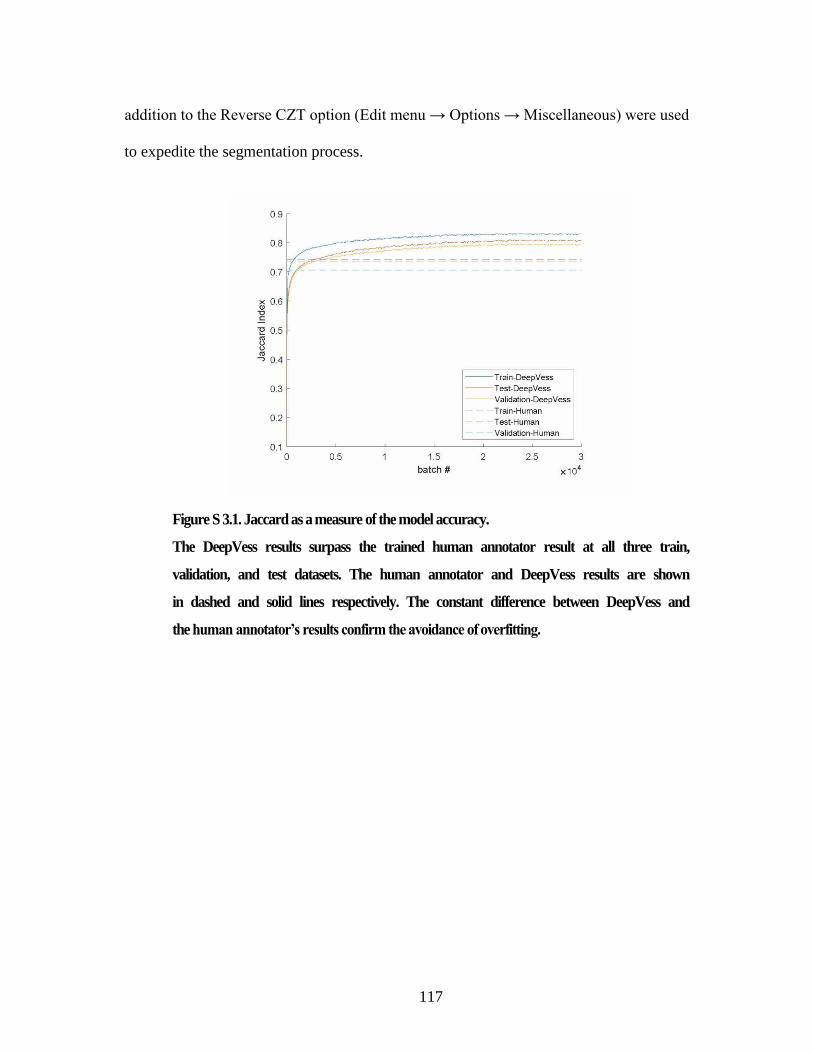
117
addition to the Reverse CZT option (Edit menu → Options → Miscellaneous) were used
to expedite the segmentation process.
Figure S 3.1. Jaccard as a measure of the model accuracy.
The DeepVess results surpass the trained human annotator result at all three train,
validation, and test datasets. The human annotator and DeepVess results are shown
in dashed and solid lines respectively. The constant difference between DeepVess and
the human annotator’s results confirm the avoidance of overfitting.
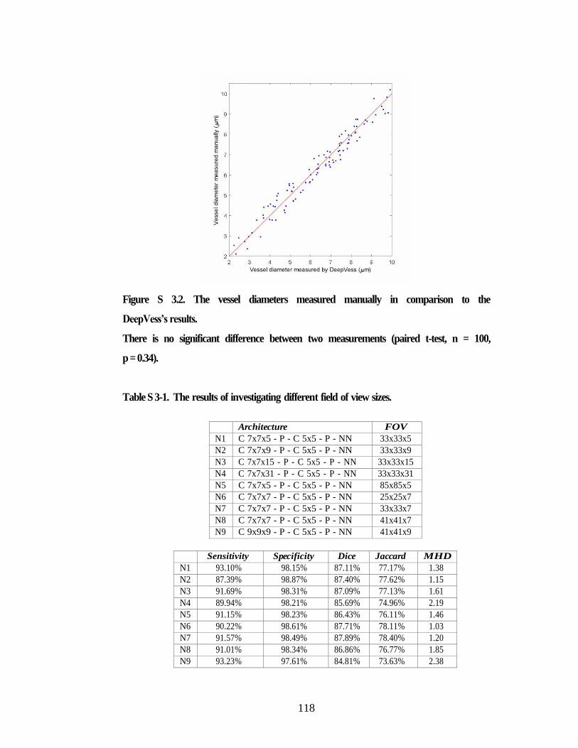
118
Figure S 3.2. The vessel diameters measured manually in comparison to the
DeepVess’s results.
There is no significant difference between two measurements (paired t-test, n = 100,
p = 0.34).
Table S 3-1. The results of investigating different field of view sizes.
Architecture FOV
N1 C 7x7x5 - P - C 5x5 - P - NN 33x33x5
N2 C 7x7x9 - P - C 5x5 - P - NN 33x33x9
N3 C 7x7x15 - P - C 5x5 - P - NN 33x33x15
N4 C 7x7x31 - P - C 5x5 - P - NN 33x33x31
N5 C 7x7x5 - P - C 5x5 - P - NN 85x85x5
N6 C 7x7x7 - P - C 5x5 - P - NN 25x25x7
N7 C 7x7x7 - P - C 5x5 - P - NN 33x33x7
N8 C 7x7x7 - P - C 5x5 - P - NN 41x41x7
N9 C 9x9x9 - P - C 5x5 - P - NN 41x41x9
Sensitivity Specificity Dice Jaccard MHD
N1 93.10% 98.15% 87.11% 77.17% 1.38
N2 87.39% 98.87% 87.40% 77.62% 1.15
N3 91.69% 98.31% 87.09% 77.13% 1.61
N4 89.94% 98.21% 85.69% 74.96% 2.19
N5 91.15% 98.23% 86.43% 76.11% 1.46
N6 90.22% 98.61% 87.71% 78.11% 1.03
N7 91.57% 98.49% 87.89% 78.40% 1.20
N8 91.01% 98.34% 86.86% 76.77% 1.85
N9 93.23% 97.61% 84.81% 73.63% 2.38
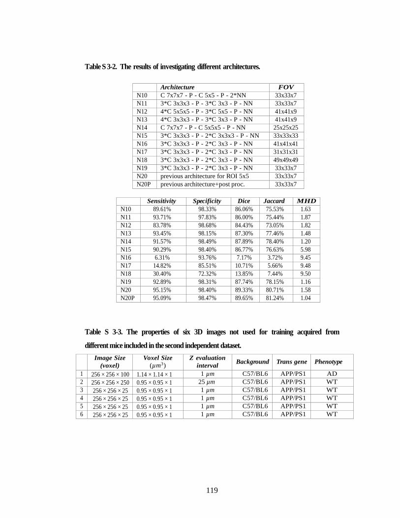
119
Table S 3-2. The results of investigating different architectures.
Architecture FOV
N10 C 7x7x7 - P - C 5x5 - P - 2*NN 33x33x7
N11 3*C 3x3x3 - P - 3*C 3x3 - P - NN 33x33x7
N12 4*C 5x5x5 - P - 3*C 5x5 - P - NN 41x41x9
N13 4*C 3x3x3 - P - 3*C 3x3 - P - NN 41x41x9
N14 C 7x7x7 - P - C 5x5x5 - P - NN 25x25x25
N15 3*C 3x3x3 - P - 2*C 3x3x3 - P - NN 33x33x33
N16 3*C 3x3x3 - P - 2*C 3x3 - P - NN 41x41x41
N17 3*C 3x3x3 - P - 2*C 3x3 - P - NN 31x31x31
N18 3*C 3x3x3 - P - 2*C 3x3 - P - NN 49x49x49
N19 3*C 3x3x3 - P - 2*C 3x3 - P - NN 33x33x7
N20 previous architecture for ROI 5x5 33x33x7
N20P previous architecture+post proc. 33x33x7
Sensitivity Specificity Dice Jaccard MHD
N10 89.61% 98.33% 86.06% 75.53% 1.63
N11 93.71% 97.83% 86.00% 75.44% 1.87
N12 83.78% 98.68% 84.43% 73.05% 1.82
N13 93.45% 98.15% 87.30% 77.46% 1.48
N14 91.57% 98.49% 87.89% 78.40% 1.20
N15 90.29% 98.40% 86.77% 76.63% 5.98
N16 6.31% 93.76% 7.17% 3.72% 9.45
N17 14.82% 85.51% 10.71% 5.66% 9.48
N18 30.40% 72.32% 13.85% 7.44% 9.50
N19 92.89% 98.31% 87.74% 78.15% 1.16
N20 95.15% 98.40% 89.33% 80.71% 1.58
N20P 95.09% 98.47% 89.65% 81.24% 1.04
Table S 3-3. The properties of six 3D images not used for training acquired from
different mice included in the second independent dataset.
Image Size
(voxel)
Voxel Size
(µm3)
Z evaluation
interval
Background
Trans gene
Phenotype
1 256 × 256 × 100 1.14 × 1.14 × 1 1 µm C57/BL6 APP/PS1 AD
2 256 × 256 × 250 0.95 × 0.95 × 1 25 µm C57/BL6 APP/PS1 WT
3 256 × 256 × 25 0.95 × 0.95 × 1 1 µm C57/BL6 APP/PS1 WT
4 256 × 256 × 25 0.95 × 0.95 × 1 1 µm C57/BL6 APP/PS1 WT
5 256 × 256 × 25 0.95 × 0.95 × 1 1 µm C57/BL6 APP/PS1 WT
6 256 × 256 × 25 0.95 × 0.95 × 1 1 µm C57/BL6 APP/PS1 WT
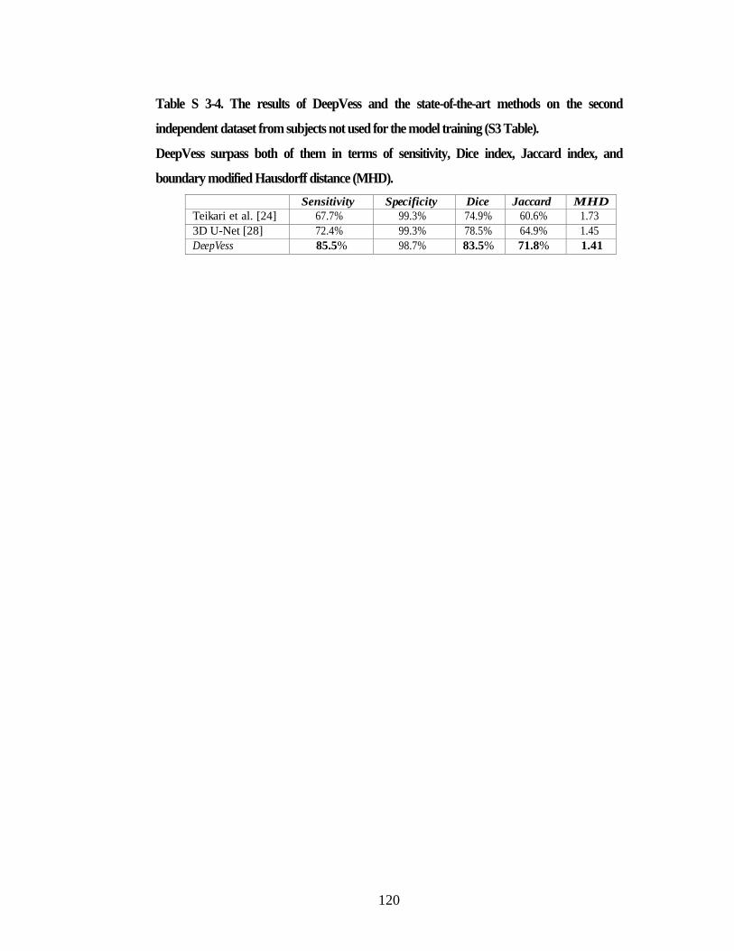
120
Table S 3-4. The results of DeepVess and the state-of-the-art methods on the second
independent dataset from subjects not used for the model training (S3 Table).
DeepVess surpass both of them in terms of sensitivity, Dice index, Jaccard index, and
boundary modified Hausdorff distance (MHD).
Sensitivity Specificity Dice Jaccard MHD
Teikari et al. [24] 67.7% 99.3% 74.9% 60.6% 1.73
3D U-Net [28] 72.4% 99.3% 78.5% 64.9% 1.45
DeepVess 85.5% 98.7% 83.5% 71.8% 1.41
121
REFERENCES
Sonntag WE, Eckman DM, Ingraham J, Riddle DR. Regulation of cerebrovascular aging.
In: Riddle DR, editor. Brain aging: models, methods, and mechanisms. Boca
Raton, FL: CRC Press/Taylor & Francis; 2007. p. 279–304.
Hossmann K. Viability thresholds and the penumbra of focal ischemia.
Annals of neurology. 1994;36(4):557–565.
Lin L, Yao J, Zhang R, Chen CC, Huang CH, Li Y, et al. High-speed photoacoustic
microscopy of mouse cortical microhemodynamics. Journal of biophotonics.
2017;10(6-7):792–798.
Erdener SE, Tang J, Sajjadi A, Kılıc K, Kura S, Schaffer CB, et al. Spatio-temporal
dynamics of cerebral capillary segments with stalling red blood cells. Journal of
Cerebral Blood Flow & Metabolism. 2017; p. 0271678X17743877.
Blinder P, Tsai PS, Kaufhold JP, Knutsen PM, Suhl H, Kleinfeld D. The cortical
angiome: an interconnected vascular network with noncolumnar patterns of
blood flow. Nature neuroscience. 2013;16(7):889–897.
Cruz Hernandez JC, Bracko O, Kersbergen CJ, Muse V, Haft-Javaherian M, Berg M, et al.
Neutrophil adhesion in brain capillaries contributes to cortical blood flow decreases
and impaired memory function in mouse models of Alzheimer’s disease. Nature
Neuroscience In press. 2019.
Kalaria RN. Cerebral vessels in ageing and Alzheimer’s disease. Pharmacology &
therapeutics. 1996;72(3):193–214.
Farkas E, Luiten PG. Cerebral microvascular pathology in aging and Alzheimer’s disease.
Progress in neurobiology. 2001;64(6):575–611.
Riddle DR, Sonntag WE, Lichtenwalner RJ. Microvascular plasticity in aging. Ageing
research reviews. 2003;2(2):149–168.
Kirbas C, Quek F. A review of vessel extraction techniques and algorithms. ACM
Computing Surveys (CSUR). 2004;36(2):81–121.
122
Lesage D, Angelini ED, Bloch I, Funka-Lea G. A review of 3D vessel lumen segmentation
techniques: Models, features and extraction schemes. Medical image analysis.
2009;13(6):819–845.
Litjens G, Kooi T, Bejnordi BE, Setio AAA, Ciompi F, Ghafoorian M, et al. A survey on
deep learning in medical image analysis. Medical Image Analysis.
2017;42(Supplement C):60 – 88.
Fraz MM, Remagnino P, Hoppe A, Uyyanonvara B, Rudnicka AR, Owen CG, et al.
Blood vessel segmentation methodologies in retinal images–a survey. Computer
methods and programs in biomedicine. 2012;108(1):407–433.
Tsai PS, Kaufhold JP, Blinder P, Friedman B, Drew PJ, Karten HJ, et al. Correlations
of neuronal and microvascular densities in murine cortex revealed by direct
counting and colocalization of nuclei and vessels. Journal of Neuroscience.
2009;29(46):14553–14570.
Yi J, Ra JB. A locally adaptive region growing algorithm for vascular segmentation.
International Journal of Imaging Systems and Technology. 2003;13(4):208–214.
Mille J, Cohen LD. Deformable tree models for 2D and 3D branching structures
extraction. In: Computer Vision and Pattern Recognition Workshops, 2009. CVPR
Workshops 2009. IEEE Computer Society Conference on. IEEE; 2009. p. 149–156.
Gulshan V, Peng L, Coram M, Stumpe MC, Wu D, Narayanaswamy A, et al. Development
and validation of a deep learning algorithm for detection of diabetic retinopathy in
retinal fundus photographs. Jama. 2016;316(22):2402–2410.
Szegedy C, Vanhoucke V, Ioffe S, Shlens J, Wojna Z. Rethinking the inception architecture
for computer vision. In: Proceedings of the IEEE Conference on Computer Vision
and Pattern Recognition; 2016. p. 2818–2826.
Wu A, Xu Z, Gao M, Buty M, Mollura DJ. Deep vessel tracking: A generalized probabilistic
approach via deep learning. In: Biomedical Imaging (ISBI), 2016 IEEE 13th
International Symposium on. IEEE; 2016. p. 1363–1367.
Fu H, Xu Y, Wong DWK, Liu J. Retinal vessel segmentation via deep learning
network and fully- connected conditional random fields. In: Biomedical
123
Imaging (ISBI), 2016 IEEE 13th International Symposium on. IEEE; 2016. p.
698–701.
Fu H, Xu Y, Lin S, Wong DWK, Liu J. Deepvessel: Retinal vessel segmentation via deep
learning and conditional random field. In: International Conference on Medical
Image Computing and Computer- Assisted Intervention. Springer; 2016. p. 132–
139.
Maninis KK, Pont-Tuset J, Arbelaez P, Van Gool L. Deep retinal image understanding. In:
International Conference on Medical Image Computing and Computer-Assisted
Intervention. Springer; 2016. p. 140– 148.
Lorthois S, Lauwers F, Cassot F. Tortuosity and other vessel attributes for arterioles and
venules of the human cerebral cortex. Microvascular research. 2014; 91:99–109.
Teikari P, Santos M, Poon C, Hynynen K. Deep learning convolutional networks for
multiphoton microscopy vasculature segmentation. arXiv preprint arXiv:160602382.
2016.
Bates R, Irving B, Markelc B, Kaeppler J, Muschel R, Grau V, et al. Extracting 3D
Vascular Structures from Microscopy Images using Convolutional Recurrent
Networks. arXiv preprint arXiv:170509597. 2017.
Ronneberger O, Fischer P, Brox T. U-net: Convolutional networks for biomedical image
segmentation.
In: International Conference on Medical Image Computing and Computer-Assisted
Intervention. Springer; 2015. p. 234–241.
Long J, Shelhamer E, Darrell T. Fully convolutional networks for semantic segmentation. In:
Proceedings of the IEEE Conference on Computer Vision and Pattern Recognition;
2015. p. 3431–3440.
C icek O , Abdulkadir A, Lienkamp SS, Brox T, Ronneberger O. 3D U-Net: learning dense
volumetric segmentation from sparse annotation. In: International Conference on
Medical Image Computing and Computer-Assisted Intervention. Springer; 2016. p.
424–432.
Jankowsky JL, Fadale DJ, Anderson J, Xu GM, Gonzales V, Jenkins NA, et al. Mutant
presenilins specifically elevate the levels of the 42 residue β-amyloid peptide in vivo:
124
evidence for augmentation of a 42-specific γ secretase. Human molecular genetics.
2003;13(2):159–170.
Denk W, Strickler JH, Webb WW, et al. Two-photon laser scanning fluorescence
microscopy. Science. 1990;248(4951):73–76.
Holtmaat A, Bonhoeffer T, Chow DK, Chuckowree J, De Paola V, Hofer SB, et al.
Long-term, high-resolution imaging in the mouse neocortex through a chronic
cranial window. Nature protocols. 2009;4(8):1128–1144.Shih AY, Driscoll JD,
Drew PJ, Nishimura N, Schaffer CB, Kleinfeld D. Two-photon microscopy as a
tool to study blood flow and neurovascular coupling in the rodent brain. Journal
of Cerebral Blood Flow & Metabolism. 2012;32(7):1277–1309.
Pologruto TA, Sabatini BL, Svoboda K. ScanImage: flexible software for operating
laser scanning microscopes. Biomedical engineering online. 2003;2(1):13.
Abramoff MD, Magalhaes PJ, Ram SJ. Image processing with ImageJ. Biophotonics
international. 2004;11(7):36–42.
Thirion JP. Image matching as a diffusion process: an analogy with Maxwell’s demons.
Medical image analysis. 1998;2(3):243–260.
Vercauteren T, Pennec X, Perchant A, Ayache N. Diffeomorphic demons: Efficient non-
parametric image registration. NeuroImage. 2009;45(1): S61–S72.
Srivastava N, Hinton GE, Krizhevsky A, Sutskever I, Salakhutdinov R. Dropout: a
simple way to prevent neural networks from overfitting. Journal of machine
learning research. 2014;15(1):1929–1958.
Dubuisson MP, Jain AK. A modified Hausdorff distance for object matching. In: Pattern
Recognition, 1994. Vol. 1-Conference A: Computer Vision & Image Processing.,
Proceedings of the 12th IAPR International Conference on. vol. 1. IEEE; 1994. p.
566–568.
Huttenlocher DP, Klanderman GA, Rucklidge WJ. Comparing images using the
Hausdorff distance. IEEE Transactions on pattern analysis and machine intelligence.
1993;15(9):850–863.
Kingma D, Ba J. Adam: A method for stochastic optimization. arXiv preprint
arXiv:14126980. 2014.
125
Abadi M, Agarwal A, Barham P, Brevdo E, Chen Z, Citro C, et al. Tensorflow: Large-
scale machine learning on heterogeneous distributed systems. arXiv preprint
arXiv:160304467. 2016.
Lee TC, Kashyap RL, Chu CN. Building skeleton models via 3-D medial surface axis
thinning algorithms. CVGIP: Graphical Models and Image Processing.
1994;56(6):462–478.
Jones JS, Small DM, Nishimura N. In Vivo Calcium Imaging of Cardiomyocytes in the
Beating Mouse Heart with Multiphoton Microscopy. Frontiers in physiology. 2018;
9:969.
Gal Y, Ghahramani Z. Dropout as a Bayesian approximation: Representing model
uncertainty in deep learning. In: international conference on machine learning; 2016.
p. 1050–1059.
So PT, Kim H, Kochevar IE. Two-photon deep tissue ex vivo imaging of mouse dermal and
subcutaneous structures. Optics express. 1998;3(9):339–350.
So PT, Dong CY, Masters BR, Berland KM. Two-photon excitation fluorescence
microscopy. Annual review of biomedical engineering. 2000;2(1):399–429.
Tsai PS, Friedman B, Ifarraguerri AI, Thompson BD, Lev-Ram V, Schaffer CB, et al.
All-optical histology using ultrashort laser pulses. Neuron. 2003;39(1):27–41.
Zoumi A, Lu X, Kassab GS, Tromberg BJ. Imaging coronary artery microstructure
using second- harmonic and two-photon fluorescence microscopy. Biophysical
journal. 2004;87(4):2778–2786.
Iadecola C. Neurovascular regulation in the normal brain and in Alzheimer’s disease.
Nature reviews Neuroscience. 2004;5(5):347.
Verant P, Serduc R, Van Der Sanden B, Remy C, Vial JC. A direct method for
measuring mouse capillary cortical blood volume using multiphoton laser scanning
microscopy. Journal of Cerebral Blood Flow & Metabolism. 2007;27(5):1072–1081.
Guti´errez-Jim´enez E, Cai C, Mikkelsen IK, Rasmussen PM, Angleys H, Merrild M, et
al. Effect of electrical forepaw stimulation on capillary transit-time heterogeneity
(CTH). Journal of Cerebral Blood Flow & Metabolism. 2016;36(12):2072–2086.
126
Dorr A, Sahota B, Chinta LV, Brown ME, Lai AY, Ma K, et al. Amyloid-β-dependent
compromise of microvascular structure and function in a model of Alzheimer’s
disease. Brain. 2012;135(10):3039–3050.
Lai AY, Dorr A, Thomason LA, Koletar MM, Sled JG, Stefanovic B, et al. Venular
degeneration leads to vascular dysfunction in a transgenic model of Alzheimer’s
disease. Brain. 2015;138(4):1046–1058.
Milliken GA, Johnson DE. Analysis of messy data volume 1: designed experiments. vol. 1.
CRC Press; 2009.
Wilkinson J, Hopewell J, Reinhold H. A quantitative study of age-related changes in
the vascular architecture of the rat cerebral cortex. Neuropathology and applied
neurobiology. 1981;7(6):451–462.
Hunziker O, Abdel’al S, Schulz U. The aging human cerebral cortex: a stereological
characterization of changes in the capillary net. Journal of gerontology.
1979;34(3):345–350.
Heinzer S, Krucker T, Stampanoni M, Abela R, Meyer EP, Schuler A, et al. Hierarchical
bioimaging and quantification of vasculature in disease models using corrosion casts
and microcomputed tomography. In: Proc. SPIE. vol. 5535. SPIE Bellingham, WA,
USA; 2004. p. 65–76.
Heinzer S, Kuhn G, Krucker T, Meyer E, Ulmann-Schuler A, Stampanoni M, et al.
Novel three- dimensional analysis tool for vascular trees indicates complete
micro-networks, not single capillaries, as the angiogenic endpoint in mice
overexpressing human VEGF 165 in the brain. Neuroimage. 2008;39(4):1549–
1558.
Boero JA, Ascher J, Arregui A, Rovainen C, Woolsey TA. Increased brain capillaries in
chronic hypoxia. Journal of applied physiology. 1999;86(4):1211–1219.
Drew PJ, Shih AY, Kleinfeld D. Fluctuating and sensory-induced vasodynamics in
rodent cortex extend arteriole capacity. Proceedings of the National Academy of
Sciences. 2011;108(20):8473–8478.

127
Hall CN, Reynell C, Gesslein B, Hamilton NB, Mishra A, Sutherland BA, et al.
Capillary pericytes regulate cerebral blood flow in health and disease. Nature.
2014;508(7494):55–60.
Cudmore RH, Dougherty SE, Linden DJ. Cerebral vascular structure in the motor
cortex of adult mice is stable and is not altered by voluntary exercise. Journal of
Cerebral Blood Flow & Metabolism. 2016; p. 0271678X16682508.
Meyer EP, Ulmann-Schuler A, Staufenbiel M, Krucker T. Altered morphology and 3D
architecture of brain vasculature in a mouse model for Alzheimer’s disease.
Proceedings of the National Academy of Sciences. 2008;105(9):3587–3592.
Heinzer S, Krucker T, Stampanoni M, Abela R, Meyer EP, Schuler A, et al. Hierarchical
microimaging for multiscale analysis of large vascular networks. Neuroimage.
2006;32(2):626–636.
Serduc R, Verant P, Vial JC, Farion R, Rocas L, Remy C, et al. In vivo two-photon
microscopy study of short-term effects of microbeam irradiation on normal mouse
brain microvasculature. International Journal of Radiation Oncology* Biology*
Physics. 2006;64(5):1519–1527.

128
CHAPTER 4
NEUTROPHIL ADHESION IN BRAIN CAPILLARIES REDUCES CORTICAL
BLOOD FLOW AND IMPAIRS MEMORY FUNCTION IN ALZHEIMER’S
DISEASE MOUSE MODELS
4.1 List of Haft-Javaherian’s contributions
• Author contributions section (4.7) reads: “… MH., G.O. and Y.K. developed custom
software for data analysis. M.H. developed custom machine learning algorithms for
image segmentation. … . J.C.C.H., O.B., N.N. and C.B.S. wrote the paper with
contributions from M.H., M.C.C., L.P., C.L., C.I. and S.L. All authors edited and
commented on the manuscript.”
• Figure 4.1: Panel E, F, and G
• Figure 4.2: Panel D and E
• Figure S 4.1: Panel A
• Figure S 4.2: Panel A, B, C, D
• Method Section: Quantification of capillary network topology and capillary segment
stalling.
• Method Section: Variations in quantification of capillary network topology and
capillary segment stalling for 5xFAD mice
• Method Section: Amyloid plaque segmentation and density analysis
129
4.2 Abstract
Cerebral blood flow (CBF) reductions in Alzheimer’s disease (AD) patients and
related mouse models have been recognized for decades, but the underlying mechanisms
and resulting consequences on AD pathogenesis remain poorly understood. In APP/PS1
and 5xFAD mice we found that an increased number of cortical capillaries had stalled
blood flow as compared to wildtype animals, largely due to neutrophils that adhered in
capillary segments and blocked blood flow. Administration of antibodies against the
neutrophil marker Ly6G reduced the number of stalled capillaries, leading to an
immediate increase in CBF and to rapidly improved performance in spatial and working
memory tasks. This study identified a novel cellular mechanism that explains the majority
of the CBF reduction seen in two mouse models of AD and demonstrated that improving
CBF rapidly improved short-term memory function. Restoring cerebral perfusion by
preventing neutrophil adhesion may provide a novel strategy for improving cognition in
AD patients.
4.3 Introduction
Alzheimer’s disease (AD) is the most common form of dementia in the elderly,
worldwide. AD is characterized by a rapid and progressive cognitive decline
accompanied by several pathological features, such as the accumulation of amyloid-beta
(A) plaques in brain tissue and along blood vessels as cerebral amyloid angiopathy, the
hyperphosphorylation of tau proteins and formation of neurofibrillary tangles in neurons,
increased density and activation of inflammatory cells, and ultimately the death of
neurons and other brain cells1.
130
Vascular dysfunction is implicated in the pathogenesis of AD. Many of the
primary risk factors for AD are associated with compromised vascular structure and
function, such as obesity, diabetes, atherosclerosis, and hypertension2. Brain blood flow
is also severely compromised in AD, with both patients with AD3-5 and mouse models of
AD6-8, which express mutated genes that encode for amyloid precursor protein (APP),
exhibiting cortical cerebral blood flow (cCBF) reductions of ~25% early in disease
development. Several mechanisms for this hypoperfusion had been proposed including
constriction of brain arterioles9, loss of vascular density10, and changes in neural activity
patterns and/or in neurovascular coupling11,12, but a full understanding of the underlying
mechanisms for CBF reduction in AD has not emerged.
These large blood flow decreases could contribute to the cognitive symptoms of
AD and drive disease progression. Cognitive functions, such as attention, were
immediately impaired by CBF reductions of ~20% in healthy humans13. When CBF was
chronically reduced by ~35% in wildtype (wt) mice, spatial memory deficits were
observed, accompanied by pathological changes in the brain including increased
inflammation14. In addition, impairing blood flow in AD mouse models led to an increase
in A deposition, suggesting that blood flow deficits can worsen A pathology14,15. These
data suggest that the decreased CBF in AD likely contributes to both the cognitive
dysfunction and to disease progression.
Because CBF reductions have been a recognized and important aspect of AD, yet
have not been well explained, we sought to uncover the cellular basis for these flow
reductions in the APP/PS1 and 5xFAD mouse models of APP overexpression.

131
4.4 Results
To investigate cortical hypoperfusion in AD, we used in vivo two-photon excited
fluorescence (2PEF) microscopy to image the cortical vasculature in APP/PS1 mice16
(Fig. 4.1.a) and looked for occluded vessels (Figure 4.1.b). We observed no obstructions
in arterioles or venules, but about 1.8% of capillaries in APP/PS1 mice had stalled blood
flow, while age- and sex-matched, wt littermates had 0.4% of capillaries not flowing
(Figure 4.1.c, video S 4.1 and S 4.2). The number of stalled capillaries was elevated by
12 weeks of age in APP/PS1 mice and remained elevated throughout disease progression
(Figure 4.1.d). Flowing and stalled capillaries (Figure 4.1.e) had about the same distance
distribution relative to the nearest penetrating arteriole (Figure 4.1.f) or ascending venule
(Figure 4.1.g). The incidence of capillary stalling did not increase with Aβ plaque density
(Figure S 4.1a) and was the same in awake and anesthetized animals (video S 4.3 and S
4.4; Figure S 4.1.b). Capillary stalling was similarly elevated in 5-6 month old 5xFAD
(Figure S 4.2.a) and 10-13 month old TgCRND8 mice17 (Figure S 4.3), two different
mouse model of APP overexpression.
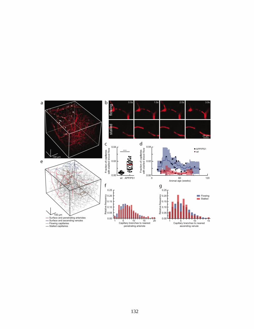
132
133
Figure 4.1. 2PEF imaging of mouse cortical vasculature revealed a higher fraction of
plugged capillaries in APP/PS1 mice.
(a) Rendering of 2PEF image stack of cortical vasculature (red; Texas Red dextran)
and amyloid deposits (white; methoxy-X04). (b) Individual brain capillaries were
scored as flowing or stalled based on the motion of unlabeled blood cells (black)
within the fluorescently labeled blood plasma (red). (c) Fraction of capillaries with
stalled blood flow in APP/PS1 and wt mice. (APP/PS1: n = 28 mice (7 female, 21
male), ~22,400 capillaries, and wt: n = 12 mice (10 female, 2 male), ~9,600 capillaries;
Two-tailed Mann-Whitney, p=6.8 X 10⁻⁹; Boxplot: whiskers extend 1.5 times the
difference between the value of the 75th and 25th percentile, median=black line and
mean= red line.) (d) same data in c shown as a function of animal age. Each data
point represents the fraction of capillaries stalled in one mouse, with a minimum of
800 capillaries scored per mouse. Curves represent sliding averages with a 10-week
window and shaded areas represent 95% confidence intervals. Data from one
outlier mouse not shown in c and d: APP/PS1, 42 weeks, 4.4% stalled. (e) Tracing of
the vascular network in panel a, with stalled capillaries indicated in brown. (f) and (g)
Histograms showing the topological location of flowing and stalled capillaries in
APP/PS1 mice relative to the nearest penetrating arteriole and ascending venule,
respectively (n = 8 mice (5 female, 3 male), 120 stalled and ~8,700 flowing capillaries).

134
Using labeling strategies to distinguish leukocytes, platelets, and RBCs (Figure
4.2.a), we found the majority of stalled capillary segments in APP/PS1 mice contained a
leukocyte, sometimes with and sometimes without one or more RBCs also present in the
capillary segment (Figure 4.2.b). We injected a low dose of fluorescently labeled
antibodies against Ly6G, a neutrophil surface marker (0.1 mg/kg animal weight,
intravenous), and found that the vast majority of capillary stalls had a labeled cell present
(Figure 4.2.c; 26 of 30 identified capillary stalls across four mice were labeled). Stalled
capillaries had a modestly smaller average diameter than flowing capillaries (Figure
4.2.d), but no difference in the density of nearby Aβ deposits (Figure 4.2.e). Most plugged
capillaries were transiently stalled with a half-life of less than 5 min, while one-third
remained stalled for 15 min and 10% began flowing and then re-stalled within 15 min
(Figure 4.2.f; Figure S 4.4). We also observed that some capillary segments alternated
between flowing and stalled in repeated imaging sessions over weeks (Figure 4.2.g). The
same capillaries were stalled across multiple imaging sessions about ten times as
frequently as predicted by a statistical model that assumed each capillary had an equal
probability of being stalled at any time point (Figure 4.2.h). Taken together, these data
suggest that the capillary stalls were caused by leukocytes (likely neutrophils based on
the specificity of Ly6G expression18) plugging a distinct subset of capillary segments.
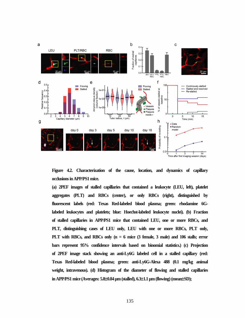
135
Figure 4.2. Characterization of the cause, location, and dynamics of capillary
occlusions in APP/PS1 mice.
(a) 2PEF images of stalled capillaries that contained a leukocyte (LEU, left), platelet
aggregates (PLT) and RBCs (center), or only RBCs (right), distinguished by
fluorescent labels (red: Texas Red-labeled blood plasma; green: rhodamine 6G-
labeled leukocytes and platelets; blue: Hoechst-labeled leukocyte nuclei). (b) Fraction
of stalled capillaries in APP/PS1 mice that contained LEU, one or more RBCs, and
PLT, distinguishing cases of LEU only, LEU with one or more RBCs, PLT only,
PLT with RBCs, and RBCs only (n = 6 mice (3 female, 3 male) and 106 stalls; error
bars represent 95% confidence intervals based on binomial statistics.) (c) Projection
of 2PEF image stack showing an anti-Ly6G labeled cell in a stalled capillary (red:
Texas Red-labeled blood plasma; green: anti-Ly6G-Alexa 488 (0.1 mg/kg animal
weight, intravenous). (d) Histogram of the diameter of flowing and stalled capillaries
in APP/PS1 mice (Averages: 5.80.84 µm (stalled), 6.31.1 µm (flowing) (meanSD);
136
Two-tailed Mann-Whitney, p=0.000020; n = 7 mice (4 female, 3 male), 116 stalled
and ~8,400 flowing capillaries). (e) Violin plot of the density of amyloid deposits
within tubes of different radii that followed the capillary centerline for flowing and
stalled capillary segments in APP/PS1 mice (n = 7 mice (4 female, 3 male), 116 stalled
and ~8,400 flowing capillaries). The vertical range of the violin plot represents the full
range of measured values, while the width of the violin indicates the frequency of
those values. The red (black) horizontal line indicates the mean (median) value. (f)
Fraction of stalled capillaries that remained stalled (red), resumed flowing (green), or
resumed flowing and then re-stalled (blue) over 15 minutes in APP/PS1 mice (n = 3
mice (all male), 31 capillary segments). (g) 2PEF images of the same capillary
alternately stalled (arrows) and flowing over several weeks (white: methoxy-X04). (h)
Probability of an initially stalled capillary to be observed stalled again at any
subsequent imaging time point, showing both real observations in APP/PS1 mice
and predictions from a model that assumed each capillary had an equal probability
of stalling at each time point (n=4 mice (2 female, 2 male), 49 stalled capillaries
followed from the first imaging session).
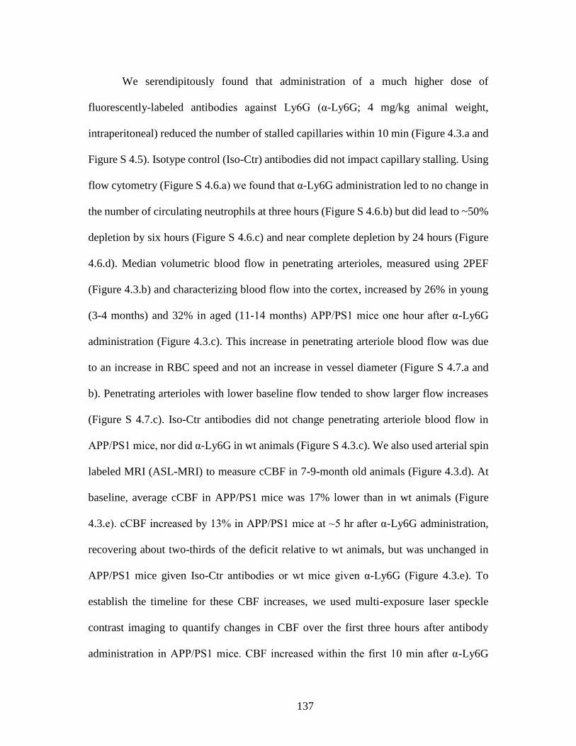
137
We serendipitously found that administration of a much higher dose of
fluorescently-labeled antibodies against Ly6G (α-Ly6G; 4 mg/kg animal weight,
intraperitoneal) reduced the number of stalled capillaries within 10 min (Figure 4.3.a and
Figure S 4.5). Isotype control (Iso-Ctr) antibodies did not impact capillary stalling. Using
flow cytometry (Figure S 4.6.a) we found that α-Ly6G administration led to no change in
the number of circulating neutrophils at three hours (Figure S 4.6.b) but did lead to ~50%
depletion by six hours (Figure S 4.6.c) and near complete depletion by 24 hours (Figure
4.6.d). Median volumetric blood flow in penetrating arterioles, measured using 2PEF
(Figure 4.3.b) and characterizing blood flow into the cortex, increased by 26% in young
(3-4 months) and 32% in aged (11-14 months) APP/PS1 mice one hour after α-Ly6G
administration (Figure 4.3.c). This increase in penetrating arteriole blood flow was due
to an increase in RBC speed and not an increase in vessel diameter (Figure S 4.7.a and
b). Penetrating arterioles with lower baseline flow tended to show larger flow increases
(Figure S 4.7.c). Iso-Ctr antibodies did not change penetrating arteriole blood flow in
APP/PS1 mice, nor did α-Ly6G in wt animals (Figure S 4.3.c). We also used arterial spin
labeled MRI (ASL-MRI) to measure cCBF in 7-9-month old animals (Figure 4.3.d). At
baseline, average cCBF in APP/PS1 mice was 17% lower than in wt animals (Figure
4.3.e). cCBF increased by 13% in APP/PS1 mice at ~5 hr after α-Ly6G administration,
recovering about two-thirds of the deficit relative to wt animals, but was unchanged in
APP/PS1 mice given Iso-Ctr antibodies or wt mice given α-Ly6G (Figure 4.3.e). To
establish the timeline for these CBF increases, we used multi-exposure laser speckle
contrast imaging to quantify changes in CBF over the first three hours after antibody
administration in APP/PS1 mice. CBF increased within the first 10 min after α-Ly6G
138
administration and remained elevated over the three hours (Figure S 4.8). Isotype control
antibodies did not lead to significant changes in CBF (Figure S 4.8). In 5-6-month-old
5xFAD mice we also found that α-Ly6G administration led to a reduction in the number
of stalled capillaries (Figure S 4.2.a) and an increase in blood flow in cortical penetrating
arterioles (Figure S 4.2.b-d) within an hour. Thus, administration of α-Ly6G led to a rapid
reduction in the number of capillary stalls that was accompanied by a rapid increase in
cCBF in APP/PS1 and 5xFAD mice. In contrast, when antibodies against LFA-1 were
administered to 11-13-month-old APP/PS1 mice, we did not observe a rapid decrease in
the number of stalled capillaries. Instead, we found that capillary stalls were reduced, and
penetrating arteriole blood flow was increased at one day after antibody injection, when
circulating leukocytes had been depleted (Figure S 4.9). Across all antibody and control
treatments in APP/PS1 mice, penetrating arteriole flows increased (decreased) when the
number of stalled capillaries decreased (increased) (Figure S 4.9.g).
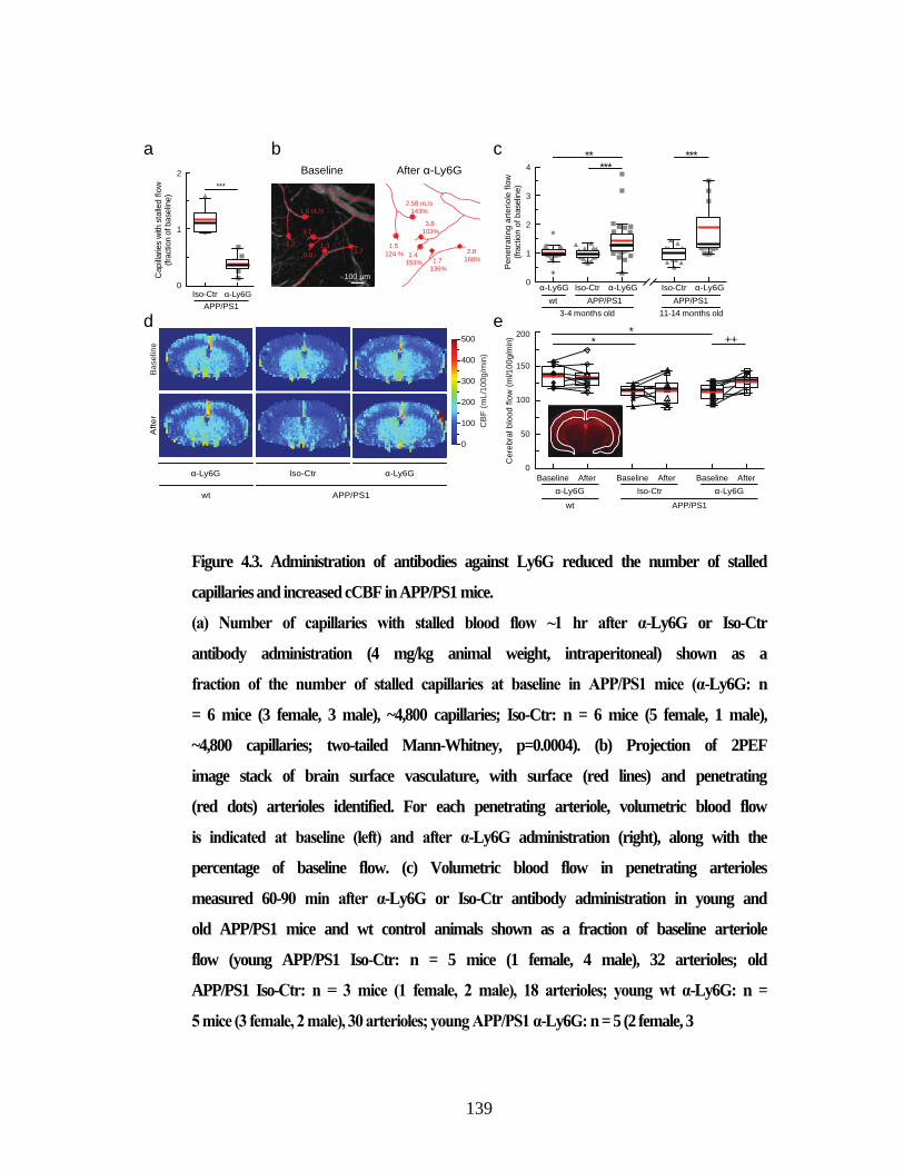
139
Figure 4.3. Administration of antibodies against Ly6G reduced the number of stalled
capillaries and increased cCBF in APP/PS1 mice.
(a) Number of capillaries with stalled blood flow ~1 hr after α-Ly6G or Iso-Ctr
antibody administration (4 mg/kg animal weight, intraperitoneal) shown as a
fraction of the number of stalled capillaries at baseline in APP/PS1 mice (α-Ly6G: n
= 6 mice (3 female, 3 male), ~4,800 capillaries; Iso-Ctr: n = 6 mice (5 female, 1 male),
~4,800 capillaries; two-tailed Mann-Whitney, p=0.0004). (b) Projection of 2PEF
image stack of brain surface vasculature, with surface (red lines) and penetrating
(red dots) arterioles identified. For each penetrating arteriole, volumetric blood flow
is indicated at baseline (left) and after α-Ly6G administration (right), along with the
percentage of baseline flow. (c) Volumetric blood flow in penetrating arterioles
measured 60-90 min after α-Ly6G or Iso-Ctr antibody administration in young and
old APP/PS1 mice and wt control animals shown as a fraction of baseline arteriole
flow (young APP/PS1 Iso-Ctr: n = 5 mice (1 female, 4 male), 32 arterioles; old
APP/PS1 Iso-Ctr: n = 3 mice (1 female, 2 male), 18 arterioles; young wt α-Ly6G: n =
5 mice (3 female, 2 male), 30 arterioles; young APP/PS1 α-Ly6G: n = 5 (2 female, 3
2.58 nL/s
143%
1.5
124 %
3.8
103%
1.4
153% 1.7
136%
2.8
160%
1.8 nL/s
1.2
3.7
0.9
1.3 1.7
Baseline After α-Ly6G
b
100 μm
e++
**
0
50
100
150
200
Ce
reb
ral b
loo
d f
low
(m
l/10
0g/m
in)
wt APP/PS1
α-Ly6G Iso-Ctr α-Ly6G
BaselineBaseline BaselineAfter After After
c
0
1
2
3
4
Pe
ne
tra
tin
g a
rte
rio
le f
low
(fra
ctio
n o
f b
aselin
e)
*****
3-4 months old
α-Ly6G Iso-Ctr α-Ly6G
wt
11-14 months old
Iso-Ctr α-Ly6G
***
APP/PS1 APP/PS1
a
0
1
2
Cap
illaries w
ith s
talle
d f
low
(fra
ctio
n o
f base
line)
***
APP/PS1
Iso-Ctr α-Ly6G
d
Ba
se
line
Aft
er
wt APP/PS1
Iso-Ctr α-Ly6Gα-Ly6G C
BF
(m
L/1
00
g/m
in)
0
100
200
300
400
500
140
male), 33 arterioles; old APP/PS1 α-Ly6G: n = 3 mice (all male), 22 arterioles; one-
way Kruskal-Wallis ANOVA with post-hoc using Dunn’s multiple comparison
correction: young wt α-Ly6G vs. young APP/PS1 α-Ly6G p = 0.0023; young
APP/PS1 Iso-Ctr vs. young APP/PS1 α-Ly6G p = 0.0000012; old APP/PS1 Iso-Ctr
vs. old APP/PS1 α-Ly6G p = 0.00055). (d) CBF map measured using ASL-MRI at
baseline and ~5 hr after administration of α-Ly6G or Iso-Ctr antibodies in APP/PS1
and wt mice. (e) cCBF measurements (ASL-MRI, inset indicates ROI on T2 MRI
image) at baseline and ~5 hr after administration of α-Ly6G or Iso-Ctr antibodies in
APP/PS1 and wt mice (wt α-Ly6G: n = 10 mice, APP/PS1 α-Ly6G: n = 10 mice,
APP/PS1 Iso-Ctr: n = 10 mice; Ordinary one-way ANOVA with post hoc using
Tukey’s multiple comparison correction to compare across groups: baseline wt α-
Ly6G vs. baseline APP/PS1 α-Ly6G p=0.011; baseline wt α-Ly6G vs. baseline
APP/PS1 Iso-Ctr p=0.014; Paired t-test to compare baseline and after treatment
within a group: baseline APP/PS1 α-Ly6G vs. after APP/PS1 α-Ly6G p=0.0058). All
boxplots are defined as: whiskers extend 1.5 times the difference between the value of
the 75th and 25th percentile, median=black line and mean= red line.

141
We next tested whether α-Ly6G administration improves cognitive function in
APP/PS1 (Figure 4.4.a) and 5xFAD mice. In the object replacement (OR) test of spatial
short-term memory (Figure 4.4.b), a single dose of α-Ly6G in ~11-month old APP/PS1
mice improved performance to the level of wt animals at 3 and 24 hours after
administration (Figure 4.4.c; Figure S 4.10.a). APP/PS1 mice treated with Iso-Ctr
antibodies showed no change, nor did wt animals with α-Ly6G (Figure 4.4.c). In ~ 6-
month-old 5xFAD mice, a single dose of α-Ly6G improved animal performance in the
OR task at 24 hours, with this trend evident at 3 hours (Figure 4.11.a and b). Similarly,
α-Ly6G improved performance of APP/PS1 and 5xFAD mice in the Y-maze test of
working memory (Figure 4.4d, Figure S 4.10.b, and Figure S 4.11.c and d). We detected
no improvement in sensory-motor function (balance beam walk, Figure S 4.12.a-d) nor
in depression- and anxiety-like behavior (forced swim, Figure S 4.12.e) in APP/PS1 mice
with α-Ly6G. To exclude an antibody specific effect we repeated the OR and Y-maze
behavioral tests in another cohort of APP/PS1 mice before and after administration of α-
LFA-1 antibodies and found improved performance on both tests at 24 hours (Figure S
4.13.a-d).
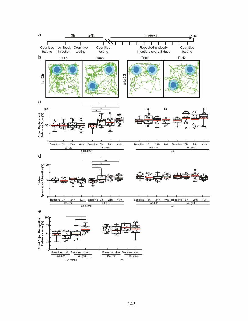
142
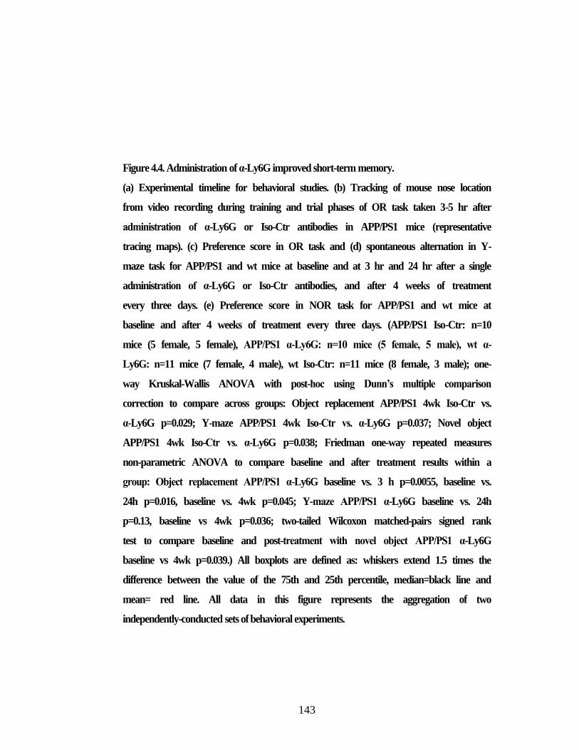
143
Figure 4.4. Administration of α-Ly6G improved short-term memory.
(a) Experimental timeline for behavioral studies. (b) Tracking of mouse nose location
from video recording during training and trial phases of OR task taken 3-5 hr after
administration of α-Ly6G or Iso-Ctr antibodies in APP/PS1 mice (representative
tracing maps). (c) Preference score in OR task and (d) spontaneous alternation in Y-
maze task for APP/PS1 and wt mice at baseline and at 3 hr and 24 hr after a single
administration of α-Ly6G or Iso-Ctr antibodies, and after 4 weeks of treatment
every three days. (e) Preference score in NOR task for APP/PS1 and wt mice at
baseline and after 4 weeks of treatment every three days. (APP/PS1 Iso-Ctr: n=10
mice (5 female, 5 female), APP/PS1 α-Ly6G: n=10 mice (5 female, 5 male), wt α-
Ly6G: n=11 mice (7 female, 4 male), wt Iso-Ctr: n=11 mice (8 female, 3 male); one-
way Kruskal-Wallis ANOVA with post-hoc using Dunn’s multiple comparison
correction to compare across groups: Object replacement APP/PS1 4wk Iso-Ctr vs.
α-Ly6G p=0.029; Y-maze APP/PS1 4wk Iso-Ctr vs. α-Ly6G p=0.037; Novel object
APP/PS1 4wk Iso-Ctr vs. α-Ly6G p=0.038; Friedman one-way repeated measures
non-parametric ANOVA to compare baseline and after treatment results within a
group: Object replacement APP/PS1 α-Ly6G baseline vs. 3 h p=0.0055, baseline vs.
24h p=0.016, baseline vs. 4wk p=0.045; Y-maze APP/PS1 α-Ly6G baseline vs. 24h
p=0.13, baseline vs 4wk p=0.036; two-tailed Wilcoxon matched-pairs signed rank
test to compare baseline and post-treatment with novel object APP/PS1 α-Ly6G
baseline vs 4wk p=0.039.) All boxplots are defined as: whiskers extend 1.5 times the
difference between the value of the 75th and 25th percentile, median=black line and
mean= red line. All data in this figure represents the aggregation of two
independently-conducted sets of behavioral experiments.

144
We continued to treat the APP/PS1 mice that received α-Ly6G with additional
doses of α-Ly6G every three days for a month, resulting in depletion of neutrophils
(Figure S 4.6.e). After this regimen, APP/PS1 mice exhibited short-term memory
performance that matched wt animals in OR (Figure 4.4.c), Y-maze (Figure 4.4.d), and
novel object recognition (NOR) (Figure 4.4.e; Figure S 4.10.c and d). We saw no
improvement in sensory-motor function (Figure S 4.12.a-d) nor in depression- and
anxiety-like behavior (Figure S 4.12.e).
Because one of the clearance pathways for Aβ is through the vasculature19 we
assessed whether improving cCBF with α-Ly6G decreases the concentration of Aβ
monomers and aggregates. Using enzyme-linked immunosorbent assays (ELISAs) of
brain extracts from the animals that received one month of antibody treatment, we found
that α-Ly6G reduced the concentration of Aβ1-40 compared to Iso-Ctr antibodies (Figure
4.5.a), while the concentration of Aβ1-42 (Figure 4.5.b) and aggregates of Aβ (Figure S
4.14.d) remained unchanged. We saw no difference in the number and density of Aβ
plaques between α-Ly6G and Iso-Ctr treated animals (Figure S 4.14.a – c).
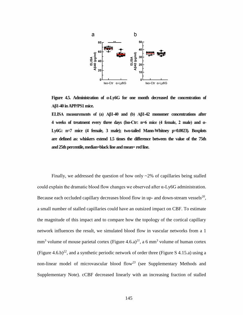
145
Figure 4.5. Administration of α-Ly6G for one month decreased the concentration of
Aβ1-40 in APP/PS1 mice.
ELISA measurements of (a) Aβ1-40 and (b) Aβ1-42 monomer concentrations after
4 weeks of treatment every three days (Iso-Ctr: n=6 mice (4 female, 2 male) and α-
Ly6G: n=7 mice (4 female, 3 male); two-tailed Mann-Whitney p=0.0023). Boxplots
are defined as: whiskers extend 1.5 times the difference between the value of the 75th
and 25th percentile, median=black line and mean= red line.
Finally, we addressed the question of how only ~2% of capillaries being stalled
could explain the dramatic blood flow changes we observed after α-Ly6G administration.
Because each occluded capillary decreases blood flow in up- and down-stream vessels20,
a small number of stalled capillaries could have an outsized impact on CBF. To estimate
the magnitude of this impact and to compare how the topology of the cortical capillary
network influences the result, we simulated blood flow in vascular networks from a 1
mm3 volume of mouse parietal cortex (Figure 4.6.a)21, a 6 mm3 volume of human cortex
(Figure 4.6.b)22, and a synthetic periodic network of order three (Figure S 4.15.a) using a
non-linear model of microvascular blood flow23 (see Supplementary Methods and
Supplementary Note). cCBF decreased linearly with an increasing fraction of stalled
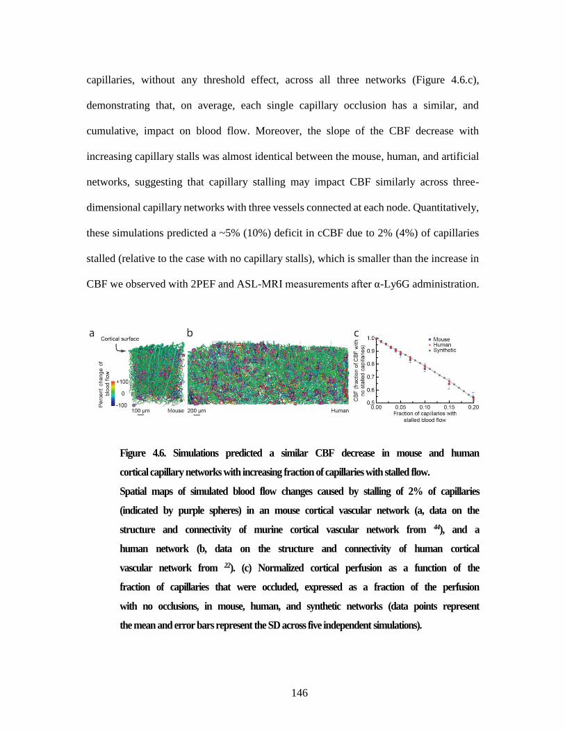
146
capillaries, without any threshold effect, across all three networks (Figure 4.6.c),
demonstrating that, on average, each single capillary occlusion has a similar, and
cumulative, impact on blood flow. Moreover, the slope of the CBF decrease with
increasing capillary stalls was almost identical between the mouse, human, and artificial
networks, suggesting that capillary stalling may impact CBF similarly across three-
dimensional capillary networks with three vessels connected at each node. Quantitatively,
these simulations predicted a ~5% (10%) deficit in cCBF due to 2% (4%) of capillaries
stalled (relative to the case with no capillary stalls), which is smaller than the increase in
CBF we observed with 2PEF and ASL-MRI measurements after α-Ly6G administration.
Figure 4.6. Simulations predicted a similar CBF decrease in mouse and human
cortical capillary networks with increasing fraction of capillaries with stalled flow.
Spatial maps of simulated blood flow changes caused by stalling of 2% of capillaries
(indicated by purple spheres) in an mouse cortical vascular network (a, data on the
structure and connectivity of murine cortical vascular network from 44), and a
human network (b, data on the structure and connectivity of human cortical
vascular network from 22). (c) Normalized cortical perfusion as a function of the
fraction of capillaries that were occluded, expressed as a fraction of the perfusion
with no occlusions, in mouse, human, and synthetic networks (data points represent
the mean and error bars represent the SD across five independent simulations).
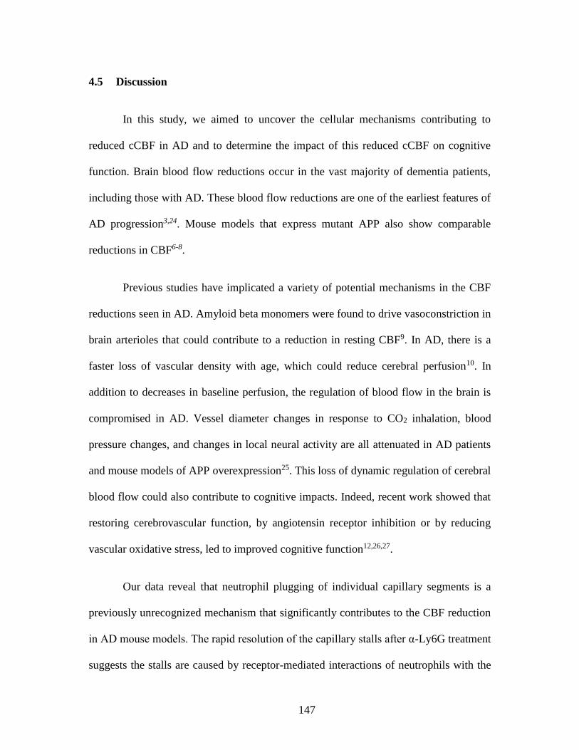
147
4.5 Discussion
In this study, we aimed to uncover the cellular mechanisms contributing to
reduced cCBF in AD and to determine the impact of this reduced cCBF on cognitive
function. Brain blood flow reductions occur in the vast majority of dementia patients,
including those with AD. These blood flow reductions are one of the earliest features of
AD progression3,24. Mouse models that express mutant APP also show comparable
reductions in CBF6-8.
Previous studies have implicated a variety of potential mechanisms in the CBF
reductions seen in AD. Amyloid beta monomers were found to drive vasoconstriction in
brain arterioles that could contribute to a reduction in resting CBF9. In AD, there is a
faster loss of vascular density with age, which could reduce cerebral perfusion10. In
addition to decreases in baseline perfusion, the regulation of blood flow in the brain is
compromised in AD. Vessel diameter changes in response to CO2 inhalation, blood
pressure changes, and changes in local neural activity are all attenuated in AD patients
and mouse models of APP overexpression25. This loss of dynamic regulation of cerebral
blood flow could also contribute to cognitive impacts. Indeed, recent work showed that
restoring cerebrovascular function, by angiotensin receptor inhibition or by reducing
vascular oxidative stress, led to improved cognitive function12,26,27.
Our data reveal that neutrophil plugging of individual capillary segments is a
previously unrecognized mechanism that significantly contributes to the CBF reduction
in AD mouse models. The rapid resolution of the capillary stalls after α-Ly6G treatment
suggests the stalls are caused by receptor-mediated interactions of neutrophils with the
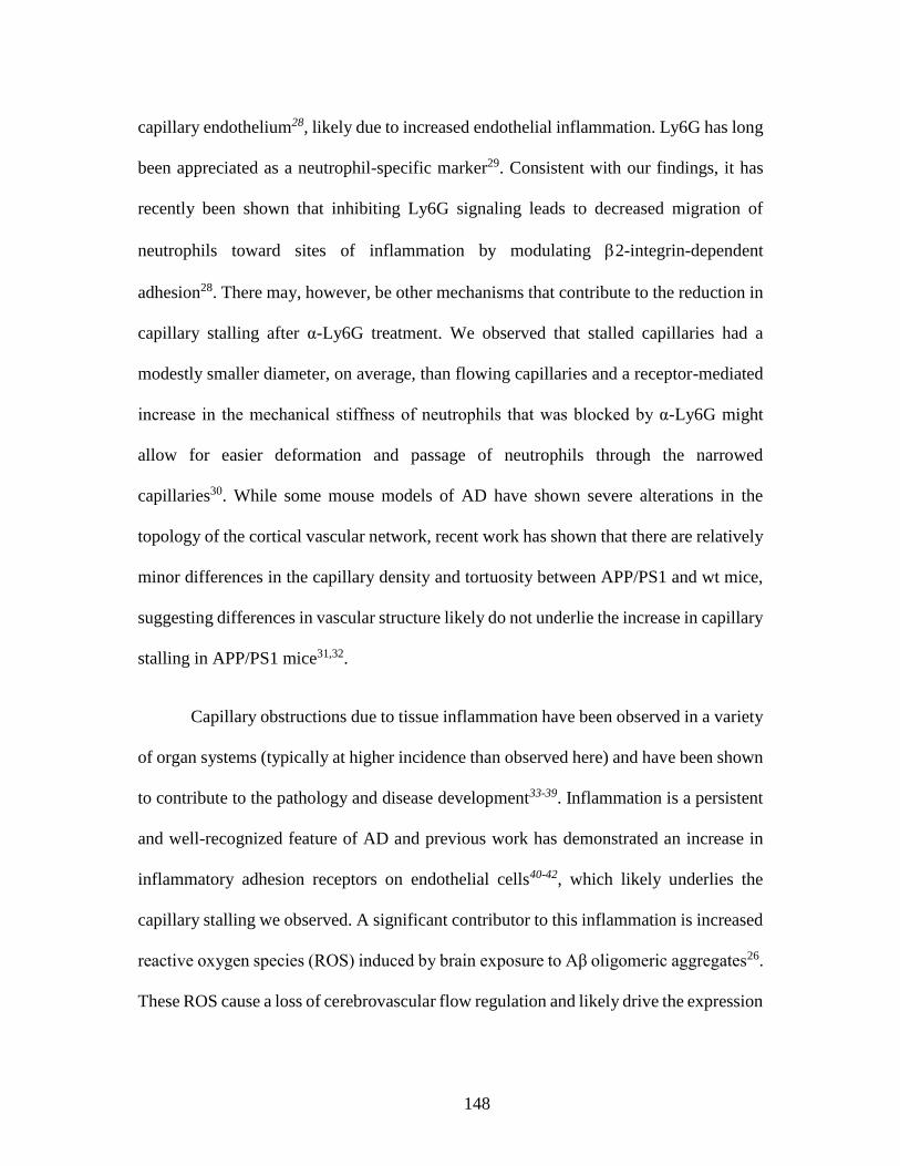
148
capillary endothelium28, likely due to increased endothelial inflammation. Ly6G has long
been appreciated as a neutrophil-specific marker29. Consistent with our findings, it has
recently been shown that inhibiting Ly6G signaling leads to decreased migration of
neutrophils toward sites of inflammation by modulating 2-integrin-dependent
adhesion28. There may, however, be other mechanisms that contribute to the reduction in
capillary stalling after α-Ly6G treatment. We observed that stalled capillaries had a
modestly smaller diameter, on average, than flowing capillaries and a receptor-mediated
increase in the mechanical stiffness of neutrophils that was blocked by α-Ly6G might
allow for easier deformation and passage of neutrophils through the narrowed
capillaries30. While some mouse models of AD have shown severe alterations in the
topology of the cortical vascular network, recent work has shown that there are relatively
minor differences in the capillary density and tortuosity between APP/PS1 and wt mice,
suggesting differences in vascular structure likely do not underlie the increase in capillary
stalling in APP/PS1 mice31,32.
Capillary obstructions due to tissue inflammation have been observed in a variety
of organ systems (typically at higher incidence than observed here) and have been shown
to contribute to the pathology and disease development33-39. Inflammation is a persistent
and well-recognized feature of AD and previous work has demonstrated an increase in
inflammatory adhesion receptors on endothelial cells40-42, which likely underlies the
capillary stalling we observed. A significant contributor to this inflammation is increased
reactive oxygen species (ROS) induced by brain exposure to Aβ oligomeric aggregates26.
These ROS cause a loss of cerebrovascular flow regulation and likely drive the expression

149
of leucocyte-binding receptors on the endothelial cell surface, such as ICAM1 and
VCAM1. Our observation that some capillary segments were more likely to stall suggests
that the underlying vascular inflammation may not be uniform.
While here our focus has been on increased leukocyte adherence causing a subset
of capillaries to be transiently stalled due to a firmly adhered leukocyte, this increased
leukocyte adherence likely also contributes to slowed, but not stalled, flow in other
capillary segments when a leukocyte is present. Our experimental approach does not
enable us to readily detect such slowed vessels. Our simulations included only the impact
of completely stalled vessels, which may have contributed to the model’s underestimation
of the increase in CBF after α-Ly6G administration. However, the simulations predicted
a similar sensitivity of brain blood flow to capillary stalling in humans and mice,
suggesting that, if capillary stalling occurs in AD patients, significant blood flow
improvements could be achieved.
We observed spatial and working memory improvements within 24 hours after
treatment with antibodies against Ly6G and/or LFA-1 in multiple mouse models of AD.
The temporal correlation between reduced capillary stalling/blood flow increase and the
improvement in cognitive function suggests that a mismatch between neuronal energy
metabolism and delivery of energy substrates through blood flow contributes to the
cognitive deficit in these AD mouse models.
We also observed improved cognitive function after one month of treatment with
α-Ly6G, which depletes neutrophils, in APP/PS1 mice, measured during the antibody
therapy. Because of the persistent depletion of neutrophils during this treatment, we
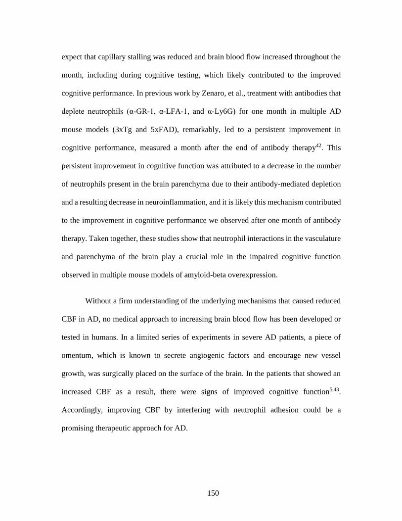
150
expect that capillary stalling was reduced and brain blood flow increased throughout the
month, including during cognitive testing, which likely contributed to the improved
cognitive performance. In previous work by Zenaro, et al., treatment with antibodies that
deplete neutrophils (α-GR-1, α-LFA-1, and α-Ly6G) for one month in multiple AD
mouse models (3xTg and 5xFAD), remarkably, led to a persistent improvement in
cognitive performance, measured a month after the end of antibody therapy42. This
persistent improvement in cognitive function was attributed to a decrease in the number
of neutrophils present in the brain parenchyma due to their antibody-mediated depletion
and a resulting decrease in neuroinflammation, and it is likely this mechanism contributed
to the improvement in cognitive performance we observed after one month of antibody
therapy. Taken together, these studies show that neutrophil interactions in the vasculature
and parenchyma of the brain play a crucial role in the impaired cognitive function
observed in multiple mouse models of amyloid-beta overexpression.
Without a firm understanding of the underlying mechanisms that caused reduced
CBF in AD, no medical approach to increasing brain blood flow has been developed or
tested in humans. In a limited series of experiments in severe AD patients, a piece of
omentum, which is known to secrete angiogenic factors and encourage new vessel
growth, was surgically placed on the surface of the brain. In the patients that showed an
increased CBF as a result, there were signs of improved cognitive function5,43.
Accordingly, improving CBF by interfering with neutrophil adhesion could be a
promising therapeutic approach for AD.
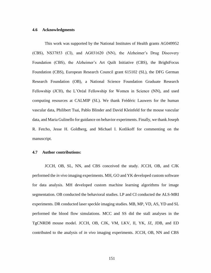
151
4.6 Acknowledgments
This work was supported by the National Institutes of Health grants AG049952
(CBS), NS37853 (CI), and AG031620 (NN), the Alzheimer’s Drug Discovery
Foundation (CBS), the Alzheimer’s Art Quilt Initiative (CBS), the BrightFocus
Foundation (CBS), European Research Council grant 615102 (SL), the DFG German
Research Foundation (OB), a National Science Foundation Graduate Research
Fellowship (JCH), the L’Oréal Fellowship for Women in Science (NN), and used
computing resources at CALMIP (SL). We thank Frédéric Lauwers for the human
vascular data, Philibert Tsai, Pablo Blinder and David Kleinfeld for the mouse vascular
data, and Maria Gulinello for guidance on behavior experiments. Finally, we thank Joseph
R. Fetcho, Jesse H. Goldberg, and Michael I. Kotlikoff for commenting on the
manuscript.
4.7 Author contributions:
JCCH, OB, SL, NN, and CBS conceived the study. JCCH, OB, and CJK
performed the in vivo imaging experiments. MH, GO and YK developed custom software
for data analysis. MH developed custom machine learning algorithms for image
segmentation. OB conducted the behavioral studies. LP and CI conducted the ALS-MRI
experiments. DR conducted laser speckle imaging studies. MB, MP, VD, AS, YD and SL
performed the blood flow simulations. MCC and SS did the stall analyses in the
TgCNRD8 mouse model. JCCH, OB, CJK, VM, LKV, II, YK, JZ, JDB, and ED
contributed to the analysis of in vivo imaging experiments. JCCH, OB, NN and CBS

152
wrote the paper with contributions from MH, MCC, LP, CL, CI, and SL. All authors
edited and commented on the manuscript.
4.8 Competing interests statement
The authors declare no competing interests.
4.9 Methods
4.9.1 Animals and surgical preparation
All animal procedures were approved by the Cornell Institutional Animal Care
and Use Committee (protocol numbers: 2009-0043 and 2015-0029) and were performed
under the guidance of the Cornell Center for Animal Resources and Education. We used
adult transgenic mice as mouse models of AD, including the APP/PS1 line (B6.Cg-Tg
(APPswe, PSEN1dE9) 85Dbo/J; MMRRC_034832-JAX, The Jackson Laboratory)45 and
the 5xFAD line (B6SJL-Tg(APPSwFlLon,PSEN1 *M146L*L286V)6799Vas/Mmjax;
MMRRC Stock No: 34840-JAX, The Jackson Laboratory)46. Littermate wild-type mice
(C57BL/6) were used as controls. Animals were of both sexes and ranged in age from 12
to 100 weeks.
For cranial window implantation, mice were anesthetized under 3% isoflurane on
a custom-built stereotactic surgery frame and then maintained on ~1.5% isoflurane in
100% oxygen. Once unresponsive to a toe pinch, mice were given 0.05 mg per 100 g of
mouse weight of glycopyrrolate (Baxter Inc.) or 0.005 mg/100 g of atropine (54925-063-
10, Med-Pharmex Inc.) to prevent lung secretions, 0.025 mg/100 g of dexamethasone
153
(07-808-8194, Phoenix Pharm Inc.) to reduce post-surgical inflammation, and 0.5 mg/100
g of ketoprofen (Zoetis Inc.) to reduce post-surgical inflammation and provide post-
surgical analgesia. Glycopyrrolate and ketoprofen were injected intramuscularly, while
atropine and dexamethasone were injected subcutaneously. Bupivacaine (0.1 ml, 0.125%)
(Hospira Inc.) was subcutaneously administered at the incision site to provide a local
nerve block. Animals were provided 1 ml per 100 g of mouse weight of 5% (w/v) glucose
in normal saline subcutaneously every hour during the procedure. We used a thermometer
and feedback-controlled heating blanket (40-90-8D DC, FHC) to maintain body
temperature at 37 °C. The head was shaved and washed 3 times with alternating 70%
(v/v) ethanol and iodine solutions (AgriLabs). A 6-mm diameter craniotomy was
performed over the cerebral cortex using a high-speed drill (HP4-917-21, Fordom) using
bits with diameters of 1.4, 0.9, 0.7, and 0.5 mm (Fine Science Tools) for different steps
in the craniotomy procedure. The craniotomy was then covered with a sterile 8-mm
diameter glass coverslip (11986309, Thermo Scientific), glued onto the remaining skull
with cyanoacrylate adhesive (Loctite) and dental cement (Co-Oral-Ite Dental). All
procedures were done using sterile technique.
Once the craniotomy was completed, mice were returned to their cages and given
injections of 0.025 mg/100 g of dexamethasone and 0.5 mg/100 g of ketoprofen
subcutaneously 1 and 2 days after surgery, and all cages were placed over a heating pad
during this period. Animals were given at least two weeks to recover from cranial window
implantation before experimentation to minimize inflammation from the surgical
procedure. Animals were excluded from further study if the clarity of the imaging window
was insufficient for 2PEF imaging.
154
4.9.2 In vivo two-photon microscopy
During imaging sessions, mice were anesthetized with 3% isoflurane, placed on a
custom stereotactic frame, and were given glycopyrrolate or atropine and glucose as
described above. During imaging, anesthesia was maintained with ~1.5% isoflurane in
100% oxygen, with small adjustments to the isoflurane made to maintain the respiratory
rate at ~1 Hz. The mouse was kept at 37 °C with a feedback-controlled heating pad.
To fluorescently label the microvasculature, Texas Red dextran (40 μl, 2.5%, MW
= 70,000 kDA, Thermo Fisher Scientific) in saline was injected retro-orbitally
immediately prior to imaging. In some animals, amyloid beta (Aβ) deposits were labeled
using methoxy-X0447. In early experiments using methoxy-X04 obtained directly from
Prof. Klunk at the University of Pittsburgh, we retro-orbitally injected 40 µL of 1 mg/ml
methoxy-X04 in 0.9% saline (adjusted to pH 12 with 0.1 N NaOH) immediately prior to
imaging. In later experiments using methoxy-X04 available commercially from Tocris,
we intraperitoneally injected methoxy-X04 (dissolved in DMSO at 100 mM) one day
prior to imaging at a dose of 1 mg/100 g. We observed no obvious differences in the
amyloid labeling between these two administration approaches. In some animals,
leukocytes and blood platelets were labeled with a retro-orbital injection of Rhodamine
6G (0.1 ml, 1 mg/ml in 0.9% saline, Acros Organics, Pure)38. Leukocytes were
distinguished from blood platelets with a retro-orbital injection of Hoechst 33342 (50 μl,
4.8 mg/ml in 0.9% saline, Thermo Fisher Scientific). Texas Red (and methoxy-X04, when
given retro-orbitally) were dosed in a single syringe, while Rhodamine 6G and Hoechst
were dosed together in a second syringe.
155
Three-dimensional images of the cortical vasculature and measurement of red
blood cell flow speeds in specific vessels were obtained via a custom-built two-photon
excited fluorescence (2PEF) microscope. Imaging was done using 830-nm, 75-fs pulses
from a Ti:Sapphire laser oscillator (MIRA HP pumped by a Verdi-V18 or Vision S,
Coherent) and 900-nm, 75-fs pulses from a second Ti:Sapphire laser oscillator (Vision S,
Coherent). Lasers were scanned by galvonometric scanners (1 frame/s) and focused into
the sample using a 20× water-immersion objective lens for high-resolution imaging
(numerical aperture (NA) = 1.0, Carl Zeiss Microscopy; or NA = 0.95, Olympus), or a 4×
objective for mapping of the cortical surface vasculature (NA = 0.28, Olympus). The
emitted fluorescence was detected on either a two-channel detection system or, for later
data sets, on an upgraded four-channel detection system. On the two-channel system, the
fluorescence was split by a 600-nm long pass dichroic and two successive image stacks
were acquired first with 645/45 nm (center wavelength/bandwidth) and 575/25 nm
bandpass filters to image Texas Red and Rhodamine 6G, respectively, and then with
645/65 nm and 460/50 nm filters to image Texas Red and both methoxy-X04 and Hoescht
(on the same channel), all under 830-nm excitation. On the four-channel system, a
secondary long-pass dichroic at 520 nm was followed by tertiary long-pass dichroics at
458 nm and one at either 562 or 605 nm. Emission was detected on four photomultiplier
tubes through the following emission filters: 417/60 nm for Hoechst, 494/41 nm for
methoxy-X04, 550/49 nm for Rhodamine 6G, and 641/75 nm for Texas Red. Laser
excitation was 830 nm except when trying to image deep cortical tissue in animals where
only Texas Red was present in which case 900-nm excitation was used. Laser scanning
and data acquisition was controlled by ScanImage software48. To visualize the cortical
156
vasculature, stacks of images spaced by 1 μm axially were taken to a cortical depth of
300-500 μm.
For imaging of neutrophils labeled with anti-Ly6G antibodies labeled with
Alexa488, imaging was performed on a custom-built 2PEF microscope at the Wellman
Center for Photomedicine. In these animals, neutrophils were labeled with a tail vein
injection of anti-Ly6G-Alexa 488 (0.1 mg/kg animal weight, 127626-Biolegend) at the
same time as the labeling of blood plasma with Texas Red dextran. Imaging was done
using 750-nm, 80-fs pulses from a Ti:Sapphire laser oscillator (Spectra-Physics Mai Tai).
The laser beam was scanned by polygon scanners (30 frames/s) and focused into the
sample using a 40x water-immersion objective lens for high-resolution imaging (NA =
0.80, Olympus), or a 10x objective for mapping of the cortical surface vasculature (NA
= 0.30, Olympus). The emitted fluorescence was detected on photomultiplier tubes
through the following emission filters: 525/50 nm for Alexa-488 and 605/50 nm for Texas
Red. Laser scanning and data acquisition was controlled by custom built software. Stacks
of images spaced by 1 μm axially were taken to a cortical depth of 100-200 μm.
4.9.3 Quantification of capillary network topology and capillary segment stalling
The 2PEF images of vascular networks were manually traced in three-dimensions
to create a vectorized skeleton that represents the cortical vasculature using custom-
written tracing software. The researchers producing these tracings were blinded to the
genotype of the animal and any treatment it had received. Volumes of these image stacks
where vessels could not be readily identified and traced were excluded from all analysis.
These regions were typically deep and near the edges of the imaged volume, or
157
occasionally directly underneath a large surface vessel. Vessel segments were classified
as surface and penetrating arterioles, capillaries, or ascending and surface venules. All
vessels smaller than 10 µm in diameter were classed as capillaries. Large surface
arterioles were distinguished from large surface venules based on morphology (arterioles
were smaller diameter, had smoother walls and less tortuosity, and tended to branch more
symmetrically and in Y-shape junctions as compared to venules). Other arterioles or
venules were classed by tracing their connectivity to these readily identifiable large
vessels.
Each capillary segment in these images was then manually classed as either
flowing or stalled based on the motion of RBCs during the entire time each capillary was
visible in the 3D image stack. The Texas Red dextran labels the blood plasma, but not the
blood cells, so RBCs and other blood cells show up as dark patches in the vessel lumen.
The motion of these dark patches indicates flowing blood cells. Each capillary segment
was visible in a minimum of ~5 successive frames in the 3D image stack, or for ~5 s
(capillaries not oriented parallel to the cortical surface were observed for significantly
more frames). We scored a capillary segment as stalled if we did not see motion of the
RBCs and other cells in the capillary segment over this observation time. This manual
scoring of capillaries as flowing or stalled was performed with the researcher blinded to
the genotype and treatment status of the animal. In addition, this scoring was performed
using only the image data visible on the Texas Red imaging channel. All animals included
in our analysis had at least 800 capillary segments scored as flowing or stalled. Animals
with fewer characterized capillaries were excluded.

158
Using the traced vascular network, the topologically shortest path from each
flowing or stalled capillary to the nearest penetrating arteriole and ascending
venule was calculated using Dijkstra's algorithm49.
4.9.4 Distinguishing causes of capillary stalls
In some animals, once capillary stalls were identified we used the additional
fluorescent labels to determine what was blocking blood flow in the capillary segment.
Stalled capillary segments with a cell-shaped object labeled with both Rhodamine 6G and
Hoechst present were scored as having a leukocyte. Stalled segments with punctate
objects labeled with Rhodamine 6G alone were scored as having platelet aggregates.
Stalled capillary segments with only RBCs present were classed as RBC stalls. We
determined what fraction of stalled capillaries had only a leukocyte, a leukocyte with one
or more RBCs present, only platelet aggregates, platelet aggregates with RBCs, and only
RBCs. With this labeling scheme, we were unable to reliably distinguish platelet
aggregates when a leukocyte was present. Additional experiments used a low-dose of
Alexa 488 labeled anti-Ly6G antibodies to assess the type of leukocyte associated with
capillary stalls.
We assessed if the diameter of flowing and stalled capillaries was different, on
average. First, image stacks were linearly interpolated to have an isotropic 1 µm voxel
size. To reduce the salt and pepper noise in the vascular images, we filtered using a 3D 5
x 5 x 5 pixel Gaussian filter. We then corrected for unevenness in the image intensity by
filtering the image (85 x 85 pixel sized mean filter) and subtracting this from the Gaussian
filtered image. The resulting image was binarized using Otsu’s method50. Finally, objects
159
smaller than 1000 voxels were eliminated, where voxels were considered part of the same
connected object whenever they shared at least a corner. We then used this binarized
image to correct the manual tracing of the vasculature by shifting the centerline, so it was
equidistant from the vessel boundaries (done within a 10-µm neighborhood to avoid
confusion between neighboring capillaries). Every 5 µm along the centerline of each
capillary segment, we estimated the vessel radius by finding the closest distance from the
centerline to the vessel boundary. Measurements of less than 2 µm or more than 10 µm
were excluded as they likely reflected imaging artifacts, and we averaged across all
measurements for each capillary segment.
4.9.5 Administration of antibodies against Ly6G or LFA-1 to interfere with capillary
stalling
We treated APP/PS1 and 5xFAD mice with intraperitoneal injections of
monoclonal antibodies against lymphocyte antigen 6 complex, locus G (Ly6G) (α-Ly6G,
clone 1A8, 4 mg/kg, BD Biosciences) or an isotype control antibody (Rat IgG2a, κ, 4
mg/kg, BD Biosciences). In addition, APP/PS1 mice were treated with retroorbital or
intraperitoneal injections of monoclonal antibodies against Lymphocyte Functional
Antigen 1 (α-LFA-1; M17/4 clone, BD Biosciences; 4 mg/kg). The same cortical
capillary bed was imaged in anesthetized mice immediately before and at 60-90 min after
treatment. Mice were randomly assigned to receive treatment or isotype control
antibodies and the experimenter was blinded to both mouse genotype and whether the
antibody was the treatment or control during the experiment. Quantification of stalled
160
capillaries was performed by researchers blinded to imaging time, animal genotype, and
treatment type.
4.9.6 Behavior experiments
All experiments were performed under red light in an isolated room. The position
of the mouse’s nose was automatically traced by Viewer III software (Biobserve, Bonn,
Germany). In addition to the automatic results obtained by Viewer III software, a blinded
experimenter independently scored mouse behavior manually. Animals were taken into
the behavior room one-hour prior to the experiment. Behavioral analysis was conducted
at baseline and at 3 and 24 h after injection with α-Ly6G, α-LFA-1, or isotype control
antibodies (IP 4 mg/kg). The α-Ly6G treated APP/PS1 mice were then treated every three
days for four weeks (IP 2 mg/kg) and behavior experiments were repeated. The OR, Y-
maze, balance beam walk, and forced swim tests were performed at all time points. The
NOR task was performed only at baseline and the 4-week time point to avoid animals
becoming accustomed to the objects. For experiments with APP/PS1 mice and α-Ly6G,
animals were ~11 months of age at the start of the experiment. For experiments with
APP/PS1 mice and α-LFA-1, animals were 11-13 months of age. For experiments with
5xFAD mice and α-Ly6G, animals were 5-6 months of age. Mice were randomly assigned
to receive treatment or isotype control antibodies and the experimenter was blinded to
both mouse genotype and whether the antibody was the treatment or control during the
experiment.
161
4.9.6.1 Object replacement test:
The object replacement (OR) task evaluated spatial memory performance. All
objects used were first validated in a separate cohort of mice to ensure that no intrinsic
preference or aversion was observed, and animals explored all objects similarly.
Exploration time for the objects was defined as any time when there was physical contact
with an object (whisking, sniffing, rearing on, or touching the object) or when the animal
was oriented toward the object and the head was within 2 cm of the object. In trial 1, mice
were allowed to explore two identical objects for 10 min in the arena and then returned
to their home cage for 60 min. Mice were then returned to the testing arena for 3 min with
one object moved to a novel location (trial 2). Care was taken to ensure that the change
of placement alters both the intrinsic relationship between objects (e.g. a rotation of the
moved object) and the position relative to internal visual cues (e.g. new location in the
arena; one wall of testing arena had a pattern). At subsequent time points, new object
positions and new pairs of objects (from the validated pool of objects) were used to
maintain animal interest. In addition to using the tracking software to determine the object
exploration times, the time spent at each object was manually scored by an independent
experimenter who was blinded to the genotype and treatment. The preference score (%)
for OR tasks was calculated as ([exploration time of the novel object]/[exploration time
of both objects]) × 100 from the data in trial 2. Automated tracking and manual scoring
yielded similar results across groups, so we report the automated tracking results.

162
4.9.6.2 Y-Maze:
The Y-Maze task was used to measure working memory by quantifying
spontaneous alternation between arms of the maze. The Y-maze consisted of three arms
at 120° and was made of light grey plastic. Each arm was 6-cm wide and 36-cm long and
had 12.5-cm high walls. The maze was cleaned with 70% ethanol after each mouse. A
mouse was placed in the Y-maze and allowed to explore for 6 min. Mouse behavior was
monitored, recorded, and analyzed using the Viewer software. A mouse was considered
to have entered an arm if the whole body (except for the tail) entered the arm and to have
exited if the whole body (except for the tail) exited the arm. If an animal consecutively
entered three different arms, it was counted as an alternating trial. Because the maximum
number of triads is the total number of arm entries minus 2, the spontaneous alternation
score was calculated as (number of alternating triads)/(total number of arm entries − 2).
4.9.6.3 Novel object recognition test:
The novel object recognition (NOR) task measures recognition memory and
is based on rodents’ innate preference for exploring novel objects. This test was
conducted only in the animals at baseline and after 4 weeks of treatment. The testing
approach was identical to the OR task, but with a novel object placed at the location
of one of the initial objects in trial 2. To exclude preference bias for particular objects
in the first trial one animal would see two of object A and another animal two of
object B. In the second trial to test for preference for a novel object, both animals
see one of object A and one of object B. For the repeat of the test at 4 weeks, we used
new objects C and D.
163
4.9.7 ELISA assay
After the conclusion of the behavior experiments, the APP/PS1 animals that had
received α-Ly6G or isotype control antibodies every 3 days for a month were sacrificed
by lethal injection of pentobarbital (5 mg/100 g). Brains were quickly extracted and
divided along the centerline. One half was immersed in 4% paraformaldehyde in
phosphate buffered saline (PBS) for later histological analysis and the other half was snap
frozen in liquid nitrogen.
The frozen APP/PS1 mouse hemi-brains (Iso-Ctr: n=6, 11.5-12.5 months old; α-
Ly6G: n=7, 11.5-12.5 months old) were weighed and homogenized in 1 ml PBS
containing complete protease inhibitor (Roche Applied Science) and 1 mM AEBSF
(Sigma) using a Dounce homogenizer. The homogenates were then sonicated and
centrifuged at 14,000 g for 30 min at 4° C. The supernatant (PBS-soluble fraction) was
removed and stored at −80° C. The pellet was re-dissolved in 0.5 ml 70% formic acid,
sonicated, and centrifuged at 14,000 g for 30 min at 4° C, and the supernatant was
removed and neutralized using 1M Tris buffer at pH 11. Protein concentration was
measured in the PBS soluble fraction and the formic acid soluble fraction using the Pierce
BCA Protein Assay (Thermo Fischer Scientific). The PBS soluble fraction extracts were
diluted 1:5. Formic acid extracts were diluted 1:1 after neutralization. These brain extracts
were analyzed by sandwich ELISA for Aβ1-40, Aβ1-42, and Aβ aggregates using
commercial ELISA kits and following the manufacturer’s protocol (Aβ1-40: KHB3481;
Aβ1-42: KHB3441; Aβ aggregates: KHB3491, Thermo Fisher Scientific). The Aβ
concentration was calculated by comparing the sample absorbance with the absorbance

164
of known concentrations of synthetic Aβ1–40 and Aβ1–42 standards on the same plate.
Data was acquired with a Synergy HT plate reader (Biotek) and analyzed using Gen5
software (BioTek) and Prism (Graphpad).
4.9.8 Statistical analysis
Boxplots were created using Prism7 (GraphPad). The box extends between the
values for the 25th and 75th percentile of the data. The whiskers extend 1.5 times the
difference between the value of the 75th and 25th percentile of the data from the top and
bottom of the box. Values lying outside the whiskers were defined as outliers and the
mean was computed excluding these outliers. The median is indicated with a black
horizontal line inside the box, while the mean is indicated with a red horizontal line.
Violin plots were created using the statistical software package, R51.
Data in all groups was tested for normality using D’Agostino-Pearson omnibus
normality test. Parametric statistics were used only if the data in all groups in the
comparison were normally distributed. The statistical significance of differences between
multiple groups was determined using one-way analysis of variance (ANOVA) followed
by Tukey’s multiple comparison correction for normally distributed data and using one-
way Kruskal-Wallis ANOVA followed by Dunn’s multiple comparison correction for
data with a non-normal distribution. To compare baseline and post-treatment
measurements at multiple time points with non-normal data, the Friedman one-way
repeated measures non-parametric ANOVA followed by Dunn’s multiple comparison
correction was used. Statistical comparisons between two groups were performed using
the Student’s t test or paired t test for normally distributed data or using the Mann-
165
Whitney test or Wilcoxon matched-pairs test for data with a non-normal distribution. P-
values smaller than 0.05 were considered statistically significant. All statistical analysis
was performed using Prism7 (GraphPad).
We use a standardized set of significance indicators across all figures in this
manuscript. For comparisons between groups: *p<0.05, **p<0.01, ***p<0.001,
****p<0.0001. For matched comparisons before and after treatment: +p<0.05, ++p<0.01.
Details of the groups compared, animal and capillary numbers, sex distributions,
statistical tests, exact p-values, and explanatory notes for individual panels are included
in the figure captions.
4.9.9 Additional methodological details
Additional information on the methods used in this study are available in the
Supplementary Methods.
4.9.10 Data availability
The raw data reported in this manuscript are archived at
https://doi.org/10.7298/9PR3-D773.
4.9.11 Code availability
Code for 3D tracing, vessel segmentation, analysis of linescan data, and
determination of amyloid density around capillaries can be obtained by contacting NN or
CBS. Code for simulation of blood flow in vascular networks can be obtained by
contacting SL.

166
References
1 Wang, J., Gu, B. J., Masters, C. L. & Wang, Y. J. A systemic view of Alzheimer
disease - insights from amyloid-beta metabolism beyond the brain. Nature
reviews. Neurology 13, 612-623, doi:10.1038/nrneurol.2017.111 (2017).
2 Santos, C. Y. et al. Pathophysiologic relationship between Alzheimer's disease,
cerebrovascular disease, and cardiovascular risk: A review and synthesis.
Alzheimer's & dementia 7, 69-87, doi:10.1016/j.dadm.2017.01.005 (2017).
3 Iturria-Medina, Y. et al. Early role of vascular dysregulation on late-onset
Alzheimer's disease based on multifactorial data-driven analysis. Nature
communications 7, 11934, doi:10.1038/ncomms11934 (2016).
4 Dai, W. et al. Mild cognitive impairment and alzheimer disease: patterns of altered
cerebral blood flow at MR imaging. Radiology 250, 856-866,
doi:10.1148/radiol.2503080751 (2009).
5 Wolters, F. J. et al. Cerebral Perfusion and the Risk of Dementia: A Population-
Based Study. Circulation, doi:10.1161/CIRCULATIONAHA.117.027448
(2017).
6 Wiesmann, M. et al. Hypertension, cerebrovascular impairment, and cognitive
decline in aged AbetaPP/PS1 mice. Theranostics 7, 1277-1289,
doi:10.7150/thno.18509 (2017).
7 Li, H. et al. Vascular and parenchymal amyloid pathology in an Alzheimer disease
knock-in mouse model: interplay with cerebral blood flow. Molecular
neurodegeneration 9, 28, doi:10.1186/1750-1326-9-28 (2014).
8 Niwa, K., Kazama, K., Younkin, S. G., Carlson, G. A. & Iadecola, C. Alterations
in cerebral blood flow and glucose utilization in mice overexpressing the amyloid
precursor protein. Neurobiology of disease 9, 61-68, doi:10.1006/nbdi.2001.0460
(2002).
167
9 Niwa, K. et al. A beta-peptides enhance vasoconstriction in cerebral circulation.
American journal of physiology. Heart and circulatory physiology 281, H2417-
2424 (2001).
10 Farkas, E. & Luiten, P. G. Cerebral microvascular pathology in aging and
Alzheimer's disease. Progress in neurobiology 64, 575-611 (2001).
11 Chen, Y. et al. Voxel-level comparison of arterial spin-labeled perfusion MRI and
FDG-PET in Alzheimer disease. Neurology 77, 1977-1985,
doi:10.1212/WNL.0b013e31823a0ef7 (2011).
12 Royea, J., Zhang, L., Tong, X. K. & Hamel, E. Angiotensin IV Receptors Mediate
the Cognitive and Cerebrovascular Benefits of Losartan in a Mouse Model of
Alzheimer's Disease. The Journal of neuroscience : the official journal of the
Society for Neuroscience 37, 5562-5573, doi:10.1523/JNEUROSCI.0329-
17.2017 (2017).
13 Marshall, R. S. et al. Recovery of brain function during induced cerebral
hypoperfusion. Brain : a journal of neurology 124, 1208-1217 (2001).
14 Wang, L. et al. Chronic cerebral hypoperfusion induces memory deficits and
facilitates Abeta generation in C57BL/6J mice. Experimental neurology 283, 353-
364, doi:10.1016/j.expneurol.2016.07.006 (2016).
15 Hattori, Y. et al. Gradual Carotid Artery Stenosis in Mice Closely Replicates
Hypoperfusive Vascular Dementia in Humans. Journal of the American Heart
Association 5, doi:10.1161/JAHA.115.002757 (2016).
16 Radde, R. et al. Abeta42-driven cerebral amyloidosis in transgenic mice reveals
early and robust pathology. EMBO reports 7, 940-946,
doi:10.1038/sj.embor.7400784 (2006).
17 Chishti, M. A. et al. Early-onset amyloid deposition and cognitive deficits in
transgenic mice expressing a double mutant form of amyloid precursor protein
695. The Journal of biological chemistry 276, 21562-21570,
doi:10.1074/jbc.M100710200 (2001).
168
18 Hasenberg, A. et al. Catchup: a mouse model for imaging-based tracking and
modulation of neutrophil granulocytes. Nature methods 12, 445-452,
doi:10.1038/nmeth.3322 (2015).
19 Deane, R., Bell, R. D., Sagare, A. & Zlokovic, B. V. Clearance of amyloid-beta
peptide across the blood-brain barrier: implication for therapies in Alzheimer's
disease. CNS & neurological disorders drug targets 8, 16-30 (2009).
20 Nishimura, N. et al. Targeted insult to subsurface cortical blood vessels using
ultrashort laser pulses: three models of stroke. Nature methods 3, 99-108,
doi:10.1038/nmeth844 (2006).
21 Tsai, P. S. et al. Correlations of neuronal and microvascular densities in murine
cortex revealed by direct counting and colocalization of nuclei and vessels. The
Journal of neuroscience : the official journal of the Society for Neuroscience 29,
14553-14570, doi:10.1523/JNEUROSCI.3287-09.2009 (2009).
22 Lauwers, F., Cassot, F., Lauwers-Cances, V., Puwanarajah, P. & Duvernoy, H.
Morphometry of the human cerebral cortex microcirculation: general
characteristics and space-related profiles. NeuroImage 39, 936-948,
doi:10.1016/j.neuroimage.2007.09.024 (2008).
23 Lorthois, S., Cassot, F. & Lauwers, F. Simulation study of brain blood flow
regulation by intra-cortical arterioles in an anatomically accurate large human
vascular network. Part II: flow variations induced by global or localized
modifications of arteriolar diameters. NeuroImage 54, 2840-2853,
doi:10.1016/j.neuroimage.2010.10.040 (2011).
24 Roher, A. E. et al. Cerebral blood flow in Alzheimer's disease. Vascular health
and risk management 8, 599-611, doi:10.2147/VHRM.S34874 (2012).
25 Iadecola, C. The Neurovascular Unit Coming of Age: A Journey through
Neurovascular Coupling in Health and Disease. Neuron 96, 17-42,
doi:10.1016/j.neuron.2017.07.030 (2017).
26 Park, L. et al. Nox2-derived radicals contribute to neurovascular and behavioral
dysfunction in mice overexpressing the amyloid precursor protein. Proceedings
169
of the National Academy of Sciences of the United States of America 105, 1347-
1352, doi:10.1073/pnas.0711568105 (2008).
27 Park, L. et al. Innate immunity receptor CD36 promotes cerebral amyloid
angiopathy. Proceedings of the National Academy of Sciences of the United
States of America 110, 3089-3094, doi:10.1073/pnas.1300021110 (2013).
28 Wang, J. X. et al. Ly6G ligation blocks recruitment of neutrophils via a beta2-
integrin-dependent mechanism. Blood 120, 1489-1498, doi:10.1182/blood-2012-
01-404046 (2012).
29 Daley, J. M., Thomay, A. A., Connolly, M. D., Reichner, J. S. & Albina, J. E. Use
of Ly6G-specific monoclonal antibody to deplete neutrophils in mice. Journal of
leukocyte biology 83, 64-70, doi:10.1189/jlb.0407247 (2008).
30 Lavkan, A. H., Astiz, M. E. & Rackow, E. C. Effects of proinflammatory
cytokines and bacterial toxins on neutrophil rheologic properties. Critical care
medicine 26, 1677-1682 (1998).
31 Bennett, R. E. et al. Tau induces blood vessel abnormalities and angiogenesis-
related gene expression in P301L transgenic mice and human Alzheimer's disease.
Proceedings of the National Academy of Sciences of the United States of America
115, E1289-E1298, doi:10.1073/pnas.1710329115 (2018).
32 Mohammad Haft-Javaherian, L. F., Victorine Muse, Chris B. Schaffer, Nozomi
Nishimura, Mert R. Sabuncu. Deep convolutional neural networks for segmenting
3D in vivo multiphoton images of vasculature in Alzheimer disease mouse
models. arXiv preprint arXiv:1801.00880. (2018).
33 Villringer, A. et al. Imaging of leukocytes within the rat brain cortex in vivo.
Microvascular research 42, 305-315 (1991).
34 Ishikawa, M. et al. Leukocyte plugging and cortical capillary flow after
subarachnoid hemorrhage. Acta neurochirurgica 158, 1057-1067,
doi:10.1007/s00701-016-2792-6 (2016).
35 Kloner, R. A. No-reflow phenomenon: maintaining vascular integrity. Journal of
cardiovascular pharmacology and therapeutics 16, 244-250,
doi:10.1177/1074248411405990 (2011).
170
36 Engler, R. L., Schmid-Schonbein, G. W. & Pavelec, R. S. Leukocyte capillary
plugging in myocardial ischemia and reperfusion in the dog. The American
journal of pathology 111, 98-111 (1983).
37 Chibber, R., Ben-Mahmud, B. M., Chibber, S. & Kohner, E. M. Leukocytes in
diabetic retinopathy. Current diabetes reviews 3, 3-14 (2007).
38 Santisakultarm, T. P. et al. Stalled cerebral capillary blood flow in mouse models
of essential thrombocythemia and polycythemia vera revealed by in vivo two-
photon imaging. Journal of thrombosis and haemostasis : JTH 12, 2120-2130,
doi:10.1111/jth.12738 (2014).
39 Ilesanmi, O. O. Pathological basis of symptoms and crises in sickle cell disorder:
implications for counseling and psychotherapy. Hematology reports 2, e2,
doi:10.4081/hr.2010.e2 (2010).
40 Zuliani, G. et al. Markers of endothelial dysfunction in older subjects with late
onset Alzheimer's disease or vascular dementia. Journal of the neurological
sciences 272, 164-170, doi:10.1016/j.jns.2008.05.020 (2008).
41 Iadecola, C. Vascular and Metabolic Factors in Alzheimer's Disease and Related
Dementias: Introduction. Cellular and molecular neurobiology 36, 151-154,
doi:10.1007/s10571-015-0319-y (2016).
42 Zenaro, E. et al. Neutrophils promote Alzheimer's disease-like pathology and
cognitive decline via LFA-1 integrin. Nature medicine 21, 880-886,
doi:10.1038/nm.3913 (2015).
43 Goldsmith, H. S. Alzheimer's disease can be treated: Why the delay? Surgical
neurology international 8, 133, doi:10.4103/sni.sni_116_17 (2017).
44 Blinder, P. et al. The cortical angiome: an interconnected vascular network with
noncolumnar patterns of blood flow. Nature neuroscience 16, 889-897,
doi:10.1038/nn.3426 (2013).
45 Jankowsky, J. L. et al. Mutant presenilins specifically elevate the levels of the 42
residue beta-amyloid peptide in vivo: evidence for augmentation of a 42-specific
gamma secretase. Hum Mol Genet 13, 159-170, doi:10.1093/hmg/ddh019 (2004).
171
46 Oakley, H. et al. Intraneuronal beta-amyloid aggregates, neurodegeneration, and
neuron loss in transgenic mice with five familial Alzheimer's disease mutations:
potential factors in amyloid plaque formation. The Journal of neuroscience : the
official journal of the Society for Neuroscience 26, 10129-10140,
doi:10.1523/JNEUROSCI.1202-06.2006 (2006).
47 Klunk, W. E. et al. Imaging Abeta plaques in living transgenic mice with
multiphoton microscopy and methoxy-X04, a systemically administered Congo
red derivative. J Neuropathol Exp Neurol 61, 797-805 (2002).
48 Pologruto, T. A., Sabatini, B. L. & Svoboda, K. ScanImage: flexible software for
operating laser scanning microscopes. Biomed Eng Online 2, 13,
doi:10.1186/1475-925X-2-13 (2003).
49 Dijkstra, E. W. A note on two problems in connexion with graphs. Numerische
Mathematik Volume 1, 269-271, doi:10.1007/BF01386390 (1959).
50 Otsu, N. A threshold selection method from gray-level histogram. IEEE Trans.
Syst. Man Cybern. 9, 62-66, doi:10.1109/TSMC.1979.4310076 (1979).
51 Team, R. C. R: A language and environment for statistical computing. Foundation
for Statistical Computing (2013).
172
SUPPLEMENTARY MATERIALS
4.10 Materials and methods
4.10.1 Animals and surgical preparation
All animal procedures were approved by the Cornell Institutional Animal Care
and Use Committee and were performed under the guidance of the Cornell Center for
Animal Resources and Education. We used adult transgenic mice as mouse models of
AD, including the APP/PS1 line (B6.Cg-Tg (APPswe, PSEN1dE9) 85Dbo/J;
MMRRC_034832-JAX, The Jackson Laboratory)45 and the 5xFAD line (B6SJL-
Tg(APPSwFlLon,PSEN1 *M146L*L286V)6799Vas/Mmjax; MMRRC Stock
No: 34840-JAX, The Jackson Laboratory)46. Littermate wild-type mice (C57BL/6) were
used as controls. Animals were of both sexes and ranged in age from 12 to 100 weeks.
For cranial window implantation, mice were anesthetized under 3% isoflurane on
a custom-built stereotactic surgery frame and then maintained on ~1.5% isoflurane in
100% oxygen. Once unresponsive to a toe pinch, mice were given 0.05 mg per 100 g of
mouse weight of glycopyrrolate (Baxter Inc.) or 0.005 mg/100 g of atropine (54925-063-
10, Med-Pharmex Inc.) to prevent lung secretions, 0.025 mg/100 g of dexamethasone
(07-808-8194, Phoenix Pharm Inc.) to reduce post-surgical inflammation, and 0.5 mg/100
g of ketoprofen (Zoetis Inc.) to reduce post-surgical inflammation and provide post-
surgical analgesia. Glycopyrrolate and ketoprofen were injected intramuscularly, while
atropine and dexamethasone were injected subcutaneously. Bupivacaine (0.1 ml, 0.125%)
(Hospira Inc.) was subcutaneously administered at the incision site to provide a local
173
nerve block. Animals were provided 1 ml per 100 g of mouse weight of 5% (w/v) glucose
in normal saline subcutaneously every hour during the procedure. We used a thermometer
and feedback-controlled heating blanket (40-90-8D DC, FHC) to maintain body
temperature at 37 °C. The head was shaved and washed 3 times with alternating 70%
(v/v) ethanol and iodine solutions (AgriLabs). A 6-mm diameter craniotomy was
performed over the cerebral cortex using a high-speed drill (HP4-917-21, Fordom) using
bits with diameters of 1.4, 0.9, 0.7, and 0.5 mm (Fine Science Tools) for different steps
in the craniotomy procedure. The craniotomy was then covered with a sterile 8-mm
diameter glass coverslip (11986309, Thermo Scientific), glued onto the remaining skull
with cyanoacrylate adhesive (Loctite) and dental cement (Co-Oral-Ite Dental). All
procedures were done using sterile technique.
Once the craniotomy was completed, mice were returned to their cages and given
injections of 0.025 mg/100 g of dexamethasone and 0.5 mg/100 g of ketoprofen
subcutaneously 1 and 2 days after surgery, and all cages were placed over a heating pad
during this period. Animals were given at least two weeks to recover from cranial window
implantation before experimentation to minimize inflammation from the surgical
procedure.
Cranial window implantations were also performed in TgCRND8 mice (41-51
weeks of age, all female)17. These animals were housed at The Rockefeller University’s
Comparative Biosciences Center and treated in accordance with IACUC-approved
protocols. The window implantation followed the same protocol as described above,
174
except that mice were anaesthetized using avertin (50 mg/100 g, intraperitoneal) and were
given atropine (0.004 mg/100 g).
4.10.2 In vivo two-photon microscopy
During imaging sessions, mice were anesthetized with 3% isoflurane, placed on a
custom stereotactic frame, and were given glycopyrrolate or atropine and glucose as
described above. During imaging, anesthesia was maintained with ~1.5% isoflurane in
100% oxygen, with small adjustments to the isoflurane made to maintain the respiratory
rate at ~1 Hz. The mouse was kept at 37 °C with a feedback-controlled heating pad.
To fluorescently label the microvasculature, Texas Red dextran (40 μl, 2.5%, MW
= 70,000 kDA, Thermo Fisher Scientific) in saline was injected retro-orbitally
immediately prior to imaging. In some animals, amyloid beta (Aβ) deposits were labeled
using methoxy-X0447. In early experiments using methoxy-X04 obtained directly from
Prof. Klunk at the University of Pittsburgh, we retro-orbitally injected 40 µL of 1 mg/ml
methoxy-X04 in 0.9% saline (adjusted to pH 12 with 0.1 N NaOH) immediately prior to
imaging. In later experiments using methoxy-X04 available commercially from Tocris,
we intraperitoneally injected methoxy-X04 (dissolved in DMSO at 100 mM) one day
prior to imaging at a dose of 1 mg/100 g. We observed no obvious differences in the
amyloid labeling between these two administration approaches. In some animals,
leukocytes and blood platelets were labeled with a retro-orbital injection of Rhodamine
6G (0.1 ml, 1 mg/ml in 0.9% saline, Acros Organics, Pure)38 Leukocytes were
distinguished from blood platelets with a retro-orbital injection of Hoechst 33342 (50 μl,
4.8 mg/ml in 0.9% saline, Thermo Fisher Scientific). Texas Red (and methoxy-X04, when
175
given retro-orbitally) were dosed in a single syringe, while Rhodamine 6G and Hoechst
were dosed together in a second syringe.
Three-dimensional images of the cortical vasculature and measurement of red
blood cell flow speeds in specific vessels were obtained via a custom-built two-photon
excited fluorescence (2PEF) microscope. Imaging was done using 830-nm, 75-fs pulses
from a Ti:Sapphire laser oscillator (MIRA HP pumped by a Verdi-V18 or Vision S,
Coherent) and 900-nm, 75-fs pulses from a second Ti:Sapphire laser oscillator (Vision S,
Coherent). Lasers were scanned by galvonometric scanners (1 frame/s) and focused into
the sample using a 20× water-immersion objective lens for high-resolution imaging
(numerical aperture (NA) = 1.0, Carl Zeiss Microscopy; or NA = 0.95, Olympus), or a 4×
objective for mapping of the cortical surface vasculature (NA = 0.28, Olympus). The
emitted fluorescence was detected on either a two-channel detection system or, for later
data sets, on an upgraded four-channel detection system. On the two-channel system, the
fluorescence was split by a 600-nm long pass dichroic and two successive image stacks
were acquired first with 645/45 nm (center wavelength/bandwidth) and 575/25 nm
bandpass filters to image Texas Red and Rhodamine 6G, respectively, and then with
645/65 nm and 460/50 nm filters to image Texas Red and both methoxy-X04 and Hoescht
(on the same channel), all under 830-nm excitation. On the four-channel system, a
secondary long-pass dichroic at 520 nm was followed by tertiary long-pass dichroics at
458 nm and one at either 562 or 605 nm. Emission was detected on four photomultiplier
tubes through the following emission filters: 417/60 nm for Hoechst, 494/41 nm for
methoxy-X04, 550/49 nm for Rhodamine 6G, and 641/75 nm for Texas Red. Laser
excitation was 830 nm except when trying to image deep cortical tissue in animals where
176
only Texas Red was present in which case 900-nm excitation was used. Laser scanning
and data acquisition was controlled by ScanImage software48. To visualize the cortical
vasculature, stacks of images spaced by 1 μm axially were taken to a cortical depth of
300-500 μm.
For TgCRND8 mice, imaging was performed using a Fluoview 1000MPE two-
photon laser scanning microscope (Olympus) equipped with a SpectraPhysics MaiTai
DeepSee laser and a 25x/1.05 NA objective at The Rockefeller University Bio-Imaging
Resource Center.
For imaging of neutrophils labeled with anti-Ly6G antibodies labeled with
Alexa488, imaging was performed on a custom-built 2PEF microscope at the Wellman
Center for Photomedicine. In these animals, neutrophils were labeled with a tail vein
injection of anti-Ly6G-Alexa 488 (0.1 mg/kg animal weight, 127626-Biolegend) at the
same time as the labeling of blood plasma with Texas Red dextran. Imaging was done
using 750-nm, 80-fs pulses from a Ti:Sapphire laser oscillator (Spectra-Physics Mai Tai).
The laser beam was scanned by polygon scanners (30 frames/s) and focused into the
sample using a 40x water-immersion objective lens for high-resolution imaging (NA =
0.80, Olympus), or a 10x objective for mapping of the cortical surface vasculature (NA
= 0.30, Olympus). The emitted fluorescence was detected on three photomultiplier tubes
through the following emission filters: 525/50 nm for Alexa-488 and 605/50 nm for Texas
Red. Laser scanning and data acquisition was controlled by custom built software. Stacks
of images spaced by 1 μm axially were taken to a cortical depth of 100-200 μm.
177
4.10.3 Awake imaging
A subset of mice was imaged with 2PEF without anesthesia. During the
craniotomy surgery, a 3D-printed skull-attached mounting frame was secured on top of
the cranial window to allow for head fixation during anesthesia-free imaging. The 3D-
printed frame was flanked by 4 screws (TX000-1-1/2 self tapping screws, Small Parts
Inc., Miami Lakes, FL) inserted into the skull. The screws and appropriate parts of the
frame were glued to the skull using Loctite and dental cement to firmly attach the
mounting frame.
We adapted and modified the awake imaging system from Dombeck et al.49, in
which a large (8-inch diameter) Styrofoam ball (Floracraft) was levitated using a thin
cushion of air between the ball and a custom made (3D printed) casting containing eight
0.25-inch diameter air jets, arranged symmetrically. The air pressure was adjusted to just
float the ball when the mouse was on top of it.
We trained mice to remain in a calm state during awake, head-fixed imaging.
During the first training session, mice were handled, with the room lights on, by a trainer
wearing gloves for ~10 min or until the mice routinely ran from hand to hand. The mice
were then transferred to the ball and allowed to move freely for ~10 min with the room
lights on while the handler rotated the ball to keep the mice centered near the top. The
second training session consisted of again allowing the mice to move freely on the ball
for ~10–15 min, again with the room lights on. The third training session began by head
restraining the mice on the ball in complete darkness for ~15–20 min. Typically it would
take 5–10 min for the mouse to learn to balance and then begin to walk or run. Mice were
178
then head-fixed and placed on the ball during imaging under the microscope. Awake
imaging lasted less than 30 min. Following awake imaging, mice were anesthetized as
described above and imaging was repeated over the same cortical area to compare
capillary physiology between the awake and anesthetized states.
4.10.4 Quantification of capillary network topology and capillary segment stalling
The 2PEF images of vascular networks were manually traced in three-dimensions
to create a vectorized skeleton that represents the cortical vasculature using custom-
written tracing software. The researchers producing these tracings were blinded to the
genotype of the animal and any treatment it had received. Volumes of these image stacks
where vessels could not be readily identified and traced were excluded from all analysis.
These regions were typically deep and near the edges of the imaged volume, or
occasionally directly underneath a large surface vessel. Vessel segments were classified
as surface and penetrating arterioles, capillaries, or ascending and surface venules. All
vessels smaller than 10 µm in diameter were classed as capillaries. Large surface
arterioles were distinguished from large surface venules based on morphology (arterioles
were smaller diameter, had smoother walls and less tortuosity, and tended to branch more
symmetrically and in Y-shape junctions as compared to venules). Other arterioles or
venules were classed by tracing their connectivity to these readily identifiable large
vessels.
Each capillary segment in these images was then manually classed as either
flowing or stalled based on the motion of RBCs during the entire time each capillary was
visible in the 3D image stack. The Texas Red dextran labels the blood plasma, but not the
179
blood cells, so RBCs and other blood cells show up as dark patches in the vessel lumen.
The motion of these dark patches indicates flowing blood cells. Each capillary segment
was visible in a minimum of ~5 successive frames in the 3D image stack, or for ~5 s
(capillaries not oriented parallel to the cortical surface were observed for significantly
more frames). We scored a capillary segment as stalled if we did not see motion of the
RBCs and other cells in the capillary segment over this observation time. This manual
scoring of capillaries as flowing or stalled was performed with the researcher blinded to
the genotype and treatment status of the animal. In addition, this scoring was performed
using only the image data visible on the Texas Red imaging channel. All animals had at
least 800 capillary segments scored as flowing or stalled.
Using the traced vascular network, the topologically shortest path from each
flowing or stalled capillary to the nearest penetrating arteriole and ascending venule was
calculated using Dijkstra's algorithm50.
For the data on the fraction of capillaries stalled in the 5xFAD mice, individual
capillary segments for categorization as flowing or stalled were identified using a more
automated approach. Briefly, the image stack was preprocessed to the remove motion
artifacts and noises. Then the vasculature network in the image stack was segmented
using deep convolutional neural network followed by the post-processing procedure to
extract the vectorized vasculature network. Finally, each identified capillary segment was
manually classified as either flowing or stalled32.

180
4.10.5 Distinguishing causes of capillary stalls
In some animals, once capillary stalls were identified we used the additional
fluorescent labels to determine what was blocking blood flow in the capillary segment.
Stalled capillary segments with a cell-shaped object labeled with both Rhodamine 6G and
Hoechst present were scored as having a leukocyte. Stalled segments with punctate
objects labeled with Rhodamine 6G alone were scored as having platelet aggregates.
Stalled capillary segments with only RBCs present were classed as RBC stalls. We
determined what fraction of stalled capillaries had only a leukocyte, a leukocyte with one
or more RBCs present, only platelet aggregates, platelet aggregates with RBCs, and only
RBCs. With this labeling scheme, we were unable to reliably distinguish platelet
aggregates when a leukocyte was present. Additional experiments used a low-dose of
Alexa 488 labeled anti-Ly6G antibodies to assess the type of leukocyte associated with
capillary stalls.
We assessed if the diameter of flowing and stalled capillaries was different, on
average. To reduce the salt and pepper noise in the vascular images, we filtered using a
3D 5 x 5 x 5 pixel Gaussian filter. We then corrected for unevenness in the image intensity
by filtering the image (85 x 85 pixel sized mean filter) and subtracting this from the
Gaussian filtered image. The resulting image was binarized using Otsu’s method51.
Finally, objects smaller than 1000 voxels were eliminated, where voxels were considered
part of the same connected object whenever they shared at least a corner. We then used
this binarized image to correct the manual tracing of the vasculature by shifting the
centerline, so it was equidistant from the vessel boundaries (done within a 10-µm
181
neighborhood to avoid confusion between neighboring capillaries). Every 5 µm along the
centerline of each capillary segment, we estimated the vessel radius by finding the closest
distance from the centerline to the vessel boundary. Measurements of less than 2 µm or
more than 10 µm were excluded as they likely reflected imaging artifacts, and we
averaged across all measurements for each capillary segment.
4.10.6 Amyloid plaque segmentation and density analysis
2PEF images of methoxy-X04 labeled amyloid plaques were filtered and
binarized. Briefly, we first reduced the background signal in a line-by-line fashion by
subtracting the median of each line. Salt and pepper image noise was reduced using the
adaptive Wiener method with a 3 x 3 pixel kernel52. The image was then binarized using
a manually-determined threshold (99% of the intensity distribution) and smoothed with a
3 x 3 pixel median filter. Objects smaller than 25 voxels were then removed, with object
connectivity here defined as voxels sharing a face. The volume fraction of amyloid either
globally or in a tube that follows the centerline of each capillary segment was then
calculated from this binarized image. The tube volume was generated by swaying a sphere
with a specified radius along the centerline of the capillary segment from one end to the
other.
4.10.7 Kinetics of capillary stalling
To determine the short-term fate of capillaries that stalled, we repeatedly imaged
the same capillary bed at baseline and at 5, 10, and 15 min later in APP/PS1 mice (n= 6
animals), and tracked the fate of all the capillaries that were stalled at baseline. If a vessel

182
was observed as stalled at all subsequent imaging time points, it was scored as remaining
stalled, and if flow had resumed the stall was scored to have resolved. If the originally
stalled capillary resumed flow, then re-stalled at a later time point that was scored as re-
stalled. In some animals, we further determined the cause of capillary stalls at each of
these time points.
To evaluate the longer-term fate of capillaries that were stalled, we imaged
APP/PS1 mice (n= 5 animals) at baseline and then 1, 3, 7, and 14 days later and
determined what fraction of the capillaries stalled at baseline were stalled at any
subsequent imaging session.
We estimated how frequently we would observe capillaries stalled at baseline to
be stalled at any subsequent imaging session assuming that no stalls lasted long enough
to stay stalled between imaging sessions and that each capillary segment was equally
likely to stall. With this model, the probability, Pc, of the capillaries stalled at baseline to
be stalled at any subsequent imaging session is:
𝑃𝑐 = 1 − (1 − 𝑟)𝑁 (𝑆1)
where r is the fraction of capillaries with stalled blood flow and N is the number
of observations after the baseline imaging.
4.10.8 Administration of antibodies against Ly6G and impact on neutrophil population
We treated APP/PS1 mice (n = 9, 12-25 weeks old) with intraperitoneal injections
of monoclonal antibodies against lymphocyte antigen 6 complex, locus G (Ly6G) (α-
183
Ly6G, clone 1A8, 4 mg/kg, BD Biosciences) or an isotype control antibody (n = 6, Rat
IgG2a, κ, 4 mg/kg, BD Biosciences). The same cortical capillary bed was imaged in
anesthetized mice immediately before and at 30-60 min and 60-90 min after treatment.
Quantification of stalled capillaries was performed blinded to imaging time and treatment
type.
To determine the impact of α-Ly6G on neutrophil number, we used flow
cytometry to determine neutrophil counts 3, 6 and 24 hr after a single treatment (4 mg/kg)
and after one month of treatment every three days (2 mg/kg).
Blood from APP/PS1 and wt mice was collected from the submandibular vein and
mixed with 1x RBC lysis buffer (00-4300-54, ThermoFisher Scientific). After incubation
at room temperature for 10 min, the sample was centrifuged at 500 g for 5 min and the
supernatant was removed. The cell pellet was re-suspended in 500 uL of Hank’s balanced
salt solution (HBSS) supplemented with 1% bovine serum albumin (BSA) and
centrifuged again; this washing procedure was repeated 3 times. Following isolation,
neutrophils were re-suspended at a density of 107 cells per ml in HBSS supplemented
with 1% BSA. The cell samples were labeled at room temperature for 45 min with the
following anti-mouse antibodies: anti-CD45 (560695, BD Bioscience), anti-CD11b
(557686, BD Bioscience) and anti-Ly6G (551460, BD Bioscience). After washing the
samples with HBSS samples have been re-suspended in FACS buffer (1% BSA and 2mM
EDTA in PBS), the remaining leukocytes were analyzed by flow cytometry using a Guava
easyCyte Flow Cytometer (EMD Millipore Corporation). Data were analyzed using
FlowJo software (FlowJo LLC). The neutrophil population was identified based on the

184
side and forward scatter and later gated for CD45high, CD11bhigh, and Ly6Ghigh using
FlowJo.
4.10.9 Measurement of volumetric blood flow in penetrating arterioles
To quantify blood flow in cortical penetrating arterioles, we measured the vessel
diameter from image stacks and the centerline RBC flow speed from line-scan
measurements, as described in Santisakultarm T.P. et al.53. The volumetric blood flow,
F, was calculated as:
𝐹 =𝜋𝑣𝑟2
2 (𝑆2)
where v is the time-averaged centerline RBC speed and r is the vessel radius. To
correlate the impact of the number of capillaries stalled on penetrating arteriole blood
flow, we imaged the same capillaries and measured blood flow in the same six to eight
penetrating arterioles in both young APP/PS1 and wt mice (ages 3-4 months) and older
APP/PS1 mice (age 11-14 months) treated with antibodies against Ly6G or with isotype
control antibodies. Images to determine capillary stalling and line scans to determine
penetrating arteriole blood flow speed were taken at baseline and at 30-60 and 60-90 min
after treatment. All analysis was conducted blinded to the animal genotype, age,
treatment, and imaging time point.
4.10.10Measurement of global blood flow using ASL-MRI
Imaging was performed on a 7.0 Tesla small animal MRI system with 450 mT/m
gradient amplitude and a 4500 T/m/s slew rate (Biospec 70/30, Bruker). The animals were

185
anesthetized with isoflurane in oxygen and immobilized in the MRI using a nose cone
and bite ring. A volume coil was used for transmission and a surface coil for reception.
We imaged APP/PS1 and wt mice (age 7-9 months) at baseline. About 48 hrs later,
animals were given an intraperiotenial injection of α-Ly6G or isotype control antibodies
(4 mg/kg) and a second set of images were acquired between 2-6 hr after injection.
Anatomical images were acquired to find a coronal slice at a location
approximately 1 mm caudal to Bregma54. This position was used for subsequent ASL
imaging, which was based on a FAIR-RARE pulse sequence that labeled the inflowing
blood by global inversion of the equilibrium magnetization55. In this method, inversion
recovery data from the imaging slice are acquired after selective inversion of the slice and
after inversion of both the slice and the surrounding tissue. The difference of the apparent
R1 relaxation rate images then yields a measure of the CBF56. Three averages of one axial
slice were acquired with a field of view of 15 × 15 mm, spatial resolution of 0.23 × 0.23
× 2 mm3, echo time TE of 5.36 ms, effective TE of 26.84 ms, repeat time TR of 10 s, and
a RARE factor of 36. This resulted in a total scan time for the CBF images of about 25
min. Turbo-RARE anatomical images were acquired with the following parameters: 10
averages of 14 slices with the same field-of-view and orientation as the ASL images,
resolution = 0.078 × 0.078 × 1 mm3, TE = 48 ms, TR = 2000 ms, and a RARE factor of
10. The total scan time was about 6 min.
For computation of CBF, the Bruker ASL perfusion processing macro was used.
It uses the model and includes steps to mask out the background and ventricles described
in Kober, et al.57. The masked CBF images were exported to Analyze format on the MRI
186
console. We then used the anatomical image to create a mask that outlined the entire
cortical region, excluding the sinus, and averaged the CBF measurement across this
region for each animal at each imaging time point. Analysis of ASL-MRI data was
conducted blinded to animal genotype and treatment.
4.10.11Multi-Exposure Laser Speckle Imaging
Mice were anesthetized for imaging using 3% isoflurane for induction and were
given atropine and glucose each hour as described above. Depth of anesthesia was
monitored using a force-sensitive square resistor placed below the mouse to detect
respiration. For imaging, anesthesia was reduced to 1.5% in medical air and then adjusted
to maintain a respiration rate between 65-75 breaths per minute. The mouse temperature
was maintained at 37°C with a feedback-controlled heating pad.
Multi-exposure laser speckle contrast imaging quantifies the degree of blurring of
a laser speckle pattern due to moving scatterers for different image exposure times58. In
the cortex, moving red blood cells are the primary moving scatterers, so this technique
yields a measure of cerebral blood flow. Images were taken using a near-IR camera
(Basler) through a 4x objective (NA=0.28, Olympus) with a 786-nm stabilized laser diode
(LD785-SEV300, ThorLabs), intensity modulated using an acousto-optic modulator
(AOMO 3100-125 and AODR 1110AF-AEFO-1.5, Gooch & Housego). Laser speckle
images were taken at 15 exposure times ranging across three decades from 50 µs to 80
ms, as described by Kaszmi et al.59, with a calibrated laser intensity for each exposure
time. Images were taken at ~10 fps with 30 images for each exposure time at each time
point.

187
Mice were imaged for 20 minutes prior to antibody injection in order to ensure
stabilization under anesthesia. Animals received either α-Ly6G or isotype control
antibodies (4mg/kg, intraperitoneal). The mice were imaged for 3 hours post-injection.
Speckle contrast values, K, were fitted to the equation:
𝐾2(𝑇, 𝜏𝑐) = 𝛽𝜌2𝑒−2𝑥 − 1 + 2𝑥
2𝑥2+ 4𝛽𝜌(1 − 𝜌)
𝑒−𝑥 − 1 + 𝑥
𝑥2+ 𝑣𝑒 (𝑆3)
with 𝑥 =𝑇
𝜏𝑐, where τc is the correlation time, considered to be inversely
proportional to average speed of moving scatterers in the sample, T is the exposure time,
ρ is the fraction of dynamically scattered light, ve accounts for any noise in the system,
and is a normalization constant indicating the mismatch between speckle and pixel
sizes. The parameter is estimated using the simpler form of the equation where ρ is
considered to be 1:
𝐾2(𝑇, 𝜏𝑐) = 𝛽𝑒
−2𝑇𝜏𝑐 − 1 + 2
𝑇𝜏𝑐
2 (𝑇𝜏𝑐
)2 + 𝑣𝑒 (4)
Fractional blood flow changes are proportional to the inverse of the correlation
time image divided by a baseline image taken immediately before antibody injection.
188
4.10.12Extraction of network topology and vessel diameters from mouse anatomical
dataset
One large postmortem dataset from the vibrissa primary sensory (vS1) cortex in
mouse previously obtained by Tsai et al21 and Blinder et al.44, was used for this study (~1
mm3 and ~15,000 vessel segments). In brief, this dataset was obtained by filling the
vessels with a fluorescent indicator, extracting the brain and imaging with 2PEF from the
pial surface to near the bottom of cortex. In this dataset, penetrating arterioles and
ascending venules that reached the pial surface were identified by following their
connections to a large cerebral arteriole or venule. We further labeled subsurface vessels
in three classes: arterioles, capillaries, and venules. Starting with the surface and
penetrating arterioles (venules) vessels were classified by iteratively seeking all vessels
with diameter above 6 µm connected to any previously labeled arteriole (venule). All
remaining vessels were labeled as capillaries. The diameter threshold was manually
chosen as the smallest integer diameter value which resulted in arteriolar and venular
trees that exhibited no loops, in contrast to the very looped capillary network.
Due to post-mortem shrinkage, vessel diameters in this mouse dataset were
smaller than those measured in-vivo, so required rescaling21,44,53. As blood flow is highly
dependent on vessel diameters, two successive corrections were applied. First, a
monotonically increasing function, which tends to one at large diameter, was applied to
all vessel diameters:
𝑑 = 𝑑0 + 𝐴 cos (tan−1 (𝑑0
𝐵)), 𝐴 > 0, 𝐵 >
2
3𝐴 sin (tan−1 (
1
√2)) (S5)

189
where d is the corrected diameter and d0 is the diameter extracted from the image
stack. A and B are constrained parameters calculated so that the corrected vessel diameter
distribution matched in vivo measurements from two photon microscopy12, as shown in
Extended Data Figure S 4.22. This function ensures that the hierarchy of diameters in the
network is preserved and the larger vessels are not rescaled. For the network represented
in Figure 6a, A=1.4 and B=10.3, so that the diameter threshold for capillary vessels
becomes 7.2 µm. A second depth-dependent correction was then applied to the diameter
of arterioles and venules:
𝑑 = 𝑑0(𝑎𝑧 + 𝑏) Eq. 6
where z is the depth below the cortical surface and a and b are parameters
determined so that the diameters of the trunks of the penetrating arterioles and ascending
venules matched in-vivo measurements60. For the network represented in Figure 4.6.a,
these parameters were a=-0.0014 µm-1 (-9.36e-4 µm-1) and b=2.54 (2.02) for arterioles
(venules).
4.10.13Extraction of network topology and vessel diameters from human anatomical
dataset
The dataset used was previously obtained by Cassot et al.61 and Lauwers et al.22
from thick sections (300 μm) of a human brain injected with India ink from the Duvernoy
collection53. The brain came from a 60-year old female who died from an abdominal
lymphoma with no known vascular or cerebral disease. It corresponds to a large volume
(6.4 mm3 of cerebral cortex) extending across 20.8 mm2 along the lateral part of the

190
collateral sulcus (fisiform gyrus) extracted from Section S2 in Lauwers et al.22, and
includes a total of 27,340 vessel segments. The mean radius and length of each segment
were rescaled by a factor of 1.1 to account for the shrinkage of the anatomical preparation.
The main vascular trunks were identified manually and divided into arterioles and venules
according to their morphological features, following Duvernoy's classification62,63.
Following Lauwers et al.22 and Lorthois et al23 (1) as in the mouse data sets, arterioles
(venules) were defined by iteratively seeking all vessels with diameter above 9.9 µm
connected to any previously identified arteriole (venule), so that no loops were present.
All remaining vessels were classified as capillaries.
4.10.14Synthetic network generation
The synthetic periodic network of order three (i.e. three edges per node) was
generated to match the mouse network parameters. A 1-mm3 vascular network was
constructed by replication of a simple periodic network (Extended Data Figure S 4.21).
Capillary diameters and lengths were uniform and were set to the averages for the mouse
network. A single penetrating arteriole and ascending venule (with diameters set to the
averages from the mouse network) served as inlet/outlet. The distance between the inlet
and outlet corresponded to the average distance between penetrating arterioles and
ascending venules from the mouse dataset.
4.10.15Blood flow simulations
The methodology for simulating blood flow in these intra-cortical vascular
networks has been presented in detail in Lorthois et al.23. Briefly, the network was
191
represented by a graph in which edges represent vessel segments between branches that
are characterized by an average diameter and length. We used a one-dimensional
(analogous to electric circuit models) nonlinear network model that was slightly modified
from Pries et al.64 to handle large networks for the flow simulations. Using an iterative
procedure, the model takes into account the complex rheological properties of blood flow
in the microcirculation (Fåhræus, Fåhræus-Lindqvist, and phase separation effects).
These effects are modeled using empirical descriptions65,66 deduced from experiments in
rats. The model was used to calculate the flow and hematocrit in each vessel and the
pressure at each intersection of vessels. For the human dataset, the parameters for the
empirical descriptions of the Fåhræus, Fåhræus -Lindqvist and phase separation effects
were re-scaled in order to account for the difference in characteristic size between human
and rat RBCs, as proposed by Lorthois et al.23 and Roman et al.67. This simulation
approach has no free parameters.
Boundary conditions: Physiologically realistic pressure drops of 60 mmHg, as
measured in rats68 and estimated in humans23, were imposed between all arteriolar and
venular trunks feeding and draining the computational volume, while a no-flow condition
was imposed on deeper arteriolar or venular vessels that intersected the lateral boundaries
of the simulated volume. A constant discharge hematocrit of 0.45, corresponding to a
typical value of the systemic hematocrit, was also imposed in arteriolar trunks. Moreover,
a pseudo-periodic boundary condition was applied to all capillaries at the lateral
boundaries, as illustrated in Extended Data Figure S 4.23. Fictitious vessels were created
that link capillaries intersecting opposing faces in a semi random fashion. A grid was
created on the two faces and refined until, for a given cell, each capillary on one face was

192
matched with at most 2 capillaries on the opposing face, allowing the creation of fictitious
bifurcations. Once the optimal grid was found, the closest neighboring vessels from the
opposing faces were connected together. The length of the resulting fictitious vessels was
set to 50 µm and their diameters to the average diameters of the connected capillaries.
This pseudo-periodic boundary condition is similar in spirit but simpler and more
computationally effective than the one recently introduced by Schmid et al.69. Finally, a
no-flow boundary condition was applied to all vessels intersecting the bottom face of the
domain. We also compared the results with no-flow boundary conditions for all
capillaries at the lateral boundaries.
Simulating stalls: In order to study the influence of capillary stalling on cerebral
blood flow, a given proportion of capillaries in each network was randomly occluded. To
simulate occlusion, the radius of the selected vessels was divided by 100. This resulted
in a large increase of the hemodynamic resistance, of order 108, and a similar decrease of
the computed flow through these vessels. At least five repetitions were performed for
each proportion of stalled capillaries and each set of conditions considered. On the mouse
data, 1000 simulations in total were run on a 32-core Intel(R) Xeon E5-2680 v2 @ 3.3
GHz for a total computational time of ~170 hours. For human data set, about 100
simulations were run on the same machine for a total computational time of ~50 hours.
4.10.16Behavior experiments
All experiments were performed under red light in an isolated room. The position
of the mouse’s nose was automatically traced by Viewer III software (Biobserve, Bonn,
Germany). In addition to the automatic results obtained by Viewer III software, a blinded
193
experimenter independently scored mouse behavior manually. Animals were taken into
the behavior room one-hour prior to the experiment. Behavioral analysis was conducted
at baseline and at 3 and 24 h after injection with α-Ly6G, α-LFA-1, or isotype control
antibodies (IP 4 mg/kg). The α-Ly6G treated APP/PS1 mice were then treated every three
days for four weeks (IP 2 mg/kg) and behavior experiments were repeated. The OR, Y-
maze, balance beam walk, and forced swim tests were performed at all time points. The
NOR task was performed only at baseline and the 4-week time point to avoid animals
becoming accustomed to the objects. For experiments with APP/PS1 mice and α-Ly6G,
animals were ~11 months of age at the start of the experiment (APP/PS1, α-Ly6G n=11;
APP/PS1 Iso-Ctl, n=9; wt α-Ly6G, n=10; and wt Iso-Ctl, n=10). For experiments with
APP/PS1 mice and α-LFA-1, animals were 11-13 months of age (APP/PS1, α-LFA-1
n=10; APP/PS1 Iso-Ctl, n=10; wt α-LFA-1, n=7; and wt Iso-Ctl, n=8). For experiments
with 5xFAD mice and α-Ly6G, animals were 5-6 months of age (5xFAD, α-Ly6G n=8;
5xFAD Iso-Ctl, n=8; and wt α-Ly6G, n=10).
Object replacement test: The object replacement (OR) task evaluated spatial
memory performance. All objects were validated in a separate cohort of mice to ensure
that no intrinsic preference or aversion was observed, and animals explored all objects
similarly. Exploration time for the objects was defined as any time when there was
physical contact with an object (whisking, sniffing, rearing on, or touching the object) or
when the animal was oriented toward the object and the head was within 2 cm of the
object. In trial 1, mice were allowed to explore two identical objects for 10 min in the
arena and then returned to their home cage for 60 min. Mice were then returned to the
testing arena for 3 min with one object moved to a novel location (trial 2). Care was taken
194
to ensure that the change of placement alters both the intrinsic relationship between
objects (e.g. a rotation of the moved object) and the position relative to internal visual
cues (e.g. new location in the arena; one wall of testing arena had a pattern). In addition
to using the tracking software to determine the object exploration times, the time spent at
each object was manually scored by an independent experimenter who was blinded to the
genotype and treatment. The preference score (%) for OR tasks was calculated as
([exploration time of the novel object]/[exploration time of both objects]) × 100 from the
data in trial 2. Automated tracking and manual scoring yielded similar results across
groups, so we report the automated tracking results.
Y-Maze: The Y-Maze task was used to measure working memory by quantifying
spontaneous alternation between arms of the maze. The Y-maze consisted of three arms
at 120° and was made of light grey plastic. Each arm was 6-cm wide and 36-cm long and
had 12.5-cm high walls. The maze was cleaned with 70% ethanol after each mouse. A
mouse was placed in the Y-maze and allowed to explore for 6 min. Mouse behavior was
monitored, recorded, and analyzed using the Viewer software. A mouse was considered
to have entered an arm if the whole body (except for the tail) entered the arm and to have
exited if the whole body (except for the tail) exited the arm. If an animal consecutively
entered three different arms, it was counted as an alternating trial. Because the maximum
number of triads is the total number of arm entries minus 2, the spontaneous alternation
score was calculated as (number of alternating triads)/ (total number of arm entries − 2).
Forced swim test: The forced swim test measured depression-like behavior. Mice
were individually placed in a 4-L glass beaker filled with 2.5 L of 25°C water. Mice were

195
allowed to adjust for 1 min and then were evaluated for 6 min. An experimenter blind to
the genotype and treatment analyzed the videotaped behavior and scored the immobility
time, defined by the absence of active, escape-oriented behaviors such as swimming,
jumping, rearing, sniffing, or diving.
Balance beam walk: The balance beam walk measured motor coordination and
balance by scoring the ability of the mice to traverse a graded series of narrow beams to
reach an enclosed safety platform. The beams consisted of long strips of wood (80 cm)
with a round cross section of 12- or 6-mm diameter. The beams were placed horizontally,
40 cm above the floor, with one end mounted on a narrow support and the other end
attached to an enclosed platform. Bright light illuminated the end of the beam where the
mice started. Mice received three consecutive trials on each of the round beams, in each
case progressing from the widest to the narrowest beam (15 min between each trial). Mice
were allowed up to 60 s to traverse each beam. The time to traverse each beam and the
number of times either hind paw slipped off each beam were recorded for each trial.
Analysis of each measure was based on the mean score across all trials for that mouse at
that time point. Experimenters were blinded to the genotype and the treatment of the mice.
Novel object recognition test: The novel object recognition (NOR) task measures
recognition memory and is based on rodents’ innate preference for exploring novel
objects. This test was conducted only in the animals at baseline and after 4 weeks of
treatment. The testing approach was identical to the OR task, but with a novel object
placed at the location of one of the initial objects in trial 2.

196
4.10.17ELISA assay
After the conclusion of the behavior experiments, the APP/PS1 animals that had
received α-Ly6G or isotype control antibodies every 3 days for a month were sacrificed
by lethal injection of pentobarbital (5 mg/100 g). Brains were quickly extracted and
divided along the centerline. One half was immersed in 4% paraformaldehyde in
phosphate buffered saline (PBS) for later histological analysis and the other half was snap
frozen in liquid nitrogen.
The frozen APP/PS1 mouse hemi-brains (Iso-Ctr: n=6, 11.5-12.5 months old; α-
Ly6G: n=7, 11.5-12.5 months old) were weighed and homogenized in 1 ml PBS
containing complete protease inhibitor (Roche Applied Science) and 1 mM AEBSF
(Sigma) using a Dounce homogenizer. The homogenates were then sonicated and
centrifuged at 14,000 g for 30 min at 4° C. The supernatant (PBS-soluble fraction) was
removed and stored at −80° C. The pellet was re-dissolved in 0.5 ml 70% formic acid,
sonicated, and centrifuged at 14,000 g for 30 min at 4° C, and the supernatant was
removed and neutralized using 1M Tris buffer at pH 11. Protein concentration was
measured in the PBS soluble fraction and the formic acid soluble fraction using the Pierce
BCA Protein Assay (Thermo Fischer Scientific). The PBS soluble fraction extracts were
diluted 1:5. Formic acid extracts were diluted 1:1 after neutralization. These brain extracts
were analyzed by sandwich ELISA for Aβ1-40, Aβ1-42, and Aβ aggregates using
commercial ELISA kits and following the manufacturer’s protocol (Aβ1-40: KHB3481;
Aβ1-42: KHB3441; Aβ aggregates: KHB3491, Thermo Fisher Scientific). The Aβ
concentration was calculated by comparing the sample absorbance with the absorbance
197
of known concentrations of synthetic Aβ1–40 and Aβ1–42 standards on the same plate.
Data was acquired with a Synergy HT plate reader (Biotek) and analyzed using Gen5
software (BioTek) and Prism (Graphpad).
4.10.18Histopathology
Immunohistochemistry was performed on the brains of mice chronically treated
every third day for 4 weeks with either α-Ly6G antibody or isotype control (Iso-Ctr n=5,
α-Ly6G n=4). A single paraformaldehyde-fixed hemisphere of each brain was cut into 40
μm thick sagittal sections.
Every sixth section from each mouse was stained with 1% Thioflavin-S (T1892,
Sigma) for 10 min at room temperature and washed twice with 80% ethanol for 2 min.
The sections were mounted using Fluoroshield with DAPI (F6057, Sigma). Images were
taken using confocal microscopy (Zeiss Examiner.D1 AXIO). For each image, the
background was subtracted using the ImageJ background subtraction plugin (Rolling ball
with 7 µm radius). Images were then manually thresholded, using the same threshold for
all sections from a given mouse. Appropriate thresholds varied mouse to mouse and were
set to ensure that the smallest Thioflavin-S labeled objects that morphologically appeared
to be an amyloid plaque remained above threshold. Cortical and hippocampal regions of
interest were defined in each section anatomically, and the fraction of pixels above
threshold was determined across all sections for these regions of interest. All image
processing was done blinded to treatment group. As a second measure of amyloid
deposition, we manually counting the number of Thioflavin-S positive amyloid plaques
in the cortex and hippocampus, again across all sections and while blinded to the
198
treatment group. All sections were stained and imaged in parallel. Artifacts such as
bubbles were eliminated from analysis by manually excluding these regions.
4.10.19Statistical analysis
Boxplots were created using Prism7 (GraphPad). The box extends between the
values for the 25th and 75th percentile of the data. The whiskers extend 1.5 times the
difference between the value of the 75th and 25th percentile of the data from the top and
bottom of the box. Values lying outside the whiskers were defined as outliers and the
mean was computed excluding these outliers. The median is indicated with a black
horizontal line inside the box, while the mean is indicated with a red horizontal line.
Violin plots were created using the statistical software package, R70.
Data in all groups was tested for normality using D’Agostino-Pearson omnibus
normality test. Parametric statistics were used only if the data in all groups in the
comparison were normally distributed. The statistical significance of differences between
multiple groups was determined using one-way analysis of variance (ANOVA) followed
by Tukey’s multiple comparison correction for normally distributed data, and using
Kruskal-Wallis one-way ANOVA followed by Dunn’s multiple comparison correction
for data with a non-normal distribution. Statistical comparisons between two groups were
performed using the Student’s t test or paired t test for normally distributed data, or using
the Mann-Whitney test or Wilcoxon matched-pairs test for data with a non-normal
distribution. P-values smaller than 0.05 were considered statistically significant. All
statistical analysis was performed using Prism7 (GraphPad).
199
We use a standardized set of significance indicators across all figures in this
manuscript. For comparisons between groups: *p<0.05, **p<0.01, ***p<0.001,
****p<0.0001. For matched comparisons before and after treatment: +p<0.05, ++p<0.01.
Supplementary Table 1 provides details of the groups compared, animal and capillary
numbers, statistical tests, and explanatory notes for individual panels in the main figures.
This information is included in the caption of supplementary figures.
4.10.20Supplementary text on numerical simulations of cerebral blood flow changes
induced by capillary occlusions
In previous work, we studied how the occlusion of a single cortical capillary
influenced blood flow in downstream vessels11 and found strong reductions in blood flow
(10% of baseline value 1 branch downstream; 25% at 2 branches; 50% at 3 and 4
branches), suggesting that even the small fraction of occluded capillaries we observed in
APP/PS1 mice could cause a significant decrease in overall brain blood flow. To test this
idea, we simulated blood flow in anatomically accurate blood vessel networks from mice
and humans and examined how flow changed when we occluded a random selection of
capillaries.
4.10.21Validation of simulations by comparison to in vivo measurements in mouse:
As described in the Materials and Methods above, our simulations resulted in
calculated values for flow (Extended Data Figure S 4.24.a), pressure (Extended Data
Figure S 4.24.b), and hematocrit (Extended Data Figure S 4.24.c) in each vessel segment
in the volume. We validated the simulation by comparing in vivo measurements of blood

200
flow at different levels in the microvascular hierarchy acquired by 2PEF from the top 300
µm of mouse cortex (data from Santisakultarm, et al.48) with the simulation predictions.
The simulation results are highly dependent on the boundary conditions imposed on
capillaries at the lateral edges of the simulation volume. The calculated velocity
distribution using pseudo-periodic boundary conditions in capillaries up to 300 µm in
depth and using the vessel diameter corrections described above matches the
experimental distribution well (Extended Data Figure S 4.24.d). For comparison, the
velocity distribution calculated using diameters from the raw datasets (without correction
for the difference in vessel size between in vivo and post mortem measurements) and that
calculated using a no-flow boundary condition both led to an order of magnitude
underestimation of capillary flow speeds (Extended Data Figure S 4.24.d). Our new
pseudo-periodic boundary condition, together with the correction of vessel diameters, led
to a velocity distribution that approaches the distribution of experimental velocities. The
experimental distribution has a sharper peak, which might be due to experimental bias
associated with the limited number of vessels in which these measurements have been
performed (147 in vivo measurements vs. 3,400 capillaries in the simulations). The
simulated speeds in penetrating arterioles and ascending venules as a function of their
diameters also closely matched experimental results from Santisakultarm, et al.48 and
from Taylor, et al.60 (Extended Data Figure S 4.24.e).
Numerical simulation of cerebral blood flow reductions caused by capillary
occlusions: The effect of occlusions in capillaries was investigated by randomly selecting
a given proportion of capillaries and reducing their flow by imposing a 100-fold reduction
in diameter (Extended Data Figure S 4.25.a, Figure 4.6.a). To quantify the effects of the
201
occlusions, we calculated the normalized cortical perfusion as the summed flow in the
penetrating arterioles feeding the region, normalized by the value calculated with no
capillary occlusions (Figure 4.6.c). While the magnitude of this summed flow is highly
dependent on the boundary conditions, the decrease in flow due to capillary occlusions
was much less sensitive to the choice of boundary conditions (Extended Data Figure S
4.25.b). For the mouse network shown in Figs. 6a and Extended Data 24a with pseudo-
periodic boundary conditions and diameter correction, we found a linear decrease in the
normalized perfusion with a slope S=-2.3±0.2 %baseline perfusion/% capillaries stalled
(mean±SD) (Figure 4.6.c). This linear behavior was very robust to variations in the
parameters chosen for the computations, with slopes equal to -2.2±0.1 (-2.1±0.2) with no-
flow boundary conditions and diameter correction (no diameter correction). In order to
evaluate the influence of boundary conditions with regard to the size of the simulated
volume, 300 µm-thick sub-volumes of the mouse anatomical datasets were randomly
extracted. The decrease in blood flow with increasing numbers of stalled capillaries was
slightly larger when 300 µm-thick sub-volumes of the datasets were used (-2.6±0.4 and -
2.9±0.5 with the pseudo-periodic boundary condition and the no-flow boundary
condition, respectively), as compared to the full ~1 mm-thick volume. In Figure 4.6.c,
only computations on the maximum simulation volume with the corrected diameters and
pseudo-periodic boundary conditions are presented.
The simulations in the human network (Figure 4.6.b) using pseudo-periodic
boundary conditions yielded a slope of S=-2.3±0.6, very similar to the mouse results. This
linear decrease was also observed in synthetic periodic networks of order three (i.e. three
edges per node; S=-2.9, Figure 4.6.c).
202
Limitations and methodological considerations: The human dataset used in the
simulations was only 300 µm thick, raising concerns about the influence of boundary
conditions. The broad agreement between simulation results in mouse datasets with 1-
mm and 300-µm thickness reduces this concern. The simulations predicted a similar CBF
increase across mouse and human vascular networks when stalls were reduced,
suggesting that the blood flow improvements we observed in APP/PS1 mice may be
achievable in humans.
The simulations predicted a smaller impact of capillary stalling on CBF than we
observed experimentally. One possible explanation is that the simulations used vascular
networks from wt mice, while AD mouse models have different vascular densities and
topologies71 that may influence the sensitivity of CBF to capillary stalls, although the
vascular density differences between APP/PS1 and wt mice have been reported to be
relatively minor. In addition, increased leukocyte adhesion in APP/PS1 mice may lead
not only to complete stalls, but also to slowed flow in some capillaries when a leukocyte
is present in the segment, which is not captured in the simulations.
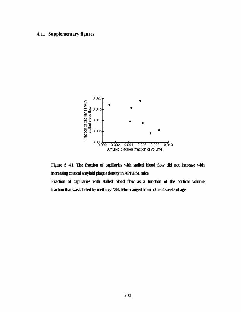
203
4.11 Supplementary figures
Figure S 4.1. The fraction of capillaries with stalled blood flow did not increase with
increasing cortical amyloid plaque density in APP/PS1 mice.
Fraction of capillaries with stalled blood flow as a function of the cortical volume
fraction that was labeled by methoxy-X04. Mice ranged from 50 to 64 weeks of age.
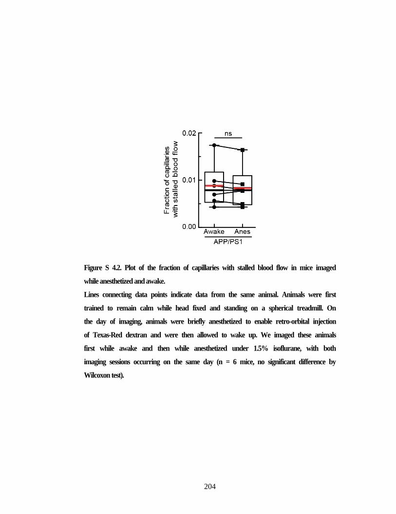
204
Figure S 4.2. Plot of the fraction of capillaries with stalled blood flow in mice imaged
while anesthetized and awake.
Lines connecting data points indicate data from the same animal. Animals were first
trained to remain calm while head fixed and standing on a spherical treadmill. On
the day of imaging, animals were briefly anesthetized to enable retro-orbital injection
of Texas-Red dextran and were then allowed to wake up. We imaged these animals
first while awake and then while anesthetized under 1.5% isoflurane, with both
imaging sessions occurring on the same day (n = 6 mice, no significant difference by
Wilcoxon test).
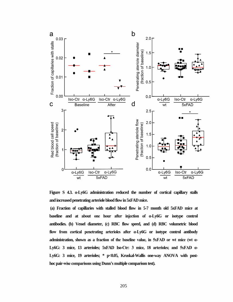
205
Figure S 4.3. α-Ly6G administration reduced the number of cortical capillary stalls
and increased penetrating arteriole blood flow in 5xFAD mice.
(a) Fraction of capillaries with stalled blood flow in 5-7 month old 5xFAD mice at
baseline and at about one hour after injection of α-Ly6G or isotype control
antibodies. (b) Vessel diameter, (c) RBC flow speed, and (d) RBC volumetric blood
flow from cortical penetrating arterioles after α-Ly6G or isotype control antibody
administration, shown as a fraction of the baseline value, in 5xFAD or wt mice (wt α-
Ly6G: 3 mice, 13 arterioles; 5xFAD Iso-Ctr: 3 mice, 18 arterioles; and 5xFAD α-
Ly6G: 3 mice, 19 arterioles; * p<0.05, Kruskal-Wallis one-way ANOVA with post-
hoc pair-wise comparisons using Dunn’s multiple comparison test).
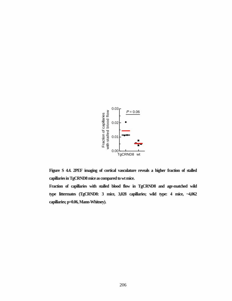
206
Figure S 4.4. 2PEF imaging of cortical vasculature reveals a higher fraction of stalled
capillaries in TgCRND8 mice as compared to wt mice.
Fraction of capillaries with stalled blood flow in TgCRND8 and age-matched wild
type littermates (TgCRND8: 3 mice, 3,028 capillaries; wild type: 4 mice, ~4,062
capillaries; p=0.06, Mann-Whitney).
0.00
0.01
0.02
0.03
TgCRND8
Fra
ctio
n o
f capillaries
with
sta
lle
d b
loo
d f
low P = 0.06
wt
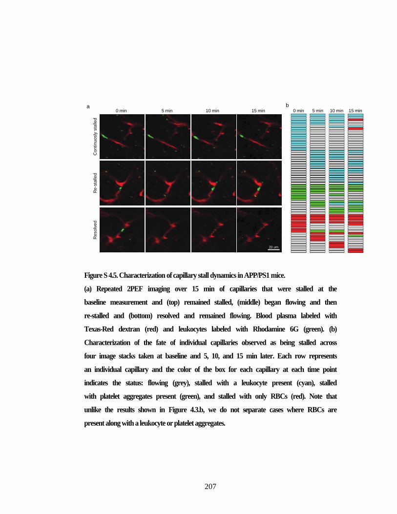
207
Figure S 4.5. Characterization of capillary stall dynamics in APP/PS1 mice.
(a) Repeated 2PEF imaging over 15 min of capillaries that were stalled at the
baseline measurement and (top) remained stalled, (middle) began flowing and then
re-stalled and (bottom) resolved and remained flowing. Blood plasma labeled with
Texas-Red dextran (red) and leukocytes labeled with Rhodamine 6G (green). (b)
Characterization of the fate of individual capillaries observed as being stalled across
four image stacks taken at baseline and 5, 10, and 15 min later. Each row represents
an individual capillary and the color of the box for each capillary at each time point
indicates the status: flowing (grey), stalled with a leukocyte present (cyan), stalled
with platelet aggregates present (green), and stalled with only RBCs (red). Note that
unlike the results shown in Figure 4.3.b, we do not separate cases where RBCs are
present along with a leukocyte or platelet aggregates.
0 min 5 min 10 min 15 min
Co
ntin
uosly
sta
lled
Re
-sta
lled
Re
so
lve
d
20 um
0 min 5 min 10 min 15 mina b
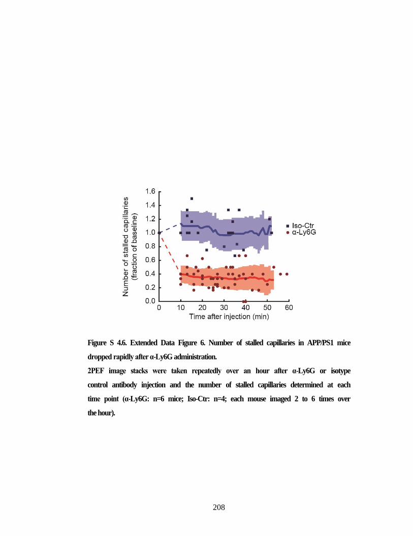
208
Figure S 4.6. Extended Data Figure 6. Number of stalled capillaries in APP/PS1 mice
dropped rapidly after α-Ly6G administration.
2PEF image stacks were taken repeatedly over an hour after α-Ly6G or isotype
control antibody injection and the number of stalled capillaries determined at each
time point (α-Ly6G: n=6 mice; Iso-Ctr: n=4; each mouse imaged 2 to 6 times over
the hour).
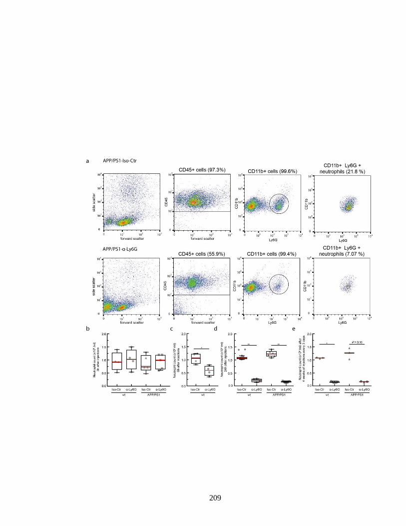
209
210
Figure S 4.7. Treatment with α-Ly6G leads to neutrophil depletion in both APP/PS1
and wildtype control mice, beginning within three hours after administration.
(a) Representative flow cytometry data for blood drawn from APP/PS1 mice 24
hours after treatment with isotype control antibodies (top row) and α-Ly6G (bottom
row). Left column shows forward and side scattering from entire population of
blood cells (after lysing and removing red blood cells). The second column shows the
gate on CD45+ cells, indicating leukocytes. The third column shows expression of
CD11b (high for monocytes and neutrophils) and Ly6G (high for neutrophils) for
the CD45+ cells. Cells with high expression levels of both CD11b and Ly6G were
considered to be neutrophils (right column). (b-d) Neutrophil counts for APP/PS1
and wt mice 3, 6, and 24 hr after a single treatment with α-Ly6G or isotype control
antibodies, respectively. (3 hr data: wt Iso-Ctr: n=4 mice; wt Ly6G: n=4; APP/PS1
Iso-Ctr: n=4; APP/PS1 Ly6G: n=5; 6 hr data: wt Iso-Ctr: n=4 mice; wt Ly6G: n=4;
24 hr data: wt Iso-Ctr: n=9 mice; wt Ly6G: n=4; APP/PS1 Iso-Ctr: n=6; APP/PS1
Ly6G: n=7) (e) Neutrophil counts for APP/PS1 and wt mice after one month of
treatment with α-Ly6G or isotype control antibodies every three days (4 week data:
wt Iso-Ctr: n=3; wt Ly6G: n=7; APP/PS1 Iso-Ctr: n=3; APP/PS1 Ly6G: n=3)
(*p<0.05, **p<0.01, Mann-Whitney comparison between Iso-Ctr and Ly6G treated
animals.)
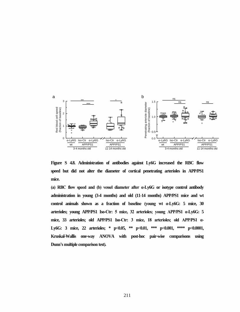
211
Figure S 4.8. Administration of antibodies against Ly6G increased the RBC flow
speed but did not alter the diameter of cortical penetrating arterioles in APP/PS1
mice.
(a) RBC flow speed and (b) vessel diameter after α-Ly6G or isotype control antibody
administration in young (3-4 months) and old (11-14 months) APP/PS1 mice and wt
control animals shown as a fraction of baseline (young wt α-Ly6G: 5 mice, 30
arterioles; young APP/PS1 Iso-Ctr: 5 mice, 32 arterioles; young APP/PS1 α-Ly6G: 5
mice, 33 arterioles; old APP/PS1 Iso-Ctr: 3 mice, 18 arterioles; old APP/PS1 α-
Ly6G: 3 mice, 22 arterioles; * p<0.05, ** p<0.01, *** p<0.001, **** p<0.0001,
Kruskal-Wallis one-way ANOVA with post-hoc pair-wise comparisons using
Dunn’s multiple comparison test).
Re
d b
loo
d c
ell
sp
ee
d
(fra
ctio
n o
f b
ase
line
)
0
1
2
3 ***
****
*
3-4 months old
α-Ly6G Iso-Ctr α-Ly6G
wt
11-14 months old
Iso-Ctr α-Ly6G
APP/PS1 APP/PS1
0.0
0.5
1.0
1.5
3-4 months old
α-Ly6G Iso-Ctr α-Ly6G
wt
11-14 months old
Iso-Ctr α-Ly6G
APP/PS1 APP/PS1P
en
etr
atin
g a
rte
rio
le d
iam
ete
r
(fra
ctio
n o
f b
ase
line
)
ns
ns ns
a b
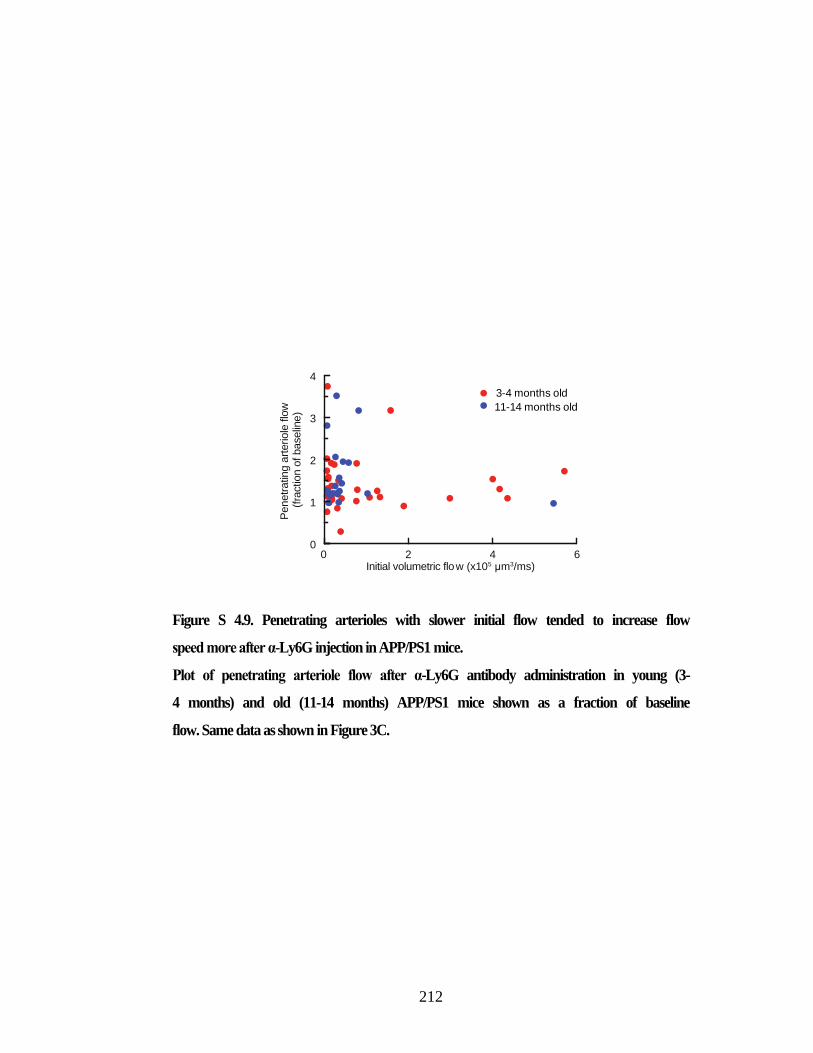
212
Figure S 4.9. Penetrating arterioles with slower initial flow tended to increase flow
speed more after α-Ly6G injection in APP/PS1 mice.
Plot of penetrating arteriole flow after α-Ly6G antibody administration in young (3-
4 months) and old (11-14 months) APP/PS1 mice shown as a fraction of baseline
flow. Same data as shown in Figure 3C.
0 2 4 6Initial volumetric flow (x105 µm3/ms)
Penetr
atin
g a
rteriole
flo
w
(fra
ction o
f baselin
e)
3-4 months old
11-14 months old
0
1
2
3
4
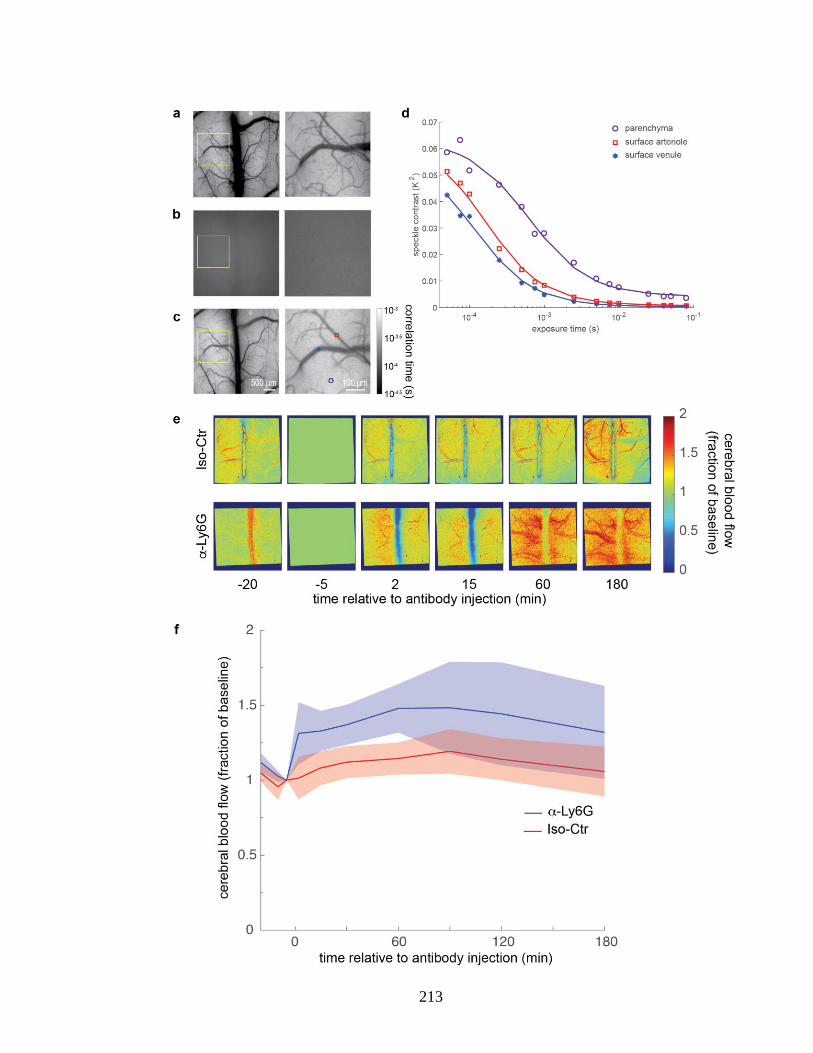
213
214
Figure S 4.10. Multi-exposure laser speckle imaging revealed CBF increased in
APP/PS1 mice within minutes of α-Ly6G administration.
(a) Green light reflectance image of parietal cortex of APP/PS1 mouse. Image to the
right is a expanded view of the region outlined with a yellow box. (b) Raw laser
speckle image of the same region as (a) with a 10 ms exposure time. (c) Correlation
time image of the same region as (a). (d) Speckle contrast values as a function of
image exposure time, showing fits for regions of interest located in a surface arteriole,
surface venule, or parenchymal region. The corresponding symbols in the expanded
view of (c) show the locations for each fit. (e) Images and (f) plot of cerebral blood
flow as a function of time after antibody injection, expressed as a fraction of the value
at 5 minutes before injection for APP/PS1 mice treated with isotype control
antibodies or α-Ly6G. (APP/PS1 α-LFA1: 5 mice; APP/PS1 Iso-Ctrl: 5 mice; age
range 9-19 months)
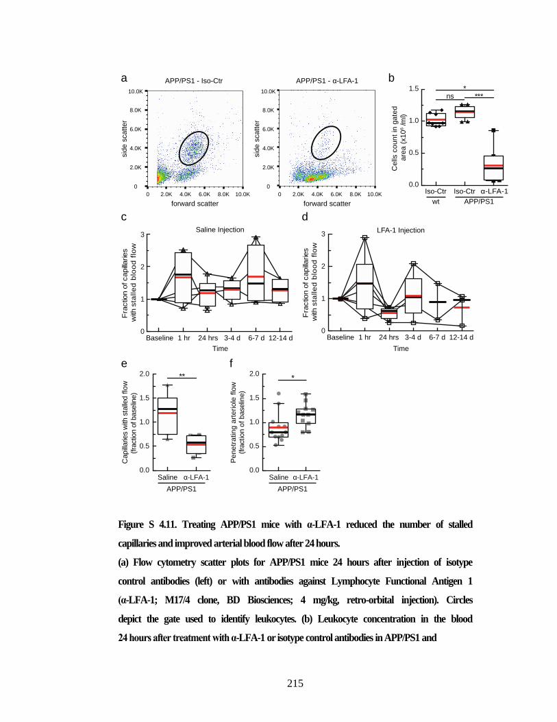
215
Figure S 4.11. Treating APP/PS1 mice with α-LFA-1 reduced the number of stalled
capillaries and improved arterial blood flow after 24 hours.
(a) Flow cytometry scatter plots for APP/PS1 mice 24 hours after injection of isotype
control antibodies (left) or with antibodies against Lymphocyte Functional Antigen 1
(α-LFA-1; M17/4 clone, BD Biosciences; 4 mg/kg, retro-orbital injection). Circles
depict the gate used to identify leukocytes. (b) Leukocyte concentration in the blood
24 hours after treatment with α-LFA-1 or isotype control antibodies in APP/PS1 and
forward scatter
sid
e s
ca
tter
a
forward scatter
sid
e s
ca
tter
0 2.0K 4.0K 6.0K 8.0K 10.0K 0 2.0K 4.0K 6.0K 8.0K 10.0K
0
2.0K
4.0K
6.0K
8.0K
10.0K
0
2.0K
4.0K
6.0K
8.0K
10.0K
b
Ce
lls c
ou
nt
in g
ate
d
are
a (
x1
06 /m
l)
0.5
1.0
1.5
0.0α-LFA-1Iso-Ctr
APP/PS1
Iso-Ctr
wt
****
ns
0
1
2
3
Fra
ctio
n o
f capillaries
with
sta
lle
d b
loo
d f
low
Baseline 1 hr 24 hrs 3-4 d 6-7 d 12-14 d
Saline Injection
c
Time
0
1
2
3
Fra
ctio
n o
f capillaries
with
sta
lle
d b
loo
d f
low
Baseline 1 hr 24 hrs 3-4 d 6-7 d 12-14 d
LFA-1 Injection
Time
d
Cap
illaries w
ith s
talle
d f
low
(fractio
n o
f baselin
e)
0.0
0.5
1.0
1.5
2.0 **
Saline
APP/PS1
α-LFA-1
e
Saline α-LFA-1
APP/PS1
0.0
0.5
1.0
1.5
2.0
Pe
ne
tra
tin
g a
rte
rio
le f
low
(fra
ctio
n o
f b
aselin
e)
*
f
APP/PS1 - Iso-Ctr APP/PS1 - α-LFA-1
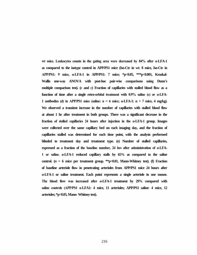
216
wt mice. Leukocytes counts in the gating area were decreased by 84% after α-LFA-1
as compared to the isotype control in APP/PS1 mice (Iso-Ctr in wt: 8 mice, Iso-Ctr in
APP/PS1: 9 mice, α-LFA-1 in APP/PS1: 7 mice; *p<0.05, ***p<0.001, Kruskal-
Wallis one-way ANOVA with post-hoc pair-wise comparisons using Dunn’s
multiple comparison test). (c and c) Fraction of capillaries with stalled blood flow as a
function of time after a single retro-orbital treatment with 0.9% saline (c) or α-LFA-
1 antibodies (d) in APP/PS1 mice (saline: n = 6 mice; α-LFA-1: n = 7 mice, 4 mg/kg).
We observed a transient increase in the number of capillaries with stalled blood flow
at about 1 hr after treatment in both groups. There was a significant decrease in the
fraction of stalled capillaries 24 hours after injection in the α-LFA-1 group. Images
were collected over the same capillary bed on each imaging day, and the fraction of
capillaries stalled was determined for each time point, with the analysis performed
blinded to treatment day and treatment type. (e) Number of stalled capillaries,
expressed as a fraction of the baseline number, 24 hrs after administration of α-LFA-
1 or saline. α-LFA-1 reduced capillary stalls by 65% as compared to the saline
control. (n = 6 mice per treatment group. **p<0.01, Mann-Whitney test). (f) Fraction
of baseline arteriole flow in penetrating arterioles from APP/PS1 mice 24 hours after
α-LFA-1 or saline treatment. Each point represents a single arteriole in one mouse.
The blood flow was increased after α-LFA-1 treatment by 29% compared with
saline controls (APP/PS1 α-LFA1: 4 mice, 11 arterioles; APP/PS1 saline: 4 mice, 12
arterioles; *p<0.05, Mann- Whitney test).
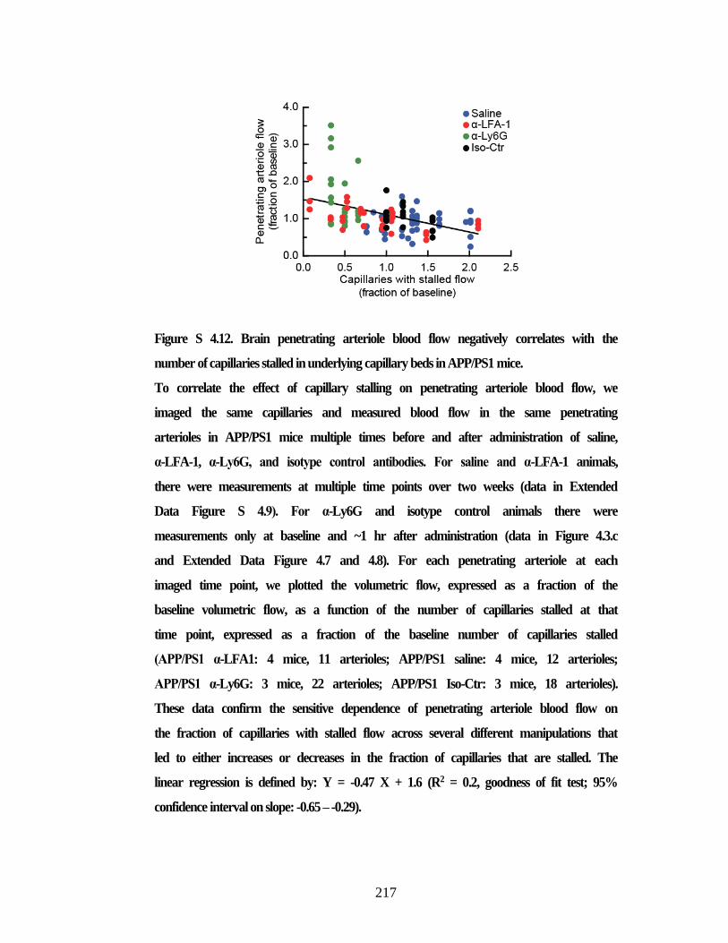
217
Figure S 4.12. Brain penetrating arteriole blood flow negatively correlates with the
number of capillaries stalled in underlying capillary beds in APP/PS1 mice.
To correlate the effect of capillary stalling on penetrating arteriole blood flow, we
imaged the same capillaries and measured blood flow in the same penetrating
arterioles in APP/PS1 mice multiple times before and after administration of saline,
α-LFA-1, α-Ly6G, and isotype control antibodies. For saline and α-LFA-1 animals,
there were measurements at multiple time points over two weeks (data in Extended
Data Figure S 4.9). For α-Ly6G and isotype control animals there were
measurements only at baseline and ~1 hr after administration (data in Figure 4.3.c
and Extended Data Figure 4.7 and 4.8). For each penetrating arteriole at each
imaged time point, we plotted the volumetric flow, expressed as a fraction of the
baseline volumetric flow, as a function of the number of capillaries stalled at that
time point, expressed as a fraction of the baseline number of capillaries stalled
(APP/PS1 α-LFA1: 4 mice, 11 arterioles; APP/PS1 saline: 4 mice, 12 arterioles;
APP/PS1 α-Ly6G: 3 mice, 22 arterioles; APP/PS1 Iso-Ctr: 3 mice, 18 arterioles).
These data confirm the sensitive dependence of penetrating arteriole blood flow on
the fraction of capillaries with stalled flow across several different manipulations that
led to either increases or decreases in the fraction of capillaries that are stalled. The
linear regression is defined by: Y = -0.47 X + 1.6 (R2 = 0.2, goodness of fit test; 95%
confidence interval on slope: -0.65 – -0.29).
218
Figure S 4.13. Time spent at the replaced object in wild type controls and APP/PS1
animals treated with α-Ly6G or isotype control antibodies.
Time spent at the replaced object measured over 6 minutes for APP/PS1 and wt
mice at baseline and at 3h and 24h after a single administration of α-Ly6G or isotype
control antibodies, and after 4 weeks of treatment every three days (APP/PS1 Iso-
Ctr: 10 mice; APP/PS1 α-Ly6G: 10 mice; wt Iso-Ctr: 11 mice; wt α-Ly6G: 11 mice;
no significant differences among groups as determined by Kruskal-Wallis one-way
ANOVA).
0
20
40
60
80
100
Ob
ject R
ep
lacem
en
t
Tim
e a
t re
pla
ce
d o
bje
ct (
s)
Baseline Baseline 3h 24h 4wk24h3h 4wk
APP/PS1
Iso-Ctr α-Ly6G
Baseline Baseline 3h 24h 4wk24h3h 4wk
wt
Iso-Ctr α-Ly6G

219
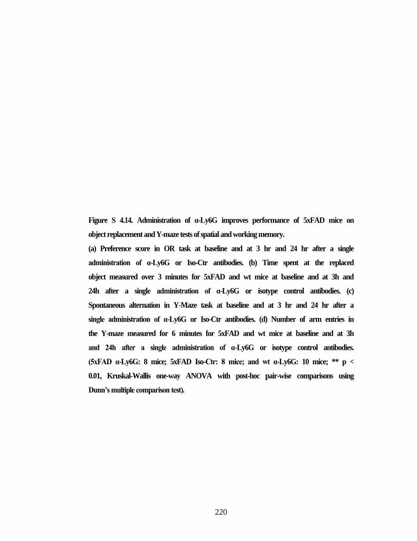
220
Figure S 4.14. Administration of α-Ly6G improves performance of 5xFAD mice on
object replacement and Y-maze tests of spatial and working memory.
(a) Preference score in OR task at baseline and at 3 hr and 24 hr after a single
administration of α-Ly6G or Iso-Ctr antibodies. (b) Time spent at the replaced
object measured over 3 minutes for 5xFAD and wt mice at baseline and at 3h and
24h after a single administration of α-Ly6G or isotype control antibodies. (c)
Spontaneous alternation in Y-Maze task at baseline and at 3 hr and 24 hr after a
single administration of α-Ly6G or Iso-Ctr antibodies. (d) Number of arm entries in
the Y-maze measured for 6 minutes for 5xFAD and wt mice at baseline and at 3h
and 24h after a single administration of α-Ly6G or isotype control antibodies.
(5xFAD α-Ly6G: 8 mice; 5xFAD Iso-Ctr: 8 mice; and wt α-Ly6G: 10 mice; ** p <
0.01, Kruskal-Wallis one-way ANOVA with post-hoc pair-wise comparisons using
Dunn’s multiple comparison test).
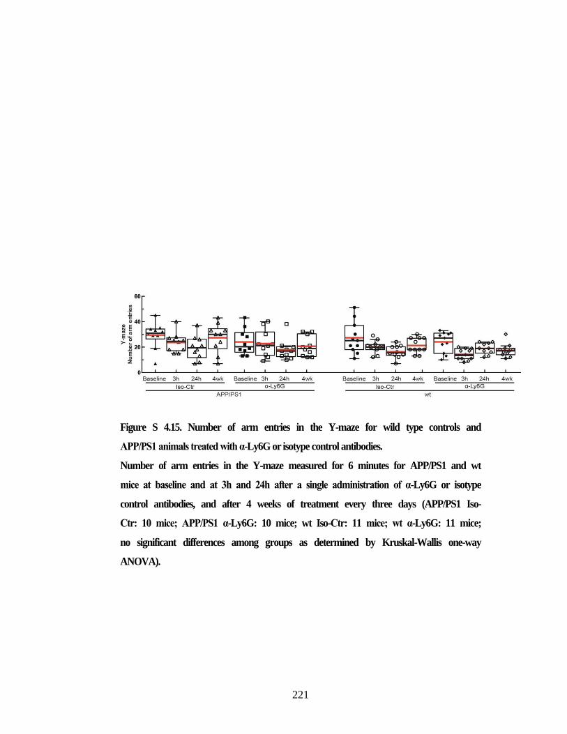
221
Figure S 4.15. Number of arm entries in the Y-maze for wild type controls and
APP/PS1 animals treated with α-Ly6G or isotype control antibodies.
Number of arm entries in the Y-maze measured for 6 minutes for APP/PS1 and wt
mice at baseline and at 3h and 24h after a single administration of α-Ly6G or isotype
control antibodies, and after 4 weeks of treatment every three days (APP/PS1 Iso-
Ctr: 10 mice; APP/PS1 α-Ly6G: 10 mice; wt Iso-Ctr: 11 mice; wt α-Ly6G: 11 mice;
no significant differences among groups as determined by Kruskal-Wallis one-way
ANOVA).
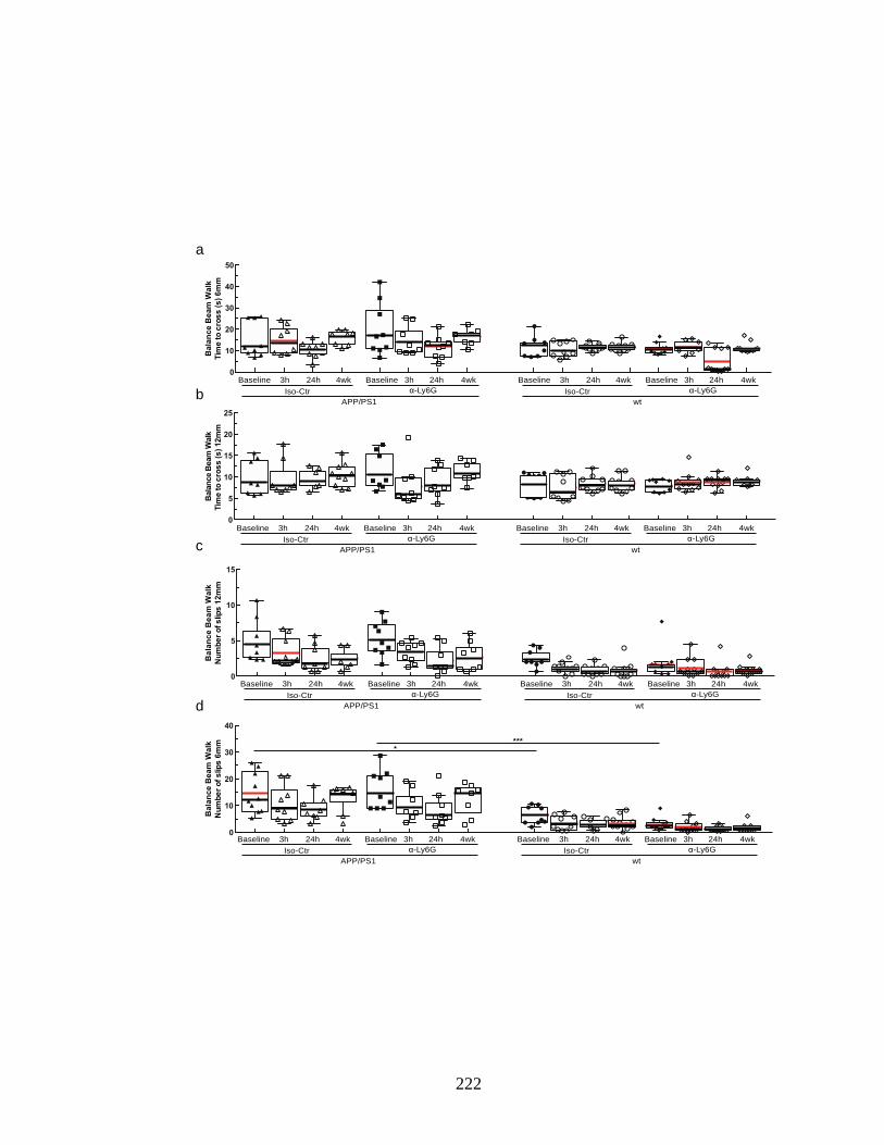
222
0
10
20
30
40
50
Bala
nce B
eam
Wa
lk
Tim
e t
o c
ros
s (
s)
6m
m
Baseline Baseline 3h 24h 4wk24h3h 4wk
APP/PS1
Iso-Ctr α-Ly6G
Baseline Baseline 3h 24h 4wk24h3h 4wk
wt
Iso-Ctr α-Ly6G
c
d
b
a
0
5
10
15
20
25
Bala
nce B
eam
Walk
Tim
e t
o c
ros
s (s
) 12m
m
Baseline Baseline 3h 24h 4wk24h3h 4wk
APP/PS1
Iso-Ctr α-Ly6G
Baseline Baseline 3h 24h 4wk24h3h 4wk
wt
Iso-Ctr α-Ly6G
0
5
10
15
Ba
lan
ce
Be
am
Wa
lk
Nu
mb
er
of s
lips 1
2m
m
Baseline Baseline 3h 24h 4wk24h3h 4wk
APP/PS1
Iso-Ctr α-Ly6G
Baseline Baseline 3h 24h 4wk24h3h 4wk
wt
Iso-Ctr α-Ly6G
0
10
20
30
40
Bala
nce B
eam
Wa
lk
Nu
mb
er
of
slip
s 6
mm
Baseline Baseline 3h 24h 4wk24h3h 4wk
APP/PS1
Iso-Ctr α-Ly6G
Baseline Baseline 3h 24h 4wk24h3h 4wk
wt
Iso-Ctr α-Ly6G
****
223
Figure S 4.16. Balance beam walk (BBW) to measure motor coordination in
wildtype controls and APP/PS1 animals treated with α-Ly6G or isotype control
antibodies.
(a and b) BBW time to cross on a 6- and 12-mm diameter beam, respectively, for
APP/PS1 and wild type mice at baseline and at 3h and 24h after a single
administration of α-Ly6G or isotype control antibodies, and after 4 weeks of
treatment every three days. APP/PS1 mice showed a modest trend toward taking
more time to cross the 6-mm diameter beam as compared to wt controls. (c and d).
Number of slips on the BBW for a 6- and 12-mm diameter beam, respectively, for
APP/PS1 and wild type mice at baseline and at 3h and 24h after a single
administration of α-Ly6G or isotype control antibodies, and after 4 weeks of
treatment every three days. For both beam diameters, APP/PS1 mice showed
significantly more slips while crossing the beam as compared to wt animals,
suggesting a motor deficit in the APP/PS1 mice. All animal groups showed a
reduction in the number of slips with subsequent trials, suggesting improved motor
coordination with practice. This improvement did not appear different between α-
Ly6G and isotype control treated APP/PS1 mice, suggesting that increases in brain
blood flow did not influence the motor learning underlying the reduction in the
number of slips (APP/PS1 Iso-Ctr: 10 mice; APP/PS1 α-Ly6G: 10 mice; wt Iso-Ctr:
11 mice; wt α-Ly6G: 11 mice; * p < 0.05, *** p < 0.001, Kruskal-Wallis one-way
ANOVA with post-hoc pair-wise comparisons using Dunn’s multiple comparison
test)
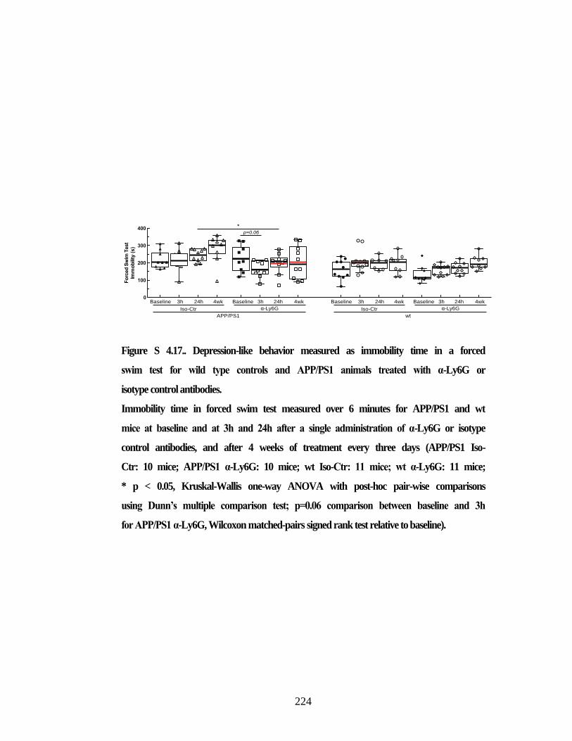
224
Figure S 4.17.. Depression-like behavior measured as immobility time in a forced
swim test for wild type controls and APP/PS1 animals treated with α-Ly6G or
isotype control antibodies.
Immobility time in forced swim test measured over 6 minutes for APP/PS1 and wt
mice at baseline and at 3h and 24h after a single administration of α-Ly6G or isotype
control antibodies, and after 4 weeks of treatment every three days (APP/PS1 Iso-
Ctr: 10 mice; APP/PS1 α-Ly6G: 10 mice; wt Iso-Ctr: 11 mice; wt α-Ly6G: 11 mice;
* p < 0.05, Kruskal-Wallis one-way ANOVA with post-hoc pair-wise comparisons
using Dunn’s multiple comparison test; p=0.06 comparison between baseline and 3h
for APP/PS1 α-Ly6G, Wilcoxon matched-pairs signed rank test relative to baseline).
0
100
200
300
400
Fo
rced
Sw
im T
est
Imm
ob
ility
(s
)
Baseline Baseline 3h 24h 4wk24h3h 4wk
APP/PS1
Iso-Ctr α-Ly6G
Baseline Baseline 3h 24h 4wk24h3h 4wk
wt
Iso-Ctr α-Ly6G
*p=0.06
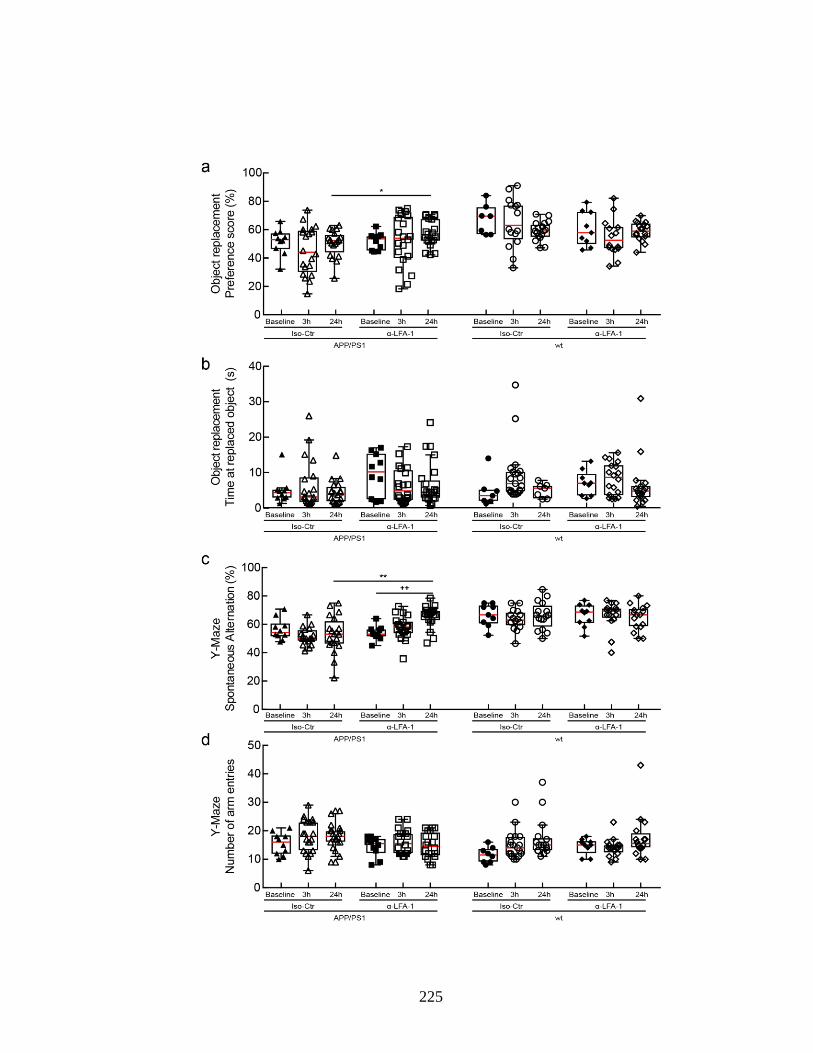
225
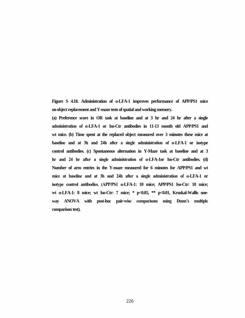
226
Figure S 4.18. Administration of α-LFA-1 improves performance of APP/PS1 mice
on object replacement and Y-maze tests of spatial and working memory.
(a) Preference score in OR task at baseline and at 3 hr and 24 hr after a single
administration of α-LFA-1 or Iso-Ctr antibodies in 11-13 month old APP/PS1 and
wt mice. (b) Time spent at the replaced object measured over 3 minutes these mice at
baseline and at 3h and 24h after a single administration of α-LFA-1 or isotype
control antibodies. (c) Spontaneous alternation in Y-Maze task at baseline and at 3
hr and 24 hr after a single administration of α-LFA-1or Iso-Ctr antibodies. (d)
Number of arm entries in the Y-maze measured for 6 minutes for APP/PS1 and wt
mice at baseline and at 3h and 24h after a single administration of α-LFA-1 or
isotype control antibodies. (APP/PS1 α-LFA-1: 10 mice; APP/PS1 Iso-Ctr: 10 mice;
wt α-LFA-1: 8 mice; wt Iso-Ctr: 7 mice; * p<0.05, ** p<0.01, Kruskal-Wallis one-
way ANOVA with post-hoc pair-wise comparisons using Dunn’s multiple
comparison test).
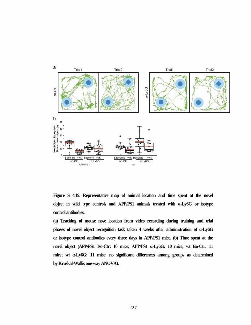
227
Figure S 4.19. Representative map of animal location and time spent at the novel
object in wild type controls and APP/PS1 animals treated with α-Ly6G or isotype
control antibodies.
(a) Tracking of mouse nose location from video recording during training and trial
phases of novel object recognition task taken 4 weeks after administration of α-Ly6G
or isotype control antibodies every three days in APP/PS1 mice. (b) Time spent at the
novel object (APP/PS1 Iso-Ctr: 10 mice; APP/PS1 α-Ly6G: 10 mice; wt Iso-Ctr: 11
mice; wt α-Ly6G: 11 mice; no significant differences among groups as determined
by Kruskal-Wallis one-way ANOVA).
228
Figure S 4.20. Amyloid plaque density and concentration of amyloid-beta oligomers
were not changed in 11-month-old APP/PS1 animals treated with α-Ly6G every
three days for a month.
(a) Thioflavin-S staining of amyloid plaques in representative cortical sections (upper
2 panels) and hippocampal sections (lower 2 panels) for APP/PS1 mice treated with
isotype control antibodies (left panels) or α-Ly6G (right panels). (b) Number of
amyloid plaques in the cortex (left) and hippocampus (right) for APP/PS1 mice after
one month of treatment (Iso-Ctr: 5 mice; α-Ly6G: 3 mice). (c) Percentage of tissue
section positive for Thioflavin-S in the cortex (left) and hippocampus (right) (Iso-Ctr:
6 mice; α-Ly6G: 3 mice). (d) ELISA measurements of Aβ aggregate concentrations
after 4 weeks of treatment with α-Ly6G or isotype control antibodies every three
days (Iso-Ctr: 7 mice; α-Ly6G: 6 mice).
% T
hio
-S p
os
itiv
e a
rea
pe
r C
ort
ex
% T
hio
-S p
os
itiv
e a
rea
pe
r H
ipp
oca
mp
us
0.0
0.2
0.4
0.6
0.8
1.0
α-Ly6GIso-Ctr
0
200
400
600
800
Hip
po
ca
mp
us
nu
mb
er
of p
laq
ue
s
α-Ly6GIso-Ctr0
2000
4000
6000
8000
Co
rte
x
nu
mb
er
of
pla
qu
es
α-Ly6GIso-Ctr
Thio-S
100μm
Iso-Ctr
Hip
po
ca
mp
us
Co
rte
x
50μm
α-Ly6Ga b
c
ag
E
LIS
A
A (p
g/m
l)
d
0
2
4
6
8
10
12
α-Ly6GIso-Ctr
0.0
0.2
0.4
0.6
0.8
1.0
α-Ly6GIso-Ctr
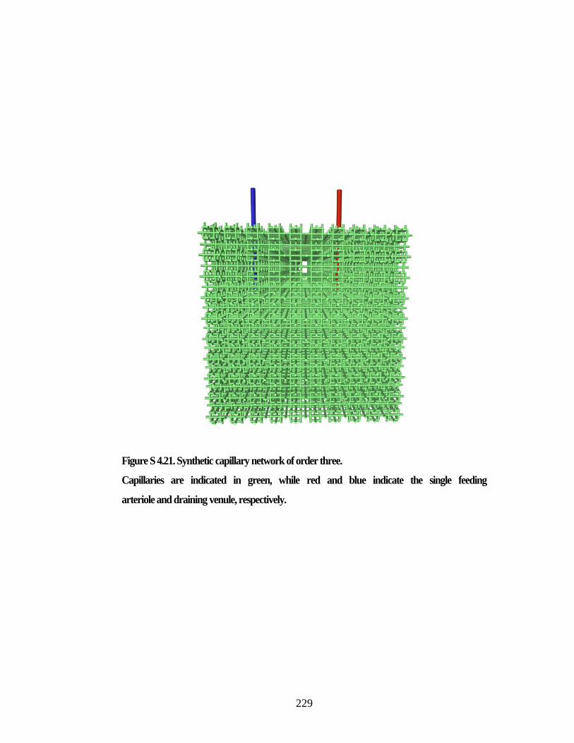
229
Figure S 4.21. Synthetic capillary network of order three.
Capillaries are indicated in green, while red and blue indicate the single feeding
arteriole and draining venule, respectively.
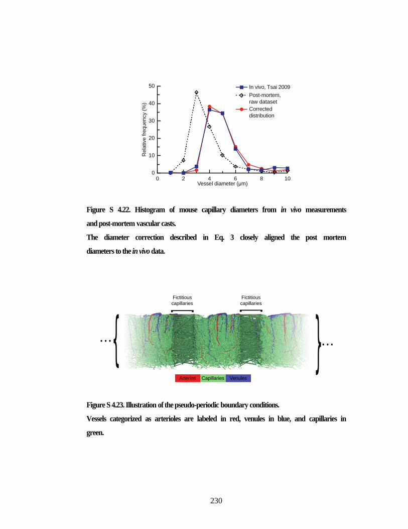
230
Figure S 4.22. Histogram of mouse capillary diameters from in vivo measurements
and post-mortem vascular casts.
The diameter correction described in Eq. 3 closely aligned the post mortem
diameters to the in vivo data.
Figure S 4.23. Illustration of the pseudo-periodic boundary conditions.
Vessels categorized as arterioles are labeled in red, venules in blue, and capillaries in
green.
0 2 4 6 8 100
10
20
30
40
50
Vessel diameter (µm)
Rela
tive fre
quency (
%)
In vivo, Tsai 2009
Post-mortem,
raw dataset
Corrected
distribution
Fictitious
capillaries
Fictitious
capillaries
Arteries Capillaries Venules
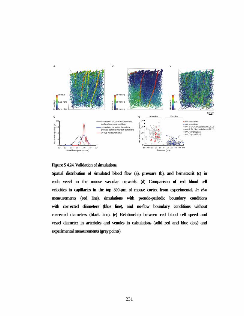
231
Figure S 4.24. Validation of simulations.
Spatial distribution of simulated blood flow (a), pressure (b), and hematocrit (c) in
each vessel in the mouse vascular network. (d) Comparison of red blood cell
velocities in capillaries in the top 300-µm of mouse cortex from experimental, in vivo
measurements (red line), simulations with pseudo-periodic boundary conditions
with corrected diameters (blue line), and no-flow boundary conditions without
corrected diameters (black line). (e) Relationship between red blood cell speed and
vessel diameter in arterioles and venules in calculations (solid red and blue dots) and
experimental measurements (grey points).
-50 -40 -30 -20 -10 0 10 20 30 40 50
Diameter (µm)
0
5
10
15
20
RB
C fl
ow
speed (
mm
/s) PA simulation
AV simulation
PA & SA, Santisakultarm (2012)
AV & SV, Santisakultarm (2012)
PA, Taylor (2016)
AV, Taylor (2016)
Arterioles Venules
simulation: uncorrected diameters,
no flow boundary condition
simulation: corrected diameters,
pseudo-periodic bounday conditions
in vivo measurements
ed
ca
Flo
w (
log
)
10 nL/s
0.01 nL/s
1e-4 nL/s Pre
ssure
80 mmHg
50 mmHg
20 mmHg Hem
ato
crit
1
0.5
0
100 µm
b
0
5
10
15
20
Rela
tive fre
quency (
%)
Blood flow speed (mm/s)
10-4 10-3 10-2 10-1 100 101 102
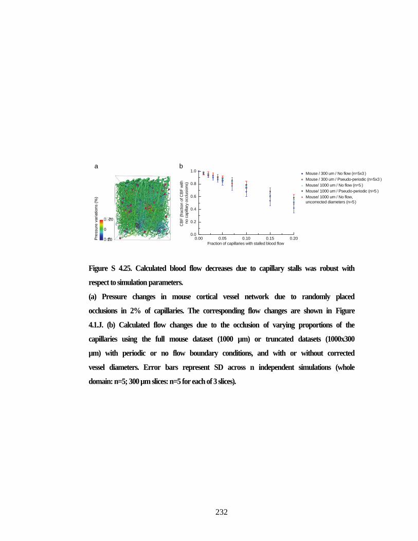
232
Figure S 4.25. Calculated blood flow decreases due to capillary stalls was robust with
respect to simulation parameters.
(a) Pressure changes in mouse cortical vessel network due to randomly placed
occlusions in 2% of capillaries. The corresponding flow changes are shown in Figure
4.1.J. (b) Calculated flow changes due to the occlusion of varying proportions of the
capillaries using the full mouse dataset (1000 µm) or truncated datasets (1000x300
µm) with periodic or no flow boundary conditions, and with or without corrected
vessel diameters. Error bars represent SD across n independent simulations (whole
domain: n=5; 300 µm slices: n=5 for each of 3 slices).
0.00 0.05 0.10 0.15 0.200.0
0.2
0.4
0.6
0.8
1.0
Fraction of capillaries with stalled blood flow
CB
F (
fraction o
f C
BF
with
no c
apill
ary
occlu
sio
ns)
Mouse / 300 um / No flow (n=5x3 )
Mouse / 300 um / Pseudo-periodic (n=5x3 )
Mouse/ 1000 um / No flow (n=5 )
Mouse/ 1000 um / Pseudo-periodic (n=5 )
Mouse/ 1000 um / No flow,
uncorrected diameters (n=5)
Pre
ssure
va
riation
s (
%)
≥+20
≥-20
0
a b
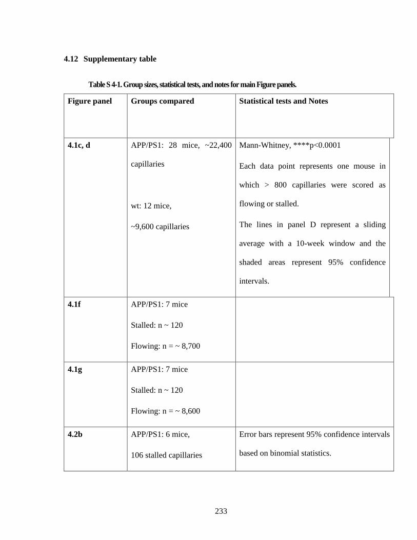
233
4.12 Supplementary table
Table S 4-1. Group sizes, statistical tests, and notes for main Figure panels.
Figure panel Groups compared Statistical tests and Notes
4.1c, d APP/PS1: 28 mice, ~22,400
capillaries
wt: 12 mice,
~9,600 capillaries
Mann-Whitney, ****p<0.0001
Each data point represents one mouse in
which > 800 capillaries were scored as
flowing or stalled.
The lines in panel D represent a sliding
average with a 10-week window and the
shaded areas represent 95% confidence
intervals.
4.1f APP/PS1: 7 mice
Stalled: n ~ 120
Flowing: n = ~ 8,700
4.1g APP/PS1: 7 mice
Stalled: n ~ 120
Flowing: n = ~ 8,600
4.2b APP/PS1: 6 mice,
106 stalled capillaries
Error bars represent 95% confidence intervals
based on binomial statistics.
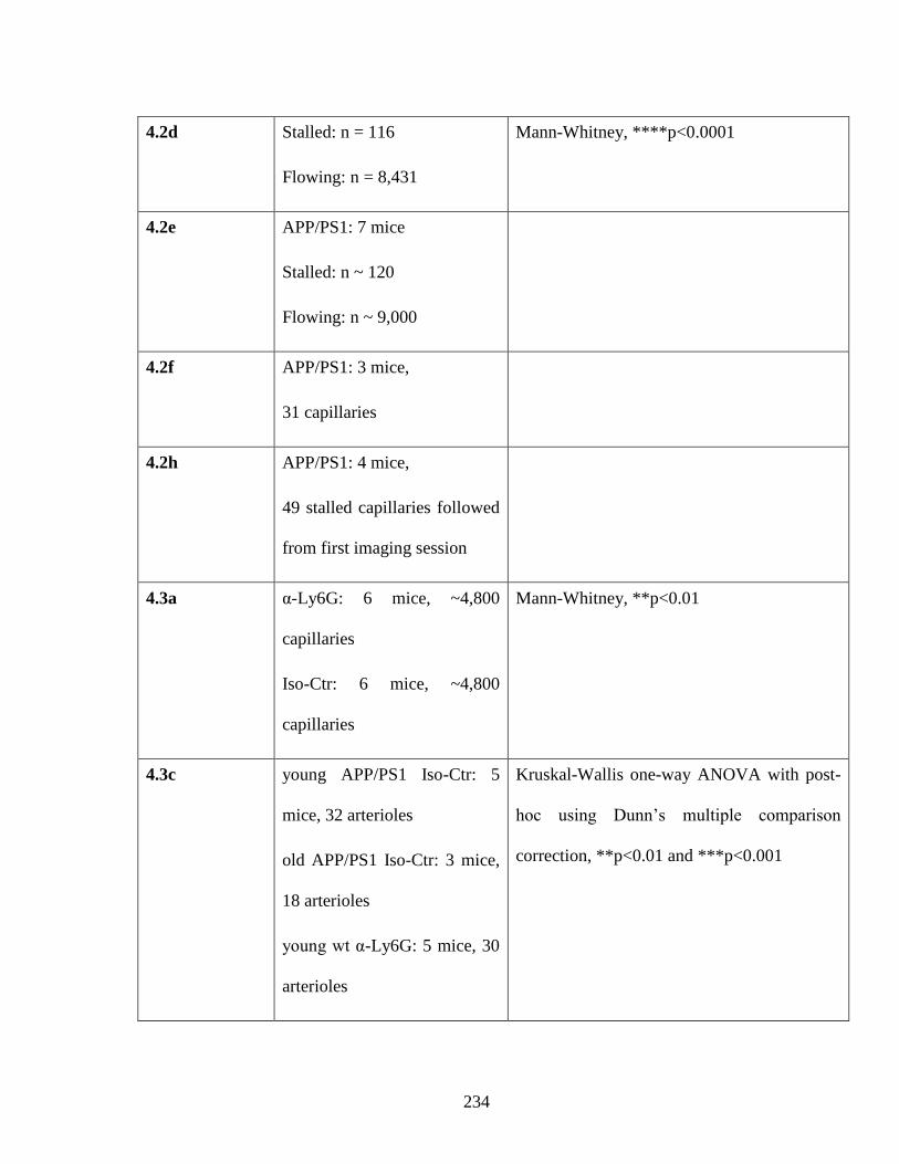
234
4.2d Stalled: n = 116
Flowing: n = 8,431
Mann-Whitney, ****p<0.0001
4.2e APP/PS1: 7 mice
Stalled: n ~ 120
Flowing: n ~ 9,000
4.2f APP/PS1: 3 mice,
31 capillaries
4.2h APP/PS1: 4 mice,
49 stalled capillaries followed
from first imaging session
4.3a α-Ly6G: 6 mice, ~4,800
capillaries
Iso-Ctr: 6 mice, ~4,800
capillaries
Mann-Whitney, **p<0.01
4.3c young APP/PS1 Iso-Ctr: 5
mice, 32 arterioles
old APP/PS1 Iso-Ctr: 3 mice,
18 arterioles
young wt α-Ly6G: 5 mice, 30
arterioles
Kruskal-Wallis one-way ANOVA with post-
hoc using Dunn’s multiple comparison
correction, **p<0.01 and ***p<0.001
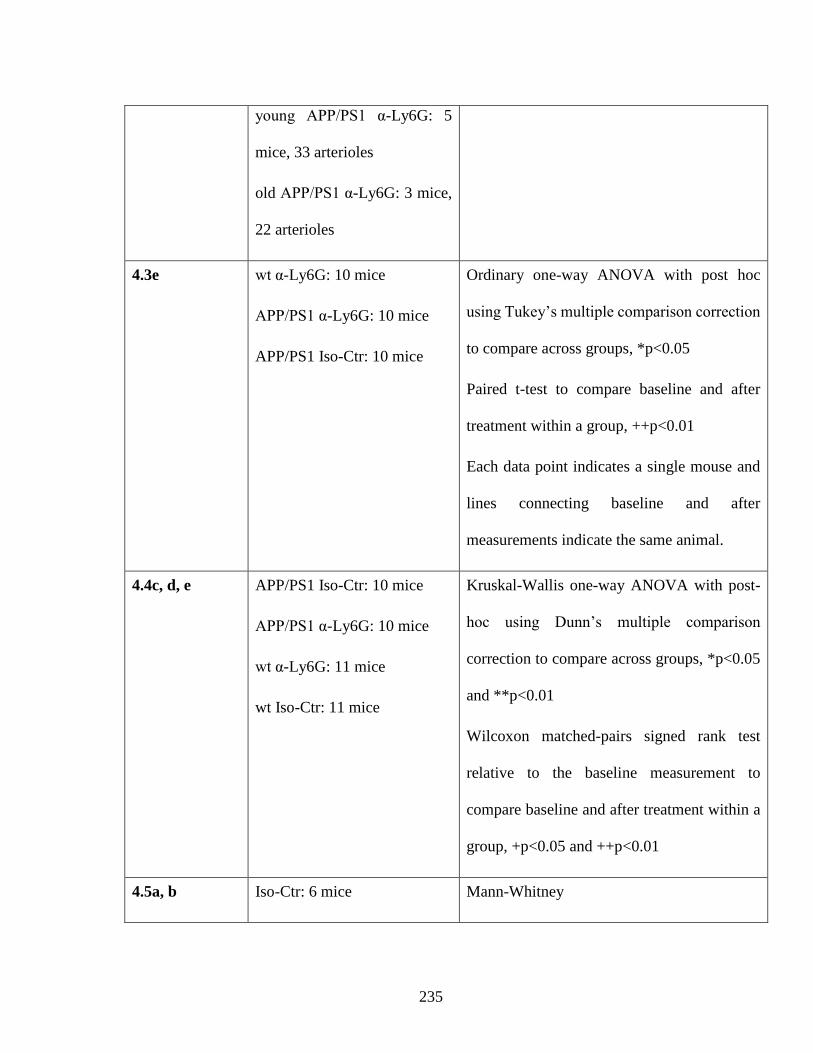
235
young APP/PS1 α-Ly6G: 5
mice, 33 arterioles
old APP/PS1 α-Ly6G: 3 mice,
22 arterioles
4.3e wt α-Ly6G: 10 mice
APP/PS1 α-Ly6G: 10 mice
APP/PS1 Iso-Ctr: 10 mice
Ordinary one-way ANOVA with post hoc
using Tukey’s multiple comparison correction
to compare across groups, *p<0.05
Paired t-test to compare baseline and after
treatment within a group, ++p<0.01
Each data point indicates a single mouse and
lines connecting baseline and after
measurements indicate the same animal.
4.4c, d, e APP/PS1 Iso-Ctr: 10 mice
APP/PS1 α-Ly6G: 10 mice
wt α-Ly6G: 11 mice
wt Iso-Ctr: 11 mice
Kruskal-Wallis one-way ANOVA with post-
hoc using Dunn’s multiple comparison
correction to compare across groups, *p<0.05
and **p<0.01
Wilcoxon matched-pairs signed rank test
relative to the baseline measurement to
compare baseline and after treatment within a
group, +p<0.05 and ++p<0.01
4.5a, b Iso-Ctr: 6 mice Mann-Whitney
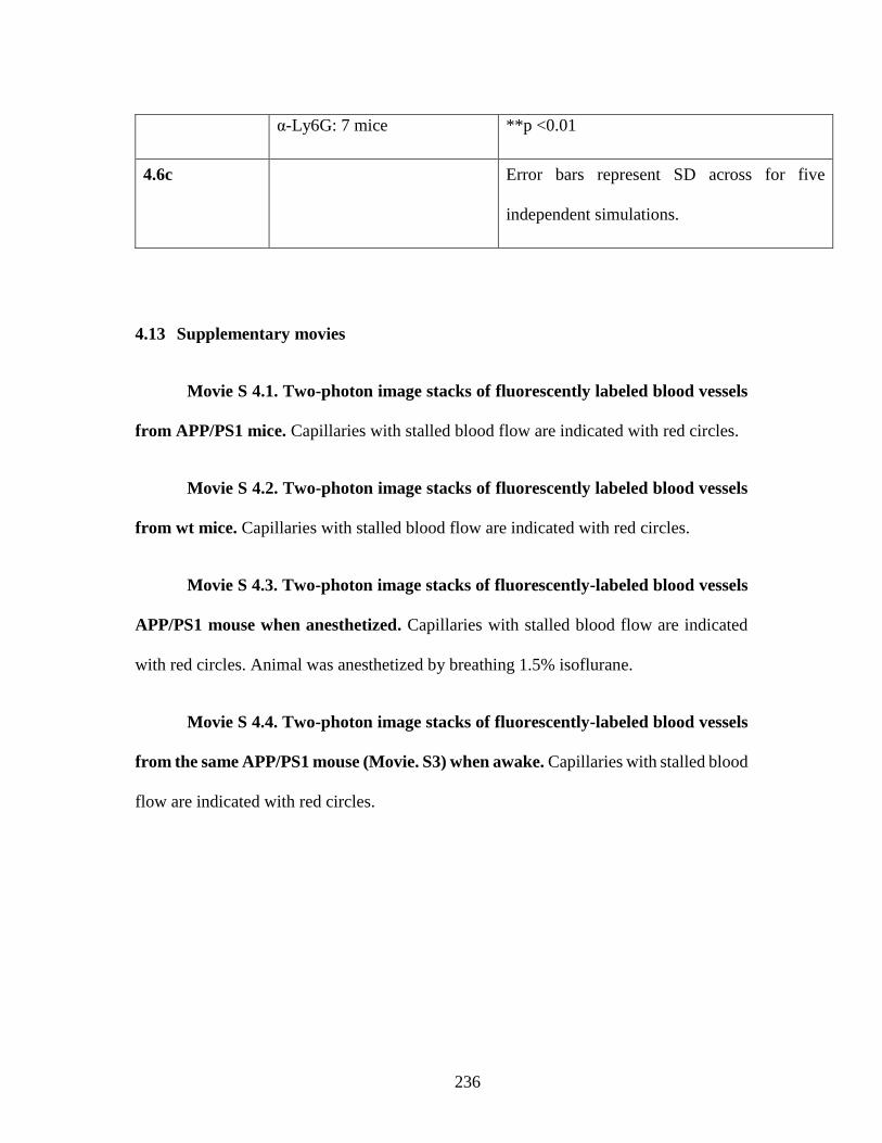
236
α-Ly6G: 7 mice **p <0.01
4.6c Error bars represent SD across for five
independent simulations.
4.13 Supplementary movies
Movie S 4.1. Two-photon image stacks of fluorescently labeled blood vessels
from APP/PS1 mice. Capillaries with stalled blood flow are indicated with red circles.
Movie S 4.2. Two-photon image stacks of fluorescently labeled blood vessels
from wt mice. Capillaries with stalled blood flow are indicated with red circles.
Movie S 4.3. Two-photon image stacks of fluorescently-labeled blood vessels
APP/PS1 mouse when anesthetized. Capillaries with stalled blood flow are indicated
with red circles. Animal was anesthetized by breathing 1.5% isoflurane.
Movie S 4.4. Two-photon image stacks of fluorescently-labeled blood vessels
from the same APP/PS1 mouse (Movie. S3) when awake. Capillaries with stalled blood
flow are indicated with red circles.
237
REFERENCES
1 Wang, J., Gu, B. J., Masters, C. L. & Wang, Y. J. A systemic view of Alzheimer
disease - insights from amyloid-beta metabolism beyond the brain. Nature
reviews. Neurology 13, 612-623, doi:10.1038/nrneurol.2017.111 (2017).
2 Santos, C. Y. et al. Pathophysiologic relationship between Alzheimer's disease,
cerebrovascular disease, and cardiovascular risk: A review and synthesis.
Alzheimer's & dementia 7, 69-87, doi:10.1016/j.dadm.2017.01.005 (2017).
3 Iturria-Medina, Y. et al. Early role of vascular dysregulation on late-onset
Alzheimer's disease based on multifactorial data-driven analysis. Nature
communications 7, 11934, doi:10.1038/ncomms11934 (2016).
4 Dai, W. et al. Mild cognitive impairment and alzheimer disease: patterns of
altered cerebral blood flow at MR imaging. Radiology 250, 856-866,
doi:10.1148/radiol.2503080751 (2009).
5 Wolters, F. J. et al. Cerebral Perfusion and the Risk of Dementia: A Population-
Based Study. Circulation, doi:10.1161/CIRCULATIONAHA.117.027448
(2017).
6 Wiesmann, M. et al. Hypertension, cerebrovascular impairment, and cognitive
decline in aged AbetaPP/PS1 mice. Theranostics 7, 1277-1289,
doi:10.7150/thno.18509 (2017).
7 Li, H. et al. Vascular and parenchymal amyloid pathology in an Alzheimer disease
knock-in mouse model: interplay with cerebral blood flow. Molecular
neurodegeneration 9, 28, doi:10.1186/1750-1326-9-28 (2014).
8 Niwa, K., Kazama, K., Younkin, S. G., Carlson, G. A. & Iadecola, C. Alterations
in cerebral blood flow and glucose utilization in mice overexpressing the amyloid
precursor protein. Neurobiology of disease 9, 61-68, doi:10.1006/nbdi.2001.0460
(2002).
238
9 Niwa, K. et al. A beta-peptides enhance vasoconstriction in cerebral circulation.
American journal of physiology. Heart and circulatory physiology 281, H2417-
2424 (2001).
10 Farkas, E. & Luiten, P. G. Cerebral microvascular pathology in aging and
Alzheimer's disease. Progress in neurobiology 64, 575-611 (2001).
11 Chen, Y. et al. Voxel-level comparison of arterial spin-labeled perfusion MRI and
FDG-PET in Alzheimer disease. Neurology 77, 1977-1985,
doi:10.1212/WNL.0b013e31823a0ef7 (2011).
12 Royea, J., Zhang, L., Tong, X. K. & Hamel, E. Angiotensin IV Receptors Mediate
the Cognitive and Cerebrovascular Benefits of Losartan in a Mouse Model of
Alzheimer's Disease. The Journal of neuroscience : the official journal of the
Society for Neuroscience 37, 5562-5573, doi:10.1523/JNEUROSCI.0329-
17.2017 (2017).
13 Marshall, R. S. et al. Recovery of brain function during induced cerebral
hypoperfusion. Brain : a journal of neurology 124, 1208-1217 (2001).
14 Wang, L. et al. Chronic cerebral hypoperfusion induces memory deficits and
facilitates Abeta generation in C57BL/6J mice. Experimental neurology 283, 353-
364, doi:10.1016/j.expneurol.2016.07.006 (2016).
15 Hattori, Y. et al. Gradual Carotid Artery Stenosis in Mice Closely Replicates
Hypoperfusive Vascular Dementia in Humans. Journal of the American Heart
Association 5, doi:10.1161/JAHA.115.002757 (2016).
16 Radde, R. et al. Abeta42-driven cerebral amyloidosis in transgenic mice reveals
early and robust pathology. EMBO reports 7, 940-946,
doi:10.1038/sj.embor.7400784 (2006).
17 Chishti, M. A. et al. Early-onset amyloid deposition and cognitive deficits in
transgenic mice expressing a double mutant form of amyloid precursor protein
695. The Journal of biological chemistry 276, 21562-21570,
doi:10.1074/jbc.M100710200 (2001).
239
18 Hasenberg, A. et al. Catchup: a mouse model for imaging-based tracking and
modulation of neutrophil granulocytes. Nature methods 12, 445-452,
doi:10.1038/nmeth.3322 (2015).
19 Deane, R., Bell, R. D., Sagare, A. & Zlokovic, B. V. Clearance of amyloid-beta
peptide across the blood-brain barrier: implication for therapies in Alzheimer's
disease. CNS & neurological disorders drug targets 8, 16-30 (2009).
20 Nishimura, N. et al. Targeted insult to subsurface cortical blood vessels using
ultrashort laser pulses: three models of stroke. Nature methods 3, 99-108,
doi:10.1038/nmeth844 (2006).
21 Tsai, P. S. et al. Correlations of neuronal and microvascular densities in murine
cortex revealed by direct counting and colocalization of nuclei and vessels. The
Journal of neuroscience : the official journal of the Society for Neuroscience 29,
14553-14570, doi:10.1523/JNEUROSCI.3287-09.2009 (2009).
22 Lauwers, F., Cassot, F., Lauwers-Cances, V., Puwanarajah, P. & Duvernoy, H.
Morphometry of the human cerebral cortex microcirculation: general
characteristics and space-related profiles. NeuroImage 39, 936-948,
doi:10.1016/j.neuroimage.2007.09.024 (2008).
23 Lorthois, S., Cassot, F. & Lauwers, F. Simulation study of brain blood flow
regulation by intra-cortical arterioles in an anatomically accurate large human
vascular network. Part II: flow variations induced by global or localized
modifications of arteriolar diameters. NeuroImage 54, 2840-2853,
doi:10.1016/j.neuroimage.2010.10.040 (2011).
24 Roher, A. E. et al. Cerebral blood flow in Alzheimer's disease. Vascular health
and risk management 8, 599-611, doi:10.2147/VHRM.S34874 (2012).
25 Iadecola, C. The Neurovascular Unit Coming of Age: A Journey through
Neurovascular Coupling in Health and Disease. Neuron 96, 17-42,
doi:10.1016/j.neuron.2017.07.030 (2017).
26 Park, L. et al. Nox2-derived radicals contribute to neurovascular and behavioral
dysfunction in mice overexpressing the amyloid precursor protein. Proceedings
240
of the National Academy of Sciences of the United States of America 105, 1347-
1352, doi:10.1073/pnas.0711568105 (2008).
27 Park, L. et al. Innate immunity receptor CD36 promotes cerebral amyloid
angiopathy. Proceedings of the National Academy of Sciences of the United States
of America 110, 3089-3094, doi:10.1073/pnas.1300021110 (2013).
28 Wang, J. X. et al. Ly6G ligation blocks recruitment of neutrophils via a beta2-
integrin-dependent mechanism. Blood 120, 1489-1498, doi:10.1182/blood-2012-
01-404046 (2012).
29 Daley, J. M., Thomay, A. A., Connolly, M. D., Reichner, J. S. & Albina, J. E. Use
of Ly6G-specific monoclonal antibody to deplete neutrophils in mice. Journal of
leukocyte biology 83, 64-70, doi:10.1189/jlb.0407247 (2008).
30 Lavkan, A. H., Astiz, M. E. & Rackow, E. C. Effects of proinflammatory
cytokines and bacterial toxins on neutrophil rheologic properties. Critical care
medicine 26, 1677-1682 (1998).
31 Bennett, R. E. et al. Tau induces blood vessel abnormalities and angiogenesis-
related gene expression in P301L transgenic mice and human Alzheimer's disease.
Proceedings of the National Academy of Sciences of the United States of America
115, E1289-E1298, doi:10.1073/pnas.1710329115 (2018).
32 Mohammad Haft-Javaherian, L. F., Victorine Muse, Chris B. Schaffer, Nozomi
Nishimura, Mert R. Sabuncu. Deep convolutional neural networks for segmenting
3D in vivo multiphoton images of vasculature in Alzheimer disease mouse models.
arXiv preprint arXiv:1801.00880 (2018).
33 Villringer, A. et al. Imaging of leukocytes within the rat brain cortex in vivo.
Microvascular research 42, 305-315 (1991).
34 Ishikawa, M. et al. Leukocyte plugging and cortical capillary flow after
subarachnoid hemorrhage. Acta neurochirurgica 158, 1057-1067,
doi:10.1007/s00701-016-2792-6 (2016).
35 Kloner, R. A. No-reflow phenomenon: maintaining vascular integrity. Journal of
cardiovascular pharmacology and therapeutics 16, 244-250,
doi:10.1177/1074248411405990 (2011).
241
36 Engler, R. L., Schmid-Schonbein, G. W. & Pavelec, R. S. Leukocyte capillary
plugging in myocardial ischemia and reperfusion in the dog. The American
journal of pathology 111, 98-111 (1983).
37 Chibber, R., Ben-Mahmud, B. M., Chibber, S. & Kohner, E. M. Leukocytes in
diabetic retinopathy. Current diabetes reviews 3, 3-14 (2007).
38 Santisakultarm, T. P. et al. Stalled cerebral capillary blood flow in mouse models
of essential thrombocythemia and polycythemia vera revealed by in vivo two-
photon imaging. Journal of thrombosis and haemostasis : JTH 12, 2120-2130,
doi:10.1111/jth.12738 (2014).
39 Ilesanmi, O. O. Pathological basis of symptoms and crises in sickle cell disorder:
implications for counseling and psychotherapy. Hematology reports 2, e2,
doi:10.4081/hr.2010.e2 (2010).
40 Zuliani, G. et al. Markers of endothelial dysfunction in older subjects with late
onset Alzheimer's disease or vascular dementia. Journal of the neurological
sciences 272, 164-170, doi:10.1016/j.jns.2008.05.020 (2008).
41 Iadecola, C. Vascular and Metabolic Factors in Alzheimer's Disease and Related
Dementias: Introduction. Cellular and molecular neurobiology 36, 151-154,
doi:10.1007/s10571-015-0319-y (2016).
42 Zenaro, E. et al. Neutrophils promote Alzheimer's disease-like pathology and
cognitive decline via LFA-1 integrin. Nature medicine 21, 880-886,
doi:10.1038/nm.3913 (2015).
43 Goldsmith, H. S. Alzheimer's disease can be treated: Why the delay? Surgical
neurology international 8, 133, doi:10.4103/sni.sni_116_17 (2017).
44 Blinder, P. et al. The cortical angiome: an interconnected vascular network with
noncolumnar patterns of blood flow. Nature neuroscience 16, 889-897,
doi:10.1038/nn.3426 (2013).
45 Jankowsky, J. L. et al. Mutant presenilins specifically elevate the levels of the 42
residue beta-amyloid peptide in vivo: evidence for augmentation of a 42-specific
gamma secretase. Human molecular genetics 13, 159-170,
doi:10.1093/hmg/ddh019 (2004).
242
46 Oakley, H. et al. Intraneuronal beta-amyloid aggregates, neurodegeneration, and
neuron loss in transgenic mice with five familial Alzheimer's disease mutations:
potential factors in amyloid plaque formation. The Journal of neuroscience : the
official journal of the Society for Neuroscience 26, 10129-10140,
doi:10.1523/JNEUROSCI.1202-06.2006 (2006).
47 Klunk, W. E. et al. Imaging Abeta plaques in living transgenic mice with
multiphoton microscopy and methoxy-X04, a systemically administered Congo
red derivative. Journal of neuropathology and experimental neurology 61, 797-
805 (2002).
48 Pologruto, T. A., Sabatini, B. L. & Svoboda, K. ScanImage: flexible software for
operating laser scanning microscopes. Biomedical engineering online 2, 13,
doi:10.1186/1475-925X-2-13 (2003).
49 Dombeck, D. A., Khabbaz, A. N., Collman, F., Adelman, T. L. & Tank, D. W.
Imaging large-scale neural activity with cellular resolution in awake, mobile mice.
Neuron 56, 43-57, doi:10.1016/j.neuron.2007.08.003 (2007).
50 Dijkstra, E. W. A note on two problems in connexion with graphs. Numerische
Mathematik Volume 1, pp 269–271, doi:doi:10.1007/BF01386390 (1959).
51 Otsu, N. A threshold selection method from gray-level histogram. IEEE Trans.
Syst. Man Cybern. vol. 9, pp. 62-66, doi:10.1109/TSMC.1979.4310076 (1979).
52 Lim, J. Two-Dimensional Signal and Image Processing. NJ, Englewood
Cliffs:Prentice Hall (1990).
53 Santisakultarm, T. P. et al. In vivo two-photon excited fluorescence microscopy
reveals cardiac- and respiration-dependent pulsatile blood flow in cortical blood
vessels in mice. American journal of physiology. Heart and circulatory
physiology 302, H1367-1377, doi:10.1152/ajpheart.00417.2011 (2012).
54 Paxinos, G. & Franklin, K. The mouse brain in stereotaxic coordinate. Elsevier
Academic Press (2004).
55 Kim, S. G. Quantification of relative cerebral blood flow change by flow-sensitive
alternating inversion recovery (FAIR) technique: application to functional
mapping. Magnetic resonance in medicine 34, 293-301 (1995).
243
56 Herscovitch, P. & Raichle, M. E. What is the correct value for the brain--blood
partition coefficient for water? Journal of cerebral blood flow and metabolism :
official journal of the International Society of Cerebral Blood Flow and
Metabolism 5, 65-69, doi:10.1038/jcbfm.1985.9 (1985).
57 Kober, F. et al. High-resolution myocardial perfusion mapping in small animals
in vivo by spin-labeling gradient-echo imaging. Magnetic resonance in medicine
51, 62-67, doi:10.1002/mrm.10676 (2004).
58 Dunn, A. K. Laser speckle contrast imaging of cerebral blood flow. Annals of
biomedical engineering 40, 367-377, doi:10.1007/s10439-011-0469-0 (2012).
59 Kazmi, S. M., Parthasarthy, A. B., Song, N. E., Jones, T. A. & Dunn, A. K.
Chronic imaging of cortical blood flow using Multi-Exposure Speckle Imaging.
Journal of cerebral blood flow and metabolism : official journal of the
International Society of Cerebral Blood Flow and Metabolism 33, 798-808,
doi:10.1038/jcbfm.2013.57 (2013).
60 Taylor, Z. J. et al. Microvascular basis for growth of small infarcts following
occlusion of single penetrating arterioles in mouse cortex. Journal of cerebral
blood flow and metabolism : official journal of the International Society of
Cerebral Blood Flow and Metabolism 36, 1357-1373,
doi:10.1177/0271678X15608388 (2016).
61 Cassot, F., Lauwers, F., Fouard, C., Prohaska, S. & Lauwers-Cances, V. A novel
three-dimensional computer-assisted method for a quantitative study of
microvascular networks of the human cerebral cortex. Microcirculation 13, 1-18,
doi:10.1080/10739680500383407 (2006).
62 Duvernoy, H. M., Delon, S. & Vannson, J. L. Cortical blood vessels of the human
brain. Brain research bulletin 7, 519-579 (1981).
63 Reina-De La Torre, F., Rodriguez-Baeza, A. & Sahuquillo-Barris, J.
Morphological characteristics and distribution pattern of the arterial vessels in
human cerebral cortex: a scanning electron microscope study. The Anatomical
record 251, 87-96 (1998).
244
64 Pries, A. R., Secomb, T. W., Gaehtgens, P. & Gross, J. F. Blood flow in
microvascular networks. Experiments and simulation. Circulation research 67,
826-834 (1990).
65 Pries, A. R., Secomb, T. W. & Gaehtgens, P. Biophysical aspects of blood flow
in the microvasculature. Cardiovascular research 32, 654-667 (1996).
66 Pries, A. R., Reglin, B. & Secomb, T. W. Structural response of microcirculatory
networks to changes in demand: information transfer by shear stress. American
journal of physiology. Heart and circulatory physiology 284, H2204-2212,
doi:10.1152/ajpheart.00757.2002 (2003).
67 Roman, S., Merlo, A., Duru, P., Risso, F. & Lorthois, S. Going beyond 20 mum-
sized channels for studying red blood cell phase separation in microfluidic
bifurcations. Biomicrofluidics 10, 034103, doi:10.1063/1.4948955 (2016).
68 Bragin, D. E., Bush, R. C., Muller, W. S. & Nemoto, E. M. High intracranial
pressure effects on cerebral cortical microvascular flow in rats. Journal of
neurotrauma 28, 775-785, doi:10.1089/neu.2010.1692 (2011).
69 Schmid, F., Tsai, P. S., Kleinfeld, D., Jenny, P. & Weber, B. Depth-dependent
flow and pressure characteristics in cortical microvascular networks. PLoS
computational biology 13, e1005392, doi:10.1371/journal.pcbi.1005392 (2017).
70 Team, R. C. R: A language and environment for statistical computing. R
Foundation for Statistical Computing. (2013).
71 Brown, W. R. & Thore, C. R. Review: cerebral microvascular pathology in ageing
and neurodegeneration. Neuropathology and applied neurobiology 37, 56-74,
doi:10.1111/j.1365-2990.2010.01139.x (2011).

245
CHAPTER 5
APPLICATION OF CROWDSOURCING CITIZEN SCIENCE IN STUDYING
BRAIN CAPILLARIES IN ALZHEIMER’S DISEASE
5.1 Introduction
Alzheimer’s disease (AD), the leading cause of dementia in the elderly, is known
to be caused by the aggregates of amyloid beta proteins and neurofibrillary tangles in the
brain. Since the cerebrovascular dysregulation is a feature of neurodegenerative diseases
(Iadecola, 2004), we are interested in studying the interaction between brain
microvasculature dysfunction and AD. Recently, we observed a significantly increased
rate of spontaneous transient capillary stalls in the cortical microvasculature of AD mice
compared to wild-type littermates, which is correlated with the brain blood flow reduction
seen in these mouse models of APP overexpression (Cruz Hernández et al., 2019). This
study similar to other research projects that investigate the interaction between brain
blood flow and neurodegenerative diseases depends heavily on both imaging techniques
such as multiphoton microscopy and fMRI and image analysis methods such as
registration, segmentation, and blood flow stalling detection (Bennett et al., 2018; Cruz
Hernández et al., 2019; T. P. Santisakultarm et al., 2014; Thom P. Santisakultarm et al.,
2012).
The brain vasculature network imaging and blood flow measurements can be done
by in vivo two-photon excited fluorescence (2PEF) microscopy (Kleinfeld, Mitra,
246
Helmchen, & Denk, 1998; Thom P. Santisakultarm et al., 2012), which allows us to map
the architecture of the vasculature throughout the top 500 μm of the mouse cortex, as well
as measure the blood flow velocity in individual vessels. Briefly, the blood plasma of an
anesthetized mouse is fluorescently labeled. A low-energy femtosecond laser pulse is
tightly focused, through a craniotomy, into the cortex of the mouse. There is no linear
absorption at the laser wavelength by the dye, so fluorescence is produced only at the
focus, where the laser intensity is high enough to excite the dye through the two-photon
absorption process. The fluorescence intensity is then recorded while the position of the
laser focus is scanned throughout the brain, providing a three-dimensional image of the
vasculature (Denk, Strickler, & Webb, 1990). To determine the flow velocity in
individual vessels based on the fact that the dye labels only the blood plasma, the motion
of the non-fluorescent red blood cells can be determined by tracking the dark patches
produced in the 2PEF image (Kleinfeld et al., 1998).
The acquired brain vasculature network images and blood flow measurements
require various image analyses to quantitatively measure different geometrical and
topological metrics in order to examine the proposed scientific hypothesis. For instance,
our stalled capillary research study requires two main image processing tasks of 3D vessel
segmentation and stalled vs. flowing capillary classification to identify each capillary
with end points, centerline, and a unique identifier because we accumulate the data from
multiple people for each vessel. Since manual image analysis tasks including both
segmentation and classification are time-consuming and become bottleneck processes,
researchers pursued different automated or semi-automated techniques to tackle this
247
problem. Alternatively, researchers tried to combine computational power and human
wisdom through a process called “citizen science”.
Citizen science is a mechanism in which citizens are participating alongside the
professional scientists in different aspects of scientific research projects (e.g.
crowdsourcing projects) such as environmental DNA data collection (Biggs et al., 2015),
avian biological pattern monitoring (Sullivan et al., 2009), and interstellar dust particle
detection (Westphal et al., 2014), and medical image analysis (Heim et al., 2018). Every
year, more than 2 million volunteers participate in thousands of crowdsourcing projects
around the world with an estimated value of $2.5B for their time investment (Theobald
et al., 2015). Without the power of the crowd, the scientific community cannot tackle
these research questions due to logistical and financial limitations (Bird et al., 2014).
The “EyesOnALZ” initiative (involves Human Computation Institute, Cornell
University, University of California at Berkeley, and Princeton University) proposed to
use citizen science for both two main image processing tasks required for our stalled
capillary research study (3D vessel segmentation and stalled vs. flowing capillary
classification).
Our proposed method for stalled vs. flowing capillary classifications starts with
utilizing the acquired segmentation results to create image samples that each one outlines
a particular vessel segment in the image and then, citizen scientists classify each vessel
segment as a stalled or flowing capillary. This method was inspired by “Stardust@home”,
a citizen science project developed by the Space Sciences Laboratory at U. C. Berkeley,
248
that analyzes samples collected by the Stardust spacecraft to detect interstellar dust
particles (Westphal et al., 2014).
In this chapter, we describe the manual solutions developed by Schaffer-
Nishimura labs for these image segmentation and classification tasks prior to
EyesOnALZ initiative. Then, we discuss the complete pipeline including automated
image segmentation and StallCatchers samples generation. In addition, we present a study
on the StallCatchers’ performance and methodology validation based on the collected
data. Finally, we present the results of a novel study produced by StallCatchers and
conclude the chapter with the discussions of the StallCatchers’ powers and limitations to
discuss the possibility of its adaptation by other researchers.
5.2 Method
5.2.1 General pipeline
Based on the StallCathers’ crowdsourcing design, each player at each round of
the game receives a 3D image stack that encompasses a particular vessel to target for the
classification task between flowing vs. stalled. Users view the acquired 3D images
through movies that show one plane at a time. Since vessels have different 3D orientation
and many vessels are visible in an image stack, we need to indicate the targeted vessel
segment to the user. Therefore, we need to identify each vessel segment within the 3D
image stack and generate a movie that encompasses a particular targeted segment and
includes a visual indicator to the segment for the user. A database is generated to save the
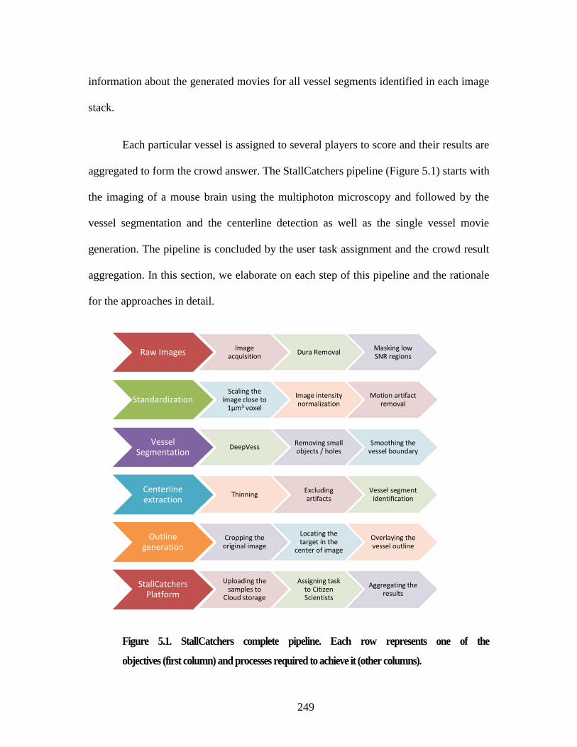
249
information about the generated movies for all vessel segments identified in each image
stack.
Each particular vessel is assigned to several players to score and their results are
aggregated to form the crowd answer. The StallCatchers pipeline (Figure 5.1) starts with
the imaging of a mouse brain using the multiphoton microscopy and followed by the
vessel segmentation and the centerline detection as well as the single vessel movie
generation. The pipeline is concluded by the user task assignment and the crowd result
aggregation. In this section, we elaborate on each step of this pipeline and the rationale
for the approaches in detail.
Figure 5.1. StallCatchers complete pipeline. Each row represents one of the
objectives (first column) and processes required to achieve it (other columns).
Raw ImagesImage
acquisition Dura Removal
Masking low SNR regions
StandardizationScaling the
image close to 1μm3 voxel
Image intensity normalization
Motion artifact removal
Vessel Segmentation
DeepVessRemoving small objects / holes
Smoothing the vessel boundary
Centerline extraction
ThinningExcluding artifacts
Vessel segment identification
Outline generation
Cropping the original image
Locating the target in the
center of image
Overlaying the vessel outline
StallCatchers Platform
Uploading the samples to
Cloud storage
Assigning task to Citizen Scientists
Aggregating the results
250
5.2.2 Manual tracing and scoring
We developed an in-house software package (Cruz Hernández et al., 2019) to
facilitate the image analysis of in vivo multiphoton microscopy images of brain
vasculature networks. Furthermore, this tool was adopted for the StallCatchers’ validation
study. Researchers load the 3D images and start with inserting a node at the location of
vessel bifurcations or the end of the vessel segments. Next, the vessel centerlines can be
drawn as a set of 3D center points between two vessel ends. Finally, each vessel is
classified as one of the defined vessel classes (i.e. surface venule, surface arteriole,
ascending venule, penetrating arteriole, flowing capillary, or stalled capillary). The final
graph representation of the vasculature network within the image is saved in an XML file
including the properties of all node’ and edges.
5.2.3 DeepVess
The manual tracing of brain vasculature network in a 3D image stack can take 20-
30 hours, depend on the researchers’ experience level. In order to remove this bottleneck,
we developed a convolutional neural network model, called DeepVess (Haft-Javaherian
et al., 2018), that performs the whole segmentation task automatically. In brief, DeepVess
is a convolutional neural network with optimized architecture that uses a greedy search
over each subgroup of the hyperparameters in addition to a new customized loss function
to tackle the fact that the segmentation labels are highly unbalanced (i.e. vessels are within
than 10% of the imaged brain volume). DeepVess consists of preprocessing,
segmentation, and postprocessing. DeepVess’ preprocessing includes splitting the image
channels, resizing the image close to 1 μm3 voxel, image intensity normalization, and

251
motion artifact removal. DeepVess’ postprocessing includes removing of small objects
and holes, smoothing vessel boundaries, and automatic vessel centerline extraction. Small
vessels connected to the boundary of the image were excluded from the analysis due to
lack of information for the classification.
The centerline extraction task is a challenging and essential task, which removes
centerline artifacts such as hairs (i.e. tiny vessels with one end not connected to any
vessels caused by noise bulge at vessel boundaries). Since images includes regions
outside the brain (the dura) which have highly fluorescent structures that are not vessels,
the slices captured outside the brain require manual rejection. Similarly, parts of the
images need to be manually masked and excluded from the analysis pipeline when the
signal-to-noise ratio (SNR) drops intensely due to light scattering caused by big vessel
optical obstructions or highly inflamed tissues in the disease animal models.
5.2.4 Vessel outlines and movie presentation for the StallCatchers user
At each round of the game, each player examines a movie for a particular vessel,
which is part of a 3D image stack with indications to the targeted vessel segment by
showing one plane at a time. The movie generation step utilizes the segmentation and
centerline information to generate movies for each identified vessel segment. A movie
for each vessel segment was generated from sub-volume of the original image stack with
a fixed aspect ratio and variable depth in z. The target vessel was located as close as
possible to the centroid with some margin proportional to the vessel diameter, which is
measure using the segmentation results along the vessel centerline. Infrequently, the
original images were rotated 90 degrees or resized to obtain a better view of the vessel.
252
The displayed image intensity within the cropped box was normalized to utilize the entire
available intensity range. Feedback from trained users suggests that contrast and
saturation are critical in the ability to discriminate red blood cell motion. In our
laboratory, users adjust the image contrast for each image stack independently and
dynamically, but we made the decision to simplify the game delivery and choose a fixed
contrast range determined by an internal multi-case multi-reader survey.
The single channel 3D image is then converted to a 3-channel RGB image. Based
on the vessel centerline and diameter an outline was overlaid on the image to annotate the
target vessel (Figure 5.2). Initially, the outline hue was set to the green similar to the
Stardust@home design. Six months after the public lunch in October, we received
negative feedback from citizen scientists on the green hue. Subsequently, we did an
external and internal multi-case multi-reader study to set an optimum hue, saturation and
lightness that resulted in the selection of blaze orange (24° hue, 100% saturation, and
50% lightness).
In the same way, the shape of the outline was optimized with an internal multi-
case multi-reader study and was selected to meet the UI/UX design criteria of minimal
user distraction caused by static annotation in the movie compare to other dynamic
annotations. To annotate the target vessel with the circular cross-sectional pipes along the
projection of vessels in 2D, the vessel centerline was projected into the x-y plane, two
mathematical dilation morphological operations with disk structuring elements were
applied to the projected centerline independently. The first disk structuring element has a
fixed radius and the second disk structuring element has a radius equal to the radius of
253
the first disk added to a fixed value as the outline thickness. The logical operation of
exclusive disjunction applied to these two dilated centerlines generates the final outcome.
Next, a median filter was applied to smooth the outline and the results were overlaid on
the original images in RGB format.
Finally, A unique 128-bit immutable universally unique identifier (UUID) was
assigned to each vessel and all the information about the vessel geometry and movie
generation steps added to a metadata record. The metadata for each particular vessel
includes the vessel’s UUID, the imaged animal ID, the image stack ID, the image
intensity ranges based on the intensity normalization, the vessel centroid coordinate, the
coordinate of the movie within the original image stack, the original size of the movie,
and the rotation of the movie. Finally, the movie was saved either as a sequence of JPEG
images, multi-page TIFF file, and/or MP4 movies.
5.2.5 Amazon AWS & Microsoft Azure
Later in the project, we expedited the image analysis process by utilizing the NC
series virtual machines on the Microsoft Azure cloud service. The generated vessel
samples in Microsoft Azure were transferred to Amazon AWS S3 storage shared between
Stardust@home and StallCatchers projects. Finally, the StallCatchers frontend and
backend was redeveloped using PHP and MySQL. Since 2016, the entire StallCatchers’
pipeline has been optimized for higher accuracy and performance continuously.
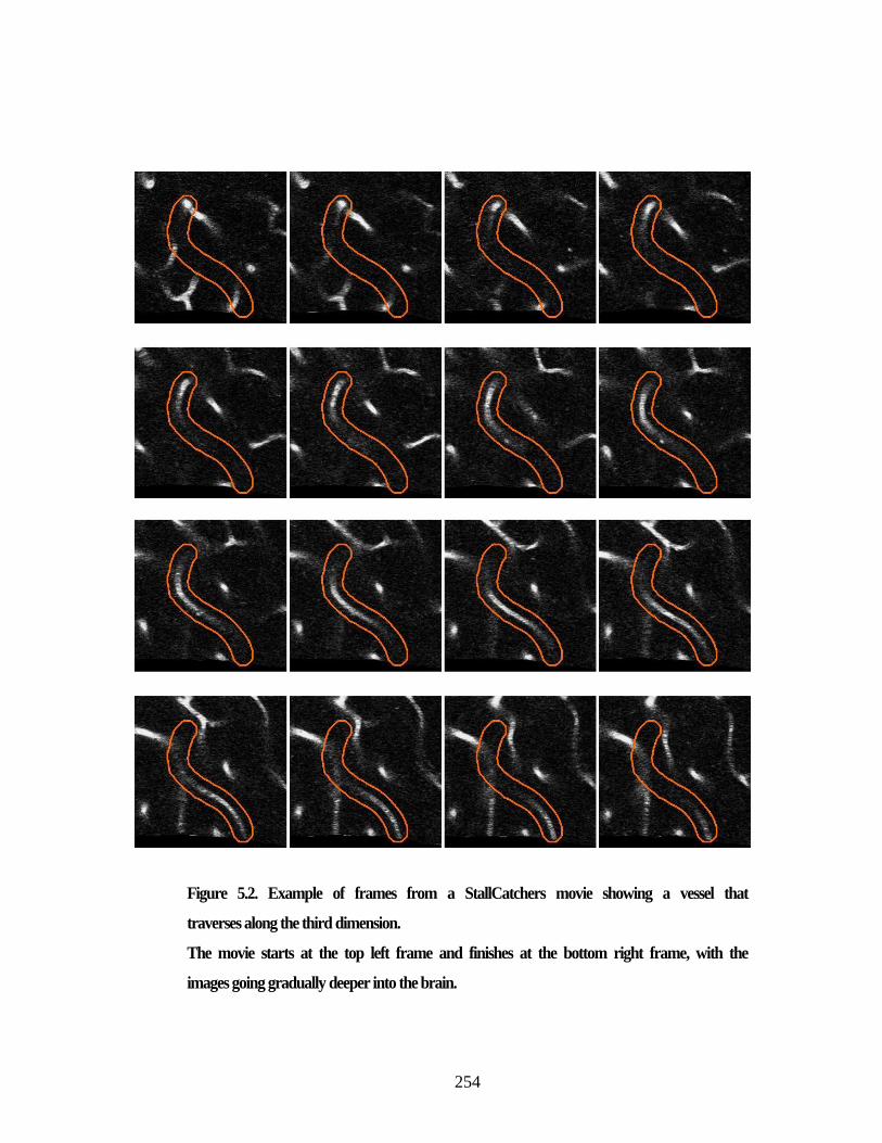
254
Figure 5.2. Example of frames from a StallCatchers movie showing a vessel that
traverses along the third dimension.
The movie starts at the top left frame and finishes at the bottom right frame, with the
images going gradually deeper into the brain.
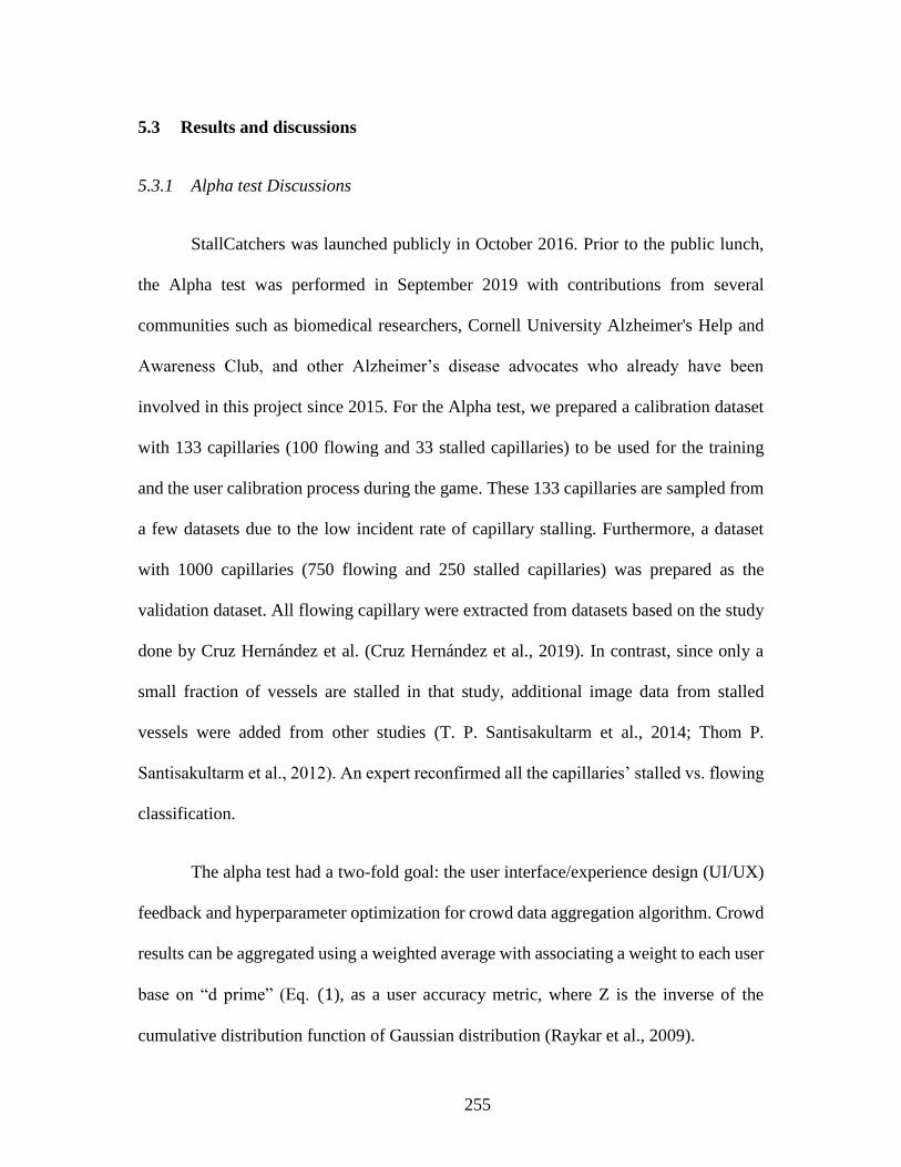
255
5.3 Results and discussions
5.3.1 Alpha test Discussions
StallCatchers was launched publicly in October 2016. Prior to the public lunch,
the Alpha test was performed in September 2019 with contributions from several
communities such as biomedical researchers, Cornell University Alzheimer's Help and
Awareness Club, and other Alzheimer’s disease advocates who already have been
involved in this project since 2015. For the Alpha test, we prepared a calibration dataset
with 133 capillaries (100 flowing and 33 stalled capillaries) to be used for the training
and the user calibration process during the game. These 133 capillaries are sampled from
a few datasets due to the low incident rate of capillary stalling. Furthermore, a dataset
with 1000 capillaries (750 flowing and 250 stalled capillaries) was prepared as the
validation dataset. All flowing capillary were extracted from datasets based on the study
done by Cruz Hernández et al. (Cruz Hernández et al., 2019). In contrast, since only a
small fraction of vessels are stalled in that study, additional image data from stalled
vessels were added from other studies (T. P. Santisakultarm et al., 2014; Thom P.
Santisakultarm et al., 2012). An expert reconfirmed all the capillaries’ stalled vs. flowing
classification.
The alpha test had a two-fold goal: the user interface/experience design (UI/UX)
feedback and hyperparameter optimization for crowd data aggregation algorithm. Crowd
results can be aggregated using a weighted average with associating a weight to each user
base on “d prime” (Eq. (1), as a user accuracy metric, where Z is the inverse of the
cumulative distribution function of Gaussian distribution (Raykar et al., 2009).
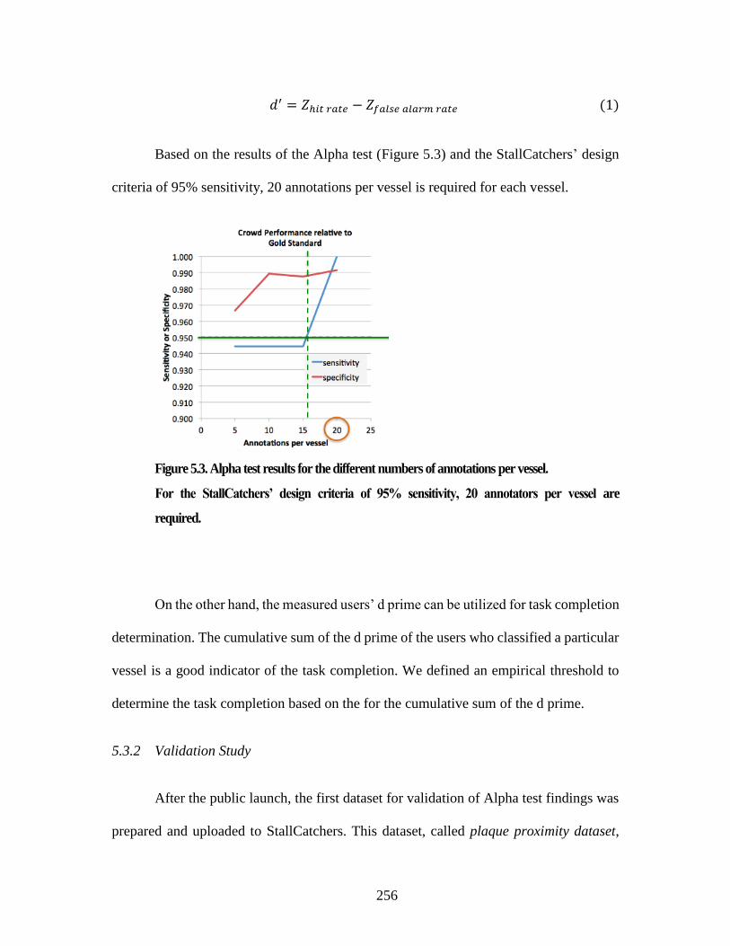
256
𝑑′ = 𝑍ℎ𝑖𝑡 𝑟𝑎𝑡𝑒 − 𝑍𝑓𝑎𝑙𝑠𝑒 𝑎𝑙𝑎𝑟𝑚 𝑟𝑎𝑡𝑒 (1)
Based on the results of the Alpha test (Figure 5.3) and the StallCatchers’ design
criteria of 95% sensitivity, 20 annotations per vessel is required for each vessel.
Figure 5.3. Alpha test results for the different numbers of annotations per vessel.
For the StallCatchers’ design criteria of 95% sensitivity, 20 annotators per vessel are
required.
On the other hand, the measured users’ d prime can be utilized for task completion
determination. The cumulative sum of the d prime of the users who classified a particular
vessel is a good indicator of the task completion. We defined an empirical threshold to
determine the task completion based on the for the cumulative sum of the d prime.
5.3.2 Validation Study
After the public launch, the first dataset for validation of Alpha test findings was
prepared and uploaded to StallCatchers. This dataset, called plaque proximity dataset,

257
served two purposes: the validation of Alpha test findings and the investigation of the
scientific question whether the amyloid beta plaque density in the vessel vicinity is
correlated with stalled capillary phenomena. Internally, we used our in-house manual
tracing and scoring software package to locate the vessel segments and classify them as
stalled or flowing. Independently, the detected stalled vessels by StallCatchers were
reconfirmed by an expert to determine the final StallCatchers result. Based on our internal
results and StallCatchers’ results as the confirmation, we concluded there is no significant
difference in terms of plaque density in the vessel vicinity and the occurrence of capillary
stalling (Cruz Hernández et al., 2019). Additionally, after conducting the analysis, we
used this dataset for the future crowd aggregation algorithm development. The centerline
in this dataset was extracted and all the vessels were classified manually to generate the
ground truth for this dataset.
After the reinvestigation of the crowd aggregation method parameters with this
larger dataset compare to the Alpha test, we concluded that 7 annotations per vessels are
required to obtain the StallCatchers’ design criteria of 95% sensitivity (Figure 5.4). The
new criterion increases the StallCatchers throughput rate by 3-fold. We incorporated all
UI/UX feedbacks and developed the second generation of StallCatchers (Figure 5.5).
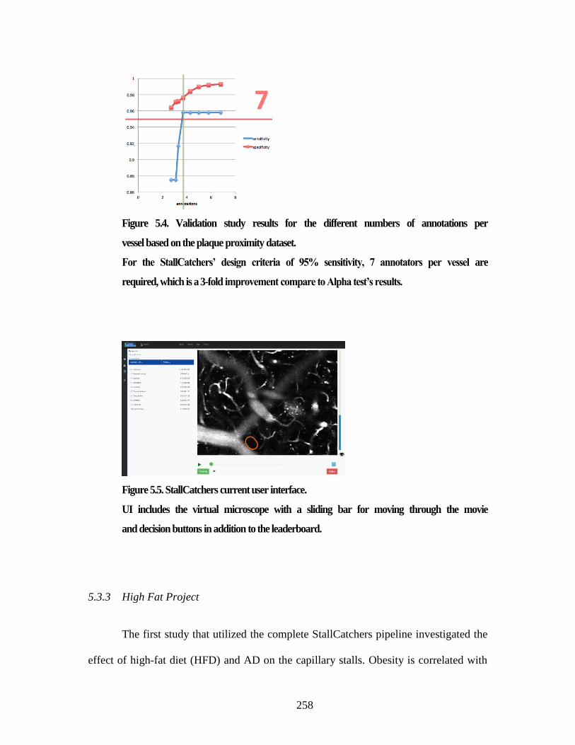
258
Figure 5.4. Validation study results for the different numbers of annotations per
vessel based on the plaque proximity dataset.
For the StallCatchers’ design criteria of 95% sensitivity, 7 annotators per vessel are
required, which is a 3-fold improvement compare to Alpha test’s results.
Figure 5.5. StallCatchers current user interface.
UI includes the virtual microscope with a sliding bar for moving through the movie
and decision buttons in addition to the leaderboard.
5.3.3 High Fat Project
The first study that utilized the complete StallCatchers pipeline investigated the
effect of high-fat diet (HFD) and AD on the capillary stalls. Obesity is correlated with
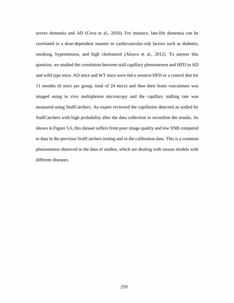
259
severe dementia and AD (Cova et al., 2016). For instance, late-life dementia can be
correlated in a dose-dependent manner to cardiovascular-risk factors such as diabetes,
smoking, hypertension, and high cholesterol (Alosco et al., 2012). To answer this
question, we studied the correlation between stall capillary phenomenon and HFD in AD
and wild type mice. AD mice and WT mice were fed a western HFD or a control diet for
11 months (6 mice per group, total of 24 mice) and then their brain vasculature was
imaged using in vivo multiphoton microscopy and the capillary stalling rate was
measured using StallCatchers. An expert reviewed the capillaries detected as stalled by
StallCatchers with high probability after the data collection to reconfirm the results. As
shown in Figure 5.6, this dataset suffers from poor image quality and low SNR compared
to data in the previous StallCatchers testing and in the calibration data. This is a common
phenomenon observed in the data of studies, which are dealing with mouse models with
different diseases.
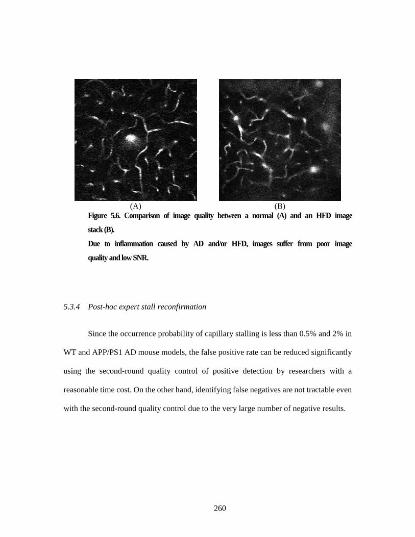
260
(A) (B)
Figure 5.6. Comparison of image quality between a normal (A) and an HFD image
stack (B).
Due to inflammation caused by AD and/or HFD, images suffer from poor image
quality and low SNR.
5.3.4 Post-hoc expert stall reconfirmation
Since the occurrence probability of capillary stalling is less than 0.5% and 2% in
WT and APP/PS1 AD mouse models, the false positive rate can be reduced significantly
using the second-round quality control of positive detection by researchers with a
reasonable time cost. On the other hand, identifying false negatives are not tractable even
with the second-round quality control due to the very large number of negative results.

261
5.3.5 Power of StallCatchers
The stalled vs. flowing capillary classification is a challenging task and time-
consuming. Currently, there is no fully automated computer algorithm that can perform
this task with an acceptable accuracy to eliminate the need for the manual classification.
StallCatchers enables us to perform this classification task ~30 times faster compared to
the traditional time-consuming manual classification, which delays the scientific research
progress, with up to 30 times faster.
5.3.6 Different stall-rate metrics
The stalled capillary phenomenon can be characterized using different metrics
depending on the stall detection methodology. The first category of the detection methods
is based on examining the whole complete 3D image stack while scrolling through slices
and the evaluator is not directed to check every vessel. This category has two variants.
The image can be examined using the raw acquired image or it can be examined after
overlaying the vessel centerlines on the image. Note that the vessel centerline also can be
extracted manually or automatically using DeepVess. The second category of the
detection methods is based on examining a sub-volume of the original 3D image stack
with annotation identifying the targeted vessel. This category also has two variants. The
examination can be done manually by an expert or it can be done using StallCatchers
followed by manually reconfirmation of the vessel classification for vessels with high
stalling probability.

262
On the other hand, the stall rate can be measured in two ways. The total number
of stalled vessels can be normalized by the total number of vessels in the image or by
total number slices in the image stack depending on the availability of the total number
of vessels in the image.
5.3.7 Comparison between StallCatchers and human manual classifications
Concerned that the difference in image quality could compromise results, we
selected 4 mice from the HFD project with ~5000 vessels total to perform vessel-by-
vessel accuracy comparisons between StallCatchers and expert manual classifications in
addition to the inter-reader and reader vs. panel accuracies. Two trained researchers
reviewed the vessel movies generated by StallCatchers pipeline one-by-one and marked
144 vessels as stalled capillary candidates. First, one expert examined the candidates and
then independently, a panel of experts met and examined the same candidates together.
We used absolute mean difference (AMD), which is the absolute difference total number
of detected stalled vessels divided by the arithmetic mean, as the accuracy metric. Note
that a lower AMD value shows higher agreement between two measurements with AMD
value of 0 means complete agreement. Additionally, we ran these vessels through
StallCatchers and an expert reviewed top 6% of vessels in terms of stalling probability.
StallCatchers and the panel agreed better with the AMD value of 0.06, than StallCatchers
and the expert or StallCatchers and the manual classification with the AMD values of
0.29 and 0.25, respectively.
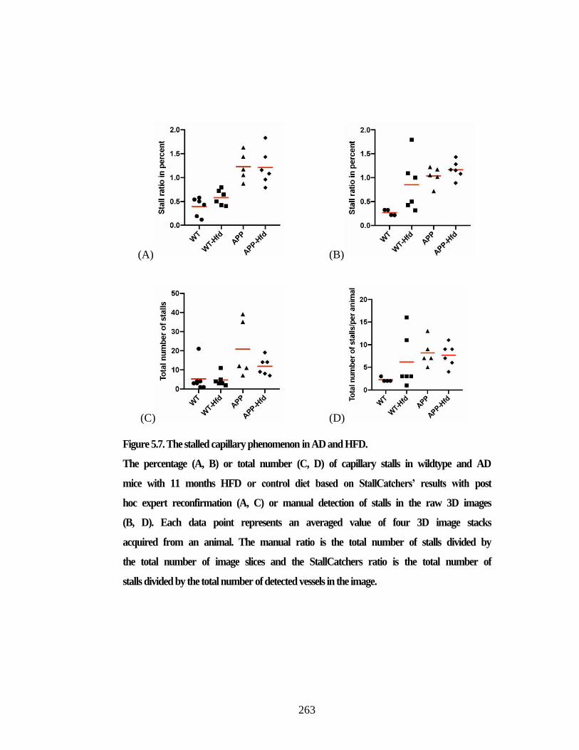
263
(A) (B)
(C) (D)
Figure 5.7. The stalled capillary phenomenon in AD and HFD.
The percentage (A, B) or total number (C, D) of capillary stalls in wildtype and AD
mice with 11 months HFD or control diet based on StallCatchers’ results with post
hoc expert reconfirmation (A, C) or manual detection of stalls in the raw 3D images
(B, D). Each data point represents an averaged value of four 3D image stacks
acquired from an animal. The manual ratio is the total number of stalls divided by
the total number of image slices and the StallCatchers ratio is the total number of
stalls divided by the total number of detected vessels in the image.
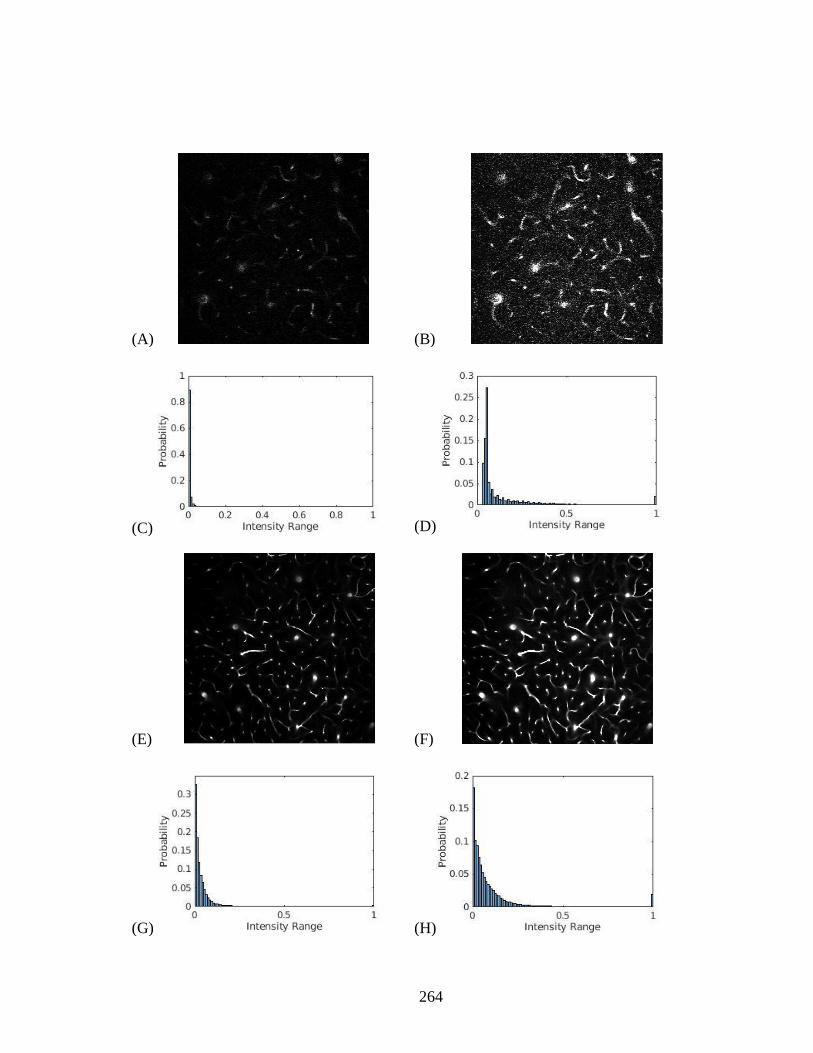
264
(A) (B)
(C) (D)
(E) (F)
(G) (H)
265
Figure 5.8. Image Intensity normalization for two different datasets.
SN Lab (A-D) and Boas Lab (E-H), before (A, C, E, G) and after (B, D, F, H)
intensity normalization illustrated as the grayscale image (A-B, E-F) and image
intensity histogram (C-D, G-H).
5.3.8 HFD results
We also compared the results between a trained user evaluating full stacks and the
StallCatchers result. An expert looks at the raw 3D images and identified the stalled
vessels. Alternatively, an expert reviewed the stalled vessels detected by StallCatchers
with high probability and reconfirmed the results similar to the previous section. The
results of this study (shown in Figure 5.7) suggests HFD increases stall rates but does not
have a synergistic effect with AD.
5.3.9 Exceptional dataset
A new dataset from an independent laboratory (Boas Lab, Boston University) was
acquired to study the generalization of the preprocessing steps to images acquired using
different microscopes and acquisition settings. These data had differences from previous
used data in terms of the different levels of noise, the pixel size, and the frame rate.
In order to utilize the current pipeline, the only hyperparameter of DeepVess that
required fine-tuning was the image intensity normalization percentile used for the
standardization. Typically, most of the intensity range can be utilized by performing 1%
saturation at the two ends of the intensity range. In contrast, the new dataset required 2%

266
saturation at the high-intensity range in order to utilize most of the intensity range (Figure
5.8). The level of saturation was determined in an empirical optimization fashion based
on intensity histogram and DeepVess’ results. Figure 5.8 shows the effect of the intensity
normalization process with having intensity distributions with the fat tail that utilizes
most of the intensity range.
As described in the last section, since the image intensity distribution depends on
the microscope and acquisition systems, the only hyperparameter that needs fine tuning
is the image normalization percentile, which maximizes the intensity range utilization.
5.4 Conclusions
5.4.1 Future work
The crowd response aggregation algorithm can be improved to decrease the
required number of responses per vessel and leads to a higher throughput rate.
Additionally, the vessel assignment can be done in a more adaptive fashion in order to
utilize the valuable time of the experienced users in more challenging cases.
Furthermore, the StallCatchers’ results can be re-utilized as the ground truth
dataset for training more sophisticated machine learning algorithm with the goal of
performing this classification task in a semi- or fully-automated manner in the near future.
267
REFERENCES
Alosco, M. L., Spitznagel, M. B., Raz, N., Cohen, R., Sweet, L. H., Colbert, L. H., …
Gunstad, J. (2012). Obesity Interacts with Cerebral Hypoperfusion to Exacerbate
Cognitive Impairment in Older Adults with Heart Failure. Cerebrovascular
Diseases Extra, 2(1), 88–98. https://doi.org/10.1159/000343222
Bennett, R. E., Robbins, A. B., Hu, M., Cao, X., Betensky, R. A., Clark, T., … Hyman,
B. T. (2018). Tau induces blood vessel abnormalities and angiogenesis-related
gene expression in P301L transgenic mice and human Alzheimer’s disease.
Proceedings of the National Academy of Sciences, 115(6), E1289–E1298.
https://doi.org/10.1073/pnas.1710329115
Biggs, J., Ewald, N., Valentini, A., Gaboriaud, C., Dejean, T., Griffiths, R. A., … Dunn,
F. (2015). Using eDNA to develop a national citizen science-based monitoring
programme for the great crested newt (Triturus cristatus). Biological
Conservation, 183, 19–28. https://doi.org/10.1016/j.biocon.2014.11.029
Bird, T. J., Bates, A. E., Lefcheck, J. S., Hill, N. A., Thomson, R. J., Edgar, G. J., …
Frusher, S. (2014). Statistical solutions for error and bias in global citizen science
datasets. Biological Conservation, 173, 144–154.
https://doi.org/10.1016/j.biocon.2013.07.037
Cova, I., Clerici, F., Rossi, A., Cucumo, V., Ghiretti, R., Maggiore, L., … Caracciolo, B.
(2016). Weight Loss Predicts Progression of Mild Cognitive Impairment to
Alzheimer’s Disease. PLOS ONE, 11(3), e0151710.
https://doi.org/10.1371/journal.pone.0151710
Cruz Hernández, J. C., Bracko, O., Kersbergen, C. J., Muse, V., Haft-Javaherian, M.,
Berg, M., … Schaffer, C. B. (2019). Neutrophil adhesion in brain capillaries
reduces cortical blood flow and impairs memory function in Alzheimer’s disease
mouse models. Nature Neuroscience, 22(3), 413–420.
https://doi.org/10.1038/s41593-018-0329-4
268
Denk, W., Strickler, J. H., & Webb, W. W. (1990). Two-photon laser scanning
fluorescence microscopy. Science, 248(4951), 73–76.
Haft-Javaherian, M., Fang, L., Muse, V., Schaffer, C. B., Nishimura, N., & Sabuncu, M.
R. (2018). Deep convolutional neural networks for segmenting 3D in vivo
multiphoton images of vasculature in Alzheimer disease mouse models.
ArXiv:1801.00880 [Cs]. Retrieved from http://arxiv.org/abs/1801.00880
Heim, E., Roß, T., Seitel, A., März, K., Stieltjes, B., Eisenmann, M., … Maier-Hein, L.
(2018). Large-scale medical image annotation with crowd-powered algorithms.
Journal of Medical Imaging, 5(3), 034002.
https://doi.org/10.1117/1.JMI.5.3.034002
Iadecola, C. (2004). Neurovascular regulation in the normal brain and in Alzheimer’s
disease. Nature Reviews Neuroscience, 5(5), 347–360.
https://doi.org/10.1038/nrn1387
Kleinfeld, D., Mitra, P. P., Helmchen, F., & Denk, W. (1998). Fluctuations and stimulus-
induced changes in blood flow observed in individual capillaries in layers 2
through 4 of rat neocortex. Proceedings of the National Academy of Sciences,
95(26), 15741–15746.
Raykar, V. C., Yu, S., Zhao, L. H., Jerebko, A., Florin, C., Valadez, G. H., … Moy, L.
(2009). Supervised Learning from Multiple Experts: Whom to Trust when
Everyone Lies a Bit. Proceedings of the 26th Annual International Conference on
Machine Learning, 889–896. https://doi.org/10.1145/1553374.1553488
Santisakultarm, T. P., Paduano, C. Q., Stokol, T., Southard, T. L., Nishimura, N., Skoda,
R. C., … Schaffer, C. B. (2014). Stalled cerebral capillary blood flow in mouse
models of essential thrombocythemia and polycythemia vera revealed by in vivo
two-photon imaging. Journal of Thrombosis and Haemostasis, 12(12), 2120–
2130. https://doi.org/10.1111/jth.12738
Santisakultarm, Thom P., Cornelius, N. R., Nishimura, N., Schafer, A. I., Silver, R. T.,
Doerschuk, P. C., … Schaffer, C. B. (2012). In vivo two-photon excited
fluorescence microscopy reveals cardiac- and respiration-dependent pulsatile
blood flow in cortical blood vessels in mice. American Journal of Physiology-
269
Heart and Circulatory Physiology, 302(7), H1367–H1377.
https://doi.org/10.1152/ajpheart.00417.2011
Sullivan, B. L., Wood, C. L., Iliff, M. J., Bonney, R. E., Fink, D., & Kelling, S. (2009).
eBird: A citizen-based bird observation network in the biological sciences.
Biological Conservation, 142(10), 2282–2292.
https://doi.org/10.1016/j.biocon.2009.05.006
Theobald, E. J., Ettinger, A. K., Burgess, H. K., DeBey, L. B., Schmidt, N. R., Froehlich,
H. E., … Parrish, J. K. (2015). Global change and local solutions: Tapping the
unrealized potential of citizen science for biodiversity research. Biological
Conservation, 181, 236–244. https://doi.org/10.1016/j.biocon.2014.10.021
Westphal, A. J., Stroud, R. M., Bechtel, H. A., Brenker, F. E., Butterworth, A. L., Flynn,
G. J., … Dusters, 30714 Stardust@home. (2014). Evidence for interstellar origin
of seven dust particles collected by the Stardust spacecraft. Science, 345(6198),
786–791. https://doi.org/10.1126/science.1252496
270
CHAPTER 6
XYLEM VESSEL CONNECTIVITY IN THE RING AND DIFFUSE POROUS TREES
6.1 Introduction
The world is full of transport networks ranging from biological to engineered.
Despite differences in their nature and purpose, networks share similar structures and
dynamics (Watts & Strogatz 1998). To model and understand these dynamics, networks
are often simplified and studied as graphs, structures comprising of nodes and edges, where
nodes represent the main elements of the network and edges represent the connections or
pathways between the elements. The specific arrangement of nodes and pathways within
the network determines both the overall topology and the functional efficiency of the
structure (Watts & Strogatz 1998; Latora & Marchiori 2001). With respect to biological
fluid transport networks, the topology can also impact the vulnerability of the system in
response to external stresses (Zimmermann 1983). Topology regulates the total throughput
of the network in terms of the hydraulic conductance and the fluid transport distributions
throughout the network. As a result, the ability to accurately map physical networks into
well-defined networks is a crucial step toward understanding the dynamics of these
complex systems. Previously, the methodologies based on the network analysis have been
utilized to study brain vascular networks (Cruz Hernández et al. 2019).
One network that has been understudied is the water transport system in plants: the
xylem network. The anatomy of this network provides reliable water transport in plants.
These networks consist of water conducting, tube-shaped vessels, called xylem vessels,
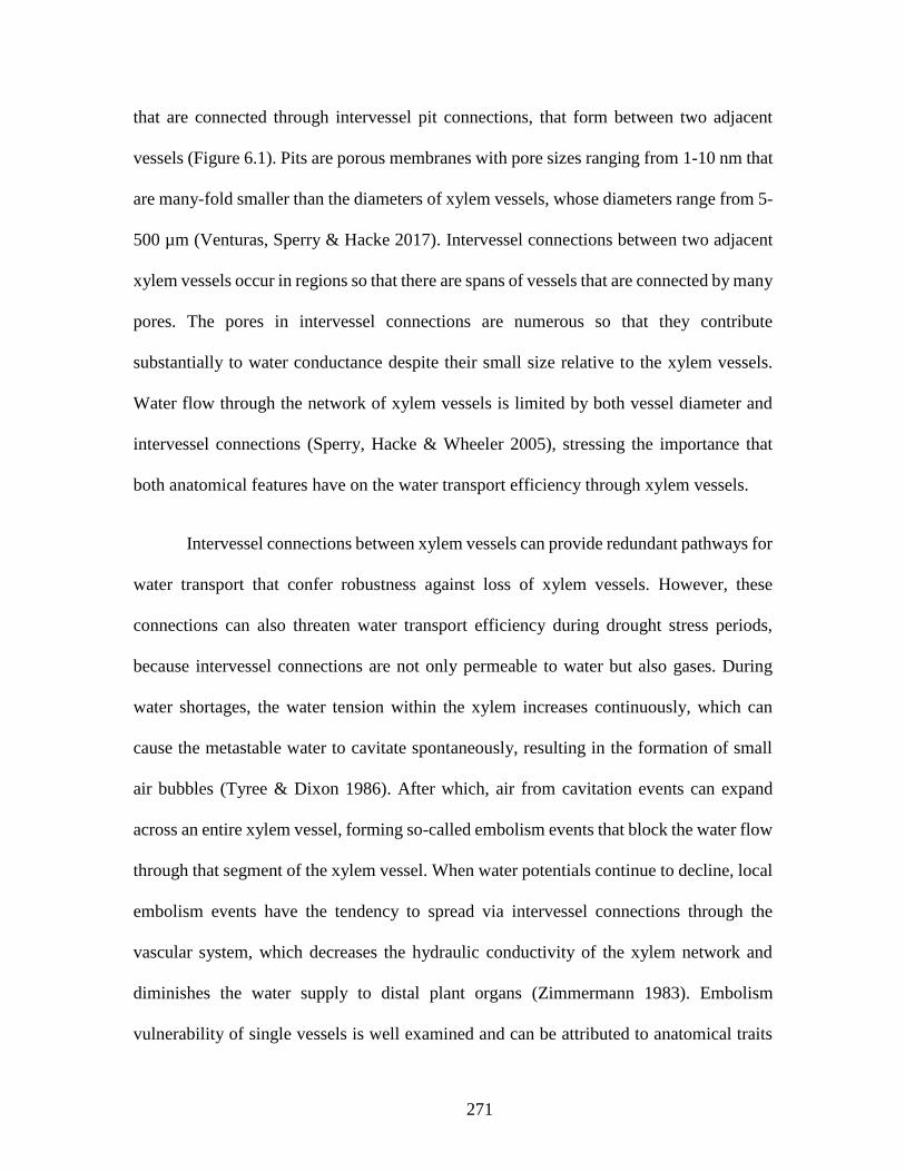
271
that are connected through intervessel pit connections, that form between two adjacent
vessels (Figure 6.1). Pits are porous membranes with pore sizes ranging from 1-10 nm that
are many-fold smaller than the diameters of xylem vessels, whose diameters range from 5-
500 µm (Venturas, Sperry & Hacke 2017). Intervessel connections between two adjacent
xylem vessels occur in regions so that there are spans of vessels that are connected by many
pores. The pores in intervessel connections are numerous so that they contribute
substantially to water conductance despite their small size relative to the xylem vessels.
Water flow through the network of xylem vessels is limited by both vessel diameter and
intervessel connections (Sperry, Hacke & Wheeler 2005), stressing the importance that
both anatomical features have on the water transport efficiency through xylem vessels.
Intervessel connections between xylem vessels can provide redundant pathways for
water transport that confer robustness against loss of xylem vessels. However, these
connections can also threaten water transport efficiency during drought stress periods,
because intervessel connections are not only permeable to water but also gases. During
water shortages, the water tension within the xylem increases continuously, which can
cause the metastable water to cavitate spontaneously, resulting in the formation of small
air bubbles (Tyree & Dixon 1986). After which, air from cavitation events can expand
across an entire xylem vessel, forming so-called embolism events that block the water flow
through that segment of the xylem vessel. When water potentials continue to decline, local
embolism events have the tendency to spread via intervessel connections through the
vascular system, which decreases the hydraulic conductivity of the xylem network and
diminishes the water supply to distal plant organs (Zimmermann 1983). Embolism
vulnerability of single vessels is well examined and can be attributed to anatomical traits
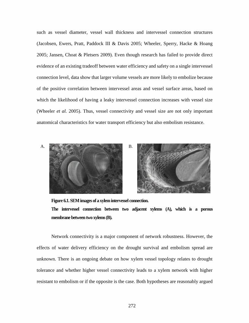
272
such as vessel diameter, vessel wall thickness and intervessel connection structures
(Jacobsen, Ewers, Pratt, Paddock III & Davis 2005; Wheeler, Sperry, Hacke & Hoang
2005; Jansen, Choat & Pletsers 2009). Even though research has failed to provide direct
evidence of an existing tradeoff between water efficiency and safety on a single intervessel
connection level, data show that larger volume vessels are more likely to embolize because
of the positive correlation between intervessel areas and vessel surface areas, based on
which the likelihood of having a leaky intervessel connection increases with vessel size
(Wheeler et al. 2005). Thus, vessel connectivity and vessel size are not only important
anatomical characteristics for water transport efficiency but also embolism resistance.
A.
B.
Figure 6.1. SEM images of a xylem intervessel connection.
The intervessel connection between two adjacent xylems (A), which is a porous
membrane between two xylems (B).
Network connectivity is a major component of network robustness. However, the
effects of water delivery efficiency on the drought survival and embolism spread are
unknown. There is an ongoing debate on how xylem vessel topology relates to drought
tolerance and whether higher vessel connectivity leads to a xylem network with higher
resistant to embolism or if the opposite is the case. Both hypotheses are reasonably argued
273
and supported: Loepfe et al. 2007 suggested that higher xylem vessel connectivity impedes
the network resistance to embolism because of the high network connectivity due to the
intervessel connections facilities the spread of embolisms throughout the system. Indirect
support for Loepe’s results is given by an empirical study conducted on eighteen North
American and Asian temperate trees and shrubs (Zanne, Sweeney, Sharma & Orians 2006)
which focused on drought tolerance. This study showed that plants with a higher drought
tolerance have less integrated, i.e., less number of intervessel connections, xylem pathways
(Zanne et al. 2006). Contrarily, the counter-theory proposes that interconnected xylem
networks are more resistant to drought stress because, in the case of an embolism event, a
highly interconnected xylem network benefits from having several pathways through
which water can be redirected. Thus, embolism events will have less impact on hydraulic
conductance in a well-connected network. Support for this theory is given by an empirical
data set on six different Acer taxa, that showed that intervessel connectivity leads to a more
resistant xylem network (Lens et al. 2011). These two contrary arguments highlight the
necessity for characterizing the architecture of xylem networks to identify networks traits
affecting embolism resistance. However, both vessel topology and vessel connections are
difficult to map due to technical limitations and therefore are poorly understood. As a
result, we are far away from understanding how network connectivity affects xylem
network vulnerability to embolism.
An established method for quantifying xylem network resistance to embolisms
without the characterization of anatomical traits is the hydraulic vulnerability curves (PLC
curves), which characterize the percent loss of hydraulic conductivity of a tissue segment
as a function of the water potential within the tissue. There is an implicit assumption that
274
the water potential within the tissue is correlated with the degree of embolism within the
vessel network and PLC curves (Cochard et al. 2013). Using the PLC curves, the P50 value
is the water potential corresponding to a 50% hydraulic conductance loss through the xylem
and is commonly used to compare drought resistance across plants. P50 values typically
range in trees from -0.2 MPa to -14.0 MPa, with more negative values corresponding to
greater tolerance to drought (Maherali, Pockman & Jackson 2004). How the overall shape
of the PLC curve is directly linked to the relevant network characteristics remains
unknown.
To address a number of these unknowns, in this manuscript we utilized laser
ablation tomography (LATscan), a method that produces three-dimensional structural
images, to explore the anatomical network characteristics of three ring-porous and three
diffuse-porous tree species. Diffuse-porous tree species typically exhibit a tight vessel size
distribution (around 40 µm in diameter) across year rings, while ring-porous tree species
typically exhibit a bimodal vessel distribution, with large vessels (<500 μm) in the spring
wood and small vessels (>20 μm) in the late wood. Ring-porous tree species have a higher
maximum hydraulic efficiency than diffuse porous tree species due to the larger vessels in
the early growth periods of the season in comparison to diffuse porous tree species
(Carlquist 1988). However, these large vessels are particularly vulnerable to air embolisms
due to the inverse correlation between vessel size and intervessel quantity and the
likelihood of gas penetrating through the intervessel connection (Zimmermann 1983;
Wheeler et al. 2005; Christman, Sperry & Smith 2012). We investigated the relationship
between the intervessel quantity and the embolism likelihood by tracing and reconstructing
the xylem networks of all six species using a deep neural network to segment images and

275
then quantify the overall network connectivity and vessel topology to identify network
characteristics for these two wood types. We then simulated the robustness of the water
flow in the network against blocked vessels and correlated these findings to P50 values.
Comparing the different vessel arrangements of these two wood types with vulnerability
curves aims towards a better understanding of the different vulnerabilities of embolism
spread in the ring and diffuse-porous trees and will allow us to examine if xylem network
connectivity contributes to the high embolism vulnerability of large early wood vessels in
ring-porous tree species.
6.2 Material and Methods
6.2.1 Plant material
Two two-year-old branches of three individual trees of either three diffuse-porous
(Fagus sylvatica, Populus x canadensis, Liriodendron tulipifera) or three ring-porous
(Quercus montana, Fraxinus excelsior, Carya ovata) tree species were harvested for each
measurement between April 2016 and June 2017. Selected tree species were grown on
Cornell Campus, and tree replicates were chosen based on their proximity to each other
(Ithaca, NY; lat. 42.44° N, long. 76.44° W). Ithaca has a continental moderate climate with
an average annual temperature of 8.5 °C and an average annual rainfall of 982 mm
(Northeast Regional Climate Center 2019).
6.2.2 Percent loss of hydraulic conductivity
Vulnerability curves were performed using the bench-top dry down method (Tyree
& Dixon 1986). Around 60 cm long branches were cut around midnight, immediately

276
double bagged, brought to the lab, and the cut end was put into water. The following
morning, the branches were spread out on the bench-top, single leaves were bagged for
allowing leaf water potential (Ψleaf) to equilibrate with the branch water potential (Ψbranch)
and dried down for varying amounts of time to archive a range of different (Ψleaf). During
this timeframe, Ψleaf was taken on the bagged leaves with a water status console
(Soilmoisture Equipment Corp., Goleta, CA). After reaching the desired Ψleaf, branches
were double bagged, equilibrated for 12 hours, and remeasured. Then, branches were cut
under water to 15 cm long segments and inserted into a custom-built low-pressure flow
meter (Melcher et al. 2012) by attaching one end of the branch segment to a reservoir that
was filled with a (0.1 µm) filtered 20 mM KCl of perfusion solution, and the other end of
the branch segment to an analytical balance (HR-200, A&D, Elk Grove, Il). Then, the
initial flow rate (Q) was measured. The hydraulic pressure difference between sample and
solution reservoir was kept constant species dependent between 1.5 kPa and 3.0 kPa during
the measurements. Afterward, branch segments were flushed for 1 hour at 100 kPa with
the perfusion solution, and the max flow rate was measured by reinserting the stem
segments in the low-pressure flow meter. The unit-length hydraulic conductivity (K) was
determined by:
K = Q 𝐿
ΔP (1)
Where, L is the length of the sample, and ΔP is the hydraulic pressure gradient.
After the measurements, the xylem cross-sectional area was determined with a caliper and
the specific hydraulic conductivity determined by dividing the K by the cross-sectional
areas. Lastly, the percent of hydraulic loss of conductivity (PLC) was calculated by:

277
PLC = 100
1 −𝐾𝑚𝑎𝑥𝐾𝑚𝑖𝑛
(2)
Where, Kmax is the maximum specific conductivity after flushing, and Kin is the
initial specific hydraulic conductivity. The PLC data were fitted with an exponential
sigmoidal equation of:
PLC = 100
1 + 𝑒𝑥𝑝(𝑎 + (Ψ − b)) (3)
Where, a and b are fitting parameters, whereby a describes the slope of the curve
and b represents the position of the curve on the x-axis at 50% PLC (Pammenter & Van
der Willigen 1998). The significance levels of the parameters were calculated based on this
fit.
6.2.3 Vessel length distribution
Vessel length distribution was calculated based on the silicon injection technique
(Sperry et al. 2005; Wheeler et al. 2005). Six branches (~60 cm) per species were cut,
brought into the lab, and flushed for 1 hour at 70 kPa with a 20 mM KCL solution to remove
native embolisms (Sperry, Donnelly & Tyree 1988). Then, basal ends of the branches were
connected via silicon tubing to a nitrogen gas tank and injected with a 10:1 two-component
silicon elastomers (RTV141 A&B, distributed by Hisco, Somerset, NJ, USA) at 70 kPa
overnight. Prior to injection, the silicon mixture was degassed under vacuum and infused
with a UV stain that was dissolved in chloroform (Ciba Uvitex OB, Ciba Specialty
Chemicals, Tarrytown, NY) in order to separate silicon injected xylem vessels from empty
vessels for imaging analysis. After the silicon cured (~2 days), branches were sectioned at
six cutting distances from the injection site with a sliding microtome (American Optical,

278
680 sliding microtome, Spencer Lens Co., Buffalo, NY). The respective cutting distances
(Li) were determined with the following equation:
𝐿𝑖 = 𝐿𝑚𝑖𝑛 (𝐿𝑚𝑎𝑥
𝐿𝑚𝑖𝑛)
[𝑖−1𝑁−1
]
(4)
With Lmin the cross section at 0.5 cm after the injection point, and Lmax the cross-
section at which 2% of the vessels were detected under the fluorescence microscope, and
N the total amount of cuts. Then, cross sections mounted in glycerol, magnified with a
10x/04 objective and imaged a with a fluorescence microscope (Olympus BX50, Olympus
Scientific Solutions, Waltham, MA, US) to which a camera was attached (Retiga Exi CCD
camera, QImagig, Burnaby, BC, Canada). Fluorescent silicon injected vessels from the
most recent formed year ring were counted and averaged over species. Lastly, the vessel
length distribution and the average vessel length was calculated for each species on the
basis of equations reported by Christmann et al. and Christman et al. (Christmann, Weiler,
Steudle & Grill 2007; Christman, Sperry & Adler 2009). The objective was to fit the
silicon-injected vessel counts with a Weibull function and to use the best fit to calculate
the second derivate, from which the vessel length distribution was calculated.
6.2.4 Laser ablation tomography
In this study, the laser source of the Laser ablation tomography scan (LATscan)
system was a Coherent Avia 355-7000 Q-switched ultraviolet laser (Coherent, 5100 Patrick
Henry Drive, Santa Clara, CA 95054 USA) with a pulse repetition rate of 25 KHz and
wavelength of 355 nm. The pulse duration of the laser was less than 30 ns and supplied
pulse energy of approximately 200 mJ. The galvanometer used to scan the laser beam to
make the ablation plane was a Scanlab HurryScan 10 (Scanlab, Siemensstr 2a, 82178

279
Puchheim, Germany). Samples were fixed to a cantilever and connected to the mechanical
stage along its travel axis, then fed into the ablation plane using an Aerotech linear drive
stage (Aerotech, Inc., 101 Zeta Dr, Pittsburgh, PA 15238, USA), with the distance between
sections ranging from 35 µm to 50 µm. Images were captured via a Canon 70D camera
equipped with a Canon Macro Photo Lens MP-E 65 mm 1:2.8 1-5X. The images were 5472
x 3648 pixels at a resolution of 1 micron per pixel.
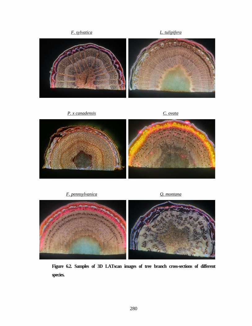
280
F. sylvatica L. tulipifera
P. x canadensis
C. ovata
F. pennsylvanica
Q. montana
Figure 6.2. Samples of 3D LATscan images of tree branch cross-sections of different
species.
281
6.2.5 Selecting vessel length and cutting distance for analysis
The maximum sample length was restricted by a combination of technical
limitation and sample trait. The digital camera tended to overheat with increasing sample
length due to the amount of image taken. Additionally, the degree of natural bending of the
branches increased with sample length. Consequently, samples tended to move out of the
imaging plane with increasing sample length and we were unable to realign the sample
with imaging plane by simply pushing the sample back in the imaging plane. To ensure
image quality we chose maximum sample length to be the 75th percentile of vessel class
length, that was determined by vessel length distribution, for diffuse-porous tree species
and 50th percentile for ring-porous tree species (Figure S 6.1). To determine the maximum
distance between cuttings, we performed a preliminary experiment in which we ablated 31
slices of a sample of all six tree species into the minimum cutting distance (5 μm and total
length of 150 μm) and manually segmented 100 vessels per species using ImageJ (Rueden
et al. 2017) using the procedure described by Haft-Javaherian et al. (Haft-Javaherian et al.
2019). We then measured the segmentation similarity between the first slice and the
following slices based on the ratio of the intersection area of two adjacent vessel cross-
sections and the first slice vessel cross-section area averaged over all detected vessels to
determine the maximum distance between two images such that we observed at least 50%
averaged cross-sectional overlaps with an upper limit of 50 μm. We found this distance to
be 50 μm for all ring-porous tree species, 40 μm for F. sylvatica, 35 μm for P. x canadensis,
and 50 μm for L. tulipifera. These cutting distances were then used for all further analysis
(Table 6-1).
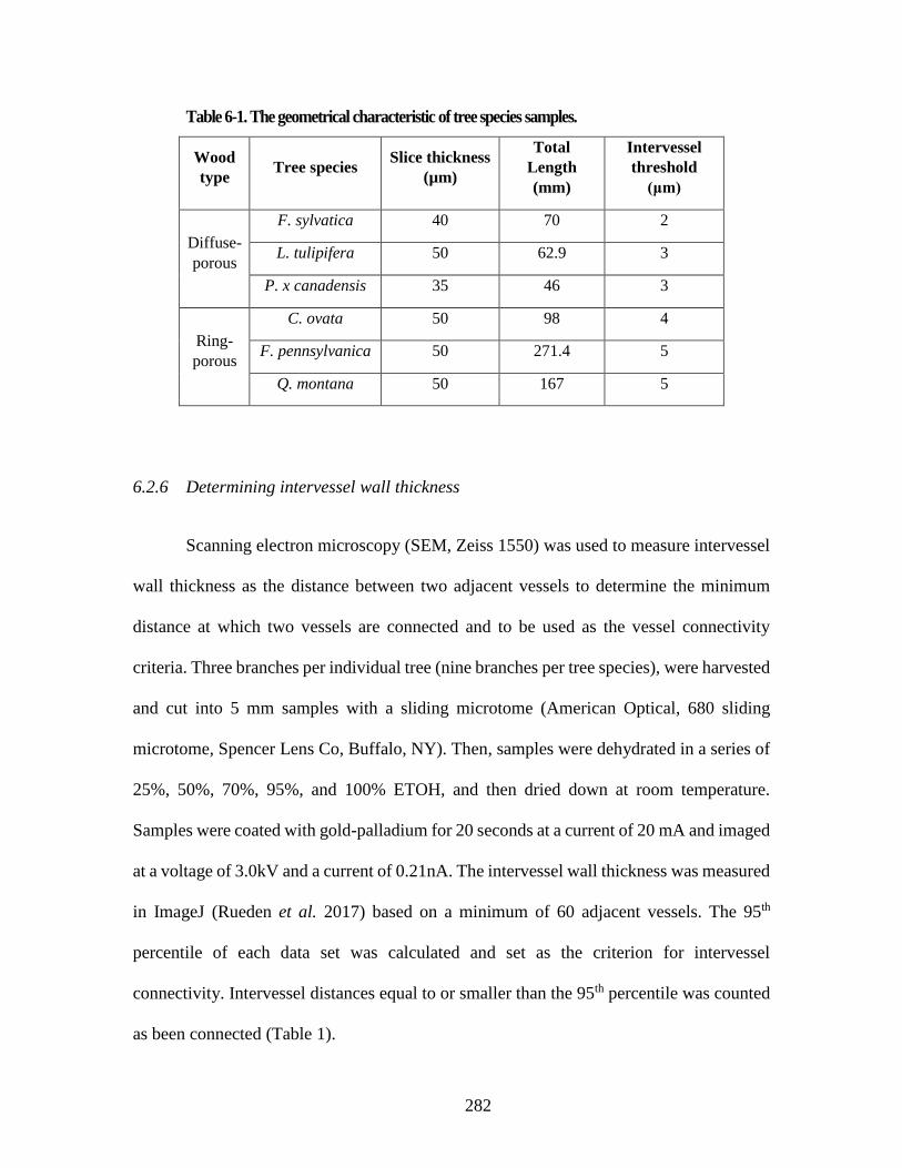
282
Table 6-1. The geometrical characteristic of tree species samples.
Wood
type Tree species
Slice thickness
(µm)
Total
Length
(mm)
Intervessel
threshold
(μm)
Diffuse-
porous
F. sylvatica 40 70 2
L. tulipifera 50 62.9 3
P. x canadensis 35 46 3
Ring-
porous
C. ovata 50 98 4
F. pennsylvanica 50 271.4 5
Q. montana 50 167 5
6.2.6 Determining intervessel wall thickness
Scanning electron microscopy (SEM, Zeiss 1550) was used to measure intervessel
wall thickness as the distance between two adjacent vessels to determine the minimum
distance at which two vessels are connected and to be used as the vessel connectivity
criteria. Three branches per individual tree (nine branches per tree species), were harvested
and cut into 5 mm samples with a sliding microtome (American Optical, 680 sliding
microtome, Spencer Lens Co, Buffalo, NY). Then, samples were dehydrated in a series of
25%, 50%, 70%, 95%, and 100% ETOH, and then dried down at room temperature.
Samples were coated with gold-palladium for 20 seconds at a current of 20 mA and imaged
at a voltage of 3.0kV and a current of 0.21nA. The intervessel wall thickness was measured
in ImageJ (Rueden et al. 2017) based on a minimum of 60 adjacent vessels. The 95th
percentile of each data set was calculated and set as the criterion for intervessel
connectivity. Intervessel distances equal to or smaller than the 95th percentile was counted
as been connected (Table 1).
283
6.2.7 The study-design image processing pipeline
We developed a graphical user interface (GUI) in Matlab for image processing and
network analysis to facilitate the preliminary study analysis and the study design (e.g.,
cutting distance determinations and methodological feasibility risk analysis). The GUI
allows the user to load a 3D stack of images and select the region of interest in addition to
tuning the image processing parameters. The image processing pipeline started with the
application of a top hat filter followed by a bottom hat filter. Top hat filter subtracts the
morphological opening of the image from the original image and similarly bottom hat filter
subtract the original image from the morphological closing of the image. The
morphological opening consists of an erosion of image followed by dilation, and in
contrast, morphological closing consists of a dilation followed by an erosion. The erosion
and dilation are the two basic mathematical morphology operations, which require a
structuring element (i.e., kernel) to operate. The combination of top hat and bottom hat
filters treat small objects with very high or low intensity. Next, we sharpened the image by
subtracting the smoothed image (using a Gaussian lowpass filter multiplied by a constant)
from the original image. Next step the grayscale image is binarized using an adaptive
threshold defined using Otsu’s method (Otsu 1979) in addition to ensuring the preservation
of the boundaries between adjacent vessels. Finally, the small isolated objects were
removed, and the holes were filled. The vessel cross-section centroids were identified to
produce the graph representation of vasculature networks using the binary segmentation
results. The GUI save the segmentation, graph representation, and the adjacency matrix of
vessel connections to the output data file.

284
6.2.8 Motion artifact compensation
Motion artifact is one of the main challenges for images processing of 3D
vasculature network images. Apparent motion can be caused by any combination of
gradual shift, sudden shift or rotation, poor focus, and burned cross-section (see Figure
6.3). In order to compensate for these different motion artifact cases, we utilized two
different methods and optimized their hyperparameter based on our images and sources of
motion artifacts. Due to the size of our dataset, the computational complexity and
scalability is the other important factor that needs to be considered because the 3D images
could contain up to 5000 slices along their third dimension. Since there are no local
distortion and motion artifacts in the images, a rigid registration (i.e., translation and
rotation) is sufficient for this task. A registration method consists of a similarity metric as
an input to the cost function and an optimizer to optimize the cost function finding the
optimal registration parameters. The first method used mean square error (Eq. 5) as the
similarity metric and the regular step gradient descent optimization, which follows the
gradient of the cost function to in the direction of extrema with reducing the step function
when the gradient changes direction.
𝑀𝑆𝐸 = 1
𝑁 × 𝑀∑ ∑(𝐼𝑖,𝑗 − 𝐼𝑖,𝑗
′ )2
𝑀
𝑗=1
𝑁
𝑖=1
(5)
We used a random grid search to find the optimal hyperparameters for the optimizer
and found two optimal sets of hyperparameters. The ensemble of two optimizers based on
the optimal sets of hyperparameters was able to handle most of the cases, and it was
successful when applied to the test cases with small sample sizes. The failure modes
include uneven illuminations, laser-burned cross-sections, color-distorted images, and
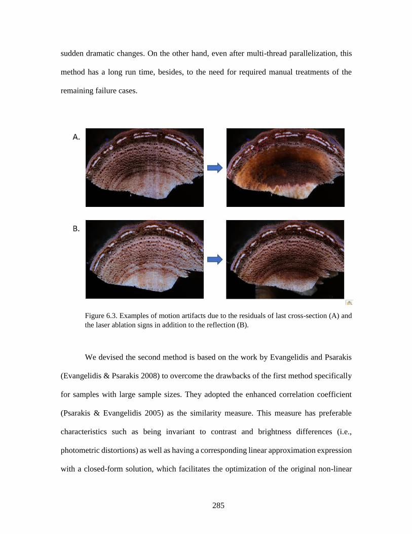
285
sudden dramatic changes. On the other hand, even after multi-thread parallelization, this
method has a long run time, besides, to the need for required manual treatments of the
remaining failure cases.
Figure 6.3. Examples of motion artifacts due to the residuals of last cross-section (A) and
the laser ablation signs in addition to the reflection (B).
We devised the second method is based on the work by Evangelidis and Psarakis
(Evangelidis & Psarakis 2008) to overcome the drawbacks of the first method specifically
for samples with large sample sizes. They adopted the enhanced correlation coefficient
(Psarakis & Evangelidis 2005) as the similarity measure. This measure has preferable
characteristics such as being invariant to contrast and brightness differences (i.e.,
photometric distortions) as well as having a corresponding linear approximation expression
with a closed-form solution, which facilitates the optimization of the original non-linear
286
measure. Additionally, Evangelidis and Psarakis proposed an iterative gradient based (e.g.,
forward additive refinement algorithm) to optimize the original non-linear measure using
the linear approximation (Evangelidis & Psarakis 2008). In order to tackle multi-scale
motion artifacts, we estimated the transformation parameters in a pyramid fashion using
10X scaled-down versions of the two images and then fine-tune the parameters using the
original resolutions. Since the images do not suffer from local motion artifacts, only the
estimation of the global transformation parameters within two consecutive images is
required.
In order to parallelize the process, images were divided into groups of 10
consecutive images and registered independently based on the first image in the group.
Then, sequentially starting from the second image group, the first image of each image
group was aligned to the last image of the preceding image group and the rest of the images
within the group were warped using the same transformation. Finally, we implemented a
failure detector using the mean structural similarity index (Wang, Bovik, Sheikh &
Simoncelli 2004) between two consecutive images. Within every 11 consecutive pairs of
images, the middle pair is considered as a failure case if its similarity index is at least 5%
lower than the median of the 11 similarity indexes. The failure cases were registered again
using the same algorithm (or in rare cases manually if the algorithm failed repeatedly)
followed by warping all the following images using the same transformation parameters.
This process was repeated until no failure cases were detected.
287
6.2.9 Segmentation
We extracted three 3D samples per species including at least 31 consecutive images
that were manually annotated as the ground truth. At least 100 vessels were manually
segmented through the depth of each sample using the manual segmentation protocol
developed by Haft-Javaherian et al. (Haft-Javaherian et al. 2019). Due to the significant
anatomical differences between different species vessel morphologies and size
distributions, we trained a separate segmentation model for each species. We adopted the
architecture and training scheme of DeepVess (Haft-Javaherian et al. 2019), that is a
convolutional neural network (CNN) model with an optimal architecture for the 3D
vasculature segmentation task and a customized cost function, and trained the model for
each species using the ground truth.
Since each sample had between 1000 and 5000 images, each 500-image stack was
stored in a separate HDF5 binary data format to be segmented using the CNN model. After
the segmentation task, the binarized segmentation results were concatenated to form the
complete segmentation results for each sample. In order to remove minimal segmentation
artifacts, we applied a dilation morphological image filter with a disk kernel of radius 1 to
remove the boundary of vessels followed by a 3D median filter with a 3-voxel box kernel
to smooth the vessel boundary and fill the holes within the vessels. The complete image
processing pipeline is illustrated in Figure 6.4.
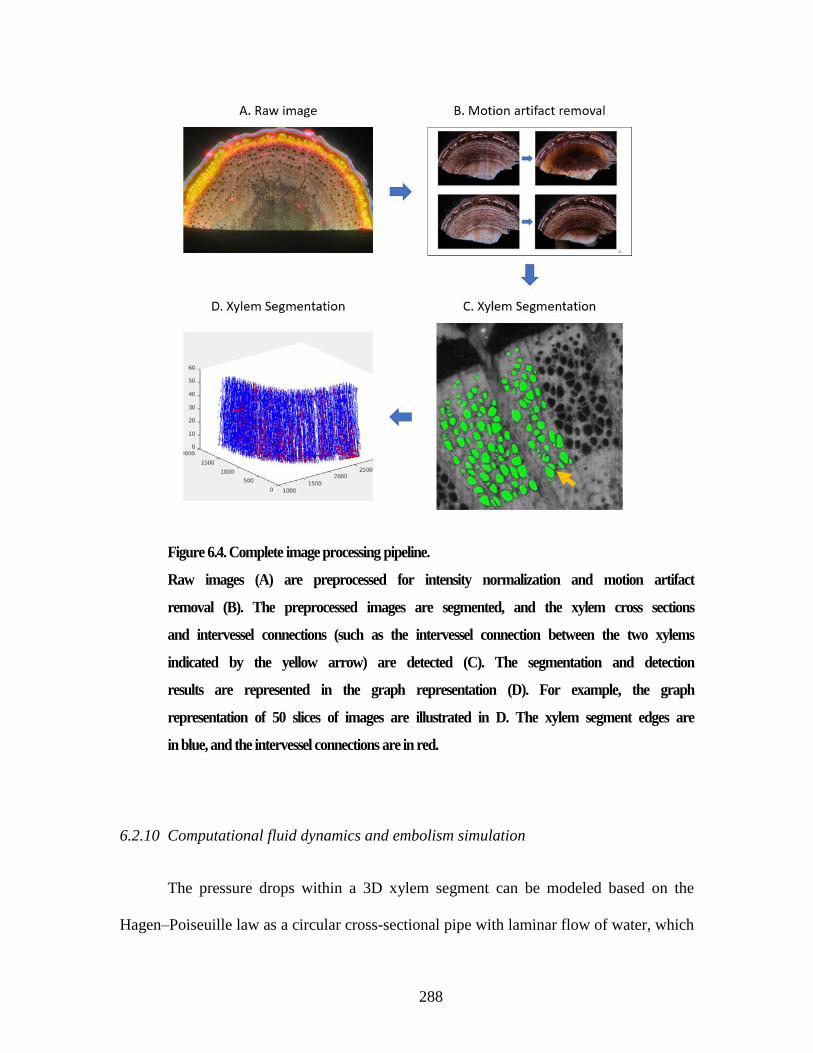
288
Figure 6.4. Complete image processing pipeline.
Raw images (A) are preprocessed for intensity normalization and motion artifact
removal (B). The preprocessed images are segmented, and the xylem cross sections
and intervessel connections (such as the intervessel connection between the two xylems
indicated by the yellow arrow) are detected (C). The segmentation and detection
results are represented in the graph representation (D). For example, the graph
representation of 50 slices of images are illustrated in D. The xylem segment edges are
in blue, and the intervessel connections are in red.
6.2.10 Computational fluid dynamics and embolism simulation
The pressure drops within a 3D xylem segment can be modeled based on the
Hagen–Poiseuille law as a circular cross-sectional pipe with laminar flow of water, which

289
is an incompressible and Newtonian fluid, correlating the fluid flow within the pipe (Q)
with the pressure drop (ΔP) as formulated in Eq. 6. Hence, the segment resistance is defined
as Eq. 7, where, μ is the dynamic viscosity of water at 25°C, D is the xylem segment
diameter, and L is the xylem segment length.
𝑄 =𝜋𝐷4∆𝑃
128𝜇𝐿(6)
𝑅𝑥 =∆𝑃
𝑄=
128𝜇𝐿
𝜋𝐷4 (7)
Sperry and Hacke (Sperry & Hacke 2004) modeled the resistance of the intervessel
connections (Ri) as infinitely thin plates with perfectly circular pores with resistance as a
function of the equivalent pore size (De) and the number of pores in the intervessel
connection (np) defined in Eq. 8. Since we can assume that np is proportional to the
intervessel connection length (Li in Eq. 9), which are measured based on 3D images of
samples, we modeled the intervessel connection resistance (Ri) as a function of Li, which
is a proxy for the np (Eq. 10).
𝑅𝑖 =24𝜇
𝐷𝑒3𝑛𝑝
(8)
𝐷𝑒3𝑛𝑝 = 𝛼𝐿𝑖 (9)
𝑅𝑖 =24𝜇
𝛼𝐿𝑖 (10)
The hydraulic network based on the xylem segments and intervessel connections
was modeled using Eq. 7 and Eq. 10. The system then is represented in a linear system of
equations, and the solution was acquired using one of the sparse systems of linear equation
solver methods (e.g., Cholesky solver) depend on the characteristics of the linear systems.
A unit pressure difference was applied between the two ends of the longest connected

290
segment within each tree sample, and the flow within the sample was measured to calculate
the sample conductance (Q/ΔP). Thirty simulations were conducted for each dropout
percentile ranging from 0% to 100% in order to simulate different embolism events. The
relative conductance, which is the ratio of conductance to the baseline conductance at 0%
dropout was reported for each sample.
6.2.11 Statistics
Statistical analysis was performed in JMP Pro 14.0.0 (SAS Institute Inc., Cary,
NC.) or Matlab. All tests were performed with probability level p < 0.05. Differences
between tree pieces were calculated using ANOVA, and multi-comparison corrections
were done using the Tukey-Kramer method. For calculating differences in intervessel wall
thickness among tree types, the dependent variable was log transformed to fulfill model
assumptions.
6.3 Results and Discussions
Graphs and networks are mathematical tools that represent a set of relationships or
processes (edges) between a set of objects (vertices) and facilitate quantitative analysis of
the objects in the context of their relationships. We utilized the xylem segmentation results
to generate the graph representation of xylem networks to study and characterize them
using network analysis and fluid mechanics.
Since 3D xylem vessels extend the length of the branch, the xylems appear in cross-
section in each image slice. The segmented image slices identified connected voxels that
together represent a distinct cross-section of a xylem vessel. Xylem vessels are connected

291
by two types of connections. First xylem vessels merged and bifurcated as they traverse
the length of the branch. Xylem segments were defined to start and end with a junction.
Two cross-sections located within two adjacent slices were defined as belonging to the
same 3D xylem segment if they are overlapped (Figure 6.5). Conversely, the xylem
junctions happen when more than one xylem merge into one xylem, or one xylem divides
into more than one xylem. The junction is apparent in images when a cross-section from
an image slice is overlapped with more than one cross-section in the preceding or
proceeding adjacent image slice. Therefore, depending on the cross-sectional overlaps in
the segmented images, the 3D xylem segments and their junctions are identifiable. Second,
because the intervessel connections are not directly visible in the images, they were
identified based on the thickness of the wall between two xylem vessels. The intervessel
connection occurs in places where the distance between the boundaries of two separate
cross-sections within an image slice is less than the intervessel threshold (Table 6-1 and
Figure 6.5.A).
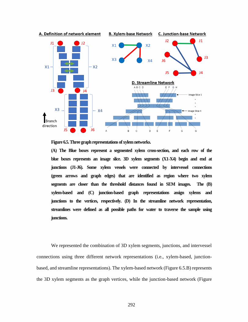
292
Figure 6.5. Three graph representations of xylem networks.
(A) The Blue boxes represent a segmented xylem cross-section, and each row of the
blue boxes represents an image slice. 3D xylem segments (X1-X4) begin and end at
junctions (J1-J6). Some xylem vessels were connected by intervessel connections
(green arrows and graph edges) that are identified as region where two xylem
segments are closer than the threshold distances found in SEM images. The (B)
xylem-based and (C) junction-based graph representations assign xylems and
junctions to the vertices, respectively. (D) In the streamline network representation,
streamlines were defined as all possible paths for water to traverse the sample using
junctions.
We represented the combination of 3D xylem segments, junctions, and intervessel
connections using three different network representations (i.e., xylem-based, junction-
based, and streamline representations). The xylem-based network (Figure 6.5.B) represents
the 3D xylem segments as the graph vertices, while the junction-based network (Figure

293
6.5.C) represents the junctions as the graph vertices. Consequently, the xylem-based
network represents the junctions and intervessel connections using the graph edges, while
the junction-based network represents 3D xylem segments and intervessel connections
using the graph edges. Alternatively, the streamline network (Figure 6.5.D) traces all the
possible distinct water streamlines between the first and last image slices based on the
junctions. Therefore, streamline network represents the streamlines as the graph vertices
and the intervessel connections between streamlines as the graph edges.
In order to characterize these networks using geometrical measures, each cross-
section was fit to a centroid, and the shortest distance to the boundary was defined as the
diameter. The diameter of each xylem vessel was defined as the median of the measured
cross-sections. Correspondingly, the xylem length, number of intervessel connections, and
total length of intervessel connections are measured for each xylem vessel.
Topological metrics characterize the graphs in terms of the relationships within the
vertices. Topological metrics are measured on the graph as a whole (e.g., density) or
measured for each vertex or edge independently (i.e., closeness). The edge- or vertex-based
topological metrics results in measurement distributions, which can be summarized in
terms of their mean (μ) and standard deviation (σ). The implications of the topological
metrics can be illustrated using an analogy based on the United States Highway System
(USHS).
The density measures the degree of connectedness within the network based on the
ratio of the current number of edges and the maximum possible number of edges. In USHS,

294
the number of highways in the current system that connects cities is compared to the case
of maximum density in which each city is connected to all other cities directly.
The centrality metrics are topological metrics measuring the importance of edges,
vertices, or paths. The centrality metrics utilize the identified shortest path between all pairs
of vertices. The edge- and vertex-betweenness measure the number of shortest paths that
include an edge or vertex, respectively. Similarly, closeness measures the average shortest
path to other vertices demonstrating the level of influence of this vertex on other vertices.
In USHS, betweenness illustrates the magnitude of effects in the case of city entrances or
a highway closure due to constructions or catastrophic events. The betweenness is the
number of shortest paths that are eliminated by the closure. Correspondingly, closeness
shows the importance of a city and how congestion in that city may have a ripple effect on
other cities.
The clustering and assortativity measure the amount of the closed loop within the
system and the level of clustering with similar edge types. In USHS, when a city is
connected to two different cities, whether those two cities are connected is correlated with
the level of interconnections and clustering in the network. The assortativity measures how
similar highways are connected for instance main highways vs. controlled access highways
(e.g., US I-95 vs. US I-495).
The graph connection can be recorded using the adjacency matrix, whose indices
represents the vertices and the entry are non-zero when there is an edge between the
corresponding vertices. The maximum eigenvalue and its eigenvector of the adjacency

295
matrices represent the importance of the main pattern of edge connections within the graph
and Katz utilized the same concept to measure the relative degree of influence of vertices.
6.3.1 Geometrical comparisons
Figure 6.6 and Table S 6-1 summarized the geometrical comparisons between
species based on the 3D segment graph representation. F. pennsylvanica and Q. montana
have larger average xylem diameters compare to the other four species, with both being
about double the diffuse-porous trees. Similarly, C. ovata has a larger average xylem
diameter compared to diffuse-porous species. Nevertheless, only F. pennsylvanica has a
significantly larger average xylem segment length compare to all other species. In terms of
intervessel connections, F. sylvatica and P. x canadensis have larger average xylem
intervessel frequency per xylem segment compared to C. ovata and F. pennsylvanica,
while, just P. x canadensis has a larger average xylem intervessel frequency compared to
L. tulipifera and Q. montana. Likewise, F. pennsylvania has a significantly larger average
xylem intervessel length (Total length of intervessel connections per xylem segment)
compare to all other species. On the other hand, Figure 6.7 and Table S 6-2 summarized
the geometrical comparisons between species based on the streamline graph representation.
While xylem diameters results based on the streamline representations imitate the results
based on the 3D segment graph representations, other three geometrical metrics are not
significantly different between species except for the intervessel frequency of C. ovata.
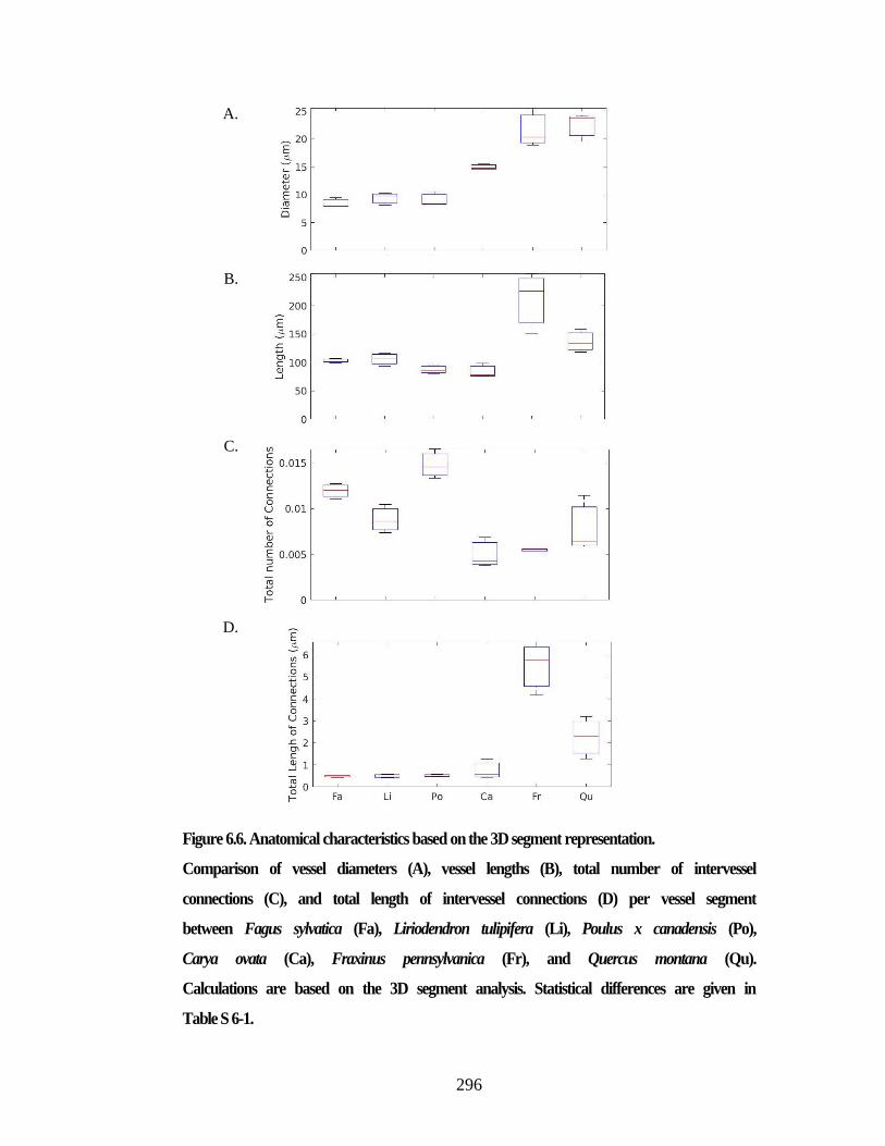
296
A.
B.
C.
D.
Figure 6.6. Anatomical characteristics based on the 3D segment representation.
Comparison of vessel diameters (A), vessel lengths (B), total number of intervessel
connections (C), and total length of intervessel connections (D) per vessel segment
between Fagus sylvatica (Fa), Liriodendron tulipifera (Li), Poulus x canadensis (Po),
Carya ovata (Ca), Fraxinus pennsylvanica (Fr), and Quercus montana (Qu).
Calculations are based on the 3D segment analysis. Statistical differences are given in
Table S 6-1.
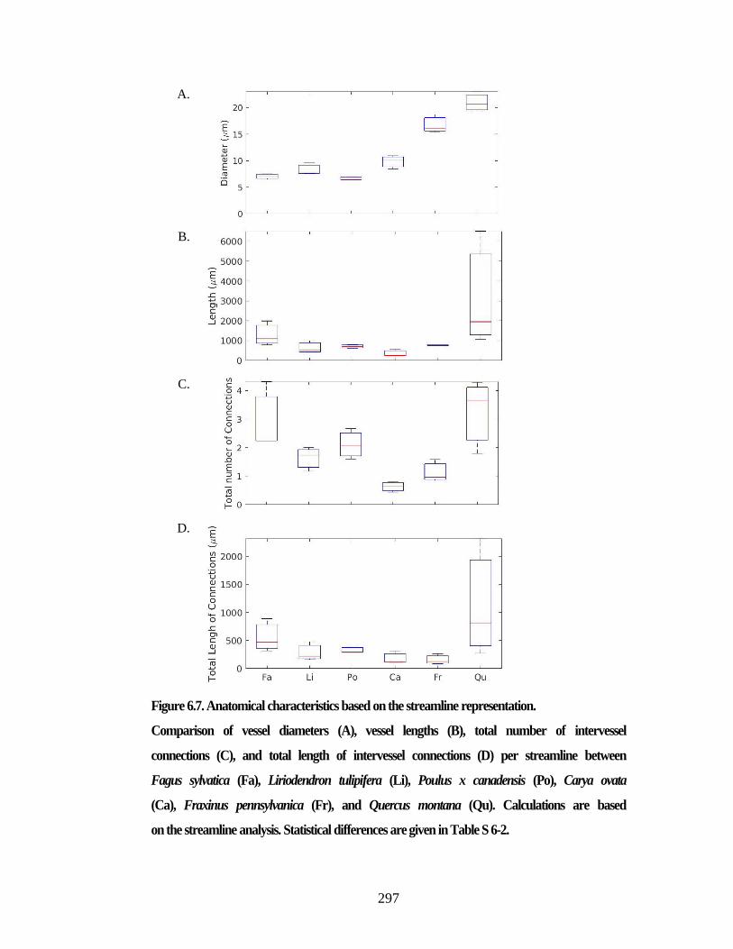
297
A.
B.
C.
D.
Figure 6.7. Anatomical characteristics based on the streamline representation.
Comparison of vessel diameters (A), vessel lengths (B), total number of intervessel
connections (C), and total length of intervessel connections (D) per streamline between
Fagus sylvatica (Fa), Liriodendron tulipifera (Li), Poulus x canadensis (Po), Carya ovata
(Ca), Fraxinus pennsylvanica (Fr), and Quercus montana (Qu). Calculations are based
on the streamline analysis. Statistical differences are given in Table S 6-2.
298
6.3.2 Topological comparisons
The geometrical comparison results describe the noticeable visual differed between
samples of species qualitatively. In contrast, topological comparisons quantify the
differences that are not detectable by visual inspections because they result from aggregate
network properties. Figure 6.8 summarizes the topological comparisons based on the
metrics described in the network analysis method section measured on the 3D segment
graph representations. While it is evident that ring-porous species have a higher density,
compare to diffuse-porous species due to the extremely lower number of xylems at each
image, Katz, clustering, and assortativity demonstrates similar discrimination between
wood types. On the other hand, C. ovata, P. x canadensis, Q. montana have higher centrality
metrics such as closeness and betweenness compare to the other three species. This division
cannot be described based on wood types or other geometrical or topological differences.
On the other hand, the topological comparisons measured on the streamline graph
representations (Figure 6.10), show an additional aspect of the topological differences
between species. For instance, only Q. montana has a higher density compared to all other
species based on this representation, while only F. sylvatica has a high eigenvalue compare
to all other species. These differences were not observed in the topological comparison
based on the 3D segment representations. Instead, Katz, clustering, and assortativity still
discriminate between wood types except for C. ovata. In contrast, the closeness metric in
this representation discriminates between wood types in the opposite direction.
Another way to visualize the nature of the networks is to use circle graphs by
aligning all the nodes along the circle and draw the edges between nodes. Even though,

299
the intervessel connectivity depicted in the Figure 6.9 and Figure 6.11 illustrate the evident
difference between wood types in terms of amount of connectivity shown as a high number
of edges, location variation of connectivity shown as edges closer to the center of the circle,
and strength of the connections shown as the width of the edges perpendicular to the
perimeter. These observations match with the visual assessments of the images of the
species and serve as a confirmation of the various analysis pipelines proposed in this study.
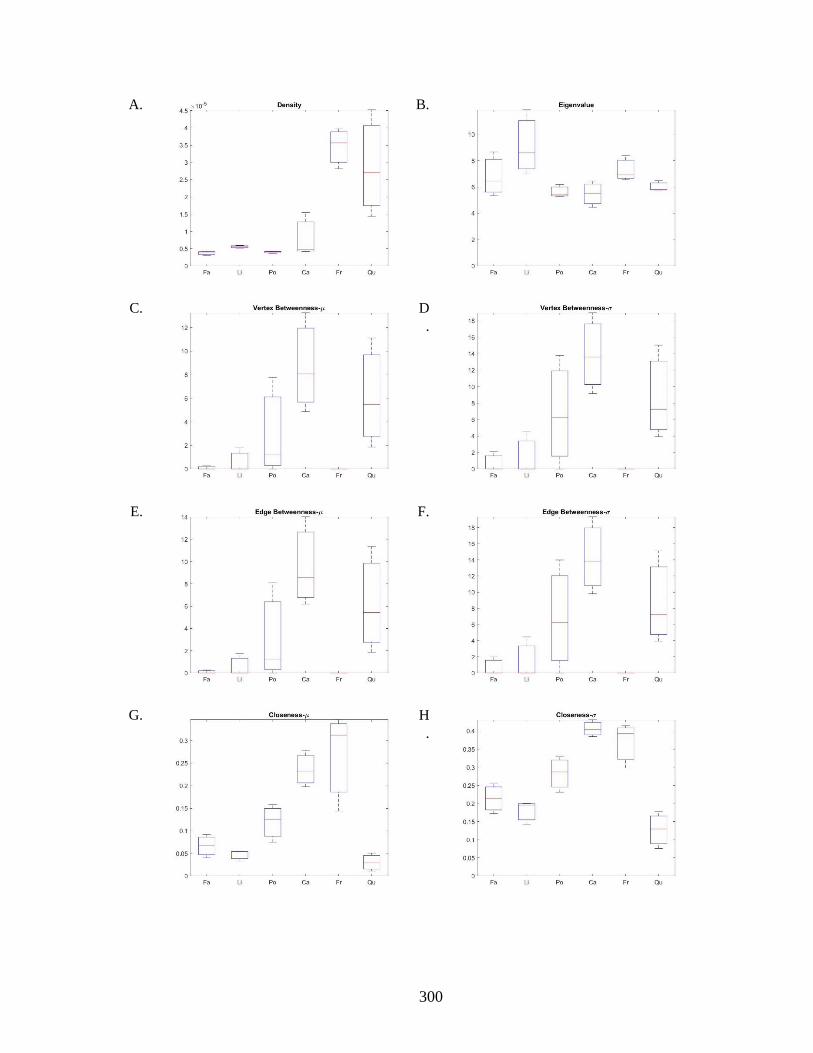
300
A.
B.
C.
D
.
E.
F.
G.
H
.
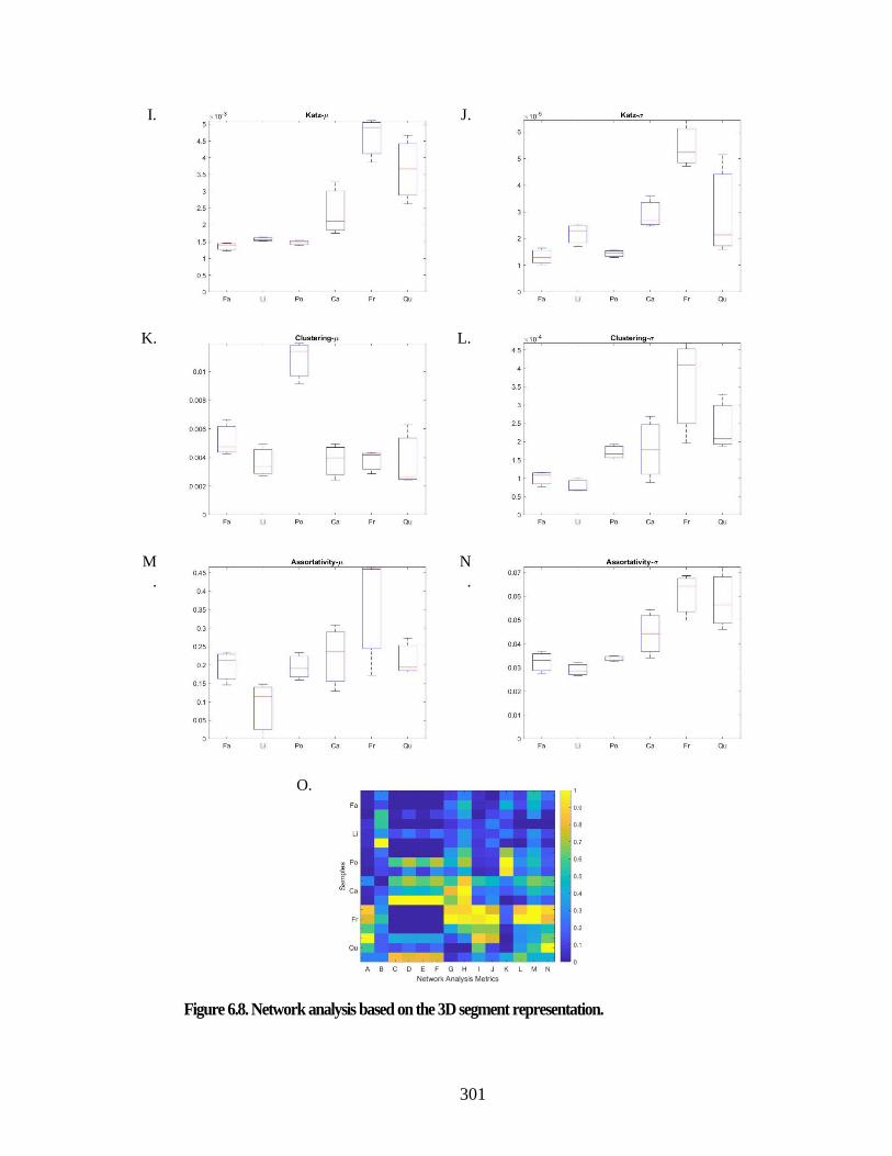
301
I.
J.
K.
L.
M
.
N
.
O.
Figure 6.8. Network analysis based on the 3D segment representation.

302
Boxplots of fourteen network metrics (A-N) are characterizing the xylem network of
Fagus sylvatica (Fa), Liriodendron tulipifera (L), Poulus x canadensis (P), Carya ovata
(C), Fraxinus pennsylvanica (Fr), and Quercus montana (Q). Data are calculated based
on the 3D network analysis. All matrices are combined in a heat map (O) in which
each row represents a sample and each column one of the network metrics (A-N).
Data in the heatmap are normalized (0-1) based on data range and the warmer color
correspond to higher values.
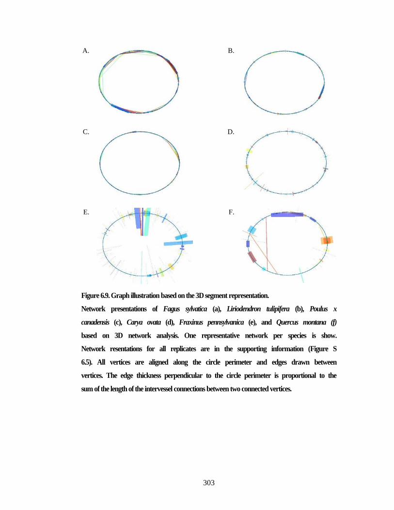
303
A.
B.
C.
D.
E.
F.
Figure 6.9. Graph illustration based on the 3D segment representation.
Network presentations of Fagus sylvatica (a), Liriodendron tulipifera (b), Poulus x
canadensis (c), Carya ovata (d), Fraxinus pennsylvanica (e), and Quercus montana (f)
based on 3D network analysis. One representative network per species is show.
Network resentations for all replicates are in the supporting information (Figure S
6.5). All vertices are aligned along the circle perimeter and edges drawn between
vertices. The edge thickness perpendicular to the circle perimeter is proportional to the
sum of the length of the intervessel connections between two connected vertices.
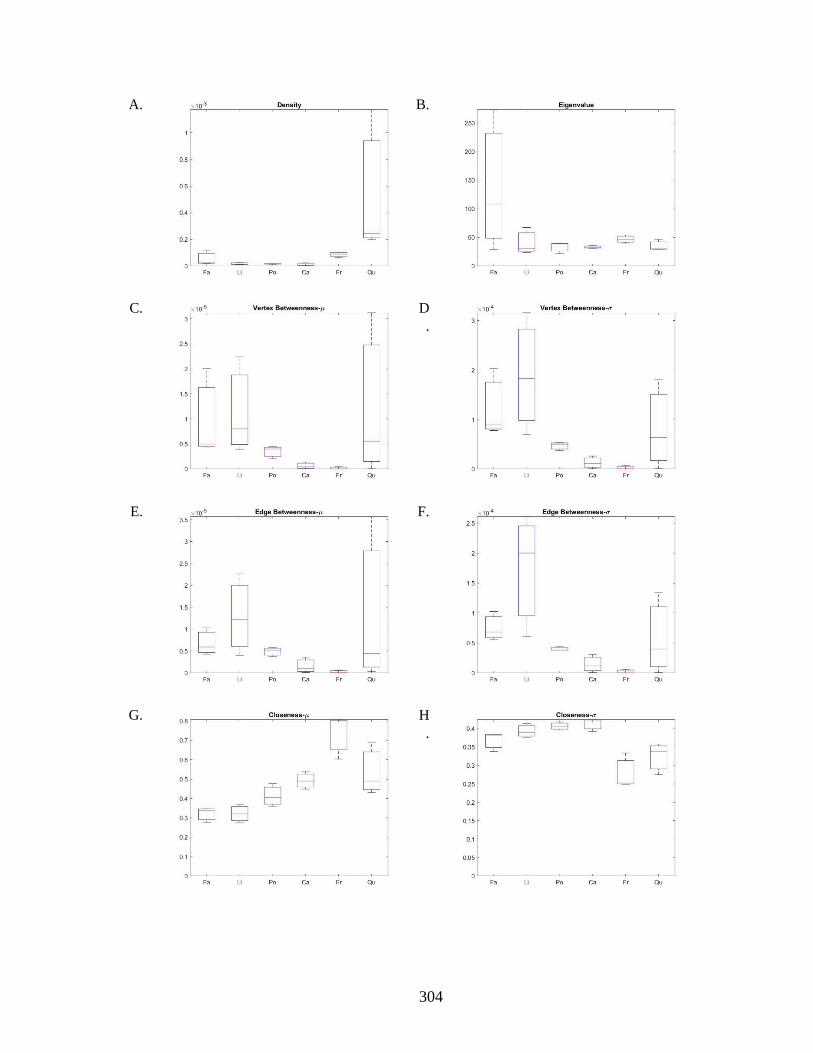
304
A.
B.
C.
D
.
E.
F.
G.
H
.
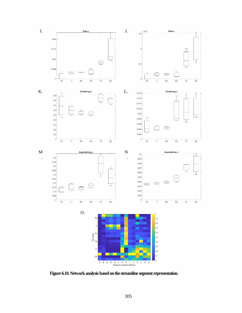
305
I.
J.
K.
L.
M
.
N
.
O.
Figure 6.10. Network analysis based on the streamline segment representation.

306
Boxplots of fourteen network metrics (A-N) are characterizing the xylem network of
Fagus sylvatica (Fa), Liriodendron tulipifera (L), Poulus x canadensis (P), Carya ovata
(C), Fraxinus pennsylvanica (Fr), and Quercus montana (Q). Data are calculated based
on the streamline analysis. All matrices are combined in a heat map (O) in which each
row represents a sample and each column one of the network metrics (A-N). Data in
the heatmap are normalized (0-1) based on the data range and the warmer color
correspond to higher values.
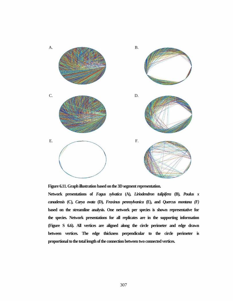
307
A.
B.
C.
D.
E.
F.
Figure 6.11. Graph illustration based on the 3D segment representation.
Network presentations of Fagus sylvatica (A), Liriodendron tulipifera (B), Poulus x
canadensis (C), Carya ovata (D), Fraxinus pennsylvanica (E), and Quercus montana (F)
based on the streamline analysis. One network per species is shown representative for
the species. Network presentations for all replicates are in the supporting information
(Figure S 6.6). All vertices are aligned along the circle perimeter and edge drawn
between vertices. The edge thickness perpendicular to the circle perimeter is
proportional to the total length of the connection between two connected vertices.

308
6.3.3 Fluid simulations and P50 comparisons
As a measure of robustness, we used computational fluid dynamics methods to
simulate the flow of water through a sample at constant pressure and characterized the
change in flow due to the elimination of increasing fractions of randomly selected xylem
vessels (dropout). Relative conductance decreased in all networks with an increasing vessel
dropout probability (Figure 6.12). The ring-porous tree species C. ovata and Q. montana
showed the highest decreasing rate in relative conductance, with a 100% conductance loss
at a vessel dropout rate of 2% (Figure 6.12.D & F). In contrast, the dropout probability that
causes a 100% conductance loss in F. pennsylvanica varies between 1-90 % due to the high
variability within the three replicates (Figure 6.12.E). In the diffuse porous tree species, F.
sylvatica and P. x canadensis show a total conductance loss at 10% vessel dropout (Figure
6.12.A & C), while the 100% conductance loss of L. tulipifera varies between 10% and
38% due to the variability within the samples (Figure 6.12.B).
Empirical P50 values range from – 0.02 MPa for F. pennsylvanica to -2.07 MPa
for F. sylvatica (Figure 6.14). Ring-porous tree species have higher P50 values than diffuse
porous tree species, with the exception of C. ovata and P. canadensis. C. ovata is with a
P50 value of -0.9 MPa more drought resistant than P. canadensis that has a P50 value of -
0.69 MPa. Fitting parameter a and b are all highly significant, except fitting parameter b
for F. pennsylvanica, indicating that a more simplistic model fit would have been sufficient
for this species (Table S 6-3).
The simulated P10 and P50 values are calculated based on the decrease in relative
conductance with increasing vessel dropout. Both P10 and P50 are not significantly

309
different between the species (Figure 6.13.A & B). Simulated mean P10 values are reached
between 0.002 % and 0.005% vessel dropout (Figure 6.13.B), while simulated P50 values
are reached between 0.01% and 0.04% vessel dropout probability (Figure 6.13.A). The
simulated dropout rate (the exponential decay rate of dropout curves) does not differ either
between tree species (Figure 6.13.C).
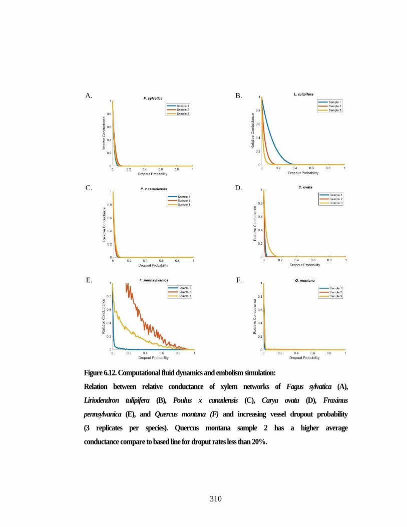
310
A.
B.
C.
D.
E.
F.
Figure 6.12. Computational fluid dynamics and embolism simulation:
Relation between relative conductance of xylem networks of Fagus sylvatica (A),
Liriodendron tulipifera (B), Poulus x canadensis (C), Carya ovata (D), Fraxinus
pennsylvanica (E), and Quercus montana (F) and increasing vessel dropout probability
(3 replicates per species). Quercus montana sample 2 has a higher average
conductance compare to based line for droput rates less than 20%.
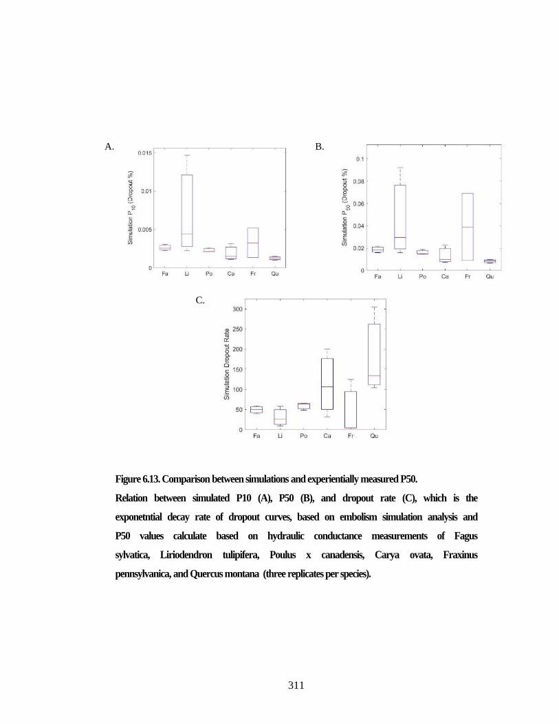
311
A.
B.
C.
Figure 6.13. Comparison between simulations and experientially measured P50.
Relation between simulated P10 (A), P50 (B), and dropout rate (C), which is the
exponetntial decay rate of dropout curves, based on embolism simulation analysis and
P50 values calculate based on hydraulic conductance measurements of Fagus
sylvatica, Liriodendron tulipifera, Poulus x canadensis, Carya ovata, Fraxinus
pennsylvanica, and Quercus montana (three replicates per species).
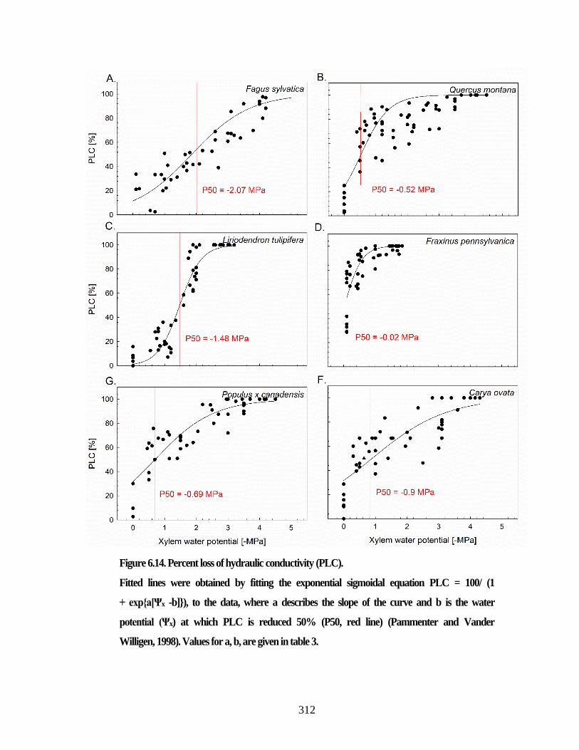
312
Figure 6.14. Percent loss of hydraulic conductivity (PLC).
Fitted lines were obtained by fitting the exponential sigmoidal equation PLC = 100/ (1
+ exp{a[Ψx -b]}), to the data, where a describes the slope of the curve and b is the water
potential (Ψx) at which PLC is reduced 50% (P50, red line) (Pammenter and Vander
Willigen, 1998). Values for a, b, are given in table 3.
313
6.4 Discussion
3D segment analysis and streamline analysis provide two different topological
analyses to characterize xylem networks (Figure 3 and 4). While 3D segmentation looks at
anatomical characteristics of xylem vessels, the streamline analysis focuses on network
characteristics based on potential water pathways (streamlines), which will traverse
through multiple different xylem segments. For example, the 3D segment analysis revealed
that F. pennsylvanica has the widest vessel diameter and the longest vessel length in this
study. However, when considering anatomical characteristics on a network level, we can
see that the average streamline length is 10-fold higher than the average 3D segment length.
The dichotomy of these two results is important because it highlights the degree to which
the factors impacting network robustness remain unknown.
In order to evaluate differences between the xylem networks, we calculated
different centrality parameters based on the 3D segment analysis and the streamline
analysis. The advantage of these metrics is that they are normalized, which facilitates
comparison between the different xylem networks. For example, the density parameter
revealed that the xylem network of F. pennsylvanica is relatively well connected compared
to the other tree species, even though the 3D segment analysis revealed that F.
pennsylvanica has relatively few connections between the xylem vessels.
Overall, we can see a lower variability in the standard deviation of the network
metrics from the streamline analysis, making it a stronger analysis. However, the heat maps
of both analyses showed that there is high variability within the samples, stressing that
314
more replicates are needed to make better predictions about the actual value of these
matrices and reduce the variability within the tree species.
All species show an exponential decline in their relative conductance with
increasing vessel dropout. Because vessel dropout was assigned randomly in the
simulation, these results correspond to randomly occurring cavitation events within the
pore network. However, the model does not include the effects of air embolisms
propagation from air seeding, and therefore, at this time we are unable to conclude if higher
connectivity leads to more embolism resistant networks or more vulnerable networks. In
order to simulate air-seeding in xylem networks, we will perform a follow-up simulation
in which randomly dropped vessels will also trigger the removal of all vessels in connection
to this one. The lack of strong differences in the simulated P10 and P50 values, the
decreasing rate of relative conductance, and the experimentally determined P50 value
based on hydraulic conductance measurements might be due to the variability between
samples. However, differences in experimental P50 values based on hydraulic
measurements were also not observed. Nevertheless, the conductance loss of 50%
(simulated P50) occurred between 0.01-0.04% dropout probability. This value seems low
in comparison to other biological networks such as mouse and human cortical capillary
networks in which a 50% reduction in blood flow occurred when 20% capillaries are stalled
with blood flow (Cruz Hernández et al. 2019).
Combinations of geometrical and topological differences based on both graph
representations reveal the complexity of this correlation between the xylem network
characteristics and drought vulnerability. For each species, we can consider each of these
characteristics as an agent, which may strengthen or weaken the tree during drought

315
incidents. The result is a multi-agent complex system with various stochastic processes,
which determine the probability of survival at a given drought episode speculation.
In this study, we were able for the first time to produce a large data set and to
reconstruct xylem networks based on actual data. Furthermore, we presented different
metrics to characterize vessel and streamline topology with which we can characterize
differences between xylem networks. However, to identify network metrics that are
specific to ring- and diffuse porous xylem networks, we need more specific analysis, for
example, the suggested air seeding dropout simulation.
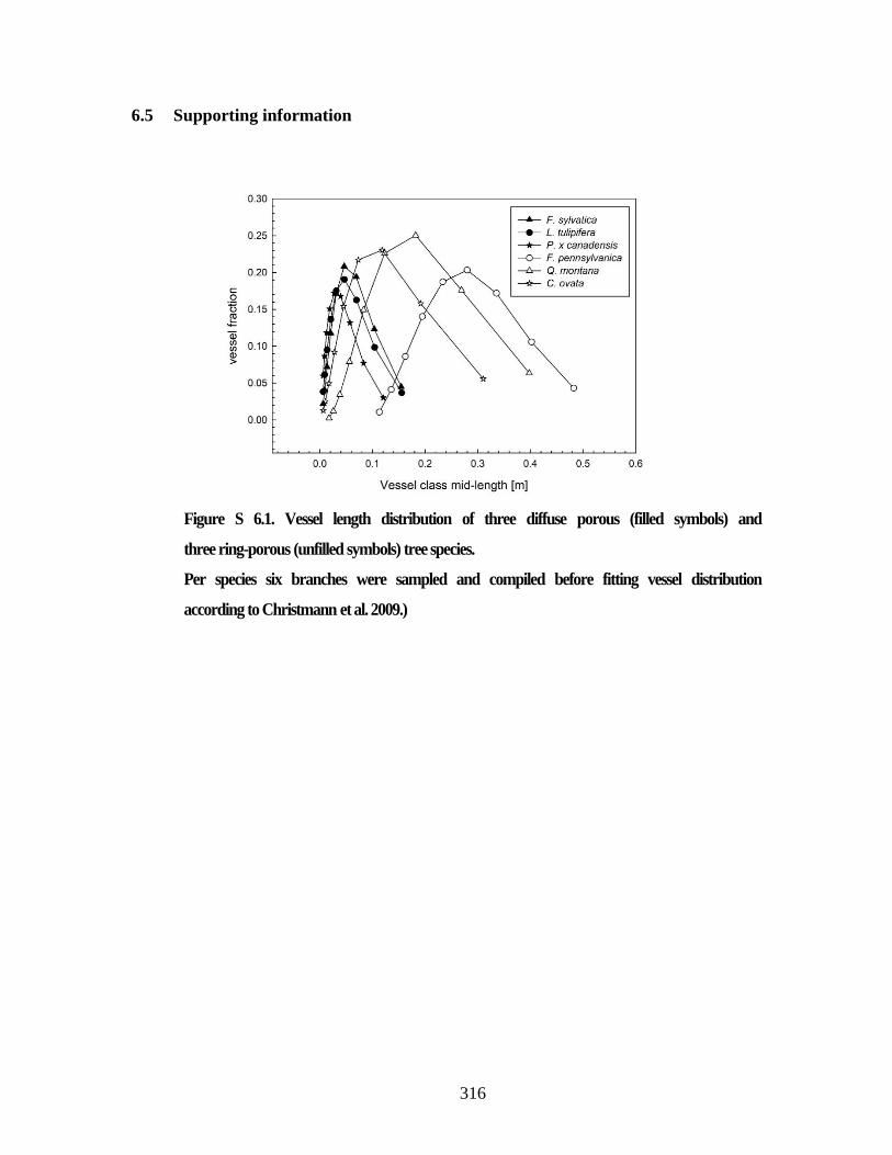
316
6.5 Supporting information
Figure S 6.1. Vessel length distribution of three diffuse porous (filled symbols) and
three ring-porous (unfilled symbols) tree species.
Per species six branches were sampled and compiled before fitting vessel distribution
according to Christmann et al. 2009.)
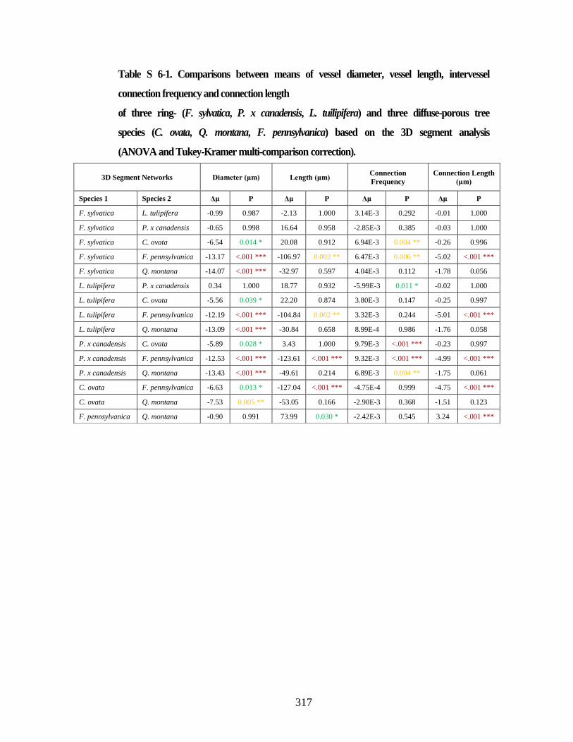
317
Table S 6-1. Comparisons between means of vessel diameter, vessel length, intervessel
connection frequency and connection length
of three ring- (F. sylvatica, P. x canadensis, L. tuilipifera) and three diffuse-porous tree
species (C. ovata, Q. montana, F. pennsylvanica) based on the 3D segment analysis
(ANOVA and Tukey-Kramer multi-comparison correction).
3D Segment Networks Diameter (μm) Length (μm) Connection
Frequency
Connection Length
(μm)
Species 1 Species 2 Δμ P Δμ P Δμ P Δμ P
F. sylvatica L. tulipifera -0.99 0.987 -2.13 1.000 3.14E-3 0.292 -0.01 1.000
F. sylvatica P. x canadensis -0.65 0.998 16.64 0.958 -2.85E-3 0.385 -0.03 1.000
F. sylvatica C. ovata -6.54 0.014 * 20.08 0.912 6.94E-3 0.004 ** -0.26 0.996
F. sylvatica F. pennsylvanica -13.17 <.001 *** -106.97 0.002 ** 6.47E-3 0.006 ** -5.02 <.001 ***
F. sylvatica Q. montana -14.07 <.001 *** -32.97 0.597 4.04E-3 0.112 -1.78 0.056
L. tulipifera P. x canadensis 0.34 1.000 18.77 0.932 -5.99E-3 0.011 * -0.02 1.000
L. tulipifera C. ovata -5.56 0.039 * 22.20 0.874 3.80E-3 0.147 -0.25 0.997
L. tulipifera F. pennsylvanica -12.19 <.001 *** -104.84 0.002 ** 3.32E-3 0.244 -5.01 <.001 ***
L. tulipifera Q. montana -13.09 <.001 *** -30.84 0.658 8.99E-4 0.986 -1.76 0.058
P. x canadensis C. ovata -5.89 0.028 * 3.43 1.000 9.79E-3 <.001 *** -0.23 0.997
P. x canadensis F. pennsylvanica -12.53 <.001 *** -123.61 <.001 *** 9.32E-3 <.001 *** -4.99 <.001 ***
P. x canadensis Q. montana -13.43 <.001 *** -49.61 0.214 6.89E-3 0.004 ** -1.75 0.061
C. ovata F. pennsylvanica -6.63 0.013 * -127.04 <.001 *** -4.75E-4 0.999 -4.75 <.001 ***
C. ovata Q. montana -7.53 0.005 ** -53.05 0.166 -2.90E-3 0.368 -1.51 0.123
F. pennsylvanica Q. montana -0.90 0.991 73.99 0.030 * -2.42E-3 0.545 3.24 <.001 ***
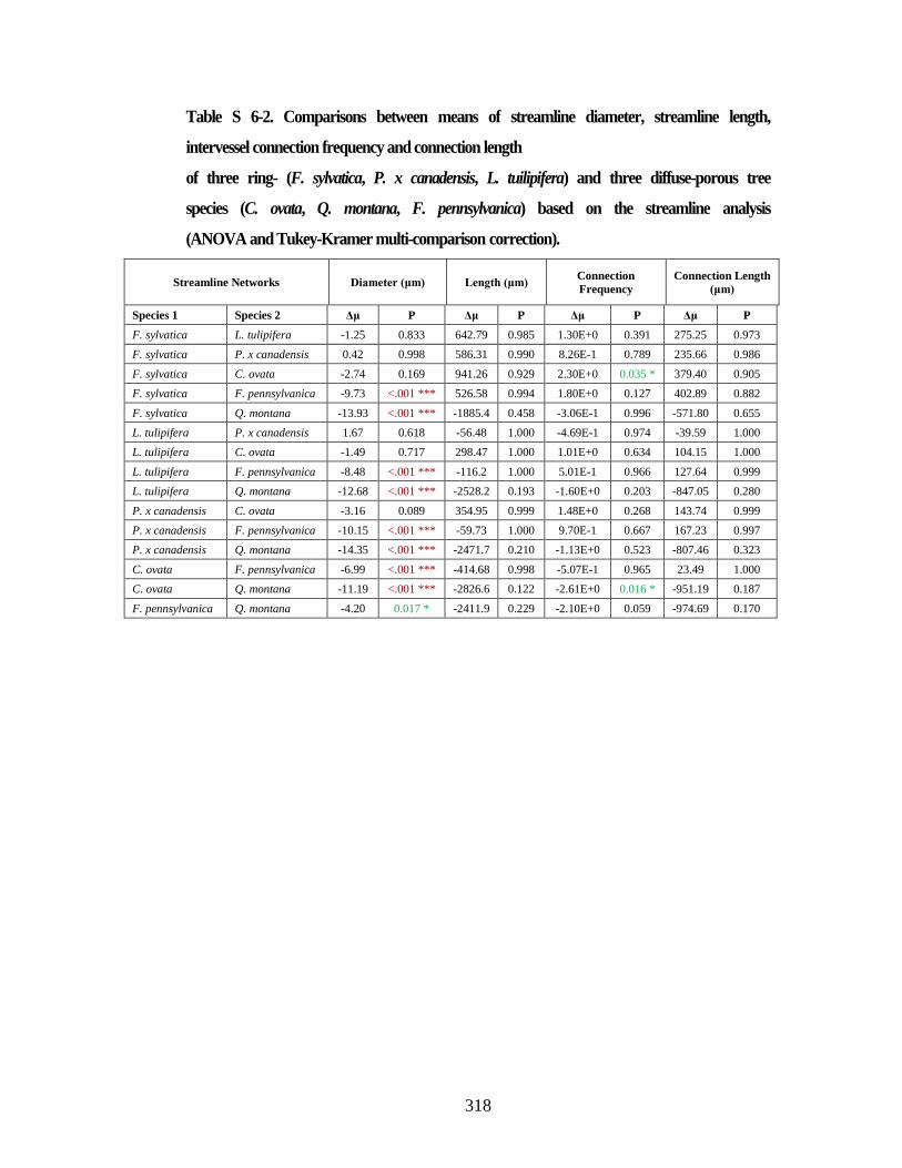
318
Table S 6-2. Comparisons between means of streamline diameter, streamline length,
intervessel connection frequency and connection length
of three ring- (F. sylvatica, P. x canadensis, L. tuilipifera) and three diffuse-porous tree
species (C. ovata, Q. montana, F. pennsylvanica) based on the streamline analysis
(ANOVA and Tukey-Kramer multi-comparison correction).
Streamline Networks Diameter (μm) Length (μm) Connection
Frequency
Connection Length
(μm)
Species 1 Species 2 Δμ P Δμ P Δμ P Δμ P
F. sylvatica L. tulipifera -1.25 0.833 642.79 0.985 1.30E+0 0.391 275.25 0.973
F. sylvatica P. x canadensis 0.42 0.998 586.31 0.990 8.26E-1 0.789 235.66 0.986
F. sylvatica C. ovata -2.74 0.169 941.26 0.929 2.30E+0 0.035 * 379.40 0.905
F. sylvatica F. pennsylvanica -9.73 <.001 *** 526.58 0.994 1.80E+0 0.127 402.89 0.882
F. sylvatica Q. montana -13.93 <.001 *** -1885.4 0.458 -3.06E-1 0.996 -571.80 0.655
L. tulipifera P. x canadensis 1.67 0.618 -56.48 1.000 -4.69E-1 0.974 -39.59 1.000
L. tulipifera C. ovata -1.49 0.717 298.47 1.000 1.01E+0 0.634 104.15 1.000
L. tulipifera F. pennsylvanica -8.48 <.001 *** -116.2 1.000 5.01E-1 0.966 127.64 0.999
L. tulipifera Q. montana -12.68 <.001 *** -2528.2 0.193 -1.60E+0 0.203 -847.05 0.280
P. x canadensis C. ovata -3.16 0.089 354.95 0.999 1.48E+0 0.268 143.74 0.999
P. x canadensis F. pennsylvanica -10.15 <.001 *** -59.73 1.000 9.70E-1 0.667 167.23 0.997
P. x canadensis Q. montana -14.35 <.001 *** -2471.7 0.210 -1.13E+0 0.523 -807.46 0.323
C. ovata F. pennsylvanica -6.99 <.001 *** -414.68 0.998 -5.07E-1 0.965 23.49 1.000
C. ovata Q. montana -11.19 <.001 *** -2826.6 0.122 -2.61E+0 0.016 * -951.19 0.187
F. pennsylvanica Q. montana -4.20 0.017 * -2411.9 0.229 -2.10E+0 0.059 -974.69 0.170
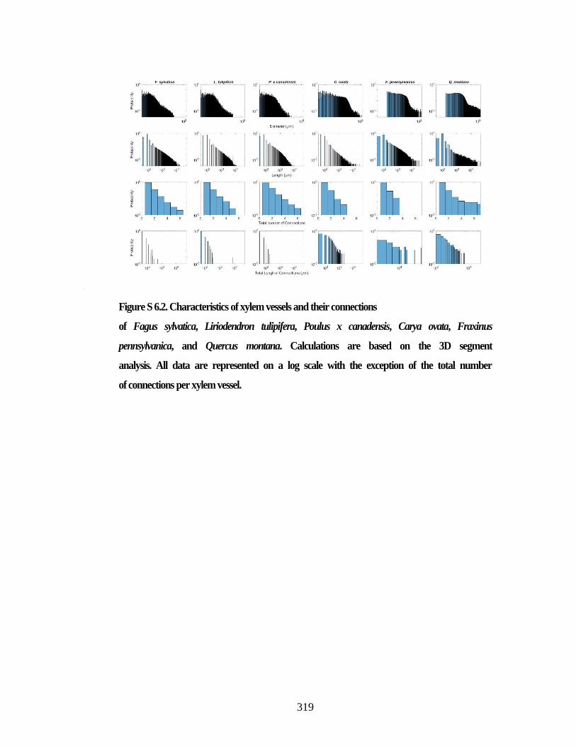
319
Figure S 6.2. Characteristics of xylem vessels and their connections
of Fagus sylvatica, Liriodendron tulipifera, Poulus x canadensis, Carya ovata, Fraxinus
pennsylvanica, and Quercus montana. Calculations are based on the 3D segment
analysis. All data are represented on a log scale with the exception of the total number
of connections per xylem vessel.
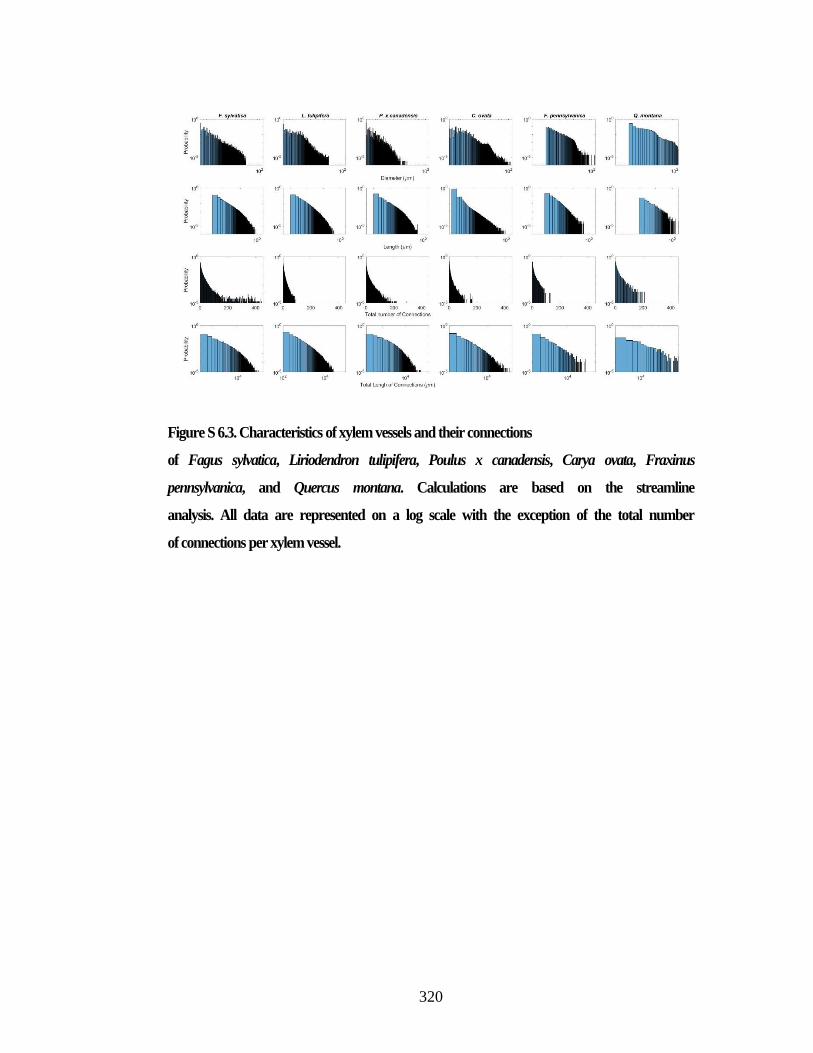
320
Figure S 6.3. Characteristics of xylem vessels and their connections
of Fagus sylvatica, Liriodendron tulipifera, Poulus x canadensis, Carya ovata, Fraxinus
pennsylvanica, and Quercus montana. Calculations are based on the streamline
analysis. All data are represented on a log scale with the exception of the total number
of connections per xylem vessel.
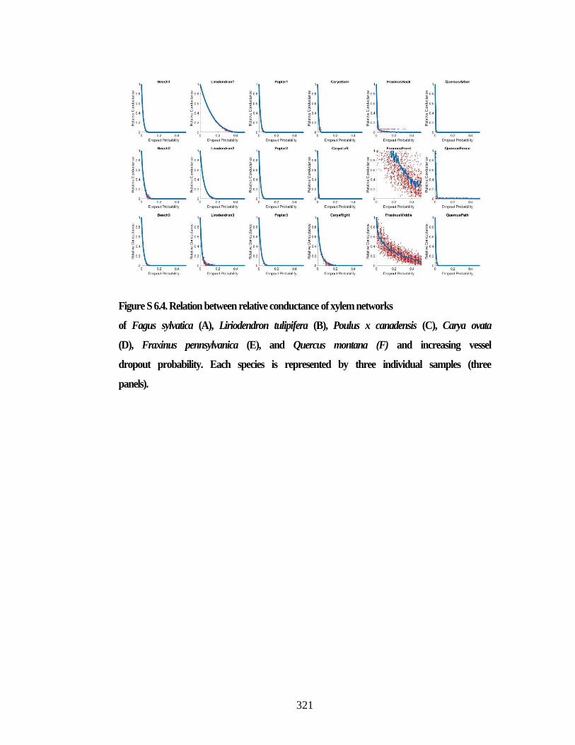
321
Figure S 6.4. Relation between relative conductance of xylem networks
of Fagus sylvatica (A), Liriodendron tulipifera (B), Poulus x canadensis (C), Carya ovata
(D), Fraxinus pennsylvanica (E), and Quercus montana (F) and increasing vessel
dropout probability. Each species is represented by three individual samples (three
panels).
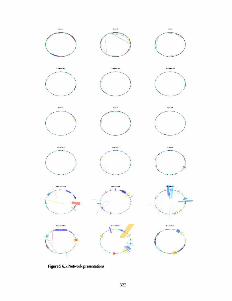
322
Figure S 6.5. Network presentations

323
of Fagus sylvatica (a), Liriodendron tulipifera (b), Poulus x canadensis (c), Carya ovata
(d), Fraxinus pennsylvanica (e), and Quercus montana (f) based on 3D network
analysis. Circle representation can be read as described in Methods and Results. Each
species is represented by three individual samples (three panels).
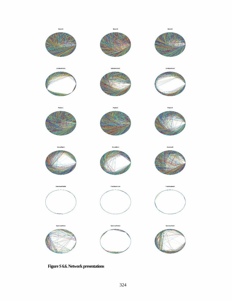
324
Figure S 6.6. Network presentations
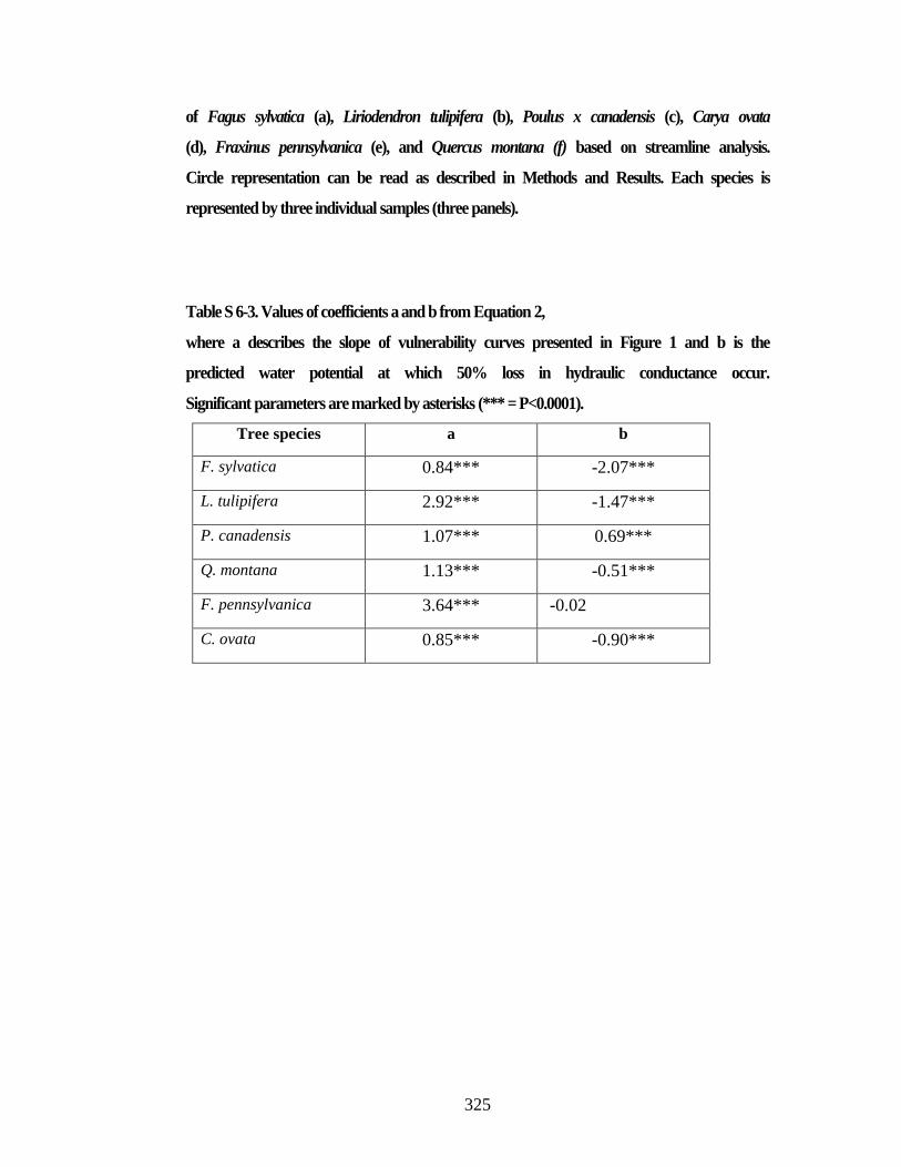
325
of Fagus sylvatica (a), Liriodendron tulipifera (b), Poulus x canadensis (c), Carya ovata
(d), Fraxinus pennsylvanica (e), and Quercus montana (f) based on streamline analysis.
Circle representation can be read as described in Methods and Results. Each species is
represented by three individual samples (three panels).
Table S 6-3. Values of coefficients a and b from Equation 2,
where a describes the slope of vulnerability curves presented in Figure 1 and b is the
predicted water potential at which 50% loss in hydraulic conductance occur.
Significant parameters are marked by asterisks (*** = P<0.0001).
Tree species a b
F. sylvatica 0.84*** -2.07***
L. tulipifera 2.92*** -1.47***
P. canadensis 1.07*** 0.69***
Q. montana 1.13*** -0.51***
F. pennsylvanica 3.64*** -0.02
C. ovata 0.85*** -0.90***
326
REFERENCES
Carlquist S. (1988) Comparative wood anatomy: systematic, ecological, and evolutionary
aspects of dycotyledon wood. Springer-Verlag, Berlin, Heidelberg.
Christman M. a, Sperry J.S. & Smith D.D. (2012) Rare pits, large vessels and extreme
vulnerability to cavitation in a ring-porous tree species. New Phytologist 193, 713–
720.
Christman M.A., Sperry J.S. & Adler F.R. (2009) Testing the “rare pit” hypothesis for
xylem cavitation resistance in three species of Acer. New Phytologist 182, 664–74.
Christmann A., Weiler E.W., Steudle E. & Grill E. (2007) A hydraulic signal in root-to-
shoot signalling of water shortage. The Plant Journal 52, 167–174.
Cochard H., Badel E., Herbette S., Delzon S., Choat B. & Jansen S. (2013) Methods for
measuring plant vulnerability to cavitation: a critical review. Journal of
Experimental Botany 64, 4779–4791.
Cruz Hernández J.C., Bracko O., Kersbergen C.J., Muse V., Haft-Javaherian M., Berg M.,
… Schaffer C.B. (2019) Neutrophil adhesion in brain capillaries reduces cortical
blood flow and impairs memory function in Alzheimer’s disease mouse models.
Nature Neuroscience 22, 413–420.
Evangelidis G. & Psarakis E. (2008) Parametric image alignment using enhanced
correlation coefficient maximization. IEEE Transactions on Pattern Analysis and
Machine Intelligence 30, 1858–1865.
Haft-Javaherian M., Fang L., Muse V., Schaffer C.B., Nishimura N. & Sabuncu M.R.
(2019) Deep convolutional neural networks for segmenting 3D in vivo multiphoton
images of vasculature in Alzheimer disease mouse models. PloS one 14, e0213539.
Jacobsen A.L., Ewers F.W., Pratt R.B., Paddock III W.A. & Davis S.D. (2005) Do xylem
fibers affect vessel cavitation resistance ? Plant Physiology 139, 546–556.
Jansen S., Choat B. & Pletsers A. (2009) Morphological variation of intervessel pit
membranes and implications to xylem function in angiosperms. American Journal
of Botany 96, 409–419.
327
Latora V. & Marchiori M. (2001) Efficient Behavior of Small-World Networks. Physical
Review Letters 87, 3–6.
Lens F., Sperry J.S., Christman M. a, Choat B., Rabaey D. & Jansen S. (2011) Testing
hypotheses that link wood anatomy to cavitation resistance and hydraulic
conductivity in the genus Acer. New Phytologist 190, 709–723.
Maherali H., Pockman W. & Jackson R.B. (2004) Adaptive variation in the vulnerability
of woody plants to xylem cavitation. Ecology 85, 2184–2199.
Melcher P.J., Michele Holbrook N., Burns M.J., Zwieniecki M.A., Cobb A.R., Brodribb
T.J., … Sack L. (2012) Measurements of stem xylem hydraulic conductivity in the
laboratory and field. Methods in Ecology and Evolution 3, 685–694.
Northeast Regional Climate Center (2019) NRCC The Ithaca Climate Page.
Otsu N. (1979) A threshold selection method from gray-level histograms. IEEE
Tansactions on Systems, Man, and Cybernetics 9, 62–66.
Pammenter N.W. & Van der Willigen C. (1998) A mathematical and statistical analysis of
the curves illustrating vulnerability of xylem to cavitation. Tree Physiology 18,
589–593.
Psarakis E. & Evangelidis G. (2005) An enhanced correlation-based method for stereo
correspondence with sub-pixel accuracy. In Computer Vision, 2005. ICCV 2005.
Tenth IEEE International Conference on. pp. 907–912. IEEE, Beijing, China.
Rueden C.T., Schindelin J., Hiner M.C., DeZonia B.E., Walter A.E., Arena E.T. & Eliceiri
K.W. (2017) ImageJ2: ImageJ for the next generation of scientific image data.
BMC Bioinformatics 18, 1–26.
Sperry J.S., Donnelly J.R. & Tyree M.T. (1988) Seasonal occurrence of xylem embolism
in sugar maple ( Acer saccharum ). American Journal of Botany 75, 1212–1218.
Sperry J.S. & Hacke U.G. (2004) Analysis of circular bordered pit function I. Angiosperm
vessels with homogenous pit membranes. American Journal of Botany 91, 369–
385.
Sperry J.S., Hacke U.G. & Wheeler J.K. (2005) Comparative analysis of end wall
resistivity in xylem conduits. Plant, Cell and Environment 28, 456–465.
Tyree M.T. & Dixon M.A. (1986) Water stress induced cavitation and embolism in some
woody plants. Physiologia Plantarum 66, 397–405.
328
Venturas M.D., Sperry J.S. & Hacke U.G. (2017) Plant xylem hydraulics: what we
understand, current research, and future challenges. Journal of Integrative Plant
Biology 59, 356–389.
Wang Z., Bovik A.C., Sheikh H.R. & Simoncelli E.P. (2004) Image quality assessment:
from error visibility to structural similarity. IEEE Transactions on Image
Processing 13, 600–612.
Watts D. & Strogatz S. (1998) Collective dynamics of networks. Nature 393, 440–442.
Wheeler J.K., Sperry J.S., Hacke U.G. & Hoang N. (2005) Inter-vessel pitting and
cavitation in woody Rosaceae and other vesselled plants: a basis for a safety versus
efficiency trade-off in xylem transport. Plant, Cell and Environment 28, 800–812.
Zanne a. E., Sweeney K., Sharma M. & Orians C.M. (2006) Patterns and consequences of
differential vascular sectoriality in 18 temperate tree and shrub species. Functional
Ecology 20, 200–206.
Zimmermann M.H. (1983) Xylem structure and the ascent of sap. Springer Verlag, New
York.

329
CHAPTER 7
CONCLUSIONS AND FUTURE DIRECTIONS
Quantitative analysis of various biomedical data modalities such as images is an
essential part of the research and medical settings. This dissertation focused on image
processing and network analysis of brain vasculature network. Many image analysis tasks
such as segmentation and object identifications are bottlenecks of biomedical research
progress and medical diagnosis throughputs. The applicability and effectiveness of the
developed techniques were demonstrated in studies focused on Alzheimer’s disease using
mouse models of the disease. Alzheimer’s disease is the sixth leading cause of death in the
US, and it kills more than breast and prostate cancer combined. Moreover, Alzheimer's is
the only leading cause of death increasing every year. Therefore, investigation of
Alzheimer’s is indispensable.
Chapter 2 is a review of the recent advancement in vessel segmentation and
centerline extraction. There are different categories of image segmentation methods with
different pros and cons that allow the researchers and practitioner to choose based on the
target application. The details of vascular segmentation of different organs and vessel
segments in health and disease states were discussed as well.
In Chapter 3, DeepVess, a deep convolutional neural network solution for fast and
fully automated segmentation of brain vasculature and centerline extraction was discussed.
I developed new open-source algorithms and software packages using machine learning
and complex network analysis to compare and describe different vascular networks and to
study the interactions between brain blood flow and diseases using the properties of
330
vascular networks extracted from mouse models. The resulting software, DeepVess, allows
researchers to extract vascular networks with unprecedented speed, finally enabling various
geometrical and topological measurements in large volumes across many samples. These
data are critical for next level analysis such as computational fluid dynamics and network
analysis. DeepVess can be applied to other organs and imaging modalities with minimal
interventions or fine-tuning. There is still room for improvement in obtaining the vessel
centerlines directly form algorithms instead of as the byproduct of the segmentation results.
Chapter 4 describes the discovery of the high incidents of stalling capillaries in
mouse models of Alzheimer’s disease due to the adhesion of the leukocyte. I developed
different analysis and image analysis methods for this paper including vessel and amyloid-
beta plaques detection, segmentation, and quantification in terms of topological and
geometrical measurements. DeepVess was used in one section of this study as well. The
downstream mechanism of the leukocyte adhesion in stalled capillaries still is unknown
and required further investigation.
In Chapter 5, our crowdsourcing citizen science project called StallCatchers was
described. This project was developed to facilitate the stalled capillary detection task with
the power of citizen science. I was involved in the development of the image processing
pipeline for this project and investigation of crowd response aggregation methods. This
project utilized DeepVess as well, and it has more than fifteen thousand users at this time.
Next steps include the improvement of methods to aggregate the crowd response and the
addition of methods for the smart distributions of tasks based on the user experiences.
331
In Chapter 6, we tested the application of DeepVess on a very different vasculature
network than mouse brain vasculature. We studied big datasets of images of xylem
networks from six different tree species from two categories of trees. In addition to use of
the DeepVess, computationally efficient preprocessing methods required for big data and
efficient network analysis metrics were developed. Furthermore, various network
representations were introduced to facilitate studying these xylem networks from different
points of views. Finally, a computational fluid dynamic simulation was conducted to study
the vulnerability of these trees to drought events and embolism incidents. This study paves
the road for further investigation for more extensive experimental data and other species.
Related Documents