QUANTITATIVE ANALYSIS OF MASTICATORY ...

i

QUANTITATIVE ANALYSIS OF MASTICATORY PERFORMANCE IN VERTEBRATES

By

SRIKANTH KANNAN

August, 2008

A thesis submitted to the Faculty of the Graduate School of the State University of New York at Buffalo in partial fulfillment of the requirements

for the degree of

MASTER OF SCIENCE

Department of Mechanical and Aerospace Engineering State University of New York at Buffalo

Buffalo, New York 14260

ii

Acknowledgement First, I would like to express my sincerest gratitude to my advisor, Dr. Venkat Krovi, for

giving me an opportunity to work under him as a Research Assistant. He was not only my

mentor, but as a friend, he always provided me with valuable suggestions whenever I

needed them most. I would like to express my gratitude to the committee members, Dr.

Frank Mendel and Dr. Andres Soom for serving on my thesis committee and reading

through my thesis and providing me with valuable suggestions.

I would like to thank Dan Murray, Bill McDougall, Brian Wolf, and David Eley for

giving me an opportunity to work with Fisher-Price, Inc and for giving me access to the

3D laser scanner and SLA machine. I would like to thank my lab members Rajan, Chin

Pei Tang, Leng-Feng Lee, Anand Naik, Kun Yu, Hao Su, Qiushi Fu, Yao Wang and

Patrick Miller for lending me an helping hand whenever I needed it the most. I convey

my special thanks to Madu for being my project partner right from the first semester till

the end of my thesis. I would also like to thank my roommates Arun, Sriniwas, Vijay,

Parthiban, Govind, Amol for providing good support and entertainment at home.

And especially I would to thank my parents, Mr. K.R. Kannan and Mrs. K.

Vijayalakshmi and my other family members Priya, Kumar, Adeep, Ayush and

Rajeshwari for being affectionate and encouraging me right throughout my education.

THANKYOU ALL ONCE AGAIN

iii

Abstract To quantitatively measure mechanical performance signals such as forces and motions

and mechanical breakdown of food during mastication, it is imperative to accurately

reproduce the mastication motion. Reproduction of the mastication motion of a vertebrate

with a robotic device will allow us to estimate muscle and bite forces required for

different animals while chewing/biting different regimen and relate them to masticatory

muscle recruitment patterns and would be used to quantitatively evaluate the dynamic

breakdown of foods during chewing, which is vital information required in the

development of new pet foods. We also examine the use of a robotic solution where a

generic parallel manipulator with six degrees of freedom (Stewart platform) was modeled

and simulated using virtual prototyping tools to reproduce the 3D mandible trajectory. To

this end, a high fidelity (speed/resolution) motion capture system was used for capture the

3D mastication motion of different vertebrates. 3D laser scanning technology and image

processing techniques were used to obtain CAD model of a skull and mandible of a

bulldog which was then rapidly prototyped and casted to create a dentition. Architectural

parameters of muscle for a human jaw were obtained from Koolstra et al. and for a

bulldog jaw by conducting dissection of masticatory muscles. A musculoskeletal model

of the vertebrate jaw was created in AnyBody Modeling System to measure the forces

acting in the masticatory muscles and temporomandibular joints. We formulate and verify

the forward dynamics of the Stewart platform using three methods: 1. S-Function in

Simulink 2. DynaFlexPro model 3. Visual Nastran Plant. A combination of Newton-Euler

and Lagrangian method was used to formulate the inverse dynamics of a 6 DOF parallel

manipulator. Feedback linearization was implemented in Matlab/Simulink, using the

inverse dynamics and forward dynamics block, to control the motion of the moving

platform. Actuator forces were determined by implementing vertebrate mastication

trajectory as inverse dynamics using Matlab/Simulink and Visual Nastran. Results from

the inverse dynamic simulations and motion control of the Stewart platform show that the

Stewart platform enables the mastication motion to be reproduced.

iv

TABLE OF CONTENTS Acknowledgement ......................................................................................... ii Abstract......................................................................................................... iii LIST OF FIGURES .................................................................................... vii LIST OF TABLES ...................................................................................... xii 1. Introduction............................................................................................ 1

1.1 Motivation................................................................................................................. 1 1.2 Virtual Prototyping/ Simulation Based Design......................................................... 4 1.3 Musculoskeletal System Analysis............................................................................. 7 1.4 Research Tasks........................................................................................................ 10 1.5 Thesis Organization ................................................................................................ 11

2. Literature Survey................................................................................. 12

2.1 Masticatory Biomechanics...................................................................................... 12 2.1.1 Jaw Muscles and Movements .......................................................................... 12 2.1.2 Redundancy...................................................................................................... 13 2.1.3 Dynamics of Masticatory System .................................................................... 13 2.1.4. Influence of Muscles and Hill Muscle Model................................................. 14 2.1.5 Active and Passive Elements ........................................................................... 15

2. 2 Medical Imaging and Rapid Prototyping............................................................... 16 2.3 Motion Capture Analysis ........................................................................................ 19 2.4 Jaw Motion Simulators ........................................................................................... 22 2.5 Parallel Manipulators .............................................................................................. 30

3. Mathematical Background.................................................................. 31

3.1 Kinematic Analysis:................................................................................................ 33 3.2 Velocity and Acceleration Analysis: ...................................................................... 34 3.3 Jacobian Analysis.................................................................................................... 37

3.3.1 Jacobian Matrix Based On Vector Loop Closure Equation............................. 37 3.3.2 Screw Theory Based Jacobian Analysis .......................................................... 39

3.4 Jacobian-Based Performance Measures (JBPM).................................................... 42 3.4.1 Singular Value Decomposition (SVD) and Manipulability Ellipsoid ............. 42 3.4.2 Yoshikawa’s Measure of Manipulability......................................................... 44 3.4.3 Condition Number ........................................................................................... 44 3.4.4 Isotropy Index .................................................................................................. 45

3.5 Dynamic Analysis................................................................................................... 45 3.6 Feedback Linearization........................................................................................... 48

v

3.7 Musculoskeletal System Analysis........................................................................... 50 4. Technological tools............................................................................... 52

4.1 Laser Scanning Technology.................................................................................... 52 4.1.1 Why 3D Scanning? .......................................................................................... 52 4.1.2 Different Types of 3D Scanning Technology [50]: ......................................... 53 4.1.3 Commercial Scanners ...................................................................................... 54 4.1.4 Generation of CAD Model of Vertebrate Skull and Mandible........................ 57

4.2 CT Scanning Technology ....................................................................................... 59 4.3 Rapid Prototyping and Casting ............................................................................... 63 4.4 Motion Capture Analysis Technology .................................................................... 65

4.4.1 Digitizing ......................................................................................................... 68 4.4.2 Transformation................................................................................................. 68 4.4.3 DLT.................................................................................................................. 71 4.4.4 Technical Aspects for Transformation............................................................. 71

4.5 Musculoskeletal Model of Vertebrate Jaw ............................................................. 73 4.6 CAD Model of Stewart platform Type 6 DOF Parallel Manipulator ..................... 82 4.7 Forward Dynamics Model in DynaFlexPro............................................................ 84

5. Simulation & Results ........................................................................... 93

5.1 Inverse Dynamic Analysis of Human Jaw Model in Anybody Modeling System. 93 5.1.1 Case Study I: One Temporalis Muscle and Muscle Model I and No External Force ......................................................................................................................... 94 5.1.2 Case Study II: Three Temporalis Muscles and Muscle Model I and No External Force........................................................................................................... 97 5.1.3. Case Study III: One Temporalis Muscle, Muscle Model 3E, No External Force ......................................................................................................................... 99 5.1.4 Case Study IV: Three Temporalis Muscles, Muscle Model 3E, No External Force ....................................................................................................................... 101

5.1.5 Case Study V: Three Temporalis Muscles, Muscle Model 3E, With External Force ........................................................................................................................... 104 5.2 Inverse Dynamic Analysis of Bulldog Jaw model in AnyBody........................... 107 5.3 Inverse Dynamic Analysis of Sabertooth Jaw Model in Anybody....................... 111 5.4 Manipulability Measures for Workspace Analysis............................................... 113

5.4.1 Case Study I: Varying the Radius of the Moving platform ........................... 114 5.4.2 Case Study II: Varying Radius of the Workspace ......................................... 117 5.4.3 Case Study III: Varying the Vertical Distance between Two platforms ....... 119

5.5 Dynamic Simulation of Stewart platform............................................................. 120 5.5.1 Simulation Using S-Function:........................................................................ 123 5.5.2 Simulation Using DynaFlexPro Model: ........................................................ 126

5.6 Simulation of the CAD Model of Stewart platform: ............................................ 129 5.6.1 Simulation Using DynaFlexPro Model.......................................................... 130 5.6.2 Simulation Using S-Function Block .............................................................. 131 5.6.3 Simulation Using Visual Nastran Plant ......................................................... 132

vi

5.7 Simulation of Jaw Motion Using Visual Nastran ................................................. 135 5.7.1 Dynamic Simulation of First Human Subject Jaw motion ............................ 136 5.7.2 Dynamic Simulation of Second Human Subject Jaw motion........................ 139 5.7.3 Dynamic Simulation of Bulldog Subject Jaw motion.................................... 141 5.7.4 Dynamic Simulation of Sabertooth Cat Jaw motion...................................... 143

6. Conclusion and Future Work ........................................................... 145

6.1 Conclusion ............................................................................................................ 145 6.2 Future work........................................................................................................... 147

Bibliography .............................................................................................. 149

vii

LIST OF FIGURES Figure 1-1: Development of Simulation Tools in Engineering .......................................... 2 Figure 1-2: Measure-Estimate-Test cycle........................................................................... 3 Figure 1-3: Vertebrate Mastication Motion Simulator Framework.................................... 3 Figure 1-4: Virtual Prototyping [4]..................................................................................... 5 Figure 1-5: Virtual Prototype of Piston (Left from Visual Nastran) and sabertooth Tiger (Right) [1] ........................................................................................................................... 5 Figure 1-6: Increase in Complexity of Musculoskeletal Modeling [1] [2] ......................... 8 Figure 1-7: Musculoskeletal system modeled as Articulated Multi-Body System with Redundancy [1]................................................................................................................... 9 Figure 1-8: Conventional Design Approach ....................................................................... 9 Figure 1-9: Virtual Prototyping Approach.......................................................................... 9 Figure 2-1: Human Masticatory Muscles [18].................................................................. 14 Figure 2-2: Dog Masticatory Muscles .............................................................................. 14 Figure 2-3: Elements of Hill Muscle Model [2] ............................................................... 15 Figure 2-4: Force Length profile of CE, SE and PE elements [2] .................................... 15 Figure 2-5: Force Length and Force-Velocity curve for two muscles with different mass [44].................................................................................................................................... 16 Figure 2-6: Force Length and Force-Velocity curve for two muscles with different fiber length [44]......................................................................................................................... 16 Figure 2-7: Framework of 3D Scanning Technology ....................................................... 17 Figure 2-8: 3D model of the Patient Skull [14] ................................................................ 18 Figure 2-9: Point cloud processed and surface reconstruction of the tray [14] ................ 18 Figure 2-10: SLA model and Titanium Prosthesis [14].................................................... 18 Figure 2-11: Cantilevered Maxillary Implant designed using a stereolithography biomodel [13].................................................................................................................... 19 Figure 2-12: Stresses in Shell Body Prosthesis [13]......................................................... 19 Figure 2-13: Motion Capture Setup with Experimental Devices [11].............................. 20 Figure 2-14: Markers positioning and figure of special pointer on Human Subject [11]. 20 Figure 2-15: The new facebow attached to a Human Subject [16]................................... 20 Figure 2-16: Snapshots of the display system [16]........................................................... 20 Figure 2-17: Ultrasonic Jaw Motion Analyzer (JMA) from Zebris GmbH [15] .............. 21 Figure 2-18: 3D jaw animation in 3D Studio Max [15].................................................... 21 Figure 2-19: CT images of the cranial part [17] ............................................................... 22 Figure 2-20: The optical 3D tracking device Polaris [17] ................................................ 22 Figure 2-21: Dry Skull for Validation Experiment [17] ................................................... 22 Figure 2-22: A display of the result of 4-dimensional analysis [17] ................................ 22 Figure 2-23: Jaw opening and closing Cycle [20] [21]..................................................... 23 Figure 2-24: Kinematic Structure of Jaw [18] [19] .......................................................... 24 Figure 2-25: SimMechanics model of Robotic chewing device [18] [19]........................ 24 Figure 2-26: Physical robot of the mastication system with Linear Actuation [21] ......... 25 Figure 2-27: Physical Kinematic model of Robotic Jaw [21]........................................... 25 Figure 2-28: Robotic Chewing Device with Crank Actuation [23].................................. 26 Figure 2-29: Co-ordinate System of RSS Linkage [23].................................................... 26 Figure 2-30: One leg of the RSS linkage [24] .................................................................. 26 Figure 2-31: WY series [31] ............................................................................................. 27

viii

Figure 2-32: WJ Series [22].............................................................................................. 28 Figure 2-33: WJ robots [22].............................................................................................. 28 Figure 2-34: JSN/2A Simulator [26]................................................................................. 29 Figure 2-35: Six bar linkage for chewing simulation [20]................................................ 29 Figure 2-36: Robotic Chewing Device [20]...................................................................... 29 Figure 3-1: Universal Joint Angles [35] ........................................................................... 31 Figure 3-2: 6DOF Stewart platform [33] .......................................................................... 31 Figure 3-3: Vector Loop of one Leg [33] ......................................................................... 31 Figure 3-4: Prismatic Actuators [33] ................................................................................ 31 Figure 3-5: Screw Co-ordinate Theory ............................................................................. 39 Figure 3-6: Manipulability Ellipsoid [34]......................................................................... 43 Figure 4-1: Sample ATOS 3D scanner generated point cloud and STL polygonal mesh images [45]........................................................................................................................ 52 Figure 4-2: Simplified serial depiction of an iterative generic Concept through Sustaining Engineering Process [45] .................................................................................................. 53 Figure 4-3: 3D Digitizer from Immersion ........................................................................ 53 Figure 4-4: Co-ordinate Measuring Machine ................................................................... 53 Figure 4-5: NextEngine Scanner [46] ............................................................................... 56 Figure 4-6: NextEngine Scanned Teeth Model [46]......................................................... 56 Figure 4-7: ATOS 3D Laser Scanner................................................................................ 57 Figure 4-8: ATOS Laser Scanner ..................................................................................... 58 Figure 4-9: Object painted in Grey color.......................................................................... 58 Figure 4-10: Scanning mandible in Capture3D ................................................................ 58 Figure 4-11: Scanned model in Capture3D ...................................................................... 58 Figure 4-12: Surface patches and holes in the geometry .................................................. 58 Figure 4-13: Cleaned Geometry in Geomagics ................................................................ 58 Figure 4-14: Scannning skull in Capture3D ..................................................................... 59 Figure 4-15: Scanned model in Capture3D ...................................................................... 59 Figure 4-16: Surface patches and holes in geometry ........................................................ 59 Figure 4-17: Cleaned geometry in Geomagics ................................................................. 59 Figure 4-18: Importing tiff images into MIMICS............................................................. 61 Figure 4-19: Setting Image and Pixel information ........................................................... 61 Figure 4-20:Specify the Orientation ................................................................................. 61 Figure 4-21: Calculate 3D to get 3D model...................................................................... 62 Figure 4-22: 3D model of bulldog .................................................................................... 62 Figure 4-23: STL import................................................................................................... 63 Figure 4-24: Importing medium resolution STL .............................................................. 63 Figure 4-25: CAD model of bulldog in Pro/E .................................................................. 64 Figure 4-26: SLA model of Bulldog................................................................................. 64 Figure 4-27: Rapid Prototype model of mandible ............................................................ 64 Figure 4-28: Rapid Prototype model of bulldog skull ...................................................... 64 Figure 4-29: Casting of the bulldog Skull and Mandible ................................................. 64 Figure 4-30: Calibration Grid from one camera view ...................................................... 66 Figure 4-31: Calibration Grid from Second Camera ........................................................ 66 Figure 4-32: Specifying the 3D Co-ordinates of the Calibration Points........................... 67 Figure 4-33: Checking the Calibration System for accuracy............................................ 67

ix

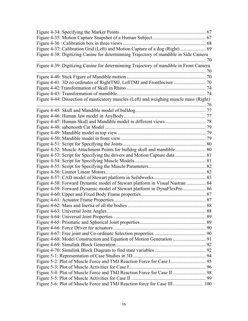
Figure 4-34: Specifying the Marker Points....................................................................... 67 Figure 4-35: Motion Capture Snapshot of a Human Subject............................................ 67 Figure 4-36 : Calibration box in three views .................................................................... 68 Figure 4-37: Calibration Grid (Left) and Motion Capture of a dog (Right) ..................... 69 Figure 4-38: Digitizing Canine for determinning Trajectory of mandible in Side Camera........................................................................................................................................... 70 Figure 4-39: Digitizing Canine for determinning Trajectory of mandible in Front Camera........................................................................................................................................... 70 Figure 4-40: Stick Figure of Mandible motion ................................................................. 70 Figure 4-41: 3D co-ordinates of RightTMJ, LeftTMJ and FrontIncisor .......................... 70 Figure 4-42:Transformation of Skull in Rhino ................................................................. 74 Figure 4-43: Transformation of mandible......................................................................... 74 Figure 4-44: Dissection of masticatory muscles (Left) and weighing muscle mass (Right)........................................................................................................................................... 76 Figure 4-45: Skull and Mandible model of bulldog.......................................................... 77 Figure 4-46: Human Jaw model in AnyBody ................................................................... 77 Figure 4-47: Human Skull and Mandible model in different views ................................. 78 Figure 4-48: sabertooth Cat Model ................................................................................... 79 Figure 4-49: Mandible model in top view ........................................................................ 79 Figure 4-50: Mandible model in front view...................................................................... 79 Figure 4-51: Script for Specifying the Joints.................................................................... 80 Figure 4-52: Muscle Attachment Points for bulldog skull and mandible......................... 80 Figure 4-53: Script for Specifying the drivers and Motion Capture data ......................... 81 Figure 4-54: Script for Specifying Muscle Models .......................................................... 81 Figure 4-55: Script for Specifying the Muscle Parameters............................................... 82 Figure 4-56: Linmot Linear Motors.................................................................................. 82 Figure 4-57: CAD model of Stewart platform in Solidworks........................................... 83 Figure 4-58: Forward Dynamic model of Stewart platform in Visual Nastran ................ 84 Figure 4-59: Forward Dynamic model of Stewart platform in DynaFlexPro................... 86 Figure 4-60: Upper and Fixed Body Frame properties..................................................... 87 Figure 4-61: Actuator Frame Properties ........................................................................... 87 Figure 4-62: Mass and Inertia of all the bodies ................................................................ 88 Figure 4-63: Universal Joint Angles ................................................................................. 88 Figure 4-64: Universal Joint Properties ............................................................................ 89 Figure 4-65: Prismatic and Spherical Joint properties...................................................... 89 Figure 4-66: Force Driver for actuators ............................................................................ 90 Figure 4-67: Free joint and Co-ordinate Selection properties .......................................... 90 Figure 4-68: Model Construction and Equation of Motion Generation ........................... 91 Figure 4-69: Simulink Block Generation.......................................................................... 92 Figure 4-70: Simulink Block Diagram to find state variables .......................................... 92 Figure 5-1: Representation of Case Studies in 3D............................................................ 94 Figure 5-2: Plot of Muscle Force and TMJ Reaction Force for Case I............................. 95 Figure 5-3: Plot of Muscle Activities for Case I............................................................... 96 Figure 5-4: Plot of Muscle Force and TMJ Reaction Force for Case II ........................... 98 Figure 5-5: Plot of Muscle Activities for Case II ............................................................. 99 Figure 5-6: Plot of Muscle Force and TMJ Reaction force for Case III......................... 100

x

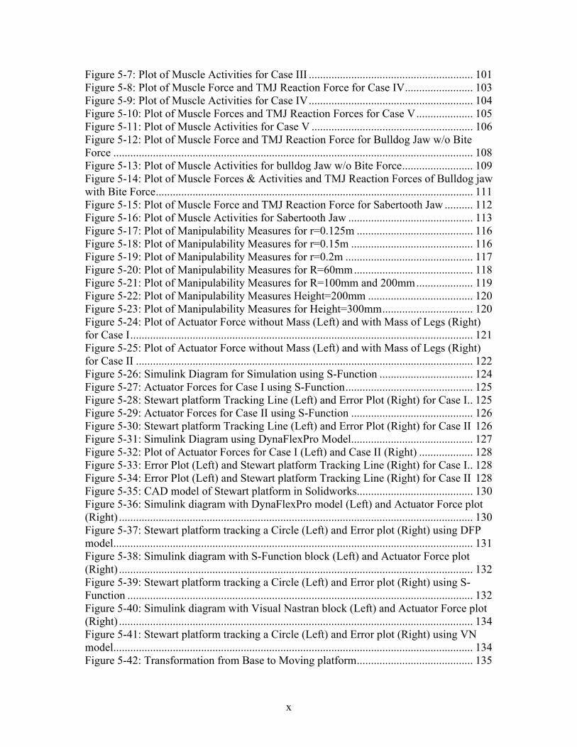
Figure 5-7: Plot of Muscle Activities for Case III .......................................................... 101 Figure 5-8: Plot of Muscle Force and TMJ Reaction Force for Case IV........................ 103 Figure 5-9: Plot of Muscle Activities for Case IV.......................................................... 104 Figure 5-10: Plot of Muscle Forces and TMJ Reaction Forces for Case V.................... 105 Figure 5-11: Plot of Muscle Activities for Case V ......................................................... 106 Figure 5-12: Plot of Muscle Force and TMJ Reaction Force for Bulldog Jaw w/o Bite Force ............................................................................................................................... 108 Figure 5-13: Plot of Muscle Activities for bulldog Jaw w/o Bite Force......................... 109 Figure 5-14: Plot of Muscle Forces & Activities and TMJ Reaction Forces of Bulldog jaw with Bite Force................................................................................................................ 111 Figure 5-15: Plot of Muscle Force and TMJ Reaction Force for Sabertooth Jaw .......... 112 Figure 5-16: Plot of Muscle Activities for Sabertooth Jaw ............................................ 113 Figure 5-17: Plot of Manipulability Measures for r=0.125m ......................................... 116 Figure 5-18: Plot of Manipulability Measures for r=0.15m ........................................... 116 Figure 5-19: Plot of Manipulability Measures for r=0.2m ............................................. 117 Figure 5-20: Plot of Manipulability Measures for R=60mm.......................................... 118 Figure 5-21: Plot of Manipulability Measures for R=100mm and 200mm.................... 119 Figure 5-22: Plot of Manipulability Measures Height=200mm ..................................... 120 Figure 5-23: Plot of Manipulability Measures for Height=300mm................................ 120 Figure 5-24: Plot of Actuator Force without Mass (Left) and with Mass of Legs (Right) for Case I......................................................................................................................... 121 Figure 5-25: Plot of Actuator Force without Mass (Left) and with Mass of Legs (Right) for Case II ....................................................................................................................... 122 Figure 5-26: Simulink Diagram for Simulation using S-Function ................................. 124 Figure 5-27: Actuator Forces for Case I using S-Function............................................. 125 Figure 5-28: Stewart platform Tracking Line (Left) and Error Plot (Right) for Case I.. 125 Figure 5-29: Actuator Forces for Case II using S-Function ........................................... 126 Figure 5-30: Stewart platform Tracking Line (Left) and Error Plot (Right) for Case II 126 Figure 5-31: Simulink Diagram using DynaFlexPro Model........................................... 127 Figure 5-32: Plot of Actuator Forces for Case I (Left) and Case II (Right) ................... 128 Figure 5-33: Error Plot (Left) and Stewart platform Tracking Line (Right) for Case I.. 128 Figure 5-34: Error Plot (Left) and Stewart platform Tracking Line (Right) for Case II 128 Figure 5-35: CAD model of Stewart platform in Solidworks......................................... 130 Figure 5-36: Simulink diagram with DynaFlexPro model (Left) and Actuator Force plot (Right) ............................................................................................................................. 130 Figure 5-37: Stewart platform tracking a Circle (Left) and Error plot (Right) using DFP model............................................................................................................................... 131 Figure 5-38: Simulink diagram with S-Function block (Left) and Actuator Force plot (Right) ............................................................................................................................. 132 Figure 5-39: Stewart platform tracking a Circle (Left) and Error plot (Right) using S-Function .......................................................................................................................... 132 Figure 5-40: Simulink diagram with Visual Nastran block (Left) and Actuator Force plot (Right) ............................................................................................................................. 134 Figure 5-41: Stewart platform tracking a Circle (Left) and Error plot (Right) using VN model............................................................................................................................... 134 Figure 5-42: Transformation from Base to Moving platform......................................... 135

xi

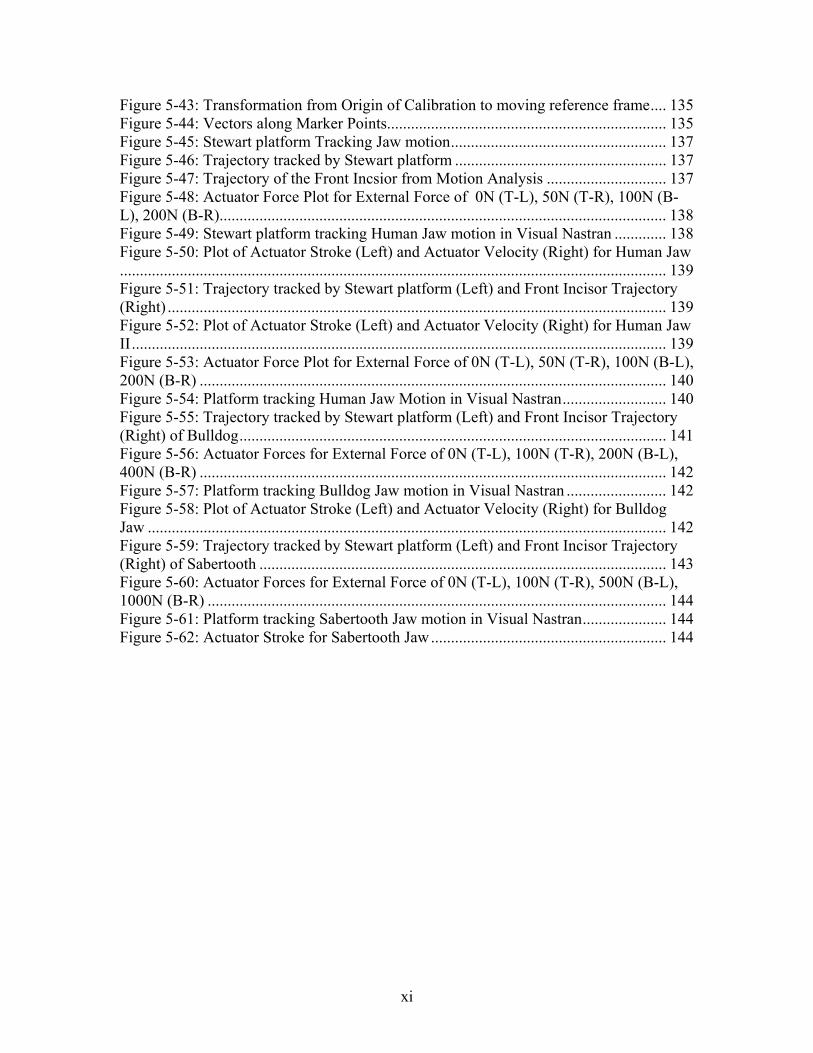
Figure 5-43: Transformation from Origin of Calibration to moving reference frame.... 135 Figure 5-44: Vectors along Marker Points...................................................................... 135 Figure 5-45: Stewart platform Tracking Jaw motion...................................................... 137 Figure 5-46: Trajectory tracked by Stewart platform ..................................................... 137 Figure 5-47: Trajectory of the Front Incsior from Motion Analysis .............................. 137 Figure 5-48: Actuator Force Plot for External Force of 0N (T-L), 50N (T-R), 100N (B-L), 200N (B-R)................................................................................................................ 138 Figure 5-49: Stewart platform tracking Human Jaw motion in Visual Nastran ............. 138 Figure 5-50: Plot of Actuator Stroke (Left) and Actuator Velocity (Right) for Human Jaw......................................................................................................................................... 139 Figure 5-51: Trajectory tracked by Stewart platform (Left) and Front Incisor Trajectory (Right) ............................................................................................................................. 139 Figure 5-52: Plot of Actuator Stroke (Left) and Actuator Velocity (Right) for Human Jaw II...................................................................................................................................... 139 Figure 5-53: Actuator Force Plot for External Force of 0N (T-L), 50N (T-R), 100N (B-L), 200N (B-R) ..................................................................................................................... 140 Figure 5-54: Platform tracking Human Jaw Motion in Visual Nastran.......................... 140 Figure 5-55: Trajectory tracked by Stewart platform (Left) and Front Incisor Trajectory (Right) of Bulldog........................................................................................................... 141 Figure 5-56: Actuator Forces for External Force of 0N (T-L), 100N (T-R), 200N (B-L), 400N (B-R) ..................................................................................................................... 142 Figure 5-57: Platform tracking Bulldog Jaw motion in Visual Nastran ......................... 142 Figure 5-58: Plot of Actuator Stroke (Left) and Actuator Velocity (Right) for Bulldog Jaw .................................................................................................................................. 142 Figure 5-59: Trajectory tracked by Stewart platform (Left) and Front Incisor Trajectory (Right) of Sabertooth ...................................................................................................... 143 Figure 5-60: Actuator Forces for External Force of 0N (T-L), 100N (T-R), 500N (B-L), 1000N (B-R) ................................................................................................................... 144 Figure 5-61: Platform tracking Sabertooth Jaw motion in Visual Nastran..................... 144 Figure 5-62: Actuator Stroke for Sabertooth Jaw........................................................... 144

xii

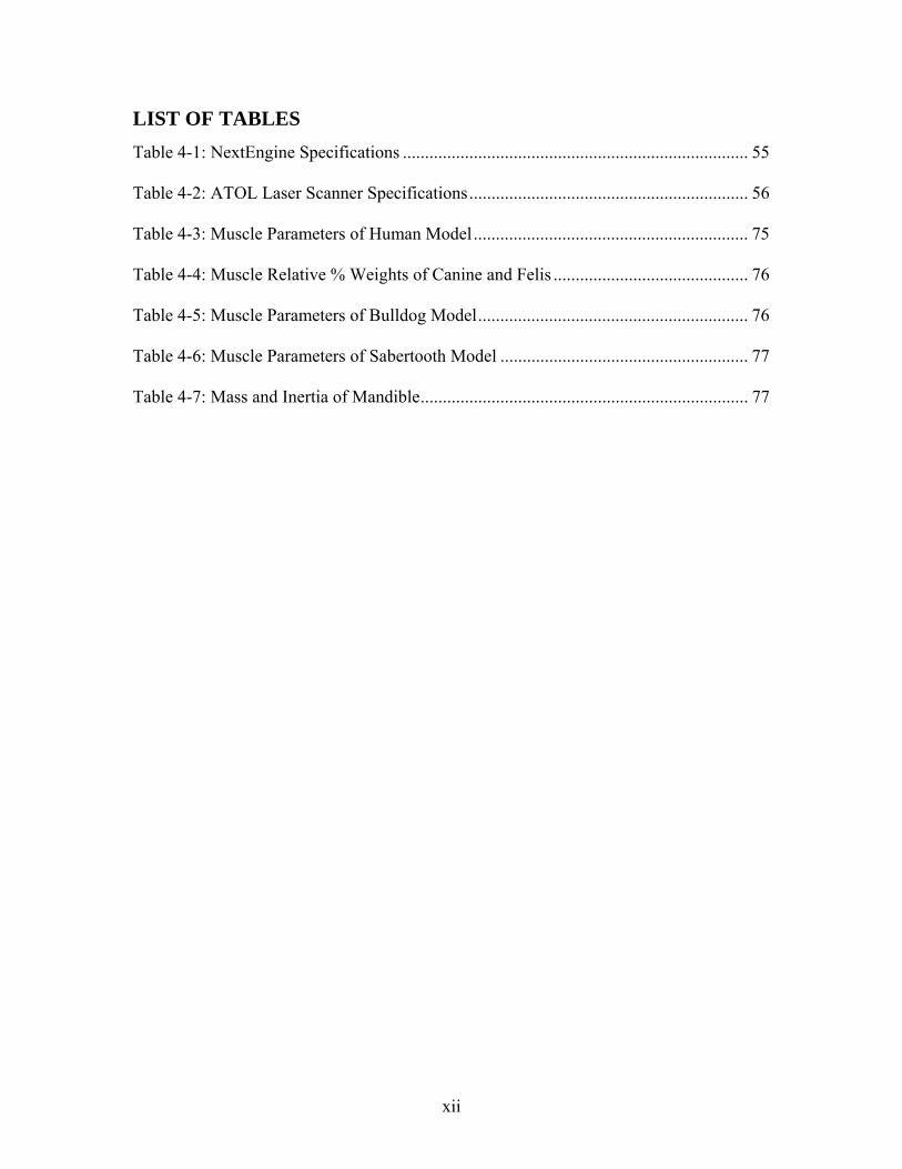
LIST OF TABLES Table 4-1: NextEngine Specifications .............................................................................. 55 Table 4-2: ATOL Laser Scanner Specifications............................................................... 56 Table 4-3: Muscle Parameters of Human Model.............................................................. 75 Table 4-4: Muscle Relative % Weights of Canine and Felis ............................................ 76 Table 4-5: Muscle Parameters of Bulldog Model............................................................. 76 Table 4-6: Muscle Parameters of Sabertooth Model ........................................................ 77 Table 4-7: Mass and Inertia of Mandible.......................................................................... 77

1

1. Introduction 1.1 Motivation

The goal of this project is to quantitatively measure mechanical performance signals such

as forces, motions and pressures during mastication with the intent of subsequently

characterizing mechanical breakdown of food in various vertebrates (including humans).

Such an understanding would be of tremendous importance from a variety of

perspectives. From a science perspective, it is useful to know how various animals

(including humans) preprocess the food for subsequent digestion. From an economic

perspective it potentially enables food manufacturing/processing companies to design and

process foods based on the “chewability index”. Such knowledge could potentially enable

the orthotists design, develop, fit and manufacture dental orthoses to support or correct

musculoskeletal deformities and or abnormalities of vertebrate jaws.

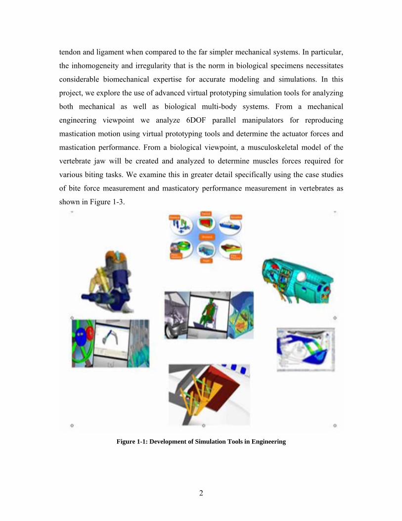
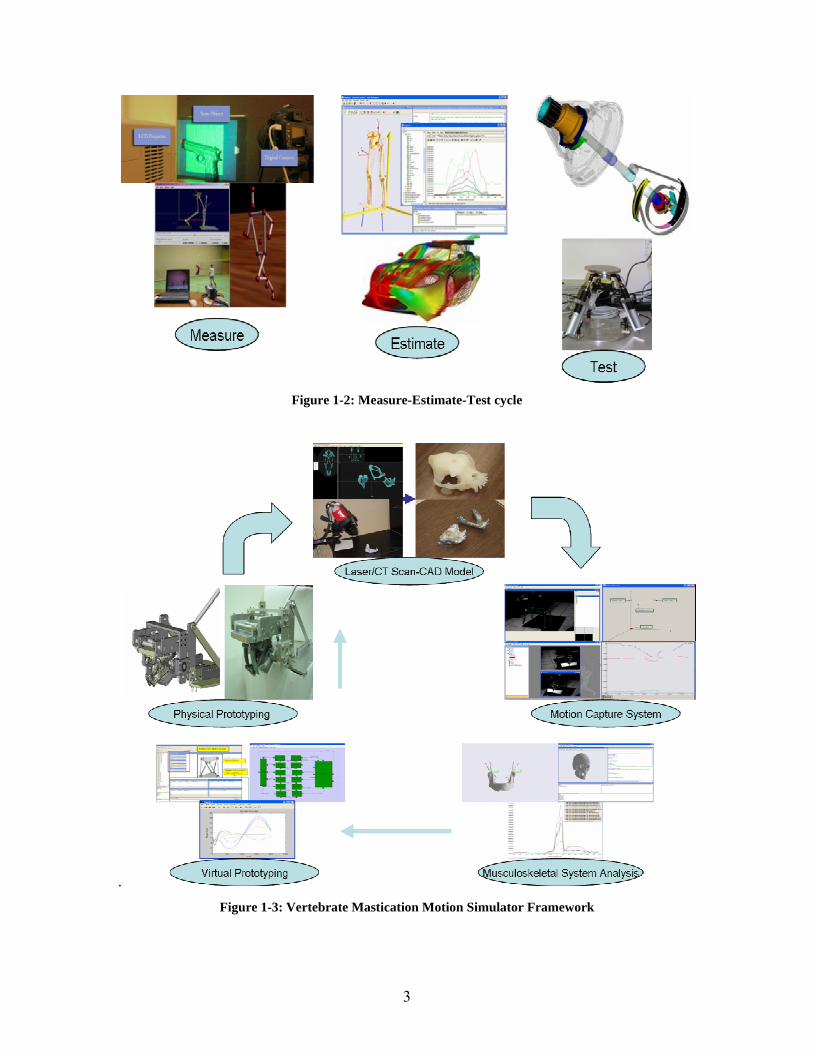
To aid us in this process of quantitatively measuring various mechanical output

parameters such as force/motion/pressure, we will examine use of current technological

tools and paradigms in measure-estimate-test cycle as shown in Figure 1-2 by a

combination of “Virtual Prototyping” and “Physical Prototyping”. In the last decade, the

science and engineering domains have been revolutionized by the ubiquitous availability

of computational power coupling with the advances in computational tools, algorithms

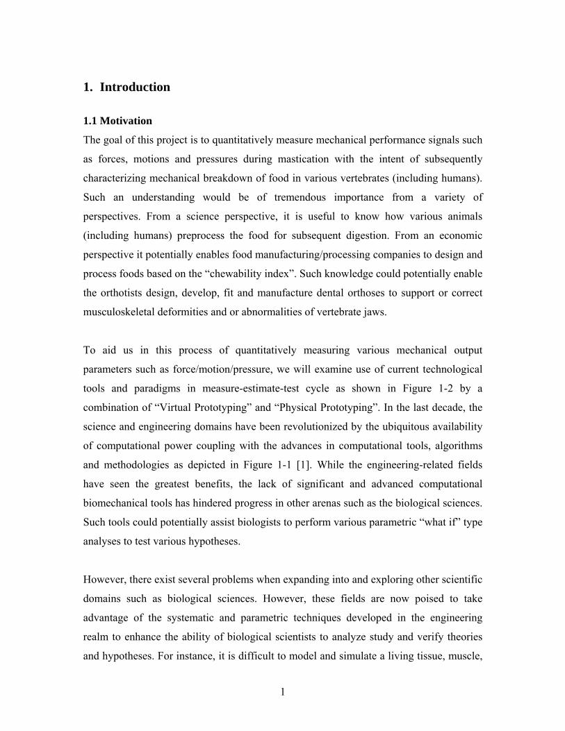
and methodologies as depicted in Figure 1-1 [1]. While the engineering-related fields

have seen the greatest benefits, the lack of significant and advanced computational

biomechanical tools has hindered progress in other arenas such as the biological sciences.

Such tools could potentially assist biologists to perform various parametric “what if” type

analyses to test various hypotheses.

However, there exist several problems when expanding into and exploring other scientific

domains such as biological sciences. However, these fields are now poised to take

advantage of the systematic and parametric techniques developed in the engineering

realm to enhance the ability of biological scientists to analyze study and verify theories

and hypotheses. For instance, it is difficult to model and simulate a living tissue, muscle,

2

tendon and ligament when compared to the far simpler mechanical systems. In particular,

the inhomogeneity and irregularity that is the norm in biological specimens necessitates

considerable biomechanical expertise for accurate modeling and simulations. In this

project, we explore the use of advanced virtual prototyping simulation tools for analyzing

both mechanical as well as biological multi-body systems. From a mechanical

engineering viewpoint we analyze 6DOF parallel manipulators for reproducing

mastication motion using virtual prototyping tools and determine the actuator forces and

mastication performance. From a biological viewpoint, a musculoskeletal model of the

vertebrate jaw will be created and analyzed to determine muscles forces required for

various biting tasks. We examine this in greater detail specifically using the case studies

of bite force measurement and masticatory performance measurement in vertebrates as

shown in Figure 1-3.

Figure 1-1: Development of Simulation Tools in Engineering

3

Figure 1-2: Measure-Estimate-Test cycle

. Figure 1-3: Vertebrate Mastication Motion Simulator Framework

4

1.2 Virtual Prototyping/ Simulation Based Design

“Virtual prototyping refers to computer based virtual simulation and analysis of a

physical system through various stages of its product cycle. Various aspects of design,

analyses, manufacturing, service and recycling can now be examined completely in the

context of a Virtual Prototype”. [4]

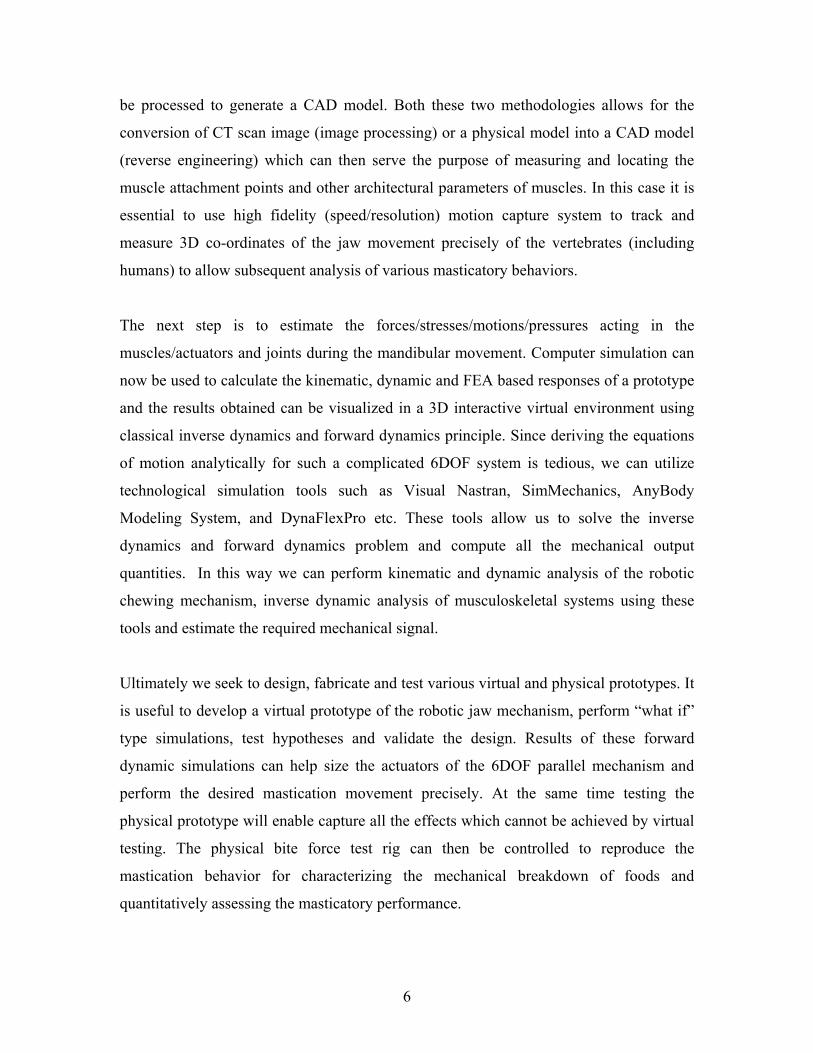
Virtual prototyping empowers engineers by eliminating the expensive process of

fabrication and testing physical prototypes as seen in Figure 1-4 and Figure 1-5. Through

virtual prototyping it is now beneficial to create, estimate/simulate and test these digital

prototypes before the fabrication and reduce the overall design cycle time. In a nutshell it

refers to the process of simulating the product and perform quantitative and performance

analysis of the product [2] [5]. Simulation based design allows parametric analysis to be

performed on these prototypes and can be refined by integrating with CAE and CAM

simulation tools. The integration of these conceptual designs with the CAE simulation

tools enables quantitative measurement of performance characteristics and their

integration with the CAM simulation tool enable the engineer to overcome challenges

regarding manufacturability of the product. These parametric simulations enable

engineers to identify the parameters affecting quality, performance, manufacturability,

cost etc and quantify the parameter interactions and interdependencies. In short, VP tools

are used to virtually create, estimate, test, validate and manage product designs within a

virtual environment to identify complex product process interdependencies and

parameters early in the product development cycle and thus reducing the cycle cost and

time. Some of the advantages of using VP techniques [2] include its ability to accelerate

and improve the product life cycle, its use as a tool for testing and analyzing various

“what if” scenarios and its ability to develop the final physical prototype without the need

for further modifications. VP is limited by things such as the accuracy of the analysis

results for a virtual prototype depends on factors like, the skill of the designer,

availability of computational power and level of detail. Further, as the intricacy of the

system increases, the effort, skill and the computational power required for developing a

virtual prototype increases exponentially.

5

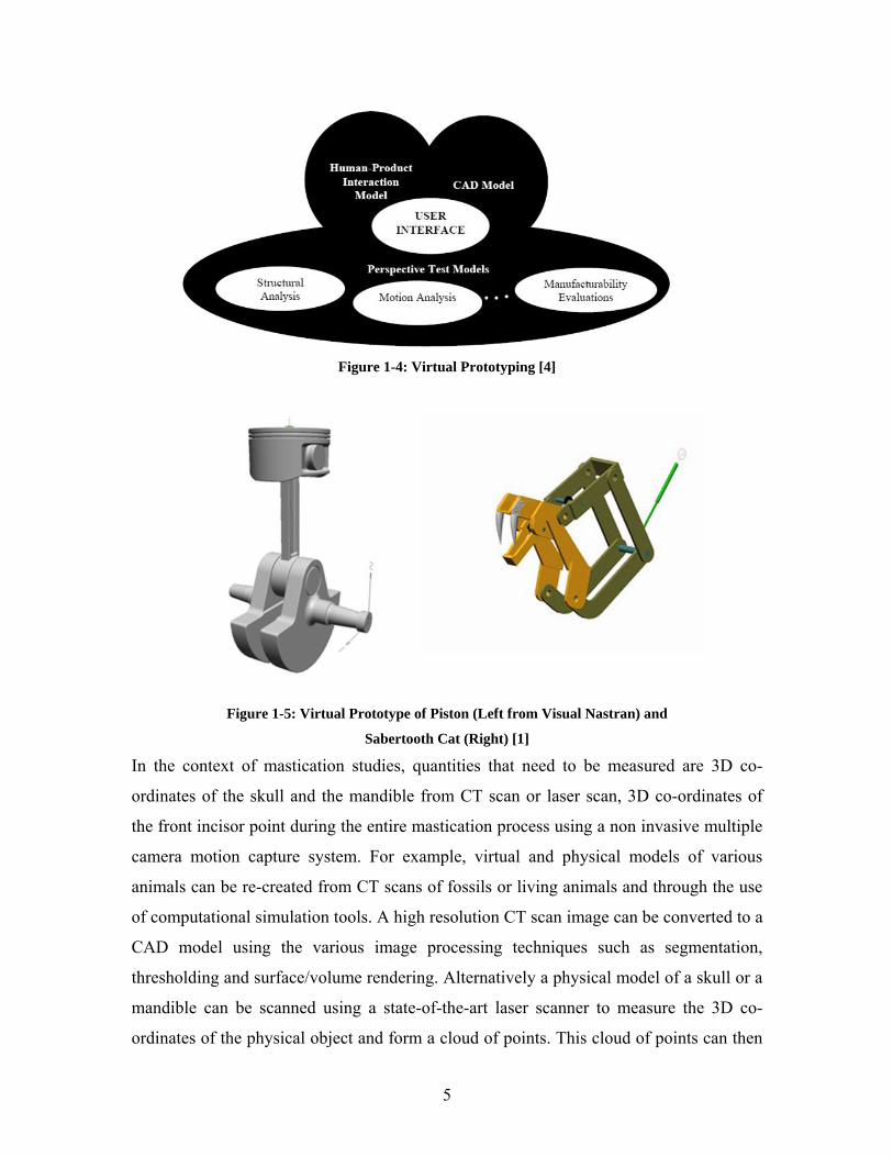
Figure 1-4: Virtual Prototyping [4]

Figure 1-5: Virtual Prototype of Piston (Left from Visual Nastran) and

Sabertooth Cat (Right) [1]

In the context of mastication studies, quantities that need to be measured are 3D co-

ordinates of the skull and the mandible from CT scan or laser scan, 3D co-ordinates of

the front incisor point during the entire mastication process using a non invasive multiple

camera motion capture system. For example, virtual and physical models of various

animals can be re-created from CT scans of fossils or living animals and through the use

of computational simulation tools. A high resolution CT scan image can be converted to a

CAD model using the various image processing techniques such as segmentation,

thresholding and surface/volume rendering. Alternatively a physical model of a skull or a

mandible can be scanned using a state-of-the-art laser scanner to measure the 3D co-

ordinates of the physical object and form a cloud of points. This cloud of points can then

6

be processed to generate a CAD model. Both these two methodologies allows for the

conversion of CT scan image (image processing) or a physical model into a CAD model

(reverse engineering) which can then serve the purpose of measuring and locating the

muscle attachment points and other architectural parameters of muscles. In this case it is

essential to use high fidelity (speed/resolution) motion capture system to track and

measure 3D co-ordinates of the jaw movement precisely of the vertebrates (including

humans) to allow subsequent analysis of various masticatory behaviors.

The next step is to estimate the forces/stresses/motions/pressures acting in the

muscles/actuators and joints during the mandibular movement. Computer simulation can

now be used to calculate the kinematic, dynamic and FEA based responses of a prototype

and the results obtained can be visualized in a 3D interactive virtual environment using

classical inverse dynamics and forward dynamics principle. Since deriving the equations

of motion analytically for such a complicated 6DOF system is tedious, we can utilize

technological simulation tools such as Visual Nastran, SimMechanics, AnyBody

Modeling System, and DynaFlexPro etc. These tools allow us to solve the inverse

dynamics and forward dynamics problem and compute all the mechanical output

quantities. In this way we can perform kinematic and dynamic analysis of the robotic

chewing mechanism, inverse dynamic analysis of musculoskeletal systems using these

tools and estimate the required mechanical signal.

Ultimately we seek to design, fabricate and test various virtual and physical prototypes. It

is useful to develop a virtual prototype of the robotic jaw mechanism, perform “what if”

type simulations, test hypotheses and validate the design. Results of these forward

dynamic simulations can help size the actuators of the 6DOF parallel mechanism and

perform the desired mastication movement precisely. At the same time testing the

physical prototype will enable capture all the effects which cannot be achieved by virtual

testing. The physical bite force test rig can then be controlled to reproduce the

mastication behavior for characterizing the mechanical breakdown of foods and

quantitatively assessing the masticatory performance.

7

1.3 Musculoskeletal System Analysis

“Biomechanics is the science concerned with the internal and external forces and

moments acting on the human body and the effects produced by these forces and

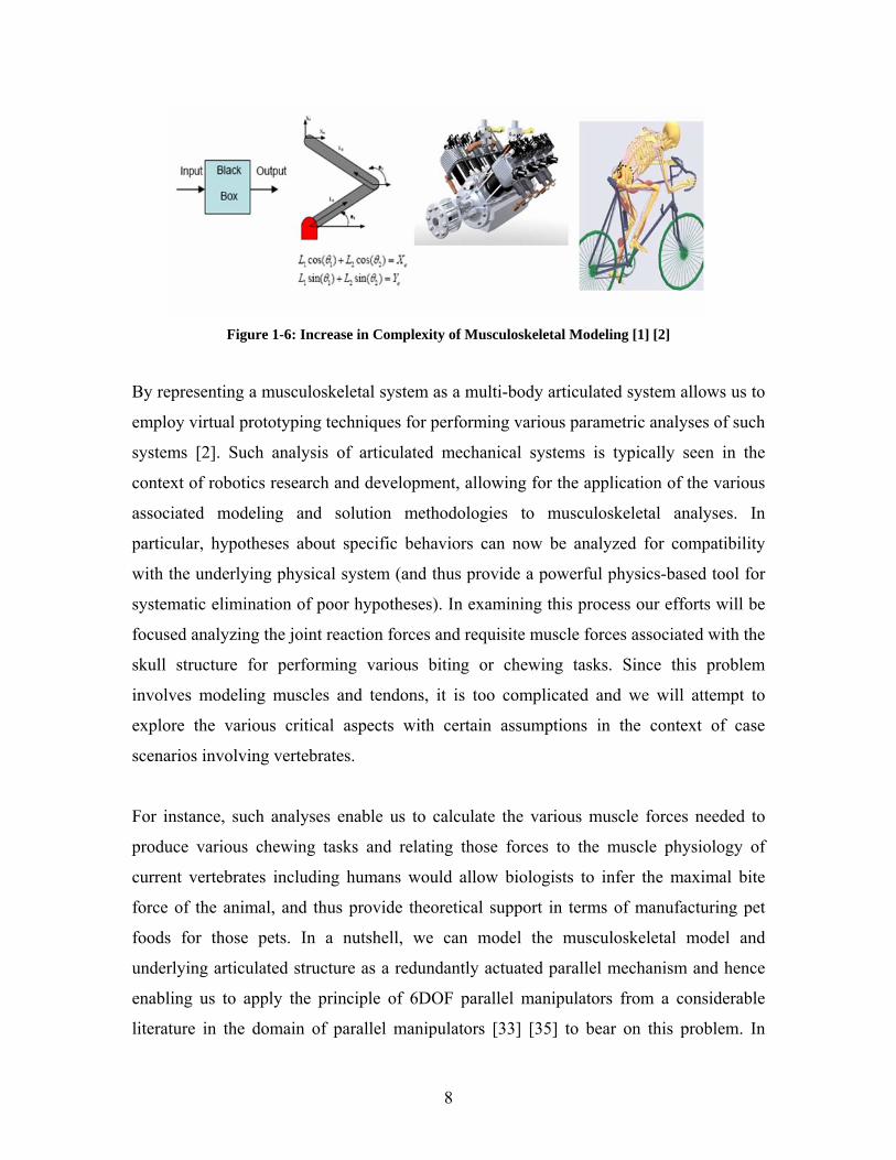
moments” [2]. As shown in Figure 1-6 conceptual model is used to make a point without

performing the mathematical analysis and is rarely used because of over-simplification and

inability to prove hypothesis. While simple models can be analyzed by

mathematical/analytical models by deriving the equations of motion and solving them

analytically, it cannot accurately model complex geometries like the ones encountered in

biomechanical modeling. CAD based models are used to represent complex systems but it is

not possible to derive its equation of motion analytically. In order to represent a more

complete biomechanical system, it is imperative to develop musculoskeletal models with

reasonable accuracy and realism which increase the degree of complexity.

Musculoskeletal system analysis can be defined as the study of the interaction between

the muscles, bones, ligaments and other physiological properties associated with humans

or animals that cause an external motion and/ or force. This type of analysis has

interested researchers throughout history and made significant headway into the

understanding of musculoskeletal systems, and has contributed to the development of

modern day musculoskeletal analyses and development of robotic systems. Applying

engineering methodologies to the analysis of a musculoskeletal system would first

involve the development of appropriate models [2]. From an engineering standpoint a

musculoskeletal system can be modeled as an articulated multi-body system (see Figure

1-7) where the bones are treated as segments/bodies coupled together at joints which are

held together and actuated by ligaments and muscles.

8

Figure 1-6: Increase in Complexity of Musculoskeletal Modeling [1] [2]

By representing a musculoskeletal system as a multi-body articulated system allows us to

employ virtual prototyping techniques for performing various parametric analyses of such

systems [2]. Such analysis of articulated mechanical systems is typically seen in the

context of robotics research and development, allowing for the application of the various

associated modeling and solution methodologies to musculoskeletal analyses. In

particular, hypotheses about specific behaviors can now be analyzed for compatibility

with the underlying physical system (and thus provide a powerful physics-based tool for

systematic elimination of poor hypotheses). In examining this process our efforts will be

focused analyzing the joint reaction forces and requisite muscle forces associated with the

skull structure for performing various biting or chewing tasks. Since this problem

involves modeling muscles and tendons, it is too complicated and we will attempt to

explore the various critical aspects with certain assumptions in the context of case

scenarios involving vertebrates.

For instance, such analyses enable us to calculate the various muscle forces needed to

produce various chewing tasks and relating those forces to the muscle physiology of

current vertebrates including humans would allow biologists to infer the maximal bite

force of the animal, and thus provide theoretical support in terms of manufacturing pet

foods for those pets. In a nutshell, we can model the musculoskeletal model and

underlying articulated structure as a redundantly actuated parallel mechanism and hence

enabling us to apply the principle of 6DOF parallel manipulators from a considerable

literature in the domain of parallel manipulators [33] [35] to bear on this problem. In

9

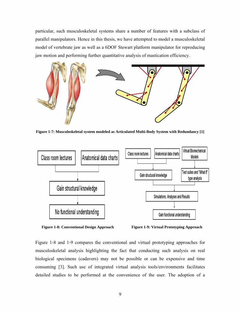
particular, such musculoskeletal systems share a number of features with a subclass of

parallel manipulators. Hence in this thesis, we have attempted to model a musculoskeletal

model of vertebrate jaw as well as a 6DOF Stewart platform manipulator for reproducing

jaw motion and performing further quantitative analysis of mastication efficiency.

Figure 1-7: Musculoskeletal system modeled as Articulated Multi-Body System with Redundancy [1]

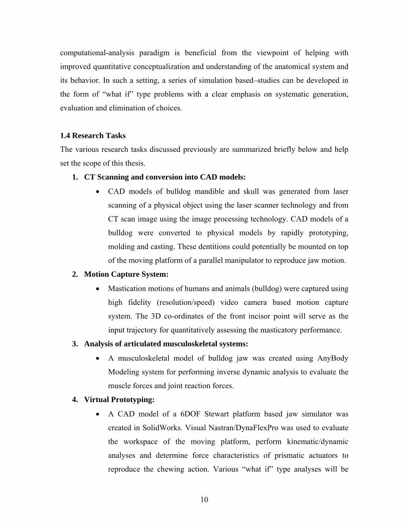
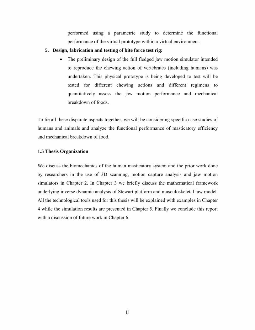
Figure 1-8: Conventional Design Approach Figure 1-9: Virtual Prototyping Approach

Figure 1-8 and 1-9 compares the conventional and virtual prototyping approaches for

musculoskeletal analysis highlighting the fact that conducting such analysis on real

biological specimens (cadavers) may not be possible or can be expensive and time

consuming [3]. Such use of integrated virtual analysis tools/environments facilitates

detailed studies to be performed at the convenience of the user. The adoption of a

10

computational-analysis paradigm is beneficial from the viewpoint of helping with

improved quantitative conceptualization and understanding of the anatomical system and

its behavior. In such a setting, a series of simulation based–studies can be developed in

the form of “what if” type problems with a clear emphasis on systematic generation,

evaluation and elimination of choices.

1.4 Research Tasks

The various research tasks discussed previously are summarized briefly below and help

set the scope of this thesis.

1. CT Scanning and conversion into CAD models:

• CAD models of bulldog mandible and skull was generated from laser

scanning of a physical object using the laser scanner technology and from

CT scan image using the image processing technology. CAD models of a

bulldog were converted to physical models by rapidly prototyping,

molding and casting. These dentitions could potentially be mounted on top

of the moving platform of a parallel manipulator to reproduce jaw motion.

2. Motion Capture System:

• Mastication motions of humans and animals (bulldog) were captured using

high fidelity (resolution/speed) video camera based motion capture

system. The 3D co-ordinates of the front incisor point will serve as the

input trajectory for quantitatively assessing the masticatory performance.

3. Analysis of articulated musculoskeletal systems:

• A musculoskeletal model of bulldog jaw was created using AnyBody

Modeling system for performing inverse dynamic analysis to evaluate the

muscle forces and joint reaction forces.

4. Virtual Prototyping:

• A CAD model of a 6DOF Stewart platform based jaw simulator was

created in SolidWorks. Visual Nastran/DynaFlexPro was used to evaluate

the workspace of the moving platform, perform kinematic/dynamic

analyses and determine force characteristics of prismatic actuators to

reproduce the chewing action. Various “what if” type analyses will be

11

performed using a parametric study to determine the functional

performance of the virtual prototype within a virtual environment.

5. Design, fabrication and testing of bite force test rig:

• The preliminary design of the full fledged jaw motion simulator intended

to reproduce the chewing action of vertebrates (including humans) was

undertaken. This physical prototype is being developed to test will be

tested for different chewing actions and different regimens to

quantitatively assess the jaw motion performance and mechanical

breakdown of foods.

To tie all these disparate aspects together, we will be considering specific case studies of

humans and animals and analyze the functional performance of masticatory efficiency

and mechanical breakdown of food.

1.5 Thesis Organization

We discuss the biomechanics of the human masticatory system and the prior work done

by researchers in the use of 3D scanning, motion capture analysis and jaw motion

simulators in Chapter 2. In Chapter 3 we briefly discuss the mathematical framework

underlying inverse dynamic analysis of Stewart platform and musculoskeletal jaw model.

All the technological tools used for this thesis will be explained with examples in Chapter

4 while the simulation results are presented in Chapter 5. Finally we conclude this report

with a discussion of future work in Chapter 6.

12

2. Literature Survey 2.1 Masticatory Biomechanics

The human masticatory system consists of a lower jaw (mandible) connected to an upper

jaw (maxilla) by two very complex shaped incongruent jaw joints, the

temporomandibular joints (TMJ) and cannot be approximated as a ball and socket joint to

prevent loss of functionality and are guided by the contraction of the muscle of

mastication. The masticatory system consists of a large number of muscles of various

shapes and sizes and co-operates to perform a certain task [10]. Furthermore, the articular

surfaces are separated by a cartilaginous articular disc which is able to move more or less

freely between these surfaces and affect the movements of the jaw. There are powerful

tools like SIMM, AnyBody for developing musculoskeletal models and such framework

can be used to explore masticatory dynamics. In this thesis we will be exploring the

inverse dynamic analysis of a vertebrate jaw model in AnyBody to determine muscle and

joint reaction forces during mastication.

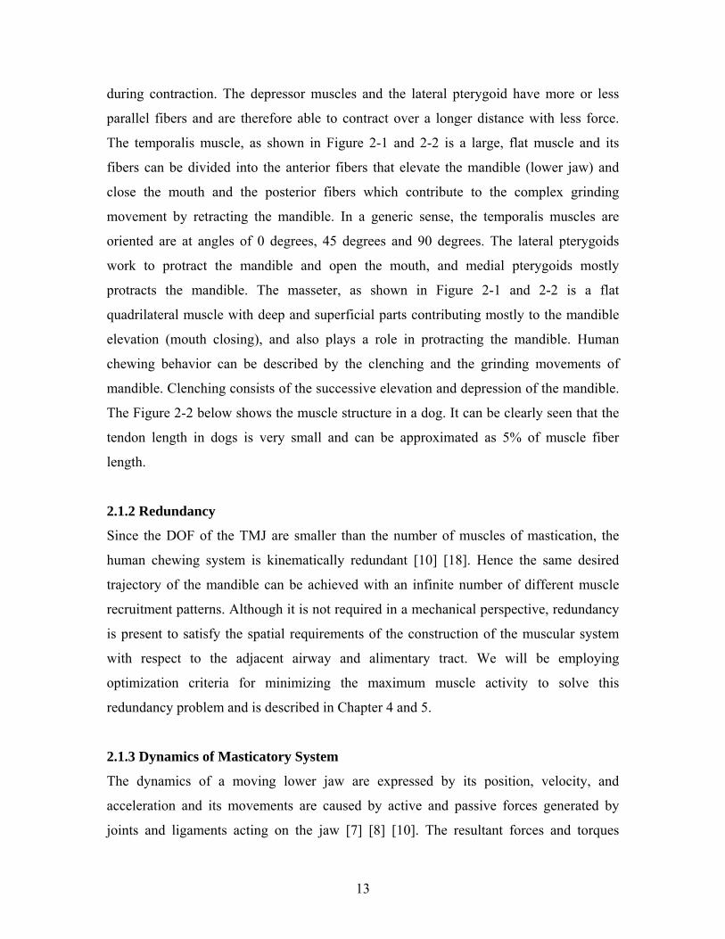
2.1.1 Jaw Muscles and Movements

More than 20 muscles are involved in the process of mastication that is controlled by the

central nervous system as shown in Figure 2-1 and 2-2 [18]. Anatomically, the muscles of

mastication are divided into elevators (masseter, temporalis, and medial pterygoid

muscles) and depressors (geniohyoid, mylohyoid, and digastric muscles). The elevator

group consists of the masseter and temporalis muscles, which are located more or less

superficially, and the medial pterygoid muscle, which is located more deeply. The

muscles of the depressor group are located in the floor of the mouth. The digastrics

muscles connect the mastoid process of the skull with the body of the mandible and are

attached to the hyoid bone via a fibrous loop which runs around its intermediate tendon.

The lateral pterygoid muscle consisting of a superior and inferior head completes the

muscular system. These muscles cannot be termed as elevator or depressor since both

heads are considered to have different actions. The elevator muscles which are heavily

pinnate are suitable for generation of large forces due to their large physiological cross-

sectional areas. But these fibers are short thus limiting their capacity for active shortening

13

during contraction. The depressor muscles and the lateral pterygoid have more or less

parallel fibers and are therefore able to contract over a longer distance with less force.

The temporalis muscle, as shown in Figure 2-1 and 2-2 is a large, flat muscle and its

fibers can be divided into the anterior fibers that elevate the mandible (lower jaw) and

close the mouth and the posterior fibers which contribute to the complex grinding

movement by retracting the mandible. In a generic sense, the temporalis muscles are

oriented are at angles of 0 degrees, 45 degrees and 90 degrees. The lateral pterygoids

work to protract the mandible and open the mouth, and medial pterygoids mostly

protracts the mandible. The masseter, as shown in Figure 2-1 and 2-2 is a flat

quadrilateral muscle with deep and superficial parts contributing mostly to the mandible

elevation (mouth closing), and also plays a role in protracting the mandible. Human

chewing behavior can be described by the clenching and the grinding movements of

mandible. Clenching consists of the successive elevation and depression of the mandible.

The Figure 2-2 below shows the muscle structure in a dog. It can be clearly seen that the

tendon length in dogs is very small and can be approximated as 5% of muscle fiber

length.

2.1.2 Redundancy

Since the DOF of the TMJ are smaller than the number of muscles of mastication, the

human chewing system is kinematically redundant [10] [18]. Hence the same desired

trajectory of the mandible can be achieved with an infinite number of different muscle

recruitment patterns. Although it is not required in a mechanical perspective, redundancy

is present to satisfy the spatial requirements of the construction of the muscular system

with respect to the adjacent airway and alimentary tract. We will be employing

optimization criteria for minimizing the maximum muscle activity to solve this

redundancy problem and is described in Chapter 4 and 5.

2.1.3 Dynamics of Masticatory System

The dynamics of a moving lower jaw are expressed by its position, velocity, and

acceleration and its movements are caused by active and passive forces generated by

joints and ligaments acting on the jaw [7] [8] [10]. The resultant forces and torques

14

generate accelerations and move the mandible with 6DOF w.r.t. the skull. If the condyles

on both joints are assumed to maintain articular contact all the time with the fossa, a

translation of the condyle in a direction perpendicular to the articular surface of the

temporal bone is restricted, and the number of DOF for condylar movement is reduced to

five. Furthermore, if both joints are assumed to be connected rigidly through the

mandibular symphysis, the rotation of the lower jaw about an antero-posterior axis is

restricted and is able to move with four degrees of freedom.

Figure 2-1: Human Masticatory Muscles [18]

Figure 2-2: Dog Masticatory Muscles

2.1.4. Influence of Muscles and Hill Muscle Model

Each muscle contraction is associated with a force which is expressed its magnitude,

point of application, and orientation. Each muscle can produce a translation of the lower

jaw along its line of action, and a rotation about an axis perpendicular to it and running

through the jaw’s center of gravity and together represent one DOF [10]. Hence the

number of degrees of freedom of a system of muscles depends on the number of

independent lines of action. Jaw movements caused by the masticatory muscles are

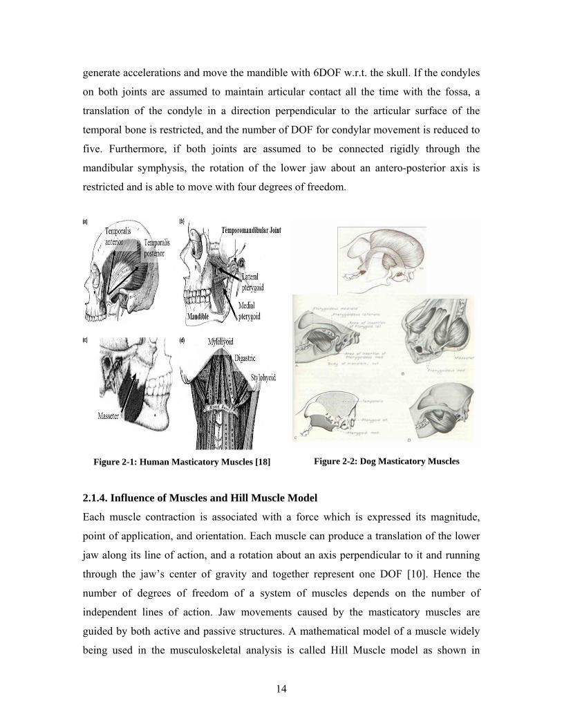
guided by both active and passive structures. A mathematical model of a muscle widely

being used in the musculoskeletal analysis is called Hill Muscle model as shown in

15

Figure 2-3. The muscle’s active component which acts against passive components

contributes the final piece of the mathematical muscle model. Readers are requested to

refer to [2] for the experimental work carried out by Hill to come up with two different

three element muscle models. The three elements of the model are contractile element

(CE, muscle fibers), the parallel elastic element (PE, connective tissues around the fibers

and fiber bundles) and the series elastic element (SE, muscle tendon).

Figure 2-3: Elements of Hill Muscle Model [2]

Figure 2-4: Force Length profile of CE, SE and PE elements [2]

2.1.5 Active and Passive Elements

Active muscles are the prime movers and dominant determinant of jaw motion. Passive

structures in the masticatory system may act as constraints for jaw movements and guide

the mandible along its path and they have the ability to resist jaw movements along one

or more degrees to generate a reaction force. When inactive, the masticatory muscles

generate passive forces which are dependent on the instantaneous length of their

sarcomeres and when the sarcomeres are at or below optimum length, they are negligible,

but increase exponentially if they are stretched beyond this length as shown in Figure 2-4.

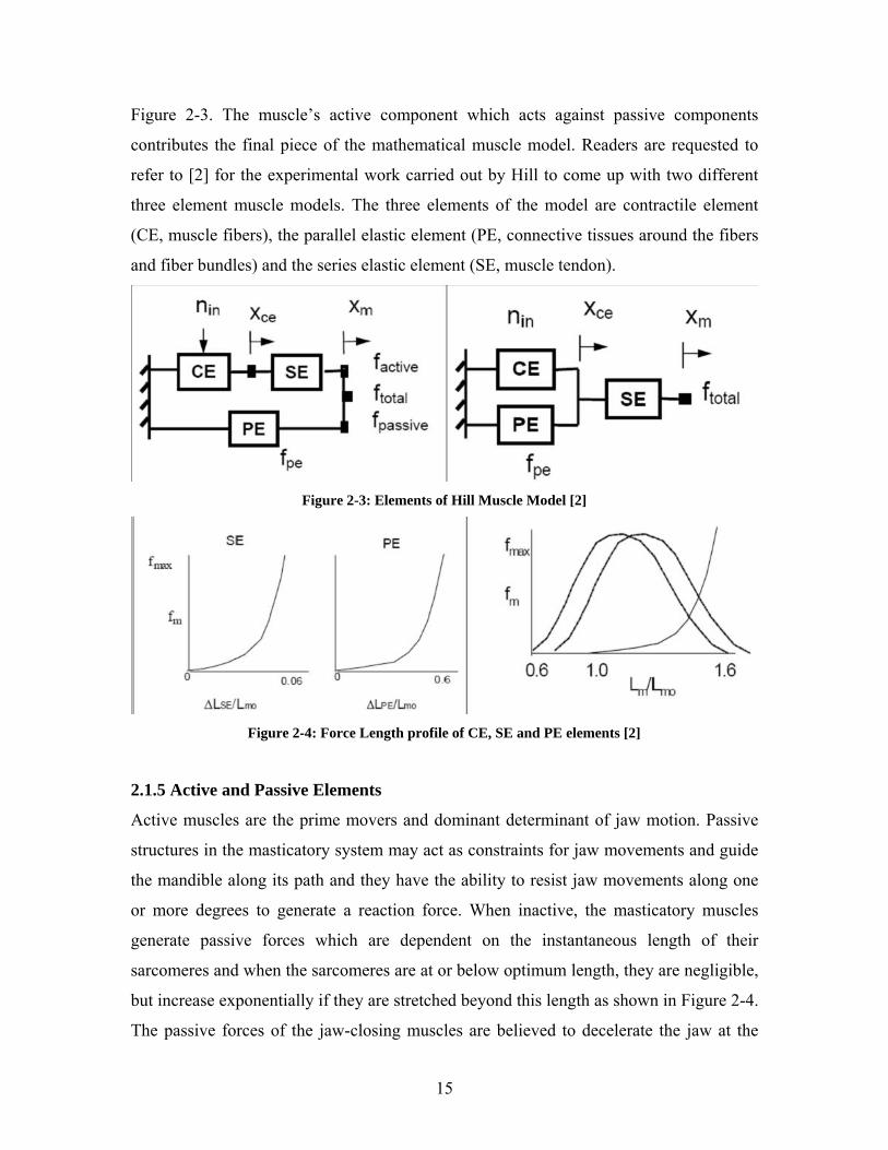
The passive forces of the jaw-closing muscles are believed to decelerate the jaw at the

16

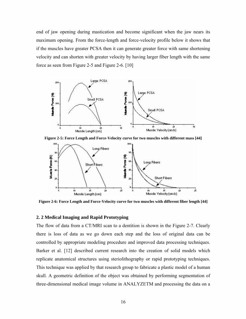
end of jaw opening during mastication and become significant when the jaw nears its

maximum opening. From the force-length and force-velocity profile below it shows that

if the muscles have greater PCSA then it can generate greater force with same shortening

velocity and can shorten with greater velocity by having larger fiber length with the same

force as seen from Figure 2-5 and Figure 2-6. [10]

Figure 2-5: Force Length and Force-Velocity curve for two muscles with different mass [44]

Figure 2-6: Force Length and Force-Velocity curve for two muscles with different fiber length [44]

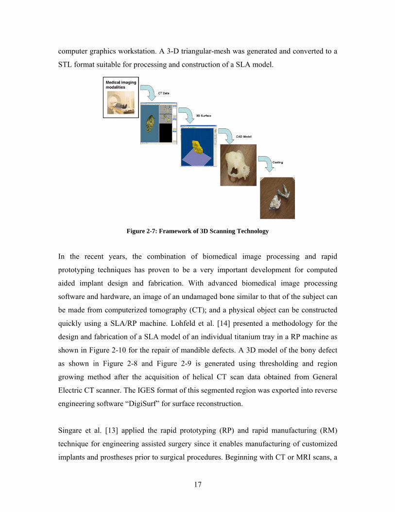
2. 2 Medical Imaging and Rapid Prototyping

The flow of data from a CT/MRI scan to a dentition is shown in the Figure 2-7. Clearly

there is loss of data as we go down each step and the loss of original data can be

controlled by appropriate modeling procedure and improved data processing techniques.

Barker et al. [12] described current research into the creation of solid models which

replicate anatomical structures using steriolithography or rapid prototyping techniques.

This technique was applied by that research group to fabricate a plastic model of a human

skull. A geometric definition of the object was obtained by performing segmentation of

three-dimensional medical image volume in ANALYZETM and processing the data on a

17

computer graphics workstation. A 3-D triangular-mesh was generated and converted to a

STL format suitable for processing and construction of a SLA model.

Figure 2-7: Framework of 3D Scanning Technology

In the recent years, the combination of biomedical image processing and rapid

prototyping techniques has proven to be a very important development for computed

aided implant design and fabrication. With advanced biomedical image processing

software and hardware, an image of an undamaged bone similar to that of the subject can

be made from computerized tomography (CT); and a physical object can be constructed

quickly using a SLA/RP machine. Lohfeld et al. [14] presented a methodology for the

design and fabrication of a SLA model of an individual titanium tray in a RP machine as

shown in Figure 2-10 for the repair of mandible defects. A 3D model of the bony defect

as shown in Figure 2-8 and Figure 2-9 is generated using thresholding and region

growing method after the acquisition of helical CT scan data obtained from General

Electric CT scanner. The IGES format of this segmented region was exported into reverse

engineering software “DigiSurf” for surface reconstruction.

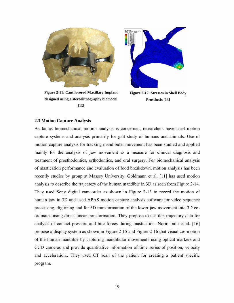
Singare et al. [13] applied the rapid prototyping (RP) and rapid manufacturing (RM)

technique for engineering assisted surgery since it enables manufacturing of customized

implants and prostheses prior to surgical procedures. Beginning with CT or MRI scans, a

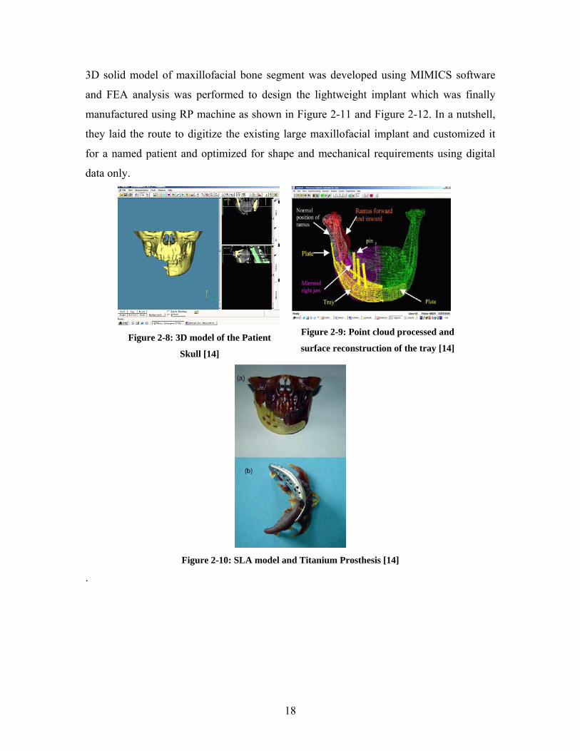
18

3D solid model of maxillofacial bone segment was developed using MIMICS software

and FEA analysis was performed to design the lightweight implant which was finally

manufactured using RP machine as shown in Figure 2-11 and Figure 2-12. In a nutshell,

they laid the route to digitize the existing large maxillofacial implant and customized it

for a named patient and optimized for shape and mechanical requirements using digital

data only.

Figure 2-8: 3D model of the Patient

Skull [14]

Figure 2-9: Point cloud processed and

surface reconstruction of the tray [14]

Figure 2-10: SLA model and Titanium Prosthesis [14]

.

19

Figure 2-11: Cantilevered Maxillary Implant

designed using a stereolithography biomodel

[13]

Figure 2-12: Stresses in Shell Body

Prosthesis [13]

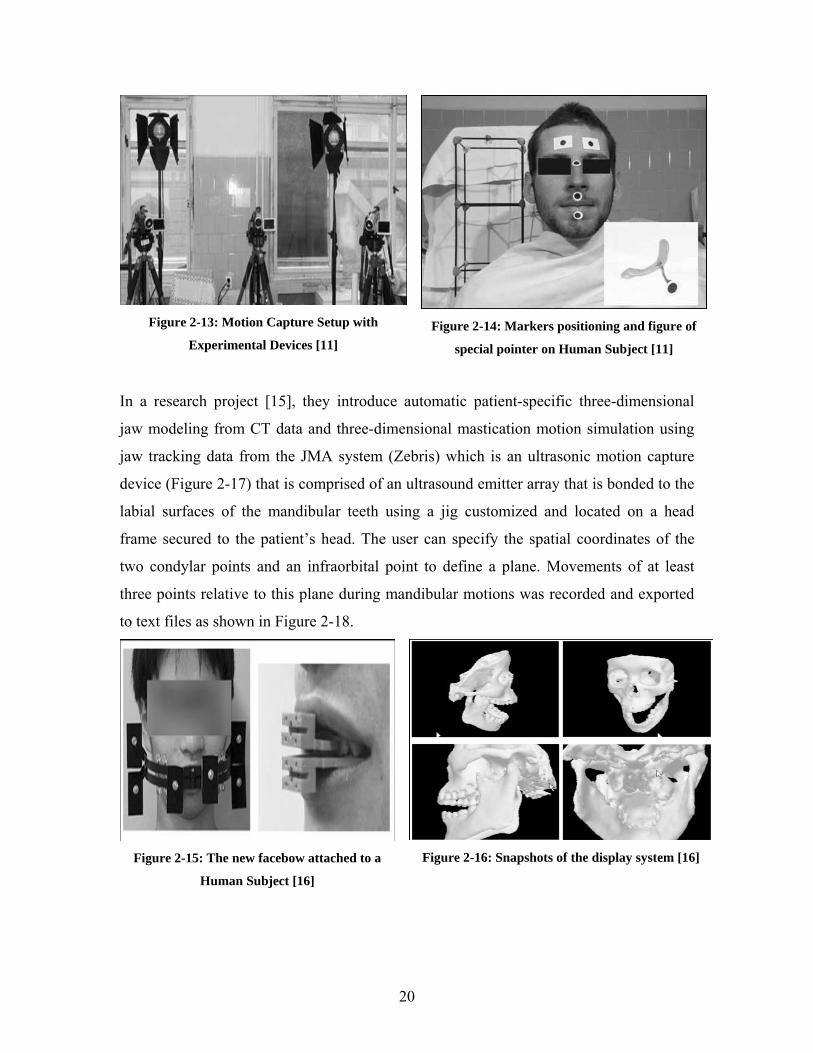
2.3 Motion Capture Analysis

As far as biomechanical motion analysis is concerned, researchers have used motion

capture systems and analysis primarily for gait study of humans and animals. Use of

motion capture analysis for tracking mandibular movement has been studied and applied

mainly for the analysis of jaw movement as a measure for clinical diagnosis and

treatment of prosthodontics, orthodontics, and oral surgery. For biomechanical analysis

of mastication performance and evaluation of food breakdown, motion analysis has been

recently studies by group at Massey University. Goldmann et al. [11] has used motion

analysis to describe the trajectory of the human mandible in 3D as seen from Figure 2-14.

They used Sony digital camcorder as shown in Figure 2-13 to record the motion of

human jaw in 3D and used APAS motion capture analysis software for video sequence

processing, digitizing and for 3D transformation of the lower jaw movement into 3D co-

ordinates using direct linear transformation. They propose to use this trajectory data for

analysis of contact pressure and bite forces during mastication. Norio Inou et al. [16]

propose a display system as shown in Figure 2-15 and Figure 2-16 that visualizes motion

of the human mandible by capturing mandibular movements using optical markers and

CCD cameras and provide quantitative information of time series of position, velocity

and acceleration.. They used CT scan of the patient for creating a patient specific

program.

20

Figure 2-13: Motion Capture Setup with

Experimental Devices [11] Figure 2-14: Markers positioning and figure of

special pointer on Human Subject [11]

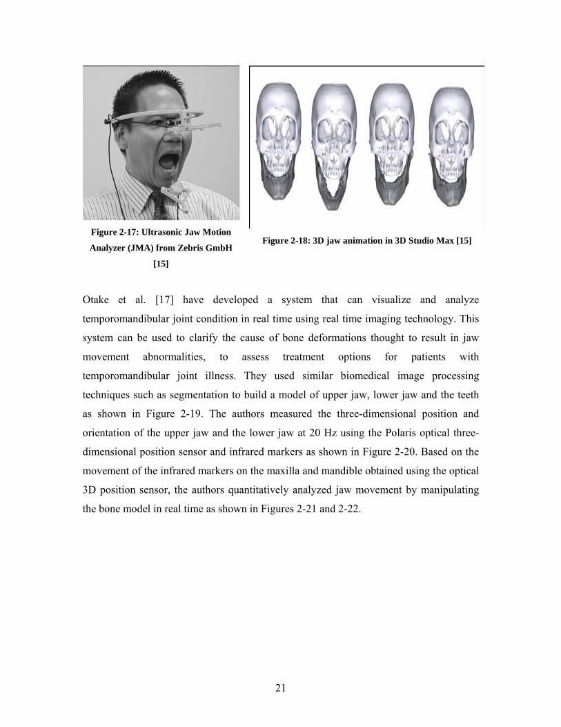
In a research project [15], they introduce automatic patient-specific three-dimensional

jaw modeling from CT data and three-dimensional mastication motion simulation using

jaw tracking data from the JMA system (Zebris) which is an ultrasonic motion capture

device (Figure 2-17) that is comprised of an ultrasound emitter array that is bonded to the

labial surfaces of the mandibular teeth using a jig customized and located on a head

frame secured to the patient’s head. The user can specify the spatial coordinates of the

two condylar points and an infraorbital point to define a plane. Movements of at least

three points relative to this plane during mandibular motions was recorded and exported

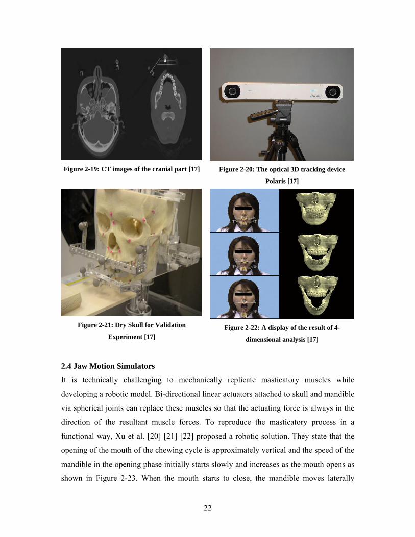
to text files as shown in Figure 2-18.

Figure 2-15: The new facebow attached to a

Human Subject [16]

Figure 2-16: Snapshots of the display system [16]

21

Figure 2-17: Ultrasonic Jaw Motion

Analyzer (JMA) from Zebris GmbH

[15]

Figure 2-18: 3D jaw animation in 3D Studio Max [15]

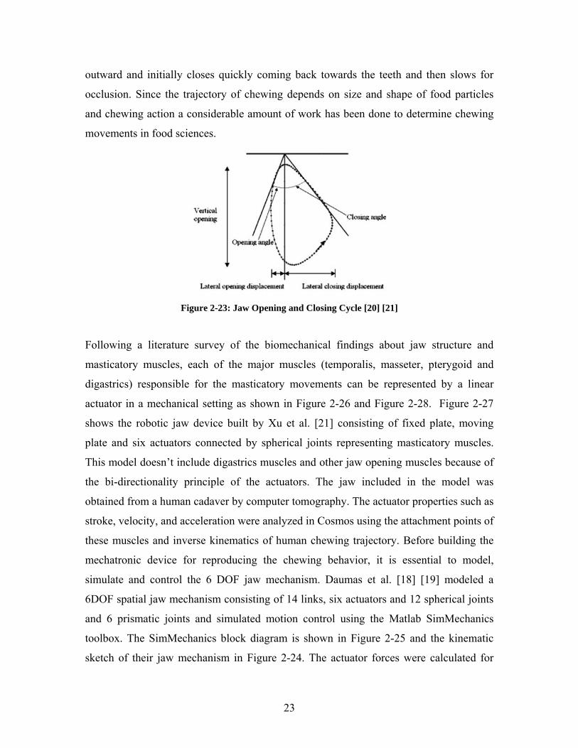
Otake et al. [17] have developed a system that can visualize and analyze

temporomandibular joint condition in real time using real time imaging technology. This

system can be used to clarify the cause of bone deformations thought to result in jaw

movement abnormalities, to assess treatment options for patients with

temporomandibular joint illness. They used similar biomedical image processing

techniques such as segmentation to build a model of upper jaw, lower jaw and the teeth

as shown in Figure 2-19. The authors measured the three-dimensional position and

orientation of the upper jaw and the lower jaw at 20 Hz using the Polaris optical three-

dimensional position sensor and infrared markers as shown in Figure 2-20. Based on the

movement of the infrared markers on the maxilla and mandible obtained using the optical

3D position sensor, the authors quantitatively analyzed jaw movement by manipulating

the bone model in real time as shown in Figures 2-21 and 2-22.

22

Figure 2-19: CT images of the cranial part [17]

Figure 2-20: The optical 3D tracking device

Polaris [17]

Figure 2-21: Dry Skull for Validation

Experiment [17] Figure 2-22: A display of the result of 4-

dimensional analysis [17]

2.4 Jaw Motion Simulators

It is technically challenging to mechanically replicate masticatory muscles while

developing a robotic model. Bi-directional linear actuators attached to skull and mandible

via spherical joints can replace these muscles so that the actuating force is always in the

direction of the resultant muscle forces. To reproduce the masticatory process in a

functional way, Xu et al. [20] [21] [22] proposed a robotic solution. They state that the

opening of the mouth of the chewing cycle is approximately vertical and the speed of the

mandible in the opening phase initially starts slowly and increases as the mouth opens as

shown in Figure 2-23. When the mouth starts to close, the mandible moves laterally

23

outward and initially closes quickly coming back towards the teeth and then slows for

occlusion. Since the trajectory of chewing depends on size and shape of food particles

and chewing action a considerable amount of work has been done to determine chewing

movements in food sciences.

Figure 2-23: Jaw Opening and Closing Cycle [20] [21]

Following a literature survey of the biomechanical findings about jaw structure and

masticatory muscles, each of the major muscles (temporalis, masseter, pterygoid and

digastrics) responsible for the masticatory movements can be represented by a linear

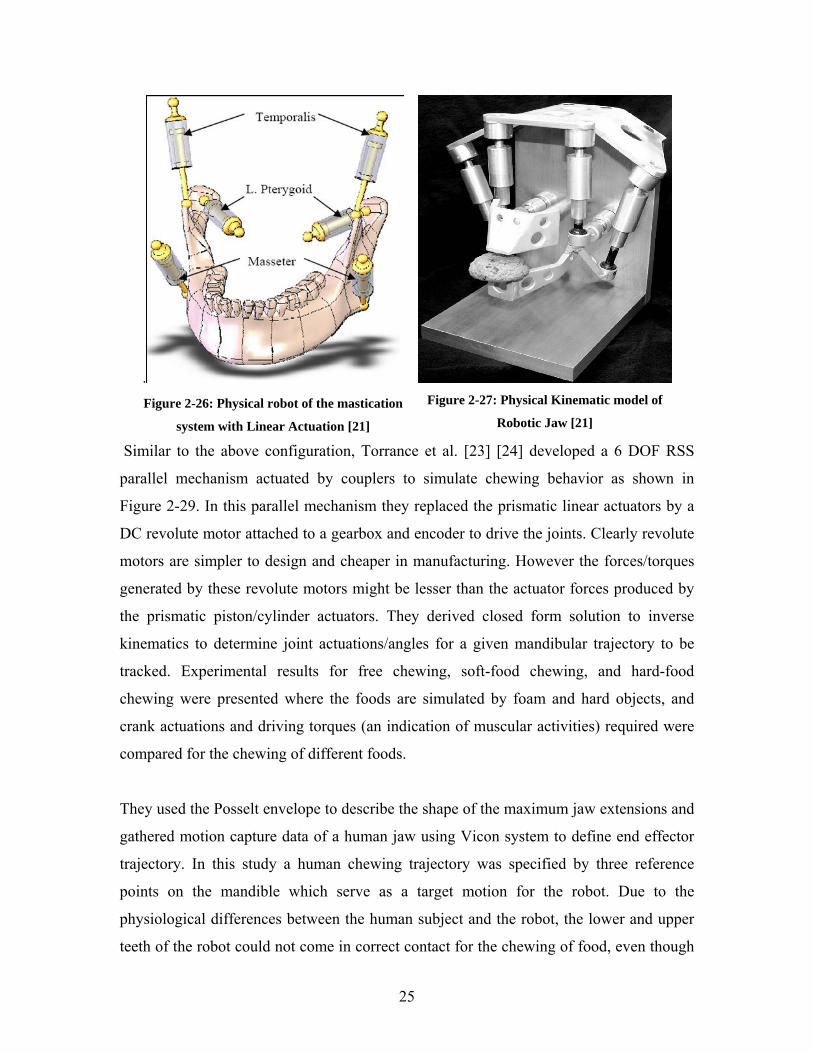
actuator in a mechanical setting as shown in Figure 2-26 and Figure 2-28. Figure 2-27

shows the robotic jaw device built by Xu et al. [21] consisting of fixed plate, moving

plate and six actuators connected by spherical joints representing masticatory muscles.

This model doesn’t include digastrics muscles and other jaw opening muscles because of

the bi-directionality principle of the actuators. The jaw included in the model was

obtained from a human cadaver by computer tomography. The actuator properties such as

stroke, velocity, and acceleration were analyzed in Cosmos using the attachment points of

these muscles and inverse kinematics of human chewing trajectory. Before building the

mechatronic device for reproducing the chewing behavior, it is essential to model,

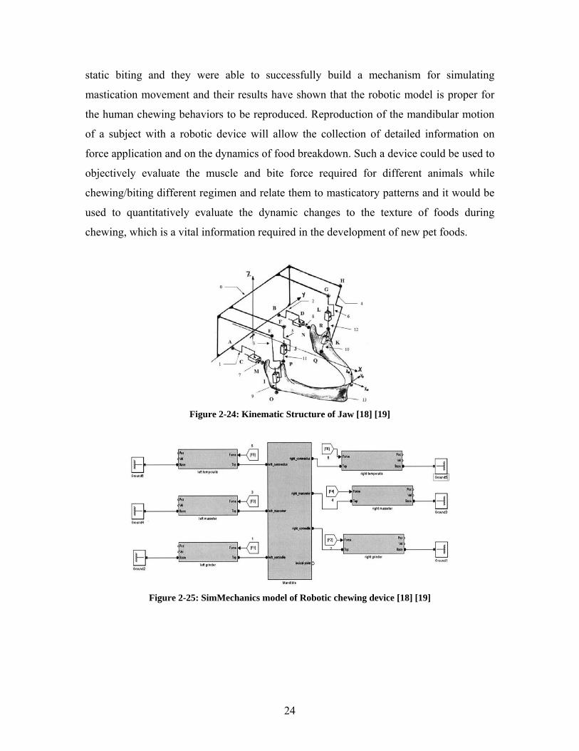
simulate and control the 6 DOF jaw mechanism. Daumas et al. [18] [19] modeled a

6DOF spatial jaw mechanism consisting of 14 links, six actuators and 12 spherical joints

and 6 prismatic joints and simulated motion control using the Matlab SimMechanics

toolbox. The SimMechanics block diagram is shown in Figure 2-25 and the kinematic

sketch of their jaw mechanism in Figure 2-24. The actuator forces were calculated for

24

static biting and they were able to successfully build a mechanism for simulating

mastication movement and their results have shown that the robotic model is proper for

the human chewing behaviors to be reproduced. Reproduction of the mandibular motion

of a subject with a robotic device will allow the collection of detailed information on

force application and on the dynamics of food breakdown. Such a device could be used to

objectively evaluate the muscle and bite force required for different animals while

chewing/biting different regimen and relate them to masticatory patterns and it would be

used to quantitatively evaluate the dynamic changes to the texture of foods during

chewing, which is a vital information required in the development of new pet foods.

Figure 2-24: Kinematic Structure of Jaw [18] [19]

Figure 2-25: SimMechanics model of Robotic chewing device [18] [19]

25

.Figure 2-26: Physical robot of the mastication

system with Linear Actuation [21]

Figure 2-27: Physical Kinematic model of

Robotic Jaw [21]

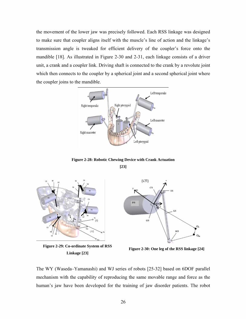
Similar to the above configuration, Torrance et al. [23] [24] developed a 6 DOF RSS

parallel mechanism actuated by couplers to simulate chewing behavior as shown in

Figure 2-29. In this parallel mechanism they replaced the prismatic linear actuators by a

DC revolute motor attached to a gearbox and encoder to drive the joints. Clearly revolute

motors are simpler to design and cheaper in manufacturing. However the forces/torques

generated by these revolute motors might be lesser than the actuator forces produced by

the prismatic piston/cylinder actuators. They derived closed form solution to inverse

kinematics to determine joint actuations/angles for a given mandibular trajectory to be

tracked. Experimental results for free chewing, soft-food chewing, and hard-food

chewing were presented where the foods are simulated by foam and hard objects, and

crank actuations and driving torques (an indication of muscular activities) required were

compared for the chewing of different foods.

They used the Posselt envelope to describe the shape of the maximum jaw extensions and

gathered motion capture data of a human jaw using Vicon system to define end effector

trajectory. In this study a human chewing trajectory was specified by three reference

points on the mandible which serve as a target motion for the robot. Due to the

physiological differences between the human subject and the robot, the lower and upper

teeth of the robot could not come in correct contact for the chewing of food, even though

26

the movement of the lower jaw was precisely followed. Each RSS linkage was designed

to make sure that coupler aligns itself with the muscle’s line of action and the linkage’s

transmission angle is tweaked for efficient delivery of the coupler’s force onto the

mandible [18]. As illustrated in Figure 2-30 and 2-31, each linkage consists of a driver

unit, a crank and a coupler link. Driving shaft is connected to the crank by a revolute joint

which then connects to the coupler by a spherical joint and a second spherical joint where

the coupler joins to the mandible.

Figure 2-28: Robotic Chewing Device with Crank Actuation

[23]

Figure 2-29: Co-ordinate System of RSS

Linkage [23]

Figure 2-30: One leg of the RSS linkage [24]

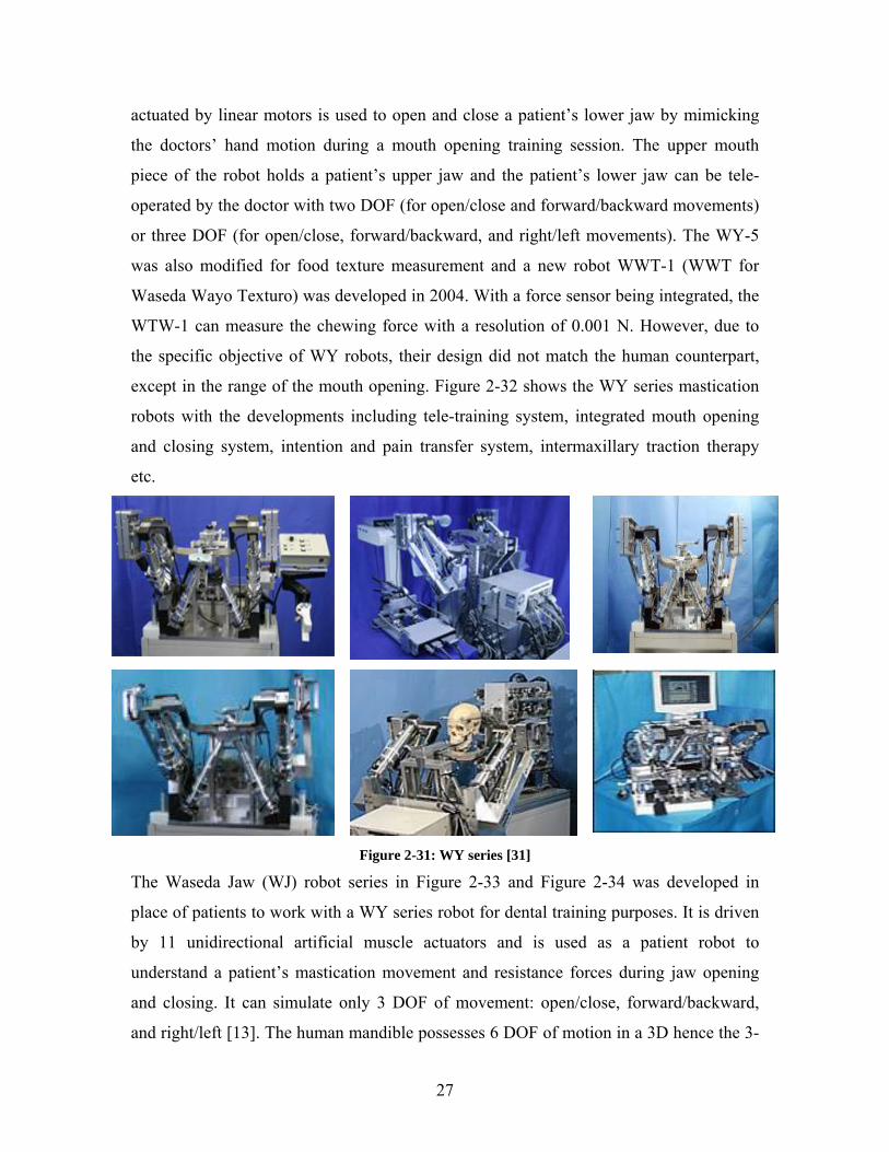
The WY (Waseda–Yamanashi) and WJ series of robots [25-32] based on 6DOF parallel

mechanism with the capability of reproducing the same movable range and force as the

human’s jaw have been developed for the training of jaw disorder patients. The robot

27

actuated by linear motors is used to open and close a patient’s lower jaw by mimicking

the doctors’ hand motion during a mouth opening training session. The upper mouth

piece of the robot holds a patient’s upper jaw and the patient’s lower jaw can be tele-

operated by the doctor with two DOF (for open/close and forward/backward movements)

or three DOF (for open/close, forward/backward, and right/left movements). The WY-5

was also modified for food texture measurement and a new robot WWT-1 (WWT for

Waseda Wayo Texturo) was developed in 2004. With a force sensor being integrated, the

WTW-1 can measure the chewing force with a resolution of 0.001 N. However, due to

the specific objective of WY robots, their design did not match the human counterpart,

except in the range of the mouth opening. Figure 2-32 shows the WY series mastication

robots with the developments including tele-training system, integrated mouth opening

and closing system, intention and pain transfer system, intermaxillary traction therapy

etc.

Figure 2-31: WY series [31]

The Waseda Jaw (WJ) robot series in Figure 2-33 and Figure 2-34 was developed in

place of patients to work with a WY series robot for dental training purposes. It is driven

by 11 unidirectional artificial muscle actuators and is used as a patient robot to

understand a patient’s mastication movement and resistance forces during jaw opening

and closing. It can simulate only 3 DOF of movement: open/close, forward/backward,

and right/left [13]. The human mandible possesses 6 DOF of motion in a 3D hence the 3-

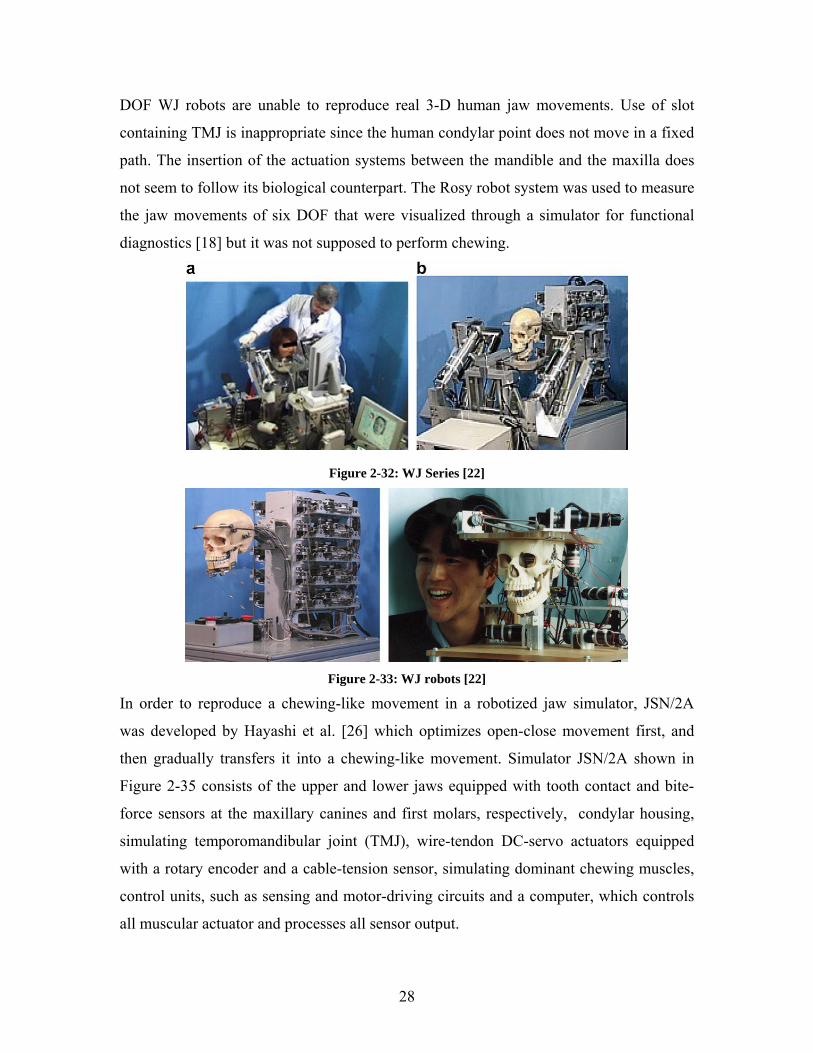
28

DOF WJ robots are unable to reproduce real 3-D human jaw movements. Use of slot

containing TMJ is inappropriate since the human condylar point does not move in a fixed

path. The insertion of the actuation systems between the mandible and the maxilla does

not seem to follow its biological counterpart. The Rosy robot system was used to measure

the jaw movements of six DOF that were visualized through a simulator for functional

diagnostics [18] but it was not supposed to perform chewing.

Figure 2-32: WJ Series [22]

Figure 2-33: WJ robots [22]

In order to reproduce a chewing-like movement in a robotized jaw simulator, JSN/2A

was developed by Hayashi et al. [26] which optimizes open-close movement first, and

then gradually transfers it into a chewing-like movement. Simulator JSN/2A shown in

Figure 2-35 consists of the upper and lower jaws equipped with tooth contact and bite-

force sensors at the maxillary canines and first molars, respectively, condylar housing,

simulating temporomandibular joint (TMJ), wire-tendon DC-servo actuators equipped

with a rotary encoder and a cable-tension sensor, simulating dominant chewing muscles,

control units, such as sensing and motor-driving circuits and a computer, which controls

all muscular actuator and processes all sensor output.

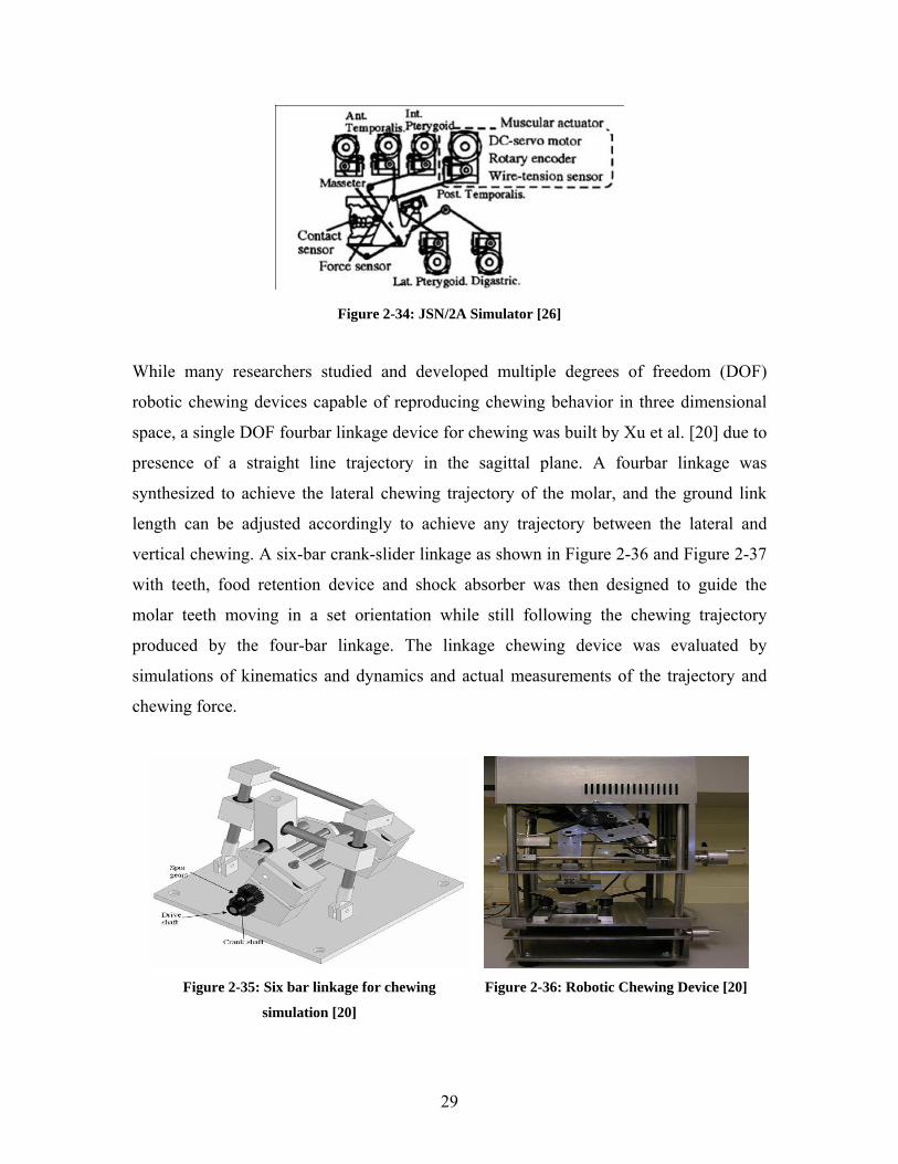
29

Figure 2-34: JSN/2A Simulator [26]

While many researchers studied and developed multiple degrees of freedom (DOF)

robotic chewing devices capable of reproducing chewing behavior in three dimensional

space, a single DOF fourbar linkage device for chewing was built by Xu et al. [20] due to

presence of a straight line trajectory in the sagittal plane. A fourbar linkage was

synthesized to achieve the lateral chewing trajectory of the molar, and the ground link

length can be adjusted accordingly to achieve any trajectory between the lateral and

vertical chewing. A six-bar crank-slider linkage as shown in Figure 2-36 and Figure 2-37

with teeth, food retention device and shock absorber was then designed to guide the

molar teeth moving in a set orientation while still following the chewing trajectory

produced by the four-bar linkage. The linkage chewing device was evaluated by

simulations of kinematics and dynamics and actual measurements of the trajectory and

chewing force.

Figure 2-35: Six bar linkage for chewing

simulation [20]

Figure 2-36: Robotic Chewing Device [20]

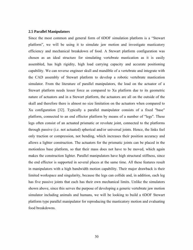
30

2.5 Parallel Manipulators

Since the most common and general form of 6DOF simulation platform is a “Stewart

platform”, we will be using it to simulate jaw motion and investigate masticatory

efficiency and mechanical breakdown of food. A Stewart platform configuration was

chosen as an ideal structure for simulating vertebrate mastication as it is easily

assembled, has high rigidity, high load carrying capacity and accurate positioning

capability. We can reverse engineer skull and mandible of a vertebrate and integrate with

the CAD assembly of Stewart platform to develop a robotic vertebrate mastication

simulator. From the literature of parallel manipulators, the load on the actuator of a

Stewart platform needs lesser force as compared to Xu platform due to its geometric

nature of actuators and in a Stewart platform, the actuators are all on the outside of the

skull and therefore there is almost no size limitation on the actuators when compared to

Xu configuration [32]. Typically a parallel manipulator consists of a fixed "base"

platform, connected to an end effector platform by means of a number of "legs". These

legs often consist of an actuated prismatic or revolute joint, connected to the platforms

through passive (i.e. not actuated) spherical and/or universal joints. Hence, the links feel

only traction or compression, not bending, which increases their position accuracy and

allows a lighter construction. The actuators for the prismatic joints can be placed in the

motionless base platform, so that their mass does not have to be moved, which again

makes the construction lighter. Parallel manipulators have high structural stiffness, since

the end effector is supported in several places at the same time. All these features result

in manipulators with a high bandwidth motion capability. Their major drawback is their

limited workspace and singularity, because the legs can collide and, in addition, each leg

has five passive joints that each has their own mechanical limits. Unlike the simulators

shown above, since this serves the purpose of developing a generic vertebrate jaw motion

simulator including animals and humans, we will be looking to build a 6DOF Stewart

platform type parallel manipulator for reproducing the masticatory motion and evaluating

food breakdowns.

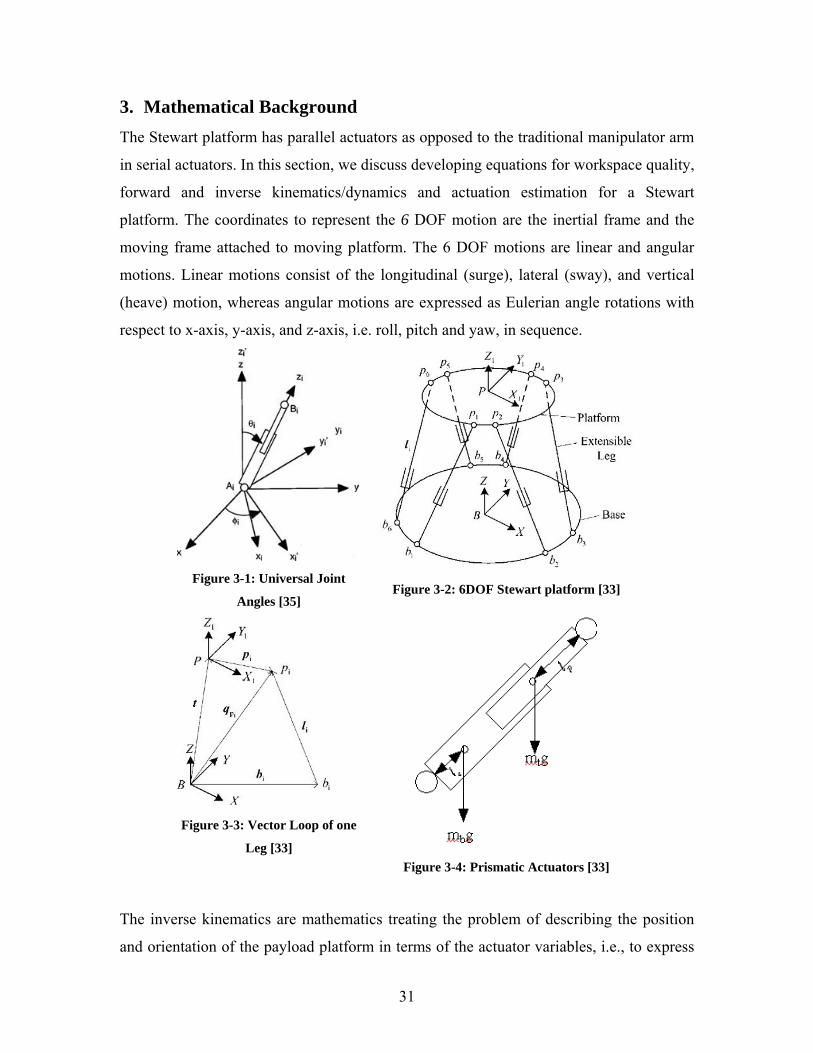
31

3. Mathematical Background The Stewart platform has parallel actuators as opposed to the traditional manipulator arm

in serial actuators. In this section, we discuss developing equations for workspace quality,

forward and inverse kinematics/dynamics and actuation estimation for a Stewart

platform. The coordinates to represent the 6 DOF motion are the inertial frame and the

moving frame attached to moving platform. The 6 DOF motions are linear and angular

motions. Linear motions consist of the longitudinal (surge), lateral (sway), and vertical

(heave) motion, whereas angular motions are expressed as Eulerian angle rotations with

respect to x-axis, y-axis, and z-axis, i.e. roll, pitch and yaw, in sequence.

Figure 3-1: Universal Joint

Angles [35]

Figure 3-2: 6DOF Stewart platform [33]

Figure 3-3: Vector Loop of one

Leg [33] Figure 3-4: Prismatic Actuators [33]

The inverse kinematics are mathematics treating the problem of describing the position

and orientation of the payload platform in terms of the actuator variables, i.e., to express

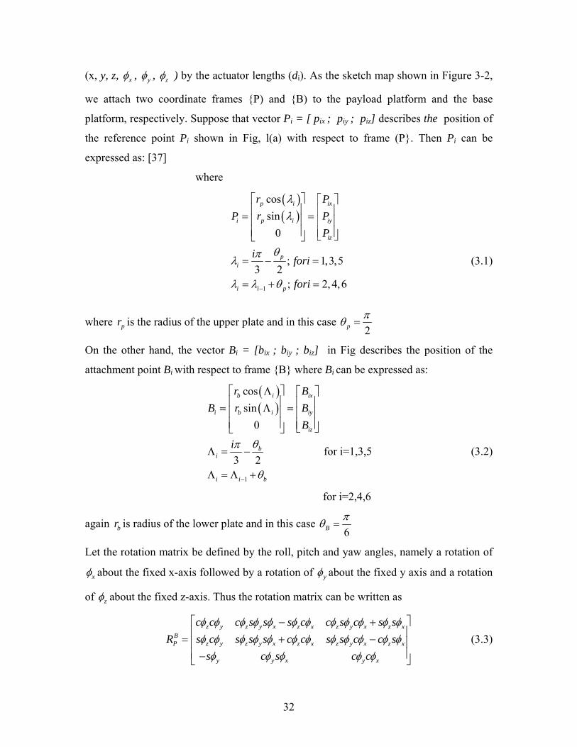
32

(x, y, z, xφ , yφ , zφ ) by the actuator lengths (di). As the sketch map shown in Figure 3-2,

we attach two coordinate frames {P) and {B) to the payload platform and the base

platform, respectively. Suppose that vector Pi = [ pix ; piy ; piz] describes the position of

the reference point Pi shown in Fig, l(a) with respect to frame (P}. Then Pi can be

expressed as: [37]

where

( )( )

1

cossin

0

; 1,3,53 2

; 2, 4,6

p i ix

i p i iy

iz

pi

i i p

r PP r P

P

i fori

fori

λλ

θπλ

λ λ θ−

⎡ ⎤ ⎡ ⎤⎢ ⎥ ⎢ ⎥= =⎢ ⎥ ⎢ ⎥⎢ ⎥ ⎢ ⎥⎣ ⎦⎣ ⎦

= − =

= + =

(3.1)

where pr is the radius of the upper plate and in this case 2pπθ =

On the other hand, the vector Bi = [bix ; biy ; biz] in Fig describes the position of the

attachment point Bi with respect to frame {B} where Bi can be expressed as:

( )( )

1

cossin

0

3 2

b i ix

i b i iy

iz

bi

i i b

r BB r B

B

i θπ

θ−

Λ⎡ ⎤ ⎡ ⎤⎢ ⎥ ⎢ ⎥= Λ =⎢ ⎥ ⎢ ⎥⎢ ⎥ ⎢ ⎥⎣ ⎦⎣ ⎦

Λ = −

Λ = Λ +

for i=1,3,5 (3.2)

for i=2,4,6

again br is radius of the lower plate and in this case 6Bπθ =

Let the rotation matrix be defined by the roll, pitch and yaw angles, namely a rotation of

xφ about the fixed x-axis followed by a rotation of yφ about the fixed y axis and a rotation

of zφ about the fixed z-axis. Thus the rotation matrix can be written as

z y z y x z x z y x z x

BP z y z y x z x z y x z x

y y x y x

c c c s s s c c s c s sR s c s s s c c s s c c s

s c s c c

φ φ φ φ φ φ φ φ φ φ φ φφ φ φ φ φ φ φ φ φ φ φ φφ φ φ φ φ

⎡ ⎤− +⎢ ⎥= + −⎢ ⎥⎢ ⎥−⎣ ⎦

(3.3)

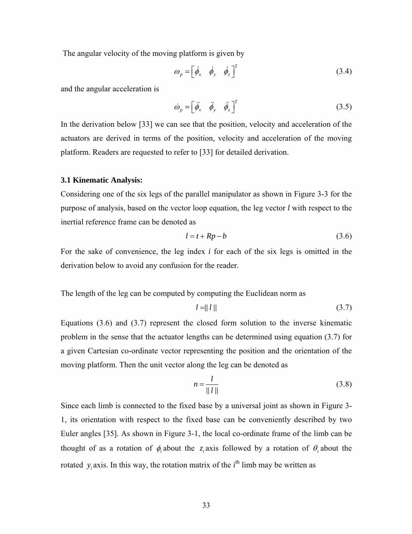
33

The angular velocity of the moving platform is given by

T

p x y zω φ φ φ⎡ ⎤= ⎣ ⎦ (3.4)

and the angular acceleration is

T

p x y zω φ φ φ⎡ ⎤= ⎣ ⎦ (3.5)

In the derivation below [33] we can see that the position, velocity and acceleration of the

actuators are derived in terms of the position, velocity and acceleration of the moving

platform. Readers are requested to refer to [33] for detailed derivation.

3.1 Kinematic Analysis:

Considering one of the six legs of the parallel manipulator as shown in Figure 3-3 for the

purpose of analysis, based on the vector loop equation, the leg vector l with respect to the

inertial reference frame can be denoted as

l t Rp b= + − (3.6)

For the sake of convenience, the leg index i for each of the six legs is omitted in the

derivation below to avoid any confusion for the reader.

The length of the leg can be computed by computing the Euclidean norm as

l l= (3.7)

Equations (3.6) and (3.7) represent the closed form solution to the inverse kinematic

problem in the sense that the actuator lengths can be determined using equation (3.7) for

a given Cartesian co-ordinate vector representing the position and the orientation of the

moving platform. Then the unit vector along the leg can be denoted as

lnl

= (3.8)

Since each limb is connected to the fixed base by a universal joint as shown in Figure 3-

1, its orientation with respect to the fixed base can be conveniently described by two

Euler angles [35]. As shown in Figure 3-1, the local co-ordinate frame of the limb can be

thought of as a rotation of iφ about the iz axis followed by a rotation of iθ about the

rotated iy axis. In this way, the rotation matrix of the ith limb may be written as

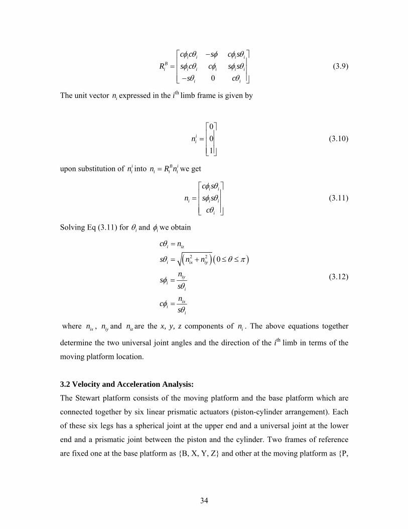
34

0

i i i iBi i i i i i

i i

c c s c sR s c c s s

s c

φ θ φ φ θφ θ φ φ θθ θ

−⎡ ⎤⎢ ⎥= ⎢ ⎥⎢ ⎥−⎣ ⎦

(3.9)

The unit vector in expressed in the ith limb frame is given by

001

iin

⎡ ⎤⎢ ⎥= ⎢ ⎥⎢ ⎥⎣ ⎦

(3.10)

upon substitution of iin into B i

i i in R n= we get

i i

i i i

i

c sn s s

c

φ θφ θθ

⎡ ⎤⎢ ⎥= ⎢ ⎥⎢ ⎥⎣ ⎦

(3.11)

Solving Eq (3.11) for iθ and iφ we obtain

( ) ( )2 2 0

i iz

i ix iy

iyi

i

ixi

i

c n

s n n

ns

sncs

θ

θ θ π

φθ

φθ

=

= + ≤ ≤

=

=

(3.12)

where ixn , iyn and izn are the x, y, z components of in . The above equations together

determine the two universal joint angles and the direction of the ith limb in terms of the

moving platform location.

3.2 Velocity and Acceleration Analysis:

The Stewart platform consists of the moving platform and the base platform which are

connected together by six linear prismatic actuators (piston-cylinder arrangement). Each

of these six legs has a spherical joint at the upper end and a universal joint at the lower

end and a prismatic joint between the piston and the cylinder. Two frames of reference

are fixed one at the base platform as {B, X, Y, Z} and other at the moving platform as {P,

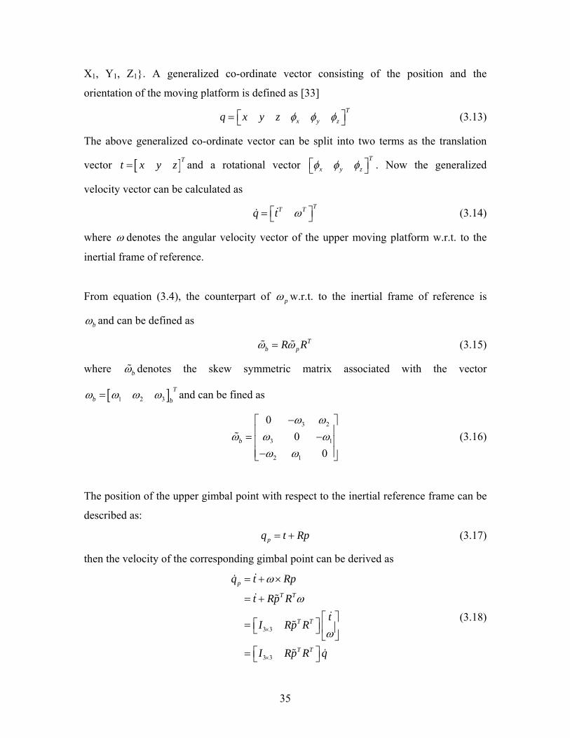
35

X1, Y1, Z1}. A generalized co-ordinate vector consisting of the position and the

orientation of the moving platform is defined as [33]

T

x y zq x y z φ φ φ⎡ ⎤= ⎣ ⎦ (3.13)

The above generalized co-ordinate vector can be split into two terms as the translation

vector [ ]Tt x y z= and a rotational vector T

x y zφ φ φ⎡ ⎤⎣ ⎦ . Now the generalized

velocity vector can be calculated as

TT Tq t ω⎡ ⎤= ⎣ ⎦ (3.14)

where ω denotes the angular velocity vector of the upper moving platform w.r.t. to the

inertial frame of reference.

From equation (3.4), the counterpart of pω w.r.t. to the inertial frame of reference is

bω and can be defined as

Tb pR Rω ω= (3.15)

where bω denotes the skew symmetric matrix associated with the vector

[ ]1 2 3T

b bω ω ω ω= and can be fined as

3 2

3 1

2 1

00

0b

ω ωω ω ω

ω ω

−⎡ ⎤⎢ ⎥= −⎢ ⎥⎢ ⎥−⎣ ⎦

(3.16)

The position of the upper gimbal point with respect to the inertial reference frame can be

described as:

pq t Rp= + (3.17)

then the velocity of the corresponding gimbal point can be derived as

3 3

3 3

p

T T

T T

T T

q t Rp

t Rp Rt

I Rp R

I Rp R q

ω

ω

ω×

×

= + ×

= +

⎡ ⎤⎡ ⎤= ⎢ ⎥⎣ ⎦

⎣ ⎦⎡ ⎤= ⎣ ⎦

(3.18)

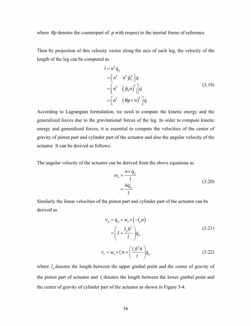
36

where Rp denotes the counterpart of p with respect to the inertial frame of reference.

Then by projection of this velocity vector along the axis of each leg, the velocity of the

length of the leg can be computed as

( )( )

Tp

T T Tb

TTb

TT

l n q

n n p q

n p n q

n Rp n q

=

⎡ ⎤= ⎣ ⎦⎡ ⎤= ⎢ ⎥⎣ ⎦⎡ ⎤= ×⎣ ⎦

(3.19)

According to Lagrangian formulation, we need to compute the kinetic energy and the

generalized forces due to the gravitational forces of the leg. In order to compute kinetic

energy and generalized forces, it is essential to compute the velocities of the center of

gravity of piston part and cylinder part of the actuator and also the angular velocity of the

actuator. It can be derived as follows:

The angular velocity of the actuator can be derived from the above equations as

pa

p

n ql

nql

ω×

=

= (3.20)

Similarly the linear velocities of the piston part and cylinder part of the actuator can be

derived as

( )

2

p p a p

pp

v q w l n

l nI q

l

= + × −

⎛ ⎞= +⎜ ⎟⎜ ⎟⎝ ⎠

(3.21)

T

cc a c p

l n nv w l n ql

⎛ ⎞= × = ⎜ ⎟

⎝ ⎠ (3.22)

where pl denotes the length between the upper gimbal point and the center of gravity of

the piston part of actuator and cl denotes the length between the lower gimbal point and

the center of gravity of cylinder part of the actuator as shown in Figure 3-4.

37

The acceleration of the upper gimbal point can be obtained by differentiating equation

(3.18) as

23 3

T Tpq I Rp R q Rpω×⎡ ⎤= +⎣ ⎦ (3.23)

3.3 Jacobian Analysis

The Jacobian matrix, in the field of robotics, is used to describes the relationship between

joint and end-effector velocities. At the inverse kinematics level the jacobian matrix is

defined as

pl J q= (3.24)

where l is the velocity vector of prismatic joint lengths and q is the end effector velocity

vector. pJ is called as parallel manipulator jacobian matrix. Similarly at statics level, by

the principle of virtual work the Jacobian also relates joint torques to end- effector

wrench as follow:

TpW J F= (3.25)

3.3.1 Jacobian Matrix Based On Vector Loop Closure Equation

In this section Jacobian matrix will be derived based on the vector loop closure

technique.

From the fig and equation (3.6) we can write the vector loop equation as

Bi i P ib l t R p+ = + (3.26)

Differentiating equation (3.26) w.r.t. time gives

38

( ) 1

3 2

3 1

2 1

00

0

00

0

1 0 0 00

Bi P i

B B BP P P i

Bi

Bi

Bix

iy

iz

Bz y ix

z x iy

y x iz

iz iy

l t R p

t R R R p

t p

t p

x py pz p

x py pz p

p p

ω

ω

ω ωω ωω ω

φ φφ φφ φ

−

= +

= +

= + ×

= +

−⎡ ⎤ ⎡ ⎤ ⎡ ⎤⎢ ⎥ ⎢ ⎥ ⎢ ⎥= + − −⎢ ⎥ ⎢ ⎥ ⎢ ⎥⎢ ⎥ ⎢ ⎥ ⎢ ⎥⎣ ⎦ ⎣ ⎦ ⎣ ⎦

⎡ ⎤−⎡ ⎤ ⎡ ⎤⎢ ⎥⎢ ⎥ ⎢ ⎥= + − −⎢ ⎥⎢ ⎥ ⎢ ⎥⎢ ⎥⎢ ⎥ ⎢ ⎥⎣ ⎦ ⎣ ⎦⎣ ⎦

−= 1 0 0

0 0 1 0iz ix

xiy ix

y

z

i l p

xyz

p pp p

l J x

φφφ

⎡ ⎤⎢ ⎥⎢ ⎥⎡ ⎤⎢ ⎥⎢ ⎥− ⎢ ⎥⎢ ⎥⎢ ⎥⎢ ⎥−⎣ ⎦ ⎢ ⎥⎢ ⎥⎢ ⎥⎣ ⎦

=

(3.27)

where lJ is called as the link jacobian matrix. The velocity vector of the joint lengths

should be w.r.t. the limb frame of reference and the Jacobian matrix will change

accordingly as, from equation (3.9) can be written as

( ) 1

1 1 0 0 00 1 0 0

0 0 0 1 0

L Bl l l

i i i i iz iy

i i i i i iz ix

i i iy ix

J R J

c c s c s p ps c c s s p p

s c p p

φ θ φ φ θφ θ φ φ θθ θ

−

−

=

⎡ ⎤− −⎡ ⎤⎢ ⎥⎢ ⎥= −⎢ ⎥⎢ ⎥⎢ ⎥⎢ ⎥− −⎣ ⎦ ⎣ ⎦

(3.28)

Now since the prismatic joint is along the iz axis for each limb, we need to extract the

third row from above matrix multiplication and assembling the matrix for each of the six

actuators gives the parallel manipulator Jacobian Matrix as

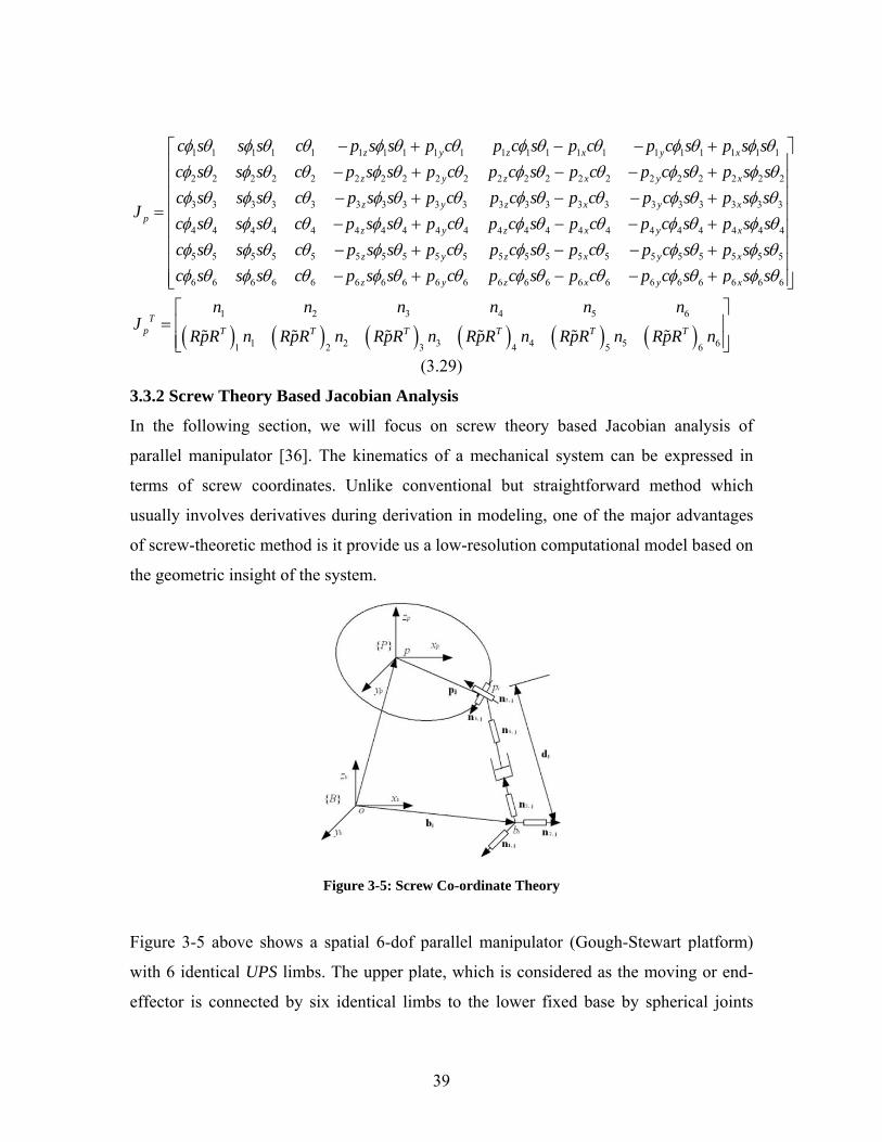
39

1 1 1 1 1 1 1 1 1 1 1 1 1 1 1 1 1 1 1 1 1

2 2 2 2 2 2 2 2 2 2 2 2 2 2 2 2 2 2 2 2 2

3 3 3 3 3 3 3 3 3 3 3 3 3 3 3 3 3 3 3

z y z x y x

z y z x y x

z y z x yp

c s s s c p s s p c p c s p c p c s p s sc s s s c p s s p c p c s p c p c s p s sc s s s c p s s p c p c s p c p c s p

J

φ θ φ θ θ φ θ θ φ θ θ φ θ φ θφ θ φ θ θ φ θ θ φ θ θ φ θ φ θφ θ φ θ θ φ θ θ φ θ θ φ θ

− + − − +− + − − +− + − − +

= 3 3

4 4 4 4 4 4 4 4 4 4 4 4 4 4 4 4 4 4 4 4 4

5 5 5 5 5 5 5 5 5 5 5 5 5 5 5 5 5 5 5 5 5

6 6 6 6 6 6 6 6 6 6 6 6 6 6 6 6 6

x

z y z x y x

z y z x y x

z y z x y

s sc s s s c p s s p c p c s p c p c s p s sc s s s c p s s p c p c s p c p c s p s sc s s s c p s s p c p c s p c p c s

φ θφ θ φ θ θ φ θ θ φ θ θ φ θ φ θφ θ φ θ θ φ θ θ φ θ θ φ θ φ θφ θ φ θ θ φ θ θ φ θ θ φ θ

− + − − +− + − − +− + − −

( ) ( ) ( ) ( ) ( ) ( )

6 6 6 6

1 2 3 4 5 6

1 2 3 4 5 61 2 3 4 5 6

x

Tp T T T T T T

p s s

n n n n n nJ

RpR n RpR n RpR n RpR n RpR n RpR n

φ θ

⎡ ⎤⎢ ⎥⎢ ⎥⎢ ⎥⎢ ⎥⎢ ⎥⎢ ⎥⎢ ⎥

+⎢ ⎥⎣ ⎦⎡ ⎤

= ⎢ ⎥⎢ ⎥⎣ ⎦

(3.29)

3.3.2 Screw Theory Based Jacobian Analysis

In the following section, we will focus on screw theory based Jacobian analysis of

parallel manipulator [36]. The kinematics of a mechanical system can be expressed in

terms of screw coordinates. Unlike conventional but straightforward method which

usually involves derivatives during derivation in modeling, one of the major advantages

of screw-theoretic method is it provide us a low-resolution computational model based on

the geometric insight of the system.

Figure 3-5: Screw Co-ordinate Theory

Figure 3-5 above shows a spatial 6-dof parallel manipulator (Gough-Stewart platform)

with 6 identical UPS limbs. The upper plate, which is considered as the moving or end-

effector is connected by six identical limbs to the lower fixed base by spherical joints

40

jb and jp , j=1, 2, 6. Several close loop kinematic chains are formed by the six limbs.

Let’s define an instantaneous reference frame ( )1 1 1, , ,P X Y Z attached to the moving

platform and an inertial frame of reference ( ), , ,B X Y Z . Then we express all the joint

screws with respect to this instantaneous reference frame. Then, the Jacobian matrix of

the Gough-Stewart platform can be derived by applying the concept of reciprocal screws

[36]. Figure 3-5 shows the equivalent kinematic chain of an UPS limb, we can consider

that the lower universal joint can be replaced by two unit screws 1S and 2S , the prismatic

joint replaced by a unit screw 3S and the upper spherical joint be replaced by three unit

screws 4S , 5S and 6S . Among these six joints, only the prismatic joint is active and the

rest of the joints are passive. Let ,ˆi jn be unit vector along the ith joint axis of the jth limb

in P frame. Then the six unit joint screws can be written as

( ),

,,

,,

,,

,

ˆˆ ; 1, 2

ˆ

0ˆ ; 3ˆ

ˆˆ ; 4,5,6ˆ

i ji j

j j i j

i ji j

i ji j

j i j

nS i

p l n

S in

nS i

p n

⎡ ⎤= =⎢ ⎥

− ×⎢ ⎥⎣ ⎦⎡ ⎤

= =⎢ ⎥⎣ ⎦⎡ ⎤

= =⎢ ⎥×⎣ ⎦

(3.30)

where jl is the vector corresponding to the thj limb and jp is the position of the thj ball

joint location w.r.t. to moving platform reference frame.

Now, we can get end-effector twist with respect to this instantaneous reference frame as:

1,

2,

1, 2, 3, 4, 5, 6,4,

5,

6,

ˆ ˆ ˆ ˆ ˆ ˆ ˆ ; 1, 2,...6

j

j

jt j j j j j j

j

j

j

lVS S S S S S S j

θθ

θωθθ

⎡ ⎤⎢ ⎥⎢ ⎥⎢ ⎥⎡ ⎤ ⎡ ⎤= = =⎢ ⎥⎢ ⎥ ⎣ ⎦ ⎢ ⎥⎣ ⎦⎢ ⎥⎢ ⎥⎢ ⎥⎣ ⎦

(3.31)

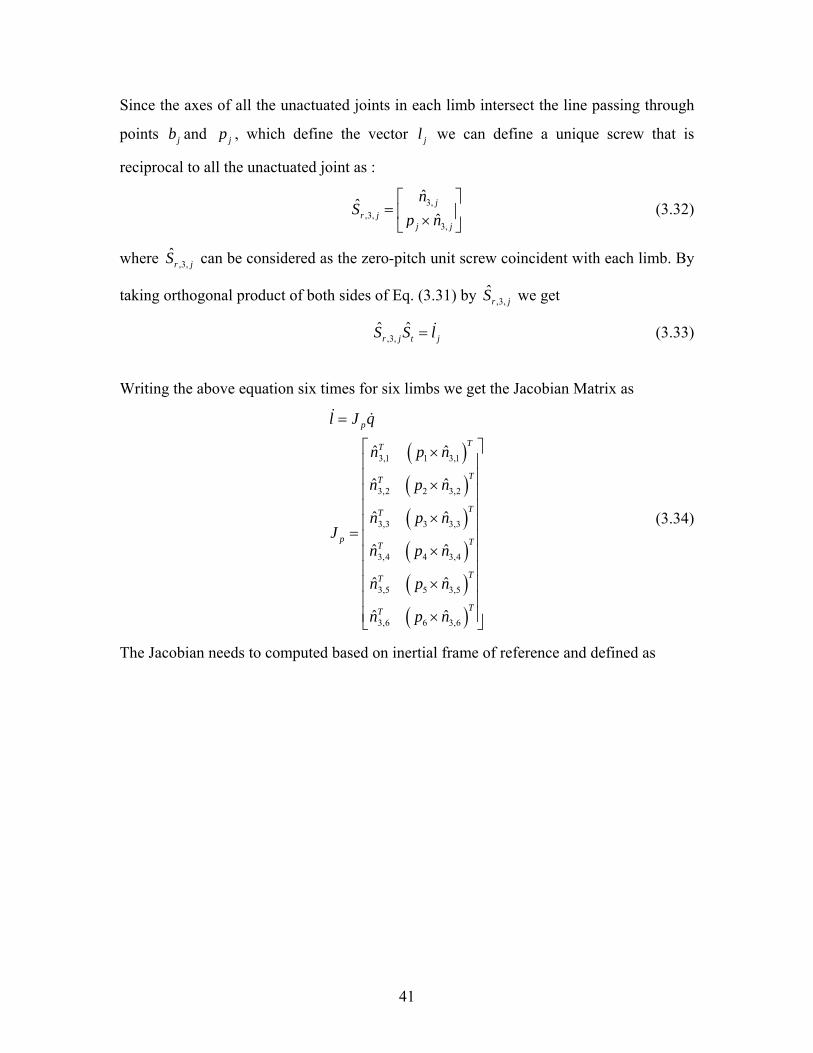
41

Since the axes of all the unactuated joints in each limb intersect the line passing through

points jb and jp , which define the vector jl we can define a unique screw that is

reciprocal to all the unactuated joint as :

3,,3,

3,

ˆˆˆj

r jj j

nS

p n⎡ ⎤

= ⎢ ⎥×⎣ ⎦ (3.32)

where ,3,ˆ

r jS can be considered as the zero-pitch unit screw coincident with each limb. By

taking orthogonal product of both sides of Eq. (3.31) by ,3,ˆ

r jS we get

,3,ˆ ˆ

r j t jS S l= (3.33)

Writing the above equation six times for six limbs we get the Jacobian Matrix as

( )( )( )( )( )( )

3,1 1 3,1

3,2 2 3,2

3,3 3 3,3

3,4 4 3,4

3,5 5 3,5

3,6 6 3,6

ˆ ˆ

ˆ ˆ

ˆ ˆ

ˆ ˆ

ˆ ˆ

ˆ ˆ

p

TT

TT

TT

p TT

TT

TT

l J q

n p n

n p n

n p nJ

n p n

n p n

n p n

=

⎡ ⎤×⎢ ⎥⎢ ⎥×⎢ ⎥⎢ ⎥×⎢ ⎥= ⎢ ⎥

×⎢ ⎥⎢ ⎥

×⎢ ⎥⎢ ⎥⎢ ⎥×⎣ ⎦

(3.34)

The Jacobian needs to computed based on inertial frame of reference and defined as

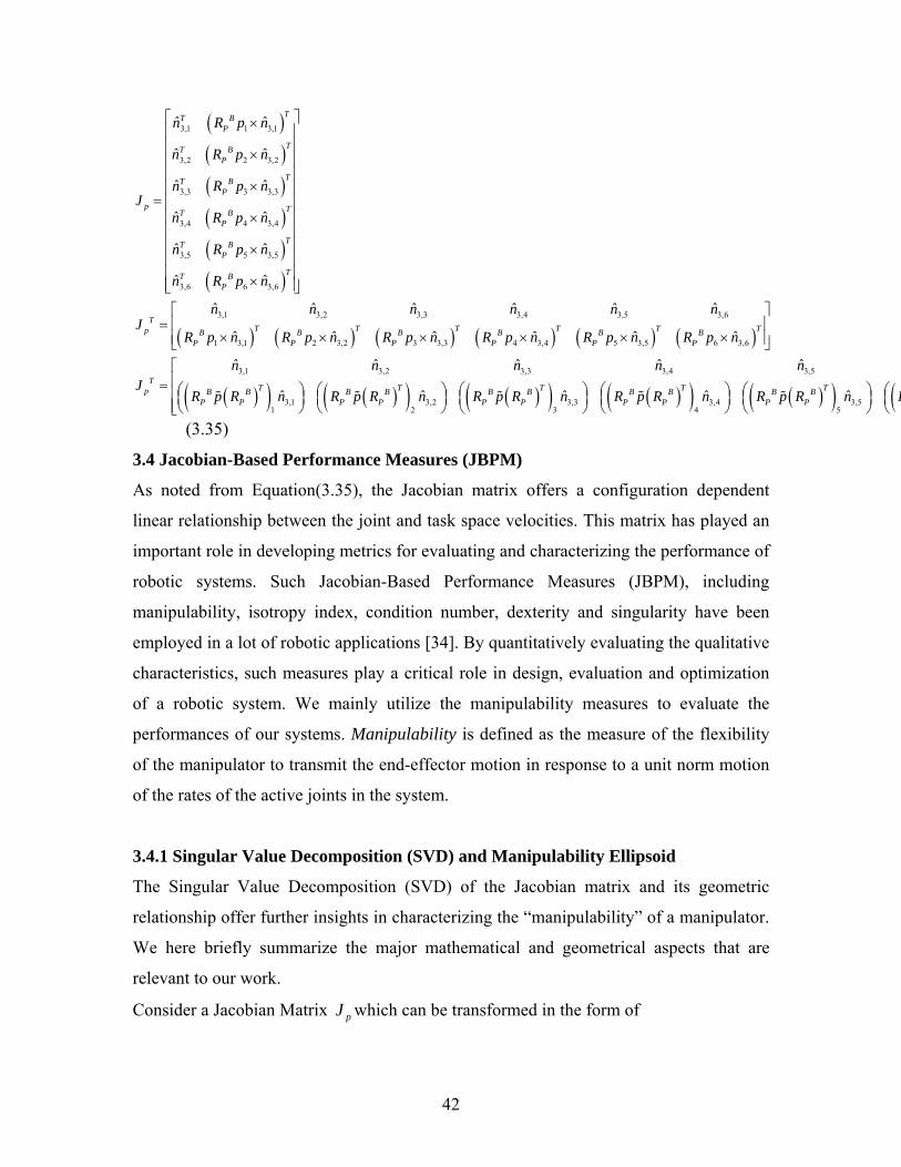
42

( )( )( )( )( )( )

( ) ( )

3,1 1 3,1

3,2 2 3,2

3,3 3 3,3

3,4 4 3,4

3,5 5 3,5

3,6 6 3,6

3,1 3,2 3,3 3,4 3,5 3,6

1 3,1 2 3,2

ˆ ˆ

ˆ ˆ

ˆ ˆ

ˆ ˆ

ˆ ˆ

ˆ ˆ

ˆ ˆ ˆ ˆ ˆ ˆ

ˆ ˆ

TT BP

TT BP

TT BP

p TT BP

TT BP

TT BP

TT Tp B B B

P P P

n R p n

n R p n

n R p nJ

n R p n

n R p n

n R p n

n n n n n nJ

R p n R p n R

⎡ ⎤×⎢ ⎥⎢ ⎥×⎢ ⎥⎢ ⎥

×⎢ ⎥= ⎢ ⎥⎢ ⎥×⎢ ⎥⎢ ⎥×⎢ ⎥⎢ ⎥×⎢ ⎥⎣ ⎦

=× × ( ) ( ) ( ) ( )

( )( ) ( )( ) ( )( ) ( )( ) ( )( )

3 3,3 4 3,4 5 3,5 6 3,6

3,1 3,2 3,3 3,4 3,5

3,1 3,2 3,3 3,4 3,51 2 3 4 5

ˆ ˆ ˆ ˆ

ˆ ˆ ˆ ˆ ˆ

ˆ ˆ ˆ ˆ ˆ

T T T TB B BP P P

TT T T T Tp B B B B B B B B B B

P P P P P P P P P P

p n R p n R p n R p n

n n n n nJ

R p R n R p R n R p R n R p R n R p R n R

⎡ ⎤⎢ ⎥

× × × ×⎢ ⎥⎣ ⎦

= ⎛ ⎞ ⎛ ⎞⎛ ⎞ ⎛ ⎞ ⎛ ⎞⎜ ⎟ ⎜ ⎟ ⎜ ⎟⎜ ⎟ ⎜ ⎟⎝ ⎠ ⎝ ⎠ ⎝ ⎠⎝ ⎠ ⎝ ⎠ (⎡⎢

⎛⎢ ⎜⎢ ⎝⎣ (3.35)

3.4 Jacobian-Based Performance Measures (JBPM)

As noted from Equation(3.35), the Jacobian matrix offers a configuration dependent

linear relationship between the joint and task space velocities. This matrix has played an

important role in developing metrics for evaluating and characterizing the performance of

robotic systems. Such Jacobian-Based Performance Measures (JBPM), including

manipulability, isotropy index, condition number, dexterity and singularity have been

employed in a lot of robotic applications [34]. By quantitatively evaluating the qualitative

characteristics, such measures play a critical role in design, evaluation and optimization

of a robotic system. We mainly utilize the manipulability measures to evaluate the

performances of our systems. Manipulability is defined as the measure of the flexibility

of the manipulator to transmit the end-effector motion in response to a unit norm motion

of the rates of the active joints in the system.

3.4.1 Singular Value Decomposition (SVD) and Manipulability Ellipsoid The Singular Value Decomposition (SVD) of the Jacobian matrix and its geometric

relationship offer further insights in characterizing the “manipulability” of a manipulator.

We here briefly summarize the major mathematical and geometrical aspects that are

relevant to our work.

Consider a Jacobian Matrix pJ which can be transformed in the form of

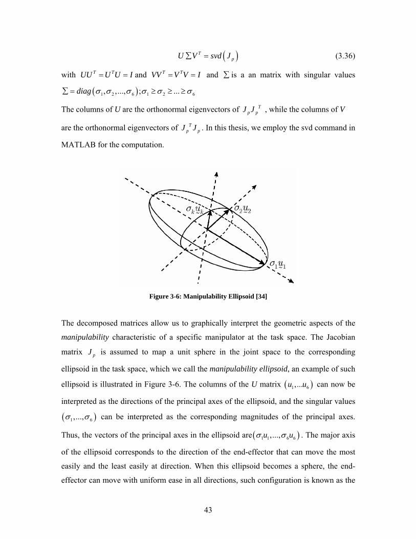
43

( )TpU V svd J∑ = (3.36)

with T TUU U U I= = and T TVV V V I= = and ∑ is a an matrix with singular values

( )1 2 6 1 2 6, ,..., ; ...diag σ σ σ σ σ σ∑ = ≥ ≥ ≥

The columns of U are the orthonormal eigenvectors of Tp pJ J , while the columns of V

are the orthonormal eigenvectors of Tp pJ J . In this thesis, we employ the svd command in

MATLAB for the computation.

Figure 3-6: Manipulability Ellipsoid [34]

The decomposed matrices allow us to graphically interpret the geometric aspects of the

manipulability characteristic of a specific manipulator at the task space. The Jacobian

matrix pJ is assumed to map a unit sphere in the joint space to the corresponding

ellipsoid in the task space, which we call the manipulability ellipsoid, an example of such

ellipsoid is illustrated in Figure 3-6. The columns of the U matrix ( )1 6,...u u can now be

interpreted as the directions of the principal axes of the ellipsoid, and the singular values

( )1 6,...,σ σ can be interpreted as the corresponding magnitudes of the principal axes.

Thus, the vectors of the principal axes in the ellipsoid are ( )1 1 6 6,...,u uσ σ . The major axis

of the ellipsoid corresponds to the direction of the end-effector that can move the most

easily and the least easily at direction. When this ellipsoid becomes a sphere, the end-

effector can move with uniform ease in all directions, such configuration is known as the

44

isotropic configuration. Hence, such SVD and the subsequent geometric interpretation as

the manipulability ellipsoid permit a very useful tool in development of various

performance measures and metrics.

Some of the manipulability measures that are used are Yoshikawa’s measure, condition

number and isotropy index. All these measures are briefly discussed below.

3.4.2 Yoshikawa’s Measure of Manipulability

Yoshikawa’s measure of manipulability is defined as

( )det Ty p pJ JΓ = (3.37)

since U and V are orthonormal

( )det TyΓ = ∑∑ (3.38)

Hence, the measures is nothing more than the product of all the singular values of pJ

However the major criticism to this measure is that it cannot distinguish between a

uniformly spherical ellipsoid which might have the same volume with a long but narrow

ellipsoid.

3.4.3 Condition Number

To evaluate the workspace, the condition number can be utilized to define the

manipulability as

1

6CN

σσ

Γ = (3.39)

where 1σ and 6σ are the minimum and maximum singular values of the Jacobian Matrix.

Geometrically, it is the ratio of the length of the major semiaxis to the length of the minor

semiaxis of the manipulability ellipsoid. Such measure has a lower bound of 1, but it

grows out of bound and tends to infinity when the manipulator is near the singular

configuration.

45

3.4.4 Isotropy Index

Manipulability can also be defined as the reciprocal of the condition number as

6

1Iso

σσ

Γ = (3.40)

Geometrically, it is the ratio of the length of the minor axis to the length of the major axis

of the manipulability ellipsoid. Such a measure is better behaved compared with the

condition number, since the values remain bounded between the values of 0 and 1.

3.5 Dynamic Analysis

For simplicity, firstly the dynamic equations of motion of a 6 DOF Stewart platform is

derived assuming all the six legs to be massless and without inertia and readers can refer

to [37] for detailed description. In general the dynamic equation of motion of the 6 DOF

Stewart platform type parallel manipulator can be written as

( ) ( ) ( ), TpM q q C q q q G q J F+ + = (3.41)

where ( )M q is a 6 6× mass/ inertia matrix; ( ),C q q q is the 6 1× Coriolis/Centripetal

vector; ( )G q and F are the 6 1× vectors containing gravity forces/torques and actuator

(input) forces/torques respectively; eF is the 6 1× external force/torque vector.

The Mass matrix is defined as:

44 45 46

54 55

64 66

0 0 0 0 00 0 0 0 00 0 0 0 00 0 00 0 0 00 0 0 0

mm

mM

m m mm mm m

⎡ ⎤⎢ ⎥⎢ ⎥⎢ ⎥

= ⎢ ⎥⎢ ⎥⎢ ⎥⎢ ⎥⎢ ⎥⎣ ⎦

(3.42)

where

46

( )

2 2 2 2 244

45 54

46 64

2 255

66

x y z y y z z y

x y y z z

z y

x z y z

z

m I c c I c s I s

m m I I c c s

m m I s

m I s I c

m I

φ φ φ φ φ

φ φ φ

φ

φ φ

= + +

= = −

= =

= +

=

(3.43)

and Coriolis/Centripetal matrix can be written as

0 00 x

CC

⎡ ⎤= ⎢ ⎥⎣ ⎦

(3.44)

where

1 2 1 3 4 2 4

1 4 5 4 5

2 4 4 5 0

y z x y z x y

x x x z x y

x y x y

a a a a a a aC a a a a a

a a a a

φ φ φ φ φ φ φφ φ φ φ φφ φ φ φ

⎡ ⎤− − − − + − +⎢ ⎥= + +⎢ ⎥⎢ ⎥− − −⎣ ⎦

(3.45)

where

( )( )( )

( )( )( )( )

2 21

22

3

4

5

12

y y z x z y z

y z z x y

z z z x y

y z z z z x y

z z x y

a c s c I s I I

a c c s I I

a c s s I I

a c c s c s I I

a c s I I

φ φ φ φ

φ φ φ

φ φ φ

φ φ φ φ φ

φ φ

= + −

= −

= −

= − + −

= −

(3.46)

and the Jacobian Matrix can be defined as

( ) ( ) ( ) ( ) ( ) ( )1 2 3 4 5 6

1 2 3 4 5 61 2 3 4 5 6

TT T T T T T

n n n n n nJ

RpR n RpR n RpR n RpR n RpR n RpR n⎡ ⎤

= ⎢ ⎥⎢ ⎥⎣ ⎦

(3.47)

In the next section dynamic equations of the Stewart platform type parallel manipulator

are derived considering the mass and inertia of all the six actuators [33]. The whole

model is split into two parts, the upper moving platform and the six prismatic actuators

with the base platform. The position and velocity of the upper gimbal point at the top of

47

piston part of the actuator has been chosen as the generalized co-ordinates and velocities

and constraint forces at the upper spherical joint has been derived using Lagrangian

formulation.

Considering pq and pq as the corresponding generalized co-ordinates and speeds

respectively, the Lagrangian equations of the six actuators can be written as

p p

d T T Qdt q q⎛ ⎞ ⎛ ⎞∂ ∂

− =⎜ ⎟ ⎜ ⎟⎜ ⎟ ⎜ ⎟∂ ∂⎝ ⎠ ⎝ ⎠ (3.48)

where Q are the generalized forces projected along the variation of the generalized co-

ordinates pq . In the above equation kinetic energy ( ),p pT q q is given by

( )

( )1 2

1 12 212

T Tp t p a t b a

Tp p

T v m v I I

q M M q

ω ω= + +

= + (3.49)

where ( )

2 2

1

2 2

T

p pt

Tt c

l n l nM I m I

l l

n n I IM

l

⎛ ⎞ ⎛ ⎞= + +⎜ ⎟ ⎜ ⎟⎜ ⎟ ⎜ ⎟⎝ ⎠ ⎝ ⎠

+=

Solving the above equations, dynamic equations of motion of all the six actuators can be

written as

( ) ( ) ( )21 2 1 2 t c

T T T Ta a m g m gf M M I Rp R q C I Rp R q M M Rp Q Qω⎡ ⎤ ⎡ ⎤= + + + + − +⎣ ⎦ ⎣ ⎦ (3.50)

where

( ) ( ) ( ) ( )2

2 3 3

2

2

t

b

t bT T T T T T T T T T T Tt t t ta p p p p p p

T

tm g t

Tb

m g b

I Im l m lC nq n n n q n n n nq n n q n n n nq n n nq nl l l

l nQ I m gl

l n nQ m gl

+= + + − + −

⎛ ⎞= +⎜ ⎟⎝ ⎠⎛ ⎞

= ⎜ ⎟⎝ ⎠

Now the dynamic equations of motion of the upper moving platform have been derived

48

using the Newton-Euler approach. By applying the equilibrium of forces principle for the

upper moving platform, Newton-Euler equations can be written as

( )6

1p c p

i i

m q f m g=

= − +∑ (3.51)

where cq t Rc= + denotes the position vector of the control point c w.r.t. inertial frame of

reference and 2T Tcq I Rc R q Rcω⎡ ⎤= +⎣ ⎦ denotes the acceleration of the control point.

Dynamic equations of motion of the upper platform is written as

2p pT T T Tp p p p

p p

m I m gM q C q Rc H F

m Rc R m Rc R gω

⎡ ⎤ ⎡ ⎤+ + = − +⎢ ⎥ ⎢ ⎥

⎣ ⎦ ⎣ ⎦ (3.52)

where

( ) ( ) ( ) ( ) ( ) ( )[ ]

1 2 3 4 5 6

1 2 3 4 5 6

0 00

T Tp p

p T T T Tp p p

Tpp

p T T T T T T

Tp

m I m Rc RM

m RcR m Rcc R RI R

CRI R

I I I I I IH

RpR RpR RpR RpR RpR RpR

F f f f f f f

ω

⎡ ⎤= ⎢ ⎥+⎢ ⎥⎣ ⎦⎡ ⎤

= ⎢ ⎥⎣ ⎦⎡ ⎤

= ⎢ ⎥⎢ ⎥⎣ ⎦

=

Now by combining the equations (3.51) and (3.52) we can define the dynamic equations

of motion for the whole 6DOF Stewart platform type parallel manipulator as

( ) ( ) ( ), TM q q C q q q G q J F+ + = (3.53)

where

( ) ( )

( ) ( ) ( ) ( )

( ) ( )

6

1 21

6 62 2

1 21 1

6

1

,

t b

T Tp T i i

i i

pT TT Tp aT T Ti i ii

i ipi i

pT m g m gT i

ip i

IM q M M M I Rp R

RpR

m II IC q q q C q C I Rp R q Rc M M Rp

m Rc RRpR Rp R

m g IG q Q Q

m RcR g RpR

ω ω

=

= =

=

⎡ ⎤ ⎡ ⎤= + +⎢ ⎥ ⎣ ⎦⎣ ⎦

⎡ ⎤⎡ ⎤ ⎡ ⎤⎡ ⎤= + + + +⎢ ⎥⎢ ⎥ ⎢ ⎥⎣ ⎦

⎣ ⎦ ⎣ ⎦⎣ ⎦⎡ ⎤ ⎡ ⎤

= − − +⎢ ⎥ ⎢ ⎥⎣ ⎦⎣ ⎦

∑

∑ ∑

∑

3.6 Feedback Linearization

In this section we formulate the feedback linearization problem to perform motion control

of the Stewart platform manipulator [36]. Given the end effector trajectory, this will

49

allow us to modulate the actuator forces so that the end effector will converge to the

desired trajectory and the error in the solution converges to zero. The basic idea of

feedback linearization is to construct a control law to cancel all nonlinearities of a

nonlinear dynamical system via full-state nonlinear feedback, allowing traditional linear

control techniques such as PD control to be easily implemented on the nonlinear system.

Due to its very good performance characteristics proven in literature, it is popular and

widely used control method in field of robotics. In this section, we briefly summarize the

application of such feedback linearization to our Stewart platform type parallel robot

system. From Equation. (3.53), we can see our system shares the same general form of

equation of motion as simple mechanical system, thus, we can derive the feedback

linearization control law in same way.

To meet the trajectory tracking requirement in our work, we consider a PD controller

based feedback linearization technique. Let dq , dq and dq represent the desired trajectory

position, velocity and acceleration information. We define error between actual and

desired trajectory as

( ) ( )de q t q t= − (3.54)

Let d p dq q K e K e= + + and substitute in equation(3.53), we get the control input as

( ) ( )( ) ( ) ( )1,T

p dF J M q q K e K e C q q q G q− ⎡ ⎤= + + + +⎣ ⎦ (3.55)

Then, by substituting Equation (3.55)into Equation (3.53) we have the error dynamics of

the system as follows

( )( ) 0p dM q e K e K e+ + = (3.56)

Since ( )M q is inertia matrix of the system we have ( ) 0M q ≠ . We have the linear

differential equation that governs the error between the actual and desired trajectories, as

follows

0p de K e K e+ + = (3.57)

By choosing pK and dK as positive definite, symmetric matrices, we can easily ensure

that the controlled system is stable and e becomes exponentially 0 when t is infinity.

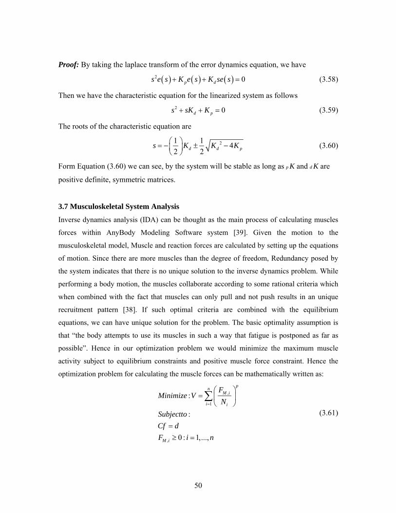
50

Proof: By taking the laplace transform of the error dynamics equation, we have

( ) ( ) ( )2 0p ds e s K e s K se s+ + = (3.58)

Then we have the characteristic equation for the linearized system as follows

2 0d ps sK K+ + = (3.59)

The roots of the characteristic equation are

21 1 42 2d d ps K K K⎛ ⎞= − ± −⎜ ⎟

⎝ ⎠ (3.60)

Form Equation (3.60) we can see, by the system will be stable as long as p K and d K are

positive definite, symmetric matrices.

3.7 Musculoskeletal System Analysis

Inverse dynamics analysis (IDA) can be thought as the main process of calculating muscles

forces within AnyBody Modeling Software system [39]. Given the motion to the

musculoskeletal model, Muscle and reaction forces are calculated by setting up the equations

of motion. Since there are more muscles than the degree of freedom, Redundancy posed by

the system indicates that there is no unique solution to the inverse dynamics problem. While

performing a body motion, the muscles collaborate according to some rational criteria which

when combined with the fact that muscles can only pull and not push results in an unique

recruitment pattern [38]. If such optimal criteria are combined with the equilibrium

equations, we can have unique solution for the problem. The basic optimality assumption is

that “the body attempts to use its muscles in such a way that fatigue is postponed as far as

possible”. Hence in our optimization problem we would minimize the maximum muscle

activity subject to equilibrium constraints and positive muscle force constraint. Hence the

optimization problem for calculating the muscle forces can be mathematically written as:

,

1

,

:

:

0 : 1,...,

pnM i

i i

M i

FMinimize V

NSubjecttoCf dF i n

=

⎛ ⎞= ⎜ ⎟

⎝ ⎠

=≥ =

∑ (3.61)

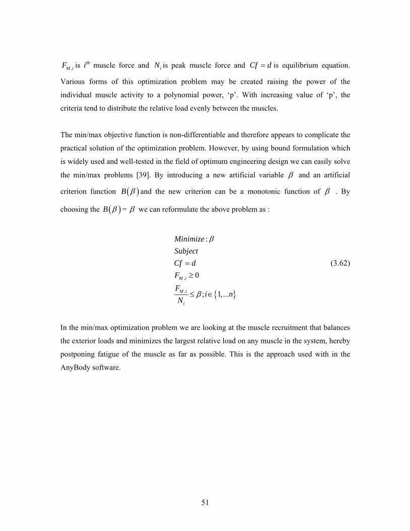
51

,M iF is ith muscle force and iN is peak muscle force and Cf d= is equilibrium equation.

Various forms of this optimization problem may be created raising the power of the

individual muscle activity to a polynomial power, ‘p’. With increasing value of ‘p’, the

criteria tend to distribute the relative load evenly between the muscles.

The min/max objective function is non-differentiable and therefore appears to complicate the

practical solution of the optimization problem. However, by using bound formulation which

is widely used and well-tested in the field of optimum engineering design we can easily solve

the min/max problems [39]. By introducing a new artificial variable β and an artificial

criterion function ( )B β and the new criterion can be a monotonic function of β . By

choosing the ( )B β = β we can reformulate the above problem as :

{ }

,

,

:

0

; 1,...

M i

M i

i

MinimizeSubjectCf dFF

i nN

β

β

=≥

≤ ∈

(3.62)

In the min/max optimization problem we are looking at the muscle recruitment that balances

the exterior loads and minimizes the largest relative load on any muscle in the system, hereby

postponing fatigue of the muscle as far as possible. This is the approach used with in the

AnyBody software.

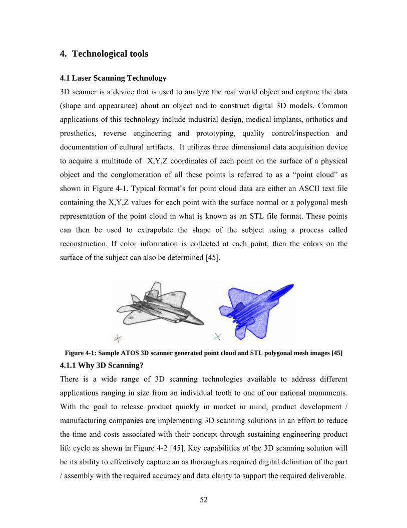
52

4. Technological tools 4.1 Laser Scanning Technology

3D scanner is a device that is used to analyze the real world object and capture the data

(shape and appearance) about an object and to construct digital 3D models. Common

applications of this technology include industrial design, medical implants, orthotics and

prosthetics, reverse engineering and prototyping, quality control/inspection and

documentation of cultural artifacts. It utilizes three dimensional data acquisition device

to acquire a multitude of X,Y,Z coordinates of each point on the surface of a physical

object and the conglomeration of all these points is referred to as a “point cloud” as

shown in Figure 4-1. Typical format’s for point cloud data are either an ASCII text file

containing the X,Y,Z values for each point with the surface normal or a polygonal mesh

representation of the point cloud in what is known as an STL file format. These points

can then be used to extrapolate the shape of the subject using a process called

reconstruction. If color information is collected at each point, then the colors on the

surface of the subject can also be determined [45].

Figure 4-1: Sample ATOS 3D scanner generated point cloud and STL polygonal mesh images [45]

4.1.1 Why 3D Scanning?

There is a wide range of 3D scanning technologies available to address different

applications ranging in size from an individual tooth to one of our national monuments.

With the goal to release product quickly in market in mind, product development /

manufacturing companies are implementing 3D scanning solutions in an effort to reduce

the time and costs associated with their concept through sustaining engineering product

life cycle as shown in Figure 4-2 [45]. Key capabilities of the 3D scanning solution will

be its ability to effectively capture an as thorough as required digital definition of the part

/ assembly with the required accuracy and data clarity to support the required deliverable.

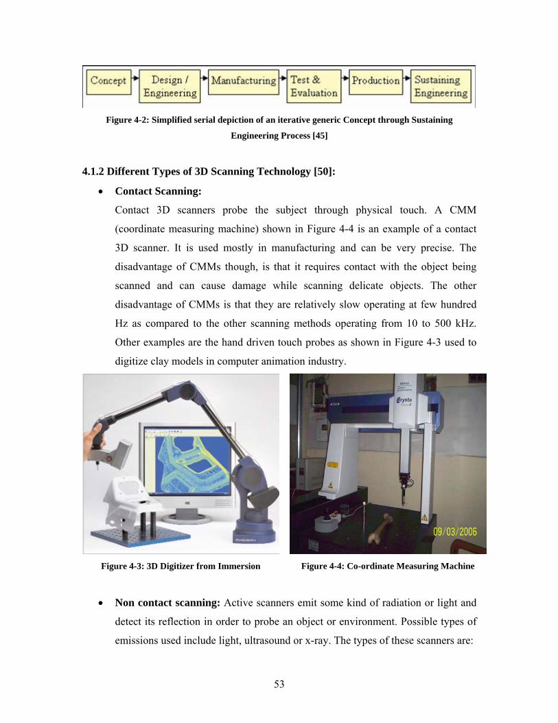
53

Figure 4-2: Simplified serial depiction of an iterative generic Concept through Sustaining

Engineering Process [45]

4.1.2 Different Types of 3D Scanning Technology [50]:

• Contact Scanning:

Contact 3D scanners probe the subject through physical touch. A CMM

(coordinate measuring machine) shown in Figure 4-4 is an example of a contact

3D scanner. It is used mostly in manufacturing and can be very precise. The

disadvantage of CMMs though, is that it requires contact with the object being

scanned and can cause damage while scanning delicate objects. The other

disadvantage of CMMs is that they are relatively slow operating at few hundred

Hz as compared to the other scanning methods operating from 10 to 500 kHz.

Other examples are the hand driven touch probes as shown in Figure 4-3 used to

digitize clay models in computer animation industry.

Figure 4-3: 3D Digitizer from Immersion Figure 4-4: Co-ordinate Measuring Machine

• Non contact scanning: Active scanners emit some kind of radiation or light and

detect its reflection in order to probe an object or environment. Possible types of

emissions used include light, ultrasound or x-ray. The types of these scanners are:

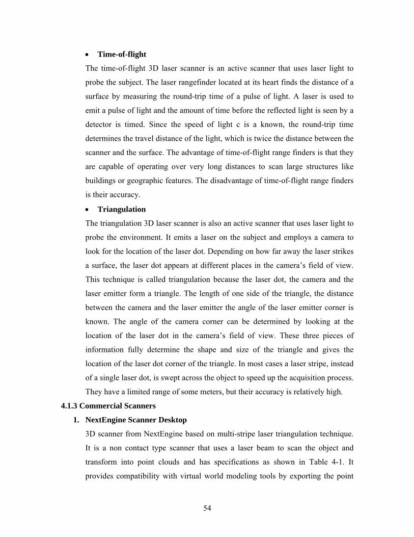
54

• Time-of-flight

The time-of-flight 3D laser scanner is an active scanner that uses laser light to

probe the subject. The laser rangefinder located at its heart finds the distance of a

surface by measuring the round-trip time of a pulse of light. A laser is used to

emit a pulse of light and the amount of time before the reflected light is seen by a

detector is timed. Since the speed of light c is a known, the round-trip time

determines the travel distance of the light, which is twice the distance between the

scanner and the surface. The advantage of time-of-flight range finders is that they

are capable of operating over very long distances to scan large structures like

buildings or geographic features. The disadvantage of time-of-flight range finders

is their accuracy.

• Triangulation

The triangulation 3D laser scanner is also an active scanner that uses laser light to

probe the environment. It emits a laser on the subject and employs a camera to

look for the location of the laser dot. Depending on how far away the laser strikes

a surface, the laser dot appears at different places in the camera’s field of view.

This technique is called triangulation because the laser dot, the camera and the

laser emitter form a triangle. The length of one side of the triangle, the distance

between the camera and the laser emitter the angle of the laser emitter corner is

known. The angle of the camera corner can be determined by looking at the

location of the laser dot in the camera’s field of view. These three pieces of

information fully determine the shape and size of the triangle and gives the

location of the laser dot corner of the triangle. In most cases a laser stripe, instead

of a single laser dot, is swept across the object to speed up the acquisition process.

They have a limited range of some meters, but their accuracy is relatively high.

4.1.3 Commercial Scanners

1. NextEngine Scanner Desktop

3D scanner from NextEngine based on multi-stripe laser triangulation technique.

It is a non contact type scanner that uses a laser beam to scan the object and

transform into point clouds and has specifications as shown in Table 4-1. It

provides compatibility with virtual world modeling tools by exporting the point

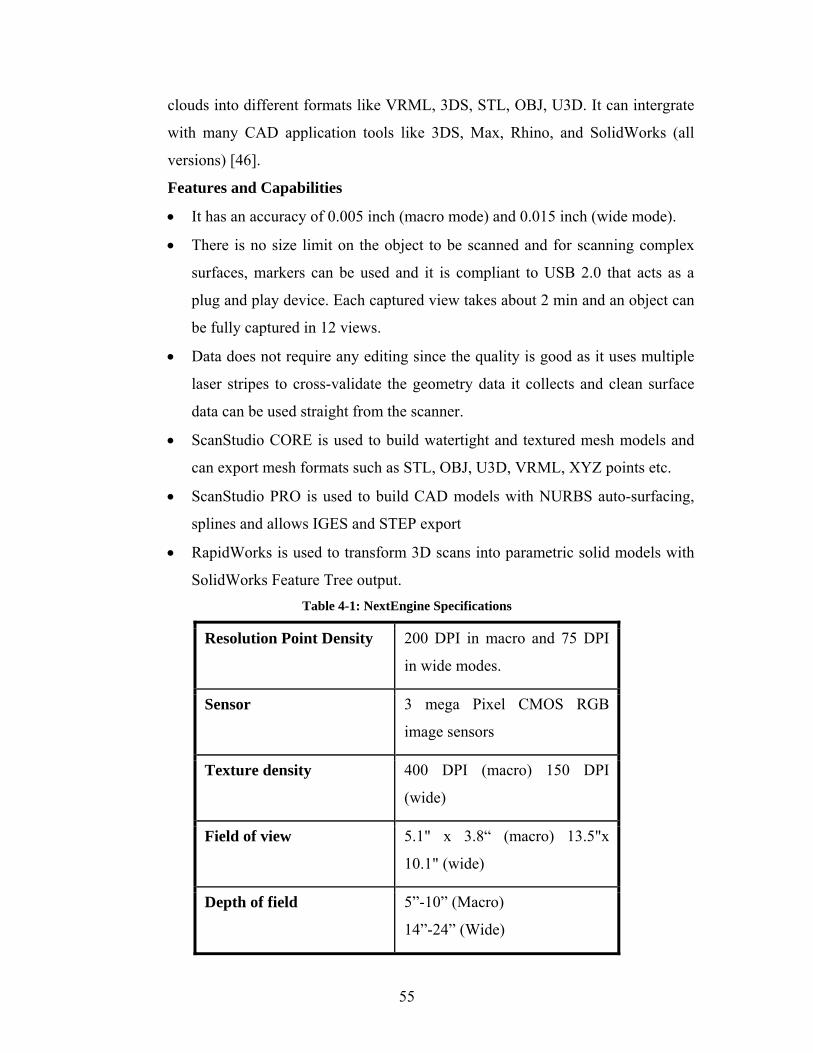
55

clouds into different formats like VRML, 3DS, STL, OBJ, U3D. It can intergrate

with many CAD application tools like 3DS, Max, Rhino, and SolidWorks (all

versions) [46].

Features and Capabilities

• It has an accuracy of 0.005 inch (macro mode) and 0.015 inch (wide mode).

• There is no size limit on the object to be scanned and for scanning complex

surfaces, markers can be used and it is compliant to USB 2.0 that acts as a

plug and play device. Each captured view takes about 2 min and an object can

be fully captured in 12 views.

• Data does not require any editing since the quality is good as it uses multiple

laser stripes to cross-validate the geometry data it collects and clean surface

data can be used straight from the scanner.

• ScanStudio CORE is used to build watertight and textured mesh models and

can export mesh formats such as STL, OBJ, U3D, VRML, XYZ points etc.

• ScanStudio PRO is used to build CAD models with NURBS auto-surfacing,

splines and allows IGES and STEP export

• RapidWorks is used to transform 3D scans into parametric solid models with

SolidWorks Feature Tree output. Table 4-1: NextEngine Specifications

Resolution Point Density 200 DPI in macro and 75 DPI

in wide modes.

Sensor 3 mega Pixel CMOS RGB

image sensors

Texture density 400 DPI (macro) 150 DPI

(wide)

Field of view 5.1" x 3.8“ (macro) 13.5"x

10.1" (wide)

Depth of field 5”-10” (Macro)

14”-24” (Wide)

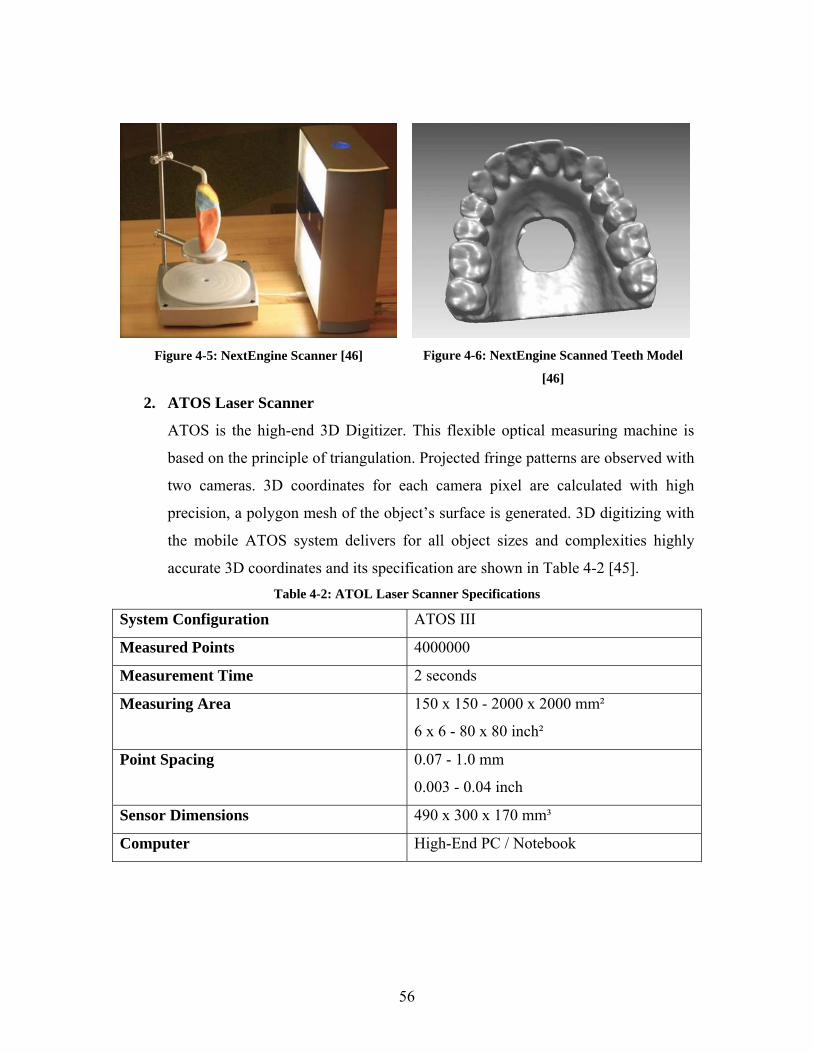
56

Figure 4-5: NextEngine Scanner [46]

Figure 4-6: NextEngine Scanned Teeth Model

[46]

2. ATOS Laser Scanner

ATOS is the high-end 3D Digitizer. This flexible optical measuring machine is

based on the principle of triangulation. Projected fringe patterns are observed with

two cameras. 3D coordinates for each camera pixel are calculated with high

precision, a polygon mesh of the object’s surface is generated. 3D digitizing with

the mobile ATOS system delivers for all object sizes and complexities highly

accurate 3D coordinates and its specification are shown in Table 4-2 [45]. Table 4-2: ATOL Laser Scanner Specifications

System Configuration ATOS III

Measured Points 4000000

Measurement Time 2 seconds

Measuring Area 150 x 150 - 2000 x 2000 mm²

6 x 6 - 80 x 80 inch²

Point Spacing 0.07 - 1.0 mm

0.003 - 0.04 inch

Sensor Dimensions 490 x 300 x 170 mm³

Computer High-End PC / Notebook

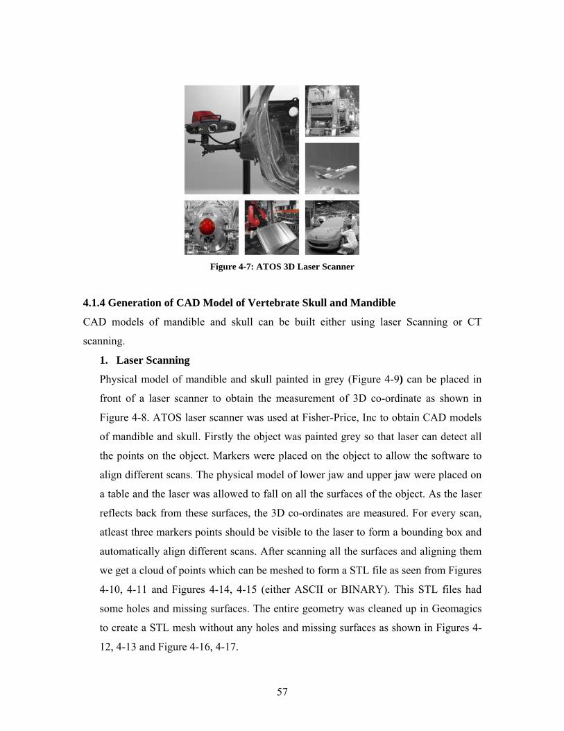
57

Figure 4-7: ATOS 3D Laser Scanner

4.1.4 Generation of CAD Model of Vertebrate Skull and Mandible

CAD models of mandible and skull can be built either using laser Scanning or CT

scanning.

1. Laser Scanning

Physical model of mandible and skull painted in grey (Figure 4-9) can be placed in

front of a laser scanner to obtain the measurement of 3D co-ordinate as shown in

Figure 4-8. ATOS laser scanner was used at Fisher-Price, Inc to obtain CAD models

of mandible and skull. Firstly the object was painted grey so that laser can detect all

the points on the object. Markers were placed on the object to allow the software to

align different scans. The physical model of lower jaw and upper jaw were placed on

a table and the laser was allowed to fall on all the surfaces of the object. As the laser

reflects back from these surfaces, the 3D co-ordinates are measured. For every scan,

atleast three markers points should be visible to the laser to form a bounding box and

automatically align different scans. After scanning all the surfaces and aligning them

we get a cloud of points which can be meshed to form a STL file as seen from Figures

4-10, 4-11 and Figures 4-14, 4-15 (either ASCII or BINARY). This STL files had

some holes and missing surfaces. The entire geometry was cleaned up in Geomagics

to create a STL mesh without any holes and missing surfaces as shown in Figures 4-

12, 4-13 and Figure 4-16, 4-17.

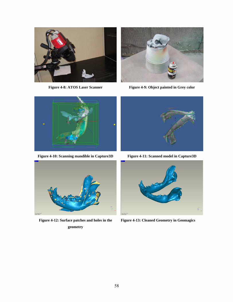
58

Figure 4-8: ATOS Laser Scanner Figure 4-9: Object painted in Grey color

Figure 4-10: Scanning mandible in Capture3D

Figure 4-11: Scanned model in Capture3D

Figure 4-12: Surface patches and holes in the

geometry

Figure 4-13: Cleaned Geometry in Geomagics

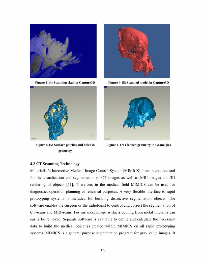
59

Figure 4-14: Scanning skull in Capture3D

Figure 4-15: Scanned model in Capture3D

Figure 4-16: Surface patches and holes in

geometry

Figure 4-17: Cleaned geometry in Geomagics

4.2 CT Scanning Technology

Materialise's Interactive Medical Image Control System (MIMICS) is an interactive tool

for the visualization and segmentation of CT images as well as MRI images and 3D

rendering of objects [51]. Therefore, in the medical field MIMICS can be used for

diagnostic, operation planning or rehearsal purposes. A very flexible interface to rapid

prototyping systems is included for building distinctive segmentation objects. The

software enables the surgeon or the radiologist to control and correct the segmentation of

CT-scans and MRI-scans. For instance, image artifacts coming from metal implants can

easily be removed. Separate software is available to define and calculate the necessary

data to build the medical object(s) created within MIMICS on all rapid prototyping

systems. MIMICS is a general purpose segmentation program for gray value images. It

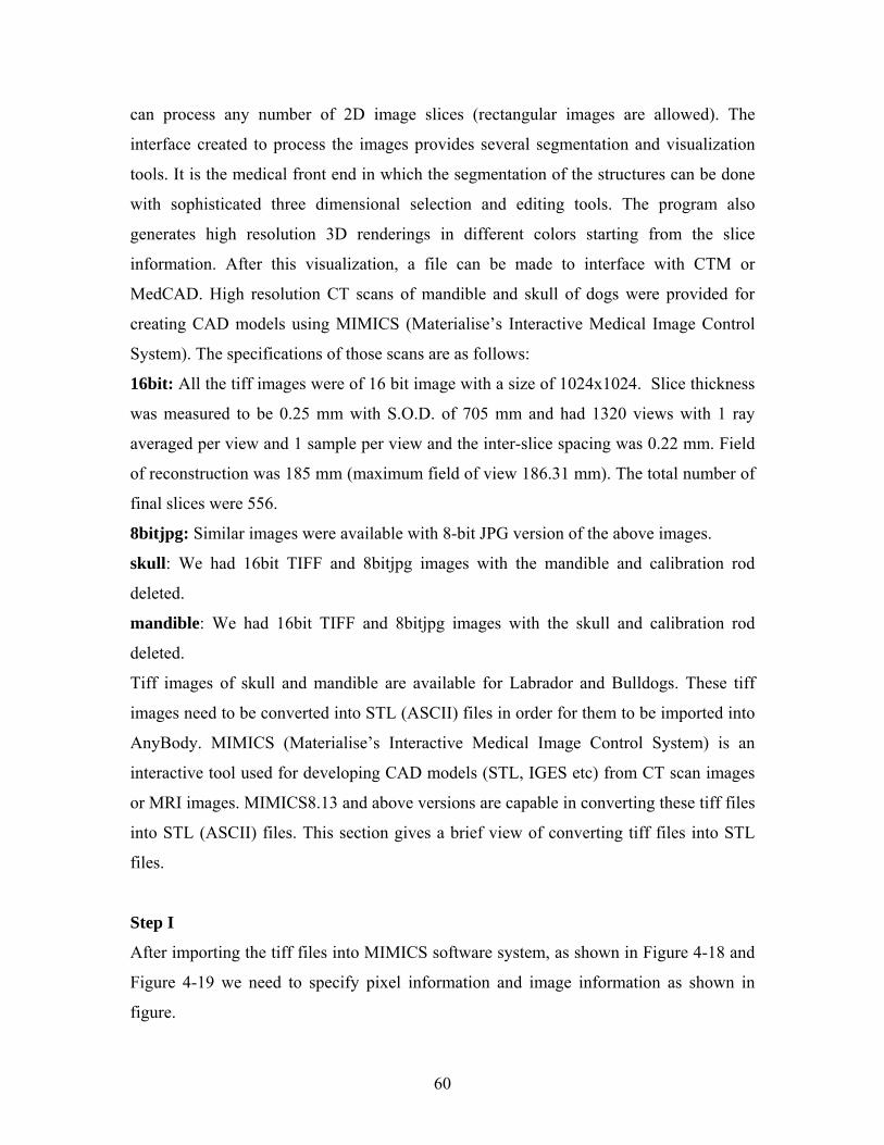
60

can process any number of 2D image slices (rectangular images are allowed). The

interface created to process the images provides several segmentation and visualization

tools. It is the medical front end in which the segmentation of the structures can be done

with sophisticated three dimensional selection and editing tools. The program also

generates high resolution 3D renderings in different colors starting from the slice

information. After this visualization, a file can be made to interface with CTM or

MedCAD. High resolution CT scans of mandible and skull of dogs were provided for

creating CAD models using MIMICS (Materialise’s Interactive Medical Image Control

System). The specifications of those scans are as follows:

16bit: All the tiff images were of 16 bit image with a size of 1024x1024. Slice thickness

was measured to be 0.25 mm with S.O.D. of 705 mm and had 1320 views with 1 ray

averaged per view and 1 sample per view and the inter-slice spacing was 0.22 mm. Field

of reconstruction was 185 mm (maximum field of view 186.31 mm). The total number of

final slices were 556.

8bitjpg: Similar images were available with 8-bit JPG version of the above images.

skull: We had 16bit TIFF and 8bitjpg images with the mandible and calibration rod

deleted.

mandible: We had 16bit TIFF and 8bitjpg images with the skull and calibration rod

deleted.

Tiff images of skull and mandible are available for Labrador and Bulldogs. These tiff

images need to be converted into STL (ASCII) files in order for them to be imported into

AnyBody. MIMICS (Materialise’s Interactive Medical Image Control System) is an

interactive tool used for developing CAD models (STL, IGES etc) from CT scan images

or MRI images. MIMICS8.13 and above versions are capable in converting these tiff files

into STL (ASCII) files. This section gives a brief view of converting tiff files into STL

files.

Step I

After importing the tiff files into MIMICS software system, as shown in Figure 4-18 and

Figure 4-19 we need to specify pixel information and image information as shown in

figure.

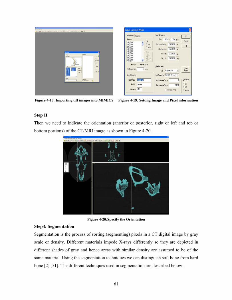
61

Figure 4-18: Importing tiff images into MIMICS

Figure 4-19: Setting Image and Pixel information

Step II

Then we need to indicate the orientation (anterior or posterior, right or left and top or

bottom portions) of the CT/MRI image as shown in Figure 4-20.

Figure 4-20:Specify the Orientation

Step3: Segmentation

Segmentation is the process of sorting (segmenting) pixels in a CT digital image by gray

scale or density. Different materials impede X-rays differently so they are depicted in

different shades of gray and hence areas with similar density are assumed to be of the

same material. Using the segmentation techniques we can distinguish soft bone from hard

bone [2] [51]. The different techniques used in segmentation are described below:

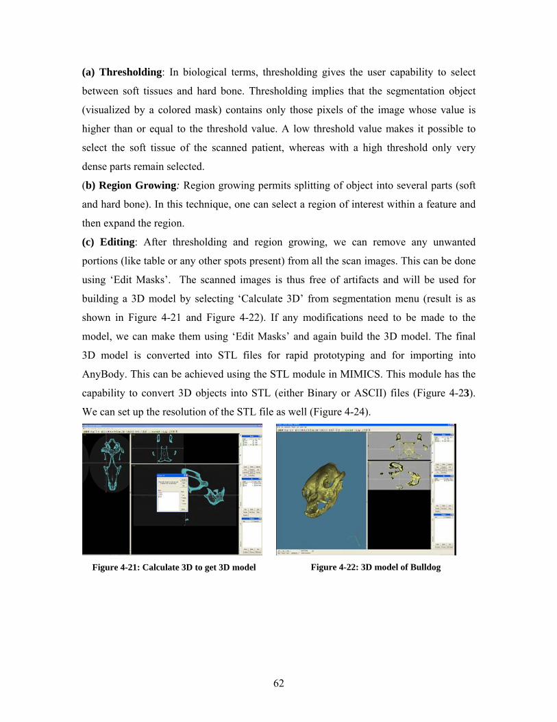
62

(a) Thresholding: In biological terms, thresholding gives the user capability to select

between soft tissues and hard bone. Thresholding implies that the segmentation object

(visualized by a colored mask) contains only those pixels of the image whose value is

higher than or equal to the threshold value. A low threshold value makes it possible to

select the soft tissue of the scanned patient, whereas with a high threshold only very

dense parts remain selected.

(b) Region Growing: Region growing permits splitting of object into several parts (soft

and hard bone). In this technique, one can select a region of interest within a feature and

then expand the region.

(c) Editing: After thresholding and region growing, we can remove any unwanted

portions (like table or any other spots present) from all the scan images. This can be done

using ‘Edit Masks’. The scanned images is thus free of artifacts and will be used for

building a 3D model by selecting ‘Calculate 3D’ from segmentation menu (result is as

shown in Figure 4-21 and Figure 4-22). If any modifications need to be made to the

model, we can make them using ‘Edit Masks’ and again build the 3D model. The final

3D model is converted into STL files for rapid prototyping and for importing into

AnyBody. This can be achieved using the STL module in MIMICS. This module has the

capability to convert 3D objects into STL (either Binary or ASCII) files (Figure 4-23).

We can set up the resolution of the STL file as well (Figure 4-24).

Figure 4-21: Calculate 3D to get 3D model

Figure 4-22: 3D model of Bulldog

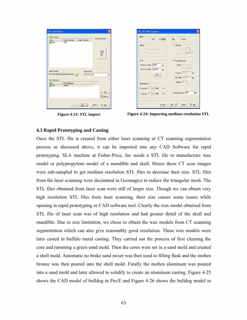
63

Figure 4-23: STL import

Figure 4-24: Importing medium resolution STL

4.3 Rapid Prototyping and Casting

Once the STL file is created from either laser scanning or CT scanning segmentation

process as discussed above, it can be imported into any CAD Software for rapid

prototyping. SLA machine at Fisher-Price, Inc needs a STL file to manufacture wax

model or polypropylene model of a mandible and skull. Hence these CT scan images

were sub-sampled to get medium resolution STL files to decrease their size. STL files

from the laser scanning were decimated in Geomagics to reduce the triangular mesh. The

STL files obtained from laser scan were still of larger size. Though we can obtain very

high resolution STL files from laser scanning, their size causes some issues while

opening in rapid prototyping or CAD software tool. Clearly the wax model obtained from

STL file of laser scan was of high resolution and had greater detail of the skull and

mandible. Due to size limitation, we chose to obtain the wax models from CT scanning

segmentation which can also give reasonably good resolution. These wax models were

later casted in buffalo metal casting. They carried out the process of first cleaning the

core and ramming a green sand mold. Then the cores were set in a sand mold and created

a shell mold. Automatic no brake sand mixer was then used to filling flask and the molten

bronze was then poured into the shell mold. Finally the molten aluminum was poured

into a sand mold and later allowed to solidify to create an aluminum casting. Figure 4-25

shows the CAD model of bulldog in Pro/E and Figure 4-26 shows the bulldog model in

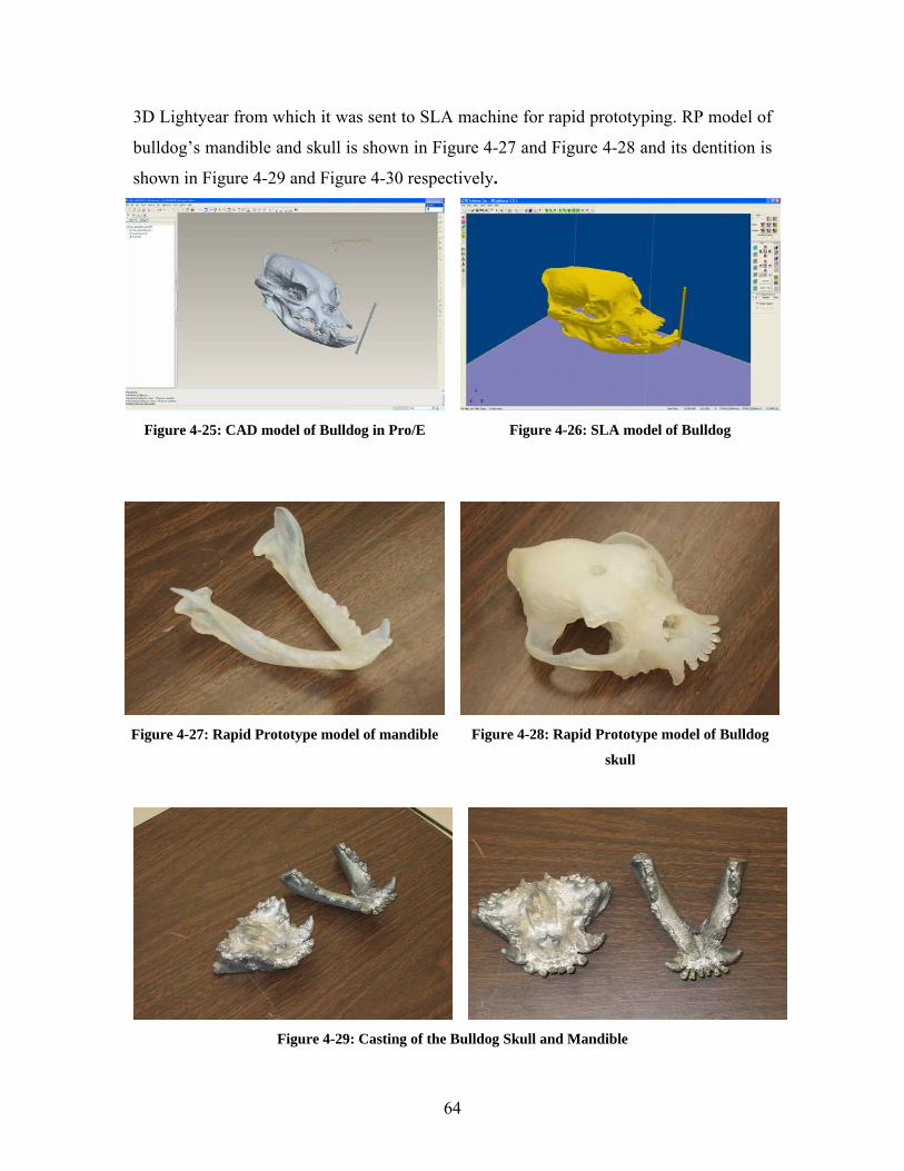
64

3D Lightyear from which it was sent to SLA machine for rapid prototyping. RP model of

bulldog’s mandible and skull is shown in Figure 4-27 and Figure 4-28 and its dentition is

shown in Figure 4-29 and Figure 4-30 respectively.

Figure 4-25: CAD model of Bulldog in Pro/E Figure 4-26: SLA model of Bulldog

Figure 4-27: Rapid Prototype model of mandible Figure 4-28: Rapid Prototype model of Bulldog

skull

Figure 4-29: Casting of the Bulldog Skull and Mandible

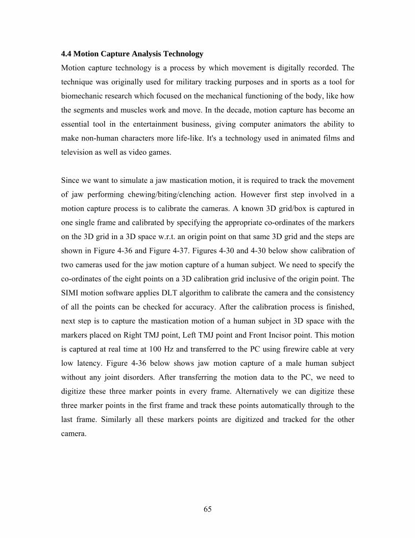
65

4.4 Motion Capture Analysis Technology

Motion capture technology is a process by which movement is digitally recorded. The

technique was originally used for military tracking purposes and in sports as a tool for

biomechanic research which focused on the mechanical functioning of the body, like how

the segments and muscles work and move. In the decade, motion capture has become an

essential tool in the entertainment business, giving computer animators the ability to

make non-human characters more life-like. It's a technology used in animated films and

television as well as video games.

Since we want to simulate a jaw mastication motion, it is required to track the movement

of jaw performing chewing/biting/clenching action. However first step involved in a

motion capture process is to calibrate the cameras. A known 3D grid/box is captured in

one single frame and calibrated by specifying the appropriate co-ordinates of the markers

on the 3D grid in a 3D space w.r.t. an origin point on that same 3D grid and the steps are

shown in Figure 4-36 and Figure 4-37. Figures 4-30 and 4-30 below show calibration of

two cameras used for the jaw motion capture of a human subject. We need to specify the

co-ordinates of the eight points on a 3D calibration grid inclusive of the origin point. The

SIMI motion software applies DLT algorithm to calibrate the camera and the consistency

of all the points can be checked for accuracy. After the calibration process is finished,

next step is to capture the mastication motion of a human subject in 3D space with the

markers placed on Right TMJ point, Left TMJ point and Front Incisor point. This motion

is captured at real time at 100 Hz and transferred to the PC using firewire cable at very

low latency. Figure 4-36 below shows jaw motion capture of a male human subject

without any joint disorders. After transferring the motion data to the PC, we need to

digitize these three marker points in every frame. Alternatively we can digitize these

three marker points in the first frame and track these points automatically through to the

last frame. Similarly all these markers points are digitized and tracked for the other

camera.

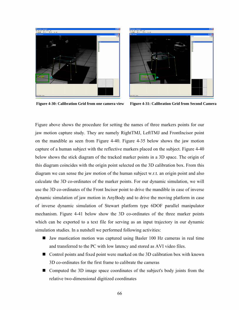
66

Figure 4-30: Calibration Grid from one camera view

Figure 4-31: Calibration Grid from Second Camera

Figure above shows the procedure for setting the names of three markers points for our

jaw motion capture study. They are namely RightTMJ, LeftTMJ and FrontIncisor point

on the mandible as seen from Figure 4-40. Figure 4-35 below shows the jaw motion

capture of a human subject with the reflective markers placed on the subject. Figure 4-40

below shows the stick diagram of the tracked marker points in a 3D space. The origin of

this diagram coincides with the origin point selected on the 3D calibration box. From this

diagram we can sense the jaw motion of the human subject w.r.t. an origin point and also

calculate the 3D co-ordinates of the marker points. For our dynamic simulation, we will

use the 3D co-ordinates of the Front Incisor point to drive the mandible in case of inverse

dynamic simulation of jaw motion in AnyBody and to drive the moving platform in case

of inverse dynamic simulation of Stewart platform type 6DOF parallel manipulator

mechanism. Figure 4-41 below show the 3D co-ordinates of the three marker points

which can be exported to a text file for serving as an input trajectory in our dynamic

simulation studies. In a nutshell we performed following activities:

Jaw mastication motion was captured using Basler 100 Hz cameras in real time

and transferred to the PC with low latency and stored as AVI video files.

Control points and fixed point were marked on the 3D calibration box with known

3D co-ordinates for the first frame to calibrate the cameras

Computed the 3D image space coordinates of the subject's body joints from the

relative two-dimensional digitized coordinates

Origin Origin

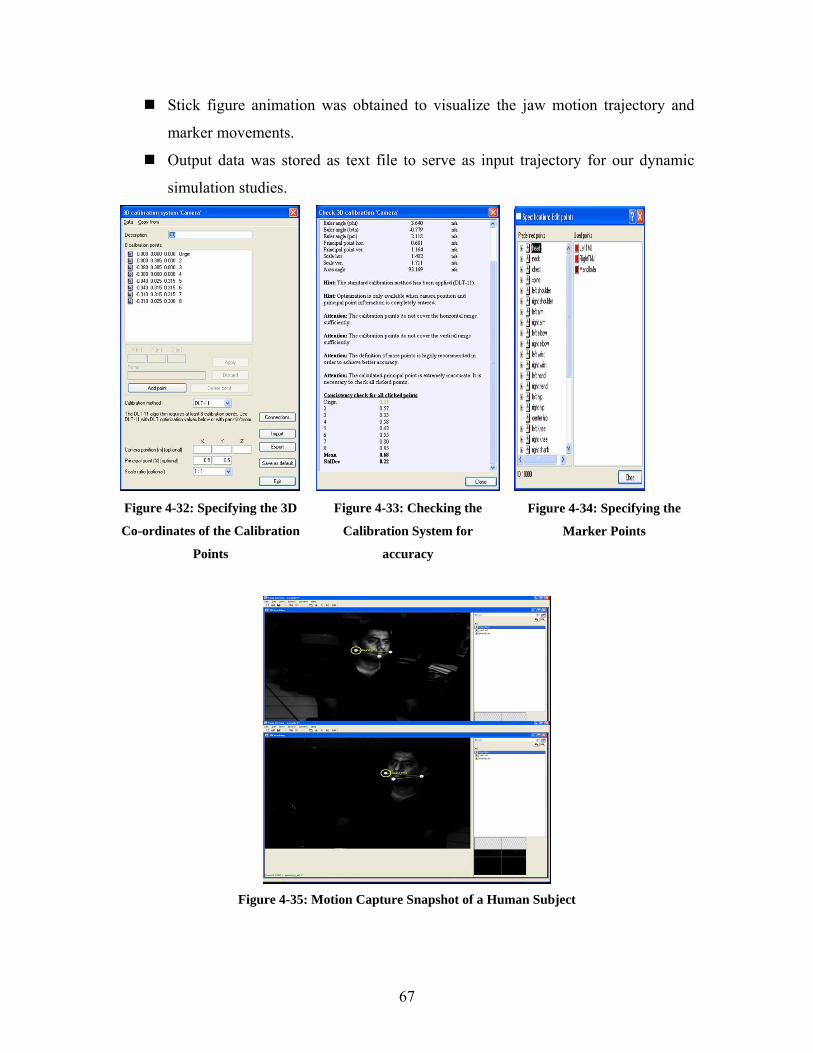
67

Stick figure animation was obtained to visualize the jaw motion trajectory and

marker movements.

Output data was stored as text file to serve as input trajectory for our dynamic

simulation studies.

Figure 4-32: Specifying the 3D

Co-ordinates of the Calibration

Points

Figure 4-33: Checking the

Calibration System for

accuracy

Figure 4-34: Specifying the

Marker Points

Figure 4-35: Motion Capture Snapshot of a Human Subject

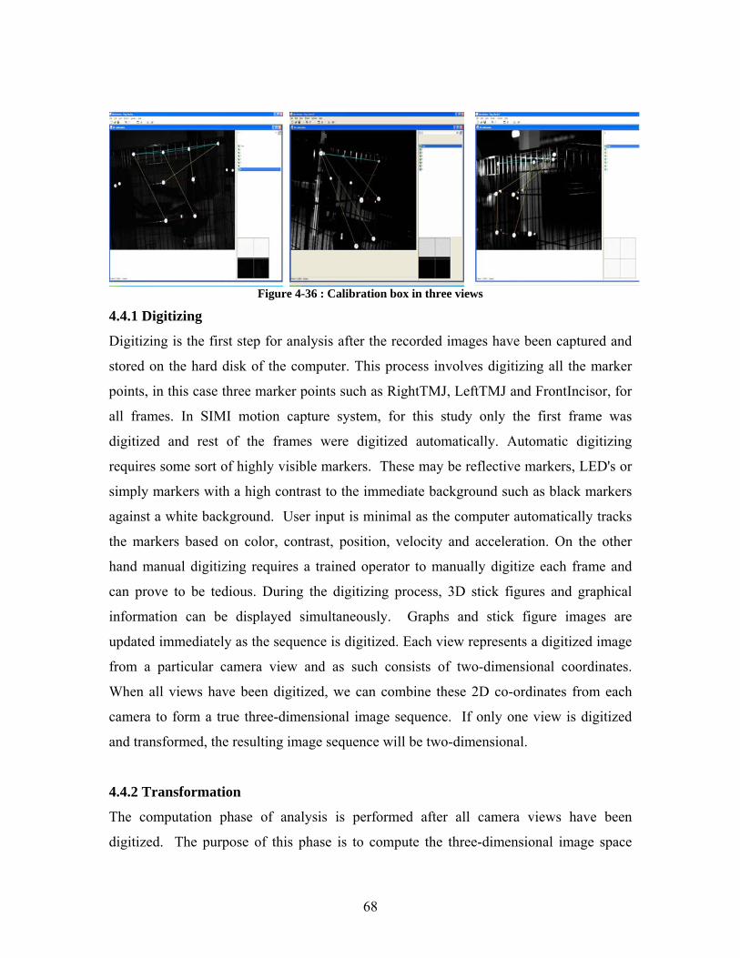
68

Figure 4-36 : Calibration box in three views

4.4.1 Digitizing

Digitizing is the first step for analysis after the recorded images have been captured and

stored on the hard disk of the computer. This process involves digitizing all the marker

points, in this case three marker points such as RightTMJ, LeftTMJ and FrontIncisor, for

all frames. In SIMI motion capture system, for this study only the first frame was

digitized and rest of the frames were digitized automatically. Automatic digitizing

requires some sort of highly visible markers. These may be reflective markers, LED's or

simply markers with a high contrast to the immediate background such as black markers

against a white background. User input is minimal as the computer automatically tracks

the markers based on color, contrast, position, velocity and acceleration. On the other

hand manual digitizing requires a trained operator to manually digitize each frame and

can prove to be tedious. During the digitizing process, 3D stick figures and graphical

information can be displayed simultaneously. Graphs and stick figure images are

updated immediately as the sequence is digitized. Each view represents a digitized image

from a particular camera view and as such consists of two-dimensional coordinates.

When all views have been digitized, we can combine these 2D co-ordinates from each

camera to form a true three-dimensional image sequence. If only one view is digitized

and transformed, the resulting image sequence will be two-dimensional.

4.4.2 Transformation

The computation phase of analysis is performed after all camera views have been

digitized. The purpose of this phase is to compute the three-dimensional image space

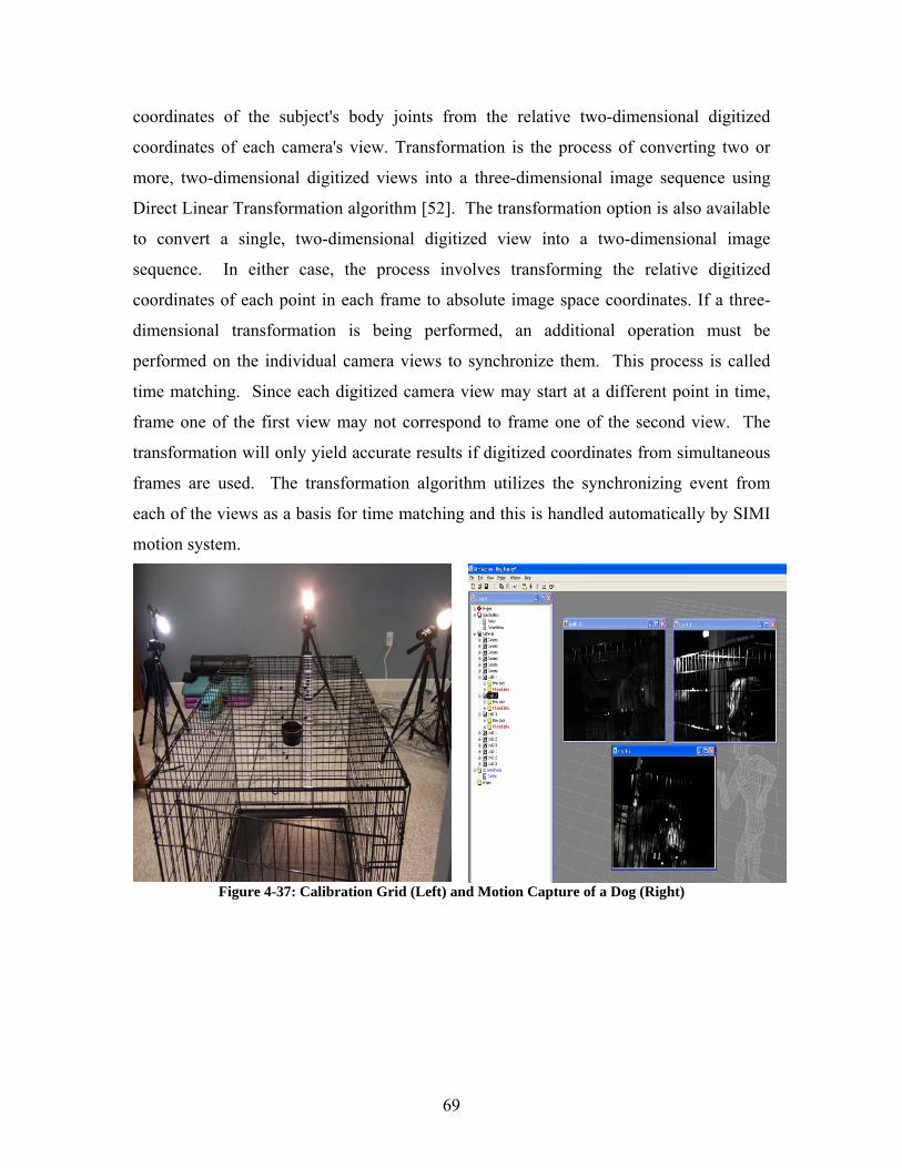
69

coordinates of the subject's body joints from the relative two-dimensional digitized

coordinates of each camera's view. Transformation is the process of converting two or

more, two-dimensional digitized views into a three-dimensional image sequence using

Direct Linear Transformation algorithm [52]. The transformation option is also available

to convert a single, two-dimensional digitized view into a two-dimensional image

sequence. In either case, the process involves transforming the relative digitized

coordinates of each point in each frame to absolute image space coordinates. If a three-

dimensional transformation is being performed, an additional operation must be

performed on the individual camera views to synchronize them. This process is called

time matching. Since each digitized camera view may start at a different point in time,

frame one of the first view may not correspond to frame one of the second view. The

transformation will only yield accurate results if digitized coordinates from simultaneous

frames are used. The transformation algorithm utilizes the synchronizing event from

each of the views as a basis for time matching and this is handled automatically by SIMI

motion system.

Figure 4-37: Calibration Grid (Left) and Motion Capture of a Dog (Right)

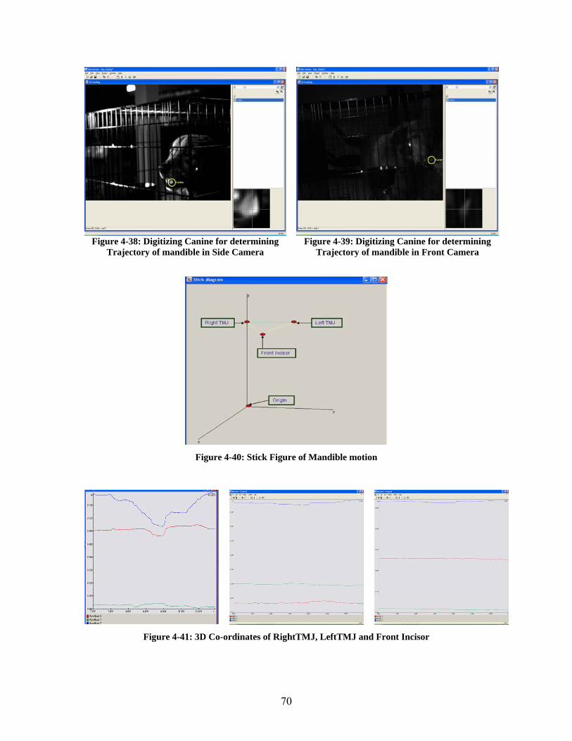
70

Figure 4-38: Digitizing Canine for determining Trajectory of mandible in Side Camera

Figure 4-39: Digitizing Canine for determining Trajectory of mandible in Front Camera

Figure 4-40: Stick Figure of Mandible motion

Figure 4-41: 3D Co-ordinates of RightTMJ, LeftTMJ and Front Incisor

71

4.4.3 DLT

The traditional method used to convert digitized coordinate locations to image space

coordinate locations utilizes a widely used method known as the Direct Linear

Transformation or DLT [52]. In this "mapping" process, the known image coordinates,

as well as the digitized coordinates of the control points, are used to solve a set of

simultaneous linear equations which relate one set of coordinates to the other. This set of

equations is solved using linear least-squares method that yields the image space

coordinates of each point, given the digitized view coordinates of that point. The

advantage of this transformation method over more traditional methods is that one does

not need to know the location or orientation of the cameras, the distance of cameras to the

subject, or any information about the camera or projections lenses such as focal length

and magnification. Instead, by directly determining the relationship between the image

space and each of the digitized views, all the intervening image changes are eliminated,

and need not be considered. In order to utilize this method, there must be a known set of

control points in the video recording of each view. At least six non-coplanar control

points are required (though more can be used) for a three-dimensional analysis. This is

the minimum number of points required to solve the set of simultaneous linear equations

that produce the transformation. For a two dimensional analysis using a single camera, at

least four co-planar but non-collinear control points must be used. It is possible to use

more than the minimum number of control points, as this will increase the accuracy of the

transformation. The control points should be distributed to fill as much of the image

space as practical. If the control points all occur in a small portion of the image space,

then image distortion is likely to increase as the distance from the image to the control

points increases.

4.4.4 Technical Aspects for Transformation

The SIMI motion software considers the image space to be described by a right-handed

cartesian coordinate system with a fixed origin and orthogonal X, Y and Z coordinate

axes and an arbitrary point in the image space is described by its coordinates (x, y, z).

When a film recording of an object in the image space is projected on a flat screen

measure the location of points on this plane of projection, it measures the location of

72

points on this plane and can be described by its horizontal and vertical digitizer

coordinates (U, V). The general form of the transformation between these coordinate

systems may be expressed as:

U = Ax + By + Cz + D (1)

V= Ex + Fy + Gz + L

The coefficients, A through L, represent various physical parameters defined in the

configuration of the camera and the playback or projection system. In general, it is a

difficult process to determine the values for these coefficients by measurement of camera

orientation, distance of camera to subject, magnification of camera and projection lenses,

etc. If, however, the image space contains an adequate number of points (control points)

whose coordinate locations are accurately known, the coefficients can be determined

through the solution of a set of simultaneous linear equations relating the image space

coordinates of the control points to the digitized coordinate of the control points. Above

Equations can be rewritten in matrix form as shown in equations (2) to express the sets of

simultaneous equations that must be solved to determine the coefficients A through L.

Subscripts are used to denote the image space and digitizer coordinates of individual

control points. A minimum of six non-coplanar control points are required to solve

equations (3), although additional points may be used as indicated by the ellipses. If

more than six points are used, the set of equations becomes over-determined and may be

solved using a standard linear least squares technique [52].

For a given unknown image space point (x, y, z), equation (1) can be rearranged as:

{A - EU}{B - FU}{C - GU}x = {U - D} (2)

{H - EV}{J - FV}{K - GV}y = {V - L}

The digitizer coordinates (U,V) are known as the coefficients A through L from the

solution of equation (3). However, equation (4) cannot be solved for (x, y, z) since this

set of linear equations is underdetermined. Digitized information from one camera is

therefore not sufficient to determine three-dimensional image space coordinates. This

problem can be resolved by the addition of a second camera. For film or video

recordings, each joint location (x, y, and z) is a function of time, and therefore, digitized

73

camera information must be combined for the same moment in time. This is the purpose

of the "Time-Matching" step in the transformation process.

4.5 Musculoskeletal Model of Vertebrate Jaw

Some prior work has been done for simulating static clenching tasks and dynamic tasks in

the case of human mandible musculoskeletal model. Our goal is to create a

musculoskeletal model of a mandible for different vertebrates such as sabertooth cat,

bulldog and human and simulate dynamics of chewing behavior and determine muscles

forces and TMJ reaction forces. For initial simulation we will recreate a musculoskeletal

model of a human mandible with our motion capture data and muscle attachment points

and properties from Koolstra et al. and compare them with human mandible model

created by Mark et al. for validation purposes. Our focus will then be to extend this for

creating musculoskeletal models of sabertooth and bulldog mandible and compute muscle

forces and TMJ reaction forces based on the motion capture data and architectural

properties of muscle obtained from CT scan and dissection.

A three dimensional model of the vertebrate masticatory system (for human see Figure 4-

41 and 4-42) containing seven masticatory muscles namely one masseter, three

temporalis, medial pterygoid, lateral pterygoid and digastric on each side and two

temporomandibular joints has been developed using AnyBody Modeling system. The

AnyBody Modeling System is a commercial software package that combines a solver for

the multi-body inverse dynamics problem with optimizers that may be used for the

solution of the muscle recruitment problem [39]. The optimizer implemented in AnyBody

uses a min/max objective function. The models in AnyBody are defined in a text-based,

declarative, object-oriented language called AnyScript. The model of the mandible was

based on repository of AnyBody Software. The two separate 3D geometries of mandible

and skull were acquired from the repository and imported into the AnyBody Modeling

System and used for defining the muscle insertions and for visualization purposes. The

model contained two rigid bodies, the skull and the mandible. Mass and mass moments of

inertia of the mandible are based on the work of Koolstra and Van Eijden (2005) and are

listed in Table 4-5. In our model the number of muscles was 7 as shown in the Table 4-3

74

and their attachment points are taken from the physical skull and mandible of a human

subject. Motion capture of a human was performed as shown in above section, to

generate an input motion trajectory for the front incisor point. Given the input jaw motion

trajectory obtained from motion capture analysis of mandibular movement, inverse

dynamic analysis principle will be performed to determine the muscles forces and joint

reaction forces required to perform the desired motion of the front incisor point. The skull

and mandible make contact at both temporomandibular joints and at one bite point. The

origin is defined between the joints in the mid-sagittal plane. The positive x-axis is

pointing forward and the positive y-axis to the right and the positive z-axis is pointing

upward. Maximum muscle force of a muscle element is assumed to be proportional to its

physiological cross section under static circumstances where the value of P=0.37*106

N/m2. PCS of the temporalis, masseter, digastric, lateral and medical pterygoid muscle

was predicted from the cross sectional area of these muscles in the case of a dog, as

imaged on CT scans and also from dissection. For modeling human masticatory model,

all the architectural properties were used from Koolstra et al. For bulldog jaw model, the

architectural properties were estimated by performing dissection of the dog’s head

muscles. In order to get the STL file of the bulldog oriented and transformed to the origin

of the musculoskeletal system, we used Rhinoceros program. Here the mandible and skull

model were transformed to the origin of the program so that while importing these STL

files into AnyBody, the center of the two TMJ’s aline with the origin of the Anybody

Reference frame as shown in Figure 4-42 and Figure 4-43.

Figure 4-42:Transformation of Skull in Rhino Figure 4-43: Transformation of mandible

Kinematically the assumption was made that there is always contact between the condyle

and the mandibular fossa at both the TMJ, though in reality there is the articular disc in

between the condyles and hence the mandible has only four degrees of freedom left.

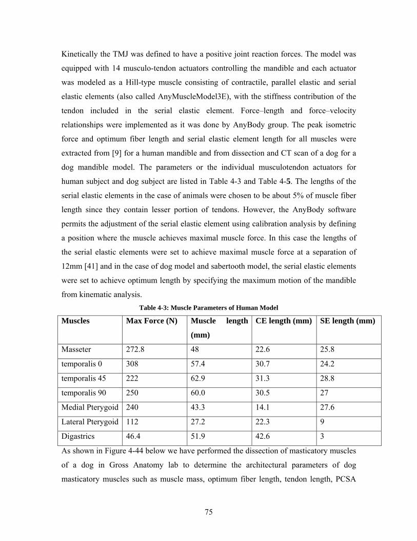
75

Kinetically the TMJ was defined to have a positive joint reaction forces. The model was

equipped with 14 musculo-tendon actuators controlling the mandible and each actuator

was modeled as a Hill-type muscle consisting of contractile, parallel elastic and serial

elastic elements (also called AnyMuscleModel3E), with the stiffness contribution of the

tendon included in the serial elastic element. Force–length and force–velocity

relationships were implemented as it was done by AnyBody group. The peak isometric

force and optimum fiber length and serial elastic element length for all muscles were

extracted from [9] for a human mandible and from dissection and CT scan of a dog for a

dog mandible model. The parameters or the individual musculotendon actuators for

human subject and dog subject are listed in Table 4-3 and Table 4-5. The lengths of the

serial elastic elements in the case of animals were chosen to be about 5% of muscle fiber

length since they contain lesser portion of tendons. However, the AnyBody software

permits the adjustment of the serial elastic element using calibration analysis by defining

a position where the muscle achieves maximal muscle force. In this case the lengths of

the serial elastic elements were set to achieve maximal muscle force at a separation of

12mm [41] and in the case of dog model and sabertooth model, the serial elastic elements

were set to achieve optimum length by specifying the maximum motion of the mandible

from kinematic analysis. Table 4-3: Muscle Parameters of Human Model

Muscles Max Force (N) Muscle length

(mm)

CE length (mm) SE length (mm)

Masseter 272.8 48 22.6 25.8

temporalis 0 308 57.4 30.7 24.2

temporalis 45 222 62.9 31.3 28.8

temporalis 90 250 60.0 30.5 27

Medial Pterygoid 240 43.3 14.1 27.6

Lateral Pterygoid 112 27.2 22.3 9

Digastrics 46.4 51.9 42.6 3

As shown in Figure 4-44 below we have performed the dissection of masticatory muscles

of a dog in Gross Anatomy lab to determine the architectural parameters of dog

masticatory muscles such as muscle mass, optimum fiber length, tendon length, PCSA

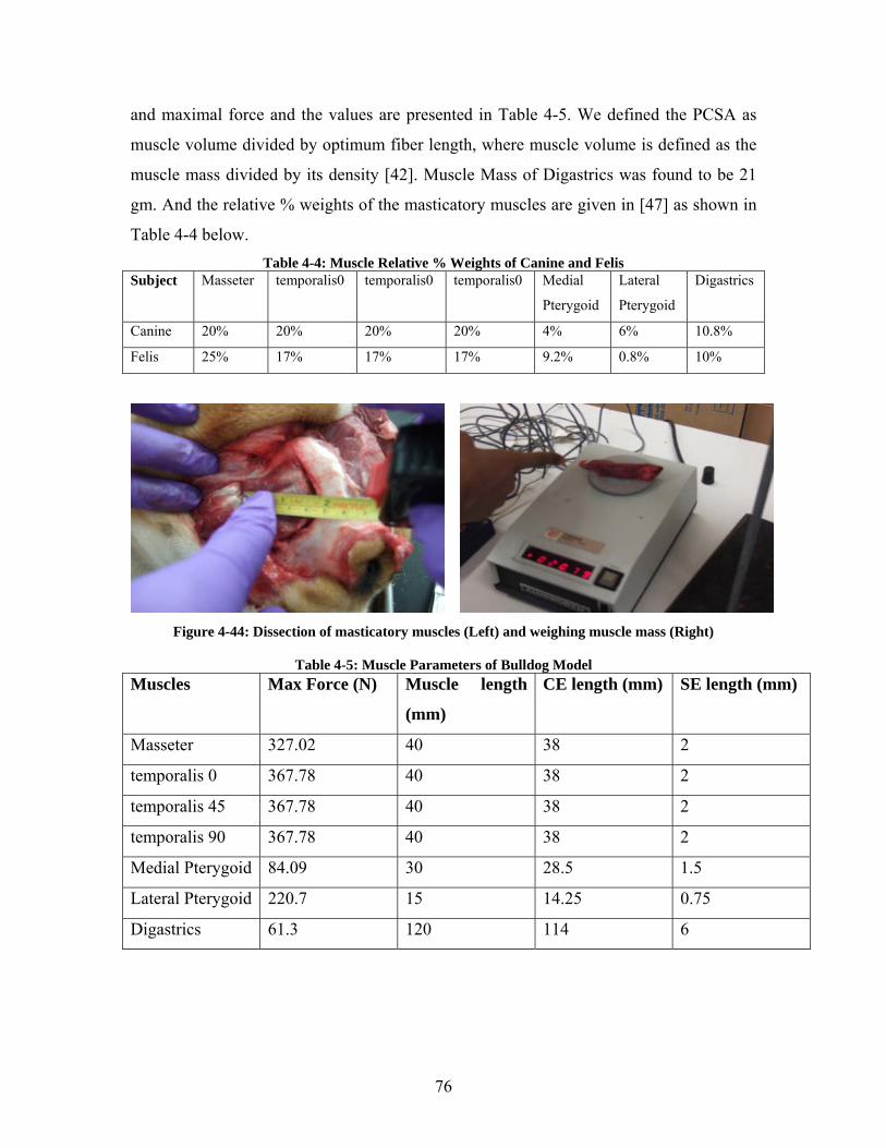
76

and maximal force and the values are presented in Table 4-5. We defined the PCSA as

muscle volume divided by optimum fiber length, where muscle volume is defined as the

muscle mass divided by its density [42]. Muscle Mass of Digastrics was found to be 21

gm. And the relative % weights of the masticatory muscles are given in [47] as shown in

Table 4-4 below. Table 4-4: Muscle Relative % Weights of Canine and Felis

Subject Masseter temporalis0 temporalis0 temporalis0 Medial

Pterygoid

Lateral

Pterygoid

Digastrics

Canine 20% 20% 20% 20% 4% 6% 10.8%

Felis 25% 17% 17% 17% 9.2% 0.8% 10%

Figure 4-44: Dissection of masticatory muscles (Left) and weighing muscle mass (Right)

Table 4-5: Muscle Parameters of Bulldog Model Muscles Max Force (N) Muscle length

(mm)

CE length (mm) SE length (mm)

Masseter 327.02 40 38 2

temporalis 0 367.78 40 38 2

temporalis 45 367.78 40 38 2

temporalis 90 367.78 40 38 2

Medial Pterygoid 84.09 30 28.5 1.5

Lateral Pterygoid 220.7 15 14.25 0.75

Digastrics 61.3 120 114 6

77

Table 4-6: Muscle Parameters of Sabertooth Model Muscles Max Force (N) Muscle length

(mm)

CE length (mm) SE length (mm)

Masseter 1751.89 60 54 6

temporalis 0 661.82 90 81 9

temporalis 45 661.82 90 81 9

temporalis 90 661.82 90 81 9

Medial Pterygoid 475.5 70 63 7

Lateral Pterygoid 58.39 30 27 3

Digastrics 134.76 250 225 25

Figure 4-45: Skull and Mandible model of Bulldog

Table 4-7: Mass and Inertia of Mandible

Model Mass (kg) Ixx (kg m2) Iyy (kg m2) Izz (kg m2)

Mandible 0.44 0.00086 0.00029 0.00061

Figure 4-46: Human Jaw model in AnyBody

78

Figure 4-47: Human Skull and Mandible model in different views

Figures 4-48-4-50 below shows the musculoskeletal model of a sabertooth cat which has

been modeled with the motion capture data of a sabertooth Jaw simulator, muscles

architectural properties measured from its CT scan and the mass and inertia properties of

the mandible were scaled up accordingly for both sabertooth and bulldog. Rest of the

modeling procedure of the TMJ and mandible are same as above mentioned human

model. Similar model was created for a bulldog and its muscle architectural properties

were extracted from dog’s dissection and CT scan. Considering all the muscles to be

acting like a vector along a straight line, Figure 4-52 below shows the muscle origin

points on the skull and the muscles insertion points on the mandible. Y-co-ordinate of the

attachment point changes sign for all the muscles on the Left side.

Vectors in pick color shows the masticatory muscles required to generate force for

producing the jaw closing and opening action. All the muscle attachment points were

defined with the origin as center of two TMJ joints. Since we know that both the skull

and mandible together have 12 degrees of freedom, it is essential to provide 12

constraints/ drivers to setup a kinematically determinate system. In this case the skull is

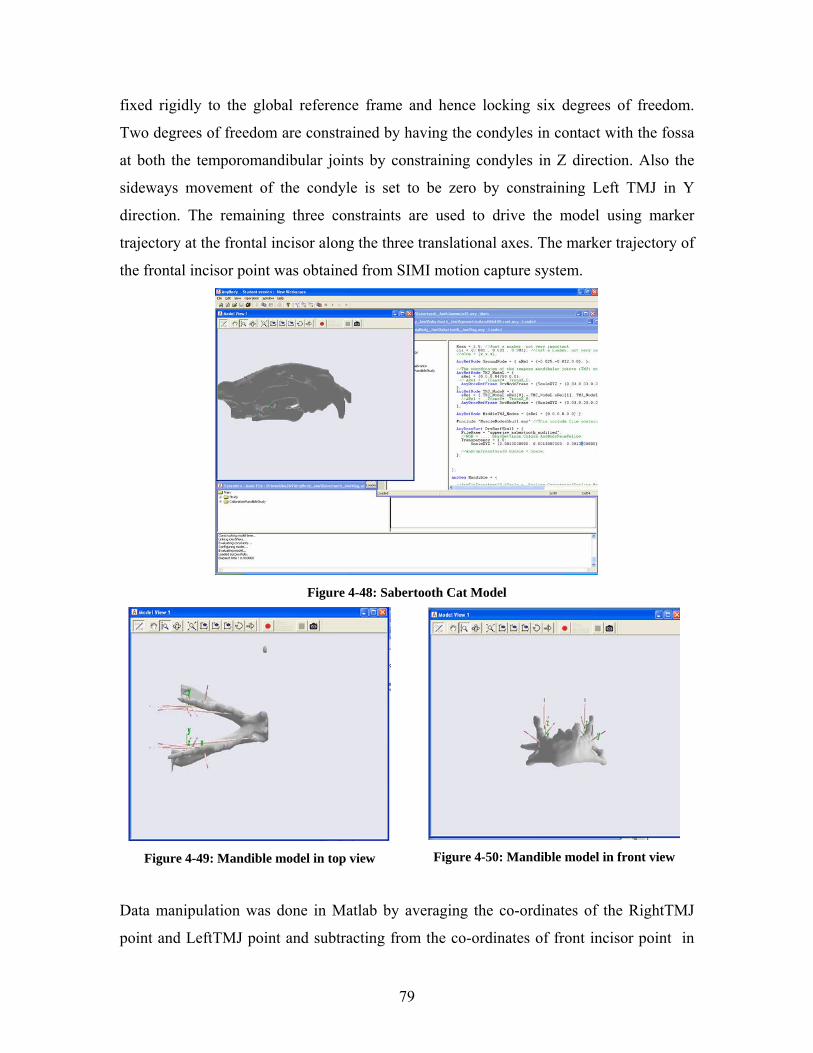
79

fixed rigidly to the global reference frame and hence locking six degrees of freedom.

Two degrees of freedom are constrained by having the condyles in contact with the fossa

at both the temporomandibular joints by constraining condyles in Z direction. Also the

sideways movement of the condyle is set to be zero by constraining Left TMJ in Y

direction. The remaining three constraints are used to drive the model using marker

trajectory at the frontal incisor along the three translational axes. The marker trajectory of

the frontal incisor point was obtained from SIMI motion capture system.

Figure 4-48: Sabertooth Cat Model

Figure 4-49: Mandible model in top view

Figure 4-50: Mandible model in front view

Data manipulation was done in Matlab by averaging the co-ordinates of the RightTMJ

point and LeftTMJ point and subtracting from the co-ordinates of front incisor point in

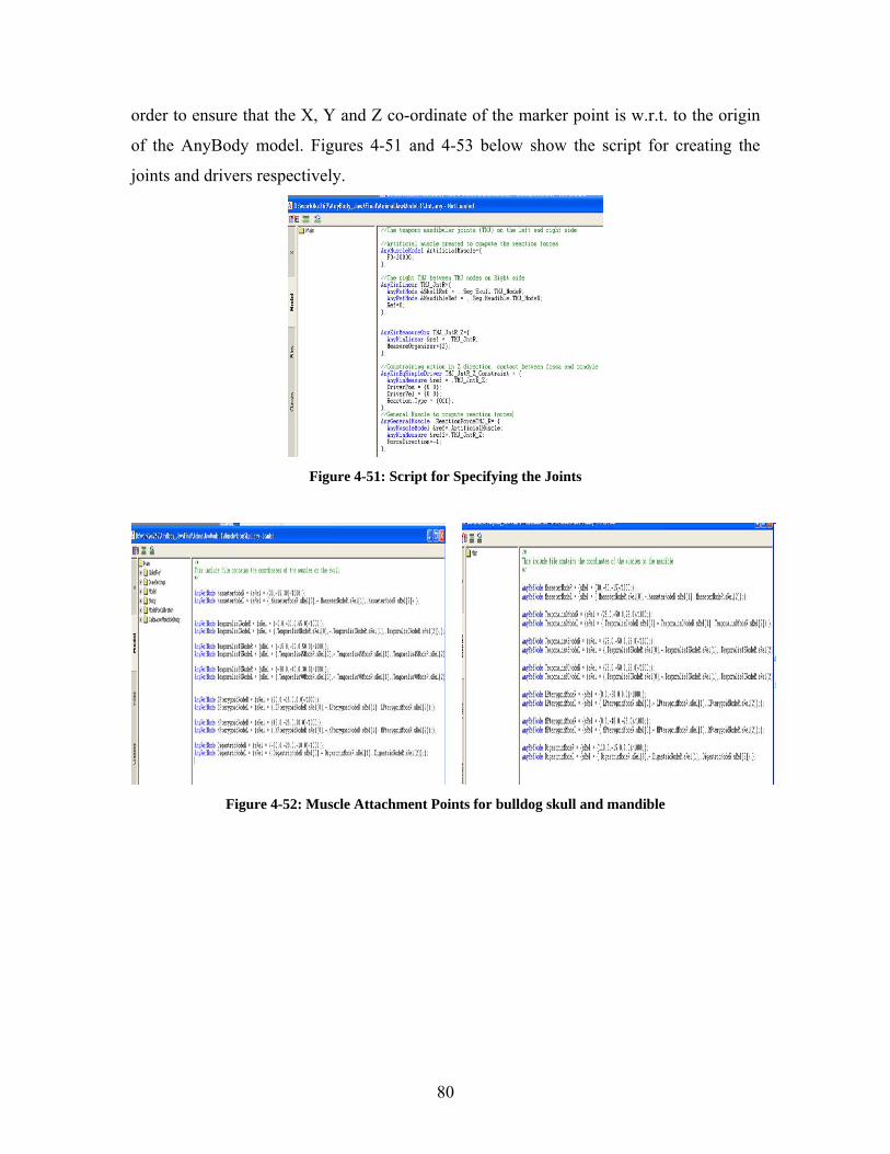
80

order to ensure that the X, Y and Z co-ordinate of the marker point is w.r.t. to the origin

of the AnyBody model. Figures 4-51 and 4-53 below show the script for creating the

joints and drivers respectively.

Figure 4-51: Script for Specifying the Joints

Figure 4-52: Muscle Attachment Points for bulldog skull and mandible

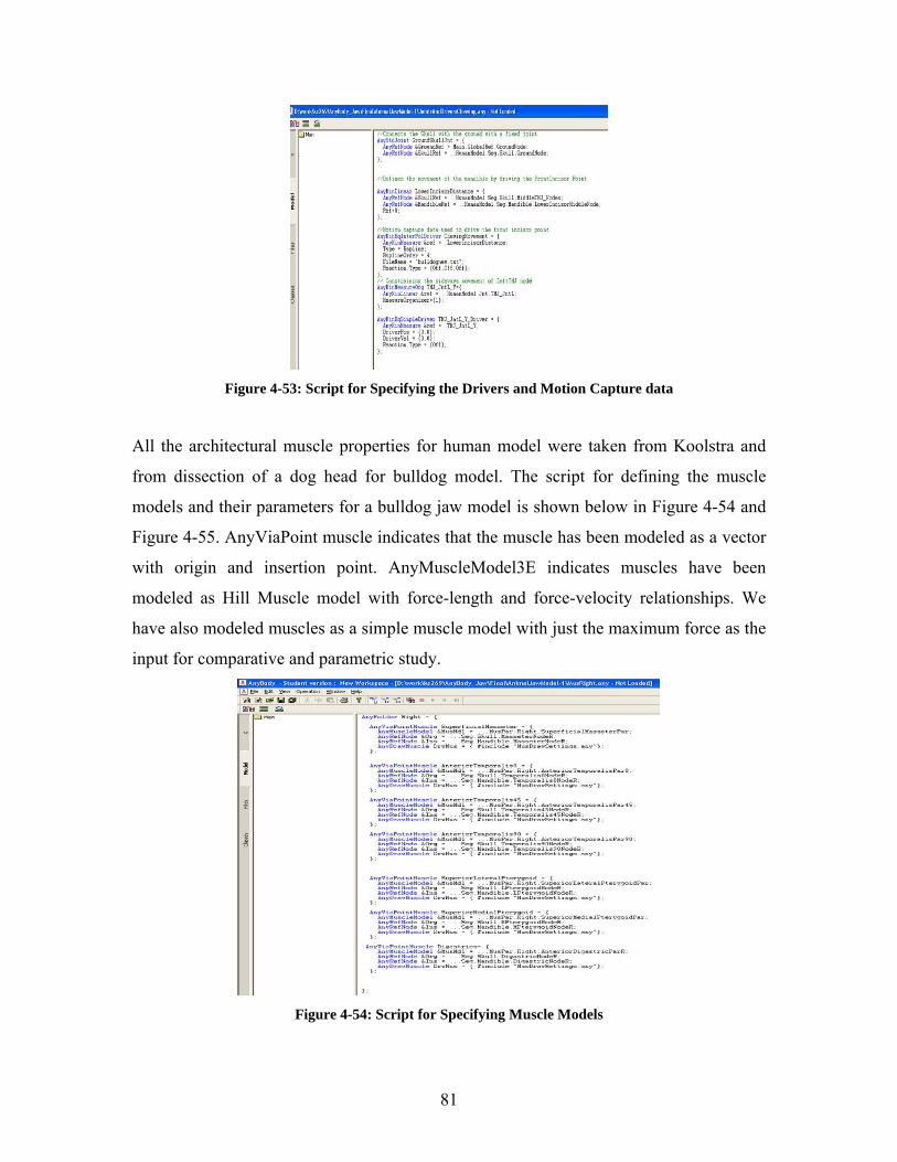
81

Figure 4-53: Script for Specifying the Drivers and Motion Capture data

All the architectural muscle properties for human model were taken from Koolstra and

from dissection of a dog head for bulldog model. The script for defining the muscle

models and their parameters for a bulldog jaw model is shown below in Figure 4-54 and

Figure 4-55. AnyViaPoint muscle indicates that the muscle has been modeled as a vector

with origin and insertion point. AnyMuscleModel3E indicates muscles have been

modeled as Hill Muscle model with force-length and force-velocity relationships. We

have also modeled muscles as a simple muscle model with just the maximum force as the

input for comparative and parametric study.

Figure 4-54: Script for Specifying Muscle Models

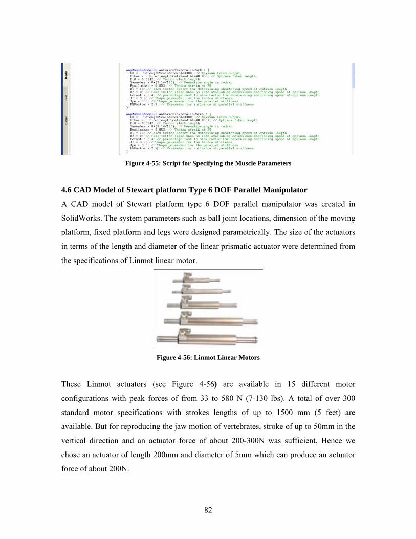
82

Figure 4-55: Script for Specifying the Muscle Parameters

4.6 CAD Model of Stewart platform Type 6 DOF Parallel Manipulator

A CAD model of Stewart platform type 6 DOF parallel manipulator was created in

SolidWorks. The system parameters such as ball joint locations, dimension of the moving

platform, fixed platform and legs were designed parametrically. The size of the actuators

in terms of the length and diameter of the linear prismatic actuator were determined from

the specifications of Linmot linear motor.

Figure 4-56: Linmot Linear Motors

These Linmot actuators (see Figure 4-56) are available in 15 different motor

configurations with peak forces of from 33 to 580 N (7-130 lbs). A total of over 300

standard motor specifications with strokes lengths of up to 1500 mm (5 feet) are

available. But for reproducing the jaw motion of vertebrates, stroke of up to 50mm in the

vertical direction and an actuator force of about 200-300N was sufficient. Hence we

chose an actuator of length 200mm and diameter of 5mm which can produce an actuator

force of about 200N.

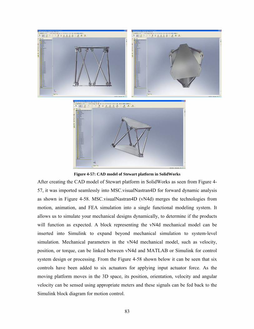
83

Figure 4-57: CAD model of Stewart platform in SolidWorks

After creating the CAD model of Stewart platform in SolidWorks as seen from Figure 4-

57, it was imported seamlessly into MSC.visualNastran4D for forward dynamic analysis

as shown in Figure 4-58. MSC.visualNastran4D (vN4d) merges the technologies from

motion, animation, and FEA simulation into a single functional modeling system. It

allows us to simulate your mechanical designs dynamically, to determine if the products

will function as expected. A block representing the vN4d mechanical model can be

inserted into Simulink to expand beyond mechanical simulation to system-level

simulation. Mechanical parameters in the vN4d mechanical model, such as velocity,

position, or torque, can be linked between vN4d and MATLAB or Simulink for control

system design or processing. From the Figure 4-58 shown below it can be seen that six

controls have been added to six actuators for applying input actuator force. As the

moving platform moves in the 3D space, its position, orientation, velocity and angular

velocity can be sensed using appropriate meters and these signals can be fed back to the

Simulink block diagram for motion control.

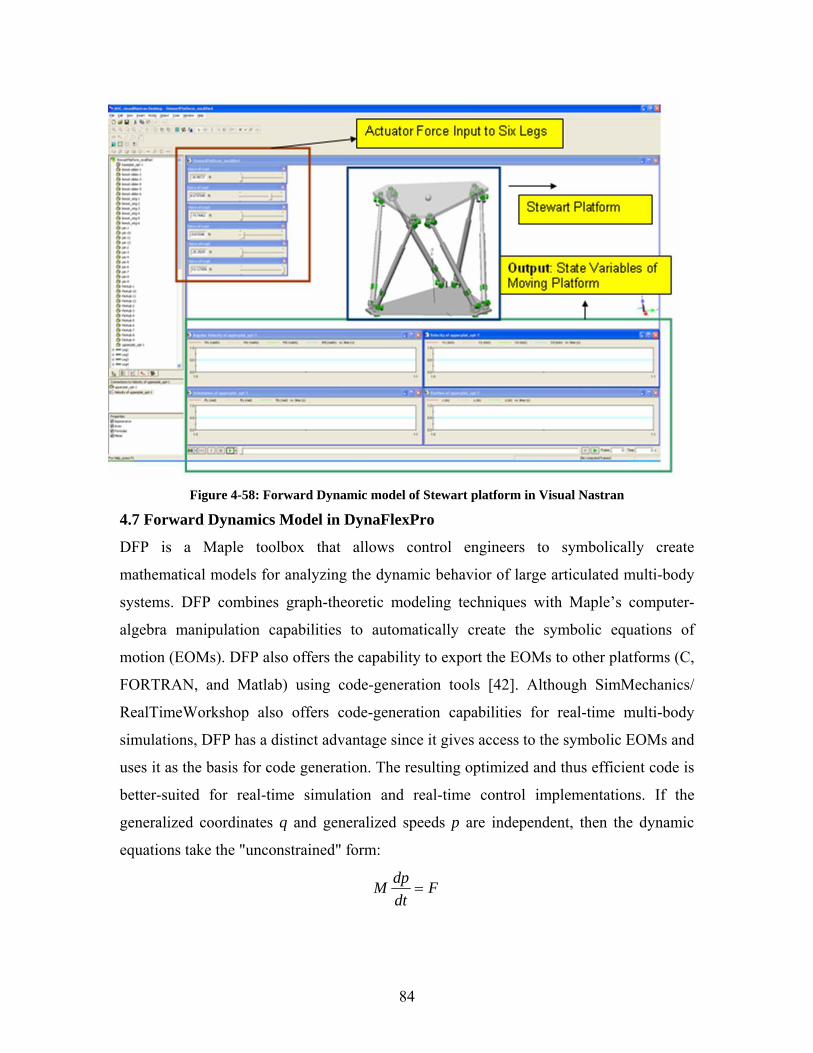
84

Figure 4-58: Forward Dynamic model of Stewart platform in Visual Nastran

4.7 Forward Dynamics Model in DynaFlexPro

DFP is a Maple toolbox that allows control engineers to symbolically create

mathematical models for analyzing the dynamic behavior of large articulated multi-body

systems. DFP combines graph-theoretic modeling techniques with Maple’s computer-

algebra manipulation capabilities to automatically create the symbolic equations of

motion (EOMs). DFP also offers the capability to export the EOMs to other platforms (C,

FORTRAN, and Matlab) using code-generation tools [42]. Although SimMechanics/

RealTimeWorkshop also offers code-generation capabilities for real-time multi-body

simulations, DFP has a distinct advantage since it gives access to the symbolic EOMs and

uses it as the basis for code generation. The resulting optimized and thus efficient code is

better-suited for real-time simulation and real-time control implementations. If the

generalized coordinates q and generalized speeds p are independent, then the dynamic

equations take the "unconstrained" form:

FdtdpM =

85

Where M is the mass matrix and F contains external loads and quadratic velocity terms.

The full set of system equations are formed by combining these dynamic equations with

the kinematic transformations, giving 2n ordinary differential equations in 2n unknowns:

⎥⎦

⎤⎢⎣

⎡=

⎥⎥⎥

⎦

⎤

⎢⎢⎢

⎣

⎡

⎥⎦

⎤⎢⎣

⎡hF

dtdqdtdp

M100

If the generalized coordinates q and generalized speeds p are dependent, then the

"augmented" dynamic equations can be written with the constraint reactions appearing

explicitly ("AugType" option set to "Reaction"):

FfCdtdpM T =+

where f contains the reaction loads in the cotree joints that enforce the kinematic

constraints, and C is the corresponding coefficient matrix [48].

With DynaFlexPro, one can represent the constraint reactions by their actual forces and

moments, or indirectly using Lagrange multipliers. One popular method for converting

these DAEs to ODEs is to replace the position constraints with the acceleration

constraints, which are then numerically integrated simultaneously with the ODEs from

the dynamic equations. In the integration process, though, the accumulation of numerical

errors will lead to violations in the position constraint equations (visually, the

cotree joints will float apart). Baumgarte proposed a method to stabilize these

constraints, by combining the position, velocity, and acceleration constraints into a single

expression:

02 2 =++∂ φβαψ

which can be written as a linear equation in terms of the accelerations:

ε

φβαψψ

=

−−= 22edtdp

p

By integrating this expression for the accelerations, the Baumgarte parameters α and β

will act to stabilize the constraints at the position level [48].

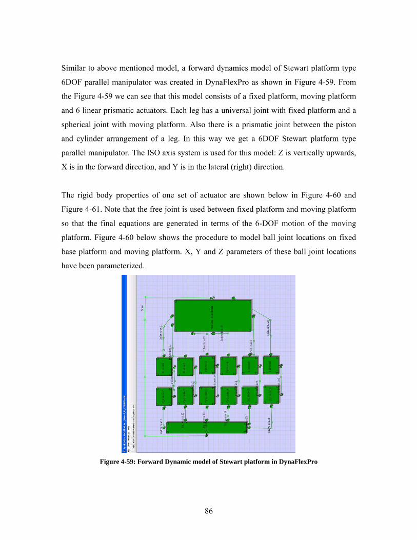
86

Similar to above mentioned model, a forward dynamics model of Stewart platform type

6DOF parallel manipulator was created in DynaFlexPro as shown in Figure 4-59. From

the Figure 4-59 we can see that this model consists of a fixed platform, moving platform

and 6 linear prismatic actuators. Each leg has a universal joint with fixed platform and a

spherical joint with moving platform. Also there is a prismatic joint between the piston

and cylinder arrangement of a leg. In this way we get a 6DOF Stewart platform type

parallel manipulator. The ISO axis system is used for this model: Z is vertically upwards,

X is in the forward direction, and Y is in the lateral (right) direction.

The rigid body properties of one set of actuator are shown below in Figure 4-60 and

Figure 4-61. Note that the free joint is used between fixed platform and moving platform

so that the final equations are generated in terms of the 6-DOF motion of the moving

platform. Figure 4-60 below shows the procedure to model ball joint locations on fixed

base platform and moving platform. X, Y and Z parameters of these ball joint locations

have been parameterized.

Figure 4-59: Forward Dynamic model of Stewart platform in DynaFlexPro

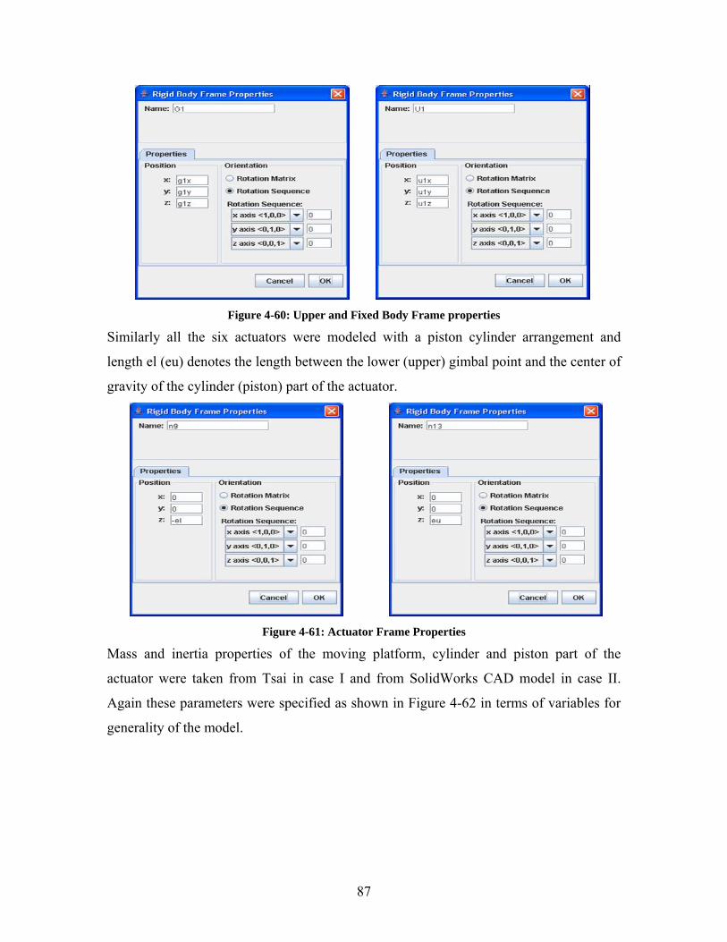
87

Figure 4-60: Upper and Fixed Body Frame properties

Similarly all the six actuators were modeled with a piston cylinder arrangement and

length el (eu) denotes the length between the lower (upper) gimbal point and the center of

gravity of the cylinder (piston) part of the actuator.

Figure 4-61: Actuator Frame Properties

Mass and inertia properties of the moving platform, cylinder and piston part of the

actuator were taken from Tsai in case I and from SolidWorks CAD model in case II.

Again these parameters were specified as shown in Figure 4-62 in terms of variables for

generality of the model.

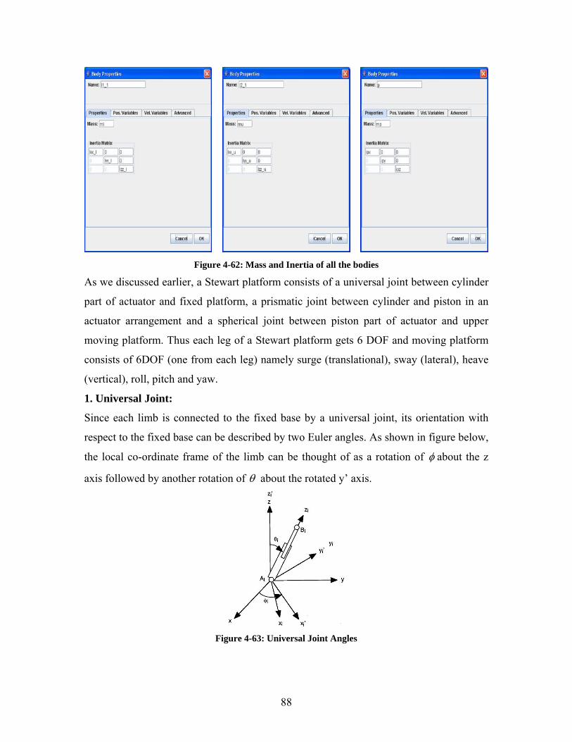
88

Figure 4-62: Mass and Inertia of all the bodies

As we discussed earlier, a Stewart platform consists of a universal joint between cylinder

part of actuator and fixed platform, a prismatic joint between cylinder and piston in an

actuator arrangement and a spherical joint between piston part of actuator and upper

moving platform. Thus each leg of a Stewart platform gets 6 DOF and moving platform

consists of 6DOF (one from each leg) namely surge (translational), sway (lateral), heave

(vertical), roll, pitch and yaw.

1. Universal Joint:

Since each limb is connected to the fixed base by a universal joint, its orientation with

respect to the fixed base can be described by two Euler angles. As shown in figure below,

the local co-ordinate frame of the limb can be thought of as a rotation of φ about the z

axis followed by another rotation of θ about the rotated y’ axis.

Figure 4-63: Universal Joint Angles

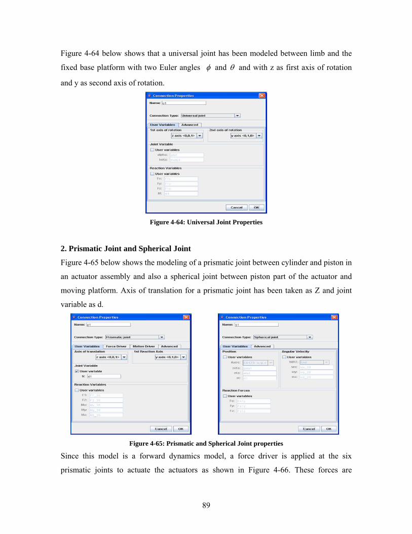
89

Figure 4-64 below shows that a universal joint has been modeled between limb and the

fixed base platform with two Euler angles φ and θ and with z as first axis of rotation

and y as second axis of rotation.

Figure 4-64: Universal Joint Properties

2. Prismatic Joint and Spherical Joint

Figure 4-65 below shows the modeling of a prismatic joint between cylinder and piston in

an actuator assembly and also a spherical joint between piston part of the actuator and

moving platform. Axis of translation for a prismatic joint has been taken as Z and joint

variable as d.

Figure 4-65: Prismatic and Spherical Joint properties

Since this model is a forward dynamics model, a force driver is applied at the six

prismatic joints to actuate the actuators as shown in Figure 4-66. These forces are

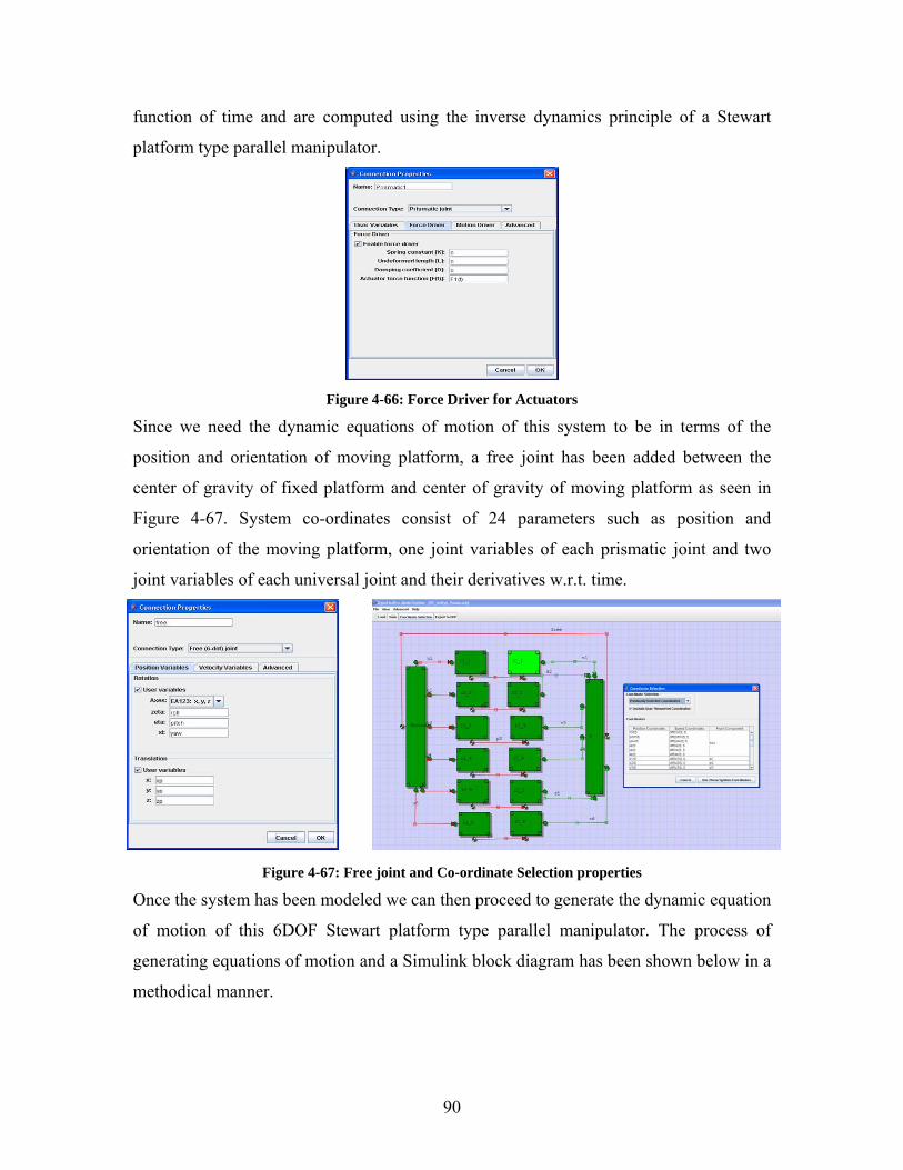
90

function of time and are computed using the inverse dynamics principle of a Stewart

platform type parallel manipulator.

Figure 4-66: Force Driver for Actuators

Since we need the dynamic equations of motion of this system to be in terms of the

position and orientation of moving platform, a free joint has been added between the

center of gravity of fixed platform and center of gravity of moving platform as seen in

Figure 4-67. System co-ordinates consist of 24 parameters such as position and

orientation of the moving platform, one joint variables of each prismatic joint and two

joint variables of each universal joint and their derivatives w.r.t. time.

Figure 4-67: Free joint and Co-ordinate Selection properties

Once the system has been modeled we can then proceed to generate the dynamic equation

of motion of this 6DOF Stewart platform type parallel manipulator. The process of

generating equations of motion and a Simulink block diagram has been shown below in a

methodical manner.

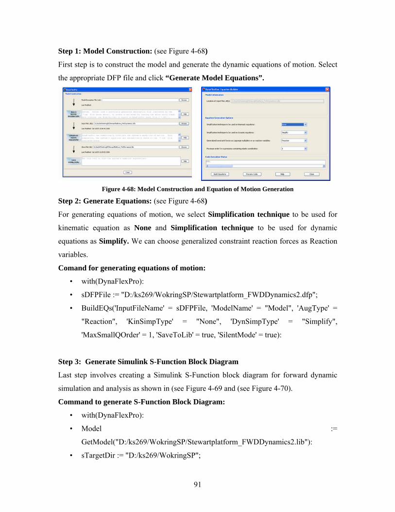
91

Step 1: Model Construction: (see Figure 4-68)

First step is to construct the model and generate the dynamic equations of motion. Select

the appropriate DFP file and click “Generate Model Equations”.

Figure 4-68: Model Construction and Equation of Motion Generation

Step 2: Generate Equations: (see Figure 4-68)

For generating equations of motion, we select Simplification technique to be used for

kinematic equation as None and Simplification technique to be used for dynamic

equations as Simplify. We can choose generalized constraint reaction forces as Reaction

variables.

Comand for generating equations of motion:

• with(DynaFlexPro):

• sDFPFile := "D:/ks269/WokringSP/Stewartplatform_FWDDynamics2.dfp";

• BuildEQs('InputFileName' = sDFPFile, 'ModelName' = "Model", 'AugType' =

"Reaction", 'KinSimpType' = "None", 'DynSimpType' = "Simplify",

'MaxSmallQOrder' = 1, 'SaveToLib' = true, 'SilentMode' = true):

Step 3: Generate Simulink S-Function Block Diagram

Last step involves creating a Simulink S-Function block diagram for forward dynamic

simulation and analysis as shown in (see Figure 4-69 and (see Figure 4-70).

Command to generate S-Function Block Diagram:

• with(DynaFlexPro):

• Model :=

GetModel("D:/ks269/WokringSP/Stewartplatform_FWDDynamics2.lib"):

• sTargetDir := "D:/ks269/WokringSP";

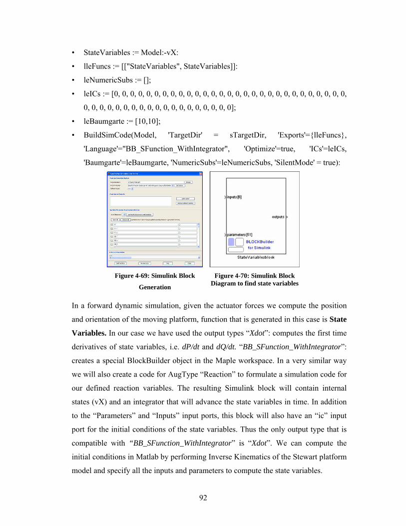
92

• StateVariables := Model:-vX:

• lleFuncs := [["StateVariables", StateVariables]]:

• leNumericSubs := [];

• leICs := [0, 0, 0, 0, 0, 0, 0, 0, 0, 0, 0, 0, 0, 0, 0, 0, 0, 0, 0, 0, 0, 0, 0, 0, 0, 0, 0, 0, 0,

0, 0, 0, 0, 0, 0, 0, 0, 0, 0, 0, 0, 0, 0, 0, 0, 0, 0, 0];

• leBaumgarte := [10,10];

• BuildSimCode(Model, 'TargetDir' = sTargetDir, 'Exports'={lleFuncs},

'Language'="BB_SFunction_WithIntegrator", 'Optimize'=true, 'ICs'=leICs,

'Baumgarte'=leBaumgarte, 'NumericSubs'=leNumericSubs, 'SilentMode' = true):

Figure 4-69: Simulink Block

Generation

Figure 4-70: Simulink Block

Diagram to find state variables

In a forward dynamic simulation, given the actuator forces we compute the position

and orientation of the moving platform, function that is generated in this case is State

Variables. In our case we have used the output types “Xdot”: computes the first time

derivatives of state variables, i.e. dP/dt and dQ/dt. “BB_SFunction_WithIntegrator”:

creates a special BlockBuilder object in the Maple workspace. In a very similar way

we will also create a code for AugType “Reaction” to formulate a simulation code for

our defined reaction variables. The resulting Simulink block will contain internal

states (vX) and an integrator that will advance the state variables in time. In addition

to the “Parameters” and “Inputs” input ports, this block will also have an “ic” input

port for the initial conditions of the state variables. Thus the only output type that is

compatible with “BB_SFunction_WithIntegrator” is “Xdot”. We can compute the

initial conditions in Matlab by performing Inverse Kinematics of the Stewart platform

model and specify all the inputs and parameters to compute the state variables.

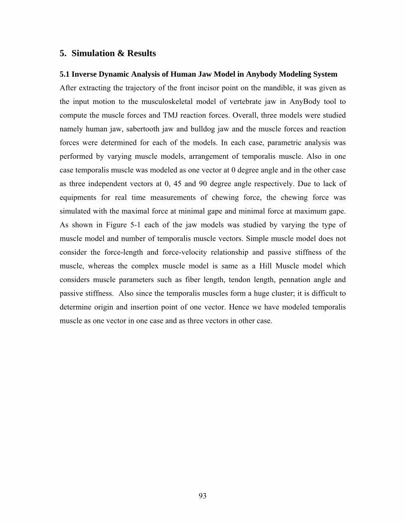
93

5. Simulation & Results 5.1 Inverse Dynamic Analysis of Human Jaw Model in Anybody Modeling System

After extracting the trajectory of the front incisor point on the mandible, it was given as

the input motion to the musculoskeletal model of vertebrate jaw in AnyBody tool to

compute the muscle forces and TMJ reaction forces. Overall, three models were studied

namely human jaw, sabertooth jaw and bulldog jaw and the muscle forces and reaction

forces were determined for each of the models. In each case, parametric analysis was

performed by varying muscle models, arrangement of temporalis muscle. Also in one

case temporalis muscle was modeled as one vector at 0 degree angle and in the other case

as three independent vectors at 0, 45 and 90 degree angle respectively. Due to lack of

equipments for real time measurements of chewing force, the chewing force was

simulated with the maximal force at minimal gape and minimal force at maximum gape.

As shown in Figure 5-1 each of the jaw models was studied by varying the type of

muscle model and number of temporalis muscle vectors. Simple muscle model does not

consider the force-length and force-velocity relationship and passive stiffness of the

muscle, whereas the complex muscle model is same as a Hill Muscle model which

considers muscle parameters such as fiber length, tendon length, pennation angle and

passive stiffness. Also since the temporalis muscles form a huge cluster; it is difficult to

determine origin and insertion point of one vector. Hence we have modeled temporalis

muscle as one vector in one case and as three vectors in other case.

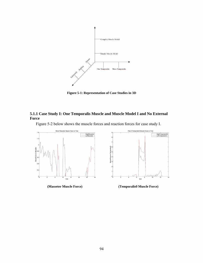
94

Figure 5-1: Representation of Case Studies in 3D

5.1.1 Case Study I: One Temporalis Muscle and Muscle Model I and No External Force

Figure 5-2 below shows the muscle forces and reaction forces for case study I.

(Masseter Muscle Force) (Temporalis0 Muscle Force)

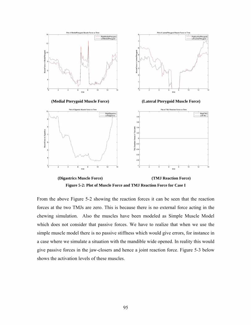
95

(Medial Pterygoid Muscle Force) (Lateral Pterygoid Muscle Force)

(Digastrics Muscle Force) (TMJ Reaction Force)

Figure 5-2: Plot of Muscle Force and TMJ Reaction Force for Case I

From the above Figure 5-2 showing the reaction forces it can be seen that the reaction

forces at the two TMJs are zero. This is because there is no external force acting in the

chewing simulation. Also the muscles have been modeled as Simple Muscle Model

which does not consider that passive forces. We have to realize that when we use the

simple muscle model there is no passive stiffness which would give errors, for instance in

a case where we simulate a situation with the mandible wide opened. In reality this would

give passive forces in the jaw-closers and hence a joint reaction force. Figure 5-3 below

shows the activation levels of these muscles.

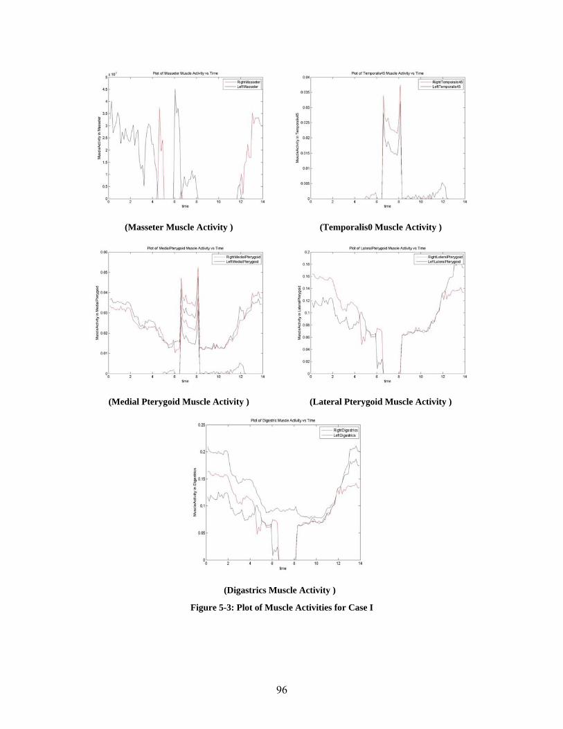
96

(Masseter Muscle Activity ) (Temporalis0 Muscle Activity )

(Medial Pterygoid Muscle Activity ) (Lateral Pterygoid Muscle Activity )

(Digastrics Muscle Activity )

Figure 5-3: Plot of Muscle Activities for Case I

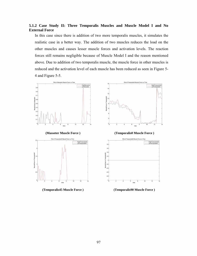
97

5.1.2 Case Study II: Three Temporalis Muscles and Muscle Model I and No External Force

In this case since there is addition of two more temporalis muscles, it simulates the

realistic case in a better way. The addition of two muscles reduces the load on the

other muscles and causes lesser muscle forces and activation levels. The reaction

forces still remains negligible because of Muscle Model I and the reason mentioned

above. Due to addition of two temporalis muscle, the muscle force in other muscles is

reduced and the activation level of each muscle has been reduced as seen in Figure 5-

4 and Figure 5-5.

(Masseter Muscle Force ) (Temporalis0 Muscle Force )

(Temporalis45 Muscle Force ) (Temporalis90 Muscle Force )

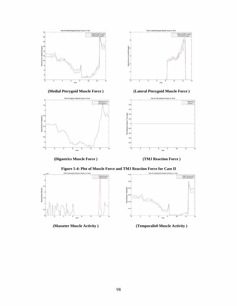
98

(Medial Pterygoid Muscle Force ) (Lateral Pterygoid Muscle Force )

(Digastrics Muscle Force ) (TMJ Reaction Force )

Figure 5-4: Plot of Muscle Force and TMJ Reaction Force for Case II

(Masseter Muscle Activity ) (Temporalis0 Muscle Activity )

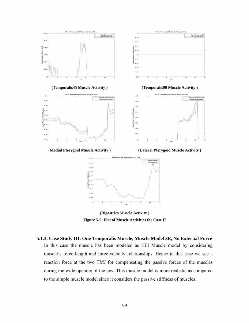
99

(Temporalis45 Muscle Activity ) (Temporalis90 Muscle Activity )

(Medial Pterygoid Muscle Activity ) (Lateral Pterygoid Muscle Activity )

(Digastrics Muscle Activity )

Figure 5-5: Plot of Muscle Activities for Case II

5.1.3. Case Study III: One Temporalis Muscle, Muscle Model 3E, No External Force In this case the muscle has been modeled as Hill Muscle model by considering

muscle’s force-length and force-velocity relationships. Hence in this case we see a

reaction force at the two TMJ for compensating the passive forces of the muscles

during the wide opening of the jaw. This muscle model is more realistic as compared

to the simple muscle model since it considers the passive stiffness of muscles.

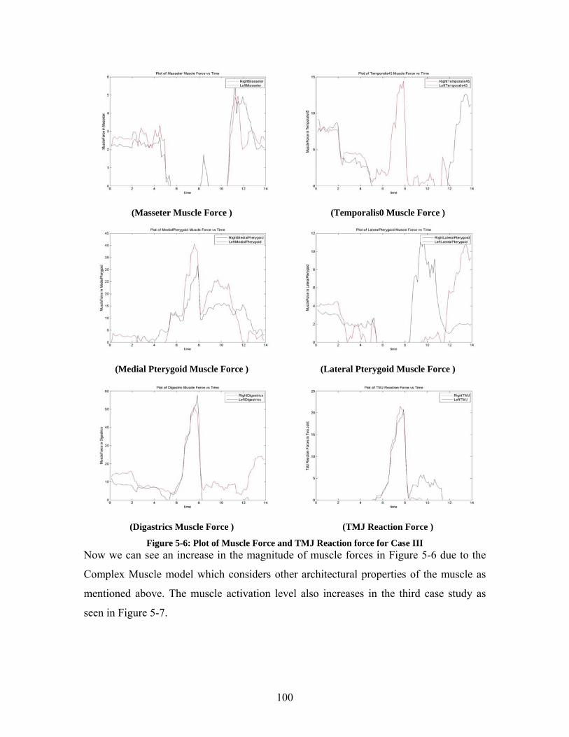
100

(Masseter Muscle Force ) (Temporalis0 Muscle Force )

(Medial Pterygoid Muscle Force ) (Lateral Pterygoid Muscle Force )

(Digastrics Muscle Force ) (TMJ Reaction Force )

Figure 5-6: Plot of Muscle Force and TMJ Reaction force for Case III Now we can see an increase in the magnitude of muscle forces in Figure 5-6 due to the

Complex Muscle model which considers other architectural properties of the muscle as

mentioned above. The muscle activation level also increases in the third case study as

seen in Figure 5-7.

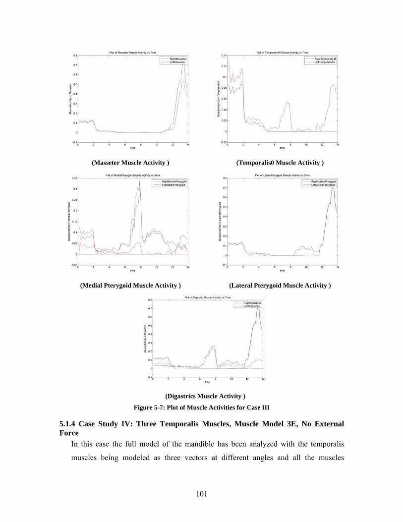
101

(Masseter Muscle Activity ) (Temporalis0 Muscle Activity )

(Medial Pterygoid Muscle Activity ) (Lateral Pterygoid Muscle Activity )

(Digastrics Muscle Activity )

Figure 5-7: Plot of Muscle Activities for Case III

5.1.4 Case Study IV: Three Temporalis Muscles, Muscle Model 3E, No External Force

In this case the full model of the mandible has been analyzed with the temporalis

muscles being modeled as three vectors at different angles and all the muscles

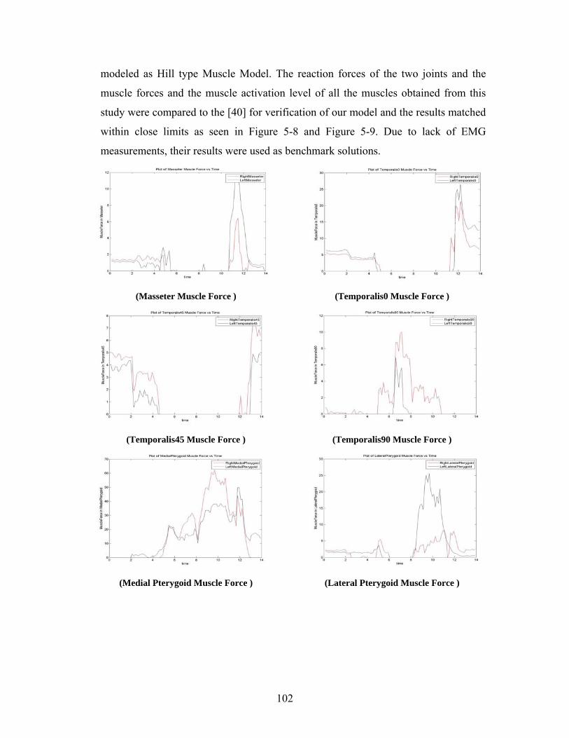
102

modeled as Hill type Muscle Model. The reaction forces of the two joints and the

muscle forces and the muscle activation level of all the muscles obtained from this

study were compared to the [40] for verification of our model and the results matched

within close limits as seen in Figure 5-8 and Figure 5-9. Due to lack of EMG

measurements, their results were used as benchmark solutions.

(Masseter Muscle Force ) (Temporalis0 Muscle Force )

(Temporalis45 Muscle Force ) (Temporalis90 Muscle Force )

(Medial Pterygoid Muscle Force ) (Lateral Pterygoid Muscle Force )

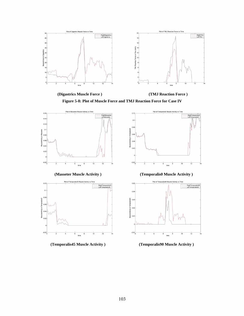
103

(Digastrics Muscle Force ) (TMJ Reaction Force )

Figure 5-8: Plot of Muscle Force and TMJ Reaction Force for Case IV

(Masseter Muscle Activity ) (Temporalis0 Muscle Activity )

(Temporalis45 Muscle Activity ) (Temporalis90 Muscle Activity )

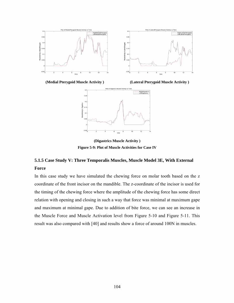
104

(Medial Pterygoid Muscle Activity ) (Lateral Pterygoid Muscle Activity )

(Digastrics Muscle Activity )

Figure 5-9: Plot of Muscle Activities for Case IV

5.1.5 Case Study V: Three Temporalis Muscles, Muscle Model 3E, With External

Force

In this case study we have simulated the chewing force on molar tooth based on the z

coordinate of the front incisor on the mandible. The z-coordinate of the incisor is used for

the timing of the chewing force where the amplitude of the chewing force has some direct

relation with opening and closing in such a way that force was minimal at maximum gape

and maximum at minimal gape. Due to addition of bite force, we can see an increase in

the Muscle Force and Muscle Activation level from Figure 5-10 and Figure 5-11. This

result was also compared with [40] and results show a force of around 100N in muscles.

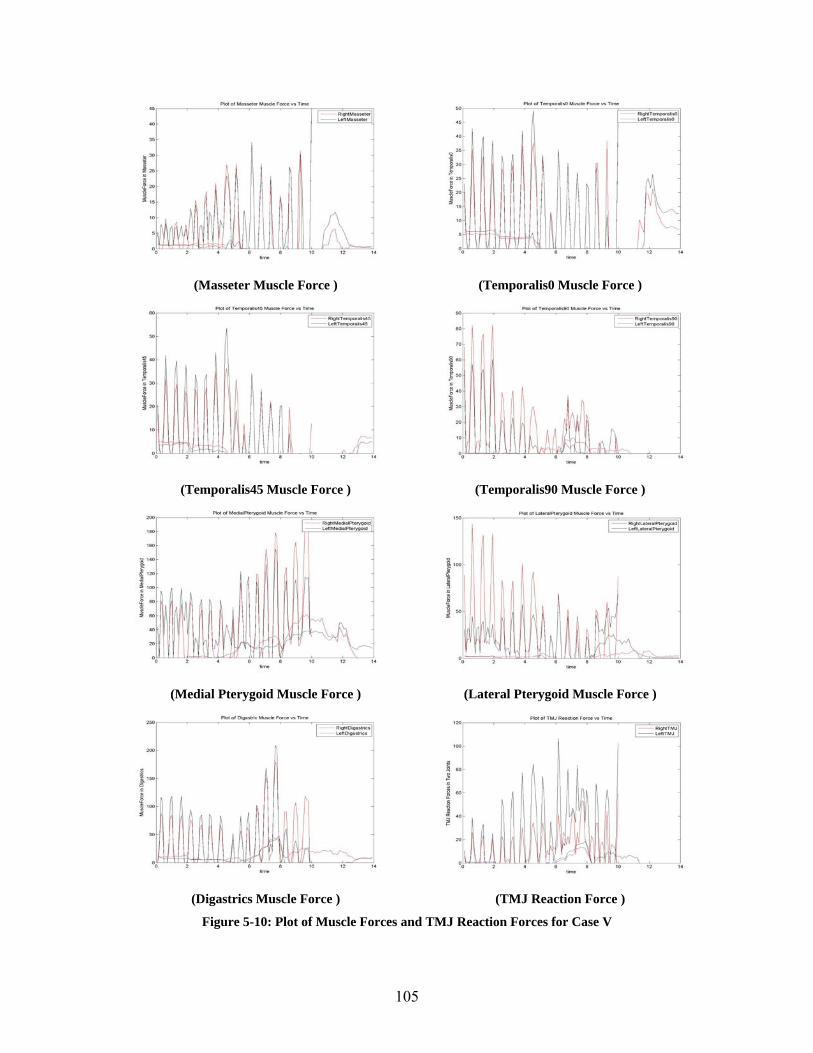
105

(Masseter Muscle Force ) (Temporalis0 Muscle Force )

(Temporalis45 Muscle Force ) (Temporalis90 Muscle Force )

(Medial Pterygoid Muscle Force ) (Lateral Pterygoid Muscle Force )

(Digastrics Muscle Force ) (TMJ Reaction Force )

Figure 5-10: Plot of Muscle Forces and TMJ Reaction Forces for Case V

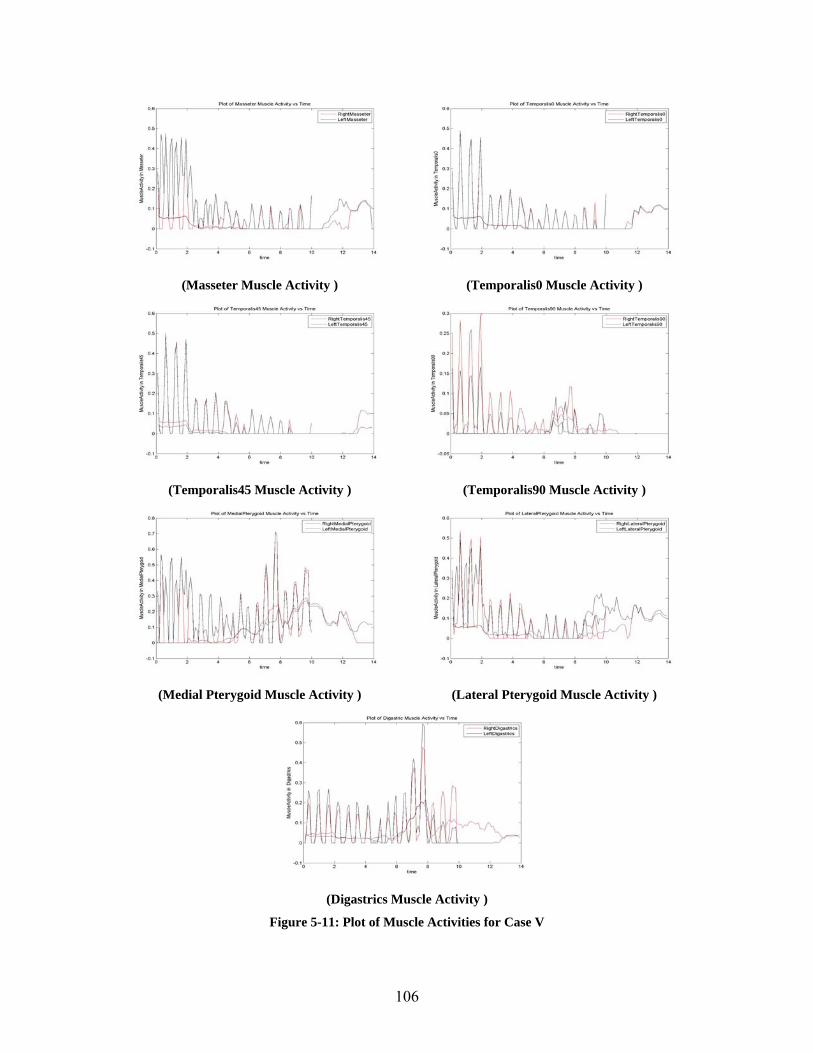
106

(Masseter Muscle Activity ) (Temporalis0 Muscle Activity )

(Temporalis45 Muscle Activity ) (Temporalis90 Muscle Activity )

(Medial Pterygoid Muscle Activity ) (Lateral Pterygoid Muscle Activity )

(Digastrics Muscle Activity )

Figure 5-11: Plot of Muscle Activities for Case V

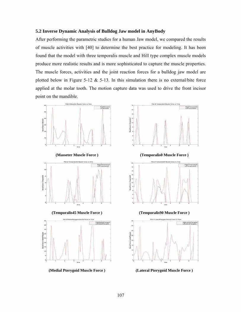
107

5.2 Inverse Dynamic Analysis of Bulldog Jaw model in AnyBody

After performing the parametric studies for a human Jaw model, we compared the results

of muscle activities with [40] to determine the best practice for modeling. It has been

found that the model with three temporalis muscle and Hill type complex muscle models

produce more realistic results and is more sophisticated to capture the muscle properties.

The muscle forces, activities and the joint reaction forces for a bulldog jaw model are

plotted below in Figure 5-12 & 5-13. In this simulation there is no external/bite force

applied at the molar tooth. The motion capture data was used to drive the front incisor

point on the mandible.

(Masseter Muscle Force ) (Temporalis0 Muscle Force )

(Temporalis45 Muscle Force ) (Temporalis90 Muscle Force )

(Medial Pterygoid Muscle Force ) (Lateral Pterygoid Muscle Force )

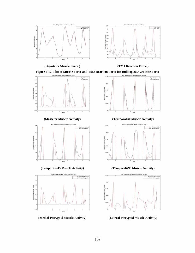
108

(Digastrics Muscle Force ) (TMJ Reaction Force )

Figure 5-12: Plot of Muscle Force and TMJ Reaction Force for Bulldog Jaw w/o Bite Force

(Masseter Muscle Activity) (Temporalis0 Muscle Activity)

(Temporalis45 Muscle Activity) (Temporalis90 Muscle Activity)

(Medial Pterygoid Muscle Activity) (Lateral Pterygoid Muscle Activity)

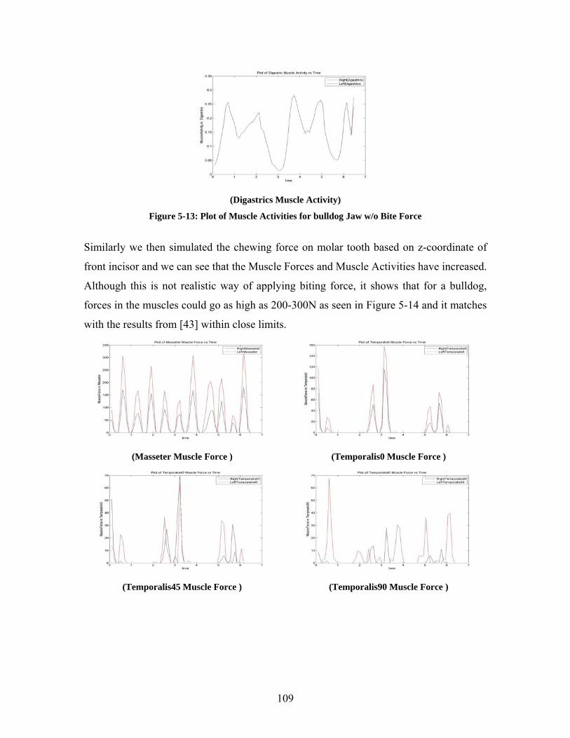
109

(Digastrics Muscle Activity)

Figure 5-13: Plot of Muscle Activities for bulldog Jaw w/o Bite Force

Similarly we then simulated the chewing force on molar tooth based on z-coordinate of

front incisor and we can see that the Muscle Forces and Muscle Activities have increased.

Although this is not realistic way of applying biting force, it shows that for a bulldog,

forces in the muscles could go as high as 200-300N as seen in Figure 5-14 and it matches

with the results from [43] within close limits.

(Masseter Muscle Force ) (Temporalis0 Muscle Force )

(Temporalis45 Muscle Force ) (Temporalis90 Muscle Force )

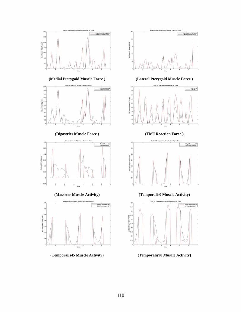
110

(Medial Pterygoid Muscle Force ) (Lateral Pterygoid Muscle Force )

(Digastrics Muscle Force ) (TMJ Reaction Force )

(Masseter Muscle Activity) (Temporalis0 Muscle Activity)

(Temporalis45 Muscle Activity) (Temporalis90 Muscle Activity)

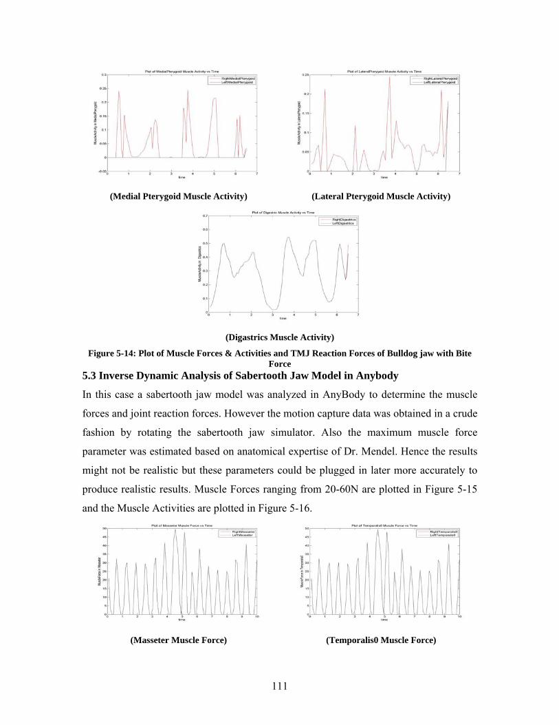
111

(Medial Pterygoid Muscle Activity) (Lateral Pterygoid Muscle Activity)

(Digastrics Muscle Activity)

Figure 5-14: Plot of Muscle Forces & Activities and TMJ Reaction Forces of Bulldog jaw with Bite Force

5.3 Inverse Dynamic Analysis of Sabertooth Jaw Model in Anybody

In this case a sabertooth jaw model was analyzed in AnyBody to determine the muscle

forces and joint reaction forces. However the motion capture data was obtained in a crude

fashion by rotating the sabertooth jaw simulator. Also the maximum muscle force

parameter was estimated based on anatomical expertise of Dr. Mendel. Hence the results

might not be realistic but these parameters could be plugged in later more accurately to

produce realistic results. Muscle Forces ranging from 20-60N are plotted in Figure 5-15

and the Muscle Activities are plotted in Figure 5-16.

(Masseter Muscle Force) (Temporalis0 Muscle Force)

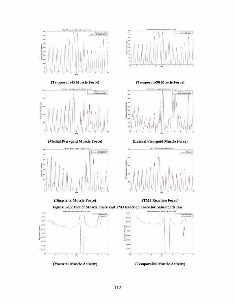
112

(Temporalis45 Muscle Force) (Temporalis90 Muscle Force)

(Medial Pterygoid Muscle Force) (Lateral Pterygoid Muscle Force)

(Digastrics Muscle Force) (TMJ Reaction Force)

Figure 5-15: Plot of Muscle Force and TMJ Reaction Force for Sabertooth Jaw

(Masseter Muscle Activity) (Temporalis0 Muscle Activity)

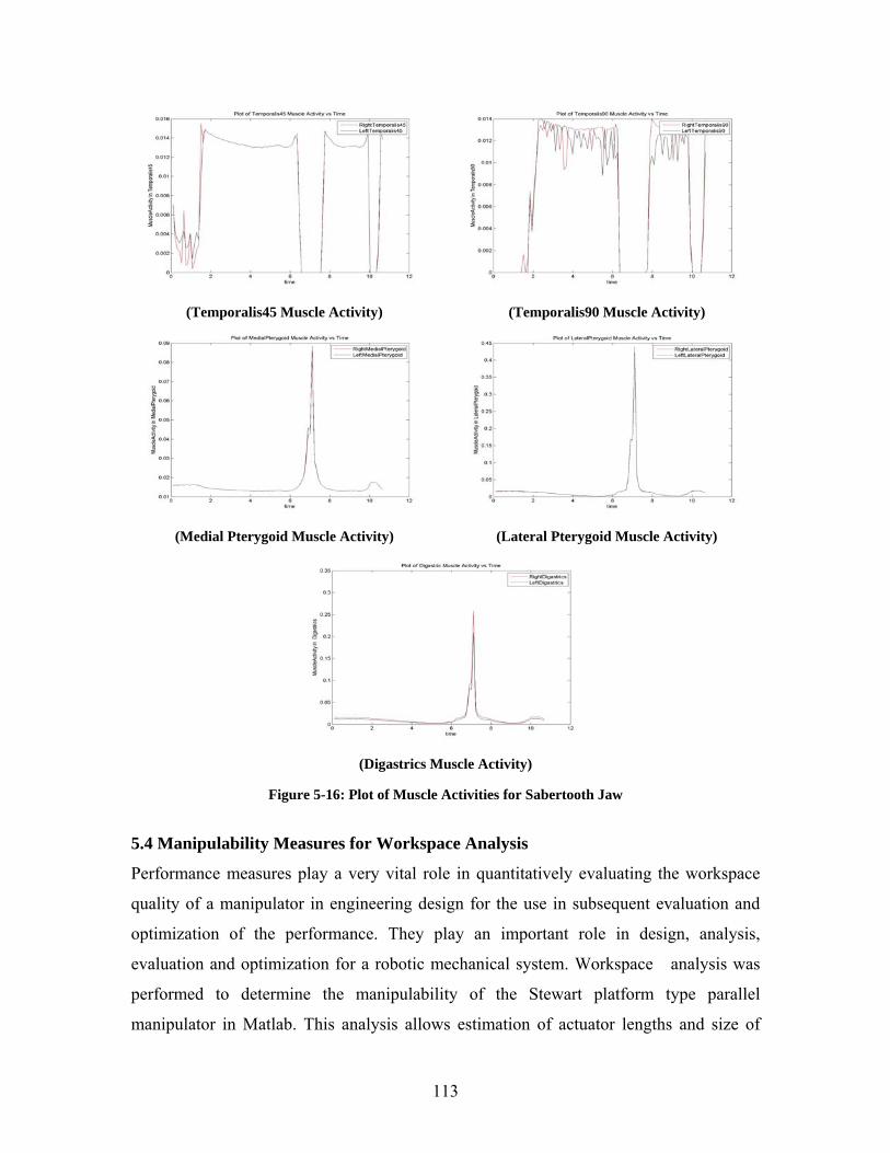
113

(Temporalis45 Muscle Activity) (Temporalis90 Muscle Activity)

(Medial Pterygoid Muscle Activity) (Lateral Pterygoid Muscle Activity)

(Digastrics Muscle Activity)

Figure 5-16: Plot of Muscle Activities for Sabertooth Jaw

5.4 Manipulability Measures for Workspace Analysis

Performance measures play a very vital role in quantitatively evaluating the workspace

quality of a manipulator in engineering design for the use in subsequent evaluation and

optimization of the performance. They play an important role in design, analysis,

evaluation and optimization for a robotic mechanical system. Workspace analysis was

performed to determine the manipulability of the Stewart platform type parallel

manipulator in Matlab. This analysis allows estimation of actuator lengths and size of

114

upper and fixed platforms required to reproduce the jaw motion trajectory of vertebrates.

By implementing workspace analysis it is possible to perform parametric analysis, by

varying the actuator lengths and platform dimensions, and determine the reachable

workspace of the parallel manipulator. As a first step, the Jacobian matrix of the 6DOF

parallel manipulator was computed as derived in Chapter 3. Singular value

decomposition of this Jacobian matrix was computed using the svd() function in Matlab.

The manipulability ellipsoid, yoshikawa measure and isotropy index were computed after

computing the singular value decomposition of Jacobian matrix, as shown in chapter 3.

The length of the actuator, radius of the upper platform and the radius of the workspace

in polar co-ordinates were parametrically varied to determine their optimum value for

best workspace quality. To suit the simulation of jaw motion, the radius of the fixed

platform was fixed at 0.2m. The upper platform’s radius was varied from 0.125m to 0.2m

and the range seems to be compatible with the size of the vertebrate jaw. The actuator are

required to produce a force of about 200-300N for withstanding the biting force. Hence

Linmot linear actuators were chosen for actuating the parallel mechanism. The lengths of

these actuators are varied from 0.175m to 0.3m to generate the required force. All these

actuators of different lengths have the capability of generating force ranging from 150-

300N which is sufficient to reproduce the mastication motion of vertebrates.

5.4.1 Case Study I: Varying the Radius of the Moving platform In the first case study the radius of the workspace was fixed at 40mm (for mastication

motion), the length of the actuator of the height between the upper and lower platform

was fixed at 0.2. The radius of the upper platform r was varied from 0.125 m to 0.2m to

determine the workspace quality of the moving platform for different dimensions.

Stewart platform configuration, surface plot of isotropy index of manipulability,

manipulability ellipsoid, and surface plot of yoshikawa measure of manipulability is

plotted in Figure 5-17 below. The manipulability ellipsoids are scaled down for clarity

and it shows that the manipulator is able to move the upper platform more along the

major axes and less along the minor axes. Since the manipulability ellipsoid does not

shrink and become straight line along minor axes, the end effector has a reasonable

workspace quality and does not get affected by singularity. Such visualization tool is

particularly useful in studying the motion transmission capability of a robotic system. We

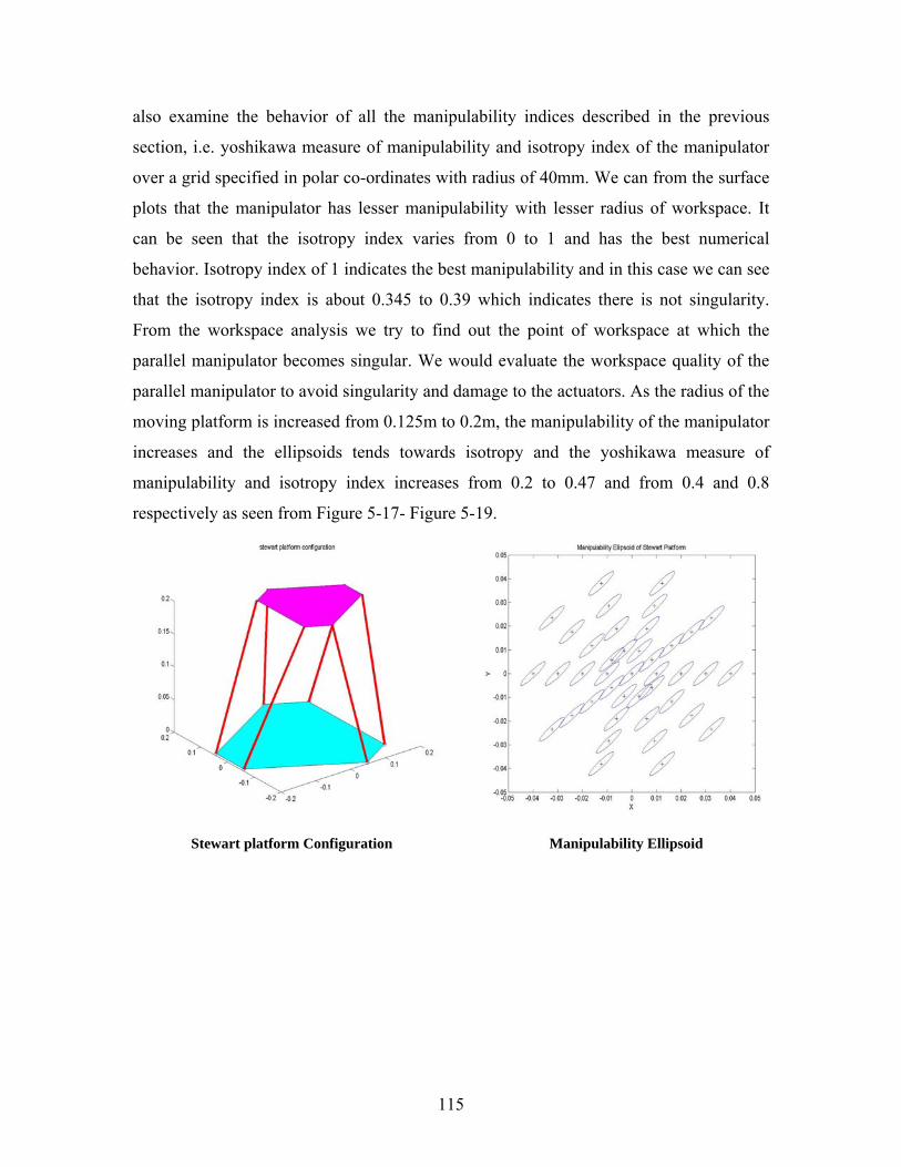
115

also examine the behavior of all the manipulability indices described in the previous

section, i.e. yoshikawa measure of manipulability and isotropy index of the manipulator

over a grid specified in polar co-ordinates with radius of 40mm. We can from the surface

plots that the manipulator has lesser manipulability with lesser radius of workspace. It

can be seen that the isotropy index varies from 0 to 1 and has the best numerical

behavior. Isotropy index of 1 indicates the best manipulability and in this case we can see

that the isotropy index is about 0.345 to 0.39 which indicates there is not singularity.

From the workspace analysis we try to find out the point of workspace at which the

parallel manipulator becomes singular. We would evaluate the workspace quality of the

parallel manipulator to avoid singularity and damage to the actuators. As the radius of the

moving platform is increased from 0.125m to 0.2m, the manipulability of the manipulator

increases and the ellipsoids tends towards isotropy and the yoshikawa measure of

manipulability and isotropy index increases from 0.2 to 0.47 and from 0.4 and 0.8

respectively as seen from Figure 5-17- Figure 5-19.

Stewart platform Configuration Manipulability Ellipsoid

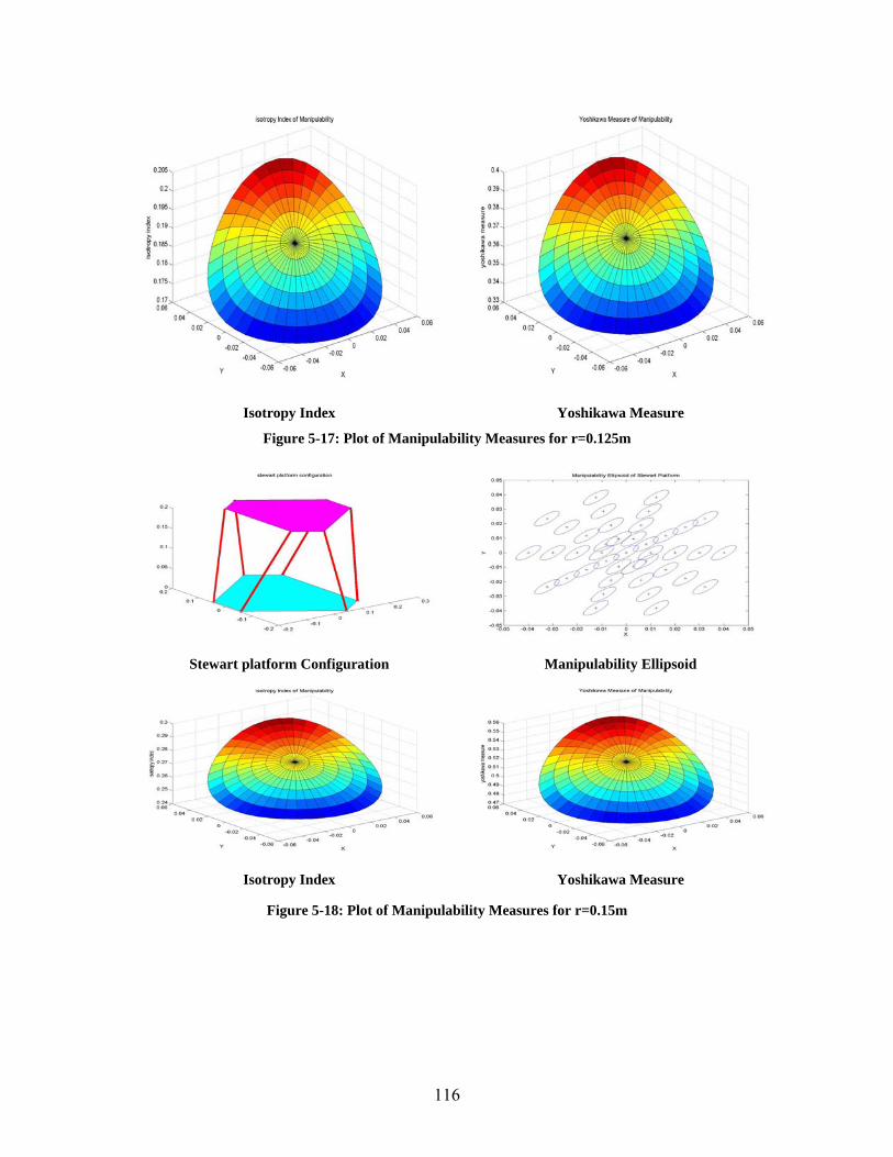
116

Isotropy Index Yoshikawa Measure

Figure 5-17: Plot of Manipulability Measures for r=0.125m

Stewart platform Configuration Manipulability Ellipsoid

Isotropy Index Yoshikawa Measure

Figure 5-18: Plot of Manipulability Measures for r=0.15m

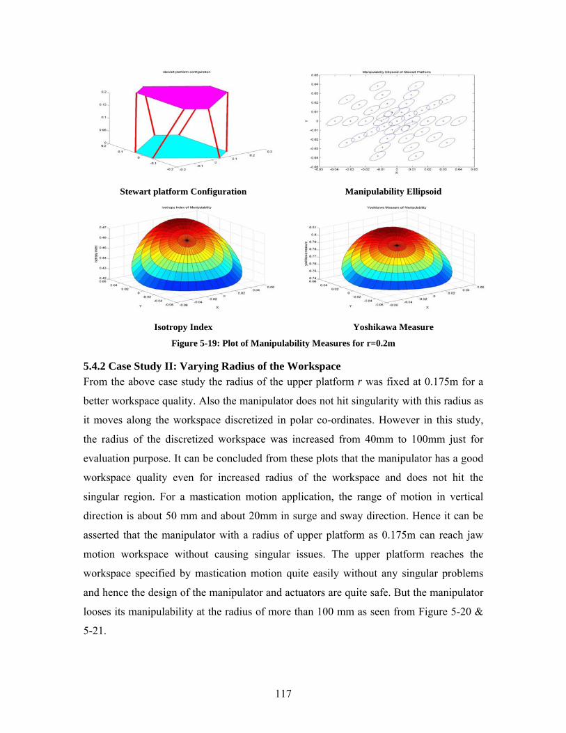
117

Stewart platform Configuration Manipulability Ellipsoid

Isotropy Index Yoshikawa Measure Figure 5-19: Plot of Manipulability Measures for r=0.2m

5.4.2 Case Study II: Varying Radius of the Workspace From the above case study the radius of the upper platform r was fixed at 0.175m for a

better workspace quality. Also the manipulator does not hit singularity with this radius as

it moves along the workspace discretized in polar co-ordinates. However in this study,

the radius of the discretized workspace was increased from 40mm to 100mm just for

evaluation purpose. It can be concluded from these plots that the manipulator has a good

workspace quality even for increased radius of the workspace and does not hit the

singular region. For a mastication motion application, the range of motion in vertical

direction is about 50 mm and about 20mm in surge and sway direction. Hence it can be

asserted that the manipulator with a radius of upper platform as 0.175m can reach jaw

motion workspace without causing singular issues. The upper platform reaches the

workspace specified by mastication motion quite easily without any singular problems

and hence the design of the manipulator and actuators are quite safe. But the manipulator

looses its manipulability at the radius of more than 100 mm as seen from Figure 5-20 &

5-21.

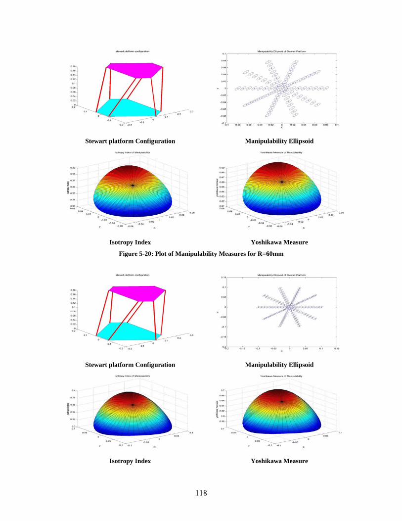
118

Stewart platform Configuration Manipulability Ellipsoid

Isotropy Index Yoshikawa Measure Figure 5-20: Plot of Manipulability Measures for R=60mm

Stewart platform Configuration Manipulability Ellipsoid

Isotropy Index Yoshikawa Measure

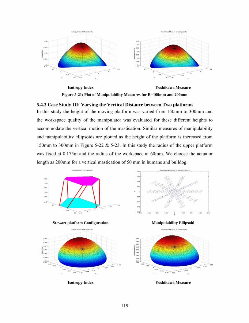
119

Isotropy Index Yoshikawa Measure Figure 5-21: Plot of Manipulability Measures for R=100mm and 200mm

5.4.3 Case Study III: Varying the Vertical Distance between Two platforms In this study the height of the moving platform was varied from 150mm to 300mm and

the workspace quality of the manipulator was evaluated for these different heights to

accommodate the vertical motion of the mastication. Similar measures of manipulability

and manipulability ellipsoids are plotted as the height of the platform is increased from

150mm to 300mm in Figure 5-22 & 5-23. In this study the radius of the upper platform

was fixed at 0.175m and the radius of the workspace at 60mm. We choose the actuator

length as 200mm for a vertical mastication of 50 mm in humans and bulldog.

Stewart platform Configuration Manipulability Ellipsoid

Isotropy Index Yoshikawa Measure

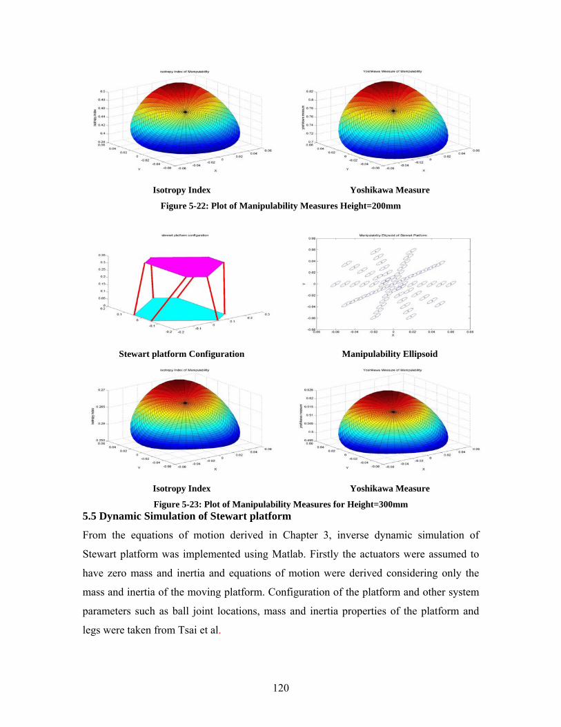
120

Isotropy Index Yoshikawa Measure Figure 5-22: Plot of Manipulability Measures Height=200mm

Stewart platform Configuration Manipulability Ellipsoid

Isotropy Index Yoshikawa Measure Figure 5-23: Plot of Manipulability Measures for Height=300mm

5.5 Dynamic Simulation of Stewart platform

From the equations of motion derived in Chapter 3, inverse dynamic simulation of

Stewart platform was implemented using Matlab. Firstly the actuators were assumed to

have zero mass and inertia and equations of motion were derived considering only the

mass and inertia of the moving platform. Configuration of the platform and other system

parameters such as ball joint locations, mass and inertia properties of the platform and

legs were taken from Tsai et al.

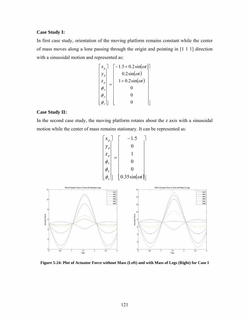
121

Case Study I:

In first case study, orientation of the moving platform remains constant while the center

of mass moves along a lone passing through the origin and pointing in [1 1 1] direction

with a sinusoidal motion and represented as:

( )( )( )

⎥⎥⎥⎥⎥⎥⎥⎥

⎦

⎤

⎢⎢⎢⎢⎢⎢⎢⎢

⎣

⎡

+

+−

=

⎥⎥⎥⎥⎥⎥⎥⎥

⎦

⎤

⎢⎢⎢⎢⎢⎢⎢⎢

⎣

⎡

000sin2.01

sin2.0sin2.05.1

tt

t

zyx

z

y

x

p

p

p

ωω

ω

φφφ

Case Study II:

In the second case study, the moving platform rotates about the z axis with a sinusoidal

motion while the center of mass remains stationary. It can be represented as:

( )⎥⎥⎥⎥⎥⎥⎥⎥

⎦

⎤

⎢⎢⎢⎢⎢⎢⎢⎢

⎣

⎡ −

=

⎥⎥⎥⎥⎥⎥⎥⎥

⎦

⎤

⎢⎢⎢⎢⎢⎢⎢⎢

⎣

⎡

t

zyx

z

y

x

p

p

p

ωφφφ

sin35.00010

5.1

Figure 5-24: Plot of Actuator Force without Mass (Left) and with Mass of Legs (Right) for Case I

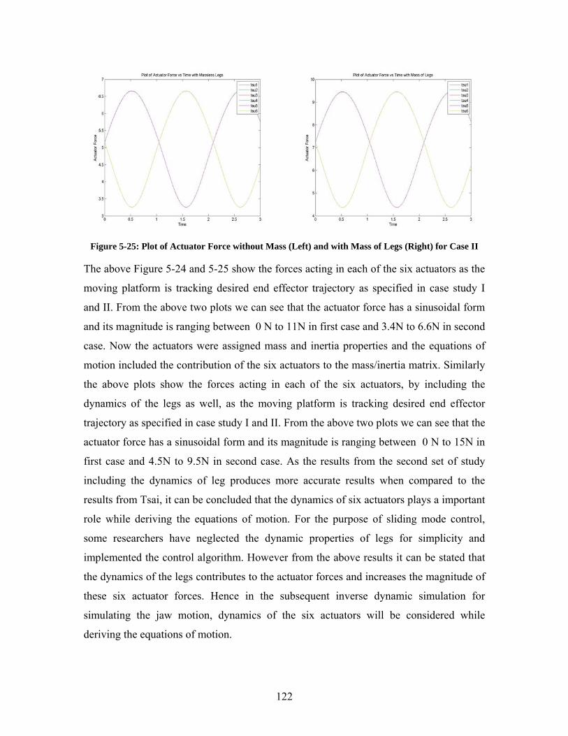
122

Figure 5-25: Plot of Actuator Force without Mass (Left) and with Mass of Legs (Right) for Case II The above Figure 5-24 and 5-25 show the forces acting in each of the six actuators as the

moving platform is tracking desired end effector trajectory as specified in case study I

and II. From the above two plots we can see that the actuator force has a sinusoidal form

and its magnitude is ranging between 0 N to 11N in first case and 3.4N to 6.6N in second

case. Now the actuators were assigned mass and inertia properties and the equations of

motion included the contribution of the six actuators to the mass/inertia matrix. Similarly

the above plots show the forces acting in each of the six actuators, by including the

dynamics of the legs as well, as the moving platform is tracking desired end effector

trajectory as specified in case study I and II. From the above two plots we can see that the

actuator force has a sinusoidal form and its magnitude is ranging between 0 N to 15N in

first case and 4.5N to 9.5N in second case. As the results from the second set of study

including the dynamics of leg produces more accurate results when compared to the

results from Tsai, it can be concluded that the dynamics of six actuators plays a important

role while deriving the equations of motion. For the purpose of sliding mode control,

some researchers have neglected the dynamic properties of legs for simplicity and

implemented the control algorithm. However from the above results it can be stated that

the dynamics of the legs contributes to the actuator forces and increases the magnitude of

these six actuator forces. Hence in the subsequent inverse dynamic simulation for

simulating the jaw motion, dynamics of the six actuators will be considered while

deriving the equations of motion.

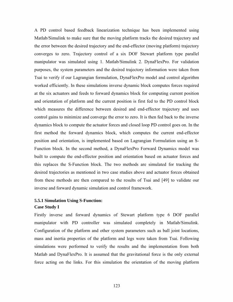
123

A PD control based feedback linearization technique has been implemented using

Matlab/Simulink to make sure that the moving platform tracks the desired trajectory and

the error between the desired trajectory and the end-effector (moving platform) trajectory

converges to zero. Trajectory control of a six DOF Stewart platform type parallel

manipulator was simulated using 1. Matlab/Simulink 2. DynaFlexPro. For validation

purposes, the system parameters and the desired trajectory information were taken from

Tsai to verify if our Lagrangian formulation, DynaFlexPro model and control algorithm

worked efficiently. In these simulations inverse dynamic block computes forces required

at the six actuators and feeds to forward dynamics block for computing current position

and orientation of platform and the current position is first fed to the PD control block

which measures the difference between desired and end-effector trajectory and uses

control gains to minimize and converge the error to zero. It is then fed back to the inverse

dynamics block to compute the actuator forces and closed loop PD control goes on. In the

first method the forward dynamics block, which computes the current end-effector

position and orientation, is implemented based on Lagrangian Formulation using an S-

Function block. In the second method, a DynaFlexPro Forward Dynamics model was

built to compute the end-effector position and orientation based on actuator forces and

this replaces the S-Function block. The two methods are simulated for tracking the

desired trajectories as mentioned in two case studies above and actuator forces obtained

from these methods are then compared to the results of Tsai and [49] to validate our

inverse and forward dynamic simulation and control framework.

5.5.1 Simulation Using S-Function: Case Study I

Firstly inverse and forward dynamics of Stewart platform type 6 DOF parallel

manipulator with PD controller was simulated completely in Matlab/Simulink.

Configuration of the platform and other system parameters such as ball joint locations,

mass and inertia properties of the platform and legs were taken from Tsai. Following

simulations were performed to verify the results and the implementation from both

Matlab and DynaFlexPro. It is assumed that the gravitational force is the only external

force acting on the links. For this simulation the orientation of the moving platform

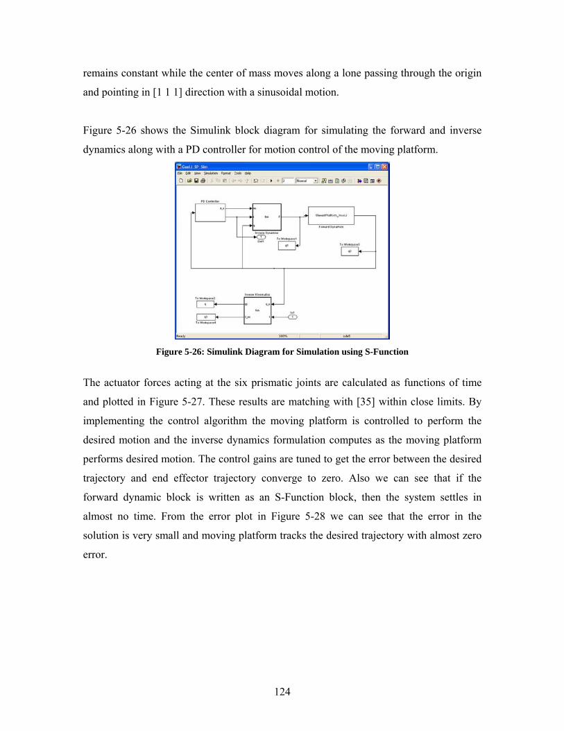
124

remains constant while the center of mass moves along a lone passing through the origin

and pointing in [1 1 1] direction with a sinusoidal motion.

Figure 5-26 shows the Simulink block diagram for simulating the forward and inverse

dynamics along with a PD controller for motion control of the moving platform.

Figure 5-26: Simulink Diagram for Simulation using S-Function

The actuator forces acting at the six prismatic joints are calculated as functions of time

and plotted in Figure 5-27. These results are matching with [35] within close limits. By

implementing the control algorithm the moving platform is controlled to perform the

desired motion and the inverse dynamics formulation computes as the moving platform

performs desired motion. The control gains are tuned to get the error between the desired

trajectory and end effector trajectory converge to zero. Also we can see that if the

forward dynamic block is written as an S-Function block, then the system settles in

almost no time. From the error plot in Figure 5-28 we can see that the error in the

solution is very small and moving platform tracks the desired trajectory with almost zero

error.

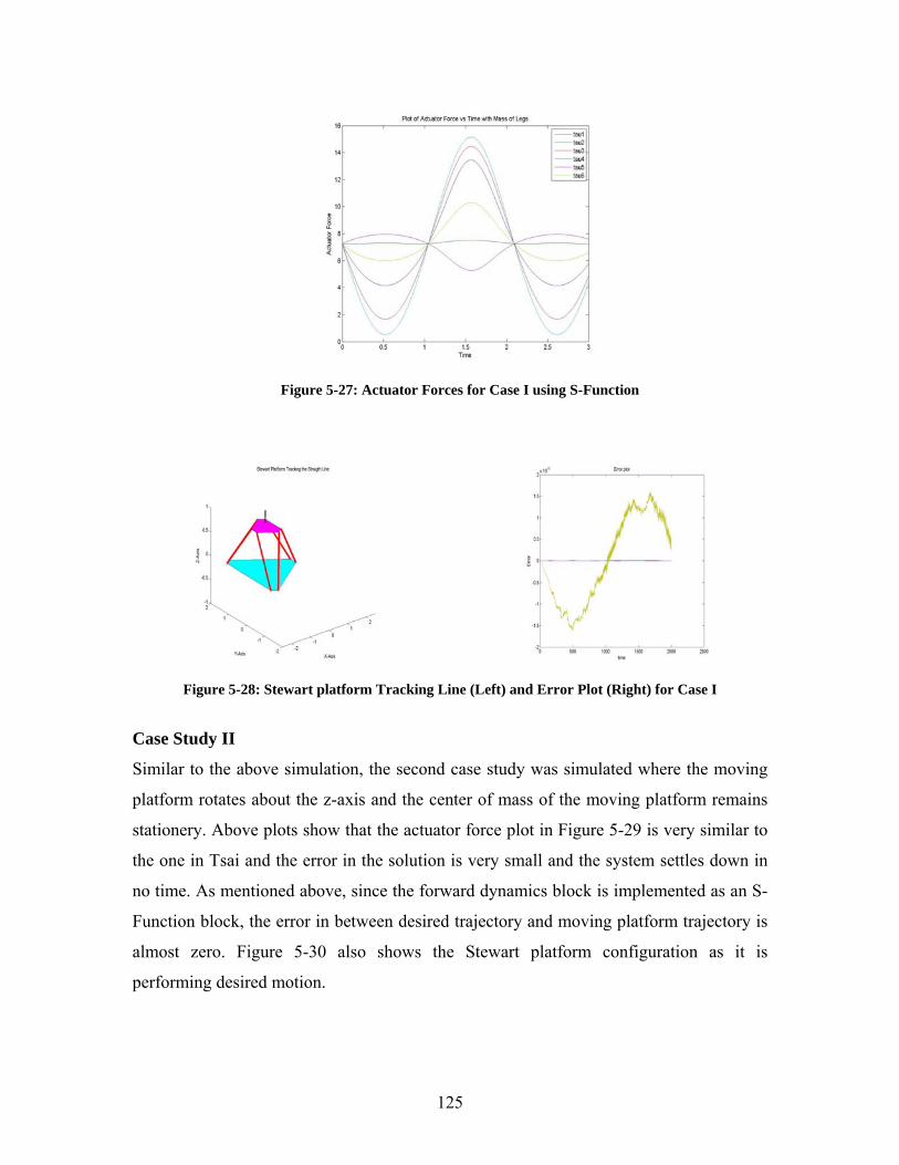
125

Figure 5-27: Actuator Forces for Case I using S-Function

Figure 5-28: Stewart platform Tracking Line (Left) and Error Plot (Right) for Case I

Case Study II

Similar to the above simulation, the second case study was simulated where the moving

platform rotates about the z-axis and the center of mass of the moving platform remains

stationery. Above plots show that the actuator force plot in Figure 5-29 is very similar to

the one in Tsai and the error in the solution is very small and the system settles down in

no time. As mentioned above, since the forward dynamics block is implemented as an S-

Function block, the error in between desired trajectory and moving platform trajectory is

almost zero. Figure 5-30 also shows the Stewart platform configuration as it is

performing desired motion.

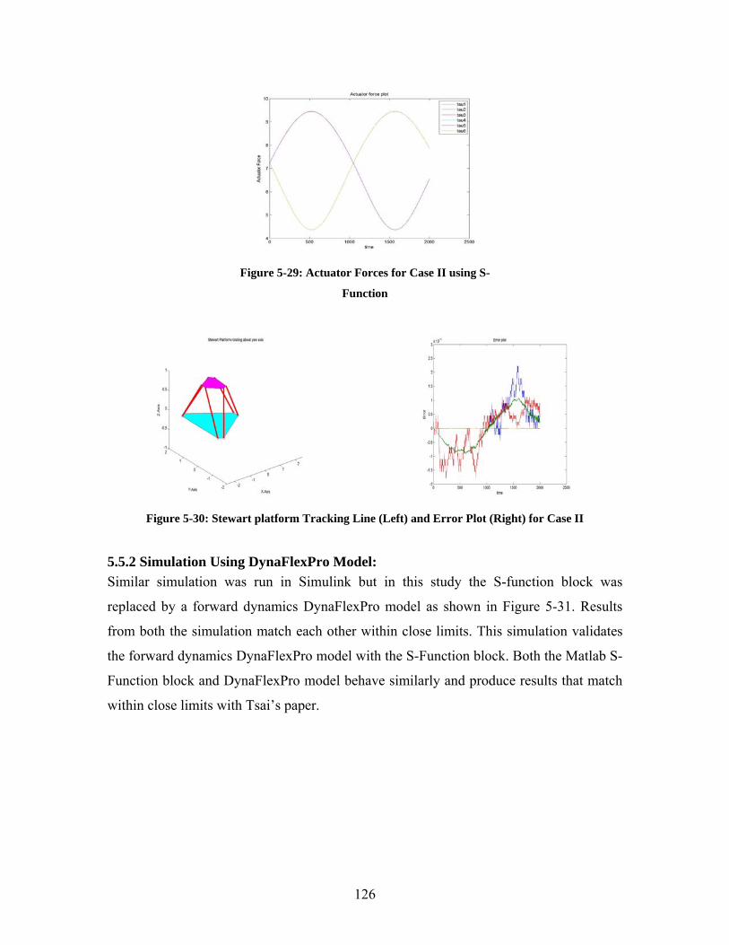
126

Figure 5-29: Actuator Forces for Case II using S-

Function

Figure 5-30: Stewart platform Tracking Line (Left) and Error Plot (Right) for Case II

5.5.2 Simulation Using DynaFlexPro Model: Similar simulation was run in Simulink but in this study the S-function block was

replaced by a forward dynamics DynaFlexPro model as shown in Figure 5-31. Results

from both the simulation match each other within close limits. This simulation validates

the forward dynamics DynaFlexPro model with the S-Function block. Both the Matlab S-

Function block and DynaFlexPro model behave similarly and produce results that match

within close limits with Tsai’s paper.

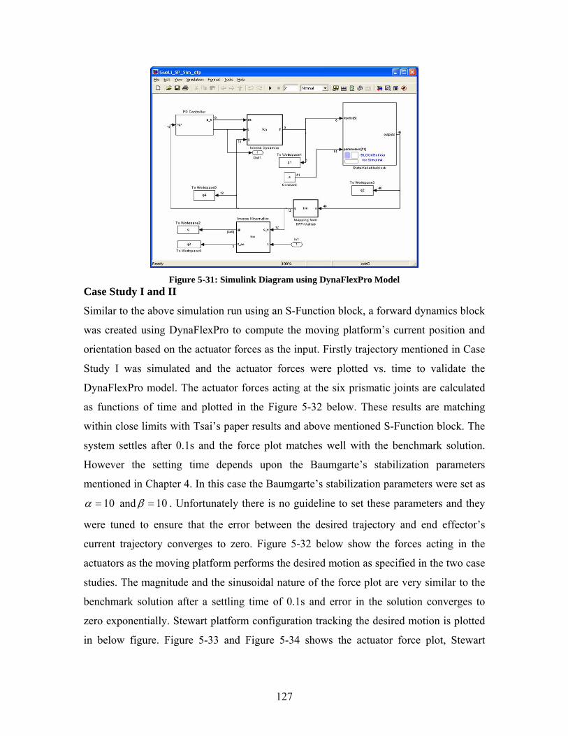
127

Figure 5-31: Simulink Diagram using DynaFlexPro Model

Case Study I and II

Similar to the above simulation run using an S-Function block, a forward dynamics block

was created using DynaFlexPro to compute the moving platform’s current position and

orientation based on the actuator forces as the input. Firstly trajectory mentioned in Case

Study I was simulated and the actuator forces were plotted vs. time to validate the

DynaFlexPro model. The actuator forces acting at the six prismatic joints are calculated

as functions of time and plotted in the Figure 5-32 below. These results are matching

within close limits with Tsai’s paper results and above mentioned S-Function block. The

system settles after 0.1s and the force plot matches well with the benchmark solution.

However the setting time depends upon the Baumgarte’s stabilization parameters

mentioned in Chapter 4. In this case the Baumgarte’s stabilization parameters were set as

10=α and 10=β . Unfortunately there is no guideline to set these parameters and they

were tuned to ensure that the error between the desired trajectory and end effector’s

current trajectory converges to zero. Figure 5-32 below show the forces acting in the

actuators as the moving platform performs the desired motion as specified in the two case

studies. The magnitude and the sinusoidal nature of the force plot are very similar to the

benchmark solution after a settling time of 0.1s and error in the solution converges to

zero exponentially. Stewart platform configuration tracking the desired motion is plotted

in below figure. Figure 5-33 and Figure 5-34 shows the actuator force plot, Stewart

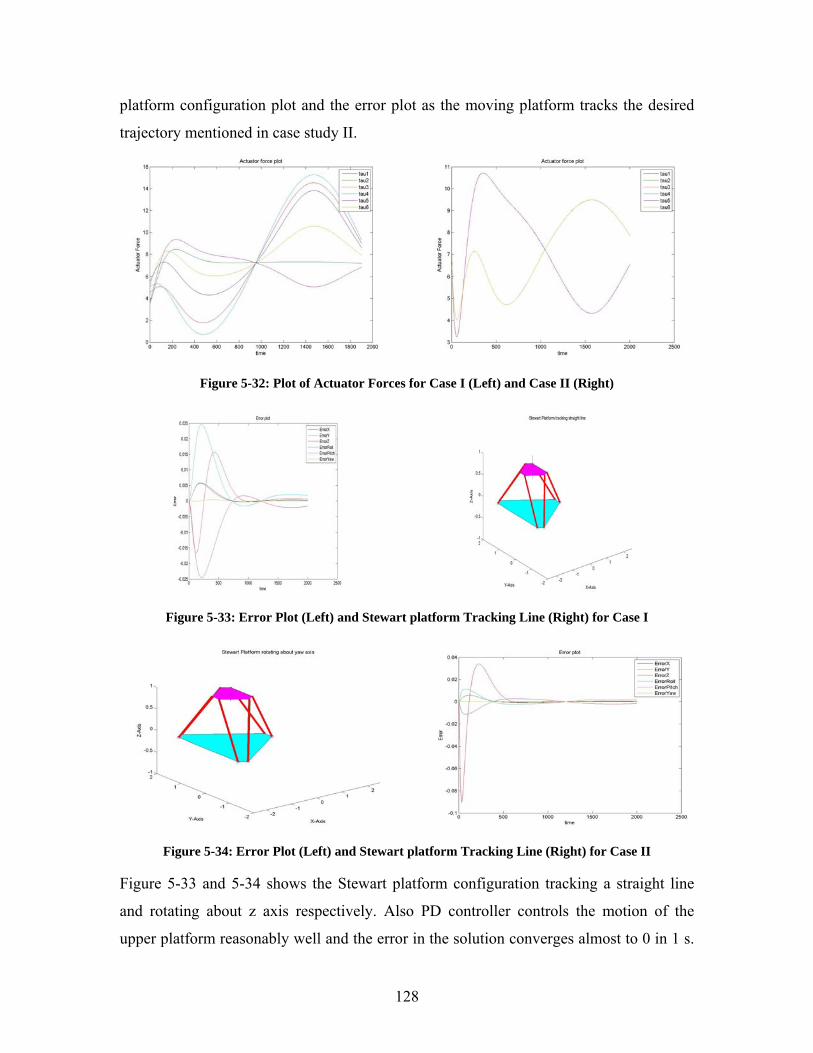
128

platform configuration plot and the error plot as the moving platform tracks the desired

trajectory mentioned in case study II.

Figure 5-32: Plot of Actuator Forces for Case I (Left) and Case II (Right)

Figure 5-33: Error Plot (Left) and Stewart platform Tracking Line (Right) for Case I

Figure 5-34: Error Plot (Left) and Stewart platform Tracking Line (Right) for Case II Figure 5-33 and 5-34 shows the Stewart platform configuration tracking a straight line

and rotating about z axis respectively. Also PD controller controls the motion of the

upper platform reasonably well and the error in the solution converges almost to 0 in 1 s.

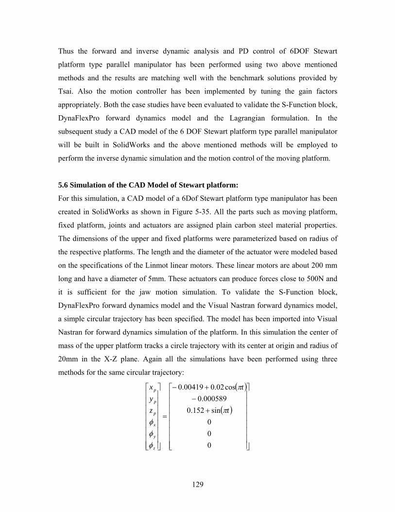
129

Thus the forward and inverse dynamic analysis and PD control of 6DOF Stewart

platform type parallel manipulator has been performed using two above mentioned

methods and the results are matching well with the benchmark solutions provided by

Tsai. Also the motion controller has been implemented by tuning the gain factors

appropriately. Both the case studies have been evaluated to validate the S-Function block,

DynaFlexPro forward dynamics model and the Lagrangian formulation. In the

subsequent study a CAD model of the 6 DOF Stewart platform type parallel manipulator

will be built in SolidWorks and the above mentioned methods will be employed to

perform the inverse dynamic simulation and the motion control of the moving platform.

5.6 Simulation of the CAD Model of Stewart platform:

For this simulation, a CAD model of a 6Dof Stewart platform type manipulator has been

created in SolidWorks as shown in Figure 5-35. All the parts such as moving platform,

fixed platform, joints and actuators are assigned plain carbon steel material properties.

The dimensions of the upper and fixed platforms were parameterized based on radius of

the respective platforms. The length and the diameter of the actuator were modeled based

on the specifications of the Linmot linear motors. These linear motors are about 200 mm

long and have a diameter of 5mm. These actuators can produce forces close to 500N and

it is sufficient for the jaw motion simulation. To validate the S-Function block,

DynaFlexPro forward dynamics model and the Visual Nastran forward dynamics model,

a simple circular trajectory has been specified. The model has been imported into Visual

Nastran for forward dynamics simulation of the platform. In this simulation the center of

mass of the upper platform tracks a circle trajectory with its center at origin and radius of

20mm in the X-Z plane. Again all the simulations have been performed using three

methods for the same circular trajectory:

( )

( )

⎥⎥⎥⎥⎥⎥⎥⎥

⎦

⎤

⎢⎢⎢⎢⎢⎢⎢⎢

⎣

⎡

+−

+−

=

⎥⎥⎥⎥⎥⎥⎥⎥

⎦

⎤

⎢⎢⎢⎢⎢⎢⎢⎢

⎣

⎡

000

sin152.0000589.0

cos02.000419.0

t

t

zyx

z

y

x

p

p

p

π

π

φφφ

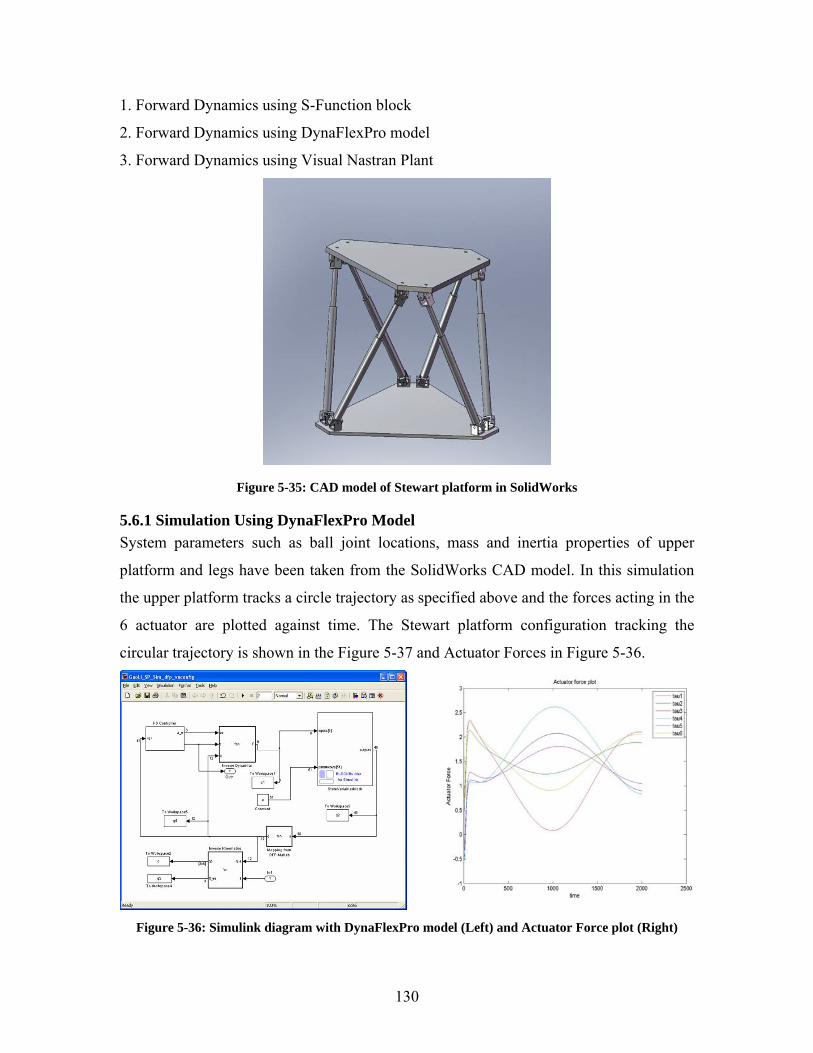
130

1. Forward Dynamics using S-Function block

2. Forward Dynamics using DynaFlexPro model

3. Forward Dynamics using Visual Nastran Plant

Figure 5-35: CAD model of Stewart platform in SolidWorks

5.6.1 Simulation Using DynaFlexPro Model System parameters such as ball joint locations, mass and inertia properties of upper

platform and legs have been taken from the SolidWorks CAD model. In this simulation

the upper platform tracks a circle trajectory as specified above and the forces acting in the

6 actuator are plotted against time. The Stewart platform configuration tracking the

circular trajectory is shown in the Figure 5-37 and Actuator Forces in Figure 5-36.

Figure 5-36: Simulink diagram with DynaFlexPro model (Left) and Actuator Force plot (Right)

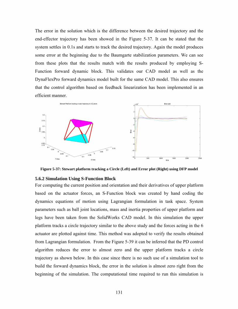
131

The error in the solution which is the difference between the desired trajectory and the

end-effector trajectory has been showed in the Figure 5-37. It can be stated that the

system settles in 0.1s and starts to track the desired trajectory. Again the model produces

some error at the beginning due to the Baumgarte stabilization parameters. We can see

from these plots that the results match with the results produced by employing S-

Function forward dynamic block. This validates our CAD model as well as the

DynaFlexPro forward dynamics model built for the same CAD model. This also ensures

that the control algorithm based on feedback linearization has been implemented in an

efficient manner.

Figure 5-37: Stewart platform tracking a Circle (Left) and Error plot (Right) using DFP model

5.6.2 Simulation Using S-Function Block For computing the current position and orientation and their derivatives of upper platform

based on the actuator forces, an S-Function block was created by hand coding the

dynamics equations of motion using Lagrangian formulation in task space. System

parameters such as ball joint locations, mass and inertia properties of upper platform and

legs have been taken from the SolidWorks CAD model. In this simulation the upper

platform tracks a circle trajectory similar to the above study and the forces acting in the 6

actuator are plotted against time. This method was adopted to verify the results obtained

from Lagrangian formulation. From the Figure 5-39 it can be inferred that the PD control

algorithm reduces the error to almost zero and the upper platform tracks a circle

trajectory as shown below. In this case since there is no such use of a simulation tool to

build the forward dynamics block, the error in the solution is almost zero right from the

beginning of the simulation. The computational time required to run this simulation is

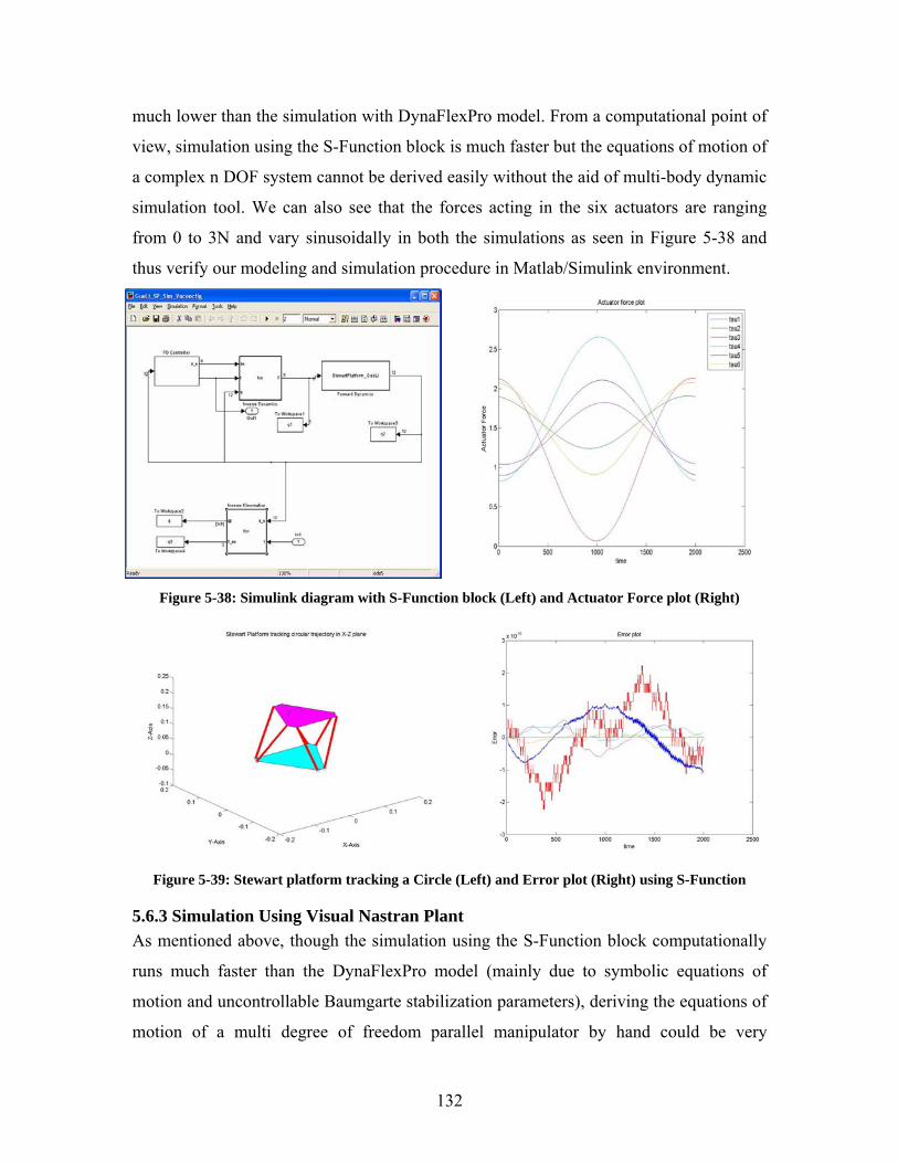
132

much lower than the simulation with DynaFlexPro model. From a computational point of

view, simulation using the S-Function block is much faster but the equations of motion of

a complex n DOF system cannot be derived easily without the aid of multi-body dynamic

simulation tool. We can also see that the forces acting in the six actuators are ranging

from 0 to 3N and vary sinusoidally in both the simulations as seen in Figure 5-38 and

thus verify our modeling and simulation procedure in Matlab/Simulink environment.

Figure 5-38: Simulink diagram with S-Function block (Left) and Actuator Force plot (Right)

Figure 5-39: Stewart platform tracking a Circle (Left) and Error plot (Right) using S-Function

5.6.3 Simulation Using Visual Nastran Plant As mentioned above, though the simulation using the S-Function block computationally

runs much faster than the DynaFlexPro model (mainly due to symbolic equations of

motion and uncontrollable Baumgarte stabilization parameters), deriving the equations of

motion of a multi degree of freedom parallel manipulator by hand could be very

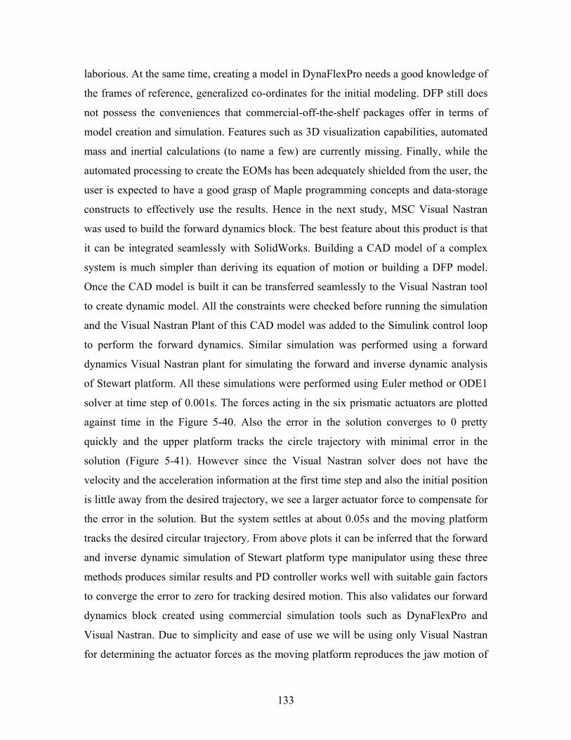
133

laborious. At the same time, creating a model in DynaFlexPro needs a good knowledge of

the frames of reference, generalized co-ordinates for the initial modeling. DFP still does

not possess the conveniences that commercial-off-the-shelf packages offer in terms of

model creation and simulation. Features such as 3D visualization capabilities, automated

mass and inertial calculations (to name a few) are currently missing. Finally, while the

automated processing to create the EOMs has been adequately shielded from the user, the

user is expected to have a good grasp of Maple programming concepts and data-storage

constructs to effectively use the results. Hence in the next study, MSC Visual Nastran

was used to build the forward dynamics block. The best feature about this product is that

it can be integrated seamlessly with SolidWorks. Building a CAD model of a complex

system is much simpler than deriving its equation of motion or building a DFP model.

Once the CAD model is built it can be transferred seamlessly to the Visual Nastran tool

to create dynamic model. All the constraints were checked before running the simulation

and the Visual Nastran Plant of this CAD model was added to the Simulink control loop

to perform the forward dynamics. Similar simulation was performed using a forward

dynamics Visual Nastran plant for simulating the forward and inverse dynamic analysis

of Stewart platform. All these simulations were performed using Euler method or ODE1

solver at time step of 0.001s. The forces acting in the six prismatic actuators are plotted

against time in the Figure 5-40. Also the error in the solution converges to 0 pretty

quickly and the upper platform tracks the circle trajectory with minimal error in the

solution (Figure 5-41). However since the Visual Nastran solver does not have the

velocity and the acceleration information at the first time step and also the initial position

is little away from the desired trajectory, we see a larger actuator force to compensate for

the error in the solution. But the system settles at about 0.05s and the moving platform

tracks the desired circular trajectory. From above plots it can be inferred that the forward

and inverse dynamic simulation of Stewart platform type manipulator using these three

methods produces similar results and PD controller works well with suitable gain factors

to converge the error to zero for tracking desired motion. This also validates our forward

dynamics block created using commercial simulation tools such as DynaFlexPro and

Visual Nastran. Due to simplicity and ease of use we will be using only Visual Nastran

for determining the actuator forces as the moving platform reproduces the jaw motion of

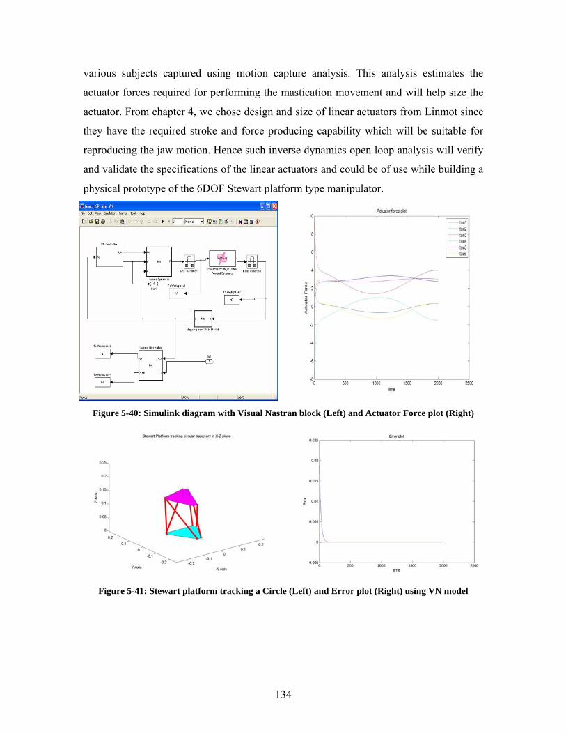
134

various subjects captured using motion capture analysis. This analysis estimates the

actuator forces required for performing the mastication movement and will help size the

actuator. From chapter 4, we chose design and size of linear actuators from Linmot since

they have the required stroke and force producing capability which will be suitable for

reproducing the jaw motion. Hence such inverse dynamics open loop analysis will verify

and validate the specifications of the linear actuators and could be of use while building a

physical prototype of the 6DOF Stewart platform type manipulator.

Figure 5-40: Simulink diagram with Visual Nastran block (Left) and Actuator Force plot (Right)

Figure 5-41: Stewart platform tracking a Circle (Left) and Error plot (Right) using VN model

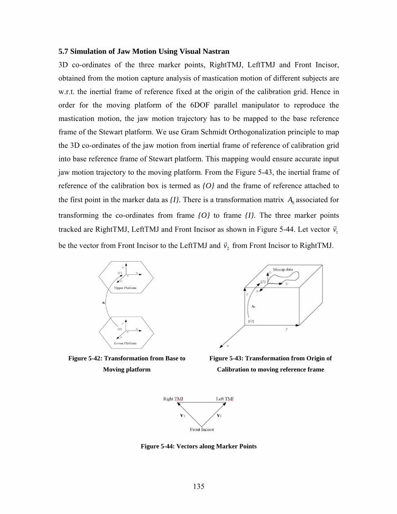
135

5.7 Simulation of Jaw Motion Using Visual Nastran

3D co-ordinates of the three marker points, RightTMJ, LeftTMJ and Front Incisor,

obtained from the motion capture analysis of mastication motion of different subjects are

w.r.t. the inertial frame of reference fixed at the origin of the calibration grid. Hence in

order for the moving platform of the 6DOF parallel manipulator to reproduce the

mastication motion, the jaw motion trajectory has to be mapped to the base reference

frame of the Stewart platform. We use Gram Schmidt Orthogonalization principle to map

the 3D co-ordinates of the jaw motion from inertial frame of reference of calibration grid

into base reference frame of Stewart platform. This mapping would ensure accurate input

jaw motion trajectory to the moving platform. From the Figure 5-43, the inertial frame of

reference of the calibration box is termed as {O} and the frame of reference attached to

the first point in the marker data as {I}. There is a transformation matrix 0A associated for

transforming the co-ordinates from frame {O} to frame {I}. The three marker points

tracked are RightTMJ, LeftTMJ and Front Incisor as shown in Figure 5-44. Let vector 1v

be the vector from Front Incisor to the LeftTMJ and 2v from Front Incisor to RightTMJ.

Figure 5-42: Transformation from Base to

Moving platform

Figure 5-43: Transformation from Origin of

Calibration to moving reference frame

Figure 5-44: Vectors along Marker Points

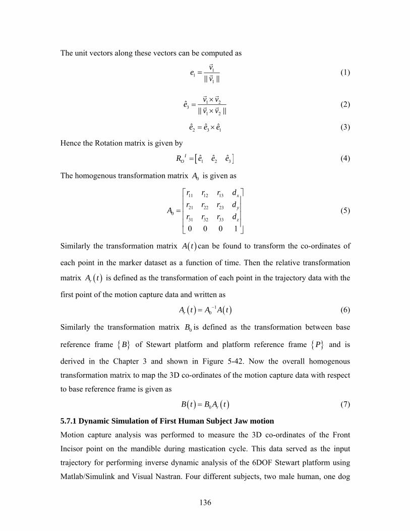
136

The unit vectors along these vectors can be computed as

11

1

vev

= (1)

1 23

1 2

ˆ v vev v×

=×

(2)

2 3 1ˆ ˆ ˆe e e= × (3)

Hence the Rotation matrix is given by

[ ]1 2 3ˆ ˆ ˆIOR e e e= (4)

The homogenous transformation matrix 0A is given as

11 12 13

21 22 230

31 32 33

0 0 0 1

x

y

z

r r r dr r r d

Ar r r d

⎡ ⎤⎢ ⎥⎢ ⎥=⎢ ⎥⎢ ⎥⎣ ⎦

(5)

Similarly the transformation matrix ( )A t can be found to transform the co-ordinates of

each point in the marker dataset as a function of time. Then the relative transformation

matrix ( )rA t is defined as the transformation of each point in the trajectory data with the

first point of the motion capture data and written as

( ) ( )10rA t A A t−= (6)

Similarly the transformation matrix 0B is defined as the transformation between base

reference frame { }B of Stewart platform and platform reference frame { }P and is

derived in the Chapter 3 and shown in Figure 5-42. Now the overall homogenous

transformation matrix to map the 3D co-ordinates of the motion capture data with respect

to base reference frame is given as

( ) ( )0 rB t B A t= (7)

5.7.1 Dynamic Simulation of First Human Subject Jaw motion

Motion capture analysis was performed to measure the 3D co-ordinates of the Front

Incisor point on the mandible during mastication cycle. This data served as the input

trajectory for performing inverse dynamic analysis of the 6DOF Stewart platform using

Matlab/Simulink and Visual Nastran. Four different subjects, two male human, one dog

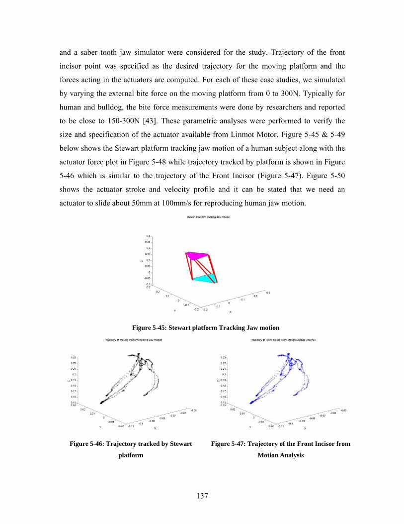
137

and a saber tooth jaw simulator were considered for the study. Trajectory of the front

incisor point was specified as the desired trajectory for the moving platform and the

forces acting in the actuators are computed. For each of these case studies, we simulated

by varying the external bite force on the moving platform from 0 to 300N. Typically for

human and bulldog, the bite force measurements were done by researchers and reported

to be close to 150-300N [43]. These parametric analyses were performed to verify the

size and specification of the actuator available from Linmot Motor. Figure 5-45 & 5-49

below shows the Stewart platform tracking jaw motion of a human subject along with the

actuator force plot in Figure 5-48 while trajectory tracked by platform is shown in Figure

5-46 which is similar to the trajectory of the Front Incisor (Figure 5-47). Figure 5-50

shows the actuator stroke and velocity profile and it can be stated that we need an

actuator to slide about 50mm at 100mm/s for reproducing human jaw motion.

Figure 5-45: Stewart platform Tracking Jaw motion

Figure 5-46: Trajectory tracked by Stewart

platform

Figure 5-47: Trajectory of the Front Incisor from

Motion Analysis

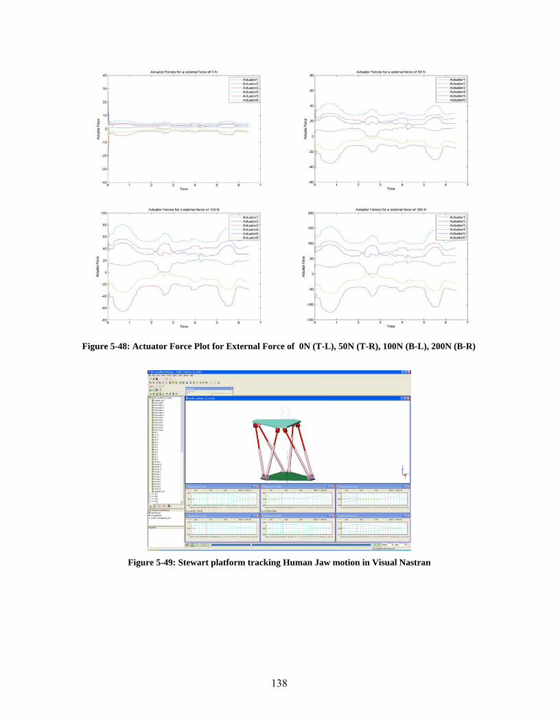
138

Figure 5-48: Actuator Force Plot for External Force of 0N (T-L), 50N (T-R), 100N (B-L), 200N (B-R)

Figure 5-49: Stewart platform tracking Human Jaw motion in Visual Nastran

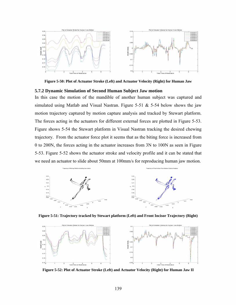
139

Figure 5-50: Plot of Actuator Stroke (Left) and Actuator Velocity (Right) for Human Jaw

5.7.2 Dynamic Simulation of Second Human Subject Jaw motion In this case the motion of the mandible of another human subject was captured and

simulated using Matlab and Visual Nastran. Figure 5-51 & 5-54 below shows the jaw

motion trajectory captured by motion capture analysis and tracked by Stewart platform.

The forces acting in the actuators for different external forces are plotted in Figure 5-53.

Figure shows 5-54 the Stewart platform in Visual Nastran tracking the desired chewing

trajectory. From the actuator force plot it seems that as the biting force is increased from

0 to 200N, the forces acting in the actuator increases from 3N to 100N as seen in Figure

5-53. Figure 5-52 shows the actuator stroke and velocity profile and it can be stated that

we need an actuator to slide about 50mm at 100mm/s for reproducing human jaw motion.

Figure 5-51: Trajectory tracked by Stewart platform (Left) and Front Incisor Trajectory (Right)

Figure 5-52: Plot of Actuator Stroke (Left) and Actuator Velocity (Right) for Human Jaw II

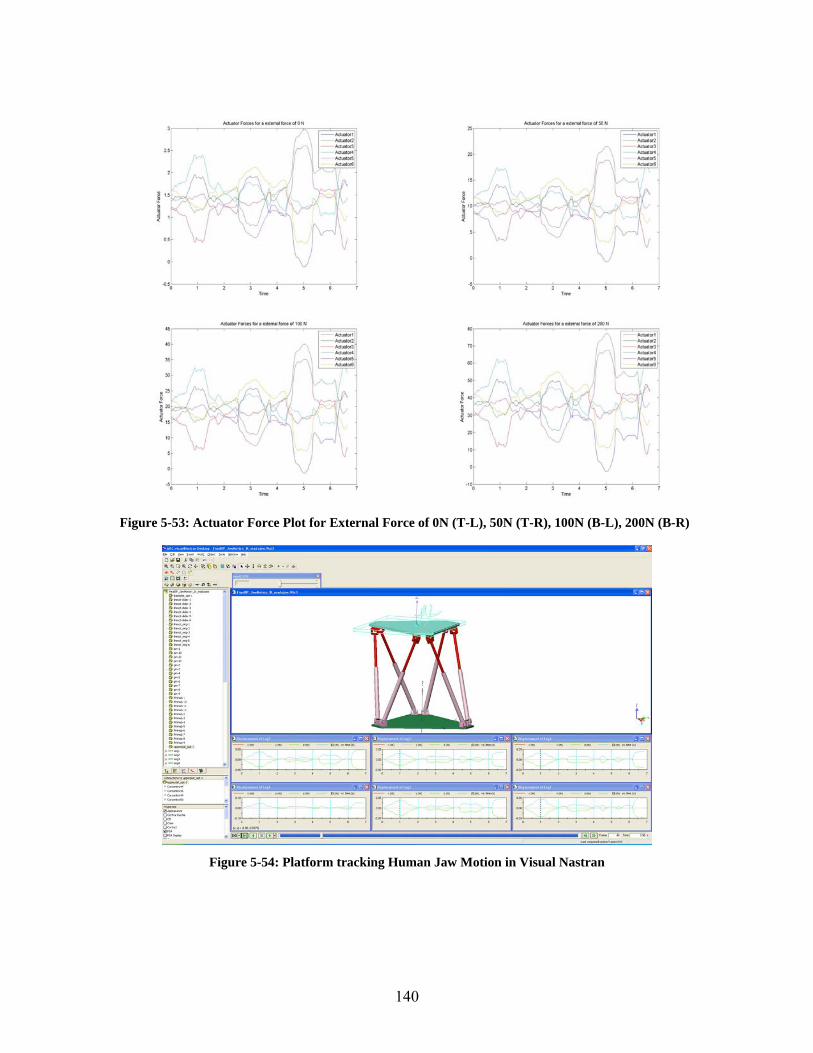
140

Figure 5-53: Actuator Force Plot for External Force of 0N (T-L), 50N (T-R), 100N (B-L), 200N (B-R)

Figure 5-54: Platform tracking Human Jaw Motion in Visual Nastran

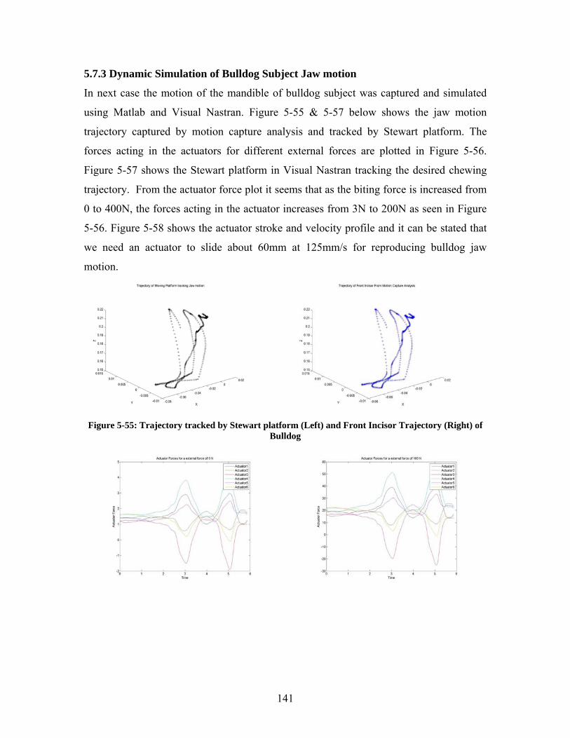
141

5.7.3 Dynamic Simulation of Bulldog Subject Jaw motion

In next case the motion of the mandible of bulldog subject was captured and simulated

using Matlab and Visual Nastran. Figure 5-55 & 5-57 below shows the jaw motion

trajectory captured by motion capture analysis and tracked by Stewart platform. The

forces acting in the actuators for different external forces are plotted in Figure 5-56.

Figure 5-57 shows the Stewart platform in Visual Nastran tracking the desired chewing

trajectory. From the actuator force plot it seems that as the biting force is increased from

0 to 400N, the forces acting in the actuator increases from 3N to 200N as seen in Figure

5-56. Figure 5-58 shows the actuator stroke and velocity profile and it can be stated that

we need an actuator to slide about 60mm at 125mm/s for reproducing bulldog jaw

motion.

Figure 5-55: Trajectory tracked by Stewart platform (Left) and Front Incisor Trajectory (Right) of

Bulldog

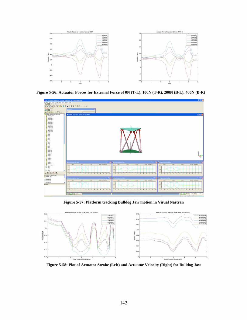
142

Figure 5-56: Actuator Forces for External Force of 0N (T-L), 100N (T-R), 200N (B-L), 400N (B-R)

Figure 5-57: Platform tracking Bulldog Jaw motion in Visual Nastran

Figure 5-58: Plot of Actuator Stroke (Left) and Actuator Velocity (Right) for Bulldog Jaw

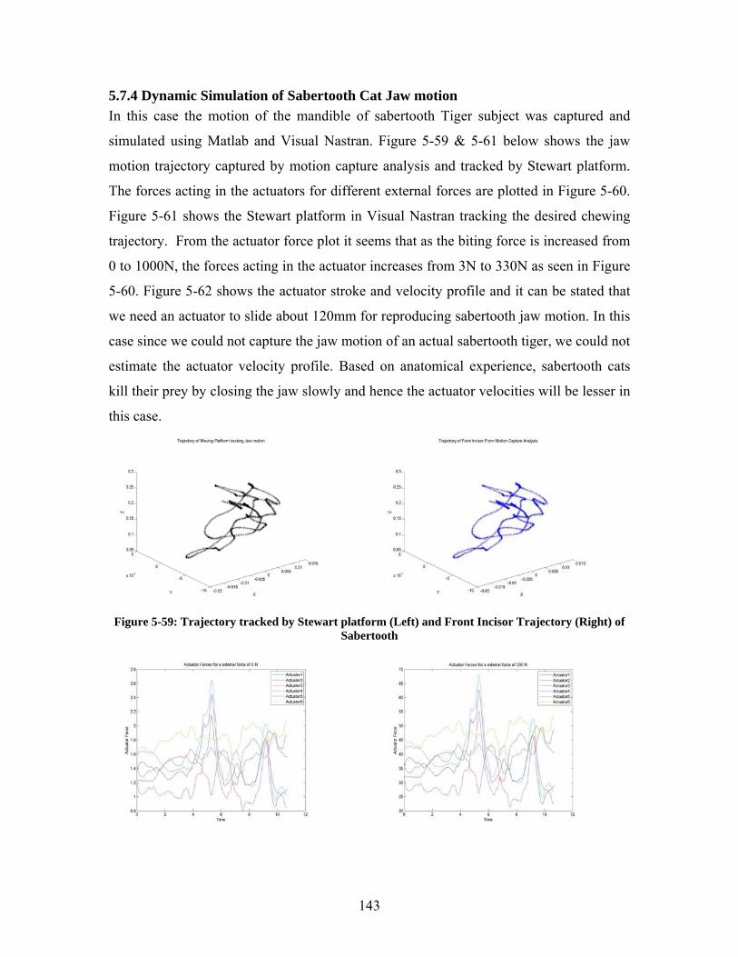
143

5.7.4 Dynamic Simulation of Sabertooth Cat Jaw motion In this case the motion of the mandible of sabertooth Tiger subject was captured and

simulated using Matlab and Visual Nastran. Figure 5-59 & 5-61 below shows the jaw

motion trajectory captured by motion capture analysis and tracked by Stewart platform.

The forces acting in the actuators for different external forces are plotted in Figure 5-60.

Figure 5-61 shows the Stewart platform in Visual Nastran tracking the desired chewing

trajectory. From the actuator force plot it seems that as the biting force is increased from

0 to 1000N, the forces acting in the actuator increases from 3N to 330N as seen in Figure

5-60. Figure 5-62 shows the actuator stroke and velocity profile and it can be stated that

we need an actuator to slide about 120mm for reproducing sabertooth jaw motion. In this

case since we could not capture the jaw motion of an actual sabertooth tiger, we could not

estimate the actuator velocity profile. Based on anatomical experience, sabertooth cats

kill their prey by closing the jaw slowly and hence the actuator velocities will be lesser in

this case.

Figure 5-59: Trajectory tracked by Stewart platform (Left) and Front Incisor Trajectory (Right) of

Sabertooth

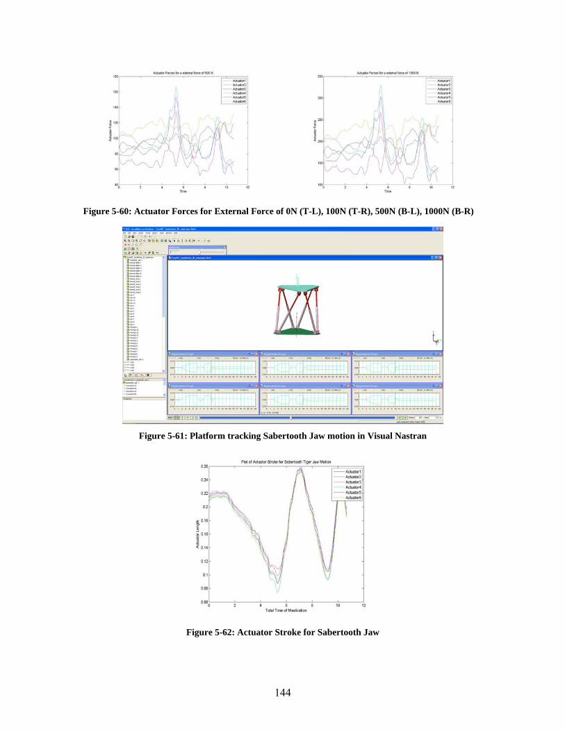
144

Figure 5-60: Actuator Forces for External Force of 0N (T-L), 100N (T-R), 500N (B-L), 1000N (B-R)

Figure 5-61: Platform tracking Sabertooth Jaw motion in Visual Nastran

Figure 5-62: Actuator Stroke for Sabertooth Jaw

145

6. Conclusion and Future Work

6.1 Conclusion

The primary goal of this project to use Virtual Prototyping tools to estimate:

1. Force acting in the actuators as the Stewart platform is reproducing the

mastication motion of vertebrates.

2. Muscle Forces and TMJ reaction Forces as the musculoskeletal model of

vertebrate jaw is performing mastication motion.

Although prior work has been done in developing human jaw motion simulators, no work

was done in reproducing the mastication motion of animals. And these human jaw motion

simulators were built for specific patient. Hence in this thesis work, we modeled and

simulated a more generic 6DOF parallel manipulator i.e. Stewart platform for

reproducing the jaw motion of vertebrates. The other reason for simulating a Stewart

platform was that there is no size limitation on the actuators as the skull and mandible

will be mounted on top of the moving platform. For achieving the first task, a CAD

model of the Stewart platform was developed in SolidWorks. Before building the CAD

model, workspace analysis was performed to measure various measures of manipulability

and its dependence on parameters such as radius of the upper platform and the length of

the actuators. These two parameters were then determined for attaining the best

workspace in the context of reproducing jaw motion. Then the inverse dynamics of the

Stewart platform was formulated based on the Lagrangian and Newton Euler Method.

The Jacobian matrix of the 6DOF parallel manipulator was derived as described in

Chapter 3. Initially to verify the inverse dynamic code, the inverse-forward dynamics

simulation was implemented using an S-Function block and a DynaFlexPro forward

dynamics model and the results were compared with the benchmark solutions for specific

case studies provided by Tsai. Feedback linearization was successfully implemented to

verify that the moving platform tracks the desired trajectory with the error converging to

zero. Then the motion capture analysis of different subjects including humans was

performed to determine the 3D trajectory of the front incisor on the mandible. This

trajectory was then used as the input trajectory for the inverse dynamic simulation of the

146

CAD model of the Stewart platform and the actuator forces were determined. Dynamic

simulations of the Stewart platform tracking jaw motion were performed in MSC. Visual

Nastran and Matlab to determine the actuator forces required for different subjects under

varying external/bite force. It was observed that the forces generated by the actuators

range between 100-200N for a human subject depending upon the external force acting

on the moving platform. Similarly the actuator forces increases up to 200-300N for dogs

and up to 400-500N for the sabertooth tiger depending upon the external force. This

study helped us to determine the size of actuators required for reproducing different jaw

motion trajectories. However, motion analysis of the subjects need to be performed at

different chewing frequencies to determine the forces, workspace and speed of the

actuators for different rates of chewing. The model that has been built and simulated

already would prove as a useful tool to perform various “what if” type of parametric

analysis before finalizing the specification of the Stewart platform. 3D CAD model of

skull and mandible of a bulldog and sabertooth was generated from high resolution CT

Scans using biomedical image processing techniques in MIMICS. Also the CAD model

of a bulldog was obtained from laser scanning a physical skull and mandible object of a

bulldog. Although the laser scanning method produced high quality STL files of skull and

mandible, it was very tedious working with the scanner and cleaning up the geometry in

Geomagics. From the STL files of skull and mandible obtained from these two methods,

SLA model of the skull and mandible were built using a SLA machine at Fisher-Price,

Inc. Finally, a dentition of the bulldog skull and mandible was created which could be

mounted on top of the Stewart platform with some fixtures to reproduce the jaw motion.

For achieving the second task, the biomechanics of the masticatory system was reviewed

to understand the function of each masticatory muscles and temporomandibular joints.

Literature from Koolstra et al. was reviewed to comprehend the modeling of TMJ. The

architectural properties of muscle such as muscle origin and insertion points, muscle fiber

length, maximum muscle force, tendon length etc. were extracted from Koolstra et al. for

human subject. As a first step, a musculoskeletal model of human jaw was built in

AnyBody Modeling system consisting of seven masticatory muscles on each side and the

motion capture date of front incisor point was used to drive the mandible. The condyles

147

were constrained to be in touch with the fossa and the sideways movement of one of the

TMJs was constrained. Muscle forces required to perform such desired jaw motion under

varying bite force were plotted. The modeling procedure was verified by comparing the

muscle activities plot with the one created by Mark De Zee et al. It was decided to model

the muscles as Hill type muscle models and model the temporalis muscles as set of three

vectors for producing more realistic results. The work was then extended to create a

musculoskeletal model of bulldog jaw and sabertooth cat jaw. In this case, the

architectural properties of the muscle were obtained from dissection of the dog head

muscles. Muscle mass were obtained from Turnbull book to determine the muscle

volume. STL files of the skull and mandible of both the animals were imported into

AnyBody for visualization and verification of muscle attachment points. Motion capture

data of the front incisor was used to drive the mandible and muscle forces and TMJ

reaction forces were determined for different bite force simulation. It was observed that

the muscle forces, TMJ reaction forces and muscle activities increases with increase in

bite force. Also the lateral pterygoid and the digastrics perform most of the work upfront

in opening the jaw, whereas the other masticatory muscles contribute little in terms of

muscle activities. In this way, a musculoskeletal model of the vertebrate jaw was built

and is designed to perform various other “what if” type parametric analyses to test

various hypothesis. Reproduction of the mastication motion of a vertebrate with a robotic

device enabled us to estimate muscle and bite forces required for different animals while

chewing/biting different regimen and relate them analyze masticatory muscle recruitment

patterns and performance and will be used to quantitatively evaluate the dynamic

breakdown of foods during chewing in the future, which is vital information required in

the development of new pet foods.

6.2 Future work

1. Sophisticated Dissection:

Dissection of the Masticatory muscles must be performed in a sophisticated

manner using 3D digitizer, laser diffraction techniques to measure the

architectural muscle parameters accurately. Also the dataset should be estimated

for specific subject for the sake of consistency.

148

2. Accurate Motion Capture Analysis:

A more sophisticated fixture should be designed to restrain the animal subject

from moving its head while performing mastication. This ensures consistent

motion capture data without loss of information in between the cycle.

3. Bite Force Measurement:

Instead of simulating chewing force, force transducers should be used to measure

the biting force while chewing different regimen. This force could then be applied

as the external force to the Stewart platform and musculoskeletal jaw model.

4. EMG measurements for validation:

Electromyography measurements of the masticatory muscles of animal subjects

must be measured during the mastication cycle. The actual muscle activities

obtained from virtual prototyping could then be compared with the experimental

EMG measurements to validate the musculoskeletal model in AnyBody.

5. Frequency of Mastication:

Since the frequency of chewing affects the speed at which actuators move or the

muscle forces required to move the mandible along desired trajectory, we need to

measure the motion capture data at different known frequencies based on the type

of regimen being chewed.

6. Physical Prototyping

Finally we need to build a 6DOF parallel manipulator and perform real time

control using Matlab Simulink xPC toolbox. The platform needs to be tested for

biting different regimens to measure the food breakdowns and masticatory

performance and forces in the actuators using force sensors.

149

Bibliography

1. M.J. Delsignore, “A Screw -Theoretic Framework for Musculoskeletal System

Modeling and Analysis”, Department of Mechanical & Aerospace Engineering.

Buffalo, State University of New York at Buffalo, Master of Science, 2005

2. K.S. Konakanchi, “Musculoskeletal modeling of Smilodon Fatalis for Virtual

Functional Performance Testing”, Department of Mechanical & Aerospace

Engineering. Buffalo, State University of New York at Buffalo, Master of

Science, 2005

3. M. Narayanan, S. Kannan, L-F. Lee, V. Krovi, and F. Mendel, “Virtual

Musculoskeletal Scenario-Testing Case-Studies”. Proceedings of 2008 Virtual

Rehabilitation, Vancouver, Canada, 2008.

4. G.G.Wang, "Definition and Review of Virtual Prototyping", Journal of

Computing and Information Science in Engineering 2(3): 232-236, 2002.

5. V. Krovi, V. Kumar, G.K. Ananthasuresh, and J.M. Vezien, "Design and Virtual

Prototyping of Rehabilitation Aids", ASME Journal of Mechanical Design

121(3): 456-458, 1999.

6. B. May, S. Saha, M. Saltzman, "A three dimensional mathematical model of

temporomandibular joint loading." Clinical Biomechanics 16: 489-495, 2001.

7. J.H. Koolstra, T.M. Van Eijden, W.A. Weijs and M. Naeije, "A Three

Dimensional Mathematical Model of the human Masticatory System Predicting

the Maximum possible Bite Forces." Journal of Biomechanics 21(7): 563-576,

1988.

150

8. J.H. Koolstra, T.M. Van Eijden, "Three-dimensional dynamical capabilities of the

human masticatory muscles." Journal of Biomechanics 32(2): 145-152, 1999.

9. J.H. Koolstra, T.M. Van Eijden, "Combined finite-element and rigid-body

analysis of human jaw joint dynamics." Journal of Biomechanics 38(12): 2431-

2439, 2005.

10. J.H. Koolstra, "Dynamics of the human Masticatory System." Critical reviews in

oral biology and medicine 13(4): 366-376, 2002.

11. T. Goldmann, L. Himmlova, “Usage of Motion Analysis for describing the

trajectory of the human Mandible in 3D”.

12. T.M. Barker, W. J. Earwaker, N. Frost, G. Wakeley, "Integration of 3-D medical

imaging and rapid prototyping to create stereolithographic models." Australas

Phys Eng Sci Med. 16(2): 79-85, 1993.

13. S. Lohfeld, P. Mchugh, D. Serban, D. Boyle, G. O'Donnell, N. Peckitt,

"Engineering Assisted Surgery™: A route for digital design and manufacturing of

customised maxillofacial implants." Journal of Materials Processing Technology

183(2-3): 333-338, 2007.

14. S. Singare, L. Dichen, L. Bingheng, L. Yanpu, G. Zhenyu, L. Yaxiong, "Design

and fabrication of custom mandible titanium tray based on rapid prototyping."

Medical Engineering & Physics 26(8): 671-676, 2004.

15. R. Enciso, A. Memon, D.A. Fidaleo, U. Neumann, J. Mah, "The virtual

craniofacial patient: 3D jaw modeling and animation." Stud Health technol

Inform. 94: 65-71, 2003.

151

16. N. Inou, M. Koseki, S. Sato, H. Kimura and K. Maki, “Development of Patient-

specific Display System of the human Mandibular Movements”.

17. Y. Otake, N. Suzuki, A. Hattori, Y. Shigeta, T. Ogawa, S. Fukushima, K.

Kobayashi, A. Uchiyama, "Real-time mandibular movement analysis system

using four-dimensional cranial bone model." Systems and Computers in Japan

37(8): 1-12, 2006.

18. B. Daumas, W. L. Xu, J. Bronlund, "Jaw mechanism modeling and simulation."

Mechanism and Machine Theory 40(7): 821-833, 2005.

19. D. Lewis, “A robotic chewing device for food evaluation”, Palmerston North,

NewZealand, Massey University. Master of Engineering in Mechatronics, 2006.

20. W.L. Xu, D. Lewis, J.E. Bronlund, M.P. Morgenstern, "Mechanism, design and

motion control of a linkage chewing device for food evaluation." Mechanism and

Machine Theory 43: 376-389, 2008.

21. W.L. Xu, J.E. Bronlund, and J. Kieser, “A Robotic Model of the human

Masticatory System for Reproducing Chewing Behaviors”, IEEE Robotics &

Automation Magazine, 2005.

22. W.L. Xu, "Review of the human masticatory system and masticatory robotics."

Mechanism and Machine Theory doi:10.1016/j.mechmachtheory.2008.06.003,

2008.

23. W. L. Xu, J. D. Torrance, B.Q. Chen, J. Potgieter, J.E. Bronlund, and J.S. Pap,

"Kinematics and Experiments of a Life-Sized Masticatory Robot for

Characterizing Food Texture." IEEE Transactions on Industrial Electronics 55(5),

2008.

152

24. J. Torrance, J. S. Pap, W.L. Xu, J. Bronlund, K.D. Foster, “Motion control of a

chewing robot of 6 RSS parallel mechanism”, 284 Proceedings of International

Conference on Autonomous Robotics and Agents. Palmerston North, New

Zealand. 13: 593-598, 2006.

25. H. Takanobu, A. Takanishi, D. Ozawa, K. Ohtsuki, M. Ohnishi, A. Okino,

“Integrated Dental Robot System for Mouth Opening and Closing Training”,

Proceedings of the 2002 IEEE International Conference on Robotics

&Automation, vol. 2, pp 1428-1433, Washington, DC, 2002.

26. T. Hayashi, S. Kato, S. Yamada, S. Nakajima, Y. Yamada, and H. Kobayashi, “A

Physiological Control of Chewing-Like Jaw Movement for Robotized Jaw

Simulator JSN/2A”, Proceedings of the 22nd Annual EMBS International

Conference, Chicago, IL, 2000.

27. H. Takanobu, A. Takanishi, I. Kato, “Design of a Mastication Robot Mechanism

using a human Skull Model”, Proceedings of the 1993 IEEE/RSJ International

Conference on Intelligent Robots and Systems, 1, pp 203-208, Yokohama, Japan,

1993.

28. H. Takanobu, N. Kuchiki, A. Takanishil, “Control of rapid closing motion of a

robot jaw using nonlinear spring mechanism”, Proceedings of the International

Conference on Intelligent Robots and Systems, 1, pp 372-377, 1995.

29. H. Takanobu, A. Takanishi, I. Kate, “Control of a Mastication Robot for

Reduction of Jaw Joint Force Focusing on Musculus temporalis”, Intelligent

Robots and Systems '94. 'Advanced Robotic Systems and the Real World', IROS

'94. Proceedings of the IEEE/RSJ/GI International Conference, 3, pp 1824-1831,

1994.

153

30. H.U. Takanobu, A. Takanishi, “Dental robotics and human model”. Proceedings

of the 1st International IEEE EMBS Conference on Neural Engineering, Capri

Island, Italy, pp 671-674, 2003.

31. “http://www.takanishi.mech.waseda.ac.jp/research/jaws/index.htm”, WY Series

32. K. Alemzadeh, R. A. Hyde, J. Gao, "Prototyping a robotic dental testing

simulator." Proceedings of the Institution of Mechanical Engineers. Part H,

Journal of Engineering in Medicine 221(4): 385-396, 2007.

33. H.B. Guo, H.R. Li, "Dynamic analysis and simulation of a six degree of freedom

Stewart platform manipulator." Proceedings of the Institution of Mechanical

Engineers, Part C: Journal of Mechanical Engineering Science 220(1), 2006.

34. C.P. Tang, “Manipulability-Based Analysis for Payload Transport by Robot

Collectives”, Department of Mechanical & Aerospace Engineering. Buffalo, State

University of New York at Buffalo, Master of Science, 2004.

35. L.W. Tsai, "Solving the Inverse Dynamics of a Stewart-Gough Manipulator by

the Principle of Virtual Work." Journal of Mechanical Design 122(1): pp. 3-9,

2000.

36. K. Yu, “Simultaneous Trajectory Tracking and Stiffness Control of Cable Driven

Parallel Manipulator”, Department of Mechanical & Aerospace Engineering.

Buffalo, State University of New York at Buffalo, Master of Science, 2008.

37. C-I Huang, C-F. Chang, M-Y Yu, L-C Fu, “Sliding-mode tracking control of the

Stewart platform”, Control Conference, 2004. 5th Asian, 1, pp 562-569, 2004.

38. J. Rasmussen, M. Damsgaard, and M. Voigt, "Muscle recruitment by the min/max

criterion – a comparative study." Journal of Biomechanics, 34: 409-415, 2001.

154

39. M. Damsgaard, J. Rasmussen, S.T. Christensen, E. Surmaa, M. Zee, "Analysis of

musculoskeletal systems in the AnyBody Modeling System." Simulation

Modelling Practice and Theory, 14(8): Pages 1100-1111, 2006.

40. M. de Zee, M. Dalstra, P. Cattaneo, J. Rasmussen, P. Svensson, B. Melsen,

"Validation of a musculo-skeletal model of the mandible and its application to

mandibular distraction osteogenesis." Journal of Biomechanics 40(6): 1192-1201,

2006

41. R. M. Bhatt, V. Krovi, “DynaFlexPro for Maple”, IEEE Control System. 26: 127-

138, 2006

42. M. Klein Horsman, H. Koopman, F. Van der Helm, L. Prose, H. Veeger,

"Morphological muscle and joint parameters for musculoskeletal modeling of the

lower extremity." Clinical Biomechanics 22(2): 239-247, 2007

43. D.L. Lindner, S. M. Marretta, G.J. Pijanowski, A.L. Johnson, C.W. Smith,

"Measurement of Bite Force in dogs: A Pilot Study." Journal of Veterinary

Dentistry 12(2): 49-52, 1995.

44. Muscle Physiology, http://muscle.ucsd.edu/musintro/jump.shtml

45. Capture3D Laser Scanners, http://capture3d.com/knowledge-column.html

46. NextEngine Scanner, https://www.nextengine.com/indexSecure.htm

47. W.D. Turnbull, "Mammalian Masticatory Apparatus”, Field Museum of Natural

History, 18(2): pp-268, 1970

48. MotionPro Inc, “DynaFlexPro User Manual”, Maplesoft Waterloo, Canada

155

49. Y. Wang, “Symbolic Kinematics and Dynamics Analysis and Control of a

General Stewart Parallel Manipulator”, Department of Mechanical & Aerospace

Engineering, State University of New York at Buffalo, Master of Science, 2008.

50. Laser scanners, http://en.wikipedia.org/wiki/3D_scanner

51. “MIMICS User Manual and Tutorials”

52. Ariel Performance Analysis System, “APAS User Manual and Tutorials”.

53. AnyBody Modeling System, “AnyBody User Manual”