Quantitative Analysis of Literary Styles Roger D. Peng Nicolas W. Hengartner Author’s footnote: Roger D. Peng ([email protected]) is Graduate Student, Department of Statistics, University of California, Los Angeles, Los Angeles CA 90095; and Nicolas W. Hengartner ([email protected]) is Associate Professor, Department of Statistics, Yale University, New Haven CT 06520-8290. The first author would like to thank Frederic Paik Schoenberg, Frauke Kreuter, and Noah Gedrich for useful comments. The authors ac- knowledge the comments and suggestions of an associate editor and two anonymous referees, which contributed substantially to the revised form of this paper.

Welcome message from author
This document is posted to help you gain knowledge. Please leave a comment to let me know what you think about it! Share it to your friends and learn new things together.
Transcript

Quantitative Analysis of Literary Styles
Roger D. Peng Nicolas W. Hengartner
Author’s footnote: Roger D. Peng ([email protected]) is Graduate Student, Department
of Statistics, University of California, Los Angeles, Los Angeles CA 90095; and Nicolas W.
Hengartner ([email protected]) is Associate Professor, Department of Statistics,
Yale University, New Haven CT 06520-8290. The first author would like to thank Frederic
Paik Schoenberg, Frauke Kreuter, and Noah Gedrich for useful comments. The authors ac-
knowledge the comments and suggestions of an associate editor and two anonymous referees,
which contributed substantially to the revised form of this paper.

Abstract
Writers are often viewed as having an inherent style which can serve as a literary
fingerprint. By quantifying relevant features related to literary style, one may hope to
classify written works and even attribute authorship to newly discovered texts. Beyond
its intrinsic interest, the study of literary styles presents the opportunity to introduce
and motivate many standard multivariate statistical techniques. Today the statisti-
cal analysis of literary styles is made much simpler by the wealth of real data readily
available from the Internet. This paper presents an overview and brief history of the
analysis of literary styles. In addition we use canonical discriminant analyis and prin-
cipal component analysis to identify structure in the data and distinguish authorship.
Keywords: authorship, canonical discriminant analysis, principal component analysis,
function words, data visualization, high dimensional data
1 Introduction
It is often recognized that authors have inherent literary styles which serve as “fingerprints”
for their written works. Thus in principle, one should be able to determine the authorship
of unsigned manuscripts by carefully analyzing the style of the text. The difficulty lies in
characterizing the style of each author, i.e. determining which sets of features in a text most
accurately summarize an author’s style. When doing a quantitative or statistical analysis
of literary style, the problem is finding adequate numerical representations of an author’s
inherent style.
1

Quantitative literary style analysis presents a unique opportunity to introduce and mo-
tivate many standard multivariate techniques. It is possible to view each text as a collection
of multivariate observations, in which case we are immediately faced with the inherent dif-
ficulties of analyzing high dimensional data. The usual questions are relevant: How can we
visualize the data? What are the significant features? Are there any interesting structures?
In this situation we also have the benefit of being able to rely on some immediate knowledge
of the subject matter to analyze and understand the data. Traditional multivariate methods
can then be used to contrast and compare the styles of several authors and possibly assign
authorship.
1.1 Previous Work
There has been much work covering different aspects of this field. For a comprehensive re-
view we direct the reader to Holmes (1985). Many early attempts to quantify style relied on
concordances, or inventories of the frequency of every word in a text. In 1901 T. C. Menden-
hall reduced the concordances of Shakespeare and Bacon to distributions of word lengths
and plotted these distributions as graphs. His so called “characteristic curves” serve as an
early example of the use of graphics in distinguishing authorship. Mendenhall examined the
differences in the shapes of the curves (such as the location of the mode) and concluded that
Bacon probably did not write any of Shakespeare’s works. C. B. Williams reproduced some
of Mendenhall’s curves and noted that he was mistaken in some of his conclusions and that
there was little evidence for or against the theory that some works written by Shakespeare
could have been written by Bacon (Williams, 1975). Brinegar (1963) also used word length
distributions to determine if Mark Twain had written the Quintus Curtius Snodgrass (QCS)
2

letters. He used χ2 tests and two-sample t-tests on the counts of 2, 3, and 4 letter words
to check the agreement of the QCS letters with Twain’s known writings. Thisted and Efron
(1987) used the idea of vocabulary richness to determine the possibility of Shakespearean
authorship of a newly discovered poem. They based their analysis of the poem on the rate
of “discovery” of new words given the number of distinct words previously observed in the
Shakespearean canon. Holmes (1992), in an example of the use of a standard multivari-
ate analysis technique, used hierarchical cluster analysis to detect changes in authorship in
Mormon scripture. He also used various measures of vocabulary richness to conduct his
analysis.
There is no general agreement on the unit of analysis that should be used in authorship
studies. In the previously mentioned examples, word length and vocabulary richness were
the units used. Williams (1940) analyzed the sentence lengths of works written by Chester-
ton, Wells, and Shaw. He noticed that the log of the number of words per sentence appeared
to follow a normal distribution. Morton (1965) also used sentence length in his analysis of
ancient Greek texts. After initially using criteria such as word length and sentence length,
Mosteller and Wallace (1963) focused on using function word counts to discriminate between
the works of Hamilton and Madison in their seminal analysis of the Federalist Papers (see
also Mosteller and Wallace, 1964). They found that Hamilton and Madison were “practi-
cally twins” with respect to the average sentence lengths in their writings. Therefore, they
decided to use function words, which are words with very little contextual meaning. These
words include conjunctions, prepositions, and pronouns. The logic behind using function
words is that writers do not necessarily think about the way they use these words. Rather
these words flow unconsciously from the mind to the paper. Therefore, the usage of function
words should be invariant under changes of topic. Mosteller and Wallace (1963) successfully
3

used the frequency distribution of a few function words to assign authorship to the unsigned
Federalist Papers. Sarndal (1967) also used word counts in an interesting attempt to quantify
type I and type II errors in authorship discrimination. He facilitated the analysis by assum-
ing independent Poisson distributions for the word counts. Mosteller and Wallace (1963)
noted that in their study, the Poisson distribution did not fit the word count distributions
particularly well, and that the negative binomial distribution provided a better fit because
of its heavier tail.
In Section 2 we will describe the data used for this study, outline the methods used to
process the data, and give a brief description of the statistical methods employed. Section 3
gives some example analyses and discusses possible ways of estimating the prediction error.
In this paper we examine the works of Jane Austen, Willa Cather, Arthur Conan Doyle,
Charles Dickens, Rudyard Kipling, Jack London, Christopher Marlowe, John Milton, and
William Shakespeare.
2 Data and Methods
The raw data for this study were obtained from Internet websites such as Project Gutenberg.
Multiple works for each author were downloaded in text format and processed. The titles
and website URL are listed in Appendix A. In this study we also take groups of function
words as the units of analysis. When analyzing word frequencies, one often makes the
following assumptions: (1) the style of an author remains the same throughout his/her life;
(2) successive occurrences of function words are independent. Neither assumption tends to
hold in practice. The purpose of using function words in the first place is to deal with (1).
4

Because function words have little contextual meaning, we can think of them abstractly as
the “noise” of language. One might reasonably assume that writers do not put as much
conscious thought into this aspect of writing. In general, when choosing the unit of analysis,
one must use something that has large variation across authors and relatively little variation
among an author’s own works. Mosteller and Wallace (1963) and Williams (1956) showed
in their separate studies that while sentence length tended not to vary much within an
author’s writings, it also did not vary much between authors. Therefore, sentence length
had relatively little power for discrimination. We feel that groups of function word counts
serve as a good numerical expressions of the stylistic habits of authors. The adequacy of
using function words can be judged by the results shown in Section 3.
The study of Mosteller and Wallace (1964) (i.e. see p. 23 of their book) revealed that
while some function words exhibit short term dependencies, their frequencies in larger blocks
can be reasonably modeled as independent replications. Indeed, we find in our dataset that
the positions of particular function words have a short term negative association. That is,
if we are examining the word “the”, then the probability that the kth word is “the” (given
that the word at position 0 is “the”) is increasing for small values of k. In Figure 1 we
plot the difference between the (empirical) conditional probability P(Xk = 1 | X0 = 1) and
the unconditional probability P(Xk = 1), where we use Xk to denote the random variable
indicating the occurrence of a function word at the kth position. Figure 1 shows this plot for
a few function words and for values of k from 1 to 50. For Figure 1(a-b) we used Austen’s
Northanger Abbey and for Figure 1(c-d) we used London’s The Call of the Wild. For each of
the words there is a sharp increase in the relative frequency up to distances of about 5 to 8
words. The exception is Austen’s usage of the word “and”. There the negative association
appears to extend to almost 15 words.
5

Examining function words in their original locations is not very useful because on smaller
scales their occurrences do not appear to be independent. However, we can divide works
into blocks and count the function words in each block. In choosing the block size, we want
to balance two conflicting aims: taking larger blocks to decrease the dependence between
the counts of function words in them, and taking smaller blocks to ensure that within each
block, the style of the author remains the same. After some trial and error, we chose to
divide each author’s work into 1700 words. Table 1 gives the block word counts of a few
selected function words in a work of Cather. This choice of block size does not completely
eliminate the dependence between consecutive blocks nor preserve homegeneity. The effect of
inhomogeneity within blocks shows up in our analysis in Section 3.3. Within each block, we
tabulated the frequency of the 69 words (listed in Table 2) chosen from the Miller-Newman-
Friedman list of function words used by Mosteller and Wallace. These words were chosen
because of their relatively frequent use in the works being examined. It was desired to avoid
having too many words for which authors had many zero counts.
It should be noted that the effect of a short term negative assocation between occurrences
of function words is to make the function word counts in each block have a smaller variance
than they would under an independence model. This effect is useful if we want to classify
blocks of text (and their respective counts) by looking at differences in means.
2.1 Canonical Discriminant Analysis
Our approach to canonical discriminant analysis (CDA) is similar to that of Gifi (1990). For
other introductions to discriminant analysis we refer the reader to Johnson and Wichern
(1982) or Lachenbruch (1975).
6

Suppose X is our data matrix of word counts whose columns are centered around their
respective means. X is an n×p matrix, where n is the total number of observations (blocks)
for all the authors being examined and p is the number of variables (i.e. different word types).
Let G be the n× g group matrix consisting of 1’s and 0’s, where g is the number of groups
we are examining (i.e. the number of authors). A 1 in the (i, j) entry of G indicates that
block i was written by Author j. We can denote the sample total covariance matrix by
CT = 1nX ′X. If we let P = G(G′G)−1G′, then we can denote the between groups covariance
matrix as CB = 1nX ′PX. Generally speaking, we want to find linear combinations of the
variables which maximize the between groups variance subject to a constraint on the total
variance. This defines a generalized eigenvalue problem of the form CB βi = λiCT βi, where
the eigenvectors βi are the solutions to the CDA problem. The βi’s are called the discriminant
functions and for a given CDA problem, there are r = min(p, g− 1) significant discriminant
functions.
Suppose β1 is the first discriminant function, where β1 is vector of length p. If X is the
n × p matrix of word counts, then y1 = Xβ1 is the first canonical vector (CV). Although
it is only feasible to plot two or three canonical vectors at a time, the first few vectors are
usually sufficient for observing separation between the groups. The eigenvalues λi can be
used to aid in deciding how many CV’s are needed to summarize the data. They have an
interpretation similar to that of principal component analysis (PCA), i.e. λi/∑λj is the
proportion of variance explained by the ith CV.
Sometimes it is useful to identify each canonical vector with a specific variable or perhaps
a small subset of the original variables. In the current application, one might want to identify
a word which is particularly effective at distinguishing between certain authors. If B is the
matrix of discriminant functions, the columns of which are β1, . . . , βr, the loadings are the
7

correlations between the columns of X and XB. We can then identify each canonical vector
with the original variables which have the largest correlations (Klecka, 1980).
Besides the assumptions made in Section 2 we must also make some technical assump-
tions. If we can reasonably believe that, given the unit of analysis, an author’s collected
works form a stable “population”, then we must furthermore assume that all of the popu-
lations have the same covariance structure. This assumption is important for determining
the performance of CDA and its ability to discriminate between groups. More specifically,
the performance of linear classification rules (which we use in Section 3.3) depends critically
on the populations having equal covariances. We do not attempt to make any formal veri-
fication of this assumption here. Some informal exploration of the data and the analyses in
Section 3 suggest that the equal covariance assumption may not hold. Nevertheless, we feel
that one can still gain a fair amount of insight into the data by using CDA.
For all of the statistical analyses we used the R Statistical Computing Environment (Ihaka
and Gentleman, 1996), which has many built-in routines for doing discriminant analysis. The
program used for counting words and compiling block counts can be downloaded from the
first author’s website (see Appendix A).
3 Analysis
Initially, each author’s works were examined by themselves to identify possible outliers or
unusual blocks (with respect to the function word counts). In order to explore the structure
of the data we applied principal component analysis (PCA) to the word counts (see Jollife,
1986, for an overview of PCA).
After applying PCA to the counts of all nine authors, one author that stood out was
8

Marlowe. It is therefore instructive to analyze Marlowe’s opus by itself. Figure 2 shows the
first two principal components (PC’s). The striking part of is the group of six points in the
upper left corner — two blocks each from The Jew of Malta, Tamburlaine the Great: Part
I, and Tamburlaine the Great: Part II. In each case, the last two blocks of the particular
work are the ones that appear to be outlying. On further examination it turns out that
the downloaded versions of those there works were critical editions containing extensive
footnotes and commentary at the ends of the works. Thus, the last two blocks of each work
most definitely were not written by Marlowe. The downloaded versions of Doctor Faustus
and Massacre at Paris did not contain any footnotes or commentary.
After the six outlying blocks were removed (i.e. their counts were removed from the
dataset) PCA was run again and the plot of the first two PC’s is shown in Figure 3. In
this plot one can still see some structure in the points. For example, almost all of the
points for The Jew of Malta and Doctor Faustus have values for PC1 less than 0. Similarly,
both Tamburlaine’s are on the right side of the plot with values of PC1 greater than 0.
The structure in Figure 3 suggests that perhaps the independence assumption is violated.
Another possibility is that there is a large scale change of style exhibited in the works (i.e.
lack of homogeneity). Both explanations represent violations of the original assumptions and
will affect adversely the performance of the discrimination procedure. However, the effect
should be minor if Marlowe’s word counts are still much different from the counts of other
the authors. In Section 3.3 we will see how violations of the assumptions may affect the rate
of error in classification.
9
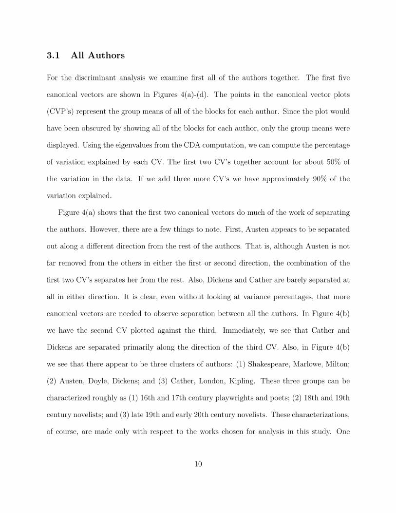
3.1 All Authors
For the discriminant analysis we examine first all of the authors together. The first five
canonical vectors are shown in Figures 4(a)-(d). The points in the canonical vector plots
(CVP’s) represent the group means of all of the blocks for each author. Since the plot would
have been obscured by showing all of the blocks for each author, only the group means were
displayed. Using the eigenvalues from the CDA computation, we can compute the percentage
of variation explained by each CV. The first two CV’s together account for about 50% of
the variation in the data. If we add three more CV’s we have approximately 90% of the
variation explained.
Figure 4(a) shows that the first two canonical vectors do much of the work of separating
the authors. However, there are a few things to note. First, Austen appears to be separated
out along a different direction from the rest of the authors. That is, although Austen is not
far removed from the others in either the first or second direction, the combination of the
first two CV’s separates her from the rest. Also, Dickens and Cather are barely separated at
all in either direction. It is clear, even without looking at variance percentages, that more
canonical vectors are needed to observe separation between all the authors. In Figure 4(b)
we have the second CV plotted against the third. Immediately, we see that Cather and
Dickens are separated primarily along the direction of the third CV. Also, in Figure 4(b)
we see that there appear to be three clusters of authors: (1) Shakespeare, Marlowe, Milton;
(2) Austen, Doyle, Dickens; and (3) Cather, London, Kipling. These three groups can be
characterized roughly as (1) 16th and 17th century playwrights and poets; (2) 18th and 19th
century novelists; and (3) late 19th and early 20th century novelists. These characterizations,
of course, are made only with respect to the works chosen for analysis in this study. One
10

notable exception to these categorizations is Kipling’s The Writings in Prose and Verse
of Rudyard Kipling, which is a collection of short works rather than a single long novel.
Although groups (2) and (3) are both groups of novelists, it is interesting to see the clear
separation between the two in the plot of the second and third CV’s. Obviously, the style
of prose writing changed dramatically between the 19th and 20th century, and perhaps this
difference is reflected in the usage of the function words. Also, Austen and Cather are similar
in some ways (they both use the word “her” almost 5 as often as the others on average) but
remain far apart in the CVP in Figure 4(b).
Beyond using three canonical vectors, visualization of the data becomes trickier. One
needs to choose projections that bring out interesting features in the data. Figures 4(c) and
4(d) show the third, fourth, and fifth CV’s. We see in all the plots that Shakespeare and
Marlowe are virtually inseparable. Similarly, Kipling and London are never far apart. In
Figure 4(d) we see that Milton is isolated in the bottem left of the plot. However, we could
not identify any particular words (associated with the fourth and fifth CV’s) which Milton
used more or less often. It is possible that there are some second order effects which cannot
be ascertained merely by looking at the mean counts for each author.
A plot of the loadings for each CV such as Figure 5 can be useful for determining good
words for discrimination. Figures 5(a) and 5(b) show the loadings for the first and second
CV’s. An arbitrary cutoff was set at ±0.5 — any loadings beyond that value were considered
large. This cutoff results in the words “not”, “be”, “upon”, and “the” for the first CV, and
“been”, “it”, “had”, and “was” for the second CV. Not shown are the loadings for the
third CV. There we find the words with large loadings to be “which”, “on”, and “may”.
Examining the original word counts for each author can help clarify the meaning of the CV’s
and the loadings. In Table 4 we show the mean word counts for the words which had large
11

loadings for the first three CV’s. All of the word counts show a fair amount of disparity
across authors, which is presumably why they are good for discrimination.
3.2 Smaller Groupings
In order to show that CDA can perform quite well in certain situations we will look at
Austen, London, and Shakespeare. In this example the qualitative differences between the
authors are already quite vast. Each author wrote in a different century and for the most
part in a different format. The language of English itself evolved significantly between the
time of Shakespeare and the time of London. However, given the nature of the data, we can
only make precise statements about the differences in word counts. Figure 6(a) shows the
CVP for this example. Since there are only three authors in this example, only the first two
CV’s are significant. However, we plot the first and third CV’s in Figure 6(b) simply to show
that the first CV alone does quite well in separating the three authors. The corresponding
variance percentage is 52%. It seems that Austen uses “to”, “her”, “any”, and “been” more
often than both London and Shakespeare. From the second CV loadings we see that the
word “the” is used far more often by London (Shakespeare and Austen have similar usage)
and “was” is used far less often by Shakespeare (Austen and London have similar usage).
While the first CV does most of the work of separating out Austen from the group, London
and Shakespeare are separated more along the second CV. In this example it seems that the
CDA procedure behaves as it should. The blocks for the three authors separate quite well
in in the space of the canonical vectors.
For contrast we look at four authors who are more similar than the previous three:
Cather, Doyle, Kipling, and London. The CVP for these four is shown in Figure 7(a)-(b).
12

One might expect poorer separation here because of the similar time periods in which the
authors lived. In Figure 7(a) Doyle is isolated on the left hand side of the plot while Cather,
Kipling, and London are bunched together on the right hand side. It appears that the first
CV does the work of separating Doyle out from the others. The second vector separates
Cather out from the rest but Kipling and London are still mixed together. Figure 7(b)
shows that Kipling and London are separated along the direction of the third CV. Doyle’s
blocks are not shown in Figure 7(b) for clarity. In both plots we see the clouds of points
associated with each author are diffuse and the boundaries between them blurred. This is
quite different from the Austen, London, Shakespeare example where the clouds of points
were neatly separated from each other. There, one CV did much to separate out the three
authors. However, in this example it is clear that all significant CV’s are necessary in order
to observe separation of the groups.
For the first CV, the words with large loadings are “which”, “upon”, and “have”. For
the second CV, the direction along which Cather is separated from the rest, the only word
with a large loading is “her”. Finally, for the third CV, we have “was” and “of”. If we look
at the usage of the word “her”, we have the mean counts for each author as 26.0 (Cather),
6.4 (Doyle), 5.4 (Kipling), and 9.0 (London). Hence, on average, Cather uses the word “her”
5 times more often per block than Doyle and Kipling and about 3 times more often than
London. If we had to use one word to discriminate between Cather and the other three
authors, “her” would be an excellent choice.
We can also look at the mean counts of “which”, “upon”, and “have” for the four authors.
Those are shown in Table 5. Here we see that Doyle uses all three words much more often
than the other authors. Also in Table 5 are the mean block counts for “was” and “of”, which
had large loadings with respect to the third CV. While Cather and Doyle appear to have
13

similar usage patterns, London uses “was” about twice as often and “of” about 1.5 times
more frequently.
3.3 Prediction Error
It is usually useful to have some measure of the potential rate of error in classification.
The estimate of the error rate used here is the cross-validation estimate (Lachenbruch and
Mickey, 1968). In fact we will use two forms of cross-validation. To compute the first
estimate, we leave out one block from the dataset and then classify it according to the rule
constructed with the remaining data. This method is also known as leave-one-out cross-
validation. For the second form of cross-validation, instead of leaving out a single block each
time, we will leave out the entire work from which each block originates. The remaining
data will be used as the training set and each block from the removed work will be classified.
This form of cross-validation should be more robust against possible correlation between
successive blocks in a single work. Note that for both forms we will use all of the significant
discriminant functions in the classification procedure.
So far, we have not discussed what rule to use in order to make classifications, but rather
have focused on the geometrical structure of the data. However, error rate estimation obvi-
ously depends on the rule that is chosen. In our case, we will use Fisher’s linear discriminant
rule: given a new block, x0, the distance from x0 to each group mean is measured. The new
observation is assigned to the group with which it has the smallest distance. The distance
is measured in the space spanned by the discriminant functions.
A useful quantity that can be computed as a by-product of both forms of cross-validation
is a “confusion matrix.” The (i, j) element of the matrix shows the percentage of blocks writ-
14

ten by Author i attributed to Author j. Thus, the diagonal shows the percentage of correct
classifications and the off-diagonal elements show the percentage incorrect classifications.
Using the first form of cross-validation, we achieve an overall error rate of 7%. This is
simply the total number of incorrect classifications divided by the total number of cases. The
overall individual error rates for each author are shown in the last column of the confusion
matrix in Table 6. Austen, Cather, Doyle, and Milton have fairly low individual error rates;
Kipling, London, and Marlowe have the highest error rates. It was pointed out in Section 3.1
that Kipling and London were difficult to discriminate, as were Shakespeare and Marlowe.
We see that almost 15% of Marlowe’s works were mistakenly classified as Shakespeare. Also,
the majority of Shakespeare’s incorrect classifications were given to Marlowe. Kipling and
London had about the same percentage of works incorrectly assigned to each other.
Using the second form of cross-validation the overall error rate increases to 14%. Table 7
shows the confusion matrix associated with this procedure. Although all authors’ error
rates increased, the increases for Austen and Shakespeare were minimal. However, the
error rates for Kipling and London more than doubled and Cather, Dickens, Doyle, and
Marlowe saw similar increases in their error rates. Milton’s error rate estimate is likely to
be unreliable under the second procedure because his sample only consisted of two works
that were roughly the same length. Therefore, when a work was left out his sample size
was cut in half. In general, it appears that the authors were sensitive to the change in
cross-validation procedure, suggesting that perhaps some correlation of blocks within works
is artificially decreasing the error rate estimates in Table 6. Another likely reason is a lack
of homogeneity between blocks. Interestingly, all of the missclassified Marlowe blocks were
from either The Jew of Malta or Doctor Faustus. The other three of Marlowe’s works were
all correctly classified. Recall that in Section 3 the PCA detected a possible violation of
15

the homogeneity assumption. We might conclude here that perhaps The Jew of Malta and
Doctor Faustus are “less characteristic” of Marlowe and that they represent a change of style
with respect to the function word counts. More specifically, the behavior of the word counts
become closer to that of Shakespeare. Clearly, the discrimination procedure is sensitive to
large scale changes in style by an author.
4 Conclusions
Literary style analysis provides an interesting venue for motivating and demonstrating many
standard multivariate statistical techniques. Conversely, we have shown in this paper that
traditional multivariate techniques can be very useful for exploring and analyzing literary
data. The data are inherently high dimensional and cannot be readily visualized or under-
stood. Initially, principal component analysis was used to examine each individual author’s
function word counts. PCA proved useful for identifying unusual blocks and possible viola-
tions of the independence and uniformity assumptions. For example, with Marlowe’s data,
we were able to identify some blocks of text that were definitely not written by Marlowe.
Also, the PCA revealed that Marlowe’s function word counts did not conform particularly
well to the given assumptions. Canonical discriminant analysis was used to provide dimen-
sion reduction and graphical displays of the differences between authors (canonical vector
plots). Also, CDA was useful for identifying key function words which were most effective
at discriminating between authors. The key words were identified by examining plots of the
loadings for each function word.
Two forms of cross-validation were used to estimate the prediction error using Fisher’s
linear discriminant rule. The first form simply left out an individual block and then con-
16

structed the classification rule from the remaining data. The second removed entire works at
a time and classifed the removed blocks using the rule constructed from the remaining data.
This second form of cross-validation increased the estimate of the error rate substantially
(relative to the estimate obtained from the first form) for Kipling, London, and Marlowe
while the estimates for Austen and Shakespeare remained essentially unchanged. This sug-
gests that either correlation of block counts or lack of homogeneity within works is artificially
lowering the error rate estimate for certain authors in the first cross-validation scheme.
Finally, function words have proven to be effective instruments for accessing literary data.
Function words were chosen as the unit analysis because they are highly variable between
authors, abundant, and easy to count and identify. The power of using groups of function
words was demonstrated in Section 3, where the mean counts of certain words were shown
to vary dramatically between authors. Whereas single indicators such as sentence length
may only work well in certain situations, the use of groups of indicators is promising because
different subsets can be used in different situations. Perhaps Mosteller and Wallace explained
it best in their 1963 paper when they argued “Words offer a great many opportunities for
discrimination; there are so many of them.”
References
Brinegar, C. S. (1963), “Mark Twain and the Quintus Curtius Snodgrass Letters: A Statis-
tical Test of Authorship,” Journal of the American Statistical Association, 58, 85–96.
Gifi, A. (1990), Nonlinear Multivariate Analysis, Wiley, NY.
Holmes, D. I. (1985), “The Analysis of Literary Style: A Review,” Journal of the Royal
17

Statistical Society, Series A, 148, 328–341.
— (1992), “A Stylometric Analysis of Mormon Scripture and Related Texts,” Journal of the
Royal Statistical Society, Series A, 155, 91–120.
Ihaka, R. and Gentleman, R. (1996), “R: A Language for Data Analysis and Graphics,”
Journal of Computational and Graphical Statistics, 5, 299–314.
Johnson, R. A. and Wichern, D. W. (1982), Applied Multivariate Statistical Analysis,
Prentice-Hall, Inc., Englewood Cliffs, New Jersey.
Jollife, I. T. (1986), Principal Component Analysis, Springer, New York.
Klecka, W. R. (1980), Discriminant Analysis, Sage Publications, California.
Lachenbruch, P. A. (1975), Discriminant Analysis, Hafner Press, New York.
Lachenbruch, P. A. and Mickey, M. R. (1968), “Estimation of Error Rates in Discriminant
Analysis (Com: V10 P204-205; Add: V10 P431),” Technometrics, 10, 1–11.
Morton, A. Q. (1965), “The Authorship of Greek Prose (with Discussion [Corr. to Comments:
65V128 P623]),” Journal of the Royal Statistical Society, Series A, 128, 169–233.
Mosteller, F. and Wallace, D. L. (1963), “Inference in An Authorship Problem,” Journal of
the American Statistical Association, 58, 275–309.
— (1964), Applied Bayesian and Classical Inference: The Case of The Federalist Papers,
Springer, NY.
Sarndal, C.-E. (1967), “On Deciding Cases of Disputed Authorship,” Applied Statistics, 16,
251–268.
18

Thisted, R. and Efron, B. (1987), “Did Shakespeare Write a Newly-discovered Poem?”
Biometrika, 74, 445–455.
Williams, C. B. (1940), “A Note on the Statistical Analysis of Sentence-Length as a Criterion
of Literary Style,” Biometrika, 31, 356–361.
— (1956), “A Note on an Early Statistical Study of Literary Style,” Biometrika, 43, 248–256.
— (1975), “Mendenhall’s Studies of Word-length Distribution in the Works of Shakespeare
and Bacon,” Biometrika, 62, 207–212.
A Appendix: Titles of Selected Works
All texts were downloaded from
• http://www.gutenberg.net
the Project Gutenberg website. The program for processing the text files and constructing
block counts can be downloaded from
• http://www.stat.ucla.edu/~rpeng/authorship
The following works were download for each author:
1. Christopher Marlowe: The Jew of Malta, Massacre at Paris, Tamburlaine the Great:
Part I, Tamburlaine the Great: Part II, The Tragical History of Doctor Faustus
2. William Shakespeare: Richard II, Henry IV: Part 1, Henry IV: Part 2, Henry V,
Julius Caesar, Troilus and Cressida, Macbeth, Cymbeline, The Tempest, King Lear,
Romeo and Juliet, Hamlet
19

3. John Milton: Paradise Lost, Paradise Regained
4. Jane Austen: Emma, Lady Susan, Mansfield Park, Pride and Prejudice, Northanger
Abbey
5. Charles Dickens: A Tale of Two Cities, David Copperfield, Great Expectations, Oliver
Twist, A Christmas Carol
6. Arthur Conan Doyle: The Adventures of Sherlock Holmes, Beyond the City, The Lost
World, Memoirs of Sherlock Holmes, The New Revelation, The Poison Belt, The Cap-
tain of the Polestar and Other Tales, The Parasite, The Return of Sherlock Holmes,
Round the Red Lamp, A Study in Scarlet, Tales of Terror and Mystery, The Vital
Message, The White Company
7. Rudyard Kipling: The Writings in Prose and Verse of Rudyard Kipling, The Jungle
Book, Puck of Pook’s Hill, Rewards and Fairies, American Notes
8. Willa Cather: My Antonia, O Pioneers!, The Song of the Lark, The Troll Garden and
Selected Stories, Alexander’s Bridge
9. Jack London: The Iron Heel, The Jacket, The Strength of the Strong, The Valley of
the Moon, White Fang, The Call of the Wild
20

B Appendix: Tables
Block # all an by must some that then this when which
1 1 3 1 2 3 30 0 5 10 62 11 8 3 4 2 30 4 3 6 23 3 5 5 2 1 20 2 2 11 24 7 4 5 2 7 20 4 0 9 05 8 3 9 2 1 23 0 6 5 36 5 2 5 2 2 21 2 7 5 27 6 1 2 1 5 16 3 4 7 2
Table 1: Some word counts for blocks of text written by Cather.
a been had its one the wereall but has may only their whatalso by have more or then whenan can her must our there whichand do his my should things whoany down if no so this willare even in not some to withas every into now such up wouldat for is of than upon yourbe from it on that was
Table 2: Function words used for all analyses.
21

Author Dates Lived # of Blocks
Marlowe 1564–1593 56Shakespeare 1564–1616 179Milton 1608–1674 56Austen 1775–1817 437Dickens 1812–1870 598Doyle 1859–1930 552Kipling 1865–1936 157Cather 1873–1947 237London 1876–1916 299
Table 3: Total number of blocks collected for each author. Each block contains 1700 words.
Author not be upon the been it had was which on may
Austen 20.1 19.2 1.4 61.4 7.6 23.5 16.9 25.9 7.3 8.6 2.3Cather 7.8 6.8 1.4 90.0 4.5 17.6 17.6 26.4 3.4 11.6 0.5Dickens 9.7 9.5 4.2 79.4 5.3 22.5 15.1 23.1 6.4 10.9 1.6Doyle 8.8 9.2 8.2 99.1 5.6 25.0 14.3 23.1 12.3 6.6 3.0Kipling 7.7 5.8 1.1 108.0 2.3 14.8 8.0 17.0 2.4 11.9 1.4London 9.0 5.7 2.3 110.0 4.2 21.5 14.2 33.6 2.9 12.3 0.4Marlowe 11.6 13.4 3.0 66.8 1.1 10.0 2.0 2.8 3.6 5.0 4.1Milton 13.6 7.4 0.6 62.8 0.7 3.3 3.9 4.5 6.1 11.2 2.6Shakespeare 16.8 12.6 3.6 55.5 1.3 14.9 2.5 4.1 4.7 5.9 3.3
Table 4: Mean counts for words with large loadings for the example using all authors. Theloadings were from the first three canonical vectors.
Author which upon have was of
Cather 3.4 1.4 6.6 26.4 35.8Doyle 12.3 8.2 12.7 23.1 49.2Kipling 2.4 1.1 6.4 17.0 35.7London 2.9 2.3 5.0 33.6 50.4
Table 5: Mean counts for “which”, “upon”, “have”, “was”, and “of” for Cather, Doyle,Kipling, and London.
22

Au Ca Di Do Ki Lo Ma Mi Sh ErrorAusten 99.5 0.2 0.2 0.5Cather 94.0 1.7 0.4 3.8 6.0Dickens 0.3 1.7 92.3 2.4 0.7 2.4 0.3 7.7Doyle 0.2 0.2 4.8 93.8 0.4 0.5 0.2 6.2Kipling 3.9 87.7 7.1 1.3 12.3London 0.3 3.7 2.0 7.4 86.1 0.3 13.9Marlowe 85.1 14.9 14.9Milton 100.0 0.0Shakespeare 0.6 8.7 90.8 9.2
Table 6: Confusion matrix from using the standard leave-one-out cross-validation. The (i, j)element of the table shows the percentage of blocks written by Author i attributed to Authorj. The rows do not necessarily sum to 100 because of rounding.
Au Ca Di Do Ki Lo Ma Mi Sh ErrorAusten 99.1 0.2 0.5 0.2 0.9Cather 89.7 2.1 2.1 6.0 10.3Dickens 0.7 2.5 87.1 5.2 1.0 3.2 0.3 12.9Doyle 0.2 0.2 7.0 90.5 0.9 0.7 0.2 0.4 9.5Kipling 11.0 0.6 66.2 20.8 1.3 33.8London 0.3 10.1 5.7 0.7 24.0 58.8 0.3 41.2Marlowe 72.3 27.7 27.7Milton 3.6 96.4 3.6Shakespeare 0.6 9.2 90.2 9.8
Table 7: Confusion matrix from using cross-validation where each block’s entire work isremoved from the training set.
23

C Appendix: Figure Captions
1. Differences between the (empirical) conditional probability P(Xk = 1 | X0 = 1) and
the unconditional probability P(Xk = 1). Xk is the random variable indicating the
occurrence of a function word at the kth position in the document.
2. The first and second principal components for the Marlowe data.
3. The first two principal components for the Marlowe data with the six outliers removed.
4. First five canonical vectors for the example with all authors.
5. Loadings for the (a) first and (b) second CV’s (using all authors).
6. Canonical vectors for the Austen, London, Shakespeare example.
7. The first, second (a), and third (b) canonical vectors for the Cather, Doyle, Kipling,
London example. In (b), Doyle’s points are not shown in order to show the separation
between the other three authors. In both (a) and (b) not all points for each author are
shown for the sake of clarity.
24

D Appendix: Figures
0 10 20 30 40 50
−0.
010
−0.
005
0.00
00.
005
Austen
(a) "the"Distance (k) in words
P(X
k =
1 |
X0
= 1
) −
P(X
k =
1)
0 10 20 30 40 50
−0.
010
−0.
004
0.00
00.
004
(b) "and"Distance (k) in words
P(X
k =
1 |
X0
= 1
) −
P(X
k =
1)
0 10 20 30 40 50
−0.
010
−0.
005
0.00
00.
005
London
(c) "of"Distance (k) in words
P(X
k =
1 |
X0
= 1
) −
P(X
k =
1)
0 10 20 30 40 50
−0.
010
0.00
00.
005
(d) "a"Distance (k) in words
P(X
k =
1 |
X0
= 1
) −
P(X
k =
1)
Figure 1: Differences between the (empirical) conditional probability P(Xk = 1 | X0 = 1)and the unconditional probability P(Xk = 1). Xk is the random variable indicating theoccurrence of a function word at the kth position in the document.
25

−4 −2 0 2 4
−4
−2
02
46
8
PC1
PC
2
Jew of MaltaDoctor FaustusTamburlaine ITamburlaine IIMassacre at Paris
Figure 2: The first and second principal components for the Marlowe data.
26

−6 −4 −2 0 2 4
−4
−2
02
46
8
PC1
PC
2
●
●
●
●
●
●
●
●
●
●
●
●
● Jew of MaltaDoctor FaustusTamburlaine ITamburlaine IIMassacre at Paris
Figure 3: The first two principal components for the Marlowe data with the six outliersremoved.
27

−0.03 −0.01 0.01 0.03
−0.
06−
0.02
0.02
(a)CV1
CV
2
●
●●
●
●
●
●
●
●
austen
catherdickens
doyle
kipling
london
marlowe
milton
shakespeare
−0.04 0.00 0.02 0.04
−0.
06−
0.02
0.02
(b)CV3
CV
2
●
●●
●
●
●
●
●
●
austen
catherdickens
doyle
kipling
london
marlowe
milton
shakespeare
−0.04 0.00 0.02 0.04
−0.
04−
0.02
0.00
0.02
(c)CV3
CV
4
●
●
●
●
●
●
●
●
●
austen
cather
dickens
doyle
kipling london
marlowe
milton
shakespeare
−0.10 −0.05 0.00 0.05
−0.
04−
0.02
0.00
0.02
(d)CV5
CV
4
●
●
●
●
●
●
●
●
●
austen
cather
dickens
doyle
kiplinglondon
marlowe
milton
shakespeare
Figure 4: First five canonical vectors for the example with all authors.
28

(a)
Lo
ad
ing
−0
.6−
0.2
0.2
0.6
a
all
also
anand
any
are
as
at
be
been
but
by
can
do
down
even
every
for
fromhad
has
have
her
his
ifin
into
isitits
may
more
must
my
no
not
nowofon
one
onlyor
our
should
so
some
such
than
that
the
their
thenthere
thingsthis
to
up
upon
waswere
what
whenwhich
who
will
with
would
your
(b)
Lo
ad
ing
−0
.20
.00
.20
.40
.6
a
all
alsoan
any
are
as
at
be
been
butby
can
dodown
even
every
for
from
had
hashaveher
hisif
ininto
is
it
its
maymore
must
my
nonot
of
on
one
only
should
so
somesuch
than
that
the
their
there
things
to
up
upon
was
were
when
which
who
willwith
would
your
Figure 5: Loadings for the (a) first and (b) second CV’s (using all authors).
29

−0.06 −0.02 0.02 0.06
−0
.05
0.0
00
.05
●
●
●
●
●
●●
●
●
●
●
●
●●
●
●
●
●
●
●
●
●
●●
●
●●
●
●
●
●●
●
●●
●●
●
●
●●
●
●
●
●
●
●
●
●
●●●
●
●
● ●
●●
●
●
●
●
●
●
●
●
●●
●
●
●
●
●
● ●
●
●
●
●
●
●●
●
●
●
●
●
●
●
●●
●●
●● ●
●
●●●
●
●●
●
●
●
●●
●
●●
●
●●
●
●
●●
●
●●
●
●
●
●
●
●
●
●
●
●
●
●●
●
●●●
●
●
●
●
●
●
●
●
●
●
●
●
●
●
●
●
●●
●
●
●
●●
●
●
●
●
●
●
●
●
●
●
●
●
●●
●
●
● ●
●
●
●
●
●
●●
●
●
● ●
●●●
●
●
●
●
●●
●
●
●●
●
●
●●
●
●
●
●
●● ●
●●
●
●●
●
●
●
●
●
●
●
●
●
●
●
●
●
●
●
●
●
●
●
●
●
●
●
●
●
●
●
●
●
●●
●
●
●
●●
●
●
●
●
●●
●
●
●
● ●
●
●
●
●
●
●
● ●
●
●
●
●
●
●
●
●
●
●●
●
●●
●
●
●
●
●
●
●
●
●
●
●
●
●
●
●
●
●
●
●●
●
●
●●
●
●
●
●
●
●
●
●
●
●
●
●
●
●
●
●
●
●
●● ●
●
●
●
●●●
●
●
●
●
●
●
●
●
●●
●
●
●
●
●
●
●●
●
●
●
●
●
●
●
●
(a)CV1
CV
2
●
●
AustenLondonShakespeare
−0.06 −0.02 0.02 0.06−
0.1
0−
0.0
50
.00
0.0
50
.10
●
●
● ●
●●
●
●
●
●
●
●
●
●
●
● ●
●
●
●
●
●
●
●
●
●
●
●
●
●
●
●
●
●
●●●
●
●
●
●
●
●
●
●
●
●
●
●
●
●
●
●
●
●
●
●
●
●
●●
●
●
●
●
●
●
●
●
●
●
●
●●
●
●
●
●
●
● ●
●
●
●
●
●
●
●
●●
●
●
●
●
●
●
●
●
●
●
●
●
●
●
●
●●
●
●
●
●
●
●
●
●
●
●
●
●
●
●
●
●
●
●
●
●●●
●
●
●
●
●
●
●
●
●
●
●
●
●
●
●
●
●
●
●
●
●
●
●
●
●
●
●
●
●
●
●
●
●
●
●
●
●●
●
●
●
●
●
●
●
●●
●
●
●
●
●
●
●
●
●
●
●
●
● ●
●
●
●
●
●
●
●
●
●
●
●
●
●
●
●
●
●●
●
●
●
●
●
●
● ●
●●
●
●
●
●
●
●
●
●
●
●
●●
●
●
●
●
●
●
●
●
●●
●
●
●
●
●
● ●
●
●●
●
●
●
●
●
●
●
●
●
●
●
●
●
●
●
●
●
●
●
●
●
●
●
●
●
●
●
●
●
●
●
●
●
●
●
●●
●
●
●
●
●
●
●
●
●
●
●
●
● ●
●
●
●
●●
●●
●
●●
●
●
●
●
●
●
●
●
●
●
●
●
●
●
●
●
●
●
●
●
●
●
●
●
●
●
●●
●
●
●
●
●
●
●
●
●
●
●
●●
●
●
●
●
●
●
●
●
●
●
●
●
●
(b)CV1
CV
3
Figure 6: Canonical vectors for the Austen, London, Shakespeare example.
30

−0.06 −0.02 0.02 0.04
−0
.05
0.0
00
.05
0.1
0
●
●
●
●
●
●
●
●
●
●
●
●
●
●
●●
●
●
●
●
●
●
●
●
● ●
●
●
●
●
●
●
●
●
●
●●
●
●
●
●
●
●
●●
●
●●
●
●●
●
●
●
●
●●
●
●
●
●
●
●
●
●
●
●
●
●●
●
●
●
●
●
●
●
●
●
●
●
●
●
●
●
●
●
●●
●
●● ●
●
●
●
● ●
●
●
●●
●
●●
●●
●●
●
●●
●
●
●●
●●
●
●
●
●
●
●
●●●
●
●
●
●
●
●
●
●
●●
●
●
●
●
●
●
●
●
●
●
●
●
●
●
●
●
● ●
●
●
●
●
●
●
●
●
●
●
●
● ●
●●
●●● ●
●
●
●
●
●
CatherDoyleKiplingLondon
(a)CV1
CV
2
−0.10 −0.05 0.00 0.05−
0.0
50
.00
0.0
50
.10
●
●
●
●
●
●
●
●
●
●
●
●
●
●
●●
●
●
●
●
●
●
●
●
●●
●
●
●
●
●
●
●
●
●
●●
●
●
●
●
●
●
●●
●
●●
●
●●
●
●
●
●
●●
●
●
●
●
●
●
●
●
●
●
●
●●
●
●
●
●
●
●
●
●
●
●
●
●
●
●
●
●
●
●●
●
●● ●
●
●
●
● ●
●
●
●●
●
●●
●●
●●
●
●●
●
●
●●
●●
●
●
●
●
●
●
●●●
●
●
●
●
●
●
●
●
●●
●
●
●
●
●
●
●
●
●
●
●
●
●
●
●
●
●●
●
●
●
●
●
●
●
●
●
●
●
● ●
●●
●● ●●
●
●
●
●
●
CatherKiplingLondon
(b)CV3
CV
2
Figure 7: The first, second (a), and third (b) canonical vectors for the Cather, Doyle, Kipling,London example. In (b), Doyle’s points are not shown in order to show the separationbetween the other three authors. In both (a) and (b) not all points for each author areshown for the sake of clarity.
31
Related Documents