Quantitative Analysis of Culture Using Millions of Digitized Books

www.sciencemag.org/cgi/content/full/science.1199644/DC1

Supporting Online Material for

Quantitative Analysis of Culture Using Millions of Digitized Books Jean-Baptiste Michel,* Yuan Kui Shen, Aviva Presser Aiden, Adrian Veres, Matthew K.

Gray, The Google Books Team, Joseph P. Pickett, Dale Hoiberg, Dan Clancy, Peter Norvig, Jon Orwant, Steven Pinker, Martin A. Nowak, Erez Lieberman Aiden*

*To whom correspondence should be addressed. E-mail: [email protected] (J.B.M.); [email protected]

(E.A.).

Published 16 December 2010 on Science Express DOI: 10.1126/science.1199644

This PDF file includes:

Materials and Methods Figs. S1 to S19 References

1

Materials and Methods

“Quantitative analysis of culture using millions of digitized books”,

Michel et al.

Contents

I. Overview of Google Books Digitization ......................................................................................... 3

I.1. Metadata ....................................................................................................................... 3

I.2. Digitization ..................................................................................................................... 4

I.3. Structure Extraction ...................................................................................................... 4

II. Construction of Historical N-grams Corpora ................................................................................ 5

II.1. Additional filtering of books .......................................................................................... 5

II.1A. Accuracy of Date-of-Publication metadata ................................................................ 5

II.1B. OCR quality ............................................................................................................... 6

II.1C. Accuracy of language metadata ................................................................................ 6

II.1D. Year Restriction ......................................................................................................... 7

II.2. Metadata based subdivision of the Google Books Collection ...................................... 7

II.2A. Determination of language ........................................................................................ 7

II.2B. Determination of book subject assignments .............................................................. 7

II.2C. Determination of book country-of-publication ............................................................ 7

II.3. Construction of historical n-grams corpora .................................................................. 8

II.3A. Creation of a digital sequence of 1-grams and extraction of n-gram counts ............. 8

II.3B. Generation of historical n-grams corpora ................................................................ 10

III. Culturomic Analyses .............................................................................................................................. 12

III.0. General Remarks ................................................................................................................... 12

III.0.1 On Corpora. ......................................................................................................................... 12

III.0.2 On the number of books published ...................................................................................... 13

III.1. Generation of timeline plots ................................................................................................... 13

III.1A. Single Query ........................................................................................................................ 13

III.1B. Multiple Query/Cohort Timelines ......................................................................................... 14

III.2. Note on collection of historical and cultural data ................................................................... 14

III.3. Controls .................................................................................................................................. 15

III.4. Lexicon Analysis .................................................................................................................... 15

2

III.4A. Estimation of the number of 1-grams defined in leading dictionaries of the English language. ....................................................................................................................................... 15

III.4B. Estimation of Lexicon Size .................................................................................................. 16

III.4C. Dictionary Coverage ............................................................................................................ 17

III.4D. Analysis New and Obsolete words in the American Heritage Dictionary ............................ 17

III.5. The Evolution of Grammar ..................................................................................................... 17

III.5A. Ensemble of verbs studied .................................................................................................. 17

III.5B. Verb frequencies.................................................................................................................. 18

III.5C. Rates of regularization ........................................................................................................ 18

III.5D. Classification of Verbs ......................................................................................................... 18

III.6. Collective Memory.................................................................................................................. 18

III.7. The Pursuit of Fame............................................................................................................... 19

III.7A) Complete procedure ............................................................................................................ 19

III.7B. Cohorts of fame ................................................................................................................... 25

III.8. History of Technology ............................................................................................................ 26

III.9. Censorship ............................................................................................................................. 26

III.9A. Comparing the influence of censorship and propaganda on various groups ...................... 26

III.9B. De Novo Identification of Censored and Suppressed Individuals ....................................... 28

III.9C. Validation by an expert annotator........................................................................................ 28

III.10. Epidemics ............................................................................................................................. 29

3

I. Overview of Google Books Digitization

In 2004, Google began scanning books to make their contents searchable and discoverable online. To date, Google has scanned over fifteen million books: over 11% of all the books ever published. The collection contains over five billion pages and two trillion words, with books dating back to as early as 1473 and with text in 478 languages. Over two million of these scanned books were given directly to Google by their publishers; the rest are borrowed from large libraries such as the University of Michigan and the New York Public Library. The scanning effort involves significant engineering challenges, some of which are highly relevant to the construction of the historical n-grams corpus. We survey those issues here.

The result of the next three steps is a collection of digital texts associated with particular book editions, as well as composite metadata for each edition combining the information contained in all metadata sources.

I.1. Metadata Over 100 sources of metadata information were used by Google to generate a comprehensive catalog of books. Some of these sources are library catalogs (e.g., the list of books in the collections of University of Michigan, or union catalogs such as the collective list of books in Bosnian libraries), some are from retailers (e.g., Decitre, a French bookseller), and some are from commercial aggregators (e.g., Ingram). In addition, Google also receives metadata from its 30,000 partner publishers. Each metadata source consists of a series of digital records, typically in either the MARC format favored by libraries, or the ONIX format used by the publishing industry. Each record refers to either a specific edition of a book or a physical copy of a book on a library shelf, and contains conventional bibliographic data such as title, author(s), publisher, date of publication, and language(s) of publication.

Cataloguing practices vary widely among these sources, and even within a single source over time. Thus two records for the same edition will often differ in multiple fields. This is especially true for serials (e.g., the Congressional Record) and multivolume works such as sets (e.g., the three volumes of The Lord of the Rings).

The matter is further complicated by ambiguities in the definition of the word „book‟ itself. Including translations, there are over three thousand editions derived from Mark Twain‟s original Tom Sawyer.

Google‟s process of converting the billions of metadata records into a single nonredundant database of book editions consists of the following principal steps:

1. Coarsely dividing the billions of metadata records into groups that may refer to the same work (e.g., Tom Sawyer).

2. Identifying and aggregating multivolume works based on the presence of cues from individual records.

3. Subdividing the group of records corresponding to each work into constituent groups corresponding to the various editions (e.g., the 1909 publication of De lotgevallen van Tom Sawyer, translated from English to Dutch by Johan Braakensiek).

4. Merging the records for each edition into a new “consensus” record.

The result is a set of consensus records, where each record corresponds to a distinct book edition and work, and where the contents of each record are formed out of fields from multiple sources. The number of records in this set -- i.e., the number of known book editions -- increases every year as more books are written.

In August 2010, this evaluation identified 129 million editions, which is the working estimate we use in this paper of all the editions ever published (this includes serials and sets but excludes kits, mixed media, and

4

periodicals such as newspapers). This final database contains bibliographic information for each of these 129 million editions (Ref. S1). The country of publication is known for 85.3% of these editions, authors for 87.8%, publication dates for 92.6%, and the language for 91.6%. Of the 15 million books scanned, the country of publication is known for 91.5%, authors for 92.1%, publication dates for 95.1%, and the language for 98.6%.

I.2. Digitization

We describe the way books are scanned and digitized. For publisher-provided books, Google removes the spines and scans the pages with industrial sheet-fed scanners. For library-provided books, Google uses custom-built scanning stations designed to impose only as much wear on the book as would result from someone reading the book. As the pages are turned, stereo cameras overhead photograph each page, as shown in Figure S1.

One crucial difference between sheet-fed scanners and the stereo scanning process is the flatness of the page as the image is captured. In sheet-fed scanning, the page is kept flat, similar to conventional flatbed scanners. With stereo scanning, the book is cradled at an angle that minimizes stress on the spine of the book (this angle is not shown in Figure S1). Though less damaging to the book, a disadvantage of the latter approach is that it results in a page that is curved relative to the plane of the camera. The curvature changes every time a page is turned, for several reasons: the attachment point of the page in the spine differs, the two stacks of pages change in thickness, and the tension with which the book is held open may vary. Thicker books have more page curvature and more variation in curvature.

This curvature is measured by projecting a fixed infrared pattern onto each page of the book, subsequently captured by cameras. When the image is later processed, this pattern is used to identify the location of the spine and to determine the curvature of the page. Using this curvature information, the scanned image of each page is digitally resampled so that the results correspond as closely as possible to the results of sheet-fed scanning. The raw images are also digitally cropped, cleaned, and contrast enhanced. Blurred pages are automatically detected and rescanned. Details of this approach can be found in U.S. Patents 7463772 and 7508978; sample results are shown in Figure S2.

Finally, blocks of text are identified and optical character recognition (OCR) is used to convert those images into digital characters and words, in an approach described elsewhere (Ref. S2). The difficulty of applying conventional OCR techniques to Google‟s scanning effort is compounded because of variations in language, font, size, paper quality, and the physical condition of the books being scanned. Nevertheless, Google estimates that over 98% of words are correctly digitized for modern English books. After OCR, initial and trailing punctuation is stripped and word fragments split by hyphens are joined, yielding a stream of words suitable for subsequent indexing.

I.3. Structure Extraction

After the book has been scanned and digitized, the components of the scanned material are classified into various types. For instance, individual pages are scanned in order to identify which pages comprise the authored content of the book, as opposed to the pages which comprise frontmatter and backmatter, such as copyright pages, tables of contents, index pages, etc. Within each page, we also identify repeated structural elements, such as headers, footers, and page numbers.

Using OCR results from the frontmatter and backmatter, we automatically extract author names, titles, ISBNs, and other identifying information. This information is used to confirm that the correct consensus record has been associated with the scanned text.

5

II. Construction of Historical N-grams Corpora

As noted in the paper text, we did not analyze the entire set of 15 million books digitized by Google. Instead, we

1. Performed further filtering steps to select only a subset of books with highly accurate metadata.

2. Subdivided the books into „base corpora‟ using such metadata fields as language, country of publication, and subject.

3. For each base corpus, construct a massive numerical table that lists, for each n-gram (often a word or phrase), how often it appears in the given base corpus in every single year between 1550 and 2008.

In this section, we will describe these three steps. These additional steps ensure high data quality, and also make it possible to examine historical trends without violating the 'fair use' principle of copyright law: our object of study is the frequency tables produced in step 3 (which are available as supplemental data), and not the full-text of the books.

II.1. Additional filtering of books

II.1A. Accuracy of Date-of-Publication metadata

Accurate date-of-publication data is crucial component in the production of time-resolved n-grams data. Because our study focused most centrally on the English language corpus, we decided to apply more stringent inclusion criteria in order to make sure the accuracy of the date-of-publication data was as high as possible.

We found that the lion's share of date-of-publication errors were due to so-called 'bound-withs' - single volumes that contain multiple works, such as anthologies or collected works of a given author. Among these bound-withs, the most inaccurately dated subclass were serial publications, such as journals and periodicals. For instance, many journals had publication dates which were erroneously attributed to the year in which the first issue of the journal had been published. These journals and serial publications also represented a different aspect of culture than the books did. For these reasons, we decided to filter out all serial publications to the extent possible. Our 'Serial Killer' algorithm removed serial publications by looking for suggestive metadata entries, containing one or more of the following:

1. Serial-associated titles, containing such phrases as 'Journal of', 'US Government report', etc.

2. Serial-associated authors, such as those in which the author field is blank, too numerous, or contains words such as 'committee'.

Note that the match is case-insensitive, and it must be to a complete word in the title; thus the filtering of titles containing the word „digest‟ does not lead to the removal of works with „digestion‟ in the title. The entire list of serial-associated title phrases and serial-associated author phrases is included as supplemental data (Appendix). For English books, 29.4% of books were filtered using the 'Serial Killer', with the title filter removing 2% and the author filter removing 27.4%. Foreign language corpora were filtered in a similar fashion.

This filtering step markedly increased the accuracy of the metadata dates. We determined metadata accuracy by examining 1000 filtered volumes distributed uniformly over time from 1801-2000 (5 per year). An annotator with no knowledge of our study manually determined the date-of-publication. The annotator was aware of the Google metadata dates during this process. We found that 5.8% of English books had

6

metadata dates that were more than 5 years from the date determined by a human examining the book. Because errors are much more common among older books, and because the actual corpora are strongly biased toward recent works, the likelihood of error in a randomly sampled book from the final corpus is much lower than 6.2%. As a point of comparison, 27 of 100 books (27%) selected at random from an unfiltered corpus contained date-of-publication errors of greater than 5 years. The unfiltered corpus was created using a sampling strategy similar to that of Eng-1M. This selection mechanism favored recent books (which are more frequent) and pre-1800 books, which were excluded in the sampling strategy for filtered books; as such the two numbers (6.2% and 27%) give a sense of the improvement, but are not strictly comparable.

Note that since the base corpora were generated (August 2009), many additional improvements have been made to the metadata dates used in Google Book Search itself. As such, these numbers do not reflect the accuracy of the Google Book Search online tool.

II.1B. OCR quality

The challenge of performing accurate OCR on the entire books dataset is compounded by variations in such factors as language, font, size, legibility, and physical condition of the book. OCR quality was assessed using an algorithm developed by Popat et al. (Ref S3). This algorithm yields a probability that expresses the confidence that a given sequence of text generated by OCR is correct. Incorrect or anomalous text can result from gross imperfections in the scanned images, or as a result of markings or drawings. This algorithm uses sophisticated statistics, a variant of the Partial by Partial Matching (PPM) model, to compute for each glyph (character) the probability that it is anomalous given other nearby glyphs. ('Nearby' refers to 2-dimensional distance on the original scanned image, hence glyphs above, below, to the left, and to the right of the target glyph.) The model parameters are tuned using multi-language subcorpora, one in each of the 32 supported languages. From the per-glyph probability one can compute an aggregate probability for a sequence of glyphs, including the entire text of a volume. In this manner, every volume has associated with it a probabilistic OCR quality score (quantized to an integer between 0-100; note that the OCR quality score should not be confused with character or word accuracy). In addition to error detection, the Popat model is also capable of computing the probability that the text is in a particular language given any sequence of characters. Thus the algorithm serves the dual purpose of detecting anomalous text while simultaneously identifying the language in which the text is written.

To ensure the highest quality data, we excluded volumes with poor OCR quality. For the languages that use a Latin alphabet (English, French, Spanish, and German), the OCR quality is generally higher, and more books are available. As a result, we filtered out all volumes whose quality score was lower than 80%. For Chinese and Russian, fewer books were available, and we did not apply the OCR filter. For Hebrew, a 50% threshold was used, because its OCR quality was relatively better than Chinese or Russian. For geographically specific corpora, English US and English UK, a less stringent 60% threshold was used, in order to maximize the number of books included (note that, as such, these two corpora are not strict subsets of the broader English corpus). Figure S4 shows the distribution of OCR quality score as a function of the fraction of books in the English corpus. Use of an 80% cut off will remove the books with the worst OCR, while retaining the vast majority of the books in the original corpus.

The OCR quality scores were also used as a localized indicator of textual quality in order to remove anomalous sections of otherwise high-quality texts. The end source text was ensured to be of comparable quality to the post-OCR text presented in "text-mode" on the Google Books website.

II.1C. Accuracy of language metadata

We applied additional filters to remove books with dubious language-of-composition metadata. This filter removed volumes whose meta-data language tag disagrees with the language determined by the statistical language detection algorithm described in section 2A. For our English corpus, 8.56%

7

(approximately 235,000) of the books were filtered out in this way. Table S1 lists the fraction removed at this stage for our other non-English corpora.

II.1D. Year Restriction

In order to further ensure publication date accuracy and consistency of dates across all our corpora, we implemented a publication year restriction and only retained books with publication years starting from 1550 and ending in 2008. We found that a significant fraction of mis-dated books have a publication year of 0 or dates prior to the invention of printing. The number of books filtered due to this year range restriction is considerably small, usually under 2% of the original number of books.

The fraction of the corpus removed by all stages of the filtering is summarized in Table S1. Note that because the filters are applied in a fixed order, the statistics presented below are influenced by the sequence in which the filters were applied. For example, books that trigger both the OCR quality filter and by the language correction filter are excluded by the OCR quality filter, which is performed first. Of course, the actual subset of books filtered is the same regardless of the order in which the filters are applied.

II.2. Metadata based subdivision of the Google Books Collection

II.2A. Determination of language

To create accurate corpora in particular languages that minimize cross-language contamination, it is important to be able to accurately associate books with the language in which they were written. To determine the language in which a text is written, we rely on metadata derived from our 100 bibliographic sources, as well as statistical language determination using the Popat algorithm (Ref S3). The algorithm takes advantage of the fact that certain character sequences, such as 'the', 'of', and 'ion", occur more frequently in English. In contrast, the sequences 'la', 'aux', and 'de' occur more frequently in French. These patterns can be used to distinguish between books written in English and those written in French. More generally, given the entire text of a book, the algorithm can reliably classify the book into one of the 32 supported language types. The final consensus language was determined based on the metadata sources as well as the results of the statistical language determination algorithm, with the statistical algorithm as the higher priority.

II.2B. Determination of book subject assignments

Book subject assignments were determined using a book's Book Industry Standards and Communication (BISAC) subject categories. BISAC subject headings are a system for categorizing books based on content developed by the BISAC subject codes committee overseen by the Book Industry Study Group. They are often used for a variety of purposes, such as to determine how books are shelved in stores. For English, 92.4% of the books had at least one BISAC subject assignment. In cases where there were multiple subject assignments, we took the more commonly used subject heading and discarded the rest.

II.2C. Determination of book country-of-publication

Country of publication was determined on the basis of our 100 bibliographic sources; 97% of the books had a country-of-publication assignment. The country code used is the 2 letter code as defined in the ISO 3166-1 alpha-2 standard. More specifically, when constructing our US versus British English corpora, we used the codes "us" (United States) and "gb" (Great Britain) to filter our volumes.

8

II.3. Construction of historical n-grams corpora

II.3A. Creation of a digital sequence of 1-grams and extraction of n-gram counts

All input source texts were first converted into UTF-8 encoding before tokenization. Next, the text of each book was tokenized into a sequence of 1-grams using Google‟s internal tokenization libraries (more details on this approach can be found in Ref. S4). Tokenization is affected by two processes: (i) the reliability of the underlying OCR, especially vis-à-vis the position of blank spaces; (ii) the specific tokenizer rules used to convert the post-OCR text into a sequence of 1-grams.

Ordinarily, the tokenizer separates the character stream into words at the white space characters (\n [newline]; \t [tab]; \r [carriage return]; “ “ [space]). There are, however, several exceptional cases:

(1) Column-formatting in books often forces the hyphenation of words across lines. Thus the word “digitized”, may appear on two lines in a book as "digi-<newline>ized". Prior to tokenization, we look for 1-grams that end with a hyphen ('-') followed by a newline whitespace character. We then concatenate the hyphen-ending 1-gram to the next 1-gram. In this manner, digi-<newline>tized became “digitized”. This step takes place prior to any other steps in the tokenization process.

(2) Each of the following characters are always treated as separate words:

! (exclamation-mark)

@ (at)

% (percent)

^ (caret)

* (star)

( (open-round-bracket)

) (close-round-bracket)

[ (open-square-bracket)

] (close-square-bracket)

- (hyphen)

= (equals)

{ (open-curly-bracket)

} (close-curly-bracket)

| (pipe)

\ (backslash)

: (colon)

: (semi-colon)

< (less-than)

9

, (comma)

> (greater-than)

? (question-mark)

/ (forward-slash)

~ (tilde)

` (back-tick)

“ (double quote)

(3) The following characters are not tokenized as separate words:

& (ampersand)

_ (underscore)

Examples of the resulting words include AT&T, R&D, and variable names such as HKEY_LOCAL_MACHINE.

(4) . (period) is treated as a separate word, except when it is part of a number or price, such as 99.99 or $999.95. A specific pattern matcher looks for numbers or prices and tokenizes these special strings as separate words.

(5) $ (dollar-sign) is treated as a separate word, except where it is the first character of a word consisting entirely of numbers, possibly containing a decimal point. Examples include $71 and $9.95

(6) # (hash) is treated as a separate word, except when it is preceded by a-g, j or x. This covers musical notes such as A# (A-sharp), and programming languages j#, and x#.

(7) + (plus) is treated as a separate word, except it appears at the end of a sequence of alphanumeric characters or “+” s. Thus the strings C++ and Na2+ would be treated as single words. These cases include many programming language names and chemical compound names.

(8) ' (apostrophe/single-quote) is treated as a separate word, except when it precedes the letter s, as in ALICE'S and Bob's

The tokenization process for Chinese was different. For Chinese, an internal CJK (Chinese/Japanese/Korean) segmenter was used to break characters into word units. The CJK segmenter inserts spaces along common semantic boundaries. Hence, 1-grams that appear in the Chinese simplified corpora will sometimes contain strings with 1 or more Chinese characters.

Given a sequence of n 1-grams, we denote the corresponding n-gram by concatenating the 1-grams with a plain space character in between. A few examples of the tokenization and 1-gram construction method are provided in Table S2.

Each book edition was broken down into a series of 1-grams on a page-by-page basis. For each page of each book, we counted the number of times each 1-gram appeared. We further counted the number of times each n-gram appeared (e.g., a sequence of n 1-grams) for all n less than or equal to 5. Because this was done on a page-by-page basis, n-grams that span two consecutive pages were not counted.

10

II.3B. Generation of historical n-grams corpora

To generate a particular historical n-grams corpus, a subset of book editions is chosen to serve as the base corpus. The chosen editions are divided by publication year. For each publication year, total counts for each n-gram are obtained by summing n-gram counts for each book edition that was published in that year. In particular, three counts are generated: (1) the total number of times the n-gram appears; (2) the number of pages on which the n-gram appears; and (3) the number of books in which the n-gram appears.

We then generate tables showing all three counts for each n-gram, resolved by year. In order to ensure that n-grams could not be easily used to identify individual text sources, we did not report counts for any n-grams that appeared fewer than 40 times in the corpus. (As a point of reference, the total number of 1-grams that appear in the 3.2 million books written in English with highest date accuracy („eng-all‟, see below) is 360 billion: a 1-gram that would appear fewer than 40 times occurs at a frequency of the order of 10

-11.) As a result, rare spelling and OCR errors were also omitted. Since most n-grams are infrequent,

this also served to dramatically reduce the size of the n-gram tables. Of course, the most robust historical trends are associated with frequent n-grams, so our ability to discern these trends was not compromised by this approach.

By dividing the reported counts by the corpus size (measured in either words, pages, or books), it is possible to determine the normalized frequency with which an n-gram appears in the base corpus. Note that the different counts can be used for different purposes. The usage frequency of an n-gram, normalized by the total number of words, reflects both the number of authors using an n-gram, and how frequently they use it. It can be driven upward markedly by a single author who uses an n-gram very frequently, for instance in a biography of 'Gottlieb Daimler' which mentions his name many times. This latter effect is sometimes undesirable. In such cases, it may be preferable to examine the fraction of books containing a particular n-gram: texts in different books, which are usually written by different authors, tend to be more independent.

Eleven corpora were generated, based on eleven different subsets of books. Five of these are English language corpora, and six are foreign language corpora.

Eng-all

This is derived from a base corpus containing all English language books which pass the filters described in section 1.

Eng-1M

This is derived from a base corpus containing 1 million English language books which passed the filters described in section 1. The base corpus is a subset of the Eng-all base corpus.

The sampling was constrained in two ways.

First, the texts were re-sampled so as to exhibit a representative subject distribution. Because digitization depends on the availability of the physical books (from libraries or publishers), we reasoned that digitized books may be a biased subset of books as a whole. We therefore re-sampled books so as to ensure that the diversity of book editions included in the corpus for a given year, as reflected by BISAC subject codes, reflected the diversity of book editions actually published in that year. We estimated the latter using our metadata database, which reflects the aggregate of our 100 bibliographic sources and includes 10-fold more book editions than the scanned collection.

Second, the total number of books drawn from any given year was capped at 6174. This has the net effect of ensuring that the total number of books in the corpus is uniform starting around the year 1883. This was done to ensure that all books passing the quality filters were included in earlier years. This

11

capping strategy also minimizes bias towards modern books that might otherwise result because the number of books being published has soared in recent decades.

Eng-Modern-1M

This corpus was generated exactly as Eng-1M above, except that it contains no books from before 1800.

Eng-US

This is derived from a base corpus containing all English language books which pass the filters described in section 1 but having a quality filtering threshold of 60%, and having 'United States' as its country of publication, reflected by the 2-letter country code "us",

Eng-UK

This is derived from a base corpus containing all English language books which pass the filters described in section 1 but having a quality filtering threshold of 60%, and having 'United Kingdom' as its country of publication, reflected by the 2-letter country code "gb",

Fre-all

This is derived from a base corpus containing all French language books which pass the series of filters described in section 1.

Ger-all

This is derived from a base corpus containing all German language books which pass the series of filters described in section 1.

Spa-all

This is derived from a base corpus containing all Spanish language books which pass the series of filters described in section 1.

Rus-all

This is derived from a base corpus containing all Russian language books which pass the series of filters described in section 1C-D.

Chi-sim-all

This is derived from a base corpus containing all books written using the simplified Chinese character set which pass the series of filters described in section 1C-D.

Heb-all

This is derived from a base corpus containing all Hebrew language books which pass the series of filter described in section 1.

12

The computations required to generate these corpora were performed at Google using the MapReduce framework for distributed computing (Ref S5). Many computers were used as these computations would take many years on a single ordinary computer.

Note that the ability to study the frequency of words or phrases in English over time was our primary focus in this study. As such, we went to significant lengths to ensure the quality of the general English corpora and their date metadata (i.e., Eng-all, Eng-1M, and Eng-Modern-1M). As a result, the accuracy of place-of-publication data in English is not as reliable as the accuracy of date metadata. In addition, the foreign language corpora are affected by issues that were improved and largely eliminated in the English data. For instance, their date metadata is not as accurate. In the case of Hebrew, the metadata for language is an oversimplification: a significant fraction of the earliest texts annotated as Hebrew are in fact hybrids formed from Hebrew and Aramaic, the latter written in Hebrew script.

The size of these base corpora is described in Tables S3-S6.

III. Culturomic Analyses

In this section we describe the computational techniques we use to analyze the historical n-grams corpora.

III.0. General Remarks

III.0.1 On Corpora.

There is significant variation in the quality of the various corpora during various time periods and their suitability for culturomic research. All the corpora are adequate for the uses to which they are put in the paper. In particular, the primary object of study in this paper is the English language from 1800-2000; this corpus during this period is therefore the most carefully curated of the datasets. However, to encourage further research, we are releasing all available datasets - far more data than was used in the paper. We therefore take a moment to describe the factors a culturomic researcher ought to consider before relying on results of new queries not highlighted in the paper.

1) Volume of data sampled. Where the number of books used to count n-gram frequencies is too small, the signal to noise ratio declines to the point where reliable trends cannot be discerned. For instance, if an n-gram's actual frequency is 1 part in n, the number of words required to create a single reliable timepoint must be some multiple of n. In the English language, for instance, we restrict our study to years past 1800, where at least 40 million words are found each year. Thus an n-gram whose frequency is 1 part per million can be reliably quantified with single-year resolution. In Chinese, there are fewer than 10 million words per year prior to the year 1956. Thus the Chinese corpus in 1956 is not in general as suitable for reliable quantification as the English corpus in 1800. (In some cases, reducing the resolution by binning in larger windows can be used to sample lower frequency n-grams in a corpus that is too smal for single-year resolution.) In sum: for any corpus and any n-gram in any year, one must consider whether the size of the corpus is sufficient to enable reliable quantitation of that n-gram in that year.

2) Composition of the corpus. The full dataset contains about 4% of all books ever published, which limits the extent to which it may be biased relative to the ensemble of all surviving books. Still, marked shifts in composition from one year to another are a potential source of error. For instance, book sampling patterns differ for the period before the creation of Google Books (2004) as compared to the period afterward. Thus, it is difficult to compare results from after 2000 with results from before 2000. As a result, significant changes in culturomic trends past the year 2000 may reflect corpus composition issues. This was an important reason for our choice of the period between 1800 and 2000 as the target period.

13

3) Quality of OCR. This varies from corpus to corpus as described above. For English, we spent a great deal of time examining the data by hand as an additional check on its reliability. The other corpora may not be as reliable.

4) Quality of Metadata. Again, the English language corpus was checked very carefully and systematically on multiple occasions, as described above and in the following sections. The metadata for the other corpora may not be equally reliable for all periods. In particular, the Hebrew corpus during the 19th century is composed largely of reprinted works, whose original publication dates farpredate the metadata date for the publication of the particular edition in question. This must be borne in mind for researchers intent on working with that corpus.

In addition to these four general issues, we note that earlier portions of the Hebrew corpus contain a large quantity of Aramaic text written in Hebrew script. As these texts often oscillate back and forth between Hebrew and Aramaic, they are particularly hard to accurately classify.

All the above issues will likely improve in the years to come. In the meanwhile, users must use extra caution in interpreting the results of culturomic analyses, especially those based on the various non-English corpora. Nevertheless, as illustrated in the main text, these corpora already contain a great treasury of useful material, and we have therefore made them available to the scientific community without delay. We have no doubt that they will enable many more fascinating discoveries.

III.0.2 On the number of books published

In the text, we report that our corpus contains about 4% of all books ever published. Obtaining this estimate relies on knowing how many books are in the corpus (5,195,769) and estimating the total number of books ever published. The latter quantity is extremely difficult to estimate, because the record of published books is fragmentary and incomplete, and because the definition of book is itself ambiguous.

One way of estimating the number of books ever published is to calculate the number of editions in the comprehensive catalog of books which was described in Section I of the supplemental materials. This produces an estimate of 129 million book editions. However, this estimate must be regarded with great caution: it is conservative, and the choice of parameters for the clustering algorithm can lead to significant variation in the results. More details are provided in Ref S1.

Another independent estimate we obtained in the study "How Much Information? (2003)" conducted at Berkeley (Ref S6). That study also produced a very rough estimate of the number of books ever published and concluded that it was between 74 million and 175 million.

The results of both estimates are in general agreement. If the actual number is closer to the low end of the Berkeley range, then our 5 million book corpus encompasses a little more than 5% of all books ever published; if it is at the high end, then our corpus would constitute a little less than 3%. We report an approximate value (about 4%) in the text; it is clear that, in the coming years, more precise estimates of the denominator will become available.

III.1. Generation of timeline plots

III.1A. Single Query

The timeline plots shown in the paper are created by taking the number of appearances of an n-gram in a given year in the specified corpus and dividing by the total number of words in the corpus in that year. This yields a raw frequency value. Results are smoothed using a three year window; i.e., the frequency of

14

a particular n-gram in year X as shown in the plots is the mean of the raw frequency value for the n-gram in the year X, the year X-1, and the year X+1.

Note that for each n-gram in the corpus, we can provide three measures as a function of year of publication:

1- the number of times it appeared 2- the number of pages where it appeared 3- the number of books where it appeared.

Throughout the paper, we make use only of the first measure; but the two others remain available. They are generally all in agreement, but can denote distinct cultural effects. These distinctions are not explored in this paper.

For example, we give in Appendix measures for the frequency of the word 'evolution'. In the first three columns, we give the number of times it appeared, the normalized number of times it appeared (relative to #words that year), the normalized number of pages it appeared in, and the normalized number of books it appeared in, as a function of the date.

III.1B. Multiple Query/Cohort Timelines

Where indicated, timeline plots may reflect the aggregates of multiple query results, such as a cohort of individuals or inventions. In these cases, the raw data for each query we used to associate each year with a set of frequencies. The plot was generated by choosing a measure of central tendency to characterize the set of frequencies (either mean or median) and associating the resulting value with the corresponding year.

Such methods can be confounded by the vast frequency differences among the various constituent queries. For instance, the mean will tend to be dominated by the most frequent queries, which might be several orders of magnitude more frequent than the least frequent queries. If the absolute frequency of the various query results is not of interest, but only their relative change over time, then individual query results may be normalized so that they yield a total of 1. This results in a probability mass function for each query describing the likelihood that a random instance of a query derives from a particular year. These probability mass functions may then be summed to characterize a set of multiple queries. This approach eliminates bias due to inter-query differences in frequency, making the change over time in the cohort easier to track.

III.2. Note on collection of historical and cultural data In performing the analyses described in this paper, we frequently required additional curated datasets of various cultural facts, such as dates of rule of various monarchs, lists of notable people and inventions, and many others. We often used Wikipedia in the process of obtaining these lists. Where Wikipedia is merely digitizing the content available in another source (for instance, the blacklists of Wolfgang Hermann), we corrected the data using the original sources. In other cases this was not possible, but we felt that the use of Wikipedia was justifiable given that (i) the data – including all prior versions - is publicly available; (ii) it was created by third parties with no knowledge of our intended analyses; and (iii) the specific statistical analyses performed using the data were robust to errors; i.e., they would be valid as long as most of the information was accurate, even if some fraction of the underlying information was wrong. (For instance, the aggregate analysis of treaty dates as compared to the timeline of the corresponding treaty, shown in the control section, will work as long as most of the treaty names and dates are accurate, even if some fraction of the records is erroneous.

We also used several datasets from the Encyclopedia Britannica, to confirm that our results were unchanged when high-quality carefully curated data was used. For the lexicographic analyses, we relied primarily on existing data from the American Heritage Dictionary.

We avoided doing manual annotation ourselves wherever possible, in an effort to avoid biasing the results. When manual annotation had to be performed, such as in the classification of samples from our

15

language lexica, we tried whenever possible to have the annotation performed by a third party with no knowledge of the analyses we were undertaking

III.3. Controls To confirm the quality of our data in the English language, we sought positive controls in the form of words that should exhibit very strong peaks around a date of interest. We used three categories of such words: heads of state („President Truman‟), treaties („Treaty of Versailles‟), and geographical name change („Byelorussia‟ to „Belarus‟). We used Wikipedia as a primary source of such words, and manually curated the lists as described below. We computed the timeserie of each n-gram, centered it on the date of interest (year when the person became president, for instance), and normalized the timeserie by overall frequency. Then, we took the mean trajectory for each of the three cohorts, and plotted in Figure S5.

The list of heads of states include all US presidents and British monarchs who gained power in the 19th or

20th centuries (we removed ambiguous names, such as „President Roosevelt‟). The list of treaties is taken

from the list of 198 treaties signed in the 19th or 20

th centuries (S7); but we kept only the 121 names that

referred to only one known treaty, and that have non zero timeseries. The list of country name changes is taken from Ref S8. The lists are given in APPENDIX.

The correspondence between the expected and observed presence of peaks was excellent. 42 out of 44 heads of state had a frequency increase of over 10-fold in the decade after they took office (expected if the year of interest was random: 1). Similarly, 85 out of 92 treaties had a frequency increase of over 10-fold in the decade after they were signed (expected: 2). Last, 23 out of 28 new country names became more frequent than the country name they replaced within 3 years of the name change; exceptions include Kampuchea/Cambodia (the name Cambodia was later reinstated), Iran/Persia (Iran is still today referred to as Persia in many contexts) and Sri Lanka/Ceylon (Ceylon is also a popular tea).

III.4. Lexicon Analysis

III.4A. Estimation of the number of 1-grams defined in leading dictionaries of the English language.

(a) American Heritage Dictionary of the English Language, 4th Edition (2000)

We are indebted to the editorial staff of AHD4 for providing us the list of the 153,459 headwords that make up the entries of AHD4. However, many headwords are not single words (“preferential voting” or “men‟s room”), and others are listed as many times as there are grammatical categories (“to console”, the verb; “console”, the piece of furniture).

Among those entries, we find 116,156 unique 1-grams (such as “materialism” or “extravagate”).

(b) Webster’s Third New International Dictionary (2002)

The editorial staff communicated to us the number of “boldface entries” of the dictionary, which are taken to be the number of n-grams defined: 476,330.

The editorial staff also communicated the number of multi-word entries 74,000 out of a total number of entries 275,000. They estimate a lower bound of multi-word entries at 27% of the entries.

Therefore, we estimate an upper bound of unique 1-grams defined by this dictionary as 0.27*476,330, which is approximately 348,000.

16

(c) Oxford English Dictionary (Reference in main text)

From the website of the OED we can read that the “number of word forms defined and/or illustrated” is 615,100; and that we find 169,000 “italicized-bold phrases and combinations”.

Therefore, we estimate an upper bound of the number of unique 1-grams defined by this dictionary as 615,100-169,000 which is approximately 446,000.

III.4B. Estimation of Lexicon Size

How frequent does a 1-gram have to be in order to be considered a word? We chose a minimum frequency threshold for „common‟ 1-grams by attempting to identify the largest frequency decile that remains lower than the frequency of most dictionary words.

We plotted a histogram showing the frequency of the 1-grams defined in AHD4, as measured in our year 2000 lexicon. We found that 90% of 1-gram headwords had a frequency greater than 10

-9, but only 70%

were more frequent than 10-8

. Therefore, the frequency 10-9

is a reasonable threshold for inclusion in the lexicon.

To estimate the number of words, we began by generating the list of common 1-grams with a higher chronological resolution, namely 11 different time points from 1900 until 2000 (1900, 1910, 1920, ... 2000) as described above. We next excluded all 1-grams with non-alphabetical characters in order to produce a list of common alphabetical forms for each time point.

For three of the time points (1900, 1950, 2000), we took a random sample of 1000 alphabetical forms from the resulting set of alphabetical forms. These were classified by a native English speaker with no knowledge of the analyses being performed. The results of the classification are found in Appendix. We asked the speaker to classify the candidate words were classified into 8 categories:

M if the word is a misspelling or a typo or seems like gibberish* N if the word derives primarily from a personal or a company name P for any other kind of proper nouns H if the word has lost its original hyphen F if the word is a foreign word not generally used in English sentences B if it is a „borrowed‟ foreign word that is often used in English sentences R for anything that does not fall into the above categories U unclassifiable for some reason

We computed the fraction of these 1000 words at each time point that were classified as P, N, B, or R, which we call the „word fraction for year X‟, or WFX. To compute the estimated lexicon size for 1900, 1950, and 2000, we multiplied the word fraction by the number of alphabetical forms in those years.

For the other 8 time points, we did not perform a separate sampling step. Instead, we estimated the word fraction by linearly interpolating the word fraction of the nearest sampled time points; i.e., the word fraction in 1920 satisfied WF1920=.WF1900+.4*(WF1950.- WF1900). We then multiplied the word fraction by the number of alphabetical forms in the corresponding year, as above.

For the year 2000 lexicon, we repeated the sampling and annotation process using a different native speaker. The results were similar, which confirmed that our findings were independent of the person doing the annotation.

We note that the trends shown in Fig 2A are similar when proper nouns (N) are excluded from the lexicon (i.e., the only categories are P, B and R). Figure S7 shows the estimates of the lexicon excluding the category „N‟ (proper nouns).

* A typo is a one-time typing error by someone who presumably knows the correct spelling (as in improtant); a misspelling, which generally has the same pronunciation as the correct spelling, arises when a person is ignorant of the correct spelling (as in abberation).

17

III.4C. Dictionary Coverage

To determine the coverage of the OED and Merriam-Webster‟s Unabridge Dictionary (MW), we performed the above analysis on randomly generated subsets of the lexicon in eight frequency deciles (ranging from 10

-9 – 10

-8 to 10

-3 – 10

-2). The samples contained 500 candidate words each for all but the

top 3 deciles; the samples corresponding to the top 3 deciles (10-5

– 10-4

, 10-4

– 10-3

, 10-3

– 10-2

) contained 100 candidate words each.

A native speaker with no knowledge of the experiment being performed determined which words from our random samples fell into the P, B, or R categories (to enable a fair comparison, we excluded the N category from our analysis as both OED an MW exclude them). The annotator then attempted to find a definition for the words in both the online edition of the Merriam-Webster Unabridged Dictionary or in the online version of the Oxford English Dictionary‟s 2

nd edition. Notably, the performance of the latter was

boosted appreciably by its inclusion of Merriam-Webster‟s Medical Dictionary. Results of this analysis are shown in Appendix.

To estimate the fraction of dark matter in the English language, we applied the formula: sum over all deciles of Pword*POED/MW*N1gram, with: - N1gram the number of 1grams in the decile - Pword the proportion of words (R,B or P) in this decile - POED/MW the proportion of words of that decile that are covered in OED or MW.

We obtain 52% of dark matter, words not listed in either MW or the OED. With the procedure above, we estimate the number of words excluding proper nouns at 572,000; this results in 297,000 words unlisted in even the most comprehensive commercial and historical dictionaries.

III.4D. Analysis New and Obsolete words in the American Heritage Dictionary

We obtained a list of the 4804 vocabulary items that were added to the AHD4 in 2000 from the dictionary‟s editorial staff. These 4804 words were not in AHD3 (1992) – although, on rare occasions a word could have featured in earlier editions of the dictionary (this is the case for “gypseous”, which was included in AHD1 and AHD2).

Similar to our study of the dictionary‟s lexicon, we restrict ourselves to 1grams. We find 2077 1-grams newly added to the AHD4. Median frequency (Fig 2D) is computed by obtaining all frequencies of this set of words and computing its median.

Next, we ask which 1grams appear in AHD4 but are not part of the year 2000 lexicon any more (frequency lower than one part per billion between 1990 and 2000). We compute the lexical frequency of the 1-gram headwords in AHD, and find a small number (2,220) that are not part of the lexicon today. We show the mean frequency of these 2,220 words (Fig 2F).

III.5. The Evolution of Grammar

III.5A. Ensemble of verbs studied

Our list of irregular verbs was derived from the supplemental materials of Ref 18 (main text). The full list of 281 verbs is given in Appendix.

Our objective is to study the way word frequency affects the trajectories of the irregular compared with regular past tense. To do so, we must be confident that - the 1grams used refer to the verbs themselves: “to dive/dove” cannot be used, as “dove” is a common noun for a bird. Or, in the verb “to bet/bet”, the irregular preterit cannot be distinguished from the

18

present (or, for that matter, from the common noun “a bet”). - the verb is not a compound, like “overpay” or “unbind”, as the effect of the underlying verb (“pay”, “bind”) is presumably stronger than that of usage frequency.

We therefore obtain a list of 106 verbs that we use in the study (marked by the denomination „True‟ in the column “Use in the study?”)

III.5B. Verb frequencies

Next, for each verb, we computed the frequency of the regular past tense (built by suffixation of „-ed‟ at the end of the verb), and the frequency of the irregular past tense (summing preterit and past participle). These trajectories are represented in Fig 3A and Fig S8.

We define the regularity of a verb: at any given point in time, the regularity of a verb is the percentage of past tense usage made using the regular version. Therefore, in a given year, the regularity of a verb is r=R/(R+I) where R is the number of times the regular past tense was used, and I the number of times the irregular past tense was used. The regularity is a continuous variable that ranges between 0 and 1 (100%).

We plot in Figure 3B the mean regularity between 1800-1825 in x-axis, and the mean regularity between 1975-2000 in y-axis.

If we assume that a speaker of the English language uses only one of the two variants (regular or irregular); and that all speakers of English are equally likely to use the verb; then the regularity translates directly into percentage of the population of speakers using the regular form. While these assumptions may not hold generally, they provide a convenient way of estimating the prevalence of a certain word in the population of English speakers (or writers).

III.5C. Rates of regularization

We can compute, for any verb, the slope of regularity as a function of time: this can be interpreted as the variation in percentage of the population of English speakers using the regular form.

By holding population size constant over the time window used to obtain the slope, we derive the variation of population using the regular form in absolute terms.

For instance, the regularity of “sneak/snuck” has decreased from 100% to 50% over the past 50 years, which is 1% per year. We consider the population of US English speakers to be roughly 300 million. As a result, snuck is sneaking in at a speed of 3 million speakers per year, or about one speaker per minute in the US.

III.5D. Classification of Verbs

The verbs were classified into different types based on the phonetic pattern they represented using the classification of Ref 18 (main text). Fig 3C shows the median regularity for the verbs „burn‟, „spoil‟, „dwell‟, „learn‟, „smell‟, „spill‟ in each year. We compute the UK rate as above, using 60 million for UK population.

III.6. Collective Memory One hundred timelines were generated, for every year between 1875 and 1975. Amplitude for each plot was measured by either computing „peak height‟ – i.e., the maximum of all the plotted values, or „area-under-the curve‟ – i.e., the sum of all the plotted values. The peak for year X always occurred within a

19

handful of years after the year X itself. The lag between a year and its peak is partly due to the length of the authorship and publication process. For instance, a book about the events of 1950 may be written over the period from 1950-1952 and only published in 1953.

For each year, we estimated the slope of the exponential decay shortly past its peak. The exponent was estimated using the slope of the curve on a logarithmic plot of frequency between the year Y+5 and the year Y+25. This estimate is robust to the specific values of the interval, as long as the first value (here, Y+5) is past the peak of Y, and the second value is in the fifty years that follow Y. The Inset in Figure 4A was generated using 5 and 25. The half-life could thus be derived.

Half-life can also be estimated directly by asking how many years past the peak elapse before frequency drops below half its peak value. These values are noisier, but exhibit the same trend as in Figure 4A, Inset (not shown).

Trends similar to those described here may capture more general events, such as those shown in Figure S9.

III.7. The Pursuit of Fame

We study the fame of individuals appearing in the biographical sections of Encyclopedia Britannica and Wikipedia. Given the encyclopedic objective of these sources, we argue these represent comprehensive lists of notable individuals. Thus, from Encyclopedia Britannica and Wikipedia, we produce databases of all individuals born between 1800-1980, recording their full name and year of birth. We develop a method to identify the most common, relevant names used to refer to all individuals in our databases. This method enables us to deal with potentially complicated full names, sometimes including multiple titles and middle names. On the basis of the amount of biographical information regarding each individual, we resolve the ambiguity arising when multiple individuals share some part, or all, their name. Finally, using the time series of the word frequency of people‟s name, we compare the fame of individuals born in the same year or having the same occupation.

III.7A) Complete procedure

7.A.1 - Extraction of individuals appearing in Wikipedia.

Wikipedia is a large encyclopedic information source, with an important number of articles referring to people. We identify biographical Wikipedia articles through the DBPedia engine (Ref S9), a relational database created by extensively parsing Wikipedia. For our purposes, the most relevant component of DBPedia is the “Categories” relational database.

Wikipedia categories are structural entities which unite articles related to a specific topic. The DBPedia “Categories” database includes, for all articles within Wikipedia, a complete listing of the categories of which this article is a member. As an example, the article for Albert Einstein (http://en.wikipedia.org/wiki/Albert_Einstein) is a member of 73 categories, including “German physicists”, “American physicists”, “Violonists”, “People from Ulm” and “1879_births”. Likewise, the article for Joseph Heller (http://en.wikipedia.org/wiki/Joseph_Heller) is a member of 23 categories, including “Russian-American Jews”, “American novelists”, “Catch-22” and “1923_births”.

We recognize articles referring to non-fictional people by their membership in a “year_births” category. The category “1879_births” includes Albert Einstein, Wallace Stevens and Leon Trotsky ,likewise “1923_births” includes Henry Kissinger, Maria Callas and Joseph Heller while “1931_births” includes Michael Gorbachev, Raul Castro and Rupert Murdoch. If only the approximate birth year of a person is

20

known, their article will be a member of a “decade_births” category such as “1890s_births” and “1930s_births”. We treat these individuals as if born at the beginning of the decade.

For every parsed article, we append metadata relating to the importance of the article within Wikipedia, namely the size in words of the article and the number of page views which it obtains. The article word count is created by directly accessing the article using its URL. The traffic statistics for Wikipedia articles are obtained from http://stats.grok.se/.

Figure S10a displays the number of records parsed from Wikipedia and retained for the final cohort analysis. Table S7 displays specific examples from the extraction‟s output, including name, year of birth, year of death, approximate word count of main article and traffic statistics for March 2010.

1) Create a database of records referring to people born 1800-1980 in Wikipedia.

a. Using the DBPedia framework, find all articles which are members of the categories

„1700_births‟ through „1980_births‟. Only people both in 1800-1980 are used for the

purposes of fame analysis. People born in 1700-1799 are used to identify naming

ambiguities as described in section III.7.A.7 of this Supplementary Material.

b. For all these articles, create a record identified by the article URL, and append the birth

year.

c. For every record, use the URL to navigate to the online Wikipedia page. Within the main

article body text, remove all HTML markup tags and perform a word count. Append this

word count to the record.

d. For every record, use the URL to determine the page‟s traffic statistics for the month of

March 2010. Append the number of views to the record.

III.7.A.2 – Identification of occupation for individuals appearing in Wikipedia.

Two types of structural elements within Wikipedia enable us to identify, for certain individuals, their occupation. The first, Wikipedia Categories, was previously described and used to recognize articles about people. Wikipedia Categories also contain information pertaining to occupation. The categories “Physicists”, “Physicists by Nationality”, “Physicists stubs”, along with their subcategories, pinpoint articles of relating to the occupation of physicist. The second are Wikipedia Lists, special pages dedicated to listing Wikipedia articles which fit a precise subject. For physicists, relevant examples are “List of physicists”, “List of plasma physicists” and “List of theoretical physicists”. Given their redundancy, these two structural elements, when used in combination provide a strong means of identifying the occupation of an individual.

Next, we selected the top 50 individuals in each category, and annotated each one manually as a function of the individual‟s main occupation, as determined by reading the associated Wikipedia article. For instance, “Che Guevara” was listed in Biologists; so even though he was a medical doctor by training, this is not his primary historical contribution. The most famous individuals of each category born between 1800 and 1920 are given in Appendix.

In our database of individuals, we append, when available, information about the occupations of people. This enables the comparison, on the basis of fame, of groups of individuals distinguished by their occupational decisions.

2) Associate Wikipedia records of individuals with occupations using relevant Wikipedia

“Categories” and “Lists” pages. For every occupation to be investigated :

a. Manually create a list of Wikipedia categories and lists associated with this defined

occupation.

b. Using the DBPedia framework, find all the Wikipedia articles which are members of the

chosen Wikipedia categories.

21

c. Using the online Wikipedia website, find all Wikipedia articles which are listed in the body

of the chosen Wikipedia lists.

d. Intersect the set of all articles belonging to the relevant Lists and Categories with the set

of people both 1800-1980. For people in both sets, append the occupation information.

e. Associate the records of these articles with the occupation.

III.7.A.3 - Extraction of individuals appearing in Encyclopedia Britannica.

Encyclopedia Britannica is a hand-curated, high quality encyclopedic dataset with many detailed biographical entries. We obtained, in a private communication, structured datasets from Encyclopedia Britannica Inc. These datasets contain a complete record of all entries relating to individuals in the Encyclopedia Britannica. Each record contains the birth and death of the person at hand, as well as set of information snippets summarizing the most critical biographical information available within the encyclopedia.

For the analysis of fame, we extract, from the dataset provided by Encyclopedia Britannica Inc., records of individuals born in between 1800 and 1980. For every person, we retain, as a measure of their notability, a count of the number of biographical snippets present in the dataset. Figure S10b outlines the number of records parsed from the Encyclopedia Britannica dataset, as well as the number of these records ultimately retained for final analysis. Table S8 displays examples of records parsed in this step of the analysis procedure.

3) Create a database of records referring to people born 1800-1980 in Encyclopedia

Britannica.

a. Using the internal database records provided by Encyclopedia Britannica Inc., find all

entries referring to individuals born 1700-1980. Only people both in 1800-1980 are used

for the purposes of fame analysis. People born in 1700-1799 are used to identify naming

ambiguities as described in section III.7.A.7 of this Supplementary Material.

b. For these entries, create a record identified by a unique integer containing the individual‟s

full name, as listed in the encyclopedia, and the individual‟s birth year.

c. For every record, find the number of encyclopedic informational snippets present in the

Encyclopedia Britannica dataset. Append this count to the record.

III.7.A.4 – Produce spelling variants of the full names of individuals.

We ultimately wish to identify the most relevant name used to commonly refer to an individual. Given the limits of OCR and the specificities of the method used to create the word frequency database, certain typographic elements such as accents, hyphens or quotation marks can complicate this process. As such, for every full name present in our database of people, we append variants of the full names where these typographic elements have been removed or, when possible, replaced. Table S9 presents examples of spelling variants for multiple names.

4) In both databases, for every record, create a set of raw names variants. To create the set:

a. Include the original raw name.

b. If the name includes apostrophes or quotation marks, include a variant where these

elements are removed.

c. If the first word in the name contains a hyphen, include a name where this hyphen is

replaced with a whitespace.

d. If the last word of the name is a numeral, include a name where this numeral has been

removed.

e. For every element in the set which contains non-Latin characters, include a variant where

this characters have been replaced using the closest Latin equivalent.

22

III.7.A.5 – Find possible names used to refer to individuals.

The common name of an individual sometimes significantly differs from the complete, formal name present in Encyclopedia Britannica and Wikipedia. This encyclopedia full name can contain details such as titles, initials and military or nobility standings, which are not commonly used when referring to individual in most publications. Even in simpler cases, when the full name contains only first, middle and last names, there exists no systematic convention on which names to use when talking about an individual. Henry David Thoreau is most commonly referred to by his full name, not “Henry Thoreau” nor “David Thoreau”, whereas Oliver Joseph Lodge is mentioned by his first and last name “Oliver Lodge”, not his full name “Oliver Joseph Lodge”.

Given a full name with complex structure potentially containing details such as titles, initials, nobility rights and ranks, in addition to multiple first and last names, we must extract a list of simple names, using three words at most, which can potentially be used to refer to this individual. This set of names is created by generating combinations of names found in the raw name. Furthermore, whenever they appear we systematically exclude common words such as titles or ranks from these names. The query name sets of several individuals are displayed in Table S10.

5) For every record, using the set of raw names, create a set of query names. Query names

are (2,3) grams which will be used in order to measure the fame of the individual. The following

procedure is iterated on every raw name variant associated with the record. Steps for which the

record type is not specified are carried out for both.

a. For Encyclopedia Britannica records, truncate the raw name at the second comma,

reorder so that the part of name preceding the first comma follows that succeeding the

comma.

b. For Wikipedia records, replace the underscores with whitespaces.

c. Truncate the name string at the first (if any) parenthesis or comma.

d. Truncate the name string at the beginning of the words „in‟, ‟In‟, ‟the‟, ‟The‟, ‟of‟ and „Of‟, if

these are present.

e. Create the last name set. Iterating from last to first in the words of the name, add the first

name with the following properties:

i. Begin with a capitalized letter.

ii. Longer than 1 character.

iii. Not ending in a period.

iv. If the words preceding this last name are identified as a prefix ('von', 'de', 'van',

'der', 'de' , „d'‟, 'al-', 'la', 'da', 'the', 'le', 'du', 'bin', 'y', 'ibn' and their capitalized

versions ), the last name is a 2gram containing both the prefix.

f. If the last name contains a capitalized character besides the first one, add a variant of

this word where the only capital letter is the first to the set of last names.

g. Create the set of first names. Iterating on the raw name elements which are not part of

the last name set, candidate first names are words with the following properties :

i. Begin with a capital letter.

ii. Longer than 1 character.

iii. Not ending in a period.

iv. Not a title. („Archduke‟, 'Saint', 'Emperor', 'Empress', 'Mademoiselle', 'Mother',

'Brother', 'Sister', 'Father', 'Mr', 'Mrs', 'Marshall', 'Justice', 'Cardinal', 'Archbishop',

'Senator', 'President', 'Colonel', 'General', 'Admiral', 'Sir', 'Lady', 'Prince',

'Princess', 'King', 'Queen', 'de', 'Baron', 'Baroness', 'Grand', 'Duchess', 'Duke',

'Lord', 'Count', 'Countess', 'Dr')

23

h. Add to the set of query names all pairs of “first names + last names” produced by

combining the sets of first and last names.

i. This procedure is carried for every raw name variant.

III.7.A.6 – Find the word match frequencies of all names.

Given the set of names which may refer to an individual, we wish to find the time resolved words frequencies of these names. The frequency of the name, which corresponds to a measure of how often an individual is mentioned, provides a metric for the fame of that person. We append the word frequencies of all the names which can potentially refer to an individual. This enables us, in a later step, to identify which name is the relevant.

6) Append the fame signal for each query name of each record. The fame signal is the

timeseries of normalized word matches in the complete English database.

III.7.A.7 – Find ambiguous names which can refer to multiple individuals.

Certain names are particularly popular and are shared by multiple people. This results in ambiguity, as the same query name may refer to a plurality of individuals. Homonimity conflicts occur between a group of individuals when they share some part of, or all, their name. When these homonimity conflicts arise, the word frequency of a specific name may not reflect the number of references to a unique person, but to that of an entire group. As such, the word frequency does not constitute a clear means of tracking the fame of the concerned individuals. We identify homonimity conflicts by finding instances of individuals whose names contain complete or partial matches. These conflicts are, when possible, resolved on the basis of the importance of the conflicted individuals in the following step. Typical homonimity conflicts are shown in Table S11.

7) Identify homonimity conflicts. Homonimity conflicts arise when the query names of two or more

individuals contain a substring match. These conflicts are distinguished as such :

a. For every query name of every record, find the set of substrings of query names.

b. For every query name of every record, search for matches in the set of query name

substrings of all other records.

c. Bidirectional homonimity conflicts occur when a query name fully matches another query

name. The name conflicted name could be used to refer to both individuals.

Unidirectional conflicts occur when a query name has a substring match within another

query name. Thus, the conflicted name can refer to one of the individuals, but also be

part of a name referring to another.

III.7.A.8 – Resolve, when possible, the most likely origin of ambiguous names.

The problem of homonymous individuals is limiting because the word frequencies data do not allow us to resolve the true identity behind a homonymous name. Nonetheless, in some cases, it is possible to distinguish conflicted individuals on the basis of their importance. For the database of people extracted from Encyclopedia Britannica, we argue that the quantity of information available about an individual provides a proxy for their relevance. Likewise, for people obtained from Wikipedia, we can judge their importance by the size of the article written about the person and the quantity of traffic the article generates. As such, we approach the problem of ambiguous names by comparing the notability of individuals, as evaluated by the amount of information available about them in the respective encyclopedic source. Examples of conflict resolution are shown in Table S12 and S13.

8) Resolve homonimity conflicts.

24

a. Conflict resolution involves the decision of whether a query name, associated with

multiple records, can unambiguously refer to a single one of them.

b. Wikipedia. Conflict resolution for Wikipedia records is carried out on the basis the main

article word count and traffic statistics. A conflict is resolved as such :

i. Find the cumulative word count of words written in the articles in conflict.

ii. Find the cumulative number of views resulting from the traffic to the articles in

conflict.

iii. For every record in the conflict, find the fraction of words and views resulting from

this record by dividing by the cumulative counts.

iv. Does a record have the largest fraction of both words written and page views?

v. Does this record have above 66% of either words written and page views?

vi. If so, the conflicted query name can be considered as being sufficiently specific

to the record with these properties.

c. Encyclopedia Britannica. Conflict resolution for Encyclopedia Britannica records is carried

on the basis of the quantity of information snippets present in the dataset.

i. Find the cumulative number of information snippets related to the records in

conflicts.

ii. For every record in the conflict, find the fraction of informational snippets by

dividing with the cumulative count

iii. If a record has greater than 66% of the cumulative total, the query name in

conflict is considered to refer to this record.

III.7.A.9 Identify the most relevant name used to refer to an individual.

So far, we have obtained, for all individuals in both our databases, a set of names by which they can plausibly be mentioned. From this set, we wish to identify the best such candidate and use its word frequency to observe the fame of the person at hand. This optimal name is identified on the basis of the amplitude of the word frequency, the potential ambiguities which arise from name homonimity and the quality of the word frequency time series. Examples are shown in Fig S11 and S12.

9) Determine the best query name for every record.

a. Order all the query names associated with a record on the basis of the integral of the

fame signal from the year of birth until the year 2000.

b. Iterating from the strongest fame signal to the lowest, the selected query name is the first

result with the following properties :

i. Unambiguously refers to the record (as determined by conflict resolution, if

needed).

ii. The average fame signal in the window [year of birth ± 10 years] is less than 10-9

or an order of magnitude less than the average fame signal from the year of birth

to the year 2000.

iii. (Wikipedia Only). The query name, when converted to a Wikipedia URL by

replacing whitespaces with underscores, refers to the record or an inexistent

article. If the name refers to another article or a disambiguation page, the query

name is rejected.

c. If the best query name is a 2-gram name corresponding the last two names in 3-gram

query name, and if the fame integral of the 3-gram name is 80% of the fame integral of

the 2-gram, the best query name is replaced by the 3-gram.

25

III.7.A.10 – Compare the fame of multiple individuals.

Having identified the best name candidate for every individual, we use the word frequency time series of this name as a metric for the fame of the each individual. We now compare the fame of multiple individuals on the basis of the properties of their fame signal. For this analysis, we group people according to specific characteristics, which in the context of this work are the years of birth and the respective occupations.

10) Assemble cohorts on the basis of a shared record property.

a. Fetch all records which match a specific record property, such as year of birth or

occupation.

b. Create fame cohorts comparing the fame of individuals born in the same year.

i. Use average lifetime fame ranking, done on the basis of the average fame as

computed from the birth of the individual to the year 2000.

c. Create fame cohorts for individuals with the same occupation.

i. Use most famous 20th year, ranking on the basis of the 20

th best year in the

terms of fame for the individual.

III.7B. Cohorts of fame

For each year, we defined a cohort of the top 50 most famous individuals born that year. Individual fame was measured in this case by the average frequency over all years after one's birth. We can compute cohorts on the basis of names from Wikipedia, or Encyclopedia Britannica. In Figure 5, we used cohorts computed with names from Wikipedia.

At each time point, we defined the frequency of the cohort as the median value of the frequencies of all individuals in the cohort.

For each cohort, we define:

(1) Age of initial celebrity. This is the first age when the cohort's frequency is greater than 10-9. This corresponds to the point at which the median individual in the cohort enter the "English lexicon" as defined in the first section of the paper.

(2) Age of peak celebrity. This is the first age when the cohort's frequency is greater than 95% of its peak value. This definition is meant to diminish the noise that exists on the exact position of the peak value of the cohort's frequency.

(3) Doubling time of fame. We compute the exponential rate at which fame increases between the 'age of fame' and the 'age of peak fame'. To do so, we fit an exponential to the timeseries with the methods of least squares. The doubling time is derived from the estimated exponent.

(4) Half-life of fame. We compute the exponential rate at which fame decreases past the year at which it reaches its peak (which is later than the "age of peak celebrity" as defined above). To do so, we fit an exponential to the timeseries with the methods of least squares. The half-life is derived from the estimated exponent.

We show the way these parameters change with the cohort‟s year of birth in Figure S13.

The dynamics of these quantities is sensibly the same when using cohorts from Wikipedia or from Encyclopedia Britannica. However, Britannica features fewer individuals in their cohorts, and therefore the cohorts from the early 19

th century are much noisier. We show in Figure S14 the fame analysis

conducted with cohorts from Britannica, restricting our analysis to the years 1840-1950.

In Figure 5E, we analyze the trade-offs between early celebrity and overall fame as a function of occupation. For each occupation, we select the top 25 most famous individuals born between 1800 and 1920. For each occupation, we define the contour within which all points are close to at least 2 member of the cohort (it is the contour of the density map created by the cohort).

26

People leave more behind them than a name. Like her fictional protagonist Victor Frankenstein, Mary Shelley is survived by her creation: Frankenstein took on a life of his own within our collective imagination (Figure S15). Such legacies, and all the many other ways in which people achieve cultural immortality, fall beyond the scope of this initial examination.

III.8. History of Technology

A list of inventions from 1800-1960 was taken from Wikipedia (Ref S10).

The year listed is used in our analysis. Where multiple listings of a particular invention appear, the year retained in the list is the one reported in the main Wikipedia article for the invention. (e.g. "Microwave Oven" is listed in 1945 and 1946; the main article lists 1945 as the year of invention, and this is the year we use in our analyses). Each entry's main Wikipedia page was checked for alternate terms for the invention. Where alternate names were listed in the main article (e.g. thiamine or thiamin or vitamin B1), all the terms were compared for their presence in the database. Where there was no single dominant term (e.g.MSG or monosodium glutamate) the invention was eliminated from the list. If a name other than the originally listed one appears to be dominant, the dominant name was used in the analysis (e.g. electroencephalograph and EEG - EEG is used). Inventions were grouped into 40-year intervals (1800-1840, 1840-1880, 1880-1920, and 1920-1960), and the median percentages of peak frequency was calculated for each bin for each year following invention: these were plotted in Fig 4B, together with examples of individual inventions in inset.

Our study of the history of technology suffers from a possible sampling bias: it is possible that some older inventions, which peaked shortly after their invention, are by now forgotten and not listed in the Wikipedia article at all. This sampling bias would be more extreme for the earlier cohorts, and would therefore tend to exaggerate the lag between invention date and cultural impact in the older invention cohorts. We have verified that our inventions are past their peaks, in all three cohorts (Fig S16). Future analyses would benefit from the use of historical invention lists to control for this effect.

Another possible bias is that observing inventions later after they were invented leaves more room for the fame of these inventions to rise. To ensure that the effect we observe is not biased in this way, we reproduce the analysis done in the paper using constant time intervals: a hundred years from time of invention. Because we have a narrower timespan, we consider only technologies invented in the 19

th

century; and we group them in only two cohorts. The effect is consistent with that observed in the main text (Fig S16).

III.9. Censorship

III.9A. Comparing the influence of censorship and propaganda on various groups

To create panel E of Fig 6, we analyzed a series of cohorts; for each cohort, we display the mean of the normalized probability mass functions of the cohort, as described in section 1B. We multiplied the result by 100 in order to represent the probability mass functions more intuitively, as a percentage of lifetime

27

fame. People whose names did not appear in the cohorts for the time periods in question (1925-1933, 1933-1945, and 1955-1965) were eliminated from the analysis.

The cohorts we generated were based on four major sources, and their content is given in Appendix.

1) The Hermann lists

The lists of the infamous librarian Wolfgang Hermann were originally published in a librarianship journal and later in Boersenblatt, a publishing industry magazine in Germany. They are reproduced in Ref S11. A digital version is available on the German-language version of Wikipedia (Ref S12). We considered digitizing Ref S10 by hand to ensure accuracy, but felt that both OCR and manual entry would be time-consuming and error prone. Consequently, we began with the list available on Wikipedia and hired a manual annotator to compare this list with the version appearing in Ref S11 to ensure the accuracy of the resulting list. The annotator did not have access to our data and made these decisions purely on the basis of the text of Ref S11. The following changes were made:

Literature 1) “Fjodor Panfjorow” was changed to “Fjodor Panferov”. 2) “Nelly Sachs” was deleted.

History 1) “Hegemann W. Ellwald, Fr. v.” was changed to “W. Hegemann” and “Fr. Von Hellwald”

Art 4) “Paul Stefan” was deleted.

Philosophy/Religion 1) “Max Nitsche” was deleted.

The results of this manual correction process were used as our lists for Politics, Literature, Literary History, History, Art-related Writers, and Philosophy/Religion.

2) The Berlin list

The lists of Hermann continued to be expanded by the Nazi regime. We also analyzed a version from 1938 (Ref S13). This version was digitized by the City of Berlin to mark the 75

th year after the book

burnings in 2008 (Ref S14). The list of authors appearing on the website occasionally included multiple authors on a single line, or errors in which the author field did not actually contain the name of a person who wrote the text. These were corrected by hand to create an initial list.

We noted that many authors were listed only using a last name and a first initial. Our manual annotator attempted to determine the full name of any such author. The results were far from comprehensive, but did lead us to expand the dataset somewhat; names with only first initials were replaced by the full name wherever possible.

Some authors were listed using a pseudonym, and on several occasions our manual annotator was able to determine the real name of the author who used a given pseudonym. In this case, the real name was added to the list.

In addition, we occasionally included multiple spelling variants for a single author. Because of this, and because an author‟s real name and pseudonym may both be included on the list, the number of author names on the list very slightly exceeds the number of individuals being examined. The numbers reported in the figure are the number of names on the list.

It is worth pointing out that Adolf Hitler appears as an author of one of the banned books from 1938. This is due to a French version of Mein Kampf, together with commentary, which was banned by the Nazi authorities. Although it is extremely peculiar to find Hitler on a list of banned authors, we did not remove Hitler‟s name, as we had no basis for doing so from the standpoint of the technical authorship and name criteria described above: Adolf Hitler is indeed listed as the author of a book that was banned by the Nazi regime. This is consistent with our stance throughout the paper, which is that we avoided making judgments ourselves that could bias the outcome of our results. Instead, we relied strictly upon our

28

secondary sources. Because Adolf Hitler is only one of many names, the list as a whole nevertheless exhibits strong evidence of suppression, especially because the measure we retained (median usage) is robust to such outliers.

3) Degenerate artists

The list of degenerate artists was taken directly from the catalog of a recent exhibition at the Los Angeles County Museum of Art which endeavored to reconstruct the original „Degenerate Art‟ exhibition (Ref S15).

4) People with recorded ties to Nazis

The list of Nazi party members was generated in a manner consistent with the occupation categories in section 7. We included the following Wikipedia categories: Nazis_from_outside_Germany, Nazi_leaders, SS_officers, Holocaust_perpetrators, Officials_of_Nazi_Germany, Nazis_convicted_of_war_crimes, together with all of their subcategories, with the exception of Nazis_from_outside_Germany. In addition, the three categories German_Nazi_politicians, Nazi_physicians, Nazis were included without their respective subcategories.

III.9B. De Novo Identification of Censored and Suppressed Individuals

We began with the list of 56,500 people, comprising the 500 most famous individuals born in each year from 1800 – 1913. This list was derived from the analysis of all biographies in Wikipedia described in section 7. We removed all individuals whose mean frequency in the German language corpus was less than 5 x 10

-9 during the period from 1925 – 1933; because their frequency is low, a statistical assessment

of the effect of censorship and suppression on these individuals is more susceptible to noise.

The suppression index is computed for the remaining individuals using an observed/expected measure. The expected fame for a given year is computed by taking the mean frequency of the individual in the German language from 1925-1933, and the mean frequency of the individual from 1955-1965. These two values are assigned to 1929 and 1960, respectively; linear interpolation is then performed in order to compute an expected fame value in 1939. This expected value is compared to the observed mean frequency in the German language during the period from 1933-1945. The ratio of these two numbers is the suppression index s. The complete list of names and suppression indices is included as supplemental data. The distribution of s was plotted for using a logarithmic binning strategy, with 100 bins between 10

-2

and 102. Three specific individuals who received scores indicating suppression in German are indicated

on the plot by arrows (Walter Gropius, Pablo Picasso, and Hermann Maas).

As a point of comparison, the entire analysis was repeated for English; these results are shown on the plot.

III.9C. Validation by an expert annotator

We wanted to see whether the findings of this high-throughput, quantitative approach were consistent with the conclusions of an expert annotator using traditional, qualitative methods. We created a list of 100 individuals at the extremes of our distribution, including the names of the fifty people with the largest s value and of the fifty people with the smallest s value. We hired a guide at Yad Vashem with advanced degrees in German and Jewish literature to manually annotate these 100 names based on her assessment of which people were suppressed by the Nazis (S), which people would have benefited from the Nazi regime (B), and lastly, which people would not obviously be affected in either direction (N). All 100 names were presented to the annotator in a single, alphabetized list; the annotator did not have access to any of our methods, data, or conclusions. Thus the annotator‟s assessment is wholly independent of our own.

29

The annotator assigned 36 names to the S category and 27 names to the B category; the remaining 37 were given the ambiguous N classification. Of the names assigned to the S category by the human annotator, 29 had been annotated as suppressed by our algorithm, and 7 as elevated, so the correspondence between the annotator and our algorithm was 81%. Of the names assigned to the B category, 25 were annotated as elevated by our algorithm, and only 2 as suppressed, so the correspondence was 93%.

Taken together, the conclusions of a scholarly annotator researching one name at a time closely matched those of our automated approach. These findings confirm that our computational method provides an effective strategy for rapidly identifying likely victims of censorship given a large pool of possibilities.

III.10. Epidemics

Disease epidemics have a significant impact on the surrounding culture (Fig. S18 A-C). It was recently shown that during seasonal influenza epidemics, users of Google are more likely to engage in influenza-related searches, and that this signature of influenza epidemics corresponds well with the results of CDC surveillance (Ref S16). We therefore reasoned that culturomic approaches might be used to track historical epidemics. These could help complement historical medical records, which are often woefully incomplete.

We examined timelines for 4 diseases: influenza (main text), cholera, HIV, and poliomyelitis. In the case of influenza, peaks in cultural interest showed excellent correspondence with known historical epidemics (the Russian Flu of 1890, leading to 1M deaths, the Spanish Flu of 1918, leading to 20-100M deaths; and the Asian Flu of 1957, leading to 1.5M deaths). Similar results were observed for cholera and HIV. However, results for polio were mixed. The US epidemic of 1916 is clearly observed, but the 1951-55 epidemic is harder to pinpoint: the observed peak is much broader, starting in the 30s and ending in the 60s. This is likely due to increased interest in polio following the election of Franklin Delano Roosevelt in 1932, as well as the development and deployment of Salk‟s polio vaccine in 1952 and Sabin‟s oral version in 1962. These confounding factors highlight the challenge of interpreting timelines of cultural interest: interest may increase in response to an epidemic, but it may also respond to a stricken celebrity or a famous cure.

The dates of important historical epidemics were derived from the Cambridge World History of Human Diseases (1993) 3

rd Edition.

For cholera, we retained the time periods which most affected the Western world, according to this resource: - 1830-35 (Second Cholera Epidemic) - 1848-52, and 1854 (Third Cholera Epidemic) - 1866-74 (Fourth Cholera Epidemic) - 1883-1887 (Fifth Cholera Epidemic) The first, sixth and seventh cholera epidemics appear not to have caused significant casualties in the Western world.

Supplementary References

“Quantitative analysis of culture using millions of digitized books”,

Michel et al.

S1. L. Taycher, “Books of the world stand up and be counted”, 2010. http://booksearch.blogspot.com/2010/08/books-of-world-stand-up-and-be-counted.html

S2. Ray Smith, Daria Antonova, and Dar-Shyang Lee, Adapting the Tesseract open source OCR engine for multilingual OCR, Proceedings of the International Conference on Multilingual OCR, Barcelona Spain, 2009, http://doi.acm.org/10.1145/1577802.1577804

S3. Popat, Ashok. "A panlingual anomalous text detector." DocEng '09: Proceedings of the 9th ACM symposium on Document Engineering, 2009, pp. 201-204.

S4. Brants, Thorsten and Franz, Alex. "Web 1T 5-gram Version 1." LDC2006T13 http://www.ldc.upenn.edu/Catalog/CatalogEntry.jsp?catalogId=LDC2006T13

S5. Dean, Jeffrey and Ghemawat, Sanjay. "MapReduce: Simplified Data Processing on Large Clusters." OSDI '04 p137--150

S6. Lyman, Peter and Hal R. Varian, "How Much Information", 2003. http://www2.sims.berkeley.edu/research/projects/how-much-info-2003/print.htm#books

S7. http://en.wikipedia.org/wiki/List_of_treaties.

S8. http://en.wikipedia.org/wiki/Geographical_renaming]

S9. Christian Bizer, Jens Lehmann, Georgi Kobilarov, Sören Auer, Christian Becker, Richard Cyganiak, Sebastian Hellmann.” DBpedia – A Crystallization Point for the Web of Data.” Journal of Web Semantics: Science, Services and Agents on the World Wide Web, 2009, pp. 154–165.

S10. http://en.wikipedia.org/wiki/Timeline_of_historic_inventions

S11. Gerhard Sauder: Die Bücherverbrennung.10. Mai 1933. Ullstein Verlag, Berlin, Wien 1985.

S12. http://de.wikipedia.org/wiki/Liste_der_verbrannten_Bücher_1933. S13. Liste Des Schädlichen Und Unerwünschten Schrifttums: Stand Vom 31. Dez.

1938. Leipzig: Hedrich, 1938. Print.

S14. http://www.berlin.de/rubrik/hauptstadt/verbannte_buecher/az-autor.php S15. Barron, Stephanie, and Peter W. Guenther. Degenerate Art: the Fate of the

Avant-garde in Nazi Germany. Los Angeles, CA: Los Angeles County Museum of Art, 1991. Print.

S16. Ginsberg, Jeremy, Matthew H. Mohebbi, Rajan S. Patel, Lynnette Brammer, Mark S. Smolinski, and Larry Brilliant. "Detecting Influenza Epidemics Using Search Engine Query Data." Nature 457 (2008): 1012-014.

Supplementary Figures

“Quantitative analysis of culture using millions of digitized books”,

Michel et al.

Figure S1

Fig. S1. Schematic of stereo scanning for Google Books.

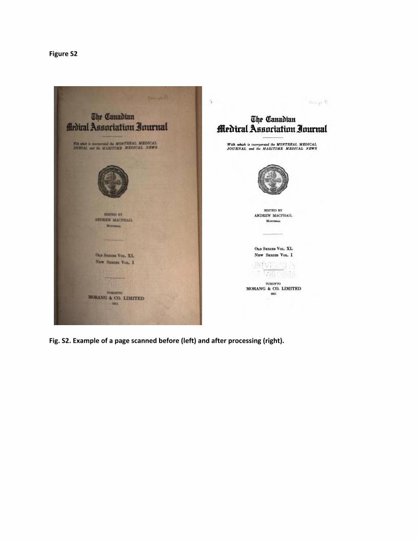
Figure S2

Fig. S2. Example of a page scanned before (left) and after processing (right).

Figure S3

Fig. S3. Outline of n-gram corpus construction. The numbering corresponds to sections of the text.

Figure S4

Fig. S4. Fraction of English Books with a given OCR quality.

Figure S5

Fig. S5. Known events exhibit sharp peaks at date of occurrence. We select groups of events that occur

at known dates, and produce the corresponding timeseries. We normalize each timeserie relative to its

total frequency, center the timeseries around the relevant event, and plot the mean. (A) A list of 124

treaties. (B) A list of 43 head of state (US presidents, UK monarchs), centered around the year when they

were elected president or became king/queen. (C) A list of 28 country name changes, centered around

the year of name change. Together, these form positive controls about timeseries in the corpus.

Figure S6

Fig. S6. Frequency distribution of words in the dictionary. We compute the frequency in our year 2000

lexicon for all 116,156 words (1-grams) in the AHD (year 2000). We represent the percentage of these

words whose frequency is smaller than the value on the x-axis (logarithmic scale, base 10). 90% of all

words in AHD are more frequent than 1 part per billion (10-9), but only 75% are more frequent than 1

part per 100 million (10-8).

Figure S7

Fig. S7. Lexical trends excluding proper nouns. We compute the number of words that are 1-grams in

the categories “P”, “B” and “R”. The same upward trend starting in 1950 is observed. The size of the

lexicon in the year 2000 is still larger than the OED or W3.

Figure S8

Fig. S8. Example of grammatical change. Irregular verbs are used as a model of grammatical evolution.

For each verb, we plot the usage frequency of its irregular form in red (for instance, ‘found’), and the

usage frequency of its regular past-tense form in blue (for instance, ‘finded’). Virtually all irregular verbs

are found from time to time used in a regular form, but those used more often tend to be used in a

regular way more rarely. This is illustrated in the top two rows with the frequently-used verb “find” and

the less often encountered “dwell”. In the third row, the trajectory of “thrive” is one of many ways by

which regularization occurs. The bottom two panels shows that the regularization of “spill” happened

earlier in the US than in the UK.

Figure S9

Fig. S9. We forget. Events of importance provoke a peak of discussion shortly after they happened, but

interest in them quickly decreases.

Figure S10

Fig. S10. Biographical Records. The number of records parsed from the two encyclopedic sources (blue

curve), and used in our analyses (green curve). See steps 7.A.1 to 7.A.10 above.

Figure S11

Fig. S11. Selection of query name. The chosen query name is in black. (A) Adrien Albert Marie de Mun.

Strongest and optimal query name is Albert de Mun, (B) Oliver Joseph Lodge, strongest and optimal

query name is Oliver Lodge, (C) Henry David Thoreau. Strongest query name is David Thoreau, but is a

substring match of Henry David Thoreau, with fame >80% of David Thoreau. Optimal query name is

Henry David Thoreau. (D) Mary Tyler Moore. Strongest name is Mary Moore, but is rejected because of

noise. Next strongest is Tyler Moor, but this is a substring match of Mary Tyler Moore, with fame >80%

of Tyler Moore. Optimal query name is thus Mary Tyler Moore.

Figure S12

Fig. S12. Filtering out names with trajectories that cannot be resolved. Illustrates the requirement for

query name filtration on the basis of premature fame. Fame a birth is the average fame in a 10 year

window around birth, lifetime fame is the average fame from year of birth to 2000. The dashed line in

(A), (D) indicates the separatrix used to excluded query names with premature fame signals. Points to

the right were rejected from further analysis. In (B), (C), (E), (F) the black line indicates the year of birth

of the individuals whose fame trajectories are plotted.

Figure S13

Fig. S13. Values of the four parameters of fame as a function of time. ‘Age of peak celebrity’ (75 years

old) has been fairly consistent. Celebrities are noticed earlier, and become more famous than ever

before: ‘Age of initial celebrity’ has dropped from 43 to 29 years, and ‘Doubling time’ has dropped from

8.1 to 3.3 years. But they are forgotten sooner as well: the half-life has declined from 120 years to 71.

Figure S14

Fig. S14. Fundamental parameters of fame do not depend on the underlying source of people studied.

We represent the analysis of fame using individuals from Encyclopedia Britannica.

Figure S15

Fig. S15. Many routes to Immortality. People leave more behind them than their name: ‘Mary Shelley’

(blue) created the monstrously famous ‘Frankenstein’ (green).

Figure S16

Fig. S16. Controls. (A) We observe over the same timespan (100 years) two cohorts invented at different

times. Again, the more recent cohort reaches 25% of its peak faster. (B) We verify that inventions have

already reached their peak. We calculate the peak of each invention, and plot the distribution of these

peaks as a function of year, grouping them along the same cohorts as used in the text. In each case, the

distribution falls within the bounds of the period observed (1800-2000).

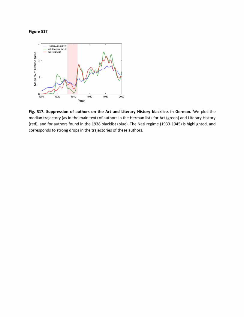
Figure S17

Fig. S17. Suppression of authors on the Art and Literary History blacklists in German. We plot the

median trajectory (as in the main text) of authors in the Herman lists for Art (green) and Literary History

(red), and for authors found in the 1938 blacklist (blue). The Nazi regime (1933-1945) is highlighted, and

corresponds to strong drops in the trajectories of these authors.

Figure S18

Fig. S18. Tracking historical epidemics using their influence on the surrounding culture. (A) Usage

frequency of various diseases: ‘fever’ (blue), ‘cancer’ (green), ‘asthma’ (red), ‘tuberculosis’ (cyan),

‘diabetes’ (purple), ‘obesity’ (yellow) and ‘heart attack’ (black). (B) Cultural prevalence of AIDS and HIV.

We highlight the year 1983 when the viral agent was discovered. (C) Usage of the term ‘cholera’ peaks

during the cholera epidemics that affected Europe and the US (blue shading). (D) Usage of the term

‘infantile paralysis’ (blue) exhibits one peak during the 1916 polio epidemic (blue shading), and a second

around the time of a series of polio epidemics that took place during the early 1950s. But the second

peak is anomalously broad. Discussion of polio during that time may have been fueled by the election of

‘Franklin Delano Roosevelt’ (green), who had been paralyzed by polio in 1936 (green shading), as well as

by the development of the ‘polio vaccine’ (red) in 1952. The vaccine ultimately eradicated ‘infantile

paralysis’ in the United States.

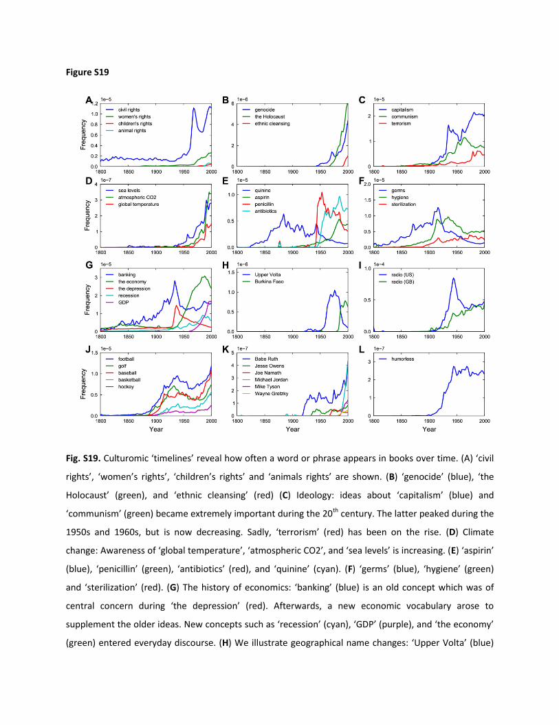
Figure S19

Fig. S19. Culturomic ‘timelines’ reveal how often a word or phrase appears in books over time. (A) ‘civil

rights’, ‘women’s rights’, ‘children’s rights’ and ‘animals rights’ are shown. (B) ‘genocide’ (blue), ‘the

Holocaust’ (green), and ‘ethnic cleansing’ (red) (C) Ideology: ideas about ‘capitalism’ (blue) and

‘communism’ (green) became extremely important during the 20th century. The latter peaked during the

1950s and 1960s, but is now decreasing. Sadly, ‘terrorism’ (red) has been on the rise. (D) Climate

change: Awareness of ‘global temperature’, ‘atmospheric CO2’, and ‘sea levels’ is increasing. (E) ‘aspirin’

(blue), ‘penicillin’ (green), ‘antibiotics’ (red), and ‘quinine’ (cyan). (F) ‘germs’ (blue), ‘hygiene’ (green)

and ‘sterilization’ (red). (G) The history of economics: ‘banking’ (blue) is an old concept which was of

central concern during ‘the depression’ (red). Afterwards, a new economic vocabulary arose to

supplement the older ideas. New concepts such as ‘recession’ (cyan), ‘GDP’ (purple), and ‘the economy’

(green) entered everyday discourse. (H) We illustrate geographical name changes: ‘Upper Volta’ (blue)

and ‘Burkina Faso’ (green). (I) ‘radio’ in the US (blue) and in the UK (red) have distinct trajectories. (J)

‘football’ (blue), ‘golf’ (green), ‘baseball’ (red), ‘basketball’ (cyan) and ‘hockey’ (purple) (K) Sportsmen: In

the 1980s, the fame of ‘Michael Jordan’ (cyan) leaped over other that of other great athletes, including

‘Jesse Owens’ (green), ‘Joe Namath’ (red), ‘Mike Tyson’ (purple), and ‘Wayne Gretsky’ (yellow).

Presently, only ‘Babe Ruth’ (blue) can compete. One can only speculate as to whether Jordan’s hang

time will match that of the Bambino. (L) ‘humorless’ is a word that rose to popularity during the first half

of the century. This indicates how these data can serve to identify words that are a marker of a specific

period in time.