Quantifying the impacts of uncertainties in coastal hazard modelling Thesis submitted in accordance with the requirements of the University of Liverpool for the degree of Doctor in Philosophy by Charlotte Lyddon School of Environmental Science Department of Geography and Planning June 2020

Welcome message from author
This document is posted to help you gain knowledge. Please leave a comment to let me know what you think about it! Share it to your friends and learn new things together.
Transcript

Quantifying the impacts of uncertainties
in coastal hazard modelling
Thesis submitted in accordance with the requirements of the University of Liverpool for the degree of
Doctor in Philosophy
by
Charlotte Lyddon
School of Environmental Science
Department of Geography and Planning
June 2020

i
Declaration
This thesis is the result of my own work and includes nothing which is the outcome of work done in
collaboration except where specifically indicated in the text. It has not been previously submitted, in
part or whole, to any university of institution for any degree, diploma, or other qualification.
In accordance with The University of Liverpool guidelines, this thesis does not exceed 100,000
words.
Signed: C. Lyddon
Date: 19.06.2020

ii
Abstract
This thesis applies coupled regional models to address coastal flood risk management needs in hyper-
tidal estuaries. The project aims to understand how tide-surge-wind-waves combine to increase flood
and wave hazard at the coast, using the Severn Estuary, southwest England as an extreme
example. Little previous research has considered the impact of tide-surge-wind-wave interaction on
total water level in a hyper-tidal estuary.
Numerical modelling tools can be used to predict the individual contributions of physical factors to total
water levels and forms a key component of flood hazard assessment. However uncertainty can be
introduced into model predictions due to inaccurate boundary forcing or representation of the physical
processes which control the volume and rate water moves through a model domain. Uncertainties in
model predictions lead to a wide spread of results within which exposure or impacts could occur.
Similarly, a range of possible values exist for a single parameter which may cause errors in the definition
of critical thresholds or presents challenges to emergency response planners. Sources of uncertainty in
flood hazard assessments should be identified and quantified as sustainable coastal management
requires confidence in the knowledge of any possible future changes to flood and wave hazard.
The thesis utilises wave, ocean and meteorological observation and model hindcast data to simulate
total water level and significant wave height using the Delft3D-FLOW-WAVE modelling package. The
validated Severn Estuary model domain is used to investigate the sensitivity of extreme water levels to
changes in event severity, timing of the peak of a storm surge relative to tidal high water and the
temporal distribution of the storm surge component, and wave heights to changes in wind-wave
direction, model coupling and forcing processes. Model outputs from Delft3D-FLOW-WAVE are
viewed in the context of the source-pathway-receptor-consequence model to better understand the
influence of coastal hazard uncertainty on flood and wave hazard. Event severity is the most important
control on flood hazard, and concurrence of the sources of flood hazard generate greatest water levels
along the coastline of the estuary. Estuarine morphology acts as a pathway for flood hazard, as
funnelling effects control the spatial variability of flood hazard and amplify surge magnitude up to
255% up-estuary. Surge predictions from forecasting systems at tide gauge locations could under-
predict the magnitude and duration of surge contribution to up-estuary water levels. Wave height and
wave period controls the response of wave generation and propagation to other factors. Wind speed
generates greatest wave hazard, and uncertainty in wind and wave direction generate a large spread of
results. Stronger, opposing winds steepen high amplitude, low period waves in the outer estuary and
stronger, following winds enhance propagation of low amplitude high period waves up-estuary. The
inclusion of locally generated winds is most important in regional models to continue to add momentum
to the estuarine system, and model coupling processes (the representation of interaction between wave
and currents) improve accuracy of flood and wave hazard predictions. Exclusion of locally generated

iii
winds can generate up to 1.45 m error in high water significant wave heights in the outer estuary, and
1.13 m error in the upper estuary.
Coastal hazard uncertainty due to model coupling and forcing processes is propagated through the
modelling chain to the two-dimensional inundation model LISFLOOD-FP to understand how changes
in boundary condition and boundary position influences depth, extent and volume of inundation over a
storm event. The exclusion of local atmospheric forcing increases coastal hazard uncertainty in the
boundary forcing and under-predicts damage by up to £26.2 M at Oldbury-on-Severn. Once the
threshold for flooding is exceeded, a few centimetres increase in coastal hazard conditions increases
both the inundation and consequent damage costs for suburbia and arable land.
The results of this thesis identify optimum model setups for simulating coastal flood hazard, which
includes incorporating local atmospheric forcing and representing two-way interaction between waves
and currents. Coastal hazard uncertainty can cause large variability in simulated total water level and
wave heights, which has implications for flood damage assessments, shoreline management plans and
emergency response plans. The research findings can aid long-term coastal defence and management
strategies for improved public safety, and improve the timing and accuracy of early warning systems.
Key sources of coastal hazard uncertainty have been identified here, e.g. the importance of storm surge
timing relative to tidal high water and sensitivity of wave propagation to winds speeds, and these can
be accounted for in future management plans. Utilising optimal model setups when predicting water
level and wave height under current and future climate conditions can also help to increase confidence
in results. Further to this, if the key sources of uncertainty which contribute to a large spread of results
are known, e.g. exclusion of local atmospheric forcing, then this can be resolved in predictions which
are used to inform early warning systems. The spread of model results can therefore be minimised to
more accurately know who or what is in a flood or wave hazard zone.

iv
Acknowledgements
I would like to thank my supervisors for the help, guidance and feedback that they have provided during
this work. Many thanks to Dr Jennifer Brown, Dr Nicoletta Leonardi and Prof Andrew Plater who have
provided endless support and enthusiasm and have been fantastic mentors and role models.
This PhD had no associated research, travel and subsistence fund, therefore I am hugely grateful to Prof
Andy Plater for providing funding from the Engineering and Physical Science Research Council
(EPSRC) funded Adaptation and Resilience of Coastal Energy Supply (ARCoES) research project
(EPSRC EP/I035390/1) and National Environmental Research Council (NERC) funded highlight topic
“Physical and biological dynamic coastal processes and their role in coastal recovery” as part of the
BLUEcoast project (NE/N015614/1) to allow me to attend and present my research at conferences. I
would also like to thank the Environmental Change Research Group which has also provided funding
to allow me to present my research at conferences.
Acknowledgement must also be made to the National Oceanography Centre for the provision of
research facilities and resources throughout this project.
Thanks are also due to friends and colleagues across the institutions and departments, who have
supported and encouraged me.
Finally, my greatest acknowledgement goes to my family and better half. I am immensely grateful and
lucky to have them; this work is dedicated to them.

v
Table of Contents
1. Background & rationale 1
1.1. Drivers of coastal flood hazard 1
1.1.1. Implications of flooding 2
1.2. Combined flood hazard events in estuaries 3
1.2.1. River influence in estuaries 4
1.2.2. Tide dominance in estuaries 5
1.2.2.1. Hyper-tidal estuaries 5
1.3. Flood hazard assessment 6
1.4. Numerical modelling tools for flood hazard assessment 7
1.5. Numerical modelling uncertainties 8
1.6. Thesis aim and research questions 9
1.7. Severn Estuary model setup 10
1.7.1. Delft-3D FLOW 10
1.7.1.1. Development of model grid and bathymetry 10
1.7.1.2. Boundary conditions 12
1.7.1.3. Model parameters 12
1.7.1.4. Calibration and validation 13
1.7.2. Delft3D-WAVE 14
1.7.3. LISFLOOD-FP 15
1.7.3.1. Digital Elevation Model 15
1.7.3.2. Model inputs 15
1.8. Thesis structure 17
2. Flood hazard assessment for a hyper-tidal estuary as a function of tide-surge-
morphology interaction 24
2.1. Abstract 25
2.2. Introduction 25
2.3. Methods 28
2.3.1. Delft3D 28
2.3.2. Model domain 28
2.3.3. Boundary conditions 30
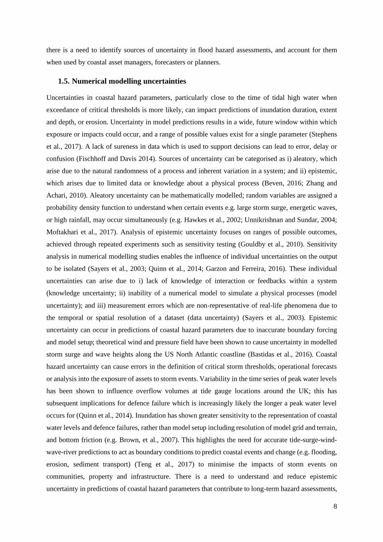
2.3.4. Timing of surge occurrence 34
2.4. Model validation 34
2.4.1. Funnelling effect vs frictional effect 37
2.5. Results 39
2.5.1. Water level variations along estuary 39

vi
2.5.2. Changes in flood hazard proxy with surge timing 43
2.6. Discussion 50
2.6.1. Physical drivers and sources of flood hazard in the Severn Estuary model domain 50
2.6.2. Implications for local management needs in the Severn Estuary and worldwide 55
2.7. Conclusion 56
2.8. Acknowledgements and Data 57
3 Uncertainty in estuarine extreme water level predictions due to surge-tide interaction 58
3.1. Abstract 59
3.2. Introduction 59
3.3. Methods 62
3.3.1. Delft3D and model domain 62
3.3.2. Long-term tide gauge records 63
3.3.3. Tested tide-surge configurations 63
3.3.4. Model validation 64
3.4. Results 66
3.4.1. Surge elevation on 3 January 2014 66
3.4.2. Surge elevation along thalweg 69
3.5. Discussion 72
3.6. Conclusion 75
3.7. Acknowledgements and Data 75
4 Increased coastal wave hazard generated by differential wind and wave direction in
hyper-tidal estuaries 76
4.1. Abstract 77
4.2. Introduction 77
4.2.1. Wave hazard impacts 77
4.2.2. Wave hazard in hyper-tidal estuaries 79
4.2.3. Case study 81
4.3. Methods 83
4.3.1. Delft3D-WAVE 83
4.3.2. Boundary conditions 83
4.3.3. Model validation and scenarios 87
4.4. Results 88
4.4.1. High amplitude waves 88
4.4.2. Low amplitude waves 91
4.5. Discussion 93
4.5.1. Younger, rougher seas show more sensitivity to wind direction. 93

vii
4.5.2. Long period, low amplitude waves amplified due to strong winds 94
4.5.3. Waves impact on flood hazard and economic activities 95
4.5.4. Changing future storm tracks and climate 96
4.6. Conclusion 97
4.7. Acknowledgements and Data 98
5 Quantification of the uncertainty in coastal storm hazard predictions due to wave-
current interaction and wind forcing 99
5.1. Abstract 100
5.2. Introduction 100
5.2.1. Case Study 101
5.2.2. Outline of the paper 102
5.3. Method 102
5.3.1. Delft3D hindcast of select historic events 102
5.3.2. Model validation and scenario test 104
5.4. Results 106
5.4.1. Uncertainty in High Water Level (HWL) 111
5.4.2. Uncertainty in High Water Significant Wave Height (HWHs) 113
5.4.3. Uncertainty in High Water Hazard Proxy (HWHP) 115
5.4.4. Spatial variability of hazard 115
5.5. Discussion 116
5.6. Conclusion 117
5.7. Acknowledgments and Data 118
6 Uncertainty propagation in flood hazard assessments 119
6.1. Abstract 120
6.2. Introduction 120
6.2.1. Case study 122
6.3. Method 125
6.3.1. Input data 125
6.3.2. Inundation model boundary conditions 126
6.3.3. Flood inundation scenarios 128
6.3.4. Depth damage curves 129
6.4. Results 129
6.4.1. Depth and extent of inundation 129
6.4.2. Flood hazard rating at operational sites 138
6.4.3. Volume of inundation in the model domain 140
6.4.4. Quantification of flood hazard due to coastal hazard uncertainty 141

viii
6.4.5. Economic cost of inundation for arable and suburban land uses 143
6.5. Discussion 145
6.6. Conclusion 148
6.7. Acknowledgments and Data 150
7 Conclusions and Implications 151
7.1. Uncertainty in sources and pathways of flood and wave hazard 151
7.1.1. Extra-model uncertainties 151
7.1.2. Intra-model uncertainties 154
7.2. Impacts of coastal hazard uncertainty on receptors and consequences of flood and wave
hazard 156
7.3. Applicability of results to other estuaries 157
7.4. Practical application of thesis results 159
7.5. Coastal hazard uncertainty: implications for long-term planning (up to 2105) with sea
level rise 161
7.5.1. Resilience and flexibility in long-term management plans 162
7.6. Coastal hazard uncertainty: implications for early warning systems 163
8 References 165
Appendix 1 – Delft3D User Guide 195
Appendix 2 – LISFLOOD User Guide 235
ix
Table of Figures
Figure 2.1: Severn Estuary model domain extending from Ilfracome (51°12.668'N,
4°6.743'W) and The Mumbles (51°34.203'N, 3°58.534'W) in the west, to Gloucester (52°
89.3020’N, -2°2. 6361’W) in the east. The bathymetry is relative to chart datum (CD).
29
Figure 2.2: Long-term tide gauge record at The Mumbles, Bristol Channel, U.K showing
tide gauge time series, points in the time series representing high water peaks and events to
be modelled. The panels on the right illustrate the three selected events representing the 95th
(i, 14th December 2012), 90th (ii, 18 December 2013) and 99th (iii, 3 January 2014) water
level percentile values.
30
Figure 2.3: Long-term tide gauge record at Ilfracombe, Bristol Channel, U.K showing tide
gauge time series, points in the time series representing high water peaks and events to be
modelled. The panel on the right illustrates one selected event representing the 95th (i.e. 5
May 2015) water level percentile values.5
31
Figure 2.4: Normalised filtered surge shape component with time, characterised by historical
event severity and skewness (measure of asymmetry). 33
Figure 2.5: Validation down-estuary, Hinkley Point tide gauge. 35
Figure 2.6: Validation up-estuary, Sharpness river gauge. As above. 36
Figure 2.7: Water level along the deepest channel in the Severn Estuary, 3 January 2014,
under varying Manning friction values (99th percentile); the shading represents the range in
results for each filtered surge time shift scenario. Subpanels show the tidal response of i)
hypersynchronous and ii) hyposynchronous estuary to changing frictional effects.
38
Figure 2.8: Maximum water level along the thalweg of the Severn Estuary; a) 99th water
level percentile event (3 January 2014); b) 95th water level percentile event (14 December
2012); c) 90th water level percentile event (18 December 2013); d) 95th water level
percentile event (5 May 2015).
41
Figure 2.9: Range of water level values for time shift configurations along deepest channel
of the Severn Estuary when overall maximum water level occurs. For each event, in the
legend the first value represents the percentile of the event and the second value is the
skewness.
42
Figure 2.10: 3 January 2014. Flood hazard proxy calculated at each tide gauge location. a)
percent change in maximum water level; b) percent change in maximum total surge
elevation; c) percent change in duration exceeding MHWS; d) percent change in area
exceeding MHWS. All data is displayed as percentage change, compared with the tide only
44

x
model scenario, apart from total surge elevation which is compared with the model run when
the peak of the surge and high water coincide.
Figure 2.11: 14 December 2012. Flood hazard proxy, as in Figure 2.10. 46
Figure 2.12: 5 May 2015. Flood hazard proxy, as in Figure 2.10. 48
Figure 2.13:18 December 2013. Flood hazard proxy as in Figure 2.10. 49
Figure 2.14: Duration and area of storm tide peak exceeding MHWS at Sharpness. 50
Figure 3.1: Severn Estuary model domain extending from Ilfracome (51°12.668'N,
4°6.743'W) and The Mumbles (51°34.203'N, 3°58.534'W) in the west, to Gloucester (52°
89.3020’N, -2°2. 6361’W) in the east. The bathymetry is relative to chart datum (CD).
63
Figure 3.2: Model output validation for realistic timing of total water level and tide only
model runs compared to observational data at Hinkley Point tide gauge, Severn Estuary,
southwest England.
65
Figure 3.3: Model output validation for realistic timing of total water level and tide only
model runs compared to observational data at Sharpness tide gauge, Severn Estuary,
southwest England.
66
Figure 3.4: Modelled tidal time series (black); modelled surge elevation for the realistic
surge timing (red line); range of surge elevations for time shifted configurations shaded
(blue band); observed filtered surge (orange line) at a) Hinkley; b) Newport; c) Portbury; d)
Oldbury; e) Sharpness for the 3rd January 2014 event.
68
Figure 3.5: a) Tidal range; b) Surge elevation range for observed event timing; c) Variability
in surge values; d) Variability in skew surge values for time shift configurations along
thalweg of the Severn Estuary.
71
Figure 4.1: 5 years of observational wave buoy data taken from Scarweather (located in
Figure 4.2), Severn Estuary, UK showing a) wave direction (deg) and significant wave
height (m), b) average wave direction and wave period (s) and c) 5 years of observational
wind data taken from Chivenor, Devon (located in Figure 4.2).
82
Figure 4.2: Deflt3D-WAVE model grid. The bathymetry is relative to chart datum (CD). 83
Figure 4.3: Model schematic for the coupled Delft3D hydrodynamic (FLOW) and wave
(SWAN) model with forcing data sources. 84
Figure 4.4: Wave selection for Hs and Tz. 25th percentile Tz (blue line) and 75th percentile
Tz (red line), color coordinated based on wave direction. 85

xi
Figure 4.5: Delft3D-WAVE model validation comparing model simulations to 5 years
observational data at Scarweather wave buoy. Symbols representing directions over a range
of 45 degrees.
87
Figure 4.6: Normalized significant wave height (model scenario – no wind baseline
scenario) for representative high amplitude, short period waves along the shoreline of Severn
Estuary, starting at Swansea to Gloucester and thence down-estuary towards Hinkley Point.
89
Figure 4.7: Normalized significant wave height (model scenario – no wind baseline
scenario) for representative low amplitude, longer period waves along the shoreline of
Severn Estuary, starting at Swansea to Gloucester and thence down-estuary towards Hinkley
Point.
92
Figure 5.1: a) Delft3D-FLOW-WAVE model domain. Bathymetry relative to CD. Average
bias and RMSE (m) of WL and Hs model results for four events to tide gauge and wave
buoy observations are shown in brackets; (b) six year Hs record from Scarweather wave
buoy; (c) Long-term tide gauge record taken from Ilfracombe, with HWHP grouped based
on wind direction at the time of the event. HWL, HWHs, and wind speed (WS) at the time of
the events are shown. Horizontal black lines indicate maximum, 90th, 50th and 10th
percentile HP thresholds.
103
Figure 5.2: Simulated a) HWL; b) HWHs; c) HWHP along the coastline of Severn Estuary
starting at Swansea to Gloucester and thence down-estuary towards Woolacombe for
maximum event (3 January 2014 07:00); d-f) % difference between each run and run 8. The
divide between north and south coastlines (dashed black vertical line) and wave limit where
Hs < 10 cm (dashed grey vertical line) is shown. Solid black vertical lines indicate locations
of critical infrastructure and coastal towns.
108
Figure 5.3: Absolute difference for a) HWL; b) HWHs; c) HWHP between each run and run
8 along the coastline of Severn Estuary starting at Swansea to Gloucester and thence down-
estuary towards Hinkley Point for maximum event (3 January 2014 07:00). The divide
between north and south coastlines (dashed black vertical line) and wave limit where Hs <
10 cm (dashed grey vertical line) is shown. Solid black vertical lines indicate locations of
critical infrastructure and towns along the coastline.
111
Figure 5.4: For the a) north (left panels) and b) south (right panels) coastlines the alongshore
maximum, mean and median percentage difference in i) HWL; ii) HWHs; iii) HWHP
between model simulations is calculated for the four events with hazard potential calculated
using the HP parameter.
111

xii
Figure 5.5: For the a) north (left panels) and b) south (right panels) coastlines the alongshore
maximum, mean and median absolute difference in i) HWL; ii) HWHs; iii) HWHP between
model simulations is calculated for the four events with hazard potential calculated using the
HP parameter.
112
Figure 5.6: % difference across the Severn Estuary model domain in HWHs for the 50th
percentile event between a) run 8 (two-way + wind) – 7 (two-way); b) run 8 (two-way +
wind) – 6 (one-way + wind); and c) % difference depth average velocity run 8 (two-way +
wind) – 6 (one-way + wind) Limits are scaled to show the main differences, but the values
may exceed these in isolated areas at the coastline.
114
Figure 6.1: a) Oldbury model domain, including the location of Delft3D outputs (coloured
dots) used to force the HP and WR boundary approach (coloured lines); boundary midpoint
to calculate change in coastal hazard uncertainty (black cross); sites of critical infrastructure
(yellow star and triangle); and b) Delft3D-FLOW-WAVE model domain with extent of the
up-estuary Oldbury model domain shown.
123
Figure 6.2: Model inputs and the process followed to propagate and quantify uncertainty in
flood hazard assessments, and results that are presented in section 3. 125
Figure 6.3: a) Coastal hazard uncertainty time series from Delft3D-FLOW-WAVE used to
force LISFLOOD-FP, for Jan 14 event using the HP approach, shown here as an example; b)
zoom of peak of the Jan 14 event to show coastal hazard uncertainty.
127
Figure 6.4: Depth and extent of flooding at Oldbury-on-Severn for HP approach to forcing
the model boundary where maps 1-8 represent coastal hazard uncertainty (see Table 6.1) for
Jan 14.
131
Figure 6.5: Depth and extent of flooding at Oldbury-on-Severn for WR approach to forcing
the model boundary where maps 1-8 represent coastal hazard uncertainty (see Table 6.1) for
Jan 14.
133
Figure 6.6: Depth and extent of flooding at Oldbury-on-Severn for HP approach to forcing
the model boundary where maps 1-8 represent coastal hazard uncertainty (see Table 6.1) for
Dec 12.
135
Figure 6.7: Depth and extent of flooding at Oldbury-on-Severn for WR approach to forcing
the model boundary where maps 1-8 represent coastal hazard uncertainty (see Table 6.1) for
Dec 12.
137
Figure 6.8: Flood hazard rating during the Jan 14 event at a) road junction; b) pylon; and
during Dec 12 event at c) road junction; and d) pylon using the HP (dashed black line) and 139

xiii
WR approach (solid black line). Modelled tidal signal at the boundary midpoint (vertical
dotted black line) and extreme (red, horizontal dotted line), significant (amber, horizontal
dotted line) and moderate (green, horizontal dotted line) thresholds for hazard to people
(DEFRA 2003).
Figure 6.9: Change in volume of inundation (Mm3) in the Oldbury model domain for Jan 14
forced by a) HP and c) WR; and Dec 12 forced by c) HP and d) WR. Modelled high tide
from low water to low water is also shown (dashed line).
140
Figure 6.10: Absolute difference in HP at the boundary midpoint (shown in Figure 6.1a)
against absolute difference in time-integrated volume for a) all runs compared to baseline
run 8; and b) zoomed into run 1, 2, 5, and 7.
141
Figure 6.11: Absolute difference in HP at the boundary midpoint (shown in Figure 6.1a)
against absolute difference in a) arable land costs and b) suburban land cost for runs 1,2,5,6
and 7 compared to baseline run 8.
144

xiv
Table of Tables
Table 2.1: Scenarios modelled in Delft3D for each historical extreme water level event. 34
Table 2.2: Statistical validation down-estuary, Hinkley tide gauge. The filtered surge is
applied at a realistic time relative to tidal high water for validation purposes.
35
Table 2.3: Statistical validation up-estuary, Sharpness river gauge 36
Table 3.1: Contribution of surge to total water level at the time of maximum surge (total
water level – predicted tidal level), tidal low water and tidal high water.
69
Table 4.1: Representative wind wave conditions close to the estuary mouth based on 5 years
of observational data from Scarweather Waverider buoy.
86
Table 4.2: Representative wind speeds based on 5 years of observational data from Chivenor
in Devon (England) and Pembrey Sands in Dyfed (Wales) UK Met Office MIDAS land
station data.
86
Table 5.1: Eight model simulations completed in Delft3D-FLOW-WAVE for each historic
storm event.
105
Table 5.2: Overall maximum, mean and median percentage difference in HWL, HWHs and
HWHP in the lower/mid estuary (to wave limit) and the entire estuary coastline.
115
Table 6.1: Eight model simulations completed in Delft3D-FLOW-WAVE for each historic
storm event, and outputs used to force the boundary of the Oldbury model domain in
LISFLOOD-FP from the low water mark and defence crest.
126
Table 6.2: Simulated economic cost of inundation for arable land cover 143
Table 6.3: Simulated economic cost of inundation for suburban land cover 143

1
1. Background & rationale
1.1. Drivers of coastal flood hazard
Coastal communities and infrastructure are increasingly vulnerable to the combined effect of
astronomical tides, storm surges, wind, waves and rivers, as floodplain development becomes
increasingly connected and interdependent (Aerts et al., 2014; Blackburn et al., 2019). Violent storms
and hurricanes can cause short-term, local variations in sea level due to the combined effect of i) reduced
atmospheric pressure (inverse barometer effect) (Proctor and Flather 1989); ii) strong winds, leading to
build up of water in shallow areas (wind setup) (Hoeke et al., 2015); iii) short-term rise in sea level due
to wave breaking (wave setup) (Brown et al., 2013); iv) cumulative effect of instantaneous uprush of
individual waves (wave runup) (Senechal et al., 2011); v) high river discharge in estuaries and deltas
(Bricheno et al., 2016). Total water level at the coast is highly sensitive to other external forces including
changes in near-shore coastal bathymetry due to sediment transport processes (Pollard et al., 2019), and
inter-annual and seasonal variability in sea level (Amiruddin et al., 2015; Dangendorf et al., 2013). The
combined effect of these coastal hazard parameters can elevate observed water levels above the
predicted level, generating extreme water levels (Marcos et al., 2019). Tide-surge and wave-current
interaction has also been shown to influence The timing and magnitude of extreme water levels at the
coast can also be influenced by tide-surge interaction, which is largely a function of surge magnitude
and enhances current velocities during storms, or wave-current interaction which can generate larger
waves at high water (Horsburgh and Wilson, 2007; Idier et al., 2012; Lewis et al., 2019). These high
frequency variations in sea level occur on an event, or weather, timescale with storms typically effecting
sea level in the UK for 3.5 days (Haigh et al., 2016), and can be superimposed onto longer term, low
frequency variations. Spring tidal cycles and nodal cycles are phase locked, which can make extreme
water levels more predictable (Boon, 2004). Inter-annual and decadal variability in sea level and
storminess can be observed because of changes in climate such as El Niño Southern Oscillation
(ENSO), North Atlantic Oscillation (NAO) or Pacific Decadal Oscillation (POD) (Barnard et al., 2017;
Idier et al., 2019). For example, positive NAO can shift storm tracks up to 180 km north, lower pressure
to generate storm surges and increase wind speeds. This has implications for the coastline response to
wind speed, direction, sea level and waves for communities on the North West European shelf (Phillips
et al., 2013). This may also have implications for river hydrograph shapes, generating greater flow
magnitude and increasing water levels in up-estuary locations (Robins et al., 2018). Thermal expansion
and contribution of melting ice caps under future, long term climate change will continue to elevate
mean sea level and the baseline on which storms are generated in the UK (Lowe and Gregory 2005)
and worldwide (Nicholls et al., 2014; Shepard et al., 2012). There is a need to understand the temporal
changes in drivers for flooding, notably high frequency variations which can elevate coastal water
levels. The impact of extreme water levels on developed, interconnected floodplains is particularly

2
critical in heavily populated and industrialised estuaries, where low-lying floodplains are increasingly
used for critical infrastructure, that provide essential services to communities (Ruckert et al.,
2019). Industrialised estuaries and deltas support transport and energy infrastructure, water supply and
access (i.e. ports & harbours), and 21 of the world’s 30 largest cities are located next to estuaries
(Ashworth et al., 2015). It is of critical, international importance that we fully understand the drivers of
flood hazard on the shores of estuaries for accurate hazard assessments in long-term management plans.
Coastal communities and critical infrastructure are often protected against the effect of extreme water
levels, due to the combined effect of coastal hazard parameters (i.e. tide, surge, wind, wave, river), by
sea walls or coastal defences. These defences are designed and built to a critical threshold height
(ℎ𝑡ℎ𝑟𝑒𝑠ℎ𝑜𝑙𝑑) which should offer protection from extreme water levels. Natural barriers, such as gravel
forelands or shingle barriers, also offer a degree of protection from extreme water levels but also face
erosion hazard during extreme events (Brown et al., 2016). If the combined effect of coastal hazard
parameters is below a critical threshold then no adverse effects at the coast are experienced. As soon as
the combined effect of these coastal hazard parameters causes highest water levels or waves to exceed
critical threshold height then a coastal community is considered vulnerable to the flood hazard, as higher
water levels represent an agent for potential damage or harm (Idier et al., 2013). Substantial impacts
can be expected at the coast once an extreme water level exceeds critical threshold, and damaging
coastal flooding can occur under present-day sea-level conditions, at a specific location (𝑥) at a specific
time (𝑡) as soon as:
ℎ𝑡ℎ𝑟𝑒𝑠ℎ𝑜𝑙𝑑(𝑥, 𝑡) < ℎ𝑝𝑟𝑒𝑑(𝑥, 𝑡) + 𝜉𝑏𝑎𝑟(𝑥, 𝑡) + 𝜉𝑤𝑖𝑛𝑑 (𝑥, 𝑡) + 𝜉𝑤𝑎𝑣𝑒𝑠(𝑥, 𝑡) + 𝜉𝑟𝑖𝑣𝑒𝑟(𝑥, 𝑡)
where ℎ𝑝𝑟𝑒𝑑 is the water level corresponding to the predicted tide and 𝜉𝑏𝑎𝑟 , 𝜉𝑏𝑤𝑖𝑛𝑑, 𝜉𝑤𝑎𝑣𝑒 and 𝜉𝑟𝑖𝑣𝑒𝑟
are the additional water levels resulting from barometric and wind effects and the wave set-up (adapted
from Le Cozannet et al., 2015). The combined effect of coastal hazard parameters can elevate water
levels and exceed critical thresholds, which poses a hazard to coastal communities. Research has
previously considered the probability of events occurring, including joint probability studies (e.g. Prime
et al., 2016) and the dependence or independence of coastal hazard parameters (e.g Williams et al.,
2016). Here we focus on hazards only, no account is being made of risk, and how physical processes
combine to elevate water level and wave height at the coast.
1.1.1. Implications of flooding
The combined effect of tide, surge, wind, waves, and rivers represents a significant flood hazard, and
critical thresholds may be exceeded to cause flooding. Flooding can have wide implications for people
and cause significant economic and environmental damage in estuarine and coastal zones (Wolf 2009).
12% of all deaths from natural disasters in the 1990s were due to flooding, which claimed over 90,000
lives across the world (Defra, 2006). Over 300 million people live in low-lying coastal zones and are

3
directly vulnerable to the effects of flooding (Hinkel et al., 2014), which can cause damages in the order
of tens of billions of US$ per year (Kron 2013). Several recent extreme meteorological events have
caused catastrophic human and economic losses in coastal areas (Brown et al., 2014), such as Cyclone
Nargis (Myanmar, 2008), Hurricane Sandy (eastern United States, Canada and Caribbean, 2012) and
Typhoon Haiyan (Philippines, 2013). Flash floods, due to heavy and persistent precipitation, have
caused fatalities and damages in coastal towns including Lynmouth, Devon (1952) and significant
damage in Boscastle, Cornwall (2004) (Archer and Fowler 2018). Floods not only directly and
immediately cause loss of human life, damage to property and environmental damage due to erosion,
but can also impact livelihoods due to destruction of crops, loss of livestock, and disruption to
communication links and infrastructure (such as power plants, roads, bridges and railways) e.g. Dawlish
railway, Devon (Dawson et al., 2016), which can cause economic standstill. Floods can increase the
transport and delivery of untreated sewage, toxic substances (i.e. heavy metals), pathogens, and
pollutants which can enter the food chain or water supply and cause deterioration of health conditions,
due to contamination and waterborne diseases (Robins et al., 2018). Impacts can be experienced long
after flood waters have receded, as saltwater intrusion can cause deterioration of water quality and
influence nutrient levels, hydration and growth of plants and crops (Williams 2009; Gimeno et al., 2012;
Tully et al., 2019) which can take years to recover from, and displacement from homes and businesses
can cause emotional distress. These impacts will be site specific, and the severity will depend on when
and where they occur, the preparedness of a community and emergency response plans that are in place.
Estuaries worldwide have high socio-economic value, are ecologically rich and have dense, growing
populations, therefore it is valuable to understand how physical processes combine to cause flooding,
as these events can have significant and long-term consequences.
1.2. Combined flood hazard events in estuaries
Estuarine environments are particularly at risk from the combined effect of coastal hazard parameters
due to their exposure to both storm tides from the ocean side and riverine discharges from the terrestrial
side (Monbaliu et al., 2014; Olbert et al., 2017). When these parameters interact, floods can be more
severe than when they occur in isolation and the impacts disproportionately large and adverse; this is
called ‘compound flooding’ (Hendry et al., 2019). The relative contribution of each coastal hazard
parameter to an extreme water level varies in estuaries dependent on differentiation at: i) a global scale
including latitude, oceanic basins and large landmasses; ii) regional variation in estuary hydrodynamic
processes, controlled by estuary basin geometry, and river and oceanic forcing; and iii) local catchment
processes due to local geology and land cover (Hume et al., 2007; Olbert et al., 2013). The geometry of
an estuary (i.e. size and shape) and the dominant drivers of flood hazard are one of the strongest controls
on flood hazard, and closely interlinked. River, tide, or wave dominance in an estuarine system can
shape the local morphology but can also be a function of local morphology.

4
1.2.1. River influence in estuaries
Rivers can be an important drivers of water levels and flooding in upper estuaries and lower catchments,
due to hydrological and atmospheric processes. Increased local rainfall intensities alone can increase
river discharges and enhance river levels to exceed critical thresholds, and cause flooding (Barker et al.,
2016). There is also a compound flood hazard when increased river discharges transport river runoff to
estuaries near-simultaneously with the peak of storm surge, which often both originate from the same
storm (Prime et al., 2015; Khanal et al., 2019). The river is not able to discharge its water at the outlet,
as high seawaters block the estuary, and river water levels rise (Van Den Hurk et al., 2015). There is a
recognised global statistical dependence between storm surge and precipitation/river floods (Svensson
and Jones 2002; Zheng et al., 2013), and the simultaneous occurrence of high discharge and sea-levels
is important for designing flood protection infrastructure (Ward et al., 2018). However, variation in
prevailing storm conditions catchment characteristics at a regional scale strongly influences the
dominance of rivers in estuarine systems. Spatial variability in storm characteristics between the east
and west of the UK influences the joint occurrence of high skew surges and high river discharges,
indicating that storms which generate both are more likely to occur on the west coast (Hendry et al.,
2019). Temporal variability in river contribution to coastal water levels is highlighted in the Scheldt
Estuary, Belgium, as rainfall intensity and subsequent magnitude of river discharge has a strong control
on tidal amplification and tidal range in the whole river (Wang et al., 2019). The characteristics of river
catchments has a strong control on the rate of transport of river discharges to estuaries, and the
subsequent likelihood and severity of compound events occurring. Estuaries with steeper catchments
are more prone to combined storm tide and riverine flooding, due to the rapid transport of abundant
rainfall through the system to the coast (Svensson and Jones, 2002). Rapid-response systems, such as
the Conwy River, Wales have smaller catchment areas and are sensitive to sub-daily river flow
variability which may influence representation of water quality modelling studies, whereas slow
response systems, such as the Humber Estuary, UK, have larger catchments with shallower slopes and
are less sensitive to high frequency variations in river flow (Robins et al., 2018). The lagged occurrence
between elevated river and coastal water levels can also influence flood hazard; clear correlation
between storm surge and increased river discharge was found in the Rhine catchment, but only when a
substantial time lag of 6 days was considered, which is the timescale for excess precipitation to reach
the estuary (Klerk et al., 2015). The occurrence of peak river flow several days after the storm surge
has also been noted in catchments with larger areas and shallow elevation gradient in the UK, such as
the Severn Estuary, therefore reducing the hazard from river flooding (Hendry et al., 2019). Rivers can
be important drivers of flooding, alone or in combination with storm surges but the relative contribution
of rivers to coastal flood hazard is site specific and primarily dependent on storm and catchment
characteristics.

5
1.2.2. Tide dominance in estuaries
Tide-dominated estuaries largely occur on coastlines with a strong M2 semi-diurnal tide, and the shape
and size of an estuary can also influence the tidal characteristics of a system (Pye and Blott, 2014).
Analytical solutions for a range of estuarine shapes and sizes indicate how by length, bed friction and
river flow influence the varying tidal characteristics (Prandle 1985). As tides, which are generated in
the deep ocean basins, propagate into estuaries they can be amplified due to the geometrical shape
(bathymetry and topography) of long, shallow, narrow funnel-shaped estuaries, causing large tidal
ranges in their head region and potentially a bore (e.g. Qiantang River, China). Tides may also be rapidly
diminished if an estuary is constricted by geology, such as open to the ocean via a narrow inlet or
constricted by a bar (e.g. Kochi Inlet, India) (De Ruiter et al., 2017). Estuaries can be classified based
on their shape or origin e.g. coastal plain (funnel-shaped), bar-built, fjords or tectonic (Prandle 2009),
which can then influence the tidal characteristics of an estuary (Davies 1964). Classifications based on
tidal characteristics and range are as follows; micro-tidal (tidal range < 2 m, e.g. Curonian Lagoon,
Baltic Sea), meso-tidal (2 m < tidal range < 4 m, e.g. Colombia River, USA), macro-tidal (4 m < tidal
range < 6 m, e.g. Gomso Bay, South Korea), and hyper-tidal (tidal range > 6 m, e.g. Bay of Fundy,
Canada). Each estuary will respond differently to drivers of flood hazard depending primarily on its
shape and size and studying the response of individual estuaries can provide useful case studies of the
dominant drivers of flood hazard.
1.2.2.1. Hyper-tidal estuaries
Hyper-tidal estuaries display some of the most extreme tidal ranges worldwide. The Bay of Fundy,
Cananda has a mean spring tidal range up to 13.5 m at Noel Bay (Marmer, 1922) and the Severn Estuary,
which borders south-west England and south Wales has a mean spring tidal range up to 12.2 m at
Avonmouth (Uncles, 2010). These estuaries both display resonance with the M2 tide, which causes
enhancement of the tide (Godin, 1993; Liang et al., 2014). The extreme tidal range has been shown to
be a result of the overall shape and length of the estuary, as a pronounced ‘funnel shape’ and channel
convergence amplifies the tidal wave up-estuary (Prandle 1985; Davies and Woodroffe 2010; Dronkers
2017). The shape and length-scale makes a hyper-tidal estuary more susceptible to the effects of
combined hazards, and the impacts of a hazard could be amplified when all parameters occur
concurrently. Small changes in water level due to the combined effect of coastal hazard parameters, can
influence fetch, wave propagation, refraction and breaking and wetting and drying, to substantially alter
flood hazard. Coincidence of the Groundhog Day storm in 1976 with sustained winds up to 102 mph
generating large waves, along with the 18.03 year tidal modulation in the Bay of Fundy, Canada, caused
up to 1.6 m flooding and substantial damage (Desplanque and Mossman 2004). The 3 January 2014
storms in southwest England and Wales saw record water levels exceeded, as a low pressure system,
with central pressure 989 mbar, coincided with a perigee new moon spring tide (Sibley et al., 2015).

6
Different combinations of high tidal levels, notably due to equinoctial spring tides or the nodal cycle
(Haigh et al., 2011), and storm surge can generate higher peak storm tides with longer duration to
increase flood hazard at specific times (Menéndez and Woodworth 2010). These examples show how
coastal hazards can combine to elevate flood hazard in hyper-tidal estuaries, however it should be noted
that increased river discharge did not contribute to flood hazard during these events. Hyper-tidal
estuaries are largely tide-dominated, and river flow has little influence on tidal dynamics (Prandle and
Lane, 2015). That is not to say that high river discharge could not coincide with a storm surge and
elevate flood hazard, but the large catchment area and additional time-take for increased fluvial
discharge to travel through these systems, sometimes up to 6 days (Hendry et al., 2019), means that
flood hazard is largely driven by forcing from the ocean side (tide, surge, wind, waves) and may not be
so important here. Further to this, there is nothing to stop any combination of drivers of flood hazard
occurring in a hyper-tidal estuary and the impacts may be amplified when they occur concurrently,
maybe more so that in a micro-tidal or bar-built estuary. Therefore, hyper-tidal estuaries present a
unique and extreme case study to understand the interactions between coastal flood hazard parameters
during high-frequency storm event, and their impacts at a regional scale to support adaptation and
mitigation planning. The extreme tidal range could also contribute to large uncertainties in predictions
of tide, storm surge and waves at locations away from tide gauges and observation stations, which
should be considered in flood hazard assessments.
1.3. Flood hazard assessment
The accurate prediction of each coastal hazard parameter and its contribution to peak storm tide along
a coastline forms a key component of flood hazard assessment (Perini et al., 2016). These assessments
ultimately aim to understand the susceptibility of coastlines to flooding and potential implications of
floods (Carrasco et al., 2012). This involves developing a thorough understanding of the characteristics
of a particular flood event due to combined effect of coastal hazard parameters, combined with an
understanding of the assets that would be exposed to the particular hazard and subsequent damage (de
Moel and Aerts 2011). Flood hazard can be represented in the form of maximum water level and wave
heights that occur along the coastline which could lead to the exceedance of critical thresholds, or hazard
maps to show subsequent impacts of exceedance including flood characteristics, such as inundation
depth, flow velocity and inundation duration (Merz et al., 2010). This information can be used to define
high risk areas where additional mitigation measures should be focused, inform cost-benefit analysis of
intervention schemes and aid the development of long-term management plans (Barnard et al., 2019).
Flood hazard assessments aim to minimise the negative effects of combined coastal hazards, not only
to reduce economic impacts but also to protect public safety and environmental integrity.

7
1.4. Numerical modelling tools for flood hazard assessment
One key aspect of flood hazard assessment is the accurate prediction and likely projection of extreme
water levels to understand the duration and intensity of a hazard for forecasts, alerts, flood warnings at
an event scale (Lewis et al., 2013) and the design of suitable, site-specific defence measures based on
potential consequences (Wadey et al., 2015). Further to this, combining predictions of coastal hazard
parameters with flood damage assessment can inform and support long-term, sustainable flood
resilience and adaptation strategies for communities at risk of flooding (Roebeling et al., 2011), notably
shoreline management plans up to 2105 (Environment Agency 2010). Process-based, numerical
modelling tools can be applied to a range of environments and can be forced with observation or model
data to generate extreme water level scenarios, and also simulate the impacts of individual coastal
hazard events. Hydrodynamic numerical models, e.g. Delft3D (Lesser et al., 2000), MIKE21 (Warren
and Bach 1992) or Telemac (Galland et al., 1991), are based on finite differences which solve unsteady
shallow water equations in two (depth-averaged) or three dimensions. These models are forced at an
open boundary with water level to simulate tide and surge propagation based on the horizontal
momentum equations, the continuity equation, the transport equation, and a turbulence closure model,
the details of which are provided in each model handbook e.g. Deltares, 2011. Simulating WAves
Nearshore (SWAN) is a 3rd generation spectral wave model to simulate nearshore waves (Booij et al.,
1999), which can be coupled with hydrodynamic models to simulate peak storm tide heights along a
coastlines length (including wave effects and natural variability) and when critical thresholds may be
exceeded. Shoreline response models, e.g. LISFLOOD (Bates et al., 2005) and X-Beach (Roelvink et
al., 2009) can help to link information on total water level components (i.e. tide, surge, runup) with
coastal impacts, by inferring likely flood extents, erosion risk and potential losses from specific events.
Bathtub flood maps are a 1D option for simulating the effects of extreme water levels, but have been
shown to underperform compared to 2D models (Didier et al., 2018). Numerical modelling tools can
provide useful assessments of the drivers of extreme water levels and their impacts to facilitate the
management and emergency response of coastal resources, improve the design of sea defences, and
inform the public and decision makers to minimise loss of life from extreme events. The prediction of
coastal hazard parameters is not only important for predicting when water level and wave heights will
exceed critical thresholds, but also in designing appropriate thresholds in the first place, for cost-
effective coastal protection strategies (Del Río et al., 2012). Finally, a thorough understanding of the
combined effect of coastal hazard parameters can aid long-term inundation assessments to understand
how estuarine and coastal zones may response to future changes in sea level and storm tracks (Pasquier
et al., 2019; Robins et al., 2016). However, uncertainty is inevitably introduced into model predictions
due to inaccurate representation of baseline / initial conditions, inaccurate boundary forcing, or the
inability of a model to accurately represent physical processes which control the volume and rate water
enters a model domain, and subsequent distribution across the domain (Quinn et al., 2014). Therefore
8
there is a need to identify sources of uncertainty in flood hazard assessments, and account for them
when used by coastal asset managers, forecasters or planners.
1.5. Numerical modelling uncertainties
Uncertainties in coastal hazard parameters, particularly close to the time of tidal high water when
exceedance of critical thresholds is more likely, can impact predictions of inundation duration, extent
and depth, or erosion. Uncertainty in model predictions results in a wide, future window within which
exposure or impacts could occur, and a range of possible values exist for a single parameter (Stephens
et al., 2017). A lack of sureness in data which is used to support decisions can lead to error, delay or
confusion (Fischhoff and Davis 2014). Sources of uncertainty can be categorised as i) aleatory, which
arise due to the natural randomness of a process and inherent variation in a system; and ii) epistemic,
which arises due to limited data or knowledge about a physical process (Beven, 2016; Zhang and
Achari, 2010). Aleatory uncertainty can be mathematically modelled; random variables are assigned a
probability density function to understand when certain events e.g. large storm surge, energetic waves,
or high rainfall, may occur simultaneously (e.g. Hawkes et al., 2002; Unnikrishnan and Sundar, 2004;
Moftakhari et al., 2017). Analysis of epistemic uncertainty focuses on ranges of possible outcomes,
achieved through repeated experiments such as sensitivity testing (Gouldby et al., 2010). Sensitivity
analysis in numerical modelling studies enables the influence of individual uncertainties on the output
to be isolated (Sayers et al., 2003; Quinn et al., 2014; Garzon and Ferreira, 2016). These individual
uncertainties can arise due to i) lack of knowledge of interaction or feedbacks within a system
(knowledge uncertainty; ii) inability of a numerical model to simulate a physical processes (model
uncertainty); and iii) measurement errors which are non-representative of real-life phenomena due to
the temporal or spatial resolution of a dataset (data uncertainty) (Sayers et al., 2003). Epistemic
uncertainty can occur in predictions of coastal hazard parameters due to inaccurate boundary forcing
and model setup; theoretical wind and pressure field have been shown to cause uncertainty in modelled
storm surge and wave heights along the US North Atlantic coastline (Bastidas et al., 2016). Coastal
hazard uncertainty can cause errors in the definition of critical storm thresholds, operational forecasts
or analysis into the exposure of assets to storm events. Variability in the time series of peak water levels
has been shown to influence overflow volumes at tide gauge locations around the UK; this has
subsequent implications for defence failure which is increasingly likely the longer a peak water level
occurs for (Quinn et al., 2014). Inundation has shown greater sensitivity to the representation of coastal
water levels and defence failures, rather than model setup including resolution of model grid and terrain,
and bottom friction (e.g. Brown, et al., 2007). This highlights the need for accurate tide-surge-wind-
wave-river predictions to act as boundary conditions to predict coastal events and change (e.g. flooding,
erosion, sediment transport) (Teng et al., 2017) to minimise the impacts of storm events on
communities, property and infrastructure. There is a need to understand and reduce epistemic
uncertainty in predictions of coastal hazard parameters that contribute to long-term hazard assessments,

9
as sustainable coastal management requires confidence in the knowledge of any possible future changes
to flood and wave hazard (Ranasinghe 2020).
1.6. Thesis aim and research questions
The overall goal of this work is to utilise numerical modelling tools to identify and quantify sources of
uncertainty in coastal hazard prediction, and quantify the impacts of coastal hazard uncertainty on
coastal communities to support the development of effective coastal hazard mitigation strategies and
builds resilience to future change.
This research uses the Severn Estuary, which borders southwest England and south Wales as an extreme
test case of how coastal hazard parameters can combine and influence flood hazard in an estuary. The
estuary has a mean spring tidal range up to 12.2 m at Avonmouth, which occurs due to the estuaries
long-length scale and shape, which causes a funnelling effect to amplify tidal propagation up-estuary
(Uncles 2010). Near resonance with the M2 tidal component (the back and forth movement of water
from head to mouth of the estuary occurs at the same frequency as the M2 tide) also amplifies the tidal
range (Liang et al., 2014). The orientation of the estuary to the Atlantic Oceans means that the fetch is
large, and it is exposed to prevailing wind, wave and storm conditions. Flood hazard is largely
attributable to tidal water sources. The contribution of river flow to flood hazard increases east towards
the tidal limit of the estuary at Gloucester (Atkins, 2013), however a time-lag up to 6 days between
occurrence of a storm surge and peak river flow occurring from the same storm means that river level
rarely contributes to coastal flood hazard (Hendry et al., 2019). Therefore, sensitivity of coastal flood
hazard to fluvial contribution is not considered in this study but could be considered in the future. 50,000
hectares of land, over 250,000 homes and £14 billion infrastructure, including the decommissioned
Oldbury Nuclear Power Station, are located between Hinkley Point, Somerset and Gloucester on the
south coastline of the estuary, and tidal floodplains extend up to 5 km inland (Environment Agency,
2011). Major Welsh cities, including Swansea, Cardiff, and Newport are located on the north coastline
of the estuary which are important centres for port operations, cargo and steel handling.
The Severn Estuary is a suitable location to assess and quantify coastal hazard uncertainty and
subsequent impacts because of its hyper-tidal regime, which is an extreme test case of how a large tidal
range can influence tide-surge-wave propagation, local fetch, wetting and drying impacts on hazard.
Many businesses, communities and hugely critical infrastructure rely on accurate flood assessments in
the Severn Estuary, and the results presented here can help to inform future adaptation, resilience and
mitigation strategies in this estuary, and other similar shaped, hyper-tidal estuaries worldwide.
This thesis will apply coupled regional models to coastal flood hazard management needs in the Severn
Estuary to answer the following research questions;

10
i. Which key sources of coastal hazard uncertainty should be considered when predicting
coastal flood and wave hazard?
ii. What is the relative importance of each source of uncertainty in coastal flood hazard
assessments?
iii. How does coastal hazard uncertainty influence the physical and economic impacts of
flooding?
1.7. Severn Estuary model setup
Process-based numerical modelling tools are based on detailed knowledge of the physical processes
and phenomena that describe hydrodynamic and sediment transport characteristics and feedback using
basic physical principles (Dissanayake et al., 2015). Delft3D is used here as a process-based model to
simulate coastal hazard parameters in the Severn Estuary, and LISFLOOD-FP is used to transform
offshore boundary forcing from Delft3D into the nearshore area. The following section describes these
models in more detail, and a user guide for each is provided in Appendix 1 and 2.
1.7.1. Delft3D-FLOW
Delft3D is an integrated flow and transport modelling system which is widely used to simulate flows,
sediment transport, waves and morphological developments in coastal, river and estuarine areas (Lesser
et al., 2004; Condon and Veeramony, 2012; George et al., 2012; Borsje et al., 2013). The FLOW module
of the model can simulate two-dimensional (2DH, depth-averaged) or three-dimensional (3D) unsteady
flow resulting from tidal and/or meteorological forcing (Deltares 2011). Delft3D-FLOW solves the
unsteady shallow water equations, derived from Navier-Stokes, which describes the flow below a
surface in an incompressible fluid over time (Dastgheib et al., 2008). The momentum and continuity
equations propagate the variables through curvilinear, rectilinear or flexible mesh grid based on the
principles that i) mass is conserved and ii) Newton’s second law (𝑀𝑎𝑠𝑠 × 𝑎𝑐𝑐𝑒𝑙𝑒𝑟𝑎𝑡𝑖𝑜𝑛 = 𝑓𝑜𝑟𝑐𝑒) (
Roelvink and Van Banning, 1994; Lesser et al., 2004). Water is driven through the model domain by
gravity and water level gradients induced by tides, wind and river, and simulates wetting and drying
processes. Density and salinity changes can be important in generating residual currents or when
considering sediment transport processes in 3D. Momentum can be dissipated within the modelled area
by bottom friction, waves, bedforms and turbulence. Delft3D-FLOW can be setup and calibrated to
include mathematical formulations of numerous physical phenomena including Coriolis force, tidal
forcing, shear stress, wind driven flows and atmospheric pressure. The flexibility of the model and range
of setup options available makes Delft3D a suitable choice for simulating complex coastal
environments.

11
1.7.1.1. Development of model grid and bathymetry
The development of the model grid and bathymetry is described here systematically however in reality
it is a trial and error process, which utilises sensitivity testing. A grid is developed, tested, improved on
and then tested again. Numerous iterations of the grid and bathymetry were developed to ensure optimal
resolution, computational efficiency, improve the Courant number (which denotes time step) and ensure
the model ran error free.
The outline of the model domain was selected in ArcMap from the Coastline feature within the
Ordnance Survey Strategi digital vector dataset, which represents the coastline at mean high water level
(Ordnance Survey, 2013). The land boundary outline was loaded into the grid generation module of
Delft3D, RGFGRID, and a series of splines specified by hand to create a curvilinear grid. It was ensured
that grid cell orientation follows direction of flow from the mouth to the head of the estuary. Grid cell
resolution is coarser near the open sea boundary, and becomes increasingly finer up-estuary to improve
computational efficiency.
The position of the open sea boundary (shown in Figure 2.1) was set as a straight line across the mouth
of the Bristol Channel between Woolacombe, Devon and Rhossili, Swansea for the reasons listed
below:
1. This position of the open sea boundary allows the model to be forced by open source,
observation data. Tide gauge data, with a high temporal resolution of 15 minutes and available
from the National Tidal and Sea Level Facility, is taken from gauges in Ilfracombe, Devon and
The Mumbles, Swansea. The results can be used as evidence of how numerical models can be
successfully forced with observation data, which represents a unique and valuable resource.
2. The model can also be forced by hindcast model data, such as the Met Office Unified Model,
as the grid nodes of this coarser model domain lie across the boundary. The position of the open
sea boundary follows the approach of the national surge forecasting system, with a high
resolution, nested model of the Bristol Channel and Severn Estuary forced at the mouth of the
estuary with offshore data. This ensures that offshore conditions can be transformed to impacts
at the coast, such as flooding or overwashing.
3. Deep water conditions are captured within the boundary conditions. Tide gauge and wave buoy
data will capture tide-surge interaction and the hindcast model data, from the Met Office
Unified Model will capture deep water wave effects.
4. The points of main interest within the research, e.g. sites of critical nuclear infrastructure
(Oldbury), and ports and harbours (Portbury, Cardiff) are located far up-estuary and will not be
subject to boundary effects.
5. The up-estuary boundary was set at Gloucester, Gloucestershire which is the tidal extent of the
Severn Estuary.

12
Once the model grid had been created, gridded bathymetry at a resolution of 1 ArcSecond was
downloaded from Edina Digimap and cropped to the land boundary and model domain extent within
ArcMap. Fortunately, data could be used from this one source, and there no need to interpolate between
disparate datasets. A vertical datum correction was applied to the bathymetry in ArcMap, and then
exported as an .xyz file. The .xyz file was loaded into Delft QUICKIN, which is used for the generation
and manipulation of grid-related parameters such as bathymetry, initial conditions, and roughness
(Deltares, 2014a). Where bathymetry data was a finer resolution than the model grid, then ‘grid cell
averaging’ was used to apply bathymetry data onto the model grid. In locations of the model grid where
bathymetry was a coarser resolution than the grid cell, then ‘triangular interpolation’ was used to
interpolate the bathymetry onto the grid. The availability of bathymetry data in the upper estuary was
low, therefore uniform depth values were applied up-estuary of Minsterworth, Gloucestershire which
become increasingly shallow towards Gloucester. Gaps in bathymetry along the coastline were filled
using the ‘internal diffusion’ function. Flat Holm Island and Steep Holm island were smoothed out of
the model domain due to the coarser grid resolution near the open sea boundary.
1.7.1.2. Boundary conditions
The position of the open sea boundary allows for the model to be forced by observation (NTSLF, 2016)
and model hindcast data (CS3X / Met Office Unified Model) (Saulter et al., 2016; Siddorn et al., 2016),
which are utilised to force the open sea boundary. The model domains used by CS3X and the Met Office
Unified Model have a resolution of 1.5 km and include the Severn Estuary so resonance effects will
also be captured in the boundary forcing. The boundary conditions become increasingly complex
through the course of the research, guided by the aims of each chapter. Chapter 2 – 4 utilise tide and
wave observation data from gauges and buoys located within the estuary, with a time-varying, but
spatially uniform open sea boundary. Tide and wave data are downloaded from online sources in .txt
or. ascii formats and processed in Matlab to create boundary condition files for Delft3D. The open sea
boundary is developed in chapter 5, so that it is time- and space-varying; 5 points along the open sea
boundary represent grid cell nodes in the Met Office Unified Model, and Delft3D linearly interpolates
between these equally spaced boundary points.
1.7.1.3. Model parameters
The model parameters are described here systematically but as with the grid and bathymetry
development, the setup of the model is not a linear process. Each parameter is decided upon based on
trial and error, and sensitivity testing.
The bottom roughness is a key parameter within Delft3D which determines the frictional energy loss at
the ocean bed boundary condition and has an impact on the long-wavelength wave propagation (Sraj et
al., 2014; Bastidas et al., 2016). A range of Manning friction coefficients were applied, based on values

13
used in similar studies and tabulated records in the literature (Chow 1959; Arcement Jr and Schneider,
1989; Bastidas et al., 2016). The sensitivity of the model to Manning friction coefficient was tested,
with some results presented here in section 2.4.1). Values were selected for a range of natural
environments which represent hydraulic resistance in natural stream channels (0.02), straight river
channels (0.03), and muddy channels (0.05) (Chow, 1959). A uniform Manning friction parameter was
applied to the model domain because this is a common approach in coastal and estuarine studies (e.g.
Condon and Veeramony, 2012) and because there was limited data available to design a spatially-
varying Manning parameter.
The computational time step describes the rate at which information is transported through the model
grid, based on the wave speed of a system. A 0.1 time step denotes that water should not move more
than 1 grid cell in a single time step. The time step is based on the Courant number, which can be
inspected within QUICKIN (Deltares, 2011). Exceeding the appropriate time step for the grid resolution
of the model domain can cause instability within the model. As the model domain used here has a
variable grid resolution, a different time step is appropriate for different parts of the grid. Therefore
sensitivity tests were completed to define the most appropriate time step for the grid, which also ensures
computational efficiency and maintains stability.
The model is used here in barotropic depth-averaged (2D-horizontal mode), which simplifies 3D flow
into 2D flow so that vertical velocities are very small, and the model runs with one horizontal layer.
This model setup is appropriate for wave and water level simulations to assess flood hazard. The tide is
the main driver of pressure changes within the Severn Estuary, and flood hazard primarily occurs due
to the vertical movement (up/down) of water. Running the model in 3D model would capture density
gradients due to temperature and salinity from the open boundary, river boundary and atmospheric
forcing if boundary conditions are provided, which are important for transport processes in the Severn
Estuary (Uncles, 2010), and their exclusion could cause some uncertainty in total water levels. Some
3D processes are important when considering flood hazard, such as wave-current interaction which can
influence variability in long-shore and cross-shore currents and bed shear stress, ultimately controlling
whether waves and tidal high water coincide (Lewis et al., 2019). Wave-current interaction in depth-
averaged mode, is represented using the radiation stress approach to take into account the mean flow
induced by wave motion and is introduced in current solvers as a barotropic forcing (Lalli et al., 2016).
A lack of high-resolution directional wave data can also limit model setups to 2D.
1.7.1.4. Calibration and validation
Model calibration is the process by which parameters and boundary conditions are adjusted to obtain
representative model outputs of the physical processes of interest (Williams and Esteves, 2017). Water
level outputs from Delft3D simulations are calibrated to tide gauge data through the estuary for the most
extreme event on record (3 January 2014), to ensure that extreme water levels can be simulated with

14
confidence. The most extreme event on record is calculated for the tide gauge record from 1991, when
the temporal resolution of observation data improved from hourly to every 15 minutes. Model
calibration is initially for tide and storm surge forcing only (chapter 2). Model outputs are compared to
observational tide gauge data at Hinkley Point, Newport, Portbury, Oldbury, and Sharpness graphically
and statistically using error metrics (R2, RMSE, Willmott Index of Agreement (Wilmott, 1981; Wilmott
et al., 2012), Bias of the maximum value)). If there is a poor agreement between the model outputs and
observation data, then a model parameter is adjusted (e.g. Manning friction coefficient) and the
simulation is re-run. Error metrics confirm if the model can reproduce observational tide gauge data
and assess the error introduced by the methodology used. When there is good agreement between the
model output and observation data, then the same model setup is applied to simulate three less severe
storm events, and the model is validated using error metrics. If the model is not able to represent certain
physical processes and cannot be validated, then the calibration process can help to identify model
parameters which contribute to uncertainty. The accuracy, or uncertainty, in model outputs should be
communicated to the end user to show it is fit for purpose.
The same process of calibration and validation is used in chapter 5, where the tide-surge-wind-wave-
river model is first calibrated to the most extreme event on record, and then validated to three less severe
events on record. The ability to calibrate and validate a model to observation data is largely dependent
on data availability. In this study the events that were selected to be simulated were based on whether
data was available within the estuary for validation at the start of the modelling process.
1.7.2. Delft3D-WAVE
The Delft3D-WAVE module is used in chapter 4 and 5, which is based on SWAN (Simulation WAves
Nearshore), a third generation, spectral wave model (Booij et al., 1999). Third generation refers to the
models ability to simulate a 2D wave spectrum freely, without restriction (rather than individual waves),
so it is appropriate to use in larger regions. Waves are described with the 2D wave action density
spectrum, based on frequency and direction, and includes the interaction of wave fields with currents
and bathymetry (Booij et al., 1999). The model represents nonlinear wave-wave interaction, refraction,
shoaling, whitecapping, and depth-induced breaking (Deltares, 2011), and predicts directional spectra
(angle of wave direction relative to the wind).
The model is used here is chapter 4 and 5, and significant wave height outputs are calibrated to the most
extreme event on record. The process of calibration helped to identify the importance of forcing the
model with a time- and space-varying wind and atmospheric pressure field, to continue to add
momentum to the wave field up-estuary. Model hindcast data from CS3X is used to represent the wind
and atmospheric pressure field. Calibration also helped to identify that a time- and space-varying open
wave boundary is required, to represent spatial-variability in wave characteristics at the mouth of the
estuary. Model hindcast data from Met Office WAVEWATCH III hindcast (Saulter et al., 2016;

15
Siddorn et al., 2016) is used to force the open wave boundary. Significant wave height outputs were
then validated for three less severe storm events (as described in section 5.3.2).
1.7.3. LISFLOOD-FP
LISFLOOD-FP, used in chapter 5, is a 2D hydrodynamic model that simulates the propagation of flood
waves across floodplains and along channels (Bates et al., 2013). The model uses a storage cell
approach, and is based on the simplified shallow water equations (momentum and continuity equations)
(Sosa et al., 2020). The momentum equation is implemented at the four interfaces of the neighbouring
cell, and describes flow rate between two cells controlled by gravity and the prescribed Manning friction
coefficient (Bates et al., 2013). The continuity equation denotes that volume remains the same. The
model calculates inundation based on volumetric flow rate, cross-sectional area of flow, water depth,
bed elevation, friction and time. Different solvers are available within LISFLOOD, depending on the
aims of the research, physical characteristics of the area to be modelled and available data. All solvers
are based on the simplified shallow water equations, but place significance on individual components
i.e. the routing solver is the simplest and assumes all shallow water terms to be negligible, whereas the
flow limited solver assumes local and convective acceleration to be negligible (Bates et al., 2013). The
acceleration solver is used in this study, which assumes only the convective acceleration term is
negligible and implements adaptive time steps.
1.7.3.1. Digital Elevation Model
A key component of a LISFLOOD-FP model setup is a raster Digital Elevation Model (DEM), which
is typically based on airborne laser altimetry surveys (LiDAR). The DEM is a raster dataset, which has
a user-defined, uniform cell size. LiDAR data was downloaded from Edina Digimap (Environment
Agency Geomatics, 2019) in .ascii format, and converted to a raster dataset in ArcMap. The LiDAR is
downloaded at 2 m resolution but resampled to 5 m for computational efficiency. This resampling
technique means that some key features in the coastal zone are smoothed out e.g. sea defences, dykes,
seawalls, therefore these are digitised by hand back into the DEM with a representative elevation. The
DEM is cropped to the required size of the model domain. The inland extent of the model domain is set
at 5 km inland, and the offshore boundary is set at the low water mark or the defence crest line depending
on the aims of the research. In some cases, disparate LiDAR data requires joins between datasets to be
smoothed used interpolation techniques. Additional practical steps to develop a DEM are provided in
Appendix 2.
1.7.3.2. Model inputs
LISFLOOD-FP requires a series of input files, describing model parameters (e.g. time steps, Manning
friction coefficient, solver), time-varying boundary conditions, and boundary condition type. A uniform
Manning friction coefficient can be implemented, or a space-varying coefficient applied if appropriate

16
data on land use is available. A uniform Manning friction coefficient is used here, and the most
appropriate value was selected here following a series of sensitivity tests. Manning friction coefficients
from similar studies were tested (e.g. Prime et al., 2015) and small differences were observed between
simulations. A value of 0.03 was finally selected. It has been shown that at an event scale, boundary
conditions can be more important than model parameters in accurately representing inundation (Wong
et al., 2015). Data availability makes calibration and validation of an inundation more challenging than
a hydrodynamic model such as Delft3D, and secondary data sources, such as photos, or newspaper
articles can be useful to understand where flooding may have occurred (Hall et al., 2005). Observed
water levels from satellite images have been successfully used in the past (Mason et al., 2009), however
this method is also dependent on data availability. This is a key limitation in inundation modelling, and
should be considered when interpreting and communicating results to an end user.

17
1.8. Thesis structure
The chapters listed below, written in the form of published and submitted manuscripts, utilise wave,
ocean and meteorological observation and model hindcast data to simulate extreme water level and
significant wave height using the Delft3D-FLOW-WAVE modelling package, and inundation using
LISFLOOD-FP. Each chapter that is presented represents an increase in the complexity of the modelling
work completed through the course of the research, by utilising different modules of Delft3D and
incorporating coupling processes between them, and including more time- and space-varying data to
force the model boundaries. The results work towards improving public safety and awareness of coastal
hazards in a hyper-tidal estuary.

18
2. Lyddon, C., Brown, J.M., Leonardi, N. and Plater, A.J., 2018. Flood Hazard Assessment for
a Hyper-Tidal Estuary as a Function of Tide-Surge-Morphology Interaction. Estuaries and
Coasts, 41(6), 1565–1586.
Contributions by authors to manuscript:
C. Lyddon: principal investigator and author, data processing, analysis and plot creation
J.M. Brown: manuscript development, and advice on experimental design, model setup and figure plot
creation
N. Leonardi: manuscript development, and advice on experimental design, model setup and figure plot
creation
A.J. Plater: manuscript development, and advice on experimental design and figure plot creation
Chapter 2 develops the model grid and bathymetry data, and validates and calibrates Delft3D-FLOW,
a numerical hydrodynamic model of the Severn Estuary, which borders south Wales and southwest
England. The model is used here in barotropic, two-dimensional horizontal mode, and forced with local
tide gauge and river inflow data to simulate tide-surge interaction, which are two key drivers of flood
hazard within the estuary. Total water level is validated at five tide gauges within the estuary for the
most extreme event on record, to ensure the model accurately simulates tide-surge propagation.
The validated and calibrated model is used to assess key sources of uncertainty in combined flood
hazard in the Severn Estuary resulting from astronomical high tides and meteorological storm surges
due to i) event severity; ii) timing of the peak of a storm surge relative to tidal high water; and iii)
temporal distribution of the storm surge component (termed the surge skewness), and their influence on
spatial-temporal variability of flood hazard up-estuary. The influence of uncertainty in combined flood
hazard is quantified by presenting percentage change in four flood hazard proxies including: i) total
water level, and consequently flood hazard; ii) time-integrated elevation; iii) duration of the peak of the
storm tide exceeding mean high water spring tide; and iv) and surge elevation. The results examine the
implications of the variability observed in the storm-tide time series at different tide gauge sites and are
analysed in the context of the source-pathway-receptor-consequence model (Narayan et al., 2012). The
results of this research identify the combined effect of the dominant factors in a hyper-tidal estuary
which contribute to extreme water levels for local scale, flood hazard management, and the relative
importance of each source of uncertainty when predicting extreme water levels.

19
3. Lyddon, C., Brown, J.M., Leonardi, N. and Plater, A.J., 2018. Uncertainty in Estuarine
Extreme Water Level Predictions Due to Surge-Tide Interaction. PLoS ONE, 13(10):
e0206200.
Contributions by authors to manuscript:
C. Lyddon: principal investigator and author, data processing, analysis and plot creation
J.M. Brown: manuscript development, and advice on experimental design, model setup and figure plot
creation
N. Leonardi: manuscript development, and advice on experimental design, model setup and figure plot
creation
A.J. Plater: manuscript development, and advice on experimental design and figure plot creation
Chapter 3 also uses the calibrated and validated tide-surge-river model of the Severn Estuary, southwest
England, but focuses solely on how modelled surge residual varies at five tide gauge location within
the estuary, and through the thalweg of the estuary. Temporal and spatial variability in the surge
residual and tide-surge interaction can cause large uncertainties in total water level predictions, which
are used by coastal asset managers for hazard mitigation strategies.
Delft3D-FLOW is used to assess the sensitivity of the surge, including a tide-surge interaction
component, to uncertainty in the storm-tide time series. The influence of the key sources of uncertainty,
presented in chapter 2, on surge residual alone is quantified by directly comparing: i) tidal range; ii)
surge elevation; and iii) variability in skew surge at five tide gauge locations and through the thalweg
of the Severn Estuary. Analysis of the residual surge identifies where variability in surge elevation
occurs through the tidal cycle, and how this varies spatially to improve understanding of tide-surge
propagation in a shallow, narrow estuary. The results show there is a need to capture uncertainties
associated with the timing and shape of representative surge curves to minimise uncertainties in
forecasting systems used in flood hazard assessments. This is particularly the case at up-estuary
locations away from tide gauges, where the funnelling effect and tide-surge interaction amplify the
magnitude and duration of surge residuals above predicted levels.

20
4. Lyddon, C., Brown, J.M., Leonardi, N. and Plater, A.J., 2019. Increased Coastal Wave
Hazard Generated by Differential Wind and Wave Direction in Hyper-Tidal Estuaries.
Estuarine, Coastal and Shelf Science, 220, 131-141.
Contributions by authors to manuscript:
C. Lyddon: principal investigator and author, data processing, analysis and plot creation
J.M. Brown: manuscript development, and advice on experimental design, model setup and figure plot
creation
N. Leonardi: manuscript development, and advice on experimental design, model setup and figure plot
creation
A.J. Plater: manuscript development, and advice on experimental design and figure plot creation
Delft3D-WAVE, a third-generation spectral wave model based on SWAN, is used in standalone mode
in chapter 4 to isolate the contribution of uncertainty in wind and wave characteristics to wave hazard
within the Severn Estuary. Isolating the effect of wind and wave characteristics on wave hazard is
important in a heavily populated and industrialised estuary, where critical infrastructure must be
designed to withstand this hazard.
The model is forced with representative values for total water level, wave period, significant wave
height and wind speed based on five years of observational data within the estuary and combined with
varying wind and wave direction to simulate wave evolution up-estuary. The research aims to identify
key combinations of wind-wave characteristics which contribute to wave hazard throughout the Severn
Estuary. Variability in wave hazard due to uncertainty in wind and wave direction is quantified by
presenting percentage change in maximum significant wave height along the shoreline of the estuary
between scenarios. The model highlights the sensitivity of higher amplitude, shorter period waves to
opposing wind direction to increase wave hazard, and the sensitivity of lower amplitude, longer period
waves to wave and wave direction to amplify wave hazard further up-estuary. The results highlight
uncertainty in wave hazard due to wind-wave characteristics, and the importance of accounting for these
processes to ensure accurate prediction of significant wave height to inform sea defence design to
withstand overwashing under a range of conditions, minimise operational downtime in ports and
harbours due to wave transmission, and to inform long-term coastal management of the potential
implications of future climate changes on wave hazard in the estuary.

21
5. Lyddon, C., Brown, J.M., Leonardi, N., Saulter, A. and Plater, A.J., 2019. Quantification of
the Uncertainty in Coastal Hazard Predictions Due to Wave‐Current Interaction and Wind
Forcing. Geophysical Research Letters, 46, 14,576 – 14,585.
Contributions by authors to manuscript:
C. Lyddon: principal investigator and author, data processing, analysis and plot creation
J.M. Brown: manuscript development, and advice on experimental design, model setup and figure plot
creation
N. Leonardi: manuscript development, and advice on experimental design, model setup and figure plot
creation
A. Saulter: provision of WAVEWATCH III data from Met Office and manuscript editing
A.J. Plater: manuscript development, and advice on experimental design and figure plot creation
The accurate definition of high water level and high water significant wave height is crucial for critical
storm threshold identification, however uncertainty in storm surge and wave forecasts due to errors in
model setups or boundary forcing may mean that flood events are underestimated or missed. Following
on from the modelling work in chapter 2 and 3 (using Delft3D-FLOW) and chapter 4 (that uses Delft3D-
WAVE in standalone mode) the complexity of the modelling process is developed further in chapter 4.
The hydrodynamic and wave model are coupled together to account for the influence of the circulation
on the waves and waves on the circulation (two-way coupling). A space- and time-varying wave, wind
and atmospheric pressure is added using data from the Met Office Unified Model to more accurately
represent wave generation and propagation. Significant wave height predictions from the two-way
coupled Delft3D‐FLOW‐WAVE simulations are statistically validated at four wave buoys within the
estuary.
Delft3D‐FLOW‐WAVE is then used in a series of standalone, uncoupled and coupled scenarios, with
and without local atmospheric forcing, to quantify the uncertainty in forecasting estuarine water
levels due to coupling and forcing processes in the Severn Estuary, southwest England. Uncertainty
introduced into coastal hazard predictions due to coupling and forcing processes are quantified by
presenting % difference in of high water level and high water significant wave height, and hazard proxy
(water level + ½ significant wave height, used to understand the severity of a hazard condition) between
simulations along the north and south shoreline. The results highlight the importance of the inclusion
of atmospheric forcing to continue to add momentum to wave generation up-estuary, and the need for
accurate, local boundary conditions when predicting coastal hazard parameters. Aspect and geometry
of an estuary is also a crucial control on spatial variability of flood hazard. The results highlight how
coastal and estuarine numerical models should be set up to ensure confidence in their results, to ensure
timely and accurate flood warnings.

22
6. Lyddon, C., Brown, J.M., Leonardi, N., and Plater, A.J., 2020. Uncertainty propagation in
flood hazard assessments. Journal of Marine Science and Engineering (under review).
Contributions by authors to manuscript:
C. Lyddon: principal investigator and author, data processing, analysis and plot creation
J.M. Brown: manuscript development, and advice on experimental design, model setup and figure plot
creation
N. Leonardi: manuscript development, and advice on experimental design, model setup and figure plot
creation
A.J. Plater: manuscript development, and advice on experimental design and figure plot creation
Uncertainties in coastal hydrodynamic models, such as those identified in chapter 4, can propagate and
accumulate through the modelling chain to influence shoreline response models, and the accuracy of
their outputs. Chapter 6 aims to quantify the sensitivity of inundation to uncertainty in coastal hazard
conditions and method used to force the open boundary of an inundation model, and the impact of
uncertainty on specific targets (e.g. people, critical infrastructure, and different land uses). LISFLOOD-
FP, a 2D finite difference inundation model based upon the storage cell approach, is used in chapter 5
to quantify uncertainty in inundation at Oldbury-on-Severn, southwest England, due to coastal hazard
uncertainty and using different approaches to force the model boundary. Outputs from standalone,
coupled and uncoupled scenarios completed in chapter 5 using Delft3D-FLOW-WAVE, which
represent coastal hazard uncertainty in water level and significant wave height, are used to force the
boundary of LISFLOOD-FP. Two approaches to forcing the open boundary of LISFLOOD-FP are used
to represent different pathways of flood hazard. The inundation is forced from the low water mark using
hazard proxy (water level + ½ significant wave height) and from the defence crest line using wave
runup (Stockdon et al., 2006). The influence of uncertainty in coastal hazard parameters and different
approaches to force the model boundary on inundation is quantified by presenting: i) flood inundation
maps; ii) hazard to people with “traffic light” ratings at two sites of critical infrastructure; iii) volume
of inundation; absolute difference in iv) time-integrated volume of inundation, and v) economic costs
to arable and suburban land uses between coupled and uncoupled simulations. The results identify the
importance of small changes in total water level at the coast for the exceedance of critical thresholds;
the optimum model setup for simulating coastal flood inundation; and how variability in inundation due
to coastal hazard uncertainty can substantially alter flood damage assessments, shoreline management
plans and emergency response plans. Contributions to uncertainty in inundation models should be
considered when developing local scale studies of storm events under present and future sea-level
scenarios for coastal hazard mitigation and adaptation or resilience planning.

23
7. Conclusion and Implications
Chapter 7 summarises the key results and findings of each chapter of this study in the context of the
Source-Pathway-Receptor-Consequence model to identify how this research can be applied to
improving the accuracy of flood hazard assessments. Finally, the results are discussed to show help they
can i) improve prediction of coastal hazards for long-term coastal planning, alongside uncertainty
arising from future changes in climate and sea level, and ii) inform early warning systems, including
flood alerts, warnings and emergency response. The discussion identifies areas of this research requiring
further consideration to support these two applications.

24
2. Flood hazard assessment for a hyper-tidal estuary as a function of tide-
surge-morphology interaction
Chapter 2 quantifies the sensitivity of two key drivers of flood hazard in a hyper-tidal estuary,
astronomical tide and meteorological storm surge, to three key sources of uncertainty. There is a need
to accurately predict total water levels arising from the combined effect of astronomical tide and
meteorological storm surges, which can elevate observed water levels above the predicted level.
Delft3D-FLOW is setup and statistically validated to five tide gauges within the Severn Estuary,
southwest England, used here as a test case for heavily populated and industrialised hyper-tidal estuaries
worldwide. The spatial and temporal variability of extreme water levels are analysed at five tide gauge
locations within the estuary, and through the thalweg of the estuary to understand the mechanisms
controlling tide-surge propagation and interaction, and its contribution to site specific flood hazard
assessment.

25
2.1. Abstract
Astronomical high tides and meteorological storm surges present a combined flood hazard to
communities and infrastructure. There is a need to incorporate the impact of tide-surge interaction and
the spatial and temporal variability of the combined flood hazard in flood risk assessments, especially
in hyper-tidal estuaries where the consequences of tide and storm surge concurrence can be catastrophic.
Delft3D-FLOW is used to assess up-estuary variability in extreme water levels for a range of historical
events of different severity within the Severn Estuary, southwest England as an example. The influence
of the following on flood hazard is investigated: i) event severity, ii) timing of the peak of a storm surge
relative to tidal high water and iii) the temporal distribution of the storm surge component (here in
termed the surge skewness). Results show when modelling a local area event severity is most important
control on flood hazard. Tide-surge concurrence increases flood hazard throughout the estuary. Positive
surge skewness can result in a greater variability of extreme water levels and residual surge component,
the effects of which are magnified up-estuary by estuarine geometry to exacerbate flood hazard. The
concepts and methodology shown here can be applied to other estuaries worldwide.
2.2. Introduction
Coastal zones worldwide are subject to the impacts of short term, local variations in sea-level,
particularly communities and industries developed on estuaries (Pye and Blott 2014). Extreme sea
levels, caused by the combination of astronomical high tides and meteorological storm surges, are a
major threat to coastal communities and infrastructure (Elliott et al., 2014; Quinn et al., 2014; Webster
et al., 2014; Prime et al., 2015). This is of particular significance in hyper-tidal estuaries, where tidal
range exceeds 6 m (Davies 1964).
Tidal range can exceed 6 m as tides are amplified through an estuary due to near resonance, shallow
bathymetry and channel convergence (Pye and Blott 2014). Surges can also be amplified through hyper-
tidal estuaries, due to reduced hydraulic drag caused by greater mean depths, as seen along the Orissa
coast of India (Sinha et al., 2008) and narrowing topography and orientation of the coastline, as seen in
the Cape Fear River Estuary, North Carolina (Familkhalili and Talke 2016). Maximum water levels and
storm surge impacts are not simply linearly related to increased tidal range (Spencer et al., 2015), but
the complex interactions seen in hyper-tidal estuaries between tide, surge and landscape changes
increases sensitivity to timing of storm events (Desplanque and Mossman 2004), and thus exaggerate
water levels. Tidal amplification and extreme surge development in hyper-tidal estuaries means
concurrence of a large astronomical tide and extreme surge can be catastrophic, as seen in the Bay of
Fundy, Canada (Desplanque and Mossman 1999), Meghna Estuary, Bangladesh (As-Salek and Yasuda
2001) and Severn Estuary, UK (Pye and Blott 2010).

26
Accurate prediction of extreme water level and its timing is essential for storm hazard mitigation in
heavily populated and industrialized, hyper-tidal estuaries (Williams and Horsburgh 2013). Such
prediction requires accurate understanding of the tide-surge propagation, how this varies as a function
of the timing and shape of the storm surge relative to high water, and how such interaction changes due
to estuary morphology and bathymetry.
The Bay of Fundy, between the Canadian provinces of New Brunswick and Nova Scotia, has a
maximum mean spring tidal range 16.9 m which is the largest in the world (Greenberg et al., 2012).
The tidal range is so large due to near resonance with incoming North Atlantic tides (Desplanque and
Mossman 1999) and shallow water depths amplify the tide through the Bay (Marvin and Wilson 2016).
Shallow water depths and dimensions of the Bay also amplify extra-tropical storm surges through the
bay, therefore, when a surge coincides with an amplified, high astronomical tide the results may be little
short of catastrophic. The concurrence of a rapid drop in pressure and a “higher than normal” tide meant
that water levels were elevated 2.5 m above predicted level on the Groundhog Day storm, 1976
(Desplanque and Mossman 2004).
The narrow geometry of the Qiantang River, east China, has a maximum tidal range of 7.72 m at Ganpu
at its head and produces one of the world’s largest tidal bores which reaches up to 9 m and travels up
to 40 km / hr (Pan et al., 2007; Zhang et al., 2012). On the Qiantang River, concurrence of high tide and
typhoon-induced storm surges can raise observed water levels up to 10 m above predicted levels (Chen
et al, 2014).
Extreme water level events are exaggerated in hyper-tidal estuaries due to the amplified tide-surge
propagation, which in turn can increase flood hazard. Flood hazard is defined as the possibility of flood
event occurring which could be damaging and harmful to communities and infrastructure (Kron 2009;
Shanze 2006). Expansion of the energy and agricultural sector, migration and residential development
in the coastal zone can increase the vulnerability of communities to flood hazard in estuaries (Pottier et
al., 2005; McGranahan et al., 2007). Shanghai, on the Yangtze River Estuary, is a centre for human
population and economic activities, with flood hazard further exacerbated by land subsidence (Wang et
al., 2012). Coastal flood hazard analysis aims to understand the processes and dynamics of coastal
flooding to assess the potential consequences for people, businesses, the natural and built environment
(Monbaliu et al., 2014; Narayan et al., 2012). However the coastal flood system is a dynamic and
complex system, with both physical and human elements possibly exacerbating hazard. Decision-
makers must therefore employ a variety of system level analysis models and frameworks that account
for key elements of the flooding system to understand the hazard (Sayers et al., 2003).
The commonly used Source-Pathway-Receptor-Consequence (SPRC) model identifies key links
between the built and natural environment and sources of physical change (Horrillo-Caraballo et al.,
2013). This model was adopted by the Environment Agency for local scale, coastal flooding to describe

27
floodwater propagation from source to floodplains, including physical processes and drivers,
infrastructure and strategy (Narayan et al., 2012; Sayers et al., 2003). The first component of the SPRC
model are the physical characteristics of flood hazard; sources which may result in flooding events such
as intense rainfall, astronomical high tides and storm surges. However quantifying sources in dynamic,
interlinked systems can be complex. Spatial & temporal variations in tidal levels, wave setup, and
rainfall, interaction between sources, natural variability and combinations of sources are hard to account
for (Sayers et al., 2002). Therefore there is a need to better understand variability and combinations of
physical processes driving local flood systems to improve flood hazard assessment.
Accurate prediction of the combination of factors driving extreme water levels is a key component of
understanding and assessing flood hazard (Pender and Néelz 2007). Numerical models can be used to
simulate physical processes and calculate rates of change across time and space that result from different
combinations of variables, e.g. meteorological conditions, tidal conditions and coastal defence systems
(Lewis et al., 2013; Quinn et al., 2014). Analysis of extreme water levels requires a hydrodynamic
model, which is able to simulate the flow and velocity of water, for example FVCOM, POLCOMS,
TELEMAC and Delft3D. Two-dimensional, depth-averaged hydrodynamic models have previously
been used to successfully simulate the barotropic hydrodynamics in estuaries to help better understand
past events, inform decisions concerning flood hazard and the development of energy resources and
coastal defence intervention (Xia et al., 2010; Cornett et al., 2013; Maskell et al., 2014). These models
rely on accurate bathymetry and boundary conditions when modelling coastal and estuarine areas to
limit uncertainties in modelled results. Modelling studies which focus on the physical drivers of coastal
flood hazard can aid decision-makers and clarify connections in the system.
This research focuses on the Severn Estuary as an exemplar of hyper-tidal estuaries worldwide, due to
its national significance for nuclear energy infrastructure (Ballinger and Stojanovic 2010), and where
complex interactions influence extreme water level and subsequent flood hazard. The Bristol Channel
and Severn Estuary, south-west England, is an example of a hyper-tidal estuary prone to relatively
frequent meteorologically-induced surges generated by North Atlantic low pressure systems (Uncles
2010). For the purposes of this paper the “Severn Estuary” is taken to include the Bristol Channel. These
storm surges can be exacerbated by the estuary’s dimensions and characteristics. The tidal range
increases from 6.2 m in the outer Bristol Channel to 12.20 m at Avonmouth as a function of geometry
(Pye and Blott 2010).
This paper uses the Severn Estuary, south-west England, as an example to describe the assessment of
combined flood hazard in the Severn Estuary resulting from astronomical high tides and meteorological
storm surges. A sensitivity study is conducted using long term tide gauge data to force the model
boundary of Delft3D-FLOW to investigate variability of extreme water levels. The effect of river flow
on extreme water levels is not considered here, because the sensitivity of the Severn Estuary to river

28
flow is not as great as tidal and meteorological drivers. Also the greatest implications of flood hazard
upon various nuclear infrastructure will result from tide-surge propagation especially because this is a
hyper-tidal estuary. River flow would be an important factor to consider in estuaries with smaller tidal
ranges or greater discharge, e.g. Pearl River Delta in China (Leonardi et al., 2015; Hoitink and Jay,
2016). The results show the severity of the combined tide and storm surge event, timing of the peak of
the surge relative to tidal high water and the surge skewness are important controls on flood hazard in
estuarine environments. This methodology can be applied to other estuaries worldwide, in the context
of the SPRC model to help to better understand past extreme events and inform local management needs
to minimise future flood hazard.
2.3. Methods
2.3.1. Delft3D
Delft3D-FLOW, an open source, hydrodynamic model which solves depth-averaged unsteady shallow-
water equations across a boundary fitted grid (Lesser et al., 2004), is used to simulate barotropic tide-
surge-river propagation and interaction in the Severn Estuary. The Delft3D-FLOW module has been
used in a number of studies to simulate tide-surge propagation and extreme water levels in a coastal
environment (Condon and Veeramony 2012; Irish and Cañizares 2009).
2.3.2. Model domain
The Severn Estuary model domain (Figure 2.1) extends from Woolacombe, Devon and the Rhossili,
Gower Peninsula in the West, up to Gloucester in the East, which is the tidal limit of the Bristol Channel.
The 2DH curvilinear grid closely follows the coastline of the Severn Estuary. The horizontal model grid
cell size varies from 3 km at the seaward boundary in the lower estuary, to less than 10 m in the upper
estuary. The model domain has two open boundaries: a sea boundary forced by 15 minute tide gauge
water level data to the West, and a river boundary forced by 15 minute river gauge water level data
from Sandhurst to the East.

29
Figure 2.1: Severn Estuary model domain extending from Ilfracombe (51°12.668'N, 4°6.743'W) and
The Mumbles (51°34.203'N, 3°58.534'W) in the west, to Gloucester (52° 89.3020’N, -2°2. 6361’W) in
the east. The bathymetry is relative to chart datum (CD).
Gridded bathymetry data at 50 m resolution (SeaZone Solutions Ltd. 2013) were interpolated onto the
model grid. Lack of bathymetric data and poor resolution of data in the upper estuary meant that a
uniform value had to be applied north of Epney to the river boundary. The value imposed was 2 m,
which represented a more realistic channel depth. Sensitivity analysis has been limited to external
barotropic tide-surge forcing and river discharge only and no meteorological or wave forcings have
been included in the model. Freshwater has not been considered as it has a lower impact on estuarine
circulation and water levels. This is shown by the Richardson number, calculated by Reynolds and West
(1988) 0.04 – 0.4 on spring tides, dependent on depth and breadth of the Severn Estuary. This is so
impact of tide-surge propagation and external surge timing on extreme water levels up-estuary can be
assessed, which is likely to have the greatest impact upon various nuclear energy infrastructure assets
within the estuary.
A 0.1 minute time step is used to allow for calculations of the shallow water equations to be solved in
the fine resolution grid up-estuary. This is validated against the Courant number for the grid. A uniform
0.025 Manning bottom roughness value is applied to the grid.
Tide gauge locations in Figure 2.1 indicate where long-term water level records are available, with
which to compare and validate the model results.

30
2.3.3. Boundary conditions
2.3.3.1. Long-term tide gauge data
Long-term tide gauge records from The Mumbles (Figure 2.2) and Ilfracombe (Figure 2.3), located
close to the western boundary of the model domain, are used to force the total and tidal water levels in
different model setups. The long-term tide gauge records collected by the UK Tidal Network
(https://www.bodc.ac.uk/data/online_delivery/ntslf/) provide hourly sampled tidal records prior to 1992
and quarter hourly sampled tidal records from 1993 to present day. All high water peaks (astronomical
tide + storm surge) in the record from Ilfracombe and The Mumbles were identified and isolated. Sea-
level values flagged in the tidal record by BODC as improbable, null or interpolated values were
discarded, to ensure only accurate observational data are used to force the model boundary.
Figure 2.2: Long-term tide gauge record at The Mumbles, Bristol Channel, U.K showing tide gauge
time series, points in the time series representing high water peaks and events to be modelled. The
panels on the right illustrate the three selected events representing the 95th (i, 14th December 2012),
90th (ii, 18 December 2013) and 99th (iii, 3 January 2014) water level percentile values.

31
Figure 2.3: Long-term tide gauge record at Ilfracombe, Bristol Channel, U.K showing tide gauge time
series, points in the time series representing high water peaks and events to be modelled. The panel on
the right illustrates one selected event representing the 95th (i.e. 5 May 2015) water level percentile
values.5
While joint probability distribution analysis is a common approach to defining event severity (McMillan
et al., 2011; Williams et al., 2016), here we use percentile values applied to long-term monitoring data.
This is because many tide-surge water level combinations have the same severity, making it hard to
choose a single event. Although return period analysis provides a statistically representative event, we
use observed events and classify their severity against long-term records by the use of percentile values.
To identify extreme events at Ilfracombe and The Mumbles we calculated the 99th, 95th and 90th
percentile values of the high water levels and created a set of severity thresholds. Extreme water level
events exceeding the 90th, 95th and 99th percentile severity thresholds are identified. Four extreme water
level events for which a positive surge occurs and a complete total water level series are available at
Ilfracombe or The Mumbles and the tide gauge locations up-estuary (Hinkley, Newport, Portbury,
Oldbury, Sharpness, Figure 2.1) for validation purposes are identified. Using the Environment Agency
return period for still water, extreme sea level values these events fall within the range between a 1/1
(5.41 m) and 1/100 (6.03 m) year event (McMillan et al., 2011). A historical water level event which
falls within the 1/200 year category would be defined as a more severe event. Missing data in the tide
gauge records did not allow for data from both Ilfracombe and The Mumbles to be interpolated across
the seaward open boundary in the model.
Small differences are present in the tide-gauge records for amplitude and phase between Ilfracombe and
The Mumbles. The maximum difference in phase between high water points is 15 minute, with high
water occurring later at The Mumbles. Small differences occur in amplitude, with a higher water level
occurring at the Mumbles, to the order of tens of centimetres. It is likely that tide and surge effects that

32
occur over a region could be coherent at neighbouring stations (Proctor and Flather 1989). The
differences could also be an artefact of the recording frequency and could potentially be smaller than
observed. Therefore differences in phase and amplitude are considered small enough to impose
conditions from either location across the sea boundary in a uniform manner
River level data from Sandhurst river gauge station, located just north of Gloucester, is used to force
the eastern model boundary. The river level data is converted to chart datum, to match the model datum.
2.3.3.2. Surge characteristics
The extreme water level event is isolated as a storm tide, 6 hours before and 6 hours after the maximum
water level. Water level time series are isolated from the tide gauge record from 3 days prior to and 2
days after the storm tide peak; each model run scenario is 5 days long. Following these criteria, it can
be seen that only events since 2012 are taken from the tide gauge record. A notably stormy winter in
2013 / 2014 coincided with the peak of the 18.6 year tidal lunar cycle (Gratiot et al., 2008; Haigh et al.,
2016).
The surge component time series during the 5 day simulations is separated from the total water level
time series. Long-term tide gauge records provide information on both total water level and residual
surge. The residual surge is calculated as the total observed water level minus the predicted tide, taken
from POLTIPS3 which is available from the National Tide and Sea Level Facility (Prime et al., 2015).
This way, any tide-surge interaction remains within this residual surge component. A Chebyshev type
II, low pass filter is applied to the residual surge component to separate out the time-varying
meteorological residual and the tide-surge interactions (an approach used by Brown et al., 2014). The
low pass filter is designed to remove all energy at tidal frequencies, using a stop-band of 26 h and a
pass-band of 30 h. A 3 dB passband ripple and 30 dB stopband attenuation was used, to leave only the
meteorological residual (low frequency surge component with no tidal energy or tide-surge interaction)
in the time series. Tidal energy and tidal interaction is removed, as it has a similar frequency to the tide
and leaves only the low-frequency (>30 h, sub-tidal) residual (Brown et al., 2014). The low pass filter
approach was validated using the 25 hour running mean of the surge component.
Storm surge features are characterized by the skewness of the residual surge component with time.
Skewness is a measure of the asymmetry of the data around the time series mean. The skewness of a
distribution is defined as:
𝑠𝑘𝑒𝑤𝑛𝑒𝑠𝑠 = 𝑁
(𝑁 − 1)(𝑁 − 2) Σ [
𝑥𝑖 − 𝑥
𝑠]
3
where 𝑁 is the number of observations, 𝑥𝑖 is the ith observation, 𝑥 is the mean of the observations, and
𝑠 is the standard deviation of the sample (Growneveld and Meeden 1984). Positive skewness describes

33
a shorter, steeper rising limb on the surge; negative skewness refers to a shorter, steeper falling limb
following the maximum surge.
Two events have a surge component with positive skewness, and 2 with negative skewness. The
skewness value of the filtered surge component as defined in this manuscript (asymmetry of the shape
of the surge curve) must not be confused with a ‘skew surge’ (the difference between the maximum
observed water level and the maximum predicted tidal level, regardless of timing (de Vries et al., 1995)).
To investigate the effects of skewness of the surges on extreme water level, 4 historical events are
presented based on the characteristics of the filtered residual surge component with time (Figure 2.4).
Figure 2.4: Normalised filtered surge shape component with time, characterised by historical event
severity and skewness (measure of asymmetry).
Results from the 99th water level percentile event (3 January 2014), the most extreme event on record,
shows a high, positive skewness value of 0.59 from the filtered surge data. This indicates the surge has
a longer falling limb; the influence of the surge is extended over time after the peak of the surge. The
filtered surge component for the 90th water level percentile event (18 December 2013) shows a lower,
positive skewness value of 0.41. This is a lower skewness value than the 99th water level percentile
event (3 January 2014), but still indicates a longer falling limb of the surge curve.
The filtered surge component for the 95th water level percentile event (5 May 2015) shows a negative
skew value of -0.45. This indicates a long rising limb of the surge. The filtered surge component for the
95th water level percentile event (14 December 2012) shows a negative skewness value of -0.14. This
value also still indicates the filtered surge component has a longer rising limb; the influence of the surge
is extended over time before the peak of the surge.
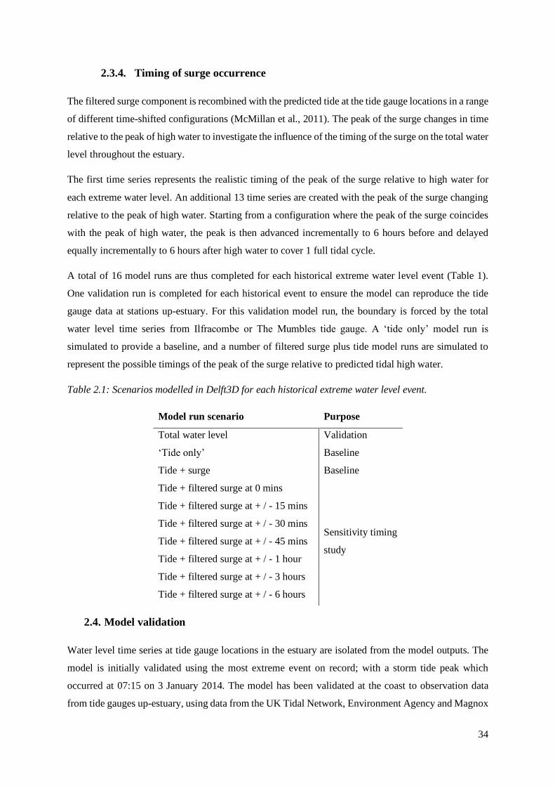
34
2.3.4. Timing of surge occurrence
The filtered surge component is recombined with the predicted tide at the tide gauge locations in a range
of different time-shifted configurations (McMillan et al., 2011). The peak of the surge changes in time
relative to the peak of high water to investigate the influence of the timing of the surge on the total water
level throughout the estuary.
The first time series represents the realistic timing of the peak of the surge relative to high water for
each extreme water level. An additional 13 time series are created with the peak of the surge changing
relative to the peak of high water. Starting from a configuration where the peak of the surge coincides
with the peak of high water, the peak is then advanced incrementally to 6 hours before and delayed
equally incrementally to 6 hours after high water to cover 1 full tidal cycle.
A total of 16 model runs are thus completed for each historical extreme water level event (Table 1).
One validation run is completed for each historical event to ensure the model can reproduce the tide
gauge data at stations up-estuary. For this validation model run, the boundary is forced by the total
water level time series from Ilfracombe or The Mumbles tide gauge. A ‘tide only’ model run is
simulated to provide a baseline, and a number of filtered surge plus tide model runs are simulated to
represent the possible timings of the peak of the surge relative to predicted tidal high water.
Table 2.1: Scenarios modelled in Delft3D for each historical extreme water level event.
Model run scenario Purpose
Total water level Validation
‘Tide only’ Baseline
Tide + surge Baseline
Tide + filtered surge at 0 mins
Sensitivity timing
study
Tide + filtered surge at + / - 15 mins
Tide + filtered surge at + / - 30 mins
Tide + filtered surge at + / - 45 mins
Tide + filtered surge at + / - 1 hour
Tide + filtered surge at + / - 3 hours
Tide + filtered surge at + / - 6 hours
2.4. Model validation
Water level time series at tide gauge locations in the estuary are isolated from the model outputs. The
model is initially validated using the most extreme event on record; with a storm tide peak which
occurred at 07:15 on 3 January 2014. The model has been validated at the coast to observation data
from tide gauges up-estuary, using data from the UK Tidal Network, Environment Agency and Magnox

35
at Oldbury. Error metrics (R2, RMSE, Willmott Index of Agreement (Wilmott, 1981; Wilmott et al.,
2012), Bias of the maximum value)) are calculated at tide gauge locations up-estuary for model runs
with realistic timings of the surge peak relative to tidal high water (total water level, filtered surge +
tide) and the tide only simulation to provide a baseline. Error metrics confirm if the model can reproduce
observational tide gauge data and assess the error introduced by this methodology.
Figure 2.5 illustrates validation runs and observational data for Hinkley Point; there is good graphical
and statistical agreement between the model output (dashed lines) and observational data (solid line).
The model is able to reproduce the tide gauge data at Hinkley Point well, with an R2 value of 0.996
(Table 2.2). High water levels are over estimated, as confirmed with a bias value of 0.242, by 15-20
cm. However this represents just 1.5% of the overall tidal range (12.29 m at Hinkley Point).
Figure 2.5: Validation down-estuary, Hinkley Point tide gauge.
Table 2.2: Statistical validation down-estuary, Hinkley tide gauge. The filtered surge is applied at a
realistic time relative to tidal high water for validation purposes.
Total water level ‘Tide only’ Tide + Filter surge
R2 0.996 0.909 0.955
RMS Error 0.172 0.255 0.212
Wilmott Index of Agreement 0.969 0.913 0.946
Bias of maximum value 0.242 - 0.91 - 0.556
The ‘tide only’ model provides a baseline which subsequent model runs can be compared with, as there
is no meteorological influence. It can be seen the ‘tide only’ model run is not resolving the high water
peaks as there is no meteorological influence, and the low water is underestimated, as shown by the

36
negative bias value. There is a bias away from the tide gauge data in a negative direction – the values
are all lower than the observation data. The tidal phase is successfully reproduced. The tide + filtered
surge model run, where there is no change in timing of the surge from the real event, also overestimates
low water. The tide + filtered surge model run is very similar to total water level simulation, suggesting
that external tide-surge interaction, which has been filtered out of the boundary conditions, has a small
contribution.
Figure 2.6 shows how the model has been tested further up-estuary, at Sharpness, using river gauge data
from the Environment Agency. The quality of bathymetry and geometry of the long, shallow, narrow
channel of the River Severn strongly influence the model results up-estuary. The lower Index of
Agreement and R2 value and higher RMSE and bias (Table 2.3) for the ‘tide only’ model run indicates
that surge has a large contribution to total water level in this location up-estuary. There remains good
graphical and statistical agreement between model runs (dashed line) and tide gauge data (solid line).
Figure 2.6 shows that the model is able to capture tidal asymmetry, which refers to the interaction
between tidal wave propagation and shallow water impacts due to changes in width and depth of the
channel up-estuary (Uncles 1981; Pye and Blott, 2010).
Figure 2.6: Validation up-estuary, Sharpness river gauge. As above.
Table 2.3: Statistical validation up-estuary, Sharpness river gauge
Total water level ‘Tide only’ Tide + Filter surge
R2 0.985 0.897 0.937
RMS Error 0.157 0.62 0.206
Wilmott Index of Agreement 0.9856 0.787 0.97
Bias of maximum value 0.634 -0.609 -0.746

37
The tidal phase is in good agreement however some of the high water points are not achieved, which is
likely to be due to error in the low resolution bathymetry influencing the propagation of the tide in the
upper estuary; the bathymetric survey will not match the bathymetry at the time of the event. Errors in
bathymetry and flushing can explain the poorer simulation of low water than high water at both
locations.
The model is in good agreement without the inclusion of meteorological forcing and waves, confirming
the approach is adequate to capture spatial variations in extreme water levels.
2.4.1. Funnelling effect vs frictional effect
The greatest maximum water elevation along the thalweg of the estuary is 8.12 m at 108 km up-estuary,
beyond Portbury, when the peak of the surge occurs 15 minutes before the peak of high water on 3
January 2014 (99th percentile). It can be seen in Figures 2.7 and Figure 2.8 that the maximum water
elevation, along the thalweg of the estuary, during each of the 4 events consistently occurs close to
Portbury. After this point, the maximum water elevation begins to fall again.
The tidal amplitude along estuary is determined by competing processes of tidal damping due to friction,
and tidal amplification due to funnelling effect and reflection. From the mouth of the estuary up to
Portbury, the funnelling effect dominates to amplify the tidal wave as it propagates up the estuary (Dyer
1995). Mean spring tidal range increases up-estuary towards Portbury due to the funnelling effect of
coastal topography, the continuously upward slope of the basin and near-resonance of the estuary to the
M2 tidal period (Liang et al., 2014; Uncles 1981). Portbury has the second largest mean spring tidal
range in the world, approaching 12.2 m (Uncles 2010). Beyond Portbury, the funnelling effect is
counteracted by friction. Friction acts to dampen the propagation of the tidal wave (Proudman 1955b).
This balance between the funnelling effect and friction determines where overall maximum water level
will occur in the estuary.
The sensitivity of the model domain to an applied friction value and the point where the friction and
funnelling effect is balanced is investigated.
A higher friction value (Manning = 0.075) and lower friction value (Manning = 0.013) was applied to
the model domain for the 99th water level percentile event (3 January 2014) model runs. The range in
maximum water elevations along the deepest channel of the estuary for results of the altered friction
values are compared to the original model run (Manning = 0.025).
Figure 2.7 shows that a higher friction value dampens the amplitude of the water elevation from the
mouth up-estuary; the funnelling effect has little influence here and there is no obvious tipping point
between funnelling and friction. A lower friction value means the funnelling effect significantly

38
amplifies the tidal wave up-estuary, producing water elevations beyond those that would realistically
be seen in this estuary. The tipping point between funnelling and friction moves up beyond Oldbury.
Figure 2.7: Water level along the deepest channel in the Severn Estuary, 3 January 2014, under varying
Manning friction values (99th percentile); the shading represents the range in results for each filtered
surge time shift scenario. Subpanels show the tidal response of i) hypersynchronous and ii)
hyposynchronous estuary to changing frictional effects.
The response of the model to changing friction follows the characteristic of tidal response in estuaries
(Dyer 1995). Under a friction value of 0.025, the estuary shows a hypersynchronous response (Figure
2.7i) where funnelling effect exceed frictional effects with increasing tidal range up to a point where
friction then dominates, due to the shallow, narrow channel morphology. With a low friction value the
estuary responds in a more extreme hypersynchronous manner. Funnelling effects exceed frictional
effects throughout the estuary and tidal range continues to increase further up-estuary. Under a high
friction value the model responds in a hyposynchronous manner (Figure 2.7ii). Friction dominates and
tidal range diminishes through the estuary. The funnelling vs friction effect is likely to be a dominating
factor in the hydrodynamics of the Severn Estuary, with a change in friction value in the model domain
changing where maximum tidal range occurs. Under future sea levels and saltmarsh extents, the estuary
dynamics under extreme could change the spatial variability in extreme water levels.

39
2.5. Results
Model outputs are analysed to identify how the total water level, and consequently flood hazard, and
local interactions change up-estuary, for different timing of surge occurrence, and surge characteristics.
Results are presented systematically for the four extreme events previously selected.
In the first part of the results, variations in maximum water level values along the estuary thalweg, and
for different timing of surge occurrence are presented. Changes in water level as a function of surge
skewness, and percentile are presented. After that, we will use the following plots as flood hazard
proxies at each tide gauge location up-estuary:
- Percentage change in maximum total water level compared with the ‘tide only’ model run is
plotted as a function of change in timing of surge at the model boundary;
- Percentage change in the time integrated elevation, i.e. the area (m2/s) under the curve of the
peak of the storm tide event, exceeding Mean High Water Spring (MHWS) compared with the
model run when the peak of the surge and high water coincide (0 minutes);
- Percentage change in duration (minutes) of the peak of the storm tide event exceeding MHWS,
calculated by interpolating between time steps exceeding the MHWS elevation, compared with
the ‘tide only’ model run;
- Percentage change in maximum total surge elevation, compared with the 0 minute model run
when the peak of the filtered surge and tide coincide; the total surge is calculated by removing
the modelled tidal time series from all total water level model run scenarios, and includes a
tide-surge interaction component and a meteorological component. The tide-surge interaction
generates harmonics at tidal frequencies, which means that relative contributions cannot be
separated.
MHWS is used as the baseline for proxy calculations as this is the reference level for all sea defence
designs (McMillan et al., 2011). All calculated water levels, areas, and timings apply to the peak of the
storm tide event within the 5 day simulation. The storm tide event is defined as 6 hours before and 6
hours after the maximum peak of high water in the time series peak. Correlation between each flood
hazard proxy, skewness of the filtered surge component and severity of the event is analysed.
2.5.1. Water level variations along estuary
Figure 2.8 a-d shows maximum water elevation every 2 km along the thalweg of the main channel of
the Severn Estuary (Figure 2.1) over the duration of the simulation, for each shift in the timing of the
peak of the surge relative to tidal high water. The plots illustrate how maximum water elevation changes
up-estuary.

40

41
Figure 2.8: Maximum water level along the thalweg of the Severn Estuary; a) 99th water level percentile
event (3 January 2014); b) 95th water level percentile event (14 December 2012); c) 90th water level
percentile event (18 December 2013); d) 95th water level percentile event (5 May 2015).
It is noticeable from Figures 2.8 a-d that there is sensitivity to the timing of the peak of the surge relative
to tidal high water and there are noticeable changes in maximum water elevations along the deepest
channel of the estuary for each time shifted configuration. Maximum range in water elevations due to
surge timing occurred for the 90th and 99th percentile events.
For the 90th water level percentile event (18 December 2013), the highest water elevation down estuary
is seen when the peak of the surge occurs 6 hours before the peak of high water. The maximum water
elevation down estuary is consistently 0.2 – 0.25 m higher than the 0 minute scenario when the peak of
the surge occurs 6 hours before the tidal peak. There is a change in which scenario results in the highest

42
water elevation at 106.5 km up-estuary. In the upper estuary, the highest water elevation is seen when
the peak of the surge occurs 6 hours after the peak of high water. The water elevation is consistently
0.1 – 0.35 m higher than the 0 minute scenario, when the peak of the surge occurs 6 hours after the tidal
peak.
For the 99th water level percentile event (3 January 2014), the highest water elevation down estuary is
seen when the peak of the surge occurs 1 hour after the peak of high water. The maximum water
elevation down estuary is consistently 0.2 – 0.25 m higher than the 0 minute scenario when the peak of
the surge occurs 1 hour after the tidal peak. The minimum water elevation down estuary is 0.1 – 0.15
m lower than the 0 minute scenario when the peak of the surge occurs 6 hours before high water. In the
upper portion of the estuary, the highest water elevation consistently occurs 0.01 – 0.05 m higher than
the 0 minute scenario when the peak of the surge is 30, 45 or 60 minutes after high water: there is no
scenario which consistently results in the maximum water elevation. However the lowest water
elevation in the upper portion of the estuary is consistently a result of when the surge peak is 6 hours
before the tidal peak, and is up to 0.25 m lower than the 0 minute scenario.
It is noticeable in the Figures 2.8 a-d that change in time of the peak of the surge relative to high water
causes little variability in the maximum water elevation in the lower estuary, and greatest variability in
water elevation between time shift scenarios beyond Portbury, 106 km up-estuary.
Figure 2.9 shows the range of maximum water elevation every 2 km along the thalweg for all time shift
configurations. The range of values are coloured according to the skewness of the surge component
with time, and also classified based on the severity of the extreme event.
Figure 2.9: Range of water level values for time shift configurations along deepest channel of the Severn
Estuary when overall maximum water level occurs. For each event, in the legend the first value
represents the percentile of the event and the second value is the skewness.

43
The greatest range between maximum and minimum water elevation across the surge time shift
scenarios is 0.44 m for the 90th water level percentile event (18 December 2013) and 0.27 m for the
99th water level percentile event (3 January 2014). Deviations in water level are not uniform along the
estuary, and the 90th water level percentile event shows a positive shift in water level in the lower part,
and negative shift in the upper part. The surge component of both of these events have a positive
skewness value. The smallest range between maximum and minimum water elevation across the surge
time shift scenarios is 0.03 m, for 95th water level percentile event (14 December 2012). This event has
a surge component with a negative skewness value.
The surge components which have a positive skewness value, a steeper rising limb and a longer falling
limb, show the greatest range of water elevation values along the deepest channel of the estuary. The
range of values increases up-estuary, with the greatest range in water level values occurring beyond
Portbury. This indicates that location in the upper estuary may be more sensitive to changes in the
timing of the peak of a surge which displays a positive skewness. The surge components which have a
negative skewness, a longer rising limb and steeper falling limb, show a more constrained range of
maximum water elevations and there is less sensitivity throughout the estuary to the timing of the surge
peak.
The maximum water elevations are stacked on top of each other according to severity of the event. It
can be seen that the 99th water level percentile event (3 January 2014) consistently results in the greatest
maximum water elevations along the thalweg of the estuary. The 95th percentile events show less
extreme maximum water elevations in the estuary. There is approximately a 1 metre difference between
the 95th water level percentile event (14 December 2012) and 95th water level percentile event (5 May
2015). The 95th water level percentile event (5 May 2015) initially shows similar water level values to
the 90th water level percentile event (18 December 2013), before increasing beyond this 90th percentile
event. As expected, the 90th water level percentile event (18 December 2013) shows the lowest
maximum water elevations along the deepest channel of the estuary.
It is also evident in Figure 2.8 and Figure 2.9 that the maximum water elevation for all extreme water
level events consistently occurs close to Portbury, the location for maximum observed tidal range in the
estuary (Pye and Blott 2014).
2.5.2. Changes in flood hazard proxy with surge timing
Figure 2.10 – 2.13 show changes in flood hazard up-estuary in locations where nuclear assets and / or
tide gauges are located, as a function of change in timing of the surge at the model boundary. Each
flood hazard proxy (maximum total water level, maximum total surge, time integrated elevation and
duration exceeding MHWS) is calculated from the storm tide peak: 6 hours before and 6 hours after
high water. All data are displayed as percentage change, compared with the ‘tide only’ model scenario,

44
apart from maximum total surge which is compared with the model run when the peak of the surge and
high tidal water coincide (‘0 minutes’).
Figure 2.10 shows flood hazard at each tide gauge location for a 99th water level percentile event (3
January 2014), the most extreme event on record.
Figure 2.10: 3 January 2014. Flood hazard proxy calculated at each tide gauge location. a) percent
change in maximum water level; b) percent change in maximum total surge elevation; c) percent change
in duration exceeding MHWS; d) percent change in area exceeding MHWS. All data is displayed as
percentage change, compared with the tide only model scenario, apart from total surge elevation which
is compared with the model run when the peak of the surge and high water coincide.
The greatest percentage change in maximum total water level between each time shift scenario and the
‘tide only’ scenario is seen in tide gauge locations down-estuary, notably Hinkley Point and Newport
(up to 10.02%). Tide gauge locations down-estuary, Hinkley Point, Portbury and Oldbury show
symmetry in the results: the highest maximum water level happens when the surge occurs at the same
time as high water. The magnitude of the maximum total water level then reduces when the peak of the
surge occurs before or after the peak of high tide.

45
There is less percentage change in maximum total water level at tide gauge locations further up-estuary.
The greatest percentage change in maximum total water level occurs when the peak of the surge happens
3 hours after the peak of high water. This is particularly clear at Sharpness, up to 8%.
There is a noticeable linear trend in the percentage change of maximum total surge value which occurs
+/- 6 hours of the storm tide peak, compared with the 0 minute scenario. The greatest positive percentage
change in maximum total surge elevation can be seen when peak of the surge occurs after 6 hours after
the peak of tidal high water. A similar magnitude of negative percentage change in maximum total surge
can be seen when the peak of the surge occurs 6 hours before the peak of tidal high water. There is little
sensitivity of maximum total surge elevation to the timing of the surge when the peak occurs around
the time of high water, and there is also little spatial variability between the locations. There is increased
variability in maximum total surge elevation across the estuary with greater shift away tidal high water.
The greatest variability can be seen when the peak of the surge occurs significantly after tidal high
water. Portbury shows the greatest positive percentage change in maximum total surge elevation
(32.5%) when the peak of the surge occurs 6 hours after tidal high water. This could be linked to the
positive skewness of the surge with greater influence after the peak.
The maximum change in duration of peak of the storm tide exceeding MHWS is seen at locations down-
estuary, Hinkley Point and Newport. Portbury and Oldbury show greatest change in duration when the
peak of the surge occurs 1 – 3 hours after the peak of high water. There is a smaller percentage change
in duration of the storm tide peak exceeding MHWS further up-estuary, at Sharpness. These tide gauge
locations show asymmetrical results, with the greatest change in duration when the peak of the surge
occurs 3 hours before the peak of high water.
The greatest change in time integrated elevation of the peak of the storm tide exceeding MHWS is seen
at Hinkley Point, with the greatest area exceeding MHWS when the peak of the surge occurs at the
same time relative to the peak of high water. Model results from Portbury and Newport also show over
28% change in time integrated elevation (m2) exceeding MHWS. Locations further up-estuary, Oldbury
and Sharpness, consistently show lower percentage change within the range of 17 – 21 %. These results
are also symmetrical, with the greatest % change in area when the peak of the surge occurs at the same
time as the peak of high water.
Figure 2.11 shows flood hazard at each tide gauge location for a 95th water level percentile event (14
December 2012). The greatest percentage change in maximum total water level between each time
shift scenario and the ‘tide only’ model run is seen in tide gauge locations down-estuary, at Hinkley
Point and Newport, up to 5%. Oldbury is located further up-estuary, where the channel of the River
Severn begins to narrow, but still shows a greater percentage change than Portbury. The change in
maximum water level for this event is not to the same extent as the 99th water level percentile event (3
January 2014). Sharpness shows the smallest percentage change in maximum total water level,

46
compared with the ‘tide only’ model run. All results show a symmetrical shape, with the greatest change
in total maximum water level when the peak of the surge coincides with the peak of high water. The
smallest percentage change in maximum water level occurs at all locations up-estuary when the peak
of the surge occurs 6 hours after the peak of high water.
Figure 2.11: 14 December 2012. Flood hazard proxy, as in Figure 2.10.
The linear trend in percentage change of maximum total surge elevation for a 95th water level percentile
event (14 December 2012) is similar to 99th water level percentile event (3 January 2014), with the
changing time of the peak of the surge relative to tidal high water. The greatest positive percentage
change occurs when the peak of the surge occurs significantly after tidal high water, at Hinkley Point
(21.2%) and Portbury (17.8%). The greatest variability and magnitude in percentage change of
maximum total surge elevation occurs when the surge occurs 6 hours before the peak of tidal high water.
This could be linked to the negative surge skewness, with greater influence before the peak of the surge.
There is less variability in maximum total surge elevation when the surge occurs 6 hours after tidal
water.

47
The greatest percentage change in duration of the peak of high water exceeding MHWS is in locations
down-estuary, notably Hinkley Point and Newport, up to 29.2%. These locations also show a
symmetrical trend; the greatest percentage change is when the peak of the surge occurs at the same time
as the peak of high water. The locations are stacked on top of each other, which is determined by the
location up-estuary. There is a notable gap in percentage change in duration between locations in the
lower estuary (Hinkley Point, Newport) and the upper estuary (Sharpness, Oldbury). Greatest duration
at Oldbury and Sharpness is when surge occurs 1 hour before high water.
The greatest percentage change in area of the peak of high water exceeding MHWS is in locations
down-estuary, notably Hinkley and Newport, up to 30.5%. Locations are stacked on top of each other,
as a function of the distance up-estuary. All locations show symmetrical trends as the peak of the surge
changes relative to high water; the greatest change in area is when the peak of the surge and tide
coincide. In addition to this there is less variation between each time shift, and results at each location
appear flatter than changes seen in maximum total water level and duration of peak exceeding MHWS.
Figure 2.12 shows flood hazard at each tide gauge location for a 95th water level percentile event (5
May 2015). The greatest percentage change in maximum total water level, compared with the ‘tide
only’ model run, is seen at Hinkley Point, Newport and Portbury, up to 8.6%. As seen in other figures,
the locations are stacked on top of each other based on their distance up-estuary. Epney, for example,
shows smallest percentage change. All locations show least percentage change at -6 hours.

48
Figure 2.12: 5 May 2015. Flood hazard proxy, as in Figure 2.10.
The linear trend in percentage change of maximum total surge elevation is also noticeable for 5 May
2015. There is a smaller overall magnitude of positive and negative percentage change compared to the
other events. Sharpness shows greatest negative percentage change (-10%) and Oldbury shows greatest
positive percentage change in maximum total surge elevation (8.6%). Newport shows little sensitivity
to the changing time of the peak of the surge relative to high water. There is less variability between
locations, excluding Newport, when the peak of the surge occurs significantly before or after tidal high
water.
The storm tide peak exceeds MHWS at all locations for a 95th water level percentile event (5 May
2015). Hinkley Point shows the greatest percentage change in duration of the storm tide peak exceeding
MHWS, but there are small changes between each time shift scenario.
The greatest change in duration at Portbury occurs at –15 mins (11.725%), followed by 0 mins (11.72%)
and –30 mins (11.71%). Small percentage changes occur across all locations (within 0.1% change in
duration) when the surge occurs within 1 hour of high water. The lowest percentage change at all
locations occurs when the peak of the surge occurs 6 hours after the peak of high water. This could be

49
due to the influence of the characteristics of the filtered surge that has been modelled for this historical
event.
Figure 2.13a shows flood hazard at each tide gauge location for 90th water level percentile event (18
December 2013). Down-estuary locations, at Hinkley Point, Newport, Portbury and Oldbury show a
similar percentage change in maximum total water level, up to 7%, compared with the ‘tide only’ model
run. The smallest percentage change is seen at Sharpness. All locations show a jump in maximum water
level at + 6 and – 6 hours, which could be due to the influence of the shape of the surge, as the other
time shifts show a flatter trend.
Figure 2.13:18 December 2013. Flood hazard proxy as in Figure 2.10.
The linear trend in percentage change of maximum total surge elevation in Figure 2.13a is similar to
other events. There is greater variability between locations when the peak of the surge occurs 3 or 6
hours before and after tidal high water like the 99th water level percentile event (3 January 2014). This
could be linked to surge skewness like the 3 January 2014. The greatest magnitude of percentage change
can be seen when the peak of the surge occurs significantly before tidal high water. The greatest positive
(29.08%) and negative (-47.57%) percentage change in maximum total surge elevation occurs at

50
Sharpness. Newport shows less sensitivity to the timing of the peak of the surge relative to high water,
with a range of 20.1% and a more symmetrical trend.
The peak of the storm tide only exceeds MHWS at Sharpness and Oldbury when the 18 December 2013
event is simulated, likely to be because it is a 90th percentile event. Oldbury shows a clear percentage
change because the ‘tide only’ scenario (6.821 m), which all time shift scenarios are compared with,
does not exceed MHWS (7.02 m). The surge is having a noticeable influence on the time the peak of
the storm tide exceeds MHWS at these locations. Figure 2.14 shows Sharpness has an asymmetrical
trend with the greatest percentage change in duration (19.9%) when the surge occurs 45 minutes after
high tide.
Figure 2.14: Duration and area of storm tide peak exceeding MHWS at Sharpness.
Oldbury also shows a noticeable percentage change for area exceeding MHWS compared with the ‘tide
only’ model run, and a very small value for Sharpness (Figure 2.14). Sharpness shows a small range of
0.1% between time-shift scenarios. The greatest change in area (3.9%) when the surge occurs 1 hour
after high tide.
2.6. Discussion
2.6.1. Physical drivers and sources of flood hazard in the Severn Estuary model
domain
Delft3D-FLOW is used to simulate barotropic tide-surge propagation, river flow and interaction in the
Severn Estuary across a 2DH grid. Results from 4 historical events are presented which show the
influence of the severity of the storm surge, the influence of the timing of the surge on the total water
level, and characteristics of the filtered surge component on the total water level throughout the Severn

51
estuary. The results presented here can help to identify variability in the sources of an extreme water
level event in a hyper-tidal estuary, which can contribute towards flood hazard. These results can help
to inform local management needs in a hyper-tidal estuary when viewed in the context of the source –
pathway – receptor – consequence (SPRC) conceptual model (Narayan et al., 2012).
2.6.1.1. Influence of storm severity on extreme water levels
The results suggest that severity of the event is an important control on the magnitude of extreme water
levels throughout the Severn Estuary. The 99th water level percentile event (3 January 2014) consistently
produced greatest water elevations along the deepest channel of the estuary and greatest percentage
change in maximum water levels at all sites. A more severe storm surge event, driven by low
atmospheric pressure, wind speed, wind direction and storm duration (Woth et al., 2006), increases
extreme water levels throughout in the Severn Estuary and is an important driver of flood hazard.
Extreme tidal levels are known to be the predominant driver of flooding events in the Severn Estuary,
particularly in locations close to the maximum MHWS at Avonmouth (Capita Symonds 2011). A 3.54
m (11.6 ft) surge was recorded at Avonmouth in March 1947 (Heaps 1983), attributed to very low
pressure (974 mb, which is 38 mb below normal regional level) and predominantly easterly track of the
depression (Lennon et al., 1963), indicating the severity of a storm surge event is a combination of
meteorological factors.
99th percentile water level events may be a rare occurrence, and equal consideration should be given to
the effect of more frequent, less severe events in the estuary. However much of the UK is defended
against high frequency, low magnitude events up to a 1:200 year event, therefore reducing flood hazard.
An understanding that a more severe, extreme water level event can increase flood hazard can be used
by local coastal planners to manage flood risk and can aid operational flood management (Menéndez
and Woodworth 2010). If the severity of an event can be forecast then warnings can be issued to
appropriate authorities and the public. Event severity is an important control when modelling to extreme
water levels on a local scale.
2.6.1.2. Influence of the timing of the peak of the surge
The timing of the peak of the storm surge relative to tidal high water is another important contribution
to the physical drivers of flood hazard at the coast. There is sensitivity to the timing of the peak of the
surge throughout the Severn Estuary model domain. This is particularly evident in the upper estuary;
when the peak of the surge occurs 2 – 6 hours after high water there is a greater percentage change in
maximum water level. Increased water depth at the time of tidal high water could induce surge
propagation through the estuary to increase extreme water levels up-estuary. Increased water depths
would limit shallow water and quadratic friction effects on the tidal amplitude. However, at these shifts
the flood hazard (area and duration of the storm tide peak exceeding MHWS) is lower.

52
There is less sensitivity to changes in the timing of the surge in the lower estuary, notably Hinkley
Point. The greatest percentage change in maximum water level occurs when the peak of the storm surge
and tide coincide. The concurrence of high tide and storm surge peak in the Severn Estuary has resulted
in extreme water levels in the past (Lennon et al., 1963). The highest recorded water level in the Severn
Estuary in a century occurred during the storm 13 December 1981 (Proctor and Flather 1989). A fast
moving secondary depression, tracking further south than usual for the time of year, produced strong
west to northwesterly gales over the Bristol Channel (Williams et al., 2012). This depression generated
a surge peak of 1.5 – 2 m, which occurred close to the time of high water of a large spring tide (Heaps,
1983; Smith et al, 2012). Little warning was given, and the event resulted in severe flooding and damage
to property and agricultural land from east of Bideford to Gloucester (Uncles 2010). The timing of the
passage of the depression, which was coincident with tidal high water in the Bristol Channel, was a
vital contributor to the water levels produced (Proctor and Flather 1989). This event was significant as
it highlighted the importance of high-resolution temporal monitoring data during fast moving
depressions, and reanalysis atmospheric data for the event has been used to test the accuracy of
operational forecasting systems (Williams et al., 2012). A larger storm surge (2.4 m) in the Severn
Estuary on 24 December 1977 occurred 3 hours before high water, giving no cause for concern (Proctor
and Flather 1989). Surges larger than 2 m rarely occur within 1 hour of tidal high water in the Severn
Estuary due to locally generated tide-surge interaction (Horsburgh and Horritt 2006). However there is
no mechanism to stop the peak of a spring tide and storm surge coinciding in the Severn Estuary (Pye
and Blott 2010).
Flood hazard is also increased in the Bay of Fundy when adverse weather conditions, e.g. a drop in
pressure greater than 5 kPa, coincides within one to two hours of high water of large spring tides
(Greenberg et al., 2012). Significant low pressure systems have coincided with a very high spring tide
on only a few occasions; November 1759, October 1869, during the Saxby Gale, and the 1976
Groundhog Day storm (Desplanque and Mossman 2004). During all events seawalls and wharfs were
breached, leading to severe flooding, damage to boats and infrastructure, and lives lost (Desplanque
and Mossman 1999). Storms not occurring near high water or on average tides will produce water levels
within the ‘normal’ range that are often reached by astronomical tides alone (Desplanque and Mossman
1999). The concurrence of the peak of a storm surge with the peak of spring tidal high water could be
rare occurrence, but would cause the greatest impacts on maximum extreme water levels. The timing
of surge events is crucial in predicting extreme water levels and assessing flood hazard in estuaries with
a large tidal range (Batstone et al., 2013).
2.6.1.3. Influence of the storm surge shape
The shape of the storm surge component with time (surge skewness) influences variability in extreme
water levels and total surge in the Severn Estuary model domain. As seen in Figure 2.8, a storm surge

53
with a positive skewness appears to create a greater range in maximum water elevation at every point
along the deepest channel of the estuary. Positive skewness can act to extend the duration of high water,
and there increase water volume and surge inflow in the estuary. This could help to amplify the tide
further up the estuary (as shallow water effects are reduced) (Proudman 1955b). With distance up-
estuary, the surge skewness may become more negative or more positive consistent with the magnitude
of the local interaction growing with tide-surge propagation up-estuary. The shape and time profile of
each storm surge generated on the continental shelf varies between historical extreme water level events,
and skewness of the storm surge component could be just one of many characteristics controlling this
driver of flood hazard. If shape of a storm surge can be forecast or detected early then locations in the
upper estuary can be warned of consequential amplification of the flood hazard.
Previous studies have highlighted the influence surge shape may have on water levels in the coastal
zone (McMillan et al., 2011; Proudman 1955b). The Environment Agency has provided time-integrated
duration design surge shapes at tide gauge locations around the UK coastline, from the 15 largest ‘skew
surge’ events on record (McMillan et al., 2011). The skewness, i.e. the measure of asymmetry, of the
design surge shapes for tide gauge locations in the Severn Estuary were calculated and shown to have
a negative skewness over a 60-hour window (Ilfracombe -0.46, The Mumbles, -0.26). These results
indicate that storm surges with a negative skewness create a constrained range of extreme water
elevations in the Severn Estuary model domain. Therefore it would be diligent to undertake sensitivity
testing of surge skewness derived from historic events to understand variability in extreme water levels.
2.6.1.4. Estuarine form as a pathway to increase flood hazard
The severity of the extreme water level event, timing and surge skewness each contribute to the source
of a potential flood event. Pathways are the mechanisms that convey floodwaters from physical drivers,
to impact receptors (people, businesses and the built environment). These are often considered to be
overland flows, flows in river channels and sea defence overtopping (Le Cozannet et al., 2015; Idier et
al., 2013). However it is known that estuaries and coastal inlets can affect surge and wave propagation
in the coastal zone (Sayers et al., 2003). Therefore the geometry, bathymetry and form of the estuary
should be considered a pathway or source in itself, and influence on flood hazard acknowledge.
The geometry of the Severn Estuary has a strong control on tide-surge propagation and total surge
contribution to water levels. The greatest percentage change in maximum total surge elevation in the
model domain occurs when the peak of the surge occurs significantly before or after tidal high water,
in locations further up-estuary e.g. Portbury and Sharpness. As the peak of the surge occurs closer to
low water there may be greater effect bottom friction and shallow water effects on tidal dynamics
(Proudman 1955a). Flood hazard is reduced when changes in maximum total surge elevation increase.
Total surge, including a meteorological component and tide-surge interaction component, does not

54
appear to contribute to extreme water levels, but appears to create variability in extreme water levels in
the upper estuary.
The smallest change in maximum total surge elevation in the model domain can be seen when the peak
of the surge occurs within 1 hour of tidal high water. This is a phenomenon often observed along the
west coast of Britain: if the peak of a storm surge occurs close to the time of tidal high water then there
is very little time for interactions to develop and little effect of bottom friction due to the greater
volumetric contribution of the tide and surge (Jones and Davies 2007). Tide-surge interaction may not
contribute to extreme water levels in the estuary but the shallow, narrow estuary creates variability
which should be considered to potentially increase exposure and consequences of coastal towns in the
upper estuary.
The geometry of the estuary has a particularly strong control over the location of maximum tidal range
in the estuary, close to Portbury (Figures 2.8 and Figure 2.9). Maximum overall water elevation in the
Severn Estuary model domain consistently occurs close to Portbury. This is known to be as a result of
the funnelling and friction effect in the estuary (Dyer 1995). Tides and surges are amplified from the
deeper part of the estuary, through the increasingly narrow, shallow channel towards Portbury (Pye and
Blott 2010). This funnelling effect, due to channel convergence, increases tidal range to a maximum
within the estuary at Portbury (Lennon 1963). The cyclic semi-diurnal tide is analogous to the incoming
resonance from the west side of the Atlantic Ocean to the east (Gao and Adcock 2016), which further
amplifies storm surges up estuary (Liang et al., 2014). Beyond Portbury, frictional effects control the
dampening of the tide as energy is lost and the tidal range decreases.
Further to this, human intervention in the estuary itself could influence how the physical drivers of flood
hazard (‘sources’) move through the estuary. The location and design of sea defences, harbours and
interventions (e.g. managed realignment schemes at Steart Marshes (Wright et al., 2011)) would also
act to influence the magnitude and variability of extreme water levels (Sayers et al., 2003). These
interventions would in turn also influence the damage caused and extent of coastal flooding that may
be experienced as a result of the event. River discharge is another pathway to consider, and can induce
interactions that lead to increases in the non-tidal residual elevation up to 0.35 m in the Severn Estuary
(Maskell et al., 2014).
Flood hazard assessment, and application of the SPRC model at a local and regional scale, should
consider that the form of a hyper-tidal estuary is a ‘source’ or ‘pathway’ in itself, influencing how
floodwaters are conveyed through the system.

55
2.6.2. Implications for local management needs in the Severn Estuary and
worldwide
When viewed in an operational context, these results help to identify contributions to the sources of
flood hazard and identify the estuarine form as a source and pathway in itself which can act to exacerbate
flood hazard. As seen in Figure 2.9, the severity of an event appears to be the most important control
on flood hazard in a hyper-tidal estuary. The events are stacked as a function of severity, and the 99th
percentile event, 3rd January 2014, consistently produces the maximum water level through the thalweg.
The ‘worst case’ combination of variables to result in greatest flood hazard would be a 99th percentile
event and concurrence of a storm surge peak with positive skewness and tidal high water. However it
should be considered that accurate bathymetry and boundary forcing data is important when testing
hypotheses in estuaries. The accuracy of models which aim to link estuarine hydrodynamic processes
and form e.g., extreme water levels is dependent on accurate bathymetry. The Severn Estuary model is
forced at the tidal boundary with data from one tide gauge, which could act limit how accurately water
levels and interactions within the estuary are reproduced. There is a need for clear, accurate information
to inform operational flood management, with the aim of reducing the hazard from flood events to the
people who are located in flood prone areas which should utilise the best available data.
Freshwater flow can be an important control on tide-surge propagation in some hyper-tidal estuaries
(Hoitink and Jay 2016). River discharge and its associated water levels can combine with storm surges
driven by the same weather system (Svensson and Jones 2002), to alter the timing and magnitude of
water levels within the estuary. Nonlinear interactions between extreme river discharge and storm
surges can elevate residual water levels up to 0.35 m in idealised estuaries (Maskell et al., 2014), and
have been shown to influence subtidal friction and the timing of high and low water in the River
Mahakam, Indonesia (Sassi and Hoitink 2013). Heavy rainfall and spring meltwater, which result in
high discharges have been shown to inhibit tide-surge propagation up-estuary in the LaHave Estuary,
Nova Scotia (Webster et al., 2014), however dredging activities in the Modaomen Estuary, China,
facilitates inland propagation of surges and can alter salinization within an estuary (Cai et al., 2012).
Flood hazard and inundation extents are largely controlled by surge elevation, except in the most
extreme river discharge events (Maskell et al., 2014). Freshwater flow and tide-surge propagation are
not statistically independent (Svensson and Jones 2002), and their combined impact is controlled by the
timing of peak river discharge, geometry of the estuary and floodplains and human intervention within
the estuary.
Under changing climate and sea-level rise, the methods and results presented here could change due to
changes in tidal range, which would alter tide-surge interaction (Robins et al., 2016). Deeper water will
change frictional influence, and the tipping point between the effect of funnelling and friction effect is
likely to change, which impact the location of maximum tidal range within the estuary and tidal

56
asymmetry. In addition to this, rising sea level may alter channel depths or alter tidal prism (Leuven et
al., 2019; Marcos et al., 2019), therefore fundamentally altering the feedback between estuarine form
and water level. In some coastal regions, sea-level rise will increase the magnitude and frequency of
extreme storm events, leading to increased flood hazard (Menéndez and Woodworth 2010; Nicholls et
al., 2014). Therefore, the need for accurate operational forecasting of extreme storm events will increase
under changing climates.
Analysis of barotropic tide-surge propagation in a hyper-tidal estuary has shown sensitivity of coastal
flood hazard, generated from the water level boundary conditions, to storm timing, storm surge shape
and event severity. This knowledge is of significance to operational modelling for local predictions and
flood hazard assessments. However sources of coastal flood hazard are not just limited to the
contributions of astronomical tide and storm surges to water level, but also wave run-up and
overwashing or overtopping, driven by coincidental sea state (Prime et al., 2016). Locally-generated
wind waves and propagating swell waves, generated by an offshore storm, which coincide with an
extreme water level can increase flood hazard at the coast (Wolf 2008). Maximum wave height at time
of tidal high water can be significant for coastal flooding (Fairley et al., 2014), and runup associated
with direct wind setup or breaking offshore waves can influence defence overtopping and breaching
(Wadey et al., 2012). Future work to consider the influence of swell and wind waves on water levels
and uncertainty in wave forcing has the potential to provide improved understanding of the combined
effect of tide-surge-river-waves on water levels in a hyper-tidal estuary. Model outputs from a study
into the combined effect of tide-surge-river-waves on water levels can be used to force an inundation
model (e.g. Bates and De Roo, 2000), to simulate the area of maximum inundation from extreme water
level events. Modelling studies that combine tide-surge-river-wave propagation with depth and extent
of inundation can be effective for floodplain development, flood defences and protection for critical
infrastructure in the estuary.
2.7. Conclusion
There is a need to understand the combination and variability of physical drivers contributing to flood
hazard in hyper-tidal estuaries, due to their dynamic nature and increasing development pressures.
Delft3D-FLOW is used to simulate tide-surge propagation in a hyper-tidal estuary to understand the
mechanisms controlling extreme water levels, which contribute to flood hazard. Long-term tide gauge
records are used to consider the influence of event severity, the timing of the peak of the surge relative
to tidal high water and storm surge skewness on spatial variability of historic extreme water level events
in the Severn Estuary example. Event severity is the most important control on extreme water levels
when modelling tide-surge propagation on a local scale. The shape of the storm surge component with
time, classified using surge skewness as a measure of asymmetry, and timing of the storm surge peak
relative to tidal high water influence spatial variability of water levels throughout the estuary.

57
Demonstration of the shallow water effect shows the effect estuarine form can have on the variability
of extreme water levels, therefore it is crucial to have accurate bathymetry and boundary conditions to
capture these changes throughout the estuary. However maximum total surge elevation does not appear
to significantly contribute to flood hazard as the maximum contribution occurs during the rise of an
adjacent tide to that of the storm tide. The results can be interpreted in the context of the SPRC model,
to identify the combined effect of factors which contribute to extreme water levels for local scale, flood
hazard management. The methodology can be applied to understand past extreme water level events,
and in turn help to identify future flood hazard in hyper-tidal estuaries worldwide.
2.8. Acknowledgements and Data
The authors thank colleagues at the British Oceanographic Data Centre (BODC) for providing tidal
data; Magnox for providing tidal data; Environment Agency for providing tidal data and river gauge
data; Gloucester Harbour Trustees for providing tidal data; and EDINA for bathymetric data.
This work was supported by the Engineering and Physical Sciences Research Council as part of the
Adaptation and Resilience of Coastal Energy Supply (ARCoES) project, grant number EP/I035390/1.

58
3. Uncertainty in estuarine extreme water level predictions due to surge-
tide interaction
Chapter 3 continues to use the statistically validated and calibrated Delft3D-FLOW modelling system
to consider the variability in residual sea level up-estuary due to three key sources of uncertainty
identified in chapter 2. Changes in the surge residual, defined as observed sea level minus predicted
tide, are quantified at five tide gauge location and through the thalweg of the estuary to show the spatial
variability of tide-surge propagation, and the influence on subsequent maximum surge residual. The
variability in the surge residual needs to be captured accurately to reduce uncertainty in site specific
flood hazard assessment.

59
3.1. Abstract
Storm surge is often the greatest threat to life and critical infrastructures during hurricanes and violent
storms. Millions of people living in low-lying coastal zones and critical infrastructure within this zone
rely on accurate storm surge forecast for disaster prevention and flood hazard mitigation. However,
variability in residual sea level up-estuary, defined here as observed sea level minus predicted tide, can
enhance total water levels; variability in the surge thus needs to be captured accurately to reduce
uncertainty in site specific hazard assessment. Delft3D-FLOW is used to investigate surge variability,
and the influence of storm surge timing on barotropic tide-surge propagation in a tide-dominant estuary
using the Severn Estuary, south-west England, as an example. Model results show maximum surge
elevation increases exponentially up-estuary and, for a range of surge timings consistently occurs on
the flood tide. In the Severn Estuary, over a distance of 40 km from the most upstream tide gauge at
Oldbury, the maximum surge elevation increases by 255 %. Up-estuary locations experience short
duration, high magnitude surge elevations and greater variability due to shallow-water effects and
channel convergence. The results show that surge predictions from forecasting systems at tide gauge
locations could under-predict the magnitude and duration of surge contribution to up-estuary water
levels. Due to the large tidal range and dynamic nature of hyper-tidal estuaries, local forecasting systems
should consider changes in surge elevation and shape with distance up-estuary from nearby tide gauge
sites to minimize uncertainties in flood hazard assessment.
3.2. Introduction
Storm surges occur in coastal zones worldwide and correspond to short-term variations in sea-level
driven by winds and atmospheric pressure changes associated with storms, tropical hurricanes and
typhoons (Lewis et al., 2011). The concurrence of storm surges and astronomical tides presents a
combined flood hazard, elevating observed water levels above the predicted tide, to create an extreme
water level at observed high water (Lewis et al., 2013; Prime et al., 2015). It is also documented that
interaction between tide and surge can alleviate flood hazard, as storm surge peak does not coincide
with tidal high water in some coastal and estuarine areas (Horsburgh and Wilson 2007). Evidence of
the damage caused by this combined flood hazard to coastal communities and critical infrastructure is
well documented for the UK (Wolf and Flather, 2005; Sibley et al., 2015; Spencer et al., 2015) and
worldwide (Kates et al., 2006). Severe storm surge events, such as the 1953 North Sea storm surge
(Wolf and Flather 2005) and the 28 foot surge generated by Hurricane Katrina in Mississippi in 2005
(Kates et al., 2006), present a serious threat to coastal communities, with an increased risk of loss of
life and damage to property. Severe flood events in recent decades and increasing numbers of assets
within the coastal zone (Hallegatte et al., 2013) have led to an increased prevalence of risk-based coastal
planning frameworks (Quinn et al., 2014).

60
Risk-based coastal planning frameworks rely on accurate water level boundary conditions, i.e. input
data, to drive model simulations of flood events, which are representative of probabilistic extreme water
levels within impact model assessments (Brown et al., 2018). However the accurate representation of
total water levels, which form the basis of flood hazard assessments in heavily populated and
industrialized coastal zones, can be undermined by the variability in the combined forcing of extreme
water levels. This variability can lead to uncertainty in flood hazard assessments, which poses a problem
to policy makers and coastal planners as this uncertainty can result in underestimation of the severity
and implications of extreme water levels (Prime et al., 2016).
Variability in the combined effect of tide-surge propagation is of particular significance in hyper-tidal
estuaries, where the tidal range exceeds 6 m due to bathymetry of the estuary funnelling and amplifying
tidal wave propagation (Davies 1964) . Even small changes in the magnitude or timing of a surge will
contribute to increased total water levels and can be catastrophic if happening during high tide
(Horsburgh and Wilson 2007; Lyddon et al., 2018a). Catastrophic flooding experienced in the Bay of
Fundy, Canada during the Groundhog Day Storm of 1976 would have been lessened if the peak of the
surge arrived 1 hour before or after tidal high water (Greenberg et al., 2012). The combined forcing of
extreme water levels, notably tide and storm surges, can interact with each other in shallow water
regions to alter the phase and amplitude of tidal high water (Wolf and Flather 2005), as shown by
examples in the English Channel (Idier et al., 2012), Taiwan coast (Liu et al., 2016), and Queensland
coast (Tang et al., 1996). Interaction effects are largely a function of storm surge magnitude and can
vary spatially across hyper-tidal estuaries, as shown in the Bay of Fundy where interaction effects are
most strongly felt in the Northumberland Strait (Bernier and Thompson 2007). Storm surges can also
enhance tidal wave propagation in estuaries and shallow coastal waters (Prandle and Wolf 1978), as in
the Bay of Bengal where advancement of high water can result in increased flood hazard (Antony and
Unnikrishnan 2013). Due to the importance of surge magnitude and timing relative to tidal high water
in a hyper-tidal estuary (Lyddon, et al., 2018a), a precise surge prediction is required, in combination
with the predicted tide, for estimation of total water levels for flood hazard assessment (Brown et al.,
2012). Current methods for storm surge prediction are limited in their accuracy as they may consider
tide and surge as independent processes (Bobanović et al., 2006), and rarely consider the important of
a coupled tide-surge interaction component or physical processes e.g. funnelling or seiches (Bernier
and Thompson 2006). This paper will show there is a need to understand the variability of combined,
coupled tide-surge boundary conditions to enable accurate representation of total water levels
(prescribed here as a mean sea level, astronomical tidal curve, representative surge curve and freshwater
input) for warning and flood hazard mitigation (Wadey et al., 2013; Knight et al., 2015; Wainwright et
al., 2015).
Hydrodynamic, numerical models can be used to assess the variability of coupled physical processes
controlling estuarine water levels to minimize uncertainty in forecasting systems for flood hazard

61
assessments (Erikson et al., 2018; Hallegatte et al., 2013). Hydrodynamic models, some of which solve
the shallow water, Navier-Stokes equations, are often used as a tool to simulate extreme water levels
and assess uncertainty of storm surge elevation due to tide-surge interaction (Bernier and Thompson
2007), bottom friction (Garzon and Ferreira 2016), land cover (Ferreira, Irish, and Olivera 2014) and
wave setup (Bastidas et al., 2016). Sensitivity analyses allow input parameters to be varied one factor
at a time to help distinguish which sources of uncertainty have most impact on an output total water
level (Saltelli 1999).
Uncertainty related to storm surge water level has been investigated by varying elevation of the storm
surge, duration of the storm surge and timing of the peak of the storm surge with respect to the peak of
the normal high tide (de Moel et al., 2012). The Environment Agency in the UK advises phase shifts in
the timing of design surge curves relative to tidal high water for shoreline management planning
(McMillan et al., 2011). This methodology captures the full range of potential outcomes of an extreme
water level event throughout a model simulation. Detailed analysis of a residual surge improves
understanding of tide-surge propagation and identifies where variability in surge elevation occurs
through the tidal cycle.
Uncertainty can also be accounted for in an operational context (Lewis et al., 2013). For flood
forecasting purposes, an ensemble of predicted storm surge conditions are combined with the predicted
tide to determine the range of likely high water level that will be observed (a parameter known as ‘skew
surge’) (Flather 2001). ‘Skew surge’, i.e. predicted astronomical high tide – nearest observed high tide,
is a key indicator for flood hazard to evaluate absolute water level and understand error or sensitivity
to surge timing and estuary morphology (Flather 2001). For flood management planning purposes,
design surge curves are used to scale tidal simulations such that an extreme water level representing a
required storm severity is generated (e.g., a 0.5 % annual probability event (Prime et al., 2016)). In
some studies uncertainty within the shape of the total water level curve is also considered (Quinn et al.,
2014) as this also impacts the duration of flooding or flood hazard at a defense. The assessment of
coastal resilience to flooding along managed coastlines requires a good understanding of the site-
specific flood hazard. Understanding of the uncertainty surrounding potential hazard from extreme
water level forecasts issued at nearby locations is critical for monitoring defense performance and
making informed decisions surrounding the delivery of shoreline management strategies over planning
epochs (typically 0-20, 20-50 and 50-100 years for shoreline management in the UK (Brown et al.,
2016)).Variability associated with storm surges in estuaries can be analyzed to minimize uncertainty in
forecasting systems and storm impact assessments.
This research simulates the tide-surge propagation in a complex, coastal region, to assess the sensitivity
of the surge, including a tide-surge interaction component, to storm timing relative to tidal high water,
using the Severn Estuary, south-west England as an example of a hyper-tidal estuary. For the purposes

62
of this paper the “Severn Estuary” is taken to include the Bristol Channel. This research uses the Severn
Estuary as test case as it represents one of the most extreme examples worldwide in terms of tidal range
and flood occurrence severity (Pye and Blott 2014). The Severn Estuary region exhibits the second
largest mean spring tidal range in the world which increases from 6.2 m in the outer Bristol Channel to
12.20 m at Portbury (Pye and Blott 2010). Approximately 120 km2 of the Somerest Levels are at or
below sea-level, and these floodplains historically suffer regular inundation (Horsburgh and Horritt
2006). The large tidal range and frequency of storm surges can increase flood hazard on heavily
populated and industrialized, low-lying floodplains. The paper aims to assess changes in the storm surge
at 5 tide gauge locations along the coast of the Severn Estuary (Hinkley Point, Newport, Portbury,
Oldbury and Sharpness) and through the thalweg of the estuary. The modelled surge residual, herein
termed the surge, contains a meteorological component and a tide-surge interaction component, and is
isolated from the total water level by removing the modelled tidal signal (Pugh 1987). The results
(section 3) show there is a need to capture uncertainties associated with storm surge elevation and shape
in representative surge curves for flood risk assessments or forecast surge residuals when applied up-
estuary of the tide gauge at which they are generated. Therefore the methodology and results could be
applied to other hyper- and macro-tidal estuaries worldwide, but these are not explicitly tested herein.
3.3. Methods
3.3.1. Delft3D and model domain
Delft3D-FLOW, a hydrodynamic, numerical model (Lesser et al., 2004), is used in this study to simulate
barotropic tide-surge-river propagation across a two-dimensional horizontal, curvilinear grid, in the
Severn Estuary (Figure 3.1). Gridded bathymetry data at 50 m resolution (EDINA Marine Digimap
Service n.d.) were interpolated onto the model grid, and a uniform Manning friction co-efficient of
0.025 is applied to the grid. The sensitivity of the model to the Manning friction co-efficient was tested
by running a 99th percentile water level event (3 January 2014), at varying friction values (0.015, 0.02,
0.025, 0.03, 0.035, 0.04) over a 5 day period. These 6 values were selected based on previous works
studying tide-surge propagation in coastal and estuarine systems (Chow 1959; Lewis et al., 2013;
Martyr et al., 2012; Shen et al., 2006). A value of 0.025 produced best validation with observational
tide gauge data and was selected (Figure 3.2 and Figure 3.3). The final mesh was chosen following an
iterative process of refining the grid to resolve the channel-bank system and the tidal propagation up
estuary. A domain of this size will experience limited internal surge, generated by local meteorological
forcing (Brown et al., 2013), so the extent of the domain was located where observations were available
to provide an external tide-surge forcing. The model domain has an open boundary to the west, from
Rhosilli, Gower Peninsula to Woolacombe, Devon which is forced using 15 minute tide gauge water
level data from Ilfracombe and The Mumbles. A river boundary at Gloucester to the east is forced by
15 minute river gauge water level data from Sandhurst. Boundary forcing excludes meteorological or

63
wave forcing, to allow tide and surge propagation from the open boundary to be assessed up-estuary
with consideration for the local interaction.
Figure 3.1: Severn Estuary model domain extending from Ilfracome (51°12.668'N, 4°6.743'W) and The
Mumbles (51°34.203'N, 3°58.534'W) in the west, to Gloucester (52° 89.3020’N, -2°2. 6361’W) in the
east. The bathymetry is relative to chart datum (CD).
3.3.2. Long-term tide gauge records
The 15-minute frequency, long-term tide gauge records, collected by the UK Tidal Network
(https://www.bodc.ac.uk/data/online_delivery/ntslf/), from Ilfracombe and The Mumbles are used to
force the water levels in a series of model setups. Four extreme water level events in the tide gauge
record exceeding the 99th, 95th and 90th percentile water level values are identified. The storm tide peak
of each extreme water level event is isolated, and the water level time series extracted from the record
3 days prior to and 2 days after the storm tide peak.
3.3.3. Tested tide-surge configurations
The surge component provided within the tide gauge record is separated from the 5-day total water level
time series (observed total water level – predicted tide). The predicted, harmonic tidal signal is based
on 114 constituents (Hibbert et al., 2015) and is removed from observed total water level at tide gauge
locations to estimate the residual and ensure any tide-surge interaction remains within this residual
surge component (Proudman 1955b). A Chebyshev type II, low-pass filter is applied to the residual

64
surge component to remove all energy at tidal frequencies, using a stop-band of 26-h and a pass-band
of 30-h (cf.(Brown et al., 2014)). The method separates out the time-varying meteorological residual
and the tide-surge interactions, which will have been removed by the filter since it is frequency-
dependent (Brown et al., 2014), to leave only the long period surge component. Atmospheric forcing is
not included to restrict the sensitivity analysis to tide-surge propagation, without the complication of a
locally generated surge contribution.
The filtered surge component is recombined with the predicted tide in a range of time-shifted
configurations. The peak of the filtered surge changes relative to the peak of tidal high water to
investigate the influence of the timing of the peak of the surge on tide-surge propagation, total water
level and surge elevation. The first time series represents the realistic timing of the peak of the surge
relative to tidal high water for each of the 4 extreme water level events. A ‘tide-only model’ run is
completed to provide the baseline water level which other model runs can be compared to. An additional
13 model time series are created in the time-shift analysis, so the peak of the filtered surge occurs 6
hours before tidal high water and advances incrementally to tidal high water and then continue to 6
hours after, to cover a 12-hour tidal cycle.
3.3.4. Model validation
Model results from the 99th percentile water level event, 3 January 2014, are isolated from the model
outputs and standard protocol is followed (Bernier and Thompson 2015; Ferrarin et al., 2013; Quinn et
al., 2012) to validate these outputs at the coast with observed data from tide gauges at Hinkley Point,
Newport, Portbury, Oldbury and Sharpness. Model outputs for the realistic timing of total water level
model run and a tide only run, which provides a baseline, are compared to observation data from the
UK Tidal Network, Environment Agency and Magnox. These tide gauge locations are spaced
throughout the estuary, and data are freely available to download from the British Oceanography Data
Centre, with uninterrupted observational records available for the extreme water level events selected.
Widely used error metrics (R2 (Roberts et al., 2015), NRMSE (Quinn et al., 2012; Brown et al., 2016),
Bias of the maximum value (Brown et al., 2016; Kim et al., 2008)) are calculated at tide gauge locations
up-estuary. These metrics confirm that the model can reproduce observational tide gauge data without
the inclusion of meteorological forcing and waves and can be used to assess the error introduced by this
methodology.
Figure 3.2 illustrates validation model runs and observational tide gauge data from Hinkley Point, on
the south shoreline of the outer estuary. There is good graphical and statistical agreement between the
model output (dashed line) and observational tide gauge data (solid line). Tidal phase is successfully
reproduced by the model. The total water level model run is able to reproduce the tide gauge data at
Hinkley Point well, with an R2 value of 0.996 and NRMSE is 1.59 % of observed tidal range. It can be
seen high water levels are overestimated by 15-20 cm for the total water level run on the largest tide of

65
3rd January 2014. This is confirmed with a bias value of 0.242, however with a tidal range of 12.29 m,
this over-estimate represents just 1.5% of the overall tidal range. The tide only model run does not
resolve the high water peaks, indicating the importance of the inclusion of a meteorological surge
component in total water level estimations.
Figure 3.2: Model output validation for realistic timing of total water level and tide only model runs
compared to observational data at Hinkley Point tide gauge, Severn Estuary, southwest England.
Figure 3.3 shows model validation at Sharpness river gauge further up-estuary. There is a notable
asymmetry in the tidal phase due to shallow water impacts, which are accurately simulated by the
model. The total water level model run is able to reproduce the tide gauge data at Sharpness well, with
an R2 value of 0.985 and NRMSE is 1.63% of observed tidal range. The results of the validation indicate
that model is in good agreement for the size and resolution of this model domain (see Figure 3.1), and
is able to reproduce extreme water levels without the inclusion of meteorological forcing and waves.

66
Figure 3.3: Model output validation for realistic timing of total water level and tide only model runs
compared to observational data at Sharpness tide gauge, Severn Estuary, southwest England.
The following modelled variables have been analyzed: surge, which is modelled total water level –
modelled tide; maximum surge elevation; tidal range, which is modelled mean high water – mean low
water; surge range, which is maximum modelled surge elevation – minimum modelled surge elevation;
variability in surge elevation, bound by the maximum and minimum surge elevation; and variability in
skew surge elevation, bound by the maximum and minimum skew surge elevation.
3.4. Results
Results identify uncertainty in the surge at tide gauge locations in the Severn Estuary. In the first part
of the results, the surge is isolated at tide gauge locations and is presented relative to the tide and filtered
surge for the 99th percentile water level event, 3 January 2014. In the second part of the results, the tidal
range, surge range, and variability in surge and skew surge elevations for time shift configurations is
presented along the thalweg of the estuary for each of the four extreme water level events.
3.4.1. Surge elevation on 3 January 2014
The surge is presented over the 5-day model simulation for 99th percentile water level event, 3 January
2014, at tide-gauge locations up-estuary (Figure 3.4). The 5-day, shaded time series (seen in blue in
Figure 3.4) captures the full range of potential surge elevations as the filtered surge is moved in time
around tidal high water at the open boundary.

67
Figure 3.4 shows that the maximum elevation of the surge increases at tide gauge locations up-estuary.
The maximum elevation of the surge is 0.84 m at Hinkley Point at 05:00. The maximum elevation of
the surge increases to 0.88 m at Newport and occurs at the earlier time of 04:30. The maximum elevation
of the surge increases further to 0.99 m at Portbury at 05:30 and 1.2 m at 07:00 at Oldbury. The surge
reaches maximum elevation, 1.96 m, at Sharpness at 08:00. The maximum elevation of the surge at
each tide gauge location consistently occurs on 3 January 2014.
Figure 3.4 shows maximum surge elevation consistently occurs on the flood tide, regardless of the phase
shift of the filtered surge at the boundary around tidal high water. Maximum surge elevation at Hinkley
Point occurs at 05:00 time on 3 January 2014, which is 2.5 hours before modelled tidal high water.
Maximum surge at Sharpness occurs closer to high water at 08:00 time on 3 January 2014, which is 45
minutes before modelled tidal high water.
The shape of the surge curve exhibits noticeable changes as it propagates up-estuary. At Hinkley Point
and Newport the surge residual displays long duration, low magnitude elevations. At Portbury, Oldbury
and Sharpness the surge curve has short duration, high magnitude elevations and exhibits an M2 tidal
signal. This may be caused by the funnelling effect, due to channel convergence (Dyer 1995), which
amplifies surges from the deeper part of the outer estuary, through the increasingly narrow, shallow
channel towards Portbury (Pye and Blott 2010). The funnelling effect, which amplifies the surge up-
estuary, is thus likely to be the driver for an increased positive surge contribution to the total water level
up-estuary.
The red line on Figure 3.4 highlights modelled surge elevation for the observed (realistic) timing of the
surge on 3 January 2014. The peak of the surge occurs 3 hours after tidal high water at the open
boundary, and shows variability in its positioning within the blue band. This demonstrates that each
time shift does not cause a consistent surge response over the duration of the modelled event. The dotted
orange line on Figure 3.4 shows the filtered modelled residual (modelled total water level – modelled
tide). The filtered residual shows a reduction in amplitude up-estuary. This may be due to the influence
of quadratic bottom friction as the channel becomes shallower (Proudman 1955b). Frictional influences
cause loss of energy in the movement of water to dampen the surges’ amplitude as it propagates up-
estuary (Garzon and Ferreira 2016). The reduction in filtered surge indicates the increase in total surge
is likely to be a consequence of increasing locally generated tide-surge interaction up-estuary to a point
where this interaction dominates the shape of the surge curve.

68
Fig
ure
3.4
: M
od
elle
d t
ida
l ti
me
seri
es (
bla
ck);
model
led s
urg
e el
evati
on f
or
the
reali
stic
surg
e ti
min
g (
red
lin
e);
ran
ge
of
surg
e el
eva
tio
ns
for
tim
e sh
ifte
d c
onfi
gura
tions
shaded
(b
lue
ba
nd
); o
bse
rved
fil
tere
d s
urg
e (o
ran
ge
lin
e) a
t a
) H
inkl
ey;
b)
New
port
; c)
Port
bu
ry;
d)
Old
bury
; e)
Sh
arp
nes
s fo
r th
e 3
rd J
an
ua
ry 2
014 e
vent.

69
Table 3.1 shows the contribution of the surge to total water level (prescribed here as a mean sea level,
astronomical tidal curve, representative surge curve and freshwater input) (1) when the surge reaches
a maximum, (2) at the time of tidal low water and (3) at the time high water at each location.
The surge contributes 11.34% to total water level at Hinkley Point and 12.92% at Newport when it
reaches a maximum elevation on 3 January 2014. The contribution of the surge to total water level
reaches a peak of 17.49% at Portbury, and then decreases up-estuary to 12.14% at Sharpness. The
contribution of the surge to total water level at the time of the surge maxima declines up-estuary despite
generating the greatest overall surge elevation. The peak of the surge at locations up-estuary occurs
closer to tidal high water than at the down-estuary locations. This larger tidal elevation acts to mask the
contribution of the surge.
The surge contributes a greater proportion to total water level at tidal low water. The surge contributes
a maximum of 94.39% to total water level at Portbury at the time of tidal low water. The contribution
of the surge to total water declines further up-estuary at Oldbury and Sharpness at tidal low water. The
contribution of the surge to total water level at the time of tidal high water is small in comparison to
tidal low water, and reaches a maximum at Oldbury. The variability in the high and low water
contributions is partly due to the phase of the surge peak relative to these times, which is why the skew
surge parameter becomes important. These results show the largest contributions occur approximately
where the tidal range is also at its largest (Uncles 1984) due to the funnelling influence of the estuary.
Table 3.1: Contribution of surge to total water level at the time of maximum surge (total water level –
predicted tidal level), tidal low water and tidal high water.
Contribution of surge to total water level at changing times (%)
Maximum surge Tidal low water Tidal high water
Hinkley Point 11.34 88.57 5.14
Newport 12.92 92.03 5.02
Portbury 17.49 94.39 4.57
Oldbury 15.50 40.3 7.09
Sharpness 12.14 27.91 5.37
3.4.2. Surge elevation along thalweg
It has been seen in Figure 3.4 that maximum surge elevation increases and occurs closer to tidal high
water as it propagates up-estuary, and there is greater influence of tidal harmonics on the surge up-
estuary. A change in the surge as it propagates through the estuary therefore influences flood hazard
up-estuary. Tidal range, surge range, and variability in the surge and skew surge elevations along the

70
entire estuary, and through the deepest channel (thalweg) for four extreme water level events are
presented in Figure 3.5.
Figure 3.5a shows tidal range increases linearly in the lower estuary, from the open model (sea)
boundary to Portbury. The tide is funnelled through the estuary to a maximum range of 13.85 m at
Portbury (cf. (Pye and Blott 2010)). A further increase in tidal range is stopped at Portbury and then
exponentially decreases beyond Sharpness, potentially due to frictional influences. The range in surge
elevations (maximum surge elevation – minimum surge elevation) (Figure 3.5b) and variability in
elevation due to the timing of the peak of the surge relative to tidal high water (Figure 3.5c) remain
constant from the model boundary to Newport. Both display an exponential increase from Portbury
beyond Sharpness. The rate of increase is seen to be greater for a more severe storm. This indicates the
system becomes more sensitive to the surge up-estuary. It is noticeable that the 99th percentile water
level event (3rd January 2014) produces the greatest variability in surge elevations beyond Portbury,
with a maximum elevation of 3.58 m beyond Sharpness.
The variability in skew surge elevations due to the time-shifted configurations (Figure 3.5d) is constant
down-estuary for all extreme water level events, similar to the trend seen in the range and variability of
surge elevations and tidal range. Skew surge values increase more rapidly than the surge, beyond
Portbury, due to the tidal range starting to become damped by friction and the surge starting to increase
due to enhanced interaction. The skew surge values decay up-estuary where there is a dominant
asymmetrical signal in the tide and surge. This trend is similar for all extreme water level events, for all
time shifts. The 99th percentile water level event (3 January 2014) and 90th percentile water level event
(18 December 2013) show greatest sensitivity to timing, with greater variability in skew surge values.
The 99th percentile water level event (3 January 2014) consistently displays the greatest skew surge
values along the channel of the estuary, reaching a maximum of 0.88 m at 112 km up-estuary.
Portbury presents a tipping point in the balance between funnelling and frictional influences, and a
change in the dominant contribution to total water level. The funnelling effect acts to increase tidal
range up to Portbury, the tide is also the dominant influence on total water level down-estuary. Frictional
influences dominate beyond Portbury to dampen the tidal range, which is most noticeable beyond
Sharpness. It is suggested that while frictional influence dampens the tidal range it also acts on both
tide and surge to enhance asymmetry in the time series, causing the surge range to increase up-estuary
in response to tide-surge interaction (Fig 3.4). The relative contribution of the surge to the total water
level thus increases past this point.

71
Fig
ure
3.5
: a
) T
ida
l ra
ng
e; b
) Surg
e el
evati
on r
ange
for
obse
rved
eve
nt
tim
ing;
c) V
ari
abil
ity
in s
urg
e va
lues
; d
) V
ari
abil
ity
in
skew
su
rge
valu
es f
or
tim
e sh
ift
confi
gura
tions
alo
ng t
halw
eg o
f th
e Sev
ern E
stuary
.

72
3.5. Discussion
Variability in the total surge and tide-surge interaction can cause large uncertainties in flood-hazard
assessment, which can be a significant concern for coastal asset managers who rely on accurate
predictions of total water level for storm hazard mitigation. Here, the barotropic tide-surge-river
propagation and interaction across a hyper-tidal estuary has been investigated using the Severn Estuary
as test case, and the numerical model Delft3D-FLOW.
The model highlights the influence of the timing of the peak of the surge relative to tidal high water on
the surge elevation for 4 historical events in a hyper-tidal estuary, where small changes in surge timing
and magnitude can have significant implications for total water levels (Horsburgh and Wilson 2007). A
shift in the timing of the peak of a storm surge nearer to the time of tidal high water can elevate water
levels and increase the risk of overwashing or overtopping of coastal defenses (Desplanque and
Mossman 1999; Lyddon et al., 2018a). The surge contains a meteorological component and a tide-surge
interaction component, and is calculated by removing the modelled tide from the total modelled water
level. Surge elevation, surge range, variability in surge and skew surge elevation along the channel, and
at gauge stations throughout the estuary are presented.
The model confirms the magnitude, duration and shape of the surge (including filtered external surge
and local tide-surge interaction) changes up-estuary. On the 99th percentile water level event, the surge
component amplifies up to 255% up-estuary as it becomes increasingly asymmetrical and peak water
levels occur when the surge is closer to high water. The model clearly illustrates how estuary
morphology amplifies tidal wave and surge propagation up-estuary due to topographic features or
changing bathymetry (Batstone et al., 2013; Dronkers 1986).The model confirms the importance of
shallow water interactions in amplifying tides and storm surges through an increasingly shallow, narrow
estuary, which can act to elevate flood hazard (Uncles 1984). The Thames Estuary shows similar
behavior as shallow water interactions have a time-displacement effect on tidal propagation (Rossiter
1961). A positive surge can increase phase speed of tidal propagation to alter the timing of tidal high
water which is critical for flood hazard during the time of a spring tide and large, positive surge (Prandle
and Wolf 1978). Analysis of residuals from tide gauges in the North Sea show that advancement of the
surge at tidal high water is of the greatest practical significance for operational forecasts of sea-level
(Horsburgh and Wilson 2007). It is of critical importance for surge predictions to consider more than a
linear super-position of predicted tide and forecast meteorological surge in shallow water regions, as
tide-surge interactions amplify surge elevation and alter the timing of tidal high water (Bobanović et
al., 2006).
In shallow water areas dynamic processes such as the effect of bottom friction can cause the tidal
and surge components to interact, and become increasingly distorted and asymmetrical (Aubrey 1985;
Dixon and Tawn 1994). This is a common phenomenon in the Meghna Delta, Bangladesh, where tidal

73
range exceeds 4.5 m and bottom friction effects influence the timing and magnitude of high water (As-
Salek 1998).The rate of rise of the water level is more rapid than the rate of fall due to decreasing depth
of the channel, giving rise to asymmetrical surges (As-Salek and Yasuda 2001). Surges are amplified
up-estuary and become more asymmetrical in shape, controlled by channel convergence and contribute
more to total water levels, until a tipping point where bottom friction becomes a more important control
on surge attenuation (Dyer, 1995). Channel convergence and shallow water effects could modify the
shape of the curve prior to tidal high water to alter the duration of high water, and lead to uncertainty
in duration and volume of water affecting a region. Modification of the shape of the surge curve up-
estuary due to shallow water effects must be captured in surge predictions to avoid incorrect total water
level forecasts, which in turn could lead to an increased risk of loss of life and damage to property.
The effect of shallow water on amplifying surge elevation and increasing total water level is well
documented in other narrow, hyper- and macro-tidal estuaries worldwide. In the Taiwan Strait, where
tidal range exceeds 4 m, nonlinear bottom friction and channel convergence intensifies tide-surge
interaction to enhance tidal elevation (Zhang et al., 2010). The influence of tide-surge interaction on
peak water levels is also dependent the path of typhoons generating the surge and wind direction (Kates
et al., 2006). Local conditions e.g. shallow bathymetry (Bernier and Thompson 2007), storm
characteristics (Rego and Li 2010) and tide-river flow interactions (Maskell et al., 2014) may also
contribute to changes in surge elevation in shallow water areas, complicating surge predictions. The
model highlights the importance of physical processes on total water levels which occur in coastal zones
worldwide, not just in estuaries. Simulations of storm surges induced by Hurricane Rita on the
Louisiana-Texas coastline present bottom friction as the most important term for surge amplification in
nearshore areas (Rego and Li 2010). The importance of considering tide-surge as combined, coupled,
physical processes in total water level predictions is shown on the North Queensland coast, where
bottom friction can lower total water levels (Tang et al., 1996). It is shown that the addition astronomical
tide and meteorological storm surge can overestimate total water level, causing errors in early warnings
(Tang et al., 1996). It is clear that local channel morphology, bathymetry and storm event characteristics
have strong controls on surge variability and behavior in estuaries which must be captured in storm
surge forecasts for accurate predictions of total water level.
The maximum surge elevation consistently occurs on the rising tide, regardless of the phase shift of the
filtered surge relative to tidal high water. This effect has been noted in other shallow water regions and
estuaries. It has been shown in the North Sea that maximum skew surges are more likely to occur 3-5
hours before tidal high water which can amplify surge magnitude as the shallow water wave travels
through deeper water (Horsburgh and Wilson 2007). Noticeable surge influence on the rising tide
should be incorporated in the surge curve shape used for flood risk analysis and considered as a source
of uncertainty in surge forecasts when applied for up-estuary locations.

74
The results show noticeable changes in the range of surge elevations through the channel, when the
realistic timing of the extreme water level event is analyzed. The range of surge elevations across all
four extreme water level events is constant down-estuary, increases slowly beyond Newport and
continues to increase exponentially beyond Portbury across all four extreme water level events. The
greater range of potential surge elevations that could occur up-estuary may be due to the greater
contribution from tide-surge interaction to total water level in these shallow regions. In the Bay of
Fundy, Canada, mean spring tidal range can exceed 15 m, which makes it the largest in the world
(Desplanque and Mossman 2004). Storm surges gain elevation up-estuary due to near-resonance with
North Atlantic tides and strong frictional effects due to shallow water depths (Desplanque and Mossman
1999). Analysis of sea level observations shows that tide-surge interaction, due to bottom friction, can
elevate total water level up to 20 cm in the Northumberland Strait during severe storm events (Bernier
and Thompson 2006, 2007). The contribution of tide-surge interactions to total water level is of practical
significance in terms of water level forecasts and flood hazard assessment. Uncertainty in a storm tide
time series, especially when the peak of the surge occurs close to tidal high water (when exceedance of
critical thresholds, e.g. defenses, is likely to occur) could influence overflow volume and defense
overtopping (Hallegatte et al., 2013). Therefore the shape of surge curves which form basis of flood
hazard assessment up-estuary could be wrong for the inner estuary regions if increased variability in
maximum surge elevation up-estuary is not accounted for. Incorrect predictions of potential flood
hazard will have significant practical implications for communities and critical infrastructure located
on low-lying land, with the potential for damage to property and people. At sites of high value (in this
case in terms of energy infrastructure) valid modelling tools are required to evaluate coastal resilience.
Using a validated model this study quantifies uncertainty surrounding extreme water level forecasts due
to tide-surge interaction. Better understanding of this uncertainty informs decisions made by
policymakers who set and plan coastal flood response strategies.
Communities and industries developed on low-lying land near tide dominated estuaries (hyper-tidal in
this case) require accurate storm surge prediction systems for effective flood hazard mitigation plans
and flood warning. Early flood warning in the UK is based on a forecasting system which combines
predicted tides and forecasted surges at tide gauge locations in the UK, from the CS3X storm surge
model (Flowerdew et al., 2013). An error in flood hazard assessment could occur for tide gauge
locations where forecasts are made available due to increased variability in maximum surge elevations
and greater magnitude, shorter duration of surge curves, most notably in locations where flood hazard
assessments are based on the surge forecast for down-estuary locations. A total water level prediction
using down-estuary tide gauge data for a location up-estuary could lead to total water level being under-
predicted, and will have consequence for the duration flood water may be able to inundate a site
(Hallegatte et al., 2013). Very often the surge forecast is used to forecast a skew surge value relative to

75
the predicted tide: it is this parameter that provides an indicator for the likelihood of flooding, although
it does not indicate the timing or the duration.
The UK Met Office and National Oceanography Centre provide sea-level forecasts, including skew
surge predictions, for tide-gauge locations within the Severn Estuary using tidal prediction and surge
forecasts (Byrne et al., 2017). The results (Figure 3.5d) show that beyond Portbury there is greater
variability in maximum skew surge elevations, indicating sensitivity to the timing of the surge relative
to tidal high water. The up-estuary response of skew surge does not follow that of the surge: skew surge
values decline beyond Oldbury as tide and surge become increasingly asymmetrical. Therefore surge
elevation is low at the time of tidal high water and large when the rising tide is close mean water level.
The consequence is a low surge contribution during elevated tidal levels and thus a reduced skew surge
up-estuary. Local forecasters should take into consideration both the variability and uncertainties in
surge forecast and skew surge forecast when issuing early warning (O’Neill et al., 2016).
3.6. Conclusion
Variability in the storm surge component of total water level thus needs to be captured accurately to
reduce uncertainty in site specific hazard assessment. This is especially the case in hyper-tidal estuaries,
where tidal range exceeds 6 m and surges can be amplified up-estuary to increase flood hazard, due to
reduced hydraulic drag caused by greater mean depths and channel convergence
This research has shown that maximum surge elevations increase up-estuary, with surge curves
displaying greater magnitude and shorter duration. A total water level prediction using down-estuary
tide gauge data for a location up-estuary could lead to total water level being under-predicted, and will
have consequence for the duration that flood water may be able to overwash coastal defenses. Local
forecasting systems, which rely on accurate estimations of storm surge, should consider changes in
surge elevation and shape with distance up-estuary from nearby tide gauge sites to minimize errors in
flood hazard assessment.
3.7. Acknowledgements and Data
The authors thank colleagues at the British Oceanographic Data Centre (BODC) for providing tidal
data; Magnox for providing tidal data; Environment Agency for providing tidal data and river gauge
data; Gloucester Harbour Trustees for providing tidal data; and EDINA for bathymetric data; Andy
Saulter at the Met Office for constructive comments on the analysis in terms of operational model
assessment requirements.

76
4. Increased coastal wave hazard generated by differential wind and wave
direction in hyper-tidal estuaries
Chapter 4 progresses the research to look beyond just astronomical tides and meteorological storm
surges as key drivers of flood hazard in the Severn Estuary, and consider the effect of wind and wave
properties on up-estuary wave propagation and wave hazard. Delft3D-WAVE, based on third-
generation spectral wave model SWAN, is used to numerically investigate the sensitivity of significant
wave height to uncertainty in representative values for wind and wave characteristics along the shoreline
of the estuary. Variability in maximum significant wave height is presented in the estuary for high
amplitude shorter period waves and low amplitude, long period, to further understanding of the
compound interaction between wind and waves, and identify critical conditions maximizing the hazard
and hazard variability along the shoreline. The results can be used to can be applied to the design of
coastal infrastructure and facilitation of emergency response planning.

77
4.1. Abstract
Wave overtopping and subsequent coastal flood hazard is strongly controlled by wind and water levels,
and is especially critical in hyper-tidal estuaries where even small changes in wave heights can be
catastrophic if they are concurrent with high spring tide. Wave hazard in estuaries is largely attributed
to high amplitude shorter period, locally generated wind waves; while low amplitude longer period
waves rarely impact low-lying coastal zones up-estuary. Here, the effect of wind and wave properties
on up-estuary wave propagation and the sensitivity of significant wave height are investigated
numerically along the shoreline of the Severn Estuary, southwest England, as an example.
Representative values for wind speed and direction, wave height, period and direction are used to
identify key combinations of factors that define the wave hazard generation. High amplitude, short
period wind waves are sensitive to opposing winds, with a steepening effect that varies along the estuary
shoreline, highlighting the effect of estuarine geometry on wave hazard. Low amplitude, long period
wind waves respond with maximum variability in significant wave height to strong winds resulting in
their propagation further up-estuary. Our results advance current understanding of the compound
interaction between wind and waves, and identify critical conditions maximizing the hazard and hazard
variability along the shoreline. The outcomes from this research can help to avoid economic losses from
operational downtime in ports and harbours, inform sustainable coastal sea defense design and
understand how wave hazard may vary under future climate due to changing storm tracks. Results can
also be applied to the design of coastal infrastructure and facilitation of emergency response planning.
4.2. Introduction
4.2.1. Wave hazard impacts
The coincidence of waves with spring high tide and strong winds with a long fetch can be catastrophic
in heavily populated and industrialized hyper-tidal estuaries (Desplanque and Mossman 2004; Wolf
2009). The highest waves superimposed on high water levels can cause an instantaneous uprush of
water at the coast and push large volumes of water over seawalls or dikes in a short period of time
(Hoeke et al., 2015; EurOtop, 2016). This has implications for run-up, wave overtopping, spray and
subsequent coastal flooding, which is critical for users and property along the coastline (Allsop et al.,
2008; Wolf, 2008; Bastidas et al., 2016; Thompson et al., 2017). Mean overtopping discharges
exceeding 0.03 l/s per m, as a function of wave height, wave steepness and water depth (Allsop et al.,
2005; Burcharth and Hughes 2011) can pose a hazard to public safety (EurOtop 2016). Despite many
seawalls designed to withstand this threshold, 4-8 people are killed each year in the UK through the
direct effects of waves on seawalls (Allsop et al., 2005) and approximately 60 killed in Italy over the
last 20 years (Allsop et al., 2003).

78
Wave overtopping imposes serious hazard in heavily populated and industrialized estuaries, where
infrastructure, transport networks and natural resources may be located (Geeraerts et al., 2007). Coastal
harbours located in hyper-tidal estuaries are economic hubs in terms of trade, communication and
tourism. For instance, the Royal Portbury Docks in the Severn Estuary are important for shipping and
distribution, and supports 10,000 jobs (Bristol Port Company, 2018). The Port of Shanghai on the
Yangtze Estuary is the busiest container port in the world facilitating one of the fastest growing coastal
economies (Yap and Lam, 2013). Liverpool Docks in the Mersey Estuary, northwest England, support
cruise ships, ferries and vessels which maintain and develop a large network of offshore windfarms
(Peel Ports, 2018). Coastal ports and harbours must maintain operating conditions throughout the year,
even during extreme conditions, to minimize economic risks and risks to humans and their property
(Santana-Ceballos et al., 2017).
Ports and critical infrastructure are often located in estuaries because they are sheltered by land from
the impacts of high-energy waves and wind conditions (Phillips 2008; Uncles 2010). It is assumed that
up-estuary locations are subject only to the effects of high amplitude, shorter period, locally generated
wind waves (Lesser 2009), tides, river flow and storm surges (Monbaliu et al., 2014). However it
cannot be assumed that large, hyper-tidal estuaries display a uniform response to forcing factors to
provide shelter at all times (Allen and Duffy 1998), and in some instances estuary orientation can act to
amplify wave hazard up-estuary (Grady and Mcinnes 2010). Longer period waves could generate a
significant and underestimated hazard up-estuary if exacerbated by local wind-wave effects (Talke and
Stacey 2003), due to their relatively high run-up compared to higher amplitude waves (Palmer et al.,
2014). The largest overtopping waves, generated under stronger winds on younger sea states in the
estuary, can plunge into water in the lee of seawalls, harbours walls and breakwaters and cause new
waves to be formed (EurOtop 2016). New waves in ports and harbours, known as transmission waves,
can excite harbour seiching and cause unnecessary back-and-forth motions of vessels and subsequent
risk for safety thresholds, including avoiding vessels coming loose from moorings (Dongeren et al.,
2016).
Run-up will increase with increasing wavelength and wave period (EurOtop 2016), therefore assuming
the influence of longer period waves is negligible in estuaries can present a hazard if defenses are not
designed to protect against them. This paper will explore how coastal wave hazard changes through a
large, hyper-tidal estuary under varying wind wave conditions, to provide an understanding of the
frequency, pattern and severity of wave overtopping events. Better understanding of the sensitivity of
coastal wave hazard to the interaction of local wind and waves enables more informed decisions by
managers of critical coastal infrastructure responsible for operational flood risk management and
implementation of policies, which may vary in time, over a 100-year management horizon.

79
4.2.2. Wave hazard in hyper-tidal estuaries
Coastal zones worldwide are subject to local changes in water level due to the combined effect of
astronomical high tides, waves and wind (Allsop et al., 2008; Letchford and Zachry, 2009; Bastidas et
al., 2016). Strong winds blowing over the surface of shallow water generate waves which propagate
towards the coast at a speed and amplitude dependent on water depth (Wolf 2009). Coastal wave hazard
can cause danger to life and property when coinciding with stronger wind speeds or around the time of
high water. This is of particular significance in hyper-tidal estuaries where the tidal range exceeds 6 m
and where even small changes in total water levels and wave setup can be catastrophic if occurring
during high tide (Davies 1964; Robins et al., 2016).
Large tidal ranges occur as a consequence of the orientation, geometry and bathymetry of the estuary
funnelling and amplifying tidal wave propagation (Pye and Blott 2014). Extreme water depths, due to
a large tidal range, allow waves to propagate far up-estuary, with the impact of waves felt along large
stretches of coastline (Brown and Davies, 2010; Brown et al., 2010). The Bay of Fundy, Canada, which
has a tidal range over 16 m (Desplanque and Mossman 1999), could in some respects be described as a
wave-dominated coast due to the long fetch creating locally-generated waves (Davis and Hayes 1984).
High amplitude storm waves can also develop in the Bay due to strong, prevailing southeasterly to
southwesterly winds (Desplanque and Mossman 2004). Severe flood conditions are “virtually
guaranteed” in the Bay of Fundy when strong winds and adverse weather conditions coincide with high
water of large, astronomical tides (Desplanque and Mossman 2004). Measurements of significant wave
height in the lower Bay at Tyner Point show that waves exceed 1 m from November to April 25% of
the time, and are characterized as swell waves with a period longer than 9 s and locally-generated waves
with a 5 s period (Greenberg 1984). Severe storms, such as the “Groundhog Day” storm of 1976 can
produce longer period waves (Greenberg et al., 2012). The Severn Estuary, south-west England, is a
long shallow, narrow estuary which creates mean spring tidal range up to 12.2 m at Avonmouth (Pye
and Blott 2010). The incidence and strength of incoming southwesterly-westerly storms from the
Atlantic, tidal modulation and current fields have a strong control on wave evolution up-estuary (Allen
and Duffy 1998). A combination of strong winds and a tidal bore caused wave overtopping in
Minsterworth, Maisemore, Elmore and Newnham in the Severn Estuary on 3-4 January 2014, causing
flooding of roads and houses (BBC, 2014; Haigh et al., 2015). Waves approaching the estuary from 200
– 250° (Sibley et al., 2015) were followed by maximum 25 m/s (55 mph) wind from 230° (CEDA,
2018). Sea defenses were overtopped by water levels up to 0.8 m above crest height, with £2.8 million
damage to Welsh sea defenses (as documented in SurgeWatch (Haigh et al., 2015)). Under certain
conditions, wind-waves could propagate up-estuary and potentially overtop sea defenses at Barry (7.39
m AOD / 12.89 m CD) or Penarth (8.53 m AOD / 14.3 m CD) (Welsh Office, 1999). Rougher wind-
wave seas are unlikely to overtop concrete sea walls at Hinkley Point as their crest height exceeds 8.5
m AOD (14.4 m CD) (Magnox 2014). However, the Bristol Channel is only affected by a narrow band

80
of storm tracks, which means there is only a 50% chance of a severe storm, and maximum wave height,
coinciding with high water (Dhoop and Mason 2018), which can make waves less significant in terms
of flooding (Fairley et al., 2014). The orientation of an estuary can also shelter it from swell waves, as
seen in the Mersey Estuary, northwest England which predominantly experiences locally wind-
generated waves (Wolf 2008). The largest waves in Liverpool Bay, which can exceed 4 m during 1-5
storm events per year, are generated by westerly-northwesterly winds which have the longest fetch
(Brown and Wolf 2009). Locally generated, high amplitude waves can still affect infrastructure and
utilities, as seen in the Dee Estuary on 5 December 2013. The railway line was closed from Holyhead
to Chester as gale force winds caused damage to the line at Colwyn Bay (Natural Resources Wales
2014). Wave amplitude is critical in overtopping hazard thresholds for setting safety margins for people,
property and transport (EurOtop 2016).
Simulations of Tropical Cyclone Agnes, August 25, 1981 and Matsa, July 21, 2005, in Hangzhou Bay,
where mean spring tidal range can exceed 8.1 m (Zhang et al., 2012), shows wave overtopping can
occur in the estuary regardless of wind direction when wind speed is strong enough. Easterly winds
with a wind speed of 40.7 m/s (90 mph) were recorded during Tropical Cyclone Matsa, which affected
31.5 million people in the region (Hu et al., 2007; Zhang et al., 2012). Due to the size and
hydrodynamics in hyper-tidal estuaries, it cannot always be assumed that ports and infrastructure
located up-estuary are sheltered from the effects of swell wave hazard. Wave overtopping volumes and
impacts will be site specific, and closely related to the local bathymetry and topography, size and use
of the receiving area (Allsop et al., 2008) and characteristics of sea defense structures (Santana-Ceballos
et al., 2017). New observations (Brown et al., 2018) at the mouth of the Mersey, NW England, found
wave overtopping alerts need to have an increased consideration for the offshore wave conditions. An
event with a NW wind caused overtopping along a seawall frontage 26th October 2017, while no alert
was triggered due to the wind direction not being directly onshore and the wave conditions being
considered as relatively low amplitude. The duration, fetch and strength of wind, in addition to water
depth, sheltering effects due to estuary orientation and geometry are important controls on wave
evolution and propagation in an estuary.
Accurate prediction of nearshore waves is essential in heavily populated and industrialized estuaries for
coastal wave and flood hazard mitigation. Accurate forecasts of coastal waves and understanding of the
potential impact is critical for the accurate provision of conditions at the coastal boundary of flood
hazard models (of overtopping or inundation) used to inform management activities (Prime et al., 2016)
or within operational flood forecast systems (Bocquet et al., 2009). Such prediction requires an accurate
understanding of wave generation and evolution at high water combined with the effect of wind, wave
type and fetch. Analysis and prediction of wave hazard can improve understanding of the processes and
contributions to maximum significant wave heights and economic impacts of waves at the coast.
Modeling approaches are often employed to simulate wave generation and evolution to assess the

81
potential consequences of wave overtopping at tidal high water, and subsequent coastal flood hazard
for people, businesses, and the natural and built environment. A coupled wave circulation model
application to Mobile Bay, Alabama during Hurricane Georges (1998) in the Gulf of Mexico (Chen et
al., 2007) shows spatial and temporal variability of wave heights and wave periods. The results can be
applied to the design of coastal infrastructure and facilitation of hurricane emergency planning. There
is a clear economic case for improved prediction of nearshore waves during storm events as the
replacement cost of sea defenses around England has been estimated at £6 billion ($8 billion USD)
(Allsop et al., 2005). However, simulation of wave hazard in a hyper-tidal estuary is complex due to
the extreme tidal range, complex geometry and bathymetry and random nature of wind-generated waves
(Santana-Ceballos et al., 2017). Prediction of maximum significant wave heights at high water can
facilitate the management and emergency response of coastal resources, improve the design of sea
defenses and coastal infrastructure to reduce economic risks, and inform the public and decision makers
to minimize loss of life from extreme wave events.
4.2.3. Case study
This research focuses on the Severn Estuary, south-west England, as a test case of hyper-tidal estuaries
worldwide, due to its national significant for nuclear and energy assets and because it has the second
largest tidal range in the world. For the purposes of this paper the “Severn Estuary” is taken to include
the Bristol Channel. The Severn Estuary has a mean spring tidal range of up to 12.2 m at Avonmouth,
due to near-resonance and tidal amplification as a result of the funnelling effect (Dyer 1995; Uncles
2010; Lyddon et al., 2018a). The width of the mouth of the Severn Estuary, up to 41 km between
Woolacombe, Devon and Rhossili, Gower Peninsula, and the westerly-southwesterly aspect means the
estuary is exposed to prevailing southwesterly winds with a long fetch and ocean waves from the North
Atlantic (Pye and Blott 2010). Observational wave data from the directional waverider buoy at
Scarweather, 15 km off the coast of Porthcawl, South Wales, between 1 January 2012 and 31 December
2016 show on average waves approach from a WSW to W direction (245.4°) (Figure 4.1). The waves
have an average significant wave height of 4.8 m, average wave period of 8.3 s and peak period up to
22.2 s. Swell waves enter the estuary from the Atlantic Ocean and can generate a bimodal wave regime,
particularly under stormy conditions (Proctor and Flather 1989). Waves approaching from a SW / W
have the longest fetch, indicating wind waves generated along longer local fetches can reach longer
periods.

82
Figure 4.1: 5 years of observational wave buoy data taken from Scarweather (located in Figure 4.2),
Severn Estuary, UK showing a) wave direction (deg) and significant wave height (m), b) average wave
direction and wave period (s) and c) 5 years of observational wind data taken from Chivenor, Devon
(located in Figure 4.2).
This paper describes the effect of wind and wave properties on spatial variability and sensitivity of
significant wave height along the shoreline of a hyper-tidal estuary. A sensitivity study is conducted
using representative values for wave height, period and direction and wind speed and direction to force
the model boundary of Delft3D-WAVE. As explained in the method (section 2), waves are simulated
on a spring tide to explore the relative significance of high amplitude, shorter period wind generated
waves compared with low amplitude, longer period waves. The results (section 3) identify key
combinations of factors which are important for exacerbating wave hazard in ports, harbours and towns
and sheltering effects along the shoreline. Before drawing conclusions in section 5 we discuss in section
4 the significance of wave hazard that can be exacerbated by local wind-wave effects in hyper-tidal
estuaries, where tide and surge are often considered the primary hazard.

83
4.3. Methods
4.3.1. Delft3D-WAVE
Delft3D is a modeling suite which is used to simulate flows, waves and morphological developments
for coastal, river and estuarine environments (Lesser et al., 2004). Delft3D-WAVE, a third generation
spectral wave model, simulates the evolution of wind-generated waves over time and space (Deltares
2014b). Delft3D-WAVE is based on the SWAN model (Simulating WAves Nearshore(Booij et al.,
1999)), which is designed to simulate short-crested waves in shallow, coastal regions dependent on
wind forcing, water depth and bottom roughness. The physical processes simulated by Delft3D-WAVE
include wave generation by wind, dissipation due to whitecapping, depth-induced wave breaking,
bottom friction (using the JONSWAP formulation) and refraction (Deltares 2014b). The modeling
system has been successfully applied to many coastal and estuarine regions (Elias et al., 2012; Bastidas
et al., 2016).
A 2DH, curvilinear model grid is used to simulate nearshore waves in the Severn Estuary, SW England
using Delft3D-WAVE. The model grid extends from Woolacombe, Devon and Rhossili, South Wales
in the west to Gloucester in the east and follows the shape of the coastline (Figure 4.2). The model grid
resolution has been refined at the coast to improve the accuracy of significant wave height prediction
along the shoreline, as this is the area of most interest in this study. Gridded bathymetry data at 50 m
resolution (SeaZone Solutions Ltd. 2013) was interpolated over the 2DH curvilinear grid by grid-cell
averaging and triangular interpolation. The wave model is forced at one open boundary to the west,
with representative water level, significant wave height, wave period and wind speed values.
Figure 4.2: Deflt3D-WAVE model grid. The bathymetry is relative to chart datum (CD).
4.3.2. Boundary conditions
84
A schematic diagram of the wave model and forcing data sources used for the model boundary
conditions is shown in Figure 4.3.
Figure 4.3: Model schematic for the coupled Delft3D hydrodynamic (FLOW) and wave (SWAN) model
with forcing data sources.
4.3.2.1. Water level
A large tidal range and strong tidal currents result in tidal modulation of wave conditions in the Severn
Estuary (Fairley et al., 2014). For the purpose of this study, which aims to isolate the effect of wind and
wave conditions on wave hazard, Delft3D-WAVE is run as a standalone wave model to remove the
influence of tidal modulation, wave-current interaction and wind setup on significant wave height. The
study aims to build on previous research into tide-surge interaction (Lyddon, et al., 2018a; 2018b), prior
to assessing the effect of wave hazard on flood inundation. The model’s open sea boundary to the west
of the model domain (Figure 4.2) is forced with a constant water level. This water level is the average
of mean high water spring tide at Mumbles (4.54 m) and Ilfracombe (4.47 m) (NTSLF, 2018) to produce
representative mean high water spring tide (MHWST) value of 4.5 m (relative to chart datum). MHWST
was chosen as a representative water level as wave hazard could be increased when wind waves are
superimposed on a higher water level.
4.3.2.2. Wave selection
Observational wave data, recorded by the WaveNet directional waverider buoy at Scarweather
(51°25'.99N, 003°55'.99W, shown in Figure 4.2) is analyzed to identify representative wave height and
period to force the model boundary (CEFAS, 2018). Five years of significant wave height and average
wave period, recorded from 1 January 2012 to 31 December 2016 which occurs when the tide is at or
above the level of MHWST, is plotted to separate and isolate representative shorter and longer period
wind waves (Figure 4.4). The wave record selected provides a series of wave conditions that are
representative of conditions which may occur in the estuary, and includes the 2013/2014 winter which

85
was the stormiest on record (Sibley et al., 2015; Masselink et al., 2016). The record captures low
probability, extreme conditions, including the 3 January 2014 storm saw wave heights in excess of 6 m
at the Scarweather wave buoy and wave periods up to 20 seconds (Sibley et al., 2015). As seen in Figure
4.4, there is no clear separation between locally generated wind waves and ocean-generated swell waves
at or above the level of MHWST. The wave buoy shows a large range of wind waves in response to the
range of local fetches NW (fetch limited), W and SW (long fetch open to the Atlantic Ocean). Lower
amplitude waves approach from a NW with an average period up to 10 s, and high and low amplitude
waves with a range of periods from low to high approach from the W.
Figure 4.4: Wave selection for Hs and Tz. 25th percentile Tz (blue line) and 75th percentile Tz (red line),
color coordinated based on wave direction.
Wave parameters typically used for coastal defense design and coastal flooding strategies are average
wave period (Tz) and significant wave height (Hs) (Palmer et al., 2014). To isolate representative wave
types from the record to force the model boundary, the 25th and 75th percentile values for average wave
period are identified, as this parameter relates to wave power and flood hazard (Prime et al., 2016;
Thompson et al., 2017). Equivalent significant wave heights are then identified to represent different
wave amplitudes, referred to here after as high and low amplitude waves. A higher significant wave
height is selected from the observations based at the 25th percentile value for wave period to represent
a higher amplitude wave, which is steeper in shape. A lower significant wave height combined with a
75th percentile value wave period is selected to represent a lower amplitude wave, which is less likely
to break at the base which results in water forced upwards and potentially overtopping (Sibley and Cox

86
2014). These two wave types have been selected to: compare higher and lower amplitude wave
propagation up-estuary; represent wave conditions that could occur in the estuary and potentially result
in wave overtopping; and, represent waves that have been documented in hyper-tidal estuaries
worldwide (Greenberg 1984; Wolf et al., 2011). Modelled results of representative values for wave
period and significant wave height (Table 4.1) will show how different waves behave and propagate
through the estuary, and the impact of estuary orientation on wave propagation up-estuary. Observations
are positioned close to the model boundary and thus the two wave conditions (Table 4.1) are
representative of the conditions at the estuary mouth and used to force the open boundary.
Table 4.1: Representative wind wave conditions close to the estuary mouth based on 5 years of
observational data from Scarweather Waverider buoy.
Hs (m) Tz (s)
High amplitude waves 1.86 4.1
Low amplitude waves 0.53 5.8
The representative wave types presented in Table 4.1 are combined with varying wave direction (SW,
W, and NW) to explore the effect of prevailing wind direction on wave propagation into and through
the estuary.
4.3.2.3. Wind selection
Observational wind data, taken from the UK Met Office MIDAS Land and Marine Surface Station Data
located in coastal locations in the outer Severn Estuary at Chivenor and Pembrey Sands (see Figure 4.2)
are used to define representative wind speeds to force the Delft3D-WAVE model (CEDA, 2018). Five
years of wind speed data, recorded from 1 January 2012 to 31 December 2016, are analyzed to identify
10th, 50th, and 90th percentile values for wind speed at each station. The average for each percentile wind
speed value is calculated from both coastal stations to provide a spread of representative wind speeds
within the estuary. The wind direction is also varied and applied to the model domain from 8 points of
the compass (N, NE, E, SE, S, SW, W, and NW). The wind speed and direction is uniform in time and
space. This will demonstrate how wave behavior responds to changes in wind speed and direction.
Delft3D-WAVE is also run with no wind speed (0 m/s) to provide a baseline scenario and to isolate the
effect of wind speed and wind direction on wave hazard.
Table 4.2: Representative wind speeds based on 5 years of observational data from Chivenor in Devon
(England) and Pembrey Sands in Dyfed (Wales) UK Met Office MIDAS land station data.
Wind speed (m/s)
10 percentile 1.8
50 percentile 5.18

87
90 percentile 11.06
4.3.3. Model validation and scenarios
Results from model simulation are compared with 5 years of observational data from the Scarweather
WaveNet wave buoy in Severn Estuary. The model represents scenario combinations of wave height
and wave period combined with varying wave and wind direction. Observational data from the
Scarweather waverider buoy, which occurs when the tide is at or above the level of MHWST, are
isolated and Hs and Tz plotted (Figure 4). Model simulations at the same location in the model domain
as the Scarweather wave buoy are plotted over the observational wave data (Figure 4.5).
Figure 4.5: Delft3D-WAVE model validation comparing model simulations to 5 years observational
data at Scarweather wave buoy. Symbols representing directions over a range of 45 degrees.
Figure 4.5 shows the scenario combinations cover a range of observed conditions. Model simulated
waves show good agreement for wind directions from the SE, S and SW. The model overestimates
waves approaching from NW, N and NE direction because more extreme winds are not typical for this
direction and are causing wave growth over the short fetch (see Figure 4.1c). The wave buoy records
lower amplitude waves approaching the estuary from these directions, as seen in Figure 4.1 & 4.4. The
scenario combinations simulate cases (NW waves) which are unlikely to occur in reality. The model
under-predicts maximum wave conditions from a W direction, from which the highest amplitude waves
approach WSW (see Figure 4.5). As seen in Figure 4.4, there is a large number of points that exceed

88
the 75th percentile value, which are dominated by higher amplitude, longer period wind waves
approaching from the W. The scenario combinations do not capture the direction-specific higher
amplitude, longer period waves which could occur.
Some 150 wind-wave scenarios are modelled to identify key combinations of factors which are
important for wave hazard and wind-wave propagation up-estuary. The model domain is forced using
a combination of different representative wind and wave conditions, including a baseline scenario for
each wave direction and wave type with no wind forcing.
4.4. Results
Model outputs are analyzed to identify maximum significant wave height every 2 km along the shoreline
of the estuary. The difference between the maximum significant wave height along the shoreline and
the ‘no wind’ scenario for each wave type and wind direction is presented to quantify the impact of
wind on wave hazard. The difference between maximum significant wave height and the baseline
scenario is plotted along the shoreline starting at Rhossili, South Wales and moving along the north
shoreline of the estuary up to Gloucester, and then along the south shoreline of the estuary to
Woolacombe, Devon. Figure 4.6 shows the difference between maximum significant wave height and
baseline scenario along the shoreline for representative high amplitude waves, and Figure 4.7 shows
representative low amplitude waves along the shoreline of the estuary. Each subplot in Figure 4.6 and
4.7 represents the wave hazard under a different incoming wave direction, line color denotes the
different wind direction and line type denotes different wind speed. Results are presented systematically
for the two representative wave types selected.
4.4.1. High amplitude waves
4.4.1.1. Maximum significant wave height for high amplitude wind waves
The maximum significant wave height (Hs) produced across all normalized high amplitude wind wave
scenarios is 2.04 m, which occurs 20 km up-estuary from the model boundary on the south shoreline.
This wave height is produced from a wind wave entering the estuary from a NW direction, with a 90th
percentile value wind in an E direction. A 90th percentile value wind speed, 11.06 m/s, represented by
the solid lines in Figure 4.6, consistently produces the maximum Hs along each shoreline. As wind
speed increases, the friction velocity increases and a steeper, rougher wind sea begins to develop (Lin
et al., 2002). There is no consistency along the shoreline as to which wind direction produces the
maximum Hs and where this occurs due to the complex orientation of the coastline, however there are
a number of general trends which have emerged.
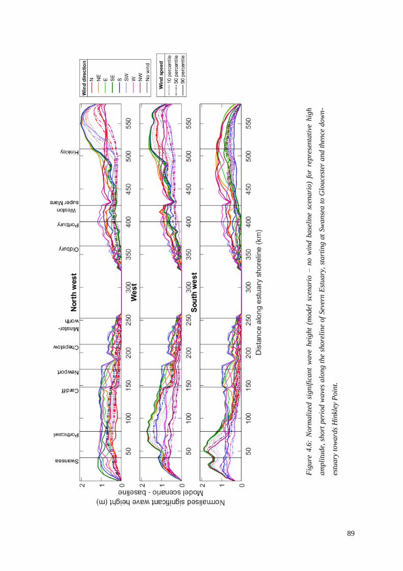
89
Fig
ure
4.6
: N
orm
ali
zed
sig
nif
icant
wave
hei
ght
(model
sce
nari
o –
no w
ind b
ase
lin
e sc
ena
rio
) fo
r re
pre
sen
tati
ve h
igh
am
pli
tud
e, s
ho
rt p
erio
d w
ave
s alo
ng t
he
shore
line
of
Sev
ern E
stuary
, st
art
ing a
t Sw
an
sea
to
Glo
uce
ster
an
d t
hen
ce d
ow
n-
estu
ary
tow
ard
s H
inkl
ey P
oin
t.

90
4.4.1.2. Following winds reduce Hs in the outer estuary
A high amplitude wind wave moving towards the shoreline with a 90th percentile value wind speed and
following wind does not produce the maximum Hs in the outer estuary. For example a wave traveling
from the NW followed by a 90th percentile value wind speed produces normalized maximum Hs of 0.79
m, 30 km up-estuary from the model boundary on the south shoreline. A NW wave followed by a 10th
percentile value wind speed value produces a normalized maximum Hs of 1.59 m, at the same point in
the model domain. Further to this, a wave moving in a SW direction followed by a 90th percentile value
wind speed in a SW direction, produces a normalized maximum Hs of 0.84 m 50 km up-estuary from
the model boundary on the north shoreline, between Swansea and Porthcawl. A SW wave followed by
a 10th percentile wind speed value produces a normalized maximum Hs of 1.23 m at the same point in
the model domain. It is evident that a following wind contributes to wave growth. The addition of wind
energy to the rougher sea could cause the wave to feel the effect of bottom friction and break before
reaching the shoreline or break due to whitecapping.
4.4.1.3. Opposing, blocking wind acts to steepen waves in the outer
estuary
Maximum waves on both south and north shorelines generally occur when wind and wave are
propagating in opposite directions. For example, the maximum normalized Hs on the south shoreline,
2.04 m, occurs when NW waves are essentially blocked by 90th percentile value wind speed from a SE
/ E direction. Likewise, the maximum normalized Hs on the north shoreline, 1.91 m, occurs when the
SW waves are blocked by 90th percentile value wind speed from a NE / E direction. Winds block the
wave propagation moving in the opposite direction to increase the steepness of waves. Further to this,
the younger, rougher wind-wave sea shows increased sensitivity to wind direction. This is particularly
the case in the outer estuary where there is greater sensitivity to changing wind direction and wind
speed. The range of normalized maximum Hs is 1.47 m between Swansea and Porthcawl on the north
shoreline and 1.35 m down-estuary of Hinkley Point on the south shoreline. The blocking effect of wind
appears to be a significant contribution to wave hazard along the shoreline of the outer estuary.
There is less sensitivity to wind direction in the upper estuary, beyond Cardiff on the north shoreline
and Portbury on the south shoreline as waves begin to attenuate. Following winds from the W and SW
produce the maximum normalized Hs in the upper estuary, as fetch may help high amplitude waves to
propagate further up-estuary. The effect of bottom friction dissipates wave energy and the lines
converge to show Hs decline. Hs is 0 m in the upper estuary at Gloucester as wave energy is not able to
propagate this far up-estuary, possibly due to the long, narrow, shallow nature of the Severn Estuary.

91
4.4.1.4. Effect of estuary geometry on significant wave height
The wind direction produces a different maximum Hs in different locations throughout the estuary, as a
function of the local geometry and complex orientation of the coastline. The maximum Hs on the south
shoreline occurs with a NW wave direction, and the maximum Hs on the north shoreline occurs with a
SW wave direction. It is clear that a shoreline facing an incoming, onshore wave direction will
experience increased wave hazard, however the incoming wave direction impacts each shoreline
differently. The maximum normalized Hs on the north shoreline occurs further up-estuary, 1.91 m at 55
km away from the model boundary. In contrast, the maximum normalized Hs on the south shoreline,
2.04 m, occurs 30 km up-estuary from the model boundary. The orientation of coast, geometry and
bathymetry of the estuary means that the shorelines do not respond in the same way and the maximum
is not observed at the same distance up-estuary.
The effect of shoreline geometry on wave hazard is further highlighted by the double peak in maximum
significant wave height observed close to Mumbles for a SW wave direction. The headland is smoothed
out in the model domain; however complex changes in water depth are reflected in the bathymetry.
4.4.2. Low amplitude waves
4.4.2.1. 90 percentile winds create maximum variability
The 90th percentile value wind speed consistently produces the maximum normalized Hs along the north
and south shoreline throughout the estuary for longer period, lower amplitude waves (Figure 4.7).
Normalized maximum Hs remains steady along the shoreline from the model boundary to Weston-
super-Mare on the south shoreline and Cardiff on the north shoreline for each scenario. This shows the
wind has a sustained influence in propagating lower amplitude, longer period waves as far up estuary
as Chepstow and Oldbury. Further up-estuary the channel begins to narrow and become increasingly
shallow, and waves rapidly decay. There is a varying magnitude of normalized maximum Hs for each
scenario with a 90th percentile value wind speed. There is over 1 m variability in normalized maximum
Hs between scenarios forced by a 90th percentile value wind speed, as opposed to 0.01 m variability for
scenarios forced by a 10th percentile value wind speed.

92
Fig
ure
4.7
: N
orm
ali
zed si
gnif
icant
wave
hei
ght
(model
sc
enari
o – no w
ind base
lin
e sc
ena
rio
) fo
r re
pre
sen
tati
ve lo
w
am
pli
tud
e, l
on
ger
per
iod w
ave
s alo
ng t
he
shore
line
of
Sev
ern E
stuary
, st
art
ing a
t Sw
an
sea t
o G
lou
cest
er a
nd
th
ence
do
wn
-
estu
ary
to
wa
rds
Hin
kley
Poin
t.

93
At Porthcawl, on the north shoreline of the estuary, maximum normalized Hs is 1.13 m with a NW wave
and a following 90th percentile value wind speed from a W wind direction. The minimum normalized
Hs for a NW wave under a 90th percentile value wind speed is 0.11 m, which occurs with a NE wind.
This produces a range of 1.02 m on the north shoreline and shows that lower amplitude, longer period
waves can propagate further up-estuary under stronger wind conditions.
In the same location on the north shoreline, normalized maximum Hs under a NW wave direction with
a 10th percentile value wind speed is 0.04 m with a SE wind. The lowest normalized Hs produced by a
10th percentile value wind speed is 0 m for a NW wave and E wind. This produces a range of just 0.04
m for Hs at Porthcawl under the 10th percentile value wind speeds. The 0 m normalized Hs at Porthcawl
under an E wind shows that the wind is having little effect on significant wave height under this
scenario.
The results at Hinkley Point on the south shoreline in the outer estuary follow a similar pattern. The
maximum normalized Hs at Hinkley Point is 1.27 m under a SW wave with a 90th percentile value wind
speed from the NW. Minimum normalized Hs for a SW wave under a 90th percentile value wind speed
is 0.2 m, which occurs with a S wind direction. This produces a range of 1.07 m on the south shoreline
of the outer estuary. There is less sensitivity in normalized Hs under 10th percentile value wind speeds.
Maximum normalized Hs under a 10th percentile value wind speed for a NW wave is 0.05 m, with a N
wind and minimum normalized Hs is 0.01 m, also under a S wind producing a range of 0.04 m. A
southerly wind produces the lowest Hs for all percentile value wind speeds, as the orientation of the
coastline minimizes the effect of wind to contribute to Hs. Along the north and south shoreline, it is
evident that higher period, low amplitude waves show greater sensitivity to wind direction for higher
wind speeds.
4.5. Discussion
The results presented here help to identify the contribution of individual factors to variability in coastal
wave hazard in a hyper-tidal estuary. Increased wave hazard along the shoreline may influence wave
overtopping, which is an important consideration for port and harbour operations, energy infrastructure
and residential communities in estuaries when considering direct flood hazard. The results can also help
to understand how wave hazard may vary under future climate change, with varying storm tracks and
wind conditions.
4.5.1. Younger, rougher seas show more sensitivity to wind direction.
The model highlights that short period, high amplitude waves are sensitive to wind direction, with a
stronger, opposing wind increasing significant wave height. There is known to be a strong coupling and
transfer of momentum between turbulent atmospheric and oceanic boundary layers. Increasing wind
speed acts to increase the drag coefficient on the sea surface (Pugh, 2004), enhancing generation of

94
wind-waves (Janssen, 1989). The transfer of energy from the atmosphere to sea waves can be affected
by sea state (Janssen 1989). Experimental results show that the drag coefficient over a younger, wind-
wave sea is up to 50% larger than an older, swell sea (Donelan, 1982). Further to this, a Boussinesq
type wave model has been used to show that wind waves are sensitive to changes in wind speed can
amplify significant wave height, due to increased energy exchange between the air and sea (Liu et al.,
2015). Stronger winds have been shown to be important in amplifying significant wave height in the
Dee Estuary. Simulations of the wind-wave climate of the Dee Estuary under a 1 in 100-year storm
under 5, 15 and 25 m/s wind speed show an increase in wave height and setup along the coast, which
could contribute significantly to flooding (Wolf, 2007). Changes in the wind speed can alter wave
conditions, resulting in local-scale changes in sea level at exposed sites.
The sensitivity of waves to wind direction can be site specific. Opposing winds can cause waves to
become shorter and higher, and therefore steeper (Wolf et al., 2011). Steeper waves can cause
unpredictable and unstable sea conditions, as seen in the mouth of the Colombia River when combined
with strong, opposing river outflow which can make the region dangerous for shipping and boats (Elias
et al., 2012). Strong, opposing winds blowing against incoming low amplitude waves can generate
surface waves and tidal rips in the Bay of Fundy, Canada (Desplanque and Mossman 2004), resulting
in dangerous sea conditions. As seen in Figure 4.6, each shoreline can respond differently to prevailing
conditions with significant wave height occurring at different distances up-estuary. Simulations of
locally wind-generated sea from westerly and northwesterly winds in the Dee Estuary, NW England
show that significant wave height varies along the estuary shoreline due to the sheltering effect of West
Hoyle Bank and the Welsh coastline and the effect of water depth on refraction (Wolf et al., 2011).
Wind direction and speed can act to amplify significant wave height and subsequent wave hazard in
hyper-tidal estuaries, and local bathymetry and topography can change influence the response of each
shoreline to varying conditions.
4.5.2. Long period, low amplitude waves amplified due to strong winds
The model confirms that stronger wind speeds are important for increasing Hs for higher period, low
amplitude waves throughout the estuary. The drag coefficient of air flow, related to shear stress of wind
speed on sea surface, low amplitude, longer period waves, does not respond to the influence of shear
stress to the same extent as younger, higher frequency wind waves (Brown and Wolf 2009). A fully
developed wave field, such as a longer period, low amplitude wave, may receive little momentum from
the air (Janssen 1989) and low amplitude waves exhibit less drag than both shoaling and breaking waves
(Anctil and Donelan 1996). The drag coefficient is Delft3D-WAVE is linearly related to wind speed
(Wu 1982), which may account for some of the effect of surface roughness due to wind. Increased
variability in significant wave height for stronger wind speeds may be the effect of increasing wind
speed on surface roughness and the drag coefficient, generating local winds on the sea surface

95
(Letchford and Zachry 2009). Long period waves propagate into the Severn Estuary throughout much
of the year (Pye and Blott 2010), and contribute to significant wave heights during low pressure, winter
storms (Sibley et al., 2015). Long period waves in the Bay of Fundy, Canada, are exacerbated by strong,
southeasterly to southerly winds due to the orientation of the estuary (Desplanque and Mossman 1999).
Strong southerly winds during the Saxby Gale, 4 October 1989 resulted in significant damage, as dykes
breached, cattle and sheep drowned and railroad beds washed away and only when the wind shifted to
a southwesterly direction did the waves cease to cause damage (Desplanque and Mossman 2004).
However, certain areas in large estuaries can be sheltered from the effect of swell waves due to
sheltering, e.g. in the Dee Estuary, NW England (Brown and Wolf 2009), or shallow water effects which
cause extensive dispersion, as seen in San Francisco Bay (Talke and Stacey 2003). The model has
shown that low amplitude, long period waves can propagate far up-estuary which disproves the
assumption that up-estuary locations are only subject to storm surges and higher amplitude, locally
generated wind waves (Lesser 2009; Monbaliu et al., 2014). The effect of low amplitude waves may
create similar impacts as an energetic swell wave, which has a longer wavelength and lower frequency,
to increase wave hazard along the shoreline (Palmer et al., 2014; Sibley et al., 2015). Further to this,
stronger wind speeds superimpose locally generated waves on the sea surface, which can result in
dangerous sea conditions for critical infrastructure, ports and harbours. Coastal defenses in hyper-tidal
estuaries must be designed to protect against the effect of long period, low amplitude wind-waves as
well as tides, storm surges and river flow.
4.5.3. Waves impact on flood hazard and economic activities
The results presented here show the effect of wind and wave properties on variability of significant
wave height along the shoreline of the estuary and can be used as an evidence base to inform future
coastal management decisions. Increased significant wave height under certain wind-wave conditions
can pose a hazard in coastal areas due to wave run-up and defense overtopping (Bastidas et al., 2016)
as individual waves exceed the available ‘freeboard’ (height above still water level) of coastal defences
(Wolf 2009). The results can be applied to understand the wind-wave condition which could result in
maximum significant wave height and subsequent wave overtopping in ports and harbours, which can
influence the safety of structures and of people working and traveling immediately behind the defense
line (Bouma et al., 2009; Diab et al., 2017). Low amplitudes waves, which can generate rough sea states
under stronger winds in the estuary, can propagate into ports and harbours and cause excessive moored
ship motions with consequences for operational downtime (Rosa-Santos and Taveira-Pinto 2013).
Operational downtime has financial implications, as cargo handling cannot occur and the ship has to
leave berth due to unsafe mooring conditions (Van Deyzen et al., 2015). Knowledge of the wind-wave
conditions that can cause wave overtopping, transmission or swell wave propagation in the harbour can
be used to divert ships away from port during hazardous conditions, to avoid damage to mooring lines
or downtime. The hazards of wave overtopping are site specific, especially when people are concerned,

96
and dependent on estuary orientation, bathymetry and topography (Santana-Ceballos et al., 2017),
characteristics of sea walls (Allsop et al., 2005) and the complex nature of wind-generated waves.
Increased wavelength and wave period, as seen with swell waves, can also contribute to overtopping
hazard as run-up is longer (Thompson et al., 2017), and should also be considered as a hazard in some
estuaries. Understanding wave overtopping hazard from combined wind-wave effects can help to
reduce economic losses from storm events in estuaries by avoiding operational downtime and damage
to vessels and moorings.
The results presented here identify key combinations of wind-wave properties which contribute to wave
hazard in a hyper-tidal estuary. While waves contribute towards total coastal water level by means of
wave run-up, wave setup and swash (Stockdon et al., 2006; Wolf 2009), the effect of astronomical tides,
atmospheric storm surges and river discharges must also be considered. Wave characteristics and
propagation in shallow water is partially dependent on tidal elevation. Wave heights may also be related
to surge magnitude, and wind has an important role in generating surge and waves (Pye and Blott 2014).
Tidal modulation of waves plays a large part of the natural regime of the Severn Estuary (Fairley et al.,
2014) and strong currents in the Bay of Fundy can generate tidal rips and hazardous surface waves
(Desplanque and Mossman 1999). Future simulations of wind-wave conditions should include tide-
surge propagation, evidently important in a hyper-tidal estuary, and the effect of wave hazard sensitivity
on morphological response (Phillips et al., 2017), overtopping volumes, and depth and extent of
subsequent flood inundation (Prime et al., 2015).
4.5.4. Changing future storm tracks and climate
The model results can also help to understand how wave hazard may develop under future, changing
climate patterns, and the impact this may have on future flood inundation and adaptation strategies. It
has been seen that maximum significant wave height varies within the estuary dependent on wind speed
and wind direction, therefore stronger wind speeds and changing storm tracks under future climate
could alter future flood risk from wave overtopping (EurOtop 2016). Changes in the number, frequency
and track of mid-latitude (30-60 °) storm tracks would alter wind speed and direction, which would
directly influence wave hazard in estuaries (Robins et al., 2016). Simulations of typhoon intensification
in the Pearl Estuary has been shown to increase significant wave height, and results have been fed into
design of seawalls (Yin et al., 2017). Increasing sea levels and river discharge will allow waves to
propagate and impact further up-estuary, and are more likely to overtop sea defenses (Wolf 2007).
Increasing frequency and magnitude of storms, or those occurring in clusters, will increase the
occurrence of economic damage and potential loss of life across a larger spatial area (Robins et al.,
2016). Further to this, changes in storminess have the potential to reduce the effectiveness of existing
coastal defenses and result in more extensive and damaging floods (Phillips 2008). Large scale
atmospheric changes, such as the North Atlantic and Southern Oscillations, could also result in changes

97
in wind speed and direction, which will have implications for where maximum significant wave heights
will occur, with potential implications in the Severn Estuary and Bay of Fundy (Phillips et al., 2013).
However wave hazard under future climate will vary depending on regional- and local-scale processes,
strong natural variability and uncertainty in anthropogenic forcing and future wave climate (Woolf and
Wolf, 2013; Haigh and Nicholls, 2017). Regional-scale simulations of wind-wave conditions in an
estuarine system can identify important processes and interactions which may be effected under future
climate. The methodology and results presented here can aid long-term coastal defense and management
strategies, as sustainable coastal management requires confidence in the knowledge of any possible
future changes to wave hazard.
4.6. Conclusion
There is a need to identify key combinations of wind-wave characteristics which contribute to wave
hazard and the relative significance of wind-generated waves compared with swell waves in heavily
populated and industrialized hyper-tidal estuaries, where critical infrastructure must be designed to
withstand this hazard. Delft3D-WAVE is used to simulate wave evolution in a hyper-tidal estuary to
identify key combinations of wind-wave characteristics which contribute to maximum significant wave
height, and subsequent wave hazard throughout the estuary. Long-term wind and wave records are used
to generate representative wind-wave conditions, and consider the influence of wind speed, wind
direction, wave type and wave direction on maximum significant wave height along the shoreline of
the Severn Estuary, SW England. Results show that a younger, rougher wind-wave sea, characterized
by low period, high amplitude waves, show increased sensitivity to wind direction. Stronger, opposing
winds generate maximum significant wave height in the outer estuary. Maximum significant wave
height occurs at different locations up-estuary along each shoreline due to estuary orientation and local
bathymetric effects. Higher period, low amplitude waves show greatest sensitivity to wind direction
under stronger wind speeds, as local wind-generated waves are superimposed. The model highlights
how different wind-wave conditions vary in the estuary, and stronger winds amplify and facilitate the
propagation of long period, low amplitude further up-estuary under all conditions to impact
infrastructure along the shoreline. The research helps to inform sea defense design to withstand wave
overtopping under a range of conditions, minimize economic losses from operational downtime in ports
and harbours due to wave transmission and inform long-term coastal management of the potential
implications of future climate changes on wave hazard in the estuary. Future work needs to consider
the effect of tide and surge on wave propagation, and results from fully coupled tide-surge-wind-wave
models can force inundation models to explore depth and extent of flooding from severe storm events.

98
4.7. Acknowledgements and Data
The authors thank colleagues at the British Oceanographic Data Centre (BODC) for providing tidal
data; Magnox for providing tidal data; Environment Agency for providing tidal data; Gloucester
Harbour Trustees for providing tidal data; UK Met Office for providing observational wind data;
CEFAS for providing observational wave buoy data; EDINA for providing bathymetric data; and Judith
Wolf at the National Oceanography Centre Liverpool for constructive comments on analysis of the
wave buoy record.

99
5. Quantification of the uncertainty in coastal storm hazard predictions
due to wave-current interaction and wind forcing
Chapter 5 progresses the modelling work further to utilize the full functionality of Delft3D by coupling
the FLOW with WAVE modules together, and incorporating a time- and space-varying wind and
atmospheric pressure field. Maximum significant wave height is statistically validated at four wave
buoy locations within the estuary to ensure this model setup can simulate tide-surge-wind-wave-river
interaction with confidence. Chapter 5 quantifies uncertainty in maximum significant wave height, total
water level and hazard proxy (water level + ½ significant wave height) when interactions between
combined hazards or local effects of atmospheric forcing are neglected. The results can help to ensure
accurate forecasts to mitigate negative consequences of combined hazards, and ensure flood alerts,
warnings and evacuation orders are timely.

100
5.1. Abstract
Coastal flood warning and design of coastal protection schemes rely on accurate estimations of water
level and waves during hurricanes and violent storms. These estimations frequently use numerical
models which, for computational reasons, neglect the interaction between the hydrodynamic and wave
fields. Here, we show that neglecting such interactions, or local effects of atmospheric forcing, causes
large uncertainties, which could have financial and operational consequences because flood warnings
are potentially missed or protection schemes under-designed. Using the Severn Estuary, SW England
we show that exclusion of locally generated winds underestimates high water significant wave height
by up to 90.1%, high water level by 1.5% and hazard proxy (water level + ½ significant wave height)
by 9.1%. The uncertainty in water level and waves is quantified using a system to model tide-surge-
wave conditions, Delft3D-FLOW-WAVE in a series of eight model simulations for four historic storm
events.
5.2. Introduction
Concurrence of astronomical high tides, meteorological storm surge due to hurricanes, cyclones or mid-
latitude storms, energetic waves, and strong winds can cause coastal flooding, and subsequent damage
to property and loss of life to some of the 600 million people estimated to live in low-lying coastal (<10
m) regions worldwide (Barnard et al., 2019; Wolf 2009). The devastating effects of concurrent coastal
hazards are well documented in hyper-tidal regions, where tidal range exceeds 6 m, in the Severn
Estuary, UK (Sibley et al., 2015), Bay of Fundy (Greenberg et al., 2012) and Yangtze Estuary (Yin et
al., 2017), as combined storm parameters can enhance high water level (HWL) and high water
significant wave height (HWHs), defined as significant wave height at the time of high water, to increase
the likelihood of overtopping and subsequent inundation. Increasing coastal population and
urbanization, potential future changes in storm tracks and sea-level rise means there is a need to plan
for the negative consequences of coastal hazards.
Operational storm surge and wave forecasts are important components of coastal storm hazard
mitigation strategies (Tunstall et al., 2004). If operational forecasts exceed pre-defined threshold levels,
corresponding to the minimum wave and total water level that represent a potential flood hazard (Del
Río et al., 2012), alerts and flood warnings will be issued to detail scale, timing and location of a hazard
(Lawless et al., 2016). To prevent negative consequences of forecast extreme storm events, flood
warnings issued by local agencies must be accurate and timely. Operational forecasts can make use of
measured and modelled meteorological and oceanic data (e.g. O’Neill et al., 2016) and outputs can be
used to estimate likelihood of coastal flooding, and the effect of wind, waves and total water level on
overtopping and breaching for specific flood events (Quinn et al., 2014). However error can be
introduced into operational forecasts due to model, knowledge and data uncertainty (Stephens et al.,

101
2017). Uncertainty due to a model’s ability to accurately represent physical processes or replicate
interactions (e.g. Bolaños et al., 2014), lack of knowledge of interactions in a physical system and
inaccurate input parameters (e.g. temporally or spatially limited) can be introduced, and propagated
through the modelling chain to inundation assessments and flood warnings (Sayers et al., 2003). There
is a need to understand and reduce uncertainty in operational forecasts of HWL and HWHs that
contribute to hazard assessments. Uncertainty in operational forecasts could mean flood events are
underestimated or missed, which may increase the risk to coastal communities and critical
infrastructure.
The accurate definition of HWL and HWHs is also important for critical storm threshold identification
for the design of cost-effective coastal protection strategies. Implementation of hard structures or
nature-based solutions, which aim to mitigate the effects of HWL and HWHs, rely on a thorough
understanding of the physical processes and interactions in a region (Conger and Chang 2019). The type
and costs of new schemes largely depend on the physical conditions at the site, and sensitivity of the
scheme to natural processes and their interaction (Temmerman et al., 2013). Uncertainty in HWL and
HWHs may lead to incorrect hazard thresholds, as defense exceedance is most likely to occur close to
the time of high water, or implementation of strategies which are not able to protect hinterlands against
normal winter conditions as well as extreme storm tide conditions. Commitment to upgrading
engineered structures, such as Canada’s recent US$114 million pledge to upgrade 64 km of dikes and
sluices in Nova Scotia (Fairclough 2019), or implementing new strategies, e.g. the new £63 million
seawall at Rossall, Lancashire (Environment Agency 2018) are based on multi-disciplinary, cost-benefit
analysis in areas with highest potential for protection benefits. Representative, site-specific information
of HWL and HWHs are needed to support decisions to ensure crest level and defense heights are
appropriate, for effective storm hazard mitigation and resilience to future change.
5.2.1. Case Study
This research focuses on the Severn Estuary (Figure 5.1a), which borders south Wales and southwest
England, as an example of hyper-tidal and funnel shaped estuaries worldwide. The estuary has the third
largest mean spring tidal range in the world, up to 12.2 m at Avonmouth due to the funnelling effect
(Dyer 1995), which is also known to modulate the local wave climate (Pye and Blott 2010). The
orientation of the mouth of the estuary to the Atlantic Ocean means it is exposed to prevailing swell
waves, and the large fetch (up to 6000 km) amplifies wave driven hazards in the outer estuary. The
south coastline of the estuary is dominated by energy and port infrastructure and large areas of low-
lyingagricultural land, highlighting the need for accurate operational forecasts in this region.

102
5.2.2. Outline of the paper
This research quantifies the sensitivity of HWL, HWHs and high water hazard proxies (HWHP) to
model coupling along the Severn Estuary coastline. Hazard proxy (HP) is defined as the WL+½ Hs and
is used to understand the severity of a condition. 32 model simulations are run in total; a series of eight
model simulations are run for four events which represent a potential hazard in Delft3D-FLOW-WAVE.
The model is applied to consider waves and circulation in isolation (standalone), the influence of
circulation on waves (one-way coupled) and the influence of the circulation on the waves and waves on
the circulation (two-way coupled). Wind and atmospheric pressure are included on four of the eight
model simulations to investigate wind influence on HWL and HWHs during storms. Water level (WL),
significant wave height (Hs) and HP are simulated to explore the sensitivity of each parameter to model
coupling (section 2), and the results (section 3) quantify uncertainty introduced into the model due to
the coupling and forcing processes. Before concluding in section 5, section 4 discusses the importance
of locally generated winds and coupling processes in simulating Hs and HP in hyper-tidal estuaries, and
the implications that uncertainty in storm parameters have on flood warnings and management
activities.
5.3. Method
5.3.1. Delft3D hindcast of select historic events
The Delft3D modelling system (Lesser et al., 2004) was used to simulate tide-surge-wave propagation
across the Severn Estuary for four historic storm events. Delft3D-FLOW simulates hydrodynamic flow
under the shallow water assumption, and Delft3D-WAVE simulates the generation and propagation of
waves, based on the third-generation spectral wave model Simulating WAves Nearshore (SWAN),
which solves the spectral action balance (Booij et al., 1999). A 2D-horizontal, curvilinear grid of the
Severn Estuary extends from Woolacombe, Devon and Rhossili, South Wales in the west, with a
maximum resolution of 5 km, to Gloucester in the east with a minimum resolution of 25 m at the coast,
to resolve fine-scale processes in shallow water (Figure 5.1a), and has been validated in Lyddon et al.,
2018a; 2018b; 2019a. Gridded bathymetry data at 50 m resolution (SeaZone Solutions Ltd. 2013) was
interpolated over the 2DH curvilinear grid. Delft3D-FLOW has two open boundaries forced by time-
varying, spatially uniform water level, representing the Atlantic Ocean to the west and the River Severn
to the east. Delft3D-WAVE was forced with five, space- and time-varying boundary points to the west.
Delft3D-WAVE explicitly represents the dissipation of wave energy due to white-capping, bottom
friction and depth-induced breaking, and wave generation by wind, and non-linear wave-wave
interactions (Deltares 2014b).

103
Figure 5.1: a) Delft3D-FLOW-WAVE model domain. Bathymetry relative to CD. Average bias and
RMSE (m) of WL and Hs model results for four events to tide gauge and wave buoy observations are
shown in brackets; (b) six year Hs record from Scarweather wave buoy; (c) Long-term tide gauge record
taken from Ilfracombe, with HWHP grouped based on wind direction at the time of the event. HWL,
HWHs, and wind speed (WS) at the time of the events are shown. Horizontal black lines indicate
maximum, 90th, 50th and 10th percentile HP thresholds.
Six years of Hs data from the Scarweather Directional Waverider buoy (Figure 5.1b) (Cefas, 2019) and
tide gauge data at Ilfracombe (NTSLF, 2019) were used to identify historical coastal flood and wave
hazard events. Hs was isolated when the tide is at or above 5.91 m (the level of lowest high water level
in the record), to leave only wave events when overtopping is most likely to have occurred (see Figure
1c). This was used to calculate HP for concurrent water level and wave conditions exceeding this
threshold (see colored dots in Figure 5.1c). Each HP event represents a real event with hazard potential,
and was grouped according to the concurrent wind direction, using data from the Met Office weather
station at Pembrey Sands (CEDA, 2018). Winds from a southwest and west direction have been shown

104
to generate maximum Hs and contribute to greatest wave hazard in the estuary (Lyddon et al., 2019a).
Four events with a southwest and west wind direction were selected, which represent the maximum (3
January 2014, 07:00), 90th (16 December 2012, 19:00), 50th (26 January 2014, 01:00) and 10th percentile
(30 June 2012, 12:00) HP thresholds (Figure 5.1c).
The open sea boundary to the west was forced with a time-varying, spatially uniform water level at a
15 minute interval using observation data from Ilfracombe tide gauge (NTSLF, 2018). For WAVE
standalone simulations, a constant WL was applied at the open sea boundary, at the level of HWL during
the selected event, to eliminate the effect of tidal currents on Hs and variability in WL. Time- and space-
varying wave conditions (Hs, wave direction, mean period and directional spread) from the Met Office
WAVEWATCH III hindcast (Saulter et al., 2016; Siddorn et al., 2016) were used at five equidistant
points along the open sea boundary (see Figure 5.1a), and were linearly interpolated along the boundary
to force the model at 15-minute intervals. A time- and space-varying wind and atmospheric pressure
field forced the model domain at hourly intervals, using data originating from the Met Office global
unified model (Walters et al., 2014) and extracted from the Extended Area Continental Shelf Model
CS3X (Williams and Horsburgh 2013). All simulations were forced with 15-minute river gauge data
from Sandhurst (Environment Agency, 2016) at an up-estuary open boundary (see Figure 5.1a).
5.3.2. Model validation and scenario test
Model outputs from two-way coupling of Delft3D-FLOW-WAVE, which represents a complete five-
way multi-hazard simulation (tide-surge-wind-wave-river), for the four events were validated at five
tide gauge locations (Hinkley Point, Newport, Severn Bridge, Oldbury, Sharpness) and four wave buoy
locations (Scarweather, Minehead, Weston-super-Mare, Severn Bridge). Average bias and root mean
squared error (RMSE) of WL and Hs were calculated at validation locations (see Figure 5.1a). The bias
is defined as:
𝐵𝑖𝑎𝑠 = �̅� − �̅� (1)
where M represents the model values, O the observed values and the overbar denotes the mean value
of the simulated storm event. A value of 0 indicates an unbiased estimate; a positive value indicates the
model is over-predicting; a negative value is under-prediction. The RMSE is defined as:
𝑅𝑀𝑆𝐸 = √(𝑀 − 𝑂)2̅̅ ̅̅ ̅̅ ̅̅ ̅̅ ̅̅
(2)
where a value closer to zero indicates better model performance.
There is good agreement for WL in outer estuary. Hinkley Point has a bias value of 0.08 m and RMSE
of 0.34 m, which represents 2.75% of the observed tidal range during the maximum event. Positive bias

105
and larger RMSE values up-estuary indicate the model overestimates WL at Oldbury and Sharpness.
Hs is well reproduced, as bias and RMSE values remain close to zero. Wave data used for validation
are available along the southern estuarine coastline, where areas of critical energy infrastructure are
located highlighting the importance of accurately representing Hs in this region.
The validated Delft3D-FLOW and WAVE model was run from 48 hours before the event to 12 hours
after, in a series of eight standalone, one-way or two-way coupled simulations. Delft3D-FLOW and
WAVE can run in ‘standalone’ mode with user-defined properties (Deltares 2014b). Delft3D-WAVE
is used in one-way coupled simulations where the FLOW simulation is completed and then input
(offline) into the wave simulation, to account for the effect of flow on waves. Two-way coupled
simulations allow dynamic (online) interaction of Delft3D-WAVE with FLOW to account for the effect
of waves on current, and the effect of current on waves. The FLOW and WAVE modules exchange
information at 15-minute intervals, such as wave radiation stresses and water level conditions needed
for wave transformation, to represent two-way wave-current interaction, refraction and depth-induced
breaking. The influence of wind is considered in both FLOW and WAVE when included, to represent
changing forcing processes. Eight model runs were completed for each of the four historical HP events
(32 in total) to explore how model coupling and forcing processes contribute to uncertainty in HWL,
HWHs, and HWHP (Table 51).
Table 5.1: Eight model simulations completed in Delft3D-FLOW-WAVE for each historic storm event.
Run Model Coupling Forcing
1 FLOW Standalone Water level
2 FLOW Standalone Water level + wind
3 WAVE Standalone Constant HW water level + Wave
4 WAVE Standalone Constant HW water level + Wave + wind
5 FLOW → WAVE One-way Water level from 1 + wave
6 FLOW → WAVE One-way Water level from 2 + wave + wind
7 FLOW → WAVE Two-way Water level + wave
8 FLOW → WAVE Two-way Water level + wave + wind
The maximum, mean and median percentage difference in HWL, HWHs, and HWHP were calculated
between each model run and model run 8 as:
𝑃𝑒𝑟𝑐𝑒𝑛𝑡𝑎𝑔𝑒 𝑑𝑖𝑓𝑓𝑒𝑟𝑒𝑛𝑐𝑒 =
(𝑅𝑢𝑛 8 − 𝑅𝑢𝑛 𝑋)
𝑅𝑢𝑛 8 × 100
(3)
Run 8 is used as the baseline run as it includes all boundary forcing, and has been successfully validated
to observational tide and wave data in the estuary. Model results are presented as the % and absolute

106
difference between each run and the validated run 8 for the north and south coastline to i) identify which
coupling HWL, HWHs and HWHP are most sensitive to and ii) quantify uncertainty introduced into the
model due to omitting coupling and forcing processes.
5.4. Results
HWL and HWHs were extracted from model results every 5 km, from the second row of grid cells in,
along the estuary coastline, and HWHP calculated, for each event. Results of the maximum event (3
January 2014) are seen in Figure 5.2a-c. HWL (Figure 5.2a) is amplified to a maximum of 11.7 m up-
estuary, beyond Newport and Oldbury, due to the funnelling effect (Uncles 1984). HWHs (Figure 5.2b)
is greatest in the outer estuary near Swansea and Porthcawl. HWHs dissipates up-estuary but shows
greater sensitivity to coupling and forcing processes. HWHP (Figure 5.2c) is greatest up-estuary, and
shows greatest sensitivity to model coupling and forcing in the outer estuary.
The cumulative effect of wave dissipation as energy propagates up-estuary, i.e. increased white capping
as waves steepen and depth-induced breaking and up-estuary cross-section friction, dampens the hazard,
therefore analyses are focused in areas where water level and waves are largest, in the lower- and mid-
estuary. Maximum, mean and median percentage difference in HWL, HWHs and HWHP between each
run with run 8 (solid black line in Figure 5.2a-c) is calculated for sections of the estuary coastline up to
the point where Hs < 10 cm in all simulations, termed the wave limit, to focus on the impact on non-
negligible wave conditions (Figure 5.2d-f).

107

108
Figure 5.2: Simulated a) HWL; b) HWHs; c) HWHP along the coastline of Severn Estuary starting at
Swansea to Gloucester and thence down-estuary towards Woolacombe for maximum event (3 January

109
2014 07:00); d-f) % difference between each run and run 8. The divide between north and south
coastlines (dashed black vertical line) and wave limit where Hs < 10 cm (dashed grey vertical line) is
shown. Solid black vertical lines indicate locations of critical infrastructure and coastal towns.
Absolute differences in HWL, HWHs and HWHP between each run with run 8 along the coastline are
shown in Figure 5.3. Run 3 and 4 greatly underestimate HWL as a constant water level at MHWST is
applied throughout the model domain, and no funnelling of the tidal wave to amplify tidal range up-
estuary occurs. Up to 6.2 m difference in HWL occurs in the upper estuary between runs 4 and 8. Runs
1, 2 and 7 show small changes in absolute HWL occur in outer estuary, and increase up-estuary from
Cardiff and Portbury as the estuary begins to narrow. 0.18 m difference occurs 270 km up-estuary,
beyond the wave limit, between run 7 and 1. This represents 2% of the tidal range, but could make a
substantial difference in coastline response models up-estuary if combined with strong winds, large
waves or substantial river discharge.
The largest absolute differences in HWHs occur in the outer estuary, on the north coastline, from the
boundary to Newport. The greatest difference is 1.44 m, which occurs 20 km up-estuary near Swansea,
between run 5 and 8. These large differences may indicate that coastlines facing into the direction of
prevailing storm conditions are more sensitive to more severe storm events, or may be the effect of the
complex geometry of the coastline. Run 7, which includes two-way coupling, shows least variability in
the outer estuary. The absolute difference in HWHs is reduced in the mid- and upper-estuary as the
cumulative effect of shallow water processes (whitecapping, bottom friction) dampen wave height. Up
to 0.8 m difference can be seen on the south coastline near Weston-super-Mare and Portbury, which
could have an impact on inundation, overtopping, erosion. The greatest difference in the mid- and
upper-estuary occurs between simulations which do not include local atmospheric forcing.
Runs 1 and 2 underestimate HWHP in the outer estuary, up to a maximum 2.2 m 15 km up-estuary on
the north coastline. Wave coupling is excluded from these runs, and highlights the importance of
coupling for hazard prediction in the outer estuary. Runs 1 and 2 do not underestimate HWHP to such
an extent up-estuary of Cardiff and Weston-super-Mare. Runs 3 and 4 greatly underestimate HWHP,
up to 6.2 m up-estuary as the funnelling effect of the tide is excluded.
Similar to HWHs, HWHP shows greatest difference in the outer estuary on the north coastline for run
5 and 6. Run 7 shows least variability, which includes two-way coupling. The greatest difference is 0.71
m, 20 km up-estuary between run 5 and 8. The greatest difference on the south coastline is smaller
compared to the north coastline, at 0.48 m, 165 km up-estuary between Weston-super-Mare and
Portbury between run 5 and 8. The difference between run 7 and 8 at this point on the south coastline
is similar in magnitude, 0.46 m. This indicates the importance of local atmospheric forcing in coastal

110
hazard predictions, but also highlights that estuary orientation and sheltering effects on the south
coastline can influence hazards.

111
Figure 5.3: Absolute difference for a) HWL; b) HWHs; c) HWHP between each run and run 8 along
the coastline of Severn Estuary starting at Swansea to Gloucester and thence down-estuary towards
Hinkley Point for maximum event (3 January 2014 07:00). The divide between north and south
coastlines (dashed black vertical line) and wave limit where Hs < 10 cm (dashed grey vertical line) is
shown. Solid black vertical lines indicate locations of critical infrastructure and towns along the
coastline.
Alongshore maximum, mean and median % difference relative to run 8 for HWL, HWHs and HWHP
are presented for the north (Figure 5.4a, left panels) and south (Figure 5.4b, right panels) coastline for
each event up to the wave limit (Hs < 10 cm), to identify the model’s response to coupling processes.
Figure 5.4: For the a) north (left panels) and b) south (right panels) coastlines the alongshore
maximum, mean and median percentage difference in i) HWL; ii) HWHs; iii) HWHP between model
simulations is calculated for the four events with hazard potential calculated using the HP parameter.
5.4.1. Uncertainty in High Water Level (HWL)
Run 3 and 4 are simulated with a constant water level at MHWST throughout the model domain, and
no funnelling of the tidal wave to amplify tidal range up-estuary occurs (Figure 5.2a). Up-estuary %

112
difference exceeds 50%, therefore these are excluded from Figure 5.4 and 5.5 to avoid masking other
results. Run 5 and 6 use the model outputs from Run 1 and 2, and are excluded to avoid repetition.
The model shows that runs 1 and 7 generate maximum % difference in HWL along the north and south
coastline for all events up to the wave limit, regardless of event severity. Maximum % difference in
HWL is 1.5% between run 8 and 1 for the 50 percentile event, which also represents maximum absolute
difference of 0.046 m (Figure 5.5a). This absolute difference is < 1% of the maximum tidal range. The
90th percentile event shows the least sensitivity to model coupling, where the range in maximum %
difference is 0.42% on the north coastline and 0.38% on the south coastline. Run 2 generates the
smallest percentage difference in HWL along the north and south coastline for all events, indicating
locally generated winds are more important than coupling processes when simulating water level,
however the differences remain small.
Figure 5.5: For the a) north (left panels) and b) south (right panels) coastlines the alongshore
maximum, mean and median absolute difference in i) HWL; ii) HWHs; iii) HWHP between model
simulations is calculated for the four events with hazard potential calculated using the HP parameter.

113
5.4.2. Uncertainty in High Water Significant Wave Height (HWHs)
Increasing HP threshold increases the % and absolute difference in HWHs on the north coastline, but
this trend is less clear on the south coastline (Figure 5.4ii). The model highlights up to 90.1% maximum
difference in HWHs 150 km up-estuary, near Cardiff, which represents 1.13 m, between run 5 and 8 for
Jan 14.
The maximum absolute difference in HWHs is 1.45 m between runs 5 and 8, which occurs just 20 km
up-estuary west of Swansea, and represents a 34.4% difference for Jan 14. The geometry of the north
coastline means some stretches of coastline have a more exposed west facing aspect as waves are
generated and propagate towards the coast contributing to increased sensitivity to incoming storms with
a west-southwest wind direction.
Runs 4 (standalone) and 6 (one-way) include local atmospheric forcing and generate a closer
representation of HWHs compared to run 8, with a 39.9% maximum difference. Run 4 and 6 generate
a range of –9.2 to 17% mean difference for all events. -51.2% % difference occurs between run 8 and
6, which represents 0.48 m, in shallow, sheltered regions (e.g. Swansea Bay and Cardiff Bay) on the
north coastline (Figure 5.6b) where the one-way simulation generates larger HWHs than two-way
simulation.
Figure 5.6 shows the % difference in HWHs across the estuary domain for the 50th percentile event (26
January 2014 01:00). The % difference in HWHs between run 8 (two-way + wind) and simulation 7
(two-way) (Figure 5.6a) highlights substantial differences in HWHs up-estuary of the wave limit
without locally generated winds. For a domain this size, it is important to continue to add momentum
to the system via atmospheric forcing, to accurately simulate up-estuary HWHs. Figure 5.6b shows
difference in HWHs between simulation 8 (two-way + wind) and 6 (one-way + wind), which represent
the two more complex model setups. Each coastline shows a different response to coupling processes;
the model shows up to –27% differences in HWHs in shallow, sheltered regions (e.g. Swansea Bay and
Cardiff Bay on the north coastline) and up-estuary of the wave limit, and over 20% difference along the
south coastline. The water level does not noticeably change between the simulations; therefore larger
HWHs in the one-way simulation is unlikely to be due to a change in wave breaking. Further to this,
wind stress does not change between simulations and so the difference in HWHs is unlikely to be
attributed to whitecapping. Run 6 generates smaller depth-averaged current velocity near Swansea Bay
and Cardiff Bay on the north coastline than simulation 8 (Figure 5.6c), with up to 95% maximum
difference. The waves, which are approaching from 250-266° during high water for this event, are
approaching the north coastline from west-southwest and the one-way simulation is not accurately
refracting the waves around the coastline and upper channels. Two-way simulations can help to
represent current refraction in shallow regions to ensure accurate HWHs predictions.

114
Figure 5.6: % difference across the Severn Estuary model domain in HWHs for the 50th percentile event
between a) run 8 (two-way + wind) – 7 (two-way); b) run 8 (two-way + wind) – 6 (one-way + wind);

115
and c) % difference depth average velocity run 8 (two-way + wind) – 6 (one-way + wind) Limits are
scaled to show the main differences, but the values may exceed these in isolated areas at the coastline.
5.4.3. Uncertainty in High Water Hazard Proxy (HWHP)
Runs 1 and 2 are not included in these comparisons as HP is underestimated in the outer estuary when
waves are not included as a physical forcing condition (Figure 5.2f), highlighting the importance of
coupling here. Runs 3 and 4 are forced with a constant water level and are not included in these
comparisons, as HP is greatly underestimated when tide is not included as a physical forcing condition
(Figure 5.2f).
As with HWHs, increasing HP threshold increases the % and absolute difference in HWHP on the north
coastline. Run 5 generates maximum % difference in HWHP of 9.02%, representing 0.71 m, with run
8 at 20 km up-estuary on the north coastline. The difference between runs 5 and 8 generates 8.43%
difference, 100 km up-estuary on the south coastline, however this represents just 0.27 m. The south
coastline is sheltered from approaching storms simulated here from the southwest, as waves do not
propagate directly towards the coastline. Therefore hazard is lower than the north coastline.
5.4.4. Spatial variability of hazard
Each metric is further analyzed up to the wave limit and the entire estuary, indicating the large impact
of model coupling and forcing processes on the upper estuary (Table 5.2). A greater maximum, mean
and median % difference for HWL and HWHs occurs when considering the entire estuary coastline.
Locally generated winds blow waves into the upper estuary, generating a larger response up-estuary.
Conversely, mean and median % difference for HWHP is smaller when including the upper estuary,
and maximum % difference in HWHP occurs in the lower estuary shows no difference.
Table 5.2: Overall maximum, mean and median percentage difference in HWL, HWHs and HWHP in
the lower/mid estuary (to wave limit) and the entire estuary coastline.
%
difference
metric
Hazard
percentile
event
HWL HWHs HWHP
To wave
limit All
To wave
limit All
To wave
limit All
Maximum
10 1.01 2.2 97.5 100 7.9 7.9
50 1.52 2.1 97.6 100 8.4 8.4
90 0.33 0.87 97.4 100 5.8 5.8
Max 0.82 1.78 98.7 100 9.1 9.1
Mean
10 0.33 0.66 52.7 71.3 5.9 5.2
50 0.69 0.89 32.7 52.7 4 3.4
90 0.16 0.21 40.2 58.1 2.5 1.9

116
Max 0.37 0.53 48.7 65.3 5.1 4
Median
10 0.18 0.55 60.2 77.1 5.5 5.8
50 0.67 0.83 18.8 62.3 3.8 2.7
90 0.13 0.16 44.1 77.2 3.1 2.2
Max 0.33 0.37 53.6 84.2 5.6 3.7
5.5. Discussion
The model highlights that HWL shows least sensitivity to forcing and coupling processes. The 90
percentile event, which showed smallest range of % and absolute difference, has a wind speed of 9.8
m/s from 232 – 247°, representing the most southerly direction of all HP events. This event may be
fetch limited, so wind speed is reduced as it approaches from a more southerly direction to reduce setup
(Brown et al., 2012), indicating estuary orientation is important when considering uncertainty in
simulated HWL at the coastline.
Accurate prediction of HWHs and HWHP in the outer estuary is important for prediction of wave run-
up and wave overtopping, and used to design crest levels of flood defense structures (Sayers et al.,
2003). This is particularly important at the time of high tide, when defense exceedance is most likely
(Quinn et al., 2014). Largest absolute changes in HWHs and HWHP occur on sections of the north
coastline in the outer estuary with a southwesterly aspect indicating uncertainty, from model and
coupling processes, may be sensitive to estuary orientation and coastline geometry in relation to the
direction of incoming storm conditions. Accurate model setup for land use planning is critical to avoid
under-design, particularly for infrastructure and communities facing the direction of prevailing storms.
Defenses could be built too low if the contribution of local winds to sea generated wave hazard is not
considered, leading to more regular, low level ‘nuisance flooding’ (Moftakhari et al., 2018). Future
flood damages to coastal cities is estimated at over US$1 trillion damage by the middle of the 21st
century (Hallegatte et al., 2013), and this could increase if implementation of new grey or green
adaptation strategies are built to inaccurate crest levels and are not able to withstand local storm
conditions (Temmerman et al., 2013). At £700-5400 / linear meter for seawalls in the UK (Hudson et
al, 2015) and US$500 million spent annually in the USA on pre-hazard mitigation (Reguero et al.,
2018), over design could be a costly use of funding and resources. Further, a high degree of error in
forecasts can propagate through the model cascade (Hewston et al., 2010) when used to then force the
boundary of shoreline response models. A 1.45 m underestimation of HWHs in the outer estuary could
mean overtopping models (e.g. EurOtop) or inundation depth and extents (e.g. LISFLOOD-FP) do not
accurately capture the impacts of extreme events. This could be costly in terms of management activity,
or result in financial losses or casualties.

117
Uncertainty in HWHs can directly impact on coastal populations up-estuary. HWHs in run 3,4,5,6 and
7 is consistently smaller than run 8, as wave propagation may have lost momentum up-estuary due to
lack of local wind, or be depth limited (Karimpour et al., 2017). Further, one-way and standalone
simulations do not account for the effect of waves on current, which may limit wave setup and
propagation up-estuary. Increased uncertainty in HWHs up-estuary of Newport and Weston-super-Mare
could underestimate the damaging effects of slopping as a source of coastal flooding (Rego and Li
2010) or simulated critical threshold levels in operational forecasts may not being reached. Flood
warnings may be missed and evacuation orders not sent to coastal communities. This is particularly
important in low-lying regions near Oldbury Naite, where simulated HWHP of 9.88 m in run 8 for the
maximum HP event would breach earthen embankments of 9.0 to 9.5 m OD (Knight et al., 2015).
Locally generated winds are an important component of operational forecasts in coastal zones and
estuaries to ensure flood warnings are timely and accurate (Marcos et al., 2019).
The importance of locally generated winds in accurate representation of Hs has been shown in coastal
and estuarine regions worldwide. Maximum wind speed and surface wind stress is shown to be
important in simulating hurricane storm surge with the Sea, Lake, and Overland Surges from Hurricanes
(SLOSH) model in northeastern US, and can underestimate hazard by 22% if excluded (Mayo and Lin
2019). The geometry of the mouth of the Mersey Estuary, NW England, at high tide makes it wide
enough for substantial local wind-wave generation and for wind setup to elevate the water surface,
which should be considered when simulating local flood hazards (Flowerdew et al., 2009). The
orientation of hyper-tidal estuaries to prevailing conditions and their large geometries, such as the Bay
of Fundy, Canada increase the likelihood that strong winds are coincident with extreme total water
levels (Desplanque and Mossman 1999). Simulated Hs during the Patriot's Day storm in the Bay of
Fundy show maximum Hs occurs in the outer Gulf of Maine due to long fetch and wind setup (Marsooli
& Lin, 2018), indicating the importance of local winds during extreme storm events. Storm surges are
often accompanied by large wind-waves in more than half of coastal regions worldwide (Marcos et al.,
2019), thus increasing the potential for coastal flooding and highlighting the need for accurate, local
boundary conditions when simulating HWHs.
5.6. Conclusion
Potential future changes in sea level and storm tracks necessitate accurate prediction of HWL and HWHs
in hyper-tidal coastal and estuarine areas for operational forecasts, inundation assessments and cost-
effective defence strategies. Delft3D-FLOW-WAVE is used in a series of 32 standalone, one-way or
two-way coupled simulations for four historic storm events, to quantify the uncertainty in forecasting
HWL and HWHs due to coupling and forcing processes in the Severn Estuary, SW England, used here
as a test case for hyper-tidal and funnel shaped estuaries worldwide. HWL shows least sensitivity to
both coupling and forcing processes, with 1.5% difference (0.046 m) between the two-way coupled and

118
standalone simulation. For a model domain this size, inclusion of local atmospheric forcing is crucial
to continue to add momentum to wave generation up-estuary for accurate HWHs and HWHP prediction.
The model shows a 34.4% difference (1.45 m) in HWHs and 9.02% (0.71 m) in HWHP on the north
shoreline in the outer estuary, and up to 90.1% difference (1.13 m) in the upper estuary when local
atmospheric forcing is excluded from simulations. Aspect and geometry of the coastline to prevailing
storm conditions is also an important consideration for coastal hazard prediction. Results highlight how
coastal and estuarine numerical models can be best set up to ensure outputs can be used in confidence
to force shoreline response models (e.g. for overtopping or inundation studies), to inform design of new
coastal protection schemes or flood warnings.
5.7. Acknowledgments and Data
The authors thank colleagues at the British Oceanographic Data Centre (BODC) for providing tidal
data; Magnox for providing tidal data; Environment Agency for providing tidal data; Gloucester
Harbour Trustees for providing tidal data; Met Office for providing observational wind data and
WAVEWATCH III data; Met Office and NOCL for providing CS3X wind and atmospheric pressure
data; CEFAS for providing observational wave buoy data; EDINA for providing bathymetric data. The
research is a contribution to the NERC highlight topic “Physical and biological dynamic coastal
processes and their role in coastal recovery” (BLUE-coast, NE/N015614/1).
Data used in this research are available from sources stated in the reference list.

119
6. Uncertainty propagation in flood hazard assessments
Modelled water level and wave height outputs, which are generated in Chapter 5 from the standalone,
coupled and uncoupled Delft3D-FLOW-WAVE simulations, are propagated through the model chain
to force the model boundary of LISFLOOD-FP, a 2D inundation model, at an up-estuary location.
LISFLOOD-FP is used in chapter 6 to quantify sensitivity of flooding to uncertainty in coastal hazard
conditions, due to coupling and forcing processes, and method used to force the coastal boundary of the
inundation model at Oldbury-on-Seven, southwest England, used as an example of a low-lying
floodplain where sites of critical infrastructure are located. The impacts of uncertainty are quantified by
presenting change in volume of inundation, hazard rating (and danger to people) and economic costs of
inundation to suburban and arable land for each simulation. The accurate quantification of impacts of
uncertainty can inform long-term coastal flood hazard mitigation and adaptation strategies and increase
knowledge of how estuaries may response to future change in sea level.

120
6.1. Abstract
Uncertainty in water level and wave height predictions for violent storms and hurricanes may lead to
errors in flood hazard assessments, which is critical in industrialized estuaries. A 2D inundation model,
LISFLOOD-FP, was used to quantify sensitivity of flooding to uncertainty in coastal hazard conditions
and method used to force the coastal boundary of the inundation model. It is shown that flood inundation
is more sensitive to small changes in coastal hazard conditions due to the setup of the regional model,
than the approach used to apply these conditions as boundary forcing. Once the threshold for flooding
is exceeded, a few centimetres increase in coastal conditions increases both the inundation and
consequent damage costs for suburbia. Improved quantification of uncertainty in inundation
assessments can aid long-term coastal flood hazard mitigation and adaptation strategies, to increase
confidence in knowledge of how estuaries will respond to future changes in sea level.
6.2. Introduction
The combined effect of astronomical high tides, storm surges, wind and waves during hurricanes and
violent storms can temporarily increase sea level at the coast to exceed critical hazard thresholds, and
lead to flooding, damage to infrastructure and potential loss of life. This is particularly critical in heavily
populated, industrialised estuaries and deltas, which are the focal point of coastal megacities and hubs
for transport, trade and critical infrastructures (Adikari et al., 2010; Sekovski et al., , 2012; Chen et al.,
2018). Estuaries with a macro- and hyper-tidal regime are vulnerable to combined hazard effects, as
even small changes in water level can influence wetting and drying, local fetch, wave & surge
propagation, wave runup, refraction and dissipation to elevate flood hazards at the coast (Lyddon et al.,
2018a).
It is of critical, international importance that we fully understand the sources, pathways and degree of
exposure of flood hazard in estuaries (Narayan et al., 2012). Typhoon Hato caused 12 fatalities and up
to USD 4.34 billion of flood damage in the city of Macau on the south coastline of the Pearl River
Estuary on 23 August 2017, as observed tides were 6.14 m above predicted level and a 2.79 m storm
surge was exacerbated by 127.9 km/hour winds (Yang et al., 2019). The combined effect of strong
winds, high tides and low atmospheric pressure has caused substantial damage on the coastline of the
Bay of Fundy, Canada; 166 km/h winds from a category 2 hurricane caused a 2 m storm surge on a
spring tide and subsequent overtopping of dykes by 0.9 m to cause damage to buildings, railroads and
livestock during the Saxby Gale on October 4-5, 1869 (Desplanque and Mossman 1999). The
Groundhog Day storm on 2 February 1976 saw wind speeds exceed 164 km/h and a 2.1 storm surge
caused up to 1.6 m flooding in coastal towns including Saint John, New Brunswick, as towns were left
without power for 14 days (Greenberg et al., 2012). A perigee new moon spring tide, combined with a
989 mb low pressure system and 6 m waves at Bristol Channel buoy caused one of the worst winter

121
storms in the UK; many defences held but some flooding occurred across low-lying agricultural land
on the Somerset Levels (Muchan et al., 2015; Sibley et al., 2015).
An understanding of the nature and degrees of exposure to coastal flood hazard from violent storms and
hurricanes is important for reducing its impacts on communities, property and infrastructure. There is a
need for accurate predictive techniques, visualisation tools, and vulnerability maps, and timely flood
alerts and warning systems to mitigate the negative consequences of combined hazards. These
mitigation techniques require an accurate understanding of the hydrodynamic processes in estuaries
during hurricanes and violent storms, and an understanding of coastal and estuarine response to
hydrodynamic forcing (Del Río et al., 2012; Teng et al., 2017). The accurate prediction of sources of
flood hazard during storms, water level (WL) and significant wave height (Hs), most notably at the time
of high water when defence exceedance is most likely to occur, is an important component of flood
hazard management, due to their influence on wave runup, wave overwashing and erosion (Lyddon et
al., 2018a; Senechal et al., 2011; Suanez et al., 2015). High water level (HWL) and high water
significant wave height (HWHs) predictions can be used to design crest levels of flood defence
structures, or force the model boundary of process-based, shoreline response models to predict the
pathway, maximum velocities and extent of floodwater, and timing of peak discharge, (Knight et al.,
2015; Prime et al., 2016; Didier et al., 2019), wave overtopping (Thompson et al., 2017), morphological
change (Karunarathna et al., 2018) and hazard rating (Defra, 2003) arising from the combined effect of
these hazards. However uncertainty can arise in HWL and HWHs predictions due to model coupling
processes, local forcing processes and coastal geometry (Lyddon et al., 2019b) . The exclusion of locally
generated winds underestimated HWHs by up to 90.1% in the upper regions of the Severn Estuary,
southwest England, during simulations of the 3 January 2014 storm event. There is a need to accurately
predict HWL and HWHs for flood hazard management, and quantify uncertainties in hydrodynamic
models due to the parameterisation and interaction of physical processes when used to force shoreline
response models.
Inaccurate representation of the complex interactions between atmospheric, meteorological, fluvial and
tidal processes in estuaries can result in large uncertainties in the hydrodynamic forcing of shoreline
response models (Hewston et al., 2010) and have been shown to cause uncertainties in subsequent model
outputs. Excluding the contribution of riverine discharge to total water level during simulations of a
storm-tide, using hydrodynamic modeling package Delft3D, underestimates flood extent by 30%
(20.5 km2) in the Shoalhaven Estuary, south-eastern Australia (Kumbier et al., 2018). LISFLOOD-FP,
a 2D inundation model, has been used to show that uncertainties in boundary conditions are an important
factor in the accurate prediction of inundation of the coastal city of Licata, in the Imera basin, Sicily, as
this determines whether or not rivers are in flood and reach bankfull stage and discharge (Savage et al.,
2016). LISFLOOD-FP has also been used to show the differential flood risk from different
combinations of storm return period, wave overtopping and river discharge in Fleetwood, northwest
122
England, and quantified economic impact (Prime et al., 2015). Large uncertainties in the hydrodynamic
forcing of shoreline response models can have substantial practical and financial impacts, as the outputs
from these models are used to understand extent and pathways of floodwater to guide decisions about
the design and location of sea defences and coastal development, assess options for flood prevention
schemes and prioritise areas which would benefit from adaptation and mitigation strategies
(Environment Agency 2019; Mcleod et al., 2010; SEPA 2018). Accurate estimation of still water-level,
wave setup and runup is crucial for accurate representation of peak storm tides, and may be important
in a coastal inundation model than intra-modeling uncertainties, such as bed roughness coefficients
(Lewis et al., 2013). Therefore, there is a pressing need to understand how uncertainties in coastal
hydrodynamic models propagate and accumulate through the modeling chain to influence shoreline
response models, and the accuracy of their outputs for practical, hazard assessment purposes in large,
developed estuaries.
6.2.1. Case study
This research aims to understand how uncertainty in the sources of coastal hazards (HWL and HWHs)
propagates into uncertainty in flood hazard at Oldbury-on-Severn on the south coastline of the Severn
Estuary, southwest England (Figure 6.1a). The Severn Estuary can be defined as hyper-tidal and has a
tidal range up to 12.2 m at Avonmouth as the tide is funnelled up-estuary. Large local fetch at high tide
means southwest-west wind direction can generate and propagate locally generated waves up-estuary
to Oldbury (Lyddon et al., 2019a). Historically Oldbury and the low-lying area of Oldbury Naite has
been susceptible to coastal flooding due to the combined effect of tide-surge-wind-wave-river hazards
(Uncles 2010). Flood hazard occurs here due to the combined effect of HW, Hs and winds resulting in
the overwashing of lowered foreshore levels and defences as greenwater (Knight et al., 2015; Pye and
Blott 2010), rather than wave overtopping which causes dense, vertical plumes of water to travel over
the crest. Further to this, inundation occurs in these low-lying areas of the Seven Estuary occur due to
overflow from tidal inlets and channels, breaching of defences and embankments (JBA 2017), and high
estuary and sea water levels causing tide locking (South Gloucestershire Council 2014). Low-lying
agricultural areas at Oldbury Naite, local transport networks and small towns are afforded a level of
protection from coastal hazards by earthen banks along the south coastline of the estuary. A
decommissioned nuclear facility at Oldbury is protected by earthen banks and concrete seawall.

123
Figure 6.1: a) Oldbury model domain, including the location of Delft3D outputs (coloured dots) used
to force the HP and WR boundary approach (coloured lines); boundary midpoint to calculate change
in coastal hazard uncertainty (black cross); sites of critical infrastructure (yellow star and triangle);
and b) Delft3D-FLOW-WAVE model domain with extent of the up-estuary Oldbury model domain
shown.
This paper aims to quantify how coastal hazard uncertainty and approach to forcing the model boundary
of LISFLOOD-FP (Bates et al., 2005) influences the impacts of inundation at an up-estuary location.
LISFLOOD-FP is a 2D finite difference inundation model based upon the storage cell approach (Bates
et al., 2005). The model simulates the movement of water across a grid representing the bathymetry and

124
land surface, based on LiDAR data, under the influence of gravity. The model has been successfully
used in other coastal applications to replicate tidal elevations and simulate inundation during storm
events in the Solent (Wadey et al., 2012), Humber Estuary (Skinner et al., 2015), and the Severn Estuary
(Smith et al., 2012; Lewis et al., 2013; Quinn et al., 2014). The DEM used for the Oldbury model
domain were obtained from EA Geomatics (2019), and the data have a 1 m horizontal resolution and
0.05 m to 0.15 m vertical accuracy. The DEM was resampled to 5 m horizontal resolution to ensure
computational efficiency. The model domain extends from the Severn Bridge to the west, up to
Sharpness harbour to the east, and includes Oldbury Technical Centre, Oldbury Naite and Oldbury tidal
pool. Defences, including earthen banks and sluices, are well represented at 5 m in the model domain.
Inland river channels, known locally as rhines, were digitised into the DEM to ensure accurate
representation of the floodplain. Topographical features, such as bridges, were removed as these can
act as artificial dams. A uniform global Manning friction coefficient of 0.03 m was used, which is a
standard value that has previously been applied to study inundation in coastal floodplains (Prime et al.,
2016).
Section 2 of this paper will discuss input data and inundation scenarios completed for two historic storm
events. Section 3 presents flood maps to systematically show the maximum depth and extent of
inundation for each scenario and presents flood hazard ratings at sites of critical infrastructure. The
uncertainty in time-integrated volume of inundation and economic cost of damage of each scenario is
quantified against uncertainty in regional model predictions of WL and Hs changes flood hazard. Before
drawing conclusions in section 5, section 4 will discuss how uncertainty in boundary conditions and
position, and local coastal morphology influences depth, extent and volume of inundation across the
model domain, and how even small changes in HWL and HWHs at the boundary have a significant
impact on coastal flood hazard.

125
6.3. Method
Figure 6.2 shows the model inputs and processes followed to derive the impact of each inundation
scenario, which are explained through section 2.
Figure 6.2: Model inputs and the process followed to propagate and quantify uncertainty in flood
hazard assessments, and results that are presented in section 3.
6.3.1. Input data
6.3.1.1. Historic storm events
Outputs from previously completed scenarios using Delft3D-FLOW-WAVE, which represent coastal
hazard uncertainty in WL and Hs, are used to force the boundary of LISFLOOD-FP. The Delft3D
modeling system has been previously validated and successfully used to simulate coastal hazards in the
Severn Estuary for two historic storm events; (i) 3 January 2014 (hereafter called Jan 14) which
represents the maximum coastal hazard condition; and (ii) 16 December 2012 (hereafter called Dec 12)
which represents the 90th percentile coastal hazard condition (Lyddon et al., 2019b). These storm events
coincide with winds from a southwest-west direction at the time of high water, as wave hazard is
amplified up-estuary with winds from this direction (Lyddon et al., 2019a). Flood warnings were issued
along large stretches of the Oldbury coastline for the 3 January 2014 storm event (Chipperfield 2014),
and flooding was reported 10 km up-estuary of Oldbury at Minsterworth as defences were overwashed
(BBC 2014).
6.3.1.2. Coastal hazard uncertainty
Coastal hazard uncertainty at the boundary of LISFLOOD-FP comes from eight model simulations
(Tabl 6.1) completed for the January 2014 and December 2012 events in Delft3D-FLOW-WAVE across
the entire Severn Estuary model domain (Figure 6.1b). The Delft3D model for the Severn Estuary has
been previously validated and successfully used in Lyddon et al., (2019b). Each model simulation was
forced with a combination of time-varying, spatially uniform WL from Ilfracombe tide gauge and time-
varying, space-varying Hs from Wavewatch III hindcast at the open sea boundary representing different
model coupling setups. Uncoupled model scenarios represent standalone water level simulations in
FLOW or wave simulations with a constant mean high water spring tide (MHWST) level in WAVE.

126
One-way coupled scenarios represent the influence of currents on waves, and two-way scenarios
represent the influence of currents on waves, and waves on currents. Simulations were forced with and
without local wind conditions, from the UK Met Office Unified Model (Saulter et al., 2016; Siddorn et
al., 2016; Met Office, 2019) to represent changing forcing processes. All simulations were forced with
river gauge data from the Environment Agency Sandhurst river gauge near Gloucester at the eastern
open boundary. Run 8 represents a complete, 5-parameter multi-hazard simulation and outputs were
graphically and statistically validated to tide gauges and wave buoys in the estuary (Lyddon et al.,
2018a, 2019b). The results of the Delft3D-FLOW-WAVE runs were used to force the boundary of the
LISFLOOD-FP Oldbury model domains to represent coastal hazard uncertainty.
Table 6.1: Eight model simulations completed in Delft3D-FLOW-WAVE for each historic storm event,
and outputs used to force the boundary of the Oldbury model domain in LISFLOOD-FP from the low
water mark and defence crest.
Run Model Coupling Forcing
1 FLOW Standalone Water level
2 FLOW Standalone Water level + wind
3 WAVE Standalone Constant HW water level + Wave
4 WAVE Standalone Constant HW water level + Wave + wind
5 FLOW → WAVE One-way Water level from 1 + wave
6 FLOW → WAVE One-way Water level from 2 + wave + wind
7 FLOW → WAVE Two-way Water level + wave
8 FLOW → WAVE Two-way Water level + wave + wind
6.3.2. Inundation model boundary conditions
LISFLOOD-FP can be forced with a water level or discharge at its open boundaries. We tested two
approaches to forcing the model boundary (as indicated in Figure 1a) to represent different pathways of
flood hazard (described in section 2.2.1 and 2.2.2).
1. HP is calculated from Delft3D-FLOW-WAVE outputs and imposed at the low water mark, to
resolve wetting and drying in the inundation model.
2. WL and Hs from further offshore are used to calculate wave runup using Stockdon et al., (2006),
and provide runup level at the crest.
For both approaches to forcing the model boundary the time- and space-varying predicted WL and Hs
from the eight Delft3D-FLOW-WAVE model simulations (see Table 6.1), representing coastal hazard
uncertainty, were used.

127
6.3.2.1. Hazard proxy approach
The first approach to forcing the LISFLOOD-FP model boundary uses a Hazard Proxy (HP = WL + ½
Hs) imposed at the low water mark. This method considers if the combined WL and Hs exceeds the
defence crest level if waves do not break before the defence crest.
WL and Hs outputs from the Delft3D Severn Estuary model domain were extracted from the Delft3D
grid cell closest to the low water mark boundary of the Oldbury model domain (see Figure 6.3).
LISFLOOD was forced with WL only from the Delft3D outputs of run 1 and 2, constant HWL + Hs
from run 3 and 4, and HP was calculated for run 5-8 along the boundary of the Oldbury model domain.
Figure 6.3: a) Coastal hazard uncertainty time series from Delft3D-FLOW-WAVE used to force
LISFLOOD-FP, for Jan 14 event using the HP approach, shown here as an example; b) zoom of peak
of the Jan 14 event to show coastal hazard uncertainty.
6.3.2.2. Wave runup approach
The second approach to forcing the boundary combines maximum wave runup (WR), which determines
the extent of which waves act (Melby et al., 2006), with water level to determine flood inundation from
the effect of overwashing at the defence. The 2% exceedance runup level was calculated from Stockdon
et al., (2006) equation (Leaman 2019);
(1)

128
where β represents the slope angle at of earthen embankments along the coastline, calculated in ArcMap
from the DEM, Hs represents significant wave height in the thalweg of the estuary, and L represents
wave length, calculated using peak wave period. H and L were extracted from the Delft3D domain from
the deepest part on the Severn Estuary channel. WR was calculated and added to Delft3D water level
outputs at the coastline, extracted from the second grid cell into the domain along the coastline. As seen
in Figure 6.1, LISFLOOD-FP is forced from the defence crest of the earthen embankments along the
south coastline of the Severn Estuary, to represent flood hazard due overwashing of greenwater from
waves and water level.
6.3.3. Flood inundation scenarios
LISFLOOD is run for 32 simulations in total (eight coastal hazard uncertainty scenarios, for two
approaches to forcing the model boundary, for two historic events). The model was run from 2 days
before the selected storm event to allow spin up, to 12 hours after the event. Inundation maps showing
maximum depth and extent of inundation are analysed systematically for all scenarios. Results are then
presented from low water to low water over the tidal cycle of each extreme event
Flood hazard rating (Bates et al., 2013) is calculated for to two locations of critical infrastructure within
the Oldbury model domain to show degree of flooding at a road junction on Oldbury Naite rhine (51.63°
N, -2.56° W) and an electricity pylon between Oldbury Technical Centre and Berkeley (51.64° N, -
2.55° W). Flood hazard rating is calculated at each location as:
𝐹𝑙𝑜𝑜𝑑 ℎ𝑎𝑧𝑎𝑟𝑑 𝑟𝑎𝑡𝑖𝑛𝑔
= 𝑤𝑎𝑡𝑒𝑟 𝑑𝑒𝑝𝑡ℎ 𝑥 (𝑓𝑙𝑜𝑜𝑑 𝑣𝑒𝑙𝑜𝑐𝑖𝑡𝑦 + 0.5) (2)
where 0.5 represents a constant value (Defra, 2003). Flood hazard rating is presented at each site of
critical infrastructure relative to thresholds to hazard to people. A flood hazard rating of 0.75 -1.25
indicates hazard to some (e.g. children), 1.25 – 2.0 represents hazard to most, and over 2.0 represents
hazard to all, including emergency responders (Defra 2003).
The volume of inundation (Mm3) in the model domain is presented, and then absolute difference in
time-integrated volume of inundation (m3) and economic cost of inundation to suburban and arable land
is calculated. This is presented against absolute difference in HP at the boundary midpoint at the time
of HW for each run to show how an increase in regional model WL and Hs changes flood hazard. Run
8 is used as a baseline to quantify absolute difference; each difference value indicates what the change
in HP, time-integrated volume of inundation or economic cost of inundation is from each model run
relative to the value simulated for run 8 (i.e. a positive value of 0.2 m difference in HP indicates run 8
is 0.2m larger than the model run). Absolute difference from each model run to model run 8 is calculated
as:

129
𝐴𝑏𝑠𝑜𝑙𝑢𝑡𝑒 𝑑𝑖𝑓𝑓𝑒𝑟𝑒𝑛𝑐𝑒 = 𝑅𝑢𝑛 8 − 𝑅𝑢𝑛 𝑋 (3)
where 𝑋 indicates results from simulations shown in Table 1.
6.3.4. Depth damage curves
The depth and extent of floodwater at the time of maximum inundation in model cells with depth greater
than 0.05 m are combined with saltwater depth damage curves (Penning-Rowsell et al., 2013) to place
an economic value on each scenario. Water depths less than 0.05 m are considered not damaging and
are below the vertical accuracy of the LiDAR data (Prime et al., 2015). Land-use was classified using
the 25 m UK Land Cover 2015 dataset (Rowland et al., 2017), and combined with depth damage curves
depending on the land use. The impact of inundation on arable (including costs for grassland and
horticulture areas) and suburban land uses (classified using a saltwater depth damage curve for
housing) was calculated for each scenario and is presented as percent difference compared to run 8.
6.4. Results
The outputs from each simulation, detailed in Table 6.1, have been displayed over Ordnance Survey
1:250,000 (Ordnance Survey, 2019) scale map to highlight infrastructure and communities impacted by
inundation. Figure 6.4 to Figure 6.7 shows the flood at its maximum extent during the four simulations.
The flood maps shows water depths above 0.05 m, which is the depth saltwater inundation is considered
damaging, and is standardised up to the average 99th percentile water depth for run 8 of each coastal
hazard conditions (2.7 m for Jan 14, and 1.6 m for Dec 12) to more clearly present shallow water
inundation. The 90th, 50th and 10th percentile water depths are quoted in the text as indicators of the
extent of shallow water inundation which could cause impacts within the model domain.
6.4.1. Depth and extent of inundation
6.4.1.1. Jan 14 HP
Figure 6.4 shows the maximum depth and extent of flood inundation for Jan 14 using the HP approach.
Run 3 and 4 flood only the tidal inlets at Oldury Naite and Berkeley, as constant water level at MHWST
+ Hs does not exceed the bank crest and floodwater does not breach channels. Excluding run 3 and 4,
as the model scenarios become more realistic (from run 1 to run 8), inundation becomes increasingly
widespread in the southwest of the model domain, near Oldbury-on-Severn and Littleton-upon-Severn,
and is focused around tidal inlets and rhines which have been exceeded. Low-lying agricultural areas
in the centre of the model domain, at Shepperdine and Bevington, see increasing extent of inundation
from run 2, 6 to 8, up to 1 m deep. Runs which do not include locally generated winds in the boundary
condition for LISFLOOD-FP (run 1, 5 and 7) do not cause inundation in these central areas of the model
domain because peak HP at the time of HW is lower. Berkeley, to the northeast of the model domain,

130
is inundated as Berkeley Pill is exceeded in all scenarios, and water depths of over 1 m occur to the east
of the channel.
Run 8 represents the greatest extent of inundation, with a 90th percentile water depth of 1.29 m, which
shows 10% of the area of inundation exceeds this depth, notably away from full or deep channels e.g.
rhines and pills. Run 6 shows a similar extent of inundation, and 90th percentile water depth of 1.3 m.
Run 8 and 6 have a 50th percentile water depth of 0.47 and 0.49 m, and a 10th percentile water depth of
0. 14 m. The 10th percentile water depth indicates that large areas of shallow water inundation occurs,
which may cause saltwater damage to roads, housing and agricultural land. Run 2 also shows similar
extent, with a similar 90th percentile water depth of 1.3 m, but lower 50th (0.36 m) and 10th (0.07 m)
percentile water depths indicate less shallow water inundation. Run 2, 6 and 8 all include local
atmospheric forcing in the boundary condition. Inclusion of locally generated wind causes greater
flooding by increases the peak HP value, and makes the HP peak wider to allow higher inflow for
longer. Run 1, 5 and 7 show smaller extent of flood inundation than run 2, 6 and 8, and also lower 50th
water depth percentiles between 0.35 – 0.37 m, indicating the majority of floodwater is shallower. The
results presented here signify that coastal hazard uncertainty influences the depth and extent of
inundation.

131
Figure 6.4: Depth and extent of flooding at Oldbury-on-Severn for HP approach to forcing the model
boundary where maps 1-8 represent coastal hazard uncertainty (see Table 6.1) for Jan 14.

132
6.4.1.2. Jan 14 WR
Figure 6.5 shows the maximum depth and extent of flood inundation for Jan 14 using the WR approach.
Inundation is widespread in the northeast of the model domain for all runs, at Berkeley, Rockhampton
and Shepperdine (excluding run 3 and 4, which show no inundation when using the WR approach).
Steeper earthen embankments along the coastline in the northeast of the model domain and large HWHs
during the Jan 14 event means overwashing occurs at multiple locations. Inundation in the southwest
of the model domain, near Littleton-upon-Severn and Severn Beach, becomes increasingly widespread
from run 1 to run 8. Less inundation is seen around Oldbury Naite rhine. The pattern of inundation seen
here can be described as being opposite what occurs when using the HP approach.
Run 8 shows the greatest extent and depth of inundation, with a 90th percentile water depth up to 1.38
m, and a 50th percentile water depth up to 0.7 m, which is up to 0.23 m larger than the HP approach.
Run 6 shows a similar extent and a 50th percentile water depth of 0.62 m. The 10th percentile water
depth is 0.21 m, indicating greater depth of shallow water inundation across the model domain and is
larger than the HP approach. Run 1, 5 and 7 show smaller extent and depths than run 6 and 8, with 50th
percentile water depths of 0.45 m, and 10th percentile water depths of 0.1 m.

133
Figure 6.5: Depth and extent of flooding at Oldbury-on-Severn for WR approach to forcing the model
boundary where maps 1-8 represent coastal hazard uncertainty (see Table 6.1) for Jan 14.

134
6.4.1.3. Dec 12 HP
Figure 6.6 shows the maximum depth and extent of flood inundation for Dec 12 using the HP approach.
Inundation is substantially less for the Dec 12 event, compared to the Jan 14 event. Inundation occurs
on tidal flats at Severn beach only for run 3 and 4 and is focused around Oldbury Naite rhine for all
other runs. Run 8 shows greatest extent of inundation, as the rhine exceeds the bank crest to flood
Chapel Road and Church Lane in Oldbury-on-Severn, and agricultural areas to the west surrounded by
Cowhill rhine. The 50th percentile water depth for run 8 is 0.34 m and 0.06 m for 10th percentile water
depth, which shows that the majority of floodwater is shallow.

135
Figure 6.6: Depth and extent of flooding at Oldbury-on-Severn for HP approach to forcing the model
boundary where maps 1-8 represent coastal hazard uncertainty (see Table 6.1) for Dec 12.

136
6.4.1.4. Dec 12 WR
Figure 6.7 shows the maximum depth and extent of flood inundation for Dec 12 using the WR approach.
No inundation occurs for run 3 and 4. Inundation in run 1, 2, 5 and 7 is focused around Oldbury Naite
rhine, with some inundation occurring at Oldbury-on-Severn and on agricultural land to the south of
the rhine. WR for runs 1, 5 and 7, with no local atmospheric forcing, does not reach a limit to cause
overwashing along the coastline. Run 4, 6 and 8 also shows inundation at Oldbury Naite rhine, which
is deeper, in addition to some inundation of agricultural land directly behind the earthen embankments
along the coastline, between Shepperdine and Bevington. The 50th percentile water depth for run 8 is
0.25 m and 0.03 m for 10th percentile water depth, which shows that the majority of floodwater is
shallow. Berkeley Pill is filled in all model runs, but the bank crest is not exceeded and no inundation
occurs in the northeast of the domain.

137
Figure 6.7: Depth and extent of flooding at Oldbury-on-Severn for WR approach to forcing the model
boundary where maps 1-8 represent coastal hazard uncertainty (see Table 6.1) for Dec 12.

138
Figure 6.4 to Figure 6.7 illustrate that the Jan 14 event causes the greatest extent of inundation overall
compared to the Dec 12 event. Inundation from the low water mark occurs in the southwest and
northeast of the model domain where rhines and pills are exceeded. Inundation from the defence crest
occurs where defences are steeper and lower, increasing peak WR to cause overwashing at multiple
locations along the central coastline of the domain. Inundation is sensitive to coastal hazard conditions,
as inundation is more widespread and deeper for simulations which include local atmospheric forcing.
Inundation also shows sensitivity to approach to forcing the model boundary and event severity; Jan 14
shows greater depth of shallow water inundation using WR approach, and Dec 12 shows greater depths
of shallow water inundation when using the HP approach. Run 3 and 4 show minimal inundation as
they are forced with a constant water level, and inundation is focused around rhines and mudflats when
it does occur.
6.4.2. Flood hazard rating at operational sites
Flood hazard rating, calculated using equation 2, is shown at two sites of critical infrastructure at
Oldbury; a road junction on Oldbury Naite rhine and an electricity pylon between Oldbury Technical
Centre and Berkeley (locations shown in Figure 6.1a). Thresholds for flood hazard rating, which are
related to hazard to people, are shown (moderate, significant, extreme), to indicate the extent and
duration of exceedance, and timing relative to HW, which is crucial information for emergency response
planning.
Figure 6.8a shows flood hazard rating for Jan 14 at the road junction, where the greatest hazard occurs
for run 8 from the HP approach, due to the combined effect of deeper water depths and increased
floodwater velocities. Run 8, 7, 6, 5 and 2 show a rapid increase in hazard which exceeds the moderate
threshold, indicating danger to some (i.e. children) 30 minutes before HW. The extreme threshold,
which indicates a flood zone with deep or fast flowing water and danger to all, is exceeded 25 minutes
before HW, and peaks 23 minutes after HW at 09:05am. Run 8 exceeds the extreme threshold for 1
hour 39 minutes, and exceeds the moderate threshold for 2 hour 13 minutes in total. The junction, at
Pickedmoor Lane, Kington Road, Chapel Road and The Naite provide access routes from the M5 to
Oldbury Technical Centre and Oldbury-on-Severn. Access routes for emergency services would be shut
for the duration of exceedance of the moderate threshold, and represents hazard to all, which may
include children and vulnerable adults living nearby. Uncertainty in the hazard time series curves shows
that for the same event there may be a danger to none or to all. Footpaths, conveniences (pub, shop,
hotel) and a primary school located within a 750 m radius of the road junction may or may not be at
risk of flooding and damage during the event, making it difficult to know if or when to issue warnings
or evacuation notices. Uncertainty in hazard time series curves is also seen on the Dec 12, however
there is a narrower spread of results, as run 8 and 6 exceed the extreme threshold for just 4 minutes, and
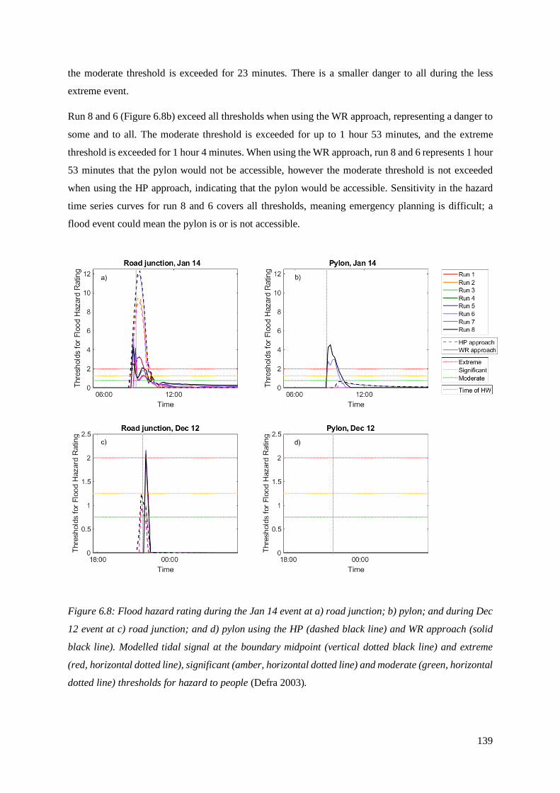
139
the moderate threshold is exceeded for 23 minutes. There is a smaller danger to all during the less
extreme event.
Run 8 and 6 (Figure 6.8b) exceed all thresholds when using the WR approach, representing a danger to
some and to all. The moderate threshold is exceeded for up to 1 hour 53 minutes, and the extreme
threshold is exceeded for 1 hour 4 minutes. When using the WR approach, run 8 and 6 represents 1 hour
53 minutes that the pylon would not be accessible, however the moderate threshold is not exceeded
when using the HP approach, indicating that the pylon would be accessible. Sensitivity in the hazard
time series curves for run 8 and 6 covers all thresholds, meaning emergency planning is difficult; a
flood event could mean the pylon is or is not accessible.
Figure 6.8: Flood hazard rating during the Jan 14 event at a) road junction; b) pylon; and during Dec
12 event at c) road junction; and d) pylon using the HP (dashed black line) and WR approach (solid
black line). Modelled tidal signal at the boundary midpoint (vertical dotted black line) and extreme
(red, horizontal dotted line), significant (amber, horizontal dotted line) and moderate (green, horizontal
dotted line) thresholds for hazard to people (Defra 2003).

140
6.4.3. Volume of inundation in the model domain
Figure 6.9 shows the change in volume of inland inundation from LW to LW for the Jan 14 and Dec 12
event. The largest volume of flood water for Jan 14 is generated by run 8 using the WR approach, which
is 12.5 Mm3. Conversely, the largest volume of flood water for the Dec 12 event is generated by run 6
using the HP approach (see Figure 6.9), which is 5.6 Mm3. The more extreme coastal hazard condition
generates a greater volume of flood water, as WL and Hs increase height and duration of peak HP and
WR at the boundary.
Figure 6.9: Change in volume of inundation (Mm3) in the Oldbury model domain for Jan 14 forced by
a) HP and c) WR; and Dec 12 forced by c) HP and d) WR. Modelled high tide from low water to low
water is also shown (dashed line).
The Jan 14 event shows greater sensitivity to coastal hazard uncertainty. Run 8 and 6 show greatest
volumes of flood water, and then run 1, 2, 7 and 5 are grouped together, with run 1 generating 7.1 Mm3
less flood water than run 8 using the WR approach. Run 3 and 4 show minimal volumes of flood water
in the model domains. The results of the Dec 12 event are similarly grouped, but show smaller
differences between them, with run 1 generating just 0.05 Mm3 less flood water than run 8 when using
the WR approach.

141
Both events show rapid inundation, and maximum volume of flood water occurs at the same time for
each event, with a lag of 8 minutes after tidal high water, which may also be a function of the time step
selected for the model simulation. Both events show asymmetric drainage from the model domain.
Drainage of floodwater after the time of high water is most rapid for the Dec 12 event using the HP
approach, and volume of inundation continues to fall for the duration of the ebb tide. Drainage is slower
when using the WR approach, and plateaus on the ebb tide indicating floodwater drains more slowly
through this model domain.
6.4.4. Quantification of flood hazard due to coastal hazard uncertainty
Figure 6.10 shows sensitivity in flood hazard (represented by volume of floodwater inundation in the
model domain) due to coastal hazard uncertainty. The difference in HP at the boundary midpoint (black
cross in Figure 6.1a) is presented against difference in time-integrated volume of inundation in each
model domain. The difference in HP is calculated as the change in WL + ½ Hs at the time of high water
between each run and run 8, which is used here as a baseline, at a point mid-domain alongshore to show
how an increase in regional model WL and Hs changes flood hazard. The difference in time-integrated
volume is calculated as the change in integrated area under the curve (Figure 6.10) between each run
and run 8. All results present positive difference; this signifies an increase in value presented from each
run to run 8. The change in symbol colour in Figure 6.10 indicates a different run; change in symbol
shape indicates coastal hazard condition (Jan 14 or Dec 12 event); unfilled symbols represent the WR
approach to forcing the model boundary and filled symbols represent the HP approach. Lines connect
same runs for each approach to forcing the model boundary for each coastal hazard condition.
Figure 6.10: Absolute difference in HP at the boundary midpoint (shown in Figure 6.1a) against
absolute difference in time-integrated volume for a) all runs compared to baseline run 8; and b) zoomed
into run 1, 2, 5, and 7.

142
Figure 6.10a shows that there is substantial difference in HP at the boundary midpoint (location shown
in Figure 1a) and time-integrated volume of inundation between run 3 and 4 with run 8 for the Jan 14
(green circles). Coastal hazard uncertainty generates up to 3.46 m difference in HP at the boundary
midpoint between run 3 and 8 for Dec 12, and 3 m for Jan 14. The difference between run 3 and 8
generates up to 582.4 Mm3 difference in inundation. Jan 14 also shows greater sensitivity to approach
to boundary forcing, and run 3 generates 280.9 Mm3 difference between WR and HP approaches. Dec
12 generates just 9.9 Mm3 differences in volume of inundation between run 3 and 8, and shows smaller
sensitivity to approach to boundary forcing with a difference of 0.8 Mm3 between WR and HP. Runs 3
and 4 are outliers, and not realistic as they are forced with a constant water level; total water level is
greatly underestimated when tide is not included as a physical forcing process at the boundary.
Figure 6.10b shows results for realistic runs 1, 2, 5, 6 and 7, compared to run 8. Run 1, 5 and 7 are
clustered together for the Jan 14 event, and sensitivity to approach to forcing the model boundary. The
Jan 14 event shows up to 353.3 Mm3 difference in volume of inundation with 5.3% (0.45 m) difference
in HP at the boundary midpoint, when forced using WR for run 1. The Dec 12 event shows substantially
smaller difference in volume of inundation. Run 7 generates 1.16 Mm3 difference in inundation with
0.07 m difference in HP, when forced using HP for run 7. The large difference in volumes of inundation
generated between the Jan 14 and Dec 12 event indicates sensitivity to coastal hazard condition. Run 1,
5 and 7 exclude local atmospheric forcing in the boundary condition, which means peak HP and WR
values are lower and less overwashing of defences and embankments occurs in the Oldbury model
domain. This indicates that the inclusion of local atmospheric forcing in boundary conditions is more
important to reduce uncertainty in simulated inundation, than model coupling processes.
Run 2 (orange) is positioned on its own in Figure 6.10b for the Jan 14 event, and shows smaller
uncertainty in HP at the boundary midpoint. Run 2 includes local atmospheric forcing, which
contributes towards to the peak of WR and HP but excludes wave contribution. This indicates model
coupling processes are important to help to improve accuracy of prediction of coastal hazard conditions,
but not as important as local atmospheric forcing.
Run 6 for Jan 14 shows smaller uncertainty in HP at the boundary midpoint, but sensitivity to approach
to forcing the model boundary remains. For the maximum event, 0.06 m difference in HP at the
boundary midpoint generates up to 97.8 Mm3 difference in time-integrated volume (purple, unfilled
circle) using the WR approach. Smaller uncertainty in HP is due to the inclusion of local atmospheric
forcing and one-way coupling in the coastal hazard from Delft3D, which generates higher WR peak to
result in more overwashing at more locations along the crest line. Even a small change in HP at the
boundary midpoint can mean hazard thresholds are exceeded to have a substantial impact on volume of
inundation.

143
Overall, the more extreme coastal hazard condition (Jan 14) generates a steeper trend. Jan 14 shows
increased uncertainty in flood hazard with increased uncertainty in coastal hazard uncertainty and
sensitivity to approach to forcing the model boundary. Dec 12 generates small volumes of inundation
as thresholds for flooding are not exceeded.
6.4.5. Economic cost of inundation for arable and suburban land uses
Table 2 and 3 show economic cost of inundation at the time of maximum inundation for arable and
suburban land uses. Run 8 for Jan 14 using the WR approach generates greatest cost to arable land (£4.3
M) and to suburban land uses (£60.9 M). Runs 3 and 4 generate smallest economic cost at the time of
maximum inundation, for both events across both model domains.
Table 6.2: Simulated economic cost of inundation for arable land cover
Arable land cost (£ M)
1 2 3 4 5 6 7 8
Maximum HP 1.55 1.91 0.07 0.01 1.56 2.96 1.51 3.06
WR 2.80 3.09 0.00 0.01 2.84 4.00 2.95 4.31
90th pc HP 0.07 0.07 0.01 0.01 0.07 0.10 0.07 0.10
WR 0.02 0.02 0.00 0.00 0.02 0.03 0.02 0.04
Table 6.3: Simulated economic cost of inundation for suburban land cover
Suburban land cost (£ M)
1 2 3 4 5 6 7 8
Maximum HP 44.85 46.48 6.13 2.46 44.89 53.10 44.71 54.35
WR 33.01 36.06 0.62 2.45 33.48 48.55 34.73 60.91
90th pc HP 17.61 17.99 1.82 1.80 17.61 19.89 17.56 19.75
WR 8.49 8.78 0.00 0.00 8.66 10.16 9.05 10.41
Figure 6.11 shows the absolute difference in HP at the boundary midpoint against absolute difference
in economic cost to (i) arable land and (ii) suburban land at time of maximum inundation against
between each run and run 8. The economic cost of flood events is important information for shoreline
management planning. The change in symbol colour in Figure 6.11 indicates a different run; change in
symbol shape indicates coastal hazard condition (Jan 14 or Dec 12 event); unfilled symbols represent
the WR approach to forcing the model boundary and filled symbols represent the HP approach. Lines
connect same runs for each approach to forcing the model boundary for each coastal hazard condition.
In the text absolute changes are shown below in brackets for context. Run 3 and 4 are not shown in the
following analysis, as they are outliers and not realistic.

144
Figure 6.11: Absolute difference in HP at the boundary midpoint (shown in Figure 6.1a) against
absolute difference in a) arable land costs and b) suburban land cost for runs 1,2,5,6 and 7 compared
to baseline run 8.
Figure 6.11a shows absolute difference HP at the boundary midpoint and arable costs compared to run
8. As also seen in Figure 6.10 for the Jan 14 event, run 1, 5 and 7 are grouped for each event, and then
run 2 is positioned on its own, with run 6 showing smallest uncertainty in HP and arable costs. Run 7
for the Jan 14 event with WR approach (unfilled, pink circle) generates up to £1.5M difference in arable
costs, against 0.45 m difference in HP at the boundary midpoint, whereas the HP approach (filled, pink
circle) generates £30.4k difference. The HP approach generates smaller absolute differences in arable
costs for all coastal hazard uncertainty conditions. Both events show steep trends indicating increased
uncertainty in boundary condition increases uncertainty in arable costs. Both events also show
sensitivity to approach to forcing the model boundary, indicated by the large differences between WR
and HP symbols. Sensitivity to approach to forcing the model boundary may also be caused by the land
types that are inundated close to flood pathways.
Figure 6.11b shows absolute difference in suburban costs compared to run 8. Wider spacing between
the WR and HP symbols for the more extreme Jan 14 event indicates greater sensitivity to boundary
forcing approach. For run 1 using the WR approach £27.9 M difference in suburban costs is generated,
whereas the HP approach generates £1.9 M difference; sensitivity to boundary forcing approach
generates up to £25.9 M uncertainty in suburban costs. Run 6 generates a 0.06 m difference in HP at
the boundary for Jan 14, and still generates up to £12.4 M cost to suburbia. It is crucial for shoreline
management, infrastructure or residential planning to consider uncertainty in flood costs for long term
assessments. For both events WR generates greater difference in suburban costs, which may be due to
suburban areas being more closely located to overwash and breach locations along the coastal defences
and embankments. The WR approach leads to greater impact as it is more realistic, in considering

145
surfzone and shoaling processes, compared to the HP approach imposed at the LW mark. Overall, there
is a steeper gradient in response to coastal hazard uncertainty for the Jan 14, compared to Dec 12.
The results show that optimal model setup should include local atmospheric forcing and two-way
coupling; run 8 has been validated in Delft3D-FLOW-WAVE and generates largest impacts of
inundation compared to all other runs. Excluding local atmospheric forcing could cost up to £26.2 M in
cost-benefit analysis when considering flooding for long-term hazard assessments and emergency
response planning. Excluding two-way coupling processes could cost £12.4M in a flood damage
assessments, and exclusion of both forcing and coupling processes could cost up to £60.9M.
6.5. Discussion
Coastal hazard uncertainty, due to coupling and forcing processes in WL and Hs prediction from
Delf3D-FLOW-WAVE, was propagated through the LISFLOOD-FP Oldbury model domain using the
hazard proxy (WL + ½ Hs) and wave runup (Stockdon et al., 2006) approach to the force the model
boundary for two historic storm events, to determine the impact on inundation. On the basis of this case
study, it has been shown that flood hazard is sensitive to event severity, as the Jan 14 event consistently
generated greatest impact of inundation, presented here as flood hazard rating, volume of floodwater
and economic cost. Flood hazard is also sensitive to coastal hazard uncertainty as the source of flood
hazard; forcing and coupling processes in boundary conditions generates a spread in results in the
impacts of inundation. Flood hazard is also sensitive to approach to forcing the model boundary as this
influences floodwater pathways, spatial pattern of inundation and drainage of floodwater.
LISFLOOD-FP confirms that run 8 (two-way coupling + local atmospheric forcing) generates the
largest volume of inundation, 12.5 Mm3 and greatest economic cost to arable (£4.31 M) and suburban
(£60.91 M) land using the wave runup approach for Jan 14 event. For this event HWHs is 0.94 m,
superimposed on HWL of 9.4 m. Larger waves during the more extreme coastal hazard condition have
a greater impact on wave runrup, and contribute more directly as a source of flood hazard. Steeper
embankments in the northeast of the domain generate larger wave runup, which is a pathway for flood
hazard to increase inundation in Shepperdine and Bevington. The Dec 12 event generates substainally
smaller time-integrated volume of inundation using both the hazard proxy and wave runup approach, as
this event has a HWHs of 0.31 m on a HWL of 8.09 m. Smaller waves for Dec 12 event means that
smaller wave runup is generated and no flood pathway over the earthen embankments is created for the
wave runup approach, and hazard thresholds are not exceeded for the hazard proxy approach. Event
severity has been shown to be an important control on flood hazard in hyper-tidal estuaries (Lyddon et
al., 2018a), as higher water levels during extreme events can propagate wave energy shoreward (Gallien
et al., 2018).

146
Larger wave runup superimposed on a large spring tide, exacerbated in the northwest of the domain due
to steeper embankments, creates a compound flood pathway (Gallien et al., 2014). The wave runup
approach generates more inundation behind steep earthen embankments due to overwash of greenwater,
in addition to inundation in the towns of Berkeley and Oldbury-on-Severn (see Figure 6.5). Once hazard
thresholds have been exceeded, the wave runup approach further exacerbates flood hazard because the
boundary is located on the defence crest, and the model domain has less floodwater accomodation so
floodwater is ‘locked in’; there is no intertidal space in the model domain for floodwater to gravity drain
into through the rhines and channels after HW. High ‘tail water’ conditions from a flood tide or storm
surge have been shown to prevent drainage, and can exacerbate other flooding source-receptor pathways
(e.g. flooding due to wave overwashing and defence breaching) (Gallien et al., 2011; Wahl et al., 2015).
Here we show that more extreme storm events and local, site-specific morphology of the coastline
generates larger wave runup and more overwashing, to increase flood hazard. The wave runup approach
increases the volume of inundation as floodwater enters the domain at multiple locations, and is retained
in the model domain which generates an additional compound flooding pathway. Different sources of
uncertainty can combine with each to increase uncertainty in flood hazard inundation, and make
important contributions to compound flooding pathways at different times during the flood simulation
(e.g. event severity durng the flood stage, boundary forcing approach during the ebb stage).
Flood hazard is also sensitive to event severity and local morphology of the coastline using the hazard
proxy approach. Run 8, used throughout as the baseline, for the 3 January 2014 event generates 311.8
Mm3 time-integrated volume of inundation using the hazard proxy approach for run 8, compared to
589.7 Mm3 generated from the wave runup approach. The position of the boundary using the hazard
proxy approach means there is greater floodwater accommodation to provide space for floodwater to
drain into in the intertidal areas, unlike the wave runup approach. This shows that boundary position is
also able to reduce compound flood hazard, by providing floodwater accommodation and easier
drainage pathways on the ebb tide. The influence and importance of uncertainty of input factors on
flood hazard sensitivity can change over the course of a flood event; it has been shown that the rising
limb of an inflow hydrograph is most important during the flood stage of inundation in the coastal city
of Licata, Sicily, then the channel friction parameter is most impotant during peak inundation and
floodplain friction parameter during drying phase of the flood (Savage et al., 2016).
The results presented here show the combined effect of extra- and intra-model uncertainties (Lewis et
al., 2013) on flood hazard. Extra-model uncertainties relate to the data and approaches used to force the
model boundary. Accurate total water level and wave predictions are important for assessing flood risk
in coastal areas with high tidal ranges, or subject to large storm surges (Hawkes et al., 2002). However,
model sensitivities vary across space and the contribution of each physical process to a compound
flooding pathway is site specific. For example, larger water levels are more important than wave height
for inundation for storm events with a 0.5% probability in Dungeness, UK, as 5.28 m WL + 0.92 m Hs

147
will cause more inundation than 1.8 m WL and 5.72 m Hs (Prime et al., 2016). Intra-model uncertainties,
such as boundary position or model domain size, influences floodwater pathways and controls the
simulated spatial pattern of inundation and retention of flood water. This research shows changing the
approach to boundary forcing influences the flooding pathways and drainage of floodwater at a local
scale. The wave runup approach is the more sophisticated approach, as it considers how surfzone and
shoaling effects transform deep water waves to the coastline, and generates £11.8 M less subsequent
damage costs for suburbia when comparing run 1 for each approach. Structures within the model
domain, e.g. the position of bridges, can influence the amount of backwater held in a modelled region
to influence flood hazard (Pappenberger et al., 2006), in addition to uncertainty in upstream boundary
conditions. The spatial resolution of the DEM may contribute to uncertainty, but is not influential during
the wetting phase of large storm events as the rapid rising limb indicates floodwaters are deep enough
to move across small fluctuations in topography, but may be more influential during the recession of
floodwaters or for less severe events (Savage et al., 2016). The causes of sensitivity in inundation
models interact with each other (Perini et al., 2016), and each input factor will require more or less
consideration dependent on the decisions or assessments the inundation model is being used to support,
or the scale of the area being considered.
The model illustrates that flood hazard is sensitive to coastal hazard uncertainty, as the inclusion of
local atmospheric forcing or coupling processes influences the impacts of flooding. Sensitivity of
inundation to boundary conditions has been shown in studies worldwide. Uncertainty in boundary
forcing, due to interpolation of boundary conditions in data poor regions, has been shown to generate
greater uncertainty within an inundation model compared to DEM uncertainty when simulating future
storm tide conditions in the Bay of Bengal (Lewis et al., 2013). Different approaches to generating
boundary conditions for LISFLOOD-FP (e.g. based on linear interpolation of extreme values, or spatial
characteristics of observed storm tides) caused up to 90 cm difference in storm tide peak along the North
Somerset coastline, UK when simulating inundation from the December 13 1981, and subsequently up
to 8.9 km2 difference in overall inundation (Lewis et al., 2011). Uncertainty in coastal water levels and
defence failures have been shown to generate greatest sensitivity in coastal flooding of Canvey Island,
UK, as opposed to model terrain and bottom friction (Brown et al., 2007). Flood inundation simulations
are sensitive to the choice and design of boundary conditions, and it is important to accurately capture
the hydrodynamic and atmospheric conditions occurring during extreme events (Pasquier et al., 2019)
for storm hazard mitigation, adaptation and resilience planning.
The model shows that for all runs, once conditions exceed hazard thresholds to cause coastal flooding
then even small changes coastal hazard uncertainty matter in terms of the cost of flood damages. A 0.45
cm difference in coastal hazard uncertainty at the boundary using the wave runup approach for the Jan
14 event can cause 353.3 Mm3 difference in time-integrated volume of inundation and £27.9 M
difference in economic cost to suburban land. Even as small a change in hazard proxy at the boundary

148
as 0.06 m can generate up to 97.7 Mm3 difference in time-integrated volume of inundation, and £12.4
M difference in cost to suburban land. A water level elevation error of 2-3 cm, due to error in
observation of tidal level or lack of wave forcing, has been shown to generate 3-25% variation in flood
area in Newport Beach, California, dependent on location and hydraulic connectivity (Gallien et al.,
2011). The changes in coastal hazard uncertainty, due to forcing and coupling processes in the boundary
conditions, can be used to infer how changes in future sea level could impact inundation in coastal and
estuarine areas.
The changes in total water level at the coastline presented here are within the range of the
Intergovernmental Panel on Climate Change (IPCC) global projections of SLR, which range from 28
to 98 cm by 2100 (Church et al., 2013) and the UKCP18 projections in Cardiff range from 0.27 to 1.31
m by 2100 (Lowe et al., 2018). Even a small change in sea-level rise will have a large impact on flood
hazard as tidal amplitudes and estuarine morphologies change (Leuven et al., 2019), and compound
flood pathways may be exacerbated (Moftakhari et al., 2017). As the baseline on which storm surges
and waves act is raised, wave energy propagates further shoreward exposing communities and
infrastructure to the increased probability of defence failure (Le Cozannet et al., 2015; Marcos et al.,
2019). Many low-lying areas that are sensitive to coastal flooding during storm events will be
overwhelmed with just 25 cm of sea-level rise along the California coastline; in combination with a
1:100 year storm event this could cause substantial flooding that would impact 150,000 residents and
cause up to $30 billion damage (Barnard et al., 2019). Future sea-level rise will increase ‘tail waters’
and reduce the rate at which low-lying coastal and estuarine areas are able to drain floodwater,
increasing the likelihood of further inundation from subsequent storm or rainfall events (Amante 2019).
Extreme events can cause initial damage from flooding, but lack of drainage, potentially exacerbated
by subsequent events, can cause ripple effects to impact economic sectors in relation to closure of ports
and harbours or disruption of transport of goods and services, and critical services (e.g. power, water,
and communications), essential for public safety. However the response of estuarine areas to sea-level
rise threats may be dependent on their size, as large estuaries may experience increased channel volume
due to sediment starvation, and subsequently flood hazard may be reduced (Leuven et al., 2019). Flood
hazard assessments should, of course, be site-specific and targeted at understanding local or regional
conditions under changing climate conditions, which can provide information on impacts in local areas
of high flood risk. Inundation studies can support targeted adaptation strategies allow coastal authorities
to warn people living in high risk areas, and reduce risk by implementing resilience measures to
minimise flood depths or improve drainage.
6.6. Conclusion
The combined effect of astronomical tides, meteorological storm surges, wind and waves can increase
flood hazard in heavily populated and industrialised estuaries, which are the focal point of coastal

149
megacities, critical infrastructure and economic activity. Accurate predictions of high water level and
high water significant wave height are required to develop hazard maps or warning systems to mitigate
the negative effects of combined flood hazards. However uncertainties in high water level and high
water significant wave height predictions can propagate through the modeling chain to cause
uncertainties in shoreline response models, which are used to support decisions for storm hazard
mitigation. Coastal hazard uncertainty is increased by an order of magnitude when assessing the
uncertainty in resulting inundation.
Time- and space-varying predicted water level and significant wave height at the coast from eight
Delft3D-FLOW-WAVE model simulations, each representing uncertainty due to coupling and forcing
processes, force LISFLOOD-FP, a 2D inundation model, at Oldbury-on-Severn, southwest England.
Two approaches to forcing the model boundary were used; hazard proxy was imposed at the low water
mark, and wave runup combined with water level at the defence crest. Simulations were completed for
3 January 2014 event, representing the most extreme coastal hazard condition on record, and 16
December 2012 representing the 90th percentile coastal hazard condition. Inundation is sensitive to
sources of flood hazard, notably coastal hazard condition and coastal hazard uncertainty. The 3 January
2014 event generates the greatest impact of inundation, as larger high water level and high water
significant wave height increases the peak and width of wave runup and hazard proxy. Run 8 generates
up to 12.5 Mm3 of flood water and £60.9 M cost of damage to suburban land using the wave runup
approach, caused by overwashing of greenwater at the defence. Once the conditions in run 8 exceed the
hazard thresholds to cause coastal flooding, then small changes in the condition matter in terms of the
cost of flood damages. The inclusion of local atmospheric forcing and coupling processes are important
for reducing uncertainty in inundation. This is confirmed by results from run 6, which simulates
inundation most closely with run 8 (used here as the baseline), and generates smallest changes in flood
hazard rating, time-integrated volume of inundation and economic costs compared to run 8. Further to
this, run 3 and 4 generate up to 582.4 Mm3 difference in time-integrated volume of inundation run 8, as
they are forced with a constant water level; total water level is unrealistic and greatly underestimated
when tide is not included as a physical forcing process at the boundary. The exclusion of local
atmospheric forcing could cost up to £26.2 M in flood damage assessments when considering flooding
for long-term, shoreline management plans. Coastal hazard uncertainty also has implications for
emergency response planning, as events can present a danger to all or to none.
Impacts of inundation are also sensitive to approach to forcing the model boundary, which interacts
with coastal hazard condition to alter the pathway of flood hazard. Once the threshold for flooding is
exceeded compound flood pathways can be exacerbated due to coastal hazard condition and approach
used to force the model boundary during the flood phase, as site-specific morphology of the coastline
increases peak wave runup and location of overwash, and floodwater accommodation in the model
domain influences drainage after the peak of the flood. The results show that even a small change in

150
coastal hazard uncertainty of 0.06 m can influence peak hazard proxy and wave runup and locations of
overwash to cause up to 97.7 Mm3 difference in time-integrated volume of inundation and £12.4 M
difference in cost of damage to suburban land. These small changes in total water level at the boundary
can be used to infer how small changes in future sea level could have a large impact on coastal
inundation. Contributions to uncertainty in inundation models should be considered when developing
local scale studies of storm events under present and future sea-level scenarios for storm hazard
mitigation and adaptation or resilience planning.
6.7. Acknowledgments and Data
The authors thank colleagues at the British Oceanographic Data Centre (BODC) for providing tidal
data; Magnox for providing tidal data; Environment Agency for providing tidal and river gauge data;
Gloucester Harbour Trustees for providing tidal data; Met Office for providing observational wind data
and WAVEWATCH III data; Met Office and NOCL for providing CS3X wind and atmospheric
pressure data; CEFAS for providing observational wave buoy data; EDINA for providing bathymetric
and LiDAR data, and Ordnance Survey basemaps. The research is a contribution to the NERC highlight
topic “Physical and biological dynamic coastal processes and their role in coastal recovery” (BLUE-
coast, NE/N015614/1).
Data used in this research are available from sources stated in the reference list.

151
7. Conclusions and Implications
The results presented in this thesis answer the three main research questions (listed again below) to
contribute to local-scale, long-term flood hazard management, particularly when viewed in the context
of the source-pathway-receptor-consequence model (Narayan et al., 2012).
i. Which key sources of coastal hazard uncertainty should be considered when predicting coastal
flood and wave hazard?
ii. What is the relative importance of each source of uncertainty in coastal flood hazard
assessments?
iii. How does coastal hazard uncertainty influence the physical and economic impacts of
flooding?
7.1. Uncertainty in sources and pathways of flood and wave hazard
The numerical modelling system Delft3D-FLOW and -WAVE was used in chapters 2, 3, 4 and 5, and
LISFLOOD-FP in chapter 6, to understand the sensitivity of coastal hazard predictions to intra- and
extra-model uncertainties (Lewis et al., 2013). The Severn Estuary, which borders southwest England
and south Wales, is used here as an extreme example of a hyper-tidal estuary. Its length, shape and size
is unique in that it generates a tidal range up to 12.2 m, so the Severn Estuary is used here to show how
severe flood and wave hazard can be when large tides are combined with storm surge, strong winds or
waves. Numerical modelling systems are used here to quantify epistemic uncertainty, which arises due
to limited data or knowledge about a physical process, in predictions of water level and wave heights
through sensitivity tests to improve confidence in flood hazard assessments. This research has focused
on the sensitivity of coastal hazards due to tide, surge, waves, and wind. This could be extended further
as future research to study sensitivities in the river flow.
7.1.1. Extra-model uncertainties
Extra-model uncertainties relate to data and approaches used to force the model boundary and its
influence on water level and wave height prediction is captured here through the use of sensitivity tests
representing variability in forcing and coupling processes. Chapter 2 identifies the combined effect of
tide + storm surge as a key source of flood hazard in a hyper-tidal estuary, and the spatial and temporal
variability of flood hazard due to different sources of uncertainty. Event severity is a key source of
uncertainty, and shown to be the most important control on flood hazard at a local scale. A more severe
event, generated by the concurrence of a severe, low atmospheric pressure system with equinoctial
spring tides or the nodal cycle (as occurred in January 2014 in the Severn Estuary (Sibley et al., 2014)),
will increase peak observed water levels above the predicted level, to potentially exceed critical flooding
thresholds. Event severity causes variability in flood hazard at tide gauge locations so should be

152
accurately forecast at a local scale to ensure warnings can be issued to appropriate authorities and the
public, so negative consequences can be avoided. Timing of the storm surge is another important
control on flood hazard and source of uncertainty; tide + surge concurrence increases maximum total
water levels by up to 10.2 %, as the peak of two coastal hazard parameters combine at the same time to
generate greater magnitude of total water levels. It is important to accurately simulate tide + surge
concurrence as this is a source of uncertainty which influences whether critical storm thresholds are
exceeded at the time of concurrence. The shape of the storm surge component with time (termed surge
skewness in chapter 2) generates variability in total water level as it controls the water volume and surge
inflow into the estuary and influences the duration of high water peaks so is considered a source of
uncertainty. Further to this, chapter 3 highlights that tide + concurrence and surge skewness generates
uncertainty in surge amplitude up-estuary, with increases up to 255% at Sharpness due surge-tide
interaction from funnelling effects. If surge skewness and timing of a storm surge can be precisely
forecast or detected early, then locations in the upper estuary can be warned of consequential
amplification of the flood hazard.
Wave hazard in estuaries is largely attributed to high amplitude shorter period, locally generated wind
waves; while low amplitude longer period waves rarely impact low-lying coastal zones up-estuary.
Representative values for wind speed and direction, wave height, period and direction are used in
Delft3D-WAVE in chapter 4 to identify key combinations of factors that define the wave hazard
generation along the shoreline of the Severn Estuary. Wave height and wave period is an important
overall control on maximum wave hazard and influences the response of the wave to other forcing
factors. Opposing wind direction acts to steepen higher amplitude, shorter period waves and generate
maximum wave hazard in the outer estuary. In contrast a following wind enhances propagation of lower
amplitude longer period waves further up-estuary. Higher wind speed contributes momentum to the
estuarine system and amplifies the responses to changing wind direction. This is particularly critical for
sites of infrastructure up-estuary, as longer period waves could generate a significant and
underestimated hazard up-estuary if exacerbated by local wind-wave effects. Accurate representation
of critical wind-wave conditions is important for the prediction of wave hazard, and results can inform
sea defence design and reduce losses from operational downtime. The results show how wave hazard
in hyper-tidal estuaries could be exacerbated if changing future storm tracks alter wind speed and
direction.
Chapter 5 identifies that the accurate prediction of flood and wave hazard depends on combined effect
of all coastal hazard parameters: tide + surge + wind + wave + river. Local atmospheric forcing is most
important when simulating coastal hazard parameters, to ensure momentum is continually added to the
estuarine system, for wave propagation and generation. The exclusion of local atmospheric forcing
from boundary forcing acts a source of uncertainty, and underestimates high water significant wave
height by up to 90.1%, high water level by 1.5%, and hazard proxy (water level + ½ significant wave

153
height) by 9.1%. Coupling processes, which represent the physical interaction between waves and
circulation in the numerical modelling system, are identified as an additional source of uncertainty when
predicting coastal hazards. Two-way coupling represents important shallow water processes to control
wave hazard along the coastline, including refraction around headlands and wave breaking. Identifying
and quantifying the uncertainty associated with these sources of flood hazard can support the
development of intervention strategies and risk management processes. It has been shown that the
exclusion of locally generated winds underestimates high water significant wave height by up to 1.45
m. Coastal sea defences, which are critical to protecting communities and infrastructure from flooding,
could be built too low if the contribution of local winds to wave hazard is not considered when designing
appropriate crest levels. This could lead to overwashing at the time of high water, and increased
nuisance flooding and economic costs.
The data used to simulate coastal hazard parameters in chapter 2, 3, 4, and 5 and drive the model
boundary utilises observation and model hindcast data, which should also be considered a source of
uncertainty. Observation water level and storm surge time series used to force the model boundary in
chapter 2, 3 and 5 is taken from two of the UK’s national A‐Class tide gauge database from the British
Oceanographic Data Centre (BODC, www.bodc.ac.uk). Water level measurements are available as 15-
minute average values, which is considered high temporal resolution, but could still introduce
uncertainty into the model as the exact time or magnitude of high water may be smoothed from the
record. Levelling and determining the absolute datum of the tide gauge can also contribute to
uncertainty in tide gauge data (Pytharouli et al., 2018). It has been shown that variability in a storm tide
time series can influence total water level and subsequent overflow volumes, which can have
implications for flood risk assessments (Quinn et al., 2014). All archived tide gauge data from BODC
has undergone rigorous quality control, and erroneous or modelled data is clearly flagged. In this study,
all modelled and erroneous data in the tide gauge record from Ilfracombe and the Mumbles is removed,
to ensure confidence in the data used to force the model boundary. River gauge data is also used from
an Environment Agency measuring station near Gloucester which is available at an hourly resolution.
This has proven to be an acceptable resolution in this study as the model is well validated in the upper
regions of the estuary, and river contribution does not appear significant during extreme coastal events.
However, sensitivity of coastal flood hazard to fluvial discharge may require finer temporal resolution
of the hydrograph to force up estuary model boundaries in smaller, steeper catchments which are subject
to flash floods, such as the Dyfi, Wales (Robins et al., 2018) to capture variability in river levels. Larger
catchments, such as the Humber Estuary, England, can be forced with daily river gauge levels as the
catchment shows less sensitivity to the shape of the flood hydrograph (Robins et al., 2018). The
accuracy of a model is largely dependent on data availability, and often modellers must make the most
of what is available. Sensitivity tests can be used to test the suitability of data used to force the model
boundary and identify key sources of uncertainty.

154
Chapters 2, 3, 4 and 5 identify that it is not just coastal hazard parameters (tide, surge, wind, wave,
river) that contribute as sources of flood and wave hazard, but estuarine morphology and local
bathymetry also act as a source of flood hazard and pathway, which conveys the hazard to people.
Chapters 2 and 3 show that estuarine morphology amplifies maximum tide and surge elevations up-
estuary; funnelling effects influence magnitude, timing and duration of peak water level. This highlights
the importance of accurate boundary conditions to capture initial water level conditions at the mouth of
the estuary, to ensure accurate representation of funnelling up-estuary which influences surge
predictions away from tide gauge sites. A tipping point occurs up-estuary between funnelling and
shallow water effects where friction effects control magnitude of total water levels as energy dissipation
minimises tide and surge elevations. This highlights the importance of accurate bathymetry to capture
shallow water effects at up-estuary locations. Measured bathymetry, which represents water depth, bed
features and the coastline, influences tide, surge and wave propagation as height of these long period
waves is controlled by water depth. Bathymetry contains two independent measurements, in the
horizontal position (x-y) and the vertical position (z), and is subject to independent uncertainty as a
function of the methods used to collect the data, using acoustic technologies from boats or planes
(Lucieer et al., 2016). Uncertainty in bathymetry is also dependent on how recently data has been
collected due to the nature of river and coastal systems, whereby erosion/deposition processes can alter
bathymetry (Byrnes et al., 2002). Therefore, bathymetry may only be accurate for a short period of time,
and assumptions must be made about the validity and usefulness of the data available by the user.
Quality control and assurance procedures are in place to ensure that uncertainty in bathymetric surveys
is reduced, and data availability often leaves modellers with little other choice than to use what is
available when setting up model domains and communicate uncertainty and assumptions to the end-
user.
7.1.2. Intra-model uncertainties
The choice of model and individual model parameter values can also contribute to uncertainty in
modelled water level and wave heights, termed intra-model uncertainties. The modelling systems used
here represent a simplification of actual physical processes in estuarine and coastal environments,
through mathematical equations including the shallow water equations. Complex hydraulics are
represented by a depth-averaged, hydrodynamic model meaning that velocities are averaged over the
water column. The structure of Delft3D introduces uncertainty so that processes that occur on a vertical
scale, such as turbulent mixing, salinity gradients and heat fluxes not accounted for (Hu et al., 2009;
Xia et al., 2010; Iglesias et al., 2019). The selection of a specific solver in LISFLOOD-FP means that
certain aspects of the shallow water equations are ignored, so sensitivity tests can be used to compare
input parameters. LISFLOOD-FP is not able to capture details of supercritical to subcritical flow, which
may be important in areas close to a dam or embankment breach (Néelz and Pender, 2013). The

155
numerical scheme used by the model has an influence on how well it can capture details of the flow
field and could generate uncertainty in results. A model should be selected based on the aims and site-
specific conditions of the research to minimise uncertainty.
The representation of the geometry of the estuary and coastline in the model grid also means that
processes that occur on a sub-grid scale are not explicitly accounted for, and can introduce uncertainty
(Fringer et al., 2019). The curvilinear grid used here in Delft3D was developed over time using a trial
and error processes and aims to achieve the best representation of the Severn Estuary. The model grid
used in LISFLOOD-FP has a regular grid size, so selecting the correct resolution is critical as it has
been shown that flood extent is dominated by topography as opposed to the physics of flood propagation
(Maskell et al., 2014). However, computational time increases as the resolution of the grid becomes
finer, and the size of output files increases as there are more grid cells and nodes, making files harder
to store. There is a balance between accuracy of the model grid and computational efficiency, so that
increasing the number of grid cells further will not create better results than achieved with the current
mesh, whilst maintaining computational efficiency (Kärnä et al., 2015).
Model parameters are derived over time through calibration and trial and error, as described in section
1.7.1.3 and 1.7.1.4, and it is the job of the modeller to identify which parameters contribute greatest
uncertainty, and work to minimise the uncertainty or ensure that the implications of uncertainty are
communicated to the end-user. The Manning’s coefficient is used to represent the amount of bed friction
(bed shear stress from bottom roughness) that is applied to the flow, and provides some control on the
flow velocity and direction (Garzon and Ferreira, 2016). The Manning’s coefficient in influenced by
geometric and hydraulic changes, including depth of flow, channel width, bed slope and sinuosity
however it cannot be measured directly (Ding et al., 2004). Incorrect selection of the Manning’s
coefficient can lead to uncertainty in model results, as model terrain largely determines flow and flood
patterns (Brown et al., 2007). Inaccurate flood friction parameters in an inundation model can also lead
to errors when modelling floodwater propagation and drainage (Kumbier et al., 2018). Values are
determined through a calibration process so that modelled water level outputs match observed water
level outputs to the highest degree possible. Monte Carlo sampling techniques can also be used to draw
random samples from random, probabilistic values and then evaluate them (Bellos et al., 2017). The
calibration process can reduce the level of uncertainty in the Manning's values, and a uniform parameter
was selected in this research based on the runs with the best R2 correlation, and smallest bias and RMSE.
A uniform parameter represents a simplification of bottom roughness and represents a common
approach in coastal and estuarine modelling studies (Condon and Veeramony, 2012). A spatially
varying coefficient can be based on land use data and may be preferred as it is able to represent changes
in surface roughness, channel bedforms and vegetation (Mattocks and Forbes 2008). A spatially varying
coefficient may be particularly valuable in the upper reaches of an estuary, where energy dissipation
and wave breaking is largely controlled by bottom friction due to the shallow nature of channels

156
(Pascolo et al., 2018). Land cover datasets can be used to represent these spatial changes in bed
roughness, and have been used to incorporate bottom friction information into hurricane storm surge
models (Liu et al., 2013). It has been shown that bottom friction formulation can have little impact on
tidal signal accuracy in the Gulf of Mexico (Kerr et al., 2013), but can cause up to 1 m errors in surge
prediction in shelf regions of the Texas coast (Ferreira et al., 2014). A temporal varying Manning’s
coefficient could also be incorporated to capture changes in erosion/ deposition processes and changing
bedforms during the model simulation. It has been shown that the Manning’s coefficient varies in time
with changes in river inflow rates and tend to decrease with increasing discharge and water depth before
reaching a threshold and remaining constant (Kim et al., 2010). Studies which utilise a time-varying
Manning’s coefficient simulate phenomena on a small temporal scale, such as single meandering
channels, small saltmarshes and drainage furrows (e.g. Mailapalli et al., 2008) and may not be
appropriate on a large scale. Land use data is not readily available worldwide to develop complex
varying Manning’s coefficients, and studies have shown that estimation and calibration methods can be
sufficient and efficient when deciding on a uniform Manning coefficient (Condon and Veeramony,
2012; Boulomytis et al., 2017).
Chapters 2, 3, 4 and 5 identify key sources of coastal hazard uncertainty (e.g. event severity, local
forcing processes and estuarine morphology) which should be considered when predicting coastal flood
and wave hazard, and the relative importance of each source of uncertainty in coastal flood hazard
assessments. Chapter 5 and 6, as summarized below, discuss the impacts of the uncertainty on flood
inundation.
7.2. Impacts of coastal hazard uncertainty on receptors and consequences of flood and
wave hazard
Chapters 5 and 6 quantify coastal hazard uncertainty and subsequent variability in the receptors and
consequences of flood hazard (e.g. people, businesses and the built environment) occurring due to
uncertainties in regional model setup, as well as the approach to forcing the boundary of an inundation
model. Chapter 5 highlights the primary importance of local forcing processes and, secondarily, model
coupling processes for accurate prediction of coastal hazards. The exclusion of local atmospheric
forcing can substantially underestimate significant wave height, high water level and hazard proxy.
Chapter 6 shows that the physical impacts of inundation are strongly controlled by coastal hazard
uncertainty. Coastal hazard uncertainty will influence whether overwashing and subsequent breaching
of defences occurs and where this will occur, which impacts the location and duration that receptors
may be affected by flood and wave hazard. Coastal hazard uncertainty also generates a large spread of
results in hazard threshold curves. This is highlighted at sites of critical infrastructure, notably a road
junction which acts as a primary access route for residents of Oldbury-on-Severn. At this location,
flooding presents a hazard to everyone at the road junction for 90 to 135 minutes, for the same event.

157
Similarly, the same event generates no hazard or up to 113 minutes hazard to everyone for the same
event at an electricity pylon located between Oldbury Technical Centre and Berkeley. This spread of
results can make emergency response challenging, as it will be difficult to know when to implement
evacuation orders for local residents or when to send in divers to stabilise electricity pylons which are
flooded.
Chapter 6 quantifies the impacts of coastal uncertainty hazard and approach to forcing the model
boundary on volume of inundation, hazard to people (including thresholds for hazard with “traffic light
rating” to young people, the elderly and to all), and the economic costs of saltwater inundation for arable
and suburban land uses at an up-estuary location. The results show that the inundation model is more
sensitive to changes in the coastal hazard parameter, due to the regional model setup shown in chapter
4. Once critical thresholds for flooding are exceeded then even small changes in coastal hazard
parameter (as small as a few centimetres) can increase inundation and costs. A 0.06 m change in coastal
hazard condition can cause up to 97.7 Mm3 difference in time-integrated volume of inundation and
£12.4 M in economic costs to suburbia at Oldbury-on-Severn and surrounding low-lying floodplains.
These small changes in coastal hazard condition can be used to infer the consequences and impacts of
flood hazard under future sea level change.
7.3. Applicability of results to other estuaries
This research has shown that estuary orientation can alter and influence exposure to coastal hazard
parameters, and estuarine morphology has a strong control on the propagation of flood and wave hazard.
The shape and size of the Severn Estuary amplifies tidal range and surge propagation up-estuary. It is a
tide-dominant estuary and an extreme example of how coastal hazard parameters combine to cause
overwashing and flooding in a hyper-tidal estuary. The key sources of coastal hazard uncertainty and
their relative importance in coastal flood hazard assessments in the Severn Estuary is largely a function
of its shape, size, orientation and exposure to prevailing storm conditions. The relative importance of
marine and terrestrial drivers which can occur in any combination to amplify hazards will vary
worldwide, as the shape and size of an estuary has a strong control on the marine drivers of coastal
hazards, and catchment size, geology and topography can influence the terrestrial drivers.
The importance of event severity and the timing of combined hazards (the impacts of which are larger
together than individual contribution) would stand as important processes to consider in estuaries
worldwide. The winter storms of 2013/2014 caused significant impacts along the UK coastline,
predominantly driven by marine and atmospheric processes (Sibley et al., 2015). The 3 January 2014
storm caused a 0.5 – 1 m skew surge in the Irish Sea (Haigh et al., 2015; SurgeWatch 2018), which
caused a large tidal bore and flooding due to overwashing in the Severn Estuary (Sibley et al., 2015).
The same event caused wave overtopping and flooded 30 homes at Barmouth, on the mouth of the
Mawddach Estuary and flooded the town centre and golf course at Aberdyfi, on the Dyfi Estuary in

158
Wales (BBC 2014; Dugan et al., 2014). These smaller estuaries on the west coast of Wales are
substantially smaller in length than the Severn Estuary, with a meso-tidal range (up to 4 m), but the
impacts of a severe event remain significant for coastal towns. The severity of an event, which largely
controls total water levels and the extent of flooding, depends on the storm characteristics. The
prevailing storm conditions and geographical location will also control the relative importance of
drivers of flood and wave hazard. Atlantic storms will driver increased rainfall, winds and storm surges
on the west coast of the UK, however, storm surges will be the main driver of flood on the east coast of
the UK (Hendry et al., 2019). Regardless of estuary shape or size, greater magnitude storms will control
extent of flooding and total water levels to cause greatest impacts in estuaries. Other drivers of change,
such as land use, ecosystem degradation, pollution and human intervention can also influence the
relative importance of drivers of flood hazard in estuaries (Rogers and Woodroffe 2016).
The importance of accurate model setup and accurate bathymetry is also important in estuaries
worldwide, irrespective of shape, size or hydrodynamics. Simulation of floodwater propagation and
inundation extent in the Shoalhaven Estuary, south-eastern Australia, demonstrates the importance of
accurately representing the unique characteristics of an estuary for accurate model simulations
(Kumbier et al., 2018). This estuary is characterised as a wave dominated barrier estuary and simulating
one or two open boundaries influences tidal range, exposure to storm-tide flooding and wave action
(Kumbier et al., 2018). Simulation of wind waves in a wide, shallow estuary, Mobile Bay, Alabama,
demonstrates the importance of sufficient spatial resolution to represent bathymetric gradients and
ambient currents to ensure accurate prediction of wave heights (Chen et al., 2005). The key sources of
coastal hazard uncertainty presented here that would hold for other estuaries worldwide are not
dependent on the shape and size of the estuary, but external factors (event severity and model setup)
that control magnitude and representation of total water levels and wave heights.
The research presented here highlights the importance of local forcing processes to accurately simulate
total water levels and wave heights in a large, hyper-tidal estuary. Local atmospheric forcing is an
important control on wave hazard in the Severn Estuary because the wide estuary mouth increases local
fetch to enhance wind wave generation. It has been shown that channel size is an important control on
wind wave generation in Manukau Harbour, a shallow macro-tidal estuary in New Zealand. Spatial
variation in wind speed is important over a short fetch in narrow stretches of the estuary for wave
generation but tidally varying depth is important over a longer fetch (Smith et al., 2001). Hilly terrain
up-estuary also controls wind speed over water and subsequent wind forcing of waves (Smith et al.,
2001). The importance of local atmospheric forcing in estuaries with a large local fetch (as a function
of estuary size) for accurate simulation of wind-waves has been shown in other large, coastal plain
estuaries including the Ems-Dollard, Germany (Hein et al., 2011), Delaware Bay, USA (Pareja-Roman
et al., 2019) and Chesapeake Bay, USA (Fisher et al., 2015). Larger estuaries, with increased local fetch,
generally drain larger catchments, and the occurrence of East Coast Lows on the east coast of Australia

159
have highlighted estuaries with a larger catchment and tidal range will experience increased flood
hazard due to increased exposure (Rogers and Woodroffe, 2016). High rainfall increase floodwaters in
the upper catchments, and the interaction between winds and storm surges in the lower catchments
increase overwash and flooding e.g. Shoalhaven River and Bega River (Rogers and Woodroffe 2016).
However, there were exceptions as the sensitivity of estuaries to flood hazard on the east coast of
Australia is a function of the site-specific geomorphology of individual estuaries, as opposed to physical
processes controlled by estuarine shape. Lake Illawarra has a small catchment and tidal range, but is
vulnerable to flooding as the estuary bedrock valley is broad and alluvial infill has created huge
expanses of low-lying floodplains vulnerable to inundation (Sloss et al., 2006; Rogers and Woodroffe
2016). Further to this, the barrier integrity controls conditions at the mouth of intermittently open-closed
estuaries; tidal conditions were experienced just 9% of the time over a 14-year period at micro-tidal
East Kleinemonde Estuary, South Africa, and fluvial outflow conditions <1 % (Whitfield et al., 2008).
Large river events in combination with large wave events are most important for natural barrier
breaching on wave dominated coastlines such as those seen on the California coastline (Harvey et al.,
2020) and Victoria coastline, Australia (McSweeney et al., 2018). In turn, this is important for
floodwater drainage, water quality and fish spawning in intermittently closed estuaries (Gillanders et
al., 2011). Fluvial outflow conditions have been shown to be more important in smaller, steeper
catchments which transport river discharge more rapidly to the coast (Hendry et al., 2019). The Dyfi
Estuary, Wales, experiences flash flood regime and displays sensitivity to rainfall at a sub-daily scale
(Robins et al., 2016), which should be accounted for in flood hazard estimations. The sensitivity of
coastal flood hazard was not considered in this research, as it is considered a smaller contribution to
total water levels in the Severn Estuary. However it would be an important consideration in estuaries
with smaller and steeper catchments. Human intervention can also control the relative importance of
physical processes controlling flood hazard; the construction of Wolwedans Dam in the Great
Brak Estuary catchment has reduced fluvial outflow to the estuary by 56%, reducing the volume and
duration of a flood event in this small, micro-tidal estuary and causing the estuary mouth to breach less
often (Human et al., 2016). No two estuaries are the same, and there are no generic rules to allow for
direct comparison between key sources of coastal hazard uncertainty in estuaries. Site-specific
consideration should be given to the relative importance of coastal hazard parameters in flood hazard
assessments based on local morphological conditions, prevailing storms, and human intervention.
7.4. Practical application of thesis results
The results presented in this thesis can be used to inform local flood hazard assessments, and the results
can support the work of coastal modellers and planners which aims to minimise the negative
consequences of flood events. The results contribute to knowledge to numerical modellers, by
identifying an optimal model setup which can be used to accurately simulate flood and wave hazard.

160
The primary recommendation is that coastal hazard modelling should include time- and space-varying
atmospheric forcing; this is successfully represented by data from the Met Office Unified Model in this
research. Simulations should utilise model coupling processes which accurately represent the influence
of the circulation on the waves and waves on the circulation (two-way coupled). The results presented
here also identify that estuarine morphology is an important control on coastal hazard uncertainty.
Numerical modelling systems should use computational grids which accurately represent complex
coastlines. The land boundary of model grids should represent headlands and bays to ensure that the
influence of wave refraction in shallow water regions on significant wave height is accurate, and
narrowing of channels to represent funnelling effects. Funnelling effects are also controlled by
shallower channels, as represented by bathymetry. Bathymetry is a key control on the accurate
representation of total water level and significant wave height in all estuarine and shelf sea modelling
studies (Williams and Esteves 2017). Bathymetric variations control volume and cross-section along
the channel, and subsequently influence water level and current variations, sediment transport, and
shallow water processes (e.g. energy dissipation and wave attenuation). Accurate numerical modelling
outputs are a product of the quality of bathymetry data used. Local atmospheric forcing is an important
control on significant wave height prediction; adding momentum to the estuarine system is particularly
important as it has been shown that stronger, opposing wind can steepen high amplitude shorter period
waves, or enhance propagation of low amplitude longer period waves up-estuary. Inaccuracies in wind
speed or direction may underestimate wave hazard up-estuary, which may cause overwashing and
subsequent flood hazard for communities on low-lying coastal plains. Modellers should utilise accurate
bathymetry and boundary forcing when developing regional models, to minimise uncertainty in total
water level and wave predictions.
Outputs from this research has been shared with Principal Hazard Consultant, David Anderson, at
Magnox Oldbury Technical Centre, responsible for managing the decommissioning strategy at Oldbury
Nuclear Power Station. The work has been useful to the team so far as providing insight into the level
of complexity and detailed required in site specific hydrodynamic and inundation models. It was beyond
the scope of this research project to consider erosion hazard and morphological development under
extreme events, but this is considered to be a crucial future consideration in the Severn Estuary, given
the soft, muddy nature of the sediments which move easily in fast tidal currents (Manning et al., 2010).
The importance of event severity and locally generated winds is not only likely to generate uncertainty
in flood and wave hazard, but also short term, storm-related variations in morphology. This is significant
as erosion-deposition cycles in estuaries can modify the tidal prism, alter shipping channels or
contribute to loss of coastal wetlands (Yin et al., 2019). Delft3D-FLOW-WAVE could be coupled to
the sediment transport module Delft3D-MOR (Lesser et al., 2001) to understand how coastal hazard
uncertainty influences net sediment transport pathways and development of sandbanks during extreme
events. Further to this, key questions from Oldbury Technical Centre include determining whether the

161
estuary will be static or stable over the next 5,700 years and how long-term evolution may influence
erosion, deposition and sediment transport and subsequently alter currents. A timeframe of 5,700 years
is suggested by Oldbury Technical Centre as it is the half-life of carbon-14, a radionuclide produced
from reactions in a nuclear reactor primary system. Understanding and predicting tidally induced
morphological variations and sea-level change under future climate scenarios over the next 5,700 years
will inform whether decommissioned nuclear energy structures should be kept or removed (D
Anderson, 2018 personal communication 10 July). Process-based morphodynamic models, such as the
sediment transport module Delf3D-MOR, could be coupled to Delft3D-FLOW-WAVE to analyse
physical processes and mechanisms which underlie the evolution of the estuary.
The results also highlight how uncertainties in coastal hazard parameters can generate substantial or no
hazard to people or infrastructure at the same time and location for the same hazard condition, making
emergency response planning more challenging, and can substantially increase inundation and cost of
damage once critical thresholds for flooding are exceeded. Large uncertainties in coastal hazard
parameters, of the order of 0.5 – 1 m, may be influential in causing initial breaches but once this
threshold has been exceeded, then increases of just centimetres can substantially increase inundation
and the cost of flood damage. Small changes in coastal hazard condition contribute up to £60.91 M
increase in economic costs of flooding events. These small changes should be accounted for when
conducting comparative flood risk analysis, which quantifies different hazards within a community, and
financial appraisals of flood events to calculate expected annual damages (Merz et al., 2010).
7.5. Coastal hazard uncertainty: implications for long-term planning (up to 2105)
with sea level rise
This thesis has quantified coastal hazard uncertainty due to external factors including event severity,
timing of the storm surge relative to tidal high water, local forcing and coupling processes, and
quantified the range of impacts these uncertainties have on receptors and consequences of flood hazard.
Coastal hazard predictions are used to inform hazard management strategies, including shoreline
management plans, adaptation and flood alleviation schemes to understand physical processes and
systems, and the impacts that intervention schemes may have on inundation and cost of damage (Sayers
et al., 2003). These strategies aim to reduce the threat of flooding and erosion to people and their
property, over the short-term (up to 2025) to the long-term (up to 2105) (Environment Agency 2010).
The design, and subsequent success, of such long-term management plans can hinge critically on
accurate flood hazard projection (Ruckert et al., 2019) however, as shown here, predictions of total
water level and maximum significant wave height can differ drastically. Uncertainties in physical
processes, which generate a large spread of results for just one event, represents a key area of risk within
long-term strategy planning (Hutter and Schanze 2008; Robins et al., 2016). Adopting a single hazard
projection neglects key uncertainties in physical processes, and can lead to over- or under-estimation of

162
hazards, and inappropriate design scenarios for the lifetime of coastal structures (Stephens et al., 2017).
Further to this, there are great uncertainties associated with future climate scenarios; how much may
sea level increase, whether extreme storm surge events intensify in a warming climate, the extent of the
Antarctic ice sheet collapse, which will all contribute to future flood hazard projections (Barnard et al.,
2019; Leuven et al., 2019; Pasquier et al., 2019; Wong and Keller 2017). These uncertainties may cause
more severe consequence for coastal communities from the effects of flooding in the future (Hall et al.,
2016; Sriver et al., 2018; Vitousek et al., 2017).
UKCP18 projects that sea level could rise up 1.13 m by 2100 (Lowe et al., 2018), meaning that a
particular critical threshold will be exceeded more frequently, as less severe storm conditions are
required to exceed that level (Haigh et al., 2016). Research recent states that large, deep estuaries
(similar to the Severn Estuary) may not experience significant impacts of future sea-level rise, as
sediment starvation will minimise the tidal prism (Leuven et al., 2019). However the results presented
here show that coastal hazard uncertainty in hyper-tidal estuaries are sensitive to event severity; this is
represented by varying higher water level and wave heights which create large changes in water level
at the estuary mouth to increase the possible number of receptors and severity of the consequences of
the hazard. Future changes in sea level in hyper-tidal estuaries may act to enhance tide-surge
propagation and wave propagation up-estuary, to increase the number of receptors in locations
previously unaffected by similar storm conditions, and increase the likelihood that critical thresholds
are exceeded. Wave-tide interaction under future climate conditions may lead to increased wave heights
at high water, which may be amplified in the long term (Lewis et al., 2019). Uncertainty in coastal
hazard predictions and future sea-level changes prove challenging when making decisions for long-
term management plans, in particular not knowing how coastlines, policies, and society will develop
into the future.
7.5.1. Resilience and flexibility in long-term management plans
Long-term plans should be based on considerable, site-specific technical knowledge which account for
future uncertainty to ensure resilience and robustness, and adaptation and flexibility in long-term plans
(André et al., 2016). Resilience can be built into long-term management plans by explicitly including
considerations on uncertainties in flood hazard modelling and decision making, to understand how
intervention schemes will develop under a range of future hazard and sea-level conditions. Robust long-
term management plans should utilise optimal model setups which are site-specific and account for
natural complexity and evolution of an estuarine system. Numerical models, which fully incorporate
and accurately represent local atmospheric wind and pressure systems and represent the influence of
the circulation on the waves and waves on the circulation (two-way coupled models), have been shown
here to provide a thorough understanding of the sources, pathways, receptors and consequences of a
range of hazards. A modelling approach which considers the whole system of physical processes can

163
be used to understand how intervention schemes can protect communities against local, prevailing
conditions (Penning-Rowsell et al., 2000). Flexible long-term plans should acknowledge that hazard
conditions, sea level and society may change with time, and soft and hard management options should
be able to adapt to uncertainty in the evolution of coastal hazards and sea level changes. The research
presented here could be developed further to improve the understanding of the receptor and
consequences of site-specific coastal hazards within the Severn Estuary. Changes in volume of
floodwater in the Oldbury-on-Severn LISFLOOD-FP model domain are asymmetric; volumes rise
rapidly but then drainage from the domain is slower. This asymmetry may occur as a result of the size
and number of channels for floodwater to drain into and accommodation for floodwater in the model
domain. A lack of drainage means that some areas experience flooding for a longer period.
Incorporating storm drainage features into inundation model domains can help to further improve
understanding of receptor and consequences at a site-specific level. Subterranean, urban drainage
systems could be incorporated into inundation models to consider their influence on economic costs of
flooding to suburbia (Gallien et al., 2018). Erosion hazard and morphological change during storm event
could also be considered, to understand how the balance of saltmarsh and mudflats will change or be
lost. It has been shown that morphological variability has a strong influence on the width of coastal
hazard zones which could alter the exceedance of critical thresholds or minimise wave energy
dissipation at the coast (Baron et al., 2014). The findings from this thesis have shown the importance
of site-specific technical knowledge for accurate model outputs, such as accurate bathymetry and land
boundaries in computational grids to represent shallow water processes, or local atmospheric forcing,
which can generate up to 90.1% difference in maximum significant wave height if excluded from wave
hazard assessments. Utilizing the best data available to setup and force hydrodynamic numerical models
will help to minimise uncertainty in water level and significant wave height predictions, which are used
to inform long-term intervention and protection strategies for coastal communities and infrastructure.
7.6. Coastal hazard uncertainty: implications for early warning systems
The impacts of uncertainty in coastal hazard modelling also has implications for early warning
management, which primarily aims to reduce loss of life, and impacts on livelihoods, health, businesses
and communities (Angove et al., 2019). Early warning frameworks have a lead time of 8-11 hours
(Bocquet et al., 2009) and aim to avoid fatalities and damage by reducing the occurrence of a hazard
(e.g. strategic evacuation), and minimise the consequences of a hazard (e.g. alerts and emergency
response planning) (UNISDR 2015). These strategies require rapid access to estimations of when peak
total water levels will occur, and when and where flooding is likely to occur during a storm event due
to exceeded of critical thresholds (Le Cozannet et al., 2015; Del Río et al., 2012) , which is particularly
important at ungauged locations. Uncertainties in predicting the timing and magnitude of a storm event
may lead to under-preparation, at the cost of avoidable damage, or over-preparation resulting in

164
unnecessary evacuation orders and expenses (Jonkman et al., 2013). A balance must be met to ensure
that uncertainties do not lead to errors in early warning systems driving alerts and warnings, which can
create public doubt and mistrust in early warning systems and emergency responses (Shaw et al., 2005).
Uncertainty in offshore conditions for flooding have been shown to cause a range of impacts, and once
a critical threshold has been exceeded then even a small change in coastal hazard condition of 0.06 m
can increase flood damage costs in suburban areas by £12.4 M. Early warning systems which account
for small changes in coastal hazard condition once a threshold has been exceeded can dramatically
reduce the number of avoidable and unnecessary deaths and cost of property damage (Doong et al.,
2012). This research can help to inform the development of early warning systems by highlighting the
extent to which coastal hazard uncertainty influences the negative impacts of storm events; small
changes in coastal hazard condition can substantially increase the consequences of events.

165
8. References
Adikari, Y., R. Osti, and T. Noro. 2010. “Flood-Related Disaster Vulnerability: An Impending Crisis
of Megacities in Asia.” Journal of Flood Risk Management 3(3):185–91.
Aerts, Jeroen C. J. H., W. J. Woute. Botzen, Kerry Emanuel, Ning Lin, Hans De Moel, and Erwann O.
Michel-Kerjan. 2014. “Climate Adaptation: Evaluating Flood Resilience Strategies for Coastal
Megacities.” Science 344(6183):473–75.
Allen, J. R. .. and M. .. Duffy. 1998. “Temporal and Spatial Depositional Patterns in the Severn
Estuary, Southwestern Britain: Intertidal Studies at Spring–neap and Seasonal Scales, 1991–
1993.” Marine Geology 146(1–4):147–71.
Allsop, W., T. Bruce, J. Pearson, and P. Besley. 2005. “Wave Overtopping at Vertical and Steep
Seawalls.” Maritime Engineering 158:103–14.
Allsop, William, T. O. M. Bruce, T. I. M. Pullen, and Jentsje V. A. N. D. E. R. Meer. 2008. “Direct
Hazards from Wave Overtopping - the Forgotten Aspect of Coastal Flood Risk Assessment?”
Pp. 1–11 in 43rd Defra Flood and Coastal Management Conference.
Allsop, William, Tom Bruce, Jonathan Pearson, John Alderson, and Tim Pullen. 2003. “Violent Wave
Overtopping at the Coast, When Are We Safe?” Pp. 54–69 in International Conference on
Coastal Management.
Amante, Christopher J. 2019. “Uncertain Seas: Probabilistic Modeling of Future Coastal Flood
Zones.” International Journal of Geographical Information Science 33(11):2188–2217.
Amiruddin, A. M., I. D. Haigh, M. N. Tsimplis, F. M. Calafat, and S. Dangendorf. 2015. “The
Seasonal Cycle and Variability of Sea Level in the South China Sea.” Journal of Geophysical
Research:Oceans 120:5490–5513.
Anctil, F. and M. A. Donelan. 1996. “Air-Water Momentum Flux Observations over Shoaling
Waves.” Journal of Physical Oceanography 26:1344–53.
André, Camille, Delphine Boulet, Hélène Rey-Valette, and Bénédicte Rulleau. 2016. “Protection by
Hard Defence Structures or Relocation of Assets Exposed to Coastal Risks: Contributions and
Drawbacks of Cost-Benefit Analysis for Long-Term Adaptation Choices to Climate Change.”
Ocean and Coastal Management 134:173–82.
Angove, Michael, Diego Arcas, Rick Bailey, Patricio Carrasco, David Coetzee, Bill Fry, Ken
Gledhill, Satoshi Harada, Christa von Hillebrandt-Andrade, Laura Kong, Charles McCreery,
Sarah Jayne McCurrach, Yuelong Miao, Andi Eka Sakya, and François Schindelé. 2019. “Ocean
Observations Required to Minimize Uncertainty in Global Tsunami Forecasts, Warnings, and

166
Emergency Response.” Frontiers in Marine Science 6(JUN).
Antony, Charls and A. S. Unnikrishnan. 2013. “Observed Characteristics of Tide-Surge Interaction
along the East Coast of India and the Head of Bay of Bengal.” Estuarine, Coastal and Shelf
Science 131:6–11.
Arcement Jr, G. .. and V. .. Schneider. 1989. Guide for Selecting Manning’s Roughness Coefficients
for Natural Channels and Flood Plains.
Archer, D. R. and H. J. Fowler. 2018. “Characterising Flash Flood Response to Intense Rainfall and
Impacts Using Historical Information and Gauged Data in Britain.” Journal of Flood Risk
Management 11:S121–33.
As-Salek, J. A. 1998. “Coastal Trapping and Funneling Effects on Storm Surges in the Meghna
Estuary in Relation to Cyclones Hitting Noakhali–Cox’s Bazar Coast of Bangladesh.” Journal of
Physical Oceanography 28(2):227–49.
As-Salek, Junaid Amin and Takashi Yasuda. 2001. “Tide–Surge Interaction in the Meghna Estuary:
Most Severe Conditions.” Journal of Physical Oceanography 31(10):3059–72.
Ashworth, P. J., J. L. Best, and D. R. Parsons. 2015. Fluvial–Tidal Sedimentology. Oxford: Elsevier.
Aubrey, D. G. 1985. “A Study of Non-Linear Shallow Inlet / Estuarine Part I : Observations.”
Estuarine, Coastal and Shelf Science (5674):185–205.
Ballinger, R. and T. Stojanovic. 2010. “Policy Development and the Estuary Environment: A Severn
Estuary Case Study.” Marine Pollution Bulletin 61(1–3):132–45.
Barker, Lucy, Jamie Hannaford, Katie Muchan, Stephen Turner, and Simon Parry. 2016. “The Winter
2015/2016 Floods in the UK: A Hydrological Appraisal.” Weather 71(12):324–33.
Barnard, Patrick L., Li H. Erikson, Amy C. Foxgrover, Juliette A. Finz. Hart, Patrick Limber, Andrea
C. O’Neill, Maarten van Ormondt, Sean Vitousek, Nathan Wood, Maya K. Hayden, and Jeanne
M. Jones. 2019. “Dynamic Flood Modeling Essential to Assess the Coastal Impacts of Climate
Change.” Scientific Reports 9(1):1–13.
Barnard, Patrick L., Daniel Hoover, David M. Hubbard, Alex Snyder, Bonnie C. Ludka, Jonathan
Allan, George M. Kaminsky, Peter Ruggiero, Timu W. Gallien, Laura Gabel, Diana
McCandless, Heather M. Weiner, Nicholas Cohn, Dylan L. Anderson, and Katherine A. Serafin.
2017. “Extreme Oceanographic Forcing and Coastal Response Due to the 2015-2016 El Niño.”
Nature Communications 8:6–13.
Baron, Heather M., Peter Ruggiero, Nathan J. Wood, Erica L. Harris, Jonathan Allan, Paul D. Komar,
and Patrick Corcoran. 2014. “Incorporating Climate Change and Morphological Uncertainty into

167
Coastal Change Hazard Assessments.” Natural Hazards 75(3):2081–2102.
Bastidas, Luis A., James Knighton, and Shaun W. Kline. 2016. “Parameter Sensitivity and
Uncertainty Analysis for a Storm Surge and Wave Model.” Natural Hazards and Earth System
Science 16:2195–2210.
Bates, P. D. and A. P. J. De Roo. 2000. “A Simple Raster-Based Model for Flood Inundation
Simulation.” Journal of Hydrology 236(1–2):54–77.
Bates, Paul D., Richard J. Dawson, Jim W. Hall, Matthew S. Horritt, Robert J. Nicholls, Jon Wicks,
Mohamed Ahmed, and Ali Mohamed. 2005. “Simplified Two-Dimensional Numerical
Modelling of Coastal Flooding and Example Applications.” Coastal Engineering 52:793–810.
Bates, Paul, Mark Trigg, Jeff Neal, and Amy Dabrowa. 2013. “LISFLOOD-FP User Manual: Code
Release 5.9.6.”
Batstone, Crispian, Mark Lawless, Jonathan Tawn, Kevin Horsburgh, David Blackman, Alastair
McMillan, David Worth, Stefan Laeger, and Tim Hunt. 2013. “A UK Best-Practice Approach
for Extreme Sea-Level Analysis along Complex Topographic Coastlines.” Ocean Engineering
71:28–39.
BBC. 2014. “River Severn Bursts Banks at Minsterworth after Bore.” BBC News. Retrieved January
10, 2020 (https://www.bbc.co.uk/news/uk-england-gloucestershire-25588120).
Bernier, N. B. and K. R. Thompson. 2007. “Tide-Surge Interaction off the East Coast of Canada and
Northeastern United States.” Journal of Geophysical Research 112(January):1–12.
Bernier, Natacha B. and Keith R. Thompson. 2006. “Predicting the Frequency of Storm Surges and
Extreme Sea Levels in the Northwest Atlantic.” Journal of Geophysical Research: Oceans
111(10):1–15.
Bernier, Natacha B. and Keith R. Thompson. 2015. “Deterministic and Ensemble Storm Surge
Prediction for Atlantic Canada with Lead Times of Hours to Ten Days.” Ocean Modelling
86:114–27.
Beven, Keith. 2016. “Facets of Uncertainty: Epistemic Uncertainty, Non-Stationarity, Likelihood,
Hypothesis Testing, and Communication.” Hydrological Sciences Journal 61(9):1652–65.
Blackburn, Sophie, Mark Pelling, and César Marques. 2019. Megacities and the Coast: Global
Context and Scope for Transformation. Elsevier Inc.
Bobanović, Joško, Keith R. Thompson, Serge Desjardins, and Harold Ritchie. 2006. “Forecasting
Storm Surges along the East Coast of Canada and the North-Eastern United States: The Storm of
21 January 2000.” Atmosphere - Ocean 44(2):151–61.
168
Bocquet, Francois, Jonathan Flowerdew, Peter Hawkes, Tim Pullen, and Nigel Tozer. 2009.
Probabilistic Coastal Flood Forecasting: Forecast Demonstration and Evaluation Science
Project SC050069/SR2.
Bolaños, Rodolfo, Jennifer M. Brown, and Alejandro J. Souza. 2014. “Wave – Current Interactions in
a Tide Dominated Estuary.” Continental Shelf Research 87:109–23.
Booij, N., C. Ris, and L. .. Holthuijsen. 1999. “A Third-Generation Wave Model for Coastal
Regions.” Journal of Geophysical Research 104(C4):7649–66.
Boon, John D. 2004. Secrets of the Tide: Tide and Tidal Current Analysis and Applications, Storm
Surges and Sea Level Trends. Philadelphia: Woodhead Publisher.
Borsje, B. W., P. C. Roos, W. M. Kranenburg, and S. J. M. H. Hulscher. 2013. “Modeling Tidal Sand
Wave Formation in a Numerical Shallow Water Model: The Role of Turbulence Formulation.”
Continental Shelf Research 60:17–27.
Bouma, Jan Jaap, Delphine François, Albert Schram, and Tom Verbeke. 2009. “Assessing Socio-
Economic Impacts of Wave Overtopping: An Institutional Perspective.” Coastal Engineering
56(2):203–9.
Bricheno, Lucy M., Judith Wolf, and Saiful Islam. 2016. “Tidal Intrusion within a Mega Delta: An
Unstructured Grid Modelling Approach.” Estuarine, Coastal and Shelf Science 182:12–26.
Brown, J. M. and A. G. Davies. 2010. “Flood/Ebb Tidal Asymmetry in a Shallow Sandy Estuary and
the Impact on Net Sand Transport.” Geomorphology 114(3):431–39.
Brown, J. M., M. J. Yelland, R. W. Pascal, T. Pullen, P. S. Bell, C. L. Cardwell, D. S. Jones, N. P.
Milliken, T. D. Prime, G. Shannon, J. H. Ludgate, A. Martin, B. Farrington, I. Gold, C. Bird, and
T. Mason. 2018. “WireWall: A New Approach to Coastal Wave Hazard Monitoring.” in 3rd
International Conference on Protection against Overtopping.
Brown, James D., Tom Spencer, and Iris Moeller. 2007. “Modeling Storm Surge Flooding of an
Urban Area with Particular Reference to Modeling Uncertainties: A Case Study of Canvey
Island, United Kingdom.” Water Resources Research 43(6):1–22.
Brown, Jennifer M., Rodolfo Bolaños, Michael J. Howarth, and Alejandro J. Souza. 2012. “Extracting
Sea Level Residual in Tidally Dominated Estuarine Environments.” Ocean Dynamics
62(7):969–82.
Brown, Jennifer M., Rodolfo Bolaños, and Alejandro J. Souza. 2014. “Process Contribution to the
Time-Varying Residual Circulation in Tidally Dominated Estuarine Environments.” Estuaries
and Coasts 37(5):1041–57.

169
Brown, Jennifer M., Rodolfo Bolaños, and Judith Wolf. 2013. “The Depth-Varying Response of
Coastal Circulation and Water Levels to 2D Radiation Stress When Applied in a Coupled Wave
– Tide – Surge Modelling System during an Extreme Storm.” Coastal Engineering 82:102–13.
Brown, Jennifer M., Karyn Morrissey, Philip Knight, Thomas D. Prime, Luis Pedro Almeida, Gerd
Masselink, Cai O. Bird, Douglas Dodds, and Andrew J. Plater. 2018. “A Coastal Vulnerability
Assessment for Planning Climate Resilient Infrastructure.” Ocean and Coastal Management
163(June):101–12.
Brown, Jennifer M., Danielle L. Norman, Laurent O. Amoudry, and Alejandro J. Souza. 2016.
“Impact of Operational Model Nesting Approaches and Inherent Errors for Coastal
Simulations.” Ocean Modelling 107:48–63.
Brown, Jennifer M., Jack J. C. Phelps, Andrew Barkwith, Martin D. Hurst, Michael A. Ellis, and
Andrew J. Plater. 2016. “The Effectiveness of Beach Mega-Nourishment, Assessed over Three
Management Epochs.” Journal of Environmental Management 184:400–408.
Brown, Jennifer M., Thomas Prime, Jack J. C. Phelps, Andrew Barkwith, Martin D. Hurst, Michael
A. Ellis, Gerd Masselink, and Andrew J. Plater. 2016. “Spatio-Temporal Variability in the
Tipping Points of a Coastal Defense.” Proceedings of the 14th International Coastal Symposium
(SI 75):1042–46.
Brown, Jennifer M., Alejandro J. Souza, and Judith Wolf. 2010. “An 11-Year Validation of Wave-
Surge Modelling in the Irish Sea, Using a Nested POLCOMS – WAM Modelling System.”
Ocean Modelling 33(1–2):118–28.
Brown, Jennifer M. and Judith Wolf. 2009. “Coupled Wave and Surge Modelling for the Eastern Irish
Sea and Implications for Model Wind-Stress.” Continental Shelf Research 29:1329–42.
Brown, Sally, Robert J. Nicholls, Susan Hanson, Geoff Brundrit, John A. Dearing, Mark E. Dickson,
Shari L. Gallop, Shu Gao, Ivan D. Haigh, Jochen Hinkel, José A. Jiménez, Richard J. T. Klein,
Wolfgang Kron, Attila N. Lázár, Claudio Freitas Neves, Alice Newton, Charitha Pattiaratachi,
Andres Payo, Kenneth Pye, Agustín Sánchez-Arcilla, Mark Siddall, Ali Shareef, Emma L.
Tompkins, Athanasios T. Vafeidis, Barend Van Maanen, Philip J. Ward, and Colin D.
Woodroffe. 2014. “Shifting Perspectives on Coastal Impacts and Adaptation.” Nature Climate
Change 4(9):752–55.
Burcharth, H. .. and S. Hughes. 2011. “Part VI, Design of Coastal Project Elements.” P. 378 in
Coastal Engineering Manual. Vol. 1100, edited by U.S. Army Corps of Engineers.
Byrne, D., G. Robbins, N. Counsell, A. How, and A. Saulter. 2017. Improving Sea Level Forecasting
at Newport.

170
Cai, Huayang, Hubert H. G. Savenije, Qingshu Yang, Suying Ou, and Yaping Lei. 2012. “Influence
of River Discharge and Dredging on Tidal Wave Propagation: Modaomen Estuary Case.”
Journal of Hydraulic Engineering VO - 138 138(10):885.
Carrasco, A. R., Ó. Ferreira, A. Matias, and P. Freire. 2012. “Flood Hazard Assessment and
Management of Fetch-Limited Coastal Environments.” Ocean and Coastal Management 65:15–
25.
Chen, Qin, Uxia Wang, Haihong Zhao, and Scott L. Douglass. 2007. “Prediction of Storm Surges and
Wind Waves on Coastal Highways in Hurricane-Prone Areas.” Journal of Coastal Research
23(5):1304–17.
Chen, R., Y. Zhang, D. Xu, and M. Liu. 2018. “Climate Change and Coastal Megacities: Disaster
Risk Assessment and Responses in Shanghai City.” in Climate Change, Extreme Events and
Disaster Risk Reduction: Sustainable Development Goals Series., edited by S. Mal, R. Singh,
and C. Huggel. Springer.
Chen, Yimei, Wenrui Huang, and Sudong Xu. 2014. “Frequency Analysis of Extreme Water Levels
Affected by Sea-Level Rise in East and Southeast Coasts of China.” Journal of Coastal
Research 68:105–12.
Chipperfield, D. 2014. “Flooded Roads Now Impassable as River Severn Bore Overtops Defences.”
Gazette. Retrieved January 10, 2020 (https://www.gazetteseries.co.uk/news/10912321.flooded-
roads-now-impassable-as-river-severn-bore-overtops-defences/).
Chow, V. T. 1959. Open-Channel Hydraulics. New York: McGraw-Hill.
Church, John A., Peter U. Clark, Jonathan M. Gregory, Svetlana Jevrejeva, Anders Levermann, Mark
A. Merrifield, Glenn A. Milne, R. Steven Nerem, and Patrick D. Nunn. 2013. “Sea-Level Rise
by 2100.” (December):1445–47.
Condon, Andrew and Jay Veeramony. 2012. “Development and Validation of a Coastal Surge and
Inundation Prediction System.” Pp. 1–8 in Oceans 2012.
Conger, Tugce and Stephanie E. Chang. 2019. “Developing Indicators to Identify Coastal Green
Infrastructure Potential: The Case of the Salish Sea Region.” Ocean and Coastal Management
175(February):53–69.
Cornett, A., J. Cousineau, and I. Nistor. 2013. “Assessment of Hydrodynamic Impacts from Tidal
Power Lagoons in the Bay of Fundy.” International Journal of Marine Energy 1:33–54.
Le Cozannet, Gonéri, Jeremy Rohmer, Anny Cazenave, Déborah Idier, Roderik van de Wal, Renske
de Winter, Rodrigo Pedreros, Yann Balouin, Charlotte Vinchon, and Carlos Oliveros. 2015.

171
“Evaluating Uncertainties of Future Marine Flooding Occurrence as Sea-Level Rises.”
Environmental Modelling and Software 73:44–56.
Dangendorf, Sönke, Thomas Wahl, Christoph Mudersbach, and Jürgen Jensen. 2013. “The Seasonal
Mean Sea Level Cycle in the Southeastern North Sea.” Journal of Coastal Research
165(65):1915–20.
Dastgheib, A., J. A. Roelvink, and Z. B. Wang. 2008. “Long-Term Process-Based Morphological
Modeling of the Marsdiep Tidal Basin.” Marine Geology 256(1–4):90–100.
Davies, Gareth and Colin D. Woodroffe. 2010. “Tidal Estuary Width Convergence: Theory and Form
in North Australian Estuaries.” Earth Surface Processes and Landforms 35(7):737–49.
Davies, J. 1964. “A Morphogenetic Approach to World Shorelines.” Zeitschrift Für Geomorphologie
8:27–42.
Davis, Richard A. and Miles O. Hayes. 1984. “What Is a Wave-Dominated Coast?” Marine Geology
60:313–29.
Dawson, David, Jon Shaw, and W. Roland Gehrels. 2016. “Sea-Level Rise Impacts on Transport
Infrastructure: The Notorious Case of the Coastal Railway Line at Dawlish, England.” Journal
of Transport Geography 51(February 2014):97–109.
DEFRA. 2003. “Flood Risks to People (Phase 2).” Flood Risks to People Phase 2: FD2321 Technical
Report 1 117.
DEFRA. 2006. Flood Risks to People: FD2321/TR1 The Flood Risks to People Methodology.
Deltares. 2011. Delft3D-FLOW: Simulation of Multi-Dimensional Hydrodynamic Flows and
Transport Phenomena, Including Sediments. User Manual. Version: 3.15 Revision: 14499.
Deltares, 2600 MH Delft, The Netherlands.
Deltares. 2014a. “Delft3D-QUICKIN: User Manual for the Generation and Manipulation of Grid-
Related Parame- Ters Such as Bathymetry, Initial Conditions and Roughness.”
Deltares. 2014b. Delft3D-WAVE. Simulations of Short Crested Waves with SWAN Version 3.05,
Revision 34160. Deltares, 2600 MH Delft, The Netherlands.
Desplanque, Con and David J. Mossman. 1999. “Storm Tides of the Fundy.” Geographical Review
89(1):23–33.
Desplanque, Con and David J. Mossman. 2004. “Tides and Their Seminal Impact on the Geology,
Geography, History, and Socio-Economics of the Bay of Fundy, Eastern Canada (Part 1:
Preface-Chapter 3).” Atlantic Geology 40(1):3–35.

172
Van Deyzen, A. F. J., P. B. Beimers, J. C. Van Der Lem, D. Messiter, and J. A. M. De Bont. 2015.
“To Improve the Efficiency of Ports Exposed to Swell.” in Australasian Coasts & Ports
Conference 2015: 22nd Australasian Coastal and Ocean Engineering Conference and the 15th
Australasian Port and Harbour Conference.
Dhoop, Thomas and Travis Mason. 2018. “Spatial Characteristics and Duration of Extreme Wave
Events around the English Coastline.” Journal of Marine Science and Engineering 6(14).
Diab, Hassan, Rafic Younes, and Pascal Lafon. 2017. “Survey of Research on the Optimal Design of
Sea Harbours.” International Journal of Naval Architecture and Ocean Engineering 9:460–72.
Didier, David, Jérémy Baudry, Pascal Bernatchez, Dany Dumont, Mojtaba Sadegh, Eliott Bismuth,
Marion Bandet, Sebastien Dugas, and Caroline Sévigny. 2019. “Multihazard Simulation for
Coastal Flood Mapping: Bathtub versus Numerical Modelling in an Open Estuary, Eastern
Canada.” Journal of Flood Risk Management 12(S1):1–19.
Dissanayake, P., H. Karunarathna, and R. Ranasinge. 2015. “Numerical Modelling of the Impact of
Sea Level Rise on Large Tidal Inlet/Basin Systems.” (JUNE).
Dixon, M. .. and J. A. Tawn. 1994. Extreme Sea-Levels at the UK A-Class Sites: Site-by-Site
Analyses.
Dongeren, Ap Van, Martijn De Jong, Cock Van Der Lem, Alex Van Deyzen, and Joost den Bieman.
2016. “Review of Long Wave Dynamics over Reefs and into Ports with Implication for Port
Operations.” Journal of Marine Science and Engineering 4(12):1–10.
Doong, D. J., L. Z. H. Chuang, L. C. Wu, Y. M. Fan, C. C. Kao, and J. H. Wang. 2012. “Development
of an Operational Coastal Flooding Early Warning System.” Natural Hazards and Earth System
Science 12(2):379–90.
Dronkers, J. 1986. “TIDAL ASYMMETRY AND ESTUARINE MORPHOLOGY.” Netherlands
Journal of Sea Research 20(2/3):117–31.
Dronkers, Job. 2017. “Convergence of Estuarine Channels.” Continental Shelf Research
144(May):120–33.
Dyer, K. .. 1995. “Sediment Transport Processes in Estuaries.” Developments in Sedimentology
53:423–49.
EDINA Marine Digimap Service. n.d. “33. Gridded Bathymetry: 1 Arcsecond (Ascii), Scale 1:50,000,
Tile: NW 55050025, NW 55050030, NW 55050035, NW 55050040, NW 55050045, NW
55100030, NW , 5100035, NW 55100040, NW 55100045, NW 55150025, NW 55150030, NW
55150035, NW 55150040, NW 55150045, Updat.”

173
Elias, Edwin P. L., Guy Gelfenbaum, and André J. Van Der Westhuysen. 2012. “Validation of a
Coupled Wave-Flow Model in a High-Energy Setting : The Mouth of the Columbia River.”
Journal of Geophysical Research 117(C09011):1–21.
Elliott, Michael, Nicholas D. Cutts, and Anna Trono. 2014. “A Typology of Marine and Estuarine
Hazards and Risks as Vectors of Change: A Review for Vulnerable Coasts and Their
Management.” Ocean and Coastal Management 93:88–99.
Environment Agency. 2010. Managing the Coast: The Wash Shoreline Management Plan.
Environment Agency. 2018. “New £63 Million Defence Scheme Is Turning the Tide against Floods in
Rossall.” Gov.Uk. Retrieved May 9, 2019 (https://www.gov.uk/government/news/new-63-
million-defence-scheme-is-turning-the-tide-against-floods-in-rossall).
Environment Agency. 2019. National Flood and Coastal Erosion Risk Management Strategy for
England.
Erikson, Li, Patrick Barnard, Andrea O’Neill, Nathan Wood, Jeanne Jones, Juliette Finzi Hart, Sean
Vitousek, Patrick Limber, Maya Hayden, Michael Fitzgibbon, Jessica Lovering, and Amy
Foxgrover. 2018. “Projected 21st Century Coastal Flooding in the Southern California Bight.
Part 2: Tools for Assessing Climate Change-Driven Coastal Hazards and Socio-Economic
Impacts.” Journal of Marine Science and Engineering 6(3):76.
EurOtop. 2016. Manual on Wave Overtopping of Sea Defences and Related Structures.
Fairclough, I. 2019. “Province, Ottawa Spending $114m to Reinforce Bay of Fundy Dikes against
Rising Seas.” The Chronicle Herald. Retrieved May 8, 2019
(https://www.thechronicleherald.ca/news/local/province-ottawa-spending-114m-to-reinforce-
bay-of-fundy-dykes-against-rising-seas-302999/).
Fairley, I., R. Ahmadian, R. A. Falconer, M. R. Willis, and I. Masters. 2014. “The Effects of a Severn
Barrage on Wave Conditions in the Bristol Channel.” Renewable Energy 68:428–42.
Familkhalili, R. and S. A. Talke. 2016. “The Effect of Channel Deepening on Tides and Storm Surge:
A Case Study of Wilmington, NC.” Geophysical Research Letters 43(17):9138–47.
Ferrarin, Christian, Aron Roland, Marco Bajo, Georg Umgiesser, Andrea Cucco, Silvio Davolio,
Andrea Buzzi, Piero Malguzzi, and Oxana Drofa. 2013. “Tide-Surge-Wave Modelling and
Forecasting in the Mediterranean Sea with Focus on the Italian Coast.” Ocean Modelling 61:38–
48.
Ferreira, Celso M., Jennifer L. Irish, and F. Olivera. 2014. “Uncertainty in Hurricane Surge
Simulation Due to Land Cover Specification.” Journal of Geophysical Research: Oceans

174
119(1):1365–82.
Fischhoff, Baruch and Alex L. Davis. 2014. “Communicating Scientific Uncertainty.” Proceedings of
the National Academy of Sciences of the United States of America 111:13664–71.
Flather, R. A. 2001. “Storm Surges.” Pp. 2882–92 in Encyclopedia of Ocean Sciences, edited by J. H.
Steele, S. A. Thorpe, and K. K. Turekian. San Diego, California.
Flowerdew, Jonathan, Peter Hawkes, Ken Mylne, Tim Pullen, Andrew Saulter, and Nigel Tozer.
2009. Coastal Flood Forecasting: Model Development and Evaluation. Environment Agency.
Flowerdew, Jonathan, Ken Mylne, Caroline Jones, Helen Titley, and Office Published. 2013.
“Extending the Forecast Range of the UK Storm Surge Ensemble.” Quarterly Journal of the
Royal Meteorological Society (139):184–97.
Galland, J. C., N. Goutal, and J. M. Hervouet. 1991. “TELEMAC: A New Numerical Model for
Solving Shallow Water Equations.” Advances in Water Resources 14(3):138–48.
Gallien, T. W., B. F. Sanders, and R. E. Flick. 2014. “Urban Coastal Flood Prediction: Integrating
Wave Overtopping, Flood Defenses and Drainage.” Coastal Engineering 91:18–28.
Gallien, T. W., J. E. Schubert, and B. F. Sanders. 2011. “Predicting Tidal Flooding of Urbanized
Embayments: A Modeling Framework and Data Requirements.” Coastal Engineering
58(6):567–77.
Gallien, Timu W., Nikos Kalligeris, Marie Pierre C. Delisle, Bo Xiang Tang, Joseph T. D. Lucey, and
Maria A. Winters. 2018. “Coastal Flood Modeling Challenges in Defended Urban Backshores.”
Geosciences (Switzerland) 8(12).
Gao, C. and T. Adcock. 2016. “Numerical Investigation of Resonance in the Bristol Channel.” in
Proceedings of the International Offshore and Polar Engineering Conference.
Garzon, Juan L. and Celso M. Ferreira. 2016. “Storm Surge Modeling in Large Estuaries: Sensitivity
Analyses to Parameters and Physical Processes in the Chesapeake Bay.” Journal of Marine
Science and Engineering 4(45).
Geeraerts, J., P. Troch, J. De Rouck, H. Verhaeghe, and J. J. Bouma. 2007. “Wave Overtopping at
Coastal Structures: Prediction Tools and Related Hazard Analysis.” Journal of Cleaner
Production 15:1514–21.
George, Douglas a., Guy Gelfenbaum, and Andrew W. Stevens. 2012. “Modelling the Hydrodynamic
and Morphologic Response of an Estuary Restoration.” Estuaries and Coasts 35(6):1510–29.
Gimeno, Vicente, James P. Syvertsen, Inmaculada Simón, Manuel Nieves, Leyanes Díaz-López,

175
Vicente Martínez, and Francisco García-Sánchez. 2012. “Physiological and Morphological
Responses to Flooding with Fresh or Saline Water in Jatropha Curcas.” Environmental and
Experimental Botany 78(3):47–55.
Godin, Gabriel. 1993. “On Tidal Resonance.” Continental Shelf Research 13(1):89–107.
Gouldby, B. P., P. B. Sayers, M. C. Panzeri, and J. E. Lanyon. 2010. “Development and Application
of Efficient Methods for the Forward Propagation of Epistemic Uncertainty and Sensitivity
Analysis within Complex Broad-Scale Flood Risk System Models.” Canadian Journal of Civil
Engineering 37(7):955–67.
Grady, Julian G. O. and Kathleen L. Mcinnes. 2010. “Wind Waves and Their Relationship to Storm
Surges in Northeastern Bass Strait.” Australian Meteorological and Oceanographic Journal
60:265–75.
Gratiot, N., E. J. Anthony, a. Gardel, C. Gaucherel, C. Proisy, and J. T. Wells. 2008. “Significant
Contribution of the 18.6 Year Tidal Cycle to Regional Coastal Changes.” Nature Geoscience
1(3):169–72.
Greenberg, David A. 1984. “A Review of the Physical Oceanography of the Bay of Fundy.” Pp. 9–30
in Update of the Marine Environmental Consequences of Tidal Power Development in the
Upper Reaches of the Bay of Fundy, edited by D. Gordon and M. Dadswell.
Greenberg, David A., Wade Blanchard, Bruce Smith, and Elaine Barrow. 2012. “Climate Change,
Mean Sea Level and High Tides in the Bay of Fundy.” Atmosphere-Ocean 50(3):261–76.
Growneveld, R. .. and G. Meeden. 1984. “Measuring Skewness and Kurtosis.” Journal of the Royal
Statistical Society. Series D (The Statistician) 33(4):391–99.
Haigh, Ivan D., Matt Eliot, and Charitha Pattiaratchi. 2011. “Global Influences of the 18.61 Year
Nodal Cycle and 8.85 Year Cycle of Lunar Perigee on High Tidal Levels.” Journal of
Geophysical Research: Oceans 116(6):1–16.
Haigh, Ivan D. and Robert J. Nicholls. 2017. “Coastal Flooding.” Marine Climate Change Impacts
Partnership: Science Review 108–14.
Haigh, Ivan D., Matthew P. Wadey, Shari L. Gallop, Heiko Loehr, Robert J. Nicholls, Kevin
Horsburgh, Jennifer M. Brown, and Elizabeth Bradshaw. 2015. “A User-Friendly Database of
Coastal Flooding in the United Kingdom from 1915-2014.” Scientific Data 2:1–13.
Haigh, Ivan D., Matthew P. Wadey, Thomas Wahl, Ozgun Ozsoy, Robert J. Nicholls, Jennifer M.
Brown, Kevin Horsburgh, and Ben Gouldby. 2016. “Analysis : Spatial and Temporal Analysis
of Extreme Sea Level and Storm Surge Events around the Coastline of the UK.” Scientific Data

176
3:1–14.
Hall, J. A., S. Gille, J. Obeysekera, W. Sweet, K. Knuuti, and J. Marburger. 2016. Regional Sea Level
Scenarios for Coastal Risk Management: Managing the Uncertainty of Future Sea Level Change
and Extreme Water Levels for Department of Defense Coastal Sites Worldwide.
Hall, J. W., S. Tarantola, P. D. Bates, and M. S. Horritt. 2005. “Distributed Sensitivity Analysis of
Flood Inundation Model Calibration.” Journal of Hydraulic Engineering 131(2):97–105.
Hallegatte, Stéphane, Colin Green, Robert J. Nicholls, and Jan Corfee-Morlot. 2013. “Future Flood
Losses in Major Coastal Cities.” Nature Climate Change 3(9):802–6.
Hawkes, Peter J., Ben P. Gouldby, Jonathan A. Tawn, and Michael W. Owen. 2002. “The Joint
Probability of Waves and Water Levels in Coastal Engineering Design.” Journal of Hydraulic
Research 40(3):241–51.
Heaps, N. .. 1983. “Storm Surges, 1967–1982.” Geophysical Journal of the Royal Astronomical
Society 74:331–76.
Hendry, Alistair, Ivan D. Haigh, Robert J. Nicholls, Hugo Winter, Robert Neal, Thomas Wahl,
Amelie Joly-Lauge, and Stephen E. Darby. 2019. “Assessing the Characteristics and Drivers of
Compound Flooding Events around the UK Coast.” Hydrology and Earth System Sciences
23(7):3117–39.
Hewston, R., Y. Chen, S. Pan, Q. Zou, D. Reeve, and I. D. Cluckie. 2010. “Quantifying Uncertainty
in Tide, Surge and Wave Modelling during Extreme Storms.” in BHS Third International
Symposium, Managing Consequences of a Changing Global Environment.
Hibbert, Angela, Samantha Jane Royston, Kevin James Horsburgh, Harry Leach, and Alan Hisscott.
2015. “An Empirical Approach to Improving Tidal Predictions Using Recent Real-Time Tide
Gauge Data.” Journal of Operational Oceanography 8(1):40–51.
Hinkel, Jochen, Daniel Lincke, Athanasios T. Vafeidis, Mahé Perrette, Robert James, and Richard S.
J. Tol. 2014. “Coastal Flood Damage and Adaptation Costs under 21st Century Sea-Level Rise.”
Proceedings of the National Academy of Sciences 111(9):3292–97.
Hoeke, Ron Karl, Kathleen L. Mcinnes, and Julian G. O. Grady. 2015. “Wind and Wave Setup
Contributions to Extreme Sea Levels at a Tropical High Island: A Stochastic Cyclone
Simulation Study for Apia, Samoa.” Journal of Marine Science and Engineering 3:1117–35.
Hoitink, A. J. F. and D. A. Jay. 2016. “Tidal River Dynamics: Implications for Deltas.” Reviews of
Geophysics 54(1):240–72.
Horrillo-Caraballo, Jose M., Dominic E. Reeve, Dave Simmonds, Shunqi Pan, Andrew Fox, Richard

177
Thompson, Simon Hoggart, Samuel S. H. Kwan, and Deborah Greaves. 2013. “Application of a
Source-Pathway-Receptor-Consequence (S-P-R-C) Methodology to the Teign Estuary, UK.”
Journal of Coastal Research 165:1939–44.
Horsburgh, K. J. and C. Wilson. 2007. “Tide-Surge Interaction and Its Role in the Distribution of
Surge Residuals in the North Sea.” Journal of Geophysical Research: Oceans 112(8):1–13.
Horsburgh, Kevin and Matt Horritt. 2006. “The Bristol Channel Floods of 1607 – Reconstruction and
Analysis.” Weather 61(10):272–77.
Hu, K., P. Ding, and J. Ge. 2007. “Modeling of Storm Surge in the Coastal Waters of Yangtze Estuary
and Hangzhou Bay , China.” Journal of Coastal Research SI50(50):527–33.
Hudson, Thomas, Kevin Keating, Angus Petit, John Chatterton, and Alan Williams. 2015. Cost
Estimation for Coastal Protection - Summary of Evidence.
Hume, Terry M., Ton Snelder, Mark Weatherhead, and Rick Liefting. 2007. “A Controlling Factor
Approach to Estuary Classification.” Ocean and Coastal Management 50(11–12):905–29.
Van Den Hurk, Bart, Erik Van Meijgaard, Paul De Valk, Klaas Jan Van Heeringen, and Jan Gooijer.
2015. “Analysis of a Compounding Surge and Precipitation Event in the Netherlands.”
Environmental Research Letters 10(3).
Hutter, Gérard and Jochen Schanze. 2008. “Learning How to Deal with Uncertainty of Flood Risk in
Long‐term Planning.” International Journal of River Basin Management 6(2):175–84.
Idier, D., F. Dumas, and H. Muller. 2012. “Tide-Surge Interaction in the English Channel.” Natural
Hazards and Earth System Science 12(12):3709–18.
Idier, D., J. Rohmer, T. Bulteau, and E. Delvallée. 2013. “Development of an Inverse Method for
Coastal Risk Management.” Natural Hazards and Earth System Science 13(4):999–1013.
Idier, Déborah, Xavier Bertin, Philip Thompson, and Mark D. Pickering. 2019. “Interactions Between
Mean Sea Level, Tide, Surge, Waves and Flooding: Mechanisms and Contributions to Sea Level
Variations at the Coast.” Surveys in Geophysics 40(6):1603–30.
Irish, Jennifer L. and Rafael Cañizares. 2009. “Storm-Wave Flow through Tidal Inlets and Its
Influence on Bay Flooding.” Journal of Waterway, Port, Coastal, and Ocean Engineering
135(April):52–60.
Janssen, P. A. E. M. 1989. “Wave-Induced Stress and the Drag of Air Flow over Sea Waves.” Journal
of Physical Oceanography 19:745–54.
JBA. 2017. South Gloucestershire Council Level 2 Strategic Flood Risk Assessment for Oldbury on

178
Severn JBA Project Manager.
Jones, John Eric and Alan Marshall Davies. 2007. “Influence of Non-Linear Effects upon Surge
Elevations along the West Coast of Britain.” Ocean Dynamics 57(4–5):401–16.
Jonkman, Sebastiaan N., Marten M. Hillen, Robert J. Nicholls, Wim Kanning, and Mathijs van
Ledden. 2013. “Costs of Adapting Coastal Defences to Sea-Level Rise— New Estimates and
Their Implications.” Journal of Coastal Research 290(5):1212–26.
Karimpour, Arash, Qin Chen, and Robert R. Twilley. 2017. “Wind Wave Behavior in Fetch and
Depth Limited Estuaries.” Nature Scientific Reports 7(40654):1–9.
Karunarathna, Harshinie, Jennifer Brown, Antonia Chatzirodou, Pushpa Dissanayake, and Paul
Wisse. 2018. “Multi-Timescale Morphological Modelling of a Dune-Fronted Sandy Beach.”
Coastal Engineering 136(November 2017):161–71.
Kates, R. W., C. E. Colten, S. Laska, and S. P. Leatherman. 2006. “Reconstruction of New Orleans
after Hurricane Katrina: A Research Perspective.” Proceedings of the National Academy of
Sciences of the United States of America 103(40):14653–60.
Khanal, Sonu, Nina Ridder, Hylke de Vries, Wilco Terink, and Bart van den Hurk. 2019. “Storm
Surge and Extreme River Discharge: A Compound Event Analysis Using Ensemble Impact
Modeling.” Frontiers in Earth Science 7(September):1–15.
Kim, Soo Youl, Tomohiro Yasuda, and Hajime Mase. 2008. “Numerical Analysis of Effects of Tidal
Variations on Storm Surges and Waves.” Applied Ocean Research 30(4):311–22.
Klerk, W. J., H. C. Winsemius, W. J. Van Verseveld, A. M. R. Bakker, and F. L. M. Diermanse.
2015. “The Co-Incidence of Storm Surges and Extreme Discharges within the Rhine-Meuse
Delta.” Environmental Research Letters 10(3).
Knight, P. J., T. Prime, J. M. Brown, K. Morrissey, and A. J. Plater. 2015. “Application of Flood Risk
Modelling in a Web-Based Geospatial Decision Support Tool for Coastal Adaptation to Climate
Change.” Natural Hazards and Earth System Sciences 15(7):1457–71.
Kron, W. 2009. “Flood Risk = Hazard · Values · Vulnerability.” Water International 30(1):58–68.
Kron, Wolfgang. 2013. “Coasts: The High-Risk Areas of the World.” Natural Hazards 66(3):1363–
82.
Kumbier, Kristian, Rafael C. Carvalho, Athanasios T. Vafeidis, and Colin D. Woodroffe. 2018.
“Investigating Compound Flooding in an Estuary Using Hydrodynamic Modelling: A Case
Study from the Shoalhaven River, Australia.” Natural Hazards and Earth System Sciences
18(2):463–77.

179
Lalli, F., A. Bruschi, M. L. Cassese, A. Lotti, and V. Pesarino. 2016. “A Numerical Model for Wave-
Current Interaction at the Scale of Marine Engineering.” Journal of Operational Oceanography
9(sup1):s215–22.
Lawless, Mark, Matthew Hird, Daniel Rodger, Ben Gouldby, Nigel Tozer, Tim Pullen, Andy Saulter,
and Kevin Horsburgh. 2016. “Investigating Coastal Flood Forecasting Good Practice
Framework.”
Leaman, C. 2019. “Python Wave Runup v0.1.4.”
Lennon, G. 1963. “The Identification of Weather Conditions Associated with the Generation of Major
Storm Surges along the West Coast of the British Isles.” Quarterly Journal of the Royal
Meteorological Society 89:381–94.
Lennon, Geoffrey William, E. J. Gumbel, N. A. Barricelli, and A. F. Jenkinson. 1963. “A Frequency
Investigation of Abnormally High Tidal Levels At Certain West Coast Ports.” ICE Proceedings
25(4):451–84.
Leonardi, Nicoletta, Alexander S. Kolker, and Sergio Fagherazzi. 2015. “Interplay between River
Discharge and Tides in a Delta Distributary.” Advances in Water Resources 80:69–78.
Lesser, G. R. 2009. An Approach to Medium-Term Coastal Morphological Modelling.
Lesser, G. R., J. Van Kester, D. J. R. Walstra, and J. a Roelvink. 2000. “Three-Dimensional
Morphological Modelling in Delft3D-FLOW.” SASME Book of Abstracts 1–5.
Lesser, G. R., J. A. Roelvink, J. A. T. M. van Kester, and G. S. Stelling. 2004. “Development and
Validation of a Three-Dimensional Morphological Model.” Coastal Engineering 51(8–9):883–
915.
Letchford, C. W. and B. C. Zachry. 2009. “On Wind, Waves, and Surface Drag.” in 5th European &
African Conferences on Wind Engineering.
Leuven, Jasper R. F. W., Harm Jan Pierik, Maarten van der Vegt, Tjeerd J. Bouma, and Maarten G.
Kleinhans. 2019. “Sea-Level-Rise-Induced Threats Depend on the Size of Tide-Influenced
Estuaries Worldwide.” Nature Climate Change 9(December).
Lewis, M., P. Bates, K. Horsburgh, J. Neal, and G. Schumann. 2013. “A Storm Surge Inundation
Model of the Northern Bay of Bengal Using Publicly Available Data.” Quarterly Journal of the
Royal Meteorological Society 139(671):358–69.
Lewis, M., G. Schumann, P. Bates, and K. Horsburgh. 2013. “Understanding the Variability of an
Extreme Storm Tide along a Coastline.” Estuarine, Coastal and Shelf Science 123:19–25.

180
Lewis, Matt, Kevin Horsburgh, Paul Bates, and Ros Smith. 2011. “Quantifying the Uncertainty in
Future Coastal Flood Risk Estimates for the U . K .” Journal of Coastal Research 27(5):870–81.
Lewis, Matt J., Tamsin Palmer, Resa Hashemi, Peter Robins, Andrew Saulter, Jenny Brown, Huw
Lewis, and Simon Neill. 2019. “Wave-Tide Interaction Modulates Nearshore Wave Height.”
Ocean Dynamics 69(3):367–84.
Liang, Dongfang, Junqiang Xia, Roger A. Falconer, and Jingxin Zhang. 2014. “Study on Tidal
Resonance in Severn Estuary and Bristol Channel.” Coastal Engineering Journal
56(01):1450002.
Lin, Weiqi, Lawrence P. Sanford, Steven E. Suttles, and R. Valigura. 2002. “Drag Coefficients with
Fetch-Limited Wind Waves.” Journal of Physical Oceanography 32:3058–74.
Liu, Wen-cheng, Wei-che Huang, and Wei-bo Chen. 2016. “Modeling the Interaction between Tides
and Storm Surges for the Taiwan Coast.” Environmental Fluid Mechanics 16(4):721–45.
Lowe, J. A. and J. M. Gregory. 2005. “The Effects of Climate Change on Storm Surges around the
United Kingdom.” Philosophical Transactions of the Royal Society A: Mathematical, Physical
and Engineering Sciences 363(1831):1313–28.
Lowe, Jason A., Dan Bernie, Philip Bett, Lucy Bricheno, Simon Brown, Daley Calvert, Robin Clark,
Karen Eagle, Tamsin Edwards, Giorgia Fosser, Fai Fung, Laila Gohar, Peter Good, Jonathan
Gregory, Glen Harris, Tom Howard, Neil Kaye, Elizabeth Kendon, Justin Krijnen, Paul Maisey,
Ruth McDonald, Rachel McInnes, Carol McSweeney, John FB Mitchell, James Murphy,
Matthew Palmer, Chris Roberts, Jon Rostron, David Sexton, Hazel Thornton, Jon Tinker, Simon
Tucker, Kuniko Yamazaki, and Stephen Belcher. 2018. UKCP18 Science Overview Report. Vol.
2.
Lyddon, Charlotte, Jennifer M. Brown, Nicoletta Leonardi, and Andrew J. Plater. 2018. “Flood
Hazard Assessment for a Hyper-Tidal Estuary as a Function of Tide-Surge-Morphology
Interaction.” Estuaries and Coasts 1–22.
Lyddon, Charlotte, Jenny M. Brown, Nicoletta Leonardi, and Andrew J. Plater. 2018. “Uncertainty in
Estuarine Extreme Water Level Predictions Due to Surge-Tide Interaction.” PLoS ONE
13(10):1–17.
Lyddon, Charlotte E., Jennifer M. Brown, Nicoletta Leonardi, and Andrew J. Plater. 2019. “Increased
Coastal Wave Hazard Generated by Differential Wind and Wave Direction in Hyper-Tidal
Estuaries.” Estuarine, Coastal and Shelf Science 220:131–41.
Lyddon, Charlotte E., Jennifer M. Brown, Nicoletta Leonardi, and Andrew Saulter. 2019.

181
“Quantification of the Uncertainty in Coastal Storm Hazard Predictions Due to Wave ‐ Current
Interaction and Wind Forcing.” Geophysical Research Letters.
Magnox. 2014. Hinkley Point A Site. Strategic Environmental Assessment Site Specific Baseline.
Manning, a. J., W. J. Langston, and P. J. C. Jonas. 2010. “A Review of Sediment Dynamics in the
Severn Estuary: Influence of Flocculation.” Marine Pollution Bulletin 61(1–3):37–51.
Marcos, Marta, Jérémy Rohmer, Michalis Vousdoukas, Lorenzo Mentaschi, Gonéri Le Cozannet, and
Angel Amores. 2019. “Increased Extreme Coastal Water Levels Due to the Combined Action of
Storm Surges and Wind‐waves.” Geophysical Research Letters (1):2019GL082599.
Marmer, H. A. 1922. “Tides in the Bay of Fundy.” Geographical Review 12(2):195–205.
Marsooli, Reza and Ning Lin. 2018. “Numerical Modeling of Historical Storm Tides and Waves and
Their Interactions along the U.S. East and Gulf Coasts.” Journal of Geophysical Research:
Oceans 123(5):3844–74.
Martyr, R. C., J. Dietrich, J. Westerink, P. Kerr, C. Dawson, J. Smith, H. Pourtaheri, N. Powell, M.
van Ledden, and S. Tanaka. 2012. “Simulating Hurricane Storm Surge in the Lower Mississippi
River under Varying FLow Conditions.” Journal of Hydraulic Engineering 139:492–501.
Marvin, Jeffrey T. and Alexander T. Wilson. 2016. “One Dimensional , Two Dimensional and Three
Dimensional Hydrodynamic Modeling of a Dyked Coastal River in the Bay of Fundy.” Journal
of Water Management Modeling 25(C404):1–13.
Maskell, J., K. Horsburgh, M. Lewis, and P. Bates. 2014. “Investigating River-Surge Interaction in
Idealised Estuaries.” Journal of Coastal Research 30(2):248–59.
Mason, D. C., P. D. Bates, and J. T. Dall’ Amico. 2009. “Calibration of Uncertain Flood Inundation
Models Using Remotely Sensed Water Levels.” Journal of Hydrology 368(1–4):224–36.
Masselink, Gerd, Bruno Castelle, Tim Scott, Guillaume Dodet, Serge Suanez, Derek Jackson, and
France Floc. 2016. “Extreme Wave Activity during 2013/2014 Winter and Morphological
Impacts along the Atlantic Coast of Europe.” Geophysical Research Letters 43:2135–43.
Mayo, Talea and Ning Lin. 2019. “The Effect of the Surface Wind Field Representation in the
Operational Storm Surge Model of the National Hurricane Center.” Atmosphere 10(4):193.
McGranahan, G., D. Balk, and B. Anderson. 2007. “The Rising Tide: Assessing the Risks of Climate
Change and Human Settlements in Low Elevation Coastal Zones.” Environment and
Urbanization 19(1):17–37.
Mcleod, Elizabeth, Benjamin Poulter, Jochen Hinkel, Enrique Reyes, and Rodney Salm. 2010. “Sea-

182
Level Rise Impact Models and Environmental Conservation: A Review of Models and Their
Applications.” Ocean and Coastal Management 53(9):507–17.
McMillan, Alastair, Crispian Baststone, David Worth, Jonathan Tawn, Kevin Horsburghb, and Mark
Lawless. 2011. Coastal Flood Boundary Conditions for UK Mainland and Islands Project:
SC060064/TR2: Design Sea Levels.
McMillan, Alastair, David Worth, and Dr Mark Lawless. 2011. Coastal Flood Boundary Conditions
for UK Mainland and Islands. Project SC060064 TR4. Practical Guidance Design Sea Levels.
Melby, J. A., N. C. Nadal-Caraballo, and N. Kobayashi. 2006. “Wave Runup Predictions for Flood
Mapping.” Pp. 1–15 in Proceedings of 33rd Conference on Coastal Engineering, Santander,
Spain, 2012.
Menéndez, Melisa and Philip L. Woodworth. 2010. “Changes in Extreme High Water Levels Based
on a Quasi-Global Tide-Gauge Data Set.” Journal of Geophysical Research: Oceans 115(10):1–
15.
Merz, B., H. Kreibich, R. Schwarze, and A. Thieken. 2010. “Assessment of Economic Flood
Damage.” Natural Hazards and Earth System Science 10(8):1697–1724.
de Moel, H. and J. C. J. H. Aerts. 2011. “Effect of Uncertainty in Land Use, Damage Models and
Inundation Depth on Flood Damage Estimates.” Natural Hazards 58(1):407–25.
de Moel, H., N. E. M. Asselman, and J. C. J. H. Aerts. 2012. “Uncertainty and Sensitivity Analysis of
Coastal Flood Damage Estimates in the West of the Netherlands.” Natural Hazards and Earth
System Science 12(4):1045–58.
Moftakhari, Hamed R., Amir AghaKouchak, Brett F. Sanders, Maura Allaire, and Richard A.
Matthew. 2018. “What Is Nuisance Flooding? Defining and Monitoring an Emerging
Challenge.” Water Resources Research 54(7):4218–27.
Moftakhari, Hamed R., Gianfausto Salvadori, Amir AghaKouchak, Brett F. Sanders, and Richard A.
Matthew. 2017. “Compounding Effects of Sea Level Rise and Fluvial Flooding.” Proceedings of
the National Academy of Sciences of the United States of America 114(37):9785–90.
Monbaliu, Jaak, Zhongyuan Chen, Didier Felts, Jianzhong Ge, Francois Hissel, Jens Kappenberg,
Siddharth Narayan, Robert J. Nicholls, Nino Ohle, Dagmar Schuster, Janina Sothmann, and
Patrick Willems. 2014. “Risk Assessment of Estuaries under Climate Change: Lessons from
Western Europe.” Coastal Engineering 87:32–49.
Muchan, Katie, Melinda Lewis, Jamie Hannaford, and Simon Parry. 2015. “The Winter Storms of
2013/2014 in the UK: Hydrological Responses and Impacts.” Weather 70(2):55–61.

183
Narayan, S., S. Hanson, R. J. Nicholls, D. Clarke, P. Willems, V. Ntegeka, and J. Monbaliu. 2012. “A
Holistic Model for Coastal Flooding Using System Diagrams and the Source-Pathway-Receptor
(SPR) Concept.” Natural Hazards and Earth System Sciences 12:1431–39.
Natural Resources Wales. 2014. Wales Coastal Flooding Review Phase 1 Report –Assessment of
Impacts.
Nicholls, Robert J., Susan E. Hanson, Jason A. Lowe, Richard A. Warrick, Xianfu Lu, and Antony J.
Long. 2014. “Sea-Level Scenarios for Evaluating Coastal Impacts.” Wiley Interdisciplinary
Reviews: Climate Change 5(1):129–50.
Nicholls, Robert J., Susan E. Hanson, Jason A. Lowe, Richard A. Warrick, Xianfu Lu, and Antony J.
Long. 2014. “Sea-Level Scenarios for Evaluating Coastal Impacts.” WIRES Climate Change
5(1):129–50.
O’Neill, C., A. Saulter, J. Williams, and K. Horsburgh. 2016. NEMO-Surge: Application of
Atmospheric Forcing and Surge Evaluation. Technical Report 619.
Olbert, Agnieszka I., Joanne Comer, Stephen Nash, and Michael Hartnett. 2017. “High-Resolution
Multi-Scale Modelling of Coastal Flooding Due to Tides, Storm Surges and Rivers Inflows. A
Cork City Example.” Coastal Engineering 121(January):278–96.
Olbert, Agnieszka Indiana, Stephen Nash, Conleth Cunnane, and Michael Hartnett. 2013. “Tide-Surge
Interactions and Their Effects on Total Sea Levels in Irish Coastal Waters.” Ocean Dynamics
63(6):599–614.
Ordnance Survey. 2013. “Strategi: User Guide and Technical Specification.” Retrieved June 8, 2020
(https://digimap.edina.ac.uk/webhelp/os/data_files/os_manuals/strategi-user-guide_9.pdf).
Palmer, T., R. J. Nicholls, N. C. Wells, A. Saulter, and T. Mason. 2014. “Identification of ‘Energetic’
Swell Waves in a Tidal Strait.” Continental Shelf Research 88:203–15.
Pan, Cun-Hong, Bing-Yao Lin, and Xian-Zhong Mao. 2007. “Case Study: Numerical Modeling of the
Tidal Bore on the Qiantang River, China.” Journal of Hydraulic Engineering 133(2):130–38.
Pappenberger, Florian, Patrick Matgen, Keith J. Beven, Jean Baptiste Henry, Laurent Pfister, and Paul
Fraipont. 2006. “Influence of Uncertain Boundary Conditions and Model Structure on Flood
Inundation Predictions.” Advances in Water Resources 29(10):1430–49.
Pasquier, Ulysse, Yi He, Simon Hooton, Marisa Goulden, and Kevin M. Hiscock. 2019. “An
Integrated 1D–2D Hydraulic Modelling Approach to Assess the Sensitivity of a Coastal Region
to Compound Flooding Hazard under Climate Change.” Natural Hazards 98(3):915–37.
Pender, Gareth and Sylvain Néelz. 2007. “Use of Computer Models of Flood Inundation to Facilitate

184
Communication in Flood Risk Management.” Environmental Hazards 7(2):106–14.
Penning-Rowsell, E. C., S. M. Tunstall, S. M. Tapsell, and D. J. Parker. 2000. “The Benefits of Flood
Warnings: Real but Elusive, and Politically Significant.” Water and Environment Journal
14(1):7–14.
Penning-Rowsell, E., S. Priest, D. Parker, and J. Morris. 2013. Flood and Coastal Erosion Risk
Management. Routledge.
Perini, L., L. Calabrese, G. Salerno, P. Ciavola, and C. Armaroli. 2016. “Evaluation of Coastal
Vulnerability to Flooding: Comparison of Two Different Methodologies Adopted by the Emilia-
Romagna Region (Italy).” Natural Hazards and Earth System Sciences 16(1):181–94.
Phillips, Benjamin T., Jennifer M. Brown, Jean-raymond Bidlot, and Andrew J. Plater. 2017. “Role of
Beach Morphology in Wave Overtopping Hazard Assessment.” Journal of Marine Science and
Engineering 5(1):1–18.
Phillips, M. R. 2008. “Consequences of Short-Term Changes in Coastal Processes : A Case Study.”
Earth Surface Processes and Landforms 2107(September 1998):2094–2107.
Phillips, M. R., E. F. Rees, and T. Thomas. 2013. “Winds, Sea Levels and North Atlantic Oscillation
(NAO) Influences: An Evaluation.” Global and Planetary Change 100:145–52.
Pollard, J. A., T. Spencer, and S. M. Brooks. 2019. “The Interactive Relationship between Coastal
Erosion and Flood Risk.” Progress in Physical Geography 43(4):574–85.
Pottier, N., E. C. Penning-Rowsell, S. Tunstall, and G. Hubbert. 2005. “Land Use and Flood
Protection: Contrasting Approaches and Outcomes in France and in England and Wales.”
Applied Geomorphology 25(1):1–27.
Prandle, D. 1985. “Classification of Tidal Response in Estuaries from Channel Geometry.”
Geophysical Journal of the Royal Astronomical Society 80(1):209–21.
Prandle, D. 2009. Estuaries: Dynamics, Mixing, Sedimentation, and Morphology. Cambridge:
University Press.
Prandle, D. and J. Wolf. 1978. “The Interaction of Surge and Tide in the North Sea and River
Thames.” Geophysical Journal International 55(1):203–16.
Prandle, David and Andrew Lane. 2015. “Sensitivity of Estuaries to Sea Level Rise: Vulnerability
Indices.” Estuarine, Coastal and Shelf Science 160:60–68.
Prime, Thomas, Jennifer M. Brown, and Andrew J. Plater. 2015. “Physical and Economic Impacts of
Sea-Level Rise and Low Probability Flooding Events on Coastal Communities.” PLoS ONE

185
10(2):1–28.
Prime, Thomas, Jennifer M. Brown, and Andrew J. Plater. 2016. “Flood Inundation Uncertainty: The
Case of a 0.5% Annual Probability Flood Event.” Environmental Science and Policy 59:1–9.
Proctor, R. and R. A. Flather. 1989. “Storm Surge Prediction in the Bristol Channel - the Floods of 13
December 1981.” Continental Shelf Research 9(10):889–918.
Proudman, J. 1955a. “The Effect of Friction on a Progressive Wave of Tide and Surge in an Estuary.”
Proceedings of the Royal Society of London. Series A, Mathematical and Physical Sciences
233(1194):407–18.
Proudman, J. 1955b. “The Propagation of Tide and Surge in an Estuary.” Proceedings of the Royal
Society of London, Series A, Mathematical and Physical Sciences 231(1184):8–24.
Pugh, D. .. 1987. Tides, Surges and Mean Sea-Level. John Wiley & Sons Ltd, London.
Pye, Kenneth and Simon J. Blott. 2010. “A Consideration of ‘Extreme Events’ at Hinkley Point.”
Tecnhical Report Series 2010 (109).
Pye, Kenneth and Simon J. Blott. 2014. “The Geomorphology of UK Estuaries: The Role of
Geological Controls, Antecedent Conditions and Human Activities.” Estuarine, Coastal and
Shelf Science 150:196–214.
Quinn, Niall, Peter M. Atkinson, and Neil C. Wells. 2012. “Modelling of Tide and Surge Elevations
in the Solent and Surrounding Waters: The Importance of Tide–surge Interactions.” Estuarine,
Coastal and Shelf Science 112:162–72.
Quinn, Niall, M. Lewis, Matthew P. Wadey, and Ivan D. Haigh. 2014. “Assessing the Temporal
Variability in Extreme Storm-Tide Time Series for Coastal Flood Risk Assessment.” Journal of
Geophysical Research: Oceans 119:2227–2237.
Ranasinghe, Roshanka. 2020. “On the Need for a New Generation of Coastal Change Models for the
21st Century.” Scientific Reports 10(1):1–6.
Rego, João L. and Chunyan Li. 2010. “Nonlinear Terms in Storm Surge Predictions: Effect of Tide
and Shelf Geometry with Case Study from Hurricane Rita.” Journal of Geophysical Research:
Oceans 115(6):1–19.
Reguero, Borja G., Michael W. Beck, David N. Bresch, Juliano Calil, and Imen Meliane. 2018.
“Comparing the Cost Effectiveness of Nature-Based and Coastal Adaptation: A Case Study from
the Gulf Coast of the United States.” PLoS ONE 13(4):1–24.
Reynolds, C. .. and J. .. West. 1988. Stratification in the Severn Estuary- Physical Aspects and

186
Biological Consequences. Ambleside: Freshwater Biological Association.
Del Río, Laura, Theocharis A. Plomaritis, Javier Benavente, María Valladares, and Pedro Ribera.
2012. “Establishing Storm Thresholds for the Spanish Gulf of Cádiz Coast.” Geomorphology
143–144:13–23.
Roberts, Keith J., Brian A. Colle, Nickitas Georgas, and Stephan B. Munch. 2015. “A Regression-
Based Approach for Cool-Season Storm Surge Predictions along the New York-New Jersey
Coast.” Journal of Applied Meteorology and Climatology 54(8):1773–91.
Robins, Peter E., Matt J. Lewis, Jim Freer, David M. Cooper, Christopher J. Skinner, and Tom J.
Coulthard. 2018. “Improving Estuary Models by Reducing Uncertainties Associated with River
Flows.” Estuarine, Coastal and Shelf Science 207:63–73.
Robins, Peter E., Martin W. Skov, Matt J. Lewis, Luis Giménez, Alan G. Davies, Shelagh K.
Malham, Simon P. Neill, James E. McDonald, Timothy A. Whitton, Suzanna E. Jackson, and
Colin F. Jago. 2016. “Impact of Climate Change on UK Estuaries: A Review of Past Trends and
Potential Projections.” Estuarine, Coastal and Shelf Science 169:119–35.
Roebeling, P. C., C. D. Coelho, and E. M. Reis. 2011. “Coastal Erosion and Coastal Defense
Interventions: A Cost-Benefit Analysis.” Journal of Coastal Research 64:1415–19.
Roelvink, D. and G. K. F. .. Van Banning. 1994. “Design and Development of DELFT3D and
Application to Coastal Morphodynamics.” Pp. 451–56 in Hydroinformatics ’94. International
Association for Hydraulic Research.
Roelvink, Dano, Ad Reniers, Ap van Dongeren, Jaap van Thiel de Vries, Robert McCall, and Jamie
Lescinski. 2009. “Modelling Storm Impacts on Beaches, Dunes and Barrier Islands.” Coastal
Engineering 56(11–12):1133–52.
Rosa-Santos, Paulo Jorge and Francisco Taveira-Pinto. 2013. “Experimental Study of Solutions to
Reduce Downtime Problems in Ocean Facing Ports: The Port of Leixões, Portugal, Case Study.”
Journal of Applied Water Engineering and Research 1(1):80–90.
Rossiter, J. R. 1961. “Interaction Between Tide and Surge in the Thames.” Geophysical Journal
International 6(1):29–53.
Rowland, C. S., R. D. Morton, L. Carrasco, G. McShane, A. W. O’Neil, and C. M. Wood. 2017.
“Land Cover Map 2015 (25m Raster, GB).” NERC Environmental Information Data Centre.
Retrieved (https://doi.org/10.5285/bb15e200-9349-403c-bda9-b430093807c7).
Ruckert, Kelsey L., Vivek Srikrishnan, and Klaus Keller. 2019. “Characterizing the Deep
Uncertainties Surrounding Coastal Flood Hazard Projections: A Case Study for Norfolk, VA.”

187
Scientific Reports 9(1):1–12.
De Ruiter, Peter J., Julia C. Mullarney, Karin R. Bryan, and Christian Winter. 2017. “The Influence of
Entrance Constriction on Hydrodynamics and Intertidal Morphology within Estuarine Basins.”
Pp. 378–84 in Australasian Coasts and Ports 2017 Conference.
Saltelli, A. 1999. “Sensitivity Analysis: Could Better Methods Be Used?” Journal of Geophysical
Research: Atmosphere 104:3789–3793.
Santana-Ceballos, J., C. .. Fortres, M. .. Reis, and G. Rodriguez. 2017. “Wave Overtopping and Flood
Risk Assessment in Harbours: A Case Study of the Port of Las Nieves, Gran Canaria.” WIT
Transactions on The Built Environment: Coastal Cities and Their Sustainable Future II 170:1–
10.
Sassi, M. .. and A. J. .. Hoitink. 2013. “River Flow Controls on Tides and Tide-Mean Water Level
Profiles in a Tidal Freshwater River.” Journal of Geophysical Research Letters 118:4139–51.
Saulter, Andy, Chris Bunney, and Jian-guo Li. 2016. Application of a Refined Grid Global Model for
Operational Wave Forecasting.
Savage, James Thomas Steven, Francesca Pianosi, Paul Bates, Jim Freer, and Thorsten Wagener.
2016. “Quantifying the Importance of Spatial Resolution and Other Factors through Global
Sensitivity Analysis of a Flood Inundation Model.” Water Resources Research 52(11):9146–63.
Sayers, P., B. Gouldby, J. Simm, I. Meadowcroft, and J. Hall. 2003. “Risk, Performance and
Uncertainty in Flood and Coastal Defence – A Review.” R&D Technical Report FD2302/TR1.
HR Wallingford 115.
Sayers, P., J. Hall, and I. Meadowcroft. 2002. “Towards Risk-Based Flood Hazard Management in the
UK.” Civil Engineering 150:36–42.
Sekovski, Ivan, Alice Newton, and William C. Dennison. 2012. “Megacities in the Coastal Zone:
Using a Driver-Pressure-State-Impact-Response Framework to Address Complex Environmental
Problems.” Estuarine, Coastal and Shelf Science 96(1):48–59.
Senechal, Nadia, Giovanni Coco, Karin R. Bryan, and Rob A. Holman. 2011. “Wave Runup during
Extreme Storm Conditions.” Journal of Geophysical Research: Oceans 116(7):1–13.
SEPA. 2018. “Flood Modelling Guidance for Responsible Authorities.” 166.
Shanze, J. 2006. “Flood Risk Management – A Basic Framework.” Pp. 1–20 in Flood Risk
Management: Hazards, Vulnerability and Mitigation Measures, edited by J. Shanze, E. Zeman,
and K. Marsalek. The Netherlands: Springer.

188
Shaw, J., S. Cudmore, D. Turner, and D. Collier. 2005. Improving Flood Warning Awareness in Low
Probability and Medium-High Consequence Flood Zones a Qualitative Study.
Shen, J., H. Wang, M. Sisson, and W. Gong. 2006. “Storm Tide Simulation in the Chesapeake Bay
Using an Unstructured Mesh Model.” Estuarine, Coastal and Shelf Science 68:1–16.
Shepard, Christine C., Vera N. Agostini, Ben Gilmer, Tashya Allen, Jeff Stone, William Brooks, and
Michael W. Beck. 2012. “Assessing Future Risk: Quantifying the Effects of Sea Level Rise on
Storm Surge Risk for the Southern Shores of Long Island, New York.” Natural Hazards
60(2):727–45.
Sibley, Andrew, D. Cox, and Helen Titley. 2015. “Coastal Flooding in England and Wales from
Atlantic and North Sea Storms during the 2013 / 2014 Winter.” Weather 70(2):62–70.
Sibley, Andrew and Dave Cox. 2014. “Flooding along English Channel Coast Due to Long-Period
Swell Waves.” Weather 69(3):59–66.
Siddorn, J. R., S. A. Good, C. M. Harris, H. W. Lewis, J. Maksymczuk, M. J. Martin, and A. Saulter.
2016. “Research Priorities in Support of Ocean Monitoring and Forecasting at the Met Office.”
Ocean Science 12(1):217–31.
Sinha, P. C., I. Jain, N. Bhardwaj, A. D. Rao, and S. K. Dube. 2008. “Numerical Modeling of Tide-
Surge Interaction along Orissa Coast of India.” Natural Hazards 45(3):413–27.
Skinner, Christopher J., Thomas J. Coulthard, Daniel R. Parsons, Jorge A. Ramirez, Liam Mullen, and
Susan Manson. 2015. “Simulating Tidal and Storm Surge Hydraulics with a Simple 2D Inertia
Based Model, in the Humber Estuary, U.K.” Estuarine, Coastal and Shelf Science 155:126–36.
Smith, Rosemary A. E., Paul D. Bates, and Christopher Hayes. 2012. “Evaluation of a Coastal Flood
Inundation Model Using Hard and Soft Data.” Environmental Modelling and Software 30:35–
46.
Sosa, Jeison, Christopher Sampson, Andrew Smith, Jeffrey Neal, and Paul Bates. 2020. “A Toolbox
to Quickly Prepare Flood Inundation Models for LISFLOOD-FP Simulations.” Environmental
Modelling and Software 123(October 2019):104561.
South Gloucestershire Council. 2014. Southampton Local Flood Risk Management Strategy Summary.
Spencer, Thomas, Susan M. Brooks, Ben R. Evans, James A. Tempest, and Iris Möller. 2015.
“Southern North Sea Storm Surge Event of 5 December 2013: Water Levels, Waves and Coastal
Impacts.” Earth-Science Reviews 146(December 2013):120–45.
Sraj, Ihab, Kyle T. Mandli, Omar M. Knio, Clint N. Dawson, and Ibrahim Hoteit. 2014. “Uncertainty
Quantification and Inference of Manning’s Friction Coefficients Using DART Buoy Data during

189
the Tōhoku Tsunami.” Ocean Modelling 83:82–97.
Sriver, Ryan L., Robert J. Lempert, Per Wikman-Svahn, and Klaus Keller. 2018. Characterizing
Uncertain Sea-Level Rise Projections to Support Investment Decisions. Vol. 13.
Stephens, Scott, Robert Bell, and Judy Lawrence. 2017. “Applying Principles of Uncertainty within
Coastal Hazard Assessments to Better Support Coastal Adaptation.” Journal of Marine Science
and Engineering 5(3):40.
Stockdon, Hilary F., Rob A. Holman, Peter A. Howd, and Asbury H. Sallenger Jr. 2006. “Empirical
Parameterization of Setup, Swash, and Runup.” Coastal Engineering 53:573–88.
Suanez, Serge, Romain Cancouët, France Floc’h, Emmanuel Blaise, Fabrice Ardhuin, Jean François
Filipot, Jean Marie Cariolet, and Christophe Delacourt. 2015. “Observations and Predictions of
Wave Runup, Extreme Water Levels, and Medium-Term Dune Erosion during Storm
Conditions.” Journal of Marine Science and Engineering 3(3):674–98.
Svensson, C. and D. .. Jones. 2002. “Dependence between Extreme Sea Surge, River Flow and
Precipitation in Eastern Britain.” International Journal of Climatology 22(10):1149–68.
Talke, S. A. and M. T. Stacey. 2003. “The Influence of Oceanic Swell on Flows over an Estuarine
Intertidal Mudflat in San Francisco Bay.” Estuarine, Coastal and Shelf Science 58:541–54.
Tang, Y. M., R. Grimshaw, B. G. Sanderson, and G. J. Holland. 1996. “A Numerical Study of Storm
Surges and Tides, with Application to the North Queensland Coast.” Journal of Physical
Oceanography 26:2700–2711.
Temmerman, Stijn, Patrick Meire, Tjeerd J. Bouma, Peter M. J. Herman, Tom Ysebaert, and Huib J.
De Vriend. 2013. “Ecosystem-Based Coastal Defence in the Face of Global Change.” Nature
504(7478):79–83.
Teng, J., A. J. Jakeman, J. Vaze, B. F. W. Croke, D. Dutta, and S. Kim. 2017. “Flood Inundation
Modelling: A Review of Methods, Recent Advances and Uncertainty Analysis.” Environmental
Modelling and Software 90:201–16.
Thompson, Daniel A., Harshinie Karunarathna, and Dominic E. Reeve. 2017. “Modelling Extreme
Wave Overtopping at Aberystwyth Promenade.” Water 9(9):1–16.
Tully, Katherine L., Danielle Weissman, W. Jesse Wyner, Jarrod Miller, and Thomas Jordan. 2019.
“Soils in Transition: Saltwater Intrusion Alters Soil Chemistry in Agricultural Fields.”
Biogeochemistry 142(3):339–56.
Tunstall, Sm, C. L. Johnson, and E. C. Penning Rowsell. 2004. “Flood Hazard Management in
England and Wales: From Land Drainage to Flood Risk Management.” Pp. 1–8 in World

190
Congress on Natural Disaster Mitigation.
Uncles, R. J. 1981. “A Numerical Simulation of the Vertical and Horizontal M2 Tide in the Bristol
Channel and Comparisons with Observed Data.” Limnology and Oceanography 26(3):571–77.
Uncles, R. J. 1984. “Hydrodynamics of the Bristol Channel.” Marine Pollution Bulletin 15(2):47–53.
Uncles, R. J. 2010. “Physical Properties and Processes in the Bristol Channel and Severn Estuary.”
Marine Pollution Bulletin 61(1–3):5–20.
UNISDR. 2015. Sendai Framework for Disaster Risk Reduction 2015 - 2030. Sendai, Japan.
Unnikrishnan, A. S. and D. Sundar. 2004. “Analysis of Extreme Sea Level along the East Coast of
India.” Journal of Geophysical Research 109(C6):1–7.
Vitousek, Sean, Patrick L. Barnard, Charles H. Fletcher, Neil Frazer, Li Erikson, and Curt D.
Storlazzi. 2017. “Doubling of Coastal Flooding Frequency within Decades Due to Sea-Level
Rise.” Scientific Reports 7(1):1–9.
de Vries, Hans, Marguerite Breton, Tom de Mulder, Yannis Krestenitis, Jose Ozer, Roger Proctor,
Kevin Ruddick, Jean Claude Salomon, and Aart Voorrips. 1995. “A Comparison of 2D Storm
Surge Models Applied to Three Shallow European Seas.” Environmental Software 10(1):23–42.
Wadey, M. P., J. M. Brown, I. D. Haigh, T. Dolphin, and P. Wisse. 2015. “Assessment and
Comparison of Extreme Sea Levels and Waves during the 2013/14 Storm Season in Two UK
Coastal Regions.” Natural Hazards and Earth System Sciences 15(10):2209–25.
Wadey, Matthew P., Robert J. Nicholls, and Ivan Haigh. 2013. “Understanding a Coastal Flood
Event: The 10th March 2008 Storm Surge Event in the Solent, UK.” Natural Hazards
67(2):829–54.
Wadey, Matthew P., Robert J. Nicholls, and Craig Hutton. 2012. “Coastal Flooding in the Solent: An
Integrated Analysis of Defences and Inundation.” Water (Switzerland) 4(2):430–59.
Wahl, Thomas, Shaleen Jain, Jens Bender, Steven D. Meyers, and Mark E. Luther. 2015. “Increasing
Risk of Compound Flooding from Storm Surge and Rainfall for Major US Cities.” Nature
Climate Change 5(12):1093–97.
Wainwright, D. J., R. Ranasinghe, D. P. Callaghan, C. D. Woodroffe, R. Jongejan, A. J. Dougherty,
K. Rogers, and P. J. Cowell. 2015. “Moving from Deterministic towards Probabilistic Coastal
Hazard and Risk Assessment: Development of a Modelling Framework and Application to
Narrabeen Beach, New South Wales, Australia.” Coastal Engineering 96:92–99.
Walters, D. N., K. D. Williams, I. A. Boutle, A. C. Bushell, J. M. Edwards, P. R. Field, A. P. Lock, C.

191
J. Morcrette, R. A. Stratton, J. M. Wilkinson, M. R. Willett, N. Bellouin, A. Bodas-Salcedo, M.
E. Brooks, D. Copsey, P. D. Earnshaw, S. C. Hardiman, C. M. Harris, R. C. Levine, C.
Maclachlan, J. C. Manners, G. M. Martin, S. F. Milton, M. D. Palmer, M. J. Roberts, J. M.
Rodríguez, W. J. Tennant, and P. L. Vidale. 2014. “The Met Office Unified Model Global
Atmosphere 4.0 and JULES Global Land 4.0 Configurations.” Geoscientific Model Development
7(1):361–86.
Wang, J., W. Gao, S. Xu, and L. Yu. 2012. “Evaluation of the Combined Risk of Sea Level Rise,
Land Subsidence, and Storm Surges on the Coastal Areas of Shanghai, China.” Climate Change
115:537–58.
Wang, Zheng Bing, Wouter Vandenbruwaene, Marcel Taal, and Han Winterwerp. 2019.
“Amplification and Deformation of Tidal Wave in the Upper Scheldt Estuary.” Ocean Dynamics
69(7):829–39.
Ward, Philip J., Anaïs Couasnon, Dirk Eilander, Ivan D. Haigh, Alistair Hendry, Sanne Muis, Ted I.
E. Veldkamp, Hessel C. Winsemius, and Thomas Wahl. 2018. “Dependence between High Sea-
Level and High River Discharge Increases Flood Hazard in Global Deltas and Estuaries.”
Environmental Research Letters 13(8).
Warren, I. .. and H. .. Bach. 1992. “MIKE 21: A Modelling System for Estuaries, Coastal Waters and
Seas.” Environmental Software 7(4):229–40.
Webster, Tim, Kevin McGuigan, Kate Collins, and Candace MacDonald. 2014. “Integrated River and
Coastal Hydrodynamic Flood Risk Mapping of the Lahave River Estuary and Town of
Bridgewater, Nova Scotia, Canada.” Water 6(3):517–46.
Williams, J. A. and K. J. Horsburgh. 2013. “Evaluation and Comparison of the Operational Bristol
Channel Model Storm Surge Suite.” NOC Research and Consultancy Report.
Williams, J., K. Horsburgh, J. .. Williams, and R. Proctor. 2016. “Tide and Skew Surge Independence:
New Insights for Flood Risk.” Geophysical Research Letters 43(12):6410–17.
Williams, J., C. Wilson, and K. Horsburgh. 2012. Re-Analysis of the December 1981 Storm Surge
Event in the Bristol Channel Using the Current Operational Tide-Surge Model Suite: National
Oceanography Centre Research & Consultancy Report No. 26.
Williams, Jon J. and Luciana S. Esteves. 2017. “Guidance on Setup, Calibration, and Validation of
Hydrodynamic, Wave, and Sediment Models for Shelf Seas and Estuaries.” Advances in Civil
Engineering 2017.
Williams, V. J. 2009. “The Ecological Effects of Salt Water Intrusion on the Agriculture Industry

192
After Hurricane Katrina.” in Proceedings of the 2007 National Conference on Environmental
Science and Technology, edited by E. Nzewi. New York, NY: Springer.
Wilmott, C. .. 1981. “On the Validation of Models.” Physical Geography 2(2):184–94.
Wilmott, C. .., S. .. Robeson, and K. Matsuura. 2012. “A Refined Index of Model Performance.”
International Journal of Climatology 32(13):2088–94.
Wolf, Judith. 2007. Development of Estuary Morphological Models: Annex A1: SWAN Modelling of
Liverpool Bay Including Dee, Mersey and Ribble Estuaries. R&D Project Record FD2107/PR.
Wolf, Judith. 2008. “Coupled Wave and Surge Modelling and Implications for Coastal Flooding.”
Advances in Geosciences 17:19–22.
Wolf, Judith. 2009. “Coastal Flooding: Impacts of Coupled Wave-Surge-Tide Models.” Natural
Hazards 49(2):241–60.
Wolf, Judith, J. M. Brown, R. Bolaños, and Hedges T. S. 2011. Waves in Coastal and Estuarine
Waters. Vol. 2. Elsevier Inc.
Wolf, Judith and R. A. Flather. 2005. “Modelling Waves and Surges during the 1953 Storm.”
Philosophical Transactions of the Royal Society A: Mathematical, Physical and Engineering
Sciences 363(1831):1359–75.
Wong, Jefferson S., Jim E. Freer, Paul D. Bates, David A. Sear, and Elisabeth M. Stephens. 2015.
“Sensitivity of a Hydraulic Model to Channel Erosion Uncertainty during Extreme Flooding.”
Hydrological Processes 29(2):261–79.
Wong, Tony E. and Klaus Keller. 2017. “Deep Uncertainty Surrounding Coastal Flood Risk
Projections: A Case Study for New Orleans.” Earth’s Future.
Woolf, David and Judith Wolf. 2013. Impacts of Climate Change on Storms and Waves.
Woth, Katja, Ralf Weisse, and Hans von Storch. 2006. “Climate Change and North Sea Storm Surge
Extremes : An Ensemble Study of Storm Surge Extremes Expected in a Changed Climate
Projected by Four Different Regional Climate Models.” Ocean Dynamics 56:3–15.
Wright, A., J. Shipton, B. Carroll, and S. Armstrong. 2011. “Lessons for Designing Managed
Realignment Sites along Hyper Tidal Estuaries - a Case Study on the Bristol Port Company’s
Steart Habitat Creation Scheme.” in Proceedings of the ICE Coastal Management 2011.
Wu, Jin. 1982. “Wind-Stress Coefficients over Sea Surfuce from Breeze to Hurricane.” Journal of
Geophysical Research 87:9704–6.
Xia, Junqiang, Roger A. Falconer, and Binliang Lin. 2010. “Impact of Different Tidal Renewable

193
Energy Projects on the Hydrodynamic Processes in the Severn Estuary, UK.” Ocean Modelling
32(1–2):86–104.
Xie, Dong-mei, Qing-ping Zou, and John W. Cannon. 2016. “Application of SWAN+ADCIRC to
Tide-Surge and Wave Simulation in Gulf of Maine during Patriot’s Day Storm.” Water Science
and Engineering 9(1):33–41.
Yang, Jie, Linlin Li, Kuifeng Zhao, Peitao Wang, Dong Wang, and In Mei Sou. 2019. “A
Comparative Study of Typhoon Hato ( 2017 ) and Typhoon Mangkhut ( 2018 ) – Their Impacts
on Coastal Inundation in Macau.” 1–30.
Yin, Kai, Sudong Xu, Wenrui Huang, and Yang Xie. 2017. “Effects of Sea Level Rise and Typhoon
Intensity on Storm Surge and Waves in Pearl River Estuary.” Ocean Engineering 136:80–93.
Yin, Yunzhu, Harshinie Karunarathna, and Dominic E. Reeve. 2019. “A Computational Investigation
of Storm Impacts on Estuary Morphodynamics.” Journal of Marine Science and Engineering
7(12).
Zhang, Jisheng, Chi Zhang, Xiuguang Wu, and Yakun Guo. 2012. “Astronomical Tide and Typhoon-
Induced Storm Surge in Hangzhou Bay, China.” in Hydrodynamics - Natural Water Bodies,
edited by H. E. Schulz, A. L. A. Simoes, and R. J. Lobosco. InTech.
Zhang, Kejiang and Gopal Achari. 2010. “Uncertainty Propagation in Environmental Decision
Making Using Random Sets.” Procedia Environmental Sciences 2(5):576–84.
Zhang, Wen Zhou, Fengyan Shi, Hua Sheng Hong, Shao Ping Shang, and James T. Kirby. 2010.
“Tide-Surge Interaction Intensified by the Taiwan Strait.” Journal of Geophysical Research:
Oceans 115(6):1–17.
Zheng, Feifei, Seth Westra, and Scott A. Sisson. 2013. “Quantifying the Dependence between
Extreme Rainfall and Storm Surge in the Coastal Zone.” Journal of Hydrology 505:172–87.

194
Source of data
CEFAS (2018) WaveNet Data download [online] Available at: http://wavenet.cefas.co.uk/Map
[Accessed August 2018].
Centre for Environmental Data Analysis (2018) Met Office Integrated Data Archive System (MIDAS)
Land and Marine Surface Stations Data [online] Available at: http://catalogue.ceda.ac.uk/ [Accessed
January 2018].
Environment Agency (2016) “River Severn hourly water level data, Sandhurst gauge”,
Environment Agency Geomatics (2019) LiDAR dataset, Tile: SO50se, ST58ne, ST59ne, ST59se,
SO60se, SO60sw, ST68ne, ST68nw, ST69sw, , ST69ne, ST69se, ST69nw. Available: https://www.
https://data.gov.uk/dataset/fba12e80-519f-4be2-806f-41be9e26ab96/lidar-composite-dsm-2m.
Accessed August 2019.
Gloucester Harbour Trustees (2016) “Sharpness 10 minute tidal data” Received fom Mike Johnson
Gridded bathymetry: 1 Arcsecond [ascii], Scale 1:50,000, Tile: NW 55050025, NW 55050030, NW
55050035, NW 55050040, NW 55050045, NW 55100030, NW , 5100035, NW 55100040, NW
55100045, NW 55150025, NW 55150030, NW 55150035, NW 55150040, NW 55150045, Updated
August 2013, Crown Copyright / SeaZone Solutions Ltd., UK. Using: EDINA Marine Digimap
Service, http://edina.ac.uk/digimap, [Accessed January 2016].
Magnox (2016) “Oldbury tide gauge record” Received from David Anderson
Met Office (2019) Hindcast WAVEWATCH III model wave data at grid points 51.217 N 4.240 W,
51.927 N 4.243 W, 51.377 N 4.246 W, 51.457 N 4.250 W, 51.537 N 4.252 W.
Ordnance Survey (2019) Ordnance Survey Backdrop mapping data. Tile SO60, SO70, ST47, ST48,
ST57, ST58, ST59, ST68, ST69, ST79. Available: http://digimap.edina.ac.uk/digimap/home.
Accessed December 2019.
National Oceanography Centre Liverpol (2019) CS3X hindcast wind and atmospheric pressure model
data.
National Tidal and Sea Level Facility (2018) UK Tide Gauge Network [online] Available at:
https://www.bodc.ac.uk/data/hosted_data_systems/sea_level/uk_tide_gauge_network/

195
Appendix 1 – Delft3D User Guide
Delft3D User Guide
March 2020

196
Contents
Table of Figures ............................................................................................................................ 198
1. How this guide works ............................................................................................................ 199
2. How Delft3D works on the UoL / NOCL system ................................................................... 199
3. Set up Delft3D on Windows .................................................................................................. 199
4. Set up Delft3D on NOCL Linux............................................................................................. 199
4.1. Recompile from source code .......................................................................................... 200
5. Starting off with Delft3D ....................................................................................................... 201
5.1. Getting Help .................................................................................................................. 201
6. Delft3D Input files ................................................................................................................. 202
6.1. Working directory .......................................................................................................... 202
6.2. Land boundary file (.ldb) ................................................................................................ 202
6.3. Curvilinear grid .............................................................................................................. 202
6.4. Bathymetry .................................................................................................................... 204
6.4.1. Courant number.......................................................................................................... 205
6.5. Boundary conditions ...................................................................................................... 206
6.5.1. Water level data ...................................................................................................... 206
6.5.2. Pressure data .......................................................................................................... 206
6.5.3. Wind data ............................................................................................................... 206
6.5.4. River level data ...................................................................................................... 207
6.6. Datums .......................................................................................................................... 207
7. Insert the data in Delft-FLOW ............................................................................................... 208
7.1. .mdf ............................................................................................................................... 208
7.1.1. Time....................................................................................................................... 208
7.1.2. Computational time step ......................................................................................... 208
7.1.3. Friction coefficient ................................................................................................. 208
7.1.4. Physical processes .................................................................................................. 208
7.1.5. Save intervals ......................................................................................................... 208
7.1.6. .grd......................................................................................................................... 209
7.1.7. .enc ........................................................................................................................ 209
7.1.8. .dep ........................................................................................................................ 209
7.1.9. .bnd ........................................................................................................................ 209
7.1.10. .bct ......................................................................................................................... 209
7.1.11. .obs ........................................................................................................................ 210
8. Decomposed Domain (DD) Boundaries ................................................................................. 210

197
8.1. Creating 2 grids with different resolution ........................................................................ 210
8.2. Add bathymetry to decomposed domain ......................................................................... 212
9. Run the model on Windows ................................................................................................... 215
9.1. Run the model on Windows with decomposed domain ................................................... 215
10. Run the model on Mobius .................................................................................................. 215
11. Validation and Calibration ................................................................................................. 216
12. Obtaining results of model run ........................................................................................... 216
12.1. GPP ........................................................................................................................... 216
12.2. QUICKPLOT ............................................................................................................. 216
12.2.1. Water level time series............................................................................................ 216
12.2.2. Cross section .......................................................................................................... 217
12.3. Obtaining results in Matlab......................................................................................... 217
13. Post-processing results ....................................................................................................... 219
13.1. Animations and GIFs. ................................................................................................. 219
13.2. Graphs /and plots........................................................................................................ 219
14. Delft3D-WAVE ................................................................................................................. 219
14.1. WAVE model grid ..................................................................................................... 219
14.2. WAVE boundary conditions ....................................................................................... 220
14.2.1. Uniform values in the [runID].mdw file .................................................................. 220
14.2.2. Time-varying: wavecon.[runID] ............................................................................. 223
14.2.3. Time-varying and space-varying: [runID].bcw ........................................................ 224
14.2.4. Some friendly advice .............................................................................................. 226
14.3. Wind and pressure boundary conditions...................................................................... 226
14.3.1. Uniform ................................................................................................................. 226
14.3.2. Time- and space-varying ........................................................................................ 226
14.4. Set up .mdw for WAVE standalone ............................................................................ 227
14.4.1. Running WAVE standalone .................................................................................... 227
14.5. Set up .mdw for one-way FLOW → WAVE ............................................................... 228
14.5.1. Running one-way coupling ..................................................................................... 228
14.6. Set up .mdw (FLOW) and .mdw (WAVE) for two way FLOW → WAVE online
coupling 228
14.6.1. Description ............................................................................................................. 228
14.6.2. Hydrodynamics ...................................................................................................... 228
14.6.3. Grids ...................................................................................................................... 228
14.6.4. Boundaries ............................................................................................................. 229
14.6.5. Physical parameters ................................................................................................ 229

198
14.6.6. Output parameters .................................................................................................. 229
14.6.7. Running online coupling ......................................................................................... 229
14.7. Obtaining WAVE results in Matlab ............................................................................ 229
15. Appendix ........................................................................................................................... 231
Appendix 1 Instructions for ArcMap, QUICKPLOT, RGFGRID and QUICKIN ............................ 231
ArcMap ..................................................................................................................................... 231
Create a grid in RGFGRID ........................................................................................................ 232
Bathymetry and LiDAR in ArcMap ........................................................................................... 233
Combine bathymetry and grid in QUICKIN ............................................................................... 234
Table of Figures
Figure 1: Example of a land boundary (red) and splines (green) created in RGFGRID. .................. 203
Figure 2: Example of a curvilinear grid created in RGFGRID ........................................................ 203
Figure 3: Example of depth and grid created in QUICKIN ............................................................. 205
Figure 4: (a) Select grid points (b) block delete exterior. ................................................................ 211
Figure 5: Small grid over large grid ............................................................................................... 211
Figure 6: (a) Select big grid to delete (b) two separate grids of different resolution. ........................ 212
Figure 7: Edit DD boundaries ........................................................................................................ 212
Figure 8: Bathymetry mismatch between big and small grid........................................................... 213
Figure 9: Take a note of the depth where the big and small grid share a grid point (black dots)....... 213
Figure 10: Updated grid with refinements at the coast to improve resolution in WAVE .................. 220
Figure 11: Delft3D-WAVE uniform boundary conditions setup ..................................................... 223
Figure 12: Delft3D-WAVE space-varying boundary setup ............................................................. 225
Table 1: Example .bct file for hourly data ...................................................................................... 209

199
1. How this guide works
Delft3D is a 2D/3D modelling suite to investigate hydrodynamics, sediment transport, morphology and water quality for fluvial, estuarine and coastal environments. Delft3D is made up of a series of modules,
including FLOW (hydrodynamic module), MOR (morphological module) and WAVE (based on 3rd
generation spectral wave model, SWAN).
This guide sets out how to set up and operate Delft3D on the UoL / NOCL system.
The guide initially provides a brief overview on how to set up a Delft3D-FLOW model run for
hydrodynamic simulations only. The guide then describes how to set up online Delft3D-FLOW / WAVE coupling.
It should be noted that this guide does not replace the Delft3D user manuals which should be referred
to throughout your journey with the model.
2. How Delft3D works on the UoL / NOCL system
• Input files compiled on Windows using the Delft Graphical User Interface (GUI). Input files
cannot be created on Linux. For Linux, please use the pre-compiled Windows GUI, and transfer the input files to Linux.
• Calibration and test runs can be completed on Windows.
• Batch model runs, larger domains, longer time frame can be run on Mobius.
• Analysis and visualisation of results is then completed in the GUI on Windows.
3. Set up Delft3D on Windows
Register with the Delft3D online; https://oss.deltares.nl/web/Delft3d/home?p_p_id=58&p_p_lifecycle=1&p_p_state=maximized&p_p_
mode=view&saveLastPath=0&_58_struts_action=%2Flogin%2Fcreate_account
You will be emailed your screen name and password for the Delft3D website.
To receive a version of the GUI and a license file valid for one year, fill out the form GUI request
form; https://docs.google.com/forms/d/1CwctKqWAlOtAjFrpij5PMlhcWKw-zGxYGt0BJulXxfQ/viewform You will need your screen name and password at this stage.
An email link will be sent to you to download the latest pre-compiled version of Delft3D (Installer, GUI, pre- and post-processing tools plus manuals and tutorials): Delft3D 4.01.01.rc.03
(Delft3d_ohmw_4.01.01.rc.03.zip and other files).
Follow the instructions in the Read Me and install locally on your Windows machine.
4. Set up Delft3D on NOCL Linux
Copy the files from the following folder to you /work area;
• /work/nicleo/Delft_bk
Inside the folder /work/nicleo/Delft_bk there is a file called INSTALLREADME, which lists all used
module, and commands necessary to recompile the source code from the beginning.
Copy the following into your $HOME/.bashrc file;

200
# Cluster environment
HOST=`hostname`
if [[ ( $HOST = "mobius-master1") || ( $HOST = "mobius-master2") ]] ; then
echo "This is Mobius cluster, so adding appropriate modules" module add shared slurm
fi
"~/.bashrc" 53L, 1163C
This will load the modules to run jobs on cluster with sbatch.
Instructions on how to run the model on the cluster can be found in section ‘Run the model on Mobius.’
4.1. Recompile from source code
Follow these instructions if you wish to recompile Delft3D from source code yourself;
Register with the Delft3D online;
https://oss.deltares.nl/web/Delft3d/home?p_p_id=58&p_p_lifecycle=1&p_p_state=maximized&p_p_mode=view&saveLastPath=0&_58_struts_action=%2Flogin%2Fcreate_account
Once registered, go to the online Delft3D depository; https://svn.oss.deltares.nl/
Choose a directory where you want the source code to be placed and execute the checkout command.
Example (to put the source code in the newly created directory "Delft3d_repository"):
svn checkout https://svn.oss.deltares.nl/repos/Delft3d/tags/5656 Delft3d_repository
You will now be prompted for your username and password following registration.
The download will start automatically.
Type the commands into the terminal specified inside /work/nicleo/Delft_bk/INSTALLREADME
If required, contact Dr Nicoletta Leonardi, Department of Geography and Planning, University of
Liverpool for further information.

201
5. Starting off with Delft3D
Read through the Delft3D manuals provided with the Windows download.
Work through the model tutorials for FLOW, RGFGRID, QUICKIN, QUICKPLOT, TIDE, GPP in
Windows. The data for each tutorial was in the download along with the GUI and 1 year license. The
instructions for each tutorial are in the respective manuals, also downloaded with the GUI and license.
Watch some of the webinars: http://oss.deltares.nl/web/Delft3d/webinars and screen casts:
http://oss.deltares.nl/web/Delft3d/screen-casts
Say hello on the Delft3D Forum. The LinkedIn Delft forum is also active.
• https://oss.deltares.nl/web/delft3d/forum
• https://www.linkedin.com/groups/3745991/profile
5.1. Getting Help
If you have any error messages or questions, someone else has almost certainly had it and posted it on
the Delft3D open source community forum. Search the forum for answers. If you can’t find the answer
you are looking for then definitely post a question. The Delft3D computer scientists prowl this forum
on a daily basis to provide comprehensive, easy to follow answers.
Training courses: https://www.deltares.nl/en/academy/Delft3d-block-1/ Expensive but maybe worth it.
Discounts on course fees are offered to full time, academic members of staff (lecturers, readers,
professors). No discounts or funding are available for PhD researchers to attend these courses.
Google! There are so many tutorials, lecture slides, presentations online in respect to most aspects of
Delft3D that you should spend time looking through them if you have any problems.

202
6. Delft3D Input files
See Appendix 1 for detailed instructions on using ArcMap, QUICKPLOT, RGFGRID and QUICKIN
for your input files.
6.1. Working directory
Create a working directory where all of your Delft input files and output files will be saved. Set your
working directory when you first start up Delft. It is recommended you create a new working directory
for each model run you complete.
6.2. Land boundary file (.ldb)
This file defines the boundary of your model and forms the template for your grid.
One method is to create a polyline in ArcMap which follows the boundary/coastline of your required
domain. Export your polyline as a shapefile. Convert your shapefile to a .ldb file in DELFT-
QUICKPLOT.
6.3. Curvilinear grid
You can create a curvilinear or flexible mesh grid in RGFGRID. The following will give brief details
on how to create a curvilinear grid;
Set your co-ordinate system to either Cartesian or spherical. The latter is recommended for larger,
regional domains.
Import you .ldb file into RGFGRID. Create splines along your land boundary, through the middle of
your domain and along any areas you want higher resolution (Figure 1).
Once your splines are complete, use the ‘Generate grid from splines’ function (Figure 2). You can
change the grid properties to your own preference. You should refer to the Delft-RGFGRID handbook
for further directions.
Tips:
• Two splines can only intersect at one point. The programme will crash and close if your splines
intersect at 2 or more points.
• Save your splines as you go along; it is recommended you save your splines to a new file each
time you draw them in. This means you have a backup of your spline creation in stages. If one
file crashes, then you do not need to start again.
• Grid cells should follow flow direction.

203
Figure 1: Example of a land boundary (red) and splines (green) created in RGFGRID.
Export your grid to your working directory as a .grd file
Figure 212: Example of a curvilinear grid created in RGFGRID

204
6.4. Bathymetry
Obtain bathymetry data for site of interest. If your bathymetry is downloaded as several tiles, then
mosaic them together in R Studio or ArcMap. Optional: resample your raw bathymetry data to a
resolution of your choice and crop to the desired size. Do not worry if there are gaps in your bathymetry,
these can be interpolated at a later data in Delft-QUICKIN.
Ensure each water depth point has an associated latitude and longitude. This can be completed in
ArcMap or R Studio.
Delft3D operates with bathymetry values increases from 0, with depth. The shallowest value is 0 and
the deepest value is largest positive number. You can multiply your bathymetry values by -1 if they are
downloaded as negative numbers.
Make a note of the coordinate system your bathymetry is in. Ensure your .grd file and bathymetry are
set to the same coordinate system (Cartesian or Spherical). If your bathymetry is downloaded in WGS84
then it is Spherical. You can convert your data to BNG (Cartesian) in ArcMap or RStudio.
Save your bathymetry file (with X and Y coordinates) as a .txt file and change file extension to .xyz.
Adjust your bathymetry to a datum of choice.
Start Delft3D and set your working directory. Open Delft3D-QUICKIN.
Import your .grd file.
Import your .xyz bathymetry file as a Sample.
Refer to instruction in Delft-QUICKIN handbook for methods of interpolation for any gaps in your data
set. The options available include;
• Triangular interpolation
• Grid cell averaging
• Internal diffusion
You will need to undertake one of the first 2 processes, so that you assign depth values to each grid cell.
This is a general rule that you can follow
(ftp://ftp.io.usp.br/lampo/19jun2012/Apresentacoes/ic_l03_quickin.ppt);
• Triangular interpolation if your grid resolution is greater than your bathymetry resolution.
• Grid cell averaging if you bathymetry resolution is greater than your grid resolution.
Save your bathymetry in your working directory as a .dep file. Reopen the grid and depth file in
QUICKIN and the colours of the bathymetry will look clearer and smoother (Figure 3).
Any -999 values in the bathymetry can be smoothed out using Internal Diffusion;
• Draw a polygon around the area to fill in with about 1-2 cell buffer, Operations, Internal
Diffusion and the space gets filled.
• Delete the polygon and repeat for all gaps
• If you have lots of little gaps you can draw one big polygon around the whole domain instead,
rather than filling them individually.

205
Figure 3: Example of depth and grid created in QUICKIN
6.4.1. Courant number
This is a user defined number which is dependent on the resolution of your grid and is used to define
the time step for the model run. The time step (Courant number) must be less than a certain time to
allow the calculations to be computed correctly across the grid. If the number is not set correctly then
water flows faster through the domain than the calculations can be completed, leading to spurious
incomplete results.
As a rule of thumb you Courant number should be less than 10. Your grid may need editing if the
Courant number is too high. Refer to the Delft3D-FLOW manual for more information on this.
You can check the Courant number across the domain in the map file once you have completed a model
run. Set the time step to 1, run a model run and then open QUICKPLOT. Once in QUICKPLOT do the
following;
- Open the trim- map file
- Click ‘File Dependent Options’ on the bar of icons under the Menu bar
- Check time step
QUICKPLOT will verify the time step restrictions. Look at the ‘Spatial variation of maximum allowed
time step.’ Any errors will likely arise where the grid is a very fine resolution. Set the time step near to
the lowest value shown on this map. If the value is smaller than 0.01 then you may need to look at
domain decomposition or derefine some areas of your grid.
The following error message is also related to having a time step set too high:
‘ERROR Water level change too high’
Water is moving through the domain faster than calculations can be completed. You should re run your
model with a lower time step. This is trial and error. It is likely you will need to run 3 or 4 runs until
you have got a number which doesn’t come back with an error.

206
6.5. Boundary conditions
6.5.1. Water level data
Create an hourly time series of water elevation. This could be obtained from CS3/CS3X.
Ensure your water level data is to the same datum as your bathymetry.
Save as a .txt file
Ideally you will have 1 set of water level data for at each point of your grid boundary. You can write
down the latitude and longitude of your grid point boundaries in RGFGRID to ensure you have
corresponding grid values and water level data.
Adding your boundary condition as a time series is only 1 option available within Delft3D-FLOW. You
should refer to the manual for other formats.
6.5.2. Pressure data
You will need to obtain time- and space-varying pressure data from your own source. See section 14.3
referring to pressure data in WAVE.
If a time- and space-varying wind and pressure file is used for the simulation then ensure that the
following text is included at the end of the .mdf:
Commnt =
Online = #N#
WaveOL = #Y#
Fwndgu = #wind.amu#
Fwndgv = #wind.amv#
Fwndgp = #pressure.amp#
Airout = #Y#
Commnt =
6.5.3. Wind data
Go to Processes and tick Wind. Then go to Physical Parameters -> Wind where you can define the
uniform wind field.
Alternatively you can select space varying wind and pressure. You will need to obtain time- and space-
varying wind data from your own source. See section 14.3 referring to pressure data in WAVE.
If a time- and space-varying wind and pressure file is used for the simulation then ensure that the
following text is included at the end of the .mdf:
Commnt =
Online = #N#
WaveOL = #Y#
Fwndgu = #wind.amu#
Fwndgv = #wind.amv#
Fwndgp = #pressure.amp#
Airout = #Y#
Commnt =

207
6.5.4. River level data
You can request hourly / quarter of an hourly river level data from the Environment Agency. You will
need to know the river gauging station number first and state this in your email request. Details can be
found on the Environment Agency website.
6.6. Datums
Ensure you adjust the bathymetry and boundary conditions to datum of your choice.

208
7. Insert the data in Delft-FLOW
Use the GUI in Windows to set up your Master Definition File (.mdf) which will be used for the model
run in Windows or Linux.
Open Delft3D and set your working directory. Navigate to ‘FLOW’ → ‘FLOW INPUT.’
Tips:
• Give your model run and all associated files a name. It is recommended you call all files for
one model run the same thing. E.g. A.mdf, A.bct, A.bnd, A.obs. It is good practice to keep a
file directory stating model parameters associated with each model run (e.g. just a .txt file).
• Save All As after every change you make in FLOW.
• Ensure you also refer to instructions in the Delft-FLOW manual for comprehensive
instructions.
• It is recommended you begin with a shorter model run and build upwards. If you have a 365
day long data set of hourly water levels at each boundary point, then consider running just 6
hours to start with. You can slowly increase the time as you become more confident in your
model set up and the parameters you have set.
7.1. .mdf
Master Definition File.
It’s in the name – this is what the model communicates with and all input files are saved to. It defines
your model run via the Flow input GUI .
Save All As as soon as you open a new model run. Same as file name e.g. ‘A.mdf’
7.1.1. Time
dd mm yy hh mm ss.
Must define the same start and end time throughout the .mdf and in your .bct file.
7.1.2. Computational time step
Your time step can be less than 1. The step time is defined by the Courant number, which is specific to
your grid. You can find this out in QUICKPLOT.
7.1.3. Friction coefficient
Can be variable or uniform.
7.1.4. Physical processes
You can select tidal processes, salinity etc to be turned on.
7.1.5. Save intervals
This can be as fine or coarse a time resolution as you wish; 15 minute save intervals matches well with
the resolution of tide gauge data making validation simpler.

209
7.1.6. .grd
Import your .grd file
7.1.7. .enc
An enclosure file will have been saved automatically too when you exported your RGFGRID. Open
this.
7.1.8. .dep
Open your bathymetry file.
7.1.9. .bnd
This file defines your open boundary/boundaries.
Go to View → Visualisation. This will open you bathymetry and grid file in a new window.
Go to Edit Mode → Add
Go to Edit → Open Boundaries.
Click, hold, drag along the boundary and then release.
This function will allow you to draw your open boundaries onto your model domain by hand. Once
completed you will see that the GUI now shows the coordinates of your boundary points. You can
rename the boundary e.g. sea or river. Click save. Save your .bnd in your working directory. Give it the
same name as your .mdf file.
Save these.
7.1.10. .bct
As previously mentioned there are a number of options available for your boundary data.
Select water level and time series as your boundary condition for all open boundaries you have drawn
if appropriate.
Save the .bct file in your working directory with the same name as your .mdf and .bnd file. Ensure you
Save All As at this point.
Open the .bct file using a text editor. E.g. TextPad.
You can now copy and paste your time series data into your .bct, and will ensure you insert your data
in the correct format.
Copy your water level series from a .txt file / Excel sheet into the .bct file in the same format shown in
Table 1. Time is shown in column 1. Table 1 shows hourly data. Column 2 and 3 show the water level.
These can be same at the start and the end. Do not edit anything else in the .bct file. Only paste in your
3 columns of data for each boundary point. Ensure there are no commas in your data. Replace these
with “.”, a full stop.
Table 1: Example .bct file for hourly data
Column 1 Column 2 Column 3
Time (mins) Water level start (m) Water level end (m)

210
0.0000000e+000 -3.6867000e+000 -3.6867000e+000
6.0000000e+001 -2.8166000e+000 -2.8166000e+000
1.2000000e+002 -1.2466000e+000 -1.2466000e+000
1.8000000e+002 7.2676000e-001 7.2676000e-001
2.4000000e+002 2.6101000e+000 2.6101000e+000
If your model run is starting at midnight then column 1 should start at 0.00
If your save interval is set to 15 minutes and your model run is starting at 07:15am (for example) then
column one should start at 435 minutes.
Save the .bct file.
Reload your .mdf file in the GUI and your boundary condition data should have updated. Your time
series data will now show for each boundary point.
7.1.11. .obs
Every model run requires at least 2 observation points. Observation points will record a water level time
series at a specific location on the grid which can be plotted after the model run.
Add these in the visualisation area.
Go to View → Visualisation.
Go to Edit Mode → Add
Go to Edit → Observations
You could place an observation point near a tide gauge or one of your open boundary points in your
domain and use this to validate to your results. The observation points appear in the GUI and these can
also be renamed to reference the real locations e.g. Avonmouth.
You can also extract water level time series from a specific location on your grid in the .mat you will
create once model runs have finished. So you do not actually need to do anything with the observation
point data file on completion of the model run.
Once all of your files and parameters have been set, ensure you Save All As
8. Decomposed Domain (DD) Boundaries
If you want to nest finer resolution grids within a coarser resolution grid then you will need to
decompose your grid. The ‘DD boundary’ function will allow you to run a coarse/big grid alongside a
fine/small grid within the same domain. I would recommend copying all of your original grid and depth
files into a new folder when starting the DD boundaries and edit these. Do not edit your originals, you
do not want to lose them or break them!
These instructions will utilize RGFGRID and QUICKIN to achieve this set up for you.
8.1. Creating 2 grids with different resolution
• Open RGFGRID.
• Import your original, big grid (e.g. SevernEstuaryGridbig.grd). Edit, Grid.

211
• Click the ‘block orthogonalise’ button on the tool bar; . You are not going to block
orthogonalise, but this function allows you to select grid points!
• Select 4 points around the area you wish to designate as your small grid (Figure 4a). Click the
4 points, then click ‘Block delete exterior’ button on the tool bar and right click; (Figure
4b).
Figure 4: (a) Select grid points (b) block delete exterior.
• Save this as your small grid e.g. SevernEstuaryGridsmall.grd
• Now refine this small grid as desired. Set the M, N refinement values; Settings, General. To
refine the grid go to Operations, Refinement, Refine Grid. Export refined grid.
• Create a new project. Import the big grid, then the small grid. It has to be in this order!
Figure 5: Small grid over large grid
• You can toggle between the big and small grid by clicking the ‘Select Domain’ button on the
tool bar;
(A) (B)

212
• Select the big grid. Click Edit, Polygon, New. Draw a polygon just inside boundary between
the big and small grid, which covers the area where the big grid covers the small (Figure 6a).
Double click to finish.
• Operations, delete, grid.
• You should now have 2 grids which share a boundary, but do not overlap (Figure 6b).
Figure 6: (a) Select big grid to delete (b) two separate grids of different resolution.
If you zoom in closely to the boundary between the 2 grids you will see that the grid cells do not line
up exactly. This will throw back errors when you try and run the 2 grids together in the model. They
need to be a perfect match!
• Load your 2 grids into RGFGRID. Select your smaller grid, using the ‘Select Domain’ button.
• Edit, DD boundaries, Start Edit.
• Draw a line along each boundary line (Figure 7). You will need to click twice at the end of a
boundary, to finish one line and start another one. Once you have your lines along the boundary
click Operations, Attach Grid at DD boundaries, Regular Grid. Your boundary should now be
perfectly joined together with no gaps.
Figure 7: Edit DD boundaries
The proof of a perfect match will become evident when we add in the bathymetry!!
8.2. Add bathymetry to decomposed domain
You will need to add bathymetry to each grid separately. Everything you do not one grid must now be
done to another!
• Open QUICKIN.
(A) (B)

213
• Load one of your 2 grids. Repeat the processes described in the Bathymetry section to apply
depth values to each grid.
Once you have bathymetry applied to each grid you may notice a jump in the depth across the
boundaries (Figure 8). This is because the grids have been refined to a finer resolution. The smaller grid
will have more accurate bathymetry due to the finer resolution, so you should apply the depth at each
coarse grid point to be the same as the corresponding fine grid point.
Figure 8: Bathymetry mismatch between big and small grid
• Open QUICKIN.
• Import the big grid, big depth, small grid, small depth to QUICKIN.
• Operations, Edit Depth.
• This is the quickest way we have found to align the bathymetry. Click the Select Domain button.
Select the small domain. Get yourself a pen and paper. Operations, Edit Depth. Click on the big
grid points which share the boundary with the small grid. Take a note of the small grid depth at
each grid point where the big grid points are, as shown by the black dots in Figure 9.
Figure 913: Take a note of the depth where the big and small grid share a grid point (black dots).
• Once you have a note of all of these, Select Domain and chose the big grid. Operations, Edit
Depth. Go back over these points and replace the depth with the value from the small grid.
• Export the big grid depth file.
You will then need to compile the 2 grids so that they speak to each other within Delft.
• Open RGFGRID.

214
• Edit, DD boundary, Start.
• Draw 3 lines around the small grid, and double click at each corner.
• Operations, compile DD. Give your .ddb file a name.
• Open the .ddb file in a text editor. Replace .grd with .mdf file extensions. This file is used when
running the model to define the decomposed domain boundaries.
See ‘Run the model on Windows with demcomposed domain’ for information on what to do next.

215
9. Run the model on Windows
Set your working directory to the file where all of your input files (.mdf, .bnd, .bct) are saved.
Navigate to ‘FLOW → ‘START’
Browse and select your .mdf file in the pop up window.
Wait for the model to run. This could take anything from 5 seconds upwards… obviously the larger the
domain and the longer the time series, then the more time the model will take to run.
There are now 2 scenarios:
• The model run completes with no errors. Congratulations! Check the diagnostics file for any
warning messages and act on these if necessary. Move onto ‘Validation and Calibration.’
• The model run does not complete and returns a series of error messages. Read the diagnostics
file once the model run has finished. Refer to the Delft forum with any errors. Re-run your
scenario.
The output files will be saved into your working directory.
9.1. Run the model on Windows with decomposed domain
You will set up 2 .mdf files. One for the big grid (which will probably include all of your open
boundaries) and one for your small domain (unlikely to include open boundaries, unless you have a
river running into the domain). Ensure you have the same settings in each .mdf file.
The time step will need to be the same in both .mdf files, and set to the appropriate time step for the
small grid. Check the new Courant number for the small grid in QUICKIN as before.
The .mdf files must have the same names as those defined in the .ddb file.
Flow → Start DD. Select the .ddb file.
10. Run the model on Mobius
You can run the model via sbatch submit.sh or just running the executable ./run_flow2d3d.sh on the
Desktop.
If you chose the former then squeue can be used to double check if your job is submitted. scancel [job
number] can be used to cancel the job. Output files will be saved on the cluster and then need to be
transferred to your Windows working directory to extract data and visualize. It is not possible to post-
process these files on the cluster as the GUI only runs on Windows.

216
11. Validation and Calibration
If required, validate your output water level to the nearest tide gauge.Double check your time step,
datum, bathymetry, friction coefficient or wall roughness (under Roughness in the .mdf input) if you
are not happy with the results. Begin calibrating your model run by making small changes to friction
etc. continue to validate your results until you are happy.
12. Obtaining results of model run
12.1. GPP
This GUI can be used to extract time series data and velocity data from individual observation points
in your domain from the history file.
• FLOW → Tools → GPP
• Datasets, Add, Select File. Delft3D Hydrodynamic History File. Select the trih-[model run].dat
file. Ok.
• Parameters, Water Level. Select Observation Point. Create.
• Export. Give File Name e.g. HinkleyDelft.txt in your working directory. Ensure you give the
file a .txt extension! Ok.
• Write Timseries to a Text File. Export.
• Repeat for each observation point you want a time series for.
• The text file can then be read into Matlab.
12.2. QUICKPLOT
Quickplot can be used to obtain datasets from your model run e.g. velocity, depth averaged velocity,
water depth and water level.
12.2.1. Water level time series
You can extract data across the whole domain (all M, N values in the grid) for every time interval. This
will create a 3D matlab file (M, N, time) which can be imported into Matlab. You can then extract a
time series at different observation points of interest (M,N).
• FLOW → QUICKPLOT.
• File, Open, trim-[model run].dat file.
• Select the data you want from the dropdown menu e.g. water level. Quickplot automatically
selects ‘morphological grid.’
• Time Step, Tick ‘All.’
• M range and N range, Tick ‘All’ for both M and N.
• Export data as a mat file (v6)
• Open Matlab. You can use the following code as an example of how to extract a time series at
a specific grid cell:
run = 1; delft_output = load([num2str(run), '_water level.mat']); wl = delft_output.data.Val; time = delft_output.data.Time; Hinkley = wl(:, 30, 2); %Hinkley is located a M=30, N=2.
plot(time, Hinkley)

217
datetick('x', 'hh:00');
12.2.2. Cross section
• FLOW → QUICKPLOT
• File, Open, com-[model run].dat file
• From the dropdown menu (which automatically selects morphological grid) select water level.
• Under Time Step check Show Times. Select the times you want a time series for along your
cross section / transect. You can select all times to show the whole model run, or just a few to
show a specific event.
• Under M range and N range uncheck All.
• Type in the range of grid cells for your transect. The estuary axis for the domain shown in
Figure 2 would be M = 2:527, n = 15. This selects every grid cell in the M direction (going
across) from 2 to 527, along the 15th.
• Axes Type: X-Val
• Export file type: Tekal file (time series). Export Data. Change ‘Save as Type’ to All File. Give
the file a name and give it a .txt file extension. It can then be opened in Matlab, TextPad or
Excel. Save.
• You will need to open your .txt file in Matlab / Excel and transpose the bottom line to the top
of the spreadsheet or file. For some reason, the time series is saved at the end of the file rather
than next to the appropriate grid reference.
12.3. Obtaining results in Matlab
QUICKPLOT is written using Matlab, therefore the writers of Delft3D have provided a plethora of
Matlab functions which can be utilized to obtain model results without opening the GUI.
The following code will extract water level data across the whole domain (all M values, all N values in
the grid), for all time intervals (T, which you can set yourself). You can open the qpread function in
more detail in a text editor for options on how to open water level data at specific times (only have 1
value for T), or at a specific location (using M,N coordinates).
Note: file pathways may differ on your machine.
clear close all addpath C:\.....\delft3d_50\delft3d_ohmw_4.01.01.rc.03\delft3d\win32\delft3d_matlab % The folder with the
matlab functions in for Delft. The underlined will be the same for all users. Filename = Filename = 'F:\...\myname\myfiles\flow\runA’; % Set this to the folder with your model output files in. You can
either write this in a loop to go through all of your model runs, or just change the file name each time. FILE = qpfopen(Filename); % When the code comes to this command you will need to select the trim.dat file in
the pop up window.
times = qpread(FILE,1,'water level','times'); % This will just provide you with a list of time intervals on for your
model runs. Useful when plotting data and using ‘datetick.’
T = 1:481; % Set this index to the total number of time intervals in your model run.

218
WaterLevel = qpread(FILE, 1, 'water level', 'data', T, 0,0) % Read qpread.m for more details on how to set your
outputs. This line will output water level data, at time interval 1:481, at all M and all N locations on the grid.
eval(['save ', ['WaterLevel.mat'] ' WaterLevel']); % Save your outputs as a .mat file
You can then use the code shown under ‘Water level time series’, section 12.2.1, on how to extract a
time series from a specific location in your grid.
You can replace ‘water level’ as the data type with one of the following; ‘d.a. suspended transport’, ‘depth
averaged water velocity.’ This list is not exhaustive.
IMPORTANT NOTE:
When you run the above code for the first time, a series of errors may appear which state some functions
are not available e.g. stack2str, qp_gettype, qp_file2function. Do not worry – these are likely saved in
this folder instead:
C:\.....\delft3d_50\delft3d_ohmw_4.01.01.rc.03\delft3d\win32\delft3d_matlab\private
Search for them in this folder, and copy the function/file into the same folder that qpread appears in (the
one defined when you added a path). If the functions are not in the ‘private’ folder, search for the name
of the function on Google, followed by Delft3D online. You should be able to copy the code into Matlab
and save as a new function, in the same folder as qpread appears.

219
13. Post-processing results
13.1. Animations and GIFs.
These can be created in QUICKPLOT using the communication file.
13.2. Graphs /and plots
You can use GPP and QUICKPLOT to produce graphs from your map or history file, however Matlab
provides more control and an easier user experience when it comes to creating your plots.
14. Delft3D-WAVE
It is advised that you work through all of the available WAVE tutorials provided, prior to setting up
your own wave model.
WAVE can operate in a number of different modes;
- Standalone
- One-way coupling
- Two-way dynamic coupling with FLOW. There is a feedback of information between both
models at a set time step. Values from FLOW will be used to compute wave fields, and WAVE
values will influence FLOW. This means wave-current interactions are included.
The manual will demonstrate how WAVE can be setup in each of these modes, including information
on how to set a uniform wave and wind boundary, time-varying wave boundary, and time- and space-
varying wave boundary. The manual will also explain how to setup a time- and space-varying wind and
pressure field.
WAVE is based on the spectral model SWAN (http://swanmodel.sourceforge.net/). When WAVE is
run in the Delft3D model suite then a series of .tmp files are created. These can be used to force SWAN
to compare Delft vs SWAN simulations.
14.1. WAVE model grid
You may want to consider editing your grid resolution at areas of interest in the domain for the WAVE
simulations, to ensure accurate results (Figure 10). This can be done in RGFGRID, but do not forget to
re-load your bathymetry in the .xyz file (aka Sample) and interpolate this back onto the new grid.
It is possible to interpolate previously edited bathymetry in a .dep onto a new grid (as long as the new
grid has the same boundary as the old grid).
• Import the original grid and .dep file into QUICKIN.
• Draw a polygon around the grid.
• Go to Operations → Copy Depth to Samples.
• Go to File → Attribute Files → Save Samples.
• Go to File → New Project.
• Import your new grid, with refinements (File → Import → Grid (RGFGRID))
• Go to File → Attribute Files → Open Samples.
• Follow the instructions in section 6.4 on how to interpolate the samples (.xyz file) onto the new
grid using Grid cell averaging, Triangular Interpolation and Internal Diffusion.

220
Figure 10: Updated grid with refinements at the coast to improve resolution in WAVE
14.2. WAVE boundary conditions
There are 3 options to force the wave boundary depending on the research aims and setup of the model.
The information below shows examples and comments on how you can set up the different options, and
there is more information available in the WAVE manual.
14.2.1. Uniform values in the [runID].mdw file
This .mdw file setup is used when WAVE is run in standalone. There will be no .mdf or com-[runID].dat
or com-[ID].def files in the project folder to define boundary conditions. You will need to define the
time steps and water level at each time step, and the wind and wave parameters. This can be setup in
the Delft3D GUI or in text editing software.
The example below shows a 15 minute time step and constant water level (4.59 m), wind speed (5.15
m/s), wind direction (0 deg (north)) (section 14.3.2 will show how to incorporate a time/space varying
wind and pressure field if required, which will automatically overwrite wind conditions set here) and
wave parameters. The example below also shows a uniform wave boundary, where conditions are
applied at every grid cell along the boundary (i.e. not spatially varying).
[WaveFileInformation]
FileVersion = 02.00
[General]
ProjectName = WindWave
ProjectNr = 1
Description = NW wave direction
Description = N wind direction
Description = 50 percentile wind
Description = Wind wave (high amplitude, low period)
OnlyInputVerify = false

221
SimMode = stationary
DirConvention = nautical
ReferenceDate = 2018-01-01
WindSpeed = 5.1500001e+000
WindDir = 0.0000000e+000
[TimePoint] Time = 0.0000000e+000
WaterLevel = 4.5939999e+000
XVeloc = 0.0000000e+000
YVeloc = 0.0000000e+000
[TimePoint]
Time = 1.5000000e+001
WaterLevel = 4.5939999e+000
XVeloc = 0.0000000e+000
YVeloc = 0.0000000e+000
[TimePoint]
Time = 3.0000000e+001
WaterLevel = 4.5939999e+000 XVeloc = 0.0000000e+000
YVeloc = 0.0000000e+000
[TimePoint]
Time = 4.5000000e+001
WaterLevel = 4.5939999e+000
XVeloc = 0.0000000e+000
YVeloc = 0.0000000e+000
[TimePoint]
Time = 6.0000000e+001
WaterLevel = 4.5939999e+000
XVeloc = 0.0000000e+000 YVeloc = 0.0000000e+000
[Constants]
WaterLevelCorrection = 0.0000000e+000
Gravity = 9.8100004e+000
WaterDensity = 1.0250000e+003
NorthDir = 9.0000000e+001
MinimumDepth = 5.0000001e-002
[Processes]
GenModePhys = 3
Breaking = true
BreakAlpha = 1.0000000e+000 BreakGamma = 7.3000002e-001
Triads = false
TriadsAlpha = 1.0000000e-001
TriadsBeta = 2.2000000e+000
WaveSetup = false
BedFriction = jonswap
BedFricCoef = 6.7000002e-002
Diffraction = false
DiffracCoef = 2.0000000e-001
DiffracSteps = 5
DiffracProp = true
WindGrowth = true WhiteCapping = Komen
Quadruplets = true
Refraction = true
FreqShift = true
WaveForces = dissipation 3d
[Numerics]
DirSpaceCDD = 5.0000000e-001
FreqSpaceCSS = 5.0000000e-001

222
RChHsTm01 = 2.0000000e-002
RChMeanHs = 2.0000000e-002
RChMeanTm01 = 2.0000000e-002
PercWet = 9.8000000e+001
MaxIter = 15
[Output] TestOutputLevel = 0
TraceCalls = false
UseHotFile = false
WriteCOM = false
[Domain]
Grid = ..\..\SevernEstuaryGrid3.grd
BedLevel = ..\..\SevernEstuaryWindStudy4.dep
DirSpace = circle
NDir = 36
StartDir = 0.0000000e+000
EndDir = 0.0000000e+000
FreqMin = 5.0000001e-002 FreqMax = 1.0000000e+000
NFreq = 24
Output = true
[Boundary]
Name = Boundary 1
Definition = orientation
Orientation = west
SpectrumSpec = parametric
SpShapeType = jonswap
PeriodType = peak
DirSpreadType = power PeakEnhanceFac = 3.3000000e+000
GaussSpread = 9.9999998e-003
WaveHeight = 1.8600000e+000
Period = 4.0999999e+000
Direction = 3.1500000e+002
DirSpreading = 4.0000000e+000
Uniform boundary conditions can be changed in the GUI by navigating from the start window ->
WAVE -> WAVE input -> Boundaries -> Edit Conditions. This is shown in Figure 14.

223
Figure 141: Delft3D-WAVE uniform boundary conditions setup
14.2.2. Time-varying: wavecon.[runID]
A wavecon.[runID] is an additional file that can be referred to in the .mdw file and added to the runID
folder to define time-varying WAVE boundary conditions. The file can be created in a text editor.
527 39 refers to the size of the model grid, and each column defines the uniform wave boundary
conditions.
*Itdate Hs Tm01 Dir(^o N) ms wl windspeed winddir(^o N) BL01
527 39
420 2.08 11.8 257 4.000 5.731 1.000 250
435 2.08 11.8 257 4.000 5.731 1.000 250
450 2.12 11.8 256 4.000 5.731 1.000 250
.
.
2580 5.27 11.8 246 4.000 5.731 1.000 250
The wavecon.[runID] does not need to be referred to in the .mdw file as it will be automatically detected.

224
14.2.3. Time-varying and space-varying: [runID].bcw
If you want to run time- and space-varying wave conditions then you will need a space varying WAVE
boundary first. This can be set in a text editor or the GUI. This is appropriate if you have a number of
data points to force the model along a certain boundary e.g. from other model data. You do this by
defining 1 boundary and splitting it into sections using CondSpecAtDist. You can specify the distance
along Boundary 1 that each section begins at. (Note: The example below has very small values for each
section as the grid is defined in decimal degrees).
[Boundary]
Name = Boundary 1
Definition = orientation Orientation = west
SpectrumSpec = parametric
SpShapeType = jonswap
PeriodType = mean
DirSpreadType = degrees
PeakEnhanceFac = 3.3000000e+000
GaussSpread = 9.9999998e-003
DistanceDir = counter-clockwise
CondSpecAtDist = 2.9999999e-002
WaveHeight = 0.0000000e+000
Period = 0.0000000e+000 Direction = 0.0000000e+000
DirSpreading = 4.0000000e+000
CondSpecAtDist = 1.0000000e-001
WaveHeight = 0.0000000e+000
Period = 0.0000000e+000
Direction = 0.0000000e+000
DirSpreading = 4.0000000e+000
CondSpecAtDist = 1.8000001e-001
WaveHeight = 0.0000000e+000
Period = 0.0000000e+000
Direction = 0.0000000e+000
DirSpreading = 4.0000000e+000 CondSpecAtDist = 2.5999999e-001
WaveHeight = 0.0000000e+000
Period = 0.0000000e+000
Direction = 0.0000000e+000
DirSpreading = 4.0000000e+000
CondSpecAtDist = 3.4000000e-001
WaveHeight = 0.0000000e+000
Period = 0.0000000e+000
Direction = 0.0000000e+000
DirSpreading = 4.0000000e+000
Each boundary section can be edited in the GUI by navigating to Boundaries -> Edit conditions (see
Figure ). The values for Hs, Tm etc. below are shown as 0 because a [runID].bcw will be used to define
boundary conditions and these values will be overwritten.

225
Figure 12: Delft3D-WAVE space-varying boundary setup
Much like a [run-ID].bct file for FLOW, a [run-ID].bcw defines the time- and space-varying boundary
conditions to be applied at each boundary section. 5 different boundary sections were defined above,
and each section required a specified boundary condition. Wave conditions at each section are defined
for each time step. The following text needs to be added to the [General] section of the .mdw file:
TSeriesFile = [run-ID].bcw
location 'Boundary 1'
time-function 'non-equidistant'
reference-time 20140101
time-unit 'minutes'
interpolation 'linear'
parameter 'time' unit '[min]'
parameter 'WaveHeight' unit '[m]' parameter 'WaveHeight' unit '[m]'
parameter 'WaveHeight' unit '[m]'
parameter 'WaveHeight' unit '[m]'
parameter 'WaveHeight' unit '[m]'
parameter 'Period' unit '[s]'
parameter 'Period' unit '[s]'
parameter 'Period' unit '[s]'
parameter 'Period' unit '[s]'
parameter 'Period' unit '[s]'
parameter 'Direction' unit '[[N^o]]'

226
parameter 'Direction' unit '[[N^o]]'
parameter 'Direction' unit '[[N^o]]'
parameter 'Direction' unit '[[N^o]]'
parameter 'Direction' unit '[[N^o]]'
parameter 'DirSpreading' unit '[degrees]'
parameter 'DirSpreading' unit '[degrees]' parameter 'DirSpreading' unit '[degrees]'
parameter 'DirSpreading' unit '[degrees]'
parameter 'DirSpreading' unit '[degrees]'
0 3.22 3.69 3.62 3.49 3.27
10.41 10.06 9.39 8.95 9.24
222.03 222.2 222.35 222.06 221.08
15.4 16.4 17 17.3 16.2
60 3.23 3.69 3.62 3.49 3.27
10.46 10.09 9.42 8.97 9.32
215.33 216.53 217.97 218.91 218.13
15.5 16.4 16.9 17.2 16.1
120 3.24 3.71 3.64 3.51 3.29 10.43 10.05 9.37 8.94 9.21
210.67 210.49 210.78 210.7 210.49
15.6 16.7 17.2 17.5 16.4
14.2.4. Some friendly advice
These instructions should not be used as standalone guidance. There are many ways to set up your
FLOW-WAVE model, and the Delft3D handbooks and forum have been invaluable in working out how
to do this. Please do refer to all available literature when setting up the model. You may find you have
to run each simulation 100 times until it actually works.
Delft3D is very sensitive to file names, and you must ensure that every input file accurately defines the
date, starting time step (make your life easy and always start at 0 minutes which is midnight/12:00am),
end time, coordinate system, total number of time steps, grid reference points in model domain.
If the simulation doesn’t work then read the Delft diagnosis file and SWAN diagnosis file will give you
a good idea as to what has gone wrong. If you can’t solve why a certain simulation won’t run then have
a go at creating the input files again – maybe the date is wrong and you might just miss this. Sometimes
it’s better for your confidence to just re-create the files rather than keep bashing away at a simulation
that won’t work.
14.3. Wind and pressure boundary conditions
14.3.1. Uniform
This is only a uniform wind field and set in a .wnd file.
14.3.2. Time- and space-varying
This type of wind and pressure field can be applied in Delft3D-FLOW standalone simulations, WAVE
standalone, one way and two way FLOW-WAVE coupling. You will need to obtain the raw data from
your own source.
You will need a grid for each wind and pressure file.
Wind should have an x and y file. An x_wind.wnd/wind.amu headers are shown below. Replicate for
y_wind.wnd/wind.amv. The .wnd and .amv are identical files but with different file endings for the .mdf
and .mdw files (see below).

227
FileVersion = 1.03
Filetype = meteo_on_curvilinear_grid
grid_file = wind.grd
first_data_value = grid_ulcorner
data_row = grid_row NODATA_value = 999.999
n_quantity = 1
quantity1 = x_wind
unit1 = m s-1
TIME = 0 minutes since 2014-01-01 00:00:00 +00:00
Pressure.amp headers are shown below:
FileVersion = 1.03
Filetype = meteo_on_curvilinear_grid
grid_file = pressure.grd
first_data_value = grid_ulcorner
data_row = grid_row
NODATA_value = 999.999
n_quantity = 1 quantity1 = air_pressure
unit1 = mbar
TIME = 0 minutes since 2014-01-01 00:00:00 +00:00
The following text should be added to the [General] section of the .mdw file.
MeteoFile = x_wind.wnd
MeteoFile = y_wind.wnd
The following text should be added to the end of the .mdf file.
Commnt =
Online = #N#
WaveOL = #Y#
Fwndgu = #wind.amu#
Fwndgv = #wind.amv#
Fwndgp = #pressure.amp#
Airout = #Y#
Commnt =
14.4. Set up .mdw for WAVE standalone
A standalone simulation has no interaction with FLOW and will require water level time series to be
defined. A standalone wave simulation can use any of the above wave boundary conditions. Standalone
mode can be run with a constant water level to eliminate influence of tides (set in the .mdw file), or can
be time-varying. The time steps when each WAVE calculation will be completed needs to be defined
as a [TimePoint].
In Grids -> Hydrodynamics select Do not Use for all parameters.
14.4.1. Running WAVE standalone
GUI → WAVE → Start

228
14.5. Set up .mdw for one-way FLOW → WAVE
Ensure that a FLOW simulation has been run in advance that uses the boundary conditions required for
your WAVE simulation. Copy the output com-[runID].dat and com-[runID].def file from a pre-existing
FLOW run in your selected working directory where WAVE files are stored.
In .mdw, go to Grids -> Hydrodynamics and select Extend and Use for all parameters.
Include wavecon. or .bcw for wave boundary conditions
14.5.1. Running one-way coupling
GUI → WAVE → Start
14.6. Set up .mdw (FLOW) and .mdw (WAVE) for two way FLOW → WAVE
online coupling
The .mdf should be set up in the same way as detailed in section 7 of this manual, in your selected
working directory. A few additional options must be ticked.
• Processes → Check WIND, WAVE, Online Delft3D – WAVE
Double check your Start time, End time and save Interval for the map and communication file are
correct.
Use the GUI in Windows to set up your Master Definition WAVE File (.mdw) which will be used for
the coupled FLOW-WAVE model run in Windows or Linux.
If a specific setup option has not been discussed explicitly, then default values have been used.
If a time- and space-varying wind and pressure file is used for the simulation then ensure that the
following text is included at the end of the .mdf:
Commnt =
Online = #N#
WaveOL = #Y#
Fwndgu = #wind.amu#
Fwndgv = #wind.amv#
Fwndgp = #pressure.amp#
Airout = #Y#
Commnt =
Open Delft3D and set your working directory. Navigate to ‘FLOW’ → ‘WAVE INPUT.’
14.6.1. Description
Specify the project name, project number and Description of your model run.
14.6.2. Hydrodynamics
Check Run WAVE together with FLOW.
Click ‘Select FLOW file’ and navigate to and select the .mdf for this model run in your working
directory. Click Ok.
14.6.3. Grids
Select ‘Import’ and navigate to the working grid you wish to use. Click Ok.

229
Click the ‘Bathymetry’ tab and then click ‘Select bathymetry data.’ Navigate to your bathymetry file.
Click the ‘Hydrodynamics’ tab. Select ‘Use but do not extend’ from the drop down menus for Water
level, Current and Bathymetry. You can change Wind depending on the boundary conditions that are
being used.
14.6.4. Boundaries
Click ‘Add.’ You can rename the boundary (e.g. ocean), and define the location of the boundary based
on orientation, between 2 grid points on your mesh or latitude and longitude.
Define the boundary conditions along the wave boundary. Click ‘Edit conditions’ and input values for
Hs, Tp, direction and directional spreading.
14.6.5. Physical parameters
Select ‘Wind’ and input your desired Speed and Direction if using uniform values.
14.6.6. Output parameters
Select the grid you wish outputs to be available on under ‘Output for computational grids.’
Save as .mdw file.
14.6.7. Running online coupling
Navigate to ‘FLOW’ → ‘Start.’ Select your .mdf and then the .mdw.
As expected, the simulation could take up to 6 or 7 times longer than the FLOW simulation alone.
Tip: For every new model run you start, ensure that only the input files are present in the folder. Delete
old diagnosis files, output files, restart files etc or archive them. The model can crash if it’s trying to
overwrite a lot of files.
14.7. Obtaining WAVE results in Matlab
Results can be quickly viewed in GPP or Quickplot. Results from WAVE can also be obtained in Matlab
(as seen in section 12.3). Note: file pathways may differ on your machine.
addpath C:\.....\delft3d_50\delft3d_ohmw_4.01.01.rc.03\delft3d\win32\delft3d_matlab Filename = 'F:\...\myname\myfiles\waves\runA’;
FILE = qpfopen(Filename); % Select the wavm.dat file
times = qpread(FILE,1,'water level','times');
T = 1:481;
Hs = qpread(FILEwav, 1, 'hsig wave height', 'data', T, 0,0);
Period = qpread(FILEwav,1,'smoothed peak period','data', T, 0,0);
eval(['save ', ['Hs.mat'] ' Hs]);
eval(['save ', ['Period.mat'] ' Period]);

230
Good luck!

231
15. Appendix
Appendix 1 Instructions for ArcMap, QUICKPLOT, RGFGRID and
QUICKIN
ArcMap
ArcMap is available on all University computers, but may not be installed on the specific machine you
are using. You can easily install it:
• Login on to a University computer
• Go to Start → All programs → Install University Applications
• Search for ‘ArcGIS Desktop 10.3’ and Install.
• A series of programmes will be installed including Arc Catalog, Globe, Map and Scene. We
will be using Arc Map. Arc Catalog is a file viewer, and can be used to copy, paste and delete
files from the geodatabase we will create in ArcMap.
• You will probably need to restart the computer after you have installed it.
• Open ArcMap.
Getting started: Close the pop up menu ‘Getting Started’ when you open the programme, or select
‘Blank map.’ You want to be able to see the different layers of data and your data files. So go to
Windows (on the top menu bar) → click Table of Contents and Catalog. You can then dock these within
the main view window.
Create a new working directory and File Geodatabase: Create a new folder in File Explorer on your
hard drive or working directory where are of your files and outputs can be saved. Go to your Arc Catalog
window and click the small yellow file with a black plus sign, ‘Connect To Folder.’ Navigate to your
new working directory, Click Ok. Right click your working directory in Arc Catalog. New → File
Geodatabase. Give it a name. You should select this geodatabase when creating or saving all files in the
future. This is an easy method to keep all of your files in one place.
Set the geographic coordinate system: You need to set the coordinate system for your data so that it
is projected in the correct format, and lines up in Delft3D. Right click Layers in the Table of Contents
window, select Properties, select Coordinate System. Choose Geographic Coordinate System, World,
WGS 1984. Then go to View, Data Frame Properties and set the coordinate system to WGS 84 too.
Add base map; File, Add Data, Add Basemap. Select one. I normally use Streets.
Add bathymetry: Bathymetry data is downloaded from the Digimap as an ascii file, but it needs to be
converted to a raster (grid) format before it can be manipulated in ArcMap.
ArcToolBox, Conversion Tools, To Raster, Ascii to Raster. Input the ascii, save the output raster to
your File GeoDatabase and give it a name e.g. Bathy1. Save the output data type as Float. Ok. Repeat
for all bathymetry files.
Add LiDAR: LiDAR data is downloaded in asci format too, so you will need to convert this as well.
Create the land boundary; this is the outside line of your domain. ArcToolbox → Data Management
Tools → Feature Class → Create Feature Class.
• Feature Class Location: Select your File Geodatabase.
• Give the feature class (line) a name e.g. LandBoundary
• Geometry Type: Polyline
• Ok

232
Go to Arc Catalog. Right click the polyline feature you have just created. Go to Properties. Set the XY
Coordinate System.
• Geographic Coordinate System
• World
• WGS 1984
To draw the land boundary:
• Editor → Start Editing: click LandBoundary. Continue
• Click LandBoundary in Create Features window. The cursor should now become a small cross.
• Draw your boundary line. It doesn’t have to meet up or be particularly detailed, but give a good
idea of the outline of the area. Each click creates a point, so you line will be made up of a series
of points. Double click to finish your line. Click Editor → Stop Editing. Save your Edits.
• You can add, delete and move points in the Editor toolbar one you have drawn the line.
Export the land boundary:
• ArcToolBox → Conversion Tools → To Shapefile → Feature Class to Shapefile
• Input Features: select your polyline from the dropdown menu.
• Select your file geodatabase as the output folder. Ok.
• Ensure your shapefile is in the WGS 84 projection.
• Open Delft
• Select working directory.
• Flow → QUICKPLOT
• File → Open File → Show All Files. Select the .shp file
• Export File Type → landboundaryfile
• Click Export Data. Give the file a name. Save.
• File. Exit.
Create a grid in RGFGRID
Delft3D menu page → Grid → RGFGRID.
Co-Ordinate system → Spherical.
File, Attribute Files, Open Land boundary file. Select your land boundary.
Create a minimum of 4 splines, which form the basis of your grid.
Edit, spline, new. Left click to place a new point. Left click to finish a spline. Select your spline, click
spline to land boundary to ensure it closely mirrors your boundary.
File, Export Splines. You can export the splines with the points you have created, or save them with
additional intermediate points. Give the splines a name e.g. SplinesHinkley1. Each time you edit your
splines, save export them as a new file. Do not overwrite them – if they crash / do not work you always
want a backup which you know does work, rather than have to start again.
Settings, General. Change the number of grid cells which are created in the M and N direction e.g. 5
and 3. Play about with the number combinations until you find a grid you are happy with.
Operations, Change Splines into Grid.
Operations, Orthogonalise Grid. See the RGFGRID manual for instructions on how to move, add, delete
grid cells.

233
File, Export Grid (RGFGRID). Save in your working directory.
Bathymetry and LiDAR in ArcMap
Join the 2 bathymetry files into one. ArcToolBox, Data Management Tools, Raster, Raster Dataset,
Mosaic.
• Select your 2 input rasters (e.g. Bathy1 and Bathy2).
• Target Raster; select Bathy1. This will add Bathy2 to Bathy1.
• Leave the other fields as they are. Ok.
You can then mosaic LiDAR data onto the bathymetry data using this method too.
You may only want a small area of the bathymetry data downloaded. You can clip it to a specific shape
that you want.
• ArcToolBox, Data Management Tools, Create Feature Class.
• Select your File Geodatabase as the location.
• Class Name e.g. BathyClip
• Geometry Type: Polygon
• Ok
• Editor, Start Editing.
• Draw a polygon roughly the shape of your domain / area you want. Save Edits. Stop Editing.
• Data Management Tools, Raster, Raster Processing, Clip.
• Input Raster: Bathy1 (the raster bathymetry file)
• Output extent: BathyClip (the hand drawn polygon)
• Tick ‘Use Input Feature for Clipping Geometry’
• Tick ‘Maintain Clipping Extent’
• Output your clipped raster to your File Geodatabase and give it a name e.g. BathymetryHinkley.
• Ok
You might want to make the resolution of your bathymetry coarser. This can be done using the resample
tool.
• ArcToolBox, Data Management Tools, Raster, Raster Processing, Resample.
• Input Raster: BathymetryHinkley.
• Output: save in your file geodatabase.
• Change the cell size in the X and Y direction. E.g. from 2.77 E-04 to 8.77E-04. Ok.
You now need to export your clipped bathymetry file to a .xyz file so it can be read into Delft QUICKIN.
• ArcToolBox, Spatial Analyst, Extraction, Sample.
• ‘Input Raster’ and ‘Input Location or point features’ both as BathymetryHinkley_Resample.
• Save the output table to your File Geodatabase e.g. BathyHinkley.
• Resampling = Nearest.
• Give the table a name. Ok.
• This may take a while. The finer the resolution the longer it will take.
• Right click BathyHinkley table when it is completed. Data, Export. Export all Records. Save in
your working directory. Use the dropdown menu to select text file.
• Open in Matlab. Delete column 1 and 2 and the top row of text. You only want column 3, 4,
and 5. Export this as a .xyz file to your working directory.
You have created a table with coordinates and bathymetry depths.

234
Open the .txt or .xyz file in Matlab and multiply the file by -1. This will give you bathymetry data which
increases in value from zero as depth increases. This is how Delft handles bathymetry.
Combine bathymetry and grid in QUICKIN
Delft -> Grid -> QUICKIN. Coordinate system, Spherical.
File, Import, Grid.
File, Attribute Files, Samples. Select your .xyz file with deleted columns and top row.
If the grid and bathymetry do not line up then this is because they are not in the same coordinate system.
Go back and ensure that everything you are working with has been exported from ArcMap in the
WGS84 projection. This includes the land boundary shapefile and the bathymetry. Double check the
grid was produced in the spherical coordinate system too. Then need to assign a depth to each grid cell:
• Edit, Polygon New. Draw a polygon around your domain. Left click to place a point, right click
to finish it.
• Operations. Select one of the 2 following;
o Triangular Interpolation: Grid resolution > bathymetry
o Grid cell averaging: Bathymetry resolution > grid.
• File, Export Depth. Save.
• New, Import Grid and then .dep file.
• If some grid cells are missing depth then draw a new polygon around them, Operations, Internal
Diffusion. Save .dep file.
The .grd file and .dep file are now ready to be loaded into a .mdf file.

235
Appendix 2 – LISFLOOD User Guide
LISFLOOD User Guide
March 2020

236
Contents
Table of Figures ............................................................................................................................ 237
Table of Tables.............................................................................................................................. 237
1. How this guide works ............................................................................................................ 238
2. How LISFLOOD-FP works on the UoL system ..................................................................... 238
3. Set up LISFLOOD-FP on Windows ....................................................................................... 238
4. Getting started with LISFLOOD-FP ....................................................................................... 238
5. LISFLOOD-FP input files...................................................................................................... 239
5.1. Digital Elevation Model (.asc) ........................................................................................ 239
5.2. Start model run DEM ..................................................................................................... 243
5.3. Boundary conditions ...................................................................................................... 243
5.3.1. Forcing data ............................................................................................................... 243
5.3.2. LISFLOOD-FP model boundary ................................................................................. 244
5.4. Boundary condition type file (.bci) ................................................................................. 245
5.5. Time varying boundary conditions file for spin-up (.bdy) ............................................... 245
5.6. Time varying boundary conditions file for model run (.bdy) ........................................... 247
5.7. Parameter file for start run (.par) .................................................................................... 248
5.8. Parameter file for model run (.par) ................................................................................. 250
6. How to run a simulation ......................................................................................................... 251
6.1. Troubleshooting ............................................................................................................. 251
6.2. Model run times ............................................................................................................. 251
7. Outputs .................................................................................................................................. 251
7.1. .max files ....................................................................................................................... 252
7.2. .vx and .vy files .............................................................................................................. 253
8. Matlab functions .................................................................................................................... 253
9. Depth Damage Curves ........................................................................................................... 254
10. Bibliography ...................................................................................................................... 256

237
Table of Figures
Figure 1: Raw LiDAR data which has been mosaic-ed to one raster dataset and resampled to 5 m. . 240
Figure 2: Polygon from the low water mark to the inland extent of the model domain. ................... 241
Figure 3: Locations where rhines (small river channels), bridges, or missing data are digitized back into
the raster. ...................................................................................................................................... 242
Figure 4: Start model domain for LISFLOOD-FP to generate baseline water level ......................... 243
Figure 5: Location of coastal boundary including orange dots (which is the location of boundary
condition data) and red dots (which is the location where data from orange dots is propagated into the
model domain). ............................................................................................................................. 244
Figure 6: Water level time series for start .bdy file ......................................................................... 246
Figure 7: BC101 water level time series. ........................................................................................ 248
Figure 8: Example start run .par file ............................................................................................... 249
Figure 9: Example .par file ............................................................................................................ 250
Figure 10: Clip .max or .wd files to the inland floodplain in ArcMaph ........................................... 252
Figure 11: 25 m land cover data used to calculate damage assessments for arable and suburban land
uses. .............................................................................................................................................. 254
Table of Tables
Table 1: Example .bci file .............................................................................................................. 245
Table 2: Example of a start .bdy file .............................................................................................. 246
Table 3: Example .bdy file ............................................................................................................. 247
Table 4: Model run times ............................................................................................................... 251
Table 5: Arable land costs used in damage assessments (Penning-Rowsell et al., 2013). ................. 255
Table 6: Suburban land costs used in damage assessments (Penning-Rowsell et al., 2013). ............ 255

238
1. How this guide works
LISFLOOD-FP is a two-dimensional hydrodynamic model that is used to simulate floodplain
inundation (Bates and de Roo, 2000). The model predicts the movement of flood water over a raster
grid and computes water depth at each time step, and has been successfully used in fluvial, coastal and
estuarine environments.
This guide sets out how to set up and operate LISFLOOD-FP on the University of Liverpool system,
complete a simulation and analyse the outputs. It should be noted that this guide does not replace the
LISFLOOD-FP user manual (Bates et al., 2013) which should be referred to throughout your journey
with the model.
The author would like to acknowledge and thank Dr Thomas Prime for his help and advice in using
LISFLOOD-FP.
2. How LISFLOOD-FP works on the UoL system
• Input files can be created in ArcMap / QGIS, and in Matlab.
• LISFLOOD-FP is run from the command line and simulations can be run in batch if required.
• Analysis can be completed in ArcMap or Matlab too.
3. Set up LISFLOOD-FP on Windows
The model files can be downloaded on request from this website:
http://www.bristol.ac.uk/geography/research/hydrology/models/lisflood/downloads/
The files downloaded from this link will provide you with all the model files needed – there are no
other prerequisites.
4. Getting started with LISFLOOD-FP
Read through the latest update of the model handbook here: http://www.bristol.ac.uk/media-
library/sites/geography/migrated/documents/lisflood-manual-v5.9.6.pdf
Training materials are provided here:
http://www.bristol.ac.uk/geography/research/hydrology/models/lisflood/training/
http://www.bristol.ac.uk/media-library/sites/geography/migrated/documents/lisflood-manual-v5.9.6.pdf

239
5. LISFLOOD-FP input files
Every simulation that is completed in LISFLOOD-FP will need a start run and a model run. A start run
is completed first to ensure that the model domain is filled with water to a baseline level. The model
run can then propagate water into the model domain from this baseline level.
It is advised that you have two working directories: one for start runs and one for model runs. All input
files (e.g. .asc, .bci, .bdy, .par which are explained below) can be kept in the same start or model run
working directory, and the model is run from the same directory. Outputs can be saved in a separate
folder.
LISFLOOD-FP start and model runs requires a series of input files most notably a digital elevation
model (DEM), time-varying water level time series (.bdy), specification of boundary location (.bci) and
a parameter file (.par).
• This guide will first describe how to set up the DEM, which is used in the model runs and used
to generate a DEM for the start runs.
• The guide will then describe how to set up the .bci file used across all model simulations (both
start and model runs).
• The guide will then describe how to set up input files (.bdy, .par) for the start runs and then the
model runs.
5.1. Digital Elevation Model (.asc)
An accurate DEM is crucial to the success of your LISFLOOD-FP modelling work. It is worth spending
some time on the development of your DEM prior to starting to set up the other model inputs, as this
will ensure the best results.
• Download LiDAR data in ASCII format for the study site of your choice. Edina Digimap is a
good option, which has a user friendly graphical user interface. The LiDAR data will be
downloaded as a series of square tiles, which need to be individually loaded into a GIS. ArcMap
is used in this guide, but QGIS will also do the job (some of the commands may be different).
• Convert the individual raw LiDAR ASCII files into raster in ArcMap, and then mosaic the
individual tiles into one raster file.
• Take a note of the geographic coordinate system used for your DEM – this will need to be used
when setting the location of the boundary. British National Grid is used here.
As can be seen in Figure , the LiDAR captures the bathymetry in the Severn Estuary (used as a case
study here) well. If it was patchier then it might be necessary to mosaic bathymetry data in. However
be careful with step changes at the join where there might be a mismatch in datums. The dataset with a
mismatched datum could be loaded into Matlab in ASCII format, and a uniform datum correction
applied to the whole dataset. It is at the discretion of the user to identify the correction.
Alternatively, set the coastal open model boundary at a point where there is less of a need for bathymetry
e.g. at the low water mark.
• The LiDAR data shown in Figure 1 has been resampled to 5 m for computational efficiency.

240
Figure 1: Raw LiDAR data which has been mosaic-ed to one raster dataset and resampled to 5 m.
• Create a polygon in the shape of the model domain you wish to use. Figure shows the model
domain from the low water mark to the inland extent of the floodplain, aiming to avoid areas
of missing data. Select the open coastal boundary at a location that is suitable for the aims of
your study.
• Clip the mosaic-ed raster dataset to this polygon.

241
Figure 2: Polygon from the low water mark to the inland extent of the model domain.
• Digitise features that are important to your study which may have been smoothed out when
resampling the raster data set. For example, channels and rivers or sea defences can be digitized
by hand using polylines. Uniform elevation values can be assigned to these features based on
observations, literature or other LiDAR sources.
• In this DEM the tidal pool in front of Oldbury Technical Centre (which can be seen in Figure
1) had an area of data missing. This was filled using a polygon with a uniform elevation value
assigned based on nearby values.
• An additional field of data can be created in the attribute table for the polylines and polygons,
and a uniform depth value assigned.
• Convert the polylines and polygons to raster. Ensure the conversion carries over their assigned
uniform value.
• Mosaic the digitized raster features to the raster elevation data.
Refer to the LISFLOOD-FP handbook on the best approach to handle bridges for your study. The
bridges were removed from the rhines (a local name in Somerset for drainage ditches) and channels in
this study.

242
Figure 3: Locations where rhines (small river channels), bridges, or missing data are digitized back
into the raster.
• Export your cropped and resampled raster dataset to an ASCII (.asc) format and save in your
working directory. This is the .asc file that will be used in the model runs.

243
5.2. Start model run DEM
Matlab code is available on request from the author which takes the .asc exported from ArcMap and
creates a new DEM for the start runs – this generates a DEM which only has data in regions which
should be wet from the start, e.g. river channels and coastal areas. Note that the highest elevation in
Figure 4 is the lowest elevation shown in Figure 3.
Figure 4: Start model domain for LISFLOOD-FP to generate baseline water level
5.3. Boundary conditions
5.3.1. Forcing data
The following section will explain how to identify the location of the data points used to force the
LISFLOOD-FP boundary, and then set the location of the LISFLOOD-FP boundary.
• First of all, it is best to identify the co-ordinates of where your forcing data is coming from, and
display this in ArcMap. This forcing data may come from outputs of a hydrodynamic model,
observational tide gauge data or tidal predictions.
• The data used to force the LISFLOOD-FP model boundary here came from Delft-3D, with
outputs from grid cells along the coastline used. The location of these outputs is shown as
orange dots in Figure 5. Ensure the location of the orange dots is in the same geographic
coordinate system as the LiDAR data (e.g. BNG for this study).
Data from the orange dots (Figure 5) will be used to force the LISFLOOD-FP model boundary. The
data will be represented in the .bdy file for each scenario.

244
5.3.2. LISFLOOD-FP model boundary
A user-defined LISFLOOD-FP model boundary is required; the user-defined boundary for LISFLOOD-
FP forms the basis of the .bci file (section 5.4), which remains the same for all model simulations.
• To create the LISFLOOD-model boundary, first create a polyline along the coastal boundary
you wish to use. Then create a points feature and assign points at a regular distance along this
coastal boundary line; this study set the points at a distance of 5 m apart.
• Assign XY values to the series of red dots, and export as a .asc file.
This series of red dots (see Figure 5 – the red dots are 5 m apart so merge to look like a line here), which
are very close together, will use data from the orange dots and propagates this into the model domain.
Figure 5: Location of coastal boundary including orange dots (which is the location of boundary
condition data) and red dots (which is the location where data from orange dots is propagated into the
model domain).

245
5.4. Boundary condition type file (.bci)
Once you have created the series of red dots along the boundary line and exported these as a .asc file,
then they will need to be formatted into a .bci file. A nearest neighbor approach is used to assign each
red dot along the user defined LISFLOOD-FP model boundary to an orange dot, which will have the
forcing data to drive the inundation model.
An example .bci file is shown in Table 1.
Column 1 in Table 1 defines the boundary as a point (P). The XY coordinates of each individual red
dot along the boundary is defined, the .bci file prescribes HVAR (time-varying water level time series)
as an input, and then defines which orange dot should be referred to for the actual time series.
HVAR can be substituted for HFIX for a constant water level, and then state the water level value in
metres.
Table 1: Example .bci file
P 355001.66 187658.54 HVAR bc101
P 355004.34 187662.76 HVAR bc101
P 355007.02 187666.98 HVAR bc101
P 355009.71 187671.2 HVAR bc101
P 355012.39 187675.41 HVAR bc101
P 355015.08 187679.63 HVAR bc101
P 355017.76 187683.85 HVAR bc101
P 355020.45 187688.07 HVAR bc101
P 355023.13 187692.29 HVAR bc101
The same .bci file will be used for both start runs and model runs.
The .bci file will need to updated if the position of the open coastal boundary changes.
5.5. Time varying boundary conditions file for spin-up (.bdy)
Once the .bci file has been created which defines which orange dot each red dot takes data from, then
the time-varying water level changes needs to be assigned to each orange dot. This is done in the .bdy
file.
The spin-up will fill the LISFLOOD-FP model domain from 0 m to the water depth of the first value in
each model run. These data are not use in the final analysis of each run. In this study, 50 time steps were
assigned to each orange dot to fill the model domain from 0 m to the first water level value in the model
run (shown in Table 2 e.g. 0.36 m for bc101).
Table 2 shows that there are 50 time steps for each orange dot, with values from 0 m which will increase
up to the first value The length of the start run is at the discretion of the user.

246
Table 2: Example of a start .bdy file
BDY file Oldbury_start No 1
bc101
50 seconds
0 0
0.01 900
0.01 1800
0.02 2700
0.03 3600
bc102
50 seconds
0 0
0.01 900
0.01 1800
0.02 2700
0.03 3600
bc103
50 seconds
0 0
0.01 900
0.01 1800
0.02 2700
0.03 3600
The 50 time steps, increasing in increments of 900 seconds (15 minutes), from 0 to 0.36 m is shown in
Figure 6, showing the model will slowly fill in even increments up to 0.36 m.
Figure 6: Water level time series for start .bdy file

247
5.6. Time varying boundary conditions file for model run (.bdy)
Once the spin-up has been completed then the model is ready to run the full simulation, as baseline
water depths will have been reached.
Table 3 shows an example of the model run .bdy file.
Row 1 defines the name of the .bdy file. Row 2 starts by defining the name of the first orange dot. Note
that this must be identical to the names of the orange dots assigned in the .bci file. Row 3 defines the
number of time intervals for each orange dot, and the time step should be defined in seconds. The
following rows show the water level changes in column 1, and increasing time interval every 900
seconds (15 minutes) in column 2. The second orange dot is then defined, with the water level time
series shown for this point along the boundary. This continues until all orange dots have an assigned
water level time series.
Table 3: Example .bdy file
BDY file Oldbury No 1
bc101
78 seconds
0.36 0
-0.05 900
-0.43 1800
-0.79 2700
-1.13 3600
bc102
78 seconds
0.36 0
-0.05 900
-0.43 1800
-0.79 2700
-1.13 3600
bc103
78 seconds
0.36 0
-0.05 900
-0.43 1800
-0.79 2700
-1.13 3600
Figure 7 shows the time-varying water level elevation at orange dot BC101 for one tidal cycle for one
simulation. The x-axis shows time changing in seconds. This is the water level that is then propagated
into the LISFLOOD-FP model domain from orange dots to red dots (assigned using a nearest neighbor
approach).

248
Figure 15: BC101 water level time series.
5.7. Parameter file for start run (.par)
The parameter file defines the inputs for each model run. The creation of .par files can be automated in
Matlab, but sometimes it is just easier to do it by hand!
Figure 8 shows an example .par for a start run.
• The DEM file should match the name of the DEM exported from ArcMap and edited in Matlab.
This should be located in the same working directory as all other input files.
• Note that the resroot and dirroot should specify that these are start runs.
• sim_time should match the length of the start .bdy file in seconds.
• saveint is set to 9999999.0 so that no output files are saved at certain time steps through the
model simulation.
• Note that the .bdy file is specified for the start run.
• The .bci file can be used across all simulations (start and model) and does not change.
• Use the keywords at the end of the .par depending on the outputs you want.
• The most important output from the start run is the .max file. This will give maximum
water depth across the model domain at the end of each simulation, and should be copied into
your model run working directory.
You will need a start run for every separate model simulation that you complete.

249
Figure 8: Example start run .par file

250
5.8. Parameter file for model run (.par)
The keywords shown in Figure 9 (e.g. elevoff, hazard) are explained further in the LISFLOOD-FP
handbook.
• The DEMfile should match the name of the DEM exported from ArcMap, and be located in the
same working directory as all other input files.
• resroot defines the name of the output files – this can be changed with each simulation you do.
o Name each simulation with a number; make a note of this in a separate document to
keep track of all runs.
• dirroot defines the directory where model outputs will be saved.
• sim_time is the total length of the simulation in seconds. This should match the final time value
in the .bdy file for each orange dot.
• massint is at the discretion of the user.
• saveint will specify how often you want output files to be saved e.g. just one file at the end, or
every 10 minutes.
• If a space-varying manning friction value is used then name the file here. Or assign a uniform
value below.
• Ensure that the name of the .bdy and .bci file is correct.
• State the name of the .max file from the start runs.
Figure 9: Example .par file
See the LISFLOOD-FP manual which will describe the key words to include in .par for certain outputs,
e.g. for hazard rating, velocity.

251
6. How to run a simulation
For both start and model runs ensure that all required input files are in each respective working
directory; .asc, .par, .bci, .bdy (start.max for model runs).
LISFLOOD-FP model files are available from the author on request.
The model is run from the command line.
• In the command line navigate to your working directory.
• Use the following command to run a simulation:
o lisflood -v run_*.par > log*.txt, where * indicates the identification (name or number)
of each simulation
o the first ‘lisflood’ command may change depending on the version you are using.
o refer to the handbook for advice on how commands may change with each version.
o The logx.txt command will save a log of the model simulation, showing the progress
of each run.
6.1. Troubleshooting
It can be quite tricky to figure out what the problem is if a simulation does not run – error messages are
not always clear…
• Refer to the log.txt file, this may give some ideas at the end of the document to identify when
the simulation stopped.
• Check that the name of each file is correctly spelled in the .par file.
• Do the orange dot values in the .bci match those in the .bdy?
• Is the duration of the simulation correctly stated in the .par?
6.2. Model run times
The table below gives an approximate idea of the time taken to run a simulation on a standalone
Windows desktop with an i5 processor, and a Windows laptop with an i7 processor, for a LISFLOOD-
FP simulation from low water to low water (approximately 12 hours).
Table 44: Model run times
Standalone desktop (i5
processor)
Laptop (i7 processor)
12 hour simulation 24 hours 1 hour
It is clearly the case that the more powerful processor substantially speeds up the model run times. It is
recommended that if modellers have access to a more powerful processor then this should be used as it
will speed things up immeasurably. It seems obvious, but always good to know.
7. Outputs
Output files will depend on what was specified in the .par file, and the save interval that was defined.

252
7.1. .max files
The .max file will show the maximum depth and extent of inundation in the model domain over the
whole course of the simulation. The instructions below can be applied to the .max file, but also .wd
which the user may have chosen to save at specific intervals.
The .max or .wd files can be clipped to the inland area only to visualize just inundation across the
floodplain.
• Rename the file extension to .asc file.
o This can be done via the command line:
▪ Change directory in the command line and set it to your output file where all
.max or .wd files are saved.
▪ Use the following command: ren *.max *.asc
▪ Or ren *.wd *.asc
• Convert from .asc to raster in ArcMap.
• Clip the raster file to a polygon which is the shape of just the inland floodplain area (Figure
10).
o Visualize the water depths in ArcMap and export as an image.
o Export this file as an ASCII and load into Matlab.
o See section 8 for more information on analyzing in Matlab.
Figure 10: Clip .max or .wd files to the inland floodplain in ArcMaph

253
7.2. .vx and .vy files
Velocity files can also be renamed to ascii, clipped in ArcMap to the inland area and loaded into Matlab
to calculate velocity at each grid cell in the model domain.
Matlab code is available on request from the author to load and analyse velocity outputs.
8. Matlab functions
The code on this website was found to be invaluable when analyzing outputs in Matlab:
https://source.ggy.bris.ac.uk/wiki/LISFLOOD-FP_and_MATLAB

254
9. Depth Damage Curves
To quantify the economic impact of each simulation, water depths of greater than 0.05 m in each grid
cell are combined with salt water depth damage curves (Penning-Rowsell et al., 2013).
25 m UK land cover data was downloaded from Edina Digimap and clipped to the floodplain area of
the model domain (Figure 11).
• https://digimap.edina.ac.uk/roam/download/environment
Figure 11: 25 m land cover data used to calculate damage assessments for arable and suburban land
uses.
The land cover raster data set was exported as an .asc file, and imported into Matlab.
Matlab code is available on request from the author to complete depth damage assessments.
Areas of arable land which are covered by water are identified and multiplied by the associated cost.
There are four land types used to calculate overall arable damage value for each simulation (Table 5).
The damage assessment does not change depending on the depth of the value; a uniform value is
applied.

255
Table 5: Arable land costs used in damage assessments (Penning-Rowsell et al., 2013).
Arable Land costs (£ per grid cell)
Arable and Horticulture 2.86
Improved Grassland 0.45
Rough Grassland 0.13
Neutral Grassland 0.25
Suburban damage is dependent on water depth and a cost is assigned to each grid cell depending on
water depth (Table 6).
Table 5: Suburban land costs used in damage assessments (Penning-Rowsell et al., 2013).
Water
depth
(m)
Suburban land costs
(£ per grid cell)
0 0
0.05 3317
0.1 5334
0.2 9109
0.3 11120
0.6 13525
0.9 14676
1.2 16084
1.5 17383
1.8 18869
2.1 20134
2.4 21325
2.7 24093
3 25308
The arable and suburban costs can be compared between simulations to quantify the impact of flood
events.

256
10. Bibliography
Bates, P., De Roo, A. (2000) A simple raster-based model for flood inundation simulation. J Hydrol
236: 54–77.
Bates, P., Trigg, M., Neal, J., Dabrowa, A. (2013) LISFLOOD-FP User manual Code release 5.9.6
[online] Available at: https://www.bristol.ac.uk/media-
library/sites/geography/migrated/documents/lisflood-manual-v5.9.6.pdf [Accessed 15 August 2019].
Penning-Rowsell, E., Priest, S., Parker, D., Morris, J. (2013) Flood and Coastal Erosion Risk
Management. 2013th ed. Routledge. https://doi.org/10.3390/jpm3040288
Land Cover Dataset 2015 (2015) Available
at https://digimap.edina.ac.uk/roam/download/environment Accessed 10 January 2020.
Related Documents