Quantifying the impact of ocean acidiﬁcation on our future ...ecite.utas.edu.au/118609/1/118609 - quantifying the impact of ocean acidification.pdf · Mk3L simulates the historical

Biogeosciences, 11, 3965–3983, 2014www.biogeosciences.net/11/3965/2014/doi:10.5194/bg-11-3965-2014© Author(s) 2014. CC Attribution 3.0 License.

Quantifying the impact of ocean acidification on our future climateR. J. Matear and A. Lenton

Centre for Australian Weather and Climate Research (CAWCR). A partnership between CSIRO and the Bureau ofMeteorology; CSIRO Marine and Atmospheric Research, CSIRO Marine Laboratories, GPO Box 1538, Hobart, Tasmania,Australia

Correspondence to:R. J. Matear ([email protected])

Received: 21 September 2013 – Published in Biogeosciences Discuss.: 12 November 2013Revised: 23 May 2014 – Accepted: 6 June 2014 – Published: 30 July 2014

Abstract. Ocean acidification (OA) is the consequence ofrising atmospheric CO2 levels, and it is occurring in con-junction with global warming. Observational studies showthat OA will impact ocean biogeochemical cycles. Here, weuse an Earth system model under the RCP8.5 emission sce-nario to evaluate and quantify the first-order impacts of OAon marine biogeochemical cycles, and its potential feedbackon our future climate. We find that OA impacts have onlya small impact on the future atmospheric CO2 (less than45 ppm) and global warming (less than a 0.25 K) by 2100.While the climate change feedbacks are small, OA impactsmay significantly alter the distribution of biological produc-tion and remineralisation, which would alter the dissolvedoxygen distribution in the ocean interior. Our results demon-strate that the consequences of OA will not be through itsimpact on climate change, but on how it impacts the flow ofenergy in marine ecosystems, which may significantly im-pact their productivity, composition and diversity.

1 Introduction

The oceans have taken up approximately a third of the to-tal fossil fuel CO2 emitted to the atmosphere since the onsetof industrialisation (140± 25 PgC, (Khatiwala et al., 2009)).This uptake has slowed the rate of global warming, but hasled to detectable changes in the ocean chemistry (e.g.Doneyet al., 2009). As the CO2 enters the ocean, primarily throughsea–air fluxes, it reacts with the seawater and reduces thecarbonate ion concentration and pH, collectively known asocean acidification (OA). This uptake of anthropogenic CO2has reduced the pH of the modern ocean surface waters by0.1 units or hydrogen ion concentration ([H+]) by 30 % since

preindustrial times (Caldeira, 2005). By the end of this cen-tury, under the higher emission scenarios, the projected [H+]change since preindustrial times maybe greater than 100 %(Orr et al., 2005).

OA has the potential to affect the major biogeochemical(BGC) cycles in the ocean (Gehlen et al., 2011), with poten-tially significant consequences for our future climate (Matearet al., 2010). In assessing the potential OA impacts on BGCcycles and climate, it is important to recognise that oceanacidification impacts do not occur in isolation, but they areassociated with global warming, which may modulate theirimpacts (e.g.Brewer and Peltzer, 2009). Therefore, assess-ing the future impacts of OA requires an Earth System Model(ESM) that considers the interactive effects of global warm-ing and OA on BGC cycling (Tagliabue et al., 2011). Thegoal of this study is to use an ESM to evaluate and quan-tify the first-order impacts and climate feedbacks of OA. Todo this, we first review the potential for ocean acidificationto alter the major BGC cycles. We then use our ESM to as-sess how these modulations of the BGC by OA alter the pro-jected climate in the current century. From our simulations,we then discuss how the OA-modulated BGC changes affectthe ocean environment. Finally, we conclude with a discus-sion of OA impacts on BGC cycling and climate that requirefurther investigation.

2 Potential impacts of ocean acidification on BGCcycles

Ocean acidification has the potential to modify marine BGCcycles in a number of ways, which could alter the future cli-mate. We define the term BGC climate feedback to denotean oceanic BGC process that may either enhance (positive

Published by Copernicus Publications on behalf of the European Geosciences Union.

3966 R. J. Matear and A. Lenton: Quantifying the impact of ocean acidification on our future climate

feedback) or reduce (negative feedback) global warming dueto rising or respectively decreasing greenhouse gases. Forthis study, we primarily focus on marine BGC processes thatare impacted by OA and global warming, which can alteroceanic uptake of carbon.

To aid the discussion of the potential impacts of OA onBGC cycles, we separate the impacts into processes that (1)alter biological production in the photic zone; and (2) alterthe remineralisation of sinking particulate organic and inor-ganic carbon in the ocean interior. These processes are sum-marised in Table1, with an indication of the sign the impacthas on global warming based on published studies.

2.1 Biological production

The rising CO2 levels in the upper ocean has the potential toaffect biological production in several ways:

1. Increase net primary productivity by making photosyn-thesis more efficient (Rost et al., 2008). Experimentalstudies have also shown an increase in particulate or-ganic carbon (POC) production in response to increasedlevels of CO2 (e.g.Zondervan et al., 2002).

2. Alter the stoichiometric nutrient to carbon ratio ofthe exported particulate organic matter, which enablesocean biology to partially overcome nutrient control oncarbon production and export. Mesocosm experimentswith natural plankton communities have reported an in-creased C / N ratio of particulate organic matter underelevated CO2 (Riebesell et al., 2007; Bellerby et al.,2008). In these experiments, the C / N ratio increasedfrom 6.0 at 350 µatm to 8.0 at about 1050 µatm. An in-crease in the C / N ratio of the export POC with a fixedC / O ratio would result in increased carbon storage andincreased oxygen consumption in the ocean (Oschlieset al., 2008).

3. Impact the ability of organisms to calcify (Fabry et al.,2008). This is anticipated to reduce the production ofcalcium carbonate. Due to the nature of the carbon-ate chemistry, reduced calcium carbonate productionallows the upper ocean to increase its carbon uptake(Raven, 2005; Heinze, 2004; Hutchins, 2011).

All three of these affects would increase the storage of car-bon in the ocean and provide a negative feedback to climatewarming.

2.2 Remineralisation of particulate material

Most of the exported POC is remineralised in the upper1000 m, but≈ 10 % escapes to the deep ocean, where it isremineralised or buried in sediments, and sequestered fromthe atmosphere on millennium timescales (Trull et al., 2001).Analysis of particulate inorganic carbon (PIC) and POCfluxes at water depths greater than 1000 m suggests a close

association between these fluxes (Armstrong et al., 2002).The ratio of PIC production to POC is called the rain ratio(e.g.Archer et al., 2000). OA has the potential to impact theremineralisation of sinking particulate material in the follow-ing ways:

1. Dissolution of CaCO3 is an abiotic process driven bythermodynamics, and the rate of dissolution is relatedto the saturation state of the ocean (Orr et al., 2005).Chemical dissolution can occur when the saturationstate of CaCO3 falls below 1 (or below the lysocline).As the lysocline moves toward the surface with oceanacidification, increased dissolution of CaCO3 sedimentsand sinking particles will increase the alkalinity in theocean (Ridgwell et al., 2009). This potentially increasesthe supply of alkalinity to the upper ocean (increasingCO2 uptake), which acts as a negative climate feedback.

2. (Armstrong et al., 2002) proposed that CaCO3 acts as acarrier for transporting POC to the deep ocean by bal-lasting the POC, thereby increasing its sinking speed.It is also hypothesised that the association betweenCaCO3and POC might protect the latter from bacte-rial degradation (Armstrong et al., 2002). If deep-waterPOC fluxes are controlled by CaCO3, then a decrease inthe CaCO3 production would result in a decreased POCtransport to the deep ocean. Consequently, POC wouldremineralise at shallower depths and therefore the netefficiency of the biological pump would decrease, re-sulting in a positive climate feedback.

3. The remineralisation length scale of POC is depen-dent on microbial activity. It has been hypothesised thatocean acidification may increase the rate of microbialactivity (Weinbauer et al., 2011), leading to more rapidremineralisation of sinking POC, which would result inless carbon sequestration, and a positive climate feed-back. A warming ocean may further accelerate micro-bial activity (Rivkin, 2001) and cause more rapid rem-ineralisation of sinking POC.

In summary, changing the strength of the biological pumpcan have either a positive or negative feedback on climatewarming.

3 Earth system model and simulations

3.1 Earth system model

For the simulations presented here an Earth system modelwas used (Mk3L-COAL). Mk3L-COAL includes a climatemodel, Mk3L (Phipps et al., 2011), coupled to a biogeo-chemical model of carbon, nitrogen and phosphorus cycleson land (CASA-CNP) in the Australian community land sur-face model, CABLE (Wang et al., 2010; Mao et al., 2011),and an ocean biogeochemical cycle model (Matear and Hirst,

Biogeosciences, 11, 3965–3983, 2014 www.biogeosciences.net/11/3965/2014/

R. J. Matear and A. Lenton: Quantifying the impact of ocean acidification on our future climate 3967

Table 1.Potential ocean acidification impacts on BGC cycles. A positive value in the Impact on global warming column signifies the processcauses greater warming (positive feedback).

Biological production

Process Impact on global warmingIncreased net primary productivity –Increased export of organic matter –Increased C / P and C / N ratio of organic matter –Reduced calcification –

Remineralisation of sinking organic matter

Process Impact on global warmingIncreasing microbial POC remineralisation +Reduced ballasting with calcium carbonate +

2003; Duteil et al., 2012). The details of the ocean biogeo-chemical model are summarised in the Appendix.

The atmosphere model has a horizontal resolution of5.6◦C by 3.2◦C, and 18 vertical layers. The land carbonmodel has the same horizontal resolution as the atmosphere.The ocean model has a resolution of 2.8◦C by 1.6◦C, and 21vertical levels. Mk3L simulates the historical climate well,as compared to the models used for earlier IPCC assess-ments (Phipps et al., 2011; Pitman et al., 2011). Furthermore,the simulated response of the land carbon cycle to increas-ing atmospheric CO2 and warming are consistent with thosefrom the Coupled Model Intercomparison Project Phase 5(CMIP5) (Zhang et al., 2014). The ocean biogeochemicalmodel was shown to realistically simulate the global oceancarbon cycle (Duteil et al., 2012). Previous studies with thisocean biogeochemical model have shown to realistically sim-ulate anthropogenic carbon and CFC uptake by the ocean(Matsumoto et al., 2004). We referred to the ocean BGC for-mulation used in these previous studies as our standard BGCformulation, which is then modified to incorporate OA im-pacts.

The land model (CABLE) with CASA-CNP simulates thetemporal evolution of heat, water and momentum fluxes atthe surface, as well as the biogeochemical cycles of car-bon, nitrogen and phosphorus in plants and soils. For thisstudy, we used the spatially explicit estimates of nitrogen de-position for 1990 (Dentener, 2006). The simulated (Zhanget al., 2014) geographic variations of nutrient limitations,major biogeochemical fluxes and pools on the land underthe present climate conditions are consistent with publishedstudies (Wang et al., 2010; Hedin, 2004).

3.2 Model simulations

The ESM was spun up under preindustrial atmospheric CO2(1850: 284.7 ppm) until the simulated climate became stable.Stability was defined as the linear trend of global mean sur-face temperature over the last 400 years of the spin-up beingless than 0.015 K per century.

For the historical period (1850–2005), the ESM was runusing the historical atmospheric CO2 concentrations as pre-scribed by the CMIP5 simulation protocol. For the historicalperiod a reference simulation (REF) was performed where at-mospheric CO2 affects both the radiative properties of the at-mosphere and the carbon cycle (Table2) (Zhang et al., 2014).

For the future, we used the RCP8.5 emissions scenario asprovided by the CMIP5 (http://cmip-pcmdi.llnl.gov/cmip5/),and let our ESM, which has full carbon–climate interac-tions, determine the future atmospheric CO2 concentrations(Zhang et al., 2014). The RCP8.5 scenario is the highestCO2 emissions scenario used in the IPCC’s Fifth Assess-ment Report, and in this scenario radiative forcing increasesto 8.5 W m−2 by 2100. For comparison, we also completed astandard CMIP5 simulation where RCP8.5 atmospheric CO2concentrations were used rather than letting our ESM deter-mine the future CO2 concentrations from the emission sce-nario (we called this simulation RCP8.5). As discussed by(Zhang et al., 2014), using RCP8.5 emissions rather thanconcentrations resulted in a slightly warmer world (0.25 K)by 2100 because of reduced land carbon uptake due to nutri-ent limitation. In all our simulations the vegetation scenarioused by (Lawrence et al., 2013) remained unchanged overthe simulation period following the CMIP5 experimental de-sign. Note that the CO2 emissions from land use change werenot included in our simulation, but are implicitly taken intoaccount in the the RCP8.5 emission scenario. We also ne-glected changes in anthropogenic N deposition over the sim-ulation period, because of the large uncertainty in the futuredeposition rate and the small impact it has on net land carbonuptake (Zaehle et al., 2010).

3.3 Ocean acidification impacts on BGC

To assess the potential impacts of OA on BGC cycles, wemodified the ocean BGC formulation in the future period(2006–2100). These idealised modifications to the marineBGC cycle are summarised in Table2 and described in moredetail below. The modifications are designed to provide a

www.biogeosciences.net/11/3965/2014/ Biogeosciences, 11, 3965–3983, 2014

http://cmip-pcmdi.llnl.gov/cmip5/


Table 2. Summary of the ocean BGC experiments presented in this study. In all simulations, both the climate and the carbon componentsexperience the impact of rising atmospheric CO2. The RCP8.5 simulation uses the prescribed atmospheric CO2 as provided by the CMIP5 forthis scenario, while the others scenarios use the RCP8.5 emissions and the ESM determines the CO2 concentration. In the REF and RCP8.5simulations, the formulation of the ocean BGC is not impacted by OA, while in the other simulations selected processes are modified toaddress the potential OA impacts. The REF simulation starts in 1850 using historical atmospheric CO2 (identical to RCP8.5) and switchesto the RCP8.5 future emissions scenario at the start of 2006. The four other simulations (EP+, EP++, REMIN+ and COMB) start from theREF simulation at the end of 2005 and go until 2100 using the RCP8.5 future emissions. Please refer to the text for a description of how theBGC cycle is modified in the EP+, EP++, REMIN+ and COMB simulations.

Name Description Duration

RCP8.5 Standard BGC with historical atmospheric CO2 and RCP8.5 future 1850–2100atmospheric CO2

REF Standard BGC with historical atmospheric CO2 and RCP8.5 future emissions 1850–2100EP+ Increased C / P ratio of POC export and reduced PIC as CO2 increased 2006–2100EP++ EP+ and increased POC export as CO2 increased 2006–2100REMIN+ Increased rate of POC and PIC remineralisation as CO2 increased 2006–2100COMB Combined affect of EP++ and REMIN+ 2006–2100

first-order assessment of the OA impacts discussed in Sect. 2on the future climate.

The reference simulation (REF), refers to the standardBGC formulation with no OA impacts. With this ocean BGCformulation, the ESM simulates the years 1850 to 2100 us-ing historical atmospheric CO2 for 1850 to 2005 and thenthe RCP8.5 emissions until the year 2100. All of the remain-ing experiments to be discussed were started from the year2006 and use the same RCP8.5 emissions as the REF sim-ulation. In the REF simulation, the ratio of exported PICto POC (ro) was kept constant, which implies the simula-tion includes a temperature effect on PIC production becausethe PIC production would increases as a warming ocean in-creases POC production (Pinsonneault et al., 2012; Schmit-tner et al., 2008).

The first OA simulation (EP+) considers the impact of ris-ing CO2 on the C / P ratio of the exported POC. The C / Pchanges are based on (Oschlies et al., 2008), while the C / Oof POC and the PIC export remain unchanged. The modi-fied POC export (QC

POC) is given by the following equations,where CO2 is the atmospheric CO2 concentration,QP

POC isthe phosphate uptake in the photic zone and1z is the depthof the photic zone.

QPOC= 106QPPOCFo 1z (1)

Fo = 1+ (CO2 − 380) · 2.3/700/6.6, for CO2 > 380 (2)

At the start of the experiment (2006), the atmospheric CO2equals 380 ppm and the scaling factor (Fo) is equal to 1 (C / N= 6.6), which is the value used in the REF experiment. At theend of the experiment (2100), the atmospheric CO2 equals1010 ppm and the scaling factor (Fo) 1026 (C / N = 1.32).

In the second OA experiment (EP++), in addition to theEP+ modification, the export of POC is prescribed to increaseas atmospheric CO2 levels rise, reflecting the enhanced pro-duction due to enhanced photosynthesis with increased CO2.In addition, the PIC export (QC

PIC) is prescribed to decline

as calcification decreases with rising CO2 (Ridgwell et al.,2009). To achieve this we increase the POC export scalingfactor (Snpp Eq. A6, see Appendix), which increases POC ex-port and reduces the rain ratio between PIC and POC export(r) with atmospheric CO2 as follows:

Snpp = Sonpp[4.5 · (CO2/380) − 3.5] (3)

QPIC = r 106QPPOC1z (4)

r = ro· 1/(9.5 · CO2/380− 8.5), (5)

where Sonpp and ro are the values used in the REF and

the RCP8.5 experiments. At an atmospheric CO2 level of1140 ppm (the approximate value in our REF simulation at2100) the POC export scaling factor is 10 times and the rainratio is 5 % of the REF experiment. Note that while the scal-ing factor was increased by 10 times, the actual increase inexport of POC was still constrained by the availability ofphosphate and light, which dramatically reduces the increasein POC export in this experiment.

In the third OA simulation (REMIN+), the standard BGCformulation was used but both the remineralisation of POCand the dissolution of PIC are enhanced. The increased POCremineralisation reflects an increasing rate of microbial ac-tivity with OA. The increased PIC dissolution reflects the im-pact of OA on the chemical dissolution of PIC. In the previ-ously discussed experiments, POC and PIC have prescribeddepth profiles (see A18 and A19 in Appendix), which arenow modified by the atmospheric CO2 as follows to give anupper bound estimate of the potential impact of increasedPOC remineralisation and increased PIC dissolution on car-bon storage in the ocean.

REMINPOC= REMINoPOC[1+ (CO2 − 380)/500] (6)

REMINPIC = REMINoPIC1/[1+ (CO2− 380)/500] (7)

The equations above give the factors used to modify theprescribed depth profiles for POC and PIC from the REF



experiment, where REMINoPOC= −0.9 and REMINoPIC =

3500 in the REF simulation (see equations A18 and A19).With an atmospheric CO2 level of 1000 ppm, the depth ofremineralisation declines by 2.25 from the REF experiment.

For POC, this means the POC that sinks below 200 m de-clines from 54 % in REF simulation to 25 %. For PIC, thePIC sinking below 1000 m reduces from 75 % in REF simu-lation to 37 %.

These BGC changes are an idealised representation of theOA impact on the ocean BGC cycle. They were deliberatelychosen to provide extreme perturbations to the BGC cycleand to test the potential for these impacts to have a significantconsequence on the future projected climate.

4 Results and discussion

We will first present and discuss the REF simulation by as-sessing its present-day ocean state and its projected responseto the RCP8.5 emission scenario. Then, we will project anddiscuss how OA impacts the ocean BGC cycle, and how thisin turn impacts the future atmospheric CO2 concentrationand climate.

4.1 Historical period

For the historical period, the simulated global surface warm-ing generally agrees with the observed warming. The ob-served global surface temperature increase between 1850–1899 and 2001–2005 is 0.76± 0.19 K (Trenberth et al., 2007)compared to the simulated increase of 0.57± 0.07 K (Zhanget al., 2014). The observed land surface temperature increasefrom 1850–1899 to 2001–2005 is 1.0± 0.25 K (Brohan et al.,2006) compared to a simulated increase of 0.75± 0.06 K(Zhang et al., 2014).

(Zhang et al., 2014) assessed the simulated anthropogenicCO2 uptake by the land and ocean, and showed that overthe historical period the model realistically reflected the ob-served estimates. From 1850 to 2005, the total carbon ac-cumulated in the land biosphere is 85 Pg C, which is withinthe estimated land carbon uptake of 135± 85 Pg C calcu-lated from the estimated rates of ocean carbon uptake andatmospheric growth (Zhang et al., 2014). The simulatedcarbon accumulated in the ocean (118 Pg C) agrees withthe estimated anthropogenic carbon storage in the ocean of135± 25 Pg C (Khatiwala et al., 2009). (Zhang et al., 2014)also showed that simulated land and ocean carbon uptakesare consistent with the latest synthesis for the period 1960 to2005 (Canadell et al., 2007).

To assess the realism of the ocean carbon simulation wecompare (1) dissolved oxygen at 500 m; (2) surface arago-nite saturation state (3) aragonite lysocline depth; (4) the sur-face phosphate; (5) global alkalinity; (6) global preindustrialdissolved inorganic carbon; (7) global phosphate; (8) globaloxygen; and (9) global apparent oxygen utilisation (AOU)

Figure 1. Taylor diagram of the comparison of the simulated fieldswith the observations for surface phosphate (1), dissolved oxygenat 500 m (2), surface aragonite saturation state (3), lysocline depth(4), and the three-dimensional fields of alkalinity (5), preindustrialdissolved inorganic carbon (6), dissolved oxygen (7), phosphate (8)and apparent oxygen utilisation (9). The observations are based on(Key et al., 2004) and (Boyer et al., 2009); the REF 1995 simulatedfields are used for the comparison except for preindustrial inorganiccarbon, which comes from the REF simulation in 1850. The colourbar gives the bias in the simulated fields normalised by the standarddeviation in the observed fields. The plotted data are summarised inTable3.

with the observations (Key et al., 2004; Boyer et al., 2009)using a Taylor (2001) (Fig.1). We use the Taylor diagram toprovide a quantitative assessment of the simulated fields, andthe statistics shown in the Taylor diagram are summarisedin Table 3. For visual comparisons of the simulation withobservations see the Appendix; where, zonally averaged sec-tions of alkalinity and preindustrial dissolved organic carbon(Fig. A1), along with global averaged profiles of alkalinity,preindustrial dissolved organic carbon, phosphate, oxygenand apparent oxygen utilisation (Fig.A2) are shown.

For dissolved oxygen at 500 m, the REF simulation ishighly correlated with the observations (r = 0.85) (Fig. 1and Table3), but overestimates the average oxygen concen-tration at 500 m (33 mmol m−3). In general, the simulateddissolved oxygen levels at mid-depths are overestimated, butthe simulated thickness of suboxic water (defined as oxy-gen concentrations less than 5 mmol m−3) was greater thanobserved (Fig.2a and b). The simulated three-dimensionaldissolved oxygen concentrations are highly correlated withobservations (r = 0.87), consistent with what was shown at500 m, the simulated global averaged dissolved oxygen con-centration is 19 mmol m−3 greater than the observed. Thesimulated excess in oxygen is associated with a simulatedglobal averaged AOU concentration, which is 17 mmol m−3



Table 3. Summary statistics of the comparison of the REF simulated fields with the observations shown in Fig.1. All simulated fields arebased on the REF 1995 values except for preindustrial dissolved inorganic carbon which comes from the REF 1850 simulation fields.

Observations versus REF simulation in 1995

Field Observed Simulated Observed Normalised Correlationaverage average σ Mean error RMS’ RMS σ coefficent

Phosphate 0.51 0.44 0.49 −0.13 0.58 0.60 1.25 0.89at 0 m(mmol m−3)

Oxygen 157.6 190.1 81.0 0.40 0.54 0.68 1.0 0.85at 500 m(mmol m−3)

Aragonite 2.97 2.75 0.85 −0.29 0.26 0.39 1.06 0.97saturation stateat 0 m

Lysocline 1024 1407 679 0.56 0.63 0.84 1.04 0.81depth (m)

3-D Alkalinity 2418.1 2418.1 44.2 0.0 0.45 0.45 1.15 0.92(mmol m−3)

3-D preindustrial 2299.8 2285.6 93.8 −0.15 0.50 0.52 1.19 0.91DIC (mmol m−3)

3-D Phosphate 2.09 2.09 0.67 0.00 0.68 0.68 1.28 0.85(mmol m−3)

3-D Oxygen 172.4 191.6 64.5 0.29 0.52 0.60 1.04 0.87(mmol m−3)

3-D AOU 146.9 129.3 68.0 −0.26 0.54 0.60 1.05 0.86(mmol m−3)

Thickness of 8.4 35.5 70.0 0.39 2.48 2.51 2.68 0.38suboxic water (m)

less than observed (Table3). While the simulated three-dimensional AOU concentrations are highly correlated withthe observations (r = 0.86), (Duteil et al., 2013) showed thatthis model has a mid-depth AOU maximum in the Pacificthat is too small. This implies that the simulation is eitherover-ventilating the Pacific intermediate waters, or underes-timating the remineralisation of POC in the ocean interior.

For surface phosphate, the REF simulation is highly spa-tially correlated with the observations (r = 0.89) (Fig.2c andd), but has slightly greater spatial variability and slightly lesssurface phosphate than observed (Fig.1 and Table3). TheREF-simulated three-dimensional phosphate concentrationsare also highly correlated with the observations (r = 0.87)with spatial variability that is slightly greater than observed(Fig. 1 and Table3). (Duteil et al., 2012) showed that of allthe models they considered in their study, this model has thesmallest error in preformed phosphate concentrations, withits ratio of preformed to total phosphate in the ocean inte-rior (0.6) being only slightly less than observed (0.64). Inthe Pacific and Atlantic sections, (Duteil et al., 2012) showedthat this model slightly underestimated the regenerated phos-phate concentrations, implying that the low global AOU val-ues reflect the underestimation of POC remineralisation inthe ocean interior.



Fig. 2. Annual mean for the year 1995 comparison of the observed and simulated fields for a-b) thicknessof suboxic layer (m), and c-d ) surface phosphate concentration (mmol/m3). The suboxic waters arecharacterised by oxygen concentrations less than 5 mmol/m3). The observed fields are based on Boyeret al. (2009).

34

Figure 2. Annual mean for the year 1995 comparison of the ob-served and simulated fields for(a, b) thickness of suboxic layer(m), and(c, d) surface phosphate concentration (mmol m−3). Thesuboxic waters are characterised by oxygen concentrations less than5 mmol m−3). The observed aragonite saturation was calculated us-ing Key et al. (2004) and Boyer et al. (2009) gridded datasets.

For surface aragonite saturation state, the REF simulationwas highly correlated with the aragonite saturation state cal-culated from the observations (Key et al., 2004), with thesimulation slightly underestimating the average saturationstate (Fig.3 and Table3).

In the ocean interior, the REF simulation has a similar pat-tern of the aragonite lysocline to that observed. In general,the simulated lysocline depth is a little deeper than observed,except in the western Pacific, where the simulated values areseveral hundred metres too deep (Fig.3 and Table3). Forthe simulated three-dimensional alkalinity and preindustrialdissolved inorganic carbon concentrations, the REF simula-tion is highly correlated with the observations (0.92 and 0.91,respectively), whereas spatial variability slightly exceeds theobservations with a mean dissolved inorganic carbon concen-tration that is 15 mmol m−3 less than observed (Table3). Thesimulated global averaged dissolved inorganic carbon con-centration that is less than observed is consistent with theunderestimation of POC remineralisation in the ocean inte-rior.

To assess the ocean circulation of the REF simulation, weuse the analysis of (Matsumoto et al., 2004). They show theCSIRO model in their study, which is nearly identical tothe REF simulation presented here, correctly ventilated theocean on decadal and centennial timescales based on simu-

Fig. 3. Annual mean for the year 1995 comparison of the observed and simulated fields for a-b) surfacearagonite saturation state c-d ) aragonite lysocline depth (m) The observations for aragonite saturationare calculated from Key et al. (2004).

35

Figure 3. Annual mean for the year 1995 comparison of the ob-served and simulated fields for(a, b) surface aragonite saturationstate(c, d) aragonite lysocline depth (m); and thickness of the sub-oxic layer (m). The observations for aragonite saturation are calcu-lated from (Key et al., 2004).

lated CFC-11, natural radiocarbon and anthropogenic carbonconcentrations.

In summary, the REF simulation generally reflects thepresent-day ocean state (correlation coefficient with observa-tions greater than 0.8). However, the important discrepancieswith the observations are that the suboxic layer is too thick,the lysocline in the Western Pacific subtropical and equato-rial water is too deep, and the remineralisation of POC in theocean interior is less than observed. These model biases areconsidered when assessing the projected regional changes as-sociated with OA.

4.2 Future OA impacts on ocean BGC

4.2.1 Carbon climate feedbacks

The addition of the OA impacts on the ocean BGC al-ters the atmospheric CO2 by less than 45 ppm by 2100(Fig. 4). Enhanced POC export increases ocean carbon up-take, and hence atmospheric CO2 drops by 43 ppm at mostby 2100. While the enhanced remineralisation of the POCand increased dissolution of PIC reduces carbon uptake,and atmospheric CO2 increases by about 18 ppm by 2100.The combination of enhanced POC export in conjunctionwith the shoaling of POC remineralisation and PIC dissolu-tion reduces atmospheric CO2 by 38 ppm. The atmosphericCO2 change in the COMB experiment is greater than the



Figure 4. (a)Change in atmospheric CO2 (ppm) for the future pe-riod relative to the REF simulation for the various OA experiments(see Table2 for a description of the experiments).(b) Simulatedglobal ocean carbon uptake for the different OA experiments.(c)Simulated 10-year running mean of the land carbon uptake by thedifferent OA experiments.(d) Simulated 10-year running mean ofthe change in global surface temperature relative to the REF simu-lation for the various OA experiments.

difference between EP++ and REMIN+ simulations becausethe combination of larger export with shallower recycling ofPOC is more efficient at storing carbon in the ocean thanwhen the two changes are considered individually. For theglobal climate, the OA impacts of these small atmosphericCO2 changes leads to global surface temperature deviationsof less than 0.25 K (Fig.4).

4.2.2 Changes in BGC fields

While the OA impacts on the ocean carbon storage and cli-mate by the end of this century are small, we investigatewhether the BGC fields in the ocean are significantly alteredby OA. Key ocean BGC fields that have been shown to be im-pacted by global warming and OA are aragonite saturationstate, lysocline depth, export production, dissolved oxygenand volume of suboxic water. Here, we focus on how the OAimpacts each of these fields relative to the REF simulation.

Figure 5.Annual mean surface aragonite saturation state during the2090–2100 period for(a) REF; (b) EP+; (c) EP++; (d) REMIN+;and(e)COMB simulations.

4.2.3 Aragonite saturation state

For the surface aragonite saturation state, there are only sub-tle differences among the simulations (Fig.5). As expected,all simulations show a dramatic reduction in the surface arag-onite saturation state by 2100, with the surface water pole-ward of approximately 40◦ S and 40◦ N being undersaturatedwith respect to aragonite (Fig.5). By 2100, the REF simu-lation has an atmospheric CO2 value of 1026 ppm. At lowlatitudes, by 2100 the maximum aragonite saturation statefrom all simulations is less than 2.75, which is a saturationstate level in which historically no living corals are observed(Guinotte et al., 2003). In all simulations, the upwelling re-gion of the eastern Equatorial Pacific shows a minimum inthe tropical aragonite saturation state.

For aragonite lysocline depth, all simulations show adramatic shoaling in the polar regions (Fig.6). In all



Figure 6. Annual mean depth of the aragonite lysocline (m) dur-ing the 2090–2100 period for:(a) REF; (b) EP+; (c) EP++; (d)REMIN+; and(e)COMB simulations.

simulations, the eastern tropical and subtropical Pacific lyso-cline is less than 100 m deep. Similarly, all simulations showlysocline depths of less than 100 m in the Indian Ocean. Itis only in the equatorial western Pacific that the lysoclinedepths remain greater than 1000 m by 2100. Note that thisis the region where the REF simulation overestimated thelysocline depth by several hundred metres, and in the OAexperiments this region retains its resilience to change. Thisprobably reflects a bias in the model, and we anticipate thatthe region would show much greater shoaling by the end ofthe century consistent with (Bopp et al., 2013).

Overall, the OA impacts only make subtle changes to theoverall dramatic reduction in surface aragonite saturationstate and lysocline depth projected with the RCP8.5 emis-sion scenario.

Figure 7. (a)Projected global export of POC from the upper 100 mof the ocean.(b) Projected global export of PIC from the upper100 m of the ocean.

4.2.4 Export production

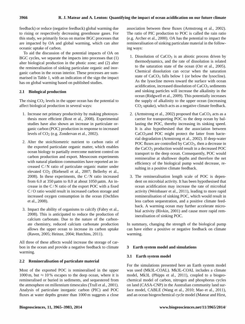
For the export of POC from the upper ocean, in the REFsimulation shows a small global reduction (Fig.7), which ismostly confined to the equatorial Pacific, Indian and NorthAtlantic oceans (Fig.8) associated with increased upperocean stratification that occurs in climate change projections(e.g.Matear and Hirst, 1999). The export of PIC from the up-per ocean is also shown in Fig.7, with all experiments show-ing a decline global export in the future except for REMIN+.In the REMIN+ simulation, the increase in POC export isassociated with an increase in PIC export because the rainratio was held constant. Interestingly, the different OA ex-periments show large regional differences in export produc-tion (Fig.8), with EP++ and COMB substantially increasingexport production in the Southern Ocean. However, for theglobal integrated value, all OA impacts cause an increase inPOC export production, with the greatest increase occurringin the COMB projection.

The large range in the export production response to thedifferent OA experiments is consistent with previous studies(e.g.Tagliabue et al., 2011). The simulations reveal that OAimpacts on export production are much greater than their im-pacts on climate change. Such behaviour demonstrates thatthe consequence of OA will not be through its impact on cli-mate change, but on how it impacts the flow of energy inmarine ecosystems. These changes may have significant im-pacts on marine ecosystems and their productivity, biodiver-sity, and our future ability to exploit them as a food resource.

4.2.5 Dissolved oxygen

While the OA impacts had only a small effect on atmo-spheric CO2 levels, the export production varied dramaticallyamongst the simulations (Fig.8), which has the potential



Figure 8. Export production (mol C m−2 yr−1) from the(a) REF in1850;(b) the change in 2090–99 mean for REF relative to(a). Forthe 2090–2099 mean, the change relative to REF for(c) EP+; (d)EP++;(e)REMIN+; (f) COMB simulations.

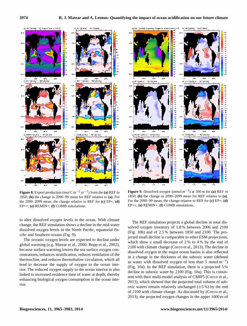
to alter dissolved oxygen levels in the ocean. With climatechange, the REF simulation shows a decline in the mid-waterdissolved oxygen levels in the North Pacific, equatorial Pa-cific and Southern oceans (Fig.9).

The oceanic oxygen levels are expected to decline underglobal warming (e.g.Matear et al., 2000; Bopp et al., 2002),because surface warming lowers the sea surface oxygen con-centrations, enhances stratification, reduces ventilation of thethermocline, and reduces thermohaline circulation, which alltend to decrease the supply of oxygen to the ocean inte-rior. The reduced oxygen supply to the ocean interior is alsolinked to increased residence time of water at depth, therebyenhancing biological oxygen consumption in the ocean inte-rior.

Figure 9. Dissolved oxygen (mmol m−3) at 500 m for(a) REF in1850; (b) the change in 2090–2099 mean for REF relative to(a).For the 2090–99 mean, the change relative to REF for(c) EP+;(d)EP++;(e)REMIN+; (f) COMB simulations.

The REF simulation projects a global decline in total dis-solved oxygen inventory of 1.8 % between 2006 and 2100(Fig. 10b) and of 2.5 % between 1850 and 2100. The pro-jected small decline is comparable to other ESM projections,which show a small decrease of 2 % to 4 % by the end of2100 with climate change (Cocco et al., 2013). The decline indissolved oxygen in the major ocean basins is also reflectedin a change in the thickness of the suboxic water (definedas water with dissolved oxygen of less than 5 mmol m−3)(Fig. 10a). In the REF simulation, there is a projected 5 %decline in suboxic water by 2100 (Fig.10a). This is consis-tent with their multi-model analysis of CMIP5 (Cocco et al.,2013), which showed that the projected total volume of sub-oxic waters remain relatively unchanged (±5 %) by the endof 2100 with climate change. As discussed by (Cocco et al.,2013), the projected oxygen changes in the upper 1000 m of



Figure 10. (a)The ratio of the simulated change in the volume ofsuboxic water to the simulated present-day (2006) value.(b) Theratio of the simulated change in the global ocean inventory of dis-solved oxygen to the simulated 2006 value.

the ocean displays a complex regional pattern with both pos-itive and negative trends reflecting the complex interactionsbetween changes in circulation, biological production, bio-logical remineralisation, and temperature.

The inclusion of OA impacts that could either increasePOC export from the upper ocean (Fig.7) and/or reduce itsdepth of remineralisation may substantially decrease oxygenlevels in the ocean interior. For the total oxygen inventoryin the ocean, the simulations reveal that increased POC ex-port causes a decline in oxygen, while the shoaling of POCremineralisation has little impact (Fig.10b).

The EP+ simulation showed a 17 % increase in the thick-ness in the suboxic water by 2100 (Fig.10a). Similar simu-lations where the C / N ratio of exported POC matter is in-creased with OA project reduced dissolved oxygen levels inthe ocean and a comparable increase in the volume of sub-oxic water to the EP+ projection (Oschlies et al., 2008; Tagli-abue et al., 2011).

(Oschlies et al., 2008) shows the volume of suboxic wa-ter is very sensitive to small changes in the remineralisationof POC in the ocean interior. Our simulations confirm thisresult, but also show the volume of suboxic water is sensi-tive to the location where OA increases POC export. Withthe shoaling of POC remineralisation (REMIN+) there is areduction in the volume of suboxic water. By confining POCremineralisation to the upper ocean, the equatorial Pacific hasless suboxic water, because this water is now more influencedby air–sea gas exchange, there is a global decline in the vol-ume of suboxic water (Fig.10). Similarly, the EP++ simu-lation with increased export production shows the greatestdecline in total oxygen inventory (Fig.10b), but a decline inthe volume of suboxic water by 2100 (Fig.10a). The COMBsimulation, with its increased POC export and shoaling of

POC remineralisation also projects a decline in the volumeof suboxic water. However, the COMB simulation projectsthe development of suboxic zones in the North Pacific andSouthern Ocean where the combination of increased exportproduction, shoaling of depth of POC remineralisation, andincreased stratification with global warming allows for thedevelopment of suboxic water in these regions.

By prescribing the POC depth profile in our model formu-lation, POC will be remineralised without consuming oxy-gen, which implies unconstrained denitrification. By havingunlimited denitrification, the consumption of oxygen may beunderestimated when POC export increases, because POCremineralisation occurs by denitrification rather than by oxy-gen consumption. Thus, the simulated response of the thick-ness of suboxic water to increasing POC export, as in theEP+ and COMB simulations, may be underestimated.

Presently, the large uncertainty in the potential changesin POC export and remineralisation with OA makes it diffi-cult to project the potential consequences of OA on dissolvedoxygen levels with confidence, and this makes it a critical is-sue for further investigation. The response of denitrificationto potential changes in POC export adds another uncertaintyto projecting the future interior oxygen levels changes withOA, warranting further study.

5 Summary and perspectives

Ocean acidification is the inevitable consequence of rising at-mospheric CO2 occurring in conjunction with global warm-ing. Published studies have hypothesised the potential of OAto impact biogeochemical cycling in the ocean. However, todate, no studies have combined these impacts to quantify theintegrated impacts on ocean biogeochemistry and the feed-backs onto the future climate. Here, we explore the integratedconsequences of these OA-induced changes using an ESMand some first-order representations of the potential OA im-pacts on marine biogeochemical cycles. A key result of thisstudy is that OA does not significantly alter the total car-bon stored in the ocean; the potential changes in atmosphericCO2 levels (45 ppm maximum) were small compared to thefuture concentration projected with the RCP8.5 emissionscenario by the end of this century (more than 1000 ppm).The small impact on future atmospheric CO2 levels meansthe OA impacts will have only a minor feedback on pro-jected global warming; our simulations suggest that by 2100the global averaged surface temperature would be altered byless than 0.25 K. Therefore, while the simulations do projectsignificant global warming (≈ 3 K by 2100), the inclusion ofOA impacts on the marine BGC cycle did not significantlyalter the projected changes. Consistent with both the smallimpact on carbon storage in the ocean and on global warm-ing, the inclusion of OA impacts did not significantly alter theprojected trajectory of future ocean acidification (e.g. surfacearagonite state and lysocline depth). However, we emphasise



that with the RCP8.5 scenario, by 2100 significant changesin OA are projected. All polar surface waters will be under-saturated with respect to aragonite, and the maximum surfacearagonite saturation state in the tropics will be less than 2.75,a value below which coral reefs are not historically found.Such changes are likely to have profound impacts on marineecosystems.

Where OA has the potential to have a significant impact ison the POC and PIC export from the upper ocean. We em-phasise the impacts of these changes on marine ecosystemsare highly uncertain and needs further study. While delib-erately conceived to be large, the changes in PIC and POCexport did not significantly change the future depth of thelysocline, however, they did significantly change the regionalexport production and the interior oxygen levels.

The inclusion of OA impacts that could either increasePOC export from the upper ocean or reduce its depth of rem-ineralisation could substantially decrease oxygen levels inthe ocean interior. However, the large variability in potentialchanges in POC export with OA, presently makes it difficultto confidently assess the consequences of OA on dissolvedoxygen levels, and therefore this remains another importantissue to address. The decline in oxygen with the rising CO2 islikely to have consequences for marine organisms with highmetabolic rates. Global warming, lower oxygen and higherCO2 levels represent physiological stresses for marine aero-bic organisms that may act synergistically with ocean acidi-fication (Portner and Farrell, 2008). Understanding how OAand global warming impact marine organisms also warrantsfurther investigation.

Our study has focused on the OA impacts on the BGCcycles and climate change only to the end of this century;however, anthropogenic changes in carbon and climate willpersist for many centuries. (Schmittner et al., 2008) usedan ESM to show that the ocean BGC had a positive feed-back on atmospheric CO2 and climate that were importanton multi-centennial to millennial timescales. In their sim-ulations, changes in ocean biology ultimately became im-portant to the ocean carbon uptake after the year 2600, andby the year 4000 the feedback by the ocean accounted for320 ppm (22 %) of the atmospheric CO2 increase since thepreindustrial period.

While our study focused on a subset of key BGC processesin the ocean that may modulate the oceanic uptake of CO2,other greenhouse gases and other BGC processes may be al-tered by OA, to put these in context. The following brieflyreviews other potential OA impacts and attempts to quantifyand compare them to our results.

The next two most important greenhouse gases producedin the ocean are methane (CH4) and nitrous oxide (N2O), andin the ocean their production is linked to the remineralisationof organic matter in low-oxygen water (Matear et al., 2010;Gruber and Galloway, 2008). The decline in the interior oxy-gen levels should be associated with increased production ofboth these gases (Glessmer et al., 2009).

(Schmittner et al., 2008) used an ESM climate changeprojection run until the year 4000 to show that a triplingof the volume of suboxic water doubled N2O productionin the ocean, increased the atmospheric concentrations by60 ppb, leading to a warming of about 0.25K, a relativelysmall change given the length of their simulation.

Enhanced dinitrogen (N2) fixation by cyanobacteria oc-curs under elevatedpCO2 concentrations (Hutchins et al.,2009). This provides an increased source of reactive nitrogen(N) that has the potential to increase primary production inthe oligotrophic tropical and subtropical areas. However, thisresponse is limited, as the relieving of N limitation will ul-timately lead to phosphate limitation, which will also limitthe potential carbon uptake. Ocean-only simulations wheresufficient N was added to remove nitrate limitation gave amaximum reduction in atmospheric CO2 of about 22 ppm by2100 (Matear and Elliott, 2004). Again, it is a small effectwhen compared to the future atmospheric value associatedwith the RCP8.5 emissions scenario.

Iron is a biologically important element, and therefore anychange in its bioavailability has the potential to change thegrowth rate of phytoplankton. At present there is little con-sensus on the sign of this change with OA. A slower ironuptake by diatoms with OA is seen in experiments with At-lantic surface water (Shi et al., 2010), while an increase hasbeen reported in coastal waters (Breitbarth et al., 2010). Ifwe assume OA can increase the bioavailability of iron suf-ficiently to remove iron limitation on phytoplankton growth,we can use previous ocean model simulations to quantify themaximum potential increase in carbon storage. Such studiesshowed that this process alone could increase carbon storagein the ocean and reduce atmospheric CO2 by 33 to 80 ppmby 2100 (Aumont and Bopp, 2006; Matear and Wong, 1999).While it is a larger response than what we project with ourOA experiments, this is an upper bound that does not mecha-nistically link OA to the bioavailability of iron. Even this up-per bound estimate is small in comparison to the atmosphericCO2 projected with the RCP8.5 emissions scenario by 2100(≈ 1000 ppm), hence it would only have a minor impact onthe future climate.

Further, iron is only one of many biologically importanttrace metals, for which bioavailability will change in re-sponse to OA (Hoffmann et al., 2012) and potentially alter bi-ological production. Therefore, more studies are required tounderstand how changes in the bioavailability of trace metalsin response to OA may impact future biological production.

The ocean is also a source of climatically active trace gasesto the atmosphere such as dimethyl sulphide (DMS), whichcan alter cloud properties. DMS is a gaseous sulphur com-pound produced by marine biota in surface seawater (Gabricet al., 1993). The marine production of DMS provides 90 %of the biogenic sulfur in the marine atmosphere, and in the at-mosphere it is rapidly oxidised to produce particles that canaffect cloud formation and climate (Arnold et al., 2013). Theeffects of increasing anthropogenic CO2 and the resulting



warming and OA on trace gas production in the oceans re-mains poorly understood.

Modelling studies vary substantially in their predictions ofthe change in DMS emissions with climate change. Elevat-ing CO2 without any other environmental changes suggesta significant decrease in the future concentration of DMS(Hopkins et al., 2011). However, studies in polar waters sug-gested increases in DMS emission ranging from 30 % tomore than 150 % (Cameron-Smith et al., 2011; Kloster et al.,2007; Gabric et al., 2011) by 2100 with only climate change.While a recent ESM study by (Six et al., 2013) projecteda global decrease in DMS production of 18± 3 % by 2100,with 83 % of this change attributed to OA, leading to onlya modest equilibrium warming of 0.23 to 0.48 K. (Six et al.,2013) simulated strong regional responses of increasing (po-lar regions) and decreasing DMS emissions, which reflectedthe combined affect of increased net primary production andregional shifts in community composition. Therefore, morestudies combining the impacts of global warming and OA onmarine DMS production are warranted to better determine itsregional response and sign, particularly at the marine speciesand ecosystem levels.

Potential climate–carbon feedbacks of OA and globalwarming appear small relative to the input of carbon into theatmosphere by human activity under the RCP8.5 scenario.However, understanding and projecting the combined OAand global warming impact on marine ecosystems remainsthe outstanding issue to tackle. In particular, biological pro-duction may change with the projected OA, and the poten-tial consequences for marine organisms and ecosystems arepoorly known.



Appendix A: Ocean Biogeochemical Model Equations

The ocean BGC module is based on (Matear and Hirst,2003), and simulates the evolution of phosphate (P), oxygen(O), carbon (C) and alkalinity (A) in the ocean. The BGCmodule includes a simple representation of the surface exportproduction of biological matter as a function of the temper-ature, mixed-layer depth, and nutrient concentration (phos-phate) in the euphotic zone, with the sinking particulate or-ganic matter (POM) and particulate inorganic carbon (PIC)remineralising according to prescribed functions of depth.The euphotic zone production of organic matter consumesdissolved phosphorous, nitrogen and carbon and releasesoxygen according to the (Redfield, 1934) ratio P : N : C : O2of 1 : 16 : 106: −138, while the subsurface remineralisationconversely releases/consumes these elements in like ratio.While nitrogen is not explicitly modelled, we include its ra-tio to P and C to make it clear how processes like denitri-fication affect the modelled P and C tracers. The follow-ing briefly summarises how the BGC processes are param-eterised and how they affect the BGC tracers. For reference,we give here the conservation equation for dissolved inor-ganic carbon concentration (C):

∂C

∂t= −∇3(uC) + ∇I (KI∇IC) (A1)

+∂

∂z(Kv

∂C

∂z) + QC

F − QCO − QC

I

The first term on the right represents the usual three-dimensional advection, the second term represents diffusionalong the neutral density surfaces, and the third term repre-sents vertical diffusion.QC

O denotes the biological produc-tion and consumption of particulate organic carbon.QC

I de-notes the production and dissolution of particulate inorganiccarbon. The carbon dioxide flux into the surface ocean acrossthe air–sea interface (QC

F ) is given by

QCF = K(pCOatmosphere

2 − pCOocean2 ), (A2)

whereK is the gas exchange coefficient, which is a func-tion of wind speed and temperature (Wanninkhof, 1992),pCOatmosphere

2 is the atmospheric partial pressure of carbondioxide (as simulated by the model), andpCOocean

2 is thepartial pressure carbon dioxide in the surface ocean wa-ter. pCOocean

2 is computed from the surface temperature,salinity, dissolved inorganic carbon concentration and alka-linity using the OCMIP2 carbon chemistry routine (Najjaret al., 2007). A similar equation is used for air–sea oxygenexchange, where the atmospheric partial pressure of oxy-gen (pOatmosphere

2 ) is fixed at 0.2048 atm (Weiss, 1970), andpOocean

2 is the effective partial pressure oxygen in the surfaceocean water computed from the simulated surface oxygenconcentration divided by the oxygen concentration in equi-librium with the atmosphere multiply bypOatmosphere

2 . Foralkalinity and phosphate there is no air–sea flux term.

Figure A1. Comparison of the observed alkalinity(a) and prein-dustrial dissolved inorganic carbon(c) (Key et al., 2004) with theREF simulation in the year 1850 for alkalinity(b) and dissolvedinorganic carbon(d) in units of mmol m−3.

In the photic zone, which is set to be the surface layer ofthe model (upper 50 m), the biological production of par-ticulate organic matter and particulate inorganic carbon oc-curs. For particulate organic matter, the production of partic-ulate organic phosphorus (POP) was defined by the followingequations:

Vmax =0.6(1.066)T (A3)

F(I) =[1− eG(I)] (A4)

G(I) =I (x, t)αPAR

Vmax(A5)

QPO =So

nppVmaxMin[P

P + Pk

,F (I )] (A6)

EPOP=QPO1z (A7)

Vmax is the maximum growth rate in day−1, which is a func-tion of the surface layer temperature (T , ◦C). F(I) is theproductivity versus irradiance equation used to describe phy-toplankton growth, which is given as a unitless value andprovides a measure of light-limited growth.G(I) a unitlessfunction of the light availability for growth, which is cal-culated from the daily averaged incident shortwave radia-tion (I ) in W m−2, the fraction of shortwave radiation that isphotosynthetically active PAR (unitless factor), and the ini-tial slope (α) of the productivity versus radiance curve forphytoplankton growth (day−1/(W m−2)). QP

O gives the up-



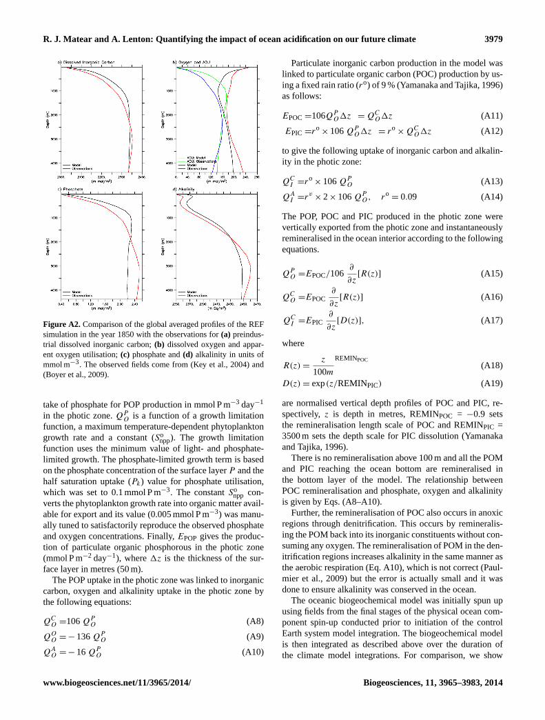
Figure A2. Comparison of the global averaged profiles of the REFsimulation in the year 1850 with the observations for(a) preindus-trial dissolved inorganic carbon;(b) dissolved oxygen and appar-ent oxygen utilisation;(c) phosphate and(d) alkalinity in units ofmmol m−3. The observed fields come from (Key et al., 2004) and(Boyer et al., 2009).

take of phosphate for POP production in mmol P m−3 day−1

in the photic zone.QPO is a function of a growth limitation

function, a maximum temperature-dependent phytoplanktongrowth rate and a constant (So

npp). The growth limitationfunction uses the minimum value of light- and phosphate-limited growth. The phosphate-limited growth term is basedon the phosphate concentration of the surface layerP and thehalf saturation uptake (Pk) value for phosphate utilisation,which was set to 0.1 mmol P m−3. The constantSo

npp con-verts the phytoplankton growth rate into organic matter avail-able for export and its value (0.005 mmol P m−3) was manu-ally tuned to satisfactorily reproduce the observed phosphateand oxygen concentrations. Finally,EPOP gives the produc-tion of particulate organic phosphorous in the photic zone(mmol P m−2 day−1), where1z is the thickness of the sur-face layer in metres (50 m).

The POP uptake in the photic zone was linked to inorganiccarbon, oxygen and alkalinity uptake in the photic zone bythe following equations:

QCO =106QP

O (A8)

QOO = − 136QP

O (A9)

QAO = − 16QP

O (A10)

Particulate inorganic carbon production in the model waslinked to particulate organic carbon (POC) production by us-ing a fixed rain ratio (ro) of 9 % (Yamanaka and Tajika, 1996)as follows:

EPOC=106QPO1z = QC

O1z (A11)

EPIC =ro× 106QP

O1z = ro× QC

O1z (A12)

to give the following uptake of inorganic carbon and alkalin-ity in the photic zone:

QCI =ro

× 106QPO (A13)

QAI =rv

× 2× 106QPO , ro

= 0.09 (A14)

The POP, POC and PIC produced in the photic zone werevertically exported from the photic zone and instantaneouslyremineralised in the ocean interior according to the followingequations.

QPO =EPOC/106

∂

∂z[R(z)] (A15)

QCO =EPOC

∂

∂z[R(z)] (A16)

QCI =EPIC

∂

∂z[D(z)], (A17)

where

R(z) =z

100m

REMINPOC(A18)

D(z) = exp(z/REMINPIC) (A19)

are normalised vertical depth profiles of POC and PIC, re-spectively,z is depth in metres, REMINPOC = −0.9 setsthe remineralisation length scale of POC and REMINPIC =3500 m sets the depth scale for PIC dissolution (Yamanakaand Tajika, 1996).

There is no remineralisation above 100 m and all the POMand PIC reaching the ocean bottom are remineralised inthe bottom layer of the model. The relationship betweenPOC remineralisation and phosphate, oxygen and alkalinityis given by Eqs. (A8–A10).

Further, the remineralisation of POC also occurs in anoxicregions through denitrification. This occurs by remineralis-ing the POM back into its inorganic constituents without con-suming any oxygen. The remineralisation of POM in the den-itrification regions increases alkalinity in the same manner asthe aerobic respiration (Eq. A10), which is not correct (Paul-mier et al., 2009) but the error is actually small and it wasdone to ensure alkalinity was conserved in the ocean.

The oceanic biogeochemical model was initially spun upusing fields from the final stages of the physical ocean com-ponent spin-up conducted prior to initiation of the controlEarth system model integration. The biogeochemical modelis then integrated as described above over the duration ofthe climate model integrations. For comparison, we show



the zonally averaged sections of dissolved inorganic carbonand alkalinity from the preindustrial period (year 1850) com-pared to the observed fields (Fig. A1). The model gener-ally captures the observed variability with the spatial cor-relation of three-dimensional alkalinity and dissolved inor-ganic carbon with observations (Key et al., 2004) being 0.92and 0.91, respectively. Also shown are comparisons of theglobal averaged profiles of alkalinity, preindustrial dissolvedinorganic carbon, phosphate, dissolved oxygen and apparentoxygen utilisation with the observations (Key et al., 2004;Boyer et al., 2009) (Fig. A2). In the intermediate water (500–1500 m), the model underestimates phosphate, dissolved in-organic carbon and apparent oxygen utilisation concentra-tions and this implies the model is underestimating the rem-ineralisation of POM in the intermediate water.



Acknowledgements.Funding for this work was provided by theAustralian Climate Change Science Program, the Pacific-AustraliaClimate Change Science and Adaptation Planning Program, andthe CSIRO Wealth from Oceans Flagship.

Edited by: M. Grégoire

References

Archer, D. E., Eshel, G., Winguth, A., Broecker, W., Pierrehumbert,R., Tobis, M., and Jacob, R.: AtmosphericpCO(2) sensitivity tothe biological pump in the ocean, Global Biogeochem. Cy., 14,1219–1230, 2000.

Armstrong, R. A., Lee, C., Hedges, J. I., Honjo, S., and Wakeham,S. G.: A new, mechanistic model for organic carbon fluxes in theocean based on the quantitative association of POC with ballastminerals, Deep Sea Res. Pt. II, 49, 219–236, 2002.

Arnold, H. E., Kerrison, P., and Steinke, M.: Interacting effects ofocean acidification and warming on growth and DMS-productionin the haptophyte coccolithophore Emiliania huxleyi, Glob.Change Biol., 19, 1007–1016, 2013.

Aumont, O. and Bopp, L.: Globalizing results from ocean insitu iron fertilization studies, Global Biogeochem. Cycles, 20,GB2017, doi:10.1029/2005GB002591, 2006.

Bellerby, R. G. J., Schulz, K. G., Riebesell, U., Neill, C., Nondal,G., Heegaard, E., Johannessen, T., and Brown, K. R.: Marineecosystem community carbon and nutrient uptake stoichiometryunder varying ocean acidification during the PeECE III exper-iment, Biogeosciences, 5, 1517–1527, doi:10.5194/bg-5-1517-2008, 2008.

Bopp, L., Quere, C. L., Heimann, M., Manning, A. C., and Monfray,P.: Climate-induced oceanic oxygen fluxes: Implications for thecontemporary carbon budget, Global Biogeochem. Cy., 16, 1022,doi:10.1029/2001GB001445, 2002.

Bopp, L., Resplandy, L., Orr, J. C., Doney, S. C., Dunne, J. P.,Gehlen, M., Halloran, P., Heinze, C., Ilyina, T., Séférian, R.,Tjiputra, J., and Vichi, M.: Multiple stressors of ocean ecosys-tems in the 21st century: projections with CMIP5 models,Biogeosciences, 10, 6225–6245, doi:10.5194/bg-10-6225-2013,2013.

Boyer, T. P., Antonov, J. I., Baranova, O. K., Garcia, H. E., Johnson,D. R., Locarnini, R. A., Mishonov, A. V., O’Brien, T., Seidov, D.,and Smolyar, I. V.: World Ocean Database 2009, Vol. 66, NOAAAtlas NESDIS, U.S. Gov. Printing Office, Wash., D.C., 2009.

Breitbarth, E., Bellerby, R. J., Neill, C. C., Ardelan, M. V.,Meyerhöfer, M., Zöllner, E., Croot, P. L., and Riebesell, U.:Ocean acidification affects iron speciation during a coastal sea-water mesocosm experiment, Biogeosciences, 7, 1065–1073,doi:10.5194/bg-7-1065-2010, 2010.

Brewer, P. G. and Peltzer, E. T.: Oceans: Limits to marine life, Sci-ence, 324, 347–348, 2009.

Brohan, P., Kennedy, J. J., Harris, I., Tett, S. F. B., and Jones, P. D.:Uncertainty estimates in regional and global observed temper-ature changes: A new data set from 1850, J. Geophys. Res.-Atmos., 111, D12106, doi:10.1029/2005JD006548, 2006.

Caldeira, K.: Ocean model predictions of chemistry changes fromcarbon dioxide emissions to the atmosphere and ocean, J. Geo-phys. Res., 110, C09S04, 2005.

Cameron-Smith, P., Elliott, S., Maltrud, M., Erickson, D., andWingenter, O.: Changes in dimethyl sulfide oceanic distribu-tion due to climate change, Geophys. Res. Lett., 38, L07704,doi:10.1029/2011GL047069, 2011.

Canadell, J. G., Le Quere, C., Raupach, M. R., Field, C. B., Buiten-huis, E. T., Ciais, P., Conway, T. J., Gillett, N. P., Houghton,R. A., and Marland, G.: Contributions to accelerating atmo-spheric CO2 growth from economic activity, carbon intensity,and efficiency of natural sinks, P. Natl. Acad. Sci. USA, 104,18 866–18 870, 2007.

Cocco, V., Joos, F., Steinacher, M., Frölicher, T. L., Bopp, L.,Dunne, J., Gehlen, M., Heinze, C., Orr, J., Oschlies, A., Schnei-der, B., Segschneider, J., and Tjiputra, J.: Oxygen and indicatorsof stress for marine life in multi-model global warming projec-tions, Biogeosciences, 10, 1849–1868, doi:10.5194/bg-10-1849-2013, 2013.

Dentener, F.: Global maps of atmospheric nitrogen deposition,1860, 1993, and 2050, Data set, available at:http://daac.ornl.gov/from Oak Ridge National Laboratory Distributed Active ArchiveCenter, Oak Ridge, Tennessee, USA, 2006.

Doney, S. C., Fabry, V. J., Feely, R. A., and Kleypas, J. A.: OceanAcidification: The Other CO2 Problem, Annu. Rev. Mar. Sci., 1,169–192, 2009.

Duteil, O., Koeve, W., Oschlies, A., Aumont, O., Bianchi, D.,Bopp, L., Galbraith, E., Matear, R., Moore, J. K.,Sarmiento, J. L., and Segschneider, J.: Preformed and re-generated phosphate in ocean general circulation models:can right total concentrations be wrong?, Biogeosciences, 9,1797–1807, doi:10.5194/bg-9-1797-2012, 2012.

Duteil, O., Koeve, W., Oschlies, A., Bianchi, D., Galbraith, E., Kri-est, I., and Matear, R.: A novel estimate of ocean oxygen utilisa-tion points to a reduced rate of respiration in the ocean interior,Biogeosciences, 10, 7723–7738, doi:10.5194/bg-10-7723-2013,2013.

Fabry, V., Seibel, B., Feely, R., and Orr, J.: Impacts of ocean acidi-fication on marine fauna and ecosystem processes, ICES J. Mar.Sci. 65, 414–432, 2008.

Gabric, A., Murray, N., Stone, L., and Kohl, M.: Modelling theproeduction of dimethylsulfide during a phytoplankton bloom,J. Geophys. Res., 98, 22805–22816, 1993.

Gabric, A., Qu, B., Matrai, P., and Hirst, A.: The simulated re-sponse of dimethylsulfide production in the Arctic Ocean toglobal warming, Tellus B, 57, 391–403, 2011.

Gehlen, M., Gruber, N., Gangstø, R., Bopp, L., and Oschlies, A.:Biogeochemical consequences of ocean acidification and feed-backs to the earth system, in: Ocean Acidification, vol. 1, editedby: Gattuso, J.-P. and Hansson, L., 230–248, Oxford UniversityPress, 2011.

Glessmer, M. S., Eden, C., and Oschlies, A.: Contribution of oxygenminimum zone waters to the coastal upwelling off Mauritania,Prog. Oceanogr., 83, 143–150, 2009.

Gruber, N. and Galloway, J.: An earth-system perspective of theglobal nitrogen cycle, Nature, 451, 293–296, 2008.

Guinotte, J. M., Buddemeier, R. W., and Kleypas, J. A.: Futurecoral reef habitat marginality: temporal and spatial effects ofclimate change in the Pacific basin, Coral Reefs, 22, 551–558,doi:10.1007/s00338-003-0331-4, 2003.

Hedin, L. O.: Global organization of terrestrial plant–nutrient inter-actions, Proc. Natl. Acad. Sci. USA, 101, 10849–10850, 2004.


http://dx.doi.org/10.1029/2005GB002591

http://dx.doi.org/10.5194/bg-5-1517-2008

http://dx.doi.org/10.5194/bg-5-1517-2008

http://dx.doi.org/10.1029/2001GB001445

http://dx.doi.org/10.5194/bg-10-6225-2013

http://dx.doi.org/10.5194/bg-7-1065-2010

http://dx.doi.org/10.1029/2005JD006548

http://dx.doi.org/10.1029/2011GL047069

http://dx.doi.org/10.5194/bg-10-1849-2013

http://dx.doi.org/10.5194/bg-10-1849-2013

http://daac.ornl.gov/

http://dx.doi.org/10.5194/bg-9-1797-2012

http://dx.doi.org/10.5194/bg-10-7723-2013

http://dx.doi.org/10.1007/s00338-003-0331-4


Heinze, C.: Simulating oceanic CaCO3 export productionin the greenhouse, Geophys. Res. Lett., 31, L16308,doi:10.1029/2004GL020613, 2004.

Hoffmann, L. J., Breitbarth, E., Boyd, P. W., and Hunter, K. A.:Influence of ocean warming and acidification on tracemetal biogeochemistry, Mar. Ecol.-Prog. Ser., 470, 191–205,doi:10.3354/meps10082, 2012.

Hopkins, F., Nightingale, P., and Liss, P.: Effects of ocean acidifica-tion on the marine source of atmospherically active trace gases,in: Ocean Acidification, edited by: Gattuso, J.-P. and Hansson,L., p. 210, Oxford University Press, 2011.

Hutchins, D. A.: Oceanography: forecasting the rain ratio, Nature,476, 41–42, 2011.

Hutchins, D. A., Mulholland, M. R., and Fu, F.: Nutrient cycles andmarine microbes in a CO2-enriched ocean, Oceanography, 22,128–145, 2009.

Key, R. M., Kozyr, A., Sabine, C. L., Lee, K., Wanninkhof, R.,Bullister, J. L., Feely, R. A., Millero, F. J., Mordy, C., andPeng, T. H.: A global ocean carbon climatology: Results fromGlobal Data Analysis Project (GLODAP), Global Biogeochem.Cy., 18, GB4031, doi:10.1029/2004GB002247, 2004.

Khatiwala, S., Primeau, F., and Hall, T.: Reconstruction of the his-tory of anthropogenic CO2 concentrations in the ocean, Nature,462, 346–349, 2009.

Kloster, S., Six, K. D., Feichter, J., Maier-Reimer, E., Roeckner, E.,Wetzel, P., Stier, P., and Esch, M.: Response of dimethylsulfide(DMS) in the ocean and atmosphere to global warming, J. Geo-phys. Res., 112, G03005, doi:10.1029/2006JG000224, 2007.

Lawrence, P. J., Feddema, J. J., Bonan, G. B., Meehl, G. A.,O’Neill, B. C., Oleson, K. W., Levis, S., Lawrence, D. M.,Kluzek, E., Lindsay, K., and Thornton, P. E.: Simulating the bio-geochemical and biogeophysical impacts of transient land coverchange and wood harvest in the Community Climate SystemModel (CCSM4) from 1850 to 2100, J. Climate, 25, 3071–3095,2013.

Mao, J., Phipps, S. J., Pitman, A. J., Wang, Y. P., Abramowitz, G.,and Pak, B.: The CSIRO Mk3L climate system model v1.0coupled to the CABLE land surface scheme v1.4b: evaluationof the control climatology, Geosci. Model Dev., 4, 1115–1131,doi:10.5194/gmd-4-1115-2011, 2011.

Matear, R. J. and Elliott, B.: Enhancement of oceanic uptake ofanthropogenic CO2 by macro-nutrient fertilization, J. Geophys.Res., 109, C4001, doi:10.1029/2000JC000321, 2004.

Matear, R. J. and Hirst, A. C.: Climate Change Feedback on theFuture Oceanic CO2 uptake, Tellus, 51B, 722–733, 1999.

Matear, R. J. and Hirst, A. C.: Long term changes in dis-solved oxygen concentrations in the ocean caused by pro-tracted global warming, Global Biogeochem. Cy., 17, 1125,doi:10.1029/2002GB001997, 2003.

Matear, R. J. and Wong, C. S.: Potential to increase the oceanicCO2 uptake by enhancing marine productivity in high nutrientlow chlorophyll regions, 249–253, 1999.

Matear, R. J., Hirst, A. C., and McNeil, B. I.: Changes in dis-solved oxygen in the Southern Ocean with climate change,Geochemistry Geophysics Geosystems (http://gcubed.magnet.fsu.edu/main.html), 1, 2000.

Matear, R. J., Wang, Y.-P., and Lenton, A.: Land and ocean nutri-ent and carbon cycle interactions, Curr. Op. Environ. Sustain., 2,258–263, 2010.

Matsumoto, K., Sarmiento, J. L., Key, R. M., Aumont, O., Bullis-ter, J. L., Caldeira, K., Campin, J. M., Doney, S. C., Drange, H.,Dutay, J. C., Follows, M. J., Gao, Y., Gnanadesikan, A., Gru-ber, N., Ishida, A., Joos, F., Lindsay, K., Maier-Reimer, E.,Marshall, J. C., Matear, R. J., Monfray, P., Mouchet, A., Naj-jar, R., Plattner, G. K., Schlitzer, R., Slater, R., Swathi, P. S.,Totterdell, I. J., Weirig, M. F., Yamanaka, Y., Yool, A.,and Orr, J. C.: Evaluation of ocean carbon cycle modelswith data-based metrics, Geophys. Res. Lett., 31, L07303,doi:10.1029/2003GL018970, 2004.

Najjar, R. G., Jin, X., Louanchi, F., Aumont, O., Caldeira, K.,Doney, S. C., Dutay, J. C., Follows, M. J., Gruber, N., Joos,F., Lindsay, K., Maier-Reimer, E., Matear, R. J., Matsumoto, K.,Monfray, P., Mouchet, A., Orr, J. C., Plattner, G. K., Sarmiento,J. L., Schlitzer, R., Slater, R. D., Weirig, M. F., Yamanaka, Y.,and Yool, A.: Impact of circulation on export production, dis-solved organic matter, and dissolved oxygen in the ocean: Resultsfrom Phase II of the Ocean Carbon-cycle Model Intercompari-son Project (OCMIP-2), Global Biogeochem. Cy., 21, GB3007,doi:10.1029/2006GB002857, 2007.

Orr, J. C., Fabry, V. J., Aumont, O., Bopp, L., Doney, S. C.,Feely, R. A., Gnanadesikan, A., Gruber, N., Ishida, A., Joos, F.,Key, R. M., Lindsay, K., Maier-Reimer, E., Matear, R. J.,Monfray, P., Mouchet, A., Najjar, R. G., Plattner, G. K.,Rodgers, K. B., Sabine, C. L., Sarmiento, J. L., Schlitzer, R.,Slater, R. D., Totterdell, I. J., Weirig, M. F., Yamanaka, Y., andYool, A.: Anthropogenic ocean acidification over the twenty-first century and its impact on calcifying organisms, Nature, 437,681–686, 2005.

Oschlies, A., Schulz, K. G., Riebesell, U., and Schmittner, A.:Simulated 21st century’s increase in oceanic suboxia by CO2-enhanced biotic carbon export, Global Biogeochem. Cy., 22,GB4008, doi:10.1029/2007GB003147, 2008.

Paulmier, A., Kriest, I., and Oschlies, A.: Stoichiometries ofremineralisation and denitrification in global biogeochemicalocean models, Biogeosciences, 6, 923–935, doi:10.5194/bg-6-923-2009, 2009.

Phipps, S. J., Rotstayn, L. D., Gordon, H. B., Roberts, J. L.,Hirst, A. C., and Budd, W. F.: The CSIRO Mk3L climate systemmodel version 1.0 – Part 1: Description and evaluation, Geosci.Model Dev., 4, 483–509, doi:10.5194/gmd-4-483-2011, 2011.

Pinsonneault, A. J., Matthews, H. D., Galbraith, E. D., andSchmittner, A.: Calcium carbonate production response to futureocean warming and acidification, Biogeosciences, 9, 2351–2364,doi:10.5194/bg-9-2351-2012, 2012.

Pitman, A. J., Avila, F. B., Abramowitz, G., Wang, Y. P.,Phipps, S. J., and de Noblet-Ducoudré, N.: Importance of back-ground climate in determining impact of land-cover change onregional climate, Nat. Clim. Change, 1, 472–475, 2011.

Portner, H. O. and Farrell, A. P.: ECOLOGY: physi-ology and climate change, Science, 322, 690–692,doi:10.1126/science.1163156, 2008.

Raven, J. A.: Ocean Acidification Due to Increasing AtmosphericCarbon Dioxide, R Society (Great Britain), 60 pp., 2005.

Redfield, A. C.: On the proportions of organic derivatives in seawater and their relation to the composition of plankton, in JamesJohnstone Memorial Volume, ed. R. J. Daniel, 172–192, 1934.

Ridgwell, A., Schmidt, D. N., Turley, C., Brownlee, C., Maldon-ado, M. T., Tortell, P., and Young, J. R.: From laboratory ma-


http://dx.doi.org/10.1029/2004GL020613

http://dx.doi.org/10.3354/meps10082

http://dx.doi.org/10.1029/2004GB002247

http://dx.doi.org/10.1029/2006JG000224

http://dx.doi.org/10.5194/gmd-4-1115-2011

http://dx.doi.org/10.1029/2000JC000321

http://dx.doi.org/10.1029/2002GB001997

http://gcubed.magnet.fsu.edu/main.html

http://gcubed.magnet.fsu.edu/main.html

http://dx.doi.org/10.1029/2003GL018970

http://dx.doi.org/10.1029/2006GB002857

http://dx.doi.org/10.1029/2007GB003147

http://dx.doi.org/10.5194/bg-6-923-2009

http://dx.doi.org/10.5194/bg-6-923-2009

http://dx.doi.org/10.5194/gmd-4-483-2011

http://dx.doi.org/10.5194/bg-9-2351-2012

http://dx.doi.org/10.1126/science.1163156


nipulations to Earth system models: scaling calcification im-pacts of ocean acidification, Biogeosciences, 6, 2611–2623,doi:10.5194/bg-6-2611-2009, 2009.

Riebesell, U., Schulz, K. G., Bellerby, R. G. J., Botros, M.,Fritsche, P., Meyerhofer, M., Neill, C., Nondal, G., Oschlies, A.,Wohlers, J., and Zollner, E.: Enhanced biological carbon con-sumption in a high CO2 ocean, Nature, 450, 545–549, 2007.

Rivkin, R. B.: Biogenic Carbon Cycling in the Upper Ocean: Effectsof Microbial Respiration, Science, 291, 2398–2400, 2001.

Rost, B., Zondervan, I., and Wolf-Gladrow, D.: Sensitivity of phyto-plankton to future changes in ocean carbonate chemistry: currentknowledge, contradictions and research directions, Mar. Ecol.-Prog. Ser., 373237., 227, 227–237, 2008.

Schmittner, A., Oschlies, A., Matthews, H. D., and Galbraith, E. D.:Future changes in climate, ocean circulation, ecosystems, andbiogeochemical cycling simulated for a business-as-usual CO2emission scenario until year 4000 AD, Global Biogeochem. Cy.,22, GB1013, doi:10.1029/2007GB002953, 2008.

Shi, D., Xu, Y., Hopkinson, B., and Morel, F.: Effect of ocean acid-ification on iron availability to marine phytoplankton, Science,327, 676, doi:10.1126/science.1183517,, 2010.

Six, K. D., Kloster, S., Ilyina, T., Archer, S. D., Zhang, K., andMaier-Reimer, E.: Global warming amplified by reduced sulphurfluxes as a result of ocean acidification, Nat. Clim. Change, 3,1–4, 2013.

Tagliabue, A., Bopp, L., and Gehlen, M.: The response of marinecarbon and nutrient cycles to ocean acidification: large uncertain-ties related to phytoplankton physiological assumptions, GlobalBiogeochem. Cy., 25, GB3017, doi:10.1029/2010GB003929,2011.

Taylor, K. E.: Summarizing multiple aspects of model performancein a single diagram, J. Geophys. Res.-Atmos., 106, 7183–7192,2001.

Trenberth, K. E., Jones, P. D., Ambenje, P., Bojariu, R., Easter-ling, D., Tank, A. K., Parker, D., Rahimzadeh, F., Renwick, J. A.,Rusticucci, M., Soden, B., and Zhai, P.: Observations: Surfaceand Atmospheric Climate Change, 2007.

Trull, T. W., Bray, S. G., Manganini, S. J., Honjo, S., and Fran-cois, R.: Moored sediment trap measurements of carbon export inthe Subantarctic and Polar Frontal Zones of the Southern Ocean,south of Australia, J. Geophys. Res.-Atmos., 106, 31489–31509,2001.

Wang, Y. P., Law, R. M., and Pak, B.: A global model of carbon,nitrogen and phosphorus cycles for the terrestrial biosphere, Bio-geosciences, 7, 2261–2282, doi:10.5194/bg-7-2261-2010, 2010.

Wanninkhof, R.: Relationship between wind speed and gas ex-change over the ocean, J. Geophys. Res., 97, 7373–7382, 1992.

Weinbauer, M. G., Mari, X., and Gattuso, J.-P.: Effects of oceanacidification on the diversity and activity of heterotrophic marinemicroorganisms, in: Ocean Acidification, edited by: Gattuso, J.-P. and Hansson, L., Oxford University Press, 2011.

Weiss, R. F.: The solubility of nitrogen, oxygen and argon in waterand seawater, Deep Sea Res., 17, 721–735, 1970.

Yamanaka, Y. and Tajika, E.: The role of the vertical fluxes of par-ticulate organic matter and calcite in the oceanic carbon cycle:studies using a ocean biogeochemical general circulation model,Global Biogeochem. Cy., 10, 361–382, 1996.

Zaehle, S., Friedlingstein, P., and Friend, A. D.: Terrestrial nitrogenfeedbacks may accelerate future climate change, Geophys. Res.Lett., 37, L01401, doi:10.1029/2009GL041345, 2010.

Zhang, Q., Wang, Y. P., Matear, R. J., Pitman, A. J., and Dai,Y. J.: Nitrogen and phosphorous limitations significantly re-duce future allowable CO2 emissions, Geophys. Res. Lett.,doi:10.1002/2013GL058352, 2014.

Zondervan, I., Rost, B., and Riebesell, U.: Effect of CO2 concen-tration on the PIC/POC ratio in the coccolithophore Emilia-nia huxleyi grown under light-limiting conditions and differentdaylengths, J. Exp. Mar. Biol. Ecol., 272, 55–70, 2002.


http://dx.doi.org/10.5194/bg-6-2611-2009

http://dx.doi.org/10.1029/2007GB002953

http://dx.doi.org/10.1126/science.1183517,

http://dx.doi.org/10.1029/2010GB003929

http://dx.doi.org/10.5194/bg-7-2261-2010

http://dx.doi.org/10.1029/2009GL041345

http://dx.doi.org/10.1002/2013GL058352

Quantifying the impact of ocean acidiﬁcation on our future ...ecite.utas.edu.au/118609/1/118609 - quantifying the impact of ocean acidification.pdf · Mk3L simulates the historical

Documents