Quantifying sources and sinks of trace gases using space-borne measurements: current ...rsta.royalsocietypublishing.org/content/roypta/366/1885/... · Quantifying sources and sinks

on July 15, 2018http://rsta.royalsocietypublishing.org/Downloaded from

Quantifying sources and sinks of trace gasesusing space-borne measurements:

current and future science

BY PAUL I. PALMER*

School of GeoSciences, University of Edinburgh, Edinburgh EH9 3JW, UK

We have been observing the Earth’s upper atmosphere from space for several decades,but only over the past decade has the necessary technology begun to match our desire toobserve surface air pollutants and climate-relevant trace gases in the lower troposphere,where we live and breathe. A new generation of Earth-observing satellites, capable ofprobing the lower troposphere, are already orbiting hundreds of kilometres above theEarth’s surface with several more ready for launch or in the planning stages.Consequently, this is one of the most exciting times for the Earth system scientistswho study the countless current-day physical, chemical and biological interactionsbetween the Earth’s land, ocean and atmosphere. First, I briefly review the theorybehind measuring the atmosphere from space, and how these data can be used to infersurface sources and sinks of trace gases. I then present some of the science highlightsassociated with these data and how they can be used to improve fundamentalunderstanding of the Earth’s climate system. I conclude the paper by discussing thefuture role of satellite measurements of tropospheric trace gases in mitigating surface airpollution and carbon trading.

Keywords: global troposphere; air pollution; greenhouse gases;satellite remote sensing; source–sink estimation

On

*pi

1. Introduction

Quantitatively understanding the physical, chemical and biological processes thatdetermine contemporary climate is a prerequisite for developing confidentprojections of how the Earth’s climate system will evolve on decadal to centennialtime scales (IPCC 2007). The climate community thus far has relied largelyon (i) detailed, small-scale in situ measurements (e.g. small land plots in theAmazon that monitor carbon uptake from vegetation), (ii) large-scale space-borne measurements that provide information on variables that embody achanging climate state (e.g. atmospheric temperature, ice sheet thickness) and(iii) mathematical models of the Earth’s climate, which attempt to link differentcomponents of the Earth (e.g. land, ocean, atmosphere). Despite many successesin understanding the broad-scale nature of the Earth’s climate using the

Phil. Trans. R. Soc. A (2008) 366, 4509–4528

doi:10.1098/rsta.2008.0176

Published online 1 October 2008

e contribution of 10 to a Triennial Issue ‘Earth science’.

[email protected]

4509 This journal is q 2008 The Royal Society

http://rsta.royalsocietypublishing.org/

P. I. Palmer4510


aforementioned data and mathematical models, the tropospheric chemistrycommunity has, until recently, been starved of satellite measurements, insteadrelying on sparse ground-based and aircraft measurements of trace gases. There hasbeen a reversal of fortunes, and here I argue that the wide range of currentmeasurements of tropospheric trace gases and surface properties from space-borneinstrumentation, and their associated temporal and spatial distributions, represent arich resource for testing understanding of couplings between land, ocean andatmospheres, and for guiding subsequent in situmeasurement campaigns. Relatingthese satellite observations to specific climate processes is challenging, oftendemanding an appreciation of physics, chemistry and biology, disciplines that havetraditionally been taught separately. Satellite observations of trace gases provide anability to sample large spatial scales on hourly time scales, as discussed below, whichcomplement the high temporal or spatial resolution distributions provided by in situinstruments. Consequently, measurement campaigns are already integrating space-based and in situ datastreams in an attempt to relate trace gas distribution overdifferent spatial and temporal scales (Jacob et al. 2003). I shall focus my research onsatellite observations of trace gases in the lower troposphere (less than 6 km).

The general problem of relating trace gas concentration measurements tosurface processes is straightforward, and in this paper, I shall consider themass balance of a generic trace gas C at time t in a frame of reference fixed onthe Earth,

dCðtÞdt

ZPðtÞKLðtÞCTðtÞCXðtÞ: ð1:1Þ

The term on the left-hand side describes how C varies with time at a particularpoint in the reference frame. The terms on the right-hand side describe surfaceproduction (P) and loss (L), atmospheric transport (T ) and additional processes(X ), e.g. atmospheric chemistry, that determine the temporal changes inmeasurements of C, all of which are likely to be functions of time. I will referback to this mass balance equation throughout the paper. To predict how C willchange with time, we have to know the functional forms of P, L, T and X; betterquantitative understanding of these functions represents one of the key challengesin predicting future changes in climate. For example, we have only a limitedbiological understanding of P and L for CO2; without better quantitativeunderstanding of the underlying processes, we cannot confidently predict howthe terrestrial biosphere will respond to future warming.

I provide a brief overview of satellite remote sensing of lower tropospherictrace gases in §2 and the estimation of surface sources and sinks of trace gasesusing satellite measurements in §3. Section 4 summarizes the current scienceheadlines associated with satellite observations of trace gases. I conclude thepaper in §5 by exploring the future of atmosphere remote sensing of trace gases.

2. Remote sensing of tropospheric trace gases

Earth observation (EO) satellite instruments that measure atmospheric tracegases generally exploit the spectroscopic properties of atmospheric trace gasesand the underlying surface, which are sensitive to atmospheric pressure and theabundance of absorbing gas in the line of sight. Most current EO satellites

Phil. Trans. R. Soc. A (2008)


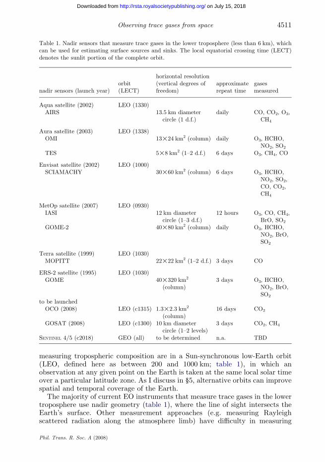
Table 1. Nadir sensors that measure trace gases in the lower troposphere (less than 6 km), whichcan be used for estimating surface sources and sinks. The local equatorial crossing time (LECT)denotes the sunlit portion of the complete orbit.

nadir sensors (launch year)orbit(LECT)

horizontal resolution(vertical degrees offreedom)

approximaterepeat time

gasesmeasured

Aqua satellite (2002) LEO (1330)AIRS 13.5 km diameter

circle (1 d.f.)daily CO, CO2, O3,

CH4

Aura satellite (2003) LEO (1338)OMI 13!24 km2 (column) daily O3, HCHO,

NO2, SO2

TES 5!8 km2 (1–2 d.f.) 6 days O3, CH4, CO

Envisat satellite (2002) LEO (1000)SCIAMACHY 30!60 km2 (column) 6 days O3, HCHO,

NO2, SO2,CO, CO2,CH4

MetOp satellite (2007) LEO (0930)IASI 12 km diameter

circle (1–3 d.f.)12 hours O3, CO, CH4,

BrO, SO2

GOME-2 40!80 km2 (column) daily O3, HCHO,NO2, BrO,SO2

Terra satellite (1999) LEO (1030)MOPITT 22!22 km2 (1–2 d.f.) 3 days CO

ERS-2 satellite (1995) LEO (1030)GOME 40!320 km2

(column)3 days O3, HCHO,

NO2, BrO,SO2

to be launchedOCO (2008) LEO (c1315) 1.3!2.3 km2

(column)16 days CO2

GOSAT (2008) LEO (c1300) 10 km diametercircle (1–2 levels)

3 days CO2, CH4

SENTINEL 4/5 (c2018) GEO (all) to be determined n.a. TBD

4511Observing trace gases from space


measuring tropospheric composition are in a Sun-synchronous low-Earth orbit(LEO, defined here as between 200 and 1000 km; table 1), in which anobservation at any given point on the Earth is taken at the same local solar timeover a particular latitude zone. As I discuss in §5, alternative orbits can improvespatial and temporal coverage of the Earth.

The majority of current EO instruments that measure trace gases in the lowertroposphere use nadir geometry (table 1), where the line of sight intersects theEarth’s surface. Other measurement approaches (e.g. measuring Rayleighscattered radiation along the atmosphere limb) have difficulty in measuring



P. I. Palmer4512


below the upper troposphere owing to optically thick clouds along the line ofsight; nadir measurements also suffer from this problem but their horizontalresolutions are typically small enough that they have a higher probability ofmeasuring (partial) cloud-free scenes. Limb-viewing instruments, such as theMichelson Interferometer for Passive Atmospheric Sounding (MIPAS; Fischeret al. 2008), the Microwave Limb Sounder (MLS; Waters et al. 2006) and theAtmospheric Chemistry Experiment (ACE; Bernath et al. 2005), occasionallyprovide valuable information on the distribution of trace gases in the freetroposphere, but they do not have sensitivity to the boundary layer. In thispaper, I focus on nadir sounders.

Nadir measurements use backscattered solar radiation at ultraviolet/visible(UV/Vis) and short-wave infrared (SWIR) wavelengths, which are sensitive tocloud, aerosol andRayleigh scattering.The thermal IR (TIR) region is alsomeasuredin this geometry using atmospheric absorption and emission phenomena. In general,observations of TIR wavelengths will be most sensitive to the middle and uppertroposphere, but will have some sensitivity to the lower troposphere when there issignificant thermal contrast between the lower andmiddle troposphere (Deeter et al.2007). Shorter wavelengths such as SWIR/Vis/UV will be sensitive to loweraltitudes and these are the wavelengths used by most tropospheric sensors. Otherfactors, such as spectral resolution, play a key role in the ability of an instrument toaccurately measure variations in lower tropospheric trace gases that are (i) orders ofmagnitude optically thinner than gases in the free troposphere (e.g. formaldehyde,HCHO) or (ii) well mixed owing to long atmospheric lifetimes (e.g. CO2).

There has been a rapid change in the emphasis of atmospheric trace gasmeasurements from those associated primarily with stratosphere O3 depletion tothose in the troposphere, associated with climate and surface air quality (AQ).This has been driven by a combination of a growing desire to quantitativelyunderstand surface sources and sinks of trace gases and the technological advancesthat are beginning to match this desire. Difficulties in measuring troposphericconcentrations arise from clouds and aerosols, a large number of ‘interfering’ tracegases with spectral lines that sometimes are close or overlap target gases, weakabsorption of target gases (e.g. HCHO), large stratospheric contributions of targetgases (e.g. nitrogen dioxide, NO2) and surface source–sink variations that representonly a small percentage of tropospheric columns of target gases (e.g. CO2).Improvements in spectroscopy (e.g. Gratien et al. 2007; Toth et al. 2007), radiativetransfer modelling (e.g. Natraj & Spurr 2007) and detector technology (increasedsensitivity and reliability) have all led to our ability to make more precise andaccurate measurements of tropospheric trace gases. These improvements areparticularly important for short-lived (lifetimes of less than hours to days) andlong-lived (lifetimes of several months to years) trace gases in the troposphere.Short-lived trace gases emitted (in)directly from surface sources typically have lowconcentrations (ppt to low ppb) and reside in the lower most atmosphere, soobserving them from space involves particularly sensitive analysis of the observedspectra. Long-lived trace gases have large background values, and fresh sourcesand sinks represent only a few per cent of this background so, as I discuss in §4, thishas led to precision requirements unprecedented in atmospheric remote sensing.

Carbon monoxide (CO) has an atmospheric lifetime ranging between weeksand months, depending on the abundance of its OH sink, which is long enoughthat it can be used effectively to track transport of atmospheric pollution





but short enough that pollution plumes can be distinguished from the globalbackground. It is therefore no coincidence that CO was one of the first moleculesto be measured in the troposphere at TIR wavelengths back in 1984 from theMeasurement of Air Pollution from Space (MAPS) instrument aboard the NASAShuttle (Connors et al. 1999). The resulting free tropospheric distributionsof CO, although sparse, were tantalizing. MAPS was a forerunner of the Measure-ment Of Pollution In The Troposphere (MOPITT), discussed in §4.

3. Estimating surface sources and sinks of trace gases from satellite data

Combining measurements and models, accounting for their respective errors,generally provides a better estimate of surface sources and sinks than using eithermeasurements or models alone. The underlying mathematics originates fromengineering and is largely developed for studying the Earth’s climate by thephysical oceanography and numerical weather prediction (NWP) communities(Kalnay 2006). The application of this mathematics to atmospheric chemistry isrelatively recent.

Relating observed variations in trace gas concentrations to the underlyingprocesses that determine the variability generally relies on using a model todescribe the processes. I define a forward model M, which includes all knownprocesses that determine variability in the observed tracer C,

CðtÞZMðPa;La;Ta;Xa;.ÞC3; ð3:1Þwhere P, L, T and X are defined as before, with subscript ‘a’ denoting our best apriori understanding of the real process. Model error, 3, represents the sum oferrors from the a priori, 3a, and the model physics and chemistry, 3m. For thepurpose of this discussion, I will estimate only surface production P. TheJacobian matrix K, containing the sensitivity of C(t) to changes in P (i.e.vC/vPa), is used to relate differences between model and observed concentrationsof trace gas C to P.

The observation and its associated error 3o, and the a priori and its error 3a,represent two pieces of information. I assume that 3o and 3a are unbiased and thatthe expected values (the average obtained after making many similarmeasurements) of the variances of the observation and model error are s2o ands2a. The inverse model I uses the measurements and a priori information todetermine the optimal estimate of production, P: PZI ðMðPaÞ; 3a;C ; 3oÞ. Thereare a number of ways to reach the optimal solution, but I use the maximum aposteriori solution to show that

P Zs2a

Ks2o Cs2a

C

KC

Ks2o

Ks2o Cs2aPa; ð3:2Þ

which is essentially a linear least-squares fit of model production rate Pa toobserved trace gas measurements C, weighted by their respective uncertainties.For example, as the relative error on the a priori s2a increases (i.e. we have less

confidence in the a priori compared with the measurements), P is increasinglydetermined by the first right-hand side term that contains information from themeasurements. Of course, this is a simple example, in which I have considered alinear problem with only one measurement and one variable to estimate, but it



P. I. Palmer4514


captures the essence of an active research problem. It is also worth noting thatmeasurements from satellite instruments generally represent a weighted mean ofthe real vertical atmospheric profile. The vertical weighting profile, determinedby the instrument type, wavelength studied and the geophysical scenario(e.g. surface albedo), should be applied to the forward model M in the inversemodel calculation.

As the precision and spatial and temporal resolutions of satellite data improve,and, more importantly, confidence about these data grows in the community,a more fundamental science objective is the estimation of the smaller scaleprocesses that determine the large-scale source and sink distributions. Thisinvolves solving for model parameters, such as the temperature sensitivity ofproduction. The method outlined above remains the same, but M is morecomplex (now explicitly describing small-scale processes that are sometimesparametrized in large-scale models) and K now describes the sensitivity of C(t) tochanges in the model parameters.

4. Current science highlights

Here, I outline a few of the many science highlights associated with understandingatmospheric and surface sources and sinks of trace gases using satellitemeasurements. As the reader will appreciate, the work shown here is the subjectof ongoing research.

(a ) Fossil fuel emissions

A number of trace gases are associated with fossil fuel emissions, and here Idiscuss NO2 and CO2. Fossil fuel emissions represent approximately half theglobal budget of NOx (NOCNO2), originating from oxygen thermolysis at hightemperatures (approximately equal to 2000 K) and subsequent reactions with N2.Space-borne NO2 measurements have been available for more than a decade(table 1). Tropospheric NO2 columns are inferred from the total columns bysubtracting the stratospheric contribution, assuming zonal invariance of thestratospheric contribution. Emissions of NOx can then be estimated from thesedata by assuming knowledge of the lifetime of NOx and of the ratio NO2–NOx

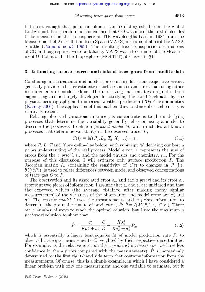
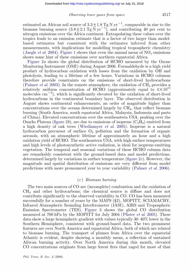
that can be taken from a model of atmospheric chemistry (Martin et al. 2003).Figure 1 shows tropospheric NO2 columns from the SCanning ImAging

spectroMeter for Atmospheric CHartographY (SCIAMACHY) between May2004 and April 2005 (Martin et al. 2006). The largest columns are generallyassociated with major industrial and metropolitan areas. There are alsoenhancements over central Africa, reflecting seasonal biomass burning; overnorthern equatorial Africa, attributed to rain-induced soil NOx emissions(discussed below); and near Kuala Lumpur along ship tracks. Figure 1 alsoshows NOx emissions determined by combining a priori NOx emissions and theSCIAMACHY NOx emissions following equation (3.2). The resulting a posterioriglobal emissions are more than 20 per cent higher than prior estimates, with theassociated uncertainty reduced by half. The biggest discrepancies between the apriori and the a posteriori are over major industrial areas, including Beijing,Tokyo, Buenos Aires and New York City; the ability to relate these discrepanciesto particular cities is a reflection of the spatial resolution of the data and the



0 1 2 3 4

tropospheric NO2 (1015 molecules cm–2)

5 6 7 8

a posteriori46.1 Tg N yr –1

5

4

3

2

1011

ato

ms

N c

m–2

s–1

1

0

(a)

(b)

Figure 1. (a) Tropospheric NO2 columns (1015 molecules cmK2) retrieved from the SCIAMACHYfor May 2004–April 2005 and (b) associated NOx emissions (1011 atoms N cmK2 sK1). NO2

columns, filtered for cloud radiance less than 0.5, are averaged on a 0.48!0.48. The NOx emissions,averaged on a 28!2.58 grid, are determined through inverse modelling of the NO2

columns using the GEOS-Chem chemistry transport model. Figure courtesy of Randall Martin,Dalhousie University.



annual mean quantities that reduce the random noise on these data. Somestudies have adopted a first-order approximation of this approach to directly usevariations in tropospheric NO2 as a proxy for local emissions (e.g. Richter et al.2005). Interpretation of these NO2 columns over multiple years allows NOx

emission trends to be studied. Data from the Global Ozone MonitoringExperiment (GOME) and SCIAMACHY instruments between 1996 and 2004showed a larger than expected accelerating trend of emissions over the industrialregions within China (50% increase over the 9 year period), due to energy growthand technology renewal (Richter et al. 2005). This study also showed asubstantial decrease over Europe and the USA, which the authors relate tocleaner car exhausts and changing economical circumstances. The SCIAMACHYhas also been used to revise emissions of NOx from international shipping, a largesource of many trace gases that is currently not included in emission treaties.



P. I. Palmer4516


The spatial distribution of observed and model NOx emissions from shipping wasconsistent, but SCIAMACHY observations were typically lower, although theyhad large uncertainties (Richter et al. 2004).

CO2 observations are currently available from three satellite sensors: theSCIAMACHY; the Atmospheric InfraRed Sounder (AIRS); and the TelevisionInfrared Observation Satellite Operational Vertical Sounder (TOVS), and will beavailable from two instruments due for launch in early 2009, the Orbiting CarbonObservatory (OCO) and the Greenhouse Observing SATellite (GOSAT; table 1).Synthetic studies have shown that for these CO2 data to be useful for regional-scale source–sink estimates, they have to have precisions of 1–2 ppm (Rayner &O’Brien 2001); even precisions as poor as 5 ppm on regional scales would improveupon our current understanding of the carbon cycle (CC; Miller et al. 2007),given the spatial coverage provided by these data. Biases on spatial scales shorterthan 100!100 km2 can be discounted as random noise. Similarly, a global offsetin the observations will not affect the inverse modelling since they introduce noerror in the observed gradients. Biases on regional to continental scales (i.e.greater than 104 km2) have the largest impact on inferred CO2 surface fluxes(Miller et al. 2007). Studies to infer CO2 sources and sinks from the AIRS andTOVS data, using TIR wavelengths, have concluded that the regional biases inthe observations, and low sensitivity to the lower troposphere, compromise theestimates (Chevallier et al. 2005a,b). The SCIAMACHY is the only instrumentcurrently in orbit which measures CO2 columns that are sensitive to the lowertroposphere by measuring SWIR wavelengths. Work has shown that the data arebroadly consistent with the observed seasonal variations of vegetation patternsover North America and agree with column variations observed by high-precisionground-based instrument and AIRS data (Barkley et al. 2006a,b; Bosch et al.2006). The year to year trend is also remarkably consistent with surfaceobservations that show an annual cycle, driven by photosynthesis andrespiration, on an upward trend (Buchwitz et al. 2007). However, theSCIAMACHY suffers from an unexplained bias that is the subject of ongoingwork. The OCO and GOSAT instruments will improve on the SCIAMACHY byhaving an order of magnitude better resolution that permits improved fitting onCO2 absorption features at SWIR wavelengths and improved spatial resolution.

(b ) Natural sources and sinks of trace gases

Terrestrial vegetation, soils, lightning (Martin et al. 2007) and wetlands areexamples of natural sources and sinks of a range of trace gases, which we arebeginning to quantify at regional scales through the use of satellite measurements.

Soils represent approximately 15 per cent of global NOx emissions, of which70 per cent are estimated to originate from the tropics. Long, dry periods intropical ecosystems allow soils to accumulate inorganic nitrogen. Through fieldmeasurements, we have known for some time that the onset of the wet seasonactivates water-stressed nitrifying bacteria, leading to large pulses of NO as aby-product of consuming the inorganic nitrogen, but the spatial and temporalextent of this source was not understood until recently. Analysis of satelliteobservations of NO2 from the GOME showed that, following the onset of the wetseason over the Sahel, large pulses of NO lasting one to three weeks affect3 million km2 of semiarid sub-Saharan savannah (Jaegle et al. 2004). This work





estimated an African soil source of 3.3G1.8 Tg N yrK1, comparable in size to thebiomass burning source (3.8G2.1 Tg N yrK1), and contributing 40 per cent tonitrogen emissions over the Africa continent. Extrapolating these values over thetropics leads to an emission estimate that is a factor of two larger than model-based estimates but consistent with the estimates inferred from othermeasurements, with implications for modelling tropical tropospheric chemistry(Jaegle et al. 2004). Figure 1 shows that even the annual mean of NOx emissionsshows some hint of these emissions over northern equatorial Africa.

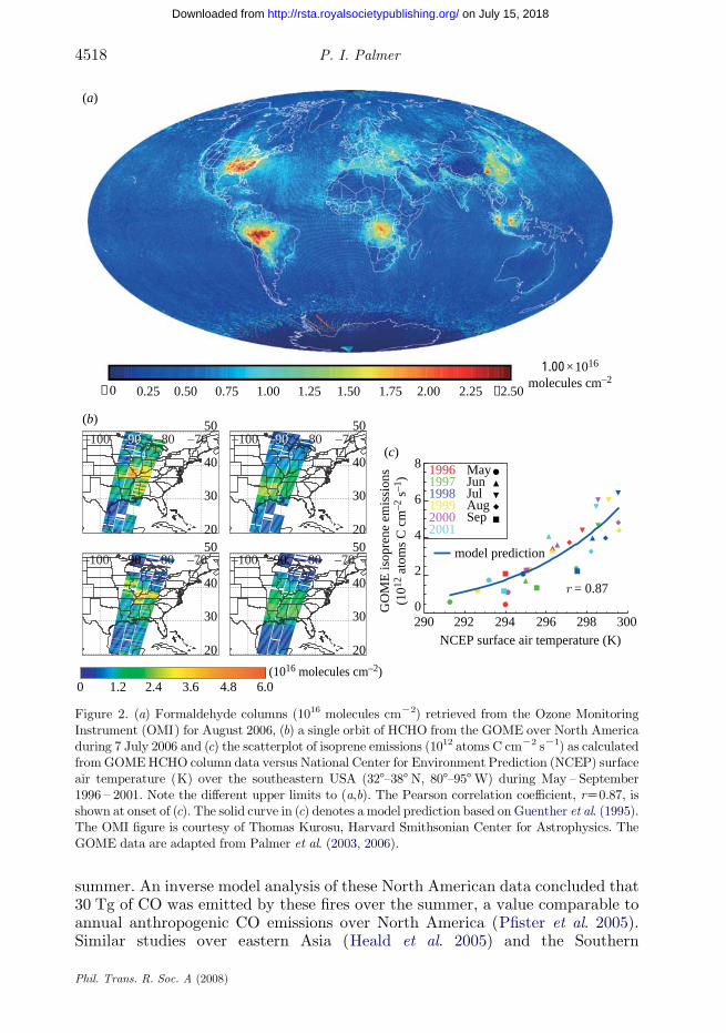
Figure 2a shows the global distribution of HCHO measured by the OzoneMonitoring Instrument (OMI) during August 2006. Formaldehyde is a high yieldproduct of hydrocarbon oxidation with losses from the oxidation by OH andphotolysis, leading to a lifetime of a few hours. Variations in HCHO columnstherefore provide constraints on the emissions of short-lived hydrocarbons(Palmer et al. 2003). In the remote atmosphere, the oxidation of CH4 provides arelatively uniform concentration of HCHO (approximately equal to 4!1015

molecules cmK2), which is significantly elevated by the oxidation of short-livedhydrocarbons in the continental boundary layer. The observed distribution inAugust shows continental enhancements, an order of magnitude higher thanconcentrations over the oceans determined largely by CH4, that reflect biomassburning (South America, south equatorial Africa, Malaysia, Indonesia and partsof China). Elevated concentrations over the southeastern USA, peaking over theOzarks Plateau (figure 2b), are due to emissions of isoprene (C5H8) emitted froma high density of oak trees (Wiedinmyer et al. 2005). Isoprene is a naturalhydrocarbon precursor of surface O3 pollution and the formation of organicaerosols, with an atmospheric lifetime of approximately an hour and a highoxidation yield of HCHO. The southeastern USA, with high surface temperaturesand high levels of photosynthetic active radiation, is ideal for isoprene-emittingvegetation. The temporal and seasonal variations of these HCHO column dataare remarkably consistent with the ground-based data and model predictions,determined largely by variations in surface temperature (figure 2c). However, themagnitude and spatial distribution of emissions are very different from modelpredictions with more pronounced year to year variability (Palmer et al. 2006).

(c ) Biomass burning

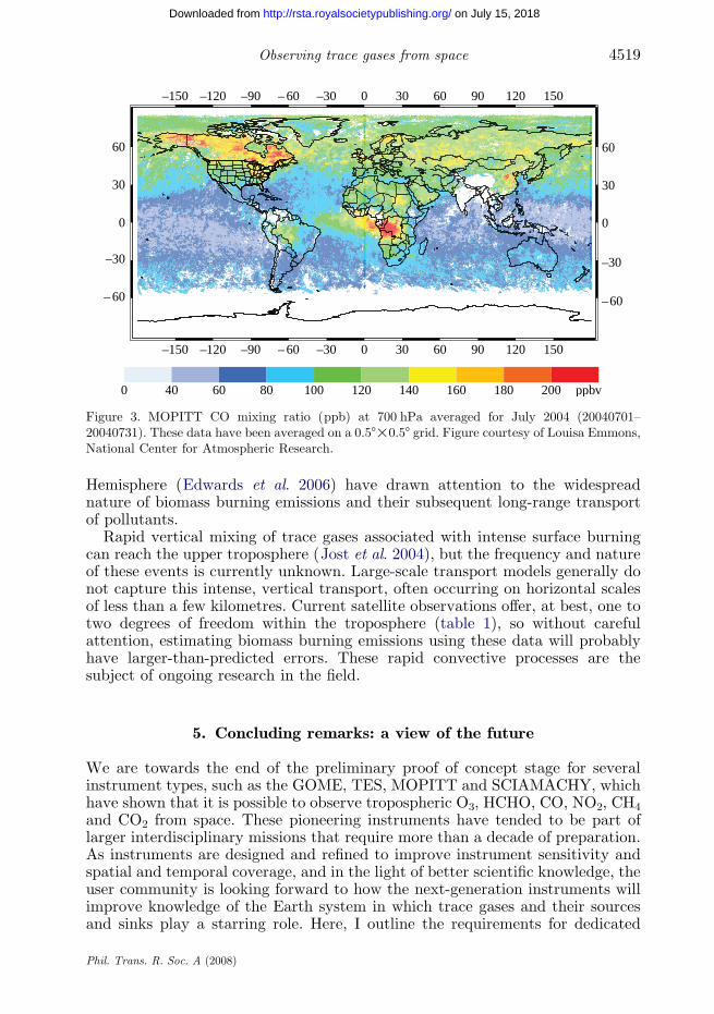
The two main sources of CO are (incomplete) combustion and the oxidation ofCH4 and other hydrocarbons; the chemical source is diffuse and does notcontribute significantly to the observed variability in CO. CO has been measuredsuccessfully for a number of years by the MAPS (§2), MOPITT, SCIAMACHY,Infrared Atmospheric Sounding Interferometer (IASI), AIRS and TroposphericEmission Spectrometer (TES). Figure 3 shows the global CO distributionmeasured at 700 hPa by the MOPITT for July 2004 (Pfister et al. 2005). Thesedata show a large hemispheric gradient with values typically 30–40% lower in theSouthern Hemisphere, consistent with ground-based data. The two prominentfeatures are over North America and equatorial Africa, both of which are relatedto biomass burning. The transport of plumes from Africa over the equatorialAtlantic is evident, despite showing a monthly mean, a reflection of sustainedAfrican burning activity. Over North America during this month, elevatedCO concentrations originate from large forest fires that raged for most of that



2900

2

4

6

8

292

GO

ME

isop

rene

em

issi

ons

(1012

ato

ms

C c

m–2

s–1

)

294NCEP surface air temperature (K)

296 298 300

≤ 0 0.25 0.50 0.75 1.00 1.25 1.50 1.75 2.00 2.25 ≥2.50

1.00×1016

molecules cm–2

(a)

(b)

(c)

= 0.87

model prediction

2.4 3.6 4.8 6.01.20(1016 molecules cm–2)

20

30

40

50–70–80–90–100

20

30

40

50–70–80–90–100

20

30

40

50–70–80–90–100

20

30

40

50–70–80–90–100

1996 MayJunJulAugSep

19971998199920002001

Figure 2. (a) Formaldehyde columns (1016 molecules cmK2) retrieved from the Ozone MonitoringInstrument (OMI) for August 2006, (b) a single orbit of HCHO from the GOME over North Americaduring 7 July 2006 and (c) the scatterplot of isoprene emissions (1012 atoms C cmK2 sK1) as calculatedfromGOMEHCHO column data versus National Center for Environment Prediction (NCEP) surfaceair temperature (K) over the southeastern USA (328–388 N, 808–958W) during May – September1996 – 2001. Note the different upper limits to (a,b). The Pearson correlation coefficient, rZ0.87, isshown at onset of (c). The solid curve in (c) denotes a model prediction based on Guenther et al. (1995).The OMI figure is courtesy of Thomas Kurosu, Harvard Smithsonian Center for Astrophysics. TheGOME data are adapted from Palmer et al. (2003, 2006).

P. I. Palmer4518


summer. An inverse model analysis of these North American data concluded that30 Tg of CO was emitted by these fires over the summer, a value comparable toannual anthropogenic CO emissions over North America (Pfister et al. 2005).Similar studies over eastern Asia (Heald et al. 2005) and the Southern



–150 –120 –90 – 60 –30 0 30 60 90 120 150

–150 –120 –90 – 60 –30 0 30 60 90 120 150

– 60

–30

0

30

60

–60

–30

0

30

60

0 40 60 80 100 120 140 160 180 200 ppbv

Figure 3. MOPITT CO mixing ratio (ppb) at 700 hPa averaged for July 2004 (20040701–20040731). These data have been averaged on a 0.58!0.58 grid. Figure courtesy of Louisa Emmons,National Center for Atmospheric Research.



Hemisphere (Edwards et al. 2006) have drawn attention to the widespreadnature of biomass burning emissions and their subsequent long-range transportof pollutants.

Rapid vertical mixing of trace gases associated with intense surface burningcan reach the upper troposphere (Jost et al. 2004), but the frequency and natureof these events is currently unknown. Large-scale transport models generally donot capture this intense, vertical transport, often occurring on horizontal scalesof less than a few kilometres. Current satellite observations offer, at best, one totwo degrees of freedom within the troposphere (table 1), so without carefulattention, estimating biomass burning emissions using these data will probablyhave larger-than-predicted errors. These rapid convective processes are thesubject of ongoing research in the field.

5. Concluding remarks: a view of the future

We are towards the end of the preliminary proof of concept stage for severalinstrument types, such as the GOME, TES, MOPITT and SCIAMACHY, whichhave shown that it is possible to observe tropospheric O3, HCHO, CO, NO2, CH4

and CO2 from space. These pioneering instruments have tended to be part oflarger interdisciplinary missions that require more than a decade of preparation.As instruments are designed and refined to improve instrument sensitivity andspatial and temporal coverage, and in the light of better scientific knowledge, theuser community is looking forward to how the next-generation instruments willimprove knowledge of the Earth system in which trace gases and their sourcesand sinks play a starring role. Here, I outline the requirements for dedicated



P. I. Palmer4520


atmospheric chemistry and CC missions and critically assess the options that arecurrently being discussed in the international community. I conclude the paperby discussing two future applications of EO data: (i) surface AQ mitigation and(ii) carbon trading.

(a ) Orbital configuration: horses for courses

The orbit in which a satellite instrument resides partly determines the scienceobjectives it can achieve. I shall consider three orbits for future tropospherictrace gas measurements: low-Earth orbit (Sun-synchronous and precessing);geostationary orbit (GEO); and a Lagrange-1 (L1) orbit. Here, I outline the orbitrequirements for AQ and CC missions and discuss them in the context of LEO,GEO and L1, based on recommendations put forward by the AQ community tothe US National Research Council decadal survey. Many, if not all, of theserequirements would also be desirable for a CC mission. I have not considered amid-Earth orbit because, at these altitudes (1500–15 000 km), incoming radiationwould damage current-generation UV/Vis technology, seriously limiting itsscience deliverables.

Fine horizontal sampling in satellite measurements is obvious for almost anyEO sensor. A horizontal resolution of 1 km or better over land, particularly oversource regions, would be required for an AQ mission, but an instrument shouldalso provide regional-scale information. A broad swath capability withoverlapping measurements would effectively relax the horizontal resolutionrestriction to 10 km.

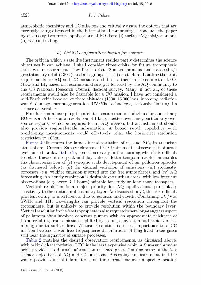
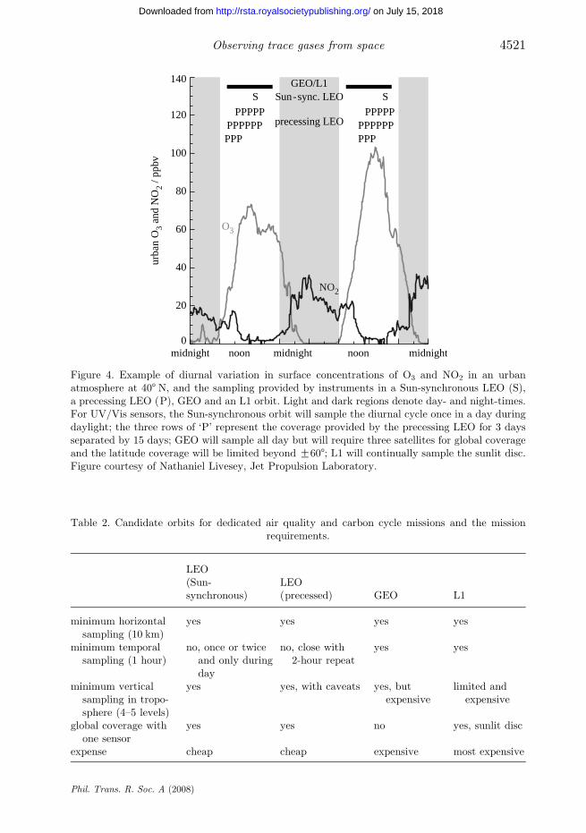
Figure 4 illustrates the large diurnal variation of O3 and NO2 in an urbanatmosphere. Current Sun-synchronous LEO instruments observe this diurnalcycle once in a day (table 1), sometimes early in the morning when it is difficultto relate these data to peak mid-day values. Better temporal resolution enablesthe characterization of (i) synoptic-scale development of air pollution episodes(as discussed below), (ii) the diurnal variation of emissions, (iii) stochasticprocesses (e.g. wildfire emission injected into the free atmosphere), and (iv) AQforecasting. An hourly resolution is desirable over urban areas, with less frequentobservations (e.g. every 3–4 hours) suitable for studying long-range transport.

Vertical resolution is a major priority for AQ applications, particularlysensitivity to the continental boundary layer. As discussed in §2, this is a difficultproblem owing to interferences due to aerosols and clouds. Combining UV/Vis,SWIR and TIR wavelengths can provide vertical resolution throughout thetroposphere, but is unlikely to provide resolution within the boundary layer.Vertical resolution in the free troposphere is also requiredwhere long-range transportof pollutants often involves coherent plumes with an approximate thickness of1 km, resulting from emissions uplifted by fronts, convection and rapid verticalmixing due to surface fires. Vertical resolution is of less importance to a CCmission because lower free tropospheric distributions of long-lived trace gasesstill bear the signature of surface processes.

Table 2 matches the desired observation requirements, as discussed above,with orbital characteristics. LEO is the least expensive orbit. A Sun-synchronousorbit provides no diurnal information on trace gases, limiting some of the keyscience objectives of AQ and CC missions. Precessing an instrument in LEOwould provide diurnal information, but the repeat time over a specific location



PPPPP PPPPPPPPPPP PPPPPPPPP PPP

precessing LEO

S SSun-sync. LEOGEO/L1

O3

NO2

midnight noon midnight noon midnight0

20

40

60

80

100

120

140

urba

n O

3 an

d N

O2

/ ppb

v

Figure 4. Example of diurnal variation in surface concentrations of O3 and NO2 in an urbanatmosphere at 408 N, and the sampling provided by instruments in a Sun-synchronous LEO (S),a precessing LEO (P), GEO and an L1 orbit. Light and dark regions denote day- and night-times.For UV/Vis sensors, the Sun-synchronous orbit will sample the diurnal cycle once in a day duringdaylight; the three rows of ‘P’ represent the coverage provided by the precessing LEO for 3 daysseparated by 15 days; GEO will sample all day but will require three satellites for global coverageand the latitude coverage will be limited beyond G608; L1 will continually sample the sunlit disc.Figure courtesy of Nathaniel Livesey, Jet Propulsion Laboratory.

Table 2. Candidate orbits for dedicated air quality and carbon cycle missions and the missionrequirements.

LEO(Sun-synchronous)

LEO(precessed) GEO L1

minimum horizontalsampling (10 km)

yes yes yes yes

minimum temporalsampling (1 hour)

no, once or twiceand only duringday

no, close with2-hour repeat

yes yes

minimum verticalsampling in tropo-sphere (4–5 levels)

yes yes, with caveats yes, butexpensive

limited andexpensive

global coverage withone sensor

yes yes no yes, sunlit disc

expense cheap cheap expensive most expensive





P. I. Palmer4522


will be longer and interpretation of these data would be difficult without a model.Temporal resolution could also be improved by (i) broad across-track swath sothat 2 hours temporal resolution can be achieved by overlapping measurementsin successive orbits, but this is eventually limited by viewing angle and also leadsto a larger probability of cloudy scenes, (ii) using an inclined orbit but thissacrifices high latitude measurements, and (iii) using a constellation of satellites.At the moment, the GOME-2 aboard MetOp and the OMI aboard Aura samplethe diurnal cycle twice (table 1). Constellation costs (each platform with adifferent local equatorial crossing time) could be reduced by exploitingcommercial piggybacking opportunities, e.g. the Iridium NEXT constellationrepresenting 66 LEO payloads that will be launched in 2013.

A GEO places a satellite at approximately 36 000 km above the Earth’s equatorand has an orbital period equal to the Earth period of rotation so that the satelliteobserves the same view all day. Such an orbit is often used for meteorological orcommunication satellites. Measurements can made at UV to TIR wavelengths andfulfils all the resolution requirements for an AQ mission (table 1), with the caveatthat achieving a vertical resolution similar to the next generation of LEO will beexpensive. Continuous temporal coverage of the sunlit disc effectively removes theproblem of cloud obscuration. Three satellites are required to globally observe lowto mid-latitudes, with resolution and signal-to-noise decreasing at higher latitudesand associated viewing zenith angles. Geostationary measurements of aerosoloptical properties, available from the Meteosat Second Generation SpinningEnhanced Visible and InfraRed Imager (SEVIRI), show great promise in helping tounravel the role of aerosols in modifying cloud radiative properties. The EuropeanSpace Agency have nominally assigned Sentinel 4 as a geostationary platform foratmospheric chemistry studies to be launched in ca 2018.

The Lagrangian (L1) orbit places an instrument at approximately 1.5 million kmaway from the Earth, a special point between the Earth and Sun, wherethe instrument will always view the complete sunlit disc. This combines theadvantage of global coverage provided by LEO/MEO and the temporal coverage ofGEO, and fulfils all the air quality mission requirements (table 1). This orbit suffersfrom a lack of vertical resolution, which, as I discussed above, is an importantdimension to consider for trace gases with short lifetimes and for studies overgeographical regions with rapid vertical transport. This is the most technicallychallenging and the most costly of all the orbits considered here, owing to the largertelescope required to observe the Earth from such a distance, but it does have aprecedent. The SOlar and Heliospheric Observatory (SOHO) is the only instrumentthat has resided in the L1 orbit at an approximate cost of 1000 M euros.

(b ) Adopting an Earth system approach

Partly due to the success of past and existing instruments, the number of newquestions we have about the Earth system is larger than the original set ofquestions we had a decade ago. This is also a reflection of our increasingawareness that the Earth system is connected together via a complex web ofinteractions that act on a wide spectrum of spatial and temporal scales. As acommunity, we are also becoming aware that some climate feedbacks fromradiative forcing can be sudden, responding to warming within a decade, e.g.melting of arctic permafrost that could release uncertain amounts of CH4 into the





atmosphere. So how do we proceed? Do we move towards a framework of rapidresponse instruments that can be proposed, built and deployed within a fewyears, which can monitor rapid climate change? Do we focus on comprehensivemonitoring of key trace gases in the atmosphere? Or do we move towards a moreintegrated approach of measuring the Earth by designing Earth systemmonitoring platforms that measure a wide suite of variables that help interprettrace gas distributions in the troposphere?

The most scientifically fruitful approach is, perhaps, to develop intermediatesize EO satellite platforms that comprehensively sample a particular aspect ofthe Earth system and can be developed and flown within 4–5 years of beingproposed. Measuring trace gases such as CH4 and CO2 to a precision required toobserve surface fluxes represents an engineering feat, but there is no uniqueinformation within the measurement itself to improve understanding aboutsource attribution, i.e. whether elevated CO2 is from biomass burning, fossil fuelcombustion or respiration. Using correlations between different trace gases (e.g.using CO to inform about the combustion source) will help with this issue butthey will not provide useful information with which to better understand theunderlying processes. Coincident measurements of terrestrial photosynthesis(using ratios of spectral bands), fire radiative power (Wooster et al. 2005) andsoil moisture, for instance, would disproportionately increase the science returnof satellite observations of trace gases. Such a synergistic approach to measuringthe CC would facilitate, for example, the study of the daily interplay betweenleaf phenology, hydrology, biology and atmospheric chemistry and transport.

(c ) A grand challenge: integrating EO data and climate policy

The science and policy of climate is becoming progressively interlinked as theeconomic and humanitarian impacts of projected climate scenarios are beingrealized. Here, I discuss two examples in which I believe EO measurements oftropospheric trace gases can play a prominent role: (i) mitigating chronic surfaceair pollution and (ii) reducing global anthropogenic carbon emissions throughcarbon trading schemes.

(i) Surface air pollution forecasting and mitigation

The chronic surface AQ event over Europe during the August 2003 heatwaveserves as an example of the human impacts of surface air pollution, with manyhundreds of deaths linked with elevated concentrations of surface ozone (greaterthan 100 ppb; Stedman 2004). The build up on pollution over the UK duringthat period was due to a stable high-pressure system that broughtin pollution from mainland Europe and prevented dilution of boundary-layerpollution to the free troposphere. The increased temperatures associated withthis meteorology led to rapid production of pollution exacerbated bytemperature-dependent emissions of isoprene, which effectively increase surfaceO3 concentrations (Lee et al. 2006). The frequency of heatwaves as hot as 2003has been projected to increase 100-fold over the next 40 years (Stott et al. 2004).If these projections are realized, current European surface air pollution episodesare likely to become more extreme with associated impacts on human healthand agriculture.



P. I. Palmer4524


So how can satellite measurements help? We already have NWP models, oneof the principal outputs from which is the weather forecasts shown in the media.NWP centres are already moving towards using satellite observations of tracegases to provide regional AQ forecasts. At some stage, we should expect forecastmaps of surface O3 and other pollutants that will guide our day-to-day lives, e.g.not to exercise vigorously when surface O3 is above a critical threshold. Whatthis approach does not consider is using these forecasts to develop mitigationstrategies. As discussed above, distributions of NO2 and HCHO provideinformation on their sources and sinks, which can be used to improve thepredictive capabilities of emission and chemistry models. If we know ahead oftime, even a few days, that the meteorological and AQ conditions over Londonduring mid-summer 2012 will be similar to those experienced during the 2003heatwave, we would have the ability to minimize or even avert a chronic AQepisode. In this case, instead of solving just for physical and chemical parameters,we can broaden equation (3.2) to simultaneously minimize the economic ‘costs’ ofair pollution episodes on regional human health, industry and food supply.Estimating the costs and risks of surface air pollution required extensiveeconomic and epidemiological analyses. However, armed with such a predictivemitigation system, national governments will be able to help control the healthand economic implications of surface air pollution.

(ii) Carbon trading

International trading of carbon emissions on the open market is an approachthat is being implemented to incrementally reduce anthropogenic CO2 emissions.The premise is that emissions from individual countries will be capped at afigure determined by emissions from prior years. If a country emits more thanthe capped amount, they must buy permits to cover the excess carbon fromanother country’s allocation that is surplus to requirement. The global cap willbe reduced over a number of years and the associated price of carbon emissionwill increase, if we assume no rapid increase in carbon capture technology. Thiscap and trade approach to carbon trading is a new and rapidly growing financialmarket that is likely to be worth trillions of sterling in coming years.

To ensure the successful operation of carbon trading schemes, it is important toensure subsequent adherence to nationwide emission commitments. A majorcriticism of carbon trading as an effective method of reducing emissions of CO2

is that there is currently no objective measure of adherence that has realisticconfidence intervals. Carbon emission permit and trading schemes currentlyrely on self-reporting by firms, based on (essentially) fixed ratios of emissionsto output, withmonitoring by local or national environmental agencies, with powersto penalize offending firms. The quality of regulation is likely to vary greatlybetween industries, regions and countries, which is clearly not satisfactory formitigating the anthropogenic contribution to climate climate. Reporting carbonemissions is less time sensitive than air quality mitigation strategies, but rapiddissemination of results is still useful. It is unlikely that, in the near future (within 10years), satellite observations of CO2 will be sufficiently accurate to provide reliableindependent flux estimates on spatial scales less than 100 km, but subcontinentregional assessments should be possible with upcoming satellite instruments. Thefirst step to integrate atmospheric measurements of CO2 in carbon trading schemes





is to determine the measurement network necessary to provide robust CO2 fluxestimates and associated uncertainties on spatial and temporal scales of interest.The extent to which satellites play a role in such a network will partly rely on thesuccess of the upcoming OCO and GOSAT instruments.

I thank Nathaniel Livesey for a critical review of an earlier draft and much advice; Randall Martin,Thomas Kurosu, Louisa Emmons and Christian Frankenberg for providing figures and generalsupport; and John Burrows, Cathy Clerbaux, Folkert Boersma and Paul Monks for advice on thework shown. I also thank Hartmut Bosch and an anonymous reviewer for providing their usefulinput on the submitted paper.

References

Barkley, M. P., Monks, P. S., Frieß, U., Mittermeier, R., Fast, H., Korner, S. & Heimann, M.2006a Comparisons between SCIAMACHY atmospheric CO2 retrieved using (FSI) WFM-DOAS to ground based FTIR data and the TM3 chemistry transport model. Atmos. Chem.Phys. 6, 4483–4498.

Barkley, M. P., Monks, P. S. & Engelen, R. J. 2006b Comparison of SCIAMACHY and AIRS CO2

measurements over North America during the summer and autumn of 2003. Geophys. Res. Lett.33, L20 805. (doi:10.1029/2006GL026807)

Bernath, P. F. et al. 2005 Atmospheric chemistry experiment (ACE): mission overview. Geophys.Res. Lett. 32, L15 S01. (doi:10.1029/2005GL022386)

Bosch, H. et al. 2006 Space-based near-infrared CO2 retrievals: testing the OCO retrieval algorithmand validation concept using SCIAMACHY measurements over Park Falls, Wisconsin.J. Geophys. Res. 111, D23 302. (doi:10.1029/2006JD007080)

Buchwitz, M., Schneising, O., Burrows, J. P., Bovensmann, H., Reuter, M. & Notholt, J. 2007First direct observation of the atmospheric CO2 year-to-year increase from space. Atmos.Chem. Phys. 7, 4249–4256.

Chevallier, F., Engelen, R. J. & Peylin, P. 2005a The contribution of AIRS data to the estimationof CO2 sources and sinks. J. Geophys. Res. 32, L23 801. (doi:10.1029/2005GL024229)

Chevallier, F., Fisher, M., Peylin, P., Serrar, S., Bousquet, P., Breon, F.-M., Chedin, A. & Ciais, P.2005b Inferring CO2 sources and sinks from satellite observations: method and application toTOVS data. J. Geophys. Res. 110, D24 309. (doi:10.1029/2005JD006390)

Connors, V. S., Gormsen, B. B., Nolf, S. & Reichle Jr, H. G. 1999 Spaceborne observations of theglobal distribution of carbon monoxide in the middle troposphere during April and October1994. J. Geophys. Res. 104, 21 455–21 470. (doi:10.1029/1998JD100085)

Deeter, M. N., Edwards, D. P., Gille, J. C. & Drummond, J. R. 2007 Sensitivity of MOPITTobservations to carbon monoxide in the lower troposphere. J. Geophys. Res. 112, D24 306.(doi:10.1029/2007JD008929)

Edwards, D. P. et al. 2006 Satellite-observed pollution from Southern Hemisphere biomassburning. J. Geophys. Res. 111, D14 312. (doi:10.1029/2005JD006655)

Fischer, H. et al. 2008 MIPAS: an instrument for atmospheric and climate research. Atmos. Chem.Phys. Discuss. 8, 2151–2188.

Gratien, A., Picquet-Varrault, B., Orphal, J., Perraudin, E., Doussin, J.-F. & Flaud, J.-M. 2007Laboratory intercomparison of the formaldehyde absorption cross sections in the infrared(1660–1820 cmK1) and ultraviolet (300–360 nm) spectral regions. J. Geophys. Res. 112,D05 305. (doi:10.1029/2006JD007201)

Guenther, A. et al. 1995 A global model of natural volatile organic compound emissions.J. Geophys. Res. 100, 8873–8892. (doi:10.1029/94JD02950)

Heald, C. L. et al. 2004 Comparative inverse analysis of satellite (MOPITT) and aircraft (TRACE-P)observations to estimate Asian sources of carbonmonoxide. J. Geophys. Res. 109, D23 306. (doi:10.1029/2004JD005185)


http://dx.doi.org/doi:10.1029/2006GL026807


http://dx.doi.org/doi:10.1029/2006JD007080











P. I. Palmer4526


IPCC 2007 Climate change 2007: the physical science basis. In Contribution of working group I to

the fourth assessment report of Intergovernmental Panel on Climate Change (eds S. Solomon,D. Qin, M. Manning, Z. Chen, M. Marquis, K.B. Averyt, M. Tignor & H. L. Miller), pp. 996.

Cambridge, UK; New York, NY: Cambridge University Press.Jacob, D. J. et al. 2003 The transport and chemical evolution over the Pacific (TRACE-P) aircraft

mission: design, execution, and first results. J. Geophys. Res. 108, 9000. (doi:10.1029/2002JD003276)

Jaegle, L. et al. 2004 Satellite mapping of rain-induced nitric oxide emissions from soils.J. Geophys. Res. 109, D21 310. (doi:10.1029/2004JD004787)

Jost, H.-K. et al. 2004 In situ observations of mid-latitude forest fire plumes deep in thestratosphere. Geophys. Res. Lett. 31, L11 101. (doi:10.1029/2003GL019253)

Kalnay, E. 2006 Atmospheric modeling, data assimilation and predictability, p. 341. Cambridge,UK: Cambridge University Press.

Lee, J. D. et al. 2006 Ozone photochemistry and elevated isoprene during the UK heatwave of 2003.Atmos. Environ. 40, 7598–7613. (doi:10.1016/j.atmosenv.2006.06.057)

Martin, R. V., Jacob, D. J., Chance, K., Kurosu, T. P., Palmer, P. I. & Evans, M. J. 2003 Globalinventory of nitrogen oxide emissions constrained by space-based observations of NO2 columns.

J. Geophys. Res. 108, 4537. (doi:10.1029/2003JD003453)Martin, R. V. et al. 2006 Evaluation of space-based constraints on global nitrogen oxide emissions

with regional aircraft measurements over and downwind of eastern North America. J. Geophys.Res. 111, D15 308. (doi:10.1029/2005JD006680)

Martin, R. V., Sauvage, B., Folkins, I., Sioris, C. E., Boone, C., Bernath, P. & Ziemke, J. 2007Space-based constraints on the production of nitric oxide by lightning. J. Geophys. Res. 112,

D09 309. (doi:10.1029/2206JD007831)Miller, C. E. et al. 2007 Precision requirements for space-based XCO2

data. J. Geophys. Res. 112,

D10 314. (doi:10.1029/2006JD007659)Natraj, V. & Spurr, R. J. D. 2007 A fast pseudo-spherical two orders of scattering model to account

for polarization in vertically inhomogeneous scattering–absorbing media. J. Quant. Spectrosc.Rad. Trans. 107, 263–293. (doi:10.1016/j.jqsrt.2007.02.011)

Palmer, P. I., Jacob, D. J., Fiore, A. M., Martin, R. V., Chance, K. & Kurosu, T. P. 2003 Mappingisoprene emissions over North America using formaldehyde column observations from space.

J. Geophys. Res. 108, 4180. (doi:10.1029/2002JD002153)Palmer, P. I. et al. 2006 Quantifying the seasonal and interannual variability of North American

isoprene emissions using satellite observations of formaldehyde column. J. Geophys. Res. 111,D12 315. (doi:10.1029/2005JD006689)

Pfister, G., Hess, P. G., Emmons, L. K., Lamarque, J.-F., Wiedinmyer, C., Edwards, D. P., Petron,G., Gille, J. C. & Sachse, G. W. 2005 Quantifying CO emissions from the 2004 Alaskan wildfires

using MOPITT CO data. Geophys. Res. Lett. 32, L11 809. (doi:10.1029/2005GL022995)Rayner, P. J. & O’Brien, D. M. 2001 The utility of remotely sensed CO2 concentration data in

surface source inversions. Geophys. Res. Lett. 28, 175–178. (doi:10.1029/2000GL011912)Richter, A., Eyring, V., Burrows, J. P., Bovensmann, H., Lauer, A., Sierk, B. & Crutzen, P. J.

2004 Satellite measurements of NO2 from international shipping emissions. Geophys. Res. Lett.31, L23 110. (doi:10.1029/2004GL020822)

Richter, A., Burrows, J. P., Nuß, H., Granier, C. & Niemeier, U. 2005 Increase in troposphericnitrogen dioxide over China observed from space. Nature 437, 129–132. (doi:10.1038/

nature04092)Stedman, J. R. 2004 The predicted number of air pollution related deaths in the UK during the

August 2003 heatwave. Atmos. Environ. 38, 1087–1090. (doi:10.1016/j.atmosenv.2003.11.011)Stott, P. A., Stone, D. A. & Allen, M. R. 2004 Human contribution to the European heatwave of

2003. Nature 432, 610–614. (doi:10.1038/nature03089)Toth, R. A., Miller, C. E., Malathy Devi, V., Benner, D. C. & Brown, L. R. 2007 Air-broadened

halfwidth and pressure shift coefficients of 12C16O2 bands: 4750–7000 cmK1. J. Mol. Spectrosc.

246, 133–157. (doi:10.1016/j.jms.2007.09.005)






http://dx.doi.org/doi:10.1016/j.atmosenv.2006.06.057





http://dx.doi.org/doi:10.1016/j.jqsrt.2007.02.011






http://dx.doi.org/doi:10.1038/nature04092


http://dx.doi.org/doi:10.1016/j.atmosenv.2003.11.011


http://dx.doi.org/doi:10.1016/j.jms.2007.09.005




Waters, J. W. et al. 2006 The earth observing system microwave limb sounder (EOS MLS) onthe Aura satellite. IEEE Trans. Geosci. Remote Sensing 44, 1075–1092. (doi:10.1109/TGRS.2006.873771)

Wiedinmyer, C. et al. 2005 The Ozarks isoprene experiment (OZIE): measurements and modelinginterpretations of the ‘isoprene volcano’. J. Geophys. Res. 110, D18 307. (doi:10.1029/2005JD005800)

Wooster, M. J., Roberts, G., Perry, G. L. W. & Kaufman, Y. J. 2005 Retrieval of biomasscombustion rates and totals from fire radiative power observations: FRP derivation andcalibration relationships between biomass consumption and fire radiative energy release.J. Geophys. Res. 110, D24 311. (doi:10.1029/2005JD006318)


http://dx.doi.org/doi:10.1109/TGRS.2006.873771

http://dx.doi.org/doi:10.1109/TGRS.2006.873771





P. I. Palmer4528


AUTHOR PROFILE

Paul I. Palmer

Paul I. Palmer obtained his BSc in physics at the University of Bristol in 1995, andhis DPhil in physics at the University of Oxford in 1999, specializing in satelliteremote sensing of the Earth’s atmosphere. He spent the following six years workingat Harvard University employing new satellite observations of tropospheric tracegases to improve quantitative understanding of tropospheric chemistry. Hereturned to the UK in late 2005 as a University Research Fellow at the Universityof Leeds and took up his present appointment as a Lecturer at the University ofEdinburgh in 2006. Knowledge of atmospheric remote sensing and troposphericchemistry have underpinnedmuch of his subsequent research, and have allowed himto explore topics in climate science, which have until recently suffered from lack ofdata. His current research interests focus on using space-borne observations toimprove estimates of the magnitude and distribution of natural sources and sinks oftrace gases from tropical terrestrial vegetation, and estimates of the magnitude,distribution and vertical transport of biomass burning emissions.



Quantifying sources and sinks of trace gases using space-borne measurements: current ...rsta.royalsocietypublishing.org/content/roypta/366/1885/... · Quantifying sources and sinks

Documents