Quantifying gerrymandering using the vote distribution

Quantifying gerrymandering using the votedistribution

Gregory S. Warrington1∗

1Department of Mathematics & Statistics, University of Vermont,16 Colchester Ave., Burlington, VT 05401, USA

∗To whom correspondence should be addressed; E-mail: [email protected].

May 15, 2017

Abstract

To assess the presence of gerrymandering, one can consider the shapes of districts orthe distribution of votes. The efficiency gap, which does the latter, plays a central role ina 2016 federal court case on the constitutionality of Wisconsin’s state legislative districtplan. Unfortunately, however, the efficiency gap reduces to proportional representation, anexpectation that is not a constitutional right. We present a new measure of partisan asym-metry that does not rely on the shapes of districts, is simple to compute, is provably relatedto the “packing and cracking” integral to gerrymandering, and that avoids the constitution-ality issue presented by the efficiency gap. In addition, we introduce a generalization of theefficiency gap that also avoids the equivalency to proportional representation. We apply thefirst function to US congressional and state legislative plans from recent decades to identifycandidate gerrymanders.

1 IntroductionTo gerrymander is to intentionally choose voting districts so as to actively (dis)advantage one ormore groups1. While gerrymandering can focus on various types of groups, such as incumbentsor those formed by shared race, our focus in this article is the case in which the disadvantagedgroup is a political party, that is, partisan gerrymandering.

1There is no universally agreed upon definition. In particular, usage in the courts differs from colloquial usage.

1

arX

iv:1

705.

0939

3v1

[st

at.A

P] 2

3 M

ay 2

017

Approaches towards preventing gerrymanders include vesting the responsibility of drawingdistricts in non-partisan commissions (see [Win08]); drawing districts by putatively neutral al-gorithms (such as the shortest splitline method [KYS07]); or moving away from the currentdistrict-based single member plurality system (see [Gro81] for various alternatives). Since ef-forts along these lines have not yet eradicated gerrymandering, there is a need for methods thatcan accurately identify any gerrymanders that do occur.

Historically, gerrymanders have been identified by unusual district boundaries [Gri]. In fact,it was the resemblance of a Massachusetts senatorial district to a salamander that gives gerry-mandering its name (Elbridge Gerry signed off on the district in 1812 while governor of Mas-sachusetts). To this day, unexpected shapes of districts lead to both zoomorphic comparisons(e.g., Pennsylvania’s 6th congressional “dragon” district) and allegations of gerrymandering.

In response, a number of researchers have created compactness metrics as a way to helpidentify gerrymandered districts (see [NGCH90] for an overview); a recent, related Markov-chain based approach is found in [CFP17]. While such approaches are important tools, the factthat partisan asymmetries arise naturally from “human geography” [CR13] strongly suggestsgerrymanders can exist without contorted boundaries. By analogy, just as one can be ill and yetnot have a fever, so can one have a gerrymander without violating compactness.

For more than four decades, vote-distribution asymmetries have been analyzed via the “seat-votes curve” (see, for example, [Tuf73, GK94, KGC08, Nag15]), the computation of which re-quires significant statistical assumptions. In 2014, McGhee [McG14] introduced an alternative,the efficiency gap (see also [MS15]). This function is easily computed from its elegant definitionwithout any assumptions at all when all races are contested. A short derivation (see [McG14]or the derivation of equation (6)) shows that a fair district plan according to the efficiency gapis one in which the seats won and the vote won are proportional with constant 2: Winning 53%(that is, 50% + 3%) of the vote will earn 56% (that is, 50% + 2 · 3%) of the seats when theefficiency gap is zero.

As detailed in [MS15, III.C], several decades of court cases predicated on partisan gerry-mandering have, until recently, been uniformly unsuccessful in the federal courts: On Novem-ber 21, 2016, a three-member circuit court panel ruled in Whitford v. Gill [Wis] that the dis-tricts drawn for the Wisconsin lower house are an unconstitutional partisan gerrymander. Thisis the first time such a determination has been made regarding an alleged partisan gerryman-der [Win16]. A significant part of the panel’s decision relies on the supporting evidence ofasymmetry afforded by the efficiency gap. However, in his dissent in Whitford v. Gill, ChiefJudge Griesbach objects to the reliance on the efficiency gap, in large part on the grounds thatthe US Supreme Court has ruled that there is no constitutional right to proportional represen-tation [Vie]. A natural question is whether there are alternative functions that do not reduce toproportional representation.

Below we do define a family of functions, indexed by nonnegative numbers τ , that special-izes to (twice) the efficiency gap when τ = 0. As we’ll describe in Section 4, for τ > 0 thesefunctions do not reduce to proportionality. However, the focus in this article will be on a newfunction for identifying gerrymandering we term the declination. It is a measure of asymmetry

2

in the vote distribution that relies only on the fraction of seats each party wins in conjunctionwith the aggregate vote each party uses to win those seats. (The declination is essentially anangle associated to the vote distribution; its name is in analogy with the angular differencebetween true north and magnetic north.) The declination does not require the significant statis-tical assumptions required to compute the seats-votes curve nor the proportional-representationassumption embedded in the efficiency gap.

To be useful for identifying gerrymanders, our functions must measure asymmetry thatarises from gerrymandering rather than from other sources. Asymmetries that are caused bypartisan gerrymandering arise from two primary techniques. The first is to pack certain districtswith members of party P so that party P wins those districts overwhelmingly, thereby wastingvotes that could have been helpful in winning districts elsewhere. A second technique, naturallypaired with the first, is to crack the party-P voters by distributing them among districts so asto prevent them from having sufficient power to win elections outside of the packed districts.Overall, party P wins a small number of overwhelming victories while suffering a large numberof narrow losses. In Theorem 1 we rigorously prove that the declination increases in responseto packing and cracking.

In Section 2 we define the declination and two variations. Analyses of elections in recentdecades using the declination are presented in Section 3. The τ -gap family of functions thatgeneralizes the efficiency gap is introduced in Section 4. In Section 5 we formally present thetheorem showing that both the declination and the τ -gap increase in response to packing andcracking. In Section 6 we discuss the relative merits of the declination, the τ -gap, the efficiencygap and the mean-median. In Section 7 we outline the data sets used as well as the statisticalmodel used to impute votes in uncontested elections. We conclude in Section 8. Additionalfigures and tables are included in the appendix.

2 The declinationOur definition of the declination stems from the observation that in a randomly chosen (i.e.,ungerrymandered) district plan, the 0.5 threshold for the fraction of democratic votes in a districtdoes not play a distinguished role. Quirks of geography and sociology will certainly shapethe distribution in various ways that we will not attempt to model. But we expect a phaseshift across the 0.5 threshold no more than we would expect one across 0.4 or 0.56. Partisangerrymandering, almost by definition, modifies a natural distribution in a manner that treats the0.5 threshold as special. Accordingly, one approach to recognizing gerrymanders is to contrastthe set of values below 0.5 with the set of values above 0.5.

In order to compare these two parts of the vote distribution, we introduce some notation:Define an election with N districts to be a triple E = (P,Q,p) consisting of political partiesP and Q along with a vector p = (p1, p2, . . . , pN) that records the fraction of the two-partyvote won by party P in each of the N districts. We assume, without loss of generality, that our

3

Figure 1: Illustration of the angles θP and θQ arising in the calculation of δ(E) ≈ 0.54 for the13-district 2014 North Carolina congressional election. Districts have been sorted in increasingorder of democratic vote share.

districts are ordered in increasing order of party-P vote share:

0 ≤ p1 ≤ p2 ≤ · · · ≤ pk ≤1

2< pk+1 ≤ · · · ≤ pN ≤ 1. (1)

Set k′ = N − k and let A = {(i/N − 1/2N, pi) : 1 ≤ i ≤ k} and B = {(i/N − 1/2N, pi) :k + 1 ≤ i ≤ N}. Let F = (k/2N, y) and H = (k/N + k′/2N, z) be the centers of mass ofthe points in A and B, respectively (we therefore assume that k, k′ ≥ 1). Set G = (k/N, 1/2),T = (0, 1/2) and U = (1, 1/2); see Fig. 1. In a district plan in which neither side has aninherent advantage, we would expect the point G to lie on the line FH . Deviation of G aboveFH is indicative of an advantage for party P while deviation below is indicative of an advantagefor party Q. This suggests, as a measure of partisan asymmetry, the declination, δ(E) = 2(θP −θQ)/π, where

θP = ∠HGU = arctan

(2z − 1

k′/N

)and θQ = ∠FGT = arctan

(1− 2y

k/N

). (2)

Dividing by π/2 converts from radians to fractions of 90 degrees; possible values of the decli-nation are between −1 and 1.

To each party we are associating a line whose direction encodes the average vote the partygets in the districts it wins along with the total number of districts it wins. When a party useslots of extra votes to win few districts, the slope of this line is high. The declination, up to theπ/2-scaling, is the angle between the lines associated to the two parties.

Fig. 2 illustrates how the declination and the efficiency gap evaluate different elections dif-ferently. In this figure and the remainder of the article, we identify Party P with the Democrats

4

and Party Q with the Republicans. As a result, positive values of the declination are favorableto Republicans.

As illustrated in Figure 3.A, packing or cracking a single district leads to a change of ap-proximately ±2/N in the declination. Hence, as a measure of the number of seats affected bythe partisan advantage, we also consider δN(E) = δ(E)N/2.

As a second variation, the value of δ(E) = δ(E) ln(N)/2 has minimal correlation with N(see Fig. 3.B) and hence is useful when comparing the declinations of elections with differentnumbers of districts.

3 Analyses of electionsFig. 4 displays the distribution of δ values over time for state legislative (lower house) andcongressional races going back to 1972 (see Section 7 for a detailed description of the dataused). We prove in Theorem 1 that the declination increases (resp., decreases) as a result ofgerrymandering engendered by packing and cracking by party Q (resp., party P ).

There is no gold standard for assessing gerrymandering. As a result, there is no direct wayto validate the declination as a measure of gerrymandering. However, we can still review theextent to which the declination agrees with other measures of gerrymandering. Table 1 lists thevalues of δ, δ and δN for congressional races in 2012. There is marked consistency betweenthe declination and who controlled the redistricting process subsequent to the 2010 census.Also, while disproportionality may not be sufficient evidence to denounce a district plan asan unconstitutional gerrymander, a successful gerrymander by definition results in one partywinning fewer seats than it would under a neutral plan. This is consistent with what happenedin the first four states in Table 1 (Pennsylvania, Ohio, Virginia and North Carolina): As notedin [Wan16], the Democrats earned approximately half the statewide vote in 2012 in each ofthese states while garnering no more than 31% of the seats in any of the four.

There is also strong agreement between the declination and compactness metrics (we workhere with δ; δ and δN are similarly concurrent). In [Ing14], each 2012 congressional district isscored by the Polsby-Popper compactness metric (scaled to run from 0 to 100; higher scoresindicate less compact). The nine states with at least eight districts and at least one districtscoring greater than 90 are North Carolina, Ohio, Pennsylvania, Virginia (the first four listed inTable 1); California, Illinois and Maryland (three of the last four in Table 1); as well as Floridaand Texas. Intriguingly, the declination identifies Indiana as a likely gerrymander, in contrast toits evaluation in [Ing14] as a state with very compact districts.

The matter of determining a standard for what qualifies as an unconstitutional partisan gerry-mander is beyond the scope of this article. (See [MS15] for a comprehensive treatment utilizingthe efficiency gap, [MSK15] for the seats-votes curve and [MB15, Wan16] for the mean-mediandifference.) In addition to the nontrivial task of addressing guidance from the courts, two sig-nificant issues that must be addressed are the reality that any measure of asymmetry in votedistributions will vary from election to election (see Fig. 5) and that there may be an inherent

5

Figure 2: (A) In the 24-district 1974 Texas congressional elections, the Democrats won approx-imately 68% of the vote and 87.5% of the seats, yielding an efficiency gap of close to zero.The declination, however, is strongly negative as a consequence of marked change in slope ofthe distribution at 0.5. (B) The vote distribution for the 18-district 2012 Pennsylvania congres-sional election. The mean district vote fraction for the Democrats is 0.504. Also plotted is theregression line (slope 0.52, intercept 0.24; r = 0.875, p < 0.001) over all districts. The fact thatit crosses the 0.5 vote threshold approximately five districts earlier than the actual results do isconsistent with δN = 4.8. (C) Hypothetical election results for a district plan with 24 districtswhose democratic vote share ranges from 0.41 in the southwest to 0.67 in the northeast. TheDemocrats win 16 seats with a mean vote share of 0.54. (D) The vote distribution from the hy-pothetical election. The declination is near zero due to the regularity with which the democraticvote varies among districts. The efficiency gap is far from zero at −0.17 due to the fact that thiselection has a constant of proportionality close to one.

6

Figure 3: (A) Change in declination relative to fraction of seats packed (California 2012 con-gressional election) or cracked (Arizona and Georgia 2012 congressional elections). Note thatthe elections referenced are used to provide an initial distribution to which packing/cracking isartificially applied. (B) Plot of N versus |δ| for 1 472 legislative and congressional elections.The regression line is 0.0007N + 0.2011 with an r-value of 0.1769 and p < 0.0001.

partisan asymmetry due to how voters are distributed geographically. We briefly address eachissue.

We consider the first problem by determining how large the declination must be in absolutevalue before we are confident that it will not equal zero for a different election in the sameten-year districting cycle. Figs. 10 and 11 illustrate the total range of δ values for each statein each redistricting cycle. With respect to our historical data set of 1 195 elections includedin these figures, for over eighty percent of the elections E with |δ(E)| > 0.47, the declination(i.e., the partisan advantage) persists in sign over the course of the entire ten-year redistrictingcycle in which E lies. With this confidence, therefore, we conclude from Table 1 (withoutexamining data from 2014 or 2016) that the partisan advantage for the congressional districtplans in Pennsylvania, Ohio, Virginia, North Carolina, Michigan, Indiana and Maryland arelikely to persist through 2020. We note that the 2012 Wisconsin legislative election, with δ =0.48, just meets this threshold (also see Fig. 6). For reference, the most extreme values of thedeclination for congressional races since 1972 are sorted in Table 2.

The second major issue, inherent partisan advantages arising from how voters are distributedgeographically, is an important one. As explored in [CR13], such realities may lead to one partynaturally garnering more than 55% of the seats with only 50% of the vote. For example, if wetake the republican advantage in Pennsylvania to be 8% (following [CR13]), this seat advantagetranslates into a value of δ of approximately 0.23. Since δ = 0.76 > 0.47 + 0.23 for the2012 Pennsylvania congressional election, we can still conclude with high confidence that thepartisan advantage for the Republicans beyond any geographic advantage will persist through

7

Figure 4: Values of δ stratified by year for 461 congressional elections (A) and 606 stateelections (B) with at least eight districts (following [MS15]) and with each party winning atleast one seat. Data for state elections after 2010 not collected. For each heat map, the numberof included elections in a given year varies (for the state elections, states have gradually movedaway from the multi-member districts (see Section 7); for congressional elections there aresporadic instances in which one party wins all seats).

8

Figure 5: Range of δ between 2012 and 2016 for congressional elections. Since Florida’scongressional districts were changed for the 2016 election, that plan is denoted by FL2 whilethe plan in place from 2012–2014 is denoted by FL1. States were omitted if one party won allseats every year of the cycle.

9

Figure 6: Comparison of the declination and (twice) the efficiency gap for 451 state legisla-tive elections from 1972 to 2010. States with multi-member districts at any time since 1972are omitted. Declination (rather than δ) is used even though we are comparing districts withdifferent sizes in order to be consistent with the efficiency gap. The correlation is r = 0.76 withp < 0.001. The three large black circles indicate the Wisconsin elections for 2012, 2014 and2016.

10

Table 1: Values of the declination and its variants for the twenty 2012 US Congressional elec-tions in states with at least eight districts for which each party won at least one seat. Politicalcontrol of the redistricting process taken from [CC16]: R indicates republican control, D in-dicates democratic control, S indicates split control. Redistricting control in New Jersey andCalifornia was ostensibly non-partisan, but evidence suggests partisan control as indicated,see [Cai12, PL11] as noted in [CC16]. Voting Rights Act (pre-clearance) states are markedby an asterisk.

δ δ δN State No. Seats Control0.76 0.53 4.8 PA 18 R0.76 0.55 4.4 OH 16 R0.58 0.48 2.6 VA 11 R*0.58 0.45 2.9 NC 13 R0.56 0.43 3.0 MI 14 R0.49 0.44 2.0 IN 9 R0.46 0.28 3.8 FL 27 R0.44 0.24 4.4 TX 36 R*0.42 0.40 1.6 MO 8 R0.42 0.38 1.7 TN 9 R0.35 0.28 1.7 NJ 12 R0.32 0.31 1.2 WI 8 R0.28 0.21 1.5 GA 14 R0.16 0.09 1.3 NY 27 S0.12 0.11 0.5 MN 8 S

-0.08 -0.07 -0.3 WA 10 S-0.16 -0.11 -1.0 IL 18 D-0.19 -0.10 -2.6 CA 53 D-0.30 -0.27 -1.2 AZ 9 S*-0.55 -0.53 -2.1 MD 8 D

2020. Ultimately, the proper way to account for any inherent geographic advantages requiresanswering the following: To what extent is it constitutional for a district plan to exacerbate (ormitigate) existing, natural advantages?

Additional summary tables and figures are included in the appendix. Specifically, Tables 3and 4 list the declination for all 1142 congressional elections and 646 state legislative electionsin the data set. Figs. 8 and 9 depict the actual vote distributions (utilizing imputed vote valuesfor uncontested races (see Section 7) along with the declination for the 2016 congressionalelections and the 2008 state legislative elections, respectively.

11

4 A generalization of the efficiency gapIn this section we introduce a variation on the efficiency gap function. We first review thedefinition of the efficiency gap before generalizing it in the next subsection.

McGhee defines a vote as wasted if either 1) it is a vote for the winning candidate in excessof the one-more-than-50% needed to win the election or 2) it is a vote for the losing candidate.The motivation for this definition is that packing and cracking produce more wasted votes inwon and lost districts, respectively. In light of this, the difference in the total number of voteswasted by each party should reflect the extent to which the packing and cracking treats theparties asymmetrically.

Given an election E = (P,Q,p), party P ’s waste in district i, wP (i), is pi − 1/2 in thosedistricts it wins and pi in those districts it loses. Party Q’s waste is wQ(i) = 1/2− wP (i).

McGhee [McG14, Eq. (2)] (using different notation and terminology) made the followingdefinition: The efficiency gap of E is∑N

i=1(wP (i)− wQ(i))

N. (3)

A positive (resp., negative) efficiency gap indicates that party P (resp., Q) is wasting morevotes. As such, “fair” district plans should have efficiency gaps close to zero.

4.1 The Gapτ functionThe efficiency gap takes a binary view of votes: Either a vote contributes to the first 50%required for a candidate’s win, and is therefore not wasted at all, or it doesn’t contribute, andis therefore completely wasted. We now explore a more general paradigm in which there is acontinuum of waste that is shaped by a parameter τ .

As motivation for this generalization, consider the party-Q gerrymanderers. They are notaiming to have the party-P candidates win districts by exactly one vote above 50%. To do sowould skirt disaster. If their projections are even slightly too optimistic, then the gerrymanderwill backfire spectacularly with each chosen candidate losing by a razor-thin margin. It is lessreckless for party Q to aim for comfortable margins in each district they aim to win. Conse-quently, it is reasonable to consider the votes just above 50% as only partially wasted whiletreating any votes near 100% as almost fully wasted.

For simplicity, we view the votes won by a given candidate as ordered. For a winningcandidate, the first half of the votes in the district contribute directly to the win. The subsequentvotes for the winner, and all votes for the loser, are assigned waste values determined by theparameter τ . As will become apparent, setting τ = 0 corresponds to weighting all wasted votesthe same amount.

Given an N -district election E , for each i, 1 ≤ i ≤ N , set ai = 2pi− 1. When ai is positive,party P wins district i and ai is the fraction of the wasted votes that are wasted by P . Whenai is negative, party Q wins district i and −ai measures the fraction of wasted votes wasted by

12

party Q. For any nonnegative real number τ and any i > k, we define the τ -waste of party P indistrict i to be

wP,τ (i) =

∫ ai

0

xτ dx =1

τ + 1aτ+1i . (4)

For i ≤ k, similarly define wQ,τ (i) = (−ai)τ+1/(τ + 1). The remaining values are determinedby requiring that the total waste in each district i, wP,τ (i) + wQ,τ (i), is constant and equal to∫ 1

0xτ dx = 1/(τ + 1). Set wP,τ =

∑Ni=1wP,τ (i) and wQ,τ =

∑Ni=1wQ,τ (i). Finally, define the

τ -gap of election E to be

Gapτ (E) =wP,τ − wQ,τwP,τ + wQ,τ

. (5)

Note that for any election E , Gap0(E) is twice the efficienct gap.We now derive a formula for the τ -gap that expresses it in terms of the ai. First we note that

wP,τ =k∑i=1

wP,τ (i) +N∑

i=k+1

wP,τ (i) =k∑i=1

(1

τ + 1− (−ai)τ+1

τ + 1

)+

N∑i=k+1

aτ+1i

τ + 1and

wQ,τ =k∑i=1

wQ,τ (i) +N∑

i=k+1

wQ,τ (i) =k∑i=1

(−ai)τ+1

τ + 1+

N∑i=k+1

(1

τ + 1− aτ+1

i

τ + 1

).

Second, wP,τ + wQ,τ = N/(τ + 1). Plugging into equation (5), we find that

Gapτ (E) =τ + 1

N

(−

k∑i=1

2(−ai)τ+1

τ + 1+

N∑i=k+1

2aτ+1i

τ + 1+k − k′

τ + 1

)

= 2

(−∑k

i=1(−ai)τ+1 +∑N

i=k+1 aτ+1i

N+

1

2− k′

N

).

It follows that

Gapτ (E) = 2

[∑Ni=1 εi(εiai)

τ+1

N+

1

2− k′

N

], (6)

where εi = −1 for i ≤ k and εi = 1 for i > k.We see that Gap0 = 0 precisely when∑N

i=1 aiN

=

∑Ni=1 2pi − 1

N=k′

N− 1

2. (7)

Let p denote the overall vote fraction won by party P . Rewriting (7), we find that the efficiencygap being zero is equivalent to 2(p − 1/2) = k′/N − 1/2. We have recovered the observationof [McG14, MS15] that the efficiency gap is zero exactly when the excess in fraction of seatswon above one half is twice the excess in vote fraction above one half.

13

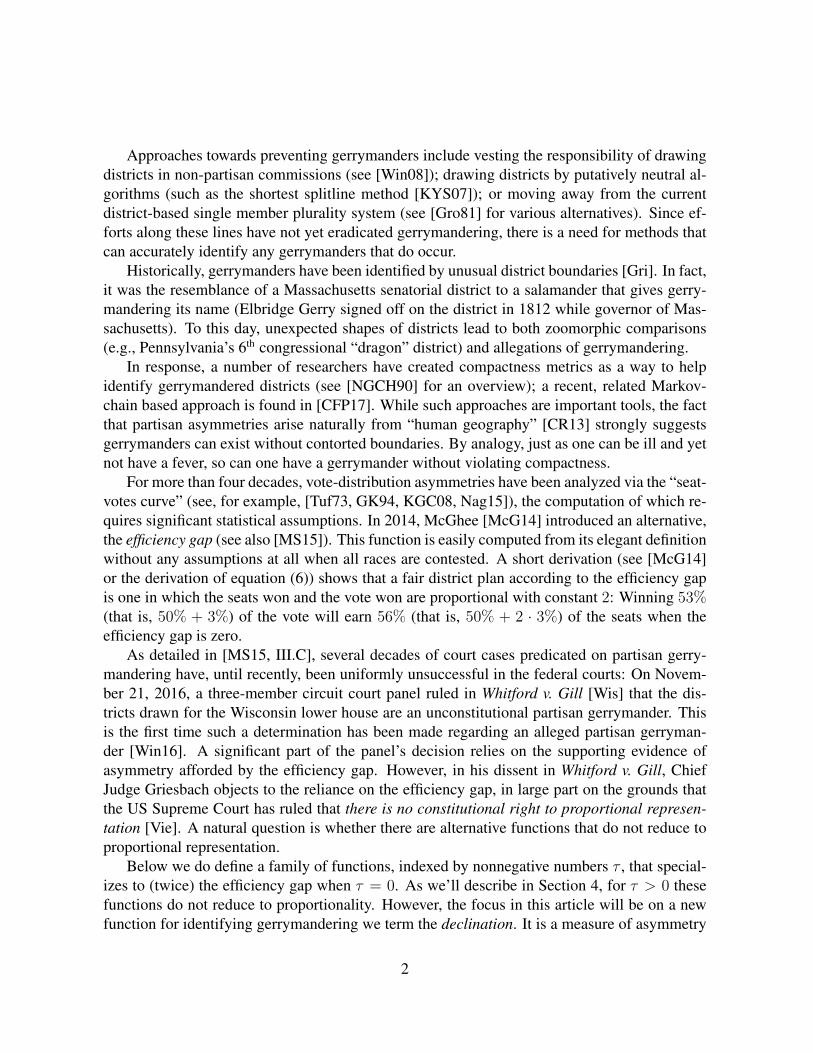
For general τ , however, the relationship between seats won and votes earned in an electionfor which Gapτ is zero is more complicated and depends on how the votes are distributed. Whenτ is a nonnegative even integer of the form τ = 2`, we can express the condition succinctly sincethen

Gapτ (E) = 2

[M2`+1(a) +

1

2− k′

N

], (8)

where M2`+1(a) denotes the (2`+ 1)th moment of the ai.In the limit as τ → ∞, Gapτ reduces (in the general case of 0 < |ai| < 1 for all i)

to 1 − 2k′/N . It follows that Gap∞ is zero if and only if each party wins half of the seats,irrespective of overall vote share.

There are at least two natural ways in which the τ -gap could be further generalized. The firstis by allowing the waste to be most pronounced close to the 50% threshold. This is convenientlyattained by considering waste functions of the form (1−ai)−τ for τ < 0. This choice has severalappealing characteristics such as the fact that the winner and loser waste equal amounts moreevenly than the 75%-25% split for the efficiency gap. In addition, the waste function is moresensitive to what is happening near the 50% threshold. Unfortunately, this latter property seemsto reduce its utility greatly as there is much more noise due to random fluctuations in voteearned.

Second, while we have restricted our attention to power functions determined by a parameterτ , the concept of τ -waste could easily be extended to more sophisticated functions. One couldalso allow different functions for the votes wasted by the winner and the votes wasted by theloser.

5 Theorem on packing and crackingWe make precise the link between packing and cracking and the functions we introduce inthe previous two sections. Define P -cracking to be the moving of party-P votes from districtk + 1 to districts 1, 2, . . . , k such that 1) the first k districts are still lost by party P after theredistribution and 2) district k + 1 becomes a district that party P loses. Similarly, define P -packing to be the moving of party-P votes from district k + 1 to districts k + 2, k + 3, . . . , Nsuch that district k + 1 is now lost by party P . Using our new terminology, we state and provethe followingTheorem 1. Let E = (P,Q,p) be an election with p in weakly increasing order. Let y be theaverage party-P vote in the k districts lost by party P and z be the corresponding average in thek′ districts won by party P . Let p′k+1 be the party-P vote fraction remaining in district k + 1after P -cracking or P -packing and E ′ the resulting election.

1. If p′k+1 > y, then δ(E ′) > δ(E).

2. If p′k+1 > pk, then Gapτ (E ′) > Gapτ (E).

14

Proof. Proof of (1). We refer the reader to Fig. 1 for the positions of points referenced. TheP -packing or P -cracking of district k + 1 will move point G to the right by 1/N units. Eachof points F and H will move to the right by only 1/2N units. Since p′k+1 > y, point F willalso move up. Since p is arranged in increasing order, point H will also move up. Together,these shifts will decrease θQ and increase θP , thereby increasing δ. By symmetry, Q-packingand Q-cracking will decrease δ(E).

Proof of (2). We show only the details for P -cracking; the argument for P -packing is similar.Let p′ = (p′1, p

′2, . . . , p

′N) be the vote distribution for E ′. Since we are P -cracking the (k + 1)st

district, we know that p′i = pi for i > k + 1. Set bi = 2p′i − 1 for i ≤ k + 1. Note in the belowequations that all ai and bi for i ≤ k are negative (bk+1 is negative as well). Recall that

Gapτ (E) = 2

[−∑k

i=1(−ai)τ+1 + aτ+1k+1 +

∑Ni=k+2 a

τ+1i

N+

1

2− k′

N

]and

Gapτ (E ′) = 2

[−∑k

i=1(−bi)τ+1 − (−bk+1)τ+1 +

∑Ni=k+2 a

τ+1i

N+

1

2− k′ − 1

N

].

We wish to show that the difference

Gapτ (E ′)−Gapτ (E) =

∑ki=1(−(−bi)τ+1 + (−ai)τ+1)− (−bk+1)

τ+1 − aτ+1k+1

N+

1

N

is positive. Multiplying by N/(τ + 1), we see that this is equivalent to showing that∑ki=1((−ai)τ+1 − (−bi)τ+1) + 1

τ + 1≥

(−bk+1)τ+1 + aτ+1

k+1

τ + 1.

We make the following observations. First, since all votes being moved are going from districtk + 1 to a district i with i ≤ k, we must have

∑ki=1((−ai) + bi) = ak+1 − bk+1. Second, since

ak+1 is positive∑k

i=1((−ai) + bi) ≥ −bk+1. So choose constants 0 = c0 ≤ c1 ≤ c2 ≤ · · · ≤ck = −bk+1 such that (−ai) − (−bi) ≥ ci − ci−1 for 1 ≤ i ≤ k. Straightforward calculusshows that, since xτ is an increasing function and −bk+1 ≤ −ai for all i ≤ k by hypothesis,that ((−ai)τ+1 − (−bi)τ+1) ≥ cτ+1

i − cτ+1i−1 for all 1 ≤ i ≤ k. It follows that

k∑i=1

∫ −ai−bi

xτ dx =k∑i=1

((−ai)τ+1 − (−bi)τ+1)

τ + 1≥ (−bk+1)

τ+1

τ + 1.

As 1/(τ + 1) ≥ aτ+1k+1/(τ + 1), the result follows.

6 Strengths and weaknesses of different functionsOur situation in identifying gerrymanders is analogous to that of assessing intelligence. Emo-tional intelligence and logical intelligence are best measured by different types of questions; no

15

single question type can capture the spectrum of ways in which intelligence can manifest itself.Every test for gerrymandering will have its strengths and weaknesses. In this section we attemptto illustrate, through concrete examples, ways in which each of the efficiency gap, the τ -gap,the mean-median difference and the declination can give misleading answers in their attemptsto identify gerrymanders.

The oldest tool for this purpose, the seats-votes curve, has been around for over 40 years [Tuf73].Notwithstanding its theoretical interest and applications in such areas as predictions (for exam-ple, [KGC08]), as it has not led to a manageable judicial standard for gerrymandering in thisspan, we will not address it directly in the remainder of this article.

6.1 The efficiency gapThe efficiency gap, through its role in Whitford v. Gill, has already proven its utility. Andwhile its simplicity is an asset, it also has several drawbacks. First, by requiring that there beproportional representation for an election to be considered fair, it conflicts with constitutionallaw [Vie]. Second, it is simple to construct hypothetical examples for which a natural districtplan leads to a constant of proportionality different from 2 (see, for example, Figs. 2.C,D).While the proportionality asserted by the efficiency gap may hold in some overall sense, for theinstances for which it doesn’t we are left in the difficult position of determining whether any de-viation from this average law is due to gerrymandering or natural deviation. And, as illustratedby our definition of the τ -gap function, the proportionality with a constant of 2 depends on asubjective decision on how to weight various wasted votes. Third, there are historical examplesin which the proportionality holds, but the shape of the vote distribution suggests significantpartisan asymmetry (see, in particular, the 1974 Texas congressional election shown in Fig. 2.Aas well as the 2012–2016 Tennessee congressional elections, the last of which is displayed inFig. 8).

6.2 The τ -gapThe τ -gap family of functions is appealing due to its close connection to the efficiency gap andthe fact that it does not reduce to proportionality. Additionally, when τ = 2, the τ -gap is closelyrelated to skewness of the ai-distribution (see (8)), a standard measure of symmetry in statisticaldistributions. We also note that when τ = 2/5, the correlation between the declination and theτ -gap is very high (r2 = 0.870, p < 0.001 among 461 congressional elections). Unfortunately,the τ -gap family has its own drawbacks.

First, there is no reason to think that one value of τ will prove superior to other values in allcases. For example, consider the 1974 Texas and North Carolina congressional elections (seeFig. 2.A and Fig. 7.A, respectively). Proportionality is essentially met in both cases as reflectedby the values of Gap0 being close to zero; each election is fair according to the efficiency gap. Incontrast, Gap1 is approximately −0.38 for each, indicating strong asymmetry. While we haveno absolute way of determining whether one or both is a gerrymander, evidence suggests that

16

Figure 7: (A) Vote distribution for 1974 North Carolina congressional election with Gap0 =−0.1 and Gap1 = −0.39. (B) Vote distribution for 2006 Tennessee congressional electionillustrating the mean-median difference of -0.13. (C) Vote distrbution for the 2012 Indianacongressional election showing a mean-median difference of 0.01.

Gap0 makes the correct assessment for the North Carolina election (little or no gerrymandering)while Gap1 makes the correct assessment for the Texas election (gerrymandering)2. We notethat the declination yields what we believe to be the correct answer in both cases.

Second, even if there were one value of τ that was superior to all others, it is unclear whattheoretical, rather empirical, justification could be used to support it. Third, as shown by (6),the τ -gap is essentially an interpolation, albeit a complicated one, between the proportionalitywith constant 2, when τ = 0, and proportionality with constant 0, when τ =∞. (A fair electionfor the latter is one in which each party gets half the seats, regardless of the fraction of voteswon by each side.)

6.3 The mean-median differenceThe difference between the mean and the median of the democratic vote fraction among alldistricts has been suggested as yet another way of measuring partisan asymmetry (see, for ex-ample, Wang [Wan16] and [KMM+16, MB15]). A large difference between these values canindeed accompany an asymmetry in the vote distribution. For example, in the 2012 Pennsylva-nia congressional election (see Fig. 2.B), the mean is 0.50 while the median is 0.43, a differenceof 0.07. However, the mean-median difference is very sensitive to the vote in a single district(practically speaking, this is less of an issue in the case of many districts). For example, in the2006 Tennessee congressional election shown in Fig. 7.B, the difference is -0.13. Had the demo-cratic support been more unevenly distributed in the districts the Democrats won, the difference

2As described in [O’C90, pg. 35], there was not significant partisan rancor during the 1971 redistricting and theDemocrats received approximately 63% of the congressional vote while winning 82% (9 of 11) congressional seats.Of course, these facts have little bearing on whether there may have been racial gerrymandering. For the Texaselection, one author [May71] suggests that for the 1965 redistricting, protecting incumbents was a higher prioritythan advantaging the Democrats as a party. The constructions of a large number of safe seats for incumbents wouldcertainly be consistent with the distribution seen.

17

would have been much smaller in absolute value. The declination, by relying on averages acrossdistricts rather than values within single districts is more robust in this respect.

Additionally, it is quite possible for packing and cracking to occur without having any effecton the mean-median difference. For example, consider the 2012 Indiana congressional electionshown in Fig. 7.C. According to the mean-median difference, this is a fair election. Howeverit is easy to see how less dominant wins in two districts could have translated into one or eventwo more seats for the Democrats: such changes need not affect the median.

It is also worth noting that the mean-median difference doesn’t keep track of the number ofseats won by each party. This is probably the main reason it is slightly more stable from electionto election than the efficiency gap or the declination. On the other hand, this independencemakes it harder to interpret the extent to which a particular value of the difference indicatesactual impact on the electoral results.

6.4 The declinationThe declination’s primary weaknesses appear to occur when one party wins almost all of theseats. Fortunately, while gerrymandering may occur in such instances, these are typically notthe cases of greatest interest. In most elections with a large number of seats, the vote fractionswhen sorted in increasing order increase essentially linearly except at the extremes. When oneparty dominates, this can lead to a declination that is large in absolute value even though the votedistribution as a whole is remarkably symmetric about the median democratic votes share. Thisis the case, for example in the 2008 Rhode Island state legislative election (shown in Fig. 9), inwhich the Democrats win two thirds of the vote. On the other hand, when there are few seatsoverall, it is not uncommon for one party to win all but one seat. In such a case, the declinationis very sensitive to the exact vote fraction found in that one special district.

7 Data collection and Statistical methodsThe US state legislature election data up through 2010 comes from [KBC+11]. We only in-cluded data on the lower house of the state legislature when two houses exist. The US congres-sional data through 2014 was provided by [Jac17]. Data on Wisconsin legislative elections from2012 to 2016 were take from Ballotpedia [Bal17]. Data for 2016 congressional races were takenfrom Wikipedia [Wik17] as they were not yet available from the Federal Election Commission.

The election data was analyzed using the python-based SageMath [S+16]. Python packagesemployed were pyStan [Tea16] for implementing a multilevel model to impute votes in un-contested races; Matplotlib [Hun07] and Seaborn [WBH+] for plotting and visualization; andSciPy [JOP+ ] for statistical methods.

For the state legislative elections, we restricted the analysis to elections that had no multi-member districts; vote fractions for uncontested races were imputed (i.e., we estimated whatthe values would have been had the races been contested).

18

Any election (year and state) in which there is at least one multi-member district (i.e., mul-tiple winners in a single district) was excluded from our analysis. We ignored any third-partycandidates and assumed there to be at most one Democrat and at most one Republican in eachrace. All vote percentages assigned to a candidate are therefore percentages of the two-partyvote. We assume all districts have equal population and we do not take into account voterturnout in any way. Unopposed candidates are allowed. The declination is mildly sensitive tothe vote distribution in each of these uncontested races (see below). Rather than assign 100%of the vote to the unopposed candidate, which is invariably not reflective of what would havehappened had their been a two-candidate race, we imputed the vote fraction for such races.

Imputation of votes was done using a multilevel model of the form

yi =1

2+ σj[i] + φk[j[i]] + γ`[i] + β1W

Di + β2W

Ri + β3I

Di + β4I

Ri + εi.

Here, yi is the fraction of the vote garnered by the democratic candidate in district i; σj[i] is arandom state effect; φk[j[i]] is a random district effect; γ`[i] is a random year effect; WD

i and WRi

are indicator variables for whether the democratic or republican candidate won, respectively;IDi and IRi are indicator variables for whether or not the democratic and republican candidatesare incumbents, respectively; β1, β2, β3 and β4 are the corresponding random effects; and εirepresents error due to individual characteristics of race i. The model was run separately foreach redistricting cycle (typically of ten years), once for state legislatures and once for the USHouse of Representatives. As there are a number of cases in which states underwent majorredistricting mid-decade, certain cycles were split. For example, Texas had one district planfor its congressional races during the years 1992–1996 and another for 1998–2000. These arerepresented in the Figure reffig:congint.C by TX1 and TX2, respectively.

There were 646 state elections in our data with a total of 68 955 races of which 25 371 ofwhich were uncontested. There were 1 142 congressional elections with a total of 9 995 racesof which 1 409 were uncontested.

When at least one race in a given district had been contested in a given cycle, imputationis straightforward using the values for the random and fixed effects provided by the modelfit. We cross-validated the estimates by removing individual races, refitting and comparing theestimated to true values. We found a root mean square error of approximately 0.05 among 100randomly chosen contested races. We note for comparison that if one uniformly assigns 65%of the vote to the winner, the error is approximately 0.09.

Of the 26 780 imputed values, there were 114 instances in which the data indicated a demo-cratic winner, but the imputed value was less than or equal to 0.50. These imputed values werereplaced with 0.505. Similarly, there were 40 instances in which a democratic loser was indi-cated, but the imputed value was greater than 0.50. These imputed values were replaced with0.495.

There a number of instances in which a district was not contested at any time during a givenreapportionment cycle. There were 11 770 state legislative district-cycle pairs. Of these, 1 281were uncontested (i.e., the race in that district was not contested in any year of the cycle). The

19

corresponding numbers for congressional elections are 2 030 and 41. For the vast majority ofthese cases, one of the two parties held the seat for the entire cycle. For these cases, we drewfrom the distribution of district effects stemming from districts that were consistently won bythe same party throughout the cycle (with at least one contested race). There were a total of19 state district-cycle pairs that were uncontested but held by both parties at some point duringthe cycle. The district effect in these cases was drawn at random from all district effects. Thisoutcome did not occur for the congressional races.

We also performed a sensitivity analysis with respect to the imputed values by introducinga systemic bias of plus 3% to the democratic imputed votes for congressional elections. Wethen performed a linear regression of change in declination with respect to the fraction of racesthat had to be imputed. Elections in which one party won all of the seats were omitted. Theslope and r2-value for the regression line was (0.09, 0.76). The corresponding regression linefor state elections was similar, but with a higher r2-value.

For congressional elections with at least eight seats, 53% had at most 10% of the racesuncontested while 90% had at most 40% of the seats uncontested. For state elections, only31% had less than 10% of the seats uncontested while 92% had less than 65% of the racesuncontested.

8 ConclusionAmong the tests discussed in the previous section, we believe that the declination, on the whole,possesses the most desirable combination of characteristics. First, it does not reduce to propor-tionality, and hence is not at odds with constitutional law. Second, it is readily visualized. Third,the declination is directly computed using fundamental aspects of the election, namely the num-ber of seats each party wins along with the average vote fraction each earns in those wins. Whilethe efficiency gap is perhaps even simpler, the general τ -gap is certainly much harder to visual-ize. Fourth, the declination is relatively robust with respect to the vote fraction in any individualdistrict, unlike the mean-median difference. The declination also must change in the presenceof packing and cracking, a feature that does not always hold for the mean-median difference.

The declination and compactness metrics are complementary, each captures particular char-acteristics of gerrymandering. These measures do not capture everything about an electionand one must be careful to not ascribe more importance to a single number than is warranted(see [O’N16]). Nonetheless, they have utility through their ability to provide a consistent wayto compare elections in different states and years. Assuming the courts ultimately accept oneor more standards for ascertaining whether a district plan amounts to unconstitutional gerry-mandering, it will be helpful if there is enough flexibility provided so that as our tools andunderstanding evolve, so do our classification standards.

20

9 AcknowledgmentsThis work was partially supported by a grant from the Simons Foundation (#429570). The datareported in this paper are archived at the following databases (TBD). The author is especiallyindebted to Gary C. Jacobson for sharing his data on US Congressional elections. The authoralso gratefully acknowledges extensive discussions with Jeff Buzas and Jill Warrington as wellas helpful input from Jim Bagrow, Sara Billey, Chris Danforth, Jeff Dinitz, Mark Moyer, JohnSchmitt, Mike Schneider, Dan Velleman and {Ann, Bob, Jeff}Warrington.

21

10 Appendix

22

Figure 8: 2016 congressional races with at least one win by each party. Listed in decreasingorder of declination.

23

Figure 9: 2008 state legislative races with at least one win by each party. Listed in decreasingorder of declination.

24

Figure 10: Range of δ over each districting cycle for congressional elections: (A) 1972–1980,(B) 1982–1990, (C) 1992–2000, (D) 2002–2010, (E) 2012–2016. Major redistrictings withineach cycle are indicated by concatenation (e.g., TX1 refers to the district plan in effect at thebeginning of the cycle and TX2 to the next plan). States were omitted if one party won all seatsduring the cycle. Subplot (E) is identical to Fig. 5 but is repeated here for comparison withearlier decades.

25

Figure 11: Range of δ over each districting cycle for state legislative elections: (A) 1972–1980, (B) 1982–1990, (C) 1992–2000, (D) 2002–2010. Major redistrictings within each cycleare indicated by concatenation (e.g., OH1 refers to the district plan in effect at the beginning ofthe cycle and OH2 to the next plan). States were omitted if one party won all seats during thecycle (or if the plan had multi-member districts).

26

Table 2: Most extreme values of δ for congressional elections since 1972.Most positive δ Most negative δ

Year State Seats δ δ δN Year State Seats δ δ δN1980 VA 10 0.80 0.69 3.5 1976 TX 24 -1.07 -0.67 -8.12012 PA 18 0.76 0.53 4.7 1982 TX 27 -0.83 -0.51 -6.82012 OH 16 0.76 0.55 4.4 1990 MA 11 -0.82 -0.68 -3.72014 NC 13 0.69 0.54 3.5 1988 MA 11 -0.79 -0.66 -3.62016 PA 18 0.67 0.47 4.2 1984 MA 11 -0.77 -0.65 -3.52012 SC 7 0.63 0.65 2.3 1986 MA 11 -0.77 -0.64 -3.52014 PA 18 0.62 0.43 3.9 1972 GA 10 -0.76 -0.66 -3.32016 NC 13 0.61 0.48 3.1 1982 MA 11 -0.75 -0.63 -3.51972 OH 23 0.61 0.39 4.5 2008 NY 29 -0.74 -0.44 -6.32010 AL 7 0.59 0.61 2.1 1978 TX 24 -0.73 -0.46 -5.52014 SC 7 0.59 0.60 2.1 1980 TX 24 -0.72 -0.46 -5.51994 WA 9 0.58 0.53 2.4 1974 TX 24 -0.71 -0.45 -5.42016 TX 36 0.58 0.32 5.8 1972 TX 24 -0.70 -0.44 -5.32012 NC 13 0.58 0.45 2.9 1992 TX 30 -0.70 -0.41 -6.12012 VA 11 0.58 0.48 2.6 1972 MO 10 -0.69 -0.60 -3.01974 OH 23 0.57 0.37 4.2 1992 WA 9 -0.68 -0.62 -2.82012 AL 7 0.57 0.59 2.1 2014 MD 8 -0.65 -0.63 -2.52016 SC 7 0.56 0.58 2.0 1990 TX 27 -0.63 -0.38 -5.22012 MI 14 0.56 0.43 3.0 1978 WA 7 -0.61 -0.63 -2.22010 FL 25 0.56 0.35 4.4 1988 TX 27 -0.60 -0.36 -4.92002 FL 25 0.56 0.35 4.4 1994 TX 30 -0.59 -0.35 -5.22006 VA 11 0.55 0.46 2.5 1976 WA 7 -0.59 -0.60 -2.12016 OH 16 0.54 0.39 3.1 1980 MD 8 -0.58 -0.56 -2.21994 OK 6 0.54 0.60 1.8 2016 MD 8 -0.58 -0.56 -2.22014 OH 16 0.53 0.38 3.1 1980 MA 12 -0.57 -0.46 -2.82006 MI 15 0.53 0.39 2.9 2014 CA 53 -0.57 -0.29 -7.62004 FL 25 0.52 0.33 4.1 1974 WA 7 -0.56 -0.58 -2.02006 OH 18 0.52 0.36 3.3 2012 MD 8 -0.55 -0.53 -2.11998 AZ 6 0.52 0.58 1.8 1978 FL 15 -0.54 -0.40 -3.02000 AZ 6 0.51 0.57 1.7 1978 OK 6 -0.54 -0.60 -1.82010 IL 19 0.51 0.35 3.3 1978 NC 11 -0.54 -0.45 -2.52014 MI 14 0.50 0.38 2.7 1980 OK 6 -0.54 -0.60 -1.8

27

Table 3: Values of declination for congressional elections. Empty entries are due to one party winning all of the seats.1972 1974 1976 1978 1980 1982 1984 1986 1988 1990 1992 1994 1996 1998 2000 2002 2004 2006 2008 2010 2012 2014 2016

AKAL 0.01 0.15 0.18 0.12 0.11 0.09 0.06 -0.10 -0.05 0.07 0.22 -0.25 0.32 0.42 0.34 0.36 0.37 0.41 -0.02 0.61 0.59 0.51 0.54AR -0.45 0.33 -0.23 0.06 -0.09 0.11 -0.51 -0.38 -0.36 -0.40 0.41 -0.10 -0.17 0.01 -0.38 -0.42 -0.24 -0.21 -0.27 0.19AZ 0.39 0.42 0.05 -0.16 -0.11 0.01 0.41 0.52 0.45 0.42 -0.16 0.48 0.52 0.58 0.57 0.36 0.43 0.05 -0.09 0.07 -0.28 -0.35 0.01CA 0.05 0.01 -0.10 -0.06 -0.02 -0.20 -0.18 -0.11 -0.08 -0.01 0.08 0.00 0.02 0.14 -0.02 -0.12 -0.06 0.00 0.13 -0.06 -0.09 -0.28 -0.10CO 0.06 0.01 -0.33 -0.24 -0.36 -0.10 -0.04 -0.23 -0.01 0.05 0.28 -0.08 0.04 0.08 0.20 0.30 0.17 0.14 -0.18 0.09 0.19 0.05 0.11CT -0.07 0.15 -0.29 -0.34 -0.15 -0.00 -0.14 0.21 -0.03 -0.13 -0.12 -0.05 0.02 -0.26 0.16 0.30 0.43 0.11DEFL -0.35 -0.14 -0.12 -0.40 -0.25 -0.00 -0.28 -0.13 0.02 0.03 0.06 0.09 0.20 0.22 0.28 0.29 0.35 0.29 0.19 0.29 0.27 0.15 0.06GA -0.66 -0.15 -0.38 -0.24 -0.23 -0.04 -0.44 0.14 0.05 0.18 0.30 0.30 0.24 0.04 -0.03 -0.05 0.09 0.07 0.21 0.31 0.36HI 0.27 0.38IA 0.07 0.02 0.08 -0.01 0.06 0.11 0.19 0.21 0.30 0.26 0.43 -0.05 0.25 0.43 0.14 0.15 -0.22 -0.11 -0.41 0.07 0.03 0.06ID -0.40 -0.27 -0.01 -0.05 -0.43IL 0.22 0.20 0.12 0.13 0.21 0.15 -0.14 -0.06 -0.19 -0.20 0.02 -0.02 0.22 0.16 0.22 0.17 0.13 0.26 0.11 0.35 -0.11 -0.01 -0.04IN 0.04 -0.29 -0.23 -0.11 -0.07 -0.02 -0.10 -0.15 -0.10 -0.36 -0.19 -0.12 0.04 0.01 0.04 0.05 0.31 -0.10 0.01 -0.02 0.44 0.21 0.31KS 0.21 0.18 -0.31 0.51 0.50 0.12 0.09 0.08 0.08 0.23 -0.19 -0.16 -0.19 -0.22 -0.02 -0.25 0.10KY -0.47 -0.01 -0.13 -0.01 -0.02 0.19 -0.07 0.03 -0.22 -0.16 -0.12 -0.12 0.23 0.09 0.18 -0.11 0.31 0.04 0.16 -0.26 0.44 0.38 0.36LA -0.12 0.14 -0.36 -0.13 -0.34 -0.24 -0.35 0.14 0.11 0.04 0.04 -0.27 0.30 0.31 0.27 -0.03 0.26 0.01 0.36 0.45 0.45 0.46 0.41MA -0.21 -0.41 -0.34 -0.43 -0.48 -0.63 -0.65 -0.64 -0.66 -0.68 0.03 0.05MD 0.10 0.13 0.24 -0.16 -0.56 -0.37 -0.08 0.07 -0.27 -0.12 0.20 0.08 0.22 0.19 0.26 -0.41 -0.34 -0.18 -0.32 -0.12 -0.53 -0.63 -0.56ME 0.12 -0.40 -0.06 0.22 0.24 0.02 0.29 0.08MI 0.26 0.19 0.15 -0.14 -0.08 -0.08 -0.12 0.04 -0.11 -0.04 -0.11 -0.18 -0.11 -0.18 0.08 0.24 0.27 0.39 0.12 0.14 0.43 0.38 0.34MN 0.16 0.09 -0.09 0.00 0.24 -0.02 -0.11 0.15 0.07 -0.26 -0.28 -0.44 -0.25 -0.33 0.01 0.08 0.15 0.01 0.21 0.09 0.11 -0.12 -0.09MO -0.60 -0.01 -0.32 -0.17 -0.02 0.12 -0.28 0.14 0.13 0.01 -0.09 -0.29 0.10 -0.06 0.17 0.01 -0.02 0.12 0.15 0.07 0.40 0.25 0.33MS 0.27 -0.14 -0.10 -0.05 -0.02 -0.05 -0.14 -0.55 0.02 -0.38 0.01 -0.07 -0.17 -0.04 -0.12 0.11 -0.24 0.33 0.36 0.25 0.33MT 0.42 0.24 0.01 0.05 0.15 0.02 0.19 0.12 -0.04NC -0.16 -0.05 -0.16 -0.45 -0.01 -0.36 0.08 0.06 -0.32 -0.09 -0.25 0.07 -0.13 -0.02 0.10 0.02 0.06 0.02 -0.06 -0.25 0.45 0.54 0.48NDNE -0.23 -0.24 -0.36 0.13 -0.24 -0.30NH -0.28 0.16 -0.10 -0.07 -0.31 -0.07 0.17 0.08NJ -0.03 -0.18 -0.27 -0.11 -0.04 0.00 -0.08 -0.05 -0.15 -0.19 -0.10 0.20 0.15 0.05 0.10 0.05 0.09 0.22 0.06 -0.01 0.28 0.17 0.07NM 0.32 0.16 -0.03 0.10 0.36 0.05 0.28 0.44 0.30 0.37 0.12 0.38 0.08 0.39 0.37 0.40 0.53 -0.11 -0.11 -0.27 -0.17NV 0.00 -0.31 -0.08 0.14 0.01 0.20 -0.27 -0.31 -0.13 0.27 0.48 0.01 0.28 0.06 0.24 -0.35NY -0.00 -0.05 -0.15 -0.13 -0.02 0.08 -0.00 0.03 -0.09 -0.04 0.07 0.02 0.14 0.06 -0.01 -0.15 -0.01 0.08 -0.44 -0.00 0.09 -0.03 0.14OH 0.39 0.37 0.12 0.11 0.02 0.20 -0.11 -0.04 -0.02 0.04 -0.04 0.22 0.08 0.14 0.14 0.23 0.31 0.36 0.01 0.28 0.55 0.38 0.39OK -0.53 0.16 -0.61 -0.60 -0.46 -0.59 -0.02 -0.04 -0.02 0.19 0.60 0.21 0.55 0.39 0.50 0.43 0.08OR 0.00 0.20 0.17 0.05 0.03 0.22 -0.43 -0.41 0.12 -0.39 -0.39 -0.52 -0.53 -0.55 -0.46 -0.44 -0.60 -0.48 -0.51 -0.53PA -0.08 0.15 -0.15 -0.18 -0.03 -0.03 -0.09 0.01 -0.03 0.06 -0.00 -0.07 0.06 -0.01 0.14 0.24 0.28 0.10 -0.05 0.21 0.53 0.43 0.47RI 0.26 0.13 0.01 -0.27 0.09 0.00SC 0.01 -0.24 -0.27 0.10 0.22 0.05 -0.01 0.19 -0.06 -0.14 0.07 -0.00 0.13 0.27 0.24 0.12 0.17 0.13 0.31 0.46 0.65 0.60 0.58SD 0.13 -0.15 0.15TN 0.27 -0.11 -0.02 -0.23 -0.18 -0.10 -0.34 -0.27 -0.29 -0.25 -0.30 -0.08 0.10 0.11 0.09 -0.18 -0.13 -0.02 -0.13 0.29 0.38 0.34 0.34TX -0.44 -0.45 -0.67 -0.46 -0.46 -0.47 -0.20 -0.14 -0.37 -0.39 -0.41 -0.35 -0.17 -0.19 -0.16 -0.20 0.22 0.18 0.23 0.20 0.24 0.24 0.32UT 0.06 -0.26 0.04 0.04 0.03 -0.43 0.14 -0.02 -0.28 -0.10 0.09 0.12 -0.32 -0.33VA 0.35 0.19 0.23 -0.04 0.58 -0.02 -0.04 0.04 -0.08 -0.08 -0.17 -0.21 -0.05 -0.08 0.25 0.25 0.29 0.46 -0.03 0.27 0.48 0.32 0.21VTWA 0.22 -0.58 -0.60 -0.63 -0.45 -0.16 -0.10 0.02 -0.16 -0.06 -0.62 0.53 0.42 -0.03 -0.16 -0.23 0.02 0.11 -0.03 -0.04 -0.07 -0.07 -0.04WI 0.16 -0.15 -0.33 -0.19 -0.05 -0.01 -0.22 -0.12 -0.16 0.16 0.10 0.00 -0.18 -0.02 -0.18 -0.07 -0.09 -0.15 -0.14 0.07 0.31 0.19 0.20WV 0.32 0.28 -0.04 0.00 0.04 0.06 0.03 -0.14WY

28

Table 4: Values of declination for state lower house elections. Empty entries are due to one party winning all of the seats orto the election containing multi-member districts.

1972 1974 1976 1978 1980 1982 1984 1986 1988 1990 1992 1994 1996 1998 2000 2002 2004 2006 2008 2010

AK 0.00 0.01 -0.02 0.03 0.13 0.06 0.09 0.05 -0.06 -0.16AL -0.61 -0.50 -0.40 -0.33 -0.15 -0.15 -0.06 0.01AR -0.18 -0.25 -0.20 -0.16 -0.10AZCA -0.11 -0.06 -0.13 -0.06 -0.11 -0.04 -0.14 -0.00 -0.09 0.00 0.02 0.08 0.09 0.05 -0.01 -0.04 -0.02 0.03 0.12 -0.07CO 0.06 0.11 0.11 0.13 0.07 0.13 0.30 0.13 0.11 0.16 0.03 0.06 0.11 0.13 0.11 0.06 -0.04 -0.04 -0.02 -0.05CT 0.13 -0.14 -0.07 -0.08 -0.04 0.01 -0.00 -0.01 -0.04 -0.09 0.17 -0.02 -0.04 -0.08 -0.05 -0.02 -0.07 -0.03 -0.07 -0.10DE 0.04 -0.02 -0.11 0.02 0.10 -0.23 0.01 -0.01 -0.06 0.08 0.06 0.17 0.19 0.22 0.29 0.40 0.29 0.27 -0.00 -0.14FL -0.16 -0.20 -0.12 -0.14 -0.08 -0.07 -0.10 0.03 0.16 0.25 0.26 0.34 0.27 0.26 0.21GA -0.19 -0.18 -0.06 -0.02 -0.04 -0.06 0.07 0.05 -0.05HI -0.32 -0.22 -0.25 -0.43 -0.29 -0.66 -0.54 -0.30 -0.25 0.01 -0.18 -0.37 -0.31 -0.46 -0.38IA 0.05 -0.02 -0.06 0.02 0.05 -0.06 -0.12 -0.04 -0.08 -0.01 0.06 0.10 0.04 0.11 0.13 0.04 0.02 0.05 -0.05 -0.02IDIL -0.01 -0.04 0.05 -0.00 -0.02 0.08 0.15 0.19 0.15 0.14 0.06 0.11 0.17 0.11 0.00IN -0.10 -0.06 -0.04 -0.07 -0.07 -0.12 -0.04 0.06 -0.01 0.01KS 0.13 0.17 0.04 0.06 -0.00 0.09 0.07 0.10 -0.00 -0.02 -0.04 -0.01 0.00 0.09 0.18 0.10 0.14 0.20 0.11 0.14KY -0.30 -0.20 -0.26 -0.17 -0.19 -0.15 -0.11 -0.10 -0.11 -0.13 -0.06 0.02 -0.09 -0.14LA -0.36MA -0.19 -0.26 -0.26 -0.28 -0.34 -0.32 -0.29 -0.33 -0.23 -0.17 -0.27 -0.29 -0.24 -0.33 -0.37 -0.41 -0.37 -0.50 -0.20MDME 0.02 -0.04 -0.03 -0.05 -0.08 -0.16 -0.06 -0.02 0.00 0.04 0.04 -0.07 0.01 0.10 0.03 -0.03 -0.02MI -0.02 0.15 0.01 -0.05 -0.03 0.11 -0.03 0.03 -0.01 0.05 0.15 0.04 0.10 0.17 0.22 0.25 0.20 0.21 0.09 0.19MN -0.20 -0.19 0.04 0.01 0.02 0.09 -0.07 -0.06 -0.02 -0.05 -0.06 0.06 0.07 0.11 0.25 0.15 0.02 -0.01 0.13MO 0.02 -0.02 -0.11 -0.13 -0.10 -0.19 -0.18 0.04 -0.04 -0.04 0.02 0.01 0.05 0.06 0.14 0.17 0.09 0.09MSMT -0.08 -0.02 -0.03 0.05 -0.03 -0.04 0.04 0.02 -0.03 0.06 0.09 0.13 0.09 0.02 0.03 -0.04 0.02 0.01 0.07NC 0.04 -0.00 0.02 0.01 -0.00NDNENHNJNM -0.32 -0.16 -0.17 -0.02 -0.15 -0.06 -0.08 -0.16 -0.08 -0.20 -0.23 -0.17 -0.03 -0.01 -0.08 -0.09 0.02 0.10 -0.01 0.05NV 0.09 -0.24 -0.47 0.05 -0.13 0.03 0.15 -0.25 -0.32 -0.00 -0.26 0.01 -0.12 -0.24 -0.21 0.01 -0.07 -0.01 -0.06 -0.08NY 0.20 0.15 0.10 0.08 0.04 -0.00 -0.06 0.05 -0.01 0.07 -0.05 -0.06 0.08 0.04 0.07 -0.01 0.02 0.09 0.05 0.00OH -0.04 0.07 -0.02 -0.08 -0.06 0.01 -0.12 -0.07 -0.10 -0.05 0.06 0.08 0.24 0.24 0.23 0.25 0.25 0.27 0.09 0.14OK -0.19 -0.21 -0.32 -0.23 -0.24 -0.27 -0.24 -0.18 -0.19 -0.11 -0.22 -0.24 -0.21 -0.10 0.05 -0.08 0.06 0.14 0.16 0.16OR 0.02 -0.03 -0.03 -0.04 -0.02 -0.10 -0.10 0.01 -0.01 0.08 0.11 0.03 0.08 0.17 0.13 0.16 0.16 0.11 0.02 0.01PA 0.02 0.10 -0.00 0.05 0.02 0.09 0.02 0.05 0.02 0.04 0.06 -0.03 0.08 0.07 0.13 0.05 0.13 0.12 0.06 0.03RI -0.10 -0.10 -0.22 -0.27 -0.18 -0.32 -0.23 -0.26 -0.28 -0.38 -0.16 -0.38 -0.25 -0.37 -0.23 -0.36 -0.16 -0.04 -0.35 -0.33SC -0.26 -0.46 -0.39 -0.43 -0.36 -0.40 -0.19 -0.18 -0.09 -0.14 -0.09 0.09 0.06 0.08 0.13 0.08 0.13 0.11 0.05SDTN -0.01 -0.01 -0.08 -0.02 -0.08 -0.06 -0.17 -0.04 -0.04 0.00 -0.18 -0.25 -0.16 -0.12 -0.10 -0.10 -0.08 0.01 0.01 0.11TX -0.53 -0.52 -0.31 -0.30 -0.22 -0.11 -0.10 -0.11 -0.15 -0.24 -0.07 -0.03 -0.01 0.07 0.02 0.05 -0.06 0.05UT 0.01 0.04 -0.05 0.10 0.12 0.16 0.21 0.11 0.01 0.03 0.05 0.06 0.15 0.15 0.08 0.12 0.16 0.20 0.11 0.15VAVTWAWI -0.11 -0.07 -0.08 -0.09 -0.08 0.05 -0.02 -0.04 -0.02 -0.07 0.00 -0.05 0.01 0.10 0.13 0.10 0.17 0.14 0.08 0.03WVWY 0.18 0.11 0.05 0.14 0.23 0.14 0.18 0.18 0.06 0.26

29

References[Bal17] Ballotpedia. State legislative historical elections by year — Ballotpedia, the ency-

clopedia of american politics, 2017. [Online; accessed 02-February-2017].

[Cai12] Bruce E. Cain. Redistricting commissions: A better political buffer? Yale L.J.1808, 121(7), 2012.

[CC16] Jowei Chen and David Cottrell. Evaluating partisan gains from congressional ger-rymandering: Using computer simulations to estimate the effect of gerrymander-ing in the U.S. House. Elec. Stud., 44:329–340, 2016.

[CFP17] Maria Chikina, Alan Frieze, and Wesley Pegden. Assessing significance in amarkov chain without mixing. Proceedings of the National Academy of Sciences,114(11):2860–2864, 2017.

[CR13] Jowei Chen and Jonathan Rodden. Unintentional gerrymandering: Political geog-raphy and electoral bias in legislatures. Quart. J. of Pol. Sci., 8:239–269, 2013.

[GK94] Andrew Gelman and Gary King. Enhancing democracy through legislative redis-tricting. Am. Political Sci. Rev., 88:541–559, 1994.

[Gri] Whitford v. Gill, No. 15-cv-421, F. Supp. 3d (2016). Griesbach, dissenting, 128.

[Gro81] Bernard Grofman. Alternatives to single-member plurality districts: Legal andempirical issues. Policy Studies Journal, 9(6):875–898, 1981.

[Hun07] J. D. Hunter. Matplotlib: A 2d graphics environment. Computing In Science &Engineering, 9(3):90–95, 2007.

[Ing14] Christopher Ingraham. Wonkblog: Americas most gerrymandered congressionaldistricts. The Washington Post, May 15, 2014. accessed online, February 10, 2017.

[Jac17] Gary C. Jacobson. Private communication, 2017.

[JOP+ ] Eric Jones, Travis Oliphant, Pearu Peterson, et al. SciPy: Open source scientifictools for Python, 2001–. [Online; accessed 2017-02-08].

[KBC+11] Carl Klarner, William D. Berry, Thomas Carsey, Malcolm Jewell, Richard Niemi,Lynda Powell, and James Snyder. State legislative election returns (1967-2010),2013-01-11. ICPSR34297-v1.

[KGC08] Jonathan P. Kastellec, Andrew Gelman, and Jamie P. Chandler. Predicting anddissecting the seats-votes curve in the 2006 U.S. House election. Political scienceand politics, 41(1):139–145, January 2008.

30

[KMM+16] Jonathan S. Krasno, Daniel Magleby, Michael D. McDonald, Shawn Donahue, andRobin E Best. Can gerrymanders be measured? an examination of Wisconsin’sstate assembly. May 22, 2016.

[KYS07] Pan Kai, Tan Yue, and Jiang Sheng. The study of a new gerrymandering method-ology. CoRR, abs/0708.2266, 2007.

[May71] David R. Mayhew. Congressional representation: Theory and practice in drawingthe districts. In Nelson W. Polsby, editor, Reapportionment in the 1970s, chap-ter 7, pages 249–284. University of California Press, Berkeley and Los Angeles,California, 1971. Accessed online, April 7, 2017.

[MB15] Michael D. McDonald and Robin E. Best. Unfair partisan gerrymanders in politicsand law: A diagnostic applied to six cases. Elect. Law J., 14(4):312–330, Dec2015.

[McG14] Eric McGhee. Measuring partisan bias in single-member district electoral systems.Legis. Stud. Q., 39:55–85, 2014.

[MS15] Eric McGhee and Nicholas Stephanopoulos. Partisan gerrymandering andthe efficiency gap. 82 University of Chicago Law Review, 831, 2015. 70pages. U of Chicago, Public Law working Paper No. 493. Available at SSRN:https://ssrn.com/abstract=2457468.

[MSK15] Anthony J. McGann, Charles Anthony Smith, and Michael Latner J. Alex Keena.A discernable and manageable standard for partisan gerrymandering. Elect. LawJ., 14(4):295–311, Dec 2015.

[Nag15] John F. Nagle. Measures of partisan bias for legislating fair elections. Elect. LawJ., 14(4):346–360, Dec 2015.

[NGCH90] Richard G. Niemi, Bernard Grofman, Carl Carlucci, and Thomas Hofeller. Mea-suring compactness and the role of a compactness standard in a test for partisanand racial gerrymandering. J. of Pol., 52:1155–1181, Nov. 1990.

[O’C90] Paul T. O’Connor. Reapportionment and redistricting: redrawing the politicallandscape. North Carolina Insight, 13(1):30–49, Dec 1990.

[O’N16] Cathy O’Neil. Weapons of Math Destruction: How Big Data Increases Inequalityand Threatens Democracy. Crown Publishing Group, New York, NY, USA, 2016.

[PL11] Olga Pierce and Jeff Larson. How Democrats fooled California’s redistrictingcommission. ProPublica, Dec. 21, 2011.

31

[S+16] W. A. Stein et al. Sage Mathematics Software (Version 7.1). The Sage Develop-ment Team, 2016. http://www.sagemath.org.

[Tea16] Stan Development Team. pyStan: the Python interface to Stan, Version 2.14.0.0,2016. http://mc-stan.org.

[Tuf73] Edward R. Tufte. The relationship between seats and votes in two-party systems.American Political Science Review, 67(3):540–54, 1973.

[Vie] Vieth v. Jubelirer, 541 U.S. 267 (2004) 287–288.

[Wan16] Samuel S.-H. Wang. Three tests for practical evaluation of partisan gerrymander-ing. Stanford Law Review, 68:1263–1321, June 2016.

[WBH+] Michael Waskom, Olga Botvinnik, Paul Hobson, John B. Cole, YaroslavHalchenko, Stephan Hoyer, Alistair Miles, Tom Augspurger, Tal Yarkoni, To-bias Megies, Luis Pedro Coelho, Daniel Wehner, cynddl, Erik Ziegler, diego0020,Yury V. Zaytsev, Travis Hoppe, Skipper Seabold, Phillip Cloud, Miikka Koskinen,Kyle Meyer, Adel Qalieh, and Dan Allan. Seaborn: v0.5.0 (November 2014).

[Wik17] Wikipedia. United states house of representatives elections, 2016 — Wikipedia,the free encyclopedia, 2017. [Online; accessed 15-February-2017].

[Win08] J. Winburn. The Realities of Redistricting: Following the Rules and Limiting Ger-rymandering in State Legislative Redistricting. G - Reference, Information andInterdisciplinary Subjects Series. Lexington Books, 2008.

[Win16] Michael Wines. Judges find Wisconsin redistricting unfairly favored Republicans.The New York Times, November 21, 2016. accessed online, February 23, 2017.

[Wis] Whitford v. Gill, No. 15-cv-421, F. Supp. 3d (2016).

32