Quantifying and explaining parameter heterogeneity in the capital regulation-bank risk nexus

Page 1

Qr

Ma

b

c

a

ARRAA

JCCGGG

KCRL

1

rrccttumfrtrst

(

1d

Journal of Financial Stability 8 (2012) 57– 68

Contents lists available at ScienceDirect

Journal of Financial Stability

journal homepage: www.elsevier.com/locate/jfstabil

uantifying and explaining parameter heterogeneity in the capitalegulation-bank risk nexus

anthos D. Delisa,∗, Kien C. Tranb, Efthymios G. Tsionasc

Faculty of Finance, Cass Business School, City University, 106 Bunhill Row, London EC1Y 8TZ, UKDepartment of Economics, University of Lethbridge, Lethbridge, Alberta T1K 3M4, CanadaDepartment of Economics, Athens University of Economics and Business, 76 Patission Street, Athens 10434, Greece

r t i c l e i n f o

rticle history:eceived 25 September 2010eceived in revised form 13 April 2011ccepted 19 April 2011vailable online 28 April 2011

EL classification:143321

a b s t r a c t

By examining the impact of capital regulation on bank risk-taking using a local estimation technique,this paper attempts to quantify for the first time the heterogeneous response of banks towards this typeof regulation in banking sectors of western-type economies. Subsequently, using this information, weexamine the sources of heterogeneity. The findings suggest that the impact of capital regulation on bankrisk is very heterogeneous across banks and the sources of this heterogeneity can be traced into bothbank and industry characteristics, as well as into macroeconomic conditions. An important implication ofthe findings is that common capital regulatory umbrellas are not sufficient to promote financial stability,especially if they are not accompanied by supervisory effectiveness. On the basis of our findings, wecontend that more focus should be placed on the actions needed to restrain excessive risk-taking of

3238

eywords:apital regulationisk-taking of banksocal generalized method of moments

banks.© 2011 Elsevier B.V. All rights reserved.

oi

dfTirsqttsi

. Introduction

The financial crisis of 2007–2008 led to the worst post-warecession and uncovered several weaknesses of the prudentialegulatory framework in place. Evidently, the failure in quick suc-ession of only a handful of moderately large institutions canreate large-scale problems to the banking sector. This implieshat it may not take many heterogeneous responses of bankso cause a uniform (one-size-fits-all) type of bank capital reg-lation to completely miss its objectives. Naturally, one of theain questions arising as an aftermath is whether this uni-

orm capital regulation is sufficient in containing excess bankisk-taking. The first step towards answering this question ishe identification of the extent of heterogeneity in the capital

egulation-risk nexus across different banks. The novelty of thistudy is exactly that: it attempts to explicitly identify and quan-ify the degree of heterogeneity in the effect of capital regulation

∗ Corresponding author. Tel.: +30 6947619110; fax: +30 2109615868.E-mail addresses: [email protected] (M.D. Delis), [email protected]

K.C. Tran), [email protected] (E.G. Tsionas).

ealthtti

572-3089/$ – see front matter © 2011 Elsevier B.V. All rights reserved.oi:10.1016/j.jfs.2011.04.002

n bank risk-taking, and analyze the sources of this heterogene-ty.

Basel I set uniform capital requirements and Basel II intro-uced the internal-rating-based system that offered some spaceor variation according to the estimated credit risk of exposure.he upcoming Basel III opts for more uniform and higher cap-tal requirements. The main argument favoring uniform capitalequirements is that distinct policies among regulators introduceubstantial discretion. Then, different regulators could end up withuite divergent capital regulatory policies, which can generate arbi-rage and further undermine banking stability (Santos, 2001). Onhis line, the related theoretical literature focuses almost exclu-ively on the response of a single representative bank. However,n the words of Van Hoose (2007) “representative-bank mod-ls fail to capture feedback effects between bank-level choicesnd market-level outcomes. Such theoretical frameworks bearittle resemblance to world banking systems composed of insti-utions displaying diverse management capabilities and utilizing

eterogeneous levels of technological sophistication.” Also, theheoretical literature on the response of banks to capital regula-ion suggests quite diverse equilibrium solutions according to thenitial conditions present at the bank or industry level, the health

Page 2

5 inanc

ota

citladt1o(agftinKibewprbthbhDmtr

abeomoltsbohfio

remwipiirfiarc

tcat

opuutes

2

2r

bm

r

wtbs

rttsaspnitei

mtiltcapwassott

rts

8 M.D. Delis et al. / Journal of F

f bank portfolios, the degree of asymmetric information or expec-ations, and even the existence of a moral hazard mechanism (for

review, see Santos, 2001; Van Hoose, 2007).Empirical studies identifying the extent of heterogeneity in the

apital regulation-bank risk nexus are, to our knowledge, lim-ted to the recent work of Jokipii and Milne (2010). By examininghe relationship between short-term capital buffer and portfo-io risk adjustments in the US commercial banking sector, theuthors show that the management of such adjustments is depen-ent on the degree of bank capitalization. They also find thathe pattern of the relationship is asymmetric: negative after the991/1992 crisis, and positive before 1991 and after 1997. A fewther studies also comment on heterogeneity issues. Barth et al.2004) indicate that while more stringent capital requirementsre associated with fewer non-performing loans, capital strin-ency is not robustly linked with banking crises when controllingor other supervisory–regulatory policies. Kendall (1992) suggestshat higher capital requirements may cause riskier bank behav-or at some point in time (especially in good times), but this doesot necessarily imply a trend towards a riskier banking system.opecky and VanHoose (2006) argue that the introduction of bind-

ng regulatory capital requirements on a previously unregulatedanking system may either improve or worsen loan quality. How-ver, once regulations are in place, increased capital requirementsill improve loan quality. Beatty and Gron (2001) examine a sam-le of U.S. banks between 1986 and 1995 and indicate that capitalegulatory variables have significant effects for low-capital banksut not necessarily for other banks. Agoraki et al. (2011) showhat capital regulation reduces risk in general, but for banks withigh market power this effect significantly weakens or can evene reversed. Finally, an important element in the relationship atand is the interaction of capital regulation with other regulations.elis and Staikouras (2011) suggest that effective supervision andarket discipline requirements are important and complemen-

ary mechanisms in reducing bank risk, while the role of capitalequirements seems to be secondary.

In the present paper, we attempt to explicitly quantify andnalyze the sources of heterogeneity in the capital requirements-ank risk nexus. We use a panel of banks for 14 western-typeconomies, spanning the period 1998–2008. The analysis is carriedut at the bank level by using a semiparametric smooth coefficientodel. In particular, we resort to the local generalized method

f moments (henceforth LGMM). The smooth coefficient modelets the marginal effect of a given variable (here a capital regula-ion index) be an unknown function of observable covariates (theources of heterogeneity). The extent of heterogeneity can thene quantified by the standard deviation of the estimated vectorf coefficients on the capital regulations variable. The sources ofeterogeneity can be easily traced by explaining the vector of coef-cients on the capital regulation variable on the basis of a numberf bank-specific, industry-specific and macroeconomic variables.

Our main findings suggest that capital regulation affects bankisk-taking in a very heterogeneous way. The level of this het-rogeneity is attributed to a series of bank-level, regulatory andacroeconomic sources. In particular, we show that for banksith negative capitalization (and thus under stress), heterogene-

ty is very large. In turn, banks with very low or very high marketower seem to take on excess credit risk when capital stringency

ncreases. Also, bank efficiency seems to be a prerequisite for cap-tal regulation to have a negative impact on bank risk. A notableesult is that common capital regulatory umbrellas are not suf-

cient to promote financial stability, especially if they are notccompanied by supervisory effectiveness. Thus, different types ofegulations should be viewed as complementary mechanisms inontaining banks’ risk-taking appetite. These results may be par-

emos

ial Stability 8 (2012) 57– 68

icularly important for the understanding of the impact that theapital regulation framework set out by Basel II has on bank risk,s well as for the formation of general regulatory guidelines underhe upcoming Basel III and beyond.

The rest of the paper proceeds as follows. The next sectionutlines the empirical methodology used to quantify and explainarameter heterogeneity in the relationship between capital reg-lation and bank risk. Also, it presents the dataset and variablessed for the empirical analysis. Section 3 discusses the extent ofhe estimated heterogeneity. Section 4 identifies the sources of het-rogeneity, distinguishing between regulatory and non-regulatoryources. Finally, Section 5 concludes the paper.

. Methodology and data

.1. Empirical identification of the relationship between risk andegulations

Existing literature on the relationship between regulations andank risk-taking (see e.g. Laeven and Levine, 2009) proposes esti-ating a panel data model of the following general form:

it = a1Rt + a2Bit + a3Mt + eit , (1)

here r is a measure of risk-taking of bank i at time t, R correspondso indices of bank regulation common to all banks, B is a number ofank characteristics and M denotes macroeconomic and industry-pecific control variables.

A significant concern of the empirical research on the risk-egulations nexus is the potential endogeneity of regulations. Inhe context of the present analysis, these concerns are well jus-ified if one considers that a history of high bank risk may forceupervisors to improve the quality of the regulatory environmentt some point in time by increasing capital requirements. The oppo-ite may also be true: in the presence of a prolonged period ofrudent risk-taking bank behavior and stable financial and eco-omic environment, supervisory authorities may become more lax

n regulating the banking system, thereby raising banks’ incentiveso increase their risk-taking activities. In these cases, endogenousffects prevail, and simple OLS estimation of Eq. (1) would producenconsistent results.

An additional, yet different in nature, element of potential esti-ation bias is the fact that bank-level risk tends to persist. At least

hree theoretical reasons can be provided to explain these dynam-cs. First, relationship-banking with risky borrowers will have aasting effect on the levels of bank risk-taking, despite the facthat dealing repeatedly with the same customer will improve effi-iency. A similar mechanism would prevail owing to informationalsymmetry between banks that deal with specific customers andotential competitive banks that have no history of transactionith these customers. Second, to the extent that bank risk is associ-

ted with the phase of the business cycle, banks may require time tomooth the effects of macroeconomic shocks. Third, risks may per-ist merely owing to regulation. In particular, deposit guaranteesr capital regulation may exacerbate moral hazard issues leadingo inefficient and risky investments over a considerable period ofime.

Virtually all existing studies (see e.g. Agoraki et al., 2011, andeferences therein) use parametric models to examine the rela-ionship between capital regulation and bank risk-taking. Thesetudies find average equilibrium relationships or, at the very best,

xamine heterogeneity by introducing in the estimated equationsultiplicative terms of regulation indices with other variables

f potential interest. We view these assumptions as particularlytrong for two interrelated reasons. First, individual bank strategies

Page 3

inancial Stability 8 (2012) 57– 68 59

mbtpbvcitseh

2

E

r

tpototiavetnotftmtolb

tbiibraopasLA

2

A

ta

Table 1Data coverage.

Country Number of banks Number ofobservations

Australia 24 167Austria 133 789Belgium 68 416France 302 2,101Germany 980 3,855Greece 30 210Netherlands 38 261Norway 45 260Portugal 33 228Spain 132 915Sweden 162 969Switzerland 207 1,112UK 94 620USA 1,262 7,350Total 3,510 19,253

Tc

Nc1lusowtosstcv

2

Omeeait“Trc

rrrlEA is the ratio of equity to assets and �(ROA) is an estimate of thestandard deviation of the rate of return on assets. To calculate the

M.D. Delis et al. / Journal of F

ay vary considerably owing to differential characteristics in (i)ank balance sheets, (ii) the general regulatory conditions and (iii)he institutional and macroeconomic environment. Second, somearametric assumptions may be particularly strong, especially ifank strategic management and/or specialization of banks indeedary considerably.1 These issues are important in estimating risk-apital regulation equations. Failing to account for them properlyn an econometric model may be (at least partially) responsible forhe many differences in the findings of the associated literature, ashown in Section 1 of the paper. In what follows, we describe anmpirical approach that completely solves the issue of parametereterogeneity.

.2. Estimation using LGMM

On the basis of the above theoretical considerations, we modifyq. (1) as follows:

it = ı(zit)ri,t−1 + a1(zit)Rt + a2(zit)Bit + a3(zit)Mt + eit . (2)

Eq. (2) presents a dynamic panel, smooth coefficient modelhat solves completely the issue of parameter heterogeneity as itrovides different estimates of a1, a2 and a3 for each and everybservation in the sample. In other words, the model allows forhe estimation of vectors of coefficients of a1, a2 and a3 of the samerder with the vectors R, B and M. In forming Eq. (2) we assumehat the coefficients on the dynamic adjustment, the regulationndices and all other independent variables may vary directly with

certain variable z, which thus becomes the so-called smoothingariable of the regression. Thus, z represents the source of het-rogeneity in the estimated coefficients a1, a2 and a3. Moreover,he smooth coefficient model retains the appealing property ofon-parametric methods that no assumptions are made globallyn noise and on the functional form of the underlying produc-ion function of banks. Thus, potential estimation bias originatingrom such misspecifications is avoided. A notable implication ofhis merit of smooth coefficient models is that they can accom-

odate samples from different banking sectors or different bankypes because concerns regarding different technology structuresf banks are dropped. Therefore, in the empirical analysis that fol-ows we can use a large sample of banks of different types that areased in different countries.

Among the different smooth coefficient models, we resort hereo the LGMM because it presents three additional virtues. First,y nature, GMM is preferable to ordinary least squares because

t removes concerns regarding the presence of heteroskedastic-ty and serial correlation, which may be particularly important inank panel datasets. Second, it avoids the bias arising from the cor-elation between any regressor and the error term by means ofppropriate instruments (i.e. accounts for potential endogeneityf capital regulation). Finally, LGMM consistently models dynamicanel data models, such as the one described in Eq. (2). All thebove, make LGMM a very general framework that is particularlyuitable in the present analysis. We provide the technical details ofGMM and practical issues arising in the estimation procedure inppendix A.

.3. Data

A large international panel dataset that includes banks fromustralia, Austria, Belgium, France, Germany, Greece, Netherlands,

1 For example, assumptions such as (i) normality of the distribution of the errorerm and (ii) the implicit imposition of a common production function for all banksnd across industries may be particularly strong.

s

nfwti

he table reports the number of banks and the number of observations for eachountry included in our panel.

orway, Portugal, Spain, Sweden, Switzerland, UK and US isonstructed for the empirical analysis. The dataset spans the998–2008 period. All data for the bank-level variables are col-

ected from Bankscope. We limit the empirical analysis to thenconsolidated statements of banks in order to reduce the pos-ibility of introducing aggregation bias in the results. A numberf M&As and bank failures took place during the sample period,hich are taken into account in our dataset so as to avoid selec-

ivity bias.2 Also, the data were reviewed for reporting errors orther inconsistencies (extreme values for the variables used), andome observations are excluded accordingly. After applying theseelection criteria, we are left with 3510 banks and 19,253 observa-ions. Table 1 presents the number of banks and observations on aountry-specific basis and Table 2 the descriptive statistics for theariables used. We analyze the choice of these variables below.

.3.1. Measures of bank riskWe consider three proxies for the risk-taking behavior of banks.

ne is the ratio of non-performing loans to total loans (NPL). Thiseasure, which has been used in several prior studies (e.g. Brissimis

t al., 2008), reflects the quality of bank assets (i.e., the extent ofxposure of earnings and asset market values due to deterioratingsset quality). Since a portion of non-performing loans will resultn losses for the bank, a high value for this ratio is unwanted. Notehat NPL represents credit risk, which is closer to the notion ofbank risk-taking”. The mean value in our sample equals 0.021.he lowest values are observed in the period 2003–2006, while thisatio increases substantially in 2007 and 2008 when the financialrisis erupted (the average value in 2008 is 0.048).

The second proxy for bank risk-taking is the Z-index, which rep-esents a more universal measure of bank risk (i.e. it encompassesisk attributed to banks’ managerial practices and other forms ofisk external to the banks’ management decision). It is defined asn[Z = (ROA + EA)/�(ROA)], where ROA is the rate of return on assets,

tandard deviation of ROA we use data from the three previous

2 In particular, we consider whether the survivorship bias (i.e. some banks mayot exist in the sample over the full time period due to mergers and acquisitions or

ailures) drives the results. Using the methodology first suggested by Dinc (2005),e reassemble the panel from individual cross-sections using previous releases of

he database from CD-ROMs. The magnitude of the survivorship bias in our samples around 9%.

Page 4

60 M.D. Delis et al. / Journal of Financ

Table 2Descriptive statistics.

Mean Std. dev. Min. Max.

Z-index 3.841 1.292 −1.301 9.048NPL 0.021 0.046 0.004 0.466�(ROA) 0.750 1.420 0.032 11.491Capitalization 0.088 0.107 −0.202 0.240Liquidity 0.045 0.060 0.002 0.503Market power 0.306 0.228 −0.194 1.042Capital regulation 6.000 1.443 3.000 8.000Other regulations 17.090 3.548 12.000 23.000Efficiency 0.408 0.445 0.092 1.241Bank size 13.003 4.821 9.957 19.845Revenue growth 0.021 0.218 −0.501 2.140Concentration 0.403 0.407 0.096 0.645GDP growth 2.240 1.872 −0.691 5.621Inflation 2.217 0.828 0.500 3.591

The table reports basic descriptive statistics for the variables used in the empir-ical analysis. The variables are defined as follows: Z-index is calculated asln[Z = (ROA + EA)/�(ROA)], where ROA is the ratio of profits before tax to total assetsand EA is the ratio of equity to total assets; NPL is the ratio of non-performing loansto total loans; �(ROA) is the variance of ROA; capitalization is the ratio of equitycapital to total assets; liquidity is the ratio of liquid assets to total assets; marketpower is the bank-level Lerner index; capital regulation is the Barth et al. (2001)(and updates) index of capital regulation; other regulations is a composite indexpertaining to all other regulations except capital regulation, as constructed on thebasis of the database of Barth et al. (2001) (and updates); efficiency is the ratio oftotal operating expenses to total bank revenue; bank size is the natural logarithm oftotal bank assets; revenue growth is the annual growth in real total revenue; con-ctp

yrbiafrtn

iTte

2

dTbrtbawlinee2

2

te

aidtrssic(sdvr

ctibitfmtcowmtetabme

oipppaL

rewcpipindustrial organization and banking literatures regarding the impo-sition of a constant marginal cost across banks when estimatingthe Lerner index, Delis and Tsionas (2009) relax this assumption.

3 The role of deposit insurance is not examined here because all countries in thesample have an explicit deposit insurance scheme.

4 An extensive literature on bank efficiency favors various frontier approaches toefficiency measurement. This is probably a side issue for the present analysis, andthus we try to keep the measurement of bank efficiency as simple as possible (fora similar strategy, see e.g. Boyd et al., 2006). However, an analysis on the basis of

entration is the 3-bank concentration ratio in terms of total assets; GDP growth ishe annual GDP growth rate of each country; inflation is the inflation rate (consumerrice index) of each country.

ears. We verified that using four or five years gives very similaresults. The Z-index is monotonically associated with a measure ofank’s probability of failure and has been widely used in the empir-

cal banking and finance literature (e.g., Boyd et al., 2006; Laevennd Levine, 2009). A higher Z indicates that a bank is more distantrom insolvency. Since Z is highly skewed, we use its natural loga-ithm, which is normally distributed. Z obtains a mean value equalo 3.84 in our sample. The correlation of the Z-score with NPL isegative and takes a value of −0.689.

The third proxy for bank risk-taking is �(ROA), which is usefuln separating the volatility of assets from leverage in the Z-index.his helps identifying whether the results are primarily driven byhe volatility in earnings or from the capitalization of banks (Boydt al., 2006).

.3.2. Index of capital regulationInformation on capital regulation is obtained from the database

eveloped by Barth et al. (2001), and updated in 2003 and 2008.he capital regulation index of this database shows the extent ofoth initial and overall capital stringency. Initial capital stringencyefers to whether the sources of funds counted as regulatory capi-al can include assets other than cash or government securities andorrowed funds, as well as whether the regulatory or supervisoryuthorities verify these sources. Overall capital stringency indicateshether risk elements and value losses are considered while calcu-

ating the regulatory capital. Higher values on the capital regulationndex indicate more stringent capital requirements. The compo-ents of this index are thoroughly discussed in the papers of Bartht al. and the index has been used in an extensive part of the rel-vant literature (see e.g. Laeven and Levine, 2009; Agoraki et al.,011).

.3.3. Potential sources of heterogeneity and control variablesThe literature on the distributional effects of capital regula-

ion on bank risk-taking is very limited, and concerns mainly theffect of capitalization of banks (Jokipii and Milne, 2010; Beatty

s

(sp

ial Stability 8 (2012) 57– 68

nd Gron, 2001), market power (Agoraki et al., 2011) and depositnsurance (Keeley and Furlong, 1990; Fegatelli, 2010). Besides theifferential effect that deposit insurance may have on the capi-al regulation-bank risk nexus,3 a number of other bank-specific,egulatory and macroeconomic variables may affect this relation-hip. In selecting these variables, we follow closely several othertudies that identify elements affecting bank decisions concern-ng lending (Kashyap and Stein, 2000), risk-taking (Keeley, 1990),ollateral (Jimenez et al., 2006) and bank margins/profitabilityCarbo-Valverde and Fernandez, 2007). The variables, their mea-ures and the data sources are given in Table 3, and are brieflyiscussed below. Note that we can only speculate on how theseariables are expected to affect the relationship between capitalegulation and bank risk, since the literature on this issue is scant.

The bank-level variables are assumed to be capitalization, effi-iency, size and market power. Bank capitalization (measured byhe ratio of total equity to total assets) is expected to have a neutral-zing effect on the bank risk-capital regulation nexus. In particular,anks with high levels of capital will probably not be affected by

ncreased capital stringency, and thus the impact of capital regula-ion on bank risk will be less potent. The same will probably holdor the efficient banks to the extent that efficiency implies better

anagement of risk-taking activities. Bank efficiency is proxied byhe ratio of total operating expenses to total bank revenue.4 Con-erning the potential effect of bank market power and size, if banksn average tend to take on higher credit risk in search for yieldhen capital regulation is in place, large banks and banks with higharket power in lending will probably not engage in such activi-

ies. That is these banks will be more risk averse, as they alreadyxtract rents from higher market power (Keeley, 1990). In contrast,o the extent that networking effects between large banks prevail,n opposite mechanism attributed to moral hazard incentives maye in place. If this holds, banks with market power and of large sizeay further increase their risk-taking (Boyd et al., 2006; Agoraki

t al., 2011).While bank size can easily be measured by the natural logarithm

f real total assets, estimation of market power is a challengingssue. Here we use the approach of Delis and Tsionas (2009), whorovide a method for the estimation of the Lerner index of marketower at the individual bank level. We opt for estimating marketower at the bank level because there may be wide differencescross banks of the same industry. The Lerner index is defined asit = (pq

it− mcit)/pq

it, and shows the disparity between the interest

ate (pqit

) on bank i’s output (q) at time t and marginal cost (mc)xpressed as a percentage of pq

it.5 It takes values between −1 and 1,

ith values closer to 1 reflecting higher market power and valuesloser to 0 increased competitive behavior of banks. In the case ofure monopoly, L is statistically equal to 1; under perfectly compet-

tive behavior, L is statistically equal to 0; and, finally, L < 0 impliesricing below marginal cost. Given the significant concerns of the

tochastic frontier efficiency is available on request.5 The main advantage of the Lerner index over other measures of market power

e.g. the H-statistic of Panzar and Rosse, 1987) is that it provides a continuous mea-ure of the degree competition. Therefore, the Lerner index has higher descriptiveower (for a discussion on these issues, see Shaffer, 2003).

Page 5

M.D. Delis et al. / Journal of Financial Stability 8 (2012) 57– 68 61

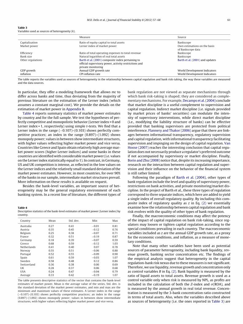
Table 3Variables used as sources of heterogeneity (k).

Measure Source

Capitalization Ratio of equity capital to total assets BankscopeMarket power Lerner index of market power Own estimations on the basis

of Bankscope dataEfficiency Ratio of total operating expenses to total revenue BankscopeBank size Natural logarithm of real total assets BankscopeOther regulations Barth et al. (2001) composite index pertaining to

official supervisory power, activity restrictions andprivate monitoring

Barth et al. (2001) and updates

GDP growth Annual GDP growth rate World Development Indicators

T betwa

Idpae

bfLLpmwCkcoUtmoM

eb

TDc

Tetm((s

bwmtcbs(piaasHliBrvi

b

inflation CPI inflation rate

he table reports the variables used as sources of heterogeneity in the relationshipnd the data sources.

n particular, they offer a modeling framework that allows mc toiffer across banks and time, thus deviating from the majority ofrevious literature on the estimation of the Lerner index (whichssumes a constant marginal cost). We provide the details on thestimation of market power in Appendix B.

Table 4 reports summary statistics of market power estimatesy country and for the full sample. We test the hypotheses of per-ectly competitive and monopolistic behavior (Lerner index = 0 anderner index = 1, respectively) using simple t-tests. We find that aerner index in the range (−0.107)–(0.103) shows perfectly com-etitive practices; an index in the range (0.897)–(1.092) showsonopoly power; values in between show intermediate structures,ith higher values reflecting higher market power and vice versa.ountries like Greece and Spain obtain relatively high average mar-et power scores (higher Lerner indices) and some banks in theseountries are identified with considerable market power (i.e. valuesn the Lerner index statistically equal to 1). In contrast, in Germany,S and UK competition is intense, as reflected in the low values on

he Lerner indices and the relatively small standard deviation of thearket power estimates. However, in most countries, for over 90%

f the banks in our sample, intermediate market structures prevail.ore information on these results is available on request.

Besides the bank-level variables, an important source of het-

rogeneity may be the general regulatory environment of eachanking system. In a recent line of literature, the different types of

able 4escriptive statistics of the bank-level estimates of market power (Lerner index) byountry.

Country Mean Std. dev. Min Max

Australia 0.27 0.41 −0.01 0.81Austria 0.35 0.45 −0.12 0.76Belgium 0.25 0.38 −0.07 0.71France 0.32 0.51 −0.19 0.87Germany 0.18 0.39 −0.07 0.59Greece 0.68 0.59 −0.12 1.03Netherlands 0.41 0.40 0.07 0.78Norway 0.55 0.51 −0.06 0.88Portugal 0.52 0.55 −0.09 0.90Spain 0.61 0.59 −0.03 1.07Sweden 0.58 0.48 0.12 0.86Switzerland 0.36 0.38 0.06 0.69UK 0.28 0.37 0.06 0.68USA 0.24 0.47 −0.04 0.79Average 0.33 0.42 −0.19 1.07

he table presents descriptive statistics of the vector that contains the bank-levelstimates of market power. Mean is the average value of the series, Std. dev. ishe standard deviation of the market power estimates, and min and max are the

inimum and maximum values of these estimates. A Lerner index in the range−0.107)–(0.103) shows perfectly competitive practices; an index in the range0.897)–(1.092) shows monopoly power; values in between show intermediatetructures, with higher values reflecting higher market power and vice versa.

rccaper

ousvft

setrTarciitia

World Development Indicators

een capital regulation and bank risk-taking, the way these variables are measured

ank regulation are not viewed as separate mechanisms throughhich bank risk-taking is shaped; they are considered as comple-entary mechanisms. For example, Decamps et al. (2004) conclude

hat market discipline is a useful complement to supervision andapital regulation. Indirect market discipline (i.e. signals providedy market prices of banks’ securities) can modulate the inten-ity of supervisory interventions, while direct market disciplinei.e., modifying the liability structure of banks) can be effectiverovided that banking supervisors are protected from political

nterference. Flannery and Thakor (2006) argue that there are link-ges between informational transparency, regulatory supervisionnd capital regulation, with informational transparency facilitatingupervision and impinging on the design of capital regulation. Vanoose (2007) reaches the interesting conclusion that capital regu-

ation does not necessarily produce a regulator’s preferred outcomef not accompanied by supervisory or market discipline. Finally,orio and Zhu (2008) notice that, despite its increasing importance,esearch on the interaction between capital regulation and super-ision and their influence on the behavior of the financial systems still rather limited.

Following the paradigm of Barth et al. (2004), other types ofank regulation include the level and quality of supervisory power,estrictions on bank activities, and private monitoring/market dis-ipline. In the project of Barth et al., these three types of regulationorrespond to three separate indices, which here are added to yield

single index of overall regulatory quality. By including this com-osite index of regulatory quality as z in Eq. (2) we essentiallyxamine how the relationship between capital regulation and bankisk evolves with the quality of other types of bank regulation.

Finally, the macroeconomic conditions may affect the potencyf the impact of capital regulation on bank risk-taking, since reg-lators may loosen or tighten capital regulation according to thepecial conditions prevailing in each country. The macroeconomicariables included as z are the annual GDP growth rate, as a proxyor the economic conditions, and inflation, as a measure of mone-ary conditions.

Note that many other variables have been used as potentialources of parameter heterogeneity, including bank liquidity, rev-nue growth, banking sector concentration etc. The findings ofhe empirical analysis suggest that heterogeneity in the capitalegulation-bank risk nexus due to these measures is not significant.herefore, we use liquidity, revenue growth and concentration onlys control variables B in Eq. (2). Bank liquidity is measured by theatio of liquid assets to total assets. Revenue growth is used as aontrol variable only when risk is measured by NPL, as profits arencluded in the calculation of both the Z-index and �(ROA), and

s measured by the annual growth in real total revenue. Concen-ration is measured by the 3-bank concentration ratio constructedn terms of total assets. Also, when the variables described aboves sources of heterogeneity (i.e. the ones reported in Table 3) are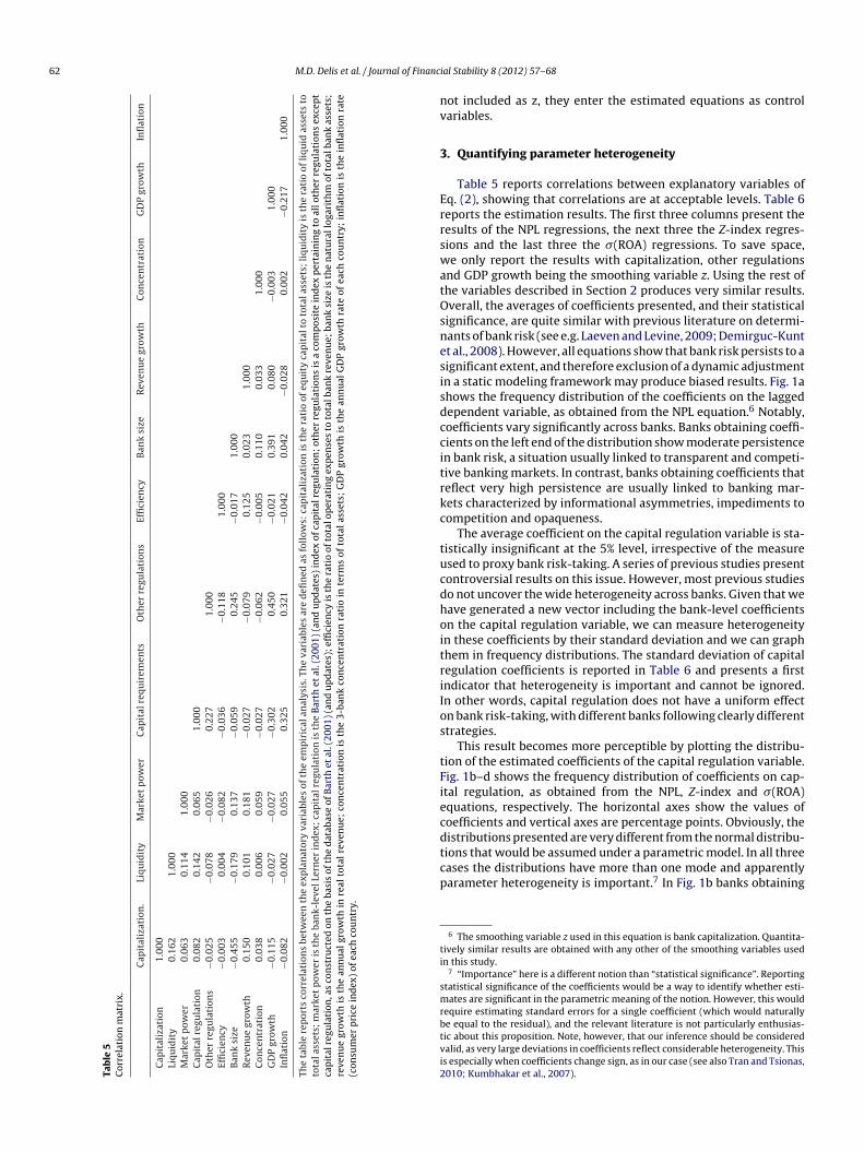

Page 6

62 M.D. Delis et al. / Journal of Financ

Tab

le

5C

orre

lati

on

mat

rix.

Cap

ital

izat

ion

.Li

quid

ity

Mar

ket

pow

erC

apit

al

requ

irem

ents

Oth

er

regu

lati

ons

Effi

cien

cyB

ank

size

Rev

enu

e

grow

thC

once

ntr

atio

nG

DP

grow

thIn

flat

ion

Cap

ital

izat

ion

1.00

0Li

quid

ity

0.16

2

1.00

0M

arke

t

pow

er0.

063

0.11

4

1.00

0C

apit

al

regu

lati

on0.

082

0.14

2

0.06

5

1.00

0O

ther

regu

lati

ons

−0.0

25

−0.0

78

−0.0

26

0.22

7

1.00

0Ef

fici

ency

−0.0

03

0.00

4

−0.0

82

−0.0

36

−0.1

18

1.00

0B

ank

size

−0.4

55

−0.1

79

0.13

7

−0.0

59

0.24

5

−0.0

17

1.00

0R

even

ue

grow

th0.

150

0.10

1

0.18

1

−0.0

27

−0.0

79

0.12

5

0.02

3

1.00

0C

once

ntr

atio

n0.

038

0.00

6

0.05

9

−0.0

27

−0.0

62

−0.0

05

0.11

0

0.03

3

1.00

0G

DP

grow

th−0

.115

−0.0

27

−0.0

27

−0.3

02

0.45

0

−0.0

21

0.39

1

0.08

0

−0.0

03

1.00

0In

flat

ion

−0.0

82

−0.0

02

0.05

5

0.32

5

0.32

1

−0.0

42

0.04

2

−0.0

28

0.00

2 −0

.217

1.00

0

The

tabl

e

rep

orts

corr

elat

ion

s

betw

een

the

exp

lan

ator

y

vari

able

s

of

the

emp

iric

al

anal

ysis

. Th

e

vari

able

s

are

defi

ned

as

foll

ows:

cap

ital

izat

ion

is

the

rati

o

of

equ

ity

cap

ital

to

tota

l ass

ets;

liqu

idit

y

is

the

rati

o

of

liqu

id

asse

ts

toto

tal a

sset

s;

mar

ket

pow

er

is

the

ban

k-le

vel L

ern

er

ind

ex; c

apit

al

regu

lati

on

is

the

Bar

th

et

al. (

2001

)

(an

d

up

dat

es)

ind

ex

of

cap

ital

regu

lati

on; o

ther

regu

lati

ons

is

a

com

pos

ite

ind

ex

per

tain

ing

to

all o

ther

regu

lati

ons

exce

pt

cap

ital

regu

lati

on, a

s

con

stru

cted

on

the

basi

s

of

the

dat

abas

e

of

Bar

th

et

al. (

2001

)

(an

d

up

dat

es);

effi

cien

cy

is

the

rati

o

of

tota

l op

erat

ing

exp

ense

s

to

tota

l ban

k

reve

nu

e;

ban

k

size

is

the

nat

ura

l log

arit

hm

of

tota

l ban

k

asse

ts;

reve

nu

e

grow

th

is

the

ann

ual

grow

th

in

real

tota

l rev

enu

e;

con

cen

trat

ion

is

the

3-ba

nk

con

cen

trat

ion

rati

o

in

term

s

of

tota

l ass

ets;

GD

P

grow

th

is

the

ann

ual

GD

P gr

owth

rate

of

each

cou

ntr

y;

infl

atio

n

is

the

infl

atio

n

rate

(con

sum

er

pri

ce

ind

ex)

of

each

cou

ntr

y.

nv

3

ErrswatOsnesisdccitrkc

tucdhoitriIos

tFiecdtcp

ti

smrbtvi2

ial Stability 8 (2012) 57– 68

ot included as z, they enter the estimated equations as controlariables.

. Quantifying parameter heterogeneity

Table 5 reports correlations between explanatory variables ofq. (2), showing that correlations are at acceptable levels. Table 6eports the estimation results. The first three columns present theesults of the NPL regressions, the next three the Z-index regres-ions and the last three the �(ROA) regressions. To save space,e only report the results with capitalization, other regulations

nd GDP growth being the smoothing variable z. Using the rest ofhe variables described in Section 2 produces very similar results.verall, the averages of coefficients presented, and their statistical

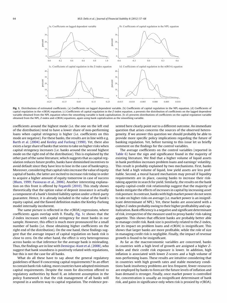
ignificance, are quite similar with previous literature on determi-ants of bank risk (see e.g. Laeven and Levine, 2009; Demirguc-Kuntt al., 2008). However, all equations show that bank risk persists to aignificant extent, and therefore exclusion of a dynamic adjustmentn a static modeling framework may produce biased results. Fig. 1ahows the frequency distribution of the coefficients on the laggedependent variable, as obtained from the NPL equation.6 Notably,oefficients vary significantly across banks. Banks obtaining coeffi-ients on the left end of the distribution show moderate persistencen bank risk, a situation usually linked to transparent and competi-ive banking markets. In contrast, banks obtaining coefficients thateflect very high persistence are usually linked to banking mar-ets characterized by informational asymmetries, impediments toompetition and opaqueness.

The average coefficient on the capital regulation variable is sta-istically insignificant at the 5% level, irrespective of the measuresed to proxy bank risk-taking. A series of previous studies presentontroversial results on this issue. However, most previous studieso not uncover the wide heterogeneity across banks. Given that weave generated a new vector including the bank-level coefficientsn the capital regulation variable, we can measure heterogeneityn these coefficients by their standard deviation and we can graphhem in frequency distributions. The standard deviation of capitalegulation coefficients is reported in Table 6 and presents a firstndicator that heterogeneity is important and cannot be ignored.n other words, capital regulation does not have a uniform effectn bank risk-taking, with different banks following clearly differenttrategies.

This result becomes more perceptible by plotting the distribu-ion of the estimated coefficients of the capital regulation variable.ig. 1b–d shows the frequency distribution of coefficients on cap-tal regulation, as obtained from the NPL, Z-index and �(ROA)quations, respectively. The horizontal axes show the values ofoefficients and vertical axes are percentage points. Obviously, the

istributions presented are very different from the normal distribu-ions that would be assumed under a parametric model. In all threeases the distributions have more than one mode and apparentlyarameter heterogeneity is important.7 In Fig. 1b banks obtaining

6 The smoothing variable z used in this equation is bank capitalization. Quantita-ively similar results are obtained with any other of the smoothing variables usedn this study.

7 “Importance” here is a different notion than “statistical significance”. Reportingtatistical significance of the coefficients would be a way to identify whether esti-ates are significant in the parametric meaning of the notion. However, this would

equire estimating standard errors for a single coefficient (which would naturallye equal to the residual), and the relevant literature is not particularly enthusias-ic about this proposition. Note, however, that our inference should be consideredalid, as very large deviations in coefficients reflect considerable heterogeneity. Thiss especially when coefficients change sign, as in our case (see also Tran and Tsionas,010; Kumbhakar et al., 2007).

Page 7

M.D

. D

elis et

al. /

Journal of

Financial Stability

8 (2012) 57– 6863

Table 6Risk and capital regulation.

NPL Z-index �(ROA)

(1) k:capitalization

(2) k: otherregulations

(3) k: GDPgrowth

(4) k:capitalization

(5) k: otherregulations

(6) k: GDPgrowth

(7) k:capitalization

(8) k: otherregulations

(9) k: GDPgrowth

Lagged dependent 0.406* (0.074) 0.423* (0.068) 0.397* (0.073) 0.307* (0.055) 0.295* (0.061) 0.323* (0.060) 0.220* (0.051) 0.219* (0.054) 0.232* (0.050)Capital regulation 0.120 (0.077) 0.149 (0.081) 0.132 (0.078) 0.058 (0.045) 0.061 (0.046) 0.060 (0.043) −0.004 (0.006) −0.004 (0.007) −0.003 (0.005)Standard deviation of

coefficients0.203 0.194 0.247 0.166 0.160 0.153 0.011 0.012 0.011

Other regulations −0.113* (0.046) −0.125* (0.043) 0.246* (0.081) 0.267* (0.079) −0.503* (0.181) −0.614* (0.203)Capitalization 0.041* (0.017) 0.043* (0.016) 0.021 (0.015) 0.019 (0.015) 0.023 (0.017)Liquidity 0.063* (0.024) 0.064* (0.022) 0.061* (0.021) 0.016 (0.023) 0.021 (0.024) 0.015 (0.025) 0.036 (0.023) 0.042* (0.021) 0.040* (0.018)Market power −0.071 (0.062) −0.077 (0.059) −0.069 (0.059) 0.313* (0.100) 0.348* (0.107) 0.295* (0.091) 0.147 (0.097) 0.172 (0.118) 0.203 (0.141)Efficiency −1.071* (0.303) −1.042* (0.349) −1.033* (0.327) 0.729* (0.181) 0.814* (0.202) 0.800* (0.209) −0.316* (0.096) −0.401* (0.117) −0.307* (0.093)Bank size −0.125 (0.104) −0.144 (0.117) −0.141 (0.113) 0.086* (0.027) 0.083* (0.031) 0.081* (0.031) −0.021 (0.082) −0.010 (0.061) 0.017 (0.030)Revenue growth −0.327 (0.248) −0.342 (0.245) −0.333 (0.237)Concentration 0.405 (0.340) 0.432 (0.363) 0.401 (0.367) −0.067 (0.104) −0.023 (0.087) −0.021 (0.061) 0.107 (0.066) 0.181* (0.078) 0.203* (0.089)GDP growth −0.047* (0.008) −0.0439* (0.009) 0.060* (0.019) 0.052* (0.016) 0.072* (0.022) −0.021* (0.009) −0.019* (0.009)Inflation 0.046* (0.010) 0.036* (0.009) 0.038* (0.011) −0.052* (0.018) −0.061* (0.025) −0.055* (0.021) 0.093* (0.028) 0.088* (0.032) 0.090* (0.030)�ê 0.081 0.084 0.077 0.103 0.095 0.095 0.081 0.077 0.086bandwidth 0.653 0.598 0.614 1.721 1.815 1.797 0.918 0.901 0.960

The table reports average coefficients and standard errors (in parentheses). For the capital regulation variable the standard deviation of the bank-level coefficients (measure of parameter heterogeneity) is also reported. Inregressions (1–3) dependent variable is the ratio of non-performing loans to total loans (NPL), in regressions (4–6) the Z-index and in regressions (7–9) �(ROA), as measured by the variance of the ratio of profits before tax tototal assets. k is the smoothing variable used in each regression of the empirical model presented in Eq. (2). For each dependent variable we report the estimates from the equations that employ capitalization, other regulationsand GDP growth as k. The variables included in the table are defined as follows: lagged dependent is the first lag of the risk variable; capital regulation is the Barth et al. (2001) (and updates) index of capital regulation; otherregulations is a composite index pertaining to all other regulations except capital regulation, as constructed on the basis of the database of Barth et al. (2001) (and updates); capitalization is the ratio of equity capital to totalassets; liquidity is the ratio of liquid assets to total assets; market power is the bank-level Lerner index; efficiency is the ratio of total operating expenses to total bank revenue; bank size is the natural logarithm of real totalbank assets; revenue growth is the annual growth in real total revenue; concentration is the 3-bank concentration ratio in terms of total assets; GDP growth is the annual GDP growth rate of each country; inflation is theinflation rate (consumer price index) of each country. �ê is the variance of the estimated error term and bandwidth is the optimal bandwidth used in each regression as estimated by the method of Zhang and Lee (2000). ‘*’denotes statistical significance at the 5% level.

Page 8

64 M.D. Delis et al. / Journal of Financial Stability 8 (2012) 57– 68

1a. Coefficients on lagged dependent variable 1b. Coefficients of capital regulation in the NPL equation

1c. Coefficients of capital regulation in the Z-index equation 1d. Co efficients of ca pit al regulati on in the σ(ROA) equation

perc

ent

perc

ent

perc

ent

perc

ent

0.0 0.40.2 1.00.80.6 -0.6 -0.3 0.60.30.0

-0.015 -0.010 -0.005 0.0100.0050.000-0.25 -0.15 0.250.150.05

30

20

10

0

30

20

10

0

0

10

20

30

40 40

30

20

10

0

Fig. 1. Distributions of estimated coefficients. (a) Coefficients on lagged dependent variable. (b) Coefficients of capital regulation in the NPL equation. (d) Coefficients ofc he Z-inv italizao ion as

colmBecmouaMct(ttagem

cZsnrgcaTsb

gtcrpr

sqgpbc

TeiTtirtebrtihioatysig

iiinit

apital regulation in the �(ROA) equation. (c) Coefficients of capital regulation in tariable obtained from the NPL equation when the smoothing variable is bank capbtained from the NPL, Z-index and �(ROA) equations, again using bank capitalizat

oefficients around the highest mode (i.e. the one on the left endf the distribution) tend to have a lower share of non-performingoans when capital stringency is higher (i.e. coefficients on this

ode are negative). For these banks, the results are in line with e.g.arth et al. (2004) and Keeley and Furlong (1990). Yet, there alsoxists a large share of banks that seems to take on higher risks whenapital stringency increases (i.e. banks around the second highestode on the right end of the distribution). This is explained by the

ther part of the same literature, which suggests that as capital reg-lation reduces future profits, banks have diminished incentives tovoid default since they have less to lose in the case of bankruptcy.oreover, considering that capital rules increase the value of equity

apital of banks, the latter are incited to increase risk today in ordero acquire a higher amount of equity tomorrow in case of successBlum, 1999; Pasiouras et al., 2006). Another interesting explana-ion on this front is offered by Fegatelli (2010). This study showsheoretically that the option value of deposit insurance is actually

component of a bank’s limited liability option under a third-partyuarantee. Hence, it is already included in the value of the bank’squity capital, and the flawed definition makes the Keeley-Furlongodel internally incoherent.The same picture is reflected in the �(ROA) regressions, where

oefficients again overlap with 0. Finally, Fig. 1c shows that the-index increases with capital stringency for most banks in ourample. However, this effect is much more pronounced for a smallumber of banks (i.e. those obtaining higher coefficients on theight end of the distribution). On the one hand, these findings sug-est that the average impact of capital regulation on bank risk islose to zero. On the other hand, the effect is very heterogeneouscross banks so that inference for the average bank is misleading.hus, the findings are in line with Demirguc-Kunt et al. (2008), whouggest that bank soundness is positively related with regulations,ut this is not the case for all banks.

What do all these have to say about the general regulatoryuidelines of Basel II concerning capital requirements? In an efforto contain bank risk-taking, most countries have adopted minimum

apital requirements. Despite the room for discretion offered toegulatory authorities by Basel II, an inherent assumption in theolicy framework is that the risk management of all banks willespond in a uniform way to capital regulation. The evidence pre-

alfr

dex equation. a presents the distribution of coefficients on the lagged dependenttion. (b–d) presents distributions of coefficients on the capital regulation variable

the smoothing variable.

ented here clearly point out to a different outcome. An immediateuestion that arises concerns the sources of the observed hetero-eneity. If we answer this question we should probably be able torovide more specific policy implications regarding the future ofanking regulation. Yet, before turning to this issue let us brieflyomment on the findings for the control variables.

The average coefficients on the control variables (reported inable 6) have the sign and significance found in the majority ofxisting literature. We find that a higher volume of liquid assetsn bank portfolios increases problem loans and earnings’ volatility.his result is probably explained by two mechanisms. First, bankshat hold a high volume of liquid, low yield assets are less prof-table. Second, a moral hazard mechanism may prevail if liquidityequirements are in place, causing banks to increase their risk-aking appetite in search for yield. Similarly, the results on the bankquity capital-credit risk relationship suggest that the majority ofanks mitigate the effects of increases in capital by increasing assetisk posture. In contrast, banks with high market power do not seemo take on higher risks on average (i.e. market power is an insignif-cant determinant of NPL). Yet, these banks are associated with aigher Z-index probably owing to their higher profitability and cap-

talization. Bank efficiency is a negative and significant determinantf risk, irrespective of the measure used to proxy banks’ risk-takingppetite. This shows that efficient banks are probably better ableo manage credit risk. Bank size is positively related to the Z-index,et its impact on problem loans and �(ROA) is insignificant. Thishows that larger banks are more profitable, while the role of sizen managing credit risk is negligible. Finally, the impact of revenuerowth is found to be insignificant.

As far as the macroeconomic variables are concerned, banksn countries with a high level of growth are assigned a higher Z-ndex and their credit risk exposure is lower. In addition, highnflation is associated with lower Z-scores and a high volume ofon-performing loans. These results are intuitive considering that

n countries with high growth rates and stable monetary condi-ions bank insolvency problems are less frequent, fewer resources

re employed by banks to forecast the future levels of inflation andoan demand is stronger. Finally, once market power is controlledor, concentration is usually an insignificant determinant of bankisk, and gains in significance only when risk is proxied by �(ROA).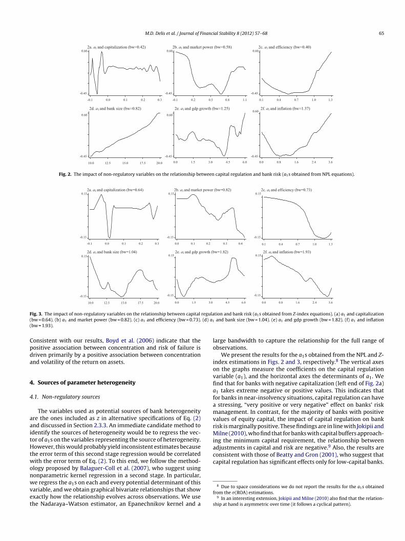

Page 9

M.D. Delis et al. / Journal of Financial Stability 8 (2012) 57– 68 65

2a. a1 2b. aand capitalization (bw=0.42) 1 2c. aand market power (bw=0.58) 1 and efficiency (bw=0.40)

2d. a1 2e. aand bank size (bw=0.82) 1 2f. aand gdp growth (bw=1.25) 1 and inflation (bw=1.37)

-0.1 0.30.20.10.0 0.1 0.4 0.7 1.0 1.3

10.0 12.5 15.0 17.5 20.0 6.0 0.0 1.5 3.0 4.5 0.0 0.8 1.6 2.4 3.6

0.60

-0.45

0.60

-0.45

0.60

-0.45

-0.45 -0.45 -0.45

0.60 0.60

0.5 0.8 1.1 -0.1 0.2

0.60

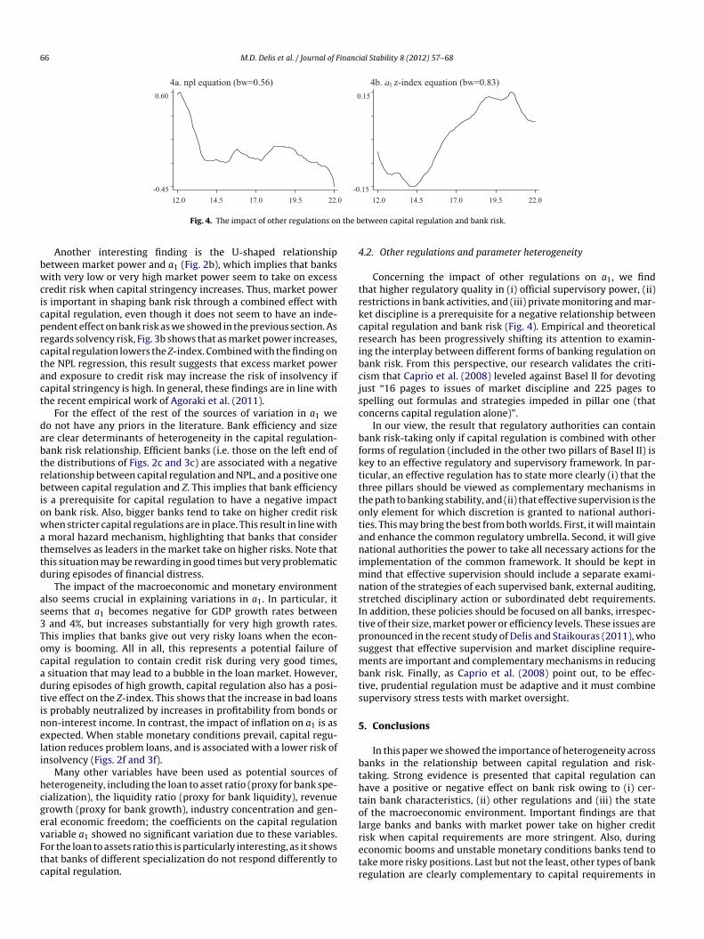
Fig. 2. The impact of non-regulatory variables on the relationship between capital regulation and bank risk (a1s obtained from NPL equations).

2a. a1 2b. aand capitalization (bw=0.64) 1 2c. aand market power (bw=0.82) 1 and efficiency (bw=0.73)

2d. a1 2e. aand bank size (bw=1.04) 1 2f. aand gdp growth (bw=1.82) 1 and inflation (bw=1.93)

-0.1 0.30.20.10.0 0.30.20.10.0 0.4 0.1 0.4 0.7 1.0 1.3

10.0 12.5 15.0 17.5 20.0 0.0 1.5 3.0 4.5 6.0 0.0 0.8 1.6 2.4 3.6

-0.15

-0.15 -0.15 -0.15

0.15 0.15 0.15

0.15

-0.15-0.15

0.15 0.15

F regula( (d) a1

(

Cpda

4

4

aaitHtwonwvet

lo

iovfiafamvrMiadjustments in capital and risk are negative.9 Also, the results areconsistent with those of Beatty and Gron (2001), who suggest thatcapital regulation has significant effects only for low-capital banks.

ig. 3. The impact of non-regulatory variables on the relationship between capital

bw = 0.64). (b) a1 and market power (bw = 0.82). (c) a1 and efficiency (bw = 0.73).bw = 1.93).

onsistent with our results, Boyd et al. (2006) indicate that theositive association between concentration and risk of failure isriven primarily by a positive association between concentrationnd volatility of the return on assets.

. Sources of parameter heterogeneity

.1. Non-regulatory sources

The variables used as potential sources of bank heterogeneityre the ones included as z in alternative specifications of Eq. (2)nd discussed in Section 2.3.3. An immediate candidate method todentify the sources of heterogeneity would be to regress the vec-or of a1s on the variables representing the source of heterogeneity.owever, this would probably yield inconsistent estimates because

he error term of this second stage regression would be correlatedith the error term of Eq. (2). To this end, we follow the method-

logy proposed by Balaguer-Coll et al. (2007), who suggest usingonparametric kernel regression in a second stage. In particular,

e regress the a1s on each and every potential determinant of this

ariable, and we obtain graphical bivariate relationships that showxactly how the relationship evolves across observations. We usehe Nadaraya–Watson estimator, an Epanechnikov kernel and a

f

s

tion and bank risk (a1s obtained from Z-index equations). (a) a1 and capitalizationand bank size (bw = 1.04). (e) a1 and gdp growth (bw = 1.82). (f) a1 and inflation

arge bandwidth to capture the relationship for the full range ofbservations.

We present the results for the a1s obtained from the NPL and Z-ndex estimations in Figs. 2 and 3, respectively.8 The vertical axesn the graphs measure the coefficients on the capital regulationariable (a1), and the horizontal axes the determinants of a1. Wend that for banks with negative capitalization (left end of Fig. 2a)1 takes extreme negative or positive values. This indicates thator banks in near-insolvency situations, capital regulation can have

stressing, “very positive or very negative” effect on banks’ riskanagement. In contrast, for the majority of banks with positive

alues of equity capital, the impact of capital regulation on bankisk is marginally positive. These findings are in line with Jokipii andilne (2010), who find that for banks with capital buffers approach-

ng the minimum capital requirement, the relationship between

8 Due to space considerations we do not report the results for the a1s obtainedrom the �(ROA) estimations.

9 In an interesting extension, Jokipii and Milne (2010) also find that the relation-hip at hand is asymmetric over time (it follows a cyclical pattern).

Page 10

66 M.D. Delis et al. / Journal of Financial Stability 8 (2012) 57– 68

4b. a4a. npl equation (bw=0.56) 1 z-index equation (bw=0.83) 0.60

-0.45 0

0.15

-0.15

the b

bwcicprctact

dabtrbiowattd

as3Tocadtineli

hcgevFtc

4

trkcribcjsc

bfktttotanimnsItpsmbts

5

bthtol

12.0 14.5 17.0 19.5 22.

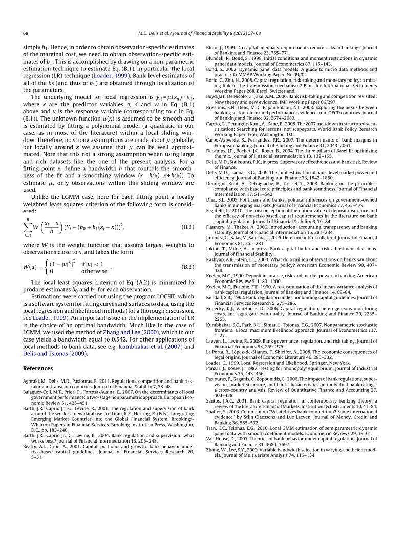
Fig. 4. The impact of other regulations on

Another interesting finding is the U-shaped relationshipetween market power and a1 (Fig. 2b), which implies that banksith very low or very high market power seem to take on excess

redit risk when capital stringency increases. Thus, market powers important in shaping bank risk through a combined effect withapital regulation, even though it does not seem to have an inde-endent effect on bank risk as we showed in the previous section. Asegards solvency risk, Fig. 3b shows that as market power increases,apital regulation lowers the Z-index. Combined with the finding onhe NPL regression, this result suggests that excess market powernd exposure to credit risk may increase the risk of insolvency ifapital stringency is high. In general, these findings are in line withhe recent empirical work of Agoraki et al. (2011).

For the effect of the rest of the sources of variation in a1 weo not have any priors in the literature. Bank efficiency and sizere clear determinants of heterogeneity in the capital regulation-ank risk relationship. Efficient banks (i.e. those on the left end ofhe distributions of Figs. 2c and 3c) are associated with a negativeelationship between capital regulation and NPL, and a positive oneetween capital regulation and Z. This implies that bank efficiency

s a prerequisite for capital regulation to have a negative impactn bank risk. Also, bigger banks tend to take on higher credit riskhen stricter capital regulations are in place. This result in line with

moral hazard mechanism, highlighting that banks that considerhemselves as leaders in the market take on higher risks. Note thathis situation may be rewarding in good times but very problematicuring episodes of financial distress.

The impact of the macroeconomic and monetary environmentlso seems crucial in explaining variations in a1. In particular, iteems that a1 becomes negative for GDP growth rates between

and 4%, but increases substantially for very high growth rates.his implies that banks give out very risky loans when the econ-my is booming. All in all, this represents a potential failure ofapital regulation to contain credit risk during very good times,

situation that may lead to a bubble in the loan market. However,uring episodes of high growth, capital regulation also has a posi-ive effect on the Z-index. This shows that the increase in bad loanss probably neutralized by increases in profitability from bonds oron-interest income. In contrast, the impact of inflation on a1 is asxpected. When stable monetary conditions prevail, capital regu-ation reduces problem loans, and is associated with a lower risk ofnsolvency (Figs. 2f and 3f).

Many other variables have been used as potential sources ofeterogeneity, including the loan to asset ratio (proxy for bank spe-ialization), the liquidity ratio (proxy for bank liquidity), revenuerowth (proxy for bank growth), industry concentration and gen-ral economic freedom; the coefficients on the capital regulation

ariable a1 showed no significant variation due to these variables.or the loan to assets ratio this is particularly interesting, as it showshat banks of different specialization do not respond differently toapital regulation.

retr

12.0 14.5 17.0 19.5 22.0

etween capital regulation and bank risk.

.2. Other regulations and parameter heterogeneity

Concerning the impact of other regulations on a1, we findhat higher regulatory quality in (i) official supervisory power, (ii)estrictions in bank activities, and (iii) private monitoring and mar-et discipline is a prerequisite for a negative relationship betweenapital regulation and bank risk (Fig. 4). Empirical and theoreticalesearch has been progressively shifting its attention to examin-ng the interplay between different forms of banking regulation onank risk. From this perspective, our research validates the criti-ism that Caprio et al. (2008) leveled against Basel II for devotingust “16 pages to issues of market discipline and 225 pages topelling out formulas and strategies impeded in pillar one (thatoncerns capital regulation alone)”.

In our view, the result that regulatory authorities can containank risk-taking only if capital regulation is combined with otherorms of regulation (included in the other two pillars of Basel II) isey to an effective regulatory and supervisory framework. In par-icular, an effective regulation has to state more clearly (i) that thehree pillars should be viewed as complementary mechanisms inhe path to banking stability, and (ii) that effective supervision is thenly element for which discretion is granted to national authori-ies. This may bring the best from both worlds. First, it will maintainnd enhance the common regulatory umbrella. Second, it will giveational authorities the power to take all necessary actions for the

mplementation of the common framework. It should be kept inind that effective supervision should include a separate exami-

ation of the strategies of each supervised bank, external auditing,tretched disciplinary action or subordinated debt requirements.n addition, these policies should be focused on all banks, irrespec-ive of their size, market power or efficiency levels. These issues areronounced in the recent study of Delis and Staikouras (2011), whouggest that effective supervision and market discipline require-ents are important and complementary mechanisms in reducing

ank risk. Finally, as Caprio et al. (2008) point out, to be effec-ive, prudential regulation must be adaptive and it must combineupervisory stress tests with market oversight.

. Conclusions

In this paper we showed the importance of heterogeneity acrossanks in the relationship between capital regulation and risk-aking. Strong evidence is presented that capital regulation canave a positive or negative effect on bank risk owing to (i) cer-ain bank characteristics, (ii) other regulations and (iii) the statef the macroeconomic environment. Important findings are thatarge banks and banks with market power take on higher credit

isk when capital requirements are more stringent. Also, duringconomic booms and unstable monetary conditions banks tend toake more risky positions. Last but not the least, other types of bankegulation are clearly complementary to capital requirements in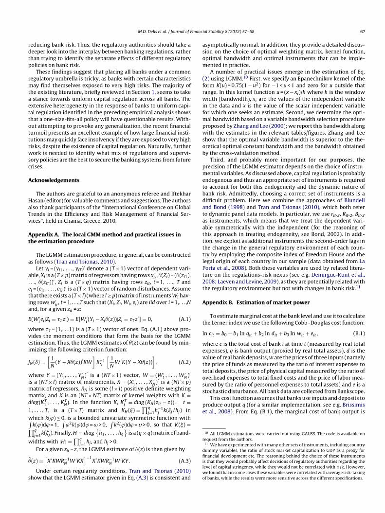

Page 11

inanci

rdtp

rmtaettottrwsc

A

HaTv

At

a

a.etia

E

wvei

J

wimmd

1w∫∏w

�

s

asom

(frwifmpwsob

pmetbdataattttlPt2t

A

t

l

wevttoss

This cost function assumes that banks use inputs and deposits toproduce output q (for a similar implementation, see e.g. Brissimiset al., 2008). From Eq. (B.1), the marginal cost of bank output is

10 All LGMM estimations were carried out using GAUSS. The code is available onrequest from the authors.

11 We have experimented with many other sets of instruments, including countrydummy variables, the ratio of stock market capitalization to GDP as a proxy for

M.D. Delis et al. / Journal of F

educing bank risk. Thus, the regulatory authorities should take aeeper look into the interplay between banking regulations, ratherhan trying to identify the separate effects of different regulatoryolicies on bank risk.

These findings suggest that placing all banks under a commonegulatory umbrella is tricky, as banks with certain characteristicsay find themselves exposed to very high risks. The majority of

he existing literature, briefly reviewed in Section 1, seems to take stance towards uniform capital regulation across all banks. Thextensive heterogeneity in the response of banks to uniform capi-al regulation identified in the preceding empirical analysis showshat a one-size-fits-all policy will have questionable results. With-ut attempting to provoke any generalization, the recent financialurmoil presents an excellent example of how large financial insti-utions may quickly face insolvency if they are exposed to very highisks, despite the existence of capital regulation. Naturally, furtherork is needed to identify what mix of regulations and supervi-

ory policies are the best to secure the banking systems from futurerises.

cknowledgements

The authors are grateful to an anonymous referee and Iftekharasan (editor) for valuable comments and suggestions. The authorslso thank participants of the “International Conference on Globalrends in the Efficiency and Risk Management of Financial Ser-ices”, held in Chania, Greece, 2010.

ppendix A. The local GMM method and practical issues inhe estimation procedure

The LGMM estimation procedure, in general, can be constructeds follows (Tran and Tsionas, 2010).

Let yi = (yi1, . . ., yiT)′ denote a (T × 1) vector of dependent vari-ble, Xi is a (T × p) matrix of regressors having rows x′

it, �(Zi) = (�(zi1),

. ., �(ziT))′, Zi is a (T × q) matrix having rows zit, t = 1, . . ., T andi = (ei1, . . ., eiT)′ is a (T × 1) vector of random disturbances. Assumehat there exists a (T × l) (where l ≥ p) matrix of instruments Wi hav-ng rows w′

it, t = 1,. . .,T such that (Xi, Zi, Wi, ei) are iid over i = 1,. . .,N

nd, for a given zit = z:

(W ′i ei|Zi = �T z′) = E[W ′

i (Yi − Xi�(z))|Zi = �T z′] = 0, (A.1)

here �T = (1,. . .1) is a (T × 1) vector of ones. Eq. (A.1) above pro-ides the moment conditions that form the basis for the LGMMstimation. Thus, the LGMM estimates of �(z) can be found by min-mizing the following criterion function:

N(ı) =[

1N

(Y − X�(z))′KW]

R−1N

[1N

W ′K(Y − X�(z))]

, (A.2)

here Y = (Y ′1, . . . , Y ′

N)′ is a (NT × 1) vector, W = (W ′1, . . . , W ′

N)′

s a (NT × l) matrix of instruments, X = (X ′1, . . . , X ′

N)′ is a (NT × p)atrix of regressors, RN is some (l × l) positive definite weightingatrix, and K is an (NT × NT) matrix of kernel weights with K =

iag{KT1 , . . . , KT

N}. In the function K, KTi

= diag (KH(zit − z)) , t =, . . . , T , is a (T × T) matrix and KH(�) =

∏qj=1h−1

jk(�j/hj) in

hich k(ϕ) ≥ 0, is a bounded univariate symmetric function withk(ϕ)dϕ = 1,

∫ϕ2k(ϕ)dϕ = ω > 0,

∫k2(ϕ)dϕ = � > 0, so that K(�) =

qj=1k(�j). Finally, H = diag

{h1, . . . , hq

}is a (q × q) matrix of band-

idths with |H| =∏q

j=1hj , and hj > 0.For a given zit = z, the LGMM estimate of �(z) is then given by

ˆ(z) =[X ′KWR−1

N W ′KX]−1

X ′KWR−1N W ′KY . (A.3)

Under certain regularity conditions, Tran and Tsionas (2010)how that the LGMM estimator given in Eq. (A.3) is consistent and

fiilwo

al Stability 8 (2012) 57– 68 67

symptotically normal. In addition, they provide a detailed discus-ion on the choice of optimal weighting matrix, kernel function,ptimal bandwidth and optimal instruments that can be imple-ented in practice.A number of practical issues emerge in the estimation of Eq.

2) using LGMM.10 First, we specify an Epanechnikov kernel of theorm K(u) = 0.75(1 − u2) for −1 < u < 1 and zero for u outside thatange. In this kernel function u = (x − xi)/h where h is the windowidth (bandwidth), xi are the values of the independent variable

n the data and x is the value of the scalar independent variableor which one seeks an estimate. Second, we determine the opti-

al bandwidth based on a variable bandwidth selection procedureroposed by Zhang and Lee (2000); we report this bandwidth alongith the estimates in the relevant tables/figures. Zhang and Lee

how that the optimal variable bandwidth is superior to the the-retical optimal constant bandwidth and the bandwidth obtainedy the cross-validation method.

Third, and probably more important for our purposes, therecision of the LGMM estimator depends on the choice of instru-ental variables. As discussed above, capital regulation is probably

ndogenous and thus an appropriate set of instruments is requiredo account for both this endogeneity and the dynamic nature ofank risk. Admittedly, choosing a correct set of instruments is aifficult problem. Here we combine the approaches of Blundellnd Bond (1998) and Tran and Tsionas (2010), which both refero dynamic panel data models. In particular, we use rit-2, Rit-2, Bit-2s instruments, which means that we treat the dependent vari-ble symmetrically with the independent (for the reasoning ofhis approach in treating endogeneity, see Bond, 2002). In addi-ion, we exploit as additional instruments the second-order lags inhe change in the general regulatory environment of each coun-ry by employing the composite index of Freedom House and theegal origin of each country in our sample (data obtained from Laorta et al., 2008). Both these variables are used by related litera-ure on the regulations-risk nexus (see e.g. Demirguc-Kunt et al.,008; Laeven and Levine, 2009), as they are potentially related withhe regulatory environment but not with changes in bank risk.11

ppendix B. Estimation of market power

To estimate marginal cost at the bank level and use it to calculatehe Lerner index we use the following Cobb–Douglas cost function:

n cit = b0 + b1 ln qit + b2 ln dit + b3 ln wit + eit, (B.1)

here c is the total cost of bank i at time t (measured by real totalxpenses), q is bank output (proxied by real total assets), d is thealue of real bank deposits, w are the prices of three inputs (namelyhe price of funds as measured by the ratio of interest expenses tootal deposits, the price of physical capital measured by the ratio ofverhead expenses to total fixed costs and the price of labor mea-ured by the ratio of personnel expenses to total assets) and e is atochastic disturbance. All bank data are collected from Bankscope.

nancial development etc. The reasoning behind the choice of these instrumentss that they would probably affect decisions of regulatory authorities regarding theevel of capital stringency, while they would not be correlated with risk. However,

e found that in some cases these variables were correlated with average risk-takingf banks, while the results were more sensitive across the different specifications.

Page 12

6 inanc

somerat

wa(icdbmafineu

we

∑

wo

W

p

ilsiLclD

R

A

B

B

B

B

B

B

B

B

B

B

C

C

D

D

D

D

D

F

F

J

J

K

K

K

K

K

K

L

L

LP

P

S

S

T

8 M.D. Delis et al. / Journal of F

imply b1. Hence, in order to obtain observation-specific estimatesf the marginal cost, we need to obtain observation-specific esti-ates of b1. This is accomplished by drawing on a non-parametric

stimation technique to estimate Eq. (B.1), in particular the localegression (LR) technique (Loader, 1999). Bank-level estimates ofll of the bs (and thus of b1) are obtained through localization ofhe parameters.

The underlying model for local regression is yit = (xit) + εit,here x are the predictor variables q, d and w in Eq. (B.1)

bove and y is the response variable (corresponding to c in Eq.B.1)). The unknown function (x) is assumed to be smooth ands estimated by fitting a polynomial model (a quadratic in ourase, as in most of the literature) within a local sliding win-ow. Therefore, no strong assumptions are made about globally,ut locally around x we assume that can be well approxi-ated. Note that this not a strong assumption when using large

nd rich datasets like the one of the present analysis. For atting point x, define a bandwidth h that controls the smooth-ess of the fit and a smoothing window (x − h(x), x + h(x)). Tostimate , only observations within this sliding window aresed.

Unlike the LGMM case, here for each fitting point a locallyeighted least squares criterion of the following form is consid-

red:n

i=1

W(

xi − x

h

)(Yi − (b0 + b1(xi − x)))2, (B.2)

here W is the weight function that assigns largest weights tobservations close to x, and takes the form

(u) ={

(1 − |u|3)3

if |u| < 10 otherwise

. (B.3)

The local least squares criterion of Eq. (A.2) is minimized toroduce estimates

�b0 and

�b1 for each observation.

Estimations were carried out using the program LOCFIT, whichs a software system for fitting curves and surfaces to data, using theocal regression and likelihood methods (for a thorough discussion,ee Loader, 1999). An important issue in the implementation of LRs the choice of an optimal bandwidth. Much like in the case ofGMM, we used the method of Zhang and Lee (2000), which in ourase yields a bandwidth equal to 0.542. For other applications ofocal methods to bank data, see e.g. Kumbhakar et al. (2007) andelis and Tsionas (2009).

eferences

goraki, M., Delis, M.D., Pasiouras, F., 2011. Regulations, competition and bank risk-taking in transition countries. Journal of Financial Stability 7, 38–48.

alaguer-Coll, M.T., Prior, D., Tortosa-Ausina, E., 2007. On the determinants of localgovernment performance: a two-stage nonparametric approach. European Eco-nomic Review 51, 425–451.

arth, J.R., Caprio Jr., G., Levine, R., 2001. The regulation and supervision of bankaround the world: a new database. In: Litan, R.E., Herring, R. (Eds.), IntegratingEmerging Market Countries into the Global Financial System. Brookings-Wharton Papers in Financial Services. Brooking Institution Press, Washington,D.C., pp. 183–240.

arth, J.R., Caprio Jr., G., Levine, R., 2004. Bank regulation and supervision: whatworks best? Journal of Financial Intermediation 13, 205–248.

eatty, A.L., Gron, A., 2001. Capital, portfolio, and growth: bank behavior underrisk-based capital guidelines. Journal of Financial Services Research 20,5–31.

V

Z

ial Stability 8 (2012) 57– 68

lum, J., 1999. Do capital adequacy requirements reduce risks in banking? Journalof Banking and Finance 23, 755–771.

lundell, R., Bond, S., 1998. Initial conditions and moment restrictions in dynamicpanel data models. Journal of Econometrics 87, 115–143.

ond, S., 2002. Dynamic panel data models. A guide to micro data methods andpractice. CeMMAP Working Paper, No 09/02.

orio, C., Zhu, H., 2008. Capital regulation, risk-taking and monetary policy: a miss-ing link in the transmission mechanism? Bank for International SettlementsWorking Paper 268, Basel, Switzerland.

oyd, J.H., De Nicolo, G., Jalal, A.M., 2006. Bank risk-taking and competition revisited:New theory and new evidence. IMF Working Paper 06/297.

rissimis, S.N., Delis, M.D., Papanikolaou, N.I., 2008. Exploring the nexus betweenbanking sector reform and performance: evidence from OECD countries. Journalof Banking and Finance 32, 2674–2683.

aprio, G., Demirgüc -Kunt, A., Kane, E., 2008. The 2007 meltdown in structured secu-ritization: Searching for lessons, not scapegoats. World Bank Policy ResearchWorking Paper 4756, Washington, D.C.

arbo-Valverde, S., Fernandez, F.R., 2007. The determinants of bank margins inEuropean banking. Journal of Banking and Finance 31, 2043–2063.

ecamps, J.P., Rochet, J.C., Roger, B., 2004. The three pillars of Basel II: optimizingthe mix. Journal of Financial Intermediation 13, 132–155.

elis, M.D., Staikouras, P.K., in press. Supervisory effectiveness and bank risk. Reviewof Finance.

elis, M.D., Tsionas, E.G., 2009. The joint estimation of bank-level market power andefficiency. Journal of Banking and Finance 33, 1842–1850.

emirguc-Kunt, A., Detragiache, E., Tressel, T., 2008. Banking on the principles:compliance with basel core principles and bank soundness. Journal of FinancialIntermediation 17, 511–542.

inc, S.I., 2005. Politicians and banks: political influences on government-ownedbanks in emerging markets. Journal of Financial Economics 77, 453–479.

egatelli, P., 2010. The misconception of the option value of deposit insurance andthe efficacy of non-risk-based capital requirements in the literature on bankcapital regulation. Journal of Financial Stability 6, 79–84.

lannery, M., Thakor, A., 2006. Introduction: accounting, transparency and bankingstability. Journal of Financial Intermediation 15, 281–284.

imenez, G., Salas, V., Saurina, J., 2006. Determinants of collateral. Journal of FinancialEconomics 81, 255–281.

okipii, T., Milne, A., in press. Bank capital buffer and risk adjustment decisions.Journal of Financial Stability.

ashyap, A.K., Stein, J.C., 2000. What do a million observations on banks say aboutthe transmission of monetary policy? American Economic Review 90, 407–428.

eeley, M.C., 1990. Deposit insurance, risk, and market power in banking. AmericanEconomic Review 5, 1183–1200.

eeley, M.C., Furlong, F.T., 1990. A re-examination of the mean-variance analysis ofbank capital regulation. Journal of Banking and Finance 14, 69–84.

endall, S.B., 1992. Bank regulation under nonbinding capital guidelines. Journal ofFinancial Services Research 5, 275–286.

opecky, K.J., VanHoose, D., 2006. Capital regulation, heterogeneous monitoringcosts, and aggregate loan quality. Journal of Banking and Finance 30, 2235–2255.

umbhakar, S.C., Park, B.U., Simar, L., Tsionas, E.G., 2007. Nonparametric stochasticfrontiers: a local maximum likelihood approach. Journal of Econometrics 137,1–27.

aeven, L., Levine, R., 2009. Bank governance, regulation, and risk taking. Journal ofFinancial Economics 93, 259–275.

a Porta, R., López-de-Silanes, F., Shleifer, A., 2008. The economic consequences oflegal origins. Journal of Economic Literature 46, 285–332.

oader, C., 1999. Local Regression and Likelihood. Springer, New York.anzar, J., Rosse, J., 1987. Testing for ‘monopoly’ equilibrium. Journal of Industrial

Economics 35, 443–456.asiouras, F., Gaganis, C., Zopounidis, C., 2006. The impact of bank regulations, super-

vision, market structure, and bank characteristics on individual bank ratings:a cross-country analysis. Review of Quantitative Finance and Accounting 27,403–438.

antos, J.A.C., 2001. Bank capital regulation in contemporary banking theory: areview of the literature. Financial Markets, Institutions & Instruments 10, 41–84.

haffer, S., 2003. Comment on “What drives bank competition? Some internationalevidence” by Stijn Claessens and Luc Laeven. Journal of Money, Credit, andBanking 36, 585–592.

ran, K.C., Tsionas, E.G., 2010. Local GMM estimation of semiparametric dynamic

panel data with smooth coefficient models. Econometric Reviews 29, 39–61.

an Hoose, D., 2007. Theories of bank behavior under capital regulation. Journal ofBanking and Finance 31, 3680–3697.

hang, W., Lee, S.Y., 2000. Variable bandwidth selection in varying-coefficient mod-els. Journal of Multivariate Analysis 74, 116–134.