Quantifier Elimination for Deduction in Econometrics * by Casey B. Mulligan University of Chicago May 2018 Abstract When combined with the logical notion of partially interpreted functions, many nonparametric results in econometrics and statistics can be understood as statements about semi-algebraic sets. Tarski’s quantifier elimination (QE) theorem therefore guarantees that a universal algorithm exists for deducing such results from their assumptions. This paper presents the general framework and then applies QE algorithms to Jensen’s inequality, omitted variable bias, partial identification of the classical measurement error model, point identification in discrete choice models, and comparative statics in the nonparametric Roy model. This paper also discusses the computational complexity of real QE and its implementation in software used for program verification, logic, and computer algebra. I expect that automation will become as routine for abstract econometric reasoning as it already is for numerical matrix inversion. * This work has benefitted from discussions with Clark Barrett, Nikolaj Bjorner, Russell Bradford, James Davenport, Matthew England, Lars Hansen, Leo de Moura, Zak Tonks, Alex Torgovitsky, comments from minicourse participants at Chicago, LSE, Tel-Aviv University, and Stanford, and the research assistance of Chanwool Kim.

Welcome message from author
This document is posted to help you gain knowledge. Please leave a comment to let me know what you think about it! Share it to your friends and learn new things together.
Transcript

Quantifier Elimination for Deduction in Econometrics*
by Casey B. Mulligan
University of Chicago
May 2018
Abstract
When combined with the logical notion of partially interpreted functions, many
nonparametric results in econometrics and statistics can be understood as statements
about semi-algebraic sets. Tarski’s quantifier elimination (QE) theorem therefore
guarantees that a universal algorithm exists for deducing such results from their
assumptions. This paper presents the general framework and then applies QE algorithms
to Jensen’s inequality, omitted variable bias, partial identification of the classical
measurement error model, point identification in discrete choice models, and comparative
statics in the nonparametric Roy model. This paper also discusses the computational
complexity of real QE and its implementation in software used for program verification,
logic, and computer algebra. I expect that automation will become as routine for abstract
econometric reasoning as it already is for numerical matrix inversion.
*This work has benefitted from discussions with Clark Barrett, Nikolaj Bjorner, Russell Bradford,
James Davenport, Matthew England, Lars Hansen, Leo de Moura, Zak Tonks, Alex Torgovitsky,
comments from minicourse participants at Chicago, LSE, Tel-Aviv University, and Stanford, and
the research assistance of Chanwool Kim.
1
Econometrics has been profoundly affected by progress in information technology
that has facilitated the collection and processing of vast amounts of data related to
economic activity. Deducing theoretical conclusions remains critical in almost every field
of the profession, but so far has received less assistance from technology. There are
automatic algebraic simplifiers, but simplicity is often in the eye of the beholder.
Computers have already been used for generating numerical examples and Monte Carlo
simulations, but approximation quality is a concern, and more thinking is always needed
to appreciate the generality of the results from examples. The purpose of this paper is to
show how approximation-free econometric reasoning is beginning to be automated,
present the mathematical foundations of those procedures, and allow readers of this paper
to access a user-friendly tool for automated reasoning.
Deductive reasoning can be described as a process of quantifier elimination (QE),
and has been described that way by mathematicians and logicians since the nineteenth
century.1 Merely as a way of describing reasoning rather than an alternative engine for
doing it, QE has historically been of little interest in economics, statistics, and related
fields. However, mathematics and computer science have more recently invented,
improved and implemented algorithms for quantifier elimination and thereby methods for
automated reasoning. Section I therefore introduces, to an econometrics audience,
quantified systems of polynomial equalities and inequalities, and their quantifier-free
equivalents, as defined in real algebraic geometry. Section II notes the parallels between
QE, projection, and the satisfiability problem in computer science. These parallels are
helpful for discovering ways that QE can be used in econometric analysis.
At first glance, automated QE methods appear too specialized for many
econometrics problems, especially the nonparametric ones, because their polynomial
structure can be subtle. Here the notion of partially interpreted functions is especially
helpful for discovering that structure and therefore making use of automated QE. Section
III introduces partially interpreted functions and uses them to apply QE to omitted
variable bias, partial identification of the classical measurement error model, comparative
statics in the nonparametric Roy model, and point identification in discrete choice
models. In other words, the polynomial framework is not nearly as restrictive as it first
1 DeMorgan (1862) is an early reference.
2
appears. Results from mathematicians Tarski, Collins, and followers – shown in Section
IV – speak to the feasibility of, and algorithms for, eliminating quantifiers from systems
of polynomial equality, inequality, and not-equal relations (hereafter “polynomial
inequalities”) and thereby for confirming, refuting, and developing many hypotheses in
econometrics. Section V points readers to existing software implementations of QE
methods.
This is the first paper to use automated QE or nonlinear software-verification
methods to deduce conclusions for econometric models.2 To my knowledge, even the
mathematics and computer science literatures have yet to treat integrals or vector dot
products as partially interpreted functions for the purpose of applying QE or software-
verification methods; this treatment dramatically broadens the scope of applicable
econometric models. Mulligan (2016) treats utility and production functions as partially
interpreted functions and uses QE algorithms to reach conclusions in economic theory.
While noting that it can be useful to “decide whether or not a given semialgebraic set is
contained in another one” (Kauers 2011, p. 2), those literatures give little specific
attention to the assumption-hypothesis framework emphasized here. That framework
reveals how QE is a tool for, among other things, recovering missing assumptions or
discovering True hypotheses. Before Mulligan (2016), QE or related methods had been
discussed, and once implemented computationally (Li and Wang 2014), in the economic
theory literature discussed below, especially as relates to economies with utility functions
that are polynomial in the commodities.
2 Software-verification tools have been used to check the software running auctions (Dennis, et al.
2012) and financial algorithms (Passmore and Ignatovich 2017) and to confirm that auctions are
strategy proof (Tadjouddine, Guerin and Vasconcelos 2009). Auctions and social choice
problems have also been studied with higher-order logic proof assistant software (Kerber, Lange
and Rowat 2016), which falls outside the Tarski framework used in this paper and requires users to manually guide the proof environment and strategy.
3
I. Sets and hypotheses represented with and without quantifiers
I.A. Semi-algebraic sets defined with quantifiers
The general framework has N < real scalar variables x1, …, xN. A quantified
representation of a set, QR, is a “Tarski formula” in the N variables with NF of them
quantified and the remaining 0 F < N free (unquantified):
𝑄𝑅 = (𝑄1𝑥1)(𝑄2𝑥2) … (𝑄𝑁−𝐹𝑥𝑁−𝐹)𝑇(𝑥1, 𝑥2, … , 𝑥𝑁)
𝑄𝑖 ∈ {∀, ∃} 𝑖 = 1, … , (𝑁 − 𝐹) (1)
where any “Tarski formula” T by itself is a quantifier-free Boolean combination, with the
logical And () and Or () operators, of a finite number of polynomial (in x1, …, xN)
inequalities.3 For brevity I also use the Negation (¬) operator, which merely refers to
reversing an inequality (or changing = to ), and the Implies () operator, which is a
shorthand for a Boolean combination of Or and Not.4 There are two possible quantifiers:
existential “Exists” () and universal “ForAll” ().
Of particular interest are universal and existential formulations that have the same
quantifier on each of the NF variables. In these cases, I show the quantifier only once
and list the quantified variables in braces:
(𝑄𝑥1)(𝑄𝑥2) … (𝑄𝑥𝑁−𝐹)𝑇(𝑥1, 𝑥2, … , 𝑥𝑁) ≡ 𝑄{𝑥1, 𝑥2, … , 𝑥𝑁−𝐹}𝑇(𝑥1, 𝑥2, … , 𝑥𝑁) (2)
Hypotheses formulated with only one kind of quantifier, e.g., (2), have the same meaning
regardless of the order of the quantifiers. Moreover, every universal formulation can be
expressed as an existential formulation, and vice versa:5
¬∀{𝑥1, 𝑥2, … , 𝑥𝑁−𝐹}𝑇(𝑥1, 𝑥2, … , 𝑥𝑁) = ∃{𝑥1, 𝑥2, … , 𝑥𝑁−𝐹}¬𝑇(𝑥1, 𝑥2, … , 𝑥𝑁) (3)
3 C.W. Brown (2004, 2). The set represented by a Tarski formula is known as semi-algebraic.
4 𝐴 ⇒ 𝐻 is equivalent to ¬𝐴 ∨ 𝐻.
5 (3) is known as “De Morgan’s law for quantifiers.”
4
If, for given values of the free variables, the Tarski formula is not True on all of ℝ𝑁−𝐹,
then there exists at least one point in ℝ𝑁−𝐹 where the Tarski formula is False, and vice
versa. The order-invariance and quantifier-interchangeability properties of universal and
existential formulations offer many opportunities for facilitating and verifying
computation.
I.B. Quantifier elimination and deductive reasoning
We are interested in a quantifier-free representation of the same set QR.
Formally,
𝑄𝑅 = 𝑃(𝑥𝑁−𝐹+1, … , 𝑥𝑁) (4)
where P is another Tarski formula (distinct from the T appearing in QR), and therefore a
quantifier-free Boolean combination of a finite number of polynomial inequalities. Real
quantifier elimination (QE) refers to an algorithmic method that derives P from QR. The
existence of such a P, and the existence of a single quantifier-elimination algorithm
applicable to all quantified formulae, is guaranteed as a special case of Tarski’s famous
proof. QR is therefore a semi-algebraic set, too.6
Because the quantified variables are absent from the result of QE, QE is
sometimes called “eliminating a variable” (from a system of polynomial inequalities),
especially when the quantifiers are existential.7 If there are no free variables (F = 0), QR
is known as a “sentence” and P must be either 1 = 1 (True) or 1 = 0 (False). A decision
method is a quantifier-elimination method for sentences: it decides whether a sentence is
True or False.
Deductive reasoning in econometrics and other fields involves deciding whether a
hypothesis H is implied by a set of assumptions A. If H and A were each semi-algebraic
sets, then we could decide two existential sentences:
6 Tarksi made the proof in 1930 (Caviness and Johnson 1998, p. 1), but the result was not
published until Tarski (1951) 7 Another branch of elimination theory deals with equations only, where Grobner-basis methods
are frequently used (Cox, Little and O'Shea 2007).
5
(i) Does there exist an example: a point 𝑣 ∈ ℝ𝑁 that is in both A and H?
(ii) Does there exist a counterexample: a point 𝑣 ∈ ℝ𝑁 that is in both A and ¬𝐻?
where I use v here and throughout the paper to denote a vector, as distinct from scalars
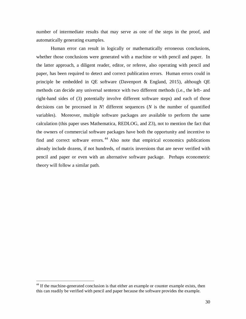
that are denoted x1, x2, etc. Four results are possible, as summarized in Table 1. Should
technology provide these two decisions automatically then the econometrician gains
important information: either a confirmation or refutation of his theory, or the knowledge
that his assumptions contradict.8
QE can do even more. It can generate True hypotheses when the econometrician
has not devised one on his own, by partitioning v into free and bound variables, f and b,
respectively, and eliminating quantifiers from ∃𝑏[𝐴(𝑓, 𝑏)]. The result is a formula P(f)
in the free variables that is a hypothesis deduced from A.9
QE is especially useful in the mixed case, where by definition the assumptions A
are insufficient. Here we can eliminate quantifiers from the set of counterexamples
∃𝑏[𝐴(𝑓, 𝑏) ∧ ¬𝐻(𝑓, 𝑏)], which gives us a formula P(f) in the free variables. Because
P(f) must be True for all counterexamples, ¬𝑃(𝑓) must rule out all counterexamples. In
other words, conditional on the assumptions A, ¬𝑃(𝑓) is sufficient to deduce the
hypothesis: ∀{𝑏, 𝑓}[𝐴(𝑓, 𝑏) ∧ ¬𝑃(𝑓) ⇒ 𝐻(𝑓, 𝑏)] = 𝑇𝑟𝑢𝑒.
Specific QE algorithms, discussed further below, have byproducts that further
assist deductive reasoning. As noted above, ¬∃𝑏[𝐴(𝑓, 𝑏) ∧ ¬𝐻(𝑓, 𝑏)] is conditionally
sufficient for H, but not necessary. A necessary and sufficient condition is 𝐴(𝑓, 𝑏) ∧
𝐻(𝑓, 𝑏), which can be informative if represented by a recursive, quantifier-free formula,
which is exactly what is constructed by the Cylindrical Algebraic Decomposition (CAD)
8 Because of their relationship with proofs, deciding sentences (F = 0) is especially useful for
automating reasoning. This contrasts with previous discussions of quantifier elimination in
economic theory, such as Brown and Matzkin (1996), Snyder (2000), Brown and Kubler (2008), Carvajal et al. (2014), and Chambers and Echenique (2016), whose purposes are to derive
restrictions on free variables that they associate with “observables.” Moreover, with an exception
appearing in the appendix of Brown and Matzkin (1996), they do not intend to “carry out” the
quantifier elimination but rather be assured that the result of doing so would be a non-empty
semi-algebraic set in ℝ𝐹. 9 By construction, there can be no counterexample. To see this, suppose otherwise:
∃{𝑓, 𝑏}[𝐴(𝑓, 𝑏) ∧ ¬𝑃(𝑓)] = ∃𝑓{∃𝑏[𝐴(𝑓, 𝑏) ∧ ¬𝑃(𝑓)]}. But if the intersection of those two sets
is not empty, then neither set can be empty by itself: ∃𝑓{∃𝑏[𝐴(𝑓, 𝑏)] ∧ ∃𝑏[¬𝑃(𝑓)]} =∃𝑓{[𝑃(𝑓)] ∧ [¬𝑃(𝑓)]}, which is impossible because P and ¬𝑃 cannot be True at the same time.
6
algorithm for QE. Many algorithms for deciding existential sentences automatically
provide examples for True sentences, which means that in Table 1’s mixed case we
would have an “example” point 𝑣 ∈ ℝ𝑁 that is in 𝐴 ∧ 𝐻 and another “counterexample”
point that is in 𝐴 ∧ ¬𝐻.10
All of these uses of QE are illustrated below with specific
examples from econometrics.
These are some of the reasons why it can be of “enormous” practical value to
“eliminate quantifiers” from a set’s definition: that is, to take a quantified definition of
the form (1) and transform it into a quantifier-free one such as the Tarski formula P on
the RHS of (4).11
Indeed, some artificial intelligence research equates quantifier
elimination with the vernacular concept of “solving” a mathematics problem (Arai, et al.
2014, p. 2).
II. QE, Projection, and Satisfiability: Illustrated with Jensen’s
Inequality
II.A. Set Projection as QE
Removing existential quantifiers from the formula defining a set in ℝ𝑁 is the
algebraic equivalent of projecting that set into the space of free variables. If there are no
free variables, then the decision or quantifier elimination is the algebraic equivalent of
projecting the set onto the origin. Specifically, an empty set has no projection on the
origin (False) and a nonempty set has a projection on the origin (True).
Consider the well-known result that the expectation of the square of a random
variable with positive variance exceeds the squared expectation of that variable. This toy
example is unusual in exhibiting an obvious polynomial structure, but that serves the
10
Any QE algorithm is a useful tool for generating an example point from a semi-algebraic set.
Existentially quantify N1 of the variables in the Tarski formula leaving free, say, x1, and then eliminate quantifiers. The result is a formula in x1 alone. Choose a real number for x1 that
satisfies the formula and substitute that value into the original N-variable Tarski formula, making
it an (N1)-variable Tarski formula. Repeat the process for x2, etc., until real numbers are
assigned to all N variables. 11
Caviness and Johnson (1998, p. 2).
7
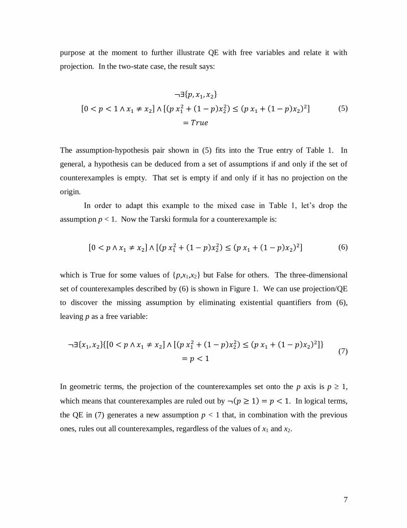
purpose at the moment to further illustrate QE with free variables and relate it with
projection. In the two-state case, the result says:
¬∃{𝑝, 𝑥1, 𝑥2}
[0 < 𝑝 < 1 ∧ 𝑥1 ≠ 𝑥2] ∧ [(𝑝 𝑥12 + (1 − 𝑝)𝑥2
2) ≤ (𝑝 𝑥1 + (1 − 𝑝)𝑥2)2]
= 𝑇𝑟𝑢𝑒
(5)
The assumption-hypothesis pair shown in (5) fits into the True entry of Table 1. In
general, a hypothesis can be deduced from a set of assumptions if and only if the set of
counterexamples is empty. That set is empty if and only if it has no projection on the
origin.
In order to adapt this example to the mixed case in Table 1, let’s drop the
assumption p < 1. Now the Tarski formula for a counterexample is:
[0 < 𝑝 ∧ 𝑥1 ≠ 𝑥2] ∧ [(𝑝 𝑥12 + (1 − 𝑝)𝑥2
2) ≤ (𝑝 𝑥1 + (1 − 𝑝)𝑥2)2] (6)
which is True for some values of {p,x1,x2} but False for others. The three-dimensional
set of counterexamples described by (6) is shown in Figure 1. We can use projection/QE
to discover the missing assumption by eliminating existential quantifiers from (6),
leaving p as a free variable:
¬∃{𝑥1, 𝑥2}{[0 < 𝑝 ∧ 𝑥1 ≠ 𝑥2] ∧ [(𝑝 𝑥12 + (1 − 𝑝)𝑥2
2) ≤ (𝑝 𝑥1 + (1 − 𝑝)𝑥2)2]}
= 𝑝 < 1 (7)
In geometric terms, the projection of the counterexamples set onto the p axis is p 1,
which means that counterexamples are ruled out by ¬(𝑝 ≥ 1) = 𝑝 < 1. In logical terms,
the QE in (7) generates a new assumption p < 1 that, in combination with the previous
ones, rules out all counterexamples, regardless of the values of x1 and x2.
8
II.B. Satisfiability as QE
Deciding existential and universal sentences is an important special case of QE,
and is closely related to the Boolean satisfiability problem in computer science, which is
whether there are any values of the Boolean variables in a formula that make the entire
formula True. The inequality atoms of a Tarski formula are Boolean valued (an
inequality is either satisfied or not), but with the added complexity that the Boolean
values in different parts of the formula are related to the extent that the inequalities
contain the same scalar variables. This and related extensions to the satisfiability
problem recently have been developed in the field of satisfiability modulo theories
(SMT). The specific theory of interest here is the theory of arithmetic (addition,
subtraction, multiplication) on real numbers, known as “nonlinear real arithmetic” (NRA)
in the SMT field (Jovanović and de Moura 2012).
Automated SMT solvers with NRA capabilities are actively being developed (see
www.SMT-LIB.org, and section V below) in the public domain and by major software
companies, especially for the purpose of verifying complicated hardware and software
systems. System inputs from external sources are represented as scalar or Boolean
variables and the Tarski formula describes a set of potential unintended results of (“bugs
from”) the computation on those inputs. The hardware or software developer uses the
SMT solver to obtain a guarantee that those bugs cannot occur. Because they are just
deciding existential sentences of the type described in subsection I.B, SMT-NRA solvers
can serve as engines for automated econometric reasoning at least to the extent that no
free variables are needed. In this way real algebraic geometry (projection) and computer
science (SMT-NRA) are tackling essentially the same automated reasoning problem from
different perspectives.
9
III. Using partially-interpreted functions to recognize instances of
real quantifier elimination in econometrics
We are also interested in the existence and properties of automated QE method(s),
but first we consider some familiar hypotheses from econometrics. At first glance many
econometrics examples do not appear to fit into the framework (1), (4) because their
polynomial structure is not obvious. But the theoretical computer science notion of a
partially interpreted function helps reveal that structure. The integration operator (on
integrable functions) is an important example for econometric analysis. Another example
is the vector dot product, which becomes a partially interpreted function when we add
Gramian matrix restrictions to the assumption set. See also Mulligan (2016), which
shows how the utility and production functions used in economic theory are also usefully
understood as partially interpreted functions.
III.A. An introduction to uninterpreted functions
So far I have used integer indices to distinguish one scalar, say x1, from another
such as x2. Although the variables in a Tarski formula must be scalars, nothing requires
that the indices be scalars. The indices could be, say, names, or natural language words,
or images. Or the indices could be integrable functions, as in the Roy model below, or
arbitrary-length vectors as in the sections that follow. In other words, the variables in a
Tarski formula can be points on any abstract mapping from objects (vectors, integrable
functions, etc.) to the real line as long as the mapping is functionally consistent.12
The notation x1, x2, etc., is also special in that the variables are distinguished with
a single index. The domain of the mapping could be multidimensional as with integrals
and dot products that map pairs of indices (pairs of functions and pairs of vectors,
respectively) to the real line. The mapping is abstract in that it stays unevaluated as part
of the analysis. For this reason, such variables are sometimes called uninterpreted
functions (Ackermann 1954, Bryant, German and Velev 1999).
12
E.g., xa is the same scalar as xb whenever a is the same as b.
10
Suppose that the integral ∫ sin 𝑥 ln 𝑥 𝑑𝑥𝑏
𝑎 appeared in our model. The
uninterpreted function approach is to leave this integral unevaluated, treating
{sin 𝑥 , ln 𝑥 , 𝑎, 𝑏} as the “name” of the scalar variable that is the value of that integral and
thereby distinguishing it from, say, ∫ cos 𝑥 ln 𝑥 𝑑𝑥𝑏
𝑎 and ∫ sin 𝑥 ln 𝑥 𝑑𝑥
𝑐
𝑎. If our reasoning
requires some of the mathematical properties of sin and ln, then the partially interpreted
function approach is to add restrictions on the functions, such as
𝑏 ≥ 𝑎 ∧ ∫ sin 𝑥 ln 𝑥 𝑑𝑥𝑏
𝑎≤ (𝑏 − 𝑎) ln 𝑏 or ∫ sin 𝑥 ln 𝑥 𝑑𝑥
𝑐
𝑎= ∫ sin 𝑥 ln 𝑥 𝑑𝑥
𝑏
𝑎+
∫ sin 𝑥 ln 𝑥 𝑑𝑥𝑐
𝑏, to the list of assumptions (Kroening and Strichman 2008, p. 73).
13
III.B. A comparative static in the nonparametric Roy model
The nonparametric Roy model provides a practical introduction to uninterpreted
and partially interpreted functions. In that model, women are assumed to have (possibly
correlated) skills h and r in market work and non-market activities, respectively. These
skills have a population distribution modeled with the joint density function f(h,r), which
is normalized to have unconditional means of zero. Women work if and only if their non-
market log wage r + μr is less than σh + μw, their market log wage. > 0 is a constant
introduced for the purposes of considering a comparative static with respect to “wage
inequality.” The model is “nonparametric” when no specific functional form is assumed
for the probability density function.
Applications of the Roy model to the female labor market are abundant in labor
supply and econometrics, although often parametric in that f is restricted to be a bivariate
normal density function as in the pioneering work of Gronau (1974), Heckman (1979),
Heckman and Sedlacek (1985).14
Mulligan and Rubinstein (2008) also used the bivariate
normal assumption to focus on comparative statics with respect to . Because the
bivariate normal density function is not a polynomial in h or r, it would seem that the Roy
model is not amenable to QE methods. But this overlooks the notion of partially
13
As might be deduced from the previous discussion of QE with free variables, QE can also be
used to discover the necessary restrictions on an uninterpreted function. 14
See also Keane, Moffitt, and Runkle (1988) and Borjas (1994). For some analysis of the nonparametric Roy model, see Heckman and Honore (1990) and Mourifie et al (2017).

11
interpreted functions, which essentially amounts to a clever choice of variables so that the
assumption and hypothesis are understood as Boolean combinations of polynomial
inequalities in those variables.
To see this, let’s stay with the nonparametric version of the Roy model and look
at the definitions of employment p and aggregate market skill S:
𝑝(𝜎, 𝜇𝑤 − 𝜇𝑟) ≡ ∫ ∫ 𝑓(ℎ, 𝑟)𝑑𝑟𝜎ℎ+𝜇𝑤−𝜇𝑟
−∞
𝑑ℎ∞
−∞
(8)
𝑆(𝜎, 𝜇𝑤 − 𝜇𝑟) ≡ ∫ ∫ ℎ𝑓(ℎ, 𝑟)𝑑𝑟𝜎ℎ+𝜇𝑤−𝜇𝑟
−∞
𝑑ℎ∞
−∞
/𝑝(𝜎, 𝜇𝑤 − 𝜇𝑟) (9)
is said to change the “selection rule” if it affects S holding p constant by varying μr.15
With some weak restrictions on the density function, QE confirms that the effect is
strictly positive:
𝐴 = {𝑑𝑝(𝜎, 𝜇𝑤 − 𝜇𝑟)
𝑑𝑧=
𝑑𝜇𝑤
𝑑𝑧= 0 ∧
𝑑𝜎
𝑑𝑧> 0 ∧
∫ ∫ 𝑓(ℎ, 𝑟)𝑑𝑟𝜎ℎ+𝜇𝑤−𝜇𝑟
−∞
𝑑ℎ∞
−∞
≥ 0 ∧
∫ 𝑓(ℎ, 𝜇𝑤 − 𝜇𝑟 + 𝜎ℎ)𝑑ℎ∞
−∞
> 0 ∧
∫ ℎ2𝑓(ℎ, 𝜇𝑤 − 𝜇𝑟 + 𝜎ℎ)𝑑ℎ∞
−∞
∫ 𝑓(ℎ, 𝜇𝑤 − 𝜇𝑟 + 𝜎ℎ)𝑑ℎ∞
−∞
> (∫ ℎ𝑓(ℎ, 𝜇𝑤 − 𝜇𝑟 + 𝜎ℎ)𝑑ℎ
∞
−∞
∫ 𝑓(ℎ, 𝜇𝑤 − 𝜇𝑟 + 𝜎ℎ)𝑑ℎ∞
−∞
)
2
}
(10)
where any woman with 𝑟 = 𝜇𝑤 − 𝜇𝑟 + 𝜎ℎ is exactly on the margin between work and
not work. The first row of assumptions defines the experiment z that increases and
adjusts μr to keep employment constant. The second row requires that employment be
nonnegative, which reflects the fact that f is a probability density function. The final two
15
It is straightforward to apply QE to questions about the shape of the control function – that is,
how μr affects S holding constant. See http://models.economicreasoning.com/SelectionRules.pdf .

12
rows assume that there are women on the margin and that they are not identical. The
hypothesis H is that 𝑆(𝜎,𝜇𝑤−𝜇𝑟)
𝑑𝑧> 0.
Using uninterpreted or partially interpreted functions, every atom of A and H
above is a polynomial inequality in ℝ8 . Treating the total derivative operator as an
uninterpreted function, evaluated at points {r,z}, {w,z}, and {,z}, gives us three
variables. Treating the single-integral operator as an uninterpreted function, evaluated at
points {1, 𝑓(ℎ, 𝜇𝑤 − 𝜇𝑟 + 𝜎ℎ)}, {ℎ, 𝑓(ℎ, 𝜇𝑤 − 𝜇𝑟 + 𝜎ℎ)}, and {ℎ2, 𝑓(ℎ, 𝜇𝑤 − 𝜇𝑟 + 𝜎ℎ)},
gives us three more variables.16
The final two variables come from treating the double-
integral operator as an uninterpreted function evaluated at points {1,f(h,r)} and {h,f(h,r)}.
These three functions become “partially interpreted” when we introduce algebraic
assumptions about them, as in each atom of the assumptions A. It is worth noting at this
point that the restrictions that A puts on the probability density function f are satisfied by
the Gaussian joint density function, so that any hypothesis deduced from A can also be
deduced from the stronger assumption that f is Gaussian.
In summary, the wage-inequality comparative static of the nonparameteric Roy
model is a QE problem in eight variables:
{𝑑𝜇𝑟
𝑑𝑧,𝑑𝜇𝑤
𝑑𝑧,𝑑𝜎
𝑑𝑧, ∫ 𝑓(ℎ, 𝜇𝑤 − 𝜇𝑟 + 𝜎ℎ)𝑑ℎ
∞
−∞
,
∫ ℎ𝑓(ℎ, 𝜇𝑤 − 𝜇𝑟 + 𝜎ℎ)𝑑ℎ∞
−∞
, ∫ ℎ2𝑓(ℎ, 𝜇𝑤 − 𝜇𝑟 + 𝜎ℎ)𝑑ℎ∞
−∞
,
∫ ∫ 𝑓(ℎ, 𝑟)𝑑𝑟𝜎ℎ+𝜇𝑤−𝜇𝑟
−∞
𝑑ℎ∞
−∞
, ∫ ∫ ℎ𝑓(ℎ, 𝑟)𝑑𝑟𝜎ℎ+𝜇𝑤−𝜇𝑟
−∞
𝑑ℎ∞
−∞
}
(11)
The result is confirmed by existentially quantifying each of these variables in the
counterexample Tarski formula 𝐴 ∧ ¬𝐻 , with A and H defined as above, and then
eliminating the eight quantifiers to find False: there is no way to assign eight real
numbers to those eight scalar variables that would involve simultaneously satisfying the
assumptions and contradicting the hypothesis. The role of partially interpreted functions
can be seen by comparing the assumptions A expressed in econometrically-natural
16
Recall that the domain of an uninterpreted function does not have to be real numbers. It can be,
for example, pairs of integrable functions of h such as h2 or 𝑓(ℎ, 𝜇𝑤 − 𝜇𝑟 + 𝜎ℎ).
13
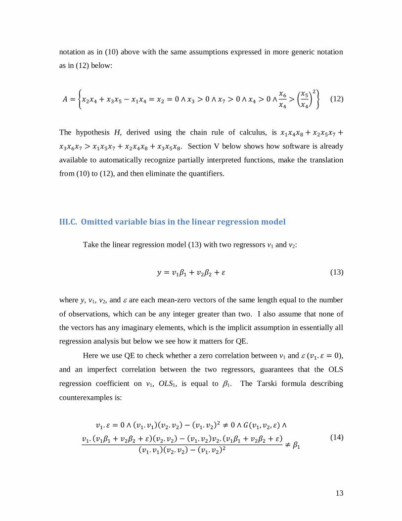
notation as in (10) above with the same assumptions expressed in more generic notation
as in (12) below:
𝐴 = {𝑥2𝑥4 + 𝑥3𝑥5 − 𝑥1𝑥4 = 𝑥2 = 0 ∧ 𝑥3 > 0 ∧ 𝑥7 > 0 ∧ 𝑥4 > 0 ∧𝑥6
𝑥4> (
𝑥5
𝑥4)
2
} (12)
The hypothesis H, derived using the chain rule of calculus, is 𝑥1𝑥4𝑥8 + 𝑥2𝑥5𝑥7 +
𝑥3𝑥6𝑥7 > 𝑥1𝑥5𝑥7 + 𝑥2𝑥4𝑥8 + 𝑥3𝑥5𝑥8. Section V below shows how software is already
available to automatically recognize partially interpreted functions, make the translation
from (10) to (12), and then eliminate the quantifiers.
III.C. Omitted variable bias in the linear regression model
Take the linear regression model (13) with two regressors v1 and v2:
𝑦 = 𝑣1𝛽1 + 𝑣2𝛽2 + 𝜀 (13)
where y, v1, v2, and are each mean-zero vectors of the same length equal to the number
of observations, which can be any integer greater than two. I also assume that none of
the vectors has any imaginary elements, which is the implicit assumption in essentially all
regression analysis but below we see how it matters for QE.
Here we use QE to check whether a zero correlation between v1 and (𝑣1. 𝜀 = 0),
and an imperfect correlation between the two regressors, guarantees that the OLS
regression coefficient on v1, OLS1, is equal to 1. The Tarski formula describing
counterexamples is:
𝑣1. 𝜀 = 0 ∧ (𝑣1. 𝑣1)(𝑣2. 𝑣2) − (𝑣1. 𝑣2)2 ≠ 0 ∧ 𝐺(𝑣1, 𝑣2, 𝜀) ∧
𝑣1. (𝑣1𝛽1 + 𝑣2𝛽2 + 𝜀)(𝑣2. 𝑣2) − (𝑣1. 𝑣2)𝑣2. (𝑣1𝛽1 + 𝑣2𝛽2 + 𝜀)
(𝑣1. 𝑣1)(𝑣2. 𝑣2) − (𝑣1. 𝑣2)2≠ 𝛽1
(14)

14
where the ratio term in the formula is OLS1 and G is a set of additional assumptions
discussed below.
Rather than assigning variable names to every element of all three vectors and
then evaluating each of the vector dot products, I treat the dot product as a partially
interpreted function. So the counterexample decision problem is whether there exists six
real numbers for {𝑣1. 𝑣1, 𝑣1. 𝑣2, 𝑣1. 𝜀, 𝑣2. 𝑣2, 𝑣2. 𝜀, 𝜀. 𝜀} that satisfy (14).17
However, given
that all three vectors are real valued, some values for these dot products must be ruled
out. For example, 𝑣1. 𝑣1 cannot be negative. More specifically, any four real-valued
vectors must have a Gramian matrix that is symmetric and positive semi-definite, and
with any symmetric positive semi-definite Gramian matrix four real-vectors can be found
to assemble that Gramian matrix, as long as the length of the vectors is greater than two.
Therefore G must be the conjunction of seven additional assumptions: that each of the
three vectors has nonnegative magnitude, that none of the three pairwise correlations is
outside the unit circle, and that the determinant of the Gramian matrix is nonnegative.18
Quantifying (14)’s six variables existentially and eliminating quantifiers yields
True. In words, it is possible to have real-valued data vectors with 𝑣1. 𝜀 = 0 and
(𝑣1. 𝑣1)(𝑣2. 𝑣2) − (𝑣1. 𝑣2)2 ≠ 0 but nonetheless OLS1 differing from 1. An additional
assumption is needed for OLS1 to be unbiased, which QE can recover using much the
same procedure that was used in section II.A. Specifically, existential QE is performed
on (14) with one free variable, and therefore results in a formula in the free variable.
With six variables, there are six ways to do this.19
Two of the six results are redundant of
the assumptions, which means that these two variables cannot be further restricted to rule
out counterexamples. But the other four are not redundant, so we can negate each one to
get four conditions that, conditional on the assumptions shown on the top row of (14), are
individually sufficient for OLS1 to be the same as 1:
17
1 and 2 are not variables because they drop out of (14) when the dot products are distributed
across addition. 18
In generic scalar notation, the Tarski formula (14) is 𝑥3 = 0 ∧ 𝑥1𝑥4 ≠ 𝑥22 ∧ (𝑥1 ≥ 0 ∧ 𝑥4 ≥ 0 ∧
𝑥6 ≥ 0 ∧ 𝑥1𝑥4 ≥ 𝑥22 ∧ 𝑥1𝑥6 ≥ 𝑥3
2 ∧ 𝑥4𝑥6 ≥ 𝑥52 ∧ 2𝑥2𝑥3𝑥5 + 𝑥1𝑥4𝑥6 ≥ 𝑥3
2𝑥4 + 𝑥1𝑥52 + 𝑥2
2𝑥6) ∧𝑥2𝑥5 ≠ 𝑥3𝑥4, where the terms in parenthesis are the Gramian matrix restrictions. Gramian matrix
restrictions are tedious to type from scratch, but software exists to automatically generate them
from the other parts of the Tarski formula (Mulligan, Davenport and England 2018). 19
In other words, the nonempty set of counterexamples can be projected on to each of six different axes.

15
𝑣2. 𝜀 = 0 ∨ 𝑣1. 𝑣2 = 0 ∨ 𝑣2. 𝑣2 = 0 ∨ 𝜀. 𝜀 = 0 (15)
Note that these results deduced for an econometric model hold for arbitrary-length
vectors and therefore can describe either a “sample” or a “population,” as long as we are
consistent. In other words, the results above by themselves allow us to deduce sample
conclusions from sample assumptions or population conclusions from population
assumptions. Deriving sample conclusions from population assumptions requires an
additional statistical inference step, which is not the subject of these examples.20
III.D. Partial identification in the classical measurement error model
Following Levi (1973), I now add measurement error to one of the two regressors:
𝑣1 = 𝑣1 + 𝑢.21
The classical measurement error assumptions are (13):
𝑣1. 𝑢 = 𝑣1. 𝜀 = 𝑢. 𝜀 = 𝑣2. 𝑢 = 𝑣2. 𝜀 = 0 ∧
𝛽1 ≠ 0 ∧(𝑣1. 𝑣2)2
(𝑣1. 𝑣1)(𝑣2. 𝑣2)< 1
(16)
where I have also added two assumptions to rule out the tedious and less interesting cases
that have 1 = 0 or perfect collinearity between the v1 and v2. QE can automatically
discover the identified set for the slope parameter 1 corresponding to the variable v1
whose values are measured with error. Here it is helpful to define the forward- and
reverse-regression coefficients:22
𝑂𝐿𝑆1 = (17)
20
See also Franklin Fisher (1966, p. 5) on the distinction between statistical inference and the logical analysis of an econometric model. 21
See Klepper and Leamer (1984) for analysis of the case where both regressors are measured
with error. See Frisch (1934), Friedman (1957), and Tamer (2010) for the single-regressor case. 22
The reverse-regression coefficient is the inverse of the coefficient on y in the regression of measured v1 on y and v2.
16
(𝑣1 + 𝑢). (𝑣1𝛽1 + 𝑣2𝛽2 + 𝜀)(𝑣2. 𝑣2) − ((𝑣1 + 𝑢). 𝑣2)𝑣2. (𝑣1𝛽1 + 𝑣2𝛽2 + 𝜀)
((𝑣1 + 𝑢). (𝑣1 + 𝑢))(𝑣2. 𝑣2) − ((𝑣1 + 𝑢). 𝑣2)2
𝑅𝐸𝑉1 =
(𝑣1 + 𝑢). (𝑣1𝛽1 + 𝑣2𝛽2 + 𝜀)(𝑣2. 𝑣2) − ((𝑣1 + 𝑢). 𝑣2)𝑣2. (𝑣1𝛽1 + 𝑣2𝛽2 + 𝜀)
((𝑣1𝛽1 + 𝑣2𝛽2 + 𝜀). (𝑣1𝛽1 + 𝑣2𝛽2 + 𝜀))(𝑣2. 𝑣2) − ((𝑣1𝛽1 + 𝑣2𝛽2 + 𝜀). 𝑣2)2
(18)
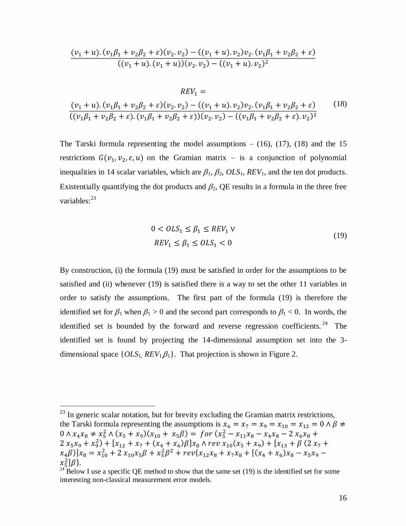
The Tarski formula representing the model assumptions – (16), (17), (18) and the 15
restrictions 𝐺(𝑣1, 𝑣2, 𝜀, 𝑢) on the Gramian matrix – is a conjunction of polynomial
inequalities in 14 scalar variables, which are 1, 2, OLS1, REV1, and the ten dot products.
Existentially quantifying the dot products and 2, QE results in a formula in the three free
variables:23
0 < 𝑂𝐿𝑆1 ≤ 𝛽1 ≤ 𝑅𝐸𝑉1 ∨
𝑅𝐸𝑉1 ≤ 𝛽1 ≤ 𝑂𝐿𝑆1 < 0 (19)
By construction, (i) the formula (19) must be satisfied in order for the assumptions to be
satisfied and (ii) whenever (19) is satisfied there is a way to set the other 11 variables in
order to satisfy the assumptions. The first part of the formula (19) is therefore the
identified set for 1 when 1 > 0 and the second part corresponds to 1 < 0. In words, the
identified set is bounded by the forward and reverse regression coefficients.24
The
identified set is found by projecting the 14-dimensional assumption set into the 3-
dimensional space {OLS1, REV1,1}. That projection is shown in Figure 2.
23
In generic scalar notation, but for brevity excluding the Gramian matrix restrictions,
the Tarski formula representing the assumptions is 𝑥6 = 𝑥7 = 𝑥9 = 𝑥10 = 𝑥12 = 0 ∧ 𝛽 ≠0 ∧ 𝑥4𝑥8 ≠ 𝑥5
2 ∧ (𝑥5 + 𝑥9)(𝑥10 + 𝑥5𝛽) = 𝑓𝑜𝑟 (𝑥52 − 𝑥11𝑥8 − 𝑥4𝑥8 − 2 𝑥6𝑥8 +
2 𝑥5𝑥9 + 𝑥92) + [𝑥12 + 𝑥7 + (𝑥4 + 𝑥6)𝛽]𝑥8 ∧ 𝑟𝑒𝑣 𝑥10(𝑥5 + 𝑥9) + [𝑥13 + 𝛽 (2 𝑥7 +
𝑥4𝛽)]𝑥8 = 𝑥102 + 2 𝑥10𝑥5𝛽 + 𝑥5
2𝛽2 + 𝑟𝑒𝑣{𝑥12𝑥8 + 𝑥7𝑥8 + [(𝑥4 + 𝑥6)𝑥8 − 𝑥5𝑥9 −𝑥5
2]𝛽}. 24
Below I use a specific QE method to show that the same set (19) is the identified set for some interesting non-classical measurement error models.

17
III.E. Point identification in discrete choice models
QE can also be used to study uniqueness or to count numbers of instances. Point
identification is a uniqueness question, which for illustration I consider here for the
prototypical discrete choice model. The choice is assumed to depend on observed factors
v and y as well as unobserved factors summarized by , were is normalized to have
unit variance and distribution function F. The discrete choice di is made in situation i if
and only if 𝜎 𝜀𝑖 < 𝛽𝑣𝑖 + 𝛾𝑦𝑖. The log likelihood function for observing v, y, d is:
𝐿 ({𝛽
𝜎,𝛾
𝜎}) = ∑ {(1 − 𝑑𝑖) ln [1 − 𝐹 (
𝛽
𝜎𝑣𝑖 +
𝛾
𝜎𝑦𝑖)] + 𝑑𝑖 ln 𝐹 (
𝛽
𝜎𝑣𝑖 +
𝛾
𝜎𝑦𝑖)}
𝑖 (20)
By definition, the parameter vector {,,} is point identified if two distinct values
for that vector cannot simultaneously attain the maximum likelihood. Conversely, the
parameter vector {,,} is point identified if knowing that 1 and 2 both attain the
maximum likelihood implies that 1 = 2.
The definition of a strictly concave function L is:
[𝐷𝑖𝑠𝑡𝑖𝑛𝑐𝑡 ({𝛽1
𝜎1,𝛾1
𝜎1
} , {𝛽2
𝜎2,𝛾2
𝜎2
}) ∧ 0 < 𝜆 < 1]
⇒ [(1 − 𝜆)𝐿 ({𝛽1
𝜎1,𝛾1
𝜎1
}) + 𝜆𝐿 ({𝛽2
𝜎2,𝛾2
𝜎2
})
< 𝐿 ((1 − 𝜆) {𝛽1
𝜎1,𝛾1
𝜎1
} + 𝜆 {𝛽2
𝜎2,𝛾2
𝜎2
})]
(21)
where Distinct is an uninterpreted Boolean-valued function introduced to compactly
represent whether its two arguments are distinct. It can be partially interpreted by
providing an algebraic definition of distinct:
𝐷𝑖𝑠𝑡𝑖𝑛𝑐𝑡 ({𝛽1
𝜎1,𝛾1
𝜎1
} , {𝛽2
𝜎2,𝛾2
𝜎2
}) ⇒ [𝛽1
𝜎1≠
𝛽2
𝜎2∨
𝛾1
𝜎1≠
𝛾2
𝜎2] (22)
If 1 and 2 are both attaining the maximum likelihood, then we have:
18
𝐿 ({𝛽1
𝜎1,𝛾1
𝜎1
}) ≥ 𝐿 ((1 − 𝜆) {𝛽1
𝜎1,𝛾1
𝜎1
} + 𝜆 {𝛽2
𝜎2,𝛾2
𝜎2
}) ∧
𝐿 ({𝛽2
𝜎2,𝛾2
𝜎2
}) ≥ 𝐿 ((1 − 𝜆) {𝛽1
𝜎1,𝛾1
𝜎1
} + 𝜆 {𝛽2
𝜎2,𝛾2
𝜎2
})
(23)
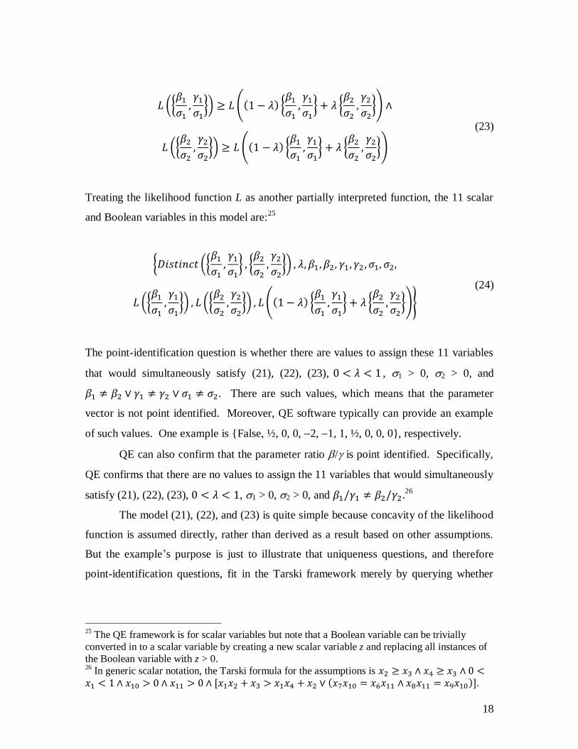
Treating the likelihood function L as another partially interpreted function, the 11 scalar
and Boolean variables in this model are:25
{𝐷𝑖𝑠𝑡𝑖𝑛𝑐𝑡 ({𝛽1
𝜎1,𝛾1
𝜎1
} , {𝛽2
𝜎2,𝛾2
𝜎2
}) , 𝜆, 𝛽1, 𝛽2, 𝛾1, 𝛾2 , 𝜎1, 𝜎2,
𝐿 ({𝛽1
𝜎1,𝛾1
𝜎1
}) , 𝐿 ({𝛽2
𝜎2,𝛾2
𝜎2
}) , 𝐿 ((1 − 𝜆) {𝛽1
𝜎1,𝛾1
𝜎1
} + 𝜆 {𝛽2
𝜎2,𝛾2
𝜎2
})}
(24)
The point-identification question is whether there are values to assign these 11 variables
that would simultaneously satisfy (21), (22), (23), 0 < 𝜆 < 1 , 1 > 0, 2 > 0, and
𝛽1 ≠ 𝛽2 ∨ 𝛾1 ≠ 𝛾2 ∨ 𝜎1 ≠ 𝜎2. There are such values, which means that the parameter
vector is not point identified. Moreover, QE software typically can provide an example
of such values. One example is {False, ½, 0, 0, 2, 1, 1, ½, 0, 0, 0}, respectively.
QE can also confirm that the parameter ratio / is point identified. Specifically,
QE confirms that there are no values to assign the 11 variables that would simultaneously
satisfy (21), (22), (23), 0 < 𝜆 < 1, 1 > 0, 2 > 0, and 𝛽1/𝛾1 ≠ 𝛽2/𝛾2.26
The model (21), (22), and (23) is quite simple because concavity of the likelihood
function is assumed directly, rather than derived as a result based on other assumptions.
But the example’s purpose is just to illustrate that uniqueness questions, and therefore
point-identification questions, fit in the Tarski framework merely by querying whether
25
The QE framework is for scalar variables but note that a Boolean variable can be trivially
converted in to a scalar variable by creating a new scalar variable z and replacing all instances of
the Boolean variable with z > 0. 26
In generic scalar notation, the Tarski formula for the assumptions is 𝑥2 ≥ 𝑥3 ∧ 𝑥4 ≥ 𝑥3 ∧ 0 <𝑥1 < 1 ∧ 𝑥10 > 0 ∧ 𝑥11 > 0 ∧ [𝑥1𝑥2 + 𝑥3 > 𝑥1𝑥4 + 𝑥2 ∨ (𝑥7𝑥10 = 𝑥6𝑥11 ∧ 𝑥8𝑥11 = 𝑥9𝑥10)].
19
two potentially distinct points satisfying the model assumptions must coincide with each
other.
III.F. A Library of Economics Examples
Since 2016 I have been using automated QE on a daily basis to process problems
encountered in teaching, research, and writing a graduate-level textbook. The more
interesting or well known of these problems have been assembled together with
background explanations at http://examples.economicreasoning.com. Mulligan et al
(2018a) provide the computer science community with forty-five of these assumption-
hypothesis pairs (for a total of 135 existential sentences), in four different computer
algebra formats, together with analysis of their algebraic structure and explanation of the
range of economics problems that fit in the QE framework.
The examples shown in this paper, chosen to illustrate QE concepts, are more
stylized than in the library of 45. Even excluding the two-state example (5) - (7), this
paper’s examples have an average of only 9.25 variables as compared to 17.2 in the
library.27
This suggests that significantly more involved econometrics models could still
be decided in seconds, as the library examples are (see also Table 2).
IV. Relevant Theorems from Real Algebraic Geometry
IV.A. Tarski: Real quantifier elimination is always possible Mathematician and logician Alfred Tarski proved that there exists a universal
algorithm (that is, one not requiring problem-specific guidance) for quantifier elimination
from systems of polynomial inequalities on real closed fields by providing such an
algorithm.28
Because the real numbers are an example of a real closed field, the Tarski
result guarantees that there exists a quantifier-free formula P satisfying (1) and (4) and
27
The library has a greater incidence of polynomials containing a cubic in a single variable,
although the classical measurement error model’s hypothesis does have a single variable raised to
the fourth power. 28
Tarksi made the proof in 1930 (Caviness and Johnson 1998, p. 1), but the result was not published until Tarski (1951).

20
gives an algorithm for finding P. If QR is a sentence, then the QE algorithm is a
“decision method”: a procedure for determining whether QR is True or False.29
IV.B. Collins: A more efficient algorithm for real QE that defines sets recursively
Although Tarski’s method is enough to prove that quantifiers can be eliminated, it
is not used in practice due to its “extreme” inefficiency.30
A major step forward came
with the Cylindrical Algebraic Decomposition (CAD) method introduced by
mathematician George E. Collins in 1973.31
IV.B.1. Properties of CAD In our setting (1) and (4), the CAD method decomposes ℝ𝑁 into finitely many
connected regions, known as “cells,” with three properties:
(i) each cell of the CAD is a semi-algebraic set (i.e., it is defined by a finite
number of quantifier-free polynomial inequalities).
(ii) The CAD result is cylindrical because the projections of any two of the
cells into ℝ𝑘 , 1 k N, are either identical or disjoint.
(iii) Each cell is adapted to the Tarski formula from which it was derived,
which means that none of the polynomials in the Tarski formula T has
more than one sign {-1,0,1} in any one of the cells.
Every Tarski formula has such a CAD (Basu, Pollack and Roy (2011, Theorem 5.6)).
The T-adapted (i.e., uniform sign) property of the cells, and the fact that the cells
are finite in number, means that any quantified formula can be confirmed in a finite
number of steps.32
The cylindrical property (in economics we would call it “recursive”)
of the decomposition means that the cells have a natural ordering and many times can be
processed more than one at a time.
29
Renegar (1998, p. 221). 30
Arai, et al. (2014). See also Davenport, Siret and Tournier (1988, p. 119), who describe
Tarski’s method as “completely impractical.” 31
Collins (1973) and Collins (1975). 32
By construction, the Tarski formula is True at any one point in a cell if and only if it is True everywhere in that cell.

21
The phrase CAD has a number of related but distinct uses in mathematics and
computer science. Narrowly speaking, CAD refers to a method, or sometimes an
expanded set of polynomials (including, among others, those in the original Tarski
formula) obtained by the method, or the full collection of cells obtained by the method.
Another result of the CAD method is its cells, described by Cylindrical Algebraic
Formulas (CAFs), which may also be referenced as CAD. 33
CAD sometimes also refers
to a decomposition of part of ℝ𝑁 with the properties (i)-(iii). CAD can also refer to a full
decomposition of ℝ𝑁 with the properties (i)-(iii), but with “adapted” defined with respect
to the truth value of the entire formula rather than the sign of each of its polynomials
(Bradford, et al. 2016). For clarity, I refer to the full collection of cells together with one
sample point each as “the full CAD.”
Although building the CAD begins with a Tarski formula, only the polynomials
of that formula and the order of quantification is used in the calculations (recall (iii)); the
inequalities and Boolean operations are ignored. A single full CAD therefore solves a
large number of QE problems: any QE problem whose Tarski formula has the same
polynomials and the same quantification order (but not necessarily the same quantifiers)
has the same full CAD. Naturally, the simultaneous solution of many QE problems
requires more computational resources than solving one QE problem, which is the
motivation for other QE algorithms.
Kauers (2011) and Mulligan (2016) include explanations, intended for non-
experts, of the methods used to construct a full CAD. Given that the full CAD would
rarely be the best QE method for econometrics problems and that it is already
implemented in various software packages, the details of its construction is beyond the
scope of this paper.
IV.B.2. Using CAFs in Econometrics: Necessary and Sufficient Conditions in the Measurement Error Model
Recall the measurement error model whose assumptions – (16), (17), (18) and the
15 restrictions 𝐺(𝑣1, 𝑣2, 𝜀, 𝑢) – guarantee that the regression parameter 1 is in the set
33
See Strzebonski (2010) and Chen and Maza (2015) for more on the distinction between CAD and CAF.
22
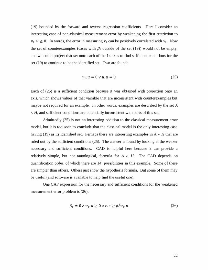
(19) bounded by the forward and reverse regression coefficients. Here I consider an
interesting case of non-classical measurement error by weakening the first restriction to
𝑣1. 𝑢 ≥ 0. In words, the error in measuring v1 can be positively correlated with v1. Now
the set of counterexamples (cases with 1 outside of the set (19)) would not be empty,
and we could project that set onto each of the 14 axes to find sufficient conditions for the
set (19) to continue to be the identified set. Two are found:
𝑣1. 𝑢 = 0 ∨ 𝑢. 𝑢 = 0 (25)
Each of (25) is a sufficient condition because it was obtained with projection onto an
axis, which shows values of that variable that are inconsistent with counterexamples but
maybe not required for an example. In other words, examples are described by the set A
H, and sufficient conditions are potentially inconsistent with parts of this set.
Admittedly (25) is not an interesting addition to the classical measurement error
model, but it is too soon to conclude that the classical model is the only interesting case
having (19) as its identified set. Perhaps there are interesting examples in A H that are
ruled out by the sufficient conditions (25). The answer is found by looking at the weaker
necessary and sufficient conditions. CAD is helpful here because it can provide a
relatively simple, but not tautological, formula for A H. The CAD depends on
quantification order, of which there are 14! possibilities in this example. Some of these
are simpler than others. Others just show the hypothesis formula. But some of them may
be useful (and software is available to help find the useful one).
One CAF expression for the necessary and sufficient conditions for the weakened
measurement error problem is (26):
𝛽1 ≠ 0 ∧ 𝑣1. 𝑢 ≥ 0 ∧ 𝜀. 𝜀 ≥ 𝛽12𝑣1. 𝑢 (26)
23
Both (25) and (26) rule out all counterexamples, but the latter is the weaker condition
because it does not rule out any cases satisfying 𝐴 ∧ 𝐻.34
Notice the CAF’s recursive
structure: it first restricts 1 relative to real numbers only, then restricts the second
variable 𝑣1. 𝑢 based on the first (trivially in this case), and then restricts the third variable
𝜀. 𝜀 based on the first two. In terms of the econometric substance, (26) shows that (19) is
still the identified set even when the measurement error is positively correlated with the
true value, as long as that correlation is not too positive.
IV.C. Other QE methods
Basu, Pollack and Roy (2011) have a unique approach to QE problems, although
not yet implemented as software. Less ambitious and computationally less costly (than
full CAD) algorithms are available for special cases of the QE problem. Virtual Term
Substitution (VTS) is designed for QE on polynomials with low own degree: that is, the
total degree may be large because several variables may multiply each other, but it is rare
for a single variable to be raised to a power of more than two or three.35
The
performance of VTS has an additional advantage in large but sparse systems where most
variables are absent from most of the polynomials in the Tarski formula. VTS is
therefore well-suited for problems in econometrics and elsewhere in economics.
34
An example that satisfies A and (26) without satisfying (25): 𝛽1 = 𝑣1. 𝑣1 = 𝑣1. 𝑢 = 𝑣2. 𝑣2 =𝑢. 𝑢 = 𝜀. 𝜀 = 1 ∧ 𝑣1. 𝑣2 = 𝑣1. 𝜀 = 𝑣2. 𝑢 = 𝑣2. 𝜀 = 𝑢. 𝜀 = 0. 35
VTS was invented by Volker Weispfenning (1988, 1997). Improvements to the method are ongoing, as with C.W. Brown (2005).
24
Regardless of degree, decision problems are a special case of QE for which
algorithms can be tailored. The decision of existential sentences has received much
attention in computer science, and specialized methods have been implemented by a
number of automated SMT solvers with NRA capabilities.36
The aforementioned library
of economic decision problems are special not only in degree, but also that the process of
repeated quantifier elimination involves just a few frequently repeated single-variable
quantifier elimination problems. Mulligan et al (2018b) show how pattern recognition
can quickly reach decisions in these cases without relying on any other QE method, even
while the same satisfiability problems are not decided with current SMT-NRA solvers.
IV.D. The Computational Complexity of QE
The worst-case complexity of (that is, the computational resources theoretically
needed for) QE with a single type of quantifier is asymptotically exponential in the
number of variables (Grigor'ev 1988, Basu, Pollack and Roy 2011). However, single-
exponential QE methods have not yet been implemented as software (Davenport and
England 2015, Sturm 2017). The construction of a full CAD has worst-case complexity
that is asymptotically double-exponential in the number of variables, with the base of
those exponents proportional to the product of the number of polynomials and their
average degree, even if the formula contains only linear polynomials (Brown and
Davenport 2007, England and Davenport 2016).
QE algorithms have rarely been discussed in economics, but in these few cases
appear notorious for the full CAD’s theoretical asymptotic properties. In his lectures to
Yale economics professors, mathematician Charles Steinhorn (2008, p. 177) conjectured
that “… quantifier elimination is something that is do-able in principle, but not by any
computer that you and I are ever likely to see.”37
In their discussion of automating high-
school level mathematics, Arai, et al. (2014p. 7) warned that “… the calculation time
36
See Jovanović and de Moura (2012) for an exposition of SMT-NRA methods. 37
Although Steinhorn added “Well, I’ll retract that last statement because it’s probably false.”
See also Carvajal, et al. (2014, p. 260) who wrote in Economic Theory that the CAD algorithm to “implement this elimination of quantified variables … [is] known to be doubly exponential.”
25
required for CAD is doubly exponential in the number of variables n in the proposition
supplied. The practical limit to obtain a solution would be at most five variables.”
The dismissal of QE algorithms in economics has been based on theoretical
asymptotic complexity results rather than experience with actual software applied to
actual economic reasoning. If we expect that an algebraic deduction problem could be
solved manually in reasonable time, why wouldn’t a machine be able to solve it in
seconds? In practice, seconds is all that it takes for QE software to solve many
meaningful problems in econometrics, and in economics generally.
The discrepancy between reputation and practice comes from a combination of:
(i) the approximation error in asymptotic complexity theory,
(ii) the algebraic structure of the applied problems, and
(iii) the distinction between a full CAD and alternative QE methods that use
the Boolean and relational structures of each problem.
The potential complexity of the full CAD, which ignores everything about the Tarski
formula except for the M polynomials it contains (after factoring), comes from the
Binomial2(M) number of ways that M polynomials can intersect pairwise because each
intersection is at the border of polynomial sign changes. Eliminating a single variable
from a formula with M polynomials therefore results in up to Binomial2(M) polynomials
to be examined in the next stage.38
After eliminating a second variable, there will be up
to Binomial2(Binomial2(M)) polynomials. Eliminating N variables this way nests the
Binomial2 function N times.
The leading term in the N-times-nested Binomial2 function is 2(𝑀/2)2𝑁, which is
doubly exponential and can grow quite rapidly with N. But note that the leading term can
be a poor approximation of the nested binomial, especially when M < 4, in that it
exaggerates the magnitude of the growth rate of the number of polynomials and for M 3
38
This discussion ignores the polynomials that must also be introduced to track singularities, but
these do not grow (with successive variable eliminations) at the rate that intersections can. See
C.W. Brown (2001) for further discussion. Moreover, in practice, the polynomials representing
singularities, such as variable sign conditions, are often already part of the original Tarski formula.
26
even gets the sign wrong. 39
A significant number of economic examples have its average
variable appearing in no more than three polynomials and therefore full CADs can be
constructed without difficulty even while each example has ten or more variables.
At the same time, a number of examples in econometrics and elsewhere in
economics are too algebraically complicated for full CAD construction to be practical.
Nevertheless QE is practical, and often achieved in mere milliseconds, with QE methods
that are tailored to the Boolean and algebraic structure of the problem.40
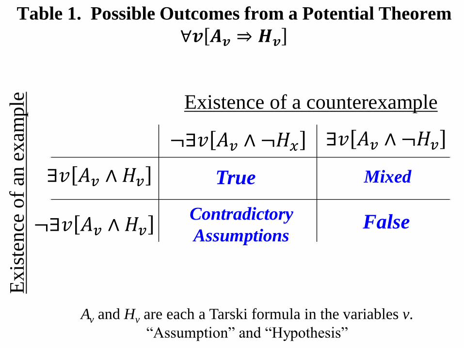
Table 2 shows
the decision times for the four examples in this paper (excluding the two-state model), as
well as a summary of the decision times for the library of 45 examples from economic
theory. The three software implementations used, as well as others, are discussed next.
V. QE Software
There are modern software implementations of QE in Mathematica (Strzebonski
2010, 2016), REDLOG (Dolzmann and Sturm 1997), Maple (Anai and Yanami 2003,
Chen and Maza 2016) and QEPCAD-B (C. W. Brown 2003). In principle, these tools
can solve any QE problem in finite time, given enough computing resources. However,
some user input, such as the order for eliminating variables, is recommended so that the
QE algorithm runs efficiently on the problem at hand. REDLOG and QEPCAD-B are
free software.
QE for existential sentences is also soluble using the technology of Satisfiability
Modulo Theory (SMT) Solvers; at least those that support the QF_NRA logic such as
SMT-RAT (Corzilius, et al. 2012), veriT (Fontaine, et al. 2017), Yices2 (Jovanović and
Dutertre 2017), and Z3 (Jovanović and de Moura 2012). These do not guarantee a
decision: the software authors note that it is possible that the software returns “unknown”
or enters an infinite loop. These SMT solvers are free.
39
For M = 3, the leading term is 83 billion times larger for the elimination of the sixth quantifier than it is for eliminating the first, whereas Binomial2(M) nested six times is no different from
Binomial2(3) itself. 40
See also Shankar (2002, p. 13), who explains that “[m]any decision procedures are of
exponential, super-exponential, or non-elementary complexity. However, this complexity often does not manifest itself on practical examples.”
27
I created a Mathematica package, intended to sharply lower the cost to economists
of using the QE tools in Mathematica, REDLOG, and SMT-NRA solvers. The user
inputs only assumptions and hypothesis, in a natural format much like shown in (10).
The software then automatically: checks for errors; parses and standardizes input;
assembles the Tarski formula using partially interpreted functions as needed; adds
Gramian-matrix assumptions as needed; makes algorithm choices and passes the QE
problem to a QE engine; interprets the QE results according to Table 1; and suggests
what the user can do next. The QE engine is primarily Mathematica’s RESOLVE
function, but the package is also capable of writing code for REDLOG and SMT-NRA
(especially, Z3). Figure 3 is a Mathematica screen shot showing the processing of the
comparative static for the nonparametric Roy model; the technical details of QE are
invisible to the user.
The free package is available by evaluating Get["http://economicreasoning.com"]
at a Mathematica prompt. Further information about Economicreasoning use and
technical background are available from http://help.economicreasoning.com and
Mulligan, Davenport, and England (2018).
With these software resources available, automated QE is easy to perform: about
as easy as running a regression with a modern statistics package. When called by the
Economicreasoning package in deduction problems encountered in my economics
teaching, research, and writing a graduate-level textbook, Mathematica’s algorithm
always performs the QE in seconds.41
At least one of the problems automatically solved
in seconds is familiar from macro and public economics yet experts in the field have been
known to get it wrong when they attempt it manually.42
REDLOG can do most of the
same QE problems even faster, although Mathematica (and Z3) more often accelerates
computation by (appropriately) discarding irrelevant parts of a formula. Z3 tends to be
even faster than REDLOG with the QE problems it can solve, which is a large majority
of the ones that I have tried, but also fails to solve a few percent of the problems. Like
other SMT solvers, Z3 cannot perform QE with free variables.
41
This is not to say that Mathematica’s QE is without limits, just that my practical and frequent
usage has not yet tested those limits. 42
See the Laffer curve problem in Mulligan (2016). Economicreasoning has also been used to generate novel and substantive conclusions about the economy (Mulligan and Tsui 2016).
28
VI. Conclusions
If-then statements about statistics, econometric models, etc., dating back to the
early pioneers of formal statistical reasoning, are implicit eliminations of “for all”
quantifiers from a True sentence. This paper makes the quantifier elimination (QE)
explicit and thereby brings to bear applicable and relatively new tools from real algebraic
geometry and computer science.
QE algorithms automatically decide the truth of hypotheses in finite time, without
approximation or functional-form assumptions. The algorithms can thereby also help
formulate and understand hypotheses by detecting inconsistent assumptions, calculating
sufficient conditions, calculating necessary and sufficient conditions, and generating
examples. These results are not merely hopeful conjectures for the practice of
econometrics. Software is already available for automatically eliminating quantifiers,
which I have incorporated into an economist-friendly interface running in Mathematica.
All of the hypotheses in this paper were refuted or verified merely by entering them as
assumptions and potential implications, as shown in Figure 3.
The QE framework requires statements that are, interpreted in the right space,
quantified (“for all”) Tarski formulas, each of which is a quantifier-free Boolean
combination of polynomial inequalities. In order for an econometric hypothesis to fit in
this framework, its elements need not be polynomial functions: the hypothesis just has to
be stated in terms of properties of the model that are expressed as a finite number of
polynomial relationships among real numbers.
A wide range of econometric models can be processed in this way, although more
work is needed to expand the range, and better understand the practical limits, of
hypotheses and proofs that can be automated with quantifier elimination. QE methods
cannot be applied until the polynomial structure of the problem is discovered. Existing
software is often capable of automatically discovering that structure, but in other cases
the software user needs to assist in the discovery by consciously using partially
interpreted functions rather than specific functional forms. Presumably partially
interpreted functions are more natural to econometricians working with nonparametric
models than those more familiar with parametric approaches.
29
Because QE is automatically done by software, the details of implementation are
of limited interest to users. However, a few implementation concepts are helpful. The
Cylindrical Algebraic Decomposition (CAD) approach defines sets with recursive
formulas, which can clearly delineate cases of interest to the user and sometimes provide
a practical roadmap for step-by-step proofs (Mulligan 2016). The CAD also neatly
illustrates how “ForAll” statements about ℝ𝑁 can be rigorously confirmed by considering
just a finite number of examples. But full CAD construction, which receives relatively
more attention in the theoretical asymptotic complexity literature, is usually doing far
more than is necessary to perform QE on a particular problem.43
Most software
implementations are therefore not constructing a full CAD.
Two quite distinct types of methods are used in modern QE software. One type
refines CAD to take advantage of the special algebraic structure of a problem, which is to
be expected for problems that people might solve “manually.” The second type consists
of nonlinear arithmetic extensions to algorithms for solving the satisfiability in computer
science, some of which are used commercially for certifying the performance of
computer hardware and software. The first type can, with enough computation resources,
solve any QE problem. The second type is limited to deciding existential sentences,
which can be a workhorse for deduction in econometric theory. Both types of methods
continue to be advanced and adapted to practical problems, now with the advantage of
substantively interesting examples from economics and statistics (Mulligan, Bradford, et
al. 2018a).
The QE methods in this paper deliver certified conclusions, but a conclusion is
not the same as a concise proof. The internal software steps of QE are themselves a
proof, and some of the QE software is capable of displaying or summarizing them, but
usually the software steps are too lengthy and tedious for a human reader to appreciate or
practically verify. But even in those cases QE could be of tremendous assistance to
someone attempting to construct a concise proof by: confirming that a hypothesis is
provable, investigating the equivalence of one hypothesis with another, incrementally
eliminating or modifying assumptions to see which of them are binding, verifying any
43
Moreover, for many practical problems, the asymptotic approximations said to describe full CAD construction not only produce the wrong orders of magnitude, but also the wrong sign.
30
number of intermediate results that may serve as one of the steps in the proof, and
automatically generating examples.
Human error can result in logically or mathematically erroneous conclusions,
whether those conclusions were generated with a machine or with pencil and paper. In
the latter approach, a diligent reader, editor, or referee, also operating with pencil and
paper, has been required to detect and correct publication errors. Human errors could in
principle be embedded in QE software (Davenport & England, 2015), although QE
methods can decide any universal sentence with two different methods (i.e., the left- and
right-hand sides of (3) potentially involve different software steps) and each of those
decisions can be processed in N! different sequences (N is the number of quantified
variables). Moreover, multiple software packages are available to perform the same
calculation (this paper uses Mathematica, REDLOG, and Z3), not to mention the fact that
the owners of commercial software packages have both the opportunity and incentive to
find and correct software errors.44
Also note that empirical economics publications
already include dozens, if not hundreds, of matrix inversions that are never verified with
pencil and paper or even with an alternative software package. Perhaps econometric
theory will follow a similar path.
44
If the machine-generated conclusion is that either an example or counter example exists, then this can readily be verified with pencil and paper because the software provides the example.
∃𝑣 𝐴𝑣 ∧ ¬𝐻𝑣 ¬∃𝑣 𝐴𝑣 ∧ ¬𝐻𝑥
Av and Hv are each a Tarski formula in the variables v.
“Assumption” and “Hypothesis”
∃𝑣 𝐴𝑣 ∧ 𝐻𝑣
¬∃𝑣 𝐴𝑣 ∧ 𝐻𝑣
True
False
Mixed
Contradictory
Assumptions
Existence of a counterexample
Exis
ten
ce o
f an
ex
amp
le
Table 1. Possible Outcomes from a Potential Theorem
∀𝒗 𝑨𝒗 ⇒ 𝑯𝒗
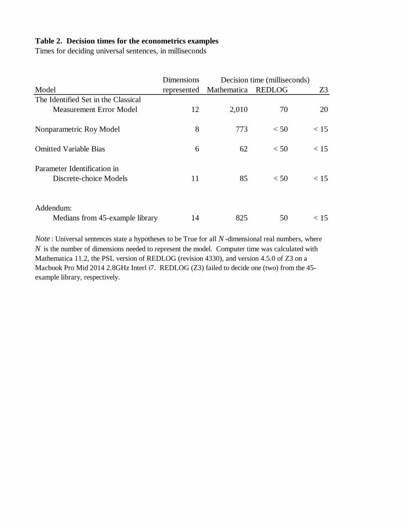
Table 2. Decision times for the econometrics examples
Times for deciding universal sentences, in milliseconds
Model Mathematica REDLOG Z3
The Identified Set in the Classical
Measurement Error Model 12 2,010 70 20
Nonparametric Roy Model 8 773 < 50 < 15
Omitted Variable Bias 6 62 < 50 < 15
Parameter Identification in
Discrete-choice Models 11 85 < 50 < 15
Addendum:
Medians from 45-example library 14 825 50 < 15 0.01
Dimensions
represented
Decision time (milliseconds)
Note : Universal sentences state a hypotheses to be True for all N -dimensional real numbers, where
N is the number of dimensions needed to represent the model. Computer time was calculated with
Mathematica 11.2, the PSL version of REDLOG (revision 4330), and version 4.5.0 of Z3 on a
Macbook Pro Mid 2014 2.8GHz Interl i7. REDLOG (Z3) failed to decide one (two) from the 45-
example library, respectively.
Figure 1. The Set of Counterexamples
The Two-State Model
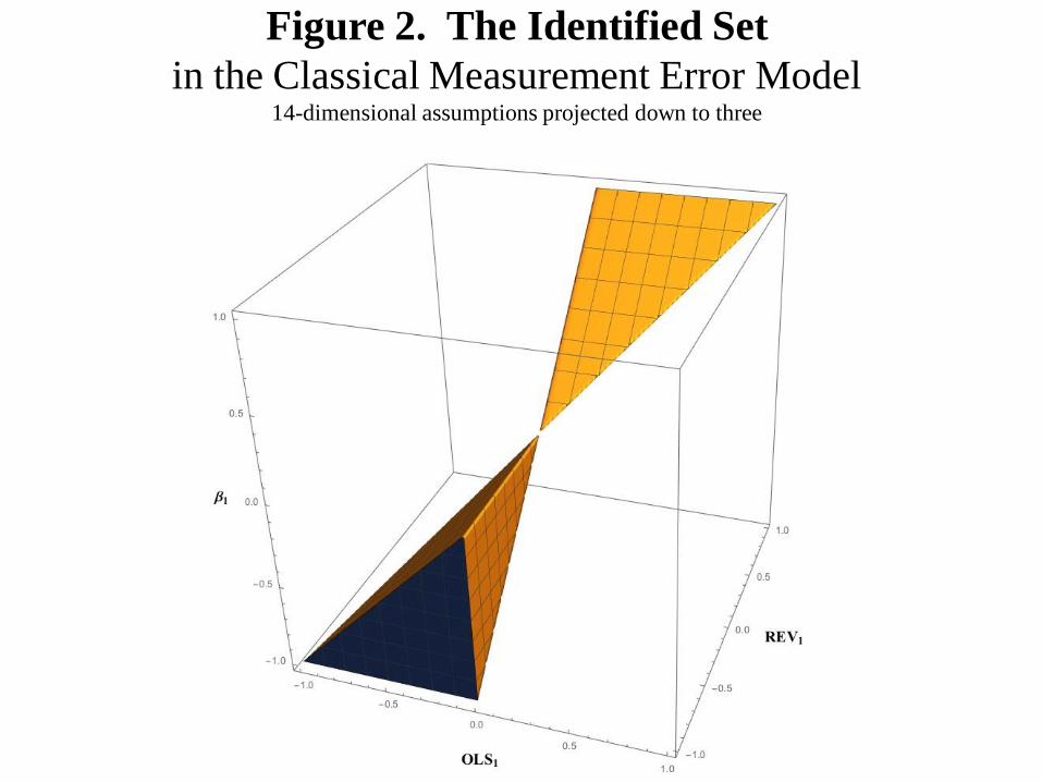
Figure 2. The Identified Set
in the Classical Measurement Error Model 14-dimensional assumptions projected down to three
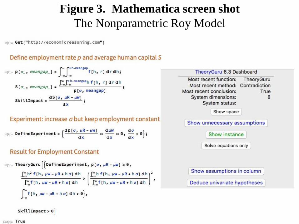
Figure 3. Mathematica screen shot
The Nonparametric Roy Model
31
Bibliography Ackermann, Wilhelm. Solvable Cases of the Decision Problem. Amsterdam: North-
Holland Publishing Company, 1954.
Anai, Hirokazu, and Hitoshi Yanami. "SyNRAC: A Maple-Package for Solving Real
Algebraic Constraints." In Computational Science - ICCS 2003, edited by Peter
M.A. Sloot, David Abramson, Alexander V. Bogdanov, Jack J. Dongarra, Albert
Y. Zomaya and Yuriy E. Gorbachev, 828-837. 2003.
Arai, Noriko H., Hidenao Iwane, Takua Matsuzaki, and Hirokazu Anai. "Mathematics by
Machine." ISSAC '14 Proceedings of the 39th International Symposium on
Symbolic and Algebraic Computation. New York: ACM, 2014. 1-8.
Basu, Saugata, Richard Pollack, and Marie-Francoise Roy. Algorithms in Real Algebraic
Geometry. Berlin: Springer-Verlag (as updated at perso.univ-rennes1.fr), 2011.
Borjas, George J. "The Economics of Immigration." Journal of Economic Literature 32,
no. 4 (December 1994): 1667-1717.
Bradford, Russell, James H. Davenport, Matthew England, Scott McCallum, and David
Wilson. "Truth Table Invariant Cylindrical Algebraic Decomposition." Journal of
Symbolic Computation 76 (September 2016): 1-35.
Brown, Christopher W. "Companion to the Tutorial Cylindrical Algebraic Decomposition
Presented at ISSAC 2004." June 30, 2004.
http://www.usna.edu/Users/cs/wcbrown/research/ISSAC04/handout.pdf.
Brown, Christopher W. "Improved Projection for Cylindrical Algebraic Decomposition."
Journal of Symbolic Computation 32, no. 5 (2001): 447-465.
Brown, Christopher W. "On Quantifer Elimination by Virtual Term Substitution." U.S.
Naval Academy Computer Science Dept. Technical Report, August 2005.
Brown, Christopher W. "QEPCAD B - a program for computing with semi-algebraic sets
using CADs." ACM SIGSAM Bulletin 37, no. 4 (December 2003): 97-108.
Brown, Christopher W., and James H. Davenport. "The Complexity of Quantifier
Elimination and Cylindrical Algebraic Decomposition." Proceedings of the 2007
international symposium on symbolic and algebraic computation, 2007: 54-60.
Brown, Donald J., and Felix Kubler. "Refutable Theories of Value." In Computational
Aspects of General Equilibrium Theory, by Donald J. Brown and Felix Kubler, 1-
10. Berlin: Springer-Verlag, 2008.
Brown, Donald J., and Rosa L. Matzkin. "Testable Restrictions on the Equilibrium
Manifold." Econometrica 64, no. 6 (November 1996): 1249-62.
Bryant, Randal E., Steven German, and Miroslav N. Velev. "Exploiting Positive Equality
in a Logic of Equality with Uninterpreted Functions." In International Conference
on Computer Aided Verification CAV 1999, edited by Nicolas Halbwachs and
Doron Peled, 470-482. Berlin: Springer-Verlag, 1999.
Carvajal, Andres, Rahul Deb, James Fenske, and John K.-H. Quah. "A Nonparametric
Analysis of Multi-product Oligopolies." Economic Theory 57, no. 2 (October
2014): 253-277.
Caviness, B.F., and J.R. Johnson. "Introduction." In Quantifier Elimination and
Cylindrical Algebraic Decomposition, by B.F. Caviness and J.R. Johnson, 1-7.
Berlin: Springer-Verlag, 1998.
Chambers, Christopher P., and Federico Echenique. Revealed Preference Theory.
Cambridge: Cambridge University Press, 2016.
32
Chen, Changbo, and Marc Moreno Maza. "Quantifier elimination by cylindrical algebraic
decomposition based on regular chains." Journal of Symbolic Computation 75
(July-August 2016): 74-93.
Chen, Changbo, and Marc Moreno Maza. "Simplification of Cylindrical Algebraic
Formulas." In Computer Algebra in Scientific Computing, by Vladimir P. Gerdt,
Wolfram Koepf, Werner M. Seiler and Evgenii V. Vorozhtsov, 119-34. Cham,
Switzerland: Springer International Publishing, 2015.
Collins, George E. "Efficient Quantifier Elimination for Elementary Algebra." Seminar
presentation at Stanford University. 1973.
—. "Quantifier Elimination for Real Closed Fields by Cylindric Algebraic
Decomposition." Second GI Conference on Automata Theory and Formal
Languages. Berlin: Springer-Verlag, 1975. 134-83.
Corzilius, Florian, Ulrich Loup, Sebastian Junges, and Erika Ábrahám. "SMT-RAT: An
SMT-Compliant Nonlinear Real Arithmetic Toolbox." In Theory and
Applications of Satisfiability Testing - SAT 2012, edited by Alessandro Cimatti
and Sebastiani Roberto, 442-448. 2012.
Cox, David A., John B. Little, and Donal O'Shea. Ideals, Varieties, and Algorithms. New
York: Springer, 2007.
Davenport, J.H., Y. Siret, and E. Tournier. Computer Algebra: Systems and Algorithms
for Algebraic Computation. London: Academic Press, 1988.
Davenport, James H., and Matthew England. "Recent Advances in Real Geometric
Reasoning." In Automated Deduction in Geometry, by Francisco Botana and
Pedro Quaresma, 37-52. Springer-Verlag, 2015.
De Morgan, Augustus. "On the syllogism: V, and on various points of the onymatic
system." Transactions of the Cambridge Philosophical Society 10 (1862): 428-87.
Dennis, Louise A., Michael Fisher, Matthew P. Webster, and Rafael H. Bordini. "Model
checking agent programming languages." Automated Software Engineering 19,
no. 1 (2012): 5-63.
Dolzmann, Andreas, and Thomas Sturm. "REDLOG: Computer Algebra Meets
Computer Logic." SIGSAM Bull 31, no. 2 (June 1997): 2-9.
England, Matthew, and James H. Davenport. "The Complexity of Cylindrical Algebraic
Decomposition with Respect to Polynomial Degree." In Computer Algebra in
Scientific Computing. CASC 2016, edited by Gerdt Vladimir, Koepf Wolfram,
Werner M. Seiler and Evgenii V. Vorozhtsov, 172-192. 2016.
Fisher, Franklin M. The identification problem in econometrics. New York: McGraw-
Hill, 1966.
Fontaine, Pascal, Mizuhito Ogawa, Thomas Sturm, and Xuan Tung Vu. "Subtropical
Satisfiability." In Frontiers of Combining Systems. FroCoS 2017, edited by Clare
Dixon and Marcelo Finger, 189-206. 2017.
Friedman, Milton. A Theory of the Consumption Function. Princeton, NJ: Princeton
University Press (for NBER), 1957.
Frisch, Ragnar. Statistical Confluence Analysis by Means of Complete Regression
Systems. Oslo: University Economic Institute, 1934.
Grigor'ev, D. Yu. "Complexity of deciding Tarski algebra." Journal of Symbolic
Computation 5, no. 1 (February-April 1988): 65-108.
Gronau, Reuben. "Wage Comparisons-A Selectivity Bias." Journal of Political Economy
82, no. 6 (March 1974): 1119-1143.
33
Heckman, James J. "Sample Selection Bias as a Specification Error." Econometrica 47,
no. 1 (January 1979): 153-161.
Heckman, James J., and Bo E. Honore. "The Empirical Content of the Roy Model."
Econometrica 58, no. 5 (September 1990): 1121-1149.
Heckman, James J., and Guilherme Sedlacek. "Heterogeneity, Aggregation, and Market
Wage Functions: An Empirical Model of Self-Selection in the Labor Market."
Journal of Political Economy 93, no. 6 (December 1985): 1077-1125.
Jovanović, Dejan, and B. Dutertre. "LibPoly: A library for reasoning about polynomials."
In Proceedings of the 15th International Workshop on Satisfiability Modulo
Theories (SMT 2017). 2017.
Jovanović, Dejan, and Leonardo de Moura. "Solving Non-linear Arithmetic." In
Automated Reasoning. IJCAR 2012, edited by Bernhard Gramlich, Dale Miller
and Uli Sattler, 339-354. 2012.
Kauers, Manuel. "How to Use Cylindrical Algebraic Decomposition." Seminaire
Lotharingien de Combinatoire 65 (2011): 1-16.
Keane, Michael, Robert Moffitt, and David Runkle. "Real Wages over the Business
Cycle Estimating the Impact of Heterogeneity with Micro Data." Journal of
Political Economy 96, no. 6 (December 1988): 1232-66.
Kerber, Manfred, Christoph Lange, and Colin Rowat. "An Introduction to Mechanized
Reasoning." Journal of Mathematical Economics 66 (October 2016): 26-39.
Klepper, Steven, and Edward E. Leamer. "Consistent Sets of Estimates for Regressions
with Errors in All Variables." Econometrica 52, no. 1 (January 1984): 163-183.
Kroening, Daniel, and Ofer Strichman. Decision Procedures: An Algorithmic Point of
View. Berlin: Springer-Verlag, 2008.
Levi, Maurice D. "Errors in the Variables Bias in the Presence of Correctly Measured
Variables." Econometrica 41, no. 5 (September 1973): 985-986.
Li, Xiaoliang, and Dongming Wang. "Computing Equilibria of Semi-algebraic
Economies Using Triangular Decomposition and Real Solution Classification."
Journal of Mathematical Economics 54 (October 2014): 48-58.
Mourifie, Ismael, Marc Henry, and Romuald Meango. "Sharp Bounds for the Roy
Model." arXiv.org. September 2017. https://arxiv.org/abs/1709.09284.
Mulligan, Casey B. "Automated Economic Reasoning with Quantifier Elimination."
NBER working paper, no. 22922 (December 2016).
Mulligan, Casey B., and Kevin K. Tsui. "The Upside-down Economics of Regulated and
Otherwise Rigid Prices." NBER working paper, no. 22305 (June 2016).
Mulligan, Casey B., and Yona Rubinstein. "Selection, Investment, and Women’s Relative
Wages over Time." Quarterly Journal of Economics 123, no. 3 (August 2008):
1061–110.
Mulligan, Casey B., James H. Davenport, and Matthew England. "TheoryGuru: A
Mathematica Package to apply Quantifier Elimination Technology to
Economics." NBER working paper, May 2018.
Mulligan, Casey B., Russell Bradford, James H. Davenport, Matthew England, and Zak
Tonks. "Non-linear Real Arithmetic Benchmarks derived from Automated
Reasoning in Economics." NBER working paper, May 2018a.
—. "Quantifier Elimination for Reasoning in Economics." arXiv.org. April 2018b.
Passmore, Grant Olney, and Denis Ignatovich. "Formal Verification of Financial
Algorithms." In Automated Deduction – CADE 26, edited by Leonardo de Moura,
26-41. Cham: Springer, 2017.
34
Renegar, James. "Recent Progress on the Complexity of the Decision Problem for the
Reals." In Quantifier Elimination and Cylindrical Algebraic Decomposition, by
B.F. Caviness and J.R. Johnson, 220-41. Berlin: Springer-Verlag, 1998.
Shankar, Natarajan. "Little Engines of Proof." In FME 2002:Formal Methods—Getting
IT Right, by Lars-Henrik Eriksson and Peter Alexander Lindsay, 1-20. Springer-
Verlag, 2002.
Snyder, Susan K. "Nonparametric Testable Restrictions of Household Behavior."
Southern Economic Journal 67, no. 1 (July 2000): 171-185.
Steinhorn, Charles. "Tame Topology and O-Minimal Structures." In Computational
Aspects of General Equilibrium Theory, by Donald J. Brown and Felix Kubler,
165-91. Berlin: Springer-Verlag, 2008.
Strzebonski, Adam. "Computation with semialgebraic sets represented by cylindrical
algebraic formulas." ISSAC '10 Proceedings of the 35th International Symposium
on Symbolic and Algebraic Computation. New York: ACM, 2010. 61-68.
Strzeboński, Adam. "Cylindrical algebraic decomposition using local projections."
Journal of Symbolic Computation 76 (September-October 2016): 36-64.
Sturm, Thomas. "A Survey of Some Methods for Real Quantifier Elimination, Decision,
and Satisfiability and Their Applications." Mathematics in Computer Science 11,
no. 3 (December 2017): 483-502.
Tadjouddine, Emmanuel M., Frank Guerin, and Wamberto Vasconcelos. "Abstracting
and Verifying Strategy-Proofness for Auction Mechanisms." In Declarative Agent
Languages and Technologies VI. DALT 2008., edited by Matteo Baldoni, Tran
Cao Son, M. Birna van Riemsdijk and Michael Winikoff, 197-214. Berlin:
Springer, 2009.
Tamer, Elie. "Partial Identification in Econometrics." Annual Review of Economics 2, no.
1 (January 2010): 167-195.
Tarski, Alfred. A Decision Method for Elementary Algebra and Geometry. Los Angeles:
RAND Corporation, 1951.
Weispfenning, Volker. "Quantifier Elimination for Real Algebra — the Quadratic Case
and Beyond." Applicable Algebra in Engineering, Communication and
Computing 8, no. 2 (1997): 85-101.
Weispfenning, Volker. "The complexity of linear problems in fields." Journal of
Symbolic Computation 5, no. 1 (1988): 3-27.
Related Documents