Quantification of Sub-Pixel Dynamics in High-Speed Neutron ...

Citation: Wissink, M.L.; Toops, T.J.;

Splitter, D.A.; Nafziger, E.J.; Finney,

C.E.A.; Bilheux, H.Z.; Santodonato,

L.J.; Zhang, Y. Quantification of

Sub-Pixel Dynamics in High-Speed

Neutron Imaging. J. Imaging 2022, 8,

201. https://doi.org/10.3390/

jimaging8070201

Academic Editors: Anders Kaestner

and Jiao Lin

Received: 23 May 2022

Accepted: 10 July 2022

Published: 18 July 2022

Publisher’s Note: MDPI stays neutral

with regard to jurisdictional claims in

published maps and institutional affil-

iations.

Copyright: © 2022 by the authors.

Licensee MDPI, Basel, Switzerland.

This article is an open access article

distributed under the terms and

conditions of the Creative Commons

Attribution (CC BY) license (https://

creativecommons.org/licenses/by/

4.0/).

Journal of

Imaging

Article

Quantification of Sub-Pixel Dynamics in High-SpeedNeutron Imaging †

Martin L. Wissink 1,* , Todd J. Toops 1 , Derek A. Splitter 1 , Eric J. Nafziger 1, Charles E. A. Finney 1 ,Hassina Z. Bilheux 2 , Louis J. Santodonato 2 and Yuxuan Zhang 2

1 Energy Science and Technology Directorate, Oak Ridge National Laboratory, Oak Ridge, TN 37830, USA;[email protected] (T.J.T.); [email protected] (D.A.S.); [email protected] (E.J.N.);[email protected] (C.E.A.F.)

2 Neutron Sciences Directorate, Oak Ridge National Laboratory, Oak Ridge, TN 37830, USA;[email protected] (H.Z.B.); [email protected] (L.J.S.); [email protected] (Y.Z.)

* Correspondence: [email protected]† This manuscript has been authored by UT-Battelle, LLC under Contract No. DE-AC05-00OR22725 with the

U.S. Department of Energy. The United States Government retains and the publisher, by accepting the articlefor publication, acknowledges that the United States Government retains a non-exclusive, paid-up,irrevocable, world-wide license to publish or reproduce the published form of this manuscript, or allowothers to do so, for United States Government purposes. The Department of Energy will provide public accessto these results of federally sponsored research in accordance with the DOE Public Access Plan(http://energy.gov/downloads/doe-public-access-plan).

Abstract: The high penetration depth of neutrons through many metals and other common materialsmakes neutron imaging an attractive method for non-destructively probing the internal structureand dynamics of objects or systems that may not be accessible by conventional means, such as X-rayor optical imaging. While neutron imaging has been demonstrated to achieve a spatial resolutionbelow 10 µm and temporal resolution below 10 µs, the relatively low flux of neutron sources andthe limitations of existing neutron detectors have, until now, dictated that these cannot be achievedsimultaneously, which substantially restricts the applicability of neutron imaging to many fieldsof research that could otherwise benefit from its unique capabilities. In this work, we present anattenuation modeling approach to the quantification of sub-pixel dynamics in cyclic ensemble neutronimage sequences of an automotive gasoline direct injector at a 5 µs time scale with a spatial noisefloor in the order of 5 µm.

Keywords: gasoline direct injector; in situ; neutron imaging; operando; quantitative; sub-pixel

1. Introduction

Neutrons offer a unique combination of properties, including high penetration throughcommon engineering materials such as aluminum and ferrous alloys, high sensitivity tocertain light elements such as H, Li, and B, and isotope-specific interactions that can be usedto generate contrast [1]. These properties make neutron imaging a powerful and highlycomplementary tool for the non-destructive investigation of materials and systems thatcannot be probed by more conventional X-ray and optical imaging techniques. However,the comparably lower spatial and temporal resolution of neutron imaging has limited thepotential application space. Here, we employ an automotive gasoline direct injector (GDI),which has geometric features and transient dynamics that push against both the spatial andtemporal resolution limits of existing neutron imaging, to demonstrate that an analyticalneutron attenuation model can be employed to quantify sub-pixel dynamics in the cyclicoperation of a real-world device.

Increasingly stringent fuel economy regulations have pushed internal combustionengine efficiency to improve at an accelerated pace. This need has led to the rapid adoptionof GDI technology in the automotive segment, with the market share increasing from

J. Imaging 2022, 8, 201. https://doi.org/10.3390/jimaging8070201 https://www.mdpi.com/journal/jimaging

J. Imaging 2022, 8, 201 2 of 26

negligible in 2007 to >50% in 2018 [2]. GDIs introduce high-pressure fuel directly intothe combustion chamber, allowing engine designers much greater flexibility in terms ofthe distribution and mixing of the fuel spray within the chamber while also providingevaporative cooling, which can enable the use of higher engine compression ratios forimproved fuel efficiency.

Although there are clear benefits to GDI technology, an improperly designed GDIsystem can easily create poor mixing or spray–wall interactions, which can result in highlevels of particulate matter [3] and potentially catastrophic abnormal combustion events,such as pre-ignition [4]. GDIs also introduces significant complexity from the perspective ofmodeling and measuring the highly transient and turbulent spray. This complexity stemsfrom several factors, including the elaborate internal geometries of injectors with featuresfrom 5 to 500 µm [5]; high pressures and flow velocities of the fuel and the wide range ofdownstream temperatures and pressures leading to highly turbulent flow within the injectorand two-phase conditions induced by cavitation or flash boiling [6]; and the inherentlystochastic nature of the flow along with small hole-to-hole manufacturing differencesleading to significant variation in the exiting spray on a hole-to-hole and cycle-to-cyclebasis [7–12].

Research on gasoline and diesel sprays has traditionally focused on processes thatoccur after the fuel exits the injector (liquid penetration, mixing, breakup, evaporation, andpotential spray–wall interactions), and has involved a suite of experimental techniquesbased on optical, laser, and X-ray diagnostics [13] in both spray chambers and opticallyaccessible engines. Research has also involved computational fluid dynamics (CFD) sim-ulations with varying degrees of complexity regarding the treatment of turbulence andmultiphase flow [14]. Only recently have simulations of sprays begun to earnestly examineflow upstream from the injector nozzle exit, with models traditionally treating the sprayas emanating from either a point source or a homogenous area. Recent X-ray imagingexperiments have quantified both the axial (lift) and nonaxial (wobble) displacement of theneedle that controls the flow of fuel into the nozzle holes of gasoline and diesel injectors,and corresponding CFD simulations have shown that using these measured displacementsas boundary conditions can generate similar fluid structures in the nozzle exit to those seenexperimentally [7–11].

X-rays at high-intensity sources can produce high-resolution measurements (~1 µm)of both geometry (from tomography) and mechanical/fluid dynamics (from high-speedimaging) in the regions at the very tip of the injector. Time-resolved tomography of fluidstructures in the nozzle is also possible with X-rays, but only when ensemble-averagedover thousands of events [15]. However, the tradeoffs among field of view, resolution, andpenetrating power required to image the thicker parts of the injector while maintainingsensitivity or contrast to the hydrocarbon fuel are not favorable [16]. Here, neutron imagingoffers an advantage from high penetrating power through common aluminum and ferrousalloys used in engines and injectors, a high sensitivity to 1H in hydrocarbon fuels, and high-speed detectors that offer a field of view of several centimeters with a spatial resolutionin the order of 50–100 µm and temporal resolution in the order of 1 ns to 1 µs [17–19].This spatial resolution can capture the geometric detail of all but the smallest featuresof an injector (nozzle holes and needle seat region), making neutron and X-ray imaginghighly complementary tools for obtaining geometric and compositional information viatomography. However, mechanical dynamics, such as needle lift and wobble, have beenobserved with X-ray imaging to occur below 5 and 50 µm, respectively [8], meaning thatsuch dynamics are below the pixel size of existing high-speed neutron imaging detectors.

Although neutron imaging methods achieving spatial resolution below 10 µm havebeen demonstrated by focusing either the neutrons [20] or the light emitted from a neutronscintillator [21], systems with a high spatial resolution have thus far been limited to atemporal resolution >1 s. Neutron imaging of transient events that occur at simultaneousµm spatial scales and µs timescales, such as the dynamics that occur inside fuel injectors, hasbeen inaccessible because of limitations of detector technology and the relatively low flux

J. Imaging 2022, 8, 201 3 of 26

of neutrons at even the world’s brightest sources. In this work, we present an attenuationmodeling approach to both observe and quantify highly transient sub-pixel dynamics atscales approaching 5 µs and 5 µm in an ensemble-averaged cyclic measurement.

2. Materials and Methods2.1. Neutron Imaging Configurations

High-speed neutron imaging and neutron computed tomography (CT) were per-formed at the CG-1D cold neutron imaging beamline [17] at the High Flux Isotope Reactor(HFIR), a Department of Energy user facility operated by the Oak Ridge National Labora-tory (ORNL).

A diagram of the two imaging configurations is shown in Figure 1. Neutrons fromthe reactor core passed through a liquid hydrogen moderator at ~20 K, slowing themand increasing their wavelength. These “cold” polychromatic neutrons traveled throughguides to the various instruments in the HFIR Cold Guide Hall. The guide exit at theCG-1D beamline was equipped with a motorized aperture with diameter D that could beadjusted from 3.3 to 16 mm. With the aperture-to-detector distance L fixed at 6.59 m, L/Dratios ranging from 400 to 2000 were possible. An Al2O3 diffuser just after the aperturewas used to spatially homogenize the beam. The beam profile was further controlledby a He-filled flight tube between the aperture and the detector that was equipped withsilicon windows and motorized boron–nitride exit slits that defined the final beam size [17].Typical open-beam neutron flux at the detector was ~107 n/cm2/s at maximum aperture.

J. Imaging 2022, 8, x FOR PEER REVIEW 3 of 26

spatial scales and μs timescales, such as the dynamics that occur inside fuel injectors, has been inaccessible because of limitations of detector technology and the relatively low flux of neutrons at even the world’s brightest sources. In this work, we present an attenuation modeling approach to both observe and quantify highly transient sub-pixel dynamics at scales approaching 5 μs and 5 μm in an ensemble-averaged cyclic measurement.

2. Materials and Methods 2.1. Neutron Imaging Configurations

High-speed neutron imaging and neutron computed tomography (CT) were per-formed at the CG-1D cold neutron imaging beamline [17] at the High Flux Isotope Reactor (HFIR), a Department of Energy user facility operated by the Oak Ridge National Labor-atory (ORNL).

A diagram of the two imaging configurations is shown in Figure 1. Neutrons from the reactor core passed through a liquid hydrogen moderator at ~20 K, slowing them and increasing their wavelength. These “cold” polychromatic neutrons traveled through guides to the various instruments in the HFIR Cold Guide Hall. The guide exit at the CG-1D beamline was equipped with a motorized aperture with diameter D that could be ad-justed from 3.3 to 16 mm. With the aperture-to-detector distance L fixed at 6.59 m, L/D ratios ranging from 400 to 2000 were possible. An Al2O3 diffuser just after the aperture was used to spatially homogenize the beam. The beam profile was further controlled by a He-filled flight tube between the aperture and the detector that was equipped with silicon windows and motorized boron–nitride exit slits that defined the final beam size [17]. Typ-ical open-beam neutron flux at the detector was ~107 n/cm2/s at maximum aperture.

Figure 1. Experimental setups for high-speed neutron imaging and neutron CT. Beam travels from right to left in all panels. (A) High-speed setup uses the MCP detector with a custom sample envi-ronment that includes the injector and spray chamber. (B) Tomography setup uses the CCD detector with injector mounted on a rotation stage. (C) Photo of aluminum spray chamber mounted in front of MCP detector.

For high-speed imaging, as shown in Figure 1A, a 10B-doped microchannel plate (MCP) was used to convert neutrons to an electron cascade, which was further amplified by a standard glass MCP. The resultant electron pulse was detected by a 2 × 2 Timepix readout positioned behind the MCP stack. This configuration is referred to here as the “MCP detector,” and has 512 × 512 pixels with 2.8 × 2.8 cm field of view, a physical pixel size of 55 μm, and 1 μs timing capability [17,18]. The fuel injector was mounted in an Al spray chamber at the sample position as shown in Figure 1C and was fired synchronously with the detector. The chamber was continuously purged with gaseous Ar at controlled

Figure 1. Experimental setups for high-speed neutron imaging and neutron CT. Beam travels fromright to left in all panels. (A) High-speed setup uses the MCP detector with a custom sampleenvironment that includes the injector and spray chamber. (B) Tomography setup uses the CCDdetector with injector mounted on a rotation stage. (C) Photo of aluminum spray chamber mountedin front of MCP detector.

For high-speed imaging, as shown in Figure 1A, a 10B-doped microchannel plate(MCP) was used to convert neutrons to an electron cascade, which was further amplifiedby a standard glass MCP. The resultant electron pulse was detected by a 2 × 2 Timepixreadout positioned behind the MCP stack. This configuration is referred to here as the“MCP detector,” and has 512 × 512 pixels with 2.8 × 2.8 cm field of view, a physical pixelsize of 55 µm, and 1 µs timing capability [17,18]. The fuel injector was mounted in an Alspray chamber at the sample position as shown in Figure 1C and was fired synchronouslywith the detector. The chamber was continuously purged with gaseous Ar at controlledtemperature and pressure to provide the ambient condition for the injected spray and toevacuate the sprayed fuel from the chamber.

For tomography, as shown in Figure 1B, a charge-coupled device (CCD)-based AndorDW936 camera system was used. This system, referred to here as the “CCD detector,” con-

J. Imaging 2022, 8, 201 4 of 26

sisted of a 6LiF/ZnS scintillator that converts the incoming neutrons into visible light, alongwith a camera and optics in a light-tight box. The CCD detector had a ~7 × 7 cm field ofview, a pixel size of 37 µm, 80–100 µm spatial resolution, and ~1 s timing resolution [17,22].The injector was mounted in a custom Al holder on a rotation stage at the sample position.Further details of the neutron CT configuration and comparison to X-ray CT are describedby Duke et al. [16].

2.2. Injector and Operating Conditions

A single-hole, solenoid-operated gasoline direct injector was shared by colleagues atGeneral Motors. A neutron CT reconstruction visualized in Figure 2 shows the internalfeatures of the device. A slice on the frontal plane is shown in Figure 2A, which alsoindicates the regions targeted in the high-speed imaging. Figure 2B offers two annotatedperspectives of a sectioned volumetric rendering created with Tomviz 1.9.0 [23], whichprovides 3-dimensional context for the construction of the device. The geometry andattenuation coefficient information from the neutron CT and from radiographs of the emptyand fuel-filled injector allowed for the creation of a simplified analytical model of theneutron attenuation through the object to enable prediction of how an injector needledisplacement of a given magnitude should appear in the normalized high-speed images.

J. Imaging 2022, 8, x FOR PEER REVIEW 4 of 26

temperature and pressure to provide the ambient condition for the injected spray and to evacuate the sprayed fuel from the chamber.

For tomography, as shown in Figure 1B, a charge-coupled device (CCD)-based An-dor DW936 camera system was used. This system, referred to here as the “CCD detector,” consisted of a 6LiF/ZnS scintillator that converts the incoming neutrons into visible light, along with a camera and optics in a light-tight box. The CCD detector had a ~7 × 7 cm field of view, a pixel size of 37 μm, 80–100 μm spatial resolution, and ~1 s timing resolution [17,22]. The injector was mounted in a custom Al holder on a rotation stage at the sample position. Further details of the neutron CT configuration and comparison to X-ray CT are described by Duke et al. [16].

2.2. Injector and Operating Conditions A single-hole, solenoid-operated gasoline direct injector was shared by colleagues at

General Motors. A neutron CT reconstruction visualized in Figure 2 shows the internal features of the device. A slice on the frontal plane is shown in Figure 2A, which also indi-cates the regions targeted in the high-speed imaging. Figure 2B offers two annotated per-spectives of a sectioned volumetric rendering created with Tomviz 1.9.0 [23], which pro-vides 3-dimensional context for the construction of the device. The geometry and attenu-ation coefficient information from the neutron CT and from radiographs of the empty and fuel-filled injector allowed for the creation of a simplified analytical model of the neutron attenuation through the object to enable prediction of how an injector needle displacement of a given magnitude should appear in the normalized high-speed images.

Figure 2. Neutron CT reconstruction of single-hole gasoline direct injector. (A) Slice from CT recon-struction with an illustration of regions targeted in the high-speed neutron image sequence and time-series displacement fits. Fuel flows from top to bottom. (B) Sectioned volumetric rendering of the injector illustrating the internal geometry and features of the device.

Figure 2. Neutron CT reconstruction of single-hole gasoline direct injector. (A) Slice from CTreconstruction with an illustration of regions targeted in the high-speed neutron image sequence andtime-series displacement fits. Fuel flows from top to bottom. (B) Sectioned volumetric rendering ofthe injector illustrating the internal geometry and features of the device.

The injector and spray chamber were operated using the conditions shown in Table A1,and the timing of the injector command and image acquisition process is illustrated inFigure A1. The trigger to begin the MCP detector shutter sequence was sent at a rate of25 Hz. Using a digital delay generator, a trigger delay of 1 ms was used before sendingthe start of energization (SOE) command to the injector driver, which allowed for a static

J. Imaging 2022, 8, 201 5 of 26

period before each injection event to be recorded by the MCP detector. After a durationof 680 µs, the command to the injector driver was released, indicating end of energization(EOE). As a result of the delays inherent to the solenoid energization and the mechanicaland hydraulic actuation processes, the injector does not fully open until just before EOE,and much of the actual spray and dynamics of interest occur after EOE.

The MCP detector was operated in an acquisition mode that uses a series of shuttersto define readout periods. A dead time precedes each shutter, during which, all recordedneutron counts from the previous shutter are aggregated into time bins on a per-pixelbasis. If a count is recorded in a given time bin for a given pixel, the stored value for thattime bin is incremented. In this way, after repeating the cyclic process many times, anensemble movie is created in which each time bin is analogous to a frame, and the valuestored in each pixel of a given frame is the total number of neutron counts recorded forthat pixel over all repetitions (cycles). Due to its cumulative nature, this is an inherentlyensemble-averaged dataset, and retrieval of the neutron counts from individual cycles isnot possible in this imaging mode.

The timing values used for the MCP detector shutters are given in Table A2. The timebin length within a shutter is defined by the length of the shutter and the number of timebins in it. As a result of the high data throughput and the design of the readout electronics,the neutron counts from some shutters did not get saved into the running time bin totals,and therefore, the total number of recorded shutters could be used to normalize the framesof the resulting movie. The injection event and the dynamics of interest for the presentwork occur entirely within Shutter 0, for which, a total of ~1.34 × 106 injection events wererecorded with a time bin length of 5.12 µs.

2.3. Neutron Attenuation Model

Neutron transmission, T, of a homogeneous single-phase material can be describedwith the Beer–Lambert law,

T =I(λ)I0(λ)

= e−µ(λ)d (1)

with incoming intensity I0(λ), transmitted intensity I(λ), attenuation coefficient µ(λ), pathlength d, and neutron wavelength λ. In general, the transmission will be wavelength-dependent; however, for the present experiment, the full polychromatic beam available atHFIR CG-1D was used with no wavelength selection. For a dynamic, nested multiphasesystem as depicted in Figure 3, the time-dependent transmission through the entire systemas measured at a given detector pixel is a function of the path lengths and macroscopicattenuation coefficients Σ for each phase (A, B, C, . . . ):

T(t) = TA(t)× TB(t)× TC(t)× · · · = e−(ΣAdA(t)+ΣBdB(t)+ΣCdC(t)+···) (2)

To detect movement of phase A as depicted in Figure 3, one can employ the fact thatthe length of a given neutron path through A will change in a manner dependent on thegeometry of A. If the time-varying, or dynamic, transmission T(t) is normalized by thestatic, or reference, transmission Tref, the transmission through the non-moving phases(e.g., C and external) will be the same in either condition, and the expression thereforereduces to one dependent only on the attenuation coefficients and dynamic path lengthdifferences through the phases A and B, which share a moving interface:

T(t)Tref

=TA(t)× TB(t)× TC(t)× · · ·TA,ref × TB,ref × TC,ref × · · ·

= e−[ΣA(dA(t)−dA,ref)+ΣB(dB(t)−dB,ref)] (3)

Figure 3 shows that, for this nested system in which the outer boundary of phase Bremains static, the total length of a given neutron path through phases A and B will beconserved as

dA,ref + dB,ref = dA(t) + dB(t) (4)

J. Imaging 2022, 8, 201 6 of 26

If this relation is substituted into Equation (3) and the natural logarithm is taken, oneobtains a measure of the dynamic path length change for phase A, which depends onlyon the log-ratio normalized transmission measurement and the difference in attenuationcoefficients between phases A and B:

loge

(T(t)Tref

)= (ΣB − ΣA)(dA(t)− dA,ref) (5)

In general, a detector does not directly measure neutron intensity or transmissionbecause of inefficiencies in the process of converting neutrons to some other measurablesignal, noise due to gamma rays (mainly produced by neutron interactions with the sam-ple), electronic noise, and other sources of measurement bias. These effects are typicallyaccounted for by measuring the intensity of the unobstructed “open beam” IOB, as wellas the intensity of the “dark frame” IDF, with the neutron shutter closed. The measuredintensity Imeas can then be normalized to transmission by

T =Imeas − IDF

IOB − IDF(6)

The dark frame measurement IDF is generally non-zero and “structured” as a charac-teristic of a CCD or complementary metal–oxide–semiconductor (CMOS) sensor, whereasthe dark frame of the Timepix-based MCP detector used here can be considered zero forall practical purposes [18], with any counts being caused by random gamma or cosmicrays. The open-beam image IOB is also structured because of imperfections in the detectorand spatial inhomogeneity of the incident neutron beam caused by the guides. The totalintensity may also evolve over time due to variation in reactor output. However, despitethe high-speed imaging experiments described here being performed continuously overa period exceeding 24 h, intermittent open-beam measurements were not necessary be-cause of the dynamic normalization approach. As described previously and illustrated inFigure A1, the MCP detector output for a single pixel at time bin ti is the sum of all countsthat were recorded as occurring within that pixel and that time bin over all cycles ck, or anensemble time bin:

Imeas(ti) =k=n

∑k=1

Imeas(ti, ck) (7)

A general expression for the transmission at a given pixel location during time bin tiof cycle ck can be written as

T(ti, ck) =Imeas(ti, ck)− IDF(ti, ck)

IOB(ti, ck)− IDF(ti, ck)∼=

Imeas(ti, ck)

IOB(ti, ck)(8)

where the dark frame intensity was assumed to be negligible for the MCP detector. Theensemble-average transmission for a given time bin over all cycles would then be

T(ti) =1n

k=n

∑k=1

T(ti, ck) ∼=1n

k=n

∑k=1

Imeas(ti, ck)

IOB(ti, ck)(9)

By averaging the time bins from ta to tb directly preceding the injection event, duringwhich the injector is in a static condition, one obtains a reference transmission Tref:

Tref =1

(b− a + 1)

i=b

∑i=a

T(ti) ∼=1

n(b− a + 1)

i=b

∑i=a

k=n

∑k=1

Imeas(ti, ck)

IOB(ti, ck)(10)

The dynamic normalization is then performed by taking the ratio of T(ti) to Tref, whichcan be reduced to an expression dependent only on Imeas(ti) if it is assumed that IOB doesnot change significantly over the course of a single cycle. For the present experiment, which

J. Imaging 2022, 8, 201 7 of 26

was conducted at 25 Hz, this assumption is quite reasonable. The dynamic normalizationis expressed as

T(ti)Tref∼=

1n ∑k=n

k=1Imeas(ti ,ck)IOB(ti ,ck)

1n(b−a+1) ∑i=b

i=a ∑k=nk=1

Imeas(ti ,ck)IOB(ti ,ck)

∼= (b− a + 1) ∑k=nk=1 Imeas(ti ,ck)

∑i=bi=a ∑k=n

k=1 Imeas(ti ,ck)

∼= (b− a + 1) Imeas(ti)

∑i=bi=a Imeas(ti)

(11)

This formulation does not explicitly treat the effects of incoherent scattering from thesample, which may be significant because of the short sample-to-detector distance usedin this study (~5 cm for the CT scans, ~10 cm for the high-speed imaging). Similarly, thepossibility of multiple scattering and beam hardening within the sample is significant in thehigh-attenuation hydrogenous regions [24–26] and is not explicitly treated in Equation (5),though it may be extended to consider path-length dependence of Σ within each phase.However, these effects are essentially constant throughout the injection cycle because of thesmall scale at which the geometric deflections occur in the injector relative to the size of thecomponents and are therefore effectively cancelled out via the dynamic normalization.

J. Imaging 2022, 8, x FOR PEER REVIEW 6 of 26

Figure 3. Illustration of neutron path length variation in moving phases. Neutron arriving at a given detector pixel after passing through a nested multiphase system (A–C) with one moving phase (A) will encounter a shorter path length through (A) when that phase moves as shown.

Figure 3 shows that, for this nested system in which the outer boundary of phase B remains static, the total length of a given neutron path through phases A and B will be conserved as 𝑑 , + 𝑑 , = 𝑑 (𝑡) + 𝑑 (𝑡) (4)

If this relation is substituted into Equation (3) and the natural logarithm is taken, one obtains a measure of the dynamic path length change for phase A, which depends only on the log-ratio normalized transmission measurement and the difference in attenuation coefficients between phases A and B: log 𝑇(𝑡)𝑇 = (Σ − Σ ) 𝑑 (𝑡) − 𝑑 , (5)

In general, a detector does not directly measure neutron intensity or transmission because of inefficiencies in the process of converting neutrons to some other measurable signal, noise due to gamma rays (mainly produced by neutron interactions with the sam-ple), electronic noise, and other sources of measurement bias. These effects are typically accounted for by measuring the intensity of the unobstructed “open beam” IOB, as well as the intensity of the “dark frame” IDF, with the neutron shutter closed. The measured in-tensity Imeas can then be normalized to transmission by 𝑇 = 𝐼meas − 𝐼DF𝐼OB − 𝐼DF

(6)

The dark frame measurement IDF is generally non-zero and “structured” as a charac-teristic of a CCD or complementary metal–oxide–semiconductor (CMOS) sensor, whereas the dark frame of the Timepix-based MCP detector used here can be considered zero for all practical purposes [18], with any counts being caused by random gamma or cosmic rays. The open-beam image IOB is also structured because of imperfections in the detector and spatial inhomogeneity of the incident neutron beam caused by the guides. The total intensity may also evolve over time due to variation in reactor output. However, despite the high-speed imaging experiments described here being performed continuously over a period exceeding 24 h, intermittent open-beam measurements were not necessary be-cause of the dynamic normalization approach. As described previously and illustrated in Figure A1, the MCP detector output for a single pixel at time bin ti is the sum of all counts

Figure 3. Illustration of neutron path length variation in moving phases. Neutron arriving at a givendetector pixel after passing through a nested multiphase system (A–C) with one moving phase (A)will encounter a shorter path length through (A) when that phase moves as shown.

2.4. Path Length Model

As shown in Figure 4A,B, the path length through the cylindrical injector needle fora neutron travelling in the y direction that strikes the detector at pixel location x, can bemodeled as the length of chord d(x) for a circle of radius r with center (a, b):

d(x) = <[

2√

r2 − (x− a)2]

(12)

The difference ∆d(x) in this path length between the displaced, or dynamic, circle at(adyn,bdyn) and the static, or reference, circle at (aref,bref) is then given by

∆d(x) = <[

2

√r2 −

(x− adyn

)2]−<

[2√

r2 − (x− aref)2]

(13)

J. Imaging 2022, 8, 201 8 of 26

Equation (13) and Figure 4 show that any displacement along the neutron beamdirection (y direction) cannot be detected in this orientation because it would not changethe path length. Orthogonal views of the object would therefore be required to obtain bothplanar components of displacement.

J. Imaging 2022, 8, x FOR PEER REVIEW 8 of 26

Figure 4. Illustration of path length variation through moving circles with discrete or probabilistic location. (A) Two circles at different discrete positions (reference and dynamic) in the xy plane with neutron path in the y direction denoted by n. (B) Path lengths and path length difference for paths in the y direction as a function of x. (C) Probability distributions for locations of two circles at dif-ferent positions (reference and dynamic) in the xy plane. (D) Expected values for path lengths and path length difference for paths in the y direction as a function of x are smoothed out in comparison to the discrete path lengths in (B).

The difference ∆d(x) in this path length between the displaced, or dynamic, circle at (adyn,bdyn) and the static, or reference, circle at (aref,bref) is then given by ∆𝑑(𝑥) = ℜ 2 𝑟 − (𝑥 − 𝑎dyn) − ℜ 2 𝑟 − (𝑥 − 𝑎ref) (13)

Equation (13) and Figure 4 show that any displacement along the neutron beam di-rection (𝑦 direction) cannot be detected in this orientation because it would not change the path length. Orthogonal views of the object would therefore be required to obtain both planar components of displacement.

This formulation assumes that the centers of the circles can be described by a single point (a,b) with each component having a fixed value. However, because the path length difference being measured in this study is an ensemble over many events, the center loca-tion should be expected to have some event-to-event variation, and therefore should be treated probabilistically as illustrated in Figure 4C,D.

For a random variable X with a probability density function (PDF) fX(x), the expected value E of a function g(X), which is dependent on X, is given by

𝐸 𝑔(𝑋) = 𝑔(𝑥) 𝑓 (𝑥)𝑑𝑥 (14)

Following on from this definition, the expected value for the path length d(x,a) where the value of a has a PDF fa(x) will be given by

𝐸 𝑑(𝑥, 𝑎) = 𝑑(𝑥, 𝛼) 𝑓 (𝛼)𝑑𝛼 (15)

Figure 4. Illustration of path length variation through moving circles with discrete or probabilisticlocation. (A) Two circles at different discrete positions (reference and dynamic) in the xy plane withneutron path in the y direction denoted by n. (B) Path lengths and path length difference for paths inthe y direction as a function of x. (C) Probability distributions for locations of two circles at differentpositions (reference and dynamic) in the xy plane. (D) Expected values for path lengths and pathlength difference for paths in the y direction as a function of x are smoothed out in comparison to thediscrete path lengths in (B).

This formulation assumes that the centers of the circles can be described by a singlepoint (a,b) with each component having a fixed value. However, because the path lengthdifference being measured in this study is an ensemble over many events, the centerlocation should be expected to have some event-to-event variation, and therefore should betreated probabilistically as illustrated in Figure 4C,D.

For a random variable X with a probability density function (PDF) fX(x), the expectedvalue E of a function g(X), which is dependent on X, is given by

E[g(X)] =

∞∫−∞

g(x) fX(x)dx (14)

Following on from this definition, the expected value for the path length d(x,a) wherethe value of a has a PDF fa(x) will be given by

E[d(x, a)] =∞∫−∞

d(x, α) fa(α)dα (15)

where a in d(x,a) and x in fa(x) are replaced by the dummy variable α within the integral.An example calculation for a single value of x in a unitless system is shown in Figure 5A,where fa(α) follows a normal distribution with mean µa and standard deviation σa. The

J. Imaging 2022, 8, 201 9 of 26

interval was discretized and E[d(x,a)] was calculated by performing numerical integrationof the shaded region.

J. Imaging 2022, 8, x FOR PEER REVIEW 10 of 26

Figure 5. Development of the probabilistic path length model. (A) Example calculation of expected value for the path length function for a given value of x. E[d(x,a)] was obtained by integrating the product of the path length function d(x,a) and the PDF fa(x) over all possible values of a (dummy variable α) as indicated by the shaded region. (B) Expected value of path length through a circle of given radius and mean x location with varying standard deviation of x location. Example calculation from A is indicated by the open circle. (C) Effect of varying the standard deviation of circle location on the expected value of path length difference for circles displaced by 1% of the radius. (D) Effect of varying the ratio of standard deviation of the dynamic and reference circle locations on the ex-pected value of path length difference for circles displaced by 1% of the radius.

Another consideration is that the apparent path length profile will also be affected by the unsharpness (blur) in the collected images, which is a function of both the detector’s inherent resolution and the geometrical blurring induced by aspects of the optical setup, such as L/D ratio and sample-to-detector distance. These effects can be addressed by esti-mating the edge spread function (ESF) for a given combination of detector and optical setup [28] and performing convolution with the path length function in the same manner as carried out for the position variation. For the experiments described here, the ESF, which may induce a blur of a few pixels, was expected to have a much greater effect on the measured path length difference than the actual variation in needle location, which is roughly 1 pixel or less. For the present work, the effects of detector blur, geometrical blur, and cyclic blur were lumped together within σa,dyn and σa,ref, but, in principle, could be

Figure 5. Development of the probabilistic path length model. (A) Example calculation of expectedvalue for the path length function for a given value of x. E[d(x,a)] was obtained by integrating theproduct of the path length function d(x,a) and the PDF fa(x) over all possible values of a (dummyvariable α) as indicated by the shaded region. (B) Expected value of path length through a circle ofgiven radius and mean x location with varying standard deviation of x location. Example calculationfrom A is indicated by the open circle. (C) Effect of varying the standard deviation of circle locationon the expected value of path length difference for circles displaced by 1% of the radius. (D) Effect ofvarying the ratio of standard deviation of the dynamic and reference circle locations on the expectedvalue of path length difference for circles displaced by 1% of the radius.

In principle, this procedure would be repeated for each value of x to obtain the pathlength profile for a given PDF of a, but the numerical integration becomes computationallyexpensive when repeated many times during iterations in the process of fitting this functionto the data. However, we took advantage of the fact that the random variable a doesnot affect the shape of d(x,a), but merely shifts the function in x. In effect, Equation (15)

J. Imaging 2022, 8, 201 10 of 26

computes the integral of the product of two functions as one is shifted past the other, whichis equivalent to convolution:

E[d(x, a)] = fa(x) ∗ d(x) =∞∫−∞

fa(β)d(x− β)dβ (16)

This was implemented by performing discrete convolution over a finite domain inMATLAB [27]. To minimize the size of the numerical domain, fa(x) and d(x) were centeredat zero and the result of the convolution was translated to µa. To guarantee that the tails ofthe distribution were adequately captured, the domain for convolution when applied tothe high-speed images was defined as

− (r + 3σa) ≤ x ≤ r + 3σa (17)

∆x = min(1 px, r/10, σa/10) (18)

An example calculation of E[d(x,a)] for several values of σa in a unitless system isshown in Figure 5B, which illustrates that treating the value of a probabilistically blursthe path length profile, adding tails to the ends while decreasing the expected value in thecenter. Both effects become more pronounced as µa approaches and exceeds r.

The object here is an expression for the expected value of the path length difference,which can now be realized by calculating E[d(x,a)] for both the reference and dynamiccircles as

E[∆d(

x, aref, adyn

)]= E

[d(

x, adyn

)]− E[d(x, aref)] (19)

An example of the effect of the probabilistic approach is provided in Figure 5C, whereinthe mean displacement µa,dyn − µa,ref is set as equal to 1% of the radius r, and the standarddeviations σa,dyn and σa,ref are set as equal over a range of 0 to 50% of r. The effect ofincreasing standard deviation is to add tails to the expected value of path length differenceand decrease the peak values.

An example of unequal standard deviations is shown in Figure 5D, which demon-strates that asymmetrical profiles with multiple minima and maxima are possible. Theimplications of this probabilistic approach are twofold: first, the theoretical possibilityexists to infer from an ensemble normalized image not only the average displacement of thegeometry but also the variation in displacement for an assumed distribution. Second, theadditional parameters introduced in this approach create the possibility of non-unique so-lutions. An example of the second point is illustrated in Figure 5C, where E[∆d(x,aref,adyn)]approaches zero everywhere for large values of σa,dyn and σa,ref, which would also occur inthe case of near-zero displacement when µa,dyn ≈ µa,ref. The possibility of non-unique solu-tions requires that some informed constraints be placed on the fitting procedure to avoidnon-physical results. One example is that the PDF describing the dynamic displacementwill be bounded by the static container that surrounds the moving phase (in this case, theinjector needle is contained within the body of the injector).

Another consideration is that the apparent path length profile will also be affected bythe unsharpness (blur) in the collected images, which is a function of both the detector’sinherent resolution and the geometrical blurring induced by aspects of the optical setup,such as L/D ratio and sample-to-detector distance. These effects can be addressed byestimating the edge spread function (ESF) for a given combination of detector and opticalsetup [28] and performing convolution with the path length function in the same manneras carried out for the position variation. For the experiments described here, the ESF,which may induce a blur of a few pixels, was expected to have a much greater effect onthe measured path length difference than the actual variation in needle location, which isroughly 1 pixel or less. For the present work, the effects of detector blur, geometrical blur,and cyclic blur were lumped together within σa,dyn and σa,ref, but, in principle, could be

J. Imaging 2022, 8, 201 11 of 26

separated if the ESF were known. These parameters will be referred to as “total blur” toemphasize the fact that they are the combination of multiple effects.

2.5. Image Processing

The raw images from the 512 × 512 pixel MCP detector were processed with anoverlap correction algorithm [29] and were also rate normalized such that images fromshutters with different time bin sizes and/or shutter counts would have the same intensity.The images shown here were also cropped to a region of 169 × 509 pixels before furtherprocessing, as illustrated in Figure 2A.

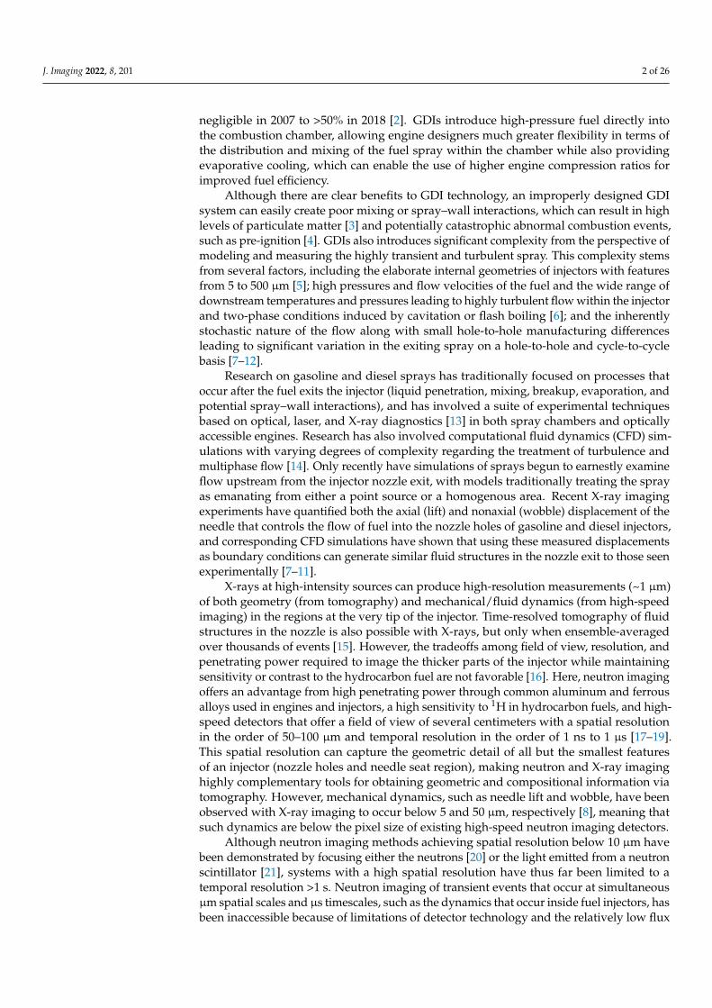
Figure 6 shows several levels of filtering and normalization that were applied to thedynamic images. As a result of the single event counting nature of the MCP detector andthe low overall count rates, the unfiltered images were significantly affected by Poissonnoise, which renders the normalized images visually unusable for qualitative purposes.

J. Imaging 2022, 8, x FOR PEER REVIEW 11 of 26

separated if the ESF were known. These parameters will be referred to as “total blur” to emphasize the fact that they are the combination of multiple effects.

2.5. Image Processing The raw images from the 512 × 512 pixel MCP detector were processed with an over-

lap correction algorithm [29] and were also rate normalized such that images from shut-ters with different time bin sizes and/or shutter counts would have the same intensity. The images shown here were also cropped to a region of 169 × 509 pixels before further processing, as illustrated in Figure 2A.

Figure 6 shows several levels of filtering and normalization that were applied to the dynamic images. As a result of the single event counting nature of the MCP detector and the low overall count rates, the unfiltered images were significantly affected by Poisson noise, which renders the normalized images visually unusable for qualitative purposes.

Figure 6. Filtering and normalization methods for high-speed imaging. Image is from a time bin with a relatively large needle deflection (t = 2.27 ms). Rows correspond to filtering, and columns correspond to normalization. The injector body outline has been overlaid on the normalized images for clarity. Variations in neutron count rate due to displacement of the injector needle are apparent in the normalized images due to the difference in attenuation coefficient between the steel needle and the surrounding hydrogenous fuel, with movement of the needle toward light and away from dark in the subtraction images, and toward blue and away from red in the log-ratio images.

Figure 6. Filtering and normalization methods for high-speed imaging. Image is from a time binwith a relatively large needle deflection (t = 2.27 ms). Rows correspond to filtering, and columnscorrespond to normalization. The injector body outline has been overlaid on the normalized imagesfor clarity. Variations in neutron count rate due to displacement of the injector needle are apparent inthe normalized images due to the difference in attenuation coefficient between the steel needle andthe surrounding hydrogenous fuel, with movement of the needle toward light and away from darkin the subtraction images, and toward blue and away from red in the log-ratio images.

J. Imaging 2022, 8, 201 12 of 26

This was first addressed by a lowpass zero-phase 10 kHz Butterworth filter appliedin the time domain, which considerably improved the signal-to-noise ratio and producedusable dynamic normalized images. Further visual improvement was made by use ofiterative Poisson denoising [30] applied in the spatial domain on a frame-by-frame basis.

For each filtering level, reference images were created by averaging the 176 framesbefore SOE. These reference images were then used to perform two different normalizationsat each filtering level. The first is a qualitative method, which consists of subtracting 95%of the reference image from the dynamic images. The second is the log-ratio normalizationdescribed in Equations (5) and (11).

2.6. Extraction of Sample Parameters from Neutron Radiographs and CT

The radius of the injector needle was extracted from the neutron CT reconstruction ofthe empty fuel injector shown in Figure 2 by converting the CT data to radial coordinatesand fitting an error function to the edges of interest:

y = a +(b− a)

2

[1 + erf

(x− µ

σ

)](20)

This function creates a step from level a to level b centered at µ with scale parameter σ.A simpler approach would be to binarize each slice in the CT and compute the equivalentdiameters of the regions, but the approach used here includes all of the data in the defined3D region in a single fit, reducing the uncertainty in the measured radii and also allowingfor the uncertainty to be quantified. Figure 7A–C show the regions used for each fit onfrontal and transverse slices. The region of the CT corresponding to the part of the injectorneedle seen in the high-speed imaging is shown in red, and the portion of the outer injectorbody used to set the scaling of the CT is shown in blue.

J. Imaging 2022, 8, x FOR PEER REVIEW 12 of 26

This was first addressed by a lowpass zero-phase 10 kHz Butterworth filter applied in the time domain, which considerably improved the signal-to-noise ratio and produced usable dynamic normalized images. Further visual improvement was made by use of it-erative Poisson denoising [30] applied in the spatial domain on a frame-by-frame basis.

For each filtering level, reference images were created by averaging the 176 frames before SOE. These reference images were then used to perform two different normaliza-tions at each filtering level. The first is a qualitative method, which consists of subtracting 95% of the reference image from the dynamic images. The second is the log-ratio normal-ization described in Equations (5) and (11).

2.6. Extraction of Sample Parameters from Neutron Radiographs and CT The radius of the injector needle was extracted from the neutron CT reconstruction

of the empty fuel injector shown in Figure 2 by converting the CT data to radial coordi-nates and fitting an error function to the edges of interest: 𝑦 = 𝑎 + (𝑏 − 𝑎)2 1 + erf 𝑥 − 𝜇𝜎 (20)

This function creates a step from level a to level b centered at μ with scale parameter σ. A simpler approach would be to binarize each slice in the CT and compute the equiva-lent diameters of the regions, but the approach used here includes all of the data in the defined 3D region in a single fit, reducing the uncertainty in the measured radii and also allowing for the uncertainty to be quantified. Figure 7A–C show the regions used for each fit on frontal and transverse slices. The region of the CT corresponding to the part of the injector needle seen in the high-speed imaging is shown in red, and the portion of the outer injector body used to set the scaling of the CT is shown in blue.

Figure 7. Process for extracting needle radius from neutron CT. Radial regions extending from the needle center were defined for both the valve needle (red) and outer body (blue) fits. (A) Axial and radial extent of each region overlaid on frontal slice. (B,C) Transverse view within each region with illustration of radial extent. (D) Attenuation coefficient of each voxel within each region plotted by radius with edge fits overlaid. Horizontal dashed line shows attenuation coefficient calculated from projections. Fit of outer body is used to set the image scaling based on the known outer body diam-eter. This scaling is used with the fit of valve needle radius to measure its size in microns.

Figure 7. Process for extracting needle radius from neutron CT. Radial regions extending from theneedle center were defined for both the valve needle (red) and outer body (blue) fits. (A) Axial andradial extent of each region overlaid on frontal slice. (B,C) Transverse view within each region withillustration of radial extent. (D) Attenuation coefficient of each voxel within each region plottedby radius with edge fits overlaid. Horizontal dashed line shows attenuation coefficient calculatedfrom projections. Fit of outer body is used to set the image scaling based on the known outer bodydiameter. This scaling is used with the fit of valve needle radius to measure its size in microns.

J. Imaging 2022, 8, 201 13 of 26

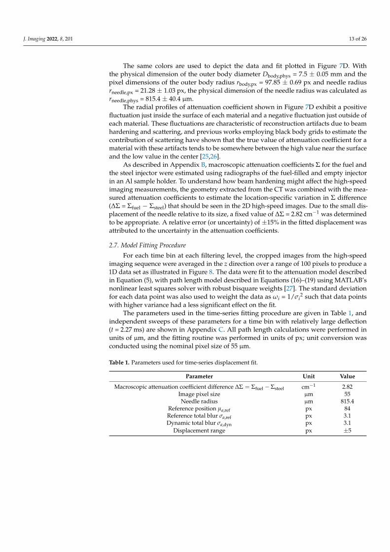
The same colors are used to depict the data and fit plotted in Figure 7D. Withthe physical dimension of the outer body diameter Dbody,phys = 7.5 ± 0.05 mm and thepixel dimensions of the outer body radius rbody,px = 97.85 ± 0.69 px and needle radiusrneedle,px = 21.28 ± 1.03 px, the physical dimension of the needle radius was calculated asrneedle,phys = 815.4 ± 40.4 µm.

The radial profiles of attenuation coefficient shown in Figure 7D exhibit a positivefluctuation just inside the surface of each material and a negative fluctuation just outside ofeach material. These fluctuations are characteristic of reconstruction artifacts due to beamhardening and scattering, and previous works employing black body grids to estimate thecontribution of scattering have shown that the true value of attenuation coefficient for amaterial with these artifacts tends to be somewhere between the high value near the surfaceand the low value in the center [25,26].

As described in Appendix B, macroscopic attenuation coefficients Σ for the fuel andthe steel injector were estimated using radiographs of the fuel-filled and empty injectorin an Al sample holder. To understand how beam hardening might affect the high-speedimaging measurements, the geometry extracted from the CT was combined with the mea-sured attenuation coefficients to estimate the location-specific variation in Σ difference(∆Σ = Σfuel − Σsteel) that should be seen in the 2D high-speed images. Due to the small dis-placement of the needle relative to its size, a fixed value of ∆Σ = 2.82 cm−1 was determinedto be appropriate. A relative error (or uncertainty) of ±15% in the fitted displacement wasattributed to the uncertainty in the attenuation coefficients.

2.7. Model Fitting Procedure

For each time bin at each filtering level, the cropped images from the high-speedimaging sequence were averaged in the z direction over a range of 100 pixels to produce a1D data set as illustrated in Figure 8. The data were fit to the attenuation model describedin Equation (5), with path length model described in Equations (16)–(19) using MATLAB’snonlinear least squares solver with robust bisquare weights [27]. The standard deviationfor each data point was also used to weight the data as ωi = 1/σi

2 such that data pointswith higher variance had a less significant effect on the fit.

The parameters used in the time-series fitting procedure are given in Table 1, andindependent sweeps of these parameters for a time bin with relatively large deflection(t = 2.27 ms) are shown in Appendix C. All path length calculations were performed inunits of µm, and the fitting routine was performed in units of px; unit conversion wasconducted using the nominal pixel size of 55 µm.

Table 1. Parameters used for time-series displacement fit.

Parameter Unit Value

Macroscopic attenuation coefficient difference ∆Σ = Σfuel − Σsteel cm−1 2.82Image pixel size µm 55Needle radius µm 815.4

Reference position µa,ref px 84Reference total blur σa,ref px 3.1Dynamic total blur σa,dyn px 3.1

Displacement range px ±5

J. Imaging 2022, 8, 201 14 of 26J. Imaging 2022, 8, x FOR PEER REVIEW 14 of 26

Figure 8. Examples of attenuation model fitting for each filtering level. Log-ratio normalized images are from a time bin with a relatively large needle displacement (t = 2.27 ms), and the injector body outline has been overlaid on the normalized images for clarity. Negative (red) in images corre-sponds to a decrease in neutron count rate relative to the reference, whereas positive (blue) indicates an increase. The blue and red vertical bands indicate the cylindrical needle moving to the left, be-cause the steel needle has a lower attenuation coefficient than the surrounding hydrogenous fuel. Boxed region in each log-ratio image was averaged in the z direction to create 1D data for fitting. Although signal-to-noise ratio and fit metrics improved dramatically with filtering, the resulting displacement prediction from the fitting procedure is similar in each case.

3. Results The displacement model was applied to the entire high-speed image sequence, with

selected frames shown in Figure 9A,B and the full time-resolved fit shown in Figure 9C.

Figure 8. Examples of attenuation model fitting for each filtering level. Log-ratio normalized imagesare from a time bin with a relatively large needle displacement (t = 2.27 ms), and the injector bodyoutline has been overlaid on the normalized images for clarity. Negative (red) in images correspondsto a decrease in neutron count rate relative to the reference, whereas positive (blue) indicates anincrease. The blue and red vertical bands indicate the cylindrical needle moving to the left, becausethe steel needle has a lower attenuation coefficient than the surrounding hydrogenous fuel. Boxedregion in each log-ratio image was averaged in the z direction to create 1D data for fitting. Althoughsignal-to-noise ratio and fit metrics improved dramatically with filtering, the resulting displacementprediction from the fitting procedure is similar in each case.

3. Results

The displacement model was applied to the entire high-speed image sequence, withselected frames shown in Figure 9A,B and the full time-resolved fit shown in Figure 9C.

J. Imaging 2022, 8, 201 15 of 26J. Imaging 2022, 8, x FOR PEER REVIEW 15 of 26

Figure 9. Results of high-speed imaging measurements and displacement model fitting. Selected frames from the 95% subtraction (A) and log-ratio (B) normalizations with lowpass + Poisson filter-ing highlighting motion of the injector needle. The injector body outline has been overlaid on the normalized images for clarity. (C) Time-series fits of needle displacement indicate sub-pixel resolu-tion relative to the 55 μm pixel size with significant noise reduction for the filtered cases but similar shape and magnitude to the unfiltered case.

As a result of the short 680 μs injection command and the inherent hydraulic and mechanical actuation delay, the injector needle only begins to lift near the end of the in-jection command, approximately 472 μs after SOE and just before the injector current ap-proaches its peak value, as shown by Point 1 in Figure 9C. The needle lift occurs rapidly and is complete by Point 2, approximately 595 μs after the SOE command and 123 μs after the start of the needle lift. The needle lift, in this case, was defined by monitoring the intensity in the void, or “sac”, directly below the check ball that becomes filled with fuel when the ball lifts. This fuel filling is seen as a darkening at the bottom of the ball in the subtraction-normalized images and as a red region in the log-ratio-normalized images because of the increase in attenuation in the sac when fuel enters a space formerly occu-pied by gaseous Ar. Conversely, the top of the ball becomes white in the subtraction and blue in the log-ratio images because the steel ball moves up and displaces fuel, decreasing the attenuation in that region. In the same way, the movement of the needle is visualized as being toward light and away from dark in the subtraction images, and toward blue and

Figure 9. Results of high-speed imaging measurements and displacement model fitting. Selectedframes from the 95% subtraction (A) and log-ratio (B) normalizations with lowpass + Poissonfiltering highlighting motion of the injector needle. The injector body outline has been overlaid onthe normalized images for clarity. (C) Time-series fits of needle displacement indicate sub-pixelresolution relative to the 55 µm pixel size with significant noise reduction for the filtered cases butsimilar shape and magnitude to the unfiltered case.

As a result of the short 680 µs injection command and the inherent hydraulic andmechanical actuation delay, the injector needle only begins to lift near the end of theinjection command, approximately 472 µs after SOE and just before the injector currentapproaches its peak value, as shown by Point 1 in Figure 9C. The needle lift occurs rapidlyand is complete by Point 2, approximately 595 µs after the SOE command and 123 µs afterthe start of the needle lift. The needle lift, in this case, was defined by monitoring theintensity in the void, or “sac”, directly below the check ball that becomes filled with fuelwhen the ball lifts. This fuel filling is seen as a darkening at the bottom of the ball in thesubtraction-normalized images and as a red region in the log-ratio-normalized imagesbecause of the increase in attenuation in the sac when fuel enters a space formerly occupiedby gaseous Ar. Conversely, the top of the ball becomes white in the subtraction and bluein the log-ratio images because the steel ball moves up and displaces fuel, decreasing theattenuation in that region. In the same way, the movement of the needle is visualized as

J. Imaging 2022, 8, 201 16 of 26

being toward light and away from dark in the subtraction images, and toward blue andaway from red in the log-ratio images. The fuel spray exiting the injector can also be seenby a darkening or reddening in the subtraction and log-ratio images, respectively, but thedownstream spray plume has been cropped out of the images shown here.

Two oscillations of the needle are apparent during the injection period: one in imagesequence 2-3-4 and another in sequence 4-5-6. These are captured by the time-series fitsas positive (to the right) displacements peaking at 17.3 ± 3.4 µm and 12.1 ± 2.9 µm,respectively, both well below the 55 µm pixel size of the detector. The seating force ofthe needle closing, which begins at Point 5, induces an immediate negative (to the left)deflection of the needle, which peaks at −37.5 ± 6.1 µm and is shown in image sequence6-7-8-9. At Point 9, the needle springs back in the positive direction to 10.2 ± 2.5 µm.Smaller oscillations continue after this point.

Although the high-frequency noise in the displacement fit results was reduced sub-stantially with the temporal (lowpass) and spatial (Poisson) filtering applied to the imagesequence, the qualitative features and magnitude of the fit were quite similar for all filteringlevels, with the two filtered cases being nearly identical. This is encouraging because itindicates that the improvements seen in fit metrics with this filtering approach do not comeat the expense of a reduced spatial or temporal resolution or introduction of artifacts intothe displacement fit.

These results indicate that the oscillatory displacement of the needle is highly consis-tent from event to event, as the images used for these fits are the ensemble of ~1.34 × 106

injections. If a high variability existed in the displacement direction and/or magnitude, thenormalized images would become blurrier during deflection periods rather than displayinga consistent structure.

The noise floor for displacement measured by this technique can be characterized bythe amplitude of displacement oscillations seen in time periods in which the geometry isknown to be static. In the period before the injection command, the displacement confi-dence interval for most points includes zero, and the maximum displacement values are23.2 ± 10.3 µm (unfiltered), 3.7 ± 3.0 µm (lowpass), and 3.4 ± 1.9 µm (lowpass + Poisson),indicating that the noise floor for displacement fitting in the filtered data is in the order of3–4 µm, or ~6% of the actual pixel size. Further improvement may be possible by increasingthe size of the cyclic ensemble, and the impact of the sample size will be investigatedin subsequent work. Additionally, a new MCP detector currently under development atORNL based on the Timepix3 readout is expected to improve the overall signal-to-noiseratio by enabling imaging with a high-bandwidth event-based acquisition mode and adata-driven readout [31,32]. This new architecture will also enable event centroiding, whichhas been shown to achieve a 3× improvement in spatial resolution in both MCP [18] andscintillator configurations [33]. By combining the attenuation modeling approach describedin this work with the new detector, it may be possible to measure cyclic motions below a1 µm scale.

4. Discussion

We have presented an approach to measuring the high-speed, sub-pixel displacementof the needle in a gasoline direct injector obtained by ensemble neutron imaging duringcyclic dynamic operation. This approach combined a normalization technique that relieson a static reference frame made from the image sequence itself with an analytical neutronattenuation model based on the geometry of the device.

The geometry was derived from a neutron CT scan, and the geometric accuracyobtained by this method was suitable because of the difference in scale between the sizeof the injector needle and the magnitude of displacement, which was <2% of the needlediameter. For systems in which sub-pixel displacement information is desired for objectsthat are on the same scale as the displacement, more accurate a priori knowledge of thegeometry would likely be required.

J. Imaging 2022, 8, 201 17 of 26

The application of an analytical attenuation model was practical because of the simplegeometry of the injector needle portion being tracked, which was represented as a circularcross section. More complex geometries would likely require a generalized numericalapproach in which simulated projections could be generated based on a given displacementof the known geometry. This may require significant computing resources because of theneed to generate many projections at each iteration of the displacement fitting process,although this could likely be mitigated by precomputing projections for a given subsetof displacement values and interpolating within those results during the fitting process.Machine learning algorithms could also be applied to this task if supplied with suitabletraining data in the form of real or simulated normalized images with known geometricdisplacements.

Parametric sweeps of the inputs to the displacement fitting model were performed,including attenuation coefficients, image pixel size, needle radius, reference position,reference total blur, and dynamic total blur. The attenuation coefficients were measuredfrom neutron radiographs of the empty and fuel-filled injector, and all other parameterswere optimized based on goodness-of-fit metrics, meaning that the entire model wasgoverned by the measured data.

The prospects for this approach to the neutron-based measurement of micron-scaledynamics at a microsecond timescale are encouraging. The field of view and resolutionof the current generation of neutron MCP detectors with a Timepix readout are sufficientto capture the dynamics of interest in the near entirety of a typical automotive gasolinedirect injector, which is being pursued in ongoing work. An MCP detector currently underdevelopment at ORNL with a high-bandwidth data-driven Timepix3 readout is expectedto enable event centroiding to improve the intrinsic spatial resolution by a factor of twoor more. The subsequent generation of neutron imaging detectors promises to enablean even wider class of measurements, with the four-side buttable Timepix4 architectureenabling the fabrication of arbitrarily large detectors with much higher data throughputcapabilities [31,32]. Large high-speed detectors would permit the measurement of dynamicsin devices such as internal combustion engines, turbines, pumps, compressors, and manyother fluid or mechanical systems with repeatable cyclic behavior. While fuel injectorspresent an interesting test case due to their highly repeatable internal dynamics over a rangeof time and length scales that push the capabilities of existing neutron imaging techniques,the approach presented here is broadly applicable to measuring sub-pixel motions in anysystem in which the geometry is known and the change in attenuation resulting frommotion of components can be modeled, whether measured by neutrons, X-rays, or othertechniques.

5. Conclusions

We have presented an approach to both observe and quantify highly transient sub-pixel dynamics at scales approaching 5 µs and 5 µm in the ensemble-averaged cyclicoperation of a fuel injector. This was achieved by first collecting high-speed neutron imagesequences over a large ensemble of ~1.34 × 106 injection events and employing an imagenormalization procedure to generate maps of dynamic neutron path length variation. Theinternal geometry of the injector was extracted from a neutron computed tomographyreconstruction to develop a model of how the neutron path lengths through the differentphases in the device would change with a given displacement of the injector needle. Thismodel was then fit to each frame in the normalized high-speed image sequence to generatea time-resolved measurement of needle displacement, resulting in the measurement ofmotions on the scale of ~6% of the pixel size. This approach opens a path to the in situ,noninvasive measurement of cyclic dynamics in real devices and systems at temporospatialscales that were not previously achievable.

Author Contributions: Conceptualization, M.L.W., T.J.T., D.A.S., E.J.N., C.E.A.F. and H.Z.B.; method-ology, M.L.W. and C.E.A.F.; software, M.L.W. and Y.Z.; validation, M.L.W.; formal analysis, M.L.W.;investigation, M.L.W., T.J.T., D.A.S., E.J.N., C.E.A.F., H.Z.B. and L.J.S.; resources, H.Z.B., L.J.S. and

J. Imaging 2022, 8, 201 18 of 26

Y.Z.; data curation, M.L.W.; writing—original draft preparation, M.L.W.; writing—review and editing,T.J.T., D.A.S., C.E.A.F. and H.Z.B.; visualization, M.L.W.; supervision, M.L.W. and T.J.T.; projectadministration, T.J.T.; funding acquisition, T.J.T. All authors have read and agreed to the publishedversion of the manuscript.

Funding: This material is based on the work supported by the US Department of Energy (DOE),Office of Energy Efficiency and Renewable Energy, Vehicle Technologies Office via the AdvancedCombustion Systems program. Special thanks to program managers Gurpreet Singh and MichaelWeismiller for their support.

Data Availability Statement: Neutron computed tomography and high-speed neutron imaging datacollected in this study are available at https://doi.org/10.13139/ORNLNCCS/1872748 (accessed on13 July 2022).

Acknowledgments: The authors would like to acknowledge the contributions of Anton Tremsinat the UC Berkeley Space Sciences Laboratory to the development of the MCP detector, JonathanWillocks at ORNL for assistance with the development of the spray apparatus and execution of theexperiments, and Singanallur Venkatakrishnan at ORNL for valuable discussions on image filteringapproaches. The authors would also like to acknowledge Scott Parish and Ronald Grover at GeneralMotors for providing the injector and injector driver. This research used resources at the High FluxIsotope Reactor, a DOE Office of Science User Facility, and the National Transportation ResearchCenter, a DOE Office of Energy Efficiency and Renewable Energy User Facility, both operated by theOak Ridge National Laboratory. Support for DOI:10.13139/ORNLNCCS/1872748 dataset is providedby the U.S. Department of Energy, project IPTS-19037 under Contract DE-AC05-00OR22725. ProjectIPTS-19037 used resources of the Oak Ridge Leadership Computing Facility at Oak Ridge NationalLaboratory, which is supported by the Office of Science of the U.S. Department of Energy underContract No. DE-AC05-00OR22725.

Conflicts of Interest: The authors declare no conflict of interest. The funders had no role in the designof the study; in the collection, analyses, or interpretation of data; in the writing of the manuscript, orin the decision to publish the results.

Appendix A. Experimental Conditions

As noted in the main text, the injector and spray chamber were operated at theconditions shown in Table A1, the timing of the injector command and image acquisitionprocess is illustrated in Figure A1, and the timing values used for the MCP detector shuttersare given in Table A2.

Table A1. Spray chamber and injector operating conditions.

Parameter Value

Fuel iso-octane (C8H18, 2,2,4-trimethylpentane)Fuel temperature (◦C) 90

Injector temperature (◦C) 90Chamber temperature (◦C) 60

Fuel pressure (MPa) 20Chamber pressure (kPa) 100Argon flow rate (slpm) 41

Injection rate (Hz) 25Injections per cycle 1

Injection trigger delay (ms) 1Injection command duration (µs) 680

J. Imaging 2022, 8, 201 19 of 26J. Imaging 2022, 8, x FOR PEER REVIEW 19 of 26

Figure A1. Timing diagram of injection and detector triggering.

Table A2. MCP detector shutter timing.

Shutter Dead Time (ms) Start Time (ms) End Time (ms) Time Bins Time Bin Length (μs) Total Recorded 0 0.1 0.1 7.0 1348 5.12 1,339,654 1 0.4 7.4 9.0 78 20.48 1,291,400 2 0.4 9.4 15.0 273 20.48 1,292,873 3 0.4 15.4 25.0 449 20.48 1,309,046 4 0.4 25.0 28.0 146 20.48 1,288,513 5 0.4 28.4 35.0 322 20.48 1,307,914

Appendix B. Attenuation Coefficients and Beam Hardening Macroscopic attenuation coefficients Σ for the fuel and the steel injector were esti-

mated using radiographs of the fuel-filled and empty injector in an Al sample holder, as shown in Figure A2A,B. The radiographs were registered using the external features of the injector, and the same axially symmetric region was selected in each radiograph to normalize the fuel-filled injector by the empty injector, producing a transmission image of only the fuel (Figure A2C). The same process was used to normalize the empty injector by a section of the empty sample holder to produce a transmission image of only the steel injector (Figure A2D). With the geometry extracted from the CT scan of the empty injector, the path length at each pixel of the fuel and steel transmission images is known, which allowed the attenuation coefficient Σ for each material to be calculated from Equation (1) by fitting a curve to the −ln(T) vs. thickness data. As shown in Figure A2E, the fit for steel was linear, indicating constant Σ with varying thickness, whereas the fit for the fuel was nonlinear, indicating significant effects from beam hardening and scattering, which are consistent with the literature [24]. The fit for steel assumes that the injector body and nee-dle have the same attenuation coefficient.

In Figure A2F, the resulting fits of the attenuation coefficient are compared against predictions for surrogate materials made using the Neutron Imaging Toolbox (NEUIT) [34], which is based on the ImagingReso library [35]. NEUIT includes a cold neutron trans-mission tool that considers the energy spectrum at the HFIR CG-1D beamline, and energy-dependent cross section data are sourced from the Evaluated Nuclear Data File (ENDF) [36]. Elemental Fe was used as a surrogate for the steel, which is of unknown composition.

Figure A1. Timing diagram of injection and detector triggering.

Table A2. MCP detector shutter timing.

Shutter Dead Time (ms) Start Time (ms) End Time (ms) Time Bins Time Bin Length (µs) Total Recorded

0 0.1 0.1 7.0 1348 5.12 1,339,6541 0.4 7.4 9.0 78 20.48 1,291,4002 0.4 9.4 15.0 273 20.48 1,292,8733 0.4 15.4 25.0 449 20.48 1,309,0464 0.4 25.0 28.0 146 20.48 1,288,5135 0.4 28.4 35.0 322 20.48 1,307,914

Appendix B. Attenuation Coefficients and Beam Hardening

Macroscopic attenuation coefficients Σ for the fuel and the steel injector were estimatedusing radiographs of the fuel-filled and empty injector in an Al sample holder, as shown inFigure A2A,B. The radiographs were registered using the external features of the injector,and the same axially symmetric region was selected in each radiograph to normalize thefuel-filled injector by the empty injector, producing a transmission image of only the fuel(Figure A2C). The same process was used to normalize the empty injector by a sectionof the empty sample holder to produce a transmission image of only the steel injector(Figure A2D). With the geometry extracted from the CT scan of the empty injector, the pathlength at each pixel of the fuel and steel transmission images is known, which allowed theattenuation coefficient Σ for each material to be calculated from Equation (1) by fitting acurve to the −ln(T) vs. thickness data. As shown in Figure A2E, the fit for steel was linear,indicating constant Σ with varying thickness, whereas the fit for the fuel was nonlinear,indicating significant effects from beam hardening and scattering, which are consistentwith the literature [24]. The fit for steel assumes that the injector body and needle have thesame attenuation coefficient.

In Figure A2F, the resulting fits of the attenuation coefficient are compared againstpredictions for surrogate materials made using the Neutron Imaging Toolbox (NEUIT) [34],which is based on the ImagingReso library [35]. NEUIT includes a cold neutron transmis-sion tool that considers the energy spectrum at the HFIR CG-1D beamline, and energy-dependent cross section data are sourced from the Evaluated Nuclear Data File (ENDF) [36].Elemental Fe was used as a surrogate for the steel, which is of unknown composition. Both

J. Imaging 2022, 8, 201 20 of 26

Fe and the measured steel show negligible beam hardening over a thickness ranging from0 to 10 mm. A larger spread in the data at thicknesses < 2 mm is due to scattering at theedges of the cylindrical injector body and needle. The fitted value of Σ for the steel injector(1.101 cm−1) is overlaid on Figure 7D and compares well with the range of values of theattenuation coefficient within the injector components obtained from the neutron CT.

Due to the fact that the fuel contained only a single component (iso-octane, C8H18), thedensity and atomic composition are known exactly. However, the cross section data for 1Hin the ENDF are for free atoms, whereas the binding of protons in molecules is known toincrease their neutron cross section considerably. Therefore, we should expect that NEUITwill underpredict the macroscopic attenuation coefficient for C8H18. Molecule-specificbound cross section data for several hydrocarbons have been manually added to NEUITbased on empirical values from literature [37], but unfortunately those do not include C8H18.Two hydrocarbons with bound cross section entries in NEUIT were chosen to bracket theprediction for the fuel based upon their similar H/C ratios to C8H18 (H/C = 2.25): C16H34(H/C = 2.125) and C4H10 (H/C = 2.5). All three compounds were set to the density ofC8H18 (0.692 g/cm3). As expected, the measured value of Σ for the fuel falls between theNEUIT predictions for C16H34 and C4H10 at zero thickness, whereas the NEUIT value forC8H18, which uses the free cross section of 1H, is considerably lower than measured. It isalso observed that, as the thickness increases, the measured value of Σ for the fuel decreasesmore rapidly than predicted by NEUIT due to incoherent scattering from 1H and the shortsample-to-detector distance (~5 cm), which is consistent with the literature [24].

To understand how beam hardening might affect the high-speed imaging measure-ments, the geometry extracted from the CT was combined with the measured attenuationcoefficients to estimate the location-specific variation in Σ difference (∆Σ = Σfuel − Σsteel)that should be seen in the 2D high-speed images. The average inner and outer diametersof the injector body were extracted from the CT over the region seen in the high-speedimaging in a similar manner as shown in Figure 7, and the expected value of path lengththrough both the fuel and steel for a filled injector were calculated by Equations (12) and (16)assuming a Gaussian blur of 175 µm. The modeled system and resulting path length as afunction of radial distance are shown in Figure A3A, where the peak in the expected valueof path length through the fuel is 4.55 mm and through the steel is 3.6 mm. The position-dependent path lengths were used to estimate position-dependent Σ using the fitted datafrom Figure A2F, with results shown in Figure A3B. The attenuation coefficient difference∆Σ was also calculated and was compared against a fixed value of ∆Σ = 2.82 cm−1, whichis representative within the region where the needle motion is found. The shaded regions inFigure A3B correspond to the 95% confidence intervals for Σ obtained from the fits shownin Figure A2F.

We then modeled what should be seen in the log-ratio normalized images for needledisplacements of 10, 50, and 100 µm using an extension of Equation (5) with considerationof both position-dependent and constant ∆Σ, with the results shown in Figure A3C. Themodel predicts nearly identical results in either scenario because of the small variationin ∆Σ over the range of interest. Similarly, generating curves with position-dependent∆Σ and then fitting their displacement with constant ∆Σ results in the total and relativedisplacement fit errors shown in Figure A3D, which have maximum absolute values of0.006 µm and 0.017%, respectively. We therefore conclude that a fixed value of ∆Σ isadequate for this system. This simplification will not apply in all systems, particularly incases where there are sharp steps in path length in phases with significant beam hardening.Fitting the model to the 95% confidence interval of the generated curves shows that aroughly constant relative error (or uncertainty) of ±15% in the fitted displacement isattributed to the uncertainty in the attenuation coefficients.

J. Imaging 2022, 8, 201 21 of 26

J. Imaging 2022, 8, x FOR PEER REVIEW 20 of 26

Both Fe and the measured steel show negligible beam hardening over a thickness ranging from 0 to 10 mm. A larger spread in the data at thicknesses < 2 mm is due to scattering at the edges of the cylindrical injector body and needle. The fitted value of Σ for the steel injector (1.101 cm−1) is overlaid on Figure 7D and compares well with the range of values of the attenuation coefficient within the injector components obtained from the neutron CT.

Due to the fact that the fuel contained only a single component (iso-octane, C8H18), the density and atomic composition are known exactly. However, the cross section data for 1H in the ENDF are for free atoms, whereas the binding of protons in molecules is known to increase their neutron cross section considerably. Therefore, we should expect that NEUIT will underpredict the macroscopic attenuation coefficient for C8H18. Molecule-specific bound cross section data for several hydrocarbons have been manually added to NEUIT based on empirical values from literature [37], but unfortunately those do not in-clude C8H18. Two hydrocarbons with bound cross section entries in NEUIT were chosen to bracket the prediction for the fuel based upon their similar H/C ratios to C8H18 (H/C = 2.25): C16H34 (H/C = 2.125) and C4H10 (H/C = 2.5). All three compounds were set to the density of C8H18 (0.692 g/cm3). As expected, the measured value of Σ for the fuel falls be-tween the NEUIT predictions for C16H34 and C4H10 at zero thickness, whereas the NEUIT value for C8H18, which uses the free cross section of 1H, is considerably lower than meas-ured. It is also observed that, as the thickness increases, the measured value of Σ for the fuel decreases more rapidly than predicted by NEUIT due to incoherent scattering from 1H and the short sample-to-detector distance (~5 cm), which is consistent with the litera-ture [24].

Figure A2. Measurement of macroscopic attenuation coefficients for fuel and injector. (A) Radio-graph of fuel-filled injector in Al sample holder. (B) Radiograph of empty injector in Al sample

Figure A2. Measurement of macroscopic attenuation coefficients for fuel and injector. (A) Radiographof fuel-filled injector in Al sample holder. (B) Radiograph of empty injector in Al sample holder.(C) Normalization of same axisymmetric region in fuel-filled and empty injector radiographs resultsin transmission image of the fuel. (D) Normalization of the empty injector by an empty region ofthe axisymmetric sample holder results in transmission image of the injector. (E) Plot of −ln(T)vs. material thickness at each pixel in C and D shows a linear response for the steel injector and anon-linear response for the iso-octane fuel, indicating that beam hardening and scattering effects fromthe fuel are significant in this geometry. (F) Same data from E plotted as macroscopic attenuationcoefficient Σ are compared to predictions from NEUIT for three hydrocarbons and Fe.

J. Imaging 2022, 8, 201 22 of 26J. Imaging 2022, 8, x FOR PEER REVIEW 22 of 26

Figure A3. Investigation of beam hardening effects. (A) Cross section of fuel and injector system with position-dependent expected path length. (B) Position-dependent expected value of attenua-tion coefficient in each component. Shading indicates 95% confidence interval from attenuation co-efficient fits. (C) Model of expected value in log-ratio normalized images due to displacement of injector needle show that position-dependent and constant ∆Σ are virtually indistinguishable. (D) Error from use of constant ∆Σ in displacement fitting model is negligible over the range of displace-ments expected in this system. Confidence interval for relative error due to uncertainty in attenua-tion coefficient fits is roughly constant at ±15%.

Appendix C. Parametric Investigation of Displacement Model The difference in macroscopic attenuation coefficients ∆Σ = Σfuel − Σsteel acts as a gain

term in the attenuation model and has a significant effect on the predicted displacement as shown in Figure A4A. The R2 fit statistic shows essentially no dependence on ∆Σ at any filtering level, and the value of ∆Σ = 2.82 cm−1 chosen for the time-series fitting was based on beam hardening calculations shown in Figure A3, which is, in turn, based on the injec-tor geometry extracted from the CT and the values of Σ extracted from images of the fuel-filled and empty injector.

The combination of image pixel size and the physical needle radius sets the geometric scale used in the path length calculations. The experimental data represented by the left side of Equation (5) are unitless and are scaled in the x-dimension by the pixel index as

Figure A3. Investigation of beam hardening effects. (A) Cross section of fuel and injector systemwith position-dependent expected path length. (B) Position-dependent expected value of attenuationcoefficient in each component. Shading indicates 95% confidence interval from attenuation coefficientfits. (C) Model of expected value in log-ratio normalized images due to displacement of injectorneedle show that position-dependent and constant ∆Σ are virtually indistinguishable. (D) Errorfrom use of constant ∆Σ in displacement fitting model is negligible over the range of displacementsexpected in this system. Confidence interval for relative error due to uncertainty in attenuationcoefficient fits is roughly constant at ±15%.

Appendix C. Parametric Investigation of Displacement Model

The difference in macroscopic attenuation coefficients ∆Σ = Σfuel − Σsteel acts as a gainterm in the attenuation model and has a significant effect on the predicted displacement asshown in Figure A4A. The R2 fit statistic shows essentially no dependence on ∆Σ at anyfiltering level, and the value of ∆Σ = 2.82 cm−1 chosen for the time-series fitting was basedon beam hardening calculations shown in Figure A3, which is, in turn, based on the injectorgeometry extracted from the CT and the values of Σ extracted from images of the fuel-filledand empty injector.

The combination of image pixel size and the physical needle radius sets the geometricscale used in the path length calculations. The experimental data represented by the leftside of Equation (5) are unitless and are scaled in the x-dimension by the pixel index as

J. Imaging 2022, 8, 201 23 of 26

shown in Figure 8. Although the physical size of the pixels on the detector are specified as55 µm, beam divergence can affect the image pixel size if the sample-to-detector distanceis large enough. A known feature (the outer body of the injector) was measured in thehigh-speed images, resulting in an estimated image pixel size of 54.9 ± 0.6 µm/px. Thenominal value of 55 µm/px was used in the time-series fitting. As shown in Figure A4B,this image pixel size is near the peak in R2, and the displacement prediction is relativelyinsensitive near this value. The needle radius of 815.4 µm extracted from the neutron CTagrees well with the peak in R2 seen in Figure A4C, though R2 is nearly flat for values from810–840 µm.

The x position of the needle center was estimated to be at pixel 84 in the croppedhigh-speed reference image. Figure A4D shows that this corresponds with the peak in R2

and that the displacement prediction is relatively insensitive within ±1 px of this value.Compared with the other parameters, the reference and dynamic total blur have

only limited a priori information available for estimation. As already discussed, one mayexpect that the static or reference blur would be of the order of a few pixels, and thatthe dynamic blur would at least be as large as the reference blur, or larger if significantcycle-to-cycle variability exists in the needle motion. The dynamic blur should also bebounded by the internal diameter of the injector body. The values used in the time-seriesfitting were chosen based on the R2 optimum at the high deflection condition. Figure A4Eshows displacement and R2 results for a sweep of blur magnitude in which the referenceand dynamic blur were set to be equal. The R2 peak at ~3.1 px agrees with intuition, anddisplacement is also relatively insensitive at this value. Figure A4F shows a sweep of theratio of dynamic to reference blur with an obvious peak near a value of unity. Lacking thedetailed ESF required to separate the components contributing to blur, both the referenceand dynamic blur parameters were set to a value of 3.1 px for the time-series fitting. Fits ofthe entire time series were performed with the dynamic total blur allowed to vary as anoptimization parameter in the fitting process, and the results remained close to the samevalue of 3.1 pixels used to obtain the fits shown, with no apparent time-dependent structurethat would indicate higher blur during injection.

One of the overall trends that stands out in Figure A4 is that the goodness-of-fit metricR2 is improved considerably by filtering, but there is a comparably minor effect on thepredicted displacement. The fits of the unfiltered data generally have a negative R2, whichmeans that the model offers a poorer fit to the data than a horizontal line at the meanvalue. The reason for this can be seen in the fitting results shown in Figure 8, for which,the unfiltered data have a bias toward negative values due to the low signal-to-noise ratio,while the model is constrained to a value of zero in the tails. The lowpass filter in the timedomain significantly reduces the noise and nearly eliminates the negative bias, yieldingR2 > 0.73 at the selected set of fit parameters. The addition of the Poisson filter in the spatialdomain offers a further improvement to noise reduction, yielding R2 > 0.86 with the samefit parameters.

J. Imaging 2022, 8, 201 24 of 26J. Imaging 2022, 8, x FOR PEER REVIEW 24 of 26

Figure A4. Effect of fit parameters on displacement prediction and fit quality. Fit parameters were independently varied at a high-displacement condition (t = 2.27 ms). Symbols indicate fit parameters chosen for the time-series displacement fitting. (A) Attenuation coefficient difference has a large effect on predicted displacement but no impact on R2. Image pixel size (B) and injector needle radius (C) together set the scaling used in the model, and the peaks in R2 for both parameters are near the values obtained from scale measurements with low sensitivity in predicted displacement at those values. (D) Reference position (nominal needle center) has clear R2 peak and low sensitivity in pre-dicted displacement at same value. (E) With reference and dynamic total blur set as equal, the fil-tered cases exhibit an R2 peak and mild sensitivity in predicted displacement. (F) Varying the ratio of dynamic to reference total blur does not provide compelling evidence for a value greater than unity.

Figure A4. Effect of fit parameters on displacement prediction and fit quality. Fit parameters wereindependently varied at a high-displacement condition (t = 2.27 ms). Symbols indicate fit parameterschosen for the time-series displacement fitting. (A) Attenuation coefficient difference has a large effecton predicted displacement but no impact on R2. Image pixel size (B) and injector needle radius (C)together set the scaling used in the model, and the peaks in R2 for both parameters are near the valuesobtained from scale measurements with low sensitivity in predicted displacement at those values.(D) Reference position (nominal needle center) has clear R2 peak and low sensitivity in predicteddisplacement at same value. (E) With reference and dynamic total blur set as equal, the filtered casesexhibit an R2 peak and mild sensitivity in predicted displacement. (F) Varying the ratio of dynamicto reference total blur does not provide compelling evidence for a value greater than unity.

References1. Bilheux, H.Z.; McGreevy, R.; Anderson, I.S. Neutron Imaging and Applications: A Reference for the Imaging Community; Springer:

New York, NY, USA, 2009. [CrossRef]2. The 2018 EPA Automotive Trends Report: Greenhouse Gas Emissions, Fuel Economy, and Technology since 1975. Available

online: https://www.epa.gov/automotive-trends (accessed on 1 October 2020).

J. Imaging 2022, 8, 201 25 of 26

3. Myung, C.L.; Park, S. Exhaust nanoparticle emissions from internal combustion engines: A review. Int. J. Automot. Technol. 2011,13, 9. [CrossRef]

4. Jatana, G.S.; Splitter, D.A.; Kaul, B.; Szybist, J.P. Fuel property effects on low-speed pre-ignition. Fuel 2018, 230, 474–482. [CrossRef]5. Strek, P.; Duke, D.; Swantek, A.; Kastengren, A.; Powell, C.F.; Schmidt, D.P. X-ray Radiography and CFD Studies of the Spray G

Injector; SAE International: Warrendale, PA, USA, 2016.6. Neroorkar, K.; Schmidt, D. A Computational Investigation of Flash-Boiling Multi-Hole Injectors with Gasoline-Ethanol Blends; SAE

International: Warrendale, PA, USA, 2011.7. Saha, K.; Som, S.; Battistoni, M.; Li, Y.; Pomraning, E.; Senecal, P. Numerical Investigation of Two-Phase Flow Evolution of In-and

Near-Nozzle Regions of a Gasoline Direct Injection Engine During Needle Transients. SAE Int. J. Engines 2016, 9, 1230–1240.[CrossRef]

8. Baldwin, E.T.; Grover, R.O.; Parrish, S.E.; Duke, D.J.; Matusik, K.E.; Powell, C.F.; Kastengren, A.L.; Schmidt, D.P. Stringflash-boiling in gasoline direct injection simulations with transient needle motion. Int. J. Multiph. Flow 2016, 87, 90–101. [CrossRef]

9. Battistoni, M.; Xue, Q.; Som, S.; Pomraning, E. Effect of off-axis needle motion on internal nozzle and near exit flow in a multi-holediesel injector. SAE Int. J. Fuels Lubr. 2014, 7, 167–182. [CrossRef]

10. Powell, C.F.; Kastengren, A.L.; Liu, Z.; Fezzaa, K. The Effects of Diesel Injector Needle Motion on Spray Structure. J. Eng. GasTurbines Power 2010, 133, 012802. [CrossRef]

11. Kastengren, A.L.; Powell, C.F.; Liu, Z.; Fezzaa, K.; Wang, J. High-Speed X-ray Imaging of Diesel Injector Needle Motion. InProceedings of the ASME 2009 Internal Combustion Engine Division Spring Technical Conference, Milwaukee, WI, USA, 3–6May 2009.

12. Kastengren, A.L.; Tilocco, F.Z.; Powell, C.F.; Manin, J.; Pickett, L.M.; Payri, R.; Bazyn, T. Engine Combustion Network (ECN):Measurements of nozzle geometry and hydraulic behavior. At. Sprays 2012, 22, 1011–1052. [CrossRef]

13. Fansler, T.D.; Parrish, S.E. Spray measurement technology: A review. Meas. Sci. Technol. 2014, 26, 012002. [CrossRef]14. Kolakaluri, R.; Subramaniam, S.; Panchagnula, M.V. Trends in Multiphase Modeling and Simulation of Sprays. Int. J. Spray

Combust. Dyn. 2014, 6, 317–356. [CrossRef]15. Tekawade, A.; Sforzo, B.A.; Matusik, K.E.; Fezzaa, K.; Kastengren, A.L.; Powell, C.F. Time-resolved 3D imaging of two-phase

fluid flow inside a steel fuel injector using synchrotron X-ray tomography. Sci. Rep. 2020, 10, 8674. [CrossRef]16. Duke, D.J.; Finney, C.E.; Kastengren, A.; Matusik, K.; Sovis, N.; Santodonato, L.; Bilheux, H.; Schmidt, D.; Powell, C.; Toops, T.

High-resolution x-ray and neutron computed tomography of an engine combustion network spray G gasoline injector. SAE Int. J.Fuels Lubr. 2017, 10, 328–343. [CrossRef]

17. Santodonato, L.; Bilheux, H.; Bailey, B.; Bilheux, J.; Nguyen, P.; Tremsin, A.; Selby, D.; Walker, L. The CG-1D Neutron ImagingBeamline at the Oak Ridge National Laboratory High Flux Isotope Reactor. Phys. Procedia 2015, 69, 104–108. [CrossRef]

18. Tremsin, A.S.; McPhate, J.B.; Vallerga, J.V.; Siegmund, O.H.W.; Hull, J.S.; Feller, W.B.; Lehmann, E. Detection efficiency, spatialand timing resolution of thermal and cold neutron counting MCP detectors. Nucl. Instrum. Methods Phys. Res. Sect. A Accel.Spectrometers Detect. Assoc. Equip. 2009, 604, 140–143. [CrossRef]

19. Tremsin, A.S.; Vallerga, J.V.; Siegmund, O.H.W. Overview of spatial and timing resolution of event counting detectors withMicrochannel Plates. Nucl. Instrum. Methods Phys. Res. Sect. A Accel. Spectrometers Detect. Assoc. Equip. 2020, 949, 162768.[CrossRef]

20. Liu, D.; Hussey, D.; Gubarev, M.V.; Ramsey, B.D.; Jacobson, D.; Arif, M.; Moncton, D.E.; Khaykovich, B. Demonstration ofachromatic cold-neutron microscope utilizing axisymmetric focusing mirrors. Appl. Phys. Lett. 2013, 102, 183508. [CrossRef]

21. Trtik, P.; Hovind, J.; Grünzweig, C.; Bollhalder, A.; Thominet, V.; David, C.; Kaestner, A.; Lehmann, E.H. Improving the SpatialResolution of Neutron Imaging at Paul Scherrer Institut—The Neutron Microscope Project. Phys. Procedia 2015, 69, 169–176.[CrossRef]

22. Koerner, S.; Lehmann, E.; Vontobel, P. Design and optimization of a CCD-neutron radiography detector. Nucl. Instrum. MethodsPhys. Res. Sect. A Accel. Spectrometers Detect. Assoc. Equip. 2000, 454, 158–164. [CrossRef]

23. Tomviz 1.9.0. Available online: https://tomviz.org/ (accessed on 1 October 2020).24. Kang, M.; Bilheux, H.Z.; Voisin, S.; Cheng, C.L.; Perfect, E.; Horita, J.; Warren, J.M. Water calibration measurements for neutron

radiography: Application to water content quantification in porous media. Nucl. Instrum. Methods Phys. Res. Sect. A Accel.Spectrometers Detect. Assoc. Equip. 2013, 708, 24–31. [CrossRef]

25. Boillat, P.; Carminati, C.; Schmid, F.; Grünzweig, C.; Hovind, J.; Kaestner, A.; Mannes, D.; Morgano, M.; Siegwart, M.; Trtik, P.;et al. Chasing quantitative biases in neutron imaging with scintillator-camera detectors: A practical method with black bodygrids. Opt. Express 2018, 26, 15769–15784. [CrossRef]

26. Carminati, C.; Boillat, P.; Schmid, F.; Vontobel, P.; Hovind, J.; Morgano, M.; Raventos, M.; Siegwart, M.; Mannes, D.; Gruenzweig,C.; et al. Implementation and assessment of the black body bias correction in quantitative neutron imaging. PLoS ONE 2019, 14,e0210300. [CrossRef]

27. MATLAB R2018b; The MathWorks, Inc.: Natick, MA, USA, 2018.28. Kaestner, A.P.; Kis, Z.; Radebe, M.J.; Mannes, D.; Hovind, J.; Grünzweig, C.; Kardjilov, N.; Lehmann, E.H. Samples to Determine

the Resolution of Neutron Radiography and Tomography. Phys. Procedia 2017, 88, 258–265. [CrossRef]29. Tremsin, A.S.; Vallerga, J.V.; McPhate, J.B.; Siegmund, O.H.W. Optimization of Timepix count rate capabilities for the applications

with a periodic input signal. J. Instrum. 2014, 9, C05026. [CrossRef]

J. Imaging 2022, 8, 201 26 of 26

30. Azzari, L.; Foi, A. Variance Stabilization for Noisy+Estimate Combination in Iterative Poisson Denoising. IEEE Signal ProcessingLett. 2016, 23, 1086–1090. [CrossRef]

31. Ballabriga, R.; Campbell, M.; Llopart, X. Asic developments for radiation imaging applications: The medipix and timepix family.Nucl. Instrum. Methods Phys. Res. Sect. A Accel. Spectrometers Detect. Assoc. Equip. 2018, 878, 10–23. [CrossRef]

32. Llopart, X.; Alozy, J.; Ballabriga, R.; Campbell, M.; Egidos, N.; Fernandez, J.M.; Heijne, E.; Kremastiotis, I.; Santin, E.; Tlustos, L.;et al. Study of low power front-ends for hybrid pixel detectors with sub-ns time tagging. J. Instrum. 2019, 14, C01024. [CrossRef]

33. Losko, A.S.; Han, Y.; Schillinger, B.; Tartaglione, A.; Morgano, M.; Strobl, M.; Long, J.; Tremsin, A.S.; Schulz, M. New perspectivesfor neutron imaging through advanced event-mode data acquisition. Sci. Rep. 2021, 11, 21360. [CrossRef]

34. Zhang, Y.; Bilheux, J.C.; Bilheux, H.Z.; Lin, J.Y.Y. An interactive web-based tool to guide the preparation of neutron imagingexperiments at oak ridge national laboratory. J. Phys. Commun. 2019, 3, 103003. [CrossRef]

35. Zhang, Y.; Bilheux, J.C. ImagingReso: A tool for neutron resonance imaging. J. Open Source Softw. 2017, 2, 407. [CrossRef]36. Brown, D.A.; Chadwick, M.B.; Capote, R.; Kahler, A.C.; Trkov, A.; Herman, M.W.; Sonzogni, A.A.; Danon, Y.; Carlson, A.D.; Dunn,

M.; et al. ENDF/B-VIII.0: The 8th Major Release of the Nuclear Reaction Data Library with CIELO-project Cross Sections, NewStandards and Thermal Scattering Data. Nucl. Data Sheets 2018, 148, 1–142. [CrossRef]

37. Melkonian, E. Slow Neutron Velocity Spectrometer Studies of O2, N2, A, H2, H2O, and Seven Hydrocarbons. Phys. Rev. 1949, 76,1750–1759. [CrossRef]