Quality Ratings and Patient Satisfaction with Norwegian GPs

I

Quality Ratings and Patient Satisfaction with Norwegian GPs

An Analysis of Municipal Capacity & Other

Predictors of Overall GP Satisfaction & Waiting Time Satisfaction

Evelyne Auer

Master Thesis

as part of the double-degree program European Master in Health

Economics and Management

UNIVERSITY OF OSLO

Department of Health Management and Health Economics

June 19, 2017

II

“Today, patient satisfaction ratings are important indicators of the efficacy, quality, and

feasibility of healthcare services.” (Boquiren, Hack, Beaver, & Williamson, 2015)

© Evelyne Auer

2017

Quality Ratings and Patient Satisfaction of Norwegian GPs

Evelyne Auer

http://www.duo.uio.no/

Print: Reprosentralen, Universitetet i Oslo

III

Abstract

Background: Quality of care and patient satisfaction with health services and providers play

an ever increasing role and has been the focus of previous policy changes in Norwegian

healthcare. In light of the 2012 Coordination Reform and the 2013 GP Regulation that

introduced competition elements into primary care, the question arises whether patient

satisfaction measures are affected by municipal capacity and reflect previously observed quality

improvements.

Objective: The aim of this analysis is to investigate whether patient satisfaction ratings

obtained from the DIFI Citizen and GP User Surveys combined with data on municipal capacity

measures correspond to existing knowledge gained from previous research. More specifically,

we investigate users’ satisfaction levels in the survey periods 2010, 2012 and 2015, and examine

whether overall GP satisfaction and waiting time satisfaction are associated with socio-

demographic variables, self-assessed health, municipal capacity, and satisfaction measures.

Method: The study employs descriptive statistics, bivariate analysis and hierarchical binomial

logistic regression to investigate associations between various predictor variables with overall

GP satisfaction and waiting time satisfaction.

Results: We find that age, general life satisfaction and waiting time satisfaction are associated

with the odds of respondents’ Overall GP Satisfaction. In determining Waiting Time

Satisfaction, we detected a consistently significant positive association with age, municipal GP

supply satisfaction and general life satisfaction. Municipal capacity was negligible in its effect

on Overall GP Satisfaction and Waiting Time Satisfaction in 2010 but became increasingly

influential and significant in 2013 and 2015. Particularly in 2015, we find that high capacity

yields the highest odds of users to express high Overall GP Satisfaction and Waiting Time

Satisfaction.

Conclusion: The results of the present analysis are consistent with previous findings and add

to the theoretical framework of overall GP satisfaction and waiting time satisfaction. The results

suggest that municipal capacity has become increasingly important in determining patient

satisfaction and that high capacity and thus increased competition among primary care

physicians influences users’ satisfaction levels.

IV

Acknowledgements

Great gratitude I owe to my friends, who never stopped believing in my abilities and offered

mental support when the way towards the goal became rough. I am particularly thankful to

Karin Kraus for the countless encouraging and inspiring skype conversations and her

proofreading efforts.

Deep gratitude I owe to Paulius Olševskas for his understanding, his ceaseless encouragement

and infallible optimism, who supported me in so many ways during my time in Oslo. Without

him, a lot would not have been possible.

I am also grateful to my supervisor Tor Iversen for his academic expertise and productive

criticism. Special thanks I would like to express to Nils Mevenkamp for his expertise in

statistics and SPSS that were instrumental in my handling the data in a suitable, professional

way.

Last but not least, I would like to voice my deep gratitude to my family, who always

supported me in my decisions and next steps.

Evelyne Auer

Oslo, June 2017

V

Abbreviations

BLR Binomial Logistic Regression

DIFI Direktoratet for Forvaltning og IKT (Norwegian Agency for Public

Management and eGovernment)

GLM Generalized Linear Models

GP General Practitioner

HC Healthcare

LKU Norwegian Survey of Living Conditions (Levekårsundersøkelse)

OLS Ordinary Least Square

PS Patient Satisfaction

PE Patient Experience

TGPS Overall GP Satisfaction

WTS Waiting Time Satisfaction

VI

List of Tables

Table 1: Norwegian data sources assessing various dimensions of quality, patient

satisfaction & patient experience

Table 2: Variables before transformation

Table 3: Transformed variables

Table 4: Satisfaction variables for longitudinal view on satisfaction development

Table 5: Mann-Whitney U Test for group differences in TGPS and WTS 2015

Table 6: Model 1.1 TGPS_1 2015

Table 7: Significant variables & coefficients in TGPS_1 2015

Table 8: Model 1.2 TGPS_2 2015

Table 9: Model 1.3 TGPS_3 2015

Table 10: Model 2.1 WTA_1 2015

Table 11: Significant variables & coefficients in WTA_1 2015

Table 12: Model 2.2 WTA_2

Table 13: Model 2.3 WTA_3

Table 14: Mann-Whitney U Test for group differences in TGPS and WTS 2013

Table 15: Model 1.1 TGPS_1 2013

Table 16: Model 1.2 TGPS_2 2013

Table 17: Model 1.3 TGPS_3 2013

Table 18: Model 2.1 WTA_1 2013

Table 19: Model 2.2 WTA_2

Table 20: Model 2.3 WTA_3

Table 21: Mann-Whitney U Test for group differences in TGPS and WTS 2010

Table 22: Model 1.1 TGPS_1 2010

Table 23: Model 1.2 TGPS_2 2010

VII

Table 24: Model 1.3 TGPS_3 2010

Table 25: Model 2.1 WTA_1 2010

Table 26: Model 2.2 WTA_2 2010

Table 27: Model 2.3 WTA_3 2010

Table 28: Municipal capacity (absolute numbers)

Table 29: Mann-Whitney U Test on Satisfaction Variables 2015 – 2013

Table 30: Mean Ranks of Mann-Whitney U Test on Satisfaction Variables 2015 – 2013

Table 31: Mann-Whitney U Test on Satisfaction Variables 2013 – 2010

Table 32: Mean Ranks of Mann-Whitney U Test on Satisfaction Variables 2013 – 2010

Table 33: Mann-Whitney U Test on Satisfaction Variables 2015 – 2010

Table 34: Mean Ranks of Mann-Whitney U Test on Satisfaction Variables 2015 – 2010

Table 35: Mean Statistics for Satisfaction Variables 2015, 2013, 2010

VIII

List of Figures

Figure 1: Frequency Distribution of Satisfaction Variables 2015 (in %)

Figure 2: Frequency Distribution of Satisfaction Variables 2013 (in %)

Figure 3: Frequency Distribution of Satisfaction Variables 2010 (in %)

Figure 4: Overall GP Satisfaction 2015, 2013, 2010

Figure 5: Waiting Time Satisfaction 2015, 2013, 2010

Figure 6: Satisfaction with Referrals to Specialists 2015, 2013, 2010

Figure 7: Satisfaction with GP’s Medical Competence 2015, 2013, 2010

Figure 8: Satisfaction with Referrals to Other Services 2015 & 2013

Figure 9: Satisfaction with Time to Explain/Consultation Length 2015 & 2013

Figure 10: Level of Trust in the GP 2015 & 2013

IX

Table of Contents

1 INTRODUCTION ............................................................................................................ 3

1.1 Quality & Patient Satisfaction ................................................................................... 4

1.1.1 Quality ................................................................................................................ 4

1.1.2 Patient Satisfaction ............................................................................................. 5

1.2 The Norwegian Primary HC Setting ....................................................................... 11

1.2.1 Reforms in the Norwegian Primary HC System .............................................. 11

1.2.2 Financial Incentives & GP Payment Scheme ................................................... 13

1.2.3 Competition in the Norwegian Primary Healthcare Market ............................ 14

1.3 Relevant Research in Norway ................................................................................. 17

1.3.1 Measuring Quality & Patient Satisfaction in Norway ...................................... 17

1.3.2 Previous Research & Findings in Norway ....................................................... 19

1.4 Study Setting............................................................................................................ 20

1.5 Aim & Outline ......................................................................................................... 22

2 METHODOLOGY ......................................................................................................... 27

2.1 Data .......................................................................................................................... 27

2.1.1 Data Quality, Reliability & Validity ................................................................ 28

2.1.2 Data Limitation ................................................................................................ 29

2.1.3 Variables ........................................................................................................... 29

2.2 Analytical methods .................................................................................................. 33

2.2.1 Descriptive Statistics & Bivariate Analysis ..................................................... 33

2.2.2 Regression Analysis ......................................................................................... 34

3 RESULTS ....................................................................................................................... 43

3.1 2015 Analysis .......................................................................................................... 43

3.1.1 Descriptives 2015 ............................................................................................. 43

3.1.2 Bivariate Analysis 2015 ................................................................................... 44

3.1.3 Regression Analyses 2015 ............................................................................... 47

3.2 2013 Analysis .......................................................................................................... 59

3.2.1 Descriptives 2013 ............................................................................................. 59

3.2.2 Group Differences 2013 ................................................................................... 60

II

3.2.3 Regression Analysis 2013 ................................................................................ 63

3.3 2010 Analysis .......................................................................................................... 70

3.3.1 Descriptives 2010 ............................................................................................. 70

3.3.2 Group Differences 2010 ................................................................................... 71

3.3.3 Regression Analyses 2010 ............................................................................... 73

3.4 Longitudinal Analysis.............................................................................................. 79

3.4.1 Municipal Capacity Measures .......................................................................... 79

3.4.2 Overall GP Satisfaction .................................................................................... 79

3.4.3 Waiting Time Satisfaction ................................................................................ 80

3.4.4 Satisfaction w. Referrals to Specialists ............................................................ 81

3.4.5 Satisfaction w. GP’s Medical Competence ...................................................... 82

3.4.6 Satisfaction with Referrals to Other Services .................................................. 83

3.4.7 Satisfaction with Time to Explain/Consultation Length .................................. 84

3.4.8 Level of Trust in the GP ................................................................................... 85

3.4.9 Detecting Differences in Satisfaction Ratings ................................................. 86

4 DISCUSSION & CONCLUSION ................................................................................. 90

4.1 Summary of Findings .............................................................................................. 90

4.2 Main Results ............................................................................................................ 96

4.3 Limitations and Strengths ...................................................................................... 100

4.4 Policy Implications & Further Research ............................................................... 102

4.5 Conclusions ........................................................................................................... 105

References ............................................................................................................................ 106

Appendix .............................................................................................................................. 110

3

1 Introduction

Quality of care and patient satisfaction with health services and providers play an ever increasing

role in health care and have received particular attention since the dawn of the new millennium.

Norway reacted to this trend by adopting the continuous improvement of quality of care into

national law. After the introduction of the patient list system for GPs in 2001 and various other

laws on quality improvement in health care, the 2012 Coordination Reform (“Samhandlings-

reformen”) delegated more responsibility and governance to the municipal level in matters of

primary care. Targeting to strengthen primary care, competition elements were introduced that

incentivized quality of service provision. In addition, the 2013 GP Regulation (“Fastlegeforskrift

2013”) added another layer to improve primary care by increasing access through reducing waiting

time.

In the light of these policy changes, the question arises if the desired change can be measured in

terms of quality of, and patient satisfaction with, primary care services. To that end, multiple studies

have traced the development of quality and patient satisfaction over the past 15 years, basing the

studies on the two most widely used data sources, the Norwegian Survey of Living Conditions

(Levekårsundersøkelse) and the website Legelisten.no. While the first one provides important

insight into objective quality data such as actual waiting time and referrals to specialist care,

Legelisten is rather subjective, less specific on satisfaction measures, and self-sampled. Relatively

little is known regarding patients’ satisfaction with primary care physicians, particularly in relation

to previous policy changes that affected municipal capacity and competition in primary health care.

For this reason, the present study aims to depict the current status quo of patients’ perceived quality

of, and satisfaction with, GPs in relation to municipal capacity. The analysis is based on the DIFI

GP User Survey that includes extensive satisfaction measures, in combination with municipal

capacity data obtained from the Norwegian Directorate of Health (Helsedirektoratet). The main

focus will be on determining in how overall satisfaction with the GP and waiting time satisfaction

are influenced by potential predictors such as socio-demographic indicators, self-assessed health

status, other satisfaction measures and, most notably, municipal capacity. In tracing the

development of these measures before and after the introduction of the Coordination Reform

(utilizing the survey periods 2010, 2012, 2015), the study will examine to what extent patient

4

satisfaction measures and various related predictors reflect previous findings that were based on

different data sources. In this way, the analysis adds to the ongoing validation process and strives

to grant deeper insight into patients’ perception.

The present thesis is structured in the following way: The first part will provide an overview over

the current theory on quality and patient satisfaction, including determinants and limitations,

followed by an outline of the Norwegian primary healthcare setting and previous research related

to competition, quality and patient satisfaction with GPs in Norway, before stating the study aim.

The second part relates to the methodology and introduces the data and statistical tests that were

employed. In part three, we will present the results of the analysis. The fourth section will

summarize the results, discuss the main findings and implications and state further research options

as well as the final conclusion.

1.1 Quality & Patient Satisfaction

1.1.1 Quality

According to Donabedian (Donabedian & Bashshur, 2003), quality in health care results from “the

science and technology of health care” on the one hand, and “the application of that science and

technology”, on the other. Since it is impossible to guarantee quality itself, we can only strive for

an increase in probability of good or high-quality care, by taking actions “to establish, protect,

promote, and improve the quality of care”. George and Sanda (2007) define quality of health care

more concisely as “the degree to which health services for individual or populations increase the

likelihood of desired health outcomes and are consistent with current professional knowledge.”

In judging the quality as good or bad, improved or deteriorated, Donabedian (Donabedian &

Bashshur, 2003) identifies three information types of quality: structure, process and outcome.

These three types are interdependent as structure influences the process, and the process, in turn,

affects the outcome, which we judge as good or bad. Under structure, Donabedian (ibid) subsumes

“the conditions under which care is provided, including material resources, human resources and

5

organizational characteristics.” Process is defined by “the activities that constitute health care” as

carried out by professionals, patients and their families, such as diagnosis, treatment, rehabilitation,

and prevention. Outcome as the third information type of quality refers to “changes (desirable or

undesirable) in individuals and populations that can be attributed to health care” (ibid) including

changes in health status, changes in knowledge acquired by patients and family members, changes

in behavior of patients or family members that may influence future health, and the satisfaction of

patients and their family members with the care received and its outcomes.”

In Donabedian’s understanding of outcome, we find both an objectively measurable dimension in

the form of change in health status and change in a patient’s acquired knowledge or behavior, as

well as a subjective dimension through patient satisfaction. Accordingly, George and Sanda (2007)

distinguish between the patient perspective and the provider perspective with quality of care.

Patient-reported outcomes are consequently measured in terms of patient satisfaction.

1.1.2 Patient Satisfaction

Despite its widespread international use and its application in various healthcare contexts, the

concept of patient satisfaction has no clear, uniform definition nor a clear relation to the technical

quality of health services (Junewicz & Youngner, 2015). One of the most popular definitions is

Pascoe’s (1983), which establishes PS as “a health care recipient’s reaction to salient aspects of the

context, process, and result of their service experience.” And according to Boquiren et al. (2015),

PS measures the perceived quality of care, and as such forms the basis for evaluation and

improvement of health services, which shall serve as the preferred definition in the present thesis.

Satisfaction in particular reflects in how far expectations were met, as “it is influenced by varying

standards, different expectations, the patient’s disposition, time since care, and previous

experience” (Crow et al., 2002). Patients’ expectations indeed seem to play a vital role in the

subjective evaluation of health services. Apparently, high satisfaction ratings can be associated

with low or non-existent patient expectations (Junewicz & Youngner, 2015).

Returning to Donabedian, we adopt his view on PS as evaluative outcomes, i.e. “client opinions

about, and satisfaction with, various aspects of care, including accessibility, continuity,

thoroughness, humaneness, informativeness, effectiveness, and cost” that do not only reflect the

6

category of outcomes per se but links in with the structure and process as well (Donabedian &

Bashshur, 2003). Nowadays, PS measurement is largely seen in the light of the evolution of HC

service provision – as a driver for and consequence of patient engagement and focus – while also

adding to the ethical and legal obligations of institutions and providers, thus serving increased

accountability.

1.1.2.1 Determinants of Patient Satisfaction

PS is multi-dimensional as surveys investigate characteristics of both exogenous and endogenous

factors of the doctor-patient encounter, thus encompassing all the evaluative aspects summarized

by Donabedian (Donabedian & Bashshur, 2003); overall satisfaction, organization/structure and

accessibility/availability (relating to the facility), communication and interaction (between the HC

professional and the patient), technical skills and competence of the medical staff or HC personnel

as perceived by the patient or user. The following section shall provide a brief overview of the

various dimensions and their effect on PS.

Communication has proven to play a key role in achieving patient satisfaction. Specifically the

doctor’s ability to explain things in an understandable way, to listen effectively and to address

questions and concerns are vital elements for providing information to the patient, and thus for

creating a good doctor-patient relationship. For this reason, the majority of PS surveys include

questions or statements regarding the available time spent for asking questions, explaining, and

listening (Boquiren et al., 2015; Junewicz & Youngner, 2015).

In addition to communication, Boquiren et al. (2015) identified 4 more domains and key influencers

of PS. Relational conduct or humanistic characteristics, i.e. the doctor’s interpersonal skills,

respect, and shared decision-making together with the patient, form the second key domain.

Technical skills including expertise and competence are another major factor contributing to PS in

addition to personal qualities such as empathy, concern, kindness and friendliness. Lastly,

availability and accessibility are also important to patients. Consequently, high PS ratings correlate

with competent (as perceived), easily accessible doctors who listen carefully, spend efficient time

with the patient, treat the patient respectfully and explain well. Concurrently, the lowest PS ratings

7

were found for physicians of the high control type, while the highest ratings referred to person-

centered doctors (Flocke, Miller, & Crabtree, 2002).

PS is mainly but not exclusively defined by characteristics of the evaluated doctor or clinician.

Non-clinician related influencers of PS include organizational factors on a systemic or practice-

specific level such as staff interaction, difficulty of getting an appointment, waiting times,

equipment and accessibility, and also patient-related determinants such as socio-cultural beliefs,

socio-demographics, personality, and previous experience. All of these factors influence PS and

affect overall satisfaction ratings (Boquiren et al., 2015). Moreover, continuity of care is strongly

associated with higher PS, particularly in the context of primary care. Various studies show that

countries lacking continuity of care have generally lower satisfaction ratings than countries where

patients seek the same general practitioner over a long period of time (Fan, Burman, McDonell, &

Fihn, 2005).

On the individual level, a patient’s perception and evaluation is influenced by demographic factors,

socio-economic status, and self-assessed health status. Age has yielded the most consistent effect

on satisfaction ratings. Numerous studies found a positive correlation of age and satisfaction

(Carlin, Christianson, Keenan, & Finch, 2012; Hall & Dornan, 1990; Russell, Johnson, & White,

2015; Sitzia & Wood, 1997; Westaway, Rheeder, Van Zyl, & Seager, 2003), while there is some

counterevidence (Kahana, Lee, Kahana, & Yu, 2015). With regard to patients’ health status, studies

have been inconsistent in showing concrete one-sided associations with PS. Carlin et al.’s study

(2012), for instance, reports higher overall satisfaction ratings from patients with one or more

chronic conditions, while at the same time increased disease complexity combined with a good

understanding of the condition and treatment options as explained by the physician correlated with

lower overall satisfaction ratings. The influence of a patient’s health status on his/her satisfaction

level is relatively small. Fan et al. (2005) found that only 7% of the variance in PS can be explained

by the patient’s health status.

1.1.2.2 Measuring Patient Satisfaction

Conceivably because of its wide range of definitions and the influence of context, patient

satisfaction is measured with several tools. How patient satisfaction data are gathered not only

seems to depend on the use or underlying motive, the specific geographical context or the

8

healthcare system. Various satisfaction surveys have been developed based on different approaches

that are not always directly related to healthcare, such as defining the patient as user or customer

receiving a service. The particular challenge in creating standardized, reliable patient satisfaction

surveys lies in achieving comparability despite its multidimensional nature and in universal

applicability for all patients in a given setting, regardless of their disease and the resulting

differences in received care (George & Sanda, 2007).

1.1.2.3 Use of Patient Satisfaction Ratings

Measuring PS has multiple advantages. It can facilitate continuity of providers in that patients

remain with a “good” doctor through creating a long-term doctor-patient relationship. This, in turn,

increases the patient’s loyalty towards the doctor. PS ratings have also shown to correlate with

fewer malpractice suits, and a higher tendency to recommend one’s doctor (Boquiren et al., 2015).

It has also become increasingly common to link PS as an indicator of healthcare quality with

payment or reimbursement schemes to incentivize the quality improvement in healthcare provision

(Godager, Hennig-Schmidt, & Iversen, 2016; Junewicz & Youngner, 2015). In addition, PS ratings

are also used for marketing and quality assessment purposes and thus function as competitive

device, affecting patient volumes and thus also profits (Godager, Iversen, & Ma, 2015).

Performance standards and efficiency measures aid the patient in choosing, and potentially in

remaining with, a provider, which results in increased revenue and other financial benefits

(Boquiren et al., 2015; Junewicz & Youngner, 2015). Regarding its multifarious application, the

use of PS can be summarized as follows (Boquiren et al., 2015): “Today, patient satisfaction ratings

are important indicators of the efficacy, quality, and feasibility of healthcare services.” Although

it is essential to know how to achieve PS, particularly for GPs in markets with financial incentives,

there are also potential disadvantages stemming from an extensive focus on PS. Boquiren et al.

(2015) point out three elements necessary to satisfy a patient: 1) providing necessary care, thus

achieving positive outcomes; 2) granting the patient’s medically unnecessary wishes; and 3)

displaying good interpersonal skills, such as respect and communication skills.

9

In the Norwegian context, PS ratings are used to provide information about the perceived quality

of care (particularly by patients for patients) to facilitate the choice of a suitable GP (Biørn &

Godager, 2010; Godager et al., 2015). However, during the past 10 to 15 years, multiple reforms

in different countries linked quality measures to financial incentives in order to achieve improved

quality of care (Godager, Iversen, & Ma, 2009; Godager & Wiesen, 2013). More details on quality

ratings and PS with primary care in Norway will be given in section 1.3.

1.1.2.4 The Relation of Patient Satisfaction & Quality of Health Services

How is PS related to quality and does PS help improve the quality of care? Based on its use as

quality indicator, benchmarking tool for choice of provider, and incentive for quality improvement,

PS is often regarded a direct proxy for quality. However, the relationship between PS and quality

has not yet been completely clarified. Furthermore, the potential effect of PS on quality of care

improvement is not established (Junewicz & Youngner, 2015).

George & Sanda (2007) for instance, argue that PS reflects the care process (regarding waiting

time, provision of information, access, speed of treatment) but also correlates directly with outcome

of care. Junewicz & Youngner (2015), by contrast, warn against the conflation of PS and quality,

particularly with regard to the technical quality of care, due to patients’ lack of knowledge and the

prevalent information asymmetry in healthcare. Detsky & Shaul (2013) corroborate that PS does

not correlate with the technical quality of care since evidence-based standards are largely unknown

by patients. What seems to be agreed on in the literature is that PS is a prerequisite for patient

compliance. Only satisfied patients comply with the recommended treatment and follow physician

advice so that clinical outcomes improve. (Junewicz & Youngner, 2015)

1.1.2.5 Limitations & Criticism of PS

Boquiren et al. (2015) point to the contexts of PS as a potential caveat. For the adequate

interpretation of PS surveys, it is vital to know what the patient’s evaluation is referring to; whether

it concerns overall health care or specific services, one specific encounter or rather multiple

encounters during a given period of time, or a healthcare team instead of an individual clinician.

10

However, the prevailing main critical argument regarding PS is its subjectivity, which causes PS to

vary tremendously among individuals. In fact, in investigating variance of PS in primary care,

Salisbury et al. (2010) found that the vast majority of 95.4% of variance in PS ratings was caused

by individual differences of patients and random error, while only 4.6% resulted from differences

between practices. This was seemingly also true for patients who visited and rated the same GP or

practice. In satisfaction with waiting time, by contrast, less than 80% of the variance resulted from

individual differences between patients (Haggerty, 2010). From that we can conclude that overall

satisfaction is highly subjective and varies tremendously among individuals, while waiting time

satisfaction shows less variance and is therefore considered a more objective and reliable indicator.

Another aspect is the predominance of positive ratings and its compromising effect of sensitivity,

which lowers the precision of the measuring tool. One study has shown, for instance, that positive

ratings do not necessarily translate to high quality of care as positive ratings were also given after

negative experiences (Schneider & Palmer, 2002; Williams, Coyle, & Healy, 1998). These false

positives occurred when patients attributed the negative experience to other aspects that they

perceived to be beyond the physician’s control. In that way, insufficient consultation lengths were

interpreted by patients as organizational time constraints rather than the doctor’s lack of interest or

inability. It has been argued that negative ratings, by contrast, do not include false negatives and

therefore carry more weight with regard to reporting incidents such as medical errors or lack of

respect (Haggerty, 2010).

Considering its flaws and dangers of misinterpretation, one might question how much sense there

is in using PS surveys at all. A practical answer to that question is that in many settings and

countries, this is the best and sometimes only available option of assessing quality or how care is

perceived by patients or users. Haggerty (2010) and Junewicz & Youngner (2015) suggest in that

matter, that PS be used for assessing the interpersonal dimension of healthcare and the subjective

perceptions of soft skills that are difficult to measure objectively, while the patient’s subjective

view does not qualify for evaluating the technical quality of care. PS instruments are still useful for

benchmarking to recognize best practices and to highlight negative assessments. Nonetheless, these

need refinement “to maximize precision and minimize bias” (ibid).

11

It stands to reason that one should be very careful with the interpretation and particularly the

generalization of PS ratings. With regard to the concrete interpretation, Haggerty (2010) opines

that it would be “better to report the proportion of patients who are less than totally satisfied rather

than the average satisfaction” and concludes that “[h]igh satisfaction ratings indicate that care is

adequate not that it is of superior quality; low ratings indicate problems and should not be masked

by reporting average scores.”

1.2 The Norwegian Primary HC Setting

The Norwegian healthcare system is governed on three levels: the state, the four health regions and

the municipalities (an exception form dental services organized on the county level), which

organize the provision of sector-bound services. While hospitals are governed by the health

regions, primary care lies within the responsibility of the municipalities. GPs are the providers of

primary care in single practices, group practices and GP or emergency hospitals (“Legevakt” and

“Sykestue”). In the function of gatekeepers, they regulate the access to specialist care through

referrals. (Ringard, Sagan, Sperre Saunes, & Lindahl, 2013)

1.2.1 Reforms in the Norwegian Primary HC System

Since the beginning of the new millennium, the Norwegian healthcare system has undergone

several reforms that centered on patient empowerment and structural reorganization of health

service provision in order to improve the coordination of health care services between different

providers and to increase patient safety as well as quality of care (Ringard et al., 2013). The primary

care sector saw the first change in 2001 with the introduction of the patient list system. In order to

foster continuity of care, patients were registered with a regular GP and signed onto the GP’s patient

list. The length of the list ranges from a minimum of 500 to a maximum of 2500 patients per GP

and is agreed upon with municipalities. Since GPs can state their preferred list size, which may

deviate from the actual number of enlisted patients, lists can be open and accessible for new

patients, or closed, in which case the GP cannot take on any additional patients. Switching the GP

is possible but limited to GPs with open lists and restricted to two times per year. (Brekke &

Straume, 2017; Ringard et al., 2013)

12

The 2012 Coordination Reform (Samhandlingsreformen) was based on the identification of

particularly vulnerable patient groups that were prone to suffer from coordination problems, which

on a system level resulted in higher healthcare expenses. Consequently, the aim was to facilitate a

smoother transfer for the patient and improved coordination of services between the primary and

secondary sector in order to reduce unnecessary hospital admissions and pre-discharge waiting

times for subsequent services. The easier transition from hospitals to homes, for instance, arguably

enhances patient focus and simultaneously curbs healthcare expenditure. In addition, primary care

is strengthened through the increased focus on prevention on the municipality level (Ringard et al.,

2013)

The reform entered into force with the Municipality Health and Care Act and the Public Health

Act of 2011. These provide the legal framework for the coordination of public health work across

sectors and actors in healthcare, as well as between authorities at local, regional and national level.

This resulted in two major changes; Firstly, “municipalities were given full responsibility for

patients ready to be discharged from hospital treatment”, and secondly, municipalities are now co-

financing non-surgical healthcare services that are provided in specialist care (ibid). By means of

voluntary agreements between municipalities and hospitals and the strong financial disincentive to

treat patients in more costly specialist care facilities, the main goals of improved integration and

cost reduction were to be achieved. (ibid)

One original idea put forward as part of the reform was the increase in capacity in the form of

municipal GP density in order to strengthen service provision in primary care so that hospital

admissions would decline. An analysis by Seim (2010) prior to the introduction of the reform

concluded, however, that, contrary to expectations, an increased number of GPs in municipalities

would most likely increase hospital admissions. Only municipalities with so-called “GP hospitals”

(Sykestue) correlated with fewer hospital admissions. Nevertheless, a high density of primary care

institutions on the municipality level would decrease the elderly’s hospital admission rate. In the

light of multi-morbidity and disease complexity of this particular group, such reduced admissions

would translate to huge savings in healthcare costs. In the end, the proposal to increase GP density

in order to reduce the patient flow to specialist care was discarded, albeit the GP density still

increased steadily over the years (Godager & Iversen, 2016).

13

In 2013, a new GP regulation entered into force (Fastlegeforskrift 20131), which aimed particularly

at reducing waiting times and increasing access by listing the following demands:

- Patients shall receive appointments as soon as possible; usually within 5 work days.

- GPs are responsible for updating the patient’s “legemiddelliste” as soon as a change in

drug prescription has occurred.

- GPs shall offer more preventive measures.

- GPs shall offer home visits if necessary.

- 80% of phone calls to the GP shall be answered within 2 minutes.

- GPs shall be able to receive appointments electronically.

Investigating suitable data sources, what we would expect to observe as a consequence of the

successful adoption of the regulation is that 1) waiting time should have decreased from 2013 to

2015, which should coincide with higher waiting time satisfaction; 2) the number of home visits

should increase; and 3) access telephonically and electronically should improve, which should

translate to increased satisfaction in this domain.

1.2.2 Financial Incentives & GP Payment Scheme

In addition to the legal framework and various reforms addressing quality in primary healthcare,

the GP payment scheme provides financial incentives to balance self-motivated interests (income

generation) and patient wellbeing. A GPs’ income is subject to a mixed payment system consisting

of a lump sum and fees that is designed to balance over- and under-provision of medical services.

The basic practice income stems from the prospective capitation payment for each listed patient on

the GP’s list and constitutes one third of the income, which is paid by the municipality. The second

third is comprised of fee-for-service payments, which the GP receives from the national insurance

scheme as retrospective reimbursement for provided services. The last source of income is

composed of patients’ copayments for each visit. Both fee-for-service and copayments are fixed

across the country as negotiated on an annual basis, and no other financial arrangements exist.

(Iversen, 2005; Iversen & Lurås, 2000; Iversen & Ma, 2011)

1 http://www.ffo.no/Tema/Helse/Ny-fastlegeforskrift-innfort/

14

1.2.3 Competition in the Norwegian Primary Healthcare Market

Formerly, the Norwegian healthcare market was practically non-competitive due to the public

provision of services and the tax-based national insurance scheme covering costs. Previous

reforms, however, enhanced private provision of care and created financial incentives that

introduced some competition among providers in primary and secondary care.

The GP payment scheme combined with the patient list system introduced a competition element

in primary care. There is competition for patients among providers because patients are free to

enlist with their preferred GP. With fixed prices and financial incentives in place - capitation as

GPs’ base practice income and fee-for-service as an additional compensation for provided health

services -, doctors compete for patients due to their income-motivated self-interest (Brekke &

Straume, 2017; Godager et al., 2009).

Nonetheless, competition is limited due to the still largely public provision of services and strong

state regulation. Competition on price is very restricted since there are fixed prices for GP services

and caps on patients’ copayments, which renders demand highly price inelastic. As a consequence,

competition among providers relies heavily on non-price elements such as quality of care and

waiting time - the targets for improvement by previous primary care reforms. (Brekke & Straume,

2017)

Economic theory defines competition in terms of consumer choice. Thus, the number of providers

or producers in a specified market or geographical region are used to measure competition

(Bernstein & Gauthier, 1998). In the case of primary healthcare in Norway, we understand GP

services as the ‘supply’ market and define municipalities as the geographic entity in which GPs

operate. For this reason, one very intuitive way to measure competition in Norwegian primary

healthcare is to utilize municipal GP capacity, which has been used in previous studies (Iversen &

Ma, 2011), even though multiple other competition measures have been proposed and used

(Bernstein & Gauthier, 1998; Godager et al., 2015). Municipal capacity comprises of the total

number of registered GPs per municipality as well as related measures that are adjusted to

population density, such as GP density, i.e. registered GPs per 1000 inhabitants. Competition or

patient choice increases, the more GPs per municipality or per 1000 inhabitants are registered.

However, the number of registered GPs in a given municipality does not represent the real choice

15

patients have among GPs because real choice requires excess capacity (Brekke & Straume, 2017).

Only if there are sufficient accessible GPs, do patients have real opportunities to choose or switch

the GP. Therefore, it is much rather the number of GPs with open lists that serves as a proper

measure for competition intensity in the Norwegian GP market (Godager et al., 2015). In the

present study, we include the following municipality-specific capacity variables as theoretical and

real competition measures: free capacity (the number of available GPs with open lists), GP density,

available list places per 1000 inhabitants (LPPT), open lists per 1000 inhabitants (OLI), and open

list ratio (OLR).

The legal and financial framework (i.e. the Regular GP Scheme and list patient system) in

Norwegian PHC is steered from the municipality level. Municipalities regulate GP capacity (the

GP supply) by contracting a sufficient number of doctors and are responsible for doctors’ base

practice income that is defined by the number of listed patients on the GP’s patient list. In order to

secure their base practice income, GPs strive to keep their patients on their lists, thus ensuring not

only short-term quality of provided services but also continuity of care in the long run. On the

demand side, it was found that the quality of services (as perceived by the patients) is positively

associated with demand. The perceived quality of care and patient satisfaction with a GP do

influence the choice of GP, thus affecting demand. This renders quality and patient satisfaction a

competitive device in Norwegian primary healthcare (Biørn & Godager, 2010).

Another intriguing finding by Godager et al. (2015) is that additional competition in the form of

increased GP supply in a given municipality results in higher referral rates to specialized care.

Apparently, GPs also compete for patients by satisfying their requests for referrals in order to gain

and retain patients. This behavior, however, weakens the GP’s gatekeeping function and, in turn,

causes rising healthcare expenditures. This implies a positive association of patients’ overall

satisfaction with the GP and the number of referrals issued by the GP, or the corresponding

satisfaction with the GP’s referral policy. Simultaneously, structural indicators and competition

measures such as GP supply or available list places need to be balanced in order not to impose

counterproductive incentives that weaken other mechanisms such as the GP’s gatekeeping

function. (ibid)

16

Similarly to referrals, prescriptions can also function as a competitive device (Kann, Biorn, &

Luras, 2010; Schaumans, 2015) as indicated by the finding that GPs in Norwegian high-

competition municipalities (i.e. municipalities with a high GP density) issued 3% more reimbursed

and 2% more addictive drugs per patient. Under patient shortage (defined as more than 50 free list

places per GP), the prescription rates were even 5% and 6%, respectively, higher for reimbursed

and addictive drugs per patient. It was concluded that high competition can lead to a higher

inclination of GPs to achieve PS by following patients’ medically unnecessary demand for

prescriptions.

Another competitive device is waiting time. GPs can regulate their patients’ waiting time for an

appointment and in this way influence the frequency of consultations. Lower waiting time, for

instance, was found to translate to a higher number of consultations. Since GPs providing high

quality services are faced with excess demand, waiting time for an appointment increases. On the

other hand, GPs of lower popularity or patient shortage (due to patients’ perceived lower quality

of services) can offer shorter waiting times. This range of perceived quality and popularity of GPs

allows for the creation of multiple equilibria through the regulation of waiting time, where the least

popular providers offer the lowest waiting time to attract patients and the most popular providers

face persistent excess demand resulting in the longest waiting times. (Iversen & Lurås, 2002)

On investigating patient satisfaction and patient shortage, Lurås (2007) found that patients visiting

a GP with patient shortage (i.e. a considerably lower number of enlisted patients compared to the

potential maximum number of patients on a GP’s list) indeed expressed lower satisfaction with the

GP’s interpersonal skills, medical skills, referral practices and consultation length while being more

satisfied with waiting time. Godager and Iversen (2010) supported the finding that patient shortage

or low demand correlates with the GP’s personality, skills and behaviors in the doctor-patient

interaction.

17

1.3 Relevant Research in Norway

1.3.1 Measuring Quality & Patient Satisfaction in Norway

We currently find four independent instruments that measure quality, patient satisfaction or patient

experience to varying degrees with regard to primary care in Norway. These include the website

Legelisten.no, the Norwegian Survey of Living Conditions (“Levekårsundersøkelse” LKU), the

DIFI user report on GPs (Innbyggerundersøkelse – Brukerdel Fastlege), and the patient experience

questionnaire by the Norwegian Knowledge Centre for Health Services (Kunnskapssenteret).

The website legelisten.no, introduced in 2012, gives patients the possibility to rate their GPs with

a five-star rating system. Authenticated, yet anonymous patients can assign their GP up to five stars

in the satisfaction domains Overall satisfaction, satisfaction with Booking, Waiting, Consultation,

Listening, Insight and Advice. In addition, patients can formulate comments to give more detailed

information on why they rated their GP in a certain way or to state whatever else might seem

noteworthy. With its GP-specific content, the website presents an accessible, easy-to-use tool that

can guide patients’ decision-making regarding the choice of GP. Nonetheless, the scope of

satisfaction is so limited that it is not particularly suitable for evaluating quality of health care

services or for comparing geographical areas. Moreover, as the website is based on people’s own

initiative and thus self-selection, it does not count among the representative data sources, even

though the patterns of satisfaction have been shown to coincide with the ones found in other

representative studies (Sivertsen, 2014).

Kunnskapssenteret developed a method to measure patient experience with Norwegian GPs with

the specific goals: 1) to provide a standardized questionnaire for national and local surveys; and 2)

to test a data collection program that is usable for national surveys and recommendations for

conducting local surveys. As the name suggests, the questionnaire focuses on patients’ experience

with their GPs (Holmboe, Danielsen, & Iversen, 2015) rather than on patient satisfaction. Based

on 26 questions on the six dimensions of Patient Safety, Mastery, Coordination, Employees, GP,

and Availability, it combines some objective measures with the subjective patient experience and

thus allows for the comparison of patients’ expectations and the evaluation of their experience (e.g.

objective duration of waiting time and experienced length of waiting time). Judging from most

18

recent literature, this approach could well be considered the most advanced tool to measure the

perceived quality of care in Norway. However, it has some drawbacks as well. Due to its design

for single GP practices or primary care centers, it is comparatively narrow in the scope of questions

and of limited use for larger scale comparisons across regions or the country. In addition, it does

not include questions on complaints, referral behavior, and accessibility. As a relatively small

survey with only 2377 respondents of a non-randomized sample, it is also non-representative of

the Norwegian population. (ibid)

The LKU survey is part of the yearly EU SILC (EU Survey on Income and Living Conditions2).

With rotating focus topics each year, health & lifestyle are assessed every third year. The collected

data includes health status and lifestyle, diseases, effects of diseases, symptoms and disability of

the Norwegian population. It features predominantly objective measures (e.g. the number of visits,

or waiting time in days) with some very basic satisfaction questions regarding the use and attitude

towards health services. The GP-patient interaction is assessed by means of the following domains:

being taken seriously (“The GP takes me and my problems seriously”), trusting the GP (“I fully

trust the treatment I get from the GP”), time to talk (“The GP does not give me enough time”),

waiting time for an appointment (“It takes too much time to get an appointment with the GP”),

referrals (“The GP refers me to other services if I am in need of it”). These few basic questions on

patient satisfaction disregard the important domain of interaction and communication, and do not

provide a sufficient base for evaluating the patient’s perceived quality of services. Nonetheless, the

LKU survey provides a large, representative dataset, so that it has been used as the main source for

studying quality and patient satisfaction in the Norwegian setting.

Lastly, the DIFI survey on GP users3 has the most extensive and detailed questionnaire on patient

satisfaction with primary care, as it includes the satisfaction dimensions availability & accessibility

of facilities, waiting time, organization, the GP’s and employees’ competence and communication,

coordination of services with other providers & referral behavior, and complaints. These domains

are all subjective and evaluated by means of satisfaction ratings on a 7-item Likert scale. However,

it does not collect any objective data from the users apart from socio-demographic characteristics

2 https://www.ssb.no/innrapportering/personer-og-husholdning/lev 3 https://www.difi.no/rapporter-og-statistikk/undersokelser/innbyggerundersokelsen-2015/hva-mener-brukerne/fastlege

19

and broadly formulated health issues. One major weakness is therefore the lack of comparability

of subjective patient satisfaction to objective measures to establish an expectation baseline that

would aid the correct interpretation of data analysis. (Kjøllesdal Eide & Nonseid, 2015)

Legelisten.no Kunnskapssenteret Patient

experience with GPs

LKU Norwegian Survey

of Living Conditions

DIFI User Report on

GPs

Patient Satisfaction Patient Experience Patient Experience Patient Satisfaction

No objective data Limited objective data Extensive objective data

(waiting time, disease &

disability, use of services)

Little objective data

(socio-demographics)

Overall Satisfaction Overall Satisfaction --- Overall Satisfaction

Booking

Waiting

Availability

&

Waiting

Availability

Accessibility

Waiting

Consultation

Listening

Insight

Advice

GP (Competence &

Interaction);

Mastering patients’ health

Competence

Communication

Employees Employees

Coordination Coordination

Patient Safety

Self-assessed health Self-assessed health

Specifics on physician

(regular GP or other)

Public vs Private GP

Switching behavior

Complaints

Table 1: Norwegian data sources assessing various dimensions of quality, patient satisfaction & patient

experience

1.3.2 Previous Research & Findings in Norway

What determines patient satisfaction with the GP in Norway? Norwegian studies have shown that

the GP’s personal characteristics and interpersonal skills are most valued by patients, along with

technical competence. More specifically, characteristics such as respect, empathy, listening and

understanding the patient, taking time as well as the patient’s impression of being taken seriously

by the GP were the most prevalent determinants. (Folmo, 2014; Kilby, 2014)

Studies based on the LKU dataset such as “Brukernes erfaringer med fastlegeordningen 2001-

2015” (Godager & Iversen, 2016) give comparatively little insight into patient satisfaction,

particularly overall satisfaction with the GP. However, they provide crucial quantitative

information on the development of waiting time, consultation length, contact frequency and

20

referrals to specialists and allow for a comparison with waiting time satisfaction, satisfaction with

referrals to specialist care, and satisfaction with consultation length. The last study showed multiple

relevant developments in the context of the last policy change (Fastlegeforskrift 2013). Waiting

time decreased steadily from 1999 to 2005 before flattening out in 2008 and 2012, and then

dropping from 2012 to 2015. Overall there was a reduction of waiting time by 48% in the period

from 1999 to 2015. Median waiting time declined from 7 days in 1999 to 2 days in 2015. As both

median and average waiting time fell, waiting time satisfaction increased steadily from 2002 to

2012 (there are no available data on waiting time satisfaction in 2015). Respondents’ satisfaction

with referrals increased as well in 2015 compared to 2002 and 2012, and so did the public’s

satisfaction levels with consultation length. By contrast, the impression of being taken seriously by

the GP dropped in 2015 compared to 2002, although it increased slightly since 2012.

The DIFI GP User Report 2015 (Kjøllesdal Eide & Nonseid, 2015) points out that overall

satisfaction with the GP largely depends on the GP’s competence and communication with the

patient; two areas, with which the users are very satisfied. Of mediocre importance for overall GP

satisfaction is customization and user-focus, with which respondents expressed satisfaction. The

elements of minor influence include service (with high satisfaction), availability (satisfaction) and

providing important information (not significant). However, there is little information on the

determinants of waiting time satisfaction on the one hand, and other influencing factors of overall

GP and waiting time satisfaction such as socio-demographic or municipality-specific competition

indicators, which will be the main focus in the present analysis.

1.4 Study Setting

The present study is based on merged data from the DIFI Citizen Survey and GP User Survey

(“Innbyggerundersøkelse” and “Brukerdel Fastlege”) from the years 2010, 2013 and 2015. The

results of the DIFI surveys are published online and provide an overview of the current state and

development of user satisfaction with all available public services in Norway. All user reports

feature the same 7 key domains and ratings scales, which allows for a comparison and ranking of

all public services in Norway according to user satisfaction.

21

1) Total Satisfaction & Trust

2) Availability & Physical Conditions

3) Employee skills & User Customization

4) Employee Services

5) Digital Services

6) Information & Communication

7) Proceedings & Complaints

In comparing the various public services, the last user report (Kjøllesdal Eide & Nonseid, 2015)

showed that health and care services are located at the midpoint between public libraries with the

highest and government agencies with the lowest user satisfaction rates. Health services improved

continuously from 2010 to 2015, and, among these, particularly GPs received very good results in

terms of overall satisfaction. However, there is little change in waiting time satisfaction from 2010

to 2015. What determines overall satisfaction with any given public service are service provision

and user customization. Also overall GP satisfaction is largely determined by these two factors.

Taking a look at the results of the GP User Report 2015, we obtain an overview of the current state

of user satisfaction with GPs. Overall GP Satisfaction increased slightly, while overall

dissatisfaction remained stable compared to 2013 and 2010. Waiting time satisfaction (waiting time

for an appointment) improved lightly since more users expressed satisfaction and increased their

satisfaction rating, while simultaneously fewer respondents were dissatisfied. Only three percent

of users reported complaints in 2015, which corroborates the generally high satisfaction levels.

Further it was found that women generally rate more positively than men. More than two thirds of

users (67%) report having no health issues; 30% state physical conditions and 8% psychological

issues. This development corresponds to an increase in users with regular health issues over the

past five years. The most frequent contact reason in 2015 was follow-ups and prescription renewals.

The majority of users (58%) stated a contact frequency of two to five times per year, including

actual consultations as well as phone calls or accessing digital information. According to

respondents’ answers, 43% of users visited a public GP and 49% a private primary care physician.

This seems to be an unrealistic distribution given the fact that 95% of Norwegian GPs are self-

employed and only 5% count as public GPs (Brekke & Straume, 2017). Therefore, this variable is

treated cautiously in the analysis.

22

1.5 Aim & Outline

Previously, the fusions of LKU (Helse) with the GP database have been used as the main data

source to provide an overview over the development of various quality indicators and patient

satisfaction with primary and specialist care. The respective studies (Godager & Iversen, 2010,

2014, 2016) analyze quality and patient satisfaction both on the GP and municipality level. This

approach and the respective findings provide the main base of the present analysis. In this way, this

study serves as an additional source of information testing similar assumption based on DIFI data

and general municipality-specific GP data. Thus, it adds to the ongoing validation process of

scientific findings, which provides an opportunity to compare outcomes to draw wider conclusions.

By contrast to the by and large objective, quantitative data in the LKU studies, the present analysis

is limited to subjective satisfaction variables on various dimensions regarding GP services, which

were combined with quantitative municipality-specific capacity and competition measures. Thus,

patient satisfaction data was merged with indicators such as municipal GP density and free

capacity. In order to adjust for the difference in measurement level, the quantitative data was

transformed into categorical data of three groups, dividing the values into 33% percentiles.

The aim of this analysis is to investigate whether patient satisfaction ratings obtained from the DIFI

Citizen and GP User Surveys combined with data on municipality-specific capacity measures

correspond to existing knowledge gained from previous research, particularly the “User Experience

with the GP Scheme” (Godager & Iversen, 2016), by utilizing different data sources on quality

and patient satisfaction with Norwegian general practitioners (LKU and Legelisten). Moreover, the

analysis aims to trace the development of patient satisfaction before and after the introduction of

the coordination reform in 2012. The specific objective is to explore potential influencing factors

such as socio-demographic characteristics, health status, health care encounter variables and

municipal capacity in relation to Overall GP Satisfaction and waiting time satisfaction. While

previous studies investigated actual waiting times extensively and waiting time satisfaction to some

degree, Overall GP Satisfaction has hardly been studied in Norway since it is not part of LKU or

Legelisten data, the prime sources of satisfaction surveys. The relation of Waiting Time

Satisfaction and Overall GP Satisfaction with one another as with municipality-specific

23

competition indicators such as GP density and free capacity (GP’s with open lists) will also be

examined.

In light of undertaken healthcare reforms and previous study findings (particularly (Godager &

Iversen, 2010, 2014, 2016), the analysis shall answer the following research questions:

1) How did the perceived quality of GP services and patient satisfaction develop over

time, particularly in light of the 2012 Coordination Reform and the 2013 GP

Regulation?

2) More specifically, does municipality-specific capacity influence respondents’ ratings

of Overall GP Satisfaction and Waiting Time Satisfaction?

3) In how far do potential predictors such as socio-demographic variables, self-assessed

health status and other satisfaction ratings influence Overall GP Satisfaction and

Waiting Time Satisfaction?

In order to answer these questions, we will investigate exogenous and endogenous factors in

relation to Overall GP Satisfaction and Waiting Time Satisfaction, respectively. To do so, we

include in our analysis socio-demographic characteristics of the patient such as age, income and

level of education as exogenous factors, the GP type (private or public) as an endogenous factor,

self-assessed health status (exogenous), structural municipality-specific competition indicators

such as GP density and free capacity (exogenous) and the subjective determinants Waiting Time

Satisfaction, Life Satisfaction or overall happiness and Municipal GP Supply Satisfaction. Based

on the results of previous satisfaction studies relating to these predictors, the following hypotheses

were formulated:

H1: Overall GP Satisfaction is associated with the socio-demographic variables age, income,

and level of education. Numerous studies show internationally that higher age correlates with

higher satisfaction levels. Based on the findings Russel et al. (2015) and Zhang (2012), we expect

a positive association between overall GP satisfaction and age as well as a negative correlation

with income. In Norway, Zhang (2012) discovered more switching as an expression of

dissatisfaction with the GP among younger people and those with below-median income. We

further assume a negative correlation between overall GP satisfaction and education level based on

studies of Norwegian GP switching behavior due to overall dissatisfaction (Zhang, 2012).

24

H2: Both Overall GP Satisfaction and Waiting Time Satisfaction correlate with users’ self-

assessed health status. In the US, patients who assessed themselves as healthy were generally more

satisfied with their GP or the GP consultation compared to those who described their health as bad

(Badri, Attia, & Ustadi, 2009). On the other hand, patients with multiple chronic illnesses reported

higher overall satisfaction as well (Carlin et al., 2012). In Norway, Zhang (2012) showed that

worse health is associated with more frequent switching and thus lower satisfaction, while a better

health status correlates with higher satisfaction ratings (Jackson, Chamberlin, & Kroenke, 2001).

An analysis of LKU data showed that good health was also positively associated with waiting time

satisfaction (Grytten, Carlsen, & Skau, 2009).

H3: Waiting Time Satisfaction correlates with the socio-demographic variables age, income,

and level of education. Grytten et al. (2009) found that waiting time satisfaction is positively

associated with age in Norway. Based on the findings that Overall GP Satisfaction is negatively

correlated with income and education, a similar effect of these predictors is assumed for waiting

time satisfaction.

H4: We assume no correlation between Overall GP Satisfaction and type of GP (public or

private), while we expect a positive association of Waiting Time Satisfaction with private GPs.

Due to a lack of evidence, we can only assume to find higher waiting time satisfaction (due to its

inverse relation with actual waiting time) with private GPs since public GPs are likely to face higher

demand and therefore longer waiting times. Since the values of the variable do not correspond to

the Norwegian composition of public vas self-employed GPs, it will be regarded with caution and

interpreted in terms of users’ perception.

H5: There is a positive relation between Overall GP Satisfaction and Waiting Time

Satisfaction. While there are no Norwegian studies investigating the relation of overall GP

satisfaction and waiting time satisfaction so far, US studies found that both actual and perceived

waiting time influence patient satisfaction and perceived quality. (George & Sanda, 2007; Michael,

Schaffer, Egan, Little, & Pritchard, 2013; Russell et al., 2015; Vogus & McClelland, 2016).

H6: Life satisfaction is positively associated with both Overall GP Satisfaction and Waiting

Time Satisfaction. In the US context, George & Sanda (2007) found that life satisfaction and

general happiness or quality of life predict patients’ overall satisfaction with their GP. Based on

25

this finding, we assume to find the same relation in the Norwegian primary care setting and expect

a similar effect on patients’ ratings of waiting time satisfaction.

H7: Municipal GP Supply Satisfaction influences Waiting Time Satisfaction. We assume that

GP supply satisfaction presents a subjective measure of the available choice of GPs in a

municipality, reflecting users’ perceived GP density or free capacity in their municipality. Based

on the assumption that the actual municipal GP supply is positively associated with waiting time

satisfaction, we also suspect municipal GP supply satisfaction as ‘perceived GP supply’ to follow

the same positive relation. We expect that the more satisfied people are with the GP supply in their

municipality, the more satisfied they will be with waiting time. (However, a positive correlation

btw WTS and GPS could also be of a reversed direction; GP supply satisfaction could result from

waiting time satisfaction since people who perceive waiting time as satisfactory would probably

consider the municipal GP supply satisfactory as well, while dissatisfaction with waiting time could

correlate with decreased municipal GP supply satisfaction). This association has not been

investigated so far as it results from the merged DIFI dataset.

H8: Some municipality-specific capacity measures influence Overall GP Satisfaction and

Waiting Time Satisfaction. Previous studies found no relation between GP density and patient

satisfaction levels (Godager & Iversen, 2014, 2016; Wensing, Baker, Szecsenyi, Grol, & Group,

2004). Nonetheless, it is conceivable that a higher GP density would increase competition among

GPs and therefore raise quality, which, in turn, could result in higher overall satisfaction with the

GP. Waiting time satisfaction is presumably also positively related to GP density based on the

finding that higher GP capacity correlated with lower waiting time (Godager & Iversen, 2014).

Free capacity (the amount of GPs with open lists per municipality) correlates positively with the

switching behavior of Norwegian patients (Iversen & Lurås, 2008; Zhang, 2012) because more

choice appears to reduce patients’ satisfaction levels. For this reason, we assume that municipalities

with a high count of free capacity will coincide with lower levels of overall GP satisfaction but

higher levels of waiting time satisfaction based on good capacity correlating with shorter waiting

time (Godager & Iversen, 2010). Further, we do not expect any relation between overall GP

satisfaction and the competition measures open list ratio, open lists per 1000 inhabitants, and

available list places per 1000 inhabitants as they rather affect accessibility positively and therefore

influence waiting time satisfaction. Consequently, we expect to find positive relations between

26

waiting time satisfaction and GP density, free capacity, open lists per 1000 inhabitants based on

the finding of increased waiting time satisfaction in municipalities with patient-shortage (Grytten

et al., 2009) and available list places per 1000 inhabitants based on the outcome that more choice

increases competition and consequently reduces waiting time. Previous studies concluded that in

2008, GP capacity was associated with lower waiting time, while no such relation was found in

2012 (Godager & Iversen, 2010, 2014). Similarly, it was shown that more than 50 free list places

per 1000 inhabitants resulted in significantly shorter waiting time (Godager & Iversen, 2010). We

assume no relation between municipality size and Overall GP Satisfaction or Waiting Time

Satisfaction. Lastly, municipalities with patient shortage yielded significantly more waiting time

satisfaction (Grytten et al., 2009). Though patient shortage is a GP-specific indicator (reflecting

the desired GP list size compared to the actual number of listed patients), it is related to the number

of available GPs as well as the number of open lists per 1000 inhabitant.

27

2 Methodology

The present study aims to analyze patient satisfaction and the population’s quality ratings of

Norwegian GPs in relation to various specified variable groups, including, among others, socio-

economic and municipal supply-side data, to investigate potential developments since the 2012

coordination reform. The analysis therefore includes descriptive statistics on single variables,

bivariate analysis to investigate the relation of a pair of potentially associated variables, and

regression analysis for a deeper understanding of correlations among dependent and independent

variables. SPSS 24 and Excel were utilized as analytical tools.

2.1 Data

The empirical analysis is based on data retrieved from two different sources. DIFI (the Norwegian

Agency for Public Management and eGovernment) provided the datasets of

“Innbyggerundersøkelse” as well as “Fastlege Brukerdel”, each covering the years 2010, 2013 and

2015, which are publicly available online. These were combined with the municipality-specific

capacity data obtained from the Norwegian Directorate of Health (Helsedirektoratet) to gain insight

into potential relations of satisfaction and available doctors or list places.

The so-called “Innbyggerundersøkelse” (Norwegian Citizen Survey) is one of the biggest surveys

on Norwegian administration and public management, with the aim of assessing the population’s

satisfaction with various public services. It consists of a total of 23 surveys that address the various

national, regional and municipal public services. The “Fastlege Brukerdel” (henceforth ‘GP User

Survey’) is a special sub-survey targeting patients and recent “users” of GP services to collect data

specifically on patient satisfaction that is based on their previous experience (Kjøllesdal Eide &

Nonseid, 2015). The previous Norwegian Citizen Survey released in 2015 was conducted over a

time period from autumn 2014 until spring 2015 targeting the Norwegian population from the age

of 18 years onwards. The corresponding GP sub-survey on patient-satisfaction with primary care

physicians was sent to 6779 individuals that were identified as suitable respondents in the Citizen

Survey based on their stated experience, out of which 4324 replies were received

(Innbyggerundersøkelsen 2014/2015. Utvalg, respons og frafall, 2015).

28

2.1.1 Data Quality, Reliability & Validity

The DIFI data were collected and analyzed by the company Epinion who used the Norwegian

population register (“Folkeregisteret”) to randomly select 30 000 individuals for the main citizen

survey from pre-defined strata with regard to sex, age, and proportional distribution by population

size on a county level (‘fylke’). In order to adjust for any skewed population representation due to

the response rate, weights were employed (‘utvalgsvekt’ as selection weight and ‘populasjonsvekt’

as population weight). In assessing the potential selection bias, it was established that the

distribution of respondents does not differ significantly from the population distribution regarding

sex, age and geographical region. Thus, the stratified randomization combined with the included

weights adjusts for skewed selection in the dataset and thus reflects the demographic characteristics

of the Norwegian population, allowing for representative data analysis. (Innbyggerundersøkelsen

2014/2015. Utvalg, respons og frafall, 2015)

The question of data reliability and representativeness is, however, more complex with regard to

the GP User survey. Since the 23 User surveys (including the GP User survey) are based on self-

selection out of the pool of respondents answering the general Citizen Survey rather than on

drawing respondents from a known probability distribution of the various services, one cannot

easily generalize outcomes for all users of the respective services. It follows that each User survey

is not necessarily fully representative of Norwegian service users, which questions in part the

reliability of the GP survey. (ibid)

Despite the potentially skewed representation of population groups due this self-selection from the

respondent pool, the GP sub-survey can arguably still give a partially representative view since

these “users” of primary care services are part of the larger representative citizen survey and also

the respective weights have been employed in the analysis. In this way, it can cautiously be used

for an estimation of what a wide range of GP users think about various aspects of the primary care

services.

29

2.1.2 Data Limitation

For the present analysis, two unrelated and independently collected datasets were merged. Due to

the fact that the time frame of the DIFI surveys stretched over five months, more specifically from

19.09.2014 until 20.02.2015 (Innbyggerundersøkelsen 2014/2015. Utvalg, respons og frafall,

2015), a compromise with regard to the utilized time frame of capacity data had to be made that

allows for the complementary analysis of the two datasets. The respective time periods of both

overlap, but the municipal supply-side data specifically represent the distribution of GPs and

numbers of patients in any given municipality during the year 2014. Some respondents of the GP

User survey, however, sent their responses in early 2015. For this reason, the municipal competition

measures might not exactly reflect the situation with regard to patient list size at the point in time

of the respondent’s experience. Since this is the case for all three surveys of the years 2010, 2013

and 2015, it was decided to utilize the respective municipal supply datasets of the previous year,

i.e. 2009, 2012 and 2014, for merging and subsequent analysis.

An important point to consider is the original contrast in level of measurement between the

municipal supply-side and survey variables. While the survey variables are predominantly ordinal

based on a 7-item Likert scale representing people’s perceptions and opinions, the municipal

supply-side variables are continuous and very specific to each municipality. The general validity

and specificity of the continuous competition variables stand in some contrast to the ordinal-scaled

individual ratings of the survey respondents. Consequently, the continuous variables were

transformed into ordinal ones, thereby becoming less specific, in order to make the two variable

groups compatible for additional cohesion in the analysis and meaningful interpretation.

2.1.3 Variables

The present analysis is a longitudinal cross-sectional study, where variables were adopted from the

respective DIFI datasets. Except for the municipal capacity variables, all data have been planned

and developed by DIFI and Epinion, respectively, and were regarded reliable high-quality sources.

The analysis is limited to variables measured by the surveys and the municipal competition

measures. New variables have been computed as necessary based on the transformation of existing

variables. Table 2 below lists all variables used in the analysis, which were taken from the three

datasets.

30

Variable Group Code Variable Label

Satisfaction with

respondent’s GP S03q55

Overall GP Satisfaction:

Considering all the experiences you had with your GP, how

satisfied or dissatisfied are you with your GP overall?

Waiting Time

Satisfaction S03q13

Satisfaction with waiting time until appointment:

How satisfied or dissatisfied are you with the waiting time?

Socio-demographic

variables

AlderKat

Age group (5 categories):

Alder 1) 18 – 24 years; Alder 2) 25 – 34 years

Alder 3) 35 – 49 years; Alder 4) 50 – 66 years

Alder 5) 67 + years

q71

Income (yearly gross income per household, 8 categories):

1) Up to 150.000 NOK;

2) From 150.000 to 300.000 NOK

3) From 300.000 to 400.000 NOK

4) From 400.000 to 500.000 NOK

5) From 500.000 to 600.000 NOK

6) From 600.000 to 700.000 NOK

7) From 700.000 to 1 mio. NOK

8) More than 1 mio. NOK

q1 Education (highest level of education, 4 categories):

1) Primary school 2) Secondary School/High-school

3) Vocational school; 4) University or College

Respondent’s self-

assessed health

status

q68

Disabilities (6 categories): Do you have any physical or psychological impairment impacting

your daily life for over 6 months?

1) Yes, motoric impairment

2) Yes, visual or hearing impairment

3) Yes, psychological issues

4) Yes, learning difficulties

5) Yes, other

6) None

S03q5

Health issues: Do you have any health issues?

1) Mental issues or disorders

2) Substance addiction (alcohol etc.)

3) Physical disorders or issues

4) None of these

Municipality-

specific (supply-

side) variables

fkap Free capacity (available GPs with open lists)

GPD GP density (registered GPs per 1000 listed inhabitants)

LPPT Available list places per 1000 listed inhabitants

OLI Available GPs per 1000 listed inhabitants

OLR Open list ratio (ratio of available GPs and registered GPs)

S03q3 Public vs. private GP: Was your GP public or private?

Kommunestr

Municipality size (4 categories)

1) Below 5000 inhabitants

2) 5000 to 20.000 inhabitants

3) 20.000 to 110.000 inhabitants

4) More than 110.000 inhabitants

Other satisfaction

ratings

q13.35 Satisfaction with GP supply in respondent’s municipality: How

satisfied or dissatisfied are you with the GP supply in your

municipality?

q72 Overall happiness/life satisfaction: All in all, how satisfied or

dissatisfied are you with your existence?

Table 2: Variables before transformation

31

DEPENDENT VARIABLES

Variable Group Code Variable Label

Satisfaction with

respondent’s GP

TGPS_1

TGPS_2

TGPS_3

Dichotomized Overall GP Satisfaction: TGPS_1) 0 = dissatisfaction/neutral, 1 = satisfaction

TGPS_2) 0 = other, 1 = rather or highly satisfied

TGPS_3) 0 = other, 1 = highly satisfied

Waiting Time

Satisfaction

WTA_1

WTA_2

WTA_3

Dichotomized Waiting Time Satisfaction WTA_1) 0 = dissatisfaction/neutral, 1 = satisfaction

WTA_2) 0 = other, 1 = rather or highly satisfied

WTA_3) 0 = other, 1 = highly satisfied

INDEPENDENT VARIABLES

Socio-

demographic

variables

Age_cat

Age group (3 categories):

1) Young

2) Middle-aged

3) Old

bm_Income Below-median income

0) Above-median

1) Below-median

bhs_education

Education (highest level of education, 4 categories):

0) Primary education

1) Secondary or higher education

Respondent’s self-

assessed health

status

No_Disabilities 0) Some disability (any disability or impairment)

1) No disability

GoodHealth 0) No good health (having one or multiple issues)

1) Good health (having no health issues)

Municipality-

specific supply-

side variables

Fkap_cat Categorized free capacity (1= low, 2= medium, 3= high)

GPD_cat Categorized GP density (low, medium, high)

LPPT_cat Categorized LPPT (low, medium, high)

OLI_cat Categorized OLI (low, medium, high)

OLR_cat Categorized OLR (low, medium, high)

publicGP 0) Private GP

1) Public GP

Other satisfaction HappyLife Dichotomized life satisfaction

0) Dissatisfied with life

1) Satisfied with life

Utilization avg_contactfreq Average contact frequency

0) Non-average (below or above average)

1) Average (2-5 times per year)

Table 3: Transformed variables

Based on the aim of the analysis, two dependent variables were identified, i.e. Overall GP

Satisfaction and Waiting Time Satisfaction. These were dichotomized in order to facilitate the

interpretation of group differences that depict the immediate relationship with selected independent

variables, on the one hand, and serve the goal of predicting one category in the course of the logistic

regression models. All satisfaction variables initially consisted of 7 categories mirroring the 7-item

Likert scale ranging from -3 to +3, which were then aggregated and collapsed into meaningful

32

dichotomies. A similar procedure was employed to transform independent variables such as health

status, education, income, contact frequency as well as life satisfaction into compact dichotomies.

After computation and selection of the relevant municipality-specific capacity variables (including

free capacity, GP density, available list places per 1000 listed inhabitants, open list per 1000

inhabitants, and open list ratio), the originally continuous scale was transformed into categories by

defining two cut points on the 33% and 66% percentiles. These divide the cases into three

categories with roughly equal case count (low, middle and high). This grouping of cases is merely

a formal one and, as such, does not depend on the initial distribution of the variable. It enhances

the coherence of the analysis and brings these variables onto the same measurement scale as the

rest of the independent variables included in the regression analysis.

Further independent variables of interest are complaints (“Have you issued a complaint during the

past 12 months?”) and the utilization variables including contact frequency, contact type (home

visit or practice consultation), and contact reason (medical check-up, follow-up, prescription

renewal etc.). Due to the extremely low case count of complaints and the potentially disruptive

influence of demand-side effects (particularly in the regression analysis), the complaints and the

utilization variables were excluded from the main analysis. For the purpose of conducting a

longitudinal analysis to trace satisfaction development, the satisfaction variables listed in table 3

were used in a Mann-Whitney U Test.

Satisfaction related

to Customization

& Communication

S03q18 Satisfaction with time to explain/ consultation length: How satisfied or dissatisfied are you with the time you had

to explain your situation?

S03q21 Satisfaction with GP’s referral practice (specialist):

How satisfied or dissatisfied are you with the GP’s referral

practice to send you to a follow-up or a specialist?

S03q41 Satisfaction with the GP’s medical competence:

How satisfied or dissatisfied are you with the GP’s medical

competence to give you a good treatment?

S03q44 Satisfaction with GP referrals to other services:

How satisfied or dissatisfied are you with the GP’s practice

to refer you to other relevant services (psychologist etc.)?

S03q58 Level of trust in the GP:

How big or small is your level of trust in your GP?

Table 4: Satisfaction variables for longitudinal view on satisfaction development

33

2.2 Analytical methods

2.2.1 Descriptive Statistics & Bivariate Analysis

As an initial step, the relevant dependent and independent variables are investigated with regard to

their frequency and distribution. Bivariate analyses are conducted subsequently in order to provide

tables and figures that demonstrate an immediate picture of the relationship between the dependent

and independent variables. To that end, Mann-Whitney U Tests are run.

The Mann-Whitney U Test is a rank-based, nonparametric test that detects differences between

two groups on a continuous or ordinal dependent variable. It presents an alternative to the

independent-samples t-test when violating the assumptions of normal distribution of the dependent

variable and ordinal scale data (Huizingh, 2007). In the context of the present analysis, it is

particularly suitable for the longitudinal investigation of the two main variables TGPS and WTS

as it provides insight into whether satisfaction ratings differed significantly between 2010 and

2012, and between 2012 and 2015, for example.

The necessary assumptions of the test include a) one dependent variable of continuous or ordinal

scale (this criterion is met since both waiting time satisfaction and overall GP satisfaction are

ordinal variables measured on a 7-item Likert scale), 2) one independent variable with two

independent categorical groups (the multiple categories of ordinal independent variables such as

age, for instance, with young, middle-aged and old respondent groups where compared in pairs of

two at a time), 3) independent observations (the two groups are mutually exclusive), and 4) the

distribution shapes for both groups that are being compared need to be determined for correct

interpretation.

If p > .05 not significant Keep Null Hypothesis H0:

The median or mean ranks of the two groups are equal.

If p < .05 significant Reject Null Hypothesis H0 & adopt Alternate Hypothesis:

The median or mean ranks of the two groups differ.

34

The distribution shapes of the two groups determine the interpretation of the test result. If the

general distribution shapes are identical or very similar, the test result can be used to determine

differences in median. If, however, the distribution shapes of the two groups being compared differ,

then only the differences in mean ranks can be compared to identify higher (or lower) scores in one

group compared to the other. The null hypothesis assumes that the distribution of the two groups

is equal. Thus the median or mean rank of group A equals the median or mean rank of group B.

With differing medians or mean ranks, the alternative hypothesis is adopted. The relevant test

statistic for large case counts in SPSS is the ‘Asymptotic Significance’ value which yields the p-

value at a significance level of 0.05. ("Laerd Statistics: SPSS Statistics Tutorials and Statistical

Guides," 2015)

2.2.2 Regression Analysis

For the investigation of the ordinal dependent variables in relation to selected independent

variables, two analytical methods were identified, i.e. binomial logistic regression (BLR) and

ordinal regression (OR). The latter can be conducted in multiple ways, the most common of which

appears to be cumulative odds ordinal logistic regression. Cumulative odds ordinal logistic

regression is a more specialized type of binomial logistic regression. BLR consists, in fact, of

multiple binomial logistic regressions that treat the ordinal dependent variable as cumulatively split

into multiple dichotomous variables. This means that as part of the necessary assumption testing

process, BLR needs to be run on every dichotomous categorical variable created out of the original

ordinal variable in order to assess the assumption of proportional odds. However, we assume that

a violation of this assumption is very likely because independent variables do not necessarily show

equal influence on proportional splits of the dependent variable, particularly with a large number

of independent variables as in the present study. For this reason, binomial logistic regression was

chosen.

2.2.2.1 Binomial Logistic Regression

BLR is considered a special type of Generalized Linear Models (GLM) that are characterized by

one dependent variable and multiple independent variables. In GLM, which utilizes the ordinary

least squares (OLS) method for error prediction, the relationship between dependent and

35

independent variables is linear. In the special case of logistic regression, by contrast, the linear

relationship exists between the logit transformation of the dependent variable (the log odds) and

the independent variables. (Huizingh, 2007; "Laerd Statistics: SPSS Statistics Tutorials and

Statistical Guides," 2015)

Since BLR tests the probability of outcomes (the odds of one event occurring or not), aiming to

predict the odds of category A rather than category B, the main assumption and testing prerequisite

is the dichotomous nature of the dependent variable (ibid). Since the two main variables

(‘Satisfaction with Waiting Time until Appointment’ and ‘Overall GP Satisfaction’) are ordinal

with a 7-item Likert scale, these were transformed into meaningful binary categories prior to

analysis. Various cut-off points can be defined to achieve dichotomization depending on which

items are subsumed into the binary categories. Due to the nature of the 7-item Likert scale, it is

intuitive to subsume all negative and neutral items (ranging from -3 up to 0) into the first category

denoting dissatisfaction, and to integrate all positive items (from +1 to +3) into the second category

indicating satisfaction. This dichotomization yielded the two main regression models (1.1 and 2.1)

for the two dependent variables in each survey year.

In addition to the two main models (1.1 and 2.1), additional analyses were conducted based on

different cut-off points along the satisfaction scale. In doing so, we can circumvent the skewed

distributions of the main variables in favor of high satisfaction and achieve a more even distribution

of the frequencies in the dependent variables. Consequently, the models 1.2 and 2.2 range from -3

to +1 in the first category, and from +2 to +3 in the second category to distinguish between negative,

neutral or mildly positive ratings as opposed to rather or very positive ratings. A third cut-off point

was defined at item +2 facilitating the investigation of very high satisfaction (+3) compared to all

other items (from -3 to +2). As a consequence of adjusting cut-off points in the dichotomization,

the baseline correct prediction model changes and so the outcomes may be influenced regarding

significance levels of independent variables in the regression models. The change in outcome will

be traced and reflected on in the outcomes and discussion sections of this paper and add to the

robustness of results.

36

2.2.2.2 Hierarchical Structure & Model Versions

A hierarchical model structure was chosen since the goal of the analysis is to investigate a range

of different predictor variables and to trace the change in their significance and influence on the

dependent variable. This approach allows us to observe the interplay of predictor variables as the

model complexity increases through addition of variables in each step. Other studies have utilized

a similar multi-level approach (Godager et al., 2009; Godager & Wiesen, 2013; Iversen & Lurås,

2002), most notably (Grytten et al., 2009) to model patient satisfaction.

The model consists of 4 steps according to the 4 variable groups identified in the 2015 and 2013

data, and 3 steps for the 2010 data, in which the users’ self-assessed health status is not included.

Step one introduces the socio-demographic variables age, income and education. In step two,

respondents’ self-assessed health status is added to the model. The municipality-specific predictors

such as capacity variables (GP density, free capacity, LPPT, OLI), type of GP (public/private), and

municipality size are introduced to the model. In the final step, the respective satisfaction variables

were entered (life satisfaction and waiting time satisfaction to predict Overall GP Satisfaction, and

life satisfaction combined with Municipal GP Supply Satisfaction to predict Waiting Time

Satisfaction). These count as the most subjective and potentially unreliable variables, which might

produce the most noise in the model.

To reduce potential multicollinearity and uncontrolled interaction effects among predictor

variables, each model was created with two model versions that feature a different set of

capacity/competition variables. Consequently, the model versions differ in step 3 and 4 within the

2015 and 2013 dataset, and steps 2 and 3 within the 2010 dataset. Version one features free capacity

and LPPT, and version two includes GP density and OLI. The pairing of these variables resulted

from a correlation coefficient analysis of the categorized competition variables in all three datasets

(cf. Appendix table 1, 2, and 3) according to the lowest correlation among the paired variables.

2.2.2.3 The Empirical Model

The decision of which variables to include in the BLR analysis occurred according to theoretical

reasoning related to the study objective and empirical evidence. It is important to note that none of

the selected covariates constitute main explanatory variables for TGPS and WTS, respectively.

37

Since these are sufficiently explained (Kjøllesdal Eide & Nonseid, 2015) and not relevant for the

aim of the present analysis, they were excluded. To assess the potential contribution of included

independent variables to the model, we conducted correlation tests prior to fitting the regression

models. The results indicated significant correlations of every selected independent variable with

the two dependent satisfaction variables. In the course of the analysis, three measures served to

evaluate the quality of the model resulting from the added covariates. A decrease in -2Log

Likelihood (that tests significance of the model step against the initial Chi2 in the baseline model),

an increase in the explained variance R2, and a non-significant Hosmer & Lemeshow test value

indicate a meaningful, beneficial addition to the model (Huizingh, 2007).

In the form of a general linear regression model, the relationship between the dependent and

independent variables can be expressed in the following equation, whereby Y constitutes the

dependent variable (Overall GP Satisfaction or Waiting Time Satisfaction), β represents the

parameters (β0 as the constant and β1 as slope parameter of the first independent variable X1), X1

stands for the first of multiple independent variables, and ε refers to the error term.

Y = β0 + β1*X1 + β2*X2 + β3*X3 + ... +ε

Since BLR determines the impact of multiple independent variables to predict the occurrence of

one category of the dependent variable rather than the other (in this case expressing satisfaction

instead of dissatisfaction), the estimation process presumes a probabilistic, binomial distribution of

the two possible events ranging from 0 to 1, that are classified according to the maximum likelihood

method, i.e. predicting the event that is most likely to occur, (which matches OLS in linear

regression). Correspondingly, the coefficient B (β1 etc.) measures each independent variable’s

partial contribution to variations in the dependent variable. As we are predicting probabilities of an

event instead of discrete values, the BLR formula with the included independent variables looks as

follows:

Logit (TGPS) = β0 + β1*Sociodemographics (Patient) + β2*Health status + β3*Municipality-

specific predictors + β4*Satisfaction (Life, WTS) +ε

Logit (WTS) = β0 + β1*Sociodemographics (Patient) + β2*Health status + β3*Competition +

β4*Satisfaction (Life, Municipal GP Supply) +ε

38

The predicted outcome of the equation is the logit or natural log of the odds of the dependent

variable Y, which occurs with a probability py [0, 1]. Thus, logistic regression calculates changes

in the log odds of the dependent variable, which have to undergo transformation to represent actual

probabilities. As expressed in the equations below, the odds of one event occurring equal the

probability of this event occurring divided by the probability of this event not occurring. Odds

ratios consequently range from 0 to positive infinity (∞). (Huizingh, 2007)

Logit (py) = loge (py

1−py ) py =

𝑒β0+ β1∗X1+β2∗X2…

1+ 𝑒β0+β1∗X1+β2∗X2…

2.2.2.4 Assumptions

Logistic regression requires a number of different assumptions in order to yield valid results and

to allow for correct interpretation. Unlike GLM, logistic regression does not assume a linear

relationship between the dependent and the independent variables. The independent variables also

do not need to be continuous, normally distributed, nor of equal variance. The following section

provides an overview of the assumptions underlying BLR and information on in how far these are

met (Huizingh, 2007; "Laerd Statistics: SPSS Statistics Tutorials and Statistical Guides," 2015).

Assumption 1: The dependent variable is dichotomous. This assumption refers to the two

mutually exclusive categories of the dependent variable that are predicted by the regression model.

Due to the dichotomization of the ordinal dependent variable (as described above), the models

fulfill this assumption.

Assumption 2: We have one or multiple independent variables of continuous or nominal type.

The selected independent variables included in the regression models were ordinal or categorical,

thus conforming to the nominal type. Since ordinal variables cannot be entered as such in the

model, it is necessary to define them as either continuous or categorical variables. In the present

analysis, all ordinal independent variables are entered as covariates and so treated as categorical.

In the case of age groups, for instance, we have multiple categories representing different ranges

of respondents’ age. Despite the fact that we cannot translate an increase in age as a specific change

of odds in the dependent variable, the model still allows for a comparison of every age category

with a reference group upon specification. We therefore decided to define the highest category of

all categorical independent variables to function as the respective reference category. In this way,

39

we can observe a change of odds in the dependent variable based on the comparison of one category

with its reference group. Taking again «age» as an example, the significance levels and exponents

(yielding the odds ratio) of all age categories are each compared to the oldest age group so that we

can observe an increase or decline of odds of being satisfied in relation to the oldest respondent

group (cf. 2.2.2.5 for interpretation).

Assumption 3: BLR requires independence of observation. This means that cases can only be

assigned to one category, and all the categories of one variable need to be mutually exclusive and

exhaustive. We conclude this assumption to be met due to the independent, random collection of

cases and the careful process of defining and assigning categories.

Assumption 4: The sample size must be sufficient. Recommendations of the minimum sample

size vary from 15 up to a minimum of 50 cases per independent variable ("Laerd Statistics: SPSS

Statistics Tutorials and Statistical Guides," 2015). In this case, all categories of independent

variable count as single independent variables, so that we reach a maximum amount of 36

covariates in the most elaborate models. Adopting 50 cases as a minimum, this equals a minimum

sample size of 1500 included cases for each model. Examining the case counts of the models, we

find that the included cases exceed that threshold (the smallest sample amounts to 1881 cases in

the 2010 model of waiting time satisfaction).

Assumption 5: There must be a linear relationship between the continuous dependent

variable and the logit transformation of the dependent variable. This assumption is not

applicable in our case since the analysis does not include any continuous variables. The originally

continuous capacity variables were transformed into ordinal variables with three categories prior

to inclusion in the regression.

Assumption 6: There is no multicollinearity. Multicollinearity occurs when two independent

variables correlate highly with one another, which causes bias and distortions in the estimated

effect of single independent variables in the form of over- or underestimation. As a result, standard

errors can be inflated. The best way to test for multicollinearity is to investigate correlation

coefficients and the resulting Tolerance and VIF values (variance inflation factor). This entails

running numerous multiple regression analyses where each independent variable is modeled as a

dependent variable. Recommendations for the Tolerance statistics state that the VIF should not

40

exceed 2.5, and the correlation matrix depicting the relationships of all independent variables

should have no correlation coefficients exceeding 0.8 ("Laerd Statistics: SPSS Statistics Tutorials

and Statistical Guides," 2015). Since we know that many independent variables correlate to some

degree with each other (cf. Appendix tables 4 to 7), multicollinearity cannot be completely

discarded. However, with large sample sizes as in the present analysis, and low correlation

coefficients, multicollinearity is only a minor concern (Midi, Sarkar, & Rana, 2010). We made an

additional effort to avoid multicollinearity among competition variables (the most prone to that

effect in the present dataset) by creating two versions of each model (cf. section above). By

grouping capacity measures of lowest correlation into pairs of one version, and their high

correlating counterparts into the second version, we can avoid strong interaction effects. In any

case, the best way to deal with the remaining possibility of multicollinearity is to observe changes

in the influence of significant independent variables through a stepwise approach. This is done in

the present analysis, so that we can trace the change in significance levels of single variables based

on the addition of other variables in the model. (Huizingh, 2007)

Assumption 7: There are no significant outliers or unusual, highly influential points. This

assumption can be disregarded since there are no continuous variables in the regressions that could

cause outliers.

2.2.2.5 Interpretation of BLR Output and Results

This section provides a brief overview of the main SPSS output on BLR that facilitate meaningful

interpretation. Some caveats with regard to variable encoding and interpretation of the odds ratio

will be given.

To being with, the “Case Processing Summary” displays all included and excluded cases in the

regression model. Secondly, variable coding is crucial for correct understanding of the results. The

coding of the dichotomous dependent variable is shown in the “Dependent Variable Encoding”

table. In the present analysis, the predicted category of all models is “satisfaction” (either overall

GP satisfaction or waiting time satisfaction) rather than dissatisfaction. The covariates of the model

are listed in the table “Categorical Variables Coding”, which in the present analysis includes all

independent variables. Here it is paramount to check the parameters the model assigns to the

variable categories because the parameters may not be the same as the initial categorical coding of

41

the variable. In the case of the dichotomous variable “public vs private GP”, for instance, the initial

variable code 0 represents “private” and 1 denotes “public”, but the BLR parameter coding is

inversed (1 signifies “private” and 0 refers to “public”). In the “Variables in the Equation” table,

we find the included variable categories displayed according to the model’s parameter coding.

("Laerd Statistics: SPSS Statistics Tutorials and Statistical Guides," 2015)

The baseline analysis referred to as “Beginning Block” is created by means of the statistical

distribution of the dichotomous dependent variable and includes only the constant. Given the

skewed distribution in favor of satisfaction (lower frequency of dissatisfaction), the logical choice

for prediction is “satisfaction”. With all satisfied cases being correctly classified and consequently

all dissatisfied cases being misclassified, we obtain the baseline correct prediction rate displayed

as “Overall Percentage” in the “Classification Table”. This rate serves as baseline for the

comparison with subsequent model steps that include an increasing number of independent

variables. As variables are added to the model, we can observe a change (desirably an

improvement) in the prediction rate. While variables included in the model are displayed in the

“Variables in the Equation” table, excluded variables are listed in the “Variables not in the

Equation” table. (ibid)

In terms of model fit, the “Omnibus Test of Model Coefficients” table offers insight into the

statistical significance of the model or respective step. Reaching a significance level of p< 0.05,

we assume adequacy of the model. Alternatively, the “Hosmer and Lemeshow Test” refers to the

goodness of fit as long as the p-value does not reach a significant level. In this case, high values

approaching 1 in the significance column are desirable as they indicate a good fit. Conversely,

lower values approaching the significance level imply a bad fit. Lastly, the “Model Summary”

displays the explained variance in the dependent variable, offering both the Cox & Snell R2 as well

as the Nagelkerke R2 value. Through adding independent variables in each step, the explained

variance changes; through a meaningful addition of variables, the value of the explained variance

is expected to increase. Another model fit estimate is the -2Log Likelihood (-2LL), which decreases

with the stepwise addition of beneficial predictors. (ibid)

42

To identify significant independent variables, we examine the “Sig.” column in the “Variables in

the Equation” table. The table shows the contribution of each variable to the model by displaying

the B coefficient (the change in log odds for a one-unit change in the independent variable, ceteris

paribus), and more importantly, presents the odds ratios in the “Exp(B)” column and the respective

confidence intervals (95% CI). The interpretation of the odds ratios for a given variable or variable

category depends on its defined reference category as the odds ratio denotes a change in the

probability of occurrence of the predicted event that is achieved by one category compared to

another. In the present analysis, the highest category was defined as a default reference category

for each covariate. With the predictor age, for instance, the change in odds produced by the

youngest age group is relative to the oldest age group (e.g. “Young respondents were 0.5 times or

50% less likely to express satisfaction compared to the oldest respondent group.”). Thus, odds

ratios yield comparative statements with regard to the selected reference category. (ibid)

43

3 Results

The results section is divided into four main parts, one for each year of the DIFI survey followed

by a longitudinal comparison of these three points in time. We will therefore investigate the results

for each year separately, looking at the descriptive statistics, correlations and regression analyses,

before examining the longitudinal perspective to identify potential changes over time.

3.1 2015 Analysis

3.1.1 Descriptives 2015

Taking a look at the 8 selected satisfaction variables, we find that the respondents are generally

very satisfied. It is visible in the left-skewed distribution graphs below (table X) that few

respondents express dissatisfaction, and the relative amount of respondents increases with higher

satisfaction levels towards the right side of the graph. All selected satisfaction variables have very

similar distribution shapes and peak in the best possible rating (+3). Municipal GP Supply

Satisfaction and waiting time satisfaction are exceptions which have the mode in +2, the second

highest satisfaction rating, and therefore a fall in relative frequency in +3. We also see a relatively

higher amount of respondents being dissatisfied with waiting time compared to other satisfaction

indicators. While the graphs of all satisfaction variables are close together in the lower range of the

satisfaction scale (from -3 to -1), the difference in relative frequencies increases towards the

positive and more satisfied end of the satisfaction scale and peaks in the highest satisfaction

variable. Waiting Time Satisfaction and Municipal GP Supply Satisfaction show the lowest relative

frequencies of most satisfied respondents. By contrast, the level of trust, satisfaction with referrals

to specialists and the respondents’ satisfaction with the GP’s medical competence rank highest in

terms of relative frequencies in +3.

Comparing cumulative percentages of dissatisfaction and indifference (rating categories -3 to 0),

we see that Waiting Time Satisfaction has the highest proportion of dissatisfied/neutral respondents

(29.3%), while only 9.4% of respondents were dissatisfied or indifferent with Overall GP

Satisfaction. At the same time, Overall GP Satisfaction has the highest proportion of very satisfied

44

respondents rating +3 (48.7%), while Waiting Time Satisfaction has the lowest proportion of

respondents rating +3 (26.9%).

Figure 2: Frequency Distribution of Satisfaction Variables 2015 (in %)

Looking more closely at the dependent variables, we see that TGPS follows a steeper, steadier

incline than WTS. TGPS has its mode at +3, which means that the majority of respondents opted

for the highest TGPS satisfaction rating. WTS, by contrast, shows a flatter incline of distribution

shape towards the right end of the satisfaction scale. The mode is at +2 and the relative frequencies

of dissatisfied respondents are higher than the ones of TGPS.

3.1.2 Bivariate Analysis 2015

The bivariate analysis allows us to examine potential differences of sub-groups of independent

variables in the rating of the two dependent variables. By conducting a Mann-Whitney-U test, we

can identify significant group differences within the categorized independent variables based on

their effect on the satisfaction rating of the dependent variable. Thus we can answer the research

question whether for example young respondents rated significantly differently from old

respondents.

-3 -2 -1 0 1 2 3

Overall GP Satisfaction 0.8 1.6 2.6 4.4 12.4 29.5 48.7

Waiting Time Satisfaction 4.8 6.0 8.9 9.6 16.7 27.1 26.9

Referrals (specialist) 1.3 2.0 2.5 5.1 11.7 29.6 47.8

Referrals (other services) 2.0 2.1 3.5 7.5 13.2 29.0 42.6

Time to Explain 1.4 1.7 4.2 6.4 15.8 32.1 38.5

Trust in the GP 1.0 1.6 2.5 4.5 11.5 30.4 48.4

GP's Medical Competence 0.6 1.5 2.3 4.6 12.7 31.7 46.6

Municipal GP Supply 1.9 1.8 3.7 9.3 17.5 34.8 31.1

0

5

10

15

20

25

30

35

40

45

50

45

Table 5 below displays the results from the Mann-Whitney-U test for group differences in the

median of Overall GP Satisfaction and Waiting Time Satisfaction in 2015. For Overall GP

Satisfaction, we find significant results in almost all independent variables. There are no significant

differences for Overall GP Satisfaction ratings according to no_disabilities, free capacity, list

places per thousand inhabitants, open list ratio (low-high), and municipality size (2+3) at a p< 0.05

significance level. Open list ratio (low-high) and municipality size (3+4, and 1+4) yielded results

at a significance level of p< 0.10 (marked in italics).

Independent Variables Overall GP

Satisfaction*

Waiting Time

Satisfaction*

HappyLife (Life satisfaction) 0.000 0.000

Below-median Income 0.000 0.009

Below High-School Education 0.000 0.000

Average Contact Frequency 0.036 0.901

Public vs Private GP 0.000 0.000

GoodHealth 0.000 0.015

Having no disabilities 0.589 0.344

Age group: young - middle 0.851 0.813

Age group: young - old 0.000 0.000

Age group: middle - old 0.000 0.000

GP density: low - medium 0.009 0.100

GP density: medium - high 0.027 0.027

GP density: low - high 0.682 0.578

Free capacity/ free GPs: low - medium 0.410 0.001

Free capacity/ free GPs: medium - high 0.796 0.013

Free capacity/ free GPs: low - high 0.581 0.420

Open Lists per 1000 Inhabitants: low - medium 0.005 0.926

Open Lists per 1000 Inhabitants: medium - high 0.452 0.407

Open Lists per 1000 Inhabitants: low - high 0.040 0.461

List places per 1000 Inhabitants: low - medium 0.136 0.627

List places per 1000 Inhabitants: medium - high 0.219 0.483

List places per 1000 Inhabitants: low - high 0.828 0.278

Open List Ratio: low - medium 0.007 0.822

Open List Ratio: medium - high 0.418 0.879

Open list Ratio: low - high 0.058 0.934

Municipality size: 1+2 (below 5000 & 5000 - 20 000) 0.008 0.188

Municipality size: 2+3 (5000-20 000 & 20 000 - 110 000) 0.504 0.006

Municipality size: 3+4 (20 000 - 110 000 & more than 110 000) 0.072 0.013

Municipality size: 1+4 (below 5000 & more than 110 000) 0.068 0.169

* Asympt. Sig. (2-tailed); bold corresponds signify p< 0.05, italics represents p< 0.10.

Table 5: Mann-Whitney U Test for group differences in TGPS and WTS 2015

46

There is a significant difference in the Overall GP Satisfaction levels according to respondents’

satisfaction with life, income, level of education, contact frequency, perceived health status, and

age. Further independent variables of significant group difference include the type of GP (private

or public) and structural competition-related indicators such as municipal GP density, open lists

per 1000 inhabitants, open list ratio and municipality size. By contrast, we find no significant

difference in Overall GP Satisfaction according to respondents’ disabilities, municipal free

capacity, and available list places per 1000 inhabitants (LPPT).

More concretely, we observe significantly higher mean ranks (cf. Appendix Group difference

tables) in respondents that perceive themselves as generally satisfied with life compared to those

that describe themselves as dissatisfied (p< .001). People with below-median income were also

significantly more satisfied with their GP than those with above-median income (p<.001).

Respondents with primary education were significantly more satisfied with their GP than

respondents with high-school or higher education (p< .001). While there is no significant difference

in Overall GP Satisfaction levels of young and middle-aged respondents, we find significant

differences comparing the young and old (p< .001), and the middle-aged and old respondent groups

(p< .001), with the highest satisfaction levels in the oldest group. People with an average contact

frequency of two to five GP visits per year were significantly more satisfied with the GP than

respondents with more or less frequent GP visits (p=.036), as were respondents with a self-assessed

good health status compared to those with perceived bad health (p< .001). People with private GPs

were significantly more satisfied with their GP than those with a public GP (p< .001). With regard

to municipal competition indicators, we find that respondents from municipalities with medium

GP density were significantly more satisfied than respondents from either low or high GP density

areas (p< .009; p=.027). Also respondents from municipalities with a low count of open lists

(available doctors) per 1000 inhabitants (OLI) yielded a higher mean rank than those from medium

or high OLI municipalities (p=.005; p=.040). Similarly, respondents from municipalities with a

low-range open list ratio were significantly more satisfied than those from medium-range OLR

municipalities (p= .007) and also more satisfied than those from high-range OLR areas (p= .058).

Lastly, respondents were significantly less satisfied with the GP in the smallest compared to the

second smallest municipalities (p= .008), and were tendentially more satisfied in the second-

biggest rather than the biggest municipalities (p= .068).

47

Similarly to Overall GP Satisfaction, we encounter significant differences in Waiting Time

Satisfaction according to respondents’ life satisfaction, income, level of education, perceived

health status, and age group. Further significant variables include the type of GP (public vs private),

and the municipality-specific competition variables GP density, free capacity and municipality

size. By contrast, there were no significant differences according to respondents’ contact frequency

with the GP, disabilities, or the competition-related variables open lists per 1000 inhabitants,

available list places per 1000 inhabitants and the open list ratio.

Respondents with life satisfaction were significantly more satisfied with waiting time than

respondents dissatisfied with life (p< .001). Above-median income compared to below-median

income (p= .009), as well as high-school or higher education compared to primary education (p<

.001) yielded significantly lower levels of waiting time satisfaction. Respondents with a

subjectively good health status expressed significantly higher satisfaction with waiting time than

those with subjectively poor health (p= .015). Private GP users were also significantly more

satisfied with waiting time than users of public GPs, as were older respondents compared to young

or middle-aged ones (p< .001). In comparing medium and high-range municipal GP density, we

see that respondents are significantly more satisfied with waiting time in municipalities with

medium-range GP density (p= .027). Also medium-range free capacity yielded significantly higher

waiting time satisfaction levels in respondents than either low or high free capacity (p<=.001;

p=.013). And the comparison of municipality size produced significantly higher mean ranks of

respondents’ waiting time satisfaction in the second biggest and third biggest municipalities

compared to the biggest (p= .006) and second-biggest municipalities (p< .013), respectively.

3.1.3 Regression Analyses 2015

As mentioned in the methodology section, one main model was created for each dependent variable

as well as two additional models with different cut-off points to achieve a less skewed, more

symmetric distribution of Overall GP Satisfaction and Waiting Time Satisfaction, respectively.

Furthermore, each model features two versions differing in the set of added competition variables

in step and 4 of the regression (fkap & LPPT, and GPD & OLI) in order to avoid significant

interaction effects that could bias the regression outcome. For this reason, the two model versions

differ in step 3 and 4 in each model.

48

3.1.3.1 Overall GP Satisfaction 2015

The main model of TGPS (model 1.1) divides the dependent variable into category 1 for negative

or neutral rating (subsuming the lowest 4 rating categories) and category 2 for positive rating

(collapsing the highest 3 categories) provides the following results (see tables below). The model

including both versions is statistically significant (p< .01) and explains a variance (R2) of 9.8% to

20.9% (version 1) and 9.9% to 21.1% (version 2) in the dependent variable and correctly classified

90.6% of cases; the models are significantly different from the baseline model (p=0.001), and they

present an acceptable fit (H&L 0.189 and H&L .260). The predictions present a minor

improvement to the baseline model with 90.3% correct prediction based on the calculated constant.

Both model versions produce very similar results, differing only in the significant competition

variable in the final step. We find significant associations with age, free list places per thousand

inhabitants/open list places per inhabitants, waiting time satisfaction and life satisfaction. There is

no significant association of TGPS with below-median income, health status, public or private GP,

highest completed education, free capacity, GP density or municipality size.

BLOCK Prediction -2Log

Likelihood R2 H&L Significant variables categories

BLOCK 0 90.3% Constant

BLOCK 1 90.3% 1780 .016 - .033 .969 Age (1-5);

BLOCK 2 90.3% 1763 .021 - .045 .222 Age (1-5); GoodHealth; No_disabilities

BLOCK 3 90.3% 1750 .026 - .054 .004 Age (1-5); GoodHealth; No_disabilities;

publicGP;

BLOCK 4 90.6% 1527 .098 - .209 .486 Age (1-4); LPPT (2); Waiting time (1-7);

Life Satisfaction (1, 2, 4);

BLOCK 3’ 90.3% 1747 .027 - .056 .049 Age (1-5); GoodHealth; No_disabilities;

OLI (2); publicGP;

BLOCK 4’ 90.6% 1525 .099 - .211 .260 Age (1-4); OLI (2); Waiting time (1-7);

Life Satisfaction (1, 2, 4);

Table 6: Model 1.1 TGPS_1 2015 (category 1 = negative/indifferent rating; catg. 2 = positive rating);

N= 2991 (69.2%). Version 1: fkap & LPPT in step 3 & 4; Version 2: GPD & OLI in step 3’ & 4’.

In terms of the odds ratio (cf. Appendix table 8 and 9), old respondents were significantly more

likely to express general satisfaction with the GP compared to younger respondents. Thus, age

serves as a significant predictor of Overall GP Satisfaction as all but one age group show significant

results compared to the reference group. The oldest age group (67+) was most likely to rate

positively. By comparison, the 50-66 year olds were 38.3% (version 1) and 37.5% (version 2) less

likely to be somewhat, rather or very satisfied with their GP, and the 35 to 49 year old group has

49

reduced odds by 46.7% (version 1) and 46.8% (version 2), while the youngest display a reduced

likelihood by 59.8% (version 1) and 59% (version 2). We find the tendency that the younger the

respondents are, the less likely is the expression of overall satisfaction with their GP. In version 1,

medium LPPT reduced the respondents’ odds of rating TGPS positively by 31.8% compared to

high LPPT (the top third percentile of free list places per thousand inhabitants). Compared to a

high number of Open Lists per 1000 Inhabitants (OLI), medium OLI reduced the probability of

rating TGPS positively by 33.7% in version 2 compared to the top 33rd percentile. Since OLI and

LPPT are related measures indicating users’ actual choice among available GPs (GPs’ competition

for patients), the two model versions present a consistent picture of the positive impact of supply-

side measures on Overall GP Satisfaction. The effect of the respondents’ health status is cancelled

out in both versions by the effects of Waiting Time Satisfaction and Life Satisfaction, which are

both positively associated with Overall GP Satisfaction.

50

Table 7: Significant variables & coefficients in TGPS_1 2015; N= 2991 (69.2%); [italics p< .010; bold p< .005]

Coeff. S.E. Coeff. S.E. Coeff. S.E. Coeff. S.E. Coeff. S.E. Coeff. S.E. Coeff. S.E.

Constant 2.235 0.063 3.018 0.217 3.265 0.227 3.309 0.307 5.043 0.428 3.442 0.347 5.082 0.458

Age (5) § § § § § § § § § § § §

Age (1) -1.243 0.329 -1.258 0.331 -1.185 0.334 -0.910 0.355 -1.156 0.334 -0.891 0.355

Age (2) -1.180 0.250 -1.218 0.251 -1.126 0.254 -0.558 0.269 -1.104 0.254 -0.539 0.269

Age (3) -1.171 0.230 -1.158 0.231 -1.106 0.233 -0.629 0.246 -1.114 0.232 -0.631 0.246

Age (4) -0.666 0.225 -0.629 0.226 -0.623 0.226 -0.483 0.236 -0.613 0.226 -0.470 0.236

Below-median

Income (1)0.011 0.140 -0.063 0.142 -0.094 0.143 -0.166 0.152 -0.095 0.143 -0.166 0.152

Education level (3) § § § § § § § § § § § §

Education level (1) 0.075 0.234 0.084 0.235 0.103 0.237 0.026 0.247 0.123 0.237 0.040 0.247

Education level (2) 0.025 0.140 0.021 0.141 0.037 0.144 0.098 0.153 0.026 0.144 0.089 0.154

GoodHealth (1) -0.369 0.137 -0.362 0.138 -0.270 0.148 -0.353 0.138 -0.261 0.148

No_disabilities (1) -0.338 0.166 -0.368 0.167 -0.197 0.180 -0.360 0.167 -0.187 0.180

free capacity (3) § § § §

free capacity (1) -0.093 0.368 -0.188 0.388

free capacity (2) 0.037 0.304 -0.088 0.323

free places per 1000

inhabitants (3)§ § § §

free places per 1000

inhabitants(1)-0.298 0.189 -0.264 0.199

free places per 1000

inhabitants (2)-0.341 0.186 -0.382 0.194

GP density (3) § § § §

GP density (1) -0.138 0.234 -0.125 0.246

GP density (2) 0.021 0.184 -0.003 0.198

open lists per 1000

inhabitants (3)§ § § §

open lists per 1000

inhabitants (1)-0.207 0.201 -0.119 0.210

open lists per 1000

inhabitants (2)-0.437 0.202 -0.412 0.210

Kommunestr (4) § § § § § § § §

Kommunestr (1) -0.152 0.432 -0.093 0.457 -0.465 0.306 -0.418 0.320

Kommunestr (2) 0.112 0.375 0.266 0.399 -0.134 0.237 -0.021 0.251

Kommunestr (3) 0.106 0.289 0.193 0.309 0.007 0.218 0.038 0.224

Public vs Private GP

(1)0.303 0.138 0.145 0.146 0.320 0.138 0.174 0.147

Waiting Time

Satsifaction (7)§ § § §

Waiting Time

Satsifaction (1)-3.247 0.334 -3.222 0.333

Waiting Time

Satsifaction (2)-2.723 0.332 -2.744 0.332

Waiting Time

Satsifaction (3)-2.030 0.328 -2.044 0.328

Waiting Time

Satsifaction (4)-2.275 0.322 -2.280 0.323

Waiting Time

Satsifaction (5)-1.599 0.319 -1.598 0.319

Waiting Time

Satsifaction (6)-0.862 0.326 -0.867 0.326

Life Satisfaction (4) § § § §

Life Satisfaction (1) -0.980 0.248 -0.989 0.249

Life Satisfaction (2) -0.633 0.219 -0.612 0.218

Life Satisfaction (3) -0.336 0.178 -0.334 0.178

Block 3' Block 4'Variables

Block 0 Block 1 Block 2 Block 3 Block 4

Regression Summary TGPS_1 2015 - N = 2991 (69.2%)

51

Additional Analyses of TGPS 2015:

Model 1.2 produces similar results as model 1.1. In both versions of model 1.2, we find that age,

Waiting Time Satisfaction and Overall Life Satisfaction show positive associations with the

respondents’ odds of rating the GP rather or very positively. In addition, having a private GP

increased respondents’ odds of rating the GP highly by 29.6% (in version 1) and 31.3% (version

2) compared to respondents with a public GP. In version 1, municipalities with a high amount (top

33rd percentile) of available List Places per 1000 Inhabitants were most likely to express high or

very high overall satisfaction with the GP. By comparison, respondents from municipalities in the

medium LPPT range had reduced odds of high or very high TGPS rating by more than a quarter

(26.2%). In version 2, the top 33% range of OLI (open lists per thousand inhabitants) has a

significance level of p= .052 and displays the highest probability for expressing high or very high

Overall GP Satisfaction.

BLOCK Prediction -2Log

Likelihood R2 H&L Significant variable categories

BLOCK 0 77.5% Constant

BLOCK 1 77.5% 2991 .025 - .038 .776 Age (1-5);

BLOCK 2 77.5% 2981 .028 - .043 .553 Age (1-5); No_disabilities;

BLOCK 3 77.5% 2955 .037 - .056 .139 Age (1-5); No_disabilities; LPPT (2);

BLOCK 4 78.7% 2575 .156 - .239 .844 Age (1-5); LPPT (2, 3); public GP;

Waiting Time Satisfaction; Life

Satisfaction (1-4);

BLOCK 3’ 77.5% 2953 .038 - .057 .236 Age (1-5); No_disabilities; publicGP;

BLOCK 4’ 79.3% 2574 .157 - .239 .144 Age (1, 3, 4, 5); OLI (3 at p= .052); public

GP; WTS (1-7); Life Satisfaction (1-4);

Table 8: Model 1.2 TGPS_2 2015 (category 1 = negative/indifferent/slightly positive rating; catg. 2 = rather & very positive

rating); N= 2991 (69.2%). Version 1: fkap & LPPT in step 3 & 4; Version 2: GPD & OLI in step 3’ & 4’.

Model 1.3 TGPS_3

In predicting very high Overall GP Satisfaction, all categories of age, Waiting Time Satisfaction

and Life Satisfaction are significantly positively associated with TGPS probability in both model

versions. We encounter the same tendency as in the two previous models. The odds ratios show a

downward trend in probability of rating TGPS very highly with decreasing age, declining Waiting

Time Satisfaction and dropping Life Satisfaction. In version 1, the competition variables free

capacity, free List Places per 1000 Inhabitants as well as municipality size have a significant,

positive correlation with the odds of very high Overall GP Satisfaction. High competition indicators

52

result in the highest probability of positive TGPS compared to their low-range counterparts. In

other words, the more free capacity or available List Places there are per 1000 Inhabitants in a

municipality, the higher is the probability of respondents expressing high TGPS. Similarly, the

bigger the municipality is (by number of inhabitants), the more likely were the respondents to rate

their Overall GP Satisfaction very highly. In version 2, by contrast, the competition variables do

not significantly correlate with the odds of very high TGPS. The smallest category of municipality

size (‘Kommunestr 1’ with below 5000 inhabitants) resulted in a significant outcome with

respondents’ reduced odds of high TGPS compared to the reference group comprising of

respondents from the biggest municipalities (with over 110.000 inhabitants).

BLOCK Prediction -2Log

Likelihood

R2 H&L Significant variable categories

BLOCK 0 52.5% Constant

BLOCK 1 57.4% 3887 .030 - .040 .889 Age (1-5);

BLOCK 2 57.4% 3882 .031 - .042 .695 Age (1-5);

BLOCK 3 58.7% 3857 .040 - .053 .868 Age (1-5); fkap (2, 3); publicGP;

BLOCK 4 69.5% 3329 .201 - .268 .791 Age (1-5); fkap (1, 2, 3); LPPT (2, 3);

Kommunestr (2, 3); WTS (1-7); Life

Satisfaction (1-4);

BLOCK 3’ 59.0% 3860 .039 - .052 .793 Age (1-5); Kommunestr (1); public GP;

BLOCK 4’ 69.4% 3335 .199 - .266 .967 Age (1-5); Kommunestr (1); public GP (at

p=.056); WTS (1-7); Life Satisfaction (1-

4);

Table 9: Model 1.3 TGPS_3 2015 (category 1 = all items except +3; catg. 2 = very positive rating); N= 2991 (69.2%).

Version 1: fkap & LPPT in step 3 & 4; Version 2: GPD & OLI in step 3’ & 4’.

Outcomes Summary of TGPS 2015 Models

In all three models, we find a consistently significant, positive influence of age, Waiting Time

Satisfaction, and Life Satisfaction on respondents’ likelihood to express overall satisfaction with

their GP. We observe that in determining high or very high Overall GP Satisfaction (as in models

2 and 3), the competition variables increased in significance, while respondents’ self-assessed

health status becomes more and more obsolete; in model 1.1, only 1 category of a single

competition variable is significant (medium LPPT and medium OLI, respectively), while in model

1.2 there are 2 significant variables (LPPT & private GP, OLI & private GP), and in model 1.3, we

find two or three competition variables with at least one significant category each. We also notice

a rather high goodness of fit in step 4 of model 1.2 and in both steps 3 and 4 of model 1.3, whereby

step 4 of model 1.3 with GDP and OLI as competitive variables present an almost perfect fit (H&L

53

= .967). Furthermore there is a decrease of Log2-Likelihood as well as an increase in the explained

variance (R2) with added variables in the models. In predicting higher TGPS satisfaction levels, R2

increases, indicating that the significant variables explain an increasing proportion of variation in

the dependent variable. While the significance of competition variables across the three models is

not fully consistent (with the exception of LPPT), we find a coherent effect of municipal

competition measures on Overall GP Satisfaction. There is no significant correlation with health

status, income (below or above median) or education level in any of the models when controlling

for all other factors.

3.1.3.2 Waiting Time Satisfaction 2015

The main model with Waiting Time Satisfaction as the dependent variable is based on the same

cut-off point as TGPS_1. Two versions of the model were created, both of which are statistically

significant, (p<.001). The final step including all variables explains 11.5% to 16.4% (version 1)

and 11.7% to 16.6% of variance (version 2) in the dependent variable. Version 1 correctly classified

73.7% and version 2 73.4% of cases, which is a considerable improvement to the baseline model

with 70.7% of correct predictions based on the calculated constant. The models are significantly

different from the baseline model (p=0.001) and present a good fit (H&L 0.416 and H&L .759).

Taking all variables into consideration, both versions show that Municipal GP Supply Satisfaction,

age (three out of five categories) as well as general Life Satisfaction (the lowest and highest

categories) display a significant, positive correlation with the odds of expressing satisfaction with

waiting time. Similarly to predicting Overall GP Satisfaction, age (p< .001) and the two highly

significant satisfaction variables point at a tendency of increased Waiting Time Satisfaction with

higher age, with rising Life Satisfaction (p< .01) and increasing Municipal GP Supply

Satisfaction (p< .001). In version 2, GP density presents an additional significant result; compared

to municipalities with a high GP density, low GP density municipalities decreased respondents’

probability of being satisfied with waiting time by almost a third (32%; p= .018). There is no

significant association of the odds of Waiting Time Satisfaction and respondents’ self-assessed

health status, the municipality size, competition variables, patient demographics or public/private

GPs. While a subjectively good health status is significant in early steps of the model, health status

loses its significance after adding GP Supply Satisfaction and Life Satisfaction in the final step.

54

BLOCK Prediction -2Log

Likelihood R2 H&L Significant variable categories

BLOCK 0 70.7% Constant

BLOCK 1 70.7% 3262 .039 - .056 .963 Age (2-5);

BLOCK 2 70.8% 3251 .043 - .061 .276 Age (2-5); GoodHealth;

BLOCK 3 71.5% 3232 .049 - .070 .849 Age (2-5); GoodHealth;

BLOCK 4 73.7% 3033 .115 - .164 .416 Age (2, 3, 5); GP Supply Sat. (1-7);

Overall Life Satisfaction (1, 4);

BLOCK 3’ 71.7% 3228 .051 - .072 .085 Age (2-5); GoodHealth; GPD (1);

Kommunestr (4, p=.055); public/private

GP (p=.053);

BLOCK 4’ 73.4% 3027 .117 - .166 .759 Age (2, 3, 5); GPD (1); GP Supply Sat.

(1-7); Overall Life Satisfaction (1, 4);

Table 10: Model 2.1 WTA_1 (category 1 = negative/neutral rating; catg. 2 = positive rating);

N= 2907 (67.2%). Version 1: fkap & LPPT in step 3 & 4; Version 2: GPD & OLI in step 3’ & 4’.

Examining the odds ratio (cf. Appendix table 12 and 13), we find that old respondents were

significantly more likely to express waiting time satisfaction compared to younger respondents.

Municipal GP Supply Satisfaction displays the same positive trend as it decreasing GPS

correlates with steadily decreasing odds of WTS. Compared to respondents stating that they were

highly satisfied with the municipality’s GP supply, the ones who were rather satisfied had reduced

odds of 39.7% (p< .001) to express WTS in both model versions. Similarly, respondents who

expressed the lowest life satisfaction (dissatisfaction) had reduced a probability of expressing

satisfaction with waiting time by 44.6% (p= .002) and 44.7% (p= .002), respectively, compared to

the ones rating their Life Satisfaction highest.

55

Table 11: Significant variables & coefficients in WTA_1 2015 - Model 2.1

N= 2907 (67.2%); [italics … p< .010; bold … p< .005]

Coeff. S.E. Coeff. S.E. Coeff. S.E. Coeff. S.E. Coeff. S.E. Coeff. S.E. Coeff. S.E.

Constant 0.882 0.042 1.416 0.124 1.542 0.130 1.411 0.187 1.787 0.211 1.629 0.216 2.000 0.239

Age (5) § § § § § § § § § § § §

Age (1) -0.375 0.241 -0.378 0.241 -0.328 0.243 0.114 0.257 -0.331 0.244 0.106 0.257

Age (2) -1.165 0.153 -1.187 0.154 -1.155 0.157 -0.773 0.166 -1.157 0.157 -0.775 0.166

Age (3) -0.993 0.136 -0.984 0.137 -0.959 0.138 -0.606 0.146 -0.970 0.138 -0.615 0.146

Age (4) -0.357 0.130 -0.341 0.130 -0.337 0.131 -0.122 0.137 -0.339 0.131 -0.125 0.137

Below-median

Income (1)0.049 0.094 0.017 0.095 -0.004 0.096 -0.035 0.101 -0.004 0.096 -0.031 0.101

Education level (3) § § § § § § § § § § § §

Education level (1) 0.213 0.151 0.210 0.152 0.244 0.153 0.212 0.160 0.240 0.153 0.204 0.160

Education level (2) -0.039 0.094 -0.047 0.094 -0.010 0.097 0.014 0.101 -0.017 0.097 0.005 0.101

GoodHealth (1) -0.223 0.093 -0.225 0.094 -0.127 0.099 -0.222 0.094 -0.125 0.099

No_disabilities (1) -0.153 0.116 -0.154 0.116 -0.088 0.123 -0.157 0.116 -0.089 0.123

free capacity (3) § § § §

free capacity (1) -0.127 0.250 -0.023 0.261

free capacity (2) -0.131 0.209 -0.073 0.218

free places per 1000

inhabitants (3)§ § § §

free places per 1000

inhabitants(1)-0.107 0.120 -0.067 0.126

free places per 1000

inhabitants (2)0.017 0.120 0.066 0.125

GP density (3) § § § §

GP density (1) -0.344 0.156 -0.385 0.163

GP density (2) -0.073 0.120 -0.117 0.125

open lists per 1000

inhabitants (3)§ § § §

open lists per 1000

inhabitants (1)0.004 0.126 0.121 0.132

open lists per 1000

inhabitants (2)0.159 0.132 0.253 0.137

Kommunestr (4) § § § § § § § §

Kommunestr (1) 0.036 0.297 0.102 0.310 -0.316 0.206 -0.128 0.216

Kommunestr (2) 0.058 0.253 0.082 0.264 -0.290 0.157 -0.177 0.164

Kommunestr (3) 0.351 0.201 0.387 0.209 0.027 0.144 0.107 0.150

Public vs Private GP

(1)0.162 0.092 0.131 0.096 0.178 0.092 0.146 0.096

Municipal GP Supply

Satisfaction (7)§ § § §

Municipal GP Supply

Satisfaction (1)-2.178 0.336 -2.161 0.337

Municipal GP Supply

Satisfaction (2)-1.880 0.315 -1.892 0.315

Municipal GP Supply

Satisfaction (3)-1.649 0.233 -1.657 0.233

Municipal GP Supply

Satisfaction (4)-1.584 0.164 -1.594 0.164

Municipal GP Supply

Satisfaction (5)-0.977 0.141 -0.993 0.141

Municipal GP Supply

Satisfaction (6)-0.506 0.124 -0.506 0.124

Life Satisfaction (4) § § § §

Life Satisfaction (1) -0.590 0.189 -0.593 0.190

Life Satisfaction (2) -0.025 0.147 -0.019 0.147

Life Satisfaction (3) -0.001 0.107 -0.001 0.107

Block 3' Block 4'Variables

Block 0 Block 1 Block 2 Block 3 Block 4

56

Additional Analyses of WTS 2015:

Model 2.2 is similar to the main model, comprising of the significant variables age, private GP,

GP Supply Satisfaction and overall Life Satisfaction in both versions. Having visited a private GP

significantly increased the odds of expressing high or very high WTS by 40.9% in version 1 and

41.9% in version 2 compared to having consulted a public GP. In version 2, we additionally find

Open Lists per 1000 Inhabitants of significant influence. High OLI yielded the highest probability

of respondents expressing Waiting Time Satisfaction.

BLOCK Prediction -2Log

Likelihood R2 H&L Significant variable categories

BLOCK 0 78.1% Constant

BLOCK 1 78.1% 2945 .025 - .038 .902 Age (1-5);

BLOCK 2 78.1% 2937 .028 - .043 .720 Age (1-5);

BLOCK 3 78.1% 2914 .035 - .055 .404 Age (1-5); publicGP;

BLOCK 4 78.9% 2611 .132 - .203 .476 Age (3); private GP; GP Supply

Satisfaction (1-7); Life Sat. (1-4);

BLOCK 3’ 78.1% 2910 .037 - .056 .222 Age (1-5); publicGP; OLI (2, 3);

BLOCK 4’ 79.1% 2607 .133 - .205 .591 Age (3); OLI (3); private GP;

GP Supply Satisfaction (1-7);

Life Satisfaction (1-4);

Table 12: Model 2.2 WTA_2 (category 1 = negative/neutral/slightly positive rating; catg. 2 = rather or very positive

rating); N= 3029 (70.1%). Version 1: fkap & LPPT in step 3 & 4; Version 2: GPD & OLI in step 3’ & 4’.

Model 2.3 produces numerous significant results. As 4 out of 5 age groups showed significant

correlations, age did not lose its significant prediction effect for very high waiting time satisfaction

due to GP supply satisfaction and life satisfaction. We find a surprising correlation of education

with WTS; compared to respondents with a university or college degree, respondents with a high

school degree or vocational education were 21.8% (20.8% in version 2) more likely to rate WTS

very highly. On the municipality level, free capacity, municipality size and consulting a private GP

had significant effects on the odds of very high WTA. Compared to respondents living in

municipalities with high free capacity of GPs, people with medium-amount of free capacity were

33% less likely to opt for very high WTS compared to respondents living in high free capacity

municipalities. Patients consulting a private GP as opposed to a public one had increased odds of

stating very high WTS by 25% (25.6% in version 2). Compared to the largest municipality size

(over 110.000 inhabitants), inhabitants in municipalities of the second largest size increased the

probability of very high WTS by 47.5%. In version 2, the smallest municipality size compared to

57

the biggest one reduced the odds of respondents expressing very high WTS by a third (33.2%).

Lastly, GPS was highly significant in all categories. While there is a tendency of declining odds

for WTS as GPS diminishes, the lowest rating GPS respondents were not the least likely ones to

rate WTS very highly. In fact, the lowest odds were identified in the respondents who stated that

they were mildly dissatisfied with GPS. This mild dissatisfaction amounts to 85.7% (85.6% in

version 2) reduced odds for high or very high WTS compared to the highest rating GPS group).

BLOCK Prediction -2Log

Likelihood R2 H&L Significant variable categories

BLOCK 0 51.9% Constant

BLOCK 1 57.6% 3880 .034 - .045 .817 Age (1-5);

BLOCK 2 57.6% 3877 .035 - .046 .780 Age (1-5);

BLOCK 3 59.0% 3853 .043 - .057 .759 Age (1-5); Education (1); fkap (2, 3);

Kommunestr (3); publicGP;

BLOCK 4 67.3% 3545 .140 - .187 .140 Age (2-5); Education (2); fkap (2);

Kommunestr (3, 4); private GP;

GP Supply Satisfaction (1-7);

Life Satisfaction (1-4);

BLOCK 3’ 59.0% 3853 .043 - .057 .771 Age (1-5); Education (1); Kommunestr (1);

publicGP;

BLOCK 4’ 66.8% 3543 .140 - .187 .174 Age (1-5); Education (2); Kommunestr

(1); private GP; GP Supply Satisfaction

(1-7); Life Satisfaction (1-4);

Table 13: Model 2.3 WTA_3 (category 1 = negative to rather positive rating; catg. 2 = very positive rating);

N= 3029 (70.1%). Version 1: fkap & LPPT in step 3 & 4; Version 2: GPD & OLI in step 3’ & 4’.

Outcomes Summary of WTS 2015 Models

In all three models and all versions, age is the only consistent, significant socio-demographic

variable that resulted to be a positive predictor of WTS probability. All models corroborated the

trend and assumption that the oldest age group was most satisfied and that the youngest respondents

displayed a reduced probability of WTS. Since the same pattern was found in TGPS, it can be

concluded that age affects both types of satisfaction ratings significantly, even in the presence of

other significant variables. The satisfaction variables GPS and LS yielded consistent, significant

results in each model and version and show a trend of a positive correlation of GP Supply

Satisfaction and Life Satisfaction with the odds of WTS. These also increased the explained

variance in the dependent variables three- to fourfold in all models and versions compared to the

previous step. The respondents’ health status (both in the form of ‘GoodHealth’ and

58

‘No_disabilities’) was not significantly correlated with WTS in any model, version or step so that

we can conclude that health does apparently not affect WTS in the 2015 respondents.

Similarly to the three TGPS models, the three WTA models also show increasing significance of

competition variables as a higher cut-off point for WTS increases the probability to predict high

or very high satisfaction. Model 2.1 had no significant competition variable in version 1 and only

GP density in version 2, while model 2.3 produced the highest number of significant competition

variables in addition to two significant socio-demographic variables (age and education). The most

consistent municipality-specific supply-side variable of significance is private GP appearing in

models 2.2 and 2.3 (in all versions). Having a private rather than public GP is associated with

significantly increased odds of WTS by around 1.4 times in both models and versions. By contrast,

other competition variables were inconsistent across the three models. In version 2 of model 2.1,

GP density was significant (indicating that a low GP density correlated with low odds of WTS).

Model 2.2 yielded a significant outcome for OLI in that the highest odds for WTS were produced

by a high number of open lists per 1000 inhabitants, and model 2.3 showed a significant result

for free capacity (medium as opposed to high free capacity in a municipality reduced the odds of

respondents expressing very high waiting time satisfaction by a third).

There is no significant correlation with health status or below-median income in any of the

models. Education is only significant in determining very high WTS (model 3) and shows that the

respondents with high-school education or vocational training were significantly more likely to

express very high WTS compared to respondents with a university or college degree. With regard

to the development of R2, we observe that the explained variance in the dependent variable WTS

increases its minimum threshold when higher satisfaction ratings are predicted. However, the upper

R2 threshold is lower in model 3 than in model 2, despite integration of the same variables.

59

3.2 2013 Analysis

3.2.1 Descriptives 2013

In 2013, respondents were very satisfied in general. The main satisfaction variables show a left-

skewed distribution with the highest relative frequencies in the highest rating items. All satisfaction

variables peak in the highest rating item +3, the only exceptions being waiting time satisfaction

and satisfaction with the municipal GP supply with the mode in +2. In the graph below, we can

also see that the relative frequencies of waiting time satisfaction from item -3 to -1 (signifying

dissatisfaction) are the highest of all satisfaction variables. We can therefore conclude that

respondents were more dissatisfied with waiting time than with other measures, including trust in

the GP, the perceived medical competence of the GP, overall satisfaction with the GP, referral

satisfaction to specialists or to other services, and satisfaction with the available time to explain the

situation to the GP during a consultation.

Figure 2: Frequency Distribution of Satisfaction Variables 2013 (in %)

-3 -2 -1 0 1 2 3

Overall GP Satisfaction 1.1 1.7 2.4 5.5 11.9 30.6 46.8

Waiting Time Satisfaction 5.2 7.4 9.0 8.5 16.2 27.8 26.0

Referrals (specialist) 2.0 1.7 2.6 5.2 11.2 27.9 49.4

Referrals (other services) 2.0 1.8 3.6 8.8 12.0 30.3 41.4

Time to Explain 1.0 2.0 4.2 6.5 15.4 33.2 37.6

Trust in the GP 1.1 1.5 2.7 5.6 11.2 30.4 47.5

GP's Medical Competence 1.3 0.9 2.1 4.5 12.4 32.5 46.4

Municipal GP Supply 1.7 2.3 3.4 9.2 19.2 34.7 29.4

0.0

5.0

10.0

15.0

20.0

25.0

30.0

35.0

40.0

45.0

50.0

60

We find very similar results in the distributions for the 2013 satisfaction ratings as in 2015. Of all

satisfaction measures, WTS shows the lowest relative frequency of respondents expressing very

high satisfaction (26%) and the highest relative frequency of respondents being dissatisfied or

indifferent (30.1%). There is relatively little variation in the distributions of the lightly positive

(+1) and rather positive (+2) satisfaction ratings and very similar relative frequencies in all

variables. The biggest variations occur in the highest satisfaction rating (+3) and in the cumulative

relative frequencies of dissatisfaction/indifference (-3 to 0) across all variables. The comparison of

the two main satisfaction variables WTS and TGPS depict a picture similar to the 2015 data.

3.2.2 Group Differences 2013

The table below displays the results from the Mann-Whitney-U Test for group differences in the

median of Overall GP Satisfaction and Waiting Time Satisfaction in 2013. For Overall GP

Satisfaction, we find significant results according to respondents’ life satisfaction, income, level of

education, age and perceived health status. Further significant results were yielded by the type of

GP (public or private), free capacity, and municipality size. There are no significant differences in

respondents’ overall GP satisfaction ratings according to contact frequency, GP density, free

capacity, open lists per 1000 inhabitants, list places per thousand inhabitants, and open list ratio

(low-high).

Significantly higher Overall GP Satisfaction levels were yielded in respondents with general life

satisfaction (p<.001), with below-median income (p<.001), primary school education (p<.001),

subjective good health (p= .003), and increasing age (p= .019; p< .001) compared to dissatisfied

respondents, respondents with above-median income, higher education, subjectively bad health and

younger age. Respondents visiting a private GP were also significantly more satisfied with the GP

in general than respondents visiting public GPs. The comparison of municipality sizes produced a

significantly higher satisfaction level in respondents living in the second biggest municipalities

rather than the biggest ones (p= .002). Middle-range free capacity municipalities produced also

higher GP satisfaction levels in respondents compared to high free capacity areas (p= .055).

61

Concurrently with Overall GP Satisfaction, we find significant results for higher Waiting Time

Satisfaction in the same socio-demographic and patient-related independent variable groups.

Respondents who are generally satisfied with life (p<.001), have a below-median income (p<.001),

primary education (p<.001), subjectively good health, and higher age expressed significantly

higher satisfaction with waiting time. Users of private GPs rather than public GPs were also

significantly more satisfied with waiting time (p<.001), as were respondents living in

municipalities of medium-range free capacity compared to low capacity (p= .019). The same holds

true for respondents from geographic areas with medium count of available list places per 1000

inhabitants compared to low count areas (p= .037) and high count areas (p= .028). Also respondents

from the second biggest municipalities expressed more waiting time satisfaction compared to those

living in the next smallest municipal areas (p= .023).

62

Independent Variables Overall GP

Satisfaction*

Waiting Time

Satisfaction*

HappyLife (Life Satisfaction) 0.000 0.000

Below median Income 0.000 0.000

Below High-School Education 0.000 0.000

Average Contact Frequency 0.461 0.549

Public vs Private GP 0.000 0.000

GoodHealth 0.003 0.011

Age group: young - middle 0.019 0.048

Age group: young - old 0.000 0.000

Age group: middle - old 0.000 0.000

GP density: low - medium 0.494 0.692

GP density: medium - high 0.806 0.808

GP density: low - high 0.665 0.526

Free capacity/ free GPs: low - medium 0.194 0.019

Free capacity/ free GPs: medium - high 0.055 0.194

Free capacity/ free GPs: low - high 0.493 0.294

Open Lists per 1000 Inhabitants: low - medium 0.333 0.551

Open Lists per 1000 Inhabitants: medium - high 0.249 0.815

Open Lists per 1000 Inhabitants: low - high 0.872 0.731

List Places per 1000 Inhabitants: low - medium 0.101 0.037

List Places per 1000 Inhabitants: medium - high 0.124 0.749

List Places per 1000 Inhabitants: low - high 0.991 0.028

Open List Ratio: low - medium 0.349 0.559

Open List Ratio: medium - high 0.350 0.467

Open List Ratio: low - high 0.966 0.864

Municipality size: 1+2 (below 5000 & 5000 - 20 000) 0.213 0.900

Municipality size: 2+3 (5000-20 000 & 20 000 - 110 000) 0.490 0.023

Municipality size: 3+4 (20 000 - 110 000 & more than 110 000) 0.002 0.121

Municipality size: 1+4 (below 5000 & more than 110 000) 0.502 0.524

* Asympt. Sig. (2-tailed)

Table 14: Mann-Whitney U Test for group differences in TGPS and WTS 2013

63

3.2.3 Regression Analysis 2013

3.2.3.1 Overall GP Satisfaction 2013

Age, public GP, waiting time satisfaction and overall life satisfaction are significantly correlated

with the odds of TGPS. The oldest age group was most likely to rate TGPS positively. By

comparison, the age group 25-39 had reduced the odds of being generally satisfied with the GP by

52.8% and 53.8% (in version 2). People visiting private GPs were 46.9% (42.9% in version 2)

more likely to be generally satisfied with their GP compared to users of public GPs. WTS was

highly significant across all categories. The most satisfied respondents were most likely to express

overall satisfaction with their GP, and the odds of doing so decline steadily with every less satisfied

group. Compared to respondents expressing the highest level of WTS, participants expressing the

most dissatisfaction were 93.6% (93.7% in version 2) less likely to be satisfied with their GP. Also

being highly satisfied with life resulted in the highest probability of perceiving the GP as

satisfactory. By comparison, being only mildly satisfied with life reduced the odds of overall GP

satisfaction by 43.6% (43.3%), and being indifferent or dissatisfied with life reduced these odds by

57% (58.7%).

In version 1, we also find that there is a significant difference in the odds of positively rating TGPS

among municipalities with a low and high amount of free list places per 1000 inhabitants.

Respondents living in municipalities with high LPPT resulted in the highest probability of being

satisfied with their GP, while respondents from municipalities with low LPPT were 51.7% less

likely to do so. In version 2, GP density is significant in predicting Overall GP Satisfaction. We

find a reduced odds ratio by 75% for respondents in municipalities with low GP density compared

to respondents from high GP density municipalities. Municipality size is also a significant

predictor in this model version. The odds ratios show that there is a general tendency of participants

from smaller municipalities producing increasingly smaller probabilities of being satisfied with the

GP. However, the highest odds stem from respondents living in the smallest municipalities

(increased odds by 16.1% compared to the biggest municipality) and respondents from the biggest

municipalities display the second-highest likelihood of expressing TGPS.

64

BLOCK Prediction -2Log

Likelihood R2 H&L Significant variable categories

BLOCK 0 89.4% Constant

BLOCK 1 89.4% 1796 .020 - .042 .865 Age (2, 3, 5);

BLOCK 2 89.4% 1789 .023 - .047 .098 Age (2, 3, 5); GoodHealth;

BLOCK 3 89.4% 1767 .030 - .062 .077 Age (2, 3, 5); GoodHealth; publicGP;

BLOCK 4 89.6% 1572 .097 - .198 .735 Age (2, 5); LPPT (1, 3); private GP;

Waiting Time Satisfaction (1-5, 7);

Overall Life satisfaction (1-4);

BLOCK 3’ 89.4% 1766 .031 - .063 .595 Age (2, 3, 5); GoodHealth; publicGP;

BLOCK 4’ 89.5% 1572 .097 - .198 .709 Age (2, 5); GPD (1, 3 at p=.058);

Kommunestr (1-3; 4 at p=.058); private

GP; Waiting Time Satisfaction (1-5, 7;

6 at p=.059); Life Satisfaction (1, 2, 4; 3

at p=.051);

Table 15: Model 1.1 TGPS_1 2013 (category 1 = negative/neutral rating; catg. 2 = positive rating);

N= 2881 (74.2%). Version 1: fkap & LPPT in step 3 & 4; Version 2: GPD & OLI in step 3’ & 4’.

Additional Analyses TGPS 2013:

For Model 1.2, both versions yield very similar results. Version1, however, needs to be interpreted

with caution due to the near-significant H&L value of .067. The significant variables include the

socio-demographic predictors age and below-median income, private GP as a supply-side variable

and the two satisfaction variables WTS and LS. Age follows the expected pattern of highest odds

for expressing satisfaction with the GP in respondents of highest age and a steady decline of these

odds in younger age categories (the group 40-54 years had 36.2% less probability to be rather or

very satisfied with GP, and the 25-39 year old respondents had reduced odds of 56.3%). Above-

median income resulted in 21.4% reduced odds of TGPS compared to respondents with below-

median income. Private GP increased respondents’ probability of being rather or very satisfied

with the GP by 41.2% compared to users consulting a public GP. Both WTS and Life Satisfaction

show the familiar pattern of yielding the highest probability for high or very high Overall GP

Satisfaction in respondents with the highest satisfaction ratings. As respondents’ Life or Waiting

Time Satisfaction decreases, so do the odds of expressing high or very high satisfaction with the

GP.

65

BLOCK Prediction -2Log

Likelihood R2 H&L Significant variable categories

BLOCK 0 77.5% Constant

BLOCK 1 77.5% 2822 .038 - .058 .688 Age (1-5);

BLOCK 2 77.5% 2819 .039 - .059 .534 Age (1-5);

BLOCK 3 77.4% 2792 .048 - .074 .047 Age (1-5); publicGP;

BLOCK 4 78.5% 2490 .148 - .225 .067

(!)

Age (2, 3, 5); bm_Income; private GP;

Waiting Time Satisfaction (1-5, 7); Life

Satisfaction (1-4);

BLOCK 3’ 77.5% 2792 .048 - .074 .147 Age (1-5); publicGP;

BLOCK 4’ 78.2% 2492 .147 - .224 .898 Age (2, 3, 5); bm_Income; private GP;

Waiting Time Satisfaction (1-7); Life

Satisfaction (1-4);

Table 16: Model 1.2 TGPS_2 2013 (category 1 = negative/neutral/slightly positive rating; catg. 2 = rather or very positive

rating); N= 2881 (74.2%). Version 1: fkap & LPPT in step 3 & 4; Version 2: GPD & OLI in step 3’ & 4’.

Model 1.3 yields results corresponding to those encountered in the other models. Thus age, having

a private GP and expressing satisfaction with waiting time and life in general correlate positively

with the odds of being very satisfied with the GP. It is noteworthy in this model that having a

private GP increased respondents’ likelihood of expressing high TGPS by 19%, although this

result is not significant at the 5% level (p=.061). Moreover, above-median income compared to

below-median income reduced the odds of expressing very high overall satisfaction by 22.9% in

version 1, and by 23% in version 2. Also in version 2, education is a near-significant predictor

(p=.059) instead of having a private GP. Compared to respondents with a university or college

degree, high school or vocational training as highest completed education increased the odds of

expressing very high TGPS by 29.9%.

BLOCK Prediction -2Log

Likelihood R2 H&L Significant variable categories

BLOCK 0 53.6%

BLOCK 1 59.5% 3664 .044 - .059 .049 Age (1-5); Education (1);

BLOCK 2 59.8% 3662 .045 - .060 .057 Age (1-5); Education (1);

BLOCK 3 60.4% 3643 .051 - .069 .595 Age (1-5); bm_Income; Education (1);

private GP;

BLOCK 4 68.7% 3222 .186 - .249 .480 Age (2, 3, 5); bm_Income; Waiting Time

Satisfaction (1- 7); Life Satisfaction (1-

4); private GP (p=.061)

BLOCK 3’ 60.1% 3643 .052 - .069 .858 Age (1-5); bm_Income; Education (1);

private GP;

BLOCK 4’ 68.8% 3223 .186 - .248 .726 Age (2, 3, 5); bm_Income; Education (1 at

p=.059); Waiting Time Satisfaction (1-

7); Life Satisfaction (1-4);

Table 17: Model 1.3 TGPS_3 2013 (category 1 = negative to slightly positive rating; catg. 2 = rather or very positive

rating); N= 2881 (74.2%). Version 1: fkap & LPPT in step 3 & 4; Version 2: GPD & OLI in step 3’ & 4’.

66

Outcomes Summary of TGPS 2013 Models

All models provide coherent results with regard to significant main variables and their relation to

the dependent variable. Age, Waiting Time Satisfaction and general Life Satisfaction have a

consistent, significantly positive effect on the probability of Overall GP Satisfaction in all models.

Private GP is a significant predictor of TGPS probability in models 1 and 2 and yields a higher

probability of respondents’ Overall GP Satisfaction compared to respondents with public GPs.

Above-median income is significantly correlated with reduced odds of TGPS compared to below-

median income in the models 2 and 3, playing a significant role when predicting high overall GP

satisfaction.

There is no consistent significant effect of municipality-specific competition variables in the

three models. However, we find that LPPT and GPD are significant in the first model and observe

that both variables hint at a positive correlation with the odds of TGPS (both the highest LPPT and

the highest GPD resulted in the highest odds of TGPS compared to medium and low LPPT and

GPD, respectively). Municipality size is significant in model 1 (version 2) as well, and we observe

that the smallest municipality coincides with the highest odds of TGPS, while the second-smallest

to the biggest municipalities show continuously increasing odds of TGPS. With regard to the

development of the explained variance, we find that R2 increases with higher cut-off points

(towards predicting higher TGPS levels) in every model. Consequently, we find the highest

proportion of R2 in model 1.3 when predicting very high Overall GP Satisfaction.

3.2.3.2 Waiting Time Satisfaction 2013

In the main model, age is a significant, positively correlating predictor of the odds of WTS in both

model versions. Compared to the oldest age group, respondents between 40 and 54 years of age

were 48.3% (47.9%) less likely to express Waiting Time Satisfaction, people between 25 and 39

had reduced odds by 45.8% (46.2%), and the youngest age group from 18 to 24 resulted in a 50.5%

(48.9%) reduced probability for WTS. Having a private GP produced 40% (42.3%) higher odds

of being satisfied with waiting time (p=.001) compared to consulting a public GP. Also GP Supply

Satisfaction and overall Life Satisfaction have a highly significant effect in predicting the odds

of WTS (p=.000). We find steadily decreasing odds with diminishing Municipal GP Supply

Satisfaction. However, the two lowest GPS ratings (rather & very dissatisfied) do not yield the

67

lowest odds; in fact, the category of mild dissatisfaction produced the lowest odds (reduced odds

of 86.8% vs. 78.5%). Similarly, overall Life Satisfaction is also a significant positive predictor of

respondents’ likelihood of WTS as the highest life satisfaction correlated with the highest odds for

expressing WTS. For instance, respondents being mildly satisfied were 34.2% (33.5) less likely to

express WTS compared to the happiest respondents.

In model version 1, four municipality-specific variables showed significant results. High free

capacity (top third percentile) resulted in the highest odds of people expressing WTS. By

comparison, a middle range free capacity had reduced respondents’ odds by 51.7%, and low free

capacity decreased the probability by 97.6%. Available list places per thousand inhabitants was

significant in its highest category, which produced the highest odds for respondents’ WTS.

Municipality size has a significant positive effect on respondents’ probability to express WTS,

with the biggest municipality resulting in the highest odds. By comparison, living in the second

smallest municipalities (between 5.000 and 20.000 inhabitants) reduced respondents’ likelihood of

stating WTS by half (50.2%, p=.007), and the smallest municipalities decreased respondents’

probability by 55.9% (p=.009). In model version 2, GP density is positively correlated with WTS.

High-density municipalities produced the highest odds of respondents’ expressing WTS.

Compared to respondents living in high GP density municipalities, people from medium-density

municipalities were 28.7% less likely to be satisfied with WT.

BLOCK Prediction -2Log

Likelihood R2 H&L Significant variable categories

BLOCK 0 69.5%

BLOCK 1 69.5% 3081 .042 - .060 .988 Age (1-5);

BLOCK 2 69.5% 3074 .045 - .063 .115 Age (1-5); GoodHealth;

BLOCK 3 69.9% 3040 .057 - .081 .480 Age (1-5); Education (1); GoodHealth;

fkap (1); Kommunestr (1, 2, 4; 3 at

p=.064); publicGP;

BLOCK 4 71.2% 2834 .130 - 183 .603 Age (1-3, 5); fkap (1-3); LPPT (3);

Kommunestr (1, 2, 4); private GP; GP

Supply Satisfaction (1-7); Life

Satisfaction (2, 4);

BLOCK 3’ 69.2% 3041 .057 - .081 .764 Age (1-5); Education (1); GoodHealth;

GPD (2; 3 at p=.056); Kommunestr (1, 2,

4); publicGP;

BLOCK 4’ 71.6% 2838 .128 - .181 .210 Age (1-3, 5); GPD (2, 3); private GP; GP

Supply Satisfaction (1-7); Life

Satisfaction (2, 4);

Table 18: Model 2.1 WTA_1 2013 (category 1 = negative/neutral rating; catg. 2 = positive rating); N= 2736 (70.5%).

Version 1: fkap & LPPT in step 3 & 4; Version 2: GPD & OLI in step 3’ & 4’.

68

Additional Analysis of WTA 2013:

Model 2.2 yields similar significant results as the main model. Age, private GP, GP supply

satisfaction and life satisfaction are positively correlated with the odds of rating waiting time

satisfaction highly or very highly. In addition, education produces a near-significant prediction

effect (p=.059) version 1, showing that respondents with high-school or vocational training as

highest completed education increased the respondents’ odds of being rather or very satisfied with

WT by a fourth (25.4%) compared to those with a university or college degree. In version 2, we

find a negative correlation of open lists per 1000 inhabitants with the odds of high or very high

WTS. The municipalities in the top third percentile of OLI resulted in the lowest odds for WTS.

Moreover, municipalities with the second-lowest number of inhabitants (5.000 to 20.000) produced

increased odds of respondents expressing high or very high WTS by 47.7% (p=.050) compared to

the biggest municipalities with the most inhabitants.

BLOCK Prediction -2Log

Likelihood R2 H&L Significant variable categories

BLOCK 0 77.8%

BLOCK 1 77.8% 2673 .041 - .063 .579 Age (1-5);

BLOCK 2 77.8% 2670 .042 - .065 .377 Age (1-5);

BLOCK 3 77.8% 2646 .051 - .078 .045 Age (1-5); public GP;

BLOCK 4 80.4% 2287 .172 - .264 .301 Age (2, 3, 5); Education (2 at p=.059);

private GP; GP Supply Satsifaction (1-

7); Life Satisfaction (1-4);

BLOCK 3’ 77.9% 2646 .051 - .078 .295 Age (1-5); public GP;

BLOCK 4’ 80.9% 2285 .173 - .265 .092 Age (2, 3, 5); OLI (1-3); Kommunestr

(2); private GP; GP Supply Satsifaction

(1-7); Life Satisfaction (1-4);

Table 19: Model 2.2 WTA_2 2013; N= 2779 (71.6%). Version 1: fkap & LPPT in step 3 & 4; Version 2: GPD

& OLI in step 3’ & 4’.

In model 2.3, we find age and below-median income to be significant socio-demographic variables

in predicting very high waiting time satisfaction. Age shows the typical positive correlation with

WTS. Above-median income decreased the odds of respondents being very satisfied with WT by

almost a fifth (18.2% and 18.7%) compared to raters with below-median income. Respondents

having private GP were 1.3 times more likely to express very high WTS than respondents with a

public GP. Both GPS and LS are highly significant predictors indicating a positive correlation with

the odds of very high WTS. Compared to being very satisfied with the municipal GP supply,

respondents who were only rather satisfied were 68.9% less likely to express very high WTS

(p=.000).

69

In version 2, municipality size has a significant prediction effect, with the second-smallest

municipalities increasing the odds of respondents’ expression of very high WTS by 42.1%

compared to respondents living in the biggest municipalities and respondents from the second-

biggest municipalities having increased odds by 39.9%. This indicates a tendency towards a

negative correlation of municipality size and the probability of WTS (the smaller the municipality,

the higher the odds of WTS).

BLOCK Prediction -2Log likelih. R2 H&L Significant variables

BLOCK 0 52.9%

BLOCK 1 59.6% 3502 .050 - .066 .207 Age (1-5); Education (1; 3 at p=.051);

BLOCK 2 59.5% 3500 .050 - .067 .303 Age (1-5); Education (1);

BLOCK 3 60.4% 3486 .056 - .074 .827 Age (1-5); Education (1; 3); public GP;

BLOCK

4

68.8% 3099 .184 - .246 .697 Age (1-3; 5); bm_Income; private GP;

GP Supply Satsifaction (1-7); Life

Satisfaction (2-4);

BLOCK

3’

60.3% 3483 .056 - .075 .714 Age (1-5); Education (1; 3); publicGP;

BLOCK

4’

69.2% 3097 .185 - .247 .699 Age (1-3; 5); bm_Income; Kommunestr

(2, 3); private GP; GP Supply Satisfaction

(1-7); Life Satisfaction (2-4);

Table 20: Model 2.3 WTA_3 (category 1 = negative to rather positive rating; catg. 2 = very positive rating);

N= 2779 (71.6%). Version 1: fkap & LPPT in step 3 & 4; Version 2: GPD & OLI in step 3’ & 4’.

Outcomes Summary of WTA 2013 Models

Age is significantly positively correlated with the odds of WTS in all three models. Private GP is

the only consistently significant municipality-specific variable in all models (and versions) and

yielded higher odds of respondents’ WTS compared to the ones with a public GP. The

municipality size is significant in version 2 of models 2 and 3, and version 1 of model 1. In model

1, the biggest municipalities had the highest odds of respondents expressing WTS. In model 2, the

second-biggest municipalities yielded the highest odds for respondents’ WTS. And in determining

very high WTS (model 3), the odds rations indicate an inverse correlation of municipality size and

WTS as the smallest municipalities produced the highest odds of WTS. We find single significant

competition variables in single models: fkap, GPD and LPPT are significant in model 1 and yield

the highest odds for respondents’ WTS in their highest category. OLI is significant in model 2 and,

based on the odds ratios of each category, indicates a negative correlation with WTS (the category

of high OLI yielded the lowest probability of WTS). GP Supply Satisfaction and general Life

70

Satisfaction are both highly significant and correlate positively with the odds of WTS in all

models. There is no significant correlation with health status or education in any of the models.

Above-median income is significant in both versions of model 3 for predicting the highest

satisfaction with waiting time. Respondents with above-median income resulted in reduced odds

of very high WTS compared to below-median income by 18.2% in version 1 and 18.7% in version

2.

3.3 2010 Analysis

3.3.1 Descriptives 2010

Also in 2010, respondents appear rather satisfied in general. The main satisfaction variables show

a left-skewed distribution with the highest relative frequencies in the highest rating items. As in

the previous years, Overall GP Satisfaction, satisfaction with the GP’s Medical Competence and

satisfaction with the GP’s Referral Practice peak in the highest rating item +3. The only exceptions

are Waiting Time Satisfaction and satisfaction with Municipal GP Supply with the mode in +2. In

the graph below, we can see that the relative frequencies of Waiting Time Satisfaction from item -

3 to -1 (signifying dissatisfaction) are the highest of all satisfaction variables. We can therefore

conclude that respondents were more dissatisfied with waiting time than with other satisfaction

measures, including Trust in the GP, the perceived Medical Competence of the GP, Overall

Satisfaction with the GP, Satisfaction with Referrals to Specialists, and satisfaction with the

available time to explain the situation to the GP during a consultation.

71

Figure 3: Frequency Distribution of Satisfaction Variables 2010 (in %)

3.3.2 Group Differences 2010

The table below displays the results from the Mann-Whitney-U test for group differences in the

median of Overall GP Satisfaction and Waiting Time Satisfaction in 2010. For Overall GP

Satisfaction, we find significant results according to respondents’ life satisfaction, income, level

of education, and age group. Further significant results were yielded by available list places per

1000 inhabitants, and municipality size. There are no significant differences in respondents’ overall

GP satisfaction ratings according to GP density, free capacity, open lists per 1000 inhabitants, and

open list ratio (low-high).

We detect significantly higher Overall GP Satisfaction levels in respondents who are satisfied with

life compared to those who expressed overall dissatisfaction with life (p=.043). Being older rather

than young or middle-aged (p< .001), having below-median income (p< .001), and primary school

education rather than high-school or higher education (p< .001), produced significantly higher GP

satisfaction levels in respondents. Respondents living in municipalities with a medium count of

available list places per 1000 inhabitants were also significantly more satisfied than respondents

from either low or high count municipalities (p= .015). Similarly, respondents from the second

largest municipality areas expressed significantly higher overall GP satisfaction compared to those

from the largest municipalities (p= .022).

-3 -2 -1 0 1 2 3

Overall GP Satisfaction 1.1 1.7 2.8 5.3 12.7 29.1 47.3

Waiting Time Satisfaction 5.8 7.6 10.4 9.3 16.3 25.4 25.1

Referrals (specialist) 1.8 1.7 2.9 7.1 11.4 29.7 45.3

GP's Medical Competence 1.1 0.9 1.8 6.4 14.2 32.0 43.6

Municipal GP Supply 1.3 2.4 3.1 9.4 18.6 35.3 29.8

0.0

5.0

10.0

15.0

20.0

25.0

30.0

35.0

40.0

45.0

50.0

72

Further, we find the same significant group differences for life satisfaction, income, level of

education and age in Waiting Time Satisfaction as in Overall GP Satisfaction. Young people,

dissatisfied respondents, as well as those with above-median income and high-school or higher

education were significantly less satisfied than their counterparts with subjective life satisfaction

(p= .043), those of old age (p< .001), the ones with below-median income (p< .001), and primary

school education (p< .001). High free capacity areas produced significantly more satisfied

respondents than the low capacity counterparts (p= .007). By contrast, there are no significant

differences in waiting time satisfaction for open lists per 1000 inhabitants, municipality size or

open list ratio. However, we observe tendencies of higher waiting time satisfaction in respondents

Independent Variables Overall GP

Satisfaction*

Waiting Time

Satisfaction*

HappyLife (Life satisfaction) 0.000 0.043

Below median Income 0.000 0.000

Below High School Education 0.000 0.000

Age group: young - middle 0.029 0.026

Age group: young - old 0.000 0.000

Age group: middle - old 0.000 0.000

GP density: low - medium 0.916 0.098

GP density: medium - high 0.662 0.260

GP density: low - high 0.775 0.574

Free capacity/ free GPs: low - medium 0.849 0.195

Free capacity/ free GPs: medium - high 0.656 0.145

Free capacity/ free GPs: low - high 0.510 0.007

Open Lists per 1000 Inhabitants: low - medium 0.698 0.186

Open Lists per 1000 Inhabitants: medium - high 0.943 0.282

Open Lists per 1000 Inhabitants: low - high 0.725 0.779

List Places per 1000 Inhabitants: low - medium 0.015 0.107

List Places per 1000 Inhabitants: medium - high 0.015 0.409

List Places per 1000 Inhabitants: low - high 0.953 0.010

Open List Ratio: low - medium 0.345 0.428

Open List Ratio: medium - high 0.650 0.731

Open List Ratio: low - high 0.596 0.615

Municipality size: 1+2 (below 5000 & 5000 - 20 000) 0.300 0.972

Municipality size: 2+3 (5000-20 000 & 20 000 - 110 000) 0.244 0.347

Municipality size: 3+4 (20 000 - 110 000 & more than 110 000) 0.022 0.812

Municipality size: 1+4 (below 5000 & more than 110 000) 0.971 0.393

* Asympt. Sig. (2-tailed); significant values p<.05 marked in bold;

Table 21: Mann-Whitney U Test for group differences in TGPS and WTS 2010

73

from middle-range GP density municipalities compared to the ones from low GP density areas (p=

.098), and find that respondents from municipalities in the top 33% percentile of available list

places express higher waiting time satisfaction compared to those in the low 33% percentile (p=

.010).

3.3.3 Regression Analyses 2010

The hierarchical regression models feature three steps due to the lack of variables related to users’

self-assessed health status. Another missing variable constitutes the type of GP (public vs private),

that is also not part of the 2010 dataset.

3.3.3.1 Overall GP Satisfaction 2010

The model yields a high goodness-of-fit (H&L =.873 in version 1 and H&L =.741 in version 2) but

a diminished predictability of 88.7% and 88.6% compared to the 88.8% of the baseline model. This

fact should be kept in mind upon interpretation of the results. Both versions produce almost

identical outcomes with regard to the significant independent variables.

Contrary to the results found in the models for 2015 and 2013, we find age not to be a significant

predictor in the 2010 model of Overall GP Satisfaction at the 5% level. However, the youngest

respondents were 53.9% and 54% less likely to rate the GP satisfactory pared to the oldest age

group at a significance level of 10% (p=.057). There are no other significant socio-demographic or

municipality-specific variables correlating with general GP satisfaction. Both Waiting Time

Satisfaction and Life Satisfaction are highly significant predictors of TGPS, and the odds ratio

indicates a positive correlation trend. Thus, the more satisfied respondents were with waiting time,

the more likely they were to be satisfied with the GP in general. Compared to the happiest

respondents, the ones being dissatisfied or indifferent were only half as likely to be satisfied with

the GP, corresponding to reduced odds by 51.3% and 51.4%, respectively.

74

BLOCK Prediction -2Log

Likelihood R2 H&L Significant variable categories

BLOCK 0 88.8%

BLOCK 1 88.8% 1317 .014 - .028 .808 Age (1-3; 5);

BLOCK 2 88.8% 1309 .018 - .036 .215 Age (1-3; 5);

BLOCK 3 88.7% 1175 .085 - .168 .873 Age (1, p=.057); Waiting Time Satisfaction

(1-5; 7); Life Satisfaction (1, 3);

BLOCK 2’ 88.8% 1311 .017 - .034 .674 Age (1-3; 5);

BLOCK 3’ 88.6% 1178 .083 - .165 .741 Age (1, p=.057); Waiting Time Satisfaction

(1-5; 7); Life Satisfaction (1, 3);

Table 22: Model 1.1 TGPS_1 2010 (category 1 = negative/indifferent rating; catg. 2 = positive rating);

N= 1912 (83.9%). Version 1: fkap & LPPT in step 2 & 3; Version 2: GPD & OLI in step 2’ & 3’.

Additional Analyses of TGPS 2010

Both versions of Model 1.2 show a significant improvement in predictability compared to baseline

model amounting to 77.1% and 77%, respectively and an acceptable goodness-of-fit (H&L =.476;

H&L =.771). Age is only significant in the youngest age group at the 10% level (p=.059 and

p=.078). The youngest age category has 47% (44.7% in version 2) decreased odds of high or very

high GP satisfaction compared to the oldest respondents. Above-median income reduced

respondents’ probability to be rather or highly satisfied with the GP by 22.4% (and 21.9%, p= .051)

compared to below-median income GP users. Both waiting time satisfaction and life satisfaction

are highly significant and indicate a positive correlation with the likelihood of overall GP

satisfaction.

BLOCK Prediction -2Log

Likelihood R2 H&L Significant variable categories

BLOCK 0 75.8% Constant

BLOCK 1 75.8% 2067 .026 - .038 .608 Age (1-5);

BLOCK 2 75.8% 2060 .029 - .043 .994 Age (1-5);

BLOCK 3 77.1% 1814 .146 - .219 .476 Bm_Income; Age (1, p=.059);

Waiting Time Satisfaction (1-7);

Life Satisfaction (1-3);

BLOCK 2’ 75.8% 2062 .028 - .042 .388 Age (1-5);

BLOCK 3’ 77.0% 1814 .146 - .219 .771 Bm_Income (p= .051);

Waiting Time Satisfaction (1-7);

Life Satisfaction (1-3);

Table 23: Model 1.2 TGPS_2 2010 (category 1 = negative/indifferent/slightly positive rating; catg. 2 = rather & very

positive rating); N= 1912 (83.9%). Version 1: fkap & LPPT in step 2 & 3; Version 2: GPD & OLI in step 2’ & 3’.

75

In predicting very high satisfaction with the GP in Model 1.3, we find similar results as in previous

models. Age is significant at the 10% level (p= .087, p= .074) and results in reduced odds for young

respondents between age 25 and 34 to rate overall GP satisfaction highly compared to the oldest

respondents. Above-median income is significant and reduces the odds of the dependent variable

by 27.5% (26.7%) compared to respondents with below-median income. Both waiting time and

life satisfaction were highly significant and indicate a positive correlation with the likelihood of

high overall GP satisfaction. Neither municipality size nor GP density or free capacity have a

significant influence on very high overall GP satisfaction. In version 1, we also find 1 municipality-

specific variable of significant influence – free list places per thousand inhabitants. Compared to

municipalities with a high number of LPPT, the ones with medium LPPT had increased odds of

respondents expressing very high satisfaction with their GP by 42.2%. In version 2, education has

a significant effect. Respondents with less than a high-school education were 32.1% more likely to

rate their GP most positively compared to those with university or college education.

BLOCK Prediction -2Log

Likelihood R2 H&L Significant variable categories

BLOCK 0 53.3% Constant

BLOCK 1 57.7% 2582 .030 - .041 .594 Age (2, 3, 5); bm_Income; Education (1);

BLOCK 2 57.6% 2570 .037 - .049 .426 Age (2, 3, 5); bm_Income; Education (1);

LPPT (2, 3);

BLOCK 3 67.6% 2338 .147 - .196 .635 Age (2, p= .087), Bm_Income; LPPT (2,

3); Waiting Time Satisfaction (1-7);

Life Satisfaction (1-3);

BLOCK 2’ 58.6% 2575 .034 - .046 .471 Age (2,3,5); bm_Income; Education (1);

BLOCK 3’ 67.6% 2343 .144 - .193 .767 Age (2, p= .074), Bm_Income; Education

(1); Waiting Time Satisfaction (1-7);

Life Satisfaction (1-3);

Table 24: Model 1.3 TGPS_3 2010 (category 1 = all items except +3; catg. 2 = very positive rating); N= 1912 (83.9%).

Version 1: fkap & LPPT in step 2 & 3; Version 2: GPD & OLI in step 2’ & 3’.

Outcomes Summary of TGPS Model 2010

TGPS is most closely tied to Waiting Time Satisfaction and Life Satisfaction as the only

consistent predictors in all models. There is a positive correlation between these satisfaction

variables and the probability of TGPS. Age is not an influential significant predictor of TGPS

probability in the 2010 models, as there is only one significant age category at a 10% significance

level. Above-median income is significant in predicting high and very high TGPS (in models 2

and 3) and yields reduced odds for respondents’ overall GP satisfaction compared to below-median

76

income. There are no consistently significant municipality-specific competition variables in

the 2010 TGPS models. LPPT is the only exception that has a significant effect in 1 category in

determining very high TGPS in model 3. Compared to a high amount of available list places per

1000 inhabitants, a medium LPPT yielded a higher probability of respondents being very satisfied

with their GP. In terms of the explained variance in the dependent variable, we observe a

continuously increasing R2 value through adding predictors to the model. We find the highest

proportion of variation explained by significant variables in model 1.2 (predicting high or very

high TGPS).

3.3.3.2 Waiting Time Satisfaction 2010

Since step 3 of version 1 yields a significant H&L value (.041), so that the outcomes need to be

interpreted with caution and cannot be regarded reliable. In step 2 of version 1, all age categories

are significant in predicting waiting time satisfaction and the odds ratios suggest a tendency of a

positive correlation. Accordingly, the oldest age group was most likely to be satisfied with WT. By

comparison, the second-oldest respondent pool (55-66 years) was 27.8% less likely to express

WTS, the group from 40 to 54 years of age had reduced odds by 64.9%, and the category of 25 to

39 year olds had 80.1% less probability of being satisfied with waiting time. Above-median

income reduced the odds of WTS by 19.7% compared to respondents with below-median income

(p=.046). In step 3, we find that age is highly significant and following the same tendency as in

step 2. In addition, GP Supply Satisfaction and Life Satisfaction have a significant, effect on

respondents’ probability of expressing waiting time satisfaction. GP supply satisfaction was highly

significant in all categories and based on the odds ratios indicates a positive correlation. Lastly, life

satisfaction was significant in the category of dissatisfaction/indifference. Compared to high LS,

this category yielded a reduction of 30.1% (29.1%) in respondents’ likelihood of expressing WTS.

Version 2 yields additional significant results of competition variables. High GP density produced

the highest odds of respondents expressing WTS (p=.053). Compared to municipalities with high

GP density, low GP density reduced respondents’ probability of being satisfied with waiting time

by almost a third (32.9%). Similarly, the biggest municipality size resulted in the highest

probability of respondents’ WTS. By comparison, the second-largest municipalities reduced

77

respondents’ odds of WTS by 29.1%, and the next smaller municipality size yielded a 43.9%

reduced probability.

BLOCK Prediction -2Log

Likelihood R2 H&L Significant variable categories

BLOCK 0 66.2%

BLOCK 1 67.3% 2282 .054 - .075 .913 Age (1- 5); bm_Income;

BLOCK 2 67.6% 2265 .063 - .087 .250 Age (1- 5); bm_Income;

BLOCK 3 70.1% 2164 .112 - .155 .041 Age (1- 3; 5); GP Supply Satisfaction (1-

7); Life Satisfaction (1);

BLOCK 2’ 67.5% 2268 .061 - .085 .817 Age (1- 5); Kommunestr (2-4);

BLOCK 3’ 70.0% 2164 .112 - .155 .324 Age (1- 3; 5); GPD (1; 3 p=.053);

Kommunestr (2-4; 1 p=.053); GP Supply

Satisfaction (1-7); Life Satisfaction (1);

Table 25: Model 2.1 WTA_1 2010 (category 1 = negative/neutral rating; catg. 2 = positive rating); N= 1866 (81.8%).

Version 1: fkap & LPPT in step 2 & 3; Version 2: GPD & OLI in step 2’ & 3’.

Additional Analyses of WTA 2010:

In Model 2.2, age is a significant predictor for high or very high WTS in four categories. The oldest

group of respondents yielded the highest probability and the youngest age group the lowest chances

for WTS. We find that the odds decrease steadily with decreasing age of respondents. No

significant correlation was found with other socio-demographic or municipality-specific variables

but GP Supply Satisfaction and Life Satisfaction are again highly significant predictors of WTS

probability. Both variables are positively correlated with the probability of WTS. Additionally, GP

density is significantly correlated with WTS probability in version 2. Medium GP density reduced

respondents’ odds of opting for WTS by 29% compared to the high GP density municipalities.

BLOCK Prediction -2Log

Likelihood R2 H&L Significant variable categories

BLOCK 0 75.8%

BLOCK 1 75.8% 2022 .031 - .046 .329 Age (1- 5); bm_Income (p=.052);

BLOCK 2 75.8% 2016 .034 - .051 .975 Age (1- 5); bm_Income¸

BLOCK 3 76.7% 1854 .114 - .170 .388 Age (1- 3; 5); GP Supply Satisfaction (1-

7); Life Satisfaction (1-3);

BLOCK 2’ 75.8% 2017 .034 - .050 .759 Age (1- 5); bm_Income (p=.059);

BLOCK 3’ 76.3% 1851 .115 - .172 .348 Age (1- 3; 5); GPD (2); GP Supply

Satisfaction (1-7); Life Satisfaction (1-3);

Table 26: Model 2.2 WTA_2 2010 (category 1 = negative/neutral/slightly positive rating; catg. 2 = rather or very positive

rating); N= 1881 (82.5%). Version 1: fkap & LPPT in step 2 & 3; Version 2: GPD & OLI in step 2’ & 3’.

78

In predicting the probability of very high waiting time satisfaction (Model 2.3), age, income, GP

Supply Satisfaction as well as Life Satisfaction are significant. We encounter the familiar trends

of increasing probability for waiting time satisfaction with respondents’ increasing age and

increasing satisfaction levels with GP supply and life. Above-median income reduced

respondents’ odds of expressing very high WTS by 28% (26.8%) compared to people with below-

median income. Medium LPPT yielded significantly higher odds of WTS (by 31.9%) compared

to high LPPT.

BLOCK Prediction -2Log

Likelihood R2 H&L Significant variable categories

BLOCK 0 53.1% Constant

BLOCK 1 58.1% 2533 .035 - .047 .884 Age (2, 3, 5); bm_Income; Education (1 at

p= .051);

BLOCK 2 58.2% 2521 .041 - .055 .438 Age (2, 3, 5); bm_Income; Education (1);

LPPT (2, 3);

BLOCK 3 63.0% 2372 .114 - .152 .295 Age (2, 5); bm_Income; LPPT (2, 3); GP

Supply Satisfaction (1-7); Life

Satisfaction (1-3);

BLOCK 2’ 58.9% 2526 .039 - .051 .418 Age (2, 3, 5); bm_Income; Education (1);

BLOCK 3’ 63.4% 2380 .110 - .147 .438 Age (2, 5); bm_Income; GP Supply

Satisfaction (1-7); Life Satisfaction (1-3);

Table 27: Model 2.3 WTA_3 2010 (category 1 = negative to rather positive rating; catg. 2 = very positive rating);

N= 1881 (82.5%). Version 1: fkap & LPPT in step 2 & 3; Version 2: GPD & OLI in step 2’ & 3’.

Outcomes Summary of WTA Models 2010

Age is a significant predictor that correlates positively with the odds of Waiting Time Satisfaction

in all models. GP Supply Satisfaction and general Life Satisfaction are significantly, positively

associated with the odds of WTS as well. Above-median income is significant in predicting the

odds of WTS in both versions of model 3, resulting in reduced odds of WTS compared to below-

median income. There is no consistent significant association of any municipality-specific

variables in all three models. We find, however, single significant correlations of LPPT in model

3 (where medium LPPT yielded significantly higher odds of WTS compared to high LPPT), and

GP density in model 1 and 2 (where the highest GP density produced the highest odds of WTS).

Municipality size was significant in model (version 2) and correlated positively with WTS.

79

3.4 Longitudinal Analysis

This section investigates the main satisfaction variables across time by conducting Mann-Whitney

U tests to identify potential changes in respondents’ ratings and satisfaction levels. First, however,

we will take a look at the development of capacity variables over time before comparing the

outcomes of the regression models for the two main variables from a longitudinal perspective.

3.4.1 Municipal Capacity Measures

As we can see in the table below, total municipal capacity increased in the form of registered GPs,

free capacity (the number of physicians with open lists) and GP density. In this way, both the

general supply of GPs as well as the real choice of patients among GPs rose. At the same time, the

number of available list places per 1000 inhabitants went down steadily, and GPs with open lists

per 1000 inhabitants decreased from 2009 to 2012, before rising in 2014 again. Godager et al.

(2016) find in addition that the average number of available list places per 1000 inhabitants

decreased over time as well, thus limiting excess capacity and patient choice for switching the GP.

2009 2012 2014

Registered GPs 4064 4299 4531

Free Capacity (open lists) 1692 1726 1941

Free List Places 325763 290941 309514

GP Density* 477 491 497

LPPT* 72378 62898 62510

OLI* 317 312 325

* rounded numbers

Table 28: Collective municipal capacity in absolute numbers (whole Norway) based on data from

Helsedirektoratet

3.4.2 Overall GP Satisfaction

The variable shows a very similar, left-skewed distribution shape with steep incline in the shape of

an exponential curve in all three years. We can see the lowest relative frequencies of dissatisfied

or indifferent respondents in combination with the highest relative frequency of the most satisfied

respondents (rating +3) in 2015. Thus, respondents’ overall satisfaction with the GP seems to have

improved. This observation is supported by the outcome of the Mann-Whitney U test, which yields

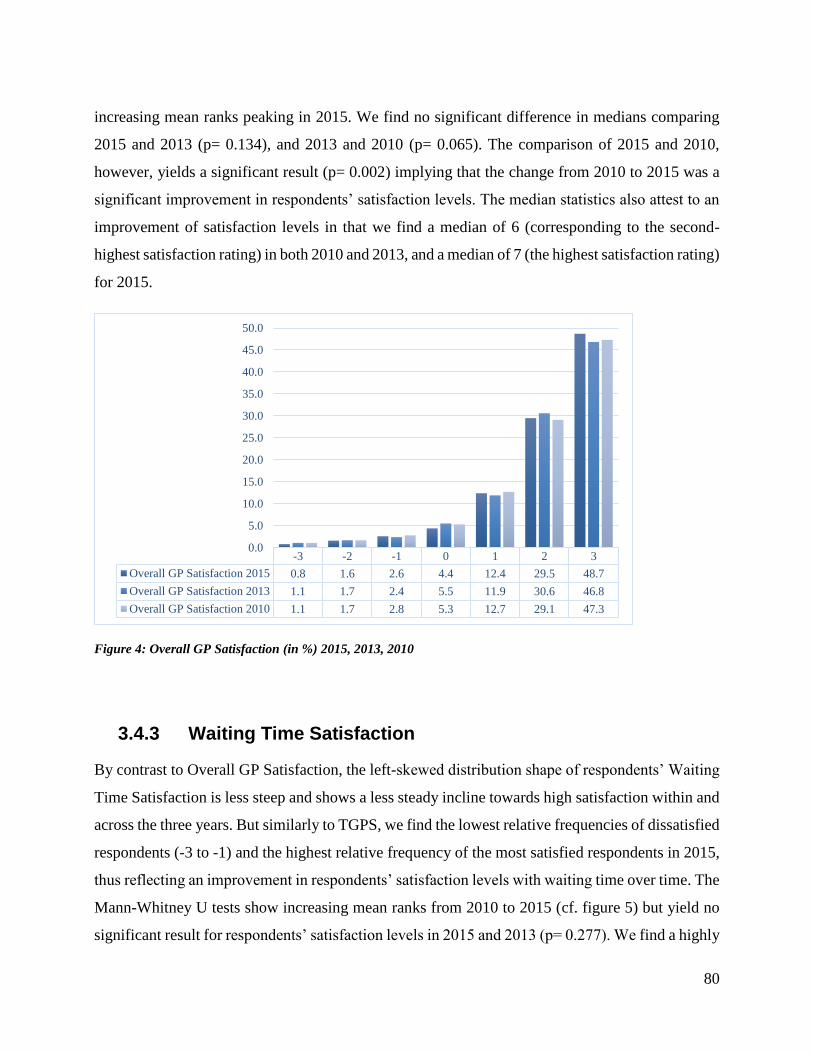
80

increasing mean ranks peaking in 2015. We find no significant difference in medians comparing

2015 and 2013 (p= 0.134), and 2013 and 2010 (p= 0.065). The comparison of 2015 and 2010,

however, yields a significant result (p= 0.002) implying that the change from 2010 to 2015 was a

significant improvement in respondents’ satisfaction levels. The median statistics also attest to an

improvement of satisfaction levels in that we find a median of 6 (corresponding to the second-

highest satisfaction rating) in both 2010 and 2013, and a median of 7 (the highest satisfaction rating)

for 2015.

Figure 4: Overall GP Satisfaction (in %) 2015, 2013, 2010

3.4.3 Waiting Time Satisfaction

By contrast to Overall GP Satisfaction, the left-skewed distribution shape of respondents’ Waiting

Time Satisfaction is less steep and shows a less steady incline towards high satisfaction within and

across the three years. But similarly to TGPS, we find the lowest relative frequencies of dissatisfied

respondents (-3 to -1) and the highest relative frequency of the most satisfied respondents in 2015,

thus reflecting an improvement in respondents’ satisfaction levels with waiting time over time. The

Mann-Whitney U tests show increasing mean ranks from 2010 to 2015 (cf. figure 5) but yield no

significant result for respondents’ satisfaction levels in 2015 and 2013 (p= 0.277). We find a highly

-3 -2 -1 0 1 2 3

Overall GP Satisfaction 2015 0.8 1.6 2.6 4.4 12.4 29.5 48.7

Overall GP Satisfaction 2013 1.1 1.7 2.4 5.5 11.9 30.6 46.8

Overall GP Satisfaction 2010 1.1 1.7 2.8 5.3 12.7 29.1 47.3

0.0

5.0

10.0

15.0

20.0

25.0

30.0

35.0

40.0

45.0

50.0

81

significant difference between 2013 and 2010 (p< 0.001) as well as between 2015 and 2010 (p<

0.001), even though the median remains constant at 6 (the second-highest satisfaction rating)

throughout all three years.

Figure 5: Waiting Time Satisfaction (in %) 2015, 2013, 2010

3.4.4 Satisfaction w. Referrals to Specialists

The distribution curve of respondents’ Satisfaction with Referrals to Specialists follows similar

patterns to the one of Overall GP Satisfaction, i.e. a steady and increasingly steep incline of relative

frequencies towards high satisfaction levels. While we encounter the highest relative frequency of

most satisfied respondents in 2013, the frequencies of mildly and rather satisfied respondents were

highest in 2015. Analogously, the lowest relative frequency of most dissatisfied respondents is

displayed in 2015, while moderately dissatisfied or indifferent respondents show very similar

relative frequencies in 2013 and 2015. The Mann-Whitney-U test yielded no significant result for

the comparison of 2015 and 2013 (p= 0.344), but highly significant results for the comparison

between 2013 and 2010 as well as 2015 and 2010 (p <0.001). Looking at the mean ranks, we see

an improvement of satisfaction with referrals to specialists from 2010 to 2013 and from 2010 to

2015 but overall respondents were most satisfied in 2013. This conclusion is corroborated by the

median statistics, which yield a median of 7 (corresponding to the highest satisfaction rating) in

2013 and a median of 6 (corresponding to +2 on the satisfaction scale) for both 2010 and 2015.

-3 -2 -1 0 1 2 3

Waiting Time Satisfaction 2015 4.8 6.0 8.9 9.6 16.7 27.1 26.9

Waiting Time Satisfaction 2013 5.2 7.4 9.0 8.5 16.2 27.8 26.0

Waiting Time Satisfaction 2010 5.8 7.6 10.4 9.3 16.3 25.4 25.1

0.0

5.0

10.0

15.0

20.0

25.0

30.0

82

Figure 6: Satisfaction with Referrals to Specialists (in %) 2015, 2013, 2010

3.4.5 Satisfaction w. GP’s Medical Competence

The left-skewed distribution follows a steady and steep incline in relative frequencies towards high

satisfaction in all three years. We observe the lowest relative frequency of respondents being very

dissatisfied in 2015, yet mild dissatisfaction (-2, -1) as well as the highest satisfaction (+3) show

the highest relative frequencies in 2015. We further find a stable median of 6 (corresponding to +2

on the satisfaction scale) for all three years. The Mann-Whitney U test yields no significant

difference for the comparison of 2015 and 2013 (p= 0.648) but highly significant results for the

comparison of 2013 and 2010 (p< 0.001) as well as 2015 and 2010 (p< 0.001) indicating an

improvement of satisfaction levels based on increasing mean ranks. Since the 2013 ratings

produced the highest mean ranks, we can conclude that satisfaction ratings were best in 2013 before

falling in 2015.

-3 -2 -1 0 1 2 3

Referrals (specialist) 2015 1.3 2.0 2.5 5.1 11.7 29.6 47.8

Referrals (specialist) 2013 2.0 1.7 2.6 5.2 11.2 27.9 49.4

Referrals (specialist) 2010 1.8 1.7 2.9 7.1 11.4 29.7 45.3

0.0

5.0

10.0

15.0

20.0

25.0

30.0

35.0

40.0

45.0

50.0

83

Figure 7: Satisfaction with GP’s Medical Competence (in %) 2015, 2013, 2010

3.4.6 Satisfaction with Referrals to Other Services

Since this variable was introduced in the 2013 dataset, we do not have available ratings for 2010,

thus limiting us to follow the development from 2013 to 2015. The relative frequencies follow the

familiar pattern of a left-skewed, increasingly steep distribution towards the right end of the

satisfaction scale in both years. We find the higher relative frequencies in +1 and +3 for 2015

respondents, while relative frequencies of dissatisfied respondents remain largely the same in 2013

and 2015. Based on the comparison of mean ranks, we detect an improvement of satisfaction ratings

in the 2015 respondents but this is not a significant difference (p=0.533), and also the median

remained stable at 6 (corresponding to +2 satisfaction rating). We can therefore conclude that

respondents were slightly but not significantly more satisfied with the referrals to other services in

2015.

-3 -2 -1 0 1 2 3

GP's Medical Competence 2015 0.6 1.5 2.3 4.6 12.7 31.7 46.6

GP's Medical Competence 2013 1.3 0.9 2.1 4.5 12.4 32.5 46.4

GP's Medical Competence 2010 1.1 0.9 1.8 6.4 14.2 32.0 43.6

0.0

5.0

10.0

15.0

20.0

25.0

30.0

35.0

40.0

45.0

50.0

84

Figure 8: Satisfaction with Referrals to Other Services (in %) 2015 & 2013

3.4.7 Satisfaction with Time to Explain/Consultation Length

This variable was not part of the 2010 survey and therefore only allows for comparison between

2015 and 2013 to track the development of satisfaction levels. Relative frequencies of high

dissatisfaction (-3) were slightly higher in 2015 than in 2013 and roughly equal for minor

dissatisfaction (-1) and indifference (0), while relative frequencies of the satisfaction levels of +1

and +3 were also higher in 2015. We find no change in median as it remained stable at 6 (second

highest satisfaction rating) and the Mann-Whitney U test yielded no significant difference in

respondents’ satisfaction levels (p= 0.904). Based on the mean ranks, we detect a minor

improvement in the satisfaction ratings of 2015 (cf. figure 9).

-3 -2 -1 0 1 2 3

Referrals (other

services) 20152.0 2.1 3.5 7.5 13.2 29.0 42.6

Referrals (other

services) 20132.0 1.8 3.6 8.8 12.0 30.3 41.4

0.0

5.0

10.0

15.0

20.0

25.0

30.0

35.0

40.0

45.0

85

3.4.8 Level of Trust in the GP

The respondents’ assessment of the level of trust towards the GP was entered into the survey in

2013. The graph below shows an increasing steep incline of relative frequencies towards the

positive end of the satisfaction scale. While the median was 6 (corresponding to +2 on the

satisfaction scale) in 2013, it was at the highest satisfaction level in 2015 indicating a generally

higher level of respondents’ satisfaction. We also find a higher mean rank score in 2015 but the

result of the Mann-Whitney U test yielded no significant difference between the 2013 and 2015

ratings (p= 0.411).

-3 -2 -1 0 1 2 3

Time to Explain 2015 1.4 1.7 4.2 6.4 15.8 32.1 38.5

Time to Explain 2013 1.0 2.0 4.2 6.5 15.4 33.2 37.6

0.0

5.0

10.0

15.0

20.0

25.0

30.0

35.0

40.0

Figure 9: Satisfaction with Time to Explain/Consultation Length (in %) 2015 & 2013

-3 -2 -1 0 1 2 3

Trust in the GP 2015 1.0 1.6 2.5 4.5 11.5 30.4 48.4

Trust in the GP 2013 1.1 1.5 2.7 5.6 11.2 30.4 47.5

0.0

5.0

10.0

15.0

20.0

25.0

30.0

35.0

40.0

45.0

50.0

Figure 10: Level of Trust in the GP (in %) 2015 & 2013

86

3.4.9 Detecting Differences in Satisfaction Ratings

To determine whether there is a significant difference in the satisfaction ratings of the main

satisfaction variables over time, Mann-Whitney U Tests were run. Visual inspection of the

distributions of each satisfaction variable across the three years showed very similar shapes

(skewed distributions in favor of high satisfaction ratings). The Mann-Whitney U Test can

therefore be used to interpret differences in medians.

3.4.8.1 Comparing 2015 & 2013

Comparing the satisfaction data from 2015 and 2013, we find no significant differences in any

satisfaction variables (cf. table 29). Satisfaction levels for both dependent variables (Overall GP

Satisfaction and Waiting Time Satisfaction) are not significantly different (p= 0.134; p= 0.277).

None of the median rating scores for the other satisfaction variables was significantly different in

2015 and 2013. Comparing the mean ranks between 2015 and 2013, we see only minor differences.

The mean ranks for the variables Overall GP Satisfaction, Waiting Time Satisfaction, Satisfaction

with Time to Explain/Consultation Length, Satisfaction with Referrals to Other Services and Level

of Trust show higher mean ranks in 2015 than in 2013. We can therefore conclude that respondents’

satisfaction increased in these domains in 2015. By contrast, Satisfaction with Referrals to

Specialists and Satisfaction with the GP’s Medical Competence show lower mean ranks in 2015

indicating a minor decrease in respondents’ satisfaction levels.

Table 29: Mann-Whitney U Test on Satisfaction Variables 2015 – 2013

2015 - 2013

Comparison

Overall GP

Satisfaction

Waiting Time

Satisfaction

Satisfaction with

Time to Explain

Satisfaction with

Referrals to

Specialists

Satisfaction with

GP's

Competence

Satisfaction with

Referrals to

Other Services

Level of Trust

Mann-Whitney U 7740854.500 7287944.500 7512359.500 5544238.000 7338767.500 2079094.500 7703255.000

Wilcoxon W 14826584.500 14101530.500 14392554.500 11646509.000 15441092.500 4270465.500 14710151.000

Z -1.497 -1.088 -0.121 -0.946 -0.457 -0.623 -0.822

Asymp. Sig. (2-tailed) 0.134 0.277 0.904 0.344 0.648 0.533 0.411

87

Year N Mean Rank Sum of

Ranks

Overall GP

Satisfaction

2013 3764 3939.05 14826584.50

2015 4188 4010.16 16794543.50

Waiting Time

Satisfaction

2013 3691 3820.52 14101530.50

2015 4005 3874.29 15516525.50

Satisfaction with

Time to Explain

2013 3709 3880.44 14392554.50

2015 4057 3886.30 15766706.50

Referral Satisfaction

(Specialists)

2013 3214 3375.47 10848769.00

2015 3493 3334.24 11646509.00

Satisfaction with

GP's Medical

Competence

2013 3667 3857.70 14146185.50

2015 4025 3836.30 15441092.50

Referral Satisfaction

(Other Services)

2013 2093 2040.36 4270465.50

2015 2008 2062.09 4140685.50

Level of Trust 2013 3743 3930.04 14710151.00

2015 4157 3968.92 16498799.00

Table 30: Mean Ranks of Mann-Whitney U Test on Satisfaction Variables 2015 – 2013

3.4.8.2 Comparing 2013 & 2010

Due to lack of comparative values in the 2010 dataset, the variables Satisfaction with the Time to

Explain, Satisfaction with Referrals to Other Services, and Level of Trust in the GP were not

included in the analysis of 2013 and 2010. In comparing respondents’ other satisfaction levels from

2013 and 2010, we discover significant results for Waiting Time Satisfaction (p< 0.001),

Satisfaction with Referrals to Specialists (p<0.001), and Satisfaction with the GP’s Medical

Competence (p< 0.001). By contrast, Overall GP Satisfaction is not significantly different in 2013

and 2010 (p= .065). The investigation of mean ranks reveals that the satisfaction levels for all

variables are higher in 2013 than in 2010. We can therefore conclude that satisfaction levels

increased from 2010 to 2013.

88

2013 - 2010

Comparison

Overall GP

Satisfaction

Waiting

Time

Satisfaction

Referral

Satisfaction

(Specialists)

Satisfaction

with GP's

Competence

Mann-Whitney U 4054625.500 3809167.500 2870107.000 3698215.500

Wilcoxon W 6504416.500 6210503.500 4700848.000 6012691.500

Z -1.847 -3.808 -4.299 -4.273

Asymp. Sig. (2-tailed) 0.065 0.000 0.000 0.000

Table 31: Mann-Whitney U Test on Satisfaction Variables 2013 – 2010

Year N Mean Rank

Sum of

Ranks

Overall GP

Satisfaction

2010 2213 2939.19 6504416.50

2013 3764 3018.29 11360836.50

Waiting Time

Satisfaction

2010 2191 2834.55 6210503.50

2013 3691 3004.98 11091399.50

Referral Satisfaction

(Specialists)

2010 1913 2457.32 4700848.00

2013 3214 2627.50 8444780.00

Satisfaction with

GP's Medical

Competence

2010 2151 2795.30 6012691.50

2013 3667 2976.49 10914779.50

Table 32: Mean Ranks of Mann-Whitney U Test on Satisfaction Variables 2013 – 2010

3.4.8.3 Comparing 2015 & 2010

The available satisfaction variables present in both datasets included Overall GP Satisfaction,

Waiting Time Satisfaction, Satisfaction with Referrals to Specialist, and Satisfaction with the GP’s

Medical Competence. We obtain significant results for all these variables (cf. Table 33).

Overall GP

Satisfaction

Waiting

Time

Satisfaction

Referral

Satisfaction

(Specialists)

Satisfaction

with GP's

Competence

Mann-Whitney U 4428823.500 4069883.500 3157349.000 4083923.500

Wilcoxon W 6878614.500 6471219.500 4988090.000 6398399.500

Z -3.161 -4.830 -3.606 -3.945

Asymp. Sig. (2-tailed) 0.002 0.000 0.000 0.000

Table 33: Mann-Whitney U Test on Satisfaction Variables 2015 – 2010

89

Year N Mean Rank

Sum of

Ranks

Overall GP

Satisfaction

2010 2213 3108.28 6878614.50

2015 4188 3250.00 13610986.50

Waiting Time

Satisfaction

2010 2191 2953.55 6471219.50

2015 4005 3177.80 12727086.50

Referral Satisfaction

(Specialists)

2010 1913 2607.47 4988090.00

2015 3493 2756.09 9627031.00

Satisfaction with

GP's Medical

Competence

2010 2151 2974.62 6398399.50

2015 4025 3149.36 12676176.50

Table 34: Mean Ranks of Mann-Whitney U Test on Satisfaction Variables 2015 – 2010

Table 35: Mean Statistics for Satisfaction Variables 2015, 2013, 2010

Overall GP

Satisfaction

Waiting Time

Satisfaction

Satisfaction

with Time to

Explain

Referral

Satisfaction

(Specialists)

GP's Medical

Competence

Referral

Satisfaction

(Other

Services)

Level of Trust

in the GP

Valid 2213 2191 0 1913 2151 0 0

Missing 67 89 2280 367 129 2280 2280

6,325 4,992 5,950 6,022

6,000 6,000 6,000 6,000

7,00 6,00 7,00 7,00

Valid 3764 3691 3709 3214 3667 2093 3743

Missing 118 191 173 668 215 1789 139

6,098 5,185 5,880 6,089 6,138 5,895 6,107

6,000 6,000 6,000 7,000 6,000 6,000 6,000

7,00 6,00 7,00 7,00 7,00 7,00 7,00

Valid 4188 4005 4057 3493 4025 2008 4157

Missing 136 319 267 831 299 2316 167

6,141 5,240 5,875 6,086 6,130 5,908 6,133

7,000 6,000 6,000 6,000 6,000 6,000 7,000

7,00 7,00 7,00 7,00 7,00 7,00 7,00

2015

N

Mean

Median

Mode

2010

N

Mean

Median

Mode

2013

N

Mean

Median

Mode

YEAR

90

4 Discussion & Conclusion

This section provides a summary of findings from a longitudinal perspective, points out the main

findings of the bivariate and regression analyses and discusses them in light of previous research

and literature, while considering the strengths and limitations of this analysis. Lastly, implications

will be inferred from the results and options for further research will be highlighted.

4.1 Summary of Findings

Satisfaction Levels

The very left-skewed frequency distributions of satisfaction levels over time indicate that

respondents are generally very satisfied; the majority of respondents expresses (high) satisfaction.

We find the mode in the highest rating item (+3) for Overall GP Satisfaction, Referrals to

Specialists, Referrals to Other Services, Time to Explain, Trust in the GP, and GP’s Medical

Competence. Only Waiting Time Satisfaction and GP Supply Satisfaction peak in +2 and display

a lower frequency of respondents expressing very high satisfaction. Moreover, we detect a higher

share of respondents expressing dissatisfaction with waiting time and municipal GP supply

compared to other satisfaction variables.

- Overall GP Satisfaction improved continuously from 2010 to 2015, peaking in 2015 with the

least amount of dissatisfied and the highest amount of highly satisfied respondents; Further, we

detect a significant improvement from 2010 to 2015.

- Waiting Time Satisfaction shows a similar development as Overall GP Satisfaction, and

significantly improved from 2010 to 2013. However, from 2013 to 2015 there was only a minor,

insignificant improvement in satisfaction with waiting time.

- Satisfaction with Referrals to Specialists significantly increased from 2010 to 2013.

Respondents were most satisfied in 2013 and satisfaction levels subsequently decline in 2015.

91

- We find a significant improvement in satisfaction with the GP’s Medical Competence from

2010 to 2013, followed by a mild, not significant decline in satisfaction levels from 2013 to

2015.

- The data indicate a minor, but not significant improvement in Satisfaction with Referrals to

Other Services from 2013 to 2015.

- Satisfaction with Time to Explain increased insignificantly from 2013 to 2015 as there is a

simultaneous increase in frequency of very dissatisfied and highly satisfied respondents.

- We observe a minor, yet insignificant increase in the level of Trust in the GP from 2013 to

2015.

- Overall municipal GP capacity increased over time in terms of GP density, registered GPs,

and free capacity (GPs with open lists), while the number of available list places decreased

steadily. We therefore observe a simultaneous increase and decrease in patients’ real choice of

GPs and competition among GPs.

Group Differences for Overall GP Satisfaction & Waiting Time Satisfaction

- Respondents who expressed general Life Satisfaction were significantly more satisfied with the

GP as well as waiting time in 2015, 2013, and 2010 compared to those who expressed

dissatisfaction with life.

- Respondents with below-median income were significantly more satisfied with the GP in

general as well as waiting time in 2015, 2013, 2010 compared to people with above-median

income.

- Respondents with primary education were significantly more satisfied with their GP and

waiting time than respondents with secondary or higher education in 2015, 2013 and 2010.

- Respondents with an average contact frequency of two to five GP visits per year were

significantly more satisfied with the GP in general in 2015 (but not in 2013) compared to those

with non-average (above or below) contact frequency. We find no significant difference in

waiting time satisfaction based on contact frequency in any year.

92

- Respondents with private GPs were significantly more satisfied with the GP as well as waiting

time in 2013 and 2015 (no data available for 2010). It has to be pointed out, though, that the

classification of public vs. private GP occurred on users’ judgment and does not correspond to

the actual distribution of 95% self-employed GPs in Norway. For this reason, we interpret the

variable as users’ subjective perception of GP type distinction, albeit we do not know the

distinguishing factor.

- Respondents with self-assessed “good health” were significantly more satisfied with their GP

as well as waiting time than those with perceived bad health in 2015 and 2013 (no data available

for 2010). By contrast, respondents with disabilities did not significantly differ in their

satisfaction levels with the GP or waiting time than respondents without disabilities in 2015 (no

data for 2013 or 2010).

- Age: We detect no significant difference in Overall GP Satisfaction or Waiting Time

Satisfaction levels comparing young and middle-aged respondents in 2015. However, these

groups differ significantly in both ratings in 2013 and 2010, with middle-aged respondents

expressing significantly higher satisfaction levels. Comparing the young with the old and the

middle-aged with the old, we find significant differences in Overall GP Satisfaction and Waiting

Time Satisfaction in every year indicating the old respondents are always more satisfied.

- GP density: In comparing low with medium-range and medium-range with high municipal GP

density, we encounter a significant difference in Overall GP Satisfaction levels in 2015, in that

respondents from municipalities with medium-range GP density were significantly more

satisfied with their GP than respondents from either low or high density areas. We detect no

such difference for TGPS or WTS in 2013 or 2010 but find also a significant difference between

low and medium-range density in respondents’ satisfaction levels with waiting time in 2015.

- Available GP’s with open lists per 1000 inhabitants (OLI): We find a significant difference

in users’ Overall GP Satisfaction levels in 2015 comparing municipalities with low and medium

as well as a low and high count of GPs with open lists per 1000 inhabitants indicating that areas

with low-count OLI yield significantly more satisfied users. We find no significant difference

for users’ Waiting Time Satisfaction in any year or for Overall GP Satisfaction in 2013 and

2010.

93

- Available List Places per 1000 Inhabitants (LPPT): There is a significant difference in users’

Overall GP Satisfaction in 2010 (but not in 2015 or 2013) comparing municipalities with a low

vs medium and a medium vs high-range of available list places per 1000 inhabitants, yielding

significantly higher satisfaction levels for respondents from medium-range rather than low or

high-count LPPT areas. We find no significant difference in TGPS comparing low and high-

count LPPT municipalities in any year. Waiting time satisfaction differed significantly in 2013

comparing low and medium-count LPPT as well as low and high-count LPPT areas (respondents

from middle-range LPPT areas were more satisfied with waiting time than those from low-range

areas, and people living in the top 33rd percentile LPPT areas also expressed significantly higher

satisfaction with waiting time than those from the bottom 33rd percentile). There is also no

difference in WTS levels comparing the middle with the top 33rd percentile of LPPT areas in

any year.

- Open List Ratio (OLR): No significant difference is detected for Waiting Time Satisfaction

according to respondents’ municipality-specific OLR range in any year. In Overall GP

Satisfaction, we do not detect significant differences comparing the middle and top 33rd

percentile. However, we find significantly more satisfied respondents in areas in the bottom

compared to the middle as well as the top (p= .058) 33rd percentile of OLR in 2015.

- Free Capacity: There is no difference in users’ Overall GP Satisfaction levels comparing

municipalities with low and medium range of free capacity as well as low and high-range free

capacity in any year. There is a near-significant result (p= .055) indicating higher Overall GP

Satisfaction levels in respondents living in the middle rather than the top third percentile of free

capacity municipalities in 2013. We find significant results in respondents’ Waiting Time

Satisfaction ratings based on range of free capacity in 2015, as respondents from the middle 33rd

percentile free capacity areas expressed more satisfaction compared to those from either the

bottom or top 33rd percentile areas. In 2010, we find that respondents from the top compared to

the bottom 33rd percentile were significantly more satisfied with waiting time.

- Municipality Size: In 2015, respondents from the second-smallest municipalities were

significantly more satisfied with their GP in general compared to those from the smallest

municipalities. Similarly, we find that in 2015, people living in the second-biggest rather than

94

the biggest municipalities tended to express higher Overall GP Satisfaction. By contrast, there

is no difference in Waiting Time Satisfaction levels between respondents from the smallest and

second-smallest or the biggest and smallest municipalities in any year. In 2015, Waiting Time

Satisfaction was significantly higher in respondents living in the second-biggest and third-

biggest municipalities compared to those from the biggest municipalities. We find a similar

significant result in 2013, in that respondents from the second-smallest municipalities were more

satisfied than those living in the smallest.

Regression Results for Overall GP Satisfaction & Waiting Time Satisfaction

In predicting Overall GP Satisfaction, the 2015 and 2013 models yield consistently significant,

positive correlation results for the independent variables age, Waiting Time Satisfaction and Life

Satisfaction. We encounter interesting outcomes in the 2015 and 2013 TGPS Models regarding

LPPT significance as there was no relation neither expected nor indicated in the bivariate analysis

with Overall GP Satisfaction. High LPPT compared to lower LPPT reflects increased patient choice

and thus a comparatively higher chance of being listed with the preferred GP of higher quality. A

similar finding is the significant correlation of OLI and TGPS in the 2015 models 1 and 2, as

anticipated in the Mann-Whitney U Test for TGPS. High OLI produced the highest likelihood of

expressing Overall GP Satisfaction compared to medium or low OLI. One possible reason for that

could be that the more GPs are available/have open lists, the higher is the probability of patients to

be able to pick the preferred GP, or the more choice there is for switching the GP. We also find

unexpected outcomes in predicting very high TGPS through free capacity and municipality size.

Contrary to assumptions based on previous findings, high free capacity resulted in the highest

probability of high Overall GP Satisfaction. The more available GPs we have in a municipality, the

higher is the likelihood that patients express Overall GP Satisfaction.

We obtain very similar results in modeling Waiting Time Satisfaction in 2015. Age, Municipal GP

Supply Satisfaction and Life Satisfaction are consistent, positive predictors. These outcomes are

consistent with the results from the Mann-Whitney U tests, which showed that old respondents and

the ones being satisfied with life yielded significantly higher satisfaction levels with waiting time.

Free capacity and GP density yielded significant results in that the middle 33rd percentile of both

variables yielded significantly higher waiting time satisfaction levels compared to low or high GP

95

density or free capacity areas. Similarly in the regression analyses, the competition measures GP

density and OLI yield the same relation to the odds of Waiting Time Satisfaction in 2015 as they

did in predicting Overall GP Satisfaction. Unlike expected from the bivariate analysis, it was high

instead of medium capacity areas that produced the highest odds of respondents expressing

satisfaction with waiting time. Moreover, municipal competition variables increasingly become

significant when we model high or very high satisfaction with the GP or waiting time in 2015.

Overall, these findings show that increased municipal capacity in the form of GP density, LPPT or

OLI augment satisfaction levels with both the GP and waiting time.

In a healthcare setting with restricted access, the municipal supply-side variables such as free

capacity, LPPT and OLI can be interpreted as measures of GP competition for users in a

municipality. As such, high capacity areas would simultaneously reflect intense competition among

GPs and enhanced accessibility for users. The results indicate that the higher the GP competition

is in a given municipality, the more high satisfaction users express. It is conceivable that people

are more satisfied, the more ‘real’ choice among available GPs exists (regardless of whether this

choice is utilized or not) rather than the amount of listed GPs that may in fact be inaccessible due

to full patient lists. This effect could mirror on a local level what has been observed on an

international level, namely that countries with free or increased access to medical services produce

higher scores of patient satisfaction compared to countries with a strong gatekeeping function and

restricted accessibility (Kroneman, Maarse, & van der Zee, 2006).

Similarly, the smallest municipalities coincided with a reduced probability of Overall GP

Satisfaction compared to big municipalities in 2015. The reason for that correlation could be that

bigger municipalities are potentially perceived as offering more choice to the users than smaller

municipalities even though the actual capacity per 1000 inhabitants (in the form of GP density,

LPPT or OLI) tends to be higher in smaller municipalities. In addition, smaller municipalities

produced higher odds of Waiting Time Satisfaction, except for the smallest municipalities which

significantly reduced satisfaction with waiting time. We assume that this is due to better access in

small municipal areas, which might coincide with lower actual waiting times. However, this

assumption would need further investigation.

96

Across all models and versions, satisfaction variables (Municipal GP Supply Satisfaction, Waiting

Time Satisfaction, Life Satisfaction) increased the explained variance in the dependent variable

tremendously (increasing it three- to fourfold), while also adding significantly to the models’

predictive accuracy. Municipal supply-side variables have a huge impact on the 2015 models of

Waiting Time Satisfaction and Overall GP Satisfaction, but this impact is diminished in 2013 and

not observable in 2010 altogether. Instead, socio-demographic variables become increasingly

influential, particularly as the cut-off points are adjusted to predict high or very high Overall GP

Satisfaction and Waiting Time Satisfaction. We therefore conclude that there seems to be a trend

of increasing influence of municipal supply-side/capacity measures and decreasing significance of

socio-demographic predictors other than age from 2010 to 2015.

4.2 Main Results

The main objective was to trace the development of satisfaction variables over time, most notably

Overall GP Satisfaction and Waiting Time Satisfaction, and to determine significant influencing

factors, particularly with regard to municipality-specific competition indicators. By means of

Mann-Whitney-U tests and multi-level binomial linear regression models, various associations

were analyzed between Overall GP Satisfaction and Waiting Time Satisfaction as dependent

variables and selected independent variables including socio-demographic predictors, self-assessed

health status, municipality-specific supply-side variables and relevant satisfaction measures. The

latter allowed to control for relevant predictors included in the model and yielded odds ratios that

were used to predict a change in the respondents’ probability to express satisfaction.

In the descriptive sections, we have seen that the majority of independent variables influence

Overall GP Satisfaction and Waiting Time Satisfaction. The BLR models on Waiting Time

Satisfaction and Overall GP Satisfaction shed additional light on the interplay of potential

determinants. While we find correlations of most independent variables with the two main

satisfaction variables conducting correlation tests, their effect is somewhat diminished through

mutual cancellation in the regression models. Below, we list each hypothesis and the respective

result that confirms or refutes it.

97

Hypothesis 1: Overall GP Satisfaction is associated with age, income and level of education. This

hypothesis was confirmed. Overall GP Satisfaction also correlates positively with age when

controlling for other predictors in the models of 2015 and 2013. In 2010, however, we do not find

a significant effect of age. Instead, below-median income as well as a low level of education

significantly increased the odds of high or very high Overall GP Satisfaction. The influence of

income and education level is inconsistent in its significance across models with different cut-off

points. In the instances where a significant association is detected (determining high or very high

satisfaction in 2013 and 2010), education and income correlate negatively with the odds of Overall

GP Satisfaction. The results confirm previous research findings (Russell et al., 2015; Zhang, 2012)

for the influence of age and education but stand in contrast to Zhang’s (2012) finding that below-

median income correlates with dissatisfaction.

Hypothesis 2: Overall GP Satisfaction and Waiting Time Satisfaction correlate positively with

health status. While the correlation and Mann-Whitney U tests revealed significant positive

associations of health with Overall GP Satisfaction and Waiting Time Satisfaction, we do not find

a significant effect in the presence of other independent variables when predicting the odds of

Waiting Time Satisfaction or Overall GP Satisfaction. This finding corroborates the results

provided by Zhang (2012) and Grytten et al. (2009).

Hypothesis 3: Waiting Time Satisfaction is associated with age, income and level of education.

Similarly to H1, this hypothesis was only partially confirmed. There is indeed a significant positive

correlation of age and Waiting Time Satisfaction in 2010, 2013 and 2015 even when controlling

for other predictors. Analogously to Overall GP Satisfaction, the predictive effect of income and

education level are of varying significance but display a negative association with Waiting Time

Satisfaction in the 2015 and 2013 models. Our findings therefore confirm previous ones (Grytten

et al., 2009) with regard to the influence of age. Additionally, they inform theory on the impact of

income and education on Waiting Time Satisfaction.

Hypothesis 4: Visiting a public or private GP does not influence the odds of Overall GP

Satisfaction while having a private GP will positively affect Waiting Time Satisfaction. This

assumption is partially refuted by the regression models in 2015 and 2013 because whenever we

detect a significant influence, we find that consulting a private GP in fact increases the odds of both

Waiting Time Satisfaction and Overall GP Satisfaction. This is a surprising result since there was

98

no indication in previous research that suggested higher overall satisfaction with private GPs.

Moreover, this result is contradictory to the fact that 95% of Norwegian GPs are self-employed and

therefore “private”. The question that is raised in this context is what the reason is for this

misperception of Norwegian GP users that categorizes GPs as public or private, or rather what the

characteristics are according to which users classify GPs as public or private. Due to the significant

relation of GP type with Overall GP Satisfaction and Waiting Time Satisfaction, it is conceivable

that users’ perception of having a ‘private’ GP increased satisfaction with waiting time and Overall

GP Satisfaction. Further research into this perception is needed to shed more light on the matter.

Hypothesis 5: Overall GP Satisfaction and Waiting Time Satisfaction are positively associated.

We found significant positive correlations in all models and all three years to confirm this

hypothesis. High levels of Waiting Time Satisfaction are a constant, significant predictor that

increased the odds of Overall GP Satisfaction in 2015, 2013 and 2010. This result confirms

previous findings from the US healthcare context (George & Sanda, 2007; Russell et al., 2015;

Vogus & McClelland, 2016) and provides the first such insight for the Norwegian primary

healthcare setting.

Hypothesis 6: Life Satisfaction correlates positively with Overall GP Satisfaction as well as with

Waiting Time Satisfaction. This hypothesis is confirmed since we detect a significant positive

correlation with the odds of Waiting Time Satisfaction and Overall GP Satisfaction in every

regression model in 2015, 2013, and 2010. We can therefore confirm the findings by George &

Sanda (2007) in the US and adopt them for the Norwegian primary care context.

We can confirm hypothesis 7 with every model of the three survey years and find that Municipal

GP Supply Satisfaction is positively associated with Waiting Time Satisfaction. Since the models

only tested Municipal GP Supply Satisfaction as an independent covariate to Waiting Time

Satisfaction, we cannot determine the direction of the correlation. It might therefore be the case

that Waiting Time Satisfaction is the actual independent variable predicting Municipal GP Supply

Satisfaction rather than vice versa as assumed in the models. We therefore suggest to conduct

further research on investigating Municipal GP Supply Satisfaction to find relevant influencing

factors and to better understand the relation with Waiting Time Satisfaction (as well as actual GP

supply).

99

Hypothesis 8 stated that various municipality-specific competition indicators influence Overall GP

Satisfaction and Waiting Time Satisfaction. Although no relation between available List Places

per 1000 Inhabitants (LPPT) and Overall GP Satisfaction was expected, we find significant

positive correlations in the 2015 and 2013 regression models suggesting that an increased

flexibility in patient lists seemingly contributes to Overall GP Satisfaction. This effect differs in

the 2010 model, however, where LPPT appears to be inversely related to Overall GP Satisfaction.

Contrary to expectations, GP density only had a significant positive effect on predicting Overall

GP Satisfaction in the 2013 model and free capacity actually increased rather than reduced the

odds of Overall GP Satisfaction in the 2015 model. We encounter little consistency in the effects

of competition indicators on Overall GP Satisfaction over time. In determining the odds of Waiting

Time Satisfaction, we observed a significant positive effect of high free capacity in the 2015 and

2013 models. Open Lists per 1000 Inhabitants served as a significant positive predictor for

Waiting Time Satisfaction in the 2015 but yielded a negative correlation in 2013. Available List

Places per 1000 Inhabitants correlated positively with the odds of Waiting Time Satisfaction in

2013 as well. In the 2010 models we detected a positive correlation of GP density and the odds of

Waiting Time Satisfaction and significantly reduced odds for high-range available List Places per

1000 Inhabitants. Consequently, we do not find a consistent influence of competition indicators on

modelling Waiting Time Satisfaction over time and suggest conducting further research to find

potential causes for this development.

To sum up, we find increased odds for respondents’ Overall GP Satisfaction in higher age, in

respondents consulting a ‘private’ GP, in users expressing high Waiting Time Satisfaction and high

Life Satisfaction. In determining Waiting Time Satisfaction, we detected a consistently significant

positive association with age, Municipal GP Supply Satisfaction and general Life Satisfaction, and

a not consistently significant influence of ‘private’ GPs. Adding satisfaction variables in the last

step of the hierarchical regression models increased the explained variance in the dependent

variable three- to fourfold. The significant effect of socio-demographic variables such as income

and education level as well as respondents’ self-assessed health status were largely cancelled out

by adding satisfaction variables in the final step of the regression models. Municipal capacity was

negligible in its effect on Overall GP Satisfaction and Waiting Time Satisfaction in 2010 but

became increasingly influential and significant in 2013 and 2015. Particularly in 2015, we find that

high capacity - in the form of GP density, available list places per 1000 inhabitants and open lists

100

per 1000 inhabitants - yields the highest probability of users to express high Overall GP Satisfaction

and Waiting Time Satisfaction.

4.3 Limitations and Strengths

Firstly, a few aspects need to be mentioned regarding the robustness and consistency of outcomes

of the bivariate and regression analyses. We find largely consistent results in both analytical types

and encountered no contradicting evidence in the regression analyses. This fact adds to the

robustness of results. We do find some minor differences with regard to the significance levels of

single variables when comparing the bivariate analysis with the additional regression models,

specifically in the capacity variables. The reason for that is the fact that the bivariate analysis is

based on the same intuitive cut-off point on the satisfaction scale of the dependent variable as the

main regression models (satisfaction vs dissatisfaction). Therefore, the results of the bivariate

analysis are best comparable to the outcomes of the main regression models rather than to the

results from the additional regression models. As we have seen, the higher cut-off points (to predict

high or very high satisfaction) yield more significant results for capacity and competition measures

and less significance for socio-demographic variables in the additional regression models that were

not indicated to that extent in the corresponding bivariate analysis. This is not surprising given the

fact that we expected the influence of predictor variables not to be equal across the ordinal scale of

the dependent variable (which was the reason for choosing BLR over ordinal logistic regression

with the proportional odds assumption). To investigate consistency and robustness of results more

deeply, further bivariate analyses could be conducted utilizing the same cut-off points that were

employed in the additional regression models. Another explanatory aspect for minor differences in

results is the methodological nature of the bivariate and regression analysis. In the bivariate

analysis, we investigate the significance of a single predictor on the dependent variable, while the

regression analysis investigates the interplay of multiple predictors that may influence each other

to some extent. In that regard, it is natural to find that not all significant variables found in the

bivariate analysis yield significant results in the regression analysis. The significant effect of some

variables, such as education or income, for instance, were cancelled out in the regression analysis

through the addition of other variables (predominantly through satisfaction measures) in the final

regression step.

101

In terms of general methodological limitations, we have to note three critical points. Although the

covariates included in the regression model were relevant to the study objective and created a broad

range of influencing factors, they are not exhaustive. Some variables of known high influence on

Overall GP Satisfaction were excluded from the analysis. Moreover, subjective patient satisfaction

data can be influenced by numerous factors so that it is difficult to consider all potential predictors.

Even with controlling for various determinants on the two main satisfaction variables, it is possible

that unobserved factors and latent variables could have influenced the outcome. Within the

category of socio-demographic variables, for instance, the gender of the patient or the visited GP

was not included in the analysis (not part of the available dataset) although previous studies have

found these factors to be significant (Godager, 2012; Sivertsen, 2014). By means of expanding the

regression models to include additional variables as well as by conducting a residual analysis, it

would be possible to investigate in how far Overall GP Satisfaction and Waiting Time Satisfaction

can be explained by other variables, which could be relevant for further studies. The second,

general methodological limitation is the relation of association and causation. Even though the

evidence shows an association, we cannot make causal inferences. Another methodological

drawback of BLR is the danger of over-fitting the model, i.e. overestimating the predictive power

as a result of sampling bias. While a certain combination of predictors might appear to predict a

category with «certainty», the actual accuracy of the prediction might be lower. (Huizingh, 2007)

The models’ goodness of fit was taken into consideration throughout the process of including

additional predictor variables by tracing the development of the explained variance in the

dependent variable, the -2Log Likelihood and the Hosmer & Lemeshow Test for goodness of

model fit. The strength of the present approach lies in the construction of multiple models based

on varying cut-off points in the dichotomized dependent variable. This process facilitated the

comparison of results from the main analyses and additional analyses. Since we obtained similar

results and observed coherent relationships between the predictors and dependent variables across

models and versions, we created additional robustness and assume reliability of results.

Lastly, a crucial question to address when analyzing patient satisfaction data is why such ratings

are skewed towards high satisfaction in general, and consequently, how useful such ratings are in

providing important, reliable information. Even though high satisfaction levels are not an

uncommon finding, neither in the international nor Norwegian context, one should consider

102

potential underlying reasons. Firstly, patients’ expectations might be low and therefore adjust the

experience accordingly. If, for instance, patients are fully aware of, and potentially even used to,

long waiting times, it is also likely that they expect and accept longer waiting times (Junewicz &

Youngner, 2015). The second reason relates to continuity of care, which has been associated with

generally higher PS reports. In Norway, continuity of care is prevalent due to the patient list system

and the relatively low rate of switching, i.e. 3% or patients (Iversen & Luras, 2011). Patients are

therefore more likely to remain with the same doctor. Thirdly, primary care has been observed to

yield generally higher PS levels than specialist care (Boquiren et al., 2015). The fourth reason could

be false positives. Patients may attribute problems to something else rather than to the GP’s

shortcomings in service quality. In particular waiting time satisfaction is higher since patients

realistically manage their expectations for the duration they have to wait (Williams et al., 1998).

Another possible cause of high ratings is long sampling time frames. GP visits that occurred longer

ago were shown to be remembered and rated more positively (Jackson et al., 2001). Lastly, it is of

course possible that patients’ satisfaction levels are that high in reality because users are genuinely

satisfied with the GP and the primary care services they receive.

4.4 Policy Implications & Further Research

The present analysis corroborates the general tendency of patient satisfaction surveys to yield very

positive outcomes indicating a generally high satisfaction of people with their GP in general

(Williams et al., 1998) as well as in the Norwegian primary healthcare setting in particular

(Godager & Iversen, 2016; Grytten et al., 2009; Zhang, 2012). The results concur with numerous

previous findings that were mainly based on two datasets (LKU and Legelisten) and add to the

ongoing validation process. Moreover, the thesis expands existing theory on patient satisfaction,

especially with regard to determinants of overall satisfaction with the GP and waiting time

satisfaction.

We observed a general trend of increasing capacity in terms of registered GPs, free capacity and

GP density, as well as in accessibility and satisfaction levels over time. By contrast, capacity

measures such as available list places per 1000 inhabitants and open lists per 1000 inhabitants were

less steady from a longitudinal perspective and even show a decline. While the increased capacity

facilitates access for patients and increases competition among GPs for patients, the decline in

103

actual accessibility through open lists and list places stands in a stark contrast. This development

creates a somewhat paradoxical situation that is reflected to some extent in the significance levels

of capacity measures in the various regression models. Nonetheless, we can conclude that real

choice and increased competition (affecting actual accessibility and switching options) have

significant effects on both users’ overall GP satisfaction and waiting time satisfaction. One possible

explanation of that is that the actual accessibility to GPs or real choice of available GPs indicates

a situation in which GPs compete for patients.

Another crucial aspect is that satisfaction measures have a large number of influencing factors. In

the context of previous reforms that sought to strengthen primary healthcare by increasing

accessibility and reducing waiting times, we might feel inclined to argue that the goals of these

reforms were achieved. We have to bear in mind, however, that firstly, we cannot make such causal

inferences, and secondly, other studies have also shown a tendency of improving quality and access

over time, even before the reforms. It is therefore possible that these improvements would have

occurred even without the 2012 Coordination reform and 2013 GP regulation. Moreover, we face

the question how users perceive or classify ‘private’ GPs, which yield significantly higher odds of

both waiting time satisfaction and overall GP satisfaction. As the underlying reasons for that

finding are not yet clarified, this leaves room for speculation. On the other hand, we find capacity

indicators to be most significant in the 2015 models, less so in 2013 and practically negligible in

2010, which coincides with the timing of previous reforms. For these reasons, it is difficult to

generalize the present findings in relation to the 2012 Coordination reform and 2013 GP regulation.

What we can argue, though, is that 1) the desired continuous improvement in Norwegian healthcare

is being achieved - not only in terms of objective quality but also as patient satisfaction - and that

2) structural improvements and capacity change and the introduction of competition elements in

primary care do affect user/patient satisfaction.

As meaningful insights were gained through the analysis of the DIFI and municipal capacity data,

we consider it a suitable dataset that builds on existing theory and knowledge and also offers a

wide range of further research opportunities to explore patient satisfaction and quality in primary

healthcare. One such opportunity is to investigate overall satisfaction with the GP in relation to

users’ referral satisfaction in order to better understand the scope of the relation. In tracing this

relationship over time, it would be possible to gain additional insight into changes that might be

104

related to previous healthcare reforms. Based on the findings related to waiting time satisfaction

and type of GP (public vs private), we suggest to conduct further research on users’ perception and

understanding of ‘public’ and ‘private’ GPs. This would yield important information about the

perception of the primary care sector and potential misconceptions regarding providers. A related

research topic would be to examine the relation of waiting time satisfaction and municipal GP

supply satisfaction to determine the direction of the relation and the underlying reasons for the

correlation. It would also be interesting to explore both municipal GP supply satisfaction and

referral satisfaction in relation to actual capacity measures and other determinants, possibly in a

similar way as conducted in the present thesis on waiting time satisfaction and overall GP

satisfaction. In doing so, we could gain a deeper understanding of the influencing factors for these

satisfaction measures and the relation of actual and perceived capacity. Yet another option is to

investigate primary care utilization in terms of contact frequency and contact reason, for instance,

in relation to waiting time satisfaction and overall GP satisfaction.

On a more general level, it would be desirable to develop and conduct standardized, nation-wide

surveys that are specifically designed for data collection on quality and patient satisfaction/

experience in primary care, as currently created by the Norwegian Knowledge Center for Health

Services (Kunnskapssenteret). Such an advanced analytical tool could generate a more complete

and specific picture of the quality of GPs and users’ satisfaction levels. On the other hand, DIFI

data could also be more widely used for research purposes on patient satisfaction because it is not

only based on a nationwide, standardized survey but also offers a much bigger set of satisfaction

variables than any other Norwegian dataset related to patient satisfaction in primary care. This

characteristic makes it a particular suitable complement to studies utilizing LKU data because it

allows to investigate whether objective quality improvement (for instance waiting time reduction

as observed in LKU) coincides with patients’ subjective perception (in the form of increased

waiting time satisfaction).

105

4.5 Conclusions

In the 2015 dataset, the consistent predictors of Overall GP Satisfaction include Age, Waiting Time

Satisfaction and Life Satisfaction, which are positively correlated. In predicting Waiting Time

Satisfaction, the variables Age, Municipal GP Supply Satisfaction and Life Satisfaction are

consistently significant and positively associated even when controlling for other influencing

factors. We detect a consistent pattern in which List Places per 1000 Inhabitants (in version 1) and

Open Lists per 1000 Inhabitants (in version 2) are positively associated with Overall GP

Satisfaction. As the highest range of competition measures (LPPT and OLI) produce the highest

probability of satisfied users, we conclude that the higher the competition for users is in a

municipality, the more satisfied users seem to be. Apparently, high capacity and thus increased

competition among primary care physicians for users does influence users’ Overall GP

Satisfaction.

Even though we find inconsistent significance levels of the various municipality-specific

competition variables in predicting Waiting Time Satisfaction, there is coherence in the positively

correlating relationships across model versions; the top percentile of competition variables (GP

density, Open Lists per 1000 Inhabitants, and free capacity) consistently yields the highest

probability of users expressing Waiting Time Satisfaction. In this way, we see that increased

capacity significantly increases the odds of Waiting Time Satisfaction. The underlying reason for

this observation could be that high municipal capacity facilitates accessibility to primary care

services and increases competition among GPs for users. This, in turn, creates an incentive for GPs

to lower waiting time and so translates to users’ high Waiting Time Satisfaction. Overall, we find

that municipality-specific competition variables become increasingly significant when predicting

high or very high levels of Overall GP Satisfaction or Waiting Time Satisfaction. These findings

are reflected to a diminished degree in the 2013 dataset and nonexistent in the 2010 models.

106

References

Badri, M. A., Attia, S., & Ustadi, A. M. (2009). Healthcare quality and moderators of patient

satisfaction: testing for causality. Int J Health Care Qual Assur, 22(4), 382-410.

doi:10.1108/09526860910964843

Bernstein, A. B., & Gauthier, A. K. (1998). Defining competition in markets: Why and how.

Health Services Research, 33(5), 1421-1438.

Biørn, E., & Godager, G. (2010). Does quality influence choice of general practitioner? An

analysis of matched doctor–patient panel data. Economic Modelling, 27(4), 842-853.

doi:10.1016/j.econmod.2009.10.016

Boquiren, V. M., Hack, T. F., Beaver, K., & Williamson, S. (2015). What do measures of patient

satisfaction with the doctor tell us? Patient Education and Counseling, 98(12), 1465-

1473. doi:10.1016/j.pec.2015.05.020

Brekke, K. R., & Straume, O. R. (2017). Competition policy for health care provision in Norway.

Health Policy, 121(2), 134-140. doi:https://doi.org/10.1016/j.healthpol.2016.11.013

Carlin, C. S., Christianson, J. B., Keenan, P., & Finch, M. (2012). Chronic illness and patient

satisfaction. Health Serv Res, 47(6), 2250-2272. doi:10.1111/j.1475-6773.2012.01412.x

Crow, R., Gage, H., Hampson, S., Hart, J., Kimber, A., Storey, L., & Thomas, H. (2002). The

measurement of satisfaction with healthcare: implications for practice from a systematic

review of the literature. Health Technol Assess, 6(32), 1-244.

Detsky, J., & Shaul, R. Z. (2013). Incentives to increase patient satisfaction: Are we doing more

harm than good? CMAJ : Canadian Medical Association Journal, 185(14), 1199-1200.

doi:10.1503/cmaj.130366

Donabedian, A., & Bashshur, R. (2003). An introduction to quality assurance in health care.

New York: Oxford University Press.

Fan, V. S., Burman, M., McDonell, M. B., & Fihn, S. D. (2005). Continuity of care and other

determinants of patient satisfaction with primary care. J Gen Intern Med, 20(3), 226-233.

doi:10.1111/j.1525-1497.2005.40135.x

Flocke, S. A., Miller, W. L., & Crabtree, B. F. (2002). Relationships between physician practice

style, patient satisfaction, and attributes of primary care. J Fam Pract, 51(10), 835-840.

Folmo, M. D. (2014). What Patients Want from their Doctors: An Analysis of Patients’ Online

Reviews and Ratings of their Regular General Practitioners. (Master Thesis).

George, A. K., & Sanda, M. G. (2007). Measuring Patient Satisfaction. In D. F. Penson & J. T.

Wei (Eds.), Clinical Research Methods for Surgeons (pp. 253-265). Totowa, NJ: Humana

Press.

Godager, G. (2012). Birds of a feather flock together: A study of doctor–patient matching.

Journal of Health Economics, 31(1), 296-305. doi:10.1016/j.jhealeco.2011.11.003

Godager, G., Hennig-Schmidt, H., & Iversen, T. (2016). Does performance disclosure influence

physicians’ medical decisions? An experimental study. Journal of Economic Behavior &

Organization, 131, 36-46. doi:http://dx.doi.org/10.1016/j.jebo.2015.10.005

Godager, G., & Iversen, T. (2010). Brukernes erfaringer med fastlegeordningen 2001 - 2008.

Trender i bruk, tilgjengelighet og fornøydhet. (2010: 1).

Godager, G., & Iversen, T. (2014). Brukernes erfaringer med fastlegeordningen 2001 – 2012.

Trender i bruk, tilgjengelighet og fornøydhet. (2014: 2).

107

Godager, G., & Iversen, T. (2016). Brukernes erfaringer med fastlegeordningen 2001 – 2015.

HERO, 2016(10).

Godager, G., Iversen, T., & Ma, C. T. (2009). Service motives and profit incentives among

physicians. Int J Health Care Finance Econ, 9(1), 39-57. doi:10.1007/s10754-008-9046-y

Godager, G., Iversen, T., & Ma, C. T. (2015). Competition, gatekeeping, and health care access. J

Health Econ, 39, 159-170. doi:10.1016/j.jhealeco.2014.11.005

Godager, G., & Wiesen, D. (2013). Profit or patients' health benefit? Exploring the heterogeneity

in physician altruism. J Health Econ, 32(6), 1105-1116.

doi:10.1016/j.jhealeco.2013.08.008

Grytten, J., Carlsen, F., & Skau, I. (2009). Services production and patient satisfaction in primary

care. Health Policy, 89(3), 312-321. doi:10.1016/j.healthpol.2008.06.006

Haggerty, J. L. (2010). Are measures of patient satisfaction hopelessly flawed? BMJ, 341, c4783.

doi:10.1136/bmj.c4783

Hall, J. A., & Dornan, M. C. (1990). Patient sociodemographic characteristics as predictors of

satisfaction with medical care: a meta-analysis. Soc Sci Med, 30(7), 811-818.

Holmboe, O., Danielsen, K., & Iversen, H. H. (2015). Utvikling av metode for måling av

pasienters erfaringer med fastleger. Retrieved from Oslo:

Huizingh, E. (2007). Applied Statistics with SPSS doi:http://dx.doi.org/10.4135/9781446249390

Innbyggerundersøkelsen 2014/2015. Utvalg, respons og frafall. (2015). Retrieved from Online:

Iversen, T. (2005) A study of income-motivated behavior among general practitioners in the

Norwegian list patient system. Working paper (Helseøkonomisk forskningsprogram :

online): Vol. 2005:8.

Iversen, T., & Luras, H. (2011). Patient switching in general practice. J Health Econ, 30(5), 894-

903. doi:10.1016/j.jhealeco.2011.07.008

Iversen, T., & Lurås, H. (2000). Economic motives and professional norms: the case of general

medical practice. Journal of Economic Behavior & Organization, 43(4), 447-470.

doi:http://dx.doi.org/10.1016/S0167-2681(00)00130-X

Iversen, T., & Lurås, H. (2002). Waiting Time as a Competitive Device: An Example from

General Medical Practice. International Journal of Health Care Finance and Economics.

Iversen, T., & Lurås, H. (2008). Bytte av lege i fastlegeordningen. Samfunnsøkonomen, 2008(3).

Iversen, T., & Ma, C.-t. A. (2011). Market conditions and general practitioners’ referrals.

International Journal of Health Care Finance and Economics, 11(4), 245.

doi:10.1007/s10754-011-9101-y

Jackson, J. L., Chamberlin, J., & Kroenke, K. (2001). Predictors of patient satisfaction. Social

Science & Medicine, 52(4), 609-620. doi:10.1016/S0277-9536(00)00164-7

Junewicz, A., & Youngner, S. J. (2015). Patient-satisfaction surveys on a scale of 0 to 10:

improving health care, or leading it astray? Hastings Cent Rep, 45(3), 43-51.

doi:10.1002/hast.453

Kahana, E., Lee, J., Kahana, B., & Yu, J. (2015). FACILITATORS OF PATIENT

SATISFACTION WITH HEALTH CARE: BOTH PATIENT AND DOCTOR

CHARACTERISTICS MATTER. The Gerontologist, 55(Suppl_2), 678-678.

doi:10.1093/geront/gnv348.02

Kann, I. C., Biorn, E., & Luras, H. (2010). Competition in general practice: prescriptions to the

elderly in a list patient system. J Health Econ, 29(5), 751-764.

doi:10.1016/j.jhealeco.2010.07.004

108

Kilby, G. (2014). A Qualitative Content Analysis of Online GP Reviews in Norway. (Master

thesis).

Kjøllesdal Eide, K., & Nonseid, J. (2015). Innbyggerundersøkelsen 2015 - Hva mener brukerne?

(2015:6). Retrieved from Oslo: https://www.difi.no/sites/difino/files/difi-

rapport_2015_6_innbyggerundersokelsen_2015_hva_mener_brukerne.pdf

Kroneman, M. W., Maarse, H., & van der Zee, J. (2006). Direct access in primary care and

patient satisfaction: a European study. Health Policy, 76(1), 72-79.

doi:10.1016/j.healthpol.2005.05.003

Laerd Statistics: SPSS Statistics Tutorials and Statistical Guides. (2015). Retrieved from

https://statistics.laerd.com/

Lurås, H. (2007). The association between patient shortage and patient satisfaction with general

practitioners. Scandinavian Journal of Primary Health Care, 25(3), 133-139.

doi:10.1080/02813430701286579

Michael, M., Schaffer, S. D., Egan, P. L., Little, B. B., & Pritchard, P. S. (2013). Improving Wait

Times and Patient Satisfaction in Primary Care. Journal for Healthcare Quality, 32(2).

Midi, H., Sarkar, S. K., & Rana, S. (2010). Collinearity diagnostics of binary logistic regression

model. Journal of Interdisciplinary Mathematics, 13(3), 253-267.

doi:10.1080/09720502.2010.10700699

Pascoe, G. C. (1983). Patient satisfaction in primary health care: a literature review and analysis.

Eval Program Plann, 6(3-4), 185-210.

Ringard, Å., Sagan, A., Sperre Saunes, I., & Lindahl, A. K. (2013). Norway Health System

Review. Health Systems in Transition, 15(8).

Russell, R. S., Johnson, D. M., & White, S. W. (2015). Patient perceptions of quality: analyzing

patient satisfaction surveys. International Journal of Operations & Production

Management, 35(8), 1158-1181. doi:doi:10.1108/IJOPM-02-2014-0074

Salisbury, C., Wallace, M., & Montgomery, A. A. (2010). Patients’ experience and satisfaction in

primary care: secondary analysis using multilevel modelling. BMJ, 341.

doi:10.1136/bmj.c5004

Schaumans, C. (2015). Prescribing behavior of general practitioners: competition matters. Health

Policy, 119(4), 456-463. doi:10.1016/j.healthpol.2014.12.018

Schneider, H., & Palmer, N. (2002). Getting to the truth? Researching user views of primary

health care. Health Policy Plan, 17(1), 32-41.

Seim, E. S. (2010). The Coordination Reform: Potential for substitution between primary- and

specialist health care in Norway.(Master thesis).

Sitzia, J., & Wood, N. (1997). Patient satisfaction: a review of issues and concepts. Soc Sci Med,

45(12), 1829-1843.

Sivertsen, C. T. (2014). Patient Satisfaction in General Medical Practice And The Association

With Patient Shortage.(Master thesis).

Vogus, T. J., & McClelland, L. E. (2016). When the customer is the patient: Lessons from

healthcare research on patient satisfaction and service quality ratings. Human Resource

Management Review, 26(1), 37-49. doi:10.1016/j.hrmr.2015.09.005

Wensing, M., Baker, R., Szecsenyi, J., Grol, R., & Group, E. (2004). Impact of national health

care systems on patient evaluations of general practice in Europe. Health Policy, 68(3),

353-357. doi:10.1016/j.healthpol.2003.10.010

109

Westaway, M. S., Rheeder, P., Van Zyl, D. G., & Seager, J. R. (2003). Interpersonal and

organizational dimensions of patient satisfaction: the moderating effects of health status.

Int J Qual Health Care, 15(4), 337-344.

Williams, B., Coyle, J., & Healy, D. (1998). The meaning of patient satisfaction: an explanation

of high reported levels. Soc Sci Med, 47(9), 1351-1359.

Zhang, Y. (2012). What characterizes Patients Who Switch General Practitioners?(Master

thesis).

110

Appendix

Appendix Table 1: Nonparametric Correlations of Categorized Capacity Variables 2015

GP density

free

capacity/

free GPs

open lists

per 1000

inhabitants

Open list

ratio

free places

per 1000

inhabitants

Correlation

Coefficient

1.000 -,591**

,372**

,247**

,159**

Sig. (2-tailed) 0.000 0.000 0.000 0.000

N 4465 4465 4465 4465 4465

Correlation

Coefficient-,591

** 1.000 -,058** -0.002 ,081

**

Sig. (2-tailed) 0.000 0.000 0.869 0.000

N 4465 4465 4465 4465 4465

Correlation

Coefficient,372

**-,058

** 1.000 ,915**

,561**

Sig. (2-tailed) 0.000 0.000 0.000 0.000

N 4465 4465 4465 4465 4465

Correlation

Coefficient,247

** -0.002 ,915** 1.000 ,557

**

Sig. (2-tailed) 0.000 0.869 0.000 0.000

N 4465 4465 4465 4465 4465

Correlation

Coefficient,159

**,081

**,561

**,557

** 1.000

Sig. (2-tailed) 0.000 0.000 0.000 0.000

N 4465 4465 4465 4465 4465

**. Correlation is significant at the 0.01 level (2-tailed).

Nonparametric Correlations of Categorized Capacity Variables 2015

Spearman's

rho

GP density

free

capacity/

free GPs

open lists

per 1000

inhabitants

Open list

ratio

free places

per 1000

inhabitants

111

Appendix Table 2: Nonparametric Correlations of Categorized Capacity Variables 2013

Appendix Table 3: Nonparametric Correlations of Categorized Capacity Variables 2010

GP density

free capacity

(open lists)

open lists

per 1000

inhabitants

open list

ratio

free places

per 1000

inhabitants

Correlation

Coefficient

1.000 -,581**

,193**

,038* 0.009

Sig. (2-tailed) 0.000 0.000 0.021 0.569

N 3683 3683 3683 3683 3683

Correlation

Coefficient-,581

** 1.000 0.019 ,106**

,184**

Sig. (2-tailed) 0.000 0.248 0.000 0.000

N 3683 3683 3683 3683 3683

Correlation

Coefficient,193

** 0.019 1.000 ,922**

,591**

Sig. (2-tailed) 0.000 0.248 0.000 0.000

N 3683 3683 3683 3683 3683

Correlation

Coefficient,038

*,106

**,922

** 1.000 ,621**

Sig. (2-tailed) 0.021 0.000 0.000 0.000

N 3683 3683 3683 3683 3683

Correlation

Coefficient

0.009 ,184**

,591**

,621** 1.000

Sig. (2-tailed) 0.569 0.000 0.000 0.000

N 3683 3683 3683 3683 3683

**. Correlation is significant at the 0.01 level (2-tailed).

*. Correlation is significant at the 0.05 level (2-tailed).

Nonparametric Correlations of Categorized Capacity Measures 2013

Spearman's

rho

GP density

free capacity

(open lists)

open lists

per 1000

inhabitants

open list

ratio

free places

per 1000

inhabitants

GP density free capacity

Open Lists

per

inhabitants)

Open List

Ratio

List Places

Per

Thousand

Inhabitants

Correlation

Coefficient

1.000 -,321**

,415**

,287**

,240**

Sig. (2-tailed) 0.000 0.000 0.000 0.000

N 2275 2275 2275 2275 2275

Correlation

Coefficient-,321

** 1.000 0.026 ,092**

,322**

Sig. (2-tailed) 0.000 0.208 0.000 0.000

N 2275 2275 2275 2275 2275

Correlation

Coefficient,415

** 0.026 1.000 ,925**

,556**

Sig. (2-tailed) 0.000 0.208 0.000 0.000

N 2275 2275 2275 2275 2275

Correlation

Coefficient,287

**,092

**,925

** 1.000 ,550**

Sig. (2-tailed) 0.000 0.000 0.000 0.000

N 2275 2275 2275 2275 2275

Correlation

Coefficient,240

**,322

**,556

**,550

** 1.000

Sig. (2-tailed) 0.000 0.000 0.000 0.000

N 2275 2275 2275 2275 2275

**. Correlation is significant at the 0.01 level (2-tailed).

Nonparametric Correlations of Categorized Capacity Variables 2010

Spearman's

rho

GP density

free capacity

Open Lists

per

inhabitants)

Open List

Ratio

List Places

Per

Thousand

Inhabitants

112

Appendix Table 4: Significant Correlations between TGPS + other variables 2015, 2013, 2010;

Correlating

Variables

Results 2015* Results 2013* Results 2010* Correlation

Strength

TGPS + WTA Kendall’s tau b= 0.389

Spearman’s rho= 0.456

Kendall’s tau b= 0.349;

Spearman’s rho= 0.411

Kendall’s tau b= 0.329;

Spearman’s rho= 0.391

Moderate - low

positive

correlation

TGPS + Age Kendall’s tau c = 0,135

Spearman’s rho = 0.189

Spearman’s rho= 0.238 Spearman’s rho= 0.391 Very low positive

correlation

TGPS +

Income Spearman’s rho =

-0.092

Spearman’s rho=

-0.111

Spearman’s rho= -0.114 Extremely weak

negative

correlation

TGPS +

Education Kendall’s tau c = -

0,069 Spearman’s rho =

- 0,089

Spearman’s rho=

-0.129

Spearman’s rho= -0.094 Extremely weak

negative

correlation

TGPS + GP

public/private Cramer’s V = 0,089

Gamma = 0,138

Cramer’s V= 0.112 Very low positive

correlation

TGPS +

Contact

frequency

Spearman’s rho = 0.074

Kendall’s tau b = 0.066

Kendall’s tau b= 0.079;

Spearman’s rho= 0.089

Very low positive

correlation

TGPS + Mun.

GP Supply

Satisf.

Spearman’s rho = 0.386

Kendall’s tau b = 0.337

Kendall’s tau b= 0.380;

Spearman’s rho= 0.435

Kendall’s tau b= 0.278

Spearman’s rho= 0.323

Moderate to low

positive

correlation

TGPS +

Satisfaction w.

Time to

Explanation

Kendall’s tau b = 0.598

Spearman’s rho = 0.661

Moderate positive

correlation

TGPS +

Satisfaction w.

Referrals

Kendall’s tau b = 0.586

Spearman’s rho = 0.645

Kendall’s tau b= 0.523;

Spearman’s rho= 0.587

Moderate positive

correlation

TGPS +

General

Happiness/

Life Satisf.

Kendall’s tau b = 0.198

Spearman’s rho = 0.224

Kendall’s tau b= 0.219;

Spearman’s rho= 0.250

Kendall’s tau b= 0.166;

Spearman’s rho= 0.189

Low positive

correlation

*nonparametric values

113

Appendix Table 5: Multicollinearity Testing of Regression-Relevant Variables 2015

Overall GP

Satisfaction Alder

Highest

completed

Education

Below

median

Income

Contact

frequency

Public vs

Private GP

Having

disabilities GoodHealth

Overall Life

Satisfaction

GP Supply

Satisfaction

Waiting time

for

appointment

Pearson

Correlation1 ,166

**-,082

**,063

** 0.030 -,080**

,033*

,074**

,173**

,403**

,421**

Sig. (2-tailed) 0.000 0.000 0.000 0.061 0.000 0.039 0.000 0.000 0.000 0.000

N 3941 3941 3914 3474 3912 3570 3800 3941 3873 3718 3707

Pearson

Correlation,166

** 1 -,221**

,232**

,044**

-,162**

-,108** 0.022 ,155

**,235

**,168

**

Sig. (2-tailed) 0.000 0.000 0.000 0.005 0.000 0.000 0.164 0.000 0.000 0.000

N 3941 4069 4040 3577 4031 3674 3925 4069 4001 3835 3813

Pearson

Correlation-,082

**-,221

** 1 -,338**

-,081**

-,065**

,123** -0.028 0.029 -,080

**-,062

**

Sig. (2-tailed) 0.000 0.000 0.000 0.000 0.000 0.000 0.075 0.071 0.000 0.000

N 3914 4040 4040 3557 4002 3647 3898 4040 3973 3806 3789

Pearson

Correlation,063

**,232

**-,338

** 1 ,109**

,072**

-,185** -0.027 -,104

**,080

**,051

**

Sig. (2-tailed) 0.000 0.000 0.000 0.000 0.000 0.000 0.113 0.000 0.000 0.003

N 3474 3577 3557 3577 3544 3250 3483 3577 3542 3382 3367

Pearson

Correlation0.030 ,044

**-,081

**,109

** 1 0.006 -,261**

-,268**

-,115** 0.031 ,049

**

Sig. (2-tailed) 0.061 0.005 0.000 0.000 0.708 0.000 0.000 0.000 0.056 0.003

N 3912 4031 4002 3544 4031 3659 3888 4031 3963 3798 3778

Pearson

Correlation-,080

**-,162

**-,065

**,072

** 0.006 1 0.019 0.021 -,047**

-,068**

-,099**

Sig. (2-tailed) 0.000 0.000 0.000 0.000 0.708 0.251 0.213 0.005 0.000 0.000

N 3570 3674 3647 3250 3659 3674 3542 3674 3611 3471 3450

Pearson

Correlation,033

*-,108

**,123

**-,185

**-,261

** 0.019 1 ,300**

,203** 0.022 0.016

Sig. (2-tailed) 0.039 0.000 0.000 0.000 0.000 0.251 0.000 0.000 0.178 0.333

N 3800 3925 3898 3483 3888 3542 3925 3925 3880 3702 3685

Pearson

Correlation,074

** 0.022 -0.028 -0.027 -,268** 0.021 ,300

** 1 ,223**

,076** 0.027

Sig. (2-tailed) 0.000 0.164 0.075 0.113 0.000 0.213 0.000 0.000 0.000 0.097

N 3941 4069 4040 3577 4031 3674 3925 4069 4001 3835 3813

Pearson

Correlation,173

**,155

** 0.029 -,104**

-,115**

-,047**

,203**

,223**

1**

,257**

,135**

Sig. (2-tailed) 0.000 0.000 0.071 0.000 0.000 0.005 0.000 0.000 0.000 0.000 0.000

N 3873 4001 3973 3542 3963 3611 3880 4001 4001 3777 3753

Pearson

Correlation,403

**,235

**-,080

**,080

** 0.031 -,068** 0.022 ,076

**,257

** 1 ,368**

Sig. (2-tailed) 0.000 0.000 0.000 0.000 0.056 0.000 0.178 0.000 0.000 0.000

N 3718 3835 3806 3382 3798 3471 3702 3835 3777 3835 3599

Pearson

Correlation,421

**,168

**-,062

**,051

**,049

**-,099

** 0.016 0.027 ,135**

,368** 1

Sig. (2-tailed) 0.000 0.000 0.000 0.003 0.003 0.000 0.333 0.097 0.000 0.000

N 3707 3813 3789 3367 3778 3450 3685 3813 3753 3599 3813

GP Supply

Satisfaction

Waiting time

for

appointment

**. Correlation is significant at the 0.01 level (2-tailed).

*. Correlation is significant at the 0.05 level (2-tailed).

Correlations of regression-relevant variables 2015

Overall GP

Satisfaction

Alder

Highest

completed

Education

Below

median

Income

Contact

frequency

Public vs

Private GP

Having

disabilities

GoodHealth

Overall Life

Satisfaction

114

Appendix Table 6: Multicollinearity Testing of Regression-Relevant Variables 2013

Overall GP

Satisfaction Age

Highest

completed

Education

Below

median

Income

contact

frequency

Public vs

Private GP GoodHealth

GP Supply

Satisfaction

Waiting time

Satisfaction

Overall Life

Satisfaction

Pearson

Correlation

1 ,205**

-,124**

,089**

,053**

-,099**

,056**

,434**

,370**

,206**

Sig. (2-tailed) 0.000 0.000 0.000 0.002 0.000 0.001 0.000 0.000 0.000

N 3569 3569 3518 3130 3548 3282 3569 3311 3457 3514

Pearson

Correlation,205

** 1 -,257**

,228**

,076**

-,158** -0.004 ,248

**,221

**,147

**

Sig. (2-tailed) 0.000 0.000 0.000 0.000 0.000 0.795 0.000 0.000 0.000

N 3569 3678 3623 3219 3618 3341 3678 3408 3509 3617

Pearson

Correlation-,124

**-,257

** 1 -,363**

-,085**

-,089** -0.030 -,125

**-,089

** -0.030

Sig. (2-tailed) 0.000 0.000 0.000 0.000 0.000 0.074 0.000 0.000 0.076

N 3518 3623 3623 3180 3564 3289 3623 3359 3464 3567

Pearson

Correlation,089

**,228

**-,363

** 1 ,100**

,082**

-,056**

,087**

,076**

-,080**

Sig. (2-tailed) 0.000 0.000 0.000 0.000 0.000 0.001 0.000 0.000 0.000

N 3130 3219 3180 3219 3169 2947 3219 2997 3086 3180

Pearson

Correlation,053

**,076

**-,085

**,100

** 1 0.018 -,211** 0.014 ,055

**-,091

**

Sig. (2-tailed) 0.002 0.000 0.000 0.000 0.297 0.000 0.425 0.001 0.000

N 3548 3618 3564 3169 3618 3328 3618 3355 3496 3559

Pearson

Correlation-,099

**-,158

**-,089

**,082

** 0.018 1 0.011 -,081**

-,133** -0.033

Sig. (2-tailed) 0.000 0.000 0.000 0.000 0.297 0.511 0.000 0.000 0.058

N 3282 3341 3289 2947 3328 3341 3341 3107 3231 3290

Pearson

Correlation,056

** -0.004 -0.030 -,056**

-,211** 0.011 1 ,063

**,050

**,182

**

Sig. (2-tailed) 0.001 0.795 0.074 0.001 0.000 0.511 0.000 0.003 0.000

N 3569 3678 3623 3219 3618 3341 3678 3408 3509 3617

Pearson

Correlation,434

**,248

**-,125

**,087

** 0.014 -,081**

,063** 1 ,371

**,244

**

Sig. (2-tailed) 0.000 0.000 0.000 0.000 0.425 0.000 0.000 0.000 0.000

N 3311 3408 3359 2997 3355 3107 3408 3408 3256 3357

Pearson

Correlation,370

**,221

**-,089

**,076

**,055

**-,133

**,050

**,371

** 1 ,153**

Sig. (2-tailed) 0.000 0.000 0.000 0.000 0.001 0.000 0.003 0.000 0.000

N 3457 3509 3464 3086 3496 3231 3509 3256 3509 3456

Pearson

Correlation,206

**,147

** -0.030 -,080**

-,091** -0.033 ,182

**,244

**,153

** 1

Sig. (2-tailed) 0.000 0.000 0.076 0.000 0.000 0.058 0.000 0.000 0.000

N 3514 3617 3567 3180 3559 3290 3617 3357 3456 3617

Waiting time

Satisfaction

Overall Life

Satisfaction

**. Correlation is significant at the 0.01 level (2-tailed).

Highest

completed

Education

Below

median

Income

contact

frequency

Public vs

Private GP

GoodHealth

GP Supply

Satisfaction

Correlations of regression-relevant variables 2013

Overall GP

Satisfaction

Age

115

Appendix Table 7: Multicollinearity Testing of Regression-Relevant Variables 2010

Overall GP

Satisfaction Age group

Highest

completed

Education

Below

median

Income

GP Supply

Satisfaction

Waiting

Time

Satisfaction

Life

Satisfaction

Pearson

Correlation

1 ,174**

-,079**

,071**

,311**

,367**

,166**

Sig. (2-tailed) 0.000 0.000 0.001 0.000 0.000 0.000

N 2213 2213 2193 2011 2111 2140 2151

Pearson

Correlation,174

** 1 -,246**

,228**

,199**

,236**

,128**

Sig. (2-tailed) 0.000 0.000 0.000 0.000 0.000 0.000

N 2213 2280 2256 2069 2176 2191 2213

Pearson

Correlation-,079

**-,246

** 1 -,285**

-,083**

-,087** 0.013

Sig. (2-tailed) 0.000 0.000 0.000 0.000 0.000 0.547

N 2193 2256 2256 2054 2152 2170 2191

Pearson

Correlation,071

**,228

**-,285

** 1 ,090**

,093**

-,051*

Sig. (2-tailed) 0.001 0.000 0.000 0.000 0.000 0.020

N 2011 2069 2054 2069 1974 1996 2044

Pearson

Correlation,311

**,199

**-,083

**,090

** 1 ,301**

,220**

Sig. (2-tailed) 0.000 0.000 0.000 0.000 0.000 0.000

N 2111 2176 2152 1974 2176 2091 2113

Pearson

Correlation,367

**,236

**-,087

**,093

**,301

** 1 ,114**

Sig. (2-tailed) 0.000 0.000 0.000 0.000 0.000 0.000

N 2140 2191 2170 1996 2091 2191 2128

Pearson

Correlation,166

**,128

** 0.013 -,051*

,220**

,114** 1

Sig. (2-tailed) 0.000 0.000 0.547 0.020 0.000 0.000

N 2151 2213 2191 2044 2113 2128 2213

*. Correlation is significant at the 0.05 level (2-tailed).

Correlations of regression-relevant variables 2010

Overall GP

Satisfaction

Age group

Highest

completed

Education

Below

median

Income

GP Supply

Satisfaction

Waiting

Time

Satisfaction

Life

Satisfaction

**. Correlation is significant at the 0.01 level (2-tailed).

116

Appendix Table 8: Significant Variables in TGPS_1 2015 Step 4 (Version 1)

Lower Upper

Age group (5) 8.878 4 0.064 1.000

Age group (1) -0.910 0.355 6.557 1 0.010 -0.598 0.402 0.200 0.808

Age group (2) -0.558 0.269 4.284 1 0.038 -0.427 0.573 0.338 0.971

Age group (3) -0.629 0.246 6.518 1 0.011 -0.467 0.533 0.329 0.864

Age group (4) -0.483 0.236 4.206 1 0.040 -0.383 0.617 0.389 0.979

Below median

Income (1)

-0.166 0.152 1.184 1 0.277 0.847 0.629 1.142

Education level (3) 0.416 2 0.812

Education level (1) 0.026 0.247 0.011 1 0.918 1.026 0.632 1.666

Education level (2) 0.098 0.153 0.404 1 0.525 1.102 0.816 1.489

GoodHealth (1) -0.270 0.148 3.336 1 0.068 0.763 0.571 1.020

Having no

disabilities

-0.197 0.180 1.194 1 0.275 0.821 0.577 1.169

free capacity (3) 0.262 2 0.877

free capacity (1) -0.188 0.388 0.236 1 0.627 0.828 0.387 1.773

free capacity (2) -0.088 0.323 0.074 1 0.785 0.916 0.486 1.725

free places per

1000 inhabitants (3)

3.948 2 0.139

free places per

1000 inhabitants (1)

-0.264 0.199 1.762 1 0.184 0.768 0.520 1.134

free places per

1000 inhabitants (2)

-0.382 0.194 3.897 1 0.048 -0.318 0.682 0.467 0.997

Kommunestr (4) 2.517 3 0.472

Kommunestr (1) -0.093 0.457 0.042 1 0.838 0.911 0.372 2.231

Kommunestr (2) 0.266 0.399 0.445 1 0.505 1.305 0.597 2.851

Kommunestr (3) 0.193 0.309 0.390 1 0.532 1.213 0.662 2.222

Public vs Private

GP (1)

0.145 0.146 0.981 1 0.322 1.156 0.868 1.539

Waiting Time

Satisfaction (7)

161.963 6 0.000 1.000

Waiting Time

Satisfaction (1)

-3.248 0.334 94.598 1 0.000 -0.961 0.039 0.020 0.075

Waiting Time

Satisfaction (2)

-2.723 0.332 67.105 1 0.000 -0.934 0.066 0.034 0.126

Waiting Time

Satisfaction (3)

-2.030 0.328 38.288 1 0.000 -0.869 0.131 0.069 0.250

Waiting Time

Satisfaction (4)

-2.275 0.322 49.769 1 0.000 -0.897 0.103 0.055 0.193

Waiting Time

Satisfaction (5)

-1.599 0.319 25.187 1 0.000 -0.798 0.202 0.108 0.377

Waiting Time

Satisfaction (6)

-0.862 0.326 6.995 1 0.008 -0.578 0.422 0.223 0.800

Life Satisfaction (4) 17.728 3 0.001 1.000

Life Satisfaction (1) -0.980 0.248 15.585 1 0.000 -0.625 0.375 0.231 0.611

Life Satisfaction (2) -0.633 0.219 8.391 1 0.004 -0.469 0.531 0.346 0.815

Life Satisfaction (3) -0.336 0.178 3.542 1 0.060 -0.285 0.715 0.504 1.014

Constant 5.043 0.428 138.568 1 0.000 154.970

Wald df Sig. Exp(B)

95% C.I.for EXP(B)

Odds

Model 1.1 TGPS 1_2015 - Version 1 (fkap & LPPT). N= 2991 (69.2%)

TGPS 1_2015 (Version 1) Step 4 - Variables in the Equation

B S.E.

117

Appendix Table 9: Significant Variables in TGPS_1 2015 Step 4 (Version 1)

Lower Upper

Age group (5) 8.723 4 0.068

Age group (1) -0.891 0.355 6.290 1 0.012 -0.590 0.410 0.205 0.823

Age group (2) -0.539 0.269 4.017 1 0.045 -0.417 0.583 0.344 0.988

Age group (3) -0.631 0.246 6.569 1 0.010 -0.468 0.532 0.328 0.862

Age group (4) -0.470 0.236 3.978 1 0.046 -0.375 0.625 0.394 0.992

Below median

Income (1)

-0.166 0.152 1.185 1 0.276 0.847 0.628 1.142

Education level (3) 0.337 2 0.845

Education level (1) 0.040 0.247 0.027 1 0.870 1.041 0.641 1.691

Education level (2) 0.089 0.154 0.337 1 0.562 1.093 0.809 1.478

GoodHealth (1) -0.261 0.148 3.113 1 0.078 0.770 0.576 1.029

Having no

disabilities (1)

-0.187 0.180 1.072 1 0.300 0.830 0.582 1.182

GP density (3) 0.336 2 0.845

GP density (1) -0.125 0.246 0.260 1 0.610 0.882 0.545 1.429

GP density (2) -0.003 0.198 0.000 1 0.989 0.997 0.676 1.470

open lists per 1000

inhabitants (3)

4.972 2 0.083

open lists per 1000

inhabitants (1)

-0.119 0.210 0.325 1 0.569 0.887 0.589 1.338

open lists per 1000

inhabitants (2)

-0.412 0.210 3.853 1 0.050 -0.337 0.663 0.439 0.999

Kommunestr (4) 2.969 3 0.396

Kommunestr (1) -0.418 0.320 1.714 1 0.191 0.658 0.352 1.231

Kommunestr (2) -0.021 0.251 0.007 1 0.934 0.980 0.599 1.601

Kommunestr (3) 0.038 0.224 0.029 1 0.866 1.039 0.669 1.611

Public vs Private

GP (1)

0.174 0.147 1.410 1 0.235 1.191 0.893 1.588

Waiting Time

Satisfaction (7)

160.884 6 0.000 1.000

Waiting Time

Satisfaction (1)

-3.222 0.333 93.580 1 0.000 -0.960 0.040 0.021 0.077

Waiting Time

Satisfaction (2)

-2.744 0.332 68.182 1 0.000 -0.936 0.064 0.034 0.123

Waiting Time

Satisfaction (3)

-2.044 0.328 38.798 1 0.000 -0.870 0.130 0.068 0.246

Waiting Time

Satisfaction (4)

-2.280 0.323 49.875 1 0.000 -0.898 0.102 0.054 0.193

Waiting Time

Satisfaction (5)

-1.598 0.319 25.158 1 0.000 -0.798 0.202 0.108 0.378

Waiting Time

Satisfaction (6)

-0.867 0.326 7.087 1 0.008 -0.580 0.420 0.222 0.796

Life Satisfaction (4) 17.638 3 0.001 1.000

Life Satisfaction (1) -0.989 0.249 15.781 1 0.000 -0.628 0.372 0.228 0.606

Life Satisfaction (2) -0.612 0.218 7.882 1 0.005 -0.458 0.542 0.353 0.831

Life Satisfaction (3) -0.334 0.178 3.512 1 0.061 0.716 0.505 1.015

Constant 5.082 0.458 122.893 1 0.000 161.135

95% C.I.for EXP(B)

Odds

TGPS 1_2015 (Version 2) Step 4' - Variables in the Equation

B S.E. Wald df Sig. Exp(B)

118

Appendix Table 10: Significant Variables in TGPS_2 2015

Coeff. S.E. Coeff. S.E. Coeff. S.E. Coeff. S.E. Coeff. S.E. Coeff. S.E. Coeff. S.E.

Constant 1.236 0.045 1.800 0.138 1.931 0.145 1.824 0.204 3.443 0.273 1.877 0.234 3.425 0.298

Age (5) § § § § § § § § § § § §

Age (1) -1.078 0.234 -1.095 0.235 -1.000 0.237 -0.759 0.255 -0.986 0.238 -0.748 0.255

Age (2) -0.959 0.168 -0.987 0.169 -0.882 0.172 -0.379 0.186 -0.864 0.172 -0.354 0.186

Age (3) -0.931 0.152 -0.934 0.152 -0.881 0.153 -0.451 0.167 -0.889 0.153 -0.456 0.167

Age (4) -0.513 0.144 -0.498 0.145 -0.490 0.145 -0.337 0.155 -0.483 0.145 -0.327 0.155

Below-median

Income (1)-0.011 0.100 -0.055 0.101 -0.090 0.102 -0.193 0.110 -0.087 0.102 -0.192 0.110

Education level (3) § § § § § § § § § § § §

Education level (1) 0.217 0.163 0.225 0.164 0.250 0.166 0.221 0.176 0.260 0.166 0.228 0.176

Education level (2) 0.090 0.100 0.091 0.100 0.102 0.103 0.145 0.112 0.097 0.103 0.142 0.112

GoodHealth (1) -0.159 0.099 -0.158 0.100 -0.040 0.109 -0.148 0.100 -0.024 0.109

No_disabilities (1) -0.255 0.122 -0.272 0.123 -0.128 0.135 -0.274 0.123 -0.127 0.135

free capacity (3) § §

free capacity (1) -0.300 0.264 -0.340 0.284

free capacity (2) -0.266 0.220 -0.346 0.237

free places per 1000

inhabitants (3)§ § § §

free places per 1000

inhabitants(1)-0.022 0.132 -0.009 0.142

free places per 1000

inhabitants (2)-0.257 0.128 -0.304 0.137

GP density (3) § § § §

GP density (1) -0.113 0.167 -0.090 0.181

GP density (2) 0.050 0.129 0.054 0.140

open lists per 1000

inhabitants (3)§ § § §

open lists per 1000

inhabitants (1)-0.046 0.138 -0.004 0.149

open lists per 1000

inhabitants (2)-0.261 0.140 -0.275 0.151

Kommunestr (4) § § § § § § § §

Kommunestr (1) 0.176 0.314 0.207 0.338 -0.209 0.221 -0.161 0.237

Kommunestr (2) 0.290 0.268 0.365 0.290 -0.074 0.169 -0.006 0.183

Kommunestr (3) 0.306 0.211 0.349 0.228 0.037 0.154 0.048 0.165

Public vs Private

GP (1)0.374 0.098 0.259 0.106 0.380 0.098 0.272 0.106

Waiting Time

Satsifaction (7)§ § § §

Waiting Time

Satsifaction (1)-2.762 0.237 -2.707 0.236

Waiting Time

Satsifaction (2)-2.377 0.225 -2.376 0.224

Waiting Time

Satsifaction (3)-2.128 0.204 -2.138 0.204

Waiting Time

Satsifaction (4)-2.181 0.203 -2.184 0.203

Waiting Time

Satsifaction (5)-1.660 0.189 -1.644 0.188

Waiting Time

Satsifaction (6)-0.809 0.189 -0.803 0.189

Life Satisfaction (4) § § § §

Life Satisfaction (1) -0.800 0.199 -0.820 0.199

Life Satisfaction (2) -1.004 0.155 -1.012 0.155

Life Satisfaction (3) -0.383 0.124 -0.390 0.124

Block 3' Block 4'Variables

Block 0 Block 1 Block 2 Block 3 Block 4

Regression Summary TGPS_2 2015 - N= 2991 (69.2%)

119

Appendix Table 11: Significant Variables in TGPS_3 2015

Coeff. S.E. Coeff. S.E. Coeff. S.E. Coeff. S.E. Coeff. S.E. Coeff. S.E. Coeff. S.E.

Constant -0.101 0.037 0.341 0.103 0.412 0.109 0.404 0.163 1.935 0.203 0.480 0.189 1.980 0.229

Age (5) § § § § § § § § § § § §

Age (1) -0.848 0.208 -0.854 0.208 -0.803 0.211 -0.498 0.228 -0.793 0.211 -0.481 0.228

Age (2) -0.978 0.140 -0.992 0.140 -0.931 0.143 -0.469 0.160 -0.912 0.143 -0.442 0.160

Age (3) -0.763 0.119 -0.762 0.119 -0.718 0.120 -0.334 0.135 -0.727 0.120 -0.342 0.134

Age (4) -0.471 0.107 -0.462 0.107 -0.452 0.107 -0.295 0.118 -0.449 0.107 -0.289 0.118

Below-median

Income (1)0.015 0.084 -0.008 0.085 -0.041 0.086 -0.132 0.096 -0.036 0.086 -0.129 0.096

Education level (3) § § § § § § § § § § § §

Education level (1) 0.182 0.126 0.182 0.127 0.223 0.128 0.251 0.141 0.219 0.128 0.245 0.141

Education level (2) 0.102 0.085 0.099 0.085 0.126 0.087 0.170 0.097 0.120 0.087 0.162 0.097

GoodHealth (1) -0.100 0.084 -0.101 0.085 0.028 0.094 -0.090 0.085 0.044 0.094

No_disabilities (1) -0.127 0.104 -0.129 0.104 -0.001 0.116 -0.137 0.104 -0.009 0.116

free capacity (3) § § § §

free capacity (1) -0.387 0.212 -0.523 0.233

free capacity (2) -0.442 0.174 -0.592 0.191

free places per 1000

inhabitants (3)§ § § §

free places per 1000

inhabitants(1)-0.003 0.108 0.031 0.120

free places per 1000

inhabitants (2)-0.195 0.106 -0.240 0.117

GP density (3) § § § §

GP density (1) -0.161 0.139 -0.149 0.155

GP density (2) -0.001 0.105 0.032 0.115

open lists per 1000

inhabitants (3)§ § § §

open lists per 1000

inhabitants (1)0.002 0.112 0.008 0.124

open lists per 1000

inhabitants (2)-0.156 0.116 -0.195 0.128

Kommunestr (4) § § § § § § § §

Kommunestr (1) 0.082 0.259 0.159 0.285 -0.394 0.189 -0.431 0.208

Kommunestr (2) 0.318 0.216 0.465 0.238 -0.166 0.142 -0.140 0.157

Kommunestr (3) 0.299 0.169 0.362 0.185 -0.117 0.129 -0.163 0.143

Public vs Private

GP (1)0.265 0.083 0.170 0.091 0.270 0.083 0.175 0.091

Waiting Time

Satsifaction (7)§ § § §

Waiting Time

Satsifaction (1)-2.496 0.234 -2.425 0.233

Waiting Time

Satsifaction (2)-2.502 0.217 -2.486 0.216

Waiting Time

Satsifaction (3)-2.113 0.169 -2.115 0.169

Waiting Time

Satsifaction (4)-2.210 0.172 -2.213 0.172

Waiting Time

Satsifaction (5)-1.644 0.133 -1.623 0.132

Waiting Time

Satsifaction (6)-1.163 0.116 -1.151 0.116

Life Satisfaction (4) § § § §

Life Satisfaction (1) -0.634 0.187 -0.649 0.188

Life Satisfaction (2) -1.122 0.143 -1.140 0.143

Life Satisfaction (3) -0.536 0.097 -0.538 0.097

Block 3' Block 4'Variables

Block 0 Block 1 Block 2 Block 3 Block 4

Regression Summary TGPS_3 2015 - N= 2991 (69.2%)

120

Appendix Table 12: WTS_1 2015 – Version 1 Step 4

Lower Upper

Age group (5) 41.149 4 0.000 1.000

Age group (1) 0.114 0.257 0.195 1 0.659 1.120 0.677 1.854

Age group (2) -0.773 0.166 21.658 1 0.000 -0.538 0.462 0.333 0.639

Age group (3) -0.606 0.146 17.169 1 0.000 -0.454 0.546 0.410 0.727

Age group (4) -0.122 0.137 0.796 1 0.372 0.885 0.677 1.157

Below median

Income (1)

-0.035 0.101 0.120 1 0.729 0.965 0.792 1.177

Education level (3) 1.892 2 0.388

Education level (1) 0.212 0.160 1.762 1 0.184 1.236 0.904 1.691

Education level (2) 0.014 0.101 0.020 1 0.888 1.014 0.832 1.236

GoodHealth (1) -0.127 0.099 1.647 1 0.199 0.881 0.725 1.069

Having no

disabilities

-0.088 0.123 0.507 1 0.476 0.916 0.720 1.166

free capacity (3) 0.205 2 0.902

free capacity (1) -0.023 0.261 0.008 1 0.931 0.978 0.586 1.629

free capacity (2) -0.073 0.218 0.113 1 0.736 0.929 0.606 1.425

free places per

1000 inhabitants (3)

1.231 2 0.540

free places per

1000 inhabitants (1)

-0.067 0.126 0.281 1 0.596 0.935 0.730 1.198

free places per

1000 inhabitants (2)

0.066 0.125 0.280 1 0.597 1.068 0.837 1.364

Kommunestr (4) 7.329 3 0.062

Kommunestr (1) 0.102 0.310 0.108 1 0.742 1.107 0.603 2.033

Kommunestr (2) 0.082 0.264 0.096 1 0.756 1.085 0.647 1.821

Kommunestr (3) 0.387 0.209 3.413 1 0.065 1.472 0.977 2.219

Public vs Private

GP (1)

0.131 0.096 1.875 1 0.171 1.140 0.945 1.376

GP Supply

Satisfaction (7)

158.873 6 0.000 1.000

GP Supply

Satisfaction (1)

-2.178 0.336 42.145 1 0.000 -0.887 0.113 0.059 0.219

GP Supply

Satisfaction (2)

-1.880 0.315 35.731 1 0.000 -0.847 0.153 0.082 0.283

GP Supply

Satisfaction (3)

-1.649 0.233 50.118 1 0.000 -0.808 0.192 0.122 0.304

GP Supply

Satisfaction (4)

-1.584 0.164 92.958 1 0.000 -0.795 0.205 0.149 0.283

GP Supply

Satisfaction (5)

-0.977 0.141 48.000 1 0.000 -0.624 0.376 0.286 0.496

GP Supply

Satisfaction (6)

-0.506 0.124 16.737 1 0.000 -0.397 0.603 0.473 0.768

Life Satisfaction (4) 11.623 3 0.009 1.000

Life Satisfaction (1) -0.590 0.189 9.706 1 0.002 -0.446 0.554 0.383 0.804

Life Satisfaction (2) -0.025 0.147 0.029 1 0.864 0.975 0.731 1.300

Life Satisfaction (3) -0.001 0.107 0.000 1 0.989 0.999 0.809 1.232

Constant 1.787 0.211 71.686 1 0.000 5.969

Model 2.1 WTS 1_2015 - Version 1 (fkap & LPPT). N= 2907 (67.2%)

Odds Exp(B)

95% C.I.for EXP(B)

WTA 1_2015 (Version 1) Step 4 - Variables in the Equation

Variables B S.E. Wald df Sig.

121

Appendix Table 13: WTS_1 2015 – Version 2 Step 4

Lower Upper

Age group (5) 41.555 4 0.000 1.000

Age group (1) 0.106 0.257 0.171 1 0.680 1.112 0.672 1.839

Age group (2) -0.775 0.166 21.710 1 0.000 -0.539 0.461 0.333 0.638

Age group (3) -0.615 0.146 17.672 1 0.000 -0.460 0.540 0.406 0.720

Age group (4) -0.125 0.137 0.835 1 0.361 0.883 0.675 1.154

Below median

Income (1)

-0.031 0.101 0.091 1 0.763 0.970 0.795 1.183

Education level (3) 1.821 2 0.402

Education level (1) 0.204 0.160 1.630 1 0.202 1.227 0.896 1.679

Education level (2) 0.005 0.101 0.002 1 0.963 1.005 0.824 1.225

GoodHealth (1) -0.125 0.099 1.580 1 0.209 0.883 0.727 1.072

Having no

disabilities

-0.089 0.123 0.518 1 0.472 0.915 0.719 1.165

GP density (3) 5.620 2 0.060

GP density (1) -0.385 0.163 5.567 1 0.018 -0.320 0.680 0.494 0.937

GP density (2) -0.117 0.125 0.869 1 0.351 0.890 0.696 1.138

open lists per 1000

inhabitants (3)

3.552 2 0.169

open lists per 1000

inhabitants (1)

0.121 0.132 0.842 1 0.359 1.128 0.872 1.460

open lists per 1000

inhabitants (2)

0.253 0.137 3.398 1 0.065 1.288 0.984 1.685

Kommunestr (4) 4.869 3 0.182

Kommunestr (1) -0.128 0.216 0.351 1 0.554 0.880 0.576 1.344

Kommunestr (2) -0.177 0.164 1.162 1 0.281 0.838 0.608 1.156

Kommunestr (3) 0.107 0.150 0.502 1 0.479 1.112 0.828 1.494

Public vs Private

GP (1)

0.146 0.096 2.295 1 0.130 1.157 0.958 1.396

GP Supply

Satisfaction (7)

159.542 6 0.000 1.000

GP Supply

Satisfaction (1)

-2.161 0.337 41.174 1 0.000 -0.885 0.115 0.060 0.223

GP Supply

Satisfaction (2)

-1.892 0.315 35.976 1 0.000 -0.849 0.151 0.081 0.280

GP Supply

Satisfaction (3)

-1.657 0.233 50.456 1 0.000 -0.809 0.191 0.121 0.301

GP Supply

Satisfaction (4)

-1.594 0.164 93.869 1 0.000 -0.797 0.203 0.147 0.280

GP Supply

Satisfaction (5)

-0.993 0.141 49.473 1 0.000 -0.630 0.370 0.281 0.488

GP Supply

Satisfaction (6)

-0.506 0.124 16.706 1 0.000 -0.397 0.603 0.473 0.768

Life Satisfaction (4) 11.756 3 0.008 1.000

Life Satisfaction (1) -0.593 0.190 9.784 1 0.002 -0.447 0.553 0.381 0.801

Life Satisfaction (2) -0.019 0.147 0.017 1 0.897 0.981 0.736 1.308

Life Satisfaction (3) -0.001 0.107 0.000 1 0.992 0.999 0.809 1.233

Constant 2.000 0.239 69.833 1 0.000 7.388

Model 2.1 WTS 1_2015 - Version 2 GPD & OLI). N= 2907 (67.2%)

Variables

95% C.I.for EXP(B)

WTA 1_2015 (Version 2) Step 4' - Variables in the Equation

S.E. Wald df Sig. Odds Exp(B)B

122

Appendix Table 14: Significant Variables in WTS_2 2015

Coeff. S.E. Coeff. S.E. Coeff. S.E. Coeff. S.E. Coeff. S.E. Coeff. S.E. Coeff. S.E.

Constant 1.273 0.045 1.836 0.135 1.957 0.142 1.803 0.202 2.504 0.240 1.897 0.233 2.567 0.270

Age (5) § § § § § § § § § § § §

Age (1) -1.106 0.235 -1.121 0.236 -1.016 0.239 -0.462 0.257 -1.008 0.239 -0.460 0.257

Age (2) -0.978 0.168 -1.001 0.168 -0.908 0.171 -0.312 0.185 -0.891 0.171 -0.293 0.185

Age (3) -0.893 0.150 -0.891 0.151 -0.845 0.152 -0.353 0.164 -0.851 0.152 -0.355 0.164

Age (4) -0.505 0.141 -0.494 0.142 -0.491 0.142 -0.202 0.152 -0.487 0.142 -0.200 0.152

Below-median

Income (1)

-0.036 0.102 -0.072 0.103 -0.100 0.104 -0.158 0.112 -0.099 0.104 -0.156 0.112

Education level (3) § § § § § § § § § § § §

Education level (1) 0.180 0.160 0.187 0.160 0.215 0.162 0.166 0.172 0.225 0.162 0.174 0.172

Education level (2) 0.064 0.101 0.063 0.102 0.085 0.104 0.122 0.111 0.084 0.105 0.121 0.112

GoodHealth (1) -0.166 0.100 -0.168 0.101 -0.035 0.109 -0.160 0.101 -0.022 0.109

No_disabilities (1) -0.215 0.124 -0.225 0.125 -0.135 0.135 -0.231 0.125 -0.139 0.135

free capacity (3) § § § §

free capacity (1) -0.216 0.264 -0.062 0.281

free capacity (2) -0.155 0.219 -0.086 0.233

free places per 1000

inhabitants (3)§ § § §

free places per 1000

inhabitants(1)

0.019 0.133 0.043 0.142

free places per 1000

inhabitants (2)

-0.185 0.129 -0.163 0.137

GP density (3) § § § §

GP density (1) -0.052 0.170 -0.089 0.181

GP density (2) -0.021 0.130 -0.061 0.139

open lists per 1000

inhabitants (3)§ § § §

open lists per 1000

inhabitants (1)

-0.060 0.139 0.069 0.149

open lists per 1000

inhabitants (2)

-0.296 0.142 -0.222 0.152

Kommunestr (4) § § § § § § § §

Kommunestr (1) 0.065 0.314 0.086 0.335 -0.242 0.221 -0.032 0.238

Kommunestr (2) 0.208 0.268 0.237 0.286 -0.047 0.171 0.117 0.181

Kommunestr (3) 0.253 0.210 0.310 0.224 0.124 0.157 0.246 0.168

Public vs Private

GP (1)

0.348 0.099 0.343 0.106 0.353 0.099 0.350 0.106

Municipal GP Supply

Satisfaction (7)§ § § §

Municipal GP Supply

Satisfaction (1)

-2.434 0.324 -2.446 0.326

Municipal GP Supply

Satisfaction (2)

-2.440 0.320 -2.471 0.321

Municipal GP Supply

Satisfaction (3)

-2.108 0.245 -2.112 0.245

Municipal GP Supply

Satisfaction (4)

-1.868 0.179 -1.863 0.179

Municipal GP Supply

Satisfaction (5)

-1.410 0.160 -1.404 0.160

Municipal GP Supply

Satisfaction (6)

-0.520 0.151 -0.524 0.151

Life Satisfaction (4) § § § §

Life Satisfaction (1) -0.513 0.205 -0.530 0.206

Life Satisfaction (2) -0.702 0.156 -0.709 0.156

Life Satisfaction (3) -0.243 0.124 -0.242 0.124

Block 3' Block 4'Variables

Block 0 Block 1 Block 2 Block 3 Block 4

Regression Summary WTS_2 2015 - N= 3029 (70.1%)

123

Appendix Table 15: Significant Variables in WTS_3 2015

Coeff. S.E. Coeff. S.E. Coeff. S.E. Coeff. S.E. Coeff. S.E. Coeff. S.E. Coeff. S.E.

Constant -0.077 0.037 0.354 0.100 0.417 0.106 0.378 0.161 1.098 0.182 0.536 0.187 1.257 0.209

Age (5) § § § § § § § § § § § §

Age (1) -0.925 0.212 -0.930 0.213 -0.871 0.215 -0.441 0.229 -0.873 0.215 -0.439 0.229

Age (2) -1.026 0.141 -1.037 0.142 -0.986 0.144 -0.521 0.155 -0.966 0.144 -0.499 0.155

Age (3) -0.735 0.118 -0.732 0.118 -0.692 0.119 -0.314 0.129 -0.704 0.119 -0.325 0.129

Age (4) -0.491 0.105 -0.485 0.105 -0.479 0.105 -0.257 0.112 -0.479 0.105 -0.257 0.112

Below-median Income

(1)

-0.014 0.085 -0.032 0.086 -0.060 0.087 -0.084 0.093 -0.055 0.087 -0.081 0.093

Education level (3) § § § § § § § § § § § §

Education level (1) 0.216 0.123 0.215 0.124 0.259 0.126 0.215 0.133 0.252 0.126 0.205 0.133

Education level (2) 0.128 0.085 0.125 0.086 0.157 0.088 0.198 0.093 0.151 0.088 0.189 0.093

GoodHealth (1) -0.099 0.084 -0.101 0.085 0.025 0.091 -0.090 0.085 0.041 0.091

No_disabilities (1) -0.105 0.104 -0.104 0.104 -0.017 0.111 -0.116 0.104 -0.029 0.111

free capacity (3) § § § §

free capacity (1) -0.400 0.212 -0.300 0.226

free capacity (2) -0.439 0.174 -0.401 0.185

free places per 1000

inhabitants (3)§ § § §

free places per 1000

inhabitants(1)

0.013 0.108 0.028 0.115

free places per 1000

inhabitants (2)

-0.143 0.106 -0.120 0.113

GP density (3) § § § §

GP density (1) -0.185 0.139 -0.211 0.148

GP density (2) -0.074 0.105 -0.089 0.111

open lists per 1000

inhabitants (3)§ § § §

open lists per 1000

inhabitants (1)

0.011 0.112 0.086 0.118

open lists per 1000

inhabitants (2)

-0.180 0.116 -0.136 0.123

Kommunestr (4) § § § § § § § §

Kommunestr (1) 0.081 0.259 0.037 0.275 -0.464 0.189 -0.403 0.200

Kommunestr (2) 0.353 0.216 0.387 0.229 -0.178 0.142 -0.070 0.151

Kommunestr (3) 0.340 0.169 0.388 0.179 -0.079 0.129 -0.007 0.137

Public vs Private GP (1) 0.232 0.083 0.223 0.088 0.240 0.083 0.228 0.088

Municipal GP Supply

Satisfaction (7)§ § § §

Municipal GP Supply

Satisfaction (1)

-1.836 0.362 -1.840 0.363

Municipal GP Supply

Satisfaction (2)

-1.756 0.355 -1.794 0.356

Municipal GP Supply

Satisfaction (3)

-1.947 0.276 -1.939 0.276

Municipal GP Supply

Satisfaction (4)

-1.671 0.166 -1.667 0.165

Municipal GP Supply

Satisfaction (5)

-1.199 0.125 -1.202 0.125

Municipal GP Supply

Satisfaction (6)

-0.717 0.099 -0.724 0.099

Life Satisfaction (4) § § § §

Life Satisfaction (1) -0.439 0.185 -0.453 0.186

Life Satisfaction (2) -0.883 0.139 -0.895 0.139

Life Satisfaction (3) -0.453 0.093 -0.450 0.093

Block 3' Block 4'Variables

Block 0 Block 1 Block 2 Block 3 Block 4

Regression Summary WTS_3 2015 - N= 3029 (70.1%)

124

Appendix Table 16: Significant Variables in TGPS_1 2013

Coeff. S.E. Coeff. S.E. Coeff. S.E. Coeff. S.E. Coeff. S.E. Coeff. S.E. Coeff. S.E.

Constant 2.134 0.062 2.712 0.210 2.849 0.217 2.517 0.312 3.799 0.407 1.956 0.352 3.091 0.437

Age (5) § § § § § § § § § § § §

Age (1) -0.581 0.341 -0.582 0.341 -0.371 0.347 0.059 0.360 -0.386 0.347 -0.386 0.347

Age (2) -1.372 0.236 -1.368 0.236 -1.252 0.240 -0.750 0.254 -1.268 0.240 -1.268 0.240

Age (3) -0.817 0.225 -0.798 0.224 -0.726 0.226 -0.259 0.237 -0.724 0.226 -0.724 0.226

Age (4) -0.405 0.216 -0.374 0.216 -0.344 0.217 -0.145 0.226 -0.341 0.217 -0.341 0.217

Below-median Income

(1)-0.078 0.138 -0.117 0.139 -0.163 0.140 -0.213 0.149 -0.180 0.140 -0.180 0.140

Education level (3) § § § § § § § § § § § §

Education level (1) 0.173 0.225 0.146 0.225 0.227 0.228 0.137 0.239 0.212 0.228 0.212 0.228

Education level (2) 0.129 0.139 0.119 0.139 0.147 0.142 0.220 0.150 0.140 0.142 0.140 0.142

GoodHealth (1) -0.353 0.130 -0.360 0.131 -0.230 0.140 -0.352 0.131 -0.352 0.131

free capacity (3) § § § §

free capacity (1) -0.278 0.341 -0.471 0.357

free capacity (2) -0.197 0.286 -0.356 0.300

free places per 1000

inhabitants (3) § § § §

free places per 1000

inhabitants(1) 0.283 0.193 0.416 0.202

free places per 1000

inhabitants (2) -0.073 0.190 -0.062 0.200

GP density (3) § § § §

GP density (1) 0.399 0.224 0.560 0.236

GP density (2) 0.094 0.187 0.215 0.197

open lists per 1000

inhabitants (3)§ § § §

open lists per 1000

inhabitants (1)0.308 0.179 0.321 0.189

open lists per 1000

inhabitants (2)0.201 0.194 0.230 0.204

Kommunestr (4) § § § § § § § §

Kommunestr (1) 0.225 0.442 0.499 0.461 0.528 0.322 0.770 0.338

Kommunestr (2) 0.137 0.365 0.414 0.383 0.380 0.242 0.644 0.256

Kommunestr (3) 0.207 0.299 0.426 0.315 0.354 0.208 0.525 0.218

Public vs Private GP (1) 0.512 0.137 0.384 0.145 0.498 0.137 0.357 0.145

Waiting Time

Satsifaction (7)§ § § §

Waiting Time

Satsifaction (1)-2.749 0.306 -2.757 0.307

Waiting Time

Satsifaction (2)-2.138 0.297 -2.134 0.297

Waiting Time

Satsifaction (3)-2.105 0.290 -2.093 0.290

Waiting Time

Satsifaction (4)-2.056 0.297 -2.024 0.297

Waiting Time

Satsifaction (5)-1.157 0.293 -1.133 0.294

Waiting Time

Satsifaction (6)-0.546 0.295 -0.557 0.295

Life Satisfaction (4) § § § §

Life Satisfaction (1) -0.843 0.248 -0.884 0.249

Life Satisfaction (2) -0.573 0.212 -0.568 0.212

Life Satisfaction (3) -0.338 0.167 -0.325 0.167

Regression Summary TGPS_1 2013 - N= 2881 (74.2%)

Block 3' Block 4'Variables

Block 0 Block 1 Block 2 Block 3 Block 4

125

Appendix Table 17: Significant Variables in TGPS_2 2013

Coeff. S.E. Coeff. S.E. Coeff. S.E. Coeff. S.E. Coeff. S.E. Coeff. S.E. Coeff. S.E.

Constant 1.234 0.046 1.863 0.149 1.925 0.154 1.621 0.228 2.828 0.283 1.418 0.258 2.541 0.309

Age (5) § § § § § § § § § § § §

Age (1) -0.791 0.237 -0.792 0.238 -0.621 0.242 -0.197 0.256 -0.628 0.242 -0.209 0.256

Age (2) -1.377 0.177 -1.375 0.177 -1.276 0.180 -0.808 0.192 -1.290 0.180 -0.827 0.193

Age (3) -0.937 0.160 -0.928 0.160 -0.865 0.161 -0.431 0.172 -0.876 0.161 -0.449 0.172

Age (4) -0.418 0.152 -0.404 0.152 -0.380 0.153 -0.200 0.162 -0.385 0.153 -0.212 0.162

Below-median Income

(1)-0.098 0.103 -0.115 0.104 -0.151 0.104 -0.234 0.113 -0.157 0.105 -0.240 0.113

Education level (3) § § § § § § § § § § § §

Education level (1) 0.110 0.160 0.096 0.161 0.185 0.163 0.139 0.174 0.168 0.163 0.120 0.174

Education level (2) 0.109 0.104 0.104 0.104 0.140 0.106 0.209 0.114 0.135 0.106 0.199 0.114

GoodHealth (1) -0.168 0.099 -0.168 0.100 0.000 0.108 -0.166 0.100 0.009 0.108

free capacity (3) § § § §

free capacity (1) -0.006 0.248 -0.176 0.265

free capacity (2) -0.162 0.205 -0.317 0.220

free places per 1000

inhabitants (3)§ § § §

free places per 1000

inhabitants(1)0.122 0.141 0.227 0.150

free places per 1000

inhabitants (2)-0.006 0.142 0.003 0.151

GP density (3) § § § §

GP density (1) 0.021 0.158 0.106 0.170

GP density (2) 0.020 0.138 0.126 0.149

open lists per 1000

inhabitants (3)§ § § §

open lists per 1000

inhabitants (1)0.228 0.131 0.226 0.140

open lists per 1000

inhabitants (2)0.210 0.144 0.238 0.153

Kommunestr (4) § § § § § § § §

Kommunestr (1) -0.033 0.325 0.167 0.346 0.168 0.239 0.294 0.254

Kommunestr (2) -0.010 0.266 0.197 0.284 0.082 0.176 0.223 0.189

Kommunestr (3) 0.135 0.217 0.304 0.232 0.117 0.154 0.202 0.163

Public vs Private GP (1) 0.457 0.101 0.355 0.108 0.456 0.101 0.345 0.109

Waiting Time

Satsifaction (7)§ § § §

Waiting Time

Satsifaction (1)-2.407 0.229 -2.395 0.229

Waiting Time

Satsifaction (2)-1.644 0.208 -1.642 0.209

Waiting Time

Satsifaction (3)-1.947 0.196 -1.930 0.196

Waiting Time

Satsifaction (4)-1.701 0.203 -1.689 0.203

Waiting Time

Satsifaction (5)-1.303 0.182 -1.293 0.182

Waiting Time

Satsifaction (6)-0.454 0.182 -0.457 0.182

Life Satisfaction (4) § § § §

Life Satisfaction (1) -1.026 0.195 -1.036 0.196

Life Satisfaction (2) -0.936 0.159 -0.937 0.159

Life Satisfaction (3) -0.451 0.123 -0.448 0.123

Block 3' Block 4'Variables

Block 0 Block 1 Block 2 Block 3 Block 4

Regression Summary TGPS_2 2013 - N= 2881 (74.2%)

126

Appendix Table 18: Significant Variables in TGPS_3 2013

Coeff. S.E. Coeff. S.E. Coeff. S.E. Coeff. S.E. Coeff. S.E. Coeff. S.E. Coeff. S.E.

Constant -0.145 0.038 0.312 0.110 0.354 0.114 0.082 0.184 1.430 0.219 0.045 0.210 1.373 0.245

Age (5) § § § § § § § § § § § §

Age (1) -0.829 0.198 -0.830 0.198 -0.719 0.202 -0.332 0.218 -0.719 0.202 -0.343 0.218

Age (2) -1.031 0.153 -1.030 0.153 -0.969 0.155 -0.543 0.170 -0.967 0.156 -0.541 0.170

Age (3) -0.810 0.125 -0.804 0.125 -0.766 0.126 -0.407 0.138 -0.760 0.126 -0.403 0.138

Age (4) -0.300 0.110 -0.291 0.110 -0.279 0.111 -0.174 0.121 -0.276 0.111 -0.171 0.121

Below-median Income (1) -0.154 0.088 -0.164 0.088 -0.192 0.089 -0.260 0.097 -0.193 0.089 -0.261 0.097

Education level (3) § § § § § § § § § § § §

Education level (1) 0.254 0.125 0.245 0.126 0.292 0.128 0.258 0.138 0.296 0.128 0.261 0.138

Education level (2) 0.100 0.089 0.096 0.089 0.117 0.091 0.127 0.099 0.118 0.091 0.129 0.098

GoodHealth (1) -0.121 0.084 -0.121 0.085 0.016 0.093 -0.120 0.085 0.022 0.093

free capacity/ free GPs (3) § § § §

free capacity/ free GPs (1) -0.062 0.199 -0.198 0.219

free capacity/ free GPs (2) 0.032 0.164 -0.040 0.180

free places per 1000

inhabitants (3)§ § § §

free places per 1000

inhabitants(1)0.127 0.118 0.203 0.128

free places per 1000

inhabitants (2)0.053 0.119 0.052 0.129

GP density (3) § § § §

GP density (1) 0.150 0.131 0.194 0.143

GP density (2) 0.009 0.115 0.086 0.125

open lists per 1000

inhabitants (3)§ § § §

open lists per 1000

inhabitants (1)0.076 0.109 0.056 0.118

open lists per 1000

inhabitants (2)-0.042 0.120 -0.057 0.131

Kommunestr (4) § § § § § § § §

Kommunestr (1) -0.013 0.269 0.120 0.293 -0.009 0.203 0.023 0.220

Kommunestr (2) 0.030 0.217 0.174 0.238 0.075 0.148 0.149 0.161

Kommunestr (3) 0.112 0.175 0.199 0.192 0.157 0.128 0.187 0.139

Public vs Private GP (1) 0.274 0.085 0.174 0.093 0.267 0.086 0.161 0.093

Waiting Time Satsifaction

(7)§ § § §

Waiting Time Satsifaction

(1)-2.452 0.247 -2.447 0.247

Waiting Time Satsifaction

(2)-1.563 0.176 -1.553 0.176

Waiting Time Satsifaction

(3)-1.831 0.169 -1.827 0.169

Waiting Time Satsifaction

(4)-2.360 0.192 -2.348 0.192

Waiting Time Satsifaction

(5)-1.583 0.136 -1.571 0.136

Waiting Time Satsifaction

(6)-1.092 0.117 -1.091 0.117

Overall Life Satisfaction (4) § § § §

Overall Life Satisfaction (1) -0.637 0.177 -0.655 0.177

Overall Life Satisfaction (2) -0.868 0.145 -0.870 0.145

Overall Life Satisfaction (3) -0.500 0.097 -0.507 0.097

Block 3' Block 4'Variables

Block 0 Block 1 Block 2 Block 3 Block 4

Regression Summary TGPS_3 2013 - N= 2881 (74.2%)

127

Appendix Table 19: Significant Variables in WTS_1 2013

Coeff. S.E. Coeff. S.E. Coeff. S.E. Coeff. S.E. Coeff. S.E. Coeff. S.E. Coeff. S.E.

Constant 0.823 0.043 1.427 0.134 1.514 0.138 1.507 0.213 2.166 0.243 1.697 0.240 2.277 0.269

Age (5) § § § § § § § § § § § §

Age (1) -1.009 0.216 -1.004 0.216 -0.933 0.221 -0.703 0.232 -0.902 0.221 -0.672 0.232

Age (2) -1.163 0.166 -1.157 0.166 -1.122 0.169 -0.612 0.180 -1.118 0.169 -0.620 0.180

Age (3) -1.068 0.145 -1.050 0.145 -1.037 0.147 -0.659 0.155 -1.022 0.147 -0.653 0.155

Age (4) -0.457 0.136 -0.435 0.136 -0.430 0.137 -0.267 0.143 -0.417 0.137 -0.254 0.143

Below-median

Income (1)0.033 0.096 0.010 0.097 -0.008 0.098 -0.046 0.104 -0.005 0.098 -0.042 0.104

Education level (3) § § § § § § § § § § § §

Education level (1) 0.230 0.149 0.211 0.150 0.303 0.152 0.196 0.159 0.310 0.152 0.196 0.159

Education level (2) -0.007 0.097 -0.014 0.097 0.042 0.100 0.048 0.105 0.043 0.100 0.050 0.105

GoodHealth (1) -0.245 0.092 -0.247 0.093 -0.155 0.099 -0.256 0.093 -0.168 0.099

free capacity (3) § § § §

free capacity (1) 0.488 0.228 0.681 0.239

free capacity (2) 0.321 0.186 0.417 0.195

free places per 1000

inhabitants (3) § § § §

free places per 1000

inhabitants(1) -0.204 0.132 -0.229 0.138

free places per 1000

inhabitants (2) 0.034 0.135 0.055 0.141

GP density (3) § § § §

GP density (1) -0.203 0.147 -0.221 0.154

GP density (2) -0.311 0.129 -0.339 0.136

open lists per 1000

inhabitants (3)§ § § §

open lists per 1000

inhabitants (1)0.081 0.123 0.152 0.129

open lists per 1000

inhabitants (2)-0.014 0.134 0.095 0.140

Kommunestr (4) § § § § § § § §

Kommunestr (1) -0.717 0.301 -0.819 0.315 -0.463 0.224 -0.319 0.235

Kommunestr (2) -0.685 0.246 -0.697 0.257 -0.477 0.164 -0.309 0.172

Kommunestr (3) -0.368 0.199 -0.387 0.207 -0.170 0.144 -0.078 0.150

Public vs Private GP

(1)0.333 0.095 0.336 0.100 0.352 0.095 0.352 0.100

Municipal GP Supply

Satisfaction (7)§ § § §

Municipal GP Supply

Satisfaction (1)-2.027 0.338 -1.996 0.339

Municipal GP Supply

Satisfaction (2)-1.517 0.289 -1.536 0.288

Municipal GP Supply

Satisfaction (3)-2.044 0.254 -2.024 0.254

Municipal GP Supply

Satisfaction (4)-1.686 0.174 -1.677 0.174

Municipal GP Supply

Satisfaction (5)-1.229 0.146 -1.231 0.146

Municipal GP Supply

Satisfaction (6)-0.571 0.135 -0.568 0.134

Life Satisfaction (4) § § § §

Life Satisfaction (1) -0.173 0.188 -0.125 0.188

Life Satisfaction (2) -0.419 0.150 -0.408 0.150

Life Satisfaction (3) -0.166 0.110 -0.149 0.110

Block 3' Block 4'Variables

Block 0 Block 1 Block 2 Block 3 Block 4

Regression Summary WTS_1 2013 - N= 2736 (70.5%)

128

Appendix Table 20: Significant Variables in WTS_2 2013

Coeff. S.E. Coeff. S.E. Coeff. S.E. Coeff. S.E. Coeff. S.E. Coeff. S.E. Coeff. S.E.

Constant 1.254 0.047 1.889 0.153 1.946 0.157 1.743 0.234 2.738 0.288 1.484 0.265 2.298 0.317

Age (5) § § § § § § § § § § § §

Age (1) -0.781 0.248 -0.775 0.248 -0.618 0.252 -0.178 0.275 -0.616 0.252 -0.616 0.252

Age (2) -1.458 0.180 -1.452 0.180 -1.363 0.183 -0.664 0.203 -1.375 0.183 -1.375 0.183

Age (3) -1.031 0.164 -1.017 0.164 -0.965 0.165 -0.404 0.181 -0.974 0.165 -0.974 0.165

Age (4) -0.458 0.155 -0.441 0.156 -0.424 0.157 -0.189 0.169 -0.427 0.157 -0.427 0.157

Below-median Income

(1)-0.036 0.106 -0.053 0.106 -0.083 0.107 -0.155 0.118 -0.090 0.107 -0.090 0.107

Education level (3) § § § § § § § § § § § §

Education level (1) 0.113 0.164 0.101 0.165 0.183 0.167 0.049 0.181 0.167 0.167 0.167 0.167

Education level (2) 0.131 0.107 0.127 0.107 0.160 0.110 0.226 0.120 0.153 0.109 0.153 0.109

GoodHealth (1) -0.165 0.102 -0.162 0.102 0.033 0.114 -0.163 0.102 -0.163 0.102

free capacity (3) § § § §

free capacity (1) 0.009 0.258 0.321 0.281

free capacity (2) -0.150 0.214 -0.019 0.231

free places per 1000

inhabitants (3)§ § § §

free places per 1000

inhabitants(1)0.026 0.146 0.022 0.159

free places per 1000

inhabitants (2)-0.060 0.147 -0.056 0.160

GP density (3) § § § §

GP density (1) 0.029 0.163 0.051 0.178

GP density (2) 0.000 0.143 0.003 0.156

open lists per 1000

inhabitants (3)§ § § §

open lists per 1000

inhabitants (1)0.179 0.135 0.324 0.149

open lists per 1000

inhabitants (2)0.207 0.149 0.385 0.163

Kommunestr (4) § § § § § § § §

Kommunestr (1) -0.075 0.336 -0.232 0.365 0.172 0.248 0.482 0.273

Kommunestr (2) -0.062 0.276 -0.070 0.299 0.055 0.182 0.390 0.199

Kommunestr (3) 0.061 0.226 0.062 0.243 0.083 0.157 0.276 0.171

Public vs Private GP (1)0.453 0.104 0.488 0.114 0.456 0.104 0.482 0.114

Municipal GP Supply

Satisfaction (7)§ § § §

Municipal GP Supply

Satisfaction (1)-2.875 0.366 -2.852 0.366

Municipal GP Supply

Satisfaction (2)-2.567 0.311 -2.573 0.311

Municipal GP Supply

Satisfaction (3)-2.515 0.269 -2.519 0.269

Municipal GP Supply

Satisfaction (4)-2.378 0.201 -2.388 0.202

Municipal GP Supply

Satisfaction (5)-1.593 0.180 -1.613 0.180

Municipal GP Supply

Satisfaction (6)-0.626 0.177 -0.631 0.177

Life Satisfaction (4) § § § §

Life Satisfaction (1) -0.610 0.207 -0.594 0.207

Life Satisfaction (2) -0.857 0.168 -0.844 0.168

Life Satisfaction (3) -0.391 0.132 -0.376 0.132

Block 3' Block 4'Variables

Block 0 Block 1 Block 2 Block 3 Block 4

Regression Summary WTS_2 2013 - N= 2779 (71.6%)

129

Appendix Table 21: Significant Variables in WTS_3 2013

Coeff. S.E. Coeff. S.E. Coeff. S.E. Coeff. S.E. Coeff. S.E. Coeff. S.E. Coeff. S.E.

Constant -0.116 0.039 0.338 0.112 0.383 0.116 0.153 0.188 1.171 0.217 0.079 0.214 0.978 0.244

Age (5) § § § § § § § § § § § §

Age (1) -0.902 0.204 -0.898 0.204 -0.803 0.208 -0.532 0.226 -0.795 0.208 -0.795 0.208

Age (2) -1.121 0.155 -1.117 0.155 -1.067 0.158 -0.491 0.173 -1.065 0.158 -1.065 0.158

Age (3) -0.882 0.127 -0.872 0.127 -0.841 0.128 -0.376 0.140 -0.833 0.128 -0.833 0.128

Age (4) -0.363 0.111 -0.350 0.112 -0.342 0.112 -0.160 0.122 -0.338 0.112 -0.338 0.112

Below-median

Income (1)-0.102 0.090 -0.114 0.090 -0.136 0.091 -0.201 0.099 -0.139 0.091 -0.139 0.091

Education level (3) § § § § § § § § § § § §

Education level (1) 0.304 0.128 0.294 0.128 0.331 0.130 0.202 0.141 0.335 0.130 0.335 0.130

Education level (2) 0.139 0.091 0.136 0.091 0.149 0.093 0.155 0.101 0.149 0.093 0.149 0.093

GoodHealth (1) -0.136 0.086 -0.137 0.087 -0.010 0.095 -0.137 0.087 -0.137 0.087

free capacity (3) § § § §

free capacity (1) -0.029 0.205 0.163 0.222

free capacity (2) 0.050 0.169 0.170 0.184

free places per 1000

inhabitants (3)§ § § §

free places per 1000

inhabitants(1)0.111 0.121 0.089 0.131

free places per 1000

inhabitants (2)0.035 0.122 0.042 0.132

GP density (3) § § § §

GP density (1) 0.192 0.134 0.224 0.144

GP density (2) -0.009 0.118 -0.019 0.128

open lists per 1000

inhabitants (3)§ § § §

open lists per 1000

inhabitants (1)0.072 0.112 0.155 0.121

open lists per 1000

inhabitants (2)-0.057 0.123 0.045 0.134

Kommunestr (4) § § § § § § § §

Kommunestr (1) -0.033 0.276 -0.123 0.298 0.037 0.208 0.238 0.226

Kommunestr (2) 0.002 0.224 0.028 0.242 0.100 0.152 0.351 0.164

Kommunestr (3) 0.087 0.181 0.093 0.195 0.180 0.131 0.336 0.142

Public/Private GP (1) 0.240 0.088 0.277 0.095 0.232 0.088 0.269 0.095

GP Supply Sat. (7) § § § §

GP Supply Sat. (1) -2.612 0.449 -2.607 0.449

GP Supply Sat. (2) -2.178 0.347 -2.178 0.347

GP Supply Sat. (3) -2.144 0.285 -2.154 0.285

GP Supply Sat. (4) -2.155 0.182 -2.160 0.183

GP Supply Sat. (5) -1.682 0.133 -1.692 0.134

GP Supply Sat. (6) -1.168 0.111 -1.171 0.111

Life Satisfaction (4) § § § §

Life Satisfaction (1) -0.331 0.185 -0.324 0.185

Life Satisfaction (2) -0.813 0.149 -0.806 0.150

Life Satisfaction (3) -0.365 0.099 -0.360 0.100

Block 3' Block 4'Variables

Block 0 Block 1 Block 2 Block 3 Block 4

Regression Summary WTS_3 2013 - N= 2779 (71.6%)

130

Appendix Table 22: Significant Variables in TGPS_1 2010

Coeff. S.E. Coeff. S.E. Coeff. S.E. Coeff. S.E. Coeff. S.E. Coeff. S.E.

Constant 2.066 0.072 2.659 0.227 2.409 0.265 3.648 0.387 2.526 0.360 3.756 0.466

Age (5) § § § § § § § § § §

Age (1) -1.245 0.381 -1.255 0.384 -0.775 0.408 -1.277 0.385 -0.777 0.408

Age (2) -0.912 0.303 -0.885 0.305 -0.256 0.325 -0.900 0.305 -0.271 0.324

Age (3) -0.802 0.243 -0.828 0.244 -0.382 0.257 -0.820 0.244 -0.368 0.257

Age (4) -0.274 0.222 -0.286 0.223 -0.121 0.234 -0.290 0.223 -0.112 0.234

Below-median Income

(1)-0.213 0.157 -0.225 0.158 -0.274 0.167 -0.222 0.157 -0.281 0.167

Education level (3) § § § § § § § § § §

Education level (1) -0.109 0.211 -0.147 0.215 -0.210 0.227 -0.145 0.214 -0.198 0.226

Education level (2) -0.050 0.171 -0.085 0.175 -0.116 0.184 -0.085 0.174 -0.109 0.183

free capacity (3) § § § §

free capacity (1) 0.020 0.319 0.071 0.335

free capacity (2) 0.183 0.237 0.199 0.249

free places per 1000

inhabitants (3)§ § § §

free places per 1000

inhabitants(1)0.232 0.210 0.333 0.222

free places per 1000

inhabitants (2)0.330 0.189 0.354 0.199

GP density (3) § § § §

GP density (1) -0.108 0.238 -0.023 0.252

GP density (2) -0.182 0.203 -0.147 0.213

open lists per 1000

inhabitants (3)§ § § §

open lists per 1000

inhabitants (1)0.280 0.226 0.260 0.237

open lists per 1000

inhabitants (2)0.130 0.210 0.088 0.222

Kommunestr (4) § § § § § § § §

Kommunestr (1) -0.070 0.374 -0.107 0.393 -0.047 0.333 -0.018 0.349

Kommunestr (2) 0.179 0.299 0.257 0.313 0.289 0.242 0.430 0.257

Kommunestr (3) 0.028 0.216 0.075 0.227 0.176 0.204 0.251 0.214

Waiting Time

Satsifaction (7)§ § § §

Waiting Time

Satsifaction (1)-2.816 0.349 -2.801 0.349

Waiting Time

Satsifaction (2)-2.013 0.347 -1.983 0.346

Waiting Time

Satsifaction (3)-1.916 0.331 -1.900 0.332

Waiting Time

Satsifaction (4)-1.833 0.342 -1.825 0.341

Waiting Time

Satsifaction (5)-1.281 0.331 -1.272 0.331

Waiting Time

Satsifaction (6)-0.591 0.339 -0.590 0.339

Life Satisfaction (1) § § § §

Life Satisfaction (2) -0.720 0.208 -0.722 0.208

Life Satisfaction (3) -0.023 0.192 -0.019 0.192

Block 2'Variables

Block 0 Block 1 Block 2 Block 3

Regression Summary TGPS_1 2010 - N= 1912 (83.9%)

Block 3'

131

Appendix Table 23: Significant Variables in TGPS_2 2010

Coeff. S.E. Coeff. S.E. Coeff. S.E. Coeff. S.E. Coeff. S.E. Coeff. S.E.

Constant 1.141 0.053 1.568 0.160 1.456 0.194 3.020 0.287 1.709 0.264 3.336 0.350

Age (5) § § § § § § § § § §

Age (1) -1.108 0.310 -1.094 0.312 -0.634 0.336 -1.084 0.313 -0.593 0.337

Age (2) -0.972 0.225 -0.949 0.227 -0.315 0.246 -0.944 0.226 -0.303 0.246

Age (3) -0.690 0.178 -0.686 0.179 -0.217 0.193 -0.676 0.178 -0.199 0.193

Age (4) -0.323 0.157 -0.322 0.158 -0.173 0.169 -0.330 0.158 -0.172 0.169

Below-median

Income (1)-0.210 0.116 -0.220 0.117 -0.253 0.127 -0.208 0.117 -0.248 0.127

Education level (3) § § § § § § § § § §

Education level (1) 0.181 0.155 0.170 0.157 0.153 0.170 0.180 0.157 0.169 0.170

Education level (2) 0.132 0.126 0.115 0.128 0.109 0.138 0.114 0.128 0.109 0.138

free capacity (3) § § § §

free capacity (1) 0.146 0.234 0.221 0.252

free capacity (2) 0.103 0.174 0.145 0.187

free places per 1000

inhabitants (3)§ § § §

free places per 1000

inhabitants(1)-0.204 0.154 -0.146 0.166

free places per 1000

inhabitants (2)0.094 0.142 0.122 0.153

GP density (3) § § § §

GP density (1) -0.145 0.172 -0.045 0.187

GP density (2) -0.137 0.150 -0.117 0.161

open lists per 1000

inhabitants (3)§ § § §

open lists per 1000

inhabitants (1)-0.116 0.164 -0.175 0.177

open lists per 1000

inhabitants (2)-0.138 0.157 -0.234 0.170

Kommunestr (4) § § § § § § § §

Kommunestr (1) -0.083 0.277 -0.074 0.298 -0.200 0.252 -0.148 0.271

Kommunestr (2) 0.086 0.214 0.195 0.230 0.038 0.177 0.211 0.193

Kommunestr (3) 0.169 0.160 0.229 0.173 0.158 0.152 0.246 0.164

Waiting Time

Satsifaction (7)§ § § §

Waiting Time

Satsifaction (1)-2.841 0.285 -2.851 0.286

Waiting Time

Satsifaction (2)-2.103 0.263 -2.116 0.263

Waiting Time

Satsifaction (3)-2.360 0.245 -2.373 0.246

Waiting Time

Satsifaction (4)-2.181 0.253 -2.194 0.253

Waiting Time

Satsifaction (5)-1.545 0.238 -1.553 0.238

Waiting Time

Satsifaction (6)-0.973 0.234 -0.986 0.234

Life Satisfaction (1) § § § §

Life Satisfaction (2) -0.876 0.166 -0.887 0.166

Life Satisfaction (3) -0.407 0.144 -0.413 0.144

Block 3'Variables

Block 0 Block 1 Block 2 Block 3 Block 2'

Regression Summary TGPS_2 2010 - N= 1912 (83.9%)

132

Appendix Table 24: Significant Variables in TGPS_3 2010

Coeff. S.E. Coeff. S.E. Coeff. S.E. Coeff. S.E. Coeff. S.E. Coeff. S.E.

Constant -0.134 0.046 0.091 0.128 0.021 0.162 1.163 0.202 -0.159 0.219 1.011 0.258

Age (5) § § § § § § § § § §

Age (1) -0.440 0.295 -0.447 0.297 -0.001 0.315 -0.433 0.297 0.020 0.316

Age (2) -0.927 0.218 -0.898 0.219 -0.400 0.234 -0.915 0.219 -0.416 0.233

Age (3) -0.407 0.148 -0.411 0.149 0.011 0.162 -0.420 0.149 0.004 0.161

Age (4) -0.055 0.122 -0.044 0.123 0.110 0.132 -0.052 0.123 0.103 0.131

Below-median

Income (1)-0.277 0.102 -0.299 0.102 -0.322 0.110 -0.288 0.102 -0.310 0.110

Education level (3) § § § § § § § § § §

Education level (1) 0.265 0.130 0.275 0.132 0.262 0.141 0.287 0.132 0.279 0.141

Education level (2) 0.051 0.111 0.056 0.113 0.026 0.121 0.065 0.113 0.036 0.120

free capacity (3) § § § §

free capacity (1) -0.015 0.197 0.003 0.210

free capacity (2) -0.064 0.148 -0.052 0.158

free places per 1000

inhabitants (3)§ § § §

free places per 1000

inhabitants(1)0.024 0.133 0.127 0.142

free places per 1000

inhabitants (2)0.277 0.120 0.352 0.129

GP density (3) § § § §

GP density (1) 0.154 0.145 0.213 0.155

GP density (2) 0.121 0.127 0.127 0.135

open lists per 1000

inhabitants (3)§ § § §

open lists per 1000

inhabitants (1)0.053 0.138 0.060 0.148

open lists per 1000

inhabitants (2)0.128 0.132 0.086 0.141

Kommunestr (4) § § § § § § § §

Kommunestr (1) -0.213 0.241 -0.144 0.258 -0.044 0.219 0.048 0.234

Kommunestr (2) 0.000 0.186 0.083 0.198 0.111 0.156 0.238 0.167

Kommunestr (3) 0.064 0.141 0.096 0.150 0.171 0.134 0.237 0.143

Waiting Time

Satsifaction (7)§ § § §

Waiting Time

Satsifaction (1)-1.872 0.253 -1.880 0.252

Waiting Time

Satsifaction (2)-1.893 0.219 -1.864 0.218

Waiting Time

Satsifaction (3)-1.739 0.191 -1.736 0.191

Waiting Time

Satsifaction (4)-1.631 0.198 -1.654 0.197

Waiting Time

Satsifaction (5)-1.379 0.160 -1.363 0.160

Waiting Time

Satsifaction (6)-0.918 0.142 -0.923 0.142

Life Satisfaction (1) § § § §

Life Satisfaction (2) -0.830 0.144 -0.825 0.144

Life Satisfaction (3) -0.436 0.114 -0.435 0.114

Block 3'Variables

Block 0 Block 1 Block 2 Block 3 Block 2'

Regression Summary TGPS_3 2010 - N= 1912 (83.9%)

133

Appendix Table 25: Significant Variables in WTS_1 2010

Coeff. S.E. Coeff. S.E. Coeff. S.E. Coeff. S.E. Coeff. S.E. Coeff. S.E.

Constant 0.674 0.049 1.374 0.147 1.662 0.186 2.221 0.219 1.718 0.245 2.399 0.281

Age (5) § § § § § § § § § §

Age (1) -1.124 0.305 -1.154 0.308 -1.047 0.317 -1.187 0.307 -1.080 0.317

Age (2) -1.540 0.215 -1.613 0.218 -1.345 0.227 -1.604 0.218 -1.325 0.226

Age (3) -1.026 0.163 -1.046 0.164 -0.872 0.170 -1.055 0.164 -0.869 0.170

Age (4) -0.336 0.142 -0.326 0.143 -0.257 0.147 -0.336 0.143 -0.262 0.147

Below-median

Income (1)-0.220 0.109 -0.219 0.110 -0.191 0.114 -0.205 0.109 -0.171 0.114

Education level (3) § § § § § § § § § §

Education level (1) -0.069 0.144 0.006 0.146 -0.011 0.151 -0.006 0.146 -0.020 0.151

Education level (2) -0.100 0.118 -0.029 0.121 -0.015 0.125 -0.030 0.121 -0.017 0.125

free capacity (3) § § § §

free capacity (1) -0.232 0.213 -0.110 0.220

free capacity (2) 0.004 0.163 0.122 0.168

free places per 1000

inhabitants (3)§ § § §

free places per 1000

inhabitants(1)-0.196 0.143 -0.201 0.147

free places per 1000

inhabitants (2)-0.002 0.132 0.024 0.136

GP density (3) § § § §

GP density (1) -0.263 0.159 -0.399 0.166

GP density (2) -0.092 0.137 -0.222 0.142

open lists per 1000

inhabitants (3)§ § § §

open lists per 1000

inhabitants (1)0.027 0.149 0.113 0.155

open lists per 1000

inhabitants (2)0.110 0.142 0.111 0.146

Kommunestr (4) § § § § § § § §

Kommunestr (1) -0.063 0.259 -0.173 0.268 -0.379 0.237 -0.473 0.245

Kommunestr (2) -0.280 0.203 -0.366 0.209 -0.532 0.171 -0.577 0.177

Kommunestr (3) -0.228 0.155 -0.293 0.160 -0.305 0.148 -0.345 0.153

Municipal GP Supply

Satisfaction (7)§ § § §

Municipal GP Supply

Satisfaction (1)-1.739 0.477 -1.750 0.476

Municipal GP Supply

Satisfaction (2)-1.750 0.347 -1.788 0.346

Municipal GP Supply

Satisfaction (3)-1.254 0.288 -1.275 0.288

Municipal GP Supply

Satisfaction (4)-1.382 0.195 -1.431 0.195

Municipal GP Supply

Satisfaction (5)-0.622 0.162 -0.646 0.162

Municipal GP Supply

Satisfaction (6)-0.398 0.141 -0.413 0.141

Life Satisfaction (3) § § § §

Life Satisfaction (1) -0.358 0.152 -0.344 0.152

Life Satisfaction (2) -0.183 0.125 -0.162 0.125

Regression Summary WTS_1 2010 - N= 1866 (81.8%)

Block 2' Block 3'Variables

Block 0 Block 1 Block 2 Block 3

134

Appendix Table 26: Significant Variables in WTS_2 2010

Coeff. S.E. Coeff. S.E. Coeff. S.E. Coeff. S.E. Coeff. S.E. Coeff. S.E.

Constant 1.142 0.054 1.630 0.162 1.517 0.195 2.511 0.249 1.795 0.268 2.988 0.322

Age (5) § § § § § § § § § §

Age (1) -1.177 0.318 -1.166 0.320 -0.973 0.338 -1.152 0.320 -0.957 0.339

Age (2) -1.068 0.228 -1.047 0.230 -0.637 0.245 -1.035 0.229 -0.617 0.245

Age (3) -0.792 0.180 -0.791 0.180 -0.529 0.190 -0.781 0.180 -0.508 0.190

Age (4) -0.383 0.159 -0.384 0.160 -0.267 0.167 -0.388 0.160 -0.269 0.167

Below-median

Income (1)-0.229 0.118 -0.236 0.118 -0.213 0.125 -0.223 0.118 -0.198 0.125

Education level (3) § § § § § § § § § §

Education level (1) 0.202 0.158 0.197 0.160 0.162 0.169 0.202 0.160 0.172 0.169

Education level (2) 0.134 0.127 0.123 0.129 0.136 0.136 0.120 0.129 0.133 0.136

free capacity (3) § § § §

free capacity (1) 0.125 0.237 0.310 0.251

free capacity (2) 0.093 0.177 0.242 0.186

free places per 1000

inhabitants (3)§ § § §

free places per 1000

inhabitants(1)-0.209 0.157 -0.206 0.165

free places per 1000

inhabitants (2)0.064 0.143 0.097 0.150

GP density (3) § § § §

GP density (1) -0.161 0.176 -0.335 0.188

GP density (2) -0.159 0.152 -0.343 0.160

open lists per 1000

inhabitants (3)§ § § §

open lists per 1000

inhabitants (1)-0.171 0.166 -0.074 0.176

open lists per 1000

inhabitants (2)-0.122 0.159 -0.140 0.167

Kommunestr (4) § § § § § § § §

Kommunestr (1) -0.036 0.280 -0.231 0.296 -0.198 0.256 -0.364 0.269

Kommunestr (2) 0.089 0.216 0.019 0.228 0.009 0.179 -0.005 0.189

Kommunestr (3) 0.205 0.161 0.169 0.170 0.175 0.153 0.169 0.161

Municipal GP Supply

Satisfaction (7)§ § § §

Municipal GP Supply

Satisfaction (1)-2.140 0.475 -2.213 0.476

Municipal GP Supply

Satisfaction (2)-1.826 0.339 -1.853 0.340

Municipal GP Supply

Satisfaction (3)-2.259 0.301 -2.295 0.303

Municipal GP Supply

Satisfaction (4)-1.803 0.216 -1.816 0.217

Municipal GP Supply

Satisfaction (5)-1.170 0.190 -1.190 0.190

Municipal GP Supply

Satisfaction (6)-0.746 0.176 -0.757 0.176

Life Satisfaction (3) § § § §

Life Satisfaction (1) -0.674 0.167 -0.684 0.167

Life Satisfaction (2) -0.303 0.143 -0.302 0.143

VariablesBlock 0 Block 1 Block 2 Block 3 Block 2' Block 3'

Regression Summary WTS_2 2010 - N= 1881 (82.5%)

135

Appendix Table 27: Significant Variables in WTS_3 2010

Coeff. S.E. Coeff. S.E. Coeff. S.E. Coeff. S.E. Coeff. S.E. Coeff. S.E.

Constant -0.125 0.046 0.137 0.129 0.056 0.163 0.857 0.190 -0.024 0.221 0.879 0.250

Age (5) § § § § § § § § § §

Age (1) -0.538 0.304 -0.545 0.306 -0.299 0.317 -0.538 0.305 -0.303 0.317

Age (2) -1.047 0.224 -1.025 0.226 -0.698 0.237 -1.032 0.225 -0.708 0.236

Age (3) -0.421 0.149 -0.431 0.150 -0.177 0.158 -0.432 0.150 -0.176 0.157

Age (4) -0.079 0.122 -0.072 0.123 0.066 0.129 -0.078 0.123 0.057 0.129

Below-median

Income (1)-0.314 0.103 -0.329 0.104 -0.328 0.109 -0.319 0.103 -0.313 0.109

Education level (3) § § § § § § § § § §

Education level (1) 0.256 0.131 0.278 0.134 0.246 0.140 0.290 0.133 0.263 0.139

Education level (2) 0.055 0.112 0.070 0.115 0.071 0.119 0.082 0.114 0.084 0.119

free capacity (3) § § § §

free capacity (1) -0.027 0.200 0.048 0.208

free capacity (2) -0.022 0.151 0.040 0.157

free places per 1000

inhabitants (3)§ § § §

free places per 1000

inhabitants(1)0.012 0.135 0.045 0.141

free places per 1000

inhabitants (2)0.277 0.121 0.341 0.127

GP density (3) § § § §

GP density (1) 0.038 0.148 -0.075 0.156

GP density (2) 0.069 0.128 -0.042 0.134

open lists per 1000

inhabitants (3)§ § § §

open lists per 1000

inhabitants (1)0.026 0.140 0.106 0.146

open lists per 1000

inhabitants (2)0.122 0.132 0.117 0.138

Kommunestr (4) § § § § § § § §

Kommunestr (1) -0.169 0.243 -0.280 0.254 -0.102 0.221 -0.215 0.230

Kommunestr (2) -0.036 0.187 -0.075 0.195 0.019 0.158 -0.002 0.164

Kommunestr (3) 0.080 0.142 0.035 0.148 0.170 0.135 0.148 0.141

Municipal GP Supply

Satisfaction (7)§ § § §

Municipal GP Supply

Satisfaction (1)-1.402 0.505 -1.423 0.503

Municipal GP Supply

Satisfaction (2)-1.810 0.391 -1.784 0.391

Municipal GP Supply

Satisfaction (3)-1.589 0.317 -1.595 0.316

Municipal GP Supply

Satisfaction (4)-1.263 0.197 -1.259 0.196

Municipal GP Supply

Satisfaction (5)-1.098 0.150 -1.081 0.150

Municipal GP Supply

Satisfaction (6)-0.684 0.123 -0.674 0.123

Life Satisfaction (3) § § § §

Life Satisfaction (1) -0.658 0.145 -0.658 0.145

Life Satisfaction (2) -0.349 0.114 -0.345 0.113

Block 3'Variables

Block 0 Block 1 Block 2 Block 3 Block 2'

Regression Summary WTS_3 2010 - N= 1881 (82.5%)

136

GROUP DIFFERENCES 2015

Ranks

Being satisfied with Life N Mean Rank Sum of Ranks

Overall GP Satisfaction ,00 Dissatisfied 331 1791,62 593026,50

1,00 Satisfied 3927 2157,98 8474384,50

Total 4258

Ventetiden for å få time ,00 Dissatisfied 318 1688,68 536999,50

1,00 Satisfied 3768 2073,45 7812741,50

Total 4086

Test Statisticsa

Overall GP

Satisfaction

Ventetiden for å

få time

Mann-Whitney U 538080,500 486278,500

Wilcoxon W 593026,500 536999,500

Z -5,656 -5,726

Asymp. Sig. (2-tailed) ,000 ,000

a. Grouping Variable: Being satisfied with Life

Median Report

Being satisfied with Life

Overall GP

Satisfaction

Ventetiden for å

få time

,00 Dissatisfied 6,0000 5,0000

1,00 Satisfied 6,0000 6,0000

Total 6,0000 6,0000

Ranks

Below median Income N Mean Rank Sum of Ranks

Overall GP Satisfaction ,00 No 1832 1814,89 3324879,50

1,00 Yes 1969 1981,12 3900821,50

Total 3801

Ventetiden for å få time ,00 No 1807 1780,16 3216750,50

1,00 Yes 1842 1868,99 3442674,50

Total 3649

137

Test Statisticsa

Overall GP

Satisfaction

Ventetiden for å

få time

Mann-Whitney U 1645851,500 1583222,500

Wilcoxon W 3324879,500 3216750,500

Z -5,055 -2,610

Asymp. Sig. (2-tailed) ,000 ,009

a. Grouping Variable: Below median Income

Ranks

Below HS Education N Mean Rank Sum of Ranks

Overall GP Satisfaction ,00 Primary Education 781 2358,76 1842190,50

1,00 High School or higher

education

3521 2105,53 7413562,50

Total 4302

Ventetiden for å få time ,00 Primary Education 704 2222,71 1564787,00

1,00 High School or higher

education

3421 2030,13 6945088,00

Total 4125

Test Statisticsa

Overall GP

Satisfaction

Ventetiden for å

få time

Mann-Whitney U 1213081,500 1091757,000

Wilcoxon W 7413562,500 6945088,000

Z -5,601 -4,006

Asymp. Sig. (2-tailed) ,000 ,000

a. Grouping Variable: Below High School Education

Ranks

Avg. Contact Frequency N Mean Rank Sum of Ranks

Overall GP Satisfaction ,00 non-average 1817 2109,79 3833483,50

1,00 average (2-5 times) 2487 2183,71 5430876,50

Total 4304

Ventetiden for å få time ,00 non-average 1741 2061,12 3588402,00

1,00 average (2-5 times) 2375 2056,58 4884384,00

Total 4116

138

Test Statisticsa

Overall GP

Satisfaction

Ventetiden for å

få time

Mann-Whitney U 2181830,500 2062884,000

Wilcoxon W 3833483,500 4884384,000

Z -2,096 -,124

Asymp. Sig. (2-tailed) ,036 ,901

a. Grouping Variable: Average Contact Frequency

Ranks

Public vs Private GP N Mean Rank Sum of Ranks

Overall GP Satisfaction ,00 Private 2117 2061,13 4363405,50

1,00 Public 1836 1880,00 3451675,50

Total 3953

Ventetiden for å få time ,00 Private 2007 1999,55 4013092,50

1,00 Public 1776 1770,46 3144343,50

Total 3783

Test Statisticsa

Overall GP

Satisfaction

Ventetiden for å

få time

Mann-Whitney U 1765309,500 1566367,500

Wilcoxon W 3451675,500 3144343,500

Z -5,417 -6,605

Asymp. Sig. (2-tailed) ,000 ,000

a. Grouping Variable: Public vs Private GP

Ranks

GoodHealth N Mean Rank Sum of Ranks

Overall GP Satisfaction ,00 No 1489 2072,09 3085344,00

1,00 Yes 2847 2218,92 6317272,00

Total 4336

Ventetiden for å få time ,00 No 1442 2016,91 2908387,00

1,00 Yes 2712 2109,72 5721548,00

Total 4154

139

Test Statisticsa

Overall GP

Satisfaction

Ventetiden for å

få time

Mann-Whitney U 1976039,000 1867984,000

Wilcoxon W 3085344,000 2908387,000

Z -3,985 -2,435

Asymp. Sig. (2-tailed) ,000 ,015

a. Grouping Variable: GoodHealth

Ranks

Having no disabilities N Mean Rank Sum of Ranks

Overall GP Satisfaction ,00 Some Disability 892 2065,24 1842191,00

1,00 No Disability 3273 2087,84 6833504,00

Total 4165

Ventetiden for å få time ,00 Some Disability 839 1967,75 1650938,50

1,00 No Disability 3161 2009,19 6351061,50

Total 4000

Test Statisticsa

Overall GP

Satisfaction

Ventetiden for å

få time

Mann-Whitney U 1443913,000 1298558,500

Wilcoxon W 1842191,000 1650938,500

Z -,540 -,947

Asymp. Sig. (2-tailed) ,589 ,344

a. Grouping Variable: Having no disabilities

Ranks

Age group N Mean Rank Sum of Ranks

Overall GP Satisfaction 1,00 Young 755 766,54 578739,00

2,00 Middle-aged 773 762,51 589417,00

Total 1528

Ventetiden for å få time 1,00 Young 771 778,16 599960,00

2,00 Middle-aged 779 772,87 602065,00

Total 1550

140

Test Statisticsa

Overall GP

Satisfaction

Ventetiden for å

få time

Mann-Whitney U 290266,000 298255,000

Wilcoxon W 589417,000 602065,000

Z -,188 -,236

Asymp. Sig. (2-tailed) ,851 ,813

a. Grouping Variable: Age group: young - middle

Ranks

Age group N Mean Rank Sum of Ranks

Overall GP satisfaction 1,00 Young 755 1522,71 1149642,50

3,00 Old 2808 1851,72 5199623,50

Total 3563

Ventetiden for å få time 1,00 Young 771 1413,56 1089857,00

3,00 Old 2604 1769,26 4607143,00

Total 3375

Test Statisticsa

Overall GP

satisfaction

Ventetiden for å

få time

Mann-Whitney U 864252,500 792251,000

Wilcoxon W 1149642,500 1089857,000

Z -8,558 -9,157

Asymp. Sig. (2-tailed) ,000 ,000

a. Grouping Variable: Age group: young - old

Ranks

Age group N Mean Rank Sum of Ranks

Overall GP satisfaction 2,00 Middle-aged 773 1527,20 1180527,00

3,00 Old 2808 1863,62 5233044,00

Total 3581

Ventetiden for å få time 2,00 Middle-aged 779 1413,22 1100896,50

3,00 Old 2604 1775,40 4623139,50

Total 3383

141

Test Statisticsa

Overall GP

satisfaction

Ventetiden for å

få time

Mann-Whitney U 881376,000 797086,500

Wilcoxon W 1180527,000 1100896,500

Z -8,784 -9,335

Asymp. Sig. (2-tailed) ,000 ,000

a. Grouping Variable: Age group: middle - old

Ranks

GP density N Mean Rank Sum of Ranks

Overall GP Satisfaction 1 Low 1503 1407,08 2114842,00

2 Medium 1382 1482,06 2048213,00

Total 2885

Ventetiden for å få time 1 Low 1434 1353,75 1941275,00

2 Medium 1319 1402,28 1849606,00

Total 2753

Test Statisticsa

Overall GP

Satisfaction

Ventetiden for å

få time

Mann-Whitney U 984586,000 912380,000

Wilcoxon W 2114842,000 1941275,000

Z -2,630 -1,643

Asymp. Sig. (2-tailed) ,009 ,100

a. Grouping Variable: GP density: low - medium

Ranks

GP density N Mean Rank Sum of Ranks

Overall GP Satisfaction 1 Low 1503 1467,19 2205185,00

3 High 1442 1479,06 2132800,00

Total 2945

Ventetiden for å få time 1 Low 1434 1421,72 2038745,00

3 High 1392 1405,03 1955806,00

Total 2826

142

Test Statisticsa

Overall GP

Satisfaction

Ventetiden for å

få time

Mann-Whitney U 1074929,000 986278,000

Wilcoxon W 2205185,000 1955806,000

Z -,409 -,556

Asymp. Sig. (2-tailed) ,682 ,578

a. Grouping Variable: GP density: low - high

Ranks

GP density N Mean Rank Sum of Ranks

Overall GP Satisfaction 2 Medium 1382 1444,27 1995981,00

3 High 1442 1382,05 1992919,00

Total 2824

Ventetiden for å få time 2 Medium 1319 1389,39 1832601,00

3 High 1392 1324,36 1843515,00

Total 2711

Test Statisticsa

Overall GP

Satisfaction

Ventetiden for å

få time

Mann-Whitney U 952516,000 873987,000

Wilcoxon W 1992919,000 1843515,000

Z -2,210 -2,218

Asymp. Sig. (2-tailed) ,027 ,027

a. Grouping Variable: GP density: medium - high

Ranks

free capacity/ free GPs N Mean Rank Sum of Ranks

Overall GP Satisfaction 1 Low 1493 1445,96 2158815,00

2 Medium 1421 1469,63 2088340,00

Total 2914

Ventetiden for å få time 1 Low 1441 1349,59 1944763,00

2 Medium 1354 1449,52 1962647,00

Total 2795

143

Test Statisticsa

Overall GP

Satisfaction

Ventetiden for å

få time

Mann-Whitney U 1043544,000 905802,000

Wilcoxon W 2158815,000 1944763,000

Z -,824 -3,355

Asymp. Sig. (2-tailed) ,410 ,001

a. Grouping Variable: free capacity/ free GPs: low -

medium

Ranks

free capacity/ free GPs N Mean Rank Sum of Ranks

Overall GP Satisfaction 1 Low 1493 1445,81 2158589,00

3 High 1413 1461,63 2065282,00

Total 2906

Ventetiden for å få time 1 Low 1441 1384,37 1994882,50

3 High 1350 1408,41 1901353,50

Total 2791

Test Statisticsa

Overall GP

Satisfaction

Ventetiden for å

få time

Mann-Whitney U 1043318,000 955921,500

Wilcoxon W 2158589,000 1994882,500

Z -,552 -,806

Asymp. Sig. (2-tailed) ,581 ,420

a. Grouping Variable: free capacity/ free GPs: low - high

Ranks

free capacity/ free GPs N Mean Rank Sum of Ranks

Overall GP Satisfaction 2 Medium 1421 1421,14 2019434,00

3 High 1413 1413,84 1997761,00

Total 2834

Ventetiden for å få time 2 Medium 1354 1388,91 1880580,00

3 High 1350 1315,99 1776580,00

Total 2704

144

Test Statisticsa

Overall GP

Satisfaction

Ventetiden for å

få time

Mann-Whitney U 998770,000 864655,000

Wilcoxon W 1997761,000 1776580,000

Z -,258 -2,495

Asymp. Sig. (2-tailed) ,796 ,013

a. Grouping Variable: free capacity/ free GPs: medium -

high

Ranks

open lists per 1000

inhabitants N Mean Rank Sum of Ranks

Overall GP Satisfaction 1 Low 1430 1523,85 2179109,00

2 Middle 1532 1441,97 2209094,00

Total 2962

Ventetiden for å få time 1 Low 1362 1409,06 1919139,50

2 Middle 1458 1411,85 2058470,50

Total 2820

Test Statisticsa

Overall GP

Satisfaction

Ventetiden for å

få time

Mann-Whitney U 1034816,000 990936,500

Wilcoxon W 2209094,000 1919139,500

Z -2,834 -,093

Asymp. Sig. (2-tailed) ,005 ,926

a. Grouping Variable: open lists per 1000 inhabitants: low -

middle

Ranks

open lists per 1000

inhabitants N Mean Rank Sum of Ranks

Overall GP Satisfaction 1 Low 1430 1426,03 2039227,50

3 High 1365 1368,63 1868182,50

Total 2795

Ventetiden for å få time 1 Low 1362 1354,61 1844979,50

3 High 1325 1333,09 1766348,50

Total 2687

145

Test Statisticsa

Overall GP

Satisfaction

Ventetiden for å

få time

Mann-Whitney U 935887,500 887873,500

Wilcoxon W 1868182,500 1766348,500

Z -2,051 -,737

Asymp. Sig. (2-tailed) ,040 ,461

a. Grouping Variable: open lists per 1000 inh.: low - high

Ranks

open lists per 1000

inhabitants N Mean Rank Sum of Ranks

Overall GP Satisfaction 2 Middle 1532 1438,80 2204234,50

3 High 1365 1460,45 1993518,50

Total 2897

Ventetiden for å få time 2 Middle 1458 1403,73 2046642,00

3 High 1325 1379,09 1827294,00

Total 2783

Test Statisticsa

Overall GP

Satisfaction

Ventetiden for å

få time

Mann-Whitney U 1029956,500 948819,000

Wilcoxon W 2204234,500 1827294,000

Z -,752 -,828

Asymp. Sig. (2-tailed) ,452 ,407

a. Grouping Variable: open lists per 1000 inhabitants:

middle - high

Ranks

free places per 1000

inhabitants N Mean Rank Sum of Ranks

Overall GP Satisfaction 1 Low 1320 1582,30 2088636,50

2 Middle 1792 1537,50 2755191,50

Total 3112

Ventetiden for å få time 1 Low 1271 1481,83 1883405,00

2 Middle 1709 1496,95 2558285,00

Total 2980

146

Test Statisticsa

Overall GP

Satisfaction

Ventetiden for å

få time

Mann-Whitney U 1148663,500 1075049,000

Wilcoxon W 2755191,500 1883405,000

Z -1,493 -,486

Asymp. Sig. (2-tailed) ,136 ,627

a. Grouping Variable: free places per 1000 inhabitants: low - middle - middle

Ranks

free places per 1000

inhabitants N Mean Rank Sum of Ranks

Overall GP Satisfaction 1 Low 1320 1270,78 1677429,50

3 High 1215 1264,98 1536950,50

Total 2535

Ventetiden for å få time 1 Low 1271 1204,05 1530353,00

3 High 1165 1234,26 1437913,00

Total 2436

Test Statisticsa

Overall GP

Satisfaction

Ventetiden for å

få time

Mann-Whitney U 798230,500 721997,000

Wilcoxon W 1536950,500 1530353,000

Z -,217 -1,086

Asymp. Sig. (2-tailed) ,828 ,278

a. Grouping Variable: free places per 1000 inhabitants: low

- high

Ranks

free places per 1000

inhabitants N Mean Rank Sum of Ranks

Overall GP Satisfaction 2 Middle 1792 1489,22 2668676,00

3 High 1215 1525,80 1853852,00

Total 3007

Ventetiden for å få time 2 Middle 1709 1428,77 2441763,00

3 High 1165 1450,31 1689612,00

Total 2874

147

Test Statisticsa

Overall GP

Satisfaction

Ventetiden for å

få time

Mann-Whitney U 1062148,000 980568,000

Wilcoxon W 2668676,000 2441763,000

Z -1,230 -,701

Asymp. Sig. (2-tailed) ,219 ,483

a. Grouping Variable: free places per 1000 inhabitants:

middle - high

Ranks

Open list ratio N Mean Rank Sum of Ranks

Overall GP Satisfaction 1 Low 1431 1475,74 2111785,50

2 Middle 1443 1399,58 2019589,50

Total 2874

Ventetiden for å få time 1 Low 1359 1370,82 1862948,50

2 Middle 1375 1364,22 1875796,50

Total 2734

Test Statisticsa

Overall GP

Satisfaction

Ventetiden for å

få time

Mann-Whitney U 977743,500 929796,500

Wilcoxon W 2019589,500 1875796,500

Z -2,678 -,224

Asymp. Sig. (2-tailed) ,007 ,822

a. Grouping Variable: Open list ratio: low - middle

Ranks

Open list ratio N Mean Rank Sum of Ranks

Overall GP Satisfaction 1 Low 1431 1469,63 2103042,50

3 High 1453 1415,78 2057127,50

Total 2884

Ventetiden for å få time 1 Low 1359 1386,76 1884604,00

3 High 1411 1384,29 1953231,00

Total 2770

148

Test Statisticsa

Overall GP

Satisfaction

Ventetiden for å

få time

Mann-Whitney U 1000796,500 957065,000

Wilcoxon W 2057127,500 1953231,000

Z -1,894 -,083

Asymp. Sig. (2-tailed) ,058 ,934

a. Grouping Variable: Open list ratio: low - high

Ranks

Open list ratio N Mean Rank Sum of Ranks

Overall GP Satisfaction 2 Middle 1443 1436,83 2073348,00

3 High 1453 1460,09 2121508,00

Total 2896

Ventetiden for å få time 2 Middle 1375 1391,20 1912902,50

3 High 1411 1395,74 1969388,50

Total 2786

Test Statisticsa

Overall GP

Satisfaction

Ventetiden for å

få time

Mann-Whitney U 1031502,000 966902,500

Wilcoxon W 2073348,000 1912902,500

Z -,809 -,153

Asymp. Sig. (2-tailed) ,418 ,879

a. Grouping Variable: Open list ratio: middle - high

Ranks

Kommunestr N Mean Rank Sum of Ranks

Overall GP Satisfaction 1 Under 5 000 innbyggere 428 769,37 329289,50

2 5 000 - 20 000 innbyggere 1206 834,58 1006505,50

Total 1634

Ventetiden for å få time 1 Under 5 000 innbyggere 415 764,75 317373,00

2 5 000 - 20 000 innbyggere 1163 798,33 928458,00

Total 1578

149

Test Statisticsa

Overall GP

Satisfaction

Ventetiden for å

få time

Mann-Whitney U 237483,500 231053,000

Wilcoxon W 329289,500 317373,000

Z -2,659 -1,318

Asymp. Sig. (2-tailed) ,008 ,188

a. Grouping Variable: Kommunestr: under 5000 inh. – btw

5000 & 20 000 inh.

Ranks

Kommunestr N Mean Rank Sum of Ranks

Overall GP Satisfaction 2 5 000 - 20 000 innbyggere 1206 1379,87 1664128,00

3 20 000 - 110 000

innbyggere

1574 1398,64 2201462,00

Total 2780

Ventetiden for å få time 2 5 000 - 20 000 innbyggere 1163 1283,25 1492418,50

3 20 000 - 110 000

innbyggere

1492 1362,88 2033421,50

Total 2655

Test Statisticsa

Overall GP

Satisfaction

Ventetiden for å

få time

Mann-Whitney U 936307,000 815552,500

Wilcoxon W 1664128,000 1492418,500

Z -,668 -2,727

Asymp. Sig. (2-tailed) ,504 ,006

a. Grouping Variable: Kommunestr: (5000 – 20 000) vs. (20

000 – 100 000)

150

Ranks

Kommunestr N Mean Rank Sum of Ranks

Overall GP Satisfaction 3 20 000 - 110 000

innbyggere

1574 1372,52 2160345,00

4 110 000 innbyggere eller

fler

1128 1322,17 1491408,00

Total 2702

Ventetiden for å få time 3 20 000 - 110 000

innbyggere

1492 1318,80 1967643,50

4 110 000 innbyggere eller

fler

1084 1246,80 1351532,50

Total 2576

Test Statisticsa

Overall GP

Satisfaction

Ventetiden for å

få time

Mann-Whitney U 854652,000 763462,500

Wilcoxon W 1491408,000 1351532,500

Z -1,802 -2,492

Asymp. Sig. (2-tailed) ,072 ,013

a. Grouping Variable: Kommunestr: (20 000 – 110 000) vs

(110 000 +)

Ranks

Kommunestr N Mean Rank Sum of Ranks

Overall GP Satisfaction 1 Under 5 000 innbyggere 428 747,20 319803,50

4 110 000 innbyggere eller

fler

1128 790,37 891542,50

Total 1556

Ventetiden for å få time 1 Under 5 000 innbyggere 415 725,69 301162,50

4 110 000 innbyggere eller

fler

1084 759,31 823087,50

Total 1499

151

Test Statistic

Overall GP

Satisfaction

Ventetiden for å

få time

Mann-Whitney U 227997,500 214842,500

Wilcoxon W 319803,500 301162,500

Z -1,822 -1,376

Asymp. Sig. (2-tailed) ,068 ,169

a. Grouping Variable: Kommunestr: under 5000 vs 110 000

or more

Median Report

Below High School

Education

Overall GP

Satisfaction

Ventetiden for å

få time

,00 Primary Education 7,0000 6,0000

1,00 High School or higher

education

6,0000 6,0000

Total 6,0000 6,0000

Median Report

Below median Income

Overall GP

Satisfaction

Ventetiden for å

få time

,00 No 6,0000 6,0000

1,00 Yes 7,0000 6,0000

Total 6,0000 6,0000

Median Report

Avg. Contact Frequency

Overall GP

Satisfaction

Ventetiden for å

få time

,00 non-average 6,0000 6,0000

1,00 average (2-5 times) 6,0000 6,0000

Total 6,0000 6,0000

152

Median Report

Public vs Private GP

Overall GP

Satisfaction

Ventetiden for å

få time

,00 Private 7,0000 6,0000

1,00 Public 6,0000 5,0000

Total 6,0000 6,0000

Median Report

GoodHealth

Overall GP

Satisfaction

Ventetiden for å

få time

,00 No 6,0000 6,0000

1,00 Yes 6,9159 6,0000

Total 6,0000 6,0000

Median Report

Having no disabilities

Overall GP

Satisfaction

Ventetiden for å

få time

,00 Some Disability 6,0000 6,0000

1,00 No Disability 6,0000 6,0000

Total 6,0000 6,0000

Median Report

Age group

Overall GP

Satisfaction

Ventetiden for å

få time

1,00 Young 6,0000 5,0000

2,00 Middle-aged 6,0000 5,0000

3,00 Old 7,0000 6,0000

Total 6,0000 6,0000

153

Median Report

GP density

Overall GP

Satisfaction

Ventetiden for å

få time

1 Low 6,0000 6,0000

2 Medium 7,0000 6,0000

3 High 6,0000 6,0000

Total 6,0000 6,0000

Median Report

free capacity/ free GPs

Overall GP

Satisfaction

Ventetiden for å

få time

1 Low 6,0000 6,0000

2 Medium 6,0000 6,0000

3 High 6,0000 6,0000

Total 6,0000 6,0000

Median Report

free places per 1000

inhabitants

Overall GP

Satisfaction

Ventetiden for å

få time

1 Low 7,0000 6,0000

2 Middle 6,0000 6,0000

3 High 6,0000 6,0000

Total 6,0000 6,0000

Median Report

open lists per 1000

inhabitants

Overall GP

Satisfaction

Ventetiden for å

få time

1 Low 7,0000 6,0000

2 Middle 6,0000 6,0000

3 High 6,0000 6,0000

Total 6,0000 6,0000

154

Median Report

Open list ratio

Overall GP

Satisfaction

Ventetiden for å

få time

1 Low 7,0000 6,0000

2 Middle 6,0000 6,0000

3 High 6,0000 6,0000

Total 6,0000 6,0000

Median Report

Kommunestr

Overall GP

Satisfaction

Ventetiden for å

få time

1 Under 5 000 innbyggere 6,0000 5,0000

2 5 000 - 20 000 innbyggere 6,0000 6,0000

3 20 000 - 110 000

innbyggere

7,0000 6,0000

4 110 000 innbyggere eller

fler

6,0000 6,0000

Total 6,0000 6,0000

GROUP DIFFERENCES 2013

Ranks

Being satisfied with Life N Mean Rank Sum of Ranks

Overall GP Satisfaction ,00 Dissatisfied 265 1410,98 373910,00

1,00 Satisfied 3278 1801,19 5904286,00

Total 3543

Ventetiden for å få time ,00 Dissatisfied 270 1495,04 403659,50

1,00 Satisfied 3203 1757,40 5628941,50

Total 3473

155

Test Statisticsa

Overall GP

Satisfaction

Ventetiden for å

få time

Mann-Whitney U 338665,000 367074,500

Wilcoxon W 373910,000 403659,500

Z -6,430 -4,228

Asymp. Sig. (2-tailed) ,000 ,000

a. Grouping Variable: Being satisfied with Life

Ranks

Below median Income N Mean Rank Sum of Ranks

Overall GP Satisfaction ,00 No 1458 1475,57 2151381,00

1,00 Yes 1685 1655,44 2789415,00

Total 3143

Ventetiden for å få time ,00 No 1437 1473,50 2117422,00

1,00 Yes 1652 1607,19 2655083,00

Total 3089

Test Statisticsa

Overall GP

Satisfaction

Ventetiden for å

få time

Mann-Whitney U 1087770,000 1084219,000

Wilcoxon W 2151381,000 2117422,000

Z -5,959 -4,254

Asymp. Sig. (2-tailed) ,000 ,000

b. Grouping Variable: Below median Income

Ranks

Below High School

Education N Mean Rank Sum of Ranks

Overall GP Satisfaction ,00 Primary Education 695 2021,34 1404833,00

1,00 High School or higher

education

2846 1709,87 4866278,00

Total 3541

Ventetiden for å få time ,00 Primary Education 677 1958,65 1326009,00

1,00 High School or higher

education

2798 1684,61 4713541,00

Total 3475

156

Test Statisticsa

Overall GP

Satisfaction

Ventetiden for å

få time

Mann-Whitney U 814997,000 797740,000

Wilcoxon W 4866278,000 4713541,000

Z -7,746 -6,531

Asymp. Sig. (2-tailed) ,000 ,000

a. Grouping Variable: Below High School Education

Ranks

Avg. Contact Frequency N Mean Rank Sum of Ranks

Overall GP Satisfaction ,00 non-average 1500 1774,59 2661888,00

1,00 average (2-5 times) 2076 1798,55 3733788,00

Total 3576

Ventetiden for å få time ,00 non-average 1467 1768,33 2594139,50

1,00 average (2-5 times) 2045 1748,01 3574688,50

Total 3512

Test Statisticsa

Overall GP

Satisfaction

Ventetiden for å

få time

Mann-Whitney U 1536138,000 1482653,500

Wilcoxon W 2661888,000 3574688,500

Z -,737 -,600

Asymp. Sig. (2-tailed) ,461 ,549

a. Grouping Variable: Average Contact Frequency

Ranks

Public vs Private GP N Mean Rank Sum of Ranks

Overall GP Satisfaction ,00 Private 1673 1743,64 2917118,00

1,00 Public 1636 1564,35 2559277,00

Total 3309

Ventetiden for å få time ,00 Private 1642 1742,30 2860857,50

1,00 Public 1607 1505,14 2418767,50

Total 3249

157

Test Statisticsa

Overall GP

Satisfaction

Ventetiden for å

få time

Mann-Whitney U 1220211,000 1126739,500

Wilcoxon W 2559277,000 2418767,500

Z -5,830 -7,379

Asymp. Sig. (2-tailed) ,000 ,000

a. Grouping Variable: Public vs Private GP

Ranks

GoodHealth N Mean Rank Sum of Ranks

Overall GP Satisfaction ,00 No 1169 1729,58 2021882,50

1,00 Yes 2429 1833,15 4452718,50

Total 3598

Ventetiden for å få time ,00 No 1156 1702,44 1968024,50

1,00 Yes 2370 1793,28 4250076,50

Total 3526

Test Statisticsa

Overall GP

Satisfaction

Ventetiden for å

få time

Mann-Whitney U 1338017,500 1299278,500

Wilcoxon W 2021882,500 1968024,500

Z -3,016 -2,547

Asymp. Sig. (2-tailed) ,003 ,011

a. Grouping Variable: GoodHealth

Ranks

Age group N Mean Rank Sum of Ranks

Overall GP Satisfaction 1,00 Young 682 673,27 459169,00

2,00 Middle-aged 713 721,66 514541,00

Total 1395

Ventetiden for å få time 1,00 Young 674 671,00 452256,50

2,00 Middle-aged 710 712,91 506163,50

Total 1384

158

Test Statisticsa

Overall GP

Satisfaction

Ventetiden for å

få time

Mann-Whitney U 226266,000 224781,500

Wilcoxon W 459169,000 452256,500

Z -2,347 -1,979

Asymp. Sig. (2-tailed) ,019 ,048

a. Grouping Variable: Age group: young - middle

Ranks

Age group N Mean Rank Sum of Ranks

Overall GP Satisfaction 1,00 Young 682 1142,05 778877,00

3,00 Old 2203 1536,17 3384178,00

Total 2885

Ventetiden for å få time 1,00 Young 674 1097,22 739525,00

3,00 Old 2142 1506,45 3226811,00

Total 2816

Test Statisticsa

Overall GP

Satisfaction

Ventetiden for å

få time

Mann-Whitney U 545974,000 512050,000

Wilcoxon W 778877,000 739525,000

Z -11,733 -11,703

Asymp. Sig. (2-tailed) ,000 ,000

a. Grouping Variable: Age group: young - old

Ranks

Age group N Mean Rank Sum of Ranks

Overall GP Satisfaction 2,00 Middle-aged 713 1227,98 875552,00

3,00 Old 2203 1533,11 3377434,00

Total 2916

Ventetiden for å få time 2,00 Middle-aged 710 1184,49 840986,50

3,00 Old 2142 1506,72 3227391,50

Total 2852

159

Test Statisticsa

Overall GP

Satisfaction

Ventetiden for å

få time

Mann-Whitney U 621011,000 588581,500

Wilcoxon W 875552,000 840986,500

Z -9,181 -9,291

Asymp. Sig. (2-tailed) ,000 ,000

a. Grouping Variable: Age group: middle-aged vs old

Ranks

GP density N Mean Rank Sum of Ranks

Overall GP Satisfaction 1 Low 1164 1171,97 1364168,50

2 Middle 1197 1189,78 1424172,50

Total 2361

Ventetiden for å få time 1 Low 1138 1164,47 1325172,50

2 Middle 1179 1153,72 1360230,50

Total 2317

Test Statisticsa

Overall GP

Satisfaction

Ventetiden for å

få time

Mann-Whitney U 686138,500 664620,500

Wilcoxon W 1364168,500 1360230,500

Z -,684 -,396

Asymp. Sig. (2-tailed) ,494 ,692

a. Grouping Variable: GP density: low – middle

Ranks

GP density N Mean Rank Sum of Ranks

Overall GP Satisfaction 1 Low 1164 1182,23 1376115,00

3 High 1211 1193,55 1445385,00

Total 2375

Ventetiden for å få time 1 Low 1138 1169,78 1331208,50

3 High 1183 1152,55 1363472,50

Total 2321

160

Test Statisticsa

Overall GP

Satisfaction

Ventetiden for å

få time

Mann-Whitney U 698085,000 663136,500

Wilcoxon W 1376115,000 1363472,500

Z -,432 -,634

Asymp. Sig. (2-tailed) ,665 ,526

a. Grouping Variable: GP density: low - high

Ranks

GP density N Mean Rank Sum of Ranks

Overall GP Satisfaction 2 Middle 1197 1207,75 1445678,50

3 High 1211 1201,29 1454757,50

Total 2408

Ventetiden for å få time 2 Middle 1179 1184,83 1396912,00

3 High 1183 1178,18 1393791,00

Total 2362

Test Statisticsa

Overall GP

Satisfaction

Ventetiden for å

få time

Mann-Whitney U 720891,500 693455,000

Wilcoxon W 1454757,500 1393791,000

Z -,246 -,243

Asymp. Sig. (2-tailed) ,806 ,808

a. Grouping Variable: GP density: middle - high

Ranks

free capacity (open lists) N Mean Rank Sum of Ranks

Overall GP Satisfaction 1 Low 1256 1196,50 1502806,00

2 Middle 1169 1230,73 1438719,00

Total 2425

Ventetiden for å få time 1 Low 1230 1156,41 1422383,50

2 Middle 1144 1220,93 1396741,50

Total 2374

161

Test Statisticsa

Overall GP

Satisfaction

Ventetiden for å

få time

Mann-Whitney U 713410,000 665318,500

Wilcoxon W 1502806,000 1422383,500

Z -1,298 -2,348

Asymp. Sig. (2-tailed) ,194 ,019

a. Grouping Variable: free capacity (open lists): low - middle

Ranks

free capacity (open lists) N Mean Rank Sum of Ranks

Overall GP Satisfaction 1 Low 1256 1210,64 1520563,50

3 High 1147 1192,54 1367842,50

Total 2403

Ventetiden for å få time 1 Low 1230 1164,74 1432632,00

3 High 1126 1193,53 1343914,00

Total 2356

Test Statisticsa

Overall GP

Satisfaction

Ventetiden for å

få time

Mann-Whitney U 709464,500 675567,000

Wilcoxon W 1367842,500 1432632,000

Z -,686 -1,049

Asymp. Sig. (2-tailed) ,493 ,294

a. Grouping Variable: free capacity (open lists): low - high

Ranks

free capacity (open lists) N Mean Rank Sum of Ranks

Overall GP Satisfaction 2 Middle 1169 1183,04 1382970,50

3 High 1147 1133,49 1300115,50

Total 2316

Ventetiden for å få time 2 Middle 1144 1152,79 1318793,00

3 High 1126 1117,93 1258792,00

Total 2270

162

Test Statisticsa

Overall GP

Satisfaction

Ventetiden for å

få time

Mann-Whitney U 641737,500 624291,000

Wilcoxon W 1300115,500 1258792,000

Z -1,921 -1,299

Asymp. Sig. (2-tailed) ,055 ,194

a. Grouping Variable: free capacity (open lists): middle - high

Ranks

open lists per 1000

inhabitants N Mean Rank Sum of Ranks

Overall GP Satisfaction 1 Low 1064 1206,14 1283337,50

2 Middle 1319 1180,59 1557198,50

Total 2383

Ventetiden for å få time 1 Low 1041 1172,50 1220573,00

2 Middle 1285 1156,21 1485728,00

Total 2326

Test Statisticsa

Overall GP

Satisfaction

Ventetiden for å

få time

Mann-Whitney U 686658,500 659473,000

Wilcoxon W 1557198,500 1485728,000

Z -,969 -,596

Asymp. Sig. (2-tailed) ,333 ,551

a. Grouping Variable: open lists per 1000 inhabitants

Ranks

open lists per 1000

inhabitants N Mean Rank Sum of Ranks

Overall GP Satisfaction 1 Low 1064 1124,83 1196821,00

3 High 1189 1128,94 1342310,00

Total 2253

Ventetiden for å få time 1 Low 1041 1112,85 1158476,50

3 High 1174 1103,70 1295743,50

Total 2215

163

Test Statisticsa

Overall GP

Satisfaction

Ventetiden for å

få time

Mann-Whitney U 630241,000 606018,500

Wilcoxon W 1196821,000 1295743,500

Z -,162 -,344

Asymp. Sig. (2-tailed) ,872 ,731

a. Grouping Variable: open lists per 1000 inhabitants

Ranks

open lists per 1000

inhabitants N Mean Rank Sum of Ranks

Overall GP Satisfaction 2 Middle 1319 1239,78 1635268,00

3 High 1189 1270,83 1511018,00

Total 2508

Ventetiden for å få time 2 Middle 1285 1226,87 1576527,50

3 High 1174 1233,43 1448042,50

Total 2459

Test Statisticsa

Overall GP

Satisfaction

Ventetiden for å

få time

Mann-Whitney U 764728,000 750272,500

Wilcoxon W 1635268,000 1576527,500

Z -1,154 -,234

Asymp. Sig. (2-tailed) ,249 ,815

a. Grouping Variable: open lists per 1000 inhabitants

Ranks

free places per 1000

inhabitants N Mean Rank Sum of Ranks

Overall GP Satisfaction 1 Low 1217 1327,01 1614975,00

2 Middle 1388 1281,95 1779340,00

Total 2605

Ventetiden for å få time 1 Low 1202 1247,00 1498889,50

2 Middle 1354 1306,47 1768956,50

Total 2556

164

Test Statisticsa

Overall GP

Satisfaction

Ventetiden for å

få time

Mann-Whitney U 815374,000 775886,500

Wilcoxon W 1779340,000 1498889,500

Z -1,641 -2,081

Asymp. Sig. (2-tailed) ,101 ,037

a. Grouping Variable: free places per 1000 inhabitants: low -

middle

Ranks

free places per 1000

inhabitants N Mean Rank Sum of Ranks

Overall GP Satisfaction 1 Low 1217 1092,38 1329422,00

3 High 967 1092,66 1056598,00

Total 2184

Ventetiden for å få time 1 Low 1202 1048,08 1259793,50

3 High 944 1105,87 1043937,50

Total 2146

Test Statisticsa

Overall GP

Satisfaction

Ventetiden for å

få time

Mann-Whitney U 588269,000 536790,500

Wilcoxon W 1329422,000 1259793,500

Z -,011 -2,194

Asymp. Sig. (2-tailed) ,991 ,028

a. Grouping Variable: free places per 1000 inhabitants: low -

high

Ranks

free places per 1000

inhabitants N Mean Rank Sum of Ranks

Overall GP Satisfaction 2 Middle 1388 1161,24 1611805,00

3 High 967 1202,05 1162385,00

Total 2355

Ventetiden for å få time 2 Middle 1354 1145,89 1551536,00

3 High 944 1154,68 1090015,00

Total 2298

165

Test Statisticsa

Overall GP

Satisfaction

Ventetiden for å

få time

Mann-Whitney U 647839,000 634201,000

Wilcoxon W 1611805,000 1551536,000

Z -1,540 -,320

Asymp. Sig. (2-tailed) ,124 ,749

a. Grouping Variable: free places per 1000 inhabitants:

middle - high

Ranks

open list ratio N Mean Rank Sum of Ranks

Overall GP Satisfaction 1 Low 1234 1272,37 1570098,50

2 middle 1284 1247,14 1601322,50

Total 2518

Ventetiden for å få time 1 Low 1202 1237,34 1487277,50

2 middle 1255 1221,02 1532375,50

Total 2457

Test Statisticsa

Overall GP

Satisfaction

Ventetiden for å

få time

Mann-Whitney U 776352,500 744235,500

Wilcoxon W 1601322,500 1532375,500

Z -,936 -,584

Asymp. Sig. (2-tailed) ,349 ,559

a. Grouping Variable: open list ratio

Ranks

open list ratio N Mean Rank Sum of Ranks

Overall GP Satisfaction 1 Low 1234 1144,00 1411691,50

3 High 1054 1145,09 1206924,50

Total 2288

Ventetiden for å få time 1 Low 1202 1120,86 1347278,50

3 High 1043 1125,46 1173856,50

Total 2245

166

Test Statisticsa

Overall GP

Satisfaction

Ventetiden for å

få time

Mann-Whitney U 649696,500 624275,500

Wilcoxon W 1411691,500 1347278,500

Z -,043 -,172

Asymp. Sig. (2-tailed) ,966 ,864

a. Grouping Variable: open list ratio

Ranks

open list ratio N Mean Rank Sum of Ranks

Overall GP Satisfaction 2 middle 1284 1158,52 1487536,50

3 High 1054 1182,88 1246754,50

Total 2338

Ventetiden for å få time 2 middle 1255 1140,54 1431374,50

3 High 1043 1160,28 1210176,50

Total 2298

Test Statisticsa

Overall GP

Satisfaction

Ventetiden for å

få time

Mann-Whitney U 662566,500 643234,500

Wilcoxon W 1487536,500 1431374,500

Z -,934 -,727

Asymp. Sig. (2-tailed) ,350 ,467

a. Grouping Variable: open list ratio

Ranks

Kommunestr_i N Mean Rank Sum of Ranks

Overall GP Satisfaction 1 Under 5 000 innbyggere 423 710,03 300341,50

2 5 000 - 20 000 innbyggere 1036 738,15 764728,50

Total 1459

Ventetiden for å få time 1 Under 5 000 innbyggere 416 713,89 296979,00

2 5 000 - 20 000 innbyggere 1015 716,86 727617,00

Total 1431

167

Test Statisticsa

Overall GP

Satisfaction

Ventetiden for å

få time

Mann-Whitney U 210665,500 210243,000

Wilcoxon W 300341,500 296979,000

Z -1,246 -,126

Asymp. Sig. (2-tailed) ,213 ,900

a. Grouping Variable: Kommunestr_i

Ranks

Kommunestr_i N Mean Rank Sum of Ranks

Overall GP Satisfaction 2 5 000 - 20 000 innbyggere 1036 1155,59 1197190,50

3 20 000 - 110 000

innbyggere

1294 1173,43 1518424,50

Total 2330

Ventetiden for å få time 2 5 000 - 20 000 innbyggere 1015 1107,75 1124367,50

3 20 000 - 110 000

innbyggere

1268 1169,42 1482818,50

Total 2283

Test Statisticsa

Overall GP

Satisfaction

Ventetiden for å

få time

Mann-Whitney U 660024,500 608747,500

Wilcoxon W 1197190,500 1124367,500

Z -,690 -2,278

Asymp. Sig. (2-tailed) ,490 ,023

a. Grouping Variable: Kommunestr_i

168

Ranks

Kommunestr_i N Mean Rank Sum of Ranks

Overall GP Satisfaction 3 20 000 - 110 000

innbyggere

1294 1101,73 1425643,00

4 110 000 innbyggere eller

fler

845 1021,40 863087,00

Total 2139

Ventetiden for å få time 3 20 000 - 110 000

innbyggere

1268 1064,12 1349303,50

4 110 000 innbyggere eller

fler

827 1023,28 846256,50

Total 2095

Test Statisticsa

Overall GP

Satisfaction

Ventetiden for å

få time

Mann-Whitney U 505652,000 503878,500

Wilcoxon W 863087,000 846256,500

Z -3,166 -1,549

Asymp. Sig. (2-tailed) ,002 ,121

a. Grouping Variable: Kommunestr_i

Ranks

Kommunestr_i N Mean Rank Sum of Ranks

Overall GP Satisfaction 1 Under 5 000 innbyggere 423 643,65 272263,50

4 110 000 innbyggere eller

fler

845 629,92 532282,50

Total 1268

Ventetiden for å få time 1 Under 5 000 innbyggere 416 613,06 255031,50

4 110 000 innbyggere eller

fler

827 626,50 518114,50

Total 1243

169

Test Statisticsa

Overall GP

Satisfaction

Ventetiden for å

få time

Mann-Whitney U 174847,500 168295,500

Wilcoxon W 532282,500 255031,500

Z -,671 -,637

Asymp. Sig. (2-tailed) ,502 ,524

a. Grouping Variable: Kommunestr_i

Median Report

Being satisfied with Life

Overall GP

Satisfaction

Ventetiden for å

få time

,00 Dissatisfied 6,0000 5,0000

1,00 Satisfied 6,0000 6,0000

Total 6,0000 6,0000

Median Report

Below High School

Education

Overall GP

Satisfaction

Ventetiden for å

få time

,00 Primary Education 7,0000 6,0000

1,00 High School or higher

education

6,0000 6,0000

Total 6,0000 6,0000

Median Report

Below median Income

Overall GP

Satisfaction

Ventetiden for å

få time

,00 No 6,0000 5,0000

1,00 Yes 7,0000 6,0000

Total 6,0000 6,0000

170

Median Report

Average Contact

Frequency

Overall GP

Satisfaction

Ventetiden for å

få time

,00 non-average 6,0000 6,0000

1,00 average (2-5 times) 6,0000 6,0000

Total 6,0000 6,0000

Median Report

Public vs Private GP

Overall GP

Satisfaction

Ventetiden for å

få time

,00 Private 7,0000 6,0000

1,00 Public 6,0000 5,0000

Total 6,0000 6,0000

Median Report

GoodHealth

Overall GP

Satisfaction

Ventetiden for å

få time

,00 No 6,0000 6,0000

1,00 Yes 6,0000 6,0000

Total 6,0000 6,0000

Median Report

Age group

Overall GP

Satisfaction

Ventetiden for å

få time

1,00 Young 6,0000 5,0000

2,00 Middle-aged 6,0000 5,0000

3,00 Old 7,0000 6,0000

Total 6,0000 6,0000

Median Report

GP density

Overall GP

Satisfaction

Ventetiden for å

få time

1 Low 6,0000 6,0000

2 Middle 6,0000 6,0000

3 High 6,0000 6,0000

Total 6,0000 6,0000

171

Median Report

free capacity (open lists)

Overall GP

Satisfaction

Ventetiden for å

få time

1 Low 6,0000 6,0000

2 Middle 6,0000 6,0000

3 High 6,0000 6,0000

Total 6,0000 6,0000

Median Report

free places per 1000

inhabitants

Overall GP

Satisfaction

Ventetiden for å

få time

1 Low 6,0000 6,0000

2 Middle 6,0000 6,0000

3 High 6,0000 6,0000

Total 6,0000 6,0000

Median Report

open lists per 1000

inhabitants

Overall GP

Satisfaction

Ventetiden for å

få time

1 Low 6,0000 6,0000

2 Middle 6,0000 6,0000

3 High 6,0000 6,0000

Total 6,0000 6,0000

Median Report

open list ratio