qt4s42f5qb.pdf - eScholarship

UNIVERSITY OF CALIFORNIARIVERSIDE

Essays on Labor Supply and Firm Productivity in Developing Countries

A Dissertation submitted in partial satisfactionof the requirements for the degree of

Doctor of Philosophy

in

Economics

by

Deepshikha

June 2020

Dissertation Committee:

Dean Anil Deolalikar, Co-ChairpersonProfesor Sarojini Hirshleifer, Co-ChairpersonProfessor Joseph Cummins

Copyright byDeepshikha

2020

The Dissertation of Deepshikha is approved:

Committee Co-Chairperson

Committee Co-Chairperson

University of California, Riverside

Acknowledgments

I would like to thank my advisors Anil Deolalikar and Sarojini Hirshleifer, and

my committee members Joseph Cummins, Mindy Marks and Robert Kaestner for their

invaluable support over the years. Through their guidance, I have learned to come up

with research ideas rooted in theory and developed the scientific temper to test them using

appropriate empirical methodology. In particular, I am grateful to my co-advisor Anil

Deolalikar, for his unwavering belief in my research abilities. My research papers have

benefitted greatly from his feedback and big-picture guidance.

I am immensely grateful to my co-advisor Sarojini Hirshleifer for taking me un-

der her wings and training me in conducting field experiments. I would like to thank her

for reading drafts of my papers and grant applications and o↵ering her valuable insights.

I wouldn’t have had the confidence to undertake the di�cult task of finding partner call

centers and conducting a field experiment, without her continued encouragement and gen-

erosity.

I would like to thank my committee member, Joseph Cummins for being an in-

valuable mentor and one of my favorite teachers. Thank you for teaching me the tools to

conduct empirical research, and for being kind and patient to my worthy and unworthy

research ideas over the years. I would also like to thank Mindy Marks, Steven Helfand,

Michael Bates and Carolyn Slone, for training me in applied microeconomics research and

o↵ering their helpful comments and suggestions on my research projects over the years. I

am indebted to all my teachers and TAs at UC Riverside for being wonderful and e↵ective

instructors. I also want to thank Gary Kuzas for generally being the most helpful and nicest

iv

person in the department, especially to lost first-year graduate students.

I am extremely grateful to my mentor, Devaki Jain who encouraged me to pursue

a PhD. I learned a lot about persistence and self-motivation from her. I wouldn’t have been

able to survive the PhD program without a foundation in economics, laid by my teachers,

Badal Mukhupadhayay Soumendu Sarkar Priya Bhagowalia and Namrata Gulati at TERI

University. Thank you, Badal Mukhupadhayay for checking-in on me throughout my PhD

years.

I would like to express my deepest gratitude to my parents, for believing in the

transformative power of higher education. They both have selflessly ensured that I have a

supportive environment to thrive. An additional thanks to my mother for all the care work

over the years, without which I wouldn’t have been able to focus on my studies. I also want

to thank my siblings, Ruhi and Rajat for always rooting for me and readily o↵ering their

help whenever I required.

A shout-out to my support group. I want to thank my old friends and study

partners in Delhi, Armaan and Vani. I am immensely thankful to my dear friends, Giselle

and Opinder for being my study partners in Riverside and my home away from home. I

also want to thank my housemates at di↵erent points in the last six years, Giselle, Andrea,

Priya, Cynthia, Stephanie and Yair for celebrating my successes and cheering me up in my

failures.

I am thankful to my classmates and seniors for making the first and possibly the

most brutal year of PhD better. I also want to thank all my seniors, especially Anaka,

Christian, Jonny and Miro for o↵ering their thoughts and feedback on my research. You

v

all made my PhD journey so much more enriching and fun. I am thankful to my friends

Rajeev Jha and Daizzy at the call center for their complete co-operation. Thank you for

believing in me and my research abilities.

Finally, I would like to thank my partner and personal cheerleader Trinayan Geet

Barua for always pushing me to achieve higher. Your everyday care and support over these

years, through every possible mode of communication is what kept me going.

vi

Education makes us the human beings we are. It has major impacts on economic

development, on social equity, gender equity. In all kinds of ways, our lives are

transformed by education and security.

- Amartya Sen, 2004

vii

ABSTRACT OF THE DISSERTATION

Essays on Labor Supply and Firm Productivity in Developing Countries

by

Deepshikha

Doctor of Philosophy, Graduate Program in EconomicsUniversity of California, Riverside, June 2020

Dean Anil Deolalikar, Co-ChairpersonProfesor Sarojini Hirshleifer, Co-Chairperson

This dissertation presents three independent research projects. The first chapter

of this thesis studies the impact of gender composition of teams on employee productivity,

using a randomized controlled trial. The study was conducted in Indian call centers located

in five Indian cities. This is the first study to estimate the causal impact of opposite gender

peers on performance in the workplace setting. For identification, call center employees

were randomized into either mixed gender teams (30-50% female peers) or control groups of

same gender teams. The study finds precisely estimated zero e↵ects on both productivity

(intensive margin) and share of days worked during the study period (extensive margin) of

being assigned to a mixed gender team. There is evidence that conditional on being assigned

to mixed gender teams, men with progressive gender attitudes have higher productivity than

men with regressive gender attitude. There is an overall increase in the secondary outcomes

of knowledge sharing, dating and comfort with the opposite gender for male employees in

mixed gender teams, relative to all male teams.

viii

The second chapter also uses the setting of Indian call center industry, and studies

the impact of air pollution on productivity. Air pollution above the threshold 35.4 g/m 3

PM2.5 is viewed as harmful according to both WHO and EPA guidelines. The study finds

that days on which pollution is above the threshold, average productivity decreases by 0.19

standard deviations. The study also finds evidence of e�ciency loss on high pollution days.

The third chapter studies the e↵ect of co-residence with parents-in-law on female

labor force participation (FLFP) in India. Using two rounds of nationally representative

panel data of women, death of healthy parent-in-law is taken as an exogenous shock to

co-residence with parent-in-law. The paper provides evidence that death of a father-in-law

leads to a 11.2 percentage point or 25% increase in FLFP. There is also an increase in FLFP

by 11 percentage points following the loss of a working mother- in-law, providing evidence

of an added worker e↵ect in the household. On the secondary outcome of empowerment,

death of mother-in-law increases women’s empowerment by 16.7%.

ix

Contents

List of Figures xii

Tables xiii

1 Gender Peer E↵ects in the Workplace: A Field Experiment in Indian Call

Centers 1

1.1 Introduction . . . . . . . . . . . . . . . . . . . . . . . . . . . . . . . . . . . . 31.2 Call center setting . . . . . . . . . . . . . . . . . . . . . . . . . . . . . . . . 9

1.2.1 Background on call center employees . . . . . . . . . . . . . . . . . . 101.2.2 Advantages of the call center setting . . . . . . . . . . . . . . . . . . 12

1.3 Experimental Design . . . . . . . . . . . . . . . . . . . . . . . . . . . . . . . 141.3.1 Selection of study subjects . . . . . . . . . . . . . . . . . . . . . . . . 151.3.2 Randomization . . . . . . . . . . . . . . . . . . . . . . . . . . . . . . 171.3.3 Teams in call centers . . . . . . . . . . . . . . . . . . . . . . . . . . . 181.3.4 Main outcomes and data collection . . . . . . . . . . . . . . . . . . . 201.3.5 Empirical Specification . . . . . . . . . . . . . . . . . . . . . . . . . . 241.3.6 Randomization and Implementation Checks . . . . . . . . . . . . . . 25

1.4 Results . . . . . . . . . . . . . . . . . . . . . . . . . . . . . . . . . . . . . . . 261.4.1 Results on primary outcome measures . . . . . . . . . . . . . . . . . 261.4.2 Heterogeneous treatment e↵ects on primary outcomes . . . . . . . . 271.4.3 Results on secondary outcome measures . . . . . . . . . . . . . . . . 29

1.5 Discussion and Conclusion . . . . . . . . . . . . . . . . . . . . . . . . . . . . 321.6 Figures . . . . . . . . . . . . . . . . . . . . . . . . . . . . . . . . . . . . . . 401.7 Tables . . . . . . . . . . . . . . . . . . . . . . . . . . . . . . . . . . . . . . . 431.8 Appendix . . . . . . . . . . . . . . . . . . . . . . . . . . . . . . . . . . . . . 50

2 Impact of Air Pollution on Employee Productivity: Evidence from Indian

Call Centers 55

2.1 Introduction . . . . . . . . . . . . . . . . . . . . . . . . . . . . . . . . . . . . 572.2 Context . . . . . . . . . . . . . . . . . . . . . . . . . . . . . . . . . . . . . . 60

2.2.1 Background on Pollution . . . . . . . . . . . . . . . . . . . . . . . . 612.2.2 Background on Call Centers in the study . . . . . . . . . . . . . . . 62

x

2.3 Data . . . . . . . . . . . . . . . . . . . . . . . . . . . . . . . . . . . . . . . . 642.4 Empirical Specification . . . . . . . . . . . . . . . . . . . . . . . . . . . . . . 652.5 Regression Results . . . . . . . . . . . . . . . . . . . . . . . . . . . . . . . . 67

2.5.1 Main Regression Results for the Extensive Margin of Productivity . 672.5.2 Main Regression Results for the Intensive Margin of Productivity . . 682.5.3 Robustness Checks . . . . . . . . . . . . . . . . . . . . . . . . . . . . 71

2.6 Conclusion and Way Forward . . . . . . . . . . . . . . . . . . . . . . . . . . 712.7 Tables . . . . . . . . . . . . . . . . . . . . . . . . . . . . . . . . . . . . . . . 76

3 E↵ect of Co-residence with Parents-in-law on Female Labor Force Partic-

ipation 82

3.1 Introduction . . . . . . . . . . . . . . . . . . . . . . . . . . . . . . . . . . . . 843.2 Data and Descriptive Statistics . . . . . . . . . . . . . . . . . . . . . . . . . 893.3 Empirical Methodology . . . . . . . . . . . . . . . . . . . . . . . . . . . . . 923.4 Regression Results . . . . . . . . . . . . . . . . . . . . . . . . . . . . . . . . 93

3.4.1 Main Results on Primary and Secondary Outcomes . . . . . . . . . . 943.4.2 Robustness Checks . . . . . . . . . . . . . . . . . . . . . . . . . . . . 96

3.5 Conclusion . . . . . . . . . . . . . . . . . . . . . . . . . . . . . . . . . . . . 963.6 Figures . . . . . . . . . . . . . . . . . . . . . . . . . . . . . . . . . . . . . . 1013.7 Table . . . . . . . . . . . . . . . . . . . . . . . . . . . . . . . . . . . . . . . . 1033.8 Appendix . . . . . . . . . . . . . . . . . . . . . . . . . . . . . . . . . . . . . 109

xi

List of Figures

1.1 Randomization design . . . . . . . . . . . . . . . . . . . . . . . . . . . . . . 401.2 Randomization design for some cases . . . . . . . . . . . . . . . . . . . . . . 411.3 Randomization design for one case . . . . . . . . . . . . . . . . . . . . . . . 42

3.1 Female Labor Force Participation by Age in 2005 . . . . . . . . . . . . . . . 1013.2 Female Labor Force Participation by Age in 2011 . . . . . . . . . . . . . . . 1023.3 Propensity Score Matching: Common Support Graph . . . . . . . . . . . . 109

xii

Tables

1.1 Pre-intervention Balance . . . . . . . . . . . . . . . . . . . . . . . . . . . . . 431.2 Balance check on baseline productivity . . . . . . . . . . . . . . . . . . . . . 441.3 Overall impact of gender integration treatment on primary outcomes . . . . 451.4 Heterogeneous treatment e↵ects on share of days worked during study period 461.5 Heterogeneous treatment e↵ects on productivity . . . . . . . . . . . . . . . 471.6 Overall impact of gender integration treatment on secondary outcomes for

males . . . . . . . . . . . . . . . . . . . . . . . . . . . . . . . . . . . . . . . 481.7 Overall impact of gender integration treatment on secondary outcomes for

females . . . . . . . . . . . . . . . . . . . . . . . . . . . . . . . . . . . . . . 491.8 Selective attrition balance check on individual characteristics . . . . . . . . 501.9 E↵ect of gender integration on primary outcomes for processes . . . . . . . 51

2.1 Sample Statistics . . . . . . . . . . . . . . . . . . . . . . . . . . . . . . . . . 762.2 Impact of Air Pollution on Attendance . . . . . . . . . . . . . . . . . . . . . 772.3 Impact of Air Pollution on Employee Productivity (Standardized) . . . . . 782.4 Impact of Air Pollution on Productivity in Inbound Processes . . . . . . . . 792.5 Impact of Air Pollution on Productivity in Outbound Processes . . . . . . . 802.6 Robustness Checks . . . . . . . . . . . . . . . . . . . . . . . . . . . . . . . . 81

3.1 Summary Statistics of Women . . . . . . . . . . . . . . . . . . . . . . . . . . 1033.2 E↵ect of Co-residence with Mother-in-law on Woman’s Labor Force Partici-

pation . . . . . . . . . . . . . . . . . . . . . . . . . . . . . . . . . . . . . . . 1043.3 E↵ect of Co-residence with Father-in-law on Woman’s Labor Force Partici-

pation . . . . . . . . . . . . . . . . . . . . . . . . . . . . . . . . . . . . . . . 1053.4 E↵ect of Co-residence with Parents-in-law on Women’s Labor Force Partici-

pation . . . . . . . . . . . . . . . . . . . . . . . . . . . . . . . . . . . . . . . 1063.5 E↵ect of Co-residence with Parents-in-law on Women’s Empowerment . . . 1073.6 Robustness Check: Propensity Score Matching . . . . . . . . . . . . . . . . 1083.7 Summary Statistics of Mothers-in-law in 2005 . . . . . . . . . . . . . . . . . 1103.8 Summary Statistics of Fathers-in-law in 2005 . . . . . . . . . . . . . . . . . 1113.9 Summary Statistics of Matched Women . . . . . . . . . . . . . . . . . . . . 112

xiii

Chapter 1

Gender Peer E↵ects in the

Workplace: A Field Experiment in

Indian Call Centers

1

Abstract

Several theories suggest that gender integration in the workplace may have negative

e↵ects in gender-segregated societies. This paper presents the results of a randomized

controlled trial on the e↵ect of gender integration on work productivity. The study was

implemented in call centers located in five Indian cities. A total of 765 employees were

randomized to either mixed gender teams (30-50% female peers) or control groups of same

gender teams. I find precisely estimated zero e↵ects on both productivity (intensive margin)

and share of days worked during the study period (extensive margin) of being assigned to

a mixed gender team. However, there is an overall increase in the secondary outcome of

peer monitoring and team support for women assigned to mixed gender teams relative to

the control team. For male employees, I find that conditional on being assigned to mixed

gender teams, men with progressive gender attitudes have higher productivity than men

with regressive gender attitude. There is an overall increase in the secondary outcomes

of knowledge sharing, dating and comfort with the opposite gender for male employees in

mixed gender teams, relative to all male teams.

2

1.1 Introduction

In the last two decades, the female labor force participation rates have been de-

clining in most South Asian countries, including India (ILO, 2017). This is in contradiction

to the female labor supply trend observed in the rest of the world during the same period.

Additionally, most occupations in South Asian countries [17] and the world [20] are gender

segregated with women sorting into lower paying and lesser skill intensive jobs than their

male counterparts. Removing the barriers to entry in the workplace for women in these de-

veloping economies will be crucial in boosting their labor supply [21, 20]. However, adverse

gender norms and gender segregation practices in South Asia may further increase these

entry barriers and make firms skeptical of integrating women into the workplace [13].1

Several theories suggest that gender integration in the workplace may have negative

e↵ects in gender segregated societies. For many boys and girls in such traditional societies,

the very first prolonged interaction (as equals) with the opposite gender, outside of family

members happens in a workplace.2 Interaction among opposite genders is likely to lead to

psychic costs in the workplace in such a setting [3, 10]. This can have a negative impact

on a firm s output if it comprises of a gender diverse employee pool, especially of young

workers. There can be negative externalities of distraction in such a setting [23, 39]. On

the other hand, gender diversity in the workplace can enhance competition, monitoring

1According to India Human Development Survey (IHDS), a nationally representative household survey,over 58% of married women in India reported to be practicing purdah or seclusion of women from publicobservation. Around 52% of the respondents in my sample report that their mother or some other femalefamily member practices burkha/purdah.

2Even in coeducational schools, peer groups are institutionally determined by gender, by segregation ofboys and girls in classrooms. In my sample, around 30% of people at baseline did not interact with theopposite gender outside of their family, while in school. They either didn’t attend a co-educational schoolor if they did, boys and girls in these schools were not allowed to sit together.

3

and peer pressure among same gender peers if the workers want to impress the opposite

gender co-workers [31]. The positive impacts can also be driven by knowledge spillovers and

mutual learning which can increase worker productivity in diverse groups [23]. Therefore,

these competitive pressures could lead to either positive or negative impacts on a worker’s

performance in mixed gender work environments. These impacts could be especially be

negative for work performance of female employees in such competitive settings [41].

The paper uses an individual level randomized controlled trial in Indian call cen-

ters to study the e↵ect of opposite gender co-workers in the workplace on work performance

of employees. I randomize employees in call centers in five cities in India into mixed gender

(30% to 50% females) and same gender teams. For male employees, I compare the produc-

tivity of those assigned to mixed gender to those assigned to all male teams (control group).

For female employees, I compare productivity of those assigned to mixed gender teams rel-

ative to those in all female teams. The study has a higher number of male employees due

to low proportion of female employees in the sample. This is because the female labor force

participation rate is low in India so there are fewer women in the workplace relative to men.

The randomization increased/intensified opposite gender exposure for male employees in

mixed teams and reduced it in the control group relative to the status quo at baseline. A

total of 765 employees (297 male employees in mixed gender teams and 320 in all male

teams and 67 female employees in mixed gender teams and 81 in all female teams) were

seated with their new teams for a median of 12 weeks. Male and female co-workers in mixed

gender teams were mapped to sit on alternate seats. The daily level administrative data

on productivity, which is internally collected by call centers through automatic technology

4

is used to study worker productivity. So, this paper uses accurate, uniform and consistent

measures of productivity for all workers.

A team is an important entity in call centers. In a typical call center, customer

support employees or agents are grouped to form teams and agents interact with their team

members on a daily basis in team meetings. As it is standard practice in call centers for

teams to be seated together, changing the gender composition of teams leads to change

in the gender composition of peers seated around a worker. Workers interact with agents

sitting next to them if they get stuck on a call and the team leader or manager is not

around.3 This interaction between nearby sitting agents takes place while waiting for calls

in the inbound processes. In the outbound processes, the agents typically take out time

between calls to talk to agents seated around them.4 The importance of peer e↵ect in this

setting is supported by evidence from the economics literature that low-skilled or routine

tasks have significant and larger peer e↵ects than high skill-intensive jobs [14, 29, 7].

The daily level productivity data from both inbound and outbound businesses or

processes, are aggregated to create a standardized index for productivity. The top three

productivity variables are chosen for each of these kinds of processes after discussion and

consensus with the call center heads and the managers. After combining these three pro-

ductivity variables, the aggregate productivity is standardized within each process. The

3 Humanyze, a Boston based company uses sensors to analyze communication patterns among employeesin the workplace in retail, pharmaceutical and finance industries. In an interview with the Wall StreetJournal, the company’s CEO reveals their finding that immediate neighbors account for 40% to 60% ofeveryday interactions for a worker, including face-to-face chats and email messages. There is as low as a 5% to10% of average interaction per day with someone sitting two rows away. (https://www.wsj.com/articles/no-headline-available-1381261423 accessed in October, 2019)

4 66% of the respondents in the baseline survey agreed that they learnt something from the agents sittingnext to them. When asked about whose help they seek when stuck on a call at the baseline, a vast majorityof agents responded that they took help from the team leader (67%) followed by agents seated nearby (27%)and then others (6%).

5

second primary outcome used is share of days worked during the course of the study period.

This is an unconditional measure based on showing up to work so there are no selection

concerns.5

My main finding is that there is no e↵ect on both productivity (intensive margin)

and share of days worked during study period (extensive margin) of being assigned to a

mixed gender team. Given that these are precisely estimated e↵ects, these are important

findings as they provide supportive evidence for integrating women into the workplace. It

does not seem that hiring women will be costly for the firms, as there is no negative impact

on productivity or on share of days worked during study period if assigned a seat next to

an opposite gender employee. I also explore whether these findings are true for all kinds of

workers.

My second finding is that conditional on being assigned to mixed gender teams,

women with high autonomy have higher proportion of days worked in the study period

than women with low autonomy. Furthermore, women with higher autonomy had a higher

proportion of days worked of about 0.08 percentage points when assigned to mixed gender

teams. This result provides evidence that there is some peer e↵ect on the extensive margin

of productivity for female employees, but only for those with relatively high empowerment

and decision making.

My third finding is that conditional on being assigned to mixed gender teams,

male employees with regressive gender attitudes have significantly lower productivity than

those with progressive gender attitudes. This indicates that interaction with women may be

costly for men with regressive gender attitudes. The significant positive impact of gender

5 A further assumption of monotonicity is made to avoid selection e↵ects (Lee, 2002).

6

integration on male employees with progressive gender attitudes on the other hand, is useful

evidence supporting gender interactions, especially for policy makers.

My final set of findings explore secondary outcomes using survey response at end-

line. There is strong evidence of knowledge spillover and learning of 0.3� (standard devia-

tions) for male employees assigned to mixed gender teams relative to control. The female

employees don’t exhibit any knowledge spillovers in the treatment. For female employees,

there is increase in peer monitoring and comfort for those assigned to mixed gender teams.

The female workers in mixed teams received 0.22� (standard deviations) more peer moni-

toring and support relative to the control group. This indicates that male employees learn

from female agents seated next to them, female employees feel comfortable around these

men and are willing to share their knowledge with them. The male employees assigned to

mixed gender teams are also significantly (around 16%) more comfortable while receiving

feedback infront of opposite gender coworkers in mixed gender teams, than those in all male

teams. I fail to find any treatment e↵ects on gender attitude and job satisfaction for both

male and female employees.

There is also evidence of an overall increase in dating and socialization by 35% for

male employees assigned to mixed gender teams. In India, more than 90% of the marriages

are arranged by the families (Centre for Monitoring Indian Economy, 2018). There is high

prevalence of caste-based segregation and intra-caste marriages, especially among the poor.

The increase in dating for men in mixed gender teams in the setting of small town India

(Patna, Udaipur and Hubli) is an important finding.

7

The study contributes to multiple threads of literature. To my knowledge, it is the

first individual-level randomized controlled trial to causally interpret the e↵ect of gender

diversity of teams on employee performance.6 It builds on the literature on performance

of gender diverse business teams comprising of students. These studies change the gender

composition of group homework or project teams in undergraduate or graduate manage-

ment classes and look at group level outcomes of students [27, 24, 6]. They find that equal

or mixed gender teams outperform male-dominated and female-dominated teams. An as-

sociated thread in the literature studies gender diversity in boardrooms [9, 1, 2, 40]. Their

outcome measures are firm’s value/profits and gender earnings gap. Some studies find a

favorable change in gender attitudes of males due to gender integration in the workplace in

developed country work place settings [15, 18]. However, this RCT looks at individual level

productivity measures as outcomes. Furthermore, all these papers address this question in

a developed country setting. This research question is more relevant in the context of a

developing country workplace, where gender is salient. This paper also adds to the thread

of experimental studies set in non-work settings in India, which have shown how diversity

has been successful in removing inter-group biases [43, 8, 35].

Human resource allocation in the workplace such as seating and team alignments,

which maximize worker productivity are integral to the workplace and personnel manage-

ment literature [32]. There is a broad literature of experimental studies that test workplace

heterogeneity and socialization in the workplace. This paper adds to these studies that

test the e↵ect of diversity along ethnicity [26] and nationality [37] lines on employee perfor-

6Randomization of team composition solves the endogeneity and selection problems associated with teamformation and also resolves Manski’s reflection problem [38]

8

mance. It also contributes to studies testing the impact of social pressure, social incentives

and social networks on worker productivity [29, 39, 7, 4, 42].

This study complements the large literature on impact of di↵erential gender com-

position in classrooms on schooling outcomes of students. They find evidence of gender peer

e↵ects on educational outcomes in kindergarten [45], elementary school [28], middle school

[34, 36, 11, 22], high school [33, 30] and college level [25]. There are some studies which

find no e↵ect of higher proportion of opposite gender in classrooms on male student’s test

scores or passing rates [5, 12].

My findings have broad policy implications for integrating women into the work-

force. Even in the context of this study, some of the sample call centers receive financial

subsidy from the central government under India BPO Promotion Scheme (IBPS) to open

up its branches in smaller cities.7 The government of India is committed expanding BPOs

to smaller cities, with special provisions of incentive in IBPS for hiring women in order to

boost female labor force participation. Due to this scheme and the lower minimum wage

requirement in smaller towns, there are now many call centers opening up in smaller cities

in India. The evidence from this study can further add to the knowledge of the state and

firms and promote hiring of women in the smaller towns of India.

1.2 Call center setting

The field experiment took place in two Indian call center companies: Call-2-

Connect India Pvt. Ltd. and Five Splash Infotech Pvt. Ltd. Call2Connect India Pvt.

Ltd. has centers in the state of Bihar (Patna), Uttar Pradesh (Noida) and in a metropoli-

7India BPO Promotion Scheme https://ibps.stpi.in/ (last accessed on 23rd September, 2019)

9

tan city in Maharashtra (Mumbai). Five Splash Infotech Pvt. Ltd. has centers in the state

of Rajasthan (Udaipur) and Karnataka (Hubli). All these five cities/locations were used in

this experiment.

Business Process Outsourcing companies perform certain contractual tasks or re-

sponsibilities for other companies in order to help them to run smoothly. They provide

both voice and non-voice support to other companies. So, a call center usually has multiple

processes/tasks. The call centers in my study are domestic call centers, providing voice

support to local customers in di↵erent kinds of processes. The voice support processes that

they deal with are broadly divided into inbound and outbound processes. The inbound

processes provide customer support services to incoming calls. The inbound processes in

sample call centers provide help to all kinds of companies such as food delivery, financial

technology, beauty retail etc. In outbound processes, calls are made to customers to mostly

make sales. In my sample, outbound calls are made during elections by a political party as

part of their campaign/advertisement. I have five inbound and five outbound processes in

the study.

1.2.1 Background on call center employees

The entry level BPO employees who make or receive calls are known as agents.

Any incoming agents/employees get hired for training on the recommendation of the hu-

man resource team after an interview. As the processes in the study are all dealing with

domestic customers, the entry-level worker requires local language spoken skills and some

basic computer training for the job. They are then trained usually for 5 to 10 days by

the training team, depending on the process requirement. They are taught the call script,

10

the call quality parameters such as courtesy on the phone, how to use the headsets and

computer software related to the process. After the training, they are required to take a

test to get certified to be an agent for a particular process. If they fail the test, they have

to leave. The training period is unpaid in many domestic call centers.

After an agent gets hired, they work 6 days a week with one day of the week as a

holiday (chosen by the agent). A regular workday for a full-time working agent involves 8

hours of logged-in time where the agent is active and available to take calls and one hour

of break. Each agent is allocated a computer system with the process information software

and a headset. In my sample, when an agent came to work (prior to the period of the

study), she had to look for a vacant seat in the assigned seating area for her team and then

login into the system with her unique identification number and password. The incoming or

outgoing calls are flashed on the computers of agents through a computerized call queueing

system. The agents cannot miss any calls if they are logged-in and idle. When it is an

agent s time for a break, they can log out of the system. Usually the entire team cannot

take lunch breaks together, especially in customer support services where a certain number

of agents are pre-decided to be logged-in at di↵erent times of day. This is based on expected

call volume during the day.

In a typical call center, agents work in teams helmed by the team leader/supervisor.

Team leaders supervise groups of 20 to 25 agents (team size), and provide those agents with

feedback about their performance using real-time information. The members of a given

team leader sit together, taking up 2-3 isles, making it easier for team leaders to monitor

agent performance and conduct on-floor team meetings. The agents are usually allocated

11

to the team leader but in many cases, the team leaders give their preference of agents

from a new batch of newly qualified workers. The team leaders in the chosen centers are

mostly male. The job role of the team leader also includes providing emotional support and

motivating the agents, incase of rude and di�cult customer experience. Assistant managers,

also known as the operations manager, supervise the team leaders.

Agents are paid a fixed salary every month and rarely receive additional incentives.

In my sample, the agents are paid an approximate salary of 100-150 per month in smaller

cities and 150-220 per month in metropolitan cities with a rare scope of earning 15-20

extra per month depending on call volume. Based on performance, agents get eligible to

become team leaders after six months of experience and they get a salary hike of anywhere

between 30 to 50 % upon promotion.

1.2.2 Advantages of the call center setting

There are many advantages to choosing call centers to conduct this experiment

about the impact of gender composition of team members on employee performance. This

industry serves as an ideal setting for this study. First, despite most industries and occu-

pations in India being male dominated (Mondal, 2018) , the call centers or the Business

Process Outsourcing (BPO) sector employs large number of female employees at the agent

level (entry level jobs involving making calls as customer support representatives) due to

their comparative advantage in interpersonal skills (Jensen, 2012). About 50% of the BPO

employees are women in Tier-1 cities and about 20% to 40% in Tier-2 cities in India.8

8There is tier-wise classification of centers in India based on population into Metropolitan (Tier-1), urbanand semi-urban centers center (Tier-2, Tier-3 and tier-4) and rural centers (Tier-5 and Tier-6)

12

Second reason for choosing this setting is that this is an entry level job and employs

young people with low prior exposure to opposite gender. The average age of an agent is

around 21 years in my sample. Since most employees are hired straight after high school,

they have low past exposure to the opposite gender. This is because even in co-educational

schools, peer groups are institutionally determined by gender, by segregation of boys and

girls in classrooms. In my sample, around 30% of people at baseline did not interact with

the opposite gender outside of their family, while in school. They either didn’t attend a

co-educational school or if they did, boys and girls in these schools were not allowed to sit

together. Domestic call center agents are used for this analysis as it is expected that they

have relatively lesser exposure to opposite gender compared to English speaking call center

agents catering to international clients.

A third reason is that there are productivity measurement advantages in this

setting. First, technology-based monitoring allows for consistent and exact measures of

productivity. Second, all agents are aware of these top productivity variables and are

provided routine feedback on their individual performance on these variables. So, there is no

kind of information asymmetry about the productivity parameters, targets and performance

for some agents and not for the others. This is important to avoid any systematic bias in

e↵ort of some agents due to lack of information. Third, agent’s incentive/pay is not tied to

her group performance. This helps in getting rid of any productivity measurement concerns

arising from free riding problems. Fourth, these productivity variables are important for

the call center profitability so the results of this analysis are of interest and are crucial to

the successful operational management of these firms.

13

The final reason is that the features of this workplace resemble other workplace

settings across the world. Workers sit in cubicles next to each other and perform individu-

ally assessed tasks. So, the results of this study have implications for other work settings

beyond this specific industry. In the context of the call center industry setting, it is the

largest private sector employer in India, providing jobs to around 3.9 million people (NASS-

COM2017). The call centers in my study are located in both metropolitan and small cities

in India. The chosen call center partners had a similar management structure to other

call centers in India that were contacted in the course of this study. Some of these call

centers also receive a subsidy from the central government (India BPO Promotion Scheme

(IBPS)) for opening centers in Tier-2 and additional incentive for hiring female employees.

Therefore, the call centers are beginning to spread into small towns to avail this subsidy

and to cut costs.

1.3 Experimental Design

This RCT experimentally alters the gender composition of teams to study gender

peer e↵ects in the workplace. This section discusses the selection criteria of the the call cen-

ters, randomization design, main outcomes and their data collection, empirical specification

and balance tests of randomization. The importance of teams in this setting is also dis-

cussed, along with the team bonding exercise which was carried out to increase knowledge

spillovers among new teammates.

14

1.3.1 Selection of study subjects

Agents from two BPO companies located in total five Indian cities were chosen for

the study. The study took place in 9 businesses/processes within these five centers. There

were several criteria for selection of these processes.

A challenge of the call center setting is that there is very high attrition - around

10-20% in smaller cities and as high as 30-40% in metropolitan cities. To circumvent this

problem, most of the call centers chosen are in small cities (Udaipur, Patna, Noida and

Hubli), so they experience lesser attrition. This also made it possible to study diversity

impacts on productivity across many states in India. In addition, the employees in small

towns are expected to have minimal opposite gender contact outside their family.

Another challenge is that most workplaces in India and these domestic call centers

is that they do not employ female employees in the evening shift. This is because labor laws

in India prohibit companies to employ women after 7 pm, unless special approval is taken

and su�cient security and conveyance is provided to the female employees. To cut costs

of arranging transport for female employees, the centers avoid hiring female employees in

evening shifts. So, full-time, morning shift agents are used for the analysis.

An important reason for choosing these particular centers was that there was

gender diversity in these centers and men and women were working together in the same

shifts. This allowed me to construct mixed gender teams. These centers had one or more

processes with atleast 60 agents (3 teams). In order to conduct this experiment, construction

of three teams (two mixed and one same gender team) was needed, which could be formed

with a process size of atleast 60 agents managed by three team leaders. In some ideal cases,

15

four teams could be formed and the gender composition of the process was almost equal

with similar numbers of men and women. The four teams that could be formed were two

mixed gender teams, one all-male team and one all-female team.

The processes that met these criteria were chosen to be in the study. Three

processes from a call center in Hubli (from the state of Karnataka), two processes from Noida

(Uttar Pradesh), two processes from Patna (Bihar), one process from Udaipur (Rajasthan)

and one from Mumbai (Maharashtra) were selected. Out of the chosen locations, Mumbai is

the most developed and is categorized as a metropolitan and Tier-1 city. Hubli, Noida and

Patna are less urbanized and are in the Tier-2 category. Udaipur in the state of Rajasthan

is in Tier-3 category. The North Indian states of Bihar, Rajasthan and Uttar Pradesh in

my study are known to perform poorly on the gender equality index than the South Indian

states of Maharashtra and Karnataka (SDG India Index Baseline report, 2018).9

In processes with more than 60% males, two mixed-gender teams and one all male

team is constructed (See Figure 2). This is so that the total number of male employees in

the two mixed gender teams is approximately equal to the total number of male employees

in the same gender team. If the size of the process allowed for the formation of a fourth

team, all female teams were constructed (See Figure 1). There is one morning-shift process

where there were greater number of female employees than male employees (See Figure 3).

In this process, two mixed gender and one all-female teams were formed. There are three

all female teams in the sample, with allocation in three di↵erent processes. When the study

9SDG Index developed by the United Nations and Niti Ayog, Government of India, for gender equalityincluded sex ratio at birth, average female to male wage gap, percentage of seats won by women in generalelections, percentage of ever married women who experienced intimate partner violence and percentage ofwomen using modern methods of family planning. Bihar, Rajasthan, Delhi and Uttar Pradesh were at thebottom ten and Karnataka and Maharashtra were in the top ten on this index.

16

began, the existing agents were aligned into teams for 6 to 14 weeks. The new batches of

employees that joined the processes in the course of the study were also randomly assigned

into teams.

1.3.2 Randomization

I use matched pair randomization method based on past productivity data to

assign individual agents into teams. Same gender agents belonging to a particular work-

shift are matched on their average performance. The average performance is calculated on

one of the chosen (by the company) productivity parameters from 3-4 weeks of pre-study

administrative data. These matched pairs of male agents are then assigned into either

treatment group (mixed gender team) or control group (male team) using random number

generator. The female employees are randomized into the various mixed groups using

random number generator. The same method of matched pair randomization is followed in

centers where female-only teams could be formed. The teams were made to sit for 6 to 14

weeks based on status of the process.10

This batch of existing employees that was randomized on past productivity, will

be called the old batch. There were new batches of employees that joined during the

course of the study and in the absence of information of past productivity, random number

generators were used to assign them into teams. The team sizes and gender proportions

were maintained during these assignments. One of the processes in Patna was less than

10The experiment went on for 12 to 14 weeks in most call centers -8 out of the 10 processes. One of theeach process in Patna and Noida was shut down by the contracting company so the study could run for 6and 9 weeks respectively in these processes.

17

a month old process so there was no information on past productivity available when the

team alignment took place. This process will also be called a new batch.

The same method of matched pair randomization is followed to assign team lead-

ers into treatment and control teams. The team leaders are first matched on the past

performance based on the average performance of the agents working in their team in the

pre-study period. One of each of the matched team leaders are assigned randomly to either

treatment or control group.

Prior to the study, flexible seating was followed in all the call centers. In the

duration of the study, seat was assigned wherever possible. In four inbound processes and

one outbound process, fixed seating assignments were followed. The seats were decided

using a random number generator. It was ensured that male and female employees in

mixed gender teams were assigned alternate seats. There were five outbound processes,

where fixed seating assignments could not be followed. However, even with flexible seating

followed within teams in these processes, it was ensured that male and female employees

in mixed gender teams sat on alternate seats. There was monitoring at the daily-level to

check if the seating plan was followed.

1.3.3 Teams in call centers

Team is an important entity in call centers. Even though it is individual-based

work, the industry promotes bonding among team members and encourages interaction

among opposite gender employees. This is crucial for mutual learning and potential knowl-

edge spillovers within teams. In the call centers in my sample, the job training involves

trainers conducting interactive games among opposite gender trainees. They carry out

18

these interactive games to enhance communication and comfort among opposite gender em-

ployees on the work floor. The training teams also deploy various kinds of mixed-gender

seating plans in the training rooms for this purpose. However, usually the training period

is very short and not su�cient to break the gender barriers.

Once the agent comes to the floor, there are daily team meetings, usually in the

morning, in which team members receive feedback from their team leader on their previous

day’s performance. The interaction between nearby sitting agents also takes place while

waiting for calls in the inbound processes. In the outbound processes, the agents typically

take out time between calls to talk to agents seated around them, since they can’t move

around on the floor to socialize.

In order to further strengthen the bonding between the newly constructed teams,

a knowledge-sharing game was conducted.11 There are quality auditing teams within call

centers which listen to about 10-20% of randomly selected calls and give performance scores

to these calls based on a pre-decided metric. With the help of these quality auditors and

training teams, three calls recordings were selected - a call with excellent quality score, a call

with average score and a call with low score. As part of the study, these three calls recordings

were shared on the computer systems of agents using google drives for one full workday.

The agent were given a small notebook in which they had to note down the strengths and

shortcomings of the call, their suggestions for improvements and any call-related issues they

had faced in the past. They were given 5-7 most important process-based quality criteria.12

11A challenge was that all the team members could not leave the floor together at any given time in theday and the call centers requested that the game be conducted in less than half an hour.

12The call recordings and quality parameters were chosen by the managers and quality auditors of eachcall center. The agents rated the calls on broadly these quality parameters 1) opening and closing saluta-tion/verbiage, 2) listening skills, 3) rapport building with the customer, 4) soft skills such as courtesy andempathy, and 5) product and process knowledge.

19

Whenever the agents were waiting for calls, they would listen to these call recordings and

make notes.

Using a random number generator two members from a team were selected to be

‘buddies.’ From mixed gender teams, opposite gender employees were chosen to be buddies.

Team bonding exercises were played under the supervision of the research team and the

quality auditor in the conference room of the call center. Each set of buddies were made to

sit across from each other and asked to discuss and share their ideas on the aforementioned

points. The objective of the exercise was also to promote work-related conversations.13

1.3.4 Main outcomes and data collection

The primary outcomes studied in this paper are work productivity and share of

days worked in the study period and the secondary measures are gender attitude, job

satisfaction, knowledge sharing, dating, peer monitoring and support and comfort with the

opposite gender. This study relies on various sources of data to study these outcomes: (i)

a baseline survey, (ii) administrative data from the firm, (iii) a follow-up survey at the end

of the study. The baseline data was collected before the randomization took place through

30-40 minute long online survey of all agents within a process. The agents took this online

survey on their o�ce computer systems in the presence of a member from the survey team

on-site. All agents within a team could not take the survey at once so team members took

the survey one at a time. The surveys took place usually in late afternoon or evening, as

there was lesser call volume during that time of the workday.

13The learnings from this exercise about work related issues faced by the agents and the gaps in trainingwere shared with the management. They found it to be helpful in improving their training and operations.

20

Baseline information was collected on family, education and employment back-

ground; gender exposure and empowerment questions on past interaction with opposite

gender, autonomy and gender attitude, and potential mechanisms of stress, comfort in

teams, self-esteem, socialization etc. At the endline, right before the study ended, there

was a short 15-20 minute online survey on the secondary outcome measures and the afore-

mentioned potential mechanisms. For processes in the first half of the study timeline,

endline data could not be collected for everyone in the sample as most of the agents had

left by the end of the study period. This was due to generally high attrition rates in this

industry. For the second half of the sample, the agents who had left the study midway were

tracked and requested for a survey response. So, the endline data is used only for the six

processes in the second half of the study.

For the main outcome of productivity, individual level daily performance data

internally collected by the call centers is used. These measures of productivity are collected

automatically by the call center s technology-based monitoring system. The main outcome

measure will be the aggregate of the top three quantitative measures of agent productivity,

typically used by the call center to track performance. The exact measures used depended

on whether the agent worked in inbound or outbound processes.

The inbound processes provide customer support services to incoming callers, so

their main productivity measures are average call handling time (ACHT), number of calls

and net login hours. The firms gain profits if the agents receive a high number of calls, login

successfully for at least 8 hours and handle the calls in less amount of time. So, ACHT is

signed as negative in the data.

21

In outbound processes entailing sales calls, the primary productivity variables are

total sales made per day, total calls made per day and their ratio of total sales by calls made

per day. The firms gain profits if total sales made per day increases and if the ratio of sales

by calls also increases per day. So, the firms benefit if an agent has a high sales conversion

rate of calls i.e., she achieves daily sales targets by making fewer number of calls. The total

number of calls made per day in the outbound processes is therefore signed as a negative.

Each individual productivity measure is standardized (with mean zero and a stan-

dard deviation of one) relative to performance of members of the control group in a re-

spective process. These measures are aggregated for each process and then standardized

again using control group mean and variance. Thus, the outcome measure of productivity

is comparable across processes.

The second main outcome is share of days present in the study period. In the

daily level administrative productivity data, there is information on the productivity of all

the logged-in agents on any particular date. This gives information on who was present and

absent on each particular day of the study from the day of joining the study. Using this,

each agent is marked to be present on the days in the study for which their productivity

data is available and for other days, they are marked absent. Hence, share of days worked

during study period is calculated as:

Share of days worked during study period =Days present in the study period from joining

Number of days of the study

(1.1)

22

The first secondary outcome measure of gender attitude is studied. A broad set

of questions are borrowed from the current literature on measuring women’s empowerment

and gender attitudes [16, 19]. The broad topics covered in these questions are education

attitude, employment attitude, attitudes on traditional gender roles and fertility attitudes.

Each individual worker in the study is surveyed on these questions prior to the start of

the study (baseline) and towards the end of the study (endline). A standardized index is

formed each at the baseline and endline using control group mean and standard deviation.

Another secondary outcome measure focused in the study is the job satisfaction

level of employees. It is collected at an individual level through baseline and endline surveys.

To determine job satisfaction, each employee is asked to evaluate her “emotional exhaustion”

using a standardized set of questions [44]. The responses to these questions standardized

and are aggregated to form an index, using control group mean and standard deviation.

Knowledge sharing within teams, peer monitoring and support, dating and comfort

while receiving feedback infront of opposite gender are other important secondary outcomes

studied. The individual employees were surveyed on these outcomes both at baseline and

endline. Only for the outcome, comfort while receiving feedback infront of opposite gen-

der, baseline data was not collected. Mid-study qualitative survey of managers about the

expected impact of the study highlighted that male employees felt uncomfortable while

receiving feedback from the team leaders infront of female employees, especially if the feed-

back is negative. Therefore, this additional question was asked at the endline. The exact

questions asked for these variables is mentioned in the Appendix in the survey questions

section.

23

For all secondary outcomes, individual level survey responses collected at endline

for five of the nine processes in the study involving male employees is used for the analysis.

The endline data could not be collected for the entire sample for four processes due to

attrition during the study period. For the sample of five processes for which endline data

could be collected, workers were followed and surveyed even after they quit employment at

the call center in the study duration. For female employees, the endline responses could be

obtained for all the entire sample involving three processes.

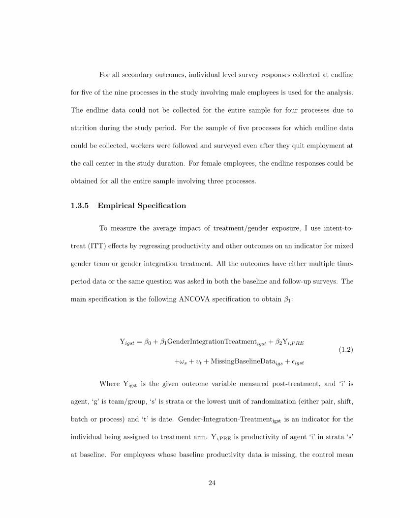
1.3.5 Empirical Specification

To measure the average impact of treatment/gender exposure, I use intent-to-

treat (ITT) e↵ects by regressing productivity and other outcomes on an indicator for mixed

gender team or gender integration treatment. All the outcomes have either multiple time-

period data or the same question was asked in both the baseline and follow-up surveys. The

main specification is the following ANCOVA specification to obtain �1:

Yigst = �0 + �1GenderIntegrationTreatmentigst + �2Yi,PRE

+!s + �t +MissingBaselineDataigs + ✏igst

(1.2)

Where Yigst is the given outcome variable measured post-treatment, and ‘i’ is

agent, ‘g’ is team/group, ‘s’ is strata or the lowest unit of randomization (either pair, shift,

batch or process) and ‘t’ is date. Gender-Integration-Treatmentigst is an indicator for the

individual being assigned to treatment arm. Yi,PRE is productivity of agent ‘i’ in strata ‘s’

at baseline. For employees whose baseline productivity data is missing, the control mean

24

value of 0 is assigned to them. Missing Baseline Dataigs is an indicator variable which takes

the value 1 if the employee was a new entrant and did not have any baseline productivity

information at the time of randomization, and it takes the value 0 if the employee had

baseline information. !s is strata fixed e↵ect, �t is date fixed e↵ect and ✏ist is the error

term. Standard errors are clustered at the team level to account for any correlated shocks

to productivity within teams.

This specification is run separately for male and female employees in the study.

There are 38 teams/clusters for male agents and 8 clusters for female employees. In cases

where an outcome variable was not collected at baseline, these same specifications is esti-

mated without the control for baseline outcome.

1.3.6 Randomization and Implementation Checks

Balance checks in Tables 1and 2 show that the randomization was successful on

baseline productivity and other individual characteristics of the sample. These balance

checks are conducted after controlling for strata fixed e↵ects (unit of randomization). The

most important variable for balance is baseline productivity and it passes the balance test

by failing to reject the null hypothesis that there is no di↵erence between the treatment

and control groups. There were some employees who left the call center before the study

began. They were included in the initial randomization because the call centers provided

old employee lists or failed to remove the employees who had submitted their resignation

prior to the randomization. Therefore, a selective attrition test is also conducted on the

remaining sample of male employees after accounting for attrition. Appendix Table 1 shows

25

that the treatment and controls arms were balanced on individual characteristics after

removing attriters.

1.4 Results

This section presents the results of the RCT on primary outcome measures. The

evidence on the extensive margins of productivity, share of days worked during the study

period is presented. On the intensive margin, impact on daily worker productivity is studied.

Heterogeneous e↵ects of treatment is also highlighted in the second subsection followed by

the results on secondary outcomes.

1.4.1 Results on primary outcome measures

For both male and female employees, there is no overall impact of being assigned

to gender integration treatment on share of days worked during the study (Table 3). The

control mean for male employees is 0.49 or male employees in the control group worked

for around 50% of the days of the study. The e↵ect of being assigned to a mixed gender

team meant a reduction of proportion of days worked by approximately 1.6% compared

to workers in all male teams (Table 3, column 1). The estimate is insignificant and is a

precisely estimated result with tight bounds around zero. The standard error is of 0.023

for male employees. The null value lies within 95% confidence interval [CI -0.037 to 0.053]

around the point estimate.

The female workers assigned to the control teams worked for a higher proportion of

days of about 56% in the study duration, than their male counterparts. The impact of being

assigned to mixed gender teams relative to same gender teams for females is approximately

26

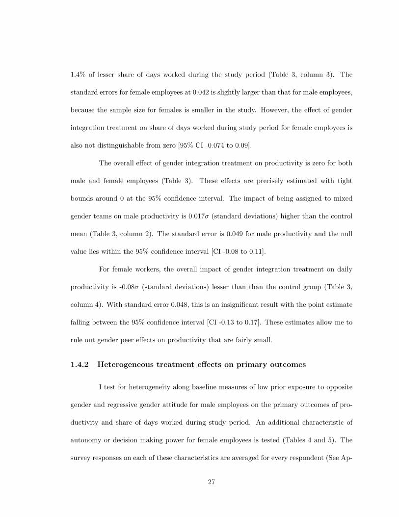
1.4% of lesser share of days worked during the study period (Table 3, column 3). The

standard errors for female employees at 0.042 is slightly larger than that for male employees,

because the sample size for females is smaller in the study. However, the e↵ect of gender

integration treatment on share of days worked during study period for female employees is

also not distinguishable from zero [95% CI -0.074 to 0.09].

The overall e↵ect of gender integration treatment on productivity is zero for both

male and female employees (Table 3). These e↵ects are precisely estimated with tight

bounds around 0 at the 95% confidence interval. The impact of being assigned to mixed

gender teams on male productivity is 0.017� (standard deviations) higher than the control

mean (Table 3, column 2). The standard error is 0.049 for male productivity and the null

value lies within the 95% confidence interval [CI -0.08 to 0.11].

For female workers, the overall impact of gender integration treatment on daily

productivity is -0.08� (standard deviations) lesser than than the control group (Table 3,

column 4). With standard error 0.048, this is an insignificant result with the point estimate

falling between the 95% confidence interval [CI -0.13 to 0.17]. These estimates allow me to

rule out gender peer e↵ects on productivity that are fairly small.

1.4.2 Heterogeneous treatment e↵ects on primary outcomes

I test for heterogeneity along baseline measures of low prior exposure to opposite

gender and regressive gender attitude for male employees on the primary outcomes of pro-

ductivity and share of days worked during study period. An additional characteristic of

autonomy or decision making power for female employees is tested (Tables 4 and 5). The

survey responses on each of these characteristics are averaged for every respondent (See Ap-

27

pendix section on survey questions) and then the median value of all the responses based on

gender is taken as cuto↵ to categorize same gender workers as high or low in that particular

characteristic. I do not find evidence for heterogeneity along these characteristics on share

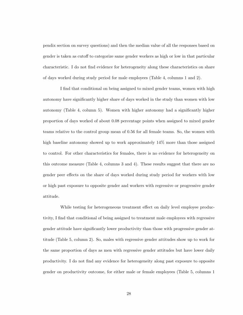
of days worked during study period for male employees (Table 4, columns 1 and 2).

I find that conditional on being assigned to mixed gender teams, women with high

autonomy have significantly higher share of days worked in the study than women with low

autonomy (Table 4, column 5). Women with higher autonomy had a significantly higher

proportion of days worked of about 0.08 percentage points when assigned to mixed gender

teams relative to the control group mean of 0.56 for all female teams. So, the women with

high baseline autonomy showed up to work approximately 14% more than those assigned

to control. For other characteristics for females, there is no evidence for heterogeneity on

this outcome measure (Table 4, columns 3 and 4). These results suggest that there are no

gender peer e↵ects on the share of days worked during study period for workers with low

or high past exposure to opposite gender and workers with regressive or progressive gender

attitude.

While testing for heterogeneous treatment e↵ect on daily level employee produc-

tivity, I find that conditional of being assigned to treatment male employees with regressive

gender attitude have significantly lower productivity than those with progressive gender at-

titude (Table 5, column 2). So, males with regressive gender attitudes show up to work for

the same proportion of days as men with regressive gender attitudes but have lower daily

productivity. I do not find any evidence for heterogeneity along past exposure to opposite

gender on productivity outcome, for either male or female employees (Table 5, columns 1

28

and 3). For female employees there is no evidence on characteristics of attitude and auton-

omy (Table 5, columns 4 and 5). This indicates that there is an overall zero treatment e↵ect

on female productivity along the distribution of these individual characteristics of opposite

gender exposure, gender attitude and autonomy/ empowerment.

1.4.3 Results on secondary outcome measures

I explore secondary outcomes using survey response at endline for male employees

and find strong positive impacts on knowledge sharing, dating and comfort with opposite

gender (Table 6).14 There is a 0.3� (standard deviations) increase in knowledge sharing,

which measures if the employee benefitted from agents sitting nearby on work related issues

(Table 6, column 3). This is a large treatment e↵ect which provides evidence of knowledge

spillover and learning for male employees assigned to mixed gender teams. This result is

significant at the 5% level. It indicates that male employees learn from female agents seated

next to them.

There is an increase of 19 percentage points in dating for male employees in treat-

ment teams, higher than the mean dating of 0.54 in the all male teams (Table 6, column

4). So, there was an increase of 35% in dating for male employees assigned to mixed gender

teams compared to the 54% dating in the control teams. This result is significant at the

5% level. However, the reporting is lower for this question as it was the last question of the

survey. A pre-intervention balance check was done on individual characteristics for men

14For male employees, the endline data is not available for the entire sample but for five of the nineprocesses. The result for these processes for which endline data is available is similar to the overall resultsfor main outcomes discussed in the previous sections (see Appendix table 2).

29

who responded to the dating question and those who didn’t and the two groups were found

to be similar.

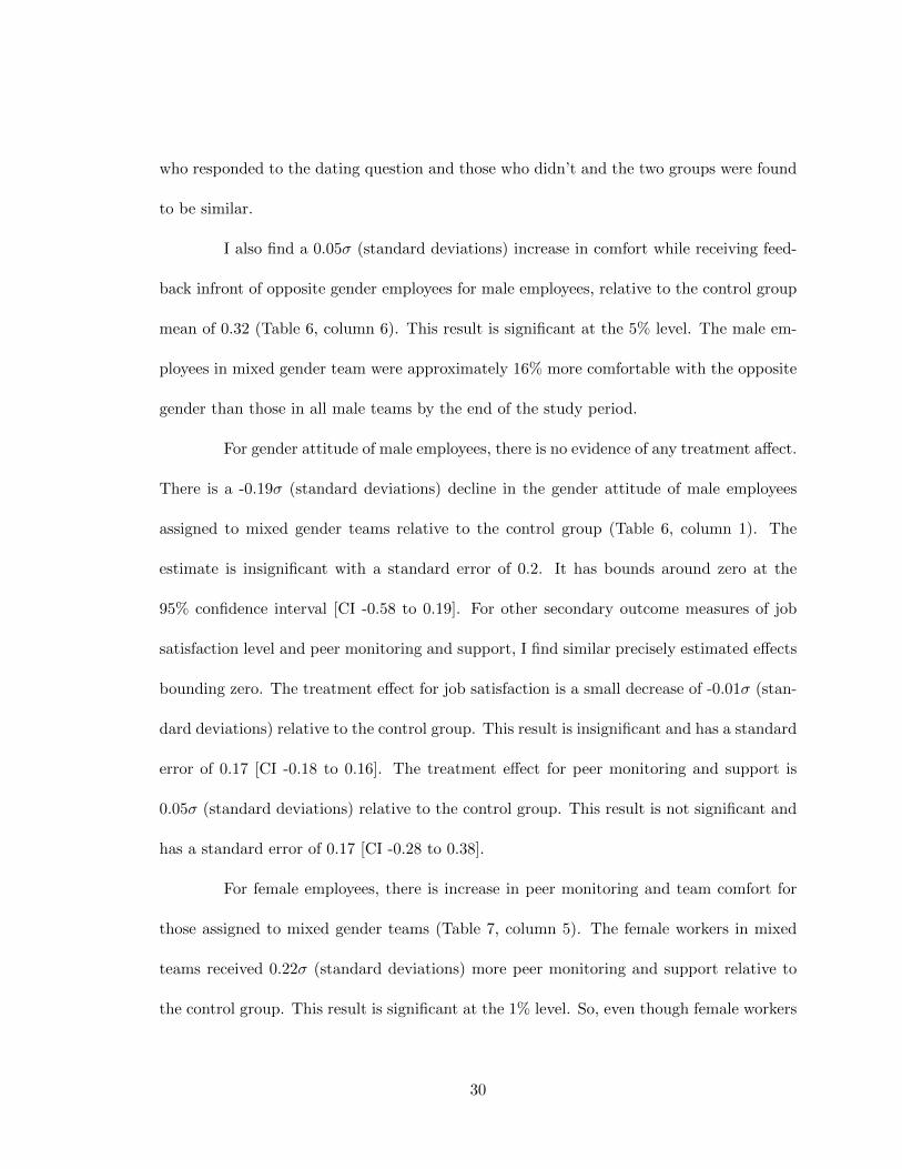
I also find a 0.05� (standard deviations) increase in comfort while receiving feed-

back infront of opposite gender employees for male employees, relative to the control group

mean of 0.32 (Table 6, column 6). This result is significant at the 5% level. The male em-

ployees in mixed gender team were approximately 16% more comfortable with the opposite

gender than those in all male teams by the end of the study period.

For gender attitude of male employees, there is no evidence of any treatment a↵ect.

There is a -0.19� (standard deviations) decline in the gender attitude of male employees

assigned to mixed gender teams relative to the control group (Table 6, column 1). The

estimate is insignificant with a standard error of 0.2. It has bounds around zero at the

95% confidence interval [CI -0.58 to 0.19]. For other secondary outcome measures of job

satisfaction level and peer monitoring and support, I find similar precisely estimated e↵ects

bounding zero. The treatment e↵ect for job satisfaction is a small decrease of -0.01� (stan-

dard deviations) relative to the control group. This result is insignificant and has a standard

error of 0.17 [CI -0.18 to 0.16]. The treatment e↵ect for peer monitoring and support is

0.05� (standard deviations) relative to the control group. This result is not significant and

has a standard error of 0.17 [CI -0.28 to 0.38].

For female employees, there is increase in peer monitoring and team comfort for

those assigned to mixed gender teams (Table 7, column 5). The female workers in mixed

teams received 0.22� (standard deviations) more peer monitoring and support relative to

the control group. This result is significant at the 1% level. So, even though female workers

30

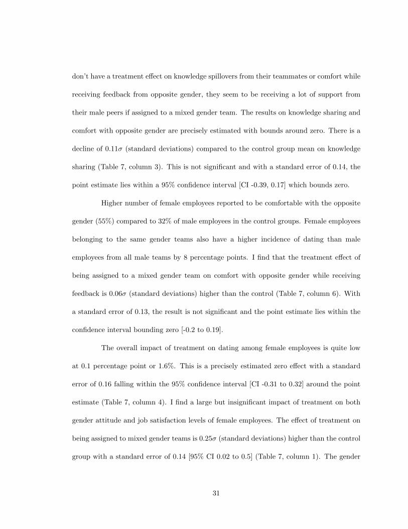
don’t have a treatment e↵ect on knowledge spillovers from their teammates or comfort while

receiving feedback from opposite gender, they seem to be receiving a lot of support from

their male peers if assigned to a mixed gender team. The results on knowledge sharing and

comfort with opposite gender are precisely estimated with bounds around zero. There is a

decline of 0.11� (standard deviations) compared to the control group mean on knowledge

sharing (Table 7, column 3). This is not significant and with a standard error of 0.14, the

point estimate lies within a 95% confidence interval [CI -0.39, 0.17] which bounds zero.

Higher number of female employees reported to be comfortable with the opposite

gender (55%) compared to 32% of male employees in the control groups. Female employees

belonging to the same gender teams also have a higher incidence of dating than male

employees from all male teams by 8 percentage points. I find that the treatment e↵ect of

being assigned to a mixed gender team on comfort with opposite gender while receiving

feedback is 0.06� (standard deviations) higher than the control (Table 7, column 6). With

a standard error of 0.13, the result is not significant and the point estimate lies within the

confidence interval bounding zero [-0.2 to 0.19].

The overall impact of treatment on dating among female employees is quite low

at 0.1 percentage point or 1.6%. This is a precisely estimated zero e↵ect with a standard

error of 0.16 falling within the 95% confidence interval [CI -0.31 to 0.32] around the point

estimate (Table 7, column 4). I find a large but insignificant impact of treatment on both

gender attitude and job satisfaction levels of female employees. The e↵ect of treatment on

being assigned to mixed gender teams is 0.25� (standard deviations) higher than the control

group with a standard error of 0.14 [95% CI 0.02 to 0.5] (Table 7, column 1). The gender

31

integration treatment e↵ect on job satisfaction level is 0.27� (standard deviations) higher

than the control with a standard error of 0.17 [95% CI 0.02 -0.06 to 0.6] (Table 7, column

2).

1.5 Discussion and Conclusion

This study provides an experimental test of productivity impacts for employees

with mixed gender composition of peers in the workplace, against employees with same

gender peers. Competing forces of knowledge spillovers, dating and socialization, comfort

and peer monitoring are also studied. I find a precisely estimated overall zero e↵ect on

daily productivity and share of days worked during study period for both males and females

assigned to mixed gender teams relative to control groups of same gender teams.

Research on productivity improvements in the high growth sector BPO industry

is crucial for sustainable job creation for many young workers, particularly women. Due

to growth and increases in employment opportunities, women who were previously doing

unpaid care work or informal work, are entering the formal labor market in regions like

Patna and Udaipur. These call centers also attract young workers from nearby villages and

small towns. The policy makers in India are interested in expanding this sector to more

of these smaller cities and even villages. Under the IBPS scheme, the government gives

incentives to firms to open up branches in these smaller places and also provides additional

incentive to call centers to hire female employees to boost their labor supply. The paper

provides supportive evidence to strengthen the objective of the policy makers. It also

informs firms skeptical of integrating women into the workplace that integration of women

32

into the workplace is not costly, as gender diversity and interactions in the workplace do

not impact the productivity of a worker negatively.

Even though this study has implications on all kinds of gender diverse workplaces,

there might be more positive e↵ects on the intensive margin of productivity in places with

lesser gender discrimination and progressive gender attitudes for male employees. Similarly,

the treatment e↵ects on extensive margins of share of days worked during study period

may be higher for women with higher autonomy. Increases in knowledge sharing, peer

monitoring and comfort of receiving feedback infront of opposite gender in mixed gender

teams is evidence that there is higher knowledge spillovers in gender integrated settings.

Therefore, the firms may benefit from policies of gender-integrated seating, such as the one

practiced in the study in mixed gender teams with alternate seating of opposite gender

employees in increasing knowledge spillovers and learning for male employees and peer

monitoring and comfort for female employees. This may prove a low cost way of increasing

learning among coworkers in firms.

In India, more than 90% of the marriages are arranged by the families (Centre for

Monitoring Indian Economy, 2018). There is high prevalence of caste-based segregation and

intra-caste marriages especially among the poor. The increase in dating for men in mixed

gender teams in the setting of mostly small town India, is an interesting finding.

33

Bibliography

[1] Renee B Adams and Daniel Ferreira. Women in the boardroom and their impact ongovernance and performance. Journal of financial economics, 94(2):291–309, 2009.

[2] Kenneth R Ahern and Amy K Dittmar. The changing of the boards: The impact onfirm valuation of mandated female board representation. The Quarterly Journal ofEconomics, 127(1):137–197, 2012.

[3] George A Akerlof and Rachel E Kranton. Economics and identity. The QuarterlyJournal of Economics, 115(3):715–753, 2000.

[4] Francesco Amodio and Miguel A Martinez-Carrasco. Input allocation, workforce man-agement and productivity spillovers: Evidence from personnel data. The Review ofEconomic Studies, 85(4):1937–1970, 2018.

[5] Heather Antecol, Ozkan Eren, and Serkan Ozbeklik. Peer e↵ects in disadvantagedprimary schools evidence from a randomized experiment. Journal of Human Resources,51(1):95–132, 2016.

[6] Jose Apesteguia, Ghazala Azmat, and Nagore Iriberri. The impact of gender composi-tion on team performance and decision making: Evidence from the field. ManagementScience, 58(1):78–93, 2012.

[7] Oriana Bandiera, Iwan Barankay, and Imran Rasul. Social incentives in the workplace.The review of economic studies, 77(2):417–458, 2010.

[8] Lori Beaman, Raghabendra Chattopadhyay, Esther Duflo, Rohini Pande, and PetiaTopalova. Powerful women: does exposure reduce bias? The Quarterly journal ofeconomics, 124(4):1497–1540, 2009.

[9] Marianne Bertrand, Sandra E Black, Sissel Jensen, and Adriana Lleras-Muney. Break-ing the glass ceiling? the e↵ect of board quotas on female labour market outcomes innorway. The Review of Economic Studies, 86(1):191–239, 2018.

[10] Marianne Bertrand, Emir Kamenica, and Jessica Pan. Gender identity and relativeincome within households. The Quarterly Journal of Economics, 130(2):571–614, 2015.

[11] Sandra E Black, Paul J Devereux, and Kjell G Salvanes. Under pressure? the e↵ect ofpeers on outcomes of young adults. Journal of Labor Economics, 31(1):119–153, 2013.

34

[12] Alison L Booth and Eiji Yamamura. Performance in mixed-sex and single-sex tourna-ments: What we can learn from speedboat races in japan. 2016.

[13] Afra R Chowdhury, Ana C Areias, Saori Imaizumi, Shinsaku Nomura, and FutoshiYamauchi. Reflections of employers’ gender preferences in job ads in India: an analysisof online job portal data. The World Bank, 2018.

[14] Thomas Cornelissen, Christian Dustmann, and Uta Schonberg. Peer e↵ects in theworkplace. American Economic Review, 107(2):425–56, 2017.

[15] Gordon Dahl, Andreas Kotsadam, and Dan-Olof Rooth. Does integration change gen-der attitudes? the e↵ect of randomly assigning women to traditionally male teams.Technical report, National Bureau of Economic Research, 2018.

[16] Diva Dhar, Tarun Jain, and Seema Jayachandran. Reshaping adolescents’ gender at-titudes: Evidence from a school-based experiment in india. Technical report, NationalBureau of Economic Research, 2018.

[17] Malathy Duraisamy and P Duraisamy. Occupational segregation, wage and job dis-crimination against women across social groups in the indian labor market: 1983–2010.Preliminary Draft. Accessed on, 11(08):2017, 2014.

[18] Henning Finseraas, Ashild A Johnsen, Andreas Kotsadam, and Gaute Torsvik. Expo-sure to female colleagues breaks the glass ceiling—evidence from a combined vignetteand field experiment. European Economic Review, 90:363–374, 2016.

[19] Rachel Glennerster, Claire Walsh, and Lucia Diaz-Martin. A practical guide to mea-suring women’s and girls’ empowerment in impact evaluations. Gender Sector, AbdulLatif Jameel Poverty Action Lab, 2018.

[20] Claudia Goldin. The u-shaped female labor force function in economic developmentand economic history. Technical report, National Bureau of Economic Research, 1994.

[21] Claudia Goldin. A grand gender convergence: Its last chapter. American EconomicReview, 104(4):1091–1119, 2014.

[22] Jie Gong, Yi Lu, and Hong Song. Gender peer e↵ects on students’ academic andnoncognitive outcomes: Evidence and mechanisms. Journal of Human Resources, pages0918–9736R2, 2019.

[23] Barton H Hamilton, Jack A Nickerson, and Hideo Owan. Diversity and productivity inproduction teams. In Advances in the Economic Analysis of participatory and Labor-managed Firms, pages 99–138. Emerald Group Publishing Limited, 2012.

[24] Zeynep Hansen, Hideo Owan, and Jie Pan. The impact of group diversity on perfor-mance and knowledge spillover–an experiment in a college classroom. Technical report,National Bureau of Economic Research, 2006.

[25] Andrew J Hill. The positive influence of female college students on their male peers.Labour Economics, 44:151–160, 2017.

35

[26] Jonas Hjort. Ethnic divisions and production in firms. The Quarterly Journal ofEconomics, 129(4):1899–1946, 2014.

[27] Sander Hoogendoorn, Hessel Oosterbeek, and Mirjam Van Praag. The impact of genderdiversity on the performance of business teams: Evidence from a field experiment.Management Science, 59(7):1514–1528, 2013.

[28] Caroline Hoxby. Peer e↵ects in the classroom: Learning from gender and race variation.Technical report, National Bureau of Economic Research, 2000.

[29] Andrea Ichino and Armin Falk. Clean evidence on peer e↵ects. Journal of LaborEconomics, 24, 2005.

[30] C Kirabo Jackson. Single-sex schools, student achievement, and course selection: Evi-dence from rule-based student assignments in trinidad and tobago. Journal of PublicEconomics, 96(1-2):173–187, 2012.

[31] Eugene Kandel and Edward P Lazear. Peer pressure and partnerships. Journal ofpolitical Economy, 100(4):801–817, 1992.

[32] Supreet Kaur, Michael Kremer, and Sendhil Mullainathan. Self-control and the devel-opment of work arrangements. American Economic Review, 100(2):624–28, 2010.

[33] Victor Lavy and Analia Schlosser. Mechanisms and impacts of gender peer e↵ects atschool. American Economic Journal: Applied Economics, 3(2):1–33, 2011.

[34] Soohyung Lee, Lesley J Turner, Seokjin Woo, and Kyunghee Kim. All or nothing? theimpact of school and classroom gender composition on e↵ort and academic achievement.Technical report, National Bureau of Economic Research, 2014.

[35] Matt Lowe. Unity in cricket: Integrated leagues and caste divisions. 2018.

[36] Fangwen Lu and Michael L Anderson. Peer e↵ects in microenvironments: The benefitsof homogeneous classroom groups. Journal of Labor Economics, 33(1):91–122, 2014.

[37] Elizabeth Lyons. Team production in international labor markets: Experimental ev-idence from the field. American Economic Journal: Applied Economics, 9(3):70–104,2017.

[38] Charles F Manski. Identification of endogenous social e↵ects: The reflection problem.The review of economic studies, 60(3):531–542, 1993.

[39] Alexandre Mas and Enrico Moretti. Peers at work. American Economic Review,99(1):112–45, 2009.

[40] David A Matsa and Amalia R Miller. A female style in corporate leadership? evidencefrom quotas. American Economic Journal: Applied Economics, 5(3):136–69, 2013.

[41] Muriel Niederle and Lise Vesterlund. Do women shy away from competition? do mencompete too much? The quarterly journal of economics, 122(3):1067–1101, 2007.

36

[42] Sangyoon Park. Socializing at work: Evidence from a field experiment with manu-facturing workers. American Economic Journal: Applied Economics, 11(3):424–55,2019.

[43] Gautam Rao. Familiarity does not breed contempt: Generosity, discrimination anddiversity in delhi schools. Manuscript, Univ. California, Berkeley, 2013.

[44] David Watson, Lee Anna Clark, and Auke Tellegen. Development and validation ofbrief measures of positive and negative a↵ect: the panas scales. Journal of personalityand social psychology, 54(6):1063, 1988.

[45] Diane Whitmore. Resource and peer impacts on girls’ academic achievement: Evidencefrom a randomized experiment. American Economic Review, 95(2):199–203, 2005.

37

ACKNOWLEDGEMENTS

The dissertation author is the primary investigator and author of this paper. The

RCT was pre-registered at the AEA registry with ID # AEARCTR-0003932.

I am grateful for the invaluable guidance, immense support and unwavering en-

couragement over the course of this project from my advisors, Anil Deolalikar, Sarojini

Hirshleifer and Joseph Cummins. This paper has also benefitted from helpful comments

from Steven Helfand, Ozkan Eren, Michael Bates, Carolyn Sloane, Bree Lang, Matthew

Lang, Gordon Dahl, Jonas Hjort and the faculty mentors as well as the faculty mentors and

selected workshop participants at the Ronald Coase Institute.

I would like to thank the International Growth Center (IGC), BLUM Initiative

at UC Riverside and Graduate Division, UC Riverside (Dissertation Year Program Fellow-

ship) for funding this project. I am grateful to the CEOs and center heads of partner call

centers, Anil Sinha, Rajeev Jha and Sujit Sharma of Call-2-Connect and Kapil Sharma,

Lakhan Joshi and Soham Ghosh of Five Splash for believing in the project and o↵ering

their support. I appreciate the help of Ministry of Electronics and IT: Government of In-

dia, Software Technology Parks of India and Bihar Industries Association for introducing

and recommending this project to call centers.

Thanks also to Anil Kumar Vaishnav, Daizzy Sharma, Prabudh Rao Kaushal,

Rajat Kumar, Priti Rao and Priyanka Jadhav for their outstanding assistance in data

collection. This project could not have taken been completed successfully without the

participation of the study subjects and the support of all the team leaders, managers, HR

38

and MIS teams at the call centers.

I appreciate the help of Mr. Anshuman Gaur, Private Secretary to Minister for

Law and Justice & Electronics and IT and Mr. Rajiv Kumar, Joint Secretary at Ministry of

Electronics and IT at Government of India (MEIT: GOI); Mr. Devesh Tyagi, Senior Director

at Software Technology Parks of India (STPI), Mr. Madhurjya Prakash Baruah, Additional

Director at STPI and Mr. K.P.S. Keshri, President of Bihar Industries Association (BIA)

for introducing and recommending this project to call centers. I also want to thank my

friend Vibhu Mishra for helping me connect to call centers.

All views expressed in this paper are those of the author alone and need not

necessarily reflect those of the call centers, MEIT: GOI, STPI or BIA.

39

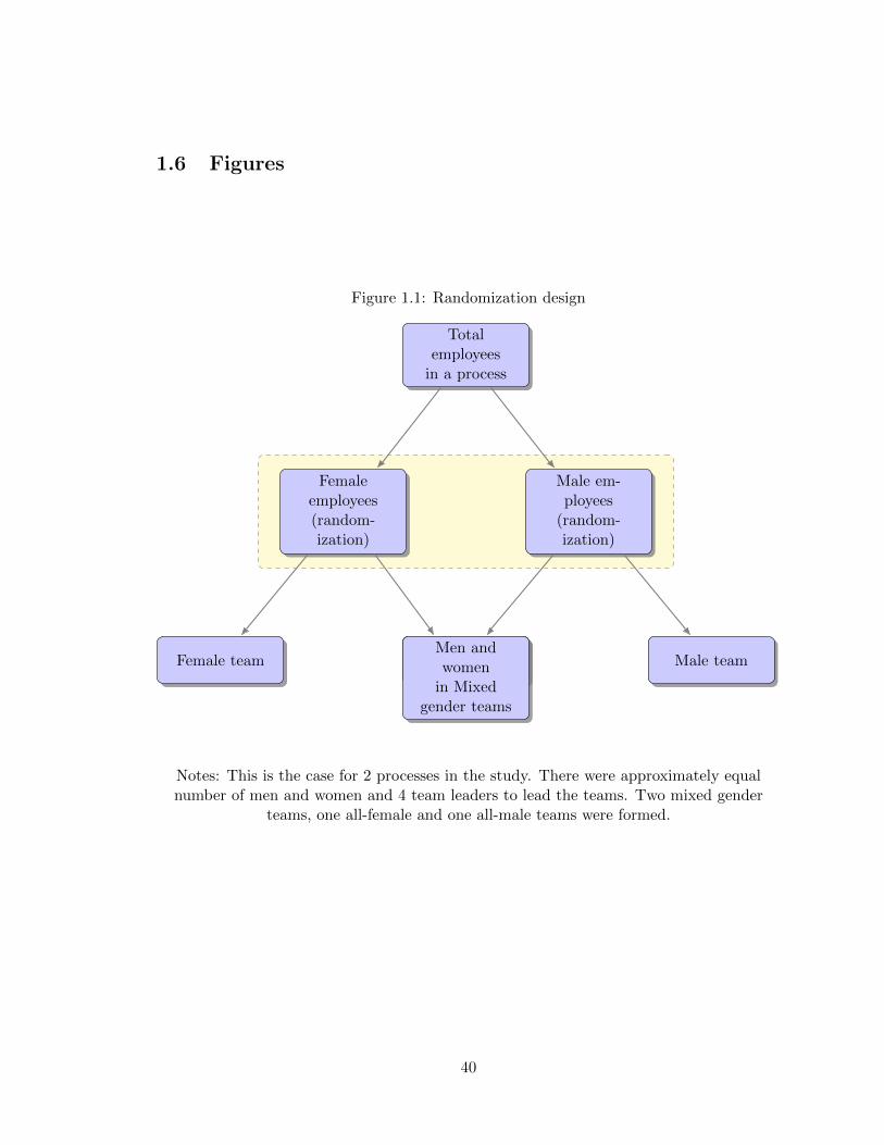
1.6 Figures

Figure 1.1: Randomization design

Totalemployeesin a process

Male em-ployees(random-ization)

Male teamMen in

mixed teams

Femaleemployees(random-ization)

Men andwomenin Mixed

gender teams

Female team

Notes: This is the case for 2 processes in the study. There were approximately equalnumber of men and women and 4 team leaders to lead the teams. Two mixed gender

teams, one all-female and one all-male teams were formed.

40

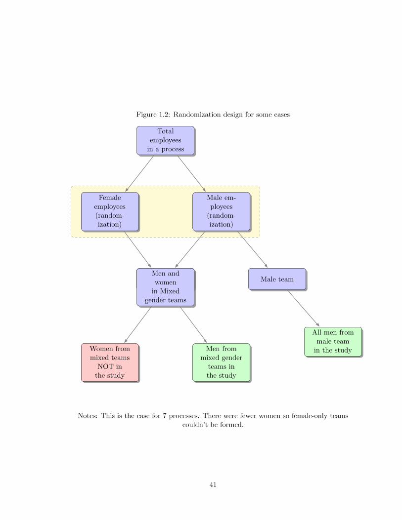
Figure 1.2: Randomization design for some cases

Totalemployeesin a process

Male em-ployees(random-ization)

Male team

All men frommale teamin the study

Men inmixed teams

Femaleemployees(random-ization)

Men andwomenin Mixed

gender teams

Men frommixed gender

teams inthe study

Women frommixed teams

NOT inthe study

Notes: This is the case for 7 processes. There were fewer women so female-only teamscouldn’t be formed.

41

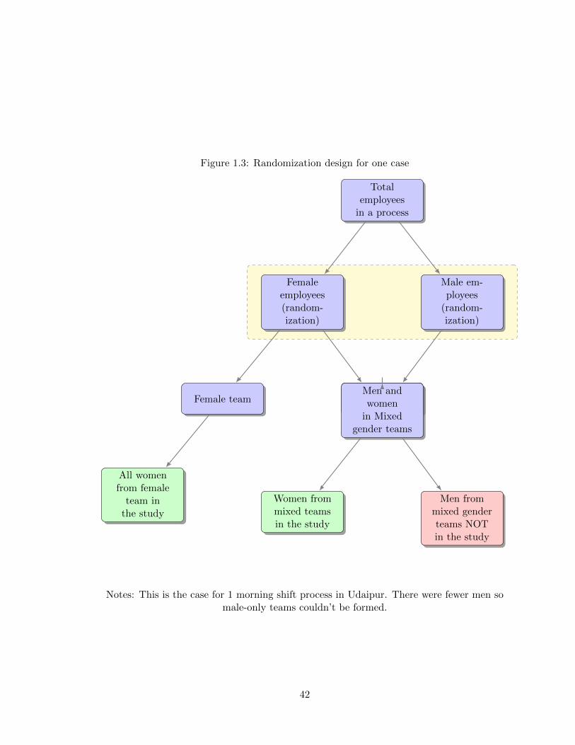
Figure 1.3: Randomization design for one case

Totalemployeesin a process

Male em-ployees(random-ization)

Men inmixed teams

Femaleemployees(random-ization)

Men andwomenin Mixed

gender teams

Men frommixed genderteams NOTin the study

Women frommixed teamsin the study

Female team

All womenfrom femaleteam inthe study

Notes: This is the case for 1 morning shift process in Udaipur. There were fewer men somale-only teams couldn’t be formed.

42

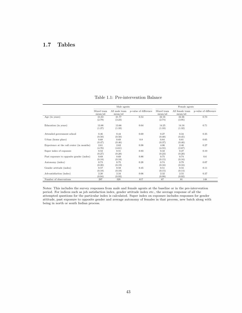
1.7 Tables

Table 1.1: Pre-intervention Balance

Male agents Female agents

Mixed team All male team p-value of di↵erence Mixed team All female team p-value of di↵erencemean/sd mean/sd mean/sd mean/sd

Age (in years) 21.63 21.77 0.54 22.16 22.36 0.73(2.79) (3.23) (2.74) (3.95)

Education (in years) 13.88 13.66 0.04 14.25 14.16 0.71(1.27) (1.33) (1.33) (1.32)

Attended government school 0.46 0.44 0.69 0.27 0.34 0.35(0.50) (0.50) (0.48) (0.45)

Urban (home place) 0.68 0.69 0.8 0.84 0.81 0.65(0.47) (0.46) (0.37) (0.40)

Experience at the call center (in months) 2.61 2.62 0.98 4.06 2.46 0.27(4.76) (4.61) (4.55) (2.67)

Super index of exposure 0.52 0.51 0.93 0.32 0.27 0.10(0.27) (0.28) (0.23) (0.20)

Past exposure to opposite gender (index) 0.69 0.69 0.86 0.75 0.74 0.6(0.18) (0.18) (0.15) (0.16)

Autonomy (index) 0.73 0.75 0.28 0.74 0.79 0.07(0.20) (0.19) (0.16) (0.16)

Gender attitude (index) 0.57 0.58 0.45 0.51 0.55 0.11(0.18) (0.18) (0.15) (0.14)

Job-satisfaction (index) 2.20 2.34 0.06 2.32 2.55 0.37(0.94) (0.93) (0.99) (0.92)

Number of observations 297 320 617 67 81 148

Notes: This includes the survey responses from male and female agents at the baseline or in the pre-interventionperiod. For indices such as job satisfaction index, gender attitude index etc., the average response of all theattempted questions for the particular index is calculated. Super index on exposure includes responses for genderattitude, past exposure to opposite gender and average autonomy of females in that process, new batch along withbeing in north or south Indian process.

43

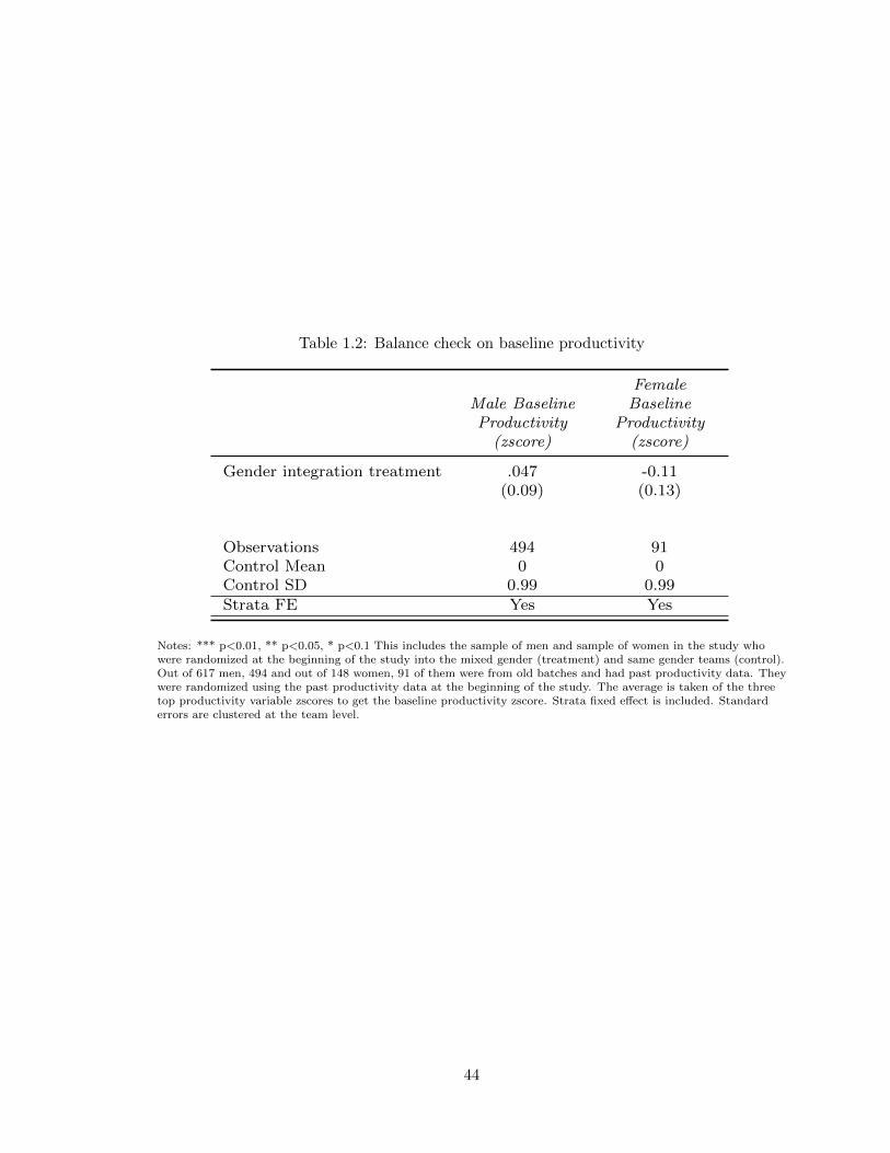
Table 1.2: Balance check on baseline productivity

Male BaselineProductivity(zscore)

FemaleBaseline

Productivity(zscore)

Gender integration treatment .047 -0.11(0.09) (0.13)

Observations 494 91Control Mean 0 0Control SD 0.99 0.99Strata FE Yes Yes

Notes: *** p<0.01, ** p<0.05, * p<0.1 This includes the sample of men and sample of women in the study whowere randomized at the beginning of the study into the mixed gender (treatment) and same gender teams (control).Out of 617 men, 494 and out of 148 women, 91 of them were from old batches and had past productivity data. Theywere randomized using the past productivity data at the beginning of the study. The average is taken of the threetop productivity variable zscores to get the baseline productivity zscore. Strata fixed e↵ect is included. Standarderrors are clustered at the team level.

44

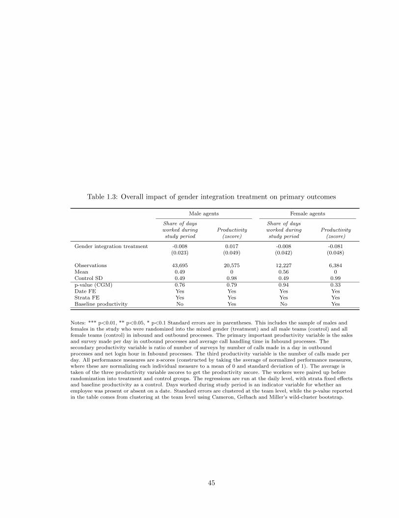
Table 1.3: Overall impact of gender integration treatment on primary outcomes

Male agents Female agents

Share of daysworked duringstudy period

Productivity(zscore)

Share of daysworked duringstudy period

Productivity(zscore)

Gender integration treatment -0.008 0.017 -0.008 -0.081(0.023) (0.049) (0.042) (0.048)

Observations 43,695 20,575 12,227 6,384Mean 0.49 0 0.56 0Control SD 0.49 0.98 0.49 0.99p-value (CGM) 0.76 0.79 0.94 0.33Date FE Yes Yes Yes YesStrata FE Yes Yes Yes YesBaseline productivity No Yes No Yes

Notes: *** p<0.01, ** p<0.05, * p<0.1 Standard errors are in parentheses. This includes the sample of males andfemales in the study who were randomized into the mixed gender (treatment) and all male teams (control) and allfemale teams (control) in inbound and outbound processes. The primary important productivity variable is the salesand survey made per day in outbound processes and average call handling time in Inbound processes. Thesecondary productivity variable is ratio of number of surveys by number of calls made in a day in outboundprocesses and net login hour in Inbound processes. The third productivity variable is the number of calls made perday. All performance measures are z-scores (constructed by taking the average of normalized performance measures,where these are normalizing each individual measure to a mean of 0 and standard deviation of 1). The average istaken of the three productivity variable zscores to get the productivity zscore. The workers were paired up beforerandomization into treatment and control groups. The regressions are run at the daily level, with strata fixed e↵ectsand baseline productivity as a control. Days worked during study period is an indicator variable for whether anemployee was present or absent on a date. Standard errors are clustered at the team level, while the p-value reportedin the table comes from clustering at the team level using Cameron, Gelbach and Miller’s wild-cluster bootstrap.

45

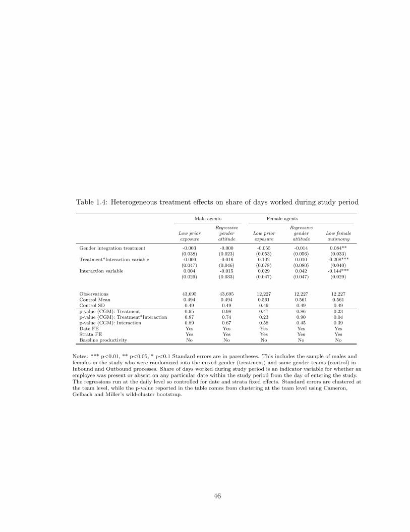
Table 1.4: Heterogeneous treatment e↵ects on share of days worked during study period

Male agents Female agents

Low priorexposure

Regressivegenderattitude

Low priorexposure

Regressivegenderattitude

Low femaleautonomy

Gender integration treatment -0.003 -0.000 -0.055 -0.014 0.084**(0.038) (0.023) (0.053) (0.056) (0.033)

Treatment*Interaction variable -0.009 -0.016 0.102 0.010 -0.208***(0.047) (0.046) (0.078) (0.080) (0.040)

Interaction variable 0.004 -0.015 0.029 0.042 -0.144***(0.029) (0.033) (0.047) (0.047) (0.029)

Observations 43,695 43,695 12,227 12,227 12,227Control Mean 0.494 0.494 0.561 0.561 0.561Control SD 0.49 0.49 0.49 0.49 0.49p-value (CGM): Treatment 0.95 0.98 0.47 0.86 0.23p-value (CGM): Treatment*Interaction 0.87 0.74 0.23 0.90 0.04p-value (CGM): Interaction 0.89 0.67 0.58 0.45 0.39Date FE Yes Yes Yes Yes YesStrata FE Yes Yes Yes Yes YesBaseline productivity No No No No No

Notes: *** p<0.01, ** p<0.05, * p<0.1 Standard errors are in parentheses. This includes the sample of males andfemales in the study who were randomized into the mixed gender (treatment) and same gender teams (control) inInbound and Outbound processes. Share of days worked during study period is an indicator variable for whether anemployee was present or absent on any particular date within the study period from the day of entering the study.The regressions run at the daily level so controlled for date and strata fixed e↵ects. Standard errors are clustered atthe team level, while the p-value reported in the table comes from clustering at the team level using Cameron,Gelbach and Miller’s wild-cluster bootstrap.

46

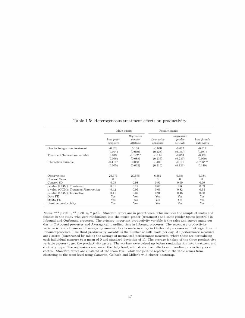
Table 1.5: Heterogeneous treatment e↵ects on productivity

Male agents Female agents

Low priorexposure

Regressivegenderattitude

Low priorexposure

Regressivegenderattitude

Low femaleautonomy

Gender integration treatment -0.023 0.105 -0.030 -0.062 -0.012(0.074) (0.069) (0.128) (0.080) (0.087)

Treatment*Interaction variable 0.079 -0.192** -0.114 -0.053 -0.128(0.096) (0.088) (0.236) (0.239) (0.090)

Interaction variable -0.114* 0.058 -0.011 -0.101 -0.706***(0.065) (0.062) (0.210) (0.123) (0.149)

Observations 20,575 20,575 6,384 6,384 6,384Control Mean 0 0 0 0 0Control SD 0.98 0.98 0.99 0.99 0.99p-value (CGM): Treatment 0.81 0.19 0.86 0.6 0.89p-value (CGM): Treatment*Interaction 0.42 0.05 0.63 0.82 0.34p-value (CGM): Interaction 0.11 0.32 0.91 0.46 0.58Date FE Yes Yes Yes Yes YesStrata FE Yes Yes Yes Yes YesBaseline productivity Yes Yes Yes Yes Yes

Notes: *** p<0.01, ** p<0.05, * p<0.1 Standard errors are in parentheses. This includes the sample of males andfemales in the study who were randomized into the mixed gender (treatment) and same gender teams (control) inInbound and Outbound processes. The primary important productivity variable is the sales and survey made perday in Outbound processes and Average call handling time in Inbound processes. The secondary productivityvariable is ratio of number of surveys by number of calls made in a day in Outbound processes and net login hour inInbound processes. The third productivity variable is the number of calls made per day. All performance measuresare z-scores (constructed by taking the average of normalized performance measures, where these are normalizingeach individual measure to a mean of 0 and standard deviation of 1). The average is taken of the three productivityvariable zscores to get the productivity zscore. The workers were paired up before randomization into treatment andcontrol groups. The regressions are run at the daily level, with strata fixed e↵ects and baseline productivity as acontrol. Standard errors are clustered at the team level, while the p-value reported in the table comes fromclustering at the team level using Cameron, Gelbach and Miller’s wild-cluster bootstrap.

47

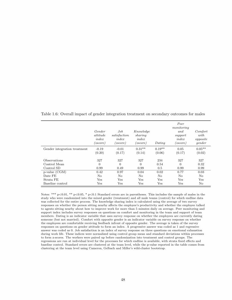
Table 1.6: Overall impact of gender integration treatment on secondary outcomes for males

Genderattitudeindex

(zscore)

Jobsatisfaction

index(zscore)

Knowledgesharingindex

(zscore) Dating

Peermonitoring

andsupportindex

(zscore)

Comfortwith

oppositegender

Gender integration treatment -0.19 -0.01 0.31** 0.19** 0.05 0.05**(0.20) (0.17) (0.14) (0.06) (0.17) (0.02)

Observations 327 327 327 234 327 327Control Mean 0 0 0 0.54 0 0.32Control SD 0.99 0.49 0.99 0.5 0.99 0.99p-value (CGM) 0.42 0.97 0.04 0.02 0.77 0.03Date FE No No No No No NoStrata FE Yes Yes Yes Yes Yes YesBaseline control Yes Yes Yes Yes Yes No

Notes: *** p<0.01, ** p<0.05, * p<0.1 Standard errors are in parentheses. This includes the sample of males in thestudy who were randomized into the mixed gender (treatment) and all male teams (control) for which endline datawas collected for the entire process. The knowledge sharing index is calculated using the average of two surveyresponses on whether the person sitting nearby a↵ects the employee’s productivity and whether the employee talkedto agents sitting nearby about how to improve work for more than 5 minutes daily on average. Peer monitoring andsupport index includes survey responses on questions on comfort and monitoring in the team and support of teammembers. Dating is an indicator variable that uses survey response on whether the employees are currently datingsomeone (but not married). Comfort with opposite gender is an indicator variable on survey response on whetherthe employees are comfortable receiving feedback infront of opposite gender. The average is taken of the surveyresponses on questions on gender attitude to form an index. A progressive answer was coded as 1 and regressiveanswer was coded as 0. Job satisfaction is an index of survey response on three questions on emotional exhaustionduring work life. These indices were normalized using control group mean and standard deviations within processesto form z-scores. The workers were paired up before randomization into treatment and control groups. Theregressions are run at individual level for the processes for which endline is available, with strata fixed e↵ects andbaseline control. Standard errors are clustered at the team level, while the p-value reported in the table comes fromclustering at the team level using Cameron, Gelbach and Miller’s wild-cluster bootstrap.

48

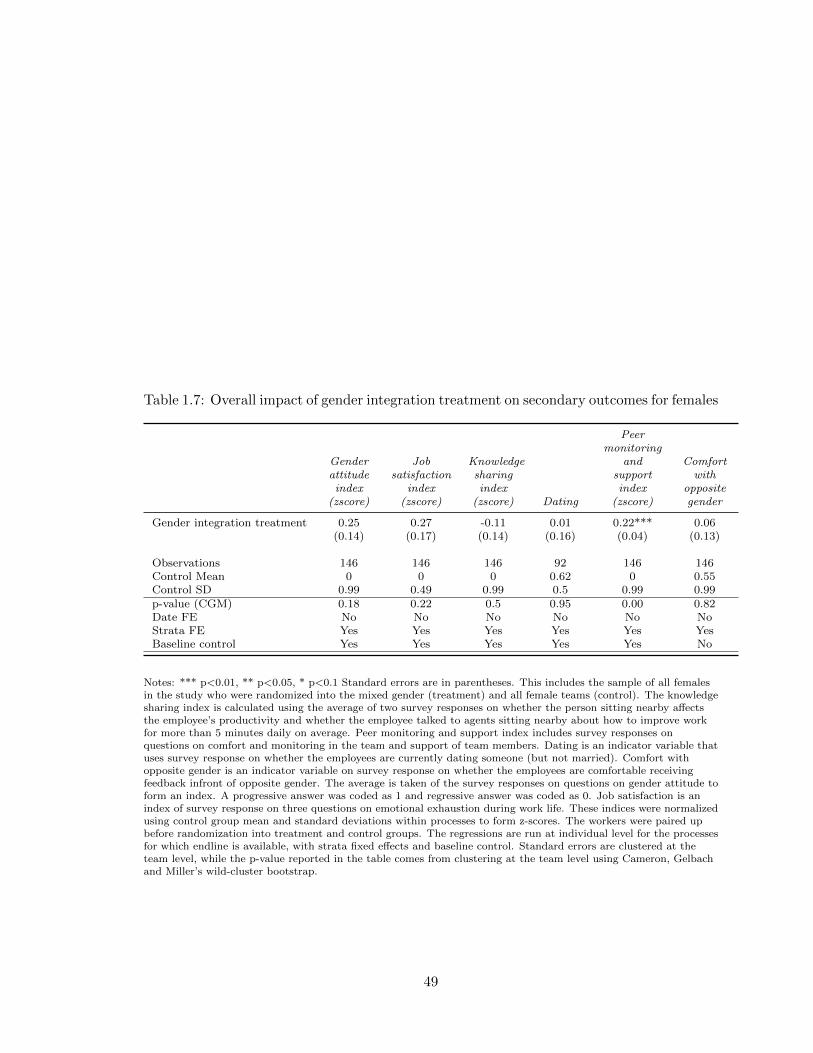
Table 1.7: Overall impact of gender integration treatment on secondary outcomes for females

Genderattitudeindex

(zscore)

Jobsatisfaction

index(zscore)

Knowledgesharingindex

(zscore) Dating

Peermonitoring

andsupportindex

(zscore)

Comfortwith

oppositegender

Gender integration treatment 0.25 0.27 -0.11 0.01 0.22*** 0.06(0.14) (0.17) (0.14) (0.16) (0.04) (0.13)

Observations 146 146 146 92 146 146Control Mean 0 0 0 0.62 0 0.55Control SD 0.99 0.49 0.99 0.5 0.99 0.99p-value (CGM) 0.18 0.22 0.5 0.95 0.00 0.82Date FE No No No No No NoStrata FE Yes Yes Yes Yes Yes YesBaseline control Yes Yes Yes Yes Yes No

Notes: *** p<0.01, ** p<0.05, * p<0.1 Standard errors are in parentheses. This includes the sample of all femalesin the study who were randomized into the mixed gender (treatment) and all female teams (control). The knowledgesharing index is calculated using the average of two survey responses on whether the person sitting nearby a↵ectsthe employee’s productivity and whether the employee talked to agents sitting nearby about how to improve workfor more than 5 minutes daily on average. Peer monitoring and support index includes survey responses onquestions on comfort and monitoring in the team and support of team members. Dating is an indicator variable thatuses survey response on whether the employees are currently dating someone (but not married). Comfort withopposite gender is an indicator variable on survey response on whether the employees are comfortable receivingfeedback infront of opposite gender. The average is taken of the survey responses on questions on gender attitude toform an index. A progressive answer was coded as 1 and regressive answer was coded as 0. Job satisfaction is anindex of survey response on three questions on emotional exhaustion during work life. These indices were normalizedusing control group mean and standard deviations within processes to form z-scores. The workers were paired upbefore randomization into treatment and control groups. The regressions are run at individual level for the processesfor which endline is available, with strata fixed e↵ects and baseline control. Standard errors are clustered at theteam level, while the p-value reported in the table comes from clustering at the team level using Cameron, Gelbachand Miller’s wild-cluster bootstrap.

49

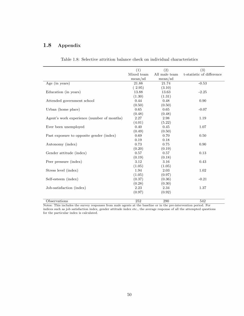
1.8 Appendix

Table 1.8: Selective attrition balance check on individual characteristics

(1) (2) (3)Mixed team All male team t-statistic of di↵erencemean/sd mean/sd

Age (in years) 21.88 21.74 -0.53( 2.95) (3.10)

Education (in years) 13.88 13.63 -2.25(1.30) (1.31)

Attended government school 0.44 0.48 0.90(0.50) (0.50)

Urban (home place) 0.65 0.65 -0.07(0.48) (0.48)

Agent’s work experience (number of months) 2.27 2.98 1.19(4.01) (5.22)

Ever been unemployed 0.40 0.45 1.07(0.49) (0.50)

Past exposure to opposite gender (index) 0.69 0.70 0.500.19 0.18

Autonomy (index) 0.73 0.75 0.90(0.20) (0.19)

Gender attitude (index) 0.57 0.57 0.13(0.19) (0.18)

Peer pressure (index) 3.12 3.16 0.43(1.05) (1.05)

Stress level (index) 1.94 2.03 1.02(1.05) (0.97)

Self-esteem (index) (0.37) (0.36) -0.21(0.28) (0.30)

Job-satisfaction (index) 2.23 2.34 1.37(0.97) (0.92)

Observations 252 290 542Notes: This includes the survey responses from male agents at the baseline or in the pre-intervention period. Forindices such as job satisfaction index, gender attitude index etc., the average response of all the attempted questionsfor the particular index is calculated.

50

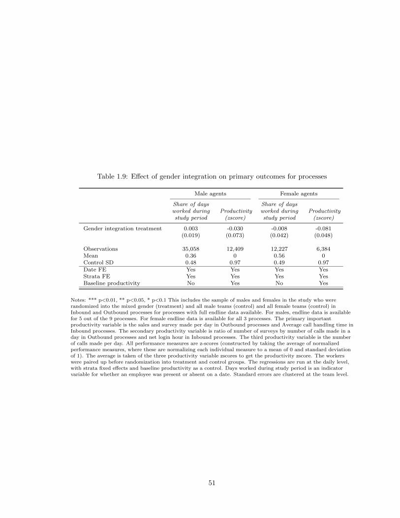
Table 1.9: E↵ect of gender integration on primary outcomes for processes

Male agents Female agents

Share of daysworked duringstudy period

Productivity(zscore)

Share of daysworked duringstudy period

Productivity(zscore)

Gender integration treatment 0.003 -0.030 -0.008 -0.081(0.019) (0.073) (0.042) (0.048)

Observations 35,058 12,409 12,227 6,384Mean 0.36 0 0.56 0Control SD 0.48 0.97 0.49 0.97Date FE Yes Yes Yes YesStrata FE Yes Yes Yes YesBaseline productivity No Yes No Yes

Notes: *** p<0.01, ** p<0.05, * p<0.1 This includes the sample of males and females in the study who wererandomized into the mixed gender (treatment) and all male teams (control) and all female teams (control) inInbound and Outbound processes for processes with full endline data available. For males, endline data is availablefor 5 out of the 9 processes. For female endline data is available for all 3 processes. The primary importantproductivity variable is the sales and survey made per day in Outbound processes and Average call handling time inInbound processes. The secondary productivity variable is ratio of number of surveys by number of calls made in aday in Outbound processes and net login hour in Inbound processes. The third productivity variable is the numberof calls made per day. All performance measures are z-scores (constructed by taking the average of normalizedperformance measures, where these are normalizing each individual measure to a mean of 0 and standard deviationof 1). The average is taken of the three productivity variable zscores to get the productivity zscore. The workerswere paired up before randomization into treatment and control groups. The regressions are run at the daily level,with strata fixed e↵ects and baseline productivity as a control. Days worked during study period is an indicatorvariable for whether an employee was present or absent on a date. Standard errors are clustered at the team level.

51

Survey Questions

Past exposure to opposite gender index : It constitutes of answers from the following Agree/Disagree

questions

1) Did you go to a co-educational school?

2) If co-ed, did boys and girls sit together?

3) Do you have opposite gender siblings?

4) Did you grow up in a joint family with any opposite gender cousins?

5) Did you have a female teacher in school?

6) Did you have any friends from your neighborhood who were from the opposite gender?

7) Have you ever been in a relationship?

8) Have you ever had a team leader of opposite gender?

9) Does your mother or female family members practice ghoonghat/burqa?

10) Do you have lunch with opposite gender?

Job Satisfaction index – rank on a scale of 1 to 5

1) I feel used up at the end of the work day

2) I dread getting up in the morning and having to face another day on the job.

3) I feel I am working too hard on my job.

Gender attitudes index- The response for each of the following questions was aggre-

gated to form an index of gender attitude. Each response was coded as 1 if the respondent answered

“Strongly Agree” or “Agree” with a gender-progressive statement or “Strongly Disagree” or “Dis-

agree” with a gender-regressive statement, and 0 otherwise. The following questions are based on

gender attitude questions in Dhar et al., 2018, Glennerster et al. (2018) and some new questions

specific to the setting, designed by the author.

Express if you agree or disagree with the following statements:

Education attitudes

1) Wives should be less educated than their husbands

52

2) I want my spouse to be more educated than me

3) Boys should be allowed to get more opportunities and resources for education than girls

I. Employment attitudes

1) I wouldn’t let my sister work in a call center as it is not a suitable job for women from good

families.

2) I want my spouse/partner to earn more than me

3) A woman’s most important role is to take care of her home, feeding kids and cook for her family

4) Men are better suited than women to work outside of the house

5) Marriage is more important for a woman than her job

7) Men are the best at leading at the highest level

8) Men should take care of the house if they earn less

9) I will not allow my sister to have a boyfriend before marriage

II. Women’s role attitudes

1) Nowadays men should participate in child rearing and household chores rather than leaving

it all to the women.

2) Brothers should monitor their sister’s friends and her phone as it is their responsibility

3) Sisters should monitor their brother’s friends and his phone as it is their responsibility

4) Daughters should have a similar right to inherited property as sons

5) Women should dress up according to what her husband or family allows for the sake of her family

honor

6) A man should have the final word about decisions in his home

7) A woman should tolerate violence in order to keep her family together

8) Parents should maintain stricter control over their daughters than their sons

9) A shy demeanour makes a girl a more suitable bride

10) A woman has to have a husband or sons or some other male kinsman to protect her.

11) I won’t allow my sister to go to college if it is in the city far away from home

12) Having a son is important to me because it will make my parents and in-laws satisfied.

III. Fertility attitudes – marked as gender regressive if answers to the first fertility question is

53

A and if the reply is answer C in question 1 and but answer B in question 2.

1) Suppose the first two children born to a husband and wife are both girls. Which of the following

should they do?

(A) have more children till they have a boy child

(B) no more children, as this is the perfect family size

(C) have one more child but no more

2) Suppose the first two children born to a husband and wife are both boys. Which of the following

should they do?

(A) have more children

(B) no more children

(C) have one more child but no more

Peer monitoring and support

1) Do your teammates monitor your work?

2) Do you feel that your teammates are interested in your performance?

3) Do your teammates o↵er suggestions for performance improvement?

4) Do you feel comfortable in the workplace?

5) Do you feel comfortable with your teammates?

Autonomy

Index of number of decisions that individual is the most important decision-maker for (they answer

respondent is most important) among following decisions:

1)Clothes for yourself

2) Whether you work outside the home

3) How money earned by you is spent

4) Time you spend socializing outside the house

5) What education/training pursuits you follow

6) Selection of a spouse for you

7) With whom do you travel to work

54

Chapter 2

Impact of Air Pollution on

Employee Productivity: Evidence

from Indian Call Centers

55

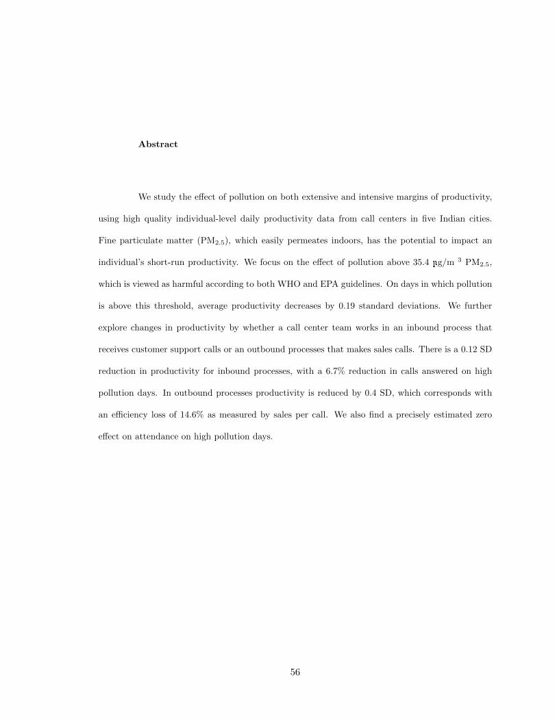
Abstract

We study the e↵ect of pollution on both extensive and intensive margins of productivity,

using high quality individual-level daily productivity data from call centers in five Indian cities.

Fine particulate matter (PM2.5), which easily permeates indoors, has the potential to impact an

individual’s short-run productivity. We focus on the e↵ect of pollution above 35.4 g/m 3 PM2.5,

which is viewed as harmful according to both WHO and EPA guidelines. On days in which pollution

is above this threshold, average productivity decreases by 0.19 standard deviations. We further

explore changes in productivity by whether a call center team works in an inbound process that

receives customer support calls or an outbound processes that makes sales calls. There is a 0.12 SD

reduction in productivity for inbound processes, with a 6.7% reduction in calls answered on high

pollution days. In outbound processes productivity is reduced by 0.4 SD, which corresponds with

an e�ciency loss of 14.6% as measured by sales per call. We also find a precisely estimated zero

e↵ect on attendance on high pollution days.

56

2.1 Introduction

Causing seven million premature deaths every year globally, air pollution has been a

growing concern all over the world (WHO, 2017).1 With six out of the ten most polluted cities

in the world in India, it has been a particularly pressing issue in India (WHO databse, 2018).2

Therefore, understanding the impact of pollution on the economy, especially in developing countries

such as India is crucial. This paper studies the impact of daily fluctuations in air quality on employee

productivity in call centers in five Indian cities.

The paper focuses on particulate matter concentrations measuring up to 2.5 microns in

size. This is because this pollutant can penetrate indoors and building shells cannot provide filtration

of these airborne particles present in ambient air (Thatcher and Layton 1995). These fine particu-

late matters cause serious health issues by impairing cardiovascular and lung functioning (Liu et al.,

2017), or can cause daily allergies resulting in nose and throat irritation and mild headaches (Bern-

stein et al., 2008; Ghio et al. 2000). So, PM2.5 can potentially hamper an individual’s productivity

both at the intensive and extensive margins.

We use a daily panel of productivity data from two call centers located in five Indian cities

for a period of 4 to 16 weeks, to study productivity at both intensive and extensive margins. The

key identifying variation is the daily fluctuation in air quality (PM2.5 levels), which is potentially

unrelated to firm’s output. This is because these firms don’t contribute to the pollution levels

directly. The objective of the study is to test whether high or low pollution decreases productivity,

by using the WHO and EPA cut o↵ of acceptable PM2.5 levels of 35.4 g/m 3. Our preferred

specification includes both date and worker fixed e↵ects. The date fixed e↵ects address the concerns

of bias from unobservables that change over time but are constant over workers, such as the server

1In addition, latest research provides evidence that long-term exposure to fine particulate matter (PM2.5)is linked to an increased risk of COVID-19 death (Wu et al., 2020; Conticini et al., 2020).

2WHO database https://www.who.int/airpollution/data/en/ (Accessed in May, 2020)

57

being down or higher tra�c on the road. And the worker fixed e↵ect controls for factors that di↵er

across workers but are constant over time, such as age, gender and education of workers.

On the intensive margin, pollution can cause decreases in e�ciency and productivity due

to allergies, irritation etc. On the extensive margin, there is a theoretically ambiguous impact of

pollution on days or hours worked. On one hand, there could be a reduction in days worked or

hours worked due to pollution caused illness of the worker or her family member. On the other

hand, there could be an increase in work hours or days worked on more polluted days if the worker

values leisure more on better health days. In this case, the worker will substitute away from work

on less polluted days compared to more polluted days. In both intensive and extensive margins

of productivity, there is a possibility that there will be no impact of pollution if individuals are

practicing mitigating behaviors on high pollution days. However, this is di�cult to follow for an

individual in a work setting, unless a firm level policy change such as installation of air purifier is

made and no such changes were made in the call center policies during the study period.

We find an e↵ect of 0.19 standard deviation reduction in overall productivity on high pol-

lution days (above 35.4 g/m 3 PM2.5), compared to that on low pollution days. This is statistically

significant at the 1% level (Table 3). The productivity measures vary by the two kinds of voice sup-

port business contracts or processes that the call centers o↵er. Inbound processes receive incoming

calls and outbound processes make outgoing sales calls. So, the productivity index is disaggregated

by the type of process for further exploration. We expect the impacts to be di↵erent in the two

kinds of processes because outbound or sales calls usually have higher pressure, heavier monitoring

and tougher targets. Therefore, it is expected that there will be a higher impact of pollution on

productivity in outbound processes than inbound ones, if the mechanism is cognitive impairment.

The inbound processes provide customer support services to incoming callers, so their

main productivity measures are average call handling time (ACHT), number of calls and net login

hours. The firm profits increase if the workers receive a high number of calls, login successfully for

58

at least 8 hours and handle the calls in less amount of time. We find an overall 0.12 SD significant

decline in productivity on high pollution days for inbound processes (Table 3). This e↵ect is driven

by decreases in calls answered by 6.7% compared to the average calls answered on low pollution days

(Table 4).

The main productivity variables in outbound processes are total sales made per day, total

calls made per day and their ratio of total sales by calls made per day. The firm gains profits if

total sales made per day increases and if the ratio of sales by calls also increases per day. So, the

firms benefit if an employee has a high sales conversion rate of calls, that is, the employee achieves

daily sales targets by making fewer number of calls. Less total number of calls made per day in the

outbound processes is therefore better for the firm. For outbound processes, the overall e↵ect on

productivity is 0.4 SD compared to that on low pollution days (Table 3). This e↵ect is largely driven

by a reduction in sales by 30% over the mean sales of 54.3 on low pollution days (Table 5). We also

find a significant decline in the e�ciency measure of sales by calls ratio per day. This amounts to

an e�ciency loss of 14.6% in the sales by calls ratio per day on high pollution days (Table 5).

Absenteeism is a particularly important issue in the context of India. In fact in the period

between 1999 and 2013, Indian firms lost an average of 8.7% scheduled worker-days due to the

absence of permanent workers (Krishnaswamy, 2019). In this paper we find precisely estimated

zero e↵ect of high pollution on attendance (Table 2). So, pollution maybe not be one of the reasons

driving the high absenteeism rates in this industry in India. In addition, the zero e↵ect on attendance

mitigates concerns about selection e↵ect on the intensive margins of productivity.

This paper adds to the literature on air pollution and productivity that uses high frequency

employee-level data. There has been a focus on productivity in physically demanding occupations

such as agricultural workers (Gra↵ Zivin and Neidell, 2012), pear-packing factory workers (Chang

et al., 2014), garment factory workers (Adhvaryu et al., 2016), textile assembly (He et al., 2019) and

59

manufacturing firms (Fu et al., 2017; Hansen-Lewis, 2018). These papers generally find negative

impact of pollution on worker productivity.

Modern and developing economies such as India rely on the service sector for their eco-

nomic output and economic growth. These high-skilled jobs require mental strength and not physical

strength. This paper makes a direct contribution to the small and growing literature on air pollution

and productivity in cognitively demanding tasks. There are papers study cognitively demanding jobs

such as decisions made by baseball umpires (Archsmith et al., 2018) and investor behavior (Heyes et

al., 2016). But our paper is most closely related to the study by Chang et al. (2019), which studies

the impact of pollution on productivity in Chinese call centers. Our study builds on that paper by

using PM2.5, instead of PM10, a measure that captures smaller particulates, which are especially

likely to permeate indoors. In addition, we are able to study outbound processes that require extra

cognitive demands, as well as inbound processes. Finally, we have access to data that focuses on

call-level e�ciency measures of productivity.

Assessing the impact of pollution on productivity has broad policy implications by making

a concrete case for stronger environment protection laws, particularly in developing countries. These

developing economies are going through urbanization and economic growth and are therefore, not

receptive to changes in environmental policies which might deter growth. However, evidence of a

causal relationship between air pollution and productivity can convince countries to take stringent

measures to protect the environment.

2.2 Context

This section provides an overview on the ill-e↵ects of air pollution on health and some

details about the call center industry in India. The first subsection provides information about the

air quality index, particulate matter and a background on pollution. The second subsection provides

information about the call center setting of this study.

60

2.2.1 Background on Pollution

Air pollution is an environmental risk to human health. Air pollution is a mixture of

particulate matter (PM), ozone, carbon monoxide, sulfur oxides, nitrogen oxides, methane, and other

gases, volatile organic compounds, and metals such as lead and iron. We focus on fine particulate

matter (PM2.5) in this study because it can penetrate indoors and cause harmful short-run e↵ects on

health. ”Small particles” are inhalable coarse particles with a diameter of 2.5 to 10 g/m 3 and ”fine

particles” are smaller than 2.5 g/m 3 in diameter. Therefore, PM2.5 are fine particulate matter

with an aerodynamic diameter of 2.5 m or less (PM2.5). Fine particulate matters are anthropogenic

emissions from fuel combustion, engine exhaust and high temperature industrial processes (Dickey,

2000). Particulate matter exposure acts as the source of various health problems such as premature

death in individuals su↵ering from heart or lung disease, non-fatal heart attacks, irregular heartbeat,

aggravated asthma, decreased lung function, and increased respiratory symptoms such as irritation

of the airways, coughing, or di�culty breathing (Kim et al., 2015).

While the epidemiological and toxicological literature have provided evidence on the long-

term morbidity and mortality e↵ects of PM2.5 through impairment of the respiratory and cardiovas-

cular systems, there is also a growing literature on the short-run e↵ect of fine particulate matter both

on health and cognition (Bell et al., 2008; Pascal et al, 2014). PM is small enough to penetrate the

lung barrier, enter the bloodstream and travel into the central nervous system (Elder et a., 2015).

The potential mechanism through which inhaled indoor pollution impairs brain function is through

neuroinflammation (Brockmeyer and D’Angiulli, 2016). Therefore, greater exposure to fine particles

is associated with cognitive problems a↵ecting intelligence, mood disorders and performance (Allen

et al., 2017; Tallon et al., 2017). Since our call center or o�ce setting, requires concentration and

critical thinking, a well-functioning brain is critical to achieving higher productivity (Chang et al,

2019).

61

According to the National Ambient Air Quality Standards for Particle Pollution (U.S.

Environmental Protection Agency (EPA)), 24-hour averages of PM2.5 levels above 35.5 g/m3 is

unhealthy for sensitive groups. PM2.5 levels above 55.5 g/m3 is unhealthy and that above 150.5

g/m3 is deemed extremely unhealthy for the general population.3 The five cities of Mumbai, Noida,

Patna, Udaipur and Hubli included in the study, experience very high levels of pollution and some

of these cities have also experienced hazardous levels of PM2.5 with daily averages even above 250.5

g/m3.

India has taken some steps to address the growing concerns about pollution in the country.

At the beginning of 2019, the Ministry of Environment, Forest and Climate Change, Government of

India announced the National Clean Air Programme (NCAP) to provide a national framework for

air quality management. A total of 122 cities in India have been identified as ’non-attainment cities’

for not meeting air quality standards for particulate matter. There are 207 realtime air monitoring

stations spread across 114 cities, and 793 manual air monitoring stations spread across 344 cities in

India. Under NCAP, massive investments are being made to further expand real-time and manual

air monitoring stations, particularly in non-attainment cities (Roychowdhury and Somvanshi, 2020).

Out of the cities in our study, Patna and Noida are included in the 30 most polluted cities in the

world and Mumbai and Udaipur are included the 100 most polluted cities (WHO databse, 2018).4).

This study aims to provide additional evidence on the economic impact of pollution to further inform

policy makers.

2.2.2 Background on Call Centers in the study

The call center industry in India is the largest private sector employer in India. We

collected data from two call centers in India: Call-2-Connect India Pvt. Ltd. and Five Splash

3Revised Air Quality Standards for Particulate Pollution and Updates to Air Quality Index (AQI)https://www.epa.gov/sites/production/files/2016-04/documents/2012_aqi_factsheet.pdf (accessedin May, 2020)

4WHO database https://www.who.int/airpollution/data/en/ (Accessed in May, 2020)

62

Infotech Pvt. Ltd. Call2Connect India Pvt. Ltd. has centers located in the states of Bihar (Patna),

Uttar Pradesh (Noida) and Maharashtra (Mumbai). Five Splash Infotech Pvt. Ltd. has centers in

the states of Rajasthan (Udaipur) and Karnataka (Hubli).

Calls centers are also known as Business Process Outsourcing (BPO) companies. They

provide voice and non-voice support to other companies. A call center can have contracts with

various companies and each of these contracts is called a process. The nine processes in our study

provide voice support in the form of either inbound or outbound calls. Entry-level workers, also

known as agents provide the voice support. Agents work in teams of 20-25 and are supervised by

team leaders.

We analyze productivity data for the agents because the firms profits rely on their work.

Call centers usually run all seven days in a week. However, the agents work six days a week and can

choose any day of the week as a day o↵. The agents in our sample receive a fixed salary of 100-150

per month in smaller cities and 150-220 per month in the bigger cities. Since attendance is a major

issue in India, agents receive a deduction in their salary if they take too many holidays in a month.

If an agent doesn’t show up to work for 3-4 days in a row without informing their team leaders,

they are marked as absconding in the attendance sheet. The agents have a di�cult time re-joining

work if they were absconding. Additionally, if an agent takes too many holidays (varies for di↵erent

centers) in a month even after informing their team leaders about it, they receive a deduction in

their salary.

Employees are expected to be logged-in for a certain number of hours so even if they come

late to work, they are expected to complete their log-in hours. Agents are also penalized for coming

late for work. If they come late to work 3-4 days a week, they face a salary deduction.

In inbound processes, agents receive calls and o↵er customer service support to customers.

The inbound processes in our study provide help to all kinds of companies such as food delivery,

financial technology, beauty retail etc. In outbound processes, agents usually make calls to make

63

sales. In our sample, outbound calls are made during elections by a political party as part of their

campaign/advertisement to provide campaign information to eligible voters.

2.3 Data

We have five inbound and four outbound processes in our study. The agents are required

to log-in to the system as soon as they show up for work. Their productivity data is recorded auto-

matically using technology-based monitoring system. We use this internally collected administrative

data for 4 to 16 weeks from all of the five cities/locations.

The inbound processes provide customer support services to incoming callers, so their

main productivity measures are average call handling time (ACHT), number of calls and net login

hours. The firms gain profits if the workers receive a high number of calls, login successfully for at

least 8 hours and handle the calls in less amount of time.

In outbound processes in which agents make sales calls, the primary productivity variables

are total sales made per day, total calls made per day and their ratio of total sales by calls made

per day. The firms gain profits if total sales made per day increases and if the ratio of sales by calls

also increases per day. So, the firms benefit if an employee has a high sales conversion rate of calls

i.e., she achieves daily sales targets by making fewer number of calls.

The main outcome measure at the extensive margin is days present in the study period.

In the daily level administrative productivity data, there is information on the productivity of all

the logged-in workers on any particular date. This gives information on who was present and absent

on each particular day of the study from the first day of appearing in the administrative data to

their last day. Using this, each worker is marked to be present on the days in the study for which

their productivity data is available till their last date of appearing in the data. For other days in

between, they are marked absent if their productivity data is missing.

64

For the daily-level data on pollution, India Central Pollution Control Board Data was

requested for data.5 National Oceanic and Atmospheric Administration (NOAA) was requested for

information on daily average temperature. The daily average temperature data was unavailable for

Udaipur and Hubli at NOAA data-base. So, the temperature data for the nearest city for which this

information was available is used as a proxy.

Table 1 provides some sample statistics on pollution in the various cities in the sample

during the study period. Noida is the most polluted city in the sample with average PM2.5 levels

of 150.33 The second most polluted city is Patna with average PM2.5 of approximately 53. Udaipur

and Mumbai follow behind Patna with average PM2.5 levels of 37.21 and 34.29. Hubli is the least

polluted city in the sample with average PM2.5 levels as 25, which is under the WHO and EPA

acceptable air quality standard of 35.4. The minimum PM2.5 levels in the study-period in all these

cities is below 35.4.

In Table 1, we also provide sample statistics of the productivity measures both at the

extensive and intensive margins. The average attendance is about 77% in the full sample. For

inbound processes, where agents answer calls as customer service support, the average call handling

time is approximately 900 seconds. The workers log-in for an average of 7.9 hours and they answer

122 calls per day on average. In outbound processes, the agents make an average of 65 sales per day

by making 180 calls on average in a day. So, the average sales per calls ratio is around 0.37. The

standard deviation for all these measures is quite high. The next sections provides details about the

empirical strategy.

2.4 Empirical Specification

We use this panel data for workers in call centers across five Indian cities to estimate the

e↵ect of pollution on productivity. The estimating equation is as follows:

5 CPCB - India Central Pollution Control Board : cpcb.nic.in/ (accessed in April, 2020)

65

Yipjt = �0 + �1HighPM2.5jt + �2AverageTemperaturejt

+�3Processp +Xi + �t + ✏ipjt

(2.1)

The dependent variable in productivity for individual ’i’ in process ’p’, at city ’j’ on date ’t’. Air

quality or air pollution is the presence of particle matter 2.5. High PM2.5 levels is PM2.5 above 35.4

which is deemed unhealthy by both WHO and EPA air quality standards. Productivity variables

are standardized within a process using pollution level (PM2.5) less than 35.4 level as control. We

first standardize each measure of intensive margin of productivity within a process using mean and

standard deviation of the acceptable pollution group. We then add these measures and re-standardize

the to create a z-score of productivity.

We add temperature controls because some of the daily variation in productivity could

be due to daily temperature fluctuations. Date fixed e↵ects are included in the regression analysis

to control for unobserved heterogeneity within date/time. These date fixed e↵ect addresses the

concerns of bias from unobservables that change over time but are constant over workers, such as

server being down or days with higher tra�c on the road. We also control for worker fixed e↵ect

in some specifications to account for time-invariant unobserved within-worker heterogeneity, such as

age, gender and education of workers. Process-level fixed e↵ects account for unobserved variations in

productivity within a business. These are included in those specifications where worker fixed e↵ects

are not included. When worker fixed e↵ects are included, Process fixed e↵ects have to be dropped

because of collinearity. Because the error term likely exhibits autocorrelation between observations

within a city on a particular date, we cluster at the city date level.

A potential threat to identification is that pollution and productivity are correlated through

the channel of increasing economic activity in an area. These call centers don’t contribute to the

pollution levels directly. However, they could potentially be working for processes which have higher

66

call volumes and higher work burden on days with high pollution. Since most of these processes are

dealing with local callers/ customers from an entire state, it is unlikely to be related to the pollution

in the city in which the call center o�ce is located. For outbound calls, these calls took place for a

few months prior to state elections. So, they are likely related to the pollution in the city if the ruling

party in the state expedited the construction work in that area just before the elections. However,

even in this case, the call center o�ce was located in the suburban area which lies out of the state

with eligible voters. Additionally, the lists of calls to be made to customers is provided to the call

centers by process owners a few days or weeks in advance. Therefore, the demand for call center’s

services is assumed to be unrelated to daily pollution. So, any links to number of callers and daily

fluctuations in pollution is improbable.

2.5 Regression Results

In this section we layout the regression results disaggregated by margin of productivity.

We further disaggregate the intensive margin of productivity by process and individual productivity

measures. Additionally, we report the results from some robustness checks.

2.5.1 Main Regression Results for the Extensive Margin of Productivity

In Table 2, we provide the regression results for the extensive margin of productivity,

attendance for the full sample as well disaggregation by the type of process. We find a precisely

estimated zero e↵ect of unhealthy air pollution levels on attendance for all the cases. There is a 0.008

increase (or 1% increase) in attendance on high pollution days, which is a small and insignificant

e↵ect, with tight confidence interval around zero [CI: -0.012 to 0.0276]. When we add worker fixed

e↵ects, the point-estimate reduces further to 0.002 (column 2), which is an e↵ect of 0.26% increase

67

in attendance over mean attendance of 0.77. This is also a null-e↵ect with tight confidence intervals

around zero [CI: -0.016 to 0.02].

For inbound processes (column 3 of Table 2), we find the same null e↵ect on attendance

with a small and insignificant point-estimate of 0.002 [CI: -0.023 to 0.0277]. When we add worker

fixed e↵ect, the point-estimate remain small and insignificant, but the sign or direction of change

becomes negative. There is a -0.003 change in attendance (column 4 of Table 2), which is a 0.4%

decrease in attendance on high pollution days over the mean attendance in inbound processes of

0.74. This is a null e↵ect because the standard errors are small and the point-estimate lies in tight

confidence intervals containing zero [CI: -0.025, 0.019].

The outbound processes have a higher average attendance of 0.81. The impact of high

air pollution on attendance in outbound processes is 0.027, which is a 3.3% increase in attendance

(column 5 of Table 2). However, this is also a small and insignificant e↵ect which is statistically

indistinguishable from zero [CI: -0.016 to 0.07]. The last column of Table 2 provides evidence on the

impact of high particulate matter in the air on attendance in outbound processes with worker fixed

e↵ects. We again find a null e↵ect with a point-estimate of 0.015 [CI: -0.026, 0.056].

The null-e↵ect on attendance is expected because of the stringent attendance policy fol-

lowed by call centers, as discussed in section II (D’Cruz and Noronha, 2013). However, despite these

policies, absenteeism is an important issue in India (Krishnaswamy, 2019). Our analysis provides

evidence that air pollution is not one of the reasons causing high absenteeism, particularly in the

BPO industry. These results also imply that our estimates on the e↵ect of pollution on intensive

margins of productivity presented in the next sub-section are not a↵ected by sample-selection bias.

2.5.2 Main Regression Results for the Intensive Margin of Productivity

In Table 3, we report the results on the intensive margins of productivity for both inbound

and outbound processes. We find an overall 0.19 standard deviation reduction in productivity on

68

high pollution days compared to that on the low pollution days. This e↵ect is significant at the 1%

level over the full sample both with and without worker fixed e↵ects (see columns 1 and 2). These

estimates lie in tight confidence intervals excluding the null-value [CI: -0.323 to -0.063].

We also report the productivity index results by the type of process. For inbound processes,

we find an e↵ect of 0.12 SD decrease in productivity on high pollution days compared to that on low

pollution days. This is again a statistically significant e↵ect at 1% level. For outbound processes,

we find a larger e↵ect of 0.46 SD decrease in productivity due to high pollution (see column 5 of

Table 3). These e↵ects are significant at 5% level, due to comparatively larger standard errors than

those for inbound processes. But the confidence intervals still exclude the null value [CI: -0.07,

0.85]. When we add worker fixed e↵ects, we find that the e↵ect reduces a little to 0.42 SD and are

significant at 5% level (see column 6 of Table 3). Overall, the coe�cients in Table 3 remain largely

unchanged by the addition of worker-specific fixed e↵ect.

We report each individual component of the standardized index for both inbound and

outbound processes (columns 5 and 6 in Table 3). For inbound processes, as discussion in section

III, a lower average call handling time (ACHT) is better so that workers can cater to more number

of customers. We find an increase in average call handling time by 75.85 seconds, which is a 9.7%

increase over the mean ACHT of 784.5 on low pollution days (column 1 of Table 4). This e↵ect is

not significant and the standard errors are quite large. Additionally, the e↵ect further diminishes to

5.4% with a point estimate of 42.05, when we add worker fixed e↵ect (column 2 or Table 4). However,

the positive sign on ACHT indicates that air pollution might be decreasing worker e�ciency, even

though this is a small and insignificant e↵ect.

The other two measures of productivity for inbound processes are logged-in hours and calls

answered. There is evidence of a significant increase in hours login hours on high pollution days.

The point-estimate is 0.31, which is a 4% increase in login hours over the mean login hours of 7.7

on low pollution days (column 3 of Table 4). However, this e↵ect decreases with worker fixed e↵ect

69

to a point estimate of 0.24, which is still significant at the 10% level (column 4 of Table 4). Call

centers often ask their workers to remain logged-in for a longer time on days that their e�ciency is

low because of the real-time monitoring facility. In addition, the call centers gain profits if workers

answer a high number of calls per day. We provide evidence that the calls answered declines by 6.7%

on high pollution days, compared to the mean of 111.7 on low pollution days. The point-estimate of

7.4 doesn’t change much with worker fixed e↵ect (see columns 5 and 6 of Table 4). This is significant

at the 5% level.

In Table 5, we report the regression results for various productivity measures for the

outbound processes. The e�ciency measure of productivity in this case is the ratio of sales by calls

per day. The call centers gain profits of the workers receive high number of sales per day by making

less number of calls to customers. The average number of sales made per days declines by 30% on

high pollution days, which is a huge e↵ect. The point estimate is 16.1 and the average sales made

on low pollution days is 54.26 (see column 1 of Table 5). This e↵ect is significant at the 10% level.

When we add worker fixed e↵ects, the e↵ect declines to 27.4% but remain significant.

For the e�ciency variable for outbound processes, there is a 14.6% decline in sales per

day on high pollution days. The point estimate is 0.06 and the average sales per calls ratio on low

pollution days is 0.41 (see column 3 of table 5). The point estimate and standard errors remain

the same with worker fixed e↵ect (column 4 of Table 5). This e↵ect is significant at the 5% level.

The last productivity measure for outbound processes is number of calls made, which is insignificant

with large standard errors of 9.9 (column 5 and 6 of Table 5). The point estimate is -8.44, which

indicates that there is a reduction in calls made on high pollution days. The average calls made

on low pollution days is 134 approximately. The e↵ect remains small and insignificant with worker

fixed e↵ects (column 6 of Table 5).

70

2.5.3 Robustness Checks

In this section, we address the concerns of serial correlation in productivity within a process

and temperature controls confounding the results. The first concern is mitigated by clustering at

the process-level instead of city-date level. Table 6 reports the results of productivity both at the

extensive and intensive margins (standardized) with clustering at the process level (columns 1, 2,

3 and 5 in Table 6). Since there are few processes, we bootstrap the estimates and report the

resultant p-values. The point estimates correspond with those in Tables 1 and 2. However, the

combined productivity (z-score) is not significant only at the 5% level, instead of 10% level in Table

2.

The second concern is mitigated by removing temperature controls (columns 4 and 6 in

Table 6). The point estimate for intensive margin of productivity is 0.14 SD without temperature

controls, than the coe�cient of 0.19 SD in Table 3 with temperature controls (column 4). This is

still significant so temperature controls are not impacting the analysis much. Even on the extensive

margin of productivity (column 6 of Table 6), we find insignificant impact of pollution on attendance

without any temperature controls.

2.6 Conclusion and Way Forward

In this paper, we study the relationship between air pollution and productivity of individ-

ual workers in two call centers in India with centers across five cities. We find a precisely estimated

null-e↵ect of high PM2.5 levels on the extensive margin of productivity (attendance). On the inten-

sive margin of productivity, we find an overall 0.19 SD e↵ect of high PM2.5 levels compared to the

average productivity below 35.4 PM2.5 level.

As a part of the next steps of the paper, we are considering collecting productivity data

from the call centers for at least one year, depending on feasibility.6 A year-long data anaylsis will

6Due to COVID-19 related lock-down in India, the call centers are unable to retrieve the data from their

71

include all the fluctuations in the pollution level, related to seasonal variations across a year and

will strengthen the anaylsis. It will increase the power to detect small e↵ects, especially the results

on productivity at the intensive margin for outbound processes.

In the future, we also plan to explore contacting the call center workers and collecting

additional information through survey method, on their underlying health conditions. There is

evidence in the health literature that particulate matter can exacerbate symptoms of asthma and

other respiratory diseases (Williams et al., 2019). So, the impact of pollution on productivity for

agents with respiratory and lung diseases is likely to be worse. We would also collect information

on the area code of agents to account for tra�c en-route to work. The individuals who travel

from a greater distance are more exposed to air pollution and are likely to have worse productivity

outcomes. Additionally, we will survey them on their mode of transport to work, to be able to study

the exposure to pollution en-route to work.

servers and send it to us. So, for this study we have only used the data previously collected during therandomized controlled trial conducted by the dissertation author, Deepshikha.

72

References

Allen, J. L., Klocke, C., Morris-Scha↵er, K., Conrad, K., Sobolewski, M., Cory-Slechta,D. A. (2017). Cognitive e↵ects of air pollution exposures and potential mechanistic underpinnings.Current environmental health reports, 4(2), 180-191.

Archsmith, J., Heyes, A., Saberian, S. (2018). Air quality and error quantity: Pollutionand performance in a high-skilled, quality-focused occupation. Journal of the Association of Envi-ronmental and Resource Economists, 5(4), 827-863.

Aragon, F. M., Miranda, J. J., Oliva, P. (2017). Particulate matter and labor supply:The role of caregiving and non-linearities. Journal of Environmental Economics and Management,86, 295-309.

Bell, M. L., Ebisu, K., Peng, R. D., Walker, J., Samet, J. M., Zeger, S. L., Dominici, F.(2008). Seasonal and regional short-term e↵ects of fine particles on hospital admissions in 202 UScounties, 1999–2005. American journal of epidemiology, 168(11), 1301-1310.

Bernstein, J. A., Alexis, N., Bacchus, H., Bernstein, I. L., Fritz, P., Horner, E., Reijula,K. (2008). The health e↵ects of nonindustrial indoor air pollution. Journal of Allergy and ClinicalImmunology, 121(3), 585-591.

Brockmeyer, S., D’Angiulli, A. (2016). How air pollution alters brain development: therole of neuroinflammation. Translational neuroscience, 7(1), 24–30.

Conticini, E., Frediani, B., Caro, D. (2020). Can atmospheric pollution be considered aco-factor in extremely high level of SARS-CoV-2 lethality in Northern Italy?. Environmental pollu-tion, 114465.

D’Cruz, P., Noronha, E. (2013). Hope to despair: The experience of organizing Indiancall centre employees. Indian Journal of Industrial Relations, 471-486.

Dickey, J. H. (2000). Selected topics related to occupational exposures Part VII. Air pol-lution: Overview of sources and health e↵ects. Disease-a-month, 46(9), 566-589.

Elder, A., Schwartz, J., Oberdorster, G. (2015). Particulate air pollution and CNS health.In Air pollution and health e↵ects (pp. 269-288). Springer, London.

Fu, S., Viard, B., Zhang, P. (2017). Air quality and manufacturing firm productivity:comprehensive evidence from China.

Ghio, Andrew J., Chong Kim, and Robert B. Devlin. 2000. Concentrated Ambient AirParticles

Hansen-Lewis, J. (2018). Does Air Pollution Lower Productivity? Evidence from Manu-facturing in India.

He, J., Liu, H., Salvo, A. (2019). Severe air pollution and labor productivity: Evidencefrom industrial towns in China. American Economic Journal: Applied Economics, 11(1), 173-201.

73

Heyes, A., Neidell, M., Saberian, S. (2016). The e↵ect of air pollution on investor behav-ior: evidence from the SP 500 (No. w22753). National Bureau of Economic Research.

Kim, K. H., Kabir, E., Kabir, S. (2015). A review on the human health impact of airborneparticulate matter. Environment international, 74, 136-143.

Krishnaswamy, N. (2019). Missing and Fired: Worker Absence, Labor Regulation, andFirm Outcomes, Working Paper

Liu, H., Salvo, A. (2017). Severe Air Pollution and School Absences: Longitudinal Dataon Expatriates in North China (No. 11134). IZA Discussion Papers.

Liu, Q., Xu, C., Ji, G., Liu, H., Shao, W., Zhang, C., Gu, A., Zhao, P. (2017). E↵ectof exposure to ambient PM2.5 pollution on the risk of respiratory tract diseases: a meta-analysis ofcohort studies. Journal of biomedical research, 31(2), 130–142.

Pascal, M., Falq, G., Wagner, V., Chatignoux, E., Corso, M., Blanchard, M., ... Larrieu,S. (2014). Short-term impacts of particulate matter (PM10, PM10–2.5, PM2. 5) on mortality innine French cities. Atmospheric Environment, 95, 175-184.

Roychowdhury, A. and Somvanshi, A., (2020). Breathing Space: How to track and reportair pollution under the National Clean Air Programme, Centre for Science and Environment, NewDelhi

Tallon, L. A., Manjourides, J., Pun, V. C., Salhi, C., Suh, H. (2017). Cognitive impactsof ambient air pollution in the National Social Health and Aging Project (NSHAP) cohort. Envi-ronment international, 104, 102-109.

Thatcher, Tracy L., and David W. Layton. 1995. “Deposition, resuspension, and pene-tration of particles within a residence.” Atmospheric Environment 29 (13): 1487–97.

World Air Quality Index Project: https://waqi.info

World Health Organization. (2017). Burden of disease from household air pollution for2012.

Williams, A. M., Phaneuf, D. J., Barrett, M. A., Su, J. G. (2019). Short-term impact ofPM2. 5 on contemporaneous asthma medication use: Behavior and the value of pollution reductions.Proceedings of the National Academy of Sciences, 116(12), 5246-5253.

Wu, X., Nethery, R. C., Sabath, B. M., Braun, D., Dominici, F. (2020). Exposure to airpollution and COVID-19 mortality in the United States. medRxiv.

74

ACKNOWLEDGEMENTS

This paper is co-authored with my co-advisor Sarojini Hirshleifer. The dissertation author

is the co-primary investigator and author of this paper.

We are grateful to the CEOs and center heads of partner call centers, Anil Sinha, Rajeev

Jha and Sujit Sharma of Call-2-Connect and Kapil Sharma, Lakhan Joshi and Soham Ghosh of Five

Splash for sharing their data and o↵ering their support.

We appreciate the help of Mr. Anshuman Gaur, Private Secretary to Minister for Law and

Justice & Electronics and IT and Mr. Rajiv Kumar, Joint Secretary at Ministry of Electronics and IT

at Government of India (MEIT: GOI); Mr. Devesh Tyagi, Senior Director at Software Technology

Parks of India (STPI), Mr. Madhurjya Prakash Baruah, Additional Director at STPI and Mr.

K.P.S. Keshri, President of Bihar Industries Association (BIA) for introducing and recommending

this project to call centers.

All views expressed in this paper are those of the authors alone and need not necessarily

reflect those of the call centers, MEIT: GOI, STPI or BIA.

75

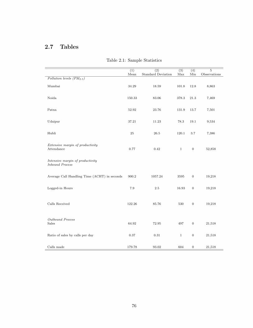
2.7 Tables

Table 2.1: Sample Statistics

(1) (2) (3) (4) 5Mean Standard Deviation Max Min Observations

Pollution levels (PM2.5)

Mumbai 34.29 18.59 101.8 12.8 8,863

Noida 150.33 83.06 378.3 21.3 7,469

Patna 52.92 23.76 131.9 13.7 7,501

Udaipur 37.21 11.23 78.3 19.1 9,534

Hubli 25 26.5 120.1 3.7 7,386

Extensive margin of productivityAttendance 0.77 0.42 1 0 52,858

Intensive margin of productivityInbound Process

Average Call Handling Time (ACHT) in seconds 900.2 1057.24 3595 0 19,218

Logged-in Hours 7.9 2.5 16.93 0 19,218

Calls Received 122.26 85.76 530 0 19,218

Outbound ProcessSales 64.92 72.95 497 0 21,518

Ratio of sales by calls per day 0.37 0.31 1 0 21,518

Calls made 179.78 93.02 604 0 21,518

76

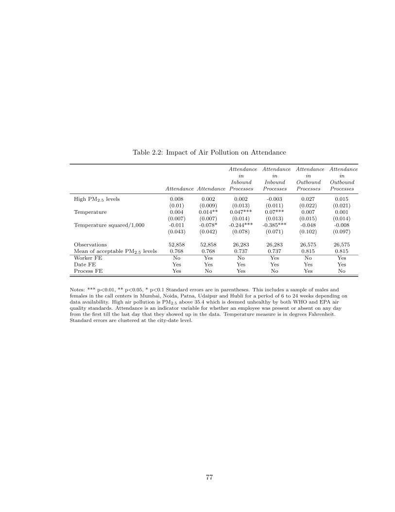
Table 2.2: Impact of Air Pollution on Attendance

Attendance Attendance

Attendancein

InboundProcesses

Attendancein

InboundProcesses

Attendancein

OutboundProcesses

Attendancein

OutboundProcesses

High PM2.5 levels 0.008 0.002 0.002 -0.003 0.027 0.015(0.01) (0.009) (0.013) (0.011) (0.022) (0.021)

Temperature 0.004 0.014** 0.047*** 0.07*** 0.007 0.001(0.007) (0.007) (0.014) (0.013) (0.015) (0.014)

Temperature squared/1,000 -0.011 -0.078* -0.244*** -0.385*** -0.048 -0.008(0.043) (0.042) (0.078) (0.071) (0.102) (0.097)

Observations 52,858 52,858 26,283 26,283 26,575 26,575Mean of acceptable PM2.5 levels 0.768 0.768 0.737 0.737 0.815 0.815Worker FE No Yes No Yes No YesDate FE Yes Yes Yes Yes Yes YesProcess FE Yes No Yes No Yes No

Notes: *** p<0.01, ** p<0.05, * p<0.1 Standard errors are in parentheses. This includes a sample of males andfemales in the call centers in Mumbai, Noida, Patna, Udaipur and Hubli for a period of 6 to 24 weeks depending ondata availability. High air pollution is PM2.5 above 35.4 which is deemed unhealthy by both WHO and EPA airquality standards. Attendance is an indicator variable for whether an employee was present or absent on any dayfrom the first till the last day that they showed up in the data. Temperature measure is in degrees Fahrenheit.Standard errors are clustered at the city-date level.

77

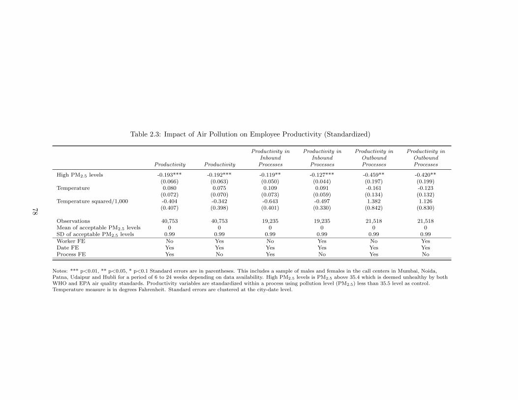
Table 2.3: Impact of Air Pollution on Employee Productivity (Standardized)

Productivity Productivity

Productivity inInboundProcesses

Productivity inInboundProcesses

Productivity inOutboundProcesses

Productivity inOutboundProcesses

High PM2.5 levels -0.193*** -0.192*** -0.119** -0.127*** -0.459** -0.420**(0.066) (0.063) (0.050) (0.044) (0.197) (0.199)

Temperature 0.080 0.075 0.109 0.091 -0.161 -0.123(0.072) (0.070) (0.073) (0.059) (0.134) (0.132)

Temperature squared/1,000 -0.404 -0.342 -0.643 -0.497 1.382 1.126(0.407) (0.398) (0.401) (0.330) (0.842) (0.830)

Observations 40,753 40,753 19,235 19,235 21,518 21,518Mean of acceptable PM2.5 levels 0 0 0 0 0 0SD of acceptable PM2.5 levels 0.99 0.99 0.99 0.99 0.99 0.99Worker FE No Yes No Yes No YesDate FE Yes Yes Yes Yes Yes YesProcess FE Yes No Yes No Yes No

Notes: *** p<0.01, ** p<0.05, * p<0.1 Standard errors are in parentheses. This includes a sample of males and females in the call centers in Mumbai, Noida,Patna, Udaipur and Hubli for a period of 6 to 24 weeks depending on data availability. High PM2.5 levels is PM2.5 above 35.4 which is deemed unhealthy by bothWHO and EPA air quality standards. Productivity variables are standardized within a process using pollution level (PM2.5) less than 35.5 level as control.Temperature measure is in degrees Fahrenheit. Standard errors are clustered at the city-date level.

78

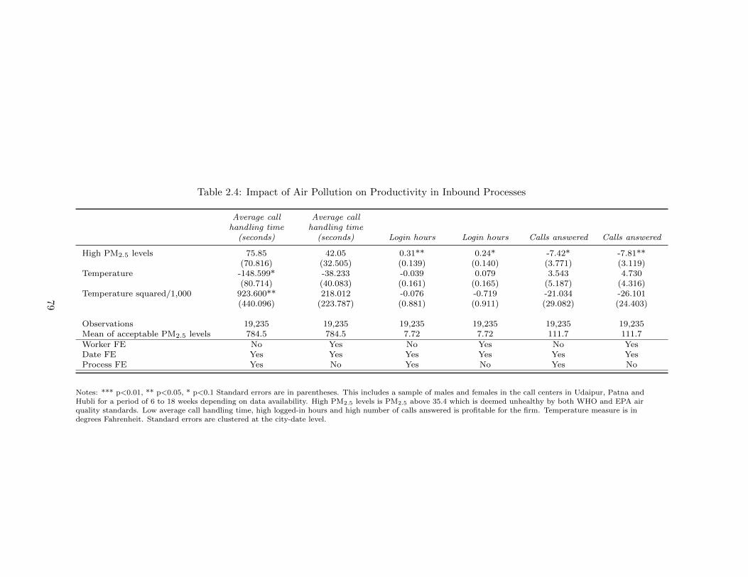
Table 2.4: Impact of Air Pollution on Productivity in Inbound Processes

Average callhandling time

(seconds)

Average callhandling time

(seconds) Login hours Login hours Calls answered Calls answered

High PM2.5 levels 75.85 42.05 0.31** 0.24* -7.42* -7.81**(70.816) (32.505) (0.139) (0.140) (3.771) (3.119)

Temperature -148.599* -38.233 -0.039 0.079 3.543 4.730(80.714) (40.083) (0.161) (0.165) (5.187) (4.316)

Temperature squared/1,000 923.600** 218.012 -0.076 -0.719 -21.034 -26.101(440.096) (223.787) (0.881) (0.911) (29.082) (24.403)

Observations 19,235 19,235 19,235 19,235 19,235 19,235Mean of acceptable PM2.5 levels 784.5 784.5 7.72 7.72 111.7 111.7Worker FE No Yes No Yes No YesDate FE Yes Yes Yes Yes Yes YesProcess FE Yes No Yes No Yes No

Notes: *** p<0.01, ** p<0.05, * p<0.1 Standard errors are in parentheses. This includes a sample of males and females in the call centers in Udaipur, Patna andHubli for a period of 6 to 18 weeks depending on data availability. High PM2.5 levels is PM2.5 above 35.4 which is deemed unhealthy by both WHO and EPA airquality standards. Low average call handling time, high logged-in hours and high number of calls answered is profitable for the firm. Temperature measure is indegrees Fahrenheit. Standard errors are clustered at the city-date level.

79

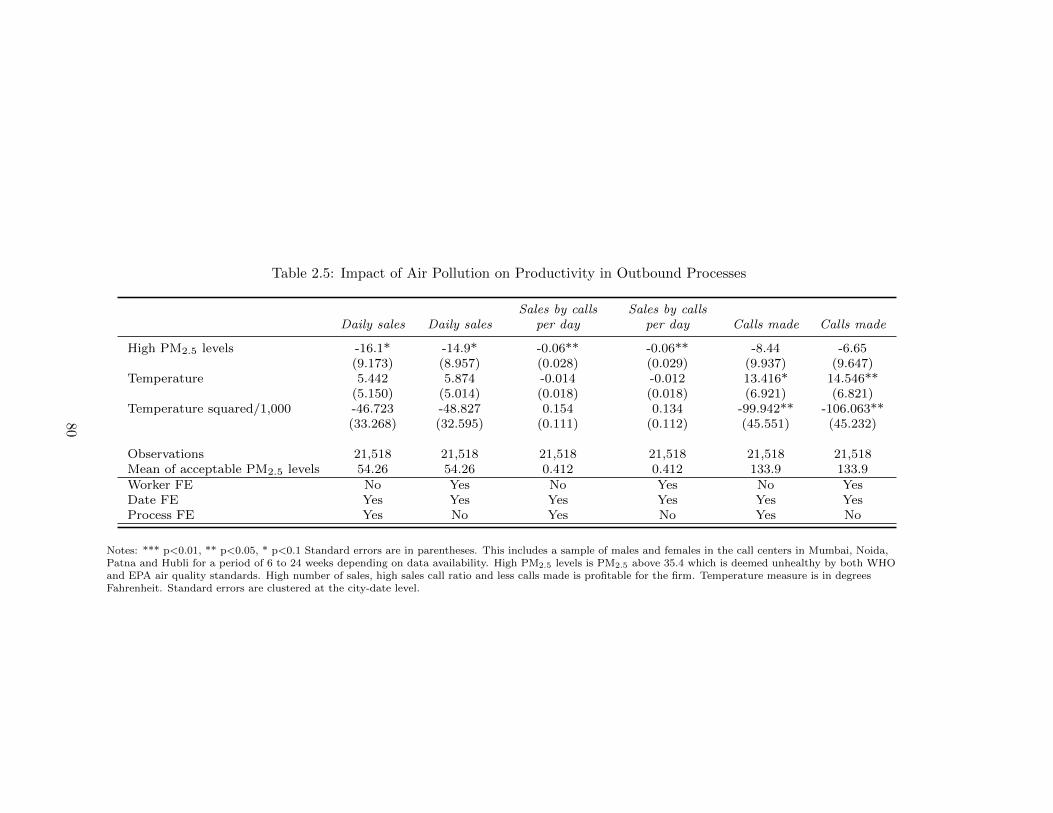
Table 2.5: Impact of Air Pollution on Productivity in Outbound Processes

Daily sales Daily salesSales by calls

per daySales by calls

per day Calls made Calls made

High PM2.5 levels -16.1* -14.9* -0.06** -0.06** -8.44 -6.65(9.173) (8.957) (0.028) (0.029) (9.937) (9.647)

Temperature 5.442 5.874 -0.014 -0.012 13.416* 14.546**(5.150) (5.014) (0.018) (0.018) (6.921) (6.821)

Temperature squared/1,000 -46.723 -48.827 0.154 0.134 -99.942** -106.063**(33.268) (32.595) (0.111) (0.112) (45.551) (45.232)

Observations 21,518 21,518 21,518 21,518 21,518 21,518Mean of acceptable PM2.5 levels 54.26 54.26 0.412 0.412 133.9 133.9Worker FE No Yes No Yes No YesDate FE Yes Yes Yes Yes Yes YesProcess FE Yes No Yes No Yes No

Notes: *** p<0.01, ** p<0.05, * p<0.1 Standard errors are in parentheses. This includes a sample of males and females in the call centers in Mumbai, Noida,Patna and Hubli for a period of 6 to 24 weeks depending on data availability. High PM2.5 levels is PM2.5 above 35.4 which is deemed unhealthy by both WHOand EPA air quality standards. High number of sales, high sales call ratio and less calls made is profitable for the firm. Temperature measure is in degreesFahrenheit. Standard errors are clustered at the city-date level.

80

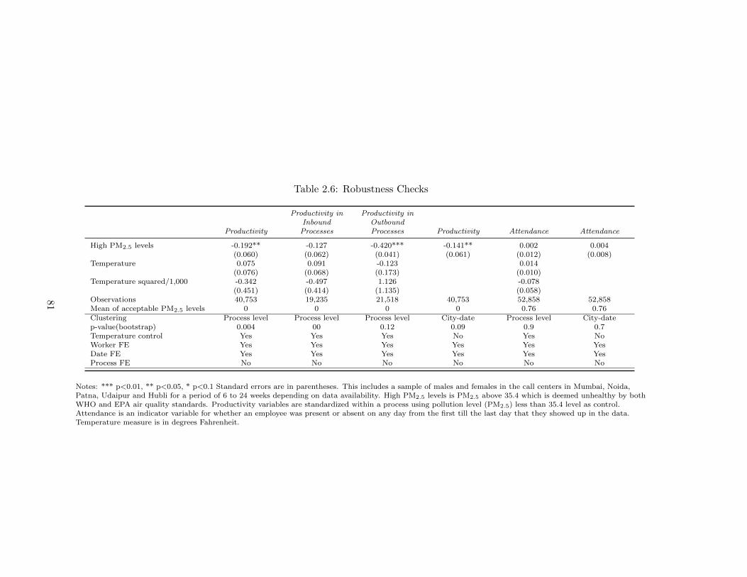
Table 2.6: Robustness Checks

Productivity

Productivity inInboundProcesses

Productivity inOutboundProcesses Productivity Attendance Attendance

High PM2.5 levels -0.192** -0.127 -0.420*** -0.141** 0.002 0.004(0.060) (0.062) (0.041) (0.061) (0.012) (0.008)

Temperature 0.075 0.091 -0.123 0.014(0.076) (0.068) (0.173) (0.010)

Temperature squared/1,000 -0.342 -0.497 1.126 -0.078(0.451) (0.414) (1.135) (0.058)

Observations 40,753 19,235 21,518 40,753 52,858 52,858Mean of acceptable PM2.5 levels 0 0 0 0 0.76 0.76Clustering Process level Process level Process level City-date Process level City-datep-value(bootstrap) 0.004 00 0.12 0.09 0.9 0.7Temperature control Yes Yes Yes No Yes NoWorker FE Yes Yes Yes Yes Yes YesDate FE Yes Yes Yes Yes Yes YesProcess FE No No No No No No

Notes: *** p<0.01, ** p<0.05, * p<0.1 Standard errors are in parentheses. This includes a sample of males and females in the call centers in Mumbai, Noida,Patna, Udaipur and Hubli for a period of 6 to 24 weeks depending on data availability. High PM2.5 levels is PM2.5 above 35.4 which is deemed unhealthy by bothWHO and EPA air quality standards. Productivity variables are standardized within a process using pollution level (PM2.5) less than 35.4 level as control.Attendance is an indicator variable for whether an employee was present or absent on any day from the first till the last day that they showed up in the data.Temperature measure is in degrees Fahrenheit.

81

Chapter 3

E↵ect of Co-residence with

Parents-in-law on Female Labor

Force Participation

82

Abstract

This paper studies the impact of co-residence with mother-in-law and father-in-law on

women’s labor force participation. We study this in the Indian context where co-residence with

parents-in-law is a common practice and women don’t have much decision-making autonomy or

empowerment in the presence of a parent-in-law in the household. On the other hand, for women

with young children, having a mother-in-law or father-in-law living nearby might have a positive

e↵ect on labor supply because the grandparents might provide childcare transfers. We use two rounds

of IHDS panel data for the analysis taking death of the parent-in-law as the exogenous variation.

Our preliminary results show that co-residence with father-in-law has a significantly negative e↵ect

on women’s labor supply. Losing one’s healthy father-in-law increases the labor force participation

of women by overall 11.4 percentage points, compared to a similar household where the father-in-

law still co-resides in the second round. This is a large increase in female labor force participation

(FLFP) of approximately 25% over the mean FLFP in the first round. There is also an increase in

FLFP by 11 percentage points following the loss of a working mother-in-law, providing evidence of

an added worker e↵ect in the household. Death of mother-in-law increases women’s empowerment

by 16.7%.

83

3.1 Introduction

Despite very rapid economic growth in India in the recent years, there has been a steady

decline in Female Labor Force Participation (FLFP) rates across all age groups and education levels

in India (Bourmpoula et al., 2014)). In fact the FLFP rates in India have declined by more than 8

percentage percentage points between 1999 and 2009 among married women (Afridi et al, 2016).1

There is some evidence that women in India may be withdrawing from the workforce to cater to their

traditional role at home as care workers.2 This is an expected outcome owing to the increases in

number of elderly and the rise in the number of joint families in India over this period.3 Therefore,

it has become important to study the labor market outcomes of women living in the traditional set

up of joint families to explain some of the decline in FLFP in the last two decades. Additionally,

with the expected increase in elder-care requirements within the households in the future, this study

has important policy implications.

This paper studies the impact of co-residing with mother-in-law and father-in-law on

woman’s labor force participation as the primary outcome in the Indian context. We use two waves

of the panel data set, India Human Development Survey (IHDS), and take the sample of women in

the first round who co-reside with healthy parents-in-law. Death of healthy parent-in-law is used

for identification in the second round. We find that losing one’s father-in-law increases the labor

force participation of women by 5 to 13 percentage points, compared to a similar household where

the father-in-law still co-resides in the second round. This is a large increase in female labor force

participation (FLFP) of approximately 11% to 25% over the mean FLFP in the first round. There

1The education levels have risen and fertility has decreased simultaneously during this period, adding tothe puzzling decline in FLFP.

2According to NSSO data, about 88% of the rural women in 2004-05 required to spend most of their timeon domestic duties, which increased to 92% in 2011-12. About 55% rural women reported to be engaged indomestic work as no other person was available to do that work and this increased to 62% in 2009-10.

3Joint families are those where more than one married couple co-resides, and patriarchal nature of Indiansociety leads to a high prevalence of inter-generational co-residence. Joint families in India constitute about27-30% of all families and between the time period 2000 to 2010, number of joint families as a percentage ofall families increased marginally. Between 2000 and 2010 the percentage of nuclear families as a percentage ofall families declined slightly, from 70.34% to 70.11% and number of joint families increased (Census Reports).

84

is also an increase in FLFP by 11 percentage points following the loss of a working mother-in-law,

providing evidence of an added worker e↵ect in the household. We also study empowerment as a

secondary measure and find that death of the mother-in-law increases women’s empowerment by

16.7%.

Patrilocality or living with parents-in-law after marriage is a common phenomenon for

women in India. Women often don’t have much decision-making autonomy, especially in the presence

of a parent-in-law in the household. There are some descriptive studies showing that living with a

mother-in-law is associated with diminished autonomy for a woman in India owing to the fact that

mother-in-law is the head’s wife (Bloom, Wypij and Das Gupta, 2001; Jejeebhoy and Sathar 2001;

Balk 1994). Mason (1997) also discuss how the household head’s wife has more decision-making

power than the “junior” wives in joint families in India. This study is relevant for other countries as

well, because many other countries practice the family structure of inter-generational co-residence or

co-residence of adult sons and elderly parents especially in Asia, the Middle East, and North Africa

and Latin America (Ebenstein, 2014).

The primary outcome variable is labor supply of women. Due to under-valuation and lack

of recognition of women’s unpaid work, the gender bias in a patriarchal society is exacerbated if

women do not contribute to the household income, making earned income an important indicator

of women’s well being and autonomy. In these societies, where sons are preferred and women’s

position is low, less household resources are spent on the education and health of a girl than a boy

(Jayachandran, 2015). Rob Jensen (2012) provides evidence for this in his paper where there was

an increase in FLFP in a northern state of India due to the increase in white-collar jobs available

for women in that region. He shows that this increase in FLFP a↵ected the human capital and

fertility decisions of girls/women and was associated with increased enrollment of school-aged girls

and improvements in their body mass index (BMI). Singh and Samara (1996) use Demographic

Health Survey (DHS) data for 40 countries to show how age at marriage of a woman positively

85

correlates with urbanization, women’s education and FLFP. Therefore, women’s earned income is

crucial for better health, nutrition and human capital investments on girl children and for a decrease

in early marriage and child bearing for women. Another reason how wage work benefits women is

because it raises their bargaining power at home. Anderson and Eswaran (2009) have empirically

shown using cross-sectional data set from Matlab Health and Socio-economic Survey (1996) from

Bangladesh, that it is earned rather than unearned income that boosts women’s relative bargaining

power and autonomy. Majlesi (JDE, 2016) uses trade shocks as exogenous demand shifts in di↵erent

manufacturing industries to show how women’s relative bargaining power at home increases in an

instance of favorable shocks to manufacturing industries with more women workers in Mexico.

Economic theory makes no clear prediction about the e↵ect of living close to one’s father-

in-law or mother-in-law on labor supply (at the extensive margin- the probability of working in the

market, or at the intensive margin- the number of hours worked per week). Konrad et al. (2002)

model migration away from parents as a non-cooperative game in which the eldest child always has

the first mover advantage and migrates away from home to avoid future transfers of care to elderly

parents. Rainer and Siedler (2009) work on a similar model and show that only children are more

likely to be living in parents’ location and therefore have worse labor market outcomes than children

with siblings. None of these papers consider the positive e↵ect of the receipt of childcare on the

labor force outcomes of women with children.

Masaru Sasaki (JHR, 2002) try to study the impact of this in the Japanese context and

also find that co-residence with parents or in-laws has a significantly positive impact. However,

they use cross-sectional data of Japanese household survey which raises significant concern about

omitted variable bias. Further, it can be that co-residence and female labor force participation

(LFP) decisions are taken together such that there is endogeneity issue. Arpino, Pronzato and

Tavares (2011) estimate the e↵ect of grandparent-provided childcare on the labor force participation

of women in Italy using a cross-sectional data set and doing the analysis on young mothers with at

86

least one child below 14 years of age. They use the number of living grandparents as an instrument for

grandparent help in childcare. They find a huge (30 percentage point) positive e↵ect of grandparent

care transfers on the probability that a woman is working but because the instrument doesn’t meet

the exclusion restriction (due to correlation with unobservable characteristics of the family like

genetic endowment) the coe�cient again may be subject to biased.

Another study that looks at this issue using richer data is by Compton and Pollak (2014).

They use the National Survey of Families and Households (NSFH) and the public use files of the

U.S. Census to study the e↵ect of proximity to mother or mother-in-law on a married women’s labor

force participation. They see the impact on women who have young children less 12 years of age

and find that the probability of living within 25 miles of their mothers or mothers-in-law increases

the probability of working in the market and also increases the number of hours worked per week.

Apart from these evidences from the developed world, there a study by Anukriti et al.

(2020) that studies the impact of co-residence with parents-in-law on outcomes such as women’s

mobility and their reproductive health in one of the states in India. However, there is no empirical

study which studies nature of co-residence in joint family systems and woman’s labor force partici-

pation as the primary outcome. In such a family structure parents-in-law have a more crucial role

in a woman’s decision to do wage work. Using household time allocation, Becker’s model (1965)

of female labor supply makes assumptions that women make their labor supply decisions not only

considering their leisure and labor trade-o↵s, but they also take into consideration home production

of goods and services, and care work. As it is true that all over the world women face the dispro-

portionate burden of care work, which includes the 3 C’s of cooking, cleaning and care work (OECD

Time-use Data), studying women’s labor supply, taking into consideration women’s time constraints

is essential. And often times, women get help in these activities from other females co-residing with

them or living nearby. Due to lack of reliable formal childcare, presence of mother-in-law can par-

tially release the daughter-in-law of this responsibility. Hence, distribution of domestic work within

87

a household among women plays a role in ascertaining the labor supply of women in a household.

Since, the younger woman or daughter-in-law is likely to have a higher marginal productivity of mar-

ket work than the older woman, but similar marginal productivity of home-based work, households

may prefer the daughter-in-law to do wage work. There could also be a generational divergence of

preference with mother-in-law preferring unpaid work and daughter-in-law preferring paid work.

Alternatively, co-residence with parents-in-law might have a negative e↵ect on labor supply

because the grandparents themselves may require care, and caregiving responsibilities often fall to

daughters-in-law who co-reside with them. To tackle this problem only healthy parents-in-law are

included in the analysis, i.e., parents-in-law with no major morbidities like Tuberculosis, Cancer,

AIDS etc. in the first round are included.

In developing countries like India where genders are socially segregated, there are risks

and costs associated with physical mobility of women, resulting in household preference of women

to stay at home. These perceived costs arise from concerns of safety in an environment of rampant

sexual harassment and sexual violence. It can also stem from protecting the family honor from risks

of intermingling of women with ‘outside men’ (Jayachandran, 2015). Therefore, for a woman to

participate in the labor market, wage should compensate for both shadow value of home-based work

and cultural costs. These costs are higher in a joint family structure and could depress the woman’s

labor supply.

As there are many opposing mechanisms through which the labor supply of women is

a↵ected in a joint family structure, to learn which of these e↵ects predominate requires empirical

analysis. Since there could be potential endogeneity between co-residence with parent-in-law and

woman’s LFP as women who live with their mother-in-law could be very di↵erent from those that

don’t live with them. Also, there could be simultaneity issue. To take care of the unobserved

di↵erences, death of mother-in-law and father-in-law are used as the exogenous variation.

88

These e↵ects on daughter-in-law’s labor supply could be di↵erent depending on whether

the loss is of a mother-in-law or father-in-law. If there is a death of a wage earning parent-in-law,

then the woman might join the labor market to compensate for the loss of income to the household

(added worker e↵ect). However, death of a mother-in-law can also posit as a home production shock.

3.2 Data and Descriptive Statistics

For this study, we use two waves of the panel data set, India Human Development Survey

(IHDS). IHDS is a nationally representative survey of more than 40,000 households. The first round

is for the year 2004-2005 and the second round is for the year 2011-12. The survey covers topics

concerning health, education, employment, economic status, marriage, fertility, gender relations, and

social capital. Information on whether the mother-in-law is co-residing with the woman in the first

round is obtained from the household roster. The sample is limited to daughters-in-law who are in

the age group 18 to 49 in the first round. As death of parent-in-law is used for identification, women

who co-reside with their parent-in-law in the first round are chosen for the analysis. Labor force

outcomes of those who lose their parents-in-law are then compared to those who are still co-residing

with them.

As parents-in-law could be co-residing with their son and daughter-in-law for care transfers

if they su↵er from any major morbidities or long-term illnesses, it would require that the daughter-

in-law stay at home for the same. However, we want to separate out this e↵ect and make death

of a parent-in-law an exogenous shock to the household. So, we only take parents-in-law who are

‘healthy’ in the first round for the analysis. ‘Healthy’ here is defined as those su↵ering from no major

morbidities like Cancer, Asthma Tuberculosis, Heart Diseases, Polio, Leprosy, Paralysis, Diabetes,

STD/AIDS, Epilepsy any form of Mental Illness, high blood pressure problems or any other long

term disease. Even if they su↵er from one of these diseases, they are not included in the analysis.

89

Therefore, families with both healthy mother-in-law and father-in-law are chosen because if even

one has a long-term disease, the labor supply of daughter-in-law will be a↵ected by it.

Table 1 reports the summary statistics to see if the two groups (the one in which woman

co-resides with her parent-in-law and one in which one of them dies by the second rounds) in 2005

are similar on variables like Household Assets, Woman’s education level, Family size and Number of

children. It can be seen that the women who lose their parents-in-law are older and therefore are less

educated on an average (measured in number of years of education). As these families are generally

older, there are fewer children in the house. The labor force participation is lesser in comparison

to the group that does not co-reside with their mother-in-law. Table 7 in the Appendix reports the

characteristics of mothers-in-law in 2005 belonging to the two groups. Here we have included both

healthy and unhealthy mothers-in-law. About 40% of the mothers-in-law worked for more than 240

hours in 2005. Table 8 in the Appendix reports the average characteristics of all fathers-in-law co-

residing with daughters-in-law in 2005 divided by the two groups of concern. I use the entire set of

fathers-in-law co-residing with their daughter-in-law (both healthy and unhealthy) and as expected

find that the ones with more diseases are likely to die.

For the first specification, the sample is restricted to those women who live/co-reside with

their mothers-in-law in the first period, which is around 9159 women out of 45,895 sample women.

In the second round, co-residence is again computed through the household roster and crosschecked

using the tracking file. Hence, we are able to di↵erentiate between women who are still co-residing

with their mothers-in-law, women who lost their mothers-in-law between the two rounds and women

who don’t co-reside with their mothers-in-law any more. Out of 9159 daughters-in-law co-residing

with their mothers-in-law in the first round, 1,948 (about 21%) of them lose their mothers-in-law

and the rest continue to live with them in the second round. Split households are excluded from the

sample. Among these, only 7,200 of the women live with healthy mother-in-law (and healthy

90

father-in-law if father-in-law also co-resides with them) in the first round of which 1,493 die by the

second round of short term illnesses and accidents and 5,707 of them are still co-residing with them.

For the second specification, the sample is restricted to women who co-reside with their

fathers-in-law in the first round. This is around 6,777 daughters-in-law, out of whom about 2,293

of them lose their father-in-law by the second round. In the sub-sample of 5,226 women co-residing

with healthy father-in-law, 1,670 of them lose their fathers-in-law and 3,556 is the comparison group

of those still co-residing with their fathers-in-law in the second round.

In the third specification, women co-residing with both healthy parents-in-law in 2005 are

chosen, which is a total of 3,850, out of which 429 lose their mother-in-law, 870 lose their father-in-

law and 208 lose both their parents-in-law to short-term illnesses and accidents by the second round.

A total of 11,633 women live with either their of parents-in-law (who is of good health) in 2005 in

the sample out of which 2,979 (about 25%) of them lose either or both of them by 2011.

To understand how co-residence with parents-in-law impacts empowerment of women in

India, we construct measures of Physical Autonomy, Financial Autonomy and Decision-making

Autonomy for women in both rounds. The measure of Physical Autonomy is based on questions

on whether they require permission to visit the health centre, visit friends/ relatives or for going

for grocery shopping. The measure of Financial Autonomy is based on questions on whether they

have cash in hand to spend on household expenditures. have bank account or have home ownership

or rental papers in their names. And the measure of Decision Autonomy is based on who in the

household makes the decision on what to cook, what to do if child falls sick, buy expensive items

like fridge/TV, how many children the woman has and about child’s marriage. Average responses

on whether daughter-in-law has the most say on these measures is calculated. A combined measure

of empowerment is estimated taking an average of Physical Autonomy, Financial Autonomy and

Decision-making Autonomy responses.

91

3.3 Empirical Methodology

We use the following empirical specifications to estimate the e↵ect of co-residence with

mother-in-law and father-in-law on various outcome measures of labor force participation, autonomy

and empowerment. Using a panel data of women, we control for individual and time fixed e↵ects

to take into account time invariant individual heterogeneity and time trends. The main outcome

variable labor force participation (LFP) is a binary variable, which takes value one if woman reports

working for more than 240 hours in a year on any work (farm or o↵-farm work, wage or self-

employed work). To allow for flexibility in age, we use the full set of age dummies. Standard errors

are clustered at the primary sampling unit to account for unobserved but correlated characteristics

a↵ecting outcomes among women from the same primary sampling unit or district in the data -set.

In the first methodology, as discussed in the previous section, women co-residing with

healthy mother-in-law are chosen and the e↵ect of death of mother-in-law on labor supply of

daughter-in-law is discussed with those still co-residing with the mother-in-law. This sub-sample also

contains healthy father-in-law for some families, who are co-residing with both their parents-in-law

in 2005.

LFPit = �0 + �1Death of Motherinlawit + �2Ageit + ⌦i + ✏it (3.1)

In the second specification, women co-residing with healthy father-in-law are chosen and

the e↵ect of death of father-in-law on labor supply of daughter-in-law is discussed with those still

co-residing with the father-in-law. This sub-sample also contains healthy mother-in-law for some

families.

LFPit = �0 + �1Death of Fatherinlawit + �2Ageit + ⌦i + ✏it (3.2)

92

In the following specification, families co-residing with both parents-in-law are chosen and to capture

the di↵erential e↵ects of each of the following, death of mother-in-law, death of father-in-law and

death of both are used in the regression analysis and the group of women which is still co-residing

with both the parents-in-law in the second round is used as comparison. Here Yit are the primary

outcomes measures of labor force participation and secondary outcome measures of autonomy and

empowerment of women.

Yit = �0 + �1Death of Motherinlawit + �2Death of Fatherinlawit

+�3Death of Motherinlaw andFatherinlawit + �4Ageit + ⌦i + ✏it

(3.3)

The regression results of these three empirical methodologies are discussed in the following

section. We also conduct some heterogeneity analysis. So, sub-group analysis is done for Urban and

Rural areas as the FLFP varies in the two greatly in India. In addition, we analyze the labor

force participation of women with children separately to check if the woman withdraws from the

labor market to provide child care transfers in the absence of parents-in-law. Families which lose an

employed parent-in-law are also discussed separately to see if there is evidence of any added worker

e↵ect owing to the negative income shock to the household.

3.4 Regression Results

This section provides an overview of the main results. The first subsection provides the

regression results on both the primary outcome of female labor force participation and the secondary

outcome of female empowerment. We also provide results for some heterogeneous groups where the

result are expected to be theoretically di↵erent. In the second subsection, the results from some

robustness checks are discussed.

93

3.4.1 Main Results on Primary and Secondary Outcomes

In Table 2, we provide regression results on the e↵ect of death of healthy mother-in-law

on the primary outcomes of labor force participation of daughter-in-law. There is no evidence of

co-residence with mother-in-law for the full sample as well as for the sub-sample of women with

children and women living in both rural and urban areas (Columns 1, 2, 3 and 4 in Table 2). Table 2

also shows that the average labor force participation rates of women co-residing with mothers-in-law

is much lesser in urban areas at 19.3% in the sample than those in rural areas at 58%. The LFP of

women with children below the age of 14 in he household for those co-residing with parents-in-law

is about 51% in 2005. The women with children are also the younger women in the sample.

We find a 11.1 percentage point increase in women’s LFP rates following the death of a

healthy and working mother-in-law (Column 5, Table 2). This is a 19% increase over the mean

FLFP of 0.57 in 2005 and is significant at the 5% level. We don’t find any e↵ects for the death

of a non-wage earning mother-in-law on FLFP. Therefore, it appears that women are working to

compensate for the negative income shock to the household.

A similar analysis on fathers-in-law shows a positive, strong and robust result on FLFP.

We also observe that the women who co-reside with healthy fathers-in-law have a lower mean LFP

in 2005 than those who live with healthy mothers-in-law (Table 2 and 3). We find an overall 11.4

percentage point increase in FLFP because of the death of father-in-law over the mean FLFP of

0.48 in the first round. This is significant at the 1% level and is a increase of approximately 24%

(See Column 1 of Table 3).

For rural women, the point-estimate increase to 12.2 which is a 22.5% increase in FLFP

following the death of a healthy father-in-law (Column 2 of Table 3. For urban women, the e↵ect is

smaller at 8 percentage points but this is significant at the 5% level (Column 3 of Table 3. This is

a 56% increase in FLFP in urban areas for the women in the sample. We find similar e↵ects of 12.1

94

percentage points on FLFP in households with children, which is a 25% increase (Column 4 of Table

3). Women with children are younger so they might find it easier to go back to the labor market.

Although the FLFP rates in 2005 were almost the same for women co-residing with working

and non-wage working father-in-law, we find a stronger e↵ect of 13.2 for working father-in-law

compared to the 5.5 percentage point e↵ect for non-wage working father-in-law (Columns 5 and 6

of Table 3). As expected, women enter the labor market to compensate for the income shock to the

household after a working father-in-law’s death. This is a 25% increase significant at the 1% level.

Surprisingly, we also find an increase in FLFP after the father-in-law’s death even if the father-in-law

was not working. This e↵ect is significant at the 10% level and is a 11% increase in FLFP.

In Table 4, we provide regression results for the sub-sample which co-resides with healthy

parents-in-law in the first round. We study this separately because it helps us in understanding the

overall impact of death on one of the parents-in-law compared to the death of both parents-in-law on

FLFP. Overall, we find that while co-residing with both parents-in-law, the death of just the father-

in-law increases FLFP by 12.2 percentage points, which is significant at the 1% level (Column 1 of

Table 4). We find similar e↵ects for both rural and urban women (Columns 2 and 3 of Table 4).

For households with younger children and therefore also younger daughters-in-law, death of just the

mother-in-law also increases the FLFP significantly by 14.5 percentage points over the mean FLFP

of 0.505 in 2005 (Column 4 of Table 4). For this case death of just the father-in-law also increases

FLFP by 13.7 percentage points. But the death of both parents-in-law reduces the overall FLFP

by 18.8 percentage points (Column 4 of Table 4). This is significant at the 10% level. This result

indicates that the parents-in-law are providing some care transfers because in the absence of both

parents-in-law, women with children have to withdraw from the labor market.

The regression results on the secondary outcome measures of autonomy or empowerment

provide evidence that daughter-in-law’s empowerment increases following the death of a healthy

mother-in-law. It is a 4.7 percentage point increase over a mean of 0.28, which is a 16.7% increase

95

(Column 4 of Table 5). This is significant at the 1% level. There is no impact of father-in-law’s

death on measures of physical, financial and decision autonomy (Table 5). We also observe that only

20% of the women in the sample have most say on their physical autonomy or decisions on visits to

their friends and relatives.

3.4.2 Robustness Checks

There is a concern that the women who lose their parents-in-law are older and less educated

on an average and therefore can’t be compared (Table 1). Therefore, for a robustness check, women

are matched on age, education, family size, household assets and location in urban/rural areas

in the first round 2005. The summary statistics of the matched women are provided in Table 9

of the Appendix. As we can see, women are balanced on all the afore-mentioned characteristics.

The common support graph in the appendix further illustrates that we have enough support and

comparison for each age and education group.

In Table 6, we report similar but stronger results as Table 4. These e↵ects are huge

while comparing matched groups, indicating more than a 50% increase in FLFP following a healthy

father-in-law’s death. This further supports our analysis and confirms our results.

3.5 Conclusion

The e↵ect of death of a healthy father-in-law on FLFP is an overall increase of 11.4

percentage points. This a large e↵ect of around 24% increase in FLFP. This is also true for death of

a working mother-in-law as it increases in FLFP by around 11 percentage points (a 19% increase).

This provides evidence of the added worker e↵ect due to a negative income shock to the household.

The death of father-in-law in the household with the presence of mother-in-law, frees the woman to

work in the labor force especially in the case of unanticipated income shocks. Labor supply of younger

women with children responds more significantly and positively to the death of one of parents-in-law.

96

However, her labor supply declines if she loses both her parents-in-law, indicating that the death

of both parents-in-law in leads to women withdrawing from the labor market. Therefore, there is

some substitution of women’s labor towards more unpaid home-based work from paid work in the

absence of healthy parents-in-law (about 18.8 percentage point negative e↵ect on FLFP).

It seems that women in India are secondary workers and their labor supply more of an

insurance to the household against income shocks. The analysis has implications for policy as it

suggests that policies that increase the availability of childcare to meet irregular or unanticipated

child care needs, including care for a sick child, might substantially increase the labor supply of

married women with young children. With increasing life expectancy and associated rise in old

people in India and other countries. This analysis also makes contribution to the literature on

ageing population, as it discusses the financial and care transfers of parents-in-law in the household.

We would like to probe more into this in the future using data on health and well-being of children

in the presence of grandparents.

97

References

Afridi, Farzana, Taryn Dinkelman, and Kanika Mahajan. Why are fewer married womenjoining the work force in India? a decomposition analysis over two decades. (2016).

Anderson, Siwan, and Mukesh Eswaran. What determines female autonomy? Evidencefrom Bangladesh. Journal of Development Economics 90.2 (2009): 179-191.

Anukriti, S., Herrera-Almanza, C., Karra, M., Pathak, P. (2020). Curse of the Mummy-ji: The Influence of Mothers-in-Law on Women in India . Boston University-Department of Eco-nomics.

Arpino, Bruno, Chiara Pronzato, and Lara Tavares. All in the family: informal childcareand mothers’ labour market participation. No. 2010-24. ISER Working Paper Series, 2010.

Balk, Deborah. “Individual and Community Aspects of Women’s Status and Fertility inRural Bangladesh.” Population Studies 48, no. 1 (1994): 21-45.

Becker, Gary S. Human capital, e↵ort, and the sexual division of labor. Journal of laboreconomics 3.1, Part 2 (1985): S33-S58.

Bloom, Shelah S., David Wypij and Monica das Gupta. 2001 “Dimensions of Women’sAutonomy and the Influence on Maternal Health Care Utilization in a North Indian City” Demog-raphy 38(1):67-78.

Bourmpoula, E. et al “Why is female labour force participation declining so sharply inIndia?” ILO (2014) Ebenstein, A. (2014): “Patrilocality and Missing Women,” Working paper, He-brew University.

Duflo, Esther. 2012. “Women empowerment and economic development.” Journal of Eco-nomic Literature, 50(4): 1051–1079.

Ebenstein, Avraham. 2014. “Patrilocality and Missing Women.” Working Paper.

Ghosh J., “Women’s Burden”, edited by Jain D., and Sujaya C.P., “Indian Women -Contemporary Essays,” Publications Division; 2015 ed

“Global Employment Trends 2013, Recovering from a second jobs dip,” International la-bor Organisation, 2013

International Labor Organization, 2012, “Global Employment Trends for Women March2004”

Jain, Devaki, and Diane Elson. Harvesting feminist knowledge for public policy: rebuild-ing progress. IDRC, 2011.

Jayachandran, Seema (2015) “The Roots of Gender Inequality in Developing Countries”American Economics Review

Jejeebhoy, Shireen J. and Zeba Sathar. “Women’s Autonomy in India and Pakistan: The

98

Influence of Religion and Region.” Population and Development Review 27, no. 4 (2001): 687-712.

Jensen, Robert. Do labor market opportunities a↵ect young women’s work and familydecisions? Experimental evidence from India. The Quarterly Journal of Economics 127.2 (2012):753-792.

Konrad, Kai, Harald Kunemund, Kjell Erik Lommerud, and Julio R. Robledo, “Geogra-phy of the Family,” American Economic Review, Vol. 92, No. 4, (September 2002), 981-998.

Lahoti, R. and Swaminathan, H., “Economic Growth and Female Labour Force Partici-pation in India,” WORKING PAPER NO: 414, Indian Institute of Management, 2013

LaFave D. and Thomas D., “Extended Families and Child Well-being”, NBER WorkingPaper No. 20702, 2014

Majlesi, Kaveh. Labor market opportunities and women’s decision making power withinhouseholds. Journal of Development Economics 119 (2016): 34-47.

Mammen, Kristin, and Christina Paxson. 2008. “Women’s Work and Economic Develop-ment.” The Journal of Economic Perspectives 14 (4): 141–164.

Mason, Karen Oppenheim. “The Status of Women: Conceptual and Methodological Is-sues in Demographic Studies.” Sociological Forum 1 no. 2 (1986): 284-300.

Mason, Karen Oppenheim and Herbert L. Smith. “Husbands’ versus Wives’ FertilityGoals and Contraceptive Use: The Influence of Gender Context in Five Asian Countries.” Demog-raphy 37, no. 3 (2000): 299-311.

Pollak R. and Compton J., Family Proximity, Childcare, and Women’s Labor Force At-tachment,” Journal of Urban Economics, January 2014

Rainer, Helmut and Thomas Siedler, “O Brother, Where Art Thou? The E↵ects of Havinga Sibling on Geographic Mobility and Labor Market Outcomes,” Economica, Vol. 76, No. 303, (July2009), 528-556.

Sasaki M., “The Causal E↵ect of Family Structure on Labor Force Participation amongJapanese Married Women” The Journal of Human Resources, 2002

Singh, Susheela, and Renee Samara. Early marriage among women in developing coun-tries. International family planning perspectives (1996): 148-175.

99

ACKNOWLEDGEMENTS

This paper is co-authored with my co-advisor Anil Deolalikar. The dissertation author is

the co-primary investigator and author of this paper.

We are grateful to Mindy Marks, Joseph Cummins, Robert Kaestner, Steven Helfand and

Michael Bates for their valuable comments at various stages of this paper. We also would like to

thank the faculty and students at the Department of Economics at UC Riverside on their comments

during various seminars in which this paper was presented. We also want to thank the audiences at

IAFFE and APPAM seminars for their useful comments.

100

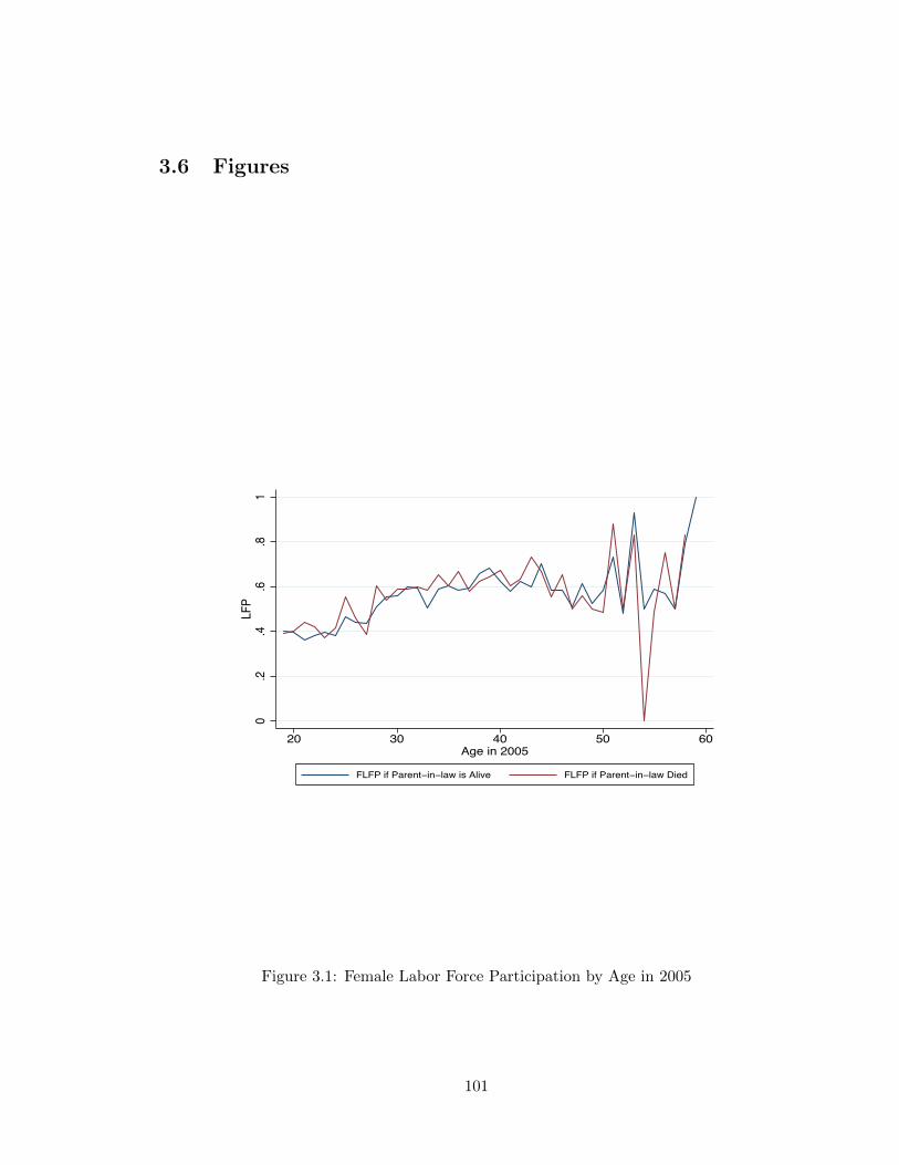
3.6 Figures

0.2

.4.6

.81

LFP

20 30 40 50 60Age in 2005

FLFP if Parent−in−law is Alive FLFP if Parent−in−law Died

Figure 3.1: Female Labor Force Participation by Age in 2005

101

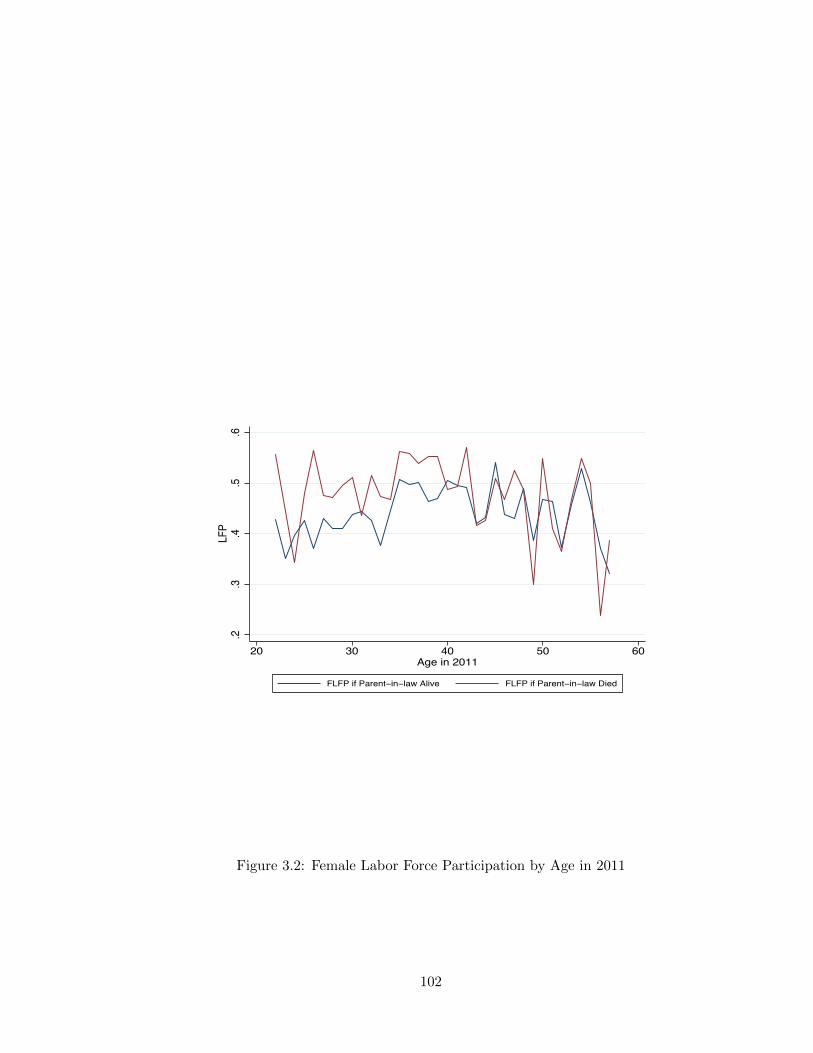
.2.3

.4.5

.6LF

P

20 30 40 50 60Age in 2011

FLFP if Parent−in−law Alive FLFP if Parent−in−law Died

Figure 3.2: Female Labor Force Participation by Age in 2011

102

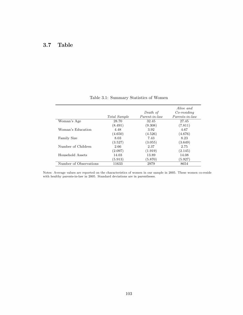
3.7 Table

Table 3.1: Summary Statistics of Women

Total SampleDeath of

Parent-in-law

Alive andCo-residing

Parents-in-lawWoman’s Age 28.70 32.45 27.45

(8.491) (9.308) (7.811)Woman’s Education 4.48 3.92 4.67

(4.650) (4.526) (4.676)Family Size 8.03 7.43 8.23

(3.527) (3.055) (3.649)Number of Children 2.66 2.37 2.75

(2.097) (1.919) (2.145)Household Assets 14.03 13.89 14.08

(5.913) (5.870) (5.927)Number of Observations 11633 2979 8654

Notes: Average values are reported on the characteristics of women in our sample in 2005. These women co-residewith healthy parents-in-law in 2005. Standard deviations are in parentheses.

103

Table 3.2: E↵ect of Co-residence with Mother-in-law on Woman’s Labor Force Participation

FullSample

RuralWomen

UrbanWomen

Householdswith Children

WorkingMother-in-law

Non-wageWorker

Mother-in-lawMother-in-law dead 0.022 0.026 -0.001 0.025 0.111** -0.035

(0.022) (0.027) (0.035) (0.024) (0.044) (0.022)Survey Year -0.102*** -0.133*** 0.025 -0.109*** -0.191*** -0.048*

(0.025) (0.028) (0.036) (0.027) (0.044) (0.025)Constant 0.035 0.137 -0.211 0.045 0.146 0.344***

(0.186) (0.159) (0.273) (0.178) (0.162) (0.048)

Observations 14,400 10,890 3,510 12,164 6,934 11,310R-squared 0.045 0.058 0.067 0.044 0.080 0.055Number of Individuals 7,200 5,445 1,755 6,082 3,467 5,655Mean LFP in 2005 0.508 0.586 0.193 0.514 0.571 0.466

Notes: *** p<0.01, ** p<0.05, * p<0.1 2005 and 2011 panel rounds of IHDS data are used with individual fixed e↵ects and time fixed e↵ect. Sample includesmarried women from the age 18 to 58 years, who are co-residing with healthy mother-in-law in 2005. We Control for age flexibly. Standard errors are clustered atthe primary sampling unit (PSU).

104

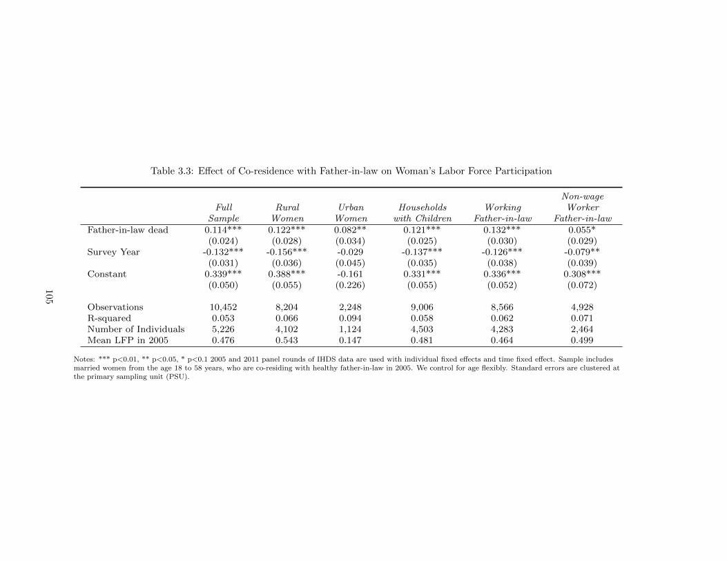
Table 3.3: E↵ect of Co-residence with Father-in-law on Woman’s Labor Force Participation

FullSample

RuralWomen

UrbanWomen

Householdswith Children

WorkingFather-in-law

Non-wageWorker

Father-in-lawFather-in-law dead 0.114*** 0.122*** 0.082** 0.121*** 0.132*** 0.055*

(0.024) (0.028) (0.034) (0.025) (0.030) (0.029)Survey Year -0.132*** -0.156*** -0.029 -0.137*** -0.126*** -0.079**

(0.031) (0.036) (0.045) (0.035) (0.038) (0.039)Constant 0.339*** 0.388*** -0.161 0.331*** 0.336*** 0.308***

(0.050) (0.055) (0.226) (0.055) (0.052) (0.072)

Observations 10,452 8,204 2,248 9,006 8,566 4,928R-squared 0.053 0.066 0.094 0.058 0.062 0.071Number of Individuals 5,226 4,102 1,124 4,503 4,283 2,464Mean LFP in 2005 0.476 0.543 0.147 0.481 0.464 0.499

Notes: *** p<0.01, ** p<0.05, * p<0.1 2005 and 2011 panel rounds of IHDS data are used with individual fixed e↵ects and time fixed e↵ect. Sample includesmarried women from the age 18 to 58 years, who are co-residing with healthy father-in-law in 2005. We control for age flexibly. Standard errors are clustered atthe primary sampling unit (PSU).

105

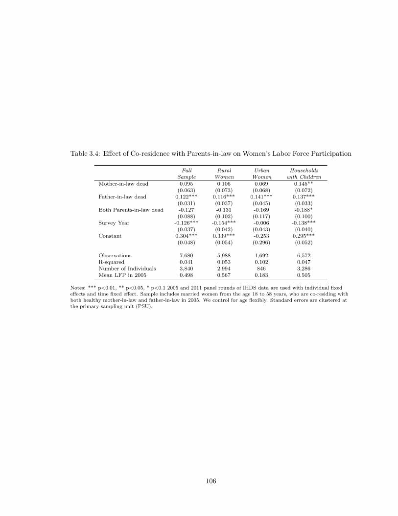
Table 3.4: E↵ect of Co-residence with Parents-in-law on Women’s Labor Force Participation

FullSample

RuralWomen

UrbanWomen

Householdswith Children

Mother-in-law dead 0.095 0.106 0.069 0.145**(0.063) (0.073) (0.068) (0.072)

Father-in-law dead 0.122*** 0.116*** 0.141*** 0.137***(0.031) (0.037) (0.045) (0.033)

Both Parents-in-law dead -0.127 -0.131 -0.169 -0.188*(0.088) (0.102) (0.117) (0.100)

Survey Year -0.126*** -0.154*** -0.006 -0.138***(0.037) (0.042) (0.043) (0.040)

Constant 0.304*** 0.339*** -0.253 0.295***(0.048) (0.054) (0.296) (0.052)

Observations 7,680 5,988 1,692 6,572R-squared 0.041 0.053 0.102 0.047Number of Individuals 3,840 2,994 846 3,286Mean LFP in 2005 0.498 0.567 0.183 0.505

Notes: *** p<0.01, ** p<0.05, * p<0.1 2005 and 2011 panel rounds of IHDS data are used with individual fixede↵ects and time fixed e↵ect. Sample includes married women from the age 18 to 58 years, who are co-residing withboth healthy mother-in-law and father-in-law in 2005. We control for age flexibly. Standard errors are clustered atthe primary sampling unit (PSU).

106

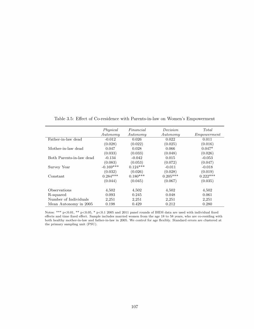
Table 3.5: E↵ect of Co-residence with Parents-in-law on Women’s Empowerment

PhysicalAutonomy

FinancialAutonomy

DecisionAutonomy

TotalEmpowerment

Father-in-law dead -0.012 0.026 0.022 0.011(0.028) (0.022) (0.025) (0.016)

Mother-in-law dead 0.047 0.028 0.066 0.047*(0.033) (0.033) (0.048) (0.026)

Both Parents-in-law dead -0.134 -0.042 0.015 -0.053(0.083) (0.053) (0.072) (0.047)

Survey Year -0.169*** 0.124*** -0.011 -0.018(0.032) (0.026) (0.028) (0.019)

Constant 0.284*** 0.180*** 0.205*** 0.222***(0.044) (0.045) (0.067) (0.035)

Observations 4,502 4,502 4,502 4,502R-squared 0.093 0.245 0.048 0.061Number of Individuals 2,251 2,251 2,251 2,251Mean Autonomy in 2005 0.198 0.429 0.212 0.280

Notes: *** p<0.01, ** p<0.05, * p<0.1 2005 and 2011 panel rounds of IHDS data are used with individual fixede↵ects and time fixed e↵ect. Sample includes married women from the age 18 to 58 years, who are co-residing withboth healthy mother-in-law and father-in-law in 2005. We control for age flexibly. Standard errors are clustered atthe primary sampling unit (PSU).

107

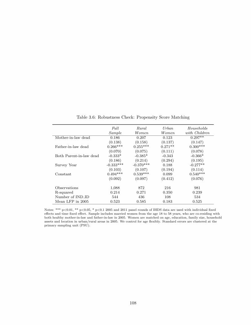
Table 3.6: Robustness Check: Propensity Score Matching

FullSample

RuralWomen

UrbanWomen

Householdswith Children

Mother-in-law dead 0.186 0.207 0.123 0.297**(0.138) (0.158) (0.137) (0.147)

Father-in-law dead 0.266*** 0.255*** 0.271** 0.300***(0.070) (0.075) (0.111) (0.078)

Both Parent-in-law dead -0.333* -0.385* -0.343 -0.366*(0.186) (0.214) (0.294) (0.195)

Survey Year -0.333*** -0.370*** 0.188 -0.277**(0.103) (0.107) (0.194) (0.114)

Constant 0.494*** 0.539*** 0.099 0.540***(0.092) (0.097) (0.412) (0.076)

Observations 1,088 872 216 981R-squared 0.214 0.271 0.350 0.239Number of IND ID 544 436 108 534Mean LFP in 2005 0.523 0.585 0.183 0.525

Notes: *** p<0.01, ** p<0.05, * p<0.1 2005 and 2011 panel rounds of IHDS data are used with individual fixede↵ects and time fixed e↵ect. Sample includes married women from the age 18 to 58 years, who are co-residing withboth healthy mother-in-law and father-in-law in 2005. Women are matched on age, education, family size, householdassets and location in urban/rural areas in 2005. We control for age flexibly. Standard errors are clustered at theprimary sampling unit (PSU).

108

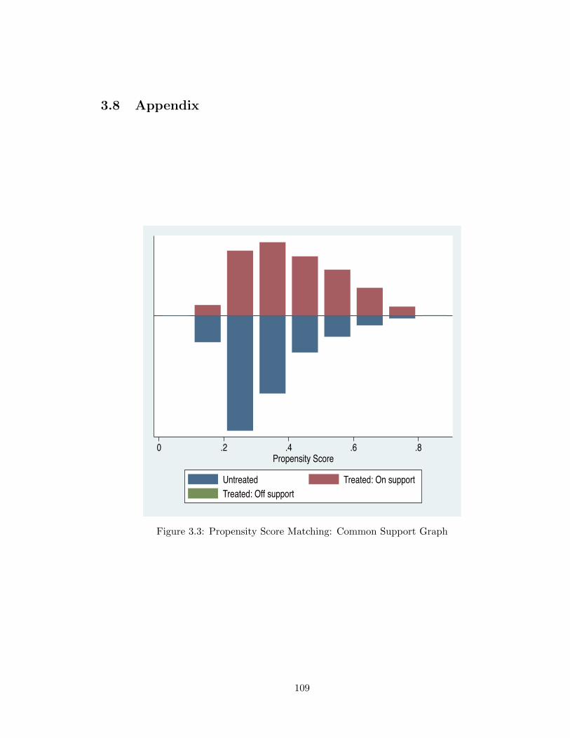
3.8 Appendix

0 .2 .4 .6 .8Propensity Score

Untreated Treated: On supportTreated: Off support

Figure 3.3: Propensity Score Matching: Common Support Graph

109

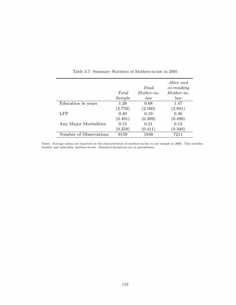
Table 3.7: Summary Statistics of Mothers-in-law in 2005

TotalSample

DeadMother-in-

law

Alive andco-residingMother-in-

lawEducation in years 1.28 0.68 1.47

(2.759) (2.160) (2.891)LFP 0.40 0.19 0.46

(0.491) (0.389) (0.499)Any Major Morbidities 0.15 0.21 0.13

(0.358) (0.411) (0.340)Number of Observations 9159 1948 7211

Notes: Average values are reported on the characteristics of mothers-in-law in our sample in 2005. This includeshealthy and unhealthy mothers-in-law. Standard deviations are in parentheses.

110

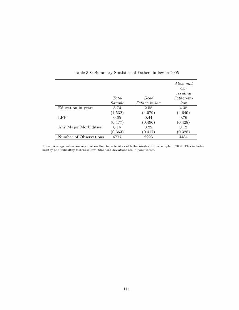
Table 3.8: Summary Statistics of Fathers-in-law in 2005

TotalSample

DeadFather-in-law

Alive andCo-

residingFather-in-

lawEducation in years 3.74 2.58 4.38

(4.532) (4.079) (4.640)LFP 0.65 0.44 0.76

(0.477) (0.496) (0.428)Any Major Morbidities 0.16 0.22 0.12

(0.363) (0.417) (0.328)Number of Observations 6777 2293 4484

Notes: Average values are reported on the characteristics of fathers-in-law in our sample in 2005. This includeshealthy and unhealthy fathers-in-law. Standard deviations are in parentheses.

111

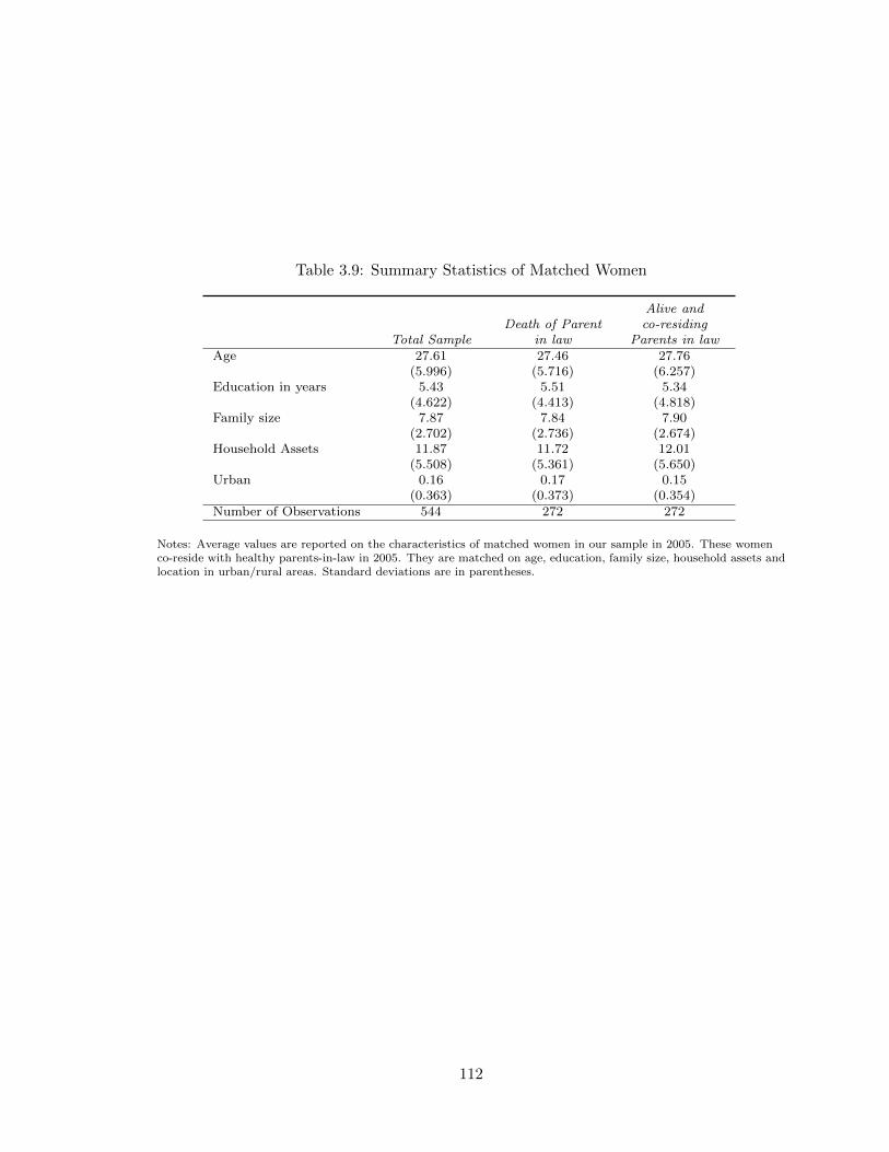
Table 3.9: Summary Statistics of Matched Women

Total SampleDeath of Parent

in law

Alive andco-residing

Parents in lawAge 27.61 27.46 27.76

(5.996) (5.716) (6.257)Education in years 5.43 5.51 5.34

(4.622) (4.413) (4.818)Family size 7.87 7.84 7.90

(2.702) (2.736) (2.674)Household Assets 11.87 11.72 12.01

(5.508) (5.361) (5.650)Urban 0.16 0.17 0.15

(0.363) (0.373) (0.354)Number of Observations 544 272 272

Notes: Average values are reported on the characteristics of matched women in our sample in 2005. These womenco-reside with healthy parents-in-law in 2005. They are matched on age, education, family size, household assets andlocation in urban/rural areas. Standard deviations are in parentheses.

112