Qpp

Quantum Predicative Programming

Anya Tafliovich and E.C.R. Hehner

University of Toronto, Toronto ON M5S 3G4, Canadaanya,[email protected]

Abstract. The subject of this work is quantum predicative program-ming — the development of programs intended for execution on a quan-tum computer. We look at programming in the context of formal meth-ods of program development, or programming methodology. Our workis based on probabilistic predicative programming, a recent generalisa-tion of the well-established predicative programming. It supports thestyle of program development in which each programming step is provencorrect as it is made. We inherit the advantages of the theory, such asits generality, simple treatment of recursive programs, time and spacecomplexity, and communication. Our theory of quantum programmingprovides tools to write both classical and quantum specifications, developquantum programs that implement these specifications, and reason abouttheir comparative time and space complexity all in the same framework.

1 Introduction

Modern physics is dominated by concepts of quantum mechanics. Today, overseventy years after its recognition by the scientific community, quantum me-chanics provides the most accurate known description of nature’s behaviour.Surprisingly, the idea of using the quantum mechanical nature of the world toperform computational tasks is very new, less than thirty years old. Quantumcomputation and quantum information is the study of information processingand communication accomplished with quantum mechanical systems. In recentyears the field has grown immensely. Scientists from various fields of computerscience have discovered that thinking physically about computation yields newand exciting results in computation and communication. There has been ex-tensive research in the areas of quantum algorithms, quantum communicationand information, quantum cryptography, quantum error-correction, adiabaticcomputation, measurement-based quantum computation, theoretical quantumoptics, and the very new quantum game theory. Experimental quantum infor-mation and communication has also been a fruitful field. Experimental quantumoptics, ion traps, solid state implementations and nuclear magnetic resonanceall add to the experimental successes of quantum computation.

The subject of this work is quantum programming — the developing pro-grams intended for execution on a quantum computer. We assume a model ofa quantum computer proposed by Knill [1]: a classical computer with access to

2

a quantum device that is capable of storing quantum bits (called qubits), per-forming certain operations and measurements on these qubits, and reporting theresults of the measurements.

We look at programming in the context of formal methods of program de-velopment, or programming methodology. This is the field of computer scienceconcerned with applications of mathematics and logic to software engineeringtasks. In particular, the formal methods provide tools to formally express soft-ware specifications, prove correctness of implementations, and reason about vari-ous properties of specifications (e.g. implementability) and implementations (e.g.time and space complexity). Today formal methods are successfully employed inall stages of software development, such as requirements elicitation and analysis,software design, and software implementation.

In this work the theory of quantum programming is based on probabilisticpredicative programming, a recent generalisation of the well-established predica-tive programming [2, 3], which we deem to be the simplest and the most elegantprogramming theory known today. It supports the style of program developmentin which each programming step is proven correct as it is made. We inherit theadvantages of the theory, such as its generality, simple treatment of recursiveprograms, and time and space complexity. Our theory of quantum program-ming provides tools to write both classical and quantum specifications, developquantum programs that implement these specifications, and reason about theircomparative time and space complexity all in the same framework.

The rest of this work is organised as follows. Section 2.1 is the introductionto quantum computation. It assumes that the reader has some basic knowledgeof linear algebra and no knowledge of quantum computing. Section 2.2 con-tains the introduction to probabilistic predicative programming. The reader isassumed to have some background in logic, but no background in programmingtheory is necessary. The contribution of this work is section 3 which definesthe quantum system, introduces programming with the quantum system, andseveral well-known problems, their classical and quantum solutions, and theirformal comparative time complexity analyses. Section 4 states conclusions andoutlines directions for future research.

1.1 Related work

Traditionally, quantum computation is presented in terms of quantum circuits.Recently, there has been an attempt to depart from this convention for the samereason that classical computation is generally not presented in terms of classicalcircuits. As we develop more complex quantum algorithms, we will need ways toexpress higher-level concepts with control structures in a readable fashion.

In 2000 Omer [4] introduced the first quantum programming language QCL.Following his work, Bettelli et. al. [5] developed a quantum programming lan-guage with syntax based on C++. These two works did not involve any verifi-cation techniques.

Sanders and Zuliani in [6] introduced a quantum language qGCL, which is anextension of pGCL [7], which in turn generalises Dijkstra’s guarded-command

3

language to include probabilism. Zuliani later extends this attempt at formalprogram development and verification in [8], which discusses treatment of non-determinism in quantum programs, and in [9], where the attempt is made to buildon Aharonov’s work [10] to reason about mixed states computations. Zulianialso provides tools to approach the task of compiling quantum programs in [11].A very similar approach was used in [12] to formally prove the bound on therunning time of Grover’s algorithm, previously established in [13].

A large amount of work in the area was performed in the past two years.In [14], [15], and [16] process algebraic approaches were explored. Tools devel-oped in the field of category theory were successfully employed by [17], [18], [19],[20], [21], and others to reason about quantum computation. In [22] and [23]a functional language with semantics in a form of a term rewrite system is in-troduced and a notion of linearity and how it pertains to quantum systemsare examined. A functional language QML with design guided by its categor-ical semantics is defined in [24]. Following on this work, [25] provides a soundand complete equational theory for QML. Weakest preconditions appropriate forquantum computation are introduced in [26]. This work is interesting, in part,because it diverts from the standard approach of reducing a quantum computa-tion to a probabilistic one. It also provides semantics for the language of [21].Other interesting work by the same authors includes reasoning about knowl-edge in quantum systems ([27]) and developing a formal model for distributedmeasurement-based quantum computation ([28]). A similar work is introducedin [29], where a language CQP for modelling communication in quantum sys-tems is defined. The latter approaches have an advantage over process algebraicapproaches mentioned earlier in that they explicitly allow a quantum state tobe transmitted between processes. Building on the work of [30], [31] defines ahigher order quantum programming language based on a linear typed lambdacalculus, which is similar to the work of [32].

1.2 Our contribution

Our approach to quantum programming amenable to formal analysis is verydifferent from almost all of those described above. Work of [6], [8], [9] is theonly one which is similar to our work. The contribution of this paper is twofold.Firstly, by building our theory on that in [3], we inherit the advantages it of-fers. The definitions of specification and program are simpler: a specification isa boolean (or probabilistic) expression and a program is a specification. Thetreatment of recursion is simple: there is no need for additional semantics ofloops. The treatment of termination simply follows from the introduction of atime variable; if the final value of the time variable is ∞, then the program isa non-terminating one. Correctness and time and space complexity are provedin the same fashion; moreover, after proving them separately, we naturally ob-tain the conjunction. Secondly, the way Probabilistic Predicative Programmingis extended to Quantum Predicative Programming is simple and intuitive. Theuse of Dirac-like notation makes it easy to write down specifications and developalgorithms. The treatment of computation with mixed states does not require

4

any additional mechanisms. Quantum Predicative Programming fully preservesPredicative Programming’s treatment of parallel programs and communication,which provides for a natural extension to reason about quantum communicationprotocols, such as BB84 ([33]), distributed quantum algorithms, such as dis-tributed Shor’s algorithm ([34]), as well as their time, space, and entanglementcomplexity.

2 Preliminaries

2.1 Quantum Computation

In this section we introduce the basic concepts of quantum mechanics, as theypertain to the quantum systems that we will consider for quantum computation.The discussion of the underlying physical processes, spin- 1

2-particles, etc. is not

our interest. We are concerned with the model for quantum computation only. Areader not familiar with quantum computing can consult [35] for a comprehensiveintroduction to the field.

The Dirac notation, invented by Paul Dirac, is often used in quantum me-chanics. In this notation a vector v (a column vector by convention) is writteninside a ket : |v〉. The dual vector of |v〉 is 〈v|, written inside a bra. The inner prod-ucts are bra-kets 〈v|w〉. For n-dimensional vectors |u〉 and |v〉 and m-dimensionalvector |w〉, the value of the inner product 〈u|v〉 is a scalar and the outer productoperator |v〉〈w| corresponds to an m by n matrix. The Dirac notation clearlydistinguishes vectors from operators and scalars, and makes it possible to writeoperators directly as combinations of bras and kets.

In quantum mechanics, the vector spaces of interest are the Hilbert spaces ofdimension 2n for some n ∈ N. A convenient orthonormal basis is what is calleda computational basis, in which we label 2n basis vectors using binary strings oflength n as follows: if s is an n-bit string which corresponds to the number xs,then |s〉 is a 2n-bit (column) vector with 1 in position xs and 0 everywhere else.The tensor product |i〉 ⊗ |j〉 can be written simply as |ij〉. An arbitrary vectorin a Hilbert space can be written as a weighted sum of the computational basisvectors.

Postulate 1 (state space) Associated to any isolated physical system is aHilbert space, known as the state space of the system. The system is com-pletely described by its state vector, which is a unit vector in the system’sstate space.

Postulate 2 (evolution) The evolution of a closed quantum system is de-scribed by a unitary transformation.

Postulate 3 (measurement) Quantum measurements are described by a col-lection {Mm} of measurement operators, which act on the state space of thesystem being measured. The index m refers to the possible measurementoutcomes. If the state of the system immediately prior to the measurement

5

is described by a vector |ψ〉, then the probability of obtaining result m is〈ψ|M †

mMm|ψ〉, in which case the state of the system immediately after the

measurement is described by the vector Mm|ψ〉√〈ψ|M†

mMm|ψ〉. The measurement

operators satisfy the completeness equation∑

m ·M †mMm = I .

An important special class of measurements is projective measurements, whichare equivalent to general measurements provided that we also have the abilityto perform unitary transformations.

A projective measurement is described by an observable M , which is a Hermi-tian operator on the state space of the system being measured. This observablehas a spectral decomposition M =

∑

m · λm × Pm, where Pm is the projectoronto the eigenspace of M with eigenvalue λm, which corresponds to the outcomeof the measurement. The probability of measuring m is 〈ψ|Pm|ψ〉, in which case

immediately after the measurement the system is found in the state Pm|ψ〉√〈ψ|Pm|ψ〉

.

Given an orthonormal basis |vm〉, 0 ≤ m < 2n, measurement with respect tothis basis is the corresponding projective measurement given by the observableM =

∑

m · λm × Pm, where the projectors are Pm = |vm〉〈vm|.Measurement with respect to the computational basis is the simplest and the

most commonly used class of measurements. In terms of the basis |m〉, 0 ≤ m <2n, the projectors are Pm = |m〉〈m| and 〈ψ|Pm|ψ〉 = |ψm|2. The state of thesystem immediately after measuring m is |m〉.

For example, measuring a single qubit in the state α × |0〉 + β × |1〉 resultsin the outcome 0 with probability |α|2 and outcome 1 with probability |β|2. Thestate of the system immediately after the measurement is |0〉 or |1〉, respectively.

Suppose the result of the measurement is ignored and we continue the com-putation. In this case the system is said to be in a mixed state. A mixed state isnot the actual physical state of the system. Rather it describes our knowledgeof the state the system is in. In the above example, the mixed state is expressedby the equation |ψ〉 = |α|2 × {|0〉} + |β|2 × {|1〉}. The equation is meant tosay that |ψ〉 is |0〉 with probability |α|2 and it is |1〉 with probability |β|2. Anapplication of operation U to the mixed state results in another mixed state,U(|α|2 × {|0〉} + |β|2 × {|1〉}) = |α|2 × {U |0〉}+ |β|2 × {U |1〉}.

Postulate 4 (composite systems) The state space of a composite physicalsystem is the tensor product of the state spaces of the component systems.If we have systems numbered 0 up to and excluding n, and each system i,0 ≤ i < n, is prepared in the state |ψi〉, then the joint state of the compositesystem is |ψ0〉 ⊗ |ψ1〉 ⊗ . . .⊗ |ψn−1〉.

While we can always describe a composite system given descriptions of thecomponent systems, the reverse is not true. Indeed, given a state vector thatdescribes a composite system, it may not be possible to factor it to obtainthe state vectors of the component systems. A well-known example is the state|ψ〉 = |00〉/

√2 + |11〉/

√2. Such a state is called an entangled state.

6

2.2 Probabilistic Predicative Programming

This section introduces the programming theory of our choice, on which our workon quantum programming is based — probabilistic predicative programming. Webriefly introduce parts of the theory necessary for understanding section 3 of thiswork. For a course in predicative programming the reader is referred to [2]. Anintroduction to probabilistic predicative programming can be found in [3].

Predicative programming In predicative programing a specification is aboolean expression. The variables in a specification represent the quantities ofinterest, such as prestate (inputs), poststate (outputs), and computation timeand space. We use primed variables to describe outputs and unprimed variablesto describe inputs. For example, specification x′ = x+1 in one integer variable xstates that the final value of x is its initial value plus 1. A computation satisfies

a specification if, given a prestate, it produces a poststate, such that the pairmakes the specification true. A specification is implementable if for each inputstate there is at least one output state that satisfies the specification.

We use standard logical notation for writing specifications: ∧ (conjunction),∨ (disjunction), ⇒ (logical implication), = (equality, boolean equivalence), 6=(non-equality, non-equivalence), and if then else. The larger operators == and=⇒ are the same as = and ⇒, but with lower precedence. We use standard math-ematical notation, such as + − ∗ /mod. We use lowercase letters for variablesof interest and uppercase letters for specifications.

In addition to the above, we use the following notations: σ (prestate), σ′

(poststate), ok (σ′ = σ), and x := e (x′ = e ∧ y′ = y ∧ . . .). The notation okspecifies that the values of all variables are unchanged. In the assignment x := e,x is a state variable (unprimed) and e is an expression (in unprimed variables)in the domain of x.

If R and S are specifications in variables x, y, . . . , then R′′ is obtained from Rby substituting all occurrences of primed variables x′, y′, . . . with double-primedvariables x′′, y′′, . . . , and S′′ is obtained from S by substituting all occurrencesof unprimed variables x, y, . . . with double-primed variables x′′, y′′, . . . , then thesequential composition of R and S is defined by

R;S == ∃x′′, y′′, . . . ·R′′ ∧ S′′

Various laws can be proven about sequential composition. One of the mostimportant ones is the substitution law, which states that for any expression e ofthe prestate, state variable x, and specification P ,

x := e;P == (for x substitute e in P )

Specification S is refined by specification P if and only if S is satisfied when-ever P is satisfied:

∀σ, σ′ · S ⇐ P

7

Specifications S and P are equal if and only if they are satisfied simultane-ously:

∀σ, σ′ · S = P

Given a specification, we are allowed to implement an equivalent specificationor a stronger one.

Informally, a bunch is a collection of objects. It is different from a set, whichis a collection of objects in a package. Bunches are simpler than sets; they don’thave a nesting structure. See [3] for an introduction to bunch theory. A bunch ofone element is the element itself. We use upper-case to denote arbitrary bunchesand lower-case to denote elements (an element is the same as a bunch of oneelement). A,B denotes the union of bunches A and B. A : B denotes bunchinclusion — bunch A is included in bunch B. We use notation x, ..y to meanfrom (including) x to (excluding) y.

If x is a fresh (previously unused) name, D is a bunch, and b is an arbitraryexpression, then λx : D · b is a function of a variable (parameter) x with domainD and body b. If f is a function, then ∆f denotes the domain of f . If x : ∆f ,then fx (f applied to x) is the corresponding element in the range. A function ofn variables is a function of 1 variable, whose body is a function of n−1 variables,for n > 0. A predicate is function whose body is a boolean expression. A relationis a function whose body is a predicate. A higher-order function is a functionwhose parameter is a function.

A quantifier is a unary prefix operator that applies to functions. If p is apredicate, then ∀p is the boolean result, obtained by first applying p to all theelements in its domain and then taking the conjunction of those results. Takingthe disjunction of the results produces ∃p. Similarly, if f is a numeric function,then

∑

f is the numeric result, obtained by first applying f to all the elementsin its domain and then taking the sum of those results.

For example, applying the quantifier∑

to the function λi : 0, ..2n · |ψi|2, forsome function ψ, yields:

∑

λi : 0, ..2n · |ψi|2, which for the sake of tradition weabbreviate to

∑

i : 0, ..2n ·|ψi|2. In addition, we allow a few other simplifications.For example, we can omit the domain of a variable if it is clear from the context.We can also group variables from several quantifications. For example, the sum∑

i : 0, ..2n ·∑

j : 0, ..2n · 2−m−n can be abbreviated to∑

i, j : 0, ..2n · 2−m−n.A program is an implemented specification. For simplicity we only take the

following to be implemented: ok, assignment, if then else, sequential composi-tion, booleans, numbers, bunches, and functions.

Given a specification S, we proceed as follows. If S is a program, there is nowork to be done. If it is not, we build a program P , such that P refines S, i.e.S ⇐ P . The refinement can proceed in steps: S ⇐ . . .⇐ R ⇐ Q⇐ P .

One of the best features of Hehner’s theory is its simple treatment of re-cursion. In S ⇐ P it is possible for S to appear in P . No additional rules arerequired to prove the refinement. For example, it is trivial to prove that

x ≥ 0 ⇒ x′ = 0 ⇐= if x = 0 then ok else (x := x− 1;x ≥ 0 ⇒ x′ = 0)

8

The specification says that if the initial value of x is non-negative, its finalvalue must be 0. The solution is: if the value of x is zero, do nothing, otherwisedecrement x and repeat.

How long does the computation take? To account for time we add a timevariable t. We use t to denote the time at which the computation starts, and t′

to denote the time at which the computation ends. In case of non-termination,t′ = ∞. This is the only characteristic by which we distinguish terminatingprograms from non-terminating ones. See [36] for a discussion on treatment oftermination. We choose to use a recursive time measure, in which we charge 1time unit for each time P is called. We replace each call to P to include the timeincrement as follows:

P ⇐= if x = 0 then ok else (x := x− 1; t := t+ 1;P )

It is easy to see that t is incremented the same number of times that x isdecremented, i.e. t′ = t + x, if x ≥ 0, and t′ = ∞, otherwise. Just as above, wecan prove:

x ≥ 0 ∧ t′ = t+ x ∨ x < 0 ∧ t′ = ∞⇐= if x = 0 then ok

else (x := x− 1; t := t+ 1; x ≥ 0 ∧ t′ = t+ x ∨ x < 0 ∧ t′ = ∞)

Probabilistic predicative programming Probabilistic predicative program-ming was introduced in [2] and was further developed in [3]. It is a generalisationof predicative programming that allows reasoning about probability distributionsof values of variables of interest. Although in this work we apply this reasoningto boolean and integer variables only, the theory does not change if we want towork with real numbers: we replace summations with integrals.

A probability is a real number between 0 and 1, inclusive. A distribution is anexpression whose value is a probability and whose sum over all values of variablesis 1. For example, if n is a positive natural variable, then 2−n is a distribution,since for any n, 2−n is a probability, and

∑

n · 2−n = 1. In two positive naturalvariables m and n, 2−n−m is also a distribution. If a distribution of severalvariables can be written as a product of distributions of the individual variables,then the variables are independent. For example,m and n in the previous exampleare independent. Given a distribution of several variables, we can sum out someof the variables to obtain a distribution of the rest of the variables. In ourexample,

∑

n · 2−n−m = 2−m, which is a distribution of m.To generalise boolean specifications to probabilistic specifications, we use 1

and 0 for boolean true and false , respectively.1 If S is an implementable deter-ministic specification and p is a distribution of the initial state x, y, ..., then thedistribution of the final state is

∑

x, y, ... · S × p

1 Readers familiar with > and ⊥ notation can notice that we take the liberty to equate> = 1 and ⊥ = 0.

9

For example, if the initial joint distribution of integers x and y is

(x = 0) × (y = 1)/3 + (x = 1) × (y = 0) × 2/3

then after executing the program x := x+ 1, the distribution is

∑

x, y · (x′ = x+ 1) × (y′ = y)×((x = 0) × (y = 1)/3 + (x = 1) × (y = 0) × 2/3)

== (x′ = 1) × (y′ = 1)/3 + (x′ = 2) × (y′ = 0) × 2/3

If R and S are specifications in variables x, y, . . . , R′′ is obtained from Rby substituting all occurrences of primed variables x′, y′, . . . with double-primedvariables x′′, y′′, . . . , and S′′ is obtained from S by substituting all occurrencesof unprimed variables x, y, . . . with double-primed variables x′′, y′′, . . . , then thesequential composition of R and S is defined by

R;S ==∑

x′′, y′′, . . . ·R′′ × S′′

If p is a probability and R and S are distributions, then

if p then R else S == p×R+ (1 − p) × S

Various laws can be proven about sequential composition. One of the mostimportant ones, the substitution law, introduced earlier, applies to probabilisticspecifications as well.

To implement a probabilistic specification we use a random (or pseudo-random) number generator. For a positive natural variable n, we say that rand nproduces a random natural number uniformly distributed in 0, ..n. To reasonabout the values supplied by the random number generator consistently, we re-place every occurrence of rand n with a fresh variable r whose value has proba-bility (r : 0, ..n)/n. If rand occurs in a context such as r = rand n, we replace theequation by (r : 0, ..n)/n. If rand occurs in the context of a loop, we parametrisethe introduced variables by the execution time.

Recall the earlier example. Let us change the program slightly by introducingprobabilism:

P ⇐= if x = 0 then ok else (x := x− rand 2; t := t+ 1;P )

In the new program at each iteration x is either decremented by 1 or itis unchanged, with equal probability. Our intuition tells us that the revisedprogram should still work, except it should take longer. Let us prove it. Wereplace rand with r : time → (0, 1) with rt having probability 1/2. We choosethe domain time according to the task at hand: reals, integers, naturals, etc.Ignoring time we can prove:

x ≥ 0 ⇒ x′ = 0

⇐= if x = 0 then ok else (x := x− rand 2;x ≥ 0 ⇒ x′ = 0)

10

As for the execution time, we can prove that it takes at least x time units tocomplete:

t′ ≥ t+ x

⇐= if x = 0 then ok else (x := x− rand 2; t := t+ 1; t′ ≥ t+ x)

How long should we expect to wait for the execution to complete? In otherwords, what is the distribution of t′? Consider the following distribution of thefinal states:

(0 = x′ = x = t′ − t) + (0 = x′ < x ≤ t′ − t) ×(

t′ − t− 1

x− 1

)

× 1

2t′−t,

where

(

n

m

)

=n!

m! × (n−m)!

We can prove that:

∑

rt · 1

2×(

if x = 0 then ok

else

(

x := x− rt; t := t+ 1;

(0 = x′ = x = t′ − t) +

(0 = x′ < x ≤ t′ − t) ×(

t′ − t− 1

x− 1

)

× 1

2t′−t

))

== (0 = x′ = x = t′ = t) + (0 = x′ < x ≤ t′ − t) ×(

t′ − t− 1

x− 1

)

× 1

2t′−t

Now, since for positive x, t′ is distributed according to the negative binomialdistribution with parameters x and 1

2, its mean value is

∑

t′ · (t′ − t) ×(

(0 = x = t′ − t) + (0 < x ≤ t′ − t) ×(

t′ − t− 1

x− 1

)

× 1

2t′−t

)

== 2 × x+ t

Therefore, we should expect to wait 2× x time units for the computation tocomplete. Notice that the theory tells us more than the expected time; it tellsus the distribution of times.

3 Quantum Predicative Programming

This section is the contribution of the paper. Here we define the quantum sys-tem, introduce programming with the quantum system and several well-knownproblems, their classical and quantum solutions, and their formal comparativetime complexity analyses. The proofs of refinements are omitted for the sake ofbrevity. The reader is referred to [37] for detailed proofs of some of the algo-rithms.

11

3.1 The quantum system

Let C be the set of all complex numbers with the absolute value operator | · |and the complex conjugate operator ∗. Then a state of an n-qubit system is afunction ψ : 0, ..2n → C, such that

∑

x : 0, ..2n · |ψx|2 == 1.If ψ and φ are two states of an n-qubit system, then their inner product,

denoted by 〈ψ|φ〉, is defined by2:

〈ψ|φ〉 =∑

x : 0, ..2n · (ψx)∗ × (φx)

A basis of an n-qubit system is a collection of 2n quantum states b0,..2n , suchthat ∀i, j : 0, ..2n · 〈bi|bj〉 = (i = j).

We adopt the following Dirac-like notation for the computational basis: if x isfrom the domain 0, ..2n, then x denotes the corresponding n-bit binary encodingof x and |x〉 : 0, ..2n → C is the following quantum state:

|x〉 = λi : 0, ..2n · (i = x)

If ψ is a state of an m-qubit system and φ is a state of an n-qubit system,then ψ ⊗ φ, the tensor product of ψ and φ, is the following state of a compositem+ n-qubit system:

ψ ⊗ φ = λi : 0, ..2m+n · ψ(i div 2n) × φ(i mod 2n)

We write ⊗n to mean tensored with itself n times.An operation defined on an n-qubit quantum system is a higher-order func-

tion, whose domain and range are maps from 0, ..2n to the complex numbers.An identity operation on a state of an n-qubit system is defined by

In = λψ : 0, ..2n → C · ψ

For a linear operation A, the adjoint of A, written A†, is the (unique) oper-ation, such that for any two states ψ and φ, 〈ψ|Aφ〉 = 〈A†ψ|φ〉.

The unitary transformations that describe the evolution of an n-qubit quan-tum system are operations U defined on the system, such that U †U = In.

In this setting, the tensor product of operators is defined in the usual way. Ifψ is a state of an m-qubit system, φ is a state of an n-qubit system, and U and Vare operations defined on m and n-qubit systems, respectively, then the tensorproduct of U and V is defined on an m+ n qubit system by (U ⊗ V )(ψ ⊗ φ) =(Uψ) ⊗ (V φ).

Just as with tensor products of states, we write U⊗n to mean operation Utensored with itself n times.

Suppose we have a system of n qubits in state ψ and we measure it. Supposealso that we have a variable r from the domain 0, ..2n, which we use to record theresult of the measurement, and variables x, y, . . ., which are not affected by themeasurement. Then the measurement corresponds to a probabilistic specification

2 We should point out that this kind of function operations is referred to as lifting.

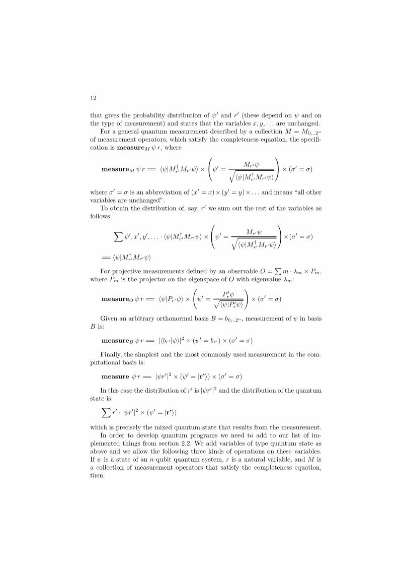
12

that gives the probability distribution of ψ′ and r′ (these depend on ψ and onthe type of measurement) and states that the variables x, y, . . . are unchanged.

For a general quantum measurement described by a collection M = M0,..2n

of measurement operators, which satisfy the completeness equation, the specifi-cation is measureM ψ r, where

measureM ψ r == 〈ψ|M †r′Mr′ψ〉 ×

ψ′ =Mr′ψ

√

〈ψ|M †r′Mr′ψ〉

× (σ′ = σ)

where σ′ = σ is an abbreviation of (x′ = x)× (y′ = y)× . . . and means “all othervariables are unchanged”.

To obtain the distribution of, say, r′ we sum out the rest of the variables asfollows:

∑

ψ′, x′, y′, . . . · 〈ψ|M †r′Mr′ψ〉 ×

ψ′ =Mr′ψ

√

〈ψ|M †r′Mr′ψ〉

×(σ′ = σ)

== 〈ψ|M †r′Mr′ψ〉

For projective measurements defined by an observable O =∑

m · λm × Pm,where Pm is the projector on the eigenspace of O with eigenvalue λm:

measureO ψ r == 〈ψ|Pr′ψ〉 ×(

ψ′ =P ′rψ

√

〈ψ|P ′rψ〉

)

× (σ′ = σ)

Given an arbitrary orthonormal basis B = b0,..2n , measurement of ψ in basisB is:

measureB ψ r == |〈br′ |ψ〉|2 × (ψ′ = br′) × (σ′ = σ)

Finally, the simplest and the most commonly used measurement in the com-putational basis is:

measure ψ r == |ψr′|2 × (ψ′ = |r’〉) × (σ′ = σ)

In this case the distribution of r′ is |ψr′|2 and the distribution of the quantumstate is:

∑

r′ · |ψr′|2 × (ψ′ = |r’〉)

which is precisely the mixed quantum state that results from the measurement.In order to develop quantum programs we need to add to our list of im-

plemented things from section 2.2. We add variables of type quantum state asabove and we allow the following three kinds of operations on these variables.If ψ is a state of an n-qubit quantum system, r is a natural variable, and M isa collection of measurement operators that satisfy the completeness equation,then:

13

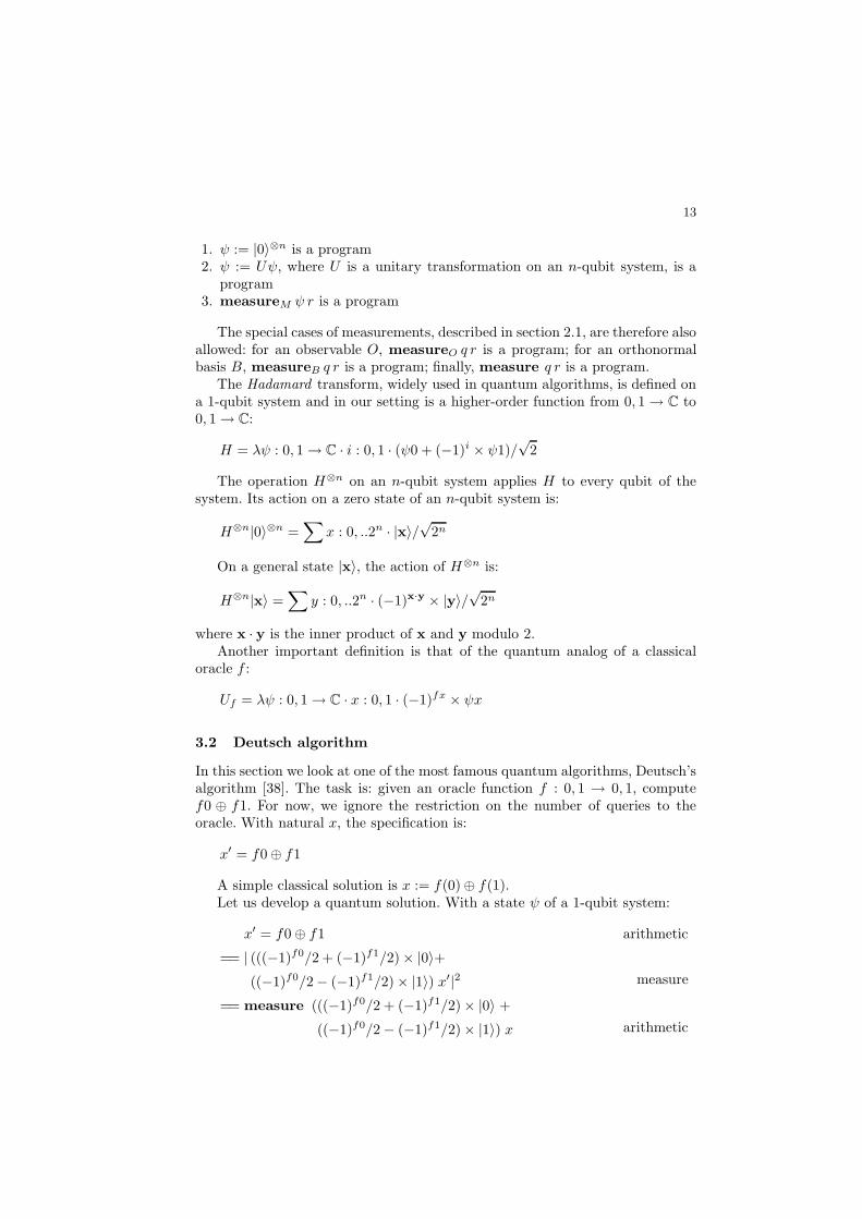
1. ψ := |0〉⊗n is a program2. ψ := Uψ, where U is a unitary transformation on an n-qubit system, is a

program3. measureM ψ r is a program

The special cases of measurements, described in section 2.1, are therefore alsoallowed: for an observable O, measureO q r is a program; for an orthonormalbasis B, measureB q r is a program; finally, measure q r is a program.

The Hadamard transform, widely used in quantum algorithms, is defined ona 1-qubit system and in our setting is a higher-order function from 0, 1 → C to0, 1 → C:

H = λψ : 0, 1 → C · i : 0, 1 · (ψ0 + (−1)i × ψ1)/√

2

The operation H⊗n on an n-qubit system applies H to every qubit of thesystem. Its action on a zero state of an n-qubit system is:

H⊗n|0〉⊗n =∑

x : 0, ..2n · |x〉/√

2n

On a general state |x〉, the action of H⊗n is:

H⊗n|x〉 =∑

y : 0, ..2n · (−1)x·y × |y〉/√

2n

where x · y is the inner product of x and y modulo 2.Another important definition is that of the quantum analog of a classical

oracle f :

Uf = λψ : 0, 1 → C · x : 0, 1 · (−1)fx × ψx

3.2 Deutsch algorithm

In this section we look at one of the most famous quantum algorithms, Deutsch’salgorithm [38]. The task is: given an oracle function f : 0, 1 → 0, 1, computef0 ⊕ f1. For now, we ignore the restriction on the number of queries to theoracle. With natural x, the specification is:

x′ = f0⊕ f1

A simple classical solution is x := f(0) ⊕ f(1).Let us develop a quantum solution. With a state ψ of a 1-qubit system:

x′ = f0 ⊕ f1 arithmetic

== | (((−1)f0/2 + (−1)f1/2) × |0〉+((−1)f0/2− (−1)f1/2) × |1〉) x′|2 measure

== measure (((−1)f0/2 + (−1)f1/2) × |0〉 +

((−1)f0/2 − (−1)f1/2) × |1〉) x arithmetic

14

== measure ((−1)f0/2× (|0〉 + |1〉)+(−1)f1/2× (|0〉 − |1〉)) x Hadamard

== measure ((−1)f0/√

2 × (H |0〉) + (−1)f1/√

2 × (H |1〉)) x linearity

== measure H((−1)f0/√

2 × |0〉 + (−1)f1/√

2 × |1〉) x Oracle

== measure H(Uf |0〉/√

2 + Uf |1〉/√

2) x linearity

== measure H(Uf (|0〉/√

2 + |1〉/√

2)) x Hadamard

== measure H(Uf (H |0〉)) x substitutions

== ψ := |0〉; ψ := Hψ; ψ := Ufψ; ψ := Hψ; measure ψ x

So far we have two solutions — a simple classical one and a complicatedquantum one. Let us add the restriction on the number of allowed calls to theoracle. We add a time variable t and decide to charge 1 unit of time for a call tothe oracle, leaving all other operations free. The new specification is:

x′ = f0⊕ f1 ∧ t′ = t+ 1

The above quantum solution still works:

x′ = f0 ⊕ f1 ∧ t′ = t+ 1

== ψ := |0〉; ψ := Hψ; t := t+ 1; ψ := Ufψ; ψ := Hψ; measure ψ x

The new specification with the above way of charging time is clearly unim-plementable classically. The corresponding strongest classically implementablespecification is:

x′ = f0⊕ f1 ∧ t′ ≤ t+ 2

3.3 Deutsch-Jozsa algorithm

Deutsch-Jozsa’s problem ([39]), an extension of Deutsch’s Problem, is an exampleof the broad class of quantum algorithms that are based on the quantum Fouriertransform ([40]). The task is: given a function f : 0, ..2n → 0, 1 , such that f iseither constant or balanced, determine which case it is. Without any restrictionson the number of calls to f , we can write the specification (let us call it S) asfollows:

(f is constant ∨ f is balanced) =⇒ b′ = f is constant

where b is a boolean variable and the informally stated properties of f aredefined formally as follows:

f is constant == ∀i : 0, ..2n · fi = f0

f is balanced ==∣

∣

∣

∑

i : 0, ..2n · (−1)fi∣

∣

∣= 0

15

It is easy to show that

(f is constant ∨ f is balanced)=⇒ (f is constant == ∀(i : 0, ..2n−1 + 1) · fi = f0)

That is, more than half of the values need to be equal to f0 .In our setting, we need to implement the specification R defined as follows:

b′ == ∀i : (0, ..2n−1 + 1) · fi = f0

The quantum solution is a direct generalisation of Deutsch’s algorithm. Theidea is to create a suitable superposition for state ψ, so that a measurement ofψ produces 0 if and only if f is constant, so that:

S ⇐= Q; b := (r = 0) , where

Q == f is constant ∨ f is balanced⇒ f is constant = (r′ = 0)

To implement Q we notice that:

f is constant ==(∣

∣

∣

∑

x · (−1)fx/2n∣

∣

∣ = 1)

f is balanced ==(∣

∣

∣

∑

x · (−1)fx/2n∣

∣

∣ = 0)

We can show that if f is constant ∨ f is balanced, variables x, y, and z arefrom the domain 0, ..2n, and x · z is the dot product of x and z, then:

f is constant = (r′ = 0)

⇐=∣

∣

∣

(

∑

z, x · (−1)x·z+fx/2n × |z〉)

r′∣

∣

∣

2

== measure(

∑

x · (−1)fx/√

2n ×(

∑

z · (−1)x·z/√

2n × |z〉))

r

== measure (H⊗n(Uf (H⊗n|0〉⊗n))) r

== ψ := |0〉⊗n; ψ := H⊗nψ; ψ := Ufψ; ψ := H⊗nψ; measure ψ r

The complete solution is:

ψ := |0〉⊗n; ψ := H⊗nψ; ψ := Ufψ; ψ := H⊗nψ; measure ψ r; b := (r′ = 0)

Let us add to the specification a restriction on the number of calls to theoracle by introducing a time variable. Suppose the new specification is:

(f is constant ∨ f is balanced =⇒ b′ = f is constant) ∧ (t′ = t+ 1)

where we charge 1 unit of time for each call to the oracle and all other operationsare free. Clearly, the above quantum solution works.

Classically the specification is unimplementable. The strongest classicallyimplementable specification is

(f is constant ∨ f is balanced =⇒ b′ = f is constant) ∧ (t′ ≤ t+ 2n−1 + 1)

16

3.4 Grover’s search

Grover’s quantum search algorithm ([41], [42]) is well-known for the quadraticspeed-up it offers in the solutions of NP-complete problems. The algorithm isoptimal up to a multiplicative constant ([13]). The task is: given a functionf : 0, ..2n → 0, 1, find x : 0, ..2n, such that fx = 1. For simplicity we assumethat there is only a single solution, which we denote x1, i.e. f x1 = 1 and f x = 0for all x 6= x1. The proofs are not very different for a general case of more thanone solutions.

As before, we use a general quantum oracle, defined by

Uf |x〉 = (−1)fx × |x〉In addition, we define the inversion about mean operator as follows:

M : (0, ..N → C) → (0, ..N → C)

Mψ == λx : 0, ..N · 2 ×(

∑

i : 0, ..N · ψi/N)

− ψx

where N = 2n.Grover’s algorithm initialises the quantum system to an equally weighted

superposition of all basis states |x〉, x : 0, ..N . It then repeatedly applies Uffollowed by M to the system. Finally, the state is measured. The probability oferror is determined by the number of iterations performed by the algorithm.

The algorithm is easily understood with the help of a geometric analysis ofthe operators. Let α be the sum over all x, which are not solutions, and let β bethe solution:

α =1√

N − 1×∑

x 6= x1 · |x〉

β = |x1〉Then the oracle Uf performs a reflection about the vector α in the plane

defined by α and β. In other words, Uf (a×α+ b×β) = a×α− b×β. Similarly,the inversion about mean operator is a reflection about the vector ψ in the planedefined by α and β. Therefore, the result of Uf followed by M is a rotation inthis plane. We define θ to be the rotation angle:

θ = 2 × arcsin√

1/N

Since each rotation leaves us in the plane defined by α and β, then the stateof the system after i rotations by θ radians is:

ψi = cos((2 × i+ 1) × θ/2) × α + sin((2 × i+ 1) × θ/2) × β

Suppose we charge one unit of time for each call to the oracle and all otheroperations are free. The specification of the problem is then:

S ==(

sin(

(2 × (t′ − t) + 1) × arcsin√

1/N))2

× (r′ = x1) +(

1 −(

sin(

(2 × (t′ − t) + 1) × arcsin√

1/N))2

)

× (r′ 6= x1)/(N − 1)

17

where r is the result variable from the domain 0, ..N . The specification says

that we want the solution(

sin((2 × (t′ − t) + 1) × arcsin√

1/N))2

of the time,

where t′ − t is the number of times we use the oracle.As before, we want to specify the quantum state that, when measured, gives

the desired distribution. With a quantum state variable ψ : 0, ..N → C, we canshow

S == ψ′ = sin((2 × (t′ − t) + 1) × θ/2) × β +

cos((2 × (t′ − t) + 1) × θ/2) × α;

measure ψ r

Let P be the description of the quantum state immediately before the mea-surement.

P == ψ′ = ψt′−t

Since ψt′−t is the state obtained by t′ − t rotations by θ radians, we definethe specification R to describe the rotation. With a natural k that representsthe number of iterations performed:

R == ψ = ψi ⇒ ψ′ = ψk ∧ t′ = t+ k − i

Adding initialisation, we prove:

P ⇐= i := 0; ψ := ψ0; R

Our task has been simplified. We now need to implement ψ := ψ0 and R andwe are done. Implementing the assignment is trivial:

ψ := |0〉⊗n;ψ := H⊗nψ

Having understood the geometry of Grover’s algorithm, implementing R iseasy. After adding the time increment before the call to the oracle, we can show:

R ⇐= if i = k then ok else (i := i+ 1; t := t+ 1; ψ := Ufψ; ψ := Mψ; R)

Note that specification R is recursive. The ease with which recursion istreated in Predicative Programming allows us to easily translate our geomet-ric understanding of the problem into an implementable specification.

The complete quantum solution is

S ==(

sin(

(2 × (t′ − t) + 1) × arcsin√

1/N))2

× (r′ = x1) +(

1 −(

sin(

(2 × (t′ − t) + 1) × arcsin√

1/N))2

)

×

(r′ 6= x1)/(N − 1)

== P ; measure ψ r

18

P ⇐= i := 0; ψ := |0〉⊗n; ψ := H⊗nψ; R

R ⇐= if i = k then ok

else (i := i+ 1; t := t+ 1; ψ := Ufψ; ψ := Mψ; R)

Specification S carries a lot of useful information. For example, it tells usthat the probability of finding a solution after k iterations is

(

sin((2 × k + 1) × arcsin√

1/N))2

Or we might ask how many iterations should be performed to minimise theprobability of an error. Examining first and second derivatives, we find that theabove probability is minimised when t′ − t = (π × i)/(4 × arcsin

√

1/N) − 1/2for integer i. Of course, the number of iterations performed must be a natu-ral number. It is interesting to note that the probability of error is periodic inthe number of iterations, but since we don’t gain anything by performing extraiterations, we pick i = 1. Finally, assuming 1 � N = 2n, we obtain an ele-gant approximation to the optimal number of iterations:

⌈

π ×√

2n/4⌉

, with theprobability of error approximately 1/2n.

3.5 Computing with Mixed States

As we have discussed in section 2.1, the state of a quantum system after ameasurement is traditionally described as a mixed state. An equation ψ ={|0〉}/2+ {|1〉}/2 should be understood as follows: the state ψ is |0〉 with proba-bility 1/2 and it is |1〉 with probability 1/2. In contrast to a pure state, a mixedstate does not describe a physical state of the system. Rather, it describes ourknowledge of what state the system is in.

In our framework, there is no need for an additional mechanism to computewith mixed states. Indeed, a mixed state is not a system state, but a distributionover system states, and all our programming notions apply to distributions. Theabove mixed state is the following distribution over a quantum state ψ of asingle-qubit system: (ψ = |0〉)/2+ (ψ = |1〉)/2. This expression tells us, for eachpossible value in the domain of ψ, the probability of ψ having that value. Forexample, ψ is the state |0〉 with probability (|0〉 = |0〉)/2 + (|0〉 = |1〉)/2, whichis 1/2; it is |1〉 with probability (|1〉 = |0〉)/2 + (|1〉 = |1〉)/2, which is also 1/2;for any scalars α and β, not equal to 0 or 1, ψ is equal to α× |0〉+ β × |1〉 withprobability (α×|0〉+β×|1〉 = |0〉)/2+(α×|0〉+β×|1〉 = |1〉)/2, which is 0. Oneway to obtain this distribution is to measure an equally weighted superpositionof |0〉 and |1〉:

ψ′ = |0〉/√

2 + |1〉/√

2; measure ψ r measure

== ψ′ = |0〉/√

2 + |1〉/√

2; |ψr′|2 × (ψ′ = |r’〉) sequential composition

==∑

r′′, ψ′′ · (ψ′′ = |0〉/√

2 + |1〉/√

2) × |ψ′′r′|2 × (ψ′ = |r’〉)

== |(|0〉/√

2 + |1〉/√

2) r′|2 × (ψ′ = |r’〉)== (ψ′ = |r’〉)/2

19

Distribution of the quantum state is then:∑

r′ · (ψ′ = |r’〉)/2 == (ψ′ = |0〉)/2 + (ψ′ = |1〉)/2

as desired.Similarly, there is no need to extend the application of unitary operators.

Consider the following toy program:

ψ := |0〉; ψ := Hψ; measure ψ r; if r = 0 then ψ := Hψ else ok

In the second application of Hadamard the quantum state is mixed, but thisis not evident from the syntax of the program. It is only in the analysis of thefinal quantum state that the notion of a mixed state is meaningful. The operatoris applied to a (pure) system state, though we are unsure what that state is.

ψ := |0〉; ψ := Hψ; measure ψ r ;

if r = 0 then ψ := Hψ else ok as before

== (ψ′ = |r’〉)/2;

if r = 0 then ψ := Hψ else ok sequential composition

==∑

r′′, ψ′′ · (ψ′′ = |r”〉)/2 ×((r′′ = 0) × (ψ′ = Hψ′′) × (r′ = r′′) +

(r′′ = 1) × (ψ′ = ψ′′) × (r′ = r′′)) one point law

== ((ψ′ = H |0〉) × (r′ = 0) + (ψ′ = |1〉) × (r′ = 1)) /2

== (ψ′ = |0〉/√

2 + |1〉/√

2) × (r′ = 0)/2 +

(ψ′ = |1〉) × (r′ = 1)/2

The distribution of the quantum state after the computation is:∑

r′ · (ψ′ = |0〉/√

2 + |1〉/√

2) × (r′ = 0)/2 + (ψ′ = |1〉) × (r′ = 1)/2

== (ψ′ = |0〉/√

2 + |1〉/√

2)/2 + (ψ′ = |1〉)/2A lot of properties of measurements and mixed states can be proven from

the definitions of measurement and sequential composition. For example, thefact that a measurement in the computational basis, performed immediatelyfollowing a measurement in the same basis, does not change the state of thesystem and yields the same result as the first measurement with probability 1,is proven as follows:

measure ψ r; measure ψ r measure

== |ψ r′|2 × (ψ′ = |r’〉); |ψ r′|2 × (ψ′ = |r’〉) sequential composition

==∑

ψ′′, r′′ · |ψ r′′|2 × (ψ′′ = |r”〉) × |ψ′′ r′|2 × (ψ′ = |r’〉) one point law

== |ψ r′|2 × (ψ′ = |r’〉) measure

== measure ψ r

In case of a general quantum measurement, the proof is similar, but a littlemore computationally involved.

20

4 Conclusion and Future Work

We have presented a new approach to developing, analysing, and proving cor-rectness of quantum programs. Since we adopt Hehner’s theory as the basis forour work, we inherit its advantageous features, such as simplicity, generality, andelegance. Our work extends probabilistic predicative programming in the samefashion that quantum computation extends probabilistic computation. We haveprovided tools to write quantum as well as classical specifications, develop quan-tum and classical solutions for them, and analyse various properties of quantumspecifications and quantum programs, such as implementability, time and spacecomplexity, and probabilistic error analysis uniformly, all in the same framework.

Current research and research in the immediate future involve reasoningabout distributed quantum computation. Current work involves expressing quan-tum teleportation, dense coding, and various games involving entanglement, ina way that makes complexity analysis of these quantum algorithms simple andnatural. These issues will be described in a forthcoming paper. We can easilyexpress teleportation as refinement of a specification φ′ = ψ, for distinct qubitsφ and ψ, in a well-known fashion. However, we are more interested in the possi-bilities of simple proofs and analysis of programs involving communication, bothvia quantum channels and exhibiting the LOCC (local operations, classical com-munication) paradigm. Future work involves formalising quantum cryptographicprotocols, such as BB84 [33], in our framework and providing formal analysis ofthese protocols. This will naturally lead to formal analysis of distributed quan-tum algorithms (e.g. distributed Shor’s algorithm of [34]).

References

1. Knill, E.: Conventions for quantum pseudocode. Technical Report LAUR-96-2724,Los Alamos National Laboratory (1996)

2. Hehner, E.: a Practical Theory of Programming. Second edn. Springer, New York(2004) Available free at www.cs.utoronto.ca/~hehner/aPToP.

3. Hehner, E.: Probabilistic predicative programming. In: Mathematics of ProgramConstruction. (2004)

4. Omer, B.: Quantum programming in QCL. Master’s thesis, TU Vienna (2000)

5. Bettelli, S., Calarco, T., Serafini, L.: Toward an architecture for quantum pro-gramming. In: The European Physical Journal. (2003) 181–200

6. Sanders, J.W., Zuliani, P.: Quantum programming. In: Mathematics of ProgramConstruction. (2000) 80–99

7. Morgan, C., McIver, A.: pQCL: formal reasoning for random algorithms. SouthAfrican Computer Journal 22 (1999) 14–27

8. Zuliani, P.: Non-deterministic quantum programming. In: QPL 2004. (2004) 179–195

9. Zuliani, P.: Quantum programming with mixed states. In: QPL 2005. (2005)

10. Aharonov, D., Kitaev, A., Nisan, N.: Quantum circuits with mixed states. In:STOC ’98: Proceedings of the thirtieth annual ACM symposium on Theory ofcomputing. (1998) 20 – 30

21

11. Zuliani, P.: Compiling quantum programs. Acta Informatica 41(7-8) (2005) 435–474

12. Butler, M.J., Hartel, P.H.: Reasoning about grover’s quantum search algorithmusing probabilistic wp. In: ACM Trans. Program. Lang. Syst. Volume 21. (1999)417–429

13. Boyer, M., Brassard, G., Høyer, P., Tapp, A.: Tight bounds on quantum searching.In: Fortschritte der Physik. (1998) 493–506

14. Adao, P., Mateus, P.: A process algebra for reasoning about quantum security. In:QPL 2005. (2005)

15. Lalire, M., Jorrand, P.: A process algebraic approach to concurrent and distributedquantum computation: operational semantics. In: QPL 2004. (2004) 109–126

16. Jorrand, P., Lalire, M.: Toward a quantum process algebra. In: Proceedings of the1st ACM Conference on Computing Frontiers. (2004)

17. Abramsky, S.: High-level methods for quantum computation and information. In:Proceedings of the 19th Annual IEEE Symposium on Logic in Computer Science.(2004)

18. Abramsky, S., Coecke, B.: A categorical semantics of quantum protocols. In: LICS2004. (2004)

19. Abramsky, S., Duncan, R.: A categorical quantum logic. In: QPL 2004. (2004)3–20

20. Coecke, B.: The logic of entanglement. (2004) quant-ph/0402014.21. Selinger, P.: Towards a quantum programming language. Mathematical Structures

in Computer Science (2004)22. Arrighi, P., Dowek, G.: Operational semantics for formal tensorial calculus. In:

QPL 2004. (2004) 21–3823. Arrighi, P., Dowek, G.: Linear-algebraic lambda-calculus. In: QPL 2005. (2005)24. Altenkirch, T., Grattage, J.: A functional quantum programming language. In:

Proceedings of the 20th Annual IEEE Symposium on Logic in Computer Science.(2005)

25. Altenkirch, T., Grattage, J., Vizzotto, J.K., Sabry, A.: An algebra of pure quantumprogramming. In: QPL 2005. (2005)

26. D’Hondt, E., Panangaden, P.: Quantum weakest precondition. In: QPL 2004.(2004) 75–90

27. D’Hondt, E., Panangaden, P.: Reasoning about quantum knowledge. (2005) quant-ph/0507176.

28. Danos, V., D’Hondt, E., Kashefi, E., Panangaden, P.: Distributed measurement-based quantum computation. In: QPL 2005. (2005)

29. Gay, S.J., Nagarajan, R.: Communicating quantum processes. In: Proceedingsof the 32nd ACM SIGACT-SIGPLAN Symposium on Principles of ProgrammingLanguages. (2005)

30. Selinger, P.: Towards a semantics for higher-order quantum computation. In: QPL2004. (2004)

31. Valiron, B.: Quantum typing. In: QPL 2004. (2004) 163–17832. van Tonder, A.: A lambda calculus for quantum computation. SIAM Journal on

Computing 33(5) (2004) 1109–113533. Bennet, C.H., Brassard, G.: Quantum cryptography: Public key distribution and

coin tossing. In: IEEE Int. Conf. Computers, Systems and Signal Processing. (1984)175–179

34. Yimsiriwattana, A., Jr, S.J.L.: Distributed quantum computing: A distributedShor algorithm. (2004) quant-ph/0403146.

22

35. Nielsen, M.A., Chuang, I.L.: Quantum Computation and Quantum Information.Cambridge University Press (2000)

36. Hehner, E.: Retrospective and prospective for unifying theories of programming.In: Symposium on Unifying Theories of Programming. (2006)

37. Tafliovich, A.: Quantum programming. Master’s thesis, University of Toronto(2004)

38. Deutsch, D.: Quantum theory, the Church-Turing principle and the universalquantum computer. In: Proceedings of the Royal Society of London. (1985) 97–117

39. Deutsch, D., Jozsa, R.: Rapid solution of problems by quantum computation.Proceedings of the Royal Society of London 439 (1992) 553–558

40. Jozsa, R.: Quantum algorithms and the Fourier transform. Proceedings of theRoyal Society of London (1998) 323–337

41. Grover, L.K.: A fast quantum mechanical algorithm for database search. In:Twenty-Eighth Annual ACM Symposium on Theory of Computing. (1996) 212–219

42. Ambainis, A.: Quantum search algorithms. SIGACT News 35(2) (2004) 22–35