QMS 6351 Statistics and Research Methods Regression Analysis: Testing for Significance Chapter 14 (14.5-14.6) Chapter 15 (15.5) Prof. Vera Adamchik

Welcome message from author
This document is posted to help you gain knowledge. Please leave a comment to let me know what you think about it! Share it to your friends and learn new things together.
Transcript

QMS 6351 Statistics and Research Methods
Regression Analysis: Testing for Significance
Chapter 14 (14.5-14.6)Chapter 15 (15.5)
Prof. Vera Adamchik
Multiple Regression ModelMultiple Regression Model
EE((yy) = ) = 00 + + 11xx1 1 + + 22xx2 2 +. . .+ +. . .+ ppxxpp + + Multiple Regression EquationMultiple Regression Equation
EE((yy) =) = 00 + + 11xx1 1 + + 22xx2 2 +. . .+ +. . .+ ppxxpp Unknown parameters areUnknown parameters are
00, , 11, , 22, . . . , , . . . , pp
Sample Data:Sample Data:xx11 x x22 . . . x . . . xpp y y. . . .. . . .. . . .. . . .
Estimated MultipleEstimated MultipleRegression EquationRegression Equation
Sample statistics areSample statistics are
bb00, , bb11, , bb22, , . . . , . . . , bbp p
bb00, , bb11, , bb22, , . . . , . . . , bbpp
provide estimates ofprovide estimates of00, , 11, , 22, . . . , , . . . , pp

Hypotheses about βi
Ho: i = specific value
Ha: i specific value
Ho: i specific value
Ha: i < specific value
Ho: i specific value
Ha: i > specific value
The most common hypothesis is
whether βi equals to zero (that is, no
relationship between y and xi

• To learn how to test for a significant regression relationship, we will use the “Programmer Salary Survey” example from the “Ch. 14-15 Part 1” Power Point file.
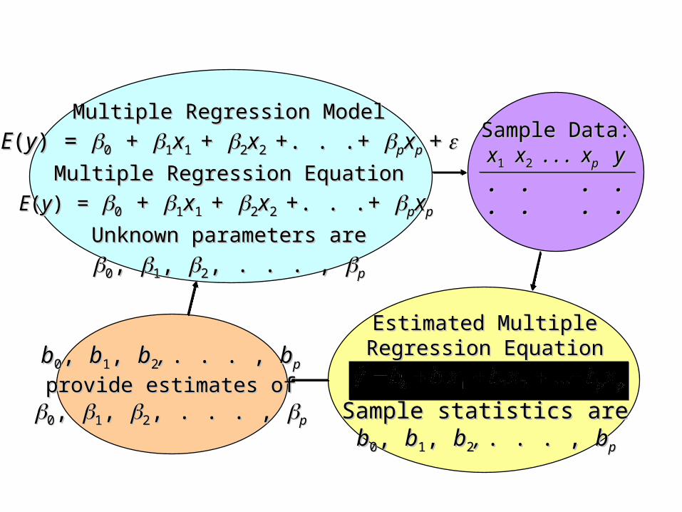
Testing for significance
• Two tests are commonly used:
the t test and the F test.
• In simple linear regression, the F and t tests provide the same conclusion.
• In multiple regression, the F and t tests have different purposes.
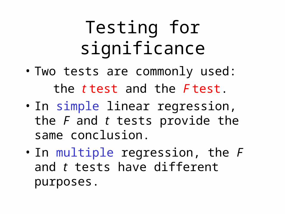
The F test
• The F test is used to determine whether a significant relationship exists between the dependent variable and the set of all the independent variables.
• The F test is referred to as the test for overall significance.
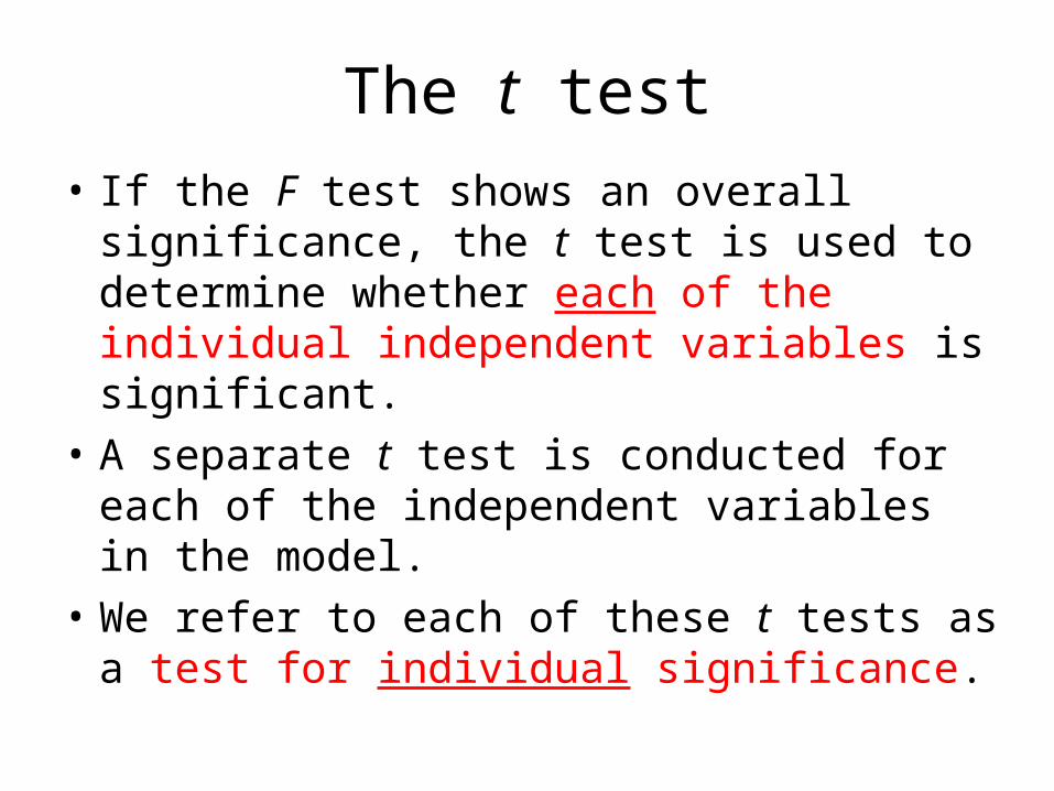
The t test
• If the F test shows an overall significance, the t test is used to determine whether each of the individual independent variables is significant.
• A separate t test is conducted for each of the independent variables in the model.
• We refer to each of these t tests as a test for individual significance.
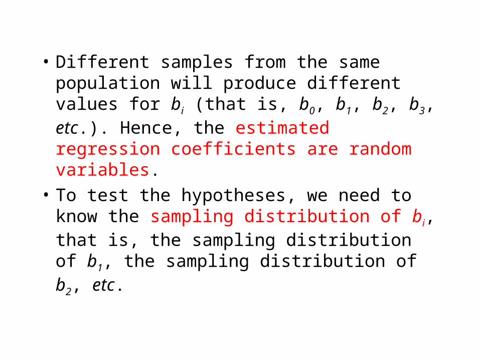
• Different samples from the same population will produce different values for bi (that is, b0, b1, b2, b3, etc.). Hence, the estimated regression coefficients are random variables.
• To test the hypotheses, we need to know the sampling distribution of bi, that is, the sampling distribution of b1, the sampling distribution of b2, etc.
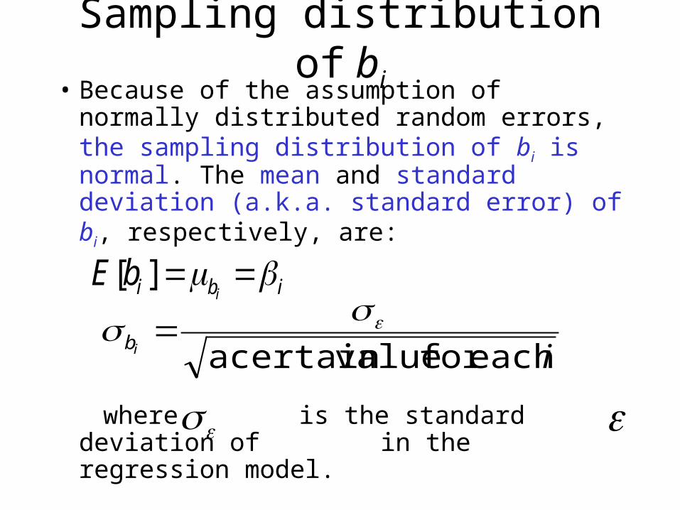
Sampling distribution of bi
• Because of the assumption of normally distributed random errors, the sampling distribution of bi is normal. The mean and standard deviation (a.k.a. standard error) of bi, respectively, are:
where is the standard deviation of in the regression model.
iib eachfor valuecertaina
ibi ibE ][
etc.
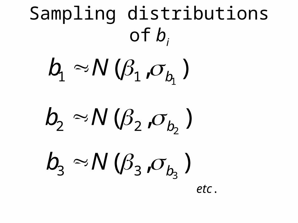
Sampling distributions of bi
),(111 bNb
),(222 bNb
),(333 bNb
• Because we do not know the value of
, we use an estimate of (see the next slide).
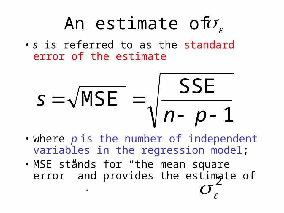
An estimate of • s is referred to as the standard error of
the estimate
• where p is the number of independent variables in the regression model;
• MSE stands for “the mean square error” and provides the estimate of .
1
SSEMSE
pns
2

Excel’s Regression Statistics
A B C23 24 SUMMARY OUTPUT2526 Regression Statistics27 Multiple R 0.92021523928 R Square 0.84679608529 Adjusted R Square 0.81807035130 Standard Error 2.39647510131 Observations 2032
Standard error of the estimate s = sqrt [91.88949/(20-3-
1)]=2.396475
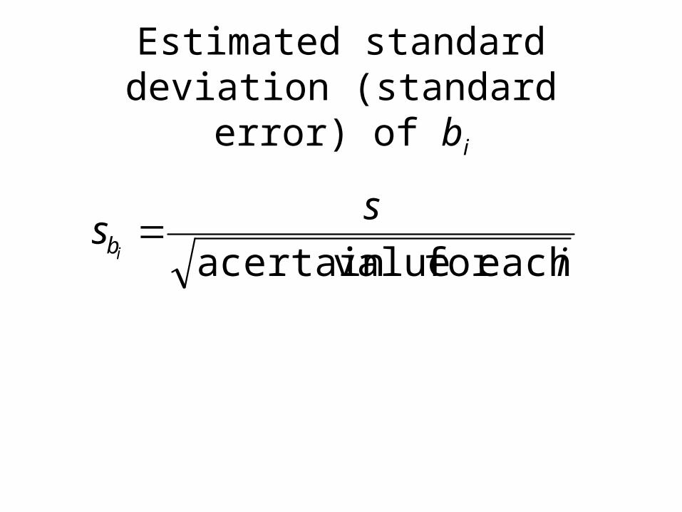
Estimated standard deviation (standard error) of bi
i
ss
ib eachfor valuecertaina
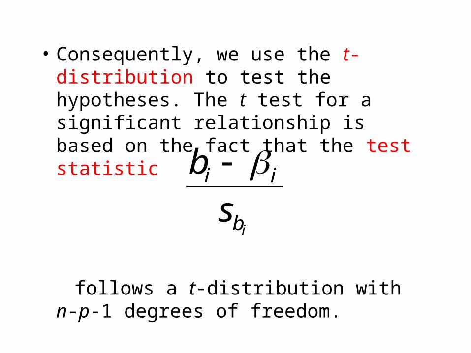
• Consequently, we use the t-distribution to test the hypotheses. The t test for a significant relationship is based on the fact that the test statistic
follows a t-distribution with n-p-1 degrees of freedom.
ib
ii
s
b

Tests for individual significance

1. Determine the hypotheses.
3. Specify the level of significance.
2. Specify the sampling distribution of b1 assuming thatthe null hypothesis is true.
OUR EXAMPLE: Testing for significance: t Test
0:
0:
1
10
aH
H
),(11]1[1 bpn stb )2976.0,0(]16[1 tb
05.0

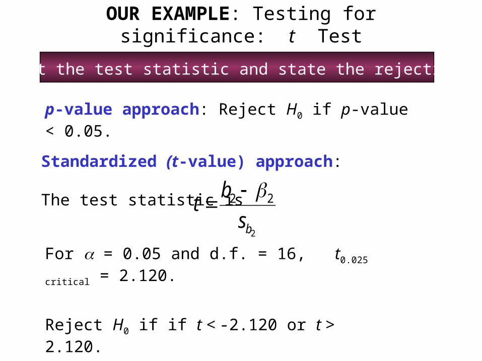
4. Select the test statistic and state the rejection rule.
Standardized (t-value) approach:
The test statistic is
1
11
bs
bt
p-value approach: Reject H0 if p-value < 0.05.
For = 0.05 and d.f. = 16, t0.025 critical = 2.120.
Reject H0 if t < -2.120 or t > 2.120.
OUR EXAMPLE: Testing for significance: t Test

5. Compute the value of the test statistics.
6. Determine whether to reject H0.
The p-value = 0.0014 < alpha = 0.05. Reject H0.
t = 3.8561 > t critical = 2.120. Reject H0.We conclude that β1 is not equal to zero. The evidence is sufficient to conclude that a statistically significant relationship exists between the annual salary and the years of experience.
856102.3297602.0
0147582.1
t
OUR EXAMPLE: Testing for significance: t Test
001397.0)856102.3(*2value tPp
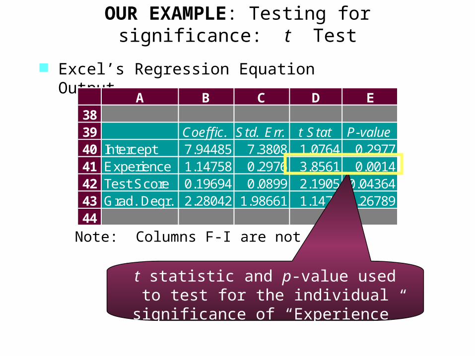
Excel’s Regression Equation Output
Note: Columns F-I are not shown.
A B C D E3839 Coeffic. Std. Err. t Stat P-value40 Intercept 7.94485 7.3808 1.0764 0.297741 Experience 1.14758 0.2976 3.8561 0.001442 Test Score 0.19694 0.0899 2.1905 0.0436443 Grad. Degr. 2.28042 1.98661 1.1479 0.2678944
t statistic and p-value used to test for the individual significance of
“Experience”
OUR EXAMPLE: Testing for significance: t Test

1. Determine the hypotheses.
3. Specify the level of significance.
2. Specify the sampling distribution of b1 assuming thatthe null hypothesis is true.
0:
0:
2
20
aH
H
),(22]1[2 bpn stb )0899.0,0(]16[2 tb
05.0
OUR EXAMPLE: Testing for significance: t Test
4. Select the test statistic and state the rejection rule.
Standardized (t-value) approach:
The test statistic is
2
22
bs
bt
p-value approach: Reject H0 if p-value < 0.05.
For = 0.05 and d.f. = 16, t0.025 critical = 2.120.
Reject H0 if if t < -2.120 or t > 2.120.
OUR EXAMPLE: Testing for significance: t Test

5. Compute the value of the test statistics.
6. Determine whether to reject H0.
The p-value = 0.04364 < alpha = 0.05. Reject H0.
t = 2.1905 > t critical = 2.120. Reject H0.We conclude that β2 is not equal to zero. The evidence is sufficient to conclude that a statistically significant relationship exists between the annual salary and the score on the programmer aptitude test.
190532.2089904.0
0196937.0
t
OUR EXAMPLE: Testing for significance: t Test
043640.0)190532.2(*2value tPp
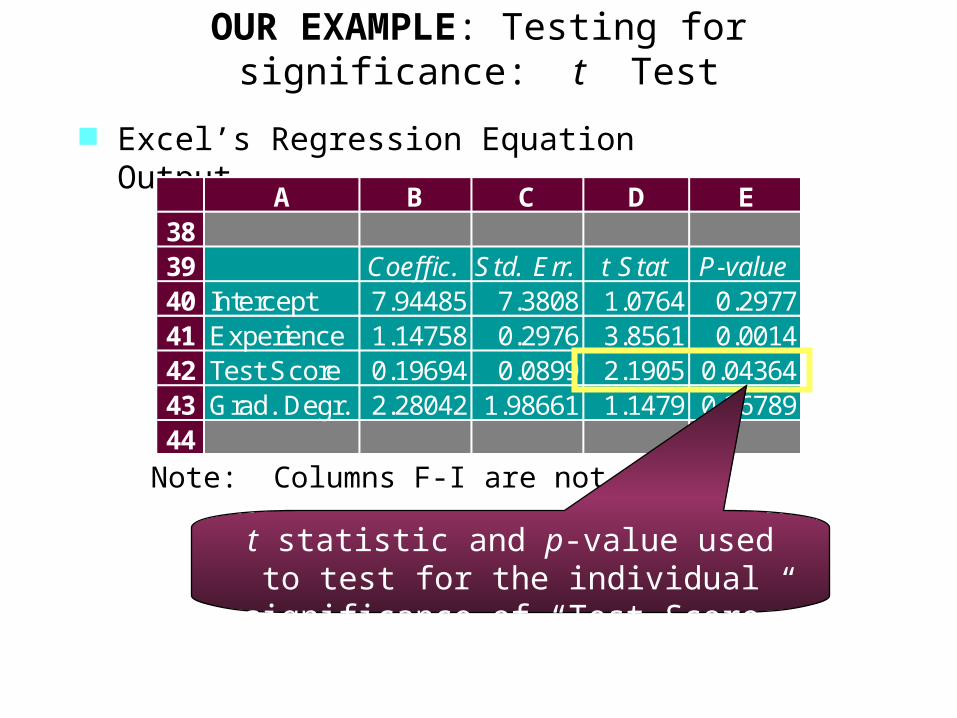
Excel’s Regression Equation Output
Note: Columns F-I are not shown.
A B C D E3839 Coeffic. Std. Err. t Stat P-value40 Intercept 7.94485 7.3808 1.0764 0.297741 Experience 1.14758 0.2976 3.8561 0.001442 Test Score 0.19694 0.0899 2.1905 0.0436443 Grad. Degr. 2.28042 1.98661 1.1479 0.2678944
t statistic and p-value used to test for the individual significance of
“Test Score”
OUR EXAMPLE: Testing for significance: t Test
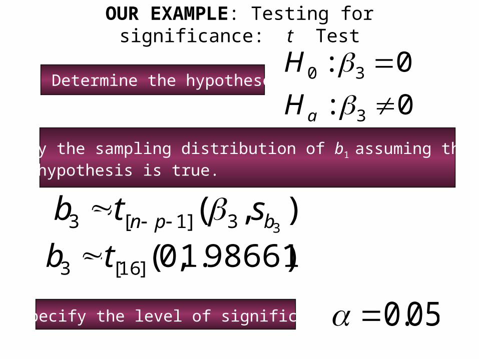
1. Determine the hypotheses.
3. Specify the level of significance.
2. Specify the sampling distribution of b1 assuming thatthe null hypothesis is true.
0:
0:
3
30
aH
H
),(33]1[3 bpn stb )98661.1,0(]16[3 tb
05.0
OUR EXAMPLE: Testing for significance: t Test

4. Select the test statistic and state the rejection rule.
Standardized (t-value) approach:
The test statistic is
3
33
bs
bt
p-value approach: Reject H0 if p-value < 0.05.
For = 0.05 and d.f. = 16, t0.025 critical = 2.120.
Reject H0 if if t < -2.120 or t > 2.120.
OUR EXAMPLE: Testing for significance: t Test
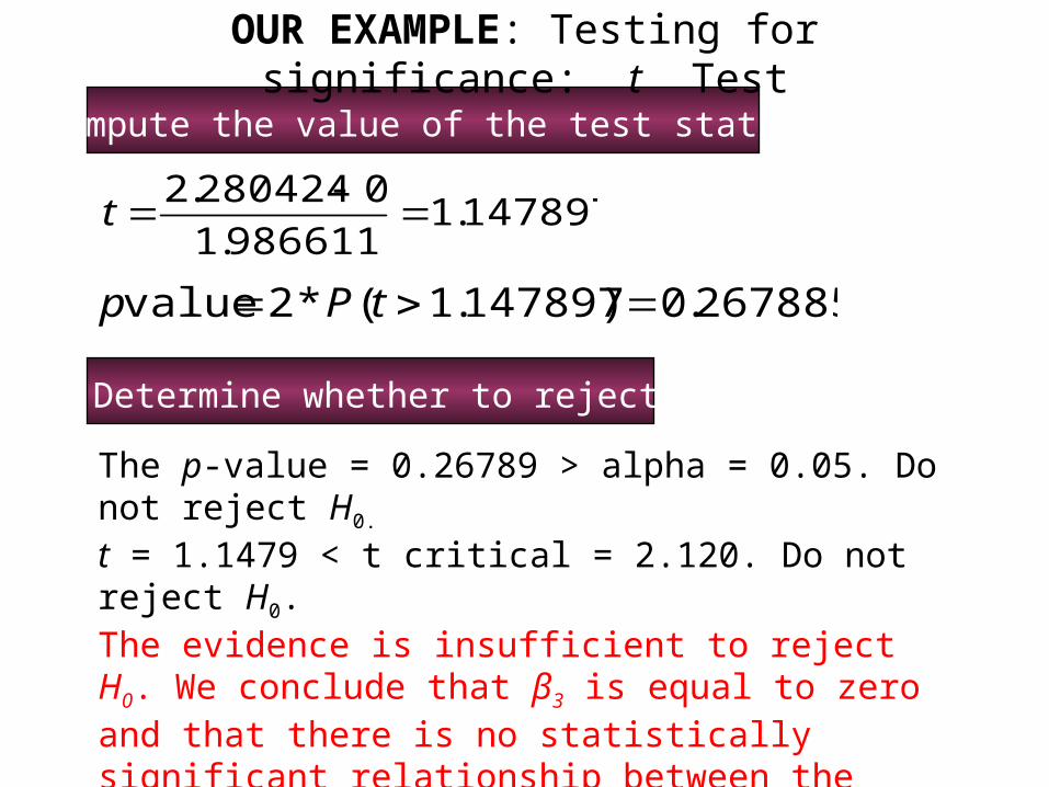
5. Compute the value of the test statistics.
6. Determine whether to reject H0.
The p-value = 0.26789 > alpha = 0.05. Do not reject H0.
t = 1.1479 < t critical = 2.120. Do not reject H0.The evidence is insufficient to reject H0. We conclude that β3 is equal to zero and that there is no statistically significant relationship between the annual salary and whether the individual has a graduate degree in computer science or information systems.
147897.1986611.1
0280424.2
t
OUR EXAMPLE: Testing for significance: t Test
267885.0)147897.1(*2value tPp

Excel’s Regression Equation Output
Note: Columns F-I are not shown.
A B C D E3839 Coeffic. Std. Err. t Stat P-value40 Intercept 7.94485 7.3808 1.0764 0.297741 Experience 1.14758 0.2976 3.8561 0.001442 Test Score 0.19694 0.0899 2.1905 0.0436443 Grad. Degr. 2.28042 1.98661 1.1479 0.2678944
t statistic and p-value used to test for the individual significance of
“Grad. Degr.”
OUR EXAMPLE: Testing for significance: t Test
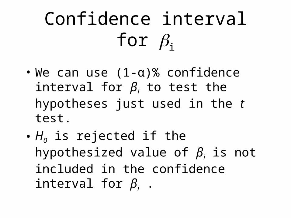
Confidence interval for i
• We can use (1-α)% confidence interval for βi to test the hypotheses just used in the t test.
• H0 is rejected if the hypothesized value of βi is not included in the confidence interval for βi .
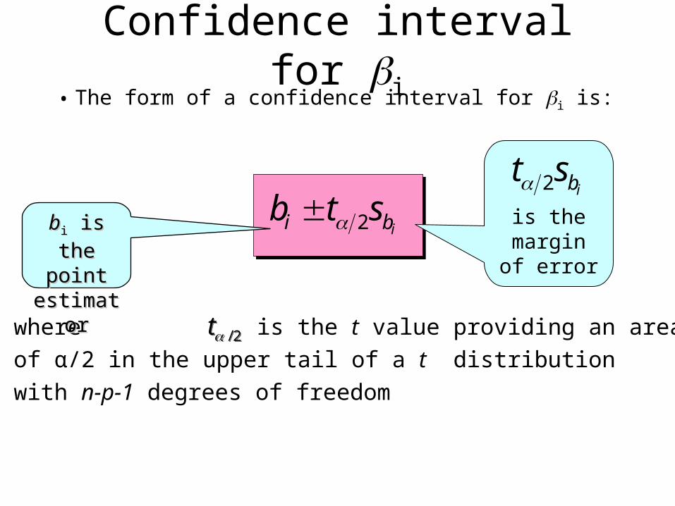
• The form of a confidence interval for i is:
Confidence interval for i
where is the t value providing an area
of α/2 in the upper tail of a t distribution
with n-p-1 degrees of freedom
2/t 2/t
bbii is the is thepointpoint
estimatestimatoror
ibi stb 2 is the margin of
error
ibst 2

t-values in EXCEL
• =TINV(probability,degrees_freedom)
• Probability is the probability associated with the two-tailed Student's t-distribution.
• Degrees_freedom is the number of degrees of freedom with which to characterize the distribution.
• =TINV(0.05,16) = 2.119905285.
• The t table in the textbook shows 2.120.
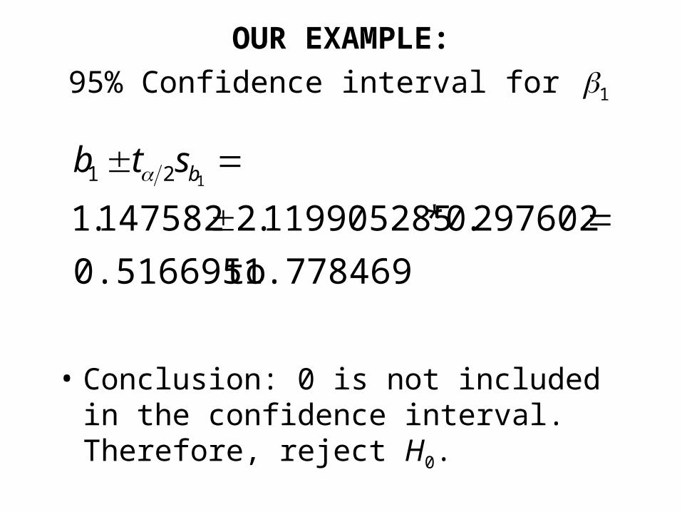
OUR EXAMPLE:
95% Confidence interval for 1
• Conclusion: 0 is not included in the confidence interval. Therefore, reject H0.
1.778469 to0.516695
297602.0*119905285.2147582.1121
bstb
OUR EXAMPLE:
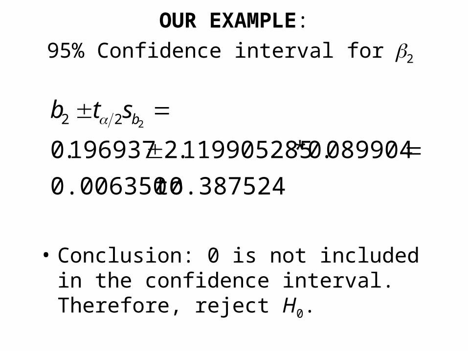
95% Confidence interval for 2
• Conclusion: 0 is not included in the confidence interval. Therefore, reject H0.
0.387524 to0.006350
089904.0*119905285.2196937.0222
bstb
OUR EXAMPLE:
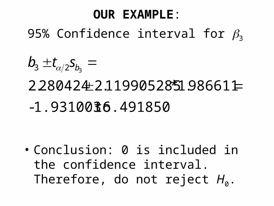
95% Confidence interval for 3
• Conclusion: 0 is included in the confidence interval. Therefore, do not reject H0.
6.491850 to1.931003-
986611.1*119905285.2280424.2323
bstb
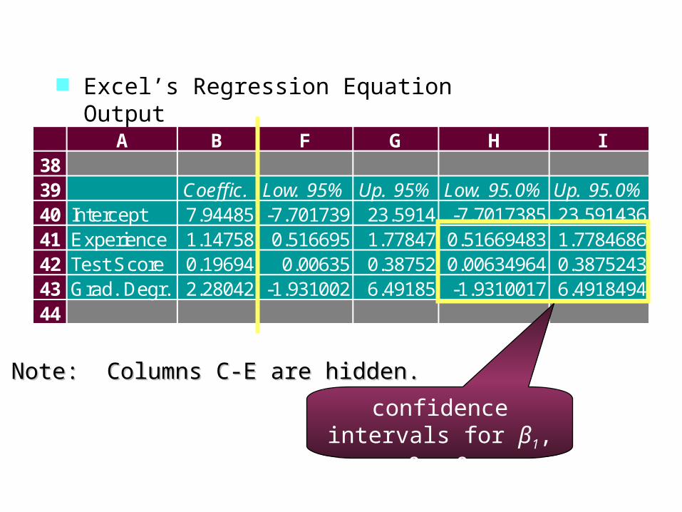
A B F G H I3839 Coeffic. Low. 95% Up. 95% Low. 95.0% Up. 95.0%40 Intercept 7.94485 -7.701739 23.5914 -7.7017385 23.59143641 Experience 1.14758 0.516695 1.77847 0.51669483 1.778468642 Test Score 0.19694 0.00635 0.38752 0.00634964 0.387524343 Grad. Degr. 2.28042 -1.931002 6.49185 -1.9310017 6.491849444
Note: Columns C-E are hidden.Note: Columns C-E are hidden.
Excel’s Regression Equation Output
confidence intervals for β1, β2, β3

The test for overall significance

1. Determine the hypotheses
2. Select the test statistics and specify its distribution
H0: 1 = 2 = . . . = p = 0
Ha: One or more of the parameters
is not equal to zero.
F = MSR/MSE (see the next slide)
an F distributionwith p d.f. in the numerator andn - p - 1 d.f. in the denominator
GENERAL STEPS: Testing for significance: F Test
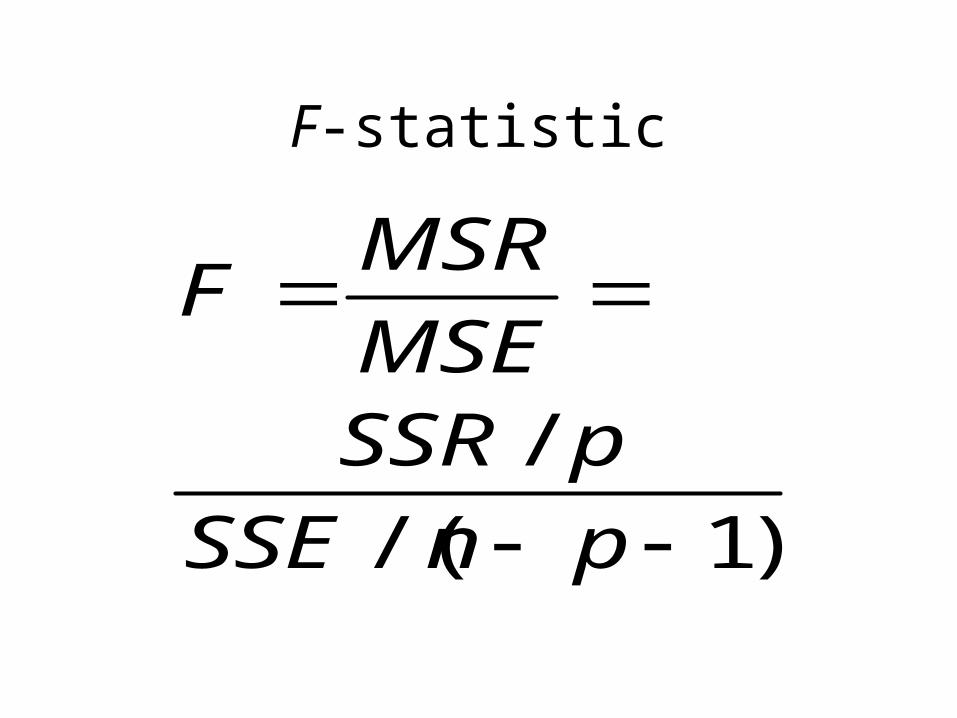
F-statistic
)1/(
/
pnSSE
pSSRMSE
MSRF

3. Specify the level of significance
4. State the rejection rule
5. Compute the value of the test statistic
p-value approach: Reject H0 if p-value < .
F-value approach: Reject H0 if F > F(critical)
05.0
6. Determine whether to reject H0
GENERAL STEPS: Testing for significance: F Test
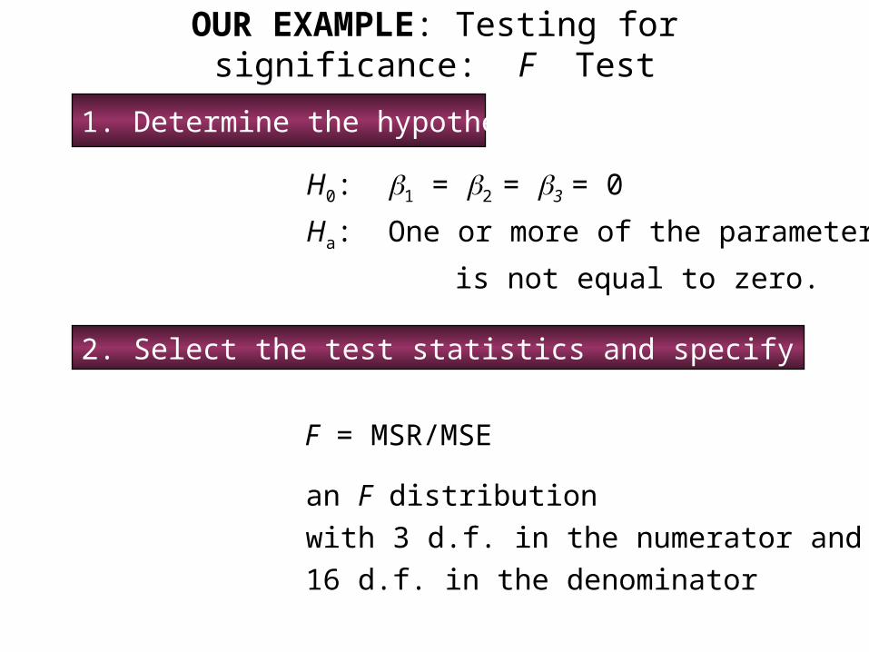
1. Determine the hypotheses
2. Select the test statistics and specify its distribution
H0: 1 = 2 = 3 = 0
Ha: One or more of the parameters
is not equal to zero.
F = MSR/MSE
an F distributionwith 3 d.f. in the numerator and16 d.f. in the denominator
OUR EXAMPLE: Testing for significance: F Test
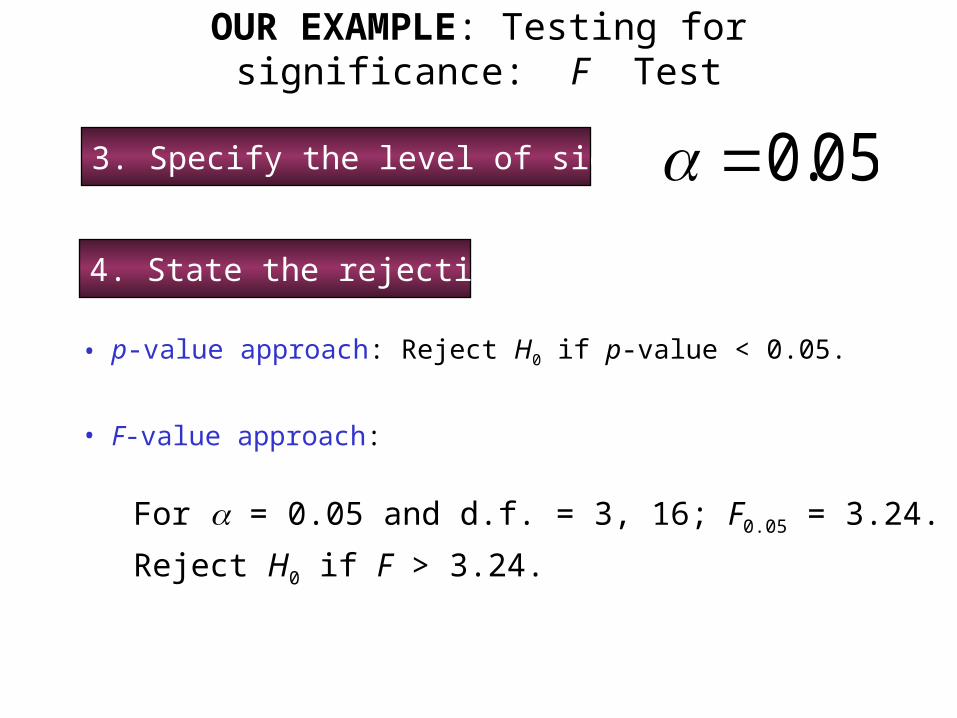
3. Specify the level of significance
4. State the rejection rule
05.0
• p-value approach: Reject H0 if p-value < 0.05.
• F-value approach:
For = 0.05 and d.f. = 3, 16; F0.05 = 3.24.
Reject H0 if F > 3.24.
OUR EXAMPLE: Testing for significance: F Test
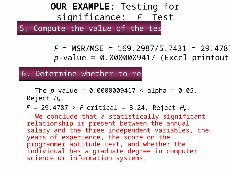
5. Compute the value of the test statistic
6. Determine whether to reject H0
F = MSR/MSE = 169.2987/5.7431 = 29.4787p-value = 0.0000009417 (Excel printout)
The p-value = 0.0000009417 < alpha = 0.05. Reject H0.
F = 29.4787 > F critical = 3.24. Reject H0. We conclude that a statistically significant
relationship is present between the annual salary and the three independent variables, the years of experience, the score on the programmer aptitude test, and whether the individual has a graduate degree in computer science or information systems.
OUR EXAMPLE: Testing for significance: F Test

Excel’s ANOVA Output
A B C D E F3233 ANOVA34 df SS MS F Significance F35 Regression 3 507.896 169.2987 29.47866 9.41675E-0736 Residual 16 91.88949 5.74309337 Total 19 599.785538
F statisticMSR and MSE
OUR EXAMPLE: Testing for significance: F Test

Excel’s ANOVA Output
A B C D E F3233 ANOVA34 df SS MS F Significance F35 Regression 3 507.896 169.2987 29.47866 9.41675E-0736 Residual 16 91.88949 5.74309337 Total 19 599.785538
p-value used to test for
overall significance
OUR EXAMPLE: Testing for significance: F Test
Some cautions about theinterpretation of significance tests
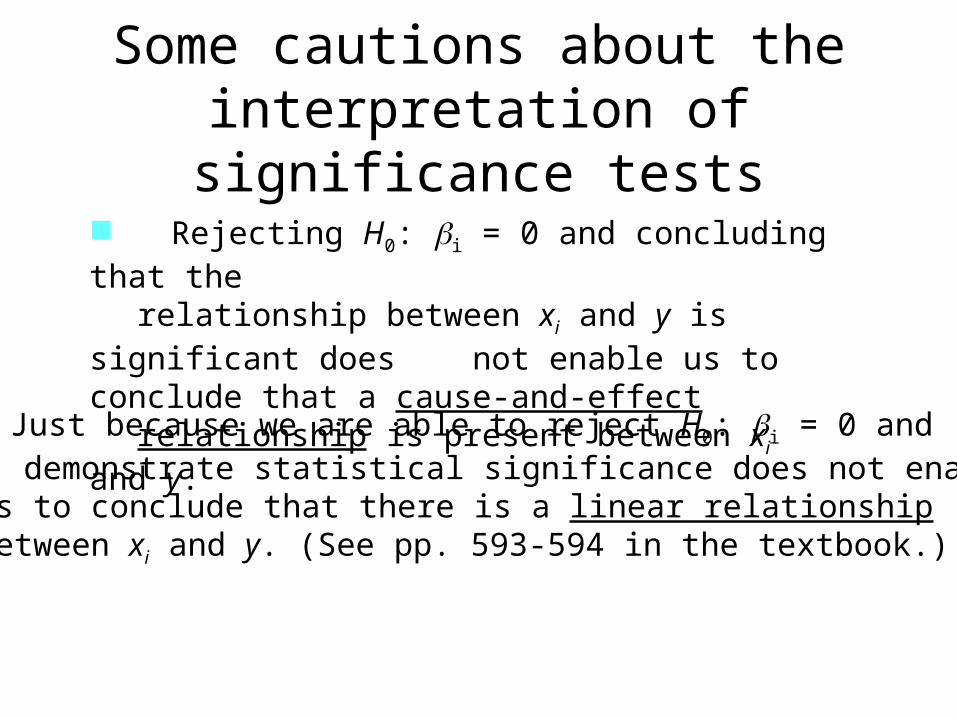
Just because we are able to reject H0: i = 0 and demonstrate statistical significance does not enable
us to conclude that there is a linear relationshipbetween xi and y. (See pp. 593-594 in the textbook.)
Rejecting H0: i = 0 and concluding that the
relationship between xi and y is significant does not enable us to conclude that a cause-and-effect
relationship is present between xi and y.
Related Documents