QGIS User Guide Release 2.0 QGIS Project 31.01.2014

QGIS-2.0-UserGuide-de.pdf
Oct 20, 2015
Welcome message from author
This document is posted to help you gain knowledge. Please leave a comment to let me know what you think about it! Share it to your friends and learn new things together.
Transcript

QGIS User GuideRelease 2.0
QGIS Project
31.01.2014

Inhaltsverzeichnis
1 Präambel 1
2 Gebrauch der Dokumentation 32.1 GUI Conventions . . . . . . . . . . . . . . . . . . . . . . . . . . . . . . . . . . . . . . . . . . . 32.2 Text or Keyboard Conventions . . . . . . . . . . . . . . . . . . . . . . . . . . . . . . . . . . . . 32.3 Platform-specific instructions . . . . . . . . . . . . . . . . . . . . . . . . . . . . . . . . . . . . 4
3 Vorwort 5
4 Funktionalitäten 74.1 Daten visualisieren . . . . . . . . . . . . . . . . . . . . . . . . . . . . . . . . . . . . . . . . . . 74.2 Daten erkunden, abfragen und Karten layouten . . . . . . . . . . . . . . . . . . . . . . . . . . . 74.3 Daten erstellen, editieren, verwalten und exportieren . . . . . . . . . . . . . . . . . . . . . . . . 84.4 Daten analysieren . . . . . . . . . . . . . . . . . . . . . . . . . . . . . . . . . . . . . . . . . . 84.5 Karten im Internet veröffentlichen . . . . . . . . . . . . . . . . . . . . . . . . . . . . . . . . . . 84.6 Extend QGIS functionality through plugins . . . . . . . . . . . . . . . . . . . . . . . . . . . . . 84.7 Python Console . . . . . . . . . . . . . . . . . . . . . . . . . . . . . . . . . . . . . . . . . . . . 9
5 What’s new in QGIS 2.0 115.1 User Interface . . . . . . . . . . . . . . . . . . . . . . . . . . . . . . . . . . . . . . . . . . . . 115.2 Data Provider . . . . . . . . . . . . . . . . . . . . . . . . . . . . . . . . . . . . . . . . . . . . . 115.3 Symbology . . . . . . . . . . . . . . . . . . . . . . . . . . . . . . . . . . . . . . . . . . . . . . 125.4 Map Composer . . . . . . . . . . . . . . . . . . . . . . . . . . . . . . . . . . . . . . . . . . . . 125.5 Labeling . . . . . . . . . . . . . . . . . . . . . . . . . . . . . . . . . . . . . . . . . . . . . . . 135.6 Programmability . . . . . . . . . . . . . . . . . . . . . . . . . . . . . . . . . . . . . . . . . . . 145.7 Analysis tools . . . . . . . . . . . . . . . . . . . . . . . . . . . . . . . . . . . . . . . . . . . . 145.8 Plugins . . . . . . . . . . . . . . . . . . . . . . . . . . . . . . . . . . . . . . . . . . . . . . . . 155.9 General . . . . . . . . . . . . . . . . . . . . . . . . . . . . . . . . . . . . . . . . . . . . . . . . 155.10 Layer Legend . . . . . . . . . . . . . . . . . . . . . . . . . . . . . . . . . . . . . . . . . . . . . 155.11 Browser . . . . . . . . . . . . . . . . . . . . . . . . . . . . . . . . . . . . . . . . . . . . . . . . 16
6 Der erste Einstieg 176.1 Installation . . . . . . . . . . . . . . . . . . . . . . . . . . . . . . . . . . . . . . . . . . . . . . 176.2 Beispieldaten . . . . . . . . . . . . . . . . . . . . . . . . . . . . . . . . . . . . . . . . . . . . . 176.3 Ein erstes Übungsbeispiel . . . . . . . . . . . . . . . . . . . . . . . . . . . . . . . . . . . . . . 186.4 QGIS Starten und Beenden . . . . . . . . . . . . . . . . . . . . . . . . . . . . . . . . . . . . . 196.5 Optionen der Kommandozeile . . . . . . . . . . . . . . . . . . . . . . . . . . . . . . . . . . . . 196.6 QGIS Projekte . . . . . . . . . . . . . . . . . . . . . . . . . . . . . . . . . . . . . . . . . . . . 216.7 Ausgabe . . . . . . . . . . . . . . . . . . . . . . . . . . . . . . . . . . . . . . . . . . . . . . . 21
7 QGIS GUI 237.1 Menu Bar . . . . . . . . . . . . . . . . . . . . . . . . . . . . . . . . . . . . . . . . . . . . . . . 247.2 Toolbar . . . . . . . . . . . . . . . . . . . . . . . . . . . . . . . . . . . . . . . . . . . . . . . . 29
i
7.3 Map Legend . . . . . . . . . . . . . . . . . . . . . . . . . . . . . . . . . . . . . . . . . . . . . 297.4 Map View . . . . . . . . . . . . . . . . . . . . . . . . . . . . . . . . . . . . . . . . . . . . . . 317.5 Status Bar . . . . . . . . . . . . . . . . . . . . . . . . . . . . . . . . . . . . . . . . . . . . . . . 32
8 Allgemeine Werkzeuge 358.1 Identify features . . . . . . . . . . . . . . . . . . . . . . . . . . . . . . . . . . . . . . . . . . . 358.2 Tastenkürzel . . . . . . . . . . . . . . . . . . . . . . . . . . . . . . . . . . . . . . . . . . . . . 368.3 Hilfe . . . . . . . . . . . . . . . . . . . . . . . . . . . . . . . . . . . . . . . . . . . . . . . . . 378.4 Layeranzeige kontrollieren . . . . . . . . . . . . . . . . . . . . . . . . . . . . . . . . . . . . . . 378.5 Messen . . . . . . . . . . . . . . . . . . . . . . . . . . . . . . . . . . . . . . . . . . . . . . . . 388.6 Dekorationen . . . . . . . . . . . . . . . . . . . . . . . . . . . . . . . . . . . . . . . . . . . . . 408.7 Beschriftungstools . . . . . . . . . . . . . . . . . . . . . . . . . . . . . . . . . . . . . . . . . . 428.8 Räumliche Lesezeichen . . . . . . . . . . . . . . . . . . . . . . . . . . . . . . . . . . . . . . . 438.9 Layer/Gruppen einbinden . . . . . . . . . . . . . . . . . . . . . . . . . . . . . . . . . . . . . . 458.10 Add Delimited Text Layer . . . . . . . . . . . . . . . . . . . . . . . . . . . . . . . . . . . . . . 45
9 QGIS Configuration 499.1 Bedienfelder und Werkzeugkästen . . . . . . . . . . . . . . . . . . . . . . . . . . . . . . . . . . 499.2 Projekteigenschaften . . . . . . . . . . . . . . . . . . . . . . . . . . . . . . . . . . . . . . . . . 509.3 Optionen . . . . . . . . . . . . . . . . . . . . . . . . . . . . . . . . . . . . . . . . . . . . . . . 509.4 Anpassung . . . . . . . . . . . . . . . . . . . . . . . . . . . . . . . . . . . . . . . . . . . . . . 56
10 Arbeiten mit Projektionen 5910.1 Überblick zur Projektionsunterstützung . . . . . . . . . . . . . . . . . . . . . . . . . . . . . . . 5910.2 Global Projection Specification . . . . . . . . . . . . . . . . . . . . . . . . . . . . . . . . . . . 5910.3 On-The-Fly (OTF) Projektion . . . . . . . . . . . . . . . . . . . . . . . . . . . . . . . . . . . . 6010.4 Eigenes Koordinatenbezugssystem definieren . . . . . . . . . . . . . . . . . . . . . . . . . . . . 61
11 QGIS Browser 63
12 Arbeiten mit Vektordaten 6512.1 Unterstützte Datenformate . . . . . . . . . . . . . . . . . . . . . . . . . . . . . . . . . . . . . . 6512.2 Vektorlayereigenschaften . . . . . . . . . . . . . . . . . . . . . . . . . . . . . . . . . . . . . . 7512.3 Editierfunktionen . . . . . . . . . . . . . . . . . . . . . . . . . . . . . . . . . . . . . . . . . . . 9612.4 Abfrageeditor . . . . . . . . . . . . . . . . . . . . . . . . . . . . . . . . . . . . . . . . . . . . . 11012.5 Feldrechner . . . . . . . . . . . . . . . . . . . . . . . . . . . . . . . . . . . . . . . . . . . . . . 111
13 Arbeiten mit Rasterdaten 11713.1 Arbeiten mit Rasterdaten . . . . . . . . . . . . . . . . . . . . . . . . . . . . . . . . . . . . . . . 11713.2 Dialogfenster Rasterlayereigenschaften . . . . . . . . . . . . . . . . . . . . . . . . . . . . . . . 11813.3 Rasterrechner . . . . . . . . . . . . . . . . . . . . . . . . . . . . . . . . . . . . . . . . . . . . . 124
14 Arbeiten mit OGC Daten 12714.1 QGIS as OGC Data Client . . . . . . . . . . . . . . . . . . . . . . . . . . . . . . . . . . . . . . 12714.2 QGIS as OGC Data Server . . . . . . . . . . . . . . . . . . . . . . . . . . . . . . . . . . . . . . 135
15 Arbeiten mit GPS Daten 13915.1 GPS Plugin . . . . . . . . . . . . . . . . . . . . . . . . . . . . . . . . . . . . . . . . . . . . . . 13915.2 Live GPS tracking . . . . . . . . . . . . . . . . . . . . . . . . . . . . . . . . . . . . . . . . . . 142
16 GRASS GIS Integration 14516.1 GRASS Plugin starten . . . . . . . . . . . . . . . . . . . . . . . . . . . . . . . . . . . . . . . . 14516.2 GRASS Layer visualisieren . . . . . . . . . . . . . . . . . . . . . . . . . . . . . . . . . . . . . 14616.3 Information zur GRASS-Datenbank . . . . . . . . . . . . . . . . . . . . . . . . . . . . . . . . . 14616.4 Daten in eine GRASS LOCATION importieren . . . . . . . . . . . . . . . . . . . . . . . . . . . 14916.5 Das GRASS Vektormodell . . . . . . . . . . . . . . . . . . . . . . . . . . . . . . . . . . . . . . 14916.6 Einen neuen GRASS Vektorlayer erstellen . . . . . . . . . . . . . . . . . . . . . . . . . . . . . 15016.7 Digitalisieren und Editieren eines GRASS Vektorlayers . . . . . . . . . . . . . . . . . . . . . . 15016.8 Einstellung der GRASS Region . . . . . . . . . . . . . . . . . . . . . . . . . . . . . . . . . . . 15316.9 Die GRASS-Werkzeugkiste . . . . . . . . . . . . . . . . . . . . . . . . . . . . . . . . . . . . . 153
ii
17 QGIS processing framework 16317.1 Einführung . . . . . . . . . . . . . . . . . . . . . . . . . . . . . . . . . . . . . . . . . . . . . . 16317.2 The toolbox . . . . . . . . . . . . . . . . . . . . . . . . . . . . . . . . . . . . . . . . . . . . . . 16517.3 The graphical modeler . . . . . . . . . . . . . . . . . . . . . . . . . . . . . . . . . . . . . . . . 17217.4 The batch processing interface . . . . . . . . . . . . . . . . . . . . . . . . . . . . . . . . . . . . 17817.5 Using processing algorithms from the console . . . . . . . . . . . . . . . . . . . . . . . . . . . 18017.6 The history manager . . . . . . . . . . . . . . . . . . . . . . . . . . . . . . . . . . . . . . . . . 18517.7 Konfiguration externer Anwendungen . . . . . . . . . . . . . . . . . . . . . . . . . . . . . . . . 18617.8 The SEXTANTE Commander . . . . . . . . . . . . . . . . . . . . . . . . . . . . . . . . . . . . 193
18 Druckzusammenstellung 19518.1 First steps . . . . . . . . . . . . . . . . . . . . . . . . . . . . . . . . . . . . . . . . . . . . . . . 19618.2 Rendering mode . . . . . . . . . . . . . . . . . . . . . . . . . . . . . . . . . . . . . . . . . . . 19818.3 Composer Items . . . . . . . . . . . . . . . . . . . . . . . . . . . . . . . . . . . . . . . . . . . 19918.4 Item alignment . . . . . . . . . . . . . . . . . . . . . . . . . . . . . . . . . . . . . . . . . . . . 21318.5 Atlas generation . . . . . . . . . . . . . . . . . . . . . . . . . . . . . . . . . . . . . . . . . . . 21518.6 Eine Ausgabe erzeugen . . . . . . . . . . . . . . . . . . . . . . . . . . . . . . . . . . . . . . . 21618.7 Manage the Composer . . . . . . . . . . . . . . . . . . . . . . . . . . . . . . . . . . . . . . . . 217
19 Erweiterungen 21919.1 QGIS Plugins . . . . . . . . . . . . . . . . . . . . . . . . . . . . . . . . . . . . . . . . . . . . . 21919.2 Using QGIS Core Plugins . . . . . . . . . . . . . . . . . . . . . . . . . . . . . . . . . . . . . . 22219.3 Koordinaten aufnehmen Plugin . . . . . . . . . . . . . . . . . . . . . . . . . . . . . . . . . . . 22219.4 DB Manager Plugin . . . . . . . . . . . . . . . . . . . . . . . . . . . . . . . . . . . . . . . . . 22319.5 Dxf2Shape Konverter Plugin . . . . . . . . . . . . . . . . . . . . . . . . . . . . . . . . . . . . . 22419.6 eVis Plugin . . . . . . . . . . . . . . . . . . . . . . . . . . . . . . . . . . . . . . . . . . . . . . 22519.7 fTools Plugin . . . . . . . . . . . . . . . . . . . . . . . . . . . . . . . . . . . . . . . . . . . . . 23419.8 GDALTools Plugin . . . . . . . . . . . . . . . . . . . . . . . . . . . . . . . . . . . . . . . . . . 23719.9 Georeferenzier Plugin . . . . . . . . . . . . . . . . . . . . . . . . . . . . . . . . . . . . . . . . 24019.10 Interpolationsplugin . . . . . . . . . . . . . . . . . . . . . . . . . . . . . . . . . . . . . . . . . 24419.11 Offline Bearbeitung . . . . . . . . . . . . . . . . . . . . . . . . . . . . . . . . . . . . . . . . . 24419.12 Oracle GeoRaster Plugin . . . . . . . . . . . . . . . . . . . . . . . . . . . . . . . . . . . . . . . 24519.13 Rastergeländeanalyse Plugin . . . . . . . . . . . . . . . . . . . . . . . . . . . . . . . . . . . . . 24719.14 Heatmap Plugin . . . . . . . . . . . . . . . . . . . . . . . . . . . . . . . . . . . . . . . . . . . 24819.15 Straßengraph Plugin . . . . . . . . . . . . . . . . . . . . . . . . . . . . . . . . . . . . . . . . . 25119.16 Räumliche Abfrage Plugin . . . . . . . . . . . . . . . . . . . . . . . . . . . . . . . . . . . . . . 25319.17 SQL-Anywhere Plugin . . . . . . . . . . . . . . . . . . . . . . . . . . . . . . . . . . . . . . . . 25319.18 Topology Checker Plugin . . . . . . . . . . . . . . . . . . . . . . . . . . . . . . . . . . . . . . 25519.19 Zonenstatistikerweiterung . . . . . . . . . . . . . . . . . . . . . . . . . . . . . . . . . . . . . . 256
20 Hilfe und Support 25720.1 Mailinglisten . . . . . . . . . . . . . . . . . . . . . . . . . . . . . . . . . . . . . . . . . . . . . 25720.2 IRC . . . . . . . . . . . . . . . . . . . . . . . . . . . . . . . . . . . . . . . . . . . . . . . . . . 25820.3 BugTracker . . . . . . . . . . . . . . . . . . . . . . . . . . . . . . . . . . . . . . . . . . . . . . 25820.4 Blog . . . . . . . . . . . . . . . . . . . . . . . . . . . . . . . . . . . . . . . . . . . . . . . . . 25920.5 Plugins . . . . . . . . . . . . . . . . . . . . . . . . . . . . . . . . . . . . . . . . . . . . . . . . 25920.6 Wiki . . . . . . . . . . . . . . . . . . . . . . . . . . . . . . . . . . . . . . . . . . . . . . . . . 259
21 Appendix 26121.1 GNU General Public License . . . . . . . . . . . . . . . . . . . . . . . . . . . . . . . . . . . . 26121.2 GNU Free Documentation License . . . . . . . . . . . . . . . . . . . . . . . . . . . . . . . . . 264
22 Literatur und Internetreferenzen 271
Stichwortverzeichnis 273
iii

iv

KAPITEL 1
Präambel
This document is the original user guide of the described software QGIS. The software and hardware described inthis document are in most cases registered trademarks and are therefore subject to the legal requirements. QGIS issubject to the GNU General Public License. Find more information on the QGIS Homepage http://www.qgis.org.
Die in diesem Werk enthaltenen Angaben, Daten, Ergebnisse usw. wurden von den Autoren nach bestem Wissenerstellt und mit Sorgfalt überprüft. Dennoch sind inhaltliche Fehler nicht völlig auszuschließen.
Therefore, all data are not liable to any duties or guarantees. The authors, editors and publishers do not takeany responsibility or liability for failures and their consequences. You are always welcome to indicate possiblemistakes.
This document has been typeset with reStructuredText. It is available as reST source code via github and onlineas HTML and PDF via http://www.qgis.org/en/docs/. Translated versions of this document can be downloaded inseveral formats via the documentation area of the QGIS project as well. For more information about contributingto this document and about translating it, please visit: http://www.qgis.org/wiki/.
Verweise in diesem Dokument
Das Dokument enthält interne und externe Verweise. Wenn Sie auf einen internen Verweis klicken dann springenSie innerhalb des Dokuments währeddessen sich wenn Sie auf einen externen Verweis klicken eine Internetadresseöffnet. Im PDF sind interne Verweise blau und externe Verweise grün dargestellt. Klicken Sie auf einen grünenVerweis dann wird mit Ihrem Webbrowser eine Seite im Internet geöffnet. In der HTML Version sind die Farbender Verweise identisch.
Autoren des englischsprachigen User Guides:
Tara-Athan Radim Blazek Godofredo Contreras Otto Dassau Martin DobiasPeter Ersts Anne Ghisla Stephan Holl N. Horning Magnus HomannWerner Macho Carson J.Q. Farmer Tyler Mitchell K. Koy Lars LuthmanClaudia A. Engel Brendan Morely David Willis Jürgen E. Fischer Marco HugentoblerLarissa Junek Diethard Jansen Paolo Corti Gavin Macaullay Gary E. ShermanTim Sutton Alex Bruy Raymond Nijssen Richard Duivenvoorde Andreas NeumannAstrid Emde Yves Jacolin Alexandre Neto Andy Schmid Hien Tran-Quang
Copyright (c) 2004 - 2013 QGIS Development Team
Internet: http://www.qgis.org
Lizenz des Dokuments
Es wird die Erlaubnis gewährt, dieses Dokument zu kopieren, zu verteilen und/oder zu modifizieren, unter denBestimmungen der GNU Free Documentation License, Version 1.3 oder jeder späteren Version, veröffentlicht vonder Free Software Foundation; ohne unveränderliche Abschnitte, ohne vordere Umschlagtexte und ohne hintereUmschlagtexte. Eine Kopie der Lizenz wird im Kapitel GNU Free Documentation License bereitgestellt.
1

QGIS User Guide, Release 2.0
2 Kapitel 1. Präambel

KAPITEL 2
Gebrauch der Dokumentation
In diesem Abschnitt werden unterschiedliche Schreibstile vorgestellt, die innerhalb der Dokumentation verwendetwerden, um das Lesen intuitiver zu machen:
2.1 GUI Conventions
Die Schreibstile der Grafischen Benutzeroberfläche versuchen, das Erscheinungsbild der GUI nachzuahmen. All-gemein soll der Benutzer dadurch besser in der Lage sein, Elemente und Icons der GUI schneller mit den Inhaltender Dokumentation zu verknüpfen.
• Menü Optionen: Layer → Rasterlayer hinzufügen oder Einstellungen → Werkzeugkasten → Digitalisierung
• Werkzeug: Rasterlayer hinzufügen
• Knopf : [Speicher als Standard]
• Titel einer Dialogbox: Layereigenschaften
• Reiter: Allgemein
• Kontrollkästchen: Darstellen
• Radioknopf: Postgis SRID EPSG ID
• Wähle eine Zahl:
• Wähle ein Wort:
• Suche nach einer Datei:
• Wähle eine Farbe:
• Schieberegler:
• Eingabetext:
Ein Schatten zeigt, dass dieses GUI Element mit der Maus anwählbar ist.
2.2 Text or Keyboard Conventions
Die Dokumentation enthält Schreibstile, um eine bessere visuelle Verknüpfung mit bestimmten Textformen, Tas-taturkommandos und Programmierelementen zu ermöglichen.
• Querverweise: http://qgis.org
• Tastenkombination: drücke :kbd:‘Ctrl+B‘bedeutet, drücke und halte die Strg-Taste und drücke auf die B-Taste.
3

QGIS User Guide, Release 2.0
• Name einer Datei: lakes.shp
• Name einer Klasse:New Layer
• Methode: classFactory
• Server: myhost.de
• User Text: qgis --help
Programmcode wird durch eine definierte Schrift und Schriftweite angezeigt
PROJCS["NAD_1927_Albers",GEOGCS["GCS_North_American_1927",
2.3 Platform-specific instructions
Einige Text- oder GUI-Anweisungen können sich für verschiedene Betriebssysteme unterscheiden: Drücke
File QGIS → Beenden um QGIS zu schließen.
Dieses Kommando bedeutet: QGIS wird unter Linux, Unix und Windows beendet, indem man im HauptmenüDatei auf Beenden drückt, während man unter Macintosh OSX im Hauptmenü QGIS auf Beenden drückt. LängereTexte können folgendermaßen formatiert sein:
• mache dies;
• mache das;
• drücke etwas anderes.
oder als Paragraph.
Mache dies und das.Dann klicke dies und dies und dies und dies und dies und dies und dies und dies unddies.
Mache dies. Dann drücke dies und dies und dies und dies und dies und dies und dies und dies und dies unddies.
Abbildungen innerhalb der Dokumentation können unter verschiedenen Betriebssystemen erstellt worden sein.Das jeweilige Betriebssystem wird dabei am Ende der Abbildungsüberschrift mit einem Icon angezeigt.
4 Kapitel 2. Gebrauch der Dokumentation

KAPITEL 3
Vorwort
Willkommen in der wunderbaren Welt der Geographischen Informationssysteme (GIS)!
QGIS is an Open Source Geographic Information System. The project was born in May of 2002 and was estab-lished as a project on SourceForge in June of the same year. We’ve worked hard to make GIS software (which istraditionally expensive proprietary software) a viable prospect for anyone with basic access to a Personal Com-puter. QGIS currently runs on most Unix platforms, Windows, and OS X. QGIS is developed using the Qt toolkit(http://qt.digia.com) and C++. This means that QGIS feels snappy to use and has a pleasing, easy-to-use graphicaluser interface (GUI).
QGIS aims to be an easy-to-use GIS, providing common functions and features. The initial goal was to provide aGIS data viewer. QGIS has reached the point in its evolution where it is being used by many for their daily GISdata viewing needs. QGIS supports a number of raster and vector data formats, with new format support easilyadded using the plugin architecture.
QGIS is released under the GNU General Public License (GPL). Developing QGIS under this license means thatyou can inspect and modify the source code, and guarantees that you, our happy user, will always have access toa GIS program that is free of cost and can be freely modified. You should have received a full copy of the licensewith your copy of QGIS, and you also can find it in Appendix GNU General Public License.
Tipp: Aktuellste DokumentationThe latest version of this document can always be found in the documentation area of the QGIS website athttp://www.qgis.org/en/docs/
5
QGIS User Guide, Release 2.0
6 Kapitel 3. Vorwort
KAPITEL 4
Funktionalitäten
QGIS bietet zahlreiche GIS Funktionalitäten, die über Kernmodule und Plugins bereitgestellt werden. Die wichtig-sten sind hier als Überblick in sechs Kategorien unterteilt aufgelistet.
4.1 Daten visualisieren
Es ist möglich, Vektor- und Rasterdaten in unterschiedlichen Formaten und aus verschiedenen Projektionenanzuschauen und zu überlagern, ohne die Daten selbst in irgendeiner Art und Weise konvertieren zu müssen.Zu den unterstützten Datenformaten gehören z.B.:
• Spatially-enabled tables and views using PostGIS, SpatiaLite and MSSQL Spatial, Oracle Spatial, vectorformats supported by the installed OGR library, including ESRI shapefiles, MapInfo, SDTS, GML and manymore, see section Arbeiten mit Vektordaten.
• Raster- und Bilddatenformate, welche durch die installierte GDAL (Geospatial Data Abstraction Library)Bibliothek unterstützt werden, wie etwa GeoTiff, Erdas Img., ArcInfo Ascii Grid, JPEG oder PNG, sieheKapitel Arbeiten mit Rasterdaten.
• QGIS processing framework to call hundreds of native and third party algorithms from QGIS, see sectionProcessing Einführung.
• GRASS Raster- und Vektordaten aus einer GRASS Datenbank (Location/Mapset), siehe Kapitel sec:grass.
• Online spatial data served as OGC Web Services, such as (WMS, WMTS, WCS, WFS, WFS-T, ...), seesection Arbeiten mit OGC Daten.
• OpenStreetMap Daten, siehe Kapitel plugins_osm.
4.2 Daten erkunden, abfragen und Karten layouten
You can compose maps and interactively explore spatial data with a friendly GUI. The many helpful tools availablein the GUI include e.g.:
• QGIS browser
• On-the-fly reprojection
• DB Manager
• Drucklayouts erstellen mit dem Map Composer
• Kartenübersichtsfenster
• Räumliche Bookmarks
• Annotation tools
• Identifizieren/Selektieren von Objekten
7

QGIS User Guide, Release 2.0
• Editieren/Visualisieren/Suchen von Attributdaten
• Feature labeling also data defined
• Change vector and raster symbology also data defined
• Add a graticule layers to create an atlas map composition
• Hinzufügen von Nordpfeil, Maßstab und Copyright Informationen
• Speichern und Laden von QGIS Projekten
4.3 Daten erstellen, editieren, verwalten und exportieren
You can create, edit, manage and export vector and raster layers in several formats. QGIS offers e.g. the following:
• Digitalisierfunktionen für OGR-unterstützte Vektorformate sowie GRASS Vektorlayer
• Erstellen und Editieren von ESRI Shapes und GRASS Vektorlayern
• Geocodierung von Bilddaten mit Hilfe des Georeferenzier-Plugins
• GPS Werkzeuge zum Import und Export von GPX Daten, zur Konvertierung anderer GPS-Datenformateins GPX-Format sowie das direkte Importieren und Exportieren von GPX Daten auf ein GPS-Gerät. UnterGNU/Linux auch über USB
• OpenStreetMap Daten visualisieren und editieren
• Create spatial database tables from shapefiles with DB Manager plugin
• Improved handling of spatial database tables
• Manage vector attribute tables
• Screenshots als georeferenziertes Bild speichern
4.4 Daten analysieren
You can perform spatial data analysis on spatial databases and other OGR supported formats. QGIS currentlyoffers vector analysis, sampling, geoprocessing, geometry and database management tools. You can also use theintegrated GRASS tools, which include the complete GRASS functionality of more than 400 modules (See SectionGRASS GIS Integration). Or you work with the Processing Plugin, which provides powerful geospatial analysisframework to call native and third party algorithms from QGIS, such as GDAL, SAGA, GRASS, fTools and more(see section Einführung).
4.5 Karten im Internet veröffentlichen
QGIS can be used as a WMS, WMTS, WMS-C or WFS and WFS-T client, and as WMS or WFS server (see sectionArbeiten mit OGC Daten). Additionally you can export data publish them on the Internet using a webserver withUMN MapServer or GeoServer installed.
4.6 Extend QGIS functionality through plugins
QGIS can be adapted to your special needs with the extensible plugin architecture. QGIS provides libraries thatcan be used to create plugins. You can even create new applications with C++ or Python!
8 Kapitel 4. Funktionalitäten

QGIS User Guide, Release 2.0
4.6.1 Kern Plugins
1. Koordinaten aufnehmen (Erfassen von Koordinaten mit der Maus in verschiedenen KBS)
2. DB Manager (Austauschen, Bearbeiten und Darstellen von Layern und Tabellen; Ausführen von SQLAbfragen.
3. Diagramm Überlagerung (Diagramme auf einem Vektorlayer platzieren)
4. Dxf2Shp Konverter (Konvertieren von DXF zu Shape)
5. eVIS (Event Visualization Tool)
6. fTools (Werkzeuge für Vektordatenanalyse und -management)
7. GDALTools (Integrate GDAL Tools into QGIS)
8. GDAL-Georeferenzierer (Einem Raster Projektionsinformationen mit GDAL hinzufügen)
9. GPS Werkzeuge (Laden und Importieren von GPS Daten
10. GRASS (GRASS GIS Integration)
11. Heatmap (Generating raster heatmaps from point data)
12. Interpolationserweiterung (Interpolation die auf Stützpunkten von Vektorlayern basiert)
13. Mapserver Export (Export QGIS project file to a MapServer map file)
14. Offline-Bearbeitung (Ermöglicht Offlinebearbeitung und Synchronisierung mit Datenbanken)
15. Open Layers plugin (OpenStreetMap, Google Maps, Bing Maps layers and more)
16. Oracle Spatial GeoRaster
17. Processing (formerly SEXTANTE)
18. Rastergeländeanalyse (Rasterbasierte Geländeanalyse)
19. Straßengraph-Erweiterung (Kürzester Weg - Netzwerkanalyse)
20. Spatial Query Plugin
21. SPIT (Importieren von Shapefiles in PostgreSQL/PostGIS)
22. SQL Anywhere Erweiterung (Speichern von Vektorlayern in einer SQL Anywhere - Datenbank)
23. Topology Checker (Finding topological errors in vector layers)
24. Zonal statistics plugin (Calculate count, sum, mean of raster for each polygon of a vector layer)
4.6.2 Externe Python Plugins
QGIS offers a growing number of external python plugins that are provided by the community. These pluginsreside in the official plugins repository, and can be easily installed using the Python Plugin Installer (See SectionLoading an external QGIS Plugin).
4.7 Python Console
For scripting, it is possible to take advantage of an integrated Python console. It can be opened from menu: Plugins→ Python Console. The console opens as a non-modal utility window. For interaction with the QGIS environment,there is the qgis.utils.iface variable, which is an instance of QgsInterface. This interface allowsaccess to the map canvas, menus, toolbars and other parts of the QGIS application.
For further information about working with the Python Console and Programming Py|qg| plugins and applications,please refer to http://www.qgis.org/html/en/docs/pyqgis_developer_cookbook/index.html.
4.7. Python Console 9

QGIS User Guide, Release 2.0
10 Kapitel 4. Funktionalitäten

KAPITEL 5
What’s new in QGIS 2.0
Please note that this is a release in our ‘cutting edge’ release series. As such it contains new features and extendsthe programmatic interface over QGIS 1.8.0. We recommend that you use this version over previous releases.
This release includes hundreds of bug fixes and many new features and enhancements that will be described inthis manual. Also compare with the visual changelog at http://changelog.linfiniti.com/qgis/version/200/
5.1 User Interface
• New icon theme: We have updated our icon theme to use the ‘GIS’ theme introducing an improved level ofconsistency and professionalism to the QGIS user interface.
• Side tabs, collapsable groups: We have standardised the layout of tabs and introduced collapsible groupboxes into many of our dialogs to make navigating the various options more easy, and to make better use ofscreen real estate.
• Soft notifications: In many cases we want to tell you something, but we don’t want to stop your work orget in your way. With the new notification system QGIS can let you know about important information viaa message bar (colour depends on the importance of the message) that appears at the top of the map canvasbut doesn’t force you to deal with it if you are busy doing something else. Programmers can create thesenotification (e.g. from a plugin) to using our python API.
• Application custom font and Qt stylesheet: The system font used for the application’s user interface cannow be set. Any C++ or Python plugin that is a child of the QGIS GUI application or has copied/applied theapplication’s GUI stylesheet can inherit its styling, which is useful for GUI fixes across platforms and whenusing custom QGIS Qt widgets, like QgsCollapsibleGroupBox.
• Live color chooser dialogs and buttons: Every color chooser button throughout the interface has beenupdated to give visual feedback on whether the current color has a transparent, or ‘alpha,’ component. Thecolor chooser opened by the new color buttons will now always be the default for the operating system. Ifthe user has Use live-updating color chooser dialogs checked under Options -> General -> Application ,any change in the color chooser will immediately be shown in the color button and for any item currentlybeing edited, where applicable.
• SVG Annotations: With QGIS 2.0 you can now add SVG annotations to your map - either pinned to aspecific place or in a relative position over the map canvas.
5.2 Data Provider
• Oracle Spatial support: QGIS 2.0 now includes Oracle Spatial support.
• Web Coverage Service provider added: QGIS now provides native support for Web Coverage Servicelayers - the process for adding WCS is similar to adding a WMS layer or WFS layer.
11

QGIS User Guide, Release 2.0
• Raster Data Provider overhaul: The raster data provider system has been completely overhauled. One ofthe best new features stemming from this work is the ability to Layer -> Save As... to save any raster layeras a new layer. In the process you can clip, resample, and reproject the layer to a new Coordinate ReferenceSystem. You can also save a raster layer as a rendered image so if you for example have single band rasterthat you have applied a colour palette to, you can save the rendered layer out to a georeferenced RGB layer.
• Raster 2% cumulative cut by default: Many raster imagery products have a large number of outliers whichresult in images having a washed out appearance. QGIS 2.0 intoduces much more fine grained control overthe rendering behaviour of rasters, including using a 2% - 98% percent cumulative cut by default whendetermining the colour space for the image.
• WMS identify format: It is now possible to select the format of the identify tool result for WMS layers ifmultiple known formats are supported by the server. The supported formats are HTML, feature (GML) andplain text. If the feature (GML) format is selected, the result is in the same form as for vector layers, thegeometry may be highlighted and the feature including attributes and geometry may be copied to clipboardand pasted to another layer.
• WMTS Support: The WMS client in QGIS now supports WMTS (Web Mapping Tile Service) includingselection of sub-datasets such as time slices. When adding a WMS layer from a compliant server, you willbe prompted to select the time slice to display.
5.3 Symbology
• Data defined properties: With the new data defined properties, it is possible to control symbol type, size,color, rotation, and many other properties through feature attributes.
• Improved symbol layer management: The new symbol layer overview uses a clear, tree-structured layoutwhich allows for easy and fast access to all symbol layers.
• Support for transparency in colour definitions: In most places where you select colours, QGIS nowallows you to specify the alpha channel (which determins how transparent the colour should be). Thisallows you to create great looking maps and to hide data easily that you don’t want users to see.
• Color Control for Raster Layers: QGIS 2.0 allows you to precisely control exactly how you’d like rasterlayers to appear. You now have complete control over the brightness, contrast and saturation of raster layers.There’s even options to allow display of rasters in grayscale or by colorising with a specified color.
• Copy symbology between layers: Its now super easy to copy symbology from one layer to another layer.If you are working with several similar layer, you can simply right-click on one layer, choose Copy Stylefrom the context menu and then right-click on another layer and choose Paste-Style.
• Save styles in your database: If you are using a database vector data store, you can now store the layer styledefinitions directly in the database. This makes it easy to share styled layers in an enterprise or multi-userenvironment.
• Colour ramp support: Colour ramps are now available in many places in QGIS symbology settings andQGIS ships with a rich, extensible set of colour ramps. You can also design your own and many cpt-citythemes are included in QGIS now ‘out of the box’. Color ramps even have full support for transparency!
• Set custom default styles for all layer types: Now QGIS lets you control how new layers will be drawnwhen they do not have an existing .qml style defined. You can also set the default transparency level for newlayers and whether symbols should have random colours assigned to them.
5.4 Map Composer
• HTML Map Items: You can now place html elements onto your map.
• Auto snap lines: Having nicely align map items is critical to making nice printed maps. Auto snapping lineshave been added to allow for easy composer object alignment by simply dragging an object close to another.
12 Kapitel 5. What’s new in QGIS 2.0

QGIS User Guide, Release 2.0
• Manual Snap Lines: Sometimes you need to align objects a curtain distance on the composer. With thenew manual snapping lines you are able to add manual snap lines which allow for better align objects usinga common alignment. Simply drag from the top or side ruler to add new guide line.
• Map series generation: Ever needed to generate a map series? Of course you have. The composer nowincludes built in map series generation using the atlas feature. Coverage layers can be points, lines, polygons,and the current feature attribute data is available in labels for on the fly value replacement.
• Multipage support: A single composer window can now contain more than one page.
• Expressions in composer labels: The composer label item in 1.8 was quite limited and only allowed asingle token $CURRENT_DATE to be used. In 2.0 full expression support has been added too greaterpower and control of the final labels.
• Automatic overview support in map frame: Need to show the current area of the main map frame in asmaller overview window. Now you can. The map frame now contains the ability to show the extents ofother and will update when moved. Using this with the atlas generation feature now core in the composerallows for some slick map generation. Overview frame style uses the same styling as a normal map polygonobject so your creativity is never restricted.
• Layer blending: Layer blending makes it possible to combine layers in new and exciting ways. While inolder versions, all you could do was to make the layer transparent, you can now choose between much moreadvanced options such as “multiply”, “darken only”, and many more. Blending can be used in the normalmap view as well as in print composer. For a short tutorial on how to use blending in print composer tomake the most out of background images, see “Vintage map design using QGIS”.
• HTML Label support: HTML support has been added map composer label item to give you even morecontrol over your final maps. HTML labels support full css styles sheets, html, and even javascript if youare that way inclined.
• Multicolumn composer legend: The composer legend now supports multiple columns. Splitting of a singlelayer with many classes into multiple columns is optional. Single symbol layers are now added by defaultas single line item. Three different styles may be assigned to layer/group title: Group, Subgroup or Hidden.Title styles allow arbitrary visual grouping of items. For example, a single symbol layer may be displayedas single line item or with layer title (like in 1.8), symbols from multiple following layers may be groupedinto a single group (hiding titles) etc. Feature counts may be added to labels.
• Updates to map composer management: The following improvements have been made to map composermanagement:
– Composer name can now be defined upon creation, optionally choosing to start from other composernames
– Composers can now be duplicated
– New from Template and from Specific (in Composer Manager) creates a composer from a templatelocated anywhere on the filesystem
– Parent project can now be saved directly from the composer work space
– All composer management actions now accessible directly from the composer work space
5.5 Labeling
• New labeling system: The labeling system has been totally overhauled - it now includes many new featuressuch as drop shadows, ‘highway shields’, many more data bound options, and various performance enhance-ments. We are slowly doing away with the ‘old labels’ system, although you will still find that functionalityavailable for this release, you should expect that it will disappear in a follow up release.
• Expression based label properties: The full power of normal label and rule expressions can now be usedfor label properties. Nearly every property can be defined with an expression or field value giving you morecontrol over the label result. Expressions can refer to a field (e.g. set the font size to the value of the field‘font’) or can include more complex logic.
5.5. Labeling 13
QGIS User Guide, Release 2.0
• Older labeling engine deprecated: Use of the older labeling engine available in QGIS <= 1.8 is nowdiscouraged (i.e. deprecated), but has not been removed. This is to allow users to migrate existing projectsfrom the old to new labeling engine. The following guidelines for working with the older engine in QGIS2.0 apply:
– Deprecated labeling tab is removed from vector layer properties dialog for new projects or olderopened projects that don’t use that labeling engine.
– Deprecated tab remains active for older opened projects, if any layer uses them, and does not go awayeven if saving the project with no layers having the older labeling engine enabled.
– Deprecated labeling tab can be enabled/disabled for the current project, via Python console commands.Please note: There is a very high likelihood the deprecated labelling engine will be completely removedprior to the next stable release of QGIS. Please migrate older projects.
5.6 Programmability
• New Python Console: The new Python console gives you even more power. Now the with auto completesupport, syntax highlighting, adjustable font settings. The side code editor allows for easier entry of largerblocks of code with the ability to open and run any Python file in the QGIS session.
• Even more expression functions: With the expression engine being used more and more though out QGISto allow for things like expression based labels and symbol, many more functions have been added to the ex-pression builder and are all accessible through the expression builder. All functions include comprehensivehelp and usage guides for ease of use.
• Custom expression functions: If the expression engine doesn’t have the function that you need. Not toworry. New functions can be added via a plugin using a simple Python API.
• New cleaner Python API: The Python API has been revamped to allow for a more cleaner, more pythonic,programming experience. The QGIS 2.0 API uses SIP V2 which removes the messy toString(), toInt() logicthat was needed when working with values. Types are now converted into native Python types making fora much nicer API. Attributes access is now done on the feature itself using a simple key lookup, no moreindex lookup and attribute maps.
• Code compatibility with version 1.x releases: As this is a major release, it is not completely API compat-ible with previous 1.x releases. In most cases porting your code should be fairly straightforward - you canuse this guide to get started. Please use the developer mailing list if you need further help.
• Python project macros: A Python module, saved into a project.qgs file, can be loaded and have specificfunctions run on the following project events: openProject(), saveProject() and closeProject(). Whether themacros are run can be configured in the application options.
5.7 Analysis tools
• Processing Commander: For quick access to geoprocessing functionality, just launch the processing com-mander (Ctrl + Alt + M) and start typing the name of the tool you are looking for. Commander will showyou the available options and launch them for you. No more searching through menus to find tools. Theyare now right at your fingertips.
• Heatmap Plugin Improvements: The heatmap plugin has seen numerous improvements and optimisa-tions, resulting in much faster creation of heatmaps. Additionally, you now have the choice of which kernelfunction is used to create the heatmap.
• Processing Support: The SEXTANTE project has been ported to and incorporated into QGIS as corefunctionality. SEXTANTE has been renamed to ‘Processing’ and introduces a new menu in QGIS fromwhere you can access a rich toolbox of spatial analysis tools. The processing toolbox has incredibly richfunctionality - with a python programming API allowing you to easily add new tools, and hooks to provideaccess to analysis capabilities of many popular open source tools such as GRASS, OTB, SAGA etc.
14 Kapitel 5. What’s new in QGIS 2.0

QGIS User Guide, Release 2.0
• Processing Modeller: One of the great features of the new processing framework is the ability to combinethe tools graphically. Using the Processing Modeller, you can build up complex analysis from a series ofsmall single purpose modules. You can save these models and then use them as building blocks in evenmore complex models. Awesome power integrated right into QGIS and very easy to use!
5.8 Plugins
• Revamped plugin manager: In QGIS 1.x managing plugins was somewhat confusing with two interfaces- one for managing already installed plugins and one for fetching python plugins from an only pluginrepository. In QGIS 2.0 we introduce a new, unified, plugin manager which provides a one stop shop fordownloading, enabling/disabling and generally managing you plugins. Oh, and the user interface is gorgeoustoo with side tabs and easy to recognise icons!
• Application and Project Options: Define default startup project and project templates. With QGIS 2.0you can specify what QGIS should do when it starts: New Project (legacy behaviour, starts with a blankproject), Most recent (when you start QGIS it will load the last project you worked on), Specific (alwaysload a specific project when QGIS starts). You can use the project template directory to specify where yourtemplate projects should be stored. Any project that you store in that directory will be available for use as atemplate when invoking the Project → New from template menu.
• System environment variables: Current system environment variables can now be viewed and many con-figured within the application Options dialog. Useful for platforms, such as Mac, where a GUI applicationdoes not necessarily inherit the user’s shell environment. Also useful for setting/viewing environment vari-ables for the external tool sets controlled by the processing toolbox, e.g. SAGA, GRASS; and, for turningon debugging output for specific sections of the source code.
• User-defined zoom scales: A listing of zoom scales can now be configured for the application and optionallyoverridden per project. The list will show up in the Scale popup combo box in the main window status bar,allowing for quick access to known scales for efficiently viewing and working with the current data sources.Defined scales can be exported to an XML file that can be imported into other projects or another QGISapplication.
5.9 General
• Quantum GIS is now known only as ‘|qg|’: The ‘Quantum’ in ‘Quantum GIS’ never had any particularsignificance and the duality of referring to our project as both Quantum GIS and QGIS caused some con-fusion. We are streamlining our project and as part of that process we are officially dropping the use of theword Quantum - henceforth we will be known only as QGIS (spelled with all letters in upper case). We willbe updating all our code and publicity material to reflect this.
5.10 Layer Legend
• Legend visual feedback and options
– Total count for features in layer, as well as per symbol
– Vector layers in edit mode now have a red pencil to indicate uncommitted (unsaved) edits
– Active layer is now underlined, to indicate it in multi-layer selections or when there is no selection
– Clicking in non-list-item whitespace now clears the selection
– Right-clicks are now treated as left-clicks prior to showing the contextual menu, allowing for one clickinstead of two
– Groups and layers can optionally be in a bold font style
5.8. Plugins 15
QGIS User Guide, Release 2.0
– Raster layer generated preview icons can now be turned off, for projects where such rendering may beslow
• Duplicate existing map layer: Duplicate selected vector and raster layers in the map layer legend. Similar toimporting the same data source again, as a separate layer, then copy/pasting style and symbology attributes.
• Multi-layer toggle editing commands: User can now select multiple layers in legend and, if any of thoseare vector layers in edit mode, choose to save, rollback, or cancel current uncommitted edits. User can alsochoose to apply those actions across all layers, regardless of selection.
5.11 Browser
• Improvements to in-app browser panel:
– Directories can be filtered by wildcard or regex expressions
– New Project home (parent directory of current project)
– View Properties of the selected directory in a dialog
– Choose which directories to Fast scan
– Choose to Add a directory directly to Favourites via filesystem browse dialog
– New /Volumes on Mac (hidden directory for access to external drives)
– New OWS group (collation of available map server connections)
– Open a second browser (View -> Panels -> Browser (2)) for drag-n-drop interactions between browserpanels
– Icons now sorted by item group type (filesystem, databases, map servers)
– Layer Properties now have better visual layout
16 Kapitel 5. What’s new in QGIS 2.0
KAPITEL 6
Der erste Einstieg
Dieses Kapitel gibt eine kurze Einführung in die Installation von QGIS, verweist auf Alaska-Beispieldaten vonder QGIS Webseite und zeigt anhand eines einfachen Beispiels, wie einfach es ist, Raster- und Vektordaten inQGIS zu visualisieren.
6.1 Installation
Die Installation von QGIS ist sehr einfach. Standard Installationspakete gibt es für MS Windows und Mac OSX. Für viele GNU/Linux Betriebssysteme stehen Binärpakete (.rpm und .deb) oder entsprechende SoftwareRepositories zur Verfügung, die man im Installationsmanager des jeweiligen Betriebsystems eintragen kann.Aktuelle Informationen zu den Binärpaketen befinden sich im Downloadbereich auf der QGIS Webseite unterhttp://www.qgis.org.
6.1.1 Kompilieren des Quellcodes
If you need to build QGIS from source, please refer to the installation instructions. They are dis-tributed with the QGIS source code in a file called ‘INSTALL’. You can also find it online athttp://htmlpreview.github.io/?https://raw.github.com/qgis/QGIS/master/doc/INSTALL.html
6.1.2 Installation auf externen Medien
QGIS allows to define a --configpath option that overrides the default path (e.g. ~/.qgis2 under Linux) foruser configuration and forces QSettings to use this directory, too. This allows users to e.g. carry a QGIS installationon a flash drive together with all plugins and settings. Also compare with section System Menu.
6.2 Beispieldaten
Die Dokumentation zeigt eine Reihe von Beispielen, die auf den Geodaten des QGIS Beispieldatensatzes basieren.
Während der Installation unter Windows gibt es die Option, den QGIS Beispieldatensatz mit herunterzuladen.Wenn die Option ausgewählt wurde, werden die Daten nach Eigene Dateien in den Ordner GIS Databaseheruntergeladen. Mit dem Windows Explorer können Sie die Daten bei Bedarf nachträglich in ein anderes Verze-ichnis verschieben. Wenn Sie die Option bei der Installation nicht ausgewählt haben, können Sie
• bereits auf Ihrem Rechner vorhandene GIS Daten verwenden;
• download sample data from at http://download.osgeo.org/qgis/data/qgis_sample_data.zip; or
• QGIS deinstallieren, wieder neu installieren und dabei die entsprechende Option auswählen, wenn die obenangesprochenen Optionen nicht funktionieren.
17
QGIS User Guide, Release 2.0
For GNU/Linux and Mac OSX there are not yet dataset installation packages available as rpm,deb or dmg. To use the sample dataset download the file qgis_sample_data as ZIP archive fromhttp://download.osgeo.org/qgis/data/qgis_sample_data.zip and unzip the archive on your system. The Alaskadataset includes all GIS data that are used as examples and screenshots in the user guide, and also includes asmall GRASS database. The projection for the QGIS sample dataset is Alaska Albers Equal Area with unit feet.The EPSG code is 2964.
PROJCS["Albers Equal Area",GEOGCS["NAD27",
DATUM["North_American_Datum_1927",SPHEROID["Clarke 1866",6378206.4,294.978698213898,
AUTHORITY["EPSG","7008"]],TOWGS84[-3,142,183,0,0,0,0],AUTHORITY["EPSG","6267"]],
PRIMEM["Greenwich",0,AUTHORITY["EPSG","8901"]],
UNIT["degree",0.0174532925199433,AUTHORITY["EPSG","9108"]],
AUTHORITY["EPSG","4267"]],PROJECTION["Albers_Conic_Equal_Area"],PARAMETER["standard_parallel_1",55],PARAMETER["standard_parallel_2",65],PARAMETER["latitude_of_center",50],PARAMETER["longitude_of_center",-154],PARAMETER["false_easting",0],PARAMETER["false_northing",0],UNIT["us_survey_feet",0.3048006096012192]]
If you intend to use QGIS as graphical frontend for GRASS, you can find a selection of sample locations (e.g.Spearfish or South Dakota) at the official GRASS GIS website http://grass.osgeo.org/download/sample-data/.
6.3 Ein erstes Übungsbeispiel
Nachdem Sie QGIS installiert und den Beispieldatensatz heruntergeladen und entpackt haben, beginnen wirmit einem einfachen und kurzen Beispiel. Ziel ist es, einen Raster- und einen Vektorlayer zu laden und wirverwenden dazu den Rasterlayer qgis_sample_data/raster/landcover.img und den Vektorlayerqgis_sample_data/gml/lakes.gml aus dem QGIS Beispieldatensatz.
6.3.1 QGIS starten
• Starten Sie QGIS, indem Sie “QGIS” in die Kommandozeile tippen und Return drücken. Bei Binärver-sionen ist es auch möglich, QGIS im Programme Menü auszuwählen.
• Starten Sie QGIS über das Start Menü, das QGIS Desktop Icon oder durch doppelklicken auf eine evtl.bereits vorhandene QGIS Projektdatei.
• Doppelklicken Sie auf das QGIS Icon in Ihrem Programmordner.
6.3.2 Laden eines Raster- und Vektorlayers aus dem Beispieldatensatz
1. Drücken Sie auf den Rasterlayer hinzufügen Knopf.
2. Browsen Sie zum Ordner qgis_sample_data/raster/, wählen Sie die ERDAS Img Dateilandcover.img und klicken dann auf [Öffnen].
3. Wenn die Datei nicht aufgelistet ist, prüfen Sie in der ‘Dateien des Typs’ Combobox im unteren Bereichdes Dialogs, ob der richtige Datentyp, in diesem Fall Erdas Imagine Images (*.img, *.IMG)eingestellt ist.
18 Kapitel 6. Der erste Einstieg
QGIS User Guide, Release 2.0
4. Nun drücken Sie auf den Vektorlayer hinzufügen Knopf.
5. und wählen im Dialogfenster als Quelltyp Datei aus. Klicken Sie auf [Durchsuchen].
6. Browsen Sie zum Ordner qgis_sample_data/gml/, wählen Sie die GML Datei lakes.gml aus undklicken auf [Öffnen]. Nun klicken Sie auf [Ok], um den Vektorlayer anzuzeigen.
7. Zoomen Sie in einen Bereich in dem sich ein paar Seen befinden.
8. Doppelklicken Sie auf lakes in der Legende. Der Dialog Layereigenschaften öffnet sich.
9. Click on the Style menu and select a blue as fill color.
10. Click on the Labels menu and check the Label this layer with checkbox to enable labeling and choose“NAMES” field as field containing labels.
11. To improve readability of labels, you can add a white buffer around them, by clicking “Buffer” in the list on
the left, checking Draw text buffer and choosing 3 as buffer size.
12. Drücken Sie nun auf den Knopf [Anwenden], prüfen Sie, ob das Ergebnis gut aussieht und bestätigen Siedann mit einem Klick auf [OK].
Sie sehen, wie einfach es ist, Raster- und Vektorlayer in QGIS zu visualisieren. Gehen Sie nun weiter zu den fol-genden Kapiteln, um mehr über die vorhandenen Funktionalitäten, Einstellungsmöglichkeiten und ihre Benutzungzu erfahren.
6.4 QGIS Starten und Beenden
In Kapitel Ein erstes Übungsbeispiel wurde bereits kurz gezeigt, wie QGIS gestarted wird. Dies wird hier wieder-holt und Sie werden sehen, dass QGIS darüber hinaus noch eine Reihe von Kommandozeilenoptionen zur Verfü-gung stellt.
• Wenn QGIS bereits in einem ausführbaren Pfad installiert ist, können Sie QGIS in einem Komman-dozeilenfenster mit dem Befehl: qgis starten, oder durch einen Doppelklick auf das QGIS Icon auf demDesktop oder im Programme Menü.
• Starten Sie QGIS über das Start Menü, das QGIS Desktop Icon oder durch Doppelklicken auf eine evtl.bereits vorhandene QGIS Projektdatei.
• Doppelklicken Sie auf das QGIS Icon in Ihrem Programmordner. Wenn Sie QGIS aus der Shell startenwollen, verwenden Sie /Pfad-zu-den-ausführbaren-Dateien/Contents/MacOS/Qgis.
Um QGIS zu beenden, klicken im Menü File QGIS → Beenden, oder benutzen Sie das TastenkürzelStrg+Q.
6.5 Optionen der Kommandozeile
Wenn Sie QGIS in der Kommandozeile starten, stehen eine Reihe von Optionen zur Verfügung. Eine Liste erhaltenSie, indem Sie qgis ---help eingeben. Die Ausgabe zeigt folgende Informationen:
qgis --helpQGIS - 2.0.1-Dufour ’Dufour’ (exported)
QGIS is a user friendly Open Source Geographic Information System.Usage: qgis [OPTION] [FILE]
options:[--snapshot filename] emit snapshot of loaded datasets to given file[--width width] width of snapshot to emit[--height height] height of snapshot to emit[--lang language] use language for interface text[--project projectfile] load the given QGIS project
6.4. QGIS Starten und Beenden 19
QGIS User Guide, Release 2.0
[--extent xmin,ymin,xmax,ymax] set initial map extent[--nologo] hide splash screen[--noplugins] don’t restore plugins on startup[--nocustomization] don’t apply GUI customization[--optionspath path] use the given QSettings path[--configpath path] use the given path for all user configuration[--code path] run the given python file on load[--help] this text
FILES:Files specified on the command line can include rasters,vectors, and QGIS project files (.qgs):1. Rasters - Supported formats include GeoTiff, DEM
and others supported by GDAL2. Vectors - Supported formats include ESRI Shapefiles
and others supported by OGR and PostgreSQL layers usingthe PostGIS extension
Tipp: Ein Beispiel mit der KommandozeileKommandozeilenoptionen beim Starten nutzen Sie können einen oder mehrere Kartenlayer in der Komman-dozeile angeben, wenn Sie QGIS starten. Z.B.: Wenn Sie sich in dem Ordner qgis_sample_data befind-en, können Sie durch folgendes Kommando QGIS mit einem Vektor- und einen Rasterlayer starten: qgis./raster/landcover.img ./gml/lakes.gml
Kommandozeilenoption --snapshot
Diese Option ermöglicht es, einen PNG-Snapshot des aktuellen Kartenfensters zu erstellen. Dies ist z.B. sinnvoll,wenn Sie zahlreiche Projekte angelegt haben und Snapshots von den Daten machen wollen.
QGIS erstellt ein PNG-Bild mit 800x600 Pixeln. Dies können Sie mit den Parametern ---width und---height anpassen und dann hinter der Option ---snapshot einen Dateinamen angeben.
Kommandozeilenoption --lang
Auf Basis der Systemsprache Ihres Rechners wird auch die Sprache der QGIS-Oberfläche eingestellt. WennSie diese ändern möchten, können Sie das mit der Option ---lang erreichen. Eine Liste der unter-stützten Sprachen finden Sie mit dem entsprechenden Länderkürzel unter http://hub.qgis.org/wiki/quantum-gis/GUI_Translation_Progress
Kommandozeilenoption --project
Es ist auch möglich, beim Starten von QGIS ein Projekt zu laden. Fügen Sie dazu die Option ‘‘—project‘ mit demNamen ihres Projektes hinzu und QGIS lädt alle darin enthaltenen Daten direkt beim Start.
Kommandozeilenoption ---extent
Um QGIS in einem bestimmten Ausschnitt Ihrer Daten zu starten, kann diese Option genutzt werden. Dazu wirddurch die Eingabe von Eckkoordinaten eine ‘Bounding Box’ eingestellt. Die Koordinaten müssen durch Kommagetrennt angegeben werden:
--extent xmin,ymin,xmax,ymax
Kommandozeilenoption --nologo
Diese Option verhindert das Anzeigen des Splashscreens beim Starten von QGIS.
Kommandozeilenoption --noplugins
Wenn Sie Probleme mit dem Starten von Erweiterungen haben können Sie das Laden beim Hochfahren von QGISverhindern. Die Erweiterungen stehen danach immer noch über den QGIS-Erweiterungsmanager zu Verfügung.
Kommandozeilenoption --nocustomization
Mit dieser Option werden GUI Anpassungen beim Start nicht angewendet.
Kommandozeilenoption --optionspath
20 Kapitel 6. Der erste Einstieg
QGIS User Guide, Release 2.0
Sie können Mehrfachkonfigurationen durchführen und entscheiden welche Sie verwenden wollen wenn SIe QGISunter Verwendung dieser Option starten. Unter Optionen können Sie überprüfen wo das Betriebssystem die Ein-stellungen speichert. Derzeit gibt es noch keine Möglichkeit die Datei festzulegen in die die Einstellungen gespe-ichert werden. Aus diesem Grund können Sie eine Kopie der Originaldatei machen und sie umbenennen.
Kommandozeilenoption --configpath
Diese Option ähnelt der vorangegangenen, überschreibt jedoch den Standardpfad (~/.qgis) für die Benutzerkonfig-uration und zwingt QSettings dieses Verzeichnis zu verwenden. So kann der Benutzer z.B. eine QGIS-Installationmit allen Erweiterungen und Einstellungen auf einem USB-Stick transportieren.
6.6 QGIS Projekte
The state of your QGIS session is considered a Project. QGIS works on one project at a time. Settings are eitherconsidered as being per-project, or as a default for new projects (see Section Optionen). QGIS can save the state
of your workspace into a project file using the menu options Project → Save or Project → Save As.
Load saved projects into a QGIS session using Project → Open ..., Project → New from template or Project→ Open Recent.
If you wish to clear your session and start fresh, choose Project → New. Either of these menu options willprompt you to save the existing project if changes have been made since it was opened or last saved.
In einer Projektdatei sind folgenden Informationen gespeichert:
• Hinzugefügte Layer
• Einstellungen der Layer, inklusive Symbologie
• Projektion für das Kartenfenster
• Zuletzt gewählte Ausdehnung im Kartenfenster
Die Projektdatei wird im XML-Format gespeichert. Dadurch können Sie die Datei auch außerhalb von QGISeditieren, wenn Sie wissen, was Sie tun. Projektdateien aus älteren QGIS-Version funktionieren meist leider nicht.Um darauf hingewiesen zu werden, können Sie im Reiter Allgemein im Menü Einstellungen→ Optionen dasKontrollkästchen:
Prompt to save project and data source changes when required
Warnung ausgeben, wenn QGIS-Projekt einer früheren Version geöffnet wird auswählen
6.7 Ausgabe
Abgesehen von der Möglichkeit, ein geöffnetes QGIS-Projekt in einer Projektdatei zu speichern, wie im obigenKapitel QGIS Projekte beschrieben, gibt es noch zwei weitere Ausgabemöglichkeiten im Menü Datei→:
• Menu option Project → Save as Image opens a file dialog where you select the name, path and type of image(PNG or JPG format). A world file with extension PNGW or JPGW saved in the same folder georeferencesthe image.
• Menu option Project → New Print Composer opens a dialog where you can layout and print the currentmap canvas (see Section Druckzusammenstellung).
6.6. QGIS Projekte 21

QGIS User Guide, Release 2.0
22 Kapitel 6. Der erste Einstieg
KAPITEL 7
QGIS GUI
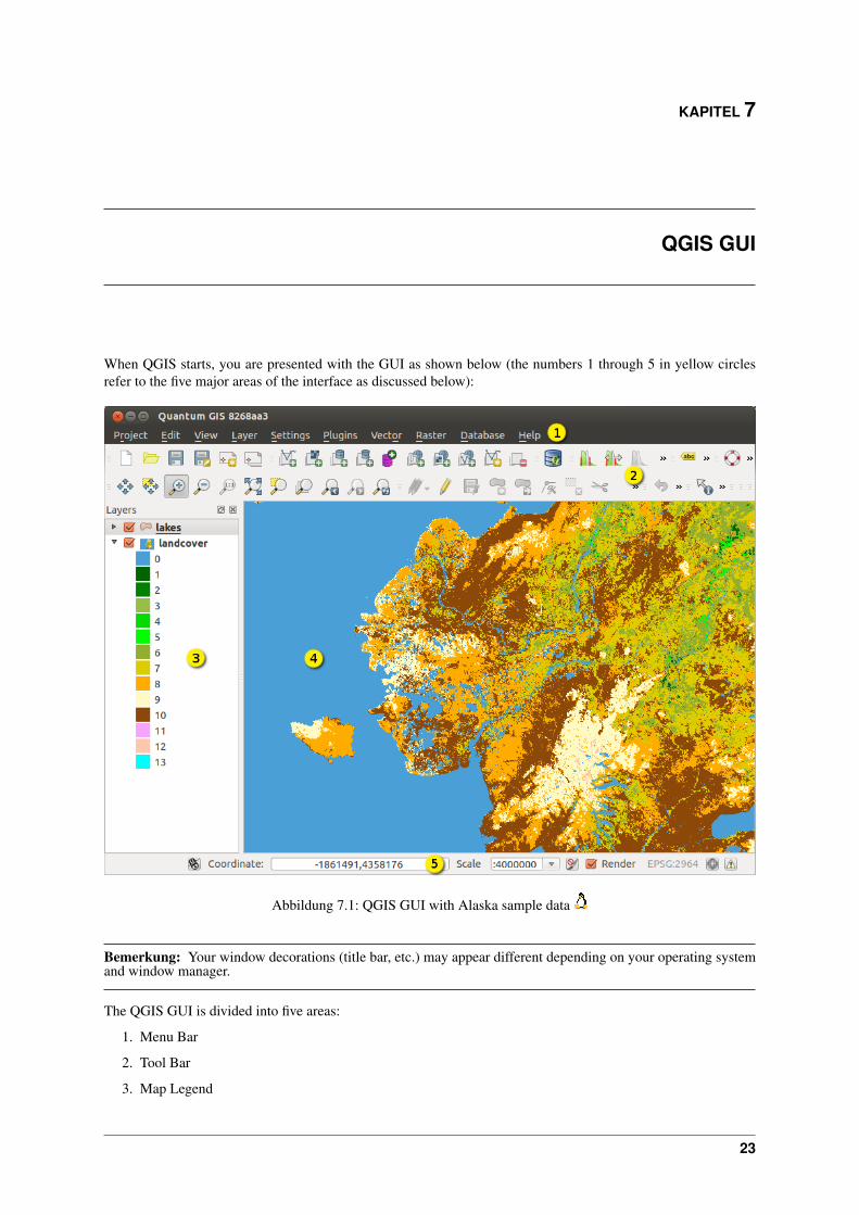
When QGIS starts, you are presented with the GUI as shown below (the numbers 1 through 5 in yellow circlesrefer to the five major areas of the interface as discussed below):
Abbildung 7.1: QGIS GUI with Alaska sample data
Bemerkung: Your window decorations (title bar, etc.) may appear different depending on your operating systemand window manager.
The QGIS GUI is divided into five areas:
1. Menu Bar
2. Tool Bar
3. Map Legend
23

QGIS User Guide, Release 2.0
4. Map View
5. Status Bar
These five components of the QGIS interface are described in more detail in the following sections. Two moresections present keyboard shortcuts and context help.
7.1 Menu Bar
The menu bar provides access to various QGIS features using a standard hierarchical menu. The top-level menusand a summary of some of the menu options are listed below, together with the icons of the corresponding toolsas they appear on the toolbar, as well as keyboard shortcuts. Keyboard shortcuts can also be configured manually(shortcuts presented in this section are the defaults), using the [Configure Shortcuts] tool under Settings.
Although most menu options have a corresponding tool and vice-versa, the menus are not organized quiet like thetoolbars. The toolbar containing the tool is listed after each menu option as a checkbox entry. Some menu optionsonly appear if the corresponding plugin is loaded. For more information about tools and toolbars, see SectionToolbar.
7.1.1 Project
Menu Option Shortcut Reference Toolbar
New Ctrl+N see QGIS Projekte Project
Open Ctrl+O see QGIS Projekte ProjectNew from template → see QGIS Projekte ProjectOpen Recent → see QGIS Projekte
Save Ctrl+S see QGIS Projekte Project
Save As Ctrl+Shift+S see QGIS Projekte Project
Save as Image see Ausgabe
New Print Composer Ctrl+P see Druckzusammenstellung Project
Composer manager ... see Druckzusammenstellung ProjectPrint Composers → see Druckzusammenstellung
Exit |qg| Ctrl+Q
24 Kapitel 7. QGIS GUI

QGIS User Guide, Release 2.0
7.1.2 Edit
Menu Option Shortcut Reference Toolbar
Undo Ctrl+Z see Erweiterte Digitalisierung AdvancedDigitizing
Redo Ctrl+Shift+Z see Erweiterte Digitalisierung AdvancedDigitizing
Cut Features Ctrl+X see Einen vorhandenen Layereditieren
Digitizing
Copy Features Ctrl+C see Einen vorhandenen Layereditieren
Digitizing
Paste Features Ctrl+V see Einen vorhandenen Layereditieren
Digitizing
Add Feature Ctrl+. see Einen vorhandenen Layereditieren
Digitizing
Move Feature(s) see Einen vorhandenen Layereditieren
Digitizing
Delete Selected see Einen vorhandenen Layereditieren
Digitizing
Rotate Feature(s) see Erweiterte Digitalisierung AdvancedDigitizing
Simplify Feature see Erweiterte Digitalisierung AdvancedDigitizing
Add Ring see Erweiterte Digitalisierung AdvancedDigitizing
Add Part see Erweiterte Digitalisierung AdvancedDigitizing
Delete Ring see Erweiterte Digitalisierung AdvancedDigitizing
Delete Part see Erweiterte Digitalisierung AdvancedDigitizing
Reshape Features see Erweiterte Digitalisierung AdvancedDigitizing
Offset Curves see Erweiterte Digitalisierung AdvancedDigitizing
Split Features see Erweiterte Digitalisierung AdvancedDigitizing
Merge Selected Features see Erweiterte Digitalisierung AdvancedDigitizing
Merge Attr. of SelectedFeatures
see Erweiterte Digitalisierung AdvancedDigitizing
Node Tool see Einen vorhandenen Layereditieren
Digitizing
Rotate Point Symbols see Erweiterte Digitalisierung AdvancedDigitizing
7.1. Menu Bar 25
QGIS User Guide, Release 2.0
After activating Toggle editing mode for a layer, you will find the Add Feature icon in the Edit menu dependingon the layer type (point, line or polygon).
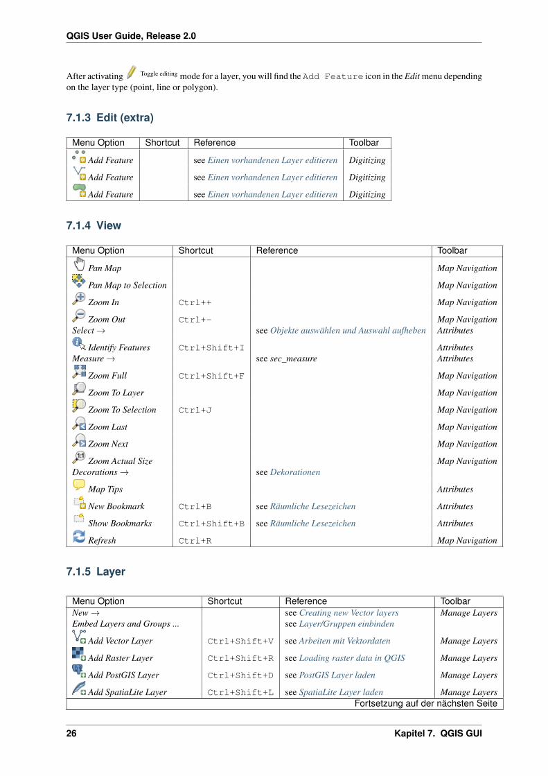
7.1.3 Edit (extra)
Menu Option Shortcut Reference Toolbar
Add Feature see Einen vorhandenen Layer editieren Digitizing
Add Feature see Einen vorhandenen Layer editieren Digitizing
Add Feature see Einen vorhandenen Layer editieren Digitizing
7.1.4 View
Menu Option Shortcut Reference Toolbar
Pan Map Map Navigation
Pan Map to Selection Map Navigation
Zoom In Ctrl++ Map Navigation
Zoom Out Ctrl+- Map NavigationSelect → see Objekte auswählen und Auswahl aufheben Attributes
Identify Features Ctrl+Shift+I AttributesMeasure → see sec_measure Attributes
Zoom Full Ctrl+Shift+F Map Navigation
Zoom To Layer Map Navigation
Zoom To Selection Ctrl+J Map Navigation
Zoom Last Map Navigation
Zoom Next Map Navigation
Zoom Actual Size Map NavigationDecorations → see Dekorationen
Map Tips Attributes
New Bookmark Ctrl+B see Räumliche Lesezeichen Attributes
Show Bookmarks Ctrl+Shift+B see Räumliche Lesezeichen Attributes
Refresh Ctrl+R Map Navigation
7.1.5 Layer
Menu Option Shortcut Reference ToolbarNew → see Creating new Vector layers Manage LayersEmbed Layers and Groups ... see Layer/Gruppen einbinden
Add Vector Layer Ctrl+Shift+V see Arbeiten mit Vektordaten Manage Layers
Add Raster Layer Ctrl+Shift+R see Loading raster data in QGIS Manage Layers
Add PostGIS Layer Ctrl+Shift+D see PostGIS Layer laden Manage Layers
Add SpatiaLite Layer Ctrl+Shift+L see SpatiaLite Layer laden Manage LayersFortsetzung auf der nächsten Seite
26 Kapitel 7. QGIS GUI
QGIS User Guide, Release 2.0
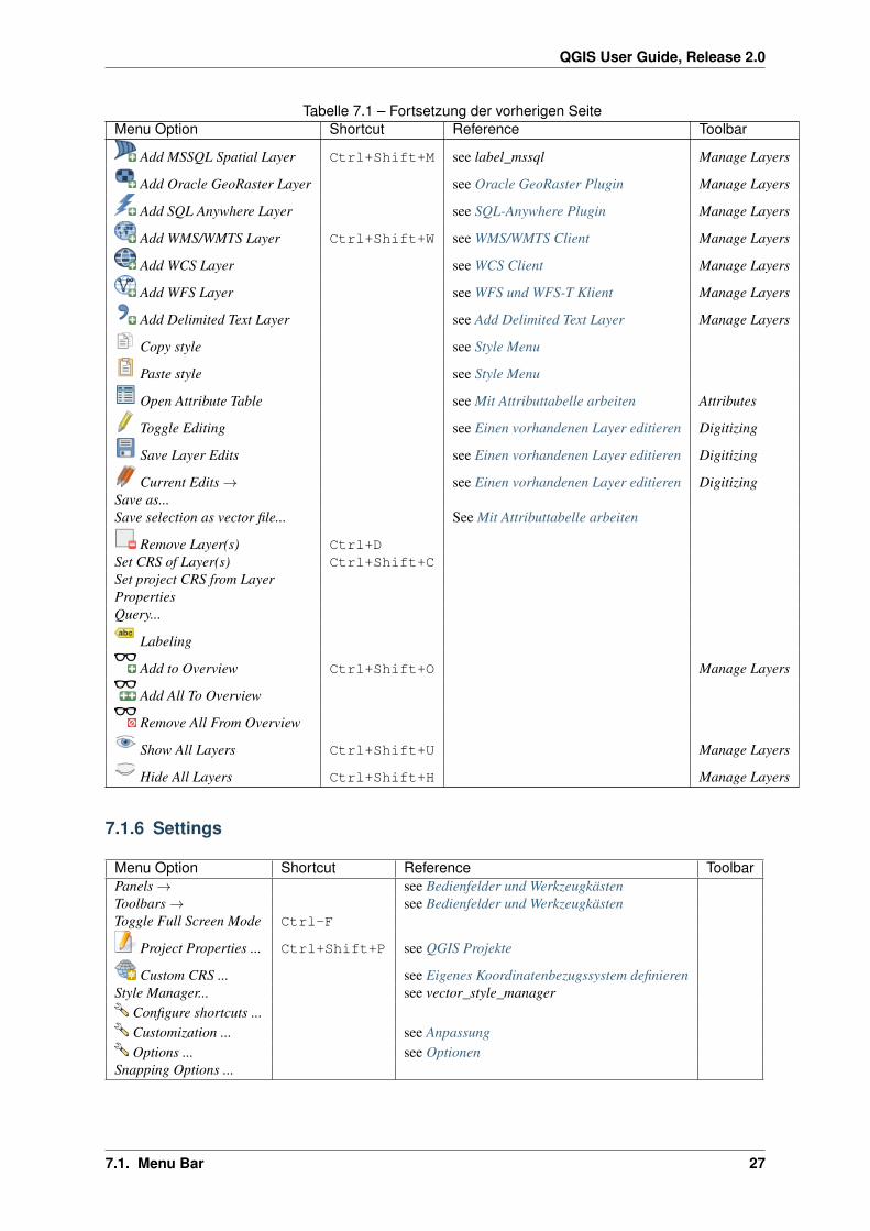
Tabelle 7.1 – Fortsetzung der vorherigen SeiteMenu Option Shortcut Reference Toolbar
Add MSSQL Spatial Layer Ctrl+Shift+M see label_mssql Manage Layers
Add Oracle GeoRaster Layer see Oracle GeoRaster Plugin Manage Layers
Add SQL Anywhere Layer see SQL-Anywhere Plugin Manage Layers
Add WMS/WMTS Layer Ctrl+Shift+W see WMS/WMTS Client Manage Layers
Add WCS Layer see WCS Client Manage Layers
Add WFS Layer see WFS und WFS-T Klient Manage Layers
Add Delimited Text Layer see Add Delimited Text Layer Manage Layers
Copy style see Style Menu
Paste style see Style Menu
Open Attribute Table see Mit Attributtabelle arbeiten Attributes
Toggle Editing see Einen vorhandenen Layer editieren Digitizing
Save Layer Edits see Einen vorhandenen Layer editieren Digitizing
Current Edits → see Einen vorhandenen Layer editieren DigitizingSave as...Save selection as vector file... See Mit Attributtabelle arbeiten
Remove Layer(s) Ctrl+DSet CRS of Layer(s) Ctrl+Shift+CSet project CRS from LayerPropertiesQuery...
Labeling
Add to Overview Ctrl+Shift+O Manage Layers
Add All To Overview
Remove All From Overview
Show All Layers Ctrl+Shift+U Manage Layers
Hide All Layers Ctrl+Shift+H Manage Layers
7.1.6 Settings
Menu Option Shortcut Reference ToolbarPanels → see Bedienfelder und WerkzeugkästenToolbars → see Bedienfelder und WerkzeugkästenToggle Full Screen Mode Ctrl-F
Project Properties ... Ctrl+Shift+P see QGIS Projekte
Custom CRS ... see Eigenes Koordinatenbezugssystem definierenStyle Manager... see vector_style_manager
Configure shortcuts ...Customization ... see AnpassungOptions ... see Optionen
Snapping Options ...
7.1. Menu Bar 27

QGIS User Guide, Release 2.0
7.1.7 Plugins
Menu Option Shortcut Reference Toolbar
Manage and Install Plugins see Plugins verwaltenPython ConsoleGRASS → see GRASS GIS Integration GRASS
When starting QGIS for the first time not all core plugins are loaded.
7.1.8 Vector
Menu Option Shortcut Reference ToolbarCoordinate Capture → see Koordinaten aufnehmen Plugin VectorDxf2Shp → see Dxf2Shape Konverter Plugin VectorGPS → see GPS Plugin VectorOpen Street Map → see Loading OpenStreetMap VectorsRoad Graph → see Straßengraph PluginSpatial Query → see Räumliche Abfrage Plugin Vector
When starting QGIS for the first time not all core plugins are loaded.
7.1.9 Raster
Menu Option Shortcut Reference ToolbarRaster calculator see RasterrechnerGeoreferencer → see Georeferenzier Plugin RasterHeatmap → see Heatmap Plugin RasterInterpolation → see Interpolationsplugin RasterZonal Statistics → see Zonenstatistikerweiterung Raster
When starting QGIS for the first time not all core plugins are loaded.
7.1.10 Database
Menu Option Shortcut Reference ToolbareVis → see eVis Plugin DatabaseSpit → see label_spit Database
When starting QGIS for the first time not all core plugins are loaded.
7.1.11 Processing
Menu Option Shortcut Reference Toolbar
Toolbox see The toolbox Toolbox
Graphical Modeler see The graphical modeler
History and Logs see The history manager
Options and configuration see Configuring the processing framework
Results viewer see Konfiguration externer Anwendungen
Commander Ctrl+Alt+M see The SEXTANTE Commander
When starting QGIS for the first time not all core plugins are loaded.
28 Kapitel 7. QGIS GUI
QGIS User Guide, Release 2.0
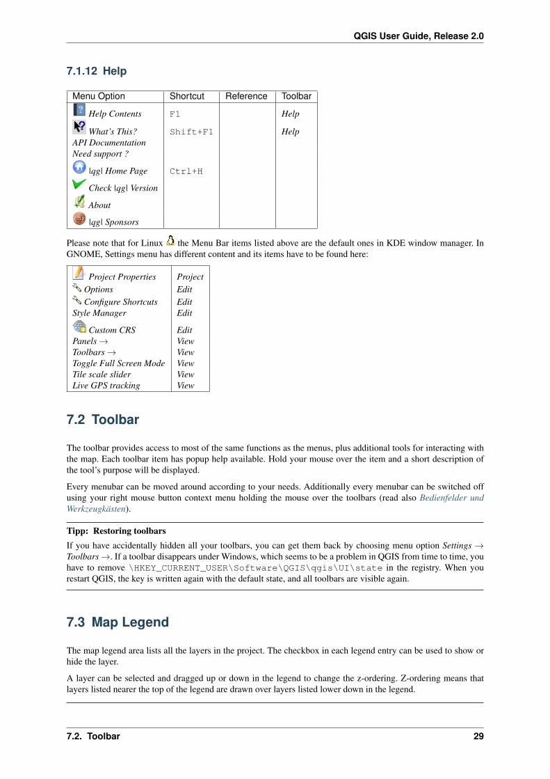
7.1.12 Help
Menu Option Shortcut Reference Toolbar
Help Contents F1 Help
What’s This? Shift+F1 HelpAPI DocumentationNeed support ?
|qg| Home Page Ctrl+H
Check |qg| Version
About
|qg| Sponsors
Please note that for Linux the Menu Bar items listed above are the default ones in KDE window manager. InGNOME, Settings menu has different content and its items have to be found here:
Project Properties ProjectOptions EditConfigure Shortcuts Edit
Style Manager Edit
Custom CRS EditPanels → ViewToolbars → ViewToggle Full Screen Mode ViewTile scale slider ViewLive GPS tracking View
7.2 Toolbar
The toolbar provides access to most of the same functions as the menus, plus additional tools for interacting withthe map. Each toolbar item has popup help available. Hold your mouse over the item and a short description ofthe tool’s purpose will be displayed.
Every menubar can be moved around according to your needs. Additionally every menubar can be switched offusing your right mouse button context menu holding the mouse over the toolbars (read also Bedienfelder undWerkzeugkästen).
Tipp: Restoring toolbarsIf you have accidentally hidden all your toolbars, you can get them back by choosing menu option Settings →Toolbars →. If a toolbar disappears under Windows, which seems to be a problem in QGIS from time to time, youhave to remove \HKEY_CURRENT_USER\Software\QGIS\qgis\UI\state in the registry. When yourestart QGIS, the key is written again with the default state, and all toolbars are visible again.
7.3 Map Legend
The map legend area lists all the layers in the project. The checkbox in each legend entry can be used to show orhide the layer.
A layer can be selected and dragged up or down in the legend to change the z-ordering. Z-ordering means thatlayers listed nearer the top of the legend are drawn over layers listed lower down in the legend.
7.2. Toolbar 29

QGIS User Guide, Release 2.0
Bemerkung: This behaviours can be overridden by ‘Layer order’ panel.
Layers in the legend window can be organised into groups. There are two ways to do so:
1. Right click in the legend window and choose Add Group. Type in a name for the group and press Enter.Now click on an existing layer and drag it onto the group.
2. Select some layers, right click in the legend window and choose Group Selected. The selected layers willautomatically be placed in a new group.
To bring a layer out of a group you can drag it out, or right click on it and choose Make to toplevel item. Groupscan be nested inside other groups.
The checkbox for a group will show or hide all the layers in the group with one click.
The content of the right mouse button context menu depends on whether the selected legend item is a raster or
a vector layer. For GRASS vector layers Toggle editing is not available. See section Digitalisieren und Editiereneines GRASS Vektorlayers for information on editing GRASS vector layers.
Right mouse button menu for raster layers
• Zoom to layer extent
• Zoom to Best Scale (100%)
• Stretch Using Current Extent
• Show in overview
• Remove
• Duplicate
• Set Layer CRS
• Set Project CRS from Layer
• Save as ...
• Properties
• Rename
• Copy Style
• Add New Group
• Expand all
• Collapse all
• Update Drawing Order
Additionally, according to layer position and selection
• Make to toplevel item
• Group Selected
Right mouse button menu for vector layers
• Zoom to Layer Extent
• Show in Overview
• Remove
• Duplicate
• Set Layer CRS
• Set Project CRS from Layer
• Open Attribute Table
30 Kapitel 7. QGIS GUI

QGIS User Guide, Release 2.0
• Toggle Editing (not available for GRASS layers)
• Save As ...
• Save Selection As
• Filter
• Show Feature Count
• Properties
• Rename
• Copy Style
• Add New Group
• Expand all
• Collapse all
• Update Drawing Order
Additionally, according to layer position and selection
• Make to toplevel item
• Group Selected
Right mouse button menu for layer groups
• Zoom to Group
• Remove
• Set Group CRS
• Rename
• Add New Group
• Expand all
• Collapse all
• Update Drawing Order
It is possible to select more than one layer or group at the same time by holding down the Ctrl key while selectingthe layers with the left mouse button. You can then move all selected layers to a new group at the same time.
You are also able to delete more than one Layer or Group at once by selecting several Layers with the Ctrl keyand pressing Ctrl+D afterwards. This way all selected Layers or groups will be removed from the layer’s list.
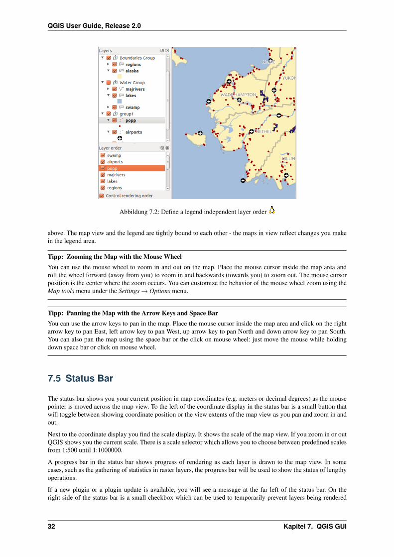
7.3.1 Working with the Legend independent layer order
There is a widget that allows to define a legend independent drawing order. You can activate it in the menuSettings → Panels → Layer order. Determine the drawing order of the layers in the map view here. Doing somakes it possible to order your layers in order of importance, for example, but to still display them in the correct
order (see figure_layer_order). Checking the Control rendering order box underneath the list of layers willcause a revert to default behavior.
7.4 Map View
This is the “business end” of QGIS - maps are displayed in this area! The map displayed in this window willdepend on the vector and raster layers you have chosen to load (see sections that follow for more information onhow to load layers). The map view can be panned (shifting the focus of the map display to another region) andzoomed in and out. Various other operations can be performed on the map as described in the toolbar description
7.4. Map View 31
QGIS User Guide, Release 2.0
Abbildung 7.2: Define a legend independent layer order
above. The map view and the legend are tightly bound to each other - the maps in view reflect changes you makein the legend area.
Tipp: Zooming the Map with the Mouse WheelYou can use the mouse wheel to zoom in and out on the map. Place the mouse cursor inside the map area androll the wheel forward (away from you) to zoom in and backwards (towards you) to zoom out. The mouse cursorposition is the center where the zoom occurs. You can customize the behavior of the mouse wheel zoom using theMap tools menu under the Settings → Options menu.
Tipp: Panning the Map with the Arrow Keys and Space BarYou can use the arrow keys to pan in the map. Place the mouse cursor inside the map area and click on the rightarrow key to pan East, left arrow key to pan West, up arrow key to pan North and down arrow key to pan South.You can also pan the map using the space bar or the click on mouse wheel: just move the mouse while holdingdown space bar or click on mouse wheel.
7.5 Status Bar
The status bar shows you your current position in map coordinates (e.g. meters or decimal degrees) as the mousepointer is moved across the map view. To the left of the coordinate display in the status bar is a small button thatwill toggle between showing coordinate position or the view extents of the map view as you pan and zoom in andout.
Next to the coordinate display you find the scale display. It shows the scale of the map view. If you zoom in or outQGIS shows you the current scale. There is a scale selector which allows you to choose between predefined scalesfrom 1:500 until 1:1000000.
A progress bar in the status bar shows progress of rendering as each layer is drawn to the map view. In somecases, such as the gathering of statistics in raster layers, the progress bar will be used to show the status of lengthyoperations.
If a new plugin or a plugin update is available, you will see a message at the far left of the status bar. On theright side of the status bar is a small checkbox which can be used to temporarily prevent layers being rendered
32 Kapitel 7. QGIS GUI
QGIS User Guide, Release 2.0
to the map view (see Section Layeranzeige kontrollieren below). The icon immediately stops the current maprendering process.
To the right of the render functions you find the EPSG code of the current project CRS and a projector icon.Clicking on this opens the projection properties for the current project.
Tipp: Calculating the correct Scale of your Map CanvasWhen you start QGIS, degrees is the default unit, and it tells QGIS that any coordinate in your layer is in degrees.To get correct scale values, you can either change this to meter manually in the General tab under Settings →
Project Properties or you can select a project Coordinate Reference System (CRS) clicking on the CRS status
icon in the lower right-hand corner of the statusbar. In the last case, the units are set to what the project projectionspecifies, e.g. ‘+units=m’.
7.5. Status Bar 33

QGIS User Guide, Release 2.0
34 Kapitel 7. QGIS GUI

KAPITEL 8
Allgemeine Werkzeuge
8.1 Identify features
Identify features allow to interact with map canvas to get data attribut on a pop-up windows. To identify feature
use View → Identify features or Ctrl+Shift+I, or click on the Identify features icon in the toolbar.
If you click on several feature, this pop-up will list all data attributes of all features. The first item is the number ofthe item in the list of result followed by layer name. Then its first child will be the name of a field with its value.Finally all informations of the feature is displayed.
This window can be customized to display custom fields but by default it will display three kind of information:
• Actions: actions can be added to the identify feature windows. When clicking on the action label, actionwill be run. By default only one action is added to View feature form for editing.
• Derived: those informations are calculated or derived from other information. You can find clicked coordi-nate, X and Y coordinates, area in map unit and perimeter in map unit for polygon, length in map unit forline and feature id.
• Data attributes: this is the list of attribute fields from data.
Abbildung 8.1: Identify feaures dialog (Gnome)
At the bottom of the windows, you have five icons:
• Expand tree
• Collapse tree
• Default behaviour
35
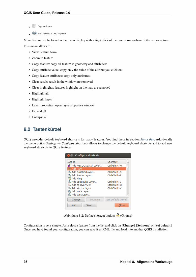
QGIS User Guide, Release 2.0
• Copy attributes
• Print selected HTML response
More feature can be found in the menu display with a right click of the mouse somewhere in the response tree.
This menu allows to:
• View Feature form
• Zoom to feature
• Copy feature: copy all feature ie geometry and attributes;
• Copy attribute value: copy only the value of the attribut you click on;
• Copy feature attributes: copy only attributes;
• Clear result: result in the window are removed
• Clear highlights: features highlight on the map are removed
• Highlight all
• Highlight layer
• Layer properties: open layer properties window
• Expand all
• Collapse all
8.2 Tastenkürzel
QGIS provides default keyboard shortcuts for many features. You find them in Section Menu Bar. Additionallythe menu option Settings → Configure Shortcuts allows to change the default keyboard shortcuts and to add newkeyboard shortcuts to QGIS features.
Abbildung 8.2: Define shortcut options (Gnome)
Configuration is very simple. Just select a feature from the list and click on [Change], [Set none] or [Set default].Once you have found your configuration, you can save it as XML file and load it to another QGIS installation.
36 Kapitel 8. Allgemeine Werkzeuge

QGIS User Guide, Release 2.0
8.3 Hilfe
Wenn Sie Hilfe zu bestimmten Themen brauchen erreichen Sie die Kontext-Hilfe über den Hilfe Knopf der Ih-nen in den meisten Dialogen zur Verfügung steht. Bitte beachten Sie daß Erweiterungen von Drittanbietern zudementsprechend gewidmeten Internetseiten verweisen.
8.4 Layeranzeige kontrollieren
By default, QGIS renders all visible layers whenever the map canvas must be refreshed. The events that trigger arefresh of the map canvas include:
• Einen Layer hinzufügen
• Karten verschieben, hinein- oder herauszoomen
• Resizing the QGIS window
• Layer ein- oder ausblenden
QGIS allows you to control the rendering process in a number of ways.
8.4.1 Maßstabsabhängige Layeranzeige
Scale dependent rendering allows you to specify the minimum and maximum scales at which a layer will bevisible. To set scale dependency rendering, open the Properties dialog by double-clicking on the layer in the
legend. On the General tab, click on the Use scale dependent rendering checkbox to activate the feature thenset the minimum and maximum scale values. .
You can determine the scale values by first zooming to the level you want to use and noting the scale value in theQGIS status bar.
8.4.2 Layeranzeige kontrollieren
Die Kartenwiedergabe kann auf folgende Art kontrolliert werden:
Wiedergabe unterdrücken
To suspend rendering, click the Render checkbox in the lower right corner of the statusbar. When theRender checkbox is not checked, QGIS does not redraw the canvas in response to any of the events described inSection Layeranzeige kontrollieren. Examples of when you might want to suspend rendering include:
• Viele Layer hinzufügen und ihre Symbologie vor der Visualisierung einstellen
• Einen oder mehrere große Layer hinzufügen und erst die maßstabsabhängige Wiedergabe einstellen
• Einen oder mehrere große Layer hinzufügen und erst in ein bestimmtes Gebiet hineinzoomen
• Eine Kombination aus den oben genannten Punkten
Wenn Sie die Zeichnen aktivieren, findet automatisch eine Erneuerung der Wiedergabe des Kartenfenstersstatt.
8.3. Hilfe 37

QGIS User Guide, Release 2.0
Option für Layer hinzufügen
You can set an option to always load new layers without drawing them. This means the layer will be added to themap, but its visibility checkbox in the legend will be unchecked by default. To set this option, choose menu option
Settings → Options → and click on the Rendering menu. Uncheck the By default new layers added to the mapshould be displayed checkbox. Any layer added to the map will be off (invisible) by default.
Another option in Settings → Options → Rendering menu is the Enable back buffer checkbox. It providesbetter graphics performance at the cost of loosing the possibility to cancel rendering and incremental featuredrawing. If it is unchecked, you can set the ‘Number of features to draw before updating the display’, otherwise itis inactive.
Finally you can activate the Use render caching where possible to speed up redraws checkbox.
Zeichnen stoppen
Um die Wiedergabe einer Karte zu stoppen drücken Sie die ESC Taste. Dies stoppt die Erneuerung der Wiedergabeund die Karte wird nur zum Teil angezeigt. Es kann sein dass etwas Zeit zwischen dem Drücken der Esc Tasteund dem Stoppen der Kartenwiedergabe vergeht.
Bemerkung: Es ist derzeit nicht möglich das Zeichnen zu stoppen - diese Funktion wurde mit der Version qt4ausgeschaltet da es zu Problemen und Abstürzen der Benutzeroberfläche kam.
Anpassen des Kartenfensters bei der Wiedergabe
You can set an option to update the map display as features are drawn. By default, QGIS does not display anyfeatures for a layer until the entire layer has been rendered. To update the display as features are read from thedatastore, choose menu option Settings → Options click on the Rendering menu. Set the feature count to anappropriate value to update the display during rendering. Setting a value of 0 disables update during drawing (thisis the default). Setting a value too low will result in poor performance as the map canvas is continually updatedduring the reading of the features. A suggested value to start with is 500.
Die Qualität der Wiedergabe beeinflussen
To influence the rendering quality of the map you have 2 options. Choose menu option Settings → Options clickon the Rendering menu and select or deselect following checkboxes.
• Linien auf Kosten der Zeichengeschwindigkeit weniger gezackt zeichnen
• Problem mit falsch gefüllten Polygonen beheben
8.5 Messen
Das Messen funktioniert mit Projektionen (z.B. UTM) und auch mit nicht projizierten Daten. Wenn die geladeneKarte als Geografisches Koordinatensystem abgebildet wird (z.B. Latitude/Longitude) sind die Messergebnissefalsch. Sie müssen dann ein passendes KBS mit einer Projektion verwenden (siehe Abschnitt Arbeiten mit Pro-jektionen). Alle Meßwerkzeuge verwenden auch die eingestellte Fangtoleranz der Digitalisierung. Dies ist zumBeispiel dann sinnvoll, wenn Sie entlang von Linien oder Polygongrenzen geladener Vektorlayer messen wollen.
Um ein Meßwerkzeug auszuwählen klicken Sie auf und suchen das Werkzeug das sie benutzen wollen aus.
38 Kapitel 8. Allgemeine Werkzeuge

QGIS User Guide, Release 2.0
8.5.1 Strecken, Flächen und Winkel messen
Measure Line: QGIS is able to measure real distances between given points according to a defined ellipsoid. Toconfigure this, choose menu option Settings → Options, click on the Map tools tab and choose the appropriateellipsoid. There you can also define a rubberband color and your preferred measurement units (meters or feet) andangle units (degrees, radians and gon). The tools then allows you to click points on the map. Each segment-lengthas well as the total shows up in the measure-window. To stop measuring click your right mouse button.
Abbildung 8.3: Measure Distance (Gnome)
Measure Area: Areas can also be measured. In the measure window the accumulated area size appears. In addition,the measuring tool will snap to the currently selected layer, provided that layer has its snapping tolerance set. (SeeSection Einstellen der Fangtoleranz und des Suchradius). So if you want to measure exactly along a line feature,or around a polygon feature, first set its snapping tolerance, then select the layer. Now, when using the measuringtools, each mouse click (within the tolerance setting) will snap to that layer.
Abbildung 8.4: Measure Area (Gnome)
Measure Angle: You can also measure angles. The cursor becomes cross-shaped. Click to draw the first segmentof the angle you wish to measure, then move the the cursor to draw the desired angle. The measure is displayed ina popup dialog.
Abbildung 8.5: Measure Angle (Gnome)
8.5.2 Objekte auswählen und Auswahl aufheben
The QGIS toolbar provides several tools to select features in the map canvas. To select one or several features just
click on and select your tool:
• Select Single Feature
8.5. Messen 39
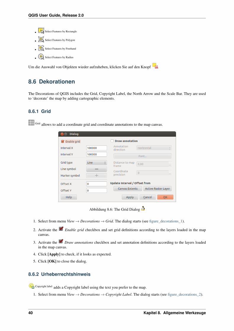
QGIS User Guide, Release 2.0
• Select Features by Rectangle
• Select Features by Polygon
• Select Features by Freehand
• Select Features by Radius
Um die Auswahl von Objekten wieder aufzuheben, klicken Sie auf den Knopf .
8.6 Dekorationen
The Decorations of QGIS includes the Grid, Copyright Label, the North Arrow and the Scale Bar. They are usedto ‘decorate’ the map by adding cartographic elements.
8.6.1 Grid
Grid allows to add a coordinate grid and coordinate annotations to the map canvas.
Abbildung 8.6: The Grid Dialog
1. Select from menu View → Decorations → Grid. The dialog starts (see figure_decorations_1).
2. Activate the Enable grid checkbox and set grid definitions according to the layers loaded in the mapcanvas.
3. Activate the Draw annotations checkbox and set annotation definitions according to the layers loadedin the map canvas.
4. Click [Apply] to check, if it looks as expected.
5. Click [OK] to close the dialog.
8.6.2 Urheberrechtshinweis
Copyright label adds a Copyright label using the text you prefer to the map.
1. Select from menu View → Decorations → Copyright Label. The dialog starts (see figure_decorations_2).
40 Kapitel 8. Allgemeine Werkzeuge
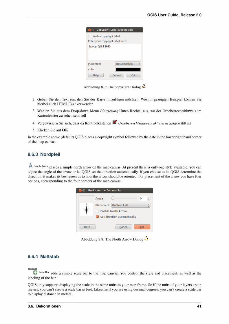
QGIS User Guide, Release 2.0
Abbildung 8.7: The copyright Dialog
2. Geben Sie den Text ein, den Sie der Karte hinzufügen möchten. Wie im gezeigten Beispiel können Siehierbei auch HTML Text verwenden
3. Wählen Sie aus dem Drop-down Menü Platzierung‘Unten Rechts’ aus, wo der Urheberrechtshinweis imKartenfenster zu sehen sein soll
4. Vergewissern Sie sich, dass da Kontrollkästchen Urheberrechtshinweis aktivieren ausgewählt ist
5. Klicken Sie auf OK
In the example above (default) QGIS places a copyright symbol followed by the date in the lower right hand cornerof the map canvas.
8.6.3 Nordpfeil
North Arrow places a simple north arrow on the map canvas. At present there is only one style available. You canadjust the angle of the arrow or let QGIS set the direction automatically. If you choose to let QGIS determine thedirection, it makes its best guess as to how the arrow should be oriented. For placement of the arrow you have fouroptions, corresponding to the four corners of the map canvas.
Abbildung 8.8: The North Arrow Dialog
8.6.4 Maßstab
Scale Bar adds a simple scale bar to the map canvas. You control the style and placement, as well as thelabeling of the bar.
QGIS only supports displaying the scale in the same units as your map frame. So if the units of your layers are inmeters, you can’t create a scale bar in feet. Likewise if you are using decimal degrees, you can’t create a scale barto display distance in meters.
8.6. Dekorationen 41
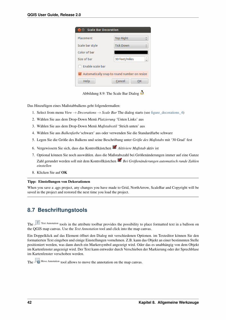
QGIS User Guide, Release 2.0
Abbildung 8.9: The Scale Bar Dialog
Das Hinzufügen eines Maßstabbalkens geht folgendermaßen:
1. Select from menu View → Decorations → Scale Bar The dialog starts (see figure_decorations_4)
2. Wählen Sie aus dem Drop-Down Menü Platzierung ‘Unten Links’ aus
3. Wählen Sie aus dem Drop-Down Menü Maßstabsstil ‘Strich unten’ aus
4. Wählen Sie aus Balkenfarbe‘schwarz’ aus oder verwenden Sie die Standardfarbe schwarz
5. Legen Sie die Größe des Balkens und seine Beschriftung unter Größe des Maßstabs mit ‘30 Grad’ fest
6. Vergewissern Sie sich, dass das Kontrollkästchen Aktiviere Maßstab aktiv ist
7. Optional können Sie noch auswählen. dass die Maßstabszahl bei Größenänderungen immer auf eine Ganze
Zahl gerundet werden soll mit dem Kontrollkästchen Bei Größenänderungen automatisch runde Zahleneinstellen
8. Klicken Sie auf OK
Tipp: Einstellungen von DekorationenWhen you save a .qgs project, any changes you have made to Grid, NorthArrow, ScaleBar and Copyright will besaved in the project and restored the next time you load the project.
8.7 Beschriftungstools
The Text Annotation tools in the attribute toolbar provides the possibility to place formatted text in a balloon onthe QGIS map canvas. Use the Text Annotation tool and click into the map canvas.
Ein Doppelklick auf das Element öffnet den Dialog mit verschiedenen Optionen. im Texteditor können Sie denformatierten Text eingeben und einige Einstellungen vornehmen. Z.B. kann das Objekt an einer bestimmten Stellepositioniert werden, was dann durch ein Markersymbol angezeigt wird. Oder das es unabhängig von dem Objektim Kartenfenster angezeigt wird. Der Text kann entweder durch Verschieben der Markierung oder der Sprechblaseim Kartenfenster verschoben werden.
The Move Annotation tool allows to move the annotation on the map canvas.
42 Kapitel 8. Allgemeine Werkzeuge
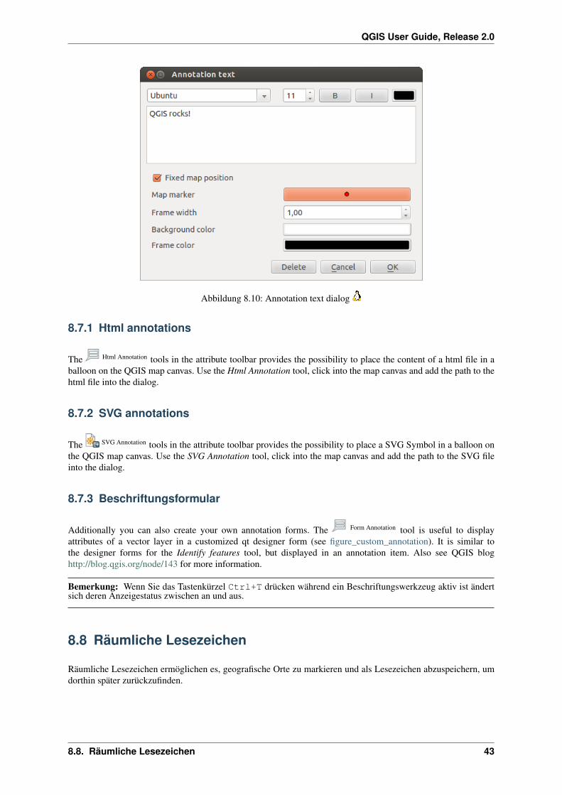
QGIS User Guide, Release 2.0
Abbildung 8.10: Annotation text dialog
8.7.1 Html annotations
The Html Annotation tools in the attribute toolbar provides the possibility to place the content of a html file in aballoon on the QGIS map canvas. Use the Html Annotation tool, click into the map canvas and add the path to thehtml file into the dialog.
8.7.2 SVG annotations
The SVG Annotation tools in the attribute toolbar provides the possibility to place a SVG Symbol in a balloon onthe QGIS map canvas. Use the SVG Annotation tool, click into the map canvas and add the path to the SVG fileinto the dialog.
8.7.3 Beschriftungsformular
Additionally you can also create your own annotation forms. The Form Annotation tool is useful to displayattributes of a vector layer in a customized qt designer form (see figure_custom_annotation). It is similar tothe designer forms for the Identify features tool, but displayed in an annotation item. Also see QGIS bloghttp://blog.qgis.org/node/143 for more information.
Bemerkung: Wenn Sie das Tastenkürzel Ctrl+T drücken während ein Beschriftungswerkzeug aktiv ist ändertsich deren Anzeigestatus zwischen an und aus.
8.8 Räumliche Lesezeichen
Räumliche Lesezeichen ermöglichen es, geografische Orte zu markieren und als Lesezeichen abzuspeichern, umdorthin später zurückzufinden.
8.8. Räumliche Lesezeichen 43
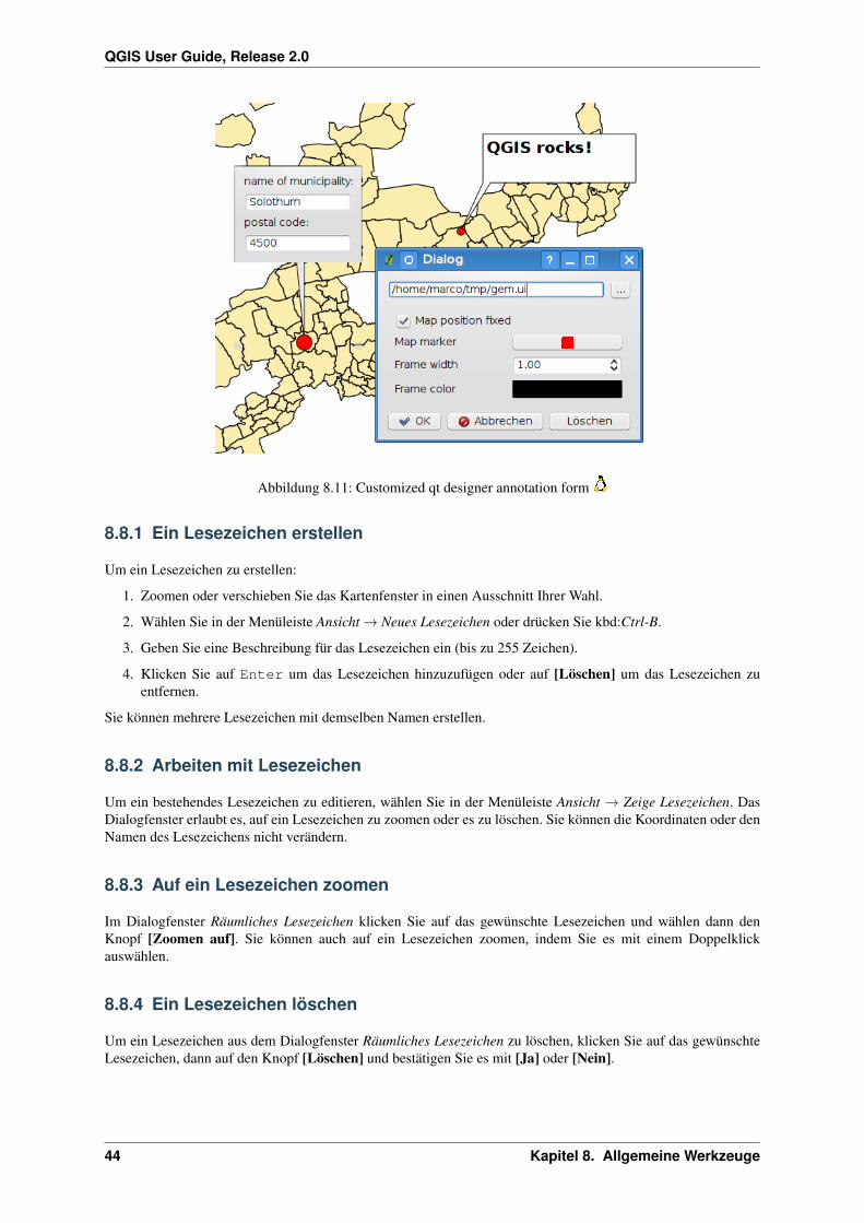
QGIS User Guide, Release 2.0
Abbildung 8.11: Customized qt designer annotation form
8.8.1 Ein Lesezeichen erstellen
Um ein Lesezeichen zu erstellen:
1. Zoomen oder verschieben Sie das Kartenfenster in einen Ausschnitt Ihrer Wahl.
2. Wählen Sie in der Menüleiste Ansicht → Neues Lesezeichen oder drücken Sie kbd:Ctrl-B.
3. Geben Sie eine Beschreibung für das Lesezeichen ein (bis zu 255 Zeichen).
4. Klicken Sie auf Enter um das Lesezeichen hinzuzufügen oder auf [Löschen] um das Lesezeichen zuentfernen.
Sie können mehrere Lesezeichen mit demselben Namen erstellen.
8.8.2 Arbeiten mit Lesezeichen
Um ein bestehendes Lesezeichen zu editieren, wählen Sie in der Menüleiste Ansicht → Zeige Lesezeichen. DasDialogfenster erlaubt es, auf ein Lesezeichen zu zoomen oder es zu löschen. Sie können die Koordinaten oder denNamen des Lesezeichens nicht verändern.
8.8.3 Auf ein Lesezeichen zoomen
Im Dialogfenster Räumliches Lesezeichen klicken Sie auf das gewünschte Lesezeichen und wählen dann denKnopf [Zoomen auf]. Sie können auch auf ein Lesezeichen zoomen, indem Sie es mit einem Doppelklickauswählen.
8.8.4 Ein Lesezeichen löschen
Um ein Lesezeichen aus dem Dialogfenster Räumliches Lesezeichen zu löschen, klicken Sie auf das gewünschteLesezeichen, dann auf den Knopf [Löschen] und bestätigen Sie es mit [Ja] oder [Nein].
44 Kapitel 8. Allgemeine Werkzeuge

QGIS User Guide, Release 2.0
8.9 Layer/Gruppen einbinden
Wenn Sie Inhalte von anderen Projekten in Ihr Projekt einbinden wollen wählen Sie Layer → Eingebettete Layerund Gruppen.
8.9.1 Layer einbetten
Der folgende Dialog ermöglicht Ihnen das Einbetten von Layern aus anderen Projekten:
1. Drückekn Sie um nach einem anderen Projekt des Alaskadatensatzes zu suchen.
2. Drücken Sie die Projektdatei grassland. Sie können den Inhalt des Projektes sehen (siehe fig-ure_embed_dialog).
3. Drücken Sie Ctrl und klicken Sie auf die Layer grassland und regions. Die Layer sind jetzt in der Karten-legende und im Kartenfenster eingebettet.
Abbildung 8.12: Select layers and groups to embed
Die eingebetteten Layer sind editierbar sie können jedoch Eigenschaften wie Stil und Beschriftung nicht ändern.
Eingebettete Layer entfernen
Right-click on the embedded layer and choose Remove.
8.10 Add Delimited Text Layer
This function allows you to load a delimited text file as a layer in QGIS. Following settings need to be defined:
1. The File format usually is CSV (comma separated values). If another delimiter is used, activate thecustom delimiter radiobutton and if each line in the file is split using a regular expression, please activatethe Regular expression delimiter radiobutton.
2. As Record options a text file usually provides a delimited header row of field names. This is usually the
first line in the text file. If there is no header row available, deactivate the first records have field namescheckbox. And if the header row isn’t the first line of the text file, define the number of header lines todiscard.
3. As Field options you can trim leading and trailing spaces from fields activating the Trim fields checkbox.
You can Discard empty fields in each record and you can define that the Decimal separator is comma.Otherwise it will be point.
4. As Geometry definitions a typical text file provides Point coordinates. This means there must be an‘X’ and ‘Y’ field with coordinate values. If the text file provides a Well Known Text field, there mustbe a ‘WKT’ field with geometry information for point, line or polygon objects. These fields can have anyname. Otherwise for attribute tables define no geometry. The x and y coordinates must be specified as a
8.9. Layer/Gruppen einbinden 45

QGIS User Guide, Release 2.0
number. The coordinate system is not important. If they are defined in degree/minutes/seconds, activate the
DMS coordinates checkbox.
5. As Layer settings you can activate Use spatial index to improve performance of displaying and spatially
selecting features. You can define to Use Subset index and to Watch file to watch for changes to thefile by other applications, while QGIS is running.
As an example of a valid text file we import the elevation point data file elevp.csv coming with the QGISsample dataset (See Section Beispieldaten):
X;Y;ELEV-300120;7689960;13-654360;7562040;521640;7512840;3[...]
Some items of note about the text file are:
1. The example text file uses ; (semicolon) as delimiter. Any character can be used to delimit the fields.
2. The first row is the header row. It contains the fields X, Y and ELEV.
3. No quotes (") are used to delimit text fields.
4. The x coordinates are contained in the X field.
5. The y coordinates are contained in the Y field.
8.10.1 Using the function
Click the toolbar icon Add Delimited Text Layer in the Manage layers toolbar to open the Create a Layer from aDelimited Text File dialog as shown in figure_delimited_text_1.
Abbildung 8.13: Delimited Text Dialog
First select the file (e.g., qgis_sample_data/csv/elevp.csv) to import by clicking on the [Browse]button. Once the file is selected, QGIS attempts to parse the file using the last used delimiter, in this case asemicolon (;). To properly parse the file, it is important to select the correct delimiter. To change the delimiter totab use \t (this is a regular expression for the tab character).
46 Kapitel 8. Allgemeine Werkzeuge
QGIS User Guide, Release 2.0
Once the file is parsed, make a Geometry definition Point coordinates and choose the X and Y fields from thedropdown lists. Finally enter a Layer name (e.g., elevp) as shown in figure_delimited_text_1 . To add the layerto the map, click [OK]. The delimited text file now behaves as any other map layer in QGIS.
8.10. Add Delimited Text Layer 47

QGIS User Guide, Release 2.0
48 Kapitel 8. Allgemeine Werkzeuge

KAPITEL 9
QGIS Configuration
QGIS is highly configurable through the Settings menu. Choose between Panels, Toolbars, Project properties,Options and Customization.
9.1 Bedienfelder und Werkzeugkästen
In the Panels→ menu you can switch on and off QGIS widgets. The Toolbars→ menu provides the possibility toswitch on and off icon groups in the QGIS toolbar (see figure_panels_toolbars).
Abbildung 9.1: The Panels and Toolbars menu
Tipp: Die QGIS-Übersicht aktivierenIn QGIS you can use an overview panel that provides a full extent view of layers added to it. It can be selectedunder the menu View → Panels. Within the view is a rectangle showing the current map extent. This allows youto quickly determine which area of the map you are currently viewing. Note that labels are not rendered to themap overview even if the layers in the map overview have been set up for labeling. If you click and drag the redrectangle in the overview that shows your current extent, the main map view will update accordingly.
Tipp: Protokoll anzeigen lassen
It’s possible to track the QGIS messages. You can activate Log Messages in the menu Settings → Panels andfollow the messages in the General and Plugin tab during loading and operation.
49

QGIS User Guide, Release 2.0
9.2 Projekteigenschaften
In the properties window for the project under Project → Project Properties or Project → Project Propertiesyou set project specific options. These include:
• In the General menu the project title, selection and background color, layer units, precision, and the optionto save relative paths to layers can be defined. If the CRS transformation is on you can choose an ellipsoidfor distance calculations. You can define the canvas units (only used when CRS transformation is disabled)and the precision of decimal places to use. You also can define a project scale list, that overrides the globalpredefined scales.
• The CRS menu enables you to choose the Coordinate Reference System for this project, and to enableon-the-fly re-projection of raster and vector layers when displaying layers from a different CRS.
• With the third Identify layers menu you set (or disable) which layers will respond to the identify tool. (Seethe Map tools paragraph from the Optionen section to enable identifying of multiple layers.)
• The menu Default Styles lets you control how new layers will be drawn when they do not have an existing.qml style defined. You can also set the default transparency level for new layers and whether symbolsshould have random colours assigned to them.
• The tab OWS Server allows to define information about the QGIS Server WMS and WFS Capabilities, theExtent and the CRS Restrictions.
• The menu Macros is to create a Python module, saved into a project.qgs file to be loaded and have specificfunctions run on the following project events: openProject(), saveProject() and closeProject().
Abbildung 9.2: Macro settings in QGIS
9.3 Optionen
Some basic options for QGIS can be selected using the Options dialog. Select the menu option Settings →Options. The menus where you can optimize your options are:
9.3.1 General Menu
Application
• Select the Style (QGIS restart required) and choose between ‘Oxygen’,’Windows’,’Motif’,’CDE’,‘Plastique’ and ‘Cleanlux’ ( ).
50 Kapitel 9. QGIS Configuration
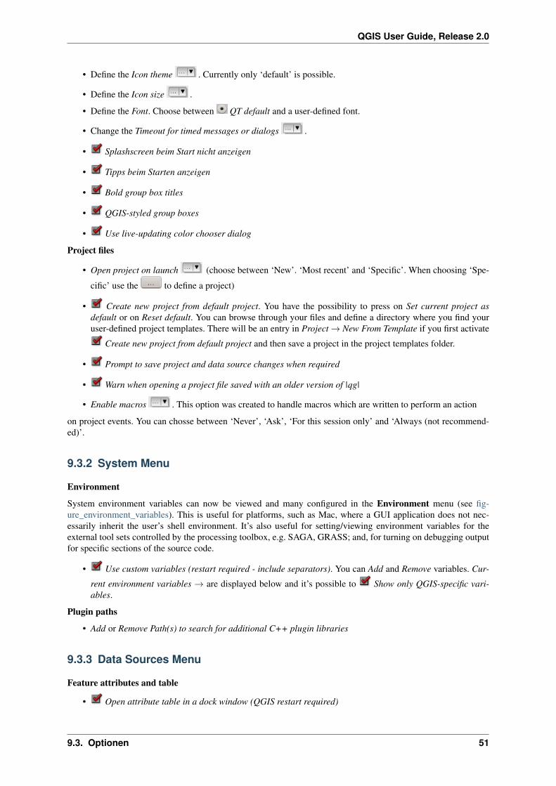
QGIS User Guide, Release 2.0
• Define the Icon theme . Currently only ‘default’ is possible.
• Define the Icon size .
• Define the Font. Choose between QT default and a user-defined font.
• Change the Timeout for timed messages or dialogs .
• Splashscreen beim Start nicht anzeigen
• Tipps beim Starten anzeigen
• Bold group box titles
• QGIS-styled group boxes
• Use live-updating color chooser dialog
Project files
• Open project on launch (choose between ‘New’. ‘Most recent’ and ‘Specific’. When choosing ‘Spe-
cific’ use the to define a project)
• Create new project from default project. You have the possibility to press on Set current project asdefault or on Reset default. You can browse through your files and define a directory where you find youruser-defined project templates. There will be an entry in Project → New From Template if you first activate
Create new project from default project and then save a project in the project templates folder.
• Prompt to save project and data source changes when required
• Warn when opening a project file saved with an older version of |qg|
• Enable macros . This option was created to handle macros which are written to perform an action
on project events. You can chosse between ‘Never’, ‘Ask’, ‘For this session only’ and ‘Always (not recommend-ed)’.
9.3.2 System Menu
Environment
System environment variables can now be viewed and many configured in the Environment menu (see fig-ure_environment_variables). This is useful for platforms, such as Mac, where a GUI application does not nec-essarily inherit the user’s shell environment. It’s also useful for setting/viewing environment variables for theexternal tool sets controlled by the processing toolbox, e.g. SAGA, GRASS; and, for turning on debugging outputfor specific sections of the source code.
• Use custom variables (restart required - include separators). You can Add and Remove variables. Cur-
rent environment variables → are displayed below and it’s possible to Show only QGIS-specific vari-ables.
Plugin paths
• Add or Remove Path(s) to search for additional C++ plugin libraries
9.3.3 Data Sources Menu
Feature attributes and table
• Open attribute table in a dock window (QGIS restart required)
9.3. Optionen 51
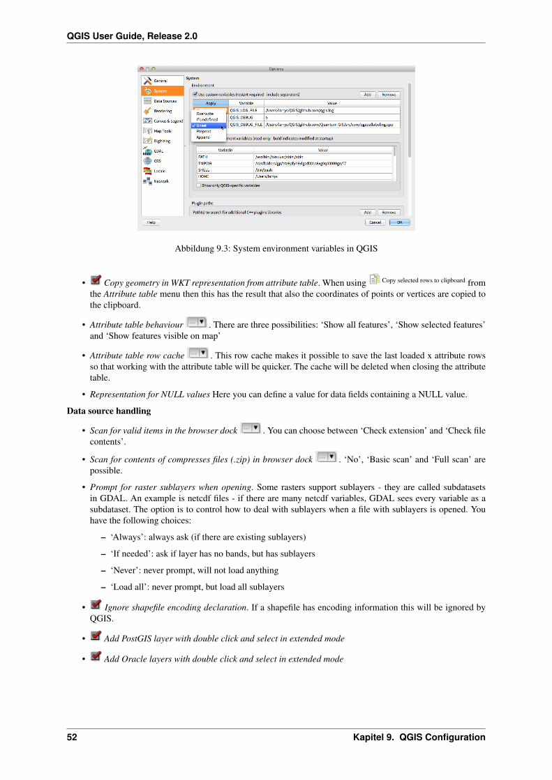
QGIS User Guide, Release 2.0
Abbildung 9.3: System environment variables in QGIS
• Copy geometry in WKT representation from attribute table. When using Copy selected rows to clipboard fromthe Attribute table menu then this has the result that also the coordinates of points or vertices are copied tothe clipboard.
• Attribute table behaviour . There are three possibilities: ‘Show all features’, ‘Show selected features’and ‘Show features visible on map’
• Attribute table row cache . This row cache makes it possible to save the last loaded x attribute rowsso that working with the attribute table will be quicker. The cache will be deleted when closing the attributetable.
• Representation for NULL values Here you can define a value for data fields containing a NULL value.
Data source handling
• Scan for valid items in the browser dock . You can choose between ‘Check extension’ and ‘Check filecontents’.
• Scan for contents of compresses files (.zip) in browser dock . ‘No’, ‘Basic scan’ and ‘Full scan’ arepossible.
• Prompt for raster sublayers when opening. Some rasters support sublayers - they are called subdatasetsin GDAL. An example is netcdf files - if there are many netcdf variables, GDAL sees every variable as asubdataset. The option is to control how to deal with sublayers when a file with sublayers is opened. Youhave the following choices:
– ‘Always’: always ask (if there are existing sublayers)
– ‘If needed’: ask if layer has no bands, but has sublayers
– ‘Never’: never prompt, will not load anything
– ‘Load all’: never prompt, but load all sublayers
• Ignore shapefile encoding declaration. If a shapefile has encoding information this will be ignored byQGIS.
• Add PostGIS layer with double click and select in extended mode
• Add Oracle layers with double click and select in extended mode
52 Kapitel 9. QGIS Configuration
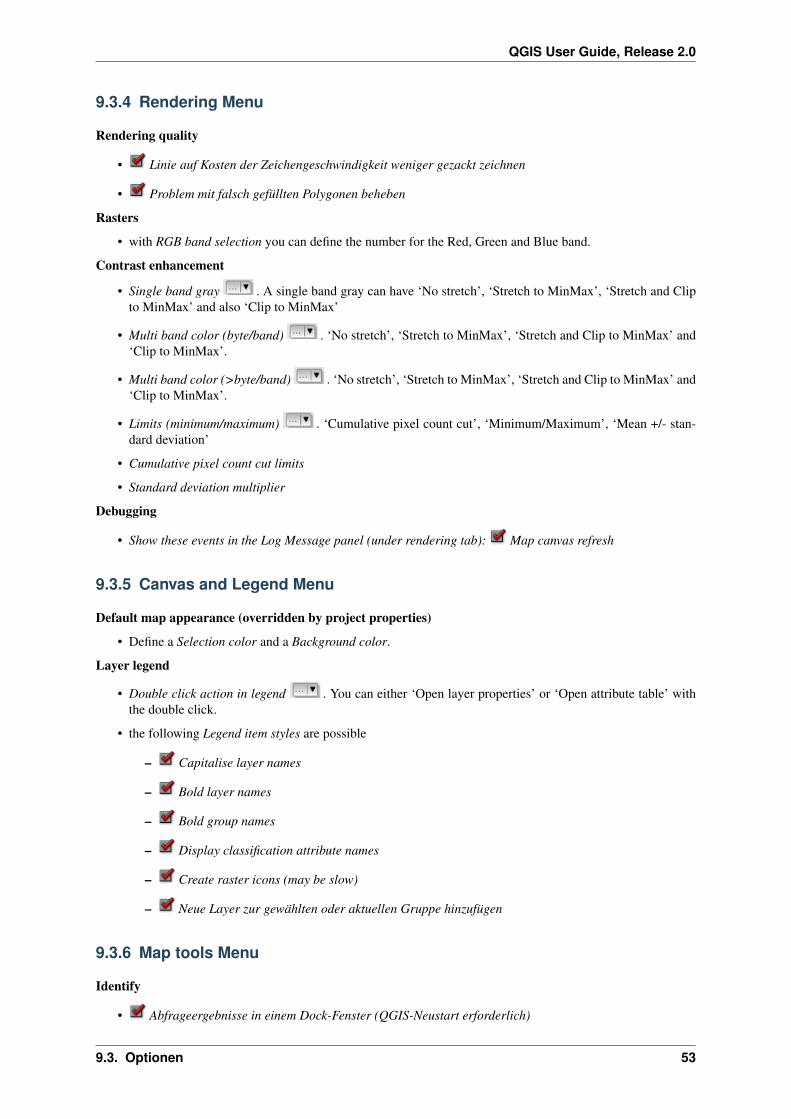
QGIS User Guide, Release 2.0
9.3.4 Rendering Menu
Rendering quality
• Linie auf Kosten der Zeichengeschwindigkeit weniger gezackt zeichnen
• Problem mit falsch gefüllten Polygonen beheben
Rasters
• with RGB band selection you can define the number for the Red, Green and Blue band.
Contrast enhancement
• Single band gray . A single band gray can have ‘No stretch’, ‘Stretch to MinMax’, ‘Stretch and Clipto MinMax’ and also ‘Clip to MinMax’
• Multi band color (byte/band) . ‘No stretch’, ‘Stretch to MinMax’, ‘Stretch and Clip to MinMax’ and‘Clip to MinMax’.
• Multi band color (>byte/band) . ‘No stretch’, ‘Stretch to MinMax’, ‘Stretch and Clip to MinMax’ and‘Clip to MinMax’.
• Limits (minimum/maximum) . ‘Cumulative pixel count cut’, ‘Minimum/Maximum’, ‘Mean +/- stan-dard deviation’
• Cumulative pixel count cut limits
• Standard deviation multiplier
Debugging
• Show these events in the Log Message panel (under rendering tab): Map canvas refresh
9.3.5 Canvas and Legend Menu
Default map appearance (overridden by project properties)
• Define a Selection color and a Background color.
Layer legend
• Double click action in legend . You can either ‘Open layer properties’ or ‘Open attribute table’ withthe double click.
• the following Legend item styles are possible
– Capitalise layer names
– Bold layer names
– Bold group names
– Display classification attribute names
– Create raster icons (may be slow)
– Neue Layer zur gewählten oder aktuellen Gruppe hinzufügen
9.3.6 Map tools Menu
Identify
• Abfrageergebnisse in einem Dock-Fenster (QGIS-Neustart erforderlich)
9.3. Optionen 53

QGIS User Guide, Release 2.0
• Die Modus-Einstellung legt fest welche Layer von dem Objekte abfragen-Werkzeug gezeigt werden. In demSie auf ‘Von oben nach unten’ oder ‘Von oben nach unten, beim ersten halten’ statt auf ‘Aktueller Layer’wechseln werden Attribute für alle abfragbaren Layer (siehe Abschnitt Projekteigenschaften unter QGISProjekte um festzulegen welche Layer abfragbar sind) mit dem Objekte abfragen-Werkzeug angezeigt.
• Objektformular öffnen, wenn ein einzelnes Objekte abgefragt wird
• Suchradius für die Objektidentifikation und zur Maptippanzeige einstellen
Measure tool
• Definieren Sie Gummibandfarbe für das Meßwerkzeug
• Definieren Sie Dezimalstellen
• Basiseinheit beibehalten
• Preferred measurements units (‘meters’ or ‘feet’)‘
• Preferred angle units (‘Angle’, ‘Radians’ or ‘Gon’)
Panning and zooming
• Definieren Sie Mausradaktion (‘Zoom’, ‘Zoomen und mittig zentrieren, Zur Mausposition zoomen, Nichts)
• Definieren Sie Zoomfaktor für das Mausrad
Predefined scales
Here you find a list of predefined scales. With the ‘+’ and ‘-‘ buttons you can add or remove your individual scales.
9.3.7 Digitizing Menu
Feature creation
• Eingabe der Attributwerte bei der Erstellung neuer Objekte unterdrücken
• Letzte Attributwerteingaben wiederverwenden
• Validate geometries. Editing complex lines/polygons with many nodes can end up with very slow rendering.This is because the default validation procedures in QGIS can use a lot of time. To speed up rendering it ispossible to select GEOS geometry validation (starting from GEOS 3.3) or to switch it off. GEOS geometryvalidation is much faster, but the disadvantage is that only the first geometry problem will be reported.
Rubberband
• Define Rubberband Line width and Line color
Snapping
• Fangoptionsdialog in einem Dockfenster anzeigen (QGIS-Neustart erforderlich)
• Define Default snap mode (‘To vertex’, ‘To segment’, ‘To vertex and segment’, ‘Off’)
• Define Default snapping tolerance in map units or pixels
• Define the Search radius for vertex edits in map units or pixels
Vertex markers
• Markierungen nur für gewählte Objekte anzeigen
• Define vertex Marker style (‘Cross’ (default), ‘Semi transparent circle’ or ‘None’)
• Define vertex Marker size
54 Kapitel 9. QGIS Configuration

QGIS User Guide, Release 2.0
Curve offset tool
Die nächsten 3 Optionen beziehen sich auf das Linie versetzen Werkzeug in Erweiterte Digitalisierung. Durch dieverschiedenen Einstellungen ist es möglich die Form des Linienversatzes zu beeinflussen.
• Verbindungsstil für Linienversatz
• Quadrant segments for curve offset
• Eckengrenze für Linienversatz
9.3.8 GDAL Menu
GDAL is a data exchange library for raster files. In this tab you can Edit create options and Edit Pyramids Optionsof the raster formats. Define which GDAL driver to be used for a raster format as in some cases more than oneGDAL driver is available.
9.3.9 CRS Menu
Default CRS for new projects
• Automatically enable ‘on the fly’ reprojection if layers have different CRS
• ‘On-The-Fly’-Reprojektion voreinstellen
• Select a CRS and Always start new projects with this CRS
CRS for new layers
This area allows to define the action, when a new layer is created, or when a layer without CRS is loaded.
• Prompt for CRS
• Use project CRS
• Use default CRS displayed below
9.3.10 Sprache
• System-Locale überschreiben und Stattdessen folgende Spracheinstellungen benutzen
• Informationen über die aktive System-Locale
9.3.11 Netzwerk
General
• WMS Suchadresse - Standard ist http://geopole.org/wms/search?search=%1&type=rss
• Define Timeout for network requests (ms) - default is 60000
• Define Default expiration period for WMSC/WMTS tiles (hours) - default is 24
Cache settings
Define the Directory and a Size for the cache.
• Proxy für Web-Zugriff benutzen und entsprechend ‘Host’, ‘Port’, ‘Benutzer’ und ‘Passwort’ definieren.
• Definieren Sie den Proxytyp → entsprechend ihrer Bedürfnisse.
– DefaultProxy →: Proxy wird auf Grundlage des Proxy der Anwendung festgelegt
9.3. Optionen 55
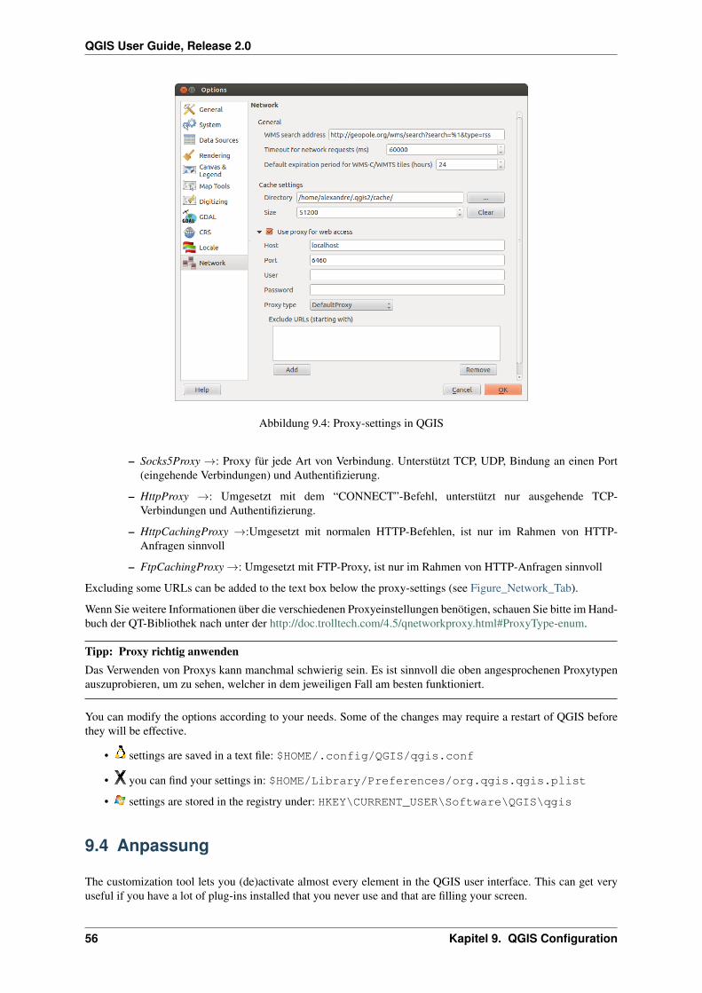
QGIS User Guide, Release 2.0
Abbildung 9.4: Proxy-settings in QGIS
– Socks5Proxy →: Proxy für jede Art von Verbindung. Unterstützt TCP, UDP, Bindung an einen Port(eingehende Verbindungen) und Authentifizierung.
– HttpProxy →: Umgesetzt mit dem “CONNECT”-Befehl, unterstützt nur ausgehende TCP-Verbindungen und Authentifizierung.
– HttpCachingProxy →:Umgesetzt mit normalen HTTP-Befehlen, ist nur im Rahmen von HTTP-Anfragen sinnvoll
– FtpCachingProxy →: Umgesetzt mit FTP-Proxy, ist nur im Rahmen von HTTP-Anfragen sinnvoll
Excluding some URLs can be added to the text box below the proxy-settings (see Figure_Network_Tab).
Wenn Sie weitere Informationen über die verschiedenen Proxyeinstellungen benötigen, schauen Sie bitte im Hand-buch der QT-Bibliothek nach unter der http://doc.trolltech.com/4.5/qnetworkproxy.html#ProxyType-enum.
Tipp: Proxy richtig anwendenDas Verwenden von Proxys kann manchmal schwierig sein. Es ist sinnvoll die oben angesprochenen Proxytypenauszuprobieren, um zu sehen, welcher in dem jeweiligen Fall am besten funktioniert.
You can modify the options according to your needs. Some of the changes may require a restart of QGIS beforethey will be effective.
• settings are saved in a text file: $HOME/.config/QGIS/qgis.conf
• you can find your settings in: $HOME/Library/Preferences/org.qgis.qgis.plist
• settings are stored in the registry under: HKEY\CURRENT_USER\Software\QGIS\qgis
9.4 Anpassung
The customization tool lets you (de)activate almost every element in the QGIS user interface. This can get veryuseful if you have a lot of plug-ins installed that you never use and that are filling your screen.
56 Kapitel 9. QGIS Configuration
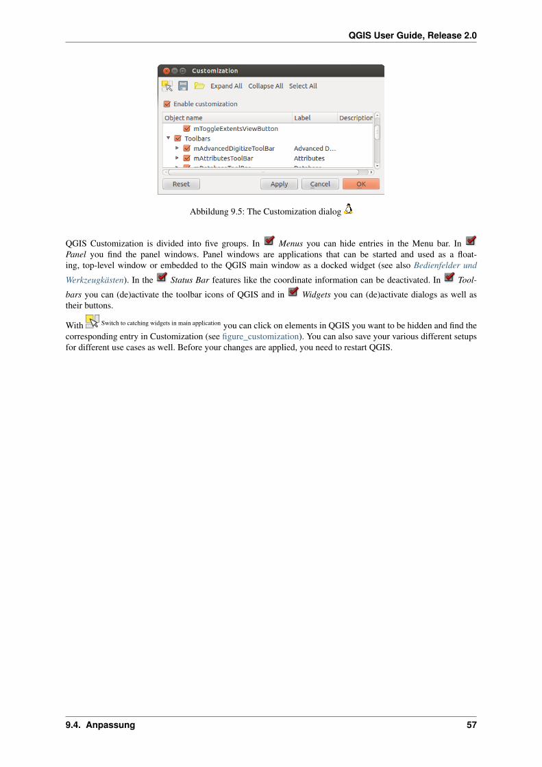
QGIS User Guide, Release 2.0
Abbildung 9.5: The Customization dialog
QGIS Customization is divided into five groups. In Menus you can hide entries in the Menu bar. InPanel you find the panel windows. Panel windows are applications that can be started and used as a float-ing, top-level window or embedded to the QGIS main window as a docked widget (see also Bedienfelder und
Werkzeugkästen). In the Status Bar features like the coordinate information can be deactivated. In Tool-
bars you can (de)activate the toolbar icons of QGIS and in Widgets you can (de)activate dialogs as well astheir buttons.
With Switch to catching widgets in main application you can click on elements in QGIS you want to be hidden and find thecorresponding entry in Customization (see figure_customization). You can also save your various different setupsfor different use cases as well. Before your changes are applied, you need to restart QGIS.
9.4. Anpassung 57

QGIS User Guide, Release 2.0
58 Kapitel 9. QGIS Configuration
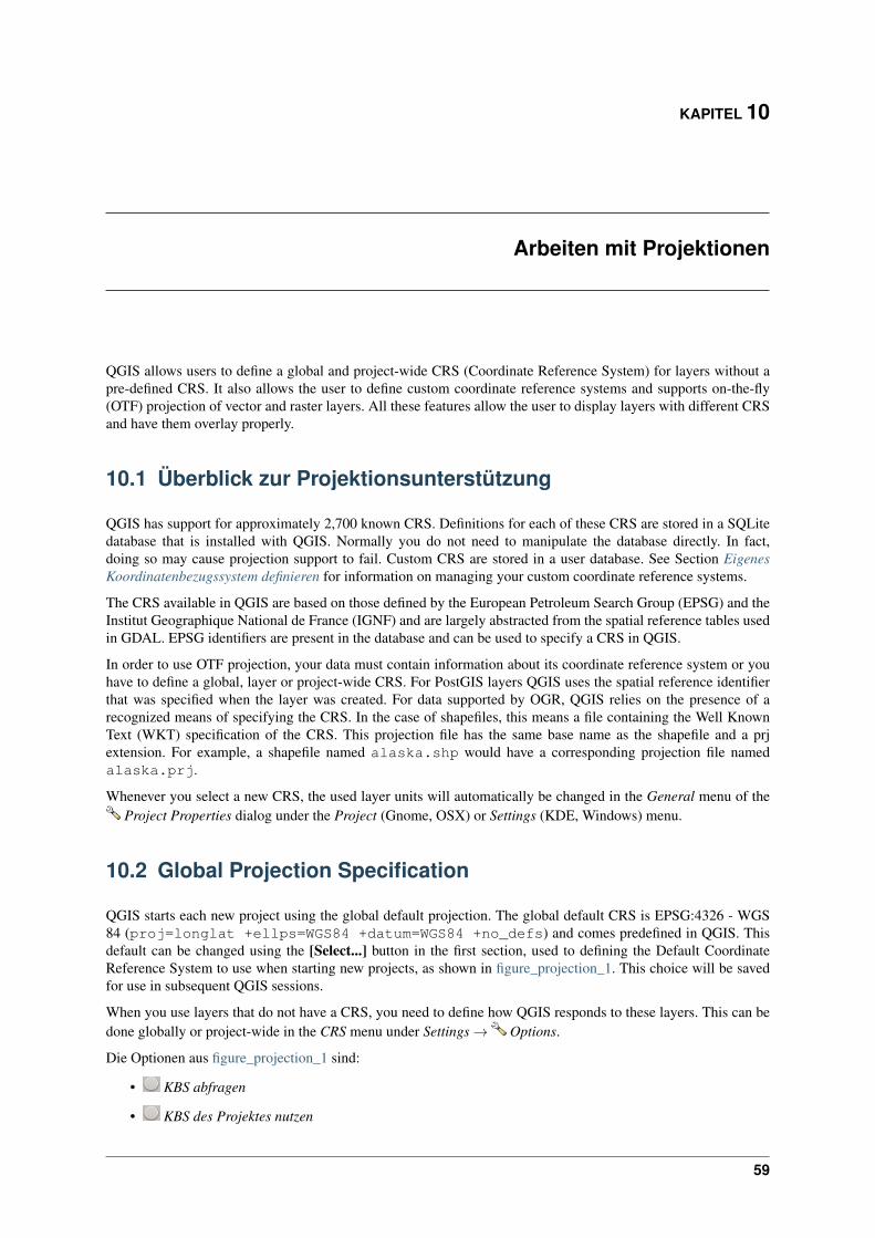
KAPITEL 10
Arbeiten mit Projektionen
QGIS allows users to define a global and project-wide CRS (Coordinate Reference System) for layers without apre-defined CRS. It also allows the user to define custom coordinate reference systems and supports on-the-fly(OTF) projection of vector and raster layers. All these features allow the user to display layers with different CRSand have them overlay properly.
10.1 Überblick zur Projektionsunterstützung
QGIS has support for approximately 2,700 known CRS. Definitions for each of these CRS are stored in a SQLitedatabase that is installed with QGIS. Normally you do not need to manipulate the database directly. In fact,doing so may cause projection support to fail. Custom CRS are stored in a user database. See Section EigenesKoordinatenbezugssystem definieren for information on managing your custom coordinate reference systems.
The CRS available in QGIS are based on those defined by the European Petroleum Search Group (EPSG) and theInstitut Geographique National de France (IGNF) and are largely abstracted from the spatial reference tables usedin GDAL. EPSG identifiers are present in the database and can be used to specify a CRS in QGIS.
In order to use OTF projection, your data must contain information about its coordinate reference system or youhave to define a global, layer or project-wide CRS. For PostGIS layers QGIS uses the spatial reference identifierthat was specified when the layer was created. For data supported by OGR, QGIS relies on the presence of arecognized means of specifying the CRS. In the case of shapefiles, this means a file containing the Well KnownText (WKT) specification of the CRS. This projection file has the same base name as the shapefile and a prjextension. For example, a shapefile named alaska.shp would have a corresponding projection file namedalaska.prj.
Whenever you select a new CRS, the used layer units will automatically be changed in the General menu of theProject Properties dialog under the Project (Gnome, OSX) or Settings (KDE, Windows) menu.
10.2 Global Projection Specification
QGIS starts each new project using the global default projection. The global default CRS is EPSG:4326 - WGS84 (proj=longlat +ellps=WGS84 +datum=WGS84 +no_defs) and comes predefined in QGIS. Thisdefault can be changed using the [Select...] button in the first section, used to defining the Default CoordinateReference System to use when starting new projects, as shown in figure_projection_1. This choice will be savedfor use in subsequent QGIS sessions.
When you use layers that do not have a CRS, you need to define how QGIS responds to these layers. This can bedone globally or project-wide in the CRS menu under Settings → Options.
Die Optionen aus figure_projection_1 sind:
• KBS abfragen
• KBS des Projektes nutzen
59
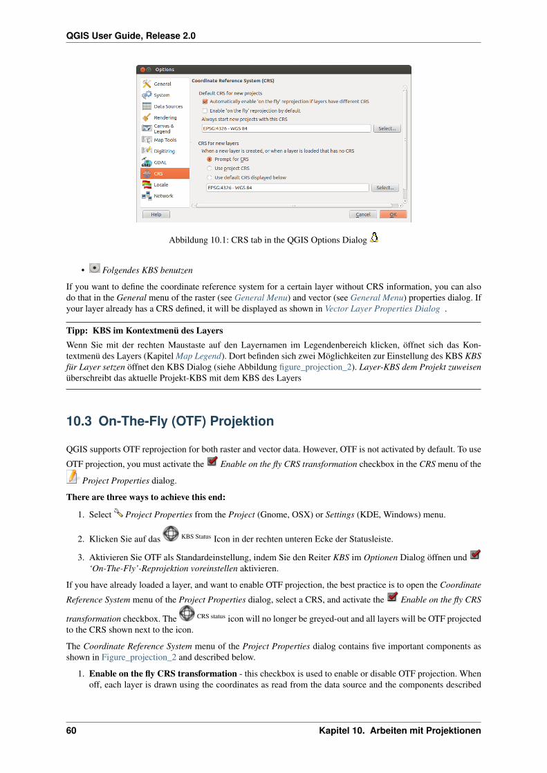
QGIS User Guide, Release 2.0
Abbildung 10.1: CRS tab in the QGIS Options Dialog
• Folgendes KBS benutzen
If you want to define the coordinate reference system for a certain layer without CRS information, you can alsodo that in the General menu of the raster (see General Menu) and vector (see General Menu) properties dialog. Ifyour layer already has a CRS defined, it will be displayed as shown in Vector Layer Properties Dialog .
Tipp: KBS im Kontextmenü des LayersWenn Sie mit der rechten Maustaste auf den Layernamen im Legendenbereich klicken, öffnet sich das Kon-textmenü des Layers (Kapitel Map Legend). Dort befinden sich zwei Möglichkeiten zur Einstellung des KBS KBSfür Layer setzen öffnet den KBS Dialog (siehe Abbildung figure_projection_2). Layer-KBS dem Projekt zuweisenüberschreibt das aktuelle Projekt-KBS mit dem KBS des Layers
10.3 On-The-Fly (OTF) Projektion
QGIS supports OTF reprojection for both raster and vector data. However, OTF is not activated by default. To use
OTF projection, you must activate the Enable on the fly CRS transformation checkbox in the CRS menu of the
Project Properties dialog.
There are three ways to achieve this end:
1. Select Project Properties from the Project (Gnome, OSX) or Settings (KDE, Windows) menu.
2. Klicken Sie auf das KBS Status Icon in der rechten unteren Ecke der Statusleiste.
3. Aktivieren Sie OTF als Standardeinstellung, indem Sie den Reiter KBS im Optionen Dialog öffnen und‘On-The-Fly’-Reprojektion voreinstellen aktivieren.
If you have already loaded a layer, and want to enable OTF projection, the best practice is to open the Coordinate
Reference System menu of the Project Properties dialog, select a CRS, and activate the Enable on the fly CRS
transformation checkbox. The CRS status icon will no longer be greyed-out and all layers will be OTF projectedto the CRS shown next to the icon.
The Coordinate Reference System menu of the Project Properties dialog contains five important components asshown in Figure_projection_2 and described below.
1. Enable on the fly CRS transformation - this checkbox is used to enable or disable OTF projection. Whenoff, each layer is drawn using the coordinates as read from the data source and the components described
60 Kapitel 10. Arbeiten mit Projektionen
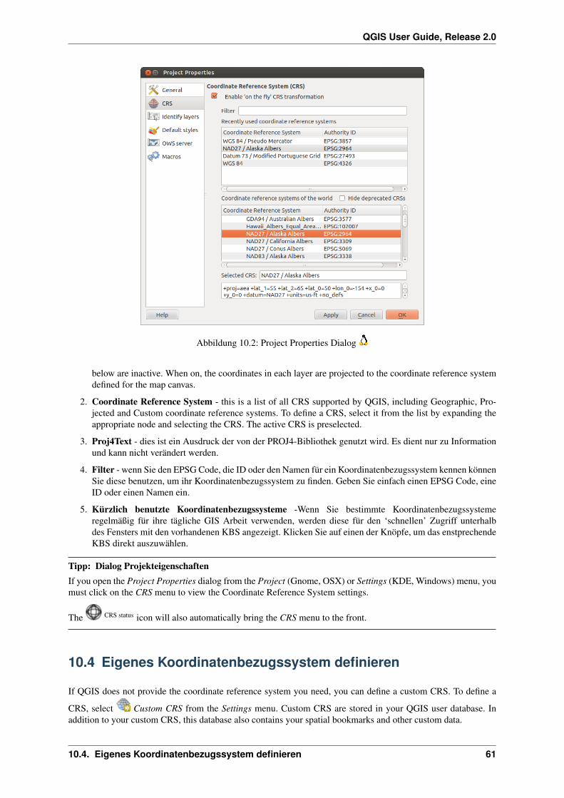
QGIS User Guide, Release 2.0
Abbildung 10.2: Project Properties Dialog
below are inactive. When on, the coordinates in each layer are projected to the coordinate reference systemdefined for the map canvas.
2. Coordinate Reference System - this is a list of all CRS supported by QGIS, including Geographic, Pro-jected and Custom coordinate reference systems. To define a CRS, select it from the list by expanding theappropriate node and selecting the CRS. The active CRS is preselected.
3. Proj4Text - dies ist ein Ausdruck der von der PROJ4-Bibliothek genutzt wird. Es dient nur zu Informationund kann nicht verändert werden.
4. Filter - wenn Sie den EPSG Code, die ID oder den Namen für ein Koordinatenbezugssystem kennen könnenSie diese benutzen, um ihr Koordinatenbezugssystem zu finden. Geben Sie einfach einen EPSG Code, eineID oder einen Namen ein.
5. Kürzlich benutzte Koordinatenbezugssysteme -Wenn Sie bestimmte Koordinatenbezugssystemeregelmäßig für ihre tägliche GIS Arbeit verwenden, werden diese für den ‘schnellen’ Zugriff unterhalbdes Fensters mit den vorhandenen KBS angezeigt. Klicken Sie auf einen der Knöpfe, um das enstprechendeKBS direkt auszuwählen.
Tipp: Dialog ProjekteigenschaftenIf you open the Project Properties dialog from the Project (Gnome, OSX) or Settings (KDE, Windows) menu, youmust click on the CRS menu to view the Coordinate Reference System settings.
The CRS status icon will also automatically bring the CRS menu to the front.
10.4 Eigenes Koordinatenbezugssystem definieren
If QGIS does not provide the coordinate reference system you need, you can define a custom CRS. To define a
CRS, select Custom CRS from the Settings menu. Custom CRS are stored in your QGIS user database. Inaddition to your custom CRS, this database also contains your spatial bookmarks and other custom data.
10.4. Eigenes Koordinatenbezugssystem definieren 61

QGIS User Guide, Release 2.0
Abbildung 10.3: Custom CRS Dialog
Defining a custom CRS in QGIS requires a good understanding of the Proj.4 projection library. To begin, refer tothe Cartographic Projection Procedures for the UNIX Environment - A User’s Manual by Gerald I. Evenden, U.S.Geological Survey Open-File Report 90-284, 1990 (available at ftp://ftp.remotesensing.org/proj/OF90-284.pdf ).
This manual describes the use of the proj.4 and related command line utilities. The cartographic parametersused with proj.4 are described in the user manual and are the same as those used by QGIS.
Der Dialog Definition eines Benutzerkoordinatensystems braucht nur zwei Einträge, um eine eigene Projektion zudefinieren:
1. einen aussagekräftigen Namen und
2. die kartografischen Parameter im PROJ.4-Format.
Um ein neues KBS zu erstellen klicken Sie Neu Knopf und geben Sie einen aussagekräftigen Namen sowie die
KBS-Parameter ein. Danach speichern Sie das neue KBS mit dem Knopf Speichern ab.
Denken Sie daran, dass die kartographischen Parameter mit einem +proj=-Block beginnen müssen, um denBeginn eines neuen KBS anzuzeigen.
Sie können das neue KBS testen, um zu sehen, ob bei einer Konvertierung von bekannten WGS84 Lat-Lon Koor-dinaten in ihre Projektion ein sinnvolles Ergebnis herauskommt. Dazu kopieren Sie ihre kartographischen Param-eter in das Fenster Parameter, geben ein paar bekannte WGS84 Lat-Lon Koordinaten an und klicken dann auf denKnopf [Berechnen]. Vergleichen Sie die Ergebnisse mit den Werten im Kartenfenster.
62 Kapitel 10. Arbeiten mit Projektionen
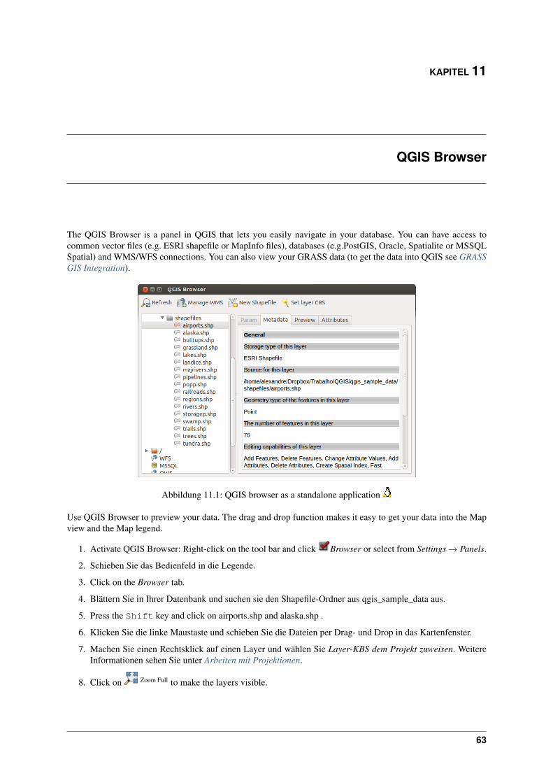
KAPITEL 11
QGIS Browser
The QGIS Browser is a panel in QGIS that lets you easily navigate in your database. You can have access tocommon vector files (e.g. ESRI shapefile or MapInfo files), databases (e.g.PostGIS, Oracle, Spatialite or MSSQLSpatial) and WMS/WFS connections. You can also view your GRASS data (to get the data into QGIS see GRASSGIS Integration).
Abbildung 11.1: QGIS browser as a standalone application
Use QGIS Browser to preview your data. The drag and drop function makes it easy to get your data into the Mapview and the Map legend.
1. Activate QGIS Browser: Right-click on the tool bar and click Browser or select from Settings → Panels.
2. Schieben Sie das Bedienfeld in die Legende.
3. Click on the Browser tab.
4. Blättern Sie in Ihrer Datenbank und suchen sie den Shapefile-Ordner aus qgis_sample_data aus.
5. Press the Shift key and click on airports.shp and alaska.shp .
6. Klicken Sie die linke Maustaste und schieben Sie die Dateien per Drag- und Drop in das Kartenfenster.
7. Machen Sie einen Rechtsklick auf einen Layer und wählen Sie Layer-KBS dem Projekt zuweisen. WeitereInformationen sehen Sie unter Arbeiten mit Projektionen.
8. Click on Zoom Full to make the layers visible.
63
QGIS User Guide, Release 2.0
There is a second browser available under Settings → Panels. Additional functions like the Add Selected Layers and
the Filter files function were inserted.
1. Activate a second QGIS Browser: Right-click on the toolbar and click Browser (2) .
2. Schieben Sie das Bedienfeld in die Legende.
3. Navigate to the Browser (2) tab and browse for a shapefile in your file system.
4. Select a file with the left mouse button. Now you can use the Add Selected Layers icon. Use the icon to beable to work with a file in QGIS without much effort.
QGIS automatically looks for the Coordinate Reference System (CRS) and zooms to the layer extent if you workin a blank QGIS project. If there are already files in your project the file just will be added and in case it has thesame extent and CRS it will be visualized. If the file has got another CRS and layer extent you must first right-clickon the layer and choose Set Project CRS from Layer. Then choose Zoom to Layer Extent.
The Filter files function works on a directory level. Browse to the folder where you want to filter files and givein a search word or a wildcard. The browser only shows matching filenames then, other data won’t be displayedthen.
It’s also possible to run QGIS Browser as a standalone application.
Start QGIS browser
• Tippen Sie qbrowser in eine Kommandozeile.
• Start QGIS browser using the Start menu or desktop shortcut, or double click on a QGIS project file.
• QGIS browser is available from your your Applications folder.
In figure_browser_standalone_metadata you can see the enhanced functionality of QGIS browser. The Param tabprovides the details of your connection based datasets like PostGIS or MSSQL Spatial. The Metadata tab containsgeneral information about the file (see Metadata Menu). With the Preview tab you can have a look at your fileswithout importing them into your QGIS project. It’s also possible to preview the attributes of your files in theAttributes tab.
64 Kapitel 11. QGIS Browser

KAPITEL 12
Arbeiten mit Vektordaten
12.1 Unterstützte Datenformate
QGIS uses the OGR library to read and write vector data formats including ESRI Shapefiles, MapInfo, Mi-crostation file formats and many more. GRASS vector, PostGIS, MSSQL Spatial and Oracle Spatial sup-port is supplied by native QGIS data providers. Vector data can also be loaded in read mode from zip andgzip archives into QGIS. At the date of this document, 69 vector formats are supported by the OGR library(see OGR-SOFTWARE-SUITE Literatur und Internetreferenzen). The complete list of supported vector da-ta formats by the OGR library (see OGR-SOFTWARE-SUITE Literatur und Internetreferenzen) is available athttp://www.gdal.org/ogr/ogr_formats.html.
Bemerkung: Einige der aufgelisteten Formate können auf ihrem Rechner aus unterschiedlichen Gründen nichtunterstützt werden. Einige brauchen z.B. kommerzielle Bibliotheken oder die GDAL Installation auf Ihrem Rech-ner wurde ohne die Unterstützung für das entsprechende Format erstellt. Nur Formate, die getestet wurden, kön-nen ausgewählt werden, wenn Sie eine Vektordatei in QGIS laden. Alle anderen werden angezeigt, wenn Sie *.*auswählen.
Das Arbeiten mit GRASS GIS Vektorlayern wird in Kapitel GRASS GIS Integration beschrieben.
This section describes how to work with several common formats: ESRI Shapefiles, PostGIS layers, SpatiaLitelayers, OpenStreetMap vectors etc. Many of the features available in QGIS work the same, regardless of the vectordata source. This is by design and includes the identify, select, labeling and attributes functions.
12.1.1 ESRI Shapes
ESRI Shape ist das Standard Vektorformat in QGIS und wird durch die OGR Simple Feature Library(http://www.gdal.org/ogr/ ) bereitgestellt.
Ein Shape besteht derzeit aus mehreren Dateien. Die folgenden drei sind erforderlich:
1. .shp Datei (enthält die Geometrien).
2. .dbf-Datei (enthält die Attribute im dBase-Format).
3. .shx (enthält den räumlichen Index).
Darüber hinaus kann eine Datei mit .prj Endung existieren. Diese enthält die Projektionsinformationen des Shapes.Während es sehr nützlich ist eine Projektionsdatei zu verwenden ist dies nicht zwingend erforderlich. Ein Shape-Datensatz kann zusätzliche Dateien enthalten. Details dazu finden sich in der technischen Spezifikation von ESRIunter http://www.esri.com/library/whitepapers/pdfs/shapefile.pdf.
65
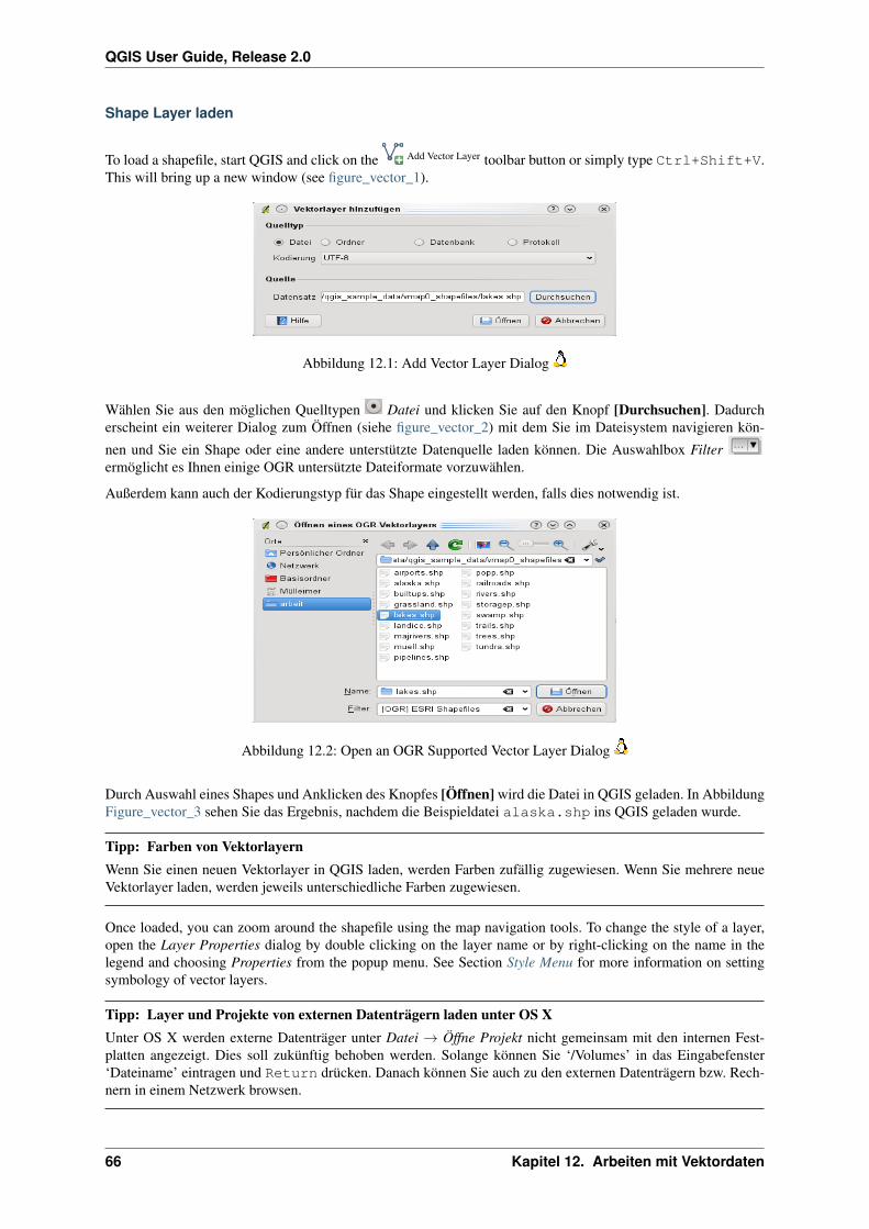
QGIS User Guide, Release 2.0
Shape Layer laden
To load a shapefile, start QGIS and click on the Add Vector Layer toolbar button or simply type Ctrl+Shift+V.This will bring up a new window (see figure_vector_1).
Abbildung 12.1: Add Vector Layer Dialog
Wählen Sie aus den möglichen Quelltypen Datei und klicken Sie auf den Knopf [Durchsuchen]. Dadurcherscheint ein weiterer Dialog zum Öffnen (siehe figure_vector_2) mit dem Sie im Dateisystem navigieren kön-
nen und Sie ein Shape oder eine andere unterstützte Datenquelle laden können. Die Auswahlbox Filterermöglicht es Ihnen einige OGR untersützte Dateiformate vorzuwählen.
Außerdem kann auch der Kodierungstyp für das Shape eingestellt werden, falls dies notwendig ist.
Abbildung 12.2: Open an OGR Supported Vector Layer Dialog
Durch Auswahl eines Shapes und Anklicken des Knopfes [Öffnen] wird die Datei in QGIS geladen. In AbbildungFigure_vector_3 sehen Sie das Ergebnis, nachdem die Beispieldatei alaska.shp ins QGIS geladen wurde.
Tipp: Farben von VektorlayernWenn Sie einen neuen Vektorlayer in QGIS laden, werden Farben zufällig zugewiesen. Wenn Sie mehrere neueVektorlayer laden, werden jeweils unterschiedliche Farben zugewiesen.
Once loaded, you can zoom around the shapefile using the map navigation tools. To change the style of a layer,open the Layer Properties dialog by double clicking on the layer name or by right-clicking on the name in thelegend and choosing Properties from the popup menu. See Section Style Menu for more information on settingsymbology of vector layers.
Tipp: Layer und Projekte von externen Datenträgern laden unter OS XUnter OS X werden externe Datenträger unter Datei → Öffne Projekt nicht gemeinsam mit den internen Fest-platten angezeigt. Dies soll zukünftig behoben werden. Solange können Sie ‘/Volumes’ in das Eingabefenster‘Dateiname’ eintragen und Return drücken. Danach können Sie auch zu den externen Datenträgern bzw. Rech-nern in einem Netzwerk browsen.
66 Kapitel 12. Arbeiten mit Vektordaten

QGIS User Guide, Release 2.0
Abbildung 12.3: QGIS with Shapefile of Alaska loaded
Improving Performance for Shapefiles
Um die Darstellungsgeschwindigkeit zu optimieren, kann ein räumlicher Index erstellt werden. Ein räumlicherIndex erhöht die Geschwindigkeit beim Zoomen und Verschieben. Räumliche Indizes haben in QGIS die Endung.qix.
Benutzen Sie folgende Schritte zum Erstellen eines räumlichen Index:
• Load a shapefile, clicking on the Add Vector Layer toolbar button or type Ctrl+Shift+V.
• Öffnen Sie den Eigenschaften-Dialog des Vektorlayers, indem Sie auf den Namen des Layers in der Legendedoppelklicken oder mit der rechten Maustaste Eigenschaften auswählen.
• In dem Reiter Allgemein klicken Sie auf den [Räumlichen Index erstellen] Knopf.
Problem beim Laden eines Shapes mit .prj Datei
If you load a shapefile with .prj file and QGIS is not able to read the coordinate reference system from that file,you have to define the proper projection manually within the General tab of the Layer Properties dialog of thelayer by clicking the [Specify...] button. This is due to the fact, that .prj files often do not provide the completeprojection parameters, as used in QGIS and listed in the CRS dialog.
Aus diesem Grund, wenn Sie ein neues Shapefile mit QGIS erstellen, werden derzeit zwei unterschiedliche Pro-jektionsdateien angelegt. Eine .prjDatei, mit den unvollständigen Projektionsparametern, wie sie z.B. von ESRISoftware gelesen und erstellt wird, und eine .qpj Datei, in der die vollständigen Projektionsparameter anthaltensind. Wenn Sie dann ein Shape in QGIS laden, und QGIS findet eine .qpj Datei, dann wird diese anstelle der.prj Datei benutzt.
12.1.2 MapInfo Layer laden
To load a MapInfo layer, click on the Add Vector Layer toolbar button or type Ctrl+Shift+V, change the
file type filter Filter : to ‘Mapinfo File [OGR]’ and select the MapInfo layer you want to load.
12.1. Unterstützte Datenformate 67
QGIS User Guide, Release 2.0
12.1.3 ArcInfo Binary Coverage laden
To load an ArcInfo binary coverage, click on the Add Vector Layer toolbar button or press Ctrl+Shift+V
to open the Add Vector Layer dialog. Select Directory. Change to Filter to ‘Arc/Info Binary Coverage’.Navigate to the directory that contains the coverage files and select it.
Auf die gleiche Art und Weise können auch andere Verzeichnis-basierte Vektorlayer geladen werden, wie etwadas U.K. National Transfer Format oder das raw TIGER Format des U.S. Census Bureau.
12.1.4 Loading OpenStreetMap Vectors
QGIS integrates Openstreetmap import as a core functionnality.
• To connect to the OSM server and download data, open the menu Vector → Openstreetmap → Load data.You can skip this step if you already got a .osm XML file using josm or overpass or any other source.
• The menu Vector → Openstreetmap → Import topology from an XML file will convert your .osm file into aspatialite database, and create a db connection.
• The menu Vector → Openstreetmap → Export topology to Spatialite then allows you to open the databaseconnection, select the type of data you want (points, lines, or polygons) and choose tags to import. This cre-
ates a spatialite geometry layer that you can then add to your project by clicking on the Add SpatiaLite Layer
toolbar button or by selecting the Add SpatiaLite Layer... option from the Layer menu, see SectionSpatiaLite Layer laden.
12.1.5 PostGIS Layer laden
PostGIS-Ebenen sind in einer PostgreSQL Datenbank gespeichert. Der Vorteil von PostGIS liegt in derFähigkeitkeit, räumliche Indizes, Filterungen und Abfragen bereitszustellen. Vektorfunktionen wie Selektierenund Abfragen funktionieren besser als bei Ebenen, die durch die OGR-Bibliothek geladen wurden.
Erstellen einer PostGIS Anbindung
The first time you use a PostGIS data source, you must create a connection to the PostgreSQL database
that contains the data. Begin by clicking on the Add PostGIS Layer toolbar button, selecting the Add PostGISLayer... option from the Layer menu or typing Ctrl+Shift+D. You can also open the Add Vector Layer dialogand select Database. The Add PostGIS Table(s) dialog will be displayed. To access the connection manager,click on the [New] button to display the Create a New PostGIS Connection dialog. The parameters required for aconnection are:
• Name:Ein Name für die Verbindung. Kann derselbe wie für die Datenbank sein
• Dienst: Service Parameter, der anstelle von Host / Port und potenziell auch Datenbank verwendet werdenkann. Kann unter pg_service.conf definiert werden
• Host: Name des Datenbank-Hosts. Dies muss einauflösbarer Name für den HOST sein, genau wie beimBenutzen von telnet oder ping Wenn die Datenbank auf demselben Computer ist wie QGIS, tragen Sie hiereinfach ‘localhost’ ein.
• Port: Port Nummer der Datenbank auf dem Server. Standard ist 5432.
• Datenbank: Name der Datenbank.
• SSL Modus: Wie die SSL-Verbindung mit dem Server festgelegt wird. Beachten Sie dass es zu erheblichenBeschleunigungen im Darstellen von PostGIS Layern kommt wenn man SSL im Verbindungseditor ab-schaltet. Die Optionen sind:
– abschalten: Versuche nur eine Nicht-SSL-Verbindung
68 Kapitel 12. Arbeiten mit Vektordaten
QGIS User Guide, Release 2.0
– erlauben: Versuche eine Nicht-SSL-Verbindung. Wenn das nicht klappt, versuche eine SSL-Verbindung
– bevorzugen (the default): Versuche eine SSL-Verbindung. Wenn das nicht klappt, versuche eine Nicht-SSL-Verbindung;
– verlangen: Versuche nur eine SSL-Verbindung.
• Benutzername: Benutzername, um sich bei der Datenbank anzumelden.
• Passwort: Passwort das zusammen mit Benutzername verwendet wird um sich bei der Datenbankanzumelden.
Optional können noch die folgenden Kontrollkästchen aktiviert werden:
• Benutzernamen speichern
• Passwort speichern
• Nur in geometry_columns nachschauen
• Don’t resolve type of unrestricted columns (GEOMETRY)
• Nur im ‘public’ Schema nachschauen
• Auch geometrielose Tabellen anzeigen
• Gechätzte Tabellenmetadaten nutzen
Wenn alle Parameter eingetragen sind, kann die Verbindung getestet werden, indem Sie auf den Knopf[Verbindung testen] drücken.
Tipp: QGIS Benutzereinstellungen und SicherheitJe nach Arbeitsumgebung birgt das Speichern von Passwörtern in Ihren QGIS-Einstellungen Risiken in sich. IhreEinstellungen für QGIS werden basierend auf ihrem Betriebssystem gespeichert:
• , the settings are stored in your home directory in .qgis2/.
• , die Einstellungen werden in der Registry gespeichert.
Laden eines Layers aus der PostGIS Datenbank
Once you have one or more connections defined, you can load layers from the PostgreSQL database. Ofcourse this requires having data in PostgreSQL. See Section Layer nach PostgreSQL/PostGIS importieren for adiscussion on importing data into the database.
Um eine Ebene aus PostGIS zu laden, führen Sie folgende Schritte durch:
• If the Add PostGIS layers dialog is not already open, selecting the Add PostGIS Layer... option from theLayer menu or typing Ctrl+Shift+D opens the dialog.
• Wählen Sie eine Verbindung aus dem Drop-Down Menü und klicken auf [Verbinden].
• Wählen Sie Auch geometrielose Tabellen anzeigen an oder ab
• Optional aktivieren Sie den Bereich Suchoptionen, um eine Auswahl anzuzeigender Objekte zu treffenoder verwenden Sie den [Abfrage erstellen] Knopf um den Abfrageerstellung-Dialog zu starten.
• Suchen Sie einen Layer den Sie laden möchten.
• Wählen Sie den Layer durch doppelklicken aus. Sie können mehrere Ebenen auswählen, indem Sie dieUmschalt-Taste beim Auswählen gedrückt halten. Siehe Abschnitt Abfrageeditor über das Benutzen desPostgreSQL Query Builder um den Layer genauer zu definieren.
12.1. Unterstützte Datenformate 69

QGIS User Guide, Release 2.0
• Klicken Sie auf den Knopf [Hinzufügen] um den Layer zu laden.
Tipp: PostGIS-LayerNormalwerweise ist ein PostGIS-Layer über einen Eintrag in der geometry_columns Tabelle definiert. Seit Version0.9.0 ist QGIS in der Lage, Layer zu laden, die keinen Eintrag in der geometry_columns Tabelle besitzen. Diesbezieht sich auf Tabellen und Views. Um einen ‘spatial view’ zu definieren, brauchen Sie ein kraftvolles System,um die Daten zu visualisieren. Beziehen Sie sich auf das PostgreSQL Handbuch, um weitere Informationen überdie Erstellung von Views zu erhalten.
Einige Details zu PostGIS-Layern
Dieser Abschnitt enthält einige Details, wie QGIS auf PostgreSQL zugreift. Meistens soll QGIS eine Liste mitein paar Datenbanktabellen bereitstellen, die bei Bedarf geladen werden können. Wenn Sie Probleme mit demLaden von Layern aus PostgreSQL haben, können die nun folgenden Informationen vielleicht eine Hilfe sein,die Fehlermeldungen von QGIS besser zu verstehen und eine Lösung zu finden, die PostgreSQL Tabellen- oderViewdefinition anzupassen, und somit den Layer laden zu können.
QGIS braucht eine Spalte in der PostgreSQL Tabelle, die als eindeutiger Schlüssel für den Layer genutzt werdenkann. Für Tabellen bedeutet dies, dass die Tabelle normalerweise einen Primärschlüssel braucht oder eine Spaltemit eindeutiger Zuordnung. Für QGIS muss diese Spalte außerdem vom Typ int4 sein (Integer mit 4 Bytes).Als Alternative kann auch die Spalte ctid als Primärschlüssel-Spalte verwendet werden. Wenn eine Tabelle dieseVoraussetzungen nicht erfüllt, wird die oid-Spalte genutzt. Die Performanz steigt, wenn für die Spalte ein Indexerstellt wurde (für Primärschlüssel wird in PostgreSQL automatisch ein Index erstellt).
If the PostgreSQL layer is a view, the same requirement exists, but views do not have primary keys or columnswith unique constraints on them. You have to define a primary key field (has to be integer) in the QGIS dialogbefore you can load the view. If a suitable column cannot does not exist in the view, QGIS will not load the layer.If this occurs, the solution is to alter the view so that it does include a suitable column (a type of integer and eithera primary key or with a unique constraint, preferably indexed).
QGIS offers a checkbox Select at id that is activated by default. This option gets the ids without the attributeswhich is faster in most cases. It can make sense to disable this option when you use expensive views.
12.1.6 Layer nach PostgreSQL/PostGIS importieren
Data can be imported into PostgreSQL/PostGIS using several tools, such as the SPIT plugin or the command linetools shp2pgsql or ogr2ogr.
DB Manager
QGIS comes with a core plugin named DB Manager. It can be used to load shapefiles and other data formats andincludes support for schemas. See Section DB Manager Plugin for more information.
shp2pgsql
PostGIS includes an utility called shp2pgsql that can be used to import shapefiles into a PostGIS enabled database.For example, to import a shapefile named lakes.shp into a PostgreSQL database named gis_data, use thefollowing command:
shp2pgsql -s 2964 lakes.shp lakes_new | psql gis_data
Dieser Befehl erzeugt eine neue Tabelle mit dem Namen lakes_new in der PostgreSQL/PostGIS Datenbankgis_data. Die neue Ebene wird die ID 2964 als ‘spatial reference identifier’ (SRID) tragen. Weitere Informa-tionen zu räumlichen Referenzsystemen finden Sie in Abschnitt Arbeiten mit Projektionen.
70 Kapitel 12. Arbeiten mit Vektordaten
QGIS User Guide, Release 2.0
Tipp: Layer aus PostGIS exportierenNeben dem Importwerkzeug shp2pgsql gibt es auch ein Werkzeug um PostGIS-Datensätze als Shapes zu ex-portieren:pgsql2shp. Diees wird mit der PostGIS-Distribution geliefert.
ogr2ogr
Beside shp2pgsql and DB Manager there is another tool for feeding geodata in PostGIS: ogr2ogr. This is part ofyour GDAL installation.
Um ein Shape nach PostGIS zu importieren, kann folgendes Kommando verwendet werden:
ogr2ogr -f "PostgreSQL" PG:"dbname=postgis host=myhost.de user=postgres \password=topsecret" alaska.shp
Damit wird das Shape alaska.shp vom Benutzer postgres mit dem Passwort topsecret in die PostGIS Daten-bank postgis auf dem Server myhost.de importiert.
Wichtig ist, dass GDAL mit PostgreSQL-Support kompiliert sein muss, damit der Import nach PostGIS möglichist. Dies kann mit folgendem Kommando getestet werden:
ogrinfo --formats | grep -i post
Wenn Sie das PostgreSQL’s Kommando COPY anstatt der Standardmethode INSERT INTO verwenden möchten,
müssen Sie vorher die folgende Variable exportieren (verifiziert unter und ):
export PG_USE_COPY=YES
Der Befehl ogr2ogr erstellt im Gegensatz zu shp2pgsl keinen räumlichen Index. In diesem Fall müssen Sieihn nachträglich manuell erstellen mit dem SQL-Kommando CREATE INDEX. Die Schritte werden im folgendenKapitel Geschwindigkeit optimieren näher beschrieben.
Geschwindigkeit optimieren
Der Datentransfer von einer PostgreSQL/PostGIS Datenbank kann langsam sein, besonders über ein Netzwerk.Die Geschwindigkeit kann optimiert werden, indem für alle Ebenen in PostgreSQL ein PostGIS räumlicher Indexerstellt wird. PostGIS unterstützt das Erstellen eines GiST (Generalized Search Tree) Index, um den Zugriff auf dieEbenen zu beschleunigen (die GiST Index Informationen wurden aus der PostGIS Dokumentation übernommenunter: http://postgis.refractions.net).
Dies ist die Syntax für das Erstellen eines GiST-Index:
CREATE INDEX [indexname] ON [tablename]USING GIST ( [geometryfield] GIST_GEOMETRY_OPS );
Bedenken Sie, dass das Erstellen eines Index bei großen Datenmengen zeitaufwendig ist. Nachdem der Indexerstellt ist, sollte ein ‘VACUUM ANALYZE’ durchgeführt werden (vgl. PostGIS Dokumentation Literatur undInternetreferenzen).
Im Folgenden sehen Sie ein Beispiel, um einen GiST-Index zu erstellen:
gsherman@madison:~/current$ psql gis_dataWelcome to psql 8.3.0, the PostgreSQL interactive terminal.
Type: \copyright for distribution terms\h for help with SQL commands\? for help with psql commands\g or terminate with semicolon to execute query\q to quit
gis_data=# CREATE INDEX sidx_alaska_lakes ON alaska_lakesgis_data-# USING GIST (the_geom GIST_GEOMETRY_OPS);
12.1. Unterstützte Datenformate 71

QGIS User Guide, Release 2.0
CREATE INDEXgis_data=# VACUUM ANALYZE alaska_lakes;VACUUMgis_data=# \qgsherman@madison:~/current$
12.1.7 Vektorlayer, die den Längengrad 180° überschreiten
Viele GIS Applikationen stellen einen Vektorlayer, der über den Längengrad 180 hinausgeht nicht zusammenhän-gend dar. So wird in QGIS der Layer geteilt und man sieht im Kartenfenster zwei, weit voneinander entfernteTeile, die eigentlich zusammen gehören. In Abbildung Figure_vector_4 sollte z.B. der kleine Punkt in der linkenEcke des Kartenfensters (Chatham Inseln) rechts neben Neuseeland angezeigt werden.
Abbildung 12.4: Map in lat/lon crossing the 180° longitude line
Eine Möglichkeit, dies zu umgehen, bietet PostGIS und die Funktion ST_Umschalt_Longitude(http://postgis.refractions.net/documentation/manual-1.4/ST_Umschalt_Longitude.html). Die Funktion liestalle Objekte der Karte ein und wenn der Längengrad <0° ist, werden 360° hinzugezählt. Das Ergebnis ist eine0-360° Karte, die als Mittelpunkt den Längengrad 180° verwendet.
Abbildung 12.5: Crossing 180° longitude applying the ST_Shift_Longitude function
Beispielanwendung
• Import data to PostGIS (Layer nach PostgreSQL/PostGIS importieren) using for example the DB Managerplugin.
• Öffnen Sie das PostGIS Kommandozeilenfenster und geben Sie folgendes Kommando ein. In diesemBeispiel steht der Name “TABELLE” für den tatsächlichen Namen der PostGIS Tabelle
gis_data=# update TABELLE set the_geom=ST_shift_longitude(the_geom);
72 Kapitel 12. Arbeiten mit Vektordaten

QGIS User Guide, Release 2.0
• Wenn alles geklappt hat, sehen Sie eine Bestätigung mit den Objekten, die verändert wurden. Danachkönnen Sie den PostGIS Layer in QGIS als eine zusammenhängende Karte laden (siehe Abbildung Fig-ure_vector_5 )
12.1.8 SpatiaLite Layer laden
Wenn Sie das erste Mal einen Layer aus einer Spatialite Datenbank laden möchten, klicken Sie auf das IconSpatiaLite Layer hinzufügen in der Werkzeugleiste oder indem Sie SpatiaLite Layer hinzufügen ... im Menü Layer
auswählen oder indem Sie die Taste Strg+Shift+L drücken. Dies öffnet einen Dialog, über den Sie entwedereine Verbindung zu einer bereits in QGIS definierten SpatiaLite Datenbank auswählen oder eine neue Verbindungerstellen können. Um eine neue Verbindung zu erstellen, klicken Sie auf den Knopf [Neu] und verwenden dannden Dateibrowser, um eine entsprechende SpatiaLite Datenbank auszuwählen. Dabei handelt es sich um eine Dateimit der Endung .sqlite.
Wenn Sie einen Vektorlayer im SpatiaLite Format abspeichern wollen, wählen Sie den Layer in der Legende aus,benutzen Sie das Kontextmenü der rechten Maustaste und klicken Sie auf Speichern als. Geben Sie den Namender Ausgabe an, wählen Sie sqlite als Format aus und das KBS. Danach fügen Sie noch SPATIALITE=YESin das Fenster ‘Datenquelle’. Damit sagen Sie OGR, dass eine SpatiaLite Datenbank erstellt werden soll. Siehehttp://www.gdal.org/ogr/drv_sqlite.html.
QGIS also supports editable views in SpatiaLite.
Einen neuen SpatiaLite Layer erzeugen
Wenn Sie einen neuen SpatiaLite Layer erzeugen wollen, finden Sie in Kapitel Einen neuen SpatiaLite Layererstellen eine Anleitung.
Tipp: SpatiaLite Datenmanagement PluginFür das Managen von SpatiaLite Daten können Sie mehrere Python Plugins verwenden: QSpatiaLite, SpatiaLiteManager oder DB Manager. Sie können mit dem Python Plugin Installer gedownloaded und installiert werden.
12.1.9 Räumliche MSSQL-Layer
QGIS also provides native MS SQL 2008 support. The Add MSSQL Spatial Layer is part of the new toolbarbutton or available in the MS SQL node in the QBrowser tree, providing drag and drop import support.
12.1.10 ORACLE Spatial Layers
QGIS also provides native ORACLE Locator/Spatial support. The Add ORACLE Spatial Layer is part of the newtoolbar button or available in the ORACLE node in the QBrowser tree, providing drag and drop import support.ORACLE Spatial layers are stored in an ORACLE database.
Erstellen einer PostGIS Anbindung
The first time you use a ORACLE Spatial data source, you must create a connection to the database that
contains the data. Begin by clicking on the Add ORACLE Spatial Layer toolbar button, selecting the Add ORACLESpatial Layer... option from the Layer menu or typing Ctrl+Shift+O. To access the connection manager, clickon the [New] button to display the Create a New ORACLE Spatial Connection dialog. The parameters requiredfor a connection are:
• Name:Ein Name für die Verbindung. Kann derselbe wie für die Datenbank sein
12.1. Unterstützte Datenformate 73

QGIS User Guide, Release 2.0
• Database SID or SERVICE_NAME of the Oracle instance.
• Host: Name des Datenbank-Hosts. Dies muss einauflösbarer Name für den HOST sein, genau wie beimBenutzen von telnet oder ping Wenn die Datenbank auf demselben Computer ist wie QGIS, tragen Sie hiereinfach ‘localhost’ ein.
• Port: Port number the PostgreSQL database server listens on. The default port is 1521.
• Benutzername: Benutzername, um sich bei der Datenbank anzumelden.
• Passwort: Passwort das zusammen mit Benutzername verwendet wird um sich bei der Datenbankanzumelden.
Optional können noch die folgenden Kontrollkästchen aktiviert werden:
• Save Username Indicates whether to save the database user name in the connection configuration.
• Save Password Indicates whether to save the database password in the connection settings. Passwordsare saved in clear text in the system configuration and in the project files!
• Only look in meta data table Restricts the displayed tables to those that are in theall_sdo_geom_metadata view. This can speed up the initial display of spatial tables.
• Only look for user’s tables When searching for spatial tables restrict the search to tables that are ownerby the user.
• Also list tables with no geometry Indicates that tables without geometry should also be listed by default.
• Use estimated table statistics for the layer metadata When the layer is setup various metadata is requiredfor the Oracle table. This includes information such as the table row count, geometry type and spatialextents of the data in the geometry column. If the table contains a large number of rows determining thismetadata is time consuming. By activating this option the following fast table metadata operations aredone: Row count is determined from all_tables.num_rows. Table extents are always determined with theSDO_TUNE.EXTENTS_OF function even if a layer filter is applied. The table geometry is determinedfrom the first 100 non-null geometry rows in the table.
• Only existing geometry types Only list the existing geometry types and don’t offer to add others.
Wenn alle Parameter eingetragen sind, kann die Verbindung getestet werden, indem Sie auf den Knopf[Verbindung testen] drücken.
Tipp: QGIS Benutzereinstellungen und SicherheitDepending on your computing environment, storing passwords in your QGIS settings may be a security risk.Passwords are saved in clear text in the system configuration and in the project files! Your customized settings forQGIS are stored based on the operating system:
• , the settings are stored in your home directory in .config/QGIS/QGIS2.conf.
• , die Einstellungen werden in der Registry gespeichert.
Loading a ORACLE Spatial Layer
Once you have one or more connections defined, you can load layers from the ORACLE database. Of coursethis requires having data in ORACLE.
To load a layer from ORACLE Spatial, perform the following steps:
• If the Add ORACLE Spatial layers dialog is not already open, click on the Add ORACLE Spatial Layer toolbarbutton.
• Wählen Sie eine Verbindung aus dem Drop-Down Menü und klicken auf [Verbinden].
74 Kapitel 12. Arbeiten mit Vektordaten

QGIS User Guide, Release 2.0
• Wählen Sie Auch geometrielose Tabellen anzeigen an oder ab
• Optional aktivieren Sie den Bereich Suchoptionen, um eine Auswahl anzuzeigender Objekte zu treffenoder verwenden Sie den [Abfrage erstellen] Knopf um den Abfrageerstellung-Dialog zu starten.
• Suchen Sie einen Layer den Sie laden möchten.
• Select it by clicking on it. You can select multiple layers by holding down the Shift key while clicking.See Section Abfrageeditor for information on using the ORACLE Query Builder to further define the layer.
• Klicken Sie auf den Knopf [Hinzufügen] um den Layer zu laden.
Tipp: ORACLE Spatial LayersNormally an ORACLE Spatial layer is defined by an entry in the USER_SDO_METADATA table.
12.2 Vektorlayereigenschaften
Der Layereigenschaften-Dialog stellt Informationen über den Layer, Darstellungseinstellungen und Beschriftung-soptionen bereit. Wenn ein Vektorlayer aus einer PostgreSQL/PostGIS Datenbank geladen wurde, können über denDialog Layereigenschaften auch SQL-Abfragen mit dem Query Builder-Dialog im Reiter Allgemein angewendetwerden. Um den Layereigenschaften-Dialog zu erreichen doppelklicken Sie einen Layer in der Legende odermachen Sie einen Rechtsklick auf den Layer und wählen Sie Eigenschaften aus dem Popupmenü.
Abbildung 12.6: Vector Layer Properties Dialog
12.2.1 Style Menu
The Style menu provides you with a comprehensive tool for rendering and symbolizing your vector data. You canuse Layer rendering → tools that are common to all vector data and special symbolizing tools that were designedfor the different kinds of vector data.
12.2. Vektorlayereigenschaften 75

QGIS User Guide, Release 2.0
Layer rendering
• Layer transparency : you can make the underlying layer in the map canvas visible withthis tool. Use the slider to adapt the visibility of your vector layer to your needs. You can also make a precisedefinition of the percentage of visibility in the the menu beside the slider.
• Layer blending mode: you can achieve special rendering effects with these tools that you previously onlyknow from graphics programs. The pixels of your overlaying and underlaying layers are mixed through thesettings described below.
– Normal: This is the standard blend mode which uses the alpha channel of the top pixel to blend withthe Pixel beneath it; the colors aren’t mixed
– Lighten: It selects the maximum of each component from the foreground and background pixels. Beaware that the results tend to be jagged and harsh.
– Screen: Light pixels from the source are painted over the destination, while dark pixels are not. Thismode is most useful for mixing the texture of one layer with another layer. E.g. you can use a hillshadeto texture another layer
– Dodge: Dodge will brighten and saturate underlying pixels based on the lightness of the top pixel. Sobrighter top pixels cause the saturation and brightness of the underlying pixels to increase. This worksbest if the top pixels aren’t too bright, otherwise the effect is too extreme.
– Addition: This blend mode simply adds pixel values of one layer with the other. In case of valuesabove 1 (in the case of RGB), white is displayed. This mode is suitable for highlighting features.
– Darken: Creates a resultant pixel that retains the smallest components of the foreground and back-ground pixels. Like lighten, the results tend to be jagged and harsh
– Multiply: It multiplies the numbers for each pixel of the top layer with the corresponding pixel for thebottom layer. The results are darker pictures.
– Burn: Darker colors in the top layer causes the underlying layers to darken. Can be used to tweak andcolorise underlying layers.
– Overlay: Combines multiply and screen blending modes. In the resulting picture light parts of thepicture become lighter and dark parts become darker.
– Soft light: Very similar to overlay, but instead of using multiply/screen it uses color burn/dodge. Thisone is supposed to emulate shining a soft light onto an image.
– Hard light: Hard light is very similar to the overlay mode. It’s supposed to emulate projecting a veryintense light onto an image.
– Difference: Difference subtracts the top pixel from the bottom pixel or the other way round, to alwaysget a positive value. Blending with black produces no change, as values for all colors are 0.
– Subtract: This blend mode simply subtracts pixel values of one layer with tshe other. In case of negativevalues, black is displayed.
Since QGIS 2.0 the old symbology is no longer available. In this version the new symbology has been redesignedand revised.
Renderers
The renderer is responsible for drawing a feature together with the correct symbol. There are four types of ren-derers: single symbol, categorized, graduated and rule-based. There is no continuous color renderer, because it isin fact only a special case of the graduated renderer. The categorized and graduated renderer can be created byspecifying a symbol and a color ramp - they will set the colors for symbols appropriately. For point layers thereis a point displacement renderer available. For each data type (points, lines and polygons) vector symbol layertypes are available. Depending on the chosen renderer, the Style menu provides different following sections. Onthe bottom right of the symbology dialog there is a [Symbol] button which gives access to the Style Manager (see
76 Kapitel 12. Arbeiten mit Vektordaten

QGIS User Guide, Release 2.0
Section vector_style_manager). The Style Manager allows you to edit and remove existing symbols and add newones.
Tipp: Auswahl und Ändern von MehrfachsymbolenThe Symbology allows to select multiple symbols and right click to change color, transparency, size, or width ofselected entries.
Einzelsymbol Darstellung
The Single Symbol Renderer is used to render all features of the layer using a single user-defined symbol. Theproperties, that can be adjusted in the Style menu, depend partially on the type of the layer, but all types sharethe following structure. In the top left part of the menu, there is a preview of the current symbol to be rendered.On the right part of the menu, there is a list of symbols already defined for the current style, prepared to be usedvia selecting them from the list. The current symbol can be modified using the menu on the right side. If youclick on the first level in the Symbol layers dialog on the left side it’s possible to define basic parameters like Size,Transparency, Color and Rotation. Here the layers are joined together.
Abbildung 12.7: Single symbol line properties
More detailed settings can be made when clicking on the second level in the Symbol layers dialog. You can defineSymbol layers that are combined afterwards. A symbol can consist of several Symbol layers. The following settingsare possible:
• Symbol layer type: You have the possibility to use Ellipse markers, Font markers, Simple markers, SVGmarkers and Vector Field markers
• Size
• Angle
• Colors
• Border width
• Offset X,Y: You can shift the symbol in x- or y-direction
Note that once you have set the size in the lower levels the size of the whole symbol can be changed with the Sizemenu in the first level again. The size of the lower levels changes accordingly while the size ratio is maintained.After having done any needed changes, the symbol can be added to the list of current style symbols (using the
[Symbol] Save in symbol library) and then easily be used in the future. Furthermore you can use the [Save
12.2. Vektorlayereigenschaften 77
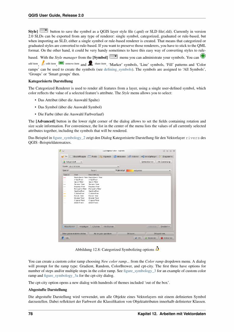
QGIS User Guide, Release 2.0
Style] button to save the symbol as a QGIS layer style file (.qml) or SLD file(.sld). Currently in version2.0 SLDs can be exported from any type of renderer: single symbol, categorized, graduated or rule-based, butwhen importing an SLD, either a single symbol or rule-based renderer is created. That means that categorized orgraduated styles are converted to rule-based. If you want to preserve those renderers, you have to stick to the QMLformat. On the other hand, it could be very handy sometimes to have this easy way of converting styles to rule-
based. With the Style manager from the [Symbol] menu you can administrate your symbols. You canadd item, edit item, remove item and share item. ‘Marker’ symbols, ‘Line’ symbols, ‘Fill’ patterns and ‘Colorramps’ can be used to create the symbols (see defining_symbols). The symbols are assigned to ‘All Symbols’,‘Groups’ or ‘Smart groups’ then.
Kategorisierte Darstellung
The Categorized Renderer is used to render all features from a layer, using a single user-defined symbol, whichcolor reflects the value of a selected feature’s attribute. The Style menu allows you to select:
• Das Attribut (über die Auswahl Spalte)
• Das Symbol (über die Auswahl Symbol)
• Die Farbe (über die Auswahl Farbverlauf)
The [Advanced] button in the lower right corner of the dialog allows to set the fields containing rotation andsize scale information. For convenience, the list in the center of the menu lists the values of all currently selectedattributes together, including the symbols that will be rendered.
Das Beispiel in figure_symbology_2 zeigt den Dialog Kategorisierte Darstellung für den Vektorlayer rivers desQGIS -Beispieldatensatzes.
Abbildung 12.8: Categorized Symbolizing options
You can create a custom color ramp choosing New color ramp... from the Color ramp dropdown menu. A dialogwill prompt for the ramp type: Gradient, Random, ColorBrewer, and cpt-city. The first three have options fornumber of steps and/or multiple stops in the color ramp. See figure_symbology_3 for an example of custom colorramp and figure_symbology_3a for the cpt-city dialog.
The cpt-city option opens a new dialog with hundreds of themes included ‘out of the box’.
Abgestufte Darstellung
Die abgestufte Darstellung wird verwendet, um alle Objekte eines Vektorlayers mit einem definierten Symboldarzustellen. Dabei reflektiert der Farbwert die Klassifikation von Objektattributen innerhalb definierter Klassen.
78 Kapitel 12. Arbeiten mit Vektordaten
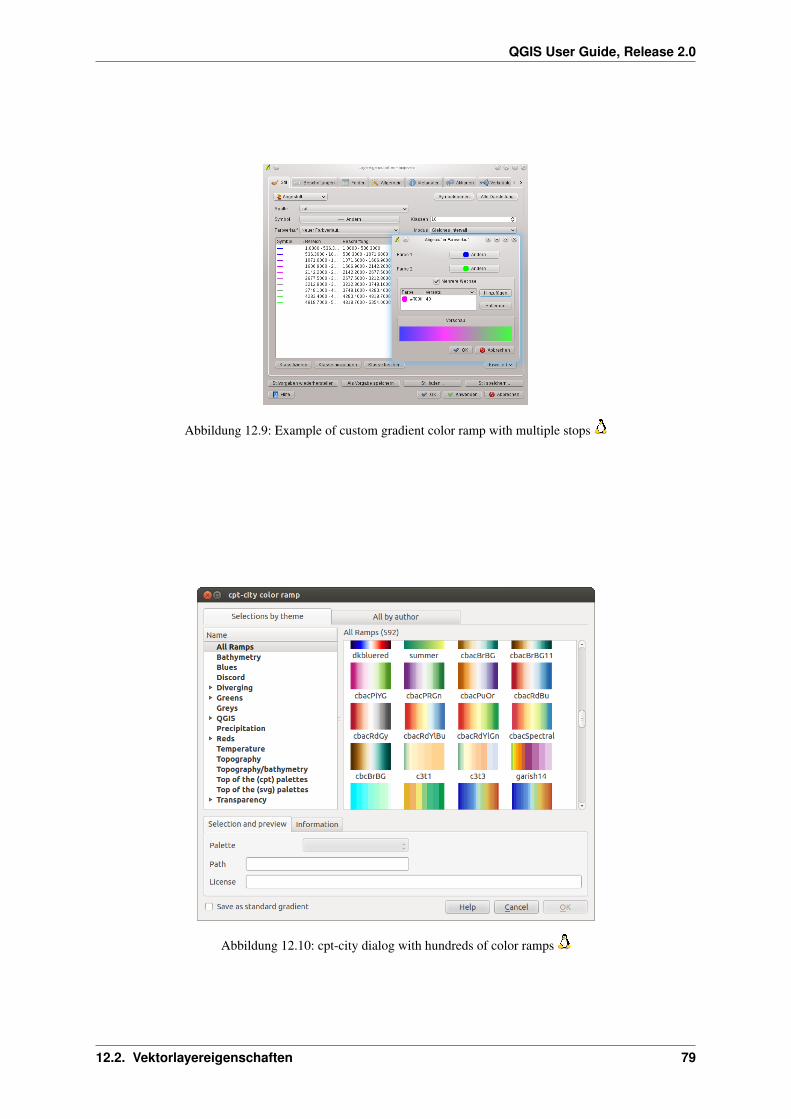
QGIS User Guide, Release 2.0
Abbildung 12.9: Example of custom gradient color ramp with multiple stops
Abbildung 12.10: cpt-city dialog with hundreds of color ramps
12.2. Vektorlayereigenschaften 79
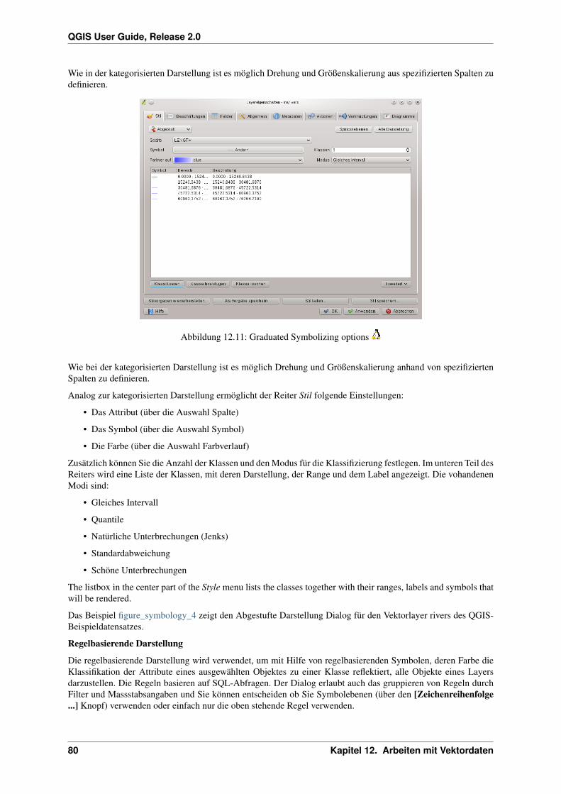
QGIS User Guide, Release 2.0
Wie in der kategorisierten Darstellung ist es möglich Drehung und Größenskalierung aus spezifizierten Spalten zudefinieren.
Abbildung 12.11: Graduated Symbolizing options
Wie bei der kategorisierten Darstellung ist es möglich Drehung und Größenskalierung anhand von spezifiziertenSpalten zu definieren.
Analog zur kategorisierten Darstellung ermöglicht der Reiter Stil folgende Einstellungen:
• Das Attribut (über die Auswahl Spalte)
• Das Symbol (über die Auswahl Symbol)
• Die Farbe (über die Auswahl Farbverlauf)
Zusätzlich können Sie die Anzahl der Klassen und den Modus für die Klassifizierung festlegen. Im unteren Teil desReiters wird eine Liste der Klassen, mit deren Darstellung, der Range und dem Label angezeigt. Die vohandenenModi sind:
• Gleiches Intervall
• Quantile
• Natürliche Unterbrechungen (Jenks)
• Standardabweichung
• Schöne Unterbrechungen
The listbox in the center part of the Style menu lists the classes together with their ranges, labels and symbols thatwill be rendered.
Das Beispiel figure_symbology_4 zeigt den Abgestufte Darstellung Dialog für den Vektorlayer rivers des QGIS-Beispieldatensatzes.
Regelbasierende Darstellung
Die regelbasierende Darstellung wird verwendet, um mit Hilfe von regelbasierenden Symbolen, deren Farbe dieKlassifikation der Attribute eines ausgewählten Objektes zu einer Klasse reflektiert, alle Objekte eines Layersdarzustellen. Die Regeln basieren auf SQL-Abfragen. Der Dialog erlaubt auch das gruppieren von Regeln durchFilter und Massstabsangaben und Sie können entscheiden ob Sie Symbolebenen (über den [Zeichenreihenfolge...] Knopf) verwenden oder einfach nur die oben stehende Regel verwenden.
80 Kapitel 12. Arbeiten mit Vektordaten

QGIS User Guide, Release 2.0
Das Beispiel figure_symbology_5 zeigt den Dialog der regelbasierenden Darstellung für den Layer rivers desQGIS Beispieldatensatzes.
To create a rule, activate an existing row by clicking on it or click on ‘+’ and click on the new rule. Then press the
[Edit rule] button. In the Rule properties dialog you can define a label for the rule. Press the button to openthe Expression builder. In the Function List, click on Fields and Values to view all attributes of the attribute tableto be searched. To add an attribute to the Field calculator Expression field, double click its name in the Fields andValues list. Generally you can use the various fields, values and functions to construct the calculation expressionor you can just type it into the box (see Feldrechner).
Abbildung 12.12: Rule-based Symbolizing options
Punkt-Verschiebung
Für Punktlayer gibt es eine Darstellungsart, mit der es möglich ist, sämtliche Punkte eines Layers auch danndarzustellen, wenn sie sich teilweise an derselben Stelle befinden. Die Punkte werden dabei um ein Zentrumssym-bol herum auf einem Versatzkreis angeordnet und dargestellt.
Tipp: Export vector symbologyYou have the possibility to export vector symbology from QGIS into the Google .kml, *.dxf and MapInfo.tab files.Just open the right mouse menu of the layer and click on Save selection as → to define the name of the outputfile and its format. Use the Symbology export menu to save the symbology either as Feature symbology → or asSymbol layer symbology →. If you have used symbol layers it is recommended to use the second setting.
12.2.2 Labels Menu
The Labels core application provides smart labeling for vector point, line and polygon layers and only requiresa few parameters. This new application also supports on-the-fly transformated layers. The core functions of theapplication have been redesigned. In QGIS 2.0. there are now a number of other features which improve thelabeling. The following menus have been created for labeling the vector layers:
• Text
• Formatting
• Buffer
12.2. Vektorlayereigenschaften 81
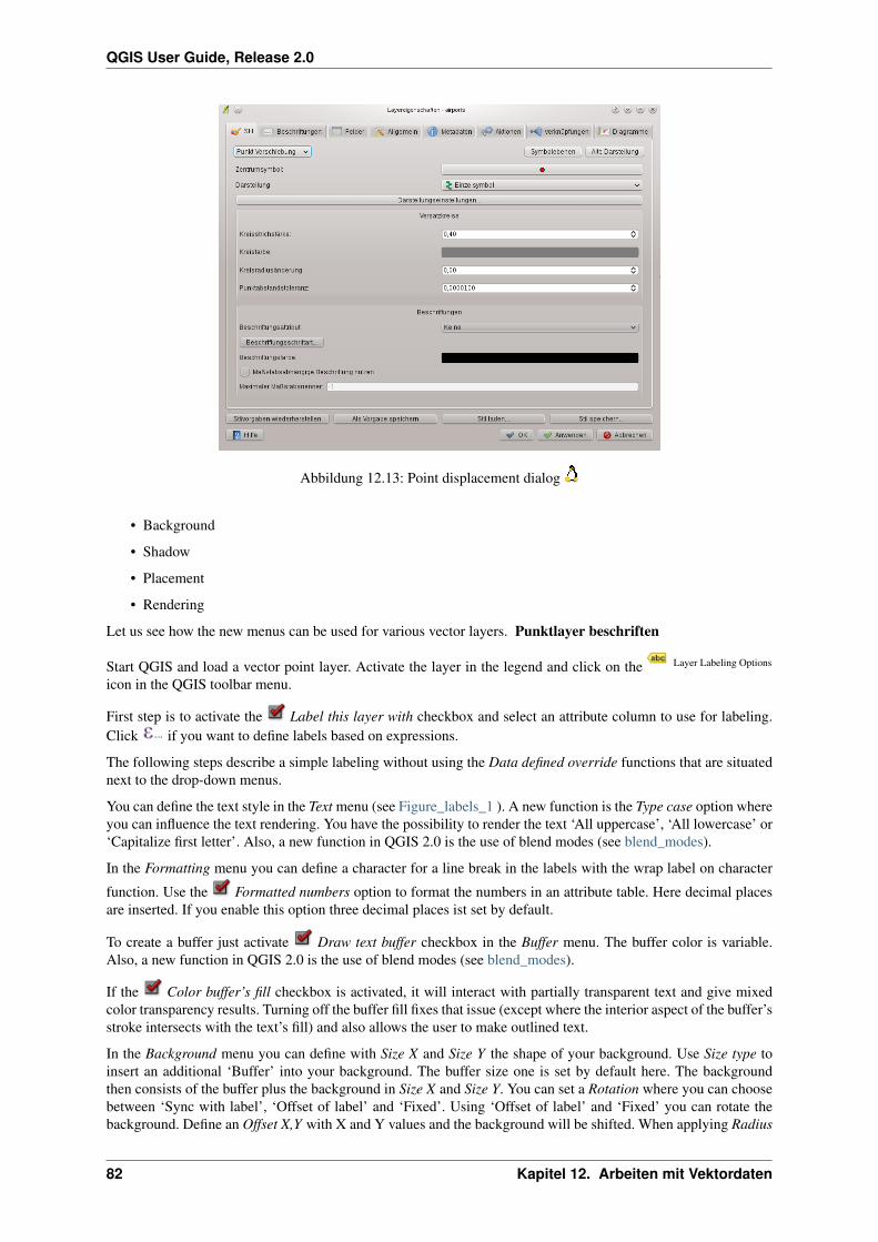
QGIS User Guide, Release 2.0
Abbildung 12.13: Point displacement dialog
• Background
• Shadow
• Placement
• Rendering
Let us see how the new menus can be used for various vector layers. Punktlayer beschriften
Start QGIS and load a vector point layer. Activate the layer in the legend and click on the Layer Labeling Options
icon in the QGIS toolbar menu.
First step is to activate the Label this layer with checkbox and select an attribute column to use for labeling.Click if you want to define labels based on expressions.
The following steps describe a simple labeling without using the Data defined override functions that are situatednext to the drop-down menus.
You can define the text style in the Text menu (see Figure_labels_1 ). A new function is the Type case option whereyou can influence the text rendering. You have the possibility to render the text ‘All uppercase’, ‘All lowercase’ or‘Capitalize first letter’. Also, a new function in QGIS 2.0 is the use of blend modes (see blend_modes).
In the Formatting menu you can define a character for a line break in the labels with the wrap label on character
function. Use the Formatted numbers option to format the numbers in an attribute table. Here decimal placesare inserted. If you enable this option three decimal places ist set by default.
To create a buffer just activate Draw text buffer checkbox in the Buffer menu. The buffer color is variable.Also, a new function in QGIS 2.0 is the use of blend modes (see blend_modes).
If the Color buffer’s fill checkbox is activated, it will interact with partially transparent text and give mixedcolor transparency results. Turning off the buffer fill fixes that issue (except where the interior aspect of the buffer’sstroke intersects with the text’s fill) and also allows the user to make outlined text.
In the Background menu you can define with Size X and Size Y the shape of your background. Use Size type toinsert an additional ‘Buffer’ into your background. The buffer size one is set by default here. The backgroundthen consists of the buffer plus the background in Size X and Size Y. You can set a Rotation where you can choosebetween ‘Sync with label’, ‘Offset of label’ and ‘Fixed’. Using ‘Offset of label’ and ‘Fixed’ you can rotate thebackground. Define an Offset X,Y with X and Y values and the background will be shifted. When applying Radius
82 Kapitel 12. Arbeiten mit Vektordaten

QGIS User Guide, Release 2.0
X,Y the background gets rounded corners. Again, it is possible to mix the background with the underlying layersin the map canvas using the Blend mode (see blend_modes).
Use the Shadow menu for a user-defined Drop shadow. The drawing of the background is very variable. Choosebetween ‘Lowest label component’, ‘Text’, ‘Buffer’ and ‘Background’. The Offset angle depends on the orienta-
tion of the label. If you choose the Use global shadow checkbox then the zero point of the angle is alwaysoriented to the north and doesn’t depend on the orientation of the label. Influence the appearance of the shadowwith the Blur radius. The higher the number, the softer the shadows.
The appearance of the drop shadow can also be altered by choosing a blend mode (see blend_modes).
Choose the Placement menu for the label placement and the labeling priority. Using the Offset from pointsetting you now have the possibility to use Quadrants to place your label. Additionally you can alter the angle ofthe label placement with the Rotation setting. Thus, a placement in a certain quadrant with a certain rotation ispossible.
In the Rendering menu you can define label and feature options. In the Label options you find the scale-based
visibility setting now. You can prevent QGIS from rendering only selected labels with the Show all labels forthis layer (including colliding labels) checkbox. In the Feature options you can define if every part of a multipartfeature is to be labeled. In QGIS 2.0 now it’s possible to define if the number of features to be labeled is limited
and to Discourage labels from covering features.
Abbildung 12.14: Smart labeling of vector point layers
Linienlayer beschriften
First step is to activate the Label this layer checkbox in the Label settings tab and select an attribute columnto use for labeling. Click if you want to define labels based on expressions.
After that you can define the text style in the Text menu. Here the same settings as for point layers are possible.
Also in the Formatting menu the same settings as for point layers are possible.
The Buffer menu has the same functions as described in section labeling_point_layers .
The Background menu has the same entries as described in section labeling_point_layers .
Also the Shadow menu has the same entries as described in section labeling_point_layers .
In the Placement menu you find special settings for line layers. The label can be placed Parallel, Curvedor Horizontal. With the Parallel and Curved option come the following settings: You can define the
position Above line, On line and Below line. It’s possible to select several options at once. QGIS willlook for the optimal position of the label then. Remember that here you can also use the line orientation for theposition of the label. Additionally you can define a Maximum angle between curved characters when selecting the
Curved option (see Figure_labels_2 ).
The Rendering menu has nearly the same entries as for point layers. In the Feature options you can now Suppresslabeling of features smaller than.
12.2. Vektorlayereigenschaften 83
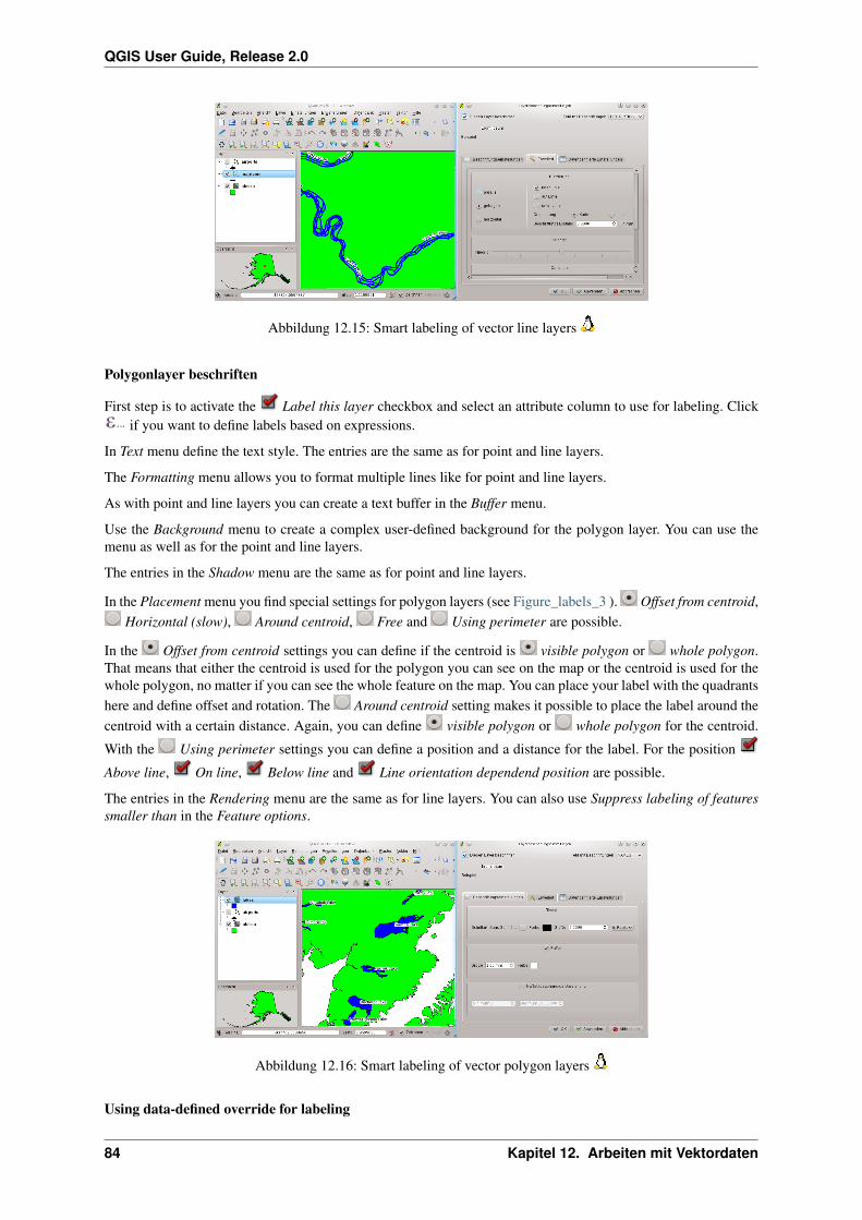
QGIS User Guide, Release 2.0
Abbildung 12.15: Smart labeling of vector line layers
Polygonlayer beschriften
First step is to activate the Label this layer checkbox and select an attribute column to use for labeling. Clickif you want to define labels based on expressions.
In Text menu define the text style. The entries are the same as for point and line layers.
The Formatting menu allows you to format multiple lines like for point and line layers.
As with point and line layers you can create a text buffer in the Buffer menu.
Use the Background menu to create a complex user-defined background for the polygon layer. You can use themenu as well as for the point and line layers.
The entries in the Shadow menu are the same as for point and line layers.
In the Placement menu you find special settings for polygon layers (see Figure_labels_3 ). Offset from centroid,Horizontal (slow), Around centroid, Free and Using perimeter are possible.
In the Offset from centroid settings you can define if the centroid is visible polygon or whole polygon.That means that either the centroid is used for the polygon you can see on the map or the centroid is used for thewhole polygon, no matter if you can see the whole feature on the map. You can place your label with the quadrantshere and define offset and rotation. The Around centroid setting makes it possible to place the label around thecentroid with a certain distance. Again, you can define visible polygon or whole polygon for the centroid.
With the Using perimeter settings you can define a position and a distance for the label. For the position
Above line, On line, Below line and Line orientation dependend position are possible.
The entries in the Rendering menu are the same as for line layers. You can also use Suppress labeling of featuressmaller than in the Feature options.
Abbildung 12.16: Smart labeling of vector polygon layers
Using data-defined override for labeling
84 Kapitel 12. Arbeiten mit Vektordaten

QGIS User Guide, Release 2.0
With the data-defined override functions the settings for the labeling are overwritten by entries in the attributetable. You can activate/deactivate the function with the right-mouse button. Hover over the symbol and you see theinformation about the data-defined override, including the current definition field. We now describe an example
how to use the data-defined override function for the Move label function (see figure_labels_4 ).
1. Import the lakes.shp from the QGIS sample dataset.
2. Double-klick the layer to open the Layer Properties. Klick on Labels and Placement. Select Offset fromcentroid.
3. Look for the Data defined entries. Klick the -Icon to define the field type for the Coordinate. Choose‘xlabel’ for X and ‘ylabel’ for Y. The Icons are now highlighted in yellow.
4. Zoom into a lake.
5. Go to the Label toolbar and klick the Icon. Now you can shift the label manually to another position(see figure_labels_5 ). The new position of the label is saved in the ‘xlabel’ and ‘ylabel’ columns of theattribute table.
Abbildung 12.17: Labeling of vector polygon layers with data-defined override
Abbildung 12.18: Move labels
12.2. Vektorlayereigenschaften 85
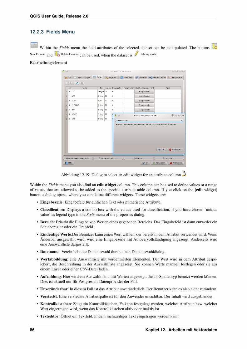
QGIS User Guide, Release 2.0
12.2.3 Fields Menu
Within the Fields menu the field attributes of the selected dataset can be manipulated. The buttonsNew Column and Delete Column can be used, when the dataset is Editing mode.
Bearbeitungselement
Abbildung 12.19: Dialog to select an edit widget for an attribute column
Within the Fields menu you also find an edit widget column. This column can be used to define values or a rangeof values that are allowed to be added to the specific attribute table column. If you click on the [edit widget]button, a dialog opens, where you can define different widgets. These widgets are:
• Eingabezeile: Eingabefeld für einfachen Text oder numerische Attribute.
• Classification: Displays a combo box with the values used for classification, if you have chosen ‘uniquevalue’ as legend type in the Style menu of the properties dialog.
• Bereich: Erlaubt die Eingabe von Werten eines gegebenen Bereichs. Das Eingabefeld ist dann entweder einSchieberegler oder ein Drehfeld.
• Eindeutige Werte:Der Benutzer kann einen Wert wählen, der bereits in dem Attribut verwendet wird. WennÄnderbar ausgewählt wird, wird eine Eingabezeile mit Autovervollständigung angezeigt. Anderseits wirdeine Auswahlliste dargestellt.
• Dateiname: Vereinfacht die Dateiauswahl durch einen Dateiauswahldialog.
• Wertabbildung: eine Auswahlliste mit vordefinierten Elementen. Der Wert wird in dem Attribut gespe-ichert, die Beschreibung in der Auswahlliste angezeigt. Sie können Werte manuell festlegen oder sie auseinem Layer oder einer CSV-Datei laden.
• Aufzählung: Hier wird ein Auswahlmenü mit Werten angezeigt, die als Spaltentyp benutzt werden können.Dies ist aktuell nur für Postgres als Datenprovider der Fall.
• Unveränderbar: In diesem Fall ist das Attribut unveränderlich. Der Benutzer kann es also nicht verändern.
• Versteckt: Eine versteckte Attributspalte ist für den Anwender unsichtbar. Der Inhalt wird ausgeblendet.
• Kontrollkästchen: Zeigt ein Kontrollkästchen. Es kann festgelegt werden, welches Attribute bzw. welcherWert eingetragen wird, wenn das Kontrollkästchen aktiv oder inaktiv ist.
• Texteditor: Öffnet ein Textfeld, in dem mehrzeiliger Text eingetragen werden kann.
86 Kapitel 12. Arbeiten mit Vektordaten

QGIS User Guide, Release 2.0
• Kalender:Öffnet ein Kalenderfenster, um ein Datum auszuwählen und in die Attributtabelle einzutragen.Der Spaltentyp muss String sein.
• Wertbeziehung: Bietet Werte aus einer verknüpften Tabelle in einem Auswahlmenü an. Sie können Layer,Schlüsselspalte und Wertspalte auswählen.
• UUID Generator: Erstellt ein schreibgeschütztes UUID (Universally Unique Identifiers)-Feld wenn es leerist.
• Photo: Field contains a filename for a picture. The width and height of the field can be defined.
• Webview: Field contains an URL. The width and height of the field is variable.
• Color: A field which allows to enter color codes. During data entry the color is visible through a color barincluded in the field.
With the Attribute editor layout you can now define builtin forms for data entry jobs (see figure_fields_2).
Choose ‘Drag and drop designer’ and an attribute column. Use the Icon to create a category that then willbe shown during the digitizing session (see figure_fields_3). Next step will be to assign the relevant fields to the
category with the Icon. You can create more categories and use the same fields again. When creating a newcategory QGIS will insert a new tab for the category in the built in form.
Other options in the dialog are ‘Autogenerate’ and ‘Provide ui-file’. ‘Autogenerate’ just creates Editors forall fields and tabulates them. The ‘Provide ui-file’ option allows you to use complex dialogs made withthe Qt-Designer. Using an UI-file allows a large freedom in creating a dialog. For detailed information seehttp://nathanw.net/2011/09/05/qgis-tips-custom-feature-forms-with-python-logic/ .
QGIS dialogs can have a python function that is called when the dialog is opened. Use this function to add extralogic to your dialogs. An example is (in module MyForms.py):
def open(dialog,layer,feature):geom = feature.geometry()control = dialog.findChild(QWidged,"My line edit")
Reference in Python Init Function like so: MyForms.open
MyForms.py must live on PYTHONPATH, .qgis2/python, or inside the project folder
Abbildung 12.20: Dialog to create categories with the Attribute editor layout
12.2. Vektorlayereigenschaften 87
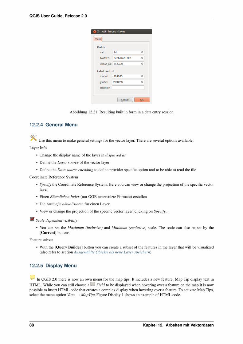
QGIS User Guide, Release 2.0
Abbildung 12.21: Resulting built in form in a data entry session
12.2.4 General Menu
Use this menu to make general settings for the vector layer. There are several options available:
Layer Info
• Change the display name of the layer in displayed as
• Define the Layer source of the vector layer
• Define the Data source encoding to define provider specific option and to be able to read the file
Coordinate Reference System
• Specify the Coordinate Reference System. Here you can view or change the projection of the specific vectorlayer.
• Einen Räumlichen Index (nur OGR-unterstüzte Formate) erstellen
• Die Ausmaße aktualisieren für einen Layer
• View or change the projection of the specific vector layer, clicking on Specify ...
Scale dependent visibility
• You can set the Maximum (inclusive) and Minimum (exclusive) scale. The scale can also be set by the[Current] buttons
Feature subset
• With the [Query Builder] button you can create a subset of the features in the layer that will be visualized(also refer to section Ausgewählte Objekte als neue Layer speichern).
12.2.5 Display Menu
In QGIS 2.0 there is now an own menu for the map tips. It includes a new feature: Map Tip display text inHTML. While you can still choose a Field to be displayed when hovering over a feature on the map it is nowpossible to insert HTML code that creates a complex display when hovering over a feature. To activate Map Tips,select the menu option View → MapTips.Figure Display 1 shows an example of HTML code.
88 Kapitel 12. Arbeiten mit Vektordaten
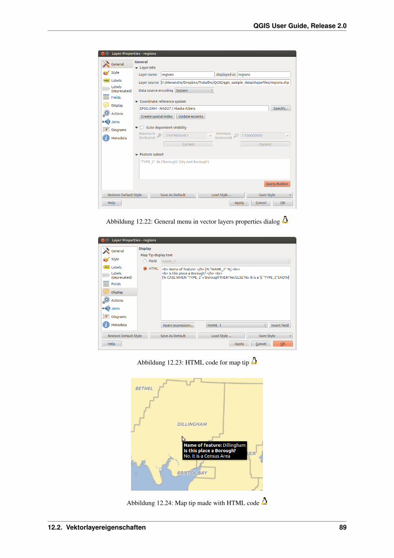
QGIS User Guide, Release 2.0
Abbildung 12.22: General menu in vector layers properties dialog
Abbildung 12.23: HTML code for map tip
Abbildung 12.24: Map tip made with HTML code
12.2. Vektorlayereigenschaften 89
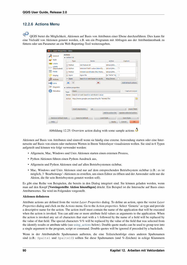
QGIS User Guide, Release 2.0
12.2.6 Actions Menu
QGIS bietet die Möglichkeit, Aktionen auf Basis von Attributen einer Ebene durchzuführen. Dies kann füreine Vielzahl von Aktionen genutzt werden, z.B. um ein Programm mit Abfragen aus der Attributdatenbank zufüttern oder um Parameter an ein Web-Reporting-Tool weiterzugeben.
Abbildung 12.25: Overview action dialog with some sample actions
Aktionen auf Basis von Attributen sind sinnvoll wenn sie häufig eine externe Anwendung starten oder eine Inter-netseite auf Basis von einem oder mehreren Werten in Ihrem Vektorlayer visualisieren wollen. Sie sind in 6 Typenaufgeteilt und können wie folgt verwendet werden:
• Allgemein, Mac, Windows und Unix Aktionen starten einen externen Prozess,
• Python Aktionen führen einen Python-Ausdruck aus,
• Allgemein und Python Aktionen sind auf allen Betriebsystemen sichtbar,
• Mac, Windows und Unix Aktionen sind nur auf dem entsprechenden Betriebsystem sichtbar (z.B.: es istmöglich, 3 ‘Bearbeitungs’-Aktionen zu erstellen, um einen Editor zu öffnen und der Anwender sieht nur dieAktion, die für sein Betriebsystem genutzt werden soll).
Es gibt eine Reihe von Beispielen, die bereits in den Dialog integriert sind. Sie können geladen werden, wennman auf den Knopf [Voreingestellte Aktion hinzufügen] drückt. Ein Beispiel ist die Intersuche auf Basis einesAttributwertes. Sie wird im Folgenden vorgestellt.
Aktionen definieren
Attribute actions are defined from the vector Layer Properties dialog. To define an action, open the vector LayerProperties dialog and click on the Actions menu. Go to the Action properties. Select ‘Generic’ as type and providea descriptive name for the action. The action itself must contain the name of the application that will be executedwhen the action is invoked. You can add one or more attribute field values as arguments to the application. Whenthe action is invoked any set of characters that start with a % followed by the name of a field will be replaced bythe value of that field. The special characters %% will be replaced by the value of the field that was selected fromthe identify results or attribute table (see using_actions below). Double quote marks can be used to group text intoa single argument to the program, script or command. Double quotes will be ignored if preceded by a backslash.
Wenn in der Attributtabelle Spaltenamen auftreten, die eine Teilzeichenfolge eines anderen Spaltenamensind (z.B.: Spalte1 und Spalte10) sollten Sie diese Spaltenamen (und %-Zeichen) in eckige Klammern
90 Kapitel 12. Arbeiten mit Vektordaten
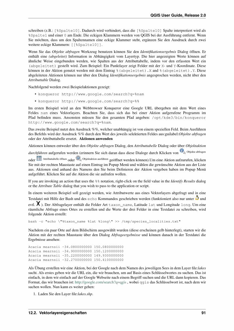
QGIS User Guide, Release 2.0
schreiben (z.B.: [%Spalte10]. Dadurch wird verhindert, dass die [%Spalte10] Spalte interpretiert wird als%Spalte1 und einer 0 am Ende. Die eckigen Klammern werden von QGIS bei der Ausführung entfernt. WennSie möchten, dass um den Spaltennamen eine eckige Klammer steht, ergänzen Sie den Ausdruck durch zweiweitere eckige Klammern: [[%Spalte10]].
Wenn Sie das Objekte abfragen Werkzeug benutzen können Sie den Identifikationsergebnis Dialog öffnen. Erenthält eine (abgeleitet) Information in Abhängigkeit vom Layertyp. Die hier angezeigten Werte können aufähnliche Weise eingebunden werden, wie Spalten aus der Attributtabelle, indem vor den erfassten Wert ein(abgeleitet) gestellt wird. Zum Beispiel: Ein Punktlayer zeigt Felder mit der X- und Y-Koordinate. Diesekönnen in der Aktion genutzt werden mit dem Eintrag %(abgeleitet).X and %(abgeleitet).Y. Dieseabgeleiteten Aktionen können nur über den Dialog Identifikationsergebnis angesprochen werden, nicht über denAttributtable Dialog.
Nachfolgend werden zwei Beispielaktionen gezeigt:
• konqueror http://www.google.com/search?q=%nam
• konqueror http://www.google.com/search?q=%%
Im ersten Beispiel wird an den Webbrowser Konqueror eine Google URL übergeben mit dem Wert einesFeldes nam eines Vektorlayers. Beachten Sie, dass sich das bei einer Aktion aufgerufene Programm imPfad befinden muss. Ansonsten müssen Sie den gesamten Pfad angeben: /opt/kde3/bin/konquerorhttp://www.google.com/search?q=%nam.
Das zweite Beispiel nutzt den Ausdruck %%, welcher unabhängig ist von einem speziellen Feld. Beim Ausführendes Befehls wird der Ausdruck %% durch den Wert des jeweils selektierten Feldes aus:guilabel:Objekte abfragenoder der Attributtabelle ersetzt. Aktionen anwenden
Aktionen können entweder über den Objekte abfragen Dialog, den Attributtabelle Dialog oder über Objektaktion
durchführen aufgerufen werden (erinnern Sie sich daran dass diese Dialoge durch Klicken von Objekte abfragen
oder Attributtabelle öffnen oder Objektaktion ausführen geöffnet werden können).Um eine Aktion aufzurufen, klickenSie mit der rechten Maustaste auf einen Eintrag im Popup Menü und wählen die gewünschte Aktion aus der Listeaus. Aktionen sind anhand des Namens den Sie beim Definieren der Aktion vergeben haben im Popup Menüaufgeführt. Klicken Sie auf die Aktion die sie aufrufen wollen.
If you are invoking an action that uses the %% notation, right-click on the field value in the Identify Results dialogor the Attribute Table dialog that you wish to pass to the application or script.
In einem weiteren Beispiel soll gezeigt werden, wie Attributwerte aus eines Vektorlayers abgefragt und in eineTextdatei mit Hilfe der Bash und des echo Kommandos geschrieben werden (funktioniert also nur unter und
evtl. ). Der Abfragelayer enthält die Felder Art taxon_name, Latitude lat und Longitude long. Um eineräumliche Abfrage eines Ortes zu erstellen und die Werte der drei Felder in eine Textdatei zu schreiben, wirdfolgende Aktion erstellt:
bash -c "echo \"%taxon_name %lat %long\" >> /tmp/species_localities.txt"
Nachdem ein paar Orte auf dem Bildschirm ausgewählt wurden (diese erscheinen gelb hinterlegt), starten wir dieAktion mit der rechten Maustaste über den Dialog Abfrageergebnisse und können danach in der Textdatei dieErgebnisse ansehen:
Acacia mearnsii -34.0800000000 150.0800000000Acacia mearnsii -34.9000000000 150.1200000000Acacia mearnsii -35.2200000000 149.9300000000Acacia mearnsii -32.2700000000 150.4100000000
Als Übung erstellen wir eine Aktion, bei der Google nach dem Namen des jeweiligen Sees in dem Layer file:lakessucht. Als erstes geben wir die URL ein, die wir brauchen, um auf Basis eines Schlüsselwortes zu suchen. Das isteinfach, in dem wir einfach auf der Google Webseite nach einem Begriff suchen und die URL dann kopieren. DasFormat, das wir brauchen ist: http://google.com/search?q=qgis , wobei qgis das Schlüsselwort ist, nach dem wirsuchen wollen. Nun kann es weiter gehen:
1. Laden Sie den Layer file:lakes.shp.
12.2. Vektorlayereigenschaften 91
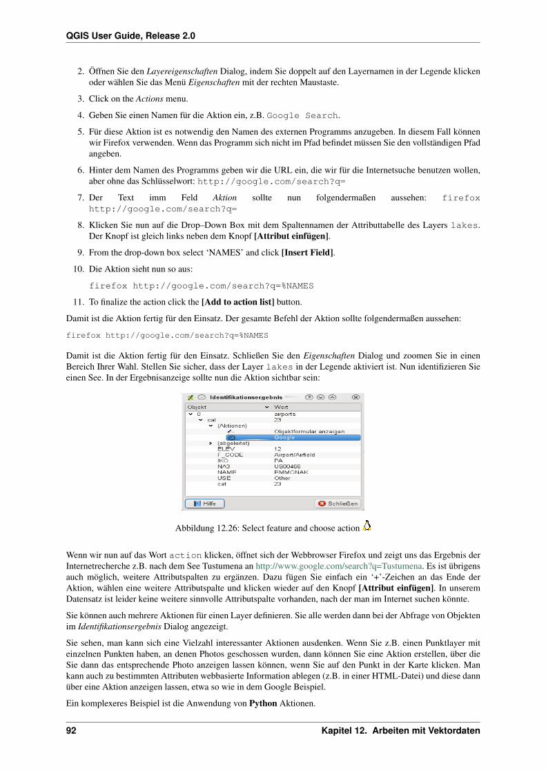
QGIS User Guide, Release 2.0
2. Öffnen Sie den Layereigenschaften Dialog, indem Sie doppelt auf den Layernamen in der Legende klickenoder wählen Sie das Menü Eigenschaften mit der rechten Maustaste.
3. Click on the Actions menu.
4. Geben Sie einen Namen für die Aktion ein, z.B. Google Search.
5. Für diese Aktion ist es notwendig den Namen des externen Programms anzugeben. In diesem Fall könnenwir Firefox verwenden. Wenn das Programm sich nicht im Pfad befindet müssen Sie den vollständigen Pfadangeben.
6. Hinter dem Namen des Programms geben wir die URL ein, die wir für die Internetsuche benutzen wollen,aber ohne das Schlüsselwort: http://google.com/search?q=
7. Der Text imm Feld Aktion sollte nun folgendermaßen aussehen: firefoxhttp://google.com/search?q=
8. Klicken Sie nun auf die Drop–Down Box mit dem Spaltennamen der Attributtabelle des Layers lakes.Der Knopf ist gleich links neben dem Knopf [Attribut einfügen].
9. From the drop-down box select ‘NAMES’ and click [Insert Field].
10. Die Aktion sieht nun so aus:
firefox http://google.com/search?q=%NAMES
11. To finalize the action click the [Add to action list] button.
Damit ist die Aktion fertig für den Einsatz. Der gesamte Befehl der Aktion sollte folgendermaßen aussehen:
firefox http://google.com/search?q=%NAMES
Damit ist die Aktion fertig für den Einsatz. Schließen Sie den Eigenschaften Dialog und zoomen Sie in einenBereich Ihrer Wahl. Stellen Sie sicher, dass der Layer lakes in der Legende aktiviert ist. Nun identifizieren Sieeinen See. In der Ergebnisanzeige sollte nun die Aktion sichtbar sein:
Abbildung 12.26: Select feature and choose action
Wenn wir nun auf das Wort action klicken, öffnet sich der Webbrowser Firefox und zeigt uns das Ergebnis derInternetrecherche z.B. nach dem See Tustumena an http://www.google.com/search?q=Tustumena. Es ist übrigensauch möglich, weitere Attributspalten zu ergänzen. Dazu fügen Sie einfach ein ‘+’-Zeichen an das Ende derAktion, wählen eine weitere Attributspalte und klicken wieder auf den Knopf [Attribut einfügen]. In unseremDatensatz ist leider keine weitere sinnvolle Attributspalte vorhanden, nach der man im Internet suchen könnte.
Sie können auch mehrere Aktionen für einen Layer definieren. Sie alle werden dann bei der Abfrage von Objektenim Identifikationsergebnis Dialog angezeigt.
Sie sehen, man kann sich eine Vielzahl interessanter Aktionen ausdenken. Wenn Sie z.B. einen Punktlayer miteinzelnen Punkten haben, an denen Photos geschossen wurden, dann können Sie eine Aktion erstellen, über dieSie dann das entsprechende Photo anzeigen lassen können, wenn Sie auf den Punkt in der Karte klicken. Mankann auch zu bestimmten Attributen webbasierte Information ablegen (z.B. in einer HTML-Datei) und diese dannüber eine Aktion anzeigen lassen, etwa so wie in dem Google Beispiel.
Ein komplexeres Beispiel ist die Anwendung von Python Aktionen.
92 Kapitel 12. Arbeiten mit Vektordaten
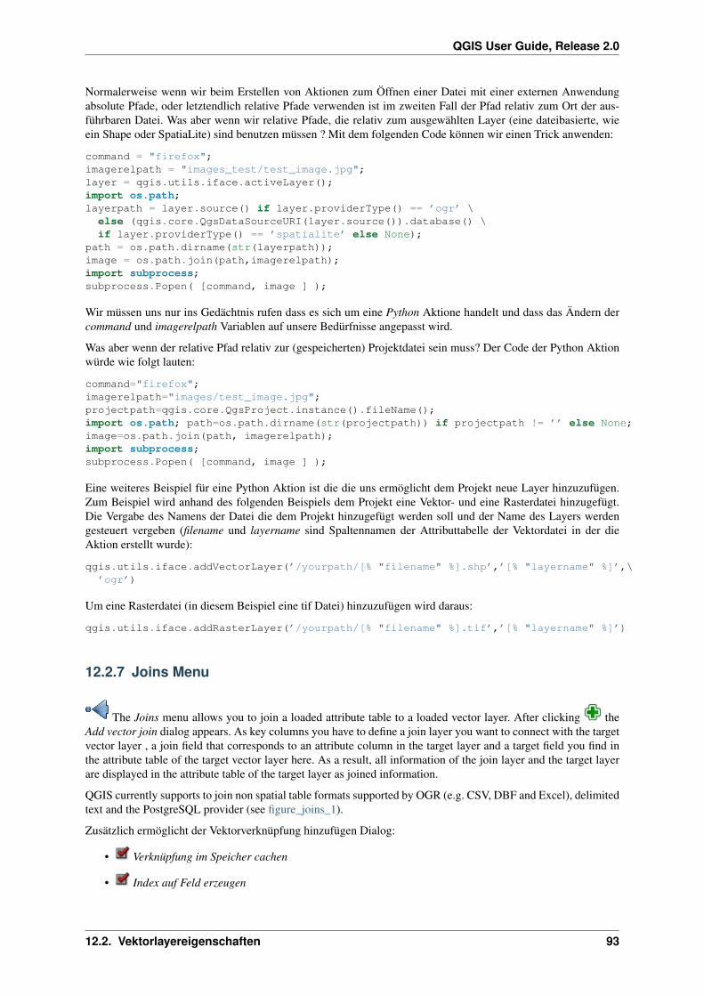
QGIS User Guide, Release 2.0
Normalerweise wenn wir beim Erstellen von Aktionen zum Öffnen einer Datei mit einer externen Anwendungabsolute Pfade, oder letztendlich relative Pfade verwenden ist im zweiten Fall der Pfad relativ zum Ort der aus-führbaren Datei. Was aber wenn wir relative Pfade, die relativ zum ausgewählten Layer (eine dateibasierte, wieein Shape oder SpatiaLite) sind benutzen müssen ? Mit dem folgenden Code können wir einen Trick anwenden:
command = "firefox";imagerelpath = "images_test/test_image.jpg";layer = qgis.utils.iface.activeLayer();import os.path;layerpath = layer.source() if layer.providerType() == ’ogr’ \
else (qgis.core.QgsDataSourceURI(layer.source()).database() \if layer.providerType() == ’spatialite’ else None);
path = os.path.dirname(str(layerpath));image = os.path.join(path,imagerelpath);import subprocess;subprocess.Popen( [command, image ] );
Wir müssen uns nur ins Gedächtnis rufen dass es sich um eine Python Aktione handelt und dass das Ändern dercommand und imagerelpath Variablen auf unsere Bedürfnisse angepasst wird.
Was aber wenn der relative Pfad relativ zur (gespeicherten) Projektdatei sein muss? Der Code der Python Aktionwürde wie folgt lauten:
command="firefox";imagerelpath="images/test_image.jpg";projectpath=qgis.core.QgsProject.instance().fileName();import os.path; path=os.path.dirname(str(projectpath)) if projectpath != ’’ else None;image=os.path.join(path, imagerelpath);import subprocess;subprocess.Popen( [command, image ] );
Eine weiteres Beispiel für eine Python Aktion ist die die uns ermöglicht dem Projekt neue Layer hinzuzufügen.Zum Beispiel wird anhand des folgenden Beispiels dem Projekt eine Vektor- und eine Rasterdatei hinzugefügt.Die Vergabe des Namens der Datei die dem Projekt hinzugefügt werden soll und der Name des Layers werdengesteuert vergeben (filename und layername sind Spaltennamen der Attributtabelle der Vektordatei in der dieAktion erstellt wurde):
qgis.utils.iface.addVectorLayer(’/yourpath/[% "filename" %].shp’,’[% "layername" %]’,\’ogr’)
Um eine Rasterdatei (in diesem Beispiel eine tif Datei) hinzuzufügen wird daraus:
qgis.utils.iface.addRasterLayer(’/yourpath/[% "filename" %].tif’,’[% "layername" %]’)
12.2.7 Joins Menu
The Joins menu allows you to join a loaded attribute table to a loaded vector layer. After clicking theAdd vector join dialog appears. As key columns you have to define a join layer you want to connect with the targetvector layer , a join field that corresponds to an attribute column in the target layer and a target field you find inthe attribute table of the target vector layer here. As a result, all information of the join layer and the target layerare displayed in the attribute table of the target layer as joined information.
QGIS currently supports to join non spatial table formats supported by OGR (e.g. CSV, DBF and Excel), delimitedtext and the PostgreSQL provider (see figure_joins_1).
Zusätzlich ermöglicht der Vektorverknüpfung hinzufügen Dialog:
• Verknüpfung im Speicher cachen
• Index auf Feld erzeugen
12.2. Vektorlayereigenschaften 93
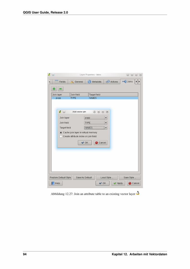
QGIS User Guide, Release 2.0
Abbildung 12.27: Join an attribute table to an existing vector layer
94 Kapitel 12. Arbeiten mit Vektordaten
QGIS User Guide, Release 2.0
12.2.8 Diagrams Menu
The Diagrams menu allows you to add a graphic overlay to a vector layer (see figure_diagrams_1).
The current core implementation of diagrams provides support for piecharts, text diagrams and histograms.
The menu is divided into four tabs now: Appearance, Size, Postion and Options.
In the case of the text diagram and piechart text values of different data columns are displayed one below theother with a circle or a box and dividers. In the Size tab diagram size is based on a fixed size or on linear scalingaccording to a classification attribute. The placement of the diagrams which is done in the Position tab interactswith the new labeling, so position conflicts between diagrams and labels are detected and solved. In addition tochart positions can be fixed by the users hand.
Abbildung 12.28: Vector properties dialog with diagram menu
Wir werden in einem Beispiel den Alaska Grenzen Layer mit einem Text Diagramm das Temperaturdaten voneinem Klima Layer zeigt überlagern. Beide Vektorlayer sind Teil des QGIS Beispieldatensatzes (siehe AbschnittBeispieldaten).
1. Als erstes klicken Sie auf das Vektorlayer hinzufügen Icon, dann navigieren Sie zum Ordner mit dem Beispiel-datensatz und laden Sie die beiden Shapes alaska.shp und climate.shp.
2. Doppelklicken Sie auf den climate Layer in der Kartenlegende um den Dialog Layereigenschaften zuöffnen.
3. Click on the Diagrams menu, activate Display diagrams and from Diagram type combobox select‘Text diagram’
4. In the Appearance tab we choose a light blue as Background color and in the Size tab we set a fixed size to18 mm.
5. In the Position tab Placement could be set to AroundPoint.
6. In the diagram we want to display the values of the three columns T_F_JAN, T_F_JUL and T_F_MEAN.
First select T_F_JAN as Attributes and click the button, then T_F_JUL and finally T_F_MEAN.
7. Klicken Sie jetzt [Anwenden] um das Diagramm in QGIS anzuzeigen.
8. You can now adapt the chart size in the Size tab. Deactivate the Fixed size and set the size of the diagramson the basis of an Attribute with the [Find maximum value] button and the Size menu. If diagrams appear
12.2. Vektorlayereigenschaften 95
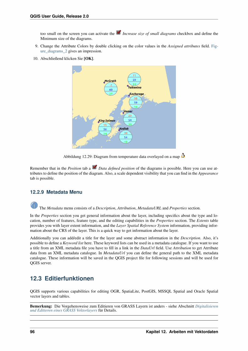
QGIS User Guide, Release 2.0
too small on the screen you can activate the Increase size of small diagrams checkbox and define theMinimum size of the diagrams.
9. Change the Attribute Colors by double clicking on the color values in the Assigned attributes field. Fig-ure_diagrams_2 gives an impression.
10. Abschließend klicken Sie [OK].
Abbildung 12.29: Diagram from temperature data overlayed on a map
Remember that in the Position tab a Data defined position of the diagrams is possible. Here you can use at-tributes to define the position of the diagram. Also, a scale dependent visibility that you can find in the Appearancetab is possible.
12.2.9 Metadata Menu
The Metadata menu consists of a Description, Attribution, MetadataURL and Properties section.
In the Properties section you get general information about the layer, including specifics about the type and lo-cation, number of features, feature type, and the editing capabilities in the Properties section. The Extents tableprovides you with layer extent information, and the Layer Spatial Reference System information, providing infor-mation about the CRS of the layer. This is a quick way to get information about the layer.
Additionally you can add/edit a title for the layer and some abstract information in the Description. Also, it’spossible to define a Keyword list here. These keyword lists can be used in a metadata catalogue. If you want to usea title from an XML metadata file you have to fill in a link in the DataUrl field. Use Attribution to get Atrributedata from an XML metadata catalogue. In MetadataUrl you can define the general path to the XML metadatacatalogue. These information will be saved in the QGIS project file for following sessions and will be used forQGIS server.
12.3 Editierfunktionen
QGIS supports various capabilities for editing OGR, SpatiaLite, PostGIS, MSSQL Spatial and Oracle Spatialvector layers and tables.
Bemerkung: Die Vorgehensweise zum Editieren von GRASS Layern ist anders - siehe Abschnitt Digitalisierenund Editieren eines GRASS Vektorlayers für Details.
96 Kapitel 12. Arbeiten mit Vektordaten
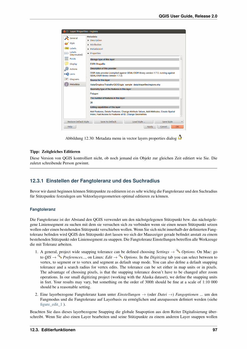
QGIS User Guide, Release 2.0
Abbildung 12.30: Metadata menu in vector layers properties dialog
Tipp: Zeitgleiches EditierenDiese Version von QGIS kontrolliert nicht, ob noch jemand ein Objekt zur gleichen Zeit editiert wie Sie. Diezuletzt schreibende Person gewinnt.
12.3.1 Einstellen der Fangtoleranz und des Suchradius
Bevor wir damit beginnen können Stützpunkte zu editieren ist es sehr wichtig die Fangtoleranz und den Suchradiusfür Stützpunkte festzulegen um Vektorlayergeometrien optimal editieren zu können.
Fangtoleranz
Die Fangtoleranz ist der Abstand den QGIS verwendet um den nächstgelegenen Stützpunkt bzw. das nächstgele-gene Liniensegment zu suchen mit dem sie versuchen sich zu verbinden wenn sie einen neuen Stützpunkt setzenwollen oder einen bestehenden Stützpunkt verschieben wollen. Wenn Sie sich nicht innerhalb der definierten Fang-toleranz befinden wird QGIS den Stützpunkt dort lassen wo sich der Mauszeiger gerade befindet anstatt zu einembestehenden Stützpunkt oder Liniensegment zu snappen. Die Fangtoleranz Einstellungen betreffen alle Werkzeugedie mit Toleranz arbeiten.
1. A general, project wide snapping tolerance can be defined choosing Settings → Options. On Mac: goto QIS → Preferences..., on Linux: Edit → Options. In the Digitizing tab you can select between tovertex, to segment or to vertex and segment as default snap mode. You can also define a default snappingtolerance and a search radius for vertex edits. The tolerance can be set either in map units or in pixels.The advantage of choosing pixels, is that the snapping tolerance doesn’t have to be changed after zoomoperations. In our small digitizing project (working with the Alaska dataset), we define the snapping unitsin feet. Your results may vary, but something on the order of 300ft should be fine at a scale of 1:10 000should be a reasonable setting.
2. Eine layerbezogene Fangtoleranz kann unter Einstellungen → (oder Datei →) Fangoptionen ... um denFangmodus und die Fangtoleranz auf Layerbasis zu ermöglichen und anzupasssen definiert werden (siehefigure_edit_1 ).
Beachten Sie dass dieses layerbezogene Snapping die globale Snapoption aus dem Reiter Digitalisierung über-schreibt. Wenn Sie also einen Layer bearbeiten und seine Stützpunkte zu einem anderen Layer snappen wollen
12.3. Editierfunktionen 97

QGIS User Guide, Release 2.0
dann stellen Sie das Snappen nur für den zu snappenden Layer ein und verringern die allgemeine Fangtoleranz aufeinen kleineren Wert. Darüberhinaus funktioniert das Snappen nicht mit Layern die nicht im Fangoptionen Dialogaktiviert sind, egal wie die allgemeine Fangtoleranz aussieht. Vergewissern Sie sich also dass die Checkbox derLayer auf die Sie snappen müssen markiert ist.
Abbildung 12.31: Edit snapping options on a layer basis
Suchradius
Der Suchradius ist die Distanz die QGIS benutzt, um den nächstgelegenen Stützpunkt, der verschoben werden soll,zu finden. Wenn Sie sich nicht innerhalb des Suchradius befinden wird QGIS keinen Stützpunkt zum Editierenfinden und auswählen und es wird dazu eine störende Warnung erscheinen. Die Fangtoleranz und der Suchra-dius werden in Karteneinheiten oder Pixeln festgelegt Sie müssen also etwas experimentieren um sie richtigeinzustellen. Wenn Sie eine zu große Toleranz festlegen, könnte QGIS zum falschen Stützpunkt snappen, beson-ders wenn es eine große Anzahl von Stützpunkten in geringer Entfernung gibt. Legen Sie den Suchradius zu kleinfest wird es nichts zum verschieben finden.
Der Suchradius für die Stützpunktbearbeitung in Layereinheiten kann im Reiter Digitalisierung unter Einstellun-gen → Optionen definiert werden. An der gleichen Stellen wo Sie die allgemeine, projektweite Fangtoleranzdefinieren.
12.3.2 Zoomen und Karte verschieben
Bevor Sie einen Layer editieren sollten Sie in den Bereich hineinzoomen, den Sie bearbeiten wollen. Dadurchvermeiden Sie lange Wartezeiten, bis alle Stützpunkte des Layers visualisiert werden.
Neben den Karte verschieben und Hineinzoomen / Hinauszoomen Icons in der Werkzeugleiste können Sie auchmit dem Mausrad, der Leertaste und den Pfeiltasten navigieren.
Mit dem Mausrad im Kartenfenster zoomen und verschieben
Während des Digitalisierens können Sie das Mausrad zum verschieben innerhalb des Hauptfenster drücken undSie können das Mausrad zum hinein- und hinauszoomen drehen. Zum Zoomen platzieren Sie den Mauscursor indie Karte und rollen es vorwärts (von Ihnen weg) um hineinzuzoomen und rückwärts (zu Ihnen hin) um herauszu-zoomen. Die Position des Mauscursors wird das Zentrum des Sie interessierenden Bereichs sein. Sie können dasVerhalten des Mausrad-Zooms anhand des Reiters Kartenwerkzeuge unter Einstellungen → Optionen anpassen.
Den Layer mit den Pfeiltasten verschieben
Das Verschieben des Layers im Kartenfenster während des Digitalisierens ist mit den Pfeiltasten möglich.Platzieren Sie den Mauszeiger in das Kartenfenster und drücken Sie rechte Pfeiltaste, um den Layer nach Os-ten zu verschieben, die linke Pfeiltaste für Westen, die Pfeiltaste nach unten für Süden und die Pfeiltaste nachoben für das Verschieben nach Norden.
98 Kapitel 12. Arbeiten mit Vektordaten

QGIS User Guide, Release 2.0
Sie können auch die gedrückte Leertaste dazu verwenden, um den Layer im Kartenfenster zu verschieben. DiePgUp und PgDown Tasten auf Ihrem Keyboard bewirken dann das hineinzoomen und herauszoomen Ihres Karten-fensters ohne das Digitalisieren zu unterbrechen.
12.3.3 Topologisches Editieren
Abgesehen von der Einstellung des layerbasierten Fangmodus können im Menü Einstellungen → Fangoptio-
nen... auch topologische Funktionen aktiviert werden. Hier können sie Topologisches Editieren an definieren
und/oder für Polygonlayer können Sie die Spalte Überschn.verm. aktivieren die eine Überschneidung neuerPolygone vermeided.
Topologisches Editieren ermöglichen
The option Enable topological editing is for editing and maintaining common boundaries in polygon mosaics.QGIS ‘detects’ a shared boundary in a polygon mosaic and you only have to move the vertex once and QGIS willtake care about updating the other boundary.
Überschneidung neuer Polygone vermeiden
The second topological option in the Avoid Int. column, called Avoid intersections of new polygons avoidsoverlaps in polygon mosaics. It is for quicker digitizing of adjacent polygons. If you already have one polygon,it is possible with this option to digitize the second one such that both intersect and QGIS then cuts the secondpolygon to the common boundary. The advantage is that users don’t have to digitize all vertices of the commonboundary.
Enable snapping on intersections
Another option is to use Enable snapping on intersection. It allows to snap on an intersection of backgroundlayers, even if there’s no vertex on the intersection.
12.3.4 Einen vorhandenen Layer editieren
By default, QGIS loads layers read-only: This is a safeguard to avoid accidentally editing a layer if there is a slip ofthe mouse. However, you can choose to edit any layer as long as the data provider supports it, and the underlyingdata source is writable (i.e. its files are not read-only).
Das Editieren von Vektorlayern in QGIS ist unterteilt in Digitalisierung und erweit-erte Digitalisierung, siehe Abschnitt Erweiterte Digitalisierung. Beide Werkzeugleisten kön-nen über das Menü Einstellungen → Werkzeugkästen → aktiviert und deaktiviert wer-den. Mit der Werkzeugleiste Digitalisierung können folgende Funktionen ausgeführt werden:
Icon Funktion Icon Funktion
Current edits Bearbeitungsstatus umschalten
Objekt hinzufügen: Punkt hinzufügen Objekt hinzufügen: Linie hinzufügen
Objekt hinzufügen: Polygon hinzufügen Objekt(e) verschieben
Knotenwerkzeug Ausgewähltes Löschen
Ausgewählte Objekte ausschneiden Objekte kopieren
Objekte einfügen Save layer edits
Tabelle Bearbeiten: Funktionen der Werkzeugleiste Digitalisierung
12.3. Editierfunktionen 99

QGIS User Guide, Release 2.0
Alle Bearbeitungssessions beginnen mit dem Aktivieren der Funktion Bearbeitungsstatus umschalten. Diese kann auchim Kontextmenü nach dem Rechtsklick auf den Legendeneintrag für den Layer aktiviert werden.
Alternativ können Sie dazu auch mit der rechten Maustaste auf den Namen des Layers in der Legende klicken unddie Option im Kontextmenü auswählen. Sobald der Layer im Bearbeitungsstatus ist, erscheinen die Stützpunkteals das von Ihnen gewählte Stützpunktsymbol und zusätzlich werden die Digitalisier-Tools in der Werkzeugleisteaktiv.
Tipp: Regelmäßiges Sichern der Daten
Remember to Save Layer Edits regularly. This will also check that your data source can accept all the changes.
Objekte digitalisieren
Danach können Sie mit den Icons Objekt hinzufügen, Objekt hinzufügen oder Objekt hinzufügen in der Werkzeu-gleiste den Mauszeiger in den Digitalisiermodus bringen.
Für jedes Objekt wird erst die Geometrie digitalisiert und dann das Attribut hinzugefügt. Um eine Geometrie zudigitalisieren, klicken Sie mit der linken Maustaste an eine gewünschte Stelle im Kartenfenster, um den erstenPunkt zu erstellen.
Für Linien und Polygone klicken Sie für jeden weiteren Knotenpunkt wieder die linke Maustaste. Zum Beendenklicken Sie irgendwo im Kartenfenster auf die rechte Maustaste, um anzuzeigen, dass die Geometrie ihres Objektesfertig gestellt ist.
The attribute window will appear, allowing you to enter the information for the new feature. Figure_edit_2 showssetting attributes for a fictitious new river in Alaska. In the Digitizing menu under the Settings → Options menu,
you can also activate Suppress attributes pop-up windows after each created feature Reuse last enteredattribute values.
Abbildung 12.32: Enter Attribute Values Dialog after digitizing a new vector feature
Mit dem Objekt(e) verschieben Icon in der Werkzeugleiste können sie komplette Objekte verschieben.
Tipp: Datentyp der AttributeQGIS kontrolliert beim Editieren, ob die eingetragenen Werte dem Datentyp der Attributspalte entspricht (z.B.:Zahl oder Text). Ansonsten ist es nicht möglich, im Dialog Attribute eine Zahl in eine Textspalte einzutragen,oder umgekehrt. Falls es dennoch notwendig sein sollte, können Sie es nachträglich im Fenster der Attributtabelleändern.
100 Kapitel 12. Arbeiten mit Vektordaten
QGIS User Guide, Release 2.0
Current Edits
This new feature allows the digitization of multiple layers. Choose Save for Selected Layers to save all changes
you made in multiple layers. You also have the opportunity to Rollback for Selected Layers so that the digiti-
zation is then withdrawn for all selected layers. If you want to stop editing the selected layers the Cancel forSelected Layer(s) is an easy way.
The same functions for editing all layers of the project are available.
Knotenwerkzeug
For shapefile-based layers as well as SpatialLite,PostgreSQL/PostGIS, MSSQL Spatial and Oracle Spatial tables
the Node Tool provides manipulation capabilites of feature vertices similar to CAD programs. It is possible tosimply select multiple vertices at once and to move, add or delete them alltogether. The node tool also works with‘on the fly’ projection turned on and supports the topological editing feature. This tool is, unlike other tools inQGIS, persistent, so when some operation is done, selection stays active for this feature and tool. If the node toolcouldn’t find any features, a warning will be displayed.
Sie sollten den Suchradius beim Digitalisieren über die Menüleiste unter Einstellungen → Optionen → Digi-talisierung größer 0 einstellen. Ansonsten ist QGIS nicht in der Lage, ein Objekt auszuwählen.
Tipp: StützpunktmarkenDie aktuelle Version von QGIS unterstützt drei Arten von Stützpunktmarken: Teiltransparenter Kreis, Kreuz undKeine. Um den Markierungsstil zu ändern wählen Sie Optionen aus dem Einstellungen Menü, klicken Sie aufden Reiter Digitalisierung und wählen Sie den entsprechenden Eintrag aus.
Eine einfache Übung
Beginnen Sie, indem Sie das Knotenwerkzeug aktivieren und dann ein Objekt selektieren. Rote Boxen erscheinenan jedem Stützpunkt des Objektes. Nun sind folgende Funktionen vorhanden.
• Stützpunkte auswählen: Sie können die Stützpunkte auswählen indem sie einmal darauf klicken, indemSie auf eine Ecke klicken um beide Enden auszuwählen oder indem Sie ein Rechteck mit der Maus übereinige Stützpunkte ziehen. Wenn ein Stützpunkt ausgewählt ist wird er blau. Sie können mehrere Stützpunk-te auswählen, indem Sie die Tasten Umschalt gedrückt halten. Mit der Taste Strg oder Shift kanndie Auswahl umgekehrt werden (selektierte Stützpunkte werden deselektiert, nicht ausgwählte Stützpunktewerden ausgewählt).
• Stützpunkte hinzufügen: Dazu klicken Sie doppelt in die Nähe einer Grenzlinie und ein neuer Stützpunkterscheint. Beachten Sie, dass der Stützpunkt auf der Grenzlinie erscheint, und nicht an der Stelle, wo derMauspfeil ist.
• Stützpunkte löschen: Wählen Sie dazu Stützpunkte aus, die gelöscht werden sollen und klicken Sie dann
auf die Taste Entfernen. Beachten Sie dass das Knotenwerkzeug nicht für das Löschen eines vollständigenObjekts benutzen können, QGIS stellt sicher dass die minimal erforderliche Anzahl von Stützpunkten für
das Objekt an dem Sie arbeiten erhalten bleibt. Um ein vollständiges Objekt zu löschen müssen Sie dasAusgewähltes löschen Werkzeug benutzen.
• Stützpunkte verschieben:Wählen Sie alle Stützpunkte aus, die verschoben werden sollen. Alle aus-gewählten Stützpunkte werden in dieselbe Richtung wie der Mauspfeil verschoben. Wenn eine Fangtolerazteingestellt ist, können die Stützpunkte zu dem nächstgelegenen Stützpunkt oder Segment snappen.
Jede Veränderung mit dem Knotenwerkzeug wird als einzelner Eintrag im Dialog Rückgängig/Wiederholungabgelegt und unterstütz die topologischen Funktionen. Ausserdem wird On-The-Fly Reprojektion wird unterstütztund Sie können Stützpunkte identifizieren, wenn Sie mit der Maus drüberfahren.
12.3. Editierfunktionen 101

QGIS User Guide, Release 2.0
Objekte ausschneiden, kopieren und einfügen
Ausgewählte Objekte können ausgeschnitten, kopiert und an andere Ebenen im aktuellen QGIS-Projekt übergeben(eingefügt) werden, wenn sich der Ziellayer auch im Editiermodus befindet, indem Sie nach Auswahl des Ziellay-
ers auf den Knopf Bearbeitungsstatus umschalten klicken.
Objekte können auch als Text an externe Applikationen übergeben werden: Dabei wird ein Objekt im .csv Formatmit ihrer Geometrie im OGC Well-Known Text (WKT) Format erzeugt.
In dieser QGIS Version können Textobjekte außerhalb von QGIS nicht in eine geladene Ebene eingefügt wer-den. Aber wann macht es Sinn, Objekte zum kopieren, auszuschneiden und einzufügen? Ein Beispiel ist, wennSie parallel an mehreren Layern arbeiten und Objekte zwischen den Layern hin- und herkopieren möchten. EinSzenario könnte sein, dass Sie einen neuen Layer erstellen möchten, in dem aber nur einige Objekte aus einembereits existierenden Layer verwendet werden sollen, wie etwa 5 Seen aus der Karte lakes.shp , die insgesamtaber tausende Seen enthält.
Wir nutzen diese Idee und machen daraus ein kleines Anwendungsbeispiel:
1. Laden Sie den Layer, von dem Sie einige Objekte kopieren wollen (Quelle)
2. Laden oder erstellen Sie einen Layer, in den die kopierten Objekte eingefügt werden sollen (Ziel)
3. Schalten Sie für den Ziel Layer den Bearbeitungsstatus ein
4. Stellen Sie die Quelle aktiv, indem Sie es in der Legende anklicken
5. Benutzen Sie das Einzelnes Objekt auswählen Werkzeug und wählen ein paar Objekte in der Quelle aus
6. Klicken Sie auf das Icon Objekte kopieren
7. Stellen Sie das ‘Ziel’ aktiv, indem Sie es in der Legende anklicken
8. Klicken Sie auf das Icon Objekte einfügen
9. Beenden Sie den Bearbeitungsstatus für beide Layer und speichern Sie das Ergebnis ab
Was passiert, wenn der Quell- und Ziellayer ein unterschiedliches Schema enthält (Spaltennamen und -typenunterscheiden sich)? QGIS verwendet die Einträge, die gleich sind und ignoriert den Rest. Wenn es Ihnen egalist, ob die Attribute korrekt übernommen werden, dann ist es egal, wie Sie die Spaltennamen und -typen derAttributtabelle erstellen. Wenn auch die Attributdaten korrekt übernommen werden sollen, dann stellen Sie sicher,dass auch die Spaltennamen und -typen beider layer zueinander passen.
Tipp: Deckungsgleichheit eingefügter ObjekteWenn der Quell- und Ziellayer die gleiche Projektion nutzen, hat das übergebene Objekt die identische Geome-trie wie in dem Quelllayer. Wenn der Quell- und Ziellayer eine unterschiedliche Projektion nutzen, kann dasübergebene Objekt eine andere Geometrie wie in dem Quelllayer besitzen. Der Grund liegt in auftretenden Run-dungsabweichungen bei der Konvertierung zwischen Projektionen.
Ausgewählte Objekte löschen
Wenn Sie ein ganzes Polygon löschen möchten, selektieren Sie es erst mit dem Einzelnes Objekt auswählen Werkzeug.Sie können dabei auch mehrere Objekte gleichzeitig auswählen. Wenn Sie die Objekte ausgewählt haben, klicken
Sie auf das Icon Ausgewähltes löschen.
Das Werkzeug Ausgewählte Objekte ausschneiden kann auch benutzt werden, um Objekte zu löschen. Die Objektewerden gelöscht aber zusätzlich noch im ‘spatial clipboard’ abgelegt. In diesem Fall könnte man dann den letzten
Schritt, falls ein Fehler unterlaufen ist, wieder rückgängig machen, indem wir auf das Werkzeug Objekte einfügen
drücken. Ausschneiden, kopieren und übergeben von Objekten funktioniert mit den gerade ausgewählten Objektenund können nach Bedarf kombiniert verwendet werden.
102 Kapitel 12. Arbeiten mit Vektordaten

QGIS User Guide, Release 2.0
Änderungen speichern
When a layer is in editing mode, any changes remain in the memory of QGIS. Therefore they are not commit-ted/saved immediately to the data source or disk. If you want to save edits to the current layer but want to continue
editing without leaving the editing mode, you can click the Save Layer Edits button. When you turn editing mode
off with the Toggle editing (or quit QGIS for that matter), you are also asked if you want to save your changes ordiscard them.
Wenn die Änderungen nicht gespeichert werden können (z.B. weil die Festplatte voll ist oder Attribute Werteaufweisen, die außerhalb der Wertespanne liegen), bleiben die Änderungen erstmal im Arbeitsspeicher. Dieserlmöglicht es, Änderungen vorzunehmen und dann nochmals die Daten zu speichern.
Tipp: DatenintegritätEs ist immer gut ein Backup von Ihren Daten zu machen bevor Sie mit dem Bearbeiten starten. Während dieAutoren von QGIS sich bemühen die Integrität Ihrer Daten zu bewahren bieten wir keine Garantie in dieserHinsicht.
12.3.5 Erweiterte Digitalisierung
Icon Funktion Icon Funktion
Rückgängig Wiederholen
Rotate Feature(s) Objekt vereinfachen
Ring hinzufügen Teil hinzufügen
Ring löschen Teil löschen
Objekte überarbeiten Linie versetzen
Objekte trennen Gewählte Objekte verschmelzen
Punktsymbole drehen Attribute gewählter Objekte vereinen
Tabelle Erweiterte Digitalisierung: Werkzeugleiste Erweiterte Digitalisierung für Vektorlayer
Rückgängig und Wiederholen
Die Werkzeuge Rückgängig und Wiederholen ermöglichen es, Arbeitsschritte der Vektoreditierung rückgängigzu machen oder zu wiederholen. Im Dialog Rücknahme/Wiederholung werden alle durchgeführten Operationenangezeigt (siehe Abbildung Figure_edit_3). Dieser Dialog wird nicht standardmäßig angezeigt. Klicken Sie dazuin einem freien Bereich der Werkzeugleiste auf die rechte Maustaste und aktivieren dann das KontrollkästchenRücknahme/Wiederholung. Die Funktion ist übrigens immer aktiv, auch wenn der Dialog nicht angezeigt wird.
Wenn Sie auf die Funktion ‘Rückgängig’ klicken, werden alle Geometrien und Attribute auf den Status zurück-gestellt, bevor die rückgängig gemachte Operation stattgefunden hat. Veränderung, die an anderer Stelle, z.B. inanderen Plugins durchgeführt wurden, können unspezifisch sein für die unterschiedlichen Operationen - d.h. siekönnen rückgängig gemacht werden oder aber einfach so bleiben.
Wenn Sie Rücknahme/Wiederholung verwenden wollen klicken Sie einfach auf eine Operation in der history; alleObjekte werden dann auf den Stand vor der ausgewählten Operation zurückgesetzt.
12.3. Editierfunktionen 103
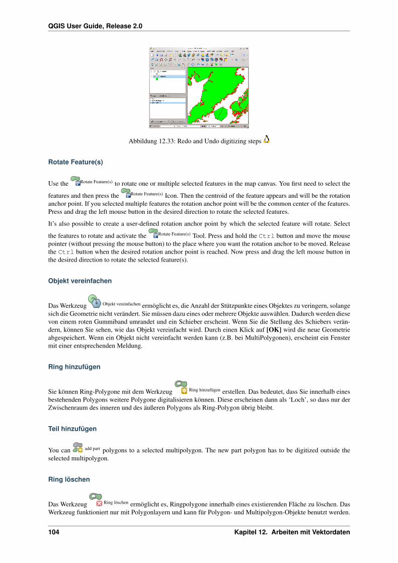
QGIS User Guide, Release 2.0
Abbildung 12.33: Redo and Undo digitizing steps
Rotate Feature(s)
Use the Rotate Feature(s) to rotate one or multiple selected features in the map canvas. You first need to select the
features and then press the Rotate Feature(s) Icon. Then the centroid of the feature appears and will be the rotationanchor point. If you selected multiple features the rotation anchor point will be the common center of the features.Press and drag the left mouse button in the desired direction to rotate the selected features.
It’s also possible to create a user-defined rotation anchor point by which the selected feature will rotate. Select
the features to rotate and activate the Rotate Feature(s) Tool. Press and hold the Ctrl button and move the mousepointer (without pressing the mouse button) to the place where you want the rotation anchor to be moved. Releasethe Ctrl button when the desired rotation anchor point is reached. Now press and drag the left mouse button inthe desired direction to rotate the selected feature(s).
Objekt vereinfachen
Das Werkzeug Objekt vereinfachen ermöglicht es, die Anzahl der Stützpunkte eines Objektes zu veringern, solangesich die Geometrie nicht verändert. Sie müssen dazu eines oder mehrere Objekte auswählen. Dadurch werden diesevon einem roten Gummiband umrandet und ein Schieber erscheint. Wenn Sie die Stellung des Schiebers verän-dern, können Sie sehen, wie das Objekt vereinfacht wird. Durch einen Klick auf [OK] wird die neue Geometrieabgespeichert. Wenn ein Objekt nicht vereinfacht werden kann (z.B. bei MultiPolygonen), erscheint ein Fenstermit einer entsprechenden Meldung.
Ring hinzufügen
Sie können Ring-Polygone mit dem Werkzeug Ring hinzufügen erstellen. Das bedeutet, dass Sie innerhalb einesbestehenden Polygons weitere Polygone digitalisieren können. Diese erscheinen dann als ‘Loch’, so dass nur derZwischenraum des inneren und des äußeren Polygons als Ring-Polygon übrig bleibt.
Teil hinzufügen
You can add part polygons to a selected multipolygon. The new part polygon has to be digitized outside theselected multipolygon.
Ring löschen
Das Werkzeug Ring löschen ermöglicht es, Ringpolygone innerhalb eines existierenden Fläche zu löschen. DasWerkzeug funktioniert nur mit Polygonlayern und kann für Polygon- und Multipolygon-Objekte benutzt werden.
104 Kapitel 12. Arbeiten mit Vektordaten

QGIS User Guide, Release 2.0
Es findet keine Veränderung statt, wenn es auf den äußeren Ring eines Polygons angewendet wird. Bevor Sie dieVertices des Ringes selektieren, stellen Sie bitte die Fangtoleranz entsprechend ein.
Teil löschen
Mit dem Teil löschen Werkzeug können Teile eines Multi-Feature Objektes gelöscht werden (z.B. ein Polygonvon einem Multipolygon Objekt löschen). Dabei wird der letzte Teil des Multi-Feature Objektes nicht gelöscht.Das Werkzeug funktioniert mit alles Multi-Feature Geometrien Punkte, Linien und Polygone. Bevor Sie die Ver-tices des Teils selektieren, stellen Sie bitte die Fangtoleranz entsprechend ein.
Objekte überarbeiten
Die Geometrien von Linien und Polygonen können mit dem Werkzeug Objekt überarbeiten. Dabei ersetzt die gezo-gene Linie die originale Linie oder Flächenlinie eines Objektes von der ersten bis zur zweiten Überschneidung.Für Polygone kann dies manchmal zu unerwünschten Resultaten führen und ist vorwiegend sinnvoll, wenn mannur kleinere Teile einer Fläche ersetzen möchte und nicht für eine vollständige Überarbeitung. Dabei ist es für dieVereinfachungslinie auch nicht erlaubt, mehrere Polygongrenzen zu überschneiden.
Als Beispiel können Sie die Grenze eines Polygons mit diesem Tool bearbeiten. Klicken Sie als erstes in dieFläche des Polygons neben den Punkt wo Sie den neuen Stützpunkt hinzufügen wollen. Dann überqueren Siedie Grenze und fügen sie Stützpunkte außerhalb des Polygons ein. Machen Sie einen Rechtsklick in die Flächedes Polygons zum Vervollständigen. Das Werkzeug wird automatisch einen Knoten an der Stelle wo die neueLinie die grenze kreuzt hinzufügen. Es ist auch möglich einen Teil der Polygonfläche zu entfernen indem manaußerhalb des Polygons anfängt, Stützpunkte innerhalb des Polygons hinzufügt und außerhalb des Ploygons miteinem Rechtklick aufhört.
Bemerkung: Das Objekte überarbeiten Werkzeug kann die Startposition eines Polygonringes oder einergeschlossenen Linie verändern. Der Punkt, der zweimal abgebildet ist wird also nicht mehr der gleiche sein.Dies mag kein Problem für die meisten Anwendungen sein, sollte aber beachtet werden.
Linie versetzen
The Offset Curve tool creates parallel shifts of line layers. The tool can be applied to the edited layer (the geome-tries are modified) or also to background layers (creates copies of the lines / rings and adds it to the the editedlayer). It is thus ideally suited for the creation of distance line layers. The displacement is shown at the bottom leftof the taskbar. To create a shift of a line layer you have to go into editing mode and then select the feature. You
can make the Offset Curve tool active and drag the cross to the desired distance. Your changes then can be saved
with the Save Layer Edits tool.
Objekte trennen
Objekte können mit dem Werkzeug Objekt teilen geteilt werden. Zeichnen Sie dazu einfach eine Linie durch dasObjekt, das Sie teilen wollen.
Gewählte Objekte verschmelzen
Das Werkzeug Gewählte Objekte verschmelzen erlaubt es, Objekte die eine gemeinsame Grenzlinie und die gleichenAttribute tragen zu verschmelzen.
12.3. Editierfunktionen 105

QGIS User Guide, Release 2.0
Attribute gewählter Objekte vereinen
The Merge Attributes of Selected Features tool allows to merge attributes of features with common boundaries and at-tributes without merging their boundaries. You can merge the attributes when selecting several features at once.
Then press the Merge Attributes of Selected Features button. Now QGIS offers you which attributes are to be applied toall selected objects. As a result, all objects have the same attribute entries.
Punktsymbole drehen
The Rotate Point Symbols allows to change the rotation of point symbols in the map canvas. You have to define arotation column from the attribute table of the point layer in the Advanced menu of the Style menu of the Layer
Properties. Also you have to go into the ‘SVG marker’ and choose Data defined properties .... Activate Angleand choose ‘rotation’ as field. Without these settings the tool is inactive.
Abbildung 12.34: Rotate Point Symbols
Um die Drehung zu ändern, wählen Sie einen Punkt im Kartenfenster aus und drehen diesen, indem Sie die linkeMaustaste gedrückt halten. Ein roter Pfeil mit dem Drehwinkel wird dann angezeigt Wenn Sie die linke Maustastewieder loslassen, wird der neue Wert in der Attributtabelle aktualisiert.
Bemerkung: Wenn Sie zusätzlich die Strg-Taste gedrückt halten, findet die Drehung in 15 Grad Schritten statt.
12.3.6 Creating new Vector layers
QGIS allows to create new Shapefile layers, new SpatiaLite layers, and new GPX Layers. Creation of a newGRASS layer is supported within the GRASS-plugin. Please refer to section Einen neuen GRASS Vektorlayererstellen for more information on creating GRASS vector layers.
Eine neue Shapedatei erstellen
Um einen neuen Shapelayer zu erstellen, wählen Sie Neu → Neuer Shapedatei Layer ... aus dem Menü Layer.Dadurch startet der Dialog Neuer Vektorlayer (vgl. Abb. Figure_edit _5_). Wählen Sie hier den Typ des neuenLayers (Punkt, Linie oder Polygon) und das KBS (Koordinatenbezugsystem).
Beachten Sie dass QGIS derzeit noch keine 2,5D Objekte erstellen kann (z.B. Objekte mit X,Y,Z Koordinaten).
To complete the creation of the new Shapefile layer, add the desired attributes by clicking on the [Add to at-tributes list] button and specifying a name and type for the attribute. A first ‘id’ column is added as default but
can be removed, if not wanted. Only Type: real , Type: integer , Type: string and Type:date
attributes are supported. Additionally and according to the attribute type you can also define the width andprecision of the new attribute column. Once you are happy with the attributes, click [OK] and provide a name forthe shapefile. QGIS will automatically add a .shp extension to the name you specify. Once the layer has been
106 Kapitel 12. Arbeiten mit Vektordaten

QGIS User Guide, Release 2.0
Abbildung 12.35: Creating a new Shapefile layer Dialog
created, it will be added to the map and you can edit it in the same way as described in Section Einen vorhandenenLayer editieren above.
Einen neuen SpatiaLite Layer erstellen
To create a new SpatiaLite layer for editing, choose New → New SpatiaLite Layer... from the Layer menu.The New SpatiaLite Layer dialog will be displayed as shown in Figure_edit_6.
Abbildung 12.36: Creating a New SpatiaLite layer Dialog
First step is to select an existing SpatiaLite database or to create a new SpatiaLite database. This can be done with
the browse button to the right of the database field. Then add a name for the new layer and define the layer
type and specify the Coordinate Reference System with [Specify CRS]. If desired you can select to Create anautoincrementing primary key.
Um die Attributtabelle des neuen SpatiaLite Layers festzulegen, geben Sie für die gewünschten Spalten die Namenund den Datentyp an und klicken dann jeweils auf den Knopf [Der Attributliste hinzufügen]. Wenn alles korrekteingegeben ist, drücken Sie auf [OK]. QGIS zeigt den neuen Layer dann automatisch in der Legende an und Siekönnen mit dem Editieren beginnen, wie in Kapitel Einen vorhandenen Layer editieren beschrieben.
12.3. Editierfunktionen 107

QGIS User Guide, Release 2.0
Das erweitere Managen von SpatiaLite-Layern kann mit dem DB Manager vorgenommen werden (siehe DBManager Plugin).
Creating a new GPX layer
To create a new GPX file you need to load the GPS plugin first. Plugins → Plugin Manager... opens the Plugin
Manager Dialog. Activate the GPS Tools checkbox.
When this plugin is loaded choose New → Create new GPX Layer... from the Layer. In the Save new GPX fileas dialog you can choose where to save the new GPX layer.
12.3.7 Mit Attributtabelle arbeiten
Die Attributtabelle zeigt alle Objekte eines ausgewählten Layers. Jede Zeile in der Attributtabelle representiertdabei ein Objekt des Layers mit seinen Attributen, die in einzelne Spalten unterteilt sind. Die Einträge der At-tributtabelle können durchsucht, selektiert, verschoben und sogar verändert werden.
To open the attribute table for a vector layer, make the layer active by clicking on it in the map legend area. Then
from the main menu Layer choose Open Attribute Table. It is also possible to rightclick on the layer and
choose Open Attribute Table from the dropdown menu and to click on the Open Attribute Table button inthe Attributes toolbar.
Dieses öffnet ein neues Fenster welches die Attribute der Objekte eines Layers abbildet (figure_attributes_1). DieAnzahl der Objekte und die Anzahl selektierter Objekte werden im Titel der Attributtabelle gezeigt.
Abbildung 12.37: Attribute Table for regions layer
Objekte einer Attributtabelle abfragen
Jede selektierte Zeile in einer Attributtabelle repräsentiert alle Attribute eines Objektes in dem ausgewähltenLayer. Die Attributtabelle zeigt alle Veränderungen bei einer Abfrage in der Attributtabelle im Kartenfenster undumgekehrt. Eine neue Abfrage in der Attributtabelle verursacht also eine Veränderung der im Kartenfenster alsausgewählt dargestellten Objekte und eine im Kartenfenster geänderte Auswahl von Objekten spiegelt sich durcheine Veränderung der ausgwählten Zeilen in der Attributtabelle wider.
108 Kapitel 12. Arbeiten mit Vektordaten
QGIS User Guide, Release 2.0
Zeilen können ausgewählt werden, indem Sie auf die Zeilennummer links neben der Zeile klicken. MehrereZeilen können ausgewählt werden, indem die Strg Taste während der Auswahl gedrückt wird.Eine kontinuier-liche Auswahl ist möglich, indem Sie bei der Selektion die Umschalt Taste gedrückt halten, während Sie dieZeilennummern auswählen. Alle Zeilen zwischen der aktuell ausgewählten Zeile und der Mauspfeilposition wer-den dadurch selektiert. Bewegt man den Mauszeiger in der Attributtabelle indem man in eine Zelle in der Tabelleklickt ändert die Zeilenauswahl nicht. Verändert man die Auswahl im Kartenfenster bewegt sich der Mauszeigerin der Attributtabelle nicht.
Jede Spalte kann sortiert werden, indem Sie auf die Kopfzeile klicken. Ein kleiner Pfeil zeigt die Sortierfolge an.Wenn er nach unten zeigt, werden die Werte von oben nach unten absteigend angezeigt. Wenn der Pfeil nach obenzeigt, werden die von oben nach unten aufsteigend angezeigt.
For a simple search by attributes on only one column choose the Column filter → from the menu in the bottomleft corner. Select the field (column) from which the search should be performed from the dropdown menu and hitthe [Apply] button. Then only the matching features are shown in the Attribute table.
To make a selection you have to use the Select features using an Expression icon on top of the Attribute table. TheSelect features using an Expression allows you to define a subset of a table using a Function List like in the Field Calculator
(see Feldrechner). The query result then can be saved as a new vector layer. For example if you want to findregions that are boroughs from the regions.shp of the QGIS sample data you have to open the >Fields and Valuesmenu and choose the field that you want to query. Double-klick the field ‘TYPE_2’ and also [Load all uniquevalues] . From list choose and double-klick ‘Borough’. In the Expression field the following query appears:
"TYPE_2" = ’Borough’
The matching rows will be selected and the total number of matching rows will appear in the title bar of theattribute table, and in the status bar of the main window. For searches that display only selected features on themap use the Query Builder described in Section Abfrageeditor.
To show selected records only, use Show Selected Features from the menu at the bottom left.
The other buttons at the top of the attribute table window provide following functionality:
• Bearbeitungsmodus umschalten um einen einzelnen Wert zu editieren und weitere Funktionen zu aktivieren auchmit Strg+E
• Save Edits also with Ctrl+S
• Unselect all also with Ctrl+U
• Auswahl nach oben (Strg + T)
• Invert selection also with Ctrl+R
• Ausgewählte Zeilen in die Zwischenablage kopieren (Strg+C)
• Zu den gewählten Zeilen zoomen (Strg+J)
• Karte zu den gewählten Zeilen verschieben (Strg+P)
• Gewählte Objekte löschen (Strg+D)
• Neue Spalte (Strg+W) für PostGIS und OGR Layer ab GDAL Version >= 1.6
• Spalte löschen (Strg. L) für PostGIS und OGR Layer ab GDAL Version >=1.9
• Feldrechner öffnen (Strg+I)
Tipp: WKT Geometrie überspringen
12.3. Editierfunktionen 109

QGIS User Guide, Release 2.0
If you want to use attribute data in external programs (such as Excel) use the Copy selected rows to clipboard button.You can copy the information without vector geometries if you deactivate Settings → Options → Data sources
menu Copy geometry in WKT representation from attribute table.
Ausgewählte Objekte als neuer Layer speichern
Ausgewählte Objekte können in jedem von OGR unterstützten Vektor-Format gespeichert werden und auch in einanderes Koordinatensystem Bezugssystem (KBS) transformiert werden. Öffnen Sie einfach das rechte Maustaste-Menü des Layers und klicken Sie auf Auswahl speichern als →. Dann definieren Sie den Namen der Ausgabe-datei, das Format und KBS (siehe Abschnitt Map Legend). Sie können zusätzlich auch OGR-Erzeugungsoptionenangeben.
Arbeiten mit nicht räumlichen Attributtabellen
QGIS allows also to load non spatial tables. This includes currently tables supported by OGR, delimited text aswell as the PostgreSQL, MSSQL and Oracle provider. The tables can be used for field lookups or just generallybrowsed and edited using the table view. When you load the table you will see it in the legend field. It can be
opened e.g. with the Open Attribute Table tool and is then editable like any other layer attribute table.
As an example you can use columns of the non spatial table to define attribute values or a range of values that areallowed to be added to a specific vector layer during digitizing. Have a closer look at the edit widget in sectionFields Menu to find out more.
12.4 Abfrageeditor
Der Abfrageeditor ermöglicht es eine Auswahl einer Tabelle anhand einer SQL-ähnlichen WHERE Klausel zudefinieren und das Ergebnis im Hauptfenster darzustellen. Das Abfrageergebnis kann dann als neuer Vektorlayerabgespeichert werden.
12.4.1 Abfrage
Open the Query Builder by opening the Layer Properties and go to the General menu. Under Feature subsetclick on the [Query Builder] button to open the Query builder. For example, if you have a regions layer with aTYPE_2 field you could select only regions that are borough in the Provider specific filter expression box of theQuery builder. Figure_attributes_2 shows an example of the Query builder populated with the regions.shp layerfrom the QGIS sample data. The Fields, Values and Operators sections help the user to construct the SQL-likequery.
Das Felderfenster enthält eine Liste alle Attributspalten, die durchsucht werden können. Um eine Spalte in das‘SQL-Where-Klausel’ Fenster zu schreiben, doppelklicken Sie auf den Namen im Felderfenster. Allgemein kön-nen Sie mehrere Felder, Werte oder Operatoren auswählen. Oder Sie schreiben die SQL-Abfrage direkt in das‘SQL-Where-Klausel’ Fenster.
Das Wertefenster enthält eine Liste aller Werte der im Feldfenster ausgewählten Attributspalte. Um allemöglichen Werte anzuzeigen, klicken Sie auf den Knopf [Alle]. Um die ersten 25 Werte einer Attributspalteaufzulisten, klicken Sie auf den Knopf [Stichprobe]. Um einen Wert in das ‘SQL-Where-Klausel’ Fenster zuschreiben, doppelklicken Sie auf den Namen im Wertefenster.
Das Operatorenfenster enthält alle verwendbaren Operatoren. Um dem ‘SQL-Where-Klausel‘ Feld einen Op-erator hinzuzufügen, klicken Sie auf das entsprechende Icon. Es stehen relationale Operatoren (= , > , ...), Textvergleichende Operatoren ( LIKE ) und logische Operatoren ( AND , OR , ...) stehen zur Verfügung.
The [Test] button shows a message box with the number of features satisfying the current query, which is usable inthe process of query construction. The [Clear] button clears the text in the SQL where clause text field. The [OK]
110 Kapitel 12. Arbeiten mit Vektordaten

QGIS User Guide, Release 2.0
Abbildung 12.38: Query Builder
button closes the window and selects the features satisfying the query. The [Cancel] button closes the windowwithout changing the current selection.
12.4.2 Ausgewählte Objekte als neue Layer speichern
Die ausgewählten Objekte können in jedes OGR-unterstüzte Vektorformat gespeichert werden und auch in einandere Koordinatenbezugssystem (CRS) transformiert werden. Öffnen Sie einfach das Rechte-Maustasten-Menüdes Layers und klicken Sie auf Auswahl speichern als ... um den Namen der Ausgabedatei, Ihr Format und dasKBS zu definieren (siehe Abschnitt Map Legend). Es ist auch möglich die OGR Erstellungsoptionen innerhalbdes Dialogs festzulegen.
12.5 Feldrechner
Der Feldrechner Knopf in der Atttributtabelle ermöglicht es, auf Basis von Attributwerten oder definierten Funk-tionen, z.B. Längen- oder Flächenberechnung neue Werte zu berechnen. Die Ergebnisse können in eine neue At-tributspalte geschrieben werden oder bereits vorhandene Werte einer bestehenden Attributspalte zu überschreiben.
Erst müssen Sie den Vektorlayer in den Bearbeitungsmodus bringen. Dann können Sie auf das Feldrechner Iconklicken, um den Dialog zu öffnen (siehe figure_attributes_3). Im Dialog müssen Sie zu Beginn auswählen, obSie nur ausgewählte Objekte updaten wollen, eine neue Attributspalte erstellen wollen wo die Ergebnisse einerBerechnung eingetragen werden oder ob Sie ein bestehendes Feld updaten wollen.
Wenn Sie eine neue Attributspalte verwenden wollen, müssen Sie einen Namen dafür angeben, den Ausgabefeld-typ (integer, real or string), die Ausgabefeldbreite und die Ausgabefeldgenauigkeit (Nachkommastellen) (siehefigure_attributes_3). Wenn Sie z.B. als Ausgabefeldbreite 10 gewählt haben und eine Ausgabefeldgenauigkeit von3, bedeutet es, dass sie 6 Zeichen vor dem Trennzeichen, das Trennzeichen und weitere 3 Nachkommastellen inder Spalte zur Verfügung haben.
Die Funktionsliste enthält Funktionen genauso wie Felder und Werte. Schauen Sie auch in die Hilfefunktion inHilfe zur gewählten Funktion. In Ausdruck sehen Sie die Berechnungsausdrücke die Sie mit der Funktionslisteerstellt haben. Die am häufigsten verwendeten Operatoren finden Sie unter Operatoren.
12.5. Feldrechner 111
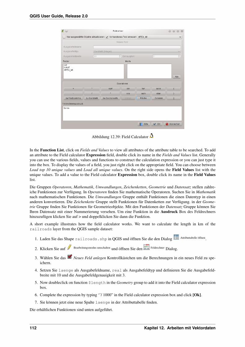
QGIS User Guide, Release 2.0
Abbildung 12.39: Field Calculator
In the Function List, click on Fields and Values to view all attributes of the attribute table to be searched. To addan attribute to the Field calculator Expression field, double click its name in the Fields and Values list. Generallyyou can use the various fields, values and functions to construct the calculation expression or you can just type itinto the box. To display the values of a field, you just right click on the appropriate field. You can choose betweenLoad top 10 unique values and Load all unique values. On the right side opens the Field Values list with theunique values. To add a value to the Field calculator Expression box, double click its name in the Field Valueslist.
Die Gruppen Operatoren, Mathematik, Umwandlungen, Zeichenketten, Geometrie und Datensatz stellen zahlre-iche Funktionen zur Verfügung. In Operatoren finden Sie mathematische Operatoren. Suchen Sie in Mathematiknach mathematischen Funktionen. Die Umwandlungen Gruppe enthält Funktionen die einen Datentyp in einenanderen konvertieren. Die Zeichenkette Gruppe stellt Funktionen für Datenketten zur Verfügung. in der Geome-trie Gruppe finden Sie Funktionen für Geometrieobjekte. Mit den Funktionen der Datensatz Gruppe können SieIhren Datensatz mit einer Nummerierung versehen. Um eine Funktion in die Ausdruck Box des Feldrechnershinzuzufügen klicken Sie auf > und doppelklicken Sie dann die Funktion.
A short example illustrates how the field calculator works. We want to calculate the length in km of therailroads layer from the QGIS sample dataset:
1. Laden Sie das Shape railroads.shp in QGIS und öffnen Sie die den Dialog Attributtabelle öffnen.
2. Klicken Sie auf Bearbeitungsmodus umschalten und öffnen Sie den Feldrechner Dialog.
3. Wählen Sie das Neues Feld anlegen Kontrollkästchen um die Berechnungen in ein neues Feld zu spe-ichern.
4. Setzen Sie laenge als Ausgabefeldname, real als Ausgabefeldtyp und definieren Sie die Ausgabefeld-breite mit 10 und die Ausgabefeldgenauigkeit mit 3.
5. Now doubleclick on function $length in the Geometry group to add it into the Field calculator expressionbox.
6. Complete the expression by typing ‘’/ 1000” in the Field calculator expression box and click [Ok].
7. Sie können jetzt eine neue Spalte laenge in der Attributtabelle finden.
Die erhältlichen Funktionen sind unten aufgeführt.
112 Kapitel 12. Arbeiten mit Vektordaten
QGIS User Guide, Release 2.0
The field calculator Function list with the Selected Function Help , Operators and Expression menu are alsoavailable through the rule-based rendering in the Style menu of the Layer properties and the expression based
labeling in the Labeling core application.
Operators
This group contains operators e.g + - *
a + b a plus ba - b a minus ba * b a multiplied by ba / b a divided by ba % b a modulo b for example 7 % 2 = 1 -> 2 fits into 7 three times rest is 1a ^ b a power b for example 2^2=4 or 2^3=8a = b a and b are equala > b a is larger than ba < b a is smaller than ba <> b a and b are not equala != b a and b are not equala <= b a is less than or equal to ba >= b a is larger than or equal to ba ~ b a matches the regular expression b+ a positive sign- a negative value of a|| joins two values together into a string ’Hello’ || ’ world’LIKE returns 1 if the string matches the supplied patternILIKE returns 1 if the string matches case-insensitive the supplied
pattern. ILIKE can be used instead of LIKE to make the match case-insensitiveIS returns 1 if a is the same as bOR returns 1 when condition a or b is trueAND returns 1 when condition a and b are trueNOT returns 1 if a is not the same as bcolumn name "column name" value of the field column name’string’ a string valueNULL null valuea IS NULL a has no valuea IS NOT NULL a has a valuea IN (value[,value]) a is below the values listeda NOT IN (value[,value]) a is not below the values listed
Conditionals
This group contains functions to handle conditional checks in expressions.
CASE evaluates multiple expressions and return a resultCASE ELSE evaluates multiple expressions and return a resultcoalesce returns the first non-NULL value from the expression listregexp_match returns true if any part of a string matches
the supplied regular expression
Mathematical Functions
This group contains math functions e.g square root, sin and cos
sqrt(a) square root of aabs returns the absolute value of a number.sin(a) sinus of acos(a) cosinus of atan(a) tangens of aasin(a) arcussinus of aacos(a) arcuscosinus of aatan(a) arcustangens of aatan2(y,x) arcustangens of y/x using the signs of the two arguments
to determine the quadrant of the resultexp exponential of an value
12.5. Feldrechner 113
QGIS User Guide, Release 2.0
ln value of the natural logarithm of the passed expressionlog10 value of the base 10 logarithm of the passed expressionlog value of the logarithm of the passed value and baseround number to number of decimal placesrand random integer within the range specified by the minimum
and maximum argument (inclusive)randf random float within the range specified by the minimum
and maximum argument (inclusive)max largest value in a set of valuesmin smallest value in a set of valuesclamp restricts an input value to a specified rangescale_linear transforms a given value from an input domain to an output
range using linear interpolationscale_exp transforms a given value from an input domain to an output
range using an exponential curvefloor rounds a number downwardsceil rounds a number upwards$pi pi as value for calculations
Conversions
This group contains functions to convert on data type to another e.g string to integer, integer to string.
toint converts a string to integer numbertoreal converts a string to real numbertostring convert number to stringtodatetime convert a string into Qt data time typetodate convert a string into Qt data typetotime convert a string into Qt time typetointerval converts a string to a interval type. Can be used to take days,
hours, month, etc off a date
Date and Time Functions
This group contains functions for handling date and time data.
$now current date and timeage difference between two datesyear extract the year part from a date, or the number of years from a Intervalmonth extract the month part from a date, or the number of months from a Intervalweek extract the week number from a date, or the number of weeks from a Intervalday extract the day from a date, or the number of days from a Intervalhour extract the hour from a datetime or time, or the number
of hours from a Intervalminute extract the minute from a datetime or time, or the number
of minutes from a Intervalsecond extract the second from a datetime or time, or the number
of minutes from a Interval
String Functions
This group contains functions that operate on strings e.g replace, convert to upper case.
lower convert string a to lower caseupper convert string a to upper casetitle converts all words of a string to title case (all words lower case
with leading capital letter)trim removes all leading and trailing whitespace (spaces, tabs, etc) from a stringlength length of string areplace returns a string with the the supplied string replacedregexp_replace(a,this,that) returns a string with the supplied regular expression replacedregexp_substr returns the portion of a string which matches a supplied regular expressionsubstr(*a*,from,len) returns a part of a stringconcat concatenates several strings to onestrpos returns the index of a regular expression in a string
114 Kapitel 12. Arbeiten mit Vektordaten
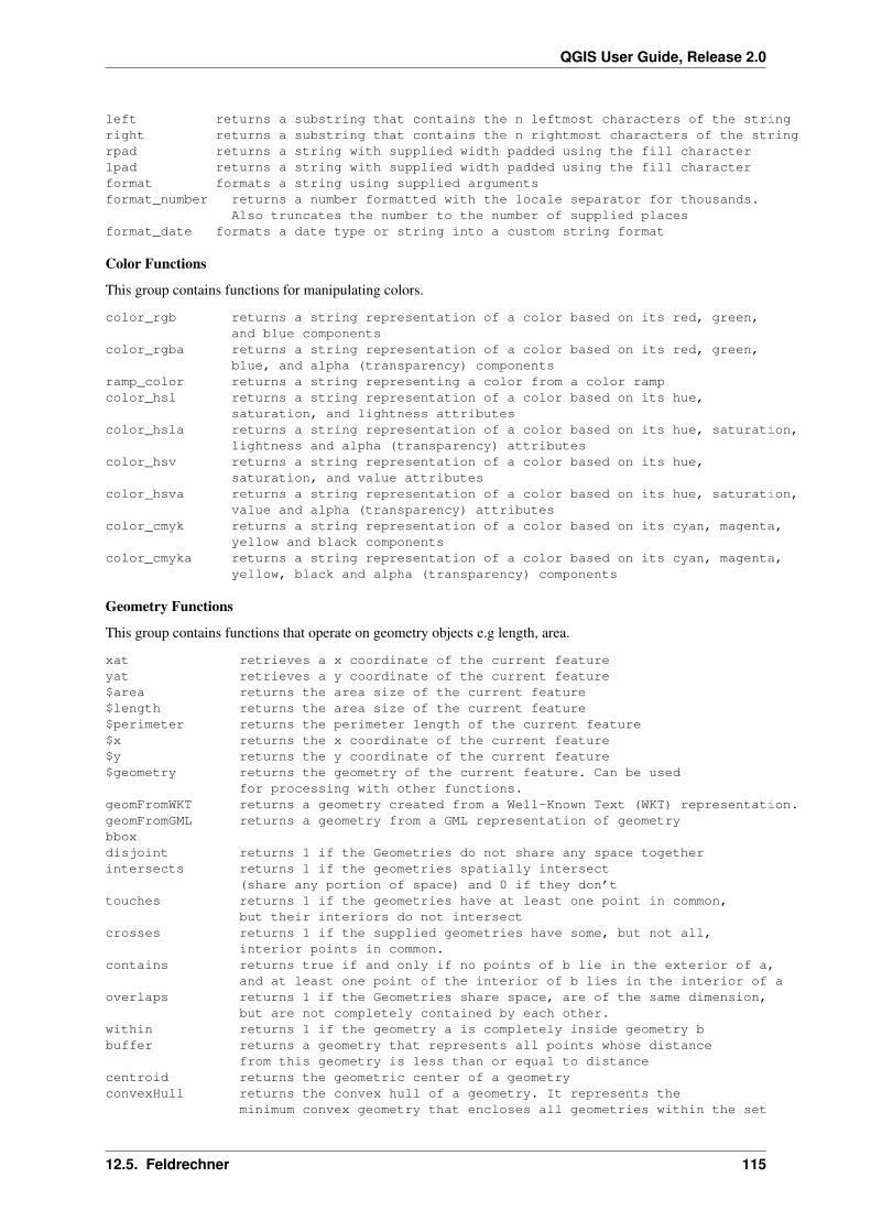
QGIS User Guide, Release 2.0
left returns a substring that contains the n leftmost characters of the stringright returns a substring that contains the n rightmost characters of the stringrpad returns a string with supplied width padded using the fill characterlpad returns a string with supplied width padded using the fill characterformat formats a string using supplied argumentsformat_number returns a number formatted with the locale separator for thousands.
Also truncates the number to the number of supplied placesformat_date formats a date type or string into a custom string format
Color Functions
This group contains functions for manipulating colors.
color_rgb returns a string representation of a color based on its red, green,and blue components
color_rgba returns a string representation of a color based on its red, green,blue, and alpha (transparency) components
ramp_color returns a string representing a color from a color rampcolor_hsl returns a string representation of a color based on its hue,
saturation, and lightness attributescolor_hsla returns a string representation of a color based on its hue, saturation,
lightness and alpha (transparency) attributescolor_hsv returns a string representation of a color based on its hue,
saturation, and value attributescolor_hsva returns a string representation of a color based on its hue, saturation,
value and alpha (transparency) attributescolor_cmyk returns a string representation of a color based on its cyan, magenta,
yellow and black componentscolor_cmyka returns a string representation of a color based on its cyan, magenta,
yellow, black and alpha (transparency) components
Geometry Functions
This group contains functions that operate on geometry objects e.g length, area.
xat retrieves a x coordinate of the current featureyat retrieves a y coordinate of the current feature$area returns the area size of the current feature$length returns the area size of the current feature$perimeter returns the perimeter length of the current feature$x returns the x coordinate of the current feature$y returns the y coordinate of the current feature$geometry returns the geometry of the current feature. Can be used
for processing with other functions.geomFromWKT returns a geometry created from a Well-Known Text (WKT) representation.geomFromGML returns a geometry from a GML representation of geometrybboxdisjoint returns 1 if the Geometries do not share any space togetherintersects returns 1 if the geometries spatially intersect
(share any portion of space) and 0 if they don’ttouches returns 1 if the geometries have at least one point in common,
but their interiors do not intersectcrosses returns 1 if the supplied geometries have some, but not all,
interior points in common.contains returns true if and only if no points of b lie in the exterior of a,
and at least one point of the interior of b lies in the interior of aoverlaps returns 1 if the Geometries share space, are of the same dimension,
but are not completely contained by each other.within returns 1 if the geometry a is completely inside geometry bbuffer returns a geometry that represents all points whose distance
from this geometry is less than or equal to distancecentroid returns the geometric center of a geometryconvexHull returns the convex hull of a geometry. It represents the
minimum convex geometry that encloses all geometries within the set
12.5. Feldrechner 115
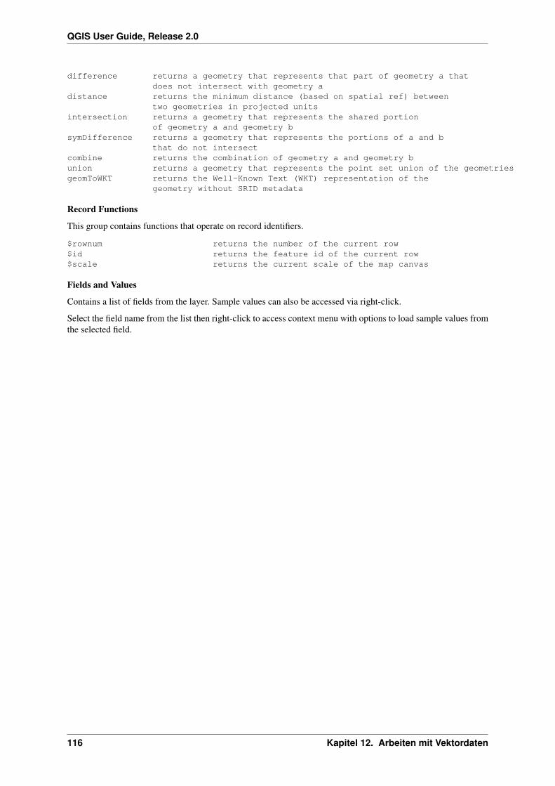
QGIS User Guide, Release 2.0
difference returns a geometry that represents that part of geometry a thatdoes not intersect with geometry a
distance returns the minimum distance (based on spatial ref) betweentwo geometries in projected units
intersection returns a geometry that represents the shared portionof geometry a and geometry b
symDifference returns a geometry that represents the portions of a and bthat do not intersect
combine returns the combination of geometry a and geometry bunion returns a geometry that represents the point set union of the geometriesgeomToWKT returns the Well-Known Text (WKT) representation of the
geometry without SRID metadata
Record Functions
This group contains functions that operate on record identifiers.
$rownum returns the number of the current row$id returns the feature id of the current row$scale returns the current scale of the map canvas
Fields and Values
Contains a list of fields from the layer. Sample values can also be accessed via right-click.
Select the field name from the list then right-click to access context menu with options to load sample values fromthe selected field.
116 Kapitel 12. Arbeiten mit Vektordaten

KAPITEL 13
Arbeiten mit Rasterdaten
13.1 Arbeiten mit Rasterdaten
This Section describes how to visualize and set raster layer properties. QGIS uses the GDAL library to read andwrite raster data formats, including Arc/Info Binary Grid, Arc/Info ASCII Grid, GeoTIFF, Erdas Imagine andmany more. GRASS raster support is supplied by a native QGIS data provider plugin. The raster data can also beloaded in read mode from zip and gzip archives into QGIS.
Zum Zeitpunkt der Erstellung diese Dokumentes werden mehr als 100 Rasterdatenformate von der GDAL-Bibliothek unterstützt (siehe GDAL-SOFTWARE-SUITE Literatur und Internetreferenzen). Eine vollständigeListe ist unter http://www.gdal.org/formats_list.html. erhältlich.
Bemerkung: Not all of the listed formats may work in QGIS for various reasons. For example, some requireexternal commercial libraries or the GDAL installation of your OS was not built to support the format you wantto use. Only those formats that have been well tested will appear in the list of file types when loading a raster intoQGIS. Other untested formats can be loaded by selecting the [GDAL] All files (*) filter.
Das Arbeiten mit GRASS Rasterdaten wird in Kapitel GRASS GIS Integration vorgestellt.
13.1.1 Was ist ein Rasterlayer?
Raster data in GIS are matrices of discrete cells that represent features on, above or below the earth’s surface. Eachcell in the raster grid is the same size, and cells are usually rectangular (in QGIS they will always be rectangular).Typical raster datasets include remote sensing data such as aerial photography or satellite imagery and modelleddata such as an elevation matrix.
Unlike vector data, raster data typically do not have an associated database record for each cell. They are geocodedby its pixel resolution and the x/y coordinate of a corner pixel of the raster layer. This allows QGIS to position thedata correctly in the map canvas.
QGIS makes use of georeference information inside the raster layer (e.g. GeoTiff) or in an appropriate world fileto properly display the data.
13.1.2 Loading raster data in QGIS
Raster layers are loaded either by clicking on the Add Raster Layer icon or by selecting the Layer → AddRaster Layer menu option. More than one layer can be loaded at the same time by holding down the Control orShift key and clicking on multiple items in the dialog Open a GDAL Supported Raster Data Source.
Ist ein Rasterlayer in die Legende geladen können Sie auf den Layernamen mit der rechten Maustaste klickenum layerspezifische Eigenschaften auszuwählen oder zu aktivieren oder um einen Dialog zum Einstellen derRastereigenschaften des Layers zu öffnen.
Rechte-Maustaste Menü für Rasterlayer
117
QGIS User Guide, Release 2.0
• Auf die Layerausdehnung zoomen
• Auf besten Maßstab zoomen (100%)
• In der Übersicht anzeigen
• Entfernen
• Duplicate
• KBS für Layer setzen
• Layer-KBS dem Projekt zuweisen
• Save as ...
• Eigenschaften
• Umbenennen
• Stil kopieren
• Neue Gruppe hinzufügen
• Alles ausklappen
• Alles zusammenfalten
• Zeichenreihenfolge aktualisieren
13.2 Dialogfenster Rasterlayereigenschaften
Um die Eigenschaften eines Rasterlayers zu sehen oder einzustellen doppelklicken Sie auf den Layernamen in derLegende oder rechtsklicken Sie auf den Layernamen und wählen Sie Eigenschaften aus dem Kontextmenü:
Dies öffnet den Layereigenschaften Dialog, (siehe figure_raster_1).
There are several menus in the dialog:
• Allgemein
• Stil
• Transparenz
• Pyramiden
• Histogramm
• Metadaten
13.2.1 General Menu
Layer Info
The General menu displays basic information about the selected raster, including the layer source path, the displayname in the legend (which can be modified) and the number of columns, rows and No-Data Values of the raster.
Coordinate reference system
Below you find the coordinate reference system (CRS) information printed as a PROJ.4-string. If this setting isnot correct, it can be modified by clicking the [Specify] button.
118 Kapitel 13. Arbeiten mit Rasterdaten

QGIS User Guide, Release 2.0
Abbildung 13.1: Raster Layers Properties Dialog
Scale Dependent visibility
Additionally Scale Dependent visibility can be set in this tab. You need to check the checkbox and set an appro-priate scale where your data will be displayed in the map canvas.
At the bottom you can see a thumbnail of the layer, its legend symbol, and the palette.
13.2.2 Style Menu
Band rendering
QGIS offers four different Render types. The renderer chosen is dependent on the data type.
1. Multiband color - if the file comes as a multi band with several bands (e.g. used with a satellite image withseveral bands)
2. Paletted - if a single band file comes with an indexed palette (e.g. used with a digital topographic map)
3. Singleband gray- (one band of) the image will be rendered as gray, QGIS will choose this renderer if thefile neither has multi bands, nor has an indexed palette nor has a continous palette (e.g. used with a shadedrelief map)
4. Singleband pseudocolor - this renderer is possible for files with a continuous palette, e.g. the file has got acolor map (e.g. used with an elevation map)
Multiband color
With the multiband color renderer three selected bands from the image will be rendered, each band representingthe red, green or blue component that will be used to create a color image. You can choose several Contrastenhancement methods: ‘No enhancement’, ‘Stretch to MinMax’, ‘Stretch and clip to MinMax’ and ‘Clip to minmax’.
This selection offers you a wide range of options to modify the appearance of your rasterlayer. First of all youhave to get the data range from your image. This can be done by choosing the Extent and pressing [Load]. QGIScan Estimate (faster) the Min and Max values of the bands or use the Actual (slower) Accuracy.
13.2. Dialogfenster Rasterlayereigenschaften 119

QGIS User Guide, Release 2.0
Abbildung 13.2: Raster Renderer - Multiband color
Now you can scale the colors with the help of the Load min/max values section. A lot of images have few verylow and high data. These outliers can be eliminated using the Cumulative count cut setting. The standard datarange is set from 2% until 98% of the data values and can be adapted manually. With this setting the gray characterof the image can disappear. With the scaling option Min/max QGIS creates a color table with the whole dataincluded in the original image. E.g. QGIS creates a color table with 256 values, given the fact that you have 8bitbands. You can also calculate your color table using the Mean +/- standard deviation x . Then only thevalues within the standard deviation or within multiple standard deviations are considered for the color table. Thisis useful when you have one or two cells with abnormally high values in a raster grid that are having a negativeimpact on the rendering of the raster.
All calculation can also be made for the Current extend.
Tipp: Einen einzelnen Kanal eines Mehrkanal-Rasterlayers anzeigenIf you want to view a single band (for example Red) of a multiband image, you might think you would set theGreen and Blue bands to “Not Set”. But this is not the correct way. To display the Red band, set the image type to‘Singleband gray’, then select Red as the band to use for Gray.
Paletted
This is the standard render option for singleband files that already include a color table, where each pixel value isassigned to a certain color. In that case, the palette is rendered automatically. If you want to change colors assignedto certain values, just double-click on the color and the Select color dialog appears.
Abbildung 13.3: Raster Renderer - Paletted
Kontrastverbesserung
Bemerkung: When adding GRASS rasters the option Contrast enhancement will be always set to automaticallyto stretch to min max regardless if the QGIS general options this is set to another value.
Singleband gray
This renderer allows you to render a single band layer with a Color gradient ‘Black to white’ or ‘White to black’.You can define a Min and a Max value with choosing the Extend first and then pressing [Load]. QGIS can
120 Kapitel 13. Arbeiten mit Rasterdaten
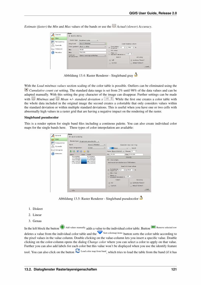
QGIS User Guide, Release 2.0
Estimate (faster) the Min and Max values of the bands or use the Actual (slower) Accuracy.
Abbildung 13.4: Raster Renderer - Singleband gray
With the Load min/max values section scaling of the color table is possible. Outliers can be eliminated using theCumulative count cut setting. The standard data range is set from 2% until 98% of the data values and can be
adapted manually. With this setting the gray character of the image can disappear. Further settings can be madewith Min/max and Mean +/- standard deviation x . While the first one creates a color table withthe whole data included in the original image the second creates a colortable that only considers values withinthe standard deviation or within multiple standard deviations. This is useful when you have one or two cells withabnormally high values in a raster grid that are having a negative impact on the rendering of the raster.
Singleband pseudocolor
This is a render option for single band files including a continous palette. You can also create individual colormaps for the single bands here. Three types of color interpolation are available:
Abbildung 13.5: Raster Renderer - Singleband pseudocolor
1. Diskret
2. Linear
3. Genau
In the left block the button Add values manually adds a value to the individual color table. Button Remove selected row
deletes a value from the individual color table and the Sort colormap items button sorts the color table according tothe pixel values in the value column. Double clicking on the value-column lets you insert a specific value. Doubleclicking on the color-column opens the dialog Change color where you can select a color to apply on that value.Further you can also add labels for each color but this value won’t be displayed when you use the identify feature
tool. You can also click on the button Load color map from band, which tries to load the table from the band (if it has
13.2. Dialogfenster Rasterlayereigenschaften 121

QGIS User Guide, Release 2.0
any). And you can use the buttons Load color map from file or Export color map to file to load an existing color tableor to save the defined color table for other sessions.
In the right block Generate new color map allows you to create newly categorized colormaps. For the Classifi-
cation mode ‘Equal interval’ you only need to select the number of classes and press the button
Classify. You can invert the colors of the the color map by clicking the Invert checkbox. In case of the Mode
‘Continous’ QGIS creates classes depending on the Min and Max automatically. Defining Min/Max valuescan be done with the help of Load min/max values section. A lot of images have few very low and high data.These outliers can be eliminated using the Cumulative count cut setting. The standard data range is set from2% until 98% of the data values and can be adapted manually. With this setting the gray character of the imagecan disappear. With the scaling option Min/max QGIS creates a color table with the whole data included in theoriginal image. E.g. QGIS creates a color table with 256 values, given the fact that you have 8bit bands. You canalso calculate your color table using the Mean +/- standard deviation x . Then only the values withinthe standard deviation or within multiple standard deviations are considered for the color table.
Color rendering
For every Band rendering a Color rendering is possible.
You can achieve special rendering effects for your raster file(s) using one one of the blending modes (seeblend_modes).
Further settings can be made in modifiying the Brightness, the Saturation and the Contrast. You can use aGrayscale option where you can choose between ‘By lightness’, ‘By luminosity’ and ‘By average’. For one huein the color table you can modiy the ‘Strength’.
Resampling
The Resampling option makes it appearance when you zoom in and out of the image. Resampling modes canoptimize the appearance of the map. They calculate a new gray value matrix through a geometric transformation.
While applying the ‘Nearest neighbour’ method the map can have a pixelated structure when zooming in. Thisappearance can be improved by using the ‘Bilinear’ or ‘Cubic’ method. Sharp features are caused to be blurrednow. The effect is a smoother image. The method can be applied e.g. to digital topographic raster maps.
13.2.3 Transparency Menu
QGIS has the ability to display each raster layer at varying transparency levels. Use the transparency slider
to indicate to what extent the underlying layers (if any) should be visible though the cur-rent raster layer. This is very useful, if you like to overlay more than one rasterlayer, e.g. a shaded relief mapoverlayed by a classified rastermap. This will make the look of the map more three dimensional.
Additionally you can enter a rastervalue, which should be treated as NODATA in the Additional no data valuemenu.
Die Transparenz kann noch flexibler über die Transparente Pixelliste angepasst werden. Die Transparenz jedesPixels kann hier eingestellt werden.
Als Beispiel wollen wir die Wasserflächen aus dem Rasterlayer landcover.tif auf eine Transparenz von 20%setzen. Folgende Schritte sind dazu notwendig:
1. Laden Sie den Rasterlayer landcover aus dem Alaska Beispieldatensatz
2. Öffnen Sie den Dialog Layereigenschaften indem Sie auf den Namen in der Legende doppelklicken, oderim Rechte-Maustaste Menü Eigenschaften auswählen.
3. Select the Transparency menu
4. From the Transparency band menu choose ‘None’.
122 Kapitel 13. Arbeiten mit Rasterdaten

QGIS User Guide, Release 2.0
5. Click the Add values manually button. A new row will appear in the pixel-list.
6. Enter the raster-value (we use 0 here) in the ‘From’ and ‘To’ column and adjust the transparency to 20 %.
7. Drücken Sie den Knopf [Anwenden] und schauen Sie sich das Ergebnis an.
You can repeat the steps 5 and 6 to adjust more values with custom transparency.
As you can see this is quite easy to set custom transparency, but it can be quite a lot of work. Therefore you
can use the button Export to file to save your transparency list to a file. The button Import from file loads yourtransparency settings and applies them to the current raster layer.
13.2.4 Pyramids Menu
Large resolution raster layers can slow navigation in QGIS. By creating lower resolution copies of the data (pyra-mids), performance can be considerably improved as QGIS selects the most suitable resolution to use dependingon the level of zoom.
Sie brauchen dazu Schreibrecht in dem Ordner, in dem sich sie Originaldaten befinden.
Sie können mehrere Resampling-Methoden zum Berechnen der Pyramiden verwenden:
• Nächster Nachbar
• Durchschnitt
• Gauss
• Cubic
• Mode
• None
If you choose ‘Internal (if possible)’ from the Overview format menu QGIS tries to build pyramids internally. Youcan also choose ‘External’ and ‘External (Erdas Imagine)’.
Bitte beachten Sie, dass das Erstellen von Pyramiden die Originaldaten verändern und dieser Schritt nicht mehrrückgängig gemacht werden kann. Wenn Sie eine ‘nicht pyramidisierte’ Version der Daten wünschen, erstellenSie vorher eine Kopie.
13.2.5 Histogram Menu
The Histogram menu allows you to view the distribution of the bands or colors in your raster. It is generatedautomatically when you open the Histogram menu. All existing bands will be displayed together. You can save
the histogram as an image with the button. With the Visibility option in the Prefs/Actions menu you candisplay histograms of the individual bands. You will need to select the option Show selected band. The Min/maxoptions allow you to ‘Always show min/max markers’, to ‘Zoom to min/max’ and to ‘Update style to min/max’.With the Actions option you can ‘Reset’ and ‘Recompute histogram’ after you have chosen the Min/max options.
13.2.6 Metadata Menu
The Metadata menu displays a wealth of information about the raster layer, including statistics about each bandin the current raster layer. From this menu entries are made for the Description, Attribution, MetadataUrl andProperties. In Properties statistics are gathered on a ‘need to know’ basis, so it may well be that a given layersstatistics have not yet been collected.
13.2. Dialogfenster Rasterlayereigenschaften 123

QGIS User Guide, Release 2.0
13.3 Rasterrechner
Der Rasterrechner im Menü Raster (siehe figure_raster_2) ermöglicht Rechenoperationen auf Basis von Pixel-werten einer in QGIS geladenen Rasterkarte. Das Ergebnis wird als neue Rasterkarte abgespeichert. Das Formatkann entsprechend der durch GDAL unterstützten Formate festgelegt werden.
Abbildung 13.6: Raster Calculator
Die Liste Rasterkanäle enthält alle geladenen Rasterlayer die verwendet werden können. Um ein Raster in dasRasterrechnerausdruck Fenster einzufügen, doppelklicken Sie einfach auf dessen Namen. Sie können dann mitden Operatoren Ausdrücke per Mausklick konstruieren oder manuell in die Box eingeben.
Im Abschnitt Ergebnislayer müssen Sie einen Ausgabelayer definieren. Sie können dann den Analysebereich aufGrundlage eines Eingaberasters oder basierend auf Min/Max X und Y-Koordinaten bzw. mittels Spalten und Zeilenangeben, um die Auflösung des Ausgabelayer festzulegen. Wenn die Eingabelayer eine abweichende Auflösungbesitzen, werden die Werte auf Basis des nearest neighbor Algorithmus resampelt.
The Operators section contains all usable operators. To add an operator to the raster calculator expression box,click the appropriate button. Mathematical calculations (+, -, *, ... ) and trigonometric functions (sin, cos, tan,... ) are available. Stay tuned for more operators to come!
Mit dem Aktivieren des Kontrollkästchens Ergebnis zum Projekt hinzufügen wird der Ausgabelayer automa-tische der Legende hinzugefügt und kann somit visualisiert werden.
13.3.1 Beispiele
Höhenwerte von Meter zu Fuß konvertieren
Für das Erstellen eines Rasterlayers in Fuß aus einem Rasterlayer in Metern müssen Sie den Konvertierungsfaktorvon Metern zu Fuß benutzen: 3.28. Der Ausdruck lautet:
elevation@1 * 3.28
Eine Maske verwenden
Wenn Sie Teile des Rasterlayers ausmaskieren wollen, weil Sie nur an Höhenwerten über 0 Metern interessiertsind, können Sie den folgenden Ausdruck zum Erstellen einer Maske und zum gleichzeitigen Anwenden auf denRasterlayer verwenden.
124 Kapitel 13. Arbeiten mit Rasterdaten
QGIS User Guide, Release 2.0
(elevation@1 >= 0) * elevation@1
Jede Zelle die größer oder gleich 0 ist wird auf den Wert 1 gesetzt, ansonsten lautet er 0. Dies erstellt erstellt dieMaske ‘on-the-fly’.
13.3. Rasterrechner 125

QGIS User Guide, Release 2.0
126 Kapitel 13. Arbeiten mit Rasterdaten
KAPITEL 14
Arbeiten mit OGC Daten
14.1 QGIS as OGC Data Client
Das Open Geospatial Consortium (OGC) ist eine internationale Organisation mit mehr als 300 Mitgliedernaus kommerziellen und behördlichen Bereichen, aus der Forschung sowie aus Vereinen (Non-Profit). Die Mit-glieder entwickeln und implementieren Standards für den Austausch räumlicher Daten (Datendienste), GIS-Datenprocessing und standardisierte Bereitstellung von Geodaten.
Zur Beschreibung von geographischen Objekten in einem einfachen Datenmodell wurden eine steigende Zahl vonSpezifikationen entwickelt, die spezielle Bedürfnisse der Interoperabilität bedienen, räumliche Informationen undGIS einbezogen. Weitere Informationen können unter http://www.opengeospatial.org/ abgerufen werden.
Important OGC specifications supported by QGIS are:
• WMS — Web Map Service (WMS/WMTS Client)
• WMTS — Web Map Tile Service (WMS/WMTS Client)
• WFS — Web Feature Service (WFS und WFS-T Klient)
• WFS-T — Web Feature Service - Transactional (WFS und WFS-T Klient)
• WCS — Web Coverage Service (WCS Client)
• SFS — Simple Features for SQL (PostGIS Layer laden)
• GML — Geography Markup Language
OGC services are increasingly being used to exchange geospatial data between different GIS implementations anddata stores. QGIS can deal with the above specifications as a client, being SFS (through support of the PostgreSQL/ PostGIS data provider, see Section PostGIS Layer laden).
14.1.1 WMS/WMTS Client
Übersicht über die WMS-Unterstützung
QGIS currently can act as a WMS client that understands WMS 1.1, 1.1.1 and 1.3 servers. It has particularly beentested against publicly accessible servers such as DEMIS.
WMS servers act upon requests by the client (e.g. QGIS) for a raster map with a given extent, set of layers,symbolization style, and transparency. The WMS server then consults its local data sources, rasterizes the map,and sends it back to the client in a raster format. For QGIS this would typically be JPEG or PNG.
WMS is generically a REST (Representational State Transfer) service rather than a fully-blown Web Service. Assuch, you can actually take the URLs generated by QGIS and use them in a web browser to retrieve the sameimages that QGIS uses internally. This can be useful for troubleshooting, as there are several brands of WMSservers in the market and they all have their own interpretation of the WMS standard.
127

QGIS User Guide, Release 2.0
WMS-Layer können sehr einfach hinzugefügt werden, solange man die URL des Servers kennt, eine Verbindungüber HTTP zu diesem Server besteht und der angefragte Server auch HTTP versteht.
Overview of WMTS Support
QGIS can also act as a WMTS client. WMTS is an OGC standard for distributing tile sets of geospatial data.This is a faster and a more efficient way of distributing data than WMS because with WMTS the tile sets arepre-generated and the client only requests the transmission of the tiles and not their production. A WMS requesttypically involves both the generation and transmission of the data. A well known example of a non-OGC standardfor viewing tiled geospatial data is Google Maps.
In order to display the data at a variety of scales close to what the user might want, the WMTS tile sets areproduced at several different scale levels and are made available for the GIS client to request them.
This diagram illustrates the concept of tile sets:
Abbildung 14.1: Concept of WMTS tile sets
The two types of WMTS interfaces that QGIS supports are via Key-Value-Pairs (KVP) and RESTful. These twointerfaces are different and you need to specify them to QGIS differently.
1) In order to access a WMTS KVP service, a QGIS user opens the WMS/WMTS interface and adds the followingstring to the URL of the WMTS tile service:
"?SERVICE=WMTS&REQUEST=GetCapabilities"
An example of this type of address is
http://opencache.statkart.no/gatekeeper/gk/gk.open_wmts?\service=WMTS&request=GetCapabilities
For testing the topo2 layer in this WMTS works nicely. Adding this string indicates that a WMTS web service isto be used instead of a WMS service
2) The RESTful WMTS service takes a different form, it is a straightforward URL, the format recommended bythe OGC is:
{WMTSBaseURL}/1.0.0/WMTSCapabilities.xml
This format helps you to recognize that it is a RESTful address. A RESTful WMTS is accessed in QGIS by simplyadding its address in the WMS setup in the URL field of the form. An example for an Austrian basemap of thistype of address is http://maps.wien.gv.at/basemap/1.0.0/WMTSCapabilities.xml
Bemerkung: You can find some old service call WMS-C. Thoses services are quiet similar to WMTS servicesame purpose but working a little bit differently). You can manage them as the same way you do it for WMTSservices. Just add ?tiled=true at the end of the url. See http://wiki.osgeo.org/wiki/Tile_Map_Service_Specificationfor more information about this specification.
When you read WMTS you can often think WMS-C also.
128 Kapitel 14. Arbeiten mit OGC Daten
QGIS User Guide, Release 2.0
Selecting WMS/WMTS Servers
Wenn Sie die WMS Funktion zum ersten Mal verwenden, sind noch keine Server definiert, mit denen Sie sichverbinden können.
Sie starten die Funktion, indem Sie auf das Icon WMS-Layer hinzufügen in der Werkzeugleiste klicken oder imMenü Layer → WMS-Layer hinzufügen ... auswählen.
Der Dialog Layer eines Servers hinzufügen erscheint dann. Sie können zum Ausprobieren aber einigevordefinierte Server hinzufügen, indem Sie auf den Knopf [Vorgegebene Server ergänzen] klicken. Dadurchwerden Ihnen zwei WMS Server zur Verfügung gestellt: die WMS Server der DM Solutions Group undvon Lizardtech. Um im Reiter Layer einen neuen WMS Server zu definieren wählen Sie [Neu]. Geben Siedann die Parameter die zur Verbindung benötig werden, ein, so wie es in table_OGC_1 aufgelistet ist:
Name Ein Name für diese Verbindung. Dieser Name wird in der Auswahlbox dervorhandenen WMS-Server erscheinen so dass Sie Ihn von anderen WMSServern unterscheiden können.
URL Die URL des Servers, der die Daten vorhält. Dieser Name muss ein auflösbarerHost-Name sein; es ist das gleiche Format dass Sie auch für das Öffnen einerTelnetverbindung oder einem Ping zu einem Host verwenden würden.
Benutzername Benutzername, um auf einen abgesicherten WMS Server zuzugreifen. DieserParameter ist optional.
Passwort Passwort für einen durch Authentifizierung abgesicherten WMS Server. DieserParameter ist optional.
Gemeldete GetMap-URIaus Diensteigenschaftenignorieren
Gemeldete GetMap-URI aus Diensteigenschaften ignorieren und benutzestattdessen die angegebene URI aus dem URL-Feld oben.
GemeldeteGetFeatureInfo-URIignorieren
Gemeldete GetFeatureInfo-URI ignorieren und benutze stattdessen dieangegebene URI aus dem URL-Feld oben
Tabelle OGC 1: WMS Verbindungs-Parameter
Wenn Sie einen Proxy-Server aufsetzen müssen, um WMS-Dienste aus dem Internet zu empfangen, können Siedie entsprechenden Optionen im Reiter Netzwerk unter Einstellungen → Optionen angeben und mit dem Kon-
trollkästchen Proxy für Webzugriff benutzen aktivieren. Vergewissern Sie sich auch, dass Sie die richtige Prox-
yeinstellung aus dem Proxytyp Menü ausgewählt haben.
Once the new WMS Server connection has been created, it will be preserved for future QGIS sessions.
Tipp: WMS-Server-URLsStellen Sie sicher, dass Sie die Basis-URL des Servers eingeben. Achten Sie darauf, dass keine Fragmente wierequest=GetCapabilities oder version=1.0.0 in der URL enthalten sind.
Loading WMS/WMTS Layers
Once you have successfully filled in your parameters you can use the [Connect] button to retrieve the capabilitiesof the selected server. This includes the Image encoding, Layers, Layer Styles and Projections. Since this is anetwork operation, the speed of the response depends on the quality of your network connection to the WMSserver. While downloading data from the WMS server, the download progress is visualized in the left bottom ofthe WMS dialog.
Ihr Bildschirm sollte in etwa so wie der in Abbildung figure_OGR_1 aussehen wie die Ausgabe durch den DMSolutions Group Server.
Bildkodierung
Der Abschnitt über die Bildkodierung gibt die Bildformate an, die der Server und QGIS unterstützen. Wählen Sieein Format aus, das ihren Ansprüchen entspricht.
14.1. QGIS as OGC Data Client 129
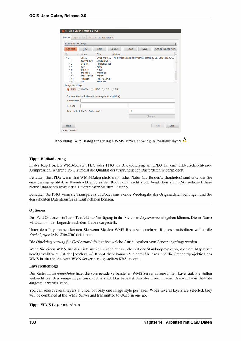
QGIS User Guide, Release 2.0
Abbildung 14.2: Dialog for adding a WMS server, showing its available layers
Tipp: BildkodierungIn der Regel bieten WMS-Server JPEG oder PNG als Bildkodierung an. JPEG hat eine bildverschlechterndeKompression, während PNG zumeist die Qualität der ursprünglichen Rasterdaten widerspiegelt.
Benutzen Sie JPEG wenn Ihre WMS-Daten photographischer Natur (Luftbilder/Orthophotos) sind und/oder Sieeine geringe qualitative Beeinträchtigung in der Bildqualität nicht stört. Verglichen zum PNG reduziert diesekleine Unannehmlichkeit den Datentransfer bis zum Faktor 5.
Benutzen Sie PNG wenn sie Transparenz und/oder eine exakte Wiedergabe der Originaldaten benötigen und Sieden erhöhten Datentransfer in Kauf nehmen können.
Optionen
Das Feld Optionen stellt ein Textfeld zur Verfügung in das Sie einen Layernamen eingeben können. Dieser Namewird dann in der Legende nach dem Laden dargestellt.
Unter dem Layernamen können Sie wenn Sie den WMS Request in mehrere Requests aufsplitten wollen dieKachelgröße (z.B. 256x256) definieren.
Die Objektbegrenzung für GetFeatureInfo legt fest welche Attributspalten vom Server abgefragt werden.
Wenn Sie einen WMS aus der Liste wählen erscheint ein Feld mit der Standardprojektion, die vom Mapserverbereitgestellt wird. Ist der [Ändern ...] Knopf aktiv können Sie darauf klicken und die Standardprojektion desWMS in ein anderes vom WMS Server bereitgestelltes KBS ändern.
Layerreihenfolge
Der Reiter Layerreihenfolge listet die vom gerade verbundenen WMS Server ausgewählten Layer auf. Sie stellenvielleicht fest dass einige Layer ausklappbar sind. Das bedeutet dass der Layer in einer Auswahl von Bildstiledargestellt werden kann.
You can select several layers at once, but only one image style per layer. When several layers are selected, theywill be combined at the WMS Server and transmitted to QGIS in one go.
Tipp: WMS Layer anordnen
130 Kapitel 14. Arbeiten mit OGC Daten

QGIS User Guide, Release 2.0
Von einem Server dargestellte Layer werden in der Reihefolge aus dem Abschnitt Layers von oben bis untenüberlagert. Wenn Sie die Layerreihenfolge ändern wollen können Sie den Reiter Layerreihenfolge benutzen.
Transparenz
In this version of QGIS, the Global transparency setting from the Layer Properties is hard-coded to be always on,where available.
Tipp: Transparenz von WMS-LayernDie WMS Bildtransparenz steht Ihnen abhänig von der Bildkodierung zur Verfügung: PNG und GIF unterstützenTransparenz währenddessen JPEG keine Untersützung bietet.
Koordinatenbezugsystem
A Coordinate Reference System (CRS) is the OGC terminology for a QGIS Projection.
Jeder WMS Layer kann in mehreren KBS dargestellt werden. Dies hängt von den Möglichkeiten des WMS Serverab.
Um ein KBS auszuwählen wählen Sie [Ändern ...] und ein Dialog ähnlich wie Figure Projection 3 aus Arbeitenmit Projektionen erscheint. Der hauptsächliche Unterschied der WMS-Version ist dass nur die KBS, die vomWMS Server unterstützt werden, gezeigt werden.
Server search
Within QGIS you can search for WMS-servers. Figure_OGC_2 shows the tab Server Search with the Add Layer(s)from a Server dialog.
Abbildung 14.3: Dialog for searching WMS servers after some keywords
As you can see it is possible to enter a search-string in the text field and hit the [Search] button. After a short whilethe search result will be populated into the list below the text field. Browse the result list and inspect your searchresults within the table. To visualize the results, select a table entry, press the [Add selected row to WMS-list]button and change back to the tab Layers. QGIS automatically has updated your server list and the selected searchresult is already enabled in the list of saved WMS-servers in the Layers tab. You only need to request the list oflayers by clicking the [Connect] button. This option is quite handy when you want to search maps by specifickeywords.
Diese Suchfunktion ist ein Frontend zur API von http://geopole.org.
14.1. QGIS as OGC Data Client 131

QGIS User Guide, Release 2.0
Tilesets
When using WMTS (Cached WMS) Services like
http://opencache.statkart.no/gatekeeper/gk/gk.open_wmts?\service=WMTS&request=GetCapabilities
you are able to browse through the tab Tilesets given by the server. Additional information like tile size, formatsand supported CRS are listed in this table. In combination with this feature you can use the tile scale slider fromthe Settings → Panels (KDE and Windows) or View → Panels (Gnome and MacOSX) then choose Tile scale,which gives you the available scales from the tileserver with nice slider docked in.
Das Objekte abfragen Werkzeug
Nachdem Sie einen Layer von einem WMS-Server geladen haben, können Sie die Layer mit dem WerkzeugObjekte Abfragen abfragen, sofern der WMS-Server diese Funktion unterstützt. Ein Klick auf einen Pixel stellt danneine Abfrage an den WMS-Server für diesen Pixel. Das Ergebnis wird in Textform geliefert. Die Formatierunghängt von dem jeweilig verwendeten WMS-Server ab. Format selection
If multiple output formats are supported by the server, a combo box with supported formats is automatically addedto the identify results dialog and the selected format will is stored in project for the layer. GML format support
The Identify tool supports WMS server response (GetFeatureInfo) in GML (it is called Feature in QGIS GUIin this context) format. If “Feature” format is supported by the server and selected, results of the Identify tool arevector features like from regular vector layer. When a single feature is selected in the tree, it is highlighted in themap and it can be copied to clipboard and pasted to another vector layer. See example setup of UMN Mapserverbelow to support GetFeatureInfo GML format.
# in layer METADATA add which fields should be included and define geometry (example):
"gml_include_items" "all""ows_geometries" "mygeom""ows_mygeom_type" "polygon"
# Then there are two possibilities/formats available, see a) and b):
# a) basic (output is generated by Mapserver and does not contain XSD)# in WEB METADATA define formats (example):"wms_getfeatureinfo_formatlist" "application/vnd.ogc.gml,text/html"
# b) using OGR (output is generated by OGR, it is send as multipart and contains XSD)# in MAP define OUTPUTFORMAT (example):OUTPUTFORMAT
NAME "OGRGML"MIMETYPE "ogr/gml"DRIVER "OGR/GML"FORMATOPTION "FORM=multipart"
END
# in WEB METADATA define formats (example):"wms_getfeatureinfo_formatlist" "OGRGML,text/html"
Eigenschaften
Nach erfolgreichem Hinzufügen eines WMS-Layers können Sie die Eigenschaften des WMS-Servers mit einemRechtsklick auf den Layernamen in der Legende das Kontextmenü aufrufen. Der Eintrag Eigenschaften öffnet einDialogfenster. Reiter Metadaten
Der Reiter Metadaten im Kontextmenü zeigt eine Vielzahl von Informationen über den WMS-Server. Diese Infossind dem Capabilities-Dokument des Servers entnommen. Viele Definitionen können reduziert werden indem
132 Kapitel 14. Arbeiten mit OGC Daten
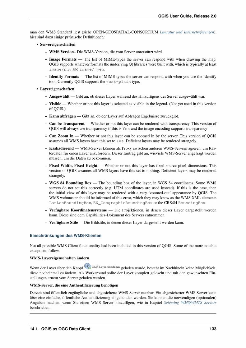
QGIS User Guide, Release 2.0
man den WMS Standard liest (siehe OPEN-GEOSPATIAL-CONSORTIUM Literatur und Internetreferenzen),hier sind dazu einige praktische Definitionen:
• Servereigenschaften
– WMS Version– Die WMS-Version, die vom Server unterstützt wird.
– Image Formats — The list of MIME-types the server can respond with when drawing the map.QGIS supports whatever formats the underlying Qt libraries were built with, which is typically at leastimage/png and image/jpeg.
– Identity Formats — The list of MIME-types the server can respond with when you use the Identifytool. Currently QGIS supports the text-plain type.
• Layereigenschaften
– Ausgewählt — Gibt an, ob dieser Layer während des Hinzufügens des Server ausgewählt war.
– Visible — Whether or not this layer is selected as visible in the legend. (Not yet used in this versionof QGIS.)
– Kann abfragen — Gibt an, ob der Layer auf Abfragen Ergebnisse zurückgibt.
– Can be Transparent — Whether or not this layer can be rendered with transparency. This version ofQGIS will always use transparency if this is Yes and the image encoding supports transparency
– Can Zoom In — Whether or not this layer can be zoomed in by the server. This version of QGISassumes all WMS layers have this set to Yes. Deficient layers may be rendered strangely.
– Kaskadierend — WMS-Server können als Proxy zwischen anderen WMS-Servern agieren, um Ras-terdaten für einen Layer anzufordern. Dieser Eintrag gibt an, wieviele WMS-Server angefragt werdenmüssen, um die Daten zu bekommen.
– Fixed Width, Fixed Height — Whether or not this layer has fixed source pixel dimensions. Thisversion of QGIS assumes all WMS layers have this set to nothing. Deficient layers may be renderedstrangely.
– WGS 84 Bounding Box — The bounding box of the layer, in WGS 84 coordinates. Some WMSservers do not set this correctly (e.g. UTM coordinates are used instead). If this is the case, thenthe initial view of this layer may be rendered with a very ‘zoomed-out’ appearance by QGIS. TheWMS webmaster should be informed of this error, which they may know as the WMS XML elementsLatLonBoundingBox, EX_GeographicBoundingBox or the CRS:84 BoundingBox.
– Verfügbare Koordinatensysteme — Die Projektionen, in denen dieser Layer dargestellt werdenkann. Diese sind dem Capabilities-Dokument des Servers entnommen.
– Verfügbare Stile — Die Bildstile, in denen dieser Layer dargestellt werden kann.
Einschränkungen des WMS-Klienten
Not all possible WMS Client functionality had been included in this version of QGIS. Some of the more notableexceptions follow.
WMS-Layereigenschaften ändern
Wenn der Layer über den Knopf WMS-Layer hinzufügen geladen wurde, besteht im Nachhinein keine Möglichkeit,diese nocheinmal zu ändern. Als Workaround sollte der Layer komplett gelöscht und mit den gewünschten Ein-stellungen erneut vom Server geladen werden.
WMS-Server, die eine Authentifizierung benötigen
Derzeit sind öffentlich zugängliche und abgesicherte WMS Server nutzbar. Ein abgesicherter WMS Server kannüber eine einfache, öffentliche Authentifizierung eingebunden werden. Sie können die notwendigen (optionalen)Angaben machen, wenn Sie einen WMS Server hinzufügen, wie in Kapitel Selecting WMS/WMTS Serversbeschrieben.
14.1. QGIS as OGC Data Client 133

QGIS User Guide, Release 2.0
Tipp: Zugriff auf abgesicherte OGC-LayerWenn Sie Zugriff auf OGC-Layer benötigen, die anders als durch einfache, öffentliche Authentifizierungabgesichert sind, können Sie InteProxy als transparenten Proxy verwenden. Dieser unterstützt verschiedeneMethoden der Authentifizierung. Weitere Informationen zu diesem Thema finden Sie auf der Webseitehttp://inteproxy.wald.intevation.org.
Tipp: |qg| WMS MapserverFrom Version 1.7.0 QGIS has its own implementation of a WMS 1.3.0 Mapserver. Read more about this at chapterQGIS as OGC Data Server.
14.1.2 WCS Client
A Web Coverage Service (WCS) provides access to raster data in forms that are useful for client-side render-ing, as input into scientific models, and for other clients. The WCS may be compared to the WFS and the WMS.As WMS and WFS service instances, a WCS allows clients to choose portions of a server’s information holdingsbased on spatial constraints and other query criteria.
QGIS has a native WCS provider and supports both version 1.0 and 1.1 (which are significantly different), butcurrently it prefers 1.0, because 1.1 has many issues, each server implements it in different way with variousparticularities.
The native WCS provider handles all network requests and uses all standard QGIS network settings (especiallyproxy). It is also possible select cache mode (always cache, prefer cache, prefer network, always network) and theprovider also supports selection of time position if temporal domain is offered by server.
14.1.3 WFS und WFS-T Klient
In QGIS, a WFS layer behaves pretty much like any other vector layer. You can identify and select features andview the attribute table. Since QGIS 1.6 editing (WFS-T) is also supported.
Das Hinzufügen eines WFS-Layers ist fast identisch mit dem Vorgehen beim Laden eines WMS-Layers. Deraktuelle Unterschied ist, dass keine Beispielserver vordefiniert sind, daher soll dies in dem folgenden Beispielvorgeführt werden.
Einen WFS-Layer laden
In diesem Beispiel verwenden wir den WFS-Server der Firma DMSolutions und laden einen Layer. Die URL ist:http://www2.dmsolutions.ca/cgi-bin/mswfs_gmap
1. Klicken Sie auf das WFS-Layer hinzufügen Werkzeug in der Werkzeugleiste. Der Dialog WFS-Layer desServers hinzufügen erscheint
2. Klicken Sie auf [Neu]
3. Geben Sie ‘DM Solutions’ als Namen ein
4. Geben Sie die URL (siehe oben) ein
5. Klicken Sie [OK]
6. Choose ‘DM Solutions’ from the dropdown list Server Connections
7. Klicken Sie [Verbinden]
8. Warten Sie bis die Liste der Layer aufgefüllt wird
9. Wählen Sie den Layer Parks aus der Liste aus
10. Klicken Sie [Anwenden] um den Layer der Karte hinzuzufügen
134 Kapitel 14. Arbeiten mit OGC Daten

QGIS User Guide, Release 2.0
Abbildung 14.4: Adding a WFS layer
Note that proxy settings you have set in your preferences are also recognized.
You’ll notice the download progress is visualized in the left bottom of the QGIS main window. Once the layer isloaded, you can identify and select a province or two and view the attribute table.
Es wird nur WFS 1.0.0 unterstützt. Bis zu diesem Zeitpunkt wurde noch nicht sehr umfangreich die Anbindungmit anderen WFS Servern getestet. Wenn Sie Probleme feststellen, zögern Sie bitte nicht, eine Email an das QGISProjekt zu schicken oder einen Fehlerreport zu schreiben. Sie finden eine Liste möglicher Kontakte in KapitelHilfe und Support.
Tipp: WFS-Server findenSie können weitere WFS Server mit Hilfe von Google oder ihrer bevorzugten Suchmaschine finden. Es gibt eineVielzahl von Listen im Internet, die Links zu öffentlichen Servern bereitstellen.
14.2 QGIS as OGC Data Server
QGIS Server is an open source WMS 1.3 and WFS 1.0.0 implementation which, in addition, implements advancedcartographic features for thematic mapping. The QGIS Server is a FastCGI/CGI (Common Gateway Interface)application written in C++ that works together with a webserver (e.g. Apache, Lighttpd). It is funded by the EUprojects Orchestra, Sany and the city of Uster in Switzerland.
It uses QGIS as backend for the GIS logic and for map rendering. Furthermore the Qt library is used for graphicsand for platform independent C++ programming. In contrast to other WMS software, the QGIS Server uses carto-graphic rules as a configuration language, both for the server configuration and for the user-defined cartographicrules.
Moreover, the QGIS Server project provides the ‘Publish to Web’ plugin, a plugin for QGIS desktop which exportsthe current layers and symbology as a web project for QGIS Server (containing cartographic visualization rulesexpressed in SLD).
As QGIS desktop and QGIS Server use the same visualization libraries, the maps that are published on the weblook the same as in desktop GIS. The ‘Publish to Web’ plugin currently supports basic symbolization, with morecomplex cartographic visualization rules introduced manually. As the configuration is performed with the SLDstandard and its documented extensions, there is only one standardised language to learn, which greatly simplifiesthe complexity of creating maps for the Web.
In one of the following manuals we will provide a sample configuration to set up a QGIS Server. But for now werecommend to read one of the following URLs to get more information:
• http://karlinapp.ethz.ch/qgis_wms/
• http://hub.qgis.org/projects/quantum-gis/wiki/QGIS_Server_Tutorial
• http://linfiniti.com/2010/08/qgis-mapserver-a-wms-server-for-the-masses/
14.2. QGIS as OGC Data Server 135

QGIS User Guide, Release 2.0
14.2.1 Beispielinstallation unter Debian Squeeze
At this point we will give a short and simple sample installation howto for Debian Squeeze. Many other OSprovide packages for QGIS Server, too. If you have to build it all from source, please refer to the URLs above.
Apart from QGIS and QGIS Server you need a webserver, in our case apache2. You can install all pack-ages with aptitude or apt-get install together with other necessary dependency packages. After installation youshould test, if the webserver and QGIS Server works as expected. Make sure the apache server is running with/etc/init.d/apache2 start. Open a web browser and type URL: http://localhost. If apache isup, you should see the message ‘It works!’.
Now we test the QGIS Server installation. The qgis_mapserv.fcgi is available at/usr/lib/cgi-bin/qgis_mapserv.fcgi and provides a standard wms that shows the state boundariesof Alaska. Add the WMS with the URL http://localhost/cgi-bin/qgis_mapserv.fcgi asdescribed in Selecting WMS/WMTS Servers.
Abbildung 14.5: Standard WMS with USA boundaries included in the QGIS Server (KDE)
14.2.2 Creating a WMS/WFS from a QGIS project
To provide a new QGIS Server WMS or WFS we have to create a QGIS project file with some data. Here we usethe ‘alaska’ shapefile from the QGIS sample dataset. Define the colors and styles of the layers in QGIS and definethe project CRS, if not already done.
Then go to the OWS Server menu of the Project → Project Properties dialog and give some informationabout the OWS in the fields under Service Capabilities. This will appear in the GetCapabilities response of the
WMS or WFS. If you don’t check Service capabilities QGIS Server will use the information given in thewms_metadata.xml file located in the cgi-bin folder.
In the WMS capabilities section you can define the extent advertised in the WMS GetCapabilities response byentering the minimum and maximum X and Y values in the fields under Advertised extent. Clicking Use Current
Canvas Extent sets these values to the extent currently displayed in the QGIS map canvas. By checking CRSrestrictions you can restrict in which coordinate reference systems (CRS) QGIS Server will offer to render maps.
Use the button below to select those CRS from the Coordinate Reference System Selector, or click Used toadd the CRS used in the QGIS project to the list.
If you have print composers defined in your project they will be listed in the GetCapabilities response, and theycan be used by the GetPrint request to create prints, using one of the print composer layouts as a template. Thisis a QGIS specific extension to the WMS 1.3.0 specification. If you want to exclude any print composer from
136 Kapitel 14. Arbeiten mit OGC Daten
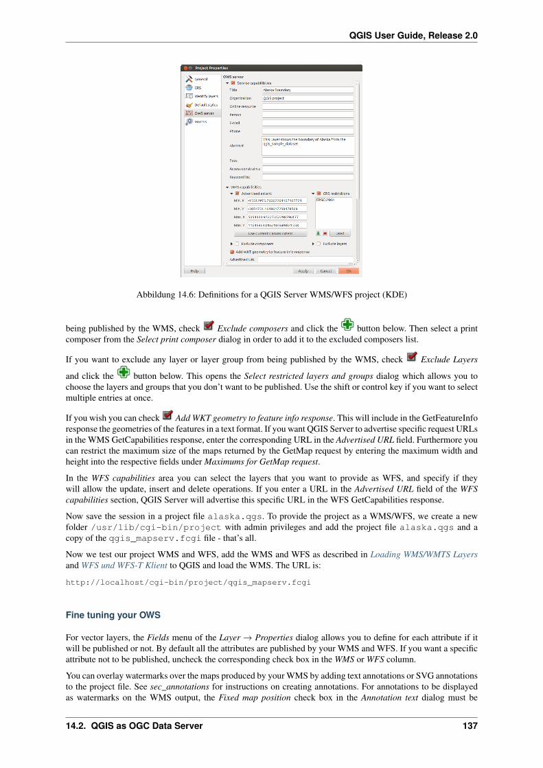
QGIS User Guide, Release 2.0
Abbildung 14.6: Definitions for a QGIS Server WMS/WFS project (KDE)
being published by the WMS, check Exclude composers and click the button below. Then select a printcomposer from the Select print composer dialog in order to add it to the excluded composers list.
If you want to exclude any layer or layer group from being published by the WMS, check Exclude Layers
and click the button below. This opens the Select restricted layers and groups dialog which allows you tochoose the layers and groups that you don’t want to be published. Use the shift or control key if you want to selectmultiple entries at once.
If you wish you can check Add WKT geometry to feature info response. This will include in the GetFeatureInforesponse the geometries of the features in a text format. If you want QGIS Server to advertise specific request URLsin the WMS GetCapabilities response, enter the corresponding URL in the Advertised URL field. Furthermore youcan restrict the maximum size of the maps returned by the GetMap request by entering the maximum width andheight into the respective fields under Maximums for GetMap request.
In the WFS capabilities area you can select the layers that you want to provide as WFS, and specify if theywill allow the update, insert and delete operations. If you enter a URL in the Advertised URL field of the WFScapabilities section, QGIS Server will advertise this specific URL in the WFS GetCapabilities response.
Now save the session in a project file alaska.qgs. To provide the project as a WMS/WFS, we create a newfolder /usr/lib/cgi-bin/project with admin privileges and add the project file alaska.qgs and acopy of the qgis_mapserv.fcgi file - that’s all.
Now we test our project WMS and WFS, add the WMS and WFS as described in Loading WMS/WMTS Layersand WFS und WFS-T Klient to QGIS and load the WMS. The URL is:
http://localhost/cgi-bin/project/qgis_mapserv.fcgi
Fine tuning your OWS
For vector layers, the Fields menu of the Layer → Properties dialog allows you to define for each attribute if itwill be published or not. By default all the attributes are published by your WMS and WFS. If you want a specificattribute not to be published, uncheck the corresponding check box in the WMS or WFS column.
You can overlay watermarks over the maps produced by your WMS by adding text annotations or SVG annotationsto the project file. See sec_annotations for instructions on creating annotations. For annotations to be displayedas watermarks on the WMS output, the Fixed map position check box in the Annotation text dialog must be
14.2. QGIS as OGC Data Server 137

QGIS User Guide, Release 2.0
unchecked. This can be accessed by double clicking the annotation while one of the annotation tools is active. ForSVG annotations you will either need to set the project to save absolute paths (in the General menu of the Project→ Project Properties dialog) or to manually modify the path to the SVG image in a way that it represents a validrelative path.
Extra parameters supported by the WMS GetMap request
In the WMS GetMap request QGIS Server accepts a couple of extra parameters in addition to the standard param-eters according to the OCG WMS 1.3.0 specification:
• MAP parameter: Similar to MapServer, the MAP parameter can be used to specify the path to the QGISproject file. You can specify an absolute path or a path relative to the location of the server executable(qgis_mapserv.fcgi). If not specified, QGIS Server searches for .qgs files in the directory where theserver executable is located.
Example:
http://localhost/cgi-bin/qgis_mapserv.fcgi?\REQUEST=GetMap&MAP=/home/qgis/mymap.qgs&...
• DPI parameter: The DPI parameter can be used to specify the requested output resolution.
Example:
http://localhost/cgi-bin/qgis_mapserv.fcgi?REQUEST=GetMap&DPI=300&...
• OPACITIES parameter: Opacity can be set on layer or group level. Allowed values range from 0 (fullytransparent) to 255 (fully opaque).
Example:
http://localhost/cgi-bin/qgis_mapserv.fcgi?\REQUEST=GetMap&LAYERS=mylayer1,mylayer2&OPACITIES=125,200&...
138 Kapitel 14. Arbeiten mit OGC Daten

KAPITEL 15
Arbeiten mit GPS Daten
15.1 GPS Plugin
15.1.1 Was ist GPS?
GPS, the Global Positioning System, is a satellite-based system that allows anyone with a GPS receiver to findtheir exact position anywhere in the world. It is used as an aid in navigation, for example in airplanes, in boats andby hikers. The GPS receiver uses the signals from the satellites to calculate its latitude, longitude and (sometimes)elevation. Most receivers also have the capability to store locations (known as waypoints), sequences of locationsthat make up a planned route and a tracklog or track of the receivers movement over time. Waypoints, routes andtracks are the three basic feature types in GPS data. QGIS displays waypoints in point layers while routes andtracks are displayed in linestring layers.
15.1.2 GPS-Daten aus einer Datei laden
There are dozens of different file formats for storing GPS data. The format that QGIS uses is called GPX (GPSeXchange format), which is a standard interchange format that can contain any number of waypoints, routes andtracks in the same file.
Um eine GPX-Datei zu laden, müssen Sie das Plugin ‘GPS Werkzeuge’ über das Menü Erweiterungen Er-
weiterungen verwalten ... aktivieren. Aktivieren Sie im QGIS Erweiterungsmanager das Kontrollkästchen vonGPS Werkzeuge.Wenn dieses Plugin geladen ist erscheinen zwei Knöpfe mit einem kleinen GPS Handgerät in derWerkzeugleiste:
• Erstelle neuen GPX-Layer
• GPS-Werkzeuge
For working with GPS data we provide an example GPX file available in the QGIS sample dataset:qgis_sample_data/gps/national_monuments.gpx. See Section Beispieldaten for more informationabout the sample data.
1. Select Vector → GPS → GPS Tools or click the GPS Tools icon in the toolbar and open the Load GPX filetab (see figure_GPS_1).
2. Suchen Sie den Ordner qgis_sample_data/gps/, wählen Sie die GPX-Dateinational_monuments.gpx und klicken Sie [Öffnen].
Verwenden Sie den [Suchen...] Knopf um die GPX-Datei auszuwählen, verwenden Sie dann die Kontrollkästchenum die Objekttypen die aus der GPX-Datei geladen werden sollen auszuwählen. Jeder Objekttyp wird in einenseparaten Layer geladen wenn Sie [OK] klicken. Die Datei national_monuments.gpx enthält nur Weg-punkte.
Bemerkung: GPS units allow to store data in different coordinate systems. When downloading a GPX
139
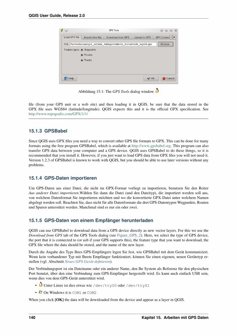
QGIS User Guide, Release 2.0
Abbildung 15.1: The GPS Tools dialog window
file (from your GPS unit or a web site) and then loading it in QGIS, be sure that the data stored in theGPX file uses WGS84 (latitude/longitude). QGIS expects this and it is the official GPX specification. Seehttp://www.topografix.com/GPX/1/1/
15.1.3 GPSBabel
Since QGIS uses GPX files you need a way to convert other GPS file formats to GPX. This can be done for manyformats using the free program GPSBabel, which is available at http://www.gpsbabel.org. This program can alsotransfer GPS data between your computer and a GPS device. QGIS uses GPSBabel to do these things, so it isrecommended that you install it. However, if you just want to load GPS data from GPX files you will not need it.Version 1.2.3 of GPSBabel is known to work with QGIS, but you should be able to use later versions without anyproblems.
15.1.4 GPS-Daten importieren
Um GPS-Daten aus einer Datei, die nicht im GPX-Format vorliegt zu importieren, benutzen Sie den ReiterAus anderer Datei importieren.Wählen Sie dann die Datei (und den Dateityp), die importiert werden soll aus,von welchem Datenformat Sie importieren möchten und wo die konvertierte GPX-Datei unter welchem Namenabgelegt werden soll. Beachten Sie, dass nicht für alle Datenformate die drei GPS-Datentypen Wegpunkte, Routenund Spuren unterstützt werden. Manchmal sind es nur ein oder zwei.
15.1.5 GPS-Daten von einem Empfänger herunterladen
QGIS can use GPSBabel to download data from a GPS device directly as new vector layers. For this we use theDownload from GPS tab of the GPS Tools dialog (see Figure_GPS_2). Here, we select the type of GPS device,the port that it is connected to (or usb if your GPS supports this), the feature type that you want to download, theGPX file where the data should be stored, and the name of the new layer.
Durch die Angabe des Typs Ihres GPS-Empfängers legen Sie fest, wie GPSBabel mit dem Gerät kommuniziert.Wenn kein vorhandener Typ mit Ihrem Empfänger funktioniert, können Sie einen eigenen, neuen Gerätetyp er-stellen (vgl. Abschnitt Neues GPS-Gerät definieren).
Der Verbindungsport ist ein Dateiname oder ein anderer Name, den Ihr System als Referenz für den physischenPort benutzt, über den eine Verbindung zum GPS-Empfänger hergestellt wird. Es kann auch einfach USB sein,wenn dies von dem GPS-Gerät unterstützt wird.
• Unter Linux ist dies etwas wie /dev/ttyS0 oder /dev/ttyS1
• On Windows it is COM1 or COM2
When you click [OK] the data will be downloaded from the device and appear as a layer in QGIS.
140 Kapitel 15. Arbeiten mit GPS Daten
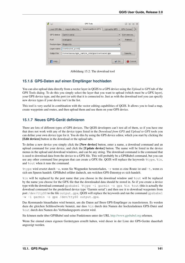
QGIS User Guide, Release 2.0
Abbildung 15.2: The download tool
15.1.6 GPS-Daten auf einen Empfänger hochladen
You can also upload data directly from a vector layer in QGIS to a GPS device using the Upload to GPS tab of theGPS Tools dialog. To do this you simply select the layer that you want to upload (which must be a GPX layer),your GPS device type, and the port (or usb) that it is connected to. Just as with the download tool you can specifynew device types if your device isn’t in the list.
This tool is very useful in combination with the vector editing capabilities of QGIS. It allows you to load a map,create waypoints and routes, and then upload them and use them on your GPS device.
15.1.7 Neues GPS-Gerät definieren
There are lots of different types of GPS devices. The QGIS developers can’t test all of them, so if you have onethat does not work with any of the device types listed in the Download from GPS and Upload to GPS tools youcan define your own device type for it. You do this by using the GPS device editor, which you start by clicking the[Edit devices] button in the download or the upload tabs.
To define a new device you simply click the [New device] button, enter a name, a download command and anupload command for your device, and click the [Update device] button. The name will be listed in the devicemenus in the upload and download windows, and can be any string. The download command is the command thatis used to download data from the device to a GPX file. This will probably be a GPSBabel command, but you canuse any other command line program that can create a GPX file. QGIS will replace the keywords %type, %in,and %out when it runs the command.
%type wird ersetzt durch -w, wenn Sie Wegpunkte herunterladen, -r wenn es eine Route ist und -t, wenn essich um Spuren handelt. GPSBabel erfährt dadurch, um welchen GPS-Datentyp es sich handelt.
%in will be replaced by the port name that you choose in the download window and %out will be replacedby the name you choose for the GPX file that the downloaded data should be stored in. So if you create a devicetype with the download command gpsbabel %type -i garmin -o gpx %in %out (this is actually thedownload command for the predefined device type ‘Garmin serial’) and then use it to download waypoints fromport /dev/ttyS0 to the file output.gpx, QGIS will replace the keywords and run the command gpsbabel-w -i garmin -o gpx /dev/ttyS0 output.gpx.
Das Kommando hinaufladen wird benutzt, um die Daten auf Ihren GPS-Empfänger zu transferieren. Es werdendazu die gleichen Schlüsselworte benutzt, nur dass %in durch den Namen der hochzuladenen GPX-Datei und%out durch den Namen des Verbindungsports ersetzt wird.
Sie können mehr über GPSBabel und seine Funktionen unter der URL http://www.gpsbabel.org erlernen.
Wenn Sie einmal einen eigenen Gerätetypen erstellt haben, wird dieser in der Liste der GPS-Geräte dauerhaftangezeigt werden.
15.1. GPS Plugin 141
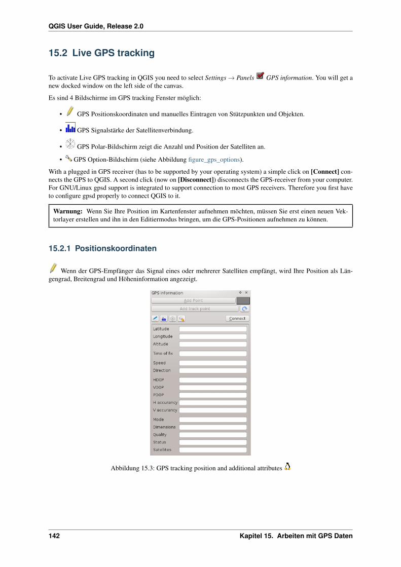
QGIS User Guide, Release 2.0
15.2 Live GPS tracking
To activate Live GPS tracking in QGIS you need to select Settings → Panels GPS information. You will get anew docked window on the left side of the canvas.
Es sind 4 Bildschirme im GPS tracking Fenster möglich:
• GPS Positionskoordinaten und manuelles Eintragen von Stützpunkten und Objekten.
• GPS Signalstärke der Satellitenverbindung.
• GPS Polar-Bildschirm zeigt die Anzahl und Position der Satelliten an.
• GPS Option-Bildschirm (siehe Abbildung figure_gps_options).
With a plugged in GPS receiver (has to be supported by your operating system) a simple click on [Connect] con-nects the GPS to QGIS. A second click (now on [Disconnect]) disconnects the GPS-receiver from your computer.For GNU/Linux gpsd support is integrated to support connection to most GPS receivers. Therefore you first haveto configure gpsd properly to connect QGIS to it.
Warnung: Wenn Sie Ihre Position im Kartenfenster aufnehmen möchten, müssen Sie erst einen neuen Vek-torlayer erstellen und ihn in den Editiermodus bringen, um die GPS-Positionen aufnehmen zu können.
15.2.1 Positionskoordinaten
Wenn der GPS-Empfänger das Signal eines oder mehrerer Satelliten empfängt, wird Ihre Position als Län-gengrad, Breitengrad und Höheninformation angezeigt.
Abbildung 15.3: GPS tracking position and additional attributes
142 Kapitel 15. Arbeiten mit GPS Daten

QGIS User Guide, Release 2.0
15.2.2 GPS Signalstärke
In diesem Fenster können Sie die Signalstärke der Satelliten sehen.
Abbildung 15.4: GPS tracking signal strength
15.2.3 GPS Polar-Bildschirm
Wenn Sie wissen wollen, wo sich die Satelliten befinden, mit denen Sie gerade verbunden sind, wechseln Siezum GPS Polarbildschirm. Sie können auch die IDs der Satelliten sehen, von denen Sie Signale empfangen.
Abbildung 15.5: GPS tracking polar window
15.2.4 GPS Optionen
Wenn es Probleme bei der Verbindung zum GPS-Gerät geben sollte können Sie innerhalb dieser Einstellungenwechseln:
• Automatisch feststellen
• Internal
• Serial device
• gpsd (selecting Host, Port and Device your GPS is connected to)
15.2. Live GPS tracking 143
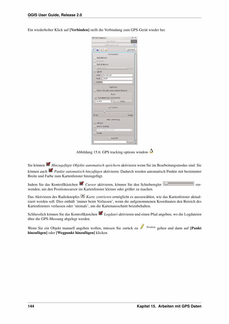
QGIS User Guide, Release 2.0
Ein wiederholter Klick auf [Verbinden] stellt die Verbindung zum GPS-Gerät wieder her.
Abbildung 15.6: GPS tracking options window
Sie können Hinzugefügte Objekte automatisch speichern aktivieren wenn Sie im Bearbeitungsmodus sind. Sie
können auch Punkte automatisch hinzufügen aktivieren. Dadurch werden automatisch Punkte mit bestimmterBreite und Farbe zum Kartenfenster hinzugefügt.
Indem Sie das Kontrollkästchen Cursor aktivieren, können Sie den Schieberegler ver-wenden, um den Positionscursor im Kartenfenster kleiner oder größer zu machen.
Das Aktivieren des Radioknopfes Karte zentrieren ermöglicht es auszuwählen, wie das Kartenfenster aktual-isiert werden soll. Dies enthält ‘immer beim Verlassen’, wenn die aufgenommenen Koordinaten den Bereich desKartenfensters verlassen oder ‘niemals’, um die Kartenausschnitt beizubehalten.
Schliesslich können Sie das Kontrollkästchen Logdatei aktivieren und einen Pfad angeben, wo die Logdateienüber die GPS-Messung abgelegt werden.
Wenn Sie ein Objekt manuell angeben wollen, müssen Sie zurück zu Position gehen und dann auf [Punkthinzufügen] oder [Wegpunkt hinzufügen] klicken.
144 Kapitel 15. Arbeiten mit GPS Daten

KAPITEL 16
GRASS GIS Integration
The GRASS plugin provides access to GRASS GIS (see GRASS-PROJECT Literatur und Internetreferenzen)databases and functionalities. This includes visualization of GRASS raster and vector layers, digitizing vectorlayers, editing vector attributes, creating new vector layers and analysing GRASS 2D and 3D data with more than400 GRASS modules.
In diesem Kapitel bekommen Sie eine Einführung in das Plugin und dessen Verwendung. Folgende Funktionenstehen über das GRASS Plugin zur Verfügung, wenn Sie es wie in Abschnitt sec_starting_grass beschriebenladen:
• Mapset öffnen
• Neues Mapset
• Schliesse Mapset
• GRASS-Vektorlayer hinzufügen
• GRASS-Rasterlayer hinzufügen
• Neuen GRASS-Vektorlayer anlegen
• GRASS-Vektorlayer bearbeiten
• GRASS-Werkzeugkiste öffnen
• Aktuelle GRASS-Region darstelllen
• Aktuelle GRASS-Region bearbeiten
16.1 GRASS Plugin starten
To use GRASS functionalities and/or visualize GRASS vector and raster layers in QGIS, you must select and load
the GRASS plugin with the Plugin Manager. Therefore go to the menu Plugins → Manage Plugins, selectGRASS and click [OK].
Sie können wie in Abschnitt sec_load_grassdata beschrieben, direkt Raster- und Vektorlayer aus einer existieren-den GRASS-Datenbank Location laden, oder Sie können eine neue GRASS Location erstellten (siehe Ab-schnitt Eine neue GRASS LOCATION erstellen), Daten in diese neue Location importieren (siehe Abschnitt im-port_loc_data) und über die GRASS-Werkzeugkiste mit den mehr als 300 GRASS Modulen analysieren (sieheAbschnitt Die GRASS-Werkzeugkiste).
145
QGIS User Guide, Release 2.0
16.2 GRASS Layer visualisieren
Wenn das GRASS-Plugin geladen ist, können Sie GRASS Vektor- und Rasterlayer mit den entsprechendenKnöpfen in der Werkzeugleiste laden. Als Beispiel benutzen wir den Alaska Beispieldatensatz (siehe KapitelBeispieldaten). Dieser enthält eine kleine GRASS LOCATION mit 3 Vektor- und einem Rasterlayer mit Höhenin-formationen.
1. Create a new folder grassdata, download the QGIS ‘Alaska’ dataset qgis_sample_data.zip fromhttp://download.osgeo.org/qgis/data/ and unzip the file into grassdata.
2. Starten Sie QGIS.
3. Falls noch nicht geschehen, laden Sie das GRASS Plugin. Dazu wechseln Sie in das Menü Erweiterungen
→ Erweiterungen verwalten und wählen GRASS aus. Die GRASS-Werkzeuge erscheinen nun inder Werkzeugleiste.
4. In the GRASS toolbar, click the Open mapset icon to bring up the MAPSET wizard.
5. Als Gisdbase suchen und wählen Sie bitte den Pfad zum Ordner grassdata.
6. Sie sollten nun als LOCATION alaska und als MAPSET demo auswählen können.
7. Klicken Sie auf [OK]. Einige weitere, zuvor grau hinterlegte GRASS-Werkzeuge sind nun aktiv.
8. Klicken Sie auf GRASS-Rasterlayer hinzufügen, wählen Sie den Layer gtopo30 und drücken Sie auf [OK].Die Höhendaten werden nun dargestellt.
9. Click on Add GRASS vector layer, choose the map name alaska and click [OK]. The Alaska boundaryvector layer will be overlayed on top of the gtopo30 map. You can now adapt the layer properties asdescribed in chapter Vektorlayereigenschaften, e.g. change opacity, fill and outline color.
10. Laden Sie auch noch die weiteren Vektorlayer rivers und airports hinzu und passen Sie deren Lay-ereigenschaften an.
As you see, it is very simple to load GRASS raster and vector layers in QGIS. See following sections for editingGRASS data and creating a new LOCATION. More sample GRASS LOCATIONs are available at the GRASSwebsite at http://grass.osgeo.org/download/sample-data/.
Tipp: Probleme beim Laden von GRASS-LayernSollten Sie Probleme beim Laden von GRASS-Layern haben (z.B. beendet sich QGIS unvorhergesehen), dannüberprüfen Sie bitte, ob das GRASS-Plugin korrekt geladen ist (siehe Abschnitt sec_starting_grass).
16.3 Information zur GRASS-Datenbank
GRASS Daten werden in einem Ordner gespeichert, der als GISDBASE bezeichnet wird. Standardmäßig wirdder Ordner grassdata genannt und er muss erstellt worden sein, bevor man beginnt, mit dem GRASS Plu-gin in QGIS zu arbeiten. Innerhalb dieses Ordners sind die GRASS Daten als Projekte (sog. LOCATION) inUnterordnern organisiert. Jede LOCATION ist durch ein Koordinatenbezugssystem und eine räumliche Gren-ze (sog. region) definiert und kann darüberhinaus weitere Unterordner MAPSETs besitzen, um die Layer derLOCATION weiter z.B. thematisch oder räumlich zu unterteilen (Neteler & Mitasova 2008 literature_and _web).Um Raster- und Vektorlayer mit den GRASS Modulen zu analysieren, müssen diese zuerst in eine passendeGRASS LOCATION importiert werden. (Dies ist nicht ganz korrekt. Mit den GRASS Modulen r.externalund v.external können Sie eine ‘read-only’ Verknüpfung zu externen durch GDAL/OGR-unterstützte Layererstellen, ohne die Daten importieren zu müssen. Da dies aber nicht der normale Weg für GRASS Anfänger ist,wird auf diese Möglichkeit nicht näher eingegangen.).
146 Kapitel 16. GRASS GIS Integration

QGIS User Guide, Release 2.0
Abbildung 16.1: GRASS data in the alaska LOCATION
16.3.1 Eine neue GRASS LOCATION erstellen
Als ein Beispiel möchten wir Ihnen zeigen, wie die GRASS Location des Alaska Beispieldatensatzes erstelltwurde. Das Koordinatenbezugssystem ist Albers Equal Area mit der Einheit ‘feet’. Diese GRASS Locationalaska wird für alle GRASS GIS Beispiele verwendet. Es ist also sinnvoll, sich diesen Datensatz zu instal-lieren (siehe Abschnitt Beispieldaten).
1. Starten Sie QGIS und laden Sie das GRASS Plugin, falls dies noch nicht geschehen ist.
2. Visualize the alaska.shp shapefile (see Section vector_load_shapefile) from the QGIS alaska datasetBeispieldaten.
3. In the GRASS toolbar, click on the New mapset icon to bring up the MAPSET wizard.
4. Wählen Sie einen existierenden Ordner mit bereits vorhandenen Locations oder erstellen Sie einen neuenOrdner grassdata für die zu erstellende Location. Klicken Sie auf [Weiter].
5. We can use this wizard to create a new MAPSET within an existing LOCATION (see section Eine neueGRASS MAPSET erstellen) or to create a new LOCATION altogether. Select Create new location (seefigure_grass_location_2).
6. Enter a name for the LOCATION - we used ‘alaska’ and click [Next].
7. Define the projection by clicking on the radio button Projection to enable the projection list.
8. We are using Albers Equal Area Alaska (feet) projection. Since we happen to know that it is representedby the EPSG ID 2964, we enter it in the search box. (Note: If you want to repeat this process for another
LOCATION and projection and haven’t memorized the EPSG ID, click on the CRS Status icon in the lowerright-hand corner of the status bar (see Section Arbeiten mit Projektionen)).
9. Geben Sie unter Filter 2964 ein um die Projektion auszuwählen.
10. Klicken Sie auf [Weiter].
11. To define the default region, we have to enter the LOCATION bounds in north, south, east, and west direc-tion. Here we simply click on the button [Set current QGIS extent], to apply the extend of the loaded layeralaska.shp as the GRASS default region extend.
16.3. Information zur GRASS-Datenbank 147

QGIS User Guide, Release 2.0
12. Klicken Sie auf [Weiter].
13. We also need to define a MAPSET within our new LOCATION. You can name it whatever you like - weused ‘demo’ (when creating a new LOCATION). GRASS automatically creates a special MAPSET calledPERMANENT designed to store the core data for the project, its default spatial extend and coordinate systemdefinitions (Neteler & Mitasova 2008 Literatur und Internetreferenzen).
14. Prüfen Sie alles, damit alles wie gewünscht ist. Klicken Sie auf [Abschliessen].
15. The new LOCATION ‘alaska’ and two MAPSETs ‘demo’ and ‘PERMANENT’ are created. The currentlyopened working set is ‘demo’, as you defined.
16. Beachten Sie, dass einige Werkzeuge des GRASS Plugins grau hinterlegt waren und nun auch zur Verfügungstehen.
Abbildung 16.2: Creating a new GRASS LOCATION or a new MAPSET in QGIS
If that seemed like a lot of steps, it’s really not all that bad and a very quick way to create a LOCATION. TheLOCATION ‘alaska‘ is now ready for data import (see section Daten in eine GRASS LOCATION importieren).You can also use the already existing vector and raster data in the sample GRASS LOCATION ‘alaska’ includedin the QGIS ‘Alaska’ dataset Beispieldaten and move on to Section Das GRASS Vektormodell.
16.3.2 Eine neue GRASS MAPSET erstellen
Ein Benutzer hat nur Schreibrechte in einer MAPSET, die er selbst erstellt hat. Darüberhinaus kann er die Dat-en der MAPSETs anderer Benutzer in der aktuellen LOCATION einsehen und für seine Analysen verwenden.Veränderungen finden aber lediglich in seiner eigenen MAPSET statt.
Alle MAPSETs enthalten eine Datei WIND, in der die aktuelle Ausdehnung und die Pixelauflösung der MAPSETgespeichert ist (Neteler & Mitasova 2008 Literatur und Internetreferenzen, siehe Abschnitt Einstellung der GRASSRegion).
1. Starten Sie QGIS und laden Sie das GRASS Plugin, falls dies noch nicht geschehen ist.
2. In the GRASS toolbar, click on the New mapset icon to bring up the MAPSET wizard.
3. Select the GRASS database (GISDBASE) folder grassdata with the LOCATION ‘alaska’, where wewant to add a further MAPSET, called ‘test’.
4. Klicken Sie auf [Weiter].
5. We can use this wizard to create a new MAPSET within an existing LOCATION or to create a newLOCATION altogether. Click on the radio button Select location (see figure_grass_location_2) and click[Next].
6. Geben Sie den Namen test für die neue MAPSET ein. Im unteren Bereich sehen Sie eine Liste bereitsvorhandener MAPSETs und ihre Besitzer.
7. Klicken Sie auf [Weiter], prüfen Sie die Einstellungen und drücken Sie dann auf [Abschließen].
148 Kapitel 16. GRASS GIS Integration
QGIS User Guide, Release 2.0
16.4 Daten in eine GRASS LOCATION importieren
This Section gives an example how to import raster and vector data into the ‘alaska’ GRASS LOCATION providedby the QGIS ‘Alaska’ dataset. Therefore we use a landcover raster map landcover.img and a vector GML filelakes.gml from the QGIS ‘Alaska’ dataset Beispieldaten.
1. Starten Sie QGIS und laden Sie das GRASS Plugin, falls dies noch nicht geschehen ist.
2. In the GRASS toolbar, click the Open MAPSET icon to bring up the MAPSET wizard.
3. Select as GRASS database the folder grassdata in the QGIS alaska dataset, as LOCATION ‘alaska’, asMAPSET ‘demo’ and click [OK].
4. Nun klicken Sie auf das Icon GRASS-Werkzeugkiste öffnen, damit die GRASS Werkzeuge (siehe Abschnitt DieGRASS-Werkzeugkiste) zur Verfügung stehen.
5. Um den Rasterlayer landcover.img zu importieren, drücken Sie auf das Modul r.in.gdal imModulbaum Reiter. Diese GRASS Module ermöglicht es, GDAL-unterstützte Rasterlayer in eine GRASSLOCATION zu importieren.
6. Browse to the folder raster in the QGIS ‘Alaska’ dataset and select the file landcover.img.
7. As raster output name define landcover_grass and click [Run]. In the Output tab you seethe currently running GRASS command r.in.gdal -o input=/path/to/landcover.imgoutput=landcover_grass.
8. Wenn Sie den Text Erfolgreich beendet sehen, klicken Sie auf den Knopf [Ergebnis visualisieren]. DerLayer landcover_grass ist nun in die aktuelle GRASS Location importiert und wird im Kartenfensterangezeigt.
9. Um den Vektor GML-Layer lakes.gml zu importieren, klicken Sie in der GRASS Werkzeugkiste aufdas Modul v.in.ogr im Modulbaum Reiter. Dieses GRASS Modul ermöglicht es, OGR-unterstützteVektorlayer in eine GRASS LOCATION zu importieren. Der Moduldialog für v.in.ogr erscheint alsneuer Reiter.
10. Browse to the folder gml in the QGIS ‘Alaska’ dataset and select the file lakes.gml as OGR file.
11. As vector output name define lakes_grass and click [Run]. You don’t have to care about the otheroptions in this example. In the Output tab you see the currently running GRASS command v.in.ogr -odsn=/path/to/lakes.gml output=lakes\_grass.
12. When it says Succesfully finished click [View output]. The lakes_grass vector layer is now importedinto GRASS and will be visualized in the QGIS canvas.
16.5 Das GRASS Vektormodell
It is important to understand the GRASS vector data model prior to digitizing.
GRASS nutzt ein topologisches Datenmodell.
Das bedeutet, dass Flächen nicht als geschlossene Polygone vorhanden sind, sondern als ein oder mehrere Umran-dungen (Boundaries). Eine Umrandung (Boundary) zwischen zwei aneinander grenzenden Flächen ist nur einmaldigitalisiert worden; beide Flächen teilen sich diese Umrandung. Umrandungen dürfen keine Lücken haben. EineFläche besteht also aus einer Umrandung und einem Zentroid, der diese Fläche als ein sog. Labelpunkt mit einerAttributtabelle verknüpft.
Neben den Umrandungen und Zentroiden kann eine Vektorkarte selbstverständlich auch Punkte und Linien en-thalten. Alle diese Geometrieelemente können innerhalb ein und dem selben Datensatz enthalten sein. Sie werdenin unterschiedlichen ‘Ebenen’ innerhalb von QGIS dargestellt. Auch wenn es möglich ist, Geometrieelemente zumischen, so ist es eigentlich unüblich und wird normalerweise auch in GRASS GIS nur selten verwendet. Etwa beiNetzwerkanalysen. Im Normalfall sollten Sie versuchen, unterschiedliche Geometrietypen in unterschiedlichenDatensätzen (Layern) zu speichern.
16.4. Daten in eine GRASS LOCATION importieren 149

QGIS User Guide, Release 2.0
Es ist auch möglich, unterschiedliche Inhalte des gleichen Geometrietyps in verschiendenen Ebenen eines Vek-torlayers zu speichern. Beispielsweise können Felder, Wälder und Seen in einem Vektordatensatz gespeichertwerden. Angrenzende Seen, Felder und Wälder teilen sich dann die gleiche Umrandung, jedoch haben sie sepa-rate Attributtabellen, die über ihre Ebene angesprochen wird. Darüber hinaus können Sie auch Attribute für dieUmrandungen vergeben, falls eine Umrandung gleichzeitg einen Weg darstellt. In diesem Fall könnte auch dieUmrandung eine separate Attributtabelle haben.
Die ‘Ebene’ eines jeden Objektes wird in GRASS intern als ‘layer’ bezeichnet. Verwechseln Sie dies bitte nichtmit dem Begriff Layer im Sinne einer Karte. Der GRASS Layer (Ebene) wird durch Zahl repräsentiert. Wennmehr als ein Layer im Datensatz enthalten ist; beim obigen Beispiel wären es 3 Layer (Felder, Wälder und Seen),gäbe es drei Layer (1,2 und 3). Derzeit werden nur Nummern als Layername unterstützt, in kommenden GRASS-Versionen werden auch Namen möglich sein.
Attribute können in externen Datenbanktabellen abgelegt werden, beispielsweise DBase, PostgreSQL, MySQL,SQLITE3, etc.
Die Attribute in den Tabellen werden über ein sog. ‘Kategoriefeld’ an die Geometrien des Datensatzes gehängt.
Die ‘Kategorie’ (oder key, ID, etc) ist eine Ganzzahl, über die eine Verknüpfung zwischen den Geometrien undden Spalten in der Datenbanktabelle hergestellt wird.
Tipp: Das GRASS Vektormodell verstehenThe best way to learn the GRASS vector model and its capabilities is to download one of the many GRASStutorials where the vector model is described more deeply. See http://grass.osgeo.org/documentation/manuals/ formore information, books and tutorials in several languages.
16.6 Einen neuen GRASS Vektorlayer erstellen
Einen neuen GRASS Vektorlayer können Sie erstellen, indem Sie auf das Icon Neuen GRASS-Vektorlayer anlegen inder GRASS Werkzeugleiste klicken. Geben Sie einen Namen in der Textbox für den neuen GRASS Vektorlayeran und Sie können in dem Layer neue Geometrien erzeugen, wie in Abschnitt Digitalisieren und Editieren einesGRASS Vektorlayers beschrieben.
In GRASS it is possible to organize all sort of geometry types (point, line and area) in one layer, because GRASSuses a topological vector model, so you don’t need to select the geometry type when creating a new GRASS vector.This is different from Shapefile creation with QGIS, because Shapefiles use the Simple Feature vector model (seeSection Creating new Vector layers).
Tipp: Erstellen einer Attributtabelle für einen neuen GRASS VektorlayerWenn Sie für ihre digitalisierten Geometrien auch eine Attributtabelle erstellen wollen, müssen Sie nach demAnlegen des GRASS-Vektorlayers eine Attributtabelle mit entsprechenden Spalten erstellen, bevor Sie mit demDigitalisieren beginnen (siehe figure_grass_digitizing_5).
16.7 Digitalisieren und Editieren eines GRASS Vektorlayers
Die Digitalisierwerkzeuge für GRASS-Vektorlayer werden über den Knopf GRASS-Vektorlayer bearbeiten in derGRASS-Werkzeugleiste gestartet. Dazu müssen Sie den zu bearbeitenden Layer in der Legende auswählen, bevorSie auf den Editier-Knopf drücken. Abbildung figure_grass_digitizing_2 zeigt den Dialog für die GRASS Digi-talisierung. Die einzelnen Werkzeuge werden im folgenden Kapitel beschrieben.
Tipp: Polygone in GRASS digitalisierenWenn Sie ein Polygon innerhalb eines GRASS Vektorlayers erstellen wollen, digitalisieren Sie zuerst die Gren-ze (Boundary) der Fläche mit der Moduseinstellung ‘Keine Kategorie’. Danach fügen Sie einen Zentroid (La-
150 Kapitel 16. GRASS GIS Integration
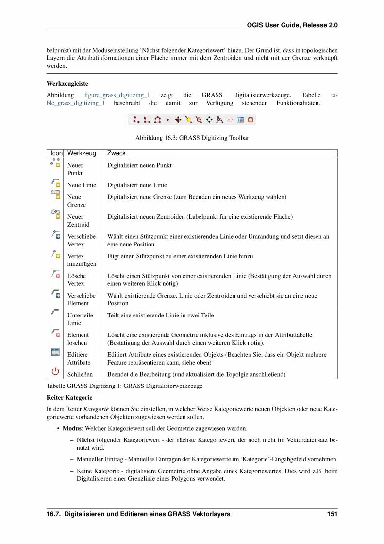
QGIS User Guide, Release 2.0
belpunkt) mit der Moduseinstellung ‘Nächst folgender Kategoriewert’ hinzu. Der Grund ist, dass in topologischenLayern die Attributinformationen einer Fläche immer mit dem Zentroiden und nicht mit der Grenze verknüpftwerden.
Werkzeugleiste
Abbildung figure_grass_digitizing_1 zeigt die GRASS Digitalisierwerkzeuge. Tabelle ta-ble_grass_digitizing_1 beschreibt die damit zur Verfügung stehenden Funktionalitäten.
Abbildung 16.3: GRASS Digitizing Toolbar
Icon Werkzeug Zweck
NeuerPunkt
Digitalisiert neuen Punkt
Neue Linie Digitalisiert neue Linie
NeueGrenze
Digitalisiert neue Grenze (zum Beenden ein neues Werkzeug wählen)
NeuerZentroid
Digitalisiert neuen Zentroiden (Labelpunkt für eine existierende Fläche)
VerschiebeVertex
Wählt einen Stützpunkt einer existierenden Linie oder Umrandung und setzt diesen aneine neue Position
Vertexhinzufügen
Fügt einen Stützpunkt zu einer existierenden Linie hinzu
LöscheVertex
Löscht einen Stützpunkt von einer existierenden Linie (Bestätigung der Auswahl durcheinen weiteren Klick nötig)
VerschiebeElement
Wählt existierende Grenze, Linie oder Zentroiden und verschiebt sie an eine neuePosition
UnterteileLinie
Teilt eine existierende Linie in zwei Teile
Elementlöschen
Löscht eine existierende Geometrie inklusive des Eintrags in der Attributtabelle(Bestätigung der Auswahl durch einen weiteren Klick nötig).
EditiereAttribute
Editiert Attribute eines existierenden Objekts (Beachten Sie, dass ein Objekt mehrereFeature repräsentieren kann, siehe oben)
Schließen Beendet die Bearbeitung (und aktualisiert die Topolgie anschließend)
Tabelle GRASS Digitizing 1: GRASS Digitalisierwerkzeuge
Reiter Kategorie
In dem Reiter Kategorie können Sie einstellen, in welcher Weise Kategoriewerte neuen Objekten oder neue Kate-goriewerte vorhandenen Objekten zugewiesen werden sollen.
• Modus: Welcher Kategoriewert soll der Geometrie zugewiesen werden.
– Nächst folgender Kategoriewert - der nächste Kategoriewert, der noch nicht im Vektordatensatz be-nutzt wird.
– Manueller Eintrag - Manuelles Eintragen der Kategoriewerte im ‘Kategorie’-Eingabgefeld vornehmen.
– Keine Kategorie - digitalisiere Geometrie ohne Angabe eines Kategoriewertes. Dies wird z.B. beimDigitalisieren einer Grenzlinie eines Polygons verwendet.
16.7. Digitalisieren und Editieren eines GRASS Vektorlayers 151

QGIS User Guide, Release 2.0
Abbildung 16.4: GRASS Digitizing Category Tab
• Kategorie - eine Nummer (ID), die dem digitalisierten Objekt zugewiesen wird und auf einen Eintrag inder Attributtabelle verweist.
• Layer - Objektidentifikation über die GRASS-Ebene (layer). Der Standardlayer in GRASS ist 1.
Tipp: Erzeugen von weiteren GRASS ‘Layern’ mit QGISWenn Sie weitere Ebenen (Layer) ihrem Datensatz hinzufügen wollen, so können Sie einfach eine neue Zahlin das ‘Layer’-Feld eintippen und im Anschluss Return drücken. Im Reiter ‘Tabelle’ können Sie nun eine neueAttributtabelle erstellen und diese mit dem neuen ‘Layer’ verbinden.
Reiter Einstellungen
Der Reiter Einstellungen erlaubt das Setzen der Fangtoleranz in Bildschirmpixeln. Dies ist der Schwellenwertin Pixeln, innerhalb dessen neu digitalisierte Knotenpunkte an vorhandene Knoten gesnappt werden. Dies hilft,Lücken oder Überlagerungen zwischen Objekten zu vermeiden. Der Standardwert ist auf 10 Pixel eingestellt.
Abbildung 16.5: GRASS Digitizing Settings Tab
Darstellung Reiter
Der Reiter Darstellung erlaubt die Farbeinstellungen für die verschiedenen Geometrietypen und ihren Topologi-estatus (z.B. offene/geschlossene Fläche).
Reiter Tabelle
Der Reiter Tabelle gibt Informationen über die Attributtabelle des aktuellen Layers. In diesem Reiter könnenSie eine Attributtabelle hinzufügen, modifizieren oder eine neue Tabelle erstellen (siehe Abschnitt Einen neuenGRASS Vektorlayer erstellen).
Tipp: GRASS SchreibberechtigungUm einen Datensatz zu editieren, müssen Sie der Besitzer des aktuellen GRASS-Mapsets sein. Es ist nichtmöglich, Karten aus einem Mapset zu editieren, das Ihnen nicht ‘gehört’, auch wenn Sie auf Dateisystemebenedie Schreibrechte haben.
152 Kapitel 16. GRASS GIS Integration
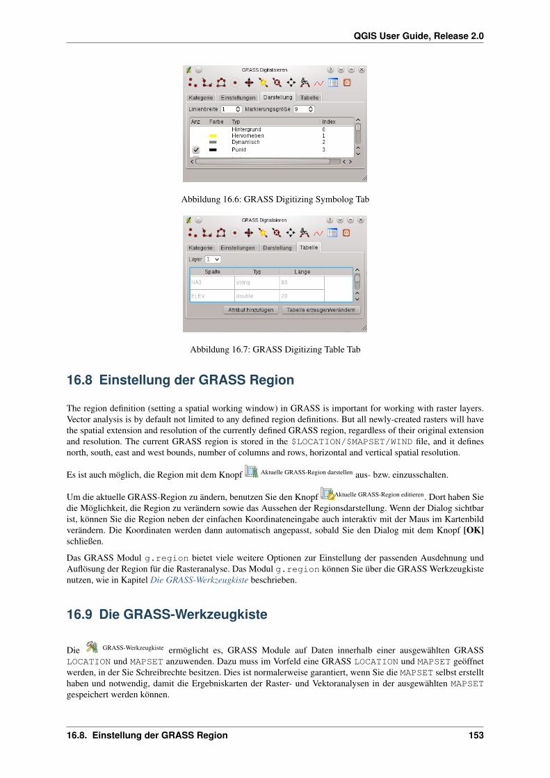
QGIS User Guide, Release 2.0
Abbildung 16.6: GRASS Digitizing Symbolog Tab
Abbildung 16.7: GRASS Digitizing Table Tab
16.8 Einstellung der GRASS Region
The region definition (setting a spatial working window) in GRASS is important for working with raster layers.Vector analysis is by default not limited to any defined region definitions. But all newly-created rasters will havethe spatial extension and resolution of the currently defined GRASS region, regardless of their original extensionand resolution. The current GRASS region is stored in the $LOCATION/$MAPSET/WIND file, and it definesnorth, south, east and west bounds, number of columns and rows, horizontal and vertical spatial resolution.
Es ist auch möglich, die Region mit dem Knopf Aktuelle GRASS-Region darstellen aus- bzw. einzusschalten.
Um die aktuelle GRASS-Region zu ändern, benutzen Sie den Knopf Aktuelle GRASS-Region editieren. Dort haben Siedie Möglichkeit, die Region zu verändern sowie das Aussehen der Regionsdarstellung. Wenn der Dialog sichtbarist, können Sie die Region neben der einfachen Koordinateneingabe auch interaktiv mit der Maus im Kartenbildverändern. Die Koordinaten werden dann automatisch angepasst, sobald Sie den Dialog mit dem Knopf [OK]schließen.
Das GRASS Modul g.region bietet viele weitere Optionen zur Einstellung der passenden Ausdehnung undAuflösung der Region für die Rasteranalyse. Das Modul g.region können Sie über die GRASS Werkzeugkistenutzen, wie in Kapitel Die GRASS-Werkzeugkiste beschrieben.
16.9 Die GRASS-Werkzeugkiste
Die GRASS-Werkzeugkiste ermöglicht es, GRASS Module auf Daten innerhalb einer ausgewählten GRASSLOCATION und MAPSET anzuwenden. Dazu muss im Vorfeld eine GRASS LOCATION und MAPSET geöffnetwerden, in der Sie Schreibrechte besitzen. Dies ist normalerweise garantiert, wenn Sie die MAPSET selbst erstellthaben und notwendig, damit die Ergebniskarten der Raster- und Vektoranalysen in der ausgewählten MAPSETgespeichert werden können.
16.8. Einstellung der GRASS Region 153

QGIS User Guide, Release 2.0
Abbildung 16.8: GRASS Toolbox and Module Tree
Die GRASS Shell der Werkzeugkiste bietet Zugriff auf fast alle (mehr als 330) GRASS Module über die Kom-mandozeile. Um eine benutzfreundliche Umgebung zu bieten, sind davon etwa 200 Module graphisch auswählbarund bieten einen Dialog in Form eines zusätzlichen Reiters in der Werkzeugkiste.
16.9.1 Arbeiten mit GRASS Modulen
Das GRASS Shell Modul in der Werkzeugkiste bietet Zugriff auf fast alle in GRASS GIS vorhandenen Module(mehr als 330). Um die Verwendung benutzerfreundlicher zu gestalten, sind etwa 200 Module über grafischeDialoge in die Werkzeugkiste integriert. Diese Module sind thematisch untergliedert, können aber auch durchsuchtwerden.
A complete list of GRASS modules available in the graphical Toolbox in QGIS version 2.0 is available in theGRASS wiki (http://grass.osgeo.org/wiki/GRASS-QGIS_relevant_module_list).
Es ist außerdem möglich, die GRASS Werkzeugkiste anzupassen und weitere Module zu integrieren. Die Herange-hensweise ist in Abschnitt Anpassen der Module beschrieben.
Wie in Abbildung figure_grass_toolbox_1 zu sehen, können Sie nach dem passenden GRASS Modul in demReiter Modulbaum nachschauen oder im Reiter Modulliste suchen.
Wenn Sie auf das grafische Icon eines Modules klicken, öffnet sich ein neuer Moduldialog mit drei Reitern Optio-nen, Ergebnis und Handbuch.
Optionen
Der Reiter Optionen stellt Ihnen in vereinfachter Form die unbedingt notwendigen Eingabeparameter zur Verfü-gung, die das Modul zum Laufen benötigt.
Bitte beachten Sie, dass diese Eingabefelder extra so einfach wie möglich gehalten wurden, um die Struktur klarzu halten. Falls Sie alle vom Modul unterstützten Parameter benötigen, nutzen Sie die GRASS-Eingabeshell, inder Sie das Modul ebenfalls aufrufen können.
A new feature since QGIS 1.8 is the support for a show advanced options button below the simplified moduledialog in the Options tab. At the moment it is only added to the module v.in.ascii as an example use, but willprobably be part of more / all modules in the GRASS toolbox in future versions of QGIS. This allows to use thecomplete GRASS module options without the need to switch to the GRASS Shell.
Ergebnis
Der Reiter Ergebnis stellt die Ausgabe des Moduls zur Laufzeit dar. Nachdem Sie den Knopf [Los] gedrückthaben, wird auf diesen Reiter gewechselt und Sie sehen die Statusausgaben des Moduls. Wenn alles funktionierthat, sehen Sie den Ausgabetext Erfolgreich beendet.
154 Kapitel 16. GRASS GIS Integration
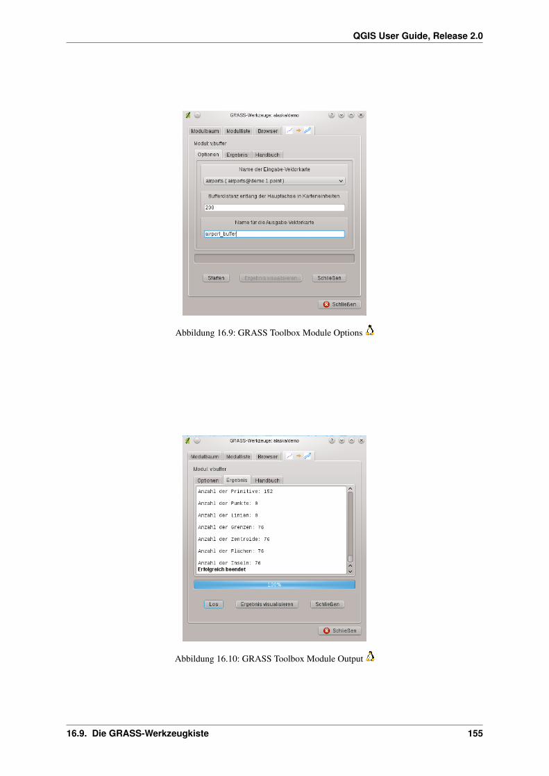
QGIS User Guide, Release 2.0
Abbildung 16.9: GRASS Toolbox Module Options
Abbildung 16.10: GRASS Toolbox Module Output
16.9. Die GRASS-Werkzeugkiste 155
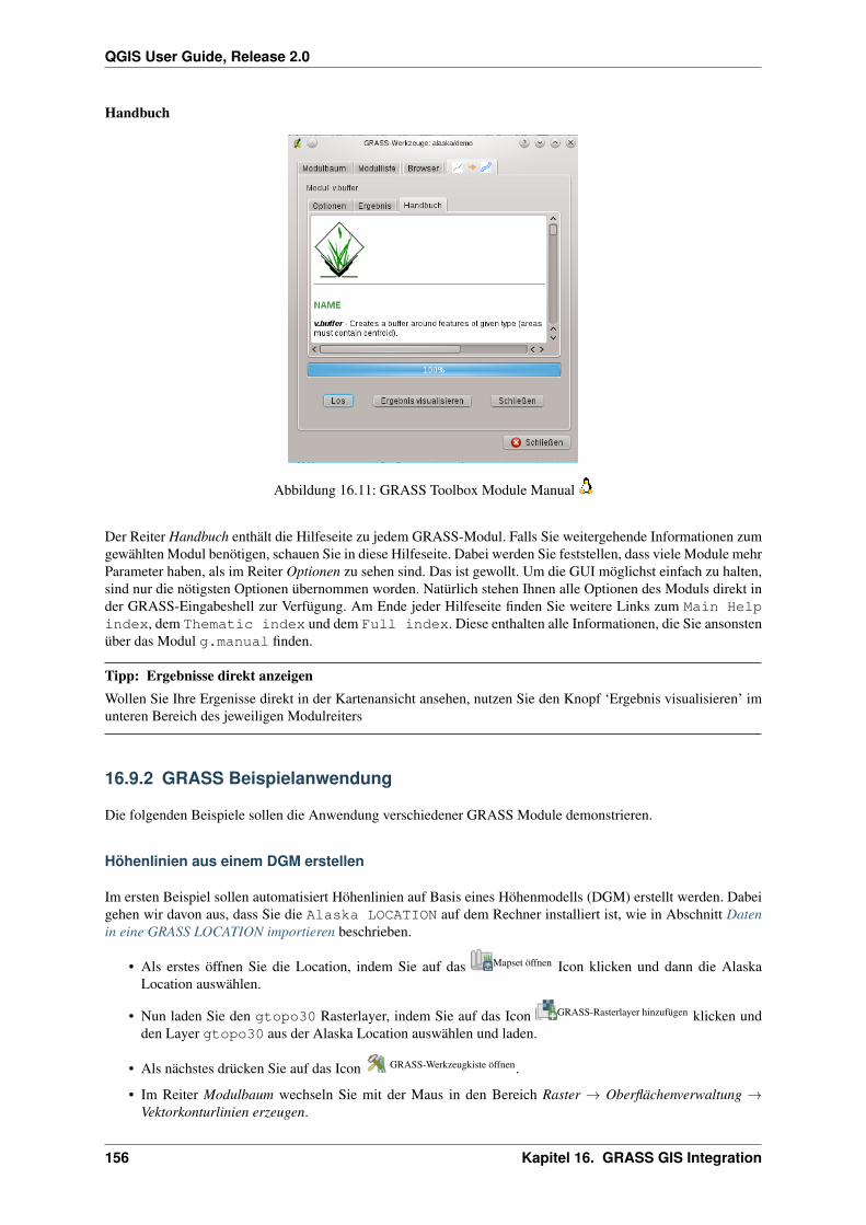
QGIS User Guide, Release 2.0
Handbuch
Abbildung 16.11: GRASS Toolbox Module Manual
Der Reiter Handbuch enthält die Hilfeseite zu jedem GRASS-Modul. Falls Sie weitergehende Informationen zumgewählten Modul benötigen, schauen Sie in diese Hilfeseite. Dabei werden Sie feststellen, dass viele Module mehrParameter haben, als im Reiter Optionen zu sehen sind. Das ist gewollt. Um die GUI möglichst einfach zu halten,sind nur die nötigsten Optionen übernommen worden. Natürlich stehen Ihnen alle Optionen des Moduls direkt inder GRASS-Eingabeshell zur Verfügung. Am Ende jeder Hilfeseite finden Sie weitere Links zum Main Helpindex, dem Thematic index und dem Full index. Diese enthalten alle Informationen, die Sie ansonstenüber das Modul g.manual finden.
Tipp: Ergebnisse direkt anzeigenWollen Sie Ihre Ergenisse direkt in der Kartenansicht ansehen, nutzen Sie den Knopf ‘Ergebnis visualisieren’ imunteren Bereich des jeweiligen Modulreiters
16.9.2 GRASS Beispielanwendung
Die folgenden Beispiele sollen die Anwendung verschiedener GRASS Module demonstrieren.
Höhenlinien aus einem DGM erstellen
Im ersten Beispiel sollen automatisiert Höhenlinien auf Basis eines Höhenmodells (DGM) erstellt werden. Dabeigehen wir davon aus, dass Sie die Alaska LOCATION auf dem Rechner installiert ist, wie in Abschnitt Datenin eine GRASS LOCATION importieren beschrieben.
• Als erstes öffnen Sie die Location, indem Sie auf das Mapset öffnen Icon klicken und dann die AlaskaLocation auswählen.
• Nun laden Sie den gtopo30 Rasterlayer, indem Sie auf das Icon GRASS-Rasterlayer hinzufügen klicken undden Layer gtopo30 aus der Alaska Location auswählen und laden.
• Als nächstes drücken Sie auf das Icon GRASS-Werkzeugkiste öffnen.
• Im Reiter Modulbaum wechseln Sie mit der Maus in den Bereich Raster → Oberflächenverwaltung →Vektorkonturlinien erzeugen.
156 Kapitel 16. GRASS GIS Integration
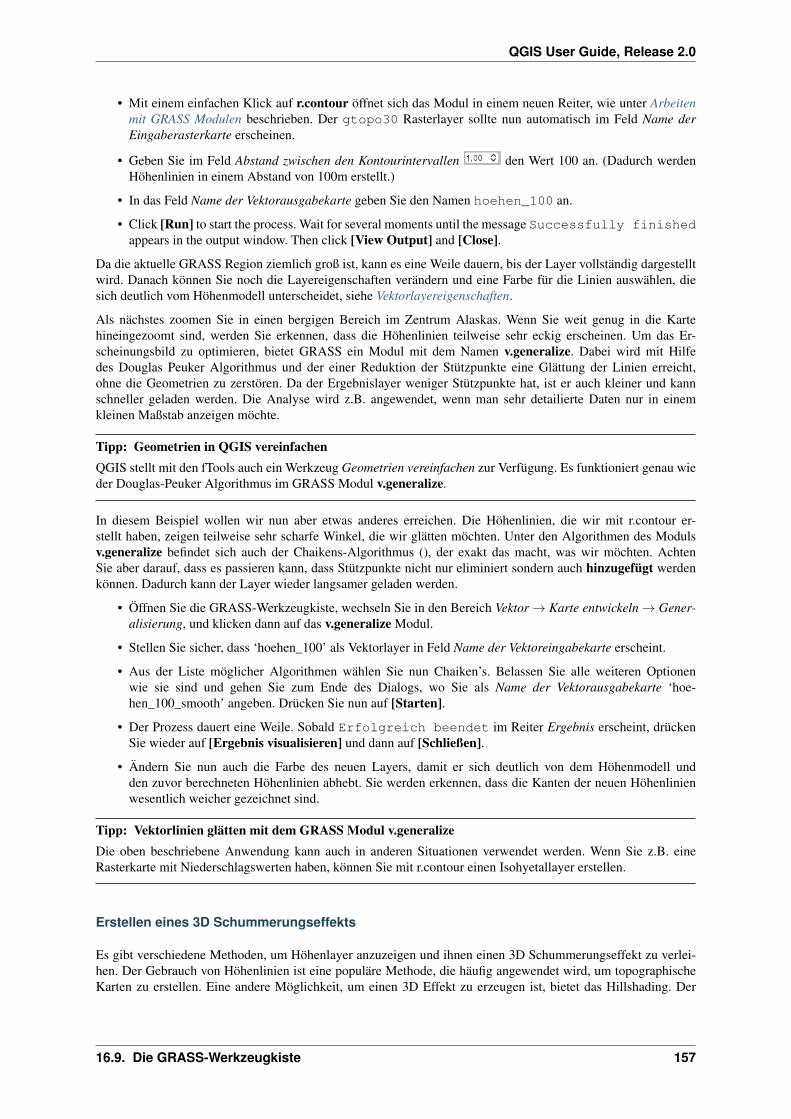
QGIS User Guide, Release 2.0
• Mit einem einfachen Klick auf r.contour öffnet sich das Modul in einem neuen Reiter, wie unter Arbeitenmit GRASS Modulen beschrieben. Der gtopo30 Rasterlayer sollte nun automatisch im Feld Name derEingaberasterkarte erscheinen.
• Geben Sie im Feld Abstand zwischen den Kontourintervallen den Wert 100 an. (Dadurch werdenHöhenlinien in einem Abstand von 100m erstellt.)
• In das Feld Name der Vektorausgabekarte geben Sie den Namen hoehen_100 an.
• Click [Run] to start the process. Wait for several moments until the message Successfully finishedappears in the output window. Then click [View Output] and [Close].
Da die aktuelle GRASS Region ziemlich groß ist, kann es eine Weile dauern, bis der Layer vollständig dargestelltwird. Danach können Sie noch die Layereigenschaften verändern und eine Farbe für die Linien auswählen, diesich deutlich vom Höhenmodell unterscheidet, siehe Vektorlayereigenschaften.
Als nächstes zoomen Sie in einen bergigen Bereich im Zentrum Alaskas. Wenn Sie weit genug in die Kartehineingezoomt sind, werden Sie erkennen, dass die Höhenlinien teilweise sehr eckig erscheinen. Um das Er-scheinungsbild zu optimieren, bietet GRASS ein Modul mit dem Namen v.generalize. Dabei wird mit Hilfedes Douglas Peuker Algorithmus und der einer Reduktion der Stützpunkte eine Glättung der Linien erreicht,ohne die Geometrien zu zerstören. Da der Ergebnislayer weniger Stützpunkte hat, ist er auch kleiner und kannschneller geladen werden. Die Analyse wird z.B. angewendet, wenn man sehr detailierte Daten nur in einemkleinen Maßstab anzeigen möchte.
Tipp: Geometrien in QGIS vereinfachenQGIS stellt mit den fTools auch ein Werkzeug Geometrien vereinfachen zur Verfügung. Es funktioniert genau wieder Douglas-Peuker Algorithmus im GRASS Modul v.generalize.
In diesem Beispiel wollen wir nun aber etwas anderes erreichen. Die Höhenlinien, die wir mit r.contour er-stellt haben, zeigen teilweise sehr scharfe Winkel, die wir glätten möchten. Unter den Algorithmen des Modulsv.generalize befindet sich auch der Chaikens-Algorithmus (), der exakt das macht, was wir möchten. AchtenSie aber darauf, dass es passieren kann, dass Stützpunkte nicht nur eliminiert sondern auch hinzugefügt werdenkönnen. Dadurch kann der Layer wieder langsamer geladen werden.
• Öffnen Sie die GRASS-Werkzeugkiste, wechseln Sie in den Bereich Vektor → Karte entwickeln → Gener-alisierung, und klicken dann auf das v.generalize Modul.
• Stellen Sie sicher, dass ‘hoehen_100’ als Vektorlayer in Feld Name der Vektoreingabekarte erscheint.
• Aus der Liste möglicher Algorithmen wählen Sie nun Chaiken’s. Belassen Sie alle weiteren Optionenwie sie sind und gehen Sie zum Ende des Dialogs, wo Sie als Name der Vektorausgabekarte ‘hoe-hen_100_smooth’ angeben. Drücken Sie nun auf [Starten].
• Der Prozess dauert eine Weile. Sobald Erfolgreich beendet im Reiter Ergebnis erscheint, drückenSie wieder auf [Ergebnis visualisieren] und dann auf [Schließen].
• Ändern Sie nun auch die Farbe des neuen Layers, damit er sich deutlich von dem Höhenmodell undden zuvor berechneten Höhenlinien abhebt. Sie werden erkennen, dass die Kanten der neuen Höhenlinienwesentlich weicher gezeichnet sind.
Tipp: Vektorlinien glätten mit dem GRASS Modul v.generalizeDie oben beschriebene Anwendung kann auch in anderen Situationen verwendet werden. Wenn Sie z.B. eineRasterkarte mit Niederschlagswerten haben, können Sie mit r.contour einen Isohyetallayer erstellen.
Erstellen eines 3D Schummerungseffekts
Es gibt verschiedene Methoden, um Höhenlayer anzuzeigen und ihnen einen 3D Schummerungseffekt zu verlei-hen. Der Gebrauch von Höhenlinien ist eine populäre Methode, die häufig angewendet wird, um topographischeKarten zu erstellen. Eine andere Möglichkeit, um einen 3D Effekt zu erzeugen ist, bietet das Hillshading. Der
16.9. Die GRASS-Werkzeugkiste 157
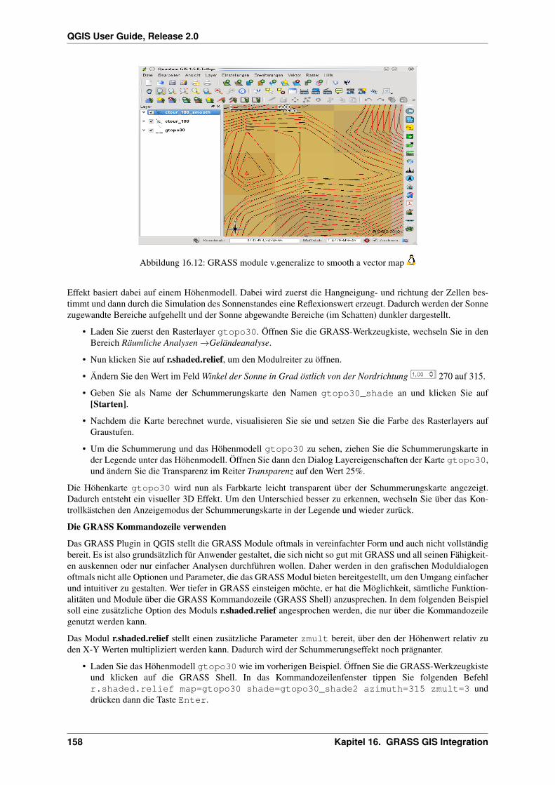
QGIS User Guide, Release 2.0
Abbildung 16.12: GRASS module v.generalize to smooth a vector map
Effekt basiert dabei auf einem Höhenmodell. Dabei wird zuerst die Hangneigung- und richtung der Zellen bes-timmt und dann durch die Simulation des Sonnenstandes eine Reflexionswert erzeugt. Dadurch werden der Sonnezugewandte Bereiche aufgehellt und der Sonne abgewandte Bereiche (im Schatten) dunkler dargestellt.
• Laden Sie zuerst den Rasterlayer gtopo30. Öffnen Sie die GRASS-Werkzeugkiste, wechseln Sie in denBereich Räumliche Analysen →Geländeanalyse.
• Nun klicken Sie auf r.shaded.relief, um den Modulreiter zu öffnen.
• Ändern Sie den Wert im Feld Winkel der Sonne in Grad östlich von der Nordrichtung 270 auf 315.
• Geben Sie als Name der Schummerungskarte den Namen gtopo30_shade an und klicken Sie auf[Starten].
• Nachdem die Karte berechnet wurde, visualisieren Sie sie und setzen Sie die Farbe des Rasterlayers aufGraustufen.
• Um die Schummerung und das Höhenmodell gtopo30 zu sehen, ziehen Sie die Schummerungskarte inder Legende unter das Höhenmodell. Öffnen Sie dann den Dialog Layereigenschaften der Karte gtopo30,und ändern Sie die Transparenz im Reiter Transparenz auf den Wert 25%.
Die Höhenkarte gtopo30 wird nun als Farbkarte leicht transparent über der Schummerungskarte angezeigt.Dadurch entsteht ein visueller 3D Effekt. Um den Unterschied besser zu erkennen, wechseln Sie über das Kon-trollkästchen den Anzeigemodus der Schummerungskarte in der Legende und wieder zurück.
Die GRASS Kommandozeile verwenden
Das GRASS Plugin in QGIS stellt die GRASS Module oftmals in vereinfachter Form und auch nicht vollständigbereit. Es ist also grundsätzlich für Anwender gestaltet, die sich nicht so gut mit GRASS und all seinen Fähigkeit-en auskennen oder nur einfacher Analysen durchführen wollen. Daher werden in den grafischen Moduldialogenoftmals nicht alle Optionen und Parameter, die das GRASS Modul bieten bereitgestellt, um den Umgang einfacherund intuitiver zu gestalten. Wer tiefer in GRASS einsteigen möchte, er hat die Möglichkeit, sämtliche Funktion-alitäten und Module über die GRASS Kommandozeile (GRASS Shell) anzusprechen. In dem folgenden Beispielsoll eine zusätzliche Option des Moduls r.shaded.relief angesprochen werden, die nur über die Kommandozeilegenutzt werden kann.
Das Modul r.shaded.relief stellt einen zusätzliche Parameter zmult bereit, über den der Höhenwert relativ zuden X-Y Werten multipliziert werden kann. Dadurch wird der Schummerungseffekt noch prägnanter.
• Laden Sie das Höhenmodell gtopo30 wie im vorherigen Beispiel. Öffnen Sie die GRASS-Werkzeugkisteund klicken auf die GRASS Shell. In das Kommandozeilenfenster tippen Sie folgenden Befehlr.shaded.relief map=gtopo30 shade=gtopo30_shade2 azimuth=315 zmult=3 unddrücken dann die Taste Enter.
158 Kapitel 16. GRASS GIS Integration

QGIS User Guide, Release 2.0
Abbildung 16.13: The GRASS shell, r.shaded.relief module
• Wenn die Berechnung abgeschlossen ist, wechseln Sie den Reiter Browser und Doppelklicken Sie auf dieneu erstellte Karte gtopo30_shade2, um Sie in QGIS anzuzeigen.
• Visualisieren Sie die Karten wie in dem obigen Beispiel beschrieben. Sie sollten dabei erkennen, dass derSchummerungseffekt stärker ist, wenn der zmult Parameter verwendet wird.
Abbildung 16.14: Displaying shaded relief created with the GRASS module r.shaded.relief
Rasterstatistik auf Basis eines Vektorlayer berechnen
Das folgende Beispiel zeigt, wie man univariate Statistik für Rasterwerte innerhalb von Vektorpolygonen berech-nen kann und die Werte in neue Attributspalten des Vektorlayers hinzufügt.
• Verwenden Sie wieder die Alaska Location (siehe Abschnitt Daten in eine GRASS LOCATION importieren),und importieren Sie das Shapefile trees aus dem Ordner shapefiles nach GRASS.
• Als erstes müssen dem Layer trees Zentroide (Labelpunkte) hinzugefügt werden. Dadurch wird es ein ko-rrekter topologischer Datensatz, bei dem an die Labelpunkte die Attribute aus der statistischen Analyseangehängt werden können.
• Wählen Sie aus der GRASS-Werkzeugkiste Vektor → Karte entwickeln →Objekte verwalten, und öffnenSie das Modul v.centroids.
• Geben Sie als Name für die Ausgabe-Vektorkarte ‘forest_areas’ an und starten Sie das Modul.
• Nun laden Sie den neuen Layer forest_areas und visualisieren Sie die verschiedenen Waldtypen inverschiedenen Farben - deciduous, evergreen und mixed. Dazu öffnen Sie den Dialog Eigenschaften des
16.9. Die GRASS-Werkzeugkiste 159

QGIS User Guide, Release 2.0
Layers, wechseln zum Reiter Darstellung, wählen ‘Eindeutiger Wert’ und setzen das Klassifikations-feld auf ‘VEGDESC’ (siehe auch Abschnitt sec_symbology).
• Als nächstes öffnen Sie wieder die GRASS-Werkzeugkiste und wechseln nach Vektor → Vektor mit anderenKarten aktualisieren.
• Klicken Sie auf das v.rast.stats Modul. Geben Sie als Name der Rasterkarte für die Statistiken berechnetwerden sollen gtopo30 und als Name der Vektorkarte (Polygone) forest_areas an.
• Nun fehlt nur noch ein Parameter: Geben Sie als Spaltenpräfix elev an, und klicken Sie dann auf [Starten].Die Berechnung wird ziemlich lange dauern (bis zu mehreren Stunden).
• Wenn es erfolgreich beendet wurden. öffnen Sie den Layer forest_areas erneut und lassen Sie sichdie Attributtabelle anzeigen. Dort gibt es nun weitere Spalten, in denen die Ergebnisse der univariateStatistik für Rasterwerte innerhalb der Vektorpolygone angezeigt werden, z.B.: elev_min, elev_max,elev_mean.
16.9.3 Der GRASS Datei-Browser
Eine weitere interessante Funktion in den GRASS-Werkzeugen ist der Browser. In figure_grass_module_7 könnenSie die aktuelle LOCATION mit den dazu gehörigen MAPSETs sehen.
In der linken Hälfte des Datei-Browsers können Sie sich alle in der aktuellen Location enthaltenen Mapsets an-schauen. In der rechten Hälfte des Fensters sehen Sie weitere Metainformationen zum ausgewählten Datensatz wiebeispielsweise Auflösung, BoundingBox, Datenquelle, bei Vektordaten die Attributtabelle und die COMMANDGeschichte.
Abbildung 16.15: GRASS LOCATION browser
Die Werkzeugleiste im GRASS Datei-Browser stellt folgende Werkzeuge für die ausgewählte LOCATION zurVerfügung:
• Ausgewählten Layer dem Kartenfenster hinzufügen
• Gewählte Karte kopieren
• Gewählte Karte umbenennen
• Gewählte Karte löschen
• Setze die Region auf die gewählte Karte
160 Kapitel 16. GRASS GIS Integration

QGIS User Guide, Release 2.0
• Neu zeichnen
Die Knöpfe Gewählte Karte umbenennen und Gewählte Karte löschen stehen nur für die aktuelleMAPSET zur Verfügung. Die anderen Werkzeuge funktionieren auch in den anderen MAPSETs.
16.9.4 Anpassen der Module
Nahezu alle GRASS-Module können in die GRASS-Werkzeugkiste integriert werden. Eine XML-Schnittstellewertet die sehr einfachen XML-Dateien, die die Module beschreiben, aus und übernimmt die Oberflächendarstel-lung.
Beispielhaft ist hier die XML-Datei zum Modul v.buffer (v.buffer.qgm) dargestellt:
<?xml version="1.0" encoding="UTF-8"?><!DOCTYPE qgisgrassmodule SYSTEM "http://mrcc.com/qgisgrassmodule.dtd">
<qgisgrassmodule label="Vector buffer" module="v.buffer"><option key="input" typeoption="type" layeroption="layer" /><option key="buffer"/><option key="output" />
</qgisgrassmodule>
Der XML-Auswerter liest diese Definition und erstellt einen neuen Reiter im Werkzeugkiste, wenn Sie das Modulauswählen. Ein detailierte Beschreibung, um neue Module in die GRASS Werkzeugkiste zu integrieren finden Sieunter: http://wiki.qgis.org/qgiswiki/Adding_New_Tools_to_the_GRASS_Toolbox
16.9. Die GRASS-Werkzeugkiste 161
QGIS User Guide, Release 2.0
162 Kapitel 16. GRASS GIS Integration
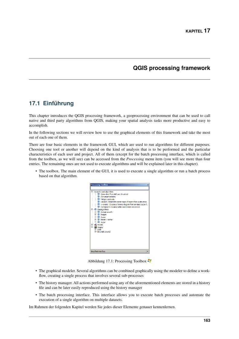
KAPITEL 17
QGIS processing framework
17.1 Einführung
This chapter introduces the QGIS processing framework, a geoprocessing environment that can be used to callnative and third party algorithms from QGIS, making your spatial analysis tasks more productive and easy toaccomplish.
In the following sections we will review how to use the graphical elements of this framework and take the mostout of each one of them.
There are four basic elements in the framework GUI, which are used to run algorithms for different purposes.Choosing one tool or another will depend on the kind of analysis that is to be performed and the particularcharacteristics of each user and project. All of them (except for the batch processing interface, which is calledfrom the toolbox, as we will see) can be accessed from the Processing menu item (you will see more than fourentries. The remaining ones are not used to execute algorithms and will be explained later in this chapter).
• The toolbox. The main element of the GUI, it is used to execute a single algorithm or run a batch processbased on that algorithm.
Abbildung 17.1: Processing Toolbox
• The graphical modeler. Several algorithms can be combined graphically using the modeler to define a work-flow, creating a single process that involves several sub-processes
• The history manager. All actions performed using any of the aforementioned elements are stored in a historyfile and can be later easily reproduced using the history manager
• The batch processing interface. This interface allows you to execute batch processes and automate theexecution of a single algorithm on multiple datasets.
Im Rahmen der folgenden Kapitel werden Sie jedes dieser Elemente genauer kennenlernen.
163
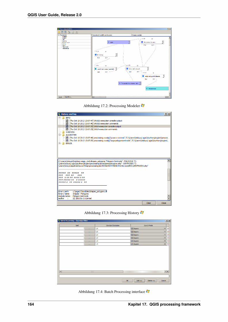
QGIS User Guide, Release 2.0
Abbildung 17.2: Processing Modeler
Abbildung 17.3: Processing History
Abbildung 17.4: Batch Processing interface
164 Kapitel 17. QGIS processing framework

QGIS User Guide, Release 2.0
17.2 The toolbox
The Toolbox is the main element of the processing GUI, and the one that you are more likely to use in your dailywork. It shows the list of all available algorithms grouped in different blocks, and is the access point to run themwhether as a single process or as a batch process involving several executions of a same algorithm on differentsets of inputs.
Abbildung 17.5: Processing Toolbox
The toolbox contains all the available algorithms, divided into predefined groups. All these groups are found undera single tree entry named Geoalgorithms.
Additionally, two more entries are found, namely Models and Scripts. These include user-created algorithms, andallow you to define your own workflows and processing tasks. We will devote a full section to them a bit later.
Im oberen Teil der Toolbox finden Sie ein Suchfeld. Um die Anzahl der angezeigten Algorithmen in der Toolboxzu reduzieren und es leichter zu machen, Sie zu finden, können Sie ein beliebiges Wort oder Satz in das Textfeldeingeben. Beachten Sie, während Sie schreiben wird die Anzahl der Algorithmen in der Toolbox reduziert, so dassnur diejenigen sichtbar sind, die den Text enthalten, den Sie im Suchfeld eingeben haben.
In the lower part you will find a box that allows you to switch between the simplified algorithm list (the oneexplained above), and the advanced list. If you change to the advanced mode, the toolbox will look like this:
Abbildung 17.6: Processing Toolbox (advanced mode)
In the advanced view, each group represents a so-called ‘algorithm provider’, which is a set of algorithms coming
17.2. The toolbox 165

QGIS User Guide, Release 2.0
from the same source, for instance, from a third-party application with geoprocessing capabilities. Some of thisgroups represent algorithms from one of such third-party applications (like SAGA, GRASS or R), while othercontain algorithms directly coded as part of the processing plugin, not relying on any additional software.
This view is recommended to those users that have a certain knowledge of the applications that are backing thosealgorithms, since they will be shown with their original names and groups.
Also, some additional algorithms are available only in the advanced view, such as LiDAR tools or scripts basedon the R statistical computing software, among others. Independent QGIS plugins that add new algorithms to thetoolbox will only be shown in the advanced view.
In particular, the simplified view contains algorithms from the following providers:
• GRASS
• SAGA
• OTB
• Native QGIS algorithms
In the particular case of running QGIS under Windows, these algorithms are fully-functional in a fresh installationof QGIS and they can be run without requiring any additional installation. Also running them requires no priorknowledge of the external applications they use, making them more accesible for first-time users.
If you want to use an algorithm not provided by the any of above providers, switch to the advanced mode byselecting the corresponding option at the bottom of the toolbox.
Um einen Algorithmus zu starten, klicken Sie einfach doppelt auf den Namen in der Toolbox.
17.2.1 Der Algorithmus Dialog
Sobald Sie auf den Namen des Algorithmus klicken, den Sie ausführen möchten, wird ein Dialog angezeigt, wieunten zu sehen (in diesem Fall der SAGA-Dialog für den “Konvergenz-Index”-Algorithmus).
Abbildung 17.7: Parameters Dialog
Dieser Dialog wird verwendet, um die Eingangs-Werte anzugeben, damit der Algorithmus ausgeführt werdenkann. Er zeigt eine Tabelle, in der Eingangswerte und Konfigurationsparameter zu setzen sind. Der Inhalt desDialogs steht in Abhängigkeit vom Algorithmus, der ausgeführt werden soll, und wird automatisch auf Basis derAnforderungen erstellt. Auf der linken Seite wird der Name des Parameters angezeigt. Auf der rechten Seite wirdder Parameter gesetzt.
166 Kapitel 17. QGIS processing framework
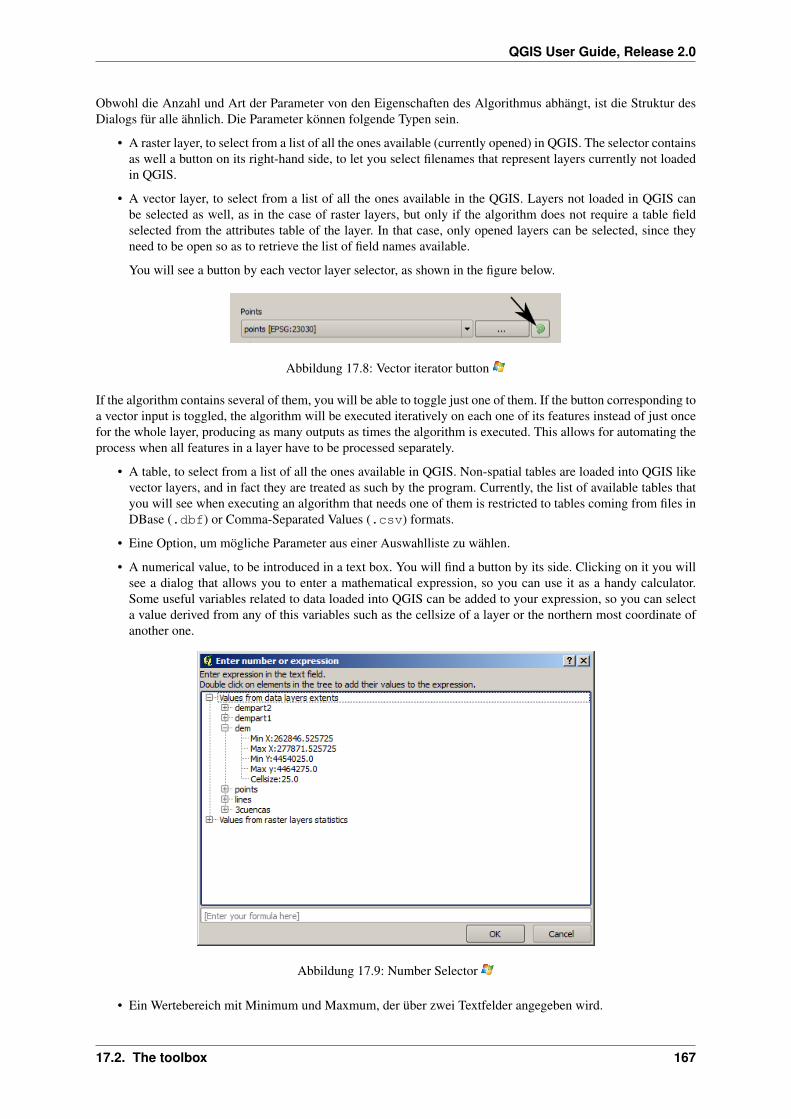
QGIS User Guide, Release 2.0
Obwohl die Anzahl und Art der Parameter von den Eigenschaften des Algorithmus abhängt, ist die Struktur desDialogs für alle ähnlich. Die Parameter können folgende Typen sein.
• A raster layer, to select from a list of all the ones available (currently opened) in QGIS. The selector containsas well a button on its right-hand side, to let you select filenames that represent layers currently not loadedin QGIS.
• A vector layer, to select from a list of all the ones available in the QGIS. Layers not loaded in QGIS canbe selected as well, as in the case of raster layers, but only if the algorithm does not require a table fieldselected from the attributes table of the layer. In that case, only opened layers can be selected, since theyneed to be open so as to retrieve the list of field names available.
You will see a button by each vector layer selector, as shown in the figure below.
Abbildung 17.8: Vector iterator button
If the algorithm contains several of them, you will be able to toggle just one of them. If the button corresponding toa vector input is toggled, the algorithm will be executed iteratively on each one of its features instead of just oncefor the whole layer, producing as many outputs as times the algorithm is executed. This allows for automating theprocess when all features in a layer have to be processed separately.
• A table, to select from a list of all the ones available in QGIS. Non-spatial tables are loaded into QGIS likevector layers, and in fact they are treated as such by the program. Currently, the list of available tables thatyou will see when executing an algorithm that needs one of them is restricted to tables coming from files inDBase (.dbf) or Comma-Separated Values (.csv) formats.
• Eine Option, um mögliche Parameter aus einer Auswahlliste zu wählen.
• A numerical value, to be introduced in a text box. You will find a button by its side. Clicking on it you willsee a dialog that allows you to enter a mathematical expression, so you can use it as a handy calculator.Some useful variables related to data loaded into QGIS can be added to your expression, so you can selecta value derived from any of this variables such as the cellsize of a layer or the northern most coordinate ofanother one.
Abbildung 17.9: Number Selector
• Ein Wertebereich mit Minimum und Maxmum, der über zwei Textfelder angegeben wird.
17.2. The toolbox 167
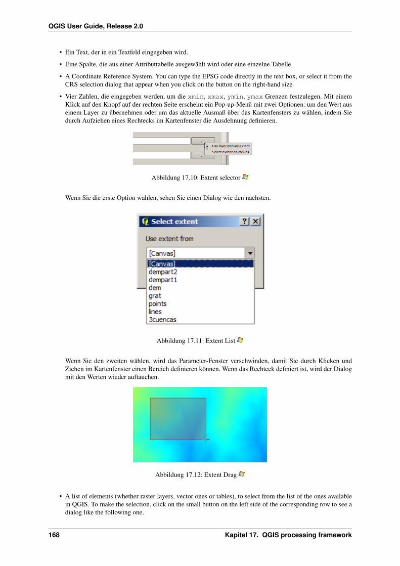
QGIS User Guide, Release 2.0
• Ein Text, der in ein Textfeld eingegeben wird.
• Eine Spalte, die aus einer Attributtabelle ausgewählt wird oder eine einzelne Tabelle.
• A Coordinate Reference System. You can type the EPSG code directly in the text box, or select it from theCRS selection dialog that appear when you click on the button on the right-hand size
• Vier Zahlen, die eingegeben werden, um die xmin, xmax, ymin, ymax Grenzen festzulegen. Mit einemKlick auf den Knopf auf der rechten Seite erscheint ein Pop-up-Menü mit zwei Optionen: um den Wert auseinem Layer zu übernehmen oder um das aktuelle Ausmaß über das Kartenfensters zu wählen, indem Siedurch Aufziehen eines Rechtecks im Kartenfenster die Ausdehnung definieren.
Abbildung 17.10: Extent selector
Wenn Sie die erste Option wählen, sehen Sie einen Dialog wie den nächsten.
Abbildung 17.11: Extent List
Wenn Sie den zweiten wählen, wird das Parameter-Fenster verschwinden, damit Sie durch Klicken undZiehen im Kartenfenster einen Bereich definieren können. Wenn das Rechteck definiert ist, wird der Dialogmit den Werten wieder auftauchen.
Abbildung 17.12: Extent Drag
• A list of elements (whether raster layers, vector ones or tables), to select from the list of the ones availablein QGIS. To make the selection, click on the small button on the left side of the corresponding row to see adialog like the following one.
168 Kapitel 17. QGIS processing framework
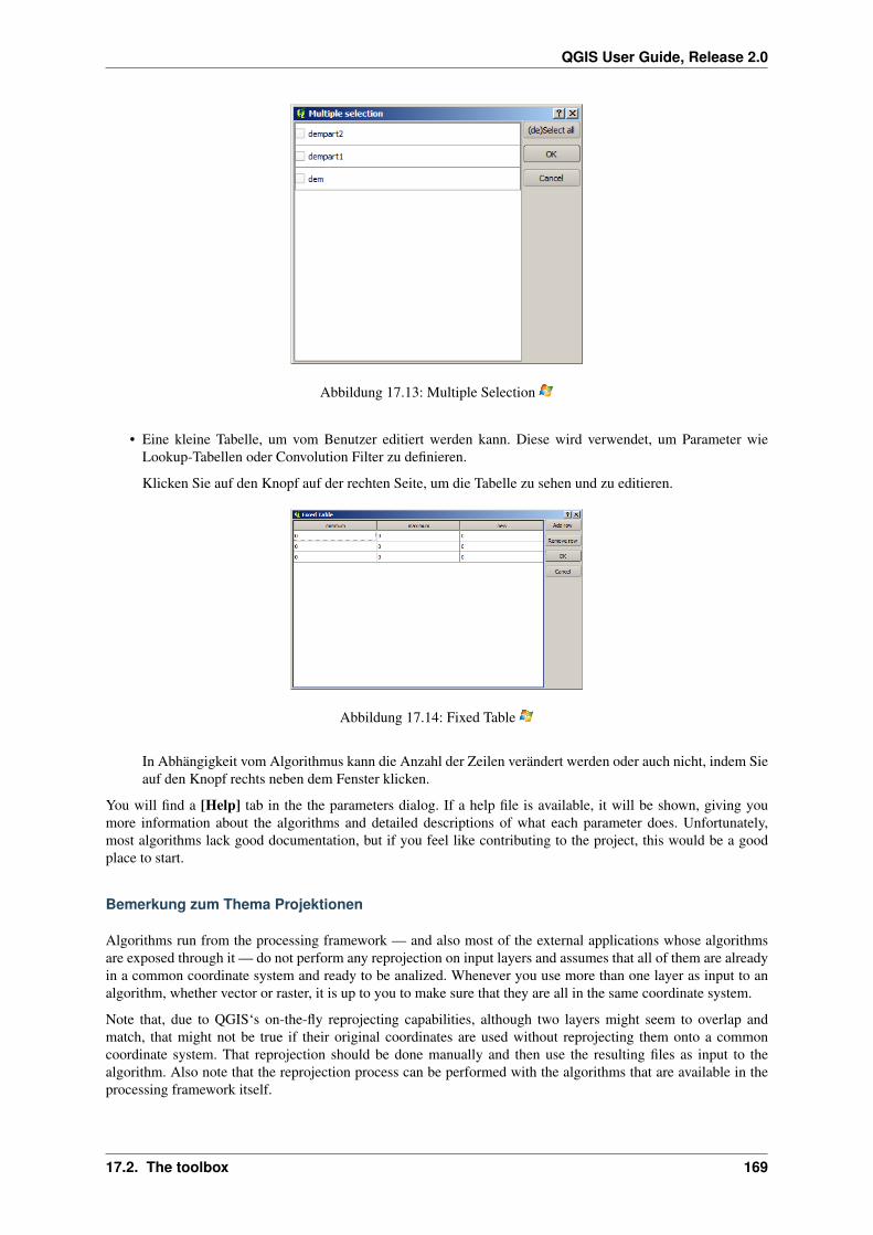
QGIS User Guide, Release 2.0
Abbildung 17.13: Multiple Selection
• Eine kleine Tabelle, um vom Benutzer editiert werden kann. Diese wird verwendet, um Parameter wieLookup-Tabellen oder Convolution Filter zu definieren.
Klicken Sie auf den Knopf auf der rechten Seite, um die Tabelle zu sehen und zu editieren.
Abbildung 17.14: Fixed Table
In Abhängigkeit vom Algorithmus kann die Anzahl der Zeilen verändert werden oder auch nicht, indem Sieauf den Knopf rechts neben dem Fenster klicken.
You will find a [Help] tab in the the parameters dialog. If a help file is available, it will be shown, giving youmore information about the algorithms and detailed descriptions of what each parameter does. Unfortunately,most algorithms lack good documentation, but if you feel like contributing to the project, this would be a goodplace to start.
Bemerkung zum Thema Projektionen
Algorithms run from the processing framework — and also most of the external applications whose algorithmsare exposed through it — do not perform any reprojection on input layers and assumes that all of them are alreadyin a common coordinate system and ready to be analized. Whenever you use more than one layer as input to analgorithm, whether vector or raster, it is up to you to make sure that they are all in the same coordinate system.
Note that, due to QGIS‘s on-the-fly reprojecting capabilities, although two layers might seem to overlap andmatch, that might not be true if their original coordinates are used without reprojecting them onto a commoncoordinate system. That reprojection should be done manually and then use the resulting files as input to thealgorithm. Also note that the reprojection process can be performed with the algorithms that are available in theprocessing framework itself.
17.2. The toolbox 169
QGIS User Guide, Release 2.0
By default, the parameters dialog will show a description of the CRS of each layer along with its name, making iteasy to select layers that share the same CRS to be used as input layers. If you do not want to see this additionalinformation, you can disable this functionality in the processing config dialog, unchecking the Show CRS option.
If you try to execute an algorithm using as input two or more layers with unmatching CRS’s, a warning dialog willbe shown.
You still can execute the algorithm, but be aware that in most cases that will produce wrong results, such as emptylayers due to input layers not overlapping.
17.2.2 Data objects generated by algorithms
Data objects generated by an algorithm can be of any of the following types:
• Rasterlayer
• Vektorlayer
• Tabelle
• HTML-Datei (wird für Text und grafische Ausgabe verwendet)
They are all saved to disk, and the parameters table will contain a text box corresponding to each one of theseoutputs, where you can type the output channel to use for saving it. An output channel contains the informationneeded to save the resulting object somewhere. In the most usual case, you will save it to a file, but the architectureallows for any other way of storing it. For instance, a vector layer can be stored in a database or even uploadedto a remote server using a WFS-T service. Although solutions like these are not yet implemented, the processingframework is prepared to handle them, and we expect to add new kinds of output channels in a near feature.
To select an output channel, just click on the button on the right side of the text box. That will open a save filedialog, where you can select the desired filepath. Supported file extensions are shown in the file format selector ofthe dialog, depending on the kind of output and the algorithm.
The format of the output is defined by the filename extension. The supported formats depend on the ones supportedby the algorithm itself. To select a format, just select the corresponding file extension (or add it if you are directlytyping the filepath instead). If the extension of the filepath you entered does not match any of the supported ones,a default extension (usually .dbf‘ for tables, .tif for raster layers and .shp for vector ones) will be appendedto the filepath and the file format corresponding to that extension will be used to save the layer or table.
If you do not enter any filename, the result will be saved as a temporary file and in the corresponding default fileformat, and will be deleted once you exit QGIS (take care with that in case you save your project and it containstemporary layers).
You can set a default folder for output data objects. Go to the configuration dialog (you can open it from theProcessing menu), and in the General group you will find a parameter named Output folder. This output folderis used as the default path in case you type just a filename with no path (i.e. myfile.shp) when executing analgorithm.
When running an algorithm that uses vector layer in iterative mode, the entered file path is used as the base pathfor all generated files, which are named using the base name and appending a number representing the index ofthe iteration. The file extension (and format) is used for all those generated files.
Apart from raster layers and tables, algorithms also generates graphics and texts as HTML files. These results areshown at the end of the algorithm execution in a new dialog. This dialog will keep the results produced by anyalgorithm during the current session, and can be shown at any time by selecting the Processing → Results viewerfrom QGIS main menu.
Some external applications might have files (with no particular extension restrictions) as output, but they do notbelong to any of the categories above. Those output files will not be processed by QGIS (opened or included intothe current QGIS project), since most of the times correspond to file formats or elements not supported by QGIS.This is, for instance, the case with LAS files used for LiDAR data. The files get created, but you won’t see anythingnew in your QGIS working session.
For all the other types of outputs, you will find a check box that you can use to tell the algorithm whether to loadthe file once it is generated by the algorithm or not. By default, all files are opened.
170 Kapitel 17. QGIS processing framework

QGIS User Guide, Release 2.0
Optional outputs are not supported, so all outputs are created, but you can uncheck the corresponding check boxif you are not interested in a given output, which virtually makes it behave like an optional output (although thelayer is created anyway, but if you leave the text box empty, it will be saved to a temporary file and deleted onceyou exit QGIS)
17.2.3 Configuring the processing framework
As it has been mentioned, the configuration menu gives access to a new dialog where you can configure howalgorithms work. Configuration parameters are structured in separate blocks that you can select on the left-handside of the dialog.
Along with the aforementioned Output folder entry, the General block contains parameters for setting the defaultrendering style for output layers (that is, layers generated by using algorithms from any of the framework GUIcomponents). Just create the style you want using QGIS, save it to a file, and then enter the path to that file in thesettings so the algorithms can use it. Whenever a layer is loaded by SEXTANTE and added to the QGIS canvas, itwill be rendered with that style.
Rendering styles can be configured individually for each algorithm and each one of its outputs. Just right-click onthe name of the algorithm in the toolbox and select Edit rendering styles. You will see a dialog like the one shownnext.
Abbildung 17.15: Rendering Styles
Wählen Sie die Stildatei (.qml) für jede Ausgabedatei und klicken Sie dann [OK].
Other configuration parameters in the General group are the following ones:
• Use filename as layer name. The name of each resulting layer created by an algorithm is defined by thealgorithm itself. In some cases, a fixed name might be used, that meaning that the same name will be used,no matter which input layer is used. In other cases, the name might depend on the name of the input layeror some of the parameters used to run the algorithm. If this checkbox is checked, the name will be takenfrom the output filename instead. Notice, that, if the output is saved to a temporary file, the filename of thistemporary file is usually long and meaningless one intended to avoid collision with other already existingfilenames.
• Use only selected features. If this option is selected, whenever a vector layer is used as input for an algorithm,only its selected features will be used. If the layer has no selected features, all of them will be used.
• Pre-execution script file and Post-execution script file. This parameters refer to scripts written using theprocessing scripting functionality, and are explained in the section covering scripting and the console.
Abgesehen vom Bereich Allgemein im Menü Einstellungen, finden Sie auch einen für jeden Algorithmus-Provider.Sie enthalten ein aktivieren Element, das Sie verwenden können, um festzulegen, ob Algorithmen dieses Providersin der Toolbox erscheinen oder nicht. Auch haben einige Provider ihre eigene Algorithmus-Konfiguration, die wirspäter noch genauer erklären.
17.2. The toolbox 171
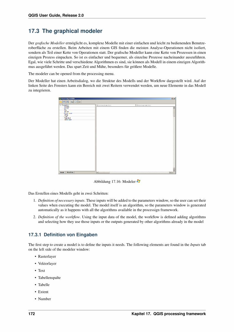
QGIS User Guide, Release 2.0
17.3 The graphical modeler
Der grafische Modeller ermöglicht es, komplexe Modelle mit einer einfachen und leicht zu bedienenden Benutze-roberfläche zu erstellen. Beim Arbeiten mit einem GIS finden die meisten Analyse-Operationen nicht isoliert,sondern als Teil einer Kette von Operationen statt. Der grafische Modeller kann eine Kette von Prozessen in eineneinzigen Prozess einpacken. So ist es einfacher und bequemer, als einzelne Prozesse nacheinander auszuführen.Egal, wie viele Schritte und verschiedene Algorithmen es sind, sie können als Modell in einem einzigen Algorith-mus ausgeführt werden. Das spart Zeit und Mühe, besonders für größere Modelle.
The modeler can be opened from the processing menu.
Der Modeller hat einen Arbeitsdialog, wo die Struktur des Modells und der Workflow dargestellt wird. Auf derlinken Seite des Fensters kann ein Bereich mit zwei Reitern verwendet werden, um neue Elemente in das Modellzu integrieren.
Abbildung 17.16: Modeler
Das Erstellen eines Modells geht in zwei Schritten:
1. Definition of necessary inputs. These inputs will be added to the parameters window, so the user can set theirvalues when executing the model. The model itself is an algorithm, so the parameters window is generatedautomatically as it happens with all the algorithms available in the processign framework.
2. Definition of the workflow. Using the input data of the model, the workflow is defined adding algorithmsand selecting how they use those inputs or the outputs generated by other algorithms already in the model
17.3.1 Definition von Eingaben
The first step to create a model is to define the inputs it needs. The following elements are found in the Inputs tabon the left side of the modeler window:
• Rasterlayer
• Vektorlayer
• Text
• Tabellenspalte
• Tabelle
• Extent
• Number
172 Kapitel 17. QGIS processing framework

QGIS User Guide, Release 2.0
• Boolean
• File
Ein Doppelklick auf einen von ihnen öffnet einen Dialog, um ihre Eigenschaften zu definieren. Je nach Parameter,enthält der Dialog nur ein Grundelement (die Beschreibung, die der Benutzer sieht, wenn er das Modell ausführt)oder mehrere. Zum Beispiel, wenn Sie einen numerischen Wert verwenden, wie es in der folgenden Abbildungzu sehen ist, müssen Sie abgesehen von der Beschreibung der Parameter auch einen Standardwert und eine Reihevon gültigen Werten setzen.
Abbildung 17.17: Model Parameters
Für jede Eingabe wird ein neues Element im Modeller-Fenster erstellt.
Abbildung 17.18: Model Parameters
17.3.2 Definition des Workflows
Wenn die Eingaben definiert sind, ist es Zeit die Algorithmen festzulegen. Die Algorithmen können im ReiterAlgorithmen ausgewählt werden. Die Gruppierung entspricht der Toolbox.
The appearance of the toolbox has two modes here as well: simplified and advanced. However, there is no elementto switch between views in the modeler, and you have to do it in the toolbox. The mode that is selected in thetoolbox is the one that will be used for the list of algorithms in the modeler.
To add an algorithm to a model, double-click on its name. An execution dialog will appear, with a content similarto the one found in the execution panel that is shown when executing the algorithm from the toolbox. The oneshown next correspond to the SAGA ‘Convergence index’ algorithm, the same one we saw in the section dedicatedto the toolbox.
As you can see, some differences exist. Instead of the file output box that was used to set the filepath for outputlayers and tables, a simple text box is. If the layer generated by the algorithm is just a temporary result that willbe used as the input of another algorithm and should not be kept as a final result, just do not edit that text box.Typing anything on it means that the result is a final one, and the text that you supply will be the description forthe output, which will be the one the user will see when executing the model.
Selecting the value of each parameter is also a bit different, since there are important differences between thecontext of the modeler and the toolbox one. Let’s see how to introduce the values for each type of parameter.
17.3. The graphical modeler 173
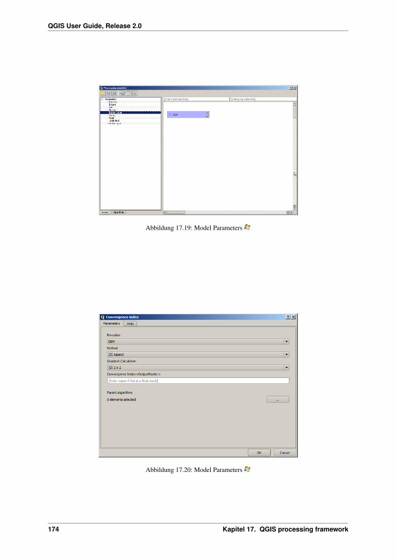
QGIS User Guide, Release 2.0
Abbildung 17.19: Model Parameters
Abbildung 17.20: Model Parameters
174 Kapitel 17. QGIS processing framework

QGIS User Guide, Release 2.0
• Layers (raster and vector) and tables. They are selected from a list, but in this case the possible values arenot the layers or tables currently loaded in QGIS, but the list of model inputs of the corresponding type, orother layers or tables generated by algorithms already added to the model.
• Numerical values. Literal values can be introduced directly on the text box. But this text box is also a listthat can be used to select any of the numerical value inputs of the model. In this case, the parameter willtake the value introduced by the user when executing the model.
• Text. Wie im Fall von numerischen Werten können Zeichenketten eingegeben werden oder ein Eingabe-String ausgewählt werden.
• Table field. The fields of the parent table or layer cannot be known at design-time, since they depend of theselection of the user each time the model is executed. To set the value for this parameter, type the name ofa field directly in the text box, or use the list to select a table field input already added to the model. Thevalidity of the selected field will be checked at run-time.
In all cases, you will find an additional parameter named Parent algorithms that is not available when calling thealgorithm from the toolbox. This parameter allows you to define the order in which algorithms are executed, byexplicitly defining one algorithm as a parent of the current one, which will force it to be executed before it.
When you use the output of a previous algorithm as the input of your algorithm, that implicitly sets the formeras parent of the current one (and places the corresponding arrow in the modeler canvas). However, in some casesan algorithm might depend on another one even if it does not use any output object from it (for instance, andalgorithm that executes an SQL sentence on a PostGIS database and another one which imports a layer into thatsame database) In that case, just select it in the Parent algorithms parameter and they will be executed in thecorrect order.
Sobald alle Parameter gültigen Werten zugewiesen wurden, klicken Sie auf [OK] und der Algorithmus wird zumDialogfenster hinzugefügt. Es wird mit allen anderen Elemente verknüpft, egal ob Algorithmus oder Parameter,die Objekte bereitstellen, die als Eingabe für diesen Algorithmus verwendet werden.
Abbildung 17.21: Model Parameters
Elemente können an eine andere Position innerhalb der Leinwand gezogen werden, um die Art der Modelldarstel-lung zu ändern und dadurch klarer und intuitiver zu machen. Verbindungen zwischen Elementen werden automa-tisch aktualisiert.
Sie können Ihren Algorithmus jederzeit starten, in dem Sie auf den [Run] Knopf drücken. Allerdings, um es ausder Toolbox zu verwenden, muss es gespeichert und der Modeller Dialog geschlossen werden, damit die Toolboxseinen Inhalt aktualisieren kann.
17.3. The graphical modeler 175
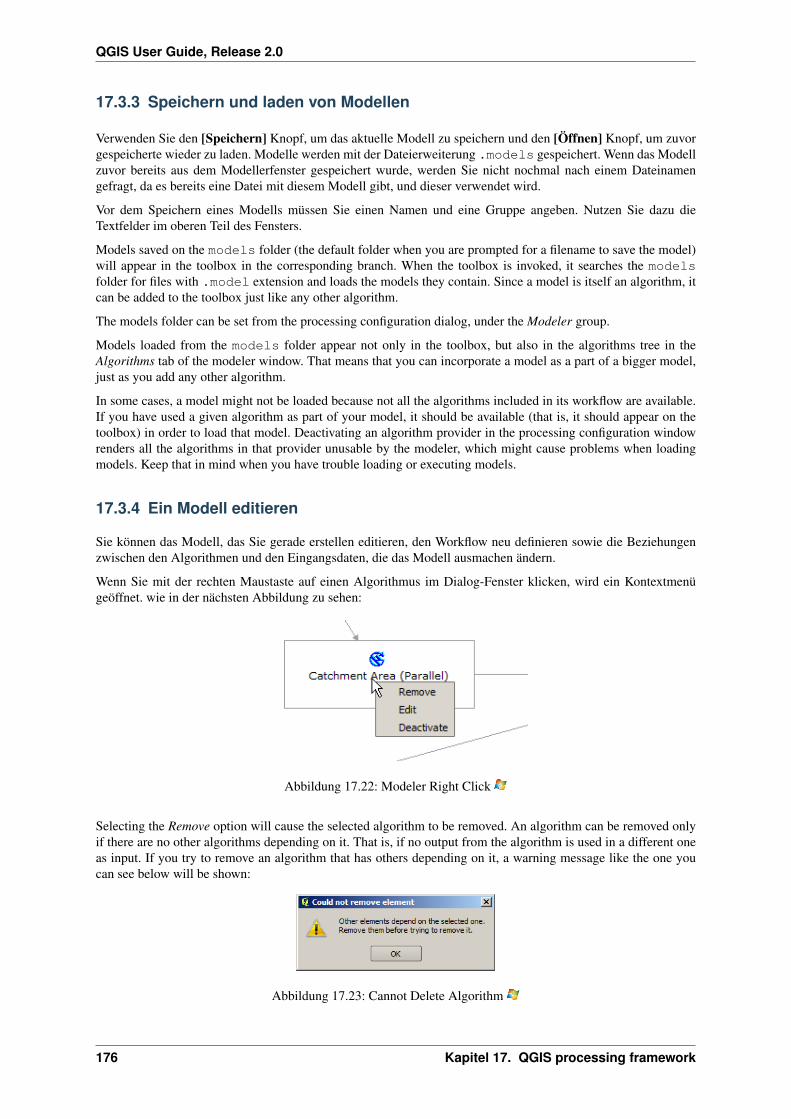
QGIS User Guide, Release 2.0
17.3.3 Speichern und laden von Modellen
Verwenden Sie den [Speichern] Knopf, um das aktuelle Modell zu speichern und den [Öffnen] Knopf, um zuvorgespeicherte wieder zu laden. Modelle werden mit der Dateierweiterung .models gespeichert. Wenn das Modellzuvor bereits aus dem Modellerfenster gespeichert wurde, werden Sie nicht nochmal nach einem Dateinamengefragt, da es bereits eine Datei mit diesem Modell gibt, und dieser verwendet wird.
Vor dem Speichern eines Modells müssen Sie einen Namen und eine Gruppe angeben. Nutzen Sie dazu dieTextfelder im oberen Teil des Fensters.
Models saved on the models folder (the default folder when you are prompted for a filename to save the model)will appear in the toolbox in the corresponding branch. When the toolbox is invoked, it searches the modelsfolder for files with .model extension and loads the models they contain. Since a model is itself an algorithm, itcan be added to the toolbox just like any other algorithm.
The models folder can be set from the processing configuration dialog, under the Modeler group.
Models loaded from the models folder appear not only in the toolbox, but also in the algorithms tree in theAlgorithms tab of the modeler window. That means that you can incorporate a model as a part of a bigger model,just as you add any other algorithm.
In some cases, a model might not be loaded because not all the algorithms included in its workflow are available.If you have used a given algorithm as part of your model, it should be available (that is, it should appear on thetoolbox) in order to load that model. Deactivating an algorithm provider in the processing configuration windowrenders all the algorithms in that provider unusable by the modeler, which might cause problems when loadingmodels. Keep that in mind when you have trouble loading or executing models.
17.3.4 Ein Modell editieren
Sie können das Modell, das Sie gerade erstellen editieren, den Workflow neu definieren sowie die Beziehungenzwischen den Algorithmen und den Eingangsdaten, die das Modell ausmachen ändern.
Wenn Sie mit der rechten Maustaste auf einen Algorithmus im Dialog-Fenster klicken, wird ein Kontextmenügeöffnet. wie in der nächsten Abbildung zu sehen:
Abbildung 17.22: Modeler Right Click
Selecting the Remove option will cause the selected algorithm to be removed. An algorithm can be removed onlyif there are no other algorithms depending on it. That is, if no output from the algorithm is used in a different oneas input. If you try to remove an algorithm that has others depending on it, a warning message like the one youcan see below will be shown:
Abbildung 17.23: Cannot Delete Algorithm
176 Kapitel 17. QGIS processing framework

QGIS User Guide, Release 2.0
Auswählen der Bearbeiten Option oder einfaches Doppelklicken auf das Symbol des Algorithmus zeigt denParameter-Dialog des Algorithmus, um die Ein- und Ausgabe Parameter-Werte zu ändern. Nicht alle Eingabe-Elemente des Modells werden in diesem Fall als verfügbare Eingänge angezeigt. Layer oder Werte, die in einemfortgeschrittenen Schritt im Workflow durch das Modell erzeugt wurden, stehen nicht zur Verfügung, wenn siezirkuläre Abhängigkeiten verursachen.
Wählen Sie die neuen Werte und klicken dann auf den [OK] Knopf wie gewohnt. Die Verbindungen zwischenden Elementen des Modells ändern sich entsprechend im Modeller-Fenster.
17.3.5 Algorithmen aktivieren und deaktivieren
Algorithmen können im Modeller deaktiviert werden, damit sie nicht ausgeführt werden, wenn das Modell ausge-führt wird. Dies kann verwendet werden, um nur einen bestimmten Teil eines Modells zu nutzen, oder wenn Sienicht alle Ausgaben brauchen.
Um einen Algorithmus zu deaktivieren, klicken Sie auf das entsprechende Symbol im Modell-Fenster mit derrechten Maustaste und wählen Sie deaktivieren. Sie werden sehen, dass der Algorithmus nun mit einem rotenLabel unter seinem Namen darauf hinweist, dass er nicht aktiv ist.
Abbildung 17.24: Deactivate
Alle Algorithmen die (direkt oder indirekt) an diesem Algorithmus hängen, werden auch als inaktiv angezeigt, dasie nicht ausgeführt werden können.
Um einen Algorithmus zu aktivieren, klicken Sie mit der rechten Maustaste auf das Icon und wählen Sie dann dieOption Aktivieren.
17.3.6 Editieren der Modell-Hilfe Datei und der Metainformationen
You can document your models from the modeler itself. Just click on the [Edit model help] button and a dialoglike the one shown next will appear.
Abbildung 17.25: Help Edition
17.3. The graphical modeler 177

QGIS User Guide, Release 2.0
On the right-hand side you will see a simple HTML page, created using the description of the input parametersand outputs of the algorithm, along with some additional items like a general description of the model or its author.The first time you open the help editor all those descriptions are empty, but you can edit them using the elementson the left-hand side of the dialog. Select an element on the upper part and the write its description in the text boxbelow.
Die Modell Hilfe wird in einer Datei im gleichen Ordner wie das Modell selbst gespeichert. Sie müssen nichtstun, um es zu speichern, da es automatisch geschieht.
17.3.7 Zu den verfügbaren Algorithmen
Sie haben vielleicht bemerkt, dass einige Algorithmen, die aus der Toolbox ausgeführt werden können nicht inder Liste der verfügbaren Algorithmen erscheint, wenn Sie ein Modell entwerfen. Um in einem Modell enthaltenzu sein, muss der Algorithmus eine korrekte Semantik haben, um im Workflow verknüpft zu werden. Wenn einAlgorithmus keine solche definierte Semantik besitzt (zum Beispiel, wenn die Anzahl der Ausgangskanäle oderLayer nicht im Voraus bekannt ist), dann ist es nicht möglich, diesen in einem Modell zu verwenden, und somiterscheint er auch nicht in der Liste.
Additionally, you will see some algorithms in the modeler that are not found in the toolbox. This algorithms aremeant to be used exclusively as part of a model, and they are of no interest in a different context. The ‘Calculator’algorithm is an example of that. It is just a simple arithmetic calculator that you can use to modify numericalvalues (entered by the user or generated by some other algorithm). This tools is really useful within a model, butoutside of that context, it doesn’t make too much sense.
17.3.8 Saving models as Python code
Given a model, it is possible to automatically create Python code that performs the same task as the model itself.This code is used to create a console script (we will explain them later in this manual) and you can modify thatscript to incorporate actions and methods not available in the graphical modeler, such as loops or conditionalsentences.
This feature is also a very practical way of learning how to use processign algorithms from the console and howto create new algorithms using Python code, so you can use it as a learning tool when you start creating your ownscripts.
Save your model in the models folder and go to the toolbox, where it should appear now, ready to be run. Rightclick on the model name and select Save as Python script in the context menu that will pop-up. A dialog willprompt you to introduce the file where you want to save the script.
17.4 The batch processing interface
17.4.1 Einführung
All algorithms (including models) can be executed as a batch process. That is, they can be executed using not asingle set of inputs, but several of them, executing the algorithm as many times as needed. This is useful whenprocessing large amounts of data, since it is not necessary to launch the algorithm many times from the toolbox.
Um einen Algorithmus als Batch-Prozess ausführen, klicken Sie mit der rechten Maustaste auf seinen Namen inder Toolbox und wählen Sie die Option Ausführen als Batch-Prozess.
Abbildung 17.26: Batch Processing Right Click
178 Kapitel 17. QGIS processing framework

QGIS User Guide, Release 2.0
17.4.2 Die Parameter-Tabelle
Ausführen eines Batch-Prozesses ist vergleichbar mit der Durchführung der einmaligen Ausführung eines Algo-rithmus. Parameter-Werte müssen definiert werden, aber in diesem Fall müssen wir nicht nur einen einzelnen Wertfür jeden Parameter angeben, sondern eine Reihe von ihnen, einen für jedes Mal, wenn der Algorithmus ausgeführtwerden soll. Werte werden mit Hilfe einer Tabelle wie in der nächsten Abbildung zu sehen übergeben.
Abbildung 17.27: Batch Processing
Jede Zeile dieser Tabelle stellt eine einzelne Ausführung des Algorithmus dar, und jede Zelle enthält den Werteines der Parameter. Es ist vergleichbar mit dem Parameter-Dialog, den Sie sehen, wenn Sie die Ausführung einesAlgorithmus aus der Toolbox starten, aber mit einer anderen Anordnung.
Standardmäßig enthält die Tabelle nur zwei Zeilen. Sie können weitere hinzufügen oder entfernen mit den Tastenam unteren Teil des Fensters.
Sobald die Größe der Tabelle gesetzt ist, muss sie mit den gewünschten Werten gefüllt werden.
17.4.3 Füllen der Parameter-Tabelle
Für die meisten Parameter ist das Setzen des Wertes trivial. Geben Sie einfach den Wert ein oder wählen Sie ihnaus der Liste der verfügbaren Optionen aus, je nach Art des Parameters.
The main differences are found for parameters representing layers or tables, and for output filepaths. Regardinginput layers and tables, when an algorithm is executed as part of a batch process those input data objects are takendirectly from files, and not from the set of them already opened in QGIS. For this reason, any algorithm can beexecuted as a batch process even if no data objects at all are opened and the algorithm cannot be run from thetoolbox.
Filenames for input data objects are introduced directly typing or, more conveniently, clicking on the buttonon the right hand of the cell, which shows a typical file chooser dialog. Multiple files can be selected at once. Ifthe input parameter represents a single data object and several files are selected, each one of them will be put in aseparate row, adding new ones if needed. If it represents a multiple input, all the selected files will be added to asingle cell, separated by semicolons (;).
Ausgabedaten Objekte werden immer in einer Datei gespeichert und im Gegensatz zur Ausführung eines Algo-rithmus aus der Toolbox, ist das vorübergehende Speichern als temporäre Datei nicht gestattet. Sie können denNamen direkt eingeben oder im Dateiauswahldialog, wenn Sie auf den zugehörigen Button klicken.
Sobald Sie die Datei auswählen, erscheint ein neuer Dialog, der Autovervollständigung von anderen Zellen inderselben Spalte (gleiche Parameter) ermöglicht.
If the default value (‘Do not autocomplete’) is selected, it will just put the selected filename in the selected cellfrom the parameters table. If any of the other options is selected, all the cells below the selected one will be
17.4. The batch processing interface 179
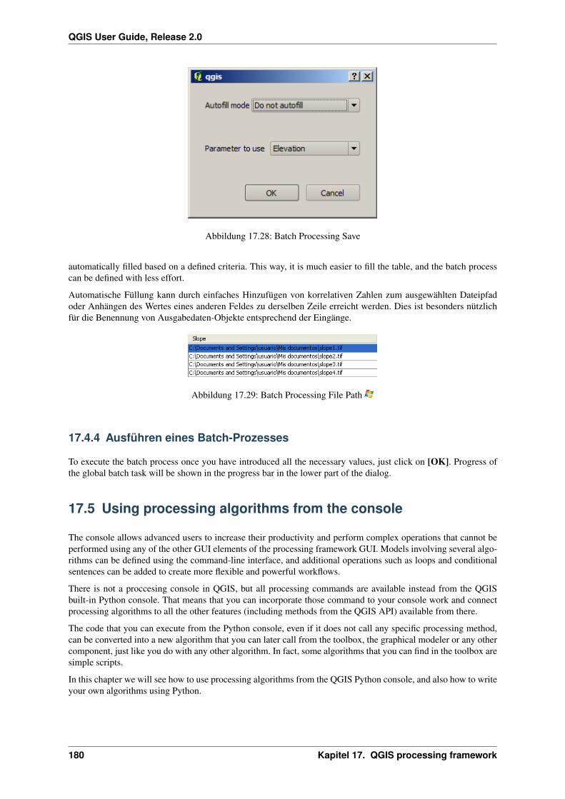
QGIS User Guide, Release 2.0
Abbildung 17.28: Batch Processing Save
automatically filled based on a defined criteria. This way, it is much easier to fill the table, and the batch processcan be defined with less effort.
Automatische Füllung kann durch einfaches Hinzufügen von korrelativen Zahlen zum ausgewählten Dateipfadoder Anhängen des Wertes eines anderen Feldes zu derselben Zeile erreicht werden. Dies ist besonders nützlichfür die Benennung von Ausgabedaten-Objekte entsprechend der Eingänge.
Abbildung 17.29: Batch Processing File Path
17.4.4 Ausführen eines Batch-Prozesses
To execute the batch process once you have introduced all the necessary values, just click on [OK]. Progress ofthe global batch task will be shown in the progress bar in the lower part of the dialog.
17.5 Using processing algorithms from the console
The console allows advanced users to increase their productivity and perform complex operations that cannot beperformed using any of the other GUI elements of the processing framework GUI. Models involving several algo-rithms can be defined using the command-line interface, and additional operations such as loops and conditionalsentences can be added to create more flexible and powerful workflows.
There is not a proccesing console in QGIS, but all processing commands are available instead from the QGISbuilt-in Python console. That means that you can incorporate those command to your console work and connectprocessing algorithms to all the other features (including methods from the QGIS API) available from there.
The code that you can execute from the Python console, even if it does not call any specific processing method,can be converted into a new algorithm that you can later call from the toolbox, the graphical modeler or any othercomponent, just like you do with any other algorithm. In fact, some algorithms that you can find in the toolbox aresimple scripts.
In this chapter we will see how to use processing algorithms from the QGIS Python console, and also how to writeyour own algorithms using Python.
180 Kapitel 17. QGIS processing framework
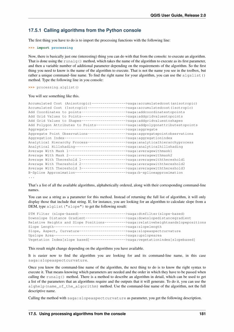
QGIS User Guide, Release 2.0
17.5.1 Calling algorithms from the Python console
The first thing you have to do is to import the processing functions with the following line:
>>> import processing
Now, there is basically just one (interesting) thing you can do with that from the console: to execute an algorithm.That is done using the runalg() method, which takes the name of the algorithm to execute as its first parameter,and then a variable number of additional parameter depending on the requirements of the algorithm. So the firstthing you need to know is the name of the algorithm to execute. That is not the name you see in the toolbox, butrather a unique command–line name. To find the right name for your algorithm, you can use the algslist()method. Type the following line in you console:
>>> processing.alglist()
You will see something like this.
Accumulated Cost (Anisotropic)---------------->saga:accumulatedcost(anisotropic)Accumulated Cost (Isotropic)------------------>saga:accumulatedcost(isotropic)Add Coordinates to points--------------------->saga:addcoordinatestopointsAdd Grid Values to Points--------------------->saga:addgridvaluestopointsAdd Grid Values to Shapes--------------------->saga:addgridvaluestoshapesAdd Polygon Attributes to Points-------------->saga:addpolygonattributestopointsAggregate------------------------------------->saga:aggregateAggregate Point Observations------------------>saga:aggregatepointobservationsAggregation Index----------------------------->saga:aggregationindexAnalytical Hierarchy Process------------------>saga:analyticalhierarchyprocessAnalytical Hillshading------------------------>saga:analyticalhillshadingAverage With Mask 1--------------------------->saga:averagewithmask1Average With Mask 2--------------------------->saga:averagewithmask2Average With Thereshold 1--------------------->saga:averagewiththereshold1Average With Thereshold 2--------------------->saga:averagewiththereshold2Average With Thereshold 3--------------------->saga:averagewiththereshold3B-Spline Approximation------------------------>saga:b-splineapproximation...
That’s a list of all the available algorithms, alphabetically ordered, along with their corresponding command-linenames.
You can use a string as a parameter for this method. Instead of returning the full list of algorithm, it will onlydisplay those that include that string. If, for instance, you are looking for an algorithm to calculate slope from aDEM, type alglist("slope") to get the following result:
DTM Filter (slope-based)---------------------->saga:dtmfilter(slope-based)Downslope Distance Gradient------------------->saga:downslopedistancegradientRelative Heights and Slope Positions---------->saga:relativeheightsandslopepositionsSlope Length---------------------------------->saga:slopelengthSlope, Aspect, Curvature---------------------->saga:slopeaspectcurvatureUpslope Area---------------------------------->saga:upslopeareaVegetation Index[slope based]----------------->saga:vegetationindex[slopebased]
This result might change depending on the algorithms you have available.
It is easier now to find the algorithm you are looking for and its command-line name, in this casesaga:slopeaspectcurvature.
Once you know the command-line name of the algorithm, the next thing to do is to know the right syntax toexecute it. That means knowing which parameters are needed and the order in which they have to be passed whencalling the runalg() method. There is a method to describe an algorithm in detail, which can be used to geta list of the parameters that an algorithms require and the outputs that it will generate. To do it, you can use thealghelp(name_of_the_algorithm) method. Use the command-line name of the algorithm, not the fulldescriptive name.
Calling the method with saga:slopeaspectcurvature as parameter, you get the following description.
17.5. Using processing algorithms from the console 181
QGIS User Guide, Release 2.0
>>> processing.alghelp("saga:slopeaspectcurvature")ALGORITHM: Slope, Aspect, Curvature
ELEVATION <ParameterRaster>METHOD <ParameterSelection>SLOPE <OutputRaster>ASPECT <OutputRaster>CURV <OutputRaster>HCURV <OutputRaster>VCURV <OutputRaster>
Now you have everything you need to run any algorithm. As we have already mentioned, there is only one singlecommand to execute algorithms: runalg(). Its syntax is as follows:
>>> processing.runalg(name_of_the_algorithm, param1, param2, ..., paramN,Output1, Output2, ..., OutputN)
The list of parameters and outputs to add depends on the algorithm you want to run, and is exactly the list that thealghelp() method gives you, in the same order as shown.
Depending on the type of parameter, values are introduced differently. The next one is a quick review of how tointroduce values for each type of input parameter:
• Raster Layer, Vector Layer or Table. Simply use a string with the name that identifies the data object to use(the name it has in the QGIS Table of Contents) or a filename (if the corresponding layer is not opened, itwill be opened, but not added to the map canvas). If you have an instance of a QGIS object representing thelayer, you can also pass it as parameter. If the input is optional and you do not want to use any data object,use None.
• Selection. If an algorithm has a selection parameter, the value of that parameter should be entered using aninteger value. To know the available options, you can use the algoptions() command, as shown in thefollowing example:
>>> processing.algoptions("saga:slopeaspectcurvature")METHOD(Method)
0 - [0] Maximum Slope (Travis et al. 1975)1 - [1] Maximum Triangle Slope (Tarboton 1997)2 - [2] Least Squares Fitted Plane (Horn 1981, Costa-Cabral & Burgess 1996)3 - [3] Fit 2.Degree Polynom (Bauer, Rohdenburg, Bork 1985)4 - [4] Fit 2.Degree Polynom (Heerdegen & Beran 1982)5 - [5] Fit 2.Degree Polynom (Zevenbergen & Thorne 1987)6 - [6] Fit 3.Degree Polynom (Haralick 1983)
In this case, the algorithm has one of such such parameters, with 7 options. Notice that ordering is zero-based.
• Multiple input. The value is a string with input descriptors separated by semicolons (;). As in the case ofsingle layers or tables, each input descriptor can be the data object name, or its filepath.
• Table Field from XXX. Use a string with the name of the field to use. This parameter is case-sensitive.
• Fixed Table. Type the list of all table values separated by commas (,) and enclosed between quotes (").Values start on the upper row and go from left to right. You can also use a 2D array of values representingthe table.
• CRS. Enter the EPSG code number of the desired CRS.
• Extent. You must use a string with xmin, xmax, ymin and ymax values separated by commas (,).
Boolean, file, string and numerical parameters do not need any additional explanations.
Input parameters such as strings booleans or numerical values have default values. To use them, use None in thecorresponding parameter entry.
For output data objects, type the filepath to be used to save it, just as it is done from the toolbox. If you want tosave the result to a temporary file, use None. The extension of the file determines the file format. If you enter a
182 Kapitel 17. QGIS processing framework

QGIS User Guide, Release 2.0
file extension not included in the ones supported by the algorithm, the default file format for that output type willbe used, and its corresponding extension appended to the given filepath.
Unlike when an algorithm is executed from the toolbox, outputs are not added to the map canvas if you executethat same algorithm from the Python Console. If you want to add an output to it, you have to do it yourself afterrunning the algorithm. To do so, you can use QGIS API commands, or, even easier, use one of the handy methodsprovided for such task.
The runalg method returns a dictionary with the output names (the ones shown in the algorithm description) askeys and the filepaths of those outputs as values. You can load those layers by passing its filepath to the load()method.
17.5.2 Additional functions for handling data
Apart from the functions used to call algorithms, importing the processing package will also import someadditional functions that make it easier to work with data, particularly vector data. They are just conveniencefunctions that wrap some functionality from the QGIS API, usually with a less complex syntax. These functionsshould be used when developing new algorithms, as they make it easier to operate with input data.
Below is a list of some of this commands. More information can be found in the classes under theprocessing/tools package, and aso in the example scripts provided with QGIS.
• getobject(obj): Returns a QGIS object (a layer or table) from the passed object, which can be afilename or the name of the object in the QGIS Table of Contents.
• values(layer, fields): Returns the values in the attributes table of a vector layer, for the passedfields. Fields can be passed as field names or as zero-based field indices. Returns a dict of lists, with thepassed field identifiers as keys. It considers the existing selection
• getfeatures(layer): Returns an iterator over the features of a vector layer, considering the existingselection.
• uniquelabels(layer, field): Returns a list of unique values for a given attribute. Attribute canbe passed as a field name or a zero-based field index. It considers the existing selection
17.5.3 Creating scripts and running them from the toolbox
You can create your own algorithms by writing the corresponding Python code and adding a few extra lines tosupply additional information needed to define the semantics of the algorithm. You can find a Create new scriptmenu under the Tools group in the Script algorithms block of the toolbox. Double-click on it to open the scriptedition dialog. That’s where you should type your code. Saving the script from there in the scripts folder (thedefault one when you open the save file dialog), with .py extension, will automatically create the correspondingalgorithm.
The name of the algorithm (the one you will see in the toolbox) is created from the filename, removing its extensionand replacing low hyphens with blank spaces.
Let’s have the following code, which calculates the Topographic Wetness Index (TWI) directly from a DEM
##dem=raster##twi=outputret_slope = processing.runalg("saga:slopeaspectcurvature", dem, 0, None,
None, None, None, None)ret_area = processing.runalg("saga:catchmentarea(mass-fluxmethod)", dem,
0, False, False, False, False, None, None, None, None, None)processing.runalg("saga:topographicwetnessindex(twi), ret_slope[’SLOPE’],
ret_area[’AREA’], None, 1, 0, twi)
As you can see, it involves 3 algorithms, all of them coming from SAGA. The last one of them calculates the TWI,but it needs a slope layer and a flow accumulation layer. We do not have these ones, but since we have the DEM,we can calculate them calling the corresponding SAGA algorithms.
17.5. Using processing algorithms from the console 183

QGIS User Guide, Release 2.0
The part of the code where this processing takes place is not difficult to understand if you have read the previoussections in this chapter. The first lines, however, need some additional explanation. They provide the informationthat is needed to turn your code into an algorithm that can be run from any of the GUI components, like the toolboxor the graphical modeler.
These lines start with a double Python comment symbol (##) and have the following structure
[parameter_name]=[parameter_type] [optional_values]
Here is a list of all the parameter types that are supported in processign scripts, their syntax and some examples.
• raster. A raster layer
• vector. A vector layer
• table. A table
• number. A numerical value. A default value must be provided. For instance, depth=number 2.4
• string. A text string. As in the case of numerical values, a default value must be added. For instance,name=string Victor
• boolean. A boolean value. Add True or False after it to set the default value. For example,verbose=boolean True
• multiple raster. A set of input raster layers.
• multiple vector. A set of input vector layers.
• field. A field in the attributes table of a vector layer. The name of the layer has to be added after thefield tag. For instance, if you have declared a vector input with mylayer=vector, you could usemyfield=field mylayer to add a field from that layer as parameter.
• folder. A folder
• file. A filename
The parameter name is the name that will be shown to the user when executing the algorithm, and also the variablename to use in the script code. The value entered by the user for that parameter will be assigned to a variable withthat name.
When showing the name of the parameter to the user, the name will be edited it to improve its appearance, replacinglow hyphens with spaces. So, for instance, if you want the user to see a parameter named A numerical value,you can use the variable name A_numerical_value.
Layers and tables values are strings containing the filepath of the corresponding object. To turn them into a QGISobject, you can use the processing.getObjectFromUri() function. Multiple inputs also have a stringvalue, which contains the filepaths to all selected object, separated by semicolons (;).
Outputs are defined in a similar manner, using the following tags:
• output raster
• output vector
• output table
• output html
• output file
• output number
• output string
The value assigned to the output variables is always a string with a filepath. It will correspond to a temporaryfilepath in case the user has not entered any output filename.
When you declare an output, the algorithm will try to add it to QGIS once it is finished. That is the reason why,although the runalg() method does not load the layers it produces, the final TWI layer will be loaded, since itis saved to the file entered by the user, which is the value of the corresponding output.
184 Kapitel 17. QGIS processing framework
QGIS User Guide, Release 2.0
Do not use the load() method in your script algorithms, but just when working with the console line. If a layeris created as output of an algorithm, it should be declared as such. Otherwise, you will not be able to properly usethe algorithm in the modeler, since its syntax (as defined by the tags explained above) will not match what thealgorithm really creates.
Hidden outputs (numbers and strings) do not have a value. Instead, it is you who has to assign a value to them. Todo so, just set the value of a variable with the name you used to declare that output. For instance, if you have usedthis declaration,
##average=output number
the following line will set the value of the output to 5:
average = 5
In addition to the tags for parameters and outputs, you can also define the group under which the algorithm willbe shown, using the group tag.
If you algorithm takes a long time to process, it is a good idea to inform the user. You have a global namedprogress available, with two available methods: setText(text) and setPercentage(percent) tomodify the progress text and the progress bar.
Several examples are provided. Please, check them to see real examples of how to create algorithms using theprocessing framework classes. You can right-click on any script algorithm and select Edit script to edit its code orjust to see it.
17.5.4 Documenting your scripts
As in the case of models, you can create additional documentation for your script, to explain what they do andhow to use them. In the script editing dialog you will find a [Edit script help] button. Click on it and it will takeyou to the help editing dialog. Check the chapter about the graphical modeler to know more about this dialog andhow to use it.
Help files are saved in the same folder as the script itself, adding the .help extension to the filename. Notice thatyou can edit your script’s help before saving it for the first time. If you later close the script editing dialog withoutsaving the script (i.e. you discard it), the help content you wrote will be lost. If your script was already saved andis associated to a filename, saving is done automatically.
17.5.5 Pre- and post-execution script hooks
Scripts can also be used to set pre- and post-execution hooks that are run before and after an algorithm is run. Thiscan be used to automate tasks that should be performed whenever an algorithm is executed.
The syntax is identical to the syntax explained above, but an additional global variable named alg is available,representing the algorithm that has just been (or is about to be) executed.
In the General group of the processing config dialog you will find two entries named Pre-execution script file andPost-execution script file where the filename of the scripts to be run in each case can be entered.
17.6 The history manager
17.6.1 The processing history
Every time you execute an algorithm, information about the process is stored in the history manager. Along withthe parameters used, the date and time of the execution are also saved.
This way, it is easy to track the and control all the work that has been developed using the processing framework,and easily reproduce it.
17.6. The history manager 185
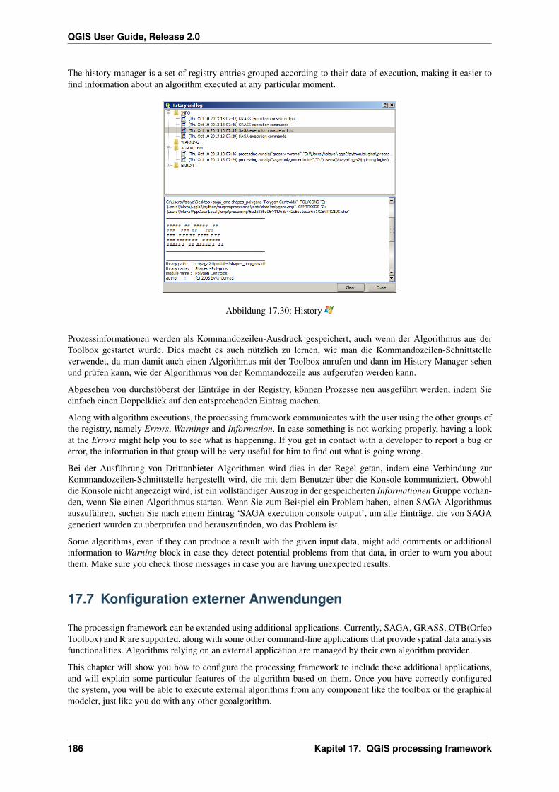
QGIS User Guide, Release 2.0
The history manager is a set of registry entries grouped according to their date of execution, making it easier tofind information about an algorithm executed at any particular moment.
Abbildung 17.30: History
Prozessinformationen werden als Kommandozeilen-Ausdruck gespeichert, auch wenn der Algorithmus aus derToolbox gestartet wurde. Dies macht es auch nützlich zu lernen, wie man die Kommandozeilen-Schnittstelleverwendet, da man damit auch einen Algorithmus mit der Toolbox anrufen und dann im History Manager sehenund prüfen kann, wie der Algorithmus von der Kommandozeile aus aufgerufen werden kann.
Abgesehen von durchstöberst der Einträge in der Registry, können Prozesse neu ausgeführt werden, indem Sieeinfach einen Doppelklick auf den entsprechenden Eintrag machen.
Along with algorithm executions, the processing framework communicates with the user using the other groups ofthe registry, namely Errors, Warnings and Information. In case something is not working properly, having a lookat the Errors might help you to see what is happening. If you get in contact with a developer to report a bug orerror, the information in that group will be very useful for him to find out what is going wrong.
Bei der Ausführung von Drittanbieter Algorithmen wird dies in der Regel getan, indem eine Verbindung zurKommandozeilen-Schnittstelle hergestellt wird, die mit dem Benutzer über die Konsole kommuniziert. Obwohldie Konsole nicht angezeigt wird, ist ein vollständiger Auszug in der gespeicherten Informationen Gruppe vorhan-den, wenn Sie einen Algorithmus starten. Wenn Sie zum Beispiel ein Problem haben, einen SAGA-Algorithmusauszuführen, suchen Sie nach einem Eintrag ‘SAGA execution console output’, um alle Einträge, die von SAGAgeneriert wurden zu überprüfen und herauszufinden, wo das Problem ist.
Some algorithms, even if they can produce a result with the given input data, might add comments or additionalinformation to Warning block in case they detect potential problems from that data, in order to warn you aboutthem. Make sure you check those messages in case you are having unexpected results.
17.7 Konfiguration externer Anwendungen
The processign framework can be extended using additional applications. Currently, SAGA, GRASS, OTB(OrfeoToolbox) and R are supported, along with some other command-line applications that provide spatial data analysisfunctionalities. Algorithms relying on an external application are managed by their own algorithm provider.
This chapter will show you how to configure the processing framework to include these additional applications,and will explain some particular features of the algorithm based on them. Once you have correctly configuredthe system, you will be able to execute external algorithms from any component like the toolbox or the graphicalmodeler, just like you do with any other geoalgorithm.
186 Kapitel 17. QGIS processing framework

QGIS User Guide, Release 2.0
By default, all algorithms that rely on an external appplication not shipped with QGIS are not enabled. You canenable them in the configuration dialog. Make sure that the corresponding application is already installed in yoursystem. Enabling an algorithm provider without installing the application it needs will cause the algorithms toappear in the toolbox, but an error will be thrown when you try to execute them.
This is because the algorithm descriptions (needed to create the parameters dialog and provide the informationneeded about the algorithm) are not included with each application, but with QGIS instead. That is,they are partof QGIS, so you have them in your installation even if you have not installed any other software. Running thealgorithm, however, needs the application binaries to be installed in your system.
17.7.1 A note for Windows users
If you are not an advanced user and you are running QGIS on windows, you might not be interested in readingthe rest of this chapter. Make sure you install QGIS in your system using the OSGeo4W application. That willautomatically install SAGA, GRASS and OTB in your system, and configure them so they can be run from QGIS.All the algorithms in the simplified view of the toolbox will be ready to be run, without needing any furtherconfiguration.
If you want to know more about how these providers work, or want to use some algorithms not included in thesimplified toolbox (such as R scripts), keep on reading.
17.7.2 Eine Bemwerkung zu den Datenformaten
When using an external software, opening a file in QGIS does not mean that it can be opened and processed as wellon that other software. In most cases, it can read what you have opened in QGIS, but in some cases, that might notbe the case. When using databases or uncommon file formats, whether for raster of vector layers, problems mightarise. If that happens, try to use well known file formats that you are sure that are understood by both programs,and check to console output (in the history and log dialog) for knowing more about what is going wrong.
Using GRASS raster layers is, for instance, one case in which you might have trouble and not be able to completeyour work if you call an external algorithm using such a layer as input. For this reason, these layers will not appearas available to algorithms.
You should, however, find no problems at all with vector layers, since QGIS automatically converts from theoriginal file format to one accepted by the external application before passing the layer to it. This adds an extraprocessing time, which might be significant if the layer has a large size, so do not be surprised if it takes more toprocess a layer from a DB connection that one of a similar size stored in a shapefile.
Providers not using external applications can process any layer that you can open in QGIS, since they open it foranalysis through QGIS.
Regarding output formats, all formats supported by QGIS as output can be used, both for raster and vector layers.Some provider do not support certain formats, but all can export to common formats raster layers that can be latertransformed by QGIS automatically. As in the case of input layers, if this conversion is needed, that might increasethe processing time.
If the extension of the filename specified when calling an algorithm does not match the extension of any of theformats supported by QGIS, then a suffix will be added to set a default format. In the case of raster layers, the tifextension is used, while shp is used for vector layer.
17.7.3 Eine Bemerkung zu Vektorlayern mit ausgewählten Objekten
External applications are also aware of the selection that exist in vector layers within QGIS. However, that re-quires rewritting all input vector layers, just as if they were originally in a format not supported by the externalapplication. Only when no selection exist, or the Use only selected features option is not enabled in the processinggeneral configuration, a layer can be directly passed to an external application.
In other cases, exporting only selected features is needed, which causes execution times to be longer.
17.7. Konfiguration externer Anwendungen 187
QGIS User Guide, Release 2.0
SAGA
SAGA algorithms can be run from QGIS if you have SAGA installed in your system and you configure the pro-cessing framework properly so it can find SAGA executables. In particular, the SAGA command-line executableis needed to run SAGA algorithms.
In case of running Windows, the standalone installer or the OSGeo4W installer, both install SAGA along withQGIS, and the path is automatically configured, so there is no need to do anything else.
If you have installed SAGA yourself (remember, you need version 2.1), the path to the SAGA executable must beconfigured. To do it, open the configuration dialog. In the SAGA block you will find a setting named SAGA Folder.Enter the path to the folder where SAGA is installed. Close the configuration dialog and now you are ready to runSAGA algorithms from QGIS.
In case you are running linux, SAGA binaries are not included with SEXTANTE, so you have to download andinstall the software yourself. Please check the SAGA website for more information. SAGA 2.1 is needed.
In this case there is no need to configure that, and you will not see those folders. Instead, you must make sure thatSAGA is properly installed and its folder is added to the PATH environment variable. Just open a console and typesaga_cmd to check that the system can find where SAGA binaries are located.
17.7.4 Über die SAGA KBS Einschränkungen
Most of SAGA algorithms that require several input raster layers, require them to have the same grid system. Thatis, to cover the same geographic area and have the same cellsize, so their corresponding grids match. When callingSAGA algorithms from QGIS, you can use any layer, regardless of its cellsize and extent. When multiple rasterlayers are used as input for a SAGA algorithm, QGIS resamples them to a common grid system and then passesthem to SAGA (unless the SAGA algorithm can operate with layers from different grid systems).
Die Definition dieses gemeinsamen KBS wird vom Benutzer gesteuert. Sie finden mehrere Parameter im SAGABereich des Konfigurationsdialogs. Es gibt zwei Möglichkeiten für die Einstellung des Ziel-KBS:
• Setzen Sie sie manuell und legen die Ausdehnung durch Definition der Werte mit folgenden Parameternfest:
– Resampling min X
– Resampling max X
– Resampling min Y
– Resampling max Y
– Resampling cellsize
Notice that QGIS will resample input layers to that extent, even if they do not overlap with it.
• Automatisch auf Basis des Eingabelayers setzen. Um diese Option zu wählen, aktivieren Sie einfach dieVerwende min Abdeckgitter für Resampling Option. Alle anderen Einstellungen werden ignoriert und dieminimalen Umfang, der alle Schichten umfasst wird verwendet. Die Pixelgröße des Ziellayers ist dann dasMaximum aller Pixelgrößen der Eingabelayer.
Für Algorithmen, die nicht mit mehreren Rasterlayern arbeiten, oder für diejenigen, die kein eindeutiges KBSbauchen, wird kein Resampling vor dem Aufruf von SAGA durchgeführt, und die Parameter werden nicht ver-wendet.
17.7.5 Einschränkungen für Multi-Band-Layer
Unlike QGIS, SAGA has no support for multi-band layers. If you want to use a multiband layer (such asan RGB or multispectral image), you first have to split it into single-banded images. To do so, you can usethe ‘SAGA/Grid - Tools/Split RGB image’ algorithm (which creates 3 images from an RGB image) or the‘SAGA/Grid - Tools/Extract band’ algorithm (to extract a single band).
188 Kapitel 17. QGIS processing framework

QGIS User Guide, Release 2.0
17.7.6 Begrenzung bei der Pixelgröße
SAGA assumes that raster layers have the same cellsize in the X and Y axis. If you are working with a layer withdifferent values for its horizontal and vertical cellsizes, you might get unexcepted results. In this case, a warningwill be added to the processing log, indicating that an input layer might not be suitable to be processed by SAGA.
17.7.7 Logging
When QGIS calls SAGA, it does it using its command-line interface, thus passing a set of commands to performall the required operation. SAGA show its progress by writing information to the console, which includes thepercentage of processing already done, along with additional content. This output is filtered and used to updatethe progress bar while the algorithm is running.
Both the commands sent by QGIS and the additional information printed by SAGA can be logged along with otherprocessing log messages, and you might find them useful to track in detailed what is going on when QGIS runs aSAGA algorithm. you will find two settings, namely Log console output and Log execution commands to activatethat logging mechanism.
Most other providers that use an external application and call it through the command-line have similar options,so you will find them as well in other places in the processing settings list.
R. Creating R scripts
R integration in QGIS is different from that of SAGA in that there is not a predefined set of algorithms you can run(except for a few examples). Instead, you should write your scripts and call R commands, much like you would dofrom R, and in a very similar manner to what we saw in the chapter dedicated to processing scripts. This chaptershows you the syntax to use to call those R commands from QGIS and how to use QGIS objects (layers, tables)in them.
The first thing you have to do, as we saw in the case of SAGA, is to tell QGIS where you R binaries are located.You can do so using the R folder entry in the processing configuration dialog. Once you have set that parameter,you can start creating your own R scripts and executing them.
Dies ist wieder anders in Linux. Dort müssen Sie nur sicherstellen, dass der R-Ordner in der UmgebungsvariablenPATH enthalten ist. Wenn Sie nur die Eingabe R in eine Konsole eingeben können, kann es losgehen.
To add a new algorithm that calls an R function (or a more complex R script that you have developed and youwould like to have available from QGIS), you have to create a script file that tells the processing framework howto perform that operation and the corresponding R commands to do so.
Script files have the extension .rsx and creating them is pretty easy if you just have a basic knowledge ofR syntax and R scripting. They should be stored in the R-scripts folder. You can set this folder in the R settingsgroup (available from the processing settings dialog), just like you do with the folder for regular processing scripts.
Let’s have a look at a very simple file script file, which calls the R method spsample to create a random gridwithin the boundary of the polygons in a given polygon layer. This method belong to the maptools package.Since almost all the algorithms that you might like to incorporate into QGIS will use or generate spatial data,knowledge of spatial packages like maptools and, specially, sp, is mandatory.
##polyg=vector##numpoints=number 10##output=output vector##sp=grouppts=spsample(polyg,numpoints,type="random")output=SpatialPointsDataFrame(pts, as.data.frame(pts))
The first lines, which start with a double Python comment sign (##), tell QGIS the inputs of the algorithm de-scribed in the file and the outputs that it will generate. They work exactly with the same syntax as the SEXTANTEscripts that we have already seen, so they will not be described here again. Check the processing_scripts sectionfor more information.
17.7. Konfiguration externer Anwendungen 189
QGIS User Guide, Release 2.0
When you declare an input parameter, QGIS uses that information for two things: creating the user interface toask the user for the value of that parameter and creating a corresponding R variable that can be later used as inputfor R commands.
In the above example, we are declaring an input of type vector named polyg. When executing the algorithm,QGIS will open in R the layer selected by the user and store it in a variable also named polyg. So the name of aparameter is also the name of the variable that we can use in R for accesing the value of that parameter (thus, youshould avoid using reserved R words as parameter names).
Spatial elements such as vector and raster layers are read using the readOGR() and brick() commands (youdo not have to worry about adding those commands to your description file, QGIS will do it) and stored asSpatial*DataFrame objects. Table fields are stored as strings containing the name of the selected field.
Tabellen werden geöffnet, indem die den read.csv()-Befehl verwenden Wenn Sie eine Tabelle angegeben, dienicht im CSV-Format ist, wird sie vor dem Import in R. umgewandelt.
Additionally, raster files can be read using the readGDAL() command instead of brick(), by using the##usereadgdal.
If you are an advanced user and do not want QGIS to create the object representing the layer, you can use the##passfilename tag to indicate that you prefer a string with the filename instead. In this case, it is up to youto open the file before performing any operation on the data it contains.
With the above information, we can now understand the first line of our first example script (the first line notstarting with a Python comment).
pts=spsample(polyg,numpoints,type="random")
Die Variable Polygon enthält bereits ein SpatialPolygonsDataFrame Objekt, damit kann es verwen-det werden, um das spsample Verfahren aufzurufen, ebenso wie die NumPoints, die die Anzahl der Punktezeigt, die zum Gitter hinzugefügt werden sollen.
Da wir eine Ausgabe vom Typ Vektor definiert haben mit dem Namen‘‘out‘‘, müssen wir nun eineVariable namens out erstellen und Spatial*DATAframe Objekt dafür erstellen (in diesem Fall einSpatialPointsDataFrame). Sie können einen beliebigen Namen für Ihre Zwischenvariablen verwenden.Stellen Sie nur sicher, dass die Variable Ihres Endergebnisses den gleichen Namen hat, den Sie zuvor definierthaben und das sie einen geeigneten Wert enthält.
In this case, the result obtained from the spsample method has to be converted explicitly into aSpatialPointsDataFrame object, since it is itself an object of class ppp, which is not a suitable classto be returned to QGIS.
If your algorithm generates raster layers, the way they are saved will depend on whether you have used or not the#dontuserasterpackage option. In you have used it, layers are saved using the writeGDAL() method. Ifnot, the writeRaster() method from the raster package will be used.
If you have used the #passfilename option, outputs are generated using the raster package (withwriteRaster()), even though it is not used for the inputs.
If you algorithm does not generate any layer, but a text result in the console instead, you have to indicate that youwant the console to be shown once the execution is finished. To do so, just start the command lines that produce theresults you want to print with the > (‘greater’) sign. The output of all other lines will not be shown. For instance,here is the description file of an algorithm that performs a normality test on a given field (column) of the attributesof a vector layer:
##layer=vector##field=field layer##nortest=grouplibrary(nortest)>lillie.test(layer[[field]])
The output ot the last line is printed, but the output of the first is not (and neither are the outputs from othercommand lines added automatically by QGIS).
Wenn Ihr Algorithmus eine Grafiken erstellt (mit der plot()-Methode), fügen Sie die folgende Zeile ein:
190 Kapitel 17. QGIS processing framework
QGIS User Guide, Release 2.0
##showplots
This will cause QGIS to redirect all R graphical outputs to a temporary file, which will be later opened once Rexecution has finished.
Both graphics and console results will be shown in the processing results manager.
Für weitere Informationen schauen Sie sich bitte die Skript-Dateien an, die SEXTANTE bereits enthält. Die meis-ten von ihnen sind ziemlich einfach und werden wesentlich dazu beitragen, wie Sie Ihre eigenen erstellen.
Bemerkung: rgdal and maptools libraries are loaded by default so you do not have to add the correspond-ing library() commands (you have to make sure, however, that those two packages are installed in your Rdistribution). However, other additional libraries that you might need have to be explicitly loaded. Just add thenecessary commands at the beginning of your script. You also have to make sure that the corresponding packagesare installed in the R distribution used by QGIS. The processing framework will not take care of any packageinstallation. If you run a script that requires an uninstalled package, the execution will fail, and SEXTANTE willtry to detect which packages are missing. You must install those missing libraries manually before you can run thealgorithm.
GRASS
Die Konfiguration von GRASS ist nicht viel anders als die Konfiguration von SAGA. Zuerst muss der Pfadzu dem Ordner GRASS definiert werden, aber nur, wenn Sie Windows verwenden. Zusätzlich gibt es einenShell-Interpreter (in der Regel: msys.exe, den Sie in den meisten GRASS für Windows-Distributionen finden)der definiert werden muss, genauso wie der Pfad dorthin.
By default, the processign framework tries to configure its GRASS connector to use the GRASS distribution thatships along with QGIS. This should work without problems in most systems, but if you experience problems, youmight have to do it manually. Also, if you want to use a different GRASS installation, you can change that settingand point to the folder where that it is installed. GRASS 6.4 is needed for algorithms to work correctly.
Wenn Sie Linux verwenden, müssen Sie nur noch sicherstellen, dass GRASS richtig installiert ist, und dass esproblemlos von einer Konsole ausgeführt werden kann.
GRASS Algorithmen verwenden eine Region für die Berechnungen. Diese Region kann manuell definiert werdenunter Verwendung von Werten ähnlich denen, die in der Sage Konfiguration stehen oder automatisch, wobei dieminimale Ausdehnung aller Eingangslayer verwendet werden, wenn der Algorithmus ausgeführt wird. Wenn diesdas Verhalten ist, das Sie bevorzugen, können Sie es über die Option Verwende min abdecken Region in denGRASS Konfigurationsparametern definieren.
The last parameter that has to be configured is related to the mapset. A mapset is needed to run GRASS, and theprocessing frmaework creates a temporary one for each execution. You have to specify if the data you are workingwith uses geographical (lat/lon) coordinates or projected ones.
GDAL
No additional configuration is needed to run GDAL algorithms, since it is already incorporated to QGIS andalgorithms can infere its configuration from it.
Orfeo ToolBox
Orfeo ToolBox (OTB) algorithms can be run from QGIS if you have OTB installed in your system and you haveconfigured QGIS properly, so it can find all necessary files (command-line tools and libraries).
As in the case of SAGA OTB binaries are included in the standalone installer for Windows, but are not includedif you are runing Linux, so you have to download and install the software yourself. Please check the OTB websitefor more information.
17.7. Konfiguration externer Anwendungen 191
QGIS User Guide, Release 2.0
Once OTB is installed, start QGIS, open the processing configuration dialog and configure the OTB algorithmprovider. In the Orfeo Toolbox (image analysis) block you will find all settings related to OTB. First ensure thatalgorithms are enabled.
Then configure the path to the folder where OTB command–line tools and libraries are installed:
• In der Regel OTB Programme-Ordner verweist auf /usr/lib/otb/applications und den OTBKommandozeilen-Tools Ordner unter /usr/bin
• if you use OSGeo4W installer, than install otb-bin package and enterC:\OSGeo4W\apps\orfeotoolbox\applications as OTB applications folder andC:\OSGeo4W\bin as OTB command line tools folder. This values should be configured by de-fault, but if you have a different OTB installation, configure them to the correspondig values in yoursystem.
TauDEM
Um diesen Anbieter zu verwenden, müssen Sie die TauDEM Kommandozeilen-Tools installieren.
17.7.8 Windows
Please visit TauDEM homepage for installation instructions and precompiled binaries for 32bit and 64bit systems.IMPORTANT: you need TauDEM 5.0.6 executables, version 5.2 is currently not supported.
17.7.9 Linux
Es gibt keine Pakete für die meisten Linux-Distribution, daher sollten Sie TauDEM selbst kompilieren. WeilTauDEM MPICH2 verwendet, installieren Sie es zuerst mit Ihrem Lieblings-Paketmanager. TauDEM arbeit auchmit OpenMPI , also können Sie auch das verwenden, statt MPICH2.
Laden Sie den TauDEM 5.0.6 Quellcode herunter und entpacken Sie die Dateien im selben Ordner.
Öffne linearpart.h und füge hinzu nach Zeile
#include "mpi.h"
füge neue Zeile hinzu mit
#include <stdint.h>
dadurch bekommen Sie
#include "mpi.h"#include <stdlib.h>
Speichern Sie Änderungen und schliessen Sie die Datei. Nun öffnen Sie die Datei tiffIO.h, suchen Sie Zeile#include "stdint.h" und tauschen Sie die Anführungsstriche ("") durch <> aus
#include <stdint.h>
Speichern Sie die Änderungen und schliessen Sie die Datei. Erstellen Sie einen build Ordner und wechseln Sie indiesen
mkdir buildcd build
Konfigurieren Sie Ihren Build mit dem Kommando
CXX=mpicxx cmake -DCMAKE_INSTALL_PREFIX=/usr/local ..
und dann kompilieren
192 Kapitel 17. QGIS processing framework

QGIS User Guide, Release 2.0
make
Schliesslich, um TauDEM unter /usr/local/bin zu installieren, führen Sie aus
sudo make install
17.8 The SEXTANTE Commander
SEXTANTE includes a practical tool that allows you to run algorithms without having to use the toolbox, but justtyping the name of the algorithm you want to run.
This tools is known as the SEXTANTE commander, and it is just a simple text box with autocompletion where youtype the command you want to run.
Abbildung 17.31: The SEXTANTE Commander
The commander is started from the Analysis menu or, more practically, pressing Shift + Ctrl + M (youcan change that default keyboard shortcut in the QGIS configuration if you prefer a different one). Apart fromexecuting SEXTANTE algorithms, the commander gives you access to most of the functionality in QGIS, whichmeans that it gives you a practical and efficient way of running QGIS tasks, and allows you to control QGISreducing the usage of buttons and menus.
Moreover, the commander is configurable and you can add your custom commands and have them just a fewkeystrokes away, making it a powerful tool to become more productive in your daily work with QGIS
17.8.1 Available commands
The commands available in the commander fall in the following categories:
• SEXTANTE algorithms. They are shown as SEXTANTE algorithm: <name of thealgorithm>.
• Menu items. They are shown as Menu item: <menu entry text>. All menus items available fromthe QGIS interface are available, even if they are included in a submenu.
• Python functions. You can create short Python functions that will be then included in the list of availablecommands. They are shown as Function: <function name>
To run any of the above, just start typing and then select the corresponding element from the list of available onesthat appears after filtering the whole list of commands with the text you have entered.
In the case of calling a Python function, you can select the entry in the list, which is prefixed byFunction: (for instance, Function: removeall), or just directly type the functionname (‘‘removeall in the previous example). There is no need to add brackets after the function name.
17.8. The SEXTANTE Commander 193

QGIS User Guide, Release 2.0
17.8.2 Creating custom functions
Custom functions are added by entering the corresponding Python code in the commands.py file that is foundin the .qgis/sextante/commander directory in your user folder. It is just a simple Python file whereyou can add the functions that you need.
The file is created the first time you open the commander, with a few example functions. If you haven’t launchedthe commander yet, you can create the file yourself. To edit the commands file, use your favorite text editor. Youcan also use a built-in editor by calling the edit command from the commander. It will open the editor with thecommands file, and you can edit it directly and then save your changes.
For instance, you can add the following function, which removes all layers:
from qgis.gui import *
def removeall():mapreg = QgsMapLayerRegistry.instance()mapreg.removeAllMapLayers()
Once you have added the function, it will be available in the commander, and you can invoke it by typingremoveall. There is no need to do anything apart from writing the function itself.
Functions can receive parameters. Add *args to your function definition, to receive argument. When calling thefunction from the commander, parameters have to be passed separated by spaces.
Here is an example of a function that loads a layer and takes a parameter with the filename of the layer to load.
import sextante
def load(*args):sextante.load(args[0])
If you want to load a layer in /home/myuser/points.shp, type load /home/myuser/points.shpin the commander text box.
194 Kapitel 17. QGIS processing framework

KAPITEL 18
Druckzusammenstellung
The print composer provides growing layout and printing capabilities. It allows you to add elements such as theQGIS map canvas, text labels, images, legends, scalebars, basic shapes, arrows, attribute tables and HTML frames.You can size, group, align and position each element and adjust the properties to create your layout. The layoutcan be printed or exported to image formats, Postscript, PDF or to SVG (export to SVG is not working properlywith some recent Qt4 versions, you should try and check individual on your system). You can save the layout astemplate and load it again in another session. Finally, generating several maps based on a template can be donethrought the Atlas generator See a list of tools in table_composer_1:
Icon Zweck Icon Zweck
Save Project New Composer
Duplicate Composer Composer Manager
Aus Vorlage laden Als Vorlage speichern
Speichern als Rasterbild Als PDF exportieren
Speichern als SVG Drucken
Volle Ausdehnung Hineinzoomen
Hinauszoomen Aktualisiere Ansicht
Letzte Änderung zurücknehmen Letzte Änderung wiederherstellen
Add new map from QGIS map canvas Bild hinzufügen
Neue Beschriftung hinzufügen Neue Legende hinzufügen
Neuen Maßstab hinzufügen Einfaches Objekt hinzufügen
Pfeil hinzufügen Fügt Attributtabelle hinzu
Add a HTML Frame
Eintrag wählen/verschieben Den Elementinhalt verschieben
Elemente gruppieren Gruppe auflösen
Hervorholen Versenken
In den Vordergrund holen In den Hintergrund schicken
Linksbündig Rechtsbündig
Zentrieren Vertikal zentrieren
Oben bündig Unten bündig
Tabelle Composer 1: Funktionen der Druckzusammenstellung
All Print Composer tools are available in menus and as icons in a toolbar. The toolbar can be switched off and on
195

QGIS User Guide, Release 2.0
using the right mouse button over the toolbar.
18.1 First steps
18.1.1 Ein neues Template öffnen
Before you start to work with the print composer, you need to load some raster and vector layers in the QGIS mapcanvas and adapt their properties to suit your own convenience. After everything is rendered and symbolized to
your liking, click the New Print Composer icon in the toolbar or choose File → New Print Composer. You will beprompt to choose a title for the new composer.
18.1.2 Die Druckzusammenstellung verwenden
Opening the print composer provides you with a blank canvas to which you can add the current QGIS mapcanvas, text labels, images, legends, scalebars, basic shapes, arrows, attribute tables and HTML frames. Fig-
ure_composer_1 shows the initial view of the print composer with an activated Snap to grid mode but beforeany elements are added.
Abbildung 18.1: Print Composer
The print composer provides four tabs:
• The Composition tab allows you to set paper size, orientation, the print quality for the output file in dpiand to activate snapping to a grid of a defined resolution. You can also choose the Number of pages your
composition will have. Please note, the Snap to grid feature only works, if you define a grid resolution
> 0. Furthermore you can also activate the Print as raster checkbox. This means all elements will berastered before printing or saving as Postscript or PDF.
• The Item Properties tab displays the properties for the selected item element. Click the Select/Move item
icon to select an element (e.g. legend, scalebar or label) on the canvas. Then click the Item Properties taband customize the settings for the selected element.
• The Command history tab (hidden by default) displays a history of all changes applied to the print composerlayout. With a mouse click it is possible to undo and redo layout steps back and forth to a certain status.
196 Kapitel 18. Druckzusammenstellung
QGIS User Guide, Release 2.0
• The Atlas generation tab allows to enable the generation of an atlas for the current composer and givesaccess to its parameters.
You can add multiple elements to the composer. It is also possible to have more than one map view or legend orscalebar in the print composer canvas, on one or several pages. Each element has its own properties and in the caseof the map, its own extent. If you want to remove any elements from the composer canvas you can do that withthe Delete or the Backspace key.
In der Druckzusammenstellung navigieren
To navigate in the canvas layout, the print composer provides 4 general tools:
• Hineinzoomen
• Hinauszoomen
• Volle Ausdehnung
• Aktualisiere Ansicht
18.1.3 Composition tab — General composition setup
In the Composition tab, you can define the global settings of your composition.
• You can choose one of the Presets for your papersheet, or enter your custom width and height.
• Composition can now be parted on several pages. For instance, a first page can show a map canvas anda second page will show the attribute table associated to a layer while a third ons shows a HTML framelinking to your organization website. Set the Number of pages to the desired value.
• Choose the page Orientation and its Exported resolution
• When checked, the print as raster means all elements will be rasterized before printing or saving asPostscript or PDF.
• Snap to grid and Snap to alignements tools make accomplishing some tasks much easier. There’s three typesof grid: Dots, Solid lines and Crosses. You can adjust spacings, offsets and color to your need.
• Selection tolerance defines the maximum distance below which an item is snapped to the grid.
• Snap to alignements shows helping lines when the borders or axis of two items are aligned.
18.1.4 Composer items general options
Composer items have a set of common properties you will find on the bottom of the Item Properties tab: Positionand size, Frame, Background, Item ID and Rendering (See figure_composer_2)
• The Position and size dialog lets you define size and position of the frame that contains the item. You canalso choose which Reference point will be set at the X and Y coordinates previously defined.
• The Frame shows or hides the frame around the label. Click on the [Color] and [Thickness] buttons toadjust those properties.
• the Background enables or disables a background color. Click on the [Color...] button to display a dialogwhere you pick a color ou choose frome a custom setting. Transparency can also be adjusted throught thealpha field.
• Use the Item ID to create a relationship to other print composer items.
• Rendering mode can be selected in the option field. See Rendering_Mode .
18.1. First steps 197
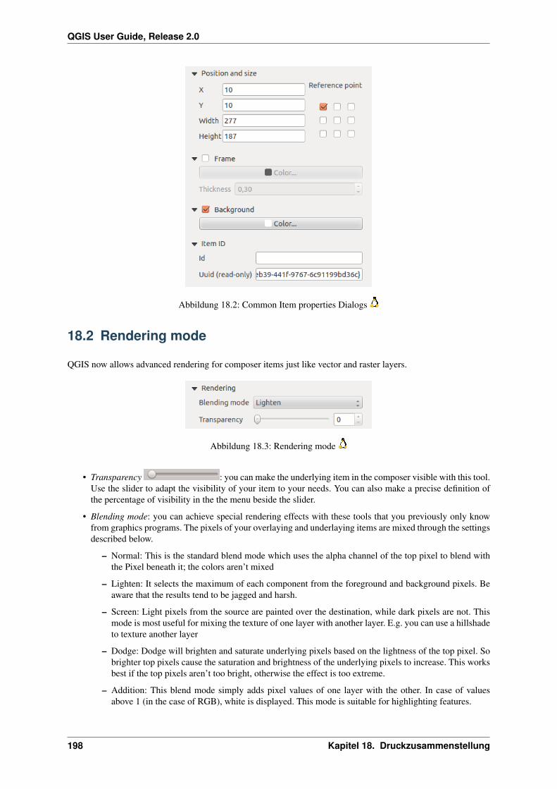
QGIS User Guide, Release 2.0
Abbildung 18.2: Common Item properties Dialogs
18.2 Rendering mode
QGIS now allows advanced rendering for composer items just like vector and raster layers.
Abbildung 18.3: Rendering mode
• Transparency : you can make the underlying item in the composer visible with this tool.Use the slider to adapt the visibility of your item to your needs. You can also make a precise definition ofthe percentage of visibility in the the menu beside the slider.
• Blending mode: you can achieve special rendering effects with these tools that you previously only knowfrom graphics programs. The pixels of your overlaying and underlaying items are mixed through the settingsdescribed below.
– Normal: This is the standard blend mode which uses the alpha channel of the top pixel to blend withthe Pixel beneath it; the colors aren’t mixed
– Lighten: It selects the maximum of each component from the foreground and background pixels. Beaware that the results tend to be jagged and harsh.
– Screen: Light pixels from the source are painted over the destination, while dark pixels are not. Thismode is most useful for mixing the texture of one layer with another layer. E.g. you can use a hillshadeto texture another layer
– Dodge: Dodge will brighten and saturate underlying pixels based on the lightness of the top pixel. Sobrighter top pixels cause the saturation and brightness of the underlying pixels to increase. This worksbest if the top pixels aren’t too bright, otherwise the effect is too extreme.
– Addition: This blend mode simply adds pixel values of one layer with the other. In case of valuesabove 1 (in the case of RGB), white is displayed. This mode is suitable for highlighting features.
198 Kapitel 18. Druckzusammenstellung
QGIS User Guide, Release 2.0
– Darken: Creates a resultant pixel that retains the smallest components of the foreground and back-ground pixels. Like lighten, the results tend to be jagged and harsh
– Multiply: It multiplies the numbers for each pixel of the top layer with the corresponding pixel for thebottom layer. The results are darker pictures.
– Burn: Darker colors in the top layer causes the underlying layers to darken. Can be used to tweak andcolorise underlying layers.
– Overlay: Combines multiply and screen blending modes. In the resulting picture light parts of thepicture become lighter and dark parts become darker.
– Soft light: Very similar to overlay, but instead of using multiply/screen it uses color burn/dodge. Thisone is supposed to emulate shining a soft light onto an image.
– Hard light: Hard light is very similar to the overlay mode. It’s supposed to emulate projecting a veryintense light onto an image.
– Difference: Difference subtracts the top pixel from the bottom pixel or the other way round, to alwaysget a positive value. Blending with black produces no change, as values for all colors are 0.
– Subtract: This blend mode simply subtracts pixel values of one layer with the other. In case of negativevalues, black is displayed.
18.3 Composer Items
18.3.1 Adding a current QGIS map canvas to the Print Composer
Click on the Add new map toolbar button in the print composer toolbar to add the QGIS map canvas. Now drag arectangle on the composer canvas with the left mouse button to add the map. To display the current map, you canchoose between three different modes in the map Item Properties tab:
• Rechteck ist die Standardeinstellung. Es wird eine leeres Kästchen mit der Meldung ‘Karte wird hiergedruckt’ angezeigt.
• Cache führt dazu, dass die Karte in der momentanen Bildschirmauflösung gerendert wird. Wenn man imComposer zoomt, wird nicht neu gerendert sondern nur das Bild skaliert.
• Zeichnen führt dazu, dass beim Zoomen im Composer neu gerendert wird, aber aus Speicherplatzgründennur bis zu einer Maximalauflösung.
Cache ist der Standard Preview Modus, wenn Sie eine Karte neu in die Druckzusammenstellung laden.
Sie können die Größe des Kartenfensters in der Druckzusammenstellung nachträglich verändern, indem sie auf
den Knopf Selektiere/Verschiebe Eintrag klicken, mit der Maus das Kartenfenster auswählen und die Größe an denblauen Ecken verändern.Sie können die Größe auch verändern, indem Sie das Element selektieren und die Breiteund Höhe im Reiter Eintrag anpassen.
Um Layer innerhalb der Druckzusammenstellung im Kartenelement zu verschieben, klicken Sie auf den KnopfDen Elementinhalt verschieben. Sie können nun mit der linken Maustaste die Layer im Kartenelement verschieben.
Nachdem Sie den richtigen Platz für das Kartenelement gefunden haben, kann es innerhalb des Print Compos-er Kartenfensters gesichert werden. Wählen Sie dazu das Kartenelement aus und drücken Sie auf die rechte
Maustaste, um es zu sichern. Mit einem erneuten rechten Mausklick ist es wieder entsichert. Sie können das
Kartenelement auch sichern, indem Sie das Kontrollkästchen Layer des Kartenelements festhalten aktivierenim Eigenschaften Reiter des Kartendialogs.
Main properties
The Main properties dialog of the map Item Properies tab provides following functionalities (see fig-ure_composer_4):
18.3. Composer Items 199
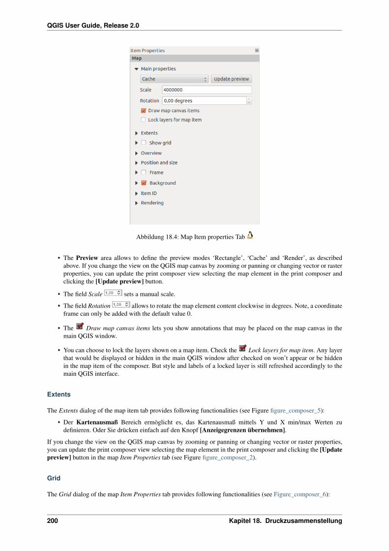
QGIS User Guide, Release 2.0
Abbildung 18.4: Map Item properties Tab
• The Preview area allows to define the preview modes ‘Rectangle’, ‘Cache’ and ‘Render’, as describedabove. If you change the view on the QGIS map canvas by zooming or panning or changing vector or rasterproperties, you can update the print composer view selecting the map element in the print composer andclicking the [Update preview] button.
• The field Scale sets a manual scale.
• The field Rotation allows to rotate the map element content clockwise in degrees. Note, a coordinateframe can only be added with the default value 0.
• The Draw map canvas items lets you show annotations that may be placed on the map canvas in themain QGIS window.
• You can choose to lock the layers shown on a map item. Check the Lock layers for map item. Any layerthat would be displayed or hidden in the main QGIS window after checked on won’t appear or be hiddenin the map item of the composer. But style and labels of a locked layer is still refreshed accordingly to themain QGIS interface.
Extents
The Extents dialog of the map item tab provides following functionalities (see Figure figure_composer_5):
• Der Kartenausmaß Bereich ermöglicht es, das Kartenausmaß mittels Y und X min/max Werten zudefinieren. Oder Sie drücken einfach auf den Knopf [Anzeigegrenzen übernehmen].
If you change the view on the QGIS map canvas by zooming or panning or changing vector or raster properties,you can update the print composer view selecting the map element in the print composer and clicking the [Updatepreview] button in the map Item Properties tab (see Figure figure_composer_2).
Grid
The Grid dialog of the map Item Properties tab provides following functionalities (see Figure_composer_6):
200 Kapitel 18. Druckzusammenstellung

QGIS User Guide, Release 2.0
Abbildung 18.5: Map Extents Dialog
Abbildung 18.6: Map Grid Dialog
18.3. Composer Items 201
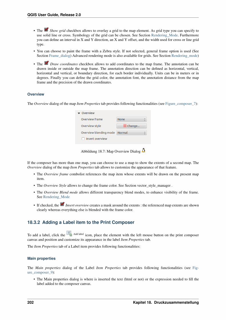
QGIS User Guide, Release 2.0
• The Show grid checkbox allows to overlay a grid to the map element. As grid type you can specify touse solid line or cross. Symbology of the grid can be chosen. See Section Rendering_Mode. Furthermoreyou can define an interval in X and Y direction, an X and Y offset, and the width used for cross or line gridtype.
• You can choose to paint the frame with a Zebra style. If not selected, general frame option is used (SeeSection Frame_dialog) Advanced rendering mode is also available for grids. See Section Rendering_mode)
• The Draw coordinates checkbox allows to add coordinates to the map frame. The annotation can bedrawn inside or outside the map frame. The annotation direction can be defined as horizontal, vertical,horizontal and vertical, or boundary direction, for each border individually. Units can be in meters or indegrees. Finally you can define the grid color, the annotation font, the annotation distance from the mapframe and the precision of the drawn coordinates.
Overview
The Overview dialog of the map Item Properties tab provides following functionalities (see Figure_composer_7):
Abbildung 18.7: Map Overview Dialog
If the composer has more than one map, you can choose to use a map to show the extents of a second map. TheOverview dialog of the map Item Properties tab allows to customize the appearance of that feature.
• The Overview frame combolist references the map item whose extents will be drawn on the present mapitem.
• The Overview Style allows to change the frame color. See Section vector_style_manager .
• The Overview Blend mode allows different transparency blend modes, to enhance visibility of the frame.See Rendering_Mode
• If checked, the Invert overview creates a mask around the extents : the referenced map extents are shownclearly whereas everything else is blended with the frame color.
18.3.2 Adding a Label item to the Print Composer
To add a label, click the Add label icon, place the element with the left mouse button on the print composercanvas and position and customize its appearance in the label Item Properties tab.
The Item Properties tab of a Label item provides following functionalities:
Main properties
The Main properties dialog of the Label Item Properties tab provides following functionalities (see Fig-ure_composer_9):
• The Main properties dialog is where is inserted the text (html or not) or the expression needed to fill thelabel added to the composer canvas.
202 Kapitel 18. Druckzusammenstellung
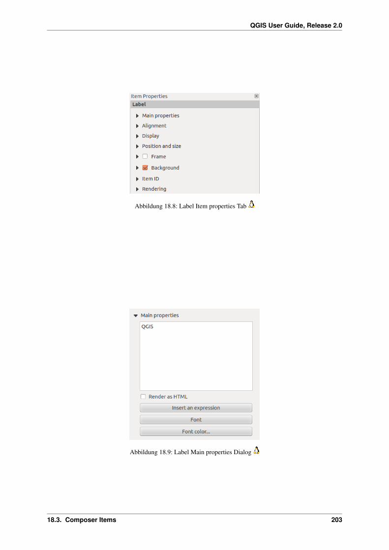
QGIS User Guide, Release 2.0
Abbildung 18.8: Label Item properties Tab
Abbildung 18.9: Label Main properties Dialog
18.3. Composer Items 203
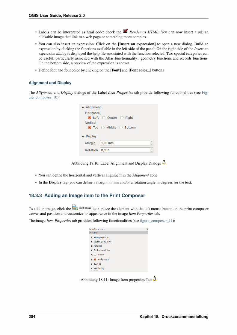
QGIS User Guide, Release 2.0
• Labels can be interpreted as html code: check the Render as HTML. You can now insert a url, anclickable image that link to a web page or something more complex.
• You can also insert an expression. Click on the [Insert an expression] to open a new dialog. Build anexpression by clicking the functions available in the left side of the panel. On the right side of the Insert anexpression dialog is displayed the help file associated with the function selected. Two special categories canbe useful, particularly associted with the Atlas functionnality : geometry functions and records functions.On the bottom side, a preview of the expression is shown.
• Define font and font color by clicking on the [Font] and [Font color...] buttons
Alignment and Display
The Alignment and Display dialogs of the Label Item Properties tab provide following functionalities (see Fig-ure_composer_10):
Abbildung 18.10: Label Alignment and Display Dialogs
• You can define the horizontal and vertical alignment in the Alignment zone
• In the Display tag, you can define a margin in mm and/or a rotation angle in degrees for the text.
18.3.3 Adding an Image item to the Print Composer
To add an image, click the Add image icon, place the element with the left mouse button on the print composercanvas and position and customize its appearance in the image Item Properties tab.
The image Item Properties tab provides following functionalities (see figure_composer_11):
Abbildung 18.11: Image Item properties Tab
204 Kapitel 18. Druckzusammenstellung
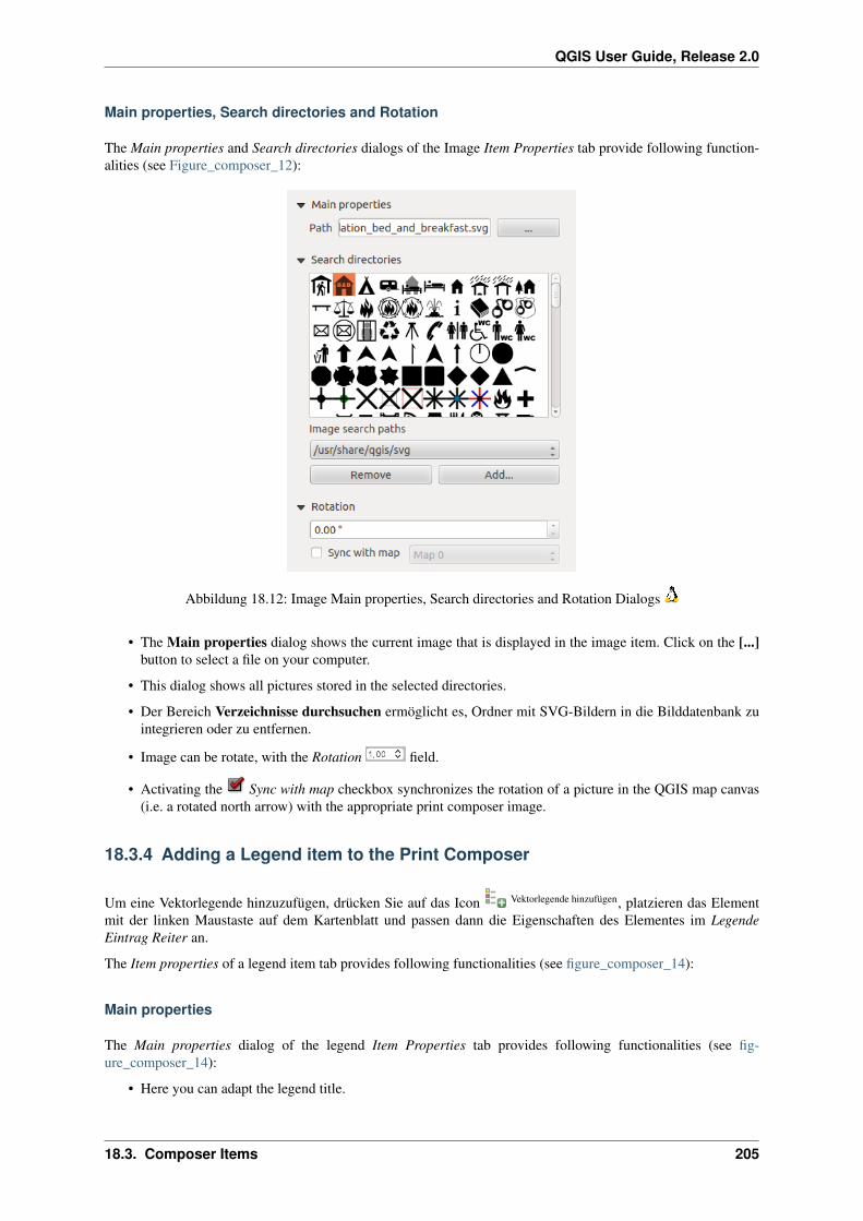
QGIS User Guide, Release 2.0
Main properties, Search directories and Rotation
The Main properties and Search directories dialogs of the Image Item Properties tab provide following function-alities (see Figure_composer_12):
Abbildung 18.12: Image Main properties, Search directories and Rotation Dialogs
• The Main properties dialog shows the current image that is displayed in the image item. Click on the [...]button to select a file on your computer.
• This dialog shows all pictures stored in the selected directories.
• Der Bereich Verzeichnisse durchsuchen ermöglicht es, Ordner mit SVG-Bildern in die Bilddatenbank zuintegrieren oder zu entfernen.
• Image can be rotate, with the Rotation field.
• Activating the Sync with map checkbox synchronizes the rotation of a picture in the QGIS map canvas(i.e. a rotated north arrow) with the appropriate print composer image.
18.3.4 Adding a Legend item to the Print Composer
Um eine Vektorlegende hinzuzufügen, drücken Sie auf das Icon Vektorlegende hinzufügen, platzieren das Elementmit der linken Maustaste auf dem Kartenblatt und passen dann die Eigenschaften des Elementes im LegendeEintrag Reiter an.
The Item properties of a legend item tab provides following functionalities (see figure_composer_14):
Main properties
The Main properties dialog of the legend Item Properties tab provides following functionalities (see fig-ure_composer_14):
• Here you can adapt the legend title.
18.3. Composer Items 205

QGIS User Guide, Release 2.0
Abbildung 18.13: Legend Item properties Tab
Abbildung 18.14: Legend Main properties Dialog
• Choose which Map item the current legend will refer to in the select list.
• Since QGIS 1.8, you can wrap the text of the legend title to a given character.
Legend items
The Legend items dialog of the legend Item Properties tab provides following functionalities (see fig-ure_composer_15):
Abbildung 18.15: Legend Legend Items Dialog
• The legend items window lists all legend items and allows to change item order, group layers, remove andrestore items of the list, edit layer names. After changing the symbology in the QGIS main window you can
206 Kapitel 18. Druckzusammenstellung

QGIS User Guide, Release 2.0
click on [Update] to adapt the changes in the legend element of the print composer. The item order can bechanged using the [Up] and [Down] buttons or with ‘drag and drop’ functionality.
• The feature count for each vector layer can be shown by enable the [Sigma] button.
• Legend can be updated automatically, Auto-update is checked.
Fonts, Columns, Symbol and Spacing
The Fonts, Columns, Symbol and Spacing dialogs of the legend Item Properties tab provide following functional-ities (see figure_composer_16):
Abbildung 18.16: Legend Fonts, Columns, Symbol and Spacing Dialogs
• You can change the font of the legend title, group, subgroup and item (layer) in the legend item. Click on acategory button to open a Select font dialog.
• All those items will get the same Color
• Legend items can be arranged in several columns. Select the correct value in the Count field.
• The Equal columns widths sets how legend columns should be adjusted.
• The Split layers option allows a categorized or a graduated layer legend to be divided upon columns.
• You can change width and height of the legend symbol in this dialog.
18.3. Composer Items 207

QGIS User Guide, Release 2.0
• Spacing aroung title, group, subgroup, symbol, icon label, box space or column space can be customizedthrought that dialog.
18.3.5 Adding a Scalebar item to the Print Composer
Um einen Maßstab hinzuzufügen, drücken Sie auf das Icon Neuen Maßstab hinzufügen, platzieren das Element mitder linken Maustaste auf dem Kartenblatt und passen dann die Eigenschaften des Elementes im Reiter MaßstabEintrag an.
The Item properties of a scalebar item tab provides following functionalities (see figure_composer_17):
Abbildung 18.17: Scalebar Item properties Tab
Main properties
The Main properties dialog of the scalebar Item Properties tab provides following functionalities (see fig-ure_composer_18):
Abbildung 18.18: Scalebar Main properties Dialog
• First choose the map the scalebar will be attached to.
• then choose the style of your scalebar. Six styles are available :
• Single box and Double box styles which contain one or two lines of boxes alternating colors,
• Middle, Up or Down line ticks,
• Numeric : the scale ratio is printed, i.e. 1:50000.
Units and Segments
The Units and Segments dialogs of the scalebar Item Properties tab provide following functionalities (see fig-ure_composer_19):
In those two dialogs, you can set how the scalebar will be represented.
208 Kapitel 18. Druckzusammenstellung
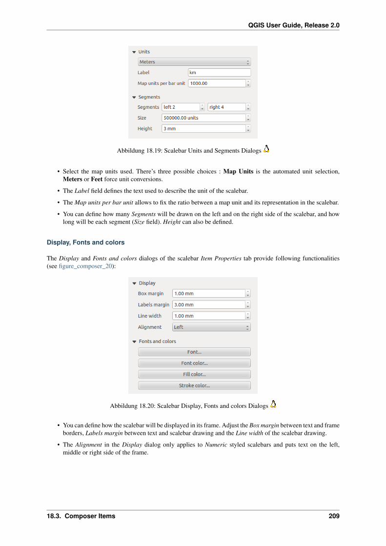
QGIS User Guide, Release 2.0
Abbildung 18.19: Scalebar Units and Segments Dialogs
• Select the map units used. There’s three possible choices : Map Units is the automated unit selection,Meters or Feet force unit conversions.
• The Label field defines the text used to describe the unit of the scalebar.
• The Map units per bar unit allows to fix the ratio between a map unit and its representation in the scalebar.
• You can define how many Segments will be drawn on the left and on the right side of the scalebar, and howlong will be each segment (Size field). Height can also be defined.
Display, Fonts and colors
The Display and Fonts and colors dialogs of the scalebar Item Properties tab provide following functionalities(see figure_composer_20):
Abbildung 18.20: Scalebar Display, Fonts and colors Dialogs
• You can define how the scalebar will be displayed in its frame. Adjust the Box margin between text and frameborders, Labels margin between text and scalebar drawing and the Line width of the scalebar drawing.
• The Alignment in the Display dialog only applies to Numeric styled scalebars and puts text on the left,middle or right side of the frame.
18.3. Composer Items 209

QGIS User Guide, Release 2.0
18.3.6 Adding a Basic shape or Arrow item to the Print Composer
It is possible to add basic shapes (Ellipse, Rectangle, Triangle) and arrows to the print composer canvas : click theAdd basic shape icon or the Add Arrow icon, place the element with the left mouse button on the print composer
canvas and position and customize their appearance in the Item Properties tab.
The Shape Item properties tab allows to draw an ellipse, rectangle, or triangle in the print composer canvas. Youcan define its outline and fill color, the outline width and a clockwise rotation.
Abbildung 18.21: Shape Item properties Tab
The Arrow Item properties tab allows to draw an arrow in the print composer canvas. You can define color, outlineand arrow width and it is possible to use a default marker and no marker and a SVG marker. For the SVG markeryou can additionally add a SVG start and end marker from a directory on your computer.
Abbildung 18.22: Arrow Item properties Tab
Main properties
• For Basic shapes, this dialog allows you to choose a Ellipse, Rectangle or Triangle shape and its rotation.
• Unlike the other items, line style, line color and background color of a basic shape are adjusted with theFrame and Background dialog. No frame is drawn.
• For arrows, you can define here the line style : Color, Line width and Arrow head width.
210 Kapitel 18. Druckzusammenstellung

QGIS User Guide, Release 2.0
• Arrows markers can be adjusted. If you want to set a SVG Start marker and/or End marker, browse to yourSVG file by clicking on the [...] button after selecting SVG radio button.
Bemerkung: Unlike other items, background color for a basic shape is the shape background and not the frameone.
18.3.7 Add attribute table values to the Print Composer
It is possible to add parts of a vector attribute table to the print composer canvas : click the Add attribute table
icon, place the element with the left mouse button on the print composer canvas and position and customize theirappearance in the Item Properties tab.
The Item properties of a attribute table item tab provides following functionalities (see figure_composer_23):
Abbildung 18.23: Scalebar Item properties Tab
Main properties, Show grid and Fonts
The Main properties, Show grid and Fonts dialogs of the attribute table Item Properties tab provide followingfunctionalities (see figure_composer_24):
• The Table dialog allows to select the vector layer and columns of the attribute table. Attribute columns canbe sorted and you can define to show its values ascending or descending (see figure_composer_25).
• You can choose to display only the attribute of features visibled on a map. Check Show only visiblefeatures and select the corresponding Composer map to filter.
• You can define the Maximum number of rows to be displayed and margin around text.
• Additionally you can define the grid characteristics of the table (Stroke width and Color of the grid) and theheader and content font.
18.3.8 Add a HTML frame to the Print Composer
It is possible to add a clickable frame, linked to an URL : click the Add html frame icon, place the element with theleft mouse button on the print composer canvas and position and customize their appearance in the Item Propertiestab.
18.3. Composer Items 211
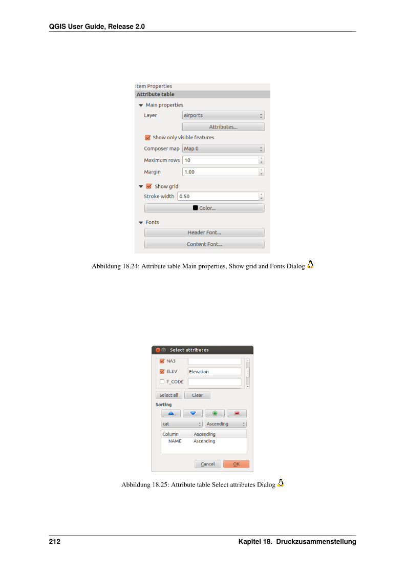
QGIS User Guide, Release 2.0
Abbildung 18.24: Attribute table Main properties, Show grid and Fonts Dialog
Abbildung 18.25: Attribute table Select attributes Dialog
212 Kapitel 18. Druckzusammenstellung
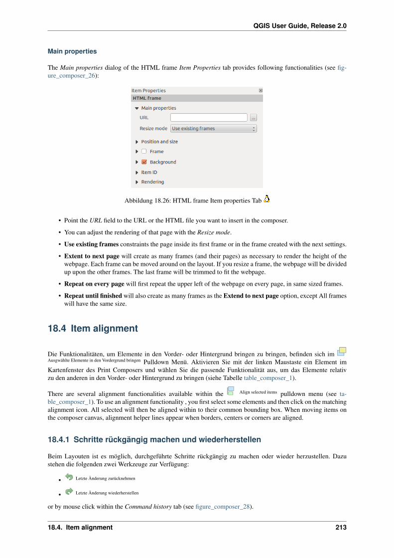
QGIS User Guide, Release 2.0
Main properties
The Main properties dialog of the HTML frame Item Properties tab provides following functionalities (see fig-ure_composer_26):
Abbildung 18.26: HTML frame Item properties Tab
• Point the URL field to the URL or the HTML file you want to insert in the composer.
• You can adjust the rendering of that page with the Resize mode.
• Use existing frames constraints the page inside its first frame or in the frame created with the next settings.
• Extent to next page will create as many frames (and their pages) as necessary to render the height of thewebpage. Each frame can be moved around on the layout. If you resize a frame, the webpage will be dividedup upon the other frames. The last frame will be trimmed to fit the webpage.
• Repeat on every page will first repeat the upper left of the webpage on every page, in same sized frames.
• Repeat until finished will also create as many frames as the Extend to next page option, except All frameswill have the same size.
18.4 Item alignment
Die Funktionalitäten, um Elemente in den Vorder- oder Hintergrund bringen zu bringen, befinden sich imAusgwählte Elemente in den Vordergrund bringen Pulldown Menü. Aktivieren Sie mit der linken Maustaste ein Element imKartenfenster des Print Composers und wählen Sie die passende Funktionalität aus, um das Elemente relativzu den anderen in den Vorder- oder Hintergrund zu bringen (siehe Tabelle table_composer_1).
There are several alignment functionalities available within the Align selected items pulldown menu (see ta-ble_composer_1). To use an alignment functionality , you first select some elements and then click on the matchingalignment icon. All selected will then be aligned within to their common bounding box. When moving items onthe composer canvas, alignment helper lines appear when borders, centers or corners are aligned.
18.4.1 Schritte rückgängig machen und wiederherstellen
Beim Layouten ist es möglich, durchgeführte Schritte rückgängig zu machen oder wieder herzustellen. Dazustehen die folgenden zwei Werkzeuge zur Verfügung:
• Letzte Änderung zurücknehmen
• Letzte Änderung wiederherstellen
or by mouse click within the Command history tab (see figure_composer_28).
18.4. Item alignment 213
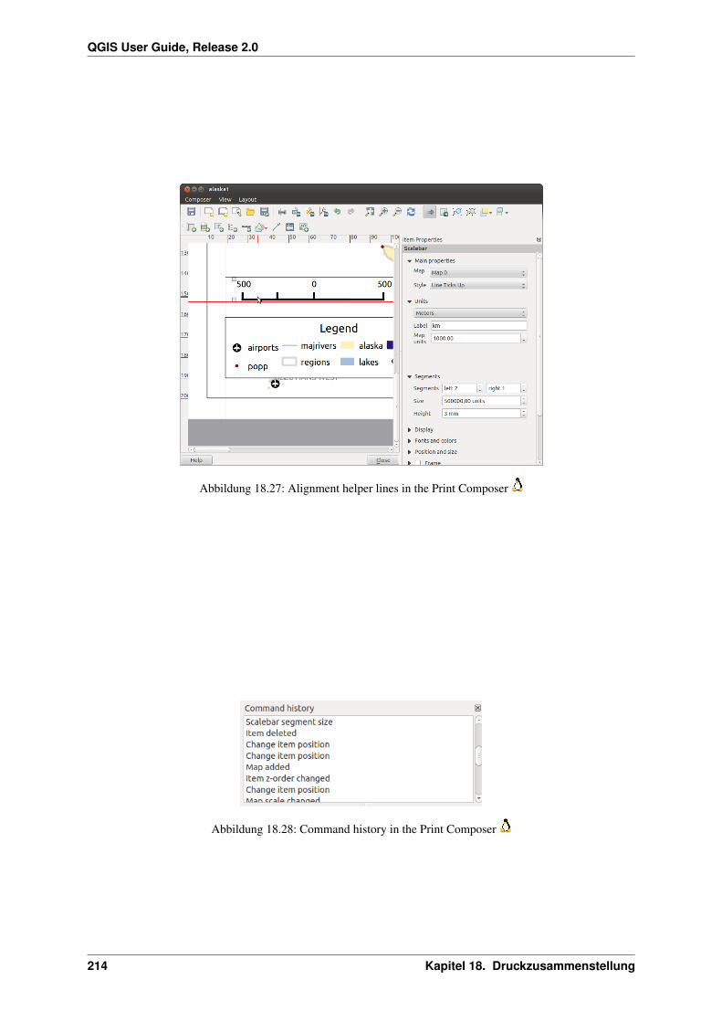
QGIS User Guide, Release 2.0
Abbildung 18.27: Alignment helper lines in the Print Composer
Abbildung 18.28: Command history in the Print Composer
214 Kapitel 18. Druckzusammenstellung

QGIS User Guide, Release 2.0
18.5 Atlas generation
The print composer includes generation functions that allow to create map books in an automated way. The conceptis to use a coverage layer, which contains geometries and fields. For each geometry in the coverage layer, a newoutput will be generated where the content of some canvas maps will be moved to highlight the current geometry.Fields associated to this geometry can be used within text labels.
There can only be one atlas map by print composer but this one can contain multiple pages. Every pages will begenerated with each feature. To enable the generation of an atlas and access generation parameters, refer to theAtlas generation tab. This tab contains the following widgets (see Figure_composer_29):
Abbildung 18.29: Atlas generation tab
• A Generate an atlas enables or disables the atlas generation.
• A combobox Composer map that allows to choose which map item will be used as the atlas map, i.e.on which map geometries from the coverage layer will be iterated over and displayed.
• A combobox Coverage layer that allows to choose the (vector) layer containing the geometries onwhich to iterate over.
• An optional Hidden coverage layer, that if checked, will hide the coverage layer (but not the other ones)during the generation.
• An optional Features sorting that, if checked, allows to sort features of the coverage layer. The associatedcombobox allows to choose which column will be used as the sorting key. Sort order (either ascending ordescending) is set by a two-state button that displays an up or a down arrow.
• An optional Feature filtering text area that allows to specify an expression for filtering features from thecoverage layer. If the expression is not empty, only features that evaluate to True will be selected. Thebutton on the right allows to display the expression builder.
• An input box Scaling that allows to select the amount of space added around each geometry within theallocated map. Its value is meaningful only when using the autoscaling mode.
• A Fixed scale that allows to toggle between auto-scale and fixed-scale mode. In fixed scale mode, themap will only be translated for each geometry to be centered. In auto-scale mode, the map’s extents arecomputed in such a way that each geometry will appear in its whole.
• An Output filename expression textbox that is used to generate a filename for each geometry if needed. It isbased on expressions. This field is meaningful only for rendering to multiple files.
18.5. Atlas generation 215
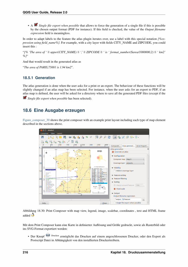
QGIS User Guide, Release 2.0
• A Single file export when possible that allows to force the generation of a single file if this is possibleby the chosen output format (PDF for instance). If this field is checked, the value of the Output filenameexpression field is meaningless.
In order to adapt labels to the feature the atlas plugin iterates over, use a label with this special notation [%ex-pression using field_name%]. For example, with a city layer with fields CITY_NAME and ZIPCODE, you couldinsert this :
“[% ‘The area of ‘ || upper(CITY_NAME) || ‘,’ || ZIPCODE || ‘ is ‘ format_number($area/1000000,2) || ‘ km2’%]“
And that would result in the generated atlas as
“The area of PARIS,75001 is 1.94 km2”.
18.5.1 Generation
The atlas generation is done when the user asks for a print or an export. The behaviour of these functions will beslightly changed if an atlas map has been selected. For instance, when the user asks for an export to PDF, if anatlas map is defined, the user will be asked for a directory where to save all the generated PDF files (except if the
Single file export when possible has been selected).
18.6 Eine Ausgabe erzeugen
Figure_composer_30 shows the print composer with an example print layout including each type of map elementdescribed in the sections above.
Abbildung 18.30: Print Composer with map view, legend, image, scalebar, coordinates , text and HTML frameadded
Mit dem Print Composer kann eine Karte in definierter Auflösung und Größe gedruckt, sowie als Rasterbild oderins SVG-Format exportiert werden:
• Der Knopf Drucken ermöglicht das Drucken auf einem angeschlossenen Drucker, oder den Export alsPostscript Datei in Abhängigkeit von den installierten Druckertreibern.
216 Kapitel 18. Druckzusammenstellung

QGIS User Guide, Release 2.0
• Der Knopf Speichere als Rasterbild exportiert das Drucklayout in verschiedene Bildformate, z.B.: PNG, BPM,TIF,JPG,...
• Der Knopf Als PDF exportieren speichert das aktuelle Kartenfenster des Print Composers als PDF.
• Der Knopf Speichern als SVG speichert das aktuelle Drucklayout als SVG (Scalable Vector Graphic).
Bemerkung: Currently the SVG output is very basic. This is not a QGIS problem, but a problem of the under-laying Qt library. This will hopefully be sorted out in future versions. Export big raster can sometimes fail, evenif there seems to be enough memory. This is also a problem of the underlaying Qt management of raster.
18.7 Manage the Composer
With the Save as template and Load from template icons you can save the current state of a print composer sessionas a .qpt template and load the template again in another session.
The Composer Manager button in the QGIS toolbar and in Composer → Composer Manager allows to add a newcomposer template, create a new composition based on a previously saved template or to manage already existingtemplates.
Abbildung 18.31: The Print Composer Manager
By default, the composer manager searches for user templates in ~/.qgis2/composer_template.
The New Composer and Duplicate Composer buttons in the QGIS toolbar and in Composer → New Composer andComposer → Duplicate Composer allow to open a new composer dialog, or to duplicate an existing compositionfrom a previously created one.
Finally you can save your print composition with the Save Project button. This is the same feature as in the QGISmain window. All changes will be saved in a QGIS project file.
18.7. Manage the Composer 217
QGIS User Guide, Release 2.0
218 Kapitel 18. Druckzusammenstellung

KAPITEL 19
Erweiterungen
19.1 QGIS Plugins
QGIS has been designed with a plugin architecture. This allows many new features/functions to be easily addedto the application. Many of the features in QGIS are actually implemented as either core or external plugins.
• Core Plugins are maintained by the QGIS Development Team and are automatically part of every QGISdistribution. They are written in one of two languages: C++ or Python. More information about core pluginsare provided in Section Using QGIS Core Plugins
• External Plugins are currently all written in Python. They are stored in external repositories and maintained
by the individual authors. They can be added to QGIS in the Get more section the of Plugin Manager.More information about external plugins is provided in Section Loading an external QGIS Plugin.
19.1.1 Plugins verwalten
Managing plugins in general means loading or unloading them using the Plugin Manager. To deactivate andreactivate external plugins, the Plugin Manager is used again.
Loading a QGIS Core Plugin
Loading a QGIS Core Plugin is done from the main menu Plugins → Manage and Install Plugins.
The Installed menu of the Plugin Manager lists all the available plugins and their status (loaded or unloaded),including all core plugins and all external plugins that have been installed and automatically activated using the
Get more menu (see Section Loading an external QGIS Plugin). Those plugins that are already loaded have a
check mark to the left of their name. Figure_plugins_1 shows the Installed dialog.
To enable a particular core plugin, click on the checkbox to the left of the plugin name, and click [OK]. When youexit the application, a list of loaded plugins is retained, and the plugins are automatically loaded.
Loading an external QGIS Plugin
External QGIS plugins are written in Python. They are by default stored in either the ‘Official’ QGIS Repository,or in various other external repositories maintained by individual authors. You can find the external plugins in the
Get more menu.
In the Installed menu you can see the path if it is an external plugin. External plugins are only installed inyour home directory while core plugins are stored in /usr .
219

QGIS User Guide, Release 2.0
Abbildung 19.1: Plugin Manager
Detailed documentation about the usage, minimum QGIS version, homepage, authors, and other important in-formation are provided for the ‘Official’ QGIS Repository at http://plugins.qgis.org/plugins/. For other externalrepositories, they might be available with the external plugins themselves. In general it is not included in thismanual.
Currently there are over 150 external plugins available from the ‘Official’ QGIS Repository. Some of these pluginsoffer functionality that will be required by many users (for example: providing the user with the ability to view andedit OpenStreetMap data, or to add GoogleMap layers) while others offer very specialized functions (for example:Calculate economic pipe diameters for water supply networks).
It is, however, quite straightforward to search through all the available external plugins by providing keywords,choosing a named repository and/or filtering on the status of plugins (currently installed or uninstalled in yoursystem). Searching and filtering is done from the QGIS Python Plugin Installer
Tipp: Weitere externe Plugin Repositorys hinzufügen
To add external author repositories, open the Plugin Installer Manage and Install Plugins, go to the menuSettings, and click [Add] (see figure_plugins_2). If you do not want one or more of the added repositories, theycan be disabled via the [Edit...] button, or completely removed with the [Delete] button.
As such, we cannot take any responsibility for them. You can also manage the repository list manually, that isadd, remove, and edit the entries. Temporarily disabling a particular repository is possible by clicking the [Edit...] button.
Tipp: Check for updates
You can stay informed about plugins. Activate the checkbox Check for updates on startup from the Settingsmenu. QGIS will inform you whenever a plugin or plugin update is available.
220 Kapitel 19. Erweiterungen
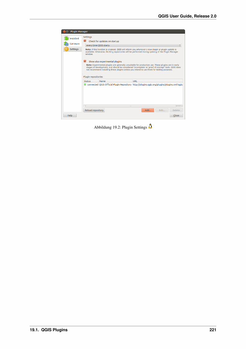
QGIS User Guide, Release 2.0
Abbildung 19.2: Plugin Settings
19.1. QGIS Plugins 221
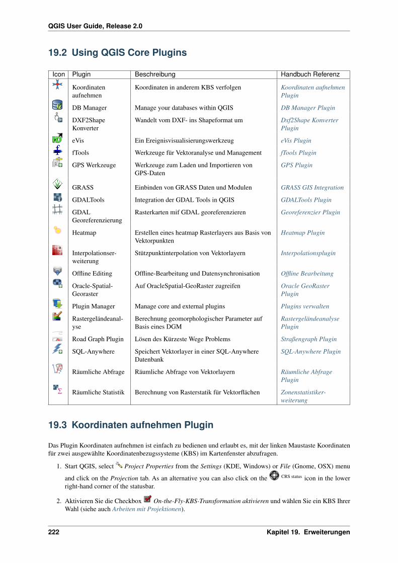
QGIS User Guide, Release 2.0
19.2 Using QGIS Core Plugins
Icon Plugin Beschreibung Handbuch Referenz
Koordinatenaufnehmen
Koordinaten in anderem KBS verfolgen Koordinaten aufnehmenPlugin
DB Manager Manage your databases within QGIS DB Manager Plugin
DXF2ShapeKonverter
Wandelt vom DXF- ins Shapeformat um Dxf2Shape KonverterPlugin
eVis Ein Ereignisvisualisierungswerkzeug eVis Plugin
fTools Werkzeuge für Vektoranalyse und Management fTools Plugin
GPS Werkzeuge Werkzeuge zum Laden und Importieren vonGPS-Daten
GPS Plugin
GRASS Einbinden von GRASS Daten und Modulen GRASS GIS Integration
GDALTools Integration der GDAL Tools in QGIS GDALTools Plugin
GDALGeoreferenzierung
Rasterkarten mif GDAL georeferenzieren Georeferenzier Plugin
Heatmap Erstellen eines heatmap Rasterlayers aus Basis vonVektorpunkten
Heatmap Plugin
Interpolationser-weiterung
Stützpunktinterpolation von Vektorlayern Interpolationsplugin
Offline Editing Offline-Bearbeitung und Datensynchronisation Offline Bearbeitung
Oracle-Spatial-Georaster
Auf OracleSpatial-GeoRaster zugreifen Oracle GeoRasterPlugin
Plugin Manager Manage core and external plugins Plugins verwalten
Rastergeländeanal-yse
Berechnung geomorphologischer Parameter aufBasis eines DGM
RastergeländeanalysePlugin
Road Graph Plugin Lösen des Kürzeste Wege Problems Straßengraph Plugin
SQL-Anywhere Speichert Vektorlayer in einer SQL-AnywhereDatenbank
SQL-Anywhere Plugin
Räumliche Abfrage Räumliche Abfrage von Vektorlayern Räumliche AbfragePlugin
Räumliche Statistik Berechnung von Rasterstatik für Vektorflächen Zonenstatistiker-weiterung
19.3 Koordinaten aufnehmen Plugin
Das Plugin Koordinaten aufnehmen ist einfach zu bedienen und erlaubt es, mit der linken Maustaste Koordinatenfür zwei ausgewählte Koordinatenbezugssysteme (KBS) im Kartenfenster abzufragen.
1. Start QGIS, select Project Properties from the Settings (KDE, Windows) or File (Gnome, OSX) menu
and click on the Projection tab. As an alternative you can also click on the CRS status icon in the lowerright-hand corner of the statusbar.
2. Aktivieren Sie die Checkbox On-the-Fly-KBS-Transformation aktivieren und wählen Sie ein KBS IhrerWahl (siehe auch Arbeiten mit Projektionen).
222 Kapitel 19. Erweiterungen

QGIS User Guide, Release 2.0
Abbildung 19.3: Coordinate Capture Plugin
3. Load the coordinate capture plugin in the Plugin Manager (see Loading a QGIS Core Plugin) and ensure
that the dialog is visible by going to View → Panels and ensuring that Coordinate Capture is enabled.The coordinate capture dialog appears as shown in Figure figure_coordinate_capture_1. Alternatively, you
can also go to Vector → Coordinate Capture and see if Coordinate Capture is enabled.
4. Klicken Sie nun auf das Icon Klicken Sie, um das KBS zur Koordinatenanzeige auszuwählen und wählen Sie ein anderesKoordinatenbezugsystem (KBS) als eben.
5. Klicken Sie nun auf [Aufnahme starten] und dann auf einen Punkt im Kartenfenster. Das Plugin zeigtihnen die Koordinaten für diesen Punkt in beiden zuvor gewählten KBS an.
6. Um die Mausverfolgungs-Funktion zu starten, klicken Sie auf das Icon Mausverfolgung.
7. Sie können die ausgewählten Koordinaten auch in die Zwischenablage kopieren.
19.4 DB Manager Plugin
The DB Manager Plugin is officially part of QGIS core and intends to replace the SPIT Plugin and additionally to
integrate all other database formats supported by QGIS in one user interface. The DB Manager Plugin providesseveral features. You can drag layers from the QGIS Browser into the DB Manager and it will import your layerinto your spatial database. You can drag and drop tables between spatial databases and they will get imported.You can also use the DB Manager to execute SQL queries against your spatial database and then view the spatialoutput for queries by adding the results to QGIS as a query layer.
The Database menu allows to connect to an existing database, to start the SQL-window and to exit the DB ManagerPlugin. One you are connected to an existing database, the menus Schema and Table additionally appear.
The Schema menu includes tools to create and delete (empty) schemas and, if topology is available (e.g. PostGIS2) to start a TopoViewer.
The menu Table allows to create and edit tables and to delete tables and views. It is also possible to empty tablesand to move tables from one to another schema. As further functionality you can perform a VACUUM and thenan ANALYZE for each selected table. Plain VACUUM simply reclaims space and makes it available for re-useand ANALYZE updates statistics to determine the most efficient way to execute a query. Finally you can importlayers/files, if they are loaded in QGIS or exist in the file system. And you can export database tables to Shapewith the Export file feature.
The Tree window lists all existing databases supported by QGIS. With a double-click you can connect to thedatabase. With the right-mouse button you can rename and delete existing schemas and tables. Tables can also beadded to the QGIS canvas with the context menu.
Wenn Sie mit einer Datenbank verbunden sind, bietet das Hauptfenster des DB Managers frei Reiter. Der InfoReiter zeigt Information zur Tabelle und Geometrie, zu existierenden Spalten, Constraints und Indices. Ausser-dem kann man die Vacuum Analyze Funktion starten und einen räumlichen Index für eine ausgewählte Tabelleerzeugen. Der Table Reiter zeigt die Attribute und der Reiter Preview zeigt eine Vorschau der Tabelle.
19.4. DB Manager Plugin 223

QGIS User Guide, Release 2.0
Abbildung 19.4: DB Manager dialog
19.5 Dxf2Shape Konverter Plugin
Das Plugin Dxf2Shape Konverter ermöglicht es, Vektorlayer von DXF (Drawing Interchange Format) ins Shape-Format zu konvertieren. Dazu müssen Sie folgende Parameter angegeben:
Abbildung 19.5: Dxf2Shape Converter Plugin
• DXF-Eingabedatei: Geben Sie hier den Pfad zur DXF-Datei an
• Ausgabedatei: Geben Sie hier einen Namen für das Ausgabe-Shape an
• Typ der Ausgabedatei: Geben Sie hier den Geometrietyp an. Unterstützt wird momentan Polylinie, Poly-gon oder Punkt.
• Beschriftungen exportieren: Wenn Sie dieses Kontrollkästchen aktivieren, wird ein zusätzlicher ShapefilePunktlayer erstellt, und die damit verknüpfte dbf-Datei enthält die Beschriftungen und Informationen dazu,die sich im ‘TEXT’-Feld der Datei befinden.
19.5.1 Das Plugin anwenden
1. Start QGIS, load the Dxf2Shape plugin in the Plugin Manager (see Section Loading a QGIS Core Plugin)
and click on the Dxf2Shape Converter icon which appears in the QGIS toolbar menu. The Dxf2Shape plugin
224 Kapitel 19. Erweiterungen
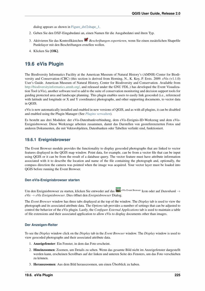
QGIS User Guide, Release 2.0
dialog appears as shown in Figure_dxf2shape_1.
2. Geben Sie den DXF-Eingabedatei an, einen Namen für die Ausgabedatei und ihren Typ.
3. Aktivieren Sie das Kontrollkästchen Beschriftungen exportieren, wenn Sie einen zusätzlichen ShapefilePunktlayer mit den Beschriftungen erstellen wollen.
4. Klicken Sie [OK].
19.6 eVis Plugin
The Biodiversity Informatics Facility at the American Museum of Natural History’s (AMNH) Center for Biodi-versity and Conservation (CBC) (this section is derived from Horning, N., K. Koy, P. Ersts. 2009. eVis (v1.1.0)User’s Guide. American Museum of Natural History, Center for Biodiversity and Conservation. Available fromhttp://biodiversityinformatics.amnh.org/, and released under the GNU FDL.) has developed the Event Visualiza-tion Tool (eVis), another software tool to add to the suite of conservation monitoring and decision support tools forguiding protected area and landscape planning. This plugin enables users to easily link geocoded (i.e., referencedwith latitude and longitude or X and Y coordinates) photographs, and other supporting documents, to vector datain QGIS.
eVis is now automatically installed and enabled in new versions of QGIS, and as with all plugins, it can be disabledand enabled using the Plugin Manager (See Plugins verwalten).
Es besteht aus drei Modulen: der eVis-Datenbankverbindung, dem eVis-Ereignis-ID-Werkzeug und dem eVis-Ereignisbrowser. Diese Werkzeuge arbeiten zusammen, damit das Darstellen von georeferenzierten Fotos undanderen Dokumenten, die mit Vektorobjekten, Datenbanken oder Tabellen verlinkt sind, funktioniert.
19.6.1 Ereignisbrowser
The Event Browser module provides the functionality to display geocoded photographs that are linked to vectorfeatures displayed in the QGIS map window. Point data, for example, can be from a vector file that can be inputusing QGIS or it can be from the result of a database query. The vector feature must have attribute informationassociated with it to describe the location and name of the file containing the photograph and, optionally, thecompass direction the camera was pointed when the image was acquired. Your vector layer must be loaded intoQGIS before running the Event Browser.
Den eVis-Ereignisbrowser starten
Um den Ereignisbrowser zu starten, klicken Sie entweder auf das eVis Event Browser Icon oder auf Datenbank →eVis → eVis Ereignisbrowser. Dies öffnet den Ereignisbrowser Dialog.
The Event Browser window has three tabs displayed at the top of the window. The Display tab is used to view thephotograph and its associated attribute data. The Options tab provides a number of settings that can be adjusted tocontrol the behavior of the eVis plugin. Lastly, the Configure External Applications tab is used to maintain a tableof file extensions and their associated application to allow eVis to display documents other than images.
Der Anzeigen-Reiter
To see the Display window click on the Display tab in the Event Browser window. The Display window is used toview geocoded photographs and their associated attribute data.
1. Anzeigefenster: Ein Fenster, in dem das Foto erscheint.
2. Hineinzoomen: Zoomen, um Details zu sehen. Wenn das gesamte Bild nicht im Anzeigefenster dargestelltwerden kann, erscheinen Scrollbars auf der linken und unteren Seite des Fensters, um das Foto verschiebenzu können.
3. Herauszoomen: Aus dem Bild herauszoomen, um einen Überblick zu haben.
19.6. eVis Plugin 225

QGIS User Guide, Release 2.0
Abbildung 19.6: The eVis display window
4. Zur vollen Ausdehnung zoomen: Zeigt die volle Ausdehnung des Fotos an.
5. Attributfenster: Alle Attribute des Vektorpunktes, der mit dem Foto verlinkt ist werden hier angezeigt.Wenn der Datentyp, auf den verwiesen wird kein Foto ist, sondern ein anderer Datentyp, der im ReiterExterne Applikationen konfigurieren definiert ist, dann öffnet sich die Anwendung mit dem speziellen Da-tentyp, indem Sie auf das Feld mit dem Pfad doppelkicken. Die Anwendung wird dann gestartet und Siekönnen den Inhalt anschauen oder anhören. Wenn die Datenendung erkannt wird, wird sie automatisch ingrün angezeigt.
6. Navigation: Verwenden Sie den ‘Vorheriges’ und ‘Nächstes’ Knopf, um weitere Objekte zu laden, fallsvorhanden und selektiert.
Der Optionen-Reiter
Abbildung 19.7: The eVis Options window
1. Dateipfad: Eine Dropdown-Liste, um das Attributfeld zu definieren, welches den Verzeichnispfad oder dieURL für die Fotos oder anderen Dokumente enthält. Wenn es ein relativer Pfad ist, dann wählen Sie das
Kontrollkästchen Pfad ist relaitiv, links neben dem Dropdown-Menü. Der Grundpfad für den relativ-en Pfad kann in dem Grundpfad eingegeben werden. Informationen über die verschiedenen Optionen zur
226 Kapitel 19. Erweiterungen
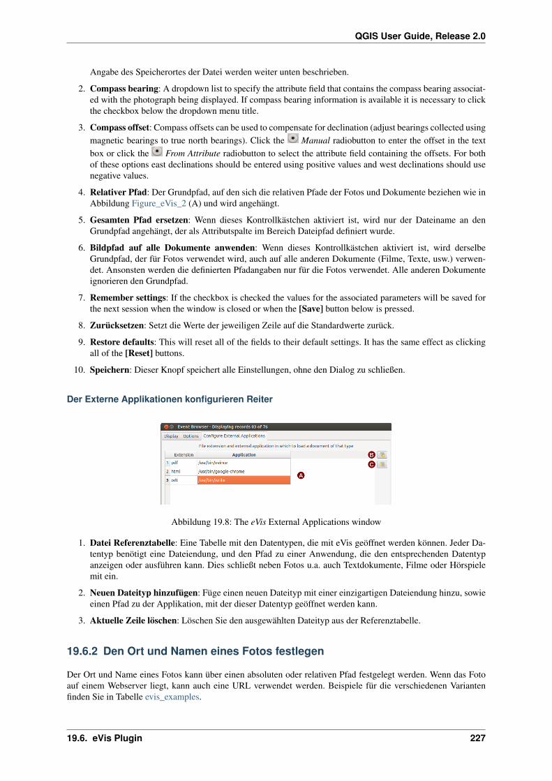
QGIS User Guide, Release 2.0
Angabe des Speicherortes der Datei werden weiter unten beschrieben.
2. Compass bearing: A dropdown list to specify the attribute field that contains the compass bearing associat-ed with the photograph being displayed. If compass bearing information is available it is necessary to clickthe checkbox below the dropdown menu title.
3. Compass offset: Compass offsets can be used to compensate for declination (adjust bearings collected usingmagnetic bearings to true north bearings). Click the Manual radiobutton to enter the offset in the textbox or click the From Attribute radiobutton to select the attribute field containing the offsets. For bothof these options east declinations should be entered using positive values and west declinations should usenegative values.
4. Relativer Pfad: Der Grundpfad, auf den sich die relativen Pfade der Fotos und Dokumente beziehen wie inAbbildung Figure_eVis_2 (A) und wird angehängt.
5. Gesamten Pfad ersetzen: Wenn dieses Kontrollkästchen aktiviert ist, wird nur der Dateiname an denGrundpfad angehängt, der als Attributspalte im Bereich Dateipfad definiert wurde.
6. Bildpfad auf alle Dokumente anwenden: Wenn dieses Kontrollkästchen aktiviert ist, wird derselbeGrundpfad, der für Fotos verwendet wird, auch auf alle anderen Dokumente (Filme, Texte, usw.) verwen-det. Ansonsten werden die definierten Pfadangaben nur für die Fotos verwendet. Alle anderen Dokumenteignorieren den Grundpfad.
7. Remember settings: If the checkbox is checked the values for the associated parameters will be saved forthe next session when the window is closed or when the [Save] button below is pressed.
8. Zurücksetzen: Setzt die Werte der jeweiligen Zeile auf die Standardwerte zurück.
9. Restore defaults: This will reset all of the fields to their default settings. It has the same effect as clickingall of the [Reset] buttons.
10. Speichern: Dieser Knopf speichert alle Einstellungen, ohne den Dialog zu schließen.
Der Externe Applikationen konfigurieren Reiter
Abbildung 19.8: The eVis External Applications window
1. Datei Referenztabelle: Eine Tabelle mit den Datentypen, die mit eVis geöffnet werden können. Jeder Da-tentyp benötigt eine Dateiendung, und den Pfad zu einer Anwendung, die den entsprechenden Datentypanzeigen oder ausführen kann. Dies schließt neben Fotos u.a. auch Textdokumente, Filme oder Hörspielemit ein.
2. Neuen Dateityp hinzufügen: Füge einen neuen Dateityp mit einer einzigartigen Dateiendung hinzu, sowieeinen Pfad zu der Applikation, mit der dieser Datentyp geöffnet werden kann.
3. Aktuelle Zeile löschen: Löschen Sie den ausgewählten Dateityp aus der Referenztabelle.
19.6.2 Den Ort und Namen eines Fotos festlegen
Der Ort und Name eines Fotos kann über einen absoluten oder relativen Pfad festgelegt werden. Wenn das Fotoauf einem Webserver liegt, kann auch eine URL verwendet werden. Beispiele für die verschiedenen Variantenfinden Sie in Tabelle evis_examples.
19.6. eVis Plugin 227
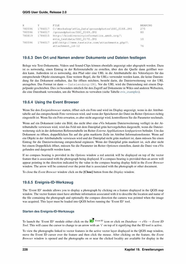
QGIS User Guide, Release 2.0
X Y FILE BEARING780596 1784017 C:\Workshop\eVis_Data\groundphotos\DSC_0168.JPG 275780596 1784017 /groundphotos/DSC_0169.JPG 80780819 1784015 http://biodiversityinformatics.amnh.org/\
evis_testdata/DSC_0170.JPG 10780596 1784017 pdf:http://www.testsite.com/attachments.php?\
attachment_id-12 76
19.6.3 Den Ort und Namen anderer Dokumente und Dateien festlegen
Belege wie Text-Dokumente, Videos und Sound-Clips können ebenfalls angezeigt oder abgespielt werden. Dazuist es notwendig, einen Eintrag in der Referenztabelle zu erstellen, über den die Quelle dann geöffnet wer-den kann. Außerdem ist es notwendig, den Pfad oder eine URL in die Attributtabelle des Vektorlayers für dasentsprechende Objekt einzutragen. Eine weitere Regel, die für URLs verwendet werden kann, die keine Dateien-dung für das Dokument enthalten, das Sie öffnen möchten, besteht darin, die Dateierweiterung vor der URLanzugeben. Das Format ist dann — Dateiendung:URL. Vor die URL wird die Dateiendung mit einem Dop-pelpunkt geschrieben. Dies ist besonders nützlich für den Zugriff auf Dokumente in Wikis und anderen Webseiten,die eine Datenbank verwenden, um die Webseiten zu verwalten (siehe Tabelle evis_examples).
19.6.4 Using the Event Browser
Wenn Sie den Ereignisbrowser starten, öffnet sich ein Foto und wird im Display angezeigt, wenn in der Attribut-tabelle auf das entsprechende Foto verwiesen wird, und wenn der Speicherort der Datei im Reiter Optionen richtigeingestellt ist. Wenn Sie ein Foto erwarten, es aber nicht angezeigt wird, kontrollieren Sie die Parameter nochmals.
Wenn auf ein Dokument (oder ein Bild, das nicht über eine eVis bekannte Dateierweiterung verfügt) in der At-tributtabelle verwiesen wird, wird das Feld mit dem Dateipfad grün hervorgehoben dargestellt, wenn die Dateier-weiterung sich in der definierten Referenztabelle im Reiter Externe Applikationen konfigurieren befindet. Um dasDokument zu öffnen, doppelklicken Sie auf die grün markierte Zeile im Attribut Informationsfenster. Wenn aufein Objekt in der Attributtabelle verwiesen wird und der Dateipfad nicht grün markiert ist, dann müssen Sie einenEintrag für die Dateierweiterung entsprechend ergänzen. Wenn der Dateipfad grün markiert ist, sich aber nichtbei einem Doppelklick öffnet, müssen Sie die Parameter im Reiter Optionen einstellen, damit die Datei von eVisgefunden und dargestellt werden kann.
If no compass bearing is provided in the Options window a red asterisk will be displayed on top of the vectorfeature that is associated with the photograph being displayed. If a compass bearing is provided then an arrow willappear pointing in the direction indicated by the value in the compass bearing display field in the Event Browserwindow. The arrow will be centered over the point that is associated with the photograph or other document.
To close the Event Browser window click on the [Close] button from the Display window.
19.6.5 Ereignis-ID-Werkzeug
The ‘Event ID’ module allows you to display a photograph by clicking on a feature displayed in the QGIS mapwindow. The vector feature must have attribute information associated with it to describe the location and name ofthe file containing the photograph and optionally the compass direction the camera was pointed when the imagewas acquired. This layer must be loaded into QGIS before running the ‘Event ID’ tool.
Starten des Ereignis-ID-Werkzeugs
To launch the ‘Event ID’ module either click on the Event ID icon or click on Database → eVis → Event IDTool. This will cause the cursor to change to an arrow with an ‘i’ on top of it signifying that the ID tool is active.
To view the photographs linked to vector features in the active vector layer displayed in the QGIS map window,move the Event ID cursor over the feature and then click the mouse. After clicking on the feature, the EventBrowser window is opened and the photographs on or near the clicked locality are available for display in the
228 Kapitel 19. Erweiterungen
QGIS User Guide, Release 2.0
browser. If more than one photograph is available, you can cycle through the different features using the [Previous]and [Next] buttons. The other controls are described in the ref:evis_browser section of this guide.
19.6.6 Datenbankverbindung
Der Dialog Datenbankverbindung ermöglicht es, sich mit einer Datenbank oder anderen ODBC Quelle, z.B.Excel-Tabellen zu verbinden.
eVis can directly connect to four types of databases:PostgreSQL, MySQL, SQLite, and can also read from ODBCconnections (e.g.MS Access). When reading from an ODBC database (such as an Excel spreadsheet) it is necessaryto configure your ODBC driver for the operating system you are using.
Starten des Dialogs Datenbankverbindung
To launch the ‘Database Connection’ module either click on the appropriate icon eVis Database Connection or clickon Database → eVis → Database Connection. This will launch the Database Connection window. The windowhas three tabs: Predefined Queries, Database Connection, and SQL Query. The Output Console window at thebottom of the window displays the status of actions initiated by the different sections of this module.
Verbinden mit einer Datenbank
Drücken Sie auf den Reiter Datenbankverbindung und definieren Sie dann im Dropdown-Menü den Datenbank-typ, mit dem Sie sich verbinden wollen. Wenn ein Passwort oder Benutzername erforderlich ist, können dieseInformationen in den Feldern Benutzername und Passwort eingegeben werden.
Enter the database host in the Database Host textbox. This option is not available if you selected ‘MS Access’ asthe database type. If the database resides on your desktop you should enter “localhost”.
Enter the name of the database in the Database Name textbox. If you selected ‘ODBC’ as the database type, youneed to enter the data source name.
Nachdem Sie alle Parameter angegeben haben, klicken Sie auf den [Verbinden] Knopf. Wenn die Verbindungerfolgreich ist, wird dies im Ausgabefenster angezeigt. Im anderen Fall müssen Sie die Parameter nochmal über-prüfen, die Sie eingegeben haben.
1. Datenbanktyp: Eine Dropdown-Liste, um den zu verwendenen Datenbanktyp festzulegen.
2. Datenbank-Host: Der Name des Datenbank-Hosts.
3. Port: Die Portnummer, wenn MYSQL oder PostgreSQL benutzt wird.
4. Datenbankname: Der Name der Datenbank.
5. Verbinden: Ein Knopf, um sich mit der definierten Datenbank zu verbinden.
6. Ausgabekonsole: Hier werden Informationen zu den Prozessen angezeigt.
7. Benutzername: Benutzername, um sich mit einer passwortgeschützten Datenbank zu verbinden.
8. Passwort: Passwort, wenn die Datenbank passwortgeschützt ist.
9. Vordefinierte Abfragen: Reiter, um den Dialog ‘Vordefinierte Abfragen’ zu öffnen.
10. Datenbankverbindung: Reiter, um den Dialog ‘Datenbankverbindung’ zu öffnen.
11. SQL-Abfrage: Reiter, um den Dialog ‘SQL-Abfrage’ zu öffnen.
12. Hilfe: Zeigt die Online-Hilfe an.
13. OK: Schließen des Dialogs ‘Datenbankverbindung’.
19.6. eVis Plugin 229
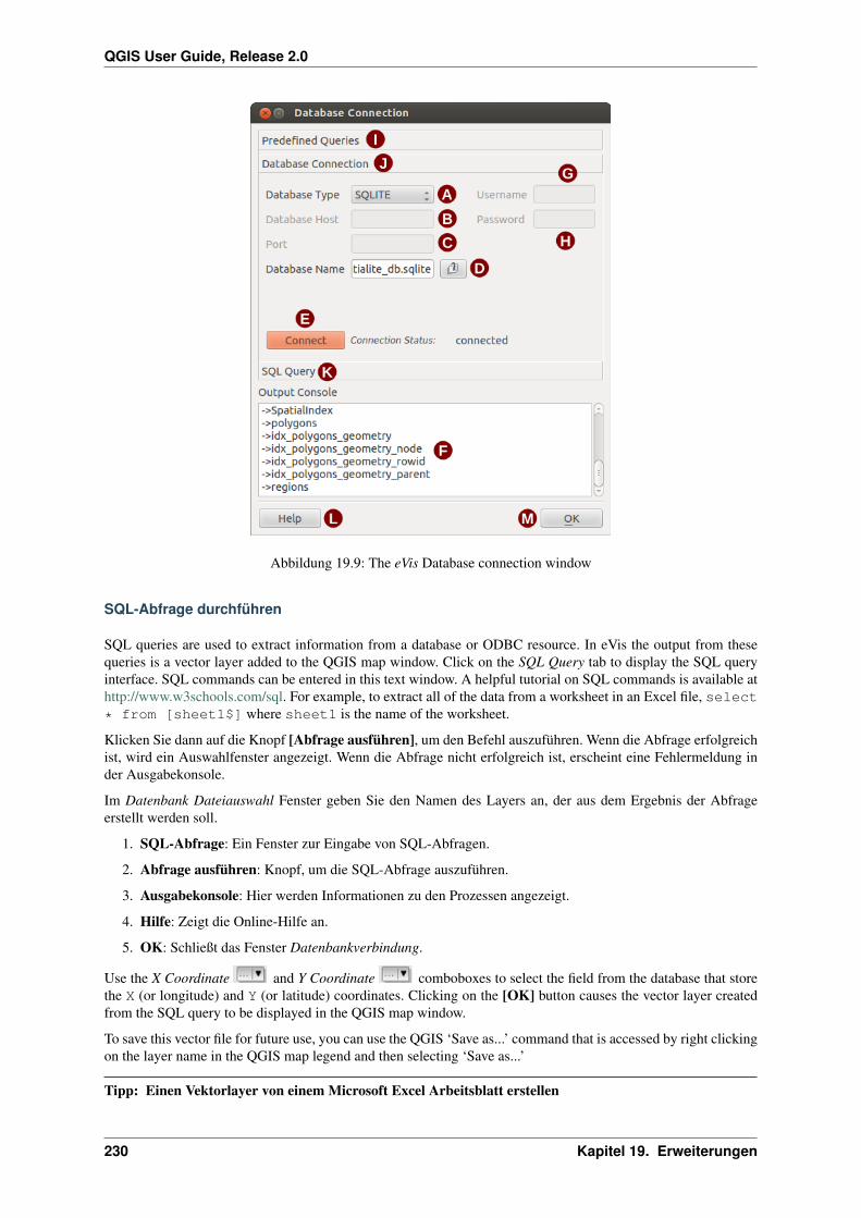
QGIS User Guide, Release 2.0
Abbildung 19.9: The eVis Database connection window
SQL-Abfrage durchführen
SQL queries are used to extract information from a database or ODBC resource. In eVis the output from thesequeries is a vector layer added to the QGIS map window. Click on the SQL Query tab to display the SQL queryinterface. SQL commands can be entered in this text window. A helpful tutorial on SQL commands is available athttp://www.w3schools.com/sql. For example, to extract all of the data from a worksheet in an Excel file, select* from [sheet1$] where sheet1 is the name of the worksheet.
Klicken Sie dann auf die Knopf [Abfrage ausführen], um den Befehl auszuführen. Wenn die Abfrage erfolgreichist, wird ein Auswahlfenster angezeigt. Wenn die Abfrage nicht erfolgreich ist, erscheint eine Fehlermeldung inder Ausgabekonsole.
Im Datenbank Dateiauswahl Fenster geben Sie den Namen des Layers an, der aus dem Ergebnis der Abfrageerstellt werden soll.
1. SQL-Abfrage: Ein Fenster zur Eingabe von SQL-Abfragen.
2. Abfrage ausführen: Knopf, um die SQL-Abfrage auszuführen.
3. Ausgabekonsole: Hier werden Informationen zu den Prozessen angezeigt.
4. Hilfe: Zeigt die Online-Hilfe an.
5. OK: Schließt das Fenster Datenbankverbindung.
Use the X Coordinate and Y Coordinate comboboxes to select the field from the database that storethe X (or longitude) and Y (or latitude) coordinates. Clicking on the [OK] button causes the vector layer createdfrom the SQL query to be displayed in the QGIS map window.
To save this vector file for future use, you can use the QGIS ‘Save as...’ command that is accessed by right clickingon the layer name in the QGIS map legend and then selecting ‘Save as...’
Tipp: Einen Vektorlayer von einem Microsoft Excel Arbeitsblatt erstellen
230 Kapitel 19. Erweiterungen

QGIS User Guide, Release 2.0
Abbildung 19.10: The eVis SQL query tab
When creating a vector layer from a Microsoft Excel Worksheet you might see that unwanted zeros (“0”) havebeen inserted in the attribute table rows beneath valid data.This can be caused by deleting the values for these cellsin Excel using the Backspace key. To correct this problem you need to open the Excel file (you’ll need to closeQGIS if there if you are connected to the file to allow you to edit the file) and then use Edit → Delete to removethe blank rows from the file. To avoid this problem you can simply delete several rows in the Excel Worksheetusing Edit → Delete before saving the file.
Vordefinierte Abfragen starten
Über den Reiter Vordefinierte Abfragen können Sie zuvor schriftlich erstellte SQL-Abfragen, die als Datei imXML-Format gespeichert werden, wieder aufrufen. Dies ist besonders hilfreich, wenn Sie nicht vertraut sind mitSQL-Befehlen. Klicken Sie auf den Reiter Vordefinierte Abfragen, um die vordefinierte Abfrage-Schnittstelle zuöffnen.
Um eine Reihe von vordefinierten Abfragen zu laden, klicken Sie auf das Datei öffnen Icon. Dann können Sie dieDatei mit den abgespeicherten SQL-Befehlen auswählen und laden. Danach erscheinen die einzelnen Abfragenim Dropdown-Menü. Eine Beschreibung der SQL-Abfrage wird jeweils im Textfenster unterhalb des Dropdown-Menüs angezeigt.
Wählen Sie nun eine Abfrage, die Sie aus dem Dropdown-Menü ausführen möchten und klicken Sie auf den ReiterSQL-Abfrage, um die Abfrage anzuschauen. Wenn Sie eine vordefinierten Abfrage das erste Mal starten, müssenSie sich erst vergewissern, dass die Datenbankverbindung steht.
Klicken Sie auf den Knopf [Abfrage ausführen] im Reiter SQL-Abfrage. Wenn die Abfrage erfolgreich ist, wirdein Auswahlfenster angezeigt. Wenn die Abfrage nicht erfolgreich ist, erscheint eine Fehlermeldung in der Aus-gabekonsole.
1. Open File: Launches the “Open File” file browser to search for the XML file holding the predefined queries.
2. Vordefinierte Abfragen: Eine Dropdown-Liste mit allen Abfragen der bereits erstellten XML-Datei.
19.6. eVis Plugin 231

QGIS User Guide, Release 2.0
Abbildung 19.11: The eVis Predefined queries tab
3. Abfragebeschreibung: Eine Beschreibung der Abfrage. Diese Beschreibung ist in der XML-Datei enthal-ten.
4. Ausgabekonsole: Hier werden Informationen zu den Prozessen angezeigt.
5. Hilfe: Zeigt die Online-Hilfe an.
6. OK: Schließt das Fenster ‘Datenbankverbindung’.
XML-Format für vordefinierte Abfragen in eVis
Die von eVis gelesenen XML-Tags
232 Kapitel 19. Erweiterungen
QGIS User Guide, Release 2.0
Tag Beschreibungquery Definiert den Anfang und das Ende einer Abfrage.shortde-scription
Eine kurze Beschreibung der Abfrage, die im eVis Dropdown-Menü erscheint.
descrip-tion
Eine detailiertere Beschreibung der Abfrage, die in der eVis Abfragebeschreibung angezeigtwird.
database-type
Der Datebanktyp, wie er im Dropdown-Menü Datenbanktyp festgelegt wurde.
database-port
Der definierte Port, über den die Verbindung mit der Datenbank stattfindet.
database-name
Der definierte Datenbankname aus dem Reiter Datenbankverbindung.
databaseuser-name
Der definierte Benutzername aus dem Reiter Datenbankverbindung.
databasep-assword
Das definierte Passwort aus dem Reiter Datenbankverbindung.
sqlstate-ment
Die SQL-Abfrage.
autocon-nect
Eine Option (‘true’ oder ‘false’), die festlegt, ob automatisch mit der Datenbank verbundenwerden soll, ohne die Routine aus dem Reiter Datenbankverbindung zu durchlaufen.
Ein Beispiel einer XML-Datei mit drei Abfragen ist unten dargestellt:
<?xml version="1.0"?><doc><query><shortdescription>Import all photograph points</shortdescription><description>This command will import all of the data in the SQLite database to QGIS
</description><databasetype>SQLITE</databasetype><databasehost /><databaseport /><databasename>C:\textbackslash Workshop/textbackslash
eVis\_Data\textbackslash PhotoPoints.db</databasename><databaseusername /><databasepassword /><sqlstatement>SELECT Attributes.*, Points.x, Points.y FROM Attributes LEFT JOIN
Points ON Points.rec_id=Attributes.point_ID</sqlstatement><autoconnect>false</autoconnect>
</query><query><shortdescription>Import photograph points "looking across Valley"</shortdescription><description>This command will import only points that have photographs "looking across
a valley" to QGIS</description><databasetype>SQLITE</databasetype><databasehost /><databaseport /><databasename>C:\Workshop\eVis_Data\PhotoPoints.db</databasename><databaseusername /><databasepassword /><sqlstatement>SELECT Attributes.*, Points.x, Points.y FROM Attributes LEFT JOIN
Points ON Points.rec_id=Attributes.point_ID where COMMENTS=’Looking acrossvalley’</sqlstatement>
<autoconnect>false</autoconnect></query><query>
<shortdescription>Import photograph points that mention "limestone"</shortdescription><description>This command will import only points that have photographs that mention
"limestone" to QGIS</description><databasetype>SQLITE</databasetype><databasehost /><databaseport />
19.6. eVis Plugin 233
QGIS User Guide, Release 2.0
<databasename>C:\Workshop\eVis_Data\PhotoPoints.db</databasename><databaseusername /><databasepassword /><sqlstatement>SELECT Attributes.*, Points.x, Points.y FROM Attributes LEFT JOIN
Points ON Points.rec_id=Attributes.point_ID where COMMENTS like ’%limestone%’</sqlstatement>
<autoconnect>false</autoconnect></query>
</doc>
19.7 fTools Plugin
Das Ziel des fTool Plugins besteht darin, eine Quelle für alltägliche, vektorbasierte GIS Aufgaben bereitzustellen,ohne zusätzliche Software, Bibliotheken oder komplexe Workarounds notwendig zu machen. Das Plugin bieteteine wachsende Zahl effektiver Werkzeuge, um räumliche Daten zu verwalten und zu analysieren.
fTools is now automatically installed and enabled in new versions of QGIS, and as with all plugins, it can bedisabled and enabled using the Plugin Manager (See Section Loading a QGIS Core Plugin). When enabled, thefTools plugin adds a Vector menu to QGIS, providing functions ranging from Analysis and Research Tools toGeometry and Geoprocessing Tools, as well as several useful Data Management Tools.
19.7.1 fTools Funktionen
Icon Werkzeug Zweck
Distanzma-trix
Messen von Distanzen zwischen zwei Punktlayern. Ausgabe ist a) StandardDistanzmatrix, b) Lineare Distanzmatrix oder c) Zusammenfassende Distanzmatrix.Die Distanzen können auf die jeweils nächsten Ziele rediziert werden.
Linienlängensummieren
Berechnet die Gesamtsumme der Linienlängen für jedes Polygon eines Polygonlayers.
Punkte inPolygonen
Zählt die Anzahl der Punkte eines Punktlayers, die innerhalb jedes Polygons einesPolygonlayers auftreten.
EindeutigeWerteauflisten
Listet alle eindeutigen Werte einer Attributspalte eines Vektorlayers.
Grundstatis-tik
Berechnet Statistikwerte für eine Attributspalte (Mittelwert, Max, Min,Standardabweichung, Anzahl, Summe, Varianzkoeffizient).
NächsterNachbarAnalyse
Berechnet Nächste Nachbar Statistik zur Bestimmung des Clustergrades einesPunktlayers
Mittlere Ko-ordinate(n)
Berechnet entweder den normalen oder gewichteten Mittelwert eines Vektorlayers odermehrerer Objekte mit eindeutiger Schlüsselspalte.
Linien-schnittpunkte
Findet Überschneidungen zwischen Linien und gibt diese als Shapefile aus.Linienüberschneidungen mit einer Länge > 0 werden ignoriert.
Table Ftools 1: fTools Analysewerkzeuge
234 Kapitel 19. Erweiterungen

QGIS User Guide, Release 2.0
19.7.2 Forschungswerkzeuge
Icon Werkzeug Zweck
Zufällige Auswahl Wählt zufällig n Objekte oder n Prozent der Objekte
Zufällige Auswahlin Untermengen
Wählt zufällig n Objekte aus einer Untermenge mit eindeutiger Schlüsselspalte.
Zufällige Punkte Erstellt pseudo-zufällige Punkte im Bereich eines Eingabelayers.
RegelmäßigePunkte
Erstellt ein regelmäßiges Punktegitter für ein bestimmtes Gebiet und exportiertdiese als Shape.
Vektorraster Erstellt ein Linien- oder Polygongitter mit definierten Abständen.
Nach Positionselektieren
Wähle Objekte nach relativer Position zu einem anderen Layer für eine neueAuswahl, oder addiere oder subtrahiere aus aktueller Auswahl.
Polygon ausLayergrenzen
Erstelle ein rechteckiges Polygon auf Basis der Ausdehnung eines Raster- oderVektorlayers.
Table Ftools 2: fTools Forschungswerkzeuge
19.7.3 Geoverarbeitungswerkzeuge
Icon Werkzeug Zweck
Konvexe Hülle Erstelle kleinste konvexe Hülle für einen Layer oder eine Schlüsselspalte.
Puffer Erstelle einen Puffer um Objekte mit definierter Distanz oder auf Basis einerSchlüsselspalte.
Schnittmengen Verschneide Layer, so dass die Ausgabe Flächen enthält, an denen beide Layerüberlagern.
Vereinigungen Verschneide Layer, so dass die Ausgabe überlagernde und nicht-überlagerndeFlächen enthält.
SymetrischeDifferenz
Verschneide Layer, so dass die Ausgabe Flächen enthält, an denen beide Layernicht überlagern.
Clip Verschneide Layer, so dass die Ausgabe nur die Flächen enthält, die mit demclip Layer überlagern.
Differenz Verschneide Layer, so dass die Ausgabe nur die Flächen enthält, die nicht mitdem clip Layer überlagern.
Auflösen Verschmelze Objekte auf Basis einer Schlüsselspalte. Objekte mit gleichenWerten werden zusammengefügt.
Eliminate sliverpolygons
Merges selected features with the neighbouring polygon with the largest area orlargest common boundary.
Table Ftools 3: fTools Geoverarbeitungswerkzeuge
19.7. fTools Plugin 235
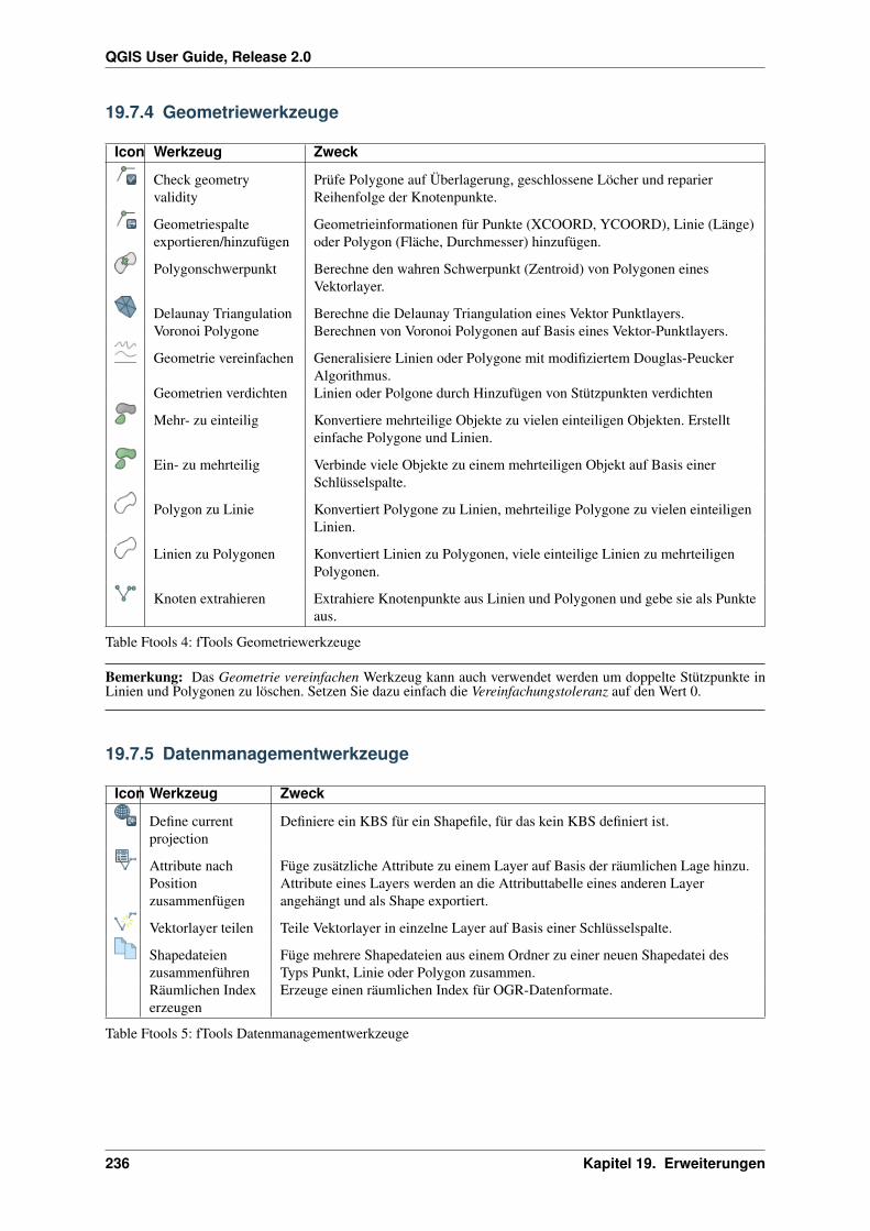
QGIS User Guide, Release 2.0
19.7.4 Geometriewerkzeuge
Icon Werkzeug Zweck
Check geometryvalidity
Prüfe Polygone auf Überlagerung, geschlossene Löcher und reparierReihenfolge der Knotenpunkte.
Geometriespalteexportieren/hinzufügen
Geometrieinformationen für Punkte (XCOORD, YCOORD), Linie (Länge)oder Polygon (Fläche, Durchmesser) hinzufügen.
Polygonschwerpunkt Berechne den wahren Schwerpunkt (Zentroid) von Polygonen einesVektorlayer.
Delaunay Triangulation Berechne die Delaunay Triangulation eines Vektor Punktlayers.Voronoi Polygone Berechnen von Voronoi Polygonen auf Basis eines Vektor-Punktlayers.
Geometrie vereinfachen Generalisiere Linien oder Polygone mit modifiziertem Douglas-PeuckerAlgorithmus.
Geometrien verdichten Linien oder Polgone durch Hinzufügen von Stützpunkten verdichten
Mehr- zu einteilig Konvertiere mehrteilige Objekte zu vielen einteiligen Objekten. Erstellteinfache Polygone und Linien.
Ein- zu mehrteilig Verbinde viele Objekte zu einem mehrteiligen Objekt auf Basis einerSchlüsselspalte.
Polygon zu Linie Konvertiert Polygone zu Linien, mehrteilige Polygone zu vielen einteiligenLinien.
Linien zu Polygonen Konvertiert Linien zu Polygonen, viele einteilige Linien zu mehrteiligenPolygonen.
Knoten extrahieren Extrahiere Knotenpunkte aus Linien und Polygonen und gebe sie als Punkteaus.
Table Ftools 4: fTools Geometriewerkzeuge
Bemerkung: Das Geometrie vereinfachen Werkzeug kann auch verwendet werden um doppelte Stützpunkte inLinien und Polygonen zu löschen. Setzen Sie dazu einfach die Vereinfachungstoleranz auf den Wert 0.
19.7.5 Datenmanagementwerkzeuge
Icon Werkzeug Zweck
Define currentprojection
Definiere ein KBS für ein Shapefile, für das kein KBS definiert ist.
Attribute nachPositionzusammenfügen
Füge zusätzliche Attribute zu einem Layer auf Basis der räumlichen Lage hinzu.Attribute eines Layers werden an die Attributtabelle eines anderen Layerangehängt und als Shape exportiert.
Vektorlayer teilen Teile Vektorlayer in einzelne Layer auf Basis einer Schlüsselspalte.
Shapedateienzusammenführen
Füge mehrere Shapedateien aus einem Ordner zu einer neuen Shapedatei desTyps Punkt, Linie oder Polygon zusammen.
Räumlichen Indexerzeugen
Erzeuge einen räumlichen Index für OGR-Datenformate.
Table Ftools 5: fTools Datenmanagementwerkzeuge
236 Kapitel 19. Erweiterungen

QGIS User Guide, Release 2.0
19.8 GDALTools Plugin
19.8.1 Was sind die GDALTools?
Die GDALTools stellen eine grafische Benutzeroberfläche bereit, Über die die verschiedenen Werkzeuge derGeospatial Data Abstraction Library (GDAL), http://gdal.osgeo.org angesprochen werden können. Dabei handeltes sich um Raster Management Tools, z.B. für die Abfrage, Umprojizierung, Transformierung oder Verschneidungvon Rasterlayern in unterschiedlichen Formaten. Außerdem stehen Werkzeuge zur Verfügung, um Konturen alsVektorlinien zu extrahieren, eine Schummerungskarte aus Höhendaten zu erzeugen oder ein VRT (Virtual RasterTile in XML format) aus einer oder mehreren Rasterkarte(n) zu erzeugen. Diese Werkzeuge können benutzt wer-den, wenn installiert und aktiviert wurde.
Die GDAL Bibliothek
Die GDAL Bibliothek besteht aus einer Reihe von Kommandozeilen-Tools, jedes mit zahlreichen Optionen. An-wender, die sich mit der Kommandozeile auskennen, werden diese Art der Anwendung sicher bevorzugen, umso den vollen Funktionsumfang nutzen zu können. Das GDAL Tools Plugin ermöglicht hingegen einen einfachenZugang zu den Funktionen, und stellt daher auch nur die am häufigsten benutzten Optionen zur Verfügung.
19.8.2 Liste der GDALTools
Abbildung 19.12: The GDALTools menu list
Projektionen
Transformieren(Reprojizieren)
Das Werkzeug kann mosaikieren, umprojizieren und konvertieren. Es kann in alleunterstützten Projektion projizieren und kann dabei sogar mit dem Bild bereitgestellteGCPs (Ground Control Points) nutzen, wenn der Rasterlayer noch im ‘Rohzustand’ ist.Weitere Informationen finden sich unter http://www.gdal.org/gdalwarp.html
Projektionzuweisen
Das Werkzeug ermöglicht es, Rasterlayern, die bereits georeferenziert sind, eineProjektionsinformation zuzuweisen oder bestehende Projektionsinformationen zuverändern. Dabei wird Einzeldatei- und Stapelverarbeitung unterstützt. WeitereInformationen finden sich unter http://www.gdal.org/gdalwarp.html
Projektionextrahieren
Dieses Werkzeug kann Projektionsinformationen aus einer Rasterdatei extrhieren. Dabeiwird Einzeldatei- und Stapelverarbeitung unterstützt. Dabei wird eine .prj und eine.wld Datei erzeugt.
19.8. GDALTools Plugin 237
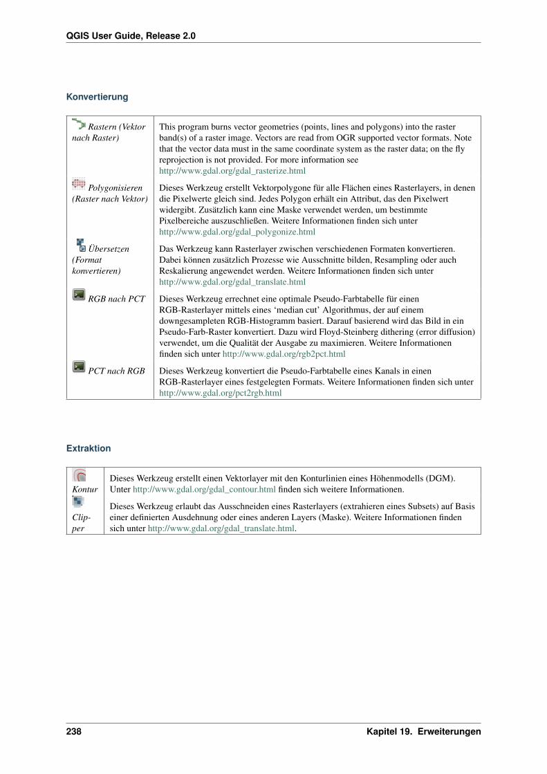
QGIS User Guide, Release 2.0
Konvertierung
Rastern (Vektornach Raster)
This program burns vector geometries (points, lines and polygons) into the rasterband(s) of a raster image. Vectors are read from OGR supported vector formats. Notethat the vector data must in the same coordinate system as the raster data; on the flyreprojection is not provided. For more information seehttp://www.gdal.org/gdal_rasterize.html
Polygonisieren(Raster nach Vektor)
Dieses Werkzeug erstellt Vektorpolygone für alle Flächen eines Rasterlayers, in denendie Pixelwerte gleich sind. Jedes Polygon erhält ein Attribut, das den Pixelwertwidergibt. Zusätzlich kann eine Maske verwendet werden, um bestimmtePixelbereiche auszuschließen. Weitere Informationen finden sich unterhttp://www.gdal.org/gdal_polygonize.html
Übersetzen(Formatkonvertieren)
Das Werkzeug kann Rasterlayer zwischen verschiedenen Formaten konvertieren.Dabei können zusätzlich Prozesse wie Ausschnitte bilden, Resampling oder auchReskalierung angewendet werden. Weitere Informationen finden sich unterhttp://www.gdal.org/gdal_translate.html
RGB nach PCT Dieses Werkzeug errechnet eine optimale Pseudo-Farbtabelle für einenRGB-Rasterlayer mittels eines ‘median cut’ Algorithmus, der auf einemdowngesampleten RGB-Histogramm basiert. Darauf basierend wird das Bild in einPseudo-Farb-Raster konvertiert. Dazu wird Floyd-Steinberg dithering (error diffusion)verwendet, um die Qualität der Ausgabe zu maximieren. Weitere Informationenfinden sich unter http://www.gdal.org/rgb2pct.html
PCT nach RGB Dieses Werkzeug konvertiert die Pseudo-Farbtabelle eines Kanals in einenRGB-Rasterlayer eines festgelegten Formats. Weitere Informationen finden sich unterhttp://www.gdal.org/pct2rgb.html
Extraktion
KonturDieses Werkzeug erstellt einen Vektorlayer mit den Konturlinien eines Höhenmodells (DGM).Unter http://www.gdal.org/gdal_contour.html finden sich weitere Informationen.
Clip-per
Dieses Werkzeug erlaubt das Ausschneiden eines Rasterlayers (extrahieren eines Subsets) auf Basiseiner definierten Ausdehnung oder eines anderen Layers (Maske). Weitere Informationen findensich unter http://www.gdal.org/gdal_translate.html.
238 Kapitel 19. Erweiterungen
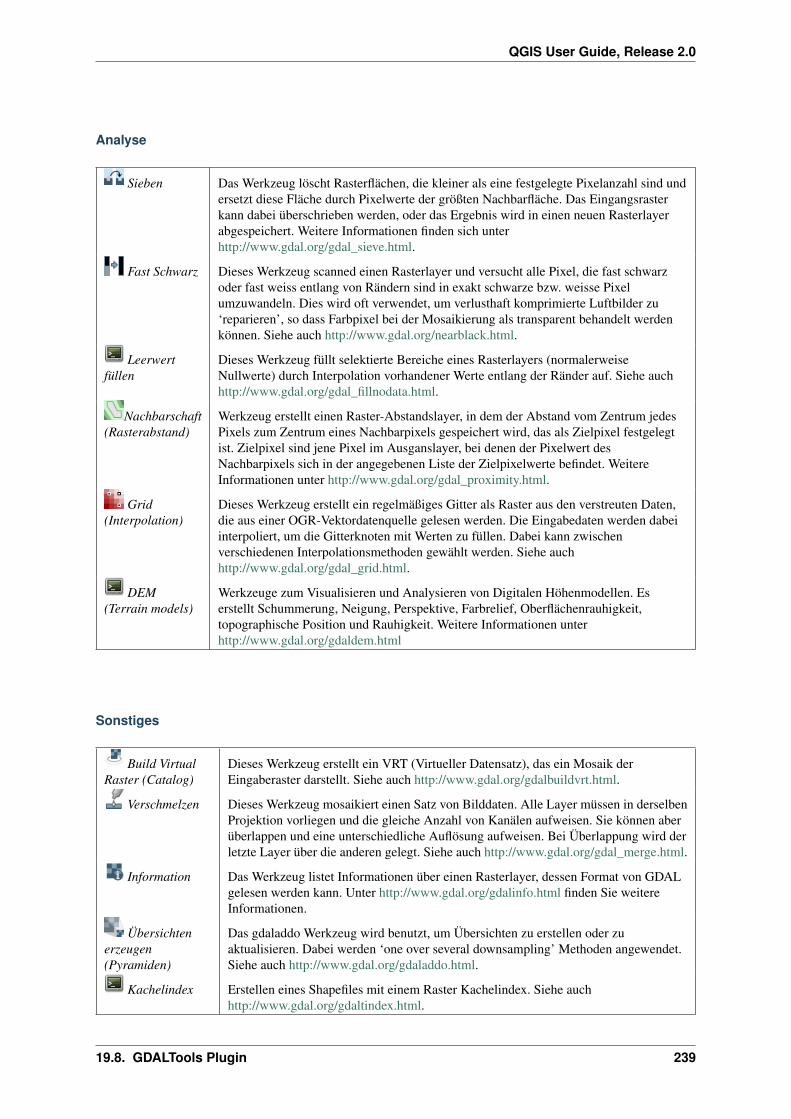
QGIS User Guide, Release 2.0
Analyse
Sieben Das Werkzeug löscht Rasterflächen, die kleiner als eine festgelegte Pixelanzahl sind undersetzt diese Fläche durch Pixelwerte der größten Nachbarfläche. Das Eingangsrasterkann dabei überschrieben werden, oder das Ergebnis wird in einen neuen Rasterlayerabgespeichert. Weitere Informationen finden sich unterhttp://www.gdal.org/gdal_sieve.html.
Fast Schwarz Dieses Werkzeug scanned einen Rasterlayer und versucht alle Pixel, die fast schwarzoder fast weiss entlang von Rändern sind in exakt schwarze bzw. weisse Pixelumzuwandeln. Dies wird oft verwendet, um verlusthaft komprimierte Luftbilder zu‘reparieren’, so dass Farbpixel bei der Mosaikierung als transparent behandelt werdenkönnen. Siehe auch http://www.gdal.org/nearblack.html.
Leerwertfüllen
Dieses Werkzeug füllt selektierte Bereiche eines Rasterlayers (normalerweiseNullwerte) durch Interpolation vorhandener Werte entlang der Ränder auf. Siehe auchhttp://www.gdal.org/gdal_fillnodata.html.
Nachbarschaft(Rasterabstand)
Werkzeug erstellt einen Raster-Abstandslayer, in dem der Abstand vom Zentrum jedesPixels zum Zentrum eines Nachbarpixels gespeichert wird, das als Zielpixel festgelegtist. Zielpixel sind jene Pixel im Ausganslayer, bei denen der Pixelwert desNachbarpixels sich in der angegebenen Liste der Zielpixelwerte befindet. WeitereInformationen unter http://www.gdal.org/gdal_proximity.html.
Grid(Interpolation)
Dieses Werkzeug erstellt ein regelmäßiges Gitter als Raster aus den verstreuten Daten,die aus einer OGR-Vektordatenquelle gelesen werden. Die Eingabedaten werden dabeiinterpoliert, um die Gitterknoten mit Werten zu füllen. Dabei kann zwischenverschiedenen Interpolationsmethoden gewählt werden. Siehe auchhttp://www.gdal.org/gdal_grid.html.
DEM(Terrain models)
Werkzeuge zum Visualisieren und Analysieren von Digitalen Höhenmodellen. Eserstellt Schummerung, Neigung, Perspektive, Farbrelief, Oberflächenrauhigkeit,topographische Position und Rauhigkeit. Weitere Informationen unterhttp://www.gdal.org/gdaldem.html
Sonstiges
Build VirtualRaster (Catalog)
Dieses Werkzeug erstellt ein VRT (Virtueller Datensatz), das ein Mosaik derEingaberaster darstellt. Siehe auch http://www.gdal.org/gdalbuildvrt.html.
Verschmelzen Dieses Werkzeug mosaikiert einen Satz von Bilddaten. Alle Layer müssen in derselbenProjektion vorliegen und die gleiche Anzahl von Kanälen aufweisen. Sie können aberüberlappen und eine unterschiedliche Auflösung aufweisen. Bei Überlappung wird derletzte Layer über die anderen gelegt. Siehe auch http://www.gdal.org/gdal_merge.html.
Information Das Werkzeug listet Informationen über einen Rasterlayer, dessen Format von GDALgelesen werden kann. Unter http://www.gdal.org/gdalinfo.html finden Sie weitereInformationen.
Übersichtenerzeugen(Pyramiden)
Das gdaladdo Werkzeug wird benutzt, um Übersichten zu erstellen oder zuaktualisieren. Dabei werden ‘one over several downsampling’ Methoden angewendet.Siehe auch http://www.gdal.org/gdaladdo.html.
Kachelindex Erstellen eines Shapefiles mit einem Raster Kachelindex. Siehe auchhttp://www.gdal.org/gdaltindex.html.
19.8. GDALTools Plugin 239

QGIS User Guide, Release 2.0
19.9 Georeferenzier Plugin
Das Plugin Georeferenzierer erlaubt die Erstellung von Worldfiles für existierende Rasterlayer und das entzerrenvon Rasterlayern in ein neues GeoTiff. Es ermöglicht damit das georeferenzieren von Rasterdaten in geographis-che und projizierte Koordinatensysteme oder die Transformation des Rasters in ein neues Koordinatensystem.Der Ansatz besteht darin, Bezugspunkte auf der Rasterkarte zu finden, denen eindeutige Koordinaten zugewiesenwerden können.
FunktionalitätenIcon Funktion Icon Funktion
Raster öffnen Georeferenzierung beginnen
GDAL Skript erzeugen GCP Punkte laden
GCP Punkte speichern als Transformationseinstellungen
Punkt hinzufügen Punkt löschen
GCP-Punkt verschieben Verschieben
Hineinzoomen Herauszoomen
Auf den Layer zoomen Zoom zurück
Zoom vor Link Georeferencer to QGIS
Link QGIS to Georeferencer
Table Georeferencer 1: Georeferenzierfunktionen
19.9.1 Wie benutzt man den Georeferenzierer
Es gibt zwei Möglichkeiten, um X und Y Koordinaten einer Rohkarte oder die Koordinaten (mmmm.mm) einerprojizierten Karte an ausgewählten Punkten eines Bildes zu georeferenzieren:
• Manchmal findet man auf dem zu georeferenzierenden Bild selbst kleine Kreuze, mit (oft auch am Bil-drand) angeschriebenen Koordinaten. In diesem Fall kann man die entsprechenden Koordinaten für dieGeoreferenzierung manuell zuweisen.
• Using already georeferenced layers, this can be either vector or raster data that contain the same ob-jects/features that you have on the image that you want to georeference and the projection you want tohave your image. In this case you can enter the coordinates by clicking on the reference dataset loaded inQGIS map canvas.
Die allgemeine Vorgehensweise besteht normalerweise darin, dass man eine Reihe von Punkten auf dem zu geo-referenzierenden Bild auswählt, diesen die entsprechenden Koordinaten der Zielprojektion zuweist und dann einepassende Transformationsmethode auswählt. Entsprechend der Eingabeparameter erstellt das Plugin dann entwed-er einen Worldfile für das Bild oder erzeugt eine entzerrte Version des Bildes als GeoTiff. Allgemein gilt, je mehrPunkte gesetzt werden, desto besser ist das Resultat.
The first step is to start QGIS, load the Georeferencer Plugin (see Section Loading a QGIS Core Plugin) and click
on the Georeferencer icon which appears in the QGIS toolbar menu. The Georeferencer Plugin dialog appears asshown in figure_georeferencer_1.
In diesem Beispiel soll ein Worldfile für eine topografische Karte aus der Gegend Süd-Dakotas erstellt werden,welche zu dem GRASS Spearfish-Datensatz passt. Diese Karte kann später zusammen mit den erstellten Daten inder GRASS spearfish60 Location dargestellt werden. Die topopgrafische Karte steht unter folgender Adressezum Download bereit - http://grass.osgeo.org/sampledata/spearfish_toposheet.tar.gz.
240 Kapitel 19. Erweiterungen

QGIS User Guide, Release 2.0
Abbildung 19.13: Georeferencer Plugin Dialog
Eingabe von Bezugspunkten (Ground Control Points (GCP))
1. To start georeferencing an unreferenced raster, we must load it using the button. The raster will showup in the main working area of the dialog. Once the raster is loaded, we can start to enter reference points.
2. Using the Add Point button, add points to the main working area and enter their coordinates (see Figurefigure_georeferencer_2). For this procedure you have three options:
• Sie klicken auf einen Punkt in der Rasterkarte und geben die X- und Y-Koordinaten ein.
• Click on a point in the raster image and choose the button from map canvas to add the X and Y coordi-nates with the help of a georeferenced map already loaded in the QGIS map canvas.
• With the button, you can move the GCPs in both windows, if they are at the wrong place.
3. Geben Sie weitere Bezugspunkte an. Sie sollten mindestens 4 Punkte festlegen, und je mehr Punkte Sie gutverteilt angeben, desto besser wird normalerweise das Ergebnis. Der Georeferenzierdialog stellt darüber-hinaus auch Icons zum Vergrößern/Verkleinern, zum Verschieben, sowie zum Hinzufügen und Löschen vonBezugspunkten zur Verfügung.
Abbildung 19.14: Add points to the raster image
The points that are added to the map will be stored in a separate text file ([filename].points) usuallytogether with the raster image. This allows us to reopen the Georeferencer plugin at a later date and add newpoints or delete existing ones to optimize the result. The points file contains values of the form: mapX, mapY,
pixelX, pixelY. You can use the Load GCP points and Save GCP points as buttons to manage the files.
19.9. Georeferenzier Plugin 241
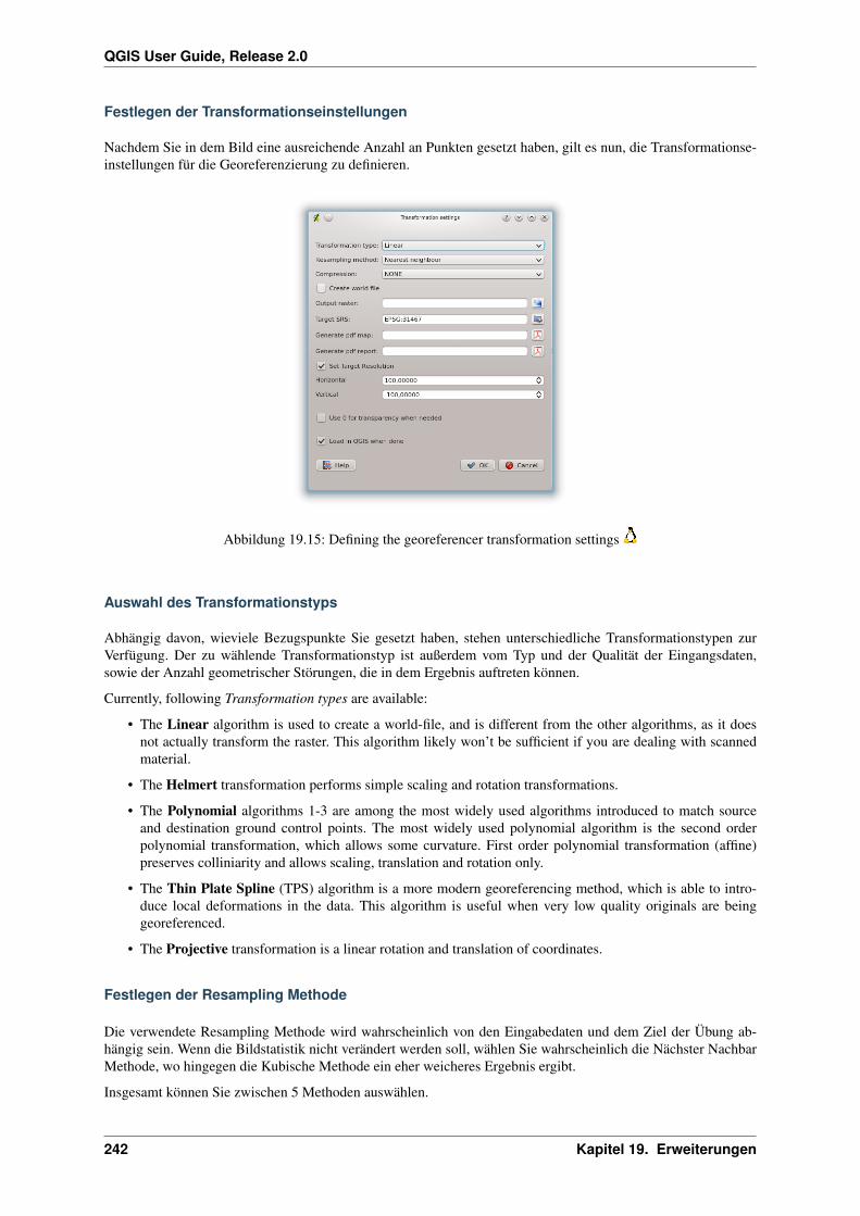
QGIS User Guide, Release 2.0
Festlegen der Transformationseinstellungen
Nachdem Sie in dem Bild eine ausreichende Anzahl an Punkten gesetzt haben, gilt es nun, die Transformationse-instellungen für die Georeferenzierung zu definieren.
Abbildung 19.15: Defining the georeferencer transformation settings
Auswahl des Transformationstyps
Abhängig davon, wieviele Bezugspunkte Sie gesetzt haben, stehen unterschiedliche Transformationstypen zurVerfügung. Der zu wählende Transformationstyp ist außerdem vom Typ und der Qualität der Eingangsdaten,sowie der Anzahl geometrischer Störungen, die in dem Ergebnis auftreten können.
Currently, following Transformation types are available:
• The Linear algorithm is used to create a world-file, and is different from the other algorithms, as it doesnot actually transform the raster. This algorithm likely won’t be sufficient if you are dealing with scannedmaterial.
• The Helmert transformation performs simple scaling and rotation transformations.
• The Polynomial algorithms 1-3 are among the most widely used algorithms introduced to match sourceand destination ground control points. The most widely used polynomial algorithm is the second orderpolynomial transformation, which allows some curvature. First order polynomial transformation (affine)preserves colliniarity and allows scaling, translation and rotation only.
• The Thin Plate Spline (TPS) algorithm is a more modern georeferencing method, which is able to intro-duce local deformations in the data. This algorithm is useful when very low quality originals are beinggeoreferenced.
• The Projective transformation is a linear rotation and translation of coordinates.
Festlegen der Resampling Methode
Die verwendete Resampling Methode wird wahrscheinlich von den Eingabedaten und dem Ziel der Übung ab-hängig sein. Wenn die Bildstatistik nicht verändert werden soll, wählen Sie wahrscheinlich die Nächster NachbarMethode, wo hingegen die Kubische Methode ein eher weicheres Ergebnis ergibt.
Insgesamt können Sie zwischen 5 Methoden auswählen.
242 Kapitel 19. Erweiterungen
QGIS User Guide, Release 2.0
1. Nächster Nachbar
2. Linear
3. Kubisch
4. Kubisches Spline
5. Lanczos
Festlegen der Transformationseinstellungen
Es gibt mehrere Optionen, die für die Ausgabe der Georeferenzierung festgelegt werden müssen.
• Das Kontrollkästchen World-Datei erzeugen ist nur auswählbar, wenn Sie sich für die Lineare Transfor-mation entscheiden. Dies bedeutet nämlich, dass der Rasterlayer selbst nicht entzerrt wird. Stattdessen wirdlediglich eine World-Datei geschrieben, über den der Rasterlayer referenziert wird.
• Für alle anderen Transformationstypen müssen Sie ein Ausgaberaster angeben. Als Standard wird eine Dateimit dem Namen ([filename]_modified) in demselben Ordner, indem sich auch die Ausgangsdatei befindetgeschrieben.
• Als nächsten Schritt müssen Sie das Ziel KBS (Koordinatenbezugsystem) für die Ergebnisdatei angeben(siehe auch Kapitel Arbeiten mit Projektionen).
• Wenn Sie wünschen, können Sie auch eine PDF-Karte und einen PDF-Bericht erzeugen. Der Berichtenthält Informationen zu den verwendeten Transformationsparametern, ein Bild der Abweichungen undeine Liste aller GCPs und ihrer RMS-Fehler.
• Desweiteren können Sie das Kontrollkästchen Zielauflösung aktivieren und eine Pixelauflösung für dasAusgaberaster festlegen. Standard ist der Wert 1,
• Das Kontrollkästchen Falls nötig 0 für Transparenz verwenden sollten Sie aktivieren, wenn es Pixelin dem Ausgaberaster mit dem Wert 0 gibt, die transparent dargestellt werden sollen. In unserem Beispielwären alle weissen Flächen transparent.
• Finally Load in |qg| when done loads the output raster automatically into the QGIS map canvas whenthe transformation is done.
Rastereigenschaften anziegen und anpassen
Wenn Sie auf den Knopf Raster properties im Menü Einstellungen klicken, öffnet sich ein Dialog, um dieRastereigenschaften des zu referenzierenden Layers zu verändern.
Den Georeferenzierer konfigurieren
• Sie können festlegen, ob GCP-Koordiniaten und/oder -IDs angezeigt werden.
• Als Einheit für die Abweichungen kann Pixel oder Karteneinheit gewählt werden.
• Für den PDF-Bericht können Sie einen linken und rechten Rand festlegen und für die PDF-Karte das Pa-pierformat.
• Schließlich können Sie noch das Kontrollkästchen Georeferenzierungsfenster docken aktivieren.Dadurch werden die Fenster gleichmäßig über den Bildschirm verteilt geöffnet.
Starten der Georeferenzierung
Nachdem alle Referenzpunkte gesetzt wurden und die Transformationseinstellungen definiert sind, klicken Sie auf
den Knopf Georeferenzierung beginnen, um den neuen Rasterlayer zu erzeugen.
19.9. Georeferenzier Plugin 243
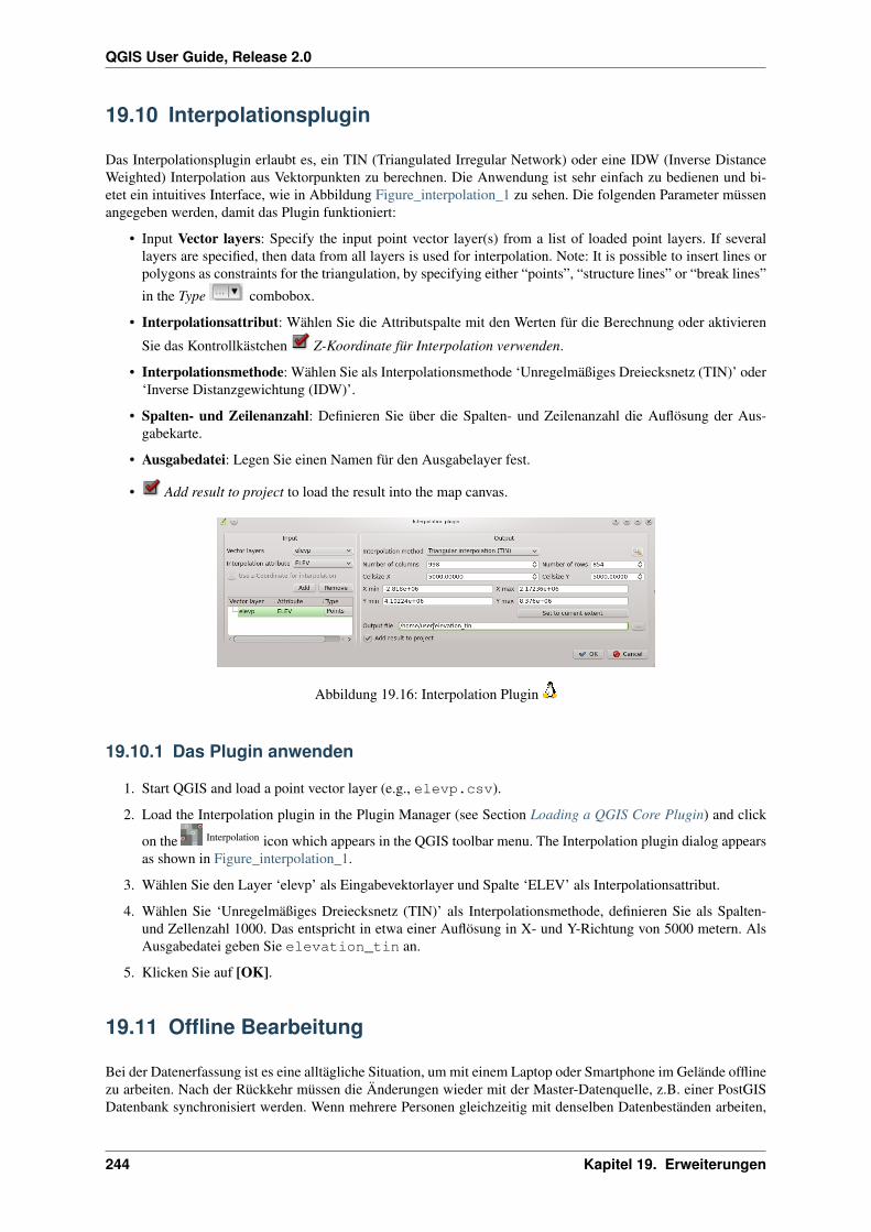
QGIS User Guide, Release 2.0
19.10 Interpolationsplugin
Das Interpolationsplugin erlaubt es, ein TIN (Triangulated Irregular Network) oder eine IDW (Inverse DistanceWeighted) Interpolation aus Vektorpunkten zu berechnen. Die Anwendung ist sehr einfach zu bedienen und bi-etet ein intuitives Interface, wie in Abbildung Figure_interpolation_1 zu sehen. Die folgenden Parameter müssenangegeben werden, damit das Plugin funktioniert:
• Input Vector layers: Specify the input point vector layer(s) from a list of loaded point layers. If severallayers are specified, then data from all layers is used for interpolation. Note: It is possible to insert lines orpolygons as constraints for the triangulation, by specifying either “points”, “structure lines” or “break lines”
in the Type combobox.
• Interpolationsattribut: Wählen Sie die Attributspalte mit den Werten für die Berechnung oder aktivieren
Sie das Kontrollkästchen Z-Koordinate für Interpolation verwenden.
• Interpolationsmethode: Wählen Sie als Interpolationsmethode ‘Unregelmäßiges Dreiecksnetz (TIN)’ oder‘Inverse Distanzgewichtung (IDW)’.
• Spalten- und Zeilenanzahl: Definieren Sie über die Spalten- und Zeilenanzahl die Auflösung der Aus-gabekarte.
• Ausgabedatei: Legen Sie einen Namen für den Ausgabelayer fest.
• Add result to project to load the result into the map canvas.
Abbildung 19.16: Interpolation Plugin
19.10.1 Das Plugin anwenden
1. Start QGIS and load a point vector layer (e.g., elevp.csv).
2. Load the Interpolation plugin in the Plugin Manager (see Section Loading a QGIS Core Plugin) and click
on the Interpolation icon which appears in the QGIS toolbar menu. The Interpolation plugin dialog appearsas shown in Figure_interpolation_1.
3. Wählen Sie den Layer ‘elevp’ als Eingabevektorlayer und Spalte ‘ELEV’ als Interpolationsattribut.
4. Wählen Sie ‘Unregelmäßiges Dreiecksnetz (TIN)’ als Interpolationsmethode, definieren Sie als Spalten-und Zellenzahl 1000. Das entspricht in etwa einer Auflösung in X- und Y-Richtung von 5000 metern. AlsAusgabedatei geben Sie elevation_tin an.
5. Klicken Sie auf [OK].
19.11 Offline Bearbeitung
Bei der Datenerfassung ist es eine alltägliche Situation, um mit einem Laptop oder Smartphone im Gelände offlinezu arbeiten. Nach der Rückkehr müssen die Änderungen wieder mit der Master-Datenquelle, z.B. einer PostGISDatenbank synchronisiert werden. Wenn mehrere Personen gleichzeitig mit denselben Datenbeständen arbeiten,
244 Kapitel 19. Erweiterungen

QGIS User Guide, Release 2.0
ist es meist schwierig, die Änderungen von Hand zu verschmelzen, selbst wenn unterschiedliche Objekte verändertwurden.
Das Offline-Bearbeitung Plugin automatisiert die Synchronisation durch Kopieren des Inhalts einer Datenquelle (inder Regel PostGIS oder WFS-T) zu einer SpatiaLite Datenbank mit dedizierten Tabellen. Nachdem man wiedermit dem Netzwerk verbunden ist, können die Offline-Änderungen wieder an die Master-Datenquell zurückgespieltwerden.
19.11.1 Verwendung der Erweiterung
• Laden Sie ein paar Vektorlayer, z.B. aus PostGIS oder WFS-T Datenquellen
• Speichern Sie die Einstellungen als Projekt
• Öffnen Sie den Dialog :sup:‘Offline Projekt erzeugen’ und wählen Sie die Layer aus, die gespeichertwerden sollen. Sie werden in SpatiaLite Tabellen abgelegt.
• Editieren Sie die Layers offline.
• Nachdem Sie wieder mit dem Internet verbunden sind, laden Sie die Änderungen wieder zurück, in dem Sie
den ‘Knopf Synchronisieren drücken.
Abbildung 19.17: Create an offline project from PostGIS or WFS layers
19.12 Oracle GeoRaster Plugin
In Oracle databases, raster data can be stored in SDO_GEORASTER objects available with the Oracle Spatial
extension. In QGIS, the OracleGeoRasterPlugin is supported by GDAL, and depends on Oracle’s database productbeing installed and working on your machine. While Oracle is proprietary software, they provide their softwarefree for development and testing purposes. Here is one simple example of how to load raster images to GeoRaster:
$ gdal_translate -of georaster input_file.tif geor:scott/tiger@orcl
Das Raster wird in diesem Beispiel in die Standard GDAL_IMPORT Tabelle als Spalte mit dem Namen RASTERgeladen.
19.12. Oracle GeoRaster Plugin 245

QGIS User Guide, Release 2.0
19.12.1 Mit der Datenbank verbinden
Firstly, the Oracle GeoRaster Plugin must be enabled using the Plugin Manager (see Section Loading a QGISCore Plugin). The first time you load a GeoRaster in QGIS, you must create a connection to the Oracle database
that contains the data. To do this, begin by clicking on the Select GeoRaster toolbar button, it will open the SelectOracle Spatial GeoRaster dialog window. Click on [New] to open the dialog window, and specify the connectionparameters (See Figure_oracle_raster_1):
• Name: Geben Sie einen Namen für die Datenbankverbindung an
• Datenbankinstanz: Geben Sie den Namen der Datenbank an, mit der Sie sich verbinden wollen
• Benutzername: Geben Sie den Benutzernamen an, mit dem Sie auf die Datenbank zugreifen wollen
• Passwort: Das Passwort für den Benutzernamen, um auf die Datenbank zuzugreifen
Abbildung 19.18: Create Oracle connection dialog
Zurück im Hauptfenster des Oracle Spatial GeoRaster Plugins (siehe Abbildung Figure_oracle_raster_2), wählenSie die Dropdown Liste, um die neue Verbindung auszuwählen und klicken dann auf [Verbinden], um dieVerbindung herzustellen. Sie können die Verbindung auch nochmals [Bearbeiten] und Veränderungen vornehmenoder mit dem Knopf [Löschen] die Verbindung aus der Dropdown Liste entfernen.
19.12.2 Ein GeoRaster auswählen
Wenn die Verbindung zur Datenbank steht, werden im Fenster ‘Unterdaten’ die Namen aller Tabellen in Formeines GDAL ‘subdataset’ angezeigt, in denen GeoRaster Spalten vorliegen.
Wählen Sie einen der ‘subdatasets’ und klicken dann auf [Wählen], um den Tabellennamen auszuwählen. Da-raufhin erscheint eine weitere Liste mit den GeoRaster Spalten, die sich in der Tabelle befinden. Dies ist nor-malerweise eine kurze Liste, da es eher selten vorkommt, dass mehr als ein oder zwei GeoRaster Spalten in einerTabelle abgelegt sind.
Wählen Sie wieder einen der ‘subdatasets’ und klicken auf [Wählen], um eine Tabellen/Spalten Kombinationauszusuchen. Der Dialog zeigt die Zeilen, die GeoRaster Objekte enthalten. Beachten Sie, dass in der Liste der‘subdatasets’ nun die Rasterdatentabelle und Raster Id Paare angezeigt werden.
Es ist übrigens zu jeder Zeit möglich, die Auswahl zu editieren, um so direkt zu einem bereits bekannten GeoRasteroder zurück zum Anfang zu gelangen.
The Selection data entry can also be used to enter a WHERE clause at the end of the iden-tification string, e.g. geor:scott/tiger@orcl,gdal_import,raster,geoid=. Seehttp://www.gdal.org/frmt_georaster.html for more information.
246 Kapitel 19. Erweiterungen
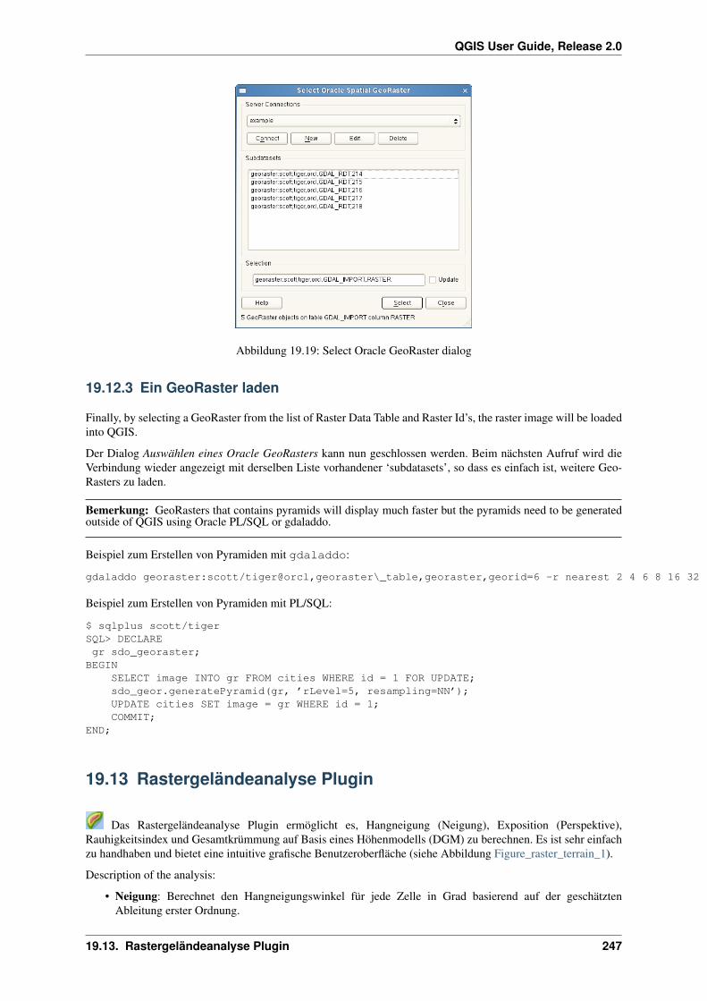
QGIS User Guide, Release 2.0
Abbildung 19.19: Select Oracle GeoRaster dialog
19.12.3 Ein GeoRaster laden
Finally, by selecting a GeoRaster from the list of Raster Data Table and Raster Id’s, the raster image will be loadedinto QGIS.
Der Dialog Auswählen eines Oracle GeoRasters kann nun geschlossen werden. Beim nächsten Aufruf wird dieVerbindung wieder angezeigt mit derselben Liste vorhandener ‘subdatasets’, so dass es einfach ist, weitere Geo-Rasters zu laden.
Bemerkung: GeoRasters that contains pyramids will display much faster but the pyramids need to be generatedoutside of QGIS using Oracle PL/SQL or gdaladdo.
Beispiel zum Erstellen von Pyramiden mit gdaladdo:
gdaladdo georaster:scott/tiger@orcl,georaster\_table,georaster,georid=6 -r nearest 2 4 6 8 16 32
Beispiel zum Erstellen von Pyramiden mit PL/SQL:
$ sqlplus scott/tigerSQL> DECLAREgr sdo_georaster;
BEGINSELECT image INTO gr FROM cities WHERE id = 1 FOR UPDATE;sdo_geor.generatePyramid(gr, ’rLevel=5, resampling=NN’);UPDATE cities SET image = gr WHERE id = 1;COMMIT;
END;
19.13 Rastergeländeanalyse Plugin
Das Rastergeländeanalyse Plugin ermöglicht es, Hangneigung (Neigung), Exposition (Perspektive),Rauhigkeitsindex und Gesamtkrümmung auf Basis eines Höhenmodells (DGM) zu berechnen. Es ist sehr einfachzu handhaben und bietet eine intuitive grafische Benutzeroberfläche (siehe Abbildung Figure_raster_terrain_1).
Description of the analysis:
• Neigung: Berechnet den Hangneigungswinkel für jede Zelle in Grad basierend auf der geschätztenAbleitung erster Ordnung.
19.13. Rastergeländeanalyse Plugin 247
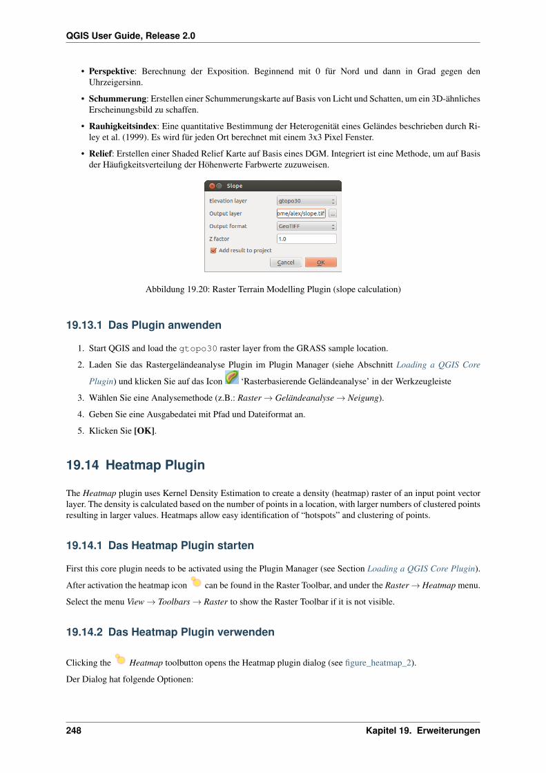
QGIS User Guide, Release 2.0
• Perspektive: Berechnung der Exposition. Beginnend mit 0 für Nord und dann in Grad gegen denUhrzeigersinn.
• Schummerung: Erstellen einer Schummerungskarte auf Basis von Licht und Schatten, um ein 3D-ähnlichesErscheinungsbild zu schaffen.
• Rauhigkeitsindex: Eine quantitative Bestimmung der Heterogenität eines Geländes beschrieben durch Ri-ley et al. (1999). Es wird für jeden Ort berechnet mit einem 3x3 Pixel Fenster.
• Relief: Erstellen einer Shaded Relief Karte auf Basis eines DGM. Integriert ist eine Methode, um auf Basisder Häufigkeitsverteilung der Höhenwerte Farbwerte zuzuweisen.
Abbildung 19.20: Raster Terrain Modelling Plugin (slope calculation)
19.13.1 Das Plugin anwenden
1. Start QGIS and load the gtopo30 raster layer from the GRASS sample location.
2. Laden Sie das Rastergeländeanalyse Plugin im Plugin Manager (siehe Abschnitt Loading a QGIS Core
Plugin) und klicken Sie auf das Icon ‘Rasterbasierende Geländeanalyse’ in der Werkzeugleiste
3. Wählen Sie eine Analysemethode (z.B.: Raster → Geländeanalyse → Neigung).
4. Geben Sie eine Ausgabedatei mit Pfad und Dateiformat an.
5. Klicken Sie [OK].
19.14 Heatmap Plugin
The Heatmap plugin uses Kernel Density Estimation to create a density (heatmap) raster of an input point vectorlayer. The density is calculated based on the number of points in a location, with larger numbers of clustered pointsresulting in larger values. Heatmaps allow easy identification of “hotspots” and clustering of points.
19.14.1 Das Heatmap Plugin starten
First this core plugin needs to be activated using the Plugin Manager (see Section Loading a QGIS Core Plugin).
After activation the heatmap icon can be found in the Raster Toolbar, and under the Raster → Heatmap menu.
Select the menu View → Toolbars → Raster to show the Raster Toolbar if it is not visible.
19.14.2 Das Heatmap Plugin verwenden
Clicking the Heatmap toolbutton opens the Heatmap plugin dialog (see figure_heatmap_2).
Der Dialog hat folgende Optionen:
248 Kapitel 19. Erweiterungen
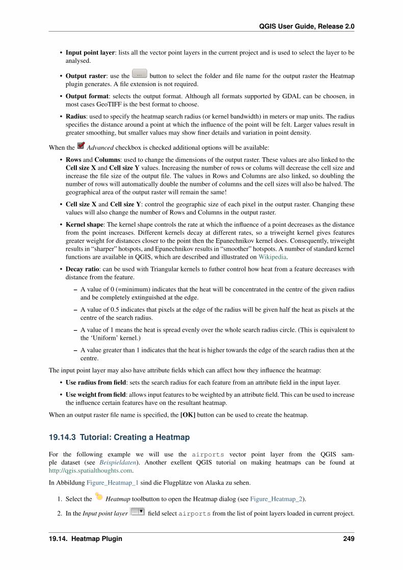
QGIS User Guide, Release 2.0
• Input point layer: lists all the vector point layers in the current project and is used to select the layer to beanalysed.
• Output raster: use the button to select the folder and file name for the output raster the Heatmapplugin generates. A file extension is not required.
• Output format: selects the output format. Although all formats supported by GDAL can be choosen, inmost cases GeoTIFF is the best format to choose.
• Radius: used to specify the heatmap search radius (or kernel bandwidth) in meters or map units. The radiusspecifies the distance around a point at which the influence of the point will be felt. Larger values result ingreater smoothing, but smaller values may show finer details and variation in point density.
When the Advanced checkbox is checked additional options will be available:
• Rows and Columns: used to change the dimensions of the output raster. These values are also linked to theCell size X and Cell size Y values. Increasing the number of rows or colums will decrease the cell size andincrease the file size of the output file. The values in Rows and Columns are also linked, so doubling thenumber of rows will automatically double the number of columns and the cell sizes will also be halved. Thegeographical area of the output raster will remain the same!
• Cell size X and Cell size Y: control the geographic size of each pixel in the output raster. Changing thesevalues will also change the number of Rows and Columns in the output raster.
• Kernel shape: The kernel shape controls the rate at which the influence of a point decreases as the distancefrom the point increases. Different kernels decay at different rates, so a triweight kernel gives featuresgreater weight for distances closer to the point then the Epanechnikov kernel does. Consequently, triweightresults in “sharper” hotspots, and Epanechnikov results in “smoother” hotspots. A number of standard kernelfunctions are available in QGIS, which are described and illustrated on Wikipedia.
• Decay ratio: can be used with Triangular kernels to futher control how heat from a feature decreases withdistance from the feature.
– A value of 0 (=minimum) indicates that the heat will be concentrated in the centre of the given radiusand be completely extinguished at the edge.
– A value of 0.5 indicates that pixels at the edge of the radius will be given half the heat as pixels at thecentre of the search radius.
– A value of 1 means the heat is spread evenly over the whole search radius circle. (This is equivalent tothe ‘Uniform’ kernel.)
– A value greater than 1 indicates that the heat is higher towards the edge of the search radius then at thecentre.
The input point layer may also have attribute fields which can affect how they influence the heatmap:
• Use radius from field: sets the search radius for each feature from an attribute field in the input layer.
• Use weight from field: allows input features to be weighted by an attribute field. This can be used to increasethe influence certain features have on the resultant heatmap.
When an output raster file name is specified, the [OK] button can be used to create the heatmap.
19.14.3 Tutorial: Creating a Heatmap
For the following example we will use the airports vector point layer from the QGIS sam-ple dataset (see Beispieldaten). Another exellent QGIS tutorial on making heatmaps can be found athttp://qgis.spatialthoughts.com.
In Abbildung Figure_Heatmap_1 sind die Flugplätze von Alaska zu sehen.
1. Select the Heatmap toolbutton to open the Heatmap dialog (see Figure_Heatmap_2).
2. In the Input point layer field select airports from the list of point layers loaded in current project.
19.14. Heatmap Plugin 249
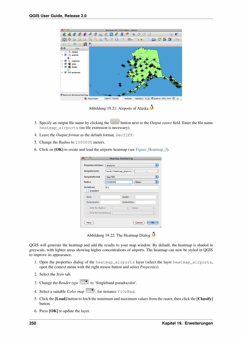
QGIS User Guide, Release 2.0
Abbildung 19.21: Airports of Alaska
3. Specify an output file name by clicking the button next to the Output raster field. Enter the file nameheatmap_airports (no file extension is necessary).
4. Leave the Output format as the default format, GeoTIFF.
5. Change the Radius to 1000000 meters.
6. Click on [OK] to create and load the airports heatmap (see Figure_Heatmap_3).
Abbildung 19.22: The Heatmap Dialog
QGIS will generate the heatmap and add the results to your map window. By default, the heatmap is shaded ingreyscale, with lighter areas showing higher concentrations of airports. The heatmap can now be styled in QGISto improve its appearance.
1. Open the properties dialog of the heatmap_airports layer (select the layer heatmap_airports,open the context menu with the right mouse button and select Properties).
2. Select the Style tab.
3. Change the Render type to ‘Singleband pseudocolor’.
4. Select a suitable Color map , for instance YlOrRed.
5. Click the [Load] button to fetch the minimum and maximum values from the raster, then click the [Classify]button.
6. Press [OK] to update the layer.
250 Kapitel 19. Erweiterungen
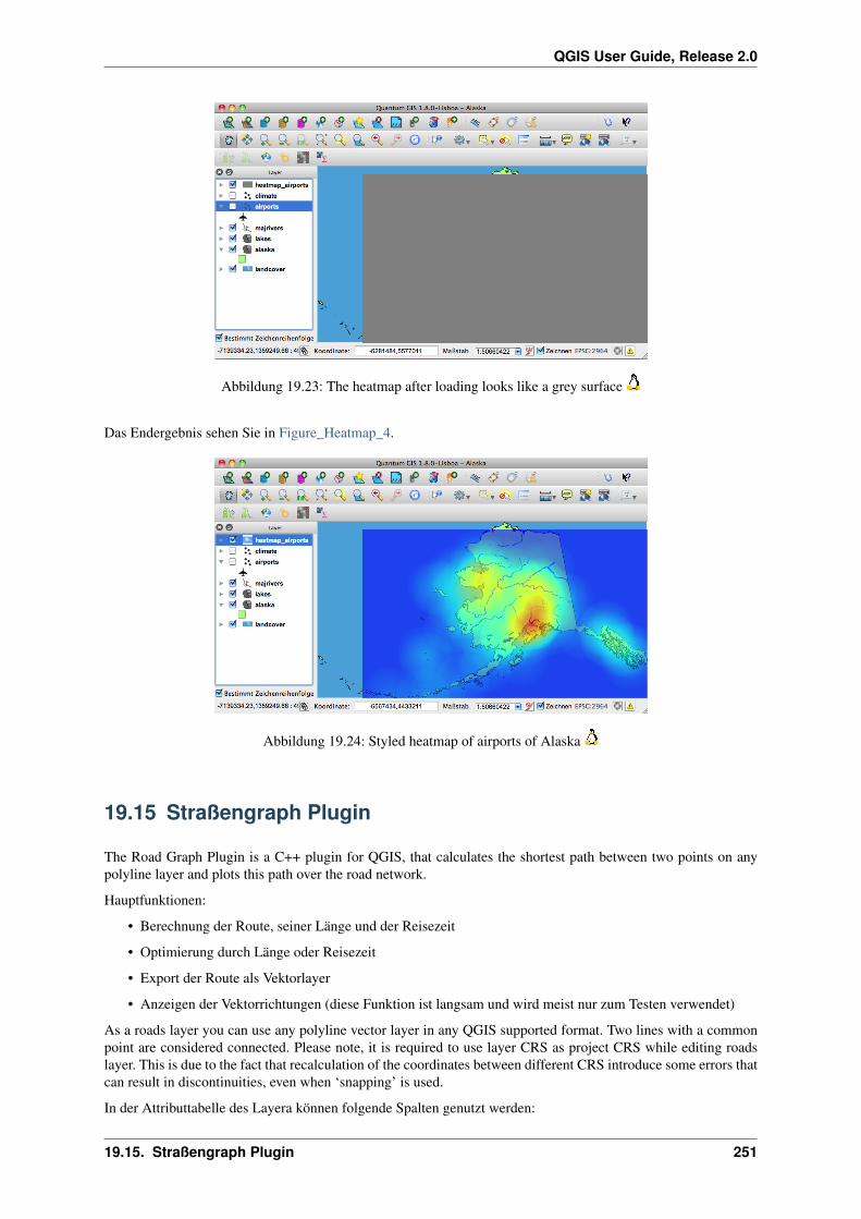
QGIS User Guide, Release 2.0
Abbildung 19.23: The heatmap after loading looks like a grey surface
Das Endergebnis sehen Sie in Figure_Heatmap_4.
Abbildung 19.24: Styled heatmap of airports of Alaska
19.15 Straßengraph Plugin
The Road Graph Plugin is a C++ plugin for QGIS, that calculates the shortest path between two points on anypolyline layer and plots this path over the road network.
Hauptfunktionen:
• Berechnung der Route, seiner Länge und der Reisezeit
• Optimierung durch Länge oder Reisezeit
• Export der Route als Vektorlayer
• Anzeigen der Vektorrichtungen (diese Funktion ist langsam und wird meist nur zum Testen verwendet)
As a roads layer you can use any polyline vector layer in any QGIS supported format. Two lines with a commonpoint are considered connected. Please note, it is required to use layer CRS as project CRS while editing roadslayer. This is due to the fact that recalculation of the coordinates between different CRS introduce some errors thatcan result in discontinuities, even when ‘snapping’ is used.
In der Attributtabelle des Layera können folgende Spalten genutzt werden:
19.15. Straßengraph Plugin 251
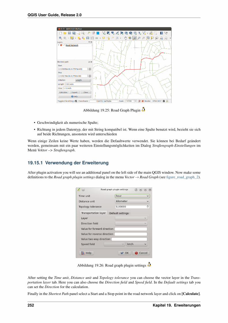
QGIS User Guide, Release 2.0
Abbildung 19.25: Road Graph Plugin
• Geschwindigkeit als numerische Spalte;
• Richtung in jedem Datentyp, der mit String kompatibel ist. Wenn eine Spalte benutzt wird, bezieht sie sichauf beide Richtungen, ansonsten wird unterschieden
Wenn einige Zeilen keine Werte haben, werden die Defaultwerte verwendet. Sie können bei Bedarf geändertwerden, gemeinsam mit ein paar weiteren Einstellungsmöglichkeiten im Dialog Straßengraph-Einstellungen imMenü Vektor –> Straßengraph.
19.15.1 Verwendung der Erweiterung
After plugin activation you will see an additional panel on the left side of the main QGIS window. Now make somedefinitions to the Road graph plugin settings dialog in the menu Vector → Road Graph (see figure_road_graph_2).
Abbildung 19.26: Road graph plugin settings
After setting the Time unit, Distance unit and Topology tolerance you can choose the vector layer in the Trans-portation layer tab. Here you can also choose the Direction field and Speed field. In the Default settings tab youcan set the Direction for the calculation.
Finally in the Shortest Path panel select a Start and a Stop point in the road network layer and click on [Calculate].
252 Kapitel 19. Erweiterungen
QGIS User Guide, Release 2.0
19.16 Räumliche Abfrage Plugin
The Spatial Query Plugin ermöglicht eine räumliche Abfrage (Objekte auswählen) in einem Quelllayer mit Ver-weis auf einen Referenzlayer. Die Funktionalität basiert auf der GEOS-Bibliothek und ist abhängig von demausgewählten Datentyp (Punkt, Linie, Polygon) des Layers mit den Quellobjekten.
Mögliche Operatoren sind:
• Enthält
• Gleicht
• Überlappt
• Kreuzt
• Überschneidet
• Ist ausserhalb
• Berührt
• Innerhalb
19.16.1 Verwendung der Erweiterung
Als Beispiel sollen die Regionen Alaskas gefunden werden, die Flugplätze enthalten. Folgende Schritte sindnotwendig:
1. Start QGIS and load the vector layers regions.shp and airports.shp.
2. Load the Spatial Query plugin in the Plugin Manager (see Section Loading a QGIS Core Plugin) and click
on the Spatial Query icon which appears in the QGIS toolbar menu. The plugin dialog appears.
3. Select layer regions as source layer and airports as reference feature layer.
4. Wählen Sie ‘Enthält’ als Operator und klicken Sie dann auf [Anwenden].
Sie bekommen dann eine Liste von Objekt IDs und haben verschiedene Optionen, siehe Abbildung fig-ure_spatial_query_1.
• Klicken Sie auf Layer mit Liste von Elementen erzeugen
• Wählen Sie eine ID aus der Liste und klicken Sie auf Layer mit gewählten erzeugen
• Wählen Sie ‘Aus aktueller Auswahl entfernen’ im Bereich Das Ergebnis speichern in .
• Zusätzlich können Sie die Kontrollkästchen Zum Element zoomen oder Protokoll aktivieren.
19.17 SQL-Anywhere Plugin
SQL Anywhere ist ein proprietäres relationales Datenbank-Managementsystem (RDBMS) von Sybase. SQL Any-where umfasst Unterstützung für räumliche Daten einschließlich OGC, Shape-Dateien etc. sowie eingebaute Funk-tionen für den Export nach KML, GML und ins SVG-Format.
The SQL Anywhere allows to connect to spatially enabled SQL Anywhere databases. The Add SQL Anywherelayer dialog is similar in functionality to the dialogs for PostGIS and SpatiaLite.
19.16. Räumliche Abfrage Plugin 253
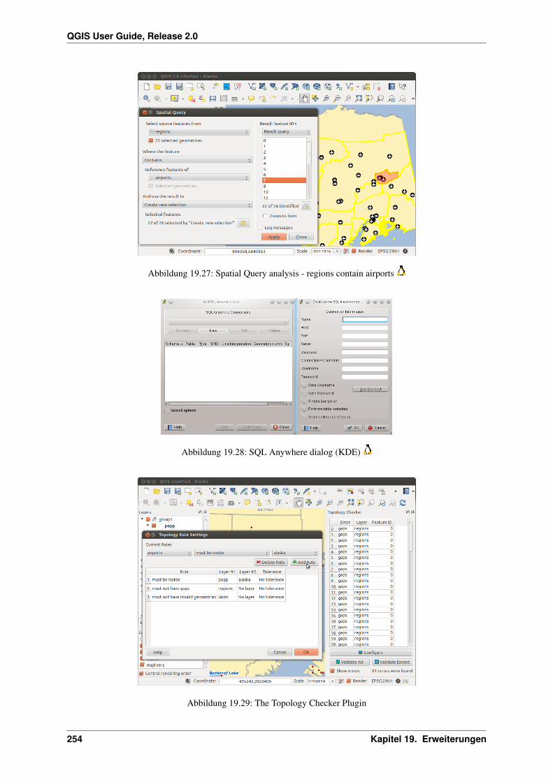
QGIS User Guide, Release 2.0
Abbildung 19.27: Spatial Query analysis - regions contain airports
Abbildung 19.28: SQL Anywhere dialog (KDE)
Abbildung 19.29: The Topology Checker Plugin
254 Kapitel 19. Erweiterungen
QGIS User Guide, Release 2.0
19.18 Topology Checker Plugin
Topology describes the relationships between points, lines and polygons that represent the features of a geographicregion. With the Topology Checker plugin you can look over your vector files and check the topology with severaltopology rules. These rules check with spatial relations whether your features ‘Equal’, ‘Contain’, ‘Cover’, are‘CoveredBy’, ‘Cross’, ‘Disjoint’, ‘Intersect’, ‘Overlap’, ‘Touches’ and are ‘Within’ each other. It depends onyour individual questions which topology rules you apply to your vector data. E.g. normally you won’t acceptovershoots in line layers but if they depict dead-end streets you won’t remove them from your vector layer.
QGIS has the built-in topological editing feature which is great for creating new features without errors. Butexisting data errors and user induced errors are hard to find out. This plugin helps you find out such errors througha list of rules.
It is very simple to create topology rules with the Topology Checker plugin.
On point layers the following rules are available:
• must be covered by: Here you can choose a vector layer from your project. Points that aren’t covered bythe given vector layer occur in the ‘Error’ field
• must be covered by endpoints of: Here you can choose a line layer from your project.
• must be inside: Here you can choose a polygon layer from your project. The points must be inside apolygon. Otherwise QGIS writes an ‘Error’ for the point.
• must not have duplicates: Whenever a point is represented twice or more it will occur in the ‘Error’ field.
• must not have invalid geometries: Checks whether the geometries are valid.
• must not have multi-part-geometries: All multi-part points are written into the ‘Error’ field.
On line layers the following rules are available:
• end points must be covered by: Here you can select a point layer from your project.
• must not have dangles: This will show the overshoots in the line layer.
• must not have duplicates: Whenever a line feature is represented twice or more it will occur in the ‘Error’field.
• must not have invalid geometries: Checks whether the geometries are valid.
• must not have multi-part geometries: Sometimes, a geometry is actually a collection of simple (single-part) geometries. Such a geometry is called multi-part geometry. If it contains just one type of simplegeometry, we call it multi-point, multi-linestring or multi-polygon. All multi-part lines are written into the‘Error’ field.
• must not have pseudos: A line geometry’s endpoint should be connected to the endpoints of two othergeometries. If the endpoint is connected to only one other geometry’s endpoint, the endpoint is called apsuedo node.
On polygon layers the following rules are available:
• must contain: Polygon layer must contain at least one point geometry from the second layer.
• must not have duplicates: Polygons from the same layer must not have identical geometries. Whenever apolygon feature is represented twice or more it will occur in the ‘Error’ field.
• must not have gaps: Adjacent polygons should not form gaps between them. Administrative boundariescould be mentioned as an example (US state polygons do not have any gaps between them...).
• must not have invalid geometries: Checks whether the geometries are valid. Some of the rules that definea valid geometry are,
– Polygon rings must close.
– Rings that define holes should be inside rings that define exterior boundaries.
– Rings may not self-intersect (they may neither touch nor cross one another).
19.18. Topology Checker Plugin 255

QGIS User Guide, Release 2.0
– Rings may not touch other rings, except at a point.
• must not have multi-part geometries: Sometimes, a geometry is actually a collection of simple (single-part) geometries. Such a geometry is called multi-part geometry. If it contains just one type of simplegeometry, we call it multi-point, multi-linestring or multi-polygon. For example, a country consisting ofmultiple islands can be represented as a multi-polygon.
• must not overlap: Adjacent polygons should not share common area.
• must not overlap with: Adjacent polygons from one layer should not share common area with polygonsfrom another layer.
19.19 Zonenstatistikerweiterung
Mit der Zonenstatistikerweiterung können Sie das Ergebnis einer thematischen Klassifikation analysieren. Es er-mögicht, verschiedene, descriptive statitische Werte von Rasterpixeln innerhalb von Flächen eines Vektorlayerszu berechnen (see figure_zonal_statistics). Sie können Summe, Mittelwert und die Anzahl der Pixel innerhalb dereinzelnen Flächen berechnen. Das Plugin erstellt für jeden zu berechnenden Wert eine Attributspalte, die man miteinem Präfix definieren kann.
Abbildung 19.30: Zonal statistics dialog (KDE)
256 Kapitel 19. Erweiterungen

KAPITEL 20
Hilfe und Support
20.1 Mailinglisten
QGIS is under active development and as such it won’t always work like you expect it to. The preferred way toget help is by joining the qgis-users mailing list. Your questions will reach a broader audience and answers willbenefit others.
20.1.1 qgis-users
This mailing list is used for discussion of QGIS in general, as well as specific questions regarding itsinstallation and use. You can subscribe to the qgis-users mailing list by visiting the following URL:http://lists.osgeo.org/mailman/listinfo/qgis-user
20.1.2 fossgis-talk-liste
For the german speaking audience the german FOSSGIS e.V. provides the fossgis-talk-liste mailing list. Thismailing list is used for discussion of open source GIS in general including QGIS. You can subscribe to the fossgis-talk-liste mailing list by visiting the following URL: https://lists.fossgis.de/mailman/listinfo/fossgis-talk-liste
20.1.3 qgis-developer
Wenn Sie ein Entwickler sind und technische Probleme haben, können Sie sich in die qgis-developer Mailinglisteeintragen unter der URL: http://lists.osgeo.org/mailman/listinfo/qgis-developer
20.1.4 qgis-commit
Each time a commit is made to the QGIS code repository an email is posted to this list. If youwant to be up to date with every change to the current code base, you can subscribe to this list at:http://lists.osgeo.org/mailman/listinfo/qgis-commit
20.1.5 qgis-trac
Diese Mailingliste stellt Nachrichten in Bezug auf das Projekt Management bereit. Dazu gehören Fehlerberichte,Aufgaben und Anfragen für neue Funktionen. Sie können sich für diese Mailingliste eintragen unter der URL:http://lists.osgeo.org/mailman/listinfo/qgis-trac
257
QGIS User Guide, Release 2.0
20.1.6 qgis-community-team
Diese Mailingliste stellt Nachrichten in Bezug auf das Projekt Management bereit. Dazu gehören Fehlerberichte,Aufgaben und Anfragen für neue Funktionen. Sie können sich für diese Mailingliste eintragen unter der URL:http://lists.osgeo.org/mailman/listinfo/qgis-community-team
20.1.7 qgis-release-team
Diese Liste beschäftigt sich mit Themen wie dem Release Management, das Erstellen von Installations-Paketenfür verschiedene Betriebssysteme und das Veröffentlichen neuer QGIS Versionen. Sie können sich für diese Mail-ingliste eintragen unter der URL: http://lists.osgeo.org/mailman/listinfo/qgis-release-team
20.1.8 qgis-tr
Diese Liste beschäftigt sich mit der Übersetzung der QGIS GUI und der Dokumentation. Sie können sich für dieseMailingliste eintragen unter der URL: http://lists.osgeo.org/mailman/listinfo/qgis-tr
20.1.9 qgis-edu
This list deals with QGIS education efforts. If you like to work on QGIS education materials, this list is a goodstarting point to ask your questions. You can subscribe to this list at: http://lists.osgeo.org/mailman/listinfo/qgis-edu
20.1.10 qgis-psc
This list is used to discuss Steering Committee issues related to overall management and direction of QGIS. Youcan subscribe to this list at: http://lists.osgeo.org/mailman/listinfo/qgis-psc
Wir heißen Sie herzlich Willkommen, sich auf jeder dieser Listen einzuschreiben und den anderen QGIS Be-nutzern und Entwicklern mit ihrer Erfahrung zu helfen. Beachten Sie bitte auch, dass die Mailinglisten qgis-commit und qgis-trac nur dazu erstellt wurden, um Benachrichtigungen zu verteilen und nicht für Anwenderfragengeeignet ist.
20.2 IRC
Wir sind außerdem im IRC präsent - Sie können uns im #qgis Kanal unter irc.freenode.net treffen. Bitte wartenSie ein wenig auf Antworten, da die meisten nur zwischendurch mal vorbeischauen, was gerade so passiert. Kom-merzieller Support ist auch möglich. Schauen Sie dazu auf die Internetseite http://www.qgis.org/de/kommerzieller-support.html.
If you missed a discussion on IRC, not a problem! We log all discussion so you can easily catch up. Just go tohttp://qgis.org/irclogs and read the IRC-logs.
20.3 BugTracker
While the qgis-users mailing list is useful for general ‘how do I do XYZ in QGIS’ type questions, youmay wish to notify us about bugs in QGIS. You can submit bug reports using the QGIS bug tracker athttp://hub.qgis.org/projects/quantum-gis/issues. When creating a new ticket for a bug, please provide an emailaddress where we can request additional information.
Denken Sie auch bitte daran, dass ein für Sie wichtiger Fehler nicht immer die gleiche Priorität bei anderenPersonen und besonders den Entwicklern hat. Einige Fehler sind sehr aufwendig zu reparieren und daher kann esschon mal ein wenig dauern, bis genügend Zeit vorhanden ist, ein Problem zu lösen.
258 Kapitel 20. Hilfe und Support
QGIS User Guide, Release 2.0
Anfragen für neue Funktionen können auch in demselben System gestellt werden. Bitte geben Sie dann den TypFeature an.
If you have found a bug and fixed it yourself you can submit this patch also. Again, the lovely redmine ticketsystemat http://hub.qgis.org/wiki/quantum-gis/issues has this type as well. Check Patch supplied checkbox andattach your patch before submitting bug. Someone of the developers will review it and apply it to QGIS. Pleasedon’t be alarmed if your patch is not applied straight away — developers may be tied up with other committments.
20.4 Blog
The QGIS community also runs a weblog at http://planet.qgis.org/planet/ which has some interesting articles forusers and developers as well provided by other blogs in the community. You are invited to contribute your ownQGIS blog!
20.5 Plugins
The website http://plugins.qgis.org provides the official QGIS plugins web portal. Here you find a list of all stableand experimental QGIS plugins available via the ‘Official QGIS Plugin Repository’.
20.6 Wiki
Schließlich gibt es auch ein QGIS WIKI unter http://www.qgis.org/wiki, wo Sie eine Vielzahl nützlicher Infor-mationen über die QGIS-Entwicklung, Pläne für neue Versionen, Links zum Herunterladen von Daten oder zuvorhandenen Übersetzungen finden. Schauen Sie mal rein, da gibt es ein paar wirkliche Attraktionen!
20.4. Blog 259
QGIS User Guide, Release 2.0
260 Kapitel 20. Hilfe und Support

KAPITEL 21
Appendix
21.1 GNU General Public License
Version 2, June 1991
Copyright (C) 1989, 1991 Free Software Foundation, Inc. 59 Temple Place - Suite 330, Boston, MA 02111-1307,USA
Everyone is permitted to copy and distribute verbatim copies of this license document, but changing it is notallowed.
Preamble
The licenses for most software are designed to take away your freedom to share and change it. By contrast,the GNU General Public License is intended to guarantee your freedom to share and change free software–tomake sure the software is free for all its users. This General Public License applies to most of the Free SoftwareFoundation’s software and to any other program whose authors commit to using it. (Some other Free SoftwareFoundation software is covered by the GNU Library General Public License instead.) You can apply it to yourprograms, too.
When we speak of free software, we are referring to freedom, not price. Our General Public Licenses are designedto make sure that you have the freedom to distribute copies of free software (and charge for this service if youwish), that you receive source code or can get it if you want it, that you can change the software or use pieces ofit in new free programs; and that you know you can do these things.
To protect your rights, we need to make restrictions that forbid anyone to deny you these rights or to ask you tosurrender the rights. These restrictions translate to certain responsibilities for you if you distribute copies of thesoftware, or if you modify it.
For example, if you distribute copies of such a program, whether gratis or for a fee, you must give the recipientsall the rights that you have. You must make sure that they, too, receive or can get the source code. And you mustshow them these terms so they know their rights.
We protect your rights with two steps: (1) copyright the software, and (2) offer you this license which gives youlegal permission to copy, distribute and/or modify the software.
Also, for each author’s protection and ours, we want to make certain that everyone understands that there is nowarranty for this free software. If the software is modified by someone else and passed on, we want its recipientsto know that what they have is not the original, so that any problems introduced by others will not reflect on theoriginal authors’ reputations.
Finally, any free program is threatened constantly by software patents. We wish to avoid the danger that redis-tributors of a free program will individually obtain patent licenses, in effect making the program proprietary. Toprevent this, we have made it clear that any patent must be licensed for everyone’s free use or not licensed at all.
The precise terms and conditions for copying, distribution and modification follow. TERMS AND CONDITIONSFOR COPYING, DISTRIBUTION AND MODIFICATION
0. This License applies to any program or other work which contains a notice placed by the copyright holdersaying it may be distributed under the terms of this General Public License. The “Program”, below, refers to
261

QGIS User Guide, Release 2.0
any such program or work, and a “work based on the Program” means either the Program or any derivativework under copyright law: that is to say, a work containing the Program or a portion of it, either verbatimor with modifications and/or translated into another language. (Hereinafter, translation is included withoutlimitation in the term “modification”.) Each licensee is addressed as “you”.
Activities other than copying, distribution and modification are not covered by this License; they are outsideits scope. The act of running the Program is not restricted, and the output from the Program is covered onlyif its contents constitute a work based on the Program (independent of having been made by running theProgram). Whether that is true depends on what the Program does.
1. You may copy and distribute verbatim copies of the Program’s source code as you receive it, in any medium,provided that you conspicuously and appropriately publish on each copy an appropriate copyright noticeand disclaimer of warranty; keep intact all the notices that refer to this License and to the absence of anywarranty; and give any other recipients of the Program a copy of this License along with the Program.
You may charge a fee for the physical act of transferring a copy, and you may at your option offer warrantyprotection in exchange for a fee.
2. You may modify your copy or copies of the Program or any portion of it, thus forming a work based on theProgram, and copy and distribute such modifications or work under the terms of Section 1 above, providedthat you also meet all of these conditions:
(a) You must cause the modified files to carry prominent notices stating that you changed the files and thedate of any change.
(b) You must cause any work that you distribute or publish, that in whole or in part contains or is derivedfrom the Program or any part thereof, to be licensed as a whole at no charge to all third parties underthe terms of this License.
(c) If the modified program normally reads commands interactively when run, you must cause it, whenstarted running for such interactive use in the most ordinary way, to print or display an announcementincluding an appropriate copyright notice and a notice that there is no warranty (or else, saying thatyou provide a warranty) and that users may redistribute the program under these conditions, and tellingthe user how to view a copy of this License. (Exception: if the Program itself is interactive but doesnot normally print such an announcement, your work based on the Program is not required to print anannouncement.)
These requirements apply to the modified work as a whole. If identifiable sections of that work are notderived from the Program, and can be reasonably considered independent and separate works in themselves,then this License, and its terms, do not apply to those sections when you distribute them as separate works.But when you distribute the same sections as part of a whole which is a work based on the Program, thedistribution of the whole must be on the terms of this License, whose permissions for other licensees extendto the entire whole, and thus to each and every part regardless of who wrote it.
Thus, it is not the intent of this section to claim rights or contest your rights to work written entirely by you;rather, the intent is to exercise the right to control the distribution of derivative or collective works based onthe Program.
In addition, mere aggregation of another work not based on the Program with the Program (or with a workbased on the Program) on a volume of a storage or distribution medium does not bring the other work underthe scope of this License.
3. You may copy and distribute the Program (or a work based on it, under Section 2) in object code or exe-cutable form under the terms of Sections 1 and 2 above provided that you also do one of the following:
(a) Accompany it with the complete corresponding machine-readable source code, which must be dis-tributed under the terms of Sections 1 and 2 above on a medium customarily used for software inter-change; or,
(b) Accompany it with a written offer, valid for at least three years, to give any third party, for a charge nomore than your cost of physically performing source distribution, a complete machine-readable copyof the corresponding source code, to be distributed under the terms of Sections 1 and 2 above on amedium customarily used for software interchange; or,
262 Kapitel 21. Appendix
QGIS User Guide, Release 2.0
(c) Accompany it with the information you received as to the offer to distribute corresponding sourcecode. (This alternative is allowed only for noncommercial distribution and only if you received theprogram in object code or executable form with such an offer, in accord with Subsection b above.)
The source code for a work means the preferred form of the work for making modifications to it. For anexecutable work, complete source code means all the source code for all modules it contains, plus any asso-ciated interface definition files, plus the scripts used to control compilation and installation of the executable.However, as a special exception, the source code distributed need not include anything that is normally dis-tributed (in either source or binary form) with the major components (compiler, kernel, and so on) of theoperating system on which the executable runs, unless that component itself accompanies the executable.
If distribution of executable or object code is made by offering access to copy from a designated place, thenoffering equivalent access to copy the source code from the same place counts as distribution of the sourcecode, even though third parties are not compelled to copy the source along with the object code.
4. You may not copy, modify, sublicense, or distribute the Program except as expressly provided under thisLicense. Any attempt otherwise to copy, modify, sublicense or distribute the Program is void, and willautomatically terminate your rights under this License. However, parties who have received copies, or rights,from you under this License will not have their licenses terminated so long as such parties remain in fullcompliance.
5. You are not required to accept this License, since you have not signed it. However, nothing else grants youpermission to modify or distribute the Program or its derivative works. These actions are prohibited by lawif you do not accept this License. Therefore, by modifying or distributing the Program (or any work basedon the Program), you indicate your acceptance of this License to do so, and all its terms and conditions forcopying, distributing or modifying the Program or works based on it.
6. Each time you redistribute the Program (or any work based on the Program), the recipient automaticallyreceives a license from the original licensor to copy, distribute or modify the Program subject to these termsand conditions. You may not impose any further restrictions on the recipients’ exercise of the rights grantedherein. You are not responsible for enforcing compliance by third parties to this License.
7. If, as a consequence of a court judgment or allegation of patent infringement or for any other reason (notlimited to patent issues), conditions are imposed on you (whether by court order, agreement or otherwise)that contradict the conditions of this License, they do not excuse you from the conditions of this License.If you cannot distribute so as to satisfy simultaneously your obligations under this License and any otherpertinent obligations, then as a consequence you may not distribute the Program at all. For example, if apatent license would not permit royalty-free redistribution of the Program by all those who receive copiesdirectly or indirectly through you, then the only way you could satisfy both it and this License would be torefrain entirely from distribution of the Program.
If any portion of this section is held invalid or unenforceable under any particular circumstance, the balanceof the section is intended to apply and the section as a whole is intended to apply in other circumstances.
It is not the purpose of this section to induce you to infringe any patents or other property right claimsor to contest validity of any such claims; this section has the sole purpose of protecting the integrity ofthe free software distribution system, which is implemented by public license practices. Many people havemade generous contributions to the wide range of software distributed through that system in reliance onconsistent application of that system; it is up to the author/donor to decide if he or she is willing to distributesoftware through any other system and a licensee cannot impose that choice.
This section is intended to make thoroughly clear what is believed to be a consequence of the rest of thisLicense.
8. If the distribution and/or use of the Program is restricted in certain countries either by patents or by copy-righted interfaces, the original copyright holder who places the Program under this License may add anexplicit geographical distribution limitation excluding those countries, so that distribution is permitted onlyin or among countries not thus excluded. In such case, this License incorporates the limitation as if writtenin the body of this License.
9. The Free Software Foundation may publish revised and/or new versions of the General Public License fromtime to time. Such new versions will be similar in spirit to the present version, but may differ in detail toaddress new problems or concerns.
21.1. GNU General Public License 263
QGIS User Guide, Release 2.0
Each version is given a distinguishing version number. If the Program specifies a version number of thisLicense which applies to it and “any later version”, you have the option of following the terms and conditionseither of that version or of any later version published by the Free Software Foundation. If the Program doesnot specify a version number of this License, you may choose any version ever published by the FreeSoftware Foundation.
10. If you wish to incorporate parts of the Program into other free programs whose distribution conditions aredifferent, write to the author to ask for permission. For software which is copyrighted by the Free SoftwareFoundation, write to the Free Software Foundation; we sometimes make exceptions for this. Our decisionwill be guided by the two goals of preserving the free status of all derivatives of our free software and ofpromoting the sharing and reuse of software generally.
NO WARRANTY
11. BECAUSE THE PROGRAM IS LICENSED FREE OF CHARGE, THERE IS NO WARRANTY FORTHE PROGRAM, TO THE EXTENT PERMITTED BY APPLICABLE LAW. EXCEPT WHEN OTH-ERWISE STATED IN WRITING THE COPYRIGHT HOLDERS AND/OR OTHER PARTIES PROVIDETHE PROGRAM “AS IS” WITHOUT WARRANTY OF ANY KIND, EITHER EXPRESSED OR IM-PLIED, INCLUDING, BUT NOT LIMITED TO, THE IMPLIED WARRANTIES OF MERCHANTABIL-ITY AND FITNESS FOR A PARTICULAR PURPOSE. THE ENTIRE RISK AS TO THE QUALITY ANDPERFORMANCE OF THE PROGRAM IS WITH YOU. SHOULD THE PROGRAM PROVE DEFEC-TIVE, YOU ASSUME THE COST OF ALL NECESSARY SERVICING, REPAIR OR CORRECTION.
12. IN NO EVENT UNLESS REQUIRED BY APPLICABLE LAW OR AGREED TO IN WRITING WILLANY COPYRIGHT HOLDER, OR ANY OTHER PARTY WHO MAY MODIFY AND/OR REDIS-TRIBUTE THE PROGRAM AS PERMITTED ABOVE, BE LIABLE TO YOU FOR DAMAGES, IN-CLUDING ANY GENERAL, SPECIAL, INCIDENTAL OR CONSEQUENTIAL DAMAGES ARISINGOUT OF THE USE OR INABILITY TO USE THE PROGRAM (INCLUDING BUT NOT LIMITED TOLOSS OF DATA OR DATA BEING RENDERED INACCURATE OR LOSSES SUSTAINED BY YOUOR THIRD PARTIES OR A FAILURE OF THE PROGRAM TO OPERATE WITH ANY OTHER PRO-GRAMS), EVEN IF SUCH HOLDER OR OTHER PARTY HAS BEEN ADVISED OF THE POSSIBILI-TY OF SUCH DAMAGES.
QGIS Qt exception for GPL
In addition, as a special exception, the QGIS Development Team gives permission to link the codeof this program with the Qt library, including but not limited to the following versions (both freeand commercial): Qt/Non-commerical Windows, Qt/Windows, Qt/X11, Qt/Mac, and Qt/Embedded(or with modified versions of Qt that use the same license as Qt), and distribute linked combinationsincluding the two. You must obey the GNU General Public License in all respects for all of the codeused other than Qt. If you modify this file, you may extend this exception to your version of the file,but you are not obligated to do so. If you do not wish to do so, delete this exception statement fromyour version.
21.2 GNU Free Documentation License
Version 1.3, 3 November 2008
Copyright 2000, 2001, 2002, 2007, 2008 Free Software Foundation, Inc
<http://fsf.org/>
Everyone is permitted to copy and distribute verbatim copies of this license document, but changing it is notallowed.
Preamble
The purpose of this License is to make a manual, textbook, or other functional and useful document “free” in thesense of freedom: to assure everyone the effective freedom to copy and redistribute it, with or without modifyingit, either commercially or noncommercially. Secondarily, this License preserves for the author and publisher a wayto get credit for their work, while not being considered responsible for modifications made by others.
264 Kapitel 21. Appendix
QGIS User Guide, Release 2.0
This License is a kind of “copyleft”, which means that derivative works of the document must themselves be freein the same sense. It complements the GNU General Public License, which is a copyleft license designed for freesoftware.
We have designed this License in order to use it for manuals for free software, because free software needs freedocumentation: a free program should come with manuals providing the same freedoms that the software does.But this License is not limited to software manuals; it can be used for any textual work, regardless of subject matteror whether it is published as a printed book. We recommend this License principally for works whose purpose isinstruction or reference.
1. APPLICABILITY AND DEFINITIONS
This License applies to any manual or other work, in any medium, that contains a notice placed by the copyrightholder saying it can be distributed under the terms of this License. Such a notice grants a world-wide, royalty-freelicense, unlimited in duration, to use that work under the conditions stated herein. The Document, below, refersto any such manual or work. Any member of the public is a licensee, and is addressed as “you”. You accept thelicense if you copy, modify or distribute the work in a way requiring permission under copyright law.
A “Modified Version” of the Document means any work containing the Document or a portion of it, either copiedverbatim, or with modifications and/or translated into another language.
A “Secondary Section” is a named appendix or a front-matter section of the Document that deals exclusivelywith the relationship of the publishers or authors of the Document to the Document’s overall subject (or to relatedmatters) and contains nothing that could fall directly within that overall subject. (Thus, if the Document is in parta textbook of mathematics, a Secondary Section may not explain any mathematics.) The relationship could be amatter of historical connection with the subject or with related matters, or of legal, commercial, philosophical,ethical or political position regarding them.
The “Invariant Sections” are certain Secondary Sections whose titles are designated, as being those of InvariantSections, in the notice that says that the Document is released under this License. If a section does not fit theabove definition of Secondary then it is not allowed to be designated as Invariant. The Document may containzero Invariant Sections. If the Document does not identify any Invariant Sections then there are none.
The “Cover Texts” are certain short passages of text that are listed, as Front-Cover Texts or Back-Cover Texts, inthe notice that says that the Document is released under this License. A Front-Cover Text may be at most 5 words,and a Back-Cover Text may be at most 25 words.
A “Transparent” copy of the Document means a machine-readable copy, represented in a format whose specifi-cation is available to the general public, that is suitable for revising the document straightforwardly with generictext editors or (for images composed of pixels) generic paint programs or (for drawings) some widely availabledrawing editor, and that is suitable for input to text formatters or for automatic translation to a variety of formatssuitable for input to text formatters. A copy made in an otherwise Transparent file format whose markup, or ab-sence of markup, has been arranged to thwart or discourage subsequent modification by readers is not Transparent.An image format is not Transparent if used for any substantial amount of text. A copy that is not “Transparent” iscalled Opaque.
Examples of suitable formats for Transparent copies include plain ASCII without markup, Texinfo input format,LaTeX input format, SGML or XML using a publicly available DTD, and standard-conforming simple HTML,PostScript or PDF designed for human modification. Examples of transparent image formats include PNG, XCFand JPG. Opaque formats include proprietary formats that can be read and edited only by proprietary word pro-cessors, SGML or XML for which the DTD and/or processing tools are not generally available, and the machine-generated HTML, PostScript or PDF produced by some word processors for output purposes only.
The “Title Page” means, for a printed book, the title page itself, plus such following pages as are needed to hold,legibly, the material this License requires to appear in the title page. For works in formats which do not have anytitle page as such, “Title Page” means the text near the most prominent appearance of the work’s title, precedingthe beginning of the body of the text.
The “publisher” means any person or entity that distributes copies of the Document to the public.
A section “Entitled XYZ” means a named subunit of the Document whose title either is precisely XYZ or containsXYZ in parentheses following text that translates XYZ in another language. (Here XYZ stands for a specificsection name mentioned below, such as “Acknowledgements”, “Dedications”, “Endorsements”, or “History”.)
21.2. GNU Free Documentation License 265
QGIS User Guide, Release 2.0
To “Preserve the Title” of such a section when you modify the Document means that it remains a section “EntitledXYZ” according to this definition.
The Document may include Warranty Disclaimers next to the notice which states that this License applies to theDocument. These Warranty Disclaimers are considered to be included by reference in this License, but only asregards disclaiming warranties: any other implication that these Warranty Disclaimers may have is void and hasno effect on the meaning of this License.
2. VERBATIM COPYING
You may copy and distribute the Document in any medium, either commercially or noncommercially, providedthat this License, the copyright notices, and the license notice saying this License applies to the Document arereproduced in all copies, and that you add no other conditions whatsoever to those of this License. You may notuse technical measures to obstruct or control the reading or further copying of the copies you make or distribute.However, you may accept compensation in exchange for copies. If you distribute a large enough number of copiesyou must also follow the conditions in section 3.
You may also lend copies, under the same conditions stated above, and you may publicly display copies.
3. COPYING IN QUANTITY
If you publish printed copies (or copies in media that commonly have printed covers) of the Document, numberingmore than 100, and the Document’s license notice requires Cover Texts, you must enclose the copies in coversthat carry, clearly and legibly, all these Cover Texts: Front-Cover Texts on the front cover, and Back-Cover Textson the back cover. Both covers must also clearly and legibly identify you as the publisher of these copies. Thefront cover must present the full title with all words of the title equally prominent and visible. You may add othermaterial on the covers in addition. Copying with changes limited to the covers, as long as they preserve the title ofthe Document and satisfy these conditions, can be treated as verbatim copying in other respects.
If the required texts for either cover are too voluminous to fit legibly, you should put the first ones listed (as manyas fit reasonably) on the actual cover, and continue the rest onto adjacent pages.
If you publish or distribute Opaque copies of the Document numbering more than 100, you must either includea machine-readable Transparent copy along with each Opaque copy, or state in or with each Opaque copy acomputer-network location from which the general network-using public has access to download using public-standard network protocols a complete Transparent copy of the Document, free of added material. If you use thelatter option, you must take reasonably prudent steps, when you begin distribution of Opaque copies in quantity, toensure that this Transparent copy will remain thus accessible at the stated location until at least one year after thelast time you distribute an Opaque copy (directly or through your agents or retailers) of that edition to the public.
It is requested, but not required, that you contact the authors of the Document well before redistributing any largenumber of copies, to give them a chance to provide you with an updated version of the Document.
4. MODIFICATIONS
You may copy and distribute a Modified Version of the Document under the conditions of sections 2 and 3 above,provided that you release the Modified Version under precisely this License, with the Modified Version filling therole of the Document, thus licensing distribution and modification of the Modified Version to whoever possessesa copy of it. In addition, you must do these things in the Modified Version:
1. Use in the Title Page (and on the covers, if any) a title distinct from that of the Document, and from those ofprevious versions (which should, if there were any, be listed in the History section of the Document). Youmay use the same title as a previous version if the original publisher of that version gives permission.
2. List on the Title Page, as authors, one or more persons or entities responsible for authorship of the modifi-cations in the Modified Version, together with at least five of the principal authors of the Document (all ofits principal authors, if it has fewer than five), unless they release you from this requirement.
3. State on the Title page the name of the publisher of the Modified Version, as the publisher.
4. Preserve all the copyright notices of the Document.
5. Add an appropriate copyright notice for your modifications adjacent to the other copyright notices.
6. Include, immediately after the copyright notices, a license notice giving the public permission to use theModified Version under the terms of this License, in the form shown in the Addendum below.
266 Kapitel 21. Appendix
QGIS User Guide, Release 2.0
7. Preserve in that license notice the full lists of Invariant Sections and required Cover Texts given in theDocument’s license notice.
8. Include an unaltered copy of this License.
9. Preserve the section Entitled “History”, Preserve its Title, and add to it an item stating at least the title, year,new authors, and publisher of the Modified Version as given on the Title Page. If there is no section Entitled“History” in the Document, create one stating the title, year, authors, and publisher of the Document asgiven on its Title Page, then add an item describing the Modified Version as stated in the previous sentence.
10. Preserve the network location, if any, given in the Document for public access to a Transparent copy of theDocument, and likewise the network locations given in the Document for previous versions it was basedon. These may be placed in the “History” section. You may omit a network location for a work that waspublished at least four years before the Document itself, or if the original publisher of the version it refersto gives permission.
11. For any section Entitled “Acknowledgements” or “Dedications”, Preserve the Title of the section, and pre-serve in the section all the substance and tone of each of the contributor acknowledgements and/or dedica-tions given therein.
12. Preserve all the Invariant Sections of the Document, unaltered in their text and in their titles. Section numbersor the equivalent are not considered part of the section titles.
13. Delete any section Entitled “Endorsements”. Such a section may not be included in the Modified Version.
14. Do not retitle any existing section to be Entitled “Endorsements” or to conflict in title with any InvariantSection.
15. Preserve any Warranty Disclaimers.
If the Modified Version includes new front-matter sections or appendices that qualify as Secondary Sections andcontain no material copied from the Document, you may at your option designate some or all of these sections asinvariant. To do this, add their titles to the list of Invariant Sections in the Modified Version’s license notice. Thesetitles must be distinct from any other section titles.
You may add a section Entitled “Endorsements”, provided it contains nothing but endorsements of your ModifiedVersion by various parties—for example, statements of peer review or that the text has been approved by anorganization as the authoritative definition of a standard.
You may add a passage of up to five words as a Front-Cover Text, and a passage of up to 25 words as a Back-CoverText, to the end of the list of Cover Texts in the Modified Version. Only one passage of Front-Cover Text and oneof Back-Cover Text may be added by (or through arrangements made by) any one entity. If the Document alreadyincludes a cover text for the same cover, previously added by you or by arrangement made by the same entity youare acting on behalf of, you may not add another; but you may replace the old one, on explicit permission fromthe previous publisher that added the old one.
The author(s) and publisher(s) of the Document do not by this License give permission to use their names forpublicity for or to assert or imply endorsement of any Modified Version.
5. COMBINING DOCUMENTS
You may combine the Document with other documents released under this License, under the terms defined insection 4 above for modified versions, provided that you include in the combination all of the Invariant Sectionsof all of the original documents, unmodified, and list them all as Invariant Sections of your combined work in itslicense notice, and that you preserve all their Warranty Disclaimers.
The combined work need only contain one copy of this License, and multiple identical Invariant Sections maybe replaced with a single copy. If there are multiple Invariant Sections with the same name but different contents,make the title of each such section unique by adding at the end of it, in parentheses, the name of the original authoror publisher of that section if known, or else a unique number. Make the same adjustment to the section titles inthe list of Invariant Sections in the license notice of the combined work.
In the combination, you must combine any sections Entitled “History” in the various original documents, formingone section Entitled “History”; likewise combine any sections Entitled “Acknowledgements”, and any sectionsEntitled “Dedications”. You must delete all sections Entitled “Endorsements”.
6. COLLECTIONS OF DOCUMENTS
21.2. GNU Free Documentation License 267
QGIS User Guide, Release 2.0
You may make a collection consisting of the Document and other documents released under this License, andreplace the individual copies of this License in the various documents with a single copy that is included in thecollection, provided that you follow the rules of this License for verbatim copying of each of the documents in allother respects.
You may extract a single document from such a collection, and distribute it individually under this License, pro-vided you insert a copy of this License into the extracted document, and follow this License in all other respectsregarding verbatim copying of that document.
7. AGGREGATION WITH INDEPENDENT WORKS
A compilation of the Document or its derivatives with other separate and independent documents or works, inor on a volume of a storage or distribution medium, is called an “aggregate” if the copyright resulting from thecompilation is not used to limit the legal rights of the compilation’s users beyond what the individual works permit.When the Document is included in an aggregate, this License does not apply to the other works in the aggregatewhich are not themselves derivative works of the Document.
If the Cover Text requirement of section 3 is applicable to these copies of the Document, then if the Documentis less than one half of the entire aggregate, the Document’s Cover Texts may be placed on covers that bracketthe Document within the aggregate, or the electronic equivalent of covers if the Document is in electronic form.Otherwise they must appear on printed covers that bracket the whole aggregate.
8. TRANSLATION
Translation is considered a kind of modification, so you may distribute translations of the Document under theterms of section 4. Replacing Invariant Sections with translations requires special permission from their copyrightholders, but you may include translations of some or all Invariant Sections in addition to the original versions ofthese Invariant Sections. You may include a translation of this License, and all the license notices in the Document,and any Warranty Disclaimers, provided that you also include the original English version of this License and theoriginal versions of those notices and disclaimers. In case of a disagreement between the translation and theoriginal version of this License or a notice or disclaimer, the original version will prevail.
If a section in the Document is Entitled “Acknowledgements”, “Dedications”, or “History”, the requirement (sec-tion 4) to Preserve its Title (section 1) will typically require changing the actual title.
9. TERMINATION
You may not copy, modify, sublicense, or distribute the Document except as expressly provided under this License.Any attempt otherwise to copy, modify, sublicense, or distribute it is void, and will automatically terminate yourrights under this License.
However, if you cease all violation of this License, then your license from a particular copyright holder is reinstated(a) provisionally, unless and until the copyright holder explicitly and finally terminates your license, and (b)permanently, if the copyright holder fails to notify you of the violation by some reasonable means prior to 60 daysafter the cessation.
Moreover, your license from a particular copyright holder is reinstated permanently if the copyright holder notifiesyou of the violation by some reasonable means, this is the first time you have received notice of violation of thisLicense (for any work) from that copyright holder, and you cure the violation prior to 30 days after your receiptof the notice.
Termination of your rights under this section does not terminate the licenses of parties who have received copiesor rights from you under this License. If your rights have been terminated and not permanently reinstated, receiptof a copy of some or all of the same material does not give you any rights to use it.
10. FUTURE REVISIONS OF THIS LICENSE
The Free Software Foundation may publish new, revised versions of the GNU Free Documentation License fromtime to time. Such new versions will be similar in spirit to the present version, but may differ in detail to addressnew problems or concerns. See http://www.gnu.org/copyleft/.
Each version of the License is given a distinguishing version number. If the Document specifies that a particularnumbered version of this License “or any later version” applies to it, you have the option of following the termsand conditions either of that specified version or of any later version that has been published (not as a draft) by theFree Software Foundation. If the Document does not specify a version number of this License, you may chooseany version ever published (not as a draft) by the Free Software Foundation. If the Document specifies that a
268 Kapitel 21. Appendix

QGIS User Guide, Release 2.0
proxy can decide which future versions of this License can be used, that proxy’s public statement of acceptanceof a version permanently authorizes you to choose that version for the Document.
11. RELICENSING
“Massive Multiauthor Collaboration Site” (or “MMC Site”) means any World Wide Web server that publishescopyrightable works and also provides prominent facilities for anybody to edit those works. A public wiki thatanybody can edit is an example of such a server. A “Massive Multiauthor Collaboration” (or “MMC”) containedin the site means any set of copyrightable works thus published on the MMC site.
“CC-BY-SA” means the Creative Commons Attribution-Share Alike 3.0 license published by Creative CommonsCorporation, a not-for-profit corporation with a principal place of business in San Francisco, California, as well asfuture copyleft versions of that license published by that same organization.
“Incorporate” means to publish or republish a Document, in whole or in part, as part of another Document.
An MMC is “eligible for relicensing” if it is licensed under this License, and if all works that were first publishedunder this License somewhere other than this MMC, and subsequently incorporated in whole or in part into theMMC, (1) had no cover texts or invariant sections, and (2) were thus incorporated prior to November 1, 2008.
The operator of an MMC Site may republish an MMC contained in the site under CC-BY-SA on the same site atany time before August 1, 2009, provided the MMC is eligible for relicensing.
ADDENDUM: How to use this License for your documents
To use this License in a document you have written, include a copy of the License in the document and put thefollowing copyright and license notices just after the title page:
Copyright © YEAR YOUR NAME. Permission is granted to copy, distribute and/or modify thisdocument under the terms of the GNU Free Documentation License, Version 1.3 or any later versionpublished by the Free Software Foundation; with no Invariant Sections, no Front-Cover Texts, and noBack-Cover Texts. A copy of the license is included in the section entitled “GNU Free DocumentationLicense”.
If you have Invariant Sections, Front-Cover Texts and Back-Cover Texts, replace the “with ... Texts.” line withthis:
with the Invariant Sections being LIST THEIR TITLES, with the Front-Cover Texts being LIST, andwith the Back-Cover Texts being LIST.
If you have Invariant Sections without Cover Texts, or some other combination of the three, merge those twoalternatives to suit the situation.
If your document contains nontrivial examples of program code, we recommend releasing these examples inparallel under your choice of free software license, such as the GNU General Public License, to permit their usein free software.
21.2. GNU Free Documentation License 269
QGIS User Guide, Release 2.0
270 Kapitel 21. Appendix

KAPITEL 22
Literatur und Internetreferenzen
GDAL-SOFTWARE-SUITE. Geospatial data abstraction library. http://www.gdal.org, 2013.
GRASS-PROJECT. Geographic ressource analysis support system. http://grass.osgeo.org , 2013.
NETELER, M., AND MITASOVA, H. Open source gis: A grass gis approach, 2008.
OGR-SOFTWARE-SUITE. Geospatial data abstraction library. http://www.gdal.org/ogr , 2013.
OPEN-GEOSPATIAL-CONSORTIUM. Web map service (1.1.1) implementation specification.http://portal.opengeospatial.org, 2002.
OPEN-GEOSPATIAL-CONSORTIUM. Web map service (1.3.0) implementation specification.http://portal.opengeospatial.org, 2004.
POSTGIS-PROJECT. Spatial support for postgresql. http://postgis.refractions.net/ , 2013.
271

QGIS User Guide, Release 2.0
272 Kapitel 22. Literatur und Internetreferenzen

Stichwortverzeichnis
%%, 90
Actions, 90annotation, 42apache, 135apache2, 135Arc/Info_ASCII_Grid, 117Arc/Info_Binary_Grid, 117ArcInfo_Binary_Coverage, 67Atlas_Generation, 213Attribute_Actions, 90Attribute_Table, 211Attribute_Table_Selection, 108Attributtabelle, 108Avoid_Intersections_Of_Polygons, 99
Beispielaktionen, 91bookmarks, 43Browse_Maps, 63
Calculator_Field, 111CAT, 127Categorized_Renderer, 78CGI, 135Colliding_labels, 83Color_interpolation, 121Color_Ramp, 78ColorBrewer, 78command line options, 19Common_Gateway_Interface, 135Compose_Maps, 195Composer_Manager, 217Composer_Template, 196Contrast_enhancement, 120Coordinate_Reference_System, 59, 131Create_Maps, 195Create_New_Layers, 106CRS, 59, 131CSV, 102Current_Edits, 100Custom_Color_Ramp, 78Custom_CRS, 61
DB_Manager, 73Debian_Squeeze, 135default_CRS, 59
define an action, 90Derived_Fields, 111Digitizing, 99Diskret, 121Displacement_plugin, 81documentation, 5
editing, 96Elements_Alignment, 213EPSG, 59Equal_Interval, 78Erdas Imagine, 117ESRI, 65European_Petroleom_Search_Group, 59Export_as_image, 216Export_as_PDF, 216Export_as_SVG, 216
Farbabbildung, 121FastCGI, 135Field_Calculator, 111Field_Calculator_Functions, 113Forschungswerkzeuge, 234fTools Funktionen, 234
GDAL, 117Georeferencer tools, 240GeoTIFF, 117GeoTiff, 117GiST (Generalized Search Tree) Index, 71GML, 127GNU General Public License, 261Gradient_Color_Ramp, 78Graduated_Renderer, 78GRASS, 145, siehe Creating new vec-
tors;editing;creating a new layerattribute linkage, 150attribute storage, 150category settings, 151digitizing tools, 150display results, 156, 157region, 153region display, 153region editing, 153snapping tolerance, 152symbology settings, 152
273
QGIS User Guide, Release 2.0
table editing, 152toolbox, 157
GRASS toolbox, 153Browser, 160customize, 161
GRASS vector data model, 149Grid
Map_Grid, 200
Hilfe, 37Histogram, 123HTML_Frame, 211
Identify features, 35IGNF, 59Import_Maps, 63Institut_Geographique_National_de_France, 59InteProxy, 133
join, 93join layer, 93
layer visibility, 29Layeranzeige kontrollieren, 37layout toolbars, 29Layout_Maps, 195legend, 29license document, 261load a shapefile, 66loading_raster, 117
main window, 23Map overview, 49Map_Legend, 205Map_Navigation, 98Map_Template, 196MapInfo, 67measure, 38
angles, 39areas, 39line length, 39
menus, 24merge attributes of features, 106Merge_Attributes_of_Selected_Features, 105Merge_Selected_Features, 105Metadata, 123MSSQL Spatial, 73Multi_Band_Raster, 119multipolygon, 104
Natural_Breaks_(Jenks), 78nesting projects, 45New_GPX_Layer, 106, 108New_Shapefile_Layer, 106New_SpatiaLite_Layer, 106New_Spatialite_Layer, 107Node_Tool, 101Nodes, 101Non_Spatial_Attribute_Tables, 110
OGC, 127OGR, 65ogr2ogr, 71Open_Geospatial_Consortium, 127OpenStreetMap, 68Oracle Spatial, 73OSM, 68output save as image, 21
Pan, 98pan arrow keys, 32pgsql2shp, 70Picture_database, 204plugins, 219
manager, 219types, 219
Point_Displacement_Renderer, 81PostGIS, 68PostGIS räumlicher Index, 71PostgreSQL, 68Pretty_Breaks, 78print composer quick print, 21print_composer
tools, 195Printing
Export_Map, 216Proj.4, 61Proj4, 60Proj4_text, 60Projections, 59Proxy, 129proxy-server, 129Publish_to_Web_plugin, 135Pyramids, 123
QGIS_mapserver, 134QGIS_Server, 135QSpatiaLite, 73Quantile, 78Query_Builder, 110
Raster, 117Raster_Calculator, 124Renderer_Categorized, 78Renderer_Graduated, 78Renderer_Point_Displacement, 81Renderer_Single_Symbol, 77Rendering halting, 38rendering quality, 38Rendering scale dependent, 37rendering update during drawing, 38Rendering_Mode, 197Rendering_Rule-based, 80Revert_Layout_Actions, 213Ring-Polygone, 104Rotate_Point_symbols, 106Rotated_North_Arrow, 204Rule-based_Rendering, 80
274 Stichwortverzeichnis

QGIS User Guide, Release 2.0
Scale, 37scale calculate, 33Scalebar
Map_Scalebar, 208Search_Radius, 98Secured_OGC_Authentication, 133Select_using_Query, 111SFS, 127Shapefile, 65Shared_Polygon_Boundaries, 99shp2pgsql, 70Single_Band_Raster, 119Single_Symbol_Renderer, 77SLD, 135SLD/SE, 135Snapping, 97Snapping_On_Intersections, 99Snapping_Tolerance, 97spatial bookmarks
see bookmarks, 43Spatialite, 73Spatialite_Manager, 73Split_Features, 105SQLite, 73SRS, 131ST_Shift_Longitude, 72Symbology, 76, 119
Tastenkürzel, 36Three_Band_Color_Raster, 119Tiger_Format, 67Topological_Editing, 99Transparency, 122
UK_National_Transfer_Format, 67US_Census_Bureau, 67
Vektorlayer, der über den Längengrad 180 hinausgeht,72
Vertex, 101Vertices, 101
WCS, 127, 134Web Coverage Service, 134WFS, 127, 134WFS-T, 134WFS_Transactional, 134WKT, 59, 102WMS, 127WMS-C, 132WMS_1.3.0, 134WMS_client, 127WMS_identify, 132WMS_layer_transparency, 131WMS_metadata, 132WMS_properties, 132WMS_tiles, 132WMTS, 132WMTS_client, 127
Work_with_Attribute_Table, 108
zoom mouse wheel, 32Zoom_In Zoom_Out, 98
Stichwortverzeichnis 275
Related Documents
![QGIS - A bis Z€¦ · QGIS - A bis Z H wie Hardware QGIS Systemvoraussetzungen (qgis-user@lists.osgeo.org vom 10.03.2019) […] I have been running QGIS with a 10 year old dual core](https://static.cupdf.com/doc/110x72/6080e6597c56b51fd2302842/qgis-a-bis-z-qgis-a-bis-z-h-wie-hardware-qgis-systemvoraussetzungen-qgis-userlistsosgeoorg.jpg)