Nuclear Physics B147 (1979) 385-447 © North-Holland Publishing Company QCD AND RESONANCE PHYSICS. THEORETICAL FOUNDATIONS M.A. SHIFMAN, A.I. VAINSHTEIN * and V.I. ZAKHAROV Institute of Theoretical and Experimental Physics, Moscow, 117259, USSR Received 24 July 1978 A systema :ic study is made of the non-perturbative effects in quantum chromodyna- mics. The basic object is the two-point functions of various currents. At large Euclidean momenta q the non-perturbative contributions induce a series in 0a2/q 2) where ~t is some typical hadronic mass. The terms of this series are shown to be of two distinct types. The first few of them are connected with vacuum fluctuations of large size, and can be con- sistently accounted for within the Wilson operator expansion. On the other hand, in high orders small-size fluctuations show up and the high-order terms do not reduce (generally speaking) to the vacuum-to-vacuum matrix elements of local operators. This signals the breakdown of the operator expansion. The corresponding critical dimension is found. We propose a Borel improvement of the power series. On one hand, it makes the two-point functions less sensitive to high-order terms, and on the other hand, it transforms the standard dispersion/epresentation into a certain integral representation with exponential weight functions. As a result we obtain a set of the sum rules for the observable spectral densities which correlate the resonance properties to a few vacuum- to-vacuum matrix elements. As the last bid to specify the sum rules we estimate the matrix elements involved and elaborate several techniques for this purpose. 1. Introduction Quantum chromodynamics is widely believed nowadays to be a true theory of strong interactions. Because of the celebrated asymptotic freedom of QCD [1], it is especially simple when applied to the so-called hard processes. Indeed, at short distances the effective coupling constant of the quark-gluon interaction % becomes small and the interaction can be treated perturbatively. The simplicity of the theory seems to be in accord with the experimental observations such as an (approximate) scaling in deep inelastic scattering. On the other hand, any comprehensive theory must include large-distance dyna- mics as well. In particular quark interaction within hadrons is strong by definition, since it binds quarks into unseparable pairs. At present there is no quantitative framework within QCD to deal with this strong interaction and such a fundamental * Permanent address: Institute for Nuclear Physics, Novosibirsk 90, USSR. 385

Welcome message from author
This document is posted to help you gain knowledge. Please leave a comment to let me know what you think about it! Share it to your friends and learn new things together.
Transcript
Nuclear Physics B147 (1979) 385-447 © North-Holland Publishing Company
QCD AND R E S O N A N C E PHYSICS. T H E O R E T I C A L F O U N D A T I O N S
M.A. SHIFMAN, A.I. V A I N S H T E I N * and V.I. Z A K H A R O V
Institute of Theoretical and Experimental Physics, Moscow, 117259, USSR
Received 24 July 1978
A systema :ic study is made of the non-perturbative effects in quantum chromodyna- mics. The basic object is the two-point functions of various currents. At large Euclidean momenta q the non-perturbative contributions induce a series in 0a2/q 2) where ~t is some typical hadronic mass. The terms of this series are shown to be of two distinct types. The first few of them are connected with vacuum fluctuations of large size, and can be con- sistently accounted for within the Wilson operator expansion. On the other hand, in high orders small-size fluctuations show up and the high-order terms do not reduce (generally speaking) to the vacuum-to-vacuum matrix elements of local operators. This signals the breakdown of the operator expansion. The corresponding critical dimension is found. We propose a Borel improvement of the power series. On one hand, it makes the two-point functions less sensitive to high-order terms, and on the other hand, it transforms the standard dispersion/epresentation into a certain integral representation with exponential weight functions. As a result we obtain a set of the sum rules for the observable spectral densities which correlate the resonance properties to a few vacuum- to-vacuum matrix elements. As the last bid to specify the sum rules we estimate the matrix elements involved and elaborate several techniques for this purpose.
1. Introduction
Q u a n t u m c h r o m o d y n a m i c s is wide ly bel ieved nowadays to be a t rue t h e o r y o f
s t rong in te rac t ions . Because o f the ce leb ra ted a s y m p t o t i c f r eedom of QCD [1] , it
is especial ly s imple w h e n appl ied to the so-called h a r d processes. Indeed, at shor t
d is tances the effect ive coupl ing c o n s t a n t o f the quark-g luon in t e rac t ion % b e c o m e s
small and the i n t e r ac t i on can be t r ea t ed pe r tu rba t ive ly . The s implic i ty o f the t heo ry
seems to be in accord wi th the e x p e r i m e n t a l observa t ions such as an ( a p p r o x i m a t e )
scaling in deep inelast ic scat ter ing.
On the o t h e r h a n d , any comprehens ive t h e o r y mus t include large-dis tance dyna-
mics as well. In par t icu lar qua rk i n t e r ac t i on wi th in h a d r o n s is s t rong by def in i t ion ,
since i t b inds quarks in to unseparab le pairs. A t p resen t there is n o quan t i t a t i ve
f r a m e w o r k wi th in QCD to deal wi th this s t rong in t e r ac t i on and such a f u n d a m e n t a l
* Permanent address: Institute for Nuclear Physics, Novosibirsk 90, USSR.
385

386 skiM. Shifman et al. / QCD and resonance physics (1)
problem as evaluation of the hadron spectrum is out of the reach of the theory yet. Moreover, recent indication is that quark confinement is due to the non-Abelian
nature of QCD and non-perturbative effects. There are two examples of such effects that at tracted great at tention: the Belavin-Polyakov-Tyupkin-Schwartz classical solutions (instantons) [2] and the Gribov gauge ambiguities for strong Yang-Mills fields [3]. Although the progress in understanding the structure of non-Abelian theories is impressive, the feeling is that it can hardly be translated into a computa- tional scheme yet.
For this reason, resonance physics is approached nowadays on phenomenological grounds, by assuming some simple ansatz which will hopefully be justified by an ultimate development of the theory. A well-known example of this kind is the bag model which introduces an energy density inside hadrons.
Here we at tempt to approach resonance physics from the "short-distance side". This has an advantage of basing the results on the first principles of the theory alone. The most straightforward derivation refers to integrals like
f e -s/M2 SOI(S ) ds ,
o (1.1)
where Ol(S) is the cross section for e+e - annihilation into hadrons with isotopic spin I = 1, and M 2 is a variable.
To be sensitive to the resonance contribution, it is necessary to be able to evaluate integrals (1.1) at M 2 of order m~ and our claim is that it is indeed possible. Then QCD clearly constrains the resonance properties in a severe way. In particular, we will get
g~/41r ~-- 27r/e, (1.2)
where e is the base of the natural logs and gp determines the electronic decay width of the p, P(p ~ e+e ) = l a 2 m o 4n/g2o. Moreover, we are able to evaluate the P mass and find the result in agreement with the data.
Similar results are obtained for other resonances and mesons such as co, ~, K*, 7r, A 1, Thus, QCD fixes the properties of a single resonance.
Still, we do not claim a complete calculation of the spectrum. The reason is that not the whole interval o f M z is available for an analysis. We can perform the compu-
2 but cannot penetrate to still lower values of M 2. An im- tation at as low M 2 as m o portant piece of information about the M 2 ~ 0 region is lacking and, as a result, our predictions are approximate. The accuracy is of order 5 -10% and further im- provements would require efforts beyond the scope of the present paper.
There is a long way to go before we can substantiate eq. (1.2) and its generaliza- tions and we find it convenient to divide the whole material into two parts. In the first part we concentrate on theoretical foundations for the QCD sum rules which eventually lead to relations like (1.2). The applications are considered in the sub- sequent paper [4] (hereafter referred to as (II)).

M.A. Shifman et al. / QCD and resonance physics {I) 387
The central object in our theoretical studies is the so-called power terms or cor- rections. The power corrections are due to non-perturbative effects of QCD. The simplest, although a bit misleading way to explain this is to remind the reader that, for example, the instanton density is proportional to exp(-cons t /%(M)) where %(M) is the running coupling constant. Since as(M ) ~ 1/ln M , we deal in fact with a power correction in M -z.
The basic idea behind all the applications is that it is the power terms (not higher orders in the % series) that limit asymptotic freedom, if one tries to extend the short- distance approach to larger distances.
Phenomenologically, the power corrections are introduced via non-vanishing vacuum expectation values such as
a a (01q-q 10) ~-~ 0 , (OlGuvGuvlO)=/=O, (1.3)
where q is a quark field and G a is the gluon field strength tensor. They vanish by ~ v
definition in the standard perturbation theory. We will argue that QCD relates the resonance properties to these vacuum expec-
tation values and in this way resonance physics reflects the vacuum structure of QCD. (Note that the quark vacuum average, (0 Iqq 10), has been known for a long
a a time [5] while the gluon condensate, (OIGuvGuvl 0), was discussed first in ref. [6].) Our starting point is the T product of two currents and the Wilson operator
expansion [7] for it; e.g., for the I = 1 piece of the electromagnetic current ju (°) one can write
i fdx e iqx T{]'~ ) (x), jy)(O)}
= (quqv - q2g, v) ~ CnOn , (1.4) n
where On are local operators. Since the operators On have various dimensions, at large QZ, eq. (1.4) can be considered as an expansion in inverse powers of Qz (QZ = _q2).
The validity of the operator expansion is by no means trivial since we include the non-perturbative effects. Indeed, the standard derivation of the operator ex- pansion [8] relies in fact on an analysis of Feynman graphs and is nothing else but a (very convenient) computational device to evaluate the graphs at large Q2.
We will argue that eq. (1.4) still holds in the presence of the non-perturbative effects as far as a few first terms are concerned. However, in higher orders in Q-2 the operator expansion becomes invalid. We find a critical dimension corresponding to the breakdown of the expansion. The advantage of knowing the explicit instan- ton solutions [2] is taken at this point so that the results are specific for QCD.
Taking the vacuum-to-vacuum matrix element of expansion (1.4) reveals an- other manifestation of non-perturbative effects. Namely, within the standard per- turbation theory only the unit operator would survive. The non-perturbative effects induce non-vanishing vacuum expectation values for other operators as well.
388 M.A. Shifman et al. / QCD and resonance physics (I)
The matrix elements like (1.3) can be introduced on purely phenomenological grounds. Another possibility is to use the present knowledge of the non-perturbative solutions to evaluate them. It is too poor and vague nowadays, however, and we rely mostly on phenomenology. Still, we will try instanton calculus [9] as well as some other tricks to explore the relations among various vacuum-to-vacuum matrix elements.
Expansion (1.4) along with the vacuum-to-vacuum matrix elements of the opera- tors involved specify the QCD predictions for the corresponding polarization opera- tors. An alternative form is provided by the general dispersion relations which give the polarization operators in terms of the observable cross sections. Equating the two representations we get QCD sum rules.
In fact, there is a variety of sum rules which correspond to different summation procedures for the power terms. We will show that the sum rules for the first Borel transform of the polarization operator are most suitable for our purposes. It is just at this point that integrals over the cross sections with an exponential weight arise (see eq. (1.1)).
Thus, our aim here is to develop all the machinery needed to extract the resonance properties by means of QCD (as was already mentioned, the concrete applications are considered in [4]). The paper is organized in the following way. In sect. 2 we present the basic ideas in an intuitive language. Sect. 3 deals with the status of the operator expansion taking account of the non-perturbative effects. Sect. 4 is devoted to computation of the operator expansion coefficients for the case of two-point functions of various currents. Sect. 5 consideres the Borel transforms of the polari- zation operators. The next step is the estimates of the vacuum-to-vacuum matrix elements (sect. 6).
Note that some of the results advertized above have already been published in letter form [6,10,11] while some of the preliminary considerations appeared first in ref. [12]. In a few recent papers of other authors, the importance of the power terms associated with non-perturbative effects of QCD is also argued for, see refs. [13-15]. However, the principal ingredients of our approach have not been over- lapped so far. Moreover, we find it convenient to discuss the literature in a special section (sect. 6 of I|) after presenting various applications of the technique devel-
oped.
2. General strategy
In this section we introduce the reader to the basic ideas formalized and devel- oped in the subsequent sections. We concentrate on the power corrections to asymp- totic freedom as they arise in the language of the Feynman graphs and argue for their relevance to resonance physics.
M.A. Shifman et al. / QCD and resonance physics {I) 389
2.1. Space-time picture o f quark graphs
Consider the polarization operator induced by the electromagnetic current of a heavy quark. There are two such quarks, c and b, known "experimentally" but we shall not specify the flavor. The only thing which counts is that the quark mass mh is large in the mass scale of strong interactions.
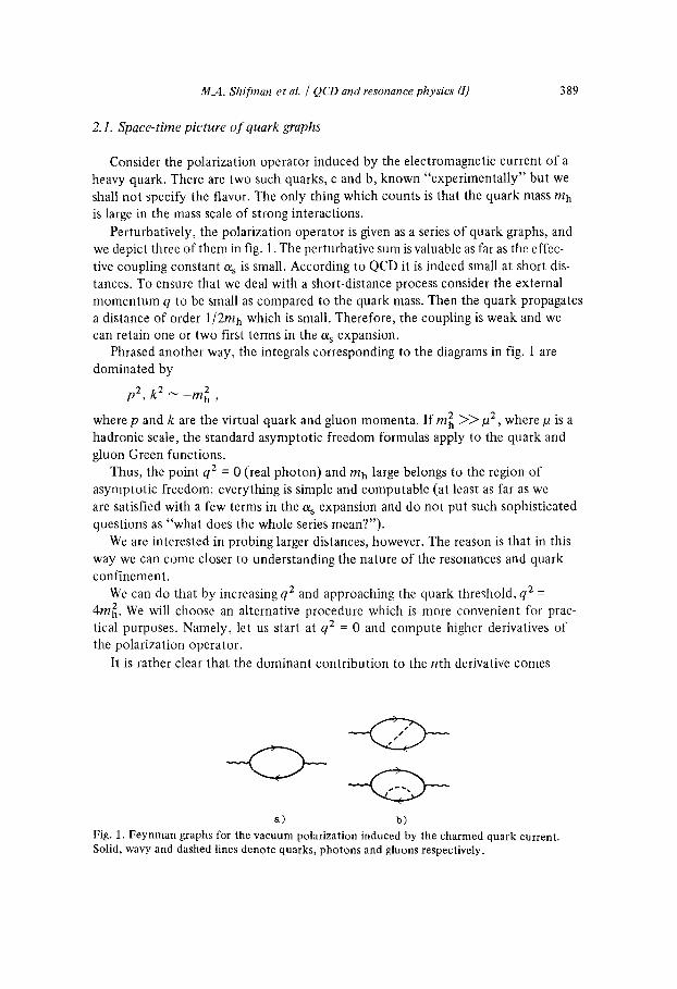
Perturbatively, the polarization operator is given as a series of quark graphs, and we depict three of them in fig. I. The perturbative sum is valuable as far as the effec- tive coupling constant as is small. According to QCD it is indeed small at short dis- tances. To ensure that we deal with a short-distance process consider the external momentum q to be small as compared to the quark mass. Then the quark propagates a distance of order 1/2mh which is small. Therefore, the coupling is weak and we can retain one or two first terms in the as expansion.
Phrased another way, the integrals corresponding to the diagrams in fig. 1 are dominated by
p2, k 2 ~ - m ~ ,
where p and k are the virtual quark and gluon momenta. If m~ > > ~2, where/l is a hadronic scale, the standard asymptotic freedom formulas apply to the quark and gluon Green functions.
Thus, the point q2 = 0 (real photon) and mh large belongs to the region of asymptotic freedom: everything is simple and computable (at least as far as we are satisfied with a few terms in the as expansion and do not put such sophisticated questions as "what does the whole series mean?").
We are interested in probing larger distances, however. The reason is that in this way we can come closer to understanding the nature of the resonances and quark confinement.
We can do that by increasing q2 and approaching the quark threshold, qZ = 4m~. We will choose an alternative procedure which is more convenient for prac- tical purposes. Namely, let us start at q2 = 0 and compute higher derivatives of the polarization operator.
It is rather clear that the dominant contribution to the nth derivative comes
< 2 > - < 2 > ....
a) b)
Fig. 1. Feynman graphs for the vacuum polarization induced by the charmed quark current. Solid, wavy and dashed lines denote quarks, photons and gluons respectively.
390 M.A. Shifman et al. / QCD and resonance physics (I)
from the virtual momenta of order
p2, k 2 ~ _ m Z /n .
Indeed, the nth derivative is determined by integrals of the kind
d4p f d4p d4k 2 + m~)n , or [(p + k)2 + rnh2]n,
where we have performed the Wick rotation so that all the momenta are Euclidean. For a fixed m~ and n tending to infinity both p2 and k 2 tend to zero. Nothing
spectacular happens with vanishing p2. Even at p2 = 0, the heavy quark is highly virtual since it is off-mass-shell by rn~ and rn h is large. Therefore, its propagation is described by the standard perturbation theory.
On the other hand, i f k 2 ~ 0 the gluon in fig. lb comes close to its would-be mass-shell. Due to confinement, the gluon propagator' is strongly modified at low k 2 and perturbation theory becomes irrelevant.
Thus at high n, the gluon propagates a rather large distance and is sensitive to the confinement mechanism.
Most probably, confinement is due to non-perturbative effects of QCD which bring in a new mass scale,/1 (in fact / l must be related to the distances where the coupling constant a s reaches some critical value). We shall assume that for k 2 >>/~2 the non-perturbative corrections are negligible while for k 2 ~</~2 they are most im- portant.
It is clear then that the real expansion parameter for the power terms is n~2/m~
so that for n ~ rn~/la 2 the perturbative expansion is badly broken.
2.2. Power corrections and resonance physics
The argument of subsect. 2.1 demonstrates that at high n large distances come into the game. Taken alone, it does not provide convincing evidence in favor of the power terms, however. Therefore, it might be useful to indicate that there exist good reasons to believe in their importance, based on phenomenological observa- tions.
Ther are two sources of large corrections at small k 2. First, according to QCD the coupling constant grows if the quark (gluon) virtuality decreases:
% (Q) = cons t / ln (Q/A) .
Formally, one approaches the infrared pole at Q2 = A 2 and it can be the origin of large corrections.
Another source of corre~ztions is non-perturbative terms which can be thought of as terms ~exp( -cons t /as (Q)) .
The strongest evidence in favor of relatively large power corrections is the ob- served difference between the mass spectra in the vector and axial-vector channels with isotopic spin I = 1. In the vector case there is a single prominent resonance,

M.A. Shifrnan et al. / QCD and resonance physics (I) 391
the p, while in the case of the axial-vector current there are two states one of which is much lighter than the p (the 7r meson) and the other is much heavier (the A 1 meson).
On the other hand, for massless quarks (and this is, beyond any doubt, a good approximation for the u and d quarks) the perturbative graphs do not differentiate between the vector and axial-vector currents. Thus, it is the spontaneous breaking of chiral symmetry that is responsible for the n-p-A 1 mass splittings. The symmetry breaking is signalled by the non-vanishing vacuum value of ~qJ. Thus we have an alternative:
either ( 0 1 ~ ] 0 ) = 0 , m p = r e a l , no pion,
or (01~10>=/= 0 , m o :¢: mA1 , massless pion.
The alternative must be reflected in the polarization operators in some way. On purely dimensional grounds it is clear that the two possibilities can be distinguished only via the power corrections.
Analogously, the non-vanishing matrix element a a <0 IGuvGuvl O> signals the break- ing of dilatation symmetry (we recall that GauvGauv is proportional to the trace of the energy-momentum tensor). The "gluon ,, a a in a sense condensate (01Guuauvl 0>is connected with the emergence of mass parameters in QCD.
Other evidence in favor of the importance of power corrections is provided by the charmonium sum rules, i.e. by the QCD predictions for the leptonic widths in charmonium. Chronologically these sum rules were considered first [12,6]. We shall sketch the derivation in paper (II). A phenomenological estimate for <OlGauvGauvl O> emerges as an outcome of the analysis.
Finally, let us mention another possibility, that both high orders in the a s expan- sion and power corrections are equally important. The possibility cannot be ruled out a priori. Basing on independent estimates of the coupling constant [16], one might conclude that this is not the case and that is is the power corrections that play the major role. True, the independent estimates of % are not too conclusive (see a discussion in sect. 6 and paper (II)). However, the sum rules derived under the assumption that the coupling constant is small agree well with the data. The agreement observed justifies a posteriori the assumption that power corrections already become important at such virtualities that the coupling constant is still far from the infrared pole.
2.3. Basic idea
Now, that we hopefully have convinced the reader of the importance of power corrections we proceed to specify their notion in more detail and explain how one can parametrize them.
Qualitatively, we have already learned that to keep the power corrections small

392 M.A. Shifman et al. / QCD and resonance physics (I}
we must choose ~ < < I where
= Ila2n/4m~a ,
'~ ( l . t 2 n / Q 2 , Q Z - _ q 2 , (heavy quarks),
(light quarks).
Of course, we want to be much more quantitative and learn the precise meaning of g, find coefficients, etc.; that is to construct a computational scheme and try to calculate hadrons. This is achieved through introducing new phenomenological parameters. (Attempts to extract these parameters theoretically are discussed in sect. 6.)
Now we explain the procedure in its gross features leaving aside all the reserva- tions (which are, of course, essential) and technical details (which are practically important). Turn again to the graph lb with a gluon exchange, but consider now the gluon Green function cl)uv(k2 ) as an exact one. Furthermore, let us split CI) uv(k 2) into two parts
(c~ _guv] (2.1) COuv(k 2) +
where we have chosen the Feynman gauge for the sake of definiteness. At large k 2
the Green function is given by the first term because of asymptotic freedom. Dis- regarding for the moment the calculable logarithmic corrections, we assume that the bracketed term in eq. (2.1) fails off as some power of k 2 at large k 2.
To get the answer for the graph we must collect all other factors and integrate over k 2. Then the first term in eq. (2.1) is absorbed into the standard perturbation theory while the second one represents something new. Since the difference (~uv(k 2) -guv/k 2) is presumably large only at small k 2 we can expand the rest of the amplitude in k 2 and approximate k 2 = 0.
To be careful, we must first extract the gluon field strength tensor, G#uGuv,a a not to violate the gauge invariance, and put k 2 = 0 afterwards. (In other words, gauge invariance implies that modification of the propagator is accompanied by a change in the vertices.)
Integrating with COuv - glav/k 2 results in a number which is sensitive to the gluon dynamics at large distances. Once we have a theory of confinement we can evaluate it. In the absence of such a theory we are forced to introduce a new parameter which is equivalent to the vacuum expectation value
(0 JGauvGauvl 0) . (2.2)
It is important that we can study vacuum properties using simple Feynman graphs as a tool. The matter is that all other lines in the graph, (in this particular case the quark lines) are far off their would be mass shell and are known.
For high derivatives the diagram lb is in fact a perfect probe, which detects gluon waves propagating through the vacuum. The probe is point-like while the gluon wave

M.4. Shi fman et al. / QCD and resonance physics (I} 393
length is relatively large. The inner structure of the probe is known, so one can extract information about the gluon-wave intensity.
If better accuracy is desired one must keep further terms in the k 2 expansion of the amplitude. This introduces naturally further parameters, such as *
a a (0l c't) ~G~lc~ @ v G w 10)
and so on. Moreover, if we consider a graph with two or more gluon lines with low momenta, it cannot be calculated in terms of the parameters mentioned above and we need new ones such as
(0 bc a b c a a b b [fa G u v G v o G a ~ [ O ) (0l , G~lvGvoGo. . /G.~[ O) . . . . .
Thins, there arises a series of parameters, all of them being independent in the absence of a consistent theory. To keep the problem manageable we must cut the series in some way. Increasing the number of gluon fields or their derivatives implies increas- ing dimension of operators, and, therefore, introducing extra powers of rn~. Thus, if power corrections are small compared to unity, the first term in the series dominates, generally speaking. All others can be safely omitted.
Thus, we will keep only the power correction of the lowest dimension and go to such n that it becomes sizable but still rather small, say, 30%. Then we would expect that such n represent a boundary for asymptotic freedom: at higher n it breaks badly since the corrections blow up almost immediately. Rather arbitrarily, we estimate neglected power corrections as a square of the kept one. The sum rules themselves will show whether this assumption is reasonable.
Then for heavy quarks we are left with a single parameter (G 2) [6,17] which is determined from experimental data by fitting charmonium sum rules.
At first sight, we do not make much progress since we describe the data with a new free parameter in hand. Not quite so. First of all, we are able to check the self-consistency of the calculation by considering charmonium sum rules alone. What is more important is that the same parameter controls the asymptotic free- dom breaking for light quarks. Indeed, if solid lines in fig. 1 denote light quarks, nothing is changed from a principal point of view. We must just substitute the heavy mass by a light one and ensure that large momentum Q flows through quark lines. (The effect of the change must still be non-trivial, see sect. 2 in paper (II).)
Thus, we are able to verify that the same force confines both heavy and light quarks.
As was already mentioned, light quarks result in a new vacuum average. They can also penetrate into large distances and this effect is important at high n. Phenomenologically, such effects are described by vacuum expectation values of
* Due to equations of motion this parameter can be expressed in terms of light-quark operators.

394 M.A. Shifman et al. / QCD and resonance physics (1)
quark fields
(OI f¢ lO) , (2.3)
(01 ~F 1 ~I~2 ~ 10), (2.4)
where F 1,2 are some matrices acting on color, flavour and Lorentz indices. The matrix element (2.3) can be found by using the PCAC hypothesis (see, e.g.,
[5,18]). As for the matrix elements (2.4), we keep only the vacuum intermediate- state contribution. This approximation is substantiated in sect. 6. Then the expec- tation values do not introduce new free parameters.
An experienced reader has certainly recognized the operator expansion technique [7] in the procedure describe above. It is quite a standard procedure by now and may not need further justification. It is worth emphasizing, however, that usually the operator expansion is used within perturbation theory. In this case the operator expansion is well established [8] and is, in fact, a technical device. We are going to rely on the operator expansion beyond perturbation theory. Every step here is a new one and by no means evident.
In particular, one can worry whether the integration with cl)uv - glav/k 2 is dominated by low k 2, so that the approximation k 2 ~ 0 for the gluon emission amplitude is justified. Even if this integral is convergent, one can expect that further expansion in k 2 generates integrals which are ultraviolet unstable. Then the proce- dure becomes inconsistent.
In other words, we must show that the matrix elements introduced, like (2.2), (2.3), (2.4), are determined by large distances. Rather surprisingly, we can do that even now, in the absence of a complete theory of confinement. Indeed, there exist good reasons to believe that at short distances the leading non-perturbative correc- tions are generated by instantons. As was mentioned above, numerically the calcula- tions are still uncertain. However, as far as problems of convergence of integrals are concerned they can be clarified. We will show that all the assumptions concerning the validity of the operator expansion which we are using turn out to be justified. It turns out that the operator expansion breaks down only at relatively high order in Q-2. For pure gluonic fields a polarization operator can be represented as
II(Q2)= I(perturbation theory)+ ~ [/a2]k + O ( Q - I ' ) 1 k=2 ..... s~Q 2]
so that expansion in Q-2 is guaranteed as far as the few first terms are concerned. Since we keep power terms small we confine ourselves to the leading corrections and the use of the expansion is justified. If the existence of nearly massless quarks is accounted for, then the series can be extended up to terms ~Q-14 inclusively.
After this preliminary exposition of the approach used, we proceed to a more detailed and technical presentation of the results obtained.

M.A. Shi fman et aL / QCD and resonance physics (I) 395
3. Operator expansion and non-perturbative effects
We start the systematic derivation with a discussion of the operator expansion. For the sake of convenience it is divided into two parts: in the present section we consider general problems while computational details are referred to sect. 4. Sub- sect. 3.1 contains some definitions and generalities which are not specific, in fact, for non-perturbative effects. The principal subsections are 3.2 and 3.3.
3.1. General remarks
We start by introducing notations common to all the cases. Consider the T pro- duct of two currents ]A, ]B which can be either light or heavy quark currents. The basic assumption is that at large external momentum q or for a large internal mass m h the operator expansion [7] is valid:
ifdx eiqxT{jA(x),jB(o)} = ~ criB(q) On, (3.1) n
where Cri B are coefficients, On are local operators constructed from light quark (u,d,s) or gluon fields. To be more precise, we assume the validity of the expansion only in the few first terms (see subsect. 3.2 for more detail).
The operators On are conveniently classified according to their Lorentz spin and dimension d. We will consider only spin-zero operators since only these contri- bute to the vacuum expectation value. Naturally, the operators in (3.1) satisfy such general requirements as gauge invariance with respect to the gluon field. An im- portant characteristic is operator dimension. An increase in dimension implies extra powers of p2/Q2 or laZ/4m~ for the corresponding contribution, where p is some typical hadronic mass entering through the matrix element of On. So we list all the operators with zero Lorentz spin and d ~< 6 *.
l (the unit operator) , (d = O) ,
0 M = ~Mff , (d = 4) , a a OG : GuvGpv , (d = 4) ,
0 0 - - ~ a = t~ouvtaM~Guv , (d : 6 ) ,
Or = ~I-' 1 ~b~I~z f f , ( d = 6 ) ,
O f = f abct'Ta t'7-b ¢'7c (d = 6) a ~ 1 2 v ~ v " I ~ " l l 2 , (3.2)
* Other operators can be reduced to those, given in eq. (3.2) plus full derivatives, for example,
- ~ - r t a t ~(-~ualav _ i~Cl)23,#(~ lat ~ - i~(~#7pC1)2~
+ full derivatives,
and the right-hand side can be expressed in terms of OM, 0 o by using the equations of motion.

396 M.A. Shifman et al. / QCD and resonance physics (I)
where Gauv is the gluon field strength tensor, t a are the Gell-Mann SU(3) matrices acting in the color space and normalized by the condition Tr(tat b) = 26ab, M, 2~ are matrices in flavor (u,d,s) space whose elements are proportional to quark masses. (The dimension of the operators OM, Oo indicated accounts for this fact.) We reserve the conventional notation )S for the SU(3) matrices acting in the flavor space. We will use the notation ff ... ff when the summation over SU(3)flavor is assumed, and ~ . . . q in other cases, for example, f f f means gu + d-d + ~-s, but ~q means fi-u or dd orgs. F~,2 stand for some matrices acting on the color, flavor and spinor indices of the quark fields, and are specified below.
A remark is in order here concerning our convention on the interaction Lagran- gian. Our definition of the quark-gluon coupling constant throughout the paper is a s = g2s/4n and the interaction Lagrangian is of the form ~gs~tl - aTu~bu,a where b~a is the gluon field.
Eq. (3.2) gives a complete set of operators which satisfy such general principles as Lorentz invariance, gauge invariance and having dimension d ~< 6. Note that we include in the list, not only the leading power correction (d = 4) but the next term (d = 6) as well. The reason is that in many cases the coefficients Cr (corresponding to O r ) are large numerically since they are associated with a Born series of graphs while, say, C O comes from a loop graph. Choosing Q2 (or rn~) large enough we could still get rid of operators with d = 6, but for practical purposes they turn out to be important.
The coefficients Cn are determined by momenta of high virtuality,p2 ~ Q2, m~. Since QCD is asymptotically free, the calculation of the coefficients is reliable. As for the matrix elements, they will be treated phenomenologically in sect. 6.
The expansion coefficients in eq. (3.1) are calculated as a series in as. Naturally, in practice one is confined to one or two first terms in the as expansion. As an ex- ample of the relations emerging let us write out the answer for the current
J. = qTuq ,
in the imaginary world with a single light quark flavor. Assuming conventional
SU(3)color we find
i f d x eiqXT{l"~ (X)jv(0)) = (quqv - q2 guv)
1 Q2 × - ~ (1 + as/~') In ~ - + 2mq_~4_ q-q
as 2has + 127rQ4 GauvGauv - 0 6 q7~75 taq~7aTstaq
4has ) - - ~ qTataqqTatUq + . . . .
where Q2 =_ _q2.
(3.3)
M.A. Shifman et al. / QCD and resonance physics (I) 397
The derivation is, in fact, given in sect. 4, where the realistic case with many quark flavors is discussed.
3.2. Status of operator expansion
As was already mentioned in sect. 1, the validity of the operator expansion in our case is by no means obvious. The problem is that non-perturbative effects are included, while the standard derivation of the operator expansion relies heavily on the Feynman graph analysis [8]. Fortunately, recently considerable progress has been made in understanding non-perturbative terms in QCD [2,3,9]. This permits us to justify the operator expansion to the extent we really use it. Tile basic point is that for pure Yang-Mills theory the leading correction to the perturba- tive treatment at short distances is associated with the one-instanton solution. The effect of (nearly) massless quarks has not been fully incorporated into the theory yet, but it only extends the validity of the operator expansion.
Let us emphasize that the effect of non-perturbative terms in QCD is twofold: (a) they induce non-vanishing vacuum expectation values, such as <OIGa~G~vl O)
which in standard perturnation theory vanish by definition; (b) they break down the operator expansion itself, starting from some power
Q - dcr.
The distinction between the two cases lies in the fact that the former effect is determined by the large-size instantons whose scale is of order of the confinement radius, P ~ Rconf. The latter effect is due to the small-size instantons, whose scale is controlled by the choice of the external parameter, p ~ 1/Q.
Let us give examples of the effects (a) and (b) above which arise within the instanton calculus [2,13,9]
(a) In the dilute-gas approximation one readily obtains
O t S a a ~Cdp <OI-2GuvGuvlO> = const × d(p) , 3 pS
i 1
o where p is the instanton scale size, d(0) is the instanton density, d~o) ~ exp{ -27r/ as(O)}, and the cut-off Pc is introduced since the integral is divergent at the upper limit of integration. Indeed, at small p
d(p) ~pe , e ~ 11 .
Thus we see, that (0[ a a - Gu~Gu,I 0> is contributed by instantons and the effect is con- trolled by the large-distance dynamics.
(b) Consider now the correlation function of two pseudoscalar densities
H (P) = i ydx eiqx(oIT{]'(P)(x), j(P)(0)}[0), j(P) = ui'YsU diTsd.
Then using the fermion zero-eigenmode solution found by 't Hooft [9] one can find for a one-instanton contribution (the anti-instanton gives the same)
II(P2e inst = 2 Q 2 y ~ d(P) [K_, (N//-Q2,o)] 2 ,
where K_ 1 is the McDonald function.

398 M.A. Shifman et aL / QCD and resonance physics (I)
Now, the dominant contribution comes from p ~ Q-1 and there is no need to introduce a cut-off by hand. Neglecting the log factors in d(p), i.e., taking it to be
d(p) = const × pe ,
we find
II(P2einst=2Q2d(p Q) 2e-3 = r _ ~ o [ r @ ) p c e - - 2 '
and at large e the following numerical approximation works well:
- - ~ d p = d : ~ [F(½e)]4 e e - 2
This is an example of an effect which is induced by non-perturbative solutions and which breaks the operator expansion.
What is the physical meaning of the operator expansion? It assumes the possibil- ity of separating short and large distance effects. Short distances are governed by asymptotic freedom and can be treated perturbatively. The corresponding contribu- tion is reflected in the operator expansion coefficients. The large-distance contribu- tion is accounted for phenomenologically, through various vacuum-to-vacuum matrix elements. It is clear then that the contribution of the large-size fluctuations, independent of Q2, can be consistently kept within the framework of the operator expansion. As for the small-scale fluctuations with p ~ 1/Q, they modify asymptotic freedom itself and cannot be included into the operator expansion, at least in its present form.
Our central point is that for a pure Yang-Mills field it is easy to find explicitly the critical dimension up to which the Wilson expansion is valid. Really, in pure gluodynamics the leading correction is due to the BPST solution [2]
4 'r/u peep 2 (3.4) Ga'uv(x;x°'P) :-g-ss [(x Xo)2 +p212 ,
where Xo is the instanton center and p is its scale. (Euclidean space-time is implied.) In the operator expansion for two colorless gluon densities only local products of the field strength tensors are involved:
(o laf , (o) ... a~(o)10~. (3.5)
n factors
(The particular form of contraction of both color and Lorentz indices is inessential here.) In the dilute-gas approximation (see ref. [13]) eq. (3.5) is reduced to the integral over Xo and p. The x o integration is always convergent resulting in an ex- pression which depends on n in the following way:
<01 a~(O) ... a~(O) I O> ~fdp p-~-l d(p), (3.6)
t/

M.4. Shifman et al. / QCD and resonance physics (I) 399
where d(p) is the instanton density [9]
(2 i° d(p) = const %(0) exp(-27r/as(p)) ,
27r 2~ - + 11 ln(Po/p), ( 3 . 7 )
,~(p) O,s(po) and the numbers are given for SU(3)color.
As is readily seen, the integral (3.6) is divergent at the upper limit for n <~ 5 and at the lower limit of integration for n ~> 6.
Thus, at d ~< 10, the vacuum expectation values (3.5) are determined by large- distance dynamics. (At large distances the dilute-gas approximation becomes invalid, and to avoid confusion we should emphasize that we do not use eq. (3.6) for numer- ical estimates. The one-instanton solution can help only to clarify the question of the integral convergence at small or large p.)
Two (and more) instanton contributions are proportional to even higher powers of 9. For this reason the one-instanton contribution is dominant at short distances.
Starting from d = 12 the vacuum expectation values (3.5) become infrared stable which automatically means that the p ~ 1/Q instantons come into play. Here the operator expansion must be forgotten.
Thus, the expansion in Q-2 cannot be extended to any power in fact. In pure gluon theory with SU(3)color symmetry it takes the form
i f dx eiqx(OlT{j A (x), /B(0)}[ O)
= (perturbation theory) X [1 + ~ ckAB (/~2/Q2)k k=2,3,4,5
+ O(Q-11)]. (3.8)
However, for the sake of brevity we will still use the term "power-correction series". Now, as to the light quarks. As is well-known, inclusion of the light quarks
changes the theory drastically [9]. Let the quark mass vanish; in the real world mu, m a ~ 5 MeV [19,18] and it is clear that one can safely neglect mu, d. In the l imit mu, d -~ 0 the one-instanton contribution to the functional integrals as a rule vanishes [9]. The only exception is the polarization operators induced by scalar and pseudoscalar currents of the light quarks, i.e., chirality changing currents (thus, the correction evaluated in point (b) above does not vanish for massless quarks). Therefore, even a qualitative understanding of the instanton effects requires a knowledge of the effective quark mass generation mechanism. Needless to say, the present theory is far from providing it.
One can argue, however, that the presence of massless quarks affects the critical value dcr but not the very fact of the operator expansion breaking. If one considers

400 M.A. Shifman et al. / QCD and resonance physics (I)
the strange quark to be heavy enough then the operator expansion is likely to be valid up to Q-16. Indeed, for dimensional estimates one can invoke the following expression for the effective quark mass [20]:
167ras (QX0 Iqq (Q)I 0) meff(Q) = mo (Q) + 02 , (3.9)
where (Q) refers to the normalization point.
Then each quark results in an extra factor of the type
[#meff(p)] (p/a) -2/3 , (3.10)
in the instanton density. The factor (p/a) -2/3 in eq. (3.10) is associated with the modification of the logarithmic dependence of the effective coupling constant %(p) which induces, in turn, a change in the instanton density (see eq. (3.7)). In the theory with two massless (u, d) and one massive (s) quarks an extra damping factor Q - s for the small-size instanton contribution emerges in this way. If instan- tons of a size smaller than the inverse mass of a heavy (say, charmed) quark are considered, then presence of these quarks must be accounted for as well.
At present, it is not clear whether eq. (3.9) can be taken literally but it seems to us quite safe as far as dimensional estimates are concerned. Still, let us men- tion that in the literature an even higher power of Q-2 for the small-size instanton contribution has been argued (see, e.g., ref. [13]).
An interesting question is how the instanton contribution is manifested in measurable cross sections.
3.3. Operator expansion and cross sections
The QCD results for the polarization operator discussed so far can be translated into the predictions for the corresponding cross sections. The well-known example of this kind is [21]
(i(e+e - --> hadrons) = ~ 3 Q q 2 [1 + as(s)/Tr I , (3.11) R(s) = o(e+ e - _+/l+/l_ ) q
where Qq are the quark charges and a s is the coupling constant. We would say that eq. (3.11) corresponds to asymptotic freedom. The series in
a s can be extended to higher powers and we denote by R(S)pert.th" the (symbolic) sum over %.
Now, turn to the power corrections. In the limit of extremely high energies, s ~ 0% the only correction to survive is due to the instantons of small size. The terms in the operator expansion which correspond to the instantons of large size do not modify the cross section (in accordance with intuition which seemingly says that the cross section is decided by short distance). For example, if we take it for granted that the operator expansion works up to the Q-14 terms while the

M.A. Shifman et al. / QCD and resonance physics (I} 401
small-size instantons show up in the Q-16 piece, then
R(s) = [R(S)]pert.th. + (/,/2/S)8 + . . . . (S "+ oo) .
Changing the power of the small-size instanton contribution to II(Q 2) would change the approach of R(s) to its asymptotic behaviour.
On the other hand, terms of lower order in Q-2 which are described by the operator expansion reflect the change in the cross section at relatively low energy.
These conclusions follow immediately from the equation
~R (s) [R (s)l 11 (Q2) _ II(Q2)pert.th ' = (127r 2 ~ Q2q)-, f - pert.th, ds q o s + Q 2 •
Expanding in Q-2 we see that the convergence of the integral f (R - Rpert.th. ) X s n - l ds at s -+ ~ is correlated with the validity of the operator expansion up to t e r m s Q-2n.
Strictly speaking, the statements must be qualified taking account of the possib- ility of oscillating contributions to the cross section, but we are reluctant to con- sider such a possibility on physical grounds.
3.4. Summary
In this section we have substantiated the validity of the operator expansion up to some critical value of the operator dimension. The dimension is certainly quite high and the precise value of it can be reasonably guessed starting with the instanton solutions.
We have also established the connection between the asymptotic behaviour of the cross section and the polarization operator in the presence of non-perturbative power corrections.
4. Operator expansion for various currents
In this section we deal with two-point functions of various currents. The set of currents considered is motivated by the forthcoming applications.
There are three distinct mass parameters relevant to the problem under consider- --1 ation. The first one is the inverse radius of confinement, R c o n f =- kt, which is mani-
fested through various vacuum expectation values, e.g., (0[(C~s/n) GauvGauvl O) ~ la 4. The second parameter is the quark mass itself. And, finally, an external mass scale is introduced by the momentum q in the definition of the two-point function (3.1).
To apply the operator expansion, at least one of the last parameters has to be large as compared to/a. Thus, there are three possibilities:
( i ) mq <~/~ , Q2 >> la2 ,

402
(ii) mq >>/~ ,
(iii) mq >>b t ,
(Here Q2 =- _q2.)
M.A. Shifman et al. / QCD and resonance physics [I)
2 Q2 < < mq ,
Q2 > 2 mq .
The first possibility implies an expansion in 112/Q 2 and m2q/Q 2. The correspond- ing technique will be referred to as the light-quark expansion. For heavy quarks it
• 2 2 2 2 is convenient to consider possibility (ii) above and expand in Q / m q , tl /mq. It is just what we shall always do, exploiting consistently the so called heaw-quark expansion [22].
Consideration of the possibility (iii) is completely legitimate within the approach used, but we will never consider this for practical reasons.
For heavy quarks we always choose Q2 = 0 and compute the derivatives with respect to Q2. This can be considered as a substitution for a change in Q2 in the polarization operator itself. In general, the two procedures are equivalent but in the case Q2 = 0 all the equations simplify greatly.
It is worth noting that the bulk of the applications is devoted to the light quarks and the consideration of heavy quarks is partly auxiliary (see sect. 2 of paper II). The operator expansion is more tractable for heavy quarks since there is no quark vacuum expectation value. Thus, we start our exercises with heavy quarks and then proceed to the light ones.
4.1. Vector current o f heavy quarks: the unit operator
The vector current of, say, charmed quarks has the form
Note that we do not include the quark charge, Qc = ~ in this case, in the definition of the current. The operator expansion takes the form
i f dx eiqxT{l'(c)(x), j(e)(0)} = (ququ - q2guv)
x [GI+CGOc + ...1, (4.1)
where the operator O a is defined in eq. (3.2) and the dots stand for operators of higher dimension.
To the lowest order in % the T product (4.1) is given by a single graph of fig. la. The corresponding result for the coeffic, ient C1 is conveniently represented in a dis- persion form:
Q2 [ 'hn C}°)(s) C}°) = - -~J s(s + Q2) ds,
ImC/(°)- 1 v ( 3 - v 2) 0 ( s_4mc 2) 47r 5
v = (1 - 4m2e/s) 1/2 . (4.2)

M.A. Shifman et al. / QCD and resonance physics (I) 403
Instead of studying C/as a function of Q2 one can choose to calculate all the deriva- tives of C I at Q2 = 0 for which one gets (see, e.g., the review [12]):
n~l(- ~ d ) n ]c(O) Q 2 = 0 = 4n z-g2n(n+l)(n--1)'(4m2c)-(2n + 3) .~. n
The correction of the first order in a s is given by fig. lb. The corresponding imagin- arc part,
ImC(I1)(s)=ImC(l°)(s)× 1 + 5 % 2v 4 - '
can be easily extracted from Schwinger, [23]. It follows from eqs. (4.2), (4.3) that the first-order corrections to the moments
of C (°) are equal to
( + ) ) / ( + ) [ = ~ ~4x/n F (n+3) __ n c ( i , __ nC(iO ) 1 +
Q2=O SL 3 F(n + 1)
( 3 ) F(n+3) l - 2 / ( 3 n + 6 ) 1-1/(3n+3) hi_ 3 2 n_4nn F(n+ 3) X l - 1 / ( 2 n + 3 ) 2 47r 3QTr 2 2) 1 - 1 / ( 2 n +
4n nln 2 ] . (4.4)
The last term in the square brackets is due to the mass renormalization. (We normalize mc at the Euclidean point pZ = _m 2. For details see ref. [12]. Notice that the n asymptotics of the coefficients are always determined by the imaginary part in the non-relativistic region. Indeed, the weight factor in the dispersion integral for the nth moment is proportional to (1 - 02) n-1 where v is the c-quark velocity, v = (1 - 4mZ/s) 1/z. Therefore, for high n only v a <~ I/n are essential.
This fact permits us to find, for high n, the whole series in as: in the non-relativis- tic limit the quark interaction reduces to the well-known Coulomb problem and the corresponding imaginary part can be computed exactly. The results are included in the review paper [ 12] and we will not dwell on them here.
4.2. Vector current of heavy quarks," operator GauvGauv
So far we have discussed ordinary perturbation theory which is absorbed into the coefficient G. Now we turn to computation of the coefficient C6 which is more specific.
To this end, let us consider formally matrix elements of expansion (4.1) over quark and gluon states. The idea is that expansion (4.1) is a general one and holds, in particular, in perturbation theory. To single out the operator a a GuvGuv, choose the gluon state. Then, to lowest order in the coupling constant, all the operators drop off except for the operator G 2 and we are left with the graphs of fig. 2.

404 M~I. Shifman et al. / QCD and resonance physics (I)
J
PEI~2.
Fig. 2. Graphs giving rise to the operator GauvGa~v in the operator expansion. Notation is the same as in fig. 1.
a a There is some complication due to the fact that GuvGuv vanishes for real gluons (k 2 = 0 , ek = 0). However, one is free to choose the polarizations arbitrarily since the whole procedure can be considered as an evaluation of the matrix element of the T-product of four currents and our aim is just to find C G in some way.
One more technical remark is in order. Straightforward calculation of the graph of fig. 2 yields not only the structure, (quqv 2 ~ G a G a
- q guy) ~ ,~, we are interested a a in but also q~GuaqsGv~.
The latter can be represented as
a a a a 1 a a qaGuaq¢Gv¢ = qaq~ [Gu~Gv¢ - gu~gva) G76 G76 ]
+ l ( q 2 g u v - quqv) Gav6Gay6 •
When averaged over vacuum state the first term vanishes since, by the symmetry argument,
(O[G~,~Ga~] O) ~ (guug,~ - g u ~ g w ) "
Thus we are left with the second term alone, which is the structure needed. Vanish- ing of the term in the square brackets exemplifies the general rule according to which non-zero Lorentz spin operators can be safely omitted.
Keeping in mind the remarks made and performing an explicit calculation of fig. 2 one gets
C ° ( Q 2 ) - 1 c~szn 4Q 41 {3(a + 1)(aa 2 - 1) 2
where
a = 1 + 4m2c/Q 2 , (Q2 - _ q 2 ) .
1 x / a + l 3 a e - 2 a + 3 t (4.5) 2x/a In ~ 1 a 2 ] '
We have derived the same result in'an alternative way as welt. Namely, one can consider the graph of fig. 2 for slightly virtual gluons (k 24 : 0) and collect all terms of second order in the gluon momentum k. The calculation is simplified by taking the polarizations of the gluons to be the same and averaging both over this polari-
1 and over the gluon 4-momentum, k u k v - + l k2guv . zation, eue v -+ - ~guv In applications, we are interested first of all in the moments. They can be com-
puted directly from eq. (4.5), expanding in powers of Q2/4m2 c. The simplest way,
M.A. Shifman et al. / QCD and resonance physics (I) 405
however, is to take one step back and not perform the last integration over the Feynman parameter, leaving the integral representation for Ca:
_ as x(1 - x ) rn c CG 67ra 2 dx -me2 + x ( l _ x ) O2 + [ m 2 + x ( l _ x ) O2]2
m c 1 I X ( 1 X ) ) ( 4 . 6 ) X ( ~ - 4 x ( 1 - x ) ) + [ m 2 c + ~ X ( l _ x ) Q 2 ] 3 ( ~ + - .
Expanding in Q2 can now be trivially performed:
( d/dQ2)nca = _ n(n + 1)(n + 2)(n + 3) -9-47raS(4mc2)- 2 (4.7) (-d/dQ2)nC}°) 02=o 2n + 5 '
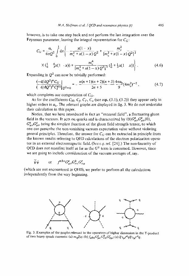
which completes our computation of Co. As for the coefficients CM, Cy, Cr, C o (see eqs. (3.1), (3.2)) they appear only in
higher orders in %. The relevant graphs are displayed in fig. 3. We do not undertake their calculation in this paper.
Notice, that we have introduced in fact an "external field", a fluctuating gluon field in the vacuum. It acts on quarks and is characterized by a a (OlG~vG~vlO>,
a a - G, vGuv being the simplest function of the gluon field strength tensor, to which one can prescribe the non-vanishing vacuum expectation value without violating general principles. Therefore, the answer for Ca can be extracted in principle from the known results referring to QED calculations of the electron polarization opera- tor in an external electromagnetic field. (See e.g. ref. [24] .) The non-linearity of QCD does not manifest itself as far as the G 2 term is concerned. However, since we are going to include consideration of the vacuum averages of, say,
t~abc(-~a (~,b (~,c
(which are not encountered in QED), we prefer to perform all the calculations independently from the very beginning.
/ ~x q ~ q
Fig. 3. Examples of the graphs relevant to the operators of higher dimension in the T-product a b c . -- -- a of two heavy quark currents: (a) mq(q; (b) fabcG#vGvaGa#, (c) qT#taqqT#t q.

406 M.A. Shifman et al. / QCD and resonance physics (I)
4.3. Pseudoscalar and scalar currents of heavy quarks
One can certainly construct the polarization operators induced by other currents as well, for example,
j(P) = UiTs c , j(s) = c-c.
The corresponding calculations were performed in collaboration with M.B. Voloshin. The results can be useful for the consideration of the 0 - and 0 ÷ charmonium states. In particular, in ref. [17] the pseudoscalar charmonium (the so-called ~c state) was discussed in detail. For the sake of completeness, we give here the final answers for the expansion coefficients * (for definitions see eqs. (3. I), (3.2)).
ClTsC current
1 ( d ) n+l _ 3 1 2 n ( n - 1)' ( n + l ) ! -d-Q ~ Cz e 2:o 8rr2(4m2e)n(2n+l)!![l+a(nP)%], (4.8)
where
3,,(v) _ (2n + 1)'[ fr r 4 0.I 1 0.69 4~n 2n+ln ~. - 3(n + 1) + 3(n + 1)(n + 2) - 1 + - - 2 n +3
+ , (4.9) 2n n + 1 2(n + 2
Furthermore,
(-d/dQ2) n+l C G
Q2=O = _
n(n + 1)(n + 2)(n - 3) 4~as ,4m2,_z . t. e j 2 n + 3 9
cc current
(n + 1)! d ~ ] Q2=o 8rr 2 (4mc2) n
where
3" 2n(n-1)!
(2n + 3)!!
_3,,(S)= ( 2 n + 3 ) , , [rr rr---6/rrl ,(rr 3 ) 4~n 3 "2h+- l~- + 1)] n + 2 _ l - ] 2 -
(4.10)
[1 + a(nS)asl , (4.1 1)
114 2 3 4 1 ] 3 n l n 2 + - - , ( 4 . 12 )
n n + l n + 2 n + 3
and finally,
(-d/dQ2)n+lCG(-d/dQ2)n+lC1 •2=o = n(n+l)(n+2)(3n+Y)47ras(4m2c)-22n + 5 9 . (4.13)
* We keep the same notation for the coefficients independently of the current considered, although Cn(Q 2) are determined by the current structure, of course, and are calculated sep- arately for each case. We hope that this makes no confusion.

M.A. Shifman et al. / QCD and resonance physics (1) 4 0 7
Notice, that the high-n behaviour of CI, CG is determined by the non-relativistic expressions for the imaginary parts of the corresponding Feynman graphs. There- fore one almost immediately finds, that at high n
( _ d / da2)n + 1 CI, G (sca lar )
' d i d t 3 2 " m + l C 1In . - - / ~ : ) L G ( p s e u d o s c a l a r )
On the other hand, the contribution of the G 2 term relative to that of the unit operator is proportional to n 3 in both cases. Numerically, the power correction in the scalar channel is approximately 3 times as large as that in the pseudoscalar one,
4.4. Vector current of light quarks (qTuq)
For definiteness let us consider the current with the p-meson quantum numbers
]~) = ~ (ff3,uu -dTud). (4.14)
In the case of light quarks we introduce a large external momentum q (_q2 = Q2 > > p2). The operator expansion has the form:
i f eiqX~ Ttiy)(x), j2)(0)} = (qua° - q2g.~)
X [Cfl+ CGO G + CMOM + CaO o + CyOf] , (4.15)
where Oi are given in eq. (3.2) and we omitted terms of higher order in Q-2. The calculations are now slightly more complicated than for heavy quarks because
new vacuum averages enter the game. In particular, in zeroth order in c~ s the coeffi- cients CI and CM are non-vanishing (see figs. la and 4a, respectively). The explicit result is:
1 nz 1 6} 0) = - ~ In ~ , C~)OM = @(muU--U + md-dd) . (4.16)
Graphs of first order in as both induce corrections to these coefficients and give rise to further operators in the expansion. The former effect is illustrated in figs. lb, 4b:
i( 2 2 1 Q2 m u _+_m ~-] (4.17)
C / = - 8 - ~ l+as / r r ) l n / ~ z + 3 Q2 ] ,
CM/C(~ ) = 1 + C~s/3~. (4.18)
Notice that the term proportional to m2u,d and the o~ s correction to CM are numeric- ally small and we will omit them in further applications.
The coefficient C c can be evaluated through the same kind of graphs as repre- sented in fig. 2, with a substitution of the heavy quark by the light one. There is

408 M.A. Shifman et al. / QCD and resonance physics (I}
a) b)
Fig. 4. Graphs giving rise to the operator 0 M = ~M~k : (a) the lowest order; (b) the one-loop correction.
an important computational difference between the two cases, however. The point is that taking the two-gluon matrix element no longer singles out the operator G a (7,a The reason is that the operator mq~q contributes to the two-gluon ~v~#v" matrix element to the same order in a s as well (see fig. 5), and these two effects must be separated.
An explicit calculation yields
I. as 2as-] CGO G = - 4~Q4 24rrQ4.j Ga~vGauv. (4.19)
Here, the first term corresponds to fig. 2 and can be readily obtained by evaluating the 1/Q 4 asymptotics of the coefficient Co obtained in subsect. 4.2 (see eq. (4.5)). The subtracted term can be immediately obtained by a straightforward calculation of the graph in fig. 5 and eq. (4.16).
The meaning of the subtraction procedure is, in fact, simple. Indeed, the 1/Q 4 asymptotics of the diagram in fig. 2 received contributions from two distinct regions of the virtual momenta, p2 ~ Q2 and p2 ~ mq2, respectively. Clearly enough, only the former region must be included into the coefficient Co, while the integration over small p must be absorbed into the matrix element of another operator. The distinction is important for theories with confined quarks. The con- tribution of short distances, p2 _ Q2 is computed reliably and is kept intact. As for the matrix element, it is drastically changed by the non-perturbative effects, which for example, make it very improbable to find a light quark with p2 ~ m~ (recall that, e.g., m d + mu "" 11 MeV [19,18]). Therefore, matrix elements must be treated separately•
One can readily check that the coefficient CG given by eq. (4.19) does corres- pond to high virtualities, p2 ~ Q2.
• - - a a and q~i'q~Fq. The Now, we come to a new kind of operators, tmqqOuvt qGuv
iqLr• M + PERM.
/ %% I %
Fig. 5. The two-gluon matrix element of the operator 0 M.
M.A. Shifrnan et al. / QCD and resonance physics (I) 409
! !
a )
I ! !
c) b)
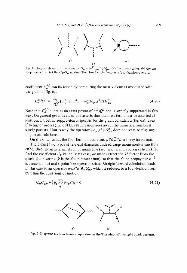
Fig. 6. Graphs relevant to the operator O o = m~olauta ~ Gauv: (a) the lowest order; (b) the one- loop correction; (c) the Oi--O o mixing. The closed circle denotes a four-fermion operator.
coefficient Co (°) can be found by computing the matrix element associated with the graph in fig. 6a:
3 - a a (4.20) C(°)Oo = tgs (m3uo. vtau + madouvt d) Guy . 1 2 Q ~ u .
Note that Co(°) contains an extra power of rnZq/Q 2 and is severely suppressed in this way. On general grounds alone one asserts that the mass term must be inserted at least once. Further suppression is specific for the graph considered (fig. 6a). Even if in higher orders (fig. 6b) this suppression goes away, the numerical smallness surely persists. That is why the operator - a a d/Ouvt d/Guy does not seem to play any important role here.
On the other hand, the four-fermion operators ~I '~q ; [ '~ are very important. There exist two types of relevant diagrams. Indeed, large momentum q can flow
either through an internal gluon or quark line (see figs. 7a and 7b, respectively). To find the coefficient C r in,the latter case, we must extract the k 2 factor from the quark-gluon vertex (k is the gluon momentum), so that the gluon propagator k -2 is cancelled out and a point-like operator arises. Straightforward calculation leads in this case to an o p e r a t o r - a a qTvt q ~ G ~ v which is reduced to a four-fermion form by using the equations of motion:
( a 1 ?)uGuv + igs ~ qTvtaq = 0 . (4.21) q
\ ; / .....
a) b)
Fig. 7. Diagrams for four-fermion operators in the T product o f two light quark currents.

410 M.A. Shifman et al. / QCD and resonance physics rIJ
From an explicit evaluation of the graphs in fig. 7a we find
gs 2 _ _ 8Q6 (u-"/~')'s tau - dTuTs tad)(uTuTs tau - dTuTs tad) ,
while the graph 7b adds the following piece: 2
gs (~7~tau + dTutad) ~ ~Tutaq . 36Q 6 q= u, cl, s
Collecting all the terms together we find for the operator expansion (4.15)
1 Q2 i f dxe iqxT{ j~ ) (x ) , j~)(O)}=(quq v - q2guv)( - ~ (1 + ~ ) i n - ~ -
1 Ots 7rO~ s + ~ ( m u U - U + rnddd ) + 2 ~ Q 4 GauvGauv -
(4.22)
(4.23)
ffO~ s X (u-3'~ 3'5 tau - d~/t~3"s tad) 2 - ~ (-ff3'~ tau + dT~ tad) qTutaq }"
q=u ,d , s
(4.24)
4.5. Axial and pseudoscalar currents o f l ight quarks
All the calculations for the current with A] quantum numbers
j(A1) = 1 Cd,),uTsU _ ~3, 3~sd) ' (4.25)
run in parallel to those for a vector current and we will give only the final answer for the difference between the vector and the axial currents:
i fdx eiqxT{](A1)(x), f ( A D ( o ) - - ]~)(x), ] ~ ) ( 0 ) }
1 = -g•v -~(muUU + mddd) - (quqv - guvq 2)
27ras ._ a - X --~-(UL3'tst U L -- dLTtatadL)(URTtstauR - dRTutadR). (4.26)
Here qL, R = ½(1 -+ 7S) q. As for the isoscalar current, there are some extra terms due to the so-called triangle anomaly [25]. We plan to discuss the question in detail in a separate publication.
In applications, we will also need the operator expansion for the pseudoscalar cur. rent with 7r-meson quantum numbers:
](~) = 1 i(ff75u _ ~Tsd) ,
M.A. Shifman et al. / QCD and resonance physics (I) 411
We give, directly, the final result
3 Q2 in i f dx e iqx T{j(70(x), j0r)(0)} =
1 ( m u K u + m d ~ d ) + as 4Q 2 i 6 ~ GauuGauv
7ras a + (~ou ,~s t u - doupTstad) 2 4Q 4
7"fas a + 6Q4(-uTut u +d'[utad) ~ q ~ t a q . (4.27)
q=u,d,s
4. 6. Anomalous dimensions
Relations obtained so far are valid to the lowest order in the strong interaction coupling constant as. It is clear that the results stand as they are if higher-order cor- rections are included but both as and all the operators are normalized at Q 2 , (by the normalization point for an operator we mean here the standard convention according to which quark (gluon) matrix elements of the operator are equal to those of the free field theory at the normalization point).
Once we want to keep the Q2 dependence explicit we must choose, however, an independent normalization point. Under the change of the normalization point the operators get factors (as(p)/as(Q))6/b where 6 is the anomalous dimension ** and b is the coefficient in the Gell-Mann-Low/3 function, b = 11 - 2 nf (for our pur-
poses we can take nf to be equal to 3 since the effect of heavy virtual quarks turns to be negligible). This recipe corresponds to a summing of the log terms of order (a s ln(Q2/p2)) n which arise in perturbation theory. In this subsection we will give
the values of 6 for the operators introduced above. For the unit operator the anomalous dimension vanishes and the summation of
* The statement is not quite accurate as far as the unit operator is concerned. It would be pre- cise if we meant, say, the derivative dC1/dQ 2. The coefficient C I itself is logarithmic even to the zeroth order in %, so the renormalization-group effects are slightly more complicated here Namely, (1 + C~s/n) ln(Q2/~ 2) goes into [21]:
as(o)/\ .5] ] ln~ . This peculiarity is inessential since we always work with the derivatives (-d/dQ2) n C/(Q2), to which the general statement made above is applicable in full.
** To be more precise, if there are more than one operator of a given dimension the anomalous dimension 6 must be substituted by an anomalous dimension matrix.

412 M.A. Shifman et al. / QCD and resonance physics (I)
the log terms reduces * to a mere substitution of a s by as(Q). Thus the effect of higher orders on CI(Q) is small in all the cases considered, except for the pseudo- scalar current. (Indeed, one can obtain the polarization operator for pseudoscalar currents by multiplying that for the corresponding axial-vector currents by q~qv/(2mq) 2. The anomalous dimension of mass (6 = - 4 ) is then converted into the power dependence on log Q2 of the unit operator contribution.)
The anomalous dimension of the operator ~q is equal to 4. However, it always enters the operator expansion multiplied by a quark mass mq which also depends on the normalization point. The net effect is that the product mqqq does not depend, in fact, on the normalization point. In other words, all the log factors are absorbed into the definition of the mass **
a a a a Similar arguments hold for the operator asGuvGuv. Independence of asG~vGuv
on the normalization point can be asserted in a number of ways. In particular, one a a
can express asGuvGuv in terms of the trace of the energy-momentum tensor [26]"
9as + ~ - (4.28) Ouu - ~ GauuGauv mqqq, q
where corrections of higher orders in a s are omitted. Since the anomalous dimen- sion of the conserved quantity, Our, vanishes, the same is true for asGauvGauv. This also can be checked by direct calculation.
The effect of higher orders is most drastic for the case of the coefficient Co. The reason is that to lowest order, Co is greatly suppressed (see eq. (4.20)) by an extra factor m2q/Q 2. This suppression is rather accidental and does not persist in higher orders. For this reason calculating the loop graphs is crucial to find Co.
Let us remark that a consistent approach would require a consideration of both one- and two-loop graphs (figs. 6b,c) to find Ca. In fact, a very similar analysis has been performed in ref. [27] where the operators
s-Guy(1 +- 75) a a t dGuv, Tour(1 +- 3'5) dFvv (Fur is the photon field),
in the weak strangeness changing, effective Hamiltonian were treated. We will not go into details here since anyhow the resulting contribution of Oo is extremely small.
For the four-fermion operators, the computation of the anomalous dimension matrix is rather standard. The details can be found in the appendix, and here we mention only some of the results.
The dominant contribution to the vacuum-to-vacuum matrix elements is associ- ated with the operator
~L XatbT#~L ~R~atbt~R , (4.29)
* See first footnote of this subsection. ** Taking account of the next orders in as, the renormalization-invariant quantity is (1 + 2%/
Ir + ...) mq~q.

M.A. Shifrnan et al. / QCD and resonance physics {I) 413
where X a and t a stand for the SU(3) matrices acting in flavor and color spaces respectively. It mixes with the operator
- - a
~hX 3'U~L~RXaTU~R. (4.30)
Within the framework of the factorization hypothesis (i.e., vacuum insertions in all the channels, see sect. 6), the vacuum expectation values of these operators are con- nected with each other:
(OIfLkatVTu~L~RXatbTu@RIO)= ~(OI~L)taTU~L~RkaTU@RIO). (4.31)
Eq. (A.15) of the appendix and eq. (4.31) imply that the strong-interaction effects reduce to multiplication of (4.29) by a factor (as(ll)/a s (Q))8/9, so that
%(Q) ~L)katbTu~L~RkatbTut~RI Q
(as(Q)/Ots(i.t))l/9 as(U ) - a b -- a b ~LX t 7p.@L@R~k t 7U~alU" (4.32)
Here Q and # indicate the normalization points. Thus, all the Q dependence is mani- fested only via (as(Q)/as(p)) 1/9 and is extremely weak.
Other four-fermion operators are encountered in the operator expansion with numerically small coefficients. Equations given in the appendix allow one to write out a full answer in every particular case. Let us give an example. For the/)-meson current (4.14), the coefficient of the Q-6 term in the corresponding polarization operator is of the form:
1 t 2 K 8/91,./(0) 81 n(qq)as(Q) (Q), (4.33)
r/co)(Q) = 1.29 - 0.29 K -° '14 + 0.07 K -° ' s6 - 0.07 K -1"z7 , (4.34)
where (~q) means (01~u(u)10> or (01dd(/~)10> or <0l~s(/J)10>, and
b Q2 K = %(u)/%(Q) = 1 + as(U) ~ In u- T .
At K = 1 the right-hand side of eq. (4.34) is normalized to unity so that averaging over the vacuum state we come back to the coefficient in front of the Q-6 term in the curly brackets of eq. (4.24). It is readily seen that the Q dependence implied by eq. (4.33) is very weak in fact. To illustrate the point let us note that for a realistic choice of K, n = 3 - 5 the parameter r? co) is given by
r/c°) = 1.06 to 1.08,
and its deviation from unity serves as a measure of the operator mixing. Moreover, the residual Q dependence is partly cancelled by the multiplicative factor as(Q) K 8/9
(ln Q)-I/9.
To summarize, most of the operator expansion coefficients start with %(Q). One might expect, therefore, that at large Q2 the coefficients are small since the quark- gluon coupling constant falls off logarithmically, with Q2. However, the analysis per- formed shows that the Q dependence of a s is cancelled by the anomalous dimensions

4 1 4 M.A. Shifman et al. / QCD and resonance physics (I]
of the operators. The cancellation is not rigorous in all the cases but holds very well numerically.
4. 7. Summary
In this section we have computed the operator expansion coefficients associated with the two-point function of the currents relevant to the forthcoming applications.
Explicit calculation has been performed for graphs of zero and first order in as. The computational recipe is simple: apart from evaluating the standard Feynman integrals it is necessary to cut the graphs in all possible ways over the gluon and light quark lines. The cut lines are then "annihilated" into vacuum. It is just these cut diagrams that determine the coefficients in front of the power terms.
The physical meaning of the procedure is that at low virtualities the gluon and quark propagators are modified drastically and this modification cannot be accoun- ted for perturbatively. Large distances, therefore, are accounted for phenomenolog- ically, through the vacuum expectation values of local operators.
In the approximation considered the expansion is especially simple for heavy quarks and is given by:
• A . B _ + a a ifdx eiqxT{] (x), ] (0)} - CI I CGGuvGuv,
where we have found Ca as a function of Q2/4m2c for the following currents:
~Tuc , c-iT sc , ~c .
(c stands for charmed, or more generally, any heavy quark field.) For the light quarks the expansion takes the form
i f dx eiqxT~jA(x), iB(0)} = C d + CM~M¢ + CGGa~uGa~u + C r O r O O r O ,
and we considered explicitly the following currents:
q'Yuq , qTu 7sq , qiTsq •
The coefficients depend in a non-trivial way on the current structure and the quark mass. In paper (II) we will show that the variety in the expansion coefficients results in a variety of resonance properties.
5. Sum rules
5.1. Introductory remarks
Taking the vacuum-to-vacuum matrix element of the operator expansion we get the QCD representation for the polarization operators. Say, for the current

M.A. Shifman et al. / QCD and resonance physics (I) 415
with the p-meson quantum numbers defined in eq. (4.14) we have
Q2 1 in - - (Olmu~U +maddlO) 17QCD (Q2) = -- 87r 2 ~2 +
1 ~ G**vGuv[ + 2 @ < ° 1 a a 0>+ .... (5.1)
where we exhibit explicitly only the few first terms. (We recall that Qz = _q=.) On the other hand, the general dispersion relation gives
II(Q2) = l_ f lm 17phys(S) ds rr~ s + 0 2 ' (5.2)
where I m 17phys($) is proportional to measurable cross sections such as that for e+e - annihilation into hadrons.
The sum rule is given by:
IIQc D (Q2) = 17(0 2) = l I Im 17phys (S) ds 7r~ s + ~ (5.3/
It is useful only at large Q2 since in this case the theory allows computat ion of IIQcD (Q2).
Expansions like (5.1) serve as a basis for the sum rules. In the present section we consider the next logical step, the derivation of the general form of the sum rules. Although the form exhibited in eq. (5.3) is the most conventional one we will show that it is not the most convenient to study resonances.
Equations like (5.3) lead to predictions which can be checked experimentally. The implications are especially simple at large s. The well-known result arising in this way is the prediction [21] for the e+e - annihilation total cross section:
o(e+e- -+ hadrons) = ~ ~ Q2 (1 + ~ ) , s -+oo, (5.4) i
where Qi are the quark charges and Us is the running coupling constant. The novel feature of the sum rules considered in this paper is the inclusion of
the power terms, (t12/Q2) k. Certainly, the asymptotic region is not the best place to search for such terms and we turn to lower energies.
Our consideration in this section is addressed to the case of the light quarks, which is central in the applications. Moreover, it turns out that the mathematical procedure is most simple for the light quarks.
We will show that there exists a variety of alternative forms of the sum rules which corresponds to freedom in the summation procedure for the power terms. For example, one can consider, instead of the polarization operator, its Borel transform. Note that for the sake of brevity we shall use expressions like "summa- tion of the Q-2 series". In fact the series is truncated, since the operator expan- sion breaks at some critical operator dimension (see sect. 2). In fact, all the results

416 M.A. Shifman et al. / QCD and resonance physics (I)
are general enough to cope with the real situation. The choice of the summation prescription fixes the weight function in the inte-
gral over the spectral density which enters the sum rules. Thus, the factor (s + Q2)-I in the integrand in the right-hand side of eq. (5.3) can be replaced by an exponential, exp(-s/Q2), or a Bessel function, say J l ( 2 ~ ) / x / s .
Since we are interested in resonance physics, we would like to have a weight func- tion which enhances the low-energy contribution relative to the high-energy one. On the other hand, it is desirable to present the Q-2 series in a way that suppresses the high-order contributions since in practice we are confined to the first one or two terms in the Q-2 expansion.
There is no surprise that, in general, these two requirements are self-contradictory and making progress in one respect implies paying the price of a setback in the other.
Our main result is that a balance can still be reached to some extent and that there exists an optimal choice. It refers to the first Borel transform of the polariza- tion operator. For that choice, QCD fixes such integrals as
f e s/M2 Im ds (5.5) [Iphys(S)
higher order in the M -2 expansion being factorially suppressed. Apart from the choice of the most suitable form of the sum rules we discuss the
possibility of determining both the coupling constant and mass of a low-lying reso- nance starting from the sum rules. We will argue that such a possibility does exist due to the gap in the dimensions in the operator expansion: there is the unit oper- ator of zero dimension, and the leading power corrections come from dimension 4, with no terms of dimension 2.
The procedure is as follows. In subsect. 5.2 we consider "conventional" sum rules for the polarization operator. In subsect. 5.3 we transform them by taking the derivatives (-d/dQ2) n II(Q 2) with both Q2 and the number of the derivative n, tending to infinity while their ratio Q2/n is kept finite. In subsect. 5.4 it is shown that taking the limit of Q2 __> o% n ~ o% Q2/n fixed, is equivalent to deriving sum rules for the Borel transform of the polarization operator. In subsect. 5.5 further Borel transforms are introduced and examined, while in subsect. 5.6 the final choice of the sum rules is substantiated and the advantages of the first Borel transform are discussed in detail.
5.2. Sum rules for the polarization operator
In sects. 3 and 4, the operator expansion for the T-product of two currents was discussed in detail. The polarization operator II(Q 2) is defined as the vacuum aver- age of this product:
(quqv - q2guu) II(Q z) = i f d x eeqx(olT{y'~z(x), /,(0)}10> , (s.s)

M.A. Shifman et al. / QCD and resonance physics (I) 417
where we take two vector currents just for the sake of definiteness. The general structure of II(Q 2) can be inferred from QCD and is given by *
Q2 _ d II(Q 2) = h o + ( ~ + ( ~ + .. . , (5.7)
where the coefficients h i are dimensional (with the subscript i specifying the dimen- sion, h i ~ (mass2) i) and are related to the vacuum expectation values of the relevant operators in the operator expansion and to the expansion coefficients. For example, in the case of the cur rent /~)= ½ (-ff~/uu - d T u d ) an explicit form of h2 is
h2 ( O l ( m u g u + m a ~ d ) + l~ aS a a = - Gu~Gu~,[ 0 ) . 7r
The coefficients h i can depend on Q2 only weakly, via log factors. On the other hand, the function FI(Q 2) satisfies the general dispersion relation:
d a =_1 f I m I I ( s ) ds (5.8) d~) ~II(Q ) 7r3 ( s+Q2) 2 '
where Im If(s) is subject, in principle, to direct experimental determination. For example, in the case of the current j~) mentioned above, it is proportional to the cross section of e+e - annihilation into hadrons with the isotopic spin equal to unity.
Equating the r.h.s, of eqs. (5.7) and (5.8) gives the sum rules which constrain the experimental cross section provided that QCD is the right theory of strong interac- tions. To apply QCD one must be sure, however, that Q2 is large enough. In practice it is important to known which Q2 can be considered as large. We will turn back to discussion of this point later on.
5.3. Differentiating the polarization operator." limit o f Q2, n -+ oo
QCD allows one to compute (d/dQ 2) II(Q 2) at any Qz provided that Q2 is large. Thus, there exists a continuum family of sum rules. One can choose an alternative procedure: fix some large Q2 and evaluate a number of derivatives with respect to Q2. Intuitively, one feels that the two procedures are equivalent to each other: computing many derivatives at some Q2 implies learning the function at lower Q2 as well and, therefore, at some n we probe small QZ.
Moreover, i f Q2 tends to infinity then the number of derivatives calculable in a reliable way is also arbitrarily large and we will consider the limit
Q2 _+ oo , n ~ o~ , Q2/n =-M 2 f ixed. (5.9)
In this way we introduce a new variable M 2 instead of Q2. The meaning of this pro- cedure is clarified in subsect. 5.4: it corresponds in fact to introducing the Borel transform of If(Q2).
* We choose to work with the derivative of H(Q 2) since the constant term in H(Q 2) is not defined.

418 M.A. Shifman et al. / QCD and resonance physics (I)
Let us rewrite the sum rules in terms of the new variable M ~. Introduce to this end an operator
Q2 ~ oo,n-+ ~, ff2/n =M2 (n -- I)~ (Q2)n _ _ , (5.10)
and apply it to both the right- and left-hand sides of eq. (5.3). The result is
7rMl~f h2 h3 Im II(s) e-S/M2ds = h o + 2!(M2) 2 + 3!(/142) 3 + .... (5.1 1)
where the coefficients h i determine IIQcD(Q 2) and are defined in eq. (5.7). Note the appearance of the exponential factor in the integral over the imaginary part. Although we start with a conventional dispersion representation, the final result has no direct resemblance to the dispersion relations any longer.
Equations like (5.1 1) play a crucial role in our analysis and we will turn to a discussion of some of their properties.
5. 4. Moment s and the Borel improvement o f the power series
Here we will show that the limiting procedure (5.10) which introduces the new variable, M 2, is equivalent to the Borel improvement of the Q 2 series.
Let us first recall some definitions *. Consider a function f(x). Furthermore, introduce f(?0 which is related to f(x)via the following equation:
1 c+i°° l f(?~) = ~ f e~/X f ( x ) x d x - ' (5.12)
where the integration contour runs to the right of all the singularities of the func- tion f (x ) . The function~X) is called the Borel transform off(x) . The inverse trans- formation is given by:
f ( x ) = ? f ( X ) e -~ /x d V x . (S.13) 0
To clarify the meaning of the Borel transform assume that f(x) is given as an expansion in x (which can be asymptotic, however):
f ( x ) =ao + a l x + a z x 2 +... + akx g + . . . . (5.14)
Then the corresponding expansion off(X) in ?~ has the form
f(X) =__+alao X + azX= + ... + akXk + ... (5.15) 0! 1! 2! k! '
,t A physical approach to the Borel summation technique is reviewed in ref. [28].

M.A. Shifinan et al. / QCD and resonance physics (I) 419
so that the coefficients are factorially suppressed as compared to the case (5.14). This suppression of higher-order terms in the expansion implies that the approxi-
mation of the whole series by the few first terms is more reliable for aT(X) than for
f(x). It is readily seen that all these definitions are realized when one introduces M s
instead of Q2. Indeed, we have considered the limit
H(M2)= 21imn---+= ~ l - - (Q2)n (-- + ) nII(Q2) ' Q2)n =M 2 (n 1)!
or using the notation (5.10)
~(M 2) = £ a II(Q2) • (5.16)
The meaning of the operator £M becomes clear if we turn again to a particular term in the power expansion. As is readily seen, application of L M transforms the series in Q-2 into a series in M-2:
- 1
LM ~ ( k - 1 ~ ~ ' (5.17)
Let us emphasize the appearance of the factorial suppression 1/(k - 1)!. This fact alone convinces us that we are dealing with the Borel transform of the polarization operator.
However, as mentioned in sect. 2, the polarization operator cannot be repre- sented as an infinite series in Q-2; the expansion may break at some place. There- fore, it is worth mentioning that the equivalence of the limiting procedure (5.10) to the Borel transform can be shown in a general form.
The only thing which is indeed important is that the polarization operator satis- fies the standard dispersion relations. Indeed, let us write down an analog of the inverse transformation (5.13) for the function H(M2):
[I(M2) e-Q2/M2Q2d - - f dslmrI(s)f ~ e -(o~+')/M: d ~ , 7"( 0 0 0
(5.18)
where we have used the integral representation for ~(M:) in terms of the imaginary part Im 1-I(s). Furthermore, performing the integration over M 2 gives
? e-Q2/M2Q2d 1 Q_2 ? l ; i i ( s ) ds _ Q 2 ( + ) o fi(M2) J14 2 - rr + Q2)2 - II(Q2), (5.19)
which proves that H(M 2) does coincide with the Borel transform of the function Q2(-d/dQ2) II(Q2).
Eq. (5.17) specifies the effect of the operator L M on the power terms. As was
420 M.A. Shifman et al. / QCD and resonance physics (1)
mentioned above the expansion coefficients h i may have some log dependence on QL In fact, it can enter either through % corrections (C~s(Q) ~ 1/ln Q) or through anomalous dimension factors of the kind 1/(ln Q)e. Therefore, we also need to know how such factors are transformed. We will show that under the procedure, hi(Q 2) are replaced by the same functions of M2:
hi(Q 2) -+ hi(M2) • (5.20)
To this end use the following representation:
( ~ ) k { , ~c i ( i )k?dze_zl/qn(Q2/la2) (5.21) Vn(Q%'jl =
0
Furthermore, applying the operator LM and using eq. (5.17) yields
. 1 k 1 e k( l '~eUl . ~s z.a L M I ( ~ ) ( ln(Q2/ /a ' ) ) I = / k ) (~2) \ln(MZ/ta2)]
(5.22)
which is just what we wanted to prove. Eqs. (5.15) and (5.20) exaust all the transformations needed in practical applica-
tions.
5.5. Further Borel transforms
The motivation to turn to the Borel transform is to improve the approximation of the whole series of the power corrections by the first few terms (in fact we will keep terms of order M -4, M -6 and neglect the others). One can reiterate the pro- cedure and introduce a new variable M '2. This subsection deals with these further improvements of the series while the meaning of the results obtained is discussed in the next subsection.
Divide the left- and right-hand sides of eq. (5.11) by M 2 and apply the operator /~M' to the both. Then we get
1 oo 2X/s -1 2 lrA/~ f In, l - l ( s )J l (~-) (s ) / ds
0
h2 =h o + + _ _ h3 7_ +... (2!)2 (M'2) 2 (3!)2 (m 2) a '
where we have used that
l e_s /M2 - 1 (2X/s 1 L~ if, M,3~/s J1 1 M' ] '
(5.23)
and J1 is the Bessel function.

M.A. Shifman et al. / QCD and resonance physics (I) 421
One can easily generate the "daughter" sum rules as well. For example, differenti- ating eq. (5.23) with respect to 1/h4 ,2 we come to the following relation:
7r~4~fhn II(s)Jo(2V~/M' ) ds = -M'2(d/dM '2) h o +
h2 h3 + + + (5.24)
2[ 1 !(M'2) 2 3!2!(/14'2) 3 ....
Note that the right-hand side of this equation vanishes in the limit of asymptotic freedom. Indeed, the coefficient h o depends on M z only via as(M') and
_M, 2 dc~ _ ba~ dJl4 '2 47r '
so that M'Z(d/dM '2) h 0 can be neglected in the approximation considered. The sequence of Borel transforms can be continued. It would introduce the
hypergeometrical functions as a weight in the integral over the spectral density. We will not go into details here and conclude with a remark that in all these cases the weight function is not positive definite.
5. 6. On the choice o f the form o f sum rules
Thus, starting with the dispersion relation for the polarization operator and applying the Borel transform we come to a variety of sum rules.
From a practical point of view some particular choice of sum rules may turn to be most helpful. Thus, it is mostly a matter of convenience as to which sum rules are used in the analysis of the experimental data. Indeed, all the dynamical informa- tion is confined to the knowledge of some of the expansion coefficients and of the corresponding matrix elements.
What are the qualities we would like to embody into the sum rules? To be sensitive to a single resonance the integrals over the cross sections must be con- centrated in as narrow an energy region as possible.
On the other hand, all the evaluations of the polarization operator in QCD are confined to a few first terms in Q-2 and introducing a factorial-like suppression of higher orders is desirable from this point of view. In particular, let us remind the reader that starting from some rather high power of Q-z , small-size instantons come into the game. They break the operator expansion and may bring a contri- bution which might be qualitatively different from those considered so far. It cer- tainly would be nice to suppress this contribution numerically. Schematically, we have:
L [small-size instanton-] 1 [small size instanton~ M Lcontribution in Q2 J ~ I_contribution inM 2 ] '
where e is the exponent encountered in the instanton density function, d(p) ~ pe. One expects that e = 1 1 - 1 6 [9].
422 M.A. Shi fman et al. / QCD and resonance physics (I)
In general, the two requirements for the sum rules show in opposite directions. Still, we will argue that the sum rules for the first Borel transform of the polariza- tion operator represent the optimal choice. The sum rules are examplified by eq. (5.11) and we turn now to their discussion.
M 2 tending to infinity implies moving towards asymptotic freedom. Indeed, only the first perturbative term, ho, survives in this limit in eq. (5.11). In other words, we deal with short-distance dynamics in this limit. On the other hand, taking low M 2 puts emphasis on the large distances.
It is remarkable that this purely theoretical distinction between short and large distances is directly manifested in the interplay between the resonance and high- energy contributions. Indeed, because of the exponential cut-off, only s ~< M 2 contributes to the integrals over the imaginary part. Thus, i fM 2 is of the order of
2 then the integral is dominated by a single resonance. a resonance mass, say, m o
At large M 2 the corrections to asymptotic freedom are small, and, as a reflection of this, the integral over the physical states is dominated by high energies. Dimin- ishing M 2 enhances the resonance contribution, on one hand, and increases the power corrections to asymptotic freedom, on the other.
Power corrections specify the very notion of "high" and "low" M2: for large M 2 the power corrections are small while for l o w M 2 they become dominant and it is necessary to sum up all the power terms to have a reliable answer for H(M2). This sets a natural bound, Mcarit, on M 2, which can be used in our approximation (which keeps only first terms in the M -2 expansion).
For M 2 >Mc2rit one may hope that the power terms of lowest dimension which are kept explicit represent the leading corrections to asymptotic freedom while the higher orders can be safely neglected.
As was proclaimed many times above we aim at extracting the QCD predictions for a single resonance. To fulfill the task we are inclined to choose M 2 as low as possible. On the other hand, taking M 2 too low makes the whole calculation un- reliable since the power corrections become large.
Our central point, which rests entirely on numerical estimates, is that it is still possible to make a balance between the low and high M 2 tendencies and find such M 2 that on the one hand, a resonance dominance is guaranteed, and on the other hand, the power corrections are still moderate and tractable.
In achieving this aim we are helped by using the sum rules for the first Borel transform of the polarization operator. Indeed, it introduces the exponential cut-off into the integral over the spectral density. Thus, if we take both Q2 and
2 then the low-lying meson dominance is M 2 to be the same and of order, say, rn 0
much more prominent for the sum rules (5.11) than for (5.3). On the other hand, the approximation of the whole series by the few first terms is also better for the Borel transform than for the polarization operator. These are advantages of the sum rules for the first Borel transform which single them out among the other
possibilities. At first sight, further Borel improvements could do even better. Indeed, the

M.A. Shifman et al. / QCD and resonance physics (I) 423
process of improving the theoretical accuracy can be extended to any degree by repetitions of the Borel transform. By this we mean, that one can achieve an arbitrary accuracy of calculation at a fixed value of an external parameter such as Q2, M 2, M,2 and so on, by going to a Borel transform of a high order.
One feels, however, that the very possibility of an unlimited improvement of the accuracy implies that the value of the external parameter becomes non-repre- sentative of the energy scale needed to verify the sum rules. A closer examination reveals that this is indeed the case. The point is that for higher Borel transforms, the weight function in the sum rules is not positive definite. Examples of this kind have been already given in eqs. (5.23), (5.24). In these equations we have oscillating Bessel functions as a weight.
It is clear that in the limit of an infinite number of repetitions of the Borel transforms, the sum rules are entirely controlled by the high-energy contribution, independent of the value of the external parameter.
It is remarkable that the correspondence between the choice of the parameter Q2, M 2 . . . . and the distances which are essential, dynamically works, strictly speak- ing only in the case of the polarization operator and its first Borel transform.
We find it difficult to analyse the sum rules with an oscillating weight function and choose to work with the first Borel transform.
Although we do not use further Borel transforms we do not rule out the pos- sibility that they are instructive in some respects. Note, as an example, that the integral with Jo vanishes in the limit of high M s while the integral with J1 does not (see eqs. (5.23) and (5.24)). Since the Bessel functions are nearly periodical, an impression arises that the resonances are " tuned" to some wavelength in energy to make the difference between J0 and J1 SO profound.
5. 7. Sum rules f o r resonances masses
In conclusion of this section let us add one comment of more technical nature con- cerning the possibility of extracting from the sum rules both the coupling constant and mass of a resonance.
Assume that at some M 2 the integral f e -s/M2 Im II(s) ds is saturated by a single resonance, and that we are still in a "safe" region so that the expansion (5.11) is an expansion in a small parameter.
It is convenient under this circumstance to consider a sum rule which is obtained by differentiating eq. (5.11) with respect to 1/M 2 *"
h 2 2h3 (5.25) nM~jImrI(s) e-S/M2sds=ho 2 ! (M2) : 3 ! (M2) 3 . . . .
Certainly, this relation is not an independent one. Nevertheless, it is useful since it
It is convenient prior to differentiating to multiply eq. (5.11) by M 2. Direct differentiation yields a linear combination of eqs. (5.11), (5.25).

4 2 4 M.A. Shifman et al. / QCD and resonance physics (I}
allows control of the accuracy of the mass calculation. Indeed, if both (5.1 i) and (5.25) were single-resonance dominated, then the ratio
of the respective left-hand sides would produce an experimental value of the reso- nance mass squared. The possibility of predicting the number theoretically depends on whether power corrections to (5.11) and (5.25) are still tractable or not.
Repetition of differentiation with respect to 1/M 2 would eliminate some of the power corrections. Thus, the second derivative eliminates the M -4 term and so on. It does not imply, of course, that the accuracy of the theoretical calculation gets improved in this way. On the contrary, elimination of the corrections which are calculated in some way implies loosing control over the accuracy of the entire procedure. We will push asymptotic freedom to the limit of its applicability where sum rules become sensitive to the resonance contribution. We cannot do that with- out learning the critical value of M 2.
Therefore, to make use of the sum rules for higher derivatives in 1/M 2 we must introduce higher orders in the M -2 expansion, estimate the corresponding matrix elements and so on. This is out of the scope of the present paper and we will con- fine ourselves to the sum rules (5.11), (5.25).
It is amusing that the first differentiation with respect to 1/M 2 does not intro- duce any new parameters and eq. (5.25) is as reliable as eq. (5. I 1). This is quite specific for QCD. Indeed, there is a gap in dimensions in the operator expansion. It starts with the unit operator which has vanishing dimension and proceeds directly
GuvGuv ). There are no operators of dimension to terms of dimension four (mq ~q, a a two because of the gauge invariance of QCD. Indeed, for scalar gluons we would have an operator of dimension two bilinear in the boson field. The same is true for a vector gluon field but with no gauge invariance. In these cases the first differentiation of eq. (5.11) with respect to 1/M 2 would eliminate the leading power correction and would require consideration of higher order in M -2.
Thus, we can say that it is just the gauge invariance of QCD that ensures the possibility of learning from the sum rules both the coupling constant and mass of low-lying states.
5. 8. Conclusions
To summarize, the first Borel transform realizes the optimal choice which ensures both resonance dominance in the sum rules and the suppression of higher-order power corrections. The sum rules are given by:
a l M = h2 h 3 2 f I m l I ( s ) e - S / M 2 d s = h o +2!(M 2 ) 2 + 3!(M2)3
o
+ ... ,
h 2 1 f Im rI(s) e - ~ / ~ s as = ho -
d 2!(11,/2) 2 o
2h3 ~ - - ° . , o
M.A. Shifman et al. / QCD and resonance physics (I) 425
In forthcoming publications we will show that the right-hand side is calculable at M 2 <~ 1 GeV 2 which implies severe constraints on the resonance properties.
If at M 2 < GeV 2 the power corrections are relatively small in both of the above sum rules, then the mass and the coupling constant of the lowest state can be found (examples will be given in subsequent parts of the paper). This possibility is in fact due to the gap in the dimensions of the operators entering the operator expansion.
To avoid misstatement, let us emphasize that a complete theory would include the possibility of considering the limit M 2 ~ 0 as well. In this limit all the contri- butions to the integral over the imaginary part die away exponentially but the lowest-lying state dominates over the others. Moreover, one can say for this reason that finding the spectrum means considering the limit o f M 2 -+ 0. Clearly enough, we cannot go to the limit M 2 = 0 with our sum rules. Our statement will be that the resonance properties are fixed to a great extent by studying moderate M z.
Thus far, about the first Borel transform. Further Borel transforms introduce integrals like
f I m [I(s)Jl(2,v/s/M~)(s) -1/2 ds , f I m II(s)Jo(2x/~/M') as,
so that oscillating weight functions emerge. For this reason we will not consider the corresponding sum rules although they might be interesting.
6. Matrix elements
6.1. Introduction
To specify the sum rules we need the vacuum expectation values for various operators. So far, we have encountered the following matrix elements:
<01~ffl0>, < 0 1 ~ F I ~ P 2 ~ I 0 > , <OlGu~Guvla a 0>,
and
<OI~%y~G~uAO>, <0 a b c IfabcGuvGuaGoul 0>,
where the division into two groups is purely pragmatic: in the former case the matrix elements govern the leading power corrections while in the latter case we deal with small terms which are actually suppressed in the numerical applications. To have a 10% accuracy in predicting the resonance properties we need an estimate valid within a factor of two for the l~ading terms and an order of magnitude evalu- ation for small corrections.
Unlike the case of the operator expansion coefficients there is no standard pro- cedure to compute the matrix elements. Indeed, the matrix elements are sensitive to the large-distance dynamics, and the present understanding of it is far from complete. Therefore, it is rather clear that we must use some experimental infor- mation as an input.

426 M.A. Shifman et al. / QCD and resonance physics (I)
An extreme attitude would be to determine all the matrix elements from the sum rules themselves. The sum rules are economical enough in the sense that the same matrix elements enter different sum rules. Thus, we can sacrifice some of them and still have independent and crucial tests of QCD. This would be a purely pheno- menological approach.
Another way is to speculate on theoretical estimates. It might be difficult to invent a computational device but the stake is rather high: once the estimate turns to be successful a new understanding of the large-distance interactions is achieved.
We will choose a middle, or exploratory way. Namely we will rely on pheno- menology as far as derivation of the principal results is concerned. On the other hand, we will try our best to estimate the matrix elements in an independent way using one or another approximation. Once we find support for a theoretical frame- work in some case, we will trust similar estimates for other matrix elements.
In particular, in subsects. 6.2, 6.3 we extract (0 Iqq t0) from the experimental data. But we do not use sum rules for this purpose. The point is that the non- vanishing (0 Iqql0) is the simplest manifestation of spontaneous chiral symmetry breaking and has been discussed for quite a long time for this reason. Therefore, we use some of the earlier results to get estimates of (01qql0). The basic ingredients here are the n -+/iv decay coupling constant, fn ~-- 0.95 ran, and an idea on the SU(3) breaking mass scale, A ~ 150 MeV. At least at first sight, these data have no connection with the resonance physics which will be studied below and, we are happy to find one of the key parameters in a very independent way.
The rest of the section is devoted to efforts to compute all the matrix elements starting from (01qql0) on purely theoretical grounds. We use to this end three techniques:
(i) dominance of the vacuum intermediate state; (ii) matching of the light and heavy quark expansions;
(iii) the dilute instanton-gas approximation. Only point (ii) is fairly new while the two others have been occasionally used in the literature. In particular, the dilute-gas approximation is strongly advocated in ref. [13]. Still, our way of using it is somewhat different.
The techniques mentioned above are discussed in subsects. 6 .5-6.8. We choose to demonstrate them with concrete examples rather than dwell on the general theory.
We find the assumption (i) to be reliable enough to use without further reserva- tions. As for the approximations (ii) and (iii) above we would like to be more care- ful. They seem to be good for a rough estimate but inadequate for a more quanti- tative treatment. For this reason having estimated one of the key parameters, (OIGauvGauvlO), by virtue.of the approximations (ii) and (iii), we shall return to its
(OlGuvGuvlO) phenomen- discussion in the subsequent paper. There we determine a a ologically, by fitting the sum rules for heavy quarks (the charmonium sum rules).
Strictly speaking, all the estimates considered in this section are model depen- dent. To have control over the approximations used, it would be important to have

M.A. Shifman et al. / QCD and resonance physics (I) 427
some general results for the matrix elements. Unfortunately, little can be said on general grounds alone. Still, we are able to fix the signs of some of the matrix ele- ments. The results are presented in subsect. 6.9. It turns out that all the estimates performed stand the test and give signs which agree with the general rules.
6.2. Matrix element (0 Imq~q 10)
This is the simplest case in fact since the matrix element can be evaluated by the standard current algebra technique.
Start with the identity
( r r - I ~ 1 0 ) = 1,
where ~Tr stands for the operator of the pion field. By virtue of the PCAC hypo- thesis it is related to the quark field and masses:
i(mu + md) dTsu (6.1) ~07r-- 2 m~rl~
where f~ is the n ~ ~v decay constant, f~r = 0.95 m, . Reducing the pion field and letting the pion momentum tend to zero one finds
then, in a standard way:
i (~-IdTsulO) = ~ (Ol~u + ddlO).
Combining eqs. (6.1) and (6.2) yields:
(m u + ma)(0[~u +dd[0 ) = -m~f~r2 2,
(6.2)
(6.3)
which fixes (0 I(m u + md)(UU + dd)l 0). Note also that by virtue of the isotopic invariance
<0 I~ulO> = (0 IddlO>, (6.4)
and this relation is expected to hold to within several per cent. If SU(3)flavo r is assumed then eq. (6.4) can be extended to the case of the strange quark, (OIs-sl 0). Further discussion of eq. (6.4) can be found in ref. [29].
6.3. Quark masses
Ratios of the quark masses can be extracted from the observed masses of the pseudoscalar mesons provided that the masses are small. Moreover, one can also include the electromagnetic contribution which turns out to be finite by virtue of the PCAC hypothesis. Explicitly, one obtains in the first order in the mechanical quark masses:
m2(K +) = (mu + ms) C + 7K÷ ,

4 2 8 M.A. Shifman et al. / QCD and resonance physics (I)
m2(K °) = (rn a + ms) C + 3,K o ,
m 2 ( 7 r + ) = (mu + md) C + %r+ ,
m20r °) = (mu + md) C+ ~ o . (6.5)
Here C is an SU(3) invariant mass parameter which is related to the vacuum average of the quark density, and ~/'s denote the electromagnetic self-energies.
Moreover, using current algebra techniques, one can show that [30]
'yn-0 ~ '~K 0 ~'~ 0 , "/rr + ~'~ ")'K + ,
which implies in turn
md - mu _ m2(K °) - m2(K +) + m2(n +) - m2(zr °) md + mu m20rO) ~ 0 .29 , (6.6a)
ms + md _ m2(K °) 14. (6.6b)
m u + m d m20r °)
These results are in no way new, of course (see, e.g. ref. [5] and recent reviews [18]). Note that eq. (6.6a) indicates that the isotopic breaking in the u, d masses is
quite strong. The result can be checked independently by studying the sum rules for pco mixing. We shall publish the analysis separately [29].
Eqs. (6.5), (6.6) fix the products mq<01~ql0) or the mass ratios but not the masses themselves. It is not incidental of course and the reason is that the quark masses are not invariant with respect to change in the normalization point while all the observables do not depend on the choice of the renormalization procedure. Thus, to specify the mass parameters we need further hypotheses and reasoning.
The masses and operators considered so far are normalized at the point of the ultraviolet cut-off,/a = A. One can readily introduce a mass parameter normalized at some finite point as well. The commonly accepted convention relates the quark masses to the inverse propagator [31 ] :
B(p2) (6.7) G - l ( p ) = p A ( p 2) - B(p2) , m(/l) = A (p2) p 2 = _ / . / 2 '
and we will follow this convention. Then one can express m(A), ~/q(A) in terms of m(/a) and ~q(/a) normalized at p2 = _/ . /2 . For/a tending to infinity, the mass tends to zero. The ratio of the masses stands finite, however. Similarly, m(~) -+ 0 and ~-q(/a) -+ oo if/1 -+ o~ but their product is finite at any p.
Note that the product mqqq is renormalization invariant in the leading log approximation. If corrections of order cq, not only (a s In(A2//12) n, are accounted for the renormalization ifivariant quantity is given by:
(1 + "ym)[mq~q] u , (6.8)
where the function 7m = -la(d/dl 1) In m0a) determines the dependence of the mass
M.A. Shifman et al. / QCD and resonance physics (I) 429
on the normalization point and is given by
4%(U) + O(%Z) . 3% - 2e
In an asymptot ica l ly free theory the product (6.8) tends to mq~q at gt -> o~ since
Ors -+ 0. All these redefinitions are useful only if one can relate m(/l) or ~q(/l) to observ-
ables in a reasonable way. Several hypotheses of this kind have been introduced in li terature (with no explicit discussion of the choice of the normalization point, however).
In particular, Leutwyler [19] proposes to use the SU(6) relation
<Oli~"/sdln> = x/~ ~ <Ol~%dlpu) (6.9) u
to fix the quark masses. Indeed, the matrix element for the current-p meson transi- tion is known experimentally while the matrix element <Oli~Tsdln> is reduced to the coupling constant fn and quark masses by virtue of the equation of motion:
(0[ ~u~TuTsdln> = i(m u + md)<Ol~Tsd ] n>. (6.10)
Clearly, eq. (6.9) cannot hold for an arbitrary normalization point since ~Tsd depends on/ l , while the operator g'),ud is not affected by a change in/a. Since SU(6) is a symmetry of consti tuent rather than current quarks it seems natural to assume that eq. (6.9) is valid at the normalization point of order of a typical hadronic mass / l ~ t ¢ *
Eqs. (6.9), (6.1 O) lead to the conclusion that light quarks are really light:
mu +rod ~ 1 1 M e V , (g = to). (6.11)
Moreover, eqs. (6.6) define then all the masses separately:
ms ~ 150 MeV, m d ~ 7 MeV, m u ~ 4 MeV,
which implies in turn:
(Ot~ulO) = (O ldd lO ) "" - ( 2 5 0 MeV) 3 . (6.12)
As mentioned above, these estimates refer to a low normalization point and are complemented, therefore, by the condition:
a ~ ( ~ ) ~ 1 ,
which completes the set of parameters which are used throughout this paper to
* In the rest of the paper ~ itself stands for a typical hadronic mass. But following a well-esta- blished tradition we denote here by U the running normalization point, and use for this reason
for the hadronic mass scale.

430 M.A. Shifman et aL / QCD and resonance physics (I}
evaluate the resonance properties within QCD. (To be precise we use a s = 0.7 which corresponds to K = 0.2 GeV if a s is normalized as suggested by the J /~ decays, %(2me) = 0.2. The mass scale K ~ 200 MeV emerges as a reasonable guess for the typical hadronic mass in a number of ways, see below.)
It would be important to check the validity of the parameters used in indepen- dent ways. Such possibilities do exist and provide further evidence in favor of the choice made.
In particular, m s = 150 MeV seems reasonable as a scale of SU(3) symmetry breaking; the strange-quark mass is the only parameter in QCD which destroys the
exact SU(3)flavor. Namely, if one assumes that
(Y, I~-sl 2:> ~ 1 <-~ I~-s I">, (6.13)
(pl~-slp> ~- O,
then m s = 150 MeV gives a very reasonable fit to the observed SU(3) mass splittings
[18]. Eqs. (6.13) amount in fact to identification of the consti tuent and current
quarks at some low normalization point, i.e., it is close in spirit to the assumption (6.9).
Small quark masses serve first of all as a measure of the symmetry breaking and are not manifested, as a rule, in dynamical effects. The reason is that for confined quarks it is the quark virtuality, not mass, that counts. Thus, if the anomalous magnetic moment of the nucleon is of order e /my, for a light quark it is of order eR, where R is the radius of confinement.
It does not mean, however, that small quark masses are a purely conceptual device with no direct experimental consequences. The possibility of finding mu, d from the data rests on the fact that matrix elements of pseudoscalar and axial cur- rents are related to each other through a quark mass:
(A] ~ s ]B) = rnq (a[/s [B)
(see, e.g., eq. (6.10)). Unfortunately, there is no source o f / s in nature. But the js current emerges in theoretical studies in at least two ways:
(i) First, amplitudes governed by short-distance dynamics are reduced to matrix elements of various local operators. In particular, the operators
/5j5 or /sis (:.s = ~iTs~ ,is = ~q:) ,
can arise compensating in this way for the absence of an observable Js. Any at tempt to estinaate the matrix elements in this case is crucially dependent on the quark
masses. Just such a situation is realized for weak non-leptonic decays and was discussed
in detail in ref. [32]. The whole set of the parameters used in these papers coin- cides with that quoted above. The results turn out to be quite encouraging. Both
_ 1 the AI - i and A/=-~ amplitudes were calculated for K-meson and hyperon decays.

M.A. Shifman et al. / QCD and resonance physics (I) 431
In all the cases the theoretical predictions agree with the data within a factor of 1.5. If one keeps in mind that this type of calculation includes matching of short- and large-distance techniques, the accuracy achieved goes far beyond any sceptic's guess.
_ 1 Moreover, the & / - 5 matrix elements are extremely sensitive to the quark mas- ses and their smallness provides a qualitative explanation for the zX/= ½ selection rule.
Thus, weak non-leptonic interactions set a "precedent" for the accuracy one can expect using the parameters quoted above.
(ii) The sum rules themselves can serve as a tool to find the quark masses, e.g., one can introduce a pseudoscalar current and construct the sum rules for the corres- ponding spectral density. We shall discuss these sum rules in a subsequent publica- tion. Here we note only that the sum rules do indicate the smallness of the quark masses. It is difficult, however, to achieve high accuracy in their determination.
6.4. Coupling constant a s
It is worth emphasizing that we assume in fact that the coupling constant is rather small at almost all distances relevant to hadronic physics. To be more quanti- tative, our choice corresponds to normalizing the constant to unity at momenta comparable to the pion mass:
~s(0.2 GeV) ~ 1 . (6.14)
(For those readers who are used to the parametrization as(Q 2) = 47r/(b ln(Q2/A2)), we note that eq. (6.14) corresponds to
A ~ 100 MeV.)
Most theoreticians would prefer a higher normalization point [33] * and there- fore we sketch the argument in favor of our choice.
First, eq. (6.14) is consistent with the observed smallness of the J / f hadronic width and can be reconstructed in fact from as(2mc) = 0.2 which follows from the application of the Appelquist-Politzer recipe to J / f [16]. It also provides at least qualitative understanding of the observed smallness of the co~0 mixing. Moreover, the choice (6.14) is favored by successful calculation of the matrix elements for the weak non-leptonic decays mentioned above.
It is also worth noting that in most recent times the choice of a low value of as has got support from numerical exercises in instanton physics. Thus, according to ref. [13], power corrections become important for as ~ ~ so that asymptotic free- dom cannot be extended beyond this point. We keep the power corrections expli- cit in our calculations (to avoid misunderstanding let us remark that the definition of a s in our paper differs from that of ref. [13] by a factor (2"n)-1).
* Estimates of % obtained by fitting data on deep inelastic scattering can be found for example in ref. [34].

432 M.A. Shifman et al. / QCD and resonance physics (1)
In principle the coupling constant % is subject to a direct experimental deter- mination through measurements of the total cross section of e+e - annihilation into hadrons. According to the current data the cross section, say, just below the J/ff production is rather high and this would imply rather large as [33], the corollary reached by most of the theoreticians. As is well-known, however, the present ex- perimental data are qualified for possible systematic errors and this uncertainty is just crucial for the a s determination. Thus, we would prefer to wait for better accuracy to make the final judgement on the value o f a s *.
If the choice (6.14) is correct, then the experimental cross section at energies of about 2 GeV is expected to exceed the simple-minded quark counting by less than 10%.
6.5. Matrix elements (01 ~F1 ~ F 2 ~10)
To estimate these matrix elements we will reduce them to the square of the vacuum expectation value for f~b. This corresponds to retaining the vacuum inter- mediate state in all the channels and neglecting the contribution of all the other states (the assumption to be substantiated below).
In this approximation we have
( 0 l ~ P ~ b f F a f f l 0 ) = g - z [ ( T r FxTrFz) - Tr(F~F2)] (0I~@t0) 2 , (6.15)
where the normalization factor N is defined as
6AB (0lf l~ 10), (6.16) <01~A42BI0> = ~ -
and the subscripts A,B include spin, color and flavor. For example, in the case of SU(3) symmetry N = 36 (36 = 4 X 3 X 3) and <01~10> -- (01~u + d d + ~-sl0>. If SU(3) breaking is taken into account explicitly, then the flavor indices are not included and
(OIq-AqBlO) = ~ ( 0 1 ~ q l 0 } ,
w i t h N = 3 X 4 = 12. Let us give a few examples of eq. (6.15):
(Ol~TuTstaq~TuTstaq[O) = -(O]~Tutaq~Tutaq[O) = ~(0]q-q] 0) 2 ,
(O]qouvTstaqqouv3'staqlO) = ~- (0l~ql 0) 2 • (6.17)
A few words are now in order on the validity of the approximation considered. It is worth noting first, that the vacuum state dominance is widely used in many- body physics [35] if a symmetry is spontaneously broken (e.g., the Cooper pair condensate).
* See n o t e added in proof .

M.A. Shifman et al. / QCD and resonance physics (I) 433
In our case the dominance of the vacuum intermediate state is due to: (a) rather large value o f ( 0 ] ~ 1 0 ) , (b) duality between the quark and physical states.
To illustrate the point, we will discuss other contributions which we neglect in eq. (6.15), e.g., for the one-pion intermediate state the coupling constant is fixed while the integral over the pion momentum diverges quadratically. Introducing a cut-off, An, one can readily find that the pion contribution equals that of the vacuum if
A] ~ 2 GeV 2 .
Clearly, such a choice of cut-off is hardly acceptable. Indeed, by definition only the effects that go beyond standard perturbation theory are included into the matrix elements (C I~Fl ~ P 2 ~]0). As for the quarks and gluons they are accoun- ted for explicitly. From the experimental data on deep inelastic scattering we learn, however, that at Q2 = 2 QeV 2 we are inside the "quark territory" and to keep the contribution of an "elementary" pion is quite senseless at such momenta.
Thus, we must introduce a lower cut-off. As we shall see below, the sum rules based on asymptotic freedom work down to Q2 ~ mp2 and, therefore, mp2 consti- tutes a reasonable upper bound on A] :
A] ~< 0.6 GeV z .
Then the pion contribution is at least four times lower than that of the vacuum. Thus we see that the quantity I(0iqql0)[ ~ (0.25 GeV) 3 is in fact quite large despite the apparent smallness of the scale involved (0.25 GeV). We shall come back to this point later on.
CONSERVATION )" )~0
COLORLESS
CURRENT QUARK GLUON HADRONIC STATE ililllltli11111111111
Fig. 8. The non-vacuum contr ibut ion to the ~Pq~Fq term in the operator expansion. Arrows mark the lines with a large virtual momentum.
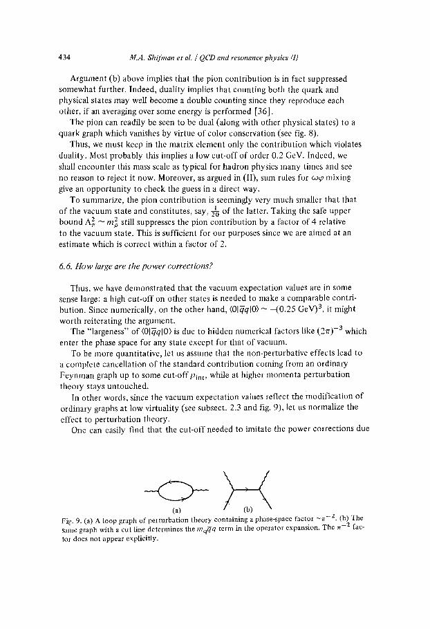
434 M.A. Shifman et al. / QCD and resonance physics (I)
Argument (b) above implies that the pion contribution is in fact suppressed somewhat further. Indeed, duality implies that counting both the quark and physical states may well become a double counting since they reproduce each other, if an averaging over some energy is performed [36].
The pion can readily be seen to be dual (along with other physical states) to a quark graph which vanishes by virtue of color conservation (see fig. 8).
Thus, we must keep in the matrix element only the contribution which violates duality. Most probably this implies a low cut-off of order 0.2 GeV. Indeed, we shall encounter this mass scale as typical for hadron physics many times and see no reason to reject it now. Moreover, as argued in (II), sum rules for co~ mixing give an opportuni ty to check the guess in a direct way.
To summarize, the pion contr ibution is seemingly very much smaller that that of the vacuum state and constitutes, say, Y60 of the latter. Taking the safe upper
2 still suppresses the pion contr ibution by a factor of 4 relative bound A 2 m o
to the vacuum state. This is sufficient for our purposes since we are aimed at an estimate which is correct within a factor of 2.
6. 6. I Iow large are the p o w e r corrections?
Thus, we have demonstrated that the vacuum expectation values are in some sense large: a high cut-off on other states is needed to make a comparable contri- bution. Since numerically, on the other hand, (01~ql0) ~- - (0 .25 GeV) 3, it might worth reiterating the argument.
The "largeness" of (0[~ql0) is due to hidden numerical factors like (27r) - 3 which enter the phase space for any state except for that of vacuum.
To be more quantitative, let us assume that the non-perturbative effects lead to a complete cancellation of the standard contribution coming from an ordinary Feynman graph up to some cut-off Pint, while at higher momenta perturbat ion theory stays untouched.
In other words, since the vacuum expectat ion values reflect the modification of ordinary graphs at low virtuality (see subsect. 2.3 and fig. 9), let us normalize the
effect to perturbation theory. One can easily find that the cut-off needed to imitate the power corrections due
(a) Fig, 9. (a) A loop graph of perturbation theory containing a phase-space factor ~n -2. (b) The same graph with a cut line determines the mq~q term in the operator expansion. The n -2 fac- tor does not appear explicitly.

M.A. Shifman et al. / QCD and resonance physics (I) 4 3 5
to <0l~ql0>, <01G210> @ 0, is indeed high:
P~nt ~ 3 GeV 2 ,
which is a resemblance of the high cut-off discussed in subsect. 6.5 and non-accept- able for the same reasons.
Since the only place left for the quark and gluon propagators to deviate from asymptotic freedom is at low momenta, the deviation must be much more violent than a mere modification of perturbation theory by order unity.
We shall demonstrate in paper (II) that this conclusion, which is based on purely phenomenological analysis, is in amusing correspondence with the instanton-based picture of the non-perturbative effects.
In conclusion, h.'t us notice that the hypothesis of the vacuum intermediate state dominance, like all the others which we introduce here, leads to some direct experi- mental consequences and is subject to an independent check in this way. In particu- lar, it implies pea degeneracy which is well-established experimentally (see (II) for details).
6. 7. Dilute instanton-gas approximation: matrix elements <0lG~vG~vl 0>, • a b c <0 IfabcGu vGvoGau[O>
So far we have discussed evaluation of matrix elements by saturating them by the intermediate vacuum state. We find the foundation of the approximation rather solid and will use the results for the four-fermion operators obtained in this way without further reservation. Unfortunately, the technique is not universally appli-
a a a b c cable. In particular, the gluonic operators G.vGuv, fabcG.vGvoGo, cannot be treated in this way (fabc here are the SU(3) color structure constants).
Here we utilize another approximation, that is the dilute instanton-gas approxi- mation elaborated in ref. [13]. The use of the approximation is qualified for im- portant theoretical uncertainties, and we shall turn back to their discussion at the end of the subsection. First let us demonstrate the technique with the example of the matrix elements specified in the title of the subsection. Start with the Belavin-Polyakov-Schwartz-Tyupkin solution (3.4).
As far as the instanton size is small, one can use the dilute instanton gas approximation [13]. In this approximation the matrix elements under considera- tion reduce to the one-instanton (+ anti-instanton) contribution. Using the explicit expression (3.4) and performing the integration over the instanton position we come to
PC dp <Olg~G~.l O>i~st.+ami-i.st. = 26"2 f ~ d(p),
o
(6.18)
<0 Ig3sfabcGa~vGboGeol ~ I O)inst.+anti_inst"

436 M.A. Shifman et al. / QCD and resonance physics (I)
PCdp 3 • 28 " 7r 2 f -~yd(p), (6.19)
5 o p
where gs is the quark-gluon coupling constant, d(p) is the instanton density function [ 13 ]. The integrals in (6.18), (6.19) are infrared divergent and the cut-off Pc is introduced for this reason.
Now, d(o) is given in eq. (3.7). The numerical constant en*ering this equation depends on the % renormalization procedure. It is typically of order 10 -1 [13,14].
Note that all the numbers here correspond to pure gluodynamics with SU(3)color. Eqs. (6.19), (6.18) give
3 a /~ c 12, -2 . . . . 2Ga G a '0" (6.20) (O[gsfabcG~vGvoGoulO)=-g~P ~Ulgs tar uvl ~,
where (p-2) is the mean value o fp -2 as weighted with the instanton density func- tion. Since the integrands are peaked at the upper limit of integration (p-2) ~ pc2.
Thus, the value of the cut-off, Oc, is a key parameter for all the instanton esti- mates. Moreover, the matrix elements in point are proportional to a high power of Pc. Therefore, any rough estimate of Pc is of little value since the corresponding uncertainty in the matrix elements is enormous.
For this reason we would prefer the other way: find one of the matrix elements from independent sources, fix Pc and evaluate further matrix elements.
In particular, one can find 2 a a (Olgs GuvGuv[O) from the sum rules for charmonium
decays
I O~S a a o) (6.21) 0 -TGuvG**v ~ 0.012 GeV 4 ,
(see (II) and ref. [6]). The corresponding value of Pc is [10]
Pc ~ 1/200 MeV, (6.22)
and
3 a b c (O]gsfabcGuvGvoGa~]O) ~ 0.045 GeV 6 "~ (0.59 GeV) 6 . (6.23)
2 a a - The reference to the experimental data to fix (0lgs GuvGuv[O) is not in fact consistent with the logic of the present section: our plan is to fix only (0 Iqql 0) from the data and reduce all the other matrix elements to this quantity. In subsect. 6.8 we shall remove this inconsistency by computing (0 [gZG2]0) theoretically in terms of (0 Iqql 0). This is achieved at the price of another approximation, however, and we would like to isolate eq. (6.21) which is on firmer basis than theoretical speculations presented in subsect. 6.8.
There are apparent weaknesses of the one-instanton approximation. The need for a cut-off seems to be the most dangerous. Thus, the approximation is no better than, say, an evaluation of the weak interaction via a four-fermion theory with a cut-off. We will demonstrate in paper II that the similarity extends rather far and the result depends on the way the cut-off is introduced.

M.A. Shifman et al. / QCD and resonance physics (1) 437
Another well-known disease is the lack of understanding of the effect of the light quarks. Formally, the instanton density vanishes in the presence of massless quarks. One may hope, however, that due to spontaneous symmetry breaking, quarks are not so important for the matrix elements controlled by instantons of large size.
Finally, let us notice that the instanton-based estimates can be tried for a limited number of matrix elements, since the matrix elements of the type (0IG n L0) with high n are ultraviolet divergent.
Still, the estimates can be useful. Indeed, the cut-off is quite high, Pc 1/200 MeV, and it is difficult to imagine that larger distances modify the answer drastically. Moreover, relations between the matrix elements like eq. (6.20) have a better chance of withstanding the modifications provided by a complete theory.
6. 8. Matching o f light and heavy quarks
Light and heavy quarks have been considered in different ways so far. For light quarks we expand in the quark mass. For heavy quarks we choose external momentum Q2 ~ 0 and expand in the inverse quark mass. Imagine that there exists a quark of an intermediate mass which is neither light nor heavy. Strictly speaking we cannot use any of the techniques. An optimist, however, could try to reverse the statement and say that for a fictitious quark of an intermediate mass both approximations are approximately valid and lead to similar results.
The world of heavy quarks is simpler in the sense that there is no need to intro- duce independent vacuum expectation values of the type (0 Ihhl0), where h is a quark of heavy mass m h. Indeed, it is reduced to the matrix elements of gluonic operators. Explicitly, we have in the first approximation (see fig. 10):
l ( ~ s ~ a ~ a 0) ( 0 1 h h t 0 ) - 12 mh 0 - - + (6.24) 1 7T ~ 1 2 v ~ 1 2 v " ' "
which is valid as far as higher orders in m~ -1 are negligible. Now, let us try to extrapolate eq. (6.24) to lower mass. Then the matrix element
(0 [hhl 0) increases until we come to the point where terms of higher order in rnff 1 neglected so far become important. At this point little can be said for certain. But we know that once we cross the boundary of the world of the light quarks, (0 I hh I O) becomes mass independent.
i I I l i I
i gluons ~ t I I ~\ I
Fig. 10. The heavy quark expansion for hh.

438 M.A. Shifman et al. / QCD and resonance physics (I)
Moreover, the breaking of eq. (6.24) is due to power corrections so that the change in the regime is hopefully fast. Thus, we would like to speculate that the light and heavy quarks match smoothly. More specifically, the approximation amounts to saying that eq. (6.24) can serve for the purpose of an estimate, if the left-hand side is evaluated in fact for a light quark while the right-hand side is taken at some transition point rn h which marks the boundary of the world of heavy quarks.
We see that the guess is right in sign, to say the least. Indeed, the (OlGauvGauv[O) is positive on general grounds (see subsect. 6.9) while <01~ql 0> is negative as follows from the phenomenological analysis presented in previous subsections.
Now, as to the absolute magnitude. The prediction for the expectation value of GauvGauv depends on the critical value ofm h for which eq. (6.24) is still valid.
A consistent way of determining the critical value of mh would be to compute next orders in mff 1 and find the point where they become appreciable. This seems to be a tractable problem and the corresponding calculations are in progress (they are being performed by Novikov and the present authors).
Here we would like to rely more on intuition. The strange quark mass is about 150 MeV. The corresponding hadron scale is represented by m~. It is not too small, indeed, so that we are rather close to the boundary of heavy quarks. Moreover, all the numerical studies in the sum rules (see (II) for details) indicate that at m~ the expansion in the inverse mass is valid and higher orders in the operator expansion
2 can be neglected. Thus, the critical mass is somewhere between m~ and rap. Therefore, m h "~ 0.2 GeV seems to be a reasonable guess for the critical value
of mh which can be still treated as "heavy". In this way we come to
(O[~ GauvGauvlOl~-12mh(OlhhlO)lmh=2OOMeV ~O.O3 GeV4 . (6.25)
In (II) we will determine the same matrix element phenomenologically and the cor- responding value has already been mentioned above (see eq. (6.21)). It differs from the rough estimate by a factor of 2.5 which is indeed not bad.
Thus, we can rely on this technique as far as rough estimates of various matrix elements are concerned. To give perspective, let us mention that matching of light and heavy quarks allows one to estimate (O[~ouvtaqGauv[ 0). This matrix element is crucial for analysing the sum rules for charmed mesons. The analysis is being per- formed in collaboration with Novikov.
6.9. On the signs o f the matrix elements
In the previous subsections we have proposed a number of techniques for esti- mating the vacuum-to-vacuum matrix elements. In particular, we have found that
a a (OIGuvGuvlO) > O and (Ol~Tutaq~Tutaq lO) < O .
(see eqs. (6.21) and (6.17), respectively). However, all the estimates explored so far are model dependent. In this sub-
section we will argue that the signs just mentioned can be established in fact on

M . A . S h i f m a n e t al. / Q C D a n d r e s o n a n c e p h y s i c s (I) 439
very general grounds. The only assumption needed is the possibility to perform the averaging over the vacuum state by means of the functional integration in the Euclidean space-time. This is indeed a very plausible assumption. Moreover, the formulation of the theory in Euclidean space-time may be considered as primary nowadays.
a a Consider first GuvGuv. In Minkowski space-time it is not a positive definite quantity since
GuvGuva a = ~ (_2GoiGo a + 2GikGik) a (Minkowski). i ,k= 1,2,3
i > k
However, written in Euclidean space it does become positive definite:
GuvGuva a = ~ (2G~iGaoi + 2GikGik)a a , (Euclidean). i ,k= 1,2,3
i > k
Therefore, representing the vacuum-to-vacuum matrix element as a functional inte- gral we find that it is positive definite:
fCDA e-S ~(2GaoiGaoi + ~a ~ a a • .. , ,1 ik t - r ikJ
( 0 a a _ [GuvG~vtO) > 0 f ~ A ... e - s
To consider the four-fermion operator mentioned above let us use first the equa- tion of motion:
2 ~Tuta q = _ _ CDuGauv ,
gs
which reduces the four-fermion operator to the gluon fields:
4 a a (~Tuta q)C47uta q) = -g~( "~uG uv)( co ~G~v)
Euclid> _ (Q)jG]0) 2 _ (Q)oGaoi + Q)jGja)2 < 0 .
When we saturate the matrix element of this operator by the vacuum intermediate state, the minus sign emerges by virtue of the Fierz transformation. Since we cannot introduce the color intermediate states the agreement in signs between the model estimates and general equations does not seem to be trivial and is gratifying, there- fore.
6.10. Conclusions
In the first part of the present section we have argued in favor of light quarks, mu, d "" 5 MeV, ms ~ 150. These low masses become more and more conventional

440 M.A. Shifman et al. / QCD and resonance physics (I)
nowadays, so that presentation is partly of a review kind. Still we hope that the dis- cussion of the value of the coupling constant which complements the choice of the mass may be new to some of the readers. The same is possibly true for the reference to the non-leptonic decays as a support for the choice of parameters favored in this paper.
In sect. 6 we proposed several techniques for rough estimates of the matr ix ele- ments relevant to the sum rules. It might worth emphasizing that even an estimate within a factor of two is very valuable for our purposes because the corresponding uncertainty in predicting the resonance properties turn out to be 10 -15% (see II)). Our feeling is now that it is possible to get an estimate of this kind practically for any matrix element.
From a more general point of view, this section completes the discussion of the general problems of the approach proposed. Indeed, we started with a proof that it is possible to use the Wilson operator expansion as far as a few first terms in the Q-2 expansion are concerned. Then we evaluated explicitly the coefficients in the two- point functions of various currents. Then we substantiated the use of the first Borel transform of the polarization operator as most convenient to study resonances within QCD. Finally, in this section we estimated the vacuum-to-vacuum matrix elements which specify the sum rules completely. Now everything is ready for appli-
cations.
Note added in proof
In subsect. 6.4 we have called for better accuracy in measuring the e+e - annihila- tion cross section at relatively low energies. Due to the efforts of the Novosibirsk, Orsay and Frascati groups such data do exist now. The data have been analyzed by Eidelman et al. ( to be published), and the analysis confirms our guess that asymp- totic freedom is violated by the power corrections rather than by higher orders in
OL s •
Appendix
Four-fermion operators
This appendix is devoted to summation of the (a s ln(Q2/ll2)) n terms in the opera- tor expansion coefficients corresponding to the four-fermion operators o f the type O r = ~ F ~ I ~ b . Many of the results are already known but are scattered in numer- ous publications [37], so we find it helpful to collect them all in one place. The whole procedure is rather standard so we only sketch the derivation. In subsect. A. 1 all independent structures are listed and classified. In subsect. A.2 we write out anomalous dimension matrices and solve the corresponding renormalization-group equations. Subsect. A.3 presents the final results.

M.A. Shifman et al. / QCD and resonance physics (I) 441
A.1. Operators
First of all it is necessary to give proper names to various four-fermion opera- tors which were previously all called Or. In considering the T-product of vector and axial-vector currents the following independent operators are encountered:
PI = ~L'Y/.L~) L~R' ) ' / .L~/R , \
P2 = ~LTlsta~L~RTuta~R , I
P3 = ~LTu~L~LTu~L + (L ~ R) , j (1.1)
P4 = ~LTuta~L~LTuta~L + (L--> R) , (A.1)
Ps = ~L~'atb')'ta~L~RXatb vlat~R '1 (s.s) J P6 - a - a l~L)k "/u~Lt~R)k ")'u~R .
Below we will discuss them in detail. For completeness we also write out here the operators involved in the expansion for scalar and pseudoscalar densities:
P7 = ~R~L~R~L + (L ~ R) ,
P8 = ~Rta~L~Rta~L + ( L ~ R) ,
P9 = ~R)ka~-/L~R~ka~m + ( L <-~ R) ,
PlO = ~RXatb~L~RXatbl~L + (L ~ R). (A.2)
In the above equations ff denotes the fermion field carrying both color (i, j, k .... : 1, 2, 3) and SU(3) flavor (a,/3, 3' .... = 1, 2, 3) indices. The summation is implicit; thus for example
fT~z~ = ~"Yts ui + di%z di + S-i"[la s i •
Furthermore t a and xa stand for the Gell-Mann SU(3) matrices acting in color and flavor spaces respectively. (They are normalized by the condition Tr(kaX b) = Tr(tat b) = 2lab.) The subscript L (R) labels the left- (right-) handed spinors,
f fL=l (1 +TS) ~ , fiR=½( l --TS) ¢ .
We indicated in parenthesis in eq. (A.1) the properties of the operators with respect to the SU(3)R ® SU(3)L symmetry. We included in the list only the SU(3)flavor singlet operators since only these have non-vanishing vacuum expectation values (under the assumption of the vacuum SU(3)flavo r symmetry). For completeness we write down a few formulae often used in working with four-fermion operators.
The Fierz transformations
~1LT#~2L~aLT/ . t~aL = ~1LT/.t~4L~aL'~/.t~2L ,
~ I L ' ~ # ~ 2 L ~ 3 R ' Y ~ 4 R = - - 2 ~ l L ~ 4 R ~ 3 R ~ 2 L " (A.3)

442 M.A. Shi fman et a L / QCD and resonance physics (I)
(Here the subscripts l, 2 .... in ~JlL, ~J2L . . . . stand symbolically for both color and flavor, e.g. 1 -={il, a l}, etc.).
Relation for the Gell-Mann matrices
a a -- 26i/6mn t6tmn = 26in6im (A.4)
A.2. Mixing matrices
In the operator expansion there emerge operators normalized at a (running) point Q. The problem is to express them in terms of operators normalized at a (fixed) point/a, where/~ is of the order of the inverse confinement radius. First, our knowledge of matrix elements, if any, refers just to this point. Second, the entire Q dependence must be exhibited explicitly.
In the leading logarithmic approximation the standard renormalization-group technique allows one to change easily one normalization point to another. All we have to know is the mixing matrix in the one-loop approximation.
In a slightly different language our procedure is as follows. When operators (A. 1) are "dressed" with gluons, there arise logarithmic corrections of the type (c~ s ln(Q2/ /12)) n which contain an explicit Q dependence and call for summation. The summa- tion can be performed either diagrammatically, after the corresponding diagram selection, or by means of the renormalization group.
Below we will use the anomalous dimension language which seems more com- pact.
Notice that the operators P1-4 and P5,6 possess different selection rules with respect to SU(3)R ® SU(3)L; therefore under the mixing they split into two distinct groups, P1, P2, P3,/°4 and Ps, P6"
In principle, the operators P1-P4 with the vacuum quantum numbers can mix also with a pure gluon operator Oy:
O f _ ~3~eabct~a r~b r . c - ~ ; s J tJuv~vot~o~ , (d = 6) .
However, the effect is important only for the Of coefficient since the O/-Or feed- back is weak; it is suppressed by an overall factor as 2 which enters along with the conventional (a s ln(Q2//~2)) n. An example of the diagram responsible for the Or- O; mixing is given in fig. 11. The three-loop structure of the diagram results in a numerical smallness which makes the effect completely inessential.
A few technical remarks are in order now. There are two completely distinct types of one-loop graph, call them conventional (fig. 12a) and annihilational (fig. 12b). In fig. 12 we denoted the four-fermion operator by a closed circle and slightly split the fermion lines in order to indicate explicitly which fermion line corresponds to this or that fermion bracket. (Each fermion bracket ( fTu~), or (~')'u~ka~) or (~Tu~atb~) is denoted by a single solid line without cuts.)
The gluon propagator 1/k 2 in the annihilational graphs is cancelled out since the

M.A. Shifman et al. / QCD and resonance physics (I) 443
I I
I I
Fig. 11. An example of the diagram responsible for the mixing of the four-fermion operators gsfabcG ~zvG voG ola. O F (closed circle) with the three-gluon operator Of= 3 a b e
adjacent quark loop is proportional to k 2. In other words, if a four-fermion opera- tor is inserted into the annihilational diagram it yields the operator -~/Tu ta@ ~vGu va where ~ is the covariant derivative and G~v is the gluon field strength tensor. The latter operator in turn reduces to a four-fermion form by virtue of the equation of motion:
a _ 1 - - a C3 uGuv- -~gs~Tvt ~ .
Calculations are conveniently performed in the Landau gauge for a gluon field. In this gauge the anomalous dimension of a fermion field vanishes and one is left with the anomalous dimension of the local operators.
In the Landau gauge the following rules take place: (i) a gluon line "dressing" a solid quark line (one fermion bracket) gives zero; (ii) a gluon line attached to two distinct brackets gives zero for operators of the
type ]uL]UL, ]uR]u R, if it connects the ingoing and the outgoing lines, and for opera- tors of the type ]UL/uR, if it connects two ingoing or two outgoing lines;
(iii) the annihilational graphs exist only for the operators P2, P3, P4. After these preliminary remarks we give the answer for the anomalous dimension
a) b)
Fig. 12. Graphs determining the anomalous dimension matrix for the four-fermion operators: (a) a conventional graph; (b) annihilational graphs. The four-fermion operator is denoted by the closed circle.

444 M.A. Shifman et al. / QCD and resonance physics (I)
matrix
Pr
1-
0; 0 0 r - Pr
PZ = l+IS&
(
2y 5 0 -1 P2
Ip3 (A.5)
1.
4rl 1-12 0 -3 0 1 -v p3’
P 4A _?J -13 p 9 3 I_ p4> w
where the subscripts p, A stand for the normalization point of the operators. The following combinations are diagonal:
D, =P, - 0.213P2 + 0.138P3 + 0.029P4, (6, = -1.134),
D2 = 0.787P,+P2 + 0.154P3 - 0.196P4, (6, = 6.774))
03 = -0.505PI - 0.238P2 + P3 - O.S6OP4 , (6 3 = 2.989) ,
D4=-l.l88P1+0.759P2+1.565P3+P4, (64 = -3.407) (A.6)
In parenthesis the corresponding eigenvalues of the mixing matrix are indicated, which just determine the anomalous dimensions. For example,
D,(Q) =K-~.~~~/~D~(/J). (A.7)
Here
(-4.8)
b is the coefficient in the Gell-Mann-Low function fl(o!,) for the effective charge,
/3(a,) = - 5 + O(c& . (A.9)
For three quark flavors (and we always work in the region where only three flavors are essential)
b=9. (A.10)
The procedure of converting the operators Pi(Q), normalized at Q, into the opera- tors P&L), normalized at p, includes in fact two steps. At first one rewrites the opera- tors Pi in terms of Dj. At this point it is convenient to introduce matrix notation. For example, eq. (A.6) can be rewritten as
PI = [Xl PI a where [D] and [P] are the operator columns, and [X] is the 4 X4 matrix which can be easily read off eq. (A.6).
Then
PI = W’l PI ,
M.A. Shifman et al. / QCD and resonance physics (I) 445
where
I 0.784 0.170 -0.080 0.035 -0.593 0.769 -0.160 0.078 (A.11)
[X- l ] = 0.534 0.048 0.495 0.271 L0.546 -0.457 -0.749 0.475
It is a trivial matter for the operators D i to proceed from a normalization point Q to a point g, since they are simply multiplied by K 6i/b (see eq. (A.7)). The corre- sponding values of 6i are given in eq. (A.6). In matrix form
where
[D(Q)] = [K ~/b] [D(u) ] ,
[K~/b] =
K -- 1.134/b
K6.774/b
0
0
(A.12) K2.989[b
K --3.407//;
Finally, the operators Di(],l ) are transformed into the operators Pi(la) with the help of the [X] matrix:
[P(Q)] = [ x - l ] [ K~/a] [x] [P6u)] . (A.13)
This relation (together with eqs. (A.6), (A.11), (A.12)) is our final result for the Q dependence of the operators P1-4. As for the operators P5,6 the answer here is even much simpler. The mixing matrix looks like
P6 2 47rln~-5- ~ ~P6j,
and the diagonal combinations are:
Ds =Ps + 2 p 6 , (65 = 8) ,
D6 = - 3 P 5 +P6, (66 = --1) .
Thus
= - f ~ 0 Ps (A. 15)
P6 Q K--l / - i g P u
A.3. Vacuum expectation values and final result
For the vacuum-to-vacuum matrix elements of the operators P1 --6(/1) w e use the factroization hypothesis discussed in detail in sect. 4. The effective recipe is to

446 M.A. Shifman et al. / QCD and resonance physics (I)
insert the vacuum intermediate state in all possible channels, then <01P, I 0> are expressed in terms (01 f f f l 0 ) 2. Namely,
( P 3 ~ ) ) = ( P 4 ~ ) ) = 0 ,
(P5 (/a)) = ~6 (P6 (/2)) = - 1 8 ~ ( ~ f f ) 2 . (A. 16)
We recall that (~qJ) means (0[~u + d d +~s ] 0). Using (A. 13), (A. 15) and (A. 16) one can finally find
(PI (Q)) = ( -0 .020g-1 .134 /b + 0.195u6.774/b + 0.030K Z.989/b
- 0.019K -3.4O7/b)(pz ( t l ) ) ,
(P2 (Q)) = (0.015K - 1.134/12 + 0.883t¢ 6.774/b + 0.060t¢ 2.989/b
+ 0.042t¢-3"407]b)(P2(ld)) ,
(P3(Q)) = ( -0 .014K-1.134/b + O.055Ke.774/b _ O.187Kz.989]b
+ 0.145K-3"407/b)(Pz(p)),
(P4(Q)) = ( - 0 . 0 1 4 t ¢ - 1 ' 134/b __ 0.525K6.774]b + 0.283K2.989//)
+ 0 . 2 5 5 g - 3 " 4 0 7 / b ) ( p 2 ( I A ) ) ,
(P5 (Q)) = t¢ 8/b(P s (t-0),
(P6(Q)) = i~6 t~ S/b(ps(la)) .
References
[ l l D.J. Gross and F. Wilczek, Phys. Rev. Lett. 30 (1973) 1343; H.D. Politzer, Phys. Rev. Lett. 30 (1973) 1346.
[2] A. Belavin, A. Polyakov, A. Schwartz and Yu. Tyupkin, Phys. Lett. 59B (1975) 85. [3] V.N. Gribov, in Proc. 12th LINP Winter School of Physics, Leningrad, 1977, vol. 1, page
147 (English translation: SLAC-TRANS-176 (1977)); Nucl. Phys. B139 (1978) 1. [4] M. Shifman, A. Vainshtein and V. Zakharov, Nucl. Phys. B147 (1979) 448. [5] M. Gell-Mann, R. Oakes and B. Renner, Phys. Rev. 175 (1968) 2195. [6] A. Vainshtein, V. Zakharov and M. Shifman, Pisma ZhETF (USSR) 27 (1978) 60. [7] K. Wilson, Phys. Rev. 179 (1969) 1499. [8] K. Symanzik, Comm. Math. Phys. 23 (,1971) 49;
C. Callan, Phys. Rev. D5 (1972) 3302; R. Brandt, Fortschr. Phys. 18 (1970) 249.
[9] C.G. Callan, R. Dashen and D.J. Gross, Phys. Rev. D17 (1978) 2717; A. Polyakov, Nucl. Phys. B120 (1977) 429; A. Belavin and A. Polyakov, Nucl. Phys. B123 (1977) 429; G. 't Hooft, Phys. Rev. Lett. 37 (1976) 8; Phys. Rev. D14 (1976) 3432; C.G. Callan et al., Phys. Lett. 63B (1976) 334; 66B (1977) 375; R. Jackiw and C. Rebbi, Phys. Rev. Lett. 37 (1976) 172.

M.A. Shifman et al. / QCD and resonance physics (I) 447
[10] M. Shifman, A. Vainshtein and V. Zakharov, Phys. Lett. 76B (1978) 471. [11] M. Shifman, A. Vainshtein and V. Zakharov, Moscow preprint ITEP-54 (1978) Phys. Rev.
Lett., submitted. [12] V. Novikov, L. Okun, M. Shifman, A. Vainshtein, M. Voloshin and V. Zakharov, Moscow
preprint ITEP-83 (1977); Phys. Reports 41 (1978) 1. [13] C.G. Callan, R. Dashen and D.J. Gross, see ref. [9]. [14] N. Andrei and D.J. Gross, Phys. Rev. D18 (1978) 468. [15] L. Baullieu, J. Ellis, M.K. Gaillard and W.J. Zakrzewski, Phys. Lett. 77B (1978) 290. [16] T. Appelquist and H. Politzer, Phys. Rev. Lett. 34 (1975) 43. [17] M. Shifman, A. Vainshtein, M. Voloshin and V. Zakharov, Phys. Lett. 77B (1978) 80;
A. Vainshtein et al., Yad. Fiz. 28 (1978) 465. [18] S. Weinberg, Harvard preprints HUTP-77/AO57, HUTP-77/AO61 (1977). [19] H. Leutwyler, Phys. Lett. 48B (1974) 45; Nucl. Phys. B76 (1974) 413. [20] H.D. Politzer, Nucl. Plays. Bl17 (1976) 397. [21] T. Appelquist aad H. Georgi, Phys. Rev. D8 (1973) 4000;
A. Zee, Phys. Rev. D8 (1973) 4038. [22] A. Vainshtein, V. Zakharov and M. Shifman, JETP Lett. 22 (1975) 55;
E. Witten, Nucl. Phys. B104 (1976) 445; B122 (1977) 109; V. Novikov et al., Phys. Reports 41 (1978) 1.
[23] J. Schwinger, Particles, sources and fields, (Addison-Wesley, 1973) v.2. [24] V.N. Baler, V.M. Katkov and V.M. Strakhovenko, ZhETF (USSR) 67 (1974) 453, and
references therein. [25] S. Adler, Phys. Rev. 177 (1969) 2426;
J.S. Bell and R. Jackiw, Nuovo Cim. 60A (1969) 47. [26] R. Crewther, Phys. Rev. Lett. 28 (1972) 1421;
M. Chanowitz and J. Ellis, Phys. Lett. 40B (1972) 397; Phys. Rev. D7 (1973) 2490; J. Collins, L. Duncan and S. Joglekar, Phys. Rev. D16 (1977) 438.
[27] A. Vainshtein, V. Zakharov and M. Shifman, JETP Lett. 23 (1976) 602; JETP (Soy. Phys.) 45 (1977) 670; M. Shifman, A. Vainshtein and V. Zakharov, Phys. Rev. D, in press.
[28] V.S. Popov, V.L. Eletsky and A.V. Turbiner, ZhETF (USSR) 74 (1978) 445. [29] M Shifman, A. Vainshtein and V. Zakharov, Nucl. Phys. B147 (1979) 519. [30] R. Dashen, Phys. Rev. 183 (1969) 1245. [31] H. Georgi and H. Politzer, Phys. Rev. D14 (1976) 1829. [32] A. Vainshtein, V. Zakharov and M. Shifman, JETP Lett. 22 (1975) 55; JETP (Soy. Phys.)
45 (1977) 670. [33] R. Shankar, Phys. Rev. D15 (1977) 755. [34] A. DeRfljula, H. Georgi and H. Politzer, Ann. of Phys. 103 (1977) 315;
M. Gluck and E. Reya, Phys. Rev. D16 (1977) 3242; G.C. Fox, Nucl. Phys. B131 (1977) 107; A. Buras and K. Gaemers, Nucl. Phys. B132 (1978) 249.
[35 ] A.A. Ahrikosov, L.P. Gor'kov and I.E. Dzyaloshinski, Methods of quantum field theory in statistical physics, (Fizmatgiz, Moscow, 1962).
[36] J.J. Sakurai, Phys. Lett. 46B (1973) 207. [37] M.K. Gaillard and B.W. Lee, Phys. Rev. Lett. 33 (1974) 108;
G. Altarelli and L. Maiani, Phys. Lett. 52B (1974) 351; M. Shifman, A. Vainshtein and Zakharov, Nucl. Phys. B120 (1977) 316; F. Wilczek, S.B. Treiman, A. Zee and R.L. Kingsley, Phys. Rev. D12 (1975) 2768.
Related Documents