Putting on the crush : market structure, information and ...

PUTTING ON THE CRUSH ... MARKET STRUCTURE, INFORMATION AND THE SOYBEAN COMPLEX

Dominic Rechner

B.A. (Economics), Simon Fraser University 1987

THESIS SUBMITTED IN PARTIAL FULFILLMENT OF

THE REQUIREMENTS FOR THE DEGREE OF

MASTER OF ARTS

in the Department

of

Economics

Dominic Rechner 1989

SIMON FRASER UNIVERSITY

November 1989

All rights reserved. This work may not be reproduced in whole or in part, by photocopy

or other means, without permission of the author.

APPROVAL

Name:

D e g r e e :

T i t l e o f Thesis :

D o m i n i c R e c h n e r

M . A . ( E c o n o m i c s )

" P u t t i n g o n t h e C r u s h " ... M a r k e t S t r u c t u r e , I n f o r m a t i o n a n d t h e S o y b e a n Complex

E x a m i n i n g C o m m i t t e e :

C h a i r m a n : S. E a s t o n

- - - f l

MI-el Bowe 2 A s s i s t a n t P r o f e s s o r S e n i o r S u p e r v i s o r

o f f r e y P o i t r a s s i s t a n t P r o f es s o r

V - " - G d o r g e B l a z e n k o - A s s i s t a n t P r o f e s s o r

. ~ i n d s a y - ~ e y e d i t h r'

Associate p r o f es sof i ' B u s i n e s s A d m i n i s t r a t i o n E x t e r n a l E x a m i n e r

D a t e A p p r o v e d :

PARTIAL COPYRIGHT L I C E N S E

I hereby g ran t t o Simon Fraser U n i v e r s i t y t h e r i g h t t o lend

my t h e s i s , p r o j e c t o r extended essay ( t h e t i t l e o f which i s shown below)

t o users o f t h e Simon Fraser U n i v e r s i t y L i b r a r y , and t o make p a r t i a l o r

s i n g l e cop ies o n l y f o r such users o r i n response t o a request f rom t h e

l i b r a r y o f any o t h e r u n i v e r s i t y , o r o t h e r educa t iona l i n s t i t u t i o n , on

i t s own b e h a l f o r f o r one o f i t s users . I f u r t h e r agree t h a t permiss ion

f o r m u l t i p l e copy ing o f t h i s work f o r s c h o l a r l y purposes may be g ran ted

by me o r t h e Dean o f Graduate Stud ies. I t i s understood t h a t copy ing

o r p u b l i c a t i o n o f t h i s work f o r f i n a n c i a l ga in s h a l l n o t be a l lowed

w i t h o u t my w r i t t e n permiss ion.

T i t l e o f Thes is /Pro ject /Extended Essay

" P u t t i n g on t h e crush" ... Market S t ruc tu re , I n f o r m a t i o n and

t h e Soybean Complex.

( s i gna tu re )

Dominic Rechner

(name)

6 December 1989

(date)

ABSTRACT

This study explores efficiency in a speculative competitive market. From a

discussion of the theoretical aspects of the efficient market hypothesis and the

structure of futures markets, "disequilibrium" pricing is rationalized on the basis

of market imperfections in the informational aspect of markets. Spread strategies

are used to test for dependency and weak form efficiency on the Chicago Board

of Trade. They are applied to daily futures prices for the commodities of the

soybean complex. The results are free of sampling bias and reasonable trading

\, costs are considered. The empirical results show strong evidence of pricing

inefficiency in the crushing margin of soybean processors.

ACKNOWLEDGEMENTS

The author is extremely grateful to Michael Bowe, Geoffrey Poitras and

George Blazenko for helpful comments and suggestions throughout the

development of this paper and to Bruce Ramsay for assistance in data

formatting.

DEDICATION

To Donna and my parents

TABLE OF CONTENTS

. . Approval ................................................................................................................... 11

... Abstract .................................................................................................................. 111

................................................................................................... Acknowledgements iv

Dedication ................................................................................................................. v

........................................................................................................ List of Tables vii ...

List of Figures ..................................................................................................... vill

I

I1

I11

IV

v VI

VII

Introduction ........................................................................................................ 1

Efficient Markets .............................................................................................. 4

Weak Form Tests ............................................................................................ 6

Market Equilibrium ......................................................................................... 9

Models Incorporating Diffuse Information .................................................... 14

........................................................................................ Empirical Evidence 17

............................................................... 0.1 The Soybean Complex 17

0.2 Previous Studies Relevant to the Soybean Complex .............. 24

0.3 Data ............................................................................................ 25

....................................................................... 0.4 Rule and Results 31

Summary and Conclusion ............................................................................ 45

Notes ...................................................................................................................... 46

References ............................................................................................................... 47

Table

LIST OF TABLES

Page

U.S. Soybeans . production. supply and disappearance ............................ 18

U.S. Soybean meal and oil . supply and distribution .............................. 20

............................................. CBOT contract details and GPM calculation 23

............................................................................ Daily return specifications 32

Margin requirements ..................................................................................... 36

Trading performance all strategies .............................................................. 37

........................................................................................ Annual summaries 40

Long1 short only strategies .......................................................................... 43

vii

LIST OF FIGURES

Figure Page

........................................................... 1 Gross processing margin. 1978- 1987 27

..................................................................................... 2 Soybeans. 1978-1987 28

............................................................................. 3 Soybean Meal. 1978-1987 29

................................................................................ 4 Soybean Oil. 1978-1987 30

... V l l l

I INTRODUCTION

Basically there are two interrelated aspects of a market: transactions

and information. The efficiency of a market simply refers to the efficiency

with which a market performs its related functions of facilitating transactions

and improving information on the terms thereof. The informational role of

prices refers to the quality of information revealed through the pricing

mechanism and thus relates to the efficiency with which a n asset is priced.

(Burns, 1983)

Fama (1970, 1976) summarizes a n efficient market as one in which

prices always "fully reflect" available information. Although this definition

stops short of defining the idea of what is meant by prices "fully reflecting"

available information, Jensen (1978) clarifies this point in tha t "a market is

efficient with respect to information set 8 if i t is impossible to make t

economic profits by trading on the basis of information set Bt." (P. 96) The

economic profits represent risk-adjusted returns, net of all costs.

There are various forms of the efficient market hypothesis which can be

tested. The forms are distinguished by the class of information employed in

empirical evaluations. The most commonly tested has been the "weak form"

where efficiency implies that there are no economic profits offered by trading

on the basis of the past history of prices. Rejection of the weak form of the

Efficient Market Hypothesis requires the establishment of dependencies in the

price history which can be profitably exploited. However, a s Burns (1983)

points out, efficiency is a variable to be explained (as a characteristic of the

equilibrium or structure of the market), not a n (implicit/explicit) exogenous

parameter. This means tha t one cannot study the efficiency of a market in

the framework of a specific industry structure where the development of many

aspects of market efficiency are assumed away. This implies tha t any theoretical

proposals must be based on a n adequate organization of the market whose

properties it is seeking to explain. I t is only then that empirical studies may

yield both meaningful conclusions and implications for policy purposes.

Danthine (1977) and Lucas (1978) note that the many tests reported in

the literature are simultaneous tests of market efficiency, perfect competition,

risk neutrality, constant returns to scale and the impossibility of corner optima.

The present study presents theoretical and empirical insights to the market

organization of futures markets and develops a n alternative to the two

mainstream views of perfectly competitive markets and competitive markets with

costly information.

The Efficient Market Hypothesis is introduced in Section 11, followed by a

critique of past weak form tests of speculative competitive markets in Section

111. The structure of the markets is discussed in Section IV where it is

proposed tha t these markets, due to search costs and the absence of enforceable

property rights with respect to informational technologies, are inherently diffuse

information markets.

Section V reviews recent models incorporating diffuse information and

proposes that , due to the absence of enforceable property rights with respect to

informational technologies, speculative capital markets will be characterized by

disequilibrium pricing.

The performance of opening-gap based spread strategies in the Chicago

Board of Trade soybean complex are tested in Section VI. I t is found tha t

significant profit potential exists and the hypotheses of a random walk and a

weak form of the Efficient Market Hypothesis are rejected. The implications are

discussed in Section VII.

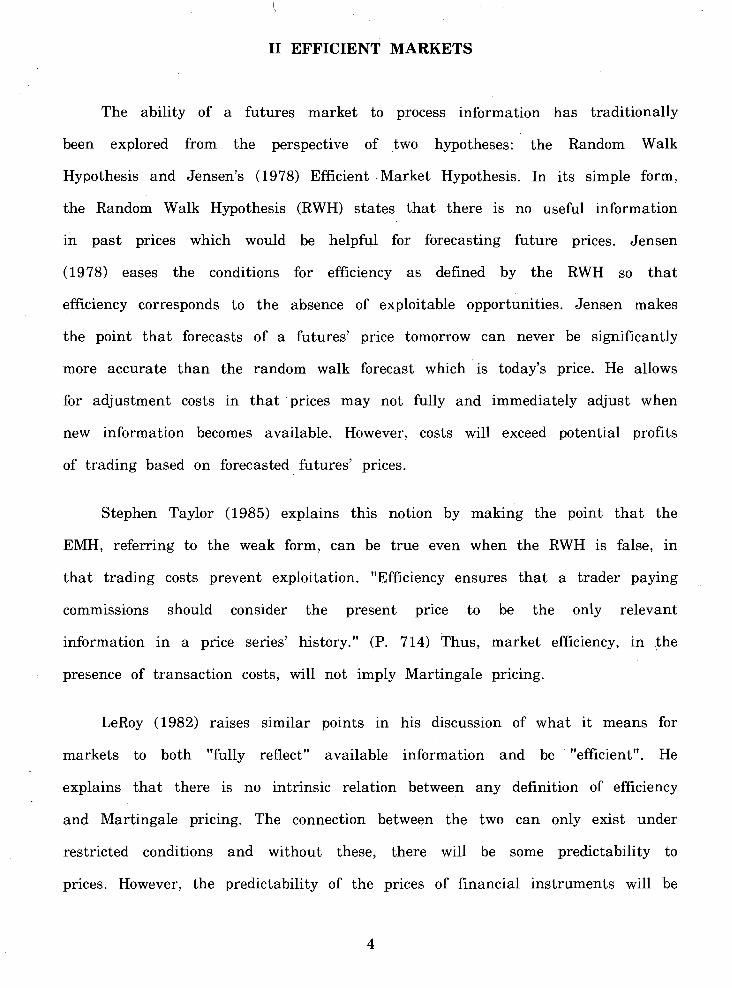
I1 EFFICIENT MARKETS

The ability of a futures market to process information has traditionally

been explored from the perspective of two hypotheses: the Random Walk

Hypothesis and Jensen's (1978) Efficient Market Hypothesis. In its simple form,

the Random Walk Hypothesis (RWH) states tha t there is no useful information

in past prices which would be helpful for forecasting future prices. Jensen

(1978) eases the conditions for efficiency as defined by the RWH so t ha t

efficiency corresponds to the absence of exploitable opportunities. Jensen makes

the point t ha t forecasts of a futures' price tomorrow can never be significantly

more accurate than the random walk forecast which is today's price. He allows

for adjustment costs in t ha t prices may not fully and immediately adjust when

new information becomes available. However, costs will exceed potential profits

of trading based on forecasted futures' prices.

Stephen Taylor (1985) explains this notion by making the point t ha t the

EMH, referring to the weak form, can be true even when the RWH is false, in

tha t trading costs prevent exploitation. "Efficiency ensures tha t a trader paying

commissions should consider the present price to be the only relevant

information in a price series' history." (P. 714) Thus, market efficiency, in the

presence of transaction costs, will not imply Martingale pricing.

LeRoy (1982) raises similar points in his discussion of what it means for

markets to both "fully reflect" available information and be "efficient". He

explains tha t there is no intrinsic relation between any definition of efficiency

and Martingale pricing. The connection between the two can only exist under

restricted conditions and without these, there will be some predictability to

prices. However, the predictability of the prices of financial instruments will be

confined to the interest rate and risk premium components of the rate of

return. This decomposition, since these two factors are merely two elements of

the opportunity cost of trading, is consistent with Jensen's (1978) EMH.

The weak form of the EMH states that basically there is no useful,

exploitable information in the past price history of a market a t any given time.

This means tha t there is no exploitable serial dependence in prices. Therefore,

since the profitability of a mechanical (reactive) rule relies on serial dependence,

evidence of systematic economic profits from trading a "system" constitutes

evidence of serial dependence. As such, the net profitability of a trading rule

constitutes evidence of a market inefficiency. (Smidt, 1965.)

I11 WEAK FORM TESTS

There have been many studies published in the literature which attempt to

test the weak form of the EMH. (Houthakker, 1961; Stevenson and Bear, 1970;

Leuthold, 1972; Rausser and Carter, 1983; Helms e t al, 1984; and Bird, 1985.)

While most of these studies have been based on Alexander's Filter, it is argued

here tha t none of the results imply anything about the efficiency of the market.

The only conclusions tha t can be drawn from these studies pertain to the

usefulness of the technical indicators employed in trading the particular

financial instruments on which they were tested. The basic problem with past

attempts to test the weak form of the EMH has been a methodological one.

I t was noted above tha t a profitable trading system is evidence of serial

dependence. However, a n unprofitable trading system is not evidence of the

absence of serial dependence. Thus, it is inappropriate to make broad

generalizations or suggestions from such a narrow approach. One cannot reject

the hypothesis t ha t there is (neglected) important information in past prices

without first establishing tha t the information used is in fact relevant.

In order to be able to draw any evidence pertaining to the EMH from a

weak form test, one would first need to consider the establishment of the

suitability of the technical indicator used for the markets which are to be

tested. A brief glance of the literature which encompasses technical trading

systems and methods would reveal a t least fifty accepted indicators. (Kaufman,

1987; Schwager, 1984.) If one were to include parameter variations and

indicator combinations, the number of potential methods increases dramatically.

If one were to further introduce money management rules such as stop

strategies and entry and exit rules, one quickly recognizes the complexity of this

field. Bearing this in mind, past studies, for reasons outlined above, do not

present any significant evidence pertaining to the weak form of the hypothesis

and yield very limited insight to the stochastic processes of the price series

tested.

The limited usefulness of the published weak form tests is recognized in

Martin et a l . (1988) who note tha t the tests are not exhaustive and do not

preclude the existence of more sophisticated viable strategies. In spite of this,

they state that: "The fact tha t no such evidence has been published is

consistent with the hypothesis tha t none exists or tha t such a scheme, if

known, is being used by a n ever wealthier trader who is concealing his or her

secret." (P. 269) In this statement, they, a s Fama (1976) and Sharp (1978),

make the error of treating the two ideas under one Efficient Market hypothesis.

However, the hypothesis t ha t no trading mechanism exists which yields

statistically significant abnormal returns and the hypothesis which allows for

the possibility of concealed profitable trading systems are two distinctly different

hypotheses since they are derived from two separate market models each having

different underlying structures and properties.

To show this distinction, one should recall t ha t i t is the assumption of a

competitive organization of the markets for information which denies the

existence of concealed trading rules. This assumption is also the foundation of

the EMH.

If a trading rule is being used by a n ever-wealthier trader who is

- concealing his secret, then the implication is tha t there is a monopolistic aspect

to the market for information. Furthermore, a s the information is the

foundation of pricing, this would in turn mean that , a past history of prices is,

in fact, quite useful for forecasting future prices and that the data series is

not (for practical purposes) merely a bank of noise.

IV MARKET EQUILIBRIUM

Equilibrium in any market is derived from the collective interaction of

market participants. A futures price reflects the opinions of producers,

consumers and speculators about the price of a financial instrument based on a

commodity for future delivery. Efficiency theorists are concerned whether, at any

given time, there is a n efficient equilibium. They claim that , a t any given time,

a futures market is either a t or sufficiently close to a n efficient equilibrium to

prevent profitable exploitation of the difference.

Jensen (1978) explains tha t "the EMH is in essence a n extension of the

zero profit condition from the certainty world of price theory to the dynamic

behavior of prices in speculative markets under conditions of uncertainty." (P.

96.)

In a competitive goods market, the existence of excess profits acts as a n

incentive to change the market structure, either firms enter or exit. In a state

of general equilibrium every firm is maximizing profits subject to given

constraints even though the maximum happens to be zero economic profits.

Thus, to make greater profits, a t least one given constraint must change. With

respect to a new technology, given no artificial constraints, the existence of

excess profits acts as a n incentive for others to imitate the new technology

until any excess profits disappear. This is the essence of the market structure

assumed in the derivation of the Efficient Markets Hypothesis.

There is, however, a basic difference between financial and goods markets -

namely, the ability to imitate. In a goods market, one can purchase the

innovative good, inspect it and reproduce it. If costs or regulatory constraints

prohibit replication of the technology, then we say the firm holds monopoly

power and can earn economic rents. With respect to financial markets, the

asset is an instrument with certain attributes such as risk and return. If we

assume that returns are intemporally stochastic, one can produce financial

instruments through purchase and sale to yield some expected return based on

one's objectives. In this way, financial instruments are in a sense "experience

goods"; the goods of the classical goods market are "search goods" where the

critical attributes are discernable from the direct examination of the good.

Therefore, in a futures market we are looking at the market for a

commodity-based instrument (which is a promise of makinghaking delivery)

where a n individual's transactions involve the opening and closing of positions

and the second party to a transaction can be either producing a n instrument or

realizing a return - closing out a n open position. With regard to common

stocks, the market is for a corporation-based instrument; however the size of the

market, through settlement practices, is limited to twice the capitalization of the

corporation in any one particular equity issue. Furthermore, common equity, in

contrast to a futures contract, may be considered to be a perpetual instrument

whereas contracts of a particular delivery month are cleared (all open positions

are closed and settled) in the delivery month. Additionally, through daily

resettlement practices, under arbitrage free pricing, all open positions may be

considered to be settled daily.

The technology of this market is the technology applied to the information

set - the past history of prices. However, there is a basic difference between

this market and the abstract of a competitive goods market as envisioned by

many theorists. Unlike a goods market, in financial markets, the specification of

a technology, due to the absence of enforceable property rights, cannot readily

be known and thus imitated. (Here, the technology refers to either technical

indicators or forecasting models.) Furthermore, even if a technology were being

imitated, due to the anonymity of the market in transactions, the imitator has

no idea t ha t he is imitating the specific technology of another market

participant.

Liquidity and anonymity are two characteristics which lie a t the heart of

futures markets and are the foundation of Telser7s (1981) liquidity theory of the

existence of futures markets. According to Telser, the futures market is a

market organization designed to facilitate trade among strangers. In this way,

anonymity, through the reduction of transaction costs, acts to promote liquidity.

Telser states that ,

"it is the demand for a fungible financial instrument traded in a liquid market tha t is necessary for the creation of a n organized futures market." (P. 8)

However, the importance of anonymity to the existence and liquidity of

futures markets is much deeper than this statement implies. Without anonymous

trading, one would expect fewer participants - not due to increased transaction

costs (although this may also be a factor) - but from the fact t ha t anonymity

is a substitute for the enforceable property rights of technological specifications

as discussed above. Anonymous trading permits the concealment of technologies.

On the other hand, if well-defined property rights were available, the markets

would need to be non-anonymous in transactions in order for those property

rights to be enforceable. Anonymity is sufficient to prevent both the

mimicking of trades and deducing technological specifications from

another's trading data.

Kyle (1984) uses liquidity and anonymity to explain squeezes as futures

market phenomena. While liquidity facilitates the execution of large orders,

"anonymity tends to dramatically change the nature of the market because

knowledge of who is trading what is in many cases a valuable commodity

itself." (P. 143) In the context of market manipulations, knowing the actions of

a manipulator would result in the adjustment of prices to levels where the

expected profit of the price setting behavior would be extracted.

In Kyle's framework, the manipulator trades in such a way tha t his

motives may be concealed through anonymous trading. In this way, anonymity

allows for non-competitive price setting by the manipulator. However, in the

spirit of the present study, anonymity allows traders to act on private

information which is the product of an informational technology as

described above. Furthermore, anonymity helps ensure that the

technological specifications also remain private information. I t should be

emphasized, a t this point, tha t the market imperfection portrayed gives

speculative markets a monopolistic aspect to the market for information, not the

markets for the actual instruments or commodities. Throughout the above

discussion i t was implicitly assumed t ha t the markets are competitive in

transactions. For discussions of monopoly in the transactions market see

Eastbrook (1986), Newberry (1984) and Kyle (1984).

Therefore, the market is characterized by search costs with respect to

technologies which are exacerbated by the absence of enforceable property rights

with respect to technology. Thus, the information set of the market and of

individual market participants will differ in tha t the latter will be a subset of

the former. This contrasts the traditional view tha t the two coincide since the

information set was assumed to include all technologies. The absence of property

rights with respect to technology implies a completely different market structure

and the only way tha t Jensen's (1978) EMH can be derived is by assuming

either non-anonymity (a personalized market) or by assuming that all feasible

technology is known - thus making it infeasible a t the margin.

In aggregate, prices will reflect all employed technologies. However, there is

no a priori reason to assume tha t this exhausts the set of all possible

technologies. Even if a competitive speculative market made optimal use of

available information including technology, no upper bound to the information

set would be implied.

Therefore, competitive speculative markets, due to the absence of

enforceable property rights with respect to technology are inherently markets

with diffuse information. Different forecasting abilities will be reflected in

different technology sets and thus constitute the source of diffuse

information.

V MODELS INCORPORATING DIFFUSE INFORMATION

Grossman and Stiglitz (1976) and Grossman (1976) present a model of a

market where information is costly. In the price system which they develop,

information is conveyed from the informed individuals to the uninformed. While

prices never fully adjust to reflect all information, the difference is just enough

to provide a normal return to the informed participants for purchasing the

information. Thus, the only equilibrium is a n informational equilibrium. The

market price must reveal just enough of the costly information so tha t

participants have no incentive to acquire such information. This structure

unilaterally suggests tha t participants know the aspects of the information and

that , if motivated to purchase the information, the individual can readily obtain

the specifications. This competitive nature of the informational aspect of the

market yields similar implications to those of Jensen (1978).

However, without access to technology-related information, there is a n

imperfection in the market for information and informational equilibrium, in the

sense tha t the returns to acquiring information are just normal risk-adjusted

returns, can never be achieved. We therefore require a model of speculative

capital markets with stronger informational constraints to properly characterize

the informational aspect of the market.

Stephen Figlewski (1978) develops a model where the assymetry is not in

"information" but in forecasting ability. He takes this position on the basis of

the idea t ha t "it is not possible to separate the impact of elementary

information such as news releases etc. from the subjective evaluation of this

information by participants in the market." (P. 585) While this notion may

seem non-scientific, in the spirit of the present study, we may consider the

"elementary" information to include the price history and imagine t ha t the

technology set, (as developed in Section IV) constitutes the basis of the set of

"subjective evaluations". The model has a n added dimension in that the market

weighs trader information by "dollar votes" rather than quality. However, this

is not a necessary condition for disequilibrium pricing in the absence of

enforceable property rights with respect to technologies.

The operational definition of a n efficient market is now "one in which the

market price a t any time (plus normal profits) is the best, tha t is minimum

variance estimate of the futures price given the individual forecasts of all the

market participants." (Figlewski, 1978; P. 585) With the absence of enforceable

property rights, disequilibrium, in the sense tha t the market price is not the

minimum variance estimate of the future price, only requires heterogeneous

expectations.

Grossman (1976) shows t ha t without wealth effects on demand, even when

traders have different information, in the long run, the market price will

discount all of the information. While this view is drawn from the competitive

organization of the market for information as discussed above, the absence of

enforceable property rights, assuming a decentralized market, creates an

imperfection in the market for information. Therefore, given t ha t the

information market is primary to transactions, the market failure in the market

for information results in "...a wide range of forecasting ability or a diversity of

expectations among the participants (and) the market may deviate relatively far

from efficiency. " (Figlewski, 1978, P.597)

Thus, the market price of a n instrument will not be the minimum

variance estimate of the future price unless all relevant technologies are

employed and exploited to the margin. Furthermore, a s there is no a priori

reason to assume this to be the case, a s different private technology sets will

result in heterogenous expectations and in the light of the market structure

developed above, the returns to the technologies may be abnormal, in the sense

tha t they may be greater than the risk-adjusted normal economic returns

predicted by the competitive structure assumed in the derivation of the EMH.

Therefore, traditional tests of weak form efficiency are more correctly

viewed as empirical tests of the significance of the technology used. If the

technology is useful, in tha t it yields economic profits through capitalizing on

dependencies, then the magnitude of the profits generated provides a relative

measure of the extent to which the market is inefficient with respect to this

information or technology.

VI EMPIRICAL EVIDENCE

The Soybean Complex

Today, the soybean is the primary oilseed produced, accounting for half of

the world's production of oilseeds. The great variety of end uses for the oil and

meal derived from soybeans has fueled the growth of this crop since commercial

development began in the 18th century.

The United States is by far the largest soybean-producing nation, claiming

more than 50 percent of global output and is the leading processor of soybeans.

The demand for U.S. soybeans (or disappearance) is divided into three

categories: crushing, exports and a residual of stocks and small amounts used

directly for feed and seed. These uses are listed in Table 1.

TABLE 1

U.S. Soybeans - production, supply and disappearance 1983-1987 a

Farm Total Total Crop Production Price Supply Exports Domestic stocks year (Mil. bu.) ($/bu.)~~il.bu)(~il.bu.)(~il.bu.)(~il. bu.)

Price support operations 1983-1987 b

Quantity N a t l l A v . Under

Crop Loan Rate Support Percentage Year ($/bu. (Mil. bu.) of Prod'n

a. Total supply includes production and beginning stocks. Total domestic disappearance includes feed, residual, and other domestic uses not shown separately.

Source: Production: U.S. Department o f Agriculture (U.S.D.A.) National Agricultural Statistics Service. Supply and disappearance: U.S.D.A. Economic Research Service, Feed Situation.

b. Source: U.S.D.A. Agricultural Stabilization and Conservation Service.

As the crushing demand is the largest component of the demand for

soybeans, the profitability of soybean processing is a n important factor in the

supply and demand situation in the soybean complex. Therefore, soybean

processing is the focal point of the marketing chain of soybeans and the two

products: soybean meal and soybean oil.

In the U.S. market, the government plays a role in the domestic market

through price support loan operations. However, as the proportions of production

under support have been low in recent years, the government's role has not

been a dominant force in the soybean market. Price support operations are

listed in Table 1.

Soybeans usually contain about 18 percent crude oil and 80 percent high

protein meal. Therefore the value of soybeans is directly determined by the

values of the meal and oil.

Soybean meal is the dominant high protein meal produced, (substitutes

include cottonseed, rapeseed, sunflower seed and corn meal) accounting for

roughly two thirds of total meal production. The versatile meal has many uses

in foods as well as feed and industrial uses.

TABLE 2

U.S. Soybean nieal and soybean oil - supply and distribution 1983 - 1987. a

Soy bean Meal Quantities are i n thousands of short tons

Average Domestic Price

Year Production Feed Exports Total ( on)

Soybean oil Quantities are in millions o f lbs.

Domestic U.S. Consumption Average production in end Price

Year Crude oil Products Exports ( $ / I 001b. )

a. Source: U.S. Department of Agriculture Economic Research Service

Soybean oil is the chief edible oil produced and has additional uses in the

production of adhesives and plastics.

The crushing margin or gross processing margin (GPM) is a measure of

- the profitability of primary processing which involves separating the crude oil

and meal from the soybeans. While there are different possible processing

methods, most processing in the U.S. is by solvent extraction. The beans are

put into a solvent which dissolves the oil component, enabling the separation of

the beans into crude soybean oil and soybean cake. The cake is then cooked

and ground into soybean meal. The entire process is very efficient as standard

yields from a 60 lb. bushel of soybeans average some 11 pounds of oil and 48

pounds of meal. The GPM measures the extent to which the proceeds from the

sale of the two products covers the cost of the beans.

The standard yields of production, together with the existence of large and

liquid cash and futures markets for all three commodities make soybean

processing a unique industry. The futures markets allow processors to hedge

against unfavourable GPMs and provide speculators with unique spreading

opportunities. (Rose and Sheldon, 1984)

Henry Arthur (1971) looks a t - the use of futures in the soybean complex

as a business management tool. He writes,

"Naturally, the most frequent use of these three futures contracts as a management tool has been made by handlers and crushers of soybeans since these are the primary coordinators of the through-put and inventories of the industry. Moreover, the crusher is in a position where he can choose between many alternative hedging methods and can thereby make additional uses of the futures market as an adjunct to commitments in the cash market for his sales of meal and oil as well as for protection of procurement or inventory exposure in the form of beans." (P. 181)

In surveying various soybean crushers, with particular attention to their

use of futures markets, Arthur finds that,

"The common characteristics of the various firms in the soybean crushing industry, so far as hedging is concerned, are far more significant than their differences. Relying in part upon indirect information, i t appears that all crushers of soybeans do use the futures market as an integral part of their commercial operations." (P. 196)

A crush spread is a three-way intercommodity spread entailing a long

position in soybeans and short positions in the other two products: oil and

meal. If this spread is balanced so as to conform to the standard yields, the

crush spread is a duplication of a processor's transactions. In this way, a n

opening crush spread order is identical to a short position in the GPM.

Similarily, a reverse crush is basically a long position in the GPM. Given the

standard contract sizes for Chicago Board of Trade (CBOT) soybeans, meal and

oil (see Table 3) the yield standards of 11 lbs. of oil and 48 lbs. of meal from

a bushel of soybeans can be achieved if, for every 10 soybean futures contracts

boughtlsold, 12 meal and 9 oil contracts were to be soldhought for a balanced

crushlreverse crush.

Table 3

CBOT contract details - soybeans, meal and oil and GPM calculation

Commodity

Soybeans Trading unit Price quote Minimum change Delivery months Daily limits CFTC Speculative Limits

Soybean Meal Trading unit Price quote Minimum change Delivery months Daily limits CFTC Speculative Limits

Soybean Oil Trading unit Price quote Minimum change Delivery months Daily limits

CFTC Speculative Limits

5000 bu. cents and quarter-cents per bu. 0.25 cents = $12.50 per contract. 01, 03, 05, 07, 08, 09, 1 1 . 30 cents per bu.

3,000,000 bu. in any one future or in all futures combined.

100 short tons of 2000 lb. each. dollars and cents per short ton. 10 cents per short ton = $10 per cc. 01, 03, 05, 07, 08, 09, 10, 12. $10 per short ton.

none

60,000 lb. (one standard tank car). dollars and cents per 100 lb. 1 cent per 100 lb. = $6 per contract. 01, 03, 05, 07, 08, 09, 10, 12. $1 per 1001b. above or below the previous day's settlement price.

none

The GPM, based on average yields, is calculated as:

(soybean meal quotel2000)48 = $lbushel:value o f meal plus

(soybean oil quote/100)11 = $lbushel:value o f oil less

(soybean quote11 00) = $lbushel:cost of beans

crush margin1 gross processing margin = $/bushel

Therefore, in taking a linear combination of the three futures contracts,

one may construct what would be the equivalent of a GPM futures contract

which may be used by processors to hedge their operations. This collapsed

series, then, provides a single series with which the soybean complex futures

and/or cash markets can be tested against efficiency criteria.

Previous Studies Relevant to the Sovbean Comtdex

In contrast to the present approach, past studies exploring the question of

efficiency in the soybean complex proceed by examining the individual markets

of soybeans, soybean oil and soybean meal.

Helms, Kaem and Rosenman (1984) used the commodities of the soybean

complex to test the speculative efficiency hypothesis - t h a t consecutive price

changes, adjusted for trend, are independent of one another - by means of

rescaled range analysis, a method of non-periodic dependence identification.

Employing the proportionate daily change in prices for six contracts (January,

1977 and March, 1976 Chicago Board of Trade (CBOT) soybean, soybean oil

and soybean meal futures) and proportionate intra-day (minute by minute) price

changes for two separate days in each of the March and May, 1977 and

January, 1978 CBOT soybeans, they "find t ha t there are non-periodic cycles

(persistent dependence) in both daily and intraday commodity futures prices." (P.

560.) On the basis of these results, they reject the speculative efficiency

hypothesis.

Rausser and Carter (1983) employed data on monthly average soybean,

soybean oil and soybean meal cash prices over the period 1966 to 1980 to test

the relative forecast accuracy of multivariate and univariate ARIMA models to

the futures markets and random walk forecasts of the individual commodities.

Based on mean squared errors and inequality coefficients, their results "support

the necessary relative accuracy condition for futures market inefficiency." (P.

477.) While Rausser and Carter were intending to extend the study to estimate

the potential speculative profits from using the ARIMA models to trade the

commodity futures and spot markets, these results have not been published to

date.

Stevenson and Bear (1970) draw together several tests of the nature of

July soybean and July corn futures over the years 1957 to 1968. On the basis

of serial correlations, analysis of runs and various filter rule tests, their results

indicate a tendency for negative dependence over short intervals and positive

dependence over longer periods.

While these studies of efficiency in the soybean complex concentrated on

the individual commodities, the present study is concerned only with the GPM.

Furthermore, the current investigation deals solely with the profitability of the

trading rules developed in this study. In simultaneously testing the efficiency of

the three futures markets, this is the first genuine test of the efficiency of the

"soybean complex" and i t is believed t ha t the study goes beyond the scope of

Rausser and Carter, Stevenson and Bear and Helms e t al.

Data

A daily GPM was calculated using open and close quotations for Chicago

Board of Trade soybean, soybean meal and soybean oil futures. A continuous

series was constructed using four month trading periods for each of March,

August and December contracts over the period February 1, 1978 to May 31,

"

1987. Due to different trading cycles and available data, the March GPM was

. calculated using March contracts for each of the three commodities, the August

GPM was calculated using July soybeans and August meal and oil and the

December series calculated using November beans and December meal and oil.

For the March GPM, the trading period runs from October 1 to January 31,

February 1 to May 31 for the August series and June 1 to September 30 for

the December contracts. In this way, about 85 observations from a given

delivery month are used in constructing the annual and continuous series.

As the only previous information required to trade the system which is

developed in the next section is the previous day's closing quotation, no

adjustments were made to the data. Rollovers, which are days on which one

ceases to trade the nearest delivery month and begins to trade the subsequent

contract used, were ignored as i t was felt t h a t their influence on the results

would be insignificant - of the 2351 trading days in the sample, only 27 are

rollovers (changes to the next delivery month used) since only 28 "GPM

contractstt are used.

The data was obtained from Commodity Systems Inc. Boca Raton, Florida.

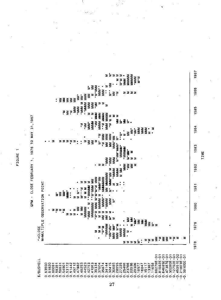
The GPM, together with the soybean, soybean meal and soybean oil prices

are plotted in figures 1 through 4.

FIG

UR

E

1

GPM

-

CLO

SE

FE

BR

UA

RY

1,

19

78

TO

M

AY

31

,19

87

*=C

LOS

E

M=

MU

LTIP

LE

OB

SE

RV

AT

ION

P

OIN

T

t

M

M

'M

M'

t.

M

MM

M

M

M

'M

MM

' M

'M

M

M

M

MM

M'

M

MM

M

M

...

M '

M

'M

MM

M

M

M

* I

M

**

M

MM

M

M

"M

M

MM

9*

*

t.

'MM

M

MM

* M

MM

M

"' M

M

'M

'M

MM

MM

M'

MM

MM

M

M M

M

M

M

'M

M

" MM

MM

MM

M

'MM

M '

M

"MM

MM

M

M

MM

M

MM

' M

M

MM

M

M

M'

MM

MM

MM

M

"M'M

MM

M

M

MM

M

MM

M '

M

MM

M

M

MM

M

'M

'M

MM

M

M'M

'M'M

M

MM

M

'M

M

MM

M

'MM

"M

'MM

M

MM

M

MM

MM

MM

M'M

MM

'MM

M

M

' ' M

M

MM

M M

MM

M

M

MM

" 'M

'M

MM

M

M

MM

M"

MM

MM

MM

M

M

'MM

MM

"M

MM

MM

M

M

MM

' 'M

MM

MM

M

M

M

'MM

MM

M

M

MM

MM

MM

'M

MM

M

M

MM

M

MM

M

MM

MM

M

"

M

M

"MM

'MM

' M

' M

M

MM

'

M'

MM

M'M

M

M

'MM

M

MM

MM

M

'M

M M

M

" M

M

M*

MM

M

MM

* M

M

a M

'M

MM

M

MM

M

MM

M'M

M

* M

M

M

* M

M

MM

M

'M

' M

MM

MM

M

'MM

'MM

M*

M'

MM

M

'M

'

MM

. .

MM

MM

'

. ..

MM

M'

MM

MM

M*

"M'

M'

M'M

M

1

MM

MM

'

MM

M

'MM

MM

M

' M

'

MM

M

M

MM

1

'M

'M

M

'MM

M

'MM

* M

M

M'

M

MM

MM

M

1 '

MM

M

MM

M

M

*

MM

' M

M

MM

MM

1

'MM

' M

M

'M

M'

M

'MM

M

1 '

MM

M

MM

M

'M

t

MM

M

MM

M

M

MM

M

MM

M

M

M

M

M

M'

' M

M

M

M

" M

MM

M

M

M

' M

M

19

78

1

97

9

19

80

1

98

1

19

82

1

98

3

19

84

1

98

5

19

86

1

98

7

TIM

E

FIG

UR

E 2

SO

YB

EA

NS

-

CLO

SIN

G

PR

ICE

S F

EB

RU

AR

Y

1,

19

78

TO

M

AY

31

, 1

98

7

'=C

LOS

E

M=

MU

LTIP

LE

OB

SE

RV

AT

ION

PO

INT

M

M

M

M . . M

' M

"

M

M

* M

M

M

'MM

M

M

M

MM

* M

MM

M

M

MM

M

MM

MM

M

M

MM

M

M

MM

MM

M

M

M

MM

'M

'M

MM

"

**

M

MM

MM

'

MM

M

nMM

MM

M

MM

'M

M

MM

M

MM

MM

'M

M

M

MM

M'M

M

M

M

M

M'

M

MM

'MM

'M

M

MM

M

M

MM

MM

M

M'M

MM

*

MM

M

M

'MM

M

MM

MM

M

*

M'M

IM

M

MM

'

MM

MM

M

M

M* M

M

' M

M'

. . 'M

* M

M

M

MM

MM

* MM

M

M

MM

M

MM

MM

M

I M

'MM

*

MM

M

MM

MM

MM

I

'MM

M

MM

M

MM

' MM

I

MM

M

M

M'M

M

M

M

'M'

MM

' M

M

M

MM

M

M

'MM

M

M

MM

M

M

' M

"

M*

M

* M

MM

M

M

MM

M

M

MM

MM

M

MM

M

MM

M

'

MM

"

M

MM

*

M

MM

M'

MM

t

MM

t

MM

M

M

MM

M

MM

M

MM

MM

M

MM

M

MM

MM

*

MM

MM

M

MM

M

MM

M

M

MM

'M

M' M

' M

MM

M

MM

MM

'

M M

MM

M

* M

M

M

MM

M

M'

M

MM

MM

M

MM

M

M

MM

M

MM

M

M"

M '

MM

' M

* MM

MM

MM

M

M

MM

MM

MM

M

'M

MM

M

M

MM

M

M

M M

M

M'M

MM

MM

M

M

'MM

MM

M

M

M

19

78

1

97

9

19

80

1

98

1

19

82

1

98

3

19

84

1

98

5

19

86

1

98

7

TIM

E

FIG

UR

E 3

SO

YB

EA

N M

EA

L -

CLO

SIN

G

PR

ICE

S F

EB

RU

AR

Y

1.

19

78

TO

M

AY

31

, 1

98

7

'=C

LOS

E

M=

MU

LTIP

LE

OB

SE

RV

AT

ION

P

OIN

T

. .

M

M

MM

M

'

MM

M

M

M

MM

M

MM

M

MM

'M

M

M

MM

MM

M

MM

M

MM

M

MM

M

M

MM

M

MM

M"

M

M

M

MM

' M

MM

MM

M

a M

* M

M

M

MM

MM

'M

M

M

M*

MM

M

M

M'

MM

M

M

M

M

MM

M

MM

'MM

M

M

M

M

M

M

M'M

M

MM

MM

MM

M'

MM

M'M

'

MM

MM

M

MM

M

MM

MM

MM

M

MM

MM

M

* M

MM

M

MM

MM

M

M

MM

M

M

MM

MM

M

M

M

MM

MM

MM

M

MM

M

M

MM

M

* M

MM

M

MM

'MM

M

M

M

MM

MM

M

MM

MM

M

M

MM

M

M

MM

'M

M '

MM

M

MM

MM

M

M

dMM

M

M

M

M'

MM

MM

'M

t*

M

dMM

MM

M

MM

M

M

M

M

M

d 'M

MM

M

M

M

M

MM

M

M

d M

M

MM

M

MM

MM

M

M

' d

'M

MM

' M

MM

M

'Ma

M

d M

M

M' M

' 'M

MM

M

M

M

M

MM

' M

MM

MM

MM

MM

M

M

MM

M

M

MM

M

MM

MM

M'M

M

MM

M

* M

M

M'

MM

M

MM

MM

MM

M

MM

M

MM

M

M M

M

MM

19

78

1

97

9

19

80

1

98

1

19

82

1

98

3

19

84

1

98

5

19

86

1

98

7

TIM

E

FIG

UR

E

4

CR

UD

E

SO

YB

EA

N O

IL

- C

LOS

ING

P

RIC

ES

FE

BR

UA

RY

1

, 1

97

8 T

O

MAY

3

1,1

98

7

*=C

LOS

E

M=

MU

LTIP

LE

OB

SE

RV

AT

ION

PO

INT

M

M

M

M

M

M

M

M

M

M

M

M

M

M"

M

t

M'M

M

M

M

M

'M '

M

M

*M

M

* M

'MM

M"

MM

M

*

MM

M'M

M'

MM

M

* M

M

MM

'M

MM

MM

MM

M

M

MM

M

MM

M

MM

M

*MM

M

'M

'M

M

MM

M

MM

M

MM

M'M

M

M

MM

'M

'M

M

M

MM

M

MM

MM

MM

* M

MM

"M

'

M

MM

M

MM

M

'MM

M

M

M

'MM

' M

MM

MM

M"

MM

M

MM

M

M

t.

M

MM

MM

M'

M'

IMM

M

MM

M

M

MM

MM

M

MM

M' M

'

M

MM

MM

MM

M

MM

IM

M M

MM

MM

.'MM

M

M

MM

MM

' M

M

MM

MM

M

IM

M M

MM

M

MM

M

M

M

MM

M

M

M

M'

M

M'M

M '

MM

M

M

M

M

M

M

M

M

I M

M

MM

M

M

'M'M

M

M

M

M

M

MM

M

M

MM

M*

I M

M

MM

M

MM

M

M

M

I M

M

M

MM

M

M

MM

MM

M

M

MM

MM

I

M

MM

MM

MM

'M

' M

MM

M

MM

MM

M

MM

M

MM

MM

M

'MM

YM

M

MM

M

M

M

'MM

M

M

MM

M

MM

M

MM

M

MM

M

M

MM

MM

M

MM

M

MM

M

M

M

M'M

MM

* M

MM

MM

MM

M

MM

M

MM

M

M

19

78

1

97

9

19

80

1

98

1

19

82

1

98

3

19

84

1

98

5

19

86

1

98

7

TIM

E

The fundamental difference between the GPM and the component series is

tha t the GPM is characterized by more frequent and larger oscillations than the

individual markets. While this characteristic makes medium to long term

speculation quite difficult, (as this would cause large swings in open equity) the

present scope is much finer, a s the rule developed below attempts to capitalize

on price changes between the open and close of a given day.

Rule and Results

While the motivation for the present test came from a visual examination

of the data, the descriptive statistics presented in Table 4 provide enough

insight into the short term price changes which the strategy developed below

attempts to exploit.

Tables 4, a to d reveal some very interesting statistics. First, while none

of the return correlation coefficients are statistically significant for the

individual commodities, very significant negative correlations are found for all

selected returns for the GPM. The largest in absolute magnitude is the

correlation between close to open and open to close returns, which is a n

indication of opening reversals (the tendency of prices to change direction on the

open).

Table 4

Daily return specifications, GPM, soybeans, and soybean meal and oil. February 2, 1978 to May 29,1987. Selected contracts.

a. GPM

Mean Daily Stnd. Coeff. of

Return Return Dev. t-value variation (dbu.) Ho: mean=O

open to open 0.0021 3.655 0.028 1,778.10 close to close 0.0042 2 .789 0.073 674.35 close to open -0 .08 1 2.727 -1 .44 -33 .63 open to close 0.085 2.837 1.45 33 .30

Correlation Coefficients t-value open to open vs. lagcopen to open) -0 .39 -20 .63 close to close vs. lag(c1ose to close) -0 .26 -12 .89 close to open vs. open to close: -0 .49 -12 .89

b. Soybeans


Return Return Dev. t-value Variation (dbu.) Ho: mean=O

open to open -0 .00011 1.097 -0 .005 -1,020.80 close to close -0 .00013 1.046 -0 .006 -826.41 close to open 0.081 0.659 0 .085 56 .87 open to close -0 .00129 0.803 0 .078 -62 .54

Correlation Coefficients t-value open to open vs. lag(open to open) -0 .027 -1.31 close to close vs. lag(c1ose to close) 0.009 0.43 close to open vs. open to close 0.015 0.70

table 4 cont'd.

c. Soybean Meal


Return Return Dev. t-value variation ($/Ton) Ho: mean=0

open to open 0.0038 3.04 0.061 794.74 close to close 0.0040 2.86 0.067 723.24 close to open 0.025 1.837 0 .662 73.83 open to close -0 .021 2.24 0 .454 -107.18

Correlation Coefficients t-value open to open vs. lag(open to open) -0.038 -1.84 close to close vs. lag(c1ose to close) 0.017 0 .82 close to open vs. open to close: -0 .019 0.92

d. Soybean oil


Return ~eturn Dev. t-value Variation ($11 001b.) Ho: mean=0

open to open -0 .00163 0.461 -0.17 close to close -0 .00164 0 .422 -0 .19 close to open -0 .00225 0.278 -0.39 open to close 0.00062 0.327 0.09

Correlation Coefficients t-value open to open vs. lagCopen to open) -0 .041 -1 .99 close to close vs. lag(c1ose to close) 0.030 1.45 close to open vs. open to close -0.035 -1.70

Secondly, with respect to the coefficients of variation, (a measure of

volatility in tha t it is calculated by expressing the standard deviation as a

percentage of the mean) the open to open and close to close coefficients are

substantially greater than those for the close to open and open to close returns

for the GPM, soybeans and meal. For the oil, the coefficient of variation for

the open to close returns is substantially greater, in absolute magnitude, than

the other returns. However, the coefficient of variation for the open to close

returns in the GPM (the only returns which are traded in the present

evaluation) is the lowest in absolute magnitude relative to all other returns of

all the series. Third, all of the returns for each commodity are not significantly

different from zero. This implies t ha t a buy and hold strategy over the present

sample (with rollover as built into the data) in any one of the commodities

would have earned a return less than the return offered from buying T-Bills.

In order to test the exploitability of the open reversals in the GPM, the

following day trading program was developed:

If the GPM on the open is lesslgreater than the previous day's close, a reverse crush/crush spread is opened. The position is then liquidated on the close of the same day.

Filters increasing by multiples of 1~ per bushel are then applied. Real

time trading results were calculated net of trading costs which are believed to

cover both commissions and the difference of expected executions from the open

and close quotations used.

In trading the 10 soybean, 12 meal and 9 oil contract spread, a 1~ per

bushel change in the GPM represents $500.00 on the position. However, in the

discussion to follow, a spread entailing 20 soybean, 24 meal and 18 oil

contracts is assumed. In this way, a 1q per bushel change in the GPM

represents $1000.00 on the spread.

The trading results are not adjusted by, nor compared to, any "naive

strategy" since it is felt that using a standard such as a buy and hold would

not be appropriate. This is because the crush margin average rates of return

are not significantly different from zero on either an open to open or a close to

close basis. Furthermore, the trading costs used, 1.5q per bushel per trade, are

believed to be significantly greater than the returns offered by such a passive

strategy. Using a benchmark, such as a risk-free rate, is deemed to be

unnecessary since no interest income is added to cash balances - increases in

equity or starting equity - as would be realized in trading such a strategy.

Furthermore, a daily rate of interest, even up to annual rates of 50 percent

would only amount to a return of 0.06 cents per bushel per day. (Based on

capital requirements of 44q per bushel - 2 0 . 5 ~ to cover initial margin and

23.5q to cover potential draw downs on equity or strings of losses.)

On the other hand, however, one could use the zero-filter strategy as a

base to which filtered results can be compared, but this would adjust the

returns upwards in all filtered cases.

In addition to this possible source of criticism, an additional possible source

may be due to sampling bias. However, as there is no optimization outside of

selecting a filter size, i t is believed that any such criticism would be

unwarranted.

While the results are catastrophic for a rule without any sort of filter,

employing filters of 1 , 2 and 3 cents, statistically significant average returns of

0.3, 1.0, and 1.69 cents per bushel per trade were recorded. This amounts to

average annual profits of 43, 70 and 56 thousand dollars per year for

the respective filter sizes. This would translate to mean returns of 210, 342

and 273 percent per year based on $20,500 margin; or average annual rates of

return of 98, 159 and 127 percent for the respective filters if one was to also

include a reserve to cover draw downs of $23,500. The margin requirements for

the three commodities for outright as well as hedge and spread

tabled in Table

Soybeans

Soybean Meal Crude Soybean O i l

Table 5 Margin Requirements

Al l amounts are in $ per contract a

Speculative Outright Hedge Spread

I: Initial. M: Maintenance a. source: Rosenthal - Collins Group Ltd.

A s o f May 24, 1989.

As presented in Table 6, as the filter is

orders are

increased to 1, 2 and 3 cents,

the mean per trade return consistently increases in steps of roughly 0.7 cents

ber bushel . The filter increases result in an average increase of $470.00 in

average profits while average loss increases by only $100.00. While the trading

record also improves as the filter is increased, due to the diminishing number

of transactions, the overall effect on annual returns is moderated. In spite of

this fact, the mean annual returns are very impressive.

Table 6 a

T r a d i n g Per formance all s trategies

F i l t e r 0.00 1 . O O 2.00 3.00

Mean per t r ade re turn Stnd. Dev. Sharpe Ratio

Prof i t Stnd. Dev. Sharpe Ratio

Loss Stnd. Dev Sharpe Ratio

Number of Trades

Percent P r o f i t a b l e Trades Adjusted Sharpe Rat io b

Average Annual Return

Annualized Sharpe Ratic

Largest Draw Down

a.All returns standard deviations and draw downs are expressed cents per bu. or $ 000's and all calculations are net of trading costs.

b. Weighted average o f profit and loss Sharpe ratios - weighted by the respective percentages of winning and losing trades.

Adjusting the returns for risk, the above-noted improvements are also

reflected in the Sharpe Ratios (SR). , The SR is a measure of the return per

unit of risk where the measure of risk is taken to be the standard deviation of

returns. The SR steadily increases with larger filters from -0.15 with no filter

to 1.11 with a 39: filter. For 1 and 29: rules, the SRs are 0.15 and 0.57

respectively.

There are, however, certain weaknesses in using the SR as a return-risk

measure, as discussed in Schwager (1984). The first weakness is in the failure

of the ratio to distinguish between intermittent and consecutive losses. However,

in the context of the present evaluation, we may refer to the largest draw

downs on realized equity (or the largest loss) to gauge this aspect. While, with

the no filter strategy, the draw down is basically the entire sample period, with

a filter of 19: the largest draw down amounts to 239: per bushel . With the 2

and 39: filters, the draw downs diminish to 209: per bushel in both cases.

Relative to average annual returns, however, these draw downs are 29 and 36

percent of average annual returns for the 2 and 39: rules respectively

An additional weakness in using the SR relates to its failure to

distinguish between positive and negative fluctuations. In Table 4, an adjusted

SR is calculated where the profit and loss SRs are weighted by their

frequencies, or the trading records. This adjustment lowers the SRs for all filter

rules to -0.42, -0.02, 0.27 and 0.67 for the 0, 1, 2, and 3@ rules.,

While Schwager notes two additional problems in using the Sharpe Ratio:

a dependency on time interval and a failure to distinguish between retracements

in unrealized profits versus retracements from entry date equity, these are not

applicable to the present evaluation. In regards to the dependency on time

interval, here, the results are presented for both per trade and per annum

bases and the per trade results are manifested in the yearly measures. Also,

the time involved in having an open equity position is the same for all

strategies, trades are all day trades only. The difference of retracements in open

versus closed equity is avoided in that all returns and evaluations are

calculated on the basis of the starting equity. There is no reinvestment and

given that these are day trading stystems, there is basically no difference in

that all retracements on open equity (as can be measured) are realized.

The annualized SRs increase through to the 2~ rule from -0.88 to 1.05 for

the raw strategy and I Q rule, to 2.07 for the 2~ strategy. The annualized SR

for the 3~ rule is 1.92.

Table 7 shows the annual summaries. As can be seen, relatively weaker

performance years are generally common to all filter sizes. (1979, 1980, 1985,

1986.) However, for 1981 and 1982, the 0 and 1~ rules seem to have

particularily weak performances yet the 2 and 3 cent results are very strong in

both records of profitable trades and expected returns per trade. Both 1983 and

1984 were relatively strong years for all trading rules. Taking the results year

by year, we see that for filter sizes of 2 and 3 ~ , all years were significantly

profitable. Annual returns range from 16.3 to 1 4 5 . 3 ~ per bushel for the 2~ rule

and from 7 to 1 2 3 . 2 ~ per bushel for the 3~ filter rule. The average returns

per trade range from $400 to $1,500 and from $530 to $2,420 for the

respective filters.

The Sharpe Ratios for the two rules range from 0.16 to 1.26 for the 2@

and from 0.26 to 3.80 for the 3~ rule.

Table 7

Annual Summaries-ALL strategies February 01,1978 to May 29, 1987

Filter Year 0.00 0.01 0.02 0.03

All returns are expressed as ~ l b u .

1978 Number trades 251 166 96 47 % profitable 48.2 1 54.22 64.58 78.72 Mean return per trade 0.03 0.54 1.16 2.15 Standard dev. 2.69 2.15 1.80 1.53 Sharpe Ratio 0.01 0.25 0.64 1.41 Annual Return 7.40 89.84 111.09 101.13

1979 Number trades 247 151 74 37 % profitable 41.7 49.67 58.11 54.05 Mean return per trade -0.08 0.48 0.92 1.03 Standard dev. 2.85 2.28 1.75 1.44 Sharpe Ratio -0.30 0.21 0.53 0.72 Annual Return -20.65 71.76 67.73 37.93

1980 Number trades 247 155 92 5 1 % profitable 40.49 51.66 56.52 58.82 Mean return per trade -0.62 -0.01 0.37 0.53 Standard dev. 3.12 2.62 2.26 2.03 Sharpe Ratio -0.20 -0.004 0.16 0.26 Annual Return -153.24 -2.05 34.00 26.93

1981 Number trades % profitable 36.80 49.23 63.64 70.83 Mean return per trade -0.49 0.34 1.20 2.20 Standard dev. 2.37 1.86 1.57 1.33 Sharpe Ratio -0.21 0.18 0.76 1.65 Annual Return -122.10 44.62 78.99 52.91

1982 Number trades % profitable 27.31 45.65 67.57 75.0 Mean return per trade -0.68 0.002 0.72 2.09 Standard dev. 1.38 0.89 0.69 0.55 Sharpe Ratio -0.49 0 .002 1.04 3.80 Annual Return -169.82 0.16 26.70 16.72

Table 7 continued.

1983 Number trades % profitable Mean return per trade Standard dev. Sharpe Ratio Annual Return


1985 Number trades % profitable Mean Return per trade Standard dev. Sharpe Ratio Annual Return


1 98 7 (August, 1987 contract only) Number trades 82 38 % profitable 29.27 44.74 Mean return per trade -0.81 -0.22 Standard dev. 1.59 1.21 Sharpe Ratio -0.50 -0.18 Cumulative Return -66.03 -8.53

The trading results for the 1~ filter were slightly mixed in that annual

returns range from -2.05 to 113.96Q per bushel . (The 1987 results to May 31

posted a cumulative loss of 8.53 cents. However, this should be discounted since

this amount is significantly lower than the maximum draw down.) The SRs

range from -0.004 to 0.26. ( For the four months to May 31, 1987, the SR

was -0.18.)

With regards to the basic strategy employing no filter, mean per trade

returns range from -0.81 to 0 . 0 3 ~ per bushel . Adjusted for risk, the Sharpe

Ratios range from -0.50 to 0.01. When coupled with the trading records which

are consistently less than 50 percent, this amounts to annual returns ranging

from -169.82 to 7 . 4 ~ per bushel .

To see if there is a significant difference between long and short trades,

performance summaries of long only and short only opening-gap strategies were

calculated. This distinction relates back to the mean daily open to close return

calculated in Table 4. While not statistically significant a t the selected level of

confidence, the mean return of 0.085 cents per bushel is statistically significant

a t a confidence level of 90 percent. Thus, one may expect better performance of

long trades. These results are tabled in Table 8.

Table 8

' Long1 Short only filter strategies

All returns in Qlbu. or $ 000's

FILTER

1 2 3

Long only

Mean Return Standard Dev. Number trades % prof itable

Short only

Mean Return Standard Dev. Number trades % profitable

While for the 1 q rule the mean per trade returns are almost equal, they

begin to diverge as the filter is increased to 2 and 3 cents. As the proportion

of long trades is basically equal to one half in each of the three scenarios,

there is no apparent bias in either the direction of the opening-gaps or their

magnitude. Therefore, the performances of long and short trades are basically

the same in terms of mean per trade returns, number of trades and standard

deviation of returns for each filter size. In this way, both types of trades

contribute equally to the overall performance of the three strategies.

These real time trading results for the noted strategies provide strong

evidence of (the so called weak-form) inefficiency in the soybean complex futures

markets. Significant dependencies (as indicated by the significant returns from

the trading strategies) indicate tha t CBOT soybean, soybean meal and soybean

oil futures prices are not random per se since while the departures implied by

the posted simulations may be intemporally random, the realized returns of the

trading rules, especially the 2 and 3~ filter strategies, offer systematic

significant "excess" returns.

This result is consistent with the result of "irregular dependencies" (or

irregular regularities) for the commodities of the soybean complex as found by

Helms e t a1 (1984).

The short term reversals found herein complement similar evidence found

in Dooley and Shafer (1983) for the New York foreign exchange market.

However, while Stevenson and Bear (1970) reported similar results for soybeans

and corn futures over the twelve year period 1957 to 1968, the evidence for

soybean futures was only significant for large filters and even then, the

performance over a buy and hold was only equal to $8,554 on the basis of two

contract positions. This return represents a n annual average return of $713. On

the basis of comparable margin requirements of $1500 per contract, this

corresponds to a n average annual rate of return of 24%. Additionally, the

estimated one period lag serial correlations for soybeans found in the present

sample are considerably less than those reported in Stevenson and Bear.

As the entire results are net of reasonable trading costs, on the basis of

the reported results, hypotheses such as Jensen's (1978) EMH and the RWH can

be rejected with high levels of confidence.

VII SUMMARY AND CONCLUSION

In this paper, day trading strategies have been used for the Chicago Board

of Trade soybean complex for the period 1978 to 1987 to test for both

dependencies in price changes and a possible profitable exploitation of these

dependencies.

Strong evidence of dependency was found. The correlation is

sufficiently great for a trading strategy to yield annual average net

returns of up to 70 cents per bushel , or $70,000 on a spread made up

of 20 soybean, 24 soybean meal and 18 crude soybean oil futures

contracts. With conservative criteria, inefficiency is indicated by persistent

profitability of a very basic rule based on trading the opening-gap in the crush

margin of soybean processors. These results lead to the rejection of the

hypothesis tha t price changes are independent of previous price changes and

suggest tha t models of speculative competitive markets with diffuse information

such a s those of Grossman (1976) and Grossman and Stiglitz (1976) require

additional constraints in the structure of the market for information.

As a n explanation for the existence of the results, it is proposed tha t due

to the absence of enforceable property rights with respect to the technology of

speculation and hedging, the informational aspect of securities markets ought to

be structured as a monopolistic competitive market. The critical implication of

this proposal is that efficiency in the pricing of securities is not

possible.

NOTES

1. The Sharpe Ratio was calculated as:

exiected rate of return ............................ standard deviation o f expected rate o f return

2. The adjusted Sharpe Ratio was calculated as:

(% profitable trades) ( SR (profit)) - (% losers) ( SR (losers))

The mean profit and loss are in @/bu or $ 000's return.

REFERENCES

Arthur, H.B. (1971) Commodity Futures as a Business Management Tool, Harvard University Press, Boston.

Bird, P. J. W. N. (1985) The weak form efficiency of the London Metal Exchange, Applied Economics, 17, 571-587.

Burns, J. M. (1983) Futures markets and market efficiency, in Futures Markets, (Ed.) M. E. Streit. Basil Blackwell, q6&%4 r7 7 Oxford.

Danthine, J.P. (1977) Martingale, market efficiency and commodity prices, European Economic Review, 10, 1 - 17.

Dooley, M.P. and J. Shafer, (1983) Ananlysis of short-run exchange behavior: March 1973 to November 1981, in Exchange Rate and Trade Instability, (Ed.) D.Bigman and T. Taya. Ballinger Publishing Co. Cambridge, Mass.

Eastbrook, F. H. (1986) Monopoly, Manipulation and the regulation of futures markets, Journal of Business, 59, s105-s127.

Fama, E. F. (1970) Efficient capital markets:a review of theory and empirical work, Journal of Finance, 25, 383-426.

---------- (1976) Foundations of Finance, Basil Blackwell, Oxford.

Figlewski, S. (1978) Market "efficiency" in a market with heterogeneous information, Journal of Political Economy, 86, 581-597.

Grossman, S. (1976) On the efficiency of competitive stock markets where traders have diverse information, Journal of Finance, 31, 573-585.

-------- and J. Stiglitz (1 976) Information and competitive price systems, American Economic Review, 66, 246-253.

Helms, B.P., R. Kaen and R. E. Rosenman. (1984) Memory in commodity futures contracts, Journal of Futures Markets, -r 4, 559-567.

Houthakker, H. S. (1961) Systematic and random elements in short-term price movements, American Economic Review,

51, 164-172.

Jensen, M. C. (1978) Some anomalous evidence regarding market efficiency, Journal of Financial Economics, 6, 95- 10 1.

Kaufman, P. J . (1987) The New Commodity Trading Systems and Methods, John Wiley & Sons, New York.

Kyle, A. S. (1984) A theory of futures market manipulations, in The Industrial Organization of Futures Markets, (Ed.) R. W. Anderson, Lexington Books, Lexington, Mass.

LeRoy, S. F. (1982) Expectation models of asset prices: A survey of theory, The Journal of Finance, 37, 185-217.

Leuthold, R. M. (1972) Random walks and price trends: the live cattle futures market, Journal of Finance, 27, 879-889.

Lucas, R. E. J r . (1978) Asset prices in a n exchange economy, Econometrica, 46, 142% 1445. .f7

/ I

Martin, J. D., S. H. Cox and R. D. MacMinn. (1988) The Theory ,

of Finance: Evidence and Applications, Dryden Press, New /d (s f (3$3 \ York.

Newberry, D.M.G. (1984) The manipulation of futures markets by a dominant. producer, in The Industrial Organization of . r f - > Futures Markets, (Ed.) R. W. Anderson, Lexindon Books, ~ 6 ; 6 0 ) f 4) ' --, Lexington.

Rausser, G. C. and C. Carter. (1983) Futures market efficiency in the soybean complex, Review of Economic Studies, 65, 469-478.

Rose, F. S. and R. E. Sheldon. (1984) The soybean complex cash (2 2

and futures markets, in Handbook of Futures Markets, ,4 6 60 . /f j 6 ; (Ed.) P. J . Kaufman. John Wiley & Sons, New York.

Schwager, J. D. A. (1984) A Complete Guide to the Futures 4 ~ 6 y r ? -' Markets, John Wiley & Sons, New York. ,

Sharp, W. F. (1978) Investments, Prentice Hall, Englewood Cliffs, N.J.

Smidt, S. (1965) A test of serial independence of price changes in soybean futures, in Selected Writings on Futures (-1 4 h '? 6 ' ' Markets: Basic Research in Commodity Markets, (Ed.) A. E. Peck, Chicago Board of Trade, (1983).

Stevenson, R. A. and R. M. Bear (1970) Commodity futures: trends or random walks, Journal of Finance, 25, 65-8 1.

Taylor, S. J. (1985) The behavior of futures prices over time, Applied Economics, 17, 713-734.

Telser, L. G. (1981) Why there are organized futures markets, The Journal of Law and Economics, 24, 1-22.

Putting on the crush : market structure, information and ...

Documents