UNIT I PURPOSE OF DATABASE SYSTEM The typical file processing system is supported by a conventional operating system. The system stores permanent records in various files, and it needs different application programs to extract records from, and add records to, the appropriate files. A file processing system has a number of major disadvantages. 1.Data redundancy and inconsistency: In file processing, every user group maintains its own files for handling its data processing applications. Example: Consider the UNIVERSITY database. Here, two groups of users might be the course registration personnel and the accounting office. The accounting office also keeps data on registration and related billing information, whereas the registration office keeps track of student courses and grades.Storing the same data multiple times is called data redundancy.This redundancy leads to several problems. •Need to perform a single logical update multiple times. •Storage space is wasted. •Files that represent the same data may become inconsistent. Data inconsistency is the various copies of the same data may no larger Agree. Example: One user group may enter a student's birth date erroneously as JAN-19-1984, whereas the other user groups may enter the correct value of JAN-29-1984. 2.Difficulty in accessing data File processing environments do not allow needed data to be retrieved in a convenient and efficient manner. Example: Suppose that one of the bank officers needs to find out the names of all customers who live within a particular area. The bank officer ha„ now two choices: cither obtain the list of all customers and extract the needed information manually or ask a system programmer to write the necessary application program. Both alternatives are obviously unsatisfactory. Suppose that such a program is written, and that, several days later, the same officer needs to trim that list to

Welcome message from author
This document is posted to help you gain knowledge. Please leave a comment to let me know what you think about it! Share it to your friends and learn new things together.
Transcript

UNIT I
PURPOSE OF DATABASE SYSTEM
The typical file processing system is supported by a conventional operating system. The system
stores permanent records in various files, and it needs different application programs to extract
records from, and add records to, the appropriate files.
A file processing system has a number of major disadvantages.
1.Data redundancy and inconsistency:
In file processing, every user group maintains its own files for handling its data processing
applications.
Example:
Consider the UNIVERSITY database. Here, two groups of users might be the course registration
personnel and the accounting office. The accounting office also keeps data on registration and
related billing information, whereas the registration office keeps track of student courses and
grades.Storing the same data multiple times is called data redundancy.This redundancy leads to
several problems.
•Need to perform a single logical update multiple times.
•Storage space is wasted.
•Files that represent the same data may become inconsistent.
Data inconsistency is the various copies of the same data may no larger Agree.
Example:
One user group may enter a student's birth date erroneously as JAN-19-1984,
whereas the other user groups may enter the correct value of JAN-29-1984.
2.Difficulty in accessing data
File processing environments do not allow needed data to be retrieved in a convenient and
efficient manner.
Example:
Suppose that one of the bank officers needs to find out the names of all customers who live
within a particular area. The bank officer ha„ now two choices: cither obtain the list of all
customers and extract the needed information manually or ask a system programmer to write the
necessary application program. Both alternatives are obviously unsatisfactory. Suppose that such
a program is written, and that, several days later, the same officer needs to trim that list to
include only those customers who have an account balance of $10,000 or more. A program to
generate such a list does not exist. Again, the officer has the preceding two options, neither of
which is satisfactory.
3.Data isolation
Because data are scattered in various files, and files may be in different formats, writing new
application programs to retrieve the appropriate data is difficult.
4.Integrity problems
The data values stored in the database must satisfy certain types of consistency constraints.
Example:
The balance of certain types of bank accounts may never fall below a prescribed amount .
Developers enforce these constraints in the system by addition appropriate code in the various
application programs
5.Atomicity problems
Atomic means the transaction must happen in its entirety or not at all. It is difficult to ensure
atomicity in a conventional file processing system.
Example:
Consider a program to transfer $50 from account A to account B. If a system failure occurs
during the execution of the program, it is possible that the $50 was removed from account A but
was not credited to account B, resulting in an inconsistent database state.
6.Concurrent access anomalies
For the sake of overall performance of the system and faster response, many systems allow
multiple users to update the data simultaneously. In such an environment, interaction of
concurrent updates is possible and may result in inconsistent data. To guard against this
possibility, the system must maintain some form of supervision. But supervision is difficult to
provide because data may be accessed by many different application programs that have not been
coordinated previously.
Example: When several reservation clerks try to assign a seat on an airline flight, the system
should ensure that each seat can be accessed by only one clerk at a time for assignment to a
passenger.
7. Security problems
Enforcing security constraints to the file processing system is difficult

VIEWS OF DATA
A major purpose of a database system is to provide users with an abstract view of the data i.e the
system hides certain details of how the data are stored and maintained.
Views have several other benefits.
•Views provide a level of security. Views can be setup to exclude data that some users should
not see.
•Views provide a mechanism to customize the appearance of the database.
•A view can present a consistent, unchanging picture of the structure of the database, even if the
underlying database is changed.
The ANSI / SPARC architecture defines three levels of data abstraction.
•External level / logical level
•Conceptual level
•Internal level / physical level
The objectives of the three level architecture are to separate each user's view of the database
from the way the database is physically represented.
External level
The users' view of the database External level describes that part of the database that is relevant
to each user.
The external level consists of a number of different external views of the database. Each user has
a view of the 'real world' represented in a form that is familiar for that user. The external view
includes only those entities, attributes, and relationships in the real world that the user is
interested in.
The use of external models has some very major advantages,
•Makes application programming much easier.
•Simplifies the database designer's task.
•Helps in ensuring the database security.
Conceptual level

The community view of the database conceptual level describes what data is stored in the
database and the relationships among the data.
The middle level in the three level architecture is the conceptual level. This level contains the
logical structure of the entire database as seen by the DBA. It is a complete view of the data
requirements of the organization that is independent of any storage considerations. The
conceptual level represents:
•All entities, their attributes and their relationships
•The constraints on the data
•Semantic information about the data
•Security and integrity information.
The conceptual level supports each external view. However, this level must not contain any
storage dependent details. For instance, the description of an entity should contain only data
types of attributes and their length, but not any storage consideration such as the number of bytes
occupied.
Internal level
The physical representation of the database on the computer Internal level describes how the data
is stored in the database.
The internal level covers the physical implementation of the database to achieve optimal runtime
performance and storage space utilization. It covers the data structures and file organizations
used to store data on storage devices.The internal level is concerned with
•Storage space allocation for data and indexes.
•Record descriptions for storage
•Record placement.
•Data compression and data encryption techniques.
•Below the internal level there is a physical level that may be managed by the operating system
under the direction of the DBMS
Physical level
•The physical level below the DBMS consists of items only the operating system knows such as
exactly how the sequencing is implemented and whether the fields of internal records are stored
as contiguous bytes on the disk.
Instances and Schemas

Similar to types and variables in programming languages which we already know, Schema is the
logical structure of the database E.g., the database consists of information about a set of
customers and accounts and the relationship between them) analogous to type information of a
variable in a program.
Physical schema: database design at the physical level
Logical schema: database design at the logical level
DATA MODELS
The data model is a collection of conceptual tools for describing data, data relationships, data
semantics, and consistency constraints. A data model provides a way to describe the design of a
data base at the physical, logical and view level.
The purpose of a data model is to represent data and to make the data understandable.
According to the types of concepts used to describe the database structure, there are three data
models:
1.An external data model, to represent each user's view of the organization.
2.A conceptual data model, to represent the logical view that is DBMS independent
3.An internal data model, to represent the conceptual schema in such a way that it can be
understood by the DBMS.
Categories of data model:
1.Record-based data models
2.Object-based data models
3.Physical-data models.
The first two are used to describe data at the conceptual and external levels, the latter is used to
describe data at the internal level.
1.Record -Based data models
In a record-based model, the database consists of a number of fixed format records possibly of
differing types. Each record type defines a fixed number of fields, each typically of a fixed
length.
There are three types of record-based logical data model.
•Hierarchical data model.

•Network data model
•Relational data model
Hierarchical data model
In the hierarchical model, data is represented as collections of records and relationships are
represented by sets. The hierarchical model allows a node to have only one parent. A hierarchical
model can be represented as a tree graph, with records appearing as nodes, also called segments,
and sets as edges.
Network data model
In the network model, data is represented as collections of records and relationships are
represented by sets. Each set is composed of at least two record types:
•An owner record that is equivalent to the hierarchical model's parent
•A member record that is equivalent to the hierarchical model's child
A set represents a 1 :M relationship between the owner and the member.
Relational data model:
The relational data model is based on the concept of mathematical relations. Relational model
stores data in the form of a table. Each table corresponds to an entity, and each row represents an
instance of that entity. Tables, also called relations are related to each other through the sharing
of a common entity characteristic.
Example
Relational DBMS DB2, oracle, MS SQLserver.
2. Object -Based Data Models
Object-based data models use concepts such as entities, attributes, and relationships.An entity is
a distinct object in the organization that is to be represents in the database. An attribute is a
property that describes some aspect of the object, and a relationship is an association between
entities. Common types of object-based data model are:
•Entity -Relationship model
•Object -oriented model
•Semantic model
Entity Relationship Model:
The ER model is based on the following components:
•Entity: An entity was defined as anything about which data are to be collected and stored. Each
row in the relational table is known as an entity instance or entity occurrence in the ER model.
Each entity is described by a set of attributes that describes particular characteristics of the entity.
Object oriented model:
In the object-oriented data model (OODM) both data and their relationships are contained in a
single structure known as an object.An object is described by its factual content. An object
includes information about relationships between the facts within the object, as well as
information about its relationships with other objects. Therefore, the facts within the object are
given greater meaning. The OODM is said to be a semantic data model because semantic
indicates meaning.The OO data model is based on the following components:
An object is an abstraction of a real-world entity.
Attributes describe the properties of an object.
DATABASE SYSTEM ARCHITECTURE
TTrraannssaaccttiioonn MMaannaaggeemmeenntt
A transaction is a collection of operations that performs a single logical function in a database
application.Transaction-management component ensures that the database remains in a
consistent (correct) state despite system failures (e.g. power failures and operating system
crashes) and transaction failures.Concurrency-control manager controls the interaction among
the concurrent transactions, to ensure the consistency of the database.
Storage Management
A storage manager is a program module that provides the interface between the low-level data
stored in the database and the application programs and queries submitted to the system.
The storage manager is responsible for the following tasks:
Interaction with the file manager
Efficient storing, retrieving, and Storage Management
A storage manager is a program module that provides the interface between the low-level data
stored in the database and the application programs and queries submitted to the system.
The storage manager is responsible for the following tasks:

Interaction with the file manager
Efficient storing, retrieving, and updating of data
Database Administrator
Coordinates all the activities of the database system; the database administrator has a good
understanding of the enterprise’s information resources and needs:
Schema definition
Storage structure and access method definition
Schema and physical organization modification
Granting user authority to access the database
Specifying integrity constraints
Acting as liaison with users
Monitoring performance and responding to changes in requirements
Database Users
Users are differentiated by the way they expect to interact with the system.
Application programmers: interact with system through DML calls.
Sophisticated users – form requests in a database query language
Specialized users – write specialized database applications that do not fit into the traditional
data processing framework
Naive users – invoke one of the permanent application programs that have been written
previously
File manager
manages allocation of disk space and data structures used to represent information on disk.
Database manager
The interface between low level data and application programs and queries.
Query processor
translates statements in a query language into low-level instructions the database manager
understands. (May also attempt to find an equivalent but more efficient form.)
DML precompiler
converts DML statements embedded in an application program to normal procedure calls in a
host language. The precompiler interacts with the query processor.
DDL compiler
converts DDL statements to a set of tables containing metadata stored in a data dictionary. In
addition, several data structures are required for physical system implementation:
Data files:store the database itself.
Data dictionary:stores information about the structure of the database. It is used heavily. Great
emphasis should be placed on developing a good design and efficient implementation of the
dictionary.
Indices:provide fast access to data items holding particular values.
ENTITY RELATIONSHIP MODEL
The entity relationship (ER) data model was developed to facilitate database design by
allowing specification of an enterprise schema that represents the overall logical structure of a
database. The E-R data model is one of several semantic data models.
The semantic aspect of the model lies in its representation of the meaning of the data. The E-R
model is very useful in mapping the meanings and interactions of real-world enterprises onto a
conceptual schema.
The ERDs represent three main components entities, attributes and relationships.
Entity sets:
An entity is a thing or object in the real world that is distinguishable from all other objects.
Example:
Each person in an enterprise is entity.

An entity has a set of properties, and the values for some set of properties may uniquely identify
an entity.
Example:
A person may have a person-id would uniquely identify one particular property whose value
uniquely identifies that person.
An entity may be concrete, such as a person or a book, or it may be abstract, such as a loan, a
holiday, or a concept.An entity set is a set of entities of the same type that share the same
properties, or attributes.
Example:
Relationship sets:
A relationship is an association among several entities.
Example:
A relationship that associates customer smith with loan L-16, specifies that Smith is a customer
with loan number L-16.
A relationship set is a set of relationships of the same type.
The number of entity sets that participate in a relationship set is also the degree of the
relationship set.
A unary relationship exists when an association is maintained within a single entity.
Attributes:
For each attribute, there is a set of permitted values, called the domain, or value set, of that
attribute. Example:
The domain of attribute customer name might be the set of all text strings of a certain length.
An attribute of an entity set is a function that maps from the entity set into a domain.
An attribute can be characterized by the following attribute types:
•Simple and composite attributes.
•Single valued and multi valued attributes.
•Derived attribute.
Simple attribute (atomic attributes)
An attribute composed of a single component with an independent existence is called simple
attribute.
Simple attributes cannot be further subdivided into smaller components.

An attribute composed of multiple components, each with an independent existence is called
composite attribute.
Example:
The address attribute of the branch entity can be subdivided into street, city, and postcode
attributes.
Single-valued Attributes:
An attribute thatholds a single value for each occurrence of an entity type is called single valued
attribute.
Example:
Each occurrence of the Branch entity type has a single value for the branch number (branch No)
attribute (for example B003).
Multi-valued Attribute
An attribute that holds multiple values for each occurrence of an entity type is called multi-
valued attribute.
Example:
Each occurrence of the Branch entity type can have multiple values for the telNo attribute (for
example, branch number B003 has telephone numbers 0141-339-2178 and 0141-339-4439).
Derived attributes
An attribute that represents a value that is derivable from the value of a related attribute or set of
attributes, not necessarily in the same entity type is called derived attributes.
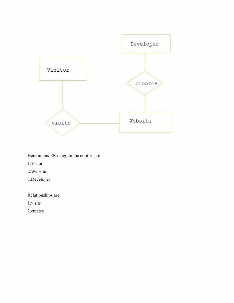
Here in this ER diagram the entities are
1.Vistor
2.Website
3.Developer
Relationships are
1.visits
2.creates
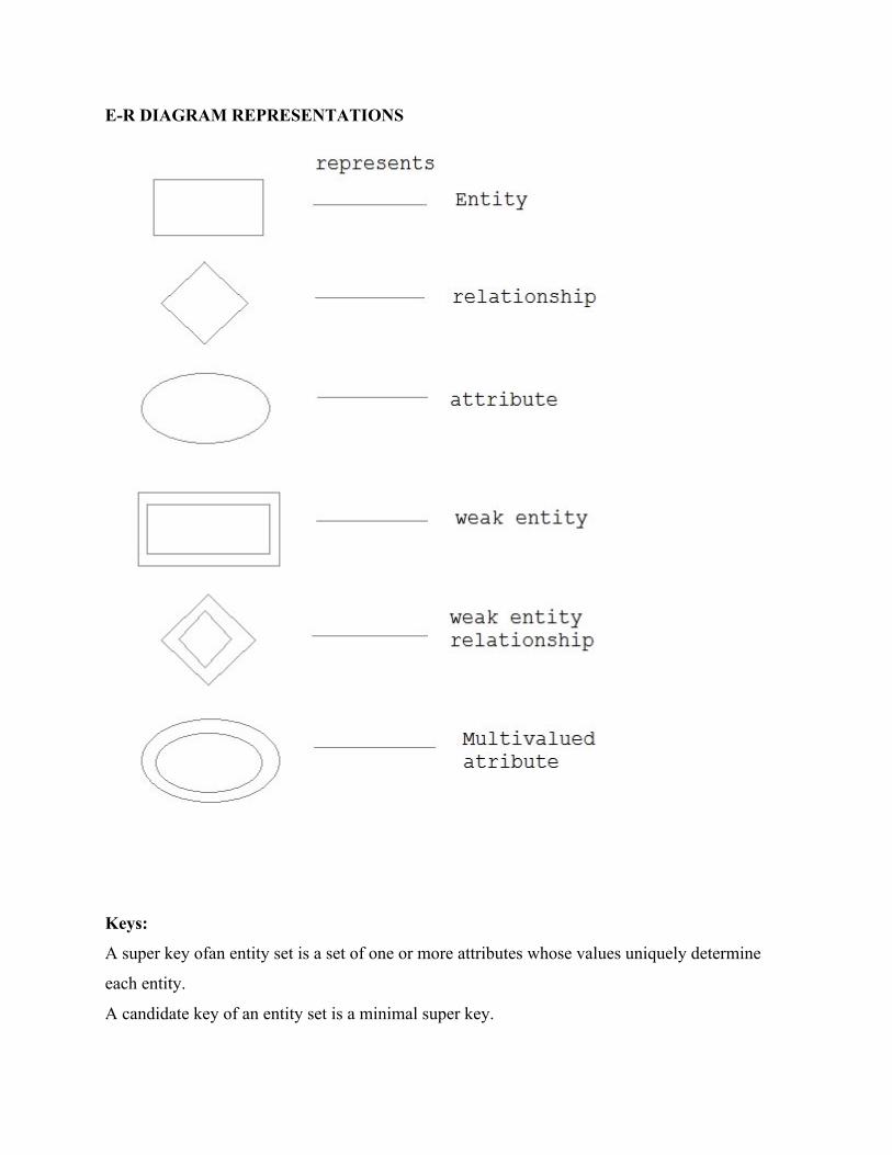
E-R DIAGRAM REPRESENTATIONS
Keys:
A super key ofan entity set is a set of one or more attributes whose values uniquely determine
each entity.
A candidate key of an entity set is a minimal super key.

–social-security is candidate key of customer
–account-number is candidate key of account
Although several candidate keys may exist, one of the candidate keys is selected to be the
primary key.
The combination of primary keys of the participating entity sets forms a candidate key of a
relationship set.
- must consider the mapping cardinality and the semantics of the relationship set when selecting
the primary key.
– (social-security, account-number) is the primary key of depositor
E-R Diagram Components
Rectangles represent entity sets.
Ellipses represent attributes.
Diamonds represent relationship sets.
Lines link attributes to entity sets and entity sets to relationship sets.
Double ellipses represent multivalued attributes.
Dashed ellipses denote derived attributes.
Primary key attributes are underlined.
Weak Entity Set
An entity set that does not have a primary key is referred to as a weak entity set. The existence of
a weak entity set depends on the existence of a strong entity set;it must relate to the strong set via
a one-to-many relationship set. The discriminator (or partial key) of a weak entity set is the set of
attributes that distinguishes among all the entities of a weak entity set. The primary key of a
weak entity set is formed by the primary key of the strong entity set on which the weak entity set
is existence dependent,plus the weak entity set’s discriminator. A weak entity set is depicted by
double rectangles
Specialization
This is a Top-down design process designate subgroupings within an entity set that are
distinctive from other entitie in the set.
These subgroupings become lower-level entity sets that have attributes or participate in
relationships that do not apply to the higher-level entity set.
Depicted by a triangle component labeled ISA (i.e., savings-account “is an”account
Generalization:
A bottom-up design process – combine a number of entity sets that share the same features into a
higher-level entity set.
Specialization and generalization are simple inversions of each other; they are represented in an
E-R diagram in the same way.
Attribute Inheritance – a lower-level entity set inherits all the attributes and relationship
participation of the higher-level entity set to which it is linked.
Design Constraints on Generalization:
Constraint on which entities can be members of a given lower-level entity set.
– condition-defined
– user-defined
-Constraint on whether or not entities may belong to more than one lower-level entity set within
a single generalization.
– disjoint
– overlapping
-Completeness constraint – specifies whether or not an entity in the higher-level entity set must
belong to at least one of the lower-level entity sets within a generalization.
– total
- partial Joints in Aggregation
– Treat relationship as an abstract entity.
– Allows relationships between relationships.
– Abstraction of relationship into new entity.
–Without introducing redundancy, the following diagram represents that:
– A customer takes out a loan
– An employee may be a loan officer for a customer-loan pair
RELATIONAL DATABASES
A relational database is based on the relational model and uses a collection of tables to
represent both data and the relationships among those data. It also includes a DML and DDL.
The relational model is an example of a record-based model.
Record-based models are so named because the database is structured in fixed-format records of
several types.
A relational database consists of a collection of tables, each of which is assigned a unique name.
A row in a table represents a relationship among a set of values.
A table is an entity set, and a row is an entity. Example: a simple relational database.
Columns in relations (table) have associated data types.
The relational model includes an open-ended set of data types, i.e. users will be able to define
their own types as well as being able to use system-defined or built in types.
Every relation value has two pairs
1)A set of column-name: type-name pairs.
2)A set of rows
The optimizer is the system component that determines how to implement user requests. The
process of navigating around the stored data in order to satisfy the user's request is performed
automatically by the system, not manually by the user. For this reason, relational systems are
sometimes said to perform automatic navigation.Every DBMS must provide a catalog or
dictionary function
. The catalog is a place where all of the various schemas (external, conceptual, internal) and all
of the corresponding mappings (external/conceptual, conceptual/internal) are kept. In other
words, the catalog contains detailed information (sometimes called descriptor information or
metadata) regarding the various objects that are of interest to it.
A relational database is based on the relational model and uses a collection of tables to
represent both data and the relationships among those data. It also includes a DML and DDL.
The relational model is an example of a record-based model. Record-based models are so named
because the database is structured in fixed-format records of several types.
A relational database consists of a collection of tables, each of which is assigned a unique name.
A row in a table represents a relationship among a set of values.
A table is an entity set, and a row is an entity. Example: a simple relational database.

Columns in relations (table) have associated data types.
The relational model includes an open-ended set of data types, i.e. users will be able to define
their own types as well as being able to use system-defined or built in types.
Every relation value has two pairs
1)A set of column-name: type-name pairs.
2)A set of rows
The optimizer is the system component thahe system itself.
Example:
Relation variables, indexes, users, integrity constraints, security constraints, and so on.
The catalog itself consists of relvars. (system relvars).
The catalog will typically include two system relvars called TABLE and COLUMN.
The purpose of which is to describe the tables in the database and the columns in those tables.
RELATIONAL MODEL EXAMPLE

RELATIONAL ALGEBRA
A basic expression in the relational algebra consists of either one of the following:
oA relation in the database
oA constant relation
Let E1and E2be relational-algebra expressions; the following are all relational-algebra
expressions:
E1nE2
E1- E2
E1x E2
p(E1), Pis a predicate on attributes in E1
s(E1), Sis a list consisting of some of the attributes in E1
x (E1), x is the new name for the result of E1
The select, project and rename operations are called unary operations, because they operate on
one relation.
The union, Cartesian product, and set difference operations operate on pairs of relations and are
called binary operations
Selection (or Restriction) (σ)
The selection operation works on a single relation R and defines a relation that contains only
those tuples of R that satisfy the specified condition (predicate).
Syntax:
σPredicate (R)
Example:
List all staff with a salary greater than 10000.
Sol:
salary > 10000 (Staff).
The input relation is staff and the predicate is salary>10000. The selection operation defines a
relation containing only those staff tuples with a salary greater than 10000.
Projection (π):
The projection operation works on a single relation R and defines a relation that contains a
vertical subset of R, extracting the values of specified attributes and eliminating duplicates.
Syntax:
π al,.......an(R)
Example:
Produce a list of salaries for all staff, showing only the staffNo, name and salary.
Π staffNo. Name, Salary (Staff).
Rename (ρ):
Rename operation can rename either the relation name or the attribute names or both
Syntax:
ρs (BI.B2,.Bn) (R) Or ρs(R) Or p (B1.B2Bn) (R)
S is the new relation name and B1, B2,.....Bn are the new attribute names.
The first expression renames both the relation and its attributes, the second renames the relation
only, and the third renames the attributes only. If the attributes of R are (Al, A2,...An) in that
order, then each Aj is renamed as Bj.
Union
The union of two relations R and S defines a relation that contains all the tuples of R or S or both
R and S, duplicate tuples being eliminated. Union is possible only if the schemas of the two
relations match.
Syntax:
R U S
Example:
List all cities where there is either a branch office or a propertyforRent.
πCity (Branch) U π civ(propertyforRent)
Set difference:
The set difference operation defines a relation consisting of the tuples that are in relation R, but
not in S. R and S must be union-compatible.
Syntax
R-S
Example:
List all cities where there is a branch office but no properties for rent.
Sol.:
Π city (Branch) –π city(propertyforRent)
Intersection
The intersection operation defines a relation consisting of the set of all tuples that are in both R
and S. R and S must be union compatible.
Syntax:
R∩S
Example:
List all cities where there is both a branch office and at least one propertyforRent.
πciity (Branch) ∩ πCjty (propertyforRent)
Cartesian product:
The Cartesian product operation defines a relation that is the concatenation of every tuple of
relation R with every tuple of relation S.
Syntax:
R X S
Example:
List the names and comments of all clients who have viewed a propertyforRent.
Sol.:
The names of clients are held in the client relation and the details of viewings are held in the
viewing relation. To obtain the list of clients and the comments on properties they have viewed,
we need to combine two relations.
DOMAIN RELATIONAL CALCULUS
Domain relational calculus uses the variables that take their values from domains of attributes.
An expression in the domain relational calculus has the following general form
{dl,d2,......dn/F(dl,d2,..............dm)} m > n
Where dl,d2,....dn.....,dtn represent domain variables and F(dl,d2,...dm)
represents a formula composed of atoms, where each atom has one of the following forms:
•R(dl,d2,.......dn), where R is a relation of degree n and each d; is a domain variable.
•dj Өdj, where dj and dj are domain variables and 9 is one of the comparison operations (<, < >,
>, =,)

•dj Ө C, where d, is a domain variable, C is a constant and 8 is one of the comparison operators.
Recursively build up formulae from atoms using the following rules:
•An atom is a formula.
•If Fl and F2 are formulae, so are their conjunction Fl ∩ F2, their disjunction Fl U F2 and the
negation ~Fl
TUPLE RELATIONAL CALCULUS
Tuple variable –associated with a relation( called the range relation)
•takes tuples from the range relation as its values
•t: tuple variable over relation rwith scheme R(A,B,C )t
.Astands for value of column Aetc
TRC Query –basic form:
{ t1.Ai1, t2.Ai2,...tm.Aim| θ}
predicate calculus expression involving tuple variables t1, t2,..., tm, tm+1,...,ts-specifies the
condition to be satisfied
FUNCTIONAL DEPENDENCY
A functional dependency is defined as a constraint between two sets of attributes in a relation
from a database.
Given a relation R, a set of attributes X in R is said to functionally determine another attribute
Y, also in R, (written X → Y) if and only if each X value is associated with at most one Y
value.
X is the determinant set and Y is the dependent attribute. Thus, given a tuple and the values of
the attributes in X, one can determine the corresponding value of the Y attribute. The set of all
functional dependencies that are implied by a given set of functional dependencies X is called
closure of X.
A set of inference rules, called Armstrong's axioms, specifies how new -functional dependencies
can be inferred from given ones.
Let A, B, C and D be subsets of the attributes of the relation R. Armstrong's axioms are as
follows:
1)Reflexivity

If B is a subset of A, then A —>B.
2)Augmentation:
If A->B, then A,C-> B,C
3)Transitivity
If A->B and B->C, then A->C
4)Self-determination
A->A
5)Decomposition
If A->B,C then A->B and A->C
6)Union
If A->B and A->C, then A->B,C
7)Composition
If A->B and C—>D then A,C-> B,D
SSN NAME JOBTYPE DEPTNAME
KEYS
A key is a set of attributes that uniquely identifies an entire tuple, a functional dependency
allows us to express constraints that uniquely identify the values of certain attributes.
However, a candidate key is always a determinant, but a determinant doesn’t need to be a key.
CLOSURE
Let a relation R have some functional dependencies F specified. The closure of F (usually
written as F+) is the set of all functional dependencies that may be logically derived from F.
Often F is the set of most obvious and important functional dependencies and F+, the closure, is
the set of all the functional dependencies including F and those that can be deduced from F. The
closure is important and may, for example, be needed in finding one or more candidate keys of
the relation.
AXIOMS

Before we can determine the closure of the relation, Student, we need a set of rules.
Developed by Armstrong in 1974, there are six rules (axioms) that all possible functional
dependencies may be derived from them.
1. Reflexivity Rule --- If X is a set of attributes and Y is a subset of X, then X ? Y holds.
each subset of X is functionally dependent on X.
2. Augmentation Rule --- If X ? Y holds and W is a set of attributes, then WX ? WY holds.
3. Transitivity Rule --- If X ? Y and Y ? Z holds, then X ? Z holds.
4. Union Rule --- If X ? Y and X ? Z holds, then X ? YZ holds.
5. Decomposition Rule --- If X ? YZ holds, then so do X ? Y and X ? Z.
6. Pseudotransitivity Rule --- If X ? Y and WY ? Z hold then so does WX ? Z.
S.NO S.NAME C.NO C.NAME INSTR. ADDR OFFICE
Based on the rules provided, the following dependencies can be derived.
(SNo, CNo) ?? SNo (Rule 1) -- subset
(SNo, CNo) ?? CNo (Rule 1) (SNo, CNo) ?? (SName, CName) (Rule 2) -- augmentation
CNo ?? office (Rule 3) -- transitivity
SNo ?? (SName, address) (Union Rule) etc.
Using the first rule alone, from our example we have 2^7 = 128 subsets. This will further lead to
many more functional dependencies. This defeats the purpose of normalizing relations. find
what attributes depend on a given set of attributes and therefore ought to be together.
Step 1 Let X^c <- X
Step 2 Let the next dependency be A -> B. If A is in X^c and B is not, X^c <- X^c + B.
Step 3 Continue step 2 until no new attributes can be added to X^c.
FOR THIS EXAMPLE

Step 1 --- X^c <- X, that is, X^c <- (SNo, CNo)
Step 2 --- Consider SNo -> SName, since SNo is in X^c and SName is not, we have: X^c <-
(SNo, CNo) + SName
Step 3 --- Consider CNo -> CName, since CNo is in X^c and CName is not, we have: X^c <-
(SNo, CNo, SName) + CName
Step 4 --- Again, consider SNo -> SName but this does not change X^c.
Step 5 --- Again, consider CNo -> CName but this does not change X^c.
NORMALIZATION
Initially Codd (1972) presented three normal forms (1NF, 2NF and 3NF) all based on
functional dependencies among the attributes of a relation. Later Boyce and Codd proposed
another normal form called the Boyce-Codd normal form (BCNF). The fourth and fifth
normal forms are based on multi-value and join dependencies and were proposed later.

Suppose we combine borrower and loan to get
bor_loan = (customer_id , loan_number , amount )
Result is possible repetition of information
The primary objective of normalization is to avoid anomalies.
Suppose we had started with bor_loan. How would we know to split up (decompose) it into
borrower and loan?
Write a rule “if there were a schema (loan_number, amount), then loan_number would be a
candidate key”
Denote as a functional dependency:
loan_number ? amount
In bor_loan, because loan_number is not a candidate key, the amount of a loan may have to be
repeated. This indicates the need to decompose bor_loan.
Not all decompositions are good. Suppose we decompose employee into
employee1 = (employee_id, employee_name)
employee2 = (employee_name, telephone_number, start_date)
The next slide shows how we lose information -- we cannot reconstruct the original employee
relation -- and so, this is a lossy decomposition
FIRST NORMAL FORM
A relational schema R is in first normal form if the domains of all attributes of R are atomic
Non-atomic values complicate storage and encourage redundant (repeated) storage of data
Example: Set of accounts stored with each customer, and set of owners stored with each
account.
Atomicity is actually a property of how the elements of the domain are used.

Example: Strings would normally be considered indivisible
Suppose that students are given roll numbers which are strings of the form CS0012 or EE1127
If the first two characters are extracted to find the department, the domain of roll numbers is not
atomic.
Doing so is a bad idea: leads to encoding of information in application program rather than in the
database.
First normal form is a relation in which the intersection of each row and column contains one
and only one value.To transform the un-normalized table (a table that contains one or more
repeating groups) to first normal form, identify and remove the repeating groups within the table,
(i.e multi valued attributes, composite attributes, and their combinations).
Example:Multi valued attribute -phone number
Composite attributes -address.
There are two common approaches to removing repeating groups from un-normalized tables:
1)Remove the repeating groups by entering appropriate data in the empty columns of rows
containing the repeating data. This approach is referred to as 'flattening' the table, with this
approach, redundancy is introduced into the resulting relation, which is subsequently removed
during the normalization process.
2)Removing the repeating group by placing the repeating data, along with a copy of the original
key attribute(s), in a separate relation. A primary key is identified for the new relation.
Example 1:
(Multi valued).
Consider the contacts table, which contains the contact tracking information
Contact_JD Name Con_date Condescl Con_date2 Con_desc2
The above table contains a repeating group of the date and description of two conversations.The
only advantage of designing the table like this is that it avoids the need
GOALS OF 1NF
Decide whether a particular relation R is in “good” form.

In the case that a relation R is not in “good” form, decompose it into a set of relations {R1, R2, ...,
Rn} such that each relation is in good form the decomposition is a lossless-join decomposition
Our theory is based on:
functional dependencies
multivalued dependencies
SECOND NORMAL FORM
A functional dependency, denoted by X —>Y, between two sets of attributes X and Y that are
subsets of R specifies a constraint on the possible tuples that can form a relation state r of R
SSN PNUMBER HOURS ENAME PNAME PLOCATION
The relation holds the following functional dependencies.
FDI {SSN, PNumber} -> Hours.
A combination of SSN and PNumber values uniquely determines the number of Hours the
employee works on the project per week.
FD2 SSN -> EName.
The value of an employee's SSN value uniquely determines EName
FD3 PNumber -> {PName, PLocation}.
The value of a project's number uniquely determines the project Name and location.
A functional dependency X—>Y is a full functional dependency if removal of any attribute A
from X means that the dependency does not hold any more.
Example:
{SSN, PNumber} ->Hours.
A functional dependency X —> Y is a partial dependency if some attribute
A £ X can be removed from X and the dependency still holds.
Example:
{SSN, PNumber} —> EName is partial because SSN —>EName holds.

Second normal form applies to relations with composite keys, ie. relations with a primary key
composed of two or more attributes. A relation with a single attribute primary key is
automatically in at least 2 NF.
A relation that is in first normal form and every non-primary-key attribute is fully functionally
dependent on the primary key is in Second Normal Form.
The Normalization of I NF relations to 2 NF involve the removal of partial dependencies. If a
partial dependency exists, remove the functionally dependent attributes from the relation by
placing them in a new relation along with a copy of their determinant.
THIRD NORMAL FORM
A functional dependency X —> Y in a relation schema R is a transitive dependency if there is a
set of attributes Z that is neither a candidate key nor a subset of any key of R, and both X->Z and
Z —>Y hold.
Example:
Consider the relation EMP_Dept
ENAME SSN BDATE ADDRESS DNO DNAME DMGRSS
N
The dependency SSN —> DMGRSSN is transitive through DNumber in EMP_DEPT because
both the dependencies
SSN—DNumber and DNumber —>DMGRSSN hold and DNumber
is neither a key itself nor a subset of the key of EMP_DEPT.
A relation that is in first and second normal form, and in which no non-primary key attribute is
transitively dependent on the primary key is in Third Normal form.The normalization of 2NF
relations to 3NF involves the removal of transitive dependencies. If a transitive dependency
exists, remove the transitively dependent attribute(s) from the relation by placing the attributes(s)
in a new relation along with a copy of the determinant.The update (insertion, deletion and
modification) anomalies arise as a result of the transitive dependency.
Example:
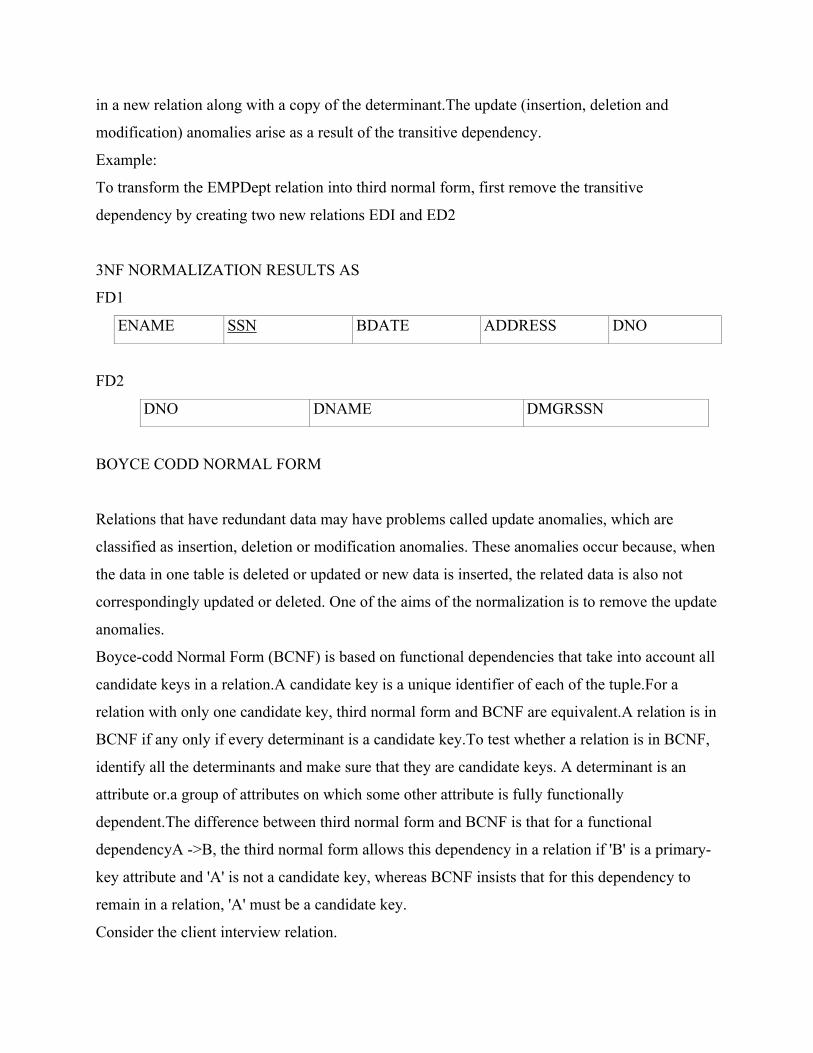
To transform the EMPDept relation into third normal form, first remove the transitive
dependency by creating two new relations EDI and ED2
3NF NORMALIZATION RESULTS AS
FD1
ENAME SSN BDATE ADDRESS DNO
FD2
DNO DNAME DMGRSSN
BOYCE CODD NORMAL FORM
Relations that have redundant data may have problems called update anomalies, which are
classified as insertion, deletion or modification anomalies. These anomalies occur because, when
the data in one table is deleted or updated or new data is inserted, the related data is also not
correspondingly updated or deleted. One of the aims of the normalization is to remove the update
anomalies.
Boyce-codd Normal Form (BCNF) is based on functional dependencies that take into account all
candidate keys in a relation.A candidate key is a unique identifier of each of the tuple.For a
relation with only one candidate key, third normal form and BCNF are equivalent.A relation is in
BCNF if any only if every determinant is a candidate key.To test whether a relation is in BCNF,
identify all the determinants and make sure that they are candidate keys. A determinant is an
attribute or.a group of attributes on which some other attribute is fully functionally
dependent.The difference between third normal form and BCNF is that for a functional
dependencyA ->B, the third normal form allows this dependency in a relation if 'B' is a primary-
key attribute and 'A' is not a candidate key, whereas BCNF insists that for this dependency to
remain in a relation, 'A' must be a candidate key.
Consider the client interview relation.

CLIENT NO INTERVIEW
DATE
INTERVIEW
TIME
STAFFNO ROOMNO
(clientNo, interviewDate),
(staffNo, interviewDate, interviewtime),
and (roomNo, interviewDate, interviewTime).
Select (clientNo, interviewDate) to act as the primary key for this relation.
The client interview relation has the following functional dependencies:
fdl: clientNo, interviewdate->interviewTime, staffNo, roomNo
fd2: staffNo, inerviewdate, interviewTime->clientNo (Candidatekey).
Fd3: RoomNo, interviewdate, interviewtime —>staffNo, clientNo(candidate)
fd4: staffNo, interviewdate—> roomNo
As functional dependencies fdl, fd2, and fd3 are all candidate keys for this relation, none of these
dependencies will cause problems for the relation.
This relation is not BCNF due to the presence of the (staffNo, interviewdate) determinant, which
is not a candidate key for the relation.BCNF requires that all determinants in a relation must be a
candidate key for the relation
MULTIVALUED DEPENDENCIES AND FOURTH NORMAL FORM
Multi-valued dependency(MVD) represents a dependency between attributes (for example, A,
B,and C) in a relation, such that for each value of A there is a set of values for B and asset of
values for C However, the set of values for B and C are independent of each other.
MVD is represented as A->>B,A->>C
Example:
Consider the Branch staff owner relation.
BRANCHNO SNAME ONAME
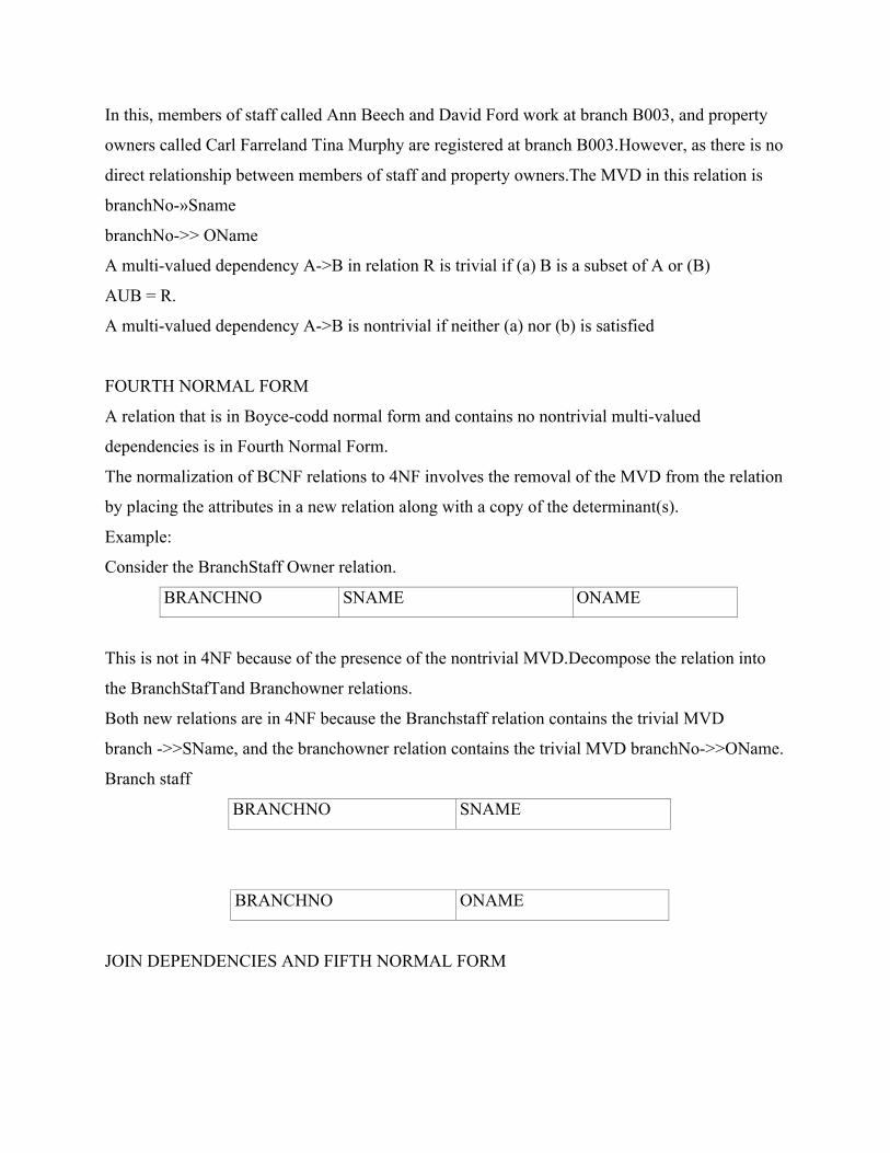
In this, members of staff called Ann Beech and David Ford work at branch B003, and property
owners called Carl Farreland Tina Murphy are registered at branch B003.However, as there is no
direct relationship between members of staff and property owners.The MVD in this relation is
branchNo-»Sname
branchNo->> OName
A multi-valued dependency A->B in relation R is trivial if (a) B is a subset of A or (B)
AUB = R.
A multi-valued dependency A->B is nontrivial if neither (a) nor (b) is satisfied
FOURTH NORMAL FORM
A relation that is in Boyce-codd normal form and contains no nontrivial multi-valued
dependencies is in Fourth Normal Form.
The normalization of BCNF relations to 4NF involves the removal of the MVD from the relation
by placing the attributes in a new relation along with a copy of the determinant(s).
Example:
Consider the BranchStaff Owner relation.
BRANCHNO SNAME ONAME
This is not in 4NF because of the presence of the nontrivial MVD.Decompose the relation into
the BranchStafTand Branchowner relations.
Both new relations are in 4NF because the Branchstaff relation contains the trivial MVD
branch ->>SName, and the branchowner relation contains the trivial MVD branchNo->>OName.
Branch staff
BRANCHNO SNAME
BRANCHNO ONAME
JOIN DEPENDENCIES AND FIFTH NORMAL FORM

Whenever we decompose a relation into two relations the resulting relations have the loss-less
join property. This property refers to the fact that we can rejoin the resulting relations to produce
the original relation.
Example:
The decomposition of the Branch staffowner relation
FIFTH NORMAL FORM
A relation that has no join dependency is in Fifth Normal Form.
Example:
Consider the property item supplier relation.
PROPRTY NO ITEM DESCRIPTION SUPPLIER NO
operation on the Branchstaff and Branchowner relations.
As this relation contains a join dependency, it is therefore not in fifth normal form. To remove
the join dependency, decompose the relation into three relations as,
FD1
PROPRTY NO ITEM DESCRIPTION
FD2
PROPRTY NO SUPPLIER NO
FD3
ITEM DESCRIPTION SUPPLIER NO
The propertyitemsupplier relation with the form (A,B,C) satisfies the join dependency JD
(R1(A,B), R2(B,C). R3(A, C)).i.e. performing the join on all three will recreate the original
propertyitemsupplier relation.

TWO MARKS WITH ANSWER
1. List the purpose of Database System (or) List the drawback of normal File Processing
System.
Problems with File Processing System:
1. Data redundancy and inconsistency
2. Difficulty in accessing data
3. Difficulty in data isolation
4. Integrity problems
5. Atomicity problems
6. Concurrent-access anomalies
7. Security problems
We can solve the above problems using Database System.
2. Define Data Abstraction and list the levels of Data Abstraction.
A major purpose of a database system is to provide users with an abstract view of the
data. That is, the system hides certain details of how the data are stored and maintained.
Since many database systems users are not computer trained, developers hide the
complexity from users through several levels of abstraction, to simplify users interaction
with the System: Physical level, Logical Level, View Level.
3. Define DBMS.
A Database-management system consists of a collection of interrelated data and a set of
programs to access those data. The collection of data, usually referred to as the database,
contains information about one particular enterprise. The primary goal of a DBMS is to
provide an environment that is both convenient and efficient to use in retrieving and
storing database information.
4. Define Data Independence.
The ability to modify a schema definition in one level without affecting a schema
definition in the next higher level is called data independence. There are two levels of
data independence: Physical data independence, and Logical data independence.

5. Define Data Models and list the types of Data Model.
Underlying the structure of a database is the data model: a collection of conceptual tools
for describing data, data relationships, data semantics, and consistency constraints. The
various data models that have been proposed fall into three different groups: object-based
logical models, record-based logical models, and physical models.
6. Discuss about Object-Based Logical Models.
Object-based logical models are used in describing data at the logical and view levels.
They provide fairly flexible structuring capabilities and allow data constraints to be
specified explicitly. There are many different models: entity-relationship model, object-
oriented model, semantic data model, and functional data model.
7. Define E-R model.
The entity-relationship data modal is based on perception of a real world that consists of
a collection of basic objects, called entities, and of relationships among these objects. The
overall logical structure of a database can be expressed graphically by an E-R diagram,
which is built up from the following components: Rectangles, which represent entity sets.
Ellipses, which represent attributes Diamonds, which represent relationships among
entity sets Lines, which link attributes to entity sets and entity sets to relationships. E.g.)
8. Define entity and entity set.
An entity is a thing or object in the real world that is distinguishable from other objects. For
example, each person is an entity, and bank accounts can be considered to be entities. The set of
all entities of the same type are termed an entity set.
9. Define relationship and relationship set.
A relationship is an association among several entities. For example, a Depositor relationship
associates a customer with each account that she has. The set of all relationships of the same
type, are termed a relationship set.

10. Define Object-Oriented Model.
The object-oriented model is based on a collection of objects. An object contains values stored in
instance variables within the object. An object also contains bodies of code that operate on the
object. These bodies of code are called methods. Objects that contain the same types of values
and the same methods are grouped together into classes. The only way in which one object can
access the data of another object is by invoking a method of that other object. This action is
called sending a message to the object.
11. Define Record-Based Logical Models.
Record-based logical models are used in describing data at the logical and view levels. They are
used both to specify the overall structure of the database and to provide a higher-level
description of the implementation. Record-based models are so named because the database is
structured in fixed-format records of several types. Each record type defines a fixed number of
fields, or attributes, and each field is usually of fixed length. The three most widely accepted
record-based data models are the relational, network, and hierarchical models.
12. Define Relational Model.
The relational model uses a collection of tables to represent both data and the relationships
among those data. Each table has multiple columns, and each column has a unique name.
13. Define Network Model.
Data in the network model are represented by collections of records, and relationships among
data are represented by links, which can be viewed as pointers. The records in the database are
organized as collections of arbitrary graphs.
14. Define Hierarchical Model.The hierarchical model is similar to the network model in the sense that data and relationships among data are represented by records and links, respectively. It differs from the network model in that the records are organized as collection of trees rather than arbitrary graphs.
15.List the role of DBA.The person who has central control over the system is called the database administrator. The

functions of the DBA include the following: Schema definitionStorage structure and access-method definitionSchema and physical-organization modificationGranting of authorization for data accessIntegrity-constraint specification 16.List the different types of database-system users.There are four different types pf database-system users, differentiated by the way that they expect to interact with the system. Application programmersSophisticated UsersSpecialized usersNaive users.
17.Write about the role of Transaction manager.TM is responsible for ensuring that the database remains in a consistent state despite system failures. The TM also ensures that concurrent transaction executions proceed without conflicting.
18.Write about the role of Storage manager.A SM is a program module that provides the interface between the low-level data stored in the database and the application programs and queries submitted to the system. The SM is responsible for interaction with the data stored on disk.
19.Define Functional Dependency.
Functional dependencies are constraints on the set of legal relations. They allow us to express
facts about the enterprise that we are modeling with our database. Syntax: A -> B e.g.) account
no -> balance for account table.
20.List the pitfalls in Relational Database Design.
1. Repetition of information
2. Inability to represent certain information
21. Define normalization.
By decomposition technique we can avoid the Pitfalls in Relational Database Design. This
process is termed as normalization.

22.List the properties of decomposition.
1. Lossless join
2. Dependency Preservation
3. No repetition of information
23.Define First Normal Form.
If the Relation R contains only the atomic fields then that Relation R is in first normal form.
E.g.) R = (account no, balance) first normal form.
24.Define Second Normal Form.
A relation schema R is in 2 NF with respect to a set F of FDs if for all FDs of the form A -> B,
where A is contained in R and B is contained in R, and A is a superkey for schema R.
25.Define BCNF.
A relation schema R is in BCNF with respect to a set F of FDs if for all FDs of the form A -> B,
where A is contained in R and B is contained in R, at least one of the following holds:
1. A -> B is a trivial FD
2. A is a superkey for schema R.
26.Define 3 Normal Form.
A relation schema R is in 3 NF with respect to a set F of FDs if for all FDs of the form A -> B,
where A is contained in R and B is contained in R, at least one of the following holds:
1. A -> B is a trivial FD
2. A is a superkey for schema R.
3. Each attribute in B ,A is contained in a candidate key for R.
27.Define Fourth Normal Form.
A relation schema R is in 4NF with respect to a set F of FDs if for all FDs of the form A ->> B
(Multi valued Dependency), where A is contained in R and B is contained in R, at least one of
the following holds:

1. A ->> B is a trivial MD
2. A is a superkey for schema R.
28. Define 5NF or Join Dependencies.
Let R be a relation schema and R1, R2, .., Rn be a decomposition of R. The join dependency
*(R1, R2, ..Rn) is used to restrict the set of legal relations to those for which R1,R2,..Rn is a
lossless-join decomposition of R. Formally, if R= R1 U R2U ..U Rn, we say that a relation r
satisfies the join dependency *(R1, R2, ...Rn) if R = A join dependency is trivial if one of the Ri
is R itself.
16 MARKS QUESTIONS
1.Briefly explain about Database system architecture:
2.Explain about the Purpose of Database system.
3. Briefly explain about Views of data.
4. Explain E-R Model in detail with suitable example.
5. Explain about various data models.
6. Draw an E – R Diagram for Banking, University, Company, Airlines, ATM, Hospital, Library,
Super market, Insurance Company.
7. Explain 1NF, 2Nf and BCNF with suitable example.
8. Consider the universal relation R={ A,B,C,D,E,F,G,H,I} and the set of functional
dependencies
F={(A,B)->{C],{A}>{D,E},{B}->{F},{F}->{G,H},{D}->[I,J}.what is the key for Decompose
R into 2NF,the 3NF relations.
9. What are the pitfalls in relational database design? With a suitable example, explain the role of
functional dependency in the process of normalization.
10. What is normalization? Explain all Normal forms.
11. Write about decomposition preservation algorithm for all FD�s.
12.Explain functional dependency concepts
13.Explain 2NF and 3NF in detail
14.Define BCNF .How does it differ from 3NF.
15.Explain the codd�s rules for relational database design

UNIT -2
SQL FUNDAMENTALS
Structural query language (SQL) is the standard command set used to communicate with the
relational database management systems. All tasks related to relational data management-
creating tables, querying the database for information.
Advantages of SQL:
•SQL is a high level language that provides a greater degree of abstraction than procedural
languages.
•Increased acceptance and availability of SQL.
•Applications written in SQL can be easily ported across systems.
•SQL as a language is independent of the way it is implemented internally.
•Simple and easy to leam.
•Set-at-a-time feature of the SQL makes it increasingly powerful than the record -at-a-time
processing technique.
•SQL can handle complex situations.
SQL data types:
SQL supports the following data types.
•CHAR(n) -fixed length string of exactlyV characters.
•VARCHAR(n) -varying length string whose maximum length is 'n' characters.
•FLOAT -floating point number.
Types of SQL commands:
SQL statements are divided into the following categories:
•Data Definition Language (DDL):
used to create, alter and delete database objects.
•Data Manipulation Language (DML):
used to insert, modify and delete the data in the database.
•Data Query Language (DQL):
enables the users to query one or more tables to get the information they want.

•Data Control Language (DCL):
controls the user access to the database objectsments.
SQL operators:
•Arithmetic operators
-are used to add, subtract, multiply, divide and negate data value (+, -, *, /).
•Comparison operators
-are used to compare one expression with another. Some comparison operators are =, >, >=, <,
<=, IN, ANY, ALL, SOME, BETWEEN, EXISTS, and so on.
•Logical operators
-are used to produce a single result from combining the two separate conditions. The logical
operators are AND, OR and NOT.
•Set operators
-combine the results of two separate queries into a single result. The set operators are UNION,
UNIONALL, INTERSECT, MINUS and so on.
Create table command
Alter table command
Truncate table command
Drop table command.
Create table
The create table statement creates a new base table.
Syntax:Create table table-name (col 1 -definition[, col2-definition]... [,coln-definition][,primary-
key-definition] [,alternate-key-definition][,foreign-key-definition]);
Example:
SQL>create table Book(ISBN char(10) not null,Title char(30) not null with default,Author
char(30) not null with default,Publisher char(30) not null with default,Year integer not null with
default,Price integer null,Primary key (ISBN));
Table created
Drop table
An existing base table can be deleted at any time by using the drop table statement.
Syntax
Drop table table-name;
Table dropped.
This command will delete the table named book along with its contents, indexes and any views
defined for that table.
DESC
Desc command used to view the structure of the table.
Syntax
Desc table-name;
Example:
SQL>Desc book;
Truncate table
If there is no further use of records stored in a table and the structure has to be retained then the
records alone can be deleted.
Syntax
Truncate table table-name;
Example:
SQL>Truncate table book;
Table truncated.
This command would delete all the records from the table, book.
INTEGRITY
Data integrity refers to the correctness and completeness of the data in a database, i.e. an
integrity constraint is a mechanism used to prevent invalid data entry into the table.
The various types of integrity constraints are
1)Domain integrity constraints
2)Entity integrity constraints
3)Referential integrity constraints

Domain integrity constraints
These constraints set a range, and any violations that take place will prevent the user from
performing the manipulation that caused the breach. There are two types of domain integrity
constraints
•Not null constraint
•Check constraint
*Not null constraints
By default all columns in a table allow null values -when a 'Not Null' constraint is enforced
though, either on a column or set of columns in a table, it will not allow Null values. The user
has to provide a value for the column.
*Check constraints a database. Each entity represents a table and each row of a table represents
an instance of that entity. Each row in a table can be uniquely identified using the entity
constraints.
•Unique constraints
•Primary key constraints.
*Unique constraints
Unique key constraints is used to prevent the duplication of values within the rows of a specified
column or a set of columns in a table. Columns defined with this constraint can also allow Null
values.
*Primary key constraints
The primary key constraint avoids duplication of rows and does not allow Null values, when
enforced in a column or set of columns. As a result it is used to identify a row. A table can have
only one primary key. Primary key constraint cannot be defined in an alter table command when
the table contains rows having null values.
Referential integrity constraints
Referential integrity constraint is used to establish a 'parent-child' relationship between two
tables having a common column. To implement this, define the column in the parent table as a
primary key and the same column in the child table as a foreign key referring to the
corresponding parent entry.
Syntax
(column constraints) Creating constraints on a new table

Crate table <table-name>(column-name 1 datatype(size) constraint <constraint-name> primary
key, column-name2 datatype(size) constraint <constraint-name> references referenced
table[(column-name)], coIumn-name3 datatype(size) constraint <constraint-
name>check(<condition>), column-name4 datatype(size) NOT NULL, column-name5
datatype(size) UNIQUE);
TRIGGER
A database trigger is procedural code that is automatically executed in response to certain events
on a particular table or view in a database
. The trigger is mostly used for maintaining the integrity of the information on the database. For
example, when a new record (representing a new worker) is added to the employees table, new
records should also be created in the tables of the taxes, vacations and salaries.
Triggers are for
Customization of database management;
centralization of some business or validation rules;
logging and audit.
Overcome the mutating-table error.
Maintain referential integrity between parent and child.
Generate calculated column values
Log events (connections, user actions, table updates, etc)
Gather statistics on table access
Modify table data when DML statements are issued against views
Enforce referential integrity when child and parent tables are on different nodes of a
distributed database
Publish information about database events, user events, and SQL statements to
subscribing applications
Enforce complex security authorizations: (i.e. prevent DML operations on a table after
regular business hours)
Prevent invalid transactions

Enforce complex business or referential integrity rules that you cannot define with
constraints
Control the behavior of DDL statements, as by altering, creating, or renaming objects
Audit information of system access and behavior by creating transparent logs
SECURITY
Authorization
Forms of authorization on parts of the database:
Read - allows reading, but not modification of data.
Insert - allows insertion of new data, but not modification of existing data.
Update - allows modification, but not deletion of data.
Delete - allows deletion of data.
Forms of authorization to modify the database schema
Index - allows creation and deletion of indices.
Resources - allows creation of new relations.
Alteration - allows addition or deletion of attributes in a relation.
Drop - allows deletion of relations.
The grant statement is used to confer authorization
grant <privilege list>on <relation name or view name> to <user list>
<user list> is:a user-id public, which allows all valid users the privilege granted
A role Granting a privilege on a view does not imply granting any privileges on the underlying
relations.
The grantor of the privilege must already hold the privilege on the specified item (or be the
database administrator).
PPrriivviilleeggeess iinn SSQQLL

select: allows read access to relation,or the ability to query using the view
Example: grant users U1, U2, and U3 select authorization on the branch relation:
grant select on branch to U1, U2, U3
insert: the ability to insert tuples
update: the ability to update using the SQL update statement
delete: the ability to delete tuples.
all privileges: used as a short form for all the allowable privileges
RReevvookkiinngg AAuutthhoorriizzaattiioonn iinn SSQQLL
The revoke statement is used to revoke authorization.
revoke <privilege list>
on <relation name or view name> from <user list>
Example:
revoke select on branch from U1, U2, U3
All privileges that depend on the privilege being revoked are also revoked.
<privilege-list> may be all to revoke all privileges the revokee may hold.
If the same privilege was granted twice to the same user by different grantees, the user may
retain the privilege after the revocation.
EMBEDDED SQL
The SQL standard defines embeddings of SQL in a variety of programming languages such as
C,Java, and Cobol.
A language to which SQL queries are embedded is referred to as a host language, and the SQL
structures permitted in the host language comprise embedded SQL.
The basic form of these languages follows that of the System R embedding of SQL into PL/I.
EXEC SQL statement is used to identify embedded SQL request to the preprocessor
EXEC SQL <embedded SQL statement > END_EXEC
Note: this varies by language (for example, the Java embedding uses
# SQL { …. }; )
From within a host language, find the names and cities of customers with more than the variable
amount dollars in some account.
Specify the query in SQL and declare a cursor for it
EXEC SQL
declare c cursor for select depositor.customer_name, customer_city from
depositor, customer, account where depositor.customer_name =
customer.customer_name and depositor account_number =
account.account_number and account.balance > :amount
END_EXEC
The open statement causes the query to be evaluated
EXEC SQL open c END_EXEC
The fetch statement causes the values of one tuple in the query result to be placed on host
language variables.
EXEC SQL fetch c into :cn, :cc END_EXEC Repeated calls to fetch get successive
tuples in the query result
A variable called SQLSTATE in the SQL communication area (SQLCA) gets set to ‘02000’ to
indicate no more data is available
The close statement causes the database system to delete the temporary relation that holds the
result of the query.
EXEC SQL close c END_EXEC

DYNAMIC SQL
Allows programs to construct and submit SQL queries at run time.
Example of the use of dynamic SQL from within a C program.char * sqlprog = “update
account set balance = balance * 1.05 where account_number = ?” EXEC
SQL prepare dynprog from :sqlprog;char account [10] = “A-101”;
EXEC SQL execute dynprog using :account;
The dynamic SQL program contains a ?, which is a place holder for a value that is provided
when the SQL program is executed.
JDBC and ODBC
API (application-program interface) for a program to interact with a database server
Application makes calls to Connect with the database server
Send SQL commands to the database server
Fetch tuples of result one-by-one into program variables
ODBC (Open Database Connectivity) works with C, C++, C#, and Visual Basic
JDBC (Java Database Connectivity) works with Java
VIEWS
A relation that is not of the conceptual model but is made visible to a user as a “virtual relation”
is called a view.
A view is defined using the create view statement which has the form
Create View V As < Query Expression>
where <query expression> is any legal SQL expression. The view name is represented by v
Once a view is defined, the view name can be used to refer to the virtual relation that the view
generates.

create view all_customer as (select branch_name, customer_name from depositor,
account where depositor.account_number =
account.account_number )
union (select branch_name, customer_name from borrower, loan
where borrower.loan_number = loan.loan_number )
USES OF VIEWS
Hiding some information from some users
Consider a user who needs to know a customer’s name, loan number and branch name, but has
no need to see the loan amount.
Define a view
create view cust_loan_data as (select customer_name, borrower.loan_number, branch_name
from borrower, loan where borrower.loan_number = loan.loan_number )
Grant the user permission to read cust_loan_data, but not borrower or loan
Predefined queries to make writing of other queries easier
Common example: Aggregate queries used for statistical analysis of data
PROCESSING OF VIEWS
When a view is created the query expression is stored in the database along with the view name
the expression is substituted into any query using the view
Views definitions containing views
One view may be used in the expression defining another view
A view relation v1 is said to depend directly on a view relation v2 if v2 is used in the expression
defining v1
A view relation v1 is said to depend on view relation v2 if either v1 depends directly to v2 or there
is a path of dependencies from v1 to v2
A view relation v is said to be recursive if it depends on itself.

VIEW EXPANSION
A way to define the meaning of views defined in terms of other views.
Let view v1 be defined by an expression e1 that may itself contain uses of view relations.
View expansion of an expression repeats the following replacement step:
repeat
Find any view relation vi in e1
Replace the view relation vi by the expression defining vi
until no more view relations are present in e1
As long as the view definitions are not recursive, this loop will terminate
DATABASE LANGUAGES
In many DBMSs where no strict separation of levels is maintained, one language, called the data
definition language (DDL), is used by the DBA and by database designer's to define both
schemas.
In DBMSs where a clear separation is maintained between the conceptual and internal levels, the
DDL is used to specify the conceptual schema only. Another language, the storage definition
language (SDL), is used to specify the internal schema.
The mappings between the two schemas may be specified in either one of these languages.
For a true three-schema architecture a third language, the view definition language (VDL), to
specify user views, and their mappings to the conceptual schema, but in most DBMSs the DDL
is used to define both conceptual and external schemas.Once the database schemas are complied
and the database is populated with data, users must have some means to manipulate the database.
The DBMS provides a set of operations or a language called the data manipulation
language(DML) for manipulations include retrieval, insertion, deletion, and modification of the
data.

The Data Definition Language (DDL):
A language that allows the DBA or user to describe and name the entities, attributes, and
relationships required for the application, together with any associated integrity and security
constraints is called DDL.
The storage structure and access methods used by the database system by a set of statements in a
special type of DDL called a data storage and definition language
These statements define the implementation details of the database schemas, which are usually
hidden from the users.The data values stored in the database must satisfy certain consistency
constraints. The DDL provides facilities to specify the following constraints. The database
systems check these constraints every time the database is updated.
Domain Constraints:
A domain of possible values must be associated with every attribute. Domain constraints are the
most elementary form integrity constraint. They are tested easily by the system whenever a new
data item is entered into the database.
Referential Integrity
There are cases to ensure that a value that appears in one relation for a given set of attributes also
appears for a certain set of attributes in another relation.
Assertions
An assertion is any condition that the database must always satisfy. Domain constraints and
referential integrity constraints are special forms of assertions. When an assertion is created, the
system tests it for validity. If the assertion is valid then any future modification to the database is
allowed only if it does not cause that assertion to be violated.
Authorization
Read authorization, which allows reading, but not modification of data.
Insert authorization, which allows insertion of new data, but not modification of existing data.
Update authorization, which allows modification, but not deletion, of data. Delete authorization,
which allows deletion of data.
We may assign the user all none or a combination of these types of authorization.
The output of the DDL is placed in the data dictionary, which contains metadata that is, data
about data.
The Data Manipulation Language (DML)
DML is a language that provides a set of operations to support the basic data manipulation
operations on the data held in the database. Data Manipulation operations usually include the
following:
•Insertion of new data into the database
•Modification of data stored in the database
•Retrieval of data contained in the database
•Deletion of data from the database
Data manipulation applied to the external, conceptual and internal level.
The part of a DML that involves data retrieval is called a Query language. A Query is a
statement requesting the retrieval of information. There are basically two types of DML
•Procedural DMLs.
•Declarative DMLs (or) nonprocedural DMLs.
Procedural DML: A language that allows the user to tell the system what data is needed and
exactly how to retrieve the data.
Non Procedural DML: A language that allows the user to state what data is needed rather than
how it is to be retrieved.
QUERY PROCESSING
The aims of query processing are to transform a query written in a high-level language, typically
SQL, into a correct and efficient execution strategy expressed in a low-level language
(implementing the relational algebra), and to execute the strategy to retrieve the required data.
The steps involved in processing a query are
• Parsing and transaction
• Optimization
• Evaluation
Before query processing can begin, the system must translate the query into a usable for (SQL).
Thus, the first action the system must take in query processing is to translate a given query into
its internal form. In generating the internal form of the query, the parser checks the syntax of the

user's query, verifies that the relation names appearing in the query are names of the relations in
the database, and so.
The system constructs a parsetree representation of the query, which it then translates into a
relational algebra expression. Example
Consider the query
Select balance from account where balance < 2500.
This query can be translated into either of the following relational algebra expressions.
• Σbalance < 2500 (Π balance (account))
• Π balance (σ balance < 2500 (account))
To specify fully how to evaluate a query, we need not only to provide the relational algebra
expression, but also to annotate it with instructions specifying how to evaluate each operation.
A relational - algebra operation annotated with instructions on how to evaluate it is called an
evaluation primitive.
A sequence of primitive operations that can be used to evaluate a query is a query execution plan
or query evaluation plan. It evaluation plan a particular index in specified for the selection
operation.
The query - execution engine takes a query - evaluation plan, executes that plan, and returns the
answers to the query.
It is the responsibility of the system to construct a query - evaluation plan that minimizes the cost
of query evaluation. This task is called query optimization.
In order to optimize a query, a query optimizer must know the cost of each operation. Although
the exact cost is hard to compute, since it depends on many parameters such as actual memory
available to the operation, it is possible to get a rough estimate of execution cost for each
operation.
SORTING ALGORITHM
External sort - merge algorithm
1. In the first stage, a number of sorted runs are created. Each run is sorted, but contains only
some of the records of the relation.
i = 0; repeat
read M blocks of the relation or the rest of the relation; sort the in - memory part op the relation;
write the sorted data to run file R;; i = i-H;
until the end of the relation
2. In the second stage, the runs are merged. The merge stage operates as follows:
read one block of each of the N files R, into a buffer page in memory; repeat
choose the first type in sort order among all buffer pages;
write the tuple to the output, and delete it from the buffer page;
if the buffer page of any run Rj is empty and not end-of-file (Rj) then
read the next block of R, into the buffer page;
until all buffer pages are empty.
DATABASE TUNING
The goals of tuning are
• To make applications run faster.
• To lower the response time of queries / transactions
• To improve the overall throughput of transactions.
The inputs to the tuning process include statistics. DBMSS can internally collect the following
statistics.
• Sizes of individual tables
• Number of distinct values in a column
• The number of time a particular query or transaction is submitted / executed in an interval of
time.
• The times required for different phases of query and transaction processing.
These and other statistics create a profile of the contents and use of the database. Other
information obtained from monitoring the database system activities and processes includes.
• Storage statistics

• I/O and device performance statistics.
• Query / transaction processing statistics.
• Locking / logging related statistics.
• Index statistics.
Tuning a database involves dealing with the following types of problems:
• How to minimize overheard of logging and unnecessary dumping of data.
• How to optimize buffer size and scheduling of processes.
• How to allocate resources such as disks, RAM and processes for most efficient utilization.
Tuning indexes
The initial choice of indexes may have to be revised for the following reasons.
• Certain queries may take too long to run for lack of an index.
• Certain indexes may not get utilized at all.
• Certain indexes may be causing excessive overhead because the index is no an attribute that
undergoes frequent changes.
Tuning the database design
If a given physical database design does not meet the expected objectives, we may revert to the
logical database design, makes adjustments to the logical schema, and remap it to a new set of
physical tables and indexes.
Tf the processing requirements are dynamically changing, the design needs, to respond by
making changes to the conceptual schema if necessary and to reflect those changes into the
logical schema and physical design. These changes may be of the following nature.
Existing tables may be joined because certain attributes from two or more tables are frequently
needed together.
For the given set of tables, there may be alternative design choices, all of which achieve 3NF or
BCNF. One may be replaced by the other.

Each table groups sets of attributes that are accessed together.
Attributes from one table may be repeated in another even though this creates redundancy and a
potential anomaly.
If a query or transaction applies to all product data, it may have to run against all the tables and
the results may have to be combined.
Tuning queries
There are mainly two indications that suggest that query tuning may be needed.
• A query issues too many disk accesses.
• The query plan shows that relevant indexes are not being used.
TWO MARKS WITH ANSWER
1.Define Query processing?
Query processing refers to the range of activities involved in extracting data form a database.
These activities include translation of queries expressed in high-level database language into
expression that can be implemented at the physical level of the file system.
2. Define Merge-join?
The merge-join algorithm can be used to compute natural joins and equi-joins.
3.Explain Hybrid Hash-join?
The hybrid hash-join algorithm performs another optimization; it is useful when memory size is
relatively large, but not all the build relation fits in memory. The partitioning phase of the hash-
join algorithm needs one block of memory as a buffer for each partition that is created, and one
block of memory as an input buffer.
4.Define hash-table overflow?
Hash-table overflow occurs in partition i of the build relation s if the hash index on H is larger
than main memory. Hash-table overflow can occur if there are many tuples in the build relation
with the same values for the join attributes.
5.Define query optimization.

Query optimization refers to the process of finding the lowest cost method of evaluating a given
query.
6.Define Aggregate Functions.
Aggregate functions are functions that take a collection of values as input and return a single
value. SQL offers five built-in aggregate functions:
Average: avg
Minimum: min
Maximum: max
Total: sum
Count: count
7.Define Null Values.
SQL allows the use of null values to indicate absence of information about the value of an
attribute.
8.Define Nested Sub queries.
SQL provides a mechanism for the nesting of sub queries. A sub query is a select-from-where
expression that is nested within another query. A common use of sub queries is to perform tests
for set membership, set comparisons, and set cardinality.
9.Define Embedded SQL.
The SQL standard defines embeddings of SQL in a variety of programming languages, such as
Pascal, PL/I, Fortran, C, and COBOL. A language in which SQL queries are embedded is
referred to as a host language, and the SQL structures permitted in the host language constitute
embedded SQL.
10.Define Integrity Constraints.
Integrity constraints provide a means of ensuring that changes made to the database by
authorized users do not result in a loss of data consistency. Thus Integrity Constraints guard
against accidental damage to the database. The constraints were in the following forms: Key
declarations, and Form of a relationship.

11.Define Referential Integrity.
Often, we wish to ensure that a value that appears in one relation for a given set of attributes also
appears for a certain set of attributes in another relation. This condition is called referential
integrity.
12.Define Assertions.
An assertion is a predicate expressing a condition that we wish the database always satisfied.
E.g.) create assertion
13.Define Triggers.
A trigger is a statement that is executed automatically by the system as a side effect of a
modification to the database. To design a trigger mechanism, we must meet two requirements:
1. Specify the conditions under which the trigger is to be executed.
2. Specify the actions to be taken when the trigger executes.
14.Define Catalog
The catalog is the place where all of the various schemas (external, conceptual, internal) and all
of the corresponding mappings are kept. the catalog contains detailed information called
descriptor information or metadata regarding the various of the system.
15.Define Types
It is defined as a set of value
16.What is a SELECT operation?
The select operation selects tuples that satisfy a given predicate.
17.What is a PROJECT operation?
The project operation is a unary operation that returns its argument relation with certain
attributes left out.

18.Define query language?
A query is a statement requesting the retrieval of information. The portion of DML that involves
information retrieval is called a query language.
19.What is foreign key?
A relation schema r1 derived from an ER schema may include among its attributes the primary
key of another relation schema r2.this attribute is called a foreign key from r1 referencing r2.
20.What are the parts of SQL language?
The SQL language has several parts:
data definitition language
Data manipulation language
View definition
Transaction control
Embedded SQL
Integrity
Authorization
21.What are the categories of SQL command?
SQL commands are divided in to the following categories:
1. data definitition language
2. data manipulation language
3. Data Query language
4. data control language
5. data administration statements
6. transaction control statements
22.What is the use of rename operation?
Rename operation is used to rename both relations and a attributes. It uses the as clause, taking
the form:
Old-name as new-name

23.Define tuple variable?
Tuple variables are used for comparing two tuples in the same relation. The tuple variables are
defined in the from clause by way of the as clause.
24.List the string operations supported by SQL?
1) Pattern matching Operation
2) Concatenation
3) Extracting character strings
4) Converting between uppercase and lower case letters.
25.What is view in SQL? How is it defined?
Any relation that is not part of the logical model, but is made visible to a user as a virtual relation
is called a view. We define view in SQL by using the
create view command. The form of the create view command is
Create view v as <query expression>
26.What does database security refer to?
Database security refers to the protection from unauthorized access and malicious destruction or
alteration.
27.List the types of authorization.
Read authorization
Write authorization
Update authorization
Drop authorization
28.Name the various privileges in SQL?
Delete
Select
Insert

Update
29.What does authentication refer?
Authentication refers to the task of verifying the identity of a person.
30.Define Embedded SQL:
Embedded SQL statements are SQL statements written inline with the program source code of
the host language.
31.Define Dynamic SQL:
Useful for applications to generate and run SQL statements, based on user inputs.Queries may
not be known in advance
16 MARKS
1.Consider the following tables:
Employee (Emp_no, Name, Emp_city)
Company (Emp_no, Company_name, Salary)
i. Write a SQL query to display Employee name and company name.
ii. Write a SQL query to display employee name, employee city ,company name and salary of all
the employees whose salary >10000
iii. Write a query to display all the employees working in “XYZ� company
2.Consider the following relational schema
Employee (empno,name,office,age)
Books(isbn,title,authors,publisher)
Loan(empno, isbn,date)
Write the following queries in relational algebra.
a. Find the names of employees who have borrowed a book Published by McGraw-Hill.
b. Find the names of employees who have borrowed all books Published by McGraw-Hill.
c. Find the names of employees who have borrowed more than five different books published by
McGraw-Hill.

d. For each publisher, find the names of employees who have borrowed more than five books of
that publisher.
3. Explain Embedded and Dynamic SQL.
4.Explain briefly about the steps required in query processing.
5..Explain the three kinds of database tunning.
6.Write about the following
i.Nested loop join
ii.Block Nested loop join
iii. Merge join
iv Hash join
UNIT -3
Transaction States
• Active
This is the initial state, the transaction stays in this state while it is executing.
• Partially committed
A transaction is in this state when it has executed the final statement.
• Failed
A transaction is in this state once the normal execution of the transaction cannot proceed.
• Aborted
A transaction is said to be aborted when the transaction has rolled back and the database is being
restored to the consistent state prior to the start of the transaction.
• Committed
A transaction is in the committed state once it has been successfully executed and the database is
transformed into a new consistent state.
A transaction starts in the active state, A transaction contains a group of statements that form a
logical unit of work. When the transaction has finished executing the last statement, it enters the

partially committed state. At this point the transaction has completed execution, but it is still
possible that it may have to be aborted. This is because the actual output may still be in the main
memory and a hardware failure can still prevent the successful completion. The database system
then writes enough information to the disk. When the last of this information is written, the
transaction enters the committed states.
A transaction enters the failed state once the system determines that the transaction can no longer
proceed with its normal execution. This could be due to hardware failures or logical errors. Such
a transaction should be rolled back. When the roll back is complete, the transaction enters the
aborted state when a transaction aborts, the system has two options as follows:
• Restart the transaction
• Kill the transaction.
ACID properties
There are properties that all transactions should possess. The four basic or so-called ACID,
properties of a transaction are
• Atomicity: The 'all or nothing' property. A transaction is an indivisible unit that is either
performed in its entirety or is not performed at all. It is the responsibility of the recovery
subsystem of the DBMS to ensure atomicity.
• Consistency: A transaction must transform the database from one consistent state to another
consistent state. It is the responsibility of both the DBMS and the application developers to
ensure consistency. The DBMS can ensure consistency by enforcing all the constraints that have
been specified on the database schema, such as integrity and enterprise constraints. However in
itself this is insufficient to ensure consistency.
Example:
A transaction that is intended to transfer money from one bank account to another and the
programmer makes an error in the transaction logic and debits one account but credits the wrong
account, then the database is in an inconsistent state.

•Isolation: Transactions execute independently of one another, i.e. the partial effects of
incomplete transactions should not be visible to other transactions. It is the responsibility of the
concurrency control subsystem to ensure isolation.
• Durability: The effects of a successfully completed transaction are permanently recorded in
the database and must not be lost because of a subsequent failure. It is the responsibility of the
recovery subsystem to ensure durability.
TWO PHASE COMMIT- LOCKING - PROTOCOL
Centralized database require only one DP (Data processing). A database operations take place at
only one site, and the consequences of database operations are immediately known to the DBMS.
In contrast distributed databases make it possible for a transaction to access data at several sites.
A final commit must not be issued until all sites have committed their parts of the transaction.
The two-phase commit protocol guarantees that if a portion of a transaction operation cannot be
committed; all changes made at the other sites participating in the transaction will be undone to
maintain a consistent database state.
Each DP maintains its own transaction log. The two-phase commit protocol requires that the
transaction entry log for each DP be written before the database fragment is actually updated.
Therefore, the two-phase commit protocol requires a Do-UNDO-REDO protocol and a write-
ahead protocol. The DO-UNDO-REDO protocol is used by the DP to roll back and / or roll
forward transactions with the help of the system's transaction log entries. The DO-UNDO-REDO
protocol defines three types of operations:
• Do performs the operation and records the "before" and "after" values in the transaction log.
• UNDO reverses an operation, using the log entries written by the DO portion of the sequence.
• REDO redoes an operation, using the log entries written by the DO portion of the sequence.
To ensure that the DO, UNDO, and REDO operations, can survive a system crash while they are
being executed, a write-ahead protocol is used. The write-ahead protocol forces the log entry to
be written to permanent storage before the actual operation takes place.
The two-phase commit protocol defines the operations between two types of nodes: The
coordinator and one or more subordinates, or cohorts. The participating nodes agree on a
coordinator. Generally, the coordinator role is assigned to the node that initiates the transaction.
However, different systems implement various, more sophisticated election methods.
The protocol is implemented in two phases:
Phasel: Preparation
1) The coordinator sends a PREPARE TO COMMIT message to all subordinates.
2) The subordinates receive the message. Write the transaction log, using the write-ahead
protocol and send an acknowledgement (YES / PREPARED TO COMMIT or NO / NOT
PREPARED) message to the coordinator.
3) The coordinator makes sure that all nodes are ready to commit, or it aborts the action.
If all nodes are PREPARED TO COMMIT, the transaction goes to phase-2. If one or more nodes
reply NO or NOT PREPARED, the coordinator broadcasts an ABORT message to all
subordinates.
Phase2: The Final Commit
1) The coordinator broadcasts a COMMIT message to all subordinates and waits for the replies.
2) Each subordinate receives the COMMIT message, then updates the database using the DO
protocol.
3) The subordinates reply with a COMMITTED or NOT COMMITTED message to the
coordinator.
If one or more subordinates did not COMMIT, the coordinator sends an ABORT message,
thereby forcing them to UNDO all changes.
The objective of the two-phase commit is to ensure that all nodes commit their part of the
transaction, otherwise, the transaction is aborted. If one of the nodes fails to commit, the
information necessary to recover the database is in the transaction log, and the database can be
recovered with the DO-UNDO-REDO protocol.
LOCKING
Locking is a procedure used to control concurrent access to data when one transaction is
accessing the database, a lock may deny access to other transactions to prevent incorrect results.
A transaction must obtain a read or write lock on a data item before it can perform a read or write
operation.
The read lock is also called a shared lock. The write lock is also known as an exclusive lock. The
lock depending on its types gives or denies access to other operations on the same data item.
The basic rules for locking are
• If a transaction has a read lock on a data item, it can read the item but not update it.
• If a transition has a read lock on a data item, other transactions can obtain a read lock on the
data item, but no write locks.
• If a transaction has a write lock on a data item, it can both read and update the data item.
• If a transaction has a write lock on a data item, then other transactions cannot obtain either a
read lock or a write lock on the data item.
The locking works as
• All transactions that needs to access a data item must first acquire a read lock or write lock on
the data item depending on whether it is a ready only operation or not.
• If the data item for which the lock is requested is not already locked, the transaction is granted
the requested lock,
• If the item is currently lock, the DBMS determines what kind of lock is the current one. The
DBMS also finds out what lock is requested.
• If a read lock is requested on an item that is already under a read lock, then the requested will
be granted.
• If a read lock or a write lock is requested on an item that is already under a write lock, then the
request is denied and the transaction must wait until the lock is released.
• A transaction continues to hold the lock until it explicitly releases it either during execution or
when it terminates.
• The effects of a write operation will be visible to other transactions only after the write lock is
released.

Live lock
Suppose a transaction T2 has a shared lock on a data item and another transaction T1 requests
and exclusive lock on the same data item. Ti will have to wait until T2 releases the lock. Mean
while, another transaction T3 request a shared lock on the data item. Since the lock request of T3
is compatible to the lock granted to T2, T3 will be granted the shared lock on the data item. At
this point even if T2 releases the lock, Ti will have to wait until T3 also releases the lock. The
transaction T| can wait for an exclusive lock endlessly if other transactions continue to request
and acquire shared locks on the data item. The transaction T1 is starved (or is in live lock), as it
is not making any progress.
Two phase locking protocol requires that each transaction issue lock and unlock requests in two
phases:
1. Growing phase
A transaction may obtain locks, but may not release any lock.
2. Shrinking phase
A transaction may release locks, but may not obtain any new locks.
Initially, a transaction is in the growing phase. The transaction acquires locks as needed. Once
the transaction releases a lock, it enters the shrinking phase, and it can issue not more lock
requests.
The point in the schedule where the transaction has obtained its final lock (the end of its growing
phase) is called the lock point of the transaction.
Another variant of two - phase locking is the rigorous two-phase locking protocol* which
requires that all locks be held until the transaction commit.
If lock conversion is allowed then upgrading of locks (from read locked to write - locked) must
be done during the expanding phase, and downgrading of locks (from write-locked to read -
locked) must be done in the shrinking phase.
Strict two-phase locking and rigorous two-phase locking (with lock conversions) are used
extensively in commercial database systems.
INTENT LOCKING

In the concurrency - control schemes, each individual data item is used as the until on which
synchronization is performed.
There are circumstances, however where it would be advantages to group several data items, and
to treat them as one individual synchronization unit.
Example:
If a transaction Tj needs to access the entire database, and a locking protocol is used, then Tj
must lock each item in the database clearly, executing these locks is time-consuming. It would be
better if Tj could issue a single lock request to lock the entire database. If transaction Tj needs to
access only a few data items, it should not be required to lock the entire database, since
otherwise concurrency is lost.
Granularity
Granularity is the size of data items chosen as the unit of protection by a concurrency control
protocol.
Hierarchy of granularity
The granularity of locks is represented in a hierarchical structure where each node represents
data items of different sizes.
The multiple granularity locking (MGL) protocol consists of the following rules.
1. It must observe the lock compatibility function.
2. It must lock the root of the tree first, and can lock it in any mode.
3. It can lock a node N in S or IS mode only if it currently has the parent of node N locked in
either IX or IS mode.
4. It can lock a node N in X, SIX, or IX mode only if it currently has the parent of node N locked
in either IX or SIX mode.
5. It can lock a node only if it has not previously unlocked any node.
6. it can unlock a node N only if it currently has none of the children of node N locked.
The multiple - granularity protocol requires that locks be acquired in top-down (root - to - leaf)
order, whereas locks must be released in bottom - up (leaf -to - root) order.

To ensure serializability with locking levels, a two-phase locking protocol is used as follows:
No lock can be granted once any node has been unlocked.
No node may be locked until its parent is locked by an intension lock.
No node may be unlocked until all its descendants are unlocked.
The notation < lock - types > (< item>), is used to display the locking operations in the schedule.
DEADLOCK
Deadlock occurs when each transaction T in a set of two or more transactions is waiting for some
item that is locked by some other transaction T in the set.
There is only one way to break deadlock: abort one or more of the transactions. This usually
involves undoing all the changes made by the aborted transactions (S).
There are three general techniques for handling deadlock:
� Timeouts
� Deadlock prevention
� Deadlock detection
� Recovery.
Timeouts
A transaction that requests a lock will wait for only a system defined period of time. If the lock
has not been granted within this period, the lock request times out. In this case, the DBMS
assumes the transaction may be deadlocked, even though it may not be, and it aborts and
automatically restarts the transaction.
Deadlock Prevention
Another possible approach to deadlock prevention is to order transactions using transaction
timestamps.
Wait - Die algorithm allows only an older transaction to wait for a younger one otherwise the
transaction is aborted and restarted with the same timestamp so that eventually it will become the
oldest active transaction and will not die.

Wound - wait, allows only a younger transaction can wait for an older one. if an older transaction
requests a lock held by a younger one the younger one is aborted.
Deadlock detection and Recovery
Deadlock detection is usually handled by the construction of a wait - for graph (WFG) that
shows the transaction dependencies, that is transaction Tj is dependent on Tj if transaction Tj
holds the lock on a data item that Tj is waiting for , Deadlock exists if and only if the WFG
contains a cycle.
When a detection algorithm determines that a deadlock exists, the system must recover from the
deadlock. The most common solution is to roll back one or more transactions to break the
deadlock.
Starvation occurs when the same transaction is always chosen as the victim, and the transaction
can never complete.
SERIALIZABILITY
The objective of a concurrency control protocol is to schedule transactions in such a way as to
avoid any interference between them.
Schedule is a sequence of the operations by a set of concurrent transactions that preserves the
order of the operations in each of the individual transactions.
Serial schedule is a schedule where the operations of each transaction are executed consecutively
without any interleaved operations from other transactions.
In a serial schedule, the transactions are performed in serial order, ie if Tj and T2 are
transactions, serial order would be Tj followed by T2 or T2 followed by Tj.
Non serial schedule is a schedule where the operations from a set of concurrent transactions are
interleaved.
The objective of serializability is to find non serial schedules that allow transactions to execute
concurrently without interfering with one another, and there by produce a database state that
could be produced by a serial execution.
Conflict serializability:
In serializability, the ordering of read and write operations is important:
� It two transactions only read a data item, they do not conflict and order is not important.

� If two transactions either read or write completely separate data items, they do not conflict and
order is not important.
It one transaction writes a data item and another either reads or writes the same data item, the
order of execution is important.
The instructions I; and Ij conflict if they are operations by different transactions on the same data
item, and atleast one of these instructions is a write operation.
View serializability:
The schedules S and S' are said to be view equivalent if the following conditions met:
For each data item x{< if transaction Ti reads the initial value of x in schedule S, then
transaction Tj must, in schedule S\ also read the initial value of x.
For each data item x, if transaction Tj executes read (x) in schedule S, and if that value was
produced by a write (x) operation executed by transaction Tj, then the read (x) operation of
transaction Tj must, in schedule S, also read the value of x that was produced by the same write
(x) operation of transaction T;.
For each data item xt the transaction that performs the final write (x) operation in schedule S
must perform the final write (x) operation in schedule S'.
TWO MARKS WITH ANSWERS
1.What is Recovery?
Recovery means to restore the database to a correct state after some failure has rendered the
current state incorrect or suspect
2.What is Transactions?
A transaction is a logical unit of work It begins with BEGIN TRANSACTION
It ends with COMMIT or ROLLBACK

3.What is Recovery Log?
A recovery log or journal keeps the before and after state for each transaction
An active (online) log is kept for immediate recovery of recent activity
An archive log is kept offline for more extensive recovery requirements
4.What is Correctness?
The database must always be consistent, which is defined as not violating any known integrity
constraint The DBMS can enforce consistency, but not correctness
5.What is COMMIT Point
Database updates are kept in buffers, and written to disk after COMMIT
6.What is Transaction Recovery?
ROLLBACK will return the database to the previous COMMIT point
7.Briefly write The ACID Properties
Atomicity :Transactions are atomic
Consistency:Transactions transform a correct state of the database into another correct state
Isolation:Transactions are isolated from one another
Durability :Once a transaction commits, its updates persist
8.What is Two Phase Commit?
Required for distributed or heterogeneous environments, so that correctness is maintained in case
of failure during a multipart COMMIT
9.What is Concurrency?
Concurrency ensures that database transactions are performed concurrently without violating the
data integrity of the respective databases.
10.What is transaction?
A transaction is a unit of program execution that accesses and possibly updates various data

items. A transaction usually results from the execution of a user program written in a high-level
data-manipulation language or programming language, and is delimited by statements of the
form begin transaction and end transaction. The transaction consists of all operations executed
between the begin and end of the transaction.
11.List the possible transaction states.
Active
Partially committed
Failed
Aborted
Committed
Terminated
12.What are the Three Concurrency Problems?
In a multi-processing environment transactions can interfere with each other
Three concurrency problems can arise, that any DBMS must account for and avoid:
Lost Updates
Uncommitted Dependency
Inconsistent Analysis
13.What is Locking?
A transaction locks a portion of the database to prevent concurrency problems
Exclusive lock –write lock, will lock out all other transactions
Shared lock –read lock, will lock out writes, but allow other reads
14.What is Deadlock?
Strict two-phase locking may result in deadlock if two transactions each take a shared lock
before one of them tries to take an exclusive lock Or if the second one tries to take an exclusive
lock where the first already has a shared lock, and the first in turn is waiting for additional shared
locks

15.Briefly explain Wait-Die and Wound-Wait
Wait-Die: Transaction 2 waits if it is older than 1; otherwise it dies
Wound-Wait: Transaction 2 wounds 1 if it is older; that is, it rolls it back
16.What is Serializability?
An interleaved execution is considered correct if and only if it is serializable
A set of transactions is serializable if and only if it is guaranteed to produce the same result as
when each transaction is completed prior to the following one being started
17.What are the two statements regarding transaction?
The two statements regarding transaction of the form:
Begin transaction
End transaction
18.When is a transaction is said to be rolled back?
Any changes that the aborted transaction made to the database must be undone. Once the
changes caused by an aborted transaction have been undone, then the transaction has been rolled
back.
16 MARK QUESTIONS
1. Explain in detail about Lock based protocols and Timestamp based protocols.
2. Write briefly about serializability with example.
3. Explain Two phase locking protocol in detail.
4. Write about immediate update and deferred update recovery techniques.
5. Explain the concept of Deadlock avoidance and prevention in detail.
UNIT -4
RAID
A variety of disks - organization techniques collectively called redundant arrays of independent
disks (RAID), have been proposed to achieve improved performance and reliability.

RAID systems are used for their higher reliability and higher performance rate, rather than for
economic reasons. Another key justification for RAID use is easier management and operations.
Improvement of reliability via redundancy
If we store only one copy of the data, then each disk failure will result in loss of a significant
amount of data.
The solution to the problem of reliability is to introduce redundancy, ie some extra information
that is not needed normally, but that can be used in the event of failure of a disk to rebuild the
lost information. Thus, even if a disk fails, data are not lost, so the effective mean time to failure
is increased.
The simplest (expensive) approach to introducing redundancy is to duplicate every disk. This
technique is called mirroring.
Mean time to repair is the time it takes to replace a failed disk and to restore the data on it.
With disk mirroring, the rate at which read requests can be handled is doubled, since read
requests can be sent to either disk. The transfer rate of each read is the same as in a single-disk
system, but the number of reads per Unit time has doubled.
With multiple disks, the transfer rate can be improved as well by striping data across multiple
disks. In its simplest from, data striping consists of splitting the bits of each byte across multiple
disks. Such striping is called bit level striping. Block - level striping stripes blocks across
multiple disks. They are two main goals of parallelism in a disk system.
• Load - balance multiple small accesses, so that the through put of such accesses increases.
• Parallelize large accesses so that the response time of large accesses is reduced.
RAID levels
Mirroring provides high reliability, but it is expensive. Striping provides high data - transfer
rates, but does not improve reliability. Various alternative schemes aim to provide redundancy at
lower cost by combining disk striping with "parity" bits. The schemes are classified into RAID
levels.
RAID level 0
RAID level 0 uses data striping at the level of blocks has not redundant data (such as mirroring
or parity bits) and hence has the best write performance since updates do not have to be
duplicated. However, its read performance is not good.
RAID level 1
RAID level 1 refers to disk mirroring with block striping. Its read performance is good than
RAID level 0. Performance improvement is possible by scheduling a read request to the disk
with shortest expected seek and rotational delay.
RAID level 2
RAID level 2 uses memory-style redundancy by using hamming codes, which contain parity bits
for distinct overlapping subsets of components. If one of the bits in the byte gets damaged, the
parity of the byte changes and thus will not match the stored parity. Similarly, if the stored parity
bit gets damaged, it will not match the computed parity.
The disks labeled P store the error-correction bits. If one of the disks fails, the remaining bits of
the byte and the associated error-correction bits can be read from other disks, and can be used to
reconstruct the damaged data.
RAID level 3
Bit inter leaved parity organization, improves on level 2 by exploiting the fact that disk,
controllers, can detect whether a sector has been read correctly, so a single parity bit can be used
for error correction.
If one of the sectors gets damaged, the system knows exactly which sector it is, and, for each bit
in the sector, the system can figure out whether it is a 1 or a 0 by computing the parity of
thecorresponding bits from sectors in the other disks. If the parity of the remaining bits is equal
to the stored parity, the missing bit is 0. otherwise, it is 1.
RAID level 3 supports a lower number of I/O operations per second, since every disk has to
participate in every I/O request.
RAID level 4
RAID level 4, block inter leaved parity organization, uses block-level striping and keeps a parity
block on a separate disk for corresponding blocks from N other disks. If one of the disks fails,
the parity block can be used with the corresponding blocks from the other disks to restore the
blocks of the failed disk.
Multiple read accesses can proceed in parallel, leading to a higher overall I/O rate.
A single write requires four disk accesses: two to read the two old blocks, and two to write the
two blocks.
RAID level 5

RAID level 5, block-inter leaved distributed parity, improves on level 4 by partitioning data and
parity among all N + 1 disks. In level 5, all disks can participate in satisfying read requests, so
level5 increases the total number of requests that can be met in a given amount of time. For each
set of N logical blocks, one of the disks stores the parity, and the other N disks store the blocks.
RAID level 6
RAID level 6, the P + Q redundancy scheme, is much like RAID level 5, but stores extra
redundant information to guard against multiple disk failures, instead of using parity, level 6 uses
error-correcting codes. In this, 2 bits of redundant data are stored for every 4 bits of data and the
system can tolerate two disk failures. Choice of RAID level
The factors to be taken into account in choosing a RAID level are
• Monetary cost of extra disk-storage requirements.
• Performance requirements in terms of number of I/O operations.
• Performance when a disk has failed.
• Performance during rebuild.
ORGANIZATION OF RECORDS IN FILES
The order in which records are stored and accessed in the file is dependent on the file
organization.
The physical arrangement of data in a file into records and pages on secondary storage is called
file organization.
The main types of file organization are:
• Heap (unordered) files
• Sequential (ordered) files
• Hash files
Heap files
Records are placed on disk in no particular order.
Records are placed in the file in the same order as they are inserted. A new record s inserted in
the last page of the file. If there is insufficient space in the last page, a new page is added to the
file.
A linear search must be performed to access a record from the file until the required record is
found.
To delete a record, the required page first has to be retrieved, the record marked as deleted, and
the page written back to disk.
Heap files are one of the best organizations for bulk loading data into a table, as records are
inserted at the end of the sequence.
Sequential (ordered files)
Records are ordered by the value of specified fields.
A binary search must be performed to access a record as follows
• Retrieve the mid-page of the file check whether the required record is between the first and last
records of this page. If so, the required record lies on this page and no more pages need to be
retrieved.
• If the value of the key field in the first record on the page is greater than the required value,
occurs on an earlier page therefore repeat the above steps.
• If value of the key field in the last record on the page is less than the required value, it occurs
on a latter page, and so repeat the above steps.
The binary search is more efficient than a linear search.
To insert and delete a record, first find the correct position in the ordering for the record and then
find space to insert it.
If there is sufficient space in the required page for the new record, then the single page can be
reordered and written back to disk. If there is no space, then move one or more records on to the
next page.
Inserting a record near the start of a large file could be very time-consuming. One solution is to
create a temporary unsorted file, called an overflow (or transaction) file and periodically, the
overflow file is merged with the main sorted file.
If the record is not found during the binary search, the overflow file has to be searched linearly.
Ordered files are rarely used for database storage unless a primary index is added to the file.
Hash files (Random or direct files)
Records are placed on disk according to a hash function. A hash function calculates the address
of the page in which the record is to be stored based on one or more fields in the record.
The base field is called the hash field, or if the field is also a key field of the file, it is called the
hash key.
. The hash function is chosen so that records are as evenly distributed as possible throughout the
file.
The division - remainder hashing. This technique uses the mod function which takes the field
value, divides it by some predetermined integer value, and uses the remainder of this division as
the disk address.
Each address generated by a hashing function corresponds to a page, or bucket, with slots for
multiple records. Within a bucket, records are placed in order of arrival. When the same address
is generated for two or more records, then it is called as a collision. The records are called
synonyms.
There are several techniques can be used to manage collisions.
• Open addressing
• Unchained overflow
• Chained overflow
• Multiple hashing
Open addressing
If a collision occurs, the system perform a linear search to find the first available slot to insert a
new record.
Unchained overflow
Instead of searching for a free slot, an overflow area is maintained for collisions that cannot be
placed at the hash address.
Chained overflow
An overflow area is maintained for collisions that cannot be placed at the hash address and each
bucket has an additional field, called a synonym pointer, that indicates whether a collision has

occurred, if so, points to the overflow page used, the pointer is zero no collision has occurred.
Multiple hashing
An alternative approach to collision management is to apply a second hashing function if the first
one results in a collision. The aim is to produce a new hash address that will avoid a collision.
The second hashing function is generally used to place records in an overflow area.
Indices whose search key specifies an order different from the sequential order of the file are
called non clustering indices or secondary indices.
All files are ordered sequentially on some search key, with a clustering index on the search key,
are called index - sequential files. There are several type of ordered indexes.
• Primary index
• Clustering index
• Secondary index
Primary indexes
A primary index is an ordered file whose records are of fixed length with two fields. The first
field is the primary key of the data file, and the second filed is a pointer to a disk block (a block
address).
There is one index entry (or index record) in the index file for each block in the data file. Each
index record has the value of the primary key field for the first record in a block and a pointer to
that block as its two field values. i = <K (i),P(i)>ordered data file. The first record in each block
of the data file is called the anchor record of block or block anchor.
Indexes can also be characterized as dense or sparse.
A dense index has an index entry for every search key value in the data file.
A sparse (or non dense) index has index entries for only some of the search values.
A primary index is hence a non dense (sparse index), since it includes an entry for each disk
block of the data file and the keys of its anchor record rather than tor every search value.
To retrieve a record, given the value K of its primary key field, do a binary search on the index
file to find the appropriate index entry i, and then retrieve the data file block whose address is P
(i).Clustering indexes

If records of a file are physically ordered on a non key field is called the clustering field. Create a
different type of index, called a clustering index, to speed up retrieval of records that have the
same value for the clustering field.
A clustering index is also an ordered file with two fields. The first field is of the same type as the
clustering field of the data file, and the second field is a block pointer.
This differs from a primary index, which requires that the ordering field of the data file have a
distinct value for each record.
Record insertion and deletion still cause problems, because the data records are physically
ordered. To alleviate the problem of insertion, it is common to reserve
a whole block for each value of the clustering field. All records with that value are placed in the
block.
A secondary index is also an ordered file similar to a primary index. However, whereas the data
file associated with a primary index is sorted on the index key, the data file associated with a
secondary index may not be sorted on the indexing key. Further, the secondary index key need
not contain unique values.
There are several techniques for handling non-unique secondary indexes.
• Produce a dense secondary index that maps on to all records in the data file, thereby allowing
duplicate key values to appear in the index.
• Allow the secondary index to have an index entry for each distinct key value, but allow the
block pointers to be multi-valued, with an entry corresponding to each duplicate key value in the
data file.
• Allow the secondary index to have an index entry for each distinct key value. However, the
block pointer would not pointer to the data file but to a bucket that contains pointers to the
corresponding records in the data file.
• The secondary index may be on a field which is a candidate key and has a unique value in
every record, or a non key with duplicate values.
• A secondary index structure on a key field that has a distinct value for every record. Such a
field is sometimes called a secondary key. In this case there is one index entry for each record in

the data file, which contains the value of the secondary key for the record and a pointer either to
the block in which the record is sorted to the record itself. Hence, such an index is dense.
• The index is an ordered file with two fields. The first field is of the same data type as some non
ordering field of the data file that is an indexing field. The second field is either a block pointer
or a record pointer.
Multilevel indexes
When an index file becomes large and extends over many pages, the search time for the required
increases.
B + TREE
A binary tree has order 2 in which each node has no more than two children. The rules for a B+
tree are as follows.
• If the root is not a leaf node, it must have at least two children.
• For a tree of order n, each node except the root and leaf nodes must have between n/2 and n
pointers and children. IF n/2 is not an integer, the result is rounded up.
• For a tree of order n, the number of key values in a leaf node must be between (n-l)/2 and (n-l)
pointers and and children. If (n-l)/2 is not an integer, the result is rounded up.
• The number of key values contained in a non leaf node is 1 less than the number of pointers.
• The tree must always be balanced ie every path from the root node to a leaf must have the same
length.
• Leaf nodes are linked in order of key values.
HASHING
In static hashing the hash address space is fixed when the file is created. The term bucket denotes
a unit of storage that can store one or more records.
A hash function h is a function from k to B. Where K denotes the set of all search-key values,
and B denote the set of all bucket addresses.
Hash functions
The worst possible hash function maps all search-key values to the same bucket.
An ideal hash function distributes the stored keys uniformly across all the buckets, so that every
bucket has the same number of records.
Choose a hash function that assigns search-key values to buckets in such a way that the
distribution has these qualities.
• The distribution is uniform
• The distribution is random
Handling of bucket overflows
When a record is inserted, the bucket to which it is mapped has space to store the record. If the
bucket does not have enough space, a bucket overflow is said to occur. Bucket overflow can
occur for several reasons
• Insufficient buckets
• Skew some buckets are assigned more records than are others.
Skew can occur for two reasons
1. Multiple records may have the same search key.
2. The chosen hash function may result in non uniform distribution of search keys.
Bucket overflow can be handled by using overflow buckets If a record must be inserted into a
bucket b, and b is already full, the system provides an overflow bucket for b and inserts the
record into the overflow bucket. If the overflow bucket is also full, the system provides another
overflow bucket, and so on. All the overflow buckets of a given bucket are chained together in a
linked list. Overflow handling using such a linked list is called overflow chaining.
Lookup algorithm
The system uses the hash function on the search key to identify a bucket b. The system must
examine all the records in bucket b to see whether they match the search key as before. If bucket
b has overflow buckets, the system must examine the records in all the overflow buckets also
closed hashing means the set of buckets is fixed and there is overflow chains.

Open hashing, the set of buckets is fixed, and there are no overflow chains. If a bucket is full, the
system inserts records in the next bucket in cyclic order that has space, is called linear probing.
Open hashing has been used to construct symbol tables for compilers and assemblers, but closed
hashing is preferable for database systems.
Hash indices
Hashing can be used not only for file organization, but also for index structure creation. A hash
index organizes the search keys, with their associated pointers, into a hash file structure.
INTRODUCTION TO DISTRIBUTED DATABASES AND CLIENT/SERVER
ARCHITECTURE
DISTRIBUTED DATABASE SYSTEM
A distributed database system consist of loosely coupled sites that share no physical component
Database systems that run on each site are independent of each other
Transactions may access data at one or more sites
In a homogeneous distributed database
All sites have identical software
Are aware of each other and agree to cooperate in processing user requests.
Each site surrenders part of its autonomy in terms of right to change schemas or software
Appears to user as a single system
In a heterogeneous distributed database
Different sites may use different schemas and software
Difference in schema is a major problem for query processing
Difference in software is a major problem for transaction processing
Sites may not be aware of each other and may provide only limited facilities for cooperation in
transaction processing
A relation or fragment of a relation is replicated if it is stored redundantly in two or more sites.
Full replication of a relation is the case where the relation is stored at all sites.
Fully redundant databases are those in which every site contains a copy of the entire database.
Advantages of Replication
Availability: failure of site containing relation r does not result in unavailability of r is replicas
exist.
Parallelism: queries on r may be processed by several nodes in parallel.
Reduced data transfer: relation r is available locally at each site containing a replica of r.
Disadvantages of Replication
Increased cost of updates: each replica of relation r must be updated.
Increased complexity of concurrency control: concurrent updates to distinct replicas may lead
to inconsistent data unless special concurrency control mechanisms are implemented.
One solution: choose one copy as primary copy and apply concurrency control operations on
primary copy
Division of relation r into fragments r1 , r2 , …, rn which contain sufficient information to
reconstruct relation r.
Horizontal fragmentation : each tuple of r is assigned to one or more fragments
Vertical fragmentation : the schema for relation r is split into several smaller schemas
All schemas must contain a common candidate key (or superkey) to ensure lossless join
property.
A special attribute, the tuple-id attribute may be added to each schema to serve as a candidate
key.
Example : relation account with following schema
Account = (account_number, branch_name , balance )

Data transparency : Degree to which system user may remain unaware of the details of how
and where the data items are stored in a distributed system
Consider transparency issues in relation to:
Fragmentation transparency
Replication transparency
Location transparency
Naming of data items: criteria
Every data item must have a system-wide unique name.
It should be possible to find the location of data items efficiently.
It should be possible to change the location of data items transparently.
Each site should be able to create new data items autonomously.
CENTRALIZED SCHEME -SERVER
Structure:
name server assigns all names
each site maintains a record of local data items
sites ask name server to locate non-local data items
Advantages:
satisfies naming criteria 1-3
Disadvantages:
does not satisfy naming criterion 4
name server is a potential performance bottleneck
name server is a single point of failure

Alternative to centralized scheme: each site prefixes its own site identifier to any name that it
generates i.e., site 17.account.
Fulfills having a unique identifier, and avoids problems associated with central control.
However, fails to achieve network transparency.
Solution:
Create a set of aliases for data items; Store the mapping of aliases to the real names at each site.
The user can be unaware of the physical location of a data item, and is unaffected if the data
item is moved from one site to another.
Transaction may access data at several sites.Each site has a local transaction manager
responsible for:
Maintaining a log for recovery purposes
Participating in coordinating the concurrent execution of the transactions executing at that site.
Each site has a transaction coordinator, which is responsible for:
Starting the execution of transactions that originate at the site.
Distributing subtransactions at appropriate sites for execution.
Coordinating the termination of each transaction that originates at the site, which may result in
the transaction being committed at all sites or aborted at all sites.
HETEROGENEOUS DISTRIBUTED DATABASE
Many database applications require data from a variety of preexisting databases located in a
heterogeneous collection of hardware and software platforms
Data models may differ (hierarchical, relational , etc.)
Transaction commit protocols may be incompatible
Concurrency control may be based on different techniques (locking, timestamping, etc.)
System-level details almost certainly are totally incompatible.

A multidatabase system is a software layer on top of existing database systems, which is
designed to manipulate information in heterogeneous databases
Creates an illusion of logical database integration without any physical database integration
ADVANTAGES
Preservation of investment in existing
hardware
system software
Applications
Local autonomy and administrative control
Allows use of special-purpose DBMSs
Step towards a unified homogeneous DBMS
Full integration into a homogeneous DBMS faces
Technical difficulties and cost of conversion
Organizational/political difficulties
Organizations do not want to give up control on their data
Local databases wish to retain a great deal of autonomy
MULTIDIMENSIONAL AND PARALLEL DATABASES
Data can be partitioned across multiple disks for parallel I/O.
Individual relational operations (e.g., sort, join, aggregation) can be executed in parallel
data can be partitioned and each processor can work independently on its own partition.
Queries are expressed in high level language (SQL, translated to relational algebra)
makes parallelization easier.
Different queries can be run in parallel with each other. Concurrency control takes care of conflicts.
Thus, databases naturally lend themselves to parallelism.
Reduce the time required to retrieve relations from disk by partitioning
the relations on multiple disks.
Horizontal partitioning – tuples of a relation are divided among many disks such that each tuple resides on one disk.
Partitioning techniques (number of disks = n):
Round-robin:
Send the ith tuple inserted in the relation to disk i mod n.
Hash partitioning:
Choose one or more attributes as the partitioning attributes.
Choose hash function h with range 0…n - 1
Let i denote result of hash function h applied to the partitioning attribute value of a tuple. Send tuple to disk i.
Range partitioning:
Choose an attribute as the partitioning attribute.
A partitioning vector [vo, v1, ..., vn-2] is chosen.
Let v be the partitioning attribute value of a tuple. Tuples such that vi vi+1 go to disk I + 1. Tuples with v< v0 go to disk 0 and tuples with v vn-2 go to disk n-1.
E.g., with a partitioning vector [5,11], a tuple with partitioning attribute value of 2 will go to disk 0, a tuple with value 8 will go to disk 1, while a tuple with value 20 will go to disk2.
INTERQUERY PARALLELISM
Queries/transactions execute in parallel with one another.
Increases transaction throughput; used primarily to scale up a transaction processing system to support a larger number of transactions per second.
Easiest form of parallelism to support, particularly in a shared-memory parallel database, because even sequential database systems support concurrent processing.
More complicated to implement on shared-disk or shared-nothing architectures
Locking and logging must be coordinated by passing messages between processors.

Data in a local buffer may have been updated at another processor.
Cache-coherency has to be maintained — reads and writes of data in buffer must find latest version of data.
INTRAQUERY PARALLELISM
Execution of a single query in parallel on multiple processors/disks; important for speeding up long-running queries.
Two complementary forms of intraquery parallelism :
Intraoperation Parallelism – parallelize the execution of each individual operation in the query.
Interoperation Parallelism – execute the different operations in a query expression in parallel.
the first form scales better with increasing parallelism becausethe number of tuples processed by each operation is typically more than the number of operations in a query
DATA WAREHOUSING AND MINING
The Web is a distributed information system based on hypertext.
Most Web documents are hypertext documents formatted via the HyperText Markup Language (HTML)
HTML documents contain
text along with font specifications, and other formatting instructions
hypertext links to other documents, which can be associated with regions of the text.
forms, enabling users to enter data which can then be sent back to the Web server
Why interface databases to the Web?
Web browsers have become the de-facto standard user interface to databases
Enable large numbers of users to access databases from anywhere
Avoid the need for downloading/installing specialized code, while providing a good graphical user interface
Examples: banks, airline and rental car reservations, university course registration and grading, an so on.

TWO MARKS WITH ANSWERS
1.Define Cache?
The cache is the fastest and most costly form of storage. Cache memory is small; its use is
managed by the operating system.
2.Explain Optical Storage Device?
The most popular form of optical storage is the compact disk read-only memory, can be read by
a laser. Optical storage is the write-once, read-many disk, which allows data to be written once,
but does not allow them to be erased and rewritten.
3.Define disk controller?
It is an interface between the computer system and the actual hardware of the disk drive. Accept
high-level command to read or write a sector. It attaches checksums to each sector that is written.
It also performs remapping of bad sectors.
4.Define RAID.
It is collectively called redundant arrays of inexpensive disk, have been proposed to address the
performance and reliability issues. Raids are used for their higher reliability and higher data
transfer rate. RAID stands for independent, instead of inexpensive.
5.Define file organization
A file is organized logically as a sequence of records. These records are mapped onto disk
blocks. Files are provided as a basic construct in operating system.
6.Define Hash indices?
Indices are based on the values being distributed uniformly across a range of buckets. The bucket
to which a value is assigned is determined by a function, called a hash function.
7.Define dense index?
An index record appears for every search-key value in the file. The index record contains the

search-key value and pointer to the first data record with that search-key value.
8.Define sparse index?
An index record is created for only some of the values. Each index record contains a search-key
value and a pointer to the first data record with that search-key value. To locate a record we find
the index entry with the largest search-key value that is less than or equal to the search-key
value.
9.Explain B+ -tree index structure?
The B+ -tree index structure is the most widely used of several index structures that maintain
their efficiency despite insertion and deletion of data. A B+ -tree index takes the form of a
balanced tree in which every path from the root of the tree to a leaf of The tree is the same
length.
10.Define Static Hashing?
File organization based on the technique of hashing allow us to avoid accessing an index
structure. Hashing also provides a way of constructing indices.
11.Define Query processing?
Query processing refers to the range of activities involved in extracting data form a database.
These activities include translation of queries expressed in high-level database language into
expression that can be implemented at the physical level of the file system.
12. Define Merge-join?
The merge-join algorithm can be used to compute natural joins and equi-joins.
13.Explain Hybrid Hash-join?
The hybrid hash-join algorithm performs another optimization; it is useful when memory size is
relatively large, but not all the build relation fits in memory. The partitioning phase of the hash-
join algorithm needs one block of memory as a buffer for each partition that is created, and one
block of memory as an input buffer.

14.Define hash-table overflow?
Hash-table overflow occurs in partition i of the build relation s if the hash index on H is larger
than main memory. Hash-table overflow can occur if there are many tuples in the build relation
with the same values for the join attributes.
16.What are the types of storage devices?
Primary storage
Secondary storage
Tertiary storage
Volatile storage
Nonvolatile storage
17.Define access time.
Access time is the time from when a read or write request is issued to when data transfer begins.
18.Define seek time.
The time for repositioning the arm is called the seek time and it increases with the distance that
the arm is called the seek time.
19.Define average seek time.
The average seek time is the average of the seek times, measured over a sequence of random
requests.
20.Define rotational latency time.
The time spent waiting for the sector to be accessed to appear under the head is called the
rotational latency time.
21.Define average latency time.
The average latency time of the disk is one half the time for a full rotation of the disk.
22.What is meant by data transfer rate?

The data transfer rate is the rate at which data can be retrieved from or stored to the disk.
23.What is meant by mean time to failure?
The mean time to failure is the amount of time that the system could run continuously without
failure.
24.What is a block and a block number?
A block is a contiguous sequence of sectors from a single track of one platter. Each request
specifies the address on the disk to be referenced. That address is in the form of a block number.
25.What are the techniques to be evaluated for both ordered indexing and hashing?
Access types
Access time
Insertion time
Deletion time
Space overhead
26.What is known as a search key?
An attribute or set of attributes used to look up records in a file is called a search key.
27.What is the use of RAID?
A variety of disk organization techniques, collectively called redundant arrays of independent
disks are used to improve the performance and reliability.
28.What is called mirroring?
The simplest approach to introducing redundancy is to duplicate every disk. This technique is
called mirroring or shadowing.

29.What is called mean time to repair?
The mean time to failure is the time it takes to replace a failed disk and to restore the data on it.
30.What is called bit level striping?
Data striping consists of splitting the bits of each byte across multiple disks. This is called bit
level striping.
31.What is called block level striping?
Block level striping stripes blocks across multiple disks. It treats the array of disks as a large
disk, and gives blocks logical numbers
32.What is known as a search key?
An attribute or set of attributes used to look up records in a file is called a search key.
33.Define Distributed databases
In a distributed database system, the database is stored on several computers.
34. What is Intraoperation Parallelism
Parallelize the execution of each individual operation in the query.
35.DefineInteroperation Parallelism
Execute the different operations in a query expression in parallel.
16 MARK QUESTIONS
1.How the records are represented and organized in files . Explain with suitable example
2.Write about the various levels of RAID with neat diagrams
3. Construct a B+ tree with the following (order of 3)
5,3,4,9,7,15,14,21,22,23
4. Explain detail in distributed databases and client/server databases.

5.Explain in detail about Dataware housing and data mining
6.Explain in detail about mobile and web databases
UNIT-5
OBJECT ORIENTED DATABASES
OBJECT ORIENTED DATA MODELS
Extend the relational data model by including object orientation and constructs to deal with added data types.
Allow attributes of tuples to have complex types, including non-atomic values such as nested relations.
Preserve relational foundations, in particular the declarative access to data, while extending modeling power.
Upward compatibility with existing relational languages.
COMPLEX DATATYPES
Motivation:
Permit non-atomic domains (atomic indivisible)
Example of non-atomic domain: set of integers,or set of tuples
Allows more intuitive modeling for applications with complex data
Intuitive definition:
allow relations whenever we allow atomic (scalar) values — relations within relations
Retains mathematical foundation of relational model
Violates first normal form.
STRUCTURED TYPES AND INHERITANCE IN SQL
Structured types can be declared and used in SQL
create type Name as (firstname varchar(20),
lastname varchar(20)) final
create type Address as (street varchar(20), city varchar(20), zipcode varchar(20))
not final
l Note: final and not final indicate whether subtypes can be created
Structured types can be used to create tables with composite attributes
create table customer (
name Name,
address Address,
dateOfBirth date)
Dot notation used to reference components: name.firstname
METHODS
Can add a method declaration with a structured type.
method ageOnDate (onDate date)
returns interval year
Method body is given separately.
create instance method ageOnDate (onDate date)
returns interval year
for CustomerType
begin
return onDate - self.dateOfBirth;
end
We can now find the age of each customer:
select name.lastname, ageOnDate (current_date)
from customer
INHERITANCE
Suppose that we have the following type definition for people:
create type Person (name varchar(20),
address varchar(20))
Using inheritance to define the student and teacher types create type Student under Person (degree varchar(20), department varchar(20)) create type Teacher under Person (salary integer, department varchar(20))
Subtypes can redefine methods by using overriding method in place of method in the method declaration
OBJECT IDENTITY AND REFERENCE TYPES
Define a type Department with a field name and a field head which is a reference to the type Person, with table people as scope:
create type Department ( name varchar (20), head ref (Person) scope people)
We can then create a table departments as follows
create table departments of Department
We can omit the declaration scope people from the type declaration and instead make an addition to the create table statement:
create table departments of Department (head with options scope people)
PATH EXPRESSIONS
Find the names and addresses of the heads of all departments:

select head –>name, head –>addressfrom departments
An expression such as “head–>name” is called a path expression
Path expressions help avoid explicit joins
If department head were not a reference, a join of departments with people would be required to get at the address
Makes expressing the query much easier for the user
XML
XML: Extensible Markup Language
Defined by the WWW Consortium (W3C)
Derived from SGML (Standard Generalized Markup Language), but simpler to use than SGML
Documents have tags giving extra information about sections of the document
E.g. <title> XML </title> <slide> Introduction …</slide>
Extensible, unlike HTML
Users can add new tags, and separately specify how the tag should be handled for display
The ability to specify new tags, and to create nested tag structures make XML a great way to exchange data, not just documents.
Much of the use of XML has been in data exchange applications, not as a replacement for HTML
Tags make data (relatively) self-documenting
E.g. <bank>
<account>
<account_number> A-101 </account_number>
<branch_name> Downtown </branch_name>
<balance> 500 </balance>
</account>
<depositor>

<account_number> A-101 </account_number>
<customer_name> Johnson </customer_name>
</depositor>
</bank>
Data interchange is critical in today’s networked world
Examples:
Banking: funds transfer
Order processing (especially inter-company orders)
Scientific data
– Chemistry: ChemML, …
– Genetics: BSML (Bio-Sequence Markup Language), …
Paper flow of information between organizations is being replaced by electronic flow of information
Each application area has its own set of standards for representing information
XML has become the basis for all new generation data interchange formats
Earlier generation formats were based on plain text with line headers indicating the meaning of fields
Similar in concept to email headers
Does not allow for nested structures, no standard “type” language
Tied too closely to low level document structure (lines, spaces, etc)
Each XML based standard defines what are valid elements, using
XML type specification languages to specify the syntax
DTD (Document Type Descriptors)
XML Schema
Plus textual descriptions of the semantics
XML allows new tags to be defined as required
However, this may be constrained by DTDs
A wide variety of tools is available for parsing, browsing and querying XML documents/data
Inefficient: tags, which in effect represent schema information, are repeated
Better than relational tuples as a data-exchange format
Unlike relational tuples, XML data is self-documenting due to presence of tags
Non-rigid format: tags can be added
Allows nested structures
Wide acceptance, not only in database systems, but also in browsers, tools, and applications
STRUCTURE OF XML
Tag: label for a section of data
Element: section of data beginning with <tagname> and ending with matching </tagname>
Elements must be properly nested
Proper nesting
<account> … <balance> …. </balance> </account>
Improper nesting
<account> … <balance> …. </account> </balance>
Formally: every start tag must have a unique matching end tag, that is in the context of the same parent element.
Every document must have a single top-level element
Example
<bank-1> <customer>
<customer_name> Hayes </customer_name>
<customer_street> Main </customer_street>
<customer_city> Harrison </customer_city>
<account>
<account_number> A-102 </account_number>
<branch_name> Perryridge </branch_name>
<balance> 400 </balance>
</account>
<account>
…
</account>
</customer> . .
</bank-1>
NESTING
Nesting of data is useful in data transfer
Example: elements representing customer_id, customer_name, and address nested within an order element
Nesting is not supported, or discouraged, in relational databases
With multiple orders, customer name and address are stored redundantly
normalization replaces nested structures in each order by foreign key into table storing customer name and address information
Nesting is supported in object-relational databases
But nesting is appropriate when transferring data
External application does not have direct access to data referenced by a foreign key
Mixture of text with sub-elements is legal in XML.
Example:
<account>
This account is seldom used any more.
<account_number> A-102</account_number>
<branch_name> Perryridge</branch_name>
<balance>400 </balance></account>
Useful for document markup, but discouraged for data representation
Elements can have attributes
<account acct-type = “checking” >
<account_number> A-102 </account_number>
<branch_name> Perryridge </branch_name>
<balance> 400 </balance>
</account>
Attributes are specified by name=value pairs inside the starting tag of an element
An element may have several attributes, but each attribute name can only occur once
<account acct-type = “checking” monthly-fee=“5”>
Distinction between subelement and attribute
In the context of documents, attributes are part of markup, while subelement contents are part of the basic document contents
In the context of data representation, the difference is unclear and may be confusing
Same information can be represented in two ways
– <account account_number = “A-101”> …. </account>
– <account> <account_number>A-101</account_number> …</account>
Suggestion: use attributes for identifiers of elements, and use subelements for contents
XML data has to be exchanged between organizations
Same tag name may have different meaning in different organizations, causing confusion on exchanged documents
Specifying a unique string as an element name avoids confusion

Better solution: use unique-name:element-name
Avoid using long unique names all over document by using XML Namespaces
<bank Xmlns:FB=‘http://www.FirstBank.com’> …
<FB:branch>
<FB:branchname>Downtown</FB:branchname>
<FB:branchcity> Brooklyn </FB:branchcity>
</FB:branch>…
</bank>
Elements without subelements or text content can be abbreviated by ending the start tag with a /> and deleting the end tag
<account number=“A-101” branch=“Perryridge” balance=“200 />
To store string data that may contain tags, without the tags being interpreted as subelements, use CDATA as below
<![CDATA[<account> … </account>]]>
Here, <account> and </account> are treated as just strings
CDATDatabase schemas constrain what information can be stored, and the data types of stored values
XML documents are not required to have an associated schema
However, schemas are very important for XML data exchange
Otherwise, a site cannot automatically interpret data received from another site
Two mechanisms for specifying XML schema
Document Type Definition (DTD)
Widely used
XML Schema
Newer, increasing use
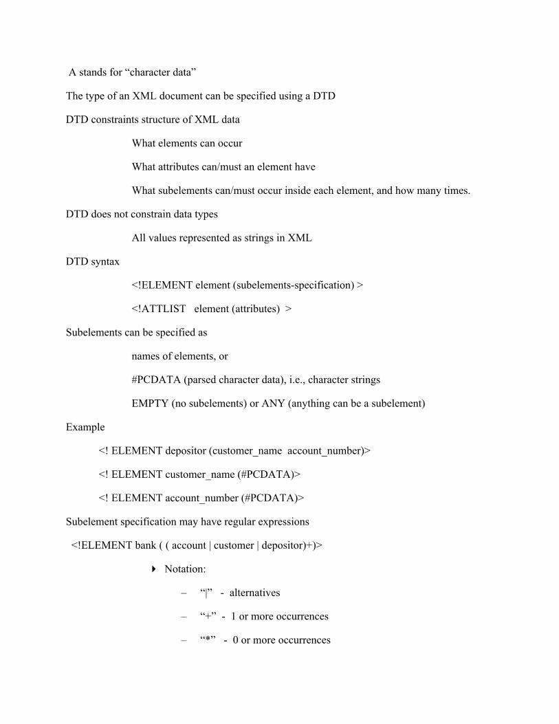
A stands for “character data”
The type of an XML document can be specified using a DTD
DTD constraints structure of XML data
What elements can occur
What attributes can/must an element have
What subelements can/must occur inside each element, and how many times.
DTD does not constrain data types
All values represented as strings in XML
DTD syntax
<!ELEMENT element (subelements-specification) >
<!ATTLIST element (attributes) >
Subelements can be specified as
names of elements, or
#PCDATA (parsed character data), i.e., character strings
EMPTY (no subelements) or ANY (anything can be a subelement)
Example
<! ELEMENT depositor (customer_name account_number)>
<! ELEMENT customer_name (#PCDATA)>
<! ELEMENT account_number (#PCDATA)>
Subelement specification may have regular expressions
<!ELEMENT bank ( ( account | customer | depositor)+)>
Notation:
– “|” - alternatives
– “+” - 1 or more occurrences
– “*” - 0 or more occurrences

<!DOCTYPE bank [
<!ELEMENT bank ( ( account | customer | depositor)+)>
<!ELEMENT account (account_number branch_name balance)>
<! ELEMENT customer(customer_name customer_street customer_city)>
<! ELEMENT depositor (customer_name account_number)>
<! ELEMENT account_number (#PCDATA)>
<! ELEMENT branch_name (#PCDATA)>
<! ELEMENT balance(#PCDATA)>
<! ELEMENT customer_name(#PCDATA)>
<! ELEMENT customer_street(#PCDATA)>
<! ELEMENT customer_city(#PCDATA)>
Attribute specification : for each attribute
Name
Type of attribute
CDATA
ID (identifier) or IDREF (ID reference) or IDREFS (multiple IDREFs)
Whether
mandatory (#REQUIRED)
has a default value (value),
or neither (#IMPLIED)
Examples
<!ATTLIST account acct-type CDATA “checking”>
<!ATTLIST customer

customer_id ID # REQUIRED
accounts IDREFS # REQUIRED >
DATA ANALYSIS AND MINING
Decision-support systems are used to make business decisions, often based on data collected by on-line transaction-processing systems.
Examples of business decisions:
What items to stock?
What insurance premium to change?
To whom to send advertisements?
Examples of data used for making decisions
Retail sales transaction details
Customer profiles (income, age, gender, etc.)
Data analysis tasks are simplified by specialized tools and SQL extensions
Example tasks
For each product category and each region, what were the total sales in the last quarter and how do they compare with the same quarter last year
As above, for each product category and each customer category
Statistical analysis packages (e.g., : S++) can be interfaced with databases
Statistical analysis is a large field, but not covered here
Data mining seeks to discover knowledge automatically in the form of statistical rules and patterns from large databases.
A data warehouse archives information gathered from multiple sources, and stores it under a unified schema, at a single site.
Important for large businesses that generate data from multiple divisions, possibly at multiple sites
Data may also be purchased externally
Online Analytical Processing (OLAP)
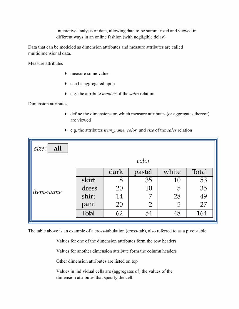
Interactive analysis of data, allowing data to be summarized and viewed in different ways in an online fashion (with negligible delay)
Data that can be modeled as dimension attributes and measure attributes are called multidimensional data.
Measure attributes
measure some value
can be aggregated upon
e.g. the attribute number of the sales relation
Dimension attributes
define the dimensions on which measure attributes (or aggregates thereof) are viewed
e.g. the attributes item_name, color, and size of the sales relation
The table above is an example of a cross-tabulation (cross-tab), also referred to as a pivot-table.
Values for one of the dimension attributes form the row headers
Values for another dimension attribute form the column headers
Other dimension attributes are listed on top
Values in individual cells are (aggregates of) the values of the dimension attributes that specify the cell.

Cross-tabs can be represented as relations
We use the value all is used to represent aggregates
The SQL:1999 standard actually uses null values in place of all despite confusion with regular null values
A data cube is a multidimensional generalization of a cross-tab
Can have n dimensions; we show 3 below
Cross-tabs can be used as views on a data cube

ONLINE ANALYTICAL PROCESSING
Pivoting: changing the dimensions used in a cross-tab is called
Slicing: creating a cross-tab for fixed values only
Sometimes called dicing, particularly when values for multiple dimensions are fixed.
Rollup: moving from finer-granularity data to a coarser granularity
Drill down: The opposite operation - that of moving from coarser-granularity data to finer-granularity data
Hierarchy on dimension attributes: lets dimensions to be viewed at different levels of detail
H E.g. the dimension DateTime can be used to aggregate by hour of day, date, day of week, month, quarter or year

Cross-tabs can be easily extended to deal with hierarchies
Can drill down or roll up on a hierarchy
The earliest OLAP systems used multidimensional arrays in memory to store data cubes, and are referred to as multidimensional OLAP (MOLAP) systems.
OLAP implementations using only relational database features are called relational OLAP (ROLAP) systems

Hybrid systems, which store some summaries in memory and store the base data and other summaries in a relational database, are called hybrid OLAP (HOLAP) systems.
Early OLAP systems precomputed all possible aggregates in order to provide online response
Space and time requirements for doing so can be very high
2n combinations of group by
It suffices to precompute some aggregates, and compute others on demand from one of the precomputed aggregates
Can compute aggregate on (item-name, color) from an aggregate on (item-name, color, size)
– For all but a few “non-decomposable” aggregates such as median
– is cheaper than computing it from scratch
Several optimizations available for computing multiple aggregates
Can compute aggregate on (item-name, color) from an aggregate on (item-name, color, size)
Can compute aggregates on (item-name, color, size), (item-name, color) and (item-name) using a single sorting of the base data
Relational representation of cross-tab that we saw earlier, but with null in place of all, can be computed by
select item-name, color, sum(number)from salesgroup by cube(item-name, color)
The function grouping() can be applied on an attribute
Returns 1 if the value is a null value representing all, and returns 0 in all other cases.
select item-name, color, size, sum(number),grouping(item-name) as item-name-flag,grouping(color) as color-flag,grouping(size) as size-flag,
from salesgroup by cube(item-name, color, size)
Can use the function decode() in the select clause to replace such nulls by a value such as all
E.g. replace item-name in first query by decode( grouping(item-name), 1, ‘all’, item-name)
Ranking is done in conjunction with an order by specification.
Given a relation student-marks(student-id, marks) find the rank of each student.
select student-id, rank( ) over (order by marks desc) as s-rank from student-marks
An extra order by clause is needed to get them in sorted order
select student-id, rank ( ) over (order by marks desc) as s-rankfrom student-marks order by s-rank
Ranking may leave gaps: e.g. if 2 students have the same top mark, both have rank 1, and the next rank is 3
dense_rank does not leave gaps, so next dense rank would be 2
WINDOWING
Used to smooth out random variations.
E.g.: moving average: “Given sales values for each date, calculate for each date the average of the sales on that day, the previous day, and the next day”
Window specification in SQL:
Given relation sales(date, value)
select date, sum(value) over (order by date between rows 1 preceding and 1 following) from sales
Examples of other window specifications:
between rows unbounded preceding and current
rows unbounded preceding
range between 10 preceding and current row
All rows with values between current row value –10 to current value
range interval 10 day preceding
Not including current row

Can do windowing within partitions
E.g. Given a relation transaction (account-number, date-time, value), where value is positive for a deposit and negative for a withdrawal
“Find total balance of each account after each transaction on the account”
select account-number, date-time, sum (value ) over
(partition by account-number order by date-timerows unbounded preceding)
as balancefrom transactionorder by account-number, date-time
DATAWAREHOUSING
Data sources often store only current data, not historical data
Corporate decision making requires a unified view of all organizational data, including historical data
A data warehouse is a repository (archive) of information gathered from multiple sources, stored under a unified schema, at a single site
Greatly simplifies querying, permits study of historical trends
Shifts decision support query load away from transaction processing systems
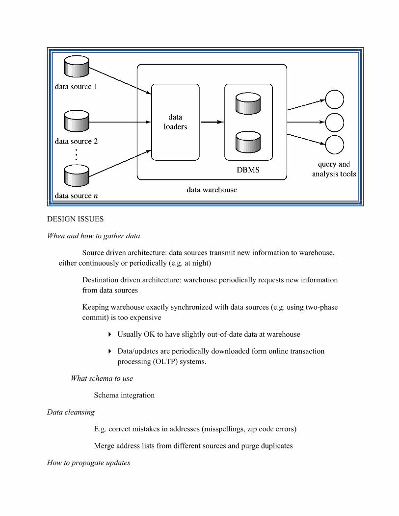
DESIGN ISSUES
When and how to gather data
Source driven architecture: data sources transmit new information to warehouse, either continuously or periodically (e.g. at night)
Destination driven architecture: warehouse periodically requests new information from data sources
Keeping warehouse exactly synchronized with data sources (e.g. using two-phase commit) is too expensive
Usually OK to have slightly out-of-date data at warehouse
Data/updates are periodically downloaded form online transaction processing (OLTP) systems.
What schema to use
Schema integration
Data cleansing
E.g. correct mistakes in addresses (misspellings, zip code errors)
Merge address lists from different sources and purge duplicates
How to propagate updates

Warehouse schema may be a (materialized) view of schema from data sources
What data to summarize
Raw data may be too large to store on-line
Aggregate values (totals/subtotals) often suffice
Queries on raw data can often be transformed by query optimizer to use aggregate values
Dimension values are usually encoded using small integers and mapped to full values via dimension tables
Resultant schema is called a star schema
More complicated schema structures
Snowflake schema: multiple levels of dimension tables
Constellation: multiple fact tables
DATAMINING

Data mining is the process of semi-automatically analyzing large databases to find useful patterns
Prediction based on past history
Predict if a credit card applicant poses a good credit risk, based on some attributes (income, job type, age, ..) and past history
Predict if a pattern of phone calling card usage is likely to be fraudulent
Some examples of prediction mechanisms:
Classification
Given a new item whose class is unknown, predict to which class it belongs
Regression formulae
Given a set of mappings for an unknown function, predict the function result for a new parameter value
Descriptive Patterns
Associations
Find books that are often bought by “similar” customers. If a new such customer buys one such book, suggest the others too.
Associations may be used as a first step in detecting causation
E.g. association between exposure to chemical X and cancer,
Clusters
E.g. typhoid cases were clustered in an area surrounding a contaminated well
Detection of clusters remains important in detecting epidemics
Classification rules help assign new objects to classes.
E.g., given a new automobile insurance applicant, should he or she be classified as low risk, medium risk or high risk?
Classification rules for above example could use a variety of data, such as educational level, salary, age, etc.

person P, P.degree = masters and P.income > 75,000
P.credit = excellent
person P, P.degree = bachelors and
(P.income 25,000 and P.income 75,000)
P.credit = good
Rules are not necessarily exact: there may be some misclassifications
Classification rules can be shown compactly as a decision tree.
CONSTRUCTION OF DECISION TREES
Training set: a data sample in which the classification is already known.
Greedy top down generation of decision trees.
Each internal node of the tree partitions the data into groups based on a partitioning attribute, and a partitioning condition for the node
Leaf node:
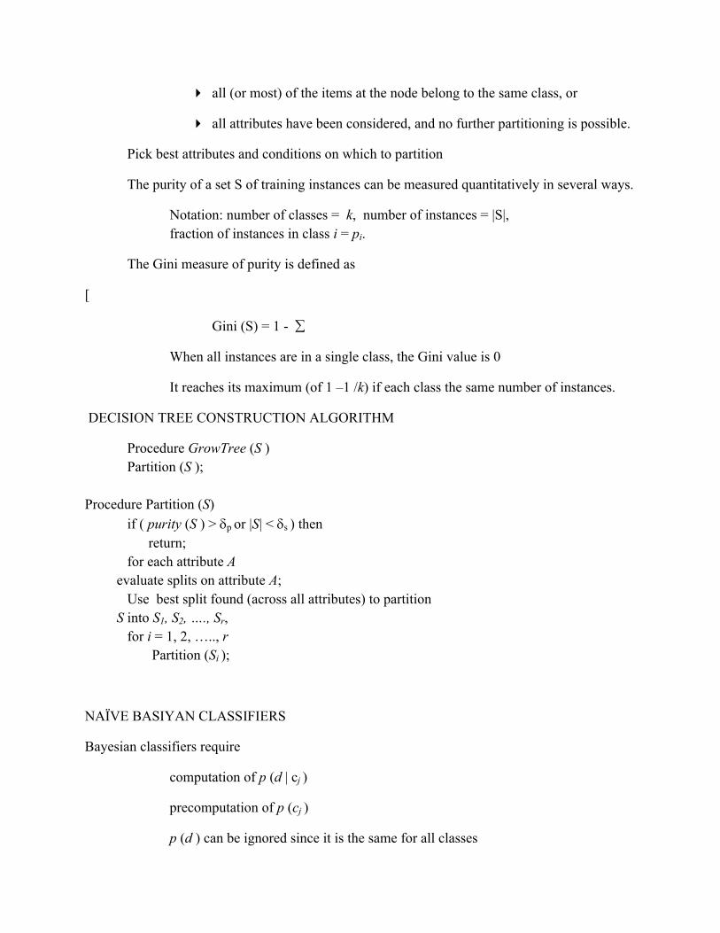
all (or most) of the items at the node belong to the same class, or
all attributes have been considered, and no further partitioning is possible.
Pick best attributes and conditions on which to partition
The purity of a set S of training instances can be measured quantitatively in several ways.
Notation: number of classes = k, number of instances = |S|, fraction of instances in class i = pi.
The Gini measure of purity is defined as
[
Gini (S) = 1 -
When all instances are in a single class, the Gini value is 0
It reaches its maximum (of 1 –1 /k) if each class the same number of instances.
DECISION TREE CONSTRUCTION ALGORITHM
Procedure GrowTree (S )Partition (S );
Procedure Partition (S)
if ( purity (S ) > p or |S| < s ) then return;for each attribute A
evaluate splits on attribute A;Use best split found (across all attributes) to partition
S into S1, S2, …., Sr,for i = 1, 2, ….., r Partition (Si );
NAÏVE BASIYAN CLASSIFIERS
Bayesian classifiers require
computation of p (d | cj )
precomputation of p (cj )
p (d ) can be ignored since it is the same for all classes

To simplify the task, naïve Bayesian classifiers assume attributes have independent distributions, and thereby estimate
p (d | cj) = p (d1 | cj ) * p (d2 | cj ) * ….* (p (dn | cj )
Each of the p (di | cj ) can be estimated from a histogram on di values for each class cj
the histogram is computed from the training instances
Histograms on multiple attributes are more expensive to compute and store
REGRESSION
Regression deals with the prediction of a value, rather than a class.
Given values for a set of variables, X1, X2, …, Xn, we wish to predict the value of a variable Y.
One way is to infer coefficients a0, a1, a1, …, an such thatY = a0 + a1 * X1 + a2 * X2 + … + an * Xn
Finding such a linear polynomial is called linear regression.
In general, the process of finding a curve that fits the data is also called curve fitting.
The fit may only be approximate
because of noise in the data, or
because the relationship is not exactly a polynomial
Regression aims to find coefficients that give the best possible fit.
ASSOCIATION RULES
Retail shops are often interested in associations between different items that people buy.
Someone who buys bread is quite likely also to buy milk
A person who bought the book Database System Concepts is quite likely also to buy the book Operating System Concepts.
Associations information can be used in several ways.

E.g. when a customer buys a particular book, an online shop may suggest associated books.
Association rules:
bread milk DB-Concepts, OS-Concepts Networks
Left hand side: antecedent, right hand side: consequent
An association rule must have an associated population; the population consists of a set of instances
E.g. each transaction (sale) at a shop is an instance, and the set of all transactions is the population
Rules have an associated support, as well as an associated confidence.
Support is a measure of what fraction of the population satisfies both the antecedent and the consequent of the rule.
E.g. suppose only 0.001 percent of all purchases include milk and screwdrivers.
The support for the rule is milk screwdrivers is low.
Confidence is a measure of how often the consequent is true when the antecedent is true.
E.g. the rule bread milk has a confidence of 80 percent if 80 percent of the purchases that include bread also include milk.
FINDING ASSOCIATION RULES
We are generally only interested in association rules with reasonably high support (e.g. support of 2% or greater)
Naïve algorithm
1. Consider all possible sets of relevant items.
2. For each set find its support (i.e. count how many transactions purchase all items in the set).
Large itemsets: sets with sufficiently high support
3. Use large itemsets to generate association rules.
From itemset A generate the rule A - {b } b for each b A.
Support of rule = support (A).

Confidence of rule = support (A ) / support (A - {b })
Determine support of itemsets via a single pass on set of transactions
Large itemsets: sets with a high count at the end of the pass
If memory not enough to hold all counts for all itemsets use multiple passes, considering only some itemsets in each pass.
Optimization: Once an itemset is eliminated because its count (support) is too small none of its supersets needs to be considered.
The a priori technique to find large itemsets:
Pass 1: count support of all sets with just 1 item. Eliminate those items with low support
Pass i: candidates: every set of i items such that all its i-1 item subsets are large
Count support of all candidates
Stop if there are no candidates
Basic association rules have several limitations
Deviations from the expected probability are more interesting
E.g. if many people purchase bread, and many people purchase cereal, quite a few would be expected to purchase both
We are interested in positive as well as negative correlations between sets of items
Positive correlation: co-occurrence is higher than predicted
Negative correlation: co-occurrence is lower than predicted
Sequence associations / correlations
E.g. whenever bonds go up, stock prices go down in 2 days
Deviations from temporal patterns
E.g. deviation from a steady growth
E.g. sales of winter wear go down in summer
Not surprising, part of a known pattern.
Look for deviation from value predicted using past patterns

CLUSTERING
Clustering: Intuitively, finding clusters of points in the given data such that similar points lie in the same cluster
Can be formalized using distance metrics in several ways
Group points into k sets (for a given k) such that the average distance of points from the centroid of their assigned group is minimized
Centroid: point defined by taking average of coordinates in each dimension.
Another metric: minimize average distance between every pair of points in a cluster
Has been studied extensively in statistics, but on small data sets
Data mining systems aim at clustering techniques that can handle very large data sets
E.g. the Birch clustering algorithm (more shortly)
TWO MARKS WITH ANSWER
1. What is called path expression ?
An expression such as “head–>name” is called a path expression
2. Define a type Department with a field name and a field head which is a reference to thetype Person, with table people as scope:
create type Department ( name varchar (20), head ref (Person) scope people)
3.Give the definition for INHERITANCE
Suppose that we have the following type definition for people:
create type Person (name varchar(20),
address varchar(20))
Using inheritance to define the student and teacher types create type Student
under Person (degree varchar(20), department varchar(20)) create type Teacher under Person (salary integer, department varchar(20))
4.Write the definition for method.
METHODS
Can add a method declaration with a structured type.
method ageOnDate (onDate date)
returns interval year
5.Define Motivation:
Permit non-atomic domains (atomic indivisible)
Example of non-atomic domain: set of integers,or set of tuples
Allows more intuitive modeling for applications with complex data
6. Define Intuitive
allow relations whenever we allow atomic (scalar) values — relations within relations
Retains mathematical foundation of relational model
Violates first normal form.
7. Define XML Extensible Markup Language
Defined by the WWW Consortium (W3C)
Derived from SGML (Standard Generalized Markup Language), but simpler to use than SGML
8.Give the syntax for XML.
Documents have tags giving extra information about sections of the document
a. E.g. <title> XML </title> <slide> Introduction …</slide>

9.Compare XML with HTML
Extensible, unlike HTML Users can add new tags, and separately specify how the tag should be handled for display
10.Compare XML tuples with RELATIONAL TUPLES
A wide variety of tools is available for parsing, browsing and querying XML documents/data
Inefficient: tags, which in effect represent schema information, are repeated
Better than relational tuples as a data-exchange format
Unlike relational tuples, XML data is self-documenting due to presence of tags
Non-rigid format: tags can be added
Allows nested structures
Wide acceptance, not only in database systems, but also in browsers, tools, and applications
11. Define Tag
label for a section of data
12.What is a Element?
section of data beginning with <tagname> and ending with matching </tagname>
Elements must be properly nested
13.Give an example for Proper nesting
<account> … <balance> …. </balance> </account>
14. Give an example for Improper nesting
<account> … <balance> …. </account> </balance>
15.Define decision support systems.
Decision-support systems are used to make business decisions, often based on data collected by on-line transaction-processing systems.
16.Define Data Analysis
Data analysis tasks are simplified by specialized tools and SQL extensions
Example tasks

For each product category and each region, what were the total sales in the last quarter and how do they compare with the same quarter last year
As above, for each product category and each customer category
17. What is Statistical analysis?Statistical analysis packages (e.g., : S++) can be interfaced with databases
Statistical analysis is a large field, but not covered here
18. Define Data mining seeks to discover knowledge automatically in the form of statistical rules and patterns from large databases.
19. What is a data warehouse?
archives information gathered from multiple sources, and stores it under a unified schema, at a single site.
a. Important for large businesses that generate data from multiple divisions, possibly at multiple sites
b. Data may also be purchased externally
20. What is Online Analytical Processing (OLAP)
Interactive analysis of data, allowing data to be summarized and viewed in different ways in an online fashion (with negligible delay)
21. Define Multidimensional data.Data that can be modeled as dimension attributes and measure attributes are called multidimensional data.
22. What are Measure attributes
measure some value
can be aggregated upon
e.g. the attribute number of the sales relation
23. What are Dimension attributes
define the dimensions on which measure attributes (or aggregates thereof) are viewed

e.g. the attributes item_name, color, and size of the sales relation
24. What is a data cube.A data cube is a multidimensional generalization of a cross-tabCan have n dimensions; we show 3 below Cross-tabs can be used as views on a data cube
16 MARKS
1. What is XML? Explain Breifly2. Explain the concepts of data mining and data warehousing in detail.3. Explain clearly the Classification& clustering techniques.4. Explain in detail about Association & regression5. Explain briefly the retrieval of information.
Related Documents