1 Analysis of Algorithms Sartaj Sahni University of Florida 1.1 Introduction ......................................... 1-1 1.2 Operation Counts .................................. 1-2 1.3 Step Counts ......................................... 1-4 1.4 Counting Cache Misses ............................ 1-6 A Simple Computer Model • Effect of Cache Misses on Run Time • Matrix Multiplication 1.5 Asymptotic Complexity ........................... 1-9 Big Oh Notation (O) • Omega (Ω) and Theta (Θ) Notations • Little Oh Notation (o) 1.6 Recurrence Equations ............................. 1-12 Substitution Method • Table-Lookup Method 1.7 Amortized Complexity ............................ 1-14 What is Amortized Complexity? • Maintenance Contract • The McWidget Company • Subset Generation 1.8 Practical Complexities ............................. 1-23 1.1 Introduction The topic “Analysis of Algorithms” is concerned primarily with determining the memory (space) and time requirements (complexity) of an algorithm. Since the techniques used to determine memory requirements are a subset of those used to determine time requirements, in this chapter, we focus on the methods used to determine the time complexity of an algorithm. The time complexity (or simply, complexity) of an algorithm is measured as a function of the problem size. Some examples are given below. 1. The complexity of an algorithm to sort n elements may be given as a function of n. 2. The complexity of an algorithm to multiply an m × n matrix and an n × p matrix may be given as a function of m, n, and p. 3. The complexity of an algorithm to determine whether x is a prime number may be given as a function of the number, n, of bits in x. Note that n = log 2 (x +1). We partition our discussion of algorithm analysis into the following sections. 1. Operation counts. 2. Step counts. 3. Counting cache misses. 1-1 © 2005 by Chapman & Hall/CRC DEMO : Purchase from www.A-PDF.com to remove the watermark

Welcome message from author
This document is posted to help you gain knowledge. Please leave a comment to let me know what you think about it! Share it to your friends and learn new things together.
Transcript

1Analysis of Algorithms
Sartaj SahniUniversity of Florida
1.1 Introduction . . . . . . . . . . . . . . . . . . . . . . . . . . . . . . . . . . . . . . . . . 1-11.2 Operation Counts . . . . . . . . . . . . . . . . . . . . . . . . . . . . . . . . . . 1-21.3 Step Counts . . . . . . . . . . . . . . . . . . . . . . . . . . . . . . . . . . . . . . . . . 1-41.4 Counting Cache Misses . . . . . . . . . . . . . . . . . . . . . . . . . . . . 1-6
A Simple Computer Model • Effect of Cache Misseson Run Time • Matrix Multiplication
1.5 Asymptotic Complexity . . . . . . . . . . . . . . . . . . . . . . . . . . . 1-9Big Oh Notation (O) • Omega (Ω) and Theta (Θ)Notations • Little Oh Notation (o)
1.6 Recurrence Equations . . . . . . . . . . . . . . . . . . . . . . . . . . . . . 1-12Substitution Method • Table-Lookup Method
1.7 Amortized Complexity . . . . . . . . . . . . . . . . . . . . . . . . . . . . 1-14What is Amortized Complexity? • MaintenanceContract • The McWidget Company • SubsetGeneration
1.8 Practical Complexities . . . . . . . . . . . . . . . . . . . . . . . . . . . . . 1-23
1.1 Introduction
The topic “Analysis of Algorithms” is concerned primarily with determining the memory(space) and time requirements (complexity) of an algorithm. Since the techniques used todetermine memory requirements are a subset of those used to determine time requirements,in this chapter, we focus on the methods used to determine the time complexity of analgorithm.
The time complexity (or simply, complexity) of an algorithm is measured as a functionof the problem size. Some examples are given below.
1. The complexity of an algorithm to sort n elements may be given as a function ofn.
2. The complexity of an algorithm to multiply an m×n matrix and an n×p matrixmay be given as a function of m, n, and p.
3. The complexity of an algorithm to determine whether x is a prime number maybe given as a function of the number, n, of bits in x. Note that n = log2(x+1).
We partition our discussion of algorithm analysis into the following sections.
1. Operation counts.2. Step counts.3. Counting cache misses.
1-1
© 2005 by Chapman & Hall/CRC
DEMO : Purchase from www.A-PDF.com to remove the watermark

1-2 Handbook of Data Structures and Applications
4. Asymptotic complexity.5. Recurrence equations.6. Amortized complexity.7. Practical complexities.
1.2 Operation Counts
One way to estimate the time complexity of a program or method is to select one or moreoperations, such as add, multiply, and compare, and to determine how many of each isdone. The success of this method depends on our ability to identify the operations thatcontribute most to the time complexity.
Example 1.1
[Max Element] Figure 1.1 gives an algorithm that returns the position of the largest elementin the array a[0:n-1]. When n > 0, the time complexity of this algorithm can be estimatedby determining the number of comparisons made between elements of the array a. Whenn ≤ 1, the for loop is not entered. So no comparisons between elements of a are made.When n > 1, each iteration of the for loop makes one comparison between two elements ofa, and the total number of element comparisons is n-1. Therefore, the number of elementcomparisons is maxn-1, 0. The method max performs other comparisons (for example,each iteration of the for loop is preceded by a comparison between i and n) that are notincluded in the estimate. Other operations such as initializing positionOfCurrentMax andincrementing the for loop index i are also not included in the estimate.
int max(int [] a, int n)
if (n < 1) return -1; // no maxint positionOfCurrentMax = 0;for (int i = 1; i < n; i++)
if (a[positionOfCurrentMax] < a[i]) positionOfCurrentMax = i;return positionOfCurrentMax;
FIGURE 1.1: Finding the position of the largest element in a[0:n-1].
The algorithm of Figure 1.1 has the nice property that the operation count is preciselydetermined by the problem size. For many other problems, however, this is not so.
element in a[0:n-1] relocates to position a[n-1]. The number of swaps performed by thisalgorithm depends not only on the problem size n but also on the particular values of theelements in the array a. The number of swaps varies from a low of 0 to a high of n − 1.
© 2005 by Chapman & Hall/CRC
See [1, 3–5] for additional material on algorithm analysis.
ure 1.2 gives an algorithm that performs one pass of a bubble sort. In this pass, the largestFig-

Analysis of Algorithms 1-3
void bubble(int [] a, int n)
for (int i = 0; i < n - 1; i++)if (a[i] > a[i+1]) swap(a[i], a[i+1]);
FIGURE 1.2: A bubbling pass.
Since the operation count isn’t always uniquely determined by the problem size, we askfor the best, worst, and average counts.
Example 1.2
[Sequential Search] Figure 1.3 gives an algorithm that searches a[0:n-1] for the first oc-currence of x. The number of comparisons between x and the elements of a isn’t uniquelydetermined by the problem size n. For example, if n = 100 and x = a[0], then only 1comparison is made. However, if x isn’t equal to any of the a[i]s, then 100 comparisonsare made.
A search is successful when x is one of the a[i]s. All other searches are unsuccessful.Whenever we have an unsuccessful search, the number of comparisons is n. For successfulsearches the best comparison count is 1, and the worst is n. For the average count assumethat all array elements are distinct and that each is searched for with equal frequency. Theaverage count for a successful search is
1n
n∑
i=1
i = (n + 1)/2
int sequentialSearch(int [] a, int n, int x)
// search a[0:n-1] for xint i;for (i = 0; i < n && x != a[i]; i++);if (i == n) return -1; // not foundelse return i;
FIGURE 1.3: Sequential search.
Example 1.3
sorted array a[0:n-1].We wish to determine the number of comparisons made between x and the elements of a.
For the problem size, we use the number n of elements initially in a. Assume that n ≥ 1.The best or minimum number of comparisons is 1, which happens when the new element x
© 2005 by Chapman & Hall/CRC
[Insertion into a Sorted Array] Figure 1.4 gives an algorithm to insert an element x into a

1-4 Handbook of Data Structures and Applications
void insert(int [] a, int n, int x)
// find proper place for xint i;for (i = n - 1; i >= 0 && x < a[i]; i--)
a[i+1] = a[i];
a[i+1] = x; // insert x
FIGURE 1.4: Inserting into a sorted array.
is to be inserted at the right end. The maximum number of comparisons is n, which happenswhen x is to be inserted at the left end. For the average assume that x has an equal chanceof being inserted into any of the possible n+1 positions. If x is eventually inserted intoposition i+1 of a, i ≥ 0, then the number of comparisons is n-i. If x is inserted into a[0],the number of comparisons is n. So the average count is
1n + 1
(n−1∑
i=0
(n − i) + n) =1
n + 1(
n∑
j=1
j + n) =1
n + 1(n(n + 1)
2+ n) =
n
2+
n
n + 1
This average count is almost 1 more than half the worst-case count.
1.3 Step Counts
The operation-count method of estimating time complexity omits accounting for the timespent on all but the chosen operations. In the step-count method, we attempt to accountfor the time spent in all parts of the algorithm. As was the case for operation counts, thestep count is a function of the problem size.
A step is any computation unit that is independent of the problem size. Thus 10 additionscan be one step; 100 multiplications can also be one step; but n additions, where n is theproblem size, cannot be one step. The amount of computing represented by one step maybe different from that represented by another. For example, the entire statement
return a+b+b*c+(a+b-c)/(a+b)+4;
can be regarded as a single step if its execution time is independent of the problem size.We may also count a statement such as
x = y;
as a single step.To determine the step count of an algorithm, we first determine the number of steps
per execution (s/e) of each statement and the total number of times (i.e., frequency) eachstatement is executed. Combining these two quantities gives us the total contribution ofeach statement to the total step count. We then add the contributions of all statements toobtain the step count for the entire algorithm.
© 2005 by Chapman & Hall/CRC

Analysis of Algorithms 1-5
Statement s/e Frequency Total stepsint sequentialSearch(· · · ) 0 0 0 0 0 0
int i; 1 1 1for (i = 0; i < n && x != a[i]; i++); 1 1 1if (i == n) return -1; 1 1 1else return i; 1 1 1
0 0 0Total 4
TABLE 1.1
Statement s/e Frequency Total stepsint sequentialSearch(· · · ) 0 0 0 0 0 0
int i; 1 1 1for (i = 0; i < n && x != a[i]; i++); 1 n + 1 n + 1if (i == n) return -1; 1 1 1else return i; 1 0 0
0 0 0Total n + 3
TABLE 1.2 Worst-case step count for Figure 1.3
Statement s/e Frequency Total stepsint sequentialSearch(· · · ) 0 0 0 0 0 0
int i; 1 1 1for (i = 0; i < n && x != a[i]; i++); 1 j + 1 j + 1if (i == n) return -1; 1 1 1else return i; 1 1 1
0 0 0Total j + 4
TABLE 1.3 Step count for Figure 1.3 when x = a[j]
Example 1.4
[Sequential Search] Tables 1.1 and 1.2 show the best- and worst-case step-count analyses
For the average step-count analysis for a successful search, we assume that the n valuesin a are distinct and that in a successful search, x has an equal probability of being any oneof these values. Under these assumptions the average step count for a successful search isthe sum of the step counts for the n possible successful searches divided by n. To obtainthis average, we first obtain the step count for the case x = a[j] where j is in the range
Now we obtain the average step count for a successful search:
1n
n−1∑
j=0
(j + 4) = (n + 7)/2
This value is a little more than half the step count for an unsuccessful search.Now suppose that successful searches occur only 80 percent of the time and that each
a[i] still has the same probability of being searched for. The average step count forsequentialSearch is.8 ∗ (average count for successful searches) + .2 ∗ (count for an unsuccessful search)= .8(n + 7)/2 + .2(n + 3)= .6n + 3.4
© 2005 by Chapman & Hall/CRC
[0, n − 1] (see Table 1.3).
Best-case step count for Figure 1.3
for sequentialSearch (Figure 1.3).

1-6 Handbook of Data Structures and Applications
1.4 Counting Cache Misses
1.4.1 A Simple Computer Model
Traditionally, the focus of algorithm analysis has been on counting operations and steps.Such a focus was justified when computers took more time to perform an operation thanthey took to fetch the data needed for that operation. Today, however, the cost of per-forming an operation is significantly lower than the cost of fetching data from memory.Consequently, the run time of many algorithms is dominated by the number of memoryreferences (equivalently, number of cache misses) rather than by the number of operations.Hence, algorithm designers focus on reducing not only the number of operations but alsothe number of memory accesses. Algorithm designers focus also on designing algorithmsthat hide memory latency.
Consider a simple computer model in which the computer’s memory consists of an L1(level 1) cache, an L2 cache, and main memory. Arithmetic and logical operations are per-formed by the arithmetic and logic unit (ALU) on data resident in registers (R). Figure 1.5gives a block diagram for our simple computer model.
mainmemoryL2L1R
ALU
FIGURE 1.5: A simple computer model.
Typically, the size of main memory is tens or hundreds of megabytes; L2 cache sizes aretypically a fraction of a megabyte; L1 cache is usually in the tens of kilobytes; and thenumber of registers is between 8 and 32. When you start your program, all your data arein main memory.
To perform an arithmetic operation such as an add, in our computer model, the data tobe added are first loaded from memory into registers, the data in the registers are added,and the result is written to memory.
Let one cycle be the length of time it takes to add data that are already in registers.The time needed to load data from L1 cache to a register is two cycles in our model. If therequired data are not in L1 cache but are in L2 cache, we get an L1 cache miss and therequired data are copied from L2 cache to L1 cache and the register in 10 cycles. When therequired data are not in L2 cache either, we have an L2 cache miss and the required dataare copied from main memory into L2 cache, L1 cache, and the register in 100 cycles. Thewrite operation is counted as one cycle even when the data are written to main memorybecause we do not wait for the write to complete before proceeding to the next operation.
1.4.2 Effect of Cache Misses on Run Time
For our simple model, the statement a = b + c is compiled into the computer instructions
load a; load b; add; store c;
© 2005 by Chapman & Hall/CRC
For more details on cache organization, see [2].

Analysis of Algorithms 1-7
where the load operations load data into registers and the store operation writes the resultof the add to memory. The add and the store together take two cycles. The two loadsmay take anywhere from 4 cycles to 200 cycles depending on whether we get no cache miss,L1 misses, or L2 misses. So the total time for the statement a = b + c varies from 6 cyclesto 202 cycles. In practice, the variation in time is not as extreme because we can overlapthe time spent on successive cache misses.
Suppose that we have two algorithms that perform the same task. The first algorithmdoes 2000 adds that require 4000 load, 2000 add, and 2000 store operations and the secondalgorithm does 1000 adds. The data access pattern for the first algorithm is such that 25percent of the loads result in an L1 miss and another 25 percent result in an L2 miss. Forour simplistic computer model, the time required by the first algorithm is 2000 ∗ 2 (for the50 percent loads that cause no cache miss) + 1000∗10 (for the 25 percent loads that causean L1 miss) + 1000 ∗ 100 (for the 25 percent loads that cause an L2 miss) + 2000 ∗ 1 (forthe adds) + 2000 ∗ 1 (for the stores) = 118,000 cycles. If the second algorithm has 100percent L2 misses, it will take 2000 ∗ 100 (L2 misses) + 1000 ∗ 1 (adds) + 1000 ∗ 1 (stores)= 202,000 cycles. So the second algorithm, which does half the work done by the first,actually takes 76 percent more time than is taken by the first algorithm.
Computers use a number of strategies (such as preloading data that will be needed inthe near future into cache, and when a cache miss occurs, the needed data as well as datain some number of adjacent bytes are loaded into cache) to reduce the number of cachemisses and hence reduce the run time of a program. These strategies are most effectivewhen successive computer operations use adjacent bytes of main memory.
Although our discussion has focused on how cache is used for data, computers also usecache to reduce the time needed to access instructions.
1.4.3 Matrix Multiplication
The algorithm of Figure 1.6 multiplies two square matrices that are represented as two-dimensional arrays. It performs the following computation:
c[i][j] =n∑
k=1
a[i][k] ∗ b[k][j], 1 ≤ i ≤ n, 1 ≤ j ≤ n (1.1)
void squareMultiply(int [][] a, int [][] b, int [][] c, int n)
for (int i = 0; i < n; i++)for (int j = 0; j < n; j++)
int sum = 0;for (int k = 0; k < n; k++)
sum += a[i][k] * b[k][j];c[i][j] = sum;
FIGURE 1.6: Multiply two n × n matrices.
© 2005 by Chapman & Hall/CRC

1-8 Handbook of Data Structures and Applications
Figure 1.7 is an alternative algorithm that produces the same two-dimensional array c as
not present in Figure 1.6 and does more work than is done by Figure 1.6 with respect toindexing into the array c. The remainder of the work is the same.
void fastSquareMultiply(int [][] a, int [][] b, int [][] c, int n)
for (int i = 0; i < n; i++)for (int j = 0; j < n; j++)
c[i][j] = 0;
for (int i = 0; i < n; i++)for (int j = 0; j < n; j++)
for (int k = 0; k < n; k++)c[i][j] += a[i][k] * b[k][j];
FIGURE 1.7: Alternative algorithm to multiply square matrices.
You will notice that if you permute the order of the three nested for loops in Figure 1.7,you do not affect the result array c. We refer to the loop order in Figure 1.7 as ijk order.When we swap the second and third for loops, we get ikj order. In all, there are 3! = 6ways in which we can order the three nested for loops. All six orderings result in methodsthat perform exactly the same number of operations of each type. So you might think allsix take the same time. Not so. By changing the order of the loops, we change the dataaccess pattern and so change the number of cache misses. This in turn affects the run time.
In ijk order, we access the elements of a and c by rows; the elements of b are accessedby column. Since elements in the same row are in adjacent memory and elements in thesame column are far apart in memory, the accesses of b are likely to result in many L2 cachemisses when the matrix size is too large for the three arrays to fit into L2 cache. In ikjorder, the elements of a, b, and c are accessed by rows. Therefore, ikj order is likely toresult in fewer L2 cache misses and so has the potential to take much less time than takenby ijk order.
For a crude analysis of the number of cache misses, assume we are interested only in L2misses; that an L2 cache-line can hold w matrix elements; when an L2 cache-miss occurs,a block of w matrix elements is brought into an L2 cache line; and that L2 cache is smallcompared to the size of a matrix. Under these assumptions, the accesses to the elements ofa, b and c in ijk order, respectively, result in n3/w, n3, and n2/w L2 misses. Therefore,the total number of L2 misses in ijk order is n3(1+w +1/n)/w. In ikj order, the numberof L2 misses for our three matrices is n2/w, n3/w, and n3/w, respectively. So, in ikj order,the total number of L2 misses is n3(2 + 1/n)/w. When n is large, the ration of ijk missesto ikj misses is approximately (1 + w)/2, which is 2.5 when w = 4 (for example when wehave a 32-byte cache line and the data is double precision) and 4.5 when w = 8 (for examplewhen we have a 64-byte cache line and double-precision data). For a 64-byte cache line andsingle-precision (i.e., 4 byte) data, w = 16 and the ratio is approximately 8.5.
The
© 2005 by Chapman & Hall/CRC
We observe that Figure 1.7 has two nested for loops that areis produced by Figure 1.6.
algorithms.Figure 1.8 shows the normalized run times of a Java version of our matrix multiplication
In this figure, mult refers to the multiplication algorithm of Figure 1.6.

Analysis of Algorithms 1-9
normalized run time of a method is the time taken by the method divided by the time takenby ikj order.
n = 500 n = 1000 n = 20000
11.11.2
mult ijk ikj
FIGURE 1.8: Normalized run times for matrix multiplication.
Matrix multiplication using ikj order takes 10 percent less time than does ijk orderwhen the matrix size is n = 500 and 16 percent less time when the matrix size is 2000.
5 percent when n = 2000). This despite the fact that ikj order does more work than isdone by the algorithm of Figure 1.6.
1.5 Asymptotic Complexity
1.5.1 Big Oh Notation (O)
Let p(n) and q(n) be two nonnegative functions. p(n) is asymptotically bigger (p(n)asymptotically dominates q(n)) than the function q(n) iff
limn→∞
q(n)p(n)
= 0 (1.2)
q(n) is asymptotically smaller than p(n) iff p(n) is asymptotically bigger than q(n).p(n) and q(n) are asymptotically equal iff neither is asymptotically bigger than the other.
Example 1.5
Since
limn→∞
10n + 73n2 + 2n + 6
=10/n + 7/n2
3 + 2/n + 6/n2= 0/3 = 0
3n2 + 2n + 6 is asymptotically bigger than 10n + 7 and 10n + 7 is asymptotically smallerthan 3n2 + 2n+ 6. A similar derivation shows that 8n4 + 9n2 is asymptotically bigger than100n3 − 3, and that 2n2 + 3n is asymptotically bigger than 83n. 12n + 6 is asymptoticallyequal to 6n + 2.
In the following discussion the function f(n) denotes the time or space complexity ofan algorithm as a function of the problem size n. Since the time or space requirements of
© 2005 by Chapman & Hall/CRC
Equally surprising is that ikj order runs faster than the algorithm of Figure 1.6 (by about

1-10 Handbook of Data Structures and Applications
a program are nonnegative quantities, we assume that the function f has a nonnegativevalue for all values of n. Further, since n denotes an instance characteristic, we assume thatn ≥ 0. The function f(n) will, in general, be a sum of terms. For example, the terms off(n) = 9n2 + 3n + 12 are 9n2, 3n, and 12. We may compare pairs of terms to determinewhich is bigger. The biggest term in the example f(n) is 9n2.
Figure 1.9 gives the terms that occur frequently in a step-count analysis. Although allthe terms in Figure 1.9 have a coefficient of 1, in an actual analysis, the coefficients of theseterms may have a different value.
Term Name1 constantlog n logarithmicn linearn log n n log nn2 quadraticn3 cubic2n exponentialn! factorial
FIGURE 1.9: Commonly occurring terms.
We do not associate a logarithmic base with the functions in Figure 1.9 that include log nbecause for any constants a and b greater than 1, loga n = logb n/ logb a. So loga n andlogb n are asymptotically equal.
The definition of asymptotically smaller implies the following ordering for the terms ofFigure 1.9 (< is to be read as “is asymptotically smaller than”):
1 < log n < n < n log n < n2 < n3 < 2n < n!
Asymptotic notation describes the behavior of the time or space complexity for largeinstance characteristics. Although we will develop asymptotic notation with reference tostep counts alone, our development also applies to space complexity and operation counts.
The notation f(n) = O(g(n)) (read as “f(n) is big oh of g(n)”) means that f(n) isasymptotically smaller than or equal to g(n). Therefore, in an asymptotic sense g(n) is anupper bound for f(n).
Example 1.6
From Example 1.5, it follows that 10n+7 = O(3n2+2n+6); 100n3−3 = O(8n4 +9n2). Wesee also that 12n+6 = O(6n+2); 3n2 +2n+6 = O(10n+7); and 8n4+9n2 = O(100n3−3).
Although Example 1.6 uses the big oh notation in a correct way, it is customary to useg(n) functions that are unit terms (i.e., g(n) is a single term whose coefficient is 1) exceptwhen f(n) = 0. In addition, it is customary to use, for g(n), the smallest unit term for whichthe statement f(n) = O(g(n)) is true. When f(n) = 0, it is customary to use g(n) = 0.
Example 1.7
The customary way to describe the asymptotic behavior of the functions used in Example 1.6is 10n + 7 = O(n); 100n3 − 3 = O(n3); 12n + 6 = O(n); 3n2 + 2n + 6 = O(n); and8n4 + 9n2 = O(n3).
© 2005 by Chapman & Hall/CRC

Analysis of Algorithms 1-11
In asymptotic complexity analysis, we determine the biggest term in the complexity;the coefficient of this biggest term is set to 1. The unit terms of a step-count functionare step-count terms with their coefficients changed to 1. For example, the unit terms of3n2 + 6n log n + 7n + 5 are n2, n log n, n, and 1; the biggest unit term is n2. So when thestep count of a program is 3n2 + 6n logn + 7n + 5, we say that its asymptotic complexityis O(n2).
Notice that f(n) = O(g(n)) is not the same as O(g(n)) = f(n). In fact, saying thatO(g(n)) = f(n) is meaningless. The use of the symbol = is unfortunate, as this symbolcommonly denotes the equals relation. We can avoid some of the confusion that resultsfrom the use of this symbol (which is standard terminology) by reading the symbol = as“is” and not as “equals.”
1.5.2 Omega (Ω) and Theta (Θ) Notations
Although the big oh notation is the most frequently used asymptotic notation, the omegaand theta notations are sometimes used to describe the asymptotic complexity of a program.
The notation f(n) = Ω(g(n)) (read as “f(n) is omega of g(n)”) means that f(n) isasymptotically bigger than or equal to g(n). Therefore, in an asymptotic sense, g(n) is alower bound for f(n). The notation f(n) = Θ(g(n)) (read as “f(n) is theta of g(n)”) meansthat f(n) is asymptotically equal to g(n).
Example 1.8
10n+7 = Ω(n) because 10n+7 is asymptotically equal to n; 100n3− 3 = Ω(n3); 12n+6 =Ω(n); 3n3+2n+6 = Ω(n); 8n4+9n2 = Ω(n3); 3n3+2n+6 = Ω(n5); and 8n4+9n2 = Ω(n5).
10n + 7 = Θ(n) because 10n + 7 is asymptotically equal to n; 100n3 − 3 = Θ(n3);12n + 6 = Θ(n); 3n3 + 2n + 6 = Θ(n); 8n4 + 9n2 = Θ(n3); 3n3 + 2n + 6 = Θ(n5); and8n4 + 9n2 = Θ(n5).
case step count is n+3, and the average step count is 0.6n+3.4. So the best-case asymptoticcomplexity of sequentialSearch is Θ(1), and the worst-case and average complexities areΘ(n). It is also correct to say that the complexity of sequentialSearch is Ω(1) and O(n)because 1 is a lower bound (in an asymptotic sense) and n is an upper bound (in anasymptotic sense) on the step count.
When using the Ω notation, it is customary to use, for g(n), the largest unit term forwhich the statement f(n) = Ω(g(n)) is true.
At times it is useful to interpret O(g(n)), Ω(g(n)), and Θ(g(n)) as being the followingsets:
O(g(n)) = f(n)|f(n) = O(g(n))
Ω(g(n)) = f(n)|f(n) = Ω(g(n))
Θ(g(n)) = f(n)|f(n) = Θ(g(n))Under this interpretation, statements such as O(g1(n)) = O(g2(n)) and Θ(g1(n)) =
Θ(g2(n)) are meaningful. When using this interpretation, it is also convenient to readf(n) = O(g(n)) as “f of n is in (or is a member of) big oh of g of n” and so on.
© 2005 by Chapman & Hall/CRC
The best-case step count for sequentialSearch (Figure 1.3) is 4 (Table 1.1), the worst-

1-12 Handbook of Data Structures and Applications
1.5.3 Little Oh Notation (o)
The little oh notation describes a strict upper bound on the asymptotic growth rate of thefunction f . f(n) is little oh of g(n) iff f(n) is asymptotically smaller than g(n). Equivalently,f(n) = o(g(n)) (read as “f of n is little oh of g of n”) iff f(n) = O(g(n)) and f(n) = Ω(g(n)).
Example 1.9
[Little oh] 3n+2 = o(n2) as 3n+2 = O(n2) and 3n+2 = Ω(n2). However, 3n+2 = o(n).Similarly, 10n2 + 4n + 2 = o(n3), but is not o(n2).
The little oh notation is often used in step-count analyses. A step count of 3n + o(n)would mean that the step count is 3n plus terms that are asymptotically smaller than n.When performing such an analysis, one can ignore portions of the program that are knownto contribute less than Θ(n) steps.
1.6 Recurrence Equations
Recurrence equations arise frequently in the analysis of algorithms, particularly in theanalysis of recursive as well as divide-and-conquer algorithms.
Example 1.10
[Binary Search] Consider a binary search of the sorted array a[l : r], where n = r− l +1 ≥ 0,for the element x. When n = 0, the search is unsuccessful and when n = 1, we compare xand a[l]. When n > 1, we compare x with the element a[m] (m = (l + r)/2) in the middleof the array. If the compared elements are equal, the search terminates; if x < a[m], wesearch a[l : m− 1]; otherwise, we search a[m + 1 : r]. Let t(n) be the worst-case complexityof binary search. Assuming that t(0) = t(1), we obtain the following recurrence.
t(n) =
t(1) n ≤ 1t(n/2) + c n > 1 (1.3)
where c is a constant.
Example 1.11
[Merge Sort] In a merge sort of a[0 : n − 1], n ≥ 1, we consider two cases. When n = 1,no work is to be done as a one-element array is always in sorted order. When n > 1, wedivide a into two parts of roughly the same size, sort these two parts using the merge sortmethod recursively, then finally merge the sorted parts to obtain the desired sorted array.Since the time to do the final merge is Θ(n) and the dividing into two roughly equal partstakes O(1) time, the complexity, t(n), of merge sort is given by the recurrence:
t(n) =
t(1) n = 1t(n/2) + t(n/2) + cn n > 1 (1.4)
where c is a constant.
Solving recurrence equations such as Equations 1.3 and 1.4 for t(n) is complicated by thepresence of the floor and ceiling functions. By making an appropriate assumption on thepermissible values of n, these functions may be eliminated to obtain a simplified recurrence.
© 2005 by Chapman & Hall/CRC
Analysis of Algorithms 1-13
In the case of Equations 1.3 and 1.4 an assumption such as n is a power of 2 results in thesimplified recurrences:
t(n) =
t(1) n ≤ 1t(n/2) + c n > 1 (1.5)
and
t(n) =
t(1) n = 12t(n/2) + cn n > 1 (1.6)
Several techniques—substitution, table lookup, induction, characteristic roots, and gen-erating functions—are available to solve recurrence equations. We describe only the substi-tution and table lookup methods.
1.6.1 Substitution Method
In the substitution method, recurrences such as Equations 1.5 and 1.6 are solved by re-peatedly substituting right-side occurrences (occurrences to the right of =) of t(x), x > 1,with expressions involving t(y), y < x. The substitution process terminates when the onlyoccurrences of t(x) that remain on the right side have x = 1.
Consider the binary search recurrence of Equation 1.5. Repeatedly substituting for t()on the right side, we get
t(n) = t(n/2) + c
= (t(n/4) + c) + c
= t(n/4) + 2c
= t(n/8) + 3c
...= t(1) + c log2 n
= Θ(log n)
For the merge sort recurrence of Equation 1.6, we get
t(n) = 2t(n/2) + cn
= 2(2t(n/4) + cn/2) + cn
= 4t(n/4) + 2cn
= 4(2t(n/8) + cn/4) + 2cn
= 8t(n/8) + 3cn
...= nt(1) + cn log2 n
= Θ(n log n)
1.6.2 Table-Lookup Method
The complexity of many divide-and-conquer algorithms is given by a recurrence of the form
t(n) =
t(1) n = 1a ∗ t(n/b) + g(n) n > 1 (1.7)
© 2005 by Chapman & Hall/CRC

1-14 Handbook of Data Structures and Applications
h(n) f(n)
O(nr), r < 0 O(1)
Θ((log n)i), i ≥ 0 Θ(((log n)i+1)/(i + 1))
Ω(nr), r > 0 Θ(h(n))
TABLE 1.4 f(n) values for various h(n) values
where a and b are known constants. The merge sort recurrence, Equation 1.6, is in thisform. Although the recurrence for binary search, Equation 1.5, isn’t exactly in this form,the n ≤ 1 may be changed to n = 1 by eliminating the case n = 0. To solve Equation 1.7, weassume that t(1) is known and that n is a power of b (i.e., n = bk). Using the substitutionmethod, we can show that
t(n) = nlogb a[t(1) + f(n)] (1.8)
where f(n) =∑k
j=1 h(bj) and h(n) = g(n)/nlogb a.Table 1.4 tabulates the asymptotic value of f(n) for various values of h(n). This table
allows us to easily obtain the asymptotic value of t(n) for many of the recurrences weencounter when analyzing divide-and-conquer algorithms.
Let us solve the binary search and merge sort recurrences using this table. ComparingEquation 1.5 with n ≤ 1 replaced by n = 1 with Equation 1.7, we see that a = 1, b = 2, andg(n) = c. Therefore, logb(a) = 0, and h(n) = g(n)/nlogb a = c = c(log n)0 = Θ((log n)0).From Table 1.4, we obtain f(n) = Θ(log n). Therefore, t(n) = nlogb a(c + Θ(log n)) =Θ(log n).
For the merge sort recurrence, Equation 1.6, we obtain a = 2, b = 2, and g(n) = cn.So logb a = 1 and h(n) = g(n)/n = c = Θ((log n)0). Hence f(n) = Θ(log n) and t(n) =n(t(1) + Θ(logn)) = Θ(n logn).
1.7 Amortized Complexity
1.7.1 What is Amortized Complexity?
The complexity of an algorithm or of an operation such as an insert, search, or delete, asdefined in Section 1.1, is the actual complexity of the algorithm or operation. The actualcomplexity of an operation is determined by the step count for that operation, and the actualcomplexity of a sequence of operations is determined by the step count for that sequence.The actual complexity of a sequence of operations may be determined by adding togetherthe step counts for the individual operations in the sequence. Typically, determining thestep count for each operation in the sequence is quite difficult, and instead, we obtain anupper bound on the step count for the sequence by adding together the worst-case stepcount for each operation.
When determining the complexity of a sequence of operations, we can, at times, obtaintighter bounds using amortized complexity rather than worst-case complexity. Unlike theactual and worst-case complexities of an operation which are closely related to the stepcount for that operation, the amortized complexity of an operation is an accounting artifactthat often bears no direct relationship to the actual complexity of that operation. Theamortized complexity of an operation could be anything. The only requirement is that the
© 2005 by Chapman & Hall/CRC

Analysis of Algorithms 1-15
sum of the amortized complexities of all operations in the sequence be greater than or equalto the sum of the actual complexities. That is
∑
1≤i≤n
amortized(i) ≥∑
1≤i≤n
actual(i) (1.9)
where amortized(i) and actual(i), respectively, denote the amortized and actual complexi-ties of the ith operation in a sequence of n operations. Because of this requirement on thesum of the amortized complexities of the operations in any sequence of operations, we mayuse the sum of the amortized complexities as an upper bound on the complexity of anysequence of operations.
You may view the amortized cost of an operation as being the amount you charge theoperation rather than the amount the operation costs. You can charge an operation anyamount you wish so long as the amount charged to all operations in the sequence is at leastequal to the actual cost of the operation sequence.
Relative to the actual and amortized costs of each operation in a sequence of n operations,we define a potential function P (i) as below
P (i) = amortized(i) − actual(i) + P (i − 1) (1.10)
That is, the ith operation causes the potential function to change by the difference be-tween the amortized and actual costs of that operation. If we sum Equation 1.10 for1 ≤ i ≤ n, we get
∑
1≤i≤n
P (i) =∑
1≤i≤n
(amortized(i) − actual(i) + P (i − 1))
or
∑
1≤i≤n
(P (i) − P (i − 1)) =∑
1≤i≤n
(amortized(i) − actual(i))
or
P (n) − P (0) =∑
1≤i≤n
(amortized(i) − actual(i))
From Equation 1.9, it follows that
P (n) − P (0) ≥ 0 (1.11)
When P (0) = 0, the potential P (i) is the amount by which the first i operations havebeen overcharged (i.e., they have been charged more than their actual cost).
Generally, when we analyze the complexity of a sequence of n operations, n can be anynonnegative integer. Therefore, Equation 1.11 must hold for all nonnegative integers.
The preceding discussion leads us to the following three methods to arrive at amortizedcosts for operations:
1. Aggregate MethodIn the aggregate method, we determine an upper bound for the sum of the actualcosts of the n operations. The amortized cost of each operation is set equal tothis upper bound divided by n. You may verify that this assignment of amortizedcosts satisfies Equation 1.9 and is, therefore, valid.
© 2005 by Chapman & Hall/CRC

1-16 Handbook of Data Structures and Applications
2. Accounting MethodIn this method, we assign amortized costs to the operations (probably by guessingwhat assignment will work), compute the P (i)s using Equation 1.10, and showthat P (n) − P (0) ≥ 0.
3. Potential MethodHere, we start with a potential function (probably obtained using good guesswork) that satisfies Equation 1.11 and compute the amortized complexities usingEquation 1.10.
1.7.2 Maintenance Contract
Problem Definition
In January, you buy a new car from a dealer who offers you the following maintenancecontract: $50 each month other than March, June, September and December (this coversan oil change and general inspection), $100 every March, June, and September (this coversan oil change, a minor tune-up, and a general inspection), and $200 every December (thiscovers an oil change, a major tune-up, and a general inspection). We are to obtain an upperbound on the cost of this maintenance contract as a function of the number of months.
Worst-Case Method
We can bound the contract cost for the first n months by taking the product of nand the maximum cost incurred in any month (i.e., $200). This would be analogous to thetraditional way to estimate the complexity–take the product of the number of operationsand the worst-case complexity of an operation. Using this approach, we get $200n as anupper bound on the contract cost. The upper bound is correct because the actual cost forn months does not exceed $200n.
Aggregate Method
To use the aggregate method for amortized complexity, we first determine an upperbound on the sum of the costs for the first n months. As tight a bound as is possible isdesired. The sum of the actual monthly costs of the contract for the first n months is
200 ∗ n/12 + 100 ∗ (n/3 − n/12) + 50 ∗ (n − n/3)= 100 ∗ n/12+ 50 ∗ n/3+ 50 ∗ n
≤ 100 ∗ n/12 + 50 ∗ n/3 + 50 ∗ n
= 50n(1/6 + 1/3 + 1)= 50n(3/2)= 75n
The amortized cost for each month is set to $75.amortized costs, and the potential function value (assuming P (0) = 0) for the first 16months of the contract.
Notice that some months are charged more than their actual costs and others are chargedless than their actual cost. The cumulative difference between what the operations arecharged and their actual costs is given by the potential function. The potential functionsatisfies Equation 1.11 for all values of n. When we use the amortized cost of $75 per month,we get $75n as an upper bound on the contract cost for n months. This bound is tighterthan the bound of $200n obtained using the worst-case monthly cost.
© 2005 by Chapman & Hall/CRC
Table 1.5 shows the actual costs, the

Analysis of Algorithms 1-17
month 1 2 3 4 5 6 7 8 9 10 11 12 13 14 15 16actual cost 50 50 100 50 50 100 50 50 100 50 50 200 50 50 100 50amortized cost 75 75 75 75 75 75 75 75 75 75 75 75 75 75 75 75P() 25 50 25 50 75 50 75 100 75 100 125 0 25 50 25 50
TABLE 1.5 Maintenance contract
Accounting Method
When we use the accounting method, we must first assign an amortized cost for eachmonth and then show that this assignment satisfies Equation 1.11. We have the option toassign a different amortized cost to each month. In our maintenance contract example, weknow the actual cost by month and could use this actual cost as the amortized cost. Itis, however, easier to work with an equal cost assignment for each month. Later, we shallsee examples of operation sequences that consist of two or more types of operations (forexample, when dealing with lists of elements, the operation sequence may be made up ofsearch, insert, and remove operations). When dealing with such sequences we often assigna different amortized cost to operations of different types (however, operations of the sametype have the same amortized cost).
To get the best upper bound on the sum of the actual costs, we must set the amortizedmonthly cost to be the smallest number for which Equation 1.11 is satisfied for all n. Fromthe above table, we see that using any cost less than $75 will result in P (n) − P (0) < 0for some values of n. Therefore, the smallest assignable amortized cost consistent withEquation 1.11 is $75.
Generally, when the accounting method is used, we have not computed the aggregatecost. Therefore, we would not know that $75 is the least assignable amortized cost. So westart by assigning an amortized cost (obtained by making an educated guess) to each of thedifferent operation types and then proceed to show that this assignment of amortized costssatisfies Equation 1.11. Once we have shown this, we can obtain an upper bound on thecost of any operation sequence by computing
∑
1≤i≤k
f(i) ∗ amortized(i)
where k is the number of different operation types and f(i) is the frequency of operationtype i (i.e., the number of times operations of this type occur in the operation sequence).
For our maintenance contract example, we might try an amortized cost of $70. Whenwe use this amortized cost, we discover that Equation 1.11 is not satisfied for n = 12 (forexample) and so $70 is an invalid amortized cost assignment. We might next try $80. Byconstructing a table such as the one above, we will observe that Equation 1.11 is satisfiedfor all months in the first 12 month cycle, and then conclude that the equation is satisfiedfor all n. Now, we can use $80n as an upper bound on the contract cost for n months.
Potential Method
We first define a potential function for the analysis. The only guideline you havein defining this function is that the potential function represents the cumulative differencebetween the amortized and actual costs. So, if you have an amortized cost in mind, you maybe able to use this knowledge to develop a potential function that satisfies Equation 1.11,and then use the potential function and the actual operation costs (or an upper bound onthese actual costs) to verify the amortized costs.
If we are extremely experienced, we might start with the potential function
© 2005 by Chapman & Hall/CRC
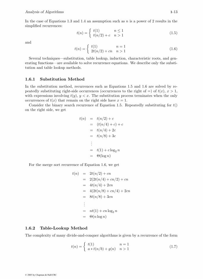
1-18 Handbook of Data Structures and Applications
t(n) =
⎧⎪⎪⎪⎪⎪⎪⎨
⎪⎪⎪⎪⎪⎪⎩
0 n mod 12 = 025 n mod 12 = 1 or 350 n mod 12 = 2, 4, or 675 n mod 12 = 5, 7, or 9100 n mod 12 = 8 or 10125 n mod 12 = 11
take quite some ingenuity to come up with this potential function. Having formulated apotential function and verified that this potential function satisfies Equation 1.11 for all n,we proceed to use Equation 1.10 to determine the amortized costs.
From Equation 1.10, we obtain amortized(i) = actual(i) + P (i) − P (i − 1). Therefore,
amortized(1) = actual(1) + P (1) − P (0) = 50 + 25 − 0 = 75amortized(2) = actual(2) + P (2) − P (1) = 50 + 50 − 25 = 75amortized(3) = actual(3) + P (3) − P (2) = 100 + 25 − 50 = 75
and so on. Therefore, the amortized cost for each month is $75. So, the actual cost for nmonths is at most $75n.
1.7.3 The McWidget Company
Problem Definition
The famous McWidget company manufactures widgets. At its headquarters, the com-pany has a large display that shows how many widgets have been manufactured so far.Each time a widget is manufactured, a maintenance person updates this display. The costfor this update is $c+dm, where c is a fixed trip charge, d is a charge per display digit thatis to be changed, and m is the number of digits that are to be changed. For example, whenthe display is changed from 1399 to 1400, the cost to the company is $c + 3d because 3digits must be changed. The McWidget company wishes to amortize the cost of maintain-ing the display over the widgets that are manufactured, charging the same amount to eachwidget. More precisely, we are looking for an amount $e = amortized(i) that should leviedagainst each widget so that the sum of these charges equals or exceeds the actual cost ofmaintaining/updating the display ($e ∗n ≥ actual total cost incurred for first n widgets forall n ≥ 1). To keep the overall selling price of a widget low, we wish to find as small an eas possible. Clearly, e > c + d because each time a widget is made, at least one digit (theleast significant one) has to be changed.
Worst-Case Method
This method does not work well in this application because there is no finite worst-casecost for a single display update. As more and more widgets are manufactured, the numberof digits that need to be changed increases. For example, when the 1000th widget is made,4 digits are to be changed incurring a cost of c + 4d, and when the 1,000,000th widget ismade, 7 digits are to be changed incurring a cost of c+7d. If we use the worst-case method,the amortized cost to each widget becomes infinity.
© 2005 by Chapman & Hall/CRC
Without the aid of the table (Table 1.5) constructed for the aggregate method, it would

Analysis of Algorithms 1-19
widget 1 2 3 4 5 6 7 8 9 10 11 12 13 14actual cost 1 1 1 1 1 1 1 1 1 2 1 1 1 1amortized cost— 1.12 1.12 1.12 1.12 1.12 1.12 1.12 1.12 1.12 1.12 1.12 1.12 1.12 1.12P() 0.12 0.24 0.36 0.48 0.60 0.72 0.84 0.96 1.08 0.20 0.32 0.44 0.56 0.68
widget 15 16 17 18 19 20 21 22 23 24 25 26 27 28actual cost 1 1 1 1 1 2 1 1 1 1 1 1 1 1amortized cost— 1.12 1.12 1.12 1.12 1.12 1.12 1.12 1.12 1.12 1.12 1.12 1.12 1.12 1.12P() 0.80 0.92 1.04 1.16 1.28 0.40 0.52 0.64 0.76 0.88 1.00 1.12 1.24 1.36
TABLE 1.6 Data for widgets
Aggregate Method
Let n be the number of widgets made so far. As noted earlier, the least significantdigit of the display has been changed n times. The digit in the ten’s place changes oncefor every ten widgets made, that in the hundred’s place changes once for every hundredwidgets made, that in the thousand’s place changes once for every thousand widgets made,and so on. Therefore, the aggregate number of digits that have changed is bounded by
n(1 + 1/10 + 1/100 + 1/1000 + ...) = (1.11111...)n
So, the amortized cost of updating the display is $c + d(1.11111...)n/n < c + 1.12d. If theMcWidget company adds $c+1.12d to the selling price of each widget, it will collect enoughmoney to pay for the cost of maintaining the display. Each widget is charged the cost ofchanging 1.12 digits regardless of the number of digits that are actually changed. Table 1.6shows the actual cost, as measured by the number of digits that change, of maintaining thedisplay, the amortized cost (i.e., 1.12 digits per widget), and the potential function. Thepotential function gives the difference between the sum of the amortized costs and the sumof the actual costs. Notice how the potential function builds up so that when it comestime to pay for changing two digits, the previous potential function value plus the currentamortized cost exceeds 2. From our derivation of the amortized cost, it follows that thepotential function is always nonnegative.
Accounting Method
We begin by assigning an amortized cost to the individual operations, and then weshow that these assigned costs satisfy Equation 1.11. Having already done an amortizedanalysis using the aggregate method, we see that Equation 1.11 is satisfied when we assignan amortized cost of $c + 1.12d to each display change. Typically, however, the use of theaccounting method is not preceded by an application of the aggregate method and we startby guessing an amortized cost and then showing that this guess satisfies Equation 1.11.
Suppose we assign a guessed amortized cost of $c + 2d for each display change.
P (n) − P (0) =∑
1≤i≤n
(amortized(i) − actual(i))
= (c + 2d)n −∑
1≤i≤n
actual(i)
= (c + 2d)n − (c + (1 + 1/10 + 1/100 + ...)d)n≥ (c + 2d)n − (c + 1.12d)n≥ 0
This analysis also shows us that we can reduce the amortized cost of a widget to $c+1.12d.
© 2005 by Chapman & Hall/CRC

1-20 Handbook of Data Structures and Applications
An alternative proof method that is useful in some analyses involves distributing theexcess charge P (i) − P (0) over various accounting entities, and using these stored excesscharges (called credits) to establish P (i + 1) − P (0) ≥ 0. For our McWidget example, weuse the display digits as the accounting entities. Initially, each digit is 0 and each digithas a credit of 0 dollars. Suppose we have guessed an amortized cost of $c + (1.111...)d.When the first widget is manufactured, $c + d of the amortized cost is used to pay for theupdate of the display and the remaining $(0.111...)d of the amortized cost is retained asa credit by the least significant digit of the display. Similarly, when the second throughninth widgets are manufactured, $c + d of the amortized cost is used to pay for the updateof the display and the remaining $(0.111...)d of the amortized cost is retained as a creditby the least significant digit of the display. Following the manufacture of the ninth widget,the least significant digit of the display has a credit of $(0.999...)d and the remaining digitshave no credit. When the tenth widget is manufactured, $c + d of the amortized cost areused to pay for the trip charge and the cost of changing the least significant digit. The leastsignificant digit now has a credit of $(1.111...)d. Of this credit, $d are used to pay for thechange of the next least significant digit (i.e., the digit in the ten’s place), and the remaining$(0.111...)d are transferred to the ten’s digit as a credit. Continuing in this way, we seethat when the display shows 99, the credit on the ten’s digit is $(0.999...)d and that on theone’s digit (i.e., the least significant digit) is also $(0.999...)d. When the 100th widget ismanufactured, $c + d of the amortized cost are used to pay for the trip charge and the costof changing the least significant digit, and the credit on the least significant digit becomes$(1.111...)d. Of this credit, $d are used to pay for the change of the ten’s digit from 9 to0, the remaining $(0.111...)d credit on the one’s digit is transferred to the ten’s digit. Thecredit on the ten’s digit now becomes $(1.111...)d. Of this credit, $d are used to pay forthe change of the hundred’s digit from 0 to 1, the remaining $(0.111...)d credit on the ten’sdigit is transferred to the hundred’s digit.
The above accounting scheme ensures that the credit on each digit of the display alwaysequals $(0.111...)dv, where v is the value of the digit (e.g., when the display is 206 thecredit on the one’s digit is $(0.666...)d, the credit on the ten’s digit is $0, and that on thehundred’s digit is $(0.222...)d.
From the preceding discussion, it follows that P (n) − P (0) equals the sum of the digitcredits and this sum is always nonnegative. Therefore, Equation 1.11 holds for all n.
Potential Method
We first postulate a potential function that satisfies Equation 1.11, and then usethis function to obtain the amortized costs. From the alternative proof used above forthe accounting method, we can see that we should use the potential function P (n) =(0.111...)d
∑i vi, where vi is the value of the ith digit of the display. For example, when the
display shows 206 (at this time n = 206), the potential function value is (0.888...)d. Thispotential function satisfies Equation 1.11.
Let q be the number of 9s at the right end of j (i.e., when j = 12903999, q = 3). Whenthe display changes from j to j + 1, the potential change is (0.111...)d(1 − 9q) and theactual cost of updating the display is $c + (q + 1)d. From Equation 1.10, it follows that theamortized cost for the display change is
actual cost + potential change = c + (q + 1)d + (0.111...)d(1 − 9q) = c + (1.111...)d
© 2005 by Chapman & Hall/CRC

Analysis of Algorithms 1-21
1.7.4 Subset Generation
Problem Definition
The subsets of a set of n elements are defined by the 2n vectors x[1 : n], where eachx[i] is either 0 or 1. x[i] = 1 iff the ith element of the set is a member of the subset. Thesubsets of a set of three elements are given by the eight vectors 000, 001, 010, 011, 100, 101,110, and 111, for example. Starting with an array x[1 : n] has been initialized to zeroes(this represents the empty subset), each invocation of algorithm nextSubset (Figure 1.10)returns the next subset. When all subsets have been generated, this algorithm returns null.
public int [] nextSubset()// return next subset; return null if no next subset
// generate next subset by adding 1 to the binary number x[1:n]int i = n;while (i > 0 && x[i] == 1)
x[i] = 0; i--;
if (i == 0) return null;else x[i] = 1; return x;
FIGURE 1.10: Subset enumerator.
We wish to determine how much time it takes to generate the first m, 1 ≤ m ≤ 2n
subsets. This is the time for the first m invocations of nextSubset.
Worst-Case Method
The complexity of nextSubset is Θ(c), where c is the number of x[i]s that change.Since all n of the x[i]s could change in a single invocation of nextSubset, the worst-casecomplexity of nextSubset is Θ(n). Using the worst-case method, the time required togenerate the first m subsets is O(mn).
Aggregate Method
The complexity of nextSubset equals the number of x[i]s that change. When nextSubsetis invoked m times, x[n] changes m times; x[n − 1] changes m/2 times; x[n − 2] changesm/4 times; x[n−3] changes m/8 times; and so on. Therefore, the sum of the actual costsof the first m invocations is
∑0≤i≤log2 m(m/2i) < 2m. So, the complexity of generating
the first m subsets is actually O(m), a tighter bound than obtained using the worst-casemethod.
The amortized complexity of nextSubset is (sum of actual costs)/m < 2m/m = O(1).
Accounting Method
We first guess the amortized complexity of nextSubset, and then show that this amor-tized complexity satisfies Equation 1.11. Suppose we guess that the amortized complexityis 2. To verify this guess, we must show that P (m) − P (0) ≥ 0 for all m.
We shall use the alternative proof method used in the McWidget example. In this method,we distribute the excess charge P (i) − P (0) over various accounting entities, and use these
© 2005 by Chapman & Hall/CRC

1-22 Handbook of Data Structures and Applications
stored excess charges to establish P (i + 1) − P (0) ≥ 0. We use the x[j]s as the accountingentities. Initially, each x[j] is 0 and has a credit of 0. When the first subset is generated, 1unit of the amortized cost is used to pay for the single x[j] that changes and the remaining 1unit of the amortized cost is retained as a credit by x[n], which is the x[j] that has changedto 1. When the second subset is generated, the credit on x[n] is used to pay for changingx[n] to 0 in the while loop, 1 unit of the amortized cost is used to pay for changing x[n−1] to1, and the remaining 1 unit of the amortized cost is retained as a credit by x[n−1], which isthe x[j] that has changed to 1. When the third subset is generated, 1 unit of the amortizedcost is used to pay for changing x[n] to 1, and the remaining 1 unit of the amortized costis retained as a credit by x[n], which is the x[j] that has changed to 1. When the fourthsubset is generated, the credit on x[n] is used to pay for changing x[n] to 0 in the whileloop, the credit on x[n−1] is used to pay for changing x[n−1] to 0 in the while loop, 1 unitof the amortized cost is used to pay for changing x[n− 2] to 1, and the remaining 1 unit ofthe amortized cost is retained as a credit by x[n− 2], which is the x[j] that has changed to1. Continuing in this way, we see that each x[j] that is 1 has a credit of 1 unit on it. Thiscredit is used to pay the actual cost of changing this x[j] from 1 to 0 in the while loop. Oneunit of the amortized cost of nextSubset is used to pay for the actual cost of changing anx[j] to 1 in the else clause, and the remaining one unit of the amortized cost is retained asa credit by this x[j].
The above accounting scheme ensures that the credit on each x[j] that is 1 is exactly 1,and the credit on each x[j] that is 0 is 0.
From the preceding discussion, it follows that P (m) − P (0) equals the number of x[j]sthat are 1. Since this number is always nonnegative, Equation 1.11 holds for all m.
Having established that the amortized complexity of nextSubset is 2 = O(1), we concludethat the complexity of generating the first m subsets equals m ∗ amortized complexity =O(m).
Potential Method
We first postulate a potential function that satisfies Equation 1.11, and then use thisfunction to obtain the amortized costs. Let P (j) be the potential just after the jth subsetis generated. From the proof used above for the accounting method, we can see that weshould define P (j) to be equal to the number of x[i]s in the jth subset that are equal to 1.
By definition, the 0th subset has all x[i] equal to 0. Since P (0) = 0 and P (j) ≥ 0 forall j, this potential function P satisfies Equation 1.11. Consider any subset x[1 : n]. Letq be the number of 1s at the right end of x[] (i.e., x[n], x[n − 1], · · · , x[n − q + 1], are all1s). Assume that there is a next subset. When the next subset is generated, the potentialchange is 1− q because q 1s are replaced by 0 in the while loop and a 0 is replaced by a 1 inthe else clause. The actual cost of generating the next subset is q + 1. From Equation 1.10,it follows that, when there is a next subset, the amortized cost for nextSubset is
actual cost + potential change = q + 1 + 1 − q = 2
When there is no next subset, the potential change is −q and the actual cost of nextSubsetis q. From Equation 1.10, it follows that, when there is no next subset, the amortized costfor nextSubset is
actual cost + potential change = q − q = 0
Therefore, we can use 2 as the amortized complexity of nextSubset. Consequently, theactual cost of generating the first m subsets is O(m).
© 2005 by Chapman & Hall/CRC

Analysis of Algorithms 1-23
1.8 Practical Complexities
We have seen that the time complexity of a program is generally some function of theproblem size. This function is very useful in determining how the time requirements varyas the problem size changes. For example, the run time of an algorithm whose complexityis Θ(n2) is expected to increase by a factor of 4 when the problem size doubles and by afactor of 9 when the problem size triples.
The complexity function also may be used to compare two algorithms P and Q thatperform the same task. Assume that algorithm P has complexity Θ(n) and that algorithmQ has complexity Θ(n2). We can assert that algorithm P is faster than algorithm Q for“sufficiently large” n. To see the validity of this assertion, observe that the actual computingtime of P is bounded from above by cn for some constant c and for all n, n ≥ n1, whilethat of Q is bounded from below by dn2 for some constant d and all n, n ≥ n2. Since cn ≤dn2 for n ≥ c/d, algorithm P is faster than algorithm Q whenever n ≥ maxn1, n2, c/d.
One should always be cautiously aware of the presence of the phrase sufficiently largein the assertion of the preceding discussion. When deciding which of the two algorithmsto use, we must know whether the n we are dealing with is, in fact, sufficiently large. Ifalgorithm P actually runs in 106n milliseconds while algorithm Q runs in n2 millisecondsand if we always have n ≤ 106, then algorithm Q is the one to use.
To get a feel for how the various functions grow with n, you should study Figures 1.11These figures show that 2n grows very rapidly with n. In fact, if a
algorithm needs 2n steps for execution, then when n = 40, the number of steps needed isapproximately 1.1 ∗ 1012. On a computer performing 1,000,000,000 steps per second, thisalgorithm would require about 18.3 minutes. If n = 50, the same algorithm would run forabout 13 days on this computer. When n = 60, about 310.56 years will be required toexecute the algorithm, and when n = 100, about 4 ∗ 1013 years will be needed. We canconclude that the utility of algorithms with exponential complexity is limited to small n(typically n ≤ 40).
log n n n log n n2 n3 2n
0 1 0 1 1 21 2 2 4 8 42 4 8 16 64 163 8 24 64 512 2564 16 64 256 4096 65,5365 32 160 1024 32,768 4,294,967,296
FIGURE 1.11: Value of various functions.
Algorithms that have a complexity that is a high-degree polynomial are also of limitedutility. For example, if an algorithm needs n10 steps, then our 1,000,000,000 steps persecond computer needs 10 seconds when n = 10; 3171 years when n = 100; and 3.17 ∗ 1013
years when n = 1000. If the algorithm’s complexity had been n3 steps instead, then thecomputer would need 1 second when n = 1000, 110.67 minutes when n = 10,000, and 11.57days when n = 100,000.
to execute an algorithm of complexity f(n) instructions. One should note that currentlyonly the fastest computers can execute about 1,000,000,000 instructions per second. From a
© 2005 by Chapman & Hall/CRC
Figure 1.13 gives the time that a 1,000,000,000 instructions per second computer needs
and 1.12 very closely.
1-24 Handbook of Data Structures and Applications
0 2 4 81 3 5 6 7 9 100
10
20
30
40
50
60
n
f
n
n 2
2n
logn
nlogn
FIGURE 1.12: Plot of various functions.
practical standpoint, it is evident that for reasonably large n (say n > 100) only algorithmsof small complexity (such as n, n log n, n2, and n3) are feasible. Further, this is the caseeven if we could build a computer capable of executing 1012 instructions per second. In thiscase the computing times of Figure 1.13 would decrease by a factor of 1000. Now when n= 100, it would take 3.17 years to execute n10 instructions and 4 ∗ 1010 years to execute 2n
instructions.
f(n)n n n log2 n n2 n3 n4 n10 2n
10 .01 µs .03 µs .1 µs 1 µs 10 µs 10 s 1 µs20 .02 µs .09 µs .4 µs 8 µs 160 µs 2.84 h 1 ms30 .03 µs .15 µs .9 µs 27 µs 810 µs 6.83 d 1 s40 .04 µs .21 µs 1.6 µs 64 µs 2.56 ms 121 d 18 m50 .05 µs .28 µs 2.5 µs 125 µs 6.25 ms 3.1 y 13 d
100 .10 µs .66 µs 10 µs 1 ms 100 ms 3171 y 4 ∗ 1013 y103 1 µs 9.96 µs 1 ms 1 s 16.67 m 3.17 ∗ 1013 y 32 ∗ 10283 y104 10 µs 130 µs 100 ms 16.67 m 115.7 d 3.17 ∗ 1023 y105 100 µs 1.66 ms 10 s 11.57 d 3171 y 3.17 ∗ 1033 y106 1 ms 19.92 ms 16.67 m 31.71 y 3.17 ∗ 107 y 3.17 ∗ 1043 y
µs = microsecond = 10−6 seconds; ms = milliseconds = 10−3 secondss = seconds; m = minutes; h = hours; d = days; y = years
FIGURE 1.13: Run times on a 1,000,000,000 instructions per second computer.
Acknowledgment
This work was supported, in part, by the National Science Foundation under grant CCR-9912395.
© 2005 by Chapman & Hall/CRC

Analysis of Algorithms 1-25
References[1] T. Cormen, C. Leiserson, and R. Rivest, Introduction to Algorithms, McGraw-Hill,
New York, NY, 1992.[2] J. Hennessey and D. Patterson, Computer Organization and Design, Second Edition,
Morgan Kaufmann Publishers, Inc., San Francisco, CA, 1998, Chapter 7.[3] E. Horowitz, S. Sahni, and S. Rajasekaran, Fundamentals of Computer Algorithms,
W. H. Freeman and Co., New York, NY, l998.[4] G. Rawlins, Compared to What: An Introduction to the Analysis of Algorithms, W.
H. Freeman and Co., New York, NY, 1992.[5] S. Sahni, Data Structures, Algorithms, and Applications in Java, McGraw-Hill, NY,
2000.
© 2005 by Chapman & Hall/CRC
Related Documents