1 Punishment without Crime? Prison as a worker discipline device Marcus Miller and Jennifer Smith University of Warwick University of Warwick and CEPR October, 2007 Abstract Could the absence of property rights and reliable monitoring have undermined the Stalinist command economy? An ‘efficiency wage’ model developed for Western economies with imperfect monitoring of effort is reinterpreted on the assumption that it is imprisonment not unemployment that acts as a ‘worker discipline device’. What does it imply? That to secure resources for investment or war, consumption must be compressed; and to avoid incentive problems, prisons should be harsher: this, we find, is the logic of coercion. Adding randomised terror for political ends can, moreover, easily prove economically counter-productive and threaten to destabilise the command economy. Why did Stalin’s system of coercion ultimately fail? We conclude with speculation based on our efficiency wage approach. JEL Nos. D82, P23 ,P26, P27 Acknowledgements For expert advice on Soviet economic history and data, we are greatly indebted to colleagues Mark Harrison and Andrei Markevich; and to Greg Huff for his comments. Marcus Miller acknowledges the financial support of an ESRC Professorial Fellowship, Grant No RES_051-27-0125.

Welcome message from author
This document is posted to help you gain knowledge. Please leave a comment to let me know what you think about it! Share it to your friends and learn new things together.
Transcript
1
Punishment without Crime? Prison as a worker discipline device
Marcus Miller and Jennifer Smith
University of Warwick University of Warwick
and CEPR
October, 2007
Abstract
Could the absence of property rights and reliable monitoring have undermined the
Stalinist command economy? An ‘efficiency wage’ model developed for Western
economies with imperfect monitoring of effort is reinterpreted on the assumption that it is
imprisonment not unemployment that acts as a ‘worker discipline device’. What does it
imply? That to secure resources for investment or war, consumption must be compressed;
and to avoid incentive problems, prisons should be harsher: this, we find, is the logic of
coercion. Adding randomised terror for political ends can, moreover, easily prove
economically counter-productive and threaten to destabilise the command economy. Why
did Stalin’s system of coercion ultimately fail? We conclude with speculation based on
our efficiency wage approach.
JEL Nos. D82, P23 ,P26, P27
Acknowledgements
For expert advice on Soviet economic history and data, we are greatly indebted to
colleagues Mark Harrison and Andrei Markevich; and to Greg Huff for his comments.
Marcus Miller acknowledges the financial support of an ESRC Professorial Fellowship,
Grant No RES_051-27-0125.
2
…… riches, poverty,
And use of service, none; contract, succession,
Bourn, bound of land, tilth, vineyard, none;
No use of metal, corn, or wine, or oil;
No occupation; all men idle, all;
And women too
Shakespeare The Tempest Act 2, scene 1
Introduction
At a time when Western economies were plagued by mass unemployment, Stalin could
rightly claim to have found a cure: a command economy with ambitious five year plans
to catch up with the West by rapid industrialisation. Massive capital investment ensured
no shortage of aggregate demand: the problem was how to compress consumption.
But those who would create a Utopia without private property rights must confront the
issue of incentives. This is evident from Gonzalo’s vision of Utopia, cited above. For old
Gonzalo the anticipated solution was natural abundance, produced “without sweat or
endeavour”1. But Joseph Stalin, for his part, was planning for great increases in
productivity through rapid industrialisation and collectivisation. How was he to motivate
workers with low levels of skill including “millions pouring in from the countryside
entirely lacking in training or experience of the rigour and rhythms of life in a factory or
on a construction site” (Acton and Stableford, 2005, p.315)?
Incentives will depend on the distribution of information: even a dictator has to solve
endemic problems of asymmetric information2, as Stalin was soon to learn. Although the
First Five-Year Plan was launched “with a wave of attacks on managers and specialists
suspected of harbouring alien class sympathies”, this was found to be “incompatible with
the discipline drive, given their direct involvement in monitoring labour performance and
1 His companions were not convinced; nor, one assumes, was Shakespeare – shareholder of his theatre
company and owner of the second most expensive residence in Stratford. 2 The incentive problems arising from asymmetric information are central to Stiglitz’s critique of the Soviet
system in Whither Socialism? (1994).
3
implementing measures to designed to raise productivity”; and there was a sharp change
of policy in 1931 (Acton and Stableford, 2005, p.316).
How was Stalin to elicit the necessary ‘sweat and endeavour’ from his compatriots in
conditions of limited information? ‘Efficiency wage’ theories may provide answers.
Akerlof and Yellen (1990), for example, emphasise how worker motivation depends on
whether employers are seen as good, and wages perceived as fair. This is the approach
adopted to study incentives under Stalin by Gregory (2003), who uses it to explain the
trade-offs involved in choosing between consumption and investment in the command
economy. In Gregory’s model, workers’ effort depends positively on the wage (or
consumption level) they receive, up to the point where they are paid the ‘fair wage’ and
supply their ‘full’ labour effort. A dictator, wishing to maximise investment in the face of
output constraints that force him to choose between investment and consumption, will
pick a wage lying below the ‘fair wage’, but above a ‘strike wage’ at which workers will
withdraw their labour. Gregory discusses how Stalin realised that consumption had to be
increased to counter declining productivity in the early 1930s: and how he attempted to
manipulate the fair wage by “promises of a brighter future”3.
The efficiency wage theory of Shapiro and Stiglitz (1989), on the other hand, focuses on
asymmetric information and ‘shirking’. Assuming the supply of effort is all or nothing, the
worker is paid to put in effort, but failure to do so (‘shirking’) leads to loss of employment
and income. Wages will need to exceed unemployment benefits by enough to preserve
incentives for effort; but with imperfect monitoring of effort, incentive problems require
the payment of ‘efficiency wages’ much exceeding the cost of effort-plus-benefit; and the
maintenance of persistent unemployment as a ‘worker discipline device’4. (Ironically,
however, if unemployment acts successfully as a discipline device, there will be no shirkers
among the unemployed, just those moving between jobs.)
The Soviet system depended not so much on the carrot as on the stick (Harrison, 2002); but
one can appeal to the ‘Coase theorem’ (1960) to show that either rewards or punishments
3 He also mentions the possible use of forced labour to incentivise workers, the principle idea developed in
this paper. 4 The loss of wages in suffering a spell of unemployment when caught and fired must be great enough to
stop shirking; they show that the efficiency wage has to increase sharply as unemployment shrinks; and is
also increasing in the level of non-incentive-related job losses.
4
can elicit effort, so long as property rights are appropriately determined. If labour power is
effectively owned by the state, workers need not be rewarded for supplying effort. But
without high ‘efficiency wages, how are incentives to be preserved? From a Coasian
perspective, shirkers could, in principle, be fined for failure to supply effort (and some such
financial penalties were used); but in practice, of course, workers on low wages simply
cannot pay.
Another solution is to extend the command economy yet further. This is the avenue we
explore in this paper. It is an avenue that ultimately leads to the Gulag Archipelago5, for
the discipline device we consider is non-pecuniary deprivation – imprisonment in
particular. As Gregory and Harrison (2005, p.740) note in their survey of allocation under
dictatorship: “The effectiveness of the Politburo accumulation model rested on the
dictator’s ability to create a gap between the civilian wage as a ‘fair’ return for effort, and
low subsistence in the Gulag as the return to shirking, so that the difference between them
was the intended punishment for shirking.” While custodial sentences (with effort levels
exceeding those in employment) replace spells of low income and unemployment as an
economic discipline device for shirking, nevertheless, as in the Shapiro-Stiglitz analysis,
no-one need be in prison for shirking if the incentive system works well. As inmates of
labour camps were made to produce, however, this provided an economic rationale for
imprisonment. But when prison is widely used for political repression, incentive
problems can reappear and may even threaten the survival of the command economy.
After a brief overview and discussion of data on the custodial population in the USSR
from 1917 to 1953 an alternative efficiency wage model is developed in Section 2, where
the Shapiro and Stiglitz model of incentives is adapted to fit Soviet forms of coercion.
While the analysis confirms that promises of future consumption may well cut efficiency
wages for a time, it also implies that randomisation of punishment will have the opposite
effect. We show, in particular, how incentive constraints can limit the power of the
dictator to achieve increasing demands for investment -- unless there is recourse to
increasing harshness. In Section 3 it is shown how a multiplicity of steady states exist
when release rates are endogenous; and how random incarceration for political ends can
5 Solzhenitsyn (1974).
5
threaten economic efficiency. Why did Stalin’s system of coercion ultimately fail? We
conclude with speculation based on our efficiency wage approach.
1. Data on custodial population; and on ‘corrective work’
While Shapiro and Stiglitz consider unemployment as a worker discipline device, it is
clear that it could not perform that role in the Soviet system: by the early 1930s the
Soviet government could rightly claim that unemployment was “liquidated”
(Rogachevskaya, 1973)6. The proposition to be considered here is that coercion not
idleness was the discipline device in the Soviet case. But, as Sherlock Holmes warned Dr.
Watson7: “It is a capital mistake to theorize before one has data”.
Emergence of the Gulag Archipelago
After Stalin and his allies took control of the Politburo in 1928-9, and after the decision
to forcibly collectivise the peasants in 1929, numbers in custody began to rise inexorably.
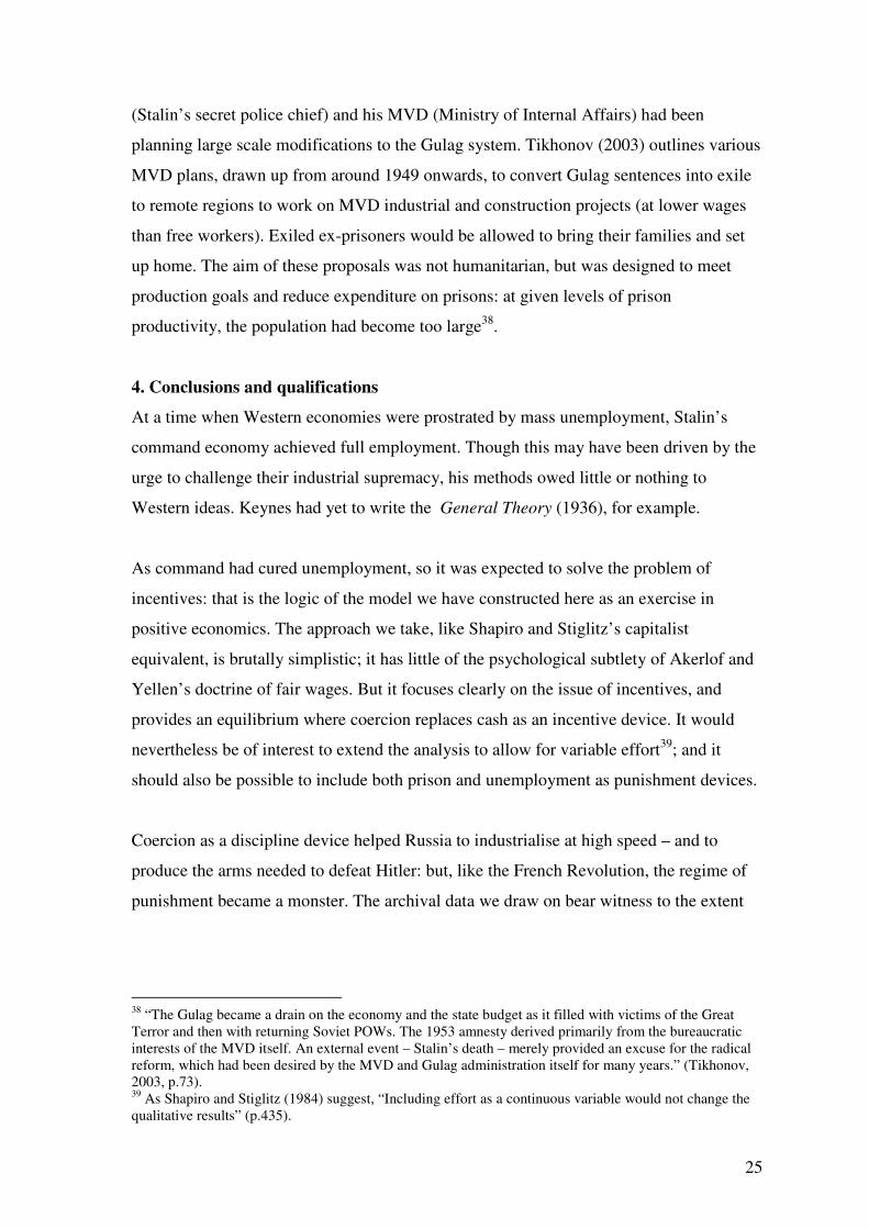
Chart 1 provides an overview of the numbers in custody over the years 1917 to 1953
(excluding settlements), with detailed figures and sources provided in Appendix 1. Note
that in the text we use the term ‘prison’ to encompass the whole of the Gulag system,
generally understood to include prisons, colonies and camps.
6 There were some people in the labour force without work, but “under conditions of socialism, the
condition of being without work (nezaniatost’) is not a synonym for ‘unemployment’. It means only an
interruption of work caused by reasons of a private character (family circumstances, changes of location)”
Kotliar (1983, p.9). 7 In ‘A Scandal in Bohemia’, for example (Conan Doyle, 1992, p.14).
6
0
500,000
1,000,000
1,500,000
2,000,000
2,500,000
3,000,000
1917
1919
1921
1923
1925
1927
1929
1931
1933
1935
1937
1939
1941
1943
1945
1947
1949
1951
1953
Year
Prisons
Labour camps + colonies
Labour colonies
Labour camps
Chart 1: USSR custodial population, 1917-1953
The Law of Corrective Labour Camps of 1930 placed all camps and colonies in the
control of the Gulag, and harsher sentencing after 1930 brought small-time crooks into
the Gulag system (Overy, 2004) so that by 1934, when the NKVD8 took charge of the
camp system, around half a million were in custody. The NKVD tightened security and
supervision, the possibility of escape diminished and the numbers imprisoned more than
doubled in a couple of years. Thus the proportion of the working population imprisoned
rose from 0.9% to 1.2% between 1934 and 1936 (when employment was 57.7m and
62.3m respectively). Imprisonment may act as a worker discipline device; but it was also
used as an instrument of political power, with people being punished not for lack of effort
but for ideological reasons.
The Great Terror
According to Lazarev ( 2003, p.191): “The Gulag came into its own with the beginning
of the Great Terror in 1937, when the upsurge in political prisoners drastically increased
the population of the archipelago … As the morose product of the tyrant’s paranoia, its
main goal was to accommodate growing numbers of repressed opponents of the regime
8 People’s Commissariat of Internal Affairs – the secret police.
7
and “socially alien elements” (like wealthy farmers and priests), while the economic use
of prison labor was simply a by-product of the main political purpose” 9
.
The ‘mass operations’ of the Great Terror lasted from July 1937 until November 193810
.
How the episode got its name – and the political drive behind it - becomes clear from the
statistics. Not only did the number of arrests rise during the Terror, but the conviction
rate also rose – from around one third in 1930 to 85 per cent in 1937 (Gregory et al,
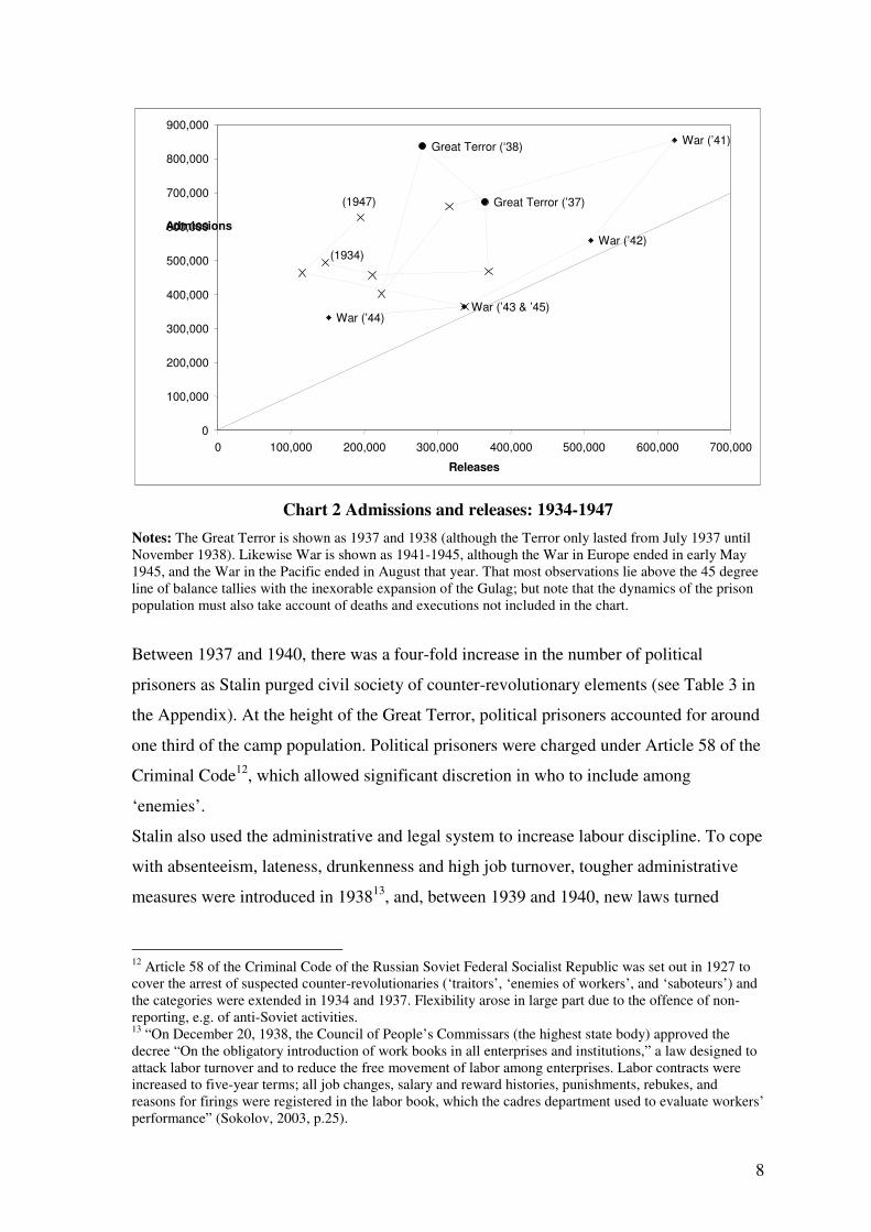
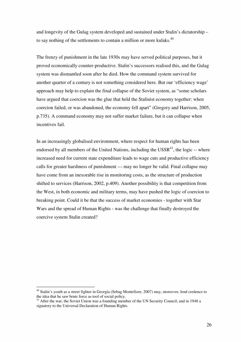
2006, p.19). The result, as Chart 2 demonstrates for camps, was a huge rise in admissions
to the prison system. There was no countervailing rise in releases – indeed, releases fell
during the Terror – resulting in a 21 per cent increase in the Gulag camp population
between January 1, 1937 and January 1, 1938, and an increase of 32 per cent the
following year. Estimates vary, but even (conservative) data from the Soviet Archive
show that, from a working population of 66 million11
, 1.4 million (over 2%) had been
convicted by 1 November 1938, of whom about half were executed (Khlevnyuk,
forthcoming).
9 Furthermore, as Overy (2004) observes, to merit punishment under Stalin’s rule, it was not necessary to
have committed an offence; it was enough that those in power thought you might do so on some future
occasion. 10
During 1935-1936, Stalin had targeted the political elite, the three Moscow Show Trials enabling him to
get rid of political rivals. In various communications and decrees of July 1937, Stalin formulated plans for a
terror campaign initially planned to start on August 5 and to last four months. Initial ‘limits’ for arrests and
executions and the duration of the campaign had to be rapidly revised upwards to meet requests by local
officials (Gregory et al, 2006). 11
In 1937.
8
Chart 2 Admissions and releases: 1934-1947
Notes: The Great Terror is shown as 1937 and 1938 (although the Terror only lasted from July 1937 until
November 1938). Likewise War is shown as 1941-1945, although the War in Europe ended in early May
1945, and the War in the Pacific ended in August that year. That most observations lie above the 45 degree
line of balance tallies with the inexorable expansion of the Gulag; but note that the dynamics of the prison
population must also take account of deaths and executions not included in the chart.
Between 1937 and 1940, there was a four-fold increase in the number of political
prisoners as Stalin purged civil society of counter-revolutionary elements (see Table 3 in
the Appendix). At the height of the Great Terror, political prisoners accounted for around
one third of the camp population. Political prisoners were charged under Article 58 of the
Criminal Code12
, which allowed significant discretion in who to include among
‘enemies’.
Stalin also used the administrative and legal system to increase labour discipline. To cope
with absenteeism, lateness, drunkenness and high job turnover, tougher administrative
measures were introduced in 193813
, and, between 1939 and 1940, new laws turned
12
Article 58 of the Criminal Code of the Russian Soviet Federal Socialist Republic was set out in 1927 to
cover the arrest of suspected counter-revolutionaries (‘traitors’, ‘enemies of workers’, and ‘saboteurs’) and
the categories were extended in 1934 and 1937. Flexibility arose in large part due to the offence of non-
reporting, e.g. of anti-Soviet activities. 13
“On December 20, 1938, the Council of People’s Commissars (the highest state body) approved the
decree “On the obligatory introduction of work books in all enterprises and institutions,” a law designed to
attack labor turnover and to reduce the free movement of labor among enterprises. Labor contracts were
increased to five-year terms; all job changes, salary and reward histories, punishments, rebukes, and
reasons for firings were registered in the labor book, which the cadres department used to evaluate workers’
performance” (Sokolov, 2003, p.25).
War (’41)
War (’42)
War (’43 & ’45)War (’44)
Great Terror (’37)
Great Terror (‘38)
0
100,000
200,000
300,000
400,000
500,000
600,000
700,000
800,000
900,000
0 100,000 200,000 300,000 400,000 500,000 600,000 700,000
Releases
Admissions
(1934)
(1947)
9
absence from work, tardiness, drunkenness and hooliganism into crimes14
punished by up
to four months in jail (Solomon, 1980, p.217). These draconian new measures affected
huge numbers: almost 1.8 million workers were convicted of absenteeism or lateness of
more than 20 minutes in 1940 – more than two thirds of all criminal convictions
(Solomon, 1996, p.299); and there were over 4.5 million convictions during 1940-1942
(Sokolov, 2003, Table 2.1, p.28).15
War and Post War
From a peak of over two million during the Great Terror, the numbers in custody fell to a
million and a third by 1944. This was in large measure due to a step increase in the
release rates connected with the war effort, see Chart 2. (Almost one million detainees
were released to military service, particularly to the ‘storm’ units which suffered the
heaviest casualties.) For those left in the Gulag during the war, however, the mortality
rate was extremely high: from 1941 to 1945, 1,005,000 inmates died in camps and
colonies (Khlevnyuk, 2003, p.51), due to scarce rations and the fact that the most able-
bodied had been sent to war.
But after the war was over, the custodial population rapidly resumed its upward march,
reaching a plateau of two and a half million in 1948. Numbers stayed at this level until
Stalin’s death in 1953 when more than half of all detainees were released. Immediately
post-war, ‘mobilization’ and organised recruitment of ex-army, ex-Gulag, and new
graduates supplied up to a quarter of labour in some industries (Sokolov, 2003). Although
pre-war labour discipline laws were retained after the war, turnover remained a problem,
reaching 34 per cent in light industry and 64 per cent in construction (Sokolov, 2003,
14
“In January of 1939, the Council of People’s Commissars decreed that tardiness of 20 minutes or more
constituted an unauthorized absence from work. On June 26, 1940, the Presidium of the Supreme Soviet
approved the decree “On the transition to an eight hour work day, a seven day work week, and the
prohibition of voluntary departures of workers from enterprises and institutions.” The June 1940 law tied
the worker to the enterprise and introduced criminal punishments for laziness, poor discipline, and
tardiness. In August of 1940, criminal punishments were introduced for minor workplace infractions, such
as drunkenness, hooliganism, and petty theft. The October 1940 reforms of vocational education
raised the term of obligatory work after graduation to four years and prohibited voluntary departures”
(Sokolov, 2003, p.25). 15
Not all of these served prison sentences: according to Sokolov (2003, p.28), there were 955,000 prison
sentences related to idleness and unauthorised departures during 1940-1941 (many more were sentenced to
corrective work – see below). But the effect on the population was even bigger than these figures suggest:
during 1940-1941 there were a total of 5.3 million trials for such offences (Sokolov, 2003, pp.27-28),
which represents 2.8 per cent and 4.3 per cent of the workforce, respectively.
10
p.37) – and living conditions were poor16
, exacerbated by a famine in 1946-47. A further
decree combating mobility was issued in 1948; almost a quarter of a million workers
were sentenced to jail terms for unauthorised absence, laziness or idleness in 1949; and of
the 2.5 million imprisoned in the Gulag in 1950, half had been sentenced under the June
1940 labour discipline law17
. Labour restrictions were eventually reduced in 195118
; but
they were only fully abolished in 1956, after Stalin’s death. As Sokolov (2003, p.38)
comments, “With the passage of the 1956 law, the post-Stalin leadership turned
decisively from ‘sticks’ to ‘carrots’.”
Non-custodial punishment
Imprisonment was not the only discipline device open to the Soviet courts: the Coasian
alternative of punishment via financial penalty was also used. What was termed
‘corrective work’ was quite common throughout the 1930s, constituting 48 per cent of all
court sentences in 1935 (Getty et al, 1993, p.1020).19
Typically, offenders were
condemned to up to one year’s ‘corrective labour’, the penalty consisting of work
typically at the usual place of employment, with a reduction in the wage of up to 25 per
cent and loss of credit for this service towards the length of service that gave rights to
non-wage benefits such as vacation, pension (Getty et al, 1993, p.1020; Sokolov, 2003,
p.32). The several laws on labour discipline passed in the late 1930s and early 1940s
increased the numbers given non-custodial sentences, but in relative terms the proportion
sent to prison rose20
.
16
“A female worker in a Moscow plant wrote: ‘We worked hard throughout the war; we awaited the
victory and counted on better conditions. The opposite occurred. They lowered our salaries and we receive
pennies. It is time to think about the workers’.” (Sokolov, 2003, p.34). In 1945 the lengthened workday was
scrapped, but bonuses for ‘plan overfulfillment’ were also abolished. 17
The relative severity of punishment for these offences rose, as the numbers fined fell by half (Sokolov,
2003, pp.38 and 41). 18
By a decree of the Praesidium of the Supreme Soviet of July 14 “About the replacement of judicial
responsibility of workers and employees for idleness, except in the case of multiple and extended absences
with disciplinary and social actions” (Sokolov, 2003, p.38). 19
Solomon (1980) describes how the non-custodial sanction of what was then known as ‘compulsory work’
had been used extensively since the start of the Bolshevik regime. In 1923, only 20 per cent of those
convicted in a criminal court were sent to prison; 25 per cent were sentenced to compulsory work (p.198).
However, by 1926 the proportion sent to prison had risen to 40%, in part due to a change in the type of
crimes coming before the courts, and in part because judges avoiding sentences of compulsory work that
were not being properly carried out, in part because of the then high unemployment (p.204). 20
From 20 per cent in 1930, to 37.8 per cent in 1934, to 55 per cent in 1938, and to more than two thirds in
1940 (Solomon, 1980, p.216), despite there being 1.7 million non-custodial sentences in 1940 (Getty et al,
1993, p.1020).
11
2. Prison as an incentive device
Shapiro and Stiglitz’s account of how shirking is monitored under capitalism has three
salient characteristics: that the punishment for being caught shirking is to lose one’s job;
that efficiency wages paid to the employed are a lot higher than effort –plus-benefits (as
paid to the unemployed – who are not required to work); that this premium rises sharply
as employment levels increase and unemployment falls. (The reason for the rising
premium is that the punishment involved in losing one’s job is diminished by the short
unemployment duration rates prevailing at low levels of unemployment.) Analytical
detail of the No Shirking Constraint that they obtain in this framework is presented in
Appendix B.
Consider now a Soviet alternative, where the monitoring of effort is still a problem but
there is no unemployment. Instead the punishment for those caught shirking is to be sent
to prison, where they have to work. Efficiency wages where shirking is treated as a crime
meriting imprisonment will of course depend on prison conditions and on duration of
punishment.
2.1 Efficiency wages and ‘Dire Punishment’
To capture the psychological impact of being ‘sent to Siberia’, we begin with the case
where imprisonment is seen as the end of normal life (labelled ‘dire punishment’, the
term is used in repeated games to denote a state from which there is no transition). As
Ertz (2007, p.27) puts it: “For individuals sentenced by the Stalinist political or criminal
justice, …their chances to turn into ‘Soviet people’ were, if not zero, then at least much
lower than for the rest of society”.21
Let w denote the real wage and e denote effort while working, so the welfare of one who
works is simply w – e, i.e. the excess of wages over effort. Let q denote the probability of
detection while shirking (putting in zero effort) and assume those caught shirking are sent
to prison where the level of welfare is Pw hδ = − , i.e. the excess of prison wages over
hard labour. The benefit of working versus being in prison will therefore be w – e – δ.
21
Even after release, an ex-con would not be able to participate normally in society: for example, on
release, political prisoners had to sign a paper stating that they would never again engage in counter-
revolutionary activity, were forbidden to live in major cities and had to report to a police station of the
NKVD for years afterwards (Overy, 2004, p.634).
12
(Note that δ will be negative if being in prison is worse than being paid just enough to put
in effort voluntarily outside prison.)
In the dire punishment case, where incarceration is treated as permanent and r denotes the
discount rate, the ‘no shirking condition’, NSC, is
( ) /e q w e rδ≤ − − (1)
i.e. the benefit of saving on effort for one period must match the risk of losing the job and
being imprisoned for ever.
The ‘efficiency wage’ is where the two are exactly equal, i.e.
/w e re qδ= + + (2)
so it falls with the harshness of prison conditions and with the efficacy of monitoring.
Simple as it is, this formulation offers useful insight into aspects of the Soviet system.
(a) Monitoring costs
Because, during the first Five-Year Plan, managers and specialists were harassed and
imprisoned for ideological reasons, monitoring costs rose sharply. But equation (2) shows
that a fall in the probability of detection q has the immediate effect of raising the
efficiency wage, with potentially serious incentive effects considered in more detail
below.
It seems that by 1931-1932 Stalin had already learnt this lesson, for the policy was
changed. “Specialists trained under the old regime, he announced, had seen the light and
could now be trusted … the authority, status and privileges of the white-collar strata now
began to be energetically buttressed” (Acton and Stableford, 2005, p.316).
(b) Stakhanovism
After the example of Stakhanov, who in 1935 mined far more coal per hour than the
norm, many managers hoped that others would follow his example and produce more
coal for the same wage22
. But the formula for the efficiency wage confirms that “harder
work deserves a bigger share of the pie and that the higher wages of Stakhanovites should
22
Output norms were already in place in the mid-1930s, and worker’s compensation consisted of base pay
plus piece rates dependent on fulfilling output norms. After Stakhanov cut 102 tons of coal in 5 hours 45
minutes, beating the ‘norm’ of 7 tons by a factor of over 14, Gosplan raised output targets (Gregory, 2003,
p.103)
13
be passed on to ordinary workers” who were also working harder (Gregory, 2003,
p.106)23
. (Because of imperfect monitoring, the efficiency wage rises more than one for
one with effort, as can be seen by differentiating (2) with respect to effort to
obtain: qrew /1/ +=δδ 24.)
(c) Promises of a brighter future
In the first and second Five Year Plans, Stalin argued that workers should accept
restraints on their current wage in return for the promise that – thanks to higher
investment – the supply of consumer goods would at least double, or perhaps even triple,
by the late 1930s. Can the efficiency wage be restrained by “visions of a brighter future”
(Gregory, 2003, p.97)?
To show that workers might be willing to accept a lower efficiency wage in return for
these future increases, we augment the right hand side of (1) by the term Je-rT
/r, where J
is the promised ‘jump’ in wages after time T; so the efficiency condition becomes:
( ) rJeewqe rT /=+−−= δ . (1’)
Hence the efficiency wage falls by the present discounted value of the jump, so:
qerJeew rT /+−+= −δ . (2’’)
Promises of a brighter future can , in principle, maintain the value of a job despite the cut
in current wages. (For incentives to be preserved, promises must be credible: and
credibility became strained as the Plans failed to deliver.)
2.2 Economic equilibrium with random terror
According to Gregory and Harrison(2005, p 739) “Such a wide range of behaviors was
criminalized that virtually every worker became liable to prosecution for something” .
But for workers faced with increased uncertainty concerning their liberty, this will have
the opposite effect of brave promises, reducing the value of a job at the existing current
wage. Allowing for ‘political’ reasons for being sent to prison, which the average worker
treats as a hazard that arrives randomly at rate dtπ independent of effort supplied, then
23
Gregory (2003) describes the conflict that arose in the mid-1930s between those who wished to reward
workers with higher pay, and those who wished to raise norms. “Ordinary workers interpreted the
Stakhanovite movement as a plot to extract more work for the same wage”, and there was “no perceptible
advance in labour productivity during or after the Stakhanovite movement, despite the fact that some
Stakahnovites raised labour productivity substantially” (p.105). 24
The industrial system at the time was indeed based on progressive piece rates (Gregory, 2003, p.105).
14
the flow of net earnings for a job must be discounted at a higher rate, r + π, to allow for
the risk of random political ‘state transition’ as well as the passage of time.
As the value of a job falls, so the efficiency wage rises to become
( ) /w e r e qδ π= + + + (3)
Thus, in terms of the efficiency wage, random threats of dire punishment militate against
promises of a bright future.
Note, in addition, that in equilibrium where wages satisfy this condition, no-one will be
shirking, so all admissions to prison will be politically inspired. To determine a steady
state equilibrium when there is random incarceration of free labour, it is necessary to
allow for a positive release rate – otherwise the prison population can only increase25
.
Once we incorporate the possibility of release from prison back to a normal working life,
at the rate ρ dt taken to be fixed at a low level26
, prison may no longer be seen as an
absorbing state or ‘dire punishment’: but it can still act as a discipline device, particularly
if conditions are harsh27
.
In steady state equilibrium, with the prison population constant, the flow of random
political incarcerations must match the flow of those being released:
pp ρπ =− )1(
where p denotes the percentage of the workforce in prison, implying ( )πρ /1/1 +=p . .
Imprisonment of a percentage p of the population for political reasons reduces the labour
available for the rest of the economy: the labour force remaining available for
employment will be L=(1-p)N
The efficiency wage becomes
( ) qerwew /πρ ++++= (4)
or
( ) qeprwew //π+++= (5)
25
Our simplified treatment does not include the impact of executions and deaths in prison. 26
Note that the lower the release rate, the longer the expected spell in prison, so one could draw an
equivalence between a model of stochastic release and one with a determinate prison sentence, where ρ is
inversely related to the length of sentence. 27
The other method of getting out of prison alive – escape – will have an effect similar to that of release.
The possibility of escape from the Gulag diminished after 1934, when the Soviet secret police (NKVD)
took over the whole of the camp and colony system. Nevertheless, archive data indicate that between 1934
and 1953, 378,375 escapes were attempted; only 38 per cent of these succeeded, however (Getty et al,
1993, p.1041).
15
In contrast to the Shapiro-Stiglitz model28
, a fixed release rate constrains steady state
equilibrium to a single level of employment. A possible equilibrium for the economy as a
whole is shown in Figure 1 where the effective labour supply turns out to have a reverse-
L shape. In the absence of monitoring problems the real wage would have to cover e-
plus-δ, i.e. the cost of effort plus net welfare in prison, shown by the point labelled e δ+
on the vertical axis. Imperfect monitoring would alone increase the efficiency wage to the
‘dire punishment’ wage wd = /e re qδ+ + . But the addition of random imprisonment
with a fixed release rate pushes the requisite wage higher, so the efficiency wage is given
by ( ) qerew /πρδ ++++= , shown as the horizontal line labelled ‘NSC’.
As for Shapiro and Stiglitz, the marginal product of labour MPL is shown as a decreasing
function of aggregate employment. The effect of imprisonment of P=N-L workers is to
reduce the supply of civilian labour from N to L, the resource constraint on employment
and civilian output shown in the figure.
As is well known, Stalin recognised the economic benefits of forcing prisoners to work29
.
Securing the output of their labour may not have been an object of imprisonment policy;
but forced labour could help national production30
. Prison production is also shown in the
diagram and provides another contrast with the model of Shapiro and Stiglitz where the
unemployed supply no labour for current production.
The productivity of civilian labour implies that a dictator seeking to increase national
output by means of forced prison labour faces a rising opportunity cost of incarceration.
But total output can be increased through imprisonment, if prisoner productivity is higher
than the marginal product of labour of free labour at full employment N31
. If per capita
28
See Appendix 2. 29
The first Five-Year Plan 1928-1933 involved the use of prisoners as a labour force. Solomon (1980,
p.208) reports a 1929 edict to establish timber and industrial colonies, with the aim of replacing most
prisons, and timber camps in remote regions under OGPU control, housing long-sentence inmates from
regular prisons. 30
As Ertz (2007, p.25) notes: “There is no contradiction between the [fact that] camp administrators were
induced to treat prisoners primarily as an economic resource, and the fact that the camp system came into
existence and developed within purely political parameters – namely, the dictator’s politically and
ideologically motivated decisions to arrest millions of subjects (and, at times, to release some of them)”. 31
Sokolov (2003, pp.39-40) records that “Labour productivity in the Gulag’s production administrations
was only 50 to 60 per cent of comparable civilian administrations”. But this figure is somewhat misleading:
Gulag workers felled timber, mined, and built where free workers would not go; ‘normal’ production was
only a part of Gulag work.

16
productivity in prison is constant as shown by the line HH in the Figure, national output
will be maximised when the prison population is MN32
. If the prison population is
increased beyond MN, then in the absence of an increase in productivity, prison
production becomes relatively non-economic and inefficient33
.
Figure 1: Coercive equilibrium: output and employment
32
For incentive compatibility, we assume that efficiency wage less is than the MPL at M, and the
administered fixed wage lies between the two. 33
Khlevnyuk (2003) describes how various methods were adopted in an attempt to raise prisoner
productivity, apart from pure coercion. Mechanisation was one method; ‘economic’ incentives were
another: workday credits – sentences were reduced if workers overfulfilled norms – were applied between
1931 and 1939 and reintroduced in 1948 (Ertz, 2005); also in 1948, the Council of Ministers decreed that
Gulag workers were to receive wages – mainly in the form of piece rates and bonuses – set at 30 per cent of
civilian wages (Sokolov, 2003, p.40). But “Measures to raise labor productivity were not generally
successful … In 1951-52, not one production administration of the Gulag fulfilled its plan for raising labor
productivity” (Sokolov, 2003, p.40).
Prison
population
(when π > 0)
P=N-L
E
M
L Employment
Real wage
Fixed real wage
e δ+
MPL Resource
constraint
I NSC under dire punishment (π = 0)
( )rq
eew ++++= ρπδ
qreew
d ++= δ
N
H H
N-M is prison population that will maximise
national product
Prisoner
productivity
wf
NSC
Political
imprisonments πL
Releases ρ P
π ρ
Employment L
(a)
(b)
17
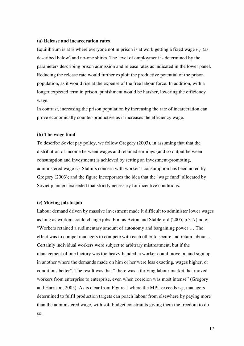
(a) Release and incarceration rates
Equilibrium is at E where everyone not in prison is at work getting a fixed wage wf (as
described below) and no-one shirks. The level of employment is determined by the
parameters describing prison admission and release rates as indicated in the lower panel.
Reducing the release rate would further exploit the productive potential of the prison
population, as it would rise at the expense of the free labour force. In addition, with a
longer expected term in prison, punishment would be harsher, lowering the efficiency
wage.
In contrast, increasing the prison population by increasing the rate of incarceration can
prove economically counter-productive as it increases the efficiency wage.
(b) The wage fund
To describe Soviet pay policy, we follow Gregory (2003), in assuming that that the
distribution of income between wages and retained earnings (and so output between
consumption and investment) is achieved by setting an investment-promoting,
administered wage wf. Stalin’s concern with worker’s consumption has been noted by
Gregory (2003); and the figure incorporates the idea that the ‘wage fund’ allocated by
Soviet planners exceeded that strictly necessary for incentive conditions.
(c) Moving job-to-job
Labour demand driven by massive investment made it difficult to administer lower wages
as long as workers could change jobs. For, as Acton and Stableford (2005, p.317) note:
“Workers retained a rudimentary amount of autonomy and bargaining power … The
effect was to compel managers to compete with each other to secure and retain labour …
Certainly individual workers were subject to arbitrary mistreatment, but if the
management of one factory was too heavy-handed, a worker could move on and sign up
in another where the demands made on him or her were less exacting, wages higher, or
conditions better”. The result was that “ there was a thriving labour market that moved
workers from enterprise to enterprise, even when coercion was most intense” (Gregory
and Harrison, 2005). As is clear from Figure 1 where the MPL exceeds wf,, managers
determined to fulfil production targets can poach labour from elsewhere by paying more
than the administered wage, with soft budget constraints giving them the freedom to do
so.
18
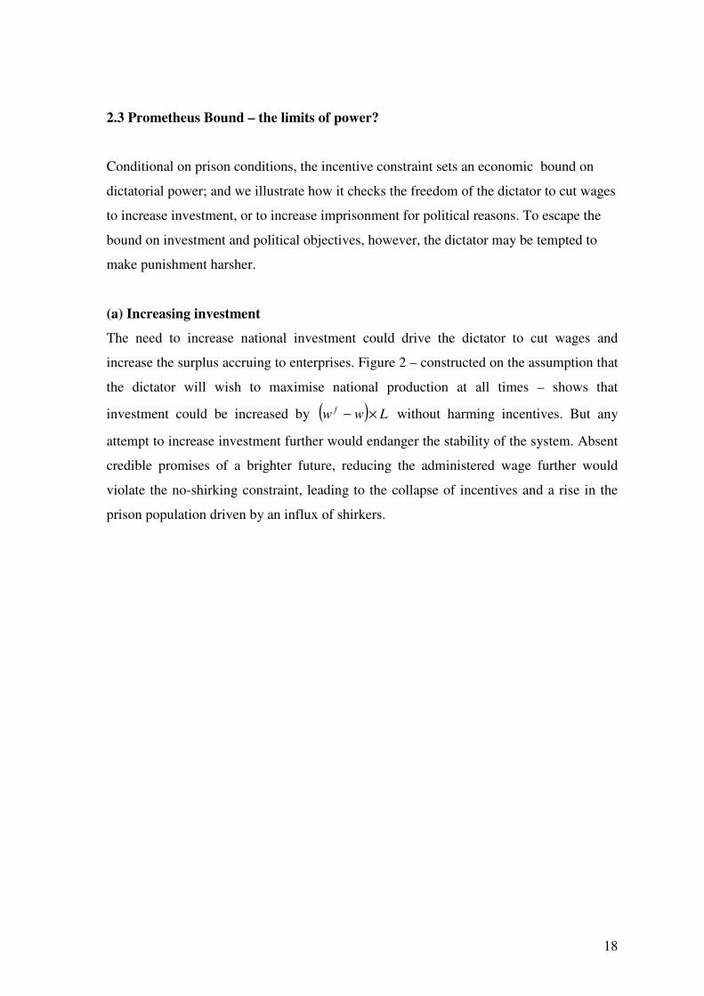
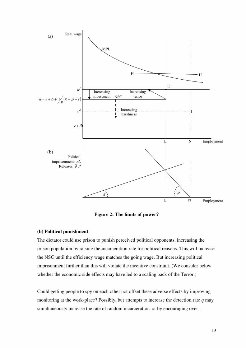
2.3 Prometheus Bound – the limits of power?
Conditional on prison conditions, the incentive constraint sets an economic bound on
dictatorial power; and we illustrate how it checks the freedom of the dictator to cut wages
to increase investment, or to increase imprisonment for political reasons. To escape the
bound on investment and political objectives, however, the dictator may be tempted to
make punishment harsher.
(a) Increasing investment
The need to increase national investment could drive the dictator to cut wages and
increase the surplus accruing to enterprises. Figure 2 – constructed on the assumption that
the dictator will wish to maximise national production at all times – shows that
investment could be increased by ( ) Lww f ×− without harming incentives. But any
attempt to increase investment further would endanger the stability of the system. Absent
credible promises of a brighter future, reducing the administered wage further would
violate the no-shirking constraint, leading to the collapse of incentives and a rise in the
prison population driven by an influx of shirkers.
19
Figure 2: The limits of power?
(b) Political punishment
The dictator could use prison to punish perceived political opponents, increasing the
prison population by raising the incarceration rate for political reasons. This will increase
the NSC until the efficiency wage matches the going wage. But increasing political
imprisonment further than this will violate the incentive constraint. (We consider below
whether the economic side effects may have led to a scaling back of the Terror.)
Could getting people to spy on each other not offset these adverse effects by improving
monitoring at the work-place? Possibly, but attempts to increase the detection rate q may
simultaneously increase the rate of random incarceration π by encouraging over-
E
L Employment
Real wage
e δ+
MPL
I
( )rq
eew ++++= ρπδ
dw
N
H H
wf
Increasing
terror
Political
imprisonments πL
Releases ρ P
π ρ
Employment L
(a)
(b)
N
Increasing
investment NSC
Increasing
harshness
20
reporting, as appears to have happened with the Stalin’s ‘five per cent rule’ introduced at
the time of the Great Terror.
(c) Harshness of prison
These limits are for a given severity of punishment. But for a dictator like Stalin, there
was always the option of making the prison regime more harsh. But the collapse of the
system could occur when this option is no longer available, as we suggest in conclusion.
3. Prison as punishment: endogenous release rates and multiple steady states
To argue that coercion played a key role as a discipline device in the USSR is one thing;
to suggest that prison admission and release rates alone determined the level of civilian
employment and the level of national output, is surely more controversial. Yet that is
what the basic model implies. In this section, however, we show that endogeneity of the
release rate is enough to allow wages policy and detection rates to have an impact on
civilian employment and output.
Evidence shows that release rates did vary: over the period 1934-1952, they varied
between 15 and 45 per cent of Gulag inmates, Appendix 1, Table 3. So, rather than one
fixed release rate, we assume that re-entry into the labour force is possible at a range of
release rates lying below a maximum, ρ . All other assumptions remain the same,
including those of an administered wage, a fixed level of prisoner productivity, and
anonymity of ex-convicts. Except that ρ is now endogenous, the definition of the
efficiency wage and the conditions for stationarity remain the same, namely
( ) /w e r e qδ π ρ= + + + + ; (6)
and
(1 )p pπ ρ− = (7).
But there is now a multiplicity of steady state equilibria as can be seen from substituting
for ρ so as to define the incentive constraint as a function of prison population,
specifically:
( / ) /w e r p e qδ π= + + + . (8)
21
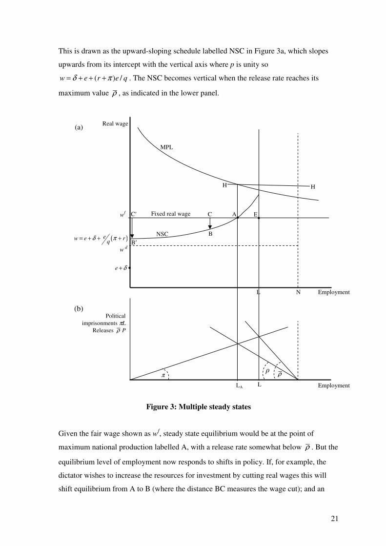
This is drawn as the upward-sloping schedule labelled NSC in Figure 3a, which slopes
upwards from its intercept with the vertical axis where p is unity so
( ) /w e r e qδ π= + + + . The NSC becomes vertical when the release rate reaches its
maximum value ρ , as indicated in the lower panel.
Figure 3: Multiple steady states
Given the fair wage shown as wf, steady state equilibrium would be at the point of
maximum national production labelled A, with a release rate somewhat below ρ . But the
equilibrium level of employment now responds to shifts in policy. If, for example, the
dictator wishes to increase the resources for investment by cutting real wages this will
shift equilibrium from A to B (where the distance BC measures the wage cut); and an
ρ
E
L Employment
Real wage
Fixed real wage
e δ+
MPL
( )ew e rq
δ π= + + +
dw
N
H H
wf
NSC
Political
imprisonments πL
Releases ρ P
π ρ
Employment L
(a)
(b)
A
C
B
C′
B′
LA
22
increase in random terror will shift the NSC curve upwards and also lower non-custodial
employment and output, shifting equilibrium from A to C (where BC measures the rise in
the NSC). In both cases the release rate needs to fall to sustain the new steady state. The
justification for this is that it behoves a dictator who wants to cut real wages, without
making any commitment to future increases, to maintain incentives by making
incarceration a greater threat – and reducing the release rate is one way of doing this. He
who wills the end must will the means.
Willingness to adjust release rates does not abolish limits set by incentive, however.
Wage cuts greater than B’C’ will violate the incentive constraint at all levels of
employment, for example: and so will random terror that raises efficiency wages by a
corresponding amount. But with endogenous release rates, non-custodial levels of
employment and production will be adversely affected as soon as such any action is taken
– and not just when the limits are reached.
Our model is consistent with Sokolov’s (2003) argument that the solutions adopted
involved a time-varying mix of coercion, moral suasion, and material incentives. The first
Five-Year Plan motivated workers during 1928-1933, but did not fulfil expectations, and
the removal of ‘class enemies’ did not bring material rewards. The availability of
consumer goods to provide material incentives was limited by the emphasis placed on
investment in heavy industry by Soviet economic planning. Stakhanovism during the
mid-1930s encouraged ever greater individual productivity, but did not succeed in the
aggregate. Coercive methods reached a peak in the Great Terror of 1937-1938.
The Great Terror
“If a major aim of the Great Terror was to overcome endemic waste and poor-quality
production, to remedy the inherent malfunctions of the Stalinist form of ‘planning’, or to
compel regional and local officials to obey Moscow to the letter, it had failed dismally”
(Acton and Stableford, 2005, p.386). The main drive behind the Terror appears to have
been political; and a chilling rationale for Stalin’s actions in these terms is discussed in
Gregory et al (2006).
We have seen that, inter alia, the Terror involved a sharp rise in the rate of incarceration.
23
In the framework we use here, increasing the parameter π will raise the prison population
and the efficiency wage. This may have been politically rational but it has potentially
adverse economic effects. How did the regime handle the adverse incentive problems that
ensued?
(a) More monitoring
First, and most directly, in Orwellian fashion by spending more on detection (i.e.
monitoring costs) so as to increase the probability of catching shirkers (increasing q). A
network of informers spread: “the volume of information grew exponentially between
1930 and 1937. NKVD operational officers maintained surveillance of suspect
individuals and special intelligence officials kept track of the military” (Gregory et al,
2006, p.21).
As when he attacked supervisors for ideological reasons in the early 1930s, Stalin let
political over-rule economic considerations. He enunciated a Five per cent Rule in the
following terms: ‘Your task is to check people at work and if something is not right, you
must report it. Every member of the party, honest non-party members, citizen of the
Soviet Union not only has the right but is obligated to report the deficiencies he sees. If
they are right, maybe only 5 percent of the time, this is nevertheless bread’. As noted
above, however, this probably increased terror more than it promoted detection34
,
particularly as “There was an official understanding during the 1937-1938 mass
operations that a large number of innocent parties were to be convicted” (Gregory et al,
2006, p.18, from the archival research of Kaustov et al, 2004, p.209).
(b) More pay
Second, on a more positive note, real incomes improved. Wages were increased
dramatically during 1937-1940; and in 1940 alone Sokolov (2003) reports that the wage
fund rose more than 50 per cent. He also records that non-pecuniary benefits were
increased, in the form of privately-farmed land plots, sanatoria, better housing, and
medals sometimes enabling advancement. There is evidence that wage rises and non-
34
There was little opportunity or effort made to stem opportunistic voluntary denunciations; denunciations
made under torture were unreliable, often naming friends or acquaintances. Incentives for officials also
promoted opportunism: “the NKVD itself opportunistically selected victims with large apartments that
became a part of the NKVD inventory” (Gregory et al, 2006, p.22, citing Vatlin, 2004).
24
pecuniary benefits were most marked where monitoring problems were most severe, e.g.
among skilled workers (whose output will be less measurable) and in large enterprises.
Wage differentials rose sharply35
, so that skilled technical workers were paid twice as
much as unskilled workers (Sokolov, 2003, p.26); and large enterprises opened clinics for
workers36
.
(c) Harsher punishment
In addition, however, conditions in camps and colonies became worse. Camp food rations
achieved only 67-70 per cent of the planned level before the war; and fell even further in
wartime (Bacon, 1992, p.1079). As the prison population rose even faster than expected
during the Terror, overcrowding became a severe problem; this worsened during the war
as prisoners were evacuated eastwards. The death rate from disease and malnutrition in
camps rose during the Great Terror from 3.1% in 1937 to 9.1% in 1938 – reaching a peak
of 17% peak during the war (Bacon, 1992, Table 5, p.1080).
In addition sentences lengthened. Archive data indicate that the length of the average
sentence rose in the years before the war (Getty et al, 1993, p.1042). Furthermore, the
harshness of sentencing policy rose: executions numbered between 975,000 and
1,200,000 during the Great Terror (Ellman, 2002).
The mass executions are enough to show that the motive for the Terror was political not
economic. But even when the Terror was called off, the harshness of the regime evidently
continued. The logic for this is described by Gregory and Harrison (2005): to get more
resources for investment or war, the actual wage must be compressed; but to avoid
incentive problems the harshness of prison may need to be intensified. For its own
purposes, the Terror explored the limits of this strategy37
possibly because of preparations
for war.
A key implication of our model, that widespread random terror is economically counter-
productive, is consistent with the fact that, even before Stalin’s death, Lavrenty Beria
35
During 1940, wages rose 28 per cent for engineering-technical workers compared to 11 per cent for
manual ferrous metallurgical workers (Sokolov, 2003, p.26). 36
By 1938, 1,838 sanatoria and 1,270 ‘houses of rest’ had been built (Sokolov, 2003, p.27). 37
That there were limits is indicated by evidence that political prisoners would choose to confess to capital
crimes as an ultimate form of release (Acton and Stableford, 2005, p.388).
25
(Stalin’s secret police chief) and his MVD (Ministry of Internal Affairs) had been
planning large scale modifications to the Gulag system. Tikhonov (2003) outlines various
MVD plans, drawn up from around 1949 onwards, to convert Gulag sentences into exile
to remote regions to work on MVD industrial and construction projects (at lower wages
than free workers). Exiled ex-prisoners would be allowed to bring their families and set
up home. The aim of these proposals was not humanitarian, but was designed to meet
production goals and reduce expenditure on prisons: at given levels of prison
productivity, the population had become too large38
.
4. Conclusions and qualifications
At a time when Western economies were prostrated by mass unemployment, Stalin’s
command economy achieved full employment. Though this may have been driven by the
urge to challenge their industrial supremacy, his methods owed little or nothing to
Western ideas. Keynes had yet to write the General Theory (1936), for example.
As command had cured unemployment, so it was expected to solve the problem of
incentives: that is the logic of the model we have constructed here as an exercise in
positive economics. The approach we take, like Shapiro and Stiglitz’s capitalist
equivalent, is brutally simplistic; it has little of the psychological subtlety of Akerlof and
Yellen’s doctrine of fair wages. But it focuses clearly on the issue of incentives, and
provides an equilibrium where coercion replaces cash as an incentive device. It would
nevertheless be of interest to extend the analysis to allow for variable effort39
; and it
should also be possible to include both prison and unemployment as punishment devices.
Coercion as a discipline device helped Russia to industrialise at high speed – and to
produce the arms needed to defeat Hitler: but, like the French Revolution, the regime of
punishment became a monster. The archival data we draw on bear witness to the extent
38
“The Gulag became a drain on the economy and the state budget as it filled with victims of the Great
Terror and then with returning Soviet POWs. The 1953 amnesty derived primarily from the bureaucratic
interests of the MVD itself. An external event – Stalin’s death – merely provided an excuse for the radical
reform, which had been desired by the MVD and Gulag administration itself for many years.” (Tikhonov,
2003, p.73). 39
As Shapiro and Stiglitz (1984) suggest, “Including effort as a continuous variable would not change the
qualitative results” (p.435).
26
and longevity of the Gulag system developed and sustained under Stalin’s dictatorship –
to say nothing of the settlements to contain a million or more kulaks.40
The frenzy of punishment in the late 1930s may have served political purposes, but it
proved economically counter-productive. Stalin’s successors realised this, and the Gulag
system was dismantled soon after he died. How the command system survived for
another quarter of a century is not something considered here. But our ‘efficiency wage’
approach may help to explain the final collapse of the Soviet system, as “some scholars
have argued that coercion was the glue that held the Stalinist economy together: when
coercion failed, or was abandoned, the economy fell apart” (Gregory and Harrison, 2005,
p.735). A command economy may not suffer market failure, but it can collapse when
incentives fail.
In an increasingly globalised environment, where respect for human rights has been
endorsed by all members of the United Nations, including the USSR41
, the logic -- where
increased need for current state expenditure leads to wage cuts and productive efficiency
calls for greater harshness of punishment --- may no longer be valid. Final collapse may
have come from an inexorable rise in monitoring costs, as the structure of production
shifted to services (Harrison, 2002, p.409). Another possibility is that competition from
the West, in both economic and military terms, may have pushed the logic of coercion to
breaking point. Could it be that the success of market economies - together with Star
Wars and the spread of Human Rights - was the challenge that finally destroyed the
coercive system Stalin created?
40
Stalin’s youth as a street fighter in Georgia (Sebag Montefiore, 2007) may, moreover, lend credence to
the idea that he saw brute force as tool of social policy. 41
After the war, the Soviet Union was a founding member of the UN Security Council; and in 1948 a
signatory to the Universal Declaration of Human Rights.
27
References
Acton, Edward and Tom Stableford (2005), The Soviet Union: A Documentary History,
Volume 1: 1917-1940, Exeter: University of Exeter Press.
Akerlof, George A and Janet L Yellen (1990), “The fair wage-effort hypothesis and
unemployment”, Quarterly Journal of Economics, 105 (2), 255-283.
Bacon, Edwin (1992), “Glasnost’ and the Gulag: new information on Soviet forced
labour around World War II”, Soviet Studies, 44 (6), 1069-1086.
Bacon, Edwin (1994), The Gulag at War: Stalin’s forced labour system in the light of the
Archives, London: Macmillan.
Coase, Richard H (1960), “The problem of social cost”, Journal of Law and Economics,
3, October, 1-44. Reprinted, with other papers, in: R. H. Coase, The Firm, the Market and
the Law, Chicago: University of Chicago Press, 1988.
Conquest, Robert (1994), “Communication to the Editor”, American Historical Review,
99 (3), 1038-1040.
Doyle, Arthur Conan (1992), The Adventures of Sherlock Holmes, London: Reader’s
Digest Association.
Ellman, Michael (2002), “Soviet repression statistics: some comments”, Europe-Asia
Studies, 54 (7), 1151-1172.
Ertz, Simon (2005), “Trading effort for freedom: workday credits in the Stalinist camp
system”, Comparative Economic Studies, 47 (2), 476-491.
Ertz, Simon (2007), “Making sense of the Gulag: analyzing and interpreting the function
of the Stalinist camp system”, PERSA working paper, 10 August.
28
Getty, J Arch, Gabor T Rittersporn, and Victor N Zemskov (1993), “Victims of the
Soviet penal system in the pre-war years: a first approach on the basis of archival
evidence”, American Historical Review, 98 (4), 1017-1049.
Gregory, Paul R (2003), The Political Economy of Stalinism: evidence from the Soviet
archives, Cambridge: Cambridge University Press.
Gregory, Paul R and Irwin L Collier, Jr (1988), “Unemployment in the Soviet Union:
evidence from the Soviet Interview Project”, American Economic Review, 78 (4), 613-
632.
Gregory, Paul R and Mark Harrison (2005), “Allocation under dictatorship: research in
Stalin’s archives”, Journal of Economic Literature, XLIII (September), 721-761.
Gregory, Paul R, Philipp Schroder and Konstantin Sonin (2006), “Dictators, repression
and the median citizen: an “eliminations model” of Stalin’s Terror (Data from the NKVD
Archives)”, CEPR Working Paper 6014, December.
Harrison, Mark (2002), “Coercion, compliance, and the collapse of the Soviet command
economy”, Economic History Review, 55 (3), 397-433.
Ivanova, Galina M (2006), Istoriia GULAGa, 1918-1958, Moscow: Nauka.
Khlevnyuk, Oleg (2003), “The economy of the OGPU, NKVD, and MVD of the USSR,
1930-1953: the scale, structure and trends of development”, 43-66 in: Paul R Gregory
and Valery Lazarev (eds.), The Economics of Forced Labor: the Soviet Gulag, Stanford,
CA: Hoover Institution.
Khlevnyuk, Oleg (forthcoming)
Kotliar, A E, ed (1983), Zaniatost’ naseleniia, Moscow: Finansy I Statistika.
29
Lazarev, Valery (2003), “Conclusions”, pp.189-198 in: Paul R Gregory and Valery
Lazarev (eds.), The Economics of Forced Labor: the Soviet Gulag, Stanford, CA: Hoover
Institution.
Markevich, Andrei (2007), “The dictator’s dilemma: to punish or to assist? Plan failures
and interventions under Stalin”, Warwick Economic Research Paper 816 (September).
Moorsteen, Richard and Raymond P Powell (1966), The Soviet Capital Stock, 1928-1962,
Homewood, IL: Irwin.
Overy, Richard (2004), The Dictators: Hitler’s Germany and Stalin’s Russia, London:
Allen Lane.
Rogachevskaya, Lyudmila S (1973), Likvidatsiya Bezrabotitsy v SSSR 1917-1930 gg,
Moscow: Izdatel’stvo ‘Nauka’.
Rosefielde, Stephen (1995), “Stalinism in post-communist perspective: new evidence on
killings, forced labour and economic growth in the 1930s”, Europe-Asia Studies, 48 (6),
959-987.
Sebag Montefiore, Simon (2007), The Young Stalin, London: Weidenfeld and Nicholson.
Shapiro, Carl and Joseph Stiglitz (1984), “Equilibrium unemployment as a worker
discipline device” American Economic Review, 74 (3), 433-444.
Sokolov, Andrei (2003), “Forced labor in Soviet industry: the end of the 1930s to the
mid-1950s”, 23-42 in Paul R Gregory and Valery Lazarev (eds), The Economics of
Forced Labor: the Soviet Gulag, Stanford, CA: Hoover Institution.
Solomon, Peter H (1980), “Soviet penal policy, 1917-1934: a reinterpretation”, Slavic
Review, 39 (2), 195-217.
Solomon, Peter H (1996), Soviet Criminal Justice Under Stalin, Cambridge: Cambridge
University Press.

30
Solzhenitsyn, Aleksandr I (1974), The Gulag Archipelago 1918-1956: an experiment in
literary investigation, New York: Harper and Row.
Stiglitz, Joseph (1994), Whither Socialism?, Cambridge, MA: MIT Press.
Tikhonov, Aleksei (2003), “The end of the Gulag”, pp.67-73 in: Paul R Gregory, and
Valery Lazarev (eds.), The Economics of Forced Labor: the Soviet Gulag, Stanford, CA:
Hoover Institution.
Vatlin, A (2004), Terror raionnogo masshtaba, Moscow: Rosspen, pp.120-215.
31
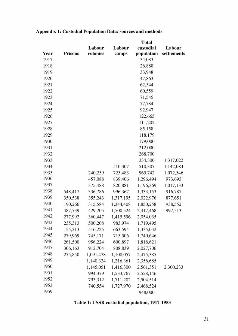
Appendix 1: Custodial Population Data: sources and methods
Year Prisons
Labour
colonies
Labour
camps
Total
custodial
population
Labour
settlements
1917 34,083
1918 26,888
1919 33,948
1920 47,863
1921 62,544
1922 60,559
1923 71,545
1924 77,784
1925 92,947
1926 122,665
1927 111,202
1928 85,158
1929 118,179
1930 179,000
1931 212,000
1932 268,700
1933 334,300 1,317,022
1934 510,307 510,307 1,142,084
1935 240,259 725,483 965,742 1,072,546
1936 457,088 839,406 1,296,494 973,693
1937 375,488 820,881 1,196,369 1,017,133
1938 548,417 336,786 996,367 1,333,153 916,787
1939 350,538 355,243 1,317,195 2,022,976 877,651
1940 190,266 315,584 1,344,408 1,850,258 938,552
1941 487,739 429,205 1,500,524 2,417,468 997,513
1942 277,992 360,447 1,415,596 2,054,035
1943 235,313 500,208 983,974 1,719,495
1944 155,213 516,225 663,594 1,335,032
1945 279,969 745,171 715,506 1,740,646
1946 261,500 956,224 600,897 1,818,621
1947 306,163 912,704 808,839 2,027,706
1948 275,850 1,091,478 1,108,057 2,475,385
1949 1,140,324 1,216,361 2,356,685
1950 1,145,051 1,416,300 2,561,351 2,300,233
1951 994,379 1,533,767 2,528,146
1952 793,312 1,711,202 2,504,514
1953 740,554 1,727,970 2,468,524
1959 948,000
Table 1: USSR custodial population, 1917-1953
32
Table 1: USSR custodial population, 1917-1953 Sources: Total custodial population 1917-1934: http://demoscope.ru/weekly/2006/0239/tema07.php.
Prisons, colonies and camps 1934-1953: Getty et al (1993). Settlements: Bacon (1992). 1959: Sokolov
(2003), from V.N.Zemskov, Ukaz. Soch., p.15.
Notes: Total custodial population does not include those in labour settlements, as is usual in the literature.
Figures for the prison population relate to January 15 except for 1938, which refers to February 10. The
1938 prison figure is taken from a note to the Table in Appendix (a) of Getty et al (1993). Figures for
labour colony and camp populations refer to January 1. The 1938 “colonies” figure here subtracts 548,417
from the figure given in Getty et al (1993), as the latter included those in prison. We note that the 1942
colonies figure is 1,000 lower than that previously given by similar sources (tabulated in Bacon, 1992); this
also affects the total custodial population estimate for 1942. Many of these figures have been widely cited
since; for example, Overy (2004).
Data on the population of Soviet labour camps and colonies, labour settlements, and prisons were made
available during glasnost’ from the Soviet Central State Archive. The Russian researchers who originally
searched the Archive for the data were A. N. Dugin and V. N. Zemskov. Dugin’s figures were published in
Western journals by Bacon (1992); these figures were checked by Zemskov, and found to be quite accurate.
Zemskov’s figures were released in Getty et al (1993). The Archival data are not without controversy (see
Ellman (2002) for a measured discussion). Authors such as Robert Conquest (eg 1994) and Stephen
Rosefielde (eg 1995) have objected that the Archive figures are too low. In comparison, their own figures
derived from anecdotal and personal experience of those in and around the camps would suggest that
several times as many people went through the Gulag system. Nevertheless, we agree with previous
arguments that the camp authorities had no incentive to run false accounts, and we also note the reported
internal consistency of Archival documents (see eg Getty et al, 1993).
The first column shows the rather sparse data available on the numbers incarcerated in prisons, as opposed
to labour camps. Prison was generally used only on a temporary basis: following an arrest, an individual
would generally pass through prison for investigation and interrogation. More often than not, this led to a
conviction. Most convicts were sent to camps or colonies to serve out their sentences (Getty et al 1993,
p.1019).
Labour settlements housed kulaks – those rich peasants fortunate enough to have escaped with their lives
after the forced collectivisation after 1929. Settlements were generally in remote inhospitable places, and
involved (albeit relatively loosely) supervised compulsory labour related to settlement-building, such as
agriculture, heavy industry and tree-felling (Overy, 2004). We will follow standard practice in excluding
those in settlements from the custodial population of interest. From the point of view of labour discipline,
settlements did not perform the same function as camps and colonies, in that the average worker faced no
risk of being sent to a settlement.
Labour camps had existed under the Tsars. Under the new Bolshevik regime, in July 1918 a new system of
approximately 300 camps was set up by the Cheka secret police (Overy, 2004) to house political offenders
(although by the middle of 1919 the camps were receiving criminal as well as political convicts – Solomon,
1980, p.200). Camps were initially intended to be economically self-sufficient, with prisoners working to
pay for their own upkeep (but not on jobs for the state). The labour was hard – but could be refused by
leftist political prisoners – and conditions were harsh. In addition to the camps, from 1919, the
Commissariat of Justice ran a system of labour colonies for prisoners convicted of petty crimes with
sentences of less than three years. Conditions in the colonies were less harsh, resembling open prisons;
often prisoners worked alongside criminals sentenced to labour duty but not incarcerated.
The end of the civil war in 1922 brought the merging of the administration of the camps and colonies. The
Cheka (OGPU) retained a small network of camps, primarily in the north, to house political opponents.
Numbers of prisoners in camps and colonies rose steadily, from around 30,000 in the early Bolshevik years
to over 100,000 in 1926-7. Solomon (1980, p.202) estimates that the (Solovki) camp detainees in 1927-28
accounted for between 10 and 15 per cent of the total camp and colony population. The annual figures mask quite substantial fluctuations in inflow rates within years. Bacon (1992, p.1077)
cites the case of a particular year. As Table 1 shows, in January 1942 there were 1,776,043 incarcerated in
camps and colonies,42
a decline of more than 200,000 compared to the camp population of 1,929,729
recorded a year earlier in January 1941. But this decline hides a rise and subsequent fall during 1941: at the
start of the Great Patriotic War on 22 June, the camp population was recorded as 2,300,000 – so during
1941 there was a rise of around 400,000 then a decline of more than half a million.
42
This figure (taken from Getty et al, 1993) is 1,000 less than that given in Bacon (1992).
33
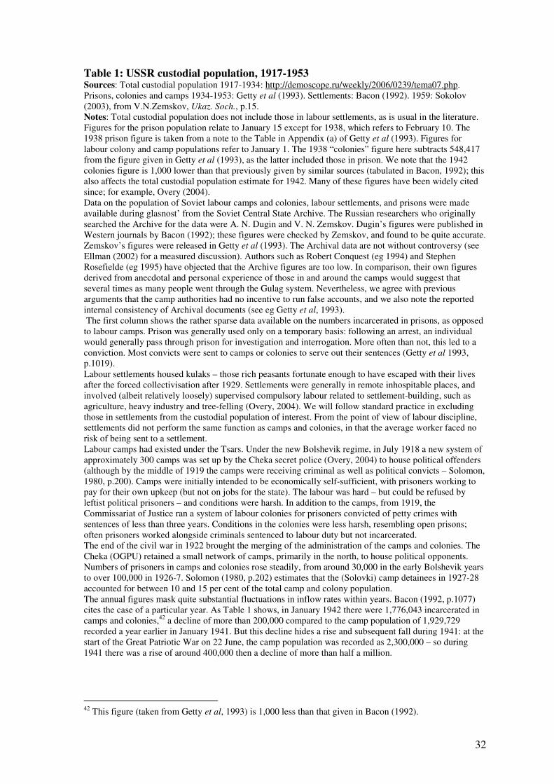
0.0
0.2
0.4
0.6
0.8
1.0
1.2
1.4
0.0 10.0 20.0 30.0 40.0 50.0
Release rate (%)
Ad
mis
sio
n r
ate
(%
)
Figure 1 Release and admission rates, 1934-1947
Notes: Release rate = releases / Gulag population. Admission rate = admissions / employment.
Year
Release rate
(%)
Admission rate
(%)
1934 28.9 0.9
1935 29.1 0.7
1936 44.0 0.8
1937 44.4 1.0
1938 28.1 1.2
1939 17.0 0.6
1940 23.6 0.8
1941 41.6 1.2
1942 36.0 1.0
1943 34.2 0.6
1944 22.9 0.5
1945 47.1 0.5
1946 19.3 0.6
1947 24.1 0.9
1948 23.6
1949 14.7
1950 15.3
1951 16.6
1952 19.3
1953 54.2
Table 2: Release and admission rates, 1934-1947
Sources: Admissions: Bacon (1994). Releases: Getty et al (1993). Employment: Moorsteen and Powell
(1966). Custodial population: See Table 1.
Notes: Release rate is releases as a proportion of the prison population as at 1 January in the relevant year.
The particularly high release rates during 1941-1945 are in part explained by releases to the armed forces.
Of the 1.956 million released during that time, Getty et al (1993, p.1040) state that 975,000 were released
to military service (particularly to punitive or ‘storm’ units, which suffered the heaviest casualties).
However, political prisoners were generally barred from release to the army (Getty et al, 1993).
34
Year
Counter-
revolutionaries
Counter-
revolutionaries
as % of camp
population
1934 135,190 26.5
1935 118,256 16.3
1936 105,849 12.6
1937 104,826 12.8
1938 185,324 18.6
1939 454,432 34.5
1940 444,999 33.1
1941 420,293 28.0
1942 407,988 28.8
1943 345,397 35.1
1944 268,861 40.5
1945 283,351 39.6
1946 333,833 55.6
1947 427,653 52.9
1948 416,156 37.6
1949 420,696 34.6
1950 578,912 40.9
1951 475,976 31.0
1952 480,766 28.1
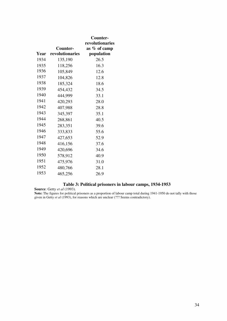
1953 465,256 26.9
Table 3: Political prisoners in labour camps, 1934-1953 Source: Getty et al (1993). Note: The figures for political prisoners as a proportion of labour camp total during 1941-1950 do not tally with those
given in Getty et al (1993), for reasons which are unclear (??? Seems contradictory).
35
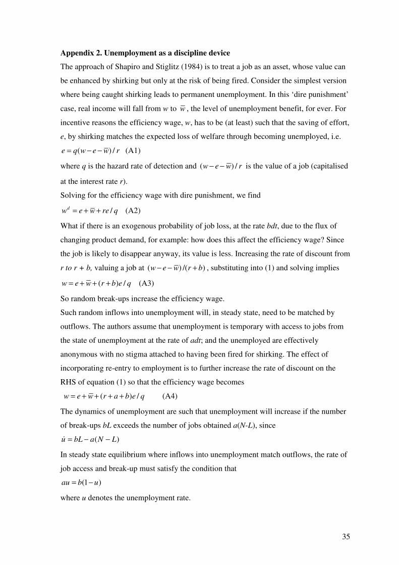
Appendix 2. Unemployment as a discipline device
The approach of Shapiro and Stiglitz (1984) is to treat a job as an asset, whose value can
be enhanced by shirking but only at the risk of being fired. Consider the simplest version
where being caught shirking leads to permanent unemployment. In this ‘dire punishment’
case, real income will fall from w to w , the level of unemployment benefit, for ever. For
incentive reasons the efficiency wage, w, has to be (at least) such that the saving of effort,
e, by shirking matches the expected loss of welfare through becoming unemployed, i.e.
( ) /e q w e w r= − − (A1)
where q is the hazard rate of detection and ( ) /w e w r− − is the value of a job (capitalised
at the interest rate r).
Solving for the efficiency wage with dire punishment, we find
/dw e w re q= + + (A2)
What if there is an exogenous probability of job loss, at the rate bdt, due to the flux of
changing product demand, for example: how does this affect the efficiency wage? Since
the job is likely to disappear anyway, its value is less. Increasing the rate of discount from
r to r + b, valuing a job at ( ) /( )w e w r b− − + , substituting into (1) and solving implies
( ) /w e w r b e q= + + + (A3)
So random break-ups increase the efficiency wage.
Such random inflows into unemployment will, in steady state, need to be matched by
outflows. The authors assume that unemployment is temporary with access to jobs from
the state of unemployment at the rate of adt; and the unemployed are effectively
anonymous with no stigma attached to having been fired for shirking. The effect of
incorporating re-entry to employment is to further increase the rate of discount on the
RHS of equation (1) so that the efficiency wage becomes
( ) /w e w r a b e q= + + + + (A4)
The dynamics of unemployment are such that unemployment will increase if the number
of break-ups bL exceeds the number of jobs obtained a(N-L), since
)( LNabLu −−=�
In steady state equilibrium where inflows into unemployment match outflows, the rate of
job access and break-up must satisfy the condition that
(1 )au b u= −
where u denotes the unemployment rate.
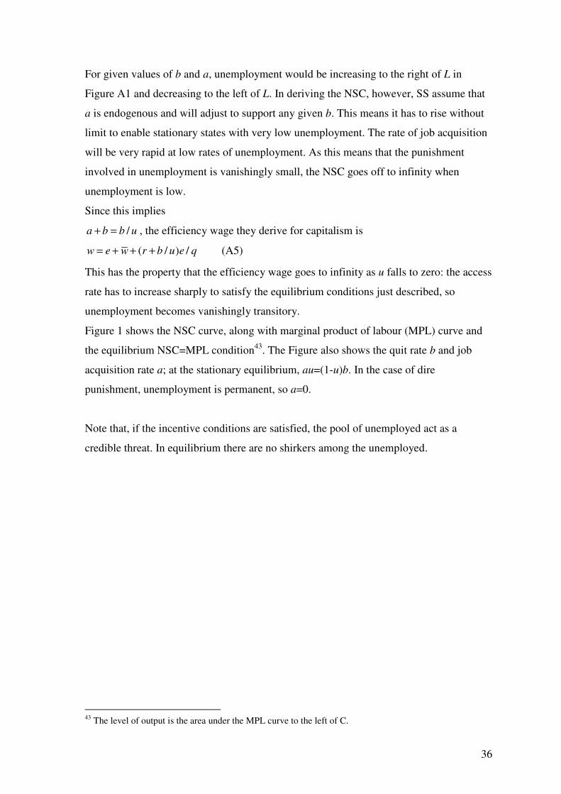
36
For given values of b and a, unemployment would be increasing to the right of L in
Figure A1 and decreasing to the left of L. In deriving the NSC, however, SS assume that
a is endogenous and will adjust to support any given b. This means it has to rise without
limit to enable stationary states with very low unemployment. The rate of job acquisition
will be very rapid at low rates of unemployment. As this means that the punishment
involved in unemployment is vanishingly small, the NSC goes off to infinity when
unemployment is low.
Since this implies
/a b b u+ = , the efficiency wage they derive for capitalism is
( / ) /w e w r b u e q= + + + (A5)
This has the property that the efficiency wage goes to infinity as u falls to zero: the access
rate has to increase sharply to satisfy the equilibrium conditions just described, so
unemployment becomes vanishingly transitory.
Figure 1 shows the NSC curve, along with marginal product of labour (MPL) curve and
the equilibrium NSC=MPL condition43
. The Figure also shows the quit rate b and job
acquisition rate a; at the stationary equilibrium, au=(1-u)b. In the case of dire
punishment, unemployment is permanent, so a=0.
Note that, if the incentive conditions are satisfied, the pool of unemployed act as a
credible threat. In equilibrium there are no shirkers among the unemployed.
43
The level of output is the area under the MPL curve to the left of C.
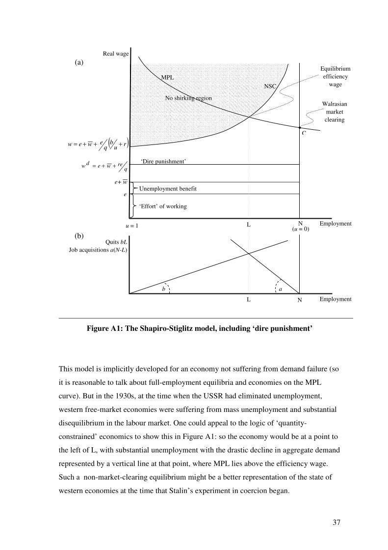
37
Figure A1: The Shapiro-Stiglitz model, including ‘dire punishment’
This model is implicitly developed for an economy not suffering from demand failure (so
it is reasonable to talk about full-employment equilibria and economies on the MPL
curve). But in the 1930s, at the time when the USSR had eliminated unemployment,
western free-market economies were suffering from mass unemployment and substantial
disequilibrium in the labour market. One could appeal to the logic of ‘quantity-
constrained’ economics to show this in Figure A1: so the economy would be at a point to
the left of L, with substantial unemployment with the drastic decline in aggregate demand
represented by a vertical line at that point, where MPL lies above the efficiency wage.
Such a non-market-clearing equilibrium might be a better representation of the state of
western economies at the time that Stalin’s experiment in coercion began.
Employment
Real wage
MPL
‘Effort’ of working
‘Dire punishment’
qrewedw ++=
N
No shirking region
(u = 0)
Walrasian
market
clearing
u = 1
Unemployment benefit e
e+ w
( )ru
bq
ewew +++=
Equilibrium
efficiency
wage NSC
Quits bL
Job acquisitions a(N-L)
Employment N
b a
C
(a)
(b)
L
L

38
Related Documents