PULSED ULTRASONIC DOPPLER VELOCIMETRY FOR MEASUREMENT OF VELOCITY PROFILES IN SMALL CHANNELS AND CAPPILARIES A Thesis Presented to The Academic Faculty by Matthias Messer In Partial Fulfillment of the Requirements for the Degree Master of Science in the School of Mechanical Engineering Georgia Institute of Technology December 2005

Welcome message from author
This document is posted to help you gain knowledge. Please leave a comment to let me know what you think about it! Share it to your friends and learn new things together.
Transcript
PULSED ULTRASONIC DOPPLER VELOCIMETRY FOR
MEASUREMENT OF VELOCITY PROFILES IN SMALL CHANNELS
AND CAPPILARIES
A Thesis Presented to
The Academic Faculty
by
Matthias Messer
In Partial Fulfillment of the Requirements for the Degree
Master of Science in the School of Mechanical Engineering
Georgia Institute of Technology December 2005

PULSED ULTRASONIC DOPPLER VELOCIMETRY FOR
MEASUREMENT OF VELOCITY PROFILES IN SMALL CHANNELS
AND CAPPILARIES
Approved by: Dr. Cyrus K. Aidun, Advisor School of Mechanical Engineering Georgia Institute of Technology
Dr. Philip J. W. Roberts School of Civil and Environmental Engineering Georgia Institute of Technology
Dr. Yves B. Berthelot School of Mechanical Engineering Georgia Institute of Technology
Date Approved: August 8, 2005
Dr. Farrokh Mistree School of Mechanical Engineering Georgia Institute of Technology
iii
Acknowledgements
I gratefully acknowledge the insight and support from my advisor Dr. Cyrus K. Aidun.
This research was funded by the Department of Energy. I acknowledge the financial
support. I would also like to thank my committee members Dr. Yves B. Berthelot, Dr.
Farrokh Mistree and Dr. Philip J. W. Roberts as well as Dr. Jean-Claude Willemetz
(Signal-Processing) for their insight and contributions as this project has progressed.
iv
Table of Contents
Acknowledgements.....................................................................................iii
List of Tables ............................................................................................viii
List of Figures.............................................................................................ix
List of Equations ......................................................................................xiv
Nomenclature............................................................................................xvi
Summary...................................................................................................xix
1 Introduction ..........................................................................................1
1.1 History of Pulsed Ultrasound Doppler Velocimetry.........................................1
1.2 Working Principle of Pulsed Ultrasound Doppler Velocimetry .......................2
1.3 Methods of Measuring the Velocity Profile......................................................3
1.4 Motivation.........................................................................................................6
2 Ultrasound Doppler Velocimetry .....................................................12
2.1 Introduction to Ultrasound Doppler Velocimetry...........................................12
2.2 Doppler Effect.................................................................................................13
2.3 Continuous Ultrasound Doppler Velocimetry ................................................15
2.4 Pulsed Ultrasound Doppler Velocimetry ........................................................19
2.5 Architecture of the Velocimeter......................................................................23
2.5.1 Master Oscillator, Gate and Emission Amplifier....................................24 2.5.2 Transducer...............................................................................................24 2.5.3 Reception Amplifier................................................................................25 2.5.4 Synchronized Demodulation and Low-Pass Filter .................................26 2.5.5 Sample/Hold Circuit ...............................................................................27 2.5.6 Logical Unit ............................................................................................28 2.5.7 Band-Pass Filter, Amplification and Analog-Digital Conversion ..........29 2.5.8 Signal Processing ....................................................................................29

v
2.5.9 Architecture DOP 1000 and DOP 2000..................................................31
2.6 Ultrasonic Field...............................................................................................34
2.6.1 Ultrasound...............................................................................................35 2.6.2 Acoustic Phenomena...............................................................................38 2.6.3 Ultrasonic Field Emitted by Transducer .................................................43 2.6.4 Sample Volume.......................................................................................46 2.6.5 Sampling Process ....................................................................................53 2.6.6 Doppler Spectrum ...................................................................................55
3 Ultrasonic Transducer .......................................................................60
3.1 Piezoelectric Effect .........................................................................................61
3.2 Transducer Architecture..................................................................................62
3.2.1 Single Element Transducer .....................................................................62 3.2.2 Transducer Arrays...................................................................................65
3.3 Transducer Characteristics..............................................................................70
3.4 Focused Transducers.......................................................................................73
3.4.1 Single Element Transducers ...................................................................74 3.4.2 Transducer Arrays...................................................................................75
4 Ultrasonic Beam Measurements .......................................................78
4.1 Experimental Setup.........................................................................................79
4.2 Principle of Measurement ...............................................................................81
4.3 Ultrasonic Beam Measurements of Various Ultrasonic Transducers .............83
4.3.1 Evaluation of Results ..............................................................................83 4.3.2 Echo Intensity and Beam Divergence Plots............................................88
4.4 Effect of Plexiglas Walls ................................................................................92
4.4.1 Evaluation of Results ..............................................................................93 4.4.2 Echo Intensity and Beam Divergence Plots..........................................101
4.5 Effect of Forming Screens ............................................................................109
4.5.1 Evaluation of Results ............................................................................111 4.5.2 Effect of the Forming Screen on the Echo Intensity.............................115 4.5.3 Echo Intensity and Beam Divergence Plots..........................................116
4.6 Evaluation of Ultrasonic Beam Measurements.............................................127
5 Measurement of Velocity Profiles in Small Channels ..................128
5.1 Principle of Measurement of Pulsed Ultrasound Doppler Velocimetry .......128

vi
5.2 Important Parameters of Pulsed Ultrasound Doppler Velocimetry ..............131
5.2.1 The Emitting Frequency .......................................................................131 5.2.2 Doppler Angle.......................................................................................131 5.2.3 Pulse Repetition Frequency ..................................................................132 5.2.4 Position of the First Gate, Wall- and Saturation-Effect ........................132 5.2.5 The Burst Length ..................................................................................133 5.2.6 The Resolution ......................................................................................133 5.2.7 The Number of Gates............................................................................133 5.2.8 The Emitting Power and Sensitivity .....................................................134 5.2.9 Number of Emissions Per Profile .........................................................134 5.2.10 Speed of Sound .....................................................................................135 5.2.11 Profiles to Record .................................................................................135
5.3 Experimental Setup.......................................................................................135
5.4 Backward Facing Step ..................................................................................138
5.5 Measurements with Pulsed Ultrasound Doppler Velocimetry......................141
5.5.1 Purpose..................................................................................................141 5.5.2 DOP 2000 Model 2125 Pulsed Ultrasonic Doppler Velocimetry.........141 5.5.3 Ultrasonic Transducers .........................................................................142 5.5.4 Channel and Probe Geometry ...............................................................144 5.5.5 Plexiglas Wall Effect ............................................................................146 5.5.6 Measurement Parameters 8 MHz 5 mm Transducer.............................146 5.5.7 Measurement Results 8 MHz 5 mm Transducer...................................148 5.5.8 Comparison to Numerical Results ........................................................151 5.5.9 Effect of Reynolds Number ..................................................................154 5.5.10 Effect of Doppler Angle........................................................................156 5.5.11 Effect of Particle Concentration............................................................157 5.5.12 Effect of Spatial Filter and Burst Length..............................................158 5.5.13 Effect of Ultrasonic Transducer............................................................158
5.6 Evaluation of Velocity Profile Measurements with PUDV in Small Channels 162
6 Limitations of Pulsed Ultrasound Doppler Velocimetry..............165
6.1 Simplifying Assumptions .............................................................................165
6.2 Accuracy and Noise ......................................................................................166
6.3 Artifacts.........................................................................................................167
6.4 Specific Limitations of Pulsed Ultrasound Doppler Velocimetry ................169
6.4.1 Maximum Depth and Velocity..............................................................169 6.4.2 Spatial Versus Velocity Resolution ......................................................177 6.4.3 Focused Transducer Limitations...........................................................178 6.4.4 Doppler Angle.......................................................................................180 6.4.5 Distance Offset......................................................................................180 6.4.6 Ringing Effect and Saturation Region ..................................................181

vii
6.4.7 Ultrasound Scatterers ............................................................................181
7 Suggestions for Improvement and Future Research ....................183
7.1 Transducer Architecture................................................................................183
7.2 Interaction of Acoustic Waves with Forming Screens .................................185
7.2.1 Forming Screen Properties....................................................................185 7.2.2 Modification Existing Experimental Setup...........................................185 7.2.3 General Effect of Moving Interfaces ....................................................186
7.3 Interaction of Acoustic Waves with Suspended Objects ..............................187
7.3.1 Acoustic Radiation Pressure Acting on Spherical Objects ...................188 7.3.2 Acoustic Radiation Pressure Acting on Cylindrical Objects ................190 7.3.3 Acoustic Radiation Pressure Acting on Shells......................................191
8 Conclusion.........................................................................................192
Appendix A ..............................................................................................195
Appendix B ..............................................................................................213
Appendix C ..............................................................................................219
Appendix D ..............................................................................................221
Appendix E ..............................................................................................226
Appendix F...............................................................................................228
Appendix G..............................................................................................230
Appendix H..............................................................................................236
Appendix I................................................................................................238
Appendix J ...............................................................................................242
References ................................................................................................249
viii
List of Tables
Table 4-1: Length of One Ultrasonic Burst Cycle in Plexiglas and Water........................97
Table 4-2: Intensity Absorption Coefficients ....................................................................98
Table 4-3: Reduction in Acoustic Intensity Due to Plexiglas Walls .................................99
Table 5-1: Measuring Parameters 8 MHz 8 mm Transducer...........................................147
Table 5-2: Measuring Parameters 4 MHz 5 mm Unfocused Transducer ........................159
Table 5-3: Measurement Parameters 4 MHz 8 mm Focused Transducer........................160
Table A-1: Parts List Experimental Setup .......................................................................196
Table D-1: Pump Drive Technical Specifications ...........................................................222
Table D-2: Pump Head Technical Specifications............................................................223
Table E-1: Particles Properties.........................................................................................227
Table E-2: Particles Processing Information ...................................................................227
Table F-1: Cost Analysis Experimental Setup.................................................................229
Table G-1: Air Permeability Measurement Results.........................................................234

ix
List of Figures
Figure 1-1: Working Principle [51] .....................................................................................3
Figure 1-2: Velocity Profile [51] .........................................................................................3
Figure 1-3: Accuracy of Pulsed Ultrasound Doppler Velocimetry [64]..............................8
Figure 2-1: Doppler Shift [52] ...........................................................................................13
Figure 2-2: Ultrasonic Transducer (Emitter and Receiver) [51]........................................16
Figure 2-3: Ultrasonic Transducer [51] .............................................................................20
Figure 2-4: General Architecture Velocimeter ..................................................................24
Figure 2-5: Swept Gain [44] ..............................................................................................26
Figure 2-6: The Doppler Frequency and Range Detection Method [7].............................28
Figure 2-7: Architecture Signal Processing DOP2000 Velocimeter .................................32
Figure 2-8: Architecture Signal Processing DOP1000 Velocimeter .................................33
Figure 2-9: Acoustic Sample Volume for a Pulsed Doppler System [64].........................35
Figure 2-10: Acoustic Spectrum [43] ................................................................................36
Figure 2-11: Longitudinal and Shear Waves [43]..............................................................37
Figure 2-12: Reflection and Refraction [51]......................................................................39
Figure 2-13: Ultrasonic Field [51] .....................................................................................43
Figure 2-14: Near and Far Ultrasonic Field [51] ...............................................................45
Figure 2-15: Piezocrystal Transducer Response [8] ..........................................................49
Figure 2-16: The Acoustic Intensity Envelope [8] ............................................................50
Figure 2-17: Teardrop Shape Sample Volume [18]...........................................................50
Figure 2-18: Dimensions Sample Volume [20] .................................................................52
Figure 2-19: The Sampling Process [8] .............................................................................53
Figure 2-20: Sample Volume Flow Entry/Exit [8] ............................................................55
Figure 2-21: Doppler Power Spectrum and Velocity Profile [8].......................................56
Figure 3-1: Main Components Ultrasonic Transducer [44]...............................................63
Figure 3-2: Transducer Arrays [49] ...................................................................................66
Figure 3-3: Zone Focusing [18] .........................................................................................69
Figure 3-4: Axial Resolution [47]......................................................................................71
Figure 3-5: Lateral Resolution [47] ...................................................................................72
Figure 3-6: Focused Beam Shape [18]...............................................................................72

x
Figure 3-7: Focusing Methods Single Element Transducer [44].......................................75
Figure 4-1: Ultrasonic Field Experimental Setup Front View...........................................79
Figure 4-2: Ultrasonic Field Experimental Setup Side Views...........................................80
Figure 4-3: Basic Experimental Setup ...............................................................................80
Figure 4-4: Principle Beam Shape Measurements.............................................................81
Figure 4-5: Interface Beam Shape Measurements .............................................................82
Figure 4-6: Echo Intensity 2 MHz 10 mm Transducer ......................................................88
Figure 4-7: Divergence 2 MHz 10 mm Transducer...........................................................88
Figure 4-8: Echo Intensity 4 MHz 5 mm Transducer ........................................................89
Figure 4-9: Divergence 4 MHz 5 mm Transducer.............................................................89
Figure 4-10: Echo Intensity 8 MHz 5 mm Transducer ......................................................90
Figure 4-11: Divergence 8 MHz 5 mm Transducer...........................................................90
Figure 4-12: Echo Intensity 4 MHz 8 mm Focussed Transducer ......................................91
Figure 4-13: Divergence 4 MHz 8 mm Focussed Transducer...........................................91
Figure 4-14: Plexiglas Wall ...............................................................................................92
Figure 4-15: Experimental Setup Plexiglas Wall...............................................................93
Figure 4-16: Distance Offset..............................................................................................95
Figure 4-17: Beam Shape 8 MHz 5 mm Transducer With/Without Plexiglas Wall .........96
Figure 4-18: Echo Intensity 2 MHz 10 mm Transducer 18 mm Plexiglas Wall .............101
Figure 4-19: Divergence 2 MHz 10 mm Transducer 18 mm Plexiglas Wall ..................101
Figure 4-20: Echo Intensity 2 MHz 10 mm Transducer 2.5 mm Plexiglas Wall ............102
Figure 4-21: Divergence 2 MHz 10 mm Transducer 2.5 mm Plexiglas Wall .................102
Figure 4-22: Echo Intensity 4 MHz 5 mm Transducer 18 mm Plexiglas Wall ...............103
Figure 4-23: Divergence 4 MHz 5 mm Transducer 18 mm Plexiglas Wall ....................103
Figure 4-24: Echo Intensity 4 MHz 5 mm Transducer 2.5 mm Plexiglas Wall ..............104
Figure 4-25: Divergence 4 MHz 5 mm Transducer 2.5 mm Plexiglas Wall ...................104
Figure 4-26: Echo Intensity 8 MHz 5 mm Transducer 18 mm Plexiglas Wall ...............105
Figure 4-27: Divergence 8 MHz 5 mm Transducer 18 mm Plexiglas Wall ....................105
Figure 4-28: Echo Intensity 8 MHz 5 mm Transducer 2.5 mm Plexiglas Wall ..............106
Figure 4-29: Divergence 8 MHz 5 mm Transducer 2.5 mm Plexiglas Wall ...................106
Figure 4-30: Echo Intensity 4 MHz Focussed Transducer 18 mm Plexiglas Wall..........107
Figure 4-31: Divergence 4 MHz Focussed Transducer 18 mm Plexiglas Wall ..............107
Figure 4-32: Echo Intensity 4 MHz Focussed Transducer 2.5 mm Plexiglas Wall.........108

xi
Figure 4-33: Divergence 4 MHz Focussed Transducer 2.5 mm Plexiglas Wall .............108
Figure 4-34: Experimental Setup Forming Screen ..........................................................109
Figure 4-35: Forming Screen ...........................................................................................110
Figure 4-36: Microtomographic Cross-Section View Forming Screen...........................111
Figure 4-37: 4 MHz Focused Transducer With/Without Screen at 40 mm (6 dB)..........114
Figure 4-38: Echo Intensity 2 MHz 10 mm Transducer With Screen at x = 20 mm.......116
Figure 4-39: Divergence 2 MHz 10 mm Transducer With Screen at x = 20 mm ...........116
Figure 4-40: Echo Intensity 2 MHz 10 mm Transducer With Screen at x = 40 mm.......117
Figure 4-41: Divergence 2 MHz 10 mm Transducer With Screen at x = 40 mm ...........117
Figure 4-42: Echo Intensity 2 MHz 10 mm Transducer With Screen at x = 60 mm.......118
Figure 4-43: Divergence 2 MHz 10 mm Transducer With Screen at x = 60 mm ...........118
Figure 4-44: Echo Intensity 2 MHz 10 mm Transducer With Screen at x = 80 mm.......119
Figure 4-45: Divergence 2 MHz 10 mm Transducer With Screen at x = 80 mm ...........119
Figure 4-46: Echo Intensity 4 MHz 5 mm Transducer With Screen at x = 20 mm.........120
Figure 4-47: Divergence 4 MHz 5 mm Transducer With Screen at x = 20 mm .............120
Figure 4-48: Echo Intensity 4 MHz 5 mm Transducer With Screen at x = 40 mm.........121
Figure 4-49: Divergence 4 MHz 5 mm Transducer With Screen at x = 40 mm .............121
Figure 4-50: Echo Intensity 4 MHz 5 mm Transducer With Screen at x = 60 mm.........122
Figure 4-51: Divergence 4 MHz 5 mm Transducer With Screen at x = 60 mm .............122
Figure 4-52: Echo Intensity 8 MHz 5 mm Transducer With Screen at x = 10 mm.........123
Figure 4-53: Divergence 8 MHz 5 mm Transducer With Screen at x = 10 mm .............123
Figure 4-54: Echo Intensity 4 MHz Focussed Transducer With Screen x = 20 mm.......124
Figure 4-55: Divergence 4 MHz Focussed Transducer With Screen at x = 20 mm........124
Figure 4-56: Echo Intensity 4 MHz Focussed Transducer With Screen at x = 40 mm ...125
Figure 4-57: Divergence 4 MHz Focussed Transducer With Screen at x = 40 mm........125
Figure 4-58: Echo Intensity 4 MHz Focussed Transducer With Screen at x = 60 mm ...126
Figure 4-59: Divergence 4 MHz Focussed Transducer With Screen at x = 60 mm........126
Figure 5-1: Principle of Measurement [55] .....................................................................130
Figure 5-2: Velocity Components [51] ............................................................................130
Figure 5-3: Experimental Setup .......................................................................................136
Figure 5-4: Experimental Setup Side Views....................................................................136
Figure 5-5: Theta-Positioner ............................................................................................137
Figure 5-6: Backward Facing Step ..................................................................................138
xii
Figure 5-7: Flow Over Backward Facing Step [35].........................................................140
Figure 5-8: Calibration of Transducer Distance Offset ...................................................144
Figure 5-9: Channel and Transducer Geometry...............................................................145
Figure 5-10: Position Measurement Points......................................................................148
Figure 5-11: Velocity Profiles Behind Step.....................................................................149
Figure 5-12: Velocity Profile Before and On Step ..........................................................150
Figure 5-13: Numerical Results .......................................................................................151
Figure 5-14: Comparison Numerical-Experimental 10 mm Before Step ........................152
Figure 5-15: Comparison Numerical-Experimental 80 mm Behind Step .......................153
Figure 5-16: Comparison Numerical-Experimental 10 mm Behind Step .......................154
Figure 5-17: Velocity Profile for Different Re-Numbers ................................................155
Figure 5-18: Velocity Profiles for Different Doppler Angles..........................................156
Figure 5-19: Velocity Profiles for Different Particle Concentrations..............................157
Figure 5-20: Velocity Profiles for Different Ultrasonic Transducers..............................161
Figure 6-1: Imaginary Velocity Components at the Far Wall [51]..................................168
Figure 6-2: Reflection and Refraction [51]......................................................................169
Figure 6-3:Aliasing [61] ..................................................................................................172
Figure 6-4: Aliasing Frequency Backfolding [51]...........................................................172
Figure 6-5: Measured Aliasing ........................................................................................173
Figure 6-6: Phase Lag [26] ..............................................................................................174
Figure 6-7: Acoustic Cavitation [57] ...............................................................................178
Figure 7-1: Modified Experimental Setup .......................................................................186
Figure A-0-1: Assembly Drawing Experimental Setup...................................................197
Figure A-0-2: Overview Channel ....................................................................................198
Figure A-0-3: Technical Drawing Channel Bottom Wall................................................199
Figure A-0-4: Technical Drawing Channel Side Wall ....................................................200
Figure A-0-5: Technical Drawing Channel Top Wall .....................................................201
Figure A-0-6: Technical Drawing Channel Pressure Part ...............................................202
Figure A-0-7: Overview Distributor ................................................................................203
Figure A-0-8: Technical Drawing Distributor Bottom Wall ...........................................204
Figure A-0-9: Technical Drawing Distributor Side Wall ................................................205
Figure A-0-10: Technical Drawing Distributor Back Wall .............................................206
Figure A-0-11: Technical Drawing Distributor Top Wall...............................................207
xiii
Figure A-0-12: Technical Drawing Distributor Front Part ..............................................208
Figure A-0-13: Technical Drawing Theta Positioner L-Profile.......................................210
Figure A-0-14: Technical Drawing Theta Positioner Transducer Holder .......................211
Figure A-0-15: Technical Drawing Theta Positioenr Support Part .................................212
Figure B-0-1: Digital Ultrasonic Synthesizer [51]...........................................................214
Figure C-0-1: Available Ultrasonic Transducers Signal Processing [51]........................220
Figure C-0-2: Available Cases Ultrasonic Transducers Signal Processing [51] .............220
Figure G-0-1: Air Permeability Tester.............................................................................231
Figure G-0-2: Schematic Diagram of the Air-Permeability Instrument [50] ..................233
Figure H-0-1: Sound Speed Measureing Unit [51]..........................................................237
Figure I-0-1: Insertion Loss Setup [51] ...........................................................................240
Figure J-0-1: Results Acoustic Impedance Models .........................................................248
xiv
List of Equations
Equation 1: Frequency at Receiver ....................................................................................14
Equation 2: Doppler Shift Frequency ................................................................................14
Equation 3: Doppler Shift Frequency (Source and Receiver Stationary) ..........................14
Equation 4: Reflector Velocity (Source and Receiver Stationary Simplified) ..................15
Equation 5: Reflector Velocity Modified ..........................................................................15
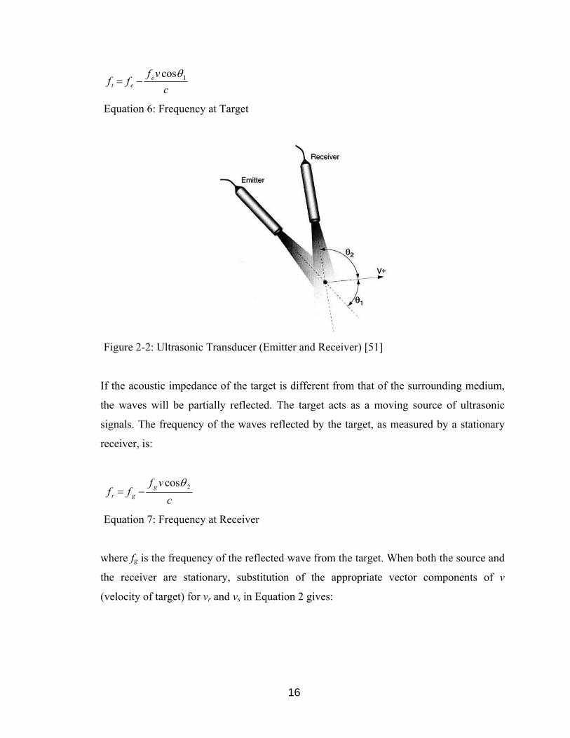
Equation 6: Frequency at Target........................................................................................16
Equation 7: Frequency at Receiver ....................................................................................16
Equation 8: Doppler Shift Frequency in General ..............................................................17
Equation 9: Doppler Shift Frequency Simplified ..............................................................17
Equation 10: Doppler Shift Frequency One Transducer....................................................17
Equation 11: Doppler Angular Frequency.........................................................................19
Equation 12: Doppler Frequency Shift ..............................................................................20
Equation 13: Depth ............................................................................................................20
Equation 14: Variation in Depth Between Two Emissions ...............................................20
Equation 15: Phase Shift of the Received Echo.................................................................21
Equation 16: Velocity Measured .......................................................................................21
Equation 17: Reflection Coefficient ..................................................................................40
Equation 18: Transmission Coefficient .............................................................................41
Equation 19: dB Loss Due to Transmission ......................................................................41
Equation 20: dB Loss Due to Reflection ...........................................................................41
Equation 21: Intensity Transmission Coefficient (Simplified)..........................................42
Equation 22: Intensity of the Acoustic Field .....................................................................44
Equation 23: Length of the Near Field ..............................................................................44
Equation 24: Directivity Function .....................................................................................45
Equation 25: Half Angle of Beam Divergence ..................................................................46
Equation 26: Distance Transducer to Beginning Sample Volume ....................................47
Equation 27: Distance Transducer to End of Sample Volume ..........................................47
Equation 28: Length Sample Volume................................................................................47
Equation 29: Spectral Broadening .....................................................................................57
Equation 30: Beam Width Unfocused Transducer ............................................................72

xv
Equation 31: Speed of Propagation of Longitudinal Waves in Solids...............................94
Equation 32: Pressure Amplitude of a Plane Wave ...........................................................98
Equation 33: Absorption Coefficients ...............................................................................99
Equation 34: Distance Perpendicular to the Flow............................................................145
Equation 35: Distance in Direction of the Ultrasonic Beam............................................145
Equation 36: Sampling Frequency...................................................................................170
Equation 37: Maximum Velocity.....................................................................................171
Equation 38: Maximum Depth.........................................................................................175
Equation 39: Relation Maximum Depth and Velocity ....................................................176
Equation 40: Insertion Loss .............................................................................................239
Equation 41: Delany-Bazley-Model ................................................................................243
Equation 42: Allard-Champoux-Model ...........................................................................246
xvi
Nomenclature
Roman Alphabet:
a transducer radius
aa amplitude absorption coefficient
A cross section area
Aa intensity absorption coefficient
c speed of sound
Dr directivity function
d transducer diameter
dp piezoelectric receiving coefficient
E Young’s modulus
F focal distance
fD Doppler shift frequency
fe emitted frequency
fr received frequency
gp piezoelectric transmitting coefficient
h height (distance perpendicular to the flow direction)
I Intensity
J Bessel function
Kb effective dynamic bulk modulus
k wavenumber
L characteristic length
LNF near field length
l distance along ultrasonic beam axis
P depth
P0 atmospheric pressure
N Prandtl number
R intensity reflection coefficient
r amplitude reflection coefficient

xvii
Sf pore shape factor
T intensity transmission coefficient
TD time delay between an emitted burst and its echo
Td time delay between the start of transmission and the moment at which the receiver
gate opens
Tg time period for which the receiver gate is open
Tp pulse duration
Tprf time delay between two emissions
t amplitude transmission coefficient
U velocity
V volume
Vt flow rate
vs velocity of source
vr velocity of receiver
W beam width
Z acoustic impedance
Greek Alphabet:
α angle of incidence
αa absorption coefficient
β angle of reflection
δfd spectral broadening
δ phase shift of received echo
εp dielectric constant of piezoelectric material
φ angular excursion
γ angle of refraction
ϕ half angle of beam divergence
λ wavelength
µ refractive index
xviii
ν Poisson ratio
θ Doppler angle
ρ density
ρb effective dynamic density of material
Ω Porosity
σ flow resistivity
ω Doppler angular frequency

xix
Summary
Pulsed ultrasound Doppler velocimetry proved to be capable of measuring velocities
accurately (relative error less than 0.5 percent). In this research, the limitations of the
method are investigated when measuring:
• in channels with a small thickness compared to the transducer diameter,
• at low velocities
• and in the presence of a flow reversal area.
A review of the fundamentals of pulsed ultrasound Doppler velocimetry reveals that the
accuracy of the measured velocity field mainly depends on the shape of the acoustic beam
through the flow field and the intensity of the echo from the incident particles where the
velocity is being measured. The ultrasonic transducer turned out to be most critical
component of the system. Fundamental limitations of the method are identified.
With ultrasonic beam measurements, the beam shape and echo intensity is further
investigated. In general, the shape of the ultrasonic beam varies depending on the
frequency and diameter of the emitter as well as the characteristics of the acoustic
interface that the beam encounters. Moreover, the most promising transducer to measure
velocity profiles in small channels is identified. Since the application of pulsed ultrasound
Doppler velocimetry often involves the propagation of the ultrasonic burst through
Plexiglas, the effect of Plexiglas walls on the measured velocity profile is analyzed and
quantified in detail. The transducer’s ringing effect and the saturation region caused by
highly absorbing acoustic interfaces are identified as limitations of the method.
By comparing measurement results in the small rectangular channel to numerically
calculated results, further limitations of the method are identified. It was not possible to
determine velocities correctly throughout the whole channel at low flow rates, in small
geometries and in the flow separation region. A discrepancy between the maximum
measured velocity, velocity profile perturbations and incorrect velocity determination at
the far channel wall were main shortcomings. Measurement results are improved by
changes in the Doppler angle, the flow rate and the particle concentration.
Suggestions to enhance the measurement system, especially its spatial resolution, and to
further investigate acoustic wave interactions are made.
1
1 Introduction
At first, the history of pulsed ultrasound Doppler velocimetry, its working principle and
other methods to measure velocity profiles in fluids are reviewed. Then, the benefits and
the outcome of this research are introduced
1.1 History of Pulsed Ultrasound Doppler Velocimetry
Ultrasound Doppler velocimetry was originally applied in the medical field and dates
back more than 60 years. The first use of ultrasound for medical diagnosis came in the
1949 with attempts at ultrasonographic cross-sectional imaging. In 1954, H. P. Kalmus
described how flow velocity in fluids could be determined by measuring the phase
difference between an upstream and downstream ultrasonic wave. His “upstream –
downstream” method was further developed by D. L. Franklin et al. who in 1959
produced a flowmeter that could be mounted directly on blood vessels. The fact that the
Doppler frequency shift could be used for the detection of blood velocity patterns was
shown by S. Satomura in 1959. In 1964, D. W. Baker and H. F. Stegall presented the first
Doppler instrument intended for transcutaneous measurement of blood flow velocity in
man using the continuous wave Doppler principle. Approximately five years later, pulsed
Doppler instruments were introduced, allowing blood flow velocity measurements at
predetermined depths.
The use of pulsed emissions has extended this technique to other fields and has opened
the way to new measuring techniques in fluid dynamics. The pulsed ultrasonic flow meter
was initially developed to measure the flow in a blood vessel by Wells and Baker around
1970 [20]. Takeda [54] subsequently extended this method to non-medical flow
measurements and developed a monitoring system for the velocity profile measurement
of general fluids. The method itself was found to be quite useful to flow measurements in
general and additionally through years of use has gradually become accepted as a tool to
study the physics and engineering of fluid flow [56]. More recently, PUDV was applied

2
to study fluid flow by Takeda in 1995 [55], by Brito in 2001 [12], by Eckert in 2002 [16],
by Alfonsi in 2003 [4], by Kikura in 1999 and 2004 [29-31] and by Aidun in 2005 [64].
Nevertheless, the limitations of pulsed ultrasound Doppler velocimetry are not yet
completely investigated, especially when dealing with small channels and capillaries.
Therefore, the limitations of pulsed ultrasound Doppler velocimetry especially in the case
of small, small compared to the ultrasonic transducer diameter, rectangular channels
characterized by a backward facing step are investigated in this research. Before
describing this research in more details, the working principle of pulsed ultrasound
Doppler velocimetry and other methods to measure velocity profiles are presented in the
following sections.
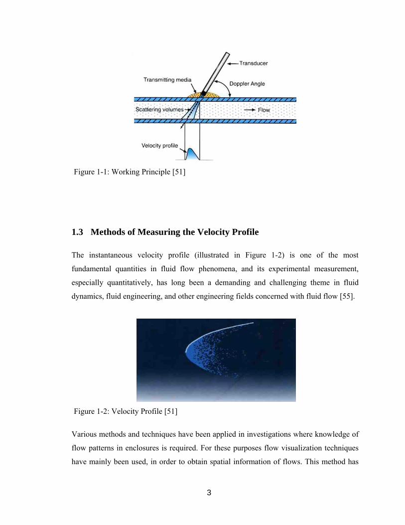
1.2 Working Principle of Pulsed Ultrasound Doppler Velocimetry
The working principle of pulsed ultrasound Doppler velocimetry is to detect and process
many ultrasonic echoes issued from pulses reflected by micro particles contained in a
flowing liquid. A single transducer emits the ultrasonic pulses and receives the echoes as
shown in Figure 1-1. By sampling the incoming echoes at the same time relative to the
emission of the pulses, the variation of the positions of scatterers are measured and
therefore their velocities. The measurement of the time lapse between the emission of
ultrasonic bursts and the reception of the pulse (echo generated by particles flowing in the
liquid) gives the position of the particles. By measuring the Doppler frequency in the
echo as a function of time shifts of these particles, a velocity profile after few ultrasonic
emissions is obtained.
3
Figure 1-1: Working Principle [51]
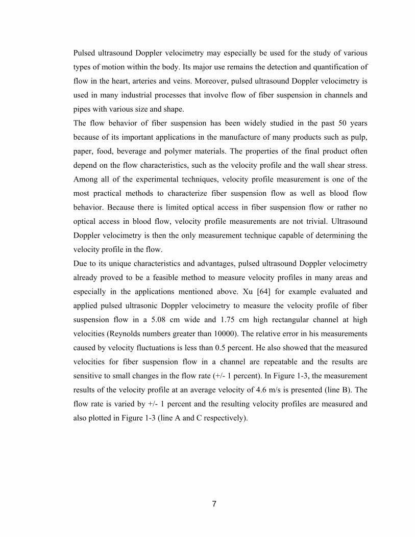
1.3 Methods of Measuring the Velocity Profile
The instantaneous velocity profile (illustrated in Figure 1-2) is one of the most
fundamental quantities in fluid flow phenomena, and its experimental measurement,
especially quantitatively, has long been a demanding and challenging theme in fluid
dynamics, fluid engineering, and other engineering fields concerned with fluid flow [55].
Figure 1-2: Velocity Profile [51]
Various methods and techniques have been applied in investigations where knowledge of
flow patterns in enclosures is required. For these purposes flow visualization techniques
have mainly been used, in order to obtain spatial information of flows. This method has

4
the disadvantage of difficulties obtaining quantitative results and real time data handling.
Furthermore, its application to opaque fluids is not possible.
Particle image velocimtery (PIV) is the newest entrant to the field of fluid flow
measurement and provides instantaneous velocity fields over a global (2- or 3-
dimensional) domain with high accuracy. PIV records the position over time of small
tracer particles introduced into the flow to extract the local fluid velocity. Thus, PIV
represents a quantitative extension of the qualitative flow-visualization techniques that
have been practiced for several decades. The basic requirements for a PIV system are an
optically transparent test-section, an illuminating light source (laser), a recording medium
(film, CCD, or holographic plate), and a computer for image processing. Illuminating
particles are a few microns in diameter in gases and perhaps a few tens of microns in
liquids [1].
Particle tracking velocimetry (PTV) is a direct descendent of flow visualization using
tracer particles in fluid flows. PTV records particle displacements in a single image over a
period of time. If the particle is illuminated by two successive bursts of light, each
particle produces two images on the same piece of film. Subsequently, the distance
between the images can be measured to approximately determine the local Eulerian
velocity of the fluid. The charge-coupled device camera integrates the signal over time as
the particle travels with the flow. Foreshortened image streaks are created when particles
move normal to the light sheet. The centroid of a dot can be located more accurately than
the end of streak. In general, velocity measurements determined by particle streaks are
less reliable and about 10 times less accurate then particle image velocimetry
measurements.
Instead of determining the displacement of individual particles, correlation-based PIV
determines the average motion of small groups of particles contained within small regions
known as interrogation spots. Essentially, the overall frame is divided into interrogation
spots, and the correlation function is computed sequentially over all spots providing one
displacement vector per spot. The process of averaging over multiple particle pairs within
an interrogation spot makes the technique remarkably noise-tolerant and robust in
comparison to PTV.
Tracer particles for PIV must satisfy two requirements. They should be able to follow the
flow streamlines without excessive slip, and they should be efficient scatterers of the

5
illuminating laser light. PIV can be accomplished using continuous wave lasers or more
optimally, pulsed lasers. The advantage of pulsed lasers is the short duration of the laser
pulse, typically a few nanoseconds. As a consequence, a particle traveling at even very
high speeds is essentially frozen during the exposure with minimal blurring. However, if
the pulse duration is too long, the particle will produce streaks rather than crisp circular
images (to a small extent, streaky images can be tolerated in correlation-based PIV).
PIV measurements contain errors arising from several sources: (1) Random error, due to
noise in the recorded images; (2) Bias error arising from the process of computing the
signal peak location to sub-pixel accuracy; (3) Gradient error resulting from rotation and
deformation of the flow within an interrogation spot leading to loss of correlation; (4)
Tracking error resulting from the inability of a particle to follow the flow without slip; (5)
Acceleration error caused by approximating the local Eulerian velocity from the
lagrangian motion of tracer particles [46].
Laser Doppler Velocimetry (LDV) is a non-intrusive measurement device that is sensitive
only to velocity. LDV allows a non-invasive measurement of flow velocity by means of
the well-known Doppler effect. A laser is spited into two equal-intensity, parallel beams.
A lens causes these beams to cross and focus at common point. LDV makes use of the
coherent wave nature of laser light. The crossing of two laser beams of the same
wavelength produces areas of constructive and destructive interference patterns. The
interference pattern, known as a 'fringe' pattern is composed of planar layers of high and
low intensity light. Velocity measurements are made when particles 'seeded' in the flow
pass through the fringe pattern created by the intersection of a pair of laser beams. These
particles scatter light in all directions when going through the beam crossing. This
scattered light is then collected by a stationary detector (receiving optics connected to a
photomultiplier). The frequency of the scattered light is Doppler shifted and referred to as
the Doppler frequency of the flow. This Doppler frequency is proportional to a
component of the particle’s velocity which is perpendicular to the planar fringe pattern
produced by the beam crossing. In order to obtain three components of velocity, three sets
of fringe patterns need to be produced at the same region in space.
Compared to laser Doppler velocimetry (LDV), that measures the velocity component,
which is perpendicular to the axis of the light beam, Ultrasound Doppler Velocimetry
(UDV) measures the component which is in the direction of the axis of the ultrasonic

6
beam. LDV identifies the velocity of a single particle, whereas UDV identifies velocities
of a great number of scatters simultaneously and gives therefore the mean value of all the
particles present in the sampling volume. In contrast to LDV, the maximum velocity is
limited in Pulsed Ultrasound Doppler Velocimetry (PUDV). On the other hand, LDV can
not be applied when the liquid contains too many particles or is non transparent, but UDV
can. Unlike LDV, UDV gives a complete velocity profile.
1.4 Motivation
As described in the previous section, pulsed ultrasound Doppler velocimetry is almost the
unique technique that is capable to measure in real time a velocity profile in liquids
containing a great number of particles by processing ultrasonic echoes generated by micro
particles flowing in the liquid. It can analyze any opaque or translucent liquid containing
particles in suspension such as dust, gas bubbles and emulsions. Moreover it can measure
other qualities, such as the echo intensity, the Doppler energy, the spectral density of the
Doppler echoes, the spatial intercorrelation, the flow rate, even in presence of very high
concentration of particles where optical techniques may be difficult to apply. This
technique is fully non-invasive: the ultrasonic beam can cross through virtually any wall
material containing the flow. In contrast to conventional techniques, the ultrasound
method also offers an efficient flow mapping process and a record of the spatiotemporal
velocity field [55]. The main advantage of pulsed Doppler ultrasound is its capability to
offer spatial information associated with velocity values instantaneously. Spatiotemporal
information (i.e., a velocity field as a function of space and time) can be obtained without
prior knowledge of the flow.
Ultrasound Doppler velocimetry is applicable to opaque liquids, such as liquid metals as
well as Ferro fluids, food material liquids, and so forth, but the working fluid must be
transparent to ultrasound (although it might not be transparent to light). Since this method
uses frequency information of the echo, it is in principle not necessary to calibrate the
system using any standard velocity field [55]. Although the pulsed ultrasound Doppler
velocimetry was developed for measurement of one-dimensional flow, profiles can also
be successfully obtained for flow which is essentially multi-dimensional.
7
Pulsed ultrasound Doppler velocimetry may especially be used for the study of various
types of motion within the body. Its major use remains the detection and quantification of
flow in the heart, arteries and veins. Moreover, pulsed ultrasound Doppler velocimetry is
used in many industrial processes that involve flow of fiber suspension in channels and
pipes with various size and shape.
The flow behavior of fiber suspension has been widely studied in the past 50 years
because of its important applications in the manufacture of many products such as pulp,
paper, food, beverage and polymer materials. The properties of the final product often
depend on the flow characteristics, such as the velocity profile and the wall shear stress.
Among all of the experimental techniques, velocity profile measurement is one of the
most practical methods to characterize fiber suspension flow as well as blood flow
behavior. Because there is limited optical access in fiber suspension flow or rather no
optical access in blood flow, velocity profile measurements are not trivial. Ultrasound
Doppler velocimetry is then the only measurement technique capable of determining the
velocity profile in the flow.
Due to its unique characteristics and advantages, pulsed ultrasound Doppler velocimetry
already proved to be a feasible method to measure velocity profiles in many areas and
especially in the applications mentioned above. Xu [64] for example evaluated and
applied pulsed ultrasonic Doppler velocimetry to measure the velocity profile of fiber
suspension flow in a 5.08 cm wide and 1.75 cm high rectangular channel at high
velocities (Reynolds numbers greater than 10000). The relative error in his measurements
caused by velocity fluctuations is less than 0.5 percent. He also showed that the measured
velocities for fiber suspension flow in a channel are repeatable and the results are
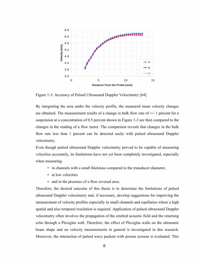
sensitive to small changes in the flow rate (+/- 1 percent). In Figure 1-3, the measurement
results of the velocity profile at an average velocity of 4.6 m/s is presented (line B). The
flow rate is varied by +/- 1 percent and the resulting velocity profiles are measured and
also plotted in Figure 1-3 (line A and C respectively).
8
3.4
3.9
4.4
4.9
5.4
5.9
6.4
6.9
0 5 10 15Distance from the Probe [mm]
Velo
city
[m/s
]A
B
C
Figure 1-3: Accuracy of Pulsed Ultrasound Doppler Velocimetry [64]
By integrating the area under the velocity profile, the measured mean velocity changes
are obtained. The measurement results of a change in bulk flow rate of +/- 1 percent for a
suspension at a concentration of 0.5 percent shown in Figure 1-3 are then compared to the
changes in the reading of a flow meter. The comparison reveals that changes in the bulk
flow rate less than 1 percent can be detected easily with pulsed ultrasound Doppler
velocimetry.
Even though pulsed ultrasound Doppler velocimetry proved to be capable of measuring
velocities accurately, its limitations have not yet been completely investigated, especially
when measuring
• in channels with a small thickness compared to the transducer diameter,
• at low velocities
• and in the presence of a flow reversal area.
Therefore, the desired outcome of this thesis is to determine the limitations of pulsed
ultrasound Doppler velocimetry and, if necessary, develop suggestions for improving the
measurement of velocity profiles especially in small channels and capillaries where a high
spatial and also temporal resolution is required. Application of pulsed ultrasound Doppler
velocimetry often involves the propagation of the emitted acoustic field and the returning
echo through a Plexiglas wall. Therefore, the effect of Plexiglas walls on the ultrasonic
beam shape and on velocity measurements in general is investigated in this research.
Moreover, the interaction of pulsed wave packets with porous screens is evaluated. This
9
research may therefore be used to increase the range of application of pulsed ultrasound
Doppler velocimetry especially in industrial processes (e.g., paper industry) but also in
the medical field and the emerging area of bioengineering.
To determine the limitations of pulsed ultrasound Doppler velocimetry, the fundamentals
of this method and the working structure of the utilized instrument as well as other
components of the measurement system have been investigated first. In Chapter 2, the
fundamentals of ultrasound Doppler velocimetry are reviewed. This part is essential to
identify fundamental limitations of pulsed ultrasound Doppler velocimetry, design an
experimental setup to investigate further limitations and make suggestions for
improvement. At first, the Doppler effect, the basis of ultrasound Doppler velocimetry, is
described in Section 2.2. Then continuous and pulsed ultrasound Doppler velocimetry are
identified as two complementary modes of ultrasound Doppler velocimetry. In the
following, the working structures of the measurement system and its components are
analyzed in detail. The fundamentals of the ultrasonic field, acoustic phenomena and the
sampling process, necessary for evaluating measurement results at a later point, are
identified. The following chapters will build on and refer to the fundamentals reviewed in
this chapter.
In Chapter 2, the ultrasonic transducer is identified to be the most critical component of
the measurement system. Therefore, the fundamentals of generally available ultrasonic
transducers, i.e., single element transducers and transducer arrays, their working
principle, architecture, characteristics and potential for focusing the emitted ultrasonic
beam have been reviewed especially to make suggestions for improving the currently
utilized pulsed ultrasound Doppler velocimeter (described in detail at a later point).
In the Chapter 3, the ultrasonic beam shape is measured. Information about the actual
beam shape of various ultrasonic transducers and especially their lateral resolution is
gained. The lateral resolution of the pulsed ultrasound Doppler velocimetry system is
extremely important in evaluating the flow over a backward facing step in small channels,
i.e., when dealing with small geometries. Ultrasonic beam measurements will therefore be
used to identify the most appropriate transducer to measure velocity profiles in small
channels and capillaries. Moreover, the interaction of walls and porous screens with the
emitted ultrasonic wave packet and their effect on measuring the velocity profile with
unfocused as well as focused ultrasonic transducers is analyzed. At first, the experimental
10
setup is described and the ultrasonic beam of various transducers is measured. Since
application of pulsed ultrasound Doppler velocimetry often involves the propagation of
the emitted ultrasonic burst through a Plexiglas wall, the interaction of the ultrasonic
burst with Plexiglas walls of different thicknesses is then investigated and quantified in
detail. Finally, the effect of a porous screen, a paper forming screen, is explored.
In Chapter 4, the 8 MHz 5 mm ultrasonic transducer was identified to be the most
promising transducer to measure velocity profiles in small channels and capillaries due to
its excellent axial and lateral resolution. In Chapter 5, velocity profiles are then non-
intrusively measured in a small rectangular channel characterized by a backward facing
step to experimentally validate the theoretical limitations of pulsed ultrasound Doppler
velocimetry (identified before), investigate further limitations in small channels in a
separated flow at low velocities and compare focused with unfocused ultrasonic
transducers. At first, the principle of measurement and important parameters of pulsed
ultrasound Doppler velocimetry are presented. Then the experimental setup that was
solely designed for this purpose is described. Technical drawings of the channel and
distributor are shown in Appendix A. After reviewing the fundamentals of flow over a
backward facing step, the measurement results are presented and finally evaluated. The
effect of Plexiglas walls on the measurement results has been evaluated in detail. Before
actually measuring velocity profiles with pulsed ultrasound Doppler velocimetry, the
purpose and necessary measurement preparations are described. The effect of Plexiglas
walls and various measurement parameters is discussed. Finally, measurement results of
focused and unfocused ultrasonic transducers are compared and evaluated.
Based on the fundamentals of pulsed ultrasound Doppler velocimetry, beam shape
measurements of various ultrasonic transducers with and without walls and porous
screens and measurements of velocity profiles in the flow over a backward facing step in
a small rectangular channel, the limitations of pulsed ultrasound Doppler velocimetry are
summarized in Chapter 6. After stating the simplifying assumptions of pulsed ultrasound
Doppler velocimetry, its accuracy and the effect of artifacts, specific limitations that have
been identified by reviewing the fundamentals of pulsed ultrasound Doppler velocimetry
and by measuring the ultrasonic beam shape as well as velocity profiles in a small
rectangular channel are identified.
11
Based on the fundamentals of pulsed ultrasound Doppler velocimetry, on the
measurements of ultrasonic beam shapes and velocity profiles in the flow over a
backward facing step in a small rectangular channel and on the limitations of pulsed
ultrasound Doppler velocimetry presented in Chapter 6 suggestions for improving the
measurement system and for future research are made in the following. The ultrasonic
transducer has been identified as the most critical component of the measurement system.
To improve especially the spatial resolution of the measurement system, it is suggested to
use annular phased array transducers and modify the measurement system accordingly.
Through electronic focusing, ultrasonic beam steering and automatic variations in the
aperture size, annular phased array transducers enhance the spatial resolution of the
system significantly. Research on a new ultrasonic transducer architecture combining the
advantages of standard pulsed ultrasound Doppler velocimetry and the ultrasound phased
array technique is therefore crucial. The necessity of future research on the interaction
between acoustic waves and acoustic interfaces encountered by the ultrasonic beam and
suspended objects in the flow is emphasized in the following sections. A literature review
on the interaction of acoustic waves with cylindrical and spherical objects is undertaken
to frame future research in this area.
12
2 Ultrasound Doppler Velocimetry
In this chapter, the fundamentals of ultrasound Doppler velocimetry are reviewed. This
part is essential to identify fundamental limitations of pulsed ultrasound Doppler
velocimetry, design an experimental setup to investigate further limitations and make
suggestions for improvement. At first, the Doppler effect, the basis of ultrasound Doppler
velocimetry, is described. Then continuous and pulsed ultrasound Doppler velocimetry
are identified as two complementary modes of ultrasound Doppler velocimetry. In the
following, the working structure of the measurement system and its components is
analyzed in detail. The fundamentals of the ultrasonic field, acoustic phenomena and the
sampling process, necessary for evaluating measurement results at a later point, are
identified. The following chapters will build on and refer to the fundamentals reviewed in
this chapter.
2.1 Introduction to Ultrasound Doppler Velocimetry
In typical applications, where ultrasound Doppler velocimetry is used to measure ambient
fluid velocity, the scatterer is presumed to be drifting along with the flow but transmitter
and receiver are outside the flow (shown in Figure 2-1). The measurements ordinarily
require the idealization that the ambient velocity and acoustical properties appear
unidirectional and stratified in the plane that contains transmitter and scatterer and is
tangential to the scatterer’s velocity vector. The same should apply for the plane
containing receiver, scatterer, and the scatterer’s velocity [45].

13
Figure 2-1: Doppler Shift [52]
Two complementary modes of ultrasound Doppler velocimetry are available: continuous
and pulsed ultrasound Doppler velocimetry. Both techniques are related to the Doppler
effect.
2.2 Doppler Effect
The Doppler effect (Johann Christian Doppler, 1803-1853; Austrian mathematician and
physicist) is the shift (change) in frequency of an acoustic or electromagnetic wave
resulting from the movement of either the emitter or receptor [8]. For example, if the
receiver is approaching the source, it will encounter more waves in unit time than if it
remains stationary; thus there is a change in the apparent wavelength. In general, when an
observer is moving relative to a wave source, the frequency he measures is different from
the emitted frequency. If the source and observer are moving towards each other, the
observed frequency is higher than the emitted frequency; if they are moving apart the
observed frequency is lower [18].
In general the apparent frequency at the receiver is given by:

14
es
rr f
vcvcf
−−
=
Equation 1: Frequency at Receiver
where fe is the frequency of the source, c is the speed of wave propagation, vr is the
velocity of the receiver away form the source and vs is the velocity of the source in the
same direction as vr.
By convention, the velocity v is considered negative when the target is moving toward the
transducer. This equation can be rearranged to give the value fD = fr – fe, the Doppler shift
frequency, thus:
es
rD f
vcvcf ⎟⎟
⎠
⎞⎜⎜⎝
⎛−
−−
= 1
Equation 2: Doppler Shift Frequency
In ultrasound Doppler velocimetry, the Doppler effect is used to study the movements of
reflecting interfaces. When both the source and the receiver are stationary, the reflecting
interface alters the direction of the waves in such a way that they appear to originate from
a virtual source at a distance from the receiver equal to the total distance traveled by the
waves. Thus the effect is the same as if the source and the receiver were moving apart
with identical velocities, equal to that of the reflector (vr = - vs = v). Therefore the change
in frequency fD at the receiver is given by:
eD fvc
vf ⎟⎟⎠
⎞⎜⎜⎝
⎛+
−=2
Equation 3: Doppler Shift Frequency (Source and Receiver Stationary)
where v is the absolute velocity of the reflector along the direction of flow. If c >> v, this
equation can be simplified to give:

15
e
D
fcfv
2−=
Equation 4: Reflector Velocity (Source and Receiver Stationary Simplified)
In cases where the various velocities do not all act along the same straight line, the
appropriate velocity vectors must be used for the calculation of fD. Thus, if θ1 is the angle
of attack (defined as the angle between the direction of movement and the effective
ultrasonic beam direction), the above equation can be modified:
1cos2 θe
D
fcfv −=
Equation 5: Reflector Velocity Modified
The algebraic sign of fD is not important in a simple system because the Doppler shift
detector is sensitive only to the magnitude of fD.
2.3 Continuous Ultrasound Doppler Velocimetry
In continuous ultrasound Doppler velocimetry, the velocity is measured by finding the
Doppler shift frequency in the received signal (for example by quadrature detection [52]).
Mathematically, the Doppler shift frequency relation is derived as follows.
Consider an ultrasonic transducer which emits waves of frequency fe and remains fixed in
a medium (vs = 0) where the speed of sound is given by c. A receptor or target in the
medium moves with a velocity v. According to Equation 1, if the trajectory of the target is
moving toward the transducer and forms an angle θ1 with respect to the direction of
propagation of the ultrasonic wave (as shown in Figure 2-2), the frequency of the waves
perceived by the target will be:
16
cvf
ff eet
1cosθ−=
Equation 6: Frequency at Target
Figure 2-2: Ultrasonic Transducer (Emitter and Receiver) [51]
If the acoustic impedance of the target is different from that of the surrounding medium,
the waves will be partially reflected. The target acts as a moving source of ultrasonic
signals. The frequency of the waves reflected by the target, as measured by a stationary
receiver, is:
cvf
ff ggr
2cosθ−=
Equation 7: Frequency at Receiver
where fg is the frequency of the reflected wave from the target. When both the source and
the receiver are stationary, substitution of the appropriate vector components of v
(velocity of target) for vr and vs in Equation 2 gives:

17
eD fvcvcf ⎟⎟
⎠
⎞⎜⎜⎝
⎛−
−−
= 1coscos
1
2
θθ
Equation 8: Doppler Shift Frequency in General
As the velocity of the target is much smaller than the speed of sound (v << c) it is
reasonable to neglect the second order terms:
( )21 coscos θθ vvcff e
D −=
Equation 9: Doppler Shift Frequency Simplified
If the same transducer is used for receiving the signals (θ2 = 180° - θ1 ⇒ cosθ2 = -
cosθ1) the above equation becomes:
cvff e
D1cos2 θ
=
Equation 10: Doppler Shift Frequency One Transducer
In continuous ultrasound Doppler velocimetry, the returning ultrasound signal is either a
slightly expanded or slightly compressed version of the transmitted signal, due to the
motion of the targets. In general, separation of the echo signal and the transmitted signal
could be made on the basis of difference in time, by separation of the strong transmitted
signal form the weak echo or by recognizing the change in the echo-signal frequency
caused by the Doppler effect when there is relative motion between radar and target [53].
In continuous ultrasound Doppler systems the velocity is measured by finding the
Doppler shift frequency in the received signal (for example by quadrature detection [52]).
Usually two adjacently positioned transducer elements are used. One element constantly
emits waves and the other continuously receives reflected signals. The simplest approach
to exploit the Doppler shift is to emit a continuous sinusoidal wave and then compare the
received with the emitted signal to detect the change in frequency. The received signal is
multiplied by a quadrature signal of frequency fe, the frequency of the emitted signal, to
18
find the Doppler shift. The result is a signal containing frequency components equal to
the sum and difference of the emitted and received signals’ frequencies. A band-(low)-
pass filter is used for removing the higher frequency signal at twice the emitted
frequency. The resulting signal after the band-pass filter contains the Doppler shift of the
emitted signal and, thus, the velocity encountered in the medium under investigation. It
must be emphasized that although only one frequency is present at this stage, the received
signal consists of a continuum of frequencies. Since all the Doppler frequencies fall in the
audio range, the velocity distribution can simply be judged by listening to the signal. The
simplest quantitative method of characterizing the flow is to detect the most dominant
frequency in the signal. This approach should characterize the dominant part of the flow.
One technique is to estimate the zero crossing rate of the signal. The zero crossing
detector counts the number of times the signal crosses its mean value. This gives a good
estimate of the frequency, when the spectrum is essentially monochromatic and contains
little noise. The zero crossing detector, thus, has some very significant drawbacks in
terms of a biased output and sensitivity to noise. They are, therefore, only used in the
simples Doppler instruments today, and more advanced digital techniques are preferred.
More flexible, accurate and nearly noise free digital implementations consist of an analog
front-end, which quadrature demodulates the Doppler signal. This is then sampled by a
pair of analog-to-digital converters and processed by a digital signal processor. A display
of the distribution of velocities can be made by Fourier transforming the received signal
and showing the result. This display is also called a sonogram [27].
Continuous ultrasound Doppler systems are unable to measure the distance between the
transducer and the moving structure. Consequently no information about the range at
which movement is occurring is provided. There is no problem with aliasing (velocity
ambiguity) of the Doppler shifted signal, since the ultrasound sampling rate (pulse
repetition frequency) is very high [28]. Continuous ultrasound Doppler systems are
simple and often inexpensive devices and ensure a potential minimal spread in the
transmitted spectrum. On the other hand, spillover, i.e., direct leakage of the transmitter
and its accompanying noise into the receiver, is a severe problem.
19
2.4 Pulsed Ultrasound Doppler Velocimetry
In contrast to continuous ultrasound Doppler systems, pulsed ultrasound Doppler systems
are able to measure the distance between the transducer and the moving structure. In
pulsed Doppler ultrasound, instead of emitting continuous ultrasonic waves, an emitter
sends a short ultrasonic burst periodically and a receiver continuously collects echoes
from targets that may be present in the path of the ultrasonic beam. Echoes are accepted
only for a short period of time following an operator-adjustable delay. The length of the
delay determines approximately the range from which signals are gathered [18]. By
sampling the incoming echoes at the same time relative to the emission of the series of
bursts at the fixed pulse repetition frequency, the shift of positions of scatterers are
measured. Instead of making an absolute measurement of frequency as in continuous
wave Doppler systems, a relative measurement of phase shift between pulses received is
employed in pulsed ultrasound Doppler velocimetry. Pulsed wave Doppler systems are
used to obtain Doppler information at a specific range from the face of the transducer.
In general, if P is the distance from the transducer to the target, the total number of
wavelengths contained in the two way path between the transducer and the target is 2P/λ.
The distance P and the wavelength λ are assumed to be measured in the same units. Since
one wavelength corresponds to an angular excursion of 2π radians, the total angular
excursion φ made by the electromagnetic wave during its transit to and from the target is
4πP/λ radians. If the target is in motion, P and the phase φ are continuously changing. A
change in φ with respect to time is equal to a frequency. This is the Doppler angular
frequency ωD, given by:
λπ
λπφπω v
dtdP
dtdfDD
442 ====
Equation 11: Doppler Angular Frequency
where fD is the Doppler frequency shift and v is the relative (or radial) velocity of target
with respect to radar. The Doppler frequency shift is:

20
cvfvf e
D22
==λ
Equation 12: Doppler Frequency Shift
where fe is the transmitted frequency and c is the velocity of propagation.
Let´s assume a situation, as illustrated in the Figure 2-3, where only one particle is
present along the ultrasonic beam. From the knowledge of the time delay TD between an
emitted burst and the echo from the particle, the depth P of this particle could be
computed by:
2DcTP =
Equation 13: Depth
where c is the sound velocity of the ultrasonic wave in the liquid.
If the particle is moving at an angle θ relative to the axis of the ultrasonic beam, its
velocity v can be measured by computing the variation of its depth (∆P as shown in
Figure 2-3) between two emissions separated in time by Tprf (prf stands for pulse
repetition frequency):
)(2
coscos)( 1212 TTcvTdPP prf −==∆=− θθ
Equation 14: Variation in Depth Between Two Emissions
Figure 2-3: Ultrasonic Transducer [51]

21
The time difference (T2 – T1) is always very short, most of the time less than a
microsecond. It is advantageous to replace this time measurement by a measurement of
the phase shift of the received echo.
)(2 12 TTft e −== πωδ
Equation 15: Phase Shift of the Received Echo
where fe is the emitting frequency. With this information the velocity of the target is
expressed by:
( )θπθ
δθ cos22cos2cos2
12
e
D
eprfprf fcf
fTc
TTTcv ==
−= with
prf
DD T
f δππ
ω21
2== .
Equation 16: Velocity Measured
This last equation gives the same result as the Doppler equation but one should always be
aware that the phenomena involved are not the same. The term “Ultrasound Doppler
Velocimetry” implies that the velocity is measured by finding the Doppler shift frequency
in the received signal (for example by quadrature detection [52]), as is the case in
Continuous ultrasound Doppler or Laser Doppler velocimetry. In fact, in pulsed
ultrasound Doppler velocimetry, this is never the case. Velocities are derived from shifts
in positions between pulses and the Doppler Effect plays a minor role.
In pulsed wave systems, a number of pulses are emitted into the fluid or medium under
investigation and the backscattered signal received by the transducer is sampled at the
same time relative to the pulse emission. The displacement of the backscattered signal, as
a consequence of the movement of the particles in the fluid, is then detected. These
systems are also called Doppler systems, which is misleading because they do not use the
Doppler effect. It is the shift in position of the scatterers, and not the shift in the emitted
frequency, that is detected in pulsed ultrasound Doppler velocimetry.
There are two distinct mechanisms affecting the received signal in the demodulation
process. The first is that of “classical” Doppler shift where, because of the motion of the

22
target, each received pulse is either an expanded or compressed version of the transmitted
pulse. The second is that because the target in the sample volume (which has a particular
“ultrasonic signature”) has either moved towards or away from the transducer,
consecutive received signals undergo a progressive time shift with respect to the time of
transmission. Consecutively received signals are shifted in time compared with the
proceeding and preceding sample volume as a result of the scatterers’ motion. This time
shift gives rise to a progressive change in the phase relationship between the ultrasound
signature and the master oscillator, which is exactly what is detected in pulsed ultrasound
Doppler velocimetry. As time increases, the time delay of the received signal also
increases, as the distance between the transducer and the scattering particle increases.
This indicates that if signals from successive emissions were acquired, one would
experience a waveform moving slowly away or toward the transducers. Two received
signals are compared in order to analyze this situation. Pulses are emitted with a delay of
Tprf seconds. Identical responses will be received if no movement takes place. Movement
will yield a small displacement in position, which can also be perceived as a shift in time
relative to the pulse emission. A time delay or corresponding phase shift is observed
between consecutive emissions. The received signal is not merely translated in time from
pulse to pulse, but does also change shape due to the construction of the signal from the
summation of responses from numerous scatterers moving at different velocities. The
received signals stem from a summation of contributions from numerous scatterers, each
weighted by the field strength and shape, and constructive and destructive interference
between the scatterers takes place. Scatterers move at different velocities and their
relative position changes over time, modifying the interference between scatterers.
Curiously enough, it can be argued that the “classical” Doppler shift on the ultrasound
pulse actually decreases the precision of velocity estimates using a pulsed wave system.
Actually the classic Doppler Effect is an artifact in these systems [27]. The important
thing to note is that the frequency shift detected due to the changing phase relationship is
virtually identical to that detected by a classical continuous wave system, and any
differences can be ignored for most practical purposes. Consequently, the basic Doppler
equation applies equally in the case of both continuous wave and pulsed wave systems.
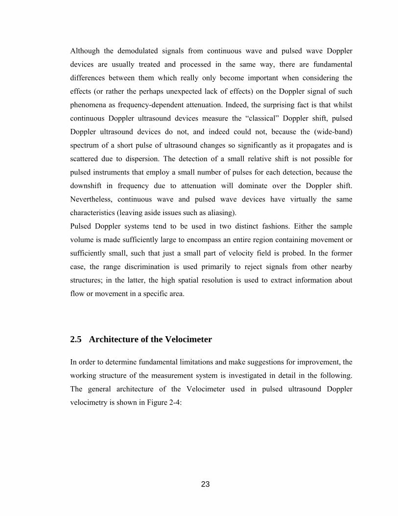
23
Although the demodulated signals from continuous wave and pulsed wave Doppler
devices are usually treated and processed in the same way, there are fundamental
differences between them which really only become important when considering the
effects (or rather the perhaps unexpected lack of effects) on the Doppler signal of such
phenomena as frequency-dependent attenuation. Indeed, the surprising fact is that whilst
continuous Doppler ultrasound devices measure the “classical” Doppler shift, pulsed
Doppler ultrasound devices do not, and indeed could not, because the (wide-band)
spectrum of a short pulse of ultrasound changes so significantly as it propagates and is
scattered due to dispersion. The detection of a small relative shift is not possible for
pulsed instruments that employ a small number of pulses for each detection, because the
downshift in frequency due to attenuation will dominate over the Doppler shift.
Nevertheless, continuous wave and pulsed wave devices have virtually the same
characteristics (leaving aside issues such as aliasing).
Pulsed Doppler systems tend to be used in two distinct fashions. Either the sample
volume is made sufficiently large to encompass an entire region containing movement or
sufficiently small, such that just a small part of velocity field is probed. In the former
case, the range discrimination is used primarily to reject signals from other nearby
structures; in the latter, the high spatial resolution is used to extract information about
flow or movement in a specific area.
2.5 Architecture of the Velocimeter
In order to determine fundamental limitations and make suggestions for improvement, the
working structure of the measurement system is investigated in detail in the following.
The general architecture of the Velocimeter used in pulsed ultrasound Doppler
velocimetry is shown in Figure 2-4:
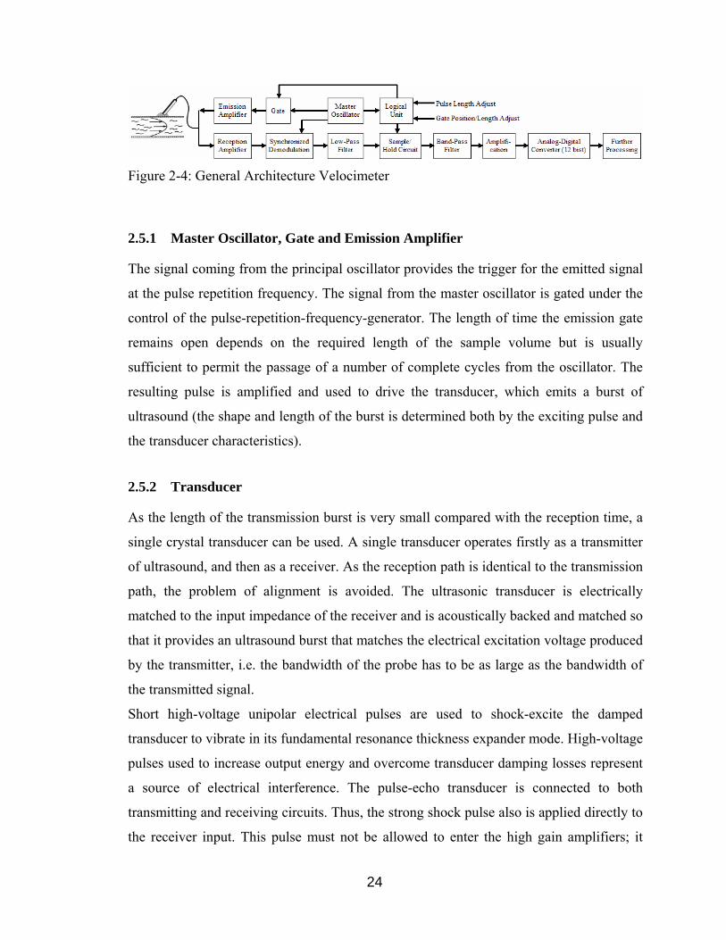
24
Figure 2-4: General Architecture Velocimeter
2.5.1 Master Oscillator, Gate and Emission Amplifier
The signal coming from the principal oscillator provides the trigger for the emitted signal
at the pulse repetition frequency. The signal from the master oscillator is gated under the
control of the pulse-repetition-frequency-generator. The length of time the emission gate
remains open depends on the required length of the sample volume but is usually
sufficient to permit the passage of a number of complete cycles from the oscillator. The
resulting pulse is amplified and used to drive the transducer, which emits a burst of
ultrasound (the shape and length of the burst is determined both by the exciting pulse and
the transducer characteristics).
2.5.2 Transducer
As the length of the transmission burst is very small compared with the reception time, a
single crystal transducer can be used. A single transducer operates firstly as a transmitter
of ultrasound, and then as a receiver. As the reception path is identical to the transmission
path, the problem of alignment is avoided. The ultrasonic transducer is electrically
matched to the input impedance of the receiver and is acoustically backed and matched so
that it provides an ultrasound burst that matches the electrical excitation voltage produced
by the transmitter, i.e. the bandwidth of the probe has to be as large as the bandwidth of
the transmitted signal.
Short high-voltage unipolar electrical pulses are used to shock-excite the damped
transducer to vibrate in its fundamental resonance thickness expander mode. High-voltage
pulses used to increase output energy and overcome transducer damping losses represent
a source of electrical interference. The pulse-echo transducer is connected to both
transmitting and receiving circuits. Thus, the strong shock pulse also is applied directly to
the receiver input. This pulse must not be allowed to enter the high gain amplifiers; it
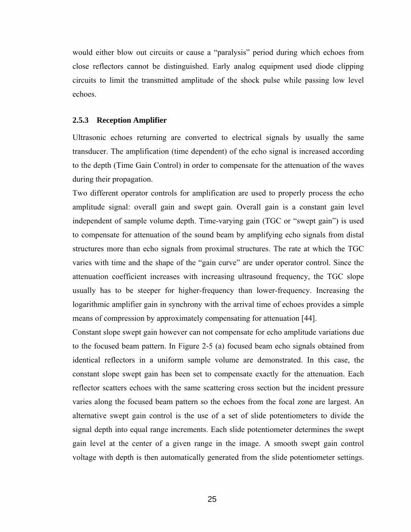
25
would either blow out circuits or cause a “paralysis” period during which echoes from
close reflectors cannot be distinguished. Early analog equipment used diode clipping
circuits to limit the transmitted amplitude of the shock pulse while passing low level
echoes.
2.5.3 Reception Amplifier
Ultrasonic echoes returning are converted to electrical signals by usually the same
transducer. The amplification (time dependent) of the echo signal is increased according
to the depth (Time Gain Control) in order to compensate for the attenuation of the waves
during their propagation.
Two different operator controls for amplification are used to properly process the echo
amplitude signal: overall gain and swept gain. Overall gain is a constant gain level
independent of sample volume depth. Time-varying gain (TGC or “swept gain”) is used
to compensate for attenuation of the sound beam by amplifying echo signals from distal
structures more than echo signals from proximal structures. The rate at which the TGC
varies with time and the shape of the “gain curve” are under operator control. Since the
attenuation coefficient increases with increasing ultrasound frequency, the TGC slope
usually has to be steeper for higher-frequency than lower-frequency. Increasing the
logarithmic amplifier gain in synchrony with the arrival time of echoes provides a simple
means of compression by approximately compensating for attenuation [44].
Constant slope swept gain however can not compensate for echo amplitude variations due
to the focused beam pattern. In Figure 2-5 (a) focused beam echo signals obtained from
identical reflectors in a uniform sample volume are demonstrated. In this case, the
constant slope swept gain has been set to compensate exactly for the attenuation. Each
reflector scatters echoes with the same scattering cross section but the incident pressure
varies along the focused beam pattern so the echoes from the focal zone are largest. An
alternative swept gain control is the use of a set of slide potentiometers to divide the
signal depth into equal range increments. Each slide potentiometer determines the swept
gain level at the center of a given range in the image. A smooth swept gain control
voltage with depth is then automatically generated from the slide potentiometer settings.

26
In Figure 2-5 (b) the use of the slide potentiometers to compensate for both medium
attenuation and the focused beam pattern is shown [44].
Figure 2-5: Swept Gain [44]
2.5.4 Synchronized Demodulation and Low-Pass Filter
Following the amplification, the echo signals are mixed with a reference signal from the
master oscillator, i.e., the echo signals are multiplied by the reference signal of the
emitted pulse. These demodulated signals (decomposed into two components of basic
frequency and Doppler-shifted frequency) are then filtered to isolate Doppler information,
i.e. the sum frequency is removed by a low-pass filter. The demodulation signal contains
the range – phase information, i.e. for each burst of ultrasound the difference in phase
between the reference signal (provided by the master oscillator) and the received echo at
the specified range.
A pulse wave Doppler system has a pulse repetition frequency that is a subharmonic of
the carrier frequency. Comparing the carrier frequency against the receive signal in a
quadrature phase detector permits the depiction of motion direction. The quadrature
demodulation, a phase sensitive demodulation technique as was employed by the
continuous wave system, gives both the real and imaginary part of the received signal,
which are both 90 degrees out of phase with each other. I is the in phase component and
Q is the quadrature component of the output signal. To obtain the direction of the flow,

27
both output signals from the quadrature detector may be processed by several methods,
many of which are now obsolete (such as zero crossing detection). The most widely used
method in modern Doppler instruments is digital Fourier spectral analysis. After
separation of the various frequency components, the direction of flow is determined by
comparing the phase of the real and imaginary parts of the signals. If the real part is 90
degrees ahead of the imaginary part in phase, then flow is directed towards the transducer,
and if the real part lags 90 degrees behind, then flow is reversed.
The output from the demodulator covers a frequency spectrum which extends from very
low frequencies up to about 10 kHz. Some of the frequency components carry useful
information; others do not. It is usual to arrange for unwanted signals to be filtered out
whenever this is possible without the loss of useful information. A low pass filter
suppresses artifactual frequencies in the spectrum generated by the demodulation. The
low pass filter is also used to define the bandwidth and therefore the spatial resolution.
2.5.5 Sample/Hold Circuit
The Doppler signal (output of the demodulator) is then sampled into channels at a
specified point in time relative to the onset of the transmission pulse. A receiver gate
opens during each transmission cycle after an operator-determined delay, to admit signals
to a sample and hold circuit. It is the delay between transmission and the opening of the
receiver gate that determines the region from which the signals are gathered, whilst the
time for which the gate is left open, together with the length of the transmitted pulse,
determines the sample volume length. The time between acquisitions determines the axial
spacing between sample volumes, while the delay between the emission and reception
determines the distance to the sample volume.
The sample and hold circuit samples the output from the demodulator stage. It is common
practice to integrate over the sample period and then hold this integrated value until the
next sampling period. The sampling duration, together with the transmitted pulse length,
sets the range over which velocity information is gathered. For optimum performance (i.e.
the best sensitivity for a given axial resolution), the length of the transmission burst is
usually set or the same length as the sampling or receiver gate length [18].

28
Figure 2-6 is a schematic of the signal-detection process. The train of pulses proportional
to the instantaneous phase difference is the input to the sample and hold unit producing a
voltage that oscillates at the Doppler frequency [8].
Figure 2-6: The Doppler Frequency and Range Detection Method [7]
a) Master Oscillator b) Transmitted Burst c) Range Gated Received Echoes d) Phase-Coherent Reference Frequency e) Phase Detector Output f) Sample and Hold Output Over Many Cycles
2.5.6 Logical Unit
The control logic (logic unit) provides the necessary timing signals to for example
implement the transmitter burst or initiate the sample and hold amplifiers at the
appropriate time relative to the transmission burst.
An output power control is provided on most systems. This is used to vary the maximum
sensitivity of the instrument by increasing or decreasing the amplitude of the acoustic
pulse launched by the transducer. This affects the amplitude of the incident and reflected
beams at each interface and the size of each echo detected by the transducer. Higher-
power levels can result in detection of echo signals from more weakly reflecting
interfaces and scatterers [49].

29
2.5.7 Band-Pass Filter, Amplification and Analog-Digital Conversion
The output from the sample and hold circuit is filtered, because it contains not only the
Doppler shift frequencies but for example also the sampling frequency which has to be
removed. In order that the full range of Doppler shift frequencies can be utilized, i.e. up to
half the pulse repetition frequency [18], a very sharp low pass filter is used to eliminate
the sampling frequency without degrading the Doppler signal. This filter must also be
variable if a variable PRF system is used. Steady and quasi steady components are
eliminated by a high pass filter. Thereby, both the sampling frequency and unwanted
(often high energy) low frequency components are removed providing the Doppler shift
frequency information at the range of interest. After amplification, and analog-to-digital
conversion (12 bits), the signal is sent for further processing and display. Finally the
frequency of the Doppler signal is estimated. The results may then be used to calculate
the velocity.
2.5.8 Signal Processing
The measurement of the velocity is based on the estimation of the mean phase shift of
successive echoes coming from a defined depth. Gates are formed by sampling the echo
signal. The depth of the gate is computed by measuring the time delay between the
emission and reception of the echo. The thickness of all the gates is defined by the burst
length and/or the bandwidth or the receiver. In order to compute the velocity in each gate,
many emissions are sent. These emissions form an array of time series data values, from
which the mean Doppler frequency is computed by an auto-correlation algorithm. The
algorithm used is based on the random statistical nature of each echo.
The amplitudes of the echoes reflected by the particles within the flowing fluid are
somewhat random in nature, corresponding to the random distribution of the particles in
the fluid medium. Thus, the Doppler signals may be treated as random processes. In order
to be able to determine the probability of occurrence of this process, one must have access
to a great number of actual occurrences of the process. In practice it is difficult to obtain
measurements of the exact same process under the exact same condition at several
different times. Therefore, a temporal average is preferable to an ensemble average. The

30
temporal average and the ensemble average will not be the same unless the process is
stationary and the analysis time is very long (tending to infinity).
In the algorithm it is assumed that the statistical properties of all collected echoes used in
the computation of the mean phase shift are stationary. This allows to transform temporal
average into spatial average and to consider all processes stationary. The Doppler
frequency calculation algorithm is based on the fact that the inverse Fourier transform of
the probability density function of a stationary process is equal to the auto-correlation
function. The algorithm computes the auto-correlation of the Doppler echoes. The auto-
correlation function is estimated using the complex envelope of the echo signal. The
Doppler frequency (fD) is then computed, and finally the velocity is extracted from the
Doppler equation. All velocity profile information is contained in the echo. Thus a
velocity profile can be obtained by analyzing the echo signal to derive instantaneous
frequencies at each instant. In practice, the echo signal is processed at 128 instants in
parallel, and thus a data set which can be converted to the velocity profile is obtained.
Let´s assume that the particles are randomly distributed inside the ultrasonic beam. The
echoes returned by each particle are then combined together in a random fashion, giving a
random echo signal. A high degree of correlation exists between different emissions. This
high degree of correlation is built into all digital processing techniques to extract
information, such as velocity [55].
Signal processing may be applied to the echo signals conditioning them suitable for
display. Any procedure performed on the echo amplitude signal after transducer reception
and before display qualifies as signal processing. The number of emissions per profile,
the number of profiles to record, optional filtering (moving average or median filter),
scale and units, Doppler angle, the speed of sound as well as the sensitivity may be
selected by the user. A change in the sensitivity of the beam of the Doppler unit will alter
effective length of the transmitted pulse and the effective beam width [18]. The user can
also choose between several computation and display options.
One of the steps involved in signal processing consists of compression. Compression
generally refers to reduction of the amplitude range of echo signals for a given range of
echo amplitudes at the input to the instrument. The range of echo signals that an
instrument is capable of handling properly is referred to as the dynamic range. Different

31
components of an instrument have different dynamic range capabilities. To allow the
display equipment to handle a wider variation in echo signal amplitudes, signal
compression is applied in the receiver. Most instruments allow selection of additional
signal processing through choice of preprocessing and post processing control settings.
Preprocessing refers to special signal processing applied before echo signals are stored in
the instrument’s memory. There are mainly two possibilities for preprocessing.
Logarithmic compression amplifies low-amplitude echo signals more than high-amplitude
signals. Thus amplitude variations among the low signal levels are emphasized. The S-
shaped curve on the other hand emphasizes variations over the middle of the echo signal
range. Preprocessing usually also includes a preamplifier, since small single element
transducers or the individual elements in multielement arrays cannot drive long lengths of
coaxial cable. Thus a preamplifier close to the piezoelectric crystal is used for some initial
signal amplification to overcome cable capacitance. Also, the preamplifier output is
electrically impedance matched to standard 50 Ohm cable impedance. Further
manipulation of echo data can be done using post processing.
Post processing refers to signal conditioning that operates on signals already stored in
memory, just before they are directed to the display. Post processing does not provide
new data but simply allows the same echo image data to be displayed differently.
2.5.9 Architecture DOP 1000 and DOP 2000
In Figure 2-7 and 2-8, the architecture of the pulsed ultrasound Doppler velocimeters
DOP2000 and DOP1000 from Signal Processing is presented. Differences in performance
characteristics between the two systems are emphasized by italic letters in the figure of
the architecture of the DOP1000 velocimeter.
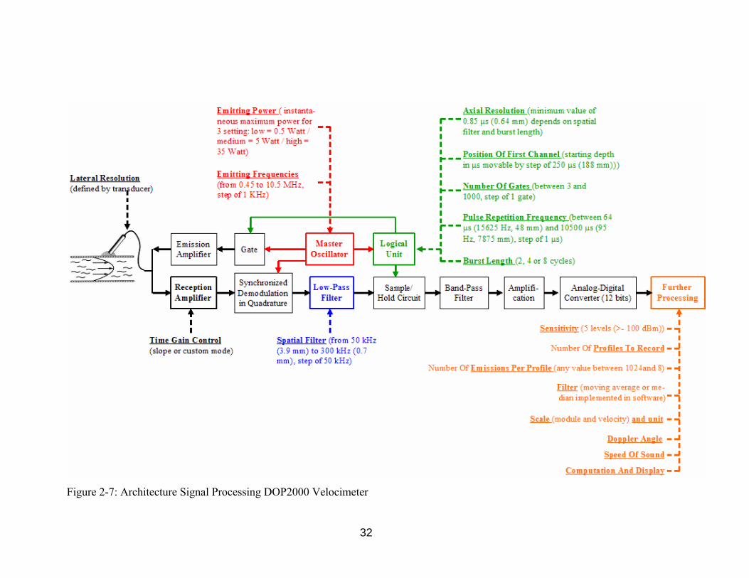
32
Figure 2-7: Architecture Signal Processing DOP2000 Velocimeter

33
Figure 2-8: Architecture Signal Processing DOP1000 Velocimeter
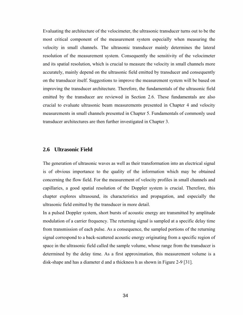
34
Evaluating the architecture of the velocimeter, the ultrasonic transducer turns out to be the
most critical component of the measurement system especially when measuring the
velocity in small channels. The ultrasonic transducer mainly determines the lateral
resolution of the measurement system. Consequently the sensitivity of the velocimeter
and its spatial resolution, which is crucial to measure the velocity in small channels more
accurately, mainly depend on the ultrasonic field emitted by transducer and consequently
on the transducer itself. Suggestions to improve the measurement system will be based on
improving the transducer architecture. Therefore, the fundamentals of the ultrasonic field
emitted by the transducer are reviewed in Section 2.6. These fundamentals are also
crucial to evaluate ultrasonic beam measurements presented in Chapter 4 and velocity
measurements in small channels presented in Chapter 5. Fundamentals of commonly used
transducer architectures are then further investigated in Chapter 3.
2.6 Ultrasonic Field
The generation of ultrasonic waves as well as their transformation into an electrical signal
is of obvious importance to the quality of the information which may be obtained
concerning the flow field. For the measurement of velocity profiles in small channels and
capillaries, a good spatial resolution of the Doppler system is crucial. Therefore, this
chapter explores ultrasound, its characteristics and propagation, and especially the
ultrasonic field emitted by the transducer in more detail.
In a pulsed Doppler system, short bursts of acoustic energy are transmitted by amplitude
modulation of a carrier frequency. The returning signal is sampled at a specific delay time
from transmission of each pulse. As a consequence, the sampled portions of the returning
signal correspond to a back-scattered acoustic energy originating from a specific region of
space in the ultrasonic field called the sample volume, whose range from the transducer is
determined by the delay time. As a first approximation, this measurement volume is a
disk-shape and has a diameter d and a thickness h as shown in Figure 2-9 [31].
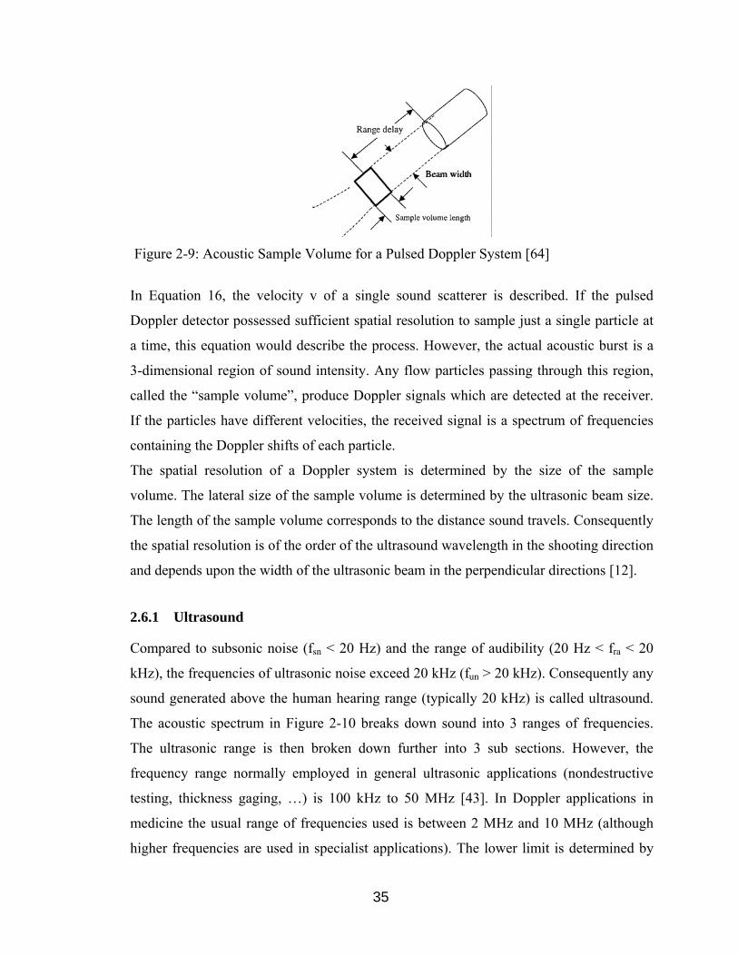
35
Figure 2-9: Acoustic Sample Volume for a Pulsed Doppler System [64]
In Equation 16, the velocity v of a single sound scatterer is described. If the pulsed
Doppler detector possessed sufficient spatial resolution to sample just a single particle at
a time, this equation would describe the process. However, the actual acoustic burst is a
3-dimensional region of sound intensity. Any flow particles passing through this region,
called the “sample volume”, produce Doppler signals which are detected at the receiver.
If the particles have different velocities, the received signal is a spectrum of frequencies
containing the Doppler shifts of each particle.
The spatial resolution of a Doppler system is determined by the size of the sample
volume. The lateral size of the sample volume is determined by the ultrasonic beam size.
The length of the sample volume corresponds to the distance sound travels. Consequently
the spatial resolution is of the order of the ultrasound wavelength in the shooting direction
and depends upon the width of the ultrasonic beam in the perpendicular directions [12].
2.6.1 Ultrasound
Compared to subsonic noise (fsn < 20 Hz) and the range of audibility (20 Hz < fra < 20
kHz), the frequencies of ultrasonic noise exceed 20 kHz (fun > 20 kHz). Consequently any
sound generated above the human hearing range (typically 20 kHz) is called ultrasound.
The acoustic spectrum in Figure 2-10 breaks down sound into 3 ranges of frequencies.
The ultrasonic range is then broken down further into 3 sub sections. However, the
frequency range normally employed in general ultrasonic applications (nondestructive
testing, thickness gaging, …) is 100 kHz to 50 MHz [43]. In Doppler applications in
medicine the usual range of frequencies used is between 2 MHz and 10 MHz (although
higher frequencies are used in specialist applications). The lower limit is determined by
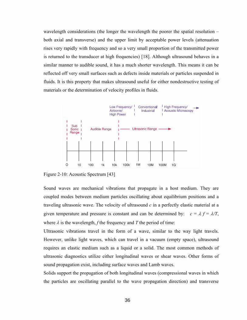
36
wavelength considerations (the longer the wavelength the poorer the spatial resolution –
both axial and transverse) and the upper limit by acceptable power levels (attenuation
rises very rapidly with frequency and so a very small proportion of the transmitted power
is returned to the transducer at high frequencies) [18]. Although ultrasound behaves in a
similar manner to audible sound, it has a much shorter wavelength. This means it can be
reflected off very small surfaces such as defects inside materials or particles suspended in
fluids. It is this property that makes ultrasound useful for either nondestructive testing of
materials or the determination of velocity profiles in fluids.
Figure 2-10: Acoustic Spectrum [43]
Sound waves are mechanical vibrations that propagate in a host medium. They are
coupled modes between medium particles oscillating about equilibrium positions and a
traveling ultrasonic wave. The velocity of ultrasound c in a perfectly elastic material at a
given temperature and pressure is constant and can be determined by: c = λ f = λ/T,
where λ is the wavelength, f the frequency and T the period of time:
Ultrasonic vibrations travel in the form of a wave, similar to the way light travels.
However, unlike light waves, which can travel in a vacuum (empty space), ultrasound
requires an elastic medium such as a liquid or a solid. The most common methods of
ultrasonic diagnostics utilize either longitudinal waves or shear waves. Other forms of
sound propagation exist, including surface waves and Lamb waves.
Solids support the propagation of both longitudinal waves (compressional waves in which
the particles are oscillating parallel to the wave propagation direction) and transverse
37
(shear) waves (particles oscillating perpendicular to the wave propagation direction.
Figure 2-11 provides an illustration of the particle motion versus the direction of wave
propagation for longitudinal waves and shear waves. Surface (Rayleigh) waves have an
elliptical particle motion and travel across the surface of a material. Their velocity is
approximately 90% of the shear wave velocity of the material and their depth of
penetration is approximately equal to one wavelength. Plate (Lamb) waves have a
complex vibration occurring in materials where thickness is less than the wavelength of
ultrasound introduced into it. Fluids (gases and liquids) only support longitudinal wave
propagation.
Figure 2-11: Longitudinal and Shear Waves [43]
Pulsed ultrasound, as in the case of pulsed ultrasound Doppler velocimetry, is produced
by applying electric pulses to an ultrasonic transducer. The number of pulses produced
per second is called the pulse repetition frequency. The spatial pulse length is the length
of space over which a pulse occurs. It is equal to the wavelength times the number of
cycles in the pulse. It decreases with increasing frequency.

38
2.6.2 Acoustic Phenomena
Ultrasound Doppler velocimetry requires some amount of scatterers suspended in the
liquid, which may disturb its flow or change its fundamental properties. In this section,
the effect of the required scatterers on the ultrasonic beam is evaluated and basic acoustic
phenomena are described.
Ultrasound attenuates as it progresses through a medium, i.e. its amplitude and intensity
decrease gradually with increasing distance of travel. Assuming no major reflections,
there are the following causes of attenuation: scattering, diffraction and absorption. The
amount of attenuation through a material can play an important role in the selection of a
transducer for an application. Attenuation is important because it limits the depth range
especially with high-frequency sound beams. The rate of attenuation, or attenuation
coefficient, depends on both the matter traversed and the ultrasound frequency. The rate
of attenuation increases with increasing frequency. Attenuation can be compensated in the
receiving amplifier by electronic circuitry which applies increasing gain as signals are
received from increasing depths. Solid plaque attenuates ultrasound strongly owing to
high reflection and refraction and therefore casts shadows in the region behind it. The
frequency dependence of attenuation results in the high frequency components of an
ultrasonic pulse being preferentially reduced in amplitude relative to the low frequency
components [18]. The attenuation coefficient increases with increasing frequency.
The ultrasonic waves generated by the standard single-element transducer (described in
detail in chapter 3) are more or less confined in a narrow cone. As they travel in this cone
they may be scattered when they touch a particle having different acoustic impedance.
The acoustic impedance of a material is the opposition to displacement of its particles by
sound and occurs in many equations. The characteristic impedance is defined by:
Z = ρ c, where ρ is the density of the medium and c the sound velocity. The boundary
between two materials of different acoustic impedances is called an acoustic interface.
When an ultrasonic wave traveling through a medium strikes an acoustic interface, i.e., a
discontinuity or any variation from uniformity in the medium of dimensions similar to or
less than a wavelength, some of the energy of the wave is scattered in many directions.
Scattering is the process of central importance, since it provides most of the signals for
echo Doppler techniques as in the case of pulsed Doppler ultrasound velocimetry. It

39
occurs at rough boundaries and within heterogeneous media. The discontinuities may be
changes in density or compressibility or both. Of particular interest is the differential
cross-section of the target of volume of material at 180 degrees to the direction of the
incident ultrasound. This is known as the backscatter cross-section and determines the
size of the signal back to the transducer. Three general types of scattering can occur:
scattering (reflection) from large flat boundaries, known as specular reflection; scattering
from point reflectors (or local variation in tissue structure or density), known as diffuse
scattering; and scattering from structures whose dimensions are commensurate with the
wavelength, known as resonance scattering.
When sound strikes an acoustic interface, some amount of sound energy is reflected and
some amount is transmitted across the boundary and consequently refracted as shown in
Figure 2-12.
Figure 2-12: Reflection and Refraction [51]
Reflection is a special case of scattering which occurs at smooth surfaces on which the
irregularities are very much smaller than a wavelength. When a wave front strikes a
smooth surface at an oblique angle of incidence, it is reflected at an equal and opposite
angle. Point reflectors (structures whose dimensions are small compared to the
wavelength) undergo Rayleigh scattering, which has a pressure scattering cross section
proportional to frequency squared. Diffuse scattering produces low-amplitudes, omni
directional echoes.
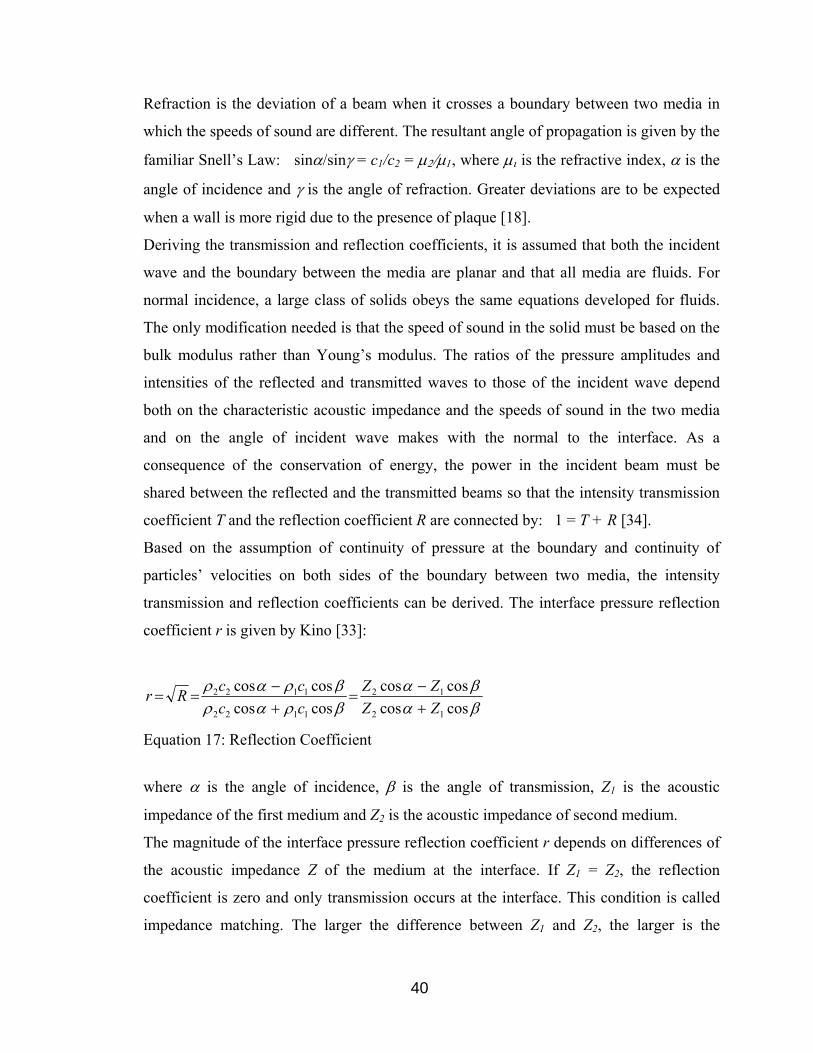
40
Refraction is the deviation of a beam when it crosses a boundary between two media in
which the speeds of sound are different. The resultant angle of propagation is given by the
familiar Snell’s Law: sinα/sinγ = c1/c2 = µ2/µ1, where µι is the refractive index, α is the
angle of incidence and γ is the angle of refraction. Greater deviations are to be expected
when a wall is more rigid due to the presence of plaque [18].
Deriving the transmission and reflection coefficients, it is assumed that both the incident
wave and the boundary between the media are planar and that all media are fluids. For
normal incidence, a large class of solids obeys the same equations developed for fluids.
The only modification needed is that the speed of sound in the solid must be based on the
bulk modulus rather than Young’s modulus. The ratios of the pressure amplitudes and
intensities of the reflected and transmitted waves to those of the incident wave depend
both on the characteristic acoustic impedance and the speeds of sound in the two media
and on the angle of incident wave makes with the normal to the interface. As a
consequence of the conservation of energy, the power in the incident beam must be
shared between the reflected and the transmitted beams so that the intensity transmission
coefficient T and the reflection coefficient R are connected by: 1 = T + R [34].
Based on the assumption of continuity of pressure at the boundary and continuity of
particles’ velocities on both sides of the boundary between two media, the intensity
transmission and reflection coefficients can be derived. The interface pressure reflection
coefficient r is given by Kino [33]:
βαβα
βραρβραρ
coscoscoscos
coscoscoscos
12
12
1122
1122
ZZZZ
ccccRr
+−
=+−
==
Equation 17: Reflection Coefficient
where α is the angle of incidence, β is the angle of transmission, Z1 is the acoustic
impedance of the first medium and Z2 is the acoustic impedance of second medium.
The magnitude of the interface pressure reflection coefficient r depends on differences of
the acoustic impedance Z of the medium at the interface. If Z1 = Z2, the reflection
coefficient is zero and only transmission occurs at the interface. This condition is called
impedance matching. The larger the difference between Z1 and Z2, the larger is the

41
reflection coefficient. This condition is called impedance mismatching. If Z1 < Z2, the
reflected wave has no phase change upon reflection and if Z1 > Z2, the reflected wave has
a π radian phase change upon reflection. Since pulse-echo ultrasonic imaging is
performed with a single transducer, the high-amplitude, directionally dependent specular
reflections are only received by the transducer if the ultrasonic beam is normal to the
medium interface (or very close to normal).
The intensity transmission coefficient T, which is equal to the ratio of the refracted
intensity to the incident intensity, is given by Kino [33]:
212
221
))cos()cos(()(cos4γα
αZZ
ZZTR +=
Equation 18: Transmission Coefficient
According to the principle of acoustic reciprocity, transmission coefficients are
independent of the direction of the wave. Transmission coefficients are small whenever
the acoustic impedances of both media have widely separated values.
These equations may also be used to predict the amount of ultrasonic energy that will
penetrate in the liquid. In other words, they predict the amount of energy that tends to
remain in the wall. The dB loss of energy on transmitting a signal from medium 1 to
medium 2 at normal incidence is given by Panametrics [43]:
( ) ⎥⎦
⎤⎢⎣
⎡
+⋅⋅
= 221
2110
4log10ZZ
ZZdBloss
Equation 19: dB Loss Due to Transmission
The dB loss of energy of the echo signal in medium 1 reflecting from an interface
boundary with medium 2 at normal incidence is given by Panametrics [43]:
( )( ) ⎥
⎦
⎤⎢⎣
⎡
+−
= 221
212
10log10ZZZZdBloss
Equation 20: dB Loss Due to Reflection

42
When dealing with transmission through a layer at normal incidence, the calculation of
the reflection and transmission coefficient becomes more complex. It is assumed that a
layer of uniform thickness L lies between two fluids and that a plane wave is normally
incident on its boundary. When an incident signal arrives at a boundary between the fluid
and the layer (or vice versa) some of the energy is reflected and some is transmitted. If the
duration of the incident signal is less than 2L/cL (cL is the sound velocity in the layer), an
observer on either side of the layer will detect a series of echoes separated in time by
2L/cL. The echo amplitude can then be calculated by applying the formulas given above
the appropriate number of times. On the other hand, if the incident wave train is long
compared to 2L and monofrequency can be assumed, the various transmitted and
reflected waves combine resulting in standing waves within the layer. In the steady-state
condition assuming continuity of the normal specific acoustic impedance at both
boundaries, the intensity transmission coefficient T is given by Kinsley [34]:
( )LkZZ
ZZ
T
L
W
W
L2
22
sin411
1
⎟⎟⎠
⎞⎜⎜⎝
⎛−+
=
Equation 21: Intensity Transmission Coefficient (Simplified)
where k = ω/c is the wave number, ω = 2 π f is the angular frequency, c is the speed of
sound, L is the layer thickness, ZL is the acoustic impedance of the layer and ZW is the
acoustic impedance of the fluid on both sides of the layer (the initial equals the final
fluid).
Absorption is the process of conversion of wave motion energy into heat. Absorption
increases rapidly with frequency. In practice, absorption on its own is rarely of interest,
since other processes are simultaneously contributing to the total attenuation of the
acoustic wave. These processes are scattering, reflection, refraction, non-linear
propagation and beam divergence. Since many of these factors are strongly frequency
dependent, it is not surprising that attenuation rises rapidly over the frequency range 1 –
20 MHz [18]. Absorption and attenuation are very important in Doppler techniques and
their influence on any examination must be considered.

43
2.6.3 Ultrasonic Field Emitted by Transducer
A pulsed ultrasonic Doppler flow meter for detailed measurements of velocity profiles
projects a beam of ultrasonic bursts. The back-scattered signals are processed to produce
a signal corresponding to the mean velocity over a small region of the flowing stream.
The size and shape of this sample volume determines the flow meter sensitivity and
accuracy. The velocity profile obtained from this instrument is a weighted average of the
ultrasonic intensity and the flow field velocity over the sample volume.
The sound-field characteristics are determined by the ultrasonic transducer’s focal
characteristics, the sound scatterers and the sensitivity of the receiver circuitry. A
sufficient description of the characteristics of the sound field requires quantitative
information about the sample-volume geometry and intensity distribution, the focused
beam shape and the amplitude of the back-scattered signal as a function of range. The
sample-volume geometry and intensity are important because they influence the spectral
content of the back-scattered signal. The focused beam shape indicates how the geometry
of the sample volume varies with range.
In Doppler echography, the object is not to make use of a plane longitudinal wave, but
rather an ultrasonic beam that is as thin as possible throughout the measurement depth.
The geometry of the acoustic field is governed by the diameter D of the emitter and the
wavelength λ, which is equal to the ratio of the speed of sound in the analyzed medium
and the emitting frequency.
Using Huygen’s principle, one may predict the geometry of the acoustic field. In the
following approach, the ultrasonic single-element transducer is modeled as a combination
of several adjacent point sources, each generating a spherical wave. The typical shape of
the ultrasonic field is illustrated in Figure 2-13:
Figure 2-13: Ultrasonic Field [51]

44
For a circular transducer of radius a operating in a piston-like manner, the intensity of the
acoustic field I along the axis is given by Kino:
( )⎥⎦⎤
⎢⎣⎡ −−= xxa
II z 222
0
sinλπ
Equation 22: Intensity of the Acoustic Field
where I0 is the maximum intensity, x is the distance from the transducer and λ is the
wavelength [33]. The acoustic field generated by a transducer possesses two characteristic
regions, separated by the distance of the furthermost maximum of the above function: the
cylindrical near field and the conical far field.
In the near field (Fresnel zone), the region that is located near the transducer surface, the
acoustic field is nearly cylindrical, with a diameter slightly less than the diameter of the
emitter. The intensity of the acoustic waves oscillates along the axis of the transducer.
The echo amplitude goes through a series of maxima and minima. As the characteristic
distances of these oscillations are much smaller than the dimensions of the measured
volumes, they do not significantly affect Doppler information collected in this region. The
length of the near field LNF is given by Kino [33]:
λλ
44 22 −
=dLNF
Equation 23: Length of the Near Field
where d is diameter of the transducer. The length of the near field is defined by the
position of the last maximum of the acoustic intensity as shown in Figure 2-14. The near
field distance is the natural focus of the transducer and a function of the transducer
frequency, element diameter (aperture size) and the speed of sound velocity in the
medium.
In the far field (Frauenhofer zone), the zone lying beyond LNF, the intensity of the
acoustic waves along the axis decreases as the inverse of the square of the distance from
the transducer (according to the inverse-square law for point sources). Small oscillations

45
appear in the radial direction (perpendicular to the axis of propagation) as shown in
Figure 2-14. The sound field pressure gradually drops to zero.
Figure 2-14: Near and Far Ultrasonic Field [51]
Most of the acoustic energy is contained in a cone. The relationship between the acoustic
field intensity and the angle off the transducer axis depends on the directivity function:
( ) ( )γ
γγsin
sin2 1
akakJDr =
Equation 24: Directivity Function
where J1 is the first order Bessel function of the first kind, and k = 2 π/λ the wave number
[33]. The half angle of divergence of the main lobe ϕ (-6 dB pulse-echo beam spread
angle) is characterized by the wavelength and the diameter of the emitter and is given by
Signal Processing [51]:

46
⎟⎟⎠
⎞⎜⎜⎝
⎛⋅
=⎟⎠⎞
⎜⎝⎛= −−
dfc
d22,1sin22,1sin 11 λϕ
Equation 25: Half Angle of Beam Divergence
It can be seen from this equation that beam spread from a transducer can be reduced by
selecting a transducer with a higher frequency or a larger element diameter or both.
All ultrasonic beams diverge. In other words, all transducers have beam spread. In the
near field, the beam has a complex shape that usually narrows. In the far field the beam
diverges. The divergence of the ultrasonic beam depends on the diameter of the emitter
and the wavelength. Most of the time, a compromise between these two parameters has to
be established in order to achieve the thinnest beam possible at a defined distance. A
higher frequency gives a better axial resolution but also often induces higher attenuation
of the ultrasonic waves.
There are a number of sound field parameters that are useful in describing the
characteristics of an ultrasonic transducer. Especially knowledge of the beam width and
focal zone may be necessary in order to determine whether a particular transducer is
appropriate for the given application. The geometry of the acoustic field generated by the
ultrasonic wave determines the lateral resolution of the ultrasonic transducer. The
characteristics of the acoustic field depend on the size and shape of the piezoelectric
element. A transducer’s sensitivity is affected by the beam diameter at the point of
interest. The smaller the beam diameter, the greater the amount of energy that is reflected
by particles. By definition, the starting and ending points of the focal zone are located
where the on-axis pulse-echo signal amplitude drops to – 6 dB of the amplitude at the
focal point [43].
2.6.4 Sample Volume
In ultrasound Doppler velocimetry, the back-scattered signals are processed to produce a
signal corresponding to the mean velocity over a small region of the flowing stream. The
size and shape of this “sample volume” determines the flow meter sensitivity and
accuracy. The velocity profile obtained is a weighted average of the ultrasonic intensity
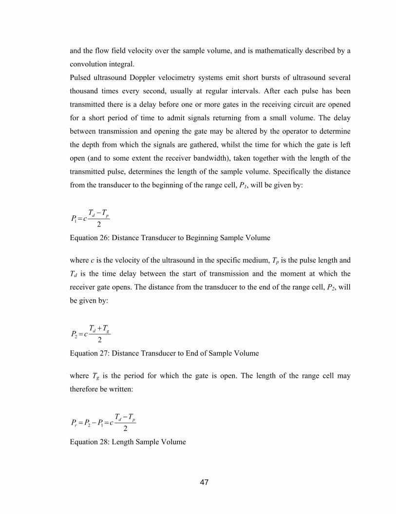
47
and the flow field velocity over the sample volume, and is mathematically described by a
convolution integral.
Pulsed ultrasound Doppler velocimetry systems emit short bursts of ultrasound several
thousand times every second, usually at regular intervals. After each pulse has been
transmitted there is a delay before one or more gates in the receiving circuit are opened
for a short period of time to admit signals returning from a small volume. The delay
between transmission and opening the gate may be altered by the operator to determine
the depth from which the signals are gathered, whilst the time for which the gate is left
open (and to some extent the receiver bandwidth), taken together with the length of the
transmitted pulse, determines the length of the sample volume. Specifically the distance
from the transducer to the beginning of the range cell, P1, will be given by:
21pd TT
cP−
=
Equation 26: Distance Transducer to Beginning Sample Volume
where c is the velocity of the ultrasound in the specific medium, Tp is the pulse length and
Td is the time delay between the start of transmission and the moment at which the
receiver gate opens. The distance from the transducer to the end of the range cell, P2, will
be given by:
22gd TT
cP+
=
Equation 27: Distance Transducer to End of Sample Volume
where Tg is the period for which the gate is open. The length of the range cell may
therefore be written:
212pd
r
TTcPPP
−=−=
Equation 28: Length Sample Volume
48
As described above, the spatial resolution of a standard pulsed wave system is related to
the length of the transmitted pulse and it follows from this equation (the last equation)
that to achieve very short range cells, or very good spatial resolution, it is necessary to use
very short pulses. The signal-to-noise ratio of a Doppler system is, however, related to the
average transmitted power and therefore, if the pulses are made shorter in order to
maintain the signal-to-noise ratio, it is necessary to increase their amplitude (the pulse
repetition frequency cannot be arbitrarily increased because of the need to avoid range
ambiguity by only having one pulse in flight at a given time). For a more general Doppler
system it is the signal bandwidth rather than the signal duration that determines the range
resolutions.
The axial dimension of the measured volumes is defined by the instrument that analyzes
the Doppler echoes (the duration of the emitted burst and the bandwidth of the receiver)
and their lateral size by the amount of acoustic energy reflected by the particles. Due to
the spatial dependence of the acoustic intensity, the lateral dimension of the measured
volumes depends on their position as simplified by the disks in Figure 2-13. More
exactly, the shape of the sample volume of a pulsed wave beam is often described as a
teardrop (Figure 2-17). This arises from the combination of the three dimensional shape
of the transmitted pulse and gated range [18].
A sufficient description of the characteristics of the sound field requires quantitative
information about the sample volume geometry and intensity distribution, the focused
beam shape and the amplitude of the back-scattered signal as a function of range. The
sample length and intensity are functions of the transducer bandwidth. In Figure 2-15 the
nature of the transducer response to an input pulse is shown [8].

49
Figure 2-15: Piezocrystal Transducer Response [8]
a) Driving Burst b) Acoustic Burst
The tail of the acoustic burst is due to transducer ringing, or the gradual decay of the
stored energy, and represents the free response characteristics of the transducer.
Transducer ringing increases the length of the sample volume, and therefore decreases the
spatial resolution of the Doppler detector. In Figure 2-15 the expected intensity envelope
with the characteristic tail due to transducer ringing is shown. The envelope can
mathematically be described as two exponentials. In Figure 2-16 the two functions which
describe the general shape of the acoustical intensity envelope are plotted [8].

50
Figure 2-16: The Acoustic Intensity Envelope [8]
Owing to noise levels it can be concluded that the sample volume will have a finite
length. Thus curve 12’’ must be a truncated exponential. In addition to the finite length of
the actual acoustic burst there is also a finite width of diameter, since the sample volume
is 3-dimensional. The 3-dimensional sample volume is simply the envelope curve
revolved about the time axis as shown in Figure 2-17 [18].
Figure 2-17: Teardrop Shape Sample Volume [18]
The size of the sample volume also depends on the sound scatterers and the focusing
characteristics of the transducer. The sample volume length now varies with both range
position and the signal intensity. The mathematical description of the sample volume
(expressions for the intensity distribution along the axis of the sample volume and
equations describing the sample volume geometry (radius)), which includes this variation

51
in effective length with trigger level, are derived in [8]. The maximum intensity at any
cross-section normal to the sound axis will occur on the axis and the intensity will
decrease radially outward.
Experimental studies [8] indicate that the sample volume has an envelope intensity curve
which can be described as two truncated exponentials. Since the sample volume is a 3-
dimensional packet of sound intensities, the exponential envelope can be revolved about
its axis to describe a body of revolution. The accuracy of this assumption depends on the
type of transducer used. If a single-crystal transducer is used for both transmitting and
receiving then the assumption is accurate.
It should be noted, that the range cell is not equally sensitive throughout, and its effective
distribution will depend on the shape of the ultrasound pulse, the relative lengths of the
transmitted pulse and the sample gate, and the bandwidth of the receiving electronics.
Furthermore, due to the properties of the ultrasound transducer and the limited bandwidth
of the receiving electronics, the ideal rectangular pulse and rectangular receiving gate
shapes will not be attained in practice.
The dimensions of the pulsed Doppler sample volume are determined by the factors given
in Figure 2-18. Their optimal values coupled with the proper transmitting frequency will
give the best sensitivity to resolution ratio for flow sensing at various depths.
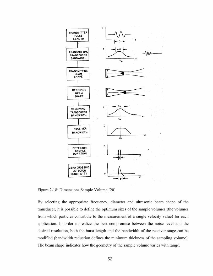
52
Figure 2-18: Dimensions Sample Volume [20]
By selecting the appropriate frequency, diameter and ultrasonic beam shape of the
transducer, it is possible to define the optimum sizes of the sample volumes (the volumes
from which particles contribute to the measurement of a single velocity value) for each
application. In order to realize the best compromise between the noise level and the
desired resolution, both the burst length and the bandwidth of the receiver stage can be
modified (bandwidth reduction defines the minimum thickness of the sampling volume).
The beam shape indicates how the geometry of the sample volume varies with range.
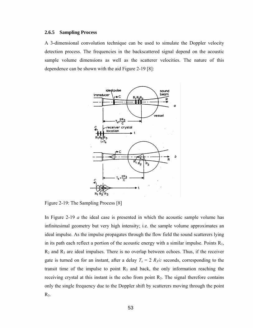
53
2.6.5 Sampling Process
A 3-dimensional convolution technique can be used to simulate the Doppler velocity
detection process. The frequencies in the backscattered signal depend on the acoustic
sample volume dimensions as well as the scatterer velocities. The nature of this
dependence can be shown with the aid Figure 2-19 [8]:
Figure 2-19: The Sampling Process [8]
In Figure 2-19 a the ideal case is presented in which the acoustic sample volume has
infinitesimal geometry but very high intensity; i.e. the sample volume approximates an
ideal impulse. As the impulse propagates through the flow field the sound scatterers lying
in its path each reflect a portion of the acoustic energy with a similar impulse. Points R1,
R2 and R3 are ideal impulses. There is no overlap between echoes. Thus, if the receiver
gate is turned on for an instant, after a delay Ts = 2 R3/c seconds, corresponding to the
transit time of the impulse to point R3 and back, the only information reaching the
receiving crystal at this instant is the echo from point R3. The signal therefore contains
only the single frequency due to the Doppler shift by scatterers moving through the point
R3.
54
The actual sample volume, of course, has finite geometry. This case is shown in Figure
2-19 b. Again as the sample volume enters the flow field, the scatterers lying in the sound
field each reflect a portion of the acoustic energy; the echoes each have the shape of the
transmitted pulse. If it is desired to sample the echo from point R3, the range gate is
turned on for an instant at time Ts = 2R3/c seconds. Since the echoes are finite in length,
overlapping occurs so that the signal reaching the receiver at time Ts contains information
from points R1 and R2 as well as point R3. In fact, the signal reaching the receiver at this
instant contains information from scatterers spread throughout the sample volume. The
frequency content of the signal therefore corresponds to the velocities throughout the
sample region. The selected frequency is a weighted average of the signal spectrum.
Mathematically a true weighed average is determined by the convolution integral. The
expression used as the basis of the 3-dimensional convolution or weighted average
technique for the analytical model can be found in [8]. The goal of the analytical model is
to simulate the sound field velocity interaction using the convolution process by taking
into account the sample volume and focusing characteristics of the transducer, the signal
detection and frequency-meter characteristics and the general parameters which describe
a given test situation.
If, however, the sample volume is only partially within the flow field, as occurs during
entry and exit of the channel, then only a portion of its energy contributes to the
backscattered signal. The intensity of the signal is therefore zero when the sample volume
is out of the flow field, and gradually rises to the level indicated by the focusing
characteristics as it enters the flow field. This is illustrated in Figure 2-20.

55
Figure 2-20: Sample Volume Flow Entry/Exit [8]
2.6.6 Doppler Spectrum
Equation 16 describes the Doppler frequency shift due to the velocity of a single sound
scatterer. If the pulsed Doppler detector possessed sufficient spatial resolution to sample
just a single particle at a time, this equation would describe the process. However, the
actual acoustic burst is a 3-dimensional region of sound intensity. Any flow particles
passing through this region, the sample volume, produce Doppler signals which are
detected at the receiver. If the particles have different velocities, the received signal
results in a spectrum of frequencies containing the Doppler shifts of each particle, the
Doppler spectrum. The sample-volume geometry and intensity are important because they
influence the spectral content of the back-scattered signal.
The Doppler shift frequency estimate is proportional to velocity. Under ideal uniform
sampling conditions the power in a particular frequency band of the Doppler spectrum is
proportional to the volume of fluid moving with velocities that produce frequencies in
that band. Therefore the Doppler power spectrum should have the same shape as a
velocity distribution plot for the flow. In Figure 2-21 the effect of the sample volume on
the Doppler power spectrum and the generation of the velocity profile vw is shown
schematically [59]. The effect of the sample volume can also be seen the experimental
results presented in Chapter 4 and Chapter 5. Among other thing, this effect causes the

56
wall effect, identified by Aidun and Xu in [64]. This wall effect is presented detail in
chapter 5.5.
Figure 2-21: Doppler Power Spectrum and Velocity Profile [8]
In practice, the shape of the velocity profile is modified by a number of mechanisms,
including non-uniform sampling, scattering, attenuation, intrinsic spectral broadening,
filtering and the limitation of spectral estimation techniques.
The spectra corresponding to flat velocity profiles have much of the power concentrated
in a relatively small range of frequencies, whilst those corresponding to parabolic profiles
are almost flat. In turbulent flow, the velocities of the targets in the ultrasound field
fluctuate rapidly with time. This causes a broadening of the spectrum that would
otherwise be obtained from flow with the same temporal average velocity profile. Gross
disturbances, such as large vortices, may cause irregular spectra with large isolated
forward and reverse components.
Since pulsed wave systems use higher peak pressures compared to continuous wave
systems (because they only transmit for a small percentage of the time and therefore to
achieve an adequate signal-to-noise ratio, the short bursts they use must have greater
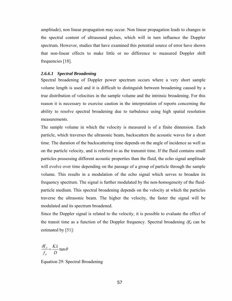
57
amplitude), non linear propagation may occur. Non linear propagation leads to changes in
the spectral content of ultrasound pulses, which will in turn influence the Doppler
spectrum. However, studies that have examined this potential source of error have shown
that non-linear effects to make little or no difference to measured Doppler shift
frequencies [18].
2.6.6.1 Spectral Broadening Spectral broadening of Doppler power spectrum occurs where a very short sample
volume length is used and it is difficult to distinguish between broadening caused by a
true distribution of velocities in the sample volume and the intrinsic broadening. For this
reason it is necessary to exercise caution in the interpretation of reports concerning the
ability to resolve spectral broadening due to turbulence using high spatial resolution
measurements.
The sample volume in which the velocity is measured is of a finite dimension. Each
particle, which traverses the ultrasonic beam, backscatters the acoustic waves for a short
time. The duration of the backscattering time depends on the angle of incidence as well as
on the particle velocity, and is referred to as the transmit time. If the fluid contains small
particles possessing different acoustic properties than the fluid, the echo signal amplitude
will evolve over time depending on the passage of a group of particle through the sample
volume. This results in a modulation of the echo signal which serves to broaden its
frequency spectrum. The signal is further modulated by the non-homogeneity of the fluid-
particle medium. This spectral broadening depends on the velocity at which the particles
traverse the ultrasonic beam. The higher the velocity, the faster the signal will be
modulated and its spectrum broadened.
Since the Doppler signal is related to the velocity, it is possible to evaluate the effect of
the transit time as a function of the Doppler frequency. Spectral broadening δfd can be
estimated by [51]:
θλδtan
DK
ff
d
d =
Equation 29: Spectral Broadening

58
where K is a constant between 2 and 3, depending on the ratio of the intensity of the
acoustic wave at its center to its intensity near the periphery, λ is the wavelength and D is
the diameter of the ultrasonic beam.
The spectral broadening created by the modulation of the echo signal amplitude may also
be explained based on geometric considerations. The finite dimension of the sample
volume implies that each particle contained within it is viewed from a slightly different
Doppler angle. This results in a spread of Doppler frequencies corresponding to this small
angle change.
2.6.6.2 Spectral Broadening Due to Attenuation and Scattering The use of pulses with large bandwidths creates additional problems in that, as both
scattering and attenuation are frequency dependent, the shape of an ultrasound pulse, and
hence its Doppler replica, can be considerably distorted.
Attenuation may effectively modify the shape of a pulsed wave Doppler beam, but this
will normally only be of importance with long-gate Doppler systems where the objective
is to insonate relatively large sample volumes uniformly. For short-gate Doppler systems
it is the frequency dependent nature of attenuation, rather than attenuation itself, that is
important in distorting the Doppler power spectrum. In general, attenuation of ultrasound
increases with increasing frequency. Therefore, the higher frequency components of the
transmitted pulse are attenuated more rapidly and scattered more strongly than the lower
frequencies. This leads to an increase in the center frequency of the pulse which,
depending on the Doppler estimator employed, may in turn result in an overestimate of
the Doppler shift frequency. Fortunately, even for estimators that are sensitive to this
source of error, it only becomes significant for extremely high bandwidth pulses [18]. It is
more difficult to generalize over the effects of frequency dependent attenuation than
frequency-dependent scattering, because the former is only determined by the Doppler
frequency estimator used and the pulse bandwidth, but also by the attenuation coefficient
of the matter through which the pulse travels (and its frequency dependence) and by the
depth of the target. In general the errors can be somewhat larger than those introduced by
frequency-dependent scattering, but are not sufficient to cause practical difficulties unless
the pulse bandwidth is large and/or the target is deep. To some extent any increase in the

59
mean Doppler shift frequency due to scattering is partially compensated for by the
decrease due to frequency dependent attenuation.
2.6.6.3 Spatial Versus Velocity Resolution In general, a compromise between the length of the range area (spatial resolution) and the
velocity resolution must be made. If a short and narrow pulse is used, a small area is
probed, but the pulse spectrum and resulting velocity spectrum are wide and give a low
velocity resolution, i.e., increasing the spatial resolution decreases the accuracy of the
estimation of the Doppler frequency. For a longer and wider pulse the reverse is true, i.e.,
an accurate estimation of the target velocity requires a narrow spectrum, and thus a long
(and wide) emitted pulse. Such an emission will decrease the depth resolution. A long
range gate is employed, and a narrow spectrum evolves. The spectral resolution is also
determined by the number of pulses (N) used, as the bandwidth of the narrow spectra is
proportional to fprf/N. A long observation time, NTprf, yields a small bandwidth.
The fundamentals of the ultrasonic field emitted by the transducer have been identified in
this section. In Section 2.5, the ultrasonic transducer was identified to be the most critical
component of the measurement system. In Chapter 3, commonly used transducer
architectures will be investigated. The transducer selection to measure the velocity in
small channels and suggestion for improving the measurement system are based on the
previous sections and the fundamentals of transducer architectures identified in Chapter 3.
60
3 Ultrasonic Transducer
In Section 2.5, the ultrasonic transducer was identified to be the most critical component
of the measurement system. It directs transmitted ultrasonic energy and receives the
returning echoes. Its beam pattern determines the velocity profile resolution. The
sensitivity of the velocimeter to weak echoes, the spatial resolution achievable and the
ultrasound frequencies used depend on the transducer. The generation of ultrasonic waves
as well as their transformation into an electrical signal is of obvious importance to the
quality of the information which may be obtained concerning the flow field. Therefore,
the fundamentals of generally available ultrasonic transducers, i.e., single element
transducers and transducer arrays, their working principle, architecture, characteristics
and potential for focusing the emitted ultrasonic beam have been reviewed in this chapter
especially to make suggestions for improving the currently utilized pulsed ultrasound
Doppler velocimeter. The following chapters build on and refer to the fundamentals
identified in this chapter.
A transducer is any device that converts one form of energy to another. An ultrasonic
transducer converts electrical energy to mechanical energy, in the form of sound, and vice
versa. The generation and reception of ultrasonic waves is usually accomplished using
piezoelectric crystals.
Pulsed Doppler probes are usually excited with peak-to-peak voltages of between 20 and
100 Volt and with a burst length ranging between 1 and 10 µs. The main constraint on the
transmitter is that it has to have a sufficient bandwidth to cope with such a signal. Also
because a single element transducer is normally permanently connected to the receiver
input, the output noise from the transmitter must be kept to an absolute minimum. An on-
off ratio of greater than 150 dB is usually adequate [18].

61
3.1 Piezoelectric Effect
In the application of ultrasound in fluid velocity measurement, the generation and
detection of ultrasound depend on the piezoelectric effect, in which mechanical energy is
converted to electrical energy and vice versa. The strain produced in a piezoelectric
material by the application of unit electric field is called the piezoelectric coefficient dp,
usually known as the transmitting constant of the material. A second piezoelectric
coefficient gp, known as the receiving constant is defined as the electric field produced, in
open-circuit conditions, for unit applied stress. These two coefficients are related to the
dielectric constant εp of the material of the transducer by: επ = dp/gp. In general, a large
value of the transmitting constant dp is desirable for a transmitter, and a large value of gp
is necessary for a sensitive receiver. If a transducer is to operate both as a transmitter and
as a receiver, it is desirable for both dp and gp to be large.
The mechanical vibration based on the piezoelectric effect can generate ultrasound. The
application of a potential difference across the ends of a piezoelectric ceramic results in a
change in thickness. The movement of the faces of the transducer radiates energy into the
media in contact with both the front and back faces. This mechanical oscillation can be
used to set up an ultrasonic wave in material coupled to the transducer, producing the
energy transfer:
electrical pulse ↔ mechanical oscillation ↔ ultrasonic wave
The application of a sinusoidal electrical driving signal to a transducer results in a
corresponding variation in the thickness of the transducer. The energy reflected at each
face of the transducer travels back across the transducer toward the opposite face. When
the crystal vibrates, its two surfaces will move periodically toward and away from each
other. If the distance between the surfaces is equal to half the wavelength of the internal
sound wave, the waves from the two surfaces will coincide in phase and reinforce each
other. The two surfaces will vibrate in synchrony, i.e., in resonance. The so-called
“fundamental resonant frequency” of an ultrasound transducer is the transmit frequency
that corresponds to the half-wavelength crystal thickness.
The received echo voltage across the piezoelectric crystal is proportional to the average
echo pressure incident on the crystal front surface. This pressure sensitivity explains the

62
fact that the transducer is a coherent detector as well as a coherent transmitter of
ultrasonic radiation.
Some materials, such as quartz, are naturally piezoelectric; quartz was used for
transducers during the early years of diagnostic ultrasound. However, most modern
transducers are formed using piezoelectric ceramics, such as lead zirconate titanate or
lead metaniobate. These materials offer advantages of greater sensitivity and shorter pulse
durations than previous materials. The ceramic is somewhat brittle, so a transducer can be
damaged if dropped.
Some modern transducer elements are composites. These elements are formed out of
piezoelectric ceramics whose faces have been diced, forming a grid arrangement with the
piezoelectric material sticking out like posts. The area between the posts is backfilled
with a type of epoxy. Piezoelectric composites have the advantage of large frequency
bandwidths, improved sensitivity and resolution.
Piezoelectric ceramic materials must be polarized before they will work as ultrasonic
transducers. This is done when the element is manufactured by heating the element,
applying a strong electrical voltage, and cooling. A transducer could become depolarized,
and hence lose its piezoelectric properties, if it were inadvertently heated excessively. For
this reason, transducers are never heat sterilized for cleaning. The temperature at which
depolarization might occur is usually a few hundred degrees centigrade. The housing on
which the piezoelectric transducer is mounted has heat-sensitive bonds; these also would
be damaged by excessive heat [49].
3.2 Transducer Architecture
In general, two transducer architectures are predominant in pulsed ultrasound Doppler
velocimetry: single element transducers and transducer arrays.
3.2.1 Single Element Transducer
Essential components of single element ultrasonic transducers, namely the active element
(transducer), backing layer and wear surface, are shown in Figure 3-1. The thin
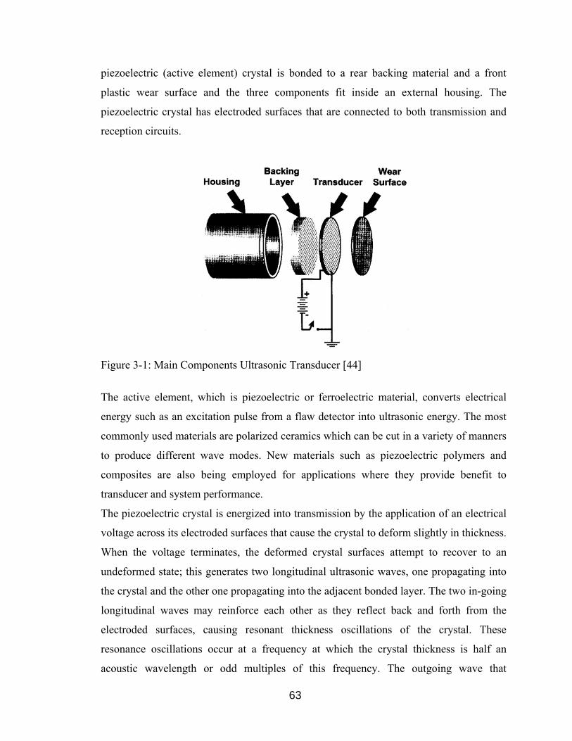
63
piezoelectric (active element) crystal is bonded to a rear backing material and a front
plastic wear surface and the three components fit inside an external housing. The
piezoelectric crystal has electroded surfaces that are connected to both transmission and
reception circuits.
Figure 3-1: Main Components Ultrasonic Transducer [44]
The active element, which is piezoelectric or ferroelectric material, converts electrical
energy such as an excitation pulse from a flaw detector into ultrasonic energy. The most
commonly used materials are polarized ceramics which can be cut in a variety of manners
to produce different wave modes. New materials such as piezoelectric polymers and
composites are also being employed for applications where they provide benefit to
transducer and system performance.
The piezoelectric crystal is energized into transmission by the application of an electrical
voltage across its electroded surfaces that cause the crystal to deform slightly in thickness.
When the voltage terminates, the deformed crystal surfaces attempt to recover to an
undeformed state; this generates two longitudinal ultrasonic waves, one propagating into
the crystal and the other one propagating into the adjacent bonded layer. The two in-going
longitudinal waves may reinforce each other as they reflect back and forth from the
electroded surfaces, causing resonant thickness oscillations of the crystal. These
resonance oscillations occur at a frequency at which the crystal thickness is half an
acoustic wavelength or odd multiples of this frequency. The outgoing wave that

64
propagates into the wear surface will pass through it and into the patient. The outgoing
wave that propagates into the backing material will be absorbed without reflection back
into the crystal.
The purpose of the backing layer is to absorb ultrasonic energy, causing the transmit time
(or output pulse length) to be as short as possible [44]. The backing layer acts as an
absorber dampening the crystal oscillations, producing a short output pulse. Usually a
highly attenuative, high density material is used to control the vibration of the transducer
by absorbing the energy radiating from the back face of the active element. The choice of
the material for the backing determines the type of acoustic impulses which may be
emitted by the transducer. When the acoustic impedance of the backing matches the
acoustic impedance of the active element, the result will be a heavily damped transducer
that displays good range resolution but may be lower in signal amplitude. For a highly
absorbent material, most of the energy is absorbed, tending to produce a short emission. If
there is a mismatch in acoustic impedance between the element and the backing, more
sound energy will be reflected forward into the test material. For a weakly absorbing
material, the energy at the rear of the transducer is returned to the front face, thereby
increasing the energy transmitted out in the medium. The end result is a transducer that is
lower in resolution due to a longer waveform duration, but may be higher in signal
amplitude or greater in sensitivity.
The basic purpose of the transducer wear surface is to protect the transducer element from
the testing environment. It also functions as an electrical insulator and as part of its
focusing mechanism. In many applications, the wear plate has the additional purpose of
serving as an acoustic transformer between the high acoustic impedance of the active
element and the water, the test piece or medium, which are of lower acoustic impedance.
This is accomplished by selecting a matching layer that is ¼ wavelength thick and of the
desired acoustic impedance (the active element is nominally ½ wavelength). The choice
of the wear surface thickness is based upon the idea of superposition that allows waves
generated by the active element to be in phase with the wave reverberating in the
matching layer. When signals are in phase, their amplitudes are additive, thus a greater
amplitude wave enters the test piece. If a transducer is not tightly controlled or designed
with care and the proper materials and the sound waves are not in phase, it causes a

65
disruption in the wave front [43]. By placing an additional layer (wear surface) between
the two given media (piezoelectric element and surrounding medium), the energy transfer
may consequently be optimized. Because of its very low impedance, even a very thin
layer of air between the transducer’s face and the test piece or medium would reflect
virtually all the sound, preventing penetration into the medium.
3.2.2 Transducer Arrays
In many instruments transducer arrays are used rather than single-element transducers. An
array transducer assembly consists of a group of piezoelectric elements, each of which
can be excited individually and whose echo signals can be detected and amplified
separately. Dividing the transducer into individual elements that can be independently
fired and utilized in reception provides great flexibility in the design of transmit and
receive beam patterns. The elements are rectangular in shape and arranged in a line (linear
array) or are ring shaped and arranged concentrically (annular array).
Advantages offered by all arrays are their potential for electronic focusing and automatic
variations in the aperture size. These two features can be exploited to enhance the spatial
resolution. The position of the focus can be electronically controlled and hence moved
very rapidly. Array transducer can be made fairly small, but it is difficult to produce very
high frequency array transducers.
A sound beam is produced by a transducer array by sending individual electrical
excitation signals to each element used to form the beam. The number of elements
involved varies with the type of array and the design. The emerging sound beam is the
sum of individual beams from each of the elements. Small elements are used because they
have much larger beam divergence angles. It is this large angle which opens up the useful
features of arrays such as dynamic focusing and beam steering. Another feature of small
elements is their energy transfer efficiency. Smaller elements take less energy to excite
and are more efficient receivers due to the lower mass to be energized.
Commonly used array transducer systems are shown in Figure 3-2 [49]. Views are from
the bottom with sound beams traveling out of the plane of the diagram.

66
Figure 3-2: Transducer Arrays [49]
Linear array transducers are widely used for imaging. A linear array is a series of
transducer elements aligned in a single housing, typically a rectangular single element
that has been segmented into smaller individual elements. Linear arrays typically contain
up to 256 piezoelectric elements whose operation is under computer control. Introducing
curvature to linear arrays has proven to be popular in imaging since the field of view is
increased. Moreover, the curved array can be used to produce a desired beam shape or
conform to the geometry of the experimental setup. Phased array transducers (curved or
linear) find widespread use in both imaging and Doppler modes. A modern phased array
transducer typically consists of 128 thin linear elements (element sized are from 0.05 mm
to 0.25 mm) and has a length of 1 – 2 cm [18].
A phased array is a multi-element linear array that uses all of its elements to form each
image line. If the elements are fired simultaneously, an unfocused “plane wave”
ultrasonic pulse will be transmitted parallel to the normal of the array surface. This is
because the cylindrical waves from each small element combine at a distance from the
array to form a plane wave parallel to the array surface and in a homogeneous medium
the direction of wave propagation is normal to the surfaces of constant phase. The
direction of wave propagation may be changed by firing the elements along the array with
a constant time delay between element transmissions. Then the cylindrical waves will
combine at a distance from the array to form a plane wave tilted at an angle
commensurate with the array geometry and the constant time delay. This is called beam
steering [44]. The transmitted ultrasonic pulse may be focused at any depth by timing the
element firings such that the cylindrical waves all arrive at the chosen focal point at the
same instant of time. Phased array transducers contrast with linear array transducers
where all elements “fire” with the same phase lag to form a beam that is directed

67
perpendicular to the transducer face. Besides the advantages of array transducer discussed
above, especially phased array transducers require circuit complexity caused by the large
number of individual elements and the need for different focus time delays at each beam
steered angel. Phased array image quality also falls off at large beam-steering angles.
Annular arrays using a smaller number of elements can achieve symmetrical electronic
focusing about the axis of the transducer at selected depths. An annular array is a series of
concentric ring elements contained in a single housing. In other words, an annular array is
a single round element divided into multiple individual concentric rings. Theoretical
modeling of the beam shape from an annular array indicates that at least five ring
elements are necessary to generate a good quality focused beam [18]. Most modern
annular phased array transducers consist of 2 to 5 annuli with active element diameters
ranging from 6 to 19 mm. Focal ranges of 1 to 10 cm are typical. The emitted frequency
of phased array transducers in general ranges from 0.5 to 25 MHz.
Single element piezoelectric transducers have a large ratio of width to thickness, so the
frequency bandwidth of their thickness-expander mode vibrations is well separated from
undesired modes of vibration. This permitted the use of shock-excitation voltage pulses
with large frequency bandwidths. The small array elements have small width to thickness
ratios with overlapping of the frequency bandwidths of desired (thickness-expander) and
undesired (shear, lateral and surface wave) modes of vibration. Excitation of these
undesired modes of vibration: (1) wastes energy, which reduces element sensitivity; (2)
degrades the single element directivity by distorting the shape of the radiating face; and
(3) leads to acoustic cross talk between elements, which degrades the beam shape. The
higher the desired operating frequency, the lower the width to thickness ratio.
Composite piezoelectric structures were designed to reduce these effects. They are
fabricated using a dice-and-fill technique, described by Papdakis [44]. This results in a
width to thickness ratio of the small array elements to much less than unity, which
separates their desired and undesired mode frequency bandwidths and reduces the
deleterious effects of the undesired modes. There is an accepted trade-off associated with
the use of composite piezoelectrics. Since the electroded area of piezoelectric material is
reduced (due to the fill), the element sensitivity is reduced proportionately. An important
feature of composite piezoelectrics is the reduction of element acoustic impedance and

68
therefore a reduction of the required acoustic matching. New acoustic matching
techniques such as acoustic matching by micro machined graded volume fraction silicon
structures and active piezoelectric layers (described by Papdakis [44]) provide improved
transmission and reception characteristics. Besides increased element sensitivity, the
improved acoustic impedance matching produces better near-field image quality, broader
bandwidth operation and less energy dissipated within the transducer (very important
when transducer is pulsed rapidly).
Only the focal zone portion of a focused ultrasonic beam pattern is narrow enough to be
effective applications where high spatial resolution is required. Use of the complex
interference pattern near-field and the wide far-field beam portions leads to reduced
spatial and contrast resolution. In analog static imaging, the single-element transducers
were weakly focused to lengthen the focal zone and minimize this problem. Modern
imaging equipment with fast digital circuitry uses zone focusing to eliminate the
undesirable portions of the beam pattern.
The first attempt to improve image quality at all depths was selectable zone focusing
(Figure 3-3 (a)). For each image there were three possible focused beam patterns: a near-
depth focus, a mid-depth focus, or a far-depth focus. The operator selected the focal depth
for each image with a three-way switch. High image quality occurred only at the selected
image depth.
A further refinement eliminated the undesirable portions of each depth’s focused beam
pattern. As shown in Figure 3-3 (b) with three depth zone, for each image line the
transducer sequentially transmits the three different focal patterns. After each
transmission, only the echoes from that beam’s focal zone are acquired. Then the
acquired focal zone echoes are combined to form an effective beam pattern that is a
composite of the three separate transmissions and partial receptions (Figure 3-3 (c)).

69
Figure 3-3: Zone Focusing [18]
Once an ultrasonic beam is transmitted, its focal properties cannot be changed. During
echo reception, however, it is possible to sequentially change the array element time
delays such that the receive beam pattern is continuously focused at the depth of origin of
the echoes being received. In other words, the receive focus moves outward at half the
acoustic velocity. This switching of array element time delays is performed in discrete
steps using fast digital circuitry. Dynamic receive focusing is accompanied by dynamic
70
aperture and dynamic apodization. That is along with changing the focus time delays, as
echoes are being received the aperture is increased stepwise (element by element) such
that the receive beam spot size remains approximately constant. Since the pulse-echo
beam pattern is the product of transmit and receive beam patterns, it is narrowed
considerably by the use of dynamic receive focusing with a commensurate lengthening of
its effective focal zone [44].
3.3 Transducer Characteristics
A transducer has a resonance frequency, or a frequency at which it operates most
efficiently. This frequency is determined by the thickness of the piezoelectric element.
The thicker the element, the lower the transducer frequencies, i.e. low frequency
piezoelectric transducer elements are thick and high frequency elements are thin.
The near field distance is the natural focus of the transducer and a function of the
transducer frequency, element diameter (aperture size) and the sound velocity of the test
material. With a constant aperture, increasing the frequency increases the length of the
near-field and decreases the angle of divergence in the far-field, producing a more
directional beam pattern. Decreasing the aperture size at a constant frequency causes a
shorter near-field and a larger angle of divergence, producing an omni directional beam
pattern. The near zone is longer for larger diameter transducers and for higher frequency
transducers
Sensitivity is the ability of an ultrasonic system to detect reflectors at a given depth in a
test material. The greater the signal that is received from these reflectors, the more
sensitive the transducer system.
There are two types of resolution: spatial and echo amplitude resolution. Spatial
resolution allows one to identify two adjacent structures in the image. It is usually
associated with high-contrast objects in the image (such as two point reflectors). Near
surface resolution is the ability of the ultrasonic system to detect reflectors located close
to the surface of the test piece. Echo amplitude resolution allows one to identify a region
of echoes (reflectors) whose amplitude is slightly greater or less than the amplitude of the
surrounding echoes (reflectors). Echo amplitude resolution is also called contrast

71
resolution and is usually associated with low contrast objects in the image [44].
Amplitude resolution mainly depends on circuit complexity considerations.
Spatial resolution refers to how closely positioned two reflectors or scattering regions can
be to one another and still be “seen” as separate reflectors on a display [49]. It also
compares to the smallest object of a given echo contrast compared with the background
matter, that can be detected. Spatial resolution is very closely tied to the properties of the
transducer.
Axial or range resolution refers to how closely positioned two reflecting targets can be
along the sound beam axis and still be distinguished on the display as shown in Figure
3-4. In other words, axial resolution is the ability of an ultrasonic system to produce
simultaneous and distinct indications from reflectors located at nearly the same positions
with respect to the sound beam. It depends mainly on the duration of each ultrasound
pulse emitted by the transducer. Optimum axial resolution is achieved by using transducer
that produce short-duration acoustic pulses [49].
Figure 3-4: Axial Resolution [47]
The pulse duration must be kept as low as practical to obtain good axial resolution. The
pulse duration is minimized by damping the vibration of the transducer as quickly as
possible following excitation. The backing layer absorbs sound waves at the back surface
of the piezoelectric element resulting in a short duration pulse and good axial resolution.
The greater the amount of damping, the shorter will be the pulse duration and the better
will be the axial resolution.
Besides the degree of damping, the ultrasonic frequency also influences the axial
resolution. For the same relative amount of damping the acoustic pulse produced by a

72
high-frequency transducer is shorter in duration than that produced by a low-frequency
transducer. Therefore, higher-frequency transducers result in better axial resolution than
lower-frequency transducers.
Lateral resolution refers to how closely spaced two reflectors can be along a line
perpendicular to the sound beam and still be seen as separate reflectors as shown in
Figure 3-5 [49].
Figure 3-5: Lateral Resolution [47]
Lateral resolution depends on the effective beam width at the position of the reflector.
According to Signal-Processing [49], the beam width W at axial distance x in the far field
of an unfocused transducer (transducer radius a as shown in Figure 3-6) may be
approximated by:
axW
222.1 λ
=
Equation 30: Beam Width Unfocused Transducer
Figure 3-6: Focused Beam Shape [18]
73
At a given transducer radius, the beam width decreases with decreasing wavelength λ.
Because wavelength is inversely proportional to frequency, beam width decreases with
increasing frequency. The beam width in the far field also decreases with increasing
transducer size (greater radius a).
For a given transducer frequency the near field length is greater for larger diameter
transducer. Beam divergence in the far field is less for larger diameter than smaller
diameter transducers.
For a given transducer diameter the near field length is greater for higher-frequency
transducers. Beam divergence in the far field is less for higher-frequency than lower-
frequency transducers.
Axial and lateral resolutions depend on pulse length and pulse width, respectively. The
shorter the pulse is, the better the axial resolution is. The narrower the pulse is, the better
the lateral resolution is. Damping and the use of higher frequencies shorten the pulse,
improving the axial resolution. Focusing narrows the pulse, improving the lateral
resolution (at least in the focal region). The smallest axial resolution is equal to one half
the pulse length. The lateral resolution is equal to the pulse width. Improved resolution
with higher frequency is accompanied by decreased penetration depth as a result of
increased attenuation.
3.4 Focused Transducers
Immersion transducers are available in three different configurations: unfocused (“flat”),
spherically (“spot”) and cylindrically (“line”) focused. The beam’s diameter at any point
depends on the frequency, transducer diameter, and distance from the transducer. It is
important to realize that even for flat, unfocused transducer elements, there is some beam
narrowing or “focusing”. Most transducers are focused to achieve better lateral resolution
than would be found with unfocused probes.
The sound may be focused by using a curved transducer element, a lens, an acoustic
mirror system or a (phased) transducer array. The addition of a lens is the most common
way to focus a transducer. An unfocused transducer may be used in general applications
or for penetration of thick materials. A spherically focused transducer is commonly used

74
to improve sensitivity to for example small flaws or small scatterers. A cylindrically
focused transducer is typically used in the inspection of tubing or bar stock.
By definition, the focal length of a transducer is the distance form the face of the
transducer to the point in the sound field where the signal with the maximum amplitude is
located. In an unfocused transducer, this occurs at a distance from the face of the
transducer which is approximately equivalent to the transducer’s near field length,
because the last signal maximum occurs at a distance greater than its near field.
When focusing a transducer, the type of focus (spherical or cylindrical), focal length and
focal target (point or flat surface) need to be specified. Based on this information, for
example the radius of curvature of the lens for the transducer can be calculated which
varies based on above parameters.
3.4.1 Single Element Transducers
Focusing at a fixed range can be done using an acoustic lens, an acoustic mirror system or
using a curved (concave) piezoelectric element. Three different methods are shown in
Figure 3-7. In the later case, to provide a flat face on the transducer and hence easier
coupling, a weak convex lens can be attached to the front of the concave element. The
combined effect of the concave element and the convex lens is designed to give focusing
at the desired range.

75
Figure 3-7: Focusing Methods Single Element Transducer [44]
Focusing reduces the beam width over a volume called the focal zone. The resulting beam
is rather wide at distances close to the transducer. It narrows and increases in intensity
along the axis near the focal distance. Beyond the focal distance the beam gradually
diverges. The focal length is the distance from the transducer to the center of the focal
region. It cannot be greater than the near zone length of the comparable unfocused
transducer.
Substituting z by the focal length F in the formula given above (Equation 30), the beam
width at the focal distance can be estimated. This equation shows that in the focal region
the lateral resolution is improved as larger-diameter transducers are employed. For a
fixed-transducer diameter the lateral resolution is improved if higher-frequency
transducers are used.
With a single-element transducer the focal distance is fixed during the manufacturing
process
3.4.2 Transducer Arrays
The transmitted beam from an array may be focused by introducing time delays in the
appropriate sequence to the excitation pulses applied to individual elements. Precision
electronic delay circuits are available and are provided in an instrument for this purpose.

76
With the time delays in action, the situation is as though a focusing lens or a curved
piezoelectric element were producing the beam.
A distinct advantage of an array over a single-element transducer is that the array’s focal
distance can be varied, simply by selecting a different delay sequence for pulses applied
to individual elements. Thus, an array is not locked into a fixed focal distance as is a
single-element transducer. Most array instruments allow the user to select the transmit
focal distance. It also is possible to provide simultaneous, multiple transmit focal
distances. If the latter is available, the instrument automatically changes the transmit
focus while scanning, optimizing the resolution throughout the depth range of the scan.
On transmission, the size of the excitation signal to each element, the timing of the
excitation of each element and the number of elements excited can all be controlled and
altered rapidly.
Array transducers also allow focusing of received echo signals. When echo signals are
picked up by elements in an array, signals from individual elements are added together in
the receiver, yielding a net signal for each reflector. An echo from a discrete target
located in the beam may arrive at individual elements of the array at slightly different
times because of slight differences in distance. This could lead to variations in the phase
of signals from individual elements. The individual signals might be brought back into
precise synchronization or phase before summing with the help of electronic delays
whose settings are adjusted for the depth of the reflector. Focusing during echo detection
is usually done dynamically. The focal distance of the array during reception may be
varied electronically. Each time a sound pulse is launched, the receiving focal distance of
the array is set (initially at a shallow depth). As the time after the transmitted pulse
increases, the receiver focus changes automatically, “keeping up” with or tracking the
position of the sound pulse as it encounters deeper reflectors. The result of using dynamic
focus is an extended focal region that is considerably greater than that achievable with a
single-element transducer or with a single focal distance applied to an array. On
reception, the echo signal at each element can be digitized accurately and rapidly to
preserve amplitude and phase information. The gain of each receiver, the delay applied to
each signal and the number of elements in use can also be controlled.
77
For most focused transducers or transducer arrays the beam width varies with distance
from the transducer. Variations of beam width with depth can be minimized with array
transducer assemblies that also provide dynamic aperture. The aperture refers to the size
of the transducer surface involved in producing and detecting echoes for each sound
beam. Variation of beam width with depth may be minimized by changing the variable a
in Equation 30, the aperture size, with reflector depth. This may be done by varying the
number of elements involved in echo detection while echo signals are being picked up by
the transducer. As echoes return from deeper and deeper structures the number of
elements used to pick up echo signals and hence the aperture is increased. This keeps
lateral resolution nearly constant over the entire image region.
Dynamic focusing, beam steering and better energy transfer efficiency are significant
advantages of phased array transducers over single element transducers. So far, phased
array transducer cannot be used with pulsed ultrasound Doppler velocimetry instruments.
The feasibility of using phased array transducers in combination with pulsed ultrasound
Doppler velocimetry is further investigated in Chapter 7. Since so far, only single element
transducer are available for measuring velocities with pulsed ultrasound Doppler
velocimetry, measurements of the ultrasonic beam emitted by various single element
transducers are performed. The results of these ultrasonic beam measurements are
presented in Chapter 4. Especially the actual beam shape and echo intensity is
investigated to select the most promising transducer to measure velocity profiles in small
channels. Since application of pulsed ultrasound Doppler velocimetry often involves the
propagation of the transmitted acoustic field and the returning echo through a Plexiglas
wall, the effect of Plexiglas walls on the beam shape and echo intensity is evaluated.
Moreover, the effect of porous screens is investigated and focused transducers are
compared to unfocused transducers.

78
4 Ultrasonic Beam Measurements
In Chapter 2, the ultrasonic transducer was identified to be the most critical component of
the measurement system. In Chapter 3, the transducer architecture was then investigated
in detail. The ultrasonic transducer mainly determines the lateral resolution of the
measurement system. In this chapter, the ultrasonic beam shape and echo intensity is
measured. Consequently, information about the actual beam shape of various ultrasonic
transducers, especially their lateral resolution, is gained. The lateral resolution of the
pulsed ultrasound Doppler velocimetry system is extremely important in evaluating the
flow over a backward facing step in small channels, i.e., when dealing with small
geometries. Ultrasonic beam measurements will therefore be used to identify the most
appropriate transducer to measure velocity profiles in small channels and capillaries.
Since application of pulsed ultrasound Doppler velocimetry often involves the
propagation of the transmitted acoustic field and the returning echo through a Plexiglas
wall, the effect of Plexiglas walls on the beam shape and echo intensity is evaluated in
detail. Moreover, the interaction of porous screens with the emitted ultrasonic wave
packet and their effect on measuring the velocity profile with unfocused as well as
focused ultrasonic transducers is analyzed.
In Chapter 4, the experimental setup is described and the ultrasonic beam of various
transducers is measured at first. Then the interaction of the ultrasonic burst with Plexiglas
walls of different thicknesses is investigated and quantified in detail. Finally, the effect of
a porous screen, a paper forming screen, is explored.
Measurement of the ultrasonic field (transmission zone) of a transducer is undertaken by
moving a small detector systematically in the region in front of the transmitting element
at various distances. The transducer face and the detector are immersed in water. It should
be remembered that the beam characteristics measured in water are different from those
in water with suspended fibers or particles. Nevertheless, a great deal can be deduced
about a beam in water with suspended fibers or particles from a plot obtained in water.

79
4.1 Experimental Setup
The pulsed Doppler ultrasound velocimetry instrument DOP2000 model 2125 (by Signal-
Processing) is used to measure the ultrasonic field generated by various ultrasonic
transducers. The effect of Plexiglas walls and forming screens placed between the
ultrasonic transducer and a target reflecting the ultrasonic wave packet emitted by the
transducer (in this case a plastic sphere) is evaluated. The plastic sphere is mounted on a
xy-positioner. Ultrasonic transducer and plastic sphere are submerged in water as shown
in Figure 4-1 and 4-2.
Figure 4-1: Ultrasonic Field Experimental Setup Front View
Water basin
Ultrasonic transducer holder
Plastic Sphere holder
x,y-positioner
z-positioner
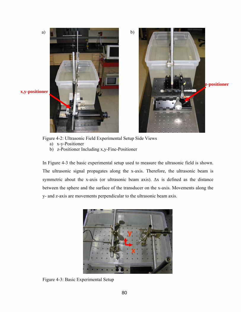
80
Figure 4-2: Ultrasonic Field Experimental Setup Side Views
a) x-y-Positioner b) z-Positioner Including x,y-Fine-Positioner
In Figure 4-3 the basic experimental setup used to measure the ultrasonic field is shown.
The ultrasonic signal propagates along the x-axis. Therefore, the ultrasonic beam is
symmetric about the x-axis (or ultrasonic beam axis). ∆x is defined as the distance
between the sphere and the surface of the transducer on the x-axis. Movements along the
y- and z-axis are movements perpendicular to the ultrasonic beam axis.
Figure 4-3: Basic Experimental Setup
y
x
x,y-positioner z-positioner
b) a)
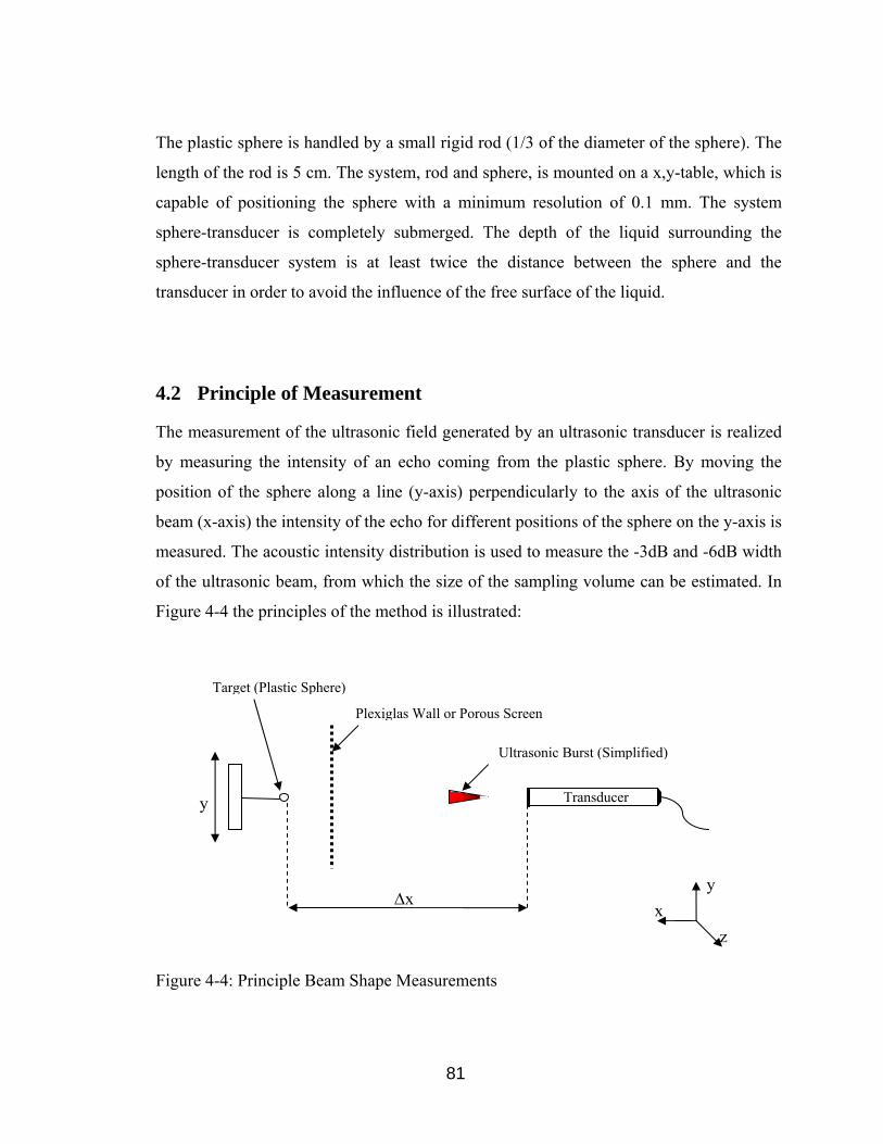
81
The plastic sphere is handled by a small rigid rod (1/3 of the diameter of the sphere). The
length of the rod is 5 cm. The system, rod and sphere, is mounted on a x,y-table, which is
capable of positioning the sphere with a minimum resolution of 0.1 mm. The system
sphere-transducer is completely submerged. The depth of the liquid surrounding the
sphere-transducer system is at least twice the distance between the sphere and the
transducer in order to avoid the influence of the free surface of the liquid.
4.2 Principle of Measurement
The measurement of the ultrasonic field generated by an ultrasonic transducer is realized
by measuring the intensity of an echo coming from the plastic sphere. By moving the
position of the sphere along a line (y-axis) perpendicularly to the axis of the ultrasonic
beam (x-axis) the intensity of the echo for different positions of the sphere on the y-axis is
measured. The acoustic intensity distribution is used to measure the -3dB and -6dB width
of the ultrasonic beam, from which the size of the sampling volume can be estimated. In
Figure 4-4 the principles of the method is illustrated:
Figure 4-4: Principle Beam Shape Measurements
∆x
y Transducer
Target (Plastic Sphere)
Plexiglas Wall or Porous Screen
Ultrasonic Burst (Simplified)
z x
y
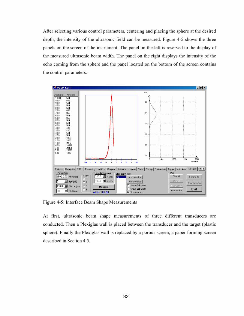
82
After selecting various control parameters, centering and placing the sphere at the desired
depth, the intensity of the ultrasonic field can be measured. Figure 4-5 shows the three
panels on the screen of the instrument. The panel on the left is reserved to the display of
the measured ultrasonic beam width. The panel on the right displays the intensity of the
echo coming from the sphere and the panel located on the bottom of the screen contains
the control parameters.
Figure 4-5: Interface Beam Shape Measurements
At first, ultrasonic beam shape measurements of three different transducers are
conducted. Then a Plexiglas wall is placed between the transducer and the target (plastic
sphere). Finally the Plexiglas wall is replaced by a porous screen, a paper forming screen
described in Section 4.5.
83
4.3 Ultrasonic Beam Measurements of Various Ultrasonic Transducers
The ultrasonic beam shape of the following transducers has been measured:
- Transducer 1: 2 MHz emitting frequency, 10 mm transducer diameter
- Transducer 2: 4 MHz emitting frequency, 5 mm transducer diameter
- Transducer 3: 8 MHz emitting frequency, 5 mm transducer diameter
- Transducer 4: 4 MHz emitting frequency, 8 mm transducer diameter, focused
The experimental setup is shown in Figure 4-3. The principle of measurement is
explained in the previous section. After evaluating the measurement results, figures of the
general ultrasonic beam divergence and echo intensity plots of each transducer are
presented (Figure 4-6 to 4-13). In the beam divergence profiles, the 3 dB and 6 dB width
of the ultrasonic beam, derived from the acoustic intensity distribution perpendicular to
the ultrasonic beam axis, is plotted along the position of the plastic sphere on the
ultrasonic beam axis. In all echo intensity plots, the echo intensity is plotted over the
distance between the plastic sphere and the transducer center perpendicular to the
ultrasonic beam axis for various distances between the plastic sphere and the transducer
face along the ultrasonic beam axis (∆x). For example in Figure 4-6, the echo intensity
distribution perpendicular to the ultrasonic beam axis is plotted at distances of 20 mm, 25
mm, 30 mm, 40 mm, 50 mm, 75 mm, 100 mm and 150 mm between the plastic sphere
and the transducer face along the ultrasonic beam axis.
4.3.1 Evaluation of Results
Ultrasonic beam measurements are conducted to gain information about the actual beam
shape of the given ultrasonic transducers and especially their lateral resolution. A good
lateral resolution is essential to measure velocity profiles in small channels and
capillaries. In the following chapters, ultrasonic beam measurements will then be used to
analyze the effect of walls and porous screens on measuring the velocity profile. Before
investigating the ultrasonic beam shape with walls or porous screens between the

84
transducer and the target (plastic sphere), the beam shape of various transducers is
determined.
At a certain minimal distance between the transducer and the plastic sphere on the x-axis,
measurements of the ultrasonic beam shape become impossible due to the transducer’s
ringing effect (described in section 2.6.4). Further decreasing ∆x beyond this minimal
distance between the transducer and the plastic sphere on the ultrasonic beam axis (x-
axis) does not yield any useful measurement results of the ultrasonic beam shape. This is
due to the fact that the ultrasonic echo of the plastic sphere can not be recognized in
between the high echo intensities caused by the transducer’s ringing effect. The ringing
noise follows the emission of the ultrasonic burst by transducer. Ringing noise can never
be completely removed. Ringing effects following the emission of the ultrasonic wave
packet cause a region of strong echoes (saturation) at depths located just after the surface
of the transducer. In this region, the ultrasonic field can consequently not be measured. In
the following, the region of high echo intensities caused by the transducer’s ringing effect
is called “saturation region”. The distance between transducer and plastic sphere at which
the saturation region begins is called “minimal distance”.
The effect of the saturation region on the echo intensity can be seen in Figure 4-6 (echo
intensity plot of the 2 MHz 10 mm transducer). The echo intensity usually forms a
maximum located on the ultrasonic beam axis. As soon as ∆x becomes smaller than the
minimal distance the magnitude of the maximum echo intensity decreases while the
overall echo intensity level increases. Further decreasing ∆x leads to a straight line at
relatively high echo intensities. In this case, the echo of the plastic sphere can not be
recognized in between this “saturation region”. Therefore, at a certain minimal distance,
beam shape measurements become impossible.
Using a 2 MHz ultrasonic transducer, the saturation region is usually 10 – 15 mm wide. In
the following, the effect of Plexiglas walls and forming screens placed between the
ultrasonic transducer and the plastic sphere is evaluated. Since walls or forming screens
absorb and reflect acoustic energy, the measurable echo intensity of the plastic sphere is
reduced. To clearly recognize the echo coming from the plastic sphere behind the forming
screen or Plexiglas wall, a high amplification must be used. Increasing the amplification
in the instrument consequently increases the transducer’s ringing effect. Therefore

85
increasing the amplification increases the saturation region and the minimal distance.
Because of the high amplification that must be used to recognize the echo of the sphere
behind the screen, the saturation region of the 2 MHz transducer is therefore about 20 mm
wide (instead of 10 – 15 mm). Using a 4 MHz transducer, the region of strong echoes is
usually 3 – 8 mm, depending on the chosen amplification. In our case with increased
amplification, the minimal distance is 5 mm for the unfocused 4 MHz transducer and 4
mm for the focused 4 MHz transducer. For the 8 MHz transducer, values of ideally 3 – 5
mm can be obtained. In our case, the minimal distance for the 8 MHz transducer is 8 mm.
In general, the minimal distance decreases with increasing frequency. Since the ultrasonic
signal emitted by the 8 MHz transducer is much stronger attenuated than the ultrasonic
signal emitted by the 4 MHz transducer, a higher amplification had to be used.
Consequently, the minimal distance of the 8 MHz transducer was increased and is higher
than the minimal distance for the 4 MHz transducer.
Looking at Figure 4-7, 4-9 and 4-11, it can clearly be seen, that at a given transducer
diameter, the beam width decreases with decreasing wavelength. Because wavelength is
inversely proportional to frequency, beam width consequently decreases with increasing
frequency. It can also be seen that the beam width in the far field decreases with
increasing transducer size (greater aperture).
In the same way as the beam width, the beam divergence decreases with increasing
frequency. The half angle of beam divergence (calculated by the instrument) for the 2
MHz 10 mm transducer is 2.27 degrees, 2.23 degrees for the 4 MHz 5 mm transducer,
1.22 degrees for the 8 MHz 5 mm transducer and 2.33 degrees for the 4 MHz 8 mm
focused transducer. Theoretically beam divergence in the far field should be less for
larger than smaller diameter transducers [18]. It can be seen that the angle of beam
divergence is smaller for the unfocused 4 MHz 5 mm than for the focused 4 MHz 8 mm
transducer. Consequently, the claim that beam divergence in the far field should be less
for larger diameter than smaller transducers is not justified when comparing focused and
unfocused transducers. Unfortunately unfocused ultrasonic transducers of the same
frequency with different diameters were not available to experimentally validate this
theoretical claim. Theoretically, for a given transducer frequency the near field length
should also be greater for larger diameter transducers [18]. Moreover, for a given
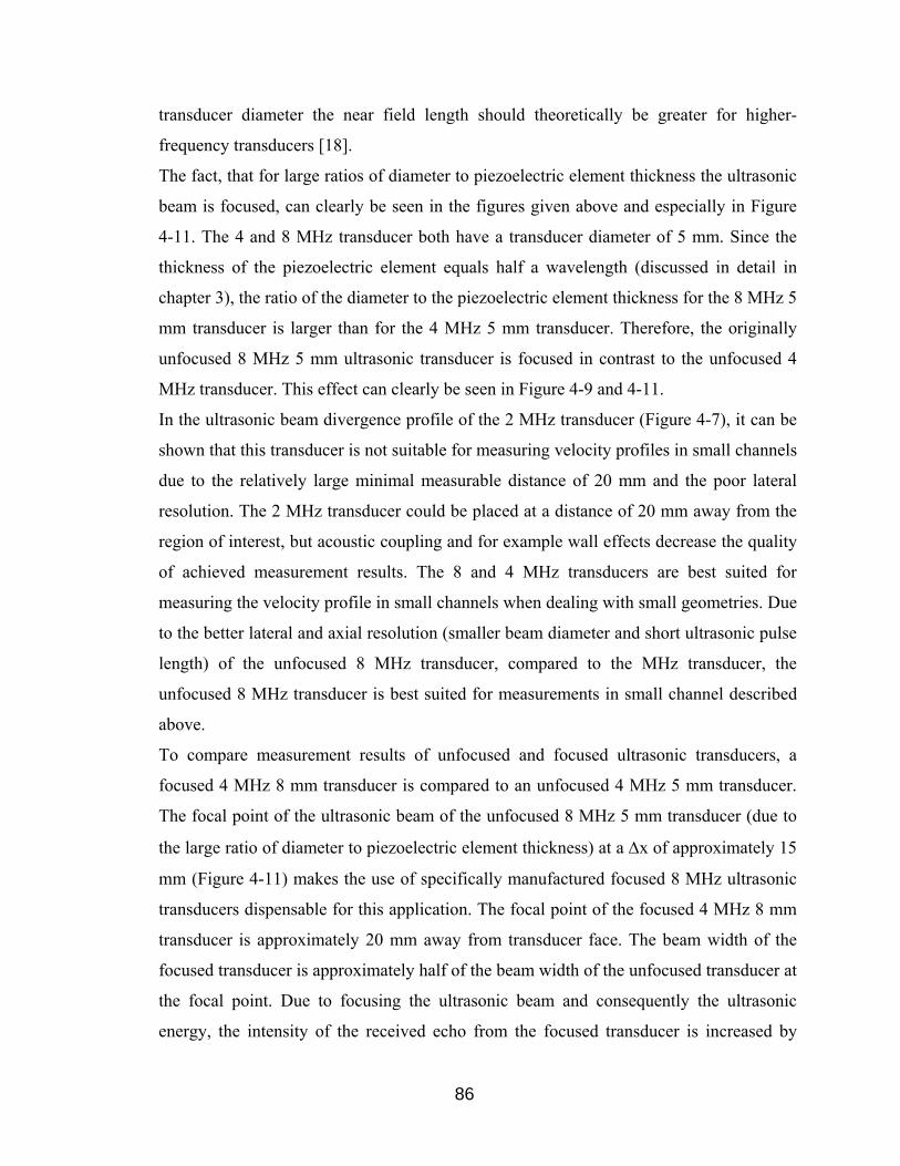
86
transducer diameter the near field length should theoretically be greater for higher-
frequency transducers [18].
The fact, that for large ratios of diameter to piezoelectric element thickness the ultrasonic
beam is focused, can clearly be seen in the figures given above and especially in Figure
4-11. The 4 and 8 MHz transducer both have a transducer diameter of 5 mm. Since the
thickness of the piezoelectric element equals half a wavelength (discussed in detail in
chapter 3), the ratio of the diameter to the piezoelectric element thickness for the 8 MHz 5
mm transducer is larger than for the 4 MHz 5 mm transducer. Therefore, the originally
unfocused 8 MHz 5 mm ultrasonic transducer is focused in contrast to the unfocused 4
MHz transducer. This effect can clearly be seen in Figure 4-9 and 4-11.
In the ultrasonic beam divergence profile of the 2 MHz transducer (Figure 4-7), it can be
shown that this transducer is not suitable for measuring velocity profiles in small channels
due to the relatively large minimal measurable distance of 20 mm and the poor lateral
resolution. The 2 MHz transducer could be placed at a distance of 20 mm away from the
region of interest, but acoustic coupling and for example wall effects decrease the quality
of achieved measurement results. The 8 and 4 MHz transducers are best suited for
measuring the velocity profile in small channels when dealing with small geometries. Due
to the better lateral and axial resolution (smaller beam diameter and short ultrasonic pulse
length) of the unfocused 8 MHz transducer, compared to the MHz transducer, the
unfocused 8 MHz transducer is best suited for measurements in small channel described
above.
To compare measurement results of unfocused and focused ultrasonic transducers, a
focused 4 MHz 8 mm transducer is compared to an unfocused 4 MHz 5 mm transducer.
The focal point of the ultrasonic beam of the unfocused 8 MHz 5 mm transducer (due to
the large ratio of diameter to piezoelectric element thickness) at a ∆x of approximately 15
mm (Figure 4-11) makes the use of specifically manufactured focused 8 MHz ultrasonic
transducers dispensable for this application. The focal point of the focused 4 MHz 8 mm
transducer is approximately 20 mm away from transducer face. The beam width of the
focused transducer is approximately half of the beam width of the unfocused transducer at
the focal point. Due to focusing the ultrasonic beam and consequently the ultrasonic
energy, the intensity of the received echo from the focused transducer is increased by

87
approximately 500 percent at the focal point, compared to approximately 20 percent at the
focal point of the unfocused 8 MHz 5 mm transducer. The echo intensity before and after
the focal point is of the same order of magnitude for the focused and unfocused
transducer. The minimal distance at which measurements are possible is approximately of
the same order for the focused and unfocused transducer. It can clearly be seen that the
beam width in the far field is smaller with the focused transducer. This is also due to the
larger aperture of the focused transducer.
Having evaluated the measurement results, figures of the general ultrasonic beam
divergence and echo intensity plots of each transducer are presented in Section 4.3.2
(Figures 4-6 to 4-13).
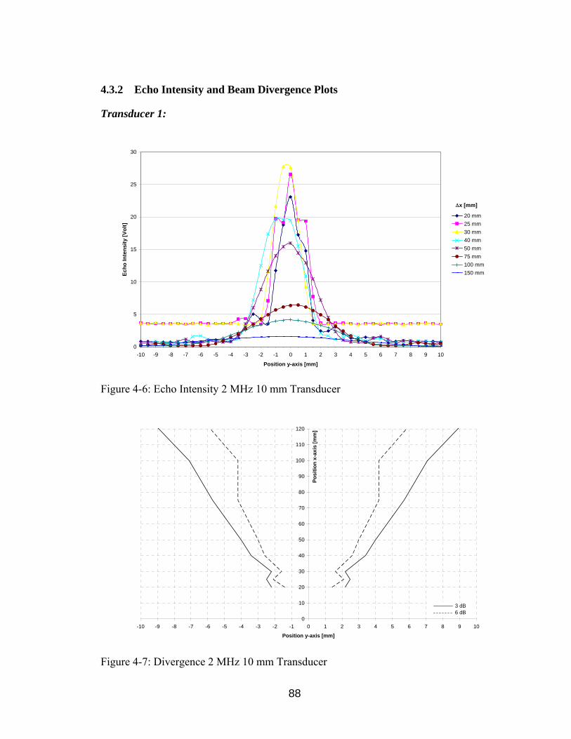
88
4.3.2 Echo Intensity and Beam Divergence Plots
Transducer 1:
0
5
10
15
20
25
30
-10 -9 -8 -7 -6 -5 -4 -3 -2 -1 0 1 2 3 4 5 6 7 8 9 10
Position y-axis [mm]
Echo
Inte
nsity
[Vol
t]
20 mm25 mm30 mm40 mm50 mm75 mm100 mm150 mm
∆x [mm]
Figure 4-6: Echo Intensity 2 MHz 10 mm Transducer
0
10
20
30
40
50
60
70
80
90
100
110
120
-10 -9 -8 -7 -6 -5 -4 -3 -2 -1 0 1 2 3 4 5 6 7 8 9 10
Position y-axis [mm]
Posi
tion
x-ax
is [m
m]
3 dB 6 dB
Figure 4-7: Divergence 2 MHz 10 mm Transducer
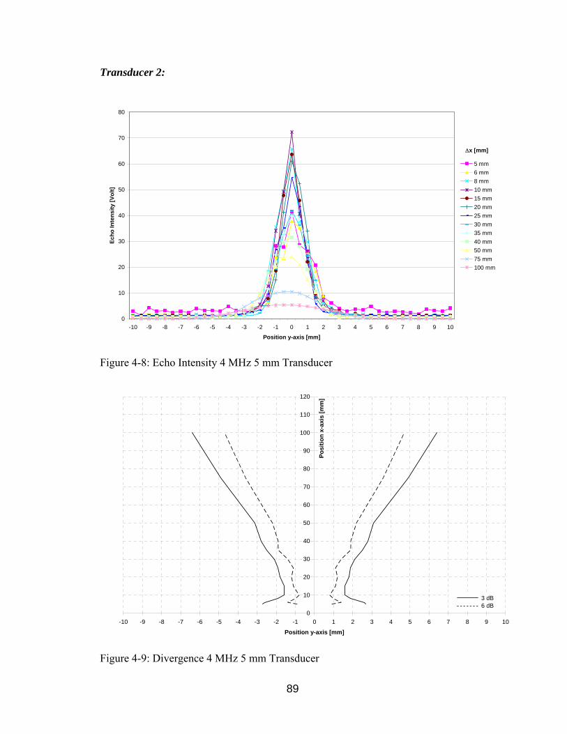
89
Transducer 2:
0
10
20
30
40
50
60
70
80
-10 -9 -8 -7 -6 -5 -4 -3 -2 -1 0 1 2 3 4 5 6 7 8 9 10
Position y-axis [mm]
Echo
Inte
nsity
[Vol
t]
5 mm6 mm8 mm10 mm15 mm20 mm25 mm30 mm35 mm40 mm50 mm75 mm100 mm
∆x [mm]
Figure 4-8: Echo Intensity 4 MHz 5 mm Transducer
0
10
20
30
40
50
60
70
80
90
100
110
120
-10 -9 -8 -7 -6 -5 -4 -3 -2 -1 0 1 2 3 4 5 6 7 8 9 10
Position y-axis [mm]
Posi
tion
x-ax
is [m
m]
3 dB 6 dB
Figure 4-9: Divergence 4 MHz 5 mm Transducer
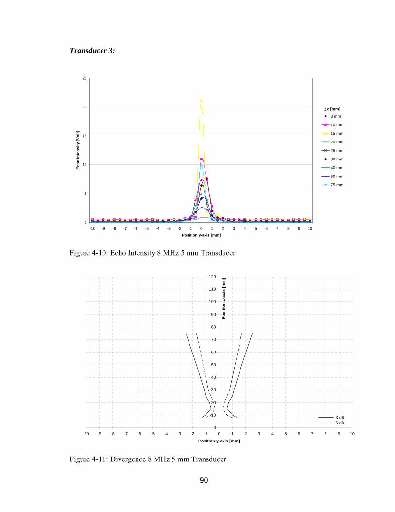
90
Transducer 3:
0
5
10
15
20
25
-10 -9 -8 -7 -6 -5 -4 -3 -2 -1 0 1 2 3 4 5 6 7 8 9 10
Position y-axis [mm]
Echo
Inte
nsity
[Vol
t]
8 mm
10 mm
15 mm
20 mm
25 mm
30 mm
40 mm
50 mm
75 mm
∆x [mm]
Figure 4-10: Echo Intensity 8 MHz 5 mm Transducer
0
10
20
30
40
50
60
70
80
90
100
110
120
-10 -9 -8 -7 -6 -5 -4 -3 -2 -1 0 1 2 3 4 5 6 7 8 9 10
Position y-axis [mm]
Posi
tion
x-ax
is [m
m]
3 dB 6 dB
Figure 4-11: Divergence 8 MHz 5 mm Transducer

91
Transducer 4:
0
50
100
150
200
250
300
350
-10 -9 -8 -7 -6 -5 -4 -3 -2 -1 0 1 2 3 4 5 6 7 8 9 10
Position y-axis [mm]
Echo
Inte
nsity
[Vol
t]
4 mm5 mm6 mm8 mm10 mm15 mm20 mm25 mm30 mm35 mm40 mm50 mm75 mm100 mm
∆x [mm]
Figure 4-12: Echo Intensity 4 MHz 8 mm Focussed Transducer
0
10
20
30
40
50
60
70
80
90
100
110
120
-10 -9 -8 -7 -6 -5 -4 -3 -2 -1 0 1 2 3 4 5 6 7 8 9 10
Position y-axis [mm]
Posi
tion
x-ax
is [m
m]
3 dB 6 dB
Figure 4-13: Divergence 4 MHz 8 mm Focussed Transducer

92
4.4 Effect of Plexiglas Walls
Since application of pulsed ultrasound Doppler velocimetry often involves the
propagation of the transmitted acoustic field and the returning echo through a Plexiglas
wall, the basic experimental setup is modified to evaluate the effect of Plexiglas walls. In
the context of measuring the velocity profile in the small channel described in chapter 5, a
Plexiglas wall as shown in Figure 4-14 is used:
Figure 4-14: Plexiglas Wall
The thin side of the Plexiglas wall is a 2.5 mm thick machined surface (according to the
2.5 mm thick machined top wall measurement area of the channel used in the following
chapter). The other side is 18 mm thick and not machined (according to the side of the
channel used in the following chapter). The Plexiglas wall is placed between the
ultrasonic transducer and the plastic sphere as shown in Figure 4-15:
After measuring the ultrasonic beam shape with both sides of the Plexiglas wall, the
effect on the ultrasonic beam shape and the echo intensity is evaluated in the following
for each transducer introduced in the previous section. All echo intensity and beam
divergence plots are presented in Section 4.4.2 (Figures 4-18 to 4-33).
2.5 mm thick machined Plexi-glas wall
18 mm thick Plexiglas wall
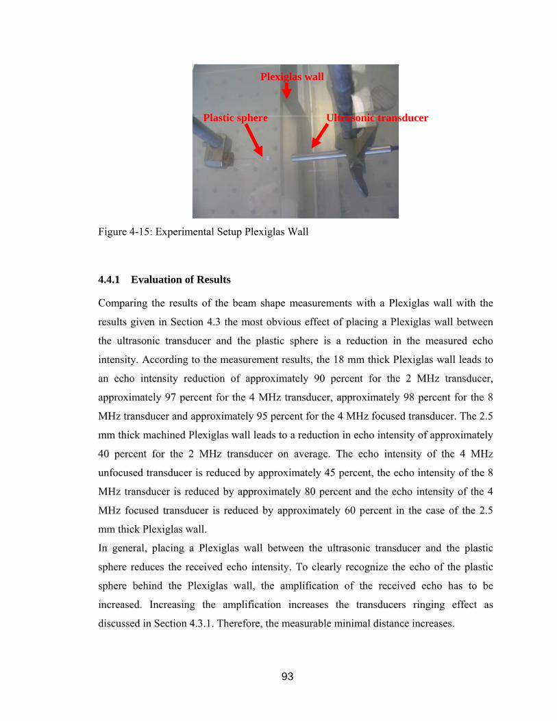
93
Figure 4-15: Experimental Setup Plexiglas Wall
4.4.1 Evaluation of Results
Comparing the results of the beam shape measurements with a Plexiglas wall with the
results given in Section 4.3 the most obvious effect of placing a Plexiglas wall between
the ultrasonic transducer and the plastic sphere is a reduction in the measured echo
intensity. According to the measurement results, the 18 mm thick Plexiglas wall leads to
an echo intensity reduction of approximately 90 percent for the 2 MHz transducer,
approximately 97 percent for the 4 MHz transducer, approximately 98 percent for the 8
MHz transducer and approximately 95 percent for the 4 MHz focused transducer. The 2.5
mm thick machined Plexiglas wall leads to a reduction in echo intensity of approximately
40 percent for the 2 MHz transducer on average. The echo intensity of the 4 MHz
unfocused transducer is reduced by approximately 45 percent, the echo intensity of the 8
MHz transducer is reduced by approximately 80 percent and the echo intensity of the 4
MHz focused transducer is reduced by approximately 60 percent in the case of the 2.5
mm thick Plexiglas wall.
In general, placing a Plexiglas wall between the ultrasonic transducer and the plastic
sphere reduces the received echo intensity. To clearly recognize the echo of the plastic
sphere behind the Plexiglas wall, the amplification of the received echo has to be
increased. Increasing the amplification increases the transducers ringing effect as
discussed in Section 4.3.1. Therefore, the measurable minimal distance increases.
Ultrasonic transducer Plastic sphere
Plexiglas wall

94
In order to evaluate the effect of Plexiglas walls on the measurable minimal distance, it
must be taken into account that different values of the speed of sound in Plexiglas and
water cause a distance offset along the ultrasonic beam axis displayed in the instrument.
Inserting a Plexiglas wall has therefore a great effect on the distance between the plastic
sphere and the transducer face displayed in the instrument. This effect can be seen in
Figure 4-22, Figure 4-26 or Figure 4-30. In Figure 4-22 for example, the measurable
minimal distance given by the instrument is 14 mm even though the Plexiglas wall is 18
mm thick.
In the following, the distance offset displayed by the instrument is calculated. Since the
lateral dimensions of the Plexiglas wall are much larger than the wavelength, Equation 31
[25] is used to calculate the speed of sound, i.e., the speed of longitudinal waves, in
Plexiglas.
( )( )221
1υυρ
υ−−
−=
WL
Ec
Equation 31: Speed of Propagation of Longitudinal Waves in Solids
For Plexiglas, Young’s modulus E is 4200 MPa, the density ρW is 1.19 g/cm3 and the
Poisson ratio υ is 0.4. Calculating the sound velocity in Plexiglas consequently yields
2750 m/s.
Calculating the time required for sound to travel through the Plexiglas wall and
subtracting it from the time needed for sound to travel the same distance in water yields
the offset displayed by the instrument as a function of the Plexiglas wall thickness. The
distance offset is given in Figure 4-16. It is seen, that values of the distance offset
displayed by the instrument increase with increasing Plexiglas wall thickness.

95
0
2
4
6
8
10
0 2 4 6 8 10 12 14 16 18 20
Plexiglas Wall Thickness [mm]
Dis
tanc
e O
ffset
[mm
]
Figure 4-16: Distance Offset
Placing a 2.5 mm thick Plexiglas wall between the transducer and the target (plastic
sphere) therefore yields a distance offset of 1 mm whereas the 18 mm thick Plexiglas wall
yields a distance offset of 7.5 mm. This offset must be taken into account when
evaluating the measurement results, especially changes in the measurable minimal
distance caused by the Plexiglas wall.
At distances between transducer and plastic sphere smaller than the minimal distance, the
echo of the plastic sphere is in the saturation region caused by the transducer’s ringing
effect and the effect of the Plexiglas wall. The saturation region leads to an increase in the
general echo intensity level of the plastic sphere. This effect can be seen in Figure 4-30
for distances of 15 mm and 14 mm between the transducer and the plastic sphere. The
width of saturation region increases with increasing Plexiglas wall thickness.
Comparing the measurement results given in Section 4.4.2 with those given in Section
4.3.2, it can be seen that the measurable minimal distance increases as a result of placing
a Plexiglas wall between the ultrasonic transducer and the plastic sphere. The lower the
frequency of ultrasound, the larger is the minimal measurable distance. Consequently the
smallest measurable minimal distance was achieved with the 8 MHz transducer. With the

96
18 mm thick Plexiglas wall in place, the broadening of the saturation region caused by the
Plexiglas wall is 2.5 mm, with the 2.5 mm thick Plexiglas wall only 1 mm (see Figure
4-17). For example with the 2 MHz ultrasonic transducer and the 18 mm thick Plexiglas
wall in place, the broadening of the saturation region caused by the Plexiglas wall is 12.5
mm, with the 4 MHz transducer and 2.5 mm thick Plexiglas wall in place 4 mm.
0
10
20
30
40
50
60
70
80
-2 -1 0 1 2
Position y-axis [mm]
Posi
tion
x-ax
is [m
m]
8 MHz 5 mm Transducer:
8 MHz 5 mm Transducer with 2.5 mm Plexiglas:
8 MHz 5 mm Transducer with 18 mm Plexiglas:
Figure 4-17: Beam Shape 8 MHz 5 mm Transducer With/Without Plexiglas Wall
Placing a Plexiglas wall between the ultrasonic transducer and the plastic sphere also
leads to distinct changes in the divergence of the ultrasonic beam. Obviously, a Plexiglas
wall modifies the general beam shape (Figure 4-17). In general, the Plexiglas wall
disturbs the beam shape (Figure 4-17). In the case of the “naturally” focused 8 MHz 5
mm ultrasonic transducer the focal point is shifted away from the transducer face.
Considering the distance offset caused by the Plexiglas wall, the focal point is shifted
further away, the thicker the Plexiglas wall is. The focal point of the 8 MHz 5 mm
transducer is shifted approximately 10 mm away from the transducer when the 2.5 mm
thick Plexiglas wall is in place and approximately 16 mm when the 18 mm thick Plexiglas
wall is in place (Figure 4-17). For the focused 4 MHz 8 mm transducer, the focal point is
almost completely removed after inserting the Plexiglas wall (Figure 4-30).

97
Placing a Plexiglas wall between the transducer and the plastic sphere also increases the
overall divergence angle of the ultrasonic beam displayed by the instrument.
Measurement results reveal that placing an 18 mm thick Plexiglas wall between the
transducer and the plastic sphere increases the divergence angle of the ultrasonic beam
much more than placing a 2.5 mm thick Plexiglas wall between the transducer and the
plastic sphere.
Besides changing the general beam shape, Plexiglas walls absorb ultrasonic energy. The
maximum measurable distance decreases with increasing frequency due to the frequency
proportional attenuation of ultrasound. The echo intensity from the plastic sphere far
away from the transducer becomes so small, that it cannot be recognized by the system.
In the following, the experimentally determined reduction of echo intensity due to the
Plexiglas walls given in the beginning of this section is calculated. Having determined the
speed of longitudinal waves in the Plexiglas, the length of the ultrasonic pulse (incident
wave train) emitted by the instrument must be determined in order to make the right
assumptions when calculating the reduction in the echo intensity due to the Plexiglas
wall. The length of one ultrasonic burst cycle (incident wave train) is given by its
wavelength λ: λ = c/f, where c is the speed of sound propagation and f is the ultrasonic
frequency. In the following calculation, a speed of sound in water (cW) at 20 degrees
Celsius of 1480 m/s is used. In Table 4-1 the length of one ultrasonic burst cycle in the
Plexiglas wall as well as in water is given.
Table 4-1: Length of One Ultrasonic Burst Cycle in Plexiglas and Water
Length of One Ultrasonic Burst Cycle Frequency of
Ultrasound Plexiglas Wall Water
2 MHz 1.375 mm 0.74 mm
4 MHz 0.688 mm 0.37 mm
8 MHz 0.344 mm 0.185 mm
Since the duration of the incident signal is less than 2L/cL (when using two ultrasonic
burst cycles for measuring velocity profiles), Equation 18, described in detail in chapter
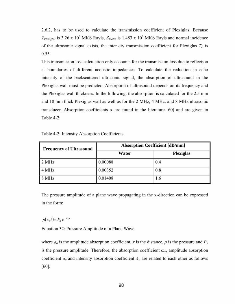
98
2.6.2, has to be used to calculate the transmission coefficient of Plexiglas. Because
ZPlexiglas is 3.26 x 10⁶ MKS Rayls, ZWater is 1.483 x 10⁶ MKS Rayls and normal incidence
of the ultrasonic signal exists, the intensity transmission coefficient for Plexiglas TP is
0.55.
This transmission loss calculation only accounts for the transmission loss due to reflection
at boundaries of different acoustic impedances. To calculate the reduction in echo
intensity of the backscattered ultrasonic signal, the absorption of ultrasound in the
Plexiglas wall must be predicted. Absorption of ultrasound depends on its frequency and
the Plexiglas wall thickness. In the following, the absorption is calculated for the 2.5 mm
and 18 mm thick Plexiglas wall as well as for the 2 MHz, 4 MHz, and 8 MHz ultrasonic
transducer. Absorption coefficients α are found in the literature [60] and are given in
Table 4-2:
Table 4-2: Intensity Absorption Coefficients
Absorption Coefficient [dB/mm] Frequency of Ultrasound
Water Plexiglas
2 MHz 0.00088 0.4
4 MHz 0.00352 0.8
8 MHz 0.01408 1.6
The pressure amplitude of a plane wave propagating in the x-direction can be expressed
in the form:
( ) xaaePtxp −= 0,
Equation 32: Pressure Amplitude of a Plane Wave
where aa is the amplitude absorption coefficient, x is the distance, p is the pressure and P0
is the pressure amplitude. Therefore, the absorption coefficient αα, amplitude absorption
coefficient aa and intensity absorption coefficient Aa are related to each other as follows
[60]:
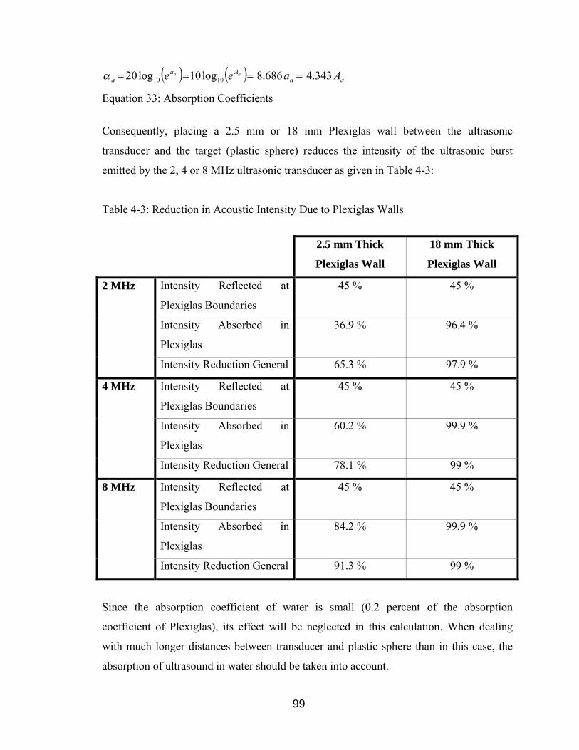
99
( ) ( ) aaAa
a Aaee aa 343.4686.8log10log20 1010 ====α
Equation 33: Absorption Coefficients
Consequently, placing a 2.5 mm or 18 mm Plexiglas wall between the ultrasonic
transducer and the target (plastic sphere) reduces the intensity of the ultrasonic burst
emitted by the 2, 4 or 8 MHz ultrasonic transducer as given in Table 4-3:
Table 4-3: Reduction in Acoustic Intensity Due to Plexiglas Walls
2.5 mm Thick
Plexiglas Wall
18 mm Thick
Plexiglas Wall
Intensity Reflected at
Plexiglas Boundaries
45 % 45 %
Intensity Absorbed in
Plexiglas
36.9 % 96.4 %
2 MHz
Intensity Reduction General 65.3 % 97.9 %
Intensity Reflected at
Plexiglas Boundaries
45 % 45 %
Intensity Absorbed in
Plexiglas
60.2 % 99.9 %
4 MHz
Intensity Reduction General 78.1 % 99 %
Intensity Reflected at
Plexiglas Boundaries
45 % 45 %
Intensity Absorbed in
Plexiglas
84.2 % 99.9 %
8 MHz
Intensity Reduction General 91.3 % 99 %
Since the absorption coefficient of water is small (0.2 percent of the absorption
coefficient of Plexiglas), its effect will be neglected in this calculation. When dealing
with much longer distances between transducer and plastic sphere than in this case, the
absorption of ultrasound in water should be taken into account.
100
Comparing the calculated and measured intensity reduction, it can be seen that for
relatively small frequencies (2 MHz), the calculated reduction is bigger than the measured
reduction in echo intensity, especially for the thin Plexiglas wall. This can be explained
by the fact, that for smaller frequencies and especially for thinner Plexiglas walls, the
threshold of the formula used to calculate the transmission coefficient (Equation 18) is
reached. The duration of the incident signal is then of the order of 2L/cL. If the duration of
the incident signal is less than 2L/cL, in other words if the incident wave train is long
compared to 2L, Equation 21 should be used to calculate the transmission coefficient.
Calculating the transmission coefficient with Equation 21 leads to a much smaller
reduction in echo intensity for relatively small frequencies and thin Plexiglas walls. Using
Equation 21 the following reduction in echo intensity can be calculated for the 2.5 mm
thick Plexiglas wall: 46 percent for the 2 MHz transducer, 66 percent for the 4 MHz
transducer and 86 percent for the 8 MHz transducer. These values better match the
measurement results. The still slightly higher calculated than measured reduction in echo
intensity can be explained by the effect of reflections of the Plexiglas wall from previous
ultrasonic burst emissions that are received by the ultrasonic transducer without having
completely propagated through the Plexiglas wall.
After having evaluated the effect on the ultrasonic beam shape and the echo intensity for
each transducer introduced, the echo intensity and beam divergence plots are presented in
Section 4.4.2 (Figures 4-18 to 4-33).

101
4.4.2 Echo Intensity and Beam Divergence Plots
Transducer 1:
18 mm Plexiglas Wall:
0
0.5
1
1.5
2
2.5
3
-10 -9 -8 -7 -6 -5 -4 -3 -2 -1 0 1 2 3 4 5 6 7 8 9 10
Position y-axis [mm]
Echo
Inte
nsity
[Vol
t]
25 mm
28 mm
30 mm
35 mm
40 mm
50 mm
70 mm
100 mm
∆x [mm]
Figure 4-18: Echo Intensity 2 MHz 10 mm Transducer 18 mm Plexiglas Wall
0
10
20
30
40
50
60
70
80
90
100
110
120
-10 -9 -8 -7 -6 -5 -4 -3 -2 -1 0 1 2 3 4 5 6 7 8 9 10
Position y-axis [mm]
Posi
tion
x-ax
is [m
m]
3 dB 6 dB
Figure 4-19: Divergence 2 MHz 10 mm Transducer 18 mm Plexiglas Wall

102
2.5 mm Plexiglas Wall:
0
5
10
15
20
25
30
-10 -9 -8 -7 -6 -5 -4 -3 -2 -1 0 1 2 3 4 5 6 7 8 9 10
Position y-axis [mm]
Echo
Inte
nsity
[Vol
t]
18 mm
20 mm
25 mm
30 mm
40 mm
50 mm
75 mm
100 mm
∆x [mm]
Figure 4-20: Echo Intensity 2 MHz 10 mm Transducer 2.5 mm Plexiglas Wall
0
10
20
30
40
50
60
70
80
90
100
110
120
-10 -9 -8 -7 -6 -5 -4 -3 -2 -1 0 1 2 3 4 5 6 7 8 9 10
Position y-axis [mm]
Posi
tion
x-ax
is [m
m]
3 dB 6 dB
Figure 4-21: Divergence 2 MHz 10 mm Transducer 2.5 mm Plexiglas Wall
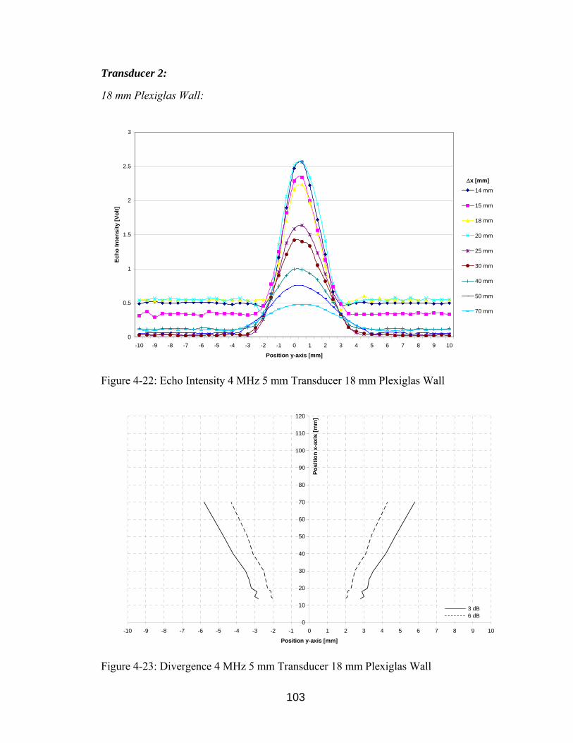
103
Transducer 2:
18 mm Plexiglas Wall:
0
0.5
1
1.5
2
2.5
3
-10 -9 -8 -7 -6 -5 -4 -3 -2 -1 0 1 2 3 4 5 6 7 8 9 10
Position y-axis [mm]
Echo
Inte
nsity
[Vol
t]
14 mm
15 mm
18 mm
20 mm
25 mm
30 mm
40 mm
50 mm
70 mm
∆x [mm]
Figure 4-22: Echo Intensity 4 MHz 5 mm Transducer 18 mm Plexiglas Wall
0
10
20
30
40
50
60
70
80
90
100
110
120
-10 -9 -8 -7 -6 -5 -4 -3 -2 -1 0 1 2 3 4 5 6 7 8 9 10
Position y-axis [mm]
Posi
tion
x-ax
is [m
m]
3 dB 6 dB
Figure 4-23: Divergence 4 MHz 5 mm Transducer 18 mm Plexiglas Wall
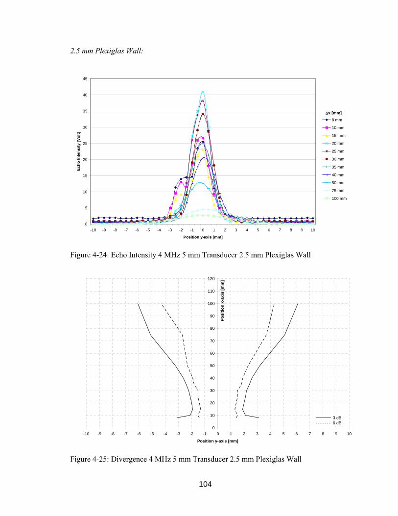
104
2.5 mm Plexiglas Wall:
0
5
10
15
20
25
30
35
40
45
-10 -9 -8 -7 -6 -5 -4 -3 -2 -1 0 1 2 3 4 5 6 7 8 9 10
Position y-axis [mm]
Echo
Inte
nsity
[Vol
t]
8 mm
10 mm
15 mm
20 mm
25 mm
30 mm
35 mm
40 mm
50 mm
75 mm
100 mm
∆x [mm]
Figure 4-24: Echo Intensity 4 MHz 5 mm Transducer 2.5 mm Plexiglas Wall
0
10
20
30
40
50
60
70
80
90
100
110
120
-10 -9 -8 -7 -6 -5 -4 -3 -2 -1 0 1 2 3 4 5 6 7 8 9 10
Position y-axis [mm]
Posi
tion
x-ax
is [m
m]
3 dB 6 dB
Figure 4-25: Divergence 4 MHz 5 mm Transducer 2.5 mm Plexiglas Wall
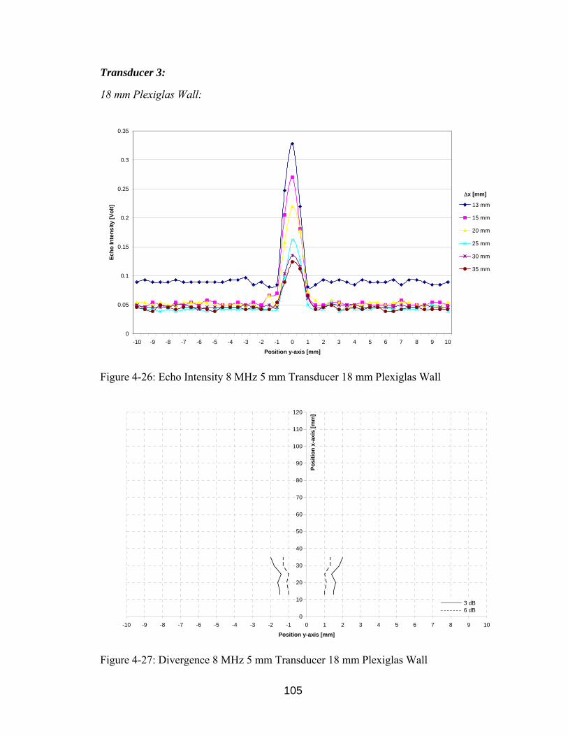
105
Transducer 3:
18 mm Plexiglas Wall:
0
0.05
0.1
0.15
0.2
0.25
0.3
0.35
-10 -9 -8 -7 -6 -5 -4 -3 -2 -1 0 1 2 3 4 5 6 7 8 9 10
Position y-axis [mm]
Echo
Inte
nsity
[Vol
t] 13 mm
15 mm
20 mm
25 mm
30 mm
35 mm
∆x [mm]
Figure 4-26: Echo Intensity 8 MHz 5 mm Transducer 18 mm Plexiglas Wall
0
10
20
30
40
50
60
70
80
90
100
110
120
-10 -9 -8 -7 -6 -5 -4 -3 -2 -1 0 1 2 3 4 5 6 7 8 9 10
Position y-axis [mm]
Posi
tion
x-ax
is [m
m]
3 dB 6 dB
Figure 4-27: Divergence 8 MHz 5 mm Transducer 18 mm Plexiglas Wall

106
2.5 mm Plexiglas Wall:
0
0.5
1
1.5
2
2.5
3
3.5
-10 -9 -8 -7 -6 -5 -4 -3 -2 -1 0 1 2 3 4 5 6 7 8 9 10
Position y-axis [mm]
Echo
Inte
nsity
[Vol
t]
8 mm
10 mm
15 mm
20 mm
25 mm
30 mm
40 mm
50 mm
75 mm
∆x [mm]
Figure 4-28: Echo Intensity 8 MHz 5 mm Transducer 2.5 mm Plexiglas Wall
0
10
20
30
40
50
60
70
80
90
100
110
120
-10 -9 -8 -7 -6 -5 -4 -3 -2 -1 0 1 2 3 4 5 6 7 8 9 10
Position y-axis [mm]
Posi
tion
x-ax
is [m
m]
3 dB 6 dB
Figure 4-29: Divergence 8 MHz 5 mm Transducer 2.5 mm Plexiglas Wall

107
Transducer 4:
18 mm Plexiglas Wall:
0
5
10
15
20
25
30
-10 -9 -8 -7 -6 -5 -4 -3 -2 -1 0 1 2 3 4 5 6 7 8 9 10
Position y-axis [mm]
Echo
Inte
nsity
[Vol
t]
14 mm15 mm18 mm20 mm25 mm30 mm40 mm50 mm70 mm
∆x [mm]
Figure 4-30: Echo Intensity 4 MHz Focussed Transducer 18 mm Plexiglas Wall
0
10
20
30
40
50
60
70
80
90
100
110
120
-10 -9 -8 -7 -6 -5 -4 -3 -2 -1 0 1 2 3 4 5 6 7 8 9 10
Position y-axis [mm]
Posi
tion
x-ax
is [m
m]
3 dB 6 dB
Figure 4-31: Divergence 4 MHz Focussed Transducer 18 mm Plexiglas Wall
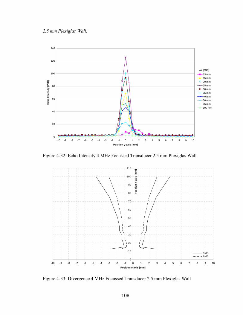
108
2.5 mm Plexiglas Wall:
0
20
40
60
80
100
120
140
-10 -9 -8 -7 -6 -5 -4 -3 -2 -1 0 1 2 3 4 5 6 7 8 9 10
Position y-axis [mm]
Echo
Inte
nsity
[Vol
t]
13 mm15 mm20 mm25 mm30 mm35 mm40 mm50 mm75 mm100 mm
∆x [mm]
Figure 4-32: Echo Intensity 4 MHz Focussed Transducer 2.5 mm Plexiglas Wall
0
10
20
30
40
50
60
70
80
90
100
110
-10 -9 -8 -7 -6 -5 -4 -3 -2 -1 0 1 2 3 4 5 6 7 8 9 10
Position y-axis [mm]
Posi
tion
x-ax
is [m
m]
3 dB 6 dB
Figure 4-33: Divergence 4 MHz Focussed Transducer 2.5 mm Plexiglas Wall

109
4.5 Effect of Forming Screens
In industrial applications, the measurement of velocity profiles in the area close to porous
forming screens is most important. Therefore, the distance from the forming screen to the
plastic sphere at which the echo of the plastic sphere can still be recognized must be as
small as possible. In evaluating the measurement results, emphasis is laid on finding the
closest distance from the plastic sphere to the screen over the widest range of transducer-
screen-distances (∆x) that produces detectable echoes of the plastic sphere behind the
forming screen. The long term goal is to use pulsed ultrasound Doppler velocimetry to
measure velocity profiles closely behind a forming screen. This is described in detail in
Section 7.2.
To evaluate the effect of forming screens, the basic experimental setup is modified. A
forming screen is placed between the ultrasonic transducer and the plastic sphere as
shown in Figure 4-34.
Figure 4-34: Experimental Setup Forming Screen
The following parameters of the forming screen sample have been identified:
- Material: Polyester
- Density Polyester: 1.35 g/cm3 = 1350 kg/m3
- Fiber volume: 0.38 cm3
Plastic sphere
Ultrasonic transducer
Forming screen

110
- Pore volume: 0.36 cm3
- Porosity: 0.95
- Sample weight (in air): 0.57 g
- Sample weight (in water): 0.873
- Sample volume: 0.74 cm3
- Apparent density (in air): 0.77 g/cm3 = 770 kg/m3
- Apparent density (in water): 1.18 g/cm3 = 1180 kg/m3
- Thickness: 0.022 in = 0.00056 m
- Mesh: 60 wires/inch = 2362 wires/meter
- Pore shape factor: 1 (cylindrical pores ≈ cubical pores)
- Double layer:
i. Fiber diameter ply 1: 0.2 mm
ii. Fiber diameter ply 2: 0.4 mm
- Specific flow resistance: 95.5 MKS Rayls
- Speed of Sound [13]: 1700 m/s
Figure 4-35 is a picture of the forming screen. The composition of the forming screen is
shown in the microtomographic cross-section views in Figure 4-36 (4 µm resolution).
Figure 4-35: Forming Screen
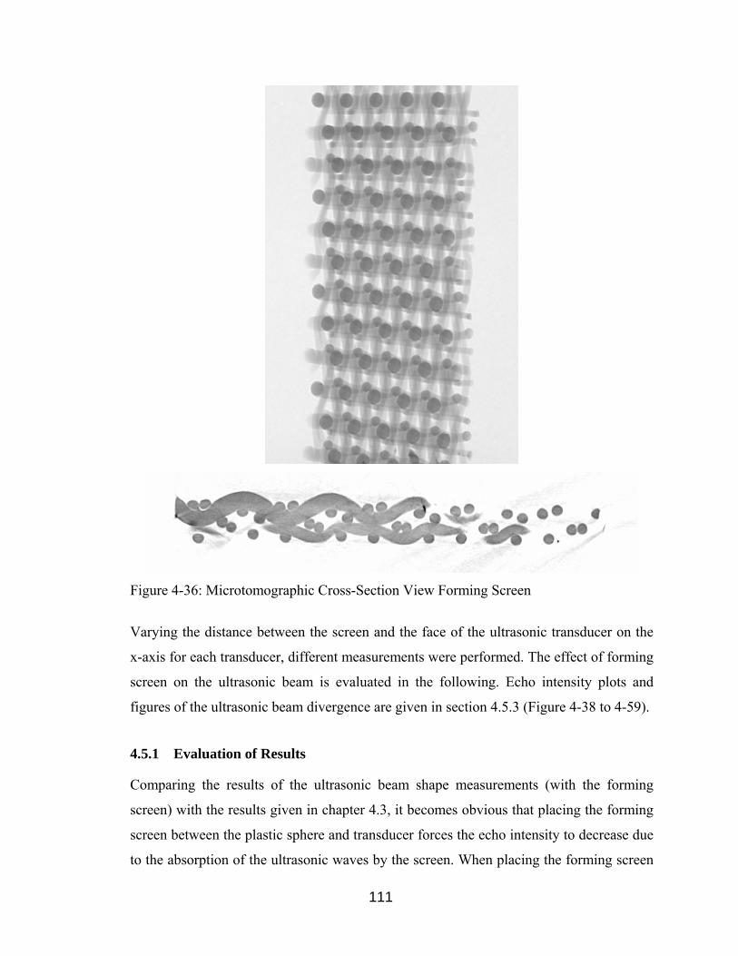
111
Figure 4-36: Microtomographic Cross-Section View Forming Screen
Varying the distance between the screen and the face of the ultrasonic transducer on the
x-axis for each transducer, different measurements were performed. The effect of forming
screen on the ultrasonic beam is evaluated in the following. Echo intensity plots and
figures of the ultrasonic beam divergence are given in section 4.5.3 (Figure 4-38 to 4-59).
4.5.1 Evaluation of Results
Comparing the results of the ultrasonic beam shape measurements (with the forming
screen) with the results given in chapter 4.3, it becomes obvious that placing the forming
screen between the plastic sphere and transducer forces the echo intensity to decrease due
to the absorption of the ultrasonic waves by the screen. When placing the forming screen
112
between the transducer and plastic sphere, the foremost effect seen is a sharp decrease in
the intensity of the echo. For the 2 MHz 10 mm transducer, the decrease in the intensity
of the echo is 60 percent when the screen is between the plastic sphere and the transducer.
For the 4 MHz 5 mm transducer, the decrease in echo intensity is 85 percent, and with the
4 MHz 8 mm focused transducer, the decrease in the intensity of the echo is
approximately 94 percent. The 8 MHz 5 mm transducer had a decrease of 98 percent in
echo intensity. It can clearly be seen that the echo intensity decreases with increasing
frequency since attenuation of acoustic waves increases with increasing frequency.
Therefore, the 8 MHz 5 mm transducer did not yield useful results. The echo intensity
decreases with increasing distance between the transducer and the screen. All
measurements reveal a significant decrease in echo intensity when the forming screen is
between the plastic sphere and transducer.
As the echo intensity decreases due to the presence of the forming screen, the gain of the
system must be increased to achieve a measurable signal. As the gain of the system is
increased, the ringing effect is also increased. This ringing effect causes the minimal
measurable distance to increase.
Using the 2 MHz 10 mm transducer and placing it 20 mm away from the screen, the
closest distance that the plastic sphere produced a detectable echo was when it was 28
mm away from the transducer (8 mm away from the screen). Placing the same transducer
40 mm away form the screen, the closest detectable distance of the plastic sphere was 46
mm away from the transducer (6 mm away from the screen). Placing the screen 60 mm
away from the same transducer, the closest measurable distance from the screen was
reduced to 4 mm (64 mm away from the transducer). Increasing the distance between the
2 MHz transducer to the screen to 80 mm, the closest measurable distance from screen
was increased to 9 mm (89 mm away from the screen). Consequently, using the 2 MHz
10 mm transducer, the closest distance from the plastic sphere to screen that produced
detectable echoes was 4 mm. It was achieved when the screen was placed 60 mm away
from the transducer.
Using the 4 MHz 5 mm transducer and placing it 20 mm away from the screen, the
closest distance that the plastic sphere produced a detectable echo was when it was 22
mm away from the transducer (2 mm away from the screen). Placing the same transducer
113
40 mm away form the screen, the closest detectable distance of the plastic sphere was 44
mm away from the transducer (4 mm away from the screen). Increasing the distance
between the 4 MHz transducer to the screen to 60 mm, the closest distance that the pin
produced a detectable echo was when it was 3 mm away from the screen (63 mm away
from the transducer). Using the 4 MHz 5 mm transducer, the closest distance from the
plastic sphere to the screen that produced detectable echoes was 2 mm.
The 8 MHz 5 mm transducer did not produce any detectable echoes at any distance away
from the transducer and away from the screen. This is due to the increased attenuation of
this high frequency transducer.
Using the 4 MHz 8 mm focused transducer and placing it 20 mm away from the screen,
the closest distance that the plastic sphere produced a detectable echo was when it was 23
mm away from the transducer (3 mm away from the screen). Placing the same transducer
40 mm away form the screen, the closest detectable distance of the plastic sphere was 43
mm away from the probe (3 mm away from the screen). Increasing the distance between
the 4 MHz transducer to the screen to 60 mm, the closest distance that the plastic sphere
produced a detectable echo was when it was 4 mm away from the screen (64 mm away
from the probe). Using the 4 MHz 8 mm focused transducer, the closest distance from the
plastic sphere to the screen that produced detectable echoes was 3 mm.
The closest distance from the plastic sphere to the screen over the widest range of
transducer-screen-distances that produced detectable echoes was achieved with the 4
MHz transducer. The 4 MHz transducer turned out to represent a good tradeoff between
the high attenuation of the 8 MHz transducer and the low resolution (measurable depth
and velocity) of the 2 MHz transducer. Keeping in mind the simplicity of the
experimental setup, the 2 mm distance from the plastic sphere to the screen could
possibly be further decreased using a more sophisticated setup.
The shape of the beam of the ultrasonic transducer changes when the screen is inserted in
the field. When the screen is in place between the plastic sphere and the transducer, the
beam seems to have two distinct regions. The “near screen field“ is the region on the
opposite side of the screen from the transducer, which is approximately 20-40 mm in
length for the 2 MHz transducer and 20 mm in length for both of the 4 MHz transducers.
The “far screen field“ is the region that is on the opposite side of the screen as the

114
transducer and is past the “near screen field“ (> 40 mm for the 2 MHz transducer and >
20 mm for the 4 MHz transducers). In all cases, the beam shape and width in the far
screen field are very close to the same with and without the screen as shown in Figure
4-37.
0
20
40
60
80
100
120
-7 -5 -3 -1 1 3 5 7Position y-axis [mm]
∆x
[mm
]
No Screen With Screen
Screen Depth
Figure 4-37: 4 MHz Focused Transducer With/Without Screen at 40 mm (6 dB)
In the near screen field, there is a common trend of beam convergence (narrowing of
beam width) followed by beam divergence (widening of the beam width) as the beam gets
closer to the far screen field (Figure 2-1). The beam width in the near screen field is
generally slightly smaller (no more than 2 mm) than the beam width when the screen is
not present (Figure 2-1). For the 4 MHz 8 mm focused transducer, the focal point without
the screen is at 20 mm, but with the screen placed 20 mm away from the transducer, the
focal point shifts back approximately 10 mm. This does not happen when the screen is at
any other position that was tested with the 4 MHz focused transducer. Since the far screen
field beam width and shape are very similar with and without the screen present, the angle
of divergence for the transducers is similar in both cases. With the screen in place, the
beam shape changes dramatically with different transducers so that the trends are
different for different transducers at different screen depths.

115
4.5.2 Effect of the Forming Screen on the Echo Intensity
To calculate the frequency dependent absorption of acoustic energy due to the forming
screen and compare this reduction of echo intensity to the reduction of echo intensity due
to the Plexiglas wall, the acoustic impedance and consequently the transmission
coefficient of the porous forming must be determined.
Different approaches were used to calculate the acoustic impedance of porous forming
screens. As a first approximation, the measured apparent density of 1.18 g/cm3 of the
forming screen sample (described in section 4.5) and the sound speed of 1700 m/s
measured by Brodeur [13] were multiplied to get a vague value of the acoustic
impedance. Consequently the order of magnitude of the acoustic impedance is 2 x 10⁶
MKS Rayls.
In order to predict the acoustic impedance of the forming screen more accurately, the
Delany-Bazley-model, a fundamental model in the area of sound propagation in fibrous
materials, and the Allard-Champoux-model, new expressions that can be used instead of
the phenomenological equations of Delany and Bazley, were used. Using the Delany-
Bazley-model an acoustic impedance which is approximately the same magnitude as the
acoustic impedance of water was predicted. This would lead to a transmission coefficient
of nearly 100 %, which is simply not realistic. The Allard-Champouc-model did not yield
useful results as well. Especially the high porosity of the forming screen and the pore
saturation with water instead of air may be the reason why both models do not yield
useful results. As a reference, both models and the results are described in Appendix J.
For now, it is not possible to predict the acoustic impedance with adequate accuracy.
Therefore, the reduction in echo intensity caused by placing a forming screen between the
ultrasonic transducer and the target is not calculated. The evaluation of the echo intensity
reduction is therefore solely based on the measurement results given above.

116
4.5.3 Echo Intensity and Beam Divergence Plots
Transducer 1:
Screen at x = 20 mm:
0
2
4
6
8
10
12
14
16
18
-10 -9 -8 -7 -6 -5 -4 -3 -2 -1 0 1 2 3 4 5 6 7 8 9 10
Position y-axis [mm]
Echo
Inte
nsity
[Vol
t]
28 mm29 mm30 mm33 mm35 mm37 mm39 mm40 mm42 mm50 mm75 mm
∆x [mm]
Figure 4-38: Echo Intensity 2 MHz 10 mm Transducer With Screen at x = 20 mm
0
10
20
30
40
50
60
70
80
90
100
110
120
-10 -9 -8 -7 -6 -5 -4 -3 -2 -1 0 1 2 3 4 5 6 7 8 9 10
Position y-axis [mm]
Posi
tion
x-ax
is [m
m]
Screen Depth
3 dB 6 dB
Figure 4-39: Divergence 2 MHz 10 mm Transducer With Screen at x = 20 mm
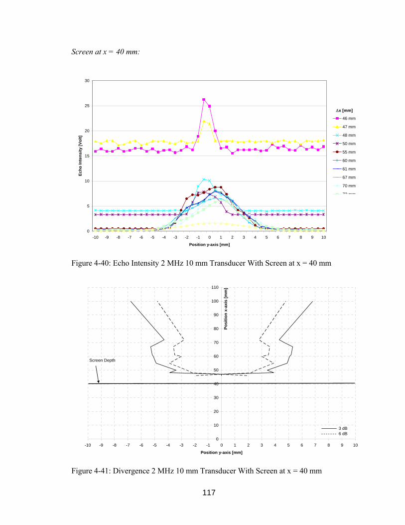
117
Screen at x = 40 mm:
0
5
10
15
20
25
30
-10 -9 -8 -7 -6 -5 -4 -3 -2 -1 0 1 2 3 4 5 6 7 8 9 10
Position y-axis [mm]
Echo
Inte
nsity
[Vol
t]
46 mm
47 mm
48 mm
50 mm
55 mm
60 mm
61 mm
67 mm
70 mm
72 mm
∆x [mm]
Figure 4-40: Echo Intensity 2 MHz 10 mm Transducer With Screen at x = 40 mm
0
10
20
30
40
50
60
70
80
90
100
110
-10 -9 -8 -7 -6 -5 -4 -3 -2 -1 0 1 2 3 4 5 6 7 8 9 10
Position y-axis [mm]
Posi
tion
x-ax
is [m
m]
Screen Depth
3 dB 6 dB
Figure 4-41: Divergence 2 MHz 10 mm Transducer With Screen at x = 40 mm

118
Screen at x = 60 mm:
0
0.5
1
1.5
2
2.5
3
3.5
4
4.5
5
-10 -9 -8 -7 -6 -5 -4 -3 -2 -1 0 1 2 3 4 5 6 7 8 9 10
Position y-axis [mm]
Echo
Inte
nsity
[Vol
t]
64 mm66 mm68 mm70 mm75 mm85 mm95 mm115 mm
∆x [mm]
Figure 4-42: Echo Intensity 2 MHz 10 mm Transducer With Screen at x = 60 mm
0
10
20
30
40
50
60
70
80
90
100
110
120
-10 -9 -8 -7 -6 -5 -4 -3 -2 -1 0 1 2 3 4 5 6 7 8 9 10
Position y-axis [mm]
Posi
tion
x-ax
is [m
m]
Screen Depth
3 dB 6 dB
Figure 4-43: Divergence 2 MHz 10 mm Transducer With Screen at x = 60 mm
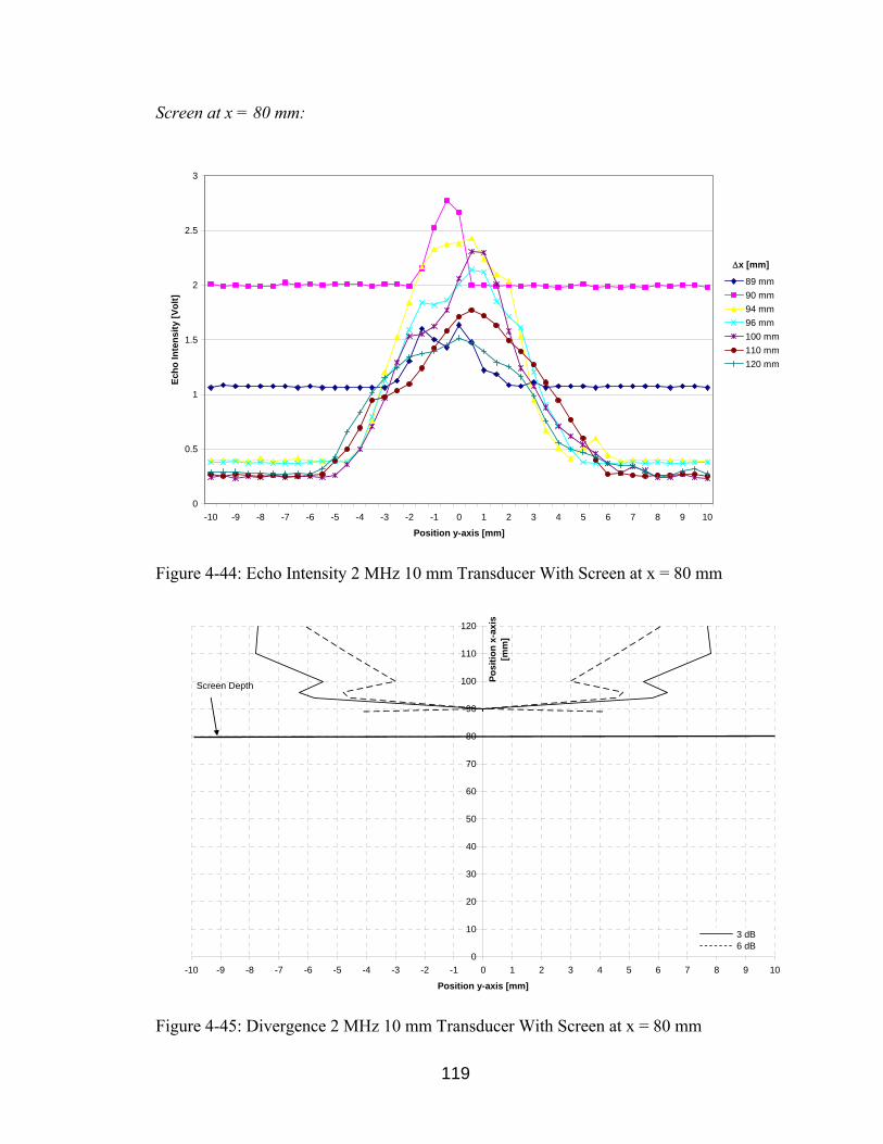
119
Screen at x = 80 mm:
0
0.5
1
1.5
2
2.5
3
-10 -9 -8 -7 -6 -5 -4 -3 -2 -1 0 1 2 3 4 5 6 7 8 9 10
Position y-axis [mm]
Echo
Inte
nsity
[Vol
t]
89 mm90 mm94 mm96 mm100 mm110 mm120 mm
∆x [mm]
Figure 4-44: Echo Intensity 2 MHz 10 mm Transducer With Screen at x = 80 mm
0
10
20
30
40
50
60
70
80
90
100
110
120
-10 -9 -8 -7 -6 -5 -4 -3 -2 -1 0 1 2 3 4 5 6 7 8 9 10
Position y-axis [mm]
Posi
tion
x-ax
is
[mm
]
Screen Depth
3 dB 6 dB
Figure 4-45: Divergence 2 MHz 10 mm Transducer With Screen at x = 80 mm

120
Transducer 2:
Screen at x = 20 mm:
0
5
10
15
20
25
-10 -9 -8 -7 -6 -5 -4 -3 -2 -1 0 1 2 3 4 5 6 7 8 9 10
Position y-axis [mm]
Echo
Inte
nsity
[Vol
t]
22 mm23 mm24 mm25 mm27 mm30 mm35 mm40 mm50 mm75 mm
∆x [mm]
Figure 4-46: Echo Intensity 4 MHz 5 mm Transducer With Screen at x = 20 mm
0
10
20
30
40
50
60
70
80
90
100
110
120
-10 -9 -8 -7 -6 -5 -4 -3 -2 -1 0 1 2 3 4 5 6 7 8 9 10
Position y-axis [mm]
Posi
tion
x-ax
is [m
m]
Screen Depth
3 dB 6 dB
Figure 4-47: Divergence 4 MHz 5 mm Transducer With Screen at x = 20 mm

121
Screen at x = 40 mm:
0
1
2
3
4
5
6
7
8
9
-10 -9 -8 -7 -6 -5 -4 -3 -2 -1 0 1 2 3 4 5 6 7 8 9 10
Position y-axis [mm]
Echo
Inte
nsity
[Vol
t]
44 mm45 mm46 mm48 mm50 mm60 mm80 mm100 mm
∆x [mm]
Figure 4-48: Echo Intensity 4 MHz 5 mm Transducer With Screen at x = 40 mm
0
10
20
30
40
50
60
70
80
90
100
110
-10 -9 -8 -7 -6 -5 -4 -3 -2 -1 0 1 2 3 4 5 6 7 8 9 10
Position y-axis [mm]
Posi
tion
x-ax
is [m
m]
Screen Depth
3 dB 6 dB
Figure 4-49: Divergence 4 MHz 5 mm Transducer With Screen at x = 40 mm
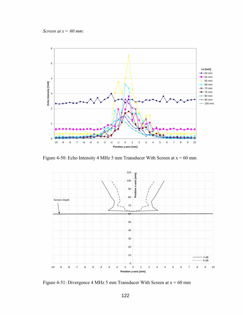
122
Screen at x = 60 mm:
0
1
2
3
4
5
6
-10 -9 -8 -7 -6 -5 -4 -3 -2 -1 0 1 2 3 4 5 6 7 8 9 10
Position y-axis [mm]
Echo
Inte
nsity
[Vol
t]
63 mm64 mm65 mm68 mm70 mm75 mm80 mm90 mm100 mm
∆x [mm]
Figure 4-50: Echo Intensity 4 MHz 5 mm Transducer With Screen at x = 60 mm
0
10
20
30
40
50
60
70
80
90
100
110
-10 -9 -8 -7 -6 -5 -4 -3 -2 -1 0 1 2 3 4 5 6 7 8 9 10
Position y-axis [mm]
Posi
tion
x-ax
is [m
m]
Screen Depth
3 dB 6 dB
Figure 4-51: Divergence 4 MHz 5 mm Transducer With Screen at x = 60 mm
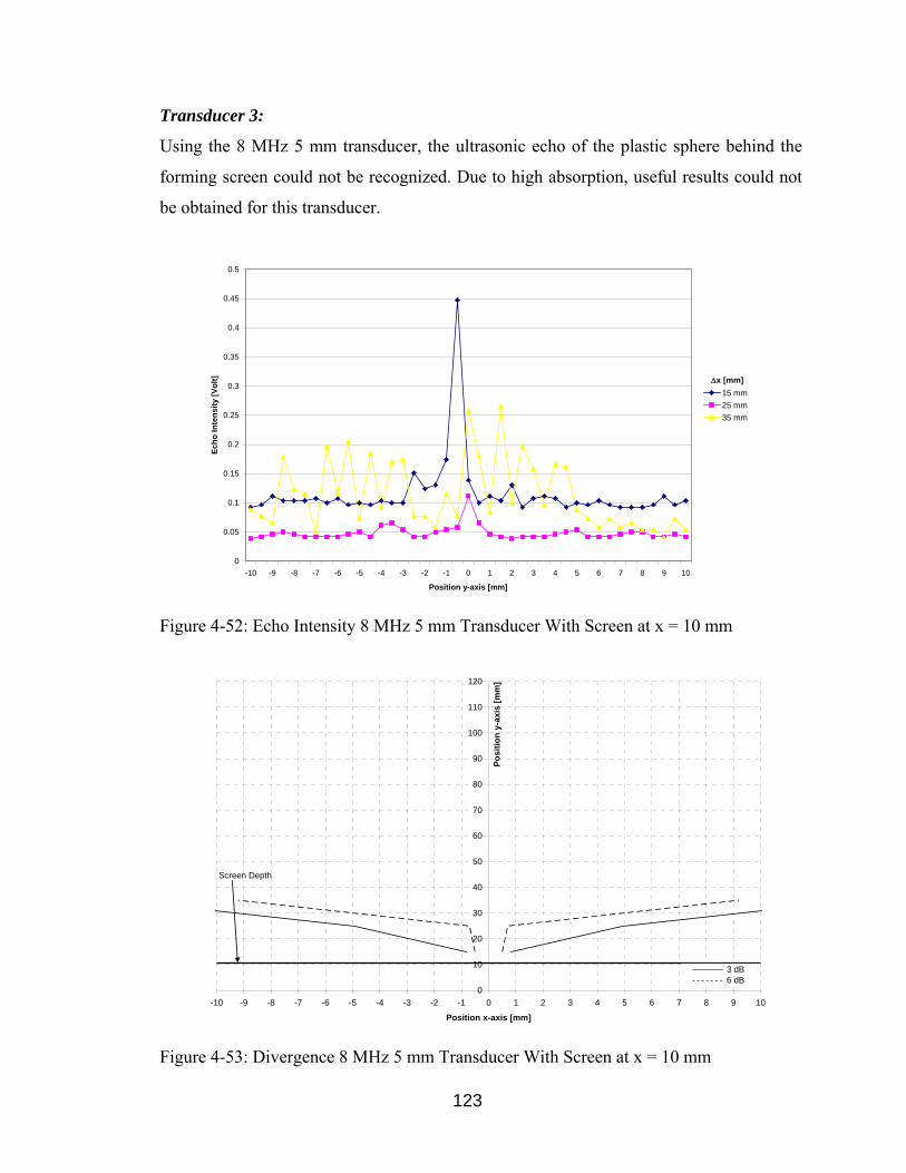
123
Transducer 3:
Using the 8 MHz 5 mm transducer, the ultrasonic echo of the plastic sphere behind the
forming screen could not be recognized. Due to high absorption, useful results could not
be obtained for this transducer.
0
0.05
0.1
0.15
0.2
0.25
0.3
0.35
0.4
0.45
0.5
-10 -9 -8 -7 -6 -5 -4 -3 -2 -1 0 1 2 3 4 5 6 7 8 9 10
Position y-axis [mm]
Echo
Inte
nsity
[Vol
t]
15 mm25 mm35 mm
∆x [mm]
Figure 4-52: Echo Intensity 8 MHz 5 mm Transducer With Screen at x = 10 mm
0
10
20
30
40
50
60
70
80
90
100
110
120
-10 -9 -8 -7 -6 -5 -4 -3 -2 -1 0 1 2 3 4 5 6 7 8 9 10
Position x-axis [mm]
Posi
tion
y-ax
is [m
m]
Screen Depth
3 dB 6 dB
Figure 4-53: Divergence 8 MHz 5 mm Transducer With Screen at x = 10 mm
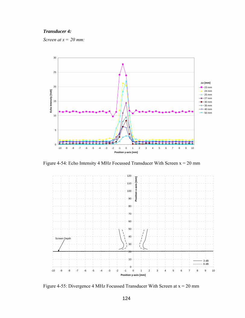
124
Transducer 4:
Screen at x = 20 mm:
0
5
10
15
20
25
30
-10 -9 -8 -7 -6 -5 -4 -3 -2 -1 0 1 2 3 4 5 6 7 8 9 10
Position y-axis [mm]
Echo
Inte
nsity
[Vol
t]
23 mm24 mm25 mm27 mm30 mm35 mm40 mm50 mm
∆x [mm]
Figure 4-54: Echo Intensity 4 MHz Focussed Transducer With Screen x = 20 mm
0
10
20
30
40
50
60
70
80
90
100
110
120
-10 -9 -8 -7 -6 -5 -4 -3 -2 -1 0 1 2 3 4 5 6 7 8 9 10
Position y-axis [mm]
Posi
tion
x-ax
is [m
m]
Screen Depth
3 dB 6 dB
Figure 4-55: Divergence 4 MHz Focussed Transducer With Screen at x = 20 mm

125
Screen at x = 40 mm:
0
1
2
3
4
5
6
-10 -9 -8 -7 -6 -5 -4 -3 -2 -1 0 1 2 3 4 5 6 7 8 9 10
Position y-axis [mm]
Echo
Inte
nsity
[Vol
t]
43 mm44 mm45 mm46 mm48 mm50 mm 60 mm80 mm
∆x [mm]
Figure 4-56: Echo Intensity 4 MHz Focussed Transducer With Screen at x = 40 mm
0
10
20
30
40
50
60
70
80
90
100
110
120
-10 -9 -8 -7 -6 -5 -4 -3 -2 -1 0 1 2 3 4 5 6 7 8 9 10
Position y-axis [mm]
Posi
tion
x-ax
is [m
m]
Screen Depth
3 dB 6 dB
Figure 4-57: Divergence 4 MHz Focussed Transducer With Screen at x = 40 mm

126
Screen at x = 60 mm:
0
0.5
1
1.5
2
2.5
3
-10 -9 -8 -7 -6 -5 -4 -3 -2 -1 0 1 2 3 4 5 6 7 8 9 10
Position y-axis [mm]
Echo
Inte
nsity
[Vol
t]
64 mm65 mm68 mm70 mm75 mm80 mm90 mm100 mm
∆x [mm]
Figure 4-58: Echo Intensity 4 MHz Focussed Transducer With Screen at x = 60 mm
0
10
20
30
40
50
60
70
80
90
100
110
120
-10 -9 -8 -7 -6 -5 -4 -3 -2 -1 0 1 2 3 4 5 6 7 8 9 10
Position y-axis [mm]
Posi
tion
x-ax
is [m
m]
Screen Depth
3 dB 6 dB
Figure 4-59: Divergence 4 MHz Focussed Transducer With Screen at x = 60 mm
127
4.6 Evaluation of Ultrasonic Beam Measurements
Ultrasonic field measurements were conducted with various transducers to determine the
transducer best suited to measure velocity profiles in small channels and capillaries, to
compare unfocused and focused ultrasonic transducers and to see the effects of Plexiglas
walls and porous forming screens inserted between the transducer and the target (plastic
sphere). The effect of Plexiglas walls and porous forming screens on the ultrasonic beam
shape can not be generalized for all transducers and should therefore be investigated
experimentally for each single transducer at various positions.
The 8 MHz 5 mm and 4 MHz 8 mm focused ultrasonic transducer turned out to be the
most promising transducer to measure velocity profiles in small channels and capillaries
due to their excellent lateral resolution. When dealing with small geometries, the 8 MHz
transducer should be preferred, since its axial resolution is half of the 4 MHz transducer’s
axial resolution. Knowledge of the focal point of both transducers is crucial to optimize
measurement results especially when dealing with flow over a backward facing step.
Much greater amplification must be used in order to get a readable signal when the
forming screens or the Plexiglas walls are used. This increase in echo intensity comes
with the cost of increased ringing of the ultrasonic signal. This ringing effect causes the
minimum measurable distance, the distance from the obstruction to the first measurable
point, to increase. Especially at high frequencies, Plexiglas walls and forming screens
attenuate more than 90 percent of the ultrasonic signal. The 4 MHz transducer turned out
to represent a good tradeoff between the high attenuation of the 8 MHz transducer and the
low lateral and axial resolution of the 2 MHz transducer. The closest distance from the
plastic sphere to the porous forming screen over the widest range of transducer-screen-
distances that produced detectable echoes was also achieved with the 4 MHz transducer.
Due to the better lateral resolution (and therefore the greater amount of energy that is
reflected from scatterers behind the porous forming screen), the 4 MHz focused
transducer turned out to be the most promising transducer to measure velocity profiles
closely behind a porous forming screen.

128
5 Measurement of Velocity Profiles in Small Channels
In Chapter 4, the 8 MHz 5 mm ultrasonic transducer was identified to be the most
promising transducer to measure velocity profiles in small channels and capillaries due to
its excellent lateral resolution. In this chapter, velocity profiles are non-intrusively
measured in a small rectangular channel characterized by a backward facing step to
experimentally validate the theoretical limitations of pulsed ultrasound Doppler
velocimetry (identified before), investigate further limitations in small channels in a
separated flow at low velocities and compare focused with unfocused ultrasonic
transducers. At first, the principle of measurement and important parameters of pulsed
ultrasound Doppler velocimetry are presented. Then the experimental setup that was
solely designed for this purpose is described. Technical drawings of the channel and
distributor are listed in Appendix A. After reviewing the fundamentals of flow over a
backward facing step, the measurement results are presented and finally evaluated. The
effect of Plexiglas walls on the measurement results has been evaluated in detail.
5.1 Principle of Measurement of Pulsed Ultrasound Doppler
Velocimetry
In pulsed ultrasound Doppler velocimetry, a transducer is placed on a wall with an angle
inclination θ (angle between transducer and flow direction) to ensure a velocity
component in the direction of the measuring line. The most important point is to ensure a
good coupling between the transducer and the liquid. Any gas interface is not allowed
because gas has very low acoustic impedance and therefore reflects all the ultrasonic
energy.
The master oscillator generates a reference frequency of from 1 to 10 MHz. This
reference frequency is the input to a gating circuit which transmits just a few cycles of the
reference frequency at preset intervals. This produces a train of pulses at a frequency
called the pulse repetition frequency. The pulse train is the input to the transmitting

129
piezocrystal to produce acoustic pulses. As the acoustic burst leaves the crystal and
propagates through the flow field, a continuous train of echoes is produced.
Figure 5-1 [55] shows an example of the signal of the received echo. Between two
emissions of ultrasonic pulses the echo can be observed, backscattered from somewhere
on the measuring line. A position axis along the measuring line is thus converted to a time
axis. The frequency of an echo signal at any instant is Doppler-shifted due to the fluid
motion as far as it is reflected inside the flow.
Since echoes are produced by a single acoustic burst, range information can be obtained.
This is accomplished by “range gating” the receiver crystal. The receiver is turned off
while a burst is transmitted. Since the acoustic burst propagates at a known acoustic
velocity through the medium, the distance which it travels corresponds to a particular
time delay. Thus, if the receiver is turned on for an instant after a given time delay from
the instant of pulse transmission, the echoes reaching the receiver crystal at that instant
will correspond to a particular range distance. At this instant, the phase of the received
signal is compared in a phase detector with the reference frequency. The phase-detector
output is a voltage pulse proportional in magnitude to the phase difference between the
echo and the reference frequency. Repeating the comparison over many pulse repetition
frequency cycles results in a train of phase detector output voltages with each pulse
proportional to an instantaneous phase difference [59].
In modern devices, after amplification, the echo signal is demodulated to eliminate the
component of basic frequency and then digitized. The time series of the digitized data is
then filtered digitally to eliminate vibration of the container or from noise, then the
Doppler shifts are detected to give a histogram of velocity values and thus the velocity
profile (Figure 5-1 (c)).

130
Figure 5-1: Principle of Measurement [55]
The velocity component measured by the velocimeter is always the component in the
direction of the ultrasonic beam as shown in Figure 5-2. The measured velocity vus
represents the projection of the three dimensional velocity vector onto the ultrasound
beam line [16]. When the direction of the real velocity is known, the velocimeter can
automatically compute the real velocity value vreal by using the value of the Doppler angle
θ. In such a case the depth values displayed by the velocimeter are the depths
perpendicular to the velocity direction (Preal).
Figure 5-2: Velocity Components [51]
a)
b)
c)
131
The acquisition time of a complete profile depends on three parameters; the sound
velocity in the liquid, the maximum depth at which measurements have to be done and
the number of ultrasonic emissions used to estimate the velocities.
5.2 Important Parameters of Pulsed Ultrasound Doppler Velocimetry
With respect to the velocimeter architecture, working structure and measurement method
identified in Section 2.5 and Section 5.1, the following parameters are essential to
correctly determine a velocity profile.
5.2.1 The Emitting Frequency
In making the choice of an emitting frequency the following four factors are crucial. First
of all, the desired position of the sampling volume is important in selecting the emitting
frequency especially when dealing with small channels and capillaries. The emitting
frequency contributes to the definition of the axial and lateral dimension of the sampling
volume. As this dimension is linked to the duration of the burst, for a defined number of
wave cycles in the burst, a higher emitting frequency will give a better resolution. Besides
the sampling volume size, attenuation of the ultrasonic signal is an important factor in
making the choice of an emitting frequency. The attenuation of ultrasonic waves depends
on their frequencies. Low frequencies are less attenuated than high frequencies. The
attenuation coefficient may vary quite a lot and depends on the material. Moreover, the
maximum measurable velocity, which is inversely proportional to the emitting frequency,
and the energy backscattered by particles depend on the ultrasonic frequency.
5.2.2 Doppler Angle
The velocimeter measures the velocity component in the direction of the ultrasonic beam
and gives therefore only one component of the velocity vector. If the direction of the real
velocity vector is known, it is possible to compute directly the module of the velocity
vector by using the Doppler angle. The Doppler angle is the angle formed by the axis of
the ultrasonic beam and the direction of the real velocity vector. When the Doppler angle
is used to compute the module of the velocity vector, the depth values, measured in the
132
direction of the ultrasonic beam are computed perpendicularly to the direction of the
velocity.
5.2.3 Pulse Repetition Frequency
The pulse repetition frequency determines the maximum measurable depth as well as the
maximum Doppler frequency and therefore the maximum velocity which can be
measured unambiguously. The choice of the pulse repetition frequency should be based
on the velocity values that have to be measured and not on the depth that has to be
reached. The best way to select a correct value is to start with a high value and reduce this
value until at least 50 percent of the velocity scale is covered. The desired analyzed depth
can then be adapted by changing the resolution, the position of the first gate or the
number of gates.
5.2.4 Position of the First Gate, Wall- and Saturation-Effect
In order to correctly determine the velocity profile, the position of the first gate should be
chosen carefully to decrease the wall effect and the effect of the saturation region.
The measuring position of each sample volume is located in the center of the sample.
When part of the sample volume is located inside the channel wall, this position will not
reflect the actual measuring position given by the instrument (wall effect). The actual
center of the measurement volume (this part of the sample volume which is in the flow
and not in the wall) can be calculated based on the Doppler angle (geometric
considerations) and simplifications on the shape of the sample volume (e.g., disk shape
sample volume). The position of the first sample volume can consequently be corrected
based on this calculation [64]. In the following, the position of the first gate will be set so
that the sampling volume begins ideally right behind the channel wall to decrease the wall
effect (see also section 5.5.3). Since the position of the first gate can be defined only in
specific increments, the starting depth should be set so that only a very small portion (in
the order of maximal 0.08 millimeter) of the sample is inside the wall. The position of the
first gate is based on the position of the center of the first sample volume which depends
on the emitted ultrasonic burst length, the speed of sound in the media located between
the transducer face and the first gate, the Doppler angle (geometry) and the starting depth
that can be set in the instrument.

133
When the first gates are close to the surface of the transducer, the burst duration and the
ringing of the piezoelectric ceramic do not allow any measurement in these gates due to a
saturation of the receiver (saturation effect). The saturation region can be visualized in the
display of the received echoes, where the levels echoes of gates located at depths near the
surface of the transducer stretch over the entire scale.
The position of the first measurable gate therefore depends on the emitting frequency, the
burst length, the Doppler angle, the geometry of the experimental setup, the emitted
power and the amplification level. The starting depth chosen in the instrument is the
distance between the transducer face and the center of the first gate.
5.2.5 The Burst Length
The length of the emitted burst affects the sampling volume. The bandwidth of the
electronic receiving unit in the ultrasonic instrument is fixed, but the number of cycles
contained in the emitted ultrasonic burst can be selected. The length of the emitted burst
depends on the selected emitting frequency and the speed of sound of the medium.
5.2.6 The Resolution
In the ultrasonic instrument, the resolution is defined as the distance between the centers
of adjacent sampling volumes. In ultrasonic Doppler velocimetry, the shape and lateral
size of the sampling volumes (measured perpendicularly to the ultrasonic beam axis) are
defined by the geometry of the ultrasonic beam. The longitudinal size of the sampling
volumes on the other hand is defined by the burst length. The borders of the sampling
volumes are not well defined since the levels of the ultrasonic echoes increase and
decrease “slowly” due to the finite bandwidth of the receiver. Whenever possible, a value
for the spatial filter that equals the resolution should be selected to achieve an optimum
signal to noise ratio.
5.2.7 The Number of Gates
The number of gates that can be measured depends on the selected pulse repetition
frequency, the position of the first gate and the selected resolution. An upper limit can be
fixed to ensure a better display of velocity profiles, especially when low pulse repetition
values are selected. The position of the first gate and the number of gates define the
134
measuring range and therefore the analyzed depth. It is often much better to change the
number of analyzed gates in order to change the measuring depth or range than to change
the pulse repetition values.
5.2.8 The Emitting Power and Sensitivity
The emitted ultrasonic power has to be selected in order to receive enough backscattered
energy from the particles and avoid as much as possible saturation in the receiver stage of
the instrument. The display of the echo profile may be used to verify this point. A high
emitting power should be avoided since it induces more ringing in the transducer and
more dissipated energy. Therefore it is generally better to increase the amplification (time
gain control) instead of increasing the emitting power. Nevertheless, a too high level of
amplification also induces saturation in the receiver stage of the instrument, which
induces wrong measurement values.
The algorithm used to measure the Doppler frequency computes the mean frequency of
the Doppler spectrum. When the Doppler energy decreases, the mean value become more
and more random due to the noise included in the spectrum. In order avoid the apparition
of random values on the screen, the instrument computes also the level of Doppler energy
received and allows the user to cancel the computation of the Doppler frequency if the
level of the Doppler energy is below a user defined value. In such a case the canceled
values are replaced by zero values. The sensitivity parameter contains five different
values, which define the level below which the computation is canceled. The sensitivity
parameter can be used to obtain information on the quality of the measured values. No
changes should occur if the sensitivity parameter is modified.
5.2.9 Number of Emissions Per Profile
The measurement of the Doppler frequencies is based on the correlation that exists
between different emissions. As each emission can be seen as a particular realization of a
random process, more samples are available and lower the variance of the estimated
quantity. The algorithm used to estimate the Doppler frequency is based on the
assumption that the particles that generate the echoes during the measurement of the
Doppler frequency remain inside the ultrasonic beam and their velocities are constant. For
low velocities in steady flows this assumption is valid, but for transient ones, with high

135
velocities, a compromise has to be taken between the quality of the estimation (minimum
variance) and the measuring time. The number of emissions per profile should be selected
in accordance to the type of flow investigated and on the width of the ultrasonic beam.
For low velocities in steady flows, a high number will decrease the variance and therefore
should be selected. For high velocities in unstationary flows this number should be
adapted to the degree of variation of the velocities versus time.
5.2.10 Speed of Sound
The knowledge of the speed of sound in the medium is necessary to transform the
Doppler frequency shifts in mm/s, and the time of flight of the ultrasonic waves in
millimeter. A good knowledge of the sound velocity in the medium especially when
dealing with suspended particles or fibers is necessary to obtain good quantitative
measurement values, as all errors in this parameter are directly transferred to the
measured values. Since the speed of sound for different particle or fiber concentrations in
water is unknown, the sound velocity is measured in a special unit before each
measurement. These measurements are described in Appendix H.
5.2.11 Profiles to Record
In pulsed ultrasound Doppler velocimetry measurements, a certain number of
“instantaneous velocity profiles” is used to calculate the mean velocity profile as defined
by the instrument parameter “profiles to record”. Possible velocity fluctuations, caused by
the recirculation of the backward facing step at high Reynolds-numbers and pressure
fluctuations caused by the pump and distributor, may lead to small differences between
different instantaneous profiles and therefore to a statistical error. Therefore, it is
necessary to determine the mean velocity profile based on enough instantaneous velocity
profiles.
5.3 Experimental Setup
The experimental setup shown in Figures 5-3 and 5-4 is used for measuring velocity
profiles in a small rectangular channel and determining current limitations of the utilized

136
pulsed ultrasound Doppler velocimetry system (Signal Processing DOP2000 model
1225).
Figure 5-3: Experimental Setup
Figure 5-4: Experimental Setup Side Views
Main parts of the experimental setup are the pulsed ultrasound Doppler velocimetry
system, the small rectangular channel (10 mm high and 80 mm wide; 0.7 liter volume)
Programmable digital drive pump
Distributor
Channel
Relocatable theta positioner
Collecting basin
Transverse movement of theta positioner
Straight movement of theta positioner
Ultrasonic transducer cable
Rotational movement ultrasonic transducer
Relocatable theta positioner
Channel
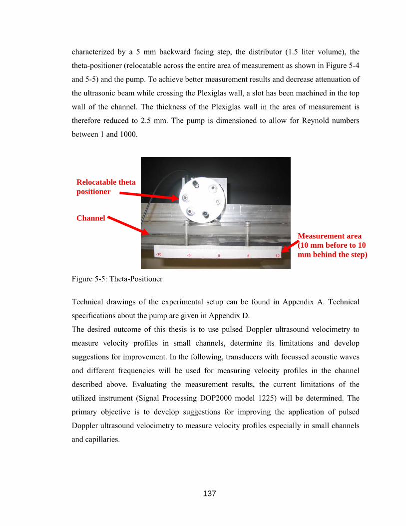
137
characterized by a 5 mm backward facing step, the distributor (1.5 liter volume), the
theta-positioner (relocatable across the entire area of measurement as shown in Figure 5-4
and 5-5) and the pump. To achieve better measurement results and decrease attenuation of
the ultrasonic beam while crossing the Plexiglas wall, a slot has been machined in the top
wall of the channel. The thickness of the Plexiglas wall in the area of measurement is
therefore reduced to 2.5 mm. The pump is dimensioned to allow for Reynold numbers
between 1 and 1000.
Figure 5-5: Theta-Positioner
Technical drawings of the experimental setup can be found in Appendix A. Technical
specifications about the pump are given in Appendix D.
The desired outcome of this thesis is to use pulsed Doppler ultrasound velocimetry to
measure velocity profiles in small channels, determine its limitations and develop
suggestions for improvement. In the following, transducers with focussed acoustic waves
and different frequencies will be used for measuring velocity profiles in the channel
described above. Evaluating the measurement results, the current limitations of the
utilized instrument (Signal Processing DOP2000 model 1225) will be determined. The
primary objective is to develop suggestions for improving the application of pulsed
Doppler ultrasound velocimetry to measure velocity profiles especially in small channels
and capillaries.
Relocatable theta positioner
Channel
Measurement area (10 mm before to 10 mm behind the step)
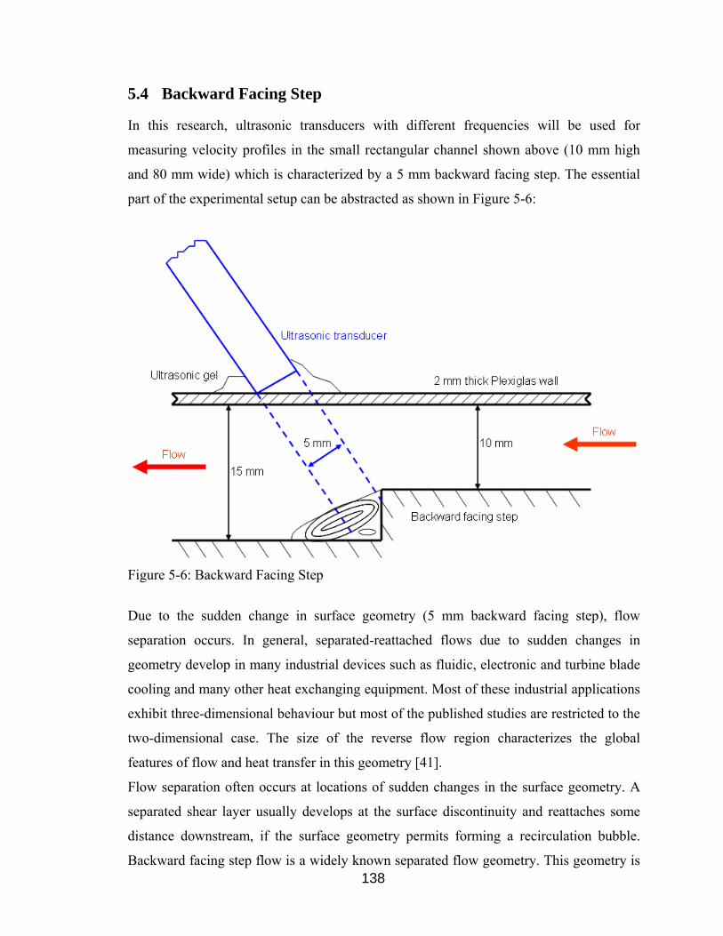
138
5.4 Backward Facing Step
In this research, ultrasonic transducers with different frequencies will be used for
measuring velocity profiles in the small rectangular channel shown above (10 mm high
and 80 mm wide) which is characterized by a 5 mm backward facing step. The essential
part of the experimental setup can be abstracted as shown in Figure 5-6:
Figure 5-6: Backward Facing Step
Due to the sudden change in surface geometry (5 mm backward facing step), flow
separation occurs. In general, separated-reattached flows due to sudden changes in
geometry develop in many industrial devices such as fluidic, electronic and turbine blade
cooling and many other heat exchanging equipment. Most of these industrial applications
exhibit three-dimensional behaviour but most of the published studies are restricted to the
two-dimensional case. The size of the reverse flow region characterizes the global
features of flow and heat transfer in this geometry [41].
Flow separation often occurs at locations of sudden changes in the surface geometry. A
separated shear layer usually develops at the surface discontinuity and reattaches some
distance downstream, if the surface geometry permits forming a recirculation bubble.
Backward facing step flow is a widely known separated flow geometry. This geometry is

139
of particular interest because it facilitates the study of the reattachment process by
minimizing the effect of the separation process, while for other separating and reattaching
flow geometries there may be a strong interaction between the two [35].
The principal flow features of the turbulent backward-facing step flow are described as
follows. A turbulent boundary layer which forms on a flow plate encounters a downward
step. The sudden expansion due to the change in surface geometry causes the boundary
layer to separate at the step edge. Immediately after detachment, the flow essentially
behaves as a free shear layer, with high-speed fluid on one side and low-speed fluid on
the other. Some distance downstream, the shear layer impinges on the surface and forms a
closed recirculation region containing turbulent, upstream moving fluid. A small “corner
eddy” of the opposite rotation sense to the main recirculating flow might also exist in this
region. Reattachment occurs over a region located about the time-averaged reattachment
point. The flow in this zone is found to be unsteady and highly three-dimensional with
large-scale structures (of size of the channel height before the step) passing through
frequently. Downstream of reattachment, the boundary layer begins to redevelop and
undergoes a relaxation to a normal turbulent boundary layer state [35]. Flow in the
vicinity of the backward facing step is shown in Figure 5-7 for various Reynolds-
numbers.
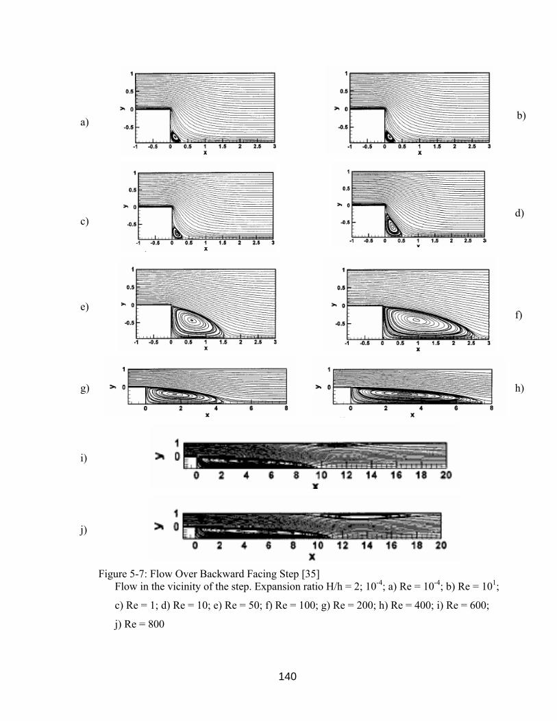
140
Figure 5-7: Flow Over Backward Facing Step [35] Flow in the vicinity of the step. Expansion ratio H/h = 2; 10-4; a) Re = 10-4; b) Re = 101;
c) Re = 1; d) Re = 10; e) Re = 50; f) Re = 100; g) Re = 200; h) Re = 400; i) Re = 600;
j) Re = 800
a) b)
c) d)
e) f)
g) h)
i)
j)

141
The size of the reverse flow regions increases and moves further downstream in the
laminar flow regime (Re < 400); decreases and moves upstream in the transitional flow
regime (400 < Re < 3400); and remains almost constant or diminishes in the turbulent
flow regime (Re > 3400); as the Reynolds number increases [41].
Usually, recirculation length is obtained from the particle image velocimetry by
measuring the distance between the step corner and the point of reattachment on the
channel bottom wall. This point is characterized by a zero longitudinal velocity in the
extreme vicinity of the bottom wall [10]. In the following, the ability of pulsed ultrasound
Doppler velocimetry to measure the recirculation length is evaluated.
5.5 Measurements with Pulsed Ultrasound Doppler Velocimetry
Before actually measuring velocity profiles with pulsed ultrasound Doppler velocimetry,
the purpose and necessary measurement preparations are described. The effect of
Plexiglas walls and various measurement parameters is discussed. Finally, measurement
results of focused and unfocused ultrasonic transducers are compared and evaluated.
5.5.1 Purpose
The desired outcome of this thesis is to use pulsed Doppler ultrasound velocimetry to
measure velocity profiles in small channels and capillaries, determine its limitations and,
if necessary develop suggestions for improvement. Velocity profiles in the small
rectangular channel described above are therefore measured in this section to further
determine the current limitations of the utilized pulsed ultrasound Doppler velocimetry
system. Measurement results of focused and unfocused ultrasonic transducer are
compared.
5.5.2 DOP 2000 Model 2125 Pulsed Ultrasonic Doppler Velocimetry
In this study, a commercially available pulsed ultrasound Doppler velocimetry system
(DOP 2000, Model 2125) manufactured by Signal Processing S.A., Switzerland, is used
to measure velocity profiles in the experimental setup described above. The basic

142
function of pulsed ultrasonic Doppler velocimetry is to measure the Doppler shift
frequency and time delay between emission and reception of ultrasound scattered back by
small particles which are moving with the fluid. The information on velocity and sample
volume position is included in the ultrasound echoes. Technical specifications of the
digital ultrasonic synthesizer are listed in Appendix B. The ultrasonic synthesizer records
data values in a binary or ASCII format. These formats insure a minimum space
requirement.
5.5.3 Ultrasonic Transducers
In Chapter 4, the 8 MHz 5 mm ultrasonic transducer turned out to be the most promising
transducer to measure velocity profiles in small channels and capillaries due to its
excellent lateral and axial resolution. To compare focused and unfocused transducers,
velocity profiles measured with the 4 MHz 5 mm unfocused and 4 MHz 8 mm focused
transducer are also evaluated. Technical specifications of these single-element ultrasonic
transducers manufactured by Signal Processing S.A., Switzerland, are presented in
Appendix C.
As mentioned in Section 5.2.6, a value for the spatial filter that equals the resolution
should be selected to achieve an optimum signal to noise ratio. The distance along the
ultrasonic beam axis, displayed by the instrument, depends on the selected ultrasonic
transducer and the selected value of the spatial filter. In order to measure the velocity
profile in small geometries, the highest possible axial resolution should be chosen, i.e.,
the distance between the centers of two sample volumes should be as small as possible.
Therefore, the smallest possible spatial filter given by the instrument must be selected to
achieve an optimum signal to noise ratio. This in turn leads to an offset in the distance
displayed by the instrument along the ultrasonic beam axis. The distance offset caused by
the selection of the spatial filter is in the order of 0.5 mm to even 4 mm (when using a
lower frequency transducer).
To obtain a precise value of the actual distance of the center of the sample volume, the
distance offset must be calibrated. The sound-velocity-measuring unit (described in
Appendix H) has been used to calibrate this offset. Since the distance offset also depends
on the distance of the sample volume to the transducer face on the ultrasonic beam axis,
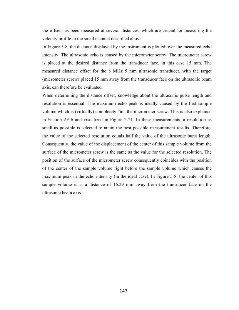
143
the offset has been measured at several distances, which are crucial for measuring the
velocity profile in the small channel described above.
In Figure 5-8, the distance displayed by the instrument is plotted over the measured echo
intensity. The ultrasonic echo is caused by the micrometer screw. The micrometer screw
is placed at the desired distance from the transducer face, in this case 15 mm. The
measured distance offset for the 8 MHz 5 mm ultrasonic transducer, with the target
(micrometer screw) placed 15 mm away from the transducer face on the ultrasonic beam
axis, can therefore be evaluated.
When determining the distance offset, knowledge about the ultrasonic pulse length and
resolution is essential. The maximum echo peak is ideally caused by the first sample
volume which is (virtually) completely “in” the micrometer screw. This is also explained
in Section 2.6.6 and visualized in Figure 2-21. In these measurements, a resolution as
small as possible is selected to attain the best possible measurement results. Therefore,
the value of the selected resolution equals half the value of the ultrasonic burst length.
Consequently, the value of the displacement of the center of this sample volume from the
surface of the micrometer screw is the same as the value for the selected resolution. The
position of the surface of the micrometer screw consequently coincides with the position
of the center of the sample volume right before the sample volume which causes the
maximum peak in the echo intensity (in the ideal case). In Figure 5-8, the center of this
sample volume is at a distance of 16.29 mm away from the transducer face on the
ultrasonic beam axis.

144
0
2
4
6
8
10
12
14
16
18
20
0 100 200 300 400 500 600 700 800
Echo Amplitude [Volt]
Dis
tanc
e [m
m]
16.29 mm on y-axis
Figure 5-8: Calibration of Transducer Distance Offset
The offset in the distance displayed by the instrument has been measured for each
ultrasonic transducer at various distances which are of importance to measuring the
velocity profile in the small channel described above. Values for the distance offset with
the target (micrometer screw) at different positions, can be found in Table 5-1.
5.5.4 Channel and Probe Geometry
To exactly determine the position of each sample volume, characteristic distances of the
experimental setup have been defined and calculated for various Doppler angles θ and
ultrasonic transducers as shown in Figure 5-9.

145
Figure 5-9: Channel and Transducer Geometry
The distance from the center of the ultrasonic transducer (with diameter d) to the outer
surface of the Plexiglas channel-top-wall, which is perpendicular to the wall, is denoted
as h1. h2 is the thickness of the Plexiglas channel-top-wall, whereas h3 is the channel
height.
32321 cos2
hhdhhhh ++=++= θ
Equation 34: Distance Perpendicular to the Flow
The distance from the center of the ultrasonic transducer to the outer surface of the
Plexiglas channel-top-wall along the ultrasonic beam axis is denoted as l1. Respectively l2
and l3 are projections of h2 and h3 on the ultrasonic beam axis.
θθθθ sinsinsinsin321
321hhhhllll =++=++=
Equation 35: Distance in Direction of the Ultrasonic Beam
An exact definition of the characteristic distances is crucial, to understand the effect of
Plexiglas walls placed between the sample volume and the ultrasonic transducer.

146
5.5.5 Plexiglas Wall Effect
Placing a Plexiglas wall between the area of interest (sample volume) and the ultrasonic
transducer leads to another offset in the distance displayed by the instrument along the
ultrasonic beam axis. This distance offset is caused by different sound velocities in
Plexiglas, ultrasonic gel and the fluid inside the channel. For example, the inner wall of
the Plexiglas-top-wall should be displayed at a distance which equals the sum l1 and l2
(given in Table 5-1). Due to different sound velocities, the distance displayed by the
instrument (L) differs from the sum of l1 and l2.
The distance offset caused by Plexiglas walls at normal incidence is already described in
Section 4.4.1. To calculate the distance offset (and therefore the distance L) caused by the
effect of the Plexiglas wall, when the ultrasonic transducer is inclined by the Doppler
angle, the time which is required for ultrasound to propagate through the ultrasonic gel
(distance l1) and the Plexiglas wall (distance l2) is compared to the time which is required
for ultrasound to propagate the same distance in the fluid inside the channel (the sound
velocity of the fluid is set in the instrument). Distance L is given in Table 5-1 for various
Doppler angles. Distance L1 (also mentioned in Table 5-1) is simply the sum of distance L
and the specific transducer offset described in Section 5.5.3. Respectively, L2,max and
L2,min are the sum of L, the specific transducer offset and the particular value of l3.
When measuring the velocity of scatterers behind the Plexiglas wall, the ultrasonic
transducer must be inclined by the Doppler angle. Normal incidence of the ultrasonic
beam is not possible. Therefore, the ultrasonic beam is refracted. Refraction leads to a
distance offset along the channel axis in direction of the flow. Since the Plexiglas wall is
only 2.5 mm thick, this distance offset will be less than 1 mm and is therefore neglected
in this study.
5.5.6 Measurement Parameters 8 MHz 5 mm Transducer
The following parameters (given in Figure 5-1) are chosen to determine the velocity
profile in the small channel (described above) with the 8 MHz 5 mm ultrasonic
transducer:

147
Table 5-1: Measuring Parameters 8 MHz 8 mm Transducer
In the first set of measurements, the velocity profile was measured at 10 different points:
10 mm before step, on the step and 10 – 80 mm behind the step. For example, 10 mm
before the step means, that the ultrasonic beams impinges on the inner side of the channel

148
bottom wall at 10 mm before the step viewed from the direction of the flow. The position
of some measurement points is shown in Figure 5-10.
Figure 5-10: Position Measurement Points
5.5.7 Measurement Results 8 MHz 5 mm Transducer
The velocity profiles measured at eight measurement points behind the backward facing
step at a Reynolds number of 400 and a Doppler of 70 degrees are presented in Figure
5-11.
In flow over a backward facing step the maximum velocity of the profile behind the step
decreases with increasing distance to the step. In Figure 5-11, it can clearly be seen, that
the maximum velocity at 10 mm behind the step is higher than the maximum velocity at
all the other measurement points behind the step. Having said that, the measurement
results do not show that the maximum velocity decreases from one profile to the next
profile behind the step. For example, the maximum velocity at 70 mm behind the step is
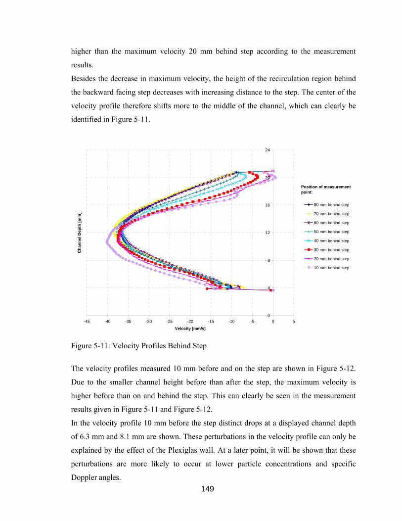
149
higher than the maximum velocity 20 mm behind step according to the measurement
results.
Besides the decrease in maximum velocity, the height of the recirculation region behind
the backward facing step decreases with increasing distance to the step. The center of the
velocity profile therefore shifts more to the middle of the channel, which can clearly be
identified in Figure 5-11.
0
4
8
12
16
20
24
-45 -40 -35 -30 -25 -20 -15 -10 -5 0 5
Velocity [mm/s]
Cha
nnel
Dep
th [m
m]
80 mm behind step
70 mm behind step
60 mm behind step
50 mm behind step
40 mm behind step
30 mm behind step
20 mm behind step
10 mm behind step
Position of measurement point:
Figure 5-11: Velocity Profiles Behind Step
The velocity profiles measured 10 mm before and on the step are shown in Figure 5-12.
Due to the smaller channel height before than after the step, the maximum velocity is
higher before than on and behind the step. This can clearly be seen in the measurement
results given in Figure 5-11 and Figure 5-12.
In the velocity profile 10 mm before the step distinct drops at a displayed channel depth
of 6.3 mm and 8.1 mm are shown. These perturbations in the velocity profile can only be
explained by the effect of the Plexiglas wall. At a later point, it will be shown that these
perturbations are more likely to occur at lower particle concentrations and specific
Doppler angles.
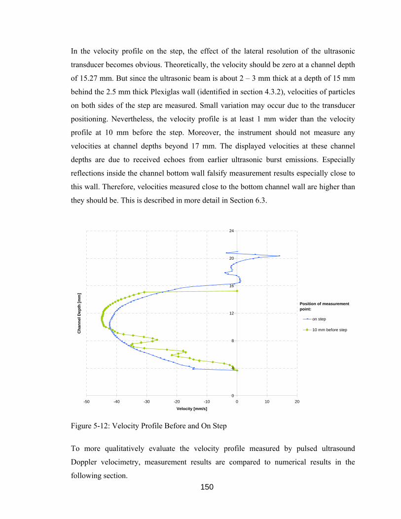
150
In the velocity profile on the step, the effect of the lateral resolution of the ultrasonic
transducer becomes obvious. Theoretically, the velocity should be zero at a channel depth
of 15.27 mm. But since the ultrasonic beam is about 2 – 3 mm thick at a depth of 15 mm
behind the 2.5 mm thick Plexiglas wall (identified in section 4.3.2), velocities of particles
on both sides of the step are measured. Small variation may occur due to the transducer
positioning. Nevertheless, the velocity profile is at least 1 mm wider than the velocity
profile at 10 mm before the step. Moreover, the instrument should not measure any
velocities at channel depths beyond 17 mm. The displayed velocities at these channel
depths are due to received echoes from earlier ultrasonic burst emissions. Especially
reflections inside the channel bottom wall falsify measurement results especially close to
this wall. Therefore, velocities measured close to the bottom channel wall are higher than
they should be. This is described in more detail in Section 6.3.
0
4
8
12
16
20
24
-50 -40 -30 -20 -10 0 10 20
Velocity [mm/s]
Cha
nnel
Dep
th [m
m]
on step
10 mm before step
Position of measurement point:
Figure 5-12: Velocity Profile Before and On Step
To more qualitatively evaluate the velocity profile measured by pulsed ultrasound
Doppler velocimetry, measurement results are compared to numerical results in the
following section.

151
5.5.8 Comparison to Numerical Results
Velocity profiles of flow over the backward facing step described above are numerically
determined by the Lattice Boltzmann simulation. The Lattice Boltzmann method is an
alternative approach to solving a fluid flow system. It is used to analyze the dynamics of
particles suspended in fluid. In Lattice Boltzmann simulations, the interaction rule
between the fluid and the suspended particles is developed for real suspensions where the
particle boundaries are treated as no-slip impermeable surfaces. This method correctly
and accurately determines the dynamics of single particles and multi-particles suspended
in the fluid [2, 3]. Results of the Lattice Boltzmann simulation for the measurement
points mentioned above are given in Figure 5-13.
3
4
5
6
7
8
9
10
11
12
13
14
15
16
17
18
19
20
21
22
-70 -60 -50 -40 -30 -20 -10 0 10
Velocity [mm/s]
Cha
nnel
Dep
th [m
m]
10 mm before step
On step
10 mm behind step
20 mm behind step
30 mm behind step
40 mm behind step
50 mm behind step
60 mm behind step
70 mm behind step
80 mm behind step
Position of measurement point:
Figure 5-13: Numerical Results
To compare measured and numerical results, the velocity profile 10 mm before the step,
10 mm behind the step (inside the recirculation area) and 80 mm behind the step (outside
the recirculation area) are presented in Figure 5-14, Figure 5-16 and Figure 5-15
respectively. In pulsed ultrasound Doppler velocimetry, the velocity component in

152
direction of the ultrasonic beam is measured. A trigonometric transformation finally
yields the velocity component in direction of the flow. Nevertheless, it must be
considered that even though the velocity is plotted along a line perpendicular to the flow,
it is measured along the ultrasonic beam axis which is inclined by the Doppler angle. In a
region of fully developed flow (that may be assumed before the step), this error may be
neglected. Nevertheless, this error must be considered in the area behind the step
especially in the presence of the recirculation region. In the following figures, the
numerical results have been projected on the ultrasonic beam axis. Nevertheless, this
assumption is only justified 10 mm before and 80 mm behind the step. Care should be
taken when comparing the numerical and measured velocity profiles 10 mm behind the
step especially inside the recirculation region. Moreover, the ultrasonic beam does not
exactly impinge at the measurement point due to refraction in the Plexiglas wall. This
effect causes an offset much smaller than 1 mm along the channel axis in direction of the
flow and is therefore neglected.
3
5
7
9
11
13
15
17
19
21
23
-70 -60 -50 -40 -30 -20 -10 0 10
Velocity [mm/s]
Cha
nnel
Dep
th [m
m]
10 mm before stepnumerical
10 mm before stepexperimental
Position of measurement point:
Figure 5-14: Comparison Numerical-Experimental 10 mm Before Step

153
The discrepancy between the numerical and measured profile becomes obvious in Figure
5-14. Apart from the distinct drops of the measured velocity profile already mentioned in
the context of Figure 5-12, the maximum velocity offset of approximately 25 percent is a
major shortcoming of the measured velocity profile. Moreover, it can clearly be seen in
Figure 5-15, that the measured velocity profile is broadened compared to the numerical
velocity profile. The broadening of the measured velocity profile is not obvious in Figure
5-14 due to the perturbations in the profile.
3
5
7
9
11
13
15
17
19
21
23
-50 -45 -40 -35 -30 -25 -20 -15 -10 -5 0
Velocity [mm/s]
Cha
nnel
Dep
th [m
m]
80 mm behind stepexperimental
80 mm behind stepnumerical
Position of measurement point:
Figure 5-15: Comparison Numerical-Experimental 80 mm Behind Step
As mentioned above, care must be taken when comparing the numerical and measured
velocity profile in Figure 5-16. The numerical velocity values are calculated
perpendicular to the flow whereas the experimental velocity values are measured along
the ultrasonic beam axis, which is inclined by 70 degrees to the direction of the flow. The
ultrasonic burst impinges on the bottom channel 10 mm behind the step, but enters the
inside of the channel at 15.5 mm behind the step. Even though the numerically calculated
velocity profile has been projected on the ultrasonic beam axis, it can still be seen that the
measured velocity profile is broadened with respect to the numerical velocity profile. In
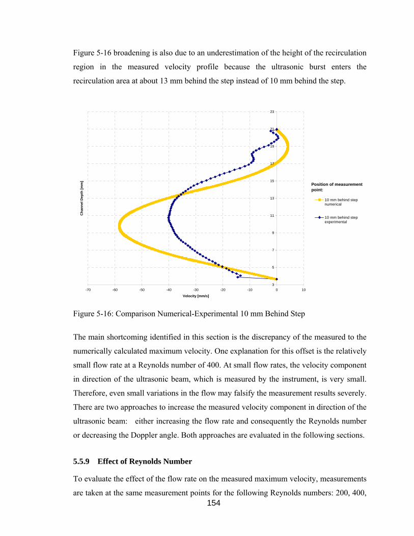
154
Figure 5-16 broadening is also due to an underestimation of the height of the recirculation
region in the measured velocity profile because the ultrasonic burst enters the
recirculation area at about 13 mm behind the step instead of 10 mm behind the step.
3
5
7
9
11
13
15
17
19
21
23
-70 -60 -50 -40 -30 -20 -10 0 10
Velocity [mm/s]
Cha
nnel
Dep
th [m
m]
10 mm behind stepnumerical
10 mm behind stepexperimental
Position of measurement point:
Figure 5-16: Comparison Numerical-Experimental 10 mm Behind Step
The main shortcoming identified in this section is the discrepancy of the measured to the
numerically calculated maximum velocity. One explanation for this offset is the relatively
small flow rate at a Reynolds number of 400. At small flow rates, the velocity component
in direction of the ultrasonic beam, which is measured by the instrument, is very small.
Therefore, even small variations in the flow may falsify the measurement results severely.
There are two approaches to increase the measured velocity component in direction of the
ultrasonic beam: either increasing the flow rate and consequently the Reynolds number
or decreasing the Doppler angle. Both approaches are evaluated in the following sections.
5.5.9 Effect of Reynolds Number
To evaluate the effect of the flow rate on the measured maximum velocity, measurements
are taken at the same measurement points for the following Reynolds numbers: 200, 400,

155
600, 800 and 1000. In Figure 5-17 results are shown for the measurement point 10 mm
behind the step.
3
5
7
9
11
13
15
17
19
21
-100 -80 -60 -40 -20 0 20
Velocity [mm/s]
Cha
nnel
Dep
th [m
m]
2004006008001000
Re-number:
Figure 5-17: Velocity Profile for Different Re-Numbers
Comparing the measurement results at 10 mm before, 10 mm behind and 80 mm behind
the step leads to the conclusion that increasing the flow rate, and therefore the velocity
component in direction of the ultrasonic beam, does not significantly decrease the
discrepancy between the measured and numerically calculated maximum velocity.
In Figure 5-17, it can clearly be seen that for higher Reynolds numbers the velocity in the
recirculation area (ranging from a channel depth of approximately 17 mm to 21 mm) is
not correctly determined by the instrument. For higher Reynolds numbers, the absolute
value of the negative velocities in the recirculation area should increase. In Figure 5-17,
no negative velocities can be identified for the higher Reynolds numbers of 600, 800 and
1000. This can be explained by the effect of the channel bottom wall and reflections
caused by previous ultrasonic burst emissions. The effect of reflections caused by the far
wall is further described in Section 6.3.
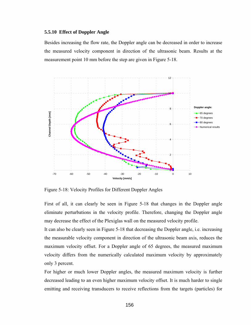
156
5.5.10 Effect of Doppler Angle
Besides increasing the flow rate, the Doppler angle can be decreased in order to increase
the measured velocity component in direction of the ultrasonic beam. Results at the
measurement point 10 mm before the step are given in Figure 5-18.
0
2
4
6
8
10
12
-70 -60 -50 -40 -30 -20 -10 0 10
Velocity [mm/s]
Cha
nnel
Dep
th [m
m]
65 degrees
70 degrees
80 degrees
Numerical results
Doppler angle:
Figure 5-18: Velocity Profiles for Different Doppler Angles
First of all, it can clearly be seen in Figure 5-18 that changes in the Doppler angle
eliminate perturbations in the velocity profile. Therefore, changing the Doppler angle
may decrease the effect of the Plexiglas wall on the measured velocity profile.
It can also be clearly seen in Figure 5-18 that decreasing the Doppler angle, i.e. increasing
the measurable velocity component in direction of the ultrasonic beam axis, reduces the
maximum velocity offset. For a Doppler angle of 65 degrees, the measured maximum
velocity differs from the numerically calculated maximum velocity by approximately
only 3 percent.
For higher or much lower Doppler angles, the measured maximum velocity is further
decreased leading to an even higher maximum velocity offset. It is much harder to single
emitting and receiving transducers to receive reflections from the targets (particles) for

157
lower Doppler angles than for angles that ensure that the ultrasonic beam is as close to
normal to the medium interface as possible.
Nevertheless, changing the Doppler angle does not reduce the broadening of the
measured velocity profile especially close to the bottom channel wall.
5.5.11 Effect of Particle Concentration
Another approach to improve the accuracy of the measured velocity profiles especially
close to the bottom channel wall is to increase the particle concentration. By increasing
the particle concentration, the intensity of the received ultrasonic echo will increase and
may lead to more accurate measured velocity profiles. In order to evaluate the effect of
the particle concentration, velocity profiles have been measured 10 mm before the step
with 4 different particle concentrations: 0.01 percent, 0.1 percent, 0.5 percent and 1
percent. Measurement results are given in Figure 5-19.
0
2
4
6
8
10
12
-70 -60 -50 -40 -30 -20 -10 0 10
Velocity [mm/s]
Cha
nnel
Dep
th [m
m] C = 0.01 %
C = 0.1 %C = 0.5 %C = 1 %Numerical Result
Concentration C:
Figure 5-19: Velocity Profiles for Different Particle Concentrations
In Figure 5-19, it can clearly be seen that for increased particle concentrations,
perturbations in the velocity profile are eliminated. Looking at Figure 5-19, it becomes
obvious that for increased particle concentrations, the measured maximum velocity

158
increases. Moreover, broadening of the velocity profile is slightly decreased. Due to
pump limitations, the particle concentration cannot arbitrarily be increased.
5.5.12 Effect of Spatial Filter and Burst Length
In general, a compromise between the length of the range area and the velocity resolution
must be made (see chapter 2.6.6). Therefore, the effect of the spatial filter and the
ultrasonic burst length on the measured velocity profile has been evaluated.
Theoretically, if a short pulse is used, a small area is probed, but the pulse spectrum and
resulting velocity spectrum are wide and give a low velocity resolution, i.e., increasing
the spatial resolution decreases the accuracy of the estimation of the Doppler frequency.
For a longer pulse the reverse is true, i.e., an accurate estimation of the target velocity
requires a narrow spectrum, and thus a long emitted pulse. On the other hand, such an
emission will decrease the depth resolution. A long range gate is employed, and a narrow
spectrum evolves. The spectral resolution is also determined by the number of pulses (N)
used, as the bandwidth of the narrow spectra is proportional to fprf/N. A long observation
time, NTprf, yields a small bandwidth.
In the hope of improving the measurable maximum velocity, the value for the spatial
filter and the ultrasonic burst length has been varied. Nevertheless, changing the value for
the spatial filter and the ultrasonic burst length did not decrease the discrepancy between
the measured and numerically calculated velocity profile, nor did it improve the shape of
the measured velocity profile.
5.5.13 Effect of Ultrasonic Transducer
In order to evaluate the effect different ultrasonic transducers and compare unfocused to
focused transducers, velocity profiles have been measured with the 4 MHz 5 mm
unfocused and 4 MHz 8 mm focused ultrasonic transducer as well. The following
parameters are chosen to determine the velocity profile at a Reynolds number of 400 for
the 4 MHz 5 mm unfocused transducer and the 4 MHz 8 mm focused transducer
respectively. Measurement parameters are given in Table 5-2 and Table 5-3 respectively.
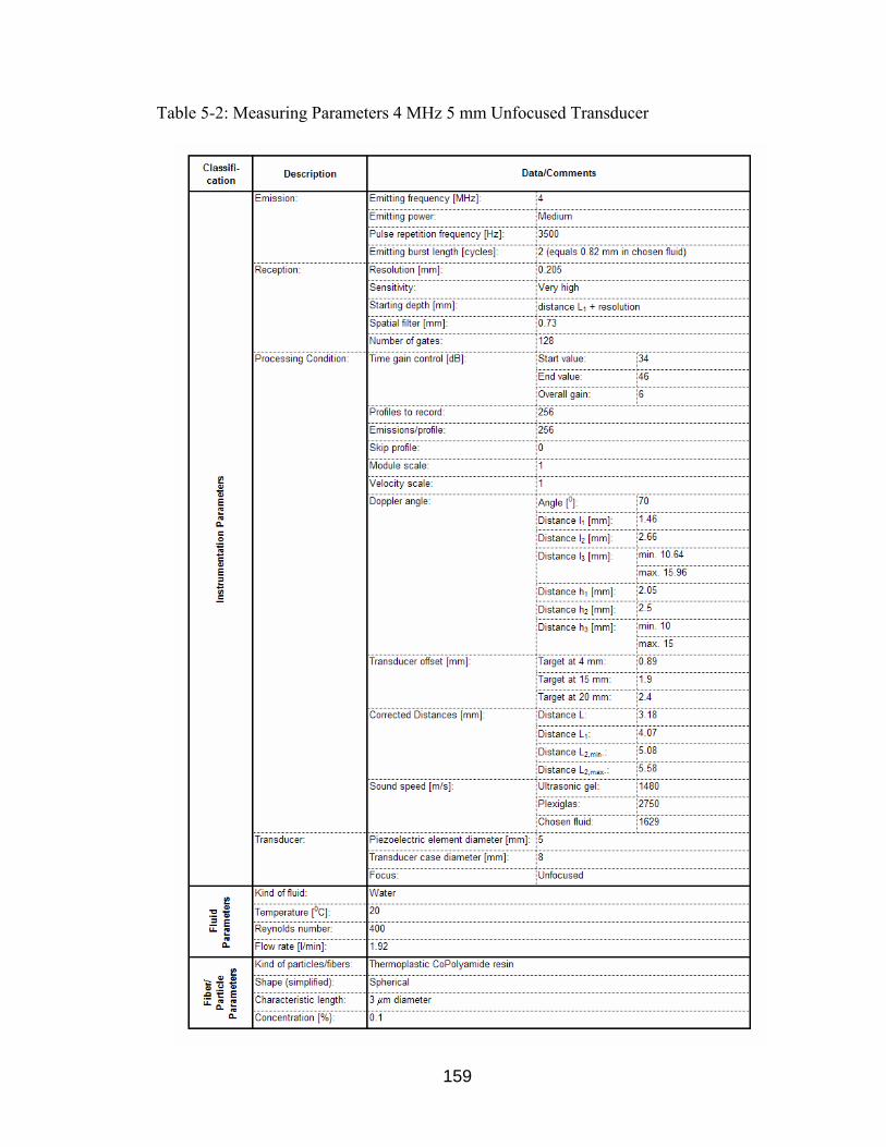
159
Table 5-2: Measuring Parameters 4 MHz 5 mm Unfocused Transducer

160
Table 5-3: Measurement Parameters 4 MHz 8 mm Focused Transducer

161
Measuring the velocity profile at 10 mm before the step with the 8 MHz 5 mm transducer,
the 4 MHz 5 mm unfocused transducer and the 4 MHz 8 mm focused transducer yields
the following results given in Figure 5-20:
0
2
4
6
8
10
12
-70 -60 -50 -40 -30 -20 -10 0 10
Velocity [mm/s]
Cha
nnel
Dep
th [m
m]
4 MHz focused4 MHz8 MHzNumerical result
Ultrasonic trans-ducer:
Figure 5-20: Velocity Profiles for Different Ultrasonic Transducers
In Figure 5-20, it can clearly be seen that it is most appropriate to measure velocity
profiles in small channels with the 8 MHz ultrasonic transducer. The larger wavelength of
the 4 MHz ultrasonic transducers leads to a poorer spatial resolution, both axial and
lateral. The effect of the poor lateral resolution of the 4 MHz transducers can clearly be
seen in Figure 5-20 by looking at the perturbations in the velocity profile. In general,
improved spatial resolution with higher frequency is accompanied by decreased
penetration depth as a result of increased attenuation. In the case of measuring the
velocity profile in small channels and capillaries, this effect is not important. Due to the
broader saturation region of the 4 MHz transducer compared to the 8 MHz transducer
(identified in Section 4.4.1), the accuracy of the measured velocity close to the channel
top wall is significantly decreased.
Since the lateral resolution is equal to the ultrasonic pulse width, measurement results of
the 4 MHz focused transducer are better than the results achieved with the 4 MHz
162
unfocused transducer. Single element focused transducers use an acoustic lens to
effectively shift the location of the focal point toward the transducer face. The end result
is a dramatic increase in sensitivity. Moreover, the smaller the beam diameter, the better
the lateral resolution and the greater the amount of energy that is reflected by the targets
(particles). The measurement results of the 4 MHz focused transducer are therefore better
than the measurement results of the 4 MHz unfocused transducer.
5.6 Evaluation of Velocity Profile Measurements with PUDV in Small Channels
Several characteristics and limitations of the Doppler velocity detection method are
immediately obvious from the measurement results presented in this chapter. In general,
the Doppler profile peak is only about 70% of the actual maximum velocity. This
discrepancy between the measured and actual maximum velocity may be decreased by
changing the Doppler angle and increasing the particle concentration. Nevertheless, the
then still existing discrepancy is ultimately due to averaging by the finite sample volume
and to frequency-meter characteristics.
Moreover, the location of the maximum Doppler frequency estimation is slightly down
range from the actual maximum-velocity location. This offset is due also to the averaging
effect of the sample volume.
Even though all important measurement parameters have been varied, the broadening of
the measured velocity profile did not significantly decrease. As mentioned above,
broadening of the measured velocity profile may be due to the effect of the bottom
channel wall and reflections from previous ultrasonic burst emissions. Another
explanation for the broadening of the measured velocity profiles is the observation during
measurements that velocities and echoes of the targets (particles) in the ultrasound field
changed rapidly with time. This causes a broadening of the Doppler spectrum und
therefore decreased velocity resolution (as described in Section 2.6.6). This effect may
consequently cause broadening of the measured velocity profile.
Gross disturbances, such as large vortices, may cause irregular spectra with large isolated
forward and reverse components. This may also lead to spectral broadening and
163
decreased velocity resolution. Gross disturbances at higher Reynolds numbers in the
recirculation region of the flow over the backward facing step (described in Section 5.5.9)
may also be the explanation for the false velocity values in the recirculation area at the
measurement point 10 mm behind the step (see Figure 5-17).
Another shortcoming of pulsed ultrasound Doppler velocimetry is that the distances
indicated on the measured velocity profiles are greater than the actual channel height
(including the orientation angle). The reason for this is the effect of the transducer offset,
caused by the selection of the spatial filter, and the effect of the Plexiglas wall, caused by
a different speed of sound in the media encountered by the ultrasonic beam. Another
reason for the limited range resolution is the sample volume length and therefore limited
range resolution.
The effect of a wall and the sample volume length on the determination of the velocity
profile is described in Section 2.6.5 and visualized in Figure 2-20. Therefore, the center of
the first sample volume inside the channel should be positioned in a way, that the distance
from the center of the sample volume equals the value for the resolution. Then, in the
ideal case, the sampling volume should be completely inside the channel and not inside
the wall. Due to the Doppler angle, the teardrop shape of the sample volume and acoustic
ringing, which de facto extends the ultrasonic burst length, this will never be the case.
Therefore, an approach to minimize the effect of the wall proposed by Xu and Aidun [64]
should be leveraged. Assuming a disc shape sample volume, Xu and Aidun proposed to
eliminate zero velocity values measured inside the wall and consequently correct the
position of the center of the sample volume and therefore the position of the first
measurement point. Following this approach and considering the teardrop shape of the
sample volume (as described in Section 2.6.4), the range resolution of the pulsed
ultrasound Doppler velocimetry can be further increased. Nevertheless, in order to follow
this approach, the transducer offset and the offset caused by different values for the speed
of sound in various media along the ultrasonic beam axis must be taken into to account to
exactly identify the specific sample volume. Another approach to minimize the effect of
the wall is to calculate the ideal position of the first sampling volume and then adjust the
positioning of the ultrasonic transducer accordingly. Nevertheless, due to the ringing
noise of the ultrasonic transducer, a small part of the first sample volume will always be

164
inside the wall. In any case, zero velocity values measured inside the wall must be
eliminated manually to improve the resolution of the instrument.
Another reason for the lack of range resolution in the experimental results is the problem
of wall reflection. As the sample volume reaches the far wall of the channel, some of the
acoustic energy is reflected back into the flow field. This reflected energy is scattered by
the moving particles to produce detected Doppler shifts. Since they occur after the sample
volume has begun to leave the flow field, they give rise to fictitious frequency-versus-
range information. In effect, the instrument is beginning to plot an image profile. This is
described in more detail in Section 6.3.
The broadening of the measured velocity profile may also be explained by these wall
reflections but also to spectral broadening caused by observed velocity fluctuations and
gross disturbances in the recirculation region.
A general drawback of ultrasound Doppler velocimetry is that flow perpendicular to the
beam is not detected and finding the velocity direction can, in some cases, be
problematic. It must always be considered that the velocity profile is measured along the
ultrasonic beam axis and not perpendicular to the flow. Therefore, care must be taken
when comparing for example a velocity profile measured along the ultrasonic beam axis
and a perpendicularly to the flow calculated velocity profile. Especially in the presence of
recirculation regions or other gross disturbances, this may lead to distortions of the
measured velocity profile. Since the Doppler angle must generally be decreased to avoid
perturbations in the measured velocity profile or to increase the velocity component in
direction of the ultrasonic beam (to obtain more accurate measurement results for
example of the maximum velocity), these distortions may be severe.
Evaluation of the measurement results shows that focused transducers yield better results
than unfocused due to higher lateral resolution and increased sensitivity.
The specific limitations of pulsed ultrasound Doppler velocimetry in small channels and
separated flow at low velocities identified in this chapter are generalized and summarized
in Chapter 6 together with the fundamental limitations identified in previous chapters.

165
6 Limitations of Pulsed Ultrasound Doppler Velocimetry
Based on the fundamentals of pulsed ultrasound Doppler velocimetry, beam shape
measurements of various ultrasonic transducers with and without walls and porous
screens and measurements of velocity profiles in the flow over a backward facing step in
a small rectangular channel, the limitations of pulsed ultrasound Doppler velocimetry
have been determined. After stating the simplifying assumptions of pulsed ultrasound
Doppler velocimetry, its accuracy and the effect of artifacts, specific limitations are
identified in this chapter.
6.1 Simplifying Assumptions
Three simplifying assumptions must be made in ultrasound Doppler velocimetry. First,
the isotropic acoustic velocity is the same throughout the sample volume. Second, the
ultrasonic pulse travels in a straight line so echoes returning at later times are interpreted
by the range equation as being caused by proportionately distant reflectors. When there
are large directional changes of the propagating ultrasonic pulse due to refraction,
reflection from oblique highly reflecting interfaces, or reverberations between two highly
reflecting interfaces, this assumption is no longer true and image artifacts will result.
Third, all detected reflectors are located on the beam central axis. This assumption is
mostly untrue but gives reasonably accurate spatial information at image depths where the
focused beam pattern is narrow. At image depths where the beam pattern is wide, this
assumption leads to blurring of reflector position lateral to the beam central axis for high-
contrast reflectors.
Concerning velocity estimation, the following assumption is made. Noise is ignored and
the motion of the particle transversal to the direction of the ultrasonic beam (the direction
of the measured motion) does not introduce a significant change in the signal received
from the particle. Consequently the shift in the position of the particle is assumed to be
the dominant source of change in the received signal and the drop in intensity due to
either transverse or axial movement of the particle is ignored. The measurements
ordinarily require the idealization that the ambient velocity and acoustical properties

166
appear unidirectional and stratified in the plane that contains transmitter and scatterer and
is tangential to the scatterer’s velocity vector.
6.2 Accuracy and Noise
The accuracy of the velocity measurement and the resolution in position and time are
deeply related to the selection of frequency of ultrasound, its pulse structure and
electronic constants for data acquisition. The accuracy in general is largely affected by the
system configuration and specifications of the electronic design. It is modified by
adapting different basic frequencies, beam diameters, maximum measurable depths, and
an algorithm to detect the Doppler shift frequency, as well as by fluid properties [55].
Any erroneous information included in the ultrasonic image can be considered noise.
There are many sources of noise. Noise in Doppler systems arises from a number of
sources. A very important source is the finite size of the sample volume and the coherent
interference of the resulting echo signals of the transducer front surface [44]. Other
important sources of noise are:
(i) The equivalent input noise of the amplifier
(ii) The demodulator acting as a mixer
(iii) Reflections from other moving structures apart from those of primary interest, and
movements of the transducer
Noise contained in the signal originates from both external and internal sources. All
electronic signals returning to the computer for analysis are contaminated by electronic
noise as well as by low intensity signals. The electronics used to amplify the weak
transducer signal contributes thermal or white noise to the signal and the transducer,
although shielded, picks up stray signals through stray coupling to the atmosphere and
surrounding noise sources. If the system has too large a bandwidth, random noise will
become a factor [47].
Real Doppler signals always contain a certain amount of noise. The cut-off frequency will
naturally affect the signal to noise ratio. There is an optimum value of the product of the
bandwidth and the impulse duration which will give the maximum signal to noise ratio,

167
provided the frequency and temporal characteristics of the noise are known. This value
also depends on the characteristics of the filter and the signal to be filtered.
6.3 Artifacts
In sonography, an artifact is anything not properly indicative of the structures imaged. It
is caused by some characteristic of the imaging technique. Display artifacts include
reverberation, refraction, mirror image, shadowing and enhancement.
With two or more reflectors in a sound path (one may be the transducer face), multiple
reflections (reverberations) occur. Reverberations are the presence of multiple echoes
reflected from the same object. When an echo of relatively strong intensity returns to the
transducer surface, a portion of this echo signal is reflected back and hits the same object
again before it returns once more to the transducer. Hence, two echoes of the same object
are generated from a single ultrasound pulse. The delay inherent in the second echo signal
causes the ultrasound unit to display a second image of the object at twice the original
depth location. This results in the placement on the image of reflectors that are not real.
They are placed beyond the second real reflector at separation intervals equal to the
separation between the first and second real reflectors [26].
Refraction can cause a reflector to be positioned improperly on the display. In a mirror-
image artifact, objects that are present on one side of a strong reflector are presented on
the other side also.
Shadowing is the reduction in an echo’s intensity from reflectors that lie behind a
strongly reflecting or attenuating structure. Enhancement is the increase in an echo’s
intensity from reflectors that lie behind a weakly attenuating structure. Shadowing and
enhancement result in reflectors being placed on the image with intensities that are too
low and too high, respectively.
Another potential artifact is that of side lobes, most commonly noted with phased-array
transducers. Ultrasonic waves generated by piezoelectric crystals travel in all directions.
A special transducer design, coupled with computer-controlled triggering of these
crystals, generates a single beam of ultrasound that travels predominantly in one
direction. However, this process is not perfect. Multiple ultrasound beams of weaker

168
intensity may still originate and will travel in a slightly different direction than the
original beam. Because of the weaker intensity, echoes reflected from these secondary
ultrasound beams are also weak and commonly rejected in the final image processing.
However when such weak ultrasound beams are reflected from a strong interface, the
resulting echoes may be of sufficient intensity to be recorded. Hence, the final
echocardiographic image will display a strong echo originating from the main ultrasound
beam together with weaker, ill-defined echoes on either side, extending throughout the
edges of the sweep.
As described above, interfaces reflect and modify the acoustic field. The intensity of the
acoustic field received in a point depends on the material, on the shape and on the number
of interfaces crossed by the ultrasonic waves. This means that it is often very difficult to
have a good knowledge of the ultrasonic intensity. This lack of knowledge does not allow
a precise determination of the size of the measuring volume. The interfaces may generate,
in certain situations, artifacts and induce modifications in the velocity profiles.
The ultrasonic beam reflected by the far interface of Figure 6-1 transforms this interface
in a transmitter. The same particles contained in the liquid will backscatter a second time
energy in the direction to the transducer. The depth associated to the path ABC is located
outside the flowing liquid. Imaginary velocity components are added to the real velocity
profile. The measurement of velocities near the far interface is affected by this
phenomenon. The size of the ultrasonic beam determines mainly the level of this artifact.
The effect mentioned above explains why it is impossible to obtain a zero velocity value
at the far wall as shown in Figure 6-1.
Figure 6-1: Imaginary Velocity Components at the Far Wall [51]
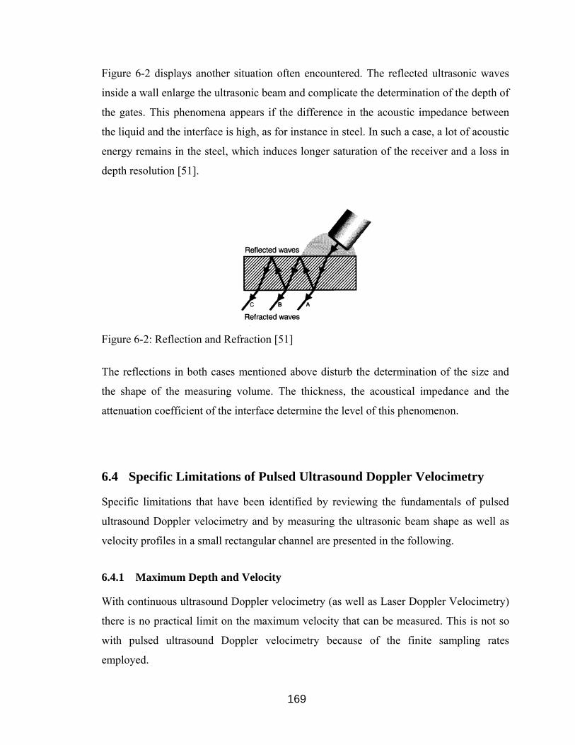
169
Figure 6-2 displays another situation often encountered. The reflected ultrasonic waves
inside a wall enlarge the ultrasonic beam and complicate the determination of the depth of
the gates. This phenomena appears if the difference in the acoustic impedance between
the liquid and the interface is high, as for instance in steel. In such a case, a lot of acoustic
energy remains in the steel, which induces longer saturation of the receiver and a loss in
depth resolution [51].
Figure 6-2: Reflection and Refraction [51]
The reflections in both cases mentioned above disturb the determination of the size and
the shape of the measuring volume. The thickness, the acoustical impedance and the
attenuation coefficient of the interface determine the level of this phenomenon.
6.4 Specific Limitations of Pulsed Ultrasound Doppler Velocimetry
Specific limitations that have been identified by reviewing the fundamentals of pulsed
ultrasound Doppler velocimetry and by measuring the ultrasonic beam shape as well as
velocity profiles in a small rectangular channel are presented in the following.
6.4.1 Maximum Depth and Velocity
With continuous ultrasound Doppler velocimetry (as well as Laser Doppler Velocimetry)
there is no practical limit on the maximum velocity that can be measured. This is not so
with pulsed ultrasound Doppler velocimetry because of the finite sampling rates
employed.
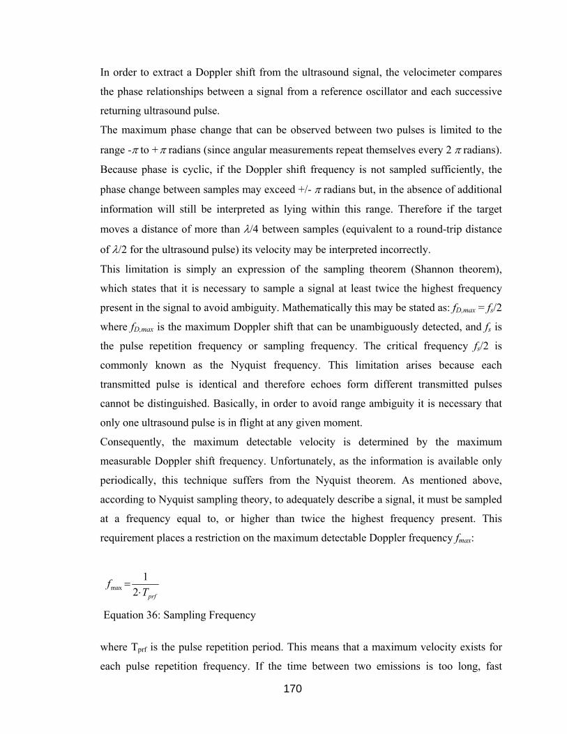
170
In order to extract a Doppler shift from the ultrasound signal, the velocimeter compares
the phase relationships between a signal from a reference oscillator and each successive
returning ultrasound pulse.
The maximum phase change that can be observed between two pulses is limited to the
range -π to +π radians (since angular measurements repeat themselves every 2 π radians).
Because phase is cyclic, if the Doppler shift frequency is not sampled sufficiently, the
phase change between samples may exceed +/- π radians but, in the absence of additional
information will still be interpreted as lying within this range. Therefore if the target
moves a distance of more than λ/4 between samples (equivalent to a round-trip distance
of λ/2 for the ultrasound pulse) its velocity may be interpreted incorrectly.
This limitation is simply an expression of the sampling theorem (Shannon theorem),
which states that it is necessary to sample a signal at least twice the highest frequency
present in the signal to avoid ambiguity. Mathematically this may be stated as: fD,max = fs/2
where fD,max is the maximum Doppler shift that can be unambiguously detected, and fs is
the pulse repetition frequency or sampling frequency. The critical frequency fs/2 is
commonly known as the Nyquist frequency. This limitation arises because each
transmitted pulse is identical and therefore echoes form different transmitted pulses
cannot be distinguished. Basically, in order to avoid range ambiguity it is necessary that
only one ultrasound pulse is in flight at any given moment.
Consequently, the maximum detectable velocity is determined by the maximum
measurable Doppler shift frequency. Unfortunately, as the information is available only
periodically, this technique suffers from the Nyquist theorem. As mentioned above,
according to Nyquist sampling theory, to adequately describe a signal, it must be sampled
at a frequency equal to, or higher than twice the highest frequency present. This
requirement places a restriction on the maximum detectable Doppler frequency fmax:
prfTf
⋅=
21
max
Equation 36: Sampling Frequency
where Tprf is the pulse repetition period. This means that a maximum velocity exists for
each pulse repetition frequency. If the time between two emissions is too long, fast

171
particles have moved too much to yield echoes that correlate. At the other extreme, slow
particles show no detectable displacements between two emissions if the repetition
frequency is too high. Substituting Equation 36 into the Doppler shift equation, the
maximum detectable velocity vmax will be:
prfe Tfcv
θcos4max =
Equation 37: Maximum Velocity
where c is the speed of sound, fe is the emitting frequency and θ the Doppler angle. To
some extent, the operator can increase vmax by choosing a low carrier frequency or a large
Doppler angel. To avoid range ambiguities, the signal must be received before the next
subsequent transmission, limiting the maximum value of the pulse repetition frequency.
If the measured velocity is higher than this maximum velocity, a phenomenon named
aliasing appears. In general, aliasing is the measurement of an incorrect or false frequency
(just as an alias refers to an assumed or false name). In Figure 6-4, the solid line
represents a sound wave with a period of T seconds and frequency f = 1/T Hertz. Let the
wave be sampled at intervals of Ts seconds corresponding to a sampling rate (sampling
frequency) of fs = 1/Ts. It can be seen from the figure that the selected sampling rate is too
low. The frequency would be incorrectly identified as that of the dashed line. Aliasing can
occur when fast Fourier transformation analyzers and other digital signal processing
instrumentation are used. If the measured noise contains frequency components above the
Nyquist frequency (half the sampling rate), then aliasing may occur. If those high-
frequency components are of interest to us, we must increase the sampling rate. In some
cases, high frequency signal components may result from electrical “noise” or other
artifacts. Low-pass anti-aliasing filters may be incorporated into fast Fourier
transformation and other analyzers to prevent spurious results due to high-frequency
signal components that we do not wish to measure [61].

172
Figure 6-3:Aliasing [61]
The problem of aliasing in pulsed wave Doppler systems arises because the Doppler shift
signal is reconstructed by determining the phase changes that occur between the returns
from each successive transmitted pulse. Aliasing is a phenomenon that appears when an
analog signal is sampled at a frequency which is lower than the half of its maximum
frequency (as described above). In such a situation, all Doppler frequencies above the half
of the sampling frequency (1/Tprf), the Nyquist frequency, are folded back in the low
frequency region. This phenomenon is called aliasing. In Figure 6-4 the effects of aliasing
encountered in pulsed ultrasound Doppler velocimetry is illustrated.
Figure 6-4: Aliasing Frequency Backfolding [51]
At point 1, the real Doppler frequency is below the Nyquist limit (Fprf/2), so the measured
frequency is equal to the real frequency. At point 2, the real Doppler frequency is much
above the Nyquist limit. Point 2 is then back folded to point 3, which gives negative
velocity. This negative frequency is equal to the real frequency from which the sampling
frequency is subtracted. For an analog signal it is possible to avoid aliasing by filtering
the signal before sampling it. The filter removes all the frequencies above the Nyquist

173
limit. Unfortunately for pulsed Doppler ultrasound only samples are available and
therefore it is not possible to remove the aliasing. The only solution is to adapt the
sampling frequency which is nothing but the pulse repetition frequency of the emitted
pulses. An easy way to check the presence of aliasing is to examine the evolution of the
measured Doppler frequency when the pulsed repetition frequency is changed.
The effect of aliasing in a directional pulsed Doppler ultrasound system (the incorrect
interpretation of frequencies above the Nyquist limit) is that as soon as the Doppler shift
frequency exceeds fs/2, it is interpreted as being –fs/2 and the top of the velocity profile
appears at the bottom of the reverse channel. This situation is shown in Figure 6-5.
Although the Doppler shift is normally interpreted as being between –fs/2 and +fs/2, it
may be interpreted as any other range of frequencies provided that the total range is only
fs.
0
2
4
6
8
10
12
14
16
-30 -25 -20 -15 -10 -5 0 5 10 15 20 25
Velocity [mm/s]
Cha
nnel
Dep
th [m
m]
Figure 6-5: Measured Aliasing
By changing the way in which the frequencies map onto the frequency scale (not a
change in the permissible frequencies), a shift in the frequency range may result in the
correct interpretation of the signal and therefore the correct velocity profile. If possible,
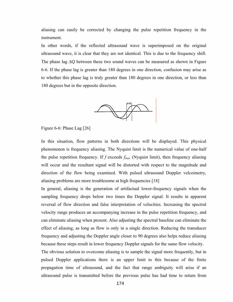
174
aliasing can easily be corrected by changing the pulse repetition frequency in the
instrument.
In other words, if the reflected ultrasound wave is superimposed on the original
ultrasound wave, it is clear that they are not identical. This is due to the frequency shift.
The phase lag ∆Q between these two sound waves can be measured as shown in Figure
6-6. If the phase lag is greater than 180 degrees in one direction, confusion may arise as
to whether this phase lag is truly greater than 180 degrees in one direction, or less than
180 degrees but in the opposite direction.
Figure 6-6: Phase Lag [26]
In this situation, flow patterns in both directions will be displayed. This physical
phenomenon is frequency aliasing. The Nyquist limit is the numerical value of one-half
the pulse repetition frequency. If f exceeds fmax (Nyquist limit), then frequency aliasing
will occur and the resultant signal will be distorted with respect to the magnitude and
direction of the flow being examined. With pulsed ultrasound Doppler velcoimetry,
aliasing problems are more troublesome at high frequencies [18]
In general, aliasing is the generation of artifactual lower-frequency signals when the
sampling frequency drops below two times the Doppler signal. It results in apparent
reversal of flow direction and false interpretation of velocities. Increasing the spectral
velocity range produces an accompanying increase in the pulse repetition frequency, and
can eliminate aliasing when present. Also adjusting the spectral baseline can eliminate the
effect of aliasing, as long as flow is only in a single direction. Reducing the transducer
frequency and adjusting the Doppler angle closer to 90 degrees also helps reduce aliasing
because these steps result in lower frequency Doppler signals for the same flow velocity.
The obvious solution to overcome aliasing is to sample the signal more frequently, but in
pulsed Doppler applications there is an upper limit to this because of the finite
propagation time of ultrasound, and the fact that range ambiguity will arise if an
ultrasound pulse is transmitted before the previous pulse has had time to return from
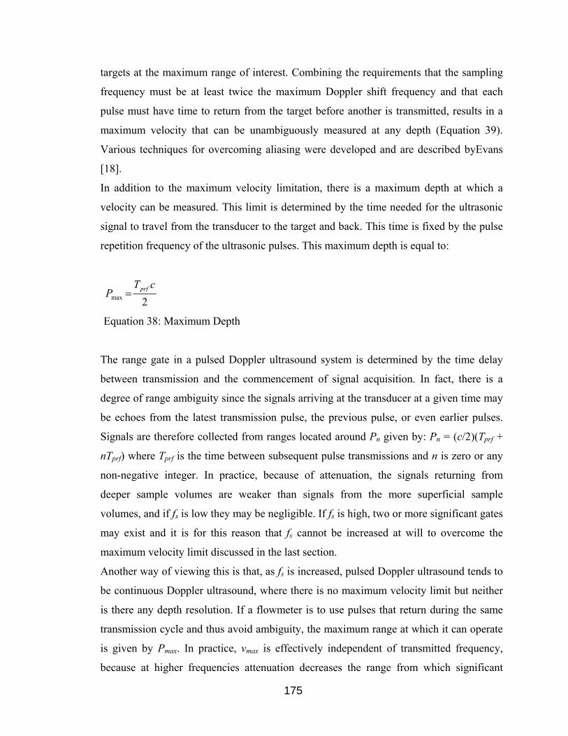
175
targets at the maximum range of interest. Combining the requirements that the sampling
frequency must be at least twice the maximum Doppler shift frequency and that each
pulse must have time to return from the target before another is transmitted, results in a
maximum velocity that can be unambiguously measured at any depth (Equation 39).
Various techniques for overcoming aliasing were developed and are described byEvans
[18].
In addition to the maximum velocity limitation, there is a maximum depth at which a
velocity can be measured. This limit is determined by the time needed for the ultrasonic
signal to travel from the transducer to the target and back. This time is fixed by the pulse
repetition frequency of the ultrasonic pulses. This maximum depth is equal to:
2max
cTP prf=
Equation 38: Maximum Depth
The range gate in a pulsed Doppler ultrasound system is determined by the time delay
between transmission and the commencement of signal acquisition. In fact, there is a
degree of range ambiguity since the signals arriving at the transducer at a given time may
be echoes from the latest transmission pulse, the previous pulse, or even earlier pulses.
Signals are therefore collected from ranges located around Pn given by: Pn = (c/2)(Tprf +
nTprf) where Tprf is the time between subsequent pulse transmissions and n is zero or any
non-negative integer. In practice, because of attenuation, the signals returning from
deeper sample volumes are weaker than signals from the more superficial sample
volumes, and if fs is low they may be negligible. If fs is high, two or more significant gates
may exist and it is for this reason that fs cannot be increased at will to overcome the
maximum velocity limit discussed in the last section.
Another way of viewing this is that, as fs is increased, pulsed Doppler ultrasound tends to
be continuous Doppler ultrasound, where there is no maximum velocity limit but neither
is there any depth resolution. If a flowmeter is to use pulses that return during the same
transmission cycle and thus avoid ambiguity, the maximum range at which it can operate
is given by Pmax. In practice, vmax is effectively independent of transmitted frequency,
because at higher frequencies attenuation decreases the range from which significant

176
echoes can be detected [18]. Some commercial pulsed Doppler ultrasound systems that do
not incorporate a continuous Doppler ultrasound facility attempt to overcome the problem
of measuring high velocities by deliberately increasing their pulse repetition frequency
beyond the maximum required to prevent range ambiguity. Doubling the pulse repetition
frequency will cause the device to monitor not only velocities at the depth of interest, but
also velocities at a depth which is in between the transducer and the depth of interest.
Continuing to increase the pulse repetition frequency will add more equally spaced
sample volumes between the transducer and initial depth of interest, but this often does
not present a problem as the higher velocities usually only occur at one point in the beam.
Reducing the sampling frequency (increasing Tprf) will increase the maximum measurable
depth, but will also reduce the maximum Doppler frequency that can be measured. The
maximum velocity and the maximum depth are thus linked according to the following
relation:
efcvP
8
2
maxmax =
Equation 39: Relation Maximum Depth and Velocity
This shows that the larger the velocity to be measured, the smaller the maximum
detectable depth. By using a suitable combination of basic ultrasound frequency,
measuring depth and inclination angles, pulsed ultrasonic Doppler velocimetry can be
adjusted to the problem at hand. The penetration length of the ultrasonic wave into the
fluid depends on the sound absorption of the fluid [29].
At any given instant, an echo signal can come from many different depths, corresponding
to echoes from previously emitted signals. The presence of several acoustic interfaces
also causes several reflections which could cause a false determination of the target depth.
Nevertheless, if the pulse repetition frequency is sufficiently low (a few kHz) the
attenuation of previously emitted pulses will render them indiscernible. The same goes
for reflected signals. With a large increase in the pulse repetition frequency, pulsed
Doppler ultrasound approaches the properties of continuous wave Doppler, with a loss of
axial resolution but no maximum velocity limitation.
177
Generally speaking the higher frequency ranges offer a higher spatial resolution and
higher velocity resolution than the lower. Thus high frequency use is ideal for small
geometries with small velocity range. 8 MHz is for instance a frequency that would be
selected to measure a blood flow. On the other hand the low frequencies allow higher
Doppler shift frequency detection corresponding to larger velocities and larger probing
distance. Moreover they have better propagation abilities through the measured liquid as
well as through walls when non-intrusive probing is required. In return lower frequency
means larger waveform and thus poorer spatial resolution, but because of larger
measurement volume in a higher velocities environment the flux of reflectors is increased
resulting in a higher sensitivity of the related transducer.
6.4.2 Spatial Versus Velocity Resolution
As mentioned earlier, a compromise between the length of the range area and the velocity
resolution must be made. If a short pulse is used, a small area is probed, but the pulse
spectrum and resulting velocity spectrum are wide and give a low velocity resolution, i.e.,
increasing the spatial resolution decreases the accuracy of the estimation of the Doppler
frequency. For a longer pulse the reverse is true, i.e., an accurate estimation of the target
velocity requires a narrow spectrum, and thus a long emitted pulse. Such an emission will
decrease the depth resolution. A long range gate is employed, and a narrow spectrum
evolves.
Unfortunately, it is impossible to increase the intensity of the emitted pulse beyond a
certain threshold with risking the appearance of unwanted phenomena such as cavitation.
If ultrasonic waves are focused into water, tiny bubbles will be produced, forming a
fractal structure and radiating sound by themselves as shown in Figure 6-7 [57]. This
phenomena is called acoustic cavitation.

178
Figure 6-7: Acoustic Cavitation [57]
Reducing the length of the emitted pulse will reduce the signal to noise ratio of the
Doppler signal if it is not possible to increase the intensity [51]. The duration of the
impulse determines the depth resolution by determining the longitudinal size of the
sample volume. The other dimensions are determined by the beam pattern of the
transducer.
The spectral resolution is also determined by the number of pulses used, as the bandwidth
of the narrow spectra is proportional to fprf/N. A long observation time, NTprf, yields a
small bandwidth.
Velocity resolution not only depends on the length of the range area, but also on the time
resolution of the ultrasound system. Especially in the case of turbulence and gross
disturbances, time resolution is essential.
6.4.3 Focused Transducer Limitations
Different architectures of focused transducers are described in detail in chapter 3.4. In
pulsed wave Doppler systems, accurate frequency measurements require minimal spectral
broadening. Highly focused beam patterns can cause excessive spectral broadening [44],
which is discussed in detail in chapter 2.6.6.
Spectral broadening can be understood physically from two equivalent viewpoints, one
considering the Doppler signals received with a finite array aperture and the other
considering the time of flight of the scatterers through the focused beam. With a finite
aperture transducer, each portion of its front (or each element in a multi-element array)
has a different Doppler angle with the direction of flow and a different detected Doppler
shifted frequency. The larger the aperture, the greater the spread of Doppler angles and
detected Doppler shifted frequencies. Or, the finite time of flight through the narrowest

179
beam width leads to a commensurate uncertainty in the measured Doppler shifted
frequency. The stronger the focus, the smaller the spot size and the larger the frequency
uncertainty.
There are limitations on focal lengths for transducers of particular frequency and element
diameter combinations and target designations. According to Papdakis, the maximum
practical focal length for a point target focal designation is 0.8 multiplied with the near
field length due to spectral broadening [44]. Transducers with focal lengths beyond these
maximums, but less than the near field are called weakly focused units. In other words,
there may not be an advantage to a focused transducer over that of a flat transducer. In
addition to the limitations on maximum focal lengths, there are limitations on the
minimum focal lengths. These limitations are typically due to the mechanical limitations
of the transducer.
Theoretically, ultrasonic beams can be strongly focused and beam widths smaller than 0.1
millimeter can be achieved [51]. In the case of focused single element transducers, the
theoretical limit depends on the material of the lens and the side effect. The side effect
simply describes the fact that the piezoelectric element never vibrates in one mode. Other
modes exist and the vibration is never in a pure “piston” mode. Therefore, the emitted
ultrasonic waves are not exactly plane waves, especially at the border (side) of the
transducer.
For single element transducers, the theoretical focal length depends on the diameter of the
piezoelectric element. For example, larger diameter piezoelectric elements lead to a small
focal zone. The measured focal length of a transducer is dependent on the material in
which it is being measured. This is due to the fact that different materials have different
sound velocities. When specifying a transducer’s focal length it is typically specified for
water. Since most materials have a higher velocity than water, the focal length is
effectively shortened. This effect is caused by refraction (according to Snell’s Law) and
must be considered to obtain more accurate measurement results.
In addition, the curvature of the surface of the test piece can affect focusing. Depending
on whether the entry surface is concave or convex, the sound beam may converge more
rapidly than it would in a flat sample or it may spread and actually defocus.

180
Focused immersion transducers use an acoustic lens to effectively shift the location of the
focal point toward the transducer face. The end result can be a dramatic increase in
sensitivity.
6.4.4 Doppler Angle
A general limitation of ultrasound Doppler velocimetry is that flow perpendicular to the
beam is not detected and finding the velocity direction can, in some cases, be
problematic. It must always be considered that the velocity profile is measured along the
ultrasonic beam axis and not perpendicular to the flow. Especially in the presence of
recirculation regions or other gross disturbances, this may lead to distortions of the
measured velocity profile. Since the Doppler angle must generally be decreased to avoid
perturbations in the measured velocity profile or to increase the velocity component in
direction of the ultrasonic beam (to obtain more accurate measurement results for
example of the maximum velocity), these distortions may be severe. Refraction, as
mentioned in section 6.3, may even facilitate this distortion.
Another limitation to further decreasing the Doppler angle is the angle of total reflection.
Setting the Doppler angle smaller than the critical angle allows one to use only the
transverse wave for the measurement. In fluids, only longitudinal waves exist, but in
solids, even at small incident angles, another mode of ultrasonic wave called transverse
wave exists (see section 2.6). For example, part of the longitudinal wave is converted into
the transverse wave at the outer surface of the Plexiglas wall. This transverse wave is
sufficient to measure the velocity in the sample volume.
6.4.5 Distance Offset
Another general limitation of pulsed ultrasound Doppler velocimetry is the distance offset
along the ultrasonic beam axis caused by the ultrasonic transducer (depending on the
spatial filter) and by acoustic interfaces with different values for the speed of sound
encountered by the ultrasonic beam (as described in section 4.4.1, 5.5.3 and 5.5.5). Exact
calculations of the distances displayed by the instrument are therefore necessary in
advance to correctly interpret the measured velocity profile. Refraction may moreover
cause a distance offset along the axis in direction of the flow.
181
6.4.6 Ringing Effect and Saturation Region
The transducer’s ringing effect and the saturation region caused by the transducer’s
acoustic ringing or highly absorbing acoustic interfaces impedes measurements close to
the transducer face or close to the highly absorbing acoustic interfaces (as described in
chapter 4.2). The ringing effect (saturation region) can only be decreased by decreasing
the amplification or decreasing the emitted ultrasonic power. This might not be possible,
when measuring the velocity profile behind highly absorbing acoustic interfaces or in
highly absorbing media. If the amplification or emitted power is decreased beyond a
certain minimal value, the intensity of ultrasonic echoes from scatterers inside the sample
volume may be too low to be received by the transducer.
6.4.7 Ultrasound Scatterers
Ultrasound Doppler velocimetry requires some amount of reflection particles suspended
in the liquid, which may disturb its flow or change its fundamental properties.
Nevertheless, due to attenuation and reflection, upper limits of particle concentration exist
(e.g., 50 percent in blood, 30 percent in mud). If the particle concentration is too low, the
received echo may be too weak and measurement results may easily be perturbed or
falsified by slight variations in the liquid.
The ultrasonic waves generated by the transducer are more or less confined in a narrow
cone. As they travel in this cone they may be reflected or scattered when they touch a
particle having different acoustic impedance. The scatterers are assumed to be in the far
field, so that the waves emitted by the transducer are planar when they impinge on the
reflector. If the size of the particle is bigger than the wave length, the ultrasonic waves are
reflected and refracted by the particle. In such a case the direction of propagation and the
intensity of the ultrasonic waves are affected. But if the size of the particle is much
smaller than the wave length another phenomenon appears, which is named scattering. In
such a case, a very small amount of the ultrasonic energy is reflected in all directions. The
intensity and the direction of propagation of the incoming waves are practically not
affected by the scattering phenomena. Thus, the transducer also receives a plane wave. In
ultrasound Doppler velocimetry particles smaller than the wavelength are therefore
required.

182
Particles in the presence of a sound field will experience forces associated with the
acoustic wave field which may falsify measurement results. The acoustic radiation
pressure is customarily interpreted as the time-averaged pressure acting on an object in a
sound field, which results in a unidirectional force that moves the object [22]. It is exactly
this movement of the object which is important for the accuracy of measurement results
with pulsed ultrasound Doppler velocimetry. Since in pulsed ultrasound Doppler
velocimetry the shift in position of suspended objects in the sample volume is measured,
i.e., the movement of these suspended objects, any movement enforced by the acoustic
wave may falsify the measurement results. This limitation has to be further investigated
in future research.
Having identified the limitations of pulsed ultrasound Doppler velocimetry based on
reviewing the fundamentals of the methods and on measuring the actual beam shape, the
echo intensity and the velocity in small channels, suggestions for improvement and future
research are given Chapter 7.

183
7 Suggestions for Improvement and Future Research
Based on the fundamentals of pulsed ultrasound Doppler velocimetry, on the
measurements of ultrasonic beam shapes and velocity profiles in the flow over a
backward facing step in a small rectangular channel and on the limitations of pulsed
ultrasound Doppler velocimetry presented in Chapter 6 suggestions for improving the
measurement system and for future research are made in the following. The ultrasonic
transducer has been identified as the most critical component of the measurement system
in Section 2.5. To improve especially the spatial resolution of the measurement system, it
is suggested to use annular phased array transducers and modify the measurement system
accordingly. Through electronic focusing, ultrasonic beam steering and automatic
variations in the aperture size, annular phased array transducers enhance the spatial
resolution of the system significantly. Research on a new ultrasonic transducer
architecture combining the advantages of standard pulsed ultrasound Doppler velocimetry
and the ultrasound phased array technique is therefore crucial. The necessity of future
research on the interaction between acoustic waves and acoustic interfaces encountered
by the ultrasonic beam and suspended objects in the flow is emphasized in the following
sections. A literature review on the interaction of acoustic waves with cylindrical and
spherical objects is then undertaken in Section 7.3 to frame future research in this area.
7.1 Transducer Architecture
The ultrasonic transducer has been identified as the most critical component of the
measurement system. The main suggestion for improving pulsed ultrasound Doppler
velocimetry therefore is to combine the advantages of standard pulsed ultrasound Doppler
velocimetry systems (e.g., real time velocity profile determination) with the advantages of
the ultrasound phased array technique (e.g., dynamic beam control, dynamic depth
focusing, … described in detail in Section 3.2.2) and enhance the measurement system
accordingly (e.g., allow for dynamic focusing, …). Therefore, detailed research on the
most appropriate transducer and system architecture is essential.
184
Most of the applications of the ultrasound phased array technique are currently in the area
of ultrasonic testing of components and structures and nondestructive materials
characterization. Using the ultrasound phased array technique for the determination of
velocity profiles in fluid flow would requires further processing the incoming ultrasonic
echo (e.g., dynamic focusing, …). After consultation with the head probe designer of R/D
TECH, using the ultrasound phased array technique for the determination of velocity
profiles in fluid flow is generally feasible.
According to R/D TECH (www.rd-tech.com), ultrasonic phased array transducers are in
the price range of 10,000 to 15,000 US-Dollars. A portable ultrasonic phased array
system would be in the price range of 60,000 to 100,000 US-Dollars. Prices ultimately
depend on the application and specific requirements (e.g., transducer diameter, number of
annular elements, shape of piezoelectric element, level of damping (of piezoelectric
element), transducer housing specifications, system electronics, …). Nevertheless, the
ultrasonic phased array transducer technique is significantly more expensive than
standard pulsed ultrasound Doppler velocimetry (prices of standard pulsed ultrasound
Doppler velocimetry and experimental setup are given in Appendix F, Table F-1). This is
especially due to the required dynamic focusing technique in phased array systems.
Annular phased array systems, but also phased array systems in general, consist of small
piezoelectric elements. Another feature besides dynamic focusing, beam steering etc. of
small piezoelectric elements is their energy transfer efficiency (as described in detail in
Section 3.2.2). Smaller elements take less energy to excite and are more efficient
receivers due to the lower mass to be energized. Lower energy consumption is crucial
when measuring over longer distances or through highly absorbing media (e.g., paper
forming screens).
To further improve the spatial resolution of pulsed ultrasound Doppler velocimetry
especially when dealing with small geometries (small channels or capillaries), it is
suggested to investigate the feasibility of emitting frequencies higher than 8 MHz. Higher
emitting frequencies lead to improved axial and also lateral resolutions (at a given
transducer radius, the beam width decreases with decreasing wavelength). Absorption of
the emitted ultrasonic signal will increase with higher ultrasonic frequencies. Since
suggestion to improve pulsed ultrasound Doppler velocimetry to measure velocity
profiles in especially small channels and capillaries are developed, higher absorption is
185
not vitally important. Improved axial resolution (shorter ultrasonic burst length) will also
be beneficial to minimize the wall effect.
To further minimize the wall effect, but also to minimize the saturation region and
maximize the measurable minimal distance, damping of the piezoelectric element and
therefore minimizing of the transducer’s ringing must be improved.
7.2 Interaction of Acoustic Waves with Forming Screens
On the one hand, the ultrasonic beam shape was determined in chapter 4 to identify the
most appropriate transducer to measure velocity profiles in small channels and capillaries.
On the other hand, results of the ultrasonic beam shape measurements will be used to
evaluate the possibility of applying pulsed ultrasound Doppler velocimetry to measure the
velocity through porous screens, i.e., paper forming screen.
7.2.1 Forming Screen Properties
To evaluate the interaction of acoustic waves with the forming screen, its acoustic
properties must precisely be determined (e.g., acoustic impedance, pore shape factor,
tortuosity, etc.). Numerical simulations with the Lattice Boltzmann method of the
propagation of an acoustic wave through the forming screen may also be useful to further
investigate the effect of the forming screen on the ultrasonic beam.
Moreover, laboratory experiments to optimize the acoustic-wire impedance matching are
essential to improve the signal to noise ratio. Other reports show that the main problem is
the power required to run the system. Once the laboratory experiments are complete, the
information to make conclusions about the required power consumption is available. The
feasibility of using the ultrasonic phased array technique instead of standard pulsed
ultrasound Doppler velocimetry may then be evaluated.
7.2.2 Modification Existing Experimental Setup
In order to investigate the possibility of using pulsed Doppler ultrasound velocimetry to
measure the velocity profile of watery pulp through the forming board and the forming
screen, the experimental setup described in chapter 3 is modified. The fluid leaving the

186
channel flows over a forming screen. The forming screen will be mounted on the steps in
both side walls of the section attached to the channel (Figure 7-1). Various ultrasonic
transducers are then used to measure the velocity profile through the forming screen.
Outcome of this research will be the information, if and how pulsed Doppler ultrasound
velocimetry can be used for this application.
Figure 7-1: Modified Experimental Setup
7.2.3 General Effect of Moving Interfaces
After pulsed Doppler ultrasound velocimetry has been successfully used to measure
velocity profiles through stagnant forming screens, the effect of moving interfaces (e.g.,
moving forming screens as encountered in paper machines) must be investigated.
As the ultrasonic waves propagate, they encounter different structures which may create
strong echoes (e.g., Plexiglas, forming screen). Furthermore, some of these structures
may themselves be moving (e.g., forming screen). Despite of the many reflections which
are necessary to reach the transducer, the energy reflected by these interfaces is often
stronger than the energy coming from the particles flowing with the liquid. When some
interfaces are in movement, the correct estimation of the velocity field is more difficult.
The echoes generated by such interfaces may affect the velocity profile in some places
due to the combination of many reflections. The Doppler frequency induced by these
movable interfaces can not be removed if their values are the same as the values of the
flowing particles. If their values are different, the echo signal may contain a certain
number of stationary and quasi-stationary echoes of low frequency and high intensity, as
well as the echoes from the particles within the fluid at higher frequencies but of smaller
intensities. The difference between the intensities of these two types of signals may be 20
187
to 60 dB. For the case of moving flow boundaries, the velocity of the wall creates a
Doppler effect which must be filtered out. These low frequency components may be
eliminated by the wall motion filter. Unfortunately, this high-pass filter also diminishes
the intensities of the already weak Doppler signals coming from the particles within the
fluid [51].
Moving screens also represent moving free surfaces and are therefore more like to
introduce perturbations in the velocity profile as can be seen in Figure 5-14. Moreover,
moving screens will lead to significant spectral broadening.
Besides the effect of large scale acoustic interfaces (e.g., Plexiglas walls, forming screens,
etc.) on the ultrasonic wave packet, its interaction with the suspended objects (particles or
fibers) in the fluid must be investigated. Especially since the acoustic wave packet, or
acoustic waves in general, exert forces on the suspended objects, this interaction and its
effect on the measurement results must be investigated.
7.3 Interaction of Acoustic Waves with Suspended Objects
When evaluating the effect of acoustic waves on the accuracy of the measurement results
in pulsed Doppler ultrasound velocimetry, an investigation of the dynamics of the
acoustic wave interaction with suspended objects in the sample volume is crucial. An
object in the presence of a sound field will experience forces associated with the acoustic
wave field which may falsify measurement results.
The so called acoustic radiation force is the time-average force exerted by an acoustic
field on an object (“target”) or on a boundary surface. In scientific practice it occurs as an
unintentional effect under various circumstances. So far, its importance lies in its
intentional and quantitative use for which at least three main areas can be identified,
namely: (a) The radiation force on a balance and serving as a measure of the ultrasonic
power; (b) the radiation force on a small target as measured by a sphere radiometer and
serving as a measure of the ultrasonic intensity; (c) the radiation force on small liquid and
solid samples for purpose of separation techniques and for levitation and positioning
purposes, with the aim of a containerless processing [11].
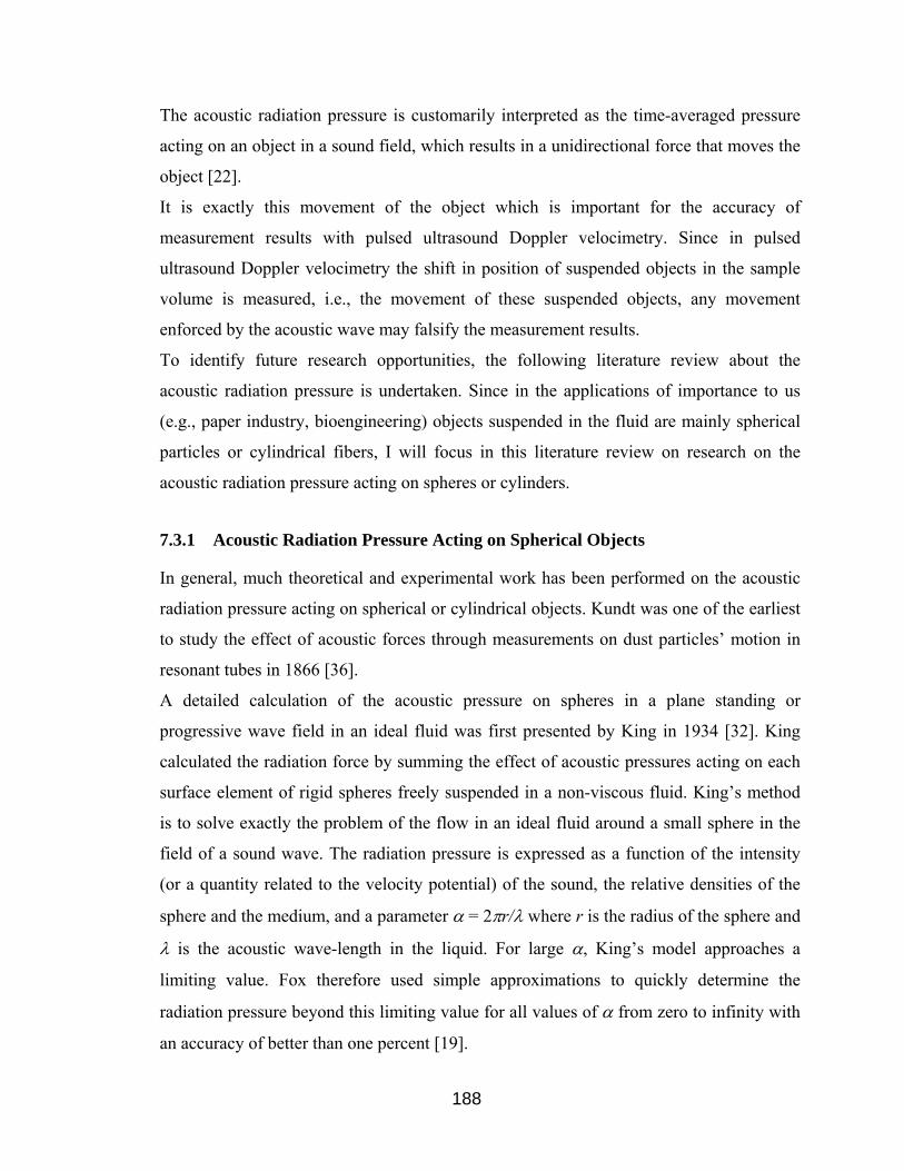
188
The acoustic radiation pressure is customarily interpreted as the time-averaged pressure
acting on an object in a sound field, which results in a unidirectional force that moves the
object [22].
It is exactly this movement of the object which is important for the accuracy of
measurement results with pulsed ultrasound Doppler velocimetry. Since in pulsed
ultrasound Doppler velocimetry the shift in position of suspended objects in the sample
volume is measured, i.e., the movement of these suspended objects, any movement
enforced by the acoustic wave may falsify the measurement results.
To identify future research opportunities, the following literature review about the
acoustic radiation pressure is undertaken. Since in the applications of importance to us
(e.g., paper industry, bioengineering) objects suspended in the fluid are mainly spherical
particles or cylindrical fibers, I will focus in this literature review on research on the
acoustic radiation pressure acting on spheres or cylinders.
7.3.1 Acoustic Radiation Pressure Acting on Spherical Objects
In general, much theoretical and experimental work has been performed on the acoustic
radiation pressure acting on spherical or cylindrical objects. Kundt was one of the earliest
to study the effect of acoustic forces through measurements on dust particles’ motion in
resonant tubes in 1866 [36].
A detailed calculation of the acoustic pressure on spheres in a plane standing or
progressive wave field in an ideal fluid was first presented by King in 1934 [32]. King
calculated the radiation force by summing the effect of acoustic pressures acting on each
surface element of rigid spheres freely suspended in a non-viscous fluid. King’s method
is to solve exactly the problem of the flow in an ideal fluid around a small sphere in the
field of a sound wave. The radiation pressure is expressed as a function of the intensity
(or a quantity related to the velocity potential) of the sound, the relative densities of the
sphere and the medium, and a parameter α = 2πr/λ where r is the radius of the sphere and
λ is the acoustic wave-length in the liquid. For large α, King’s model approaches a
limiting value. Fox therefore used simple approximations to quickly determine the
radiation pressure beyond this limiting value for all values of α from zero to infinity with
an accuracy of better than one percent [19].

189
Since the work on the acoustic radiation force on a rigid sphere in an axisymmetric wave
field by King in 1934, the radiation force on a sphere with different properties in different
wave field has been reported. Extending and elaborating King’s approach, the radiation
force on a rigid sphere in a progressive, diverging spherical or cylindrical wave field was
reported by Embleton in 1954 [17]. Yosioka and Kawasima extended this method to
include the effects of a compressible sphere, i.e., to calculate the radiation force on fluid
spheres suspended freely in a plane traveling wave or plane standing wave [66].
According to their theory, the radiation force on a spherical particle in the stationary
standing-wave field is proportional to the wavenumber, the ultrasound energy density and
the cube of the particle radius. The radiation force on a fluid sphere in a plane traveling
wave was later reported again by Maidanik in 1957 [39]. The special case of a rigid
sphere in a plane traveling wave was reported by Maidanik and Westervelt in 1957 [40].
Gor’kov, using a different approach than King, derived a simple method to determine the
forces acting on a particle in an arbitrary acoustic field in 1962 [21]. The force on a small
sphere was expressed as a function of mean square fluctuations of the pressure and
velocity at the point where the particle is located. Gorkov derived an expression for the
potential of the acoustic force that acts on a small spherical particle in an arbitrary
acoustic field in an ideal fluid. He showed that his expression was equivalent to King’s in
the case of a plane standing wave.
Nyborg also derived simple expression for the acoustic force on a small rigid sphere in an
axisymmetric wave by extending the methods of King and Embleton in 1967 [42]. He
expressed the radiation force as a function of spatial gradients of potential energy density
and kinetic energy density, and suggested that only the field in the vicinity of the sphere
needs to be axisymmetric. In the case of standing waves, Nyborg’s expression reduced to
that of Gor’kov.
In 1969, Hasegawa et al. [24] developed a theory for the acoustic radiation pressure
acting on an elastic sphere in a plane progressive sound field, which includes the solution
for elastic spheres with complex wave speeds later used for calibration of plane-wave
fields [23]. Since then, the subject of the radiation pressure on spheres has been
extensively studied [9, 37, 38, 48, 62]. Barmatz and Collas applied the method of
Gor’kov for deriving the acoustic radiation potential on a sphere in an arbitrary sound
field. Generalized potential and force expression are derived for arbitrary standing wave

190
modes in rectangular, cylindrical and spherical geometries for the case where the sphere
radius is much smaller than the wavelength. The developed expressions were analyzed
primarily for a rigid sphere but are also applicable to the general case of samples with
arbitrary density and compressibility. A general expression for the acoustic radiation
force on a small compressible sphere in a focused beam has been derived and expressed
in terms of the time-averaged densities Ti and Vi of kinetic and potential energies,
respectively, in the incident sound field by Wu and Du in 1990 [62]. The results have
been applied to two focused beams: Gaussian beams and piston beams. The effect of
viscosity and surface tension on radiation force due to a plane traveling or standing wave
were discussed by Lofstedt and Putterman in 1991 [38]
In most of the studies cited above, a plane incident wave was used due to its simplicity.
For the nonplanar incident wave only the rigid sphere has been studied. Various
approximations are used by different authors. In 1996, Chen and Apfel unify the various
treatments of the radiation force on an elastic sphere (which includes other types of
sphere as limiting cases) and provide a general formulation suitable for any
axissymmetric incident wave, regardless of the size of the sphere [14]. The sphere is
described in general by its density, compressional wave speed and shear wave speed.
Other types of spheres, including the rigid and immovable sphere and the infinitely soft
sphere (void), are treated as limiting cases. Specialized formulations of the radiation force
function are provided for several types of incident waves of common interest. A low-
frequency expansion for each case is provided for comparison with results form the
literature.
Yasuda and Kamakura correlated predictions made by the theory of the acoustic radiation
force as proposed by Yosioka and Kawasima with actual experimental data in 1997 [65].
They measured the radiation force on micrometer-sized polystyrene spheres through
observation of the sphere’s microscopic movement in a 500 kHz ultrasonic standing
wave.
7.3.2 Acoustic Radiation Pressure Acting on Cylindrical Objects
Very little is known about the acoustic radiation force on a small-diameter rigid cylinder,
although the subject of the radiation pressure on spheres has been extensively studied.
191
Awatani [6] and Hasegawa [22] have derived numerical results for acoustic radiation
forces on rigid and elastic cylinders in a plane progressive sound field. Simple and
general analytical expressions for the acoustic radiation force of any acoustic field, that is
symmetrical about its axis, on a rigid cylinder, whose diameter is much smaller than the
wavelength of the sound wave and whose axis is perpendicular to the wave propagation,
are derived by Wu et al. in 1990 [63]. Wu et al. follow King and Nyborg’s approach to
derive acoustic radiation forces on the rigid cylinder. Results are expressed in terms of the
time-averaged densities of kinetic and potential energies of the incident sound field. They
show that for the case of a standing wave field, the theoretical results agree well with the
experimental observations of the acoustic radiation force exerted on a glass microneedle
in a standing-wave field of megahertz frequency.
The radiation force-per-length on an infinitely long circular, compressible cylinder in an
acoustic plane standing wave is expressed in terms of partial-wave scattering coefficients
for the corresponding traveling wave scattering problem by Wei, Thiessen and Marston in
2004 [58]. This information allows a dimensionless radiation force function to be
expressed using coefficients available from two-dimensional scattering theory. Wei et al.
also examine a long-wavelength approximation for the force, which is analogous to one
for the radiation force on compressible spheres giaven by Yosioka and Kawasima [66].
7.3.3 Acoustic Radiation Pressure Acting on Shells
Hasegawa et al. [22] theoretically investigate the acoustic radiation pressure resulting
from a plane wave incident on spherical shells and cylindrical shells immersed in a fluid
in relation to the thickness of the shell and the contents of the hollow region in 1988. The
spherical and cylindrical shell is placed freely in a plane progressive sound field in a
nonviscous fluid. Numerical calculations showed that the differences between the
frequency dependence of the acoustic radiation pressure on spherical shells and that on
cylindrical shells are more remarkable than those between spheres and cylinders.

192
8 Conclusion
Based on a review of the fundamentals of pulsed ultrasound Doppler velocimetry, on the
measurements of ultrasonic beam shapes of focused and unfocused ultrasonic transducers
emitting ultrasonic wave packets at different ultrasonic frequencies and on the
measurements of velocity profiles in the flow over a backward facing step in a small
rectangular channel (small compared to the transducer diameter), the limitations of pulsed
ultrasound Doppler velocimetry have been determined. Moreover, suggestions to improve
the measurement system and its spatial resolution have been made. Future research to
enhance pulsed ultrasound Doppler velocimetry has been framed.
The accuracy of the measured velocity field mainly depends on the shape of the acoustic
beam through the flow field and the intensity of the echo from the incident particle where
the velocity is being measured. With ultrasonic beam measurements the actual beam
shape and echo intensity was investigated to select the most promising transducer to
measure the velocity in small channels. The 8 MHz 5 mm ultrasonic transducer was
identified to be the most promising single element transducer due to its excellent spatial
(lateral and axial) resolution. Since application of pulsed ultrasound Doppler velocimetry
for measurements often involves the propagation of the emitted acoustic field and the
returning echo through a Plexiglas wall, the effect of Plexiglas walls on the measured
velocity profile has been analyzed and quantified in detail. The distance offset displayed
in the instrument, which is caused by the Plexiglas wall, and the echo intensity reduction
has been determined. To minimize the effect of Plexiglas walls, wall corrections based on
the calculated distance offset are introduced. Evaluating the effect of porous screens
(forming screens), the 4 MHz 8 mm focused ultrasonic transducer turned out to be most
promising single element transducer to measure velocity profiles closely behind highly
absorbing porous screens. In general, the shape of the ultrasonic beam varies depending
on the frequency and diameter of the emitter as well as the characteristics of the acoustic
interfaces that the beam encounters.
By comparing measurement results in a small rectangular channel characterized by a
backward facing step to numerically calculated results, further limitations of the method
have been identified. It was not possible to determine velocities correctly throughout the

193
whole channel at low flow rates, in small geometries and in flow separation regions. A
discrepancy between the absolute value and position of the maximum measured velocity,
broadening of the velocity profile, various distance offsets displayed in the instrument,
perturbations in the velocity profile and wrong velocity determination at the far channel
wall and in the recirculation region were main shortcomings. Measurement results have
been improved by changes in the Doppler angle, the flow rate, the particle concentration
and the use of focused ultrasonic transducers (when compared to unfocused transducers).
The effect of Plexiglas walls on the measurement results has been quantified and
minimized by correcting the position of the first sample volume.
Analyzing the fundamentals of the method and working structure of the instrument
revealed limitations in the measurable maximum velocity due to aliasing, in the
measurable maximum depth due to frequency dependent absorption of ultrasound, in the
spatial resolution due to emitting frequency constraints, in the time resolution due to
spectral broadening as well as in the appropriate amount of ultrasound scatterers. After
having measured the ultrasonic beam shape of various transducers with and without walls
and porous screens, the transducer’s ringing effect and the saturation region caused by
highly absorbing acoustic interfaces have been identified as further limitations that
restrict measurements close to the transducer face or close to highly absorbing acoustic
interfaces. Evaluation of measured velocity profiles in a small rectangular channel (small
compared to the transducer diameter) revealed further fundamental limitations concerning
the measurement of the velocity component along the ultrasonic beam axis (inclined by
the Doppler angle), the appropriate amount of ultrasound scatterers, the displayed
distances, the velocity determination close to the far wall and the right selection of the
Doppler angle.
Nevertheless, pulsed ultrasound Doppler velocimetry turned out to be a feasible method
for quantitatively determining velocity profiles in small channels (compared to the
transducer diameter). Especially when dealing with flow at low velocities in small
channels and flow separation, pulsed ultrasound Doppler velocimetry revealed several
limitations. The ultrasonic transducer turned out to be the most critical component of the
ultrasonic system. It determines the frequency of ultrasound, the sensitivity of the
velocimeter and the achievable spatial resolution. To improve especially the spatial
resolution, it is suggested to use annular phased array transducers and modify the
194
measurement system accordingly. Through electronic focusing, ultrasonic beam steering
and automatic variations in the aperture size, annular phased array transducers enhance
the spatial resolution of the system significantly. Research on a new ultrasonic
architecture combining the advantages of standard pulsed ultrasound Doppler velocimetry
and the ultrasound phased array technique is essential. The necessity of future research on
the interaction between acoustic waves and acoustic interfaces encountered by the
ultrasonic beam and suspended objects in the flow is emphasized. A literature review on
the interaction of acoustic waves with cylindrical and spherical objects has been
undertaken to frame future research in this area in order to enhance pulsed ultrasound
Doppler velocimetry for accurate measurement of velocity profiles especially in small
channels and capillaries.
195
Appendix A: Technical Drawings Experimental Setup
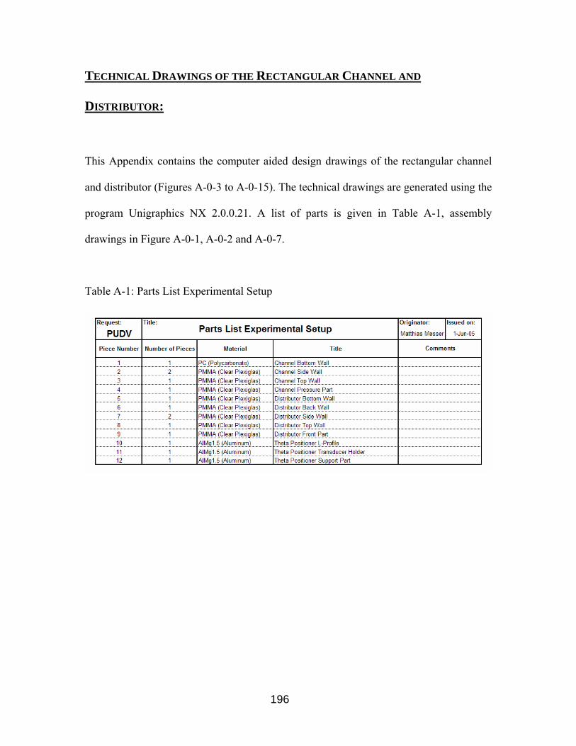
196
TECHNICAL DRAWINGS OF THE RECTANGULAR CHANNEL AND
DISTRIBUTOR:
This Appendix contains the computer aided design drawings of the rectangular channel
and distributor (Figures A-0-3 to A-0-15). The technical drawings are generated using the
program Unigraphics NX 2.0.0.21. A list of parts is given in Table A-1, assembly
drawings in Figure A-0-1, A-0-2 and A-0-7.
Table A-1: Parts List Experimental Setup

197
Assembly Drawing Experimental Setup:
Figure A-0-1: Assembly Drawing Experimental Setup
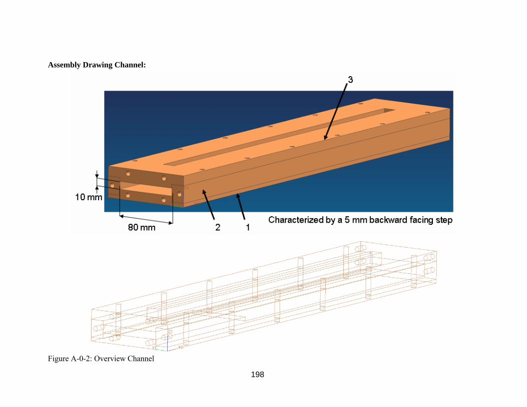
198
Assembly Drawing Channel:
Figure A-0-2: Overview Channel
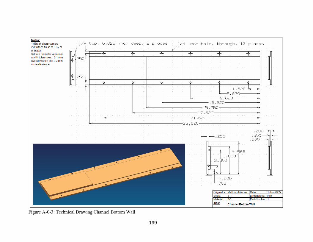
199
Figure A-0-3: Technical Drawing Channel Bottom Wall
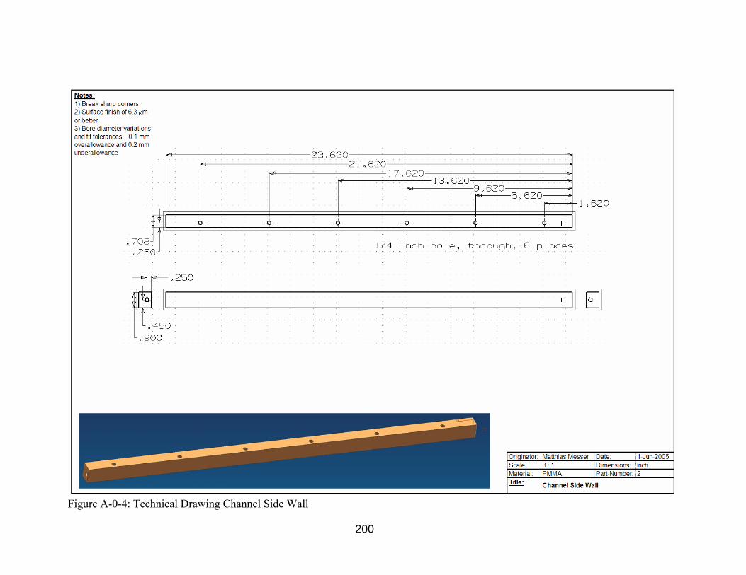
200
Figure A-0-4: Technical Drawing Channel Side Wall
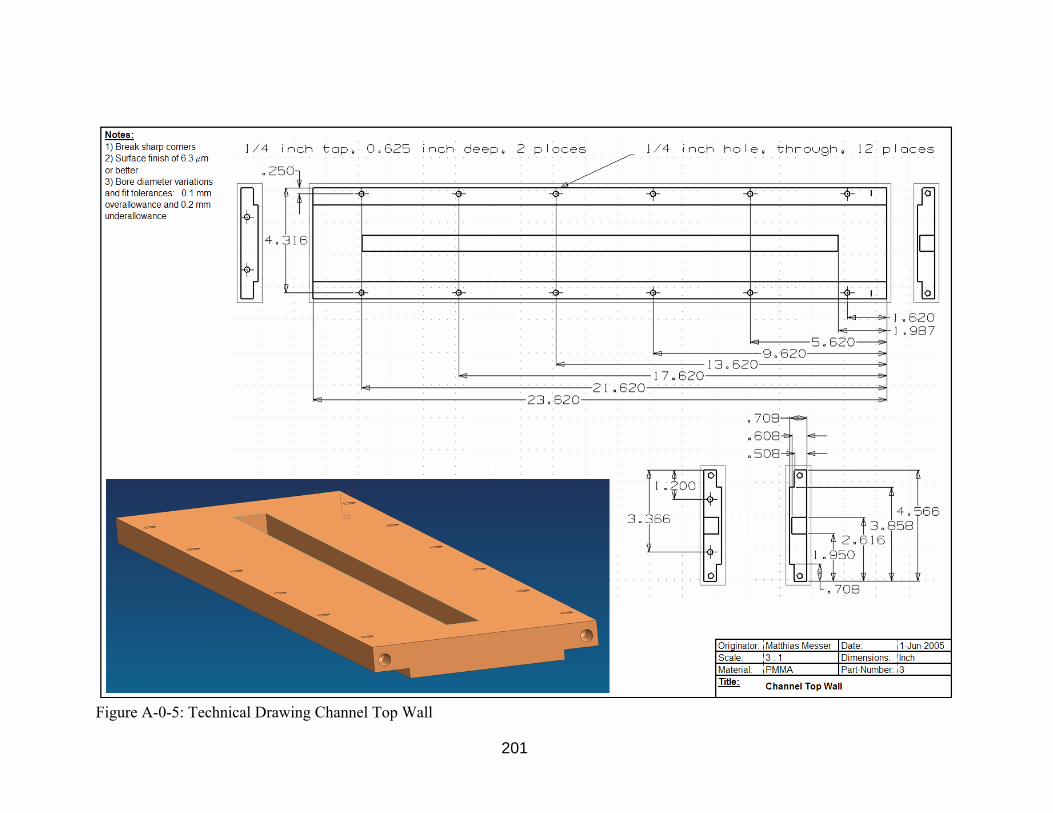
201
Figure A-0-5: Technical Drawing Channel Top Wall
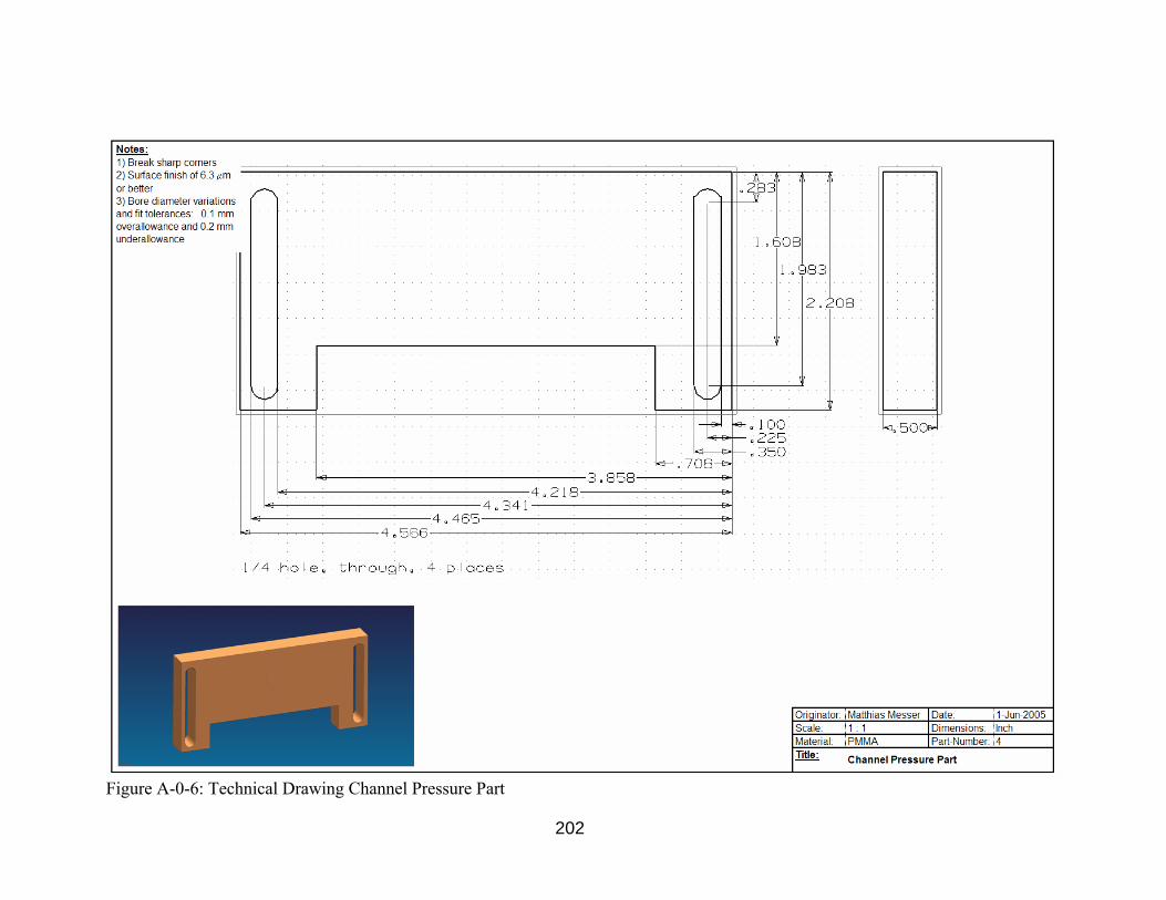
202
Figure A-0-6: Technical Drawing Channel Pressure Part
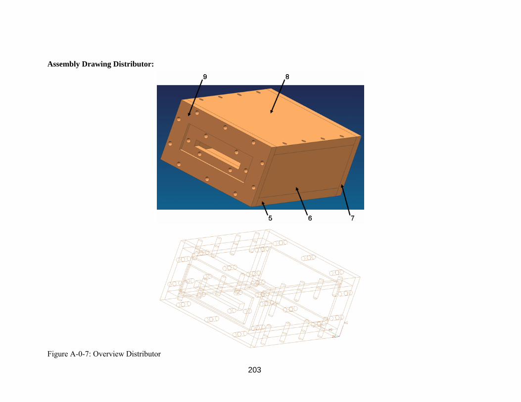
203
Assembly Drawing Distributor:
Figure A-0-7: Overview Distributor

204
Figure A-0-8: Technical Drawing Distributor Bottom Wall

205
Figure A-0-9: Technical Drawing Distributor Side Wall

206
Figure A-0-10: Technical Drawing Distributor Back Wall

207
Figure A-0-11: Technical Drawing Distributor Top Wall

208
Figure A-0-12: Technical Drawing Distributor Front Part

209
TECHNICAL DRAWINGS OF MOUNTING PARTS
Technical Drawings of Mounting Parts required to attach a theta-positioner to the top channel
wall are presented in the following. These parts can be seen in Figure 5-3.
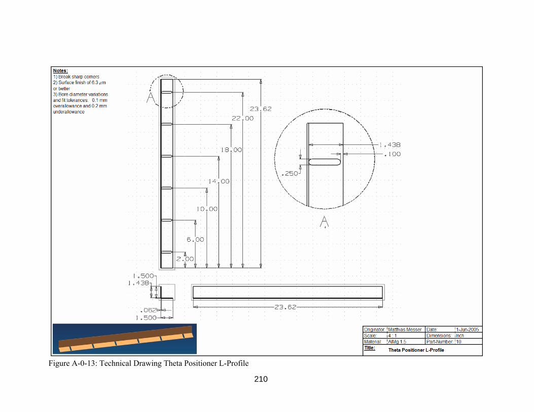
210
Figure A-0-13: Technical Drawing Theta Positioner L-Profile
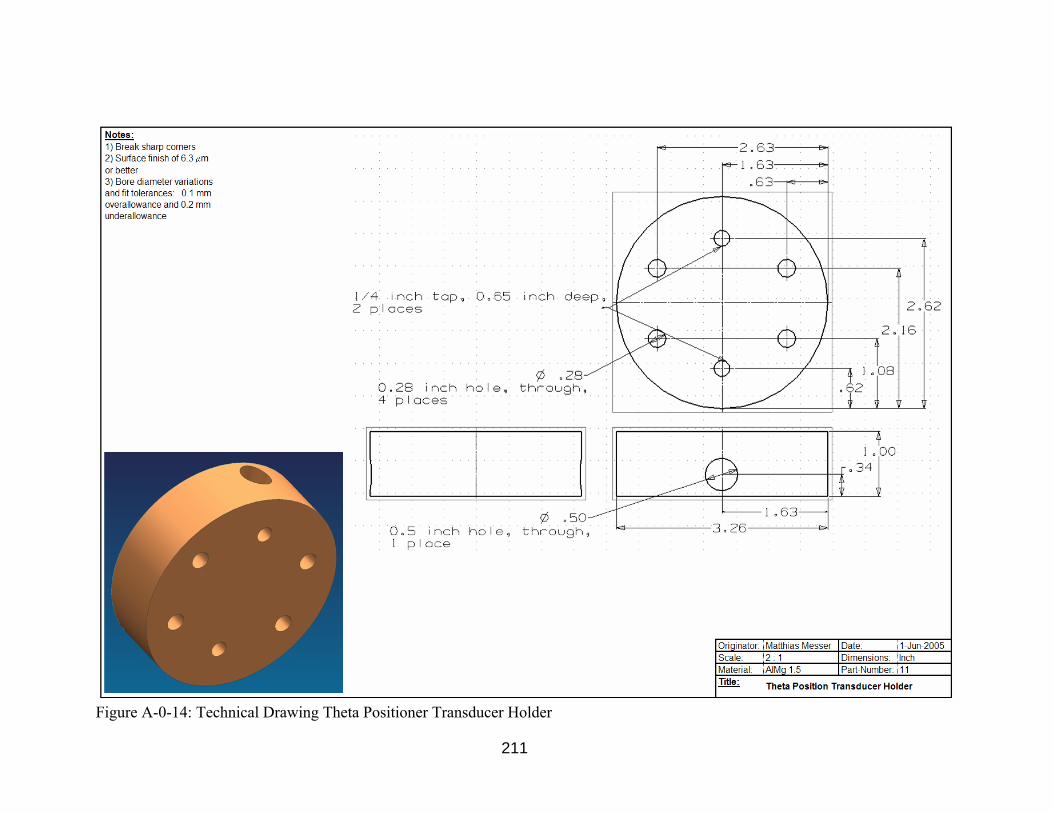
211
Figure A-0-14: Technical Drawing Theta Positioner Transducer Holder

212
Figure A-0-15: Technical Drawing Theta Positioenr Support Part

213
Appendix B: Technical Specifications Pulsed Ultrasound Doppler Velocimetry System

214
The digital ultrasonic synthesizer (Figure B-0-1) can generate any emitting frequencies
between 0.45 MHz and 10.5 MHz. Associated to this performance, the DOP2000
includes a variable spatial resolution filter that allows to adapt the size of the sampling
volume to the application and therefore improves the signal to noise ratio of the
measurements.
Figure B-0-1: Digital Ultrasonic Synthesizer [51]
All the ultrasonic parameters (Frequency, PRF, Tgc..) and the processing conditions
(number of gates, filters ...) are set by the user. The smart trigger capability of the
instrument allows to synchronize the acquisition to any periodic or non periodic event.
This high flexibility applies to the 10 channels multiplexer and up to 32’000 profiles
could be recorded in binary and/or ASCII format.
If desired, the DOP2000 can record simultaneously two types of data profiles, such as the
velocity profiles and the Doppler energy profiles. A separate emitter output connector
enables to use two different transducers for emission and reception.
Operating in a Windows 9x® environment, the measured profiles are displayed on screen
and are recorded in its internal memory or send through the build-in Ethernet connection
to any storage device within few milliseconds.

215
Technical specifications DOP2000 Model 2125
Emission:
Emitting frequencies from 0.45 MHz to 10.5 MHz, step of 1 kHz Emitting power 3 levels Burst length 2, 4 or 8 cycles
PRF between 64 µs (48 mm) and 10’500 µs (7'875 mm), step of 1 µs
Reception:
Number of gates between 3 and 1000, step of 1 gate Position of the first channel movable by step of 250 ns
Amplification (TGC) Uniform, Slope, Custom Slope mode exponential amplification between two defined depth values. Value at both depths variable between -40dB and +40dB Custom mode user's defined values between -40dB and +40dB in cells. Variable number, size and position of the cells.
Sensitivity >-100 dBm
Resolution:
Lateral resolution defined by the transducer
Longitudinal resolution minimum value of 0.85 s (0.64 mm) depends on spatial filter and burst length. (approximate value, defined at 50% of the received)
Spatial filter from 50 KHz (3.9 mm) to 300 KHz (0.7 mm) , step of 50 KHz
Display resolution distance between the center of each sample volume selectable between 0.25 s (0.187 mm) and 20 s (15 mm), step of 0.25 s
Velocity resolution 1 LSB (maximum = 0.0091 mm/s; minimum = 91.5 mm/s), Doppler frequency given in a signed byte format
Ultrasonic Processor:
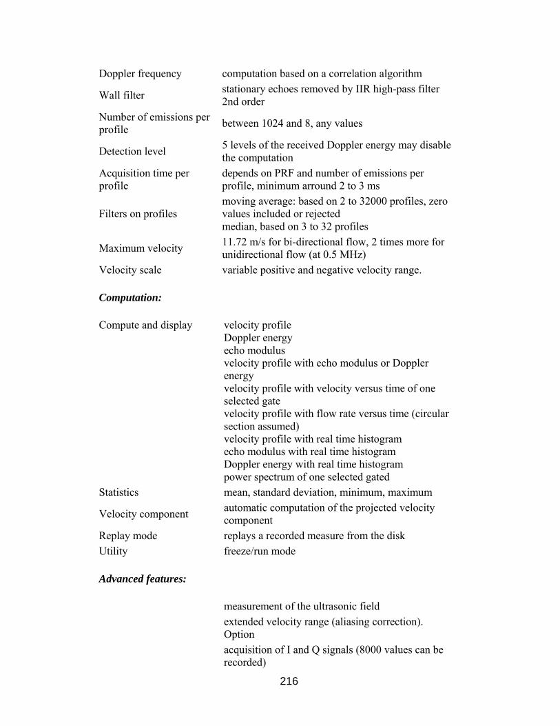
216
Doppler frequency computation based on a correlation algorithm
Wall filter stationary echoes removed by IIR high-pass filter 2nd order
Number of emissions per profile between 1024 and 8, any values
Detection level 5 levels of the received Doppler energy may disable the computation
Acquisition time per profile
depends on PRF and number of emissions per profile, minimum arround 2 to 3 ms
Filters on profiles moving average: based on 2 to 32000 profiles, zero values included or rejected median, based on 3 to 32 profiles
Maximum velocity 11.72 m/s for bi-directional flow, 2 times more for unidirectional flow (at 0.5 MHz)
Velocity scale variable positive and negative velocity range.
Computation:
Compute and display velocity profile Doppler energy echo modulus velocity profile with echo modulus or Doppler energy velocity profile with velocity versus time of one selected gate velocity profile with flow rate versus time (circular section assumed) velocity profile with real time histogram echo modulus with real time histogram Doppler energy with real time histogram power spectrum of one selected gated
Statistics mean, standard deviation, minimum, maximum
Velocity component automatic computation of the projected velocity component
Replay mode replays a recorded measure from the disk Utility freeze/run mode
Advanced features:
measurement of the ultrasonic field
extended velocity range (aliasing correction). Option
acquisition of I and Q signals (8000 values can be recorded)
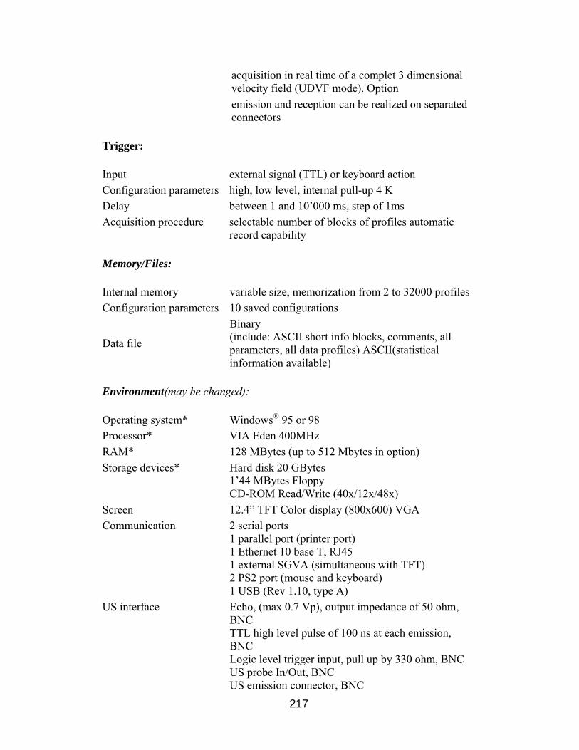
217
acquisition in real time of a complet 3 dimensional velocity field (UDVF mode). Option
emission and reception can be realized on separated connectors
Trigger:
Input external signal (TTL) or keyboard action Configuration parameters high, low level, internal pull-up 4 K Delay between 1 and 10’000 ms, step of 1ms Acquisition procedure selectable number of blocks of profiles automatic
record capability
Memory/Files:
Internal memory variable size, memorization from 2 to 32000 profilesConfiguration parameters 10 saved configurations
Data file
Binary (include: ASCII short info blocks, comments, all parameters, all data profiles) ASCII(statistical information available)
Environment(may be changed):
Operating system* Windows® 95 or 98 Processor* VIA Eden 400MHz RAM* 128 MBytes (up to 512 Mbytes in option) Storage devices* Hard disk 20 GBytes
1’44 MBytes Floppy CD-ROM Read/Write (40x/12x/48x)
Screen 12.4” TFT Color display (800x600) VGA Communication 2 serial ports
1 parallel port (printer port) 1 Ethernet 10 base T, RJ45 1 external SGVA (simultaneous with TFT) 2 PS2 port (mouse and keyboard) 1 USB (Rev 1.10, type A)
US interface Echo, (max 0.7 Vp), output impedance of 50 ohm, BNC TTL high level pulse of 100 ns at each emission, BNC Logic level trigger input, pull up by 330 ohm, BNC US probe In/Out, BNC US emission connector, BNC
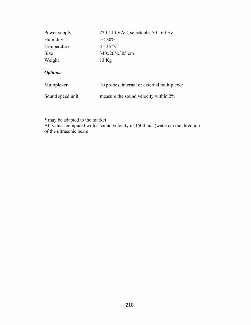
218
Power supply 220-110 VAC, selectable, 50 - 60 Hz Humidity =< 80% Temperature 5 - 35 °C Size 340x265x305 cm Weight 13 Kg
Options:
Multiplexer Sound speed unit
10 probes, internal or external multiplexer measure the sound velocity within 2%
* may be adapted to the market All values computed with a sound velocity of 1500 m/s (water),in the direction of the ultrasonic beam

219
Appendix C: Technical Specifications Ultrasonic Transducers
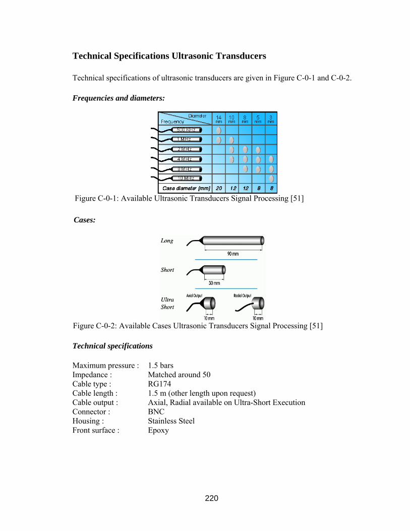
220
Technical Specifications Ultrasonic Transducers
Technical specifications of ultrasonic transducers are given in Figure C-0-1 and C-0-2.
Frequencies and diameters:
Figure C-0-1: Available Ultrasonic Transducers Signal Processing [51]
Cases:
Figure C-0-2: Available Cases Ultrasonic Transducers Signal Processing [51] Technical specifications
Maximum pressure : Impedance : Cable type : Cable length : Cable output : Connector : Housing : Front surface :
1.5 bars Matched around 50 RG174 1.5 m (other length upon request) Axial, Radial available on Ultra-Short Execution BNC Stainless Steel Epoxy
221
Appendix D: Technical Specifications Pump

222
PUMP DRIVE
Technical Specification Ismatec Programmable Digital Drive
Table D-1: Pump Drive Technical Specifications
Duty cycle continuous from 60 to 6000 rpm
Max rpm 60 to 6000
Motor type 24 VDC, PMDC
Motor (hp) 1/5
Pump head 07002-25 1.02 to 102 mL/min
Pump head 07002-26 2.52 to 252 mL/min
Pump head 07002-27 5.04 to 504 mL/min
Pump head 07002-14 5.52 to 552 mL/min
Pump head 07002-17 19.2 to 1920 mL/min
Pump head 07003-02 34.8 to 3480 mL/min
Pump head 07002-23 38.4 to 3840 mL/min
Pump head 07001-80 38.4 to 3840 mL/min
Pump head 07001-70 38.4 to 3840 mL/min
Pump head 07001-40 54.6 to 5460 mL/min
Max flow rate with indicated pump head
Pump head 07003-04 70.2 to 702 mL/min
Temp range 104°F (40°C)
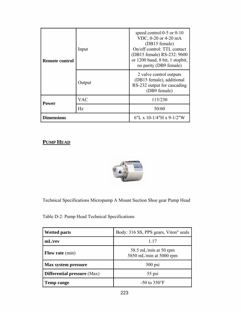
223
Input
speed control:0-5 or 0-10 VDC, 0-20 or 4-20 mA
(DB15 female) On/off control: TTL contact
(DB15 female) RS-232: 9600 or 1200 baud, 8 bit, 1 stopbit,
no parity (DB9 female) Remote control
Output
2 valve control outputs (DB15 female), additional
RS-232 output for cascading (DB9 female)
VAC 115/230 Power
Hz 50/60
Dimensions 6"L x 10-1/4"H x 9-1/2"W
PUMP HEAD
Technical Specifications Micropump A Mount Suction Shoe gear Pump Head
Table D-2: Pump Head Technical Specifications
Wetted parts Body: 316 SS, PPS gears, Viton® seals
mL/rev 1.17
Flow rate (min) 58.5 mL/min at 50 rpm 5850 mL/min at 5000 rpm
Max system pressure 300 psi
Differential pressure (Max) 55 psi
Temp range -50 to 350°F
224
Port size 1/8" NPT(F)
Suction lift 24" H2O (at 1750 rpm)
Viscosity 100 cp
Particulates none
Run dry under 30 seconds
Relief valve yes
Reversible no
Duty cycle continuous (from 150 to 5000 rpm)
Motor rpm 10,000
Internal bypass Yes
PUMP DIMENSIONING
Cross-sectional area: Minimal: 8 cm2 = 0.0008 m2 (3.15 inch2)
Maximal: 12 cm2 = 0.0012 m2 (4.72 inch2)
Characteristic length: Lmin = 10 mm = 10-2 m
Lmax = 15 mm = 1.5 10-2 m
Volume: Vdistributor = 1.5 l
Vchannel = 0.7 l
Density: ρwater = 1000 kg/m3
Kinematic viscosity: νwater = 10-6 m2/s
Reynolds number: Re = ρUL/η = UL/ν = VtL/Aν
Remin = 1
Remax = 1000
225
Required minimal flow rate:
Vt,min = ReAν/L = 8 * 10-8 m3/s = 4.8 * 10-3 l/min (1.666 * 10-5 m3/s = 1 l/min)
Required maximal flow rate:
Vt,max = 8 * 10-5 m3/s = 4.8 l/min
Minimal velocity:
Umin = Vt,min/Amax = 0.0000666 m/s
Maximal velocity:
Umax = Vt,max/Amin = 0.1 m/s

226
Appendix E: Technical Specifications Particles
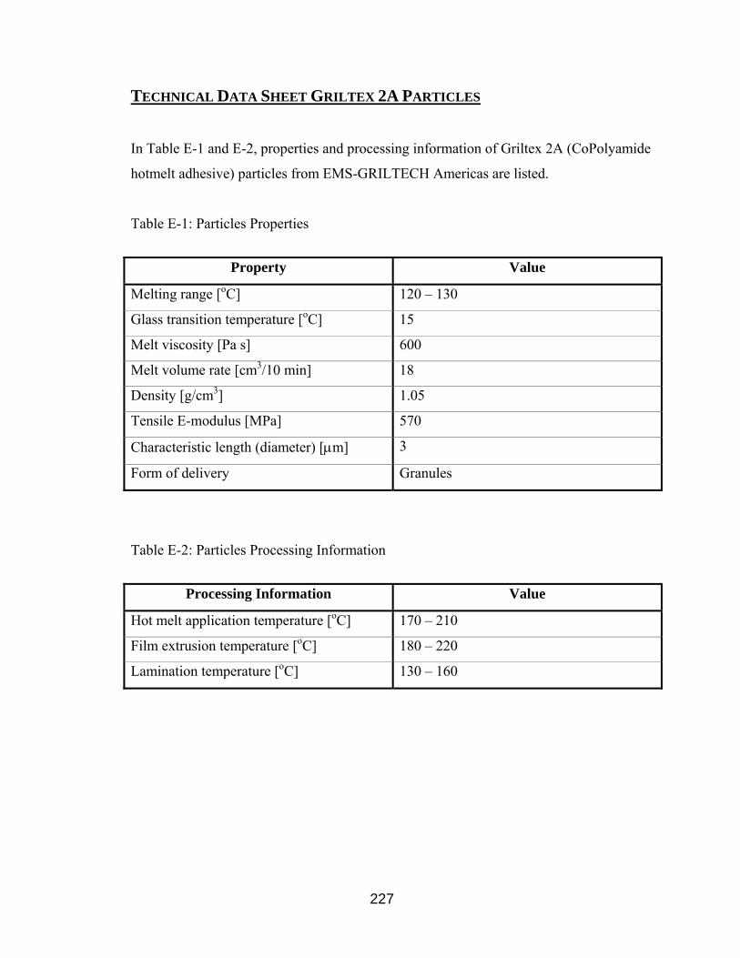
227
TECHNICAL DATA SHEET GRILTEX 2A PARTICLES
In Table E-1 and E-2, properties and processing information of Griltex 2A (CoPolyamide
hotmelt adhesive) particles from EMS-GRILTECH Americas are listed.
Table E-1: Particles Properties
Property Value
Melting range [oC] 120 – 130
Glass transition temperature [oC] 15
Melt viscosity [Pa s] 600
Melt volume rate [cm3/10 min] 18
Density [g/cm3] 1.05
Tensile E-modulus [MPa] 570
Characteristic length (diameter) [µm] 3
Form of delivery Granules
Table E-2: Particles Processing Information
Processing Information Value
Hot melt application temperature [oC] 170 – 210
Film extrusion temperature [oC] 180 – 220
Lamination temperature [oC] 130 – 160

228
Appendix F: Cost Analysis Experimental Setup
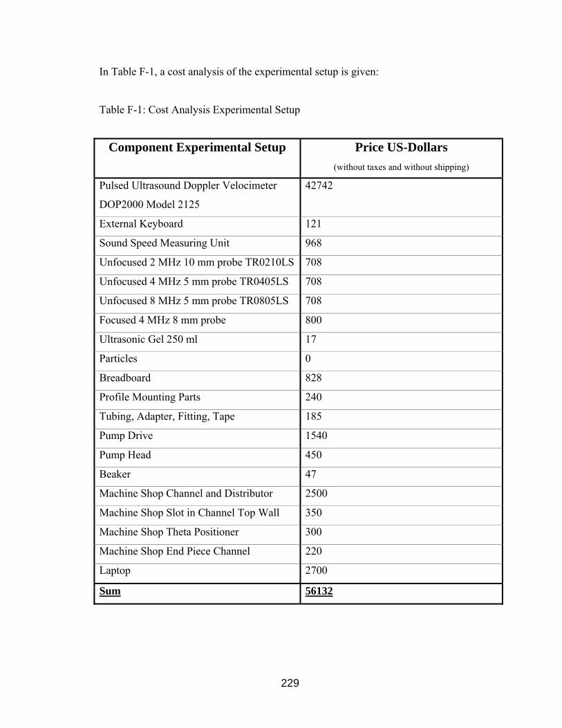
229
In Table F-1, a cost analysis of the experimental setup is given: Table F-1: Cost Analysis Experimental Setup
Component Experimental Setup Price US-Dollars (without taxes and without shipping)
Pulsed Ultrasound Doppler Velocimeter
DOP2000 Model 2125
42742
External Keyboard 121
Sound Speed Measuring Unit 968
Unfocused 2 MHz 10 mm probe TR0210LS 708
Unfocused 4 MHz 5 mm probe TR0405LS 708
Unfocused 8 MHz 5 mm probe TR0805LS 708
Focused 4 MHz 8 mm probe 800
Ultrasonic Gel 250 ml 17
Particles 0
Breadboard 828
Profile Mounting Parts 240
Tubing, Adapter, Fitting, Tape 185
Pump Drive 1540
Pump Head 450
Beaker 47
Machine Shop Channel and Distributor 2500
Machine Shop Slot in Channel Top Wall 350
Machine Shop Theta Positioner 300
Machine Shop End Piece Channel 220
Laptop 2700
Sum 56132

230
Appendix G: Measurement of Flow Resistivity of Forming Screen
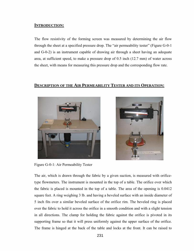
231
INTRODUCTION:
The flow resistivity of the forming screen was measured by determining the air flow
through the sheet at a specified pressure drop. The “air permeability tester” (Figure G-0-1
and G-0-2) is an instrument capable of drawing air through a sheet having an adequate
area, at sufficient speed, to make a pressure drop of 0.5 inch (12.7 mm) of water across
the sheet, with means for measuring this pressure drop and the corresponding flow rate.
DESCRIPTION OF THE AIR PERMEABILITY TESTER AND ITS OPERATION:
Figure G-0-1: Air Permeability Tester
The air, which is drawn through the fabric by a given suction, is measured with orifice-
type flowmeters. The instrument is mounted in the top of a table. The orifice over which
the fabric is placed is mounted in the top of a table. The area of the opening is 0.0412
square feet. A ring weighing 3 lb. and having a beveled surface with an inside diameter of
5 inch fits over a similar beveled surface of the orifice rim. The beveled ring is placed
over the fabric to hold it across the orifice in a smooth condition and with a slight tension
in all directions. The clamp for holding the fabric against the orifice is pivoted in its
supporting frame so that it will press uniformly against the upper surface of the orifice.
The frame is hinged at the back of the table and locks at the front. It can be raised to
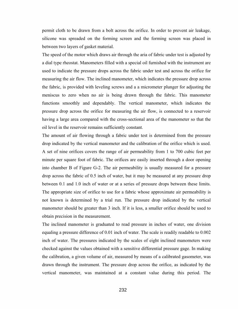
232
permit cloth to be drawn from a bolt across the orifice. In order to prevent air leakage,
silicone was spreaded on the forming screen and the forming screen was placed in
between two layers of gasket material.
The speed of the motor which draws air through the aria of fabric under test is adjusted by
a dial type rheostat. Manometers filled with a special oil furnished with the instrument are
used to indicate the pressure drops across the fabric under test and across the orifice for
measuring the air flow. The inclined manometer, which indicates the pressure drop across
the fabric, is provided with leveling screws and a a micrometer plunger for adjusting the
meniscus to zero when no air is being drawn through the fabric. This manometer
functions smoothly and dependably. The vertical manometer, which indicates the
pressure drop across the orifice for measuring the air flow, is connected to a reservoir
having a large area compared with the cross-sectional area of the manometer so that the
oil level in the reservoir remains sufficiently constant.
The amount of air flowing through a fabric under test is determined from the pressure
drop indicated by the vertical manometer and the calibration of the orifice which is used.
A set of nine orifices covers the range of air permeability from 1 to 700 cubic feet per
minute per square foot of fabric. The orifices are easily inserted through a door opening
into chamber B of Figure G-2. The air permeability is usually measured for a pressure
drop across the fabric of 0.5 inch of water, but it may be measured at any pressure drop
between 0.1 and 1.0 inch of water or at a series of pressure drops between these limits.
The appropriate size of orifice to use for a fabric whose approximate air permeability is
not known is determined by a trial run. The pressure drop indicated by the vertical
manometer should be greater than 3 inch. If it is less, a smaller orifice should be used to
obtain precision in the measurement.
The inclined manometer is graduated to read pressure in inches of water, one division
equaling a pressure difference of 0.01 inch of water. The scale is readily readable to 0.002
inch of water. The pressures indicated by the scales of eight inclined manometers were
checked against the values obtained with a sensitive differential pressure gage. In making
the calibration, a given volume of air, measured by means of a calibrated gasometer, was
drawn through the instrument. The pressure drop across the orifice, as indicated by the
vertical manometer, was maintained at a constant value during this period. The
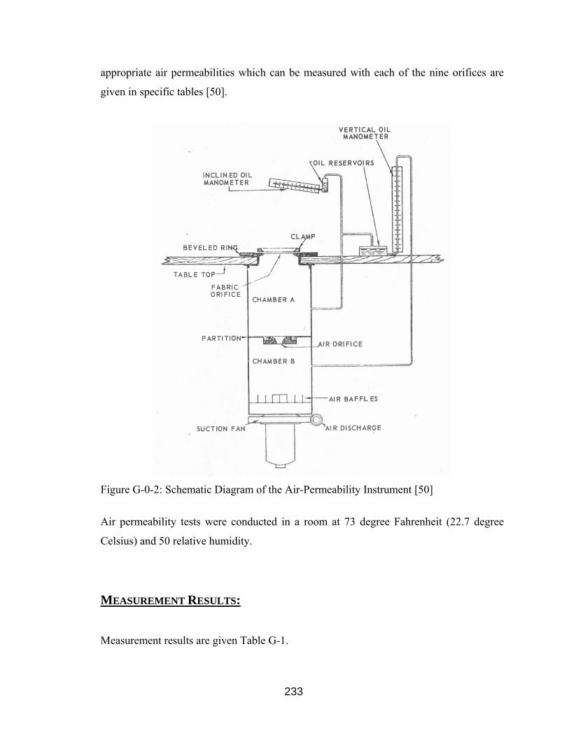
233
appropriate air permeabilities which can be measured with each of the nine orifices are
given in specific tables [50].
Figure G-0-2: Schematic Diagram of the Air-Permeability Instrument [50]
Air permeability tests were conducted in a room at 73 degree Fahrenheit (22.7 degree
Celsius) and 50 relative humidity.
MEASUREMENT RESULTS:
Measurement results are given Table G-1.

234
Table G-1: Air Permeability Measurement Results
Air Permeability Sample Number and Positioning
Cubic Feet /
Square Foot
/ Minute
Rayls
Sample 1 478.8 94.2278
Sample 1 – 90 degree converted 477.1 93.8933
Sample 1 – upside down 472 92.8896
Sample 1 – upside down 90 degree converted 475.4 93.5587
Sample 2 492.4 96.9043
Sample 2 – 90 degree converted 492.4 96.9043
Sample 2 – upside down 492.4 96.9043
Sample 2 – upside down 90 degree converted 492.4 96.9043
Sample 3 489 96.2352
Sample 3 – 90 degree converted 487.3 95.9006
Sample 3 – upside down 487.3 95.9006
Sample 3 – upside down 90 degree converted 485.6 95.5661
Conversion cubic feet per square foot per minute in Rayls:
min1968.0
min7639.10118.2
min602222
2
ftsqftcu
ftsqftcu
ml
smkg
ms
smmkg
smmN
Rayl ======
1 cu ft = 28.3168466 l
1 sq ft = 0.09290304 m2
EVALUATION OF RESULTS:
In general, a knowledge of the flow-resistance of a material permits the relevant acoustic
impedence to be predicted, although care must be taken to ensure that a representative
235
value of flow-resistance is used, as many practical materials are subject to considerable
variation between and within batches. However, for many purposes high accuracy is not
required for instance, in the initial design stages where selection of a potentially suitable
absorbing material is the objective. Unfortunately, manufactures do not usually include
data on flow-resistance in their technical literature. It is emphasized that the purpose of
these flow resistivity measurements is solely to provide an indication of the order of
magnitude of the flow-resistance to be expected for a given material.
Therefore, the value used for predicting the flow resistivity of the forming screen is the
average over all given measurement results (for three different samples and various
orientations). The mean value therefore is: 95.4824 Rayls.

236
Appendix H: Measurement of Speed of Sound

237
Technical Specifications Sound Speed Measuring Unit:
The sound speed measuring unit (Figure H-0-1) allows to measure the sound speed in any
kind of liquid by measuring with precision the time that is taken by an ultrasonic burst to
propagate over a define distance. Therefore, the transducer is connected to the DOP 2000
velocimeter. The measurement is based on a phase analysis of an echo generated by a
mobile plate when this plate is moved over a known distance. Any transducers having a
case diameter of 8mm or 12mm can be used, which enables the measurement of the sound
speed at different ultrasonic frequencies. The sound speed unit is delivered with a special
software module which is installed in the WDOP software of the velocimeter.
Figure H-0-1: Sound Speed Measureing Unit [51]

238
Appendix I: Measurement of the Insertion Loss

239
INTRODUCTION:
The insertion loss characterizes the sensitivity of a transducer, and is given by:
Equation 40: Insertion Loss
In order to measure the insertion loss, an ultrasonic burst is emitted by a transducer. The
same transducer receives an echo issued from a plane perpendicular target, which
acoustic impedance differs very much from the liquid used as a transmitting media.
The voltage ratio between the echo and the emitted burst, expressed in logarithm, is called
Insertion Loss [53]. Signal Processing's transducers have an IL between 10 and 20 dB,
depending on the type of transducer. To measure the Insertion Loss of your transducer,
you need the following equipment:
- 1 burst generator
- 1 oscilloscope
- 2 coaxial cable
- 1 water container, with a transducer holder
- 1 target (stainless steel preferred)
SET UP:
Connect the transducer, the burst generator and the oscilloscope as shown in Figure I-0-1.
You can trig the Echo signal by using the TTL output signal coming from the burst
generator (if available).
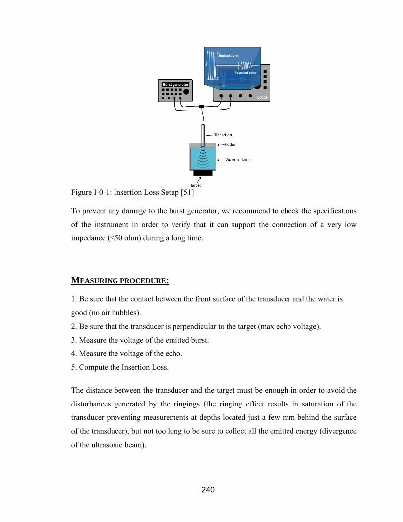
240
Figure I-0-1: Insertion Loss Setup [51]
To prevent any damage to the burst generator, we recommend to check the specifications
of the instrument in order to verify that it can support the connection of a very low
impedance (<50 ohm) during a long time.
MEASURING PROCEDURE:
1. Be sure that the contact between the front surface of the transducer and the water is
good (no air bubbles).
2. Be sure that the transducer is perpendicular to the target (max echo voltage).
3. Measure the voltage of the emitted burst.
4. Measure the voltage of the echo.
5. Compute the Insertion Loss.
The distance between the transducer and the target must be enough in order to avoid the
disturbances generated by the ringings (the ringing effect results in saturation of the
transducer preventing measurements at depths located just a few mm behind the surface
of the transducer), but not too long to be sure to collect all the emitted energy (divergence
of the ultrasonic beam).
241
The thickness of the target must also be considered. To avoid any interferences generated
by second echo, coming from the far wall of the target, a minimum thickness is required.
As the amount of the energy that penetrates inside the target depends on the difference in
acoustic impedance between the target and the transmitting media, it is recommended to
use a target with the highest acoustic impedance as possible.

242
Appendix J: Delany-Bazley-Model and Allard-Champoux-Model

243
The Delany-Bazley-Model and the Allard-Champoux-Model were used to model the
acoustic impedance of the porous forming screen. Both models and the results are
described in the following.
DELANY-BAZLEY MODEL (MIKI CORRECTION)
The equations of Delany and Bayley, presented for the first time in 1970, have since been
widely used to describe sound propagation in fibrous materials. These laws have been
used in various applications such as sound attenuation in ducts, room acoustics, the
calculation of transmission loss through walls, and primarily in models describing sound
propagation above various types of ground. Slightly different but similar laws were later
suggested to handle specific fibrous materials, and also to improve the low-frequency
behavior of the Delany and Bazley equations. The geometry of fibrous materials, in spite
of its apparent simplicity has however not been taken into account in these works [5].
The power laws of Delany and Bazley involve eight adjustable parameters that are the
same for all fibrous materials. According to Delany and Bazley, the acoustic impedence is
predicted by:
[ ]βαρ iBFAFciXRZ ++=+= 100
with the constants:
A = 0.057
B = 0.087
α = - 0.75
β = - 0.732
Equation 41: Delany-Bazley-Model
where f is the frequency, ρ0 is the density of the fluid, σ = ∆p/(U l) is the flow resistivity,
∆p is the pressure drop, U is the fluid velocity, l is the material thickness, c0 is the speed
of sound in the fluid and the constant F is ρ0f/σ.
In general, knowledge of the flow-resistance of a material permits the relevant acoustic
impedance to be predicted, although care must be taken to ensure that a representative

244
value of flow-resistance is used, as many practical materials are subject to considerable
variation between and within batches. However, for many purposes high accuracy is not
required for instance, in the initial design stages where selection of a potentially suitable
absorbing material is the objective. Unfortunately, manufactures do not usually include
data on flow-resistance in their technical literature. It is emphasized that the purpose of
these flow resistivity measurements (see appendix) is solely to provide an indication of
the order of magnitude of the flow-resistance to be expected for a given material.
Manufacturers do not necessarily control the flow-resistance of their product and it will
usually be necessary to sample-test a specific material before final evaluation. The main
factors influencing the flow-resistance of fibrous materials are the fiber size and the bulk
density, and it is known that for given fiber size the relation between bulk density and
flow-resistance approximates closely to a simple power law [15].
The formulas given above were implemented in the following MATLAB code to
calculate the acoustic impedance from 2 to 8 MHz.
%Acoutic Impedance Description of the Forming Screen clear all %Forming screen roperties: rhop=1620; %density of polyester in kg/m3 Omega=0.95; %porosity sigmae=95.5; %specific flow resistivity in MKS-Rayls l=0.00056; %thickness in m sigma=sigmae/l; %flow resistivity in MKS-Rayls/m %Fluid properties: rho0=1000; %density of water in kg/m3 c0=1482; %speed of sound in water at 20 degree celsius in m/s %Specific Acoustic Impedance Zs %a) Delany-Bazley model: N1=2000000; N2=8000000; f=N1:1:N2; %frequency in Hertz A=0.057; B=0.087; F=f.*rho0/sigma; %Non-dimensional frequency alpha=-0.750; beta=-0.732; Zs=rho0*c0*(1+A*F.^alpha+i*B*F.^beta); figure(1) subplot(2,2,1) semilogx(f,real(Zs),'b')

245
xlabel('Frequency [log]') ylabel('Real Part Spec. Ac. Impedance') title('Delany-Bazley Model') subplot(2,2,2) semilogx(f,imag(Zs),'b') xlabel('Frequency [log]') ylabel('Imaginary Part Spec. Ac. Impedance') title('Delany-Bazley Model') hold on
The results are shown in Figure J-1 and discussed in chapter 4.5.
ALLARD-CHAMPOUX-MODEL
Jean-F. Allard and Yvan Champoux developed new expressions that can be used instead
of the phenomenological equations of Delany and Bazley. They provide similar
predictions in the range of validity of these equations, and in addition are valid at low
frequencies where the equations of Delany and Bazley provide unphysical predictions.
These new expressions have been worked out by using the general frequency dependence
of the viscous forces in porous materials proposed by Johnson et al. [J. Fluid Mech. 176,
379 (1987)], with a transportation carried out to predict the dynamic bulk modulus of air.
The model used suggests how sound propagation in fibrous materials can depend both on
the diameter of the fibers and on the density of the material [5].
Typical fibers are modeled here as infinite circular-cylindrical rods of radius r that lie in
planes parallel to the surface of the layers. Only the case where the velocity of the fluid
for from the fibers is perpendicular to the direction of the fibers is considered here. The
detailed description of the model which will be used to describe the propagation of sound
through the porous forming screen and the derivation of the equations which will be
applied in the following can be found in the paper of Allard et al. [5]. The acoustic
impedance Z is:
( ) ( )ωωρ bb KZ =
Effective dynamic density of material ρb:

246
( )⎥⎥⎥⎥
⎦
⎤
⎢⎢⎢⎢
⎣
⎡−
−=ωτ
ωτ
ρωρi
i
b2
110
Effective dynamic bulk modulus Kb:
( )⎥⎥⎥⎥
⎦
⎤
⎢⎢⎢⎢
⎣
⎡
−−
−−=
τωτω
γγγω
NiNi
PKb
421
1
10
Equation 42: Allard-Champoux-Model
where ρ0 is the density of the fluid, ω = 2πf is the angular frequency, τ equals ρ0/σ, σ =
4Ωσe/Sf2 is the flow resistivity, Ω = Vp/VS is the porosity (Vp is the volume of the sample
and Vs is the volume of the fibers), σe is the specific flow resistivity, Sf is the pore shape
factor, γ is the ratio of the specific heats, P0 is the atmospheric pressure and N is Prandtl
number.
The predictions obtained from the laws of Delany and Bazley as well as from Allard and
Champoux, are very similar in the range of validity of the laws of Delany and Bazley.
The expressions given by Allard and Champoux are, however, also valid at low
frequencies and can be used to describe the steady flow of air through fibrous media. The
Allard-Champoux-model predicts a dependence of the dynamic density and the bulk
modulus as a function of the bulk density of the material and the diameter of the fibers,
that can be neglected at low frequencies, but is measurable at high frequencies.
The formulas given above were implemented in the following MATLAB code to
calculate the acoustic impedance from 2 to 8 MHz.
%Acoutic Impedance Description of the Forming Screen clear all %Forming screen roperties: rhop=1620; %density of polyester in kg/m3 Omega=0.95; %porosity sigmae=95.5; %specific flow resistance in MKS-Rayls l=0.00056; %thickness in m s=1; %pore shape factor sigma=sigmae/l; %flow resistivity in MKS-Rayls/m
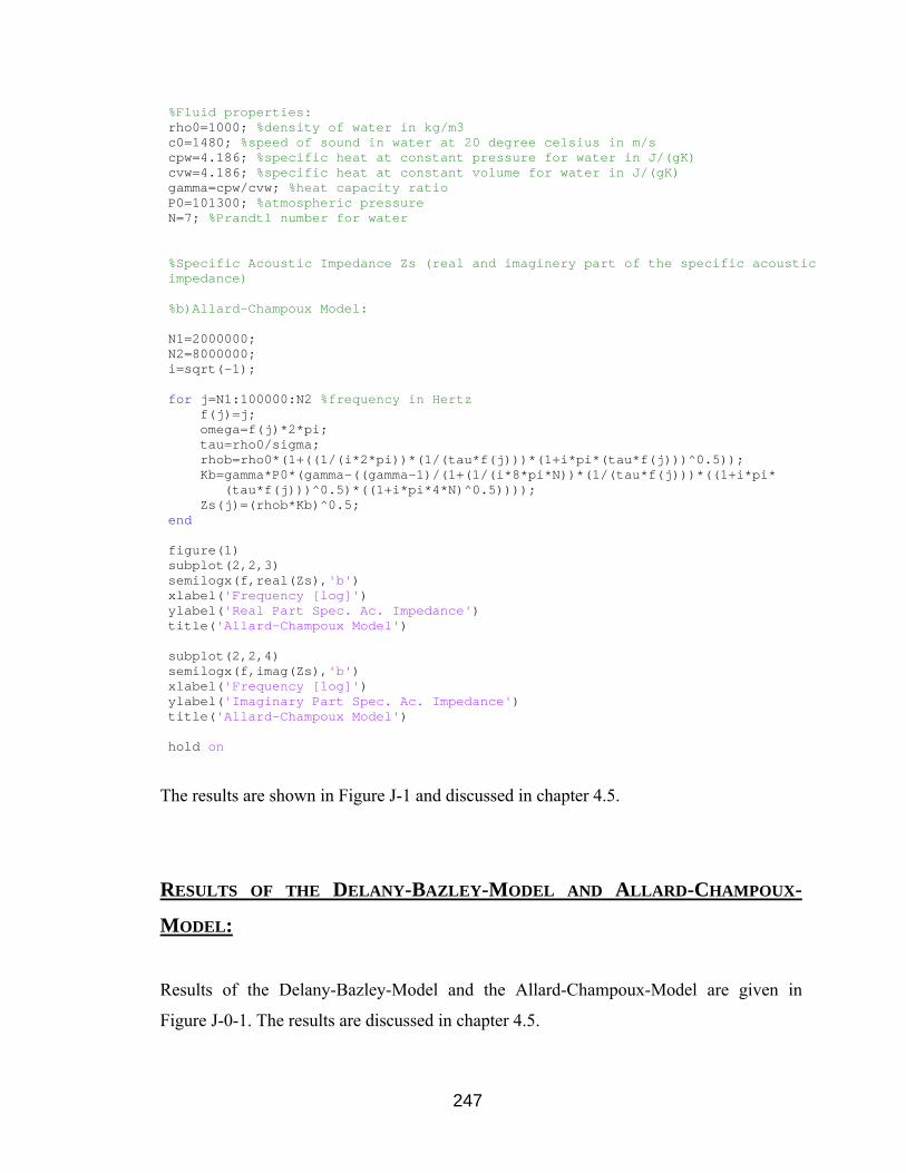
247
%Fluid properties: rho0=1000; %density of water in kg/m3 c0=1480; %speed of sound in water at 20 degree celsius in m/s cpw=4.186; %specific heat at constant pressure for water in J/(gK) cvw=4.186; %specific heat at constant volume for water in J/(gK) gamma=cpw/cvw; %heat capacity ratio P0=101300; %atmospheric pressure N=7; %Prandtl number for water %Specific Acoustic Impedance Zs (real and imaginery part of the specific acoustic impedance) %b)Allard-Champoux Model: N1=2000000; N2=8000000; i=sqrt(-1); for j=N1:100000:N2 %frequency in Hertz f(j)=j; omega=f(j)*2*pi; tau=rho0/sigma; rhob=rho0*(1+((1/(i*2*pi))*(1/(tau*f(j)))*(1+i*pi*(tau*f(j)))^0.5)); Kb=gamma*P0*(gamma-((gamma-1)/(1+(1/(i*8*pi*N))*(1/(tau*f(j)))*((1+i*pi* (tau*f(j)))^0.5)*((1+i*pi*4*N)^0.5)))); Zs(j)=(rhob*Kb)^0.5; end figure(1) subplot(2,2,3) semilogx(f,real(Zs),'b') xlabel('Frequency [log]') ylabel('Real Part Spec. Ac. Impedance') title('Allard-Champoux Model') subplot(2,2,4) semilogx(f,imag(Zs),'b') xlabel('Frequency [log]') ylabel('Imaginary Part Spec. Ac. Impedance') title('Allard-Champoux Model') hold on
The results are shown in Figure J-1 and discussed in chapter 4.5.
RESULTS OF THE DELANY-BAZLEY-MODEL AND ALLARD-CHAMPOUX-
MODEL:
Results of the Delany-Bazley-Model and the Allard-Champoux-Model are given in
Figure J-0-1. The results are discussed in chapter 4.5.
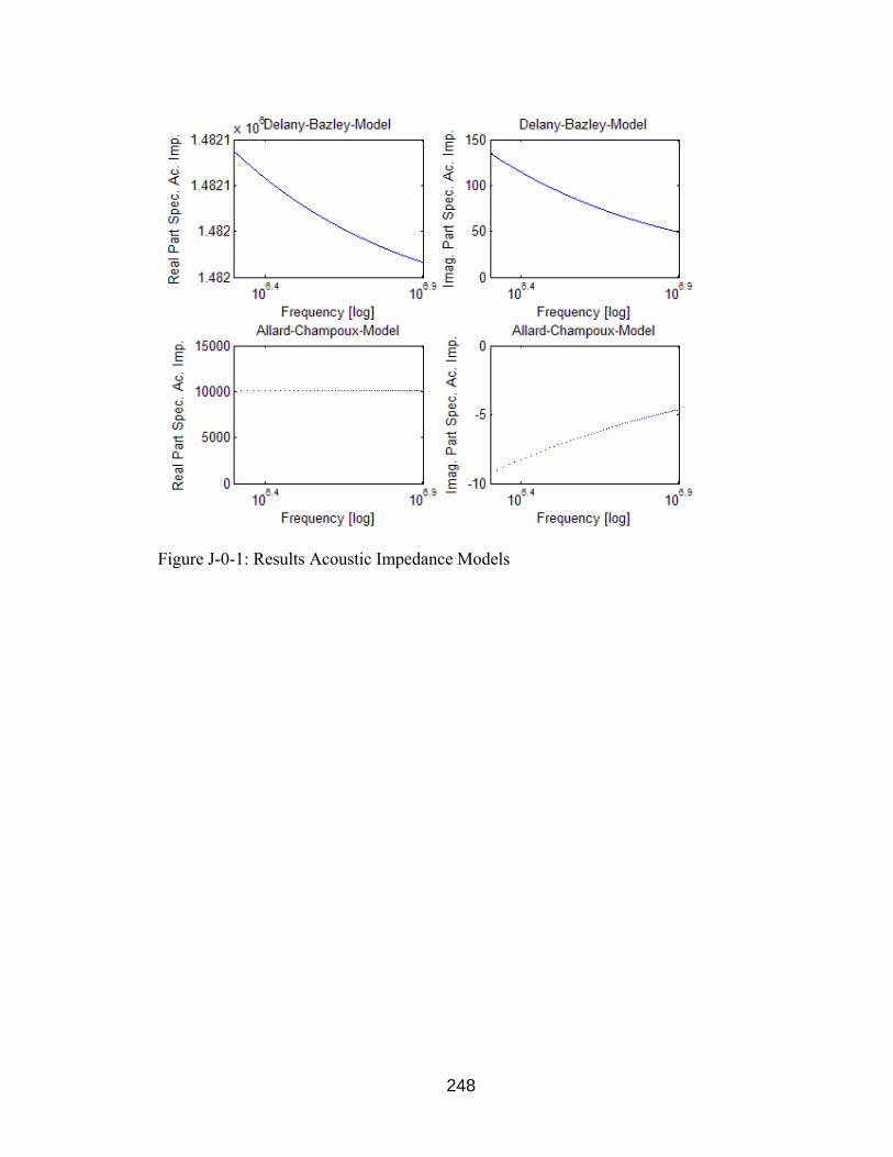
248
Figure J-0-1: Results Acoustic Impedance Models

249
References
1. Adrian, R. J. (2004). "Twenty Years of Particle Image Velocimetry." 12th
International Symposium on Applications of Laser Techniques to Fluid
Mechanics.
2. Aidun, C. K.; Lu, Y. (1995). "Lattice Boltzmann Simulation of Solid Particles
Suspended in Fluid." Journal of Statistical Physics 81.
3. Aidun, C. K.; Lu, Y.; Ding, E.-J. (1998). "Direct Analysis of Particulate
Suspensions with Inertia Using the Discrete Boltzmann Equation." Journal of
Fluid Mechanics 373: 287-311.
4. Alfonsi, G.; Brambilla, S.; Chiuch, D. (2003). "The Use of an Ultrasonic Doppler
Velocimeter in Turbulent Pipe Flow." Exepriments in Fluids 35: 553-559.
5. Allard, J.-F.; Champoux, Y. (1992). "New Empirical Equations for Sound
Propagation in Rigid Frame Fibrous Materials." J. Acoust. Soc. Am. 91(6).
6. Awatani, J. (1955). "Study on Acoustic Radiation Pressure, Radiation Pressure on
a Cylinder." Mem. Inst. Sci. Ind. Osake Univ. 12: 95-102.
7. Baker, D. W. (1965). "The Doppler Shift Principle Applied to Flow and
Displacement Measurement, Proceedings of the 18th Annual Conference on
Engineering in Medicne and Biology.
8. Baker, D. W. (1973). "Characteristics and Mathematical Modeling of the Pulsed
Ultrasonic Flowmeter." Medical and Biological Engineering(July): 404-421.
9. Barmatz, M.; Collas, P. (1985). "Acoustic Radiation Force Experienced by a Solid
Cylinder in a Plane Progressive Sound Field." J. Acoust. Soc. Am. 77(9280945).

250
10. Beaudoin, J.; Cadot, O.; Aider, J.; Wesfreid, J. (2004). "Three-Dimensional
Stationary Flow over a Backward-Facing Step." European Journal of Mechanics
B-Fluids 23(1): 147-155.
11. Beissner, K. (1998). "The Acoustic Radiation Force in Lossless Fluids in Eulerian
and Lagrangian Coordinates." J. Acoust. Soc. Am. 103(5): 2321-2332.
12. Brito, D.; Nataf, H. C.; Cardin, P.; Aubert, J.; Masson, J. P. (2001). "Ultrasonic
Doppler Velocimetry in Liquid Gallium." Experiments in Fluids 31(6): 653-663.
13. Brodeur, P. H.; Lewis, E. L. (1993). "Ultrasonic Characterization of Forming
Fabrics." IPST Technical Paper Series.
14. Chen, X. C.; Apfel, R. E. (1996). "Radiation Force on a Spherical Object in an
Axisymmetric Wave Field and Its Application to the Calibration of High-
Frequency Transducers." J. Acoust. Soc. Am. 99: 713-724.
15. Delany, M. E.; Bazley, E. N. (1970). "Acoustical Properties of Fibrous Absorbent
Materials." Applied Acoustics 3.
16. Eckert, S.; Gerbeth, G. (2002). "Velocity Measurements in Liquid Sodium by
Means of Ultrasound Doppler Velocimetry." Experiments in Fluids 32(5): 542-
546.
17. Embleton, T. F. W. (1954). "Mean Force on a Sphere in a Spherical Sound Field."
J. Acoust. Soc. Am. 20: 40-45.
18. Evans, D. H.; McDicken, W. N. (2000). "Doppler Ultrasound - Physics,
Instrumentation and Signal Processing." Wiley.
19. Fox, F. E. (1940). "Sound Pressure on Spheres." J. Acoust. Soc. Am. 12: 147-149.
20. Fry, F. J. (1978). "Ultrasound: Its Applications in Medicine and Biology."
Amsterdam, Elsevier Scientific Pub. Co.
21. Gorkov, L. P. (1962). "On the Forces Acting on a Small Particle in an Acoustic
Field in an Ideal Fluid." Sov. Phys. Kokl. 6: 772-775.

251
22. Hasegawa, T.; Saka, K.; Inouse, N.; Matsuzawa, K. (1988). "Acoustic Radiation
Force Experienced by a Solid Cylinder in a Plane Progressive Sound Field." J.
Acoust. Soc. Am. 83: 1770-1775.
23. Hasegawa, T.; Watanabe, Y. (1978). "Acoustic Radiation Pressure on an
Absorbing Sphere." J. Acoust. Soc. Am. 46: 1733-1737.
24. Hasegawa, T.; Yosioka, K. (1969). "Acoustic Radiation Force on a Solid Elastic
Sphere." J. Acoust. Soc. Am. 46: 1139-1143.
25. Hueter, T. F.; Bolt, R. H. (1954). "Sonics - Techniques for the Use of Sound and
Ultrasound in Engineering and Science." John Wiley & Sons, Inc.
26. Jawad, I. A. (1996). "A Practical Guide to Echocardiogrpahy and Cardiac Doppler
Ultrasound." John Wiley & Sons, Inc.
27. Jensen, J. A. (1996). "Estimation of Blood Velocities Using Ultrasound."
Cambridge University Press.
28. Kerut, E. K.; McIlwain, E. F.; Plotnick, G. D. (1996). "Handbook of Echo-
Doppler Interpretation." John Wiley & Sons, Inc.
29. Kikura, H.; Takeda, Y.; Durst, F. (1999). "Velocity Profile Measurement of the
Taylor Vortex Flow of a Magnetic Fluid Using the Ultrasonic Doppler Method."
Experiments in Fluids 26(3): 208-214.
30. Kikura, H.; Takeda, Y.; Sawada, T. (1999). "Velocity Profile Measurements of
Magnetic Fluid Flow Using Ultrasonic Doppler Method." Jorunal of Magnetism
and Magnetic Materials 201: 276-280.
31. Kikura, H.; Yamanaka, G.; Aritomi, M. (2004). "Effect of Measurement Volume
Size on Turbulent Flow Measurement Using Ultrasonic Doppler Method."
Experiments in Fluids 36(1): 187-196.
32. King, L. V. (1934). "On the Acoustic Radiation Pressure on Spheres." Proc. R.
Soc. London Ser. 147: 212-240.
252
33. Kino, G. S. (1987). "Acoustic Waves: Devices, Imaging and Analog Signal
Processing." Engelwood Cliffs, N.J., Prentice-Hall.
34. Kinsley, L. E.; Frey, A. R. (1982). "Fundamentals of Acoustics." John Wiley &
Sons, Inc.
35. Kostas, J.; Soria, J.; Chong, M. (2002). "Particle Image Velocimetry
Measurements of a Backward-Facing Step Flow." Experiments in Fluids 33(6):
838-853.
36. Kundt, A. (1866). "Ueber Eine Neue Art Akustischer Staubfiguren Und Ueber Die
Anwendung Derselben Zur Bestimmung Der Schallgeschwindigkeit in Festen
Koerpern Und Gasen." Ann. Phy. (Leipzig) 127(497).
37. Leung, E.; Jacobe, N.; Wang, T. (1981). "Acoustic Radiation Force on a Rigid
Sphere in a Resonance Chamber." J. Acoust. Soc. Am. 70: 1762-1767.
38. Lofstedt, R.; Putterman, S. (1991). "Theory of Long Wavelength Acoustic
Radiation Pressure." J. Acoust. Soc. Am. 90: 2027-2033.
39. Maidanik, G. (1957). "Acoustic Radiation Pressure Due to Incident Plane
Progressive Waves in Spherical Objects." J. Acoust. Soc. Am. 29: 738-742.
40. Maidanik, G.; Westervelt, P. J. (1957). "Acoustic Radiation Pressure Due to
Incident Plane Progressive Waves on Spherical Objects." J. Acoust. Soc. Am. 29:
936-940.
41. Nie, J.; Armaly, B. (2004). "Reverse Flow Regions in Three-Dimensional
Backward-Facing Step Flow." International Journal of Heat and Fluid Flow
47(22): 4713-4720.
42. Nyborg (1967). "Radiation Pressure on a Small Rigid Sphere." J. Acoust. Soc.
Am. 42: 947-952.
43. Panametrics, I. (2004). "Technical Notes." http://www.panametrics-
ndt.com/ndt/ndt_transducers/downloads/transducer_technotes.pdf.
253
44. Papadakis, E. P. (1999). "Ultrasonic Instruments and Devices." Academic Press.
45. Pierce, A. D. (1981). "Acoustics: An Introduction to Its Physical Principles and
Applications." New York, McGraw-Hill.
46. Prasad, A. K. (2000). "Particle Image Velocimetry." Current Science 79(1).
47. Reneman, R. S. (1973). "Cardiovascular Applications of Ultrasound." McGraw-
Hill.
48. Rudnick, I. (1977). "Measurement of the Acoustic Radiation Pressure on a Sphere
in a Standing Wave Field." J. Acoust. Soc. Am. 62: 20-22.
49. Sabbagha, R. (1994). "Diagnostic Ultrasound: Applied to Obstetrics and
Gynecology." McGraw-Hill.
50. Schiefer, H. F.; Boyland, P. M. (1942). "Improved Instrument for Measuring the
Air Permeability of Fabrics." Journal of Research of the National Bureau of
Standards 29.
51. Signal-Processing (2004). "Introducing Ultrasonic Doppler Velocimetry."
www.signal-processing.com.
52. Skolnik, M. I. (1990). "Radar Handbook." McGraw-Hill.
53. Skolnik, M. I. (2001). "Introduction to Radar Systems." New York, McGraw-Hill.
54. Takeda, Y. (1986). "Velocity Measurement by Ultrasound Doppler Shift Method."
International Journal Heat and Fluid Flow 7(4): 313-318.
55. Takeda, Y. (1995). "Velocity Profile Measurement by Ultrasonic Doppler
Method." Experimental Thernal and Fluid Science 10(4): 444-453.
56. Takeda, Y. (1999). "Ultrasonic Doppler Method for Velocity Profile Measurement
in Fluid Dynamics and Fluid Engineering." Experiments in Fluids 26(3): 177-178.

254
57. Technische-Universitaet-Darmstadt (2005). "Acoustic Cavitation and Nonlinear
Dynamics." http://www.physik.tu-darmstadt.de/nlp/cavitation.html.
58. Wei, W.; Thiessen, D.; Marston, P. (2004). "Acoustic Radiation Force on a
Compressible Cylinder in a Standing Wave." J. Acoust. Soc. Am. 116(1): 201-
208.
59. Wells, P. N. T. (1969). "Physical Principle of Ultrasonic Diagnosis." Academic
Press.
60. Wells, P. N. T. (1977). "Biomedical Ultrasonics." Academic Press.
61. Wilson, C. E. (1994). "Noise Control." Krieger Publishing Company.
62. Wu, J.; Du, G. (1990). "Acoustic Radiation Force on a Small Compressible
Sphere in a Focused Beam." J. Acoust. Soc. Am. 87: 997-1003.
63. Wu, J.; Du, G.; Work, S.; Warshaw, D. (1990). "Acoustic Radiation Pressure on a
Rigid Cylinder - an Analytical Theory and Experiments." J. Acoust. Soc. Am.
87(2): 581-586.
64. Xu, H. (2003). Measurement of Fiber Suspension Flow and Forming Jet Velocity
Profile by Pulsed Ultrasonic Doppler Velocimetry. Atlanta, Institute of Paper
Science and Technology. Ph.D.
65. Yasuda, K.; Kamakura, T. (1997). "Acoustic Radiation Force on Micrometer-Size
Particles." Applied Physics Letters 71(13): 1771-1773.
66. Yosioka, K.; Kawasima, Y. (1955). "Acoustic Radiation Pressure on a
Compressible Sphere." Acoustica 5: 167-173.
Related Documents