Pulse flow of liquid in flexible tube - EPJ Web of Conferences

* Corresponding author: [email protected]

Pulse flow of liquid in flexible tube

Roman Klas1,* and Simona Fialová1

1Brno University of Technology, Faculty of Mechanical Engineering, Victor Kaplan Department of Fluids Engineering, Technická 2,

61669 Brno, Czech Republic

Abstract. The simulation of liquid flow in significantly deformed elastic material is one of the more

challenging tasks. Tube wall motion prediction implemented directly into CFD software can noticeably

reduce the computational and time demands of such problems. The FSI simulation of a liquid-flowed flexible

plastic tube was analyzed on the FEA and CFD solvers coupling basis. The flexible tube is the basic symmetric

test body that could be appropriately tested on the experimental stand. A comparison of experimental data

and FSI problem using commercial code and one-dimensional tube models was made by evaluating the tube

wall deformation magnitudes at defined flow ratios. The type of tube material, which can be understood as a

nonlinear from the stress and deformation point of view, was considered. The paper shows several possibilities

of tube modeling using the main constitutive relations of linear and nonlinear mechanics. The hyperelastic

material models such as neo-Hookean and Mooney-Rivlin were tested. The results represent differences in

impacts on the tube liquid flow and differences in the magnitudes of the wall tube deformations. Based on

these findings it should be possible to simulate the problems of liquid flow in more complicated shape flow

zones, such as arteries affected by various defects, in our future research.

1 Introduction

In the following work, the case of fluid flow in the flexible

tube will be analyzed. The main tools for assessing this

task were CFD simulation of fluid flow and structural

simulation of elastic wall deformation (FSI), one-

dimensional mathematical models of flexible pipeline and

experimental data. From the analysis of the elastic tube

behavior it is possible to experimentally determine the

deformation of the pipe wall at the defined points and, of

course, to trace the corresponding hydraulic variables

such as flow and pressure. A similar case of deformation

of the elastic wall due to the action of fluid occurs, for

example, in the blood flow through the artery or the aorta

[1-4]. Permanent or destructive deformation of the aortic,

of course, has a significant impact on human health and

life. For this reason, it is advantageous to study the above-

mentioned models. The model situation can predict fluid

flow in the true aorta or its replacement.

A major complication is the fact that numerical FSI

simulations are quite time consuming. Also, for all

possible cases, it is not always realistic to carry out

experimental measurements. Therefore, it is possible to

try to simplify FSI's role by, for example, the prescribed

movement of a flexible wall in simple CFD simulations,

or to use simpler mathematical models. Another

unfavorable fact is the nonlinear behavior of the tube wall

material with respect to stress dependence and wall

deformation. Therefore, the following study should be

supplemented by at least a brief overview of basic non-

linear materials.

2 FEA and CFD methods and description of the tube

ANSYS Mechanical and ANSYS Fluent 18.2 were used

as software for FSI simulation. The simulation was

realized in coupling mode. The flexible wall geometry,

fluid tube, and computational mesh were created in

ANSYS DesignModeler and ANSYS Meshing software.

Due to time-consuming FSI simulations, the number of

computational cells was reduced by considering only one

quarter of the tube.

Table 1. Description of numerical model.

Reynolds number ~ 30 000, ~ 2000

Tube diameter

Wall thickness

Tube length

Material constants

d0 = 12.7 mm

s0 = 1.6 mm

L = 0.5 m

E = 4 MPa

ν = 0.5

C12 = 650 000 Pa

C1 = 600 000 Pa, C2 = 50 000 Pa

Number of

computational

cells

FEM CFD

25 200 ~ 156 000

Material neo-Hookean water liquid

Turbulence model

and near wall

modeling

realizable k – ε

enhanced wall treatment

© The Authors, published by EDP Sciences. This is an open access article distributed under the terms of the Creative Commons Attribution License 4.0

(http://creativecommons.org/licenses/by/4.0/).

EPJ Web of Conferences 213, 02041 (2019) https://doi.org/10.1051/epjconf/201921302041EFM 2018

mailto:[email protected]

Boundary

conditions

FEM CFD

frictionless

fixed

fluid solid

interface

Inlet: velocity

inlet, pressure

inlet

Outlet: pressure

outlet

Calculation mode unsteady, incompressible flow,

incompressible solid

The unsteady boundary conditions based on

experimental measurements were considered in the CFD

analysis. The number of iterations of CFD simulation

within one time step was slightly reduced with respect to

the time consuming FSI analysis.

3 One-dimensional tube model

As it was mentioned above, the flexible tube is generally

characterized by a non-linear dependence of a shear stress

and deformation. This can complicate the simulation of

pulsatile fluid flow through the tube. However, it will be

interesting to see how significantly the non-linear

properties of the tube material actually occur. For this

reason, a standard Hookean material, non-linear neo-

Hooken [5-7] and Mooney-Rivlin [8,9] materials will be

included in one-dimensional models. In case of Hookean

material and shear stress in the tube, we also need to

consider whether it is a thin-walled or thick-walled

cylinder. For thin-walled cylinders, some definitions can

be partially simplified.

The continuity equation and the equation of motion

represent the second part of the one-dimensional model

that will describe the fluid flow through an elastic tube.

Both equations will be written in a general form so that

the equations are valid for all types of materials.

Following must be considered in terms of some one-

dimensional models: whether the properties of the system

represented by inertial forces, hydraulic resistances and

compressibility of the fluid and the tube wall concentrate

on the selected points, or if their properties continuously

decompose along the tube length. For comparison, both

cases will be presented. However, Tab. 2 with the list of

symbols that are used in the following equations will be

listed first.

Table 2. List of symbols.

c speed of sound

C hydraulic capacity

C* unsteady friction coefficient

C12, C1, C2 neo-Hookean and Mooney-Rivlin

material constants

d0, d, D inner diameter of the thin-walled tube

d2 outer diameter of the thick walled tube

E Young's modulus of the tube material

fq, fqu hydraulic steady and unsteady friction

factor

g gravitational acceleration

H hydraulic induction

K, Kc bulk modulus and corrected bulk

modulus

L tube length

pI, pII, p1, p2 static pressure inlet and outlet, inner

and outer static pressure

Q, Qo,

Qc,Qv volumetric flow rate

r0, r10, r20 radii of the unloaded thin-walled and

thick-walled tubes

r, r1, r2

inner radius of the thin-walled tube,

inner and outer radius of the thick-

walled tube

R hydraulic resistance of the tube

s0, s wall thickness of the unloaded and

loaded tube

S variable cross-section of the tube

t time

ua, u1, u2 axial displacement and radial

displacement at the inner and outer

surface of the tube

v absolute velocity

V tube volume

x x-coordinate, axis of the tube

ε, εa, εr, εt engineering strain, axial, radial and

circumferential strain

λ, λa, λr, λt stretch ratio, axial, radial and

circumferential stretch ratio

ν Poisson's ratio

Пji strain rate tensor

ρ fluid density

σa, σr, σt axial, radial and circumferential stress

3.1 Equation of motion and continuity equation

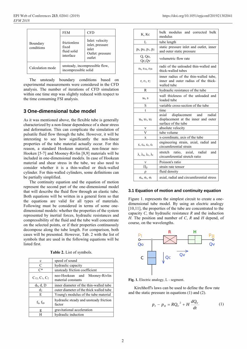
Figure 1. represents the simplest circuit to create a one-

dimensional tube model. By using an electric analogy

[10,11], the properties of the tube are concentrated to the

capacity C, the hydraulic resistance R and the induction

H. The position and number of C, R and H depend, of

course, on the wavelengths.

Fig. 1. Electric analogy, L - segment.

Kirchhoff's laws can be used to define the flow rate

and the static pressure in equations (1) and (2).

dt

dQHQRpp V

VIII 2 (1)

2


dt

dpCQQ I

V 0 (2)

Capacity C includes a corrected bulk modulus that

describes the influence of the fluid compressibility and the

tube wall flexibility (3). Of course, the Kc formulation is

subject to a description of the stress and deformation of

the tube. The definition of H and R corresponds to

common procedures.

CK

VC (3)

From the Navier-Stokes equations (4), the Darcy-

Weisbach equation and the continuity equation (5) for the

compressible fluid and the bulk modulus more precise

relationships for determining the flow rate and static

pressure in the vertical tube can be obtained.

j

ji

i

ij

j

ii

xx

pgv

x

v

t

v

(4)

0

j

j

x

v

t

(5)

If we consider all the variables in the equations,

besides fq and g, as a function of the x-coordinate and

time, we can obtain an equation of motion (6) and a

continuity equation (7) that neglects convective terms.

Both equations consider the variable inner radius of tube

r. For now, we will assume that convective terms in the

(6) and (7), or in (8), will be negligible.

2

1

22

2

S

QQ

r

f

x

pg

S

t

r

r

Q

t

Q q

(6)

x

Q

SK

t

pC

11 (7)

The corrected bulk modulus Kc in (7) includes the

influence of fluid compressibility and tube deformations

[12]. Using basic water hammer equations of motion,

modulus Kc must be generally defined according to (8).

1

121

r

p

r

K

KKC

(8)

3.2 Basic stress equations and constitutive laws

The wall of the test tube is relatively thin and its material

is hyperelastic. The brand name of tube material is named

Tygon. In terms of the definition of the following

relationships, it will be important to mark the dimensions,

deformations and stresses in the tube (Fig. 2, 3).

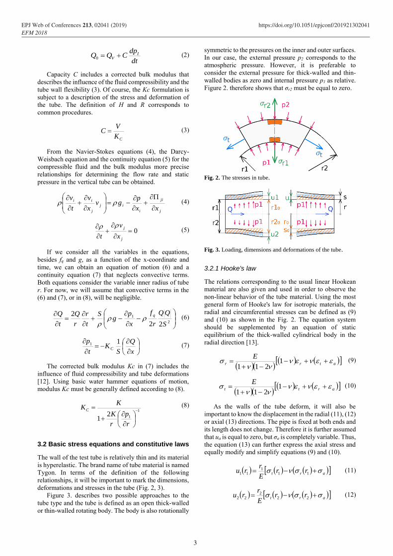
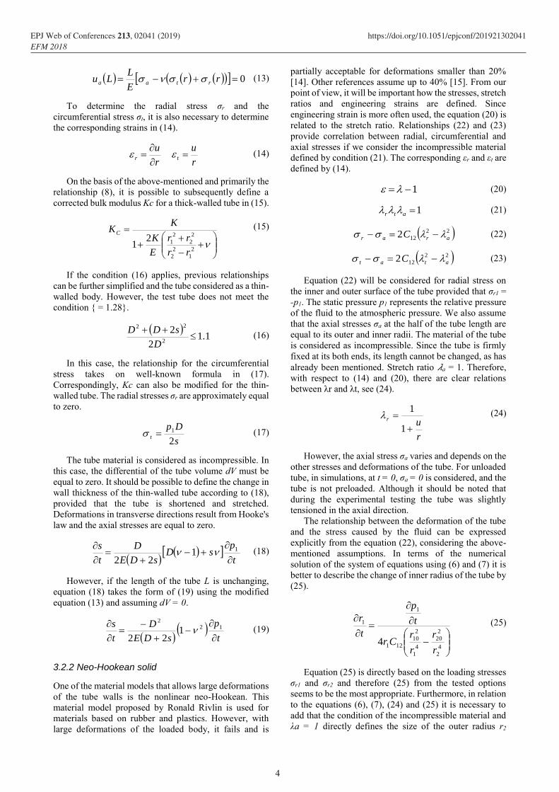
Figure 3. describes two possible approaches to the

tube type and the tube is defined as an open thick-walled

or thin-walled rotating body. The body is also rotationally

symmetric to the pressures on the inner and outer surfaces.

In our case, the external pressure p2 corresponds to the

atmospheric pressure. However, it is preferable to

consider the external pressure for thick-walled and thin-

walled bodies as zero and internal pressure p1 as relative.

Figure 2. therefore shows that σr2 must be equal to zero.

Fig. 2. The stresses in tube.

Fig. 3. Loading, dimensions and deformations of the tube.

3.2.1 Hooke's law

The relations corresponding to the usual linear Hookean

material are also given and used in order to observe the

non-linear behavior of the tube material. Using the most

general form of Hooke's law for isotropic materials, the

radial and circumferential stresses can be defined as (9)

and (10) as shown in the Fig. 2. The equation system

should be supplemented by an equation of static

equilibrium of the thick-walled cylindrical body in the

radial direction [13].

atrr

E

1

211 (9)

artt

E

1

211 (10)

As the walls of the tube deform, it will also be

important to know the displacement in the radial (11), (12)

or axial (13) directions. The pipe is fixed at both ends and

its length does not change. Therefore it is further assumed

that ua is equal to zero, but σa is completely variable. Thus,

the equation (13) can further express the axial stress and

equally modify and simplify equations (9) and (10).

art rrE

rru 11

111

(11)

art rrE

rru 22

222

(12)

3


0 rrE

LLu rtaa (13)

To determine the radial stress σr and the

circumferential stress σt, it is also necessary to determine

the corresponding strains in (14).

r

ur

r

ut (14)

On the basis of the above-mentioned and primarily the

relationship (8), it is possible to subsequently define a

corrected bulk modulus Kc for a thick-walled tube in (15).

2

1

2

2

2

2

2

121

rr

rr

E

K

KKC

(15)

If the condition (16) applies, previous relationships

can be further simplified and the tube considered as a thin-

walled body. However, the test tube does not meet the

condition { = 1.28}.

1.1

2

22

22

D

sDD (16)

In this case, the relationship for the circumferential

stress takes on well-known formula in (17).

Correspondingly, Kc can also be modified for the thin-

walled tube. The radial stresses σr are approximately equal

to zero.

s

Dpt

2

1 (17)

The tube material is considered as incompressible. In

this case, the differential of the tube volume dV must be

equal to zero. It should be possible to define the change in

wall thickness of the thin-walled tube according to (18),

provided that the tube is shortened and stretched.

Deformations in transverse directions result from Hooke's

law and the axial stresses are equal to zero.

t

psD

sDE

D

t

s

1122

(18)

However, if the length of the tube L is unchanging,

equation (18) takes the form of (19) using the modified

equation (13) and assuming dV = 0.

t

p

sDE

D

t

s

122

122

(19)

3.2.2 Neo-Hookean solid

One of the material models that allows large deformations

of the tube walls is the nonlinear neo-Hookean. This

material model proposed by Ronald Rivlin is used for

materials based on rubber and plastics. However, with

large deformations of the loaded body, it fails and is

partially acceptable for deformations smaller than 20%

[14]. Other references assume up to 40% [15]. From our

point of view, it will be important how the stresses, stretch

ratios and engineering strains are defined. Since

engineering strain is more often used, the equation (20) is

related to the stretch ratio. Relationships (22) and (23)

provide correlation between radial, circumferential and

axial stresses if we consider the incompressible material

defined by condition (21). The corresponding εr and εt are

defined by (14).

1 (20)

1atr (21)

22

122 arar C (22)

22

122 atat C (23)

Equation (22) will be considered for radial stress on

the inner and outer surface of the tube provided that σr1 =

-p1. The static pressure p1 represents the relative pressure

of the fluid to the atmospheric pressure. We also assume

that the axial stresses σa at the half of the tube length are

equal to its outer and inner radii. The material of the tube

is considered as incompressible. Since the tube is firmly

fixed at its both ends, its length cannot be changed, as has

already been mentioned. Stretch ratio 𝜆a = 1. Therefore,

with respect to (14) and (20), there are clear relations

between λr and λt, see (24).

r

ur

1

1 (24)

However, the axial stress σa varies and depends on the

other stresses and deformations of the tube. For unloaded

tube, in simulations, at t = 0, σa = 0 is considered, and the

tube is not preloaded. Although it should be noted that

during the experimental testing the tube was slightly

tensioned in the axial direction.

The relationship between the deformation of the tube

and the stress caused by the fluid can be expressed

explicitly from the equation (22), considering the above-

mentioned assumptions. In terms of the numerical

solution of the system of equations using (6) and (7) it is

better to describe the change of inner radius of the tube by

(25).

4

2

2

20

4

1

2

10

121

1

1

4r

r

r

rCr

t

p

t

r (25)

Equation (25) is directly based on the loading stresses

σr1 and σr2 and therefore (25) from the tested options

seems to be the most appropriate. Furthermore, in relation

to the equations (6), (7), (24) and (25) it is necessary to

add that the condition of the incompressible material and

λa = 1 directly defines the size of the outer radius r2

4


depending on the change of radius r1. From there using

(22) and (23) to obtain the stresses on the outer surface of

the tube seems appropriate. We assume, of course, that σr1

can be determined or is the result of the interaction

between the fluid and the inner wall and σr2 is known from

the definition of the task.

The Kc modulus for the neo-Hookean solid takes the

form (26) and we get it from (8) and (22) if we assume

that the stress σa on the outer and inner surfaces is far

enough from the ends of the tube the same.

4

2

2

20

4

1

2

10

12

2

12

1

r

r

r

rCr

K

KKC

(26)

If the thickness of the tube wall is very small relative

to its radius, we could further simplify this case. Similarly

to Hookean solid we will consider that the circumferential

stress σt is unchanging in the thin tube wall and is defined

as in (17). Previous relationships (25) and (26) will take

the form of equations (27) and (28).

13

2

0

2

0

12

1

24 pr

r

r

rsC

t

pr

t

r

(27)

13

2

0

2

0

122

1

pr

r

r

rsC

K

KKC

(28)

3.2.3 Mooney-Rivlin solid

The imperfections of the neo-Hookean model that are

occasionally mentioned may in some cases remove the

more non-linear Mooney-Rivlin model. An analogous

sequence of equations from the previous part will be used

to describe the material model. The tube material will also

be considered as incompressible, see (21). The tube is

fixed at both ends and the stresses on the tube walls are

defined by the equations (29) and (30).

222

22

1

1122

ar

arar CC

(29)

222

22

1

1122

at

atat CC

(30)

Using the same procedure as the Neo-Hookean solid,

the dependence between the change of tube radius r1 and

the static pressure p1 can be obtained, see (31). The

corrected modulus Kc is then defined in the equation (32).

If we again assume a constant distribution of the

circumferential stress σt in the tube wall, we can

reformulate the equation (31) to (33) that is formally

identical to (27). For the same type of tube material, of

course, the relation (34) applies.

2

20

2

10

24

2

2

20

4

1

2

10

11

1

1

114

rrC

r

r

r

rCr

t

p

t

r (31)

2

20

2

10

24

2

2

20

4

1

2

10

1

2

1

112

1

rrC

r

r

r

rCr

K

KKC

(32)

13

2

0

2

0

21

1

24 pr

r

r

rsCC

t

pr

t

r

(33)

2112 CCC (34)

By using equations (28) and (34), we can also describe

the relationship for the corrected modulus Kc in the case

of Mooney-Rivlin solid, which is, however, identical to

the neo-Hokean formulation (28).

The necessary background data for one-dimensional

FSI analysis has now been gathered to compare with

experimental testing and FSI ANSYS analysis.

4 FSI analysis

The conditions and implementation of FSI simulations are

based on experimental testing. The tube was positioned

vertically to eliminate its deflection by its own weight.

Ovality may cause additional stresses due to the bending

moment that is caused by the change in curvature of the

tube cross section [16].

Input and output static pressure conditions obtained

from pressure sensors are also known. Experimental

testing was carried out at Victor Kaplan Department of

Fluids Engineering and is described in [17]. Pressure

conditions are the main boundary conditions determining

the flow regime and subsequent deformations of the tube.

In ANSYS FSI analysis, the tube is fixed at its ends.

In one-dimensional FSI analysis, its length does not

change during loading and deforms over its entire length.

The tube is fixed and slightly axially preloaded in a real

experimental testing. Unfortunately, the degree of tube

fixation cannot be specified in terms of initiating stress in

the tube. However, axial preloading is important for

maintaining the straightness of the tube. Neo-Hookean

solid was assumed in the ANSYS FSI simulation, which

was characterized by the numerical stability of the

solution as compared to the Mooney-Rivlin solid.

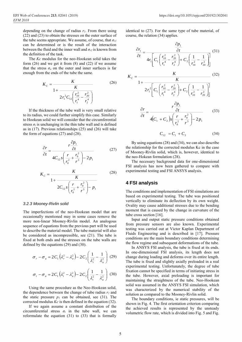
The boundary conditions, ie static pressures, will be

shown in Fig. 4. The first orientation criterion comparing

the achieved results is represented by the unsteady

volumetric flow rate, which is divided into Fig. 5 and Fig.

5


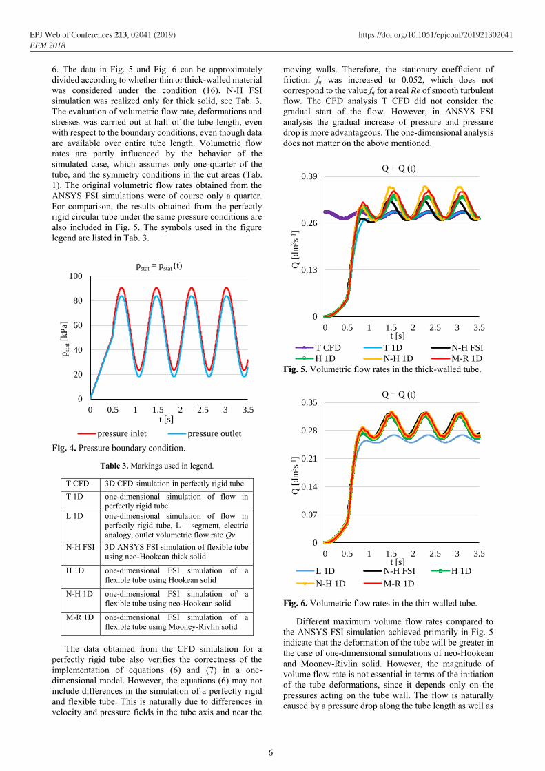
6. The data in Fig. 5 and Fig. 6 can be approximately

divided according to whether thin or thick-walled material

was considered under the condition (16). N-H FSI

simulation was realized only for thick solid, see Tab. 3.

The evaluation of volumetric flow rate, deformations and

stresses was carried out at half of the tube length, even

with respect to the boundary conditions, even though data

are available over entire tube length. Volumetric flow

rates are partly influenced by the behavior of the

simulated case, which assumes only one-quarter of the

tube, and the symmetry conditions in the cut areas (Tab.

1). The original volumetric flow rates obtained from the

ANSYS FSI simulations were of course only a quarter.

For comparison, the results obtained from the perfectly

rigid circular tube under the same pressure conditions are

also included in Fig. 5. The symbols used in the figure

legend are listed in Tab. 3.

Fig. 4. Pressure boundary condition.

Table 3. Markings used in legend.

T CFD 3D CFD simulation in perfectly rigid tube

T 1D one-dimensional simulation of flow in

perfectly rigid tube

L 1D one-dimensional simulation of flow in

perfectly rigid tube, L – segment, electric

analogy, outlet volumetric flow rate Qv

N-H FSI 3D ANSYS FSI simulation of flexible tube

using neo-Hookean thick solid

H 1D one-dimensional FSI simulation of a

flexible tube using Hookean solid

N-H 1D one-dimensional FSI simulation of a

flexible tube using neo-Hookean solid

M-R 1D one-dimensional FSI simulation of a

flexible tube using Mooney-Rivlin solid

The data obtained from the CFD simulation for a

perfectly rigid tube also verifies the correctness of the

implementation of equations (6) and (7) in a one-

dimensional model. However, the equations (6) may not

include differences in the simulation of a perfectly rigid

and flexible tube. This is naturally due to differences in

velocity and pressure fields in the tube axis and near the

moving walls. Therefore, the stationary coefficient of

friction fq was increased to 0.052, which does not

correspond to the value fq for a real Re of smooth turbulent

flow. The CFD analysis T CFD did not consider the

gradual start of the flow. However, in ANSYS FSI

analysis the gradual increase of pressure and pressure

drop is more advantageous. The one-dimensional analysis

does not matter on the above mentioned.

Fig. 5. Volumetric flow rates in the thick-walled tube.

Fig. 6. Volumetric flow rates in the thin-walled tube.

Different maximum volume flow rates compared to

the ANSYS FSI simulation achieved primarily in Fig. 5

indicate that the deformation of the tube will be greater in

the case of one-dimensional simulations of neo-Hookean

and Mooney-Rivlin solid. However, the magnitude of

volume flow rate is not essential in terms of the initiation

of the tube deformations, since it depends only on the

pressures acting on the tube wall. The flow is naturally

caused by a pressure drop along the tube length as well as

0

20

40

60

80

100

0 0.5 1 1.5 2 2.5 3 3.5

pst

at[k

Pa]

t [s]

pstat = pstat (t)

pressure inlet pressure outlet

0

0.13

0.26

0.39

0 0.5 1 1.5 2 2.5 3 3.5

Q [

dm

3s-1

]

t [s]

Q = Q (t)

T CFD T 1D N-H FSI

H 1D N-H 1D M-R 1D

0

0.07

0.14

0.21

0.28

0.35

0 0.5 1 1.5 2 2.5 3 3.5

Q [

dm

3s-1

]

t [s]

Q = Q (t)

L 1D N-H FSI H 1D

N-H 1D M-R 1D

6


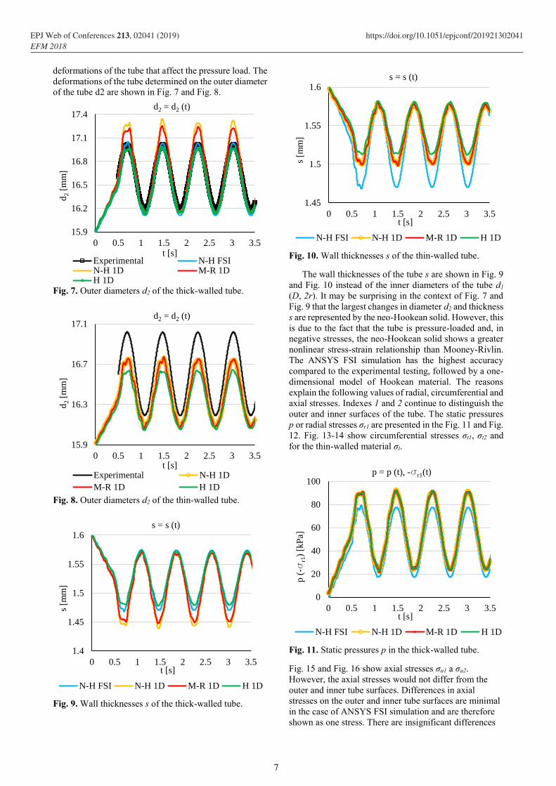
deformations of the tube that affect the pressure load. The

deformations of the tube determined on the outer diameter

of the tube d2 are shown in Fig. 7 and Fig. 8.

Fig. 7. Outer diameters d2 of the thick-walled tube.

Fig. 8. Outer diameters d2 of the thin-walled tube.

Fig. 9. Wall thicknesses s of the thick-walled tube.

Fig. 10. Wall thicknesses s of the thin-walled tube.

The wall thicknesses of the tube s are shown in Fig. 9

and Fig. 10 instead of the inner diameters of the tube d1

(D, 2r). It may be surprising in the context of Fig. 7 and

Fig. 9 that the largest changes in diameter d2 and thickness

s are represented by the neo-Hookean solid. However, this

is due to the fact that the tube is pressure-loaded and, in

negative stresses, the neo-Hookean solid shows a greater

nonlinear stress-strain relationship than Mooney-Rivlin.

The ANSYS FSI simulation has the highest accuracy

compared to the experimental testing, followed by a one-

dimensional model of Hookean material. The reasons

explain the following values of radial, circumferential and

axial stresses. Indexes 1 and 2 continue to distinguish the

outer and inner surfaces of the tube. The static pressures

p or radial stresses σr1 are presented in the Fig. 11 and Fig.

12. Fig. 13-14 show circumferential stresses σt1, σt2 and

for the thin-walled material σt.

Fig. 11. Static pressures p in the thick-walled tube.

Fig. 15 and Fig. 16 show axial stresses σa1 a σa2.

However, the axial stresses would not differ from the

outer and inner tube surfaces. Differences in axial

stresses on the outer and inner tube surfaces are minimal

in the case of ANSYS FSI simulation and are therefore

shown as one stress. There are insignificant differences

15.9

16.2

16.5

16.8

17.1

17.4

0 0.5 1 1.5 2 2.5 3 3.5

d2

[mm

]

t [s]

d2 = d2 (t)

Experimental N-H FSIN-H 1D M-R 1DH 1D

15.9

16.3

16.7

17.1

0 0.5 1 1.5 2 2.5 3 3.5

d2

[mm

]

t [s]

d2 = d2 (t)

Experimental N-H 1D

M-R 1D H 1D

1.4

1.45

1.5

1.55

1.6

0 0.5 1 1.5 2 2.5 3 3.5

s [m

m]

t [s]

s = s (t)

N-H FSI N-H 1D M-R 1D H 1D

1.45

1.5

1.55

1.6

0 0.5 1 1.5 2 2.5 3 3.5

s [m

m]

t [s]

s = s (t)


0

20

40

60

80

100

0 0.5 1 1.5 2 2.5 3 3.5

p (

-sr1

) [k

Pa]

t [s]

p = p (t), -sr1(t)


7


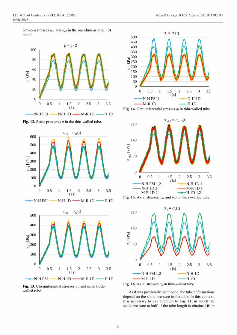
between stresses σa1 and σa2 in the one-dimensional FSI

model.

Fig. 12. Static pressures p in the thin-walled tube.

Fig. 13. Circumferential stresses σt1 and σt2 in thick-

walled tube.

Fig. 14. Circumferential stresses σt in thin-walled tube.

Fig. 15. Axial stresses σa1 and σa2 in thick-walled tube.

Fig. 16. Axial stresses σa in thin-walled tube.

As it was previously mentioned, the tube deformations

depend on the static pressure in the tube. In this context,

it is necessary to pay attention to Fig. 11, in which the

static pressure at half of the tube length is obtained from

0

20

40

60

80

100

0 0.5 1 1.5 2 2.5 3 3.5

p [

kP

a]

t [s]

p = p (t)


0

100

200

300

400

500

600

0 0.5 1 1.5 2 2.5 3 3.5

st1

[kP

a]

t [s]

st1 = st1(t)


0

100

200

300

400

500

0 0.5 1 1.5 2 2.5 3 3.5

st2

[kP

a]

t [s]

st2 = st2(t)


0

50

100

150

200

250

300

350

400

450

500

0 0.5 1 1.5 2 2.5 3 3.5

st[k

Pa]

t [s]

st = st(t)

N-H FSI 1 N-H 1D

M-R 1D H 1D

0

70

140

210

0 0.5 1 1.5 2 2.5 3 3.5

sa1

,2[k

Pa]

t [s]

sa1,2 = sa1,2(t)

N-H FSI 1,2 N-H 1D 1N-H 1D 2 M-R 1D 1M-R 1D 2 H 1D 1,2

0

70

140

210

0 0.5 1 1.5 2 2.5 3 3.5

sa

[kP

a]

t [s]

sa = sa(t)

N-H FSI 1,2 N-H 1D

M-R 1D H 1D

8


the ANSYS FSI simulation. If we compare Fig. 11 with

Fig. 4 we must note the decrease of the maximum static

pressure value compared to the maximum static pressure

on the inlet and outlet of the tube. This situation can occur,

but from the analysis of the linear case, this condition

should become at frequencies higher than the frequencies

of the pressures in Fig. 4. The cause of the decrease of

static pressure amplitudes shown in the Fig. 11 may be in

the case of ANSYS FSI simulation under the boundary

conditions by which a quarter of the tube has been fitted,

see Tab. 1. It should also be remembered that the tube

does not deform at its ends compared to one-dimensional

simulations. Conformity of ANSYS FSI simulation of

neo-Hookean material with experimental testing may

therefore be only incidental, but this is of course not a

software problem. However, the degree of fixation of the

experimentally tested tube cannot be retrospectively

determined.

The question is why the data from experimental

testing with ANSYS FSI simulation corresponds,

although the agreement is not perfect in the lower

displacements of the outer diameter d2. There are two

probable explanations. The cross section of the tube was

not always completely circular, causing additional stress

due to ovality. And the second option lies essentially with

the Tygon material itself, which in fact does not have such

a pronounced non-linear character as it was considered. In

this context, it is also necessary to mention the general

recommendation to simulate the Tygon material as a

Mooney-Rivlin solid. The ANSYS FSI simulation of neo-

Hookean solid was chosen due to Mooney-Rivlin material

convergence difficulties.

Also, the one-dimensional FSI models have some

drawbacks, and the most obvious one is to predict the

volume flow rate. The volume flow through the tubes can

be unnaturally changed by the coefficient fq. However, the

change in the coefficient within reasonable limits has only

a slight effect on static pressures along the tube length. Of

course, this corresponds to the character of the

mathematical-physical model described in particular in

(6). The inlet and outlet of the tube are controlled by the

pressures in Fig. 4. Moreover, the tube is very short, L =

0.5 m. The pressure pattern in the tube further depends on

the frequency, which is very low in our case

(approximately 1Hz). The case appears almost as a static

despite the relatively considerable deformation of the tube

wall with regard to wavelengths.

Three facts can contribute to a better understanding of

the problem. The first will deal with the hydraulic

coefficient of friction fq, which was formulated for

stationary flow. However, the flow in the tube is unsteady.

Considering the above, the coefficient fq in (6) by

Brunone, Vardy and Vítkovsky [18 - 20] can be replaced

by fqu, see (35).

x

Q

SQsignc

t

r

Sr

Q

t

Q

SQQ

SDk

ff qqu

1212 (35)

The other parameters are defined in (36) - (38) and are

valid in the interval, Re = 2000 - 108.

2

*Ck (36)

Re

86.12* C (37)

0567.010Re

29.15log (38)

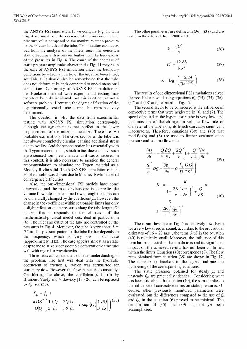
The results of one-dimensional FSI simulations solved

for neo-Hokean solid using equations 6), (25), (35), (36),

(37) and (38) are presented in Fig. 17.

The second factor to be considered is the influence of

convective terms that were neglected in (6) and (7). The

speed of sound in the hyperelastic tube is very low, and

the omission of the changes in volume flow rate or

diameter of the tube along its length can cause significant

inaccuracies. Therefore, equations (39) and (40) that

modify (6) and (8) are used to further evaluate static

pressure and volume flow rate.

2

1

2

12

S

QQ

D

f

x

pg

S

t

r

Sc

Q

r

Q

x

Q

S

Q

t

Q

q

(39)

1

1

1

1

21

21

r

p

r

K

K

Sc

Q

r

p

r

K

KKC

(40)

The mean flow rate in Fig. 5 is relatively low. Even

for a very low speed of sound, according to the provisional

estimates of 16 – 20 m.s-1, the term Q/cS in the equation

(40) is relatively small. Moreover, the influence of this

term has been tested in the simulations and its significant

impact on the achieved results has not been confirmed

within the limits. Equation (40) corresponds (8). The flow

rates obtained from equation (39) are shown in Fig. 17.

The numbers in brackets in the legend indicate the

numbering of the corresponding equations.

The static pressures obtained for steady fq and

unsteady fqu are practically identical. Considering what

has been said about the equation (40), the same applies to

the influence of convective terms on static pressures. Of

course, other previously monitored parameters were

evaluated, but the differences compared to the use of fq

and fqu in the equation (6) proved to be minimal. The

combination of (35) and (39) has not yet been

accomplished.

9


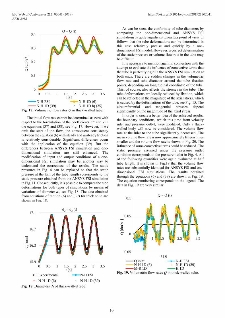
Fig. 17. Volumetric flow rates Q in thick-walled tube.

The initial flow rate cannot be determined as zero with

respect to the formulation of the coefficients C* and κ in

the equations (37) and (38), see Fig. 17. However, if we

omit the start of the flow, the consequent consistency

between the equation (6) with steady and unsteady friction

is relatively considerable. Significant differences occur

with the application of the equation (39). But the

differences between ANSYS FSI simulation and one-

dimensional simulation are still enhanced. The

modification of input and output conditions of a one-

dimensional FSI simulation may be another way to

understand the correctness of the results. The static

pressures in Fig. 4 can be replaced so that the static

pressure at the half of the tube length corresponds to the

static pressure obtained from the ANSYS FSI simulation

in Fig. 11. Consequently, it is possible to compare the tube

deformations for both types of simulations by means of

variations of diameter d2, see Fig. 18. The data obtained

from equations of motion (6) and (39) for thick solid are

shown in Fig. 18.

Fig. 18. Diameters d2 of thick-walled tube.

As can be seen, the conformity of tube diameters by

comparing the one-dimensional and ANSYS FSI

simulations is quite significant from this point of view. It

follows that the tube deformations can be determined in

this case relatively precise and quickly by a one-

dimensional FSI model. However, a correct determination

of the static pressure or volume flow rate in the tube may

be difficult.

It is necessary to mention again in connection with the

attempt to evaluate the influence of convective terms that

the tube is perfectly rigid in the ANSYS FSI simulation at

both ends. There are sudden changes in the volumetric

flow rate and tube diameter around the tube fixation

points, depending on longitudinal coordinate of the tube.

This, of course, also affects the stresses in the tube. The

tube deformations are locally reduced by fixation, which

can be reflected in the magnitude of the axial stress, which

is caused by the deformations of the tube, see Fig. 15. The

circumferential and tangential stresses depend

significantly on the magnitude of the axial stress.

In order to create a better idea of the achieved results,

the boundary conditions, which this time form velocity

inlet and pressure outlet, were modified. Only a thick-

walled body will now be considered. The volume flow

rate at the inlet to the tube significantly decreased. The

mean volume flow rate is now approximately fifteen times

smaller and the volume flow rate is shown in Fig. 20. The

influence of some convective terms could be reduced. The

static pressure assumed under the pressure outlet

condition corresponds to the pressure outlet in Fig. 4. All

of the following quantities were again evaluated at half

tube length. It is shown in Fig.19 that the volume flow

rates are substantially identical for ANSYS FSI and one-

dimensional FSI simulations. The results obtained

through the equations (6) and (39) are shown in Fig. 19.

The equation numbering corresponds to the legend. The

data in Fig. 19 are very similar.

Fig. 19. Volumetric flow rates Q in thick-walled tube.

0

0.1

0.2

0.3

0.4

0 0.5 1 1.5 2 2.5 3 3.5

Q [

dm

3s-1

]

t [s]

Q = Q (t)

N-H FSI N-H 1D (6)N-H 1D (39) N-H 1D fq (35)

15.9

16.3

16.7

17.1

0 0.5 1 1.5 2 2.5 3 3.5

d2

[mm

]

t [s]

d2 = d2 (t)

Experimental N-H FSI

N-H 1D (6) N-H 1D (39)

-0.05

0

0.05

0.1

0 0.5 1 1.5 2 2.5 3 3.5

Q [

dm

3s-1

]

t [s]

Q = Q (t)

Q inlet N-H FSIN-H 1D (6) N-H 1D (39)M-R 1D H 1D

10


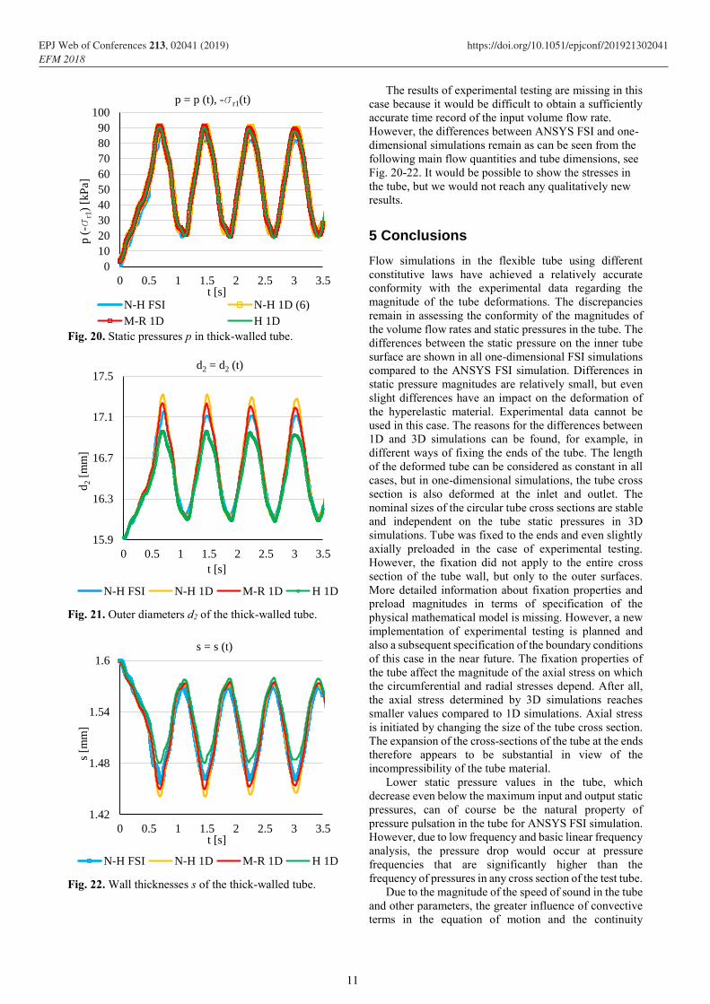
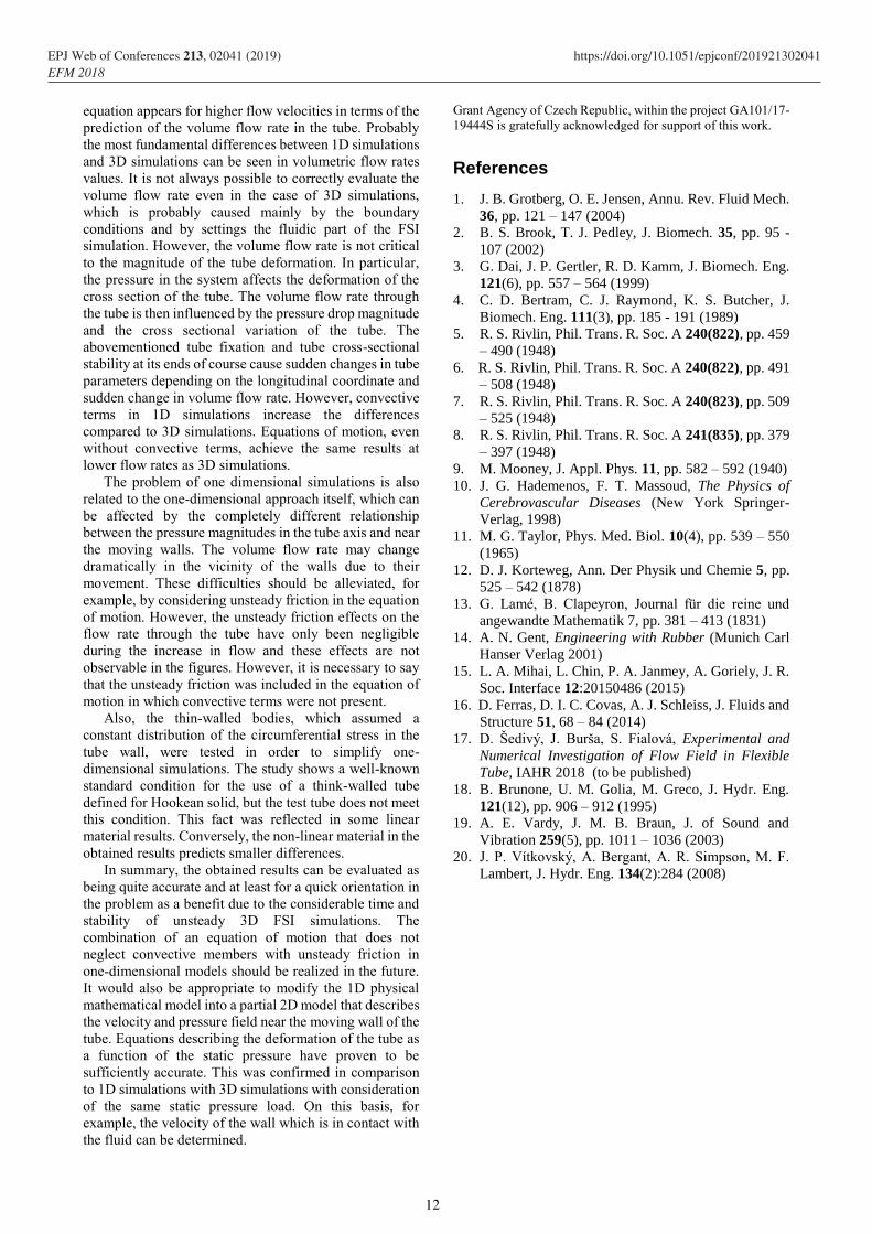
Fig. 20. Static pressures p in thick-walled tube.

Fig. 21. Outer diameters d2 of the thick-walled tube.

Fig. 22. Wall thicknesses s of the thick-walled tube.

The results of experimental testing are missing in this

case because it would be difficult to obtain a sufficiently

accurate time record of the input volume flow rate.

However, the differences between ANSYS FSI and one-

dimensional simulations remain as can be seen from the

following main flow quantities and tube dimensions, see

Fig. 20-22. It would be possible to show the stresses in

the tube, but we would not reach any qualitatively new

results.

5 Conclusions

Flow simulations in the flexible tube using different

constitutive laws have achieved a relatively accurate

conformity with the experimental data regarding the

magnitude of the tube deformations. The discrepancies

remain in assessing the conformity of the magnitudes of

the volume flow rates and static pressures in the tube. The

differences between the static pressure on the inner tube

surface are shown in all one-dimensional FSI simulations

compared to the ANSYS FSI simulation. Differences in

static pressure magnitudes are relatively small, but even

slight differences have an impact on the deformation of

the hyperelastic material. Experimental data cannot be

used in this case. The reasons for the differences between

1D and 3D simulations can be found, for example, in

different ways of fixing the ends of the tube. The length

of the deformed tube can be considered as constant in all

cases, but in one-dimensional simulations, the tube cross

section is also deformed at the inlet and outlet. The

nominal sizes of the circular tube cross sections are stable

and independent on the tube static pressures in 3D

simulations. Tube was fixed to the ends and even slightly

axially preloaded in the case of experimental testing.

However, the fixation did not apply to the entire cross

section of the tube wall, but only to the outer surfaces.

More detailed information about fixation properties and

preload magnitudes in terms of specification of the

physical mathematical model is missing. However, a new

implementation of experimental testing is planned and

also a subsequent specification of the boundary conditions

of this case in the near future. The fixation properties of

the tube affect the magnitude of the axial stress on which

the circumferential and radial stresses depend. After all,

the axial stress determined by 3D simulations reaches

smaller values compared to 1D simulations. Axial stress

is initiated by changing the size of the tube cross section.

The expansion of the cross-sections of the tube at the ends

therefore appears to be substantial in view of the

incompressibility of the tube material.

Lower static pressure values in the tube, which

decrease even below the maximum input and output static

pressures, can of course be the natural property of

pressure pulsation in the tube for ANSYS FSI simulation.

However, due to low frequency and basic linear frequency

analysis, the pressure drop would occur at pressure

frequencies that are significantly higher than the

frequency of pressures in any cross section of the test tube.

Due to the magnitude of the speed of sound in the tube

and other parameters, the greater influence of convective

terms in the equation of motion and the continuity

0

10

20

30

40

50

60

70

80

90

100

0 0.5 1 1.5 2 2.5 3 3.5

p (

-sr1

) [k

Pa]

t [s]

p = p (t), -sr1(t)

N-H FSI N-H 1D (6)

M-R 1D H 1D

15.9

16.3

16.7

17.1

17.5

0 0.5 1 1.5 2 2.5 3 3.5

d2

[mm

]

t [s]

d2 = d2 (t)


1.42

1.48

1.54

1.6

0 0.5 1 1.5 2 2.5 3 3.5

s [m

m]

t [s]

s = s (t)


11


equation appears for higher flow velocities in terms of the

prediction of the volume flow rate in the tube. Probably

the most fundamental differences between 1D simulations

and 3D simulations can be seen in volumetric flow rates

values. It is not always possible to correctly evaluate the

volume flow rate even in the case of 3D simulations,

which is probably caused mainly by the boundary

conditions and by settings the fluidic part of the FSI

simulation. However, the volume flow rate is not critical

to the magnitude of the tube deformation. In particular,

the pressure in the system affects the deformation of the

cross section of the tube. The volume flow rate through

the tube is then influenced by the pressure drop magnitude

and the cross sectional variation of the tube. The

abovementioned tube fixation and tube cross-sectional

stability at its ends of course cause sudden changes in tube

parameters depending on the longitudinal coordinate and

sudden change in volume flow rate. However, convective

terms in 1D simulations increase the differences

compared to 3D simulations. Equations of motion, even

without convective terms, achieve the same results at

lower flow rates as 3D simulations.

The problem of one dimensional simulations is also

related to the one-dimensional approach itself, which can

be affected by the completely different relationship

between the pressure magnitudes in the tube axis and near

the moving walls. The volume flow rate may change

dramatically in the vicinity of the walls due to their

movement. These difficulties should be alleviated, for

example, by considering unsteady friction in the equation

of motion. However, the unsteady friction effects on the

flow rate through the tube have only been negligible

during the increase in flow and these effects are not

observable in the figures. However, it is necessary to say

that the unsteady friction was included in the equation of

motion in which convective terms were not present.

Also, the thin-walled bodies, which assumed a

constant distribution of the circumferential stress in the

tube wall, were tested in order to simplify one-

dimensional simulations. The study shows a well-known

standard condition for the use of a think-walled tube

defined for Hookean solid, but the test tube does not meet

this condition. This fact was reflected in some linear

material results. Conversely, the non-linear material in the

obtained results predicts smaller differences.

In summary, the obtained results can be evaluated as

being quite accurate and at least for a quick orientation in

the problem as a benefit due to the considerable time and

stability of unsteady 3D FSI simulations. The

combination of an equation of motion that does not

neglect convective members with unsteady friction in

one-dimensional models should be realized in the future.

It would also be appropriate to modify the 1D physical

mathematical model into a partial 2D model that describes

the velocity and pressure field near the moving wall of the

tube. Equations describing the deformation of the tube as

a function of the static pressure have proven to be

sufficiently accurate. This was confirmed in comparison

to 1D simulations with 3D simulations with consideration

of the same static pressure load. On this basis, for

example, the velocity of the wall which is in contact with

the fluid can be determined.

Grant Agency of Czech Republic, within the project GA101/17-

19444S is gratefully acknowledged for support of this work.

References

1. J. B. Grotberg, O. E. Jensen, Annu. Rev. Fluid Mech.

36, pp. 121 – 147 (2004)

2. B. S. Brook, T. J. Pedley, J. Biomech. 35, pp. 95 -

107 (2002)

3. G. Dai, J. P. Gertler, R. D. Kamm, J. Biomech. Eng.

121(6), pp. 557 – 564 (1999)

4. C. D. Bertram, C. J. Raymond, K. S. Butcher, J.

Biomech. Eng. 111(3), pp. 185 - 191 (1989)

5. R. S. Rivlin, Phil. Trans. R. Soc. A 240(822), pp. 459

– 490 (1948)


– 508 (1948)


– 525 (1948)


– 397 (1948)

9. M. Mooney, J. Appl. Phys. 11, pp. 582 – 592 (1940)

10. J. G. Hademenos, F. T. Massoud, The Physics of

Cerebrovascular Diseases (New York Springer-

Verlag, 1998)

11. M. G. Taylor, Phys. Med. Biol. 10(4), pp. 539 – 550

(1965)

12. D. J. Korteweg, Ann. Der Physik und Chemie 5, pp.

525 – 542 (1878)

13. G. Lamé, B. Clapeyron, Journal für die reine und

angewandte Mathematik 7, pp. 381 – 413 (1831)

14. A. N. Gent, Engineering with Rubber (Munich Carl

Hanser Verlag 2001)

15. L. A. Mihai, L. Chin, P. A. Janmey, A. Goriely, J. R.

Soc. Interface 12:20150486 (2015)

16. D. Ferras, D. I. C. Covas, A. J. Schleiss, J. Fluids and

Structure 51, 68 – 84 (2014)

17. D. Šedivý, J. Burša, S. Fialová, Experimental and

Numerical Investigation of Flow Field in Flexible

Tube, IAHR 2018 (to be published)

18. B. Brunone, U. M. Golia, M. Greco, J. Hydr. Eng.

121(12), pp. 906 – 912 (1995)

19. A. E. Vardy, J. M. B. Braun, J. of Sound and

Vibration 259(5), pp. 1011 – 1036 (2003)

20. J. P. Vítkovský, A. Bergant, A. R. Simpson, M. F.

Lambert, J. Hydr. Eng. 134(2):284 (2008)

12


https://eudml.org/journal/10147

https://eudml.org/journal/10147

Pulse flow of liquid in flexible tube - EPJ Web of Conferences

Documents