Pulsar wind zone processes in LS 5039

arX

iv:0

801.

3427

v3 [

astr

o-ph

] 2

9 Se

p 20

08

Pulsar wind zone processes in LS 5039

Agnieszka Sierpowska-Bartosik & a Diego F. Torres a,b

aInstitut de Ciencies de l’Espai (IEEC-CSIC) Campus UAB, Fac. de Ciencies,Torre C5, parell, 2a planta, 08193 Barcelona, Spain. E-mail: [email protected] Catalana de Recerca i Estudis Avancats (ICREA), Spain. E-mail:

[email protected]

Abstract

Several γ-ray binaries have been recently detected by the High-Energy Stere-oscopy Array (H.E.S.S.) and the Major Atmospheric Imaging Cerenkov (MAGIC)telescope. In at least two cases, their nature is unknown. In this paper we aim toprovide the details of a theoretical model of close γ-ray binaries containing a youngenergetic pulsar as compact object, earlier presented in recent Letters. This modelincludes a detailed account of the system geometry, the angular dependence of pro-cesses such as Klein-Nishina inverse Compton and γγ absorption in the anisotropicradiation field of the massive star, and a Monte Carlo simulation of leptonic cas-cading. We present and derive the used formulae and give all details about theirnumerical implementation, particularly, on the computation of cascades. In thismodel, emphasis is put in the processes occurring in the pulsar wind zone of thebinary, since, as we show, opacities in this region can be already important for closesystems. We provide a detailed study on all relevant opacities and geometrical de-pendencies along the orbit of binaries, exemplifying with the case of LS 5039. Thisis used to understand the formation of the very high-energy lightcurve and phasedependent spectrum. For the particular case of LS 5039, we uncover an interestingbehavior of the magnitude representing the shock position in the direction to theobserver along the orbit, and analyze its impact in the predictions. We show thatin the case of LS 5039, the H.E.S.S. phenomenology is matched by the presentedmodel, and explore the reasons why this happens while discussing future ways oftesting the model.

Key words: γ-rays: theory, X-ray binaries (individual LS 5039), γ-rays:observations

Preprint submitted to Elsevier 11 February 2013

1 Introduction

Very recently, a few massive binaries have been identified as variable very-high-energy (VHE) γ-ray sources. They are PSR B1259-63 (Aharonian et al.2005a), LS 5039 (Aharonian et al. 2005b, 2006), LS I +61 303 (Albert et al.2006, 2008a,b), and Cyg X-1 (Albert et al. 2007). The nature of only two ofthese binaries is considered known: PSR B 1259-63 is formed with a pulsarwhereas Cyg X-1 is formed with a black hole compact object. The nature of thetwo remaining systems is under discussion. The high-energy phenomenologyof Cyg X-1 is different from that of the others. It has been detected just oncein a flare state for which a duty cycle is yet unknown. The three other sources,instead, present a behavior that is fully correlated with the orbital period. Thelatter varies from about 4 days in the case of LS 5039 to several years in thecase of PSR B1259-63: this span of orbital periodicities introduces its owncomplications in analyzing the similarities among the three systems.

LS I +61 303 shares with LS 5039 the quality of being the only two knownmicroquasars/γ-ray binaries that are spatially coincident with sources above100 MeV listed in the Third Energetic Gamma-Ray Experiment (EGRET)catalog (Hartman et al. 1999). These sources both show low X-ray emissionand variability, and no signs of emission lines or disk accretion. For LS I +61303, extended, apparently precessing, radio emitting structures at angular ex-tensions of 0.01-0.05 arcsec have been reported by Massi et al. (2001, 2004);this discovery has earlier supported its microquasar interpretation. But theuncertainty as to what kind of compact object, a black hole or a neutron star,is part of the system (e.g., Casares et al. 2005a), seems settled for many afterthe results presented by Dhawan et al. (2006). These authors have presentedobservations from a July 2006 VLBI campaign in which rapid changes areseen in the orientation of what seems to be a cometary tail at periastron.This tail is consistent with it being the result of a pulsar wind. Indeed, nolarge features or high-velocity flows were noted on any of the observing days,which implies at least its non-permanent nature. The changes within 3 hourswere found to be insignificant, so the velocity can not be much over 0.05c.Still, discussion is on-going (e.g. see Romero et al. 2007, Zdziarski et al. 2008).New campaigns with similar radio resolution, as well as new observations inthe γ-ray domain have been obtained since the Dhawan’s et al. original results(Albert et al. 2008b). A key aspect in these high-angular-resolution campaignsis the observed maintenance in time of the morphology of the radio emissionof the system: the changing morphology of the radio emission along the orbitwould require a highly unstable jet, which details are not expected to be re-produced orbit after orbit as indicated by current results (Albert et al. 2008b).The absence of accretion signatures in X-rays in Chandra and XMM-Newtonobservations (as reported by Sidoli et al. 2006, Chernyakova et al. 2006, andParedes et al. 2007) is another relevant aspect of the discussion about the

2

compact object companion. Finally, it is interesting to note that neutrino de-tection or non-detection with ICECUBE will shed light on the nature of theγ-ray emission irrespective of the system composition (e.g., Aharonian et al.2006b, Torres and Halzen 2007).

For LS 5039, a periodicity in the γ-ray flux, consistent with the orbital timescaleas determined by Casares et al. (2005b), was found with amazing precision(Aharonian et al. 2006). Short timescale variability displayed on top of thisperiodic behavior, both in flux and spectrum, was also reported. It was foundthat the parameters of power-law fits to the γ-ray data obtained in 0.1 phasebinning already displayed significant variability. Current H.E.S.S. observationsof LS 5039 (∼ 70 hours distributed over many orbital cycles, Aharonian et al.2006) constitute one of the most detailed datasets of high-energy astrophysics.Similarly to LS I +61 303, the discovery of a jet-like radio structure in LS 5039and the fact of it being the only radio/X-ray source co-localized with a mildlyvariable (Torres et al. 2001a,b) EGRET detection, prompted a microquasarinterpretation (advanced already by Paredes et al. 2000). However, the cur-rent mentioned findings at radio and VHE γ-rays in the cases of LS I +61 303(Dhawan et al. 2006, Albert et al. 2006, 2008b) or PSR B1259-63 (Aharonianet al. 2005), gave the perspective that all three systems are different real-izations of the same scenario: a pulsar-massive star binary. Dubus (2006a,b)has studied these similarities. He provided simulations of the extended radioemission of LS 5039 showing that the features found in high resolution radioobservations could also be interpreted as the result of a pulsar wind. Recently,Ribo et al. (2008) provided VLBA radio observations of LS 5039 with mor-phological and astrometric information at milliarcsecond scales. They showedthat a microquasar scenario cannot easily explain the observed changes in mor-phology. All these results, together with the assessment of the low X-ray state(Martocchia et al. 2005) made the pulsar hypothesis tenable, and the possi-bility of explaining the H.E.S.S. phenomenology in such a case, an interestingworking hypothesis.

High energy emission from pulsar binaries has been subject of study for along time (just to quote a non-exhaustive list of references note the worksof Maraschi and Treves 1981; Protheroe and Stanev 1987, Arons and Tavani1993, 1994; Moskalenko et al. 1993; Bednarek 1997, Kirk et al. 1999, Ball andKirk 2000, Romero et al. 2001, Anchordoqui et al. 2003, and others alreadycited above). LS 5039 has been recently subject of intense theoretical studies(e.g., Bednarek 2006, 2007; which we comment on in more detail below, Bosch-Ramon et al. 2005; Bottcher 2007; Bottcher and Dermer 2005; Dermer andBottcher 2006; Dubus 2006a,b; Paredes et al. 2006; Khangulyan et al. 2007;Dubus et al. 2007).

In the penultimate paper mentioned in the list above, Khangulyan et al.(2007), and contrary to the assumption here, authors assumed a jet structure

3

perpendicular to the orbital plane of the system. The energy spectrum andlightcurves were computed, accounting for the acceleration efficiency, the loca-tion of the accelerator along the jet, the speed of the emitting flow, the inclina-tion angle of the system, as well as specific features related to anisotropic in-verse Compton (IC) scattering and pair production. Different magnetic fields,affecting Synchrotron emission, and the losses they produced, were also testedgiven a large model parameter space. Authors found a good agreement be-tween H.E.S.S. data for some of their models.

In the last of these papers, Dubus et al. (2007) computed the phase depen-dent lightcurve and spectra expected from inverse Compton interactions fromelectrons injected close to the compact object, assumed as a likely rotation-powered pulsar. Since the angle at which an observer sees the binary andpropagating electrons changes with the orbit (see below), a phase dependenceof the spectrum is expected, and anisotropic inverse Compton is needed tocompute it. In general, they found that the lightcurve is a good fit to the ob-servations, except at the phases of maximum attenuation where pair cascadeemission plays a role. Dubus et al. (2007) do not consider cascading in theirmodels, as we do here. Without cascading, zero flux is expected at a broadphase around periastron, which is not found. This lack of cascading in theirmodel also affects the spectra, which are not reproduced well, particularlyat the superior conjunction broad phases of the orbit. They mentioned thatboth, cascading and/or a change in the slope of the power-law injection forthe interacting electron distribution could be needed to explain the spectrumin these phases, what we explore in detail in this work.

In order to compute inverse Compton emission from LS 5039, we use, as inprevious works, leptons interacting with the star photon field. Geometry isdescribed there with different levels of detail, what influence the results. Ingeneral, cascading processes were not taken into account, and the goodness offitting the H.E.S.S. data is arguable in most cases, both for the lightcurve andspectrum.

In none of the papers mentioned above, the theoretical predictions for theshort timescale spectral variability found by H.E.S.S. in 0.1 phase binningwas shown and compared with data. We discuss these results from our modelbelow.

In recent Letters (Sierpowska-Bartosik and Torres 2007, 2008) under the as-sumption that LS 5039 is composed by a pulsar rotating around an O6.5Vstar in the ∼ 3.9 day orbit, we presented the results of a leptonic (for ageneric hadronic model see Romero et al. 2003) theoretical modeling for thehigh-energy phenomenology observed by H.E.S.S. These works studied thelightcurve, the spectral orbital variability in both broad orbital phases and inshorter (0.1 phase binning) timescales and have found a complete agreement

4

between H.E.S.S. observations and our predictions. We have also analyzedhow this model could be tested by Gamma-ray Large Area Space Telescope(GLAST), and how much time would be needed for this satellite in order torule the model out in case theory significantly departs from reality. But manydetails of implementation which are not only useful for the case of LS 5039 butfor all others close massive γ-ray binaries, as well as many interesting resultsconcerning the binary geometry, wind termination, opacities to different pro-cesses along the orbit of the system, and further testing at the highest energyγ-ray domain were left without discussion in our previous works. Here, weprovide these details, together with benchmark cases that are useful to under-stand the formation of the very high-energy lightcurve and phase dependentspectra.

The rest of this paper is organized as follows. Next Section introduces themodel concept and its main properties. It provides a discussion of geometry,wind termination, and opacities along the orbit of the system (we focus onLS 5039). An accompanying Appendix provides mathematical derivations ofthe formulae used and useful intermediate results that are key for the model,but too cumbersome to include them as part of the main text. It also dealswith numerical implementation, and describes in detail the Monte Carlo sim-ulation of the cascading processes. The results follow: Section 3 deals with amono-energetic interacting particle population, and Section 4, with power-lawprimary distributions. Comparison with H.E.S.S. results is made in these Sec-tions and details about additional tests are given. Final concluding remarksare provided at the end.

2 Description of the model and its implementation

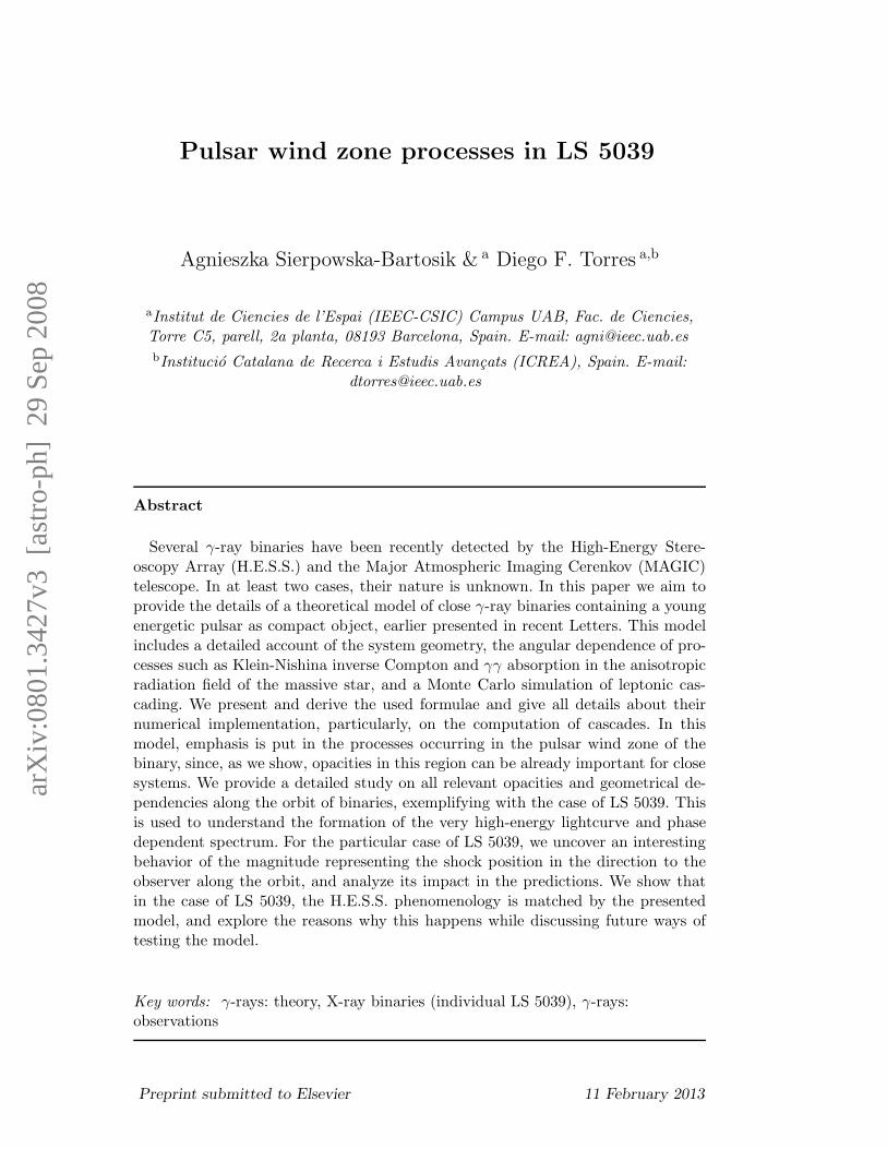
Under the assumption that the pulsar in the binary is energetic enough toprevent matter from the massive companion from accreting, a terminationshock is created in the interaction region of the pulsar and donor star winds.This is represented in Fig. 1. We focus on the specific case of the binaryLS 5039, which we use as a testbed all along this paper. The volume of thesystem is separated by the termination shock, which structure depends onfeatures of the colliding winds: it may be influenced by the anisotropy of thewinds themselves, the motion of the pulsar along the orbit, turbulences in theshock flow, etc. For simplicity it is assumed here that the winds are radial andspherically symmetric, and that the termination of the pulsar wind is an axialsymmetric structure with negligible thickness. In this general picture thereare three regions of different properties in the binary: the pulsar wind zone(PWZ), the shock (SR), and the massive star wind zone (MSWZ).

The energy content in the interaction population of particles is assumed as a

5

SUPC

MS

αobs

P

φ A=0.5

=0.058φ =0.0φ

=0.716φ

to observer

INFC PSR

α

γ

γ

γ

γ

γ

γ

obs e e

e e

e e

e ee e

e e+ −

+ −

+ −

+ −

+ −+ −

ε

ε

ε

ε

εε

εε

ε

ε

ε

ε

e e+ −

MS

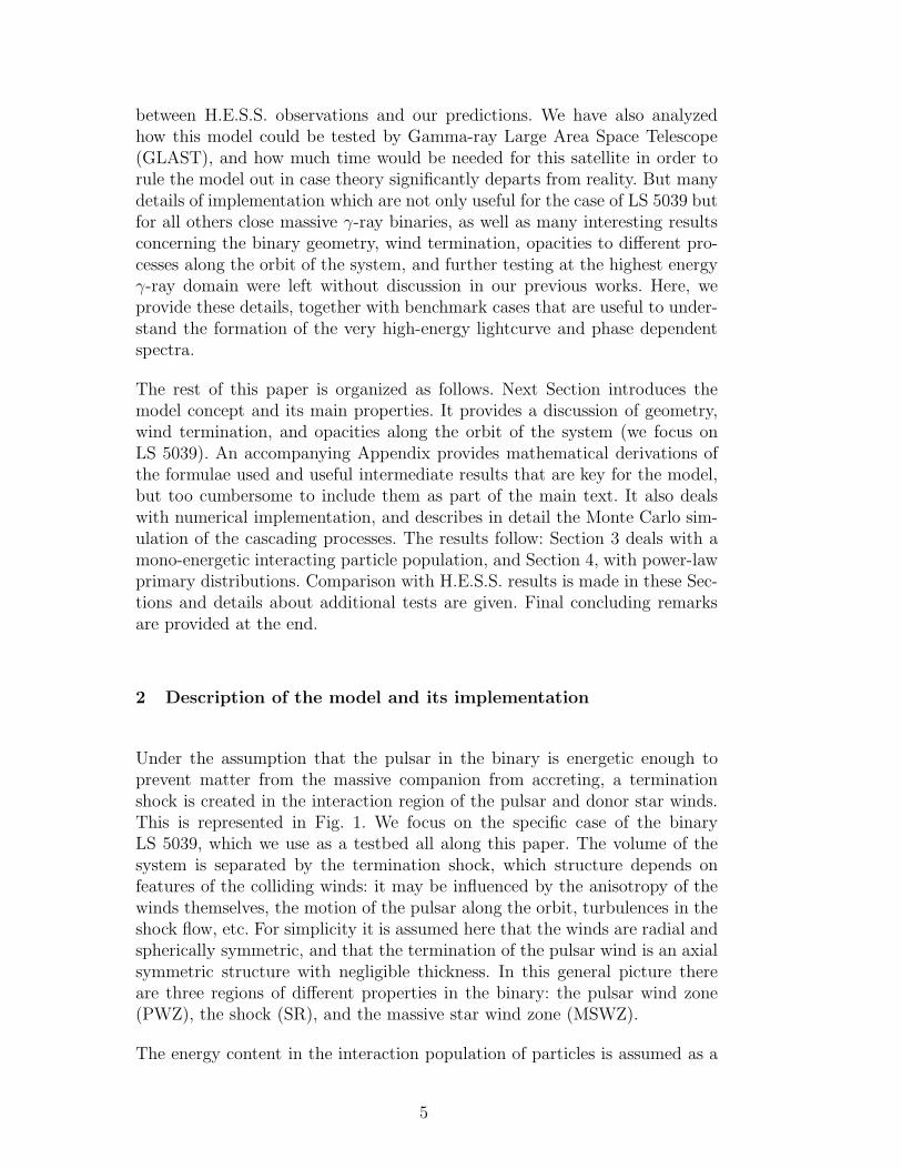
Fig. 1. Left: Sketch of a close binary, such as the LS 5039 system. P stands for theorbital position of periastron, A for apastron, INFC for inferior conjunction, andSUPC for superior conjunction. The orbital phase, φ, and the angle to the observer,αobs, are marked. The orbital plane is inclined with respect to the direction of theobserver (this angle is not marked). The termination shock created in the interactionof the pulsar and the massive star winds is also marked for two opposite phases–periastron and apastron– together with the direction to the observer for bothphases. Right: The physical scenario for high-energy photon production in the PWZterminated by the shock. e+e− are injected by the pulsar or by a close-to-the-pulsarshock and travel towards the observer, producing Inverse Compton photons, γ, viaup-scattering thermal photons from the massive star, ε. γ-photons can initiate ICcascade due to absorption in the same thermal field. The cascade is developing upto the termination shock. Electron reaching the shock are trapped there in the localmagnetic field, while photons propagate further and escape from the binary or areabsorbed in massive star radiation field. The cascade develops radially following theinitial injection direction given by αobs.

fraction of pulsar spin-down power Lsd. In case of young energetic pulsars, thispower is typically ∼ 1036 − 1037 erg s−1. Propagating pairs up-scatter thermalphotons from the massive star due to inverse Compton process. For closebinaries, the radiation field of hot massive stars (type O, Be or WR, havingtypical surface temperatures in the range Ts ∼ 104−105 K and linear dimensionRs ∼ 10R⊙) dominates along the whole orbit over other possible fields (e.g.,the magnetic field or the thermal field of the neutron star). This thermalradiation field is anisotropic, particularly for e+e− injected close to the pulsar(the radiation source is misplaced with respect to the electron injection place).

The high-energy photons produced by pairs can initiate cascades due to sub-sequent pair production in absorption (γγ) process with the same radiationfield (as sketched in Fig. 1). We assume that these cascades develop alongthe primary injection direction, i.e., in a one-dimensional way, which is cer-tainly justified based on the relativistic velocity of the interacting electrons.

6

This process is followed up to the termination shock unless leptons lose theirenergy before reaching it. Those leptons which propagate to the shock regionare trapped there by its magnetic field. Radiation from them is isotropised.The photons produced in cascades which reach the shock can get through itand finally escape from the binary or be absorbed in the radiation field closeto the massive star, some may even reach the stellar surface.

In the shock region leptons move along it with velocity ∼ c/3. They couldbe re-accelerated and produce radiation via synchrotron (local magnetic fieldfrom the pulsar side) or inverse Compton scattering (ICS, thermal radiationfield from the massive star) processes. However, as they are isotropised inthe local magnetic field, photons are produced in different directions and theirdirectionality towards the observer is lost. It was already shown by Sierpowskaand Bednarek (2005) that in compact binary systems (as an example, theparameters of Cyg X-3 were taken by these authors) the radiation processesin the shock region do not dominate: the energy carried by e+e− reaching theshock is a small fraction of total injected power. Furthermore, we will showthat for the parameters relevant to the LS 5039 scenario, the PWZ is relativelylarge with respect to the whole volume of the system for the significant rangeof the binary orbit.

2.1 Hydrodynamic balance

Assuming that both, the pulsar and the massive star winds are sphericallysymmetric, and based on the hydrodynamic equilibrium of the flows, the ge-ometry of the termination shock is described by parameter η = MiVi/MoVo,where MiVi and MoVo are the loss mass rates and velocities of the two winds(Girard and Wilson, 1987). The shock will be symmetric with respect to theline joining two stars, with a shock front at a distance rs from the one of thestars:

rs = D

√η

(1 +√η). (1)

The surface of the shock front can be approximated then by a cone-like

structure with opening angle given by ψ = 2.1(

1 − η2/5

4

)

η1/3, where η =

min(η, η−1) takes the smaller value between the two magnitudes quoted. Thislast expression was achieved under the assumption of non-relativistic windsin the simulations of the termination shock structure in Girard and Wilson(1987), albeit it is also in agreement with the relativistic winds case (e.g.,Eichler and Usov, 1993; Bogovalov et al., 2007). If one of the stars is a pulsarof a spin down luminosity Lsd and the power of the massive star is MsVs, theparameter η can be calculated from the formula η = Lsd

c(MsVs)(e.g., Ball and

7

Kirk 2000). Note that for η < 1, the star wind dominates over the pulsar’s andthe termination shock wraps around it. Note also that for η = 1, the shockis at equal distance, d/2, between the stars. In the case of LS 5039, for theassumed (nominal) spin-down luminosity Lsd discussed below, the value of ηis between 0.5 (periastron) and 0.3 (apastron).

The massive star in the LS 5039 binary system is of O type, which windis radiation driven. The velocity of the wind at a certain distance can be

described by classical velocity law Vs(r) = V0 + (V∞ − V0)(

1 − Rs

r

)β, where

V∞ is the wind velocity at infinity, Rs the hydrostatic radius of the star, V0

is the velocity close to the stellar surface, and β = 0.8 − 1.5 (e.g., Cassinelli1979, Lamers and Cassinelli 1999) and we assume β = 1.5. As can be seenby plotting the velocity law, the influence of this parameter is minor. Typicalwind velocities for O/Be type stars are V∞ ≈ (1−3)× 103 km s−1. For LS 5039we have V∞ = 2.4 × 103 km s−1 and V0 = 4 km s−1 (Casares et al. 2005). Theassumed value for the star mass-loss rate is 10−7 M⊙ yr−1, while the typicalvalues for O/Be stars are 10−6 − 10−7 M⊙ yr−1.

2.2 The PWZ and the interacting lepton population

The magnetization parameter σ = B2/4πγnmc2, (e.g., Langdon et al. 1988)is defined as the ratio of Poynting flux to relativistic particle energy flux.The magnetic field in σ is that of the upstream shock propagating with bulkLorentz factor γ and n being the relativistic particle density. The processes es-tablishing the effective change of σ along the PWZ are the central issue in thediscussion of dissipation mechanisms in relativistic plasma flows, exemplifiedwith the Crab pulsar wind (e.g., Kennel and Coroniti, 1984), where variationsseem notable. The Crab wind is originally Poynting-dominated (σ ∼ 104 closeto the neutron star, e.g. Arons 1979); but it is kinetic-dominated near thetermination shock (σ ∼ 10−3, e.g., Kennel & Coroniti 1984). The change inσ is produced as a result of dissipative plasma processes in the PWZ, whichis characterized by high bulk Lorentz factor (e.g., Melatos 1998). Dissipa-tion (plasma processes engaged in the conversion of electromagnetic towardsparticle kinetic energy) in Poynting flux dominated plasma flows can be inthe form of stochastic/non-stochastic and adiabatic/non-adiabatic processes,thermal heating/non- thermal particle generation, and isotropic adiabatic ex-pansion/directed bulk acceleration of the plasma flow (Jaroschek et al. 2008).The microphysical details are decisive when looking for the type of particleenergization and their spectra.

The existence of wisps in the inner structure of the Crab nebula has beendiscussed by, e.g., Lou (1998). The interesting fact of some of them beingclose to the pulsar, apparently well inside the PWZ, was interpreted as being

8

produced by slightly inhomogeneous wind streams, demonstrating that reversefast MHD shocks at various spin latitudes can appear quasi-stationary in spacewhen their propagation speeds relative to the pulsar wind are comparable tothe relativistic outflow. The possibility of an inhomogeneous wind stream isnot implausible. Successive radio pulses from a pulsar indeed vary in theirshapes, eventhough the average pulse is stable. A slower wind stream will beeventually caught by a faster one to trigger forward and reverse fast MHDshocks inside the PWZ. In this zone, charged particles can be further acceler-ated by these turbulences and magnetic reconnection. Lou proposed that anisotropised power-law like energy distribution of the electrons thus producedhelp to understand the properties of the changing and brilliant inner nebula.

A mono-energetic assumption for the distribution of leptons in the PWZ canbe considered as a first approach to the problem. On one hand, the magne-tization parameter may be a function of angle, and although must be verysmall in the equatorial part of the wind (e.g., Kirk 2006), simulations do notfavor an angle-independent low value (Komissarov & Lyubarsky 2004). On theother hand, Contopoulos & Kazanas (2002) already showed that the Lorentzfactor of the outflowing plasma could increase linearly with distance fromthe light cylinder (implying that σ decreases inversely proportional to thedistance). Contopoulos & Kazanas (2002) mentioned that this specific radialdependence of the pulsar winds Lorentz factor is expected to have additionalobservational consequences: e.g., Bogovalov & Aharonian (2000) computedthe Comptonization of soft photons to TeV energies in the Crab through theirinteraction with the expanding MHD wind, while Tavani & Arons (1997) andBall & Kirk (2000) computed the corresponding radiation expected by theradio-pulsar Be star binary system PSR B1259-63 through the interaction ofthe relativistic wind with the photon field of the companion in much the sameway we do here. Indeed, the details in these predictions would be modified,as shown by Sierpowska & Bednarek (2004, 2005) should the linear accelera-tion model be adopted. Hibschman and Arons (2001) discussed the creation ofelectron-positron cascades in the context of pulsar polar cap acceleration mod-els. They computed the spectrum of pairs that would be produced outflowingthe magnetosphere. They found that the pair spectra should be described bya power-law.

One possibility for the dissipative conversion is established by magnetic re-connection processes between anti-parallel magnetic stripes during outwardspropagation in the PWZ (Lyubarsky and Kirk, 2001; Kirk and Skjaeraasen,2003). Kirk (2004) considered acceleration in relativistic current sheets (large

magnetization parameter, with Alfven speed vA = c√

(σ/(σ+1) close to c). Re-

cently, Jaroschek et al. (2008, and see references therein for related work) ad-dressed the problem of interacting relativistic current sheets in self-consistentkinetic plasma simulations, identifying the generation of non-thermal particlesand formation of a stable power-law shape in the particle energy distributions

9

f(γ)dγ ∝ γ−sdγ. Depending on the dimension of the simulation, spectral in-dex from 2 (1D, attributed to a stochastic Fermi-type acceleration) to 3-4(recognized as a rather universal index of relativistic magnetic reconnectionin previous 2D and 3D kinetic simulations, see Jaroschek et al. 2004, Zenitaniand Hoshino 2005) were found. Lyubarsky and Liverts (2008) also studiedthe compression driven magnetic reconnection in the relativistic pair plasma,using 2.5D (i.e., 2D spatial, 3D velocity) simulations, finding that the spec-trum of particles was non-thermal, and a power law was produced. It seemsa power-law distribution for the leptons inside the PWZ is then a plausibleassumption.

All in all, to find an a-priori dissipation solution for pulsars, and in particular,for the assumed pulsar in the LS 5039 which is the one we focus, is beyond thescope of this work (and actually, for the latter particular case, such solution isbeyond what is by definition possible for a pulsar that we do not know exists).In general, we note that an additional difficulty resides in the fact that thePWZ of pulsars in binaries may be subject to conditions others than thosefound in isolated pulsars. It is not implausible that close systems may triggerdifferent phenomenology within the PWZ, ultimately affecting particle accel-eration there. Nevertheless, it is relevant for this paper to assume a particularparticle’s energy spectra with which we compute high energy processes in thePWZ, e.g. the up-Comptonization of the stellar field. We will assume twocases, a mono-energetic spectra -as a benchmark- (e.g., see Bogovalov & Aha-ronian 2000) and a generic power-law spectra (that could itself be subject toorbital variability). Both act as a phenomenological assumption in this paper,which goodness is to be assessed a posteriori, by comparison with data.

As discussed, initial injection could come directly from the pulsar (the inter-acting particle population can of course be later affected by the equilibriumbetween this injected distribution and the losses to which it is subject, just asin the case of shock-provided electron primaries). The more compact the bi-nary is, the more these two settings (shock and pulsar injection, equilibrated bylosses) are similar to each other. Given the directionality of the high Lorentzfactor inverse Compton process, photons directed towards the observer aregenerally those coming from electrons moving in the same direction. Opaci-ties to processes such as inverse Compton and γγ absorption are high in closeγ-ray binaries, cascades can develop, and high-energy processes can alreadyhappen, as we explicitly show below, in the pre-shock region.

In the model where e± pairs are injected as monoenergetic particles with theenergy corresponding to the bulk Lorentz factor of the pulsar wind, they arefrozen in the B-field. Under this assumption we neglect here the synchrotronlosses, since there are none.

When the injected e± pairs distribution is given by a power law spectrum the

10

1.0 1.5 2.0 2.5 3.0 3.5 4.0 4.50

1

2

3

4

5

6

7

8 BPSR apastron BPSR periastron

r@A

PA

Bmax (10 TeV)

B [G

]

r/Rs

Bmax (1 TeV)

r@P

ER

0.0 5.0x103 1.0x104 1.5x104 2.0x104

10-1

100

101

102

103

104

Bmin

r sh@

PE

R BAPAmax(1 TeV)

BAPAmax(10 TeV)

BPERmax(1 TeV)

BPERmax(10 TeV)

BPWZ

r@A

PA

B [G

]

r/RLC

r@P

ER

Bmax

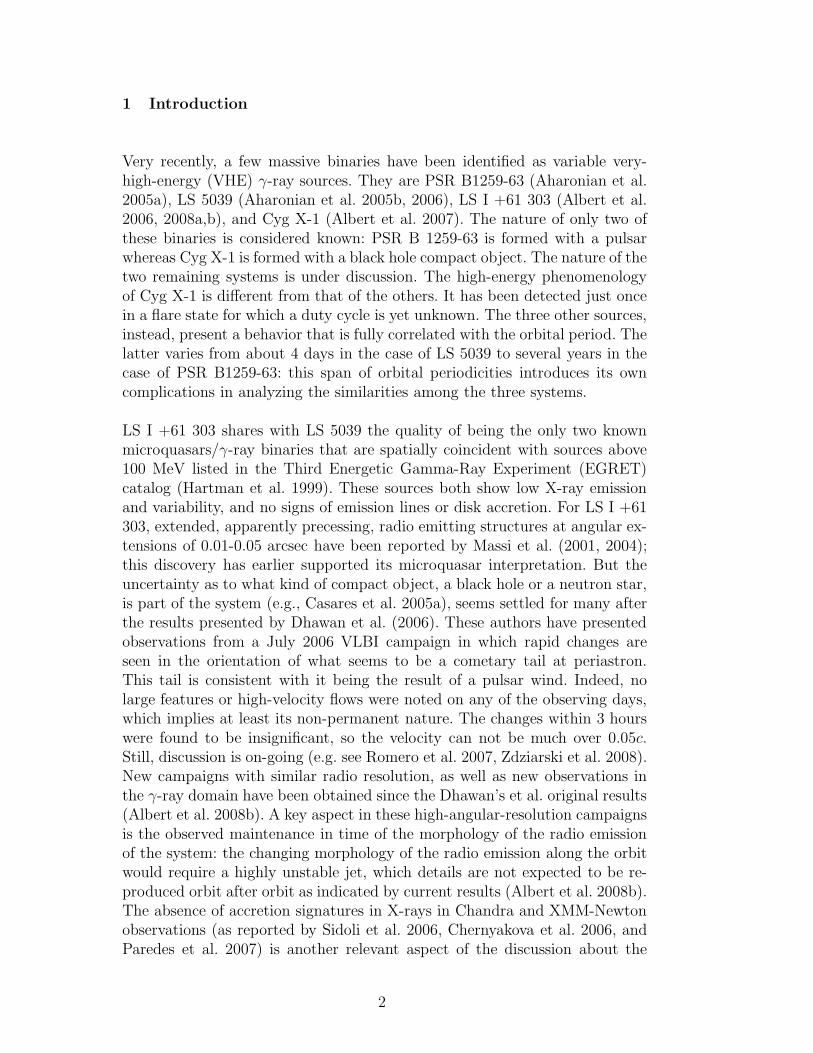
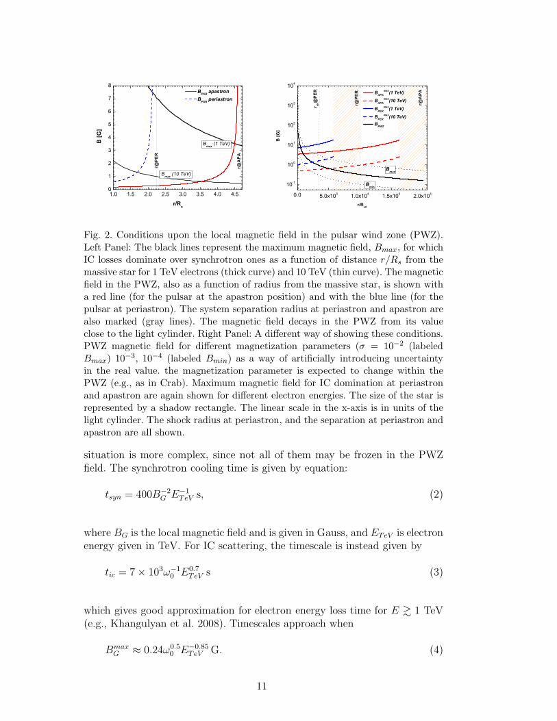
Fig. 2. Conditions upon the local magnetic field in the pulsar wind zone (PWZ).Left Panel: The black lines represent the maximum magnetic field, Bmax, for whichIC losses dominate over synchrotron ones as a function of distance r/Rs from themassive star for 1 TeV electrons (thick curve) and 10 TeV (thin curve). The magneticfield in the PWZ, also as a function of radius from the massive star, is shown witha red line (for the pulsar at the apastron position) and with the blue line (for thepulsar at periastron). The system separation radius at periastron and apastron arealso marked (gray lines). The magnetic field decays in the PWZ from its valueclose to the light cylinder. Right Panel: A different way of showing these conditions.PWZ magnetic field for different magnetization parameters (σ = 10−2 (labeledBmax) 10−3, 10−4 (labeled Bmin) as a way of artificially introducing uncertaintyin the real value. the magnetization parameter is expected to change within thePWZ (e.g., as in Crab). Maximum magnetic field for IC domination at periastronand apastron are again shown for different electron energies. The size of the star isrepresented by a shadow rectangle. The linear scale in the x-axis is in units of thelight cylinder. The shock radius at periastron, and the separation at periastron andapastron are all shown.

situation is more complex, since not all of them may be frozen in the PWZfield. The synchrotron cooling time is given by equation:

tsyn = 400B−2G E−1

TeV s, (2)

where BG is the local magnetic field and is given in Gauss, and ETeV is electronenergy given in TeV. For IC scattering, the timescale is instead given by

tic = 7 × 103ω−10 E0.7

TeV s (3)

which gives good approximation for electron energy loss time for E & 1 TeV(e.g., Khangulyan et al. 2008). Timescales approach when

BmaxG ≈ 0.24ω0.5

0 E−0.85TeV G. (4)

11

For a star with effective temperature Ts = 3.9 × 104 K, the thermal fielddensity at certain point at distance r from the massive star center is given by:

ω0 = 4σT 4/c× (Rs/2r)2 ≈ 1.75 × 104(Rs/2r)

2 erg cm−3. (5)

Thus, the local magnetic field in the pulsar wind region is given by:

BmaxG ≈ 31.75(Rs/2r)E

−0.85TeV G. (6)

Applying this condition at periastron (r = 2.25Rs), the local magnetic fieldat the assumed injection place results in Bmax−per ∼ 7 G. At apastron (r =4.72Rs), it results in an stronger condition Bmax−apa ∼ 3.4 G. That is, themagnetic field should be less than these values in order for IC to dominateover synchrotron losses at that particular position (the light cylinder) in thePWZ. Figure 2 shows this in detail.

The magnetic field at the light cylinder distance RLC is given by the dipoleformula BLC = B0(Rpsr/RLC)3. In the PWZ, the magnetic field is decreasing

with distance as B(r) ∼√

σ/(1 + σ)BLC(RLC/r). For a millisecond pulsar

we get RLC ∼ 5 × 107 cm and BLC ∼ 105 G (assuming B0 = 1012 G andP = 10 ms) up to RLC ∼ 5 × 108 cm and BLC ∼ 8 × 104 G (assumingB0 = 1013 G and P ∼ 100 ms), where Rpsr ≈ 10 km. The results for thesedifferent parameters are similar as there were obtained with fixed pulsar powerin the model Lsd = 1037 erg s−1 and they are related by the standard formulaLsd = B2

0R6psrc/4R

4LC . We also assume here that the magnetization parameter

is σ = 0.001, but have explored other values of this and other parameters aswell, with similar results (see Figure 2).

Given our results (see Fig. 2) where we show the local magnetic field for whichIC dominates and the magnetic field in the PWZ as a function of the distancefrom the light cylinder we can conclude that the injection for the model have to(generically) occur at some distance from the light cylinder, or/and, if closer toit, the synchrotron losses can be important. However, as the separation of thebinary is ∼ 1012 cm, several orders of magnitude larger than the light cylinder(e.g., RLC ∼ 108 cm), the change of the injection place within e.g. ∼ 1%− 5%already gives the initial injection distance at ∼ (100 − 500)RLC . Thus, nosignificant effect in the PWZ photon spectra and lightcurve is produced.

12

2.3 Normalization of the relativistic particle power

The fraction of the pulsar spin-down power ending in the e+e− interactingpairs can then be written as:

βLsd =∫

Ne+e−(E)EdE. (7)

Assuming that the distance to the source is d = 2.5 kpc, the normalizationfactor for electrons traveling towards Earth is A = Ne+e−/4πd

2. The specificnormalization factors in the expression of the injection rate Ne+e−(E) will begiven together with the results for two models in the corresponding sectionsbelow. In the models presented here, only a small fraction (∼1%) of the pul-sar’s LSD ends up in relativistic leptons. This is consistent with ions carryingmuch of the wind energetics. In the case of mono-energetic lepton distribu-tion, where the energy of the primaries is fixed at E0 = 10 TeV, we haveNe+e−(E) ∝ δ(E − E0). In the case of a power-law in energy, that may beconstant or vary along the orbit, we have Ne+e−(E) ∝ E−αi .

2.4 On parameter interdependencies

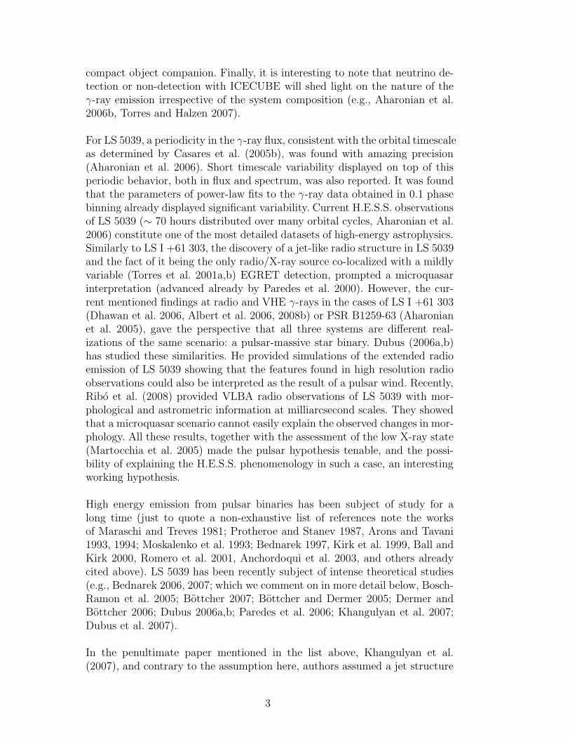
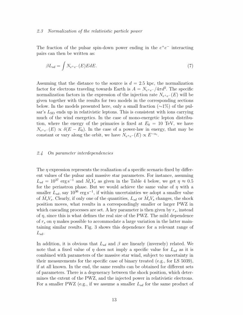
The η expression represents the realization of a specific scenario fixed by differ-ent values of the pulsar and massive star parameters. For instance, assumingLsd = 1037 erg s−1 and MsVs as given in the Table 4 below, we get η ≈ 0.5for the periastron phase. But we would achieve the same value of η with asmaller Lsd, say 1036 erg s−1, if within uncertainties we adopt a smaller valueof MsVs. Clearly, if only one of the quantities, Lsd or MsVs changes, the shockposition moves, what results in a correspondingly smaller or larger PWZ inwhich cascading processes are set. A key parameter is then given by rs, insteadof η, since this is what defines the real size of the PWZ. The mild dependenceof rs on η makes possible to accommodate a large variation in the latter main-taining similar results. Fig. 3 shows this dependence for a relevant range ofLsd.

In addition, it is obvious that Lsd and β are linearly (inversely) related. Wenote that a fixed value of η does not imply a specific value for Lsd as it iscombined with parameters of the massive star wind, subject to uncertainty intheir measurements for the specific case of binary treated (e.g., for LS 5039),if at all known. In the end, the same results can be obtained for different setsof parameters. There is a degeneracy between the shock position, which deter-mines the extent of the PWZ, and the injected power in relativistic electrons.For a smaller PWZ (e.g., if we assume a smaller Lsd for the same product of

13

1035 1036 10370,0

0,5

1,0

1,5

2,0

2,5

periastron

r s / R

s

Lsd [ erg s-1 ]

apastron

Fig. 3. Dependence of the distance to the shock form the pulsar side, rs, as a functionof the spin-down power, Lsd, for fixed values of star mass loss rate, M = 10−7 M⊙

yr−1, and terminal star wind velocity, V∞ = 2.4 × 103 km s−1.

MsVs) a larger amount of injected power compensates the reduced interact-ing region. We found that to get the similar results when the η parameter issmaller, the β parameter have to be increased roughly by the same factor.

2.5 Wind termination

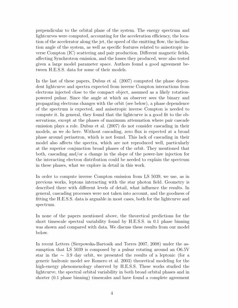
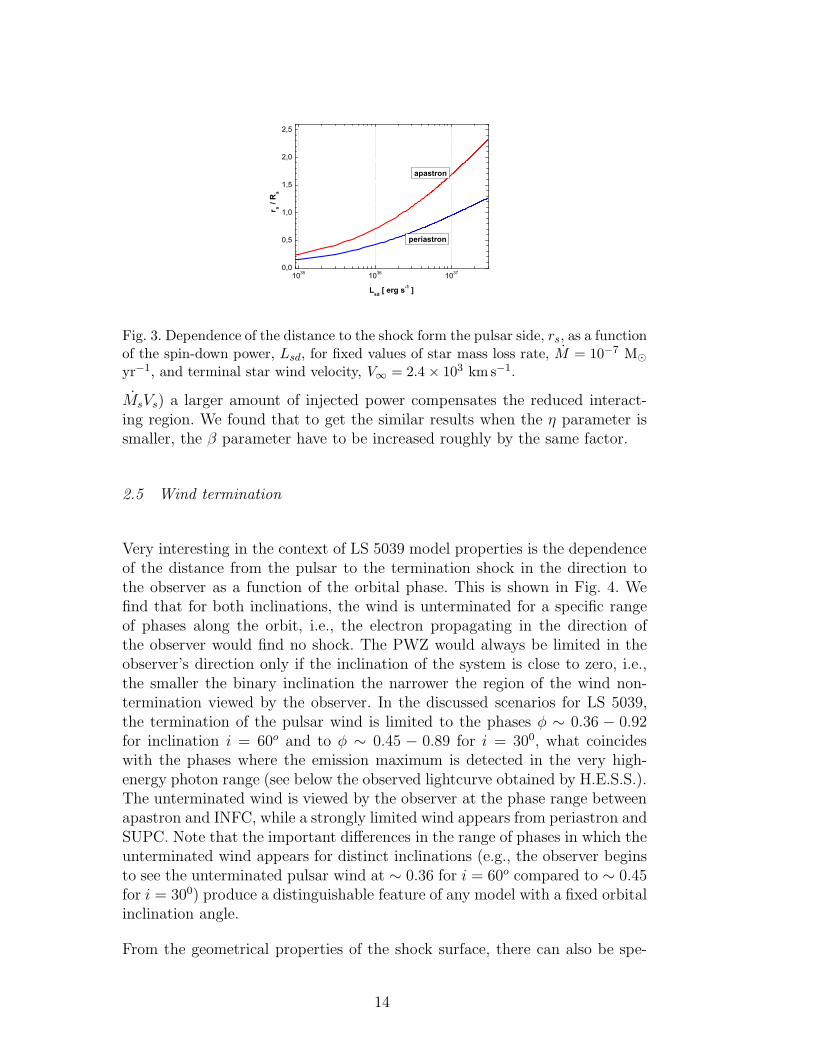
Very interesting in the context of LS 5039 model properties is the dependenceof the distance from the pulsar to the termination shock in the direction tothe observer as a function of the orbital phase. This is shown in Fig. 4. Wefind that for both inclinations, the wind is unterminated for a specific rangeof phases along the orbit, i.e., the electron propagating in the direction ofthe observer would find no shock. The PWZ would always be limited in theobserver’s direction only if the inclination of the system is close to zero, i.e.,the smaller the binary inclination the narrower the region of the wind non-termination viewed by the observer. In the discussed scenarios for LS 5039,the termination of the pulsar wind is limited to the phases φ ∼ 0.36 − 0.92for inclination i = 60o and to φ ∼ 0.45 − 0.89 for i = 300, what coincideswith the phases where the emission maximum is detected in the very high-energy photon range (see below the observed lightcurve obtained by H.E.S.S.).The unterminated wind is viewed by the observer at the phase range betweenapastron and INFC, while a strongly limited wind appears from periastron andSUPC. Note that the important differences in the range of phases in which theunterminated wind appears for distinct inclinations (e.g., the observer beginsto see the unterminated pulsar wind at ∼ 0.36 for i = 60o compared to ∼ 0.45for i = 300) produce a distinguishable feature of any model with a fixed orbitalinclination angle.

From the geometrical properties of the shock surface, there can also be spe-

14

0,0 0,1 0,2 0,3 0,4 0,5 0,6 0,7 0,8 0,9 1,00

2

4

6

8

10

12

14

16

18

20

INFC i = 300

i = 600

D/R

s r s

hock/R

s

apas

tron

SUPC

Fig. 4. The distance from the pulsar to the termination shock in the direction tothe observer (in units of stellar radius Rs), for the two different inclination angles, i,analyzed in this paper. INFC, SUPC, periastron, and apastron phases are marked.Additionally, the gray line shows the separation of the binary (also in units of Rs)as a function of phase along the orbit.

cific phases for which the termination shock is directed edge-on to the ob-server. These are phases close to the non-terminated wind viewing conditions:slightly before and after those specific phases for which the wind becomesnon-terminated, e.g., for the case of LS 5039 and i = 300, φ ∼ 0.4 and 0.93;whereas for i = 600, it appears at φ ∼ 0.32 and 0.93. Thus, we find thatthe condition for lepton propagation change significantly in a relatively shortphase period, when the termination shock is getting further and closer to thepulsar (phases periods ∼ 0.2 − 0.45 and ∼ 0.9 − 0.96). In Table 1 we showthe differences in these geometrical parameters for a few characteristic orbitalphases. Note that even when they are essential to understand the formationof the lightcurve and phase dependent high energy photon spectra, all theabove features are based on the simple approximation of the geometry of thetermination shock. In a more realistic scenario, the transition between the ter-minated and unterminated wind, and its connection with orbital phases andinclination are expected to be more complicated yet.

2.6 Opacities along the LS 5039 orbit

The conditions for leptonic processes for this specific binary can be discussedbased on optical depths to ICS and γγ absorption. The target photons forIC scattering of injected electrons and for e+e− pair production for secondaryphotons are low energy photons of black-body spectrum with temperatureTs = 3.9 × 104, which is the surface temperature of the massive star. This isan anisotropic field as the source of thermal photons differ from the place ofinjection of relativistic electrons, which for simplicity is assumed to be at thepulsar location for any given orbital phase. For fixed geometry parameters,

15

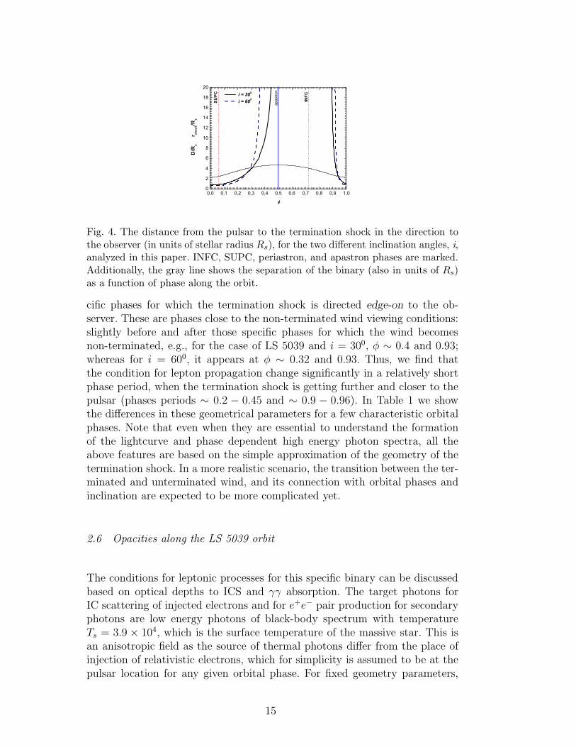
Table 1Geometrical properties for specific phases along the orbit. p1 and p2 stand for

the phases at which the angle to the observer is 90o; r1 and r2 stand for the phasesbetween which the shock in the observer direction is non-terminated. The separationd and the shock distance rs are given in units of star radii Rs.

i = 300 i = 600

θ [o] φ d αobs rs φ d αobs rs

Periastron 0 0.0 2.25 1110 0.8 0.0 2.25 1300 0.6

SUPC 44 0.06 2.45 1200 0.8 0.06 2.45 1500 0.6

p1 134 0.27 4.06 900 3.2 0.27 4.06 900 3.2

r1 171 0.45 4.7 720 . . . 0.36 4.5 730 . . .

Apastron 180 0.5 4.72 690 . . . 0.5 4.72 430 . . .

INFC 224 0.72 4.1 600 . . . 0.72 4.1 300 . . .

r2 285 0.89 2.8 760 . . . 0.92 2.6 800 . . .

p2 314 0.94 2.47 900 2.4 0.94 2.47 900 2.4

100 101 102 103 104 105

10-1

100

101

102

103

= 30o

= 60o

= 90o

= 120o

= 180o

= 0o

= 150o ICS

E [ GeV ]100 101 102 103 104 105

10-1

100

101

102

103

= 150o

= 120o

= 90o

= 60o

= 30o

= 0o

= 180o ICS

E [GeV]

Fig. 5. Opacities to ICS for electrons and pair production for photons as a functionof electron/photon energy. Opacities were calculated up to infinity for injection atthe periastron (left panel) and apastron (right panel) pulsar distance for differentangles of propagation with respect to the massive star.

the optical depths change with the separation of the binary (in general withthe distance to the massive star), the angle of injection (the direction of prop-agation with respect to the massive star), and the energy of injected particle(the electrons or photons for γ absorption).

To have a first handle on opacities, we have calculated the optical depthsadopting the binary separation at periastron and apastron. In case of theoptical depths for photons we had to do an additional simplifying assumptionto allow for a direct comparison with the optical depth for electrons. In thediscussed model of this paper, photons are secondary particles and they do

16

0o 20o 40o 60o 80o 100o 120o 140o 160o 180o0.01

0.1

1

10 ICS

15 Rs

apastron

periastron

1.5 Rs

E = 1 TeV

0o 20o 40o 60o 80o 100o 120o 140o 160o 180o0.01

0.1

1

10 ICS

15 Rs

apastron

periastron

1.5 Rs

E = 10 TeV

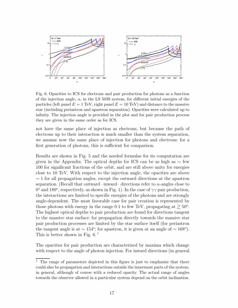
Fig. 6. Opacities to ICS for electrons and pair production for photons as a functionof the injection angle, α, in the LS 5039 system, for different initial energies of theparticles (left panel E = 1 TeV, right panel E = 10 TeV) and distance to the massivestar (including periastron and apastron separation). Opacities were calculated up toinfinity. The injection angle is provided in the plot and for pair production processthey are given in the same order as for ICS.

not have the same place of injection as electrons, but because the path ofelectrons up to their interaction is much smaller than the system separation,we assume now the same place of injection for photons and electrons: for afirst generation of photons, this is sufficient for comparison.

Results are shown in Fig. 5 and the needed formulae for its computation aregiven in the Appendix. The optical depths for ICS can be as high as ∼ few100 for significant fractions of the orbit, and are still above unity for energiesclose to 10 TeV. With respect to the injection angle, the opacities are above∼ 1 for all propagation angles, except the outward directions at the apastronseparation. (Recall that outward –inward– directions refer to α-angles close to0o and 180o, respectively, as shown in Fig. 1). In the case of γγ pair production,the interactions are limited to specific energies of the photons and are stronglyangle-dependent. The most favorable case for pair creation is represented bythose photons with energy in the range 0.1 to few TeV, propagating at & 50o.The highest optical depths to pair production are found for directions tangentto the massive star surface: for propagation directly towards the massive starpair production processes are limited by the star surface itself (for periastronthe tangent angle is at ∼ 154o; for apastron, it is given at an angle of ∼ 168o).This is better shown in Fig. 6. 1

The opacities for pair production are characterized by maxima which changewith respect to the angle of photon injection. For inward directions (in general

1 The range of parameters depicted in this figure is just to emphasize that therecould also be propagation and interactions outside the innermost parts of the system,in general, although of course with a reduced opacity. The actual range of anglestowards the observer allowed in a particular system depend on the orbit inclination.

17

0.0 0.1 0.2 0.3 0.4 0.5 0.6 0.7 0.8 0.9 1.0

10-1

100

101 i = 30o

SUPC

apas

tron

INFC

ICS E = 104 GeV

E = 103 GeV

E = 102 GeV

0.0 0.1 0.2 0.3 0.4 0.5 0.6 0.7 0.8 0.9 1.0

10-1

100

101 i = 60o

SUPC

apas

tron

INFC

E = 104 GeV

E = 103 GeV

E = 102 GeV

ICS

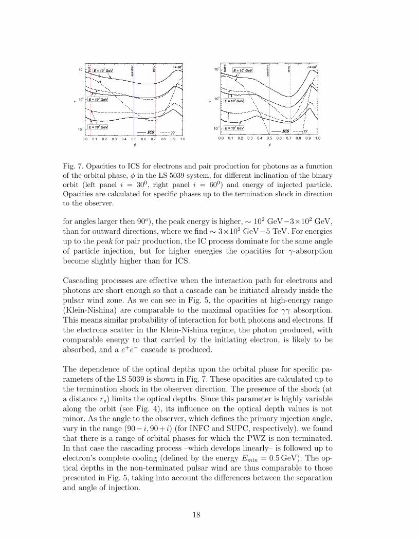
Fig. 7. Opacities to ICS for electrons and pair production for photons as a functionof the orbital phase, φ in the LS 5039 system, for different inclination of the binaryorbit (left panel i = 300, right panel i = 600) and energy of injected particle.Opacities are calculated for specific phases up to the termination shock in directionto the observer.

for angles larger then 90o), the peak energy is higher, ∼ 102 GeV−3×102 GeV,than for outward directions, where we find ∼ 3×102 GeV−5 TeV. For energiesup to the peak for pair production, the IC process dominate for the same angleof particle injection, but for higher energies the opacities for γ-absorptionbecome slightly higher than for ICS.

Cascading processes are effective when the interaction path for electrons andphotons are short enough so that a cascade can be initiated already inside thepulsar wind zone. As we can see in Fig. 5, the opacities at high-energy range(Klein-Nishina) are comparable to the maximal opacities for γγ absorption.This means similar probability of interaction for both photons and electrons. Ifthe electrons scatter in the Klein-Nishina regime, the photon produced, withcomparable energy to that carried by the initiating electron, is likely to beabsorbed, and a e+e− cascade is produced.

The dependence of the optical depths upon the orbital phase for specific pa-rameters of the LS 5039 is shown in Fig. 7. These opacities are calculated up tothe termination shock in the observer direction. The presence of the shock (ata distance rs) limits the optical depths. Since this parameter is highly variablealong the orbit (see Fig. 4), its influence on the optical depth values is notminor. As the angle to the observer, which defines the primary injection angle,vary in the range (90− i, 90+ i) (for INFC and SUPC, respectively), we foundthat there is a range of orbital phases for which the PWZ is non-terminated.In that case the cascading process –which develops linearly– is followed up toelectron’s complete cooling (defined by the energy Emin = 0.5 GeV). The op-tical depths in the non-terminated pulsar wind are thus comparable to thosepresented in Fig. 5, taking into account the differences between the separationand angle of injection.

18

0.0 0.1 0.2 0.3 0.4 0.5 0.6 0.7 0.8 0.9 1.0

100

101

SUPC i = 30o

ICS i = 60o

ICS

E = 100 GeVap

astron

INFC

0.0 0.1 0.2 0.3 0.4 0.5 0.6 0.7 0.8 0.9 1.0

100

101

SUPC

apas

tron

INFCi = 30o

ICS i = 60o

ICS

E = 1 TeV

0.0 0.1 0.2 0.3 0.4 0.5 0.6 0.7 0.8 0.9 1.0

10-1

100

SUPC

apas

tron

INFC

i = 30o ICS

i = 60o ICS

E = 10 TeV

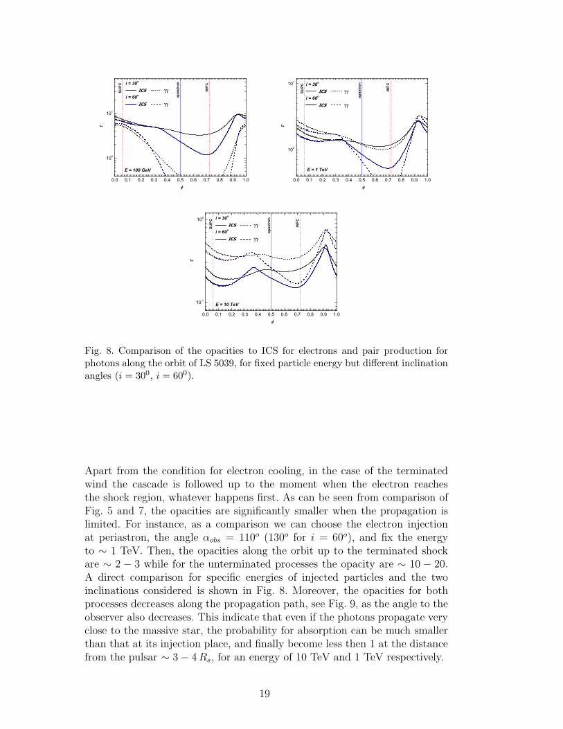
Fig. 8. Comparison of the opacities to ICS for electrons and pair production forphotons along the orbit of LS 5039, for fixed particle energy but different inclinationangles (i = 300, i = 600).

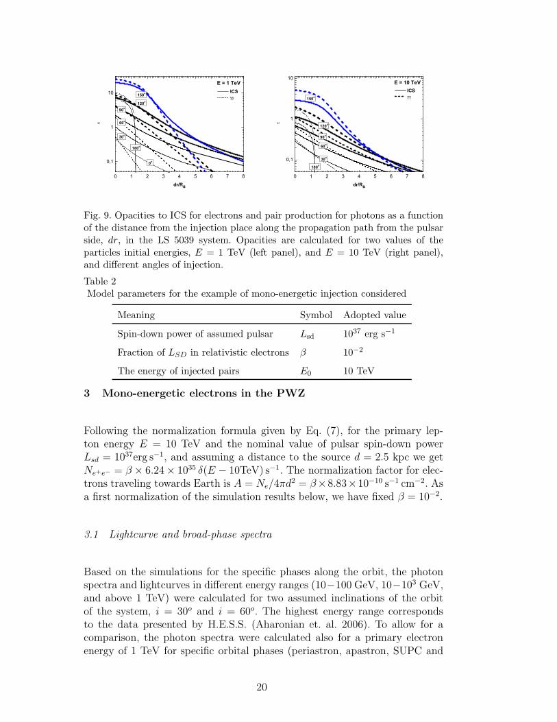
Apart from the condition for electron cooling, in the case of the terminatedwind the cascade is followed up to the moment when the electron reachesthe shock region, whatever happens first. As can be seen from comparison ofFig. 5 and 7, the opacities are significantly smaller when the propagation islimited. For instance, as a comparison we can choose the electron injectionat periastron, the angle αobs = 110o (130o for i = 60o), and fix the energyto ∼ 1 TeV. Then, the opacities along the orbit up to the terminated shockare ∼ 2 − 3 while for the unterminated processes the opacity are ∼ 10 − 20.A direct comparison for specific energies of injected particles and the twoinclinations considered is shown in Fig. 8. Moreover, the opacities for bothprocesses decreases along the propagation path, see Fig. 9, as the angle to theobserver also decreases. This indicate that even if the photons propagate veryclose to the massive star, the probability for absorption can be much smallerthan that at its injection place, and finally become less then 1 at the distancefrom the pulsar ∼ 3 − 4Rs, for an energy of 10 TeV and 1 TeV respectively.

19

0 1 2 3 4 5 6 7 8

0,1

1

10 ICS

180o

150o

120o

90o

60o

0o

dr/Rs

30o

E = 1 TeV

0 1 2 3 4 5 6 7 8

0,1

1

10E = 10 TeV

ICS

180o

150o

120o

90o

60o

dr/Rs

30o

Fig. 9. Opacities to ICS for electrons and pair production for photons as a functionof the distance from the injection place along the propagation path from the pulsarside, dr, in the LS 5039 system. Opacities are calculated for two values of theparticles initial energies, E = 1 TeV (left panel), and E = 10 TeV (right panel),and different angles of injection.

Table 2Model parameters for the example of mono-energetic injection considered

Meaning Symbol Adopted value

Spin-down power of assumed pulsar Lsd 1037 erg s−1

Fraction of LSD in relativistic electrons β 10−2

The energy of injected pairs E0 10 TeV

3 Mono-energetic electrons in the PWZ

Following the normalization formula given by Eq. (7), for the primary lep-ton energy E = 10 TeV and the nominal value of pulsar spin-down powerLsd = 1037erg s−1, and assuming a distance to the source d = 2.5 kpc we getNe+e− = β × 6.24 × 1035 δ(E − 10TeV) s−1. The normalization factor for elec-trons traveling towards Earth is A = Ne/4πd

2 = β×8.83×10−10 s−1 cm−2. Asa first normalization of the simulation results below, we have fixed β = 10−2.

3.1 Lightcurve and broad-phase spectra

Based on the simulations for the specific phases along the orbit, the photonspectra and lightcurves in different energy ranges (10−100 GeV, 10−103 GeV,and above 1 TeV) were calculated for two assumed inclinations of the orbitof the system, i = 30o and i = 60o. The highest energy range correspondsto the data presented by H.E.S.S. (Aharonian et. al. 2006). To allow for acomparison, the photon spectra were calculated also for a primary electronenergy of 1 TeV for specific orbital phases (periastron, apastron, SUPC and

20

10-1 100 101 102 103 104

10-15

10-14

10-13

10-12

10-11INFC

periastron

E2 F(E

) [er

g cm

-2 s

-1]

E [GeV]

apastron

SUPC

i = 30o

10-1 100 101 102 103 104

10-15

10-14

10-13

10-12

10-11

INFC

periastron

E2 F(E

) [er

g cm

-2 s

-1]

E [GeV]

apastron

SUPC

i = 30o

10-1 100 101 102 103 104

10-15

10-14

10-13

10-12

10-11INFC

periastron

E2 F(E

) [er

g cm

-2 s

-1]

E [GeV]

apastron

SUPC

i = 60o

10-1 100 101 102 103 104

10-15

10-14

10-13

10-12

10-11

INFC

periastron

E2 F(E

) [er

g cm

-2 s

-1]

E [GeV]

apastron

SUPC

i = 60o

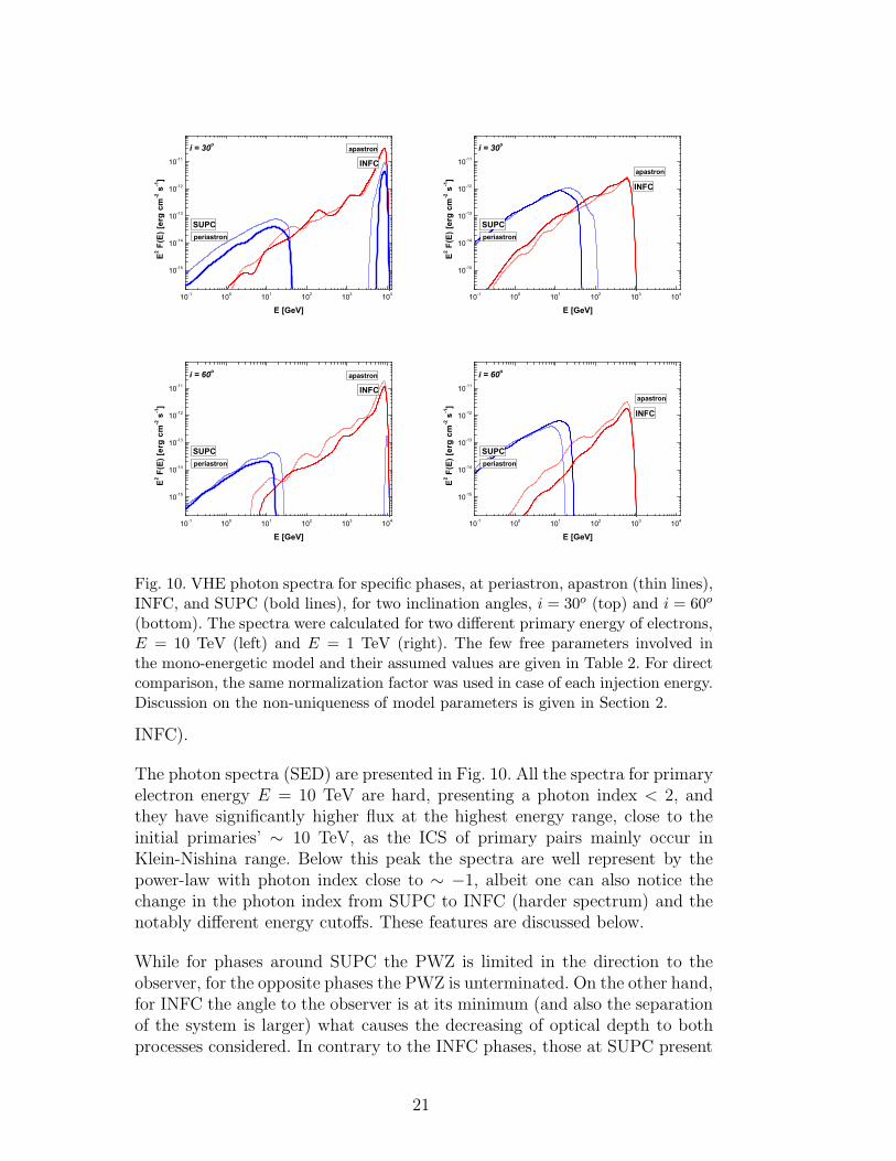
Fig. 10. VHE photon spectra for specific phases, at periastron, apastron (thin lines),INFC, and SUPC (bold lines), for two inclination angles, i = 30o (top) and i = 60o

(bottom). The spectra were calculated for two different primary energy of electrons,E = 10 TeV (left) and E = 1 TeV (right). The few free parameters involved inthe mono-energetic model and their assumed values are given in Table 2. For directcomparison, the same normalization factor was used in case of each injection energy.Discussion on the non-uniqueness of model parameters is given in Section 2.

INFC).

The photon spectra (SED) are presented in Fig. 10. All the spectra for primaryelectron energy E = 10 TeV are hard, presenting a photon index < 2, andthey have significantly higher flux at the highest energy range, close to theinitial primaries’ ∼ 10 TeV, as the ICS of primary pairs mainly occur inKlein-Nishina range. Below this peak the spectra are well represent by thepower-law with photon index close to ∼ −1, albeit one can also notice thechange in the photon index from SUPC to INFC (harder spectrum) and thenotably different energy cutoffs. These features are discussed below.

While for phases around SUPC the PWZ is limited in the direction to theobserver, for the opposite phases the PWZ is unterminated. On the other hand,for INFC the angle to the observer is at its minimum (and also the separationof the system is larger) what causes the decreasing of optical depth to bothprocesses considered. In contrary to the INFC phases, those at SUPC present

21

0,0 0,2 0,4 0,6 0,8 1,0 1,2 1,4 1,6 1,8 2,0

0

1

2

3

INFC

SU

PC

apas

tron

F (>

1 Te

V) [

10- 1

2 ph

cm-2 s

-1 ]

orbital phase

peria

stro

n

apas

tron

SU

PC

INFC

0,0 0,2 0,4 0,6 0,8 1,0 1,2 1,4 1,6 1,8 2,0

0

1

2

INFC

SU

PC

apas

tron

F (1

00-1

03 GeV

) [ 1

0- 12 p

h cm

-2 s

-1 ]

orbital phase

peria

stro

n

apas

tron

SU

PC

INFC

0,0 0,2 0,4 0,6 0,8 1,0 1,2 1,4 1,6 1,8 2,0

0

1

2

3

4

5 INFC

SU

PC

apas

tron

F (1

0-10

0 G

eV) [

10- 1

2 ph

cm-2 s

-1 ]

orbital phase

peria

stro

n

apas

tron

SU

PC

INFC

0,0 0,2 0,4 0,6 0,8 1,0 1,2 1,4 1,6 1,8 2,0

0

1

2

INFC

SU

PC

apas

tron

F (1

-10

GeV

) [ 1

0- 11 p

h cm

-2 s

-1 ]

orbital phase

peria

stro

n

apas

tron

SU

PC

INFC

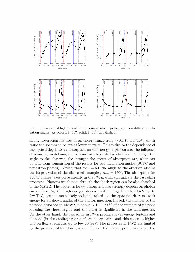
Fig. 11. Theoretical lightcurves for mono-energetic injection and two different incli-nation angles. As before: i=600, solid; i=300, dot-dashed.

strong absorption features at an energy range from ∼ 0.1 to few TeV, whichcause the spectra to be cut at lower energies. This is due to the dependence ofthe optical depth to γγ absorption on the energy of photon and the influenceof geometry in defining the photon path towards the observer. The larger theangle to the observer, the stronger the effects of absorption are, what canbe seen from comparison of the results for two inclination angles (SUPC andperiastron phases). Notice, that for i = 60o the angle to the observer attainsthe largest value of the discussed examples, αobs = 150o. The absorption forSUPC phases takes place already in the PWZ, what can initiate the cascadingprocesses. Photons which pass through the shock region can be also absorbedin the MSWZ. The opacities for γγ absorption also strongly depend on photonenergy (see Fig. 8). High energy photons, with energy from few GeV up tofew TeV, are the most likely to be absorbed, as the opacities decrease withenergy for all shown angles of the photon injection. Indeed, the number of thephotons absorbed in MSWZ is about ∼ 10 − 20 % of the number of photonsreaching the shock region and the effect is significant in the final spectra.On the other hand, the cascading in PWZ produce lower energy leptons andphotons (in the cooling process of secondary pairs) and this causes a higherphoton flux at energies up to few 10 GeV. The processes in PWZ are limitedby the presence of the shock, what influence the photon production rate. For

22

INFC phases the absorption of γ-rays is minor, as the photons propagateoutwards of the massive star; once produced, most photons can escape fromthe system (also because of the threshold to pair production). Higher energyphotons are produced mostly in the first IC interaction of the primary pairs,while further electron cooling, not limited by the termination shock, supplythe spectrum in lower energy photons. This flux is not as high as in the caseof SUPC phases, where most of the cascading takes place.

Similar dependencies, both for INFC and SUPC phases, are present in thespectra obtained from the simulations for primary energy of pairs E = 1 TeV.As the optical depths to IC scattering are higher in that case, the processesare more efficient and the number of produced photons are higher. To give anexample, most photons of energy > 20-30 GeV at SUPC-periastron phase areabsorbed in MSWZ.

Comparing the photon spectra produced at SUPC and INFC, an anticorrela-tion between GeV and TeV photon fluxes is evident, at least comparing thespectra at energies below and above ∼ 10 GeV. All these effects play a rolein the formation of the γ-ray lightcurve, shown in Fig. 11. The lightcurve inthe highest energy range (> 1 TeV) has a broad minimum around SUPC,0.96 < φ < 0.25. From the comparison of the position of the terminationshock along the orbit, the opacities to ICS and γγ absorption we see thatthis minimum is formed despite being at phases with the highest opacities toboth processes considered and so having an effective cascading in the PWZregion. This minimum is mainly due to the absorption of the photons whichget through the shock and propagate into the massive star wind region. Thebroad maximum in the high-energy lightcurve is formed at opposite phasesaround INFC, 0.4 < φ < 0.9. The maximum for higher inclination is alsocharacterized by a local minimum close to the INFC phase, what is the re-sult of the IC opacity dependence on the propagation angle. The range ofINFC phases corresponds to the unterminated pulsar wind in the observerdirection. The opacities for both inclinations have local peaks in this range,what was discussed in the previous paragraph. The local minimum in photonflux within the INFC range reflects a similar behavior of the opacities. So,as far as the propagation of the particles in the PWZ is unterminated, thehigh-energy lightcurve formation is in agreement with the dependence of theoptical depths. Additionally, we can also see that the first local peak in thislightcurve is formed earlier in phase for inclination i = 60o (φ ∼ 0.35), what isalso in agreement with the dependence shown by the distance to the termina-tion shock. Note that the second peak in the broad TeV lightcurve maximum,at ∼ 0.85, is higher than the first one, at ∼ 0.4 what is the result of a changein the separation of the system together with the angle to the observer.

23

3.2 Peaks and dips in the lightcurve

The geometrical conditions for leptonic processes change significantly alongthe orbit, and they are more efficient for phases around SUPC. However,these processes, as we can already see from the opacities dependence on theorbital phases, is limited by the presence of the termination shock. This causesthat the best conditions for very high-energy photon production, and finallyescaping from the system, occur for an specific combination of the angle tothe observer, the separation of the system, and the distance to the shock fromthe pulsar side. From Figs. 7 and 4 we can see that this happens at the phases∼ 0.3 − 0.4 and ∼ 0.9 what reflects in the TeV lightcurve. At phases close toINFC photons are produced mainly in the primary e+e− pairs cooling whenthe propagating electron undergo frequent scatterings. Together with the factthat there is no efficient absorption of photons once they are produced, theyfinally escape from the system, what yields to the broad maximum in the TeVlightcurve. On the other hand, at phases around SUPC, high-energy photonsare absorbed when propagating through the system in the MSWZ, what causesa dip in the lightcurve. For these phases many more lower energy photons areproduced in cascades in the PWZ, what yields to a maximum in the GeVlightcurve for SUPC, anticorrelated with the behavior at TeV energies.

4 A power-law electron distribution

For further exploration of the γ-ray production model we set a new assump-tion: the energy distribution of the interacting e+e− pairs is given by a power-law spectrum. We will additionally assume that the power-law may be con-stant or vary along the orbit. Motivated by the different observational behaviorfound, we have assumed that two different spectral indices correspond to thetwo broad orbital intervals proposed by HESS (Aharonian et. al., 2006). For di-rect comparison we have specified the interval around the inferior conjunction(with the apastron phase): 0.45 < φ < 0.90, and around superior conjunction(including the periastron phase): φ < 45 and φ > 0.90 as being bathed bydifferent electron distributions. The results for power-laws distribution werealready summarily presented in our earlier work Sierpowska-Bartosik and Tor-res (2007a,b) and we refer to these works for further details. The agreement inboth spectra and lightcurve is notable (particularly for the case of a variablelepton spectrum along the orbit), as can be seen in Figs. 14 and 15 discussedbelow.

As we could have already noticed from Fig. 5, the optical depth for highenergy electrons is below unity. In that case, part of the initial electrons willbe interacting in the PWZ less efficiently and finally will reach the shock

24

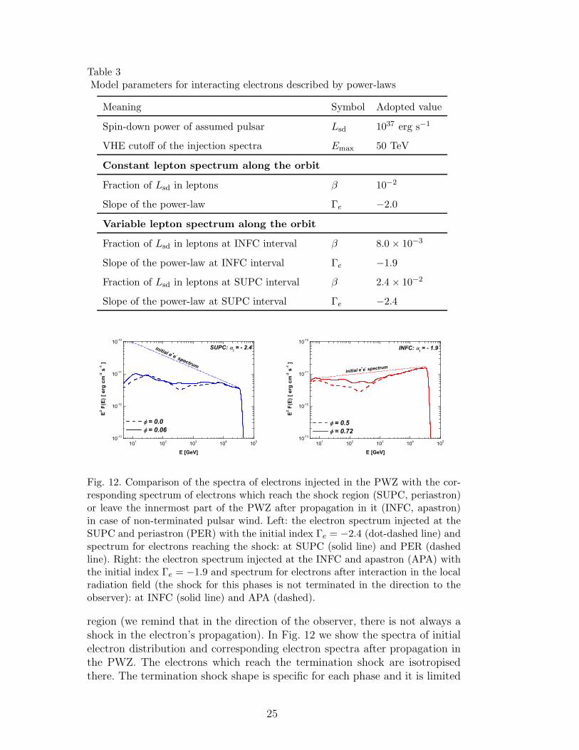
Table 3Model parameters for interacting electrons described by power-laws

Meaning Symbol Adopted value

Spin-down power of assumed pulsar Lsd 1037 erg s−1

VHE cutoff of the injection spectra Emax 50 TeV

Constant lepton spectrum along the orbit

Fraction of Lsd in leptons β 10−2

Slope of the power-law Γe −2.0

Variable lepton spectrum along the orbit

Fraction of Lsd in leptons at INFC interval β 8.0 × 10−3

Slope of the power-law at INFC interval Γe −1.9

Fraction of Lsd in leptons at SUPC interval β 2.4 × 10−2

Slope of the power-law at SUPC interval Γe −2.4

101 102 103 104 10510-13

10-12

10-11

10-10

initial e +e - spectrum

SUPC: i = - 2.4

= 0.0 = 0.06

E2 F(E

) [ e

rg c

m-2 s

-1 ]

E [GeV]101 102 103 104 105

10-13

10-12

10-11

10-10

INFC: i = - 1.9

= 0.5 = 0.72

E2 F(E

) [ e

rg c

m-2 s

-1 ]

E [GeV]

initial e+e- spectrum

Fig. 12. Comparison of the spectra of electrons injected in the PWZ with the cor-responding spectrum of electrons which reach the shock region (SUPC, periastron)or leave the innermost part of the PWZ after propagation in it (INFC, apastron)in case of non-terminated pulsar wind. Left: the electron spectrum injected at theSUPC and periastron (PER) with the initial index Γe = −2.4 (dot-dashed line) andspectrum for electrons reaching the shock: at SUPC (solid line) and PER (dashedline). Right: the electron spectrum injected at the INFC and apastron (APA) withthe initial index Γe = −1.9 and spectrum for electrons after interaction in the localradiation field (the shock for this phases is not terminated in the direction to theobserver): at INFC (solid line) and APA (dashed).

region (we remind that in the direction of the observer, there is not always ashock in the electron’s propagation). In Fig. 12 we show the spectra of initialelectron distribution and corresponding electron spectra after propagation inthe PWZ. The electrons which reach the termination shock are isotropisedthere. The termination shock shape is specific for each phase and it is limited

25

100 101 102 103 104 10510-14

10-13

10-12

10-11

10-10

injection in PWZ injection @ D

E2 F(E

) [ e

rg c

m-2 s

-1 ]

E [GeV]100 101 102 103 104 105

10-14

10-13

10-12

10-11

10-10

injection in PWZ injection @ D

E2 F(E

) [ e

rg c

m-2 s

-1 ]

E [GeV]

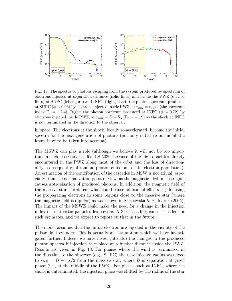
Fig. 13. The spectra of photons escaping from the system produced by spectrum ofelectrons injected at separation distance (solid lines) and inside the PWZ (dashedlines) at SUPC (left figure) and INFC (right). Left: the photon spectrum producedat SUPC (φ ∼ 0.06) by electrons injected inside PWZ, at rinit = rsh/2 (the spectrumindex Γe = −2.4). Right: the photon spectrum produced at INFC (φ ∼ 0.72) byelectrons injected inside PWZ, at rinit = D−Rs (Γe = −1.9) as the shock at INFCis not terminated in the direction to the observer.

in space. The electrons at the shock, locally re-accelerated, become the initialspectra for the next generation of photons (not only radiative but adiabaticlosses have to be taken into account).

The MSWZ can play a role (although we believe it will not be too impor-tant in such close binaries like LS 5039, because of the high opacities alreadyencountered in the PWZ along most of the orbit and the loss of direction-ality –consequently, of random photon emission– of the electron population).An estimation of the contribution of the cascades in MSW is not trivial, espe-cially from the normalization point of view, as the magnetic filed in this regioncauses isotropisation of produced photons. In addition, the magnetic field ofthe massive star is ordered, what could cause additional effects e.g. focusingthe propagating electrons in some regions close to the massive star (wherethe magnetic field is dipolar) as was shown in Sierpowska & Bednarek (2005).The impact of the MSWZ could make the need for a change in the injectionindex of relativistic particles less severe. A 3D cascading code is needed forsuch estimates, and we expect to report on that in the future.

The model assumes that the initial electron are injected in the vicinity of thepulsar light cylinder. This is actually an assumption which we have investi-gated further. Indeed. we have investigate also the changes in the producedphoton spectra if injection take place at a further distance inside the PWZ.Results are given in Fig. 13. For phases where the wind is terminated inthe direction to the observer (e.g., SUPC) the new injected radius was fixedto rinit = D − rsh/2 from the massive star, where D is separation at givenphase (i.e., at the middle of the PWZ). For phases such as INFC, where theshock is unterminated, the injection place was shifted by the radius of the star

26

102 103 104 105

10-13

10-12

10-11

e=-1.9

e=-2.4

e=-2.0

E2 F

(E) [

erg

cm

-2 s

-1 ]

E [GeV]

i = 30o

102 103 104 105

10-13

10-12

10-11

e=-1.9

e=-2.4

e=-2.0

i = 60o

E2 F

(E) [

erg

cm

-2 s

-1 ]

E [GeV]

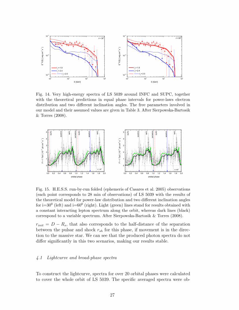
Fig. 14. Very high-energy spectra of LS 5039 around INFC and SUPC, togetherwith the theoretical predictions in equal phase intervals for power-laws electrondistribution and two different inclination angles. The free parameters involved inour model and their assumed values are given in Table 3. After Sierpowska-Bartosik& Torres (2008).

0,0 0,2 0,4 0,6 0,8 1,0 1,2 1,4 1,6 1,8 2,0

0

1

2

3

4

5

i = 30o

INFC

SU

PC

apas

tron

F >

1 Te

V [

10-1

2 ph

cm-2 s

-1 ]

orbital phase

peria

stro

n

apas

tron

SU

PC

INFC

0,0 0,2 0,4 0,6 0,8 1,0 1,2 1,4 1,6 1,8 2,0

0

1

2

3

4

5

i = 60o

INFC

SU

PC

apas

tron

F >

1 Te

V [

10-1

2 ph

cm-2 s

-1 ]

orbital phase

peria

stro

n

apas

tron

SU

PC

INFC

Fig. 15. H.E.S.S. run-by-run folded (ephemeris of Casares et al. 2005) observations(each point corresponds to 28 min of observations) of LS 5039 with the results ofthe theoretical model for power-law distribution and two different inclination anglesfor i=300 (left) and i=600 (right). Light (green) lines stand for results obtained witha constant interacting lepton spectrum along the orbit, whereas dark lines (black)correspond to a variable spectrum. After Sierpowska-Bartosik & Torres (2008).

rinit = D − Rs, that also corresponds to the half-distance of the separationbetween the pulsar and shock rsh for this phase, if movement is in the direc-tion to the massive star. We can see that the produced photon spectra do notdiffer significantly in this two scenarios, making our results stable.

4.1 Lightcurve and broad-phase spectra

To construct the lightcurve, spectra for over 20 orbital phases were calculatedto cover the whole orbit of LS 5039. The specific averaged spectra were ob-

27

tained based on the same orbital intervals as presented in H.E.S.S. data. Theaveraged spectra were obtained summing up individual contributions from or-bital spectra in given phases, each with a weight (δt/T ) corresponding to thefraction of orbital time that the system spends in the corresponding phasebin. Then, comparing the observational and theoretical averaged spectra, theparameter β was estimated. Both for constant and variable injection model,we get that the fraction of the spin-down power in the primary leptons hasto be at the level of ∼ 1 %. With this parameter in hand each of the singlespectra can be equally normalized.

It is worth noticing how well these lightcurves compare with those in the workby Bednarek (2007), at least for some of the specific phases considered by him.Bednarek also included cascading in his simulations, and the physical inputof his model (although in the case of a microquasar scenario) is similar toours. As a result, the anti-correlation phenomena (from GeV to TeV energies)is also a result of his work. The spectrum along the orbit with respect toH.E.S.S. datapoints and the possible short-timescale variability (see below)was not provided by Bednarek, so that a comparison with these results is notpossible. A detailed differentiation between these two models is a key inputfor distinguishing (microquasar or γ-ray binary) scenarios, even when someassumptions are intrinsic to each of the models, isolating the contribution ofan equal physical input can help decide on what object constitute the systemLS 5039. As an example: Bednarek did find in his model that a fixed inclinationangle (i = 600) was needed in order to reproduce the shape of the H.E.S.S.lightcurve results, whereas in our case, as we see in Figure 15 the influence ofinclination is minor.

For completeness, we mention that as noted above, H.E.S.S. has also providedthe evolution of the normalization and slope of a power-law fit to the 0.2–5 TeVdata in 0.1 phase-binning along the orbit (Aharonian et al. 2006). The use of apower-law fit was limited by low statistics in such shorter sub-orbital intervals,i.e., higher-order functional fittings such as a power-law with exponential cutoffwere reported to provide a no better fit and were not justified. To directlycompare with these results, we have applied the same approach to treat themodel predictions, i.e., we fit a power-law in the same energy range and phasebinning. We show here this comparison in Fig. 16 (taken from Sierpowska-Bartosik and Torres 2008) in the case of a variable lepton distribution alongthe orbit. We find a rather good agreement between model predictions anddata. Results for constant lepton distribution along the orbit can be seen inSierpowska-Bartosik and Torres (2007a).

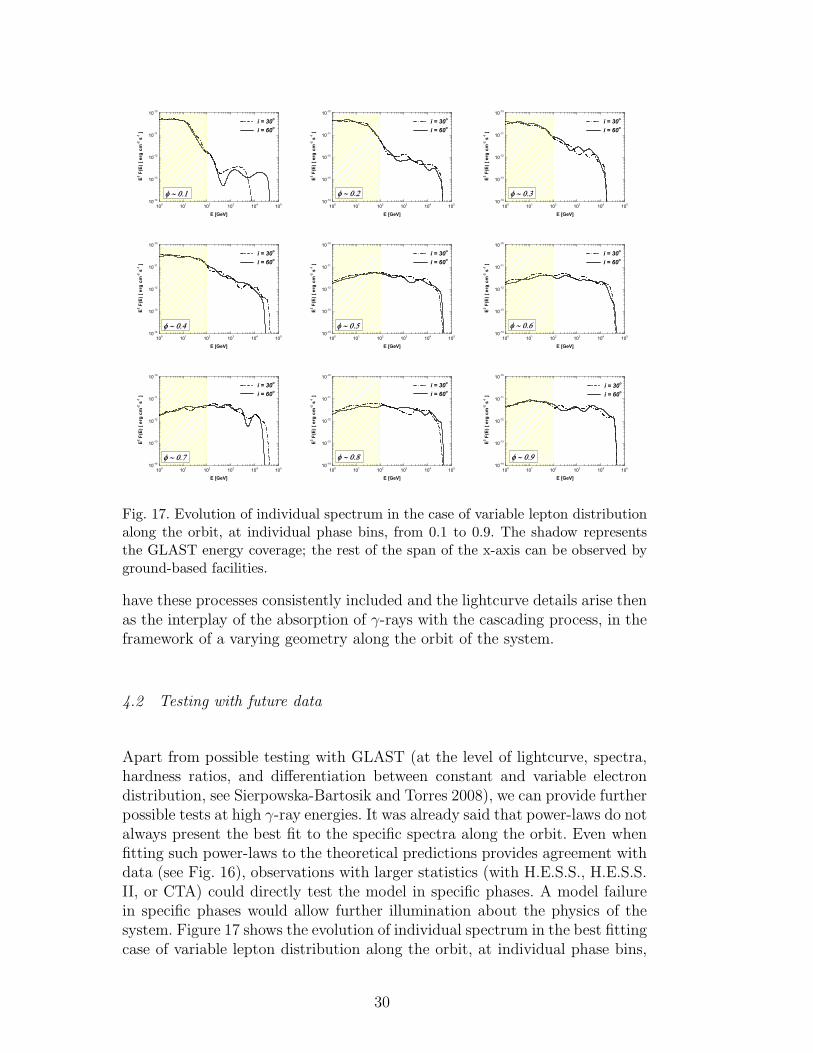
In Fig. 14 the SED in H.E.S.S. energy range are shown for both, constant andvariable lepton distributions along the orbit, and two inclination of the systemi = 30o and i = 60o. It was shown in the previous Section that in case of themono-energetic injection, there are photon flux differences in INFC phase due

28

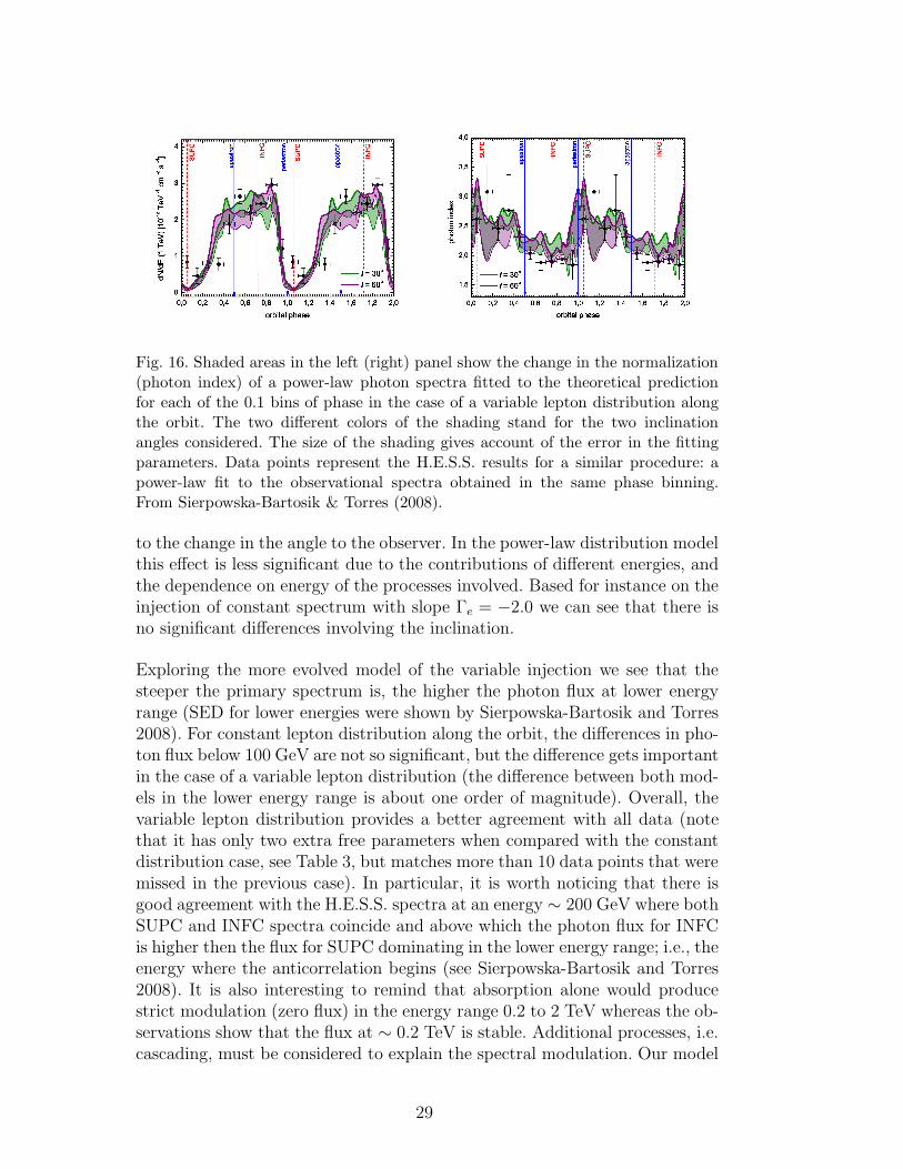
Fig. 16. Shaded areas in the left (right) panel show the change in the normalization(photon index) of a power-law photon spectra fitted to the theoretical predictionfor each of the 0.1 bins of phase in the case of a variable lepton distribution alongthe orbit. The two different colors of the shading stand for the two inclinationangles considered. The size of the shading gives account of the error in the fittingparameters. Data points represent the H.E.S.S. results for a similar procedure: apower-law fit to the observational spectra obtained in the same phase binning.From Sierpowska-Bartosik & Torres (2008).

to the change in the angle to the observer. In the power-law distribution modelthis effect is less significant due to the contributions of different energies, andthe dependence on energy of the processes involved. Based for instance on theinjection of constant spectrum with slope Γe = −2.0 we can see that there isno significant differences involving the inclination.

Exploring the more evolved model of the variable injection we see that thesteeper the primary spectrum is, the higher the photon flux at lower energyrange (SED for lower energies were shown by Sierpowska-Bartosik and Torres2008). For constant lepton distribution along the orbit, the differences in pho-ton flux below 100 GeV are not so significant, but the difference gets importantin the case of a variable lepton distribution (the difference between both mod-els in the lower energy range is about one order of magnitude). Overall, thevariable lepton distribution provides a better agreement with all data (notethat it has only two extra free parameters when compared with the constantdistribution case, see Table 3, but matches more than 10 data points that weremissed in the previous case). In particular, it is worth noticing that there isgood agreement with the H.E.S.S. spectra at an energy ∼ 200 GeV where bothSUPC and INFC spectra coincide and above which the photon flux for INFCis higher then the flux for SUPC dominating in the lower energy range; i.e., theenergy where the anticorrelation begins (see Sierpowska-Bartosik and Torres2008). It is also interesting to remind that absorption alone would producestrict modulation (zero flux) in the energy range 0.2 to 2 TeV whereas the ob-servations show that the flux at ∼ 0.2 TeV is stable. Additional processes, i.e.cascading, must be considered to explain the spectral modulation. Our model

29

100 101 102 103 104 10510-14

10-13

10-12

10-11

10-10

i = 30o

i = 60o

E2 F(E

) [ e

rg c

m-2 s

-1 ]

E [GeV]100 101 102 103 104 105

10-14

10-13

10-12

10-11

10-10

i = 30o

i = 60o

E2 F(E

) [ e

rg c

m-2 s

-1 ]

E [GeV]100 101 102 103 104 105

10-14

10-13

10-12

10-11

10-10

i = 30o

i = 60o

E2 F(E

) [ e

rg c

m-2 s

-1 ]

E [GeV]

100 101 102 103 104 10510-14

10-13

10-12

10-11

10-10

i = 30o

i = 60o

E2 F(E

) [ e

rg c

m-2 s

-1 ]

E [GeV]100 101 102 103 104 105

10-14

10-13

10-12

10-11

10-10

i = 30o

i = 60o

E2 F(E

) [ e

rg c

m-2 s

-1 ]

E [GeV]100 101 102 103 104 105

10-14

10-13

10-12

10-11

10-10

i = 30o

i = 60o

E2 F(E

) [ e

rg c

m-2 s

-1 ]

E [GeV]

100 101 102 103 104 10510-14

10-13

10-12

10-11

10-10

i = 30o

i = 60o

E2 F(E

) [ e

rg c

m-2 s

-1 ]

E [GeV]100 101 102 103 104 105

10-14

10-13

10-12

10-11

10-10

i = 30o

i = 60o

E2 F(E

) [ e

rg c

m-2 s

-1 ]

E [GeV]100 101 102 103 104 105

10-14

10-13

10-12

10-11

10-10

i = 30o

i = 60o

E2 F(E

) [ e

rg c

m-2 s

-1 ]

E [GeV]

Fig. 17. Evolution of individual spectrum in the case of variable lepton distributionalong the orbit, at individual phase bins, from 0.1 to 0.9. The shadow representsthe GLAST energy coverage; the rest of the span of the x-axis can be observed byground-based facilities.

have these processes consistently included and the lightcurve details arise thenas the interplay of the absorption of γ-rays with the cascading process, in theframework of a varying geometry along the orbit of the system.

4.2 Testing with future data

Apart from possible testing with GLAST (at the level of lightcurve, spectra,hardness ratios, and differentiation between constant and variable electrondistribution, see Sierpowska-Bartosik and Torres 2008), we can provide furtherpossible tests at high γ-ray energies. It was already said that power-laws do notalways present the best fit to the specific spectra along the orbit. Even whenfitting such power-laws to the theoretical predictions provides agreement withdata (see Fig. 16), observations with larger statistics (with H.E.S.S., H.E.S.S.II, or CTA) could directly test the model in specific phases. A model failurein specific phases would allow further illumination about the physics of thesystem. Figure 17 shows the evolution of individual spectrum in the best fittingcase of variable lepton distribution along the orbit, at individual phase bins,

30

from 0.1 to 0.9, for testing with future quality of data.

5 Concluding remarks

We presented the details of a theoretical model for the high-energy emissionfrom close γ-ray binaries, and applied it to the particular case of LS 5039.The model assumes a pulsar scenario, where either the pulsar or a close-to-the-pulsar shock injects leptons that after being reprocessed by losses to constitutea steady population, are assumed to interact with the target photon fieldprovided by the companion star within the PWZ. The model accounts for thehighly variable system geometry with respect to the observer, and radiativeprocesses; essentially, anisotropic Klein-Nishina ICS and γγ absorption, puttogether with a Monte Carlo computation of cascading. The formation oflightcurve and spectra in this model was discussed in detail for the case wherethe interacting leptons are assumed mono-energetic and described by power-laws.

Comparing the interacting models of mono-energetic leptons and power-lawdistributions we can see similar dependencies for the spectral changes alongthe orbit and the GeV to TeV lightcurves. Thus, the case of a mono-energeticpopulation is useful to understand some of the aspects regarding the forma-tion of the observational features, although it does not match observationaldata. For the mono-energetic case, we have shown the spectra produced atcharacteristic phases (INFC, SUPC, periastron, apastron) for primary ener-gies of 1 TeV and 10 TeV. In the power-law distribution model, the specificfeatures of the photon spectra and the lightcurves produced for an specificprimary electron energy overlap. We can still notice the absorption featuresin the spectra produced at SUPC. We have discussed effects solely based onthe optical depths and the general geometrical dependence along the orbit, aswell as on the presence of the shock which terminates the pulsar wind in thedirection to the observer at SUPC phases.

A power-law lepton distribution interacting in the PWZ describes very wellthe phenomenology found in the LS 5039 system at all timescales, both fluxand spectrum-wise, even at the shortest timescales measured. This latter re-sult is unexpected: we find that there is nothing a priori in the model thatallows one to predict that when broad phase spectra data (INFC and SUPC)are reproduced so will be the data at the individual and much shorter phase-binning, less with such a good agreement. This result point perhaps to somereliability of the model, at least in its essential ingredients: geometry, cascad-ing, interacting electron population.

However, this model certainly has room for improvement. We emphasize here

31

that we do not have an a priori model for the interacting lepton populationitself, although we have discussed the research on dissipation processes in thePWZ which may give raise to such distributions if it results from pulsar injec-tion. In any case, the assumption of power-laws is an approximation to a morecomplex scenario where the real interacting lepton population is the result ofa full escape-loss equation. In addition, we are not considering yet the multi-wavelength emission at lower energies, since we left out of our description thesynchrotron emission of electrons accelerated at the shock and the morphologyof the shock along the orbit, what we expect to discuss elsewhere. Other thansystem scalings that are fixed by multiwavelength observations, the model isbased on just a handful of free parameters, and it is subject to tests at highand very high-energy γ-ray observations with both GLAST (described in moredetail in Sierpowska-Bartosik & Torres 2008) and future samples of data athigher energies, where more statistics at finer phase bins can determine betterthe spectral evolution along the orbit of this interesting system.

We acknowledge extended use of IEEC-CSIC parallel computers cluster. We

acknowledge W. Bednarek for discussions, and the Referee for useful com-

ments. This work was supported by grants AYA 2006-00530 and CSIC-PIE

200750I029.

32

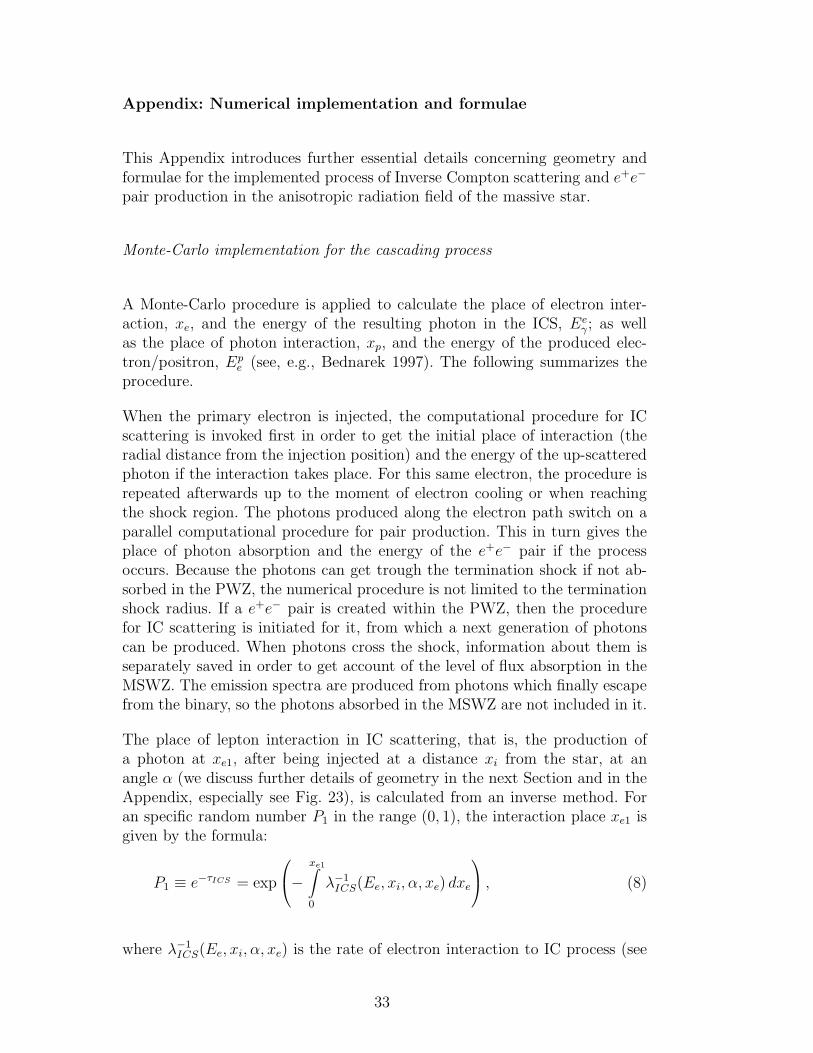
Appendix: Numerical implementation and formulae

This Appendix introduces further essential details concerning geometry andformulae for the implemented process of Inverse Compton scattering and e+e−

pair production in the anisotropic radiation field of the massive star.

Monte-Carlo implementation for the cascading process

A Monte-Carlo procedure is applied to calculate the place of electron inter-action, xe, and the energy of the resulting photon in the ICS, Ee

γ; as wellas the place of photon interaction, xp, and the energy of the produced elec-tron/positron, Ep

e (see, e.g., Bednarek 1997). The following summarizes theprocedure.

When the primary electron is injected, the computational procedure for ICscattering is invoked first in order to get the initial place of interaction (theradial distance from the injection position) and the energy of the up-scatteredphoton if the interaction takes place. For this same electron, the procedure isrepeated afterwards up to the moment of electron cooling or when reachingthe shock region. The photons produced along the electron path switch on aparallel computational procedure for pair production. This in turn gives theplace of photon absorption and the energy of the e+e− pair if the processoccurs. Because the photons can get trough the termination shock if not ab-sorbed in the PWZ, the numerical procedure is not limited to the terminationshock radius. If a e+e− pair is created within the PWZ, then the procedurefor IC scattering is initiated for it, from which a next generation of photonscan be produced. When photons cross the shock, information about them isseparately saved in order to get account of the level of flux absorption in theMSWZ. The emission spectra are produced from photons which finally escapefrom the binary, so the photons absorbed in the MSWZ are not included in it.

The place of lepton interaction in IC scattering, that is, the production ofa photon at xe1, after being injected at a distance xi from the star, at anangle α (we discuss further details of geometry in the next Section and in theAppendix, especially see Fig. 23), is calculated from an inverse method. Foran specific random number P1 in the range (0, 1), the interaction place xe1 isgiven by the formula:

P1 ≡ e−τICS = exp

−xe1∫

0

λ−1ICS(Ee, xi, α, xe) dxe

, (8)

where λ−1ICS(Ee, xi, α, xe) is the rate of electron interaction to IC process (see

33

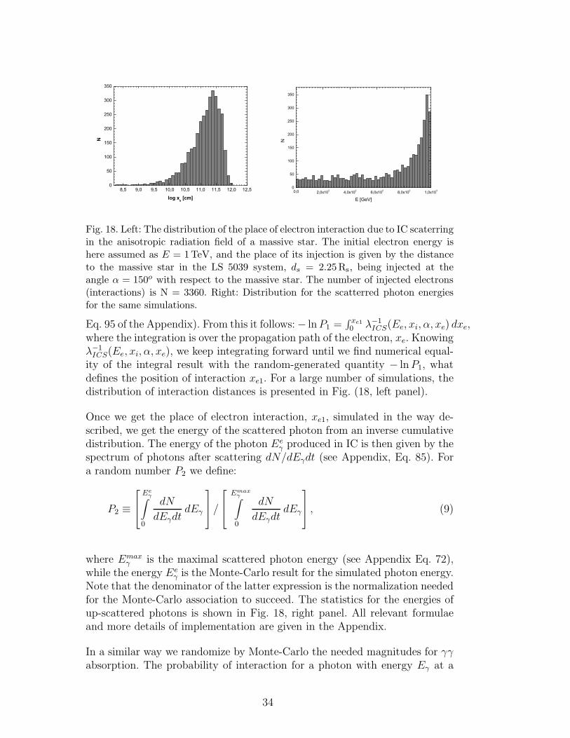
8,5 9,0 9,5 10,0 10,5 11,0 11,5 12,0 12,50

50

100

150

200

250

300

350

N

log xe [cm]0,0 2,0x102 4,0x102 6,0x102 8,0x102 1,0x1030

50

100

150

200

250

300

350

N

E [GeV]

Fig. 18. Left: The distribution of the place of electron interaction due to IC scaterringin the anisotropic radiation field of a massive star. The initial electron energy ishere assumed as E = 1TeV, and the place of its injection is given by the distanceto the massive star in the LS 5039 system, ds = 2.25Rs, being injected at theangle α = 150o with respect to the massive star. The number of injected electrons(interactions) is N = 3360. Right: Distribution for the scatterred photon energiesfor the same simulations.

Eq. 95 of the Appendix). From this it follows: − lnP1 =∫ xe10 λ−1

ICS(Ee, xi, α, xe) dxe,where the integration is over the propagation path of the electron, xe. Knowingλ−1

ICS(Ee, xi, α, xe), we keep integrating forward until we find numerical equal-ity of the integral result with the random-generated quantity − lnP1, whatdefines the position of interaction xe1. For a large number of simulations, thedistribution of interaction distances is presented in Fig. (18, left panel).

Once we get the place of electron interaction, xe1, simulated in the way de-scribed, we get the energy of the scattered photon from an inverse cumulativedistribution. The energy of the photon Ee

γ produced in IC is then given by thespectrum of photons after scattering dN/dEγdt (see Appendix, Eq. 85). Fora random number P2 we define:

P2 ≡

Eeγ

∫

0

dN

dEγdtdEγ

/

Emaxγ∫

0

dN

dEγdtdEγ

, (9)

where Emaxγ is the maximal scattered photon energy (see Appendix Eq. 72),

while the energy Eeγ is the Monte-Carlo result for the simulated photon energy.

Note that the denominator of the latter expression is the normalization neededfor the Monte-Carlo association to succeed. The statistics for the energies ofup-scattered photons is shown in Fig. 18, right panel. All relevant formulaeand more details of implementation are given in the Appendix.

In a similar way we randomize by Monte-Carlo the needed magnitudes for γγabsorption. The probability of interaction for a photon with energy Eγ at a

34

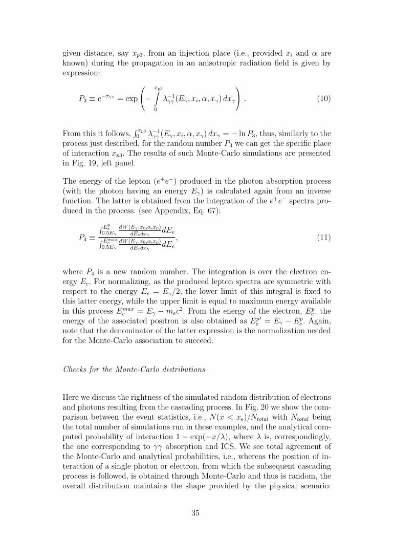
given distance, say xp3, from an injection place (i.e., provided xi and α areknown) during the propagation in an anisotropic radiation field is given byexpression:

P3 ≡ e−τγγ = exp

−xp3∫

0

λ−1γγ (Eγ , xi, α, xγ) dxγ

. (10)

From this it follows,∫ xp3

0 λ−1γγ (Eγ, xi, α, xγ) dxγ = − lnP3, thus, similarly to the

process just described, for the random number P3 we can get the specific placeof interaction xp3. The results of such Monte-Carlo simulations are presentedin Fig. 19, left panel.

The energy of the lepton (e+e−) produced in the photon absorption process(with the photon having an energy Eγ) is calculated again from an inversefunction. The latter is obtained from the integration of the e+e− spectra pro-duced in the process: (see Appendix, Eq. 67):

P4 ≡∫ Ep

e0.5Eγ

dW (Eγ ,x0,α,xp)dEedxγ

dEe

∫ Emaxe

0.5Eγ

dW (Eγ ,x0,α,xp)dEedxγ

dEe

, (11)

where P4 is a new random number. The integration is over the electron en-ergy Ee. For normalizing, as the produced lepton spectra are symmetric withrespect to the energy Ee = Eγ/2, the lower limit of this integral is fixed tothis latter energy, while the upper limit is equal to maximum energy availablein this process Emax

e = Eγ −mec2. From the energy of the electron, Ep

e , theenergy of the associated positron is also obtained as Ep

e′ = Eγ − Ep

e . Again,note that the denominator of the latter expression is the normalization neededfor the Monte-Carlo association to succeed.

Checks for the Monte-Carlo distributions

Here we discuss the rightness of the simulated random distribution of electronsand photons resulting from the cascading process. In Fig. 20 we show the com-parison between the event statistics, i.e., N(x < xe)/Ntotal with Ntotal beingthe total number of simulations run in these examples, and the analytical com-puted probability of interaction 1 − exp(−x/λ), where λ is, correspondingly,the one corresponding to γγ absorption and ICS. We see total agreement ofthe Monte-Carlo and analytical probabilities, i.e., whereas the position of in-teraction of a single photon or electron, from which the subsequent cascadingprocess is followed, is obtained through Monte-Carlo and thus is random, theoverall distribution maintains the shape provided by the physical scenario:

35

8,5 9,0 9,5 10,0 10,5 11,0 11,5 12,00

20

40

60

80

100

120

140

160

180

N

log x [cm]2,70 2,72 2,74 2,76 2,78 2,80 2,82 2,84 2,86 2,88 2,900

20

40

60

80

100

120

140

N

log Ee [GeV]

Fig. 19. Left: Distribution of the position of the γ-photon interaction due to absorp-tion in the anisotropic radiation field. The initial photon energy in this example isassumed as E = 1TeV and the place of its injection is given by the distance tothe massive star in the LS 5039 system, ds = 2.25Rs at the angle α = 150o withrespect to the massive star. The number of injected photons (interaction) is N =3358. Right: Distribution of the produced electron energy for the same simulations.

8,5 9,0 9,5 10,0 10,5 11,0 11,5 12,0 12,50,0

0,1

0,2

0,3

0,4

0,5

0,6

0,7

0,8

0,9

1,0

P( x

< x

)

log x /cm8,0 8,5 9,0 9,5 10,0 10,5 11,0 11,5 12,0 12,5

0,0

0,1

0,2

0,3

0,4

0,5

0,6

0,7

0,8

0,9

1,0

P( x

< x

e )

log x / cm

Fig. 20. Comparison between the event statistics, i.e., N(x < xe)/Ntotal with Ntotal

being the total number of simulations run, and the analytical computed probabil-ity of interaction 1 − exp(−x/λ), where λ is both, the one corresponding to γγabsorption (left) and ICS (right).

given the target and injection energy, the mean free path defines the distribu-tion for a sufficiently high number of runs.

Basic geometry

Parameters such as the viewing angle towards the observer, αobs, the separationof the binary, d, and the distance to the shock region along the orbit, rs (Eq.1), are directly connected to γ-ray observational results and are thus crucialfor detailed model discussion. Table 4 gives the set of LS 5039 orbital andbinary parameters that are relevant for modeling. These parameters come

36

Table 4LS 5039: system parameters

Parameter Symbol Adopted value

Radius of star R⋆ 9.3R⊙

Mass of star M⋆ 23M⊙

Temperature of star T⋆ 3.9 × 104 K

Mass loss rate of star M 10−7 M⊙ yr−1

Wind termination velocity V∞ 2400 km s−1

Wind initial velocity V0 4 km s−1

Distance to the system D 2.5 kpc

Eccentricity of the orbit ε 0.35

Semimajor axis a 0.15AU ∼ 3.5R⋆

Longitude of periastron ωp 226o

PSR

α

o

β

MS

t,

t i

obs

iN

θ

θ

observer

Fig. 21. The geometry of the orbit of the inclination i in the binary system (with theMS - massive star in the center) where the angle to the observer, αobs, is defined.No is the normal to the orbital plane, θt is the angle related to the orbital phaseand θ′t is its projection in the plane of the observer. The angle β gives the height ofthe pulsar for given phase above the observer plane.

from the recent work by Casares et al. (2005b), either directly from theirmeasurements or from the values compiled by them. The inferior conjunction(INFC) is defined as the phase when the binary is viewed from the pulsar side(the smallest αobs). Exactly in the opposite side of the orbit we find superiorconjunction (SUPC), when the pulsar is behind the massive star (the largestαobs), see also Fig. 1. One can see that for LS 5039, INFC (φ ≈ 0.72) is closeto apastron phase, while SUPC (φ ≈ 0.06) is close to periastron.

Figs. 21 and 22 shows the angle to the observer, αobs, as a function of orbitalphase for two considered inclination of the binary, i = 30o and i = 60o. Inaddition, the separation of the binary is marked. The viewing angle changes

37

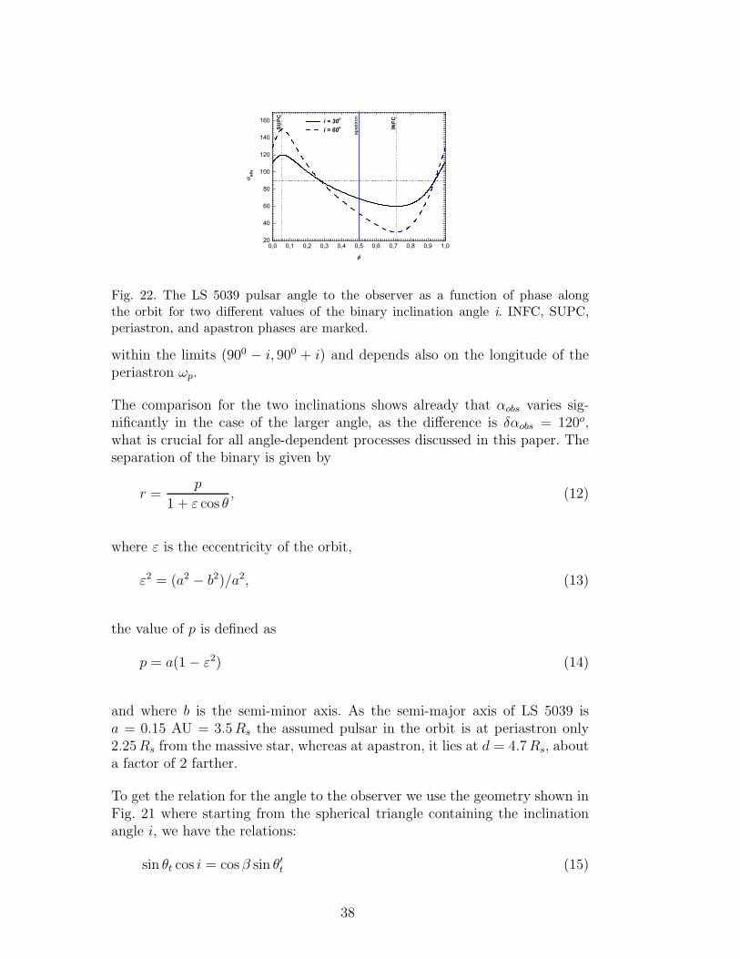
0,0 0,1 0,2 0,3 0,4 0,5 0,6 0,7 0,8 0,9 1,020

40

60

80

100

120

140

160

apas

tron

SUPC

INFC i = 30o

i = 60o

obs

Fig. 22. The LS 5039 pulsar angle to the observer as a function of phase alongthe orbit for two different values of the binary inclination angle i. INFC, SUPC,periastron, and apastron phases are marked.

within the limits (900 − i, 900 + i) and depends also on the longitude of theperiastron ωp.

The comparison for the two inclinations shows already that αobs varies sig-nificantly in the case of the larger angle, as the difference is δαobs = 120o,what is crucial for all angle-dependent processes discussed in this paper. Theseparation of the binary is given by

r =p

1 + ε cos θ, (12)

where ε is the eccentricity of the orbit,

ε2 = (a2 − b2)/a2, (13)

the value of p is defined as

p = a(1 − ε2) (14)

and where b is the semi-minor axis. As the semi-major axis of LS 5039 isa = 0.15 AU = 3.5Rs the assumed pulsar in the orbit is at periastron only2.25Rs from the massive star, whereas at apastron, it lies at d = 4.7Rs, abouta factor of 2 farther.

To get the relation for the angle to the observer we use the geometry shown inFig. 21 where starting from the spherical triangle containing the inclinationangle i, we have the relations:

sin θt cos i = cosβ sin θ′t (15)

38

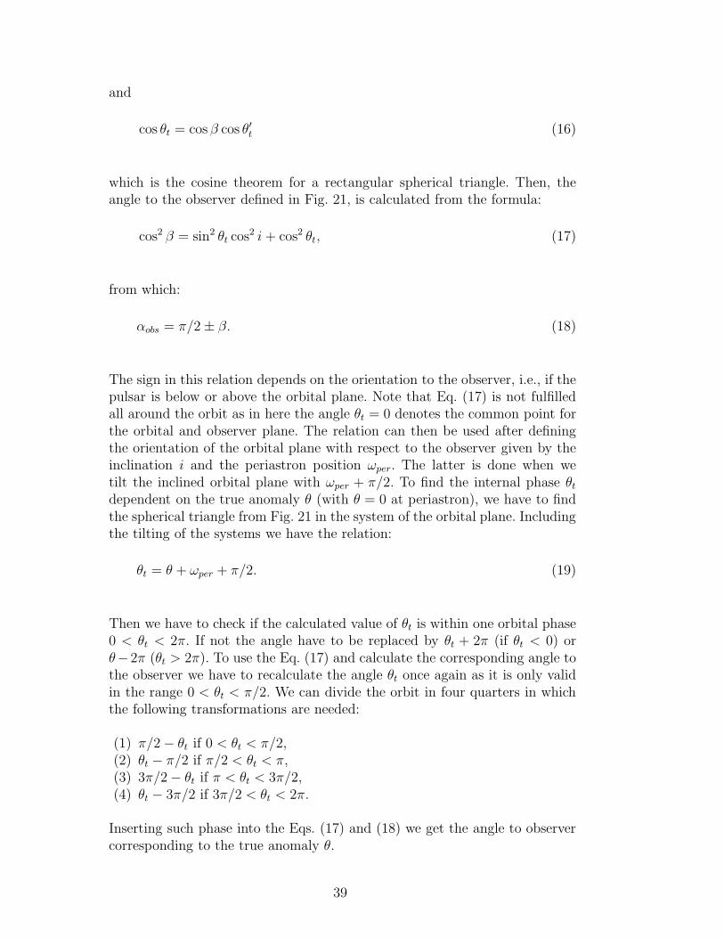
and

cos θt = cosβ cos θ′t (16)

which is the cosine theorem for a rectangular spherical triangle. Then, theangle to the observer defined in Fig. 21, is calculated from the formula:

cos2 β = sin2 θt cos2 i+ cos2 θt, (17)

from which:

αobs = π/2 ± β. (18)

The sign in this relation depends on the orientation to the observer, i.e., if thepulsar is below or above the orbital plane. Note that Eq. (17) is not fulfilledall around the orbit as in here the angle θt = 0 denotes the common point forthe orbital and observer plane. The relation can then be used after definingthe orientation of the orbital plane with respect to the observer given by theinclination i and the periastron position ωper. The latter is done when wetilt the inclined orbital plane with ωper + π/2. To find the internal phase θt

dependent on the true anomaly θ (with θ = 0 at periastron), we have to findthe spherical triangle from Fig. 21 in the system of the orbital plane. Includingthe tilting of the systems we have the relation:

θt = θ + ωper + π/2. (19)

Then we have to check if the calculated value of θt is within one orbital phase0 < θt < 2π. If not the angle have to be replaced by θt + 2π (if θt < 0) orθ−2π (θt > 2π). To use the Eq. (17) and calculate the corresponding angle tothe observer we have to recalculate the angle θt once again as it is only validin the range 0 < θt < π/2. We can divide the orbit in four quarters in whichthe following transformations are needed:

(1) π/2 − θt if 0 < θt < π/2,(2) θt − π/2 if π/2 < θt < π,(3) 3π/2 − θt if π < θt < 3π/2,(4) θt − 3π/2 if 3π/2 < θt < 2π.

Inserting such phase into the Eqs. (17) and (18) we get the angle to observercorresponding to the true anomaly θ.

39

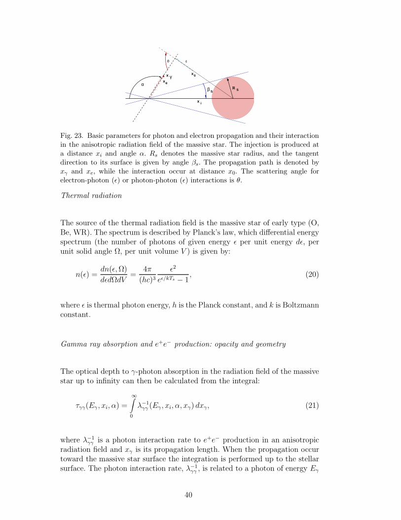
αγ

θ

x

x

x

x

Rβ S S

ε

e

i

0

Fig. 23. Basic parameters for photon and electron propagation and their interactionin the anisotropic radiation field of the massive star. The injection is produced ata distance xi and angle α. Rs denotes the massive star radius, and the tangentdirection to its surface is given by angle βs. The propagation path is denoted byxγ and xe, while the interaction occur at distance x0. The scattering angle forelectron-photon (ǫ) or photon-photon (ǫ) interactions is θ.

Thermal radiation

The source of the thermal radiation field is the massive star of early type (O,Be, WR). The spectrum is described by Planck’s law, which differential energyspectrum (the number of photons of given energy ǫ per unit energy dǫ, perunit solid angle Ω, per unit volume V ) is given by:

n(ǫ) =dn(ǫ,Ω)

dǫdΩdV=

4π

(hc)3

ǫ2

eǫ/kTs − 1, (20)

where ǫ is thermal photon energy, h is the Planck constant, and k is Boltzmannconstant.

Gamma ray absorption and e+e− production: opacity and geometry

The optical depth to γ-photon absorption in the radiation field of the massivestar up to infinity can then be calculated from the integral:

τγγ(Eγ , xi, α) =

∞∫

0

λ−1γγ (Eγ , xi, α, xγ) dxγ, (21)

where λ−1γγ is a photon interaction rate to e+e− production in an anisotropic

radiation field and xγ is its propagation length. When the propagation occurtoward the massive star surface the integration is performed up to the stellarsurface. The photon interaction rate, λ−1

γγ , is related to a photon of energy Eγ

40

injected at a distance xi from the massive star, at angle α (see Fig. 23), andis given by the formula:

λγγ−1(Eγ , xi, α, xγ) =

∫

(1 + µ)dµ∫

dφ∫

n(ǫ)σγγ(β)dǫ, (22)

where xγ is the distance to the interacting photon from the injection placealong its propagating path. The integration limits will be discussed in a dif-ferent part of the Appendix. For now we focus on the variable µ in the firstintegration. It is the cosine of the photon-photon scattering angle µ = cos θ(see Fig. 23). The angle φ is the azimuthal angle between the photon (γ-ray)propagation direction and the direction to the massive star, while φs givesits limit value for the direction tangent to the massive star surface (see Fig.25). The cross section to e+e− production is denoted as σγγ(β), where theparameter β in the center of mass system is

β =√ω2 −m2/ω, (23)

with

ω2 =1

2Eγǫ(1 + cos θ) (24)

being the photon energy squared (in this notation it is assumed also thatc = 1). From this we get

β2 = 1 − 2m2/Eγǫ(1 + µ). (25)

The kinematic condition for the angle θ which defines the threshold for thee+e− creation is given by expression:

µ ≥ µlim =2m2

Eγǫ− 1. (26)

To simplify the equations we rewrite the internal integration in Eq. (22) mak-ing use of I1(µ), such that,

I1(µ) =∫

n(ǫ)σγγ(β)dǫ. (27)

With the replacement

β2 = 1 − a/ǫ, (28)

41

where

a = 2m2/Eγ(1 + µ), (29)

and defining the constant S = 8π/(hc)3, the spectrum of thermal photons isnow given by the formula:

n(ǫ) = Sa2

(1 − β2)2

1

e(a/[(1−β2)kTs)] − 1. (30)

Substituting in the internal integral I1(µ), and introducing the integrationvariable to β, via

dǫ = 2a β/(1 − β2)2 dβ, (31)

yields to the integral:

I1(a) = 2S

1∫

0

a3

(1 − β2)2

1

e(a/(1−β2)kTs) − 1σγγ(β)dβ. (32)

The lower limit of integration is from the energy condition for the processγ + γ → e+e−, i.e., it follows from the threshold condition Eγǫ(1 + µ) = 2m2,where ω = m. . The upper integration limit comes from the relativistic limitω ≫ m, where we get β ≈ 1. To proceed forward, we introduce a dumbvariable, b, by a = kTsb, to get:

I1(b) = 2S

1∫

0

(kTs)3b3σγγ(β)

β

(1 − β2)4

1

e(b/(1−β2)) − 1dβ. (33)

The cross section for e+e− pair production is (Jauch and Rohrlich, 1980):

σγγ(β) =1

2r20π(1 − β2)[(3 − β4) ln

1 + β

1 − β− 2β(2 − β2)], (34)

where r0 is the classical electron radius, and σT = 83πr2

0 is the Thomson crosssection. When putting this expression into the integral I1(b) (Eq. 33) we getfinally,

I1(b) = C13

16b3

1∫

0

[

(3 − β4) ln1 + β

1 − β− 2β(2 − β2)

]

×

42

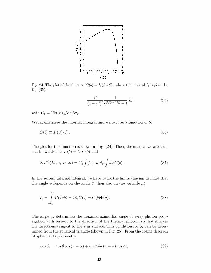
Fig. 24. The plot of the function C(b) = I1(β)/C1, where the integral I1 is given byEq. (35).

β

(1 − β2)3

1

e(b/(1−β2)) − 1dβ, (35)

with C1 = 16π(kTs/hc)3σT .

Weparametrizee the internal integral and write it as a function of b,

C(b) ≡ I1(β)/C1. (36)

The plot for this function is shown in Fig. (24). Then, the integral we are aftercan be written as I1(b) = C1C(b) and

λγγ−1(Eγ , xi, α, xγ) = C1

∫

(1 + µ)dµ∫

dφC(b). (37)

In the second internal integral, we have to fix the limits (having in mind thatthe angle φ depends on the angle θ, then also on the variable µ),

I2 =

φs∫

−φs

C(b)dφ = 2φsC(b) = C(b)Φ(µ). (38)

The angle φs determines the maximal azimuthal angle of γ-ray photon prop-agation with respect to the direction of the thermal photon, so that it givesthe directions tangent to the star surface. This condition for φs can be deter-mined from the spherical triangle (shown in Fig. 25). From the cosine theoremof spherical trigonometry

cosβs = cos θ cos (π − α) + sin θ sin (π − α) cosφs, (39)

43

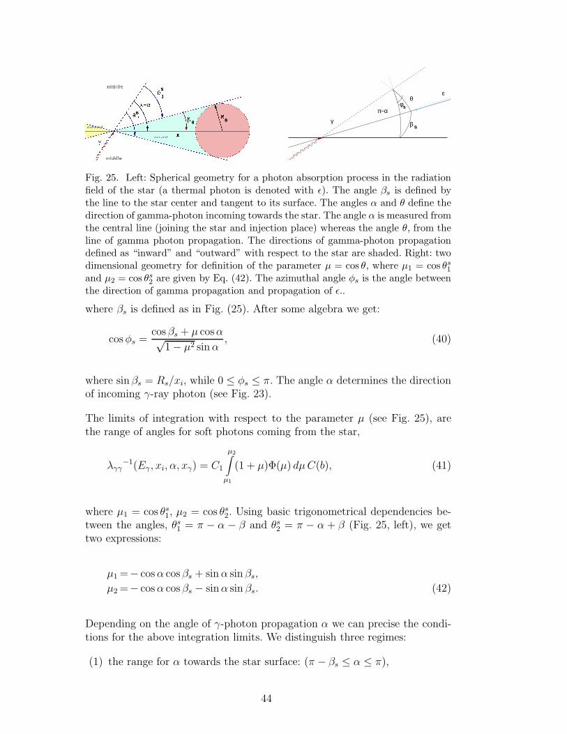
ε

γ

θ

β s

π−αφs

Fig. 25. Left: Spherical geometry for a photon absorption process in the radiationfield of the star (a thermal photon is denoted with ǫ). The angle βs is defined bythe line to the star center and tangent to its surface. The angles α and θ define thedirection of gamma-photon incoming towards the star. The angle α is measured fromthe central line (joining the star and injection place) whereas the angle θ, from theline of gamma photon propagation. The directions of gamma-photon propagationdefined as “inward” and “outward” with respect to the star are shaded. Right: twodimensional geometry for definition of the parameter µ = cos θ, where µ1 = cos θs

1

and µ2 = cos θs2 are given by Eq. (42). The azimuthal angle φs is the angle between

the direction of gamma propagation and propagation of ǫ..

where βs is defined as in Fig. (25). After some algebra we get:

cosφs =cosβs + µ cosα√

1 − µ2 sinα, (40)

where sin βs = Rs/xi, while 0 ≤ φs ≤ π. The angle α determines the directionof incoming γ-ray photon (see Fig. 23).

The limits of integration with respect to the parameter µ (see Fig. 25), arethe range of angles for soft photons coming from the star,

λγγ−1(Eγ , xi, α, xγ) = C1

µ2∫

µ1

(1 + µ)Φ(µ) dµC(b), (41)

where µ1 = cos θs1, µ2 = cos θs

2. Using basic trigonometrical dependencies be-tween the angles, θs

1 = π − α − β and θs2 = π − α + β (Fig. 25, left), we get

two expressions:

µ1 =− cosα cosβs + sinα sin βs,

µ2 =− cosα cosβs − sinα sin βs. (42)

Depending on the angle of γ-photon propagation α we can precise the condi-tions for the above integration limits. We distinguish three regimes:

(1) the range for α towards the star surface: (π − βs ≤ α ≤ π),

44

(2) the “middle” range: (βs < α < π − βs),(3) the range outwards of the massive star surface: (0 ≤ α ≤ βs).

Integration over µ can be simplified by separating the main integral, Eq. (41),in the sum of the corresponding integrals for these regimes, each dependingon their limits µ1, µ2, µlim (see Eq. 42 and 26). A simplification occurs forthe specific range of the angle θ for which the function Φ(µ) = 2φs (Eq.38) is maximal, i.e., Φ(µ) = 2π, what corresponds to the scenario when thephoton propagate toward the star. Another simplification happens when Φ(µ)is minimal, i.e., Φ(µ) = 0, for an outgoing photon. To simplify the formulae fornumerical implementation we introduce the function f(µ, b) = C1C(b)(1 + µ)such that

λγγ−1(Eγ , xi, α, xγ) =

µ2∫

µ1

f(µ, b)Φ(µ) dµ, (43)

where we introduced internal function f(µ, b) = C1(1 + µ)C(b). To fasten thesimulations the integration limits can be fixed following the rules (note thatrelation (µ1 ≥ µ2) is always fulfilled):

(1) for “inward” propagation :• if (µlim ≤ µ2 ≤ µ1):λγγ

−1(Eγ , xi, α, xγ) =∫ µ1

µ2f(µ, b)Φ(µ) dµ+

∫ 1µ1f(µ, b)2π dµ,

• if (µ2 ≤ µlim ≤ µ1):λγγ

−1(Eγ , xi, α, xγ) =∫ µ1

µlimf(µ, b)Φ(µ) dµ+

∫ 1µ1f(µ, b)2π dµ,

• if (µ2 ≤ µ1 ≤ µlim):λγγ

−1(Eγ , xi, α, xγ) =∫ 1µlim

f(µ, b)2π dµ.Apart from these, the case of α = π can also be separately defined (incom-ing at a central spot of the star) when (µ1 = µ2) and λγγ

−1(Eγ, xi, α, xγ) =∫ 1µmin

f(µ, b)2π dµ, where µmin is the smaller value from (µ1, µlim).

(2) for the “middle” range of propagation:• if (µlim ≤ µ2 ≤ µ1):λγγ

−1(Eγ , xi, α, xγ) =∫ µ1

µ2f(µ, b)Φ(µ) dµ,

• if (µ2 ≤ µlim ≤ µ1):λγγ

−1(Eγ , xi, α, xγ) =∫ µ1

µlimf(µ, b)Φ(µ) dµ,

• if (µ2 ≤ µ1 ≤ µlim):λγγ

−1(Eγ , xi, α, xγ) = 0.(3) for “outwards” directions:

• if (µlim ≤ µ2 ≤ µ1):λγγ

−1(Eγ , xi, α, xγ) =∫ µ1

µ2f(µ, b)Φ(µ) dµ+

∫ µ2

µlimf(µ, b)2π dµ,

• if (µ2 ≤ µlim ≤ µ1):λγγ

−1(Eγ , xi, α, xγ) =∫ µ1

µlimf(µ, b)Φ(µ) dµ,

• if (µ2 ≤ µ1 ≤ µlim):

45

λγγ−1(Eγ , xi, α, xγ) = 0.

Apart from these, as before, the case of α = 0 can also be defined (es-caping radially from a central spot of the star) when (µ1 = µ2) i if(µ1 > µlim), and we have λγγ

−1(Eγ , xi, α, xγ) =∫ µ1

µlimf(µ, b)2π dµ, other-

wise λγγ−1(Eγ, xi, α, xγ) = 0.

The energy spectrum for e+e− pairs produced by γγ absorption process

To simulate the energy of an electron (positron) produced in the process ofgamma absorption we follow the energy distribution of e+e− pairs (see Eq.11). The e+e− pair spectrum produced by a photon of energy Eγ at a specificdistance xp is given by the expression:

dW (Eγ, xi, α, xγ)

dEedxγ=∫

(1 + µ)dµ∫

dφ∫

n(ǫ)σ(Eγ , Ee, µ)dǫ, (44)

where Eγ is the energy of the interacting photon, xγ is the propagation length,xi the distance of the injection place form the massive star, α is the angle ofpropagation, and Ee is the energy of produced lepton (e+e−). The limits ofintegration are discussed in the following paragraph.

The energy spectrum of thermal photons ǫ is again given by the Planck’sspectrum n(ǫ) (Eq. 20). The cross section for pair production σ(Eγ , Ee, µ)depends on the photon energy Eγ and energy of electron Ee. The variableµ = cos θ, angles θ and φs are defined in Fig. 25).

The cross section is given by the formula (Akhieser & Berestezki, 1965):

σ(Eγ , Ee, µ)=r20

2

m2

Eγ

1

εcβcγc

× [2ε2

c −m2 + (ε2c −m2)A2(Ee, εc)

m2B2(Ee, εc) + ε2cA

2(Ee, εc)

−2(ε2

c −m2)2A4(Ee, εc)

(m2B2(Ee, εc) + ε2cA

2(Ee, εc))2], (45)

where εc is the photon energy in centrum of momentum (CM) of the interactingphotons ε2

c = 12Eγǫ(1 + µ). The parameter γc = (Eγ + ǫ)/2εc is Lorentz factor

in CM system and m = mec2 is the electron mass. In Eq. (45), the following

functions are introduced:

B2(Ee, εc)=(Ee − γcεc)

2

(γcβc)2(ε2c −m2)

, (46)

A2(Ee, εc)= 1 −B2(Ee, εc), (47)

46

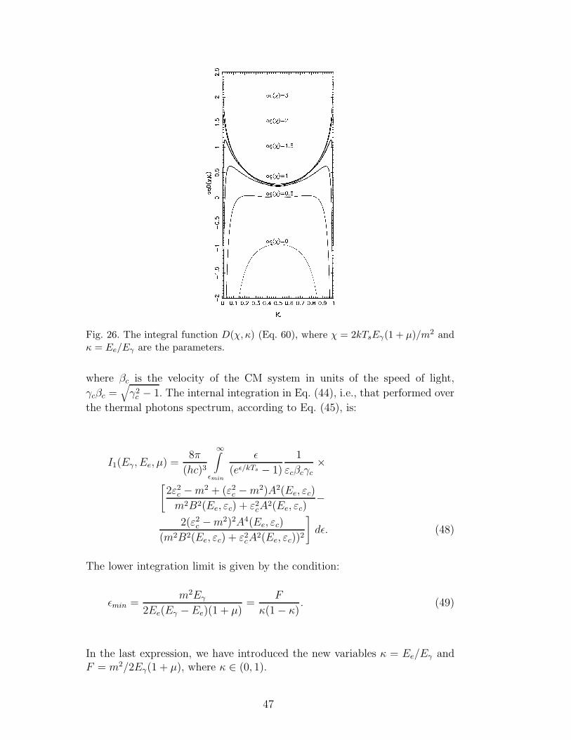
Fig. 26. The integral function D(χ, κ) (Eq. 60), where χ = 2kTsEγ(1 + µ)/m2 andκ = Ee/Eγ are the parameters.

where βc is the velocity of the CM system in units of the speed of light,

γcβc =√

γ2c − 1. The internal integration in Eq. (44), i.e., that performed over

the thermal photons spectrum, according to Eq. (45), is:

I1(Eγ, Ee, µ) =8π

(hc)3

∞∫

ǫmin

ǫ

(eǫ/kTs − 1)

1

εcβcγc×

[

2ε2c −m2 + (ε2

c −m2)A2(Ee, εc)

m2B2(Ee, εc) + ε2cA

2(Ee, εc)−

2(ε2c −m2)2A4(Ee, εc)

(m2B2(Ee, εc) + ε2cA

2(Ee, εc))2

]

dǫ. (48)

The lower integration limit is given by the condition:

ǫmin =m2Eγ

2Ee(Eγ −Ee)(1 + µ)=

F

κ(1 − κ). (49)

In the last expression, we have introduced the new variables κ = Ee/Eγ andF = m2/2Eγ(1 + µ), where κ ∈ (0, 1).

47

For a photon energy Eγ ≫ ǫ, we have γc ≫ 1, β ≃ 1, and εcβcγc = Eγ/2.After rewriting Eq. (48) we get

I1(Eγ, Ee, µ) =8π

(hc)3

2

Eγ

∞∫

ǫmin

ǫ

(eǫ/kTs − 1)f(ǫ) dǫ, (50)

where, to simplify the formula, we have defined

f(ǫ) =2ε2

c −m2 + (ε2c −m2)A2(Ee, εc)

m2B2(Ee, εc) + ε2cA

2(Ee, εc)−

2(ε2c −m2)2A4(Ee, εc)

(m2B2(Ee, εc) + ε2cA

2(Ee, εc))2. (51)

To proceed forward, we introduce the variable z = ǫ/kTs, so that kTsdz = dǫ,and the integral is now given by the expression:

I1(Eγ, Ee, µ) =8π

(hc)3

2(kTs)2

Eγ

∞∫

zmin

z

ez − 1f(z) dz, (52)

where the lower limit of the integral is given by zmin = ǫmin/kTs,

zmin = m2/(2EγkTs(1 + µ)κ(1 − κ)) = m2/χκ(1 − κ) (53)

and a new parameter,

χ = 2EγkTs(1 + µ), (54)

was introduced. The parameter χ is limited by the condition ε2c > m2, so then

χ > 4m2/zmax = 4kTsm2/ǫmax, (55)

where ǫmax is the maximal thermal photon energy from the blackbody spec-trum (we assume ǫmax = 30kTs). By using the variable

= ε2c =

1

2Eγǫ(1 + µ) = zχ/4, (56)

the additional needed functions are given by expressions:

48

B2(χ, κ)=(2κ− 1)2

−m2, (57)

A2(χ, κ)= 1 −B2(χ, κ). (58)

Function (51) can now be rewritten as:

f(z) =2−m2 + (−m2)A2(χ, κ)

m2B2(χ, κ) + A2(χ, κ)−

2(−m2)2A4(χ, κ)

[m2B2(χ, κ) + A2(χ, κ)]2. (59)

We can further conveniently replace the parameter χ with a dimensionlessform χ = 2kTsEγ(1 + µ)/m2 to get finally the full set of needed magnitudesin a useful way for integrating:

I1(Eγ, Ee, µ) =16π(kTs)

2

(hc)3

1

EγD(χ, κ), (60)

D(χ, κ) =

∞∫

zmin

z

ez − 1f(z) dz, (61)

f(z) =2− 1 + (− 1)A2(χ, κ)

B2(χ, κ) + A2(χ, κ)−

2(− 1)2A4(χ, κ)

[B2(χ, κ) + A2(χ, κ)]2, (62)

B2(χ, κ) =(2κ− 1)2

− 1, (63)

A2(χ, κ) = 1 −B2(χ, κ). (64)

To produce the electron of the energy κ the process is limited by the conditionz > zκ, where

zκ =1

χκ(1 − κ). (65)

On the other hand, from the kinematics of the process we have limitationz > zχ, where

zχ =4

χ=

2m2

EγkTs(1 + µ). (66)

The lower limit of the sought integral is the greater value of the two expressionsquoted above. The integral given in Eq. (61) can be tabulated with respect to

49

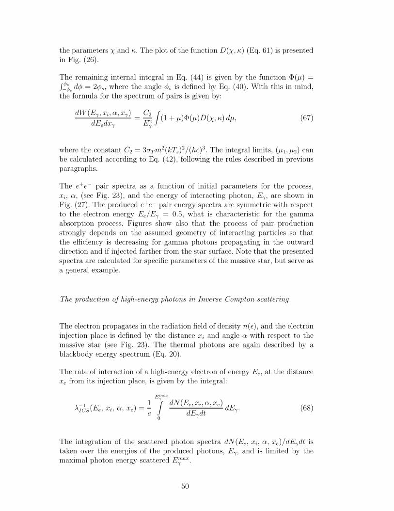
the parameters χ and κ. The plot of the function D(χ, κ) (Eq. 61) is presentedin Fig. (26).

The remaining internal integral in Eq. (44) is given by the function Φ(µ) =∫ φs

−φsdφ = 2φs, where the angle φs is defined by Eq. (40). With this in mind,

the formula for the spectrum of pairs is given by:

dW (Eγ, xi, α, xγ)

dEedxγ

=C2

E2γ

∫

(1 + µ)Φ(µ)D(χ, κ) dµ, (67)

where the constant C2 = 3σTm2(kTs)

2/(hc)3. The integral limits, (µ1, µ2) canbe calculated according to Eq. (42), following the rules described in previousparagraphs.

The e+e− pair spectra as a function of initial parameters for the process,xi, α, (see Fig. 23), and the energy of interacting photon, Eγ , are shown inFig. (27). The produced e+e− pair energy spectra are symmetric with respectto the electron energy Ee/Eγ = 0.5, what is characteristic for the gammaabsorption process. Figures show also that the process of pair productionstrongly depends on the assumed geometry of interacting particles so thatthe efficiency is decreasing for gamma photons propagating in the outwarddirection and if injected farther from the star surface. Note that the presentedspectra are calculated for specific parameters of the massive star, but serve asa general example.

The production of high-energy photons in Inverse Compton scattering

The electron propagates in the radiation field of density n(ǫ), and the electroninjection place is defined by the distance xi and angle α with respect to themassive star (see Fig. 23). The thermal photons are again described by ablackbody energy spectrum (Eq. 20).

The rate of interaction of a high-energy electron of energy Ee, at the distancexe from its injection place, is given by the integral:

λ−1ICS(Ee, xi, α, xe) =

1

c

Emaxγ∫

0

dN(Ee, xi, α, xe)

dEγdtdEγ. (68)

The integration of the scattered photon spectra dN(Ee, xi, α, xe)/dEγdt istaken over the energies of the produced photons, Eγ, and is limited by themaximal photon energy scattered Emax

γ .

50

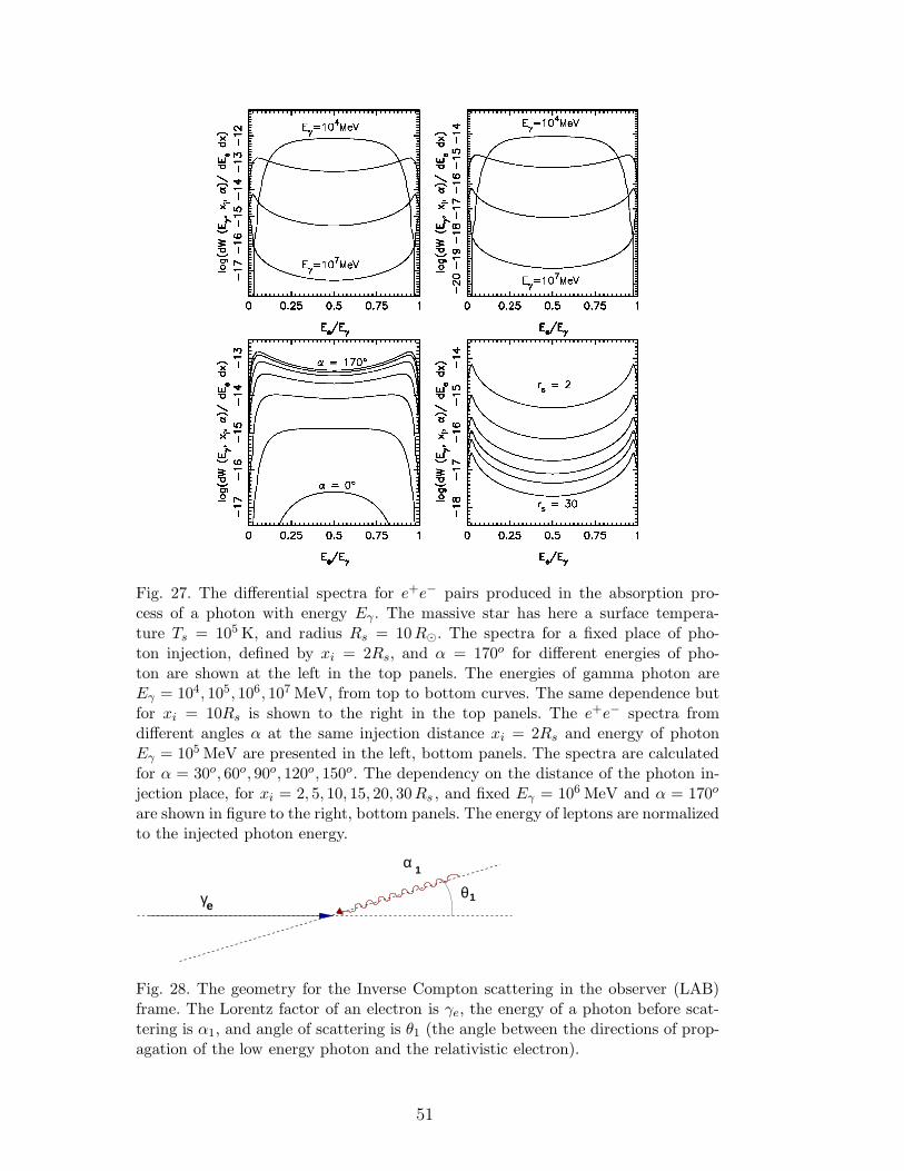
Fig. 27. The differential spectra for e+e− pairs produced in the absorption pro-cess of a photon with energy Eγ . The massive star has here a surface tempera-ture Ts = 105 K, and radius Rs = 10R⊙. The spectra for a fixed place of pho-ton injection, defined by xi = 2Rs, and α = 170o for different energies of pho-ton are shown at the left in the top panels. The energies of gamma photon areEγ = 104, 105, 106, 107 MeV, from top to bottom curves. The same dependence butfor xi = 10Rs is shown to the right in the top panels. The e+e− spectra fromdifferent angles α at the same injection distance xi = 2Rs and energy of photonEγ = 105 MeV are presented in the left, bottom panels. The spectra are calculatedfor α = 30o, 60o, 90o, 120o, 150o. The dependency on the distance of the photon in-jection place, for xi = 2, 5, 10, 15, 20, 30Rs , and fixed Eγ = 106 MeV and α = 170o

are shown in figure to the right, bottom panels. The energy of leptons are normalizedto the injected photon energy.

α

θ1

1

eγ

Fig. 28. The geometry for the Inverse Compton scattering in the observer (LAB)frame. The Lorentz factor of an electron is γe, the energy of a photon before scat-tering is α1, and angle of scattering is θ1 (the angle between the directions of prop-agation of the low energy photon and the relativistic electron).

51

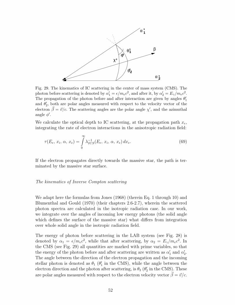
β

α

θ

θ

χ

’’

’

α ’

φ’

1

1’

2

2

Fig. 29. The kinematics of IC scattering in the center of mass system (CMS). Thephoton before scattering is denoted by α′

1 = ǫ/mec2, and after it, by α′

2 = Eγ/mec2.

The propagation of the photon before and after interaction are given by angles θ′1and θ′2, both are polar angles measured with respect to the velocity vector of the

electron ~β = ~v/c. The scattering angles are the polar angle χ′, and the azimuthalangle φ′.

We calculate the optical depth to IC scattering, at the propagation path xe,integrating the rate of electron interactions in the anisotropic radiation field:

τ(Ee, xi, α, xe) =

∞∫

0

λ−1ICS(Ee, xi, α, xe) dxe. (69)

If the electron propagates directly towards the massive star, the path is ter-minated by the massive star surface.

The kinematics of Inverse Compton scattering

We adapt here the formulas from Jones (1968) (therein Eq. 1 through 10) andBlumenthal and Gould (1970) (their chapters 2.6-2.7), wherein the scatteredphoton spectra are calculated in the isotropic radiation case. In our work,we integrate over the angles of incoming low energy photons (the solid anglewhich defines the surface of the massive star) what differs from integrationover whole solid angle in the isotropic radiation field.

The energy of photon before scattering in the LAB system (see Fig. 28) isdenoted by α1 = ǫ/mec

2, while that after scattering, by α2 = Eγ/mec2. In

the CMS (see Fig. 29) all quantities are marked with prime variables, so thatthe energy of the photon before and after scattering are written as α′

1 and α′2.

The angle between the direction of the electron propagation and the incomingstellar photon is denoted as θ1 (θ′1 in the CMS), while the angle between theelectron direction and the photon after scattering, is θ2 (θ′2 in the CMS). These

are polar angles measured with respect to the electron velocity vector ~β = ~v/c.

52

The angles of scattering in the electron rest frame generate a spherical triangle,so that

cos θ′2 = cos θ′1 cosχ′ + sin θ′1 sinχ′ cosφ′ (70)

(see Fig. 29). The energy of the scattered photon in the CMS is given by theformula:

α′2 =

α′1

1 + α′1(1 − cosχ′)

, (71)

where χ′ is the photon scattering angle, defined as the azimuthal angle betweenthe propagation direction of the photon after scattering, α′

2, and the photonpropagation direction before it, α′

1.

The energy of photon in the LAB system can be found from a Lorentz transfor-mation. In a simplified case, when the photon propagate head-on with respectto the electron direction, and after interaction, it has the energy:

α2 = γeα′2(1 + β cos(π − χ′)) ≈ γeα

′2(1 − cosχ′). (72)

In the electron’s rest frame (see Fig. 29), for the polar angle θ′1 = 0 we haveχ′ = θ′2 (see Eq. 72), what means that the photon energy after scattering (seeEq. 72) does not depend on the azimuthal scattering angle φ′.

We can calculate the maximal energy of the scattered photon from relations(71) and (72), such that αmax = 2γeα

′2. In the Thomson limit (α′

1 ≪ 1), themaximal photon energy depends on the electron energy and equals αT

max ≈4γ2

eα1. In the Klein-Nishina limit, which is the highly relativistic case, thisenergy is proportional to the initial electron energy and it is αKN

max ≈ γeα1.

The IC scattered photon spectrum in an anisotropic target field

In the case of mono-energetic isotropic photon background (in the LAB sys-tem) the angular spectrum of incoming low energy photons in the electronrest frame is given by the formula (Jones 1968):

n′(θ′1)d cos θ′1 =d cos θ′1

2γe(1 − β cos θ′1)2. (73)

For relativistic electrons (γe ≫ 1), the incoming target photon polar anglesare in the range 0 ≤ θ′1 ≤ θ′1/2, where θ1/2 ≈ 1/γe is the angle of a photon‘cone’ apex.

53

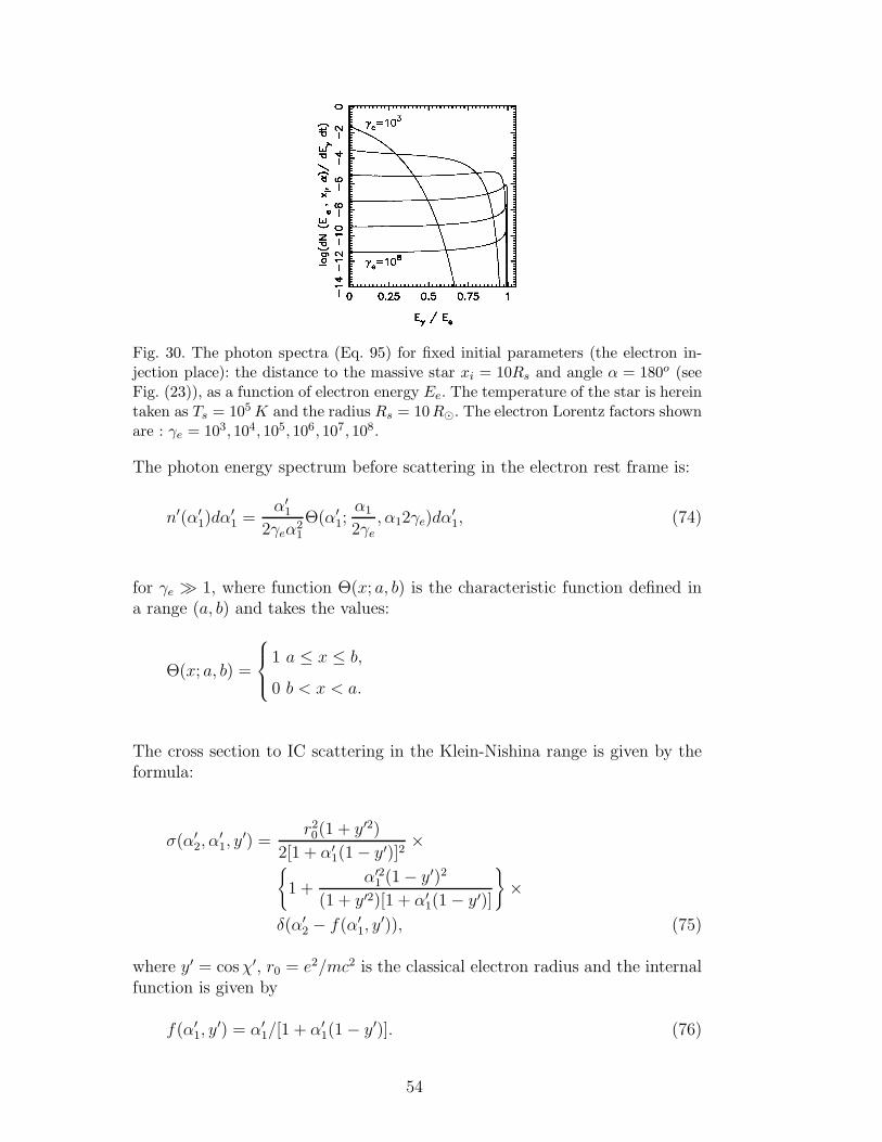
Fig. 30. The photon spectra (Eq. 95) for fixed initial parameters (the electron in-jection place): the distance to the massive star xi = 10Rs and angle α = 180o (seeFig. (23)), as a function of electron energy Ee. The temperature of the star is hereintaken as Ts = 105 K and the radius Rs = 10R⊙. The electron Lorentz factors shownare : γe = 103, 104, 105, 106, 107, 108.

The photon energy spectrum before scattering in the electron rest frame is:

n′(α′1)dα

′1 =

α′1

2γeα21

Θ(α′1;α1

2γe, α12γe)dα

′1, (74)

for γe ≫ 1, where function Θ(x; a, b) is the characteristic function defined ina range (a, b) and takes the values:

Θ(x; a, b) =

1 a ≤ x ≤ b,

0 b < x < a.

The cross section to IC scattering in the Klein-Nishina range is given by theformula:

σ(α′2, α

′1, y

′) =r20(1 + y′2)

2[1 + α′1(1 − y′)]2

×

1 +α′2

1 (1 − y′)2

(1 + y′2)[1 + α′1(1 − y′)]

×

δ(α′2 − f(α′

1, y′)), (75)

where y′ = cosχ′, r0 = e2/mc2 is the classical electron radius and the internalfunction is given by

f(α′1, y

′) = α′1/[1 + α′

1(1 − y′)]. (76)

54

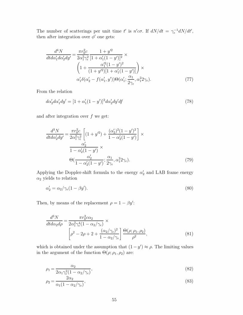
The number of scatterings per unit time t′ is n′cσ. If dN/dt = γ−1e dN/dt′,

then after integration over φ′ one gets:

d4N

dtdα′1dα

′2dy

′=

πr20c

2α21γ

2e

1 + y′2

[1 + α′1(1 − y′)]2

×(

1 +α′2

1 (1 − y′)2

(1 + y′2)[1 + α′1(1 − y′)]

)

×

α′1δ(α

′2 − f(α′

1, y′))Θ(α′

1;α1

2γe

, α212γe). (77)

From the relation

dα′2dα

′1dy

′ = [1 + α′1(1 − y′)]2dα′

2dy′df (78)

and after integration over f we get:

d3N

dtdα′2dy

′=

πr20c

2α21γ

2e

[

(1 + y′2) +(α′

2)2(1 − y′)2

1 − α′2(1 − y′)

]

×

α′2

1 − α′2(1 − y′)

×

Θ(α′

2

1 − α′2(1 − y′)

;α1

2γe, α2

12γe). (79)

Applying the Doppler-shift formula to the energy α′2 and LAB frame energy

α2 yields to relation

α′2 = α2/γe(1 − βy′). (80)

Then, by means of the replacement ρ = 1 − βy′:

d3N

dtdα2dρ=

πr20cα2

2α21γ

4e (1 − α2/γe)

×[

ρ2 − 2ρ+ 2 +(α2/γe)

2

1 − α2/γe

]

Θ(ρ; ρ1, ρ2)

ρ2, (81)

which is obtained under the assumption that (1− y′) ≈ ρ. The limiting valuesin the argument of the function Θ(ρ; ρ1, ρ2) are:

ρ1 =α2

2α1γ2e (1 − α2/γe)

, (82)

ρ2 =2α2

α1(1 − α2/γe), (83)

55

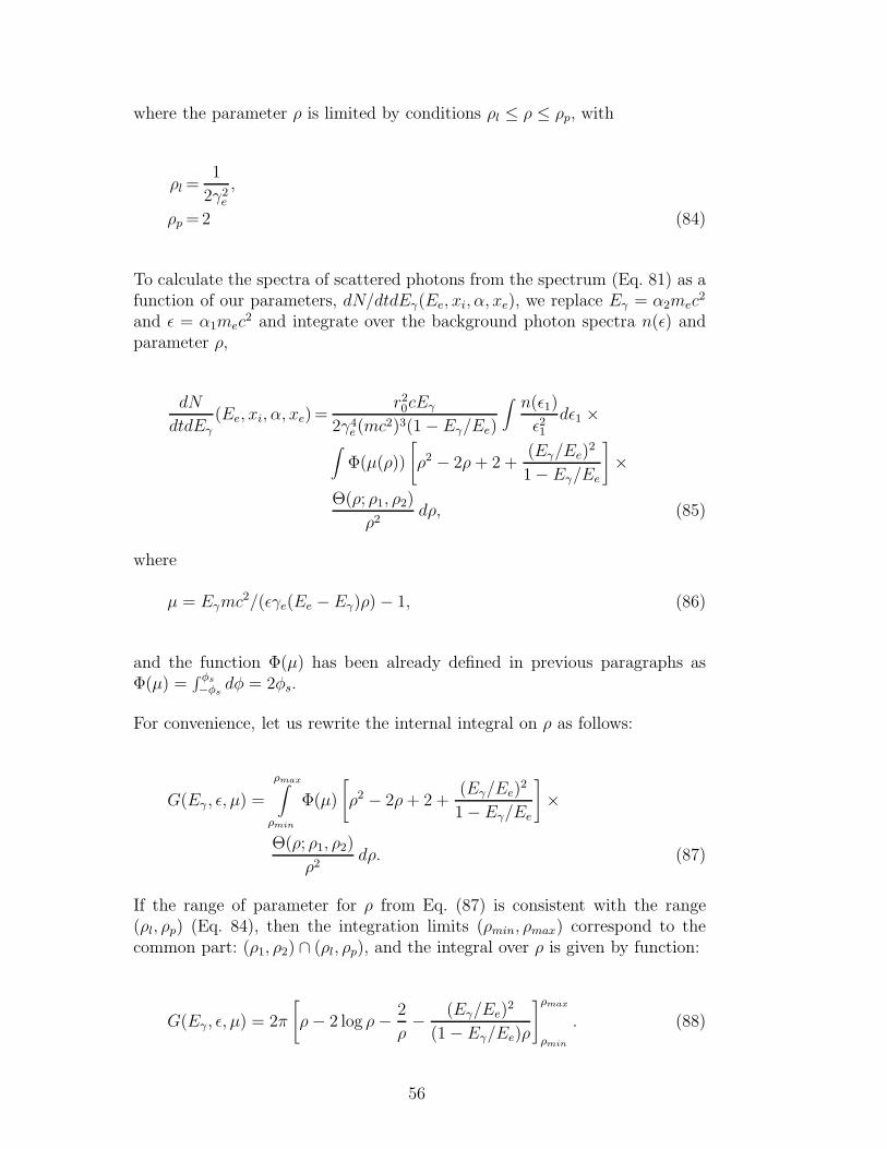
where the parameter ρ is limited by conditions ρl ≤ ρ ≤ ρp, with

ρl =1

2γ2e

,

ρp =2 (84)

To calculate the spectra of scattered photons from the spectrum (Eq. 81) as afunction of our parameters, dN/dtdEγ(Ee, xi, α, xe), we replace Eγ = α2mec

2

and ǫ = α1mec2 and integrate over the background photon spectra n(ǫ) and

parameter ρ,

dN

dtdEγ(Ee, xi, α, xe) =

r20cEγ

2γ4e(mc

2)3(1 − Eγ/Ee)

∫

n(ǫ1)

ǫ21dǫ1 ×

∫

Φ(µ(ρ))

[

ρ2 − 2ρ+ 2 +(Eγ/Ee)

2

1 − Eγ/Ee

]

×

Θ(ρ; ρ1, ρ2)

ρ2dρ, (85)

where

µ = Eγmc2/(ǫγe(Ee − Eγ)ρ) − 1, (86)

and the function Φ(µ) has been already defined in previous paragraphs asΦ(µ) =

∫ φs

−φsdφ = 2φs.

For convenience, let us rewrite the internal integral on ρ as follows:

G(Eγ , ǫ, µ) =

ρmax∫

ρmin

Φ(µ)

[

ρ2 − 2ρ+ 2 +(Eγ/Ee)

2

1 − Eγ/Ee

]

×

Θ(ρ; ρ1, ρ2)

ρ2dρ. (87)

If the range of parameter for ρ from Eq. (87) is consistent with the range(ρl, ρp) (Eq. 84), then the integration limits (ρmin, ρmax) correspond to thecommon part: (ρ1, ρ2) ∩ (ρl, ρp), and the integral over ρ is given by function:

G(Eγ , ǫ, µ) = 2π

[

ρ− 2 log ρ−2

ρ−

(Eγ/Ee)2

(1 − Eγ/Ee)ρ

]ρmax

ρmin

. (88)

56

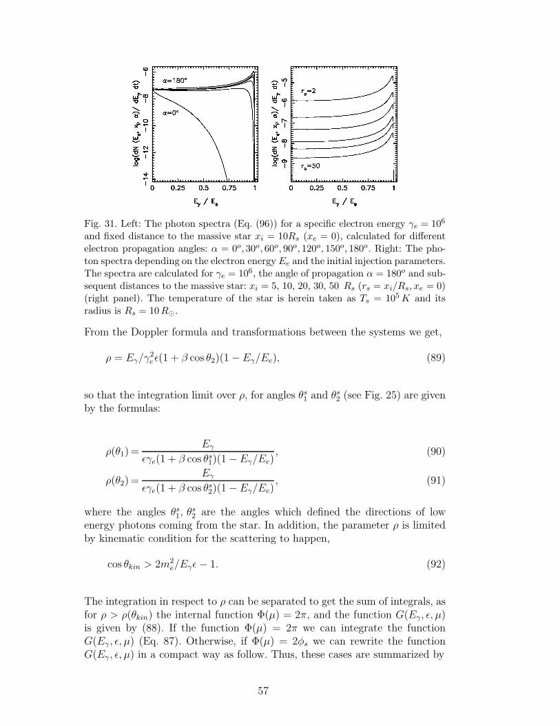
Fig. 31. Left: The photon spectra (Eq. (96)) for a specific electron energy γe = 106

and fixed distance to the massive star xi = 10Rs (xe = 0), calculated for differentelectron propagation angles: α = 0o, 30o, 60o, 90o, 120o, 150o, 180o. Right: The pho-ton spectra depending on the electron energy Ee and the initial injection parameters.The spectra are calculated for γe = 106, the angle of propagation α = 180o and sub-sequent distances to the massive star: xi = 5, 10, 20, 30, 50 Rs (rs = xi/Rs, xe = 0)(right panel). The temperature of the star is herein taken as Ts = 105 K and itsradius is Rs = 10R⊙.

From the Doppler formula and transformations between the systems we get,

ρ = Eγ/γ2e ǫ(1 + β cos θ2)(1 − Eγ/Ee), (89)

so that the integration limit over ρ, for angles θs1 and θs

2 (see Fig. 25) are givenby the formulas:

ρ(θ1) =Eγ

ǫγe(1 + β cos θs1)(1 − Eγ/Ee)

, (90)

ρ(θ2) =Eγ

ǫγe(1 + β cos θs2)(1 − Eγ/Ee)

, (91)

where the angles θs1, θ

s2 are the angles which defined the directions of low

energy photons coming from the star. In addition, the parameter ρ is limitedby kinematic condition for the scattering to happen,

cos θkin > 2m2e/Eγǫ− 1. (92)

The integration in respect to ρ can be separated to get the sum of integrals, asfor ρ > ρ(θkin) the internal function Φ(µ) = 2π, and the function G(Eγ, ǫ, µ)is given by (88). If the function Φ(µ) = 2π we can integrate the functionG(Eγ , ǫ, µ) (Eq. 87). Otherwise, if Φ(µ) = 2φs we can rewrite the functionG(Eγ , ǫ, µ) in a compact way as follow. Thus, these cases are summarized by

57

G(Eγ , ǫ, µ) =

ρmax∫

ρmin

2φsGρ(Eγ , ǫ, µ) dρ, (93)

G(Eγ , ǫ, µ) = 2π [Gint(Eγ, ǫ, µ)]ρmax

ρmin. (94)

where Gρ(Eγ , ǫ, µ) = [ρ2 − 2ρ+ 2 + (Eγ/Ee)2/(1 −Eγ/Ee)] × Θ(ρ; ρ1, ρ2)/ρ

2

and Gint(Eγ, ǫ, µ) = ρ−2 log ρ−2/ρ−(Eγ/Ee)2/((1 − Eγ/Ee)ρ). The limits of

integration depend on combinations of (ρ(θ1), ρ(θ2)) and (ρl, ρp), and respect-ing the constraints put by ρ(θkin). The final integration G(Eγ , ǫ, µ) is given bythe formulas:

(1) for “outwards” propagation :• if (ρmax < ρ1): G(Eγ , ǫ, µ) = 0,

• if (ρmax > ρ1) and (ρmin < ρ1) :and (ρmax < ρ2) :G(Eγ, ǫ, µ) =

∫ ρmax

ρ12φsGρ(Eγ, ǫ, µ) dρ,

or (ρmax > ρ2) :G(Eγ, ǫ, µ) =

∫ ρ2

ρ12φsGρ(Eγ , ǫ, µ) dρ+ 2π [Gint(Eγ , ǫ, µ)]ρmax

ρ2,

• if (ρmax > ρ1) and (ρmin > ρ1):if (ρmin < ρ2) and (ρmax < ρ2):G(Eγ, ǫ, µ) =

∫ ρmaxρmin

2φsGρ(Eγ, ǫ, µ) dρ,if (ρmin < ρ2) and (ρmax > ρ2) :G(Eγ, ǫ, µ) =

∫ ρ2

ρmin2φsGρ(Eγ, ǫ, µ) dρ+ 2π [Gint(Eγ , ǫ, µ)]ρmax

ρ2,

if (ρmin > ρ2):G(Eγ, ǫ, µ) = 2π [Gint(Eγ , ǫ, µ)]ρmax

ρ2.

(2) for the “middle” range of propagation:• if (ρmax < ρ1) or (ρmin > ρ2):G(Eγ , ǫ, µ) = 0,

• if (ρmax > ρ1) and (ρmax < ρ2):G(Eγ , ǫ, µ) =

∫ ρmax

MAX(ρmin,ρ1) 2φsGρ(Eγ, ǫ, µ) dρ,• if (ρmax > ρ1) and (ρmax > ρ2):G(Eγ , ǫ, µ) =

∫ ρ2

MAX(ρmin,ρ1) 2φsGρ(Eγ, ǫ, µ) dρ.where MAX(a, b) gives the larger number from the brackets.

(3) for “inward” directions:• if (ρmin > ρ2) : G(Eγ, ǫ, µ) = 0,• if (ρmin < ρ2) and (ρmin > ρ1):

if (ρmax > ρ2) :G(Eγ, ǫ, µ) =

∫ ρ2

ρmin2φsGρ(Eγ, ǫ, µ) dρ,

if (ρmax < ρ2) :G(Eγ, ǫ, µ) =

∫ ρmaxρmin

2φsGρ(Eγ, ǫ, µ) dρ,• if (ρmin < ρ2) and (ρmin < ρ1):

if (ρmax > ρ2) :G(Eγ, ǫ, µ) =

∫ ρ2

ρ12φsGρ(Eγ , ǫ, µ) dρ+ 2π [Gint(Eγ , ǫ, µ)]ρ1

ρmin,

if (ρmax < ρ2) and (ρmax > ρ1) :

58

G(Eγ, ǫ, µ) =∫ ρmaxρ1

2φsGρ(Eγ, ǫ, µ) dρ+ 2π [Gint(Eγ , ǫ, µ)]ρ1

ρmin,

if (ρmax < ρ2) and (ρmax < ρ1) :G(Eγ, ǫ, µ) = 2π [Gint(Eγ , ǫ, µ)]ρmax

ρmin.

Finally the rate of electron scattering on its propagation way to IC process isgiven by expression:

λ−1ICS(Ee, xi, α, xe) =

1

c

Emaxγ∫

0

dN

dEγdt(Ee, xi, α, xe) dEγ, (95)

where,

dN

dtdEγ(Ee, xi, α, xe) = C

1

γ4e

Eγ

(1 − Eγ/Ee)×

ǫmax∫

ǫmin

dǫ

eǫ/kTs − 1G(Eγ, ǫ, µ), (96)

with the constant C = r20c/2(mc2)3. The function G(Eγ, ǫ, µ) is described by

Eqs. (87) and (88), which have to be chosen with respect to the value of thefunction Φ(µ) and the limits to the parameter ρ, as explained. The lower limitfor the integral in Eq. (96) corresponds to the lowest energy of the scatteredphoton

ǫmin = Eγ/4γ2e , (97)

while the upper one in the integral of Eq. (95) is the maximal scattered photonenergy

Emaxγ = 4γ2

eǫ. (98)

The photon spectra calculated from Eq. (96) are presented in Figs. (30) and(31). They are calculated with respect to the electron energy Ee and its initialparameters of injection close to the massive star (see Fig. 23). The photonenergy spectra reflect the features of the cross section for IC scattering, withcharacteristic peaks at the high energy range (for Eγ/Ee ∼ 1) – Klein-Nishinaregime if the energy of the incoming electron is relativistic. These plots showsalso the dependence on the propagation angle (with the highest productionrate for direction toward the massive star) and place of the electron injection.

59

References

[80] Aharonian F., et al. 2005a, A&A 442, 1[80] Aharonian F., et al. 2005b, Science 309, 746[80] Aharonian F., et al. 2006, A&A 460, 743[80] Aharonian F. et al. 2006b Journal of Physics: Conference Series 39, 408[80] Albert J. et al. 2006, Science 312, 1771[80] Albert J. et al. 2007, ApJ Letters 665, 51[80] Albert J. et al. 2008a, Submitted to ApJ, arXiv:0806.1865[80] Albert J. et al. 2008b, Submitted to ApJ Letters, ArXiv: 0801.3150[80] Akhieser, A. & Berestezki, W. 1965, Quantum Electrodynamics, New

York: Interscience Publishers[80] Anchordoqui L., Torres D. F., McCauley T., Romero G. E., & Aharonian

F. A. 2003, ApJ 589, 481[80] Arons J. 1979, Space Sci. Rev., 24, 437[80] Arons, J., & Tavani, M. 1993, ApJ, 403, 249[80] Arons, J., & Tavani, M. 1994, ApJS, 90, 797[80] Ball, L., & Kirk, J. G. 2000, Astroparticle Physics, 12, 335[80] Ball, L. & Dodd, J. 2001, PASA, 18, 98[80] Bednarek W. 1997, A&A 322, 523[80] Bednarek W. 2006, MNRAS 368, 579[80] Bednarek W. 2007, A&A 464, 259[80] Blumenthal, G. R. & Gould, R. J. 1970, Reviews of Modern Physics, 42,

237[80] Bogovalov S. V. & Aharonian F. A., 2000 MNRAS 313, 504[80] Bogovalov S. V. et al. 2007, astro-ph/0710.1961[80] Bosch-Ramon, V., Paredes, J. M., Ribo, M., et al. 2005, ApJ, 628, 388[80] Bottcher, M. 2007, Astroparticle Physics 27, 278[80] Bottcher, M., & Dermer, C. D. 2005, ApJ, 634, L81[80] Casares, J., Ribo, M., Ribas, I., et al. 2005a, MNRAS, 364, 899[80] Casares, J., Ribas, I., Paredes, J.M.,Martı, J., & Allende Prieto, C. 2005b,

MNRAS, 360, 1105[80] Cassinelli, J. P. 1979, ARA&A 17, 275[80] Chernyakova, M. et al. 2006, MNRAS, 372, 1585[80] Contopoulos, I., Kazanas, D. 2002, ApJ 566, 336[80] Dermer, C. D. & Bottcher, M. 2006, ApJ 644, 409[80] Dhawan, V., Mioduszewski, A., Rupen, M. 2006, Proc. of VI Microquasar

Workshop, Como, Italy., p.52.1[80] Dubus G. 2006a, A&A 451, 9[80] Dubus G. 2006b, A&A 456, 801[80] Dubus G. et al. 2007, astro-ph/0710.0968[80] Eichler, D. & Usov, H. 1993, ApJ 402, 271[80] Girard T., & Wilson L. A., 1987, A&A, 183, 247[80] Hartman, R. C., et al., 1999, ApJS, 123, 79[80] Hibschman, J.A., Arons, J. 2001, ApJ 560, 871

60

[80] Jauch, J. M. & Rohrlich, F. 1980 The theory of photons and electrons,Springer-Verlag, New York

[80] Jaroschek C. H., Treumann, R.A., Lesch, H., and Scholer, M. 2004 Phys.Plasmas 11, 1153

[80] Jaroschek C. H., Hoshino M., Lesc H. & Treumann R. A. 2008, Advancesin Space Research 41, 481

[80] Jones F. C. 1968 Physical Review 167, 1159[80] Kennel C. F., & Coroniti, F. V. 1984a, ApJ, 283, 694[80] Kennel C. F., & Coroniti, F. V. 1984b, ApJ, 283, 710[80] Kirk, J. G., 2004, Physical Review Letters 92, 181101.[80] Kirk, J. G., 2006, Advances in Space Research 37, 1970[80] Kirk, J.G., Skjaeraasen, O. 2003, . ApJ 591, 366[80] Kirk J. G., Ball, L., & Skjaeraasen, O. 1999, Astroparticle Physics, 10,

31[80] Khangulyan D., Aharonian F. A., Bosch-Ramon V. 2008 MNRAS 383,

467[80] Komissarov, S. S., & Lyubarsky, Y. E. 2004, MNRAS, 349, 779[80] Lamers H. J. G. L.M., & Cassinelli, J. P. 1999, Introduction to Stellar

Winds, Cambridge University Press, Cambridge[80] Langdon, A.B., Arons, J., Max, C.E. 1988, Phys. Rev. Lett. 61, 779[80] Lou Y-Q. 1998, MNRAS 294, 443[80] Lyubarsky, Y.E., Kirk, 2001 ApJ 547, 437[80] Lyubarsky Y. & Liverts M. 2008, arXiv:0805.0085, ApJ in press[80] Maraschi L. & Treves A. 1981, MNRAS, 194, 1[80] Martocchia A., Motch C., Negueruela I. 2005, A&A 430, 245[80] Massi M., Ribo M., Paredes J. M., Peracaula, M & Estalella, M. 2001,

A&A 376, 217[80] Massi M., et al. 2004, A&A 414, L1[80] Melatos, A. 1998 Memorie della Societa Astronomia Italiana 69, 1009[80] Moskalenko, I.V., Karakula, S., Tkaczyk, W. 1993, A&AS 97, 269[80] Paredes, J. M., Martı, J., Ribo, M., & Massi, M. 2000, Science, 288, 2340[80] Paredes, J. M., Bosch-Ramon, V., Romero, G. E. 2006, A&A 451, 259[80] Paredes, J. M., et al. 2007, ApJ Letters, 664, 39[80] Protheroe, R. J. & Stanev, T. 1987, ApJ 322, 838[80] Ribo M., Paredes J. M., Moldon J., MArtı J. & Massi M. 2008, to appear

in A&A Letters, arXiv: 0801.2940[80] Romero G. E. et al. 2001, A&A 376, 599[80] Romero G. E. Torres D. F., Kaufman-Bernado M.M., and Mirabel I. F.

2003, A&A 410, L1[80] Romero G. E. et al. 2007, A&A 474, 15[80] Sidoli, L. et al. 2006, A&A 459, 901[71] Sierpowska, A., Bednarek, W. 2004, in Proc. International School of Cos-

mic Ray Astrophysics - 13th Course, eds. M.M. Shapiro, T. Stanev & J.P.Wefel (World Scientific), p.95

[80] Sierpowska A. & Bednarek W. 2005, MNRAS 356, 711

61

[80] Sierpowska-Bartosik A. & Torres D. F. 2007, ApJ Letters 671, 145[80] Sierpowska-Bartosik A. & Torres D. F. 2008, ApJ Letters 674, 89[80] Tavani, M., & Arons, J. 1997, ApJ, 477, 439[80] Torres D. F. et al. 2001a, A&A 370, 468[80] Torres D. F. et al. 2001b, Astronomische Nachrichten 322, 223[80] Torres D. F. & Halzen F. 2007, Astroparticle Physics 27, 500[80] Zenitani, S.; Hoshino, M. 2005, ApJ Letters, 618, 111[80] Zdziarski A. A., Neronov A., & Chernyakova M. 2008, arXiv:0802.1174

62

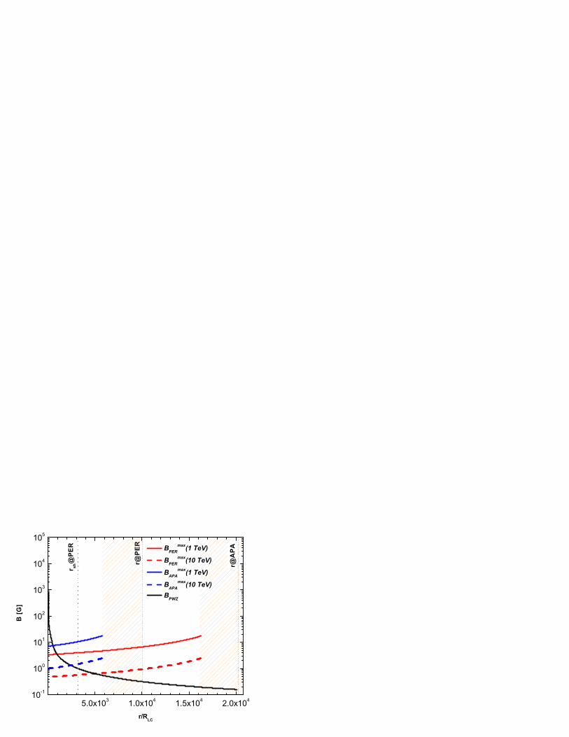
5.0x103 1.0x104 1.5x104 2.0x10410-1

100

101

102

103

104

105

r sh@

PE

R BPERmax(1 TeV)

BPERmax(10 TeV)

BAPAmax(1 TeV)

BAPAmax(10 TeV)

BPWZ

r@A

PA

B [G

]

r/RLC

r@P

ER

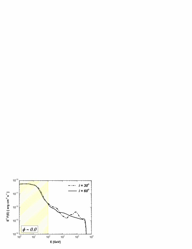
100 101 102 103 104 10510-14

10-13

10-12

10-11

10-10

i = 30o

i = 60o

E2 F(E

) [ e

rg c

m-2 s

-1 ]

E [GeV]