Publication No. 13 Trophic State of Lakes in North Central ...

"I ~ ....

Publication No. 13

Trophic State of Lakes in North Central Florida

By

Patrick L. Brezonik and Earl E. Shannon

Department of Environmental Engineering Sciences University of Florida

Gainesville

TROPHIC STATE OF LAKES IN NORTH CENTRAL FLORLDA_

by

PATRICK L. BREZONIK

and

EARL E. SHANNON

PUBLICATION NO. 13

FLORIDA WATER RESOURCES RESEARCH CENTER

RESEARCH PROJECT TECHNICAL COMPLETION REPORT

OWRR Project Number B-004-FLA

Matching Grant Agreement Numbers

14-31-0001-3068 (1970) 14-31-0001-3068 (1971)

Report Submitted: August 3, 1971

The work upon which this report is based was supported in part by funds provided by the United States Department of the

Interior, Office of Water Resources Research as Authorized under the Water Resources

Research Act of 1964.

',"

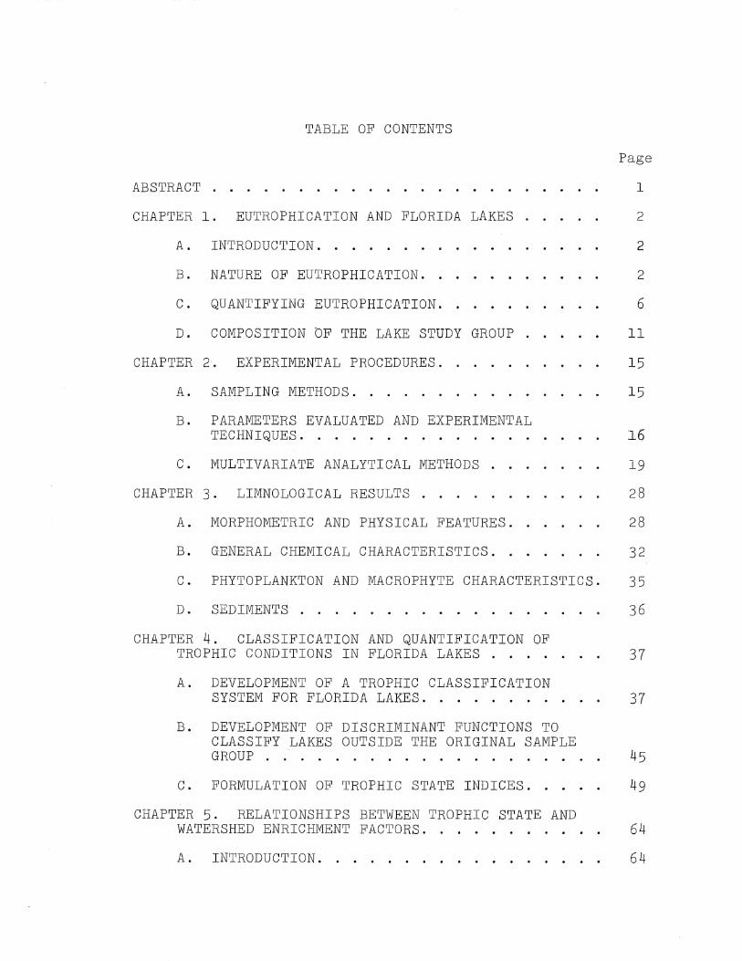
TABLE OF CONTENTS

ABSTRACT .

CHAPTER 1. EUTROPHICATION AND FLORIDA LAKES .

A. INTRODUCTION .....

B. NATURE OF EUTROPHICATION.

C. QUANTIFYING EUTROPHICATION ..

D. COMPOSITION OF THE LAKE STUDY GROUP . . . CHAPTER 2. EXPERIMENTAL PROCEDURES.

A. SAMPLING METHODS ..... .

B. PARAMETERS EVALUATED AND EXPERIMENTAL

Page

1

2

2

2

6

11

15

15

TECHNIQUES. . . . . . . . . .. ..... 16

C. MULTIVARIATE ANALYTICAL METHODS .

CHAPTER 3. LIMNOLOGICAL RESULTS .

A. MORPHOMETRIC AND PHYSICAL FEATURES.

19

28

28

B. GENERAL CHEMICAL CHARACTERISTICS. . . 32

C. PHYTOPLANKTON AND MACROPHYTE CHARACTERISTICS. 35

D. SEDIMENTS ..

CHAPTER 4. CLASSIFICATION AND QUANTIFICATION OF TROPHIC CONDITIONS IN FLORIDA LAKES . . . .

A. DEVELOPMENT OF A TROPHIC CLASSIFICATION SYSTEM FOR FLORIDA LAKES ....... .

B. DEVELOPMENT OF DISCRIMINANT FUNCTIONS TO CLASSIFY LAKES OUTSIDE THE ORIGINAL SAMPLE

36

37

37

GROUP . . . . . . . . . . . . . . . . 45

C. FORMULATION OF TROPHIC STATE INDICES. . . .. 49

CHAPTER 5. RELATIONSHIPS BETWEEN TROPHIC STATE AND WATERSHED ENRICHMENT FACTORS. . . . . . 64

A. INTRODUCTION. . . . . . . . . . . . . . . .. 64

Page

B. NITROGEN AND PHOSPHORUS BUDGETS . . . . 65

C. RELATIVE IMPORTANCE OF VARIOUS NUTRIENT SOURCES . . . . . . . . . . . . . . . . 72

D. STATISTICAL ANALYSIS OF TSI VB. NITROGEN AND PHOSPHORUS LOADING RATES. . . . . . . 74

E. CRITICAL NUTRIENT LOADING RATES: APPLICATION TO LAKE MANAGEMENT .. 76

F. EFFECT OF DEPTH ON LAKE CAPACITY TO ASSIMILATE NUTRIENTS. . 80

G. SOURCES OF UNCERTAINTY. 84

H. RELATIONSHIPS BETWEEN TROPHIC STATE AND GENERAL WATERSHED CONDITIONS. . . . 84

I. RELATIONSHIP BETWEEN TSI AND TOTAL WATERSHED AREA. . . . . . 89

CHAPTER 6. CONCLUSIONS.

APPENDIX .

ACKNOWLEDGEMENTS

BIBLIOGRAPHY .

ADDENDUM . .

89

92

95

96

101

ABSTRACT

TROPHIC STATES OF LAKES IN NORTH CENTRAL FLORIDA

General limnological and trophic conditions of 55 lakes and ponds in north and central Florida were established over an extensive one year sampling period. Florida lakes are typically shallow and in a sandy terrain. Most of the lakes have soft water, and high organic color is a common but vari­able property. Trophic conditions range from ultraoligotrophy in the sand-hill lakes of the Trail Ridge region to hyper­eutrophy in some large drainage lakes in Alachua County and in the Oklawaha River Basin.

Trophic data were analyzed by multivariate techniques, and logical trophic groups derived by cluster analysis. A quantitative index of trophic state (TSI) was derived using 7 trophic indicators, and the TSI values were used to estab­lish quantitative relationships between lake trophic condi­tions and watershed characteristics. Nitrogen and phosphorus budgets were calculated for the lakes based on land use and population patterns in the watersheds, and critical loading rates were estimated from the budgets and the trophic condi­tions.

Brezonik, P.L. and Shannon, E.E. TROPHIC STATES OF LAKES IN NORTH AND CENTRAL FLORIDA Completion Report to the Office of Water Resources Research, Department of Interior, July, 1971, Washington, D.C. 20240 KEYWORDS: eutrophication/ nitrogen/ phosphorus! ~UltiVariate analysis/ water quality/ lakes/ nutrients/ Flo~idal models.

I

CHAPTER 1. EUTROPHICATION AND FLORIDA LAKES

A. INTRODUCTION

Although Florida has more than 7500 lakes (Florida Board of Conservation 1969), limnological investigations of these lakes have been few and limited to special interests. Most detailed studies have been centered on a few unusual or recre­ationally important lakes; for example, Mud Lake (Marion County) (Bradley and Beard, 1969; Iovino and Bradley, 1969), Lake Mize (Alachua County) (Brezonik and Harper, 1969; Keirn and Brezonik, in press) and Lake Apopka (Orange and Lake Coun­ties) (for a review, see Sheffield and Kuhrt, 1970). Yount (1963) has reviewed most pre-1960 limnological studies in discussing some general features of Florida lakes.

However, as a group Florida lakes are almost limnologi­cally unknown. Threatening of the recreational assets of Florida lakes by cultural encroachment and consequent nutrient enrichment has stimulated studies on these lakes. In 1968 the University of Florida Department of Environmental Engi­neering initiated an extensive survey of the physical, chemi­cal and biological characteristics of 55 lakes in north and central Florida. The investigation had five main objectives: i) to determine the basic limnological features of lakes in the region; ii) to assess the present water quality Ctroph~c state) characteristics of the lakes and provide baseline data for future studies; iii) to evaluate the applicability of the common trophic state indicators to sub-tropical lakes; iv) to provide necessary data to develop an index of trophic state for sub-tropical lakes; v) to study the relationships between lake trophic state and lake watershed conditions influencing trophic state.

B. NATURE OF EUTROPHICATION

Cultural lake eutrophication is an undesirable consequence of the interaction between man and his environment. Many of his agricultural, industrial, domestic and recreational activ­ities are introducing excess nutrients into surface waters, causing significant water quality deterioration. Since fresh water is vital to the total well-being of the environment, man has an obligation to protect h~s valuable lacustrine re­sources. However, progress in solving the problem has been retarded by the inherent complexity of the eutroph~cation pro­cess, and considerable vagueness still exists concerning the definition of cause and effect relationsh~ps in the overall process (Brezonik, 1969; Putnam, 1969).

2

It is generally agreed that eutrophication involves nutri­ent enrichment, and a lake in time responds to this enrichment. This response is reflected in a lake's trophic state (eutrophic condition). However, few efforts have been devoted to quan­tifying the relationship of eutrophication to trophic state.

One of the problems in the study of lake eutrophication is of a semantical nature; i.e. distinguishing between and defining the causes, symptoms and effects. Considerable liter­ature has been devoted to discussing these concepts. The mean­ing of the term "eutrophication" has been stated by Hasler (1947) as being, simply, the enrichment of water, be it in­tentional (cultural) or unintentional (natural). This nutrient enrichment is generally considered as the causal mechanism in the overall eutrophication process. As originally suggested by Naumann (1919) perhaps primary consideration should be given to nitrogen and phosphorus nutrients. The concept of trophic state (degree of eutrophy) is difficult to define. Eutrophic conditions are the consequences or effects of a lake's nutrient enrichment, but there is no way to express this state in sim­ple, quantitative terms. Much of the conceptual difficulty with the idea of trophic state could have been avoided long ago had limnologis.ts defined trophic state in precise terms as a measure either of a lake's productivity or of a lake's nutrient status. Instead the term has been used to refer to both characteristics. While correlated to a degree, produc­tivity and nutrient status are both also functions of other independent phenomena (e.g. hydrology and climate).

Adequate description of a lake's trophic state requires consideration of several different physical, biological and chemical characteristics. For this reason the coricept of trophic state is not only mUlti-dimensional but hybrid, as suggested by Margalef (1958). The trophic state of a lake cannot be measured directly because of its mUlti-dimensional nature. However, it is evidenced by various symptoms called trophic state indicators. A list of common indicators of trophic state is in Table 1. Reviews of trophic state indi­cators have been compiled by Fruhetal. (1966), Vollenweider (19682, Hooper (1969) and Stewart andRohlich (1967).

There has been no scarcity of lake classification schemes and a review of such is beyond the scope of this report. Birge and Juday (1927) made a fundamental distinction concern­ing the origin of dissolved organic matter in lakes. Lakes dependent on internal sources ~rimary production) were auto­trophic and lakes dependent on external sources were allo­trophic. Later Aberg and Rohde (1942) related the classical trophic types of lakes in a two-dimensional concept of auto­trophy and allotrophy. This general approach was used for the classification purposes in this study and the idealized two-dimensional relationship is shown in Figure 1. Organic color measurements were assumed to be indicative of external-

3

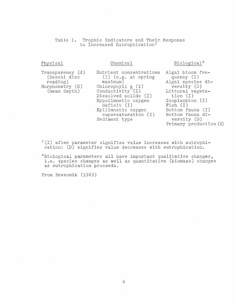
Table 1. Trophic Indicators and Their Response to Increased Eutrophication l

Physical

Transparency (d) (Secchi disc reading)

Morphometry CD} (mean depth)

Chemical

Nutrient concentrations (I) (e.g. at spring maximum)

Chlorophyll a CI) Conductivity-CI) Dissolved solids Cll Hypolimnetic oxygen

deficit CI 2 Epilimnetic oxygen

supersaturation (I) Sediment type

Biologica1 2

Algal bloom fre­quency (I)

Algal species di­versity (D)

Littoral vegeta-tion (I)

Zooplankton (I) Fish (I) Bottom fauna (12 Bottom fauna di-

versity (D) Primary production (I)

1(12 after parameter signifies value increases with eutrophi­cation: (D) signifies value decreases with eutrophication.

2Biological parameters all have important qualitative changes, i.e. species changes as well as quantitative (biomass) changes as eutrophication proceeds.

From Brezonik (1969)

4

0:::

9 o (.) t

c U lLI

0::: Z 0 « -I (!) 0 0::: (.)

C/)

lLI ~ « -I

o ~ ~ °T lLI 0::: ::) C/)

« lLI :::E

~ ~ ~ La.! <:)

(.) -::t: Q. 0 0::: t-0 (!) --I 0

(.)

::t: Q. 0 0::: t-0 (!) --I 0

2 (.) ::t:

Q. ::t: (.) 0 Q.

0::: 0 l: t-0::: Q. ;:) t- o lLI 0 0::: 0::: C/) t- lLI lLI ;:) Q. 2 lLI >-::t:

(.) (.) 1111111 -- (.) ::t: ::t: Q. Q. ::t: 0 0 Q. 0::: 0::: 0 t-t- o::: ;:)

L 0 ,t- lLI C/) ;:) 0::: lLI

! lLI 2

MEASURE OF TROPHIC STATE

,.. " 0,' f" c:. "'f

Figure 1. TWO-Dimensional Concept of Lake Classification Based on Autotrophy (Internal Organic Production) and Allotrophy (External Organic Input)

5

source dissolved organic matter and thus denote lake allo­trophy. As originally suggested by Hansen (1962), colored and relatively clear lakes were recognized as two fundamentally different lake types. Within each of these types, oligo-, meso-, and eutrophic state subdivisions could occur as deter­mined by some measure of lake trophic state.

C. QUANTIFYING EUTROPHICATION

From a qualitative viewpoint the phenomenon of eutrophi­cation is now fairly well understood. However, for lake management eutrophication control qualitative facts are seldom sufficient. For example, it is generally recognized that increased nitrogen and phosphorus input to a lake will gener­ate increased plant production. But information concerning the precise nutrient loading rates that stimulate excessive production and scum-forming algal blooms is sorely lacking. Lakes are highly complex ecosystems, and the factors control­ling nutrient cycling and primary and secondary production in them are at best poorly understood. Furthermore, lakes cannot be regarded as isolated entities, but the interactions of the entire watershed with the lake itself must be taken into account (Hutchinson, 1969). The general significancem various land use patterns and cultural activities as nutrient sources are largely unknown, and in particular the total nutrient loading rates for specific lakes of varying trophic conditions are .known with accuracy for only a few cases.

The complexities of the eutrophication problem suggest the utility of systems analysis techniques and of mathematical modeling in properly defining the problem and simplifying it to the extent that solutions become feasible. The theory and nature of mathematical ecosystem models have been discussed in several recent papers and books (Moreau, 1969; Patten, 1969; Watt, 1968; and Thomann, 1971). In general mathematical models can be divided into two types. Analytical or mechanis­tic models consist of a series of equations (algebraic, or in ecosystem models more commonly, differential) which attempt to explain the fundamental (functional) relationships between certain parameters. For example, differential equation models of primary production have been developed (Patten, 1968) in terms of the basic relationships between photosynthesis and light intensity, nutrient levels, etc. Empirical or statis­tical models are composed of approximate parameter relation­ships which are derived by such techniques as regression, multi-variate, or time series analyses. Such models are attractive in management of complex systems where cause-: effect relationships are unknown. Empirical models can be use­ful in predicting system response to changes in environmental conditions, and they can give clues to the significance of the relationships (i. e. the dependency) between variables. However their lack of foundation in causal relationships renders

6

empirically developed models susceptible to misuse and over­extension (to conditions in which they may not be applicable).

The inherent complexities of nutrient enrichment and its attendant effects on lakes imply that a purely deterministic approach is beyond our present capabilities. While functional relationships are known for various lacustrine phenomenon, and relatively sophisticated analytical (i.e. differential equations) models have recently been formulated for even as complicated a process as planktonic production (Chen, 1970; DiToro et al., 1970; Patten, 1968), the much larger scope of the eutrophication problem precludes such approaches at the present time, especially in the general case. For particularly unique and valuable resources like Lake Tahoe or the St. Lawrence Great Lakes, the manpower and time expenditures re­quired for development of such models may be justified. This seems. not to be the case for the thousands of smaller and locally important recreational lakes in the U. S. and else­where. A simpler, less costly approach is required for these lakes.

Where large numbers of lakes must be managed an attractive possibility is th.e development of empirical models based on data from a representative sample of the lakes in question. Such management tools as critical nutrient loading rates can be developed by empirical manipulation of basic limnological and watershed information. While empirical models are perhaps not the ultimate answer to eutrophication problems, they can provide direction for further studies and models while simul­taneously providing interim predictive capacities required for proper water quality management.

Eutrophication is a multivariable problem and thus lends itself to analysis by multivariate statistical techniques. Beneficial applications of empirical multivariate models can be anticipated in three major areas of eutrophication research, and Table 2 summarizes potential applications in each area. Because of the broad, multi-dimensional concept of trophic state, multivariate techniques seem especially appropriate for the long standing problem of rational lake classification. Trophic classification systems can be useful in several ways: a) for identification Ia certain class (name) calls to mind certaj..n disti.nctive characteristics]; b} for organization of our knowledge concerning the obj ects (lakes 1 being classified; cl as the basi.s for development of theories regarding causes of phenomena associated with a particular class (e. g. what do lakes. in a class have in common that might induce their similar behavior Land d 1 for management purposes (different classes. of lakes may have different IIbest uses" and require different land use and water management controls).

ThB ill-defined concept of trophic state is in reference to both. a lake'·s general nutrient status and its productivity,

7

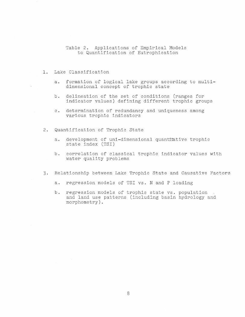
Table 2. Applications of Empirical Models to Quantification of Eutrophication

1. Lake Classification

a. formation of logical lake groups according to multi-dimensional concept of trophic state .

b. delineation of the set of conditions (ranges for indicator values} defining different trophic groups

c. determination of redundancy and uniqueness among various trophic indicators

2. Quantification of Trophic State

a. development of uni-dimensional quantitative trophic state index (TSI2

b. correlation of classical trophic indicator values with water quality problems

3. Relationship between Lake Trophic State and Causative Factors

a. regression models of TSI vs. Nand P loading

b. regression models of trophic state vs. population and land use patterns (including basin hydrology and morphometry) .

8

which are not always correlated. The circumstances defining a given state (e.g. eutrophy) are not at all agreed upon by limnologists. No single measure of nutrient status or pro­ductivity is satisfactory or sufficient, and the results one obtains depend on which indicators are used. Thus the lim­nologist is left with the difficult task of subjectively deciding which indicators to use and which to disregard or weigh less heavily.

Reviews on trophic state indicators have been published elsewhere (Fruh et al., 1966; Vollenweider, 1968; Hooper, 1969). Selection-or-appropriate indicators is a difficult task, but consideration of the following criteria should facilitate the decision: a) an indicator should be quanti­fiable in order to permit numerical differentiation between lakes of varying trophic states, b) each indicator should be unique (i.e. not measure the same lake characteristic as another indicator), c) an indicator should have fundamental significance in terms of the concept of trophic state (as a general measure of a lake's nutrient and productivity status), and d) an indicator should be sensitive to levels of enrich­ment and relatively simple to measure. The uniqueness of trophic indicators can be studied by several multivariate statistical methods, including factor analysis (Shannon, 1969; Lee, 1971), principal component analysis (Lee, 1971) and cluster analysis (Goldman et al., 1968; Shannon, 1969). While different geographical regionS-may require somewhat different treatment, indicators should be widespread properties of aquatic environments in order to insure general interpreta­bility of the generated classes.

The subjectivity involved in forming logical trophic classes from conflicting indicator data can be minimized with certain multivariate techniques such as cluster analysis (Sokal and Sneath, 1963). Another important classification problem is the assignment of lakes outside the original sam­ple group into appropriate pre-established classes. The method of discriminant function analysis (Shannon, 1970; Lee, 1971) is useful in this regard.

In order to predict and evaluate the consequences of watershed management practices on trophic conditions in a lake, trophic state must somehow be quantified. As discussed above, this has heretofore been obviated by the multi­dimensional nature of the trophic concept. Development of a single numerical index of trophic state from a combination of several important indicators avoids the misleading and fragmentary situation arising when only one indicator is used and the confusion which results when several indicators are considered individually. An index also allows quantitative interpretation of trophic state not otherwise feasible. At least five applications and advantages derive from develop­ment of a trophic state index: 1) a numerical index would be

9

valuable in conveying lake quality information to the non­and semi-technical public; 2) an index would be useful in comparing overall trophic conditions between lakes; 3) in the dynamic process of lake succession and trophic change, an index would provide a means to evaluate the direction and rate of changes; 4) an index would facilitate development of empirical models of trophic conditions as a function of watershed "enrichment" factors for predictive and manage­ment purposes; 5) a properly developed index would be highly relevant to (i.e. identified with) water quality from a human (or user's) perspective. In contrast to the last point, many indicators (especially qualitative species composition indi­cators) are largely of academic or research interest.

On the other hand an index can be criticized as having no real physical meaning and as improperly combining diverse parameters (the "can't add apples and oranges" syndrome). However, the first argument is irrelevant; a relative index of trophic state, in so far as it reflects the trophic concept, has value regardless of its interpretability in actual physical terms. With proper selection of indicators and rational development of an index, the second criticism can be largely overcome, but it must be realized that no index can or should be expected to supply the detailed information available in the individual parameters.

Proper selection of indicators is a vital consideration in developing an index of trophic state. Criteria discussed previously with regard to trophic classification apply equally here; that the individual indicators be quantifiable is of course essential. The number of indicators desirable in an index bears some discussion. Generally an index should include sufficient indicators to account for the essential attributes denoted by the broad trophic concept. As fewer variables are used, the index becomes more unstable, i.e. a large de­viation from "normall1 for a given indicator will tend to af­fect an index incorporating few variables more than one incor­porating many. Use of only one variable could result in very misleading rankings of lake I1trophic states." For example if plankton biomass (expressed as packed cell volume, numbers per ml, or chlorophyll a) were the sole measure, lakes with a dense and active macrophyte and periphyton population but low phytoplankton levels would be misranked as oligotrophic. Similar criticisms apply to any other single indicator, and to a lesser extent when only a few indicators are used. How­ever, redundant indicators (i.e. those that measure essentially the same phenomenon as another indicator) should be avoided to prevent biasing the index, i.e. weighing it too heavily toward that aspect or phenomenon. For example, specific con­ductance and dissolved solids should not both be used in an index since they measure nearly the same thing.

The multivariate statistical method of principal component

10

analysis represents one means of deriving a single numerical trophic state index from a number of indicators. Given such an index, empirical models of trophic state as simple func­tions of nutrient loading rates or other watershed enrich­ment factors can then be developed by multiple regression analysis or other appropriate means.

D. COMPOSITION OF THE LAKE STUDY GROUP

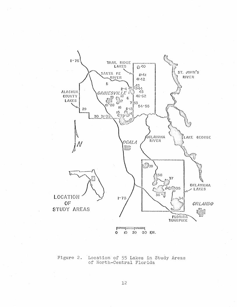
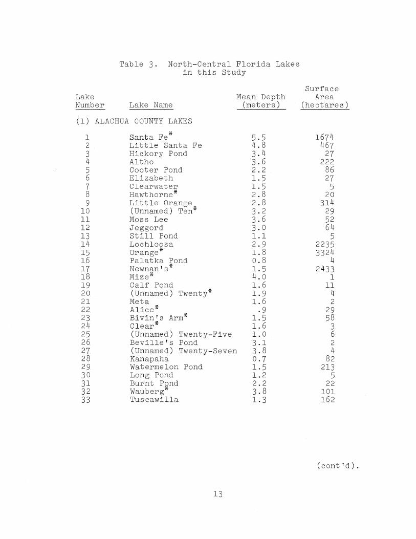
Fifty-five lakes from three different areas of north­central Florida were selected for the study (Figure 2). Table 3 lists the lakes by name and code number and gives the surface area and mean depth of each. The study originated in early 1968 with a survey of 33 lakes within Alachua County, in which Gainesville and the University of Florida are located. This group, comprising all accessible and potentially important recreational lakes in the county, exhibits considerable di­versity in trophic conditions. Most of the lakes are very shallow, and moderate to high organic color is common, re­flecting the large expanses of pine forest in the county. The small lakes typically have outlets only during periods of extended rain whereas the large lakes have permanent out­lets. General physical features of the Alachua County lakes and initial chemical and biological measurements were summar­ized by Brezonik et al. (1969); Clark et al. (1962) have described the geological formations an~general land forms which affect the lakes.

In early 1969 lakes from two important north-central Florida lake regions outside of Alachua County were included in the study. Sixteen lakes in the Trail Ridge region of the Central Highlands (east of Alachua County) comprise one of these groups. This scrub-oak, sand-hill region is richly endowed with lakes, most of which are clear and lie within small drainage basins. Lakes in the Trail Ridge area are naturally low in nutrients and subject to only light cultural influence. While still shallow and typically unstratified, these lakes are generally deeper than lakes in the other two groups. Anderson-Cue and McCloud Lakes are being used as model lakes in a separate eutrophication study (Brezonik and Putnam, 1968; Brezonik et al., 1969). Artificial nut­rient enrichment of Anderson-Cue Lake has been proceeding since 1967, and the relevant chemical, biological and physi­cal characteristics of both lakes have been monitored since 1966.

The final group consists of six lakes in the upper Oklawaha River Basin northwest of Orlando, Florida. Five of the Oklawaha lakes are joined by watercourses with the general pattern of flow being from Lake Apopka through Lake Dora to Lake Eustis which drains into Lake Griffin. The effluent

11

LOCATION OF

STUDY AREAS

TRAIL RIDGE r--......,.-~'-=j LAKES

SANTA FE '---, RIVEH

~41

.42

F I -:~ o 10 2.0 -:;0 KM.

Figure 2. Location of 55 Lakes in Study Areas of North-Central Florida

12

GEORGE

Lake Number

Table 3. North-Central Florida Lakes in this Study

Lake Name Mean Depth

(meters)

(1) ALACHUA COUNTY LAKES

1 2 3 4 5 6 7 8 9

10 11 12 13 14 15 16 17 18 19 20 21 22 23. 24 25 26 27 28 29 30 31 32 33

* Santa Fe Little Santa Fe Hickory Pond Altho Cooter Pond Elizabeth Clearwater Hawthorne* Little Orange (Unnamed) Ten* Moss Lee Jeggord Still Pond Lochloosa Orange* Palatka Pond Newnan's* Mize* Calf Pond (Unnamed) Twenty* Meta Alice* Bivinls Arm* Clear* (Unnamed) Twenty-Five Beville's Pond (Unnamed) Twenty-Seven Kanapaha Watermelon Pond Long Pond Burnt Pond Wauberg* Tuscawilla

13

5.5 4.8 3.4 3.6 2.2 1.5 1.5 2.8 2.8 3.2 3.6 3.0 1.1 2.9 1.8 0.8 1.5 4.0 1.6 1.9 1.6

. 9 1.5 1.6 1.0 3.1 3.8 0.7 1.5 1.2 2.2 3.8 1.3

Surface Area

(hectares)

1674 467

27 222

86 27

5 20

314 29 52 64

5 2235 3324

4 2433

1 11

4 2

29 58

3 6 2 4

82 213

5 22

101 162

(cont'd).

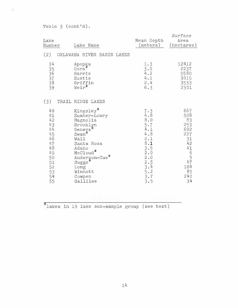
Table 3 (cont'd).

Surface Lake Mean Depth Area Number Lake Name (me't.'ers) (hectares)

(2 ) OKLAWAHA RIVER BASIN LAKES

34 Apopka 1.3 12412 35 Dora* 3.0 2237 36 Harris 4.2 5580 37 Eustis 4.1 3015 38 Griffin 2.4 3533 39 Weir* 6.3 2301

(3) TRAIL RIDGE LAKES

40 Kingsley* 7.3 667 41 Sumter-Lowry 4.8 508 42 Magnolia 8.0 83 43 Brookl¥n 5.7 253 44 Geneva 4.1 692 45 Swan* 4.8 227 46 Wall 2.1 31 47 Santa Rosa 8.1 42 48 Adaho 3.5 41 49 McCloud* 2.0 6 50 Anderson-Cue* 2.0 5 51 Suggs * 2.5 47 52 Long 3.4 104 53 Winnott 5.2 85 54 Cowpen 3.7 240 55 Gallilee 3.5 34

* lakes in 19 lake sub-sample group (see text)

14

from Lake Griffin forms the Oklawaha River. Lake Harris also flows into Lake Eustis. Lake Weir, although in the Oklawaha River basin, does not discharge directly into the Oklawaha River. All six lakes in this group are important recreational lakes; in the past Lake Apopka was among the best known bass fishing lakes in the country. However, considerable cultural eutrophication (and consequently water quality impairment) has occurred in the five connected lakes within recent years. The watersheds of these lakes are utilized primarily for cit­rus farming, but a large area on the north shore of Lake Apopka is devoted to vegetable farming of muck soils (recovered marshland) .

CHAPTER 2. EXPERIMENTAL PROCEDURES

A. SAMPLING METHODS

The sampling schedule used in this study was designed to provide information on the average chemical, biological and physical characteristics of the 55 lakes over a one-year period. Systematic sampling of all lakes began in June, 1969, and all 55 lakes were sampled at four-month intervals up to June, 1970. In order to obtain greater detail on seasonal trends, a 19 lake sub-group from the 55 lakes was sampled at two-month intervals during this same time period. The 19 lakes (denoted by asterisks in Table 3) were selected on the basis of being representative of the different trophic types present in the 55 lake group. It was felt that this sub­group adequately reflected seasonal trends in lake character­istics without sampling all 55 lakes on a closer time interval.

Water samples taken from the lakes for chemical and bio­logical analysis were composites. The small lakes (surface area less than 10 hectares and maximum depth less than 4 meters) were sampled at two stations over depth (surface, middle, and bottom). These samples were combined into a composite sample from which aliquots were taken for major chemical characteristics~ for nutrient analyses (preserved with mercuric chloride), for primary production and chloro­phyll analysis, and for plankton identification and counts (preserved with formalin). For the larger lakes that were relatively shallow (maximum depth <10 meters) the procedure of sample collection was the same except that three stations were sampled and composited. For the few deep lakes in which stable stratification was evident, samples were composited from the euphotic zone (estimated as twice the Secchi disc reading) for biological analyses and from the entire water column for major chemical analyses, and nutrient analyses were done in profile on uncomposited samples taken at regular depth intervals. Sediment samples were taken by Ekman dredge from

15

the deepest region of the lake.

B. PARAMETERS EVALUATED AND EXPERIMENTAL TECHNIQUES

A total of 6 morphometric, 2 physical, 29 chemical and 6 biological parameters were evaluated for each lake during the project. In addition 11 parameters were evaluated for the lake sediments. Six land use and three population char­acteristics were evaluated for each lake drainage basin. Table 4 lists all the parameters measured at various times during the project. The physical parameters were measured in situ; biological and chemical parameters were determined on the composite samples using standard limnological procedures (see Brezonik et ale 1969 for details). Primary production was measured inthe laboratory with a "light box" procedure rather than in situ in order to standardize light and temper­ature conditions and offer a more uniform basis of comparison among the lakes.

Bathymetric maps were available for about 20 of the lakes (Kenner, 1964); the remainder were sounded and mapped with a Heath Co. depth sounder as part of the project. Basic morphometric parameters such as volume, mean depth, volume development index and shoreline development index were computed from the bathymetric maps by methods described in Hutchinson (1957).

Land use patterns in the lake watersheds were determined by aerial photograph and topographic map interpretation. Lake watershed areas were outlined and planimetered from United States OeQlogical Survey (Scale: 1/24,000) topographic maps. Recent (1965-1968) aerial photographs (Scale: 1" = 1667') were obtained for (each watershed from the Florida Soil Conservation Service Office. Using photogrammetric techniques, areas of various types of land use patterns were delineated and measured. Lake surface areas were also d~termined from the aerial photographs.

The population in each watershed was characterized in four categories. Residences on a shoreline were classified as immediate cultural units (ICU). Other residences within the lake watershed were categorized as remote cultural units (RCU). The lCU's and RCU's were evaluated from aerial photo­graphs. Residences served by sanitary sewer facilities were

. not included in the two previous categories. Recent popula­tion figures were obtained for all of the municipalities served by sewage treatment plants within each of the lake watersheds. These figures were converted to equivalent cul­tural units by dividing by a factor of 2.5, which represents the average population of a single rural family residence in

16

Table 4. Lake and Basin Parameters Evaluated for this Study

Land Use

Fertilized cropland Pastured area Forested area Urban area

Watershed

Unproductive cleared area Total watershed area

Bathymetric map Mean depth

Morphorrietric

Shoreline development

Temperature profile Turbidity

Acidity Alkalinity Ammonia Calcium Chloride C.O,D. Color Copper Dissolved oxygen Fluoride Iron Magnesium Manganese Mercury Nitrate Nitrite

Chlorophyll a Total carotenoids

Physical

Chemical

Biological

Algal identification and counts

17

Population Characteristics

Cultural units l on lake shore

Cultural units in rest of basin

Sewage treatment plant Cultural units

Lake surface area Maximum depth Volume development

Secchi disc transparency

Organic nitrogen Ortho phosphate pH Potassium Silica Sodium Specific conductance Strontium Sulfate Suspended solids Total phosphate Total solids Zinc

Primary production Algal species diversity

(cont 'd).

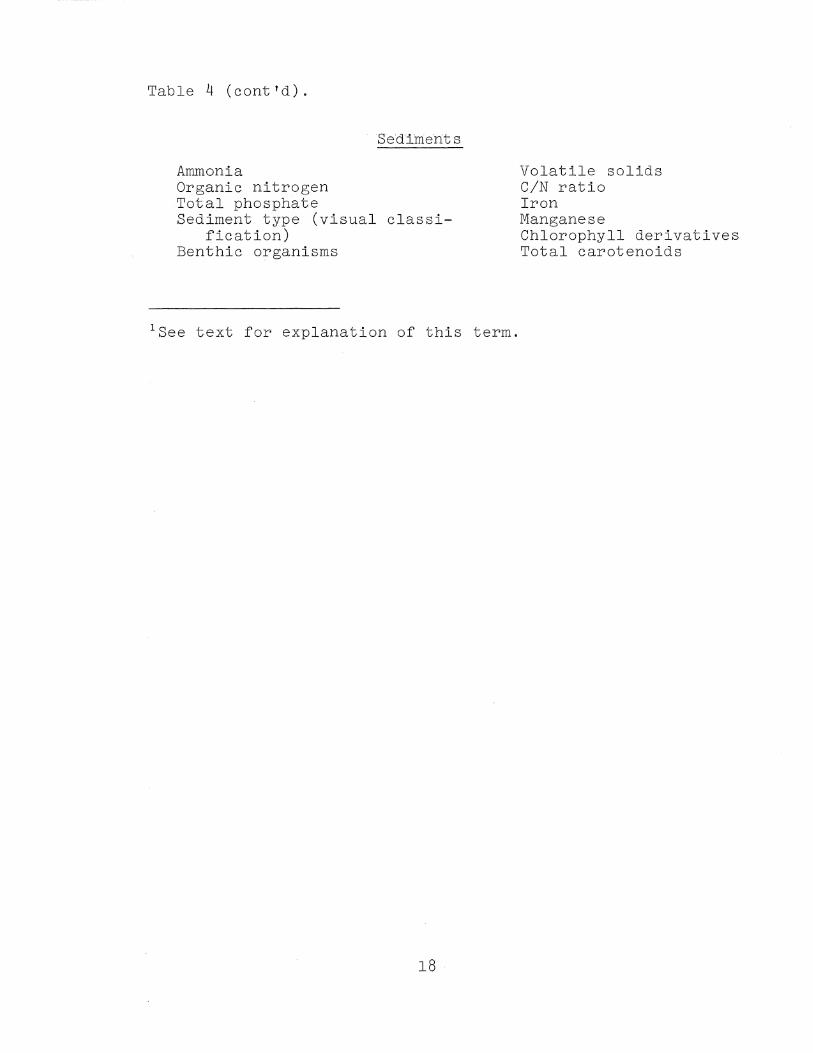
Table 4 (cont'd).

Ammonia Organic nitrogen Total phosphate

Sediments

Sediment type (visual classi­fication)

Benthic organisms

ISee text for explanation of this term.

18

Volatile solids CIN ratio Iron Manganese Chlorophyll derivatives Total carotenoids

the State of Florida (U.S. Bureau of Census, 1961). Cultural units of municipalities discharging sewage effluent directly into a lake were classified as immediate sewage treatment plant cultural units (ISPU). Cultural units of municipalities discharging sewage effluent somewhere else in the watershed were classified as remote sewage treatment plant cultural units (RSPU). The total cultural units (TeU) in the water­shed was obtained by summing the cultural units in each of the four categories. Estimates of total watershed population couid in turn be obtained by multiplying the TCU by 2.5.

C. MULTIVARIATE ANALYTICAL METHODS

Relationships among the several trophic indicators and watershed eutrophication factors were investigated by a vari­ety of multivariate statistical techniques .. This term is used to describe statistical methods concerned with analyzing data collected on several dimensions (variables) on a set of objects or individuals. Some dependency is assumed among the variables so that they are considered as a system. Because of their multi~dimensional nature, these techniques are most conveniently described using vector and matrix notation. Theoretical aspects of these techniques are discussed by Morrison (1967), Sokal and Sneath (1963), and Lee (1971). The applications and computational aspects of the techniques used in this$udy are described below; see Appendix for a description of the terminology used for vectors, matrices, and multivariate statistics.

1.Clu·ster Analysis is concerned with the problem of classifying N objects (e.g. lakes) into groups based on p variables measured on each obj ect, when the number .of groups that best fit the data is not predetermined. Express~d geo­metrically, the method attempts to distinguish logical group­ings of obJects in the p-dimensional hyperspace described by the p data attributes of the objects. Figure 3 illustrates a simple bivariate cluster problem involving groups formed by hypothetical data for color and productivity in lakes (cf. Figure 1). Cluster analysis of objects is referred to as a Q~type analysis; a second type which clusters the variables measured on a set of objects is referred to as R-type cluster analysis. Cluster analysis was used in this study to find natural groupings of lakes, i.e. those with similar trophic st~tes or chemical characteristics, as measured by several li:mnological parameters (indicators) considered simultaneously and weighed equally. Cluster analysis progressively combines a set of objects into a smaller and smaller number of groups according to the degree of similarity among the objects; ob­jects (lakes) wit~the greatest similarity are joined first.

The starting point for any cluster analysis is the N x

19

H CJ ,-I o o CJ

°2 CD bfl H o

.,;-----------........ , / ,

/ B \ I \

I \ I I \ I \ / , /' ,~ /

"'"----------

-------------/' A "-

/' "-/ . \

/ . .. \ I. • \ \ I II· J

\ / \ • • 'j , / " ./ ......... _-----_._-----

Primary Production

Figure.3. Hypothetical bivariate plot showing clusters formed by data for organic color and primary production in lakes. Solid circles represent clusters formed around 4 groups with good i~-group. similari ty: 1. low color, low production; II. low color, high production; III. high color, low production; IV. high color, high production. Dashed lines represent less similar clusters of (A) low color and (B) high color lakes formed later (at higher objective function values).

20

p raw data matrix X. If it is desired to group objects, the matrix X is normally transformed to the matrix of standardized variates Z since the variables may have been measured in quite different sized units. The standardized data are used to calculate product-moment correlation coefficients for all possible pairs of objects. The resultant N x N symmetric matrix is called the similarity matrix Q, with general element qij being the correlation between objects i and j considering the p variables measured on each object. The Q matrix repre­sents the starting point of the cluster analysis.

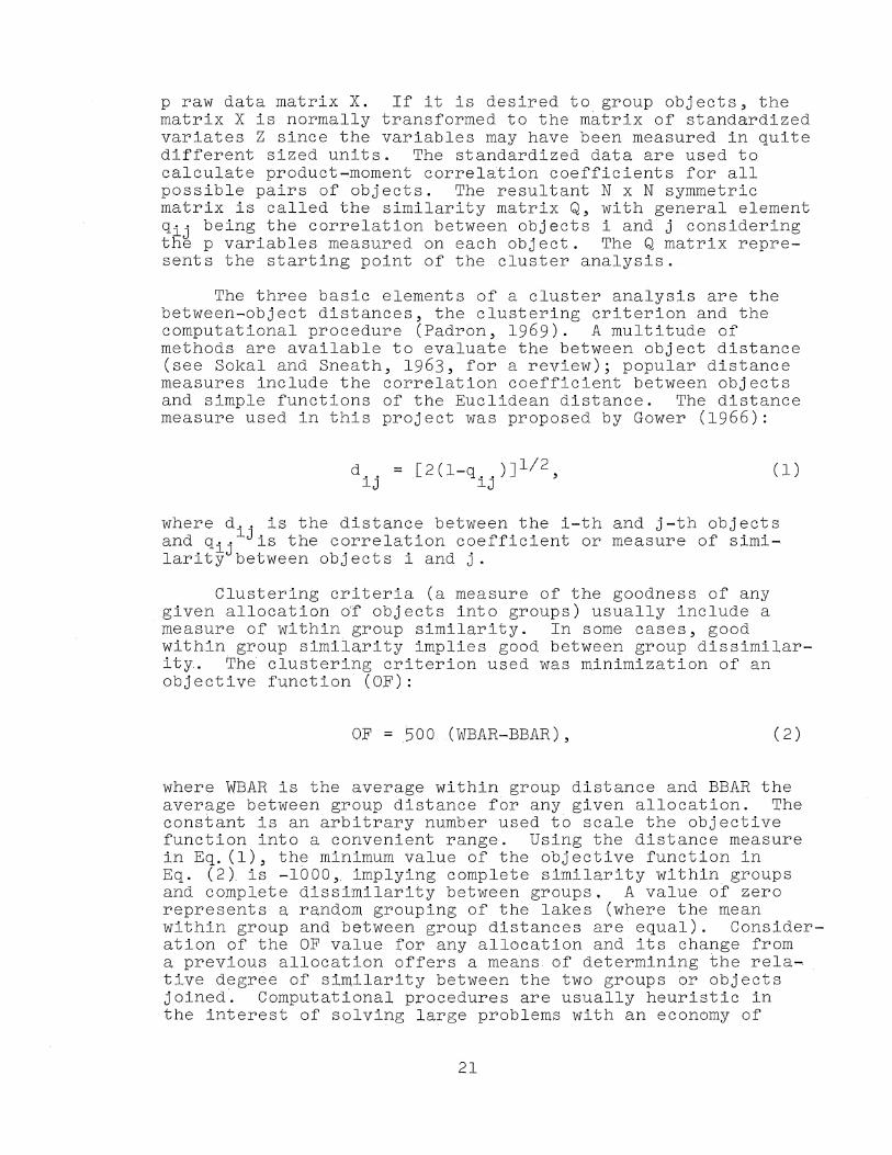
The three basic elements of a cluster analysis are the between-object distances, the clustering criterion and the computational procedure (Padron, 1969). A multitude of methods are available to evaluate the between object distance (see Sokal and Sneath, 1963, for a review); popular distance measures include the correlation coefficient between objects and simple functions of the Euclidean distance. The distance measure used in this project was proposed by Gower (1966):

d .. = [2(1-q .. )J l / 2 , (1) lJ lJ

where d .. is the distance between the i-th and j-th objects and qijlJiS the correlation coefficient or measure of simi­larity between objects i and j.

Clustering criteria (a measure of the goodness of any given allocation of objects into groups) usually include a measure of within group similarity. In some cases, good with~n group similarity implies good between group dissimilar­ity. The clustering criterion used was minimization of an objective function (OF):

OF =500 (WBAR-BBAR), (2)

where WBAR is the average within group distance and BBAR the average between group distance for any given allocation. The constant ~s an arbitrary number used to scale the objective function into a convenient range. Using the distance measure in Eq. (1), the minimum value of the objective function in Eq. (2) is -1000, implying complete similarity within groups and complete dissimilarity between groups, A value of zero represents a random grouping of the lakes (where the mean within group and between group distances are equal). Consider­ation of the OF value for any allocation and its change from a previous allocatiDn offers a means of determining the rela­tive degree of similarity between the tWD groups or objects joined. Computational procedures are usually heuristic in the interest of solving large problems with an economy of

21

computer time. A clustering algorithm in Fortran IV developed by Padron (1969) was used infue cluster analyses.

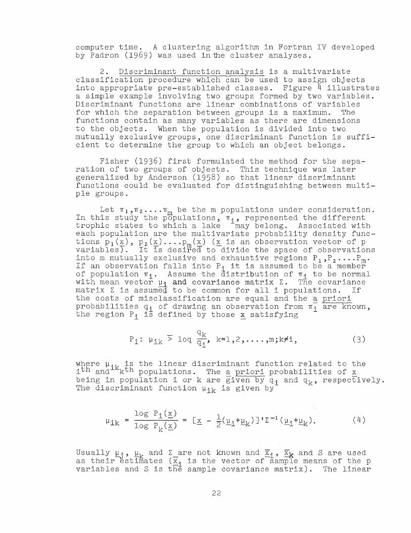
2. Discriminant function analysis is a multivariate classification procedure which can be used to assign objects into appropriate pre-established classes. Figure 4 illustrates a simple example involving two groups formed by two variables. Discriminant functions are linear combinations of variables for which the separation between groups is a maximum. The functions contain as many variables as there are dimensions to the objects. When the population is divided into two mutually exclusive groups, one discriminant function is suffi­cient to determine the group to which an object belongs.

Fisher (1936) first formulated the method for the sepa­ration of two groups of objects. This technique was later generalized by Anderson (1958) so that linear discriminant functions could be evaluated for distinguishing between multi­ple groups.

Let TIl,TI2'" • TIm be the m populations under consideration. In this study the populations, TIi' represented the different trophic states to which a lake may belong. Associated with each population are the multivariate probability density func­tions Pl(x), P2(~)'" .Pm(~) (~is an observation vector of p variables). It is desired to divide the space of observations into m mutually exclusive and exhaustive regions P1 ,P 2 ••• .Pm. If an observation falls into Pi it is assumed to be a member of population TIi' Assume the distribution of TIi to be normal with mean vecto~ ~i and covariance matrix~. The covariance matrix ~ is assumed to be common for all i populations. If the costs of misclassification are equal and the a priori probabilities qi of drawing an observation from TIl are known, the region Fi is defined by those x satisfying

where P' k is the linear discriminant function related to the ith and l kth populations. The a priori probabilities of x being in population i or kare given by qi and qk' respectively. The discriminant function Pik is given by

~ik = log Pi (~)

log Pk(x) (4 )

Usually ~j' ~k and ~ are not known and ~i' ~ and S are used as their estimates (x. is the vector of sample means of the p variables and S is th§ sample covariance matrix). The linear

22

COLORED LAKES

CLEAR LAKES

.TURBIDITY (X)

'DISCRIMINANT FUNCTION; Vxy .= aY - bX

Figure 4. Hypothe~ical Two-Dimensional Plot Showing Relationship Between Discriminant Function

and Two Clusters of Inverse Secchi Disc Transparency and Turbidity Data.

Clusters repp~sen~ the envelopes of points (not shown) for colored and .cle:ar (uncolored) iakes. Color decreas.es Secchi disc visibility;h·encecolored· lakes tend toward bigher (l!SD) values for a given turbidity .. Bell .... shaped· curves represent ideali~ed distribution on a given axis for data points within each cluster. 23

discriminant function then becomes v ik and is given by:

v l' k == [x ~. !( x. +x, ) ] IS ~l (Xl' +xk ) - 2 -l -J - -

(5 )

For sufficiently large samples vil;\: is considered to be a good estimator of 'J.lik" If the a priorl probabilities~qk and qi are equal in Eq. 3, the region Pi is defined for 'J.lik>O.

The method used to calculate the linear discriminant functions in this study was the stepwise procedure (BMD07M) described in Biomedical Computer Programs (Dixon, 1968), In the stepWise procedure variables are brought into the dis~ criminant function one at a time based on an IF' test for significance. In essence, the most powerful discriminatory variables are entered into the discriminant function first and less important variables at later stages.

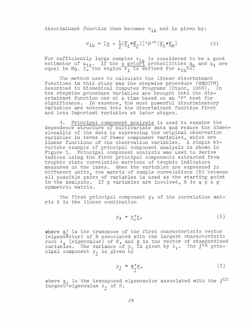
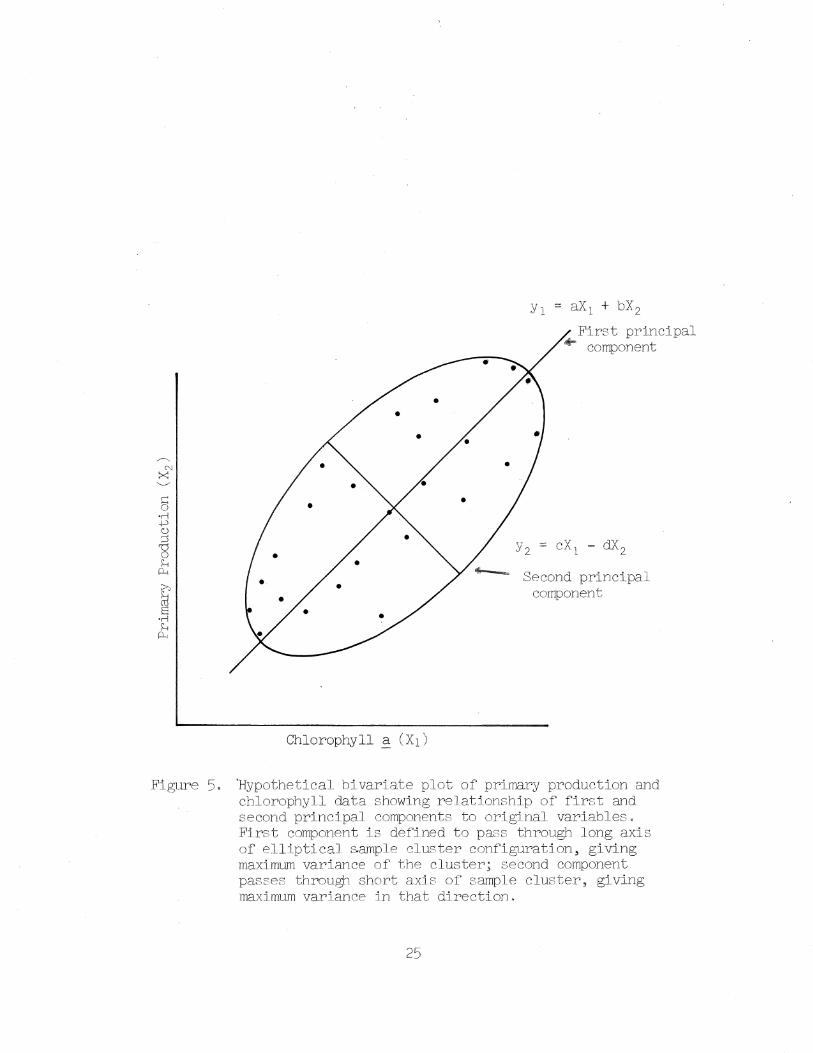
3. Principal component analysis is used to examine the dependence structure of multivariate data and reduce the dimen­sionality of the data by expressing the original observation variables in terms of fewer component variables, which are linear functions of the observation variables. A simple bi­variate example of principal component analysis is shown in Figure 5. Principal component analysis was used to derive indices using the first principal components extracted from trophic state correlation matrices of trophic indicators measured on the lakes. When the variables are expressed in different units, the matrix of sample correlations (R) between all possible pairs of variables is used as the starting point in the analysis. If p variables are involved, R is a p x p symmetric matrix.

The first principal component Yl of the correlation mat­rix R is the linear combination

y,== a' z "" -1-'

( 6 )

where a' is the transpose of the first characteristic vector (eigenv§ctor) of R associated with the largest characteristic root ~l (eigenvalue) of R, and! is the vector of standardized variables. The variance of Yl is given by ~l' The jth prin­cipal component Yj is given by

(7)

where a, is the transposed eigenvector associated with the jth largestJeigenvalue/l., of R.

. J

24

N ?<:

§ . r! -P C)

:::s 'd 0 H

jl.,

»

.~ H

jl.,

•

•

•

Chlorophyll ~ (Xl)

Yl = aX I + bX2

First principal ~ component

Second principal component

Figure 5. tiypothetical bivariate plot of primary production and chlorophyll data showing relationship of first and second principal components to original variables. First component is defined to pass through long axis of elliptical &ample cluster configuration, giving maximum variance of the cluster; second component passes through short axis of sample cluster, giving maximum variance in that direction.

25

In principal component analysis the main objective is to explain as much of the variance in the original observa­tions as possible with a minimum number of components. The first principal component is that linear combination of vari­ables which explains the maximum variance in the original data; the second principal component is the linear combina­tion of variables explaining as much of the remaining vari­ance as possible, and so on. As many component variables as original variables can be derived, at which point all the variance is explained, but this subverts the purpose of the procedure (i.e. reducing the dimensionality of the data). The proportion of the total variation that anyone component Yj explains is given by

tr(R) Aj p

(8 )

where A. is the jth eigenvalue of Rand tr(R) is the trace of R(s~m of the diagonal elements). The trace of R is also equal to p (the number of variables) since each diagonal ele­ment of R has a value of unity.

Theoretical and computational aspects involved in cal­culating principal components from covariance or correlation matrices are presented by Morrison (1967). The BMDX 72 program from the Biomedical Computer Programs Library (Dixon, 1968) was used to perform the analyses in this project.

4. Canonical correlation is used to analyze the statisti­cal relationships between two sets of variables considered in vector form. In this project canonical analysis was used to study the relationships between a trophic state vector con­sisting of seven trophic indicator variables, and a eutrophi­cation factor vector, consisting of several land use and popu­lation characteristics of the lake watersheds. The advantage of canonical correlation over conventional multi-regression analysis is that the former allows one to study relationships between two sets of variables without defining anyone vari­able as dependent and without assuming orthogonality (inde­pendence among the variables). This method determines the linear combination of the variables within each set which produces the maximum correlation coefficient between the two sets. Thus canonical analysis can be used to determine the dependency structure, i.e. the nature and extent of covaria­tion, between two sets of variables.

Consider a random vector ~ composed of observations on p variables with a covariance matr~x E. This vector x may be partitioned into two subvectors Xl and ~z with PI and Pz components, respectively. Usually the variables of each subvector will have some common feature, e.g. let ~l consist of several trophic state indicators for a lake and the vari-

26

abIes ~z be various eutrophication factors that influence trophic state, For convenience, it is assumed that Pl<PZ' From the population, N independent observation vectors are drawn and the p x p sample covariance matrix S calculated. It ~s assumed that N > (PI + pz + 1) and S is the unbiased estimator of t:. The covariance matrix may be partitioned into submatrices in a manner similar to x where

where the dimensions of S11' SIZ and Szzare PI x PI' PI X Pz and pz x Pz, respectively. Once a tenting procedure (de­scribed by Morrison, 1967) indicates a significant dependence between Xl and ~z, the method of canonical correlation may proceed.-

In canonical correlation analysis the following question is proposed. What are the linear compounds

]Jl = b' ~1 , • . , ·,]Jt = b' ~l -1 -t

VI = c 1 ~2. , •• , , ,vt = c' ~z _.1 -t

with the property that the sample correlation of ]Jl and VI is greatest, the sample correlation of ]Jz andv z greatest among all linear compounds uncorrelated with ]JI and VI and so on for t ~ min(Pl'PZ) possible pairs? These pairs of linear compounds are called canonical variates. It should

(10)

be noted that the correlation matrix R could have been par­titioned in a similar manner to S resulting in similar canon­ical correlations. However, canonical variates based on the correlation matrix are dimensionless and are expressed in terms of the standardized variables. The BMD06M program (Dixon, 1968) was used to perform the canonical correlation analyses.

5. Multiple regression analysis may be described as a method to predict the value of one variable (Y) from the values of other variables (X.), Variable Y is assumed to be depen­dent on the values of1the independent variables X.. Strictly

1 speaking multiple regression analysis is not a method of multivariate analysis since variates are considered inter­dependent ~n the latter, and no single variable can be con­sidered as the "dependent variable." The general model of (linear) multiple regression may be written as

27

(11)

where Y is the dependent variable, Xl' X2 , , •• X are indepen­dent variables, b o is the intercept value, and b~, b 2 , ••• b are regression coefficients. The variables may be raw dataP values or may be transformed values of the raw data. The principle value of multiple regression analysis lies in its predictive capacity (i.e. prediction of Y values from a mea­sured set of Xi)' The technique was used to evaluate statisti­cal relationships between the trophic state index (TSI) and eutrophication factor (land use and population) variables. The BMD02R program (Dixon, 1968) was used with the zero inter­cept (i.e. bo=O) option. This option was used since it is desirable to have a situation where the TSI is equal to zero when all the eutrophication factors are zero. The computer program is a stepwise multiple regression procedure and adds the variables to the equation in decreasing order of their statistical significance (i.e. their partial correlation with the dependent variable).

CHAPTER 3. LIMNOLOGICAL RESULTS

Detailed descriptions of the morphometry and physical features of the lakes in the study group are the subject of another report in this series. Similarly the chemical and biological limnology of the lakes will be described in detail in a third report (Brezonik, in preparation). This chapter will describe the limnological results in general terms as background information for analysis of eutrophication factors and lake trophic conditions in the following chapters.

A. MORPHOMETRIC AND PHYSICAL FEATURES

The geology Of Florida is dominated by a limestone sub­stratum underlying the entire peninsula. In north-central Florida the upper limestone deposits are of Eocene to Miocene age and are covered by more recent deposits of sand and clay_ Thickness Of the overlying formations ranges from a meter or so (e.g. in southern Alachua County) to over 30 meters. The limestone deposits~ve rise to a karstic topography through­out the peninsula with artesian springs, sink holes and solu­tion lakes as prominent features of the landscape.

The morphometry and physical features of Florida lakes are to a large extent determined by the geological structure and resulting topography. Table S summarizes these features for the 19 lakes sampled bimonthly. In general the lakes are shallow, and maximum depths of more than 10 m are uncommon.

28

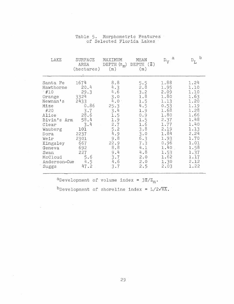
Table 5. Morphometr~c Features of Selected Florida Lakes

LAKE SURFACE MAXIMUM MEAN AREA DEPTH (zm) DEPTH (z)

(hectares) (m) (m)

Santa Fe 1674 8.8 5.5 Hawthorne 20.4 4.3 2.8 '#10 29.3 4.6 3.2 Orange 3324 3.0 1.8 Newnan's 2433 4.0' 1.5 Mize 0.86 25.3 4.5

#20 3.7 3.4 1.9 Alice 28.6 1.5 0.9 Bivin's Arm 58.4 1.9 1.5 Clear 3.4 2.7 1.6 Wauberg 101 5.2 3.8 Dora 2237 4.9 3.0 Weir 2301 9.8 6.3 Kingsley 667 22.9 7.3 Geneva 692 8.8 4.1 Swan 227 9.4 4.8 McCloud 5.6 3.7 2.0 Anderson-Cue 4.5 4.6 2.0 Suggs 47.2 3.7 2.5

aDevelopment of volume index = 3 z/ Zm·

DV

1. 88 1. 95 2.09 1. 80 1.13 0.53 1. 68 1. 80 2.37 1. 77 2.19 1. 84 1. 93 0.96 1. 40 1.53 1. 62 1. 30 2.03

bDevelopment of shoreline index = L/2/TIA.

29

a DL

b

1. 24 1.10 1.10 1. 63 1. 20 1.19 1. 28 1. 66 1. 48 1.40 1.13 2.24. 1. 70 1. 01 1. 58 1. 37 1.17 2.12 1. 22

Mean depths for all 55 lakes range from about 0.7 to 8.1 m, and maximum depths range from about 1.0 to 25 m. Most of the shallow lakes haveU~shaped basins; i.e. the lake basin walls are concave toward the water. The rleeper lakes gener­ally are more cone-shaped; in the deepest lake of the survey, Lake Mize, the lake basin walls are considerably convex to­ward the water. The trend can be seen by examining the volume development indices (Dy) in Table 5. Index values less than 1.0 indicate a convex toward the water) lake basin while values greater than 1.0 are indicative of U-shaped basins. Lakes with a DV of 1.0 have a basin similar in form to that of a cone (Hutchinson, 1957; Zafar, 1959).

Many small Florida lakes are hydraulically perched; i.e. their connection to groundwater is with a perched water table located above and not directly connected to the principal aquifer in the peninsula, the Floridan aquifer. Most of the small Alachua County and Trail Ridge region lakes are seepage (Birge and JudaY,1934) with no visible outlets or permanent inlets, and water levels may vary as much as several meters between dry and wet periods. Thus few lakes have a definite land-lake interface, and the shorelines may be intermittently submerged land. Water levels in the larger drainage lakes (e.g. Newnan's, Orange and Lochloosa Lakes, Alachua County) frequently are structurally controlled so that water level variations are much smaller. Some of the Trail Ridge lakes (e.g. Kingsley, Swan, Brooklyn), because of their occurrence in a region of very sandy soil, do possess fine natural sandy beaches in spite of the periodically wide fluctuations in water levels.

Nearly all the natural lakes in Florida have been derived or substantially modified by limestone solution processes. Numerous lakes are situated in sink-hole depressions formed by dissolution of underlying limestone (Stubbs, 1940; Hutchinson, 1957). In some cases lake basins have originated by other mechanisms (e.g. fluviatile action) but solution activity has substantially modified the original basin (e.g. Lake Tsala Apopka in Citrus County; Cooke, 1939). Many small and some larger lakes are simple dolines which tend to have simple circular basins. Perhaps the best example is Kingsley Lake (Clay County), an almost perfectly circular basin (shoreline development index, SD=l.Ol) about 3 km in diameter. Lake Santa Rosa (SD=1.09), a lake 0.8 km in diameter in Putnam County, is another example. SD is defined as the ratio of the actual length of a lake's shoreline to the min­imum length (i.e. the circumference of a circle) which would enclose an area equal to that of the lake surface. Other lakes are complex dolines with more irregular shorelines. For example, Lake Brooklyn (Clay County) consists of at least 9 separate solution basins and has an SD=2.37, and Cowpen Lake (Putnam County) with an SD=1.80 consists of at least 5 basins.

30

The shallowness of Florida lakes suggests that thermal stratification would be unimportant in these lakes, and in­deed most lakes do not exhibit classical Birgean thermoclines with stagnant hypolimnia as is common in temperate lakes. Eight lakes are sufficiently deep to develop stable strati­fication and oxygen deficient bottom waters; these are Lakes Mize (Brezonik and Keirn, in press), Kingsley~ Magnolia, Moss Lee, Santa Rosa, unnamed lakes numbered 20 and 27, and Beville's Pond. Climatic circumstances favor a long period of stratification; for example Lake Mize is stratified from February or early March till November. The surprising fea­ture of some of the lakes is the shallowness at which stable thermal stratification can occur. Lake No. 20 is only about 4 m deep but the temperature in the bottom meter is several °C cooler than the minimum temperatures in the region during Summer. Lake No. 27 is only about 7 m deep, yet it has a pronounced thermocline between 2.7 and 4.2 m (9-12ft), and the bottom water was 11.4°c in June, 1969, which is only 1°C warmer than the mid-winter bottom temperature. Clearly morpho­metric factors are important in producing the thermal stability of these lakes. Both are fairly small (1.5-4.5 ha), are in a rolling terrain and are surrounded by high pine forest. Thermal stratification is not limited to the summer months; temporary stratification can develop as a result of the highly changeable weather that occurs during January and February. While none of the lakes are meromictic, low to zero, dissolved oxygen values in the bottom waters of Beville's Pond, Lake No. 27, and Lake Mize throughout the year indicate "the bottom waters circulate rather incompletely even during winter.

At least 6 other lakes among the 55 exhibit incipient thermal stratification. Typical of these are Lake Wauberg and Hickory Pond. Stratification develops only near the bottom in these shallow lakes, preventing the formation of a distinct hypollmnion, but the bottom water temperatures during SUmmer are at least as cool as the nocturnal minima in the region so that fairly stable conditions can be assumed. Low dissolved oxygen values in the bottom waters of these lakes also imply stable stratification. These lakes are some­what larger or less wind protected by forest than the small lakes discussed previously. Size is obviously an important factor in determining whether stratification will occur in a lake. For example, neither Lake Santa Fe (surface area = 1650 ha, Zm =8.8 m) nor Lake Weir (surface area = 2300 ha, Zm =9.8 m ) have shown any evidence of stratification on any sampling date.

Many other shallow lakes show signs of stratified con­ditions even in the absence of a typical thermocline. Temper­ature differences of 4-5°C from top to bottom in lakes that are only 2-4 m deep are common during summer, but the decline is continuous with depth rather than confined to a narrow layer (also see Yount, 1961). At surface temperatures of

31

25,.....30 9 C, temperature differences of a few degrees are suffi­cient to impart considerable stability. to the water column (Hutchinson, 1957). Bottom temperatures are greater than regional nocturnal air temperatures' during. summer, and strati­fication thus is not highly stable. HoweVer, oxygen deple­tion in the bottom waters of several lakes impli~s a metas­table circumstance (i.e. mixing is not a daily phenomenon).

B. GENERAL CHEMICAL CHARACTERISTICS

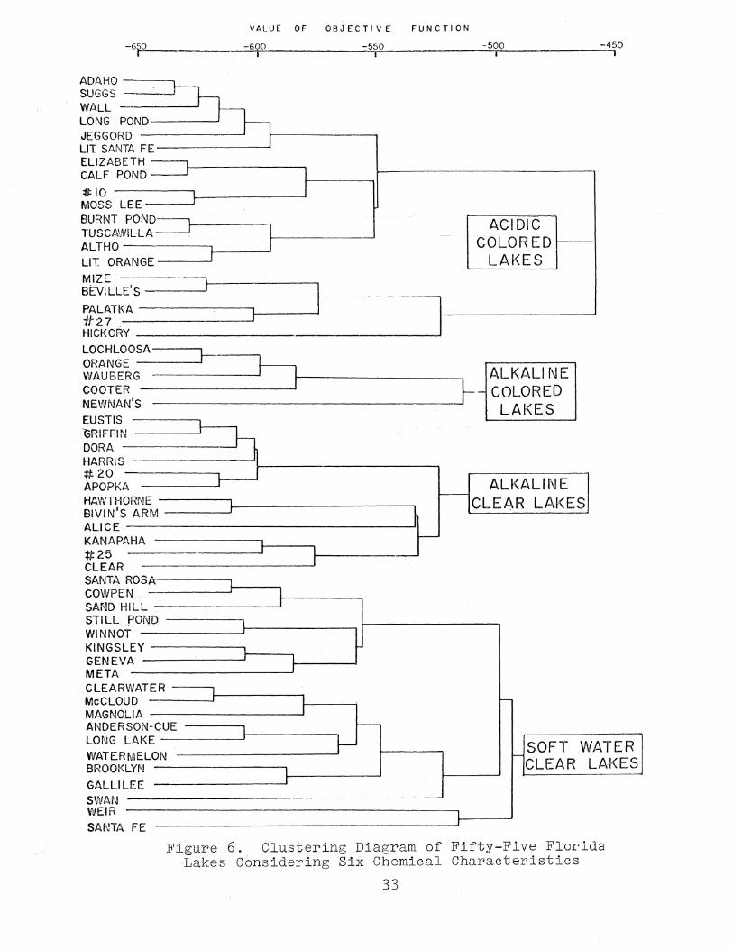
In order to determine general patterns in chemical compo­sition among the lakes (i.e. classify the lakes into distinct chemical types), a cluster analysis was performed on data for six basic chemical parameters for the 55 lakes. The para­meters considered were pH, alkalinity, acidity, conductivity, color and calcium, and mean values for each lake over the sampling period were used for the analysis. The resulting cluster diagram is shown in Figure 6.

The 55 lakes fall into four easily interpreted groups: (i) acid colored lakes, (ii) alkaline colored lakes, (iii) alkaline (hardwater) clear lakes; and (iv) soft, clear lakes. A comparison of the six chemical characteristics in these 4 lake types is shown in Table 6. Assuming the 55 lakes are a reasonable cross-section of the lakes iri north~central Florida, several conclusions derive from the results in Figure 6. Slightly less than 50 percent of the lakes are classified as colored, and the bulk of these are also acidic. Thus color would appear to be a common feature of Florida lakes. However, all but three of the colored lakes lie in Alachua County, which fact both implies a rather heterogene­ous geography in the region and suggests that caution should beobs~rved in extrapolating the statistics of the sample

. group to the population of Florida lakes.

Several other regional differences can be noted. The alkaline-colored group is composed entirely of lakes from Alachua County. Three (Newnan's, Orange, Lochloosa) are large connected drainage lakes; the other two are seepage or semi-drainage. All five lakes are moderately enriched. The alkaline clear group includes the five culturally en­riched lakes of the Oklawaha chain plus the small eutrophic lakes of Alachua County. The soft water clear lakes are located primarily in the Trail Ridge region and eastern Alachua County, which geographically comprise one topographic unit. .

One conclusion that seems a valid extrapolation is that Florida lakes generally have soft water; only the 12alkaline olear lakes can be considered to exhibit hardness, and even here the degree is moderate. This may seem contradictory in

32

VALUE OF OBJECTIVE FUNCTION

-6FF-- -600 i

-55.-"°. _____ --::-5°. '? r~

ADAHO SUGGS WALL LONG JEGGO LIT SA ELIZA CALF

POND~~ RD NTA FE r BETH --POND

LEE #10 MOSS BURNT TUSC~

ALTHO

LIT 0

MiZE BEViL

POND-.,WILLA==:=]

RANGE

LE'S

KA PALAT 11:27 HICKO RY

r

LOCHLOOSA-~._--.

l I

1 I

ACIDIC COLOR ED

LAf<ES

1 I

ORANGE --- ~ WAUBERG '/t--------~ ALKALI NE COOTER I - COLORED NEWNAN'S r-EUSTIS LAKES

~;::IN ___ --1"-'g HARRIS -------}-. __________ _ #20 APOPKA ALKALINE

-450 --.

HAWTHORNE -_-_-=--=--=--==Jr--~-------_, BIVIN'S ARM l

r--CLEAR LAKES

ALICE ______________________ J'I

KANAPAHA f--

#25

A N ILL POND

CLEAR SANTA ROS COWPE SAND H STILL WINNO KINGS GENE\. META CLEAR McCLO MAGNO ANDER LONG

WATER BROOK

T LEY fA

WATER UD LlA SON-CUE LAKE

MELON LYN

GALLIL SWAN WEIR

EE

SANTA E F

l

1

1 1

~

~ l

I---

SOFT WATER f--

CLEAR LAKES

I

Figure 6. Clustering Diagram of Fifty-Five Florida Lakes Considering Si~ Chemical Characteristics

33

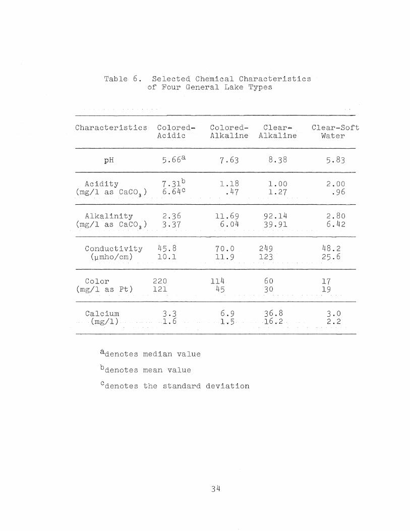
Table 6. Selected Chemical Characteristics of Four General Lake Types

Characteristics Colored-Acidic

pH 5.66a

Acidity 7.31b (mg/l as CaC0 3 ) 6.64 c

Alkalinity 2.36 (mg/l as CaC0 3 ) 3.37

Conductivity 45.8 (jJmho/cm) 10.1

Color 220 (mg/1 as Pt) 121

Calcium 3.3 (mg/l) 1.6

adenotes median value

bdenotes mean value

Co1ored-Alkaline

7.63

1.18 .47

11.69 6.04

70.0 11.9

114 45

6.9 1.5

cdenotes the standard deviation

34

Clear ... Alkaline

8.38

1.00 1. 27

92.14 39.91

249 123.

60 30

36.8 16.2

Clear-Soft Water

5.83

2.00 .96

2.80 6.42

48.2 25.6

17 19

3.0 2.2

view of the solution origin of the lakes and the abundance of hard water springs in Florida, but few Florida lakes are spring fed. Rather, most of the lakes receive the bulk of their water either directly from precipitation or by surface and subsurface runoff from the sandy, low calcareous soils. In fact several of the hard water lakes are not naturally calcareous but have hard water because of cultural effects, i.e. the influx of ground water as treated sewage or septic tank drainage.

The mean and median values of the chemical parameters in Table 6 indicate highly distinct and readily apparent differences among the 4 lake types, perhaps much greater than when the lakes are considered individually (as the large standard deviations for some parameters would suggest). The acidic-colored lake group has a much higher mean color than the alkaline-colored group (220 to 114 mg/l as Pt), and the high color probably contributes to the low pH values. Color concentrations as high as 700 mg/l have been found in some lakes (e.g. Lake Mize). Color certainly contributes to acidity (cf. acidity values of the acidic-colored and clear-soft water groups, both of which have acid pH values). Color is the only parameter which has a significantly differ­ent value in each of the 4 types and as such appears to be an important chemical characteristic for distinguishing between the lake types.

C. PHYTOPLANKTON AND MACROPHYTE CHARACTERISTICS

Algal identification and enumeration was done on all 55 lakes at each sampling. Because of year-round favorable growth conditions (solar radiation and temperature), some of the fertile lakes such as Apopka, Bivin's Arm and Dora exhibit virtually continuous algal blooms. However maximum bloom conditions usually obtain during summer. Lake Apopka has exhib~ted phytoplankton blooms of 88,000cells/ml or higher, predominated by blue-green genera such as Lyngbya and Mic~ocyatis and green genera such as PediaatrUm and Scenedesmus. Blooms of 32,000 cells/ml or more have been found in Lake Dora. Newnan's Lake, a colored eutrophic lake, has summer populations predominated by blue-green algae (Microcystis, Anabaena, Spirulina). In winter this lake usually produces an extremely dense bloom of Aphanizomenon, which fixes nitrogen at high rates (Brezonik and Keirn, unpublished data). However this alga is not present in the lake during other seasons of the year and is nota common constituent ·of the phytoplankton in other eutrophic lakes . Microcystis and Anabaena are the summer bloom formers in Bivin's Arm. The latter organism is found in all lakes in which nitrogen fixation has been detected, and seems to be the primary algal agent for this process in all the lakes except Newnan's Lake.

35

Oligotrophic lakes have typically low algal populations. For exa~ple, in Swan Lake (a clear s.oft water, oligotrophic type) a summer 1969 population of about 36 organisms/ml was dominated by the diatoms· Syried·ra and Navi.cula and the green alga Sphaerocystis. Dinobryon and Synura (cl~ss Chrysophyceae) are common in the low pH, low icmic strength waters of the soft water clear (oligotrophic) lakes as are a variety of Desmidaceae (e,g. Staurastrum, Closterium, and Cosmarium).

Diatoms are comparatively rare in the plankton of Florida lakes, especially in the oligotrophic soft water lakes. Low silica concentrations in Florida lakes may in part account for this distribution. An exception to this general trend is Lake Apopka, which normally supports a high (although not usually dominant) population of diatoms, including MelOSira, Tabellaria, and NaVicula, and perhaps not coincidentally has one of the highest silica concentrations (3.7 ppm) of the 55 lakes. Bivin's Arm with a mean silica content of 1.8 ppm also supports a spring bloom of diatoms (Maslin, 1970).

The dominant primary producers in a number of the 55 lakes are floating macrophytes, For example, Lake Alice, on the University of Florida campus was until recently covered alm.ost entirely by a dense crop of water hyacinth (Eichorriia crassipes). While a faculty-student effort succeeded in mechanically clearing this lake (at least temporarily), the plant is common in canals and other lakes (e.g. Lakes Tuscawilla and Apopka). Chemical spraying is used to control the plant in a number of lakes including Bivin's Arm and Lake Apopka. Duckweed (I:iemna ruinor) partially covers the surface of Lake No. 27 throughout the year, while perhaps one-third of Beville's Pond is covered by SalVinia during the summer months, Such growths limit light penetration, drastically reducing phytoplankton populations, and under severe conditions may inhibit oxygen transfer from the atmosphere to the water.

D. SEDIMENTS

Florida lakes have a wide variety of sediment types, including sand, peat, and sludge-like (ooze) deposits. In som,e of the oligotrophic lakes a light nearly pure sand bottom occupies most of the lake bottom" suggesting the geo .... logical newness of these lakes. Organic deposits in the lakes range in color from light brown (peat) to nearly black (ooze) and the sediment consistency similarly covers a wide range with large fragments of plant remains evident in peat sedi­ments and very fine, slowly settling particles in some of the oozes. In many of the lakes there is no defined sediment­water interface. Rather a gradation from thin suspensions of sedim,entto m,ore compact strata occurs often over depths of a meter or more. This characteristic makes sampling of

36

bottom water (and surface sediments) rather difficult. In shallow lakes the suspended sediments undoubtedly become mixed with the overlying water during periods of wind stress, and considerable nutrient exchange is thus effected. The carbon: nitrogen ratios in nearly all the sediments are greater than 10 indicating a Hdyl1 type of sediment in Hansen's (1962) ter~ minology. A crude correlation also exists between CIN ratio and trophic conditions. The most eutrophic lakes have CIN ratios in the range 10~15 and oligotrophic lakes have gener­ally higher ratios, but considerable scatter occurs when all 55 lake sediments are considered.

CHAPTER 4. CLASSIFICATION AND QUANTIFICATION OF TROPHIC CONDITIONS IN FLORIDA LAKES

As discussed in Chapter 1, eutrophication and trophic state are extremely complex, multivariable phenomena. At present our understanding of them and their interrelationships is primarily qualitative. A broad effort to quantify these relationships was made using the statistical techniques de­scribed in Chapter 2 and the collected limnological and water­shed data. The analyses were applied to three major aspects of eutrophication research listed in 1) the long standing problem of rational classification of lakes according to trophic state, 2) quantification of the presently nebulous term "trophic state," and 3) delineating the relationships between lake trophic conditions and watershed enrichment factors. This chapter presents results for the first two aspects; Chapter 5 discusses the third.

A. DEVELOPMENT OF A TROPHIC CLASSIFICATION SYSTEM FOR FLORIDA LAKES

The multi~dimensionality of the trophic state concept has heretofore obviated objective and consistent classifica­tion of lakes according to their trophic states. In an attempt to minimize subjectivity in delineating trophic classifica­tions for Florida lakes, similarity (cluster) analyses were performed on trophic indicator data from the 55 lakes. Seven indicators; viz., primary production (PP), chlorophyll a (CHA), total organic nitrogen (TON), total phosphorus (TP), Secchi disc transparency (SD),conductivity (COND), and a cation ratio CCR) due to Pearsall (1922) were chosen as the dimensions describing the hybrid concept of trophic state and were considered Simultaneously in the cluster analysis to derive logical lake groups according to their trophic stateB (at least as defined by the 7 indicators).

The main considerations in selecting the first six

37

indicators are. that (;iJ they are quantitative, (ii) they are fundamentally significant as measures of t.rophicstate, (iii) they satisfy HQoper's (1969) criteria for useful trophic indicators reasonably well, and (1v ) they apply to Florida lakes. The first Six indicators have all beeri used with some degree of success in various lake classification schemes.

The selection of Pearsall's cation rati~(Na + K) was a somewhat subjective attempt to incorporate Mg + Ca information on the major cations into the concept of trophic state without adding each cation as an individual indicator. Pearsall (1922) reported that English lakes with high nitrate and silica and a Na + K ratio less than 1.5 had periodic algal blooms. Mg + Ca Thus this ratio should be inversely related to increasing eutrophy. Parenthetically it might be noted that many workers have suggested a general correlation between high productivity and water hardness (Ca and Mg con­centrations). This ratio has not been used to any extent in other investigations, but it was suggested as a potentially effective parameter for differentiation between lake trophic types by Zafar (1959). For Florida lakes the cation ratio appears to be a reasonably good indicator of trophic state with high values of the inverse cation ratio being indicative of eutrophic conditions. .

Averages of the lake parameters over the one year sampling period would seem the most appropriate values for the purposes of statistical analysis. In some respects extreme values (e.g. maximum nutrient concentrations, algal densities at the height of bloom conditions, etc.) are more critical deter­minants of a lake's water quality and may thus be better and more sensitive indicators of trophic state. But extreme values are less reproducible, and their magnitude depends greatly on the vagaries of sampling frequency and climatic circumstances. Since the breadth of this project pre~luded detailed (e.g. weekly) sampling, it is felt that mean values are more appropri­ate in the ensuing analysis. In order not to bias the means toward summer conditions, the June, 1910, values were not included in the comput.ations. Means of the trophic indicators, color, and turbidity for the 55 lakes are listed in Table 7. So that each indicator would denote trophic state in a positive sense (an increase in indicator value denotes an increase in trophic state) the Secchi disc and cation ratio indicators were inversely transformed. Obviously there are many more possible indicators of trophic state that could be included. Alternatively, it may be that fewer trophic indicators will eventually prove sufficient to describe the concept of trophic state, The selection of 7 indicators was a somewhat arbitrary attempt to incorporate as much information into the concept of trophic state as possible without getting into a prolifer­ation of secondary or redundant indi6ators~

Because of the basic typological differences caused by

38

Table 7. Trophic State Indicator, Color and Turbidity Dat~l

Color -Lake Scaled

Number l/SD l/SD Cond TON TP PP CHA l/CR COL TUR

1 0.43 0.52 53.2 0.50 0.021 9.3 5.6 1. 24 59.0 1.9 2 0.66 0.46 53.7 0.61 0.015 1.8 4.5 0.90 149.0 1.5 3 0.56 0.52 45.7 0.70 0.027 4.1 7.6 0.64 62.0 1.9 4 0·73 0.58 53.3 0.59 0.023 12.4 5.9 0.65 133.7 2.3 5 1.16 0.92 59.7 1. 26 0.165 29.6 22.6 1. 01 83.3 4.5 6 1.66 0.89 47.7 0.81 0.036 6.9 8.0 0.85 236.7 4.3 7 0.41 0.39 40.0 1. 32 0.012 0.5 2.3 0.53 21.3 1.0 8 1.41 0.91 167.7 1. 86 0.079 96.6 56.8 1. 88 58.3 4.4 9 1. 06 0.54 50.7 0.94 0.105 20.8 9.8 0.55 165.7 2.0

10 0.65 0.53 50.4 0.86 0.064 18.2 12.6 0.47 123.7 1.9 LV 11 0.70 0.53 43.0 0.77 0.036 25.4 8.1 0.49 98.3 1.9 \0

12 1. 23 0.77 55.7 0.47 0.087 6.8 7.0 0.39 192.7 3.5 13 0.50 0.47 38.0 0.63 0.013 0.5 3.1 0.61 26.0 1.5 14 1.15 0.81 87.0 1. 42 0.058 20.9 23.3 1. 41 116.3 3.8 15 1. 00 0.74 77.4 1. 07 0.063 27.4 15.6 1. 01 107.1 3.3 16 0.81 0.44 25.0 1. 22 0.024 8.5 15.6 0.78 93.3 1.3 17 1. 91 0.88 59.8 1. 41 0.110 102.5 47.4 0.85 188.9 4.2 18 1. 83 0.47 53.0 0.85 0.113 11.2 33.9 0.62 433.4 1.5 19 1.41 0.42 43.7 1. 41 0.184 12.7 23.5 0.83 404.0 1.2 20 2.87 2.88 314.3 2.06 0.410262.8 92.8 4.04 68.5 17.4 21 0.45 0.49 93.3 0.81 0.030 2.4 3.3 1. 50 25.0 1.7 22 0.67 0.46 552.2 0.50 0.900 7.9 4.4 3.42 25.5 1.5 23 1.65 1.79 253.8 1. 88 0.546 25L. 7 56.00 2.48 42.1 10.2 24 1.33 1.17 136.4 1. 27 0.392 87.4 26.4 2.91 85.4 6.1 25 0.66 0.57 92.7 0.73 0.028 2.6 3.5 9.88 36.0 2.2 26 0.46 0.39 39.7 0.65 0.087 1.8 23.7 0.54 181.7 1.0 27 0.71 1. 37 47.0 0.58 0.325 1.2 30.1 1.21 92.0 7.5 28 2.81 2.27 121. 7 2.20 o .422 1~3. 7 42.7 5.12 120.7 13.8 29 1.04 1.08 37.7 0.86 0.05217.0 9".0 0.73 74.0 5.6

(cont lei)

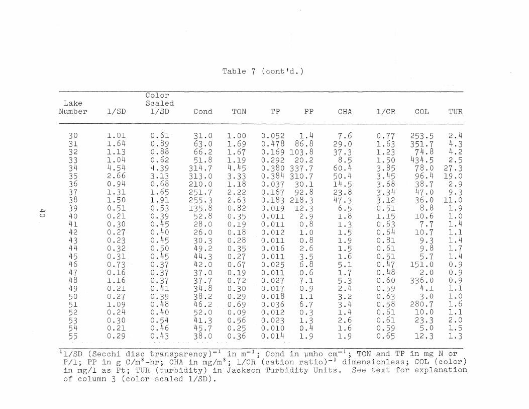
Table 7 (cont'd.)

Color Lake Scaled

Number l/SD l/SD Cond TON TP PP CHA l/CR COL TUR

30 1. 01 0.61 31. 0 1. 00 0.052 1.4 7.6 0.77 253.5 2.4 31 1. 64 0.89 63.0 1. 69 0.478 86.8 29.0 1. 63 351. 7 4.3 32 1.13 0.88 66.2 1. 67 0.169 103.8 37.3 1. 23 74.8 4.2 33 1. 04 0.62 51. 8 1.19 0.292 20.2 8.5 1. 50 434.5 2.5 34 4.54 4.39 314.7 4.45 0.380 337.7 60.4 3.85 78.0 27.3 35 2.66 3.13 313.0 3.33 0.384 310.7 50.4 3.45 96.4 19.0 36 0.94 0.68 210.0 1.18 0.037 30.1 14.5 3.68 38.7 2.9 37 1. 31 1. 65 251. 7 2.22 0.167 92.8 23.8 3.34 47.0 9.3 38 1. 50 1. 91 255.3 2.63 0.183 218.3 47.3 3.12 36.0 11.0

+:=- 39 0.51 0.53 135.8 0.82 0.019 12.3 6.5 0.51 8.8 1.9 0 40 0.21 0.39 52.8 0.35 0.011 2.9 1.8 1.15 10.6 1.0

41 0.30 0.45 28.0 0.19 0.011 0.8 1.3 0.63 7.7 1.4 42 0.27 0.40 26.0 0.18 0.012 1.0 1.5 0.64 10.7 1,1 43 0.23 0.45 30.3 0.28 0.011 0.8 1.9 0.81 9.3 1.4 44 0.32 0.50 49.2 0.35 0.016 2.6 1.5 0.61 9.8 1.7 45 0.31 0.45 44.3 0.27 0.011 3.5 1.6 0.51 5.7 1.4 46 0.73 0.37 42.0 0.67 0.025 6.8 5.1 0.47 151.0 0.9 47 0.16 0.37 37.0 0.19 0.011 0.6 1.7 0.48 2.0 0.9 48 1.16 0.37 37.7 0.72 0.027 7.1 5.3 0.60 336.0 0.9 49 0.21 0.41 34.8 0.30 0.017 0.9 2.4 0.59 4.1 1.1 50 0.27 0.39 38.2 0.29 0.018 1.1 3.2 0.63 3.0 1.0 51 1. 09 0.48 46.2 0.69 0.036 6.7 3.4 0.58 280.7 1.6 52 0.24 0.40 52.0 0.09 0.012 0.3 1.4 0.61 10.0 1.1 53 0.30 0.54 41. 3 0.56 0.023 1.3 2.6 0.61 23.3 2.0 54 0.21 0.46 45.7 0.25 0.010 0.4 1.6 0.59 5.0 1.5 55 0.29 0.43 38.0 o .J6 0.014 1.9 1.9 0.65 12.3 1.3

Il/SD (Secchi disc transparency)-l in m- l ; Cond in ~mho cm~l; TON and TP in mg N or P/l; PP in g C/m 3 -hr; CHA in mg/m 3 ; l/CR (cation ratio)-l dimensionless; COL (color) in mg/l as Pt; TUR (turbidity) in Jackson Turbidity Units. See text for explanation of column 3 (color scaled l/SD).

organic color (Figure 6 and Table 6), it seemed best to con~ sider clear and colored lakes as separate classes in each of which a range of trophic subclasses could exist. In fact, a cluster analysis of the 55 lakes considering the 7 trophic indicators plus color divided the lakes into essentially the same 31 clear and 24 colored lakes shown in Figure 6. (Lakes Wauberg and Kanapaha, which are in the alkaline colored and alkaline clear groups, respectively, in Figure 6, are the only lakes which fall into the opposite groups in the color plus trophic indicator cluster analysis.) The lakes in the colored group had mean color levels greater than about 75 ppm, whereas the clear lakes had color levels less than this value. Thus the horizontal line separating clear and colored lakes in Figure 1 would appear to have a value of about 75 ppm for Florida lakes.

The lakes within each of the main classes were grouped into subclasses of similar trophic state by performing cluster analyses with the 7 trophic indicators. The clear lakes (Figure 7) formed three apparently natural groups which can be inter­preted in the classical (oligotrophic-mesotrophic-eutrophic) sense. Nearly all the lakes of the Trail Ridge region comprise the oligotrophic Group A. These demonstrate a good within­group similarity as denoted by the low objective function values at which they are joined. Themesotrophic Group B includes a few lakes from the Trail Ridge region (e.g. Kingsley and Winnott) which have been subjected to some cultural in­fluence. As a whole the lakes in Group B (especially those from the Trail Ridge) are perhaps closer to being oligotrophic than eutrophic, but nonetheless they are distinctly (if slightly) more productive than the Group A lakes. The lakes of the eutrophic Group C include the 5 Oklawaha chain lakes plus the small eutrophic and hypereutrophic lakes in Alachua County. The latter are located primarily in urbanized areas, especially around Gainesville, and cultural sources seem to exert a heavy influence on their trophic states. The meso­trophic and eutrophic groups exhibit greater diversity in values for the individual trophic indicators and consequently are joined at higher objective function values.

The colored lakes exhibited considerable diversity, and the results were not as interpretable in terms of classical trophic groupings, Perhaps this reflects a basic difference between colored and clear lakes; in this regard it should be noted that the position of dystrophic lakes in the usual trophic (i.e, nutritional state) classification has long been a subject of contention (Hansen, 1962; see Brezonik etal., 1969 for fUrther discussion). As previously mentioned.-We have considered color (roughly equivalent to dystrophy) as a major lake type parallel to a clear lake type (as proposed by Hansen, 1962, and Stewart and Rohlich,1967) , and a range of nutrient states was considered possible for both. However the results of the cluster analysis imply that a simple har-

41

VALUE OF THE OBJECTIVE FUNCTION -600 -500 -400 -300 -200

I i I I I

(41) SAND HIll

(42) MAGNOLIA

(55) GAlUlEE

(43) BROOKLYN

I

(47) SANTA ROSA -.....;.-----., 1----...,

(54) COWPEN I

(52) LONG LAKE

(50) Me CLOUD

(49) ANDERSON- CUE

(44) GENEVA

(45) SWAN

------'~ I ,

-

(7) CLEARWATER ----------------------,

(53) WI NNOTT

(13) STILL POND I

(29) WATERMELON ---------'1

I

GROUP A

GROUP B (I) SANTA FE

(40) "(NGSlEY

(21) META ---------------------_I--------~~~--~ (39) WEIR

(25) No. 25

(36) HARRiS

(37) EUSTIS

(34) APOPKA

(3~) DORA

(38) GRIFFIN

( 8 ) HAWTHORNE'

(20) No. 20

(32) WAUBERG

(23) BIVINS ARM

(24) CLEAR

(22) ALICE

I I

I GROUP C

L , -

I 1

Figure 7. Cluster Analysis of 31 Low-Color (Clear) Lakes Considering 7 1rophic Indicators

42

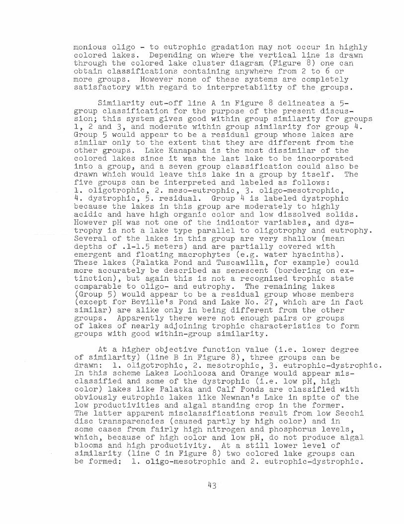
monious oligo ..., to eutrophic grada.tion may not :occur in highly colored lakes. Depending on where the. vertical line is drawn through the colored lake cluster diagram (FigureS) one can obtain clas.sificationscontaining anywhere from 2 to 6 or more groups. However none of these systems are completely satisfactory with regard to inte~pret~bility of the groups.

Similarity cut~off line A in Figure 8 delineates a 5-group classification for the purpose of the present discus~ sion; this system gives good within group similarity for groups 1, 2 and 3, and moderate within group similarity for group 4. Group 5 would appear to be a residual group whose lakes are simil~r only to the extent that they are different from the other groups. Lake Kanapaha is the most dissimilar of the colored lakes since it was the last lake to be incorporated into a group, and a seven group classification could also be drawn which would leave this lake in a group by itself. The five groups can be interpreted and labeled as follows: 1. oligotrophic, 2. meso-eutrophic, 3. oligo-mesotrophic, 4. dystrophic, 5. residual. Group 4 is labeled dystrophic because the lakes in this group are moderately to highly acidic and have high organic color and low dissolved solids. However pH was not one of the indicator variables, and dys­trophy is not a lake type parallel to oligotrophy and eutrophy. Several of the lakes in this group are very shallow (mean depths of .1-1.5 meters) and. are partially covered with emergent and floating macrophytes (e.g. water hyacinths). These lakes (Palatka Pond and Tuscawilla, for example) could more accurately be described as senescent (bordering on ex~ tinction), but again this is not a recognized trophic state comparable to oligo- and eutrophy. The remaining lakes (Group 5) would appear to be a residual group whose members (exceptfQr Beville's Pond and Lake No. 27, which are in fact similar) are alike only in being different from the other groups. Apparently there were not enough pairs or groups of lakes of nearly adjoining trophic characteristics to form groups with good within-group similarity.

At a higher objective function value (i.e. lower degree of Similarity) (line B in Figure 8), three groups can be drawn: 1. oligotrophic, 2.· mesotrophic, 3. eutrophic~dystrophic. In this scheme Lakes Lochloosa and Orange would appear mis­classified and some of the dystrophic (i.e, low pH, high cQlor) lakes like Palatka and Calf Ponds are classified with obviously eutrophic lakes like NewnantsLake in spite of the low productivities and algal standing crop in the former. The. latter apparent misclassifications result from low Secchi disc transparencies (caused partly by high color) and in some cases from fairly high nitrogen and phosphorus levels, which, because of highc610r and low pH, 40 not produce algal blooms and high productivity. At a still lower level of sim,j.,larity (lineC in Figure 8) two colored lake groups can be formed; 1. oligo~mesotrophic and 2. eutrophic ...... dystrophic.

43

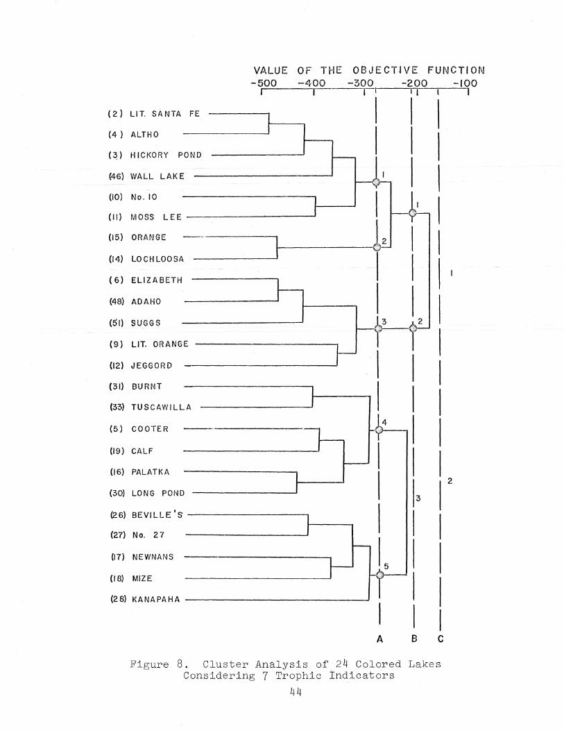
(2) LIT. SANTA FE

(4) ALTI-IO

(~) HICKORY P OND

(46) WALL LAK E

(10) No. 10

(II) MOSS LEE

(15) ORANGE --

(14) LOCHLOOSA

(6) ELIZABETH .

(48) ADAHO

(51) SUGGS

(9) LIT. ORANGE

(12) JEGGORD

(31) BURNT

(33) TUSCAWILL A

(5) COOTER --,

(19) CALF

(16) PALATKA

(30) LONG POND

(26) BEVILLE'S

(27) No. 27

(17) NEWNANS

(18) MIZE

(28) KANAPAHA

VALUE OF THE 08JECT~VE FUNCTION -500 -400 -300 -200 -100

r I I i II I

I I

I r

~

I

-, r

I J

I I I

~

I I

}-

I

I I-..-.-! L

1- I I

3 2 I--t~;}---~~ 1 I

14 y

~I

I--

5

A

1 I I I I I

B

I I

C

2

Figure 8. Cluster Analysis of 24 Colored Lakes Considering 7 Trophic Indicators

44

This is not a Vel:'Y useful classification since the groups then conta,in highly dissimilar lakes and are nQteasily interpreted in terms of classical trophic gl:'OUps. ltis apparent that none of the colored lake classifications is ideal. The five group classification is not readily interpret­able in terms of classical trophic groups, and the two group system has groups that are too broad to be of much use. The three group classification has some advantages in terms of interpreting classical trophic states, but some obvious mis­classifications occur in this system.

Mean values and standard deviations of the trophic indi­cators within the 3 clear lake subgroups and 5 colored lake subgroups delineated by the cluster analyses (Figures 7 and 8) are presented in Table 8. All seven indicators appear to reflect trophic levels reasonably well. Among the clear lakes indicator mean values without exception increase in each succeeding trophic group (from oligotrophy to eutrophy). Among the colored lakes the same trend is noted although some exceptions occur. There is little difference between mean values for the colored oligotrophic (Group 1) and oligo -mesotrophic (Group 3) groups; primary production and chloro­phyll means are actually somewhat higher in the former than in the latter. The high values for the residual group derive from the bypereutrophic conditions in Newnan's and Kanapaha Lakes; the other lakes in this group have varied indicator values.

It is interesting to note that the colored lakes have a much smaller range of values for most of the indicators compared to the clear lakes. Thus the clear oligotrophic lakes reflect much greater nutrient impoverishment than the colored oligotrophic lakes, and similarly the apparent degree of eutrophy is greater in the clear lakes. For example, the range of mean primary production values in the clear lakes is 1.3 to 150 mg C/m3_hr, while in the colored lakes the range is 9.7 to 55.

B. DEVELOPMENT OF DISCRIMINANT FUNCTIONS TO CLASSIFY LAKES OUTSIDE THE ORIGINAL

SAMPLE GROUP

Discriminant functions were derived for the three trophic classes delineated by cluster analysis of the 311ow~color lakes and are presented in Table 9. In addition, the 55 lakes were grouped into five trophic categories ranging from ultra­oligotrophic to hypereutrophic based on the trophic state index described in the next section. Discriminant functions were derived for these classes and are shown in Table 10. The colored lake group was too small and diverse to form meaningful discriminant functions. Using the criterion de~

45

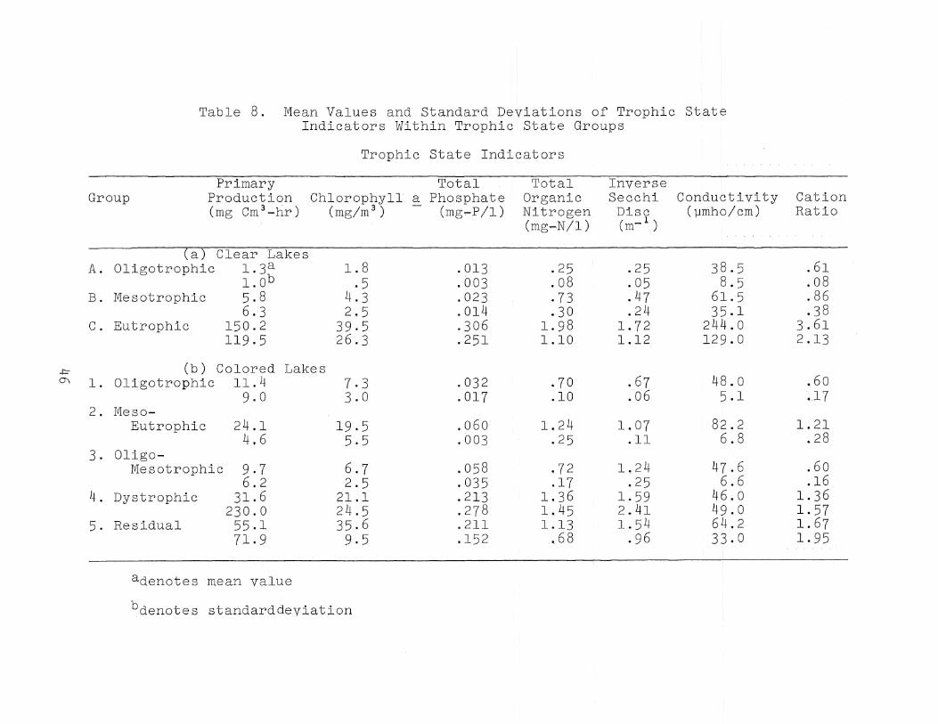
-l= 0\

Table 8. Mean Values and Standard Deviations of Trophic State Indicators Within Trophic State Groups

Trophic State Indicators

Primary Total Group Production Chlorophyll a Phosphate

(mg Cm 3 -hr) (mg/m 3 ) - (mg-P/l)

rCiTCiear-Lakes A. Oligotrophic 1. 3a 1.8 .013

1. Ob .5 .003 B. Mesotrophic 5.8 4.3 .023

6.3 2.5 .014 C. Eutrophic 150.2 39.5 .306

119.5 26.3 .251

(b) Colored Lakes 1. Oligotrophic 11. 4 7.3 .032

9.0 3.0 .017 2. Meso-

Eutrophic 24.1 19.5 .060 4.6 5.5 .003

3. Oligo-Mesotrophic 9.7 6.7 .058

6.2 2.5 .035 4. Dystrophic 31. 6 21.1 .213

230.0 24.5 .278 5. Residual 55.1 35.6 .211

71. 9 9.5 .152

adenotes mean value

bdenotes standard deviation

Total Organic Nitrogen (mg-N/l)

.25 ,08 .73 .30

1. 98 1.10

.70

.10

1. 24 .25

.72

.17 1. 36 1. 45 1.13

.68

Inverse Secchi Conductivity Cation

Disc (~mho/cm) Ratio (m-l)

.25 38.5 .61

.05 8.5 .08

.47 61. 5 .86

.24 35.1 .38 1. 72 244.0 3.61 1.12 129.0 2.13

.67 48.0 .60

.06 5.1 .17

1.07 82.2 1. 21 .11 6.8 .28

1. 24 47.6 .60 .25 6.6 .16

1. 59 46.0 1. 36 2.41 49.0 1. 57 1. 54 64.2 1. 67

.96 33.0 1. 95

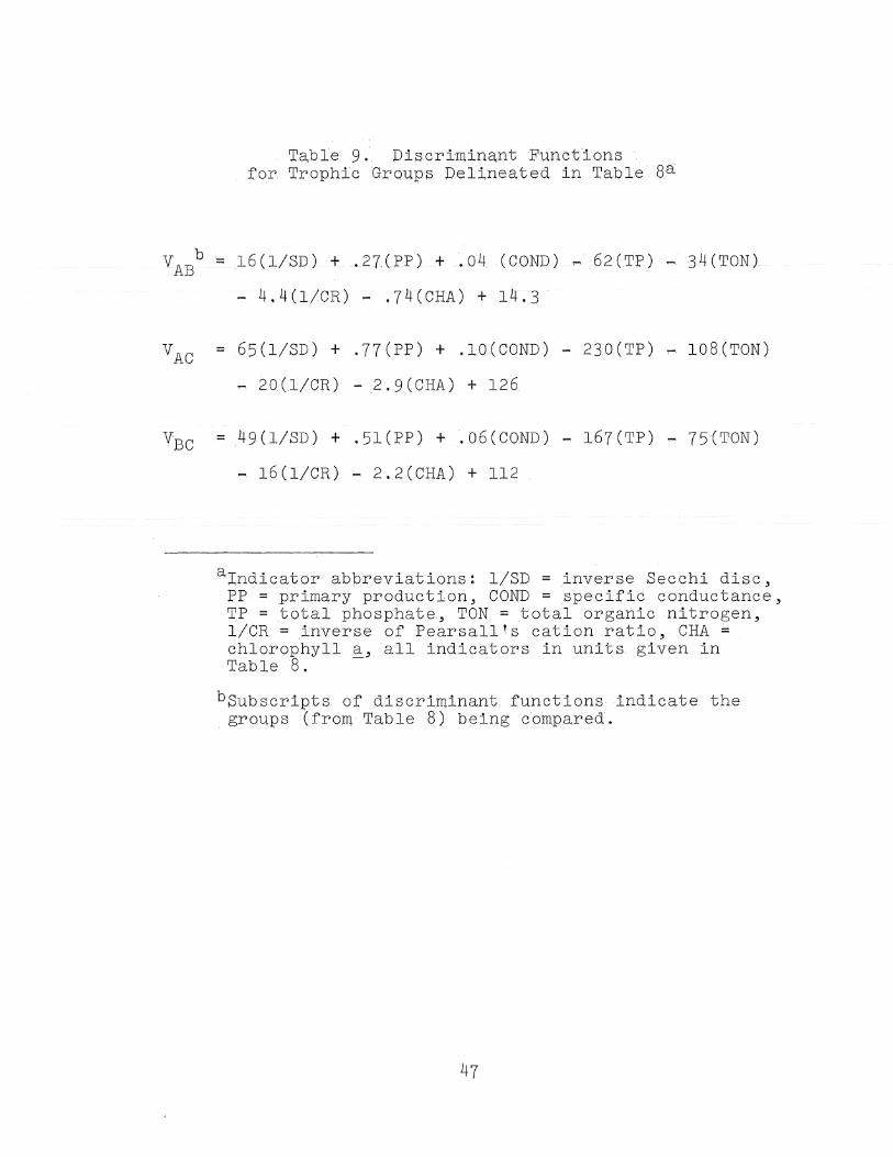
VAB b

VAC

VBC

Table 9 . Discriminant Eu'nctions for Trophic Grou,ps Delineated in Table8a

~ 16 (l/SD) + .27(PP) + .04 (COND) ,.... 62 (TP) ~. 34(TON)

~ 4.4(l/CR) - .74(CHA) + 14.3

= 65(l/SD) + .77(PP) + .10 (COND) - 230 (TP) ,... 108(TON)

~. 20 (l/CR) -2.9 (CHA) + 126

= 4g(1/SD) + .51(PP) + .06(COND) - 167(TP) ,.... 75(TON)

-. 16 (l/CR) - 2.2 (CHA) + 112

alndicator abbreviations: l/SD = inverse Sec chi disc, PP = primary production, COND = specific conductance, TP = .total phosphate, TON = total organic nitrogen, l/CR = inverse of Pearsall's cation ratio, CHA = chlorophyll a, all indicators in units given in Table 8. -

bSubscripts of discriminant functions indicate the groups (from Table 8) being compared.

47

Table 10 . Discriminant FunctiQns.fQr Five Groups of Lakes D.etermined from TrQphicSt.ate. Indicator

Ranges (From Table 18)

VHE b = 23.99(1/SD)a + .47(COND) + 15.17(TON) + 148.76(TP4)

+ .38(pp) ~ .o4(CHA) + 8.19(1/CR) ~ 289.io

VHM

VHO

VEM

YEO

VEU

VMO

VMU

YOU

=

=

-22.44(.1/Sb) + .53(COND) + 35.93(TON) + 289.93(TP4) + 91(PP) + .77(CHA) + 11.11(I/CR) -- 369.94

~34.88(1/SD) + .59(COND) + 74.56(TON) + 427.32(TP4) + .59(PP) + 2.45(CHA) + 23:39(1/CR) - 451.87

= -44.33(1/SD) + .64(COND) + 111.06(TON) + 490.95(TP4) ~ .33(PP) + 3.27(CHA) + 26.56(1/CR) -475.42

=

=

=

=

=

=

,..,46,43(l/SD) + .06(COND) + 20.77(TON} + 141.17(TP4) + .53(PP) + ,81(CHA) + 2.92(1/CR) - 80.85

-58.87(1/SD) + .12(COND) + 59.40(TON) + 278.56(TP4) + .21(PP) + 2.49(CHA) + 15.19(l/CR) - 162.78

-68.32(1/SD) + .17(COND) + 95.90(TON) + 342.20(TP4) -.OS(PP) + 3.31(CHA)" + 18.37(1/CR) - 186.32

-12.44(1/SD) + .07(COND) + 38.63(TON) + 137.39(TP4) -.32(PP) + 1.68(CHA) + 12.28(1/CR) - 81.93·

-21.88(1/SD) + .12(COND) + 75.13(TON) + 2bl.03(TP4) -.58(PP) + 2.50(CHA) + 15.4S(1/CR) - ioS.48

-9.~5(1/SD) + ~OS(COND) + 36.50(TON) + 63.64(TP4) -.26(pp) + .82(CHA) + 3.18(1/CR) - 21.55

a Key to indicator abbreviations identiDal to Table 9

bSubscripts of discriminantfunctlons refer to groups labeled in Table 18: hypereutr.ophic (H), eutrophic (E), mes6trophic (M), oligotrophic (0), ultraoligotrophic(U) •

48

scribed in Chapter 2, a lake belongs to Group A (oligotrophic) if VAB and VAC' the respective discriminant functions between the subscrip~ed groups in Table 9, are both greater than or equal to zero.

To demonstrate the application of this technique to lake classification, trophic indicator data for three well known North American lakes (Table 11) were assembled from various sources, and the lakes were classified according to the discrim­inant functions of Tables 9 and 10.

Data for Lake Tahoe was taken from Ludwig et al. (1964) and Goldman and Armstrong (1968). Data for the-rwo-great lakes was obtained from Saunders (1964), Putnam et al. (1966) and Beeton (1969). As expected, Lakes Tahoe and-Superior were assigned to the oligotrophic class and Lake Erie to the eutrophic class using the discriminant functions for the clear lakes (Table 9). The discriminant functions of Table 10 de­rived from all 55 lakes classified Lake Tahoe in the ultra­oligotrophic group (D), Lake Superior with the oligotrophic lakes (0), and Lake Erie in the mesotrophic group (M).

It should be emphasized that use of these three lakes is for illustrative purposes only. The validity of assigning large temperate lakes into classes delineated from a sample of small sub-tropical lakes has not been tested. Certainly the general effects of eutrophication are similar in all "normal" lakes, and in this sense the examples are not in­appropriate. However, if geographically broad (or universal) trophic groups are to be delineated, the original sample group shoul~ be similarly broadly based, which of course the ~lorida lakes use~ to develop the discriminant functions are not. A further word of caution regarding this method is the deleterious effect of small sample size on the probability of misclassification (Wallis, 1967). For good differentiating power the functions should be based on sample groups of 50 or more.

C. FORMULATION OF TROPHIC STATE INDICES

The multivariate statistical method of principal component analysis (Chapter 2) represents one means of deriving a single numerical index from a number of indicators, and this technique was used to derive indices from the trophic indicator data for the 55 lakes.

As seen in Figure 6, organic color can be used to separate lakes into the two fundamentally different classes of colored and clear lakes. Nutrient enrichment may cause different ef­fects in each class, i.e., various trophic indicators may respond differently to nutrient enrichment in clear vs. colored

49

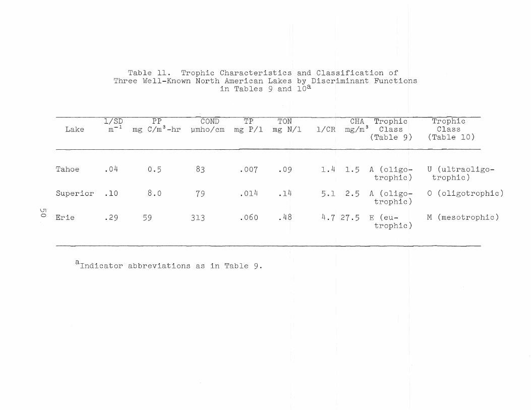
Vl 0

Lake

Tahoe

Superior

Erie

Table 11. Trophic Characteristics and Classification of Three Well-Known North American Lakes by Discriminant Functions

in Tables 9 and lOa

l/SD PP m- I mg C/m 3 -hr

.04 0.5

.10 8.0

.29 59

COND ymho/cm

83

79

313

TP mg P/l

.007

.014

.060

TON mg N/l

.09

.14

.48

l/CR

1.4

5.1

CHA Trophic mg/m 3 Class

(Table 9)

1.5 A (oligo-trophic)

2.5 A (oligo-trophic)

4.7 27.5 E (eu-trophic)

alndicator abbreviations as in Table 9.

Trophic Class

(Table 10)

U (ultraoligo-trophic)

o (oligotrophic)

M (mesotrophic)

lakes, and a single trophic index for all lakes could possibly be inappropriate. Consequently separate trophic state indices were developed from the correlative relationships of indicators within each of the two basic classes defined previously by cluster analysis. The annual mean values for each lake (Table 7) were used in the derivation of the indices. Table 12 lists the means and standard deviations of each indicator for all 24 colored lakes and all 31 clear lakes, and Table 13 presents the respective correlation matrices. The first principal components, y co andy 01' extracted from the colored and clear lake correlatlon matrlces, respectively, are shown in Table 14. The first principal components extract a good portion of the information from the R's since Yco and Ycl explain 72 and 71% of the total variances in their respective correlative matrices.

The principal components are simple linear functions of the 7 trophic state indicators with weighting factors for each indicator. The indicator values are standardized values (i.e. the actual raw value from Table 7 minus its mean value and divided by its standard deviation from Table 12). The trophic state index for each group of lakes, i.e. TSIco and TSIcl ' was derived by slightly modifying the respective first principal components. The modification consisted in adding a constant value to the principal component so that the TSI would always be greater than zero. The constant was obtained by evaluating the first principal component with raw data values of zero for each indicator. A zero raw data value results in a negative standardized value and hence a negative value for y, which value was then added to y to produce the TSI (see Table 14). Hence a hypothetical lake with zero pro­ductivity and zero values for the other indicators would then have a TSI of zero. (In actuality this would never occur since even pure water has a finite Secchi disc transparency, and all natural waters have a non-zero cation ratio.) In general, lakes with increasingly positive indicator values will exhibit correspondingly higher TSI's.

The TSI's of the lakes in each group were calculated by substituting the standardized indicator values into the appropri­ate TSI formula, and Table 15 presents the results for each group ranked in descending order of TSI value. Thus the above analysis indicates that Lake Kanapaha is the most eutrophic colored lake and Wall Lake is the least eutrophic in this group; similarly Lake Apopka (eutrophic) and Lake Santa Rosa (oligotrophic) represent the extremes of trophic state within the clear lake group.

The results of the cluster analyses (Figures 7 and 8) are also included in Table 15 for comparative purposes. Rank­ings of the clear lakes according to their TSI's are in ex­cellent agreement with the clear lake groups formed by cluster analysis. The first 12 lakes (in order of decreasing TSI)

51

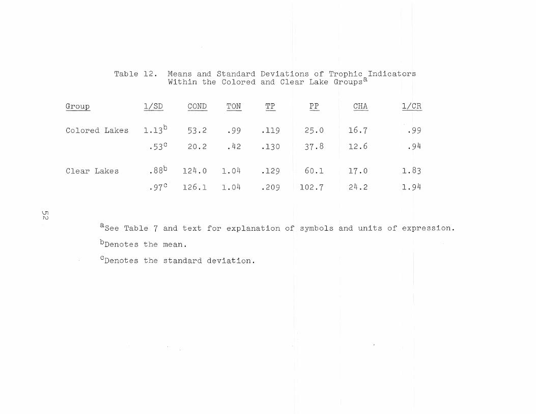
\.Jl I\.)

Table 12. Means and Standard Deviations of Trophic Indicators Within the Colored and Clear Lake Groupsa

Group l/SD COND TON TP PP CRA l/CR

Colored Lakes 1.13b 53.2 .99 .119 25.0 16.7 .99

.53 c 20.2 .42 .130 37.8 12.6 .94

Clear Lakes .88b 124.0 1. 04 .129 60.1 17.0 1.83

.97 c 126.1 1. 04 .209 102.7 24.2 1. 94

a See Table 7 and text for explanation of symbols and units of expression.

bDenotes the mean.

cDenotes the standard deviation.

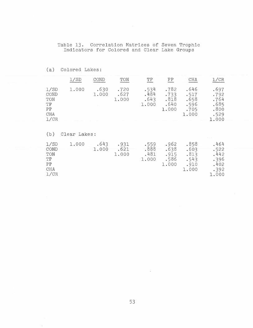
(a)

l/SD COND TON TP PP CRA l/CR

(b)

l/SD COND TON TP PP CRA

Table 13. Correlation Matrices of Seven Trophic Indicators for Colored and Clear Lake Groups

Colored Lakes:

l/SD COND TON TP PP CHA

1. 000 .630 .720 .534 .782 .646 1. 000 .627 .484 .733 .517

1. 000 .643 .818 .658 1. 000 .640 .596

1. 000 .705 1. 000

Clear Lakes:

1.000 .643 .931 .559 .962 .858 1. 000 .621 .888 .638 .603

1. 000 .481 .915 .813 1. 000 .586 .543

1.000 .910 1. 000

l/CR

53

l/CR

.697

.792

.764

.685

.800

.529 1. 000

.464

.522

.442

.396

.402

.392 1. 000

Table 14. First Principal Components (Yeo and Ycl) and Trophic State Indices (TSI co ana TSI cl )

(a) Colored Lakes;

Yco = .848(1/SD) + .809(COND) + .887(TON) + .768(TP)

+ .930(PP) + .780(CHA) + .893(1/CR)

Cumulative Percent of Total Variance Explained by Ycol = 72%

TSIcol = Ycol + 9.33

(b) Clear Lakes:

Ycl = .936(1/SD) + .827(COND) + ~907(TON) + .748(TP)

+ .938(Pp) + .892(CHA) + .579(1/CR)

Cumulative Percent of Total Variance Explained by Ycl =71%

TSIcl =Ycl + 4.76

54

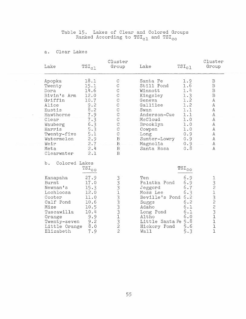
Table 15. Lakes of Clear and Colored Groups Ranked According to TSIcl and TSI co

a. Clear Lakes

Lake

Apopka Twenty Dora Bivin's Arm Griffin Alice Eustis Hawthorne Clear Wauberg Harris Twenty-five Watermelon Weir Meta Clearwater

18.1 15.1 14.6 12.0 10.7

9.2 8.2 7.9 7.3 6.3 5.3 5.1 2.9 2.7 2.4 2.1

b. Colored Lakes TSI co

Kanapaha Burnt Newnan's Lochloosa Cooter Calf Pond Mize Tuscawilla Orange Twenty-seven Little Orange Elizabeth

27.9 17.0 15.3 12.0 11. 0 10.6 10.5 10.4

9.9 9.2 8.0 7.9

Cluster Group

C C C C C C C C C C C C B B B B

3 3 3 1 3 3 3 3 1 3 2 2

55

Lake

Santa Fe Still Pond Winnott Kingsley Geneva Gallilee Swan Anderson-Cue McCloud Brooklyn Cowpen Long Sumter-Lowry Magnolia Santa Rosa

TSIcl

1.9 1.6 1.4 1.3 1.2 1.2 1.1 1.1 1.0 1.0 1.0 0.9 0.9 0.9 0.8

TSTco

Ten 6.9 Palatka Pond 6.9 Jeggord 6.7 Moss Lee 6.3 Beville's Pond 6.2 Suggs 6.2 Adaho 6.1 Long Pond 6.1 Altho 6.0 Little Santa Fe 5.8 Hickory Pond 5.6 Wall 5.3

Cluster Group

B B B B A A A A A A A A A A A

1 3 2 1 3 2 2 3 1 1 1 1

correspond to the lakes in eutrophic group C of Figure 7; the next 8 lakes are in mesotrophic groupB, and the last 11 lakes comprise oligotrophic group A. Thus the TSI for clear lakes can be used to separate classical trophic states quantitatively. A TSlcl of about 5.0 would appear to be the dividing line between mesotrophy and eutrophy, and a value of about 1.2-1.3 separates mesotrophy and oligotrophy. Qual­itative inspection of other trophic indicators for Lakes Kingsley and Winnott suggests these lakes are more typically oligotrophic thanmesotrophic and the TSI dividing line should perhaps be raised to 1.5. The colored lakes ranked according to TSl co are in general agreement with the cluster analysis (Figure 8), but some discrepancies are noted. For example, Lakes Lochloosa and Orange have a high degree of similarity; however, the lakes have high but somewhat dissimilar TSI values, and four lakes have TSI rankings between the values for the two lakes. Also Beville's, Palatka and Long Ponds were clustered into eutrophic groups although their TSI values indicate oligotrophy. The discrepancies in comparing the two analyses probably arise within the cluster analyses since the colored lakes exhibited considerable diversity and did not form groups with good within-group similarity.

For management and identification purposes it would be desirable to have a single trophic state index to rank all lakes regardless of color. Large differences in the specific conductance, primary production and cation ratio mean. values for the two groups (Table 8) and the cluster analysis of basic chemical parameters (Figure 6) suggest a basic difference which could possibly cause different trophic indicator responses in the two types. On the other hand, that the two groups can be viewed as two samples of one (larger and more diverse) popu­lation, and a single TSI to rank all 55 lakes was developed under this assumption.

Of the seven indicators used to assess trophic state in this study, the one most directly affected by organic color is Secchi disc transparency. This parameter is essentially a function of ~olor and turbidity, and a multiple regression of inverse Secchi disc reading as dependent variable vs.color and turbidity as independent variables produced the following relationship;

l/SD =0.003(Col) + 0.152(Tur) (12)

Data for the analysis were from Table 7, and the zero inter­cept option was used in the regression analysis. The relation­ship is significant at the 99% confidence level, and the per­cent Df variation in l/SD explained by Eq.12 is 96%. Using Eq. 12, a color value of 75 mg/l, and turbidity values from Table 7, new color-scaled inverse Secchi disc values were calculated for each of the 55 lakes; the results are listed in Table 7. A color value of 75 mg/l was chosen for the

56

scaling purposes because it represents the dividing line between clear and colored lakes and is also in the middle range (zone of best prediction) of the regression equation.

Once the Secchi disc values had been color scaled, the correlative relationships between the seven trophic indicators for all 55 lakes were subjected to a principal component analysis, and the means, standard deviations and the correla­tion matrix are given in Table 16. The first principal component Yt extracted from R is given by

Yt =.919(1/SD) + .800(COND) + .896(TON) + .738(TP)

+ .942(PP) + .862(CHA) + .634(1/CR) (13)

Yt extracts a good portion of the information from Rand explains 70% of the total variation in R. The TSI is given by

TSI =Yt + 5.19, (14)

where the value of 5.19 was determined as described previously in the derivations of TSI co and TSlcl '

TSI1s were calculated for each of the 55 lakes by sub­stituting the standardized indicator values (computed from Tables 7 and 16) into Eqs. 13 and 14. The lakes are ranked in descending order of TSI in Table 17. Using the cluster analyses of Figures 7 and 8 as a guide, the 55 lakes were separated in terms of classical trophic state terminology into five groups as follows: 1. Hyper-eutrophic (TSI>iO), 2. Eutrophic (10.2:TSI~7), 3. Mesotrophic (7)TSIL3), 4. Oligo,...., trophic C3 >TSI.L2), 5 . Ultra-oligotrophic (TSI<2). The se groups are delineated and labeled in Table 17. The relative rank­ings of the lakes in the TSlcl and TSI 0 formulat~ons of Table 15 are also shown in Table 17. 8omparison shows that the clear lakes are ranked in almost identical order accord~ ing to the total (55 lake) TSI (excluding the interspersed colored lakes) as they are by the TSlcl ' Further it is ob~ vious that the clear lakes as a group are more extreme in their trophic behavior than are the colored lakes; all but one of the hypereutrophic lakes and all the ultraoligotrophic lakes in Table 17 belong to the clear lake group. Nearly all the colored lakes are included in the oligotrophic and meso­trophic categories. Comparison of the colored lake rankings according to the 55 lake TSI and the TSl c also indicates a general correspondence. The lake most ouB of order is Lake Twenty-seven, which is the fourth listed colored lake in Table 17 and the tenth ranked lake according to the TSlco ' Many of the other colored lakes are "misranked" by one or two places, but there are no major discrepancies. Most of the changes in relative rankings between Tables 15 and 17 probably

57

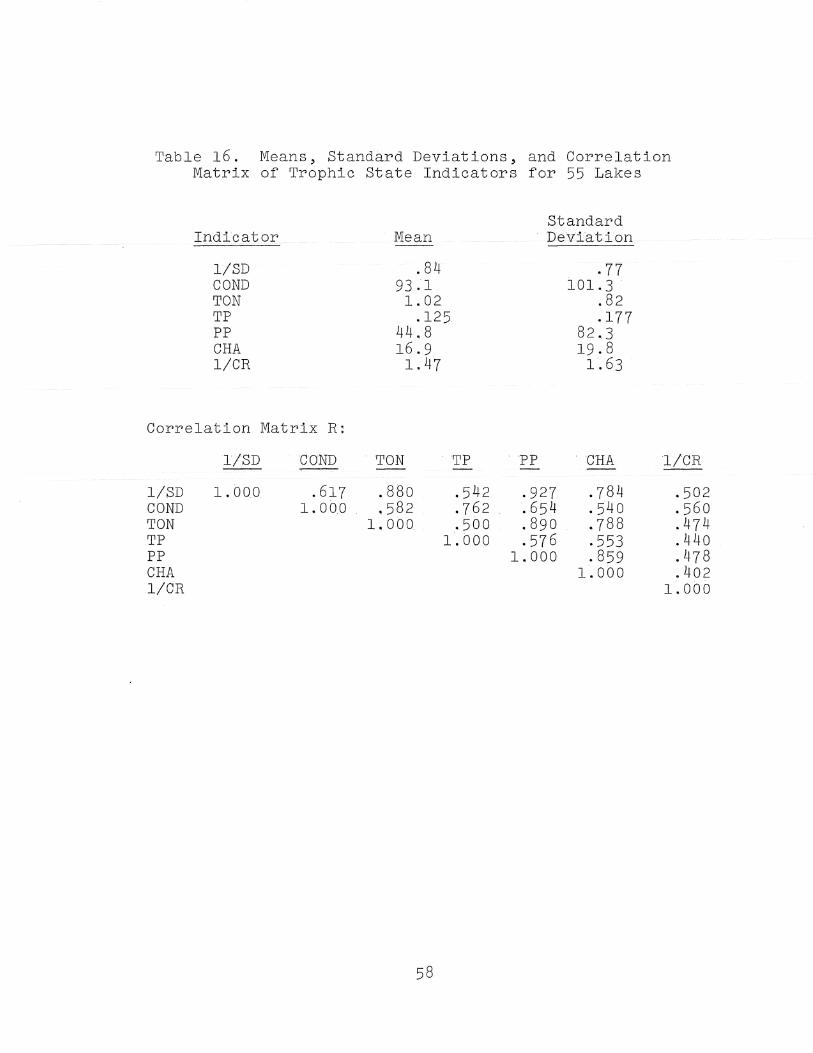
Table 16. Means, Standard Deviations, and Correlation Matrix of Trophic State Indicators for 55 Lakes

Standard Indicator Mean DeViation

l/SD .84 .77 COND 93.1 101. 3 TON 1. 02 .82 TP .125 .177 PP 44.8 82.3 CRA 16.9 19.8 l/CR 1. 47 1.63

Correlation Matrix R:

l/SD GOND TON TP PP CRA l/CR

l/SD 1.000 .617 .880 .542 .927 .784 .502 COND 1. 000 ,582 .762 .654 .540 .560 TON 1. 000 .500 .890 .788 .474 TP 1.000 .576 .553 .440 PP 1.000 .859 .478 CRA 1. 000 .402 l/CR 1.000

58

\Jl \D

Lake

1.

2.

3 .

Table 17. Fifty-five Florida Lakes Ranked According to Trophic State Index (TSI)

Hypereutrophic group

Apopka Twenty Dora Bivin's Arm Griffin Kanapaha Alice Eustis

Eutrophic group

Hawthorne Clear Bur.nt Fond Wauberg Newnan's

Mesotrophic group

Twenty-five Harris Twenty-seven

Rank in TSI Table 15 1 Lake

22.1 lS.5 lS.5 14.7 13.7 13.5 10.7 10.5

9.1 S.S S.3 7.4 7.1

6.4 6.3 5.S

lA 2A 3A 4A 5A IB 6A 7A

SA 9A 2B

lOA 3B

12A llA lOB

4.

Cooter Pond Lochloosa Tuscawilla Calf Pond Orange Mize Watermelon Pond Little Orange Weir . Elizabeth fJ;1en Palatka Pond Beville's Pond Meta

Oligotrophic group

Jeggord Moss Lee Long Pond Clearwater Altho Hickory Pond Santa Fe

Rank in TSI Table 15 1

5.3 5.2 4.S 4.6 4.3 4.2 3.6 3.4 3.3 3.2 3.2 3.2 3.1 3.IL

2.8 2.8 2.8 2.6 2.5 2.5 2.5

5B 4B SB 6B 9B 7B

13A lIB 14A 12B 13B 14B 17B 15A

15B 16B 20B 16A 21B 23B 17A

(cont'd.)

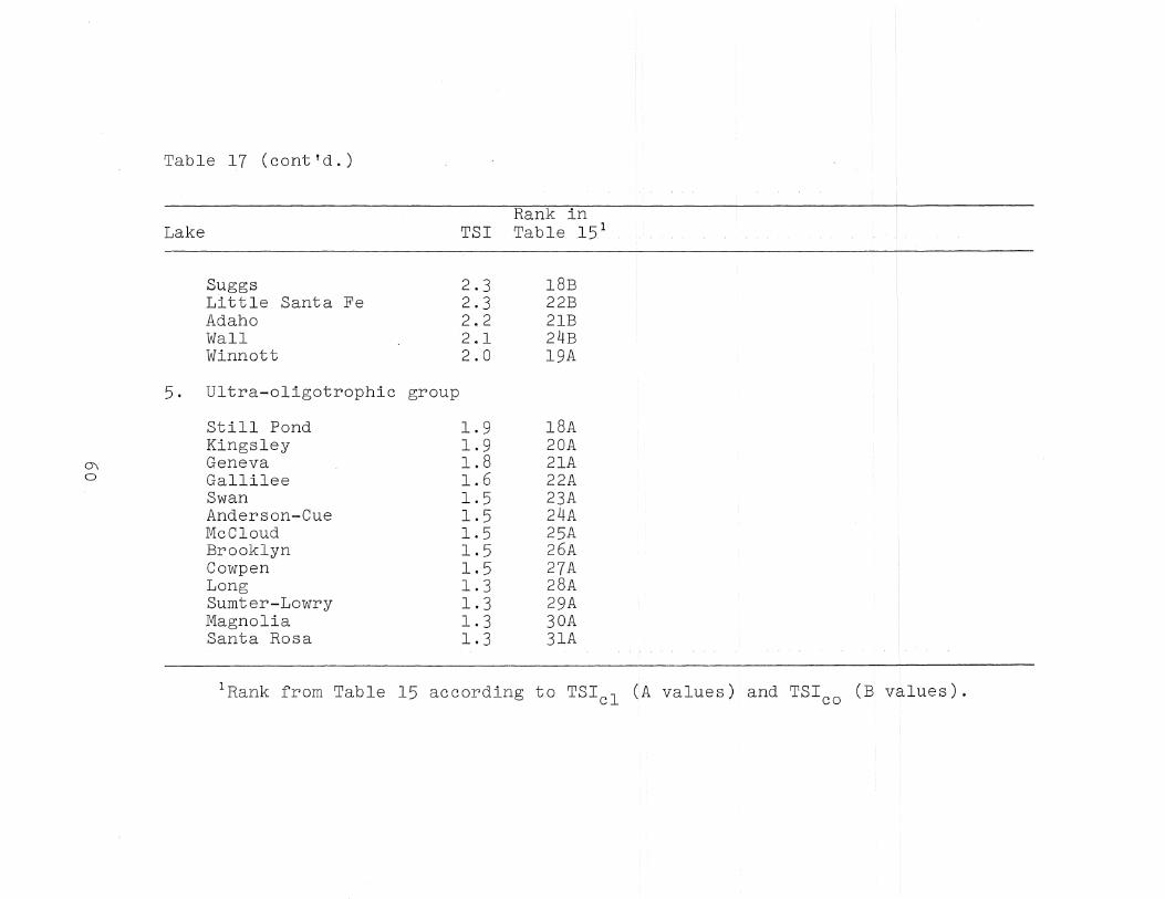
Table 17 (cont'd.)

Rank in Lake TSI TablelS1

Suggs 2.3 18B Little Santa Fe 2.3 22B Adaho 2.2 21B Wall 2.1 24B Winnott 2.0 19A

5. Ultra-oligotrophic group

Still Pond 1.9 18A Kingsley 1.9 20A

0\ Geneva 1.8 21A 0 Gallilee 1.6 22A

Swan 1.5 23A Anderson-Cue 1.5 24A McCloud 1.5 25A Brooklyn 1.5 26A Cowpen 1.5 27A Long 1.3 28A Sumter-Lowry 1.3 29A Magnolia 1.3 30A Santa Rosa 1.3 31A

lRank from Table 15 according to TSIcl (A values) and TSIco (B values).

result from the use of color-corrected Sec chi disc trans­parencies for the TSI values in Table 17, which presumably should produce a more accurate relative ranking of the lakes according to their trophic states.

The question concerning the soundness of one TSI for both clear and colored lakes remains. A definitive answer is perhaps impossible. However, the first principal component on which the 55 lake TSI is based accounts for about as much ~f the variance (70%) in the correlation matrix of trophic indicators for all lakes as do the first principal components for the clear and color groups, which accounted for 71 and 72% of the variances in their respective correlation matrices. Further, there appear to be no obvious misclassifications or misrankings in the 55 lake TSI's. One of the major values of the TSI concept is the possibility of ranking rather diverse objects (lakes) in a logical and objective manner. Obviously if the sample is too diverse, the rankings will have little or no meaning. Thus extrapolation of the TSI concept to development of a single, universal index for all lakes is not suggested. To rank Arctic bogs, acid volcanic lakes, tropical ponds and the Great Lakes on the same scale would be pointless and meaningless. On the other hand, the more "harmonious" the sample, the more meaningful and logical (and easier) it will be to rank the objects. The relat~vely harmonious series of clear lakes is easily and logically ranked (Table 15). Inclusion of the colored lakes produc.esamore diverse sample with an inevitable loss in clarity in inter­pretation of the resulting TSI. Nevertheless, it is felt that the 55 lake TSI is a useful, interpretable and logical means of ranking Florida lakes.

Some interesting features of the TSI rankings deserve mention. Lake Alice has been ranked in the hypereutrophic group although it might be classified oligotrophic on the basis of plankton productivity alone. Lake Alice has extremely high nitrogen and phosphorus concentrations and supports a profuse growth of water hyacinths, which along with a short hydraulic detention time (in the order of 2-3 days), have restricted plankton productivity. In this case, the other trophic state indicators (nitrogen, phosphorus, and conduc­tivity) have been sufficiently high to counteract the low primary production and chlorophyll a values. Lake Twenty­seven was also ranked higher than it would be on the basis of plankton production alone. This lake is almost completely covered with duckweed (Le~n~ ~inor), and as with Lake Alice the other indicators have counteracted the low primary pro­duction value,

The usefulness of the trophic state index can be best determined by its application, e.g. in practical (e.g. manage­ment and control) situations or in development of empirical m,odels relating trophic state to watershed enrichment factors

61

(see the next section). However, the validity of the approach can be inferred from closer inspection of the TSI and its component parameters. Table 18 presents the means and 95% confidence intervals for the 7 trophic indicators in each of the classes delineated in Table 17. In nearly every case the mean parameter values increase in progressing toward more eutrophic classes. However the large confidence intervals for most parameters implies considerable overlap between the classes delineated by any single indicator. These facts demon­strate three important points. First, because of -the over­lap, any single parameter is inadequate to define trophic state or trophic classes. Second, the wide and overlapping ranges of indicator values preclude easy placement of lakes into appropriate trophic classes since the values for a lake could fit within the confidence intervals of the parameters in two adjacent classes. Finally, the increasing mean values in progressing toward eutrophic conditions imply that the TSI provides at least an objective means of placing lakes into appropriate trophic classes and suggests that the rela­tive ranking of the lakes by their TSI values is reasonable.

The TSI described above reflects the general trophic conditions of Florida lakes; whether it is the best index that can be developed will have to be answered by further work comparing its attributes with those of other indices that might be developed. The seven indicators in the present index reflect the major limnological consequences of eutro­phication with the exception of macrophyte problems. Indices with fewer variables would reflect a narrower concept of trophic state and would be more likely to yield misleading results.

Specific water quality problems resulting from eutrophi­cation are not directly considered by the index, but some of the indicators are indirectly related to such problems. For example, chlorophyll a, a biomass parameter, might be correlated with taste and odor p~oblems arising from algal blooms; Secchi disc transparency is associated with water turbidity, which should be correlated with the length of sand filter runs in water treatment plants. Perhaps other indices could be developed which would be directly related to water quality problems, but it is not always a simple matter to find ap­propriate quantitative indicators for such purposes.

The index described above should be practical for rou­tine assessment of general trophic conditions since the indi­vidual parameters are commonly and rather simply measured. The only exception possibly is primary production. This parameter, while of fundamental significance to the trophic state concept, also suffers from the fact that measured values are highly variable in a given lake and are greatly dependent on physical factors such as light and temperature. Perhaps a simpler TSI not incorporating this parameter would prove

62

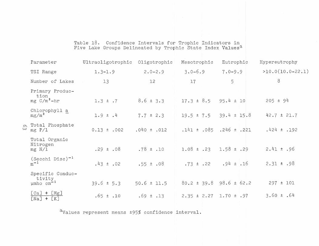
Table 18. Confidence Intervals for Trophic lndicators in Five Lake Groups Delineated by Trophic State Index Valuesa

Parameter Ultraoligotrophic Oligotrophic Mesotrophic Eutrophic Hypereutrophy

TSI Range 1.3-1.9 2.0-2.9 3.0-6.9 7.0-9.9 >10.0(10.0-22-;1)

Number of Lakes 13 12 17 5 8

Primary Produc-tion

mg C/m 3 -hr 1. 3 ± .7 8.6 ± 3.3 17.3 ± 8.5 95.4 ± 10 205 ± 94

Chlorophyll a mg/m 3 - 1.9 ± .4 7.7 ± 2.3 19.5 ± 7.5 39.4 ± 15.8 42.7 ± 21.7

0\ Total Phosphate !

LA) mg P/l 0.13 ± .002 .040 ± .012 .141 ± .085 .246 ± .221 .424 ± .192

Total Organic Nitrogen mg N/l .29 ± .08 .78 ± .10 1. 08 ± .23 1. 58 ± .29 2.41 ± .96

(Secchi Disc)-l m- 1 .43 ± .02 .55 ± .08 .73 ± .22 .94 ± .16 2.31 ± .98

Specific Conduc-tivity

llmho cm- 1 39.6 ± 5.3 50.6 ± 11.5 80.2 ± 39.8 98.6 ± 62.2 297 ± 101

[Ca] + [Mg] .65 ± .10 .69 ± .13 2.35 ± 2.27 1. 70 ± .9'J 3.60 ± .64 [Na] + [K]

aValues represent means ±95% confidence interval.

more useful to governmental agencies faced with evaluating the trophic characteristics of large numbers of lakes.

CHAPTER 5. RELATIONSHIPS BETWEEN TROPHIC STATE AND WATERSHED ENRICHMENT FACTORS

A. INTRODUCTION

Empirical relationships between lacustrine trophic condi­tions and watershed conditions can be developed by regression analysis using the TSI as dependent variable and appropriate conditions in the watershed as independent variables. A general model for eutrophication can be written as:

TS =j"(N,M,H,S,t ... ),

where TS is the trophic state resulting from nutrient (N) loading (nitrogen, phosphorus and other essential nutrients), M represents morphometric characteristics such as mean depth, H represents hydrological conditions (e.g. water detention time), S is a sedimentation factor, and t is time. The re­lationships among these parameters is presently too vague for the development of functional relationships. However, simpli­fied empirical approximations of Eq. 15 can be developed.

As a first approach models of the type

TSI = g(N,P) + C, (16)

were developed, where the TSI described in Eq. 14 represents the trophic state parameter of Eq. 15, Nand P represent annual nitrogen and phosphorus loading rates, and C is an uncertainty term. Although nitrogen and phosphorus are not the only nutri­ents required for algal growth, it is generally agreed that they are the two main nutrients involved in the lake eutrophi­cation process. In spite of current controversy over the role of carbon (Bowen, 1970; Legge and Dingeldein, 1970; Kerr et al., 1970), researchers as a whole regard phosphorus as thelTIost frequent limiting nutrient in lakes. Vollenweider (1968) and others have emphasized the importance of nutrient (particularly nitrogen and phosphorus) supply in determining a lake's trophic state. Although various lake factors, such as mean depth, detention time, basin shape, and sedimentation rate, affect the amounts of nutrients a lake can assimilate, nutrient budget calculations represent a first step in quan­tifying this dependence.

64

A few lacustrine nitrogen and phosphorus budgets have been reported in the literature, e.g. Rohlich and Lea (1949) for Lake Mendota, OOcGauheyetal. (1963) for Lake Tahoe and Edmondson (1968) for Lake Washington. Vollenweider (1968, 1969) has summarized most of the budget calculations for American European Lakes. Comprehensive evaluation of the nutrient balance for a lake requires measurement of all poten­tial nutrient sources and sinks (Table 19) over an extended period in order to assess seasonal and other effects. Some sourceB and sinks~ e.g. groundwater, nitrogen fixation an~ denitrification, require elaborate sampling and experimental procedures to be adequately evaluated. Consequently, man­power and time constraints have resulted in very few complete nutrient balances being attempted. An alternative and simpler method is to use literature estimates for nutrient exports from various sources and information on the various land use and population characteristics of the lake watershed. This approach was used by Leeet al. (1966) for nitrogen and phosphorus budget calculations for Lake Mendota. While per­haps not as accurate as actual measurement, there is no other realistic alternative when evaluating budgets for a large number of small lakes.

B. NITROGEN AND PHOSPHORUS BUDGETS

Partial nitrogen and phosphorus budgets for the 55 lakes in the study group have been computed by this latter approach. The budgets are referred to as partial since no attempt was made to account for such sources as nitrogen fixation, leaves and pollen and groundwater. Adequate data were not available to evaluate most sinks, and consequently none were considered. The partial budget calculations therefore estimate gross supply or loading.

The morphometric, land use, and population figures for each lake were determined according to the methods described in Chapter 2. Watersheds were divided into forest, urban, pasture, fertilized cropland, and cleared unproductive areas. Table 20 lists the pertinent watershed and morphometric data for each lake.

Literature figures for the expected contributions of nitrogen and phosphorus from the various sources were compiled, and the values used in this study are summarized in Table 21. Where applicable, each value is accompanied by the literature reference. Literature estimates were not available for two sources. Muck (recovered marshland) and citrus farm contribu,.... tions were calculated. from average fertilizer composition and application rates, assuming that 10 percent of the applied nitrogen and one percent of the applied phosphorus was ex­ported from the soil to the lake. The figures for percentage

65

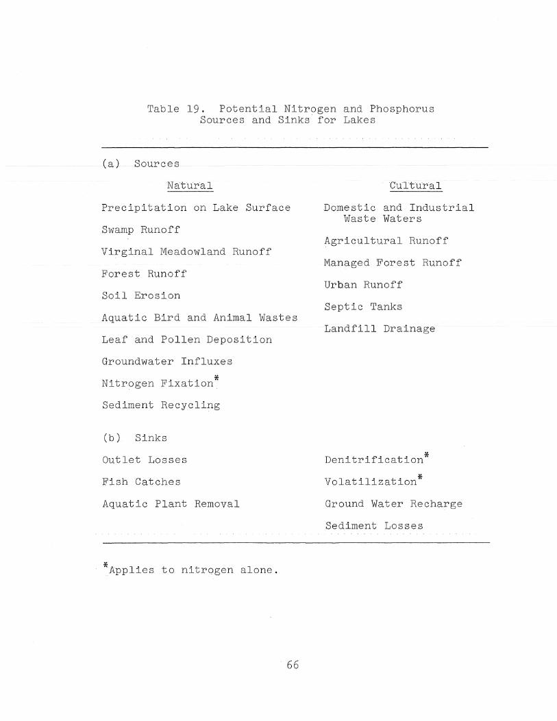
Table 19. Potential Nitrogen and Phosphorus Sources and Sinks for Lakes

~a} - Sources

Natural

Precipitation on Lake Surface

Swamp Runoff

Virginal Meadowland Runoff

Forest Runoff

Soil Erosion

Aquatic Bird and Animal Wastes

Leaf and Pollen Deposition

Groundwater Influxes

Not FO to * 1 r.ogen lxa lon

Sediment Recycling

(b) Sinks

Outlet Losses

Fish Catches

Aquatic Plant Removal

*Applies to nitrogen alone.

66

Gultural

Domestic and Industrial Waste Waters

Agricultural Runoff

Managed Forest Runoff

Urban Runoff

Septic Tanks

Landfill Drainage

Denitrification*

Volatilization*

Ground Water Recharge

Sediment Losses

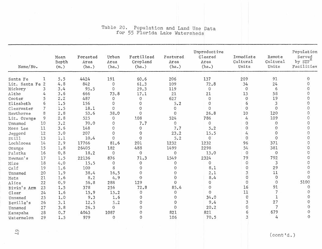
Mean Forested Depth Area

Name/No. (m. ) (ha. )

Santa Fe 1 5.5 4424 Lit. Santa Fe 2 4.8 842 Hickory' 3 3.4 95.5 Altho 4 3.6 666 Cooter 5 2.2 487 Elizabeth 6 1.5 156 Clearwater 7 1.5 18.1 Hawthorne 8 2.8 53.6 Lit. Orange 9 2.8 525 Unnamed 10 3.2 70.0 Moss Lee 11 3.6 148 Jeggord 12 3.0 207 Still 13 1.1 10.4 Lochloosa 14 2.9 17766 Orange 15 1.8 26405 Palatka 16 0.8 18.2 Newnan's 17 1.5 22136 Mize 18 4.0 15.5 Calf 19 1.6 100 Unnamed 20 1.9 38.4 Meta 21 1.6 8.2 Alice 22 0.9 56.8 Bivin's Arm 23 1.5 378 Clear 24 1.6 15.9 Unnamed 25 1.0 9.3 Beville's 26 3.1 12.5 Unnamed 27 3.8 26.3 Kanapaha 28 0.7 4043 Watermelon 29 1.5 979

0\ -..::J

Table 20. Population and Land Use Data for 55 Florida Lake W~tersheds!

Unproductive Urban Fertilized Pastured Cleared Area Cropland Area Area (ha.) (ha.) Cha.) (ha. )

191 60.6 206 137 0 61.3 109 72.8 0 29.3 119 0

13.8 17.1 21 21 0 0 627 0 0 0 5.2 0 0 0 0 0

38.0 0 0 26.8 0 108 524 786 0 7.7 0 0 0 0 7.7 5.2 0 0 23.2 15.5 0 0 5.2 0

81.6 201 1232 1232 182 488 1499 2298

0 0 0 13.0 876 71.3 1549 2324

0 0 0 0 8 0 0 8.1

16.5 0 0 2.1 4.9 0 0 8.4

288 129 0 0 256 72.8 85.4 0 15.2 0 0 0 1.6 0 0 34.0 5.2 0 Q 9.4 0 0 b 20.2

1087 0 821 821 0 0 10q 70.5

Immedi~te Population

Remote Served Cultural Cultural by STpa

Unit:s Units Facilities

2091 91 0 34i 24 0

0 6 0 131 58 0

01 19 0 61 3 0

I

O! 0 0 10i 120 0

4: 109 0 01 0 0 01 0 0 4' 0 0 01 0 0

961 371 0 54i 381 0

i oi 0 0 I

79' 792 0 01 3 0 d

I 29 0

31 11 0 0 I 0 0 a 0 5100

16 1

91 0 1Ji 7 0

d I

1 0 3! 27 0 d 7 0 e 679 0 3 4 0

I

(cont'd.)

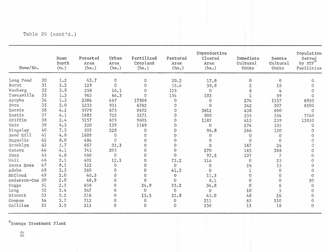
Table 20 (cont'd.)

Unproductive I

Population Mean. Forested Urban Fertilized Pastured Cleared Innn.ed ~a t e Remote Served Depth Area Area Cropland Area Area Cu1tur:a1 Cultural by STpa

Name/No. (m. ) (ha. ) (ha. ) (ha.) (ha.) (ha.) unitls Units Facilities

Long Pond 30 1.2 43.7 0 0 20.2 17.8 01 0 0 Burnt 31 2.2 129 0 0 55.4 38.8 21 18 0 Wauberg 32 3.8 258 16.1 0 123 0 6) 4 0

I Tuscawi11a 33 1.3 963 66.3 0 154 103 11 59 0 Apopka 34 1.3 2384 467 17508 0 0 274j 1157 6950 Dora 35 3.0 1233 931 6762 0 10 3421 507 6500 Harris 36 4.2 5979 675 8672 0 3612 438 690 0

!

Eustis 37 4.1 1683 722 5271 0 900 3551 554 7740 Griffin 38 2.4 5157 679 9605 0 1187 4151 239 13850 tveir 39 6.3 320 139 1168 0 0 27~ 105 0 Kingsley 40 7.3 503 328 0 0 96.8 266 120 0 Sand Hill 41 4.8 16·89 0 0 0 0 d 0 0 Magnolia 42 8.0 484 0 0 0' 0 d 0 0 I Brooklyn 43 5.7 667 32.3 0 0 0 167

1

24· 0 Geneva 44 4.1 741 205 0 0 2'70 16~ 388 0

I Swan 45 4.8 460 0 0 0 97.5 1071 7 0 Wall 46 2.1 401 12.1 0 73.2 114 d 25' 0

I

Santa Rosa 47 8.1 122 0 0 0 0 26 15 0 Adaho 48 3.5 369 0 0 41..3 0 JJ 0 0

I

McCloud 49 2.0 40.5 0 0 0 11.3 d 0 0 Anderson-Cue 50 2.0 48.9 0 0 0 8.1 d 0 50 Suggs 51 2.5 658 0 24.9 23.2 34.8 d 6 0

I Long 52 3.4 547 0 0 0 0 1q 5 0 Winnott 53 5.2 216 0 15.5 23.8 45.0 4~ 26 0 Cowpen 54 3.7 712 0 0 0 211 6~ 110 0 Galli1ee 55 3.5 213 0 0 0 150 II 18 0

I !

a Sewage Treatment plant

0\ (X)

Table 21. Expected Quantities of Nitrogen and Phosphorus from Various Sources

Quantity Source .:Reference Nit.roge.n

Domestic Sewage Vollenweider (196S) 3940a

Fertilized Area

Citrus Farms 2'.'24b

Muck Farms .11b

Pastured Area Miller (1955) .S5b

Unproductive .18b Cleared Area Brink (1964)

FClrested Area. Sylvester (1§)61) .24b

Urban Area Weibel (1969) .SSb

Rainfall Brezonik etal. (1969) .58 c --

Septic Tanks

Immediate 24 20d

Remote 970d

Domestic Ducks Paloumpis & Starret (1960) 480e

agrams/capita ~ year

bgrams/square meter of land use area ~ year

Cgrams/square meter of lake area '"" year

dgrams/septic tank ,..., year

egrams/duck - year

69

of Quantity of PhorphoruB

795a

.OlSb

.135b

.018b

.OO6b

.OO8b

.110b

.o44c

13Sd

13.Sd

90 e

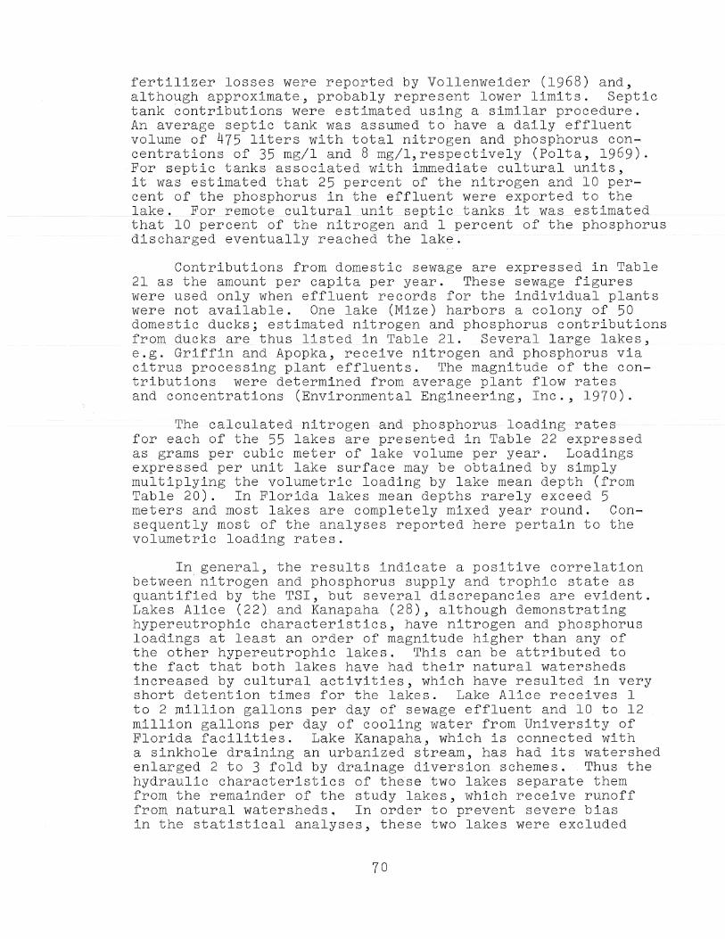
fertilizer losses were reported by Vollenweider (1968) and, although approximate, probably represent lower limits. Septic tank contributions were estimated using a similar procedure. An average septic tank was assumed to have a daily effluent volume of 475 liters with total nitrogen and phosphorus con­centrations of 35 mg/l and 8 mg/l,respectively (Folta, 1969). For septic tanks associated with immediate cultural units, it was estimated that 25 percent of the nitrogen and 10 per­cent of the phosphorus in the effluent were exported to the lakE:;--,_For_rernote cultural_unit_septic tanks it w_a_s_estirnat_ed that 10 percent of the nitrogen and I percent of the phosphorus discharged eventually reached the lake.

Contr~butions from domestic sewage are expressed in Table 21 as the amount per capita per year. These sewage figures were used only when effluent records for the individual plants were not available. One lake (Mize) harbors a colony of 50 domestic ducks; estimated nitrogen and phosphorus contributions from ducks are thus listed in Table 21. Several large lakes, e.g. Griffin and Apopka, receive nitrogen and phosphorus via citrus processing plant effluents. The magnitude of the con­tributions were determined from average plant flow rates and concentrations (Environmental Engineering, Inc., 1970).

Th€ caleulateEl nitrogen and phesphepus leading pates for each of the 55 lakes are presented in Table 22 expressed as grams per cubic meter of lake volume per year. Loadings expressed per unit lake surface may be obtained by simply multiplying the volumetric loading by lake mean depth (from Table 20). In Florida lakes mean depths rarely exceed 5 meters and most lakes are completely mixed year round. Con­sequently most of the analyses reported here pertain to the volumetric loading rates.

In general, the results indicate a positive correlation between nitrogen and phosphorus supply and trophic state as quantified by the TSI, but several discrepancies are evident. Lakes Alice (22) and Kanapaha (28), although demonstrating hypereutrophic characteristics, have nitrogen and phosphorus loadings at least an order of magnitude higher than any of the other hypereutrophic lakes. This can be attributed to the fact that both lakes have had their natural watersheds increased by cultural activities, which have resulted in very short detention times for the lakes. Lake Alice receives 1 to 2 million gallons per day of sewage effluent and 10 to 12 million gallons per day of cooling water from University of Florida facilities. Lake Kanapaha, which is connected with a sinkhole draining an urbanized stream, has had its watershed enlarged 2 to 3 fold by drainage diversion schemes. Thus the hydraulic characteristics of these two lakes separate them from the remainder of the study lakes, which receive runoff from natural watersheds. In order to prevent severe bias in the statistical analyses, these two lakes were excluded

70

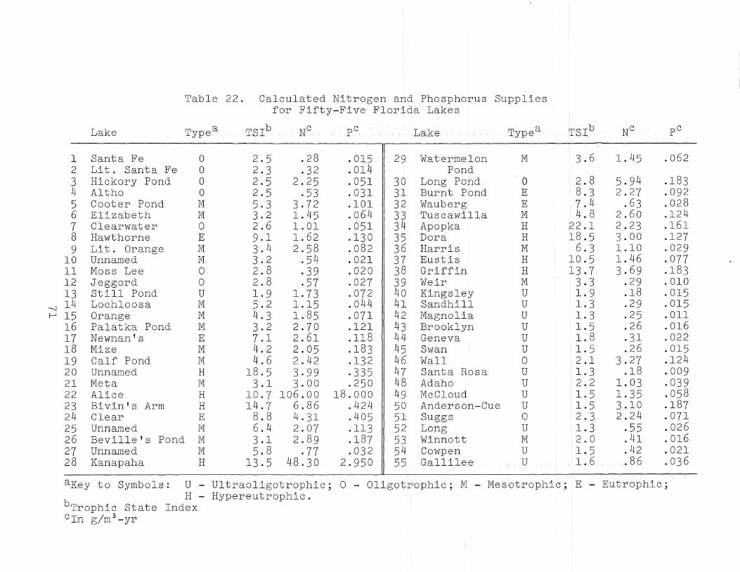
Table 22. Calculated Nitrogen and Phosphorus Supplies for Fifty~Five Flor~da Lakes

Lake a Type . b TST N c . c .p . ....... Lake .. Typea i b ['31; NC pc

1 Santa Fe 0 2.5 .28 .015 29 Watermelon M 3.6 1. 45 .062 2 Lit. Santa Fe 0 2.3 .32 .014 Pond 3 Hickory Pond 0 2.5 2.25 .051 30 Long Pond 0 2.S 5.94 .183 4 Altho 0 2.5 .53 .031 31 Burnt Pond E 8.3 2.27 .092 5 Cooter Pond M 5.3 3.72 .101 32 Wauberg E i 7 . 4 .63 .028 6 Elizabeth M 3.2 1.45 .064 33 Tuscawilla M i 4.8 2.60 .124 7 Clearwater 0 2.6 1.01 .051 34 Apopka H 22.1 2.23 .161 8 Hawthorne E 9.1 1. 62 .130 35 Dora H R8.5 3.00 .127 9 Lit. Orange M 3.4 2.58 .082 36 Harris M 1 6 .3 1.10 .029

10 Unnamed M 3.2 .54 .021 37 Eustis H 10.5 1. 46 .077 11 Moss Lee 0 2.8 .39 .020 38 Griffin H 13.7 3.69 .183 12 Jeggord 0 2.8 .57 .027 39 Weir M 3.3 .29 .010 13 Still Pond U 1.9 1. 73 .072 40 Kingsley U 1.9 .18 .015

--.:] 14 Lochloosa M 5.2 1.15 .044 41 Sandhill U 1.3 .29 .015 I-' 15 Orange M 4.3 1.85 .071 42 Magnolia U 1.3 .25 .011

16 Palatka Pond M 3.2 2.70 .121 43 Brooklyn U ' 1.5 .26 .016 17 Newnan's E 7.1 2.61 .11S 44 Geneva U i 1. 8 .31 .022 18 Mize M 4.2 2.05 .183 45 Swan U 11. 5 .26 .015 19 Calf Pond M 4.6 2.42 .132 46 Wall 0 2.1 3.27 .124 20 Unnamed H 18.5 3·99 .335 4/: Santa Rosa U i 1. 3 .18 .009 21 Meta M 3.1 3.00 .250 4$ Adaho U 2.2 1. 03 .039 22 Alice H 10.7 106.00 18.000 49 McCloud U 1.5 1.35 .058 23 Bivin's Arm H 14.7 6.86 .424 50 Anderson~Cue U 1.5 3.10 .187 24 Clear E 8.8 4.31 .405 51 Suggs 0 12.3 2.24 .071 25 Unnamed M 6.4 2.07 .113 5~ Long U i 1. 3 .55 .026 26 Beville's Pond M 3.1 2.89 .187 53 Winnott M '2.0 .41 .016 27 Unnamed M 5.8 .77 .032 5~ Cowpen U 1.5 .42 .021 28 Kanapaha H 13.5 48.30 . 2.950 55 Gall.ilee. U . i 1 ... 6 .. ..86 .036

, aKey to Symbols: U - Ultraoligotrophic; 0 - Oligotrophic; M - Mesotrophic; E - Eutrophic;

H - Hypereutrophic. bTrophic State Index cIn g/m 3 _yr

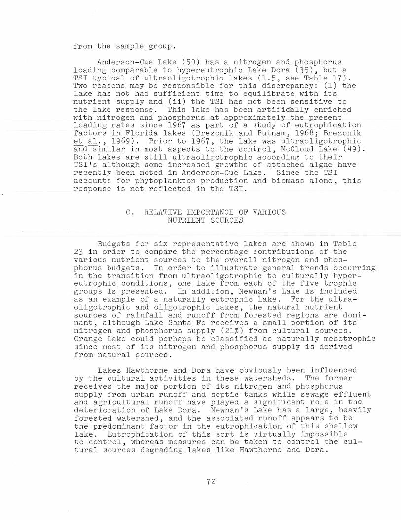
from the sample group,

Anderson~Cue Lake (50) has a nitrogen and phosphorus loading comparable to hypereutrophic Lake Dora (35), but a TSI typical of ultraoligotrophic lakes (1.5, see Table 17). Two reasons may be responsible for this discrepancy: (1) the lake has not had sufficient time to equilibrate with its nutrient supply and (ii) the TSI has not been sensitive to the lake response. This lake has been artifictally enriched

____ ................ _wit.h __ ni tra.g.enand_pho.sphorus_ at_approximat.elY'_thepr.esent loading rates since 1967 as part of a study of eutrophication factors in Florida lakes (Brezonik and Putnam" 1968; Brezonik et al., 1969). Prior to 1967, the lake was ultraoligotrophic andsimilar in most aspects to the control, McCloud Lake (49). Both lakes are still ultraoligotrophic according to their TSI's although some increased growths of attached algae have recently been noted in Anderson~Cue Lake. Since the TSI accounts for phytoplankton production and biomass alone, this response is not reflected in the TSI.

C, RELATIVE IMPORTANCE OF VARIOUS NUTRIENT SOURCES

Budgets for six representative lakes are shown in Table 23 in order to compare the percentage contributions of the various nutrient sources to the overall nitrogen and phos­phorus budgets. In order to illustrate general trends occurring in the transition from ultraoligotrophic to culturally hyper­eutrophic conditions, one lake from each of the five trophic groups is presented. In addition, Newnan's Lake is included as an example of a naturally eutrophic lake. For the ultra­oligotrophic and oligotrophic lakes, the natural nutrient sources of rainfall and runoff from forested regions are domi­nant, although Lake Santa Fe receives a small portion of its nitrogen and phosphorus supply (21%) from cultural sources. Orange Lake could perhaps be classified as naturally mesotrophic since most of its nitrogen and phosphorus supply is derived from natural sources.

Lakes Hawthorne and Dora have obviously been influenced by the cultural activities in these watersheds. The former receives the major portion of its nitrogen and phosphorus supply from urban runoff and septic tanks while sewage effluent and agricultural runoff have played a significant role in the deterioration of Lake Dora. Newnan's Lake has a large, heavily forested watershed, and the associated runoff appears to be the predominant factor in the eutrophication of this shallow lake. Eutrophication of this sort is virtually impossible to control, whereas measures can be taken to control the cul­tural sources degrading lakes like Hawthorne and Dora.

72

Table 23. Percentage Contributions From Various Cultural and. Natural Sources for S"elected Lakes

Lake Unproductive Rainfall % and Urban Fertilized Pasture Cleared Forest Septic on Lake Cul-

Type a Nutrient Sewage Runoff Area Area Area Area Tanks Surface tural

Santa Rosa (U) N 0 0 0 0 0 47 13 40 13 P 0 0 0 0 0 30 11 59 11

Santa Fe (0) N 0 7 5 7 1 41 2 37 22 P 0 15 1 3 N.S. 25 2 54 21

Orange (M) N 0 1 10 11 4 57 N.S. 17 21 P 0 5 2 6 3 49 N.S. 35 13

---1 (E) N 0 8 14 4 56 w Newnan I s 2 1 15 25 P 0 22 N.S. b 7 3 41 1 26 30

Hawthorne (E) N 0 36 N.S. N.S. 5 14 32 13 68 P 0 57 N.S. N.S. 2 6 23 12 80

Dora (H) N 13 4 74 N.S. N.S. 1 2 6 93 P 60 12 14 N.S. N.S. 1 1 12 87

aSee Table 4 for key to symbols.

bNot significant (less than 1%).

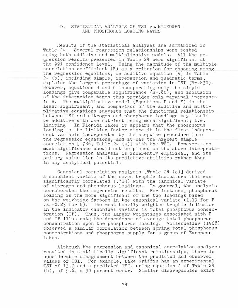
D. STATISTICAL ANALYSIS OF TSI vs. NITROGEN AND PHOSPHORUS LOADING RATES

Results of the statistical analyses are summarized in Table 24. Several regreSSion relatLonshLps were tested using both additive and multiplicative models. All the re­gression results presented in Table 24 were significant at the 99% confidence level. Using the magnitude of the multiple correlation coeffj.cient (R) as a cl'iterion_ for choQsing among the regre~sion equations, an additive equation (A) in Table 24 (b), including Simple, interaction and quadratic terms, ~xplains the largest percentage of variation in TSI (R=.830). However, equations Band C incorporating only the simple loadings give comparable Significance (R-.BO), and inclusion of the interaction terms thus provides only marginal increases in R. The multiplicative model (Equations D and E) is the least significant, and comparison of the additive and multi­plicative equations suggests that the functional relationship between TSI and nitrogen and phosphorus loadings may itself be additive with one nutrient being more significant; i.e. limiting. In Florida lakes it appears that the phosphorus loading is the limiting factor since it is the first indepen­dent variable incorporated by the stepwise procedure into the regression equations, and it has the highes~ simple correlation [.786, Table 24 (a)] with the TSI. However, too much significance should not be placed on the above interpreta­tions. RegreSSion analysis is inherently empirical~ and its primary value lies in its predictive abilities rather than in any analytical potential.

Canonical correlation analysis [Table 24 (c)] derived a canonical variate of the seven trophic indicators that was significantly correlated (.723) with the canonical variate of nitrogen and phosphorus loadings. In general, the analysis corroborates the regression results. For instance, phosphorus loading is the more significant of the two loadings based on the weighting factors in the canonical variate (1.19 for P vs. -0.23 for N). The most heavily weighted trophic indicator in the indicator canonical variate is total phosphorus concen~ tration (TP). Thus, the larger weightings associated with P and TP illustrat~ the dependence of average total phosphorus concentration upon the phosphorus loading. Vollenweider (1968) observed a similar correlation between spring total phosphorus concentrations and phosphorus supply for a group of European lakes.

Although the regreSSion and canonical correlation analyses resulted in statistically significant relationships, there is considerable disagreement between the predicted and observed values of TSI. For example, Lake Griffin has an experimental TSI of 13.7 and a predicted TSI, using equation A of Table 24 (b), of 9.6, a 30 percent error. Similar discrepancies exist

74

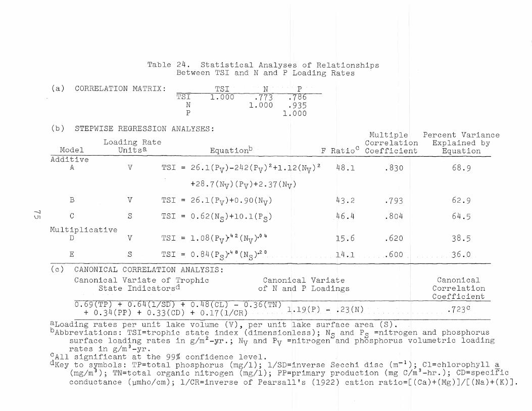
--...;J

\J1

(a)

Table 24. Statistical Analys~s of Rela~ionships Between TSI and Nand PLoading R~tes

CORRELATION MATRIX: TSI

N P

TSI 1.000

N .773

1. 000

p.

f786 .935

1.000

(b) STEPWISE REGRESSION ANALYSES: Multiple!

Loading Rate Model Unitsa Equationb

Correlation F Ratio C Coefficieht

Additive A V

B V

C S

TSI = 26.1(Py)-242(PV)2.+1.~2(NV)2.

+28.7(NV)(PV)+2.37(Ny)

TSI = 26.1(PV)+0.90(NV)

TSI = 0.62(NS)+10.1(PS)

48.1

43.2

46.4

Multiplicative D V

E S

TSI = 1.08(PV)-lt2.(NV)·Olt

TSI = 0 84(p ~lt8{N )~O . S S .

15.6

14.1

(c) CANONICAL CORRELATION ANALYSIS: Canonical Variate of Trophic

State Indicatorsd Canonical Variate

of Nand P Loadi~gs

0.69(TP) + 0.64(1/SD) +b~lrs(CL) - 0.36(TN) . + 0.34(pp) + 0.33(CD) + 0.17(I/GR)·· .... li· 1 9(P) .""' .. 23(N)

.830

.793

.804

.620

.60.0

Percent Variance Explained by

Equation

68.9

62.9

64.5

38.5

36.0

Canonical Correlation Coefficient

.J23C

aLoading rates per unit lake volume (V), per unit lake surface area (S). bAbbreviations: TSI=trophic state index (dimension~ess); NS and Ps =nitrog~n and phosphorus

surface loading rates in g/m2._yr .; NV and Pv =nitrogen and phosphorus volumetric loading rates in g/m 3-yr.

cAll significant at the 99% confidence level. dKey to symbols: TP=total phosphorus (mg/l); l/SD=inverse Secchi disc (m~l); Cl=chlorophyll a

(mg/m 3); TN=total organic nitrogen (mg/l); PP=primary production (mg C1m3-hr.); CD=specific conductance (~mho/cm); l/CR=inverse of Pearsall's (1922) cation ratio=8(Ca)+(Mg)]/[(Na)+(K)].

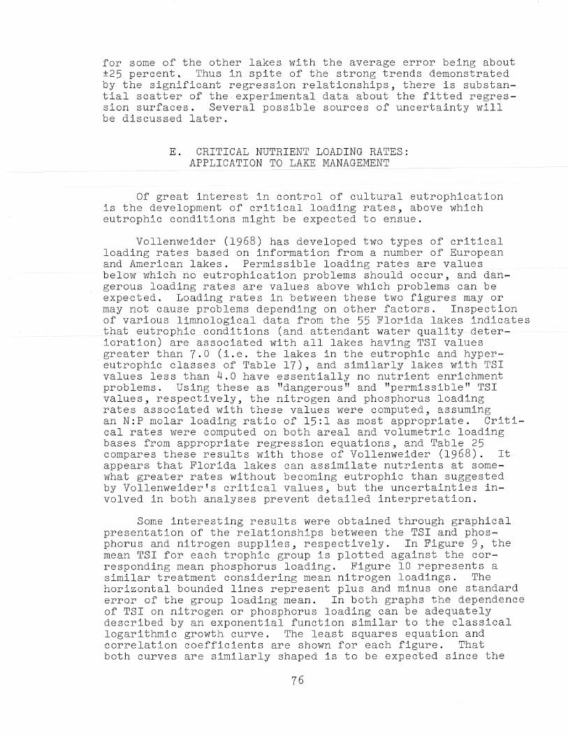
for some of the other lakes with the average error being about ±25. percent. Thus in spite. of the strong trends demonstrated by the significant regression relationships, there is substan,... tial scatter of the experimental data about the fitted regres­sion surfaces. Several possible sources of uncertainty will be discussed later.

E. CRITICAL NUTRIENT LOADING RATES: APPLIC~TION_TO LA}\El'IA1iAG_~l'1ENrr__

Of great interest in control of cultural eutrophication is the development of critical loading rates, above which eutrophic conditions might be expeDt~d to ensue.

Vollenweider (1968) has developed two types of critical loading rates based on information from a number of European and American lakes. Permissible loading rates are values beloW which·hoeutrophication problems should occur, and dan,"" gerous loading rates are values above which problems can be expected, Loading rates in between these two figures mayor may not cause problems depending on other factors, Inspection of various limnological data from the 55 Florida lakes indicates that eutrophic conditions (and attendant wat@r quality deter­ioration) are associated with all lakes having TSI values greater than 7.0 (i.e. the lakes in the eutrophic and hyper-

. eutrophic classes of Table 17), and similarly lakes with TSI values less than 4.0 have essentially no nutrient enrichment problems. Using these as "dangerous" and "permissible" TSI values, respectively, the nitrogen and phosphorus loading rates associated with these values were computed, assuming an N:P molar loading ratio of 15:1 as most appropriate. Criti,"" cal rates were computed on both areal and volumetric loading bases from appropriate regression equations, and Table 25 compares these results with those of Vollenweider (1968). It appears that Florida lakes can assimilate nutrients at some­what greater rates without becoming eutrophic than suggested by Vollenweider's critical values, but the uncertainties in­volved in both analyses prevent detailed interpretation.

Some interesting results were obtained through graphical presentation of the relationships bet~een the TSI and phos­phorus and nitrogen supplies, respectively. In Figure 9, the ~ean TSI for ea6h trophic group is plotted against the cor­responding mean phosphoru~ loading. Figure 10 represents. a similar treatment considering mean nitrogen loadings. The horizontal bounded lines represent plus and minus one standard error of the group loading mean. In both graphs the dependence of TSI on nitrogen or phosphorus loading can be adequately described by an exponential function similar to. the classical logarithmic growth curve, The least squares equation and correlation coefficients are shown for each figure. That both curves are similarly shaped is to be expected since the

76

Shannon and Brezonik, 1971c

Ibid.

Table 25. Critical Loading Rates for Nitrogen and Phosphorus

Loading Permissible Loading - -R-at@-·gnits-- -----":"'~~{~El...:.t8:c..).---,

N P

Volumetric (g!m 3 .... yr) .86 .12

Areal(g!m 2 .... yr) 2.0 .28.

Vollenweider Areal (g!m2. .... yr ) 1.0 .07 (1968)a

aFor lakes with mean depths of 5 ill or less.

77

Dangerous Loading . . "':'~iFl..:e*0eSS8f)

N P

1.51 .22

3.4 .49

2.0 .13

~--

-(f)

..... -X W 0 Z

w l-<t I-(f)

()

a.. 0 0:: I-

PHOSPHORUS SUPPLY (g Im2 - yr) o .10 .20 .30 .40 .50

20

16

12 r= .992

S

:;;-' '/

~)1/1 4

hO~" I- u4,," '"

CiIIIIIIiiI-VOLUMETRIC LOADING CURVE

- - - SURFACE LOADING CURVE

o L-______ ~ ________ ~ ________ i_ ______ ~~ ______ ~ ________ ~

o .05 .10

PHOSPHORUS .15

SUPPLY .20 .25 . 3

(g/m -yr)

Figure 9. Mean TSI Values for Five Trophic Groups vs. Annual Phosphorus Loading in 'g/Ih 3._yr ancig/m 2 -yr.

Brackets indicate range for one standard er~or. Sym­bols of trophic grou~s are: ultraoligotrophic (U), oligotrophiC (0), mesotrophic (M), eutrophic (E), hy­pereutrophic (H).

78

.30

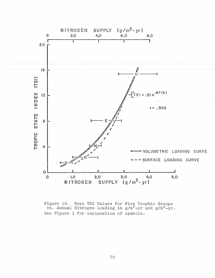
-en I--

20

16

x 12 w ~ ~ ~~ ___ ~~_~~ _____ ~_~ ______ __c ___ ~ __

z

lIJ ..... <t 8 I-

~U)

u CI.. o a::: I- 4

NITROGEN SUPPLY (g/m2 -yr) o 2.0 4.0 6.0 8.0

I-U

""

-------------------

I 1----- H ----I

-{TSI = .8Ie·S7 (N)

r = .995

- VOLUMETRIC LOADING CURVE

- - - SURFACE LOADING CURVE

O~------~--------~--------~--------~---------o 1.0

NITROGEN 2.0

SUPPLY 3.0 4.0 5~0

(g/m3 -yr)

Figure 10. Mean TSI Values for Five Trophic Groups vs. Annual Nitrogen Loading in g/m 3 -yr and g/m 2 -yr.

See Figure I for explanation of symbols.

79

nitr.ogen and phosphorus loadings are themselves highly corre­lated [See Table 24 (a)J. The within-group deviation of load­ings is considerably more pronounced for the phosphorus re­lationships, particularly for the hypereutrophic and eutrophic groups of lakes. Such deviations are to be expected when representing the complex process of trophic state change in terms of a single nutrient input. In addition, the hypereu­trophic group is essentially unbounded at the upper end and therefore not subjected to artificial boundary constraints

.... -as.ar.e.-the.-o theI'-.four .. g.rou.p.s.-.... Qu:it e-l-i-ke I-JZ'-G-hange-s--l.I'l-t.R€ limiting nutrient will occur over any extended range of trophic state response, Thus, the relationships of Figures 1 and 2 reflect only an average situation, and their major utility probably lies in the area of lake management. For example, given that either nitrogen or phosphorus is limiting and a known or proposed nutrient loading, potential lake response can be determined by consulting the appropriate relationship. It should be emphasized that the graphical relationships in

.. Figures 9 and 10 are. most applicable for shal-lowsubtrop-i.cal lakes, and their use in other situations may be unwarranted.

F. EFFECT OF DEPTH ON LAKE CAPACITY TO ASSIMILATE NUTRIENTS

As our data base expands it should be possible to incor­porate other factors of Eq. 15 into empirical eutrophication models. For example, mean depth is probably the most impor­tant morphometric factor affecting eutrophication. Figure 11 indicates a slight mean depth-trophic state relationship ex­ists for the 55 Florida lakes, with the most eutrophic lakes having mean depthsof 4 m or less and the deepest lakes being the most oligotrophic. As expected a large scatter occurs. The proper relation of mean depth to eutrophication has been confused by:many. It is neither a trophic indicator nor a causal factor per se. Rather mean depth affects the rate at which a lake can assimilate nutrients and maintain desirable trophic conditions. The graphical approach taken by Vollen­weider (1968) might prove useful in quantifying the effects of depth. The method plots nutrient (N or P) loading rates vs. lake mean depth, and the lines delineating the regions in which oligotrophic and eutrophic lakes occur are estimated by inspection. Figures 12 and 13 illustrate this approach for Florida lakes using phosphorus and nitrogen loading rates, respectively. However it is obvious that insufficient shallow oligotrophic and deep eutrophic lakes occur in the sample group to permit accurate delineation of boundary lines. Per­haps a better approach to evaluating the role of mean depth in the trophic state calculus would be the method of response surfaces (Box, 1954; Goldman, 1967).

80

r-. H U)

e 15

@ "{:!

~ IJ) u cd

~ 10 ()

-rl .r:: p.. o ~ H

5 -

o o

o

o

o

o 0

o

(>

() 0 o

o o

o 0

o o o o o

Mean Depth, M.

Figure 11. Trophic State Index (TSI) Values vs. Mean Depth for the Florida Lakes

81

1.0

HE HE

.5 -

~------------------------------~------------~--------

HE E HE

HE

o

M Eutrophic

Lakes (Florida)

./ ./

HE /

-~--------- ----- ----------- ~~--------- ---- ---------~~-~-- ------~-------~- HE./ ~-~-~ - -------~------------------

. t!>

.2

.1

/ ./

o ,,/

E o E,,/

HE M __ /

./ o

M/ /'

/ /0

U

E ./ M,,/ /'

0 0

/0

M

u

Eutrophic Lakes /' (Vollenweider) ,/

o

M

o

o M

U E o /' M

U,/ u /6 u

/' 0 U o B /

/ / ,/ Oligotrophic / ,/ Lakes

Florida)

Oligotrophi~ Lakes (Vollemveider.)

/ /

/

o

/ /

,,/

.02 ~5----------J~--------~I---------------.J~-~ ___ . ______ ~1 . 1 2 5 10

MEAN DEPTH, M.

Figure 12. Annual Phosphorus Loading Rate . Vel. Mean Depth for 55 Florida Lakes.

Each datum represents a lake in the trophic group denoted by that symbol. U = u1traoligotrophic, 0 = oligotrophic, M = mesotrophic, E = eutrophic, ·HE = l:).ypereutrophic.

82

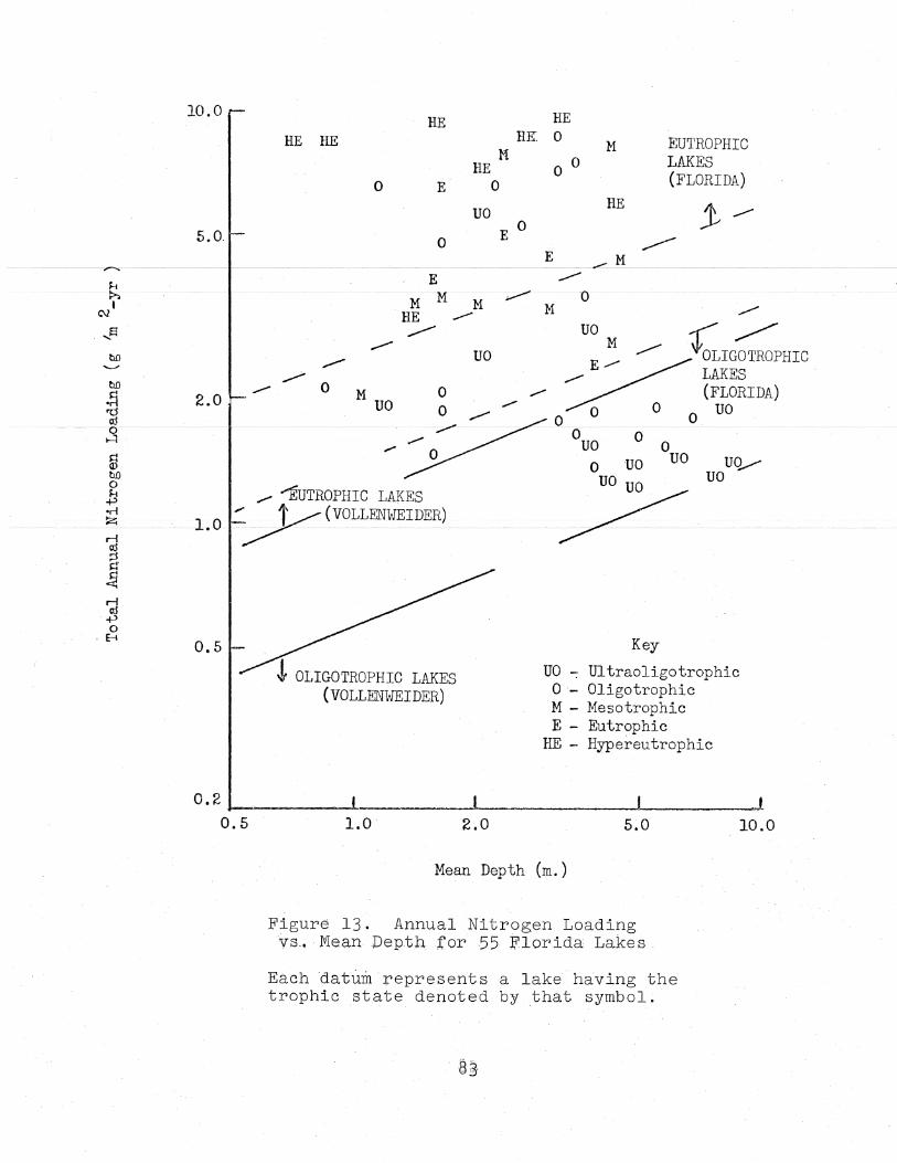
10.0 HE

HE HE

HE 0 E

UO 5.0. 0

HK M

0

E 0

HE 0

o 0

E

M

HE

EUTROPHIC LAKES (FLORIDA)

--~.,-..--------I------------_M

tto

.~ 'd cO

/

2.0

~

~

0 M UO

E M M

HE ~

0 0

M ..- M

-----UO

UO ,r ~

~~ ~ ~OLIGOTROPHIC ..- LAKES-

.- (FLORIDA) o 0 0 UO o -

~----~-o---------------~---~-~ ------------------~~ ----~O--~--~----

H

OUO UO UQ..-

......• ~.uo ~ ~UTROPHIC LAKES ~ ____ ~(VOLLENWEIDER) 1-.0 --~ -- ----

0.5

~ OLIGOTROPHIC LAKES (VOLLENWEIDER)

Key

UO ~ Ultraoligotrophic 0-- Oligotrophic M - Mesotrophic E - Eutrophic

HE - Hypereutrophic

O.2~ ________ ~, __________ ~ ____________ ~ __________ ~

0.5 1.0 2.0 5.0

Mean Depth (m.)

Figure 13. Annual Nitrogen Loading ys .• JVieanPe.p.tl1. tor 55 J;l'lorida Lakes

Each datum represents a lake having the trophic state denoted by that symbol.

10.0

G. SOURCES OF UNCERTAINTY

The above analysis represents an attempt to approximate the general trophic response function (Eq. 15) by the simple relationship between TSI and nitrogen and phosphorus loadings in Eq. 16. The uncertainty term in Eq. 16 represents the discrepancy between values of TSI predicted by the function g(N,P) and the actual (measured) TSI values, assuming the ~SI in fact represents tbe-true trophic status of' -the lake.· -

Individual components of the uncerta~nty term may include the following: (i) g is an approximation of f' (ii) the nitro~ gen and phosphorus supply calculations are in error, and (iii) the TSI does not represent the concept of trophic state (TS) completely. Approximations of f were obtained here by using multiple regression techniques. These approximations included only two of a number of potentially important variables 3 i.e.

_ nitrogen and phosphorus loadings. The loadings were estimated using land use and population characteristics and literature values of individual source contributions, a procedure that contains some inherent uncertainty. The TSI may not completely describe the concept of trophic state in spite of the fact that it incorporates seven of the more significant trophic state indicators. As previouBly discussed in reference tn Anderson-Cue Lake, it does not account for macrophyte and periphyton biomass or primary production, which in some lakes may constitute a significant proportion of total lake primary production,

H. RELATIONSHIPS BETWEEN TROPHIC STATE AND GENERAL WATERSHED CONDITIONS

Another approach to relating trophic state to watershed factors is direct regression of lake conditions (expressed by a TSI) to the extent of various land use practices and population characteristics with the watershed (expressed on a per unit lake volume or area basis), The trophic indicator data (Table 7), the TSI values (Table 17), and the population and land use data (Table 20) were used for these analyses. In addition, the correlative relationship between the seven trophic state indicators and the eutrophication factors was investigated using canonical correlation analysis. The eutro~ phication factors were expressed on a per unit lake volume basis in the ensuing analyses by dividing the values in Table 2Q by the total lake volume, Thus, the units for land use patterns were square meters for a particular land use per cubic meter of lake water, and population characteristics were expressed as number of cultural units per cubic meter of lake water. The eutrophication factors could alternatively have been expressed per unit lake surface area. However, it

84

seems more logical to express eutrophication factors for shallow Florida lakes on a unit volume basis since the entire volume is involved in assimilation and dilution of nutrient influxes. Results considering land use and population factors on a unit surface area basis were similar to the results ob­tained on a volumetric basis (Shannon, 1970). For the reasons discussed in the section on statistical analysis of the TSI vs. nutrient loading rates, Lakes Alice and Kanapaha were ex­cluded from the following analyses.

Results of regression analyses for TSI (as independent variable) vs. various eutrophication factors are shown in Table 26. Two regression equations are given; the first con­siders TSI as a linear function of the land use patterns within the watershed plus the immediate and remote cultural units. The second considers TSI as a function of the land use patterns plus total cultural units (TCU), i.e. the sum of remote, immediate and sewage treatment cultural units. The independent v-ariables of the regression equations are written in the step""" wise order in which they were incorporated into the equation, i.e. in decreasing order of their partial correlation with TSI. Both equations in Table 26 are statistically Significant at the 99% confidence level and both explain about 80% of the total variance in the TSI.

The first independent variable in both equations is the fertilized cropland; other culturally influenced factors such as urban area and immediate cultural units are important var­iables in explaining the variance in TSI. A natural factor, forested areas, is also important, but other factors like un...., productive cleared area, remote septic tanks and pastured areas add little to the predictive abilities of the equations. These results can be interpreted as suggesting that culturally influenced factors (fertilized cropland, ~rban runoff, septic tank drainage) are among the most .important variables deter­mining the trophic states of Florida lakes. However, it should also be emphasized that regression analyses are inherently empirical, and while they may suggest, they never prove cause­effect relationships.

A canonical analysis of the seven trophic indicators (Table 7) and six eutrophication factors (the land use areas and total cultural units) (Table 20) for the 55 lakes is pre­sented in Table 27. The correlation coefficient between the two canonical variates II and JEF is high (0.94) and signifi­cant at the 99% confidence leveI. In the trophic indicator canonical variate (II)' primary production is weighted consider,.... ably higher than the other indicators, suggesting it is of fundamental importance in the trophic state_eutrophication factor relationship. At the other extreme the cation ratio has a low weight and appears to be of minor importance in the relationship. Cultural factors (urban area and fertilized cropland) carry the heaviest weightings in the eutrophication

85

Table 26. Stepwise Regression Analysis of TSI vs, Eutrophication Factors Expressed Per Unit

Lake Volume 1

(1) Regression Equation:

TSI = 14.95(HFA) + .64(FOR) + 2.72(ICU) + 1.59(URB) 59.6 73.9 80.0 81.2

~ .35(UCA) + .06(RCU) ~ .02(PA) 81.5 81.5 81.5

F Ratio = 28.9B*** Multiple Correlation Coefficient Cr) = .903· Percent of total variation explained ldythe

regression equation =81.5%

(2) Regression Equation:

TSI = 14~49CHFA) + .61(FOR) + 2.2~CURB) + .53(TCU) . 59.6 73.9 79.4 80.0

+ .31(UCA) - .01(PA) 80.3 80.3

F Ratio =31.91*** Multiple correlation coefficient (r) = .896 Percent of total variation explained by the

regression equation = 80.3%

Key to Eu,trophicatiQn ';F'actor Sy'mbols:

BFA = Heavily fertilized cropland CmZ/m3) FOR = Forested area (mZ/m3) ICU = Immediate cultural unitsC#/m3 xlOIt) URB = Urban area CmZ/m3) UCA = Unproductive waste cleared area Cmz/m') RCU = Remote cultural units C#/m'xlOIt) . PA = Pastured area Cm Z/m 3) TCU = Total cultural units C#/m3 x lOIt)

***Denotes significant F valu,e at the 99% confidence level.

lValues below symbols in regression equati.on indicate curnu,latiye percent of total variance explained by independent variables up to that point.

86

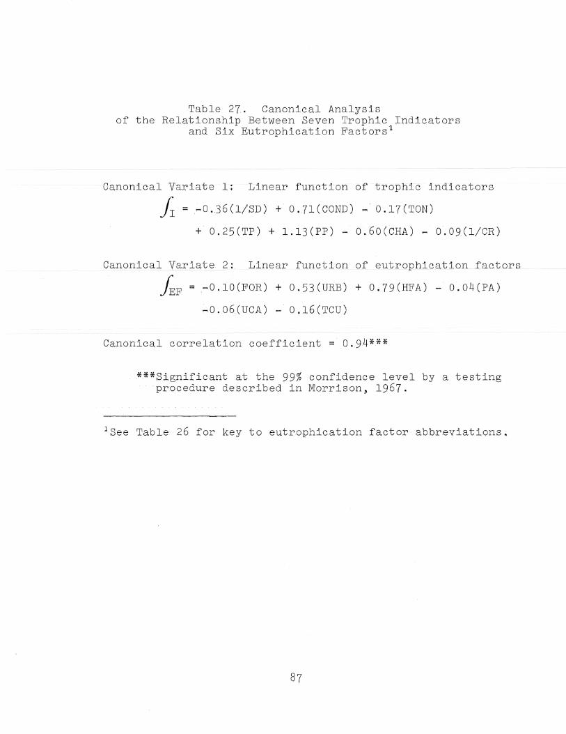
Table 27. Canonical Analysis of the Relationship Between Seven Trophic Indicators

and Six Eutrophication Factorsl

Canonical Variate 1: Linear function of trophic indicators

fr =~0.36(l/SD) + 0.71(COND) ~ 0.17(TON)

+ 0.25(TP) + 1.13(PP) - 0.60(CHA) - 0.09(1/CR)

Canonical Variate~2; Linear function of eutrophication factors

hF = - 0 . 10 (F OR) + o. 53 (URB) + O. 79 (HF A) - O. 04 ( P A)

-0.06(UCA) - 0.16(TCU)

Canonical correlation coefficient = 0.94***

***Significantat the 99% confidence level by a testing procedure described in Morrison, 1967.

lSee Table 26 for key to eutrophication factor abbreviations.

87

factors canonical variate ((E ); pasture and unproductive cleared areas carry the lo~s~ weightings, which corroborates the regression results of Table 26. Thus in general it appears that the major link between trophic state ((I) and eutrophi­cation factors (fEE) is one of primary prodfiction and the cultural factors of urban and heavily fertilized areas.

Comparing the canonical correlation of trophic indicators vs, nitrogen and phosphorus loadings (Table 24) with the _C3.J::>9ve_ anC3.JYsj.§ iQCl.i~a~E:'!_~a higher __ cor~e_lat_iDn_cDei'f'icient _was_ obtained in the latter analysis. There is some inherent error in using literature values of the expected nitrogen and phos­phorus contributions from land use patterns in order to ob­tain nutrient loadings, and this quite likely explains the lower correlation for the analysis using the nutrient loading rates. In other words, the land use and population character ...... istiDS in their raw form contain more significant information than the calculated nitrogen and phosphorus loadings.

E~pirical relationships such as those in Tables 26 and 27 depend on the fact that runoff from various land use prac-tiDes has different and to an extent defined nutrient enrich­ment effects on receiving bodies of water. Similarly the population within a watershed can be dIvided into a few main -g-rQups(e. €,:}.- people on sewerag.esy-stems,peeple usingsept±c tanks in the immediate vicinity of a lake, etc.) which have similar (within group) enrichment effects. Refinement of this type ot regression relationship could prove beneficial to regional planners and land use (zoning) boards.

In evaluating the statistical relationships between trophic state and eutrophication factors, the time element has not been considered. ;It has been assumed that lake trophic state as reflected by. the TSI or certain tr.ophicstate indica ..... tors waS a r,esult of the eutrophication factOrs at that time or, in other wQrds~ trophic statea.nd the eutrophication fac,... tors were in equilibrium at the time they were evaluated. In reality, the trophic state of a lake is the result of the eutrophication factors influence over a period of years. For example, the hypereutrophic conditions of Lakes Apopka and Dora in the Oklawaha group are due to the intense cultural activities around the lake in the past two or three decades. On the other hand, Anderson-Cue Lake has been subjected to a high rate of nutrient enrichment over a period of three years but remains in an oligotrophic condition, presumably because it has not had sufficient time to demonstrate a re~ sponse. Very little is known about the response time of a lake to nutrient enrichment, and as yet it is impossible to quantify. However, it seems reasonable to assume that the majority of the lakes are in a state of dynamic equilibrium with their environments; the relatively high correlations between causal factors and effects would seem to substantiate this point.

88

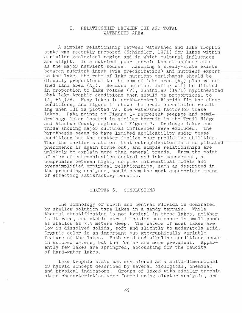
I. RELATIONSHIP BETWEEN TSI AND TOTAL WATERSHED AREA

A simpler relationship between watershed and lake trophic state was recently proposed (Schindler, 1971) for lakes within a similar geological region and in which cultural influences are slight. In a nutrient poor terrain the atmosphere acts as the major nutrient source. Assuming a steady-state exists

--------- --- -------be-t-ween-nut-I'-i-ent--i-rl-pu-t--(-v-ia--pp-@Gi-p~ta t-1-gn -J-anQ--nu-t-F-1-e-nt-e-*-£3 E>F-t - ---- --­to the lake, the rate of lake nutrierit enrichment should be directly proportional to the sum of lake area (Ao) plus water-shed land area (Ad)' Because nutrient influx will be diluted in proportion to lake volume (V), Schindler (1971) hypothesized that lake trophic conditions then should be proportional to (Ad +AQ)/V. Many lakes in north-central Florida fit the above conditlons, and Figure 14 shows the crude correlation result-ing when TSI is plotted vs. the wa-tershed factor for these lake-s-. Data-poin-ts in F-igu±,& 1-4--I'&pr&s@nt s-&epag@-ar:J..Q- s-€l-mi .... drainage lakes located in similar terrain in the Trail Ridge and Alachua County regions of Figure 2. Drainage lakes and those showing major cultural influences were excluded. The hypothesis seems to have limited applicability under these conditions but the scatter implies poor predictive abilities. Thu-s-thee-arlierstatement thateutrophicat"1:on is a c;omplicated phenomenon is again borne out, and simple relationships are unlikely to explain more than general trends. From the point of view of eutrophication cont~ol and lake management, a compromise between highly complex mathematical models and oversimplified empirical relationships, such as described in the preceding analyses, would seem the most appropriate means of effecting satisfactory results.

CHAPTER 6. CONCLUSIONS

The limnology of north and central Florida is dominated by shallow solution type lakes in a sandy terrain. While thermal stratification is not typical in these lakes, neither is it rare, and stable stratification can occur in small ponds as shallow as 3.5 meters deep. The waters of most lakes are low in dissolved solids, soft and slightly to moderately acid. Organic color is an important but geographically variable feature of the lakes. Both acid and alkaline conditions occur in colored waters, but the former are more prevalent. Appar­ently few lakes are springfed, accounting for the paucity of hard-water lakes. .

Lake trophic state was envisioned as a multi-dimensional or hybrid concept described by several biological, chemical and physical indicators. Groups of lakes w1th similar trophic state characteristics were formed using cluster analysis, and

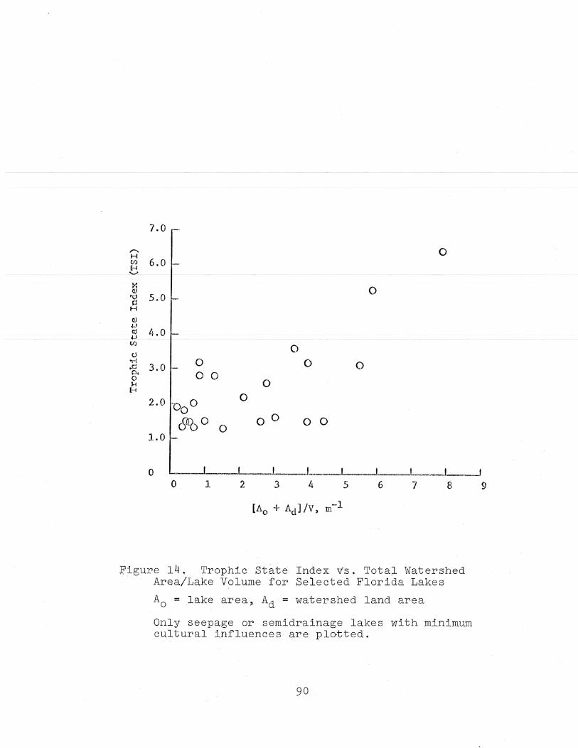
7.0

,..... H ~ 6.0

~ ~~~ ~-~--~------ -------~

@ ] 5.0 H

OJ +J Cll 4.0 __ ~~ ____ ~,u_ ~_

til

t.I ..-l ..c:: 3.0 p. o ~

E-t

2.0

1.0

0 o 0

0 0

8£60

o

o

0 0 0

0 0

0 0° o °

o ~--~----~--~----~ _____ ~ __ ~I __ ~L-.,. I o 1 2 3 4 5 6 7 8

-1 m

Jrigure14. Trophic State Index. v's. Total Watershed . Area/Lake Volume ~or Select~d Florida Lakes

Ao = lake area, Ad = watershed land area

Only seepage or semidrainage lakes with minimum cultural influences are plo·t.ted.

90

, 9

these groups could be interpreted in the classical (oligo­trophic-mesotrophic~eutrophic) sense.

A trophic state index (TSI) was formulated using prin­cipal component analysis incorporating seven trophic state indicators. The TSI quantified the concept of trophic state on a numerical scale, thus providing a method for ranking and comparing lake trophic states.

The t_rophic_states_ of -Florida lakes are largelydepen­dent on gross nitrogen and phosphorus supplies (loading rates) as evidenced by significant regression relationships between TSI and Nand P loading rates and significant canonical cor­relation between seven trophic indicators and the Nand P loadings. Phosphorus loading was the most important vari~ able from a statistical viewpoint in the regression and canon­ical relationships, and it might be inferred that on an average basis phosphorus is the (most common) limiting nutrient for Florida lakes.

Cultural nutrient sources are relatively unimportant in oligotrophic lakes, but for many eutrophic lakes, cultural sources are by far the most significant. Critical nutrient loading rates were calculated for Florida lakes based on the regression relationships. Florida lakes seem capable of assimilating greater quantities of nutrients than suggested by Vollenweider's critical loading figures~ but the two studies are in general agreement.

A positive correlation exists for Florida lakes, between lake trophic state and lake watershed land use and population characteristics. The relationship was verified by statisti­cally significant multiple regression equations using the TSI as the dependent variable and several watershed land use and population characteristics as independent variables. Canonical correlation analysis of several trophic state indi­cators versus the population and land use characteristics showed high correlation and corroborated the regression re­sults. It appears that cultural influences have played a major role in determining the trophic states of Florida lakes. Regression and canonical analyses results indicate that the most influential eutrophication factor from a statistical viewpoint is fertilized cropland.

In spite of the statistically significant results ob­ta~ned in this study there are several sources of uncertainty in the methodology. These sources have been discussed in the text and should not be overlooked in studies of a similar nature.

91

APPENDIX

MULTIVARIATE TERMINOLOGY

The term "multivariate analysis" is used to describe statics t-i-&al-t-e-e :8-nic~-ue-s-----e-e n&e-p-B-B-a-w-i-t-:8-ana-l y-z4-B-g-aa-ta--e e l-~e 0 tea­for p different variables on N objects.. For example, the variables in this study are chemical, biological, and physi~ cal characteristics measured on several lakes representing the objects, Some dependency is assumed among the variables so that they are considered as a system, implying that no vari~ able can be separated from the group and considered individu~ ally. This feature distinguishes multivariate data and tech~ niques from their multi-dimensional nature multivariate tech­niqu@s are-.-most--egnvenie-ntly--dese-pilded u-singv@e-t~H?·an-d matl?ix notation. .

Vector quantities in the text are underscored, for ex­ample ~i represents the vector of p variables for lake i. Matrix quantities are denoted by capital letters, and scalar quantities are denoted by small le-t-ters. Vectors are c-olumn vectors unless the transpose is indicated by priming the vector (e.g. x.' is the transpose of xi)' The inverse of a rna trix A lS deAoted by A -1 • The (ij T -th element of a matrix A is denoted by aij'

Suppose that the assumptions of random and independent sam,pling have been satisfied and observation vectors of p variables are evaluated for N lakes. The resulting collec~ tion of data may be expressed in an Nxp (N rows and p columns) raw data matrix:

x x X 1 1 1 2 1P I

X X22 x (A-I) 21 2p X = . , . .

XN1 XN2 xNp

The X matrix is the starting point .for most multivariate pro­cedures. Analogous to the univariate situation where a ran­dom variable x is considered to be normally distributed with mean 11 and variance .cr 2 ,. multi va.riate . .ctata.areconsidered to be realizations of a p-dimerisional random variable distributed multivariate normal with mean vector 11 and covariance matrix L:. AS)1 andcr 2 are estimated by the Sample .mean x and the sample variance 8 2 in the univariate case, )1 and E are estimated

92

by the vector of sample means of the p variables X and the sample covariance matrix S:

and CA-3)

S is the p x p matrix of covariance between all possible pairs of variables, ~. e. si,i = t~e cova::ian?e hetween variables x· and x·. S 1S a sy~etr1c matr1x, 1.e. 8i' =s .. , except f~r i=j.J The variance of variable xi is coniaine~lin the element sii'

The matrix of sample correlations between all possible pairs of variables is denoted by the matrix R where:

Slj

Is .. s· . 11 JJ

The matrix R can be computed from S by the expression:

R = C 1 ) 'c 1 ) D-.S.D-, 'si si

CA-4)

(A-5)

where DCJ:-.) denotes a matrix containing the reciprocals of the si standard deviations in the diagonal elements and zeros in all other elements of the matrix. The matrix R is also p x p and symmetric.

When the variables under consideration are in different units and ranges it is necessary to transform (or standardize) them to a scale of common origin and units. The Z score method is a commonly used standardization technique. The raw data matrix X is transformed to the standardized matrix Z by

CA-6)

where Z and X are the Nxp matrices of transformed and raw variables, respectively. I is theNxN identity matr~x with l's on the diagonal and zeros elsewhere, E is an NxN matrix with lIs in every position and D is a pxp diagonal matr~x with reciprocals of the standard deviations on the diagonal ele­ments and zeros elsewhere. The general element of Z is given by

93

z·· . lJ = X'ij,"",Xj

Sj

94

ACKNOWLEDGEMENTS

This research was supported in part by Office of Water Resources Research Matching Grant DI 14-31-0001-3068 and a grant from the State of Florida Game and Fresh Water Fish Commission. A Federal Water Quality Administration Grant -DON 16010 - (H. D. Putnam, principal investigatgr) ,_ supported a sub-stantial porTion -of the proj ect, especially in its early phases.

A number of faculty colleagues have contributed advice and encouragement, including Drs. Hugh D. Putnam, James P. Heaney, William H. Morgan, and Jackson L. Fox. Dr. Fox was especially helpful in providing needed assistance in sampling and in the various biological aspects of the project. The assistance of Dr. Morgan in administrative affairs and in the compretion of this report is truly appreciated.

Special thanks also go to Roger Yorton and Michael Keirn, project assistants and graduate students in the Department of Environmental Engineering, for their cooperation in arranging and conducting the sampling trips and running the chemical and biological analyses.

95

BIBLIOGRAPHY

Aberg, B. and Ro hde, W., HUber die Milieufaktoren in einigen su.dschwedischen Seen, "Symb. Botan'. Up'psala, Vol. 5, 1942, pp. 1-256.

Anders on, T. W., An Tntr'od\ictiontoMuTt'ivariate Statistical Analysis, John Wiley and Sons, Inc., New York (1958).

-Beet on~A--:--~196-S--:---Eu troph-i c a '[1 on 0 r-'fhe -S't~awrence ---------­Great Lakes. Limnol. Oceanogr., 10:240-254.

Birge, E. A. and Juday, C., "The Organic Content of the Waters , of Small Lakes," Proc. Amer. Phil. Soc., Vol. 66, 1927,

pp. 357-372.

Birge, E. A. and Juday, C. 1934. Particulate and Dissolved Organic Matter in Inland Lakes. Ecol. Monographs, 1:440-474.

Box, G. E. P. 1954. The exploration and exploitation of response surfaces: some general considerations and ex­amples. Biometrics 10, 16-60.

Bowen, D.H. M. EmTiron ._S~L.TeGhnQ~. 1., 725--.726 (197Q1.

Bradley, W. H. and M. E. Beard. 1969. Mud Lake, Florida; its algae and alkaline brown water. Limnol. Oceanogr., 14: 1277-1279. --

Brezonik, P. L., "Eutrophication: The Process and Its Modeling Potential," Proc. Workshop Modeling the Eutrophication Process, Univ. Florida, Gainesville, 1969, pp. 68-110.

Brezonik, P. L.and C. L.HarpSr. 1969. Nitrogen fixation in some anoxic lacustrine environments. Science, 164,:1277-1279.

Brezonik, P. L., Morgan, W. H., Shannon, E. E., and Putnam, H. D. 1969. Eutrophication factors in north central Florida lakes. Univ. Florida Industr. Engrg. Exper. Station, Bull. Ser. No. 134, Gainesville, 101 p.

Brezonik, P. L. and Putnam, H. D., "Eutrophication: Small Florida Lakes as Models to Study the Process." Proceedings, 17th South. Water Resources and Poll. Contr. Conf., Univ. North Carolina, 1968, pp. 315-333.

Brezonik, P. L. 1971. Nitrogen: sources and transformations in natural waters. Presented at 161st Nat. Meeting, Amer. Chern. Soc., Los Angeles, Calif., April, 1971.

Brink, N. in "Nordisk Killokium om Eutrofieringsproblemer," O. Skulberg, ed., Norsk Inst. Vannforskning, Blindern, Norway, 1964.

96

Chen, C. 1970. Concepts and utilities of an ecologic model. J. Sanit. Engrg. Div., Amer. Soc. Civil Engr. 96, 1085-1097.

Clark, W. E., Musgrove, R. H., Menke, C. D. and Cagle, J. W., Jr. 1962. Interim report on the water resources of Alachua, Bradford, Clay and Union Counties, Florida. Florida Geol. Survey, Information Circular No.~, 92 p .

. c:;ooke ,_C .. _W. 19 3g . Scenery of Florida. _ F.lor ida_G.eo 1. Sur.­vey, Geol. Bull. No U, 118 p.

DiToro, D. M., O'Connor, D. J. and Thomann, R. V. 1970. A dynamic model of phyto-plankton populations in natural waters. Environ. Engrg. and Sci. Program, Manhattan College, Bronx, New York (mimeo).

Dixon, W. J . (Ed.), Biomedical Computer Programs , Uni v. California Publ. in Automatic Computation No. 2, Univ~ Calif, Press, Berkeley, 1968.

Edmondson, W. T.,in "Water Quality Control," Univ. Washington Press, Seattl~ Wash., 1968.

Env~ronmental Engineering Ine., Gainesville, Florida, personal communication, 1970.

Fisher, R. A., "The Use of Multivariate Measurements in Taxonomic problems,!! Annals of Eugenics, 7:179 (1936).

~lorida Board of Conservation. 1969. Florida lakes. Part III. Gazetteer. Div. Water Resources, Tallahassee. 145 p.

Fruh, E. G., Stewart, K. 00., Lee, G. F., and Rohlich, G. A. 1966. Measurement of eutrophication and trends. J.WaterPolT.Contr. Fed. 38, 1237~1258.

Goldman, C. R. 1967. Integration of field and laboratory experiments in productivity studies. In Estuaries, G. Lauff (ed.), Amer. Assoc. Adv. Sci., Washington, D.C. pp. 346,..,352.

Goldman, C. R. and Armstrong, R. 1968. studies in Lake Tahoe, California. Ve~. Limnol, 17, 49.

Primary productivity Verh. Tnternat.

Goldman, C, R.~ Gerletti, 00., Javornicky,P., Melchiorri~~ Santolini, U., and DeAmezaga, E. 1968. Primary produc,.., tivity, bacteria, phyto- and zooplankton in Lake Maggiore; Correlations and relationships with ecological factors.

Mem. 1st. TtaT.ldrohio1. 23, 49':""127.

97

Gower, J. C., "A Comparison of Some Methods of Cluster Analysis," Biometrics, Vol. 22, 1966, p. 623.

Hansen, K. 1962. The dystrophic lake type. Hydrobiologia, 19: 183~191.

Hasler, A. D., "Eutrophication of Lakes by Domestic Drainage," Eco16gy, Vol. 28, 1947, pp. 383-395.

Hos)peI'_~ F. F. ~ "Eutro:Qhication InciJces and Their Relation tQ _____ _ Other Indices of Ecosystem Change," In: Eutrophica'tion: Causes,Consequences,Corre'ctiVes, National Acad. Sci., Wash., D.C., 1969, p. 225-235.

Hutchinson, G.E. 1957. Wiley, New York.

A treatise on limnology. Vol. 1. 1015 p.

Hutchinson, G.E. 1969. Eutrophication past and present. In Eutrophication : Causes ,Conseq\ien'ces', CorrectiVe s, _

'Rat. Acad. Sci" U. S., Washington, D.C. pp. 17~26.

Iovino, A. J. and Bradley~ W. H. 1969. The role of larval Chironomidae in the production of lacustrine copropel in Mud Lake, Marion County, Florida. Limnol. Oceanogr., 14 :.898=-905.

Keirn, M. A. and Brezonik, P. L. 1971. Nitrogen fixation by ba~teria in Lake Mize, Florida and in some lacustrine sediments. Limnol. Oceanogr.16 (in press).

Kenner, W. E., "Maps ~howing Depths of Selected Lakes in J;i'lorida, II lnformation Circ. No. 40, .Pla. Geol. Surv., Tallahassee, 196~.

Kerr, P. C., PariS, D. F., BDockway" D. L., "The Interrela .... tion of Carbon and Phosphorus in Regulating Heterotrophic and Autotrophic Populations in Aquatic Ecosystems, I' Water Poll. Contr. Res. Serf 16050, Fed. Water Qual. Admin., 1970. '

Lee, G. F.,etal., "Report on the Nutrient Sources of Lake Mendota-;rr Nutrient Sources Subcommittee of the Lake Mendota Problems Committee, Madison, Wis., 1966 (mimeo).

Lee ", P. J. 1971.JVIultiVariate 'an'alys'isf'c:ir' 't'h:e'fis'h'e'r,i'eq biology. Fish. Res. Bd. Canada, Tech. Rept. 244, )1reshwater Institute, Winnipeg, Manitoba, 182p.

Legge, R. F., Dingeldein, D., Canad. Res. Develop" March~ 1970" p. 19,...,42.

Ludwig, H. F., Kazmierczak, E., and Carter,R. C., "'Waste , Disposal and the Future of Lake Tahoe ,'I J. ASCE,90 (3) : 27(1964),

Margalef, R. 1958. Trophic typology versus biotic typology, as exemplified in the regional limnology of northern Spain. Verh. Internat. Verein. Limnol.13:339-349.

Maslin, K. E. Ph.D. thesis, University of Florida, Gainesville, 1970.

McGauhey, P. H., et al., "Comprehensive Study on Protection of Water Resources of the Lake Tahoe Basin through Con-trolled Waste D:i.12J2_Qsal,_"_Lake_Tahoe_.Ar.e_a_GQun.c_iL)----~ ____ _ Tahoe, California, 1963.

Miller" C. E., "Soil Fertility," Wiley, New York, 1955.

Moreau, D. H. 1969. Concepts of mathematical models. In Modeling the eutrophication proc~ss, Proc. workshop, St. Petersburg, Florida, Univ. Florida, Dept. Envir. Eng., Gainesville, pp. 1-21.

-------

MorrIson, D. F. 1961: Multivariate statistical methods. McGraw-Hill, New York.

Naumann, E., "Nagra Synpunkter Angaende Limnoplanktons Okologic Med Sarskild Hansyn Till Fytoplankton," Svensk. Bot.an. Tid-skr'-.,. .. VG.l.l-3 ,1919 T P.- 1-~9-1€i3.

Padron, M. 1969. An axiomatic basis and computational method for optional clustering. Dept. Industr. Systems Engi­neering Tech. Rept. No. 18, Univ. Florida, Gainesville.

Paloumpis, A. A., Starret, W. C., Amer. Midl. Natur. 64, 406-421 (1960). --

Patten, B. C. duction.

1968. Mathematical models of plankton pro­Int. Revue ges. Hydrobiol. 53, 357-408.

Patten, B. C. 1969. Models of aquatic systems. In Modeling the eutrophication process , Proc. workshop, St. Petersburg, Florida, Dept. Envir. Eng., Univ. Florida, Gainesville, pp. 32-53.

Pearsall, W. H. 1922. A suggestion as to factors influencing the distribution of free-floating vegetation. J. Ecology 9, 241.

Polta, R. P., in "Water Pollution by Nutrients-Sources, Effects and Control," Water Resources Res. Center, Bull. 13, Univ. Minnesota, Minneapolis, 1969.

Putnam, H. D. (Ed.), "Modeling the Eutrophication Process," Proceedings, Workshop at St. Petersburg, Florida, Nov., 1969, Univ. Florida and Fed. Wat. Qual. Admin., 1970, 290 p.

99

Putnam, H. D., Olson, T. A. and Odlaug, T. O. 1966. Primary production at a fixed station in Lake Superior. Proc. 9th Conf. Great Lakes Res., University Michigan, Great Lakes Res. Div.

Rohlich, G. A., Lea, W. L., "The Origin of Plant Nutrients in Lake Mendota," Rept. to Univ. Wisconsin Lake Investiga­tions Committee, Madison, Wis., 1949 (mimeo).

_________ $aunders, G. W. , __ Tram~,~,_B_._anD-Hackman,~.--W-.,-----RV"aluat-iO-n---­of a Modified 14C Technique for Shipb6ard Estimation of Photosynthesis in Large Lakes, Great Lakes Research Division, Publication No. 8, Univ. of Michigan, Ann Arbor, Mich. (1962).

Schindler, D. W. 1971. A hypothesis to explain differences and similarities among lakes in the Experimental Lakes Area, northwestern Ontario. J. Fish. Res.Bd.Canada 2 8, __ ?95 ... 3 01._

Sheffield, C. W. and Kuhrt, W. H. 1970. Lake Apopka - its decline and proposed restoration, p. 130-146. In Proc. conf. water poll. contr. Univ. Florida Industr.~ngrg. Exper. Sta. BUll. Ser. No. 135, Gainesville, pp. 130-146.

Shannon, E. E. 1969. Multivariate techniques for the classi­fication of lakes and the study of eutrophication. In Modeling the eutrophication process, Proc. workshop, St. Petersburg, Florida, Dept. Envir. Eng., Univ. Fla., Gainesville, pp. 175-212.

Shannon, E. E. 1970. Eutrophication-trophic state relation­ships in north and central Florida lakes. Ph.D. thesis, Univ. Florida, Gainesville, 257 p.

Sokal, R. R. and Sneath, P. H. 1963. Principles of numerical taxonomy, W. H. Freeman, San Francisco, Calif.

Stewart, K. M. and Rohlich, G. A. 1967. Eutrophication - a review. Calif. State Water Qual. Control Bd. Publ. No. 34, 188 p.

Stubbs, S. A. 1940. Solution a dominant factor in the geo­morphology of peninsular Florida. Quart. J. Florida Acad. Sci., 5:148-167.

Sylvester, R. 0., in "Algae and Metropolitan Wastes," U. S. Publ. Health Servo Rept. W61-3, p. 80-87, 1961.

Thomann, R. V. 1971. Systems analysis and water quality management. Envir. Science Services Div., Envir. Res. Application, Inc., Wilton, Connecticut.

100

U. S. Bureau of the Census, "United States Census of Popula­tion, 1960," U. S. Govt. Printing Office, Washington, D. C., 1961.

Vollenweider, R. A., Arch. Hydrobiol. 66, 1-36 (1969).

Vollenweider, R. V. 1968. The scientific basis of lake and stream eutrophication, with particular reference to phos­phorus and nitrogen as eutrophication factors. Technical B-ep~rt to 0 .~. C._D., Paris, DAS/CSI/68-,---27 :_1-182 . (mimeo L-

Wallis, J. R. 1967. When is it safe to extend a prediction equation? - An answer based upon factor and discriminant function analysis. Water Resources Research. 3, 375-

Watt, K. E. F. 1968. Ecology and resource management. McGraw­Hill, New York.

Weibel, S . H., ig"Eutroph:Lca t ion : Causes , Consequences, Correcti\Tes"~ Nat. Acad. Sci., Washington, D. C., 1969.

Yount, J. L. 1961. A note on stability in central Florida lakes, with discussion of the effect of hurricanes. Limnol. Oceanogr., i:322-325.

Yount, J. L. 1963. South Atlantic states, p. 269-286. In D. G. Frey (ed.), Limnology in North America. Univ. Wisconsin Press, Madison.

Zafar, A. R. 1959. Taxonomy of lakes. Hydrobiologia,13: 287-299.

ADDENDUM

Publications arising from this project thus far are:

Brezonik, P. L. 1971. Nitrogen: Sources and Transformations in Natural Waters. Presented at 161st Nat. Meeting American Chemical Society, Los Angeles, Calif., April, 1971. Proceedings of symposium to be published by J. Wiley.

Brezonik, P. L. 1971. Morphometry and physical character­istics of Florida lakes. Florida Water Resources Research Center Publ. (in preparation).

Brezonik, P. L. and Shannon, E. E. 1971. Eutrophication in Florida Lakes: Criteria for management. Presented at XVIIIth Congress of International Assoc. Limnol., Leningrad, U.S,S.R., August, 1971. Verh. internat. Verein Limnol. 18 (in press).

101

Shannon, E. E. 1970. Eutrophication - trophic state relation­ships in north and central Florida lakes. Ph.D. thesis, Univ. Florida, Gainesville, 258 p.

Shannon, E. E. and Brezonik, P. L. 1971a. Limnological char­acteristics of north and central Florida lakes. Limnol. Oceanogr. 16 (in press).

Shannon, E. E. and Brezonik, P. L. 1971b. Eutrophication analysis: arnultiva.riate approach. J. Sanit. Eng. Div' J

AIDer: Soc. Civil Eng.- 97 (in- pre s s) .

Shannon, E. E. and Brezonik, P. L. 1971c. Relationships between trophic state and nitrogen and phosphorus loading rates. Submitted to Envir. Sci. Technol.

102