QGIS User Guide Publicación 1.8 QGIS Project 10 de November de 2013

Welcome message from author
This document is posted to help you gain knowledge. Please leave a comment to let me know what you think about it! Share it to your friends and learn new things together.
Transcript

QGIS User GuidePublicación 1.8
QGIS Project
10 de November de 2013


Índice general
1. Preamble 1
2. Conventions 3
3. Foreword 53.1. Introduction To GIS . . . . . . . . . . . . . . . . . . . . . . . . . . . . . . . . . . . . . . . . . 5
4. Features 94.1. View data . . . . . . . . . . . . . . . . . . . . . . . . . . . . . . . . . . . . . . . . . . . . . . . 94.2. Explore data and compose maps . . . . . . . . . . . . . . . . . . . . . . . . . . . . . . . . . . . 94.3. Create, edit, manage and export data . . . . . . . . . . . . . . . . . . . . . . . . . . . . . . . . . 104.4. Analyse data . . . . . . . . . . . . . . . . . . . . . . . . . . . . . . . . . . . . . . . . . . . . . 104.5. Publish maps on the Internet . . . . . . . . . . . . . . . . . . . . . . . . . . . . . . . . . . . . . 104.6. Extend QGIS functionality through plugins . . . . . . . . . . . . . . . . . . . . . . . . . . . . . 104.7. What’s new in the version 1.8 . . . . . . . . . . . . . . . . . . . . . . . . . . . . . . . . . . . . 11
5. Getting Started 155.1. Installation . . . . . . . . . . . . . . . . . . . . . . . . . . . . . . . . . . . . . . . . . . . . . . 155.2. Sample Data . . . . . . . . . . . . . . . . . . . . . . . . . . . . . . . . . . . . . . . . . . . . . 155.3. Sample Session . . . . . . . . . . . . . . . . . . . . . . . . . . . . . . . . . . . . . . . . . . . . 165.4. Starting and Stopping QGIS . . . . . . . . . . . . . . . . . . . . . . . . . . . . . . . . . . . . . 175.5. Command Line Options . . . . . . . . . . . . . . . . . . . . . . . . . . . . . . . . . . . . . . . 175.6. Projects . . . . . . . . . . . . . . . . . . . . . . . . . . . . . . . . . . . . . . . . . . . . . . . . 195.7. Output . . . . . . . . . . . . . . . . . . . . . . . . . . . . . . . . . . . . . . . . . . . . . . . . 19
6. QGIS GUI 216.1. Menu Bar . . . . . . . . . . . . . . . . . . . . . . . . . . . . . . . . . . . . . . . . . . . . . . . 226.2. Toolbar . . . . . . . . . . . . . . . . . . . . . . . . . . . . . . . . . . . . . . . . . . . . . . . . 276.3. Map Legend . . . . . . . . . . . . . . . . . . . . . . . . . . . . . . . . . . . . . . . . . . . . . 276.4. Map View . . . . . . . . . . . . . . . . . . . . . . . . . . . . . . . . . . . . . . . . . . . . . . 296.5. Status Bar . . . . . . . . . . . . . . . . . . . . . . . . . . . . . . . . . . . . . . . . . . . . . . . 30
7. General Tools 337.1. Keyboard shortcuts . . . . . . . . . . . . . . . . . . . . . . . . . . . . . . . . . . . . . . . . . . 337.2. Context help . . . . . . . . . . . . . . . . . . . . . . . . . . . . . . . . . . . . . . . . . . . . . 337.3. Rendering . . . . . . . . . . . . . . . . . . . . . . . . . . . . . . . . . . . . . . . . . . . . . . 337.4. Measuring . . . . . . . . . . . . . . . . . . . . . . . . . . . . . . . . . . . . . . . . . . . . . . 357.5. Decorations . . . . . . . . . . . . . . . . . . . . . . . . . . . . . . . . . . . . . . . . . . . . . . 367.6. Annotation Tools . . . . . . . . . . . . . . . . . . . . . . . . . . . . . . . . . . . . . . . . . . . 387.7. Spatial Bookmarks . . . . . . . . . . . . . . . . . . . . . . . . . . . . . . . . . . . . . . . . . . 397.8. Nesting Projects . . . . . . . . . . . . . . . . . . . . . . . . . . . . . . . . . . . . . . . . . . . 40
8. QGIS Configuration 41
I
8.1. Panels and Toolbars . . . . . . . . . . . . . . . . . . . . . . . . . . . . . . . . . . . . . . . . . 418.2. Project Properties . . . . . . . . . . . . . . . . . . . . . . . . . . . . . . . . . . . . . . . . . . . 428.3. Options . . . . . . . . . . . . . . . . . . . . . . . . . . . . . . . . . . . . . . . . . . . . . . . . 428.4. Customization . . . . . . . . . . . . . . . . . . . . . . . . . . . . . . . . . . . . . . . . . . . . 46
9. Working with Projections 499.1. Overview of Projection Support . . . . . . . . . . . . . . . . . . . . . . . . . . . . . . . . . . . 499.2. Specifying a Projection . . . . . . . . . . . . . . . . . . . . . . . . . . . . . . . . . . . . . . . . 499.3. Define On The Fly (OTF) Reprojection . . . . . . . . . . . . . . . . . . . . . . . . . . . . . . . 509.4. Custom Coordinate Reference System . . . . . . . . . . . . . . . . . . . . . . . . . . . . . . . . 52
10. QGIS Browser 53
11. Working with Vector Data 5511.1. Supported Data Formats . . . . . . . . . . . . . . . . . . . . . . . . . . . . . . . . . . . . . . . 5511.2. The Vector Properties Dialog . . . . . . . . . . . . . . . . . . . . . . . . . . . . . . . . . . . . 6311.3. Editing . . . . . . . . . . . . . . . . . . . . . . . . . . . . . . . . . . . . . . . . . . . . . . . . 8211.4. Query Builder . . . . . . . . . . . . . . . . . . . . . . . . . . . . . . . . . . . . . . . . . . . . 9411.5. Field Calculator . . . . . . . . . . . . . . . . . . . . . . . . . . . . . . . . . . . . . . . . . . . 95
12. Working with Raster Data 9912.1. Working with Raster Data . . . . . . . . . . . . . . . . . . . . . . . . . . . . . . . . . . . . . . 9912.2. Raster Properties Dialog . . . . . . . . . . . . . . . . . . . . . . . . . . . . . . . . . . . . . . . 10012.3. Raster Calculator . . . . . . . . . . . . . . . . . . . . . . . . . . . . . . . . . . . . . . . . . . . 103
13. Working with OGC Data 10513.1. Working with OGC Data . . . . . . . . . . . . . . . . . . . . . . . . . . . . . . . . . . . . . . . 10513.2. QGIS Server . . . . . . . . . . . . . . . . . . . . . . . . . . . . . . . . . . . . . . . . . . . . . 111
14. Working with GPS Data 11514.1. GPS Plugin . . . . . . . . . . . . . . . . . . . . . . . . . . . . . . . . . . . . . . . . . . . . . . 11514.2. Live GPS tracking . . . . . . . . . . . . . . . . . . . . . . . . . . . . . . . . . . . . . . . . . . 117
15. GRASS GIS Integration 12115.1. Starting the GRASS plugin . . . . . . . . . . . . . . . . . . . . . . . . . . . . . . . . . . . . . 12115.2. Loading GRASS raster and vector layers . . . . . . . . . . . . . . . . . . . . . . . . . . . . . . 12215.3. GRASS LOCATION and MAPSET . . . . . . . . . . . . . . . . . . . . . . . . . . . . . . . . . 12215.4. Importing data into a GRASS LOCATION . . . . . . . . . . . . . . . . . . . . . . . . . . . . . 12415.5. The GRASS vector data model . . . . . . . . . . . . . . . . . . . . . . . . . . . . . . . . . . . 12515.6. Creating a new GRASS vector layer . . . . . . . . . . . . . . . . . . . . . . . . . . . . . . . . . 12615.7. Digitizing and editing a GRASS vector layer . . . . . . . . . . . . . . . . . . . . . . . . . . . . 12615.8. The GRASS region tool . . . . . . . . . . . . . . . . . . . . . . . . . . . . . . . . . . . . . . . 12915.9. The GRASS toolbox . . . . . . . . . . . . . . . . . . . . . . . . . . . . . . . . . . . . . . . . . 129
16. OpenStreetMap 13916.1. The OpenStreetMap project . . . . . . . . . . . . . . . . . . . . . . . . . . . . . . . . . . . . . 13916.2. QGIS - OSM Connection . . . . . . . . . . . . . . . . . . . . . . . . . . . . . . . . . . . . . . 14016.3. Installation . . . . . . . . . . . . . . . . . . . . . . . . . . . . . . . . . . . . . . . . . . . . . . 14116.4. Basic user interface . . . . . . . . . . . . . . . . . . . . . . . . . . . . . . . . . . . . . . . . . . 14116.5. Loading OSM data . . . . . . . . . . . . . . . . . . . . . . . . . . . . . . . . . . . . . . . . . . 14216.6. Viewing OSM data . . . . . . . . . . . . . . . . . . . . . . . . . . . . . . . . . . . . . . . . . . 14316.7. Editing basic OSM data . . . . . . . . . . . . . . . . . . . . . . . . . . . . . . . . . . . . . . . 14316.8. Editing relations . . . . . . . . . . . . . . . . . . . . . . . . . . . . . . . . . . . . . . . . . . . 14516.9. Downloading OSM data . . . . . . . . . . . . . . . . . . . . . . . . . . . . . . . . . . . . . . . 14616.10.Uploading OSM data . . . . . . . . . . . . . . . . . . . . . . . . . . . . . . . . . . . . . . . . . 14716.11.Saving OSM data . . . . . . . . . . . . . . . . . . . . . . . . . . . . . . . . . . . . . . . . . . . 14816.12.Import OSM data . . . . . . . . . . . . . . . . . . . . . . . . . . . . . . . . . . . . . . . . . . . 149
17. SEXTANTE 15117.1. Introduction . . . . . . . . . . . . . . . . . . . . . . . . . . . . . . . . . . . . . . . . . . . . . 151
II

17.2. The SEXTANTE toolbox . . . . . . . . . . . . . . . . . . . . . . . . . . . . . . . . . . . . . . 15317.3. The SEXTANTE graphical modeler . . . . . . . . . . . . . . . . . . . . . . . . . . . . . . . . . 16017.4. The SEXTANTE batch processing interface . . . . . . . . . . . . . . . . . . . . . . . . . . . . . 16517.5. Using SEXTANTE from the console . . . . . . . . . . . . . . . . . . . . . . . . . . . . . . . . 16717.6. The SEXTANTE history manager . . . . . . . . . . . . . . . . . . . . . . . . . . . . . . . . . . 17217.7. Configuring external applications . . . . . . . . . . . . . . . . . . . . . . . . . . . . . . . . . . 173
18. Print Composer 17918.1. Open a new Print Composer Template . . . . . . . . . . . . . . . . . . . . . . . . . . . . . . . . 18018.2. Using Print Composer . . . . . . . . . . . . . . . . . . . . . . . . . . . . . . . . . . . . . . . . 18018.3. Adding a current QGIS map canvas to the Print Composer . . . . . . . . . . . . . . . . . . . . . 18118.4. Adding other elements to the Print Composer . . . . . . . . . . . . . . . . . . . . . . . . . . . . 18318.5. Navigation tools . . . . . . . . . . . . . . . . . . . . . . . . . . . . . . . . . . . . . . . . . . . 18718.6. Revert and Restore tools . . . . . . . . . . . . . . . . . . . . . . . . . . . . . . . . . . . . . . . 18818.7. Add Basic shape and Arrow . . . . . . . . . . . . . . . . . . . . . . . . . . . . . . . . . . . . . 18818.8. Add attribute table values . . . . . . . . . . . . . . . . . . . . . . . . . . . . . . . . . . . . . . 18818.9. Raise, lower and align elements . . . . . . . . . . . . . . . . . . . . . . . . . . . . . . . . . . . 19018.10.Creating Output . . . . . . . . . . . . . . . . . . . . . . . . . . . . . . . . . . . . . . . . . . . 19018.11.Saving and loading a print composer layout . . . . . . . . . . . . . . . . . . . . . . . . . . . . . 191
19. Plugins 19319.1. QGIS Plugins . . . . . . . . . . . . . . . . . . . . . . . . . . . . . . . . . . . . . . . . . . . . . 19319.2. Using QGIS Core Plugins . . . . . . . . . . . . . . . . . . . . . . . . . . . . . . . . . . . . . . 19719.3. Coordinate Capture Plugin . . . . . . . . . . . . . . . . . . . . . . . . . . . . . . . . . . . . . . 19819.4. DB Manager Plugin . . . . . . . . . . . . . . . . . . . . . . . . . . . . . . . . . . . . . . . . . 19819.5. Delimited Text Plugin . . . . . . . . . . . . . . . . . . . . . . . . . . . . . . . . . . . . . . . . 19919.6. Diagram Overlay Plugin . . . . . . . . . . . . . . . . . . . . . . . . . . . . . . . . . . . . . . . 20019.7. Dxf2Shp Converter Plugin . . . . . . . . . . . . . . . . . . . . . . . . . . . . . . . . . . . . . . 20219.8. eVis Plugin . . . . . . . . . . . . . . . . . . . . . . . . . . . . . . . . . . . . . . . . . . . . . . 20219.9. fTools Plugin . . . . . . . . . . . . . . . . . . . . . . . . . . . . . . . . . . . . . . . . . . . . . 21219.10.GDAL Tools Plugin . . . . . . . . . . . . . . . . . . . . . . . . . . . . . . . . . . . . . . . . . 21519.11.Georeferencer Plugin . . . . . . . . . . . . . . . . . . . . . . . . . . . . . . . . . . . . . . . . . 21819.12.Interpolation Plugin . . . . . . . . . . . . . . . . . . . . . . . . . . . . . . . . . . . . . . . . . 22119.13.MapServer Export Plugin . . . . . . . . . . . . . . . . . . . . . . . . . . . . . . . . . . . . . . 22219.14.Offline Editing Plugin . . . . . . . . . . . . . . . . . . . . . . . . . . . . . . . . . . . . . . . . 22619.15.Oracle GeoRaster Plugin . . . . . . . . . . . . . . . . . . . . . . . . . . . . . . . . . . . . . . . 22719.16.Raster Terrain Analysis Plugin . . . . . . . . . . . . . . . . . . . . . . . . . . . . . . . . . . . . 22919.17.Heatmap Plugin . . . . . . . . . . . . . . . . . . . . . . . . . . . . . . . . . . . . . . . . . . . 23019.18.Road Graph Plugin . . . . . . . . . . . . . . . . . . . . . . . . . . . . . . . . . . . . . . . . . . 23219.19.Spatial Query Plugin . . . . . . . . . . . . . . . . . . . . . . . . . . . . . . . . . . . . . . . . . 23419.20.SPIT Plugin . . . . . . . . . . . . . . . . . . . . . . . . . . . . . . . . . . . . . . . . . . . . . 23519.21.SQL Anywhere Plugin . . . . . . . . . . . . . . . . . . . . . . . . . . . . . . . . . . . . . . . . 23619.22.Zonal Statistics Plugin . . . . . . . . . . . . . . . . . . . . . . . . . . . . . . . . . . . . . . . . 236
20. Help and Support 23920.1. Mailing lists . . . . . . . . . . . . . . . . . . . . . . . . . . . . . . . . . . . . . . . . . . . . . 23920.2. IRC . . . . . . . . . . . . . . . . . . . . . . . . . . . . . . . . . . . . . . . . . . . . . . . . . . 24020.3. BugTracker . . . . . . . . . . . . . . . . . . . . . . . . . . . . . . . . . . . . . . . . . . . . . . 24020.4. Blog . . . . . . . . . . . . . . . . . . . . . . . . . . . . . . . . . . . . . . . . . . . . . . . . . 24120.5. Plugins . . . . . . . . . . . . . . . . . . . . . . . . . . . . . . . . . . . . . . . . . . . . . . . . 24120.6. Wiki . . . . . . . . . . . . . . . . . . . . . . . . . . . . . . . . . . . . . . . . . . . . . . . . . 241
21. Appendix 24321.1. GNU General Public License . . . . . . . . . . . . . . . . . . . . . . . . . . . . . . . . . . . . 24321.2. GNU Free Documentation License . . . . . . . . . . . . . . . . . . . . . . . . . . . . . . . . . 246
22. Literature and Web References 253
Índice 255
III

IV

CAPÍTULO 1
Preamble
This document is the original user guide of the described software Quantum GIS. The software and hardwaredescribed in this document are in most cases registered trademarks and are therefore subject to the legal require-ments. Quantum GIS is subject to the GNU General Public License. Find more information on the Quantum GISHomepage http://www.qgis.org.
The details, data, results etc. in this document have been written and verified to the best of knowledge and respon-sibility of the authors and editors. Nevertheless, mistakes concerning the content are possible.
Therefore, all data are not liable to any duties or guarantees. The authors, editors and publishers do not takeany responsibility or liability for failures and their consequences. Your are always welcome to indicate possiblemistakes.
This document has been typeset with reStructuredText. It is available as reST source code via github and onlineas HTML and PDF via http://documentation.qgis.org. Translated versions of this document can be downloaded inseveral formats via the documentation area of the QGIS project as well. For more information about contributingto this document and about translating it, please visit: http://www.qgis.org/wiki/.
Links in this Document
This document contains internal and external links. Clicking on an internal link moves within the document, whileclicking on an external link opens an internet address. In PDF form, internal and external links are shown in blueand are handled by the system browser. In HTML form, the browser displays and handles both identically.
User, Installation and Coding Guide Authors and Editors:
Tara Athan Radim Blazek Godofredo Contreras Otto Dassau Martin DobiasPeter Ersts Anne Ghisla Stephan Holl N. Horning Magnus HomannWerner Macho Carson J.Q. Farmer Tyler Mitchell K. Koy Lars LuthmanClaudia A. Engel Brendan Morely David Willis Jürgen E. Fischer Marco HugentoblerLarissa Junek Diethard Jansen Paolo Corti Gavin Macaulay Gary E. ShermanTim Sutton Alex Bruy Raymond Nijssen Richard Duivenvoorde Andreas Neumann
Sponsors
The update of this user manual was kindly sponsored by Kanton Solothurn, Switzerland.
Copyright (c) 2004 - 2013 QGIS Development Team
Internet: http://www.qgis.org
License of this document
Permission is granted to copy, distribute and/or modify this document under the terms of the GNU Free Docu-mentation License, Version 1.3 or any later version published by the Free Software Foundation; with no InvariantSections, no Front-Cover Texts and no Back-Cover Texts. A copy of the license is included in Appendix GNUFree Documentation License.
1

QGIS User Guide, Publicación 1.8
2 Capítulo 1. Preamble

CAPÍTULO 2
Conventions
This section describes a collection of uniform styles throughout the manual. The conventions used in this manualare as follows:
GUI Conventions
The GUI convention styles are intended to mimic the appearance of the GUI. In general, the objective is to use thenon-hover appearance, so a user can visually scan the GUI to find something that looks like the instruction in themanual.
Menu Options: Layer → Add a Raster Layer or Settings → Toolbars → Digitizing
Tool: Add a Raster Layer
Button : [Save as Default]
Dialog Box Title: Layer Properties
Tab: General
Checkbox: Render
Radio Button: Postgis SRID EPSG ID
Select a Number:
Select a String:
Browse for a File:
Select a Color:
Slider:
Input Text:
A shadow indicates a clickable GUI component.
Text or Keyboard Conventions
The manual also includes styles related to text, keyboard commands and coding to indicate different entities, suchas classes, or methods. They don’t correspond to any actual appearance.
Hyperlinks: http://qgis.org
Keystroke Combinations: press Ctrl+B, meaning press and hold the Ctrl key and then press the B key.
Name of a File: lakes.shp
Name of a Class: NewLayer
Method: classFactory
Server: myhost.de
3

QGIS User Guide, Publicación 1.8
User Text: qgis --help
Lines of code are indicated by a fixed-width font
PROJCS["NAD_1927_Albers",GEOGCS["GCS_North_American_1927",
Platform-specific instructions
GUI sequences and small amounts of text can be formatted inline: Click File QGIS → Quit to closeQGIS.
This indicates that on Linux, Unix and Windows platforms, click the File menu option first, then Quit fromthe dropdown menu, while on Macintosh OSX platforms, click the QGIS menu option first, then Quit from thedropdown menu. Larger amounts of text may be formatted as a list:
do this;
do that;
do something else.
or as paragraphs.
Do this and this and this. Then do this and this and this and this and this and this and this and this and this.
Do that. Then do that and that and that and that and that and that and that and that and that and that and thatand that and that and that and that.
Screenshots that appear throughout the user guide have been created on different platforms; the platform is indi-cated by the platform-specific icon at the end of the figure caption.
4 Capítulo 2. Conventions
CAPÍTULO 3
Foreword
Welcome to the wonderful world of Geographical Information Systems (GIS)!
Quantum GIS (QGIS) is an Open Source Geographic Information System. The project was born in May of 2002and was established as a project on SourceForge in June of the same year. We’ve worked hard to make GISsoftware (which is traditionally expensive proprietary software) a viable prospect for anyone with basic accessto a Personal Computer. QGIS currently runs on most Unix platforms, Windows, and OS X. QGIS is developedusing the Qt toolkit (http://qt.digia.com) and C++. This means that QGIS feels snappy to use and has a pleasing,easy-to-use graphical user interface (GUI).
QGIS aims to be an easy-to-use GIS, providing common functions and features. The initial goal was to provide aGIS data viewer. QGIS has reached the point in its evolution where it is being used by many for their daily GISdata viewing needs. QGIS supports a number of raster and vector data formats, with new format support easilyadded using the plugin architecture.
QGIS is released under the GNU General Public License (GPL). Developing QGIS under this license means thatyou can inspect and modify the source code, and guarantees that you, our happy user, will always have access toa GIS program that is free of cost and can be freely modified. You should have received a full copy of the licensewith your copy of QGIS, and you also can find it in Appendix GNU General Public License.
Truco: Up-to-date DocumentationThe latest version of this document can always be found in the documentation area of the QGIS website athttp://documentation.qgis.org
3.1 Introduction To GIS
A Geographical Information System (GIS) (Mitchell 2005 Literature and Web References) is a collection of soft-ware that allows you to create, visualize, query and analyze geospatial data. Geospatial data refers to informationabout the geographic location of an entity. This often involves the use of a geographic coordinate, like a latitude orlongitude value. Spatial data is another commonly used term, as are: geographic data, GIS data, map data, locationdata, coordinate data and spatial geometry data.
Applications using geospatial data perform a variety of functions. Map production is the most easily understoodfunction of geospatial applications. Mapping programs take geospatial data and render it in a form that is viewable,usually on a computer screen or printed page. Applications can present static maps (a simple image) or dynamicmaps that are customised by the person viewing the map through a desktop program or a web page.
Many people mistakenly assume that geospatial applications just produce maps, but geospatial data analysis isanother primary function of geospatial applications. Some typical types of analysis include computing:
1. distances between geographic locations
2. the amount of area (e.g., square meters) within a certain geographic region
3. what geographic features overlap other features
5
QGIS User Guide, Publicación 1.8
4. the amount of overlap between features
5. the number of locations within a certain distance of another
6. and so on...
These may seem simplistic, but can be applied in all sorts of ways across many disciplines. The results of analysismay be shown on a map, but are often tabulated into a report to support management decisions.
The recent phenomena of location-based services promises to introduce all sorts of other features, but many willbe based on a combination of maps and analysis. For example, you have a cell phone that tracks your geographiclocation. If you have the right software, your phone can tell you what kind of restaurants are within walkingdistance. While this is a novel application of geospatial technology, it is essentially doing geospatial data analysisand listing the results for you.
3.1.1 Why is all this so new?
Well, it’s not. There are many new hardware devices that are enabling mobile geospatial services. Many opensource geospatial applications are also available, but the existence of geospatially focused hardware and softwareis nothing new. Global positioning system (GPS) receivers are becoming commonplace, but have been used invarious industries for more than a decade. Likewise, desktop mapping and analysis tools have also been a majorcommercial market, primarily focused on industries such as natural resource management.
What is new is how the latest hardware and software is being applied and who is applying it. Traditional users ofmapping and analysis tools were highly trained GIS Analysts or digital mapping technicians trained to use CAD-like tools. Now, the processing capabilities of home PCs and open source software (OSS) packages have enabledan army of hobbyists, professionals, web developers, etc. to interact with geospatial data. The learning curve hascome down. The costs have come down. The amount of geospatial technology saturation has increased.
How is geospatial data stored? In a nutshell, there are two types of geospatial data in widespread use today. Thisis in addition to traditional tabular data that is also widely used by geospatial applications.
3.1.2 Raster Data
One type of geospatial data is called raster data or simply “a raster”. The most easily recognised form of rasterdata is digital satellite imagery or air photos. Elevation shading or digital elevation models are also typicallyrepresented as raster data. Any type of map feature can be represented as raster data, but there are limitations.
A raster is a regular grid made up of cells, or in the case of imagery, pixels. They have a fixed number of rows andcolumns. Each cell has a numeric value and has a certain geographic size (e.g. 30x30 meters in size).
Multiple overlapping rasters are used to represent images using more than one colour value (i.e. one raster for eachset of red, green and blue values is combined to create a colour image). Satellite imagery also represents data inmultiple “bands”. Each band is essentially a separate, spatially overlapping raster, where each band holds valuesof certain wavelengths of light. As you can imagine, a large raster takes up more file space.
A raster with smaller cells can provide more detail, but takes up more file space. The trick is finding the rightbalance between cell size for storage purposes and cell size for analytical or mapping purposes.
3.1.3 Vector Data
Vector data is also used in geospatial applications. If you stayed awake during trigonometry and coordinate geom-etry classes, you will already be familiar with some of the qualities of vector data. In its simplest sense, vectorsare a way of describing a location by using a set of coordinates. Each coordinate refers to a geographic locationusing a system of x and y values.
This can be thought of in reference to a Cartesian plane - you know, the diagrams from school that showed anx and y-axis. You might have used them to chart declining retirement savings or increasing compound mortgageinterest, but the concepts are essential to geospatial data analysis and mapping.
6 Capítulo 3. Foreword

QGIS User Guide, Publicación 1.8
There are various ways of representing these geographic coordinates depending on your purpose. This is a wholearea of study for another day - map projections.
Vector data takes on three forms, each progressively more complex and building on the former.
1. Points - A single coordinate (x y) represents a discrete geographic location
2. Lines - Multiple coordinates (x1 y1, x2 y2, x3 y3, ... xn yn) strung together in a certain order, like drawinga line from Point (x1 y1) to Point (x2 y2) and so on. These parts between each point are considered linesegments. They have a length and the line can be said to have a direction based on the order of the points.Technically, a line is a single pair of coordinates connected together, whereas a line string is multiple linesconnected together.
3. Polygons - When lines are strung together by more than two points, with the last point being at the samelocation as the first, we call this a polygon. A triangle, circle, rectangle, etc. are all polygons. The key featureof polygons is that there is a fixed area within them.
3.1. Introduction To GIS 7

QGIS User Guide, Publicación 1.8
8 Capítulo 3. Foreword

CAPÍTULO 4
Features
QGIS offers many common GIS functionalities provided by core features and plugins. As a short summary theyare presented in six categories to gain a first insight.
4.1 View data
You can view and overlay vector and raster data in different formats and projections without conversion to aninternal or common format. Supported formats include:
Spatially-enabled tables and views using PostGIS, SpatiaLite and MSSQL Spatial, vector formats supportedby the installed OGR library, including ESRI shapefiles, MapInfo, SDTS, GML and many more, see sectionWorking with Vector Data.
Raster and imagery formats supported by the installed GDAL (Geospatial Data Abstraction Library) library,such as GeoTiff, Erdas Img., ArcInfo Ascii Grid, JPEG, PNG and many more, see section Working withRaster Data.
GRASS raster and vector data from GRASS databases (location/mapset), see section GRASS GIS Integra-tion.
Online spatial data served as OGC-compliant Web Map Service (WMS) or Web Feature Service (WFS), seesection Working with OGC Data.
OpenStreetMap data, see section OpenStreetMap.
4.2 Explore data and compose maps
You can compose maps and interactively explore spatial data with a friendly GUI. The many helpful tools availablein the GUI include:
QGIS browser
On the fly projection
Map composer
Overview panel
Spatial bookmarks
Identify/select features
Edit/view/search attributes
Feature labeling
Change vector and raster symbology
Add a graticule layer - now via fTools plugin and as decoration
9

QGIS User Guide, Publicación 1.8
Decorate your map with a north arrow scale bar and copyright label
Save and restore projects
4.3 Create, edit, manage and export data
You can create, edit, manage and export vector maps in several formats. Raster data have to be imported intoGRASS to be able to edit and export them into other formats. QGIS offers the following:
Digitizing tools for OGR supported formats and GRASS vector layer
Create and edit shapefiles and GRASS vector layers
Geocode images with the Georeferencer plugin
GPS tools to import and export GPX format, and convert other GPS formats to GPX or down/upload directlyto a GPS unit (on Linux, usb: has been addedto list of GPS devices)
Visualize and edit OpenStreetMap data
Create PostGIS layers from shapefiles with the SPIT plugin
Improved handling of PostGIS tables
Manage vector attribute tables with the new attribute table (see section Working with the Attribute Table) orTable Manager plugin
Save screenshots as georeferenced images
4.4 Analyse data
You can perform spatial data analysis on PostgreSQL/PostGIS and other OGR supported formats using the fToolsPython plugin. QGIS currently offers vector analysis, sampling, geoprocessing, geometry and database manage-ment tools. You can also use the integrated GRASS tools, which include the complete GRASS functionality ofmore than 400 modules (See Section GRASS GIS Integration). Or you work with SEXTANTE, which providespowerful a geospatial analysis framework to call native and third party algorithms from QGIS, such as GDAL,SAGA, GRASS, fTools and more (see section SEXTANTE).
4.5 Publish maps on the Internet
QGIS can be used to export data to a mapfile and to publish them on the Internet using a webserver with UMNMapServer installed. QGIS can also be used as a WMS, WMS-C or WFS and WFS-T client, and as WMS or WFSserver (see section Working with OGC Data).
4.6 Extend QGIS functionality through plugins
QGIS can be adapted to your special needs with the extensible plugin architecture. QGIS provides libraries thatcan be used to create plugins. You can even create new applications with C++ or Python!
4.6.1 Core Plugins
1. Add Delimited Text Layer (Loads and displays delimited text files containing x,y coordinates)
2. Coordinate Capture (Capture mouse coordinates in different CRS)
3. DB Manager (Exchange, edit and view layers and tables; execute SQL queries)
10 Capítulo 4. Features

QGIS User Guide, Publicación 1.8
4. Diagram Overlay (Placing diagrams on vector layer)
5. Dxf2Shp Converter (Convert DXF to Shape)
6. GPS Tools (Loading and importing GPS data)
7. GRASS (GRASS GIS integration)
8. GDALTools (Integrate GDAL Tools into QGIS)
9. Georeferencer GDAL (Adding projection information to raster using GDAL)
10. Heatmap tool (Generating raster heatmaps from point data)
11. Interpolation plugin (interpolate based on vertices of a vector layer)
12. Mapserver Export (Export QGIS project file to a MapServer map file)
13. Offline Editing (Allow offline editing and synchronizing with database)
14. OpenStreetMap plugin (Viewer and editor for openstreetmap data)
15. Oracle Spatial GeoRaster support
16. Plugin Installer (Download and install QGIS python plugins)
17. Raster terrain analysis (Raster based terrain analysis)
18. Road graph plugin (Shortest Path network analysis)
19. SPIT (Import Shapefile to PostgreSQL/PostGIS)
20. SQL Anywhere Plugin (Store vector layers within a SQL Anywhere database)
21. Zonal statictics plugin (Calculate count, sum, mean of raster for each polygon of a vector layer)
22. Spatial Query plugin (Makes spatial queries on vector layers)
23. eVIS (Event Visualization Tool)
24. fTools (Tools for vector data analysis and management)
4.6.2 External Python Plugins
QGIS offers a growing number of external python plugins that are provided by the community. These pluginsreside in the official plugins repository, and can be easily installed using the Python Plugin Installer (See SectionLoading an external QGIS Plugin).
4.7 What’s new in the version 1.8
Please note that this is a release in our ‘cutting edge’ release series. As such it contains new features and extends theprogrammatic interface over QGIS 1.0.x and QGIS 1.7.0. We recommend that you use this version over previousreleases.
This release includes hundreds of bug fixes and many new features and enhancements that will be described inthis manual.
QGIS Browser
A stand alone app and a new panel in QGIS. The browser lets you easily navigate your file system and connectionbased (PostGIS, WFS etc.) datasets, preview them and drag and drop items into the canvas.
DB Manager
The DB manager is now officially part of QGIS core. You can drag layers from the QGIS Browser into DBManager and it will import your layer into your spatial database. Drag and drop tables between spatial databasesand they will get imported. You can use the DB Manager to execute SQL queries against your spatial database and
4.7. What’s new in the version 1.8 11

QGIS User Guide, Publicación 1.8
then view the spatial output for queries by adding the results to QGIS as a query layer. You can also create, edit,delete, and empty tables, and move them to another schema.
Terrain Analysis Plugin
A new core plugin was added for doing terrain analysis (slope, aspect, hillshade, relief and ruggedness index).
New symbol layer types
Line Pattern Fill
Point Pattern Fill
Ellipse renderer (render ellipse and also rectangles, triangles, crosses)
New plugin repository
Note that the old repository is now no longer supported by default; plugin authors are kindly requested to movetheir plugins to the new repository. Get the QGIS Plugins list at http://plugins.qgis.org/plugins/.
More new features
Support for nesting projects within other projects to embed content from other project files
Group Selected: Option to group layers to a group
Message log: Lets you keep an eye on the messages QGIS generates during loading and operation
GUI Customization: Allows setting up simplified QGIS interface by hiding various components of mainwindow and widgets in dialogs
Action Tool is now accessible from the map tools toolbar and allows you to click on a vector feature andexecute an action
New scale selector: select from a list of predefined scales
Pan To Selected tool: Pans the map to selected feature(s); does not change the zoom level
Copy and paste styles between layers
Updated CRS selector dialog
Define Legend-independent drawing order
MSSQL Spatial Support - you can now connect to your Microsoft SQL Server spatial databases using QGIS
Print Composers allows to have multiple lines on legend items using a specified character
Expression based labeling
Heatmap Plugin - a new core plugin has been added for generating raster heatmaps from point data
The GPS live tracking user interface was overhauled and many fixes and improvements were added to it
The menu was re-organised a little - we now have separate menus for Vector, Raster, Web and many pluginswere updated to place their menus in the new Vector, Raster and Web top level menus
Offset Curves - a new digitising tool for creating offset curves was added
New tools in the Vector menu to Densify geometries and Build spatial index
Export/add geometry column tool can export info using layer CRS, project CRS or ellipsoidal measurements
Model/view based tree for rules in rule-based renderer
Improvements in Spatial Bookmarks
New Plugin metadata in metadata.txt
Refactored postgres data provider: support for arbitrary key (including non-numeric and multi column),support for requesting a certain geometry type and/or srid in QgsDataSourceURI
Added gdal_fillnodata to GDALTools plugin
Support for PostGIS TopoGeometry datatype
12 Capítulo 4. Features
QGIS User Guide, Publicación 1.8
Python bindings for vector field symbol layer and general updates to the Python bindings
Added a Benchmark program
Added Row cache for attribute table
UUID generation widget for attribute table
Added support of editable views in SpatiaLite databases
added expression based widget in field calculator
Creation of event layers in analysis lib using linear referencing
Load/save layer styles in the new symbology renderer from/to SLD document
QGIS Server can act as WFS Server
WFS Client support is now a core feature in QGIS
Option to skip WKT geometry when copying from attribute table
Support loading of zipped and gzipped layers
The QGIS test suite now passes all tests on major platforms and nightly tests
You can set tile size for WMS layers
4.7. What’s new in the version 1.8 13
QGIS User Guide, Publicación 1.8
14 Capítulo 4. Features

CAPÍTULO 5
Getting Started
This chapter gives a quick overview of installing QGIS, some sample data from the QGIS web page and runninga first and simple session visualizing raster and vector layers.
5.1 Installation
Installation of QGIS is very simple. Standard installer packages are available for MS Windows and MacOS X. For many flavors of GNU/Linux binary packages (rpm and deb) or software repositories to add toyour installation manager are provided. Get the latest information on binary packages at the QGIS website athttp://download.qgis.org.
5.1.1 Installation from source
If you need to build QGIS from source, please refer to the installation instructions. They are distributed with theQGIS source code in a file called ‘INSTALL’. You can also find it online at https://github.com/qgis/Quantum-GIS/blob/master/INSTALL
5.1.2 Installation on external media
QGIS allows to define a --configpath option that overrides the default path (e.g. ~/.qgis under Linux) for userconfiguration and forces QSettings to use this directory, too. This allows users to e.g. carry a QGIS installation ona flash drive together with all plugins and settings.
5.2 Sample Data
The user guide contains examples based on the QGIS sample dataset.
The Windows installer has an option to download the QGIS sample dataset. If checked, the data will be down-loaded to your My Documents folder and placed in a folder called GIS Database. You may use WindowsExplorer to move this folder to any convenient location. If you did not select the checkbox to install the sampledataset during the initial QGIS installation, you can either
use GIS data that you already have;
download the sample data from the qgis website at http://download.qgis.org; or
uninstall QGIS and reinstall with the data download option checked, only if the above solutions are unsuc-cessful.
For GNU/Linux and Mac OSX there are not yet dataset installation packages available as rpm, debor dmg. To use the sample dataset download the file qgis_sample_data as ZIP or TAR archive fromhttp://download.osgeo.org/qgis/data/ and unzip or untar the archive on your system. The Alaska dataset includes
15

QGIS User Guide, Publicación 1.8
all GIS data that are used as examples and screenshots in the user guide, and also includes a small GRASSdatabase. The projection for the qgis sample dataset is Alaska Albers Equal Area with unit feet. The EPSG codeis 2964.
PROJCS["Albers Equal Area",GEOGCS["NAD27",
DATUM["North_American_Datum_1927",SPHEROID["Clarke 1866",6378206.4,294.978698213898,
AUTHORITY["EPSG","7008"]],TOWGS84[-3,142,183,0,0,0,0],AUTHORITY["EPSG","6267"]],
PRIMEM["Greenwich",0,AUTHORITY["EPSG","8901"]],
UNIT["degree",0.0174532925199433,AUTHORITY["EPSG","9108"]],
AUTHORITY["EPSG","4267"]],PROJECTION["Albers_Conic_Equal_Area"],PARAMETER["standard_parallel_1",55],PARAMETER["standard_parallel_2",65],PARAMETER["latitude_of_center",50],PARAMETER["longitude_of_center",-154],PARAMETER["false_easting",0],PARAMETER["false_northing",0],UNIT["us_survey_feet",0.3048006096012192]]
If you intend to use QGIS as graphical frontend for GRASS, you can find a selection of sample locations (e.g.Spearfish or South Dakota) at the official GRASS GIS website http://grass.osgeo.org/download/data.php.
5.3 Sample Session
Now that you have QGIS installed and a sample dataset available, we would like to demonstrate ashort and simple QGIS sample session. We will visualize a raster and a vector layer. We will usethe landcover raster layer qgis_sample_data/raster/landcover.img and the lakes vector layerqgis_sample_data/gml/lakes.gml.
5.3.1 Start QGIS
Start QGIS by typing: “QGIS” at a command prompt, or if using precompiled binary, using the Applica-tions menu.
Start QGIS using the Start menu or desktop shortcut, or double click on a QGIS project file.
Double click the icon in your Applications folder.
5.3.2 Load raster and vector layers from the sample dataset
1. Click on the Load Raster icon.
2. Browse to the folder qgis_sample_data/raster/, select the ERDAS Img file landcover.imgand click [Open].
3. If the file is not listed, check if the Filetype combobox at the bottom of the dialog is set on the right type, inthis case “Erdas Imagine Images (*.img, *.IMG)”.
4. Now click on the Load Vector icon.
5. File should be selected as Source Type in the new Add Vector Layer dialog. Now click [Browse] toselect the vector layer.
16 Capítulo 5. Getting Started

QGIS User Guide, Publicación 1.8
6. Browse to the folder qgis_sample_data/gml/, select “GML” from the filetype combobox, then selectthe GML file lakes.gml and click [Open], then in Add Vector dialog click [OK].
7. Zoom in a bit to your favorite area with some lakes.
8. Double click the lakes layer in the map legend to open the Properties dialog.
9. Click on the Style tab and select a blue as fill color.
10. Click on the Labels tab and check the Display lables checkbox to enable labeling. Choose NAMES fieldas field containing label.
11. To improve readability of labels, you can add a white buffer around them, by clicking “Buffer” in the list on
the left, checking Buffer labels? and choosing 3 as buffer size.
12. Click [Apply], check if the result looks good and finally click [OK].
You can see how easy it is to visualize raster and vector layers in QGIS. Let’s move on to the sections that followto learn more about the available functionality, features and settings and how to use them.
5.4 Starting and Stopping QGIS
In Section Sample Session you already learned how to start QGIS. We will repeat this here and you will see thatQGIS also provides further command line options.
Assuming that QGIS is installed in the PATH, you can start QGIS by typing: qgis at a command promptor by double clicking on the QGIS application link (or shortcut) on the desktop or in the application menu.
Start QGIS using the Start menu or desktop shortcut, or double click on a QGIS project file.
Double click the icon in your Applications folder. If you need to start QGIS in a shell, run /path-to-installation-executable/Contents/MacOS/Qgis.
To stop QGIS, click the menu options File QGIS → Quit, or use the shortcut Ctrl+Q.
5.5 Command Line Options
QGIS supports a number of options when started from the command line. To get a list of the options, enterqgis --help on the command line. The usage statement for QGIS is:
qgis --helpQuantum GIS - 1.8.0-Lisboa ’Lisboa’ (exported)Quantum GIS (QGIS) is a viewer for spatial data sets, includingraster and vector data.Usage: qgis [options] [FILES]
options:[--snapshot filename] emit snapshot of loaded datasets to given file[--width width] width of snapshot to emit[--height height] height of snapshot to emit[--lang language] use language for interface text[--project projectfile] load the given QGIS project[--extent xmin,ymin,xmax,ymax] set initial map extent[--nologo] hide splash screen[--noplugins] don’t restore plugins on startup[--nocustomization] don’t apply GUI customization[--optionspath path] use the given QSettings path[--configpath path] use the given path for all user configuration[--help] this text
FILES:
5.4. Starting and Stopping QGIS 17

QGIS User Guide, Publicación 1.8
Files specified on the command line can include rasters,vectors, and QGIS project files (.qgs):1. Rasters - Supported formats include GeoTiff, DEM
and others supported by GDAL2. Vectors - Supported formats include ESRI Shapefiles
and others supported by OGR and PostgreSQL layers usingthe PostGIS extension
Truco: Example Using command line argumentsYou can start QGIS by specifying one or more data files on the command line. For example, assuming you are inthe qgis_sample_data directory, you could start QGIS with a vector layer and a raster file set to load on startupusing the following command: qgis ./raster/landcover.img ./gml/lakes.gml
Command line option --snapshot
This option allows you to create a snapshot in PNG format from the current view. This comes in handy when youhave a lot of projects and want to generate snapshots from your data.
Currently it generates a PNG-file with 800x600 pixels. This can be adapted using the --width and --heightcommand line arguments. A filename can be added after --snapshot.
Command line option --lang
Based on your locale QGIS, selects the correct localization. If you would like to change your language,you can specify a language code. For example: --lang=it starts QGIS in italian localization. A list ofcurrently supported languages with language code and status is provided at http://hub.qgis.org/wiki/quantum-gis/GUI_Translation_Progress
Command line option --project
Starting QGIS with an existing project file is also possible. Just add the command line option --project fol-lowed by your project name and QGIS will open with all layers loaded described in the given file.
Command line option --extent
To start with a specific map extent use this option. You need to add the bounding box of your extent in the followingorder separated by a comma:
--extent xmin,ymin,xmax,ymax
Command line option --nologo
This command line argument hides the splash screen when you start QGIS.
Command line option --noplugins
If you have trouble at startup with plugins, you can avoid loading them at startup. They will still be available inPlugins Manager after-wards.
Command line option --nocustomization
Using this command line argument existing GUI customization will not be applied at startup.
Command line option --optionspath
You can have multiple configurations and decide which one to use when starting QGIS using this option. SeeOptions to check where does the operating system save the settings files. Presently there is no way to specify inwhich file where to write the settings, therefore you can create a copy of the original settings file and rename it.
Command line option --configpath
This option is similar to the one above, but furthermore overrides the default path (~/.qgis) for user configurationand forces QSettings to use this directory, too. This allows users to e.g. carry QGIS installation on a flash drivetogether with all plugins and settings.
18 Capítulo 5. Getting Started

QGIS User Guide, Publicación 1.8
5.6 Projects
The state of your QGIS session is considered a Project. QGIS works on one project at a time. Settings are eitherconsidered as being per-project, or as a default for new projects (see Section Options). QGIS can save the state of
your workspace into a project file using the menu options File → Save Project or File → Save Project As.
Load saved projects into a QGIS session using File → Open Project or File → Open Recent Project.
If you wish to clear your session and start fresh, choose File → New Project. Either of these menu optionswill prompt you to save the existing project if changes have been made since it was opened or last saved.
The kinds of information saved in a project file include:
Layers added
Layer properties, including symbolization
Projection for the map view
Last viewed extent
The project file is saved in XML format, so it is possible to edit the file outside QGIS if you know what you aredoing. The file format was updated several times compared to earlier QGIS versions. Project files from older QGISversions may not work properly anymore. To be made aware of this, in the General tab under Settings → Optionsyou can select:
Prompt to save project changes when required
Warn when opening a project file saved with an older version of QGIS
5.7 Output
There are several ways to generate output from your QGIS session. We have discussed one already in SectionProjects saving as a project file. Here is a sampling of other ways to produce output files:
Menu option File → Save as Image opens a file dialog where you select the name, path and type of image(PNG or JPG format). A world file with extension PNGW or JPGW saved in the same folder georeferencesthe image.
Menu option File → New Print Composer opens a dialog where you can layout and print the currentmap canvas (see Section Print Composer).
5.6. Projects 19

QGIS User Guide, Publicación 1.8
20 Capítulo 5. Getting Started

CAPÍTULO 6
QGIS GUI
When QGIS starts, you are presented with the GUI as shown below (the numbers 1 through 5 in yellow ovals referto the six major areas of the interface as discussed below):
Figura 6.1: QGIS GUI with Alaska sample data
Nota: Your window decorations (title bar, etc.) may appear different depending on your operating system andwindow manager.
The QGIS GUI is divided into five areas:
1. Menu Bar
2. Tool Bar
3. Map Legend
4. Map View
5. Status Bar
These five components of the QGIS interface are described in more detail in the following sections. Two moresections present keyboard shortcuts and context help.
21
QGIS User Guide, Publicación 1.8
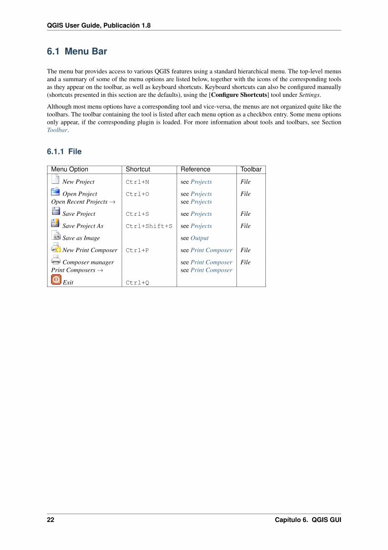
6.1 Menu Bar
The menu bar provides access to various QGIS features using a standard hierarchical menu. The top-level menusand a summary of some of the menu options are listed below, together with the icons of the corresponding toolsas they appear on the toolbar, as well as keyboard shortcuts. Keyboard shortcuts can also be configured manually(shortcuts presented in this section are the defaults), using the [Configure Shortcuts] tool under Settings.
Although most menu options have a corresponding tool and vice-versa, the menus are not organized quite like thetoolbars. The toolbar containing the tool is listed after each menu option as a checkbox entry. Some menu optionsonly appear, if the corresponding plugin is loaded. For more information about tools and toolbars, see SectionToolbar.
6.1.1 File
Menu Option Shortcut Reference Toolbar
New Project Ctrl+N see Projects File
Open Project Ctrl+O see Projects FileOpen Recent Projects → see Projects
Save Project Ctrl+S see Projects File
Save Project As Ctrl+Shift+S see Projects File
Save as Image see Output
New Print Composer Ctrl+P see Print Composer File
Composer manager see Print Composer FilePrint Composers → see Print Composer
Exit Ctrl+Q
22 Capítulo 6. QGIS GUI

QGIS User Guide, Publicación 1.8
6.1.2 Edit
Menu Option Shortcut Reference Toolbar
Undo Ctrl+Z see Advanced digitizing Advanced Digitizing
Redo Ctrl+Shift+Z see Advanced digitizing Advanced Digitizing
Cut Features Ctrl+X see Digitizing an existing layer Digitizing
Copy Features Ctrl+C see Digitizing an existing layer Digitizing
Paste Features Ctrl+V see Digitizing an existing layer Digitizing
Add Feature Ctrl+. see Digitizing an existing layer Digitizing
Move Feature(s) see Digitizing an existing layer Digitizing
Delete Selected see Digitizing an existing layer Digitizing
Simplify Feature see Advanced digitizing Advanced Digitizing
Add Ring see Advanced digitizing Advanced Digitizing
Add Part see Advanced digitizing Advanced Digitizing
Delete Ring see Advanced digitizing Advanced Digitizing
Delete Part see Advanced digitizing Advanced Digitizing
Reshape Features see Advanced digitizing Advanced Digitizing
Offset Curves see Advanced digitizing Advanced Digitizing
Split Features see Advanced digitizing Advanced Digitizing
Merge selected Features see Advanced digitizing Advanced Digitizing
Merge attr. of selected Features see Advanced digitizing Advanced Digitizing
Node Tool see Digitizing an existing layer Digitizing
Rotate Point Symbols see Advanced digitizing Advanced Digitizing
After activating Toggle editing mode for a layer, you will find the Add Feature icon in the Edit menu dependingon the layer type (point, line or polygon).
6.1.3 Edit (extra)
Menu Option Shortcut Reference Toolbar
Add Feature see Digitizing an existing layer Digitizing
Add Feature see Digitizing an existing layer Digitizing
Add Feature see Digitizing an existing layer Digitizing
6.1. Menu Bar 23

QGIS User Guide, Publicación 1.8
6.1.4 View
Menu Option Shortcut Reference Toolbar
Pan Map Map Navigation
Pan Map to Selection Map Navigation
Zoom In Ctrl++ Map Navigation
Zoom Out Ctrl+- Map NavigationSelect → see Select and deselect features Attributes
Identify Features Ctrl+Shift+I AttributesMeasure → see Measuring Attributes
Zoom Full Ctrl+Shift+F Map Navigation
Zoom To Layer Map Navigation
Zoom To Selection Ctrl+J Map Navigation
Zoom Last Map Navigation
Zoom Next Map Navigation
Zoom Actual Size Map NavigationDecorations → see Decorations
Map Tips Attributes
New Bookmark Ctrl+B see Spatial Bookmarks Attributes
Show Bookmarks Ctrl+Shift+B see Spatial Bookmarks Attributes
Refresh Ctrl+R Map NavigationTile scale slider see Tilesets Tile scale
6.1.5 Layer
Menu Option Shortcut Reference ToolbarNew → see Creating a new Vector layer Manage LayersEmbed Layers and Groups ... see Nesting Projects
Add Vector Layer Ctrl+Shift+V see Working with Vector Data Manage Layers
Add Raster Layer Ctrl+Shift+R see Loading raster data in QGIS Manage Layers
Add PostGIS Layer Ctrl+Shift+D see PostGIS Layers Manage Layers
Add SpatiaLite Layer Ctrl+Shift+L see SpatiaLite Layers Manage Layers
Add MSSQL Spatial Layer Ctrl+Shift+M see MSSQL Spatial Layers Manage Layers
Add WMS Layer Ctrl+Shift+W see WMS Client Manage Layers
Add Delimited Text Layer see Delimited Text Plugin Manage Layers
Create new GPX layer see GPS Plugin Manage Layers
Add Oracle GeoRaster layer see Oracle GeoRaster Plugin Manage Layers
Add SQL Anywhere Layer see SQL Anywhere Plugin Manage Layers
Add WFS Layer Manage Layers
Copy style see Style TabContinúa en la página siguiente
24 Capítulo 6. QGIS GUI

QGIS User Guide, Publicación 1.8
Cuadro 6.1 – proviene de la página anteriorMenu Option Shortcut Reference Toolbar
Paste style see Style Tab
Open Attribute Table Attributes
Save edits Digitizing
Toggle editing DigitizingSave as...Save selection as vector file... See Working with the Attribute Table
Remove Layer Ctrl+DSet CRS of Layer(s) Ctrl+Shift+CSet project CRS from LayerPropertiesQuery...
Labeling
Add to Overview Ctrl+Shift+O Manage Layers
Add All To Overview
Remove All From Overview
Show All Layers Ctrl+Shift+U Manage Layers
Hide All Layers Ctrl+Shift+H Manage Layers
6.1.6 Settings
Menu Option Shortcut Reference ToolbarPanels → see Panels and ToolbarsToolbars → see Panels and ToolbarsToggle Full Screen Mode Ctrl-F
Project Properties ... Ctrl+Shift+P see Projects
Custom CRS ... see Custom Coordinate Reference SystemStyle Manager... see Style Manager
Configure shortcuts ...Customization ... see CustomizationOptions ... see Options
Snapping Options ...
6.1.7 Plugins
Menu Option Shortcut Reference Toolbar
Fetch Python Plugins see QGIS Plugins
Manage Plugins see Managing PluginsPython ConsoleGRASS → see GRASS GIS Integration GRASS
6.1. Menu Bar 25

QGIS User Guide, Publicación 1.8
6.1.8 Vector
Menu Option Shortcut Reference ToolbarAnalysis Tools → see fTools PluginCoordinate Capture → see Coordinate Capture PluginData Management Tools → see fTools PluginDxf2Shp → see Dxf2Shp Converter Plugin VectorGeometry Tools → see fTools PluginGeoprocessing Tools → see fTools PluginGPS → see GPS Plugin VectorResearch Tools → see fTools PluginRoad Graph → see Road Graph PluginSpatial Query → see Spatial Query Plugin Vector
6.1.9 Raster
Menu Option Shortcut Reference ToolbarRaster calculator see Raster CalculatorGeoreferencer → see Georeferencer Plugin RasterHeatmap → see Heatmap Plugin RasterInterpolation → see Interpolation Plugin Raster
Terrain Analysis see Raster Terrain Analysis PluginZonal Statistics → see Zonal Statistics Plugin RasterProjections → see GDAL Tools PluginConversion → see GDAL Tools PluginExtraction → see GDAL Tools PluginAnalysis → see GDAL Tools PluginMiscellaneous → see GDAL Tools PluginGdalTools settings see GDAL Tools Plugin
6.1.10 Database
Menu Option Shortcut Reference ToolbarDB manager → see DB Manager Plugin DatabaseeVis → see eVis Plugin DatabaseOffline Editing → see Offline Editing Plugin DatabaseSpit → see SPIT Plugin Database
6.1.11 Web
Menu Option Shortcut Reference ToolbarMapServer Export ... → see MapServer Export Plugin WebOpenStreetMap → see OpenStreetMap OpenStreetMap
26 Capítulo 6. QGIS GUI

QGIS User Guide, Publicación 1.8
6.1.12 Help
Menu Option Shortcut Reference Toolbar
Help Contents F1 Help
What’s This? Shift+F1 HelpAPI Documentation
QGIS Home Page Ctrl+H
Check QGIS Version
About
QGIS Sponsors
Please not that for Linux the Menu Bar items listed above are the default ones in KDE window manager. InGNOME, Settings menu is missing and its items are to be found here:
Project Properties FileOptions EditConfigure Shortcuts Edit
Style Manager Edit
Custom CRS EditPanels → ViewToolbars → ViewToggle Full Screen Mode ViewTile scale slider ViewLive GPS tracking View
6.2 Toolbar
The toolbar provides access to most of the same functions as the menus, plus additional tools for interacting withthe map. Each toolbar item has popup help available. Hold your mouse over the item and a short description ofthe tool’s purpose will be displayed.
Every menubar can be moved around according to your needs. Additionally every menubar can be switched offusing your right mouse button context menu holding the mouse over the toolbars (read also Panels and Toolbars).
Truco: Restoring toolbarsIf you have accidentally hidden all your toolbars, you can get them back by choosing menu option Settings →Toolbars →. If a toolbar disappears under Windows, which seems to be a problem in QGIS from time to time,you have to remove \HKEY_CURRENT_USER\Software\QuantumGIS\qgis\UI\state in the registry.When you restart QGIS, the key is written again with the default state, and all toolbars are visible again.
6.3 Map Legend
The map legend area lists all the layers in the project. The checkbox in each legend entry can be used to show orhide the layer.
A layer can be selected and dragged up or down in the legend to change the z-ordering. Z-ordering means thatlayers listed nearer the top of the legend are drawn over layers listed lower down in the legend.
Layers in the legend window can be organised into groups. There are two ways to do so:
6.2. Toolbar 27
QGIS User Guide, Publicación 1.8
1. Right click in the legend window and choose Add Group. Type in a name for the group and press Enter.Now click on an existing layer and drag it onto the group.
2. Select some layers, right click in the legend window and choose Group Selected. The selected layers willautomatically be placed in a new group.
To bring a layer out of a group you can drag it out, or right click on it and choose Make to toplevel item. Groupscan be nested inside other groups.
The checkbox for a group will show or hide all the layers in the group with one click.
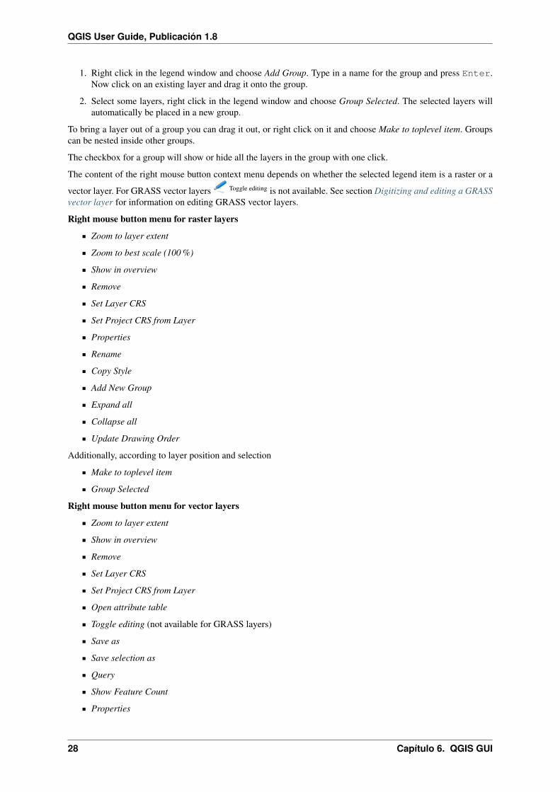
The content of the right mouse button context menu depends on whether the selected legend item is a raster or a
vector layer. For GRASS vector layers Toggle editing is not available. See section Digitizing and editing a GRASSvector layer for information on editing GRASS vector layers.
Right mouse button menu for raster layers
Zoom to layer extent
Zoom to best scale (100 %)
Show in overview
Remove
Set Layer CRS
Set Project CRS from Layer
Properties
Rename
Copy Style
Add New Group
Expand all
Collapse all
Update Drawing Order
Additionally, according to layer position and selection
Make to toplevel item
Group Selected
Right mouse button menu for vector layers
Zoom to layer extent
Show in overview
Remove
Set Layer CRS
Set Project CRS from Layer
Open attribute table
Toggle editing (not available for GRASS layers)
Save as
Save selection as
Query
Show Feature Count
Properties
28 Capítulo 6. QGIS GUI

QGIS User Guide, Publicación 1.8
Rename
Copy Style
Add New Group
Expand all
Collapse all
Update Drawing Order
Additionally, according to layer position and selection
Make to toplevel item
Group Selected
Right mouse button menu for layer groups
Zoom to group
Remove
Set group CRS
Rename
Add New Group
Expand all
Collapse all
Update Drawing Order
It is possible to select more than one layer or group at the same time by holding down the Ctrl key while selectingthe layers with the left mouse button. You can then move all selected layers to a new group at the same time.
You are also able to delete more than one Layer or Group at once by selecting several Layers with the Ctrl keyand pressing Ctrl+D afterwards. This way all selected Layers or groups will be removed from the layerlist.
6.3.1 Working with the Legend independent layer order
Since QGIS 1.8 there is a widget that allows to define a legend independent drawing order. You can activate it inthe menu Settings → Panels. Determine the drawing order of the layers in the map view here. Doing so makes itpossible to order your layers in order of importance, for example, but to still display them in the correct order (see
figure_layer_order). Checking the control rendering order box underneath the list of layers will cause a revertto default behavior.
6.4 Map View
This is the “business end” of QGIS - maps are displayed in this area! The map displayed in this window willdepend on the vector and raster layers you have chosen to load (see sections that follow for more information onhow to load layers). The map view can be panned (shifting the focus of the map display to another region) andzoomed in and out. Various other operations can be performed on the map as described in the toolbar descriptionabove. The map view and the legend are tightly bound to each other - the maps in view reflect changes you makein the legend area.
Truco: Zooming the Map with the Mouse WheelYou can use the mouse wheel to zoom in and out on the map. Place the mouse cursor inside the map area androll the wheel forward (away from you) to zoom in and backwards (towards you) to zoom out. The mouse cursorposition is the center where the zoom occurs. You can customize the behavior of the mouse wheel zoom using theMap tools tab under the Settings → Options menu.
6.4. Map View 29

QGIS User Guide, Publicación 1.8
Figura 6.2: Define a legend independent layer order
Truco: Panning the Map with the Arrow Keys and Space BarYou can use the arrow keys to pan in the map. Place the mouse cursor inside the map area and click on the rightarrow key to pan East, left arrow key to pan West, up arrow key to pan North and down arrow key to pan South.You can also pan the map using the space bar: just move the mouse while holding down space bar.
6.5 Status Bar
The status bar shows you your current position in map coordinates (e.g. meters or decimal degrees) as the mousepointer is moved across the map view. To the left of the coordinate display in the status bar is a small button thatwill toggle between showing coordinate position or the view extents of the map view as you pan and zoom in andout.
Next to the coordinate display you find the scale display. It shows the scale of the map view. If you zoom in or outQGIS shows you the current scale. Since QGIS 1.8 there is a scale selector which allows you to choose betweenpredefined scales from 1:500 until 1:1000000.
A progress bar in the status bar shows progress of rendering as each layer is drawn to the map view. In somecases, such as the gathering of statistics in raster layers, the progress bar will be used to show the status of lengthyoperations.
If a new plugin or a plugin update is available, you will see a message at the far right of the status bar. On the rightside of the status bar is a small checkbox which can be used to temporarily prevent layers being rendered to the
map view (see Section Rendering below). The icon immediately stops the current map rendering process.
To the right of the render functions you find the EPSG code of the current project CRS and a projector icon.Clicking on this opens the projection properties for the current project.
Truco: Calculating the correct Scale of your Map CanvasWhen you start QGIS, degrees is the default unit, and it tells QGIS that any coordinate in your layer is in degrees.
30 Capítulo 6. QGIS GUI

QGIS User Guide, Publicación 1.8
To get correct scale values, you can either change this to meter manually in the General tab under Settings →
Project Properties or you can select a project Coordinate Reference System (CRS) clicking on the CRS status
icon in the lower right-hand corner of the statusbar. In the last case, the units are set to what the project projectionspecifies, e.g. ‘+units=m’.
6.5. Status Bar 31

QGIS User Guide, Publicación 1.8
32 Capítulo 6. QGIS GUI

CAPÍTULO 7
General Tools
7.1 Keyboard shortcuts
QGIS provides default keyboard shortcuts for many features. You find them in Section Menu Bar. Additionallythe menu option Settings → Configure Shortcuts allows to change the default keyboard shortcuts and to add newkeyboard shortcuts to QGIS features.
Figura 7.1: Define shortcut options (KDE)
Configuration is very simple. Just select a feature from the list and click on [Change], [Set none] or [Set default].Once you have found your configuration, you can save it as XML file and load it to another QGIS installation.
7.2 Context help
When you need help on a specific topic, you can access context help via the Help button available in most dialogs- please note that third-party plugins can point to dedicated web pages.
7.3 Rendering
By default, QGIS renders all visible layers whenever the map canvas must be refreshed. The events that trigger arefresh of the map canvas include:
Adding a layer
33

QGIS User Guide, Publicación 1.8
Panning or zooming
Resizing the QGIS window
Changing the visibility of a layer or layers
QGIS allows you to control the rendering process in a number of ways.
7.3.1 Scale Dependent Rendering
Scale dependent rendering allows you to specify the minimum and maximum scales at which a layer will bevisible. To set scale dependency rendering, open the Properties dialog by double-clicking on the layer in the
legend. On the General tab, set the minimum and maximum scale values and then click on the Use scaledependent rendering checkbox.
You can determine the scale values by first zooming to the level you want to use and noting the scale value in theQGIS status bar.
7.3.2 Controlling Map Rendering
Map rendering can be controlled in the following ways:
Suspending Rendering
To suspend rendering, click the Render checkbox in the lower right corner of the statusbar. When theRender checkbox is not checked, QGIS does not redraw the canvas in response to any of the events described inSection Rendering. Examples of when you might want to suspend rendering include:
Add many layers and symbolize them prior to drawing
Add one or more large layers and set scale dependency before drawing
Add one or more large layers and zoom to a specific view before drawing
Any combination of the above
Checking the Render checkbox enables rendering and causes an immediate refresh of the map canvas.
Setting Layer Add Option
You can set an option to always load new layers without drawing them. This means the layer will be added to themap, but its visibility checkbox in the legend will be unchecked by default. To set this option, choose menu option
Settings → Options → and click on the Rendering tab. Uncheck the By default new layers added to the mapshould be displayed checkbox. Any layer added to the map will be off (invisible) by default.
Stopping Rendering
To stop the map drawing, press the ESC key. This will halt the refresh of the map canvas and leave the mappartially drawn. It may take a bit of time between pressing ESC and the time the map drawing is halted.
Nota: It is currently not possible to stop rendering - this was disabled in qt4 port because of User Interface (UI)problems and crashes.
34 Capítulo 7. General Tools
QGIS User Guide, Publicación 1.8
Updating the Map Display During Rendering
You can set an option to update the map display as features are drawn. By default, QGIS does not display anyfeatures for a layer until the entire layer has been rendered. To update the display as features are read fromthe datastore, choose menu option Settings → Options click on the Rendering tab. Set the feature count to anappropriate value to update the display during rendering. Setting a value of 0 disables update during drawing (thisis the default). Setting a value too low will result in poor performance as the map canvas is continually updatedduring the reading of the features. A suggested value to start with is 500.
Influence Rendering Quality
To influence the rendering quality of the map you have 2 options. Choose menu option Settings → Options clickon the Rendering tab and select or deselect following checkboxes.
Make lines appear less jagged at the expense of some drawing performance
Fix problems with incorrectly filled polygons
7.4 Measuring
Measuring works within projected coordinate systems (e.g., UTM) and unprojected data. If the loaded map isdefined with a geographic coordinate system (latitude/longitude), the results from line or area measurements willbe incorrect. To fix this you need to set an appropriate map coordinate system (See Section Working with Pro-jections). All measuring modules also use the snapping settings from the digitizing module. This is useful, if youwant to measure along lines or areas in vector layers.
To select a measure tool click on and select the tool you want to use.
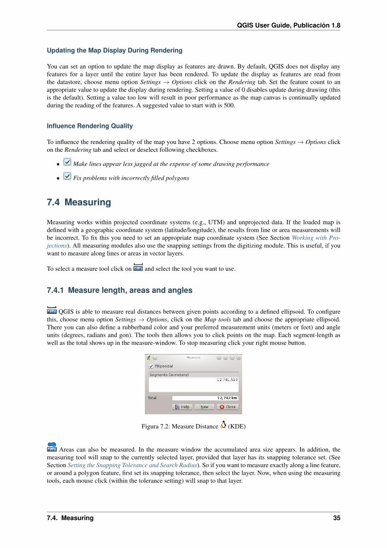
7.4.1 Measure length, areas and angles
QGIS is able to measure real distances between given points according to a defined ellipsoid. To configurethis, choose menu option Settings → Options, click on the Map tools tab and choose the appropriate ellipsoid.There you can also define a rubberband color and your preferred measurement units (meters or feet) and angleunits (degrees, radians and gon). The tools then allows you to click points on the map. Each segment-length aswell as the total shows up in the measure-window. To stop measuring click your right mouse button.
Figura 7.2: Measure Distance (KDE)
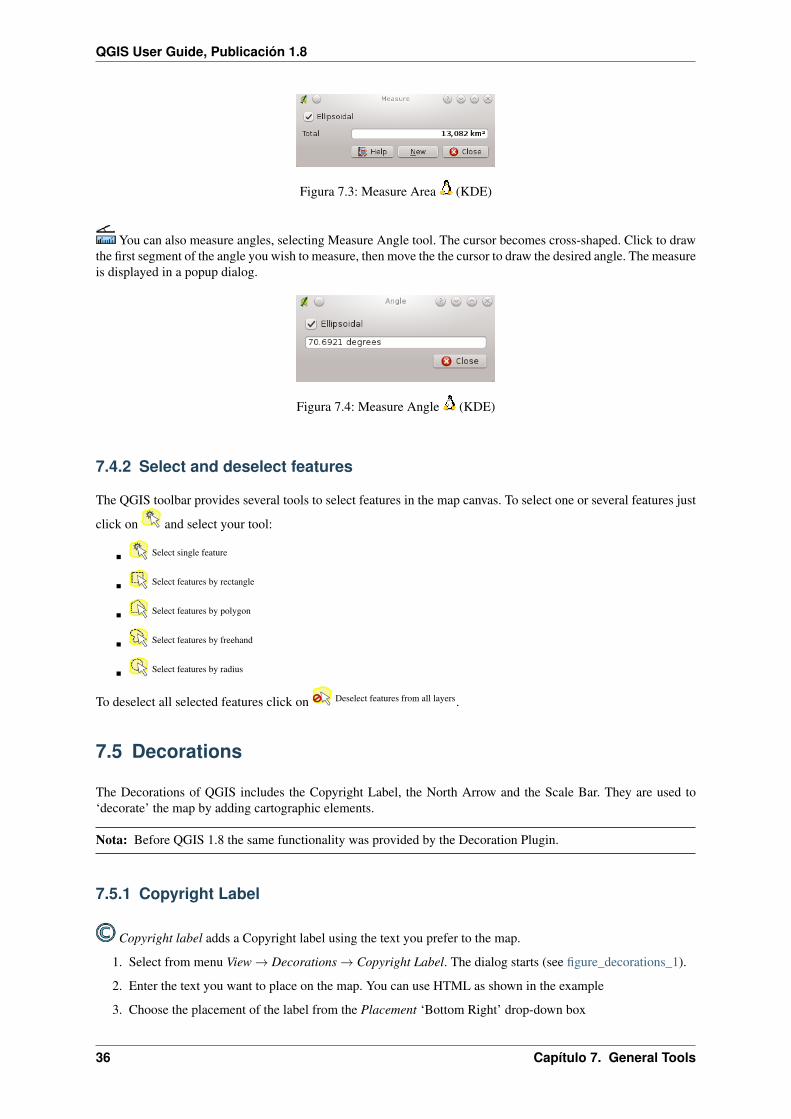
Areas can also be measured. In the measure window the accumulated area size appears. In addition, themeasuring tool will snap to the currently selected layer, provided that layer has its snapping tolerance set. (SeeSection Setting the Snapping Tolerance and Search Radius). So if you want to measure exactly along a line feature,or around a polygon feature, first set its snapping tolerance, then select the layer. Now, when using the measuringtools, each mouse click (within the tolerance setting) will snap to that layer.
7.4. Measuring 35
QGIS User Guide, Publicación 1.8
Figura 7.3: Measure Area (KDE)
You can also measure angles, selecting Measure Angle tool. The cursor becomes cross-shaped. Click to drawthe first segment of the angle you wish to measure, then move the the cursor to draw the desired angle. The measureis displayed in a popup dialog.
Figura 7.4: Measure Angle (KDE)
7.4.2 Select and deselect features
The QGIS toolbar provides several tools to select features in the map canvas. To select one or several features just
click on and select your tool:
Select single feature
Select features by rectangle
Select features by polygon
Select features by freehand
Select features by radius
To deselect all selected features click on Deselect features from all layers.
7.5 Decorations
The Decorations of QGIS includes the Copyright Label, the North Arrow and the Scale Bar. They are used to‘decorate’ the map by adding cartographic elements.
Nota: Before QGIS 1.8 the same functionality was provided by the Decoration Plugin.
7.5.1 Copyright Label
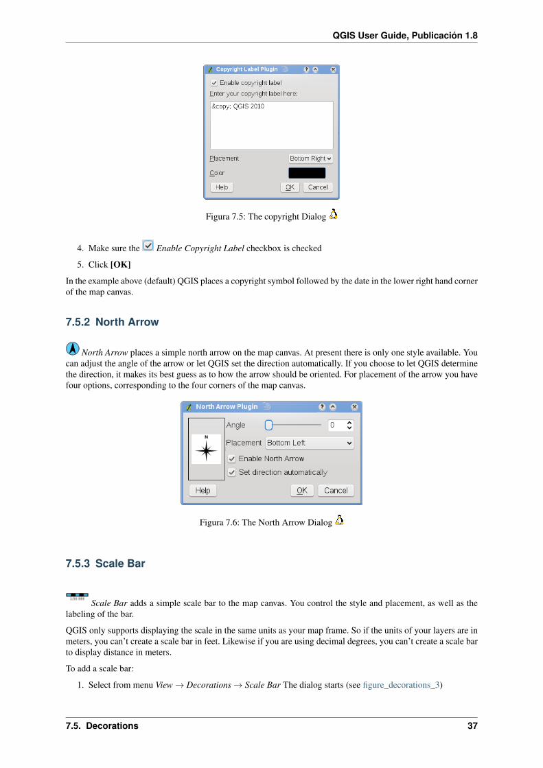
Copyright label adds a Copyright label using the text you prefer to the map.
1. Select from menu View → Decorations → Copyright Label. The dialog starts (see figure_decorations_1).
2. Enter the text you want to place on the map. You can use HTML as shown in the example
3. Choose the placement of the label from the Placement ‘Bottom Right’ drop-down box
36 Capítulo 7. General Tools
QGIS User Guide, Publicación 1.8
Figura 7.5: The copyright Dialog
4. Make sure the Enable Copyright Label checkbox is checked
5. Click [OK]
In the example above (default) QGIS places a copyright symbol followed by the date in the lower right hand cornerof the map canvas.
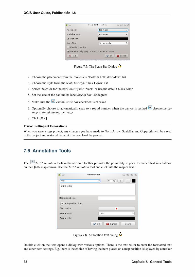
7.5.2 North Arrow
North Arrow places a simple north arrow on the map canvas. At present there is only one style available. Youcan adjust the angle of the arrow or let QGIS set the direction automatically. If you choose to let QGIS determinethe direction, it makes its best guess as to how the arrow should be oriented. For placement of the arrow you havefour options, corresponding to the four corners of the map canvas.
Figura 7.6: The North Arrow Dialog
7.5.3 Scale Bar
Scale Bar adds a simple scale bar to the map canvas. You control the style and placement, as well as thelabeling of the bar.
QGIS only supports displaying the scale in the same units as your map frame. So if the units of your layers are inmeters, you can’t create a scale bar in feet. Likewise if you are using decimal degrees, you can’t create a scale barto display distance in meters.
To add a scale bar:
1. Select from menu View → Decorations → Scale Bar The dialog starts (see figure_decorations_3)
7.5. Decorations 37
QGIS User Guide, Publicación 1.8
Figura 7.7: The Scale Bar Dialog
2. Choose the placement from the Placement ‘Bottom Left’ drop-down list
3. Choose the style from the Scale bar style ‘Tick Down’ list
4. Select the color for the bar Color of bar ‘black’ or use the default black color
5. Set the size of the bar and its label Size of bar ‘30 degrees’
6. Make sure the Enable scale bar checkbox is checked
7. Optionally choose to automatically snap to a round number when the canvas is resized Automaticallysnap to round number on resize
8. Click [OK]
Truco: Settings of DecorationsWhen you save a .qgs project, any changes you have made to NorthArrow, ScaleBar and Copyright will be savedin the project and restored the next time you load the project.
7.6 Annotation Tools
The Text Annotation tools in the attribute toolbar provides the possibility to place formatted text in a balloonon the QGIS map canvas. Use the Text Annotation tool and click into the map canvas.
Figura 7.8: Annotation text dialog
Double click on the item opens a dialog with various options. There is the text editor to enter the formatted textand other item settings. E.g. there is the choice of having the item placed on a map position (displayed by a marker
38 Capítulo 7. General Tools

QGIS User Guide, Publicación 1.8
symbol) or to have the item on a screen position (not related to the map). The item can be moved by map position(drag the map marker) or by moving only the balloon. The icons are part of GIS theme, and are used by default inthe other themes too.
The Move Annotation tool allows to move the annotation on the map canvas.
7.6.1 Form annotations
Additionally you can also create your own annotation forms. The Form Annotation tool is useful to dis-play attributes of a vector layer in a customized qt designer form (see figure_custom_annotation). It is similarto the designer forms for the Identify features tool, but displayed in an annotation item. Also see QGIS bloghttp://blog.qgis.org/node/143 for more information.
Figura 7.9: Customized qt designer annotation form
Nota: If you press Ctrl+T while an Annotation tool is active (move annotation, text annotation, form annota-tion), the visibility states of the items are inverted.
7.7 Spatial Bookmarks
Spatial Bookmarks allow you to “bookmark” a geographic location and return to it later.
7.7.1 Creating a Bookmark
To create a bookmark:
1. Zoom or pan to the area of interest.
2. Select the menu option View → New Bookmark or press Ctrl-B.
3. Enter a descriptive name for the bookmark (up to 255 characters).
4. Press Enter to add the bookmark or [Delete] to remove the bookmark.
Note that you can have multiple bookmarks with the same name.
7.7. Spatial Bookmarks 39

QGIS User Guide, Publicación 1.8
7.7.2 Working with Bookmarks
To use or manage bookmarks, select the menu option View → Show Bookmarks. The Geospatial Bookmarks dialogallows you to zoom to or delete a bookmark. You can not edit the bookmark name or coordinates.
7.7.3 Zooming to a Bookmark
From the Geospatial Bookmarks dialog, select the desired bookmark by clicking on it, then click [Zoom To]. Youcan also zoom to a bookmark by double-clicking on it.
7.7.4 Deleting a Bookmark
To delete a bookmark from the Geospatial Bookmarks dialog, click on it then click [Delete]. Confirm your choiceby clicking [Yes] or cancel the delete by clicking [No].
7.8 Nesting Projects
If you want to embed content from other project files into your project you can choose Layer → Embed Layersand Groups.
7.8.1 Embedding layers
The following dialog allows you to embed layers from other projects:
1. Press to look for another project from the Alaska dataset.
2. Select the project file grassland. You can see the content of the project (see figure_embed_dialog).
3. Press Ctrl and klick on the layers grassland and regions. The layers are embedded in the map legend andthe map view now.
Figura 7.10: Select layers and groups to embed
While the embedded layers are editable you can’t change it’s properties like Style and Labeling.
Removing embedded layers
Right-click on the embedded layer and choose Remove .
40 Capítulo 7. General Tools

CAPÍTULO 8
QGIS Configuration
QGIS is highly configurable through the Settings menu. Choose between Panels, Toolbars, Project properties,Options and Customization.
8.1 Panels and Toolbars
In the Panels→ menu you can switch on and off QGIS widgets. The Toolbars→ menu provides the possibility toswitch on and off icon groups in the QGIS toolbar (see figure_panels_toolbars).
Figura 8.1: The Panels and Toolbars menu
Truco: Activating the QGIS OverviewIn QGIS you can use an overview panel that provides a full extent view of layers added to it. It can be selectedunder the menu Settings → Panels. Within the view is a rectangle showing the current map extent. This allowsyou to quickly determine which area of the map you are currently viewing. Note that labels are not rendered to themap overview even if the layers in the map overview have been set up for labeling. If you click and drag the redrectangle in the overview that shows your current extent, the main map view will update accordingly.
Truco: Show Log Messages
Since QGIS 1.8 it’s possible to track the QGIS messages. You can activate Log Messages in the menu Settings→ Panels and follow the messages in the General and Plugin tab during loading and operation.
41
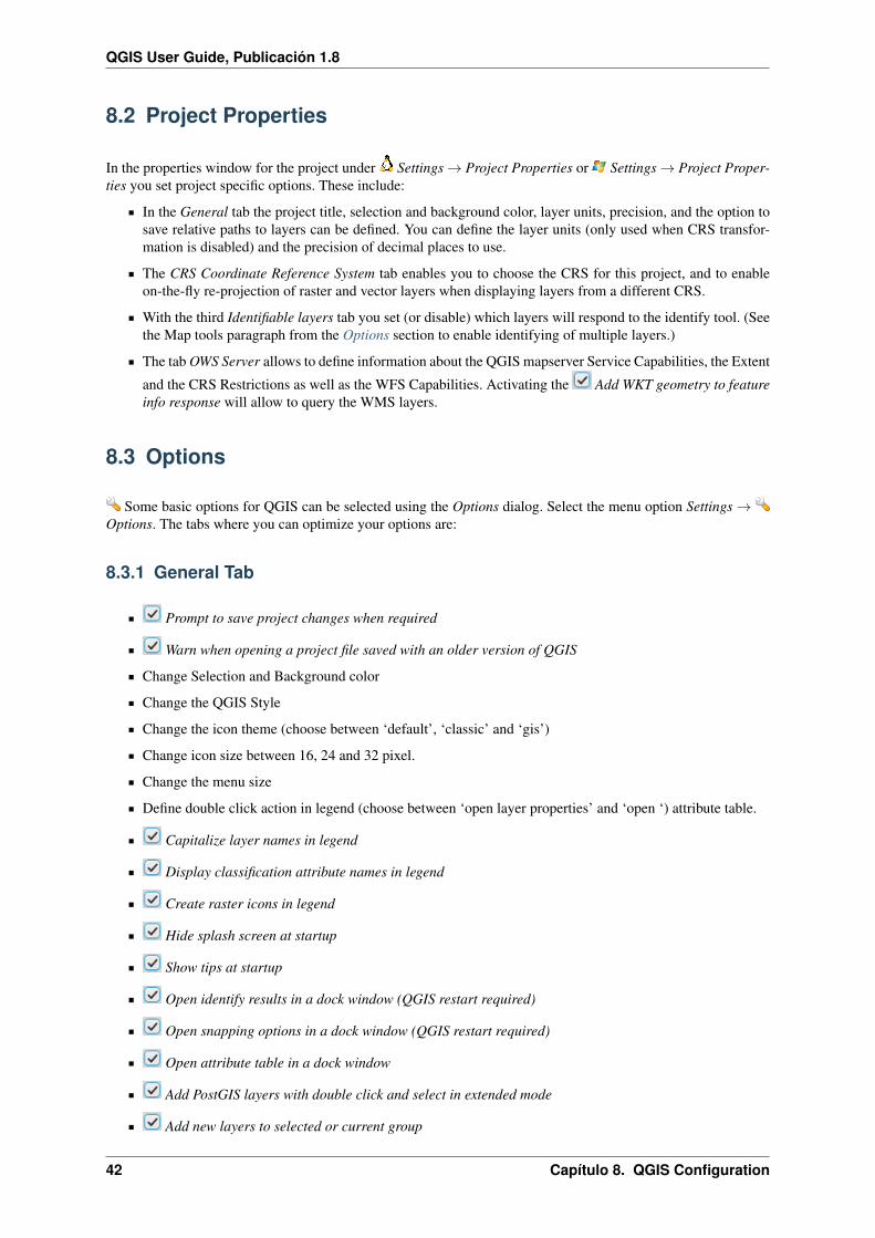
QGIS User Guide, Publicación 1.8
8.2 Project Properties
In the properties window for the project under Settings → Project Properties or Settings → Project Proper-ties you set project specific options. These include:
In the General tab the project title, selection and background color, layer units, precision, and the option tosave relative paths to layers can be defined. You can define the layer units (only used when CRS transfor-mation is disabled) and the precision of decimal places to use.
The CRS Coordinate Reference System tab enables you to choose the CRS for this project, and to enableon-the-fly re-projection of raster and vector layers when displaying layers from a different CRS.
With the third Identifiable layers tab you set (or disable) which layers will respond to the identify tool. (Seethe Map tools paragraph from the Options section to enable identifying of multiple layers.)
The tab OWS Server allows to define information about the QGIS mapserver Service Capabilities, the Extent
and the CRS Restrictions as well as the WFS Capabilities. Activating the Add WKT geometry to featureinfo response will allow to query the WMS layers.
8.3 Options
Some basic options for QGIS can be selected using the Options dialog. Select the menu option Settings →Options. The tabs where you can optimize your options are:
8.3.1 General Tab
Prompt to save project changes when required
Warn when opening a project file saved with an older version of QGIS
Change Selection and Background color
Change the QGIS Style
Change the icon theme (choose between ‘default’, ‘classic’ and ‘gis’)
Change icon size between 16, 24 and 32 pixel.
Change the menu size
Define double click action in legend (choose between ‘open layer properties’ and ‘open ‘) attribute table.
Capitalize layer names in legend
Display classification attribute names in legend
Create raster icons in legend
Hide splash screen at startup
Show tips at startup
Open identify results in a dock window (QGIS restart required)
Open snapping options in a dock window (QGIS restart required)
Open attribute table in a dock window
Add PostGIS layers with double click and select in extended mode
Add new layers to selected or current group
42 Capítulo 8. QGIS Configuration

QGIS User Guide, Publicación 1.8
Copy geometry in WKT representation from attribute table
Attribute table behavior (choose between ‘Show all features’ (default), ‘Show selected features’,’Showfeatures in current canvas’)
Attribute table row cache
Define Representation for NULL values
Prompt for raster sublayers . Some rasters support sublayers - they are called subdatasets in GDAL.An example is netcdf files - if there are many netcdf variables, GDAL sees every variable as a subdataset.The option is to control how to deal with sublayers when a file with sublayers is opened. You have thefollowing choices:
• ‘Always’: always ask (if there are existing sublayers)
• ‘If needed’: ask if layer has no bands, but has sublayers
• ‘Never’: never prompt, will not load anything
• ‘Load all’: never prompt, but load all sublayers
Scan for valid items in the browser dock . The ‘Check extension’ option was designed to speed upthe loading of a directory, which can be time-consuming when ‘Check file contents’ is activated and thereare many files (tens or hundreds).
Scan for contents of compressed files (.zip) in browser dock This option was also designed to speedup the loading of a directory. You have the following choices:
• ‘Basic Scan’: checks that the extension is supported by one of the drivers
• ‘Full Scan’: opens every file to check it is valid
• ‘Passthru’: don’t use this option it will be removed in the next QGIS version
8.3.2 GDAL tab
GDAL is a data exchange library for raster files. In this tab you can define which GDAL driver to be used for araster format as in some cases more than one GDAL driver is available.
8.3.3 Plugins tab
Add Path(s) to search for additional C++ plugin libraries.
8.3.4 Rendering Tab
By default new layers added to the map should be displayed
Define Number of features to draw before updating the display.
Use render caching where possible to speed up redraws
Make lines appear less jagged at the expense of some drawing performance
Fix problems with incorrectly filled polygons
Use new generation symbology for rendering
Define the default Raster settings for visualisation: ‘RGB band selection’, Use standard deviation and‘Contrast Enhancement’
8.3. Options 43

QGIS User Guide, Publicación 1.8
Add/remove Path(s) to search for Scalable Vector Graphics (SVG) symbols
Additionally you can define whether to save the path for svg textures absolute or relative in the General tab of theSettings → Project Properties menu.
8.3.5 Map tools Tab
The Mode setting determines which layers will be shown by the Identify tool. By switching to ‘Top down’or ‘Top down, stop at first’ instead of ‘Current layer’ attributes for all identifiable layers (see the Projectproperties section under: Projects to set which layers are identifiable) will be shown with the Identify tool.
Open feature form, if a single feature is identified
Define Search radius for identifying and displaying map tips as a percentage of the map width
Define Ellipsoid for distance calculations
Define Rubberband color for measure tools
Define Decimal places
Keep base unit
Define preferred measurement units (‘meters’ or ‘feet’)
Define preferred angle units (‘Degrees’, ‘Radians’ or ‘Gon’)
Define Mouse wheel action (‘Zoom’, ‘Zoom and recenter’, ‘Zoom to mouse cursor’, ‘Nothing’)
Define Zoom factor for wheel mouse
8.3.6 Overlays Tab
Define Placement algorithm for labels, symboly and diagrams (choose between ‘Central point’(standard), ‘Chain’, ‘Popmusic tabu chain’, ‘Popmusic tabu’ and ‘Popmusic chain’)
8.3.7 Digitizing Tab
Define Rubberband Line color and Line width
Define Default snap mode (‘To vertex’, ‘To segment’, ‘To vertex and segment’)
Define Default snapping tolerance in map units or pixel
Define search radius for vertex edits in ‘map units’ or ‘pixel’
Show markers only for selected features
Define vertex Marker style (‘Cross’ (default), ‘Semi transparent circle’ or ‘None’) and vertexMarker size.
Suppress attributes pop-up windows after each created feature
Reuse last entered attribute values
Validate geometries Editing complex lines/polygons with many nodes can end up with very slow rendering.This is because the default validation procedures in QGIS can use a lot of time. To speed up rendering it ispossible to select GEOS geometry validation (starting from GEOS 3.3) or to switch it off. GEOS geometryvalidation is much faster, but the disadvantage is that only the first geometry problem will be reported.
44 Capítulo 8. QGIS Configuration

QGIS User Guide, Publicación 1.8
The next 3 options refer to the Offset Curve tool in Advanced digitizing. Through the various settings, it is possibleto influence the shape of the line offset. These options are possible from GEOS 3.3 .
Join style for curve offset
Quadrantsegments for curve offset
Miter limit for curve offset
8.3.8 CRS Tab
The CRS tab is divided in two areas. The first area allows to define the default CRS for new projects.
Select a CRS and Always start new projects with this CRS.
Enable on the fly re-projection by default
The second area allows to define the action, when a new layer is created, or when a layer without CRS is loaded.
Prompt for Coordinate Reference System (CRS)
Use project Coordinate Reference System (CRS)
Use default Coordinate Reference System (CRS) displayed below
8.3.9 Locale Tab
Overwrite system locale and Locale to use instead
Information about active system locale
8.3.10 Network Tab
Figura 8.2: Proxy-settings in QGIS
Use proxy for web access and define ‘Host’, ‘Port’, ‘User’, and ‘Password’.
Set the Proxy type according to your needs.
• Default Proxy: Proxy is determined based on the application proxy set using
8.3. Options 45
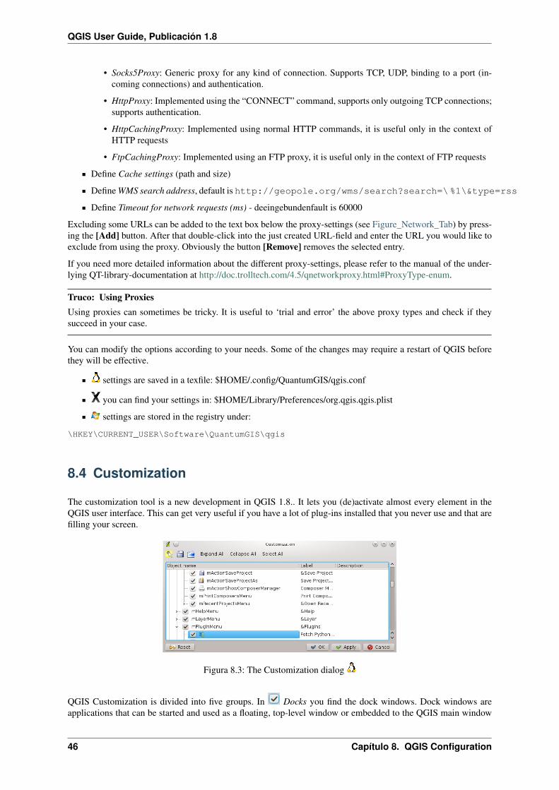
QGIS User Guide, Publicación 1.8
• Socks5Proxy: Generic proxy for any kind of connection. Supports TCP, UDP, binding to a port (in-coming connections) and authentication.
• HttpProxy: Implemented using the “CONNECT” command, supports only outgoing TCP connections;supports authentication.
• HttpCachingProxy: Implemented using normal HTTP commands, it is useful only in the context ofHTTP requests
• FtpCachingProxy: Implemented using an FTP proxy, it is useful only in the context of FTP requests
Define Cache settings (path and size)
Define WMS search address, default is http://geopole.org/wms/search?search=\%1\&type=rss
Define Timeout for network requests (ms) - deeingebundenfault is 60000
Excluding some URLs can be added to the text box below the proxy-settings (see Figure_Network_Tab) by press-ing the [Add] button. After that double-click into the just created URL-field and enter the URL you would like toexclude from using the proxy. Obviously the button [Remove] removes the selected entry.
If you need more detailed information about the different proxy-settings, please refer to the manual of the under-lying QT-library-documentation at http://doc.trolltech.com/4.5/qnetworkproxy.html#ProxyType-enum.
Truco: Using ProxiesUsing proxies can sometimes be tricky. It is useful to ‘trial and error’ the above proxy types and check if theysucceed in your case.
You can modify the options according to your needs. Some of the changes may require a restart of QGIS beforethey will be effective.
settings are saved in a texfile: $HOME/.config/QuantumGIS/qgis.conf
you can find your settings in: $HOME/Library/Preferences/org.qgis.qgis.plist
settings are stored in the registry under:
\HKEY\CURRENT_USER\Software\QuantumGIS\qgis
8.4 Customization
The customization tool is a new development in QGIS 1.8.. It lets you (de)activate almost every element in theQGIS user interface. This can get very useful if you have a lot of plug-ins installed that you never use and that arefilling your screen.
Figura 8.3: The Customization dialog
QGIS Customization is divided into five groups. In Docks you find the dock windows. Dock windows areapplications that can be started and used as a floating, top-level window or embedded to the QGIS main window
46 Capítulo 8. QGIS Configuration
QGIS User Guide, Publicación 1.8
as a docked widget (see also Panels and Toolbars). In Menus you can hide entries in the Menu bar. In the
Status Bar features like the coordinate information can be daectivated. In Toolbars you can (de)activate the
toolbar icons of QGIS and in Widgets you can (de)activate dialogs as well as their buttons.
With Switch to catching widgets in main application you can click on elements in QGIS you want to behidden and find the corresponding entry in Customization (see figure_customization). You can also save yourvarious different setups for different use cases as well. Before your changes are applied, you need to restart QGIS.
8.4. Customization 47

QGIS User Guide, Publicación 1.8
48 Capítulo 8. QGIS Configuration

CAPÍTULO 9
Working with Projections
QGIS allows users to define a global and project-wide CRS (Coordinate Reference System) for layers without apre-defined CRS. It also allows the user to define custom coordinate reference systems and supports on-the-fly(OTF) projection of vector and raster layers. All these features allow the user to display layers with different CRSand have them overlay properly.
9.1 Overview of Projection Support
QGIS has support for approximately 2,700 known CRS. Definitions for each of these CRS are stored in a SQLitedatabase that is installed with QGIS. Normally you do not need to manipulate the database directly. In fact, doingso may cause projection support to fail. Custom CRS are stored in a user database. See Section Custom CoordinateReference System for information on managing your custom coordinate reference systems.
The CRS available in QGIS are based on those defined by the European Petroleum Search Group (EPSG) and theInstitut Geographique National de France (IGNF) and are largely abstracted from the spatial reference tables usedin GDAL. EPSG identifiers are present in the database and can be used to specify a CRS in QGIS.
In order to use OTF projection, your data must contain information about its coordinate reference system or youhave to define a global, layer or project-wide CRS. For PostGIS layers QGIS uses the spatial reference identifierthat was specified when the layer was created. For data supported by OGR, QGIS relies on the presence of arecognized means of specifying the CRS. In the case of shapefiles, this means a file containing the Well KnownText (WKT) specification of the CRS. This projection file has the same base name as the shapefile and a prjextension. For example, a shapefile named alaska.shp would have a corresponding projection file namedalaska.prj.
Whenever you select a new CRS, the used layer units will automatically be changed in the General tab of theProject Properties dialog under the Edit (Gnome, OSX) or Settings (KDE, Windows) menu.
9.2 Specifying a Projection
QGIS starts each new project using the global default projection.The global default CRS is EPSG:4326 - WGS84 (proj=longlat +ellps=WGS84 +datum=WGS84 +no_defs) and comes predefined in QGIS. Thisdefault can be changed using the [Select...] button in the first section, used to defining the Default CoordinateReference System to use when starting new projects, as shown in figure_projection_1. This choice will be savedfor use in subsequent QGIS sessions.
When you use layers that do not have a CRS, you need to define how QGIS responds to these layers. This can bedone globally or project-wide in the CRS tab under Edit → Options (Gnome, OSX) or Settings → Options(KDE, Windows).
The options shown in figure_projection_1 are:
Prompt for CRS
49

QGIS User Guide, Publicación 1.8
Figura 9.1: CRS tab in the QGIS Options Dialog
Use project CRS
Use default CRS displayed below
If you want to define the coordinate reference system for a certain layer without CRS information, you can alsodo that in the General tab of the raster (see General Tab) and vector (see General Tab) properties dialog. If yourlayer already has a CRS defined, it will be displayed as shown in Vector Layer Properties Dialog .
Truco: CRS in the Map LegendRight-clicking on a layer in the Map Legend (Section Map Legend) provides two CRS short cuts. Set layer CRStakes you directly to the Coordinate Reference System Selector dialog (see figure_projection_2). Set project CRSfrom Layer redefines the project CRS using the layer’s CRS
9.3 Define On The Fly (OTF) Reprojection
QGIS supports OTF reprojection for both raster and vector data. However, OTF is not activated by default. To use
OTF projection, you must activate the Enable on the fly CRS transformation checkbox in the CRS tab of the
Project Properties dialog.
There are three ways to achieve this end:
1. Select Project Properties from the Edit (Gnome, OSX) or Settings (KDE, Windows) menu.
2. Click on the CRS status icon in the lower right-hand corner of the statusbar.
3. Turn OTF on by default, by selecting the CRS tab of the Options dialog and selecting Enable ‘on the fly’reprojection by default.
If you have already loaded a layer, and want to enable OTF projection, the best practice is to open the Coordinate
Reference System tab of the Project Properties dialog, select a CRS, and activate the Enable on the fly CRS
transformation checkbox. The CRS status icon will no longer be greyed-out and all layers will be OTF projectedto the CRS shown next to the icon.
50 Capítulo 9. Working with Projections
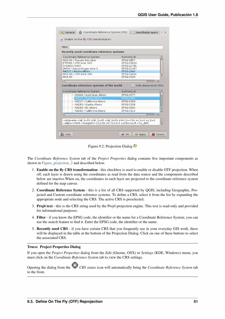
QGIS User Guide, Publicación 1.8
Figura 9.2: Projection Dialog
The Coordinate Reference System tab of the Project Properties dialog contains five important components asshown in Figure_projection_2 and described below.
1. Enable on the fly CRS transformation - this checkbox is used to enable or disable OTF projection. Whenoff, each layer is drawn using the coordinates as read from the data source and the components describedbelow are inactive.When on, the coordinates in each layer are projected to the coordinate reference systemdefined for the map canvas.
2. Coordinate Reference System - this is a list of all CRS supported by QGIS, including Geographic, Pro-jected and Custom coordinate reference systems. To define a CRS, select it from the list by expanding theappropriate node and selecting the CRS. The active CRS is preselected.
3. Proj4 text - this is the CRS string used by the Proj4 projection engine. This text is read-only and providedfor informational purposes.
4. Filter - if you know the EPSG code, the identifier or the name for a Coordinate Reference System, you canuse the search feature to find it. Enter the EPSG code, the identifier or the name.
5. Recently used CRS - if you have certain CRS that you frequently use in your everyday GIS work, thesewill be displayed in the table at the bottom of the Projection Dialog. Click on one of these buttons to selectthe associated CRS.
Truco: Project Properties DialogIf you open the Project Properties dialog from the Edit (Gnome, OSX) or Settings (KDE, Windows) menu, youmust click on the Coordinate Reference System tab to view the CRS settings.
Opening the dialog from the CRS status icon will automatically bring the Coordinate Reference System tabto the front.
9.3. Define On The Fly (OTF) Reprojection 51
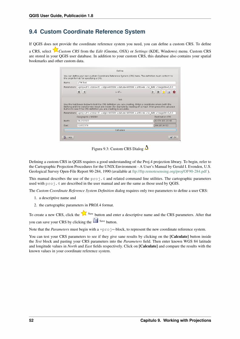
QGIS User Guide, Publicación 1.8
9.4 Custom Coordinate Reference System
If QGIS does not provide the coordinate reference system you need, you can define a custom CRS. To define
a CRS, select Custom CRS from the Edit (Gnome, OSX) or Settings (KDE, Windows) menu. Custom CRSare stored in your QGIS user database. In addition to your custom CRS, this database also contains your spatialbookmarks and other custom data.
Figura 9.3: Custom CRS Dialog
Defining a custom CRS in QGIS requires a good understanding of the Proj.4 projection library. To begin, refer tothe Cartographic Projection Procedures for the UNIX Environment - A User’s Manual by Gerald I. Evenden, U.S.Geological Survey Open-File Report 90-284, 1990 (available at ftp://ftp.remotesensing.org/proj/OF90-284.pdf ).
This manual describes the use of the proj.4 and related command line utilities. The cartographic parametersused with proj.4 are described in the user manual and are the same as those used by QGIS.
The Custom Coordinate Reference System Definition dialog requires only two parameters to define a user CRS:
1. a descriptive name and
2. the cartographic parameters in PROJ.4 format.
To create a new CRS, click the New button and enter a descriptive name and the CRS parameters. After that
you can save your CRS by clicking the Save button.
Note that the Parameters must begin with a +proj=-block, to represent the new coordinate reference system.
You can test your CRS parameters to see if they give sane results by clicking on the [Calculate] button insidethe Test block and pasting your CRS parameters into the Parameters field. Then enter known WGS 84 latitudeand longitude values in North and East fields respectively. Click on [Calculate] and compare the results with theknown values in your coordinate reference system.
52 Capítulo 9. Working with Projections

CAPÍTULO 10
QGIS Browser
The QGIS Browser is a new panel in QGIS that lets you easily navigate in your database. You can have ac-cess to common vector files (e.g. ESRI shapefile or MapInfo files), databases (e.g.PostGIS or MSSQL Spatial)and WMS/WFS connections. You can also view your GRASS data (to get the data into QGIS see GRASS GISIntegration).
Figura 10.1: Qgis browser as a standalone application to view metadata, preview and attributes
Use QGIS Browser to preview your data. The drag and drop function makes it easy to get your data into the Mapview and the Map legend.
1. Activate QGIS Browser: Right-click on the tool bar and click Browser.
2. Drag the panel into the legend window.
3. Klick on the Browser tab.
4. Browse in your database and choose the shapefile folder from qgis_sample_data.
5. Press the Shift key and klick on airports.shp and alaska.shp .
6. Press the left mouse button then drag and drop the files into the map canvas.
7. Right-click on a layer and choose Set project CRS from layer. For more information see Working withProjections.
53
QGIS User Guide, Publicación 1.8
8. Click on Zoom Full to make the layers visible.
It’s also possible to run QGIS Browser as a standalone application.
Start qgis browser
Type in “qbrowser” at a command prompt.
Start QGIS browser using the Start menu or desktop shortcut, or double click on a QGIS project file.
QGIS browser is not available yet from your your Applications folder. However it caneasily be made available. In Finder use Go → Go to map... and use it to find the fold-er /Applications/QGIS.app/Contents/MacOS/bin. Use the key combination option -command and drag qbrowser.app while holding down the left mouse button to the Applications folder.This will create a link that you can use to start QGIS browser.
In figure_browser_standalone_metadata you can see the enhanced functionality of Qgis browser. The Param tabprovides the details of your connection based datasets like PostGIS or MSSQL Spatial. The Metadata tab containsgeneral information about the file (see Metadata Tab). With the Preview tab you can have a look at your fileswithout importing them into your QGIS project. It’s also possible to preview the attributes of your files in theAttributes tab.
54 Capítulo 10. QGIS Browser
CAPÍTULO 11
Working with Vector Data
11.1 Supported Data Formats
QGIS uses the OGR library to read and write vector data formats (GRASS vector and PostgreSQL support issupplied by native QGIS data provider plugins),including ESRI Shapefiles, MapInfo and Microstation file formats;PostGIS, SpatiaLite, Oracle Spatial databases and many more. The vector data can also be loaded in read modefrom zip and gzip archives into QGIS. At the date of this document, 69 vector formats are supported by theOGR library (see OGR-SOFTWARE-SUITE Literature and Web References). The complete list is available athttp://www.gdal.org/ogr/ogr_formats.html.
Nota: Not all of the listed formats may work in QGIS for various reasons. For example, some require externalcommercial libraries or the GDAL/OGR installation of your OS was not build to support the format you want touse. Only those formats that have been well tested will appear in the list of file types when loading a vector intoQGIS. Other untested formats can be loaded by selecting *.*.
Working with GRASS vector data is described in Section GRASS GIS Integration.
This section describes how to work with several common formats: ESRI Shapefiles, PostGIS layers and SpatiaLitelayers. Many of the features available in QGIS work the same, regardless of the vector data source. This is bydesign and includes the identify, select, labeling and attributes functions.
11.1.1 ESRI Shapefiles
The standard vector file format used in QGIS is the ESRI Shapefile. Support is provided by the OGR SimpleFeature Library ( http://www.gdal.org/ogr/ ).
A shapefile actually consists of several files. The following three are required:
1. .shp file containing the feature geometries.
2. .dbf file containing the attributes in dBase format.
3. .shx index file.
Shapefiles also can include a file with a .prj suffix, which contains the projection information. While it is veryuseful to have a projection file, it is not mandatory. A shapefile dataset can contain additional files. For furtherdetails see the ESRI technical specification at: http://www.esri.com/library/whitepapers/pdfs/shapefile.pdf.
Loading a Shapefile
To load a shapefile, start QGIS and click on the Add Vector Layer toolbar button or simply typeCtrl+Shift+V. This will bring up a new window (see figure_vector_1).
55

QGIS User Guide, Publicación 1.8
Figura 11.1: Add Vector Layer Dialog
From the available options check File. Click on button [Browse]. That will bring up a standard open file dialog(see figure_vector_2) which allows you to navigate the file system and load a shapefile or other supported data
source. The selection box Filter allows you to preselect some OGR supported file formats.
You can also select the Encoding type for the shapefile if desired.
Figura 11.2: Open an OGR Supported Vector Layer Dialog
Selecting a shapefile from the list and clicking [Open] loads it into QGIS. Figure_vector_3 shows QGIS afterloading the alaska.shp file.
Truco: Layer ColorsWhen you add a layer to the map, it is assigned a random color. When adding more than one layer at a time,different colors are assigned to each layer.
Once loaded, you can zoom around the shapefile using the map navigation tools. To change the style of a layer,open the Layer Properties dialog by double clicking on the layer name or by right-clicking on the name in thelegend and choosing Properties from the popup menu. See Section Style Tab for more information on settingsymbology of vector layers.
Truco: Load layer and project from mounted external drives on OS XOn OS X, portable drives that are mounted besides the primary hard drive do not show up under File → OpenProject as expected. We are working on a more OSX-native open/save dialog to fix this. As a workaround you cantype ‘/Volumes’ in the File name box and press return. Then you can navigate to external drives and networkmounts.
56 Capítulo 11. Working with Vector Data
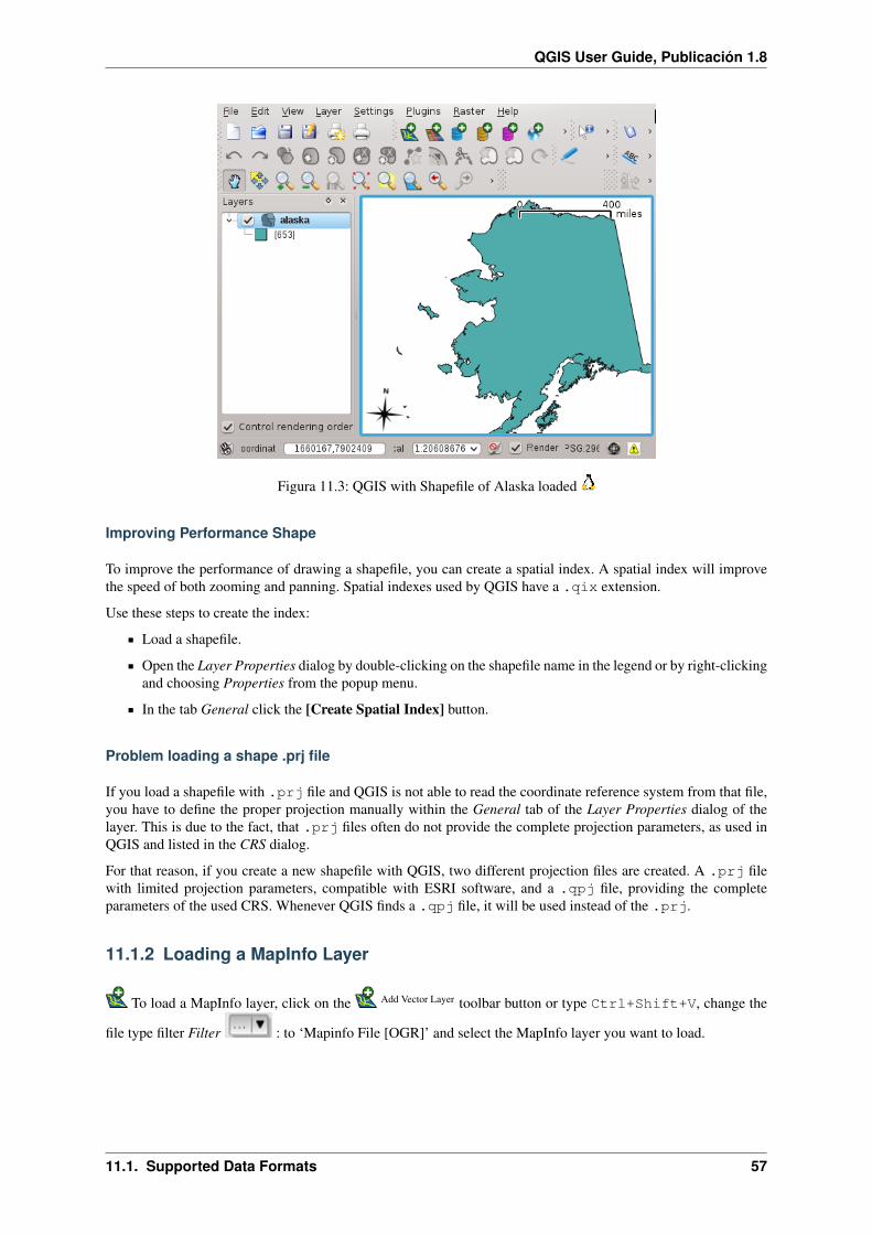
QGIS User Guide, Publicación 1.8
Figura 11.3: QGIS with Shapefile of Alaska loaded
Improving Performance Shape
To improve the performance of drawing a shapefile, you can create a spatial index. A spatial index will improvethe speed of both zooming and panning. Spatial indexes used by QGIS have a .qix extension.
Use these steps to create the index:
Load a shapefile.
Open the Layer Properties dialog by double-clicking on the shapefile name in the legend or by right-clickingand choosing Properties from the popup menu.
In the tab General click the [Create Spatial Index] button.
Problem loading a shape .prj file
If you load a shapefile with .prj file and QGIS is not able to read the coordinate reference system from that file,you have to define the proper projection manually within the General tab of the Layer Properties dialog of thelayer. This is due to the fact, that .prj files often do not provide the complete projection parameters, as used inQGIS and listed in the CRS dialog.
For that reason, if you create a new shapefile with QGIS, two different projection files are created. A .prj filewith limited projection parameters, compatible with ESRI software, and a .qpj file, providing the completeparameters of the used CRS. Whenever QGIS finds a .qpj file, it will be used instead of the .prj.
11.1.2 Loading a MapInfo Layer
To load a MapInfo layer, click on the Add Vector Layer toolbar button or type Ctrl+Shift+V, change the
file type filter Filter : to ‘Mapinfo File [OGR]’ and select the MapInfo layer you want to load.
11.1. Supported Data Formats 57

QGIS User Guide, Publicación 1.8
11.1.3 Loading an ArcInfo Binary Coverage
To load an ArcInfo binary coverage, click on the Add Vector Layer toolbar button or press Ctrl+Shift+V to
open the Add Vector Layer dialog. Select Directory. Change to Filter to ‘Arc/Info Binary Coverage’.Navigate to the directory that contains the coverage files and select it.
Similarly, you can load directory based vector files in the UK National Transfer Format as well as the raw TIGERFormat of the US Census Bureau.
11.1.4 PostGIS Layers
PostGIS layers are stored in a PostgreSQL database. The advantages of PostGIS are the spatial indexing, filter-ing and query capabilities it provides. Using PostGIS, vector functions such as select and identify work moreaccurately than with OGR layers in QGIS.
Creating a stored Connection
The first time you use a PostGIS data source, you must create a connection to the PostgreSQL database
that contains the data. Begin by clicking on the Add PostGIS Layer toolbar button, selecting the Add PostGISLayer... option from the Layer menu or typing Ctrl+Shift+D. You can also open the Add Vector Layer dialogand select Database. The Add PostGIS Table(s) dialog will be displayed. To access the connection manager,click on the [New] button to display the Create a New PostGIS Connection dialog. The parameters required for aconnection are:
Name: A name for this connection. Can be the same as Database
Service: Service parameter to be used alternatively to hostname/port (and potentially database). This can bedefined in pg_service.conf
Host: Name of the database host. This must be a resolvable host name the same as would be used to open atelnet connection or ping the host. If the database is on the same computer as QGIS, simply enter ‘localhost’here.
Port: Port number the PostgreSQL database server listens on. The default port is 5432.
Database: Name of the database.
SSL mode: How the SSL connection will be negotiated with the server. Note that massive speedups inPostGIS layer rendering can be achieved by disabling SSL in the connection editor. Following options areavailable:
• disable: only try an unencrypted SSL connection
• allow: try a non-SSL connection, if that fails, try an SSL connection
• prefer (the default): try an SSL connection, if that fails, try a non-SSL connection;
• require: only try an SSL connection.
Username: User name used to login to the database.
Password: Password used with Username to connect to the database.
Optional you can activate following checkboxes:
Save Username
Save Password
Only look in the geometry_columns table
Only look in the ‘public’ schema
58 Capítulo 11. Working with Vector Data

QGIS User Guide, Publicación 1.8
Also list tables with no geometry
Use estimated table metadata
Once all parameters and options are set, you can test the connection by clicking on the [Test Connect] button.
Truco: QGIS User Settings and SecurityDepending on your computing environment, storing passwords in your QGIS settings may be a security risk. Yourcustomized settings for QGIS are stored based on the operating system:
, the settings are stored in your home directory in .qgis/.
, the settings are stored in the registry.
Loading a PostGIS Layer
Once you have one or more connections defined, you can load layers from the PostgreSQL database. Ofcourse this requires having data in PostgreSQL. See Section Importing Data into PostgreSQL for a discussion onimporting data into the database.
To load a layer from PostGIS, perform the following steps:
If the Add PostGIS layers dialog is not already open, click on the Add PostGIS Layer toolbar button.
Choose the connection from the drop-down list and click [Connect].
Select or unselect Also list tables with no geometry
Optionally use some Search Options to define which features to load from the layer or use the [Buildquery] button to start the Query builder dialog.
Find the layer(s) you wish to add in the list of available layers.
Select it by clicking on it. You can select multiple layers by holding down the Shift key while clicking.See Section Query Builder for information on using the PostgreSQL Query Builder to further define thelayer.
Click on the [Add] button to add the layer to the map.
Truco: PostGIS LayersNormally a PostGIS layer is defined by an entry in the geometry_columns table. From version 0.9.0 on, QGIS canload layers that do not have an entry in the geometry_columns table. This includes both tables and views. Defininga spatial view provides a powerful means to visualize your data. Refer to your PostgreSQL manual for informationon creating views.
Some details about PostgreSQL layers
This section contains some details on how QGIS accesses PostgreSQL layers. Most of the time QGIS shouldsimply provide you with a list of database tables that can be loaded, and load them on request. However, if youhave trouble loading a PostgreSQL table into QGIS, the information below may help you understand any QGISmessages and give you direction on changing the PostgreSQL table or view definition to allow QGIS to load it.
QGIS requires that PostgreSQL layers contain a column that can be used as a unique key for the layer. For tablesthis usually means that the table needs a primary key, or a column with a unique constraint on it. In QGIS, thiscolumn needs to be of type int4 (an integer of size 4 bytes). Alternatively the ctid column can be used as primarykey. If a table lacks these items, the oid column will be used instead. Performance will be improved if the columnis indexed (note that primary keys are automatically indexed in PostgreSQL).
11.1. Supported Data Formats 59

QGIS User Guide, Publicación 1.8
If the PostgreSQL layer is a view, the same requirement exists, but views do not have primary keys or columnswith unique constraints on them. In this case QGIS will try to find a column in the view that is derived from asuitable table column. It does this by parsing the view definition SQL. However there are several aspects of SQLthat QGIS ignores these include the use of table aliases and columns that are generated by SQL functions.
If a suitable column cannot be found, QGIS will not load the layer. If this occurs, the solution is to alter the viewso that it does include a suitable column (a type of int4 and either a primary key or with a unique constraint,preferably indexed).
11.1.5 Importing Data into PostgreSQL
Data can be imported into PostgreSQL/PostGIS using several tools, such as the SPIT plugin, or the command linetools shp2pgsql or ogr2ogr.
SPIT Plugin
QGIS comes with a core plugin named SPIT (Shapefile to PostGIS Import Tool). SPIT can be used to loadmultiple shapefiles at one time and includes support for schemas. See Section SPIT Plugin for more information.
shp2pgsql
PostGIS includes a utility called shp2pgsql that can be used to import shapefiles into a PostGIS enabled database.For example, to import a shapefile named lakes.shp into a PostgreSQL database named gis_data, use thefollowing command:
shp2pgsql -s 2964 lakes.shp lakes_new | psql gis_data
This creates a new layer named lakes_new in the gis_data database. The new layer will have a spatial ref-erence identifier (SRID) of 2964. See Section Working with Projections for more information on spatial referencesystems and projections.
Truco: Exporting datasets from PostGISLike the import-tool shp2pgsql there is also a tool to export PostGIS-datasets as shapefiles: pgsql2shp. This isshipped within your PostGIS distribution.
ogr2ogr
Beside shp2pgsql and SPIT there is another tool for feeding geodata in PostGIS: ogr2ogr. This is part of yourGDAL installation.
To import a shapefile into PostGIS, do the following:
ogr2ogr -f "PostgreSQL" PG:"dbname=postgis host=myhost.de user=postgres \password=topsecret" alaska.shp
This will import the shapefile alaska.shp into the PostGIS-database postgis using the user postgres with thepassword topsecret on host server myhost.de.
Note that OGR must be built with PostgreSQL to support PostGIS. You can see this by typing
ogrinfo --formats | grep -i post
If you like to use PostgreSQL’s COPY -command instead of the default INSERT INTO method you can export
the following environment-variable (at least available on and ):
60 Capítulo 11. Working with Vector Data
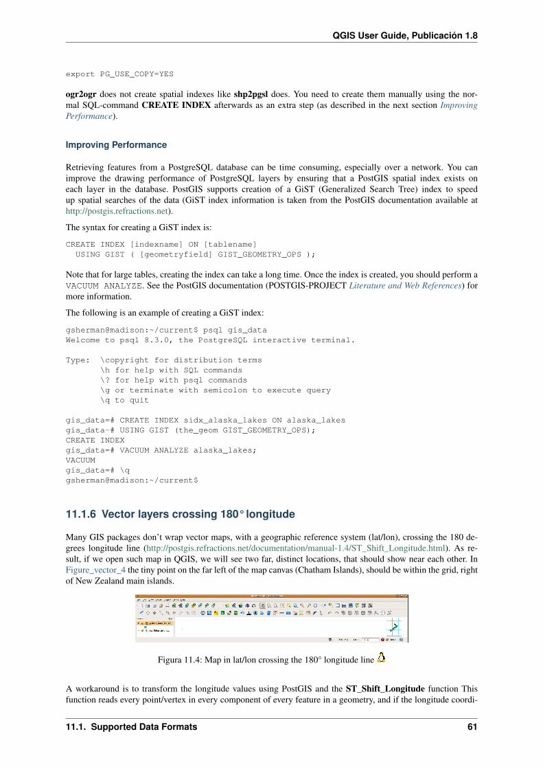
QGIS User Guide, Publicación 1.8
export PG_USE_COPY=YES
ogr2ogr does not create spatial indexes like shp2pgsl does. You need to create them manually using the nor-mal SQL-command CREATE INDEX afterwards as an extra step (as described in the next section ImprovingPerformance).
Improving Performance
Retrieving features from a PostgreSQL database can be time consuming, especially over a network. You canimprove the drawing performance of PostgreSQL layers by ensuring that a PostGIS spatial index exists oneach layer in the database. PostGIS supports creation of a GiST (Generalized Search Tree) index to speedup spatial searches of the data (GiST index information is taken from the PostGIS documentation available athttp://postgis.refractions.net).
The syntax for creating a GiST index is:
CREATE INDEX [indexname] ON [tablename]USING GIST ( [geometryfield] GIST_GEOMETRY_OPS );
Note that for large tables, creating the index can take a long time. Once the index is created, you should perform aVACUUM ANALYZE. See the PostGIS documentation (POSTGIS-PROJECT Literature and Web References) formore information.
The following is an example of creating a GiST index:
gsherman@madison:~/current$ psql gis_dataWelcome to psql 8.3.0, the PostgreSQL interactive terminal.
Type: \copyright for distribution terms\h for help with SQL commands\? for help with psql commands\g or terminate with semicolon to execute query\q to quit
gis_data=# CREATE INDEX sidx_alaska_lakes ON alaska_lakesgis_data-# USING GIST (the_geom GIST_GEOMETRY_OPS);CREATE INDEXgis_data=# VACUUM ANALYZE alaska_lakes;VACUUMgis_data=# \qgsherman@madison:~/current$
11.1.6 Vector layers crossing 180° longitude
Many GIS packages don’t wrap vector maps, with a geographic reference system (lat/lon), crossing the 180 de-grees longitude line (http://postgis.refractions.net/documentation/manual-1.4/ST_Shift_Longitude.html). As re-sult, if we open such map in QGIS, we will see two far, distinct locations, that should show near each other. InFigure_vector_4 the tiny point on the far left of the map canvas (Chatham Islands), should be within the grid, rightof New Zealand main islands.
Figura 11.4: Map in lat/lon crossing the 180° longitude line
A workaround is to transform the longitude values using PostGIS and the ST_Shift_Longitude function Thisfunction reads every point/vertex in every component of every feature in a geometry, and if the longitude coordi-
11.1. Supported Data Formats 61

QGIS User Guide, Publicación 1.8
nate is < 0° adds 360° to it. The result would be a 0° - 360° version of the data to be plotted in a 180° centric map.
Figura 11.5: Crossing 180° longitude applying the ST_Shift_Longitude function
Usage
Import data to PostGIS (Importing Data into PostgreSQL) using for example the PostGIS Manager pluginor the SPIT plugin
Use the PostGIS command line interface to issue the following command (this is an example where “TA-BLE” is the actual name of your PostGIS table)
gis_data=# update TABLE set the_geom=ST_Shift_Longitude(the_geom);
If everything went right you should receive a confirmation about the number of features that were updated,then you’ll be able to load the map and see the difference (Figure_vector_5)
11.1.7 SpatiaLite Layers
The first time you load data from a SpatiaLite database, begin by clicking on the Add SpatiaLite Layer toolbar
button or by selecting the Add SpatiaLite Layer... option from the Layer menu or by typing Ctrl+Shift+L.This will bring up a window, which will allow you to either connect to a SpatiaLite database already known toQGIS, which you can choose from the dropdown menu or to define a new connection to a new database. To definea new connection, click on [New] and use the file browser to point to your SpatiaLite database, which is a file witha .sqlite extension.
If you want to save a vector layer to SpatiaLite format you can do this by right clicking the layer in the legend.Then click on Save as.., define the name of the output file, select ‘SpatiaLite’ as format and the CRS. Also you canselect ‘SQLite’ as format, and then add SPATIALITE=YES in the OGR data source creation option field. Thistells OGR to create a SpatiaLite database. See also http://www.gdal.org/ogr/drv_sqlite.html.
QGIS also supports editable views in SpatiaLite.
Creating a new SpatiaLite layer
If you want to create a new SpatiaLite layer, please refer to section Creating a new SpatiaLite layer.
62 Capítulo 11. Working with Vector Data

QGIS User Guide, Publicación 1.8
Truco: SpatiaLite data management PluginsFor SpatiaLite data management you can also use several Python plugins: QSpatiaLite, SpatiaLite Manager or DBManager (core plugin, recommended). They can be downloaded and installed with the Plugin Installer.
11.1.8 MSSQL Spatial Layers
QGIS also provides native MS SQL 2008 support. The Add MSSQL Spatial Layer is part of the new toolbarbutton or available in the MS SQL node in the QBrowser tree, providing drag and drop import support.
11.2 The Vector Properties Dialog
The Layer Properties dialog for a vector layer provides information about the layer, symbology settings andlabeling options. If your vector layer has been loaded from a PostgreSQL/PostGIS datastore, you can also alterthe underlying SQL for the layer by invoking the Query Builder dialog on the General tab. To access the LayerProperties dialog, double-click on a layer in the legend or right-click on the layer and select Properties from thepopup menu.
Figura 11.6: Vector Layer Properties Dialog
11.2.1 Style Tab
Since QGIS 1.4.0 a new symbology was integrated in parallel to improve and finally replace the old sym-bology. QGIS 1.8 now uses the new symbology as default, which provides a variety of improvements and newfeatures.
A description of the old symbology is available in section Old Symbology.
There are three types of symbols: marker symbols (for points), line symbols (for lines) and fill and outline symbols(for polygons). Symbols can consist of one or more symbol layers. It is possible to define the color of a symboland this color is then defined for all symbol layers. Some layers may have the color locked - for those the color can
11.2. The Vector Properties Dialog 63
QGIS User Guide, Publicación 1.8
not be altered. This is useful when you define the color of a multilayer symbol. Similarly, it is possible to definethe width for line symbols, as well as size and rotation for marker symbols.
Available symbol layer types
Point layers
• Font marker: Rendering with a font.
• Simple marker: Rendering with a hardcoded marker.
• SVG marker: Rendering with a SVG picture.
• Ellipse marker: Rendering with ellipse shapes derived from attributes.
• Vector field marker: Rendering with vector fields derived from attributes.
Line layers
• Line decoration: Add a line decoration, e.g an arrow to indicate line direction.
• Marker line: A line rendered by repeating a marker symbol.
• Simple line: Usual rendering of a line (with specified width color and pen style).
Polygon layers
• Centroid fill: Fill a polygon centroid with a hardcoded marker.
• SVG fill: Fill a polygon with a SVG symbol.
• Simple fill: Usual rendering of a polygon (with defined fill color, fill pattern and outline).
• Line pattern fill: Fill a polygon with a line pattern.
• Point pattern fill: Fill a polygon with a point pattern.
• Outline: Line decoration: Add a line decoration, e.g an arrow to indicate line direction.
• Outline: Marker line: Use a hardcoded marker as area outline.
• Outline: Simple line: Define width, color and pen style as area outline.
Color ramps
Color ramps are used to define a range of colors that can be used during the creation of renderers. The symbol’scolor will be set from the color ramp.
There are three types of color ramps:
Gradient: Linear gradient from one color to some other.
Random: Randomly generated colors from a specified area of color space.
ColorBrewer: Create color area from a color shema and a defined number of color classes.
Color ramps can be defined in the Color ramp tab of the Style Manager by clicking the [Add] button and thenchoosing a color ramp type (see section vector_style_manager ).
Styles
A style groups a set of various symbols and color ramps. You can define your prefered or frequently used symbols,and can use it without having to recreate it everytime. Style items (symbols and color ramps) have always a nameby which they can be queried from the style. There is at least one default style in QGIS (modifiable) and the usercan add further styles. In the lower part of the Style tab there are four buttons for managing styles: Use [RestoreDefault Style] to get back to your default settings, [Save As Default] to save your style as default, [Load Style...]to get to your own styles and [Save Style] to save your own styles. Layer styles can also be transferred from one
layer to another layer. Activate a layer and choose Layer → Copy style and switch to another layer. Then
choose Layer → Paste style.
Renderers
64 Capítulo 11. Working with Vector Data

QGIS User Guide, Publicación 1.8
The renderer is responsible for drawing a feature together with the correct symbol. There are four types of render-ers: single symbol, categorized (called unique color in the old symbology), graduated and rule-based. There is nocontinuous color renderer, because it is in fact only a special case of the graduated renderer. The categorized andgraduated renderer can be created by specifying a symbol and a color ramp - they will set the colors for symbolsappropriately. Working with the New Generation Symbology
In the Style tab you can choose one of the five renderers: single symbol, categorized, graduated, rule-based andpoint displacement. For each data type (points, lines and polygons) vector symbol layer types are available (seevector_symbol_types). Depending on the chosen renderer, the symbology Depending on the chosen renderer,the Style tab provides different following sections. The new generation symbology dialog also provides a [StyleManager] button which gives access to the Style Manager (see Section Style Manager). The Style Manager allowsyou to edit and remove existing symbols and add new ones.
Truco: Select and change multiple symbolsThe New Generation Symbology allows to select multiple symbols and right click to change color, transparency,size, or width of selected entries.
Single Symbol Renderer
The Single Symbol Renderer is used to render all features of the layer using a single user-defined symbol. Theproperties, that can be adjusted in the Style tab, depend partially on the type of the layer, but all types sharethe following structure. In the top left part of the tab, there is a preview of the current symbol to be rendered. Inthe bottom part of the tab, there is a list of symbols already defined for the current style, prepared to be used viaselecting them from the list. The current symbol can be modified using the [Change] button below the preview,which opens a Symbol Properties dialog, or the [Change] button right of the preview, which opens an ordinaryColor dialog.
Figura 11.7: Single symbol line properties
In the Style tab you can apart from a general layer transparency also define to use millimeter or map units for thesize scale. In the [Advanced] button next to the [Save as style] button you can use data-defined size scale androtation. Here the Symbol levels → menu allows to enable and define the order in which the symbol layers arerendered (if the symbol consists of more than one layer).
After having done any needed changes, the symbol can be added to the list of current style symbols (using the[Save as style] button) and then easily be used in the future. Furthermore you can use the [Save Style] button tosave the symbol as a QGIS layer style file (.qml) or SLD file(.sld). Currently in version 1.8 SLDs can be exportedfrom any type of renderer: single symbol, categorized, graduated or rule-based, but when importing an SLD, eithera single symbol or rule-based renderer is created. That means that categorized or graduated styles are convertedto rule-based. If you want to preserve those renderers, you have to stick to the QML format. On the other hand, itcould be very handy sometimes to have this easy way of converting styles to rule-based.
Categorized Renderer
11.2. The Vector Properties Dialog 65

QGIS User Guide, Publicación 1.8
The Categorized Renderer is used to render all features from a layer, using a single user-defined symbol, whichcolor reflects the value of a selected feature’s attribute. The Style tab allows you to select:
The attribute (using the Column listbox)
The symbol (using the Symbol dialog)
The colors (using the Color Ramp listbox)
The [Advanced] button in the lower right corner of the dialog allows to set the fields containing rotation and sizescale information. For convenience, the list in the bottom part of the tab lists the values of all currently selectedattributes together, including the symbols that will be rendered.
The example in figure_symbology_2 shows the category rendering dialog used for the rivers layer of the QGISsample dataset.
Figura 11.8: Categorized Symbolizing options
You can create a custom color ramp choosing New color ramp... from the Color ramp dropdown menu. A dialogwill prompt for the ramp type: Gradient, Random, ColorBrewer, then each one has options for number of stepsand/or multiple stops in the color ramp. See figure_symbology_3 for an example of custom color ramp.
Figura 11.9: Example of custom gradient color ramp with multiple stops
Graduated Renderer
The Graduated Renderer is used to render all the features from a layer, using a single user-defined symbol, whosecolor reflects the classification of a selected feature’s attribute to a class.
Like Categorized Renderer, it allows to define rotation and size scale from specified columns.
Analogue to the categorized rendered, the Style tab allows you to select:
66 Capítulo 11. Working with Vector Data
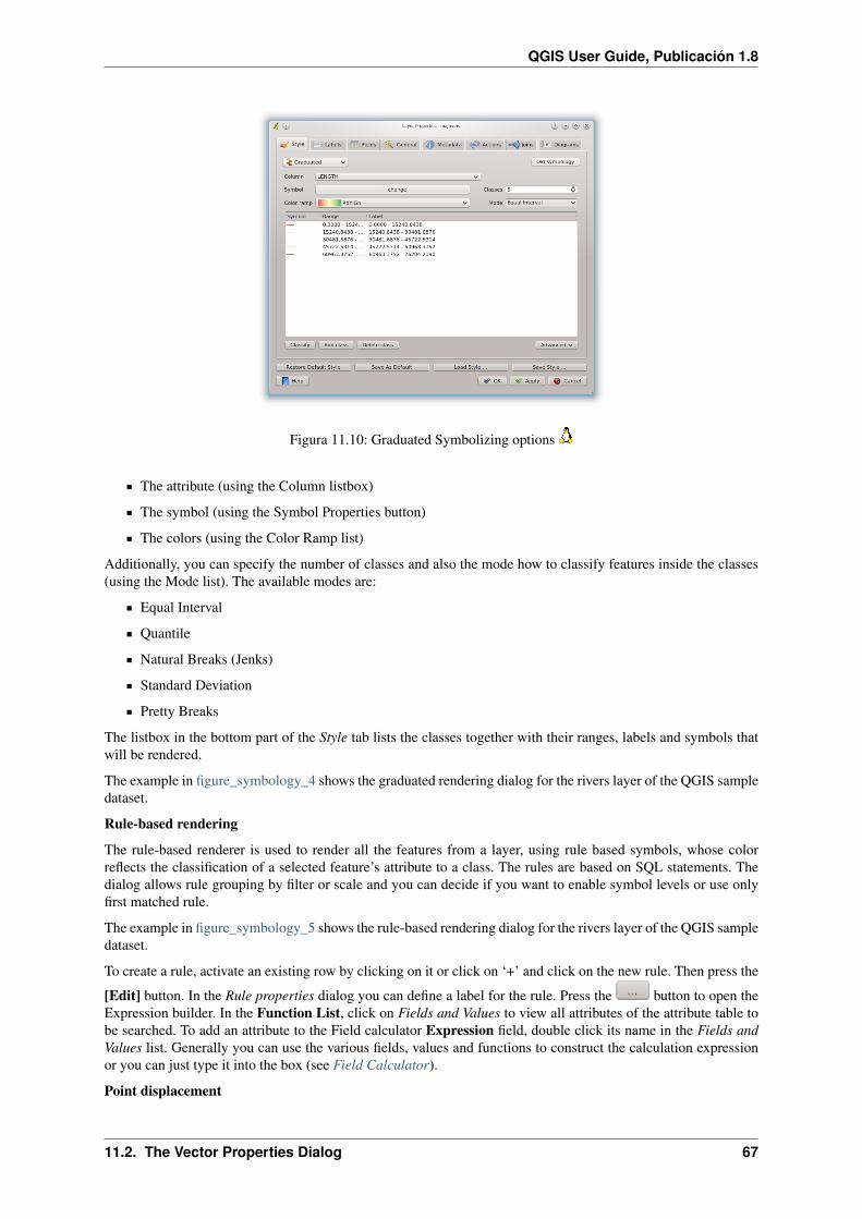
QGIS User Guide, Publicación 1.8
Figura 11.10: Graduated Symbolizing options
The attribute (using the Column listbox)
The symbol (using the Symbol Properties button)
The colors (using the Color Ramp list)
Additionally, you can specify the number of classes and also the mode how to classify features inside the classes(using the Mode list). The available modes are:
Equal Interval
Quantile
Natural Breaks (Jenks)
Standard Deviation
Pretty Breaks
The listbox in the bottom part of the Style tab lists the classes together with their ranges, labels and symbols thatwill be rendered.
The example in figure_symbology_4 shows the graduated rendering dialog for the rivers layer of the QGIS sampledataset.
Rule-based rendering
The rule-based renderer is used to render all the features from a layer, using rule based symbols, whose colorreflects the classification of a selected feature’s attribute to a class. The rules are based on SQL statements. Thedialog allows rule grouping by filter or scale and you can decide if you want to enable symbol levels or use onlyfirst matched rule.
The example in figure_symbology_5 shows the rule-based rendering dialog for the rivers layer of the QGIS sampledataset.
To create a rule, activate an existing row by clicking on it or click on ‘+’ and click on the new rule. Then press the
[Edit] button. In the Rule properties dialog you can define a label for the rule. Press the button to open theExpression builder. In the Function List, click on Fields and Values to view all attributes of the attribute table tobe searched. To add an attribute to the Field calculator Expression field, double click its name in the Fields andValues list. Generally you can use the various fields, values and functions to construct the calculation expressionor you can just type it into the box (see Field Calculator).
Point displacement
11.2. The Vector Properties Dialog 67

QGIS User Guide, Publicación 1.8
Figura 11.11: Rule-based Symbolizing options
The point displacement renderer offers to visualize all features of a point layer, even if they have the same location.To do this, the symbols of the points are placed on a displacement circle around a center symbol.
Figura 11.12: Point displacement dialog
Symbol Properties
The symbol properties dialog allows the user to specify different properties of the symbol to be rendered. In thebottom left part of the dialog, you find a preview of the current symbol as it will be displayed in the map canvas.Above the preview is the list of symbol layers. To start the Symbol properties dialog, click the [ Change...]button in the Style tab of the Layer Properties dialog.
The buttons allow adding or removing layers, changing the position of layers, or locking layers for color changes.In the right part of the dialog, there are shown the settings applicable to the single symbol layer selected in the
symbol layer list. The most important is the Symbol Layer Type combobox, which allows you to choosethe layer type. The available options depend on the layer type (Point, Line, Polygon). The symbol layer typeoptions are described in section vector_symbol_types. You can also change the symbol layer properties in the
68 Capítulo 11. Working with Vector Data
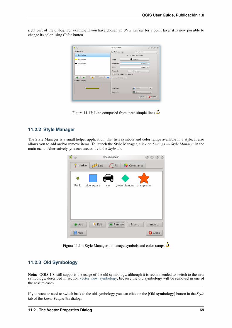
QGIS User Guide, Publicación 1.8
right part of the dialog. For example if you have chosen an SVG marker for a point layer it is now possible tochange its color using Color button.
Figura 11.13: Line composed from three simple lines
11.2.2 Style Manager
The Style Manager is a small helper application, that lists symbols and color ramps available in a style. It alsoallows you to add and/or remove items. To launch the Style Manager, click on Settings → Style Manager in themain menu. Alternatively, you can access it via the Style tab.
Figura 11.14: Style Manager to manage symbols and color ramps
11.2.3 Old Symbology
Nota: QGIS 1.8. still supports the usage of the old symbology, although it is recommended to switch to the newsymbology, described in section vector_new_symbology, because the old symbology will be removed in one ofthe next releases.
If you want or need to switch back to the old symbology you can click on the [Old symbology] button in the Styletab of the Layer Properties dialog.
11.2. The Vector Properties Dialog 69

QGIS User Guide, Publicación 1.8
You can also make the old symobolgy the default, deactivating Use new generation symbology for renderingin the Rendering tab under Settings → Options.
The old QGIS symbology supports the following renderers:
Single symbol - a single style is applied to every object in the layer.
Graduated symbol - objects within the layer are displayed with different symbols classified by the valuesof a particular field.
Continuous color - objects within the layer are displayed with a spread of colours classified by the numer-ical values within a specified field.
Unique value - objects are classified by the unique values within a specified field with each value having adifferent symbol.
To change the symbology for a layer, simply double click on its legend entry and the vector Layer Propertiesdialog will be shown.
Style Options
Within this dialog you can style your vector layer. Depending on the selected rendering option you have thepossibility to also classify your map features.
At least the following styling options apply for nearly all renderers:
Fill style - Style for filling. Beside the given brushes you can select Fill style: ‘Texture’ and click
the button for selecting your own texture file. Currently the fileformats *.jpeg, *.xpm, and *.pngare supported.
Fill color - fill-color of your features.
Outline options
• Outline style - Pen-style for your outline of your feature. You can also set this to ‘no Pen’.
• Outline color - color of the ouline of your feature.
• Outline width - width of your features.
Once you have styled your layer you also could save your layer-style to a separate file (ending with *.qml). Todo this, use the button [Save Style...]. No need to say that [Load Style...] loads your saved layer-style-file.
If you wish to always use a particular style whenever the layer is loaded, use the [Save As Default] button tomake your style the default. Also, if you make changes to the style that you are not happy with, use the [RestoreDefault Style] button to revert to your default style.
Vector transparency
QGIS allows to set a transparency for every vector layer. This can be done with the slider Transparency
inside the Style tab. This is very useful for overlaying several vector layers.
11.2.4 Labels Tab
As for the symbology QGIS 1.8 currently provides an old and a new labeling engine in parallel. The Labelstab still contains the old labeling. The new labeling is implemented as a core application and will replace thefeatures of the old labels tab in one of the next versions.
We recommend to switch to the new labeling, described in section New Labeling.
The old labeling in the Labels tab allows you to enable labeling features and control a number of options relatedto fonts, placement, style, alignment and buffering. We will illustrate this by labeling the lakes shapefile of theQGIS sample dataset:
1. Load the Shapefile alaska.shp and GML file lakes.gml in QGIS
70 Capítulo 11. Working with Vector Data
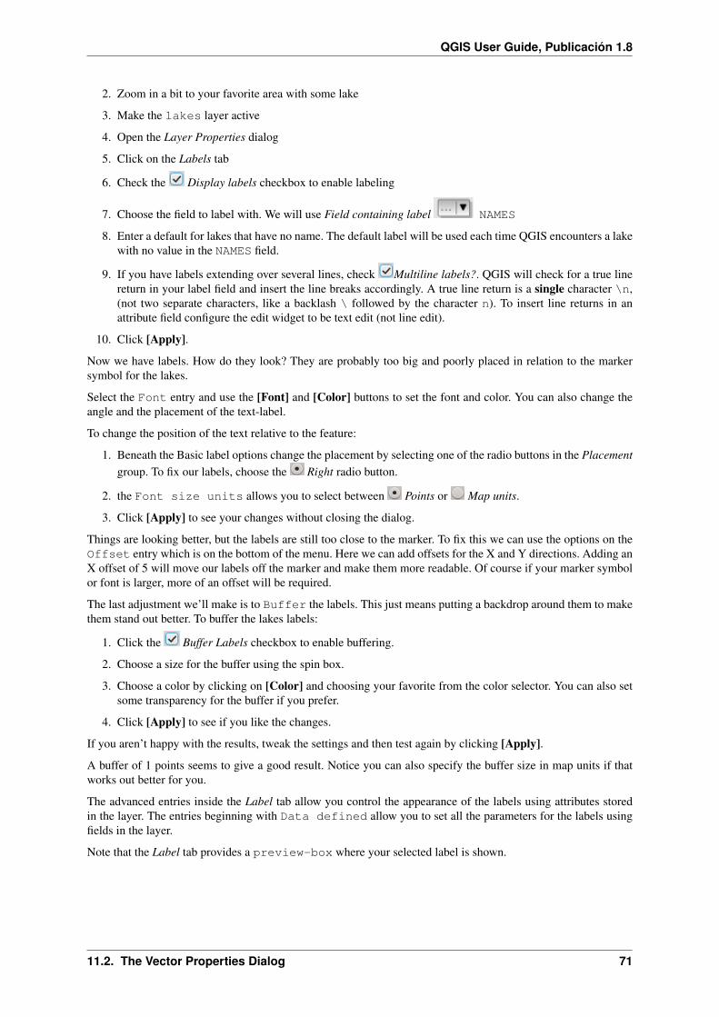
QGIS User Guide, Publicación 1.8
2. Zoom in a bit to your favorite area with some lake
3. Make the lakes layer active
4. Open the Layer Properties dialog
5. Click on the Labels tab
6. Check the Display labels checkbox to enable labeling
7. Choose the field to label with. We will use Field containing label NAMES
8. Enter a default for lakes that have no name. The default label will be used each time QGIS encounters a lakewith no value in the NAMES field.
9. If you have labels extending over several lines, check Multiline labels?. QGIS will check for a true linereturn in your label field and insert the line breaks accordingly. A true line return is a single character \n,(not two separate characters, like a backlash \ followed by the character n). To insert line returns in anattribute field configure the edit widget to be text edit (not line edit).
10. Click [Apply].
Now we have labels. How do they look? They are probably too big and poorly placed in relation to the markersymbol for the lakes.
Select the Font entry and use the [Font] and [Color] buttons to set the font and color. You can also change theangle and the placement of the text-label.
To change the position of the text relative to the feature:
1. Beneath the Basic label options change the placement by selecting one of the radio buttons in the Placementgroup. To fix our labels, choose the Right radio button.
2. the Font size units allows you to select between Points or Map units.
3. Click [Apply] to see your changes without closing the dialog.
Things are looking better, but the labels are still too close to the marker. To fix this we can use the options on theOffset entry which is on the bottom of the menu. Here we can add offsets for the X and Y directions. Adding anX offset of 5 will move our labels off the marker and make them more readable. Of course if your marker symbolor font is larger, more of an offset will be required.
The last adjustment we’ll make is to Buffer the labels. This just means putting a backdrop around them to makethem stand out better. To buffer the lakes labels:
1. Click the Buffer Labels checkbox to enable buffering.
2. Choose a size for the buffer using the spin box.
3. Choose a color by clicking on [Color] and choosing your favorite from the color selector. You can also setsome transparency for the buffer if you prefer.
4. Click [Apply] to see if you like the changes.
If you aren’t happy with the results, tweak the settings and then test again by clicking [Apply].
A buffer of 1 points seems to give a good result. Notice you can also specify the buffer size in map units if thatworks out better for you.
The advanced entries inside the Label tab allow you control the appearance of the labels using attributes storedin the layer. The entries beginning with Data defined allow you to set all the parameters for the labels usingfields in the layer.
Note that the Label tab provides a preview-box where your selected label is shown.
11.2. The Vector Properties Dialog 71

QGIS User Guide, Publicación 1.8
11.2.5 New Labeling
The new Labeling core application provides smart labeling for vector point, line and polygon layers and onlyrequires a few parameters. This new application will replace the current QGIS labeling, described in section LabelsTab and also supports on-the-fly transformated layers.
Using new labeling
1. Start QGIS and load a vector point, line or polygon layer.
2. Activate the layer in the legend and click on the Labeling icon in the QGIS toolbar menu.
Labeling point layers
First step is to activate the Label this layer checkbox and select an attribute column to use for labeling. Click
if you want to define labels based on expressions. After that you can define the text style and the scale-basedvisibility in the Label settings tab (see Figure_labels_1 ). Choose the Advanced tab for the label placement and thelabeling priority. You can define if every part of a multipart feature is to be labeled here. With the wrap label oncharacter function you can define a character for a line break in the labels. The Data defined settings tab providesyou with the attribute-based definition of Font properties, Buffer properties and Position.
Figura 11.15: Smart labeling of vector point layers
Labeling line layers
First step is to activate the Label this layer checkbox in the Label settings tab and select an attribute column touse for labeling. Here you can also define labels based on expressions. After that you can define the text style andthe scale-based visibility. Further labeling options are available through the Advanced tab. You can define the labelplacement and label distance, a line orientation dependend position and the labeling priority here. Furthermore youcan define if every part of a multipart line is to be labeled, if lines shall be merged to avoid duplicate labels andif a direction symbol is added (see Figure_labels_2 ). It is also possible to supress labeling of features and wraplables on characters. Use Data defined settings for attribute-based or database-connection-based settings.
Labeling polygon layers
First step is to activate the Label this layer checkbox and select an attribute column to use for labeling. Hereyou can also define labels based on expressions. In Label settings define the text style and the scale-based visibility(see Figure_labels_3 ). Use the Advanced tab for label placement, label distance and labeling priority. Define ifevery part of a multipart feature is to be labeled, suppress labeling of features and wrap labels on characters here.Use Data defined settings for attribute-based or database-connection-based settings.
Change engine settings
Additionally you can click the [Engine settings] button and select the search method, used to find the best labelplacement. Available is Chain, Popmusic Tabu, Popmusic Chain, Popmusic Tabu Chain and FALP.
Furthermore the number of candidates can be defined for point, line and polygon features, and you can definewhether to show all labels (including colliding labels) and label candidates for debugging.
72 Capítulo 11. Working with Vector Data

QGIS User Guide, Publicación 1.8
Figura 11.16: Smart labeling of vector line layers
Figura 11.17: Smart labeling of vector polygon layers
Figura 11.18: Dialog to change label engine settings
11.2. The Vector Properties Dialog 73

QGIS User Guide, Publicación 1.8
Keywords to use in attribute columns for labeling
There is a list of supported key words, that can be used for the placement of labels in defined attribute columns.
For horizontal alignment: left, center, right
For vertical alignment: bottom, base, half, top
Colors can be specified in svg notation, e.g. #ff0000
for bold, underlined, strikeout and italic: 0 = false 1 = true
A combination of key words in one column also works, e.g.: base right or bottom left.
11.2.6 Fields Tab
Within the Fields tab the field attributes of the selected dataset can be manipulated. The buttons New Column
and Delete Column can be used, when the dataset is Editing mode.
At the moment only columns from PostGIS layers can be removed and added. The OGR library supports to addand remove columns, if you have a GDAL version >= 1.9 installed.
Edit Widget
Figura 11.19: Dialog to select an edit widget for an attribute column
Within the Fields tab you also find an edit widget column. This column can be used to define values or arange of values that are allowed to be added to the specific attribute table column. If you click on the [edit widget]button, a dialog opens, where you can define different widgets. These widgets are:
Line edit: an edit field which allows to enter simple text (or restrict to numbers for numeric attributes).
Classification: Displays a combo box with the values used for classification, if you have chosen ‘uniquevalue’ as legend type in the Style tab of the properties dialog.
Range: Allows to set numeric values from a specific range. The edit widget can be either a slider or a spinbox.
Unique values: The user can select one of the values already used in the attribute table. If editable isactivated, a line edit is shown with autocompletion support, otherwise a combo box is used.
File name: Simplifies the selection by adding a file chooser dialog.
74 Capítulo 11. Working with Vector Data

QGIS User Guide, Publicación 1.8
Value map: a combo box with predefined items. The value is stored in the attribute, the description is shownin the combo box. You can define values manually or load them from a layer or a CSV file.
Enumeration: Opens a combo box with values that can be used within the columns type. This is currentlyonly supported by the postgres provider.
Immutable: The immutable attribute column is read-only. The user is not able to modify the content.
Hidden: A hidden attribute column is invisible. The user is not able to see its content.
Checkbox: Displays a checkbox and you can define what attribute is added to the column when the check-box is activated or not.
Text edit: This opens a text edit field that allows multiple lines to be used.
Calendar: Opens a calendar widget to enter a date. Column type must be text.
Value Relation: Offers values from a related table in a combobox. You can select layer, key column andvalue column.
UUID Generator: Generates a read-only UUID (Universally Unique Identifiers) field, if empty.
11.2.7 General Tab
The General tab is essentially like that of the raster dialog. There are several options available:
Change the display name of the layer
Set a display field to be used for the Identify Results dialog
Define a certain Edit User Interface for the vector layer written with the Qt Creator IDE and tools athttp://qt.digia.com/Product/Developer-Tools/
Create a Spatial Index (only for OGR supported formats)
Add an Init function for the layer. They will overwrite existing QGIS widget initializations, if applied
Update Extents information for a layer
View or change the projection of the specific vector layer, clicking on Specify CRS
Furthermore you can activate and set Use scale dependent rendering, define provider specific options (e.g.encoding) and with the [Query Builder] button you can create a subset of the features in the layer that will bevisualized (also refer to section Selection).
11.2.8 Metadata Tab
The Metadata tab contains general information about the layer, including specifics about the type and lo-cation, number of features, feature type, and the editing capabilities. The Extents section, providing layer extentinformation, and the Layer Spatial Reference System section, providing information about the CRS of the layer.This is a quick way to get information about the layer.
Additionally you can add/edit a title for the layer and some abtract information. These information will be savedin the QGIS project file for following sessions and will be used for QGIS server.
11.2.9 Actions Tab
QGIS provides the ability to perform an action based on the attributes of a feature. This can be used toperform any number of actions, for example, running a program with arguments built from the attributes of afeature or passing parameters to a web reporting tool.
11.2. The Vector Properties Dialog 75

QGIS User Guide, Publicación 1.8
Figura 11.20: General tab in vector layers properties dialog
Figura 11.21: Metadata tab in vector layers properties dialog
76 Capítulo 11. Working with Vector Data

QGIS User Guide, Publicación 1.8
Figura 11.22: Overview action dialog with some sample actions
Actions are useful when you frequently want to run an external application or view a web page based on one ormore values in your vector layer. They are devided into 6 types and can be used like this:
Generic, Mac, Windows and Unix actions start an external process,
Python actions execute a python expression,
Generic and Python actions are visible everywhere,
Mac, Windows and Unix actions are visible only on the respective platform (i.e. you can define three ‘Edit’actions to open an editor and the users can only see and execute the one ‘Edit’ action for their platform torun the editor).
There are several examples included in the dialog. You can load them clicking on [Add default actions]. Anexample is performing a search based on an attribute value. This concept is used in the following discussion.
Defining Actions
Attribute actions are defined from the vector Layer Properties dialog. To define an action, open the vector LayerProperties dialog and click on the Actions tab. Select ‘Generic’ as type and provide a descriptive name for theaction. The action itself must contain the name of the application that will be executed when the action is invoked.You can add one or more attribute field values as arguments to the application. When the action is invoked anyset of characters that start with a% followed by the name of a field will be replaced by the value of that field. Thespecial characters % % will be replaced by the value of the field that was selected from the identify results orattribute table (see using_actions below). Double quote marks can be used to group text into a single argument tothe program, script or command. Double quotes will be ignored if preceded by a backslash.
If you have field names that are substrings of other field names (e.g., col1 and col10) you should indicate so,by surrounding the field name (and the % character) with square brackets (e.g., [%col10]). This will preventthe%col10 field name being mistaken for the%col1 field name with a 0 on the end. The brackets will beremoved by QGIS when it substitutes in the value of the field. If you want the substituted field to be surroundedby square brackets, use a second set like this: [[%col10]].
Using the Identify Features tool you can open Identify Results dialog. It includes a (Derived) item that containsinformation relevant to the layer type. The values in this item can be accessed in a similar way to the other fieldsby using preceeding the derived field name by (Derived).. For example, a point layer has an X and Y field andthe value of these can be used in the action with%(Derived).X and%(Derived).Y. The derived attributesare only available from the Identify Results dialog box, not the Attribute Table dialog box.
Two example actions are shown below:
11.2. The Vector Properties Dialog 77

QGIS User Guide, Publicación 1.8
konqueror http://www.google.com/search?q=%nam
konqueror http://www.google.com/search?q=%%
In the first example, the web browser konqueror is invoked and passed a URL to open. The URL performs aGoogle search on the value of the nam field from our vector layer. Note that the application or script called bythe action must be in the path or you must provide the full path. To be sure, we could rewrite the first exam-ple as: /opt/kde3/bin/konqueror http://www.google.com/search?q=%nam. This will ensurethat the konqueror application will be executed when the action is invoked.
The second example uses the % % notation which does not rely on a particular field for its value. When the actionis invoked, the % % will be replaced by the value of the selected field in the identify results or attribute table.Using Actions
Actions can be invoked from either the Identify Results dialog, an Attribute Table dialog or from Run Fea-
ture Action (recall that these dialogs can be opened by clicking Identify Features or Open Attribute Table orRun Feature Action). To invoke an action, right click on the record and choose the action from the popup menu. Actionsare listed in the popup menu by the name you assigned when defining the actions. Click on the action you wish toinvoke.
If you are invoking an action that uses the % % notation, right-click on the field value in the Identify Results dialogor the Attribute Table dialog that you wish to pass to the application or script.
Here is another example that pulls data out of a vector layer and inserts them into a file using bash and the
echo command (so it will only work or perhaps ). The layer in question has fields for a species nametaxon_name, latitude lat and longitude long. I would like to be able to make a spatial selection of a localitiesand export these field values to a text file for the selected record (shown in yellow in the QGIS map area). Here isthe action to achieve this:
bash -c "echo \"%taxon_name%lat%long\" >> /tmp/species_localities.txt"
After selecting a few localities and running the action on each one, opening the output file will show somethinglike this:
Acacia mearnsii -34.0800000000 150.0800000000Acacia mearnsii -34.9000000000 150.1200000000Acacia mearnsii -35.2200000000 149.9300000000Acacia mearnsii -32.2700000000 150.4100000000
As an exercise we create an action that does a Google search on the lakes layer. First we need to determinethe URL needed to perform a search on a keyword. This is easily done by just going to Google and doing asimple search, then grabbing the URL from the address bar in your browser. From this little effort we see that theformat is: http://google.com/search?q=qgis, where QGIS is the search term. Armed with this information, we canproceed:
1. Make sure the lakes layer is loaded.
2. Open the Layer Properties dialog by double-clicking on the layer in the legend or right-click and chooseProperties from the popup menu.
3. Click on the Actions tab.
4. Enter a name for the action, for example Google Search.
5. For the action, we need to provide the name of the external program to run. In this case, we can use Firefox.If the program is not in your path, you need to provide the full path.
6. Following the name of the external application, add the URL used for doing a Google search, up to but notincluded the search term: http://google.com/search?q=
7. The text in the Action field should now look like this: firefox http://google.com/search?q=
8. Click on the drop-down box containing the field names for the lakes layer. It’s located just to the left ofthe [Insert Field] button.
78 Capítulo 11. Working with Vector Data
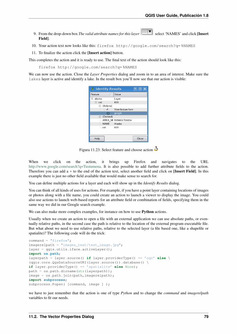
QGIS User Guide, Publicación 1.8
9. From the drop-down box The valid attribute names for this layer select ‘NAMES’ and click [InsertField].
10. Your action text now looks like this: firefox http://google.com/search?q=%NAMES
11. To finalize the action click the [Insert action] button.
This completes the action and it is ready to use. The final text of the action should look like this:
firefox http://google.com/search?q=%NAMES
We can now use the action. Close the Layer Properties dialog and zoom in to an area of interest. Make sure thelakes layer is active and identify a lake. In the result box you’ll now see that our action is visible:
Figura 11.23: Select feature and choose action
When we click on the action, it brings up Firefox and navigates to the URLhttp://www.google.com/search?q=Tustumena. It is also possible to add further attribute fields to the action.Therefore you can add a + to the end of the action text, select another field and click on [Insert Field]. In thisexample there is just no other field available that would make sense to search for.
You can define multiple actions for a layer and each will show up in the Identify Results dialog.
You can think of all kinds of uses for actions. For example, if you have a point layer containing locations of imagesor photos along with a file name, you could create an action to launch a viewer to display the image. You couldalso use actions to launch web-based reports for an attribute field or combination of fields, specifying them in thesame way we did in our Google search example.
We can also make more complex examples, for instance on how to use Python actions.
Usually when we create an action to open a file with an external application we can use absolute paths, or even-tually relative paths, in the second case the path is relative to the location of the external program executable file.But what about we need to use relative paths, relative to the selected layer (a file based one, like a shapefile orspatialite)? The following code will do the trick:
command = "firefox";imagerelpath = "images_test/test_image.jpg";layer = qgis.utils.iface.activeLayer();import os.path;layerpath = layer.source() if layer.providerType() == ’ogr’ else \(qgis.core.QgsDataSourceURI(layer.source()).database() \if layer.providerType() == ’spatialite’ else None);path = os.path.dirname(str(layerpath));image = os.path.join(path,imagerelpath);import subprocess;subprocess.Popen( [command, image ] );
we have to just remember that the action is one of type Python and to change the command and imagerelpathvariables to fit our needs.
11.2. The Vector Properties Dialog 79
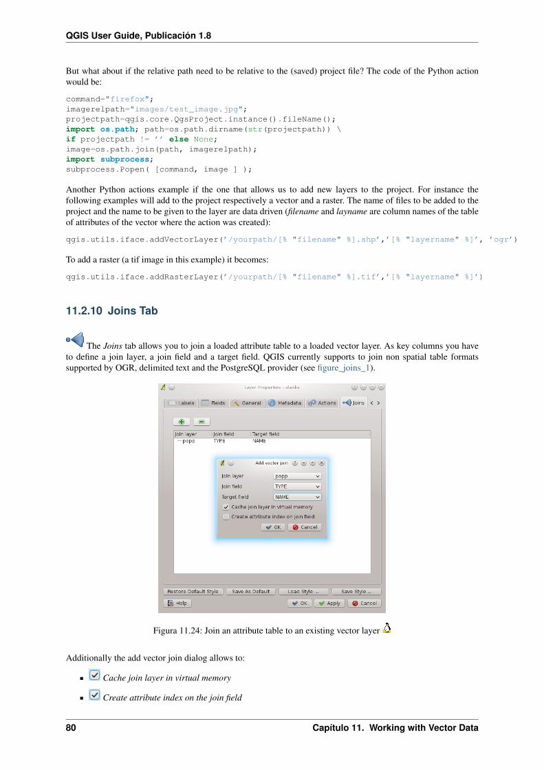
QGIS User Guide, Publicación 1.8
But what about if the relative path need to be relative to the (saved) project file? The code of the Python actionwould be:
command="firefox";imagerelpath="images/test_image.jpg";projectpath=qgis.core.QgsProject.instance().fileName();import os.path; path=os.path.dirname(str(projectpath)) \if projectpath != ’’ else None;image=os.path.join(path, imagerelpath);import subprocess;subprocess.Popen( [command, image ] );
Another Python actions example if the one that allows us to add new layers to the project. For instance thefollowing examples will add to the project respectively a vector and a raster. The name of files to be added to theproject and the name to be given to the layer are data driven (filename and layname are column names of the tableof attributes of the vector where the action was created):
qgis.utils.iface.addVectorLayer(’/yourpath/[% "filename" %].shp’,’[% "layername" %]’, ’ogr’)
To add a raster (a tif image in this example) it becomes:
qgis.utils.iface.addRasterLayer(’/yourpath/[% "filename" %].tif’,’[% "layername" %]’)
11.2.10 Joins Tab
The Joins tab allows you to join a loaded attribute table to a loaded vector layer. As key columns you haveto define a join layer, a join field and a target field. QGIS currently supports to join non spatial table formatssupported by OGR, delimited text and the PostgreSQL provider (see figure_joins_1).
Figura 11.24: Join an attribute table to an existing vector layer
Additionally the add vector join dialog allows to:
Cache join layer in virtual memory
Create attribute index on the join field
80 Capítulo 11. Working with Vector Data

QGIS User Guide, Publicación 1.8
11.2.11 Diagrams Tab
The Diagrams tab allows you to add a graphic overlay to a vector layer (see figure_diagrams_1).
The current core implementation of diagrams provides support for piecharts and text diagrams. Text values ofdifferent data columns are displayed one below the other with a circle or a box and dividers. Diagram size is basedon a fixed size or on linear scaling according to a classification attribute. The placement of the diagrams interactswith the new labeling, so position conflicts between diagrams and labels are detected and solved. In addition tochart positions can be fixed by the users hand.
Figura 11.25: Vector properties dialog with diagram tab
We will demonstrate an example and overlay the alaska boundary layer a text diagram showing some temperaturedata from a climate vector layer. Both vector layers are part of the QGIS sample dataset (see Section SampleData).
1. First click on the Load Vector icon, browse to the QGIS sample dataset folder and load the two vector shapelayers alaska.shp and climate.shp.
2. Double click the climate layer in the map legend to open the Layer Properties dialog.
3. Click on the Diagrams tab, activate Display diagrams and from Diagram type combobox select‘Text diagram’
4. As Background color we choose a light blue and set a fixed size to 18 mm.
5. Placement could be set to AroundPoint.
6. In the diagram we want to display the values of the three columns T_F_JAN, T_F_JUL and T_F_MEAN.First select T_F_JAN as Attributes and click the green [+] button, then T_F_JUL and finally T_F_MEAN.
7. Now click [Apply] to display the diagram in the QGIS main window.
8. You can now adapt the chart size, or change the attribute colors by double clicking on the color values inthe attribute field. Figure_diagrams_2 gives an impression.
9. Finally click [Ok].
Additionally in the Settings → Options dialog, there is a Overlay tab where it is possible to select the placementalgorithm of the diagrams. The central point method is a generic one, the others use algorithms of the PAL library.
11.2. The Vector Properties Dialog 81

QGIS User Guide, Publicación 1.8
Figura 11.26: Diagram from temperature data overlayed on a map
They also consider diagram objects and labels in different layers. Also see section Diagram Overlay Plugin foradditional diagram features.
11.3 Editing
QGIS supports various capabilities for editing OGR, PostGIS and SpatiaLite vector layers.
Nota: The procedure for editing GRASS layers is different - see Section Digitizing and editing a GRASS vectorlayer for details.
Truco: Concurrent EditsThis version of QGIS does not track if somebody else is editing a feature at the same time as you. The last personto save their edits wins.
11.3.1 Setting the Snapping Tolerance and Search Radius
Before we can edit vertices, we must set the snapping tolerance and search radius to a value that allows us anoptimal editing of the vector layer geometries.
Snapping tolerance
Snapping tolerance is the distance QGIS uses to search for the closest vertex and/or segment you are tryingto connect when you set a new vertex or move an existing vertex. If you aren’t within the snapping tolerance,QGIS will leave the vertex where you release the mouse button, instead of snapping it to an existing vertex and/orsegment. The snapping tolerance setting affects all tools which work with tolerance.
1. A general, project wide snapping tolerance can be defined choosing Settings → Options. On Mac: goto QIS → Preferences..., on Linux: Edit → Options. In the Digitizing tab you can select between tovertex, to segment or to vertex and segment as default snap mode. You can also define a default snappingtolerance and a search radius for vertex edits. The tolerance an be set either in map units or in pixels.The advantage of choosing pixels, is that the snapping tolerance doesn’t have to be changed after zoomoperations. In our small digitizing project (working with the Alaska dataset), we define the snapping units
82 Capítulo 11. Working with Vector Data

QGIS User Guide, Publicación 1.8
in feet. Your results may vary, but something on the order of 300ft should be fine at a scale of 1:10 000should be a reasonable setting.
2. A layer based snapping tolerance can be defined by choosing Settings → (or File →) Snapping options... toenable and adjust snapping mode and tolerance on a layer basis (see figure_edit_1 ).
Note that this layer based snapping overrides the global snapping option set in the Digitizing tab. So if you needto edit one layer, and snap its vertices to another layer, then enable snapping only on the snap to layer, thendecrease the global snapping tolerance to a smaller value. Furthermore, snapping will never occur to a layer whichis not checked in the snapping options dialog, regardless of the global snapping tolerance. So be sure to mark thecheckbox for those layers that you need to snap to.
Figura 11.27: Edit snapping options on a layer basis
Search radius
Search radius is the distance QGIS uses to search for the closest vertex you are trying to move when you clickon the map. If you aren’t within the search radius, QGIS won’t find and select any vertex for editing and it willpop up an annoying warning to that effect. Snap tolerance and search radius are set in map units or pixels, so youmay find you need to experiment to get them set right. If you specify too big of a tolerance, QGIS may snap to thewrong vertex, especially if you are dealing with a large number of vertices in close proximity. Set search radiustoo small and it won’t find anything to move.
The search radius for vertex edits in layer units can be defined in the Digitizing tab under Settings → Options.The same place where you define the general, project wide snapping tolerance.
11.3.2 Zooming and Panning
Before editing a layer, you should zoom in to your area of interest. This avoids waiting while all the vertex markersare rendered across the entire layer.
Apart from using the pan and zoom-in / zoom-out icons on the toolbar with the mouse, navigating can alsobe done with the mouse wheel, spacebar and the arrow keys.
Zooming and panning with the mouse wheel
While digitizing you can press the mouse wheel to pan inside of the main window and you can roll the mousewheel to zoom in and out on the map. For zooming place the mouse cursor inside the map area and roll it forward(away from you) to zoom in and backwards (towards you) to zoom out. The mouse cursor position will be thecenter of the zoomed area of interest. You can customize the behavior of the mouse wheel zoom using the Maptools tab under the Settings → Options menu.
Panning with the arrow keys
Panning the map during digitizing is possible with the arrow keys. Place the mouse cursor inside the map area andclick on the right arrow key to pan east, left arrow key to pan west, up arrow key to pan north and down arrow key
11.3. Editing 83

QGIS User Guide, Publicación 1.8
to pan south.
You can also use the spacebar to temporarily cause mouse movements to pan then map. The PgUp and PgDownkeys on your keyboard will cause the map display to zoom in or out without interrupting your digitizing session.
11.3.3 Topological editing
Besides layer based snapping options you can also define some topological functionalities in the Snapping op-
tions... dialog in the Settings (or File) menu. Here you can define Enable topological editing and/or for polygon
layers you can activate the column Avoid Int. which avoids intersection of new polygons.
Enable topological editing
The option Enable topological editing is for editing and maintaining common boundaries in polygon mosaics.QGIS ‘detects’ a shared boundary in a polygon mosaic and you only have to move the vertex once and QGIS willtake care about updating the other boundary.
Avoid intersections of new polygons
The second topological option in the Avoid Int. column, called Avoid intersections of new polygons avoidsoverlaps in polygon mosaics. It is for quicker digitizing of adjacent polygons. If you already have one polygon,it is possible with this option to digitise the second one such that both intersect and QGIS then cuts the secondpolygon to the common boundary. The advantage is that users don’t have to digitize all vertices of the commonboundary.
11.3.4 Digitizing an existing layer
By default, QGIS loads layers read-only: This is a safeguard to avoid accidentally editing a layer if there is aslip of the mouse. However, you can choose to edit any layer as long as the data provider supports it, and theunderlying data source is writable (i.e. its files are not read-only). Layer editing is most versatile when used onPostgreSQL/PostGIS data sources.
In general, editing vector layers is divided into a digitizing and an advanced digitizing tool-bar, described in Section Advanced digitizing. You can select and unselect both under Set-tings → Toolbars →. Using the basic digitizing tools you can perform the following functions:
Icon Purpose Icon Purpose
Toggle editing Adding Features: Capture Point
Adding Features: Capture Line Adding Features: Capture Polygon
Move Feature Node Tool
Delete Selected Cut Features
Copy Features Paste Features
Save edits and continue
Table Editing: Vector layer basic editing toolbar
All editing sessions start by choosing the Toggle editing option. This can be found in the context menu after rightclicking on the legend entry for that layer.
Alternately, you can use the Toggle Editing Toggle editing button from the digitizing toolbar to start or stop theediting mode. Once the layer is in edit mode, markers will appear at the vertices, and additional tool buttons onthe editing toolbar will become available.
84 Capítulo 11. Working with Vector Data
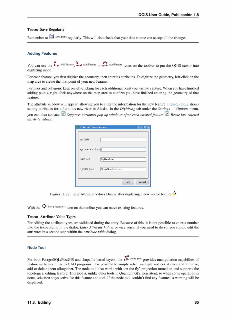
QGIS User Guide, Publicación 1.8
Truco: Save Regularly
Remember to Save Edits regularly. This will also check that your data source can accept all the changes.
Adding Features
You can use the Add Feature, Add Feature or Add Feature icons on the toolbar to put the QGIS cursor intodigitizing mode.
For each feature, you first digitize the geometry, then enter its attributes. To digitize the geometry, left-click on themap area to create the first point of your new feature.
For lines and polygons, keep on left-clicking for each additional point you wish to capture. When you have finishedadding points, right-click anywhere on the map area to confirm you have finished entering the geometry of thatfeature.
The attribute window will appear, allowing you to enter the information for the new feature. Figure_edit_2 showssetting attributes for a fictitious new river in Alaska. In the Digitizing tab under the Settings → Options menu,
you can also activate Suppress attributes pop-up windows after each created feature Reuse last enteredattribute values.
Figura 11.28: Enter Attribute Values Dialog after digitizing a new vector feature
With the Move Feature(s) icon on the toolbar you can move existing features.
Truco: Attribute Value TypesFor editing the attribute types are validated during the entry. Because of this, it is not possible to enter a numberinto the text-column in the dialog Enter Attribute Values or vice versa. If you need to do so, you should edit theattributes in a second step within the Attribute table dialog.
Node Tool
For both PostgreSQL/PostGIS and shapefile-based layers, the Node Tool provides manipulation capabilites offeature vertices similar to CAD programs. It is possible to simply select multiple vertices at once and to move,add or delete them alltogether. The node tool also works with ‘on the fly’ projection turned on and supports thetopological editing feature. This tool is, unlike other tools in Quantum GIS, persistent, so when some operation isdone, selection stays active for this feature and tool. If the node tool couldn’t find any features, a warning will bedisplayed.
11.3. Editing 85

QGIS User Guide, Publicación 1.8
Important is to set the property Settings → Options → Digitizing → Search Radius: to a numbergreater than zero (i.e. 10). Otherwise QGIS will not be able to tell which vertex is being edited.
Truco: Vertex MarkersThe current version of QGIS supports three kinds of vertex-markers: Semi transparent circle, Cross and None. Tochange the marker style, choose Options from the Settings menu and click on the Digitizing tab and select theappropriate entry.
Basic operations
Start by activating the Node Tool and selecting a feature by clicking on it. Red boxes will appear at each vertexof this feature.
Selecting vertices: You can select vertices by clicking on them one at a time, by clicking on an edge to selectthe vertices at both ends, or by clicking and dragging a rectangle around some vertices. When a vertex isselected its color changes to blue. To add more vertices to the current selection, hold down the Ctrl keywhile clicking. Hold down Ctrl or Shift when clicking to toggle the selection state of vertices (verticesthat are currently unselected will be selected as usual, but also vertices that are already selected will becomeunselected).
Adding vertices: To add a vertex simply double click near an edge and a new vertex will appear on the edgenear to the cursor. Note that the vertex will appear on the edge, not at the cursor position, therefore it has tobe moved if necessary.
Deleting vertices: After selecting vertices for deletion, click the Delete key. Note that you cannot use theNode Tool to delete a complete feature; QGIS will ensure it retains the minimum number of vertices for
the feature type you are working on. To delete a complete feature use the Delete Selected tool.
Moving vertices: Select all the vertices you want to move. Click on a selected vertex or edge and drag in thedirection you wish to move. All the selected vertices will move together. If snapping is enabled, the wholeselection can jump to the nearest vertex or line.
Each change made with the node tool is stored as a separate entry in the undo dialog. Remember that all operationssupport topological editing when this is turned on. On the fly projection is also supported, and the node toolprovides tooltips to identify a vertex by hovering the pointer over it.
Cutting, Copying and Pasting Features
Selected features can be cut, copied and pasted between layers in the same QGIS project, as long as destination
layers are set to Toggle editing beforehand.
Features can also be pasted to external applications as text: That is, the features are represented in CSV formatwith the geometry data appearing in the OGC Well-Known Text (WKT) format.
However in this version of QGIS, text features from outside QGIS cannot be pasted to a layer within QGIS. Whenwould the copy and paste function come in handy? Well, it turns out that you can edit more than one layer at atime and copy/paste features between layers. Why would we want to do this? Say we need to do some work on anew layer but only need one or two lakes, not the 5,000 on our big_lakes layer. We can create a new layer anduse copy/paste to plop the needed lakes into it.
As an example we are copying some lakes to a new layer:
1. Load the layer you want to copy from (source layer)
2. Load or create the layer you want to copy to (target layer)
3. Start editing for target layer
4. Make the source layer active by clicking on it in the legend
86 Capítulo 11. Working with Vector Data

QGIS User Guide, Publicación 1.8
5. Use the Select Single Feature tool to select the feature(s) on the source layer
6. Click on the Copy Features tool
7. Make the destination layer active by clicking on it in the legend
8. Click on the Paste Features tool
9. Stop editing and save the changes
What happens if the source and target layers have different schemas (field names and types are not the same)?QGIS populates what matches and ignores the rest. If you don’t care about the attributes being copied to the targetlayer, it doesn’t matter how you design the fields and data types. If you want to make sure everything - feature andits attributes - gets copied, make sure the schemas match.
Truco: Congruency of Pasted FeaturesIf your source and destination layers use the same projection, then the pasted features will have geometry identicalto the source layer. However if the destination layer is a different projection then QGIS cannot guarantee thegeometry is identical. This is simply because there are small rounding-off errors involved when converting betweenprojections.
Deleting Selected Features
If we want to delete an entire polygon, we can do that by first selecting the polygon using the regularSelect Single Feature tool. You can select multiple features for deletion. Once you have the selection set, use theDelete Selected tool to delete the features.
The Cut Features tool on the digitizing toolbar can also be used to delete features. This effectively deletes the
feature but also places it on a “spatial clipboard”. So we cut the feature to delete. We could then use thePaste Features tool to put it back, giving us a one-level undo capability. Cut, copy, and paste work on the currentlyselected features, meaning we can operate on more than one at a time.
Truco: Feature Deletion SupportWhen editing ESRI shapefiles, the deletion of features only works if QGIS is linked to a GDAL version 1.3.2 orgreater. The OS X and Windows versions of QGIS available from the download site are built using GDAL 1.3.2or higher.
Saving Edited Layers
When a layer is in editing mode, any changes remain in the memory of QGIS. Therefore they are not commit-ted/saved immediately to the data source or disk. If you want to save edits to the current layer but want to continue
editing without leaving the editing mode, you can click the Save Edits button. When you turn editing mode off
with the Toggle editing (or quit QGIS for that matter), you are also asked if you want to save your changes ordiscard them.
If the changes cannot be saved (e.g. disk full, or the attributes have values that are out of range), the QGIS in-memory state is preserved. This allows you to adjust your edits and try again.
Truco: Data IntegrityIt is always a good idea to back up your data source before you start editing. While the authors of QGIS havemade every effort to preserve the integrity of your data, we offer no warranty in this regard.
11.3. Editing 87

QGIS User Guide, Publicación 1.8
11.3.5 Advanced digitizing
Icon Purpose Icon Purpose
Undo Redo
Simplify Feature Add Ring
Add Part Delete Ring
Delete Part Reshape Features
Offset Curve Split Features
Merge Selected Features Rotate Point Symbols
Merge Attributes of Selected Features
Table Advanced Editing: Vector layer advanced editing toolbar
Undo and Redo
The Undo and Redo tools allow the user to undo or redo vector editing operations. There is also a dockablewidget, which shows all operations in the undo/redo history (see Figure_edit_3). This widget is not displayed bydefault; it can be displayed by right clicking on the toolbar and activating the Undo/Redo check box. Undo/Redois however active, even if the widget is not displayed.
Figura 11.29: Redo and Undo digitizing steps
When Undo is hit, the state of all features and attributes are reverted to the state before the reverted operationhappened. Changes other than normal vector editing operations (for example changes done by a plugin), may ormay not be reverted, depending on how the changes were performed.
To use the undo/redo history widget simply click to select an operation in the history list; all features will bereverted to the state they were in after the selected operation.
Simplify Feature
The Simplify Feature tool allows to reduce the number of vertices of a feature, as long as the geometry doesn’tchange. You need to select a feature, it will be highlighted by a red rubber band and a slider appears. Moving theslider, the red rubber band is changing its shape to show how the feature is being simplified. Clicking [OK] thenew, simplified geometry will be stored. If a feature cannot be simplified (e.g. MultiPolygons), a message showsup.
88 Capítulo 11. Working with Vector Data
QGIS User Guide, Publicación 1.8
Add Ring
You can create ring polygons using the Add Ring icon in the toolbar. This means inside an existing area it ispossible to digitize further polygons, that will occur as a ‘hole’, so only the area in between the boundaries of theouter and inner polygons remain as a ring polygon.
Add Part
You can add part polygons to a selected multipolygon. The new part polygon has to be digitized outside theselected multipolygon.
Delete Ring
The Delete Ring tool allows to delete ring polygons inside an existing area. This tool only works with polygonlayers. It doesn’t change anything when it is used on the outer ring of the polygon. This tool can be used onpolygon and multi-polygon features. Before you select the vertices of a ring, adjust the vertex edit tolerance.
Delete Part
The Delete Part tool allows to delete parts from multifeatures (e.g. to delete polygons from a multipolygonfeature). It won’t delete the last part of the feature, this last part will stay untouched. This tool works with allmulti-part geometries point, line and polygon. Before you select the vertices of a part, adjust the vertex edittolerance.
Reshape Features
You can reshape line and polygon features using the Reshape Features icon on the toolbar. It replaces the line orpolygon part from the first to the last intersection with the original line. With polygons this can sometimes lead tounintended results. It is mainly useful to replace smaller parts of a polygon, not major overhauls and the reshapeline is not allowed to cross several polygon rings as this would generate an invalid polygon.
For example, you can edit the boundary of a polygon with this tool. First, click in the inner area of the polygonnext to the point where you want to add a new vertex. Then, cross the boundary and add the vertices outside thepolygon. To finish, right-click in the inner area of the polygon. The tool will automatically add a node where thenew line crosses the border. It is also possible to remove part of the area from the polygon, starting the new lineoutside the polygon, adding vertices inside, and ending the line outside the polygon with a right click.
Nota: The reshape tool may alter the starting position of a polygon ring or a closed line. So the point that isrepresented ‘twice’ will not be the same any more. This may not be a problem for most applications, but it issomething to consider.
Offset Curves
The Offset Curve tool is a new editing tool. It creates parallel shifts of lines and polygon rings. The tool canbe applied to the edited layer (the geometries are modified) or also to background layers (creates copies of thelines / rings and adds it to the the edited layer). It is thus ideally suited for the creation of distance line layers.Thedisplacement is shown at the bottom left of the taskbar.
11.3. Editing 89

QGIS User Guide, Publicación 1.8
Split Features
You can split features using the Split Features icon on the toolbar. Just draw a line across the feature you want tosplit.
Merge selected features
The Merge Selected Features tool allows to merge features that have common boundaries and the same attributes.
Merge attributes of selected features
The Merge Attributes of Selected Features tool allows to merge attributes of features with common boundaries and at-tributes without merging their boundaries.
Rotate Point Symbols
The Rotate Point Symbols tool is currently only supported by the old symbology engine. It allows to change therotation of point symbols in the map canvas, if you have defined a rotation column from the attribute table of thepoint layer in the Style tab of the Layer Properties. Otherwise the tool is inactive.
Figura 11.30: Rotate Point Symbols
To change the rotation, select a point feature in the map canvas and rotate it holding the left mouse button pressed.A red arrow with the rotation value will be visualized (see Figure_edit_4). When you release the left mouse buttonagain, the value will be updated in the attribute table.
Nota: If you hold the Ctrl key pressed, the rotation will be done in 15 degree steps.
11.3.6 Creating a new Vector layer
QGIS allows to create new Shapefile layers and new SpatiaLite layers. Creation of a new GRASS layer is supportedwithin the GRASS-plugin. Please refer to section Creating a new GRASS vector layer for more information oncreating GRASS vector layers.
Creating a new Shapefile layer
To create a new Shape layer for editing, choose New → New Shapefile Layer... from the Layer menu. The NewVector Layer dialog will be displayed as shown in Figure_edit_5. Choose the type of layer (point, line or polygon)and the CRS (Coordinate Reference System).
90 Capítulo 11. Working with Vector Data
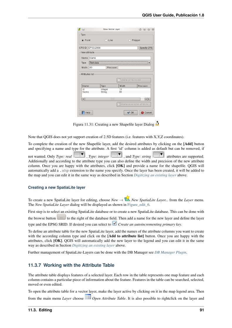
QGIS User Guide, Publicación 1.8
Figura 11.31: Creating a new Shapefile layer Dialog
Note that QGIS does not yet support creation of 2.5D features (i.e. features with X,Y,Z coordinates).
To complete the creation of the new Shapefile layer, add the desired attributes by clicking on the [Add] buttonand specifying a name and type for the attribute. A first ‘id’ column is added as default but can be removed, if
not wanted. Only Type: real , Type: integer , and Type: string attributes are supported.Additionally and according to the attribute type you can also define the width and precision of the new attributecolumn. Once you are happy with the attributes, click [OK] and provide a name for the shapefile. QGIS willautomatically add a .shp extension to the name you specify. Once the layer has been created, it will be added tothe map and you can edit it in the same way as described in Section Digitizing an existing layer above.
Creating a new SpatiaLite layer
To create a new SpatiaLite layer for editing, choose New → New SpatiaLite Layer... from the Layer menu.The New SpatiaLite Layer dialog will be displayed as shown in Figure_edit_6.
First step is to select an existing SpatiaLite database or to create a new SpatiaLite database. This can be done with
the browse button to the right of the database field. Then add a name for the new layer and define the layer
type and the EPSG SRID. If desired you can select to Create an autoincrementing primary key.
To define an attribute table for the new SpatiaLite layer, add the names of the attribute columns you want to createwith the according column type and click on the [Add to attribute list] button. Once you are happy with theattributes, click [OK]. QGIS will automatically add the new layer to the legend and you can edit it in the sameway as described in Section Digitizing an existing layer above.
Further management of SpatiaLite-Layers can be done with the DB Manager see DB Manager Plugin.
11.3.7 Working with the Attribute Table
The attribute table displays features of a selected layer. Each row in the table represents one map feature and eachcolumn contains a particular piece of information about the feature. Features in the table can be searched, selected,moved or even edited.
To open the attribute table for a vector layer, make the layer active by clicking on it in the map legend area. Then
from the main menu Layer choose Open Attribute Table. It is also possible to rightclick on the layer and
11.3. Editing 91

QGIS User Guide, Publicación 1.8
Figura 11.32: Creating a New SpatiaLite layer Dialog
choose Open Attribute Table from the dropdown menu.
This will open a new window which displays the feature attributes in the layer (figure_attributes_1). The numberof features and the number of selected features are shown in the attribute table title.
Selecting features in an attribute table
Each selected row in the attribute table displays the attributes of a selected feature in the layer. If the set of featuresselected in the main window is changed, the selection is also updated in the attribute table. Likewise, if the set ofrows selected in the attribute table is changed, the set of features selected in the main window will be updated.
Rows can be selected by clicking on the row number on the left side of the row. Multiple rows can be marked byholding the Ctrl key. A continuous selection can be made by holding the Shift key and clicking on severalrow headers on the left side of the rows. All rows between the current cursor position and the clicked row areselected. Moving the cursor position in the attribute table, by clicking a cell in the table, does not change the rowselection. Changing the selection in the main canvas does not move the cursor position in the attribute table.
The table can be sorted by any column, by clicking on the column header. A small arrow indicates the sort order(downward pointing means descending values from the top row down, upward pointing means ascending valuesfrom the top row down).
For a simple search by attributes on only one column the Look for field can be used. Select the field (column)from which the search should be performed from the dropdown menu and hit the [Search] button. The matchingrows will be selected and the total number of matching rows will appear in the title bar of the attribute table, and
in the status bar of the main window. For more complex searches use the Advanced search button , whichwill launch the Search Query Builder described in Section Query Builder.
To show selected records only, use the checkbox Show selected only. To search selected records only, use the
checkbox Search selected only. The Case sensitive checkbox allows to select case sensitive. The otherbuttons at the bottom left of the attribute table window provide following functionality:
Unselect all also with Ctrl+U
92 Capítulo 11. Working with Vector Data
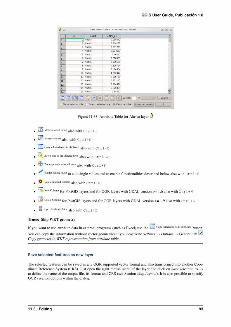
QGIS User Guide, Publicación 1.8
Figura 11.33: Attribute Table for Alaska layer
Move selected to top also with Ctrl+T
Invert selection also with Ctrl+S
Copy selected rows to clipboard also with Ctrl+C
Zoom map to the selected rows also with Ctrl+J
Pan map to the selected rows also with Ctrl+P
Toggle editing mode to edit single values and to enable functionalities described below also with Ctrl+E
Delete selected features also with Ctrl+D
New Column for PostGIS layers and for OGR layers with GDAL version >= 1.6 also with Ctrl+W
Delete Column for PostGIS layers and for OGR layers with GDAL version >= 1.9 also with Ctrl+L
Open field calculator also with Ctrl+I
Truco: Skip WKT geometry
If you want to use attribute data in external programs (such as Excel) use the Copy selected rows to clipboard button.
You can copy the information without vector geometries if you deactivate Settings → Options → General tabCopy geometry in WKT representation from attribute table.
Save selected features as new layer
The selected features can be saved as any OGR supported vector format and also transformed into another Coor-dinate Reference System (CRS). Just open the right mouse menu of the layer and click on Save selection as →to define the name of the output file, its format and CRS (see Section Map Legend). It is also possible to specifyOGR creation options within the dialog.
11.3. Editing 93

QGIS User Guide, Publicación 1.8
Working with non spatial attribute tables
QGIS allows also to load non spatial tables. This includes currently tables supported by OGR, delimited text andthe PostgreSQL provider. The tables can be used for field lookups or just generally browsed and edited using
the table view. When you load the table you will see it in the legend field. It can be opened e.g. with theOpen Attribute Table tool and is then editable like any other layer attribute table.
As an example you can use columns of the non spatial table to define attribute values or a range of values that areallowed to be added to a specific vector layer during digitizing. Have a closer look at the edit widget in sectionFields Tab to find out more.
11.4 Query Builder
The Query Builder allows you to define a subset of a table using a SQL-like WHERE clause and display the resultin the main window. The query result then can be saved as a new vector layer.
11.4.1 Query
Open the attribute table choosing Open Attribute Table from the menu bar. Click on the [Advanced Search] buttonto open the Query builder. For example, if you have a towns layer with a population field you could select on-ly larger towns by entering population > 100000 in the SQL box of the Query builder. Figure_attributes_2shows an example of the Query builder populated with data from a PostGIS layer with attributes stored in Post-greSQL. The Fields, Values and Operators sections help the user to construct the SQL-like query.
Figura 11.34: Query Builder
The Fields list contains all attribute columns of the attribute table to be searched. To add an attribute column to theSQL where clause field, double click its name in the Fields list. Generally you can use the various fields, valuesand operators to construct the query or you can just type it into the SQL box.
The Values list lists the values of an attribute table. To list all possible values of an attribute, select the attribute inthe Fields list and click the [all] button. To list the first 25 unique values of an attribute column, select the attribute
94 Capítulo 11. Working with Vector Data

QGIS User Guide, Publicación 1.8
column in the Fields list and click the [Sample] button. To add a value to the SQL where clause field, double clickits name in the Values list.
The Operators section contains all usable operators. To add an operator to the SQL where clause field, click theappropriate button. Relational operators ( = , > , ...), string comparison operator (LIKE), logical operators (AND,OR, ...) are available.
The [Test] button shows a message box with the number of features satisfying the current query, which is usablein the process of query construction. The [Clear] button clears the text in the SQL where clause text field. The[Save] and [Load] button allow to save and load SQL queries. The [OK] button closes the window and selects thefeatures satisfying the query. The [Cancel] button closes the window without changing the current selection.
Truco: Changing the Layer DefinitionYou can change the layer definition after it is loaded by altering the SQL query used to define the layer. To do this,open the vector Layer Properties dialog by double-clicking on the layer in the legend and click on the [QueryBuilder] button on the General tab. See Section The Vector Properties Dialog for more information.
11.4.2 Selection
With QGIS it is possible also to select features for visualisation using a similar query builder interface to that usedin Query Builder. In the above section the purpose of the query builder is to highlight all selected features meetingthe filter criteria in yellow. The rest of the features do not change their appearance.
Another possibility is to make a selection by right clicking on a layer in the legend and choosing Query .... If youperform a SQL query here only the selected features are displayed in the map view. Features that don’t match theSQL query are not visualised in the map view. The same function is available from the General tab in the vectorLayer Properties dialog. You can find a [Query builder] button right below. The selection described above can beused with all vector data providers.
11.4.3 Save selected features as new layer
The selected features can be saved as any OGR supported vector format and also transformed into another Coor-dinate Reference System (CRS). Just open the right mouse menu of the layer and click on Save selection as →to define the name of the output file, its format and CRS (see Section Map Legend). It is also possible to specifyOGR creation options within the dialog.
11.5 Field Calculator
The Field Calculator button in the attribute table allows to perform calculations on basis of existing attributevalues or defined functions, e.g to calculate length or area of geometry features. The results can be written to anew attribute column or it can be used to update values in an already existing column.
You have to bring the vector layer in editing mode, before you can click on the field calculator icon to open thedialog (see figure_attributes_3). In the dialog you first have to select whether you want to only update selectedfeatures, create a new attribute field where the results of the calculation will be added or update an existing field.
If you choose to add a new field, you need to enter a field name, a field type (integer, real or string), the total fieldwidth, and the field precision (see figure_attributes_3). For example, if you choose a field width of 10 and a fieldprecision of 3 it means you have 6 signs before the dot, then the dot and another 3 signs for the precision.
The Function List contains functions as well as fields and values. View the help function in the Selected FunctionHelp. In Expression you see the calculation expressions you create with the Function List. The most commonlyused operators, see Operators.
In the Function List, click on Fields and Values to view all attributes of the attribute table to be searched. To addan attribute to the Field calculator Expression field, double click its name in the Fields and Values list. Generally
11.5. Field Calculator 95

QGIS User Guide, Publicación 1.8
Figura 11.35: Field Calculator
you can use the various fields, values and functions to construct the calculation expression or you can just type itinto the box. To display the values of a field, you just right click on the appropriate field. You can choose betweenLoad top 10 unique values and Load all unique values. On the right side opens the Field Values list with theunique values. To add a value to the Field calculator Expression box, double click its name in the Field Valueslist.
The Operators, Math, Conversions, String, Geometry and Record groups provides several functions. In Operatorsyou find mathematical operators. Find Math for mathematical functions. The Conversions group contains functionsthat convert one data type to another. The String group provides functions for data strings. In the Geometry groupyou find functions for geometry objects. With Record group functions you can add a numeration to your data set.To add a function to the Field calculator Expression box, click on the > and then doubleclick the function.
A short example illustrates how the field calculator works. We want to calculate the length of the railroadslayer from the QGIS sample dataset:
1. Load the Shapefile railroads.shp in QGIS and press Open Attribute Table.
2. Click on Toggle editing mode and open the Field Calculator dialog.
3. Select the Create a new field checkbox to safe the calculations into a new field.
4. Add length as Output field name, real as Output field type and define Output field width 10 and aPrecision of 3.
5. Now click on function length in the Geometry group to add it as $length into the Field calculatorexpression box and click [Ok].
6. You can now find a new column length in the attribute table.
The available functions are listed below.
column name "column name" value of the field column name’string’ a string valueNULL null value
96 Capítulo 11. Working with Vector Data

QGIS User Guide, Publicación 1.8
a IS NULL a has no valuea IS NOT NULL a has a valuea IN (value[,value]) a is below the values listeda NOT IN (value[,value]) a is not below the values listeda OR b a or *b* is truea AND b a and *b* is trueNOT a inverted truth value of asqrt(a) square root of asin(a) sinus of acos(a) cosinus of btan(a) tangens of aasin(a) arcussinus of aacos(a) arcuscosinus of aatan(a) arcustangens of ato int(a) convert string a to integerto real(a) convert string a to realto string(a) convert number a to stringlower(a) convert string a to lower caseupper(a) convert string a to upper caselength(a) length of string aatan2(y,x) arcustangens of y/x using the signs of the two
arguments to determine the quadrant of the resultreplace(*a*, replacethis, withthat) replace this with that in string aregexp_replace(a,this,that) replace the regular expression this with thatsubstr(*a*,from,len) len characters of string *a* starting from from
(first character index is 1)a || b concatenate strings a and b$rownum number current row$area area of polygon$perimeter perimeter of polygon$length length of line$id feature id$x x coordinate of point$y y coordinate of pointxat(n) X coordinate of the point of an n-th line (indeces
start at 0; negative values refer to the line end)yat(n) y coordinate of the point of an n-th line (indeces
start at 0; negative values refer to the line end)a = b a and b are equala != b and a <> b a and b are not equala >= b a is larger than or equal to ba <= b a is less than or equal to ba > b a is larger than ba < b a is smaller than ba ~ b a matches the regular expression ba LIKE b a equals ba ILIKE b a equals b (without regard to case-sensitive)a |wedge| b a raised to the power of ba * b a multiplied by ba / b a divided by ba + b a plus ba - b a minus b+ a positive sign- a negative value of a
The field calculator Function list with the Selected Function Help , Operators and Expression menu are alsoavailable through the rule-based rendering in the Style tab of the Layer properties and the expression based labeling
in the Labeling core application.
11.5. Field Calculator 97

QGIS User Guide, Publicación 1.8
98 Capítulo 11. Working with Vector Data

CAPÍTULO 12
Working with Raster Data
12.1 Working with Raster Data
This Section describes how to visualize and set raster layer properties. QGIS uses the GDAL library to read andwrite raster data formats, including Arc/Info Binary Grid, Arc/Info ASCII Grid, GeoTIFF, Erdas Imagine andmany more. GRASS raster support is supplied by a native QGIS data provider plugin. The raster data can also beloaded in read mode from zip and gzip archives into QGIS.
At the date of this document, more than 100 raster formats are supported by the GDAL li-brary (see GDAL-SOFTWARE-SUITE Literature and Web References). A complete list is available athttp://www.gdal.org/formats_list.html.
Nota: Not all of the listed formats may work in QGIS for various reasons. For example, some require externalcommercial libraries or the GDAL installation of your OS was not built to support the format you want to use.Only those formats that have been well tested will appear in the list of file types when loading a raster into QGIS.Other untested formats can be loaded by selecting the [GDAL] All files (*) filter.
Working with GRASS raster data is described in Section GRASS GIS Integration.
12.1.1 What is raster data?
Raster data in GIS are matrices of discrete cells that represent features on, above or below the earth’s surface. Eachcell in the raster grid is the same size, and cells are usually rectangular (in QGIS they will always be rectangular).Typical raster datasets include remote sensing data such as aerial photography or satellite imagery and modelleddata such as an elevation matrix.
Unlike vector data, raster data typically do not have an associated database record for each cell. They are geocodedby its pixel resolution and the x/y coordinate of a corner pixel of the raster layer. This allows QGIS to position thedata correctly in the map canvas.
QGIS makes use of georeference information inside the raster layer (e.g. GeoTiff) or in an appropriate world fileto properly display the data.
12.1.2 Loading raster data in QGIS
Raster layers are loaded either by clicking on the Load Raster icon or by selecting the Layer → Add RasterLayer menu option. More than one layer can be loaded at the same time by holding down the Control or Shiftkey and clicking on multiple items in the dialog Open a GDAL Supported Raster Data Source.
Once a raster layer is loaded in the map legend you can click on the layer name with the right mouse button toselect and activate layer specific features or to open a dialog to set raster properties for the layer.
Right mouse button menu for raster layers
99

QGIS User Guide, Publicación 1.8
Zoom to layer extent
Zoom to Best Scale (100 %)
Show in Overview
Remove
Set Layer CRS
Set Project CRS from Layer
Properties
Rename
Copy Style
Add New Group
Expand all
Collapse all
Update Drawing Order
12.2 Raster Properties Dialog
To view and set the properties for a raster layer, double click on the layer name in the map legend or right click onthe layer name and choose Properties from the context menu:
This will open the Raster Layer Properties dialog, (see figure_raster_1).
There are several tabs on the dialog:
Style
Transparency
Colormap
General
Metadata
Pyramids
Histogram
12.2.1 Style Tab
QGIS can render raster layers in two different ways:
1. Single band - one band of the image will be rendered as gray or in pseudocolor or a freak out.
2. Three band color - three bands from the image will be rendered, each band representing the red, green orblue component that will be used to create a color image.
Within both render types you can invert the color output using the Invert color map checkbox.
Single Band Rendering
This selection offers you two possibilites to choose. At first you can select which band you like to use for rendering(if the dataset has more than one band).
The second option offers a selection of available colortables for rendering.
The following settings are available through the dropdownbox Color map
100 Capítulo 12. Working with Raster Data

QGIS User Guide, Publicación 1.8
Figura 12.1: Raster Layers Properties Dialog
Grayscale (default)
Pseudocolor
Freak Out
Colormap
When selecting the entry ‘Colormap’ from Color map combobox, the tab Colormap becomes available.For more information see Colormap.
QGIS can restrict the data displayed to only show cells whose values are within a given number of standarddeviations of the mean for the layer.
This is useful when you have one or two cells with abnormally high values in a raster grid that are having anegative impact on the rendering of the raster. This option is only available for pseudocolor and freak out images.
Three band color
This selection offers you a wide range of options to modify the appearance of your rasterlayer. For example youcould switch color-bands from the standard RGB-order to something else.
Also scaling of colors are available.
Truco: Viewing a Single Band of a Multiband RasterIf you want to view a single band (for example Red) of a multiband image, you might think you would set theGreen and Blue bands to “Not Set”. But this is not the correct way. To display the Red band, set the image type tograyscale, then select Red as the band to use for Gray.
Contrast enhancement
Nota: When adding GRASS rasters the option Contrast enhancement will be always set to automatically tostretch to min max regardless if the Quantum GIS general options this is set to another value.
12.2. Raster Properties Dialog 101

QGIS User Guide, Publicación 1.8
12.2.2 Transparency Tab
QGIS has the ability to display each raster layer at varying transparency levels. Use the transparency slider toindicate to what extent the underlying layers (if any) should be visible though the current raster layer. This isvery useful, if you like to overlay more than one rasterlayer, e.g. a shaded relief map overlayed by a classifiedrastermap. This will make the look of the map more three dimensional.
Additionally you can enter a rastervalue, which should be treated as NODATA. This can be done manually or with
the Add values from display icon.
An even more flexible way to customize the transparency can be done in the Custom transparency options section.The transparency of every pixel can be set here.
As an example we want to set the water of our example raster file landcover.tif to a transparency of 20 %.The following steps are neccessary:
1. Load the rasterfile landcover.
2. Open the Properties dialog by double-clicking on the raster name in the legend or by right-clicking andchoosing Properties from the popup menu.
3. Select the Transparency tab
4. Click the Add values manually button. A new row will appear in the pixel-list.
5. Enter the raster-value (we use 0 here) and adjust the transparency to 20 %.
6. Press the [Apply] button and have a look at the map.
You can repeat the steps 4 and 5 to adjust more values with custom transparency.
As you can see this is quite easy to set custom transparency, but it can be quite a lot of work. Therefore you
can use the button Export to file to save your transparency list to a file. The button Import from file loads yourtransparency settings and applies them to the current raster layer.
12.2.3 Colormap
The Colormap tab is only available, when you have selected a singleband rendering within the Style tab (see StyleTab).
Three ways of color interpolation are available:
1. Discrete
2. Linear
3. Exact
The button [Add Entry] adds a color to the individual color table. Button [Delete Entry] deletes a color from theindividual color table and the [Sort] button sorts the color table according to the pixel values in the value column.Double clicking on the value-column lets you insert a specific value. Double clicking on the color-column opensthe dialog Select color where you can select a color to apply on that value. Further you can also add labels foreach color but this value won’t be displayed when you use the identify feature tool.
You can also click on the button Load color map from band, which tries to load the table from the band (if it has any).
And you can use the buttons Load color map from file or Export color map to file to load an existing color table or tosave the defined color table for other sessions.
The block Generate new color map allows you to create newly categorized colormaps. You only need to select
the number of entries and press the button Classify. Currently only one Classification mode issupported - ‘Equal interval’
102 Capítulo 12. Working with Raster Data
QGIS User Guide, Publicación 1.8
12.2.4 General Tab
The General tab displays basic information about the selected raster, including the layer source and display namein the legend (which can be modified). This tab also shows a thumbnail of the layer, its legend symbol, and thepalette.
Additionally scale-dependent visibility can be set in this tab. You need to check the checkbox and set an appropriatescale where your data will be displayed in the map canvas.
Also the coordinate reference system (CRS) is printed here as a PROJ.4-string. This can be modified by hittingthe [Specify] button.
12.2.5 Metadata Tab
The Metadata tab displays a wealth of information about the raster layer, including statistics about each band inthe current raster layer. Statistics are gathered on a ‘need to know’ basis, so it may well be that a given layersstatistics have not yet been collected.
This tab is mainly for information. You cannot change any values printed inside this tab.
12.2.6 Pyramids Tab
Large resolution raster layers can slow navigation in QGIS. By creating lower resolution copies of the data (pyra-mids), performance can be considerably improved as QGIS selects the most suitable resolution to use dependingon the level of zoom.
You must have write access in the directory where the original data is stored to build pyramids.
Several resampling methods can be used to calculate the pyramids:
Average
Nearest Neighbour
When checking the checkbox Build pyramids internally if possible QGIS tries to build pyramids internally.
Please note that building pyramids may alter the original data file and once created they cannot be removed. If youwish to preserve a ‘non-pyramided’ version of your raster, make a backup copy prior to building pyramids.
12.2.7 Histogram Tab
The Histogram tab allows you to view the distribution of the bands or colors in your raster. It is generated auto-maticaly when you open Histogram tab. All existing bands will be displayed together. You can save the histogram
as an image with the button.
12.3 Raster Calculator
The Raster Calculator in the Raster menu (see figure_raster_2) allows to perform calculations on basis of existingraster pixel values. The results are written to a new raster layer with a GDAL supported format.
The Raster bands list contains all loaded raster layers that can be used. To add a raster to the raster calculatorexpression field, double click its name in the Fields list. You can then use the operators to construct calculationexpressions or you can just type it into the box.
In the Result layer section you have to define an output layer. You can then define the extent of the calculationarea based on an input raster layer or based on X,Y coordinates and on Columns and Rows to set the resolutionof the output layer. If the input layer has a different resolution, the values will be resampled with nearest neighboralgorithm.
12.3. Raster Calculator 103

QGIS User Guide, Publicación 1.8
Figura 12.2: Raster Calculator
The Operators section contains all usable operators. To add an operator to the raster calculator expression box,click the appropriate button. Mathematical calculations (+, -, *, ... ) and trigonometric functions (sin, cos, tan,... ) are available. Stay tuned for more operators to come!
With the Add result to project checkbox the result layer will automatically added to the legend area and canbe visualized.
12.3.1 Examples
Convert elevation values from meter to feet
Creating an elevation raster feet from a raster in meter, you need to use the conversion factor for meters to feet:3.28. The expression is:
elevation@1 * 3.28
Using a mask
If you want to mask out parts of a raster, because you are only interested in elevations above 0 meter, you can usefollowing expression to create a mask and apply the result to a raster in one step.
(elevation@1 >= 0) * elevation@1
For every cell greater than or equal to 0, set its value to 1, otherwise set it to 0. This creates the mask on the fly.
104 Capítulo 12. Working with Raster Data

CAPÍTULO 13
Working with OGC Data
13.1 Working with OGC Data
QGIS supports WMS and WFS as data sources.
13.1.1 What is OGC Data
The Open Geospatial Consortium (OGC), is an international organization with more than 300 commercial, gov-ernmental, nonprofit and research organizations worldwide. Its members develop and implement standards forgeospatial content and services, GIS data processing and exchange.
Describing a basic data model for geographic features an increasing number of specifications are developed toserve specific needs for interoperable location and geospatial technology, including GIS. Further information canbe found under http://www.opengeospatial.org/.
Important OGC specifications are:
WMS — Web Map Service
WFS — Web Feature Service
WCS — Web Coverage Service
CAT — Web Catalog Service
SFS — Simple Features for SQL
GML — Geography Markup Language
OGC services are increasingly being used to exchange geospatial data between different GIS implementationsand data stores. QGIS can now deal with three of the above specifications, being SFS (through support of thePostgreSQL / PostGIS data provider, see Section PostGIS Layers), WFS and WMS as a client.
13.1.2 WMS Client
Overview of WMS Support
QGIS currently can act as a WMS client that understands WMS 1.1, 1.1.1 and 1.3 servers. It has particularly beentested against publicly accessible servers such as DEMIS.
WMS servers act upon requests by the client (e.g. QGIS) for a raster map with a given extent, set of layers,symbolization style, and transparency. The WMS server then consults its local data sources, rasterizes the map,and sends it back to the client in a raster format. For QGIS this would typically be JPEG or PNG.
WMS is generically a REST (Representational State Transfer) service rather than a fully-blown Web Service. Assuch, you can actually take the URLs generated by QGIS and use them in a web browser to retrieve the same
105

QGIS User Guide, Publicación 1.8
images that QGIS uses internally. This can be useful for troubleshooting, as there are several brands of WMSservers in the market and they all have their own interpretation of the WMS standard.
WMS layers can be added quite simply, as long as you know the URL to access the WMS server, you have aserviceable connection to that server, and the server understands HTTP as the data transport mechanism.
Selecting WMS Servers
The first time you use the WMS feature, there are no servers defined.
Begin by clicking the Add WMS layer button inside the toolbar, or through the Layer → Add WMS Layer... menu.
The dialog Add Layer(s) from a Server for adding layers from the WMS server appears. You can add some serversto play with by clicking the [Add default servers] button. This will add two WMS demo servers for you to use, theWMS servers of the DM Solutions Group and Lizardtech. To define a new WMS server in the tab Layers, selectthe [New] button. Then enter the parameters to connect to your desired WMS server, as listed in table_OGC_1:
Name A name for this connection. This name will be used in the Server Connections drop-downbox so that you can distinguish it from other WMS Servers.
URL URL of the server providing the data. This must be a resolvable host name; the sameformat as you would use to open a telnet connection or ping a host.
Username Username to access a secured WMS-server. This parameter is optional.Password Password for a basic authenticated WMS-server. This parameter is optional.
Ignore GetMapURI
Ignore GetMap URI reported in capabilities, use given URI from URL-field above.
IgnoreGetFeatureInfoURI
Ignore GetFeatureInfo URI reported in capabilities , use given URI from URL-fieldabove
Table OGC 1: WMS Connection Parameters
If you need to set up a proxy-server to be able to receive WMS-services from the internet, you can add yourproxy-server in the options. Choose menu Settings → Options and click on the tab Network & Proxy. There you
can add your proxy-settings and enable them by setting the Use proxy for web access. Make sure that you
select the correct proxy type from the Proxy type dropdown menu.
Once the new WMS Server connection has been created, it will be preserved for future QGIS sessions.
Truco: On WMS Server URLsBe sure, when entering in the WMS server URL, that you have the base URL. For example, you shouldn’t havefragments such as request=GetCapabilities or version=1.0.0 in your URL.
Loading WMS Layers
Once you have successfully filled in your parameters you can select the [Connect] button to retrieve the capabil-ities of the selected server. This includes the Image encoding, Layers, Layer Styles and Projections. Since this isa network operation, the speed of the response depends on the quality of your network connection to the WMSserver. While downloading data from the WMS server, the download progress is visualized in the left bottom ofthe WMS dialog.
Your screen should now look a bit like figure_OGR_1, which shows the response provided by the DM SolutionsGroup WMS server.
Image Encoding
The Image encoding section now lists the formats that are supported by both the client and server. Choose onedepending on your image accuracy requirements.
Truco: Image Encoding
106 Capítulo 13. Working with OGC Data

QGIS User Guide, Publicación 1.8
Figura 13.1: Dialog for adding a WMS server, showing its available layers
You will typically find that a WMS server offers you the choice of JPEG or PNG image encoding. JPEG is a lossycompression format, whereas PNG faithfully reproduces the raw raster data.
Use JPEG if you expect the WMS data to be photographic in nature and/or you don’t mind some loss in picturequality. This trade-off typically reduces by 5 times the data transfer requirement compared to PNG.
Use PNG if you want precise representations of the original data, and you don’t mind the increased data transferrequirements.
Options
The Options field provides a text field where you can add a Layer name for the WMS-layer. This name will bepresented in the legend after loading the layer.
Below the layer name you can define Tile size, if you want to set tile sizes (eg. 256x256) to split up the WMSrequest into multiple requests.
The Feature limit for GetFeatureInfo defines what features from the server to query.
If you select a WMS from the list a field with the default projection, provided by the mapserver, appears. If the[Change...] button is active, you can click on it and change the default projection of the WMS to another CRS,provided by the WMS server.
Layer Order
The tab Layer Order lists the selected layers available from the current connected WMS server. You may noticethat some layers are expandable, this means that the layer can be displayed in a choice of image styles.
You can select several layers at once, but only one image style per layer. When several layers are selected, theywill be combined at the WMS Server and transmitted to QGIS in one go.
Truco: WMS Layer Ordering
13.1. Working with OGC Data 107
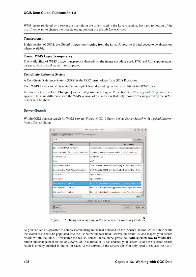
QGIS User Guide, Publicación 1.8
WMS layers rendered by a server are overlaid in the order listed in the Layers section, from top to bottom of thelist. If you want to change the overlay order, you can use the tab Layer Order.
Transparency
In this version of QGIS, the Global transparency setting from the Layer Properties is hard-coded to be always on,where available.
Truco: WMS Layer TransparencyThe availability of WMS image transparency depends on the image encoding used: PNG and GIF support trans-parency, whilst JPEG leaves it unsupported.
Coordinate Reference System
A Coordinate Reference System (CRS) is the OGC terminology for a QGIS Projection.
Each WMS Layer can be presented in multiple CRSs, depending on the capability of the WMS server.
To choose a CRS, select [Change...] and a dialog similar to Figure Projection 3 in Working with Projections willappear. The main difference with the WMS version of the screen is that only those CRSs supported by the WMSServer will be shown.
Server-Search
Within QGIS you can search for WMS-servers. Figure_OGC_2 shows the tab Server Search with the Add Layer(s)from a Server dialog.
Figura 13.2: Dialog for searching WMS servers after some keywords
As you can see it is possible to enter a search-string in the text field and hit the [Search] button. After a short whilethe search result will be populated into the list below the text field. Browse the result list and inspect your searchresults within the table. To visualize the results, select a table entry, press the [Add selected row to WMS-list]button and change back to the tab Layers. QGIS automatically has updated your server list and the selected searchresult is already enabled in the list of saved WMS-servers in the Layers tab. You only need to request the list of
108 Capítulo 13. Working with OGC Data
QGIS User Guide, Publicación 1.8
layers by clicking the [Connect] button. This option is quite handy when you want to search maps by specifickeywords.
Basically this option is a frontend to the API of http://geopole.org.
Tilesets
When using WMS-C (Cached WMS) Services like http://labs.metacarta.com/wms-c/Basic.py you are able tobrowse through the tab Tilesets given by the server. Additional information like tile size, formats and support-ed CRS are listed in this table. In combination with this feature you can use the tile scale slider from the View →Tile scale slider, which gives you the available scales from the tileserver with nice slider docked in.
Using the Identify Tool
Once you have added a WMS server, and if any layer from a WMS server is queryable, you can then use theIdentify tool to select a pixel on the map canvas. A query is made to the WMS server for each selection made. Theresults of the query are returned in plain text. The formatting of this text is dependent on the particular WMSserver used. Viewing Properties
Once you have added a WMS server, you can view its properties by right-clicking on it in the legend, and selectingProperties. Metadata Tab
The tab Metadata displays a wealth of information about the WMS server, generally collected from the Capa-bilities statement returned from that server. Many definitions can be cleaned by reading the WMS standards (seeOPEN-GEOSPATIAL-CONSORTIUM Literature and Web References), but here are a few handy definitions:
Server Properties
• WMS Version — The WMS version supported by the server.
• Image Formats — The list of MIME-types the server can respond with when drawing the map.QGIS supports whatever formats the underlying Qt libraries were built with, which is typically at leastimage/png and image/jpeg.
• Identity Formats — The list of MIME-types the server can respond with when you use the Identifytool. Currently QGIS supports the text-plain type.
Layer Properties
• Selected — Whether or not this layer was selected when its server was added to this project.
• Visible — Whether or not this layer is selected as visible in the legend. (Not yet used in this versionof QGIS.)
• Can Identify — Whether or not this layer will return any results when the Identify tool is used on it.
• Can be Transparent — Whether or not this layer can be rendered with transparency. This version ofQGIS will always use transparency if this is Yes and the image encoding supports transparency
• Can Zoom In — Whether or not this layer can be zoomed in by the server. This version of QGISassumes all WMS layers have this set to Yes. Deficient layers may be rendered strangely.
• Cascade Count — WMS servers can act as a proxy to other WMS servers to get the raster data for alayer. This entry shows how many times the request for this layer is forwarded to peer WMS serversfor a result.
• Fixed Width, Fixed Height — Whether or not this layer has fixed source pixel dimensions. Thisversion of QGIS assumes all WMS layers have this set to nothing. Deficient layers may be renderedstrangely.
• WGS 84 Bounding Box — The bounding box of the layer, in WGS 84 coordinates. Some WMSservers do not set this correctly (e.g. UTM coordinates are used instead). If this is the case, thenthe initial view of this layer may be rendered with a very ‘zoomed-out’ appearance by QGIS. The
13.1. Working with OGC Data 109

QGIS User Guide, Publicación 1.8
WMS webmaster should be informed of this error, which they may know as the WMS XML elementsLatLonBoundingBox, EX_GeographicBoundingBox or the CRS:84 BoundingBox.
• Available in CRS — The projections that this layer can be rendered in by the WMS server. These arelisted in the WMS-native format.
• Available in style — The image styles that this layer can be rendered in by the WMS server.
WMS Client Limitations
Not all possible WMS Client functionality had been included in this version of QGIS. Some of the more notableexceptions follow.
Editing WMS Layer Settings
Once you’ve completed the Add WMS layer procedure, there is no ability to change the settings. A workaround isto delete the layer completely and start again.
WMS Servers Requiring Authentication
Currently public accessible and secured WMS-services are supported. The secured WMS-servers can be accessedby public authentication. You can add the (optional) credentials when you add a WMS-server. See section SelectingWMS Servers for details.
Truco: Accessing secured OGC-layersIf you need to access secured layers with other secured methods than basic authentication, you could use InteProxyas a transparent proxy, which does support several authentication methods. More information can be found at theInteProxy manual found on the website http://inteproxy.wald.intevation.org.
Truco: QGIS WMS MapserverFrom Version 1.7.0 QGIS has its own implementation of a WMS 1.3.0 Mapserver. Read more about this at chapterQGIS Server.
13.1.3 WFS and WFS-T Client
In QGIS, a WFS layer behaves pretty much like any other vector layer. You can identify and select features andview the attribute table. Since QGIS 1.6 editing (WFS-T) is also supported.
In general adding a WFS layer is very similar to the procedure used with WMS. The difference is there are nodefault servers defined, so we have to add our own.
Loading a WFS Layer
As an example we use the DM Solutions WFS server and display a layer. The URL is:http://www2.dmsolutions.ca/cgi-bin/mswfs_gmap
1. Click on the Add WFS Layer tool on the Layers toolbar, the dialog Add WFS Layer from a Server appears
2. Click on [New]
3. Enter ‘DM Solutions’ as name
4. Enter the URL (see above)
5. Click [OK]
6. Choose ‘DM Solutions’ from the Server Connections combobox
7. Click [Connect]
8. Wait for the list of layers to be populated
110 Capítulo 13. Working with OGC Data

QGIS User Guide, Publicación 1.8
9. Select the Parks layer in the list
10. Click [Apply] to add the layer to the map
Note that proxy-settings you have set in your preferences are also recognized.
Figura 13.3: Adding a WFS layer
You’ll notice the download progress is visualized in the left bottom of the QGIS main window. Once the layer isloaded, you can identify and select a province or two and view the attribute table.
Only WFS 1.0.0 is supported. At this point there have not been many tests against WFS versions implemented inother WFS-servers. If you encounter problems with any other WFS-server, please do not hesitate to contact thedevelopment team. Please refer to Section Mailing lists for further information about the mailinglists.
Truco: Finding WFS ServersYou can find additional WFS servers by using Google or your favorite search engine. There are a number of listswith public URLs, some of them maintained and some not.
13.2 QGIS Server
QGIS Server is an open source WMS 1.3 and WFS 1.0.0 implementation which, in addition, implements advancedcartographic features for thematic mapping. The QGIS Server is a FastCGI/CGI (Common Gateway Interface)application written in C++ that works together with a webserver (e.g. Apache, Lighttpd). It is funded by the EUprojects Orchestra, Sany and the city of Uster in Switzerland.
It uses QGIS as backend for the GIS logic and for map rendering. Furthermore the Qt library is used for graphicsand for platform independent C++ programming. In contrast to other WMS software, the QGIS Server uses carto-graphic rules as a configuration language, both for the server configuration and for the user-defined cartographicrules.
Moreover, the QGIS Server project provides the ‘Publish to Web’ plugin, a plugin for QGIS desktop which exportsthe current layers and symbology as a web project for QGIS Server (containing cartographic visualization rulesexpressed in SLD).
As QGIS desktop and QGIS Server use the same visualization libraries, the maps that are published on the weblook the same as in desktop GIS. The ‘Publish to Web’ plugin currently supports basic symbolization, with morecomplex cartographic visualization rules introduced manually. As the configuration is performed with the SLDstandard and its documented extensions, there is only one standardised language to learn, which greatly simplifiesthe complexity of creating maps for the Web.
In one of the following manuals we will provide a sample configuration to set up a QGIS Server. But for now werecommend to read one of the following URLs to get more information:
13.2. QGIS Server 111

QGIS User Guide, Publicación 1.8
http://karlinapp.ethz.ch/qgis_wms/
http://hub.qgis.org/projects/quantum-gis/wiki/QGIS_Server_Tutorial
http://linfiniti.com/2010/08/qgis-mapserver-a-wms-server-for-the-masses/
13.2.1 Sample installation on Debian Squeeze
At this point we will give a short and simple sample installation howto for Debian Squeeze. Many other OSprovide packages for QGIS Server, too. If you have to build it all from source, please refer to the URLs above.
Apart from qgis and qgis-mapserver you need a webserver, in our case apache2. You can install all pack-ages with aptitude or apt-get install together with other necessary dependency packages. After installation youshould test, if the webserver and qgis server works as expected. Make sure the apache server is running with/etc/init.d/apache2 start. Open a web browser and type URL: http://localhost. If apache isup, you should see the message ‘It works!’.
Now we test the qgis server installation. The qgis_mapserv.fcgi is available at/usr/lib/cgi-bin/qgis_mapserv.fcgi and provides a standard wms that shows the state boundariesof Alaska. Add the WMS with the URL http://localhost/cgi-bin/qgis_mapserv.fcgi asdescribed in Selecting WMS Servers.
Figura 13.4: Standard WMS with USA boundaries included in the qgis server (KDE)
13.2.2 Creating a WMS/WFS from a QGIS project
To provide a new qgis wms/wfs server we have to create a qgis project file with some data. Here we use the‘alaska’ shapefile from the qgis_sample_dataset. Define the colors and styles of the layers in QGIS and define theproject CRS, if not already done.
Then open the OWS Server tab in the menu Settings → Project Properties and define the general fields under‘Service Capabilities’. For WMS Capabilities define ‘Coordinate System Restrictions’ and ‘Advertised Ex-
tend’. Additionally you can enable the checkbox Add WKT geometry to feature into response to make the layersqueryable and add a ‘Maximum width’ and height that can be requested. For WFS Capabilities you onlyneed to select the layers that you want to provide as WFS. Now save the session in a project file alaska.qgs.To provide the project as a WMS/WFS, we create a new folder /usr/lib/cgi-bin/project with adminprivileges and add the project file alaska.qgs and a copy of the qgis_mapserv.fcgi file - that’s all.
Now we test our project WMS and WFS, add the WMS and WFS as described in Loading WMS Layers and WFSand WFS-T Client to QGIS and load the WMS. The URL is:
112 Capítulo 13. Working with OGC Data
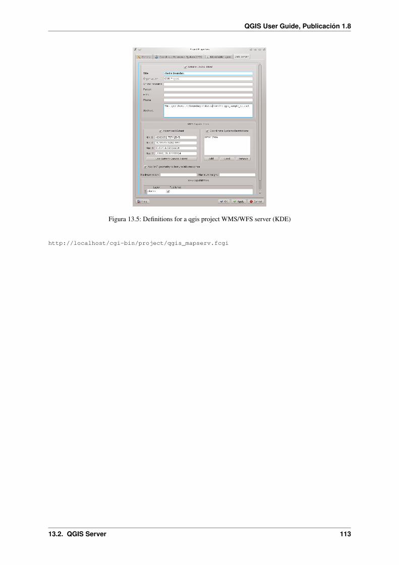
QGIS User Guide, Publicación 1.8
Figura 13.5: Definitions for a qgis project WMS/WFS server (KDE)
http://localhost/cgi-bin/project/qgis_mapserv.fcgi
13.2. QGIS Server 113
QGIS User Guide, Publicación 1.8
114 Capítulo 13. Working with OGC Data

CAPÍTULO 14
Working with GPS Data
14.1 GPS Plugin
14.1.1 What is GPS?
GPS, the Global Positioning System, is a satellite-based system that allows anyone with a GPS receiver to findtheir exact position anywhere in the world. It is used as an aid in navigation, for example in airplanes, in boats andby hikers. The GPS receiver uses the signals from the satellites to calculate its latitude, longitude and (sometimes)elevation. Most receivers also have the capability to store locations (known as waypoints), sequences of locationsthat make up a planned route and a tracklog or track of the receivers movement over time. Waypoints, routes andtracks are the three basic feature types in GPS data. QGIS displays waypoints in point layers while routes andtracks are displayed in linestring layers.
14.1.2 Loading GPS data from a file
There are dozens of different file formats for storing GPS data. The format that QGIS uses is called GPX (GPSeXchange format), which is a standard interchange format that can contain any number of waypoints, routes andtracks in the same file.
To load a GPX file you first need to load the plugin. Plugins → Plugin Manager... opens the Plugin Manager
Dialog. Activate the GPS Tools checkbox. When this plugin is loaded two buttons with a small handheld GPSdevice will show up in the toolbar:
Create new GPX Layer
GPS Tools
For working with GPS data we provide an example GPX file available in the QGIS sample dataset:qgis_sample_data/gps/national_monuments.gpx. See Section Sample Data for more informationabout the sample data.
1. Click on the GPS Tools icon and open the Load GPX file tab (see figure_GPS_1).
2. Browse to the folder qgis_sample_data/gps/, select the GPX file national_monuments.gpxand click [Open].
Use the [Browse...] button to select the GPX file, then use the checkboxes to select the feature types you wantto load from that GPX file. Each feature type will be loaded in a separate layer when you click [OK]. The filenational_monuments.gpx only includes waypoints.
Nota: GPS units allow to store data in different coordinate systems. When downloading a GPX file (fromyour GPS unit or a web site) and then loading it in Quantum GIS, be sure that the data stored in the GPXfile uses WGS84 (latitude/longitude). Quantum GIS expects this and it is the official GPX specification. Seehttp://www.topografix.com/GPX/1/1/
115
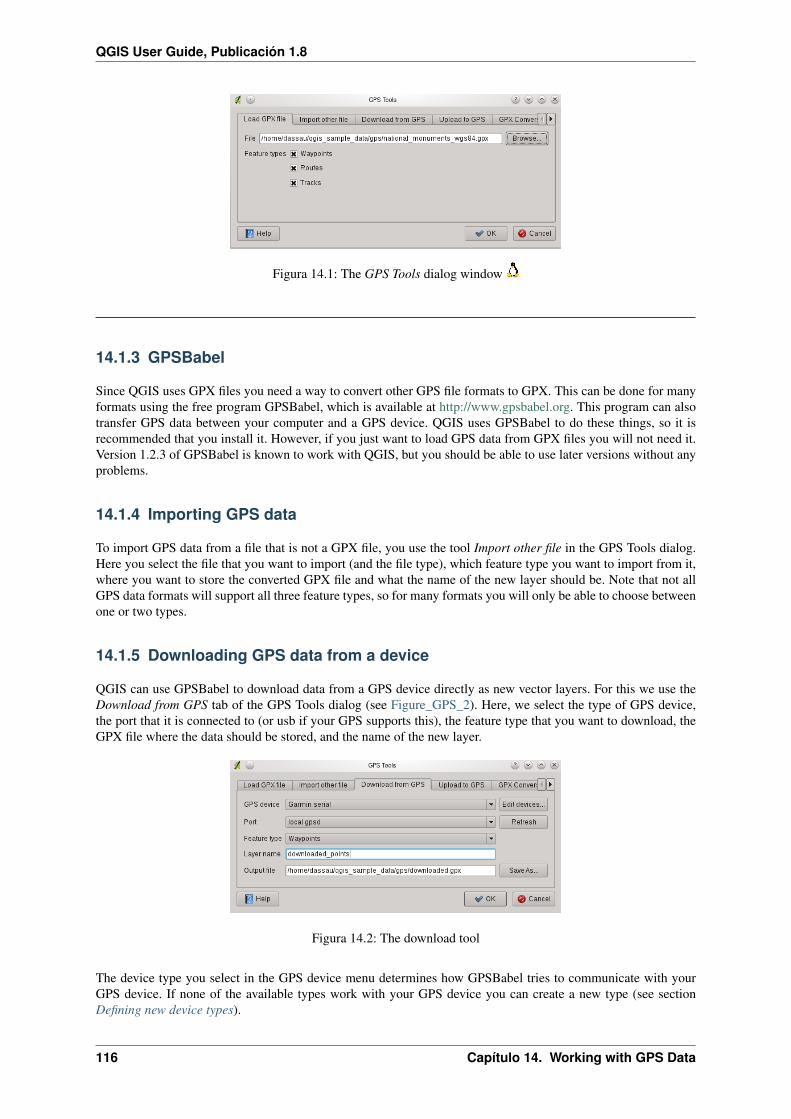
QGIS User Guide, Publicación 1.8
Figura 14.1: The GPS Tools dialog window
14.1.3 GPSBabel
Since QGIS uses GPX files you need a way to convert other GPS file formats to GPX. This can be done for manyformats using the free program GPSBabel, which is available at http://www.gpsbabel.org. This program can alsotransfer GPS data between your computer and a GPS device. QGIS uses GPSBabel to do these things, so it isrecommended that you install it. However, if you just want to load GPS data from GPX files you will not need it.Version 1.2.3 of GPSBabel is known to work with QGIS, but you should be able to use later versions without anyproblems.
14.1.4 Importing GPS data
To import GPS data from a file that is not a GPX file, you use the tool Import other file in the GPS Tools dialog.Here you select the file that you want to import (and the file type), which feature type you want to import from it,where you want to store the converted GPX file and what the name of the new layer should be. Note that not allGPS data formats will support all three feature types, so for many formats you will only be able to choose betweenone or two types.
14.1.5 Downloading GPS data from a device
QGIS can use GPSBabel to download data from a GPS device directly as new vector layers. For this we use theDownload from GPS tab of the GPS Tools dialog (see Figure_GPS_2). Here, we select the type of GPS device,the port that it is connected to (or usb if your GPS supports this), the feature type that you want to download, theGPX file where the data should be stored, and the name of the new layer.
Figura 14.2: The download tool
The device type you select in the GPS device menu determines how GPSBabel tries to communicate with yourGPS device. If none of the available types work with your GPS device you can create a new type (see sectionDefining new device types).
116 Capítulo 14. Working with GPS Data

QGIS User Guide, Publicación 1.8
The port may be a file name or some other name that your operating system uses as a reference to the physicalport in your computer that the GPS device is connected to. It may also be simply usb, for usb enabled GPS units.
On Linux this is something like /dev/ttyS0 or /dev/ttyS1
On Windows it is COM1 or COM2.
When you click [OK] the data will be downloaded from the device and appear as a layer in QGIS.
14.1.6 Uploading GPS data to a device
You can also upload data directly from a vector layer in QGIS to a GPS device using the Upload to GPS tab of theGPS Tools dialog. To do this you simply select the layer that you want to upload (which must be a GPX layer),your GPS device type, and the port (or usb) that it is connected to. Just as with the download tool you can specifynew device types if your device isn’t in the list.
This tool is very useful in combination with the vector editing capabilities of QGIS. It allows you to load a map,create waypoints and routes, and then upload them and use them on your GPS device.
14.1.7 Defining new device types
There are lots of different types of GPS devices. The QGIS developers can’t test all of them, so if you have onethat does not work with any of the device types listed in the Download from GPS and Upload to GPS tools youcan define your own device type for it. You do this by using the GPS device editor, which you start by clicking the[Edit devices] button in the download or the upload tabs.
To define a new device you simply click the [New device] button, enter a name, a download command and anupload command for your device, and click the [Update device] button. The name will be listed in the devicemenus in the upload and download windows, and can be any string. The download command is the command thatis used to download data from the device to a GPX file. This will probably be a GPSBabel command, but you canuse any other command line program that can create a GPX file. QGIS will replace the keywords%type,%in,and%out when it runs the command.
%type will be replaced by -w if you are downloading waypoints, -r if you are downloading routes and -t ifyou are downloading tracks. These are command line options that tell GPSBabel which feature type to download.
%in will be replaced by the port name that you choose in the download window and%out will be replaced bythe name you choose for the GPX file that the downloaded data should be stored in. So if you create a devicetype with the download command gpsbabel%type -i garmin -o gpx%in%out (this is actually thedownload command for the predefined device type ‘Garmin serial’) and then use it to download waypoints fromport /dev/ttyS0 to the file output.gpx, QGIS will replace the keywords and run the command gpsbabel-w -i garmin -o gpx /dev/ttyS0 output.gpx.
The upload command is the command that is used to upload data to the device. The same keywords are used,but%in is now replaced by the name of the GPX file for the layer that is being uploaded, and%out is replacedby the port name.
You can learn more about GPSBabel and it’s available command line options at http://www.gpsbabel.org.
Once you have created a new device type it will appear in the device lists for the download and upload tools.
14.2 Live GPS tracking
To activate Live GPS tracking in QGIS you need to select Settings → GPS information. You will get a newdocked window on the left side of the canvas.
There are 4 possible screens in this GPS tracking window:
GPS position coordinates and for manually entering Vertices and Features.
14.2. Live GPS tracking 117
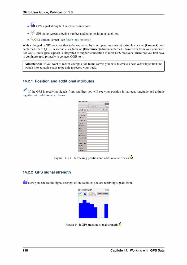
QGIS User Guide, Publicación 1.8
GPS signal strength of satellite connections.
GPS polar screen showing number and polar position of satellites.
GPS options screen (see figure_gps_options).
With a plugged in GPS receiver (has to be supported by your operating system) a simple click on [Connect] con-nects the GPS to QGIS. A second click (now on [Disconnect]) disconnects the GPS-receiver from your computer.For GNU/Linux gpsd support is integrated to support connection to most GPS receivers. Therefore you first haveto configure gpsd properly to connect QGIS to it.
Advertencia: If you want to record your position to the canvas you have to create a new vector layer first andswitch it to editable status to be able to record your track.
14.2.1 Position and additional attributes
If the GPS is receiving signals from satellites you will see your position in latitude, longitude and altitudetogether with additional attributes.
Figura 14.3: GPS tracking position and additional attributes
14.2.2 GPS signal strength
Here you can see the signal strenght of the satellites you are receiving signals from.
Figura 14.4: GPS tracking signal strength
118 Capítulo 14. Working with GPS Data

QGIS User Guide, Publicación 1.8
14.2.3 GPS polar window
If you want to know where in the sky all the connected satellites are, you have to switch to the polar screen.You can also see the ID numbers of the satellites you are receiving signals from.
Figura 14.5: GPS tracking polar window
14.2.4 GPS options
In case of connection problems you can switch between:
Autodetect
Internal,
Serial device
gpsd (selecting Host, Port and Device your GPS is connected to).
A click on [Connect] again initiates the connection to the GPS receiver.
Figura 14.6: GPS tracking options window
You can activate Automatically save added features when you are in editing mode. Or you can can activateAutomatically add points to the map canvas with a certain width and color.
14.2. Live GPS tracking 119

QGIS User Guide, Publicación 1.8
Activating Cursor you can use a slider to shrink and grow the position cursor on thecanvas.
Activating Map centering allows to decide in which way the canvas will be updated. This includes ‘always’,‘when leaving’ if your recorded coordinates start either to move out of canvas or ‘never’ to keep map extent.
Finally you can activate Log file and define a path and a file where log messages about the gps tracking alogged.
If you want to set a feature manually you have to go back to Position and click on [Add Point] or [Add trackpoint].
120 Capítulo 14. Working with GPS Data

CAPÍTULO 15
GRASS GIS Integration
The GRASS plugin provides access to GRASS GIS (see GRASS-PROJECT Literature and Web References)databases and functionalities. This includes visualization of GRASS raster and vector layers, digitizing vectorlayers, editing vector attributes, creating new vector layers and analysing GRASS 2D and 3D data with more than300 GRASS modules.
In this Section we’ll introduce the plugin functionalities and give some examples on managing and working withGRASS data. Following main features are provided with the toolbar menu, when you start the GRASS plugin, asdescribed in section Starting the GRASS plugin :
Open mapset
New mapset
Close mapset
Add GRASS vector layer
Add GRASS raster layer
Create new GRASS vector
Edit GRASS vector layer
Open GRASS tools
Display current GRASS region
Edit current GRASS region
15.1 Starting the GRASS plugin
To use GRASS functionalities and/or visualize GRASS vector and raster layers in QGIS, you must select and load
the GRASS plugin with the Plugin Manager. Therefore click the menu Plugins → Manage Plugins, selectGRASS and click [OK].
You can now start loading raster and vector layers from an existing GRASS LOCATION (see section LoadingGRASS raster and vector layers). Or you create a new GRASS LOCATION with QGIS (see section Creatinga new GRASS LOCATION) and import some raster and vector data (see Section Importing data into a GRASSLOCATION) for further analysis with the GRASS Toolbox (see section The GRASS toolbox).
121

QGIS User Guide, Publicación 1.8
15.2 Loading GRASS raster and vector layers
With the GRASS plugin, you can load vector or raster layers using the appropriate button on the toolbar menu.As an example we use the QGIS alaska dataset (see Section Sample Data). It includes a small sample GRASSLOCATION with 3 vector layers and 1 raster elevation map.
1. Create a new folder grassdata, download the QGIS alaska dataset qgis_sample_data.zip fromhttp://download.osgeo.org/qgis/data/ and unzip the file into grassdata.
2. Start QGIS.
3. If not already done in a previous QGIS session, load the GRASS plugin clicking on Plugins → Manage
Plugins and activate GRASS. The GRASS toolbar appears in the QGIS main window.
4. In the GRASS toolbar, click the Open mapset icon to bring up the MAPSET wizard.
5. For Gisdbase browse and select or enter the path to the newly created folder grassdata.
6. You should now be able to select the LOCATION alaska and the MAPSET demo.
7. Click [OK]. Notice that some previously disabled tools in the GRASS toolbar are now enabled.
8. Click on Add GRASS raster layer, choose the map name gtopo30 and click [OK]. The elevation layer willbe visualized.
9. Click on Add GRASS vector layer, choose the map name alaska and click OK. The alaska boundary vectorlayer will be overlayed on top of the gtopo30 map. You can now adapt the layer properties as describedin chapter The Vector Properties Dialog, e.g. change opacity, fill and outline color.
10. Also load the other two vector layers rivers and airports and adapt their properties.
As you see, it is very simple to load GRASS raster and vector layers in QGIS. See following sections for editingGRASS data and creating a new LOCATION. More sample GRASS LOCATIONs are available at the GRASSwebsite at http://grass.osgeo.org/download/data.php.
Truco: GRASS Data LoadingIf you have problems loading data or QGIS terminates abnormally, check to make sure you have loaded theGRASS plugin properly as described in section Starting the GRASS plugin.
15.3 GRASS LOCATION and MAPSET
GRASS data are stored in a directory referred to as GISDBASE. This directory often called grassdata, mustbe created before you start working with the GRASS plugin in QGIS. Within this directory, the GRASS GISdata are organized by projects stored in subdirectories called LOCATION. Each LOCATION is defined by itscoordinate system, map projection and geographical boundaries. Each LOCATION can have several MAPSETs(subdirectories of the LOCATION) that are used to subdivide the project into different topics, subregions, or asworkspaces for individual team members (Neteler & Mitasova 2008 Literature and Web References). In order toanalyze vector and raster layers with GRASS modules, you must import them into a GRASS LOCATION (Thisis not strictly true - with the GRASS modules r.external and v.external you can create read-only linksto external GDAL/OGR-supported data sets without importing them. But because this is not the usual way forbeginners to work with GRASS, this functionality will not be described here.).
15.3.1 Creating a new GRASS LOCATION
As an example here is how the sample GRASS LOCATION alaska, which is projected in Albers Equal Areaprojection with unit feet was created for the QGIS sample dataset. This sample GRASS LOCATION alaska
122 Capítulo 15. GRASS GIS Integration

QGIS User Guide, Publicación 1.8
Figura 15.1: GRASS data in the alaska LOCATION
will be used for all examples and exercises in the following GRASS GIS related chapters. It is useful to downloadand install the dataset on your computer Sample Data).
1. Start QGIS and make sure the GRASS plugin is loaded.
2. Visualize the alaska.shp Shapefile (see Section Loading a Shapefile) from the QGIS alaska datasetSample Data.
3. In the GRASS toolbar, click on the New mapset icon to bring up the MAPSET wizard.
4. Select an existing GRASS database (GISDBASE) folder grassdata or create one for the new LOCATIONusing a file manager on your computer. Then click [Next].
5. We can use this wizard to create a new MAPSET within an existing LOCATION (see section Adding a newMAPSET) or to create a new LOCATION altogether. Click on the radio button Create new location (seefigure_grass_location_2).
6. Enter a name for the LOCATION - we used alaska and click [Next].
7. Define the projection by clicking on the radio button Projection to enable the projection list.
8. We are using Albers Equal Area Alaska (feet) projection. Since we happen to know that it is representedby the EPSG ID 2964, we enter it in the search box. (Note: If you want to repeat this process for another
LOCATION and projection and haven’t memorized the EPSG ID, click on the projector icon in the lowerright-hand corner of the status bar (see Section Working with Projections)).
9. In Filter insert 2964 to select the projection.
10. Click [Next].
11. To define the default region, we have to enter the LOCATION bounds in north, south, east, and west direc-tion. Here we simply click on the button Set current QGIS extent, to apply the extend of the loaded layeralaska.shp as the GRASS default region extend.
12. Click [Next].
13. We also need to define a MAPSET within our new LOCATION. You can name it whatever you like - weused demo (When creating a new LOCATION). GRASS automatically creates a special MAPSET calledPERMANENT designed to store the core data for the project, its default spatial extend and coordinate systemdefinitions (Neteler & Mitasova 2008 Literature and Web References)
14. Check out the summary to make sure it’s correct and click [Finish].
15.3. GRASS LOCATION and MAPSET 123

QGIS User Guide, Publicación 1.8
15. The new LOCATION alaska and two MAPSETs demo and PERMANENT are created. The currentlyopened working set is MAPSET demo, as you defined.
16. Notice that some of the tools in the GRASS toolbar that were disabled are now enabled.
Figura 15.2: Creating a new GRASS LOCATION or a new MAPSET in QGIS
If that seemed like a lot of steps, it’s really not all that bad and a very quick way to create a LOCATION. TheLOCATION alaska is now ready for data import (see section Importing data into a GRASS LOCATION). Youcan also use the already existing vector and raster data in the sample GRASS LOCATION alaska included inthe QGIS alaska dataset Sample Data and move on to Section The GRASS vector data model.
15.3.2 Adding a new MAPSET
A user has only write access to a GRASS MAPSET he created. This means that besides access to his own MAPSET,each user can read maps in other user’s MAPSETs, but he can modify or remove only the maps in his own MAPSET.
All MAPSETs include a WIND file that stores the current boundary coordinate values and the currently selectedraster resolution (Neteler & Mitasova 2008 Literature and Web References, see Section The GRASS region tool).
1. Start QGIS and make sure the GRASS plugin is loaded.
2. In the GRASS toolbar, click on the New mapset icon to bring up the MAPSET wizard.
3. Select the GRASS database (GISDBASE) folder grassdata with the LOCATION alaska, where wewant to add a further MAPSET, called test.
4. Click [Next].
5. We can use this wizard to create a new MAPSET within an existing LOCATION or to create a newLOCATION altogether. Click on the radio button Select location (see figure_grass_location_2) and click[Next].
6. Enter the name text for the new MAPSET. Below in the wizard you see a list of existing MAPSETs andits owners.
7. Click [Next], check out the summary to make sure it’s all correct and click [Finish].
15.4 Importing data into a GRASS LOCATION
This Section gives an example how to import raster and vector data into the alaskaGRASS LOCATION providedby the QGIS alaska dataset. Therefore we use a landcover raster map landcover.img and a vector GML File
124 Capítulo 15. GRASS GIS Integration

QGIS User Guide, Publicación 1.8
lakes.gml from the QGIS alaska dataset Sample Data.
1. Start QGIS and make sure the GRASS plugin is loaded.
2. In the GRASS toolbar, click the Open MAPSET icon to bring up the MAPSET wizard.
3. Select as GRASS database the folder grassdata in the QGIS alaska dataset, as LOCATION alaska,as MAPSET demo and click [OK].
4. Now click the Open GRASS tools icon. The GRASS Toolbox (see section The GRASS toolbox) dialog ap-pears.
5. To import the raster map landcover.img, click the module r.in.gdal in the Modules Tree tab. ThisGRASS module allows to import GDAL supported raster files into a GRASS LOCATION. The moduledialog for r.in.gdal appears.
6. Browse to the folder raster in the QGIS alaska dataset and select the file landcover.img.
7. As raster output name define landcover_grass and click [Run]. In the Output tab you seethe currently running GRASS command r.in.gdal -o input=/path/to/landcover.imgoutput=landcover_grass.
8. When it says Succesfully finished click [View output]. The landcover_grass raster layer is nowimported into GRASS and will be visualized in the QGIS canvas.
9. To import the vector GML file lakes.gml, click the module v.in.ogr in the Modules Tree tab. ThisGRASS module allows to import OGR supported vector files into a GRASS LOCATION. The module dialogfor v.in.ogr appears.
10. Browse to the folder gml in the QGIS alaska dataset and select the file lakes.gml as OGR file.
11. As vector output name define lakes_grass and click [Run]. You don’t have to care about the otheroptions in this example. In the Output tab you see the currently running GRASS command v.in.ogr -odsn=/path/to/lakes.gml output=lakes_grass.
12. When it says Succesfully finished click [View output]. The lakes_grass vector layer is now importedinto GRASS and will be visualized in the QGIS canvas.
15.5 The GRASS vector data model
It is important to understand the GRASS vector data model prior to digitizing.
In general, GRASS uses a topological vector model.
This means that areas are not represented as closed polygons, but by one or more boundaries. A boundary betweentwo adjacent areas is digitized only once, and it is shared by both areas. Boundaries must be connected and closedwithout gaps. An area is identified (and labeled) by the centroid of the area.
Besides boundaries and centroids, a vector map can also contain points and lines. All these geometry elementscan be mixed in one vector and will be represented in different so called ‘layers’ inside one GRASS vector map.So in GRASS a layer is not a vector or raster map but a level inside a vector layer. This is important to distinguishcarefully (Although it is possible to mix geometry elements, it is unusual and even in GRASS only used inspecial cases such as vector network analysis. Normally you should prefere to store different geometry elementsin different layers.).
It is possible to store several ‘layers’ in one vector dataset. For example, fields, forests and lakes can be stored inone vector. Adjacent forest and lake can share the same boundary, but they have separate attribute tables. It is alsopossible to attach attributes to boundaries. For example, the boundary between lake and forest is a road, so it canhave a different attribute table.
The ‘layer’ of the feature is defined by ‘layer’ inside GRASS. ‘Layer’ is the number which defines if there aremore than one layer inside the dataset, e.g. if the geometry is forest or lake. For now, it can be only a number, inthe future GRASS will also support names as fields in the user interface.
15.5. The GRASS vector data model 125
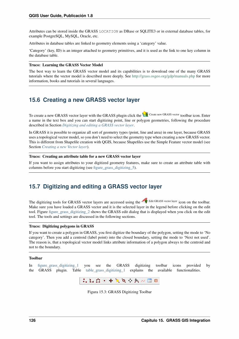
QGIS User Guide, Publicación 1.8
Attributes can be stored inside the GRASS LOCATION as DBase or SQLITE3 or in external database tables, forexample PostgreSQL, MySQL, Oracle, etc.
Attributes in database tables are linked to geometry elements using a ‘category’ value.
‘Category’ (key, ID) is an integer attached to geometry primitives, and it is used as the link to one key column inthe database table.
Truco: Learning the GRASS Vector ModelThe best way to learn the GRASS vector model and its capabilities is to download one of the many GRASStutorials where the vector model is described more deeply. See http://grass.osgeo.org/gdp/manuals.php for moreinformation, books and tutorials in several languages.
15.6 Creating a new GRASS vector layer
To create a new GRASS vector layer with the GRASS plugin click the Create new GRASS vector toolbar icon. Entera name in the text box and you can start digitizing point, line or polygon geometries, following the proceduredescribed in Section Digitizing and editing a GRASS vector layer.
In GRASS it is possible to organize all sort of geometry types (point, line and area) in one layer, because GRASSuses a topological vector model, so you don’t need to select the geometry type when creating a new GRASS vector.This is different from Shapefile creation with QGIS, because Shapefiles use the Simple Feature vector model (seeSection Creating a new Vector layer).
Truco: Creating an attribute table for a new GRASS vector layerIf you want to assign attributes to your digitized geometry features, make sure to create an attribute table withcolumns before you start digitizing (see figure_grass_digitizing_5).
15.7 Digitizing and editing a GRASS vector layer
The digitizing tools for GRASS vector layers are accessed using the Edit GRASS vector layer icon on the toolbar.Make sure you have loaded a GRASS vector and it is the selected layer in the legend before clicking on the edittool. Figure figure_grass_digitizing_2 shows the GRASS edit dialog that is displayed when you click on the edittool. The tools and settings are discussed in the following sections.
Truco: Digitizing polygons in GRASSIf you want to create a polygon in GRASS, you first digitize the boundary of the polygon, setting the mode to ‘Nocategory’. Then you add a centroid (label point) into the closed boundary, setting the mode to ‘Next not used’.The reason is, that a topological vector model links attribute information of a polygon always to the centroid andnot to the boundary.
Toolbar
In figure_grass_digitizing_1 you see the GRASS digitizing toolbar icons provided bythe GRASS plugin. Table table_grass_digitizing_1 explains the available functionalities.
Figura 15.3: GRASS Digitizing Toolbar
126 Capítulo 15. GRASS GIS Integration
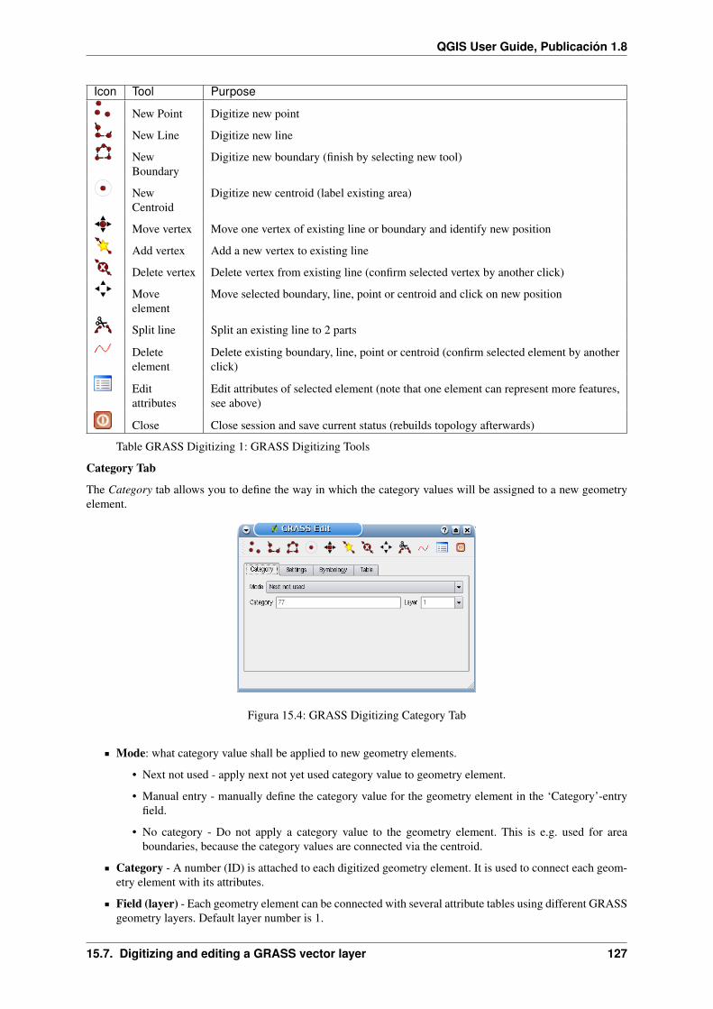
QGIS User Guide, Publicación 1.8
Icon Tool Purpose
New Point Digitize new point
New Line Digitize new line
NewBoundary
Digitize new boundary (finish by selecting new tool)
NewCentroid
Digitize new centroid (label existing area)
Move vertex Move one vertex of existing line or boundary and identify new position
Add vertex Add a new vertex to existing line
Delete vertex Delete vertex from existing line (confirm selected vertex by another click)
Moveelement
Move selected boundary, line, point or centroid and click on new position
Split line Split an existing line to 2 parts
Deleteelement
Delete existing boundary, line, point or centroid (confirm selected element by anotherclick)
Editattributes
Edit attributes of selected element (note that one element can represent more features,see above)
Close Close session and save current status (rebuilds topology afterwards)
Table GRASS Digitizing 1: GRASS Digitizing Tools
Category Tab
The Category tab allows you to define the way in which the category values will be assigned to a new geometryelement.
Figura 15.4: GRASS Digitizing Category Tab
Mode: what category value shall be applied to new geometry elements.
• Next not used - apply next not yet used category value to geometry element.
• Manual entry - manually define the category value for the geometry element in the ‘Category’-entryfield.
• No category - Do not apply a category value to the geometry element. This is e.g. used for areaboundaries, because the category values are connected via the centroid.
Category - A number (ID) is attached to each digitized geometry element. It is used to connect each geom-etry element with its attributes.
Field (layer) - Each geometry element can be connected with several attribute tables using different GRASSgeometry layers. Default layer number is 1.
15.7. Digitizing and editing a GRASS vector layer 127
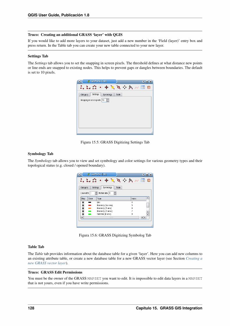
QGIS User Guide, Publicación 1.8
Truco: Creating an additional GRASS ‘layer’ with QGISIf you would like to add more layers to your dataset, just add a new number in the ‘Field (layer)’ entry box andpress return. In the Table tab you can create your new table connected to your new layer.
Settings Tab
The Settings tab allows you to set the snapping in screen pixels. The threshold defines at what distance new pointsor line ends are snapped to existing nodes. This helps to prevent gaps or dangles between boundaries. The defaultis set to 10 pixels.
Figura 15.5: GRASS Digitizing Settings Tab
Symbology Tab
The Symbology tab allows you to view and set symbology and color settings for various geometry types and theirtopological status (e.g. closed / opened boundary).
Figura 15.6: GRASS Digitizing Symbolog Tab
Table Tab
The Table tab provides information about the database table for a given ‘layer’. Here you can add new columns toan existing attribute table, or create a new database table for a new GRASS vector layer (see Section Creating anew GRASS vector layer).
Truco: GRASS Edit PermissionsYou must be the owner of the GRASS MAPSET you want to edit. It is impossible to edit data layers in a MAPSETthat is not yours, even if you have write permissions.
128 Capítulo 15. GRASS GIS Integration

QGIS User Guide, Publicación 1.8
Figura 15.7: GRASS Digitizing Table Tab
15.8 The GRASS region tool
The region definition (setting a spatial working window) in GRASS is important for working with raster layers.Vector analysis is by default not limited to any defined region definitions. But all newly-created rasters will havethe spatial extension and resolution of the currently defined GRASS region, regardless of their original extensionand resolution. The current GRASS region is stored in the $LOCATION/$MAPSET/WIND file, and it definesnorth, south, east and west bounds, number of columns and rows, horizontal and vertical spatial resolution.
It is possible to switch on/off the visualization of the GRASS region in the QGIS canvas using theDisplay current GRASS region button.
With the Edit current GRASS region icon you can open a dialog to change the current region and the symbology ofthe GRASS region rectangle in the QGIS canvas. Type in the new region bounds and resolution and click [OK]. Italso allows to select a new region interactively with your mouse on the QGIS canvas. Therefore click with the leftmouse button in the QGIS canvas, open a rectangle, close it using the left mouse button again and click [OK].
The GRASS module g.region provide a lot more parameters to define an appropriate region extend and reso-lution for your raster analysis. You can use these parameters with the GRASS Toolbox, described in Section TheGRASS toolbox.
15.9 The GRASS toolbox
The Open GRASS Tools box provides GRASS module functionalities to work with data inside a selected GRASSLOCATION and MAPSET. To use the GRASS toolbox you need to open a LOCATION and MAPSET where youhave write-permission (usually granted, if you created the MAPSET). This is necessary, because new raster orvector layers created during analysis need to be written to the currently selected LOCATION and MAPSET.
The GRASS Shell inside the GRASS Toolbox provides access to almost all (more than 330) GRASS modulesthrough a command line interface. To offer a more user friendly working environment, about 200 of the availableGRASS modules and functionalities are also provided by graphical dialogs within the GRASS plugin Toolbox.
15.9.1 Working with GRASS modules
The GRASS Shell inside the GRASS Toolbox provides access to almost all (more than 300) GRASS modules ina command line interface. To offer a more user friendly working environment, about 200 of the available GRASSmodules and functionalities are also provided by graphical dialogs.
A complete list of GRASS modules available in the graphical Toolbox in QGIS version 1.8.0 is available in theGRASS wiki ( http://grass.osgeo.org/wiki/GRASS-QGIS_relevant_module_list).
15.8. The GRASS region tool 129

QGIS User Guide, Publicación 1.8
Figura 15.8: GRASS Toolbox and Module Tree
It is also possible to customize the GRASS Toolbox content. This procedure is described in Section Customizingthe GRASS Toolbox.
As shown in figure_grass_toolbox_1 , you can look for the appropriate GRASS module using the thematicallygrouped Modules Tree or the searchable Modules List tab.
Clicking on a graphical module icon a new tab will be added to the toolbox dialog providing three new sub-tabsOptions, Output and Manual.
Options
The Options tab provides a simplified module dialog where you can usually select a raster or vector layer visualizedin the QGIS canvas and enter further module specific parameters to run the module.
The provided module parameters are often not complete to keep the dialog clear. If you want to use further moduleparameters and flags, you need to start the GRASS Shell and run the module in the command line.
A new feature in QGIS 1.8.0 is the support for a show advanced options button below the simplified module dialogin the Options tab. At the moment it is only added to the module v.in.ascii as an example use, but will probablybe part of more / all modules in the GRASS toolbox in future versions of QGIS. This allows to use the completeGRASS module options without the need to switch to the GRASS Shell.
Output
The Output tab provides information about the output status of the module. When you click the [Run] button, themodule switches to the Output tab and you see information about the analysis process. If all works well, you willfinally see a Successfully finished message.
Manual
The Manual tab shows the HTML help page of the GRASS module. You can use it to check further moduleparameters and flags or to get a deeper knowledge about the purpose of the module. At the end of each modulemanual page you see further links to the Main Help index, the Thematic index and the Full index.These links provide the same information as if you use the module g.manual.
Truco: Display results immediatelyIf you want to display your calculation results immediately in your map canvas, you can use the ‘View Output’button at the bottom of the module tab.
15.9.2 GRASS module examples
The following examples will demonstrate the power of some of the GRASS modules.
130 Capítulo 15. GRASS GIS Integration

QGIS User Guide, Publicación 1.8
Figura 15.9: GRASS Toolbox Module Options
Figura 15.10: GRASS Toolbox Module Output
15.9. The GRASS toolbox 131

QGIS User Guide, Publicación 1.8
Figura 15.11: GRASS Toolbox Module Manual
Creating contour lines
The first example creates a vector contour map from an elevation raster (DEM). Assuming you have the AlaskaLOCATION set up as explained in Section Importing data into a GRASS LOCATION.
First open the location by clicking the Open mapset button and choosing the Alaska location.
Now load the gtopo30 elevation raster by clicking Add GRASS raster layer and selecting the gtopo30raster from the demo location.
Now open the Toolbox with the Open GRASS tools button.
In the list of tool categories double click Raster → Surface Management → Generate vector contour lines.
Now a single click on the tool r.contour will open the tool dialog as explained above Working with GRASSmodules. The gtopo30 raster should appear as the Name of input raster.
Type into the Increment between Contour levels the value 100. (This will create contour lines atintervals of 100 meters.)
Type into the Name for output vector map the name ctour_100.
Click [Run] to start the process. Wait for several moments until the message Successfully finishedappears in the output window. Then click [View Output] and [close].
Since this is a large region, it will take a while to display. After it finishes rendering, you can open the layerproperties window to change the line color so that the contours appear clearly over the elevation raster, as in TheVector Properties Dialog.
Next zoom in to a small mountainous area in the center of Alaska. Zooming in close you will notice that thecontours have sharp corners. GRASS offers the v.generalize tool to slightly alter vector maps while keeping their
132 Capítulo 15. GRASS GIS Integration
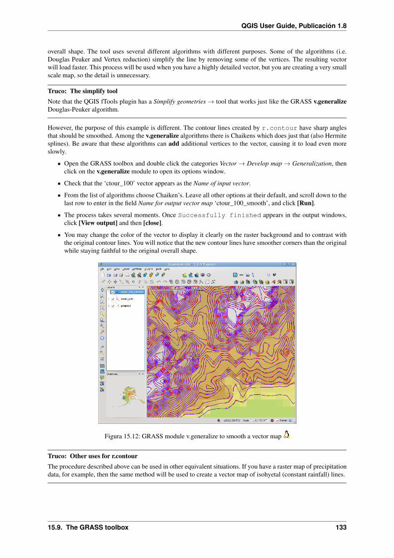
QGIS User Guide, Publicación 1.8
overall shape. The tool uses several different algorithms with different purposes. Some of the algorithms (i.e.Douglas Peuker and Vertex reduction) simplify the line by removing some of the vertices. The resulting vectorwill load faster. This process will be used when you have a highly detailed vector, but you are creating a very smallscale map, so the detail is unnecessary.
Truco: The simplify toolNote that the QGIS fTools plugin has a Simplify geometries → tool that works just like the GRASS v.generalizeDouglas-Peuker algorithm.
However, the purpose of this example is different. The contour lines created by r.contour have sharp anglesthat should be smoothed. Among the v.generalize algorithms there is Chaikens which does just that (also Hermitesplines). Be aware that these algorithms can add additional vertices to the vector, causing it to load even moreslowly.
Open the GRASS toolbox and double click the categories Vector → Develop map → Generalization, thenclick on the v.generalize module to open its options window.
Check that the ‘ctour_100’ vector appears as the Name of input vector.
From the list of algorithms choose Chaiken’s. Leave all other options at their default, and scroll down to thelast row to enter in the field Name for output vector map ‘ctour_100_smooth’, and click [Run].
The process takes several moments. Once Successfully finished appears in the output windows,click [View output] and then [close].
You may change the color of the vector to display it clearly on the raster background and to contrast withthe original contour lines. You will notice that the new contour lines have smoother corners than the originalwhile staying faithful to the original overall shape.
Figura 15.12: GRASS module v.generalize to smooth a vector map
Truco: Other uses for r.contourThe procedure described above can be used in other equivalent situations. If you have a raster map of precipitationdata, for example, then the same method will be used to create a vector map of isohyetal (constant rainfall) lines.
15.9. The GRASS toolbox 133

QGIS User Guide, Publicación 1.8
Creating a Hillshade 3D effect
Several methods are used to display elevation layers and give a 3D effect to maps. The use of contour lines asshown above is one popular method often chosen to produce topographic maps. Another way to display a 3Deffect is by hillshading. The hillshade effect is created from a DEM (elevation) raster by first calculating the slopeand aspect of each cell, then simulating the sun’s position in the sky and giving a reflectance value to each cell.Thus you get sun facing slopes lighted and the slopes facing away from the sun (in shadow) are darkened.
Begin this example by loading the gtopo30 elevation raster. Start the GRASS toolbox and under the Rastercategory double click to open Spatial analysis → Terrain analysis.
Then click r.shaded.relief to open the module.
Change the azimuth angle 270 to 315.
Enter gtopo30_shade for the new hillshade raster, and click [Run].
When the process completes, add the hillshade raster to the map. You should see it displayed in grayscale.
To view both the hill shading and the colors of the gtopo30 together shift the hillshade map below thegtopo30 map in the table of contents, then open the Properties window of gtopo30, switch to thetransparency tab and set its transparency level to about 25 %.
You should now have the gtopo30 elevation with its colormap and transparency setting displayed above thegrayscale hillshade map. In order to see the visual effects of the hillshading, turn off the gtopo30_shade map,then turn it back on.
Using the GRASS shell
The GRASS plugin in QGIS is designed for users who are new to GRASS, and not familiar with all the modulesand options. As such, some modules in the toolbox do not show all the options available, and some modules donot appear at all. The GRASS shell (or console) gives the user access to those additional GRASS modules thatdo not appear in the toolbox tree, and also to some additional options to the modules that are in the toolbox withthe simplest default parameters. This example demonstrates the use of an additional option in the r.shaded.reliefmodule that was shown above.
Figura 15.13: The GRASS shell, r.shaded.relief module
The module r.shaded.relief can take a parameter zmult which multiplies the elevation values relative to the X-Ycoordinate units so that the hillshade effect is even more pronounced.
Load the gtopo30 elevation raster as above, then start the GRASS toolbox and click onthe GRASS shell. In the shell window type the command r.shaded.relief map=gtopo30shade=gtopo30_shade2 azimuth=315 zmult=3 and press [Enter].
134 Capítulo 15. GRASS GIS Integration
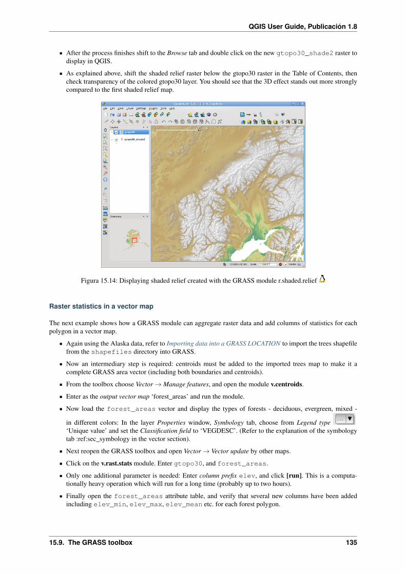
QGIS User Guide, Publicación 1.8
After the process finishes shift to the Browse tab and double click on the new gtopo30_shade2 raster todisplay in QGIS.
As explained above, shift the shaded relief raster below the gtopo30 raster in the Table of Contents, thencheck transparency of the colored gtopo30 layer. You should see that the 3D effect stands out more stronglycompared to the first shaded relief map.
Figura 15.14: Displaying shaded relief created with the GRASS module r.shaded.relief
Raster statistics in a vector map
The next example shows how a GRASS module can aggregate raster data and add columns of statistics for eachpolygon in a vector map.
Again using the Alaska data, refer to Importing data into a GRASS LOCATION to import the trees shapefilefrom the shapefiles directory into GRASS.
Now an intermediary step is required: centroids must be added to the imported trees map to make it acomplete GRASS area vector (including both boundaries and centroids).
From the toolbox choose Vector → Manage features, and open the module v.centroids.
Enter as the output vector map ‘forest_areas’ and run the module.
Now load the forest_areas vector and display the types of forests - deciduous, evergreen, mixed -
in different colors: In the layer Properties window, Symbology tab, choose from Legend type‘Unique value’ and set the Classification field to ‘VEGDESC’. (Refer to the explanation of the symbologytab :ref:sec_symbology in the vector section).
Next reopen the GRASS toolbox and open Vector → Vector update by other maps.
Click on the v.rast.stats module. Enter gtopo30, and forest_areas.
Only one additional parameter is needed: Enter column prefix elev, and click [run]. This is a computa-tionally heavy operation which will run for a long time (probably up to two hours).
Finally open the forest_areas attribute table, and verify that several new columns have been addedincluding elev_min, elev_max, elev_mean etc. for each forest polygon.
15.9. The GRASS toolbox 135

QGIS User Guide, Publicación 1.8
15.9.3 Working with the GRASS LOCATION browser
Another useful feature inside the GRASS Toolbox is the GRASS LOCATION browser. In figure_grass_module_7you can see the current working LOCATION with its MAPSETs.
In the left browser windows you can browse through all MAPSETs inside the current LOCATION. The rightbrowser window shows some meta information for selected raster or vector layers, e.g. resolution, bounding box,data source, connected attribute table for vector data and a command history.
Figura 15.15: GRASS LOCATION browser
The toolbar inside the Browser tab offers following tools to manage the selected LOCATION:
Add selected map to canvas
Copy selected map
Rename selected map
Delete selected map
Set current region to selected map
Refresh browser window
The Rename selected map and Delete selected map only work with maps inside your currently selectedMAPSET. All other tools also work with raster and vector layers in another MAPSET.
15.9.4 Customizing the GRASS Toolbox
Nearly all GRASS modules can be added to the GRASS toolbox. A XML interface is provided to parse the prettysimple XML files which configures the modules appearance and parameters inside the toolbox.
A sample XML file for generating the module v.buffer (v.buffer.qgm) looks like this:
<?xml version="1.0" encoding="UTF-8"?><!DOCTYPE qgisgrassmodule SYSTEM "http://mrcc.com/qgisgrassmodule.dtd">
<qgisgrassmodule label="Vector buffer" module="v.buffer">
136 Capítulo 15. GRASS GIS Integration
QGIS User Guide, Publicación 1.8
<option key="input" typeoption="type" layeroption="layer" /><option key="buffer"/><option key="output" />
</qgisgrassmodule>
The parser reads this definition and creates a new tab inside the toolbox when you select the module. A moredetailed description for adding new modules, changing the modules group, etc. can be found on the QGIS wiki athttp://hub.qgis.org/projects/quantum-gis/wiki/Adding_New_Tools_to_the_GRASS_Toolbox
15.9. The GRASS toolbox 137

QGIS User Guide, Publicación 1.8
138 Capítulo 15. GRASS GIS Integration

CAPÍTULO 16
OpenStreetMap
In recent years, the OpenStreetMap project has gained popularity because in many countries no free geodata suchas digital roadmaps are available. The objective of the OSM project is to create a free editable map of the worldfrom GPS data, aerial photography or from local knowledge. To support this objective, QGIS provides a pluginthat enables its users to work with OSM data.
The OpenStreetMap plugin, a core QGIS plugin, provides the basic functionalities for OSM data manipulation;this includes data loading, importing, saving, downloading, editing and uploading data back to the OpenStreetMapserver. While implementing the OSM plugin an inspiration was taken from existing OSM data editors. The purposewas to combine their functionalities to get the best possible result.
The following section gives a brief introduction to principles of the OSM project.
Parts of the following paragraphs are copied from the OpenStreetMap web site at http://www.openstreetmap.org.
16.1 The OpenStreetMap project
OpenStreetMap is a project to create a free editable map of the world. The maps are created using data fromportable GPS devices, aerial photography, other free sources or simply from local knowledge. The project wasstarted because most maps have legal or technical restrictions on their use, restricting people from using them increative, productive, or unexpected ways. Both rendered images and the vector dataset of OSM are available fordownload under a Creative Commons Attribution ShareAlike 2.0 license.
OpenStreetMap was inspired by sites such as Wikipedia - the map display (see Figure_OpenStreetMap_1 ) featuresa prominent Edit tab and a full revision history is maintained. Registered users can upload GPS track logs and editthe vector data using the given editing tools.
OSM data primitive is an object class that can be stored via the API in the server. The three supported types ofdata are: Node, Way and Relation.
A node is a latitude/longitude pair of coordinates. It is used as building a block for other features and as afeature itself (Points Of Interest), if they are tagged as required.
A way is a list of at least two nodes that describe a linear feature such as a street, or similar. Nodes can bemembers of multiple ways.
A relation is a group of zero or more primitives with associated roles. It is used to specify relationshipsbetween objects, and may also model an abstract object.
Several different logical features in a common map ‘Point Of Interest’, ‘Street’, ‘Tram Line’, ‘Bus Stop’ etc.) aredefined by these primitives. Map features are well-known in the OSM community and are stored as tags, based ona key and a value. OSM is usually distributed in XML format. XML payload is used for the communication withthe OSM server as well.
139
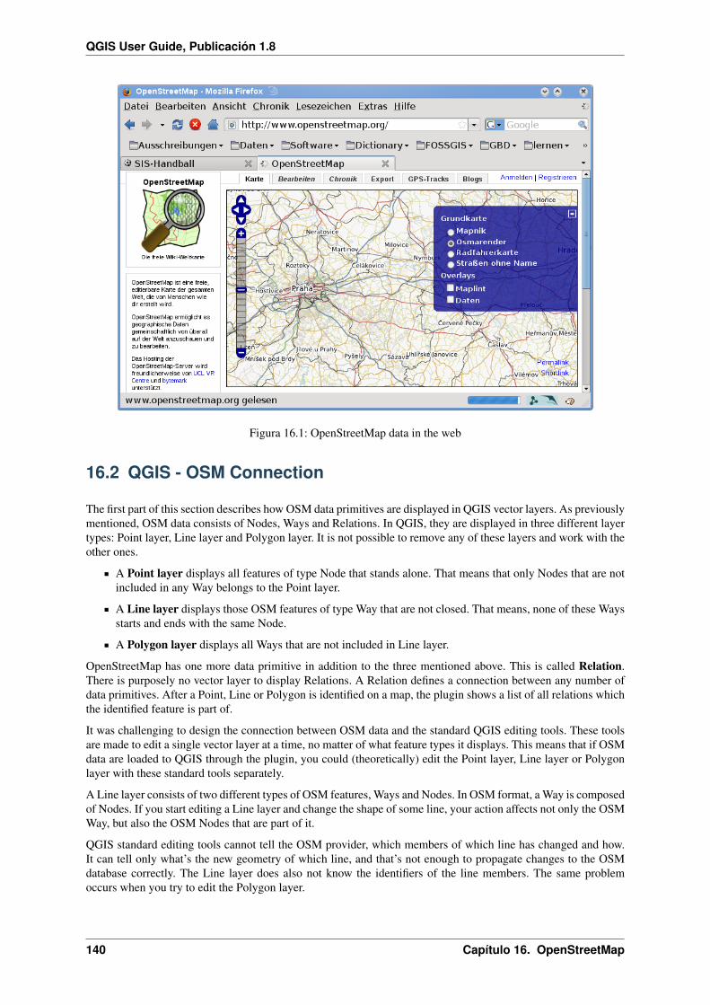
QGIS User Guide, Publicación 1.8
Figura 16.1: OpenStreetMap data in the web
16.2 QGIS - OSM Connection
The first part of this section describes how OSM data primitives are displayed in QGIS vector layers. As previouslymentioned, OSM data consists of Nodes, Ways and Relations. In QGIS, they are displayed in three different layertypes: Point layer, Line layer and Polygon layer. It is not possible to remove any of these layers and work with theother ones.
A Point layer displays all features of type Node that stands alone. That means that only Nodes that are notincluded in any Way belongs to the Point layer.
A Line layer displays those OSM features of type Way that are not closed. That means, none of these Waysstarts and ends with the same Node.
A Polygon layer displays all Ways that are not included in Line layer.
OpenStreetMap has one more data primitive in addition to the three mentioned above. This is called Relation.There is purposely no vector layer to display Relations. A Relation defines a connection between any number ofdata primitives. After a Point, Line or Polygon is identified on a map, the plugin shows a list of all relations whichthe identified feature is part of.
It was challenging to design the connection between OSM data and the standard QGIS editing tools. These toolsare made to edit a single vector layer at a time, no matter of what feature types it displays. This means that if OSMdata are loaded to QGIS through the plugin, you could (theoretically) edit the Point layer, Line layer or Polygonlayer with these standard tools separately.
A Line layer consists of two different types of OSM features, Ways and Nodes. In OSM format, a Way is composedof Nodes. If you start editing a Line layer and change the shape of some line, your action affects not only the OSMWay, but also the OSM Nodes that are part of it.
QGIS standard editing tools cannot tell the OSM provider, which members of which line has changed and how.It can tell only what’s the new geometry of which line, and that’s not enough to propagate changes to the OSMdatabase correctly. The Line layer does also not know the identifiers of the line members. The same problemoccurs when you try to edit the Polygon layer.
140 Capítulo 16. OpenStreetMap

QGIS User Guide, Publicación 1.8
For this reason, the OSM plugin need its own tools for editing OSM data. While they are used, the OSM layerscan be changed correctly. The Plugin editing tools consists of tools for Point, Line, Polygon and Relation creation,deletion and moving.
Nota: To create a connection between the OSM plugin and standard editing tools, changes in QuantumGIS corecode would be necessary.
16.3 Installation
The OpenStreetMap plugin is a core plugin inside QGIS. The ‘OpenStreetMap’ plugin can be selected in thePlugin Manager as described in section Loading a QGIS Core Plugin.
16.4 Basic user interface
The first time the OSM plugin is started (and after the first data are loaded), several new OSM plugin icons appearin the QGIS toolbar menu together with new dock windows as shown in figure_OpenStreetMap_2.
Figura 16.2: OSM plugin user interface
16.4.1 OSM Features widget
The OSM Feature widget helps to identify OSM features. It shows basic information on the feature type andidentifier as well as information on who has changed a feature, and when. The OSM Feature widget also providesall editing tools (in the top part of it). More information on those tools can be found in the sections below. Thewidget is initially disabled. It activates itself after successful loading some OSM data.
16.4.2 OSM Undo/Redo widget
This Undo/Redo widget is used to undo and redo edit actions. It consists not only a classic Undo and Redo button,but also shows a list with a brief description of the edit actions that were done. The OSM Undo/Redo widget isinitially closed. You can show it using a button on the OSM Feature widget.
16.3. Installation 141

QGIS User Guide, Publicación 1.8
16.4.3 Toolbar menu icons
Load OSM from file is used to load data from a special OpenStreetMap XML file.
Show/Hide OSM Feature Manager is used to show or hide the OSM Feature widget. The OSM Feature widget is a panelthat helps with OSM feature identification and with OSM data editing.
Download OSM data is used to download data from the OpenStreetMap server.
Upload OSM data is used to upload changes (on current data).
Import data from a layer is used to import data from a vector layer. At least one vector layer must be loaded andcurrent OSM data must be selected.
Save OSM to file is used to save OSM data back to an XML file.
More detailed information on all the widgets, buttons and dialogs can be found in appropriate sections of thisplugin section according to their functionality (editing, identification, etc.).
16.5 Loading OSM data
The first action that should be done after starting the OSM Plugin is opening data from an OSM file. OSM datacan be import as shapefile or downloaded directly from the OpenStreetMap server. Here we are focusing on thefirst mentioned method.
To load data from a file use the Load OSM from file icon. If there is no such button, maybe someone disabledOpenStreetMap toolbar in your QGIS installation. You can enable it again selecting Settings → Toolbars →OpenStreetMap.
Figura 16.3: Load OSM data dialog
The purpose of its elements is explained below.
OpenStreetMap file to load: Click on the button to select the file:.osm file you want to load data from.
Add columns for tags: This option determines a connection between OSM and QGIS data. Each feature of OSMdata has some tags (pairs of key and value), that define the feature properties. Each feature of a QGIS vector layeralso has its attributes (key and value). With this option you can define which properties of OSM objects should bevisible when displaying detailed information about QGIS features.
142 Capítulo 16. OpenStreetMap

QGIS User Guide, Publicación 1.8
Replace current data: Checking this option means that new data should replace current data the user is workingwith. Layers of current data will be removed and new ones will be loaded. When loading OSM data for the firsttime, this option is not active, because there is nothing to replace.
Use custom renderer: This option determines how many details of the map will be used. There are three pre-defined OSM styles for map displaying. Use ‘Small scale’ if you want to view OSM data at low level, to see alldetails and to edit something. If not you can use ‘Medium scale’ or ‘Large scale’. QGIS 1.8.0 doesn’t supportchanging the renderer style dynamically.
Click [OK] to load your data. If this is the first time the OSM file is loaded, the plugin must first parse the database.This may take few seconds or minutes - it depends on the amount of loaded data.
16.6 Viewing OSM data
After the OSM data are loaded, you can identify map features using the appropriate tool. Use the Identify feature
button on the top-left of the OSM Feature widget. Using this tool you can easily explore all map objects. Whenthe mouse cursor is placed over an object, you can see all information on it directly in the OSM Feature widget.There is also a dynamic rubberband displayed on the map so that the user is able to determine which feature iscurrently identified.
The Properties tab of the widget contains of all feature tags. Clicking on the Relation tab shows you a list of allrelations connected with identified feature.
If you want to hold a feature for a while to be able to read its properties and relations, move the mouse cursor at thesame time, try left-clicking while you are over the feature. Identification process will stop until next left-clicking.
Sometimes there is more than one feature at a point where left-clicking was performed. This happens especiallywhen clicking on cross-roads or if you did not zoom enough into the map. In this situation only one of suchfeatures is identified (and marked with the rubberband) but the plugin remembers all of them. Then (still in thepause mode) you can cycle through the identified features by right-clicking.
16.7 Editing basic OSM data
‘Basic data’ in this context means non-relational OSM features - nodes and ways. If you prefer to examine how toperform relational editing, skip this section and move on to the next one.
Basic data editing is a key part of the OSM Plugin. You can change the property, position or shape of any existingbasic feature. You can remove features or add new ones. All changes on nodes and ways are remembered byUndo/Redo all changes can be easily uploaded to the OpenStreetMap server.
16.7.1 Changing feature tags
Changing the property/tag of an OSM feature can be done directly in the table of feature tags. The Tags table ofbasic features can be found on the OSM Feature widget. Don’t forget to identify feature first.
If you want to change a tag value, just double-click in the appropriate row of column ‘Value’ and type, or select
a new value. If you want to remove a tag, click in the relevant row, then use the button Remove selected tags on theright bottom under the table.
To add new tags just type the key and value into the last row of the table where ‘<next tag value>’ is written.Notice that you cannot change the key of an existing tag pair. Conveniently, there are some combo boxes of allexisting tag keys and their typical values.
16.6. Viewing OSM data 143

QGIS User Guide, Publicación 1.8
Figura 16.4: Changing an OSM feature tag
16.7.2 Point creation
For point creation there is a Create point button on the OSM Feature widget. To create some points, just click onthe button and start clicking on the map. If your cursor is over some map feature, the feature is marked/identifiedimmediately. If you click on the map when a line or polygon is marked, a new point is created directly on suchline or polygon as its new member. If your cursor is over an existing point, a new point cannot be created. In suchcase the OSM plugin will show following message:
Figura 16.5: OSM point creation message
The mechanism of helping a user to hit the line or polygon is called snapping and is enabled by default. If youwant to create a point very close to some line (but not on it) you must disable snapping by holding the Ctrl keyfirst.
16.7.3 Line creation
For line creation, there is a Create Line button on the OSM Feature widget. To create a line just click the buttonand start left-clicking on the map. Each of your left-clicks is remembered as a vertex of the new line. Line creationends when the first right-click is performed. The new line will immediately appear on the map.
Nota: A Line with less than two members cannot be created. In such case the operation is ignored.
144 Capítulo 16. OpenStreetMap

QGIS User Guide, Publicación 1.8
Snapping is performed to all map vertices - points from the Point vector layer and all Line and Polygon members.Snapping can be disabled by holding the Ctrl key.
16.7.4 Polygon creation
For polygon creation there is a Create polygon button on the OSM Feature widget. To create a polygon just clickthe button and start left-clicking on the map. Each of your left-clicks is remembered as a member vertex of thenew polygon. The Polygon creation ends when first right-click is performed. The new polygon will immediatelyappear on the map. Polygon with less than three members cannot be created. In such case operation is ignored.Snapping is performed to all map vertexes - points (from Point vector layer) and all Line and Polygon members.Snapping can be disabled by holding the Ctrl key.
16.7.5 Map feature moving
If you want to move a feature (no matter what type) please use the Move feature button from the OSM Featurewidget menu. Then you can browse the map (features are identified dynamically when you go over them) andclick on the feature you want to move. If a wrong feature is selected after your click, don’t move it from the place.Repeat right-clicking until the correct feature is identified. When selection is done and you move the cursor, youare no more able to change your decision what to move. To confirm the move, click on the left mouse button. Tocancel a move, click another mouse button.
If you are moving a feature that is connected to another features, these connections won’t be damaged. Otherfeatures will just adapt themselves to a new position of a moved feature.
Snapping is also supported in this operation, this means:
When moving a standalone (not part of any line/polygon) point,snapping to all map segments and verticesis performed.
When moving a point that is a member of some lines/polygons,snapping to all map segments and verticesis performed, except for vertices of point parents.
When moving a line/polygon, snapping to all map vertices is performed. Note that the OSM Plugin triesto snap only to the 3 closest-to-cursor vertices of a moved line/polygon, otherwise the operation would byvery slow. Snapping can be disabled by holding Ctrl key during the operation.
16.7.6 Map feature removing
If you want to remove a feature, you must identify it first. To remove an identified feature, use theRemove this feature button on the OSM Feature widget. When removing a line/polygon, the line/polygon itself is delet-ed, so are all its member points that doesn’t belong to any other line/polygon.
When removing a point that is member of some lines/polygons, the point is deleted and the geometries of parentlines/polygons are changed. The new parent geometry has less vertices than the old one.
If the parent feature was a polygon with three vertexes, its new geometry has only two vertexes. And because therecannot exist polygon with only two vertices, as described above, the feature type is automatically changed to Line.
If the parent feature was a line with two vertexes, its new geometry has only one vertex. And because there cannotexist a line with only one vertex, the feature type is automatically changed to Point.
16.8 Editing relations
Thanks to existence of OSM relations we can join OSM features into groups and give them common properties -in such way we can model any possible map object: borders of a region (as group of ways and points), routes of a
16.8. Editing relations 145

QGIS User Guide, Publicación 1.8
bus, etc. Each member of a relation has its specific role. There is a pretty good support for OSM Relations in ourplugin. Let’s see how to examine, create, update or remove them.
16.8.1 Examining relation
If you want to see relation properties, first identify one of its members. After that open the Relations tab on theOSM Feature widget. At the top of the tab you can see a list of all relations the identified feature is part of. Pleasechoose the one you want to examine and look at its information below. In the first table called ‘Relation tags’ youfind the properties of the selected relation. In the table called ‘Relation members’ you see brief information on therelation members. If you click on a member, the plugin will make a rubberband on it in the map.
16.8.2 Relation creation
There are 2 ways to create a relation:
1. You can use the Create relation button on OSM Feature widget.
2. You can create it from the Relation tab of OSM Feature widget using the Add relation button.
In both cases a dialog will appear. For the second case, the feature that is currently identified is automaticallyconsidered to be the first relation member, so the dialog is prefilled a little. When creating a relation, please selectits type first. You can select one of predefined relation types or write your own type. After that fill the relation tagsand choose its members.
If you have already selected a relation type, try using the Generate tags button. It will generate typical tags to yourrelation type. Then you are expected to enter values to the keys. Choosing relation members can be done either by
writing member identifiers, types and roles or using the Identify tool and clicking on map.
Finally when type, tags and members are chosen, the dialog can be submitted. In such case the plugin creates anew relation for you.
16.8.3 Changing relation
If you want to change an existing relation, identify it first (follow steps written above in Section Examining
relation). After that click on the Edit relation button. You will find it on the OSM Feature widget. A new dialogappears, nearly the same as for the ‘create relation’ action. The dialog is pre-filled with information on givenrelations. You can change relation tags, members or even its type. After submitting the dialog your changes willbe committed.
16.9 Downloading OSM data
To download data from OpenStreetMap server click on the Download OSM data button. If there is no such button,the OSM toolbar may be disabled in your QGIS instalation. You can enable it again at Settings → Toolbars →OpenStreetMap . After clicking the button a dialog occurs and provides following functionalities:
Extent: Specifies an area to download data from intervals of latitude and longitude degrees. Because there is somerestriction of OpenStreetMap server on how much data can be downloaded, the intervals must not be too wide.
More detailed info on extent specification can is shown after clicking the Help button on the right.
Download to: Here you are expected to write a path to the file where data will be stored. If you can’t remember
the structure of your disk, don’t panic. The browse button will help you.
146 Capítulo 16. OpenStreetMap
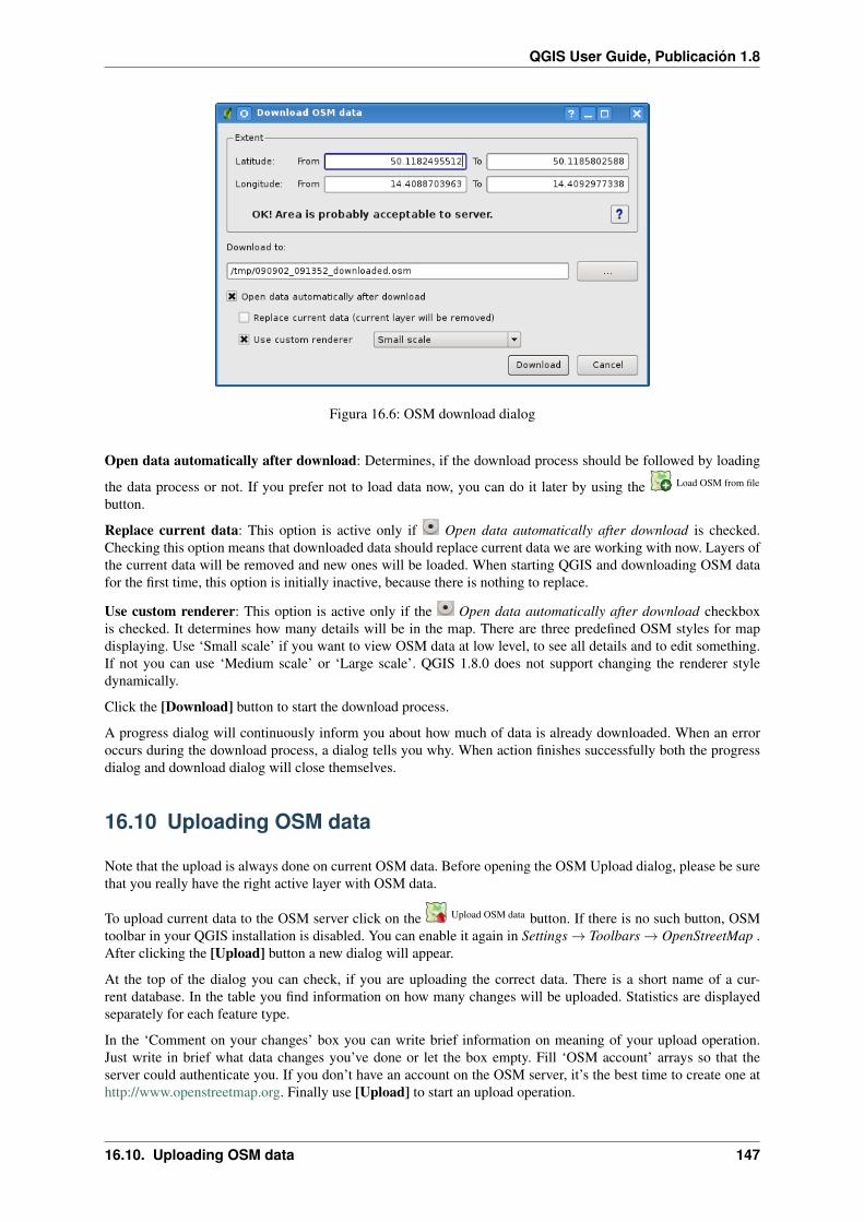
QGIS User Guide, Publicación 1.8
Figura 16.6: OSM download dialog
Open data automatically after download: Determines, if the download process should be followed by loading
the data process or not. If you prefer not to load data now, you can do it later by using the Load OSM from file
button.
Replace current data: This option is active only if Open data automatically after download is checked.Checking this option means that downloaded data should replace current data we are working with now. Layers ofthe current data will be removed and new ones will be loaded. When starting QGIS and downloading OSM datafor the first time, this option is initially inactive, because there is nothing to replace.
Use custom renderer: This option is active only if the Open data automatically after download checkboxis checked. It determines how many details will be in the map. There are three predefined OSM styles for mapdisplaying. Use ‘Small scale’ if you want to view OSM data at low level, to see all details and to edit something.If not you can use ‘Medium scale’ or ‘Large scale’. QGIS 1.8.0 does not support changing the renderer styledynamically.
Click the [Download] button to start the download process.
A progress dialog will continuously inform you about how much of data is already downloaded. When an erroroccurs during the download process, a dialog tells you why. When action finishes successfully both the progressdialog and download dialog will close themselves.
16.10 Uploading OSM data
Note that the upload is always done on current OSM data. Before opening the OSM Upload dialog, please be surethat you really have the right active layer with OSM data.
To upload current data to the OSM server click on the Upload OSM data button. If there is no such button, OSMtoolbar in your QGIS installation is disabled. You can enable it again in Settings → Toolbars → OpenStreetMap .After clicking the [Upload] button a new dialog will appear.
At the top of the dialog you can check, if you are uploading the correct data. There is a short name of a cur-rent database. In the table you find information on how many changes will be uploaded. Statistics are displayedseparately for each feature type.
In the ‘Comment on your changes’ box you can write brief information on meaning of your upload operation.Just write in brief what data changes you’ve done or let the box empty. Fill ‘OSM account’ arrays so that theserver could authenticate you. If you don’t have an account on the OSM server, it’s the best time to create one athttp://www.openstreetmap.org. Finally use [Upload] to start an upload operation.
16.10. Uploading OSM data 147
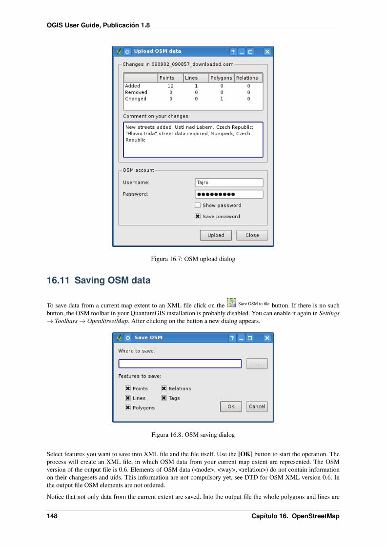
QGIS User Guide, Publicación 1.8
Figura 16.7: OSM upload dialog
16.11 Saving OSM data
To save data from a current map extent to an XML file click on the Save OSM to file button. If there is no suchbutton, the OSM toolbar in your QuantumGIS installation is probably disabled. You can enable it again in Settings→ Toolbars → OpenStreetMap. After clicking on the button a new dialog appears.
Figura 16.8: OSM saving dialog
Select features you want to save into XML file and the file itself. Use the [OK] button to start the operation. Theprocess will create an XML file, in which OSM data from your current map extent are represented. The OSMversion of the output file is 0.6. Elements of OSM data (<node>, <way>, <relation>) do not contain informationon their changesets and uids. This information are not compulsory yet, see DTD for OSM XML version 0.6. Inthe output file OSM elements are not ordered.
Notice that not only data from the current extent are saved. Into the output file the whole polygons and lines are
148 Capítulo 16. OpenStreetMap

QGIS User Guide, Publicación 1.8
saved even if only a small part of them is visible in the current extent. For each saved line/polygon all its membernodes are saved too.
16.12 Import OSM data
To import OSM data from an opened non-OSM vector layer follow this instructions. Choose current OSM data
by clicking on one of their layers. Click on the Import data from a layer button. If there is no such button, someonehas probably disabled the OpenStreetMap toolbar in your QGIS installation. You can enable it again in Settings→ Toolbars → OpenStreetMap.
After clicking on the button following message may show up:
Figura 16.9: OSM import message dialog
In such case there is no vector layer currently loaded. The import must be done from a loaded layer - please load avector layer from which you want to import data. After a layer is opened, your second try should give you a betterresult (don’t forget to mark the current OSM layer again):
Figura 16.10: Import data to OSM dialog
Use the submit dialog to start the process of OSM data importing. Reject it if you are not sure you want to importsomething.
16.12. Import OSM data 149

QGIS User Guide, Publicación 1.8
150 Capítulo 16. OpenStreetMap

CAPÍTULO 17
SEXTANTE
17.1 Introduction
This chapter introduces SEXTANTE, the powerful geospatial analysis framework of QGIS. SEXTANTE is ageoprocessing environment that can be used to call native and third party algorithms from QGIS, making yourspatial analysis tasks more productive and easy to accomplish.
In the following sections we will review how to use the graphical elements of SEXTANTE and take the most outof each one of them
17.1.1 Basic elements of the SEXTANTE GUI
There are four basic elements in the SEXTANTE GUI, which are used to run SEXTANTE algorithms for differentpurposes. Choosing one tool or another will depend on the kind of analysis that is to be performed and theparticular characteristics of each user and project. All of them (except for the batch processing interface, which iscalled from the toolbox, as we will see) can be accessed from the SEXTANTE menu item (you will see more thanfour entries. The remaining ones are not used to execute algorithms and will be explained later in this chapter).
The SEXTANTE toolbox. The main element of the SEXTANTE GUI, it is used to execute a single algorithmor run a batch process based on that algorithm.
Figura 17.1: SEXTANTE Toolbox
The SEXTANTE graphical modeler. Several algorithms can be combined graphically using the modeler todefine a workflow, creating a single process that involves several sub-processes
The SEXTANTE history manager. All actions performed using any of the aforementioned elements arestored in a history file and can be later easily reproduced using the history manager
151

QGIS User Guide, Publicación 1.8
Figura 17.2: SEXTANTE Models
Figura 17.3: SEXTANTE History
152 Capítulo 17. SEXTANTE

QGIS User Guide, Publicación 1.8
The SEXTANTE batch processing interface manager. This interface allows you to execute batch processesand automate the execution of a single algorithm on multiple datasets.
Figura 17.4: SEXTANTE Batch Processing
Along the following sections we will review each one of this elements in detail.
17.2 The SEXTANTE toolbox
17.2.1 Introduction
The Toolbox is the main element of the SEXTANTE GUI, and the one that you are more likely to use in your dailywork. It shows the list of all available algorithms grouped in different blocks, and is the access point to run themwhether as a single process or as a batch process involving several executions of a same algorithm on differentsets of inputs.
Figura 17.5: SEXTANTE Toolbox
The toolbox contains all the algorithms available, divided into groups. Each group represents a so-called ‘algorithmprovider’, which is a set of algorithms coming from the same source, for instance, from a third-party applicationwith geoprocessing capabilities. Some of this groups represent algorithms from one of such third-party applica-tions (like SAGA, GRASS or R), while other contain algorithms directly coded along with SEXTANTE elements,not relying on any additional software. Currently, these providers all reuse code from already existing QGISplugins (more specifically, from the fTools vector library shiped along with QGIS and the contributed mmqgis
17.2. The SEXTANTE toolbox 153

QGIS User Guide, Publicación 1.8
plugin that you can install using the Plugin Manager), making them more useful, since they can be executed fromelements such as the modeler or the batch processing interface, which we will soon describe.
Additionally, two more providers can be found, namely ‘Models’ and ‘Scripts’. This providers include user-createdalgorithms, and allow you to define your own workflows and processing tasks. We will devote a full section tothem a bit later.
In the upper part of the toolbox you can find a text box. To reduce the number of algorithms shown in the toolboxand make it easier to find the one you need, you can enter any word or phrase on the text box. Notice that, as youtype, the number of algorithms in the toolbox is reduced to just those which contain the text you have entered intheir names.
To execute an algorithm, just double-click on its name in the toolbox.
17.2.2 The algorithm dialog
Once you double-click on the name of the algorithm that you want to execute, a dialog similar to the next one isshown (in this case, the dialog corresponds to the SAGA ‘Convergence index’ algorithm).
Figura 17.6: Parameters Dialog
This dialog is used to set the input values that the algorithm needs to be executed. It shows a table where inputvalues and configuration parameters are to be set. It, of course, has a different content depending on the require-ments of the algorithm to be executed, and is created automatically based on those requirements. On the left side,the name of the parameter is shown. On the right side the value of the parameter can be set.
Although the number and type of parameters depend on the characteristics of the algorithm, the structure is similarfor all of them. The parameters found on the table can be of one of the following types.
A raster layer, to select from a list of all the ones available (currently opened) in QGIS. The selector containsas well a button on its right-hand side, to let you select filenames that represent layers currently not loadedin QGIS.
A vector layer, to select from a list of all the ones available in the QGIS. Layers not loaded in QGIS canbe selected as well, as in the case of raster layers, but only if the algorithm does not require a table fieldselected from the attributes table of the layer. In that case, only opened layers can be selected, since theyneed to be open so as to retrieve the list of field names available.
You will see a button by each vector layer selector. If the algorithm contains several of them, you will beable to toggle just one of them. If the button corresponding to a vector input is toggled, the algorithm will
154 Capítulo 17. SEXTANTE
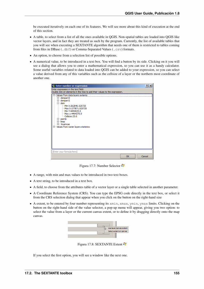
QGIS User Guide, Publicación 1.8
be executed iteratively on each one of its features. We will see more about this kind of execution at the endof this section.
A table, to select from a list of all the ones available in QGIS. Non-spatial tables are loaded into QGIS likevector layers, and in fact they are treated as such by the program. Currently, the list of available tables thatyou will see when executing a SEXTANTE algorithm that needs one of them is restricted to tables comingfrom files in DBase (.dbf) or Comma-Separated Values (.csv) formats.
An option, to choose from a selection list of possible options.
A numerical value, to be introduced in a text box. You will find a button by its side. Clicking on it you willsee a dialog that allows you to enter a mathematical expression, so you can use it as a handy calculator.Some useful variables related to data loaded into QGIS can be added to your expression, so you can selecta value derived from any of this variables such as the cellsize of a layer or the northern most coordinate ofanother one.
Figura 17.7: Number Selector
A range, with min and max values to be introduced in two text boxes.
A text string, to be introduced in a text box.
A field, to choose from the attributes table of a vector layer or a single table selected in another parameter.
A Coordinate Reference System (CRS). You can type the EPSG code directly in the text box, or select itfrom the CRS selection dialog that appear when you click on the button on the right-hand size
A extent, to be entered by four number representing its xmin, xmax, ymin, ymax limits. Clicking on thebutton on the right-hand side of the value selector, a pop-up menu will appear, giving you two option: toselect the value from a layer or the current canvas extent, or to define it by dragging directly onto the mapcanvas.
Figura 17.8: SEXTANTE Extent
If you select the first option, you will see a window like the next one.
17.2. The SEXTANTE toolbox 155

QGIS User Guide, Publicación 1.8
Figura 17.9: SEXTANTE Extent List
If you select the second one, the parameters window will hide itself, so you can click and drag onto thecanvas. Once you have defined the selected rectangle, the dialog will reappear, containing the values in theextent text box.
Figura 17.10: Extent Drag
A list of elements (whether raster layers, vector ones or tables), to select from the list of the ones availablein QGIS. To make the selection, click on the small button on the left side of the corresponding row to see adialog like the following one.
A small table to be edited by the user. These are used to define parameters like lookup tables or convolutionkernels, among others.
Click on the button on the right side to see the table and edit its values.
Depending on the algorithm, the number of rows can be modified or not, using the buttons on the right sideof the window.
You will find a [Help] button in the lower part of the parameters dialog. If a help file is available, it will beshown, giving you more information about the algorithms and detailed descriptions of what each parameter does.Unfortunately, most algorithms lack good documentation, but if you feel like contributing to the project, this wouldbe a good place to start.
A note on projections
SEXTANTE — and also most of the external applications whose algorithms are available from SEXTANTE —does not perform any reprojection on input layers and assumes that all of them are already in a common coordinatesystem and ready to be analized. Whenever you use more than one layer as input to an algorithm, whether vectoror raster, it is up to you to make sure that they are all in the same coordinate system.
156 Capítulo 17. SEXTANTE

QGIS User Guide, Publicación 1.8
Figura 17.11: Multiple Selection
Figura 17.12: Fixed Table
17.2. The SEXTANTE toolbox 157

QGIS User Guide, Publicación 1.8
Note that, due to QGIS’s ‘on-the-fly’ reprojecting capabilities, although two layers might seem to overlap andmatch, that might not be true if their original coordinates are used without reprojecting them onto a common coor-dinate system. That reprojection should be done manually and then use the resulting files as input to SEXTANTE.Also note that the reprojection process can be performed with SEXTANTE, which incorporates tools to do so.
17.2.3 Data objects generated by SEXTANTE algorithms
Data objects generated by SEXTANTE can be of any of the following types:
A raster layer
A vector layer
A table
An HTML file (used for text and graphical outputs)
They are all saved to disk (there are no in-memory results), and the parameters table will contain a text boxcorresponding to each one of these outputs, where you can type the output channel to use for saving it. An outputchannel contains the information needed to save the resulting object somewhere. In the most usual case, you willsave it to a file, but the architecture of SEXTANTE allows for any other way of storing it. For instance, a vectorlayer can be stored in a database or even uploaded to a remote server using a WFS-T service. Although solutionslike these are not yet implemented, SEXTANTE is prepared to handle them, and we expect to add new kinds ofoutput channels in a near feature.
To select an output channel, just click on the button on the right side of the text box. That will open a save-filedialog, where you can select the desired filepath. Supported file extensions are shown in the file format selector ofthe dialog, depending on the kind of output and the algorithm.
The format of the output is defined by the filename extension. The supported formats depend on the ones supportedby the algorithm itself. To select a format, just select the corresponding file extension (or add it if you are directlytyping the filepath instead). If the extension of the filepath you entered does not match any of the supported ones,a default extension (usually .dbf for tables, .tif for raster layers and .shp for vector ones) will be appendedto the filepath and the file format corresponding to that extension will be used to save the layer or table.
If you do not enter any filename, the result will be saved as a temporary file and in the corresponding default fileformat, and will be deleted once you exit QGIS (take care with that in case you save your project and it containstemporary layers).
You can set a default folder for output data objects. Go to the configuration dialog (you can open it from theSEXTANTE menu), and in the General group you will find a parameter named Output folder. This output folderis used as the default path in case you type just a filename with no path (i.e. myfile.shp) when executing analgorithm.
Apart from raster layers and tables, SEXTANTE also generates graphics and texts as HTML files. These resultsare shown at the end of the algorithm execution in a new dialog. This dialog will keep the results producedby SEXTANTE during the current session, and can be shown at any time by selecting in menu SEXTANTE →SEXTANTE results viewer.
Some external applications might have files (with no particular extension restrictions) as output, but they do notbelong to any of the categories above. Those outut files will not be processed by QGIS (opened or included intothe current QGIS project), since most of the times correspond to file formats or elements not supported by QGIS.This is, for instance, the case with LAS files used for LiDAR data. The files get created, but you won’t see anythingnew in your QGIS working session.
For all the other types of outputs, you will find a check box that you can use to tell SEXTANTE not whether toload the file once it is generated by the algorithm or not. By default, all files are opened.
SEXTANTE does not support optional outputs, so all outputs are created, but you can uncheck the correspondingcheck box if you are not interested in a given output, which virtually makes it behave like an optional output(although the layer is created anyway, but if you leave the text box empty, it will be saved to a temporary file anddeleted once you exit QGIS)
158 Capítulo 17. SEXTANTE

QGIS User Guide, Publicación 1.8
17.2.4 Configuring SEXTANTE
As it has been mentioned, the configuration menu gives access to a new dialog where you can configure howSEXTANTE works. Configuration parameters are structured in separate blocks that you can select on the left-hand side of the dialog.
Along with the aforementioned Output folder entry, the General block contains parameters for setting the defaultrendering style for SEXTANTE layers (that is, layers generated by using algorithms from any of the SEXTANTEcomponents). Just create the style you want using QGIS, save it to a file, and then enter the path to that file in thesettings so SEXTANTE can use it. Whenever a layer is loaded by SEXTANTE and added to the QGIS canvas, itwill be rendered with that style.
Rendering stlyes can be configured individually for each algorithm and each one of its outputs. Just right-click onthe name of the algorithm in the toolbox and select Edit rendering styles. You will see a dialog like the one shownnext.
Figura 17.13: Rendering Styles
Select the style file (.qml) that you want for each output and press [OK].
Other configuration parameters in the General group are explained below:
Use filename as layer name. The name of each resulting layer created by SEXTANTE is defined by thealgorithm generating it. In some cases, a fixed name might be used, that meaning that the same name will beused, no matter which input layer is used. In other cases, the name might depend on the name of the inputlayer or some of the parameters used to run the algorithm. If this checkbox is checked, the name will betaken from the output filename instead. Notice, that, if the output is saved to a temporary file, the filenameof this temporary file is usually long and meaningless one intended to avoid collision with other alreadyexisting filenames.
Use only selected features. If this option is selected, whenever a vector layer is used as input for an al-gorithm, only its selected features will be used. If the layer has no selected features, all of them will beused.
Apart from the General block in the settings dialog, you will also find one for each algorithm provider. Theycontain an Activate item that you can use to make algorithms appear or not in the toolbox. Also, some algo-rithm providers have their own configuration items, that we will explain later when covering particular algorithmproviders.
17.2. The SEXTANTE toolbox 159
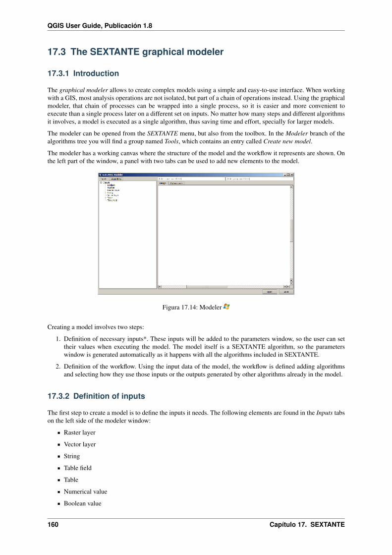
QGIS User Guide, Publicación 1.8
17.3 The SEXTANTE graphical modeler
17.3.1 Introduction
The graphical modeler allows to create complex models using a simple and easy-to-use interface. When workingwith a GIS, most analysis operations are not isolated, but part of a chain of operations instead. Using the graphicalmodeler, that chain of processes can be wrapped into a single process, so it is easier and more convenient toexecute than a single process later on a different set on inputs. No matter how many steps and different algorithmsit involves, a model is executed as a single algorithm, thus saving time and effort, specially for larger models.
The modeler can be opened from the SEXTANTE menu, but also from the toolbox. In the Modeler branch of thealgorithms tree you will find a group named Tools, which contains an entry called Create new model.
The modeler has a working canvas where the structure of the model and the workflow it represents are shown. Onthe left part of the window, a panel with two tabs can be used to add new elements to the model.
Figura 17.14: Modeler
Creating a model involves two steps:
1. Definition of necessary inputs*. These inputs will be added to the parameters window, so the user can settheir values when executing the model. The model itself is a SEXTANTE algorithm, so the parameterswindow is generated automatically as it happens with all the algorithms included in SEXTANTE.
2. Definition of the workflow. Using the input data of the model, the workflow is defined adding algorithmsand selecting how they use those inputs or the outputs generated by other algorithms already in the model.
17.3.2 Definition of inputs
The first step to create a model is to define the inputs it needs. The following elements are found in the Inputs tabson the left side of the modeler window:
Raster layer
Vector layer
String
Table field
Table
Numerical value
Boolean value
160 Capítulo 17. SEXTANTE

QGIS User Guide, Publicación 1.8
Double-clicking on any of them, a dialog is shown to define its characteristics. Depending on the parameter itself,the dialog will contain just one basic element (the description, which is what the user will see when executing themodel) or more of them. For instance, when adding a numerical value, as it can be seen in the next figure, apartfrom the description of the parameter you have to set a default value and a range of valid values.
Figura 17.15: Model Parameters
For each added input, a new element is added to the modeler canvas.
Figura 17.16: Model Parameters
17.3.3 Definition of the workflow
Once the inputs have been defined, it is time to define the algorithms to apply on them. Algorithms can be foundin the Algorithms tab, grouped much in the same way as they are in the toolbox.
Figura 17.17: Model Parameters
To add an algorithm, double-click on its name. An execution dialog will appear, with a content similar to theone found in the execution panel that SEXTANTE shows when executing the algorithm from the toolbox. the one
17.3. The SEXTANTE graphical modeler 161

QGIS User Guide, Publicación 1.8
shown next correspond to the SAGA ‘Convergence index’ algorithm, the same one we saw in the section dedicatedto the SEXTANTE toolbox.
Figura 17.18: Model Parameters
As you can see, some differences exist. Instead of the file output box that was used to set the filepath for outputlayers and tables, a simple text box is. If the layer generated by the algorithm is just a temporary result that willbe used as the input of another algorithm and should not be kept as a final result, just do not edit that textbox.Typing anything on it means that the result is a final one, and the text that you supply will be the description forthe output, which will be the one the user will see when executing the model.
Selecting the value of each parameter is also a bit different, since there are importante differences between thecontext of the modeler and the toolbox one. Let’s see how to introduce the values for each type of parameter.
Layers (raster and vector) and tables. They are selected from a list, but in this case the possible values arenot the layers or tables currently loaded in QGIS, but the list of model inputs of the corresponding type, orother layers or tables generated by algorithms already added to the model.
Numerical values. Literal values can be introduced directly on the textbox. But this textbox is also a list thatcan be used to select any of the numerical value inputs of the model. In this case, the parameter will takethe value introduced by the user when executing the model.
String. Like in the case of numerical values, literal strings can be typed, or an input string can be selected.
Table field. The fields of the parent table or layer cannot be known at design-time, since they depend of theselection of the user each time the model is executed. To set the value for this parameter, type the name ofa field directly in the textbox, or use the list to select a table field input already added to the model. Thevalidity of the selected field will be checked by SEXTANTE at run-time.
Once all the parameter have been assigned valid values, click on [OK] and the algorithm will be added to thecanvas. It will be linked to all the other elements in the canvas, whether algorithms or inputs, which provideobjects that are used as inputs for that algorithm.
Elements can be dragged to a different position within the canvas, to change the way the module structure isdisplayed and make it more clear and intuitive. Links between elements are update automatically.
You can run your algorithm anytime clicking on the [Run] button. However, in order to use it from the toolbox, ithas to be saved and the modeler dialog closed, to allow the toolbox to refresh its contents.
162 Capítulo 17. SEXTANTE

QGIS User Guide, Publicación 1.8
Figura 17.19: Model Parameters
17.3.4 Saving and loading models
Use the [Save] button to save the current model and the [Open] one to open any model previously saved. Modelare saved with the .model extension. If the model has been previously saved from the modeler window, you willnot be prompted for a filename, since there is already a file associated with that model, and it will be used.
Before saving a model, you have to enter a name and a group for it, using the text boxes in the upper part of thewindow.
Models saved on the models folder (the default folder when you are prompted for a filename to save the model)will appear in the toolbox in the corresponding branch. When the toolbox is invoked, SEXTANTE searches themodels folder for files with .model extension and loads the models they contain. Since a model is itself aSEXTANTE algorithm, it can be added to the toolbox just like any other algorithm.
The models folder can be set from the SEXTANTE configuration dialog, under the Modeler group.
Models loaded from the models folder appear not only in the toolbox, but also in the algorithms tree in theAlgorithms tab of the modeler window. That means that you can incorporate a model as a part of a bigger model,just as you add any other algorithm.
In some cases, SEXTANTE might not be able to load a model because it cannot find all the algorithms includedin its workflow. If you have used a given algorithm as part of your model, it should be available (that is, itshould appear on the toolbox) in order to load that model. Deactivating an algorithm provider in the SEXTANTEconfiguration window renders all the algorithms in that provider unusable by the modeler, which might causeproblems when loading models. Keep that in mind when you have trouble loading or executing models.
17.3.5 Editing a model
You can edit the model you are currently creating, redefining the workflow and the relationships between thealgorithms and inputs that define the model itself.
If you right-click on an algorithm in the canvas representing the model, you will see a context menu like the oneshown next:
Selecting the Remove option will cause the selected algorithm to be removed. An algorithm can be removed onlyif there are no other algorithms dependind on it. That is, if no output from the algorithm is used in a different oneas input. If you try to remove an algorithm that has others depending on it, SEXTANTE will show you a warningmessage like the one you can see below:
Selecting the Edit option or simply double-clicking on the algorithm icon will show the parameters dialog of thealgorithm, so you can change the inputs and parameter values. Not all input elements available in the model will
17.3. The SEXTANTE graphical modeler 163

QGIS User Guide, Publicación 1.8
Figura 17.20: Modeler Right Click
Figura 17.21: Cannot Delete ALG
appear in this case as available inputs. Layers or values generated at a more advanced step in the workflow definedby the model will not be available if they cause circular dependencies.
Select the new values and then click on the [OK] button as usual. The connections between the model elementswill change accordingly in the modeler canvas.
17.3.6 Activating and deactivating algorithms
Algorithms can be deactivated in the modeler, so they will not be executed once the model is run. This can be usedto test just a given part of the model, or when you do not need all the outputs it generates.
To deactivate an algorithm, right-click on its icon in the model canvas and select the Deactivate option. You willsee that the algorithm is represented now with a red label under its name indicating that is not active.
Figura 17.22: Deactivate
All algorithms depending (directly or undirectly) on that algorithm will also appear as inactive, since they cannotbe executed now.
To activate an algorithm, just right–click on its icon and select the Activate option.
17.3.7 Editing model help files and meta-information
You can document your models from SEXTANTE. Just click on the [Edit model help] button and a dialog likethe one shown next will appear.
On the right-hand side you will see a simple HTML page, created using the description of the input parametersand outputs of the algorithm, along with some additional items like a general description of the model or its author.The first time you open the help editor all those descriptions are empty, but you can edit them using the elementson the left-hand side of the dialog. Select an element on the upper part and the write its description in the texboxbelow.
164 Capítulo 17. SEXTANTE

QGIS User Guide, Publicación 1.8
Figura 17.23: Help Edition
Model help is saved in a file in the same folder as the model itself. You do not have to worry about saving it, sinceit is done automatically.
17.3.8 About available algorithms
You might notice that some algorithms that can be be executed from the toolbox do not appear in the list ofavailable ones when you are designing a model. To be included in a model, and algorithm must have a correctsemantic, so as to be properly linked to other in the workflow. If an algorithm does not have such well-definedsemantic (for instance, if the number of output layers cannot be know in advance), then it is not possible to use itwithin a model, and thus does not appear in the list of them that you can find in the modeler dialog.
Additionaly, you will see some algorithms in the modeler that are not found in the toolbox. This algorithms aremeant to be used exclusively as part of a model, and they are of no interest in a different context. The ‘Calculator’algorithm is an example of that. It is just a simple arithmetic calculator that you can use to modify numericalvalues (entered by the user or generated by some other algorithm). This tools is really useful within a model, butoutside of that context, it doesn’t make too much sense.
17.3.9 SEXTANTE models as Python code
This feature is temporarily unavailable
Along with the tab that contains the graphical design of the model, you will find another one containing a Pythonscript which performs the same task as the model itself. Using that code, you can create a console script (we willexplain them later in this same manual) and modify it to incorporate actions and methods not available in thegraphical modeler, such as loops or conditional sentences.
This feature is also a very practical way of learning how to use SEXTANTE from the console and how to createSEXTANTE algorithms using Python code, so you can use it as a learning tool when you start creating your ownSEXTANTE scripts.
You will find a button below the text field containing the Python code. Click on it to directly create a new scriptfrom that code, without having to copy and paste it in the SEXTANTE script editor.
17.4 The SEXTANTE batch processing interface
17.4.1 Introduction
SEXTANTE algorithms (including models) can be executed as a batch process. That is, they can be executed usingnot a single set of inputs, but several of them, executing the algorithm as many times as needed. This is useful
17.4. The SEXTANTE batch processing interface 165
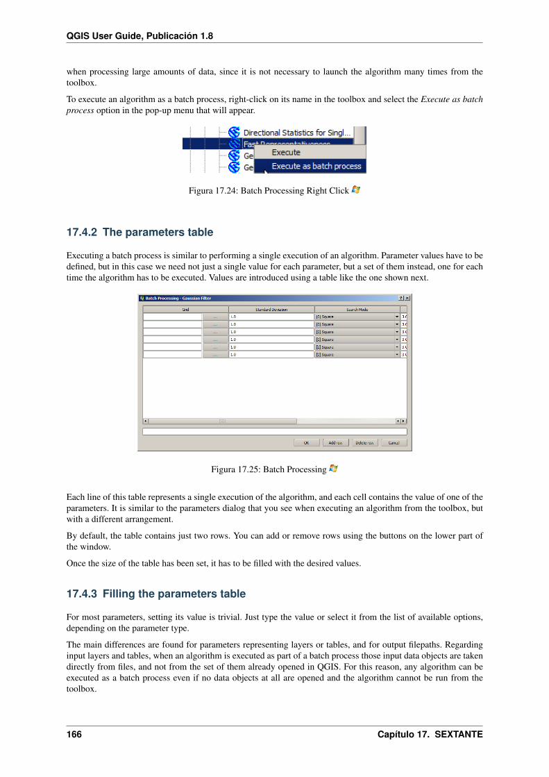
QGIS User Guide, Publicación 1.8
when processing large amounts of data, since it is not necessary to launch the algorithm many times from thetoolbox.
To execute an algorithm as a batch process, right-click on its name in the toolbox and select the Execute as batchprocess option in the pop-up menu that will appear.
Figura 17.24: Batch Processing Right Click
17.4.2 The parameters table
Executing a batch process is similar to performing a single execution of an algorithm. Parameter values have to bedefined, but in this case we need not just a single value for each parameter, but a set of them instead, one for eachtime the algorithm has to be executed. Values are introduced using a table like the one shown next.
Figura 17.25: Batch Processing
Each line of this table represents a single execution of the algorithm, and each cell contains the value of one of theparameters. It is similar to the parameters dialog that you see when executing an algorithm from the toolbox, butwith a different arrangement.
By default, the table contains just two rows. You can add or remove rows using the buttons on the lower part ofthe window.
Once the size of the table has been set, it has to be filled with the desired values.
17.4.3 Filling the parameters table
For most parameters, setting its value is trivial. Just type the value or select it from the list of available options,depending on the parameter type.
The main differences are found for parameters representing layers or tables, and for output filepaths. Regardinginput layers and tables, when an algorithm is executed as part of a batch process those input data objects are takendirectly from files, and not from the set of them already opened in QGIS. For this reason, any algorithm can beexecuted as a batch process even if no data objects at all are opened and the algorithm cannot be run from thetoolbox.
166 Capítulo 17. SEXTANTE

QGIS User Guide, Publicación 1.8
Filenames for input data objects are introduced directly typing or, more conveniently, clicking on the button on theright hand of the cell, which shows a typical file chooser dialog. Multiple files can be selected at once. If the inputparameter represents a single data object and several files are selected, each one of them will be put in a separaterow, adding new ones if needed. If it represents a multiple input, all the selected files will be added to a single cell,separated by semicolons (;).
Output data objects are always saved to a file and, unlike when executing an algorithm from the toolbox, saving toa temporary one is not permitted. You can type the name directly or use the file chooser dialog that appears whenclicking on the accompanying button.
Once you select the file, a new dialog is shown to allow for autocompletion of other cells in the same column(same parameter).
Figura 17.26: Batch Processing Save
If the default value (‘Do not autocomplete’) is selected, SEXTANTE will just put the selected filename in theselected cell from the parameters table. If any of the other options is selected, all the cells below the selected onewill be automatically filled based on a defined criteria. This way, it is much easier to fill the table, and the batchprocess can be defined with less effort.
Automatic filling can be done simply adding correlative numbers to the selected filepath, or appending the valueof another field at the same row. This is particularly useful for naming output data object according to input ones.
Figura 17.27: Batch Processing File Path
17.4.4 Executing the batch process
To execute the batch process once you have introduced all the necessary values, just click on [OK]. SEXTANTEwill show the progress of the global batch process in the progress bar in the lower part of the dialog.
17.5 Using SEXTANTE from the console
17.5.1 Introduction
The console allows advanced users to increase their productivity and perform complex operations that cannot beperformed using any of the other elements of the SEXTANTE GUI. Models involving several algorithms can be
17.5. Using SEXTANTE from the console 167

QGIS User Guide, Publicación 1.8
defined using the command-line interface, and additional operations such as loops and conditional sentences canbe added to create more flexible and powerful workflows.
There is not a SEXTANTE console in QGIS, but all SEXTANTE commands are available instead from QGISbuilt-in Python console. That means that you can incorporate those command to your console work and connectSEXTANTE algorithms to all the other features (including methods from the QGIS API) available from there.
The code that you can execute from the Python console, even if it does call any SEXTANTE method, can beconverted into a new SEXTANTE algorithm that you can later call from the toolbox, the graphical modeler or anyother SEXTANTE component, just like you do with any other SEXTANTE algorithm. In fact, some algorithmsthat you can find in the toolbox, like all the ones in the mmqgis group, are simple scripts.
In this chapter we will see how to use SEXTANTE from the QGIS Python console, and also how to write yourown algorithms using Python.
17.5.2 Calling SEXTANTE from the Python console
The first thing you have to do is to import the SEXTANTE functions with the following line:
>>> import sextante
Now, there is basically just one (interesting) thing you can do with SEXTANTE from the console: to execute analgorithm. That is done using the runalg() method, which takes the name of the algorithm to execute as its firstparameter, and then a variable number of additional parameter depending on the requirements of the algorithm.So the first thing you need to know is the name of the algorithm to execute. That is not the name you see in thetoolbox, but rather a unique command–line name. To find the right name for your algorithm, you can use thealgslist() method. Type the following line in you console:
>>> sextante.alglist()
You will see something like this.
Accumulated Cost (Anisotropic)---------------->saga:accumulatedcost(anisotropic)Accumulated Cost (Isotropic)------------------>saga:accumulatedcost(isotropic)Add Coordinates to points--------------------->saga:addcoordinatestopointsAdd Grid Values to Points--------------------->saga:addgridvaluestopointsAdd Grid Values to Shapes--------------------->saga:addgridvaluestoshapesAdd Polygon Attributes to Points-------------->saga:addpolygonattributestopointsAggregate------------------------------------->saga:aggregateAggregate Point Observations------------------>saga:aggregatepointobservationsAggregation Index----------------------------->saga:aggregationindexAnalytical Hierarchy Process------------------>saga:analyticalhierarchyprocessAnalytical Hillshading------------------------>saga:analyticalhillshadingAverage With Mask 1--------------------------->saga:averagewithmask1Average With Mask 2--------------------------->saga:averagewithmask2Average With Thereshold 1--------------------->saga:averagewiththereshold1Average With Thereshold 2--------------------->saga:averagewiththereshold2Average With Thereshold 3--------------------->saga:averagewiththereshold3B-Spline Approximation------------------------>saga:b-splineapproximation...
That’s a list of all the available algorithms, alphabetically ordered, along with their corresponding command-linenames.
You can use a string as a parameter for this method. Instead of returning the full list of algorithm, it will onlydisplay those that include that string. If, for instance, you are looking for an algorithm to calculate slope from aDEM, type alglist("slope") to get the following result:
DTM Filter (slope-based)---------------------->saga:dtmfilter(slope-based)Downslope Distance Gradient------------------->saga:downslopedistancegradientRelative Heights and Slope Positions---------->saga:relativeheightsandslopepositionsSlope Length---------------------------------->saga:slopelengthSlope, Aspect, Curvature---------------------->saga:slopeaspectcurvature
168 Capítulo 17. SEXTANTE

QGIS User Guide, Publicación 1.8
Upslope Area---------------------------------->saga:upslopeareaVegetation Index[slope based]----------------->saga:vegetationindex[slopebased]
This result might change depending on the algorithms you have available.
It is easier now to find the algorithm you are looking for and its command-line name, in this casesaga:slopeaspectcurvature.
Once you know the command-line name of the algorithm, the next thing to do is to know the right syntax toexecute it. That means knowing which parameters are needed and the order in which they have to be passed whencalling the runalg() method. SEXTANTE has a method to describe an algorithm in detail, which can be usedto get a list of the parameters that an algorithms require and the outputs that it will generate. To do it, you can usethe alghelp(name_of_the_algorithm) method. Use the command-line name of the algorithm, not thefull descriptive name.
Calling the method with saga:slopeaspectcurvature as parameter, you get the following description.
>>> sextante.alghelp("saga:slopeaspectcurvature")ALGORITHM: Slope, Aspect, Curvature
ELEVATION <ParameterRaster>METHOD <ParameterSelection>SLOPE <OutputRaster>ASPECT <OutputRaster>CURV <OutputRaster>HCURV <OutputRaster>VCURV <OutputRaster>
Now you have everything you need to run any algorithm. As we have already mentioned, there is only one singlecommand to execute algorithms: runalg(). Its syntax is as follows:
>>> sextante.runalg{name_of_the_algorithm, param1, param2, ..., paramN,Output1, Output2, ..., OutputN)
The list of parameters and outputs to add depends on the algorithm you want to run, and is exactly the list that thealghelp() method gives you, in the same order as shown.
Depending on the type of parameter, values are introduced differently. The next one is a quick review of how tointroduce values for each type of input parameter
Raster Layer, Vector Layer or Table. Simply use a string with the name that identifies the data object to use(the name it has in the QGIS Table of Contents) or a filename (if the corresponding layer is not opened, itwill be opened, but not added to the map canvas). If you have an instance of a QGIS object representing thelayer, you can also pass it as parameter. If the input is optional and you do not want to use any data object,use None.
Selection. If an algorithm has a selection parameter, the value of that parameter should be entered usingan integer value. To know the available options, you can use the algoptions command, as shown in thefollowing example:
>>> sextante.algoptions("saga:slopeaspectcurvature")METHOD(Method)
0 - [0] Maximum Slope (Travis et al. 1975)1 - [1] Maximum Triangle Slope (Tarboton 1997)2 - [2] Least Squares Fitted Plane (Horn 1981, Costa-Cabral & Burgess 1996)3 - [3] Fit 2.Degree Polynom (Bauer, Rohdenburg, Bork 1985)4 - [4] Fit 2.Degree Polynom (Heerdegen & Beran 1982)5 - [5] Fit 2.Degree Polynom (Zevenbergen & Thorne 1987)6 - [6] Fit 3.Degree Polynom (Haralick 1983)
In this case, the algorithm has one of such such parameters, with 7 options. Notice that ordering is zero-based.
Multiple input. The value is a string with input descriptors separated by semicolons. As in the case of singlelayers or tables, each input descriptor can be the data object name, or its filepath.
17.5. Using SEXTANTE from the console 169

QGIS User Guide, Publicación 1.8
Table Field from XXX. Use a string with the name of the field to use. This parameter is case-sensitive.
Fixed Table. Type the list of all table values separated by commas and enclosed between quotes. Values starton the upper row and go from left to right. You can also use a 2D array of value representing the table.
CRS. Enter the EPSG code number of the desired CRS.
Extent. You must use a string with xmin, xmax, ymin and ymax values separated by commas.
Boolean, file, string and numerical parameters do not need any additional explanations.
Input parameters such as strings booleans or numerical values have default values. To use them, use None in thecorresponding parameter entry.
For output data objects, type the filepath to be used to save it, just as it is done from the toolbox. If you want tosave the result to a temporary file, use None. The extension of the file determines the file format. If you enter afile extension not included in the ones supported by the algorithm, the default file format for that output type willbe used, and its corresponding extension appended to the given filepath.
Unlike when an algorithm is executed from the toolbox, outputs are not added to the map canvas if you executethat same algorithm from the Python console. If you want to add an output to it, you have to do it yourself afterrunning the algorithm. To do so, you can use QGIS API commands, or, even easier, use one of the handy methodsprovided by SEXTANTE for such task.
The runalg() method returns a dictionary with the output names (the ones shown in the algorithm description)as keys and the filepaths of those outputs as values. To add all the outputs generated by an algorithm, pass thatdictionary to the loadFromAlg() method. You can also load an individual layer passing its filepath to theload() method.
17.5.3 Creating scripts and running them from the toolbox
You can create your own algorithms by writing the corresponding Python code and adding a few extra lines tosupply additional information needed by SEXTANTE. You can find a Create new script under the tools group inthe script algorithms block of the toolbox. Double click on it to open the script edition dialog. That’s where youshould type your code. Saving the script from there in the scripts folder (the default one when you open thesave file dialog), with .py extension, will automatically create the corresponding algorithm.
The name of the algorithm (the one you will see in the toolbox) is created from the filename, removing its extensionand replacing low hyphens with blank spaces.
Let’s have the following code, which calculates the Topographic Wetness Index (TWI) directly from a DEM
##dem=raster##twi=outputret_slope = sextante.runalg("saga:slopeaspectcurvature", dem, 0, None,
None, None, None, None)ret_area = sextante.runalg("saga:catchmentarea(mass-fluxmethod)", dem,
0, False, False, False, False, None, None, None, None, None)sextante.runalg("saga:topographicwetnessindex(twi), ret_slope[’SLOPE’],
ret_area[’AREA’], None, 1, 0, twi)
As you can see, it involves 3 algorithms, all of them coming from SAGA. The last one of them calculates de TWI,but it needs a slope layer and a flow accumulation layer. We do not have these ones, but since we have the DEM,we can calculate them calling the corresponding SAGA algorithms.
The part of the code where this processing takes place is not difficult to understand if you have read the previoussections in this chapter. The first lines, however, need some additional explanation. They provide SEXTANTEthe information it needs to turn your code into an algorithm that can be run from any of its components, like thetoolbox or the graphical modeler.
These lines start with a double Python comment symbol and have the following structure:
[parameter_name]=[parameter_type] [optional_values]
Here is a list of all the parameter types that SEXTANTE supports in its scripts, their syntax and some examples.
170 Capítulo 17. SEXTANTE

QGIS User Guide, Publicación 1.8
raster. A raster layer
vector. A vector layer
table. A table
number. A numerical value. A default value must be provided. For instance, depth=number 2.4
string. A text string. As in the case of numerical values, a default value must be added. For instance,name=string Victor
boolean. A boolean value. Add True or False after it to set the default value. For example,verbose=boolean True
multiple raster. A set of input raster layers.
multiple vector. A set of input vector layers.
field. A field in the attributes table of a vector layer. The name of the layer has to be added after thefield tag. For instance, if you have declared a vector input with mylayer=vector, you could usemyfield=field mylayer to add a field from that layer as parameter.
folder. A folder
file. A filename
The parameter name is the name that will be shown to the user when executing the algorithm, and also the variablename to use in the script code. The value entered by the user for that parameter will be assigned to a variable withthat name.
When showing the name of the parameter to the user, SEXTANTE will edit it to improve its appearance, replacinglow hyphens with blankspaces. So, for instance, if you want the user to see a parameter named A numericalvalue, you can use the variable name A_numerical_value.
Layers and tables values are strings containing the filepath of the corresponding object. To turn them into a QGISobject, you can use the sextante.getObjectFromUri() function. Multiple inputs also have a string value,which contains the filepaths to all selected object, separated by semicolons.
Outputs are defined in a similar manner, using the following tags:
output raster
output vector
output table
output html
output file
output number
output string
The value assigned to the output variables is always a string with a filepath. It will correspond to a temporaryfilepath in case the use has not entered any output filename.
When you declare an output, SEXTANTE will try to add it to QGIS once the algorithm is finished. That is thereason why, although the runalg() method does not load the layers it produces, the final TWI layer will beloaded, since it is saved to the file entered by the user, which is the value of the corresponding output.
Do not use the load() method in your script algorithms, but just when working with the console line. If a layeris created as output of an algorithm, it should be declared as such. Otherwise, you will not be able to properly usethe algorithm in the modeler, since its syntax (as defined by the tags explained above) will not match what thealgorithm really creates.
Hidden outputs (numbers and strings) do not have a value. Instead, it is you who has to assign a value to them. Todo so, just set the value of a variable with the name you used to declare that output. For instance, if you have usedthis declaration,
17.5. Using SEXTANTE from the console 171

QGIS User Guide, Publicación 1.8
##average=output number
the following line will set the value of the output to 5:
average = 5
In addition to the tags for parameters and outputs, you can also define the group under which the algorithm willbe shown, using the group tag.
If you algorithm takes a long time to process, it is a good idea to inform the user. You have a global namedprogress available, with two available methods: setText(text) and setPercentage(percent) tomodify the progress text and the progress bar.
Several examples are provided with SEXTANTE. Please, check them to see real examples of how to create algo-rithms using this feature of SEXTANTE. You can right-click on any script algorithm and select Edit script to editits code or just to see it.
17.5.4 Documenting your scripts
As in the case of models, you can create additional documentation for your script, to explain what they do andhow to use them. In the script editing dialog you will find a [Edit script help] button. Click on it and it will takeyou to the help editing dialog. Check the chapter about the graphical modeler to know more about this dialog andhow to use it.
Help files are saved in the same folder as the script itself, adding the .help extension to the filename. Notice thatyou can edit your script’s help before saving it for the first time. If you later close the script editing dialog withoutsaving the script (i.e. you discard it), the help content you wrote will be lost. If your script was already saved andis associated to a filename, saving is done automatically.
17.6 The SEXTANTE history manager
17.6.1 The SEXTANTE history
Every time you execute a SEXTANTE algorithm, information about the process is stored in the SEXTANTEhistory manager. Along with the parameters used, the date and time of the execution are also saved.
This way, it is easy to track the and control all the work that has been developed using SEXTANTE, and easilyreproduce it.
The SEXTANTE history manager is a set of registry entries grouped according to their date of execution, makingit easier to find information about an algorithm executed at any particular moment.
Figura 17.28: History
172 Capítulo 17. SEXTANTE

QGIS User Guide, Publicación 1.8
Process information is kept as a command-line expression, even if the algorithm was launched from the toolbox.This makes it also useful for those learning how to use the command-line interface, since they can call an algorithmusing the toolbox and then check the history manager to see how that same algorithm could be called from thecommand line.
Apart from browsing the entries in the registry, processes can be re-executed, simply double-clicking on thecorresponding entry.
Along with algorithm executions, SEXTANTE communicates with the user using the other groups of the registry,namely Errors, Warnings and Information. In case something is not working properly, having a look at the Errorsmight help you to see what is happening. If you get in contact with a SEXTANTE developer to report a bug orerror, the information in that group will be very useful for him to find out what is going wrong.
When executing third party algorithms, this is usually done calling their command-line interfaces, which com-municate with the user using the console. Although that console is not shown, a full dump of it is stored in theInformation group each time you run one of those algorithms. If, for instance, you are having problems executinga SAGA algorithm, look for an entry name ‘SAGA execution console output’ to check all the messages generatedby SAGA and try to find out where the problem is.
Some algorithms, even if they can produce a result with the given input data, might add comments or additionalinformation to Warning in case they detect potential problems from that data, in order to warn you about them.Make sure you check those messages in case you are having unexpected results.
17.7 Configuring external applications
17.7.1 Introduction
SEXTANTE can be extended using additional applications, calling them from within SEXTANTE. Currently,SAGA, GRASS, OTB(Orfeo Toolbox) and R are supported, along with some other command-line applicationsthat provide spatial data analysis functionalities. Algorithms relying on an external application are managed bytheir own algorithm provider.
This chapter will show you how to configure SEXTANTE to include these additional applications, and will explainsome particular features of the algorithm based on them. Once you have correctly configured the system, you willbe able to execute external algorithms from any SEXTANTE component like the toolbox or the graphical modeler,just like you do with any other SEXTANTE geoalgorithm.
By default, all algorithms that rely on an external appplication not shipped with QGIS are not enabled. You canenable them in the SEXTANTE configuration dialog. Make sure that the corresponding application is alreadyinstalled in your system. Enabling an algorithm provider without installing the application it needs will cause thealgorithms to appear in the toolbox, but an error will be thrown when you try to execute them.
This is because the algorithm descriptions (needed to create the parameters dialog and give SEXTANTE theinformation it needs about the algorithm) are not included with each appllication, but with SEXTANTE instead.That is,they are part of SEXTANTE, so you have them in your installation even if you have not installed any othersoftware. Running the algorithm, however, needs the application binaries to be installed in your system.
A note on file formats
When using an external software, opening a file in QGIS does not mean that it can be opened and processed as wellon that other software. In most cases, it can read what you have opened in QGIS, but in some cases, that might notbe the case. When using databases or uncommon file formats, whether for raster of vector layers, problems mightarise. If that happens, try to use well known file formats that you are sure that are understood by both programs,and check to console output (in the history and log dialog) for knowing more about what is going wrong.
Using GRASS raster layers is, for instance, one case in which you might have trouble and not be able to completeyour work if you call an external algorithm using such a layer as input. For this reason, these layers will not appearas available to SEXTANTE algorithms (we are currently working on solving this, and expect to have it readysoon).
17.7. Configuring external applications 173

QGIS User Guide, Publicación 1.8
You should, however, find no problems at all with vector layers, since SEXTANTE automatically converts fromthe original file format to one accepted by the external application before passing the layer to it. This adds an extraprocessing time, which might be significant if the layer has a large size, so do not be surprised if it takes more toprocess a layer from a DB connection that one of a similar size stored in a shapefile.
Providers not using external applications can process any layer that you can open in QGIS, since they open it foranalysis trough QGIS.
Regarding output formats, raster layers can be saved as TIFF (.tif) files, while vector layers are saved as shape-files (.shp). These have been chosen as the ‘lingua franca’ between supported third party applications and QGIS.If the output filename that you select is not one of the above, it will be modified, adding the corresponding suffix,and the default file format will be used.
In the case of GDAL, the number of supported output formats is larger. When you open the file selection dialog,you will see that you have more formats (and their corresponding extensions available). For more informationabout which formats are supported, check the GDAL documentation.
A note on vector layer selections
By default, when an external algorithm takes a vector layer, it will use all its features, even if a selection existin QGIS. You can make an external algorithm aware of that selection by checking the Use selected features inexternal applications item in the General settings group. When you do so, each time you execute an externalalgorithm that uses a vector layer, the selected features of that layer will be exported to a new layer, and thealgorithm will work with that new layer instead.
Notice that if you select this option, a layer with no selection will behave like a layer with all its features selected,not like an empty layer.
17.7.2 SAGA
SAGA algorithms can be run from SEXTANTE if you have SAGA installed in your system and you configureSEXTANTE properly so it can find SAGA executables. In particular, the SAGA command-line executable isneeded to run SAGA algorithms. SAGA binaries are not included with SEXTANTE, so you have to download andinstall the software yourself. Please check the SAGA website at for more information. SAGA 2.0.8 is needed.
Once SAGA is installed, and if you are running Windows, open the SEXTANTE configuration dialog. In the SAGAblock you will find a setting named SAGA Folder. Enter the path to the folder where SAGA is installed. Close theconfiguration dialog and now you are ready to run SAGA algorithms from SEXTANTE.
In case you are using Linux, there is no need to configure that, and you will not see those folders. Instead, youmust make sure that SAGA is properly installed and its folder is added to the PATH environment variable. Justopen a console and type saga_cmd to check that the system can found where SAGA binaries are located.
About SAGA grid system limitations
Most of SAGA algorithms that require several input raster layers, require them to have the same grid system. Thatis, to cover the same geographic area and have the same cellsize, so their corresponding grids match. When callingSAGA algorithms from SEXTANTE, you can use any layer, regardless of its cellsize and extent. When multipleraster layers are used as input for a SAGA algorithm, SEXTANTE resamples them to a common grid system andthen passes them to SAGA (unless the SAGA algorithm can operate with layers from different grid systems).
The definition of that common grid system is controlled by the user, and you will find several parameters in theSAGA group of the setting window to do so. There are two ways of setting the target grid system:
Setting it manually. You define the extent setting the values of the following parameters:
• Resampling min X
• Resampling max X
• Resampling min Y
174 Capítulo 17. SEXTANTE

QGIS User Guide, Publicación 1.8
• Resampling max Y
• Resampling cellsize
Notice that SEXTANTE will resample input layers to that extent, even if they do not overlap with it.
Setting it automatically from input layers. To select this option, just check the Use min covering grid systemfor resampling option. All the other settings will be ignored and the minimum extent that covers all the inputlayers will be used. The cellsize of the target layer is the maximum of all cellsizes of the input layers.
For algorithms that do not use multiple raster layers, or for those that do not need a unique input grid system, noresampling is performed before calling SAGA, and those parameters are not used.
Limitations for multi-band layers
Unlike QGIS, SAGA has no support for multiband layers. If you want to use a multiband layer (such asan RGB or multispectral image), you first have to split it into singlebanded images. To do so, you can usethe ‘SAGA/Grid - Tools/Split RGB image’ algorithm (which creates 3 images from an RGB image) or the‘SAGA/Grid - Tools/Extract band’ algorithm (to extract a single band).
Limitations in cellsize
SAGA assumes that raster layers have the same cellsize in the X and Y axis. If you are working with a layer withdifferent values for its horizontal and vertical cellsizes, you might get unexcepted results. In this case, a warningwill be added to the SEXTANTE log, indicating that an input layer might not be suitable to be processed bySAGA.
Logging
When SEXTANTE calls SAGA, it does it using its command-line interface, thus passing a set of commands toperform all the required operation. SAGA show its progress by writing information to the console, which includesthe percentage of processing already done, along with additional content. This output is filtered by SEXTANTEand used to update the progress bar while the algorithm is running.
Both the commands sent by SEXTANTE and the additional information printed by SAGA can be logged alongwith other SEXTANTE log messages, and you might find them useful to track in detailed what is going on whenSEXTANTE runs a SAGA algorithm. You will find two settings, namely Log console output and Log executioncommands to activate that logging mechanism.
Most other providers that use an external application and call it through the command-line have similar options,so you will find them as well in other places in the SEXTANTE settings list.
17.7.3 R and R scripts
R integration in SEXTANTE is different from that of SAGA in that there is not a predefined set of algorithms youcan run (except for a few examples). Instead, you should write your scripts and call R commands, much like youwould do from R, and in a very similar manner to what we saw in the chapter dedicated to SEXTANTE scripts.This chapter shows you the syntax to use to call those R commands from SEXTANTE and how to use SEXTANTEobjects (layers, tables) in them.
The first thing you have to do, as we saw in the case of SAGA, is to tell SEXTANTE where you R binaries arelocated. You can do so using the R folder entry in the SEXTANTE configuration dialog. Once you have set thatparameter, you can start creating your own R scripts and executing them.
Once again, this is different in Linux, and you just have to make sure that the R folder is included in the PATHenvironment variable. If you can start R just typing R in a console, then you are ready to go.
To add a new algorithm that calls an R function (or a more complex R script that you have developed and youwould like to have available from SEXTANTE), you have to create a script file that tells SEXTANTE how toperform that operation and the corresponding R commands to do so.
17.7. Configuring external applications 175

QGIS User Guide, Publicación 1.8
Script files have the extension .rsx and creating them is pretty easy if you just have a basic knowledge of Rsyntax and R scripting. They should be stored in the R scripts folder. You can set this folder in the R settings group(available from the SEXTANTE settings dialog), just like you do with the folder for regular SEXTANTE scripts.
Let’s have a look at a very simple file script file, which calls the R method spsample to create a random gridwithin the boundary of the polygons in a given polygon layer. This method belong to the maptools package.Since almost all the algorithms that you might like to incorporate into SEXTANTE will use or generate spatialdata, knowledge of spatial packages like maptools and, specially, sp, is mandatory.
##polyg=vector##numpoints=number 10##output=output vector##sp=grouppts=spsample(polyg,numpoints,type="random")output=SpatialPointsDataFrame(pts, as.data.frame(pts))
The first lines, which start with a double Python comment sign (##), tell SEXTANTE the inputs of the algorithmdescribed in the file and the outputs that it will generate. They work exactly with the same syntax as the SEX-TANTE scripts that we have already seen, so they will not be described here again. Check the correspondingsection for more information.
When you declare an input parameter, SEXTANTE uses that information for two things: creating the user interfaceto ask the user for the value of that parameter and creating a corresponding R variable that can be later used asinput for R commands.
In the above example, we are declaring an input of type vector named polyg. When executing the algorithm,SEXTANTE will open in R the layer selected by the user and store it in a variable also named polyg. So thename of a parameter is also the name of the variable that we can use in R for accesing the value of that parameter(thus, you should avoid using reserved R words as parameter names).
Spatial elements such as vector and raster layers are read using the readOGR() and readGDAL() commands(you do not have to worry about adding those commands to your description file, SEXTANTE will do it) andstored as Spatial*DataFrame objects. Table fields are stored as strings containing the name of the selectedfield.
Tables are opened using the read.csv() command. If a table entered by the user is not in CSV format, it willbe converted prior to importing it in R.
Knowing that, we can now understand the first line of our example script (the first line not starting with a Pythoncomment).
pts=spsample(polyg,numpoints,type="random")
The variable polygon already contains a SpatialPolygonsDataFrame object, so it can be used to call thespsample method, just like the numpoints one, which indicates the number of points to add to the createdsample grid.
Since we have declared an output of type vector named out, we have to create a variable named out and store aSpatial*DataFrame object in it (in this case, a SpatialPointsDataFrame). You can use any name foryour intermediate variables. Just make sure that the variable storing your final result has the same name that youused to declare it, and contains a suitable value.
In this case, the result obtained from the spsample method has to be converted explicitly into aSpatialPointsDataFrame object, since it is itself an object of class ppp, which is not a suitable classto be retuned to SEXTANTE.
If you algorithm does not generate any layer, but a text result in the console instead, you have to tell SEXTANTEthat you want the console to be shown once the execution is finished. To do so, just start the command lines thatproduce the results you want to print with the > (‘greater’) sign. The output of all other lines will not be shown.For instance, here is the description file of an algorithms that performs a normality test on a given field (column)of the attributes of a vector layer:
##layer=vector##field=field layer##nortest=group
176 Capítulo 17. SEXTANTE

QGIS User Guide, Publicación 1.8
library(nortest)>lillie.test(layer[[field]])
The output ot the last line is printed, but the output of the first is not (and neither are the outputs from othercommand lines added automatically by SEXTANTE).
If your algorithm creates any kind of graphics (using the plot() method), add the following line:
##showplots
This will cause SEXTANTE to redirect all R graphical outputs to a temporary file, which will be later opened onceR execution has finished.
Both graphics and console results will be shown in the SEXTANTE results manager.
For more information, please check the script files provided with SEXTANTE. Most of them are rather simple andwill greatly help you understand how to create your own ones.
17.7.4 GRASS
Configuring GRASS is not much different from configuring SAGA. First, the path to the GRASS folder has to bedefined, but only if you are running Windows. Additionaly, a shell interpreter (usually msys.exe, which can befound in most GRASS for Windows distributions) has to be defined and its path set up as well.
By default, SEXTANTE tries to configure its GRASS connector to use the GRASS distribution that ships alongwith QGIS. This should work without problems in most systems, but if you experience problems, you might haveto do it manually. Also, if you want to use a different GRASS version, you can change that setting and point to thefolder where that other version is kept. GRASS 6.4 is needed for algorithms to work correctly.
If you are running Linux, you just have to make sure that GRASS is correctly installed, and that it can be runwithout problem from a console.
GRASS algorithms use a region for calculations. This region can be defined manually using values similar to theones found in the SAGA configuration, or automatically, taking the minimum extent that covers all the input layersused to execute the algorithm each time. If this is the behaviour you prefer, just check the Use min covering regionoption in the GRASS configuration parameters.
GRASS includes help files describing each algorithm. If you set the GRASS help folder parameter, SEXTANTEwill open them when you use the [Show help] button from the parameters window of the algorithm.
The last parameter that has to be configured is related to the mapset. A mapset is needed to run GRASS, andSEXTANTE creates a temporary one for each execution. You have to tell SEXTANTE if the data you are workingwith uses geographical (lat/lon) coordinates or projected ones.
17.7.5 GDAL
No additional configuration is needed to run GDAL algorithms, since it is already incorporated to QGIS andSEXTANTE can infere its configuration from it.
17.7.6 Orfeo ToolBox
Orfeo ToolBox (OTB) algorithms can be run from SEXTANTE if you have OTB installed in your system andconfigured SEXTANTE properly so it can find all necessary files (command-line tools and libraries). Please notethat OTB binaries are not included in SEXTANTE, so you have to download and install the software yourself.Please check the OTB website for more information.
Once OTB is installed, start QGIS, open the SEXTANTE configuration dialog and configure OTB algorithmprovider. In the Orfeo Toolbox (image analysis) block you will find all settings related to OTB. First ensure thatalgorithms are enabled.
Then configure path to the folder where OTB command-line tools and libraries are installed:
17.7. Configuring external applications 177

QGIS User Guide, Publicación 1.8
usually OTB applications folder point to /usr/lib/otb/applications and OTB command linetools folder is /usr/bin
if you use OSGeo4W installer, than install otb-bin package and enterC:\OSGeo4W\apps\orfeotoolbox\applications as OTB applications folder andC:\OSGeo4W\bin as OTB command line tools folder
17.7.7 TauDEM
To use this provider you need to install TauDEM command line tools.
Windows
Please visit TauDEM homepage for installation instructions and precompiled binaries for 32bit and 64bit systems.IMPORTANT: you need TauDEM 5.0.6 executables, version 5.2 currently not supported.
Linux
There are no packages for most Linux distribution, so you should compile TauDEM by yourself. As TauDEM usesMPICH2, first install it using your favorite package manager. Also TauDEM works fine with OpenMPI, so youcan use it instead of MPICH2.
Download TauDEM 5.0.6 source code and extract files in some folder.
Open linearpart.h file and add after line
#include "mpi.h"
add new line with
#include <stdint.h>
so you’ll get
#include "mpi.h"#include <stdlib.h>
Save changes and close file. Now open tiffIO.h, find line #include "stdint.h" and replace quotes ("")with <>, so you’ll get
#include <stdint.h>
Save changes and close file. Create build directory and cd into it
mkdir buildcd build
Configure your build with command
CXX=mpicxx cmake -DCMAKE_INSTALL_PREFIX=/usr/local ..
and then compile
make
Finaly, to install TauDEM into /usr/local/bin, run
sudo make install
178 Capítulo 17. SEXTANTE

CAPÍTULO 18
Print Composer
The print composer provides growing layout and printing capabilities. It allows you to add elements such as theQGIS map canvas, legend, scalebar, images, basic shapes, arrows and text labels. You can size, group, align andposition each element and adjust the properties to create your layout. The layout can be printed or exported toimage formats, Postscript, PDF or to SVG (export to SVG is not working properly with some recent Qt4 versions.You should try and check individual on your system). You can save the layout as template and load it again inanother session. See a list of tools in table_composer_1:
Icon Purpose Icon Purpose
Load from template Save as template
Export to an image format Export as PDF
Export print composition to SVG Print or export as Postscript
Zoom to full extent Zoom in
Zoom out Refresh view
Revert last change Restore last change
Add new map from QGIS map canvas Add image to print composition
Add label to print composition Add new legend to print composition
Add new scalebar to print composition Add basic shape to print composition
Add arrow to print composition Add attribute table to print composition
Select/Move item in print composition Move content within an item
Group items of print composition Ungroup items of print composition
Raise selected items Lower selected items
Move selected items to top Move selected items to bottom
Align selected items left Align selected items right
Align selected items center Align selected items center vertical
Align selected items top Align selected items bottom
Table Composer 1: Print Composer Tools
All Print Composer tools are available in menus and as icons in a toolbar. The toolbar can be switched off and onusing the right mouse button holding the mouse over the toolbar.
179

QGIS User Guide, Publicación 1.8
18.1 Open a new Print Composer Template
Before you start to work with the print composer, you need to load some raster and vector layers in the QGIS mapcanvas and adapt their properties to suite your own convenience. After everything is rendered and symbolized to
your liking you click the New Print Composer icon in the toolbar or choose File → New Print Composer.
18.2 Using Print Composer
Opening the print composer provides you with a blank canvas to which you can add the current QGIS map canvas,legend, scalebar, images, basic shapes, arrows and text. Figure_composer_1 shows the initial view of the print
composer with an activated Snap to grid mode but before any elements are added.
Figura 18.1: Print Composer
The print composer provides three tabs:
The Composition tab allows you to set paper size, orientation, the print quality for the output file in dpi and
to activate snapping to a grid of a defined resolution. Please note, the Snap to grid feature only works,
if you define a grid resolution > 0. Furthermore you can also activate the Print as raster checkbox. Thismeans all elements will be rastered before printing or saving as Postscript of PDF.
The Item Properties tab displays the properties for the selected map element. Click the Select/Move item
icon to select an element (e.g. legend, scalebar or label) on the canvas. Then click the Item Properties taband customize the settings for the selected element.
The Command history tab displays a history of all changes applied to the print composer layout. With amouse click it is possible to undo and redo layout steps back and forth to a certain status.
You can add multiple elements to the composer. It is also possible to have more than one map view or legend orscalebar in the print composer canvas. Each element has its own properties and in the case of the map, its ownextent. If you want to remove any elements from the composer canvas you can do that with the Delete or theBackspace key.
180 Capítulo 18. Print Composer

QGIS User Guide, Publicación 1.8
18.3 Adding a current QGIS map canvas to the Print Composer
Click on the Add new map toolbar button in the print composer toolbar, to add the QGIS map canvas. Now drag arectangle on the composer canvas with the left mouse button to add the map. To display the current map, you canchoose between three different modes in the map Item Properties tab:
Rectangle is the default setting. It only displays an empty box with a message ‘Map will be printed here’.
Cache renders the map in the current screen resolution. If case you zoom in or out the composer window,the map is not rendered again but the image will be scaled.
Render means, that if you zoom in or out the composer window, the map will be rendered again, but forspace reasons, only up to a maximum resolution.
Cache is default preview mode for newly added print composer maps.
You can resize the map element by clicking on the Select/Move item button, selecting the element, and draggingone of the blue handles in the corner of the map. With the map selected, you can now adapt more properties in themap Item Properties tab.
To move layers within the map element select the map element, click the Move item content icon and move thelayers within the map element frame with the left mouse button. After you found the right place for an element,you can lock the element position within the print composer canvas. Select the map element and click on the right
mouse button to Lock the element position and again to unlock the element. You can lock the map element also
activating the Lock layers for map item checkbox in the Map dialog of the Item Properties tab.
Nota: QGIS is now able to show labels from the new labeling plugin also in the map composer, but it is not yetscaled correctly. So it might be necessary to switch back to the standard labeling in some cases.
18.3.1 Map item properties tab — Map and Extents dialog
Map dialog
The Map dialog of the map Item Properies tab provides following functionalities (see figure_composer_2):
Figura 18.2: Map Dialog
The Preview area allows to define the preview modes ‘Rectangle’, ‘Cache’ and ‘Render’, as describedabove. Click on the [Update preview] button to apply changes to the map view.
The Map area allows to resize the map element specifying the width and height or the scale. The field
Rotation allows to rotate the map element content clockwise in degrees. Note, a coordinate frame
can only be added with the default value 0. Furthermore you can enable the checkboxes Lock layers for
map items and Draw map canvas items.
18.3. Adding a current QGIS map canvas to the Print Composer 181

QGIS User Guide, Publicación 1.8
If you change the view on the QGIS map canvas by zooming or panning or changing vector or raster properties,you can update the print composer view selecting the map element in the print composer and clicking the [Updatepreview] button.
Extents dialog
The Extents dialog of the map item tab provides following functionalities (see Figure figure_composer_3)):
Figura 18.3: Extents Dialog
The Map extent area allow to specify the map extent using Y and X min/max values or clicking the [Set tomap canvas extent] button.
If you change the view on the QGIS map canvas by zooming or panning or changing vector or raster properties,you can update the print composer view selecting the map element in the print composer and clicking the [Updatepreview] button in the map Item Properties tab (see Figure figure_composer_2 a)).
18.3.2 Map item properties tab — Grid and General options dialog
Grid dialog
The Grid dialog of the map Item Properties tab provides following functionalities (see Figure_composer_4):
Figura 18.4: Grid Dialog
The Show grid checkbox allows to overlay a grid to the map element. As grid type you can specify touse solid line or cross. Furthermore you can define an interval in X and Y direction, an X and Y offset, andthe width used for cross or line grid type.
The Draw annotation checkbox allows to add coordinates to the map frame. The annotation can bedrawn inside or outside the map frame. The annotation direction can be defined as horizontal, vertical,horizontal and vertical, or boundary direction. And finally you can define the grid color, the annotation font,the annotation distance from the map frame and the precision of the drawn coordinates.
General options dialog
182 Capítulo 18. Print Composer

QGIS User Guide, Publicación 1.8
The General options dialog of the map Item Properties tab provides following functionalities (see Fig-ure_composer_5):
Figura 18.5: General Options Dialog
Here you can define color and outline width for the element frame, set a background color and opacity forthe map canvas. The [Position and size] button opens the Set item position dialog and allows to set the mapcanvas position using reference points or coordinates. Furthermore you can select or unselect to display the
element frame with the Show frame checkbox. With the Item ID you can create a relationship to theother print composer items.
18.4 Adding other elements to the Print Composer
Besides adding a current QGIS map canvas to the Print Composer, it is also possible to add, position, move andcustomize legend, scalebar, images and label elements.
18.4.1 Label item properties tab - Label and General options dialog
To add a label, click the Add label icon, place the element with the left mouse button on the print composercanvas and position and customize their appearance in the label Item Properties tab.
Label dialog
The Label dialog of the label item tab provides following functionalities:
Figura 18.6: Label Options Dialog
The Label dialog offers to add text labels to the composer canvas. You can define the horizontal and verticalalignment, select font and font color for the text and it is possible to define a text margin in mm.
18.4. Adding other elements to the Print Composer 183

QGIS User Guide, Publicación 1.8
General options dialog
The General options dialog of the label Item Properties tab provides following functionalities:
Figura 18.7: General Options Dialog
Here you can define color and outline width for the element frame, set a background color and opacity forthe label. The Position button opens the Set items position dialog and allows to set the map canvas positionusing reference points or coordinates. Furthermore you can select or unselect to display the element frame
with the Show frame checkbox. Use the Item ID to create a relationship to other print composer items.
18.4.2 Image item properties tab - Picture options and General options dialog
To add an image, click the Add image icon, place the element with the left mouse button on the print composercanvas and position and customize their appearance in the image Item Properties tab.
Picture options dialog
The Picture options dialog of the image Item Properties tab provides following functionalities (see fig-ure_composer_5 a):
Figura 18.8: Picture Options Dialog Dialog
The Preloaded Images field then shows all pictures stored in the selected directories.
The Options area shows the current selected picture and allows to define width, height and clockwise
rotation of the picture. It is also possible to add a user specific SVG path. Activating the Sync with mapcheckbox synchronizes the rotation of a picture in the QGIS map canvas (i.e. a rotated north arrow) with theappropriate print composer image.
184 Capítulo 18. Print Composer

QGIS User Guide, Publicación 1.8
The Search directories area allows to add and remove directories with images in SVG format to the picturedatabase.
General options dialog
The General options dialog of the image Item Properties tab provides following functionalities:
Figura 18.9: General Options Dialog Dialog
Here you can define color and outline width for the element frame, set a background color and opacity forthe picture. The [Position and size] button opens the Set item position dialog and allows to set the mapcanvas position using reference points or coordinates. Furthermore you can select or unselect to display the
element frame with the Show frame checkbox. With the Item ID you can create a relationship to otherprint composer items.
18.4.3 Legend item properties tab - General, Legend items and Item option dia-log
To add a map legend, click the Add new legend icon, place the element with the left mouse button on the printcomposer canvas and position and customize their appearance in the legend Item Properties tab.
General dialog
The General dialog of the legend item tab provides following functionalities (see figure_composer_10):
Figura 18.10: General Dialog
Here you can adapt the legend title. You can change the font of the legend title, layer and item name. Youcan change width and height of the legend symbol and you can add layer, symbol, icon label and box space.Since QGIS 1.8, you can wrap the text of the legend title to a given character.
18.4. Adding other elements to the Print Composer 185

QGIS User Guide, Publicación 1.8
Legend items dialog
The Legend items dialog of the legend Item Properties tab provides following functionalities (see fig-ure_composer_11):
Figura 18.11: Legend Items Dialog
The legend items window lists all legend items and allows to change item order, edit layer names, removeand restore items of the list. After changing the symbology in the QGIS main window you can click on[Update] to adapt the changes in the legend element of the print composer. The item order can be changedusing the [Up] and [Down] buttons or with ‘drag and drop’ functionality.
General options dialog
The General options dialog of the legend Item Properties tab provides following functionalities (see fig-ure_composer_12):
Figura 18.12: General Options Dialog
Here you can define color and outline width for the element frame, set a background color and opacity forthe legend. The [Position and size] button opens the Set item position dialog and allows to set the mapcanvas position using reference points or coordinates. Furthermore you can select or unselect to display the
element frame with the Show frame checkbox. Use the Item ID to create a relationship to other printcomposer items.
18.4.4 Scalebar item properties tab - Scalebar and General options dialog
To add a scalebar, click the Add new scalebar icon, place the element with the left mouse button on the printcomposer canvas and position and customize their appearance in the scalebar Item Properties tab.
Scalebar dialog
186 Capítulo 18. Print Composer

QGIS User Guide, Publicación 1.8
The Scalebar dialog of the scalebar Item Properties tab provides following functionalities (see fig-ure_composer_13):
Figura 18.13: Scalebar Options Dialog
The Scalebar dialog allows to define the segment size of the scalebar in map units, the map units used perbar units, and how many left and right segments units from 0 should be used.
You can define the scalebar style, available is single and double box, line ticks middle, up and down and anumeric style.
Furthermore you can define height, line width, label and box space of the scalebar. Add a unit label anddefine the scalebar font and color.
General options dialog
The General options dialog of the scalebar Item Properties tab provides following features (see figure_composer_7b)):
Figura 18.14: General Options Dialog
Here you can define color and outline width for the element frame, set a background color and opacity forthe scalebar. The [Position and size] button opens the Set items position dialog and allows to set the mapcanvas position using reference points or coordinates. Furthermore you can select or unselect to display the
element frame with the Show frame checkbox. With the Item ID you can create a relationship to theother print composer items.
18.5 Navigation tools
For map navigation the print composer provides 4 general tools:
Zoom in
18.5. Navigation tools 187
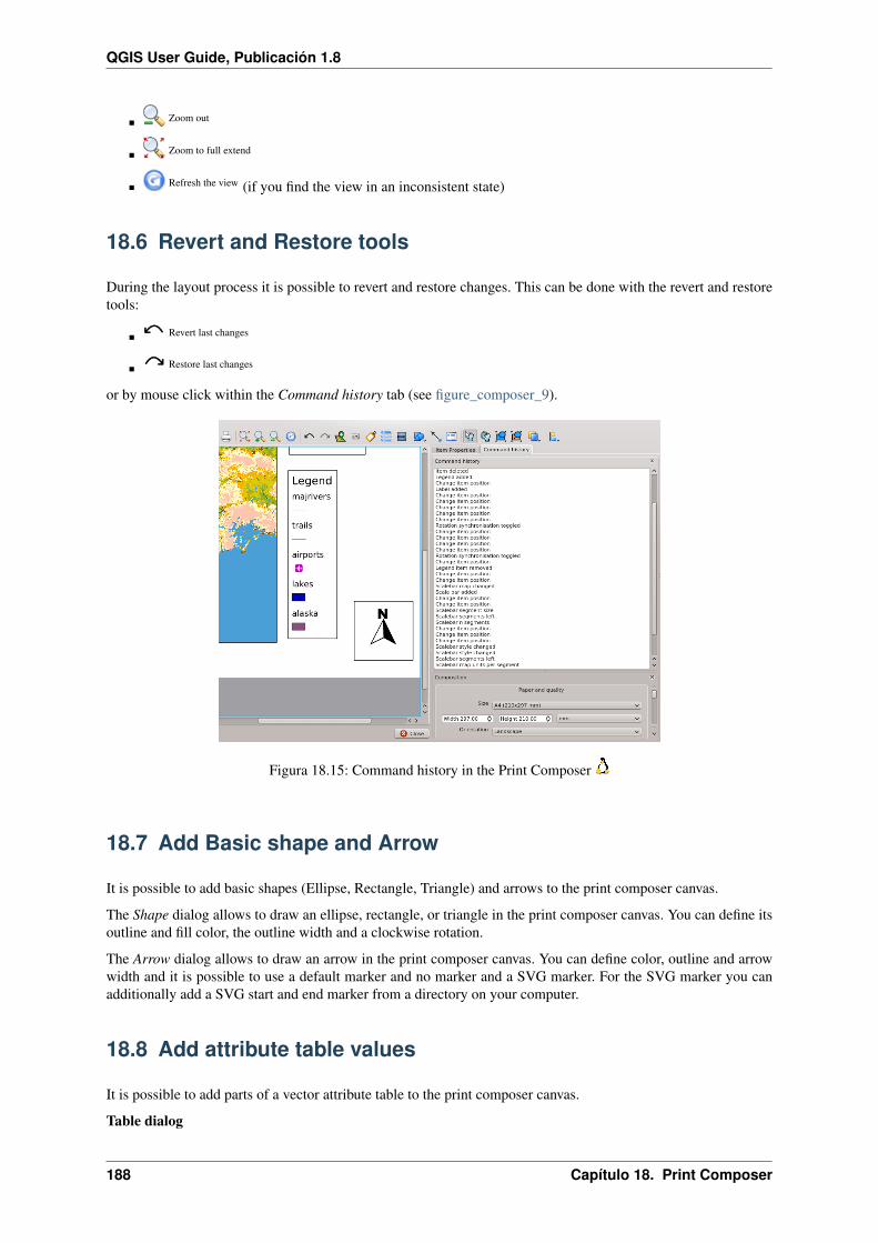
QGIS User Guide, Publicación 1.8
Zoom out
Zoom to full extend
Refresh the view (if you find the view in an inconsistent state)
18.6 Revert and Restore tools
During the layout process it is possible to revert and restore changes. This can be done with the revert and restoretools:
Revert last changes
Restore last changes
or by mouse click within the Command history tab (see figure_composer_9).
Figura 18.15: Command history in the Print Composer
18.7 Add Basic shape and Arrow
It is possible to add basic shapes (Ellipse, Rectangle, Triangle) and arrows to the print composer canvas.
The Shape dialog allows to draw an ellipse, rectangle, or triangle in the print composer canvas. You can define itsoutline and fill color, the outline width and a clockwise rotation.
The Arrow dialog allows to draw an arrow in the print composer canvas. You can define color, outline and arrowwidth and it is possible to use a default marker and no marker and a SVG marker. For the SVG marker you canadditionally add a SVG start and end marker from a directory on your computer.
18.8 Add attribute table values
It is possible to add parts of a vector attribute table to the print composer canvas.
Table dialog
188 Capítulo 18. Print Composer

QGIS User Guide, Publicación 1.8
Figura 18.16: Shape Dialog
Figura 18.17: Arrow Dialog
The Table dialog of the attribute table item tab provides following functionalities (see figure_composer_20):
Figura 18.18: Table Dialog
The Table dialog allows to select the vector layer and columns of the attribute table. Attribute columns canbe sorted and you can define to show its values ascending or descending.
You can define the maximum number of rows to be displayed and if attributes are only shown for visiblefeatures of the current composer canvas.
Additionally you can define the grid characteristics of the table and the header and content font.
General options dialog
The General options dialog of the attribute table item tab provides following functionalities (see fig-ure_composer_21):
Here you can define color and outline width for the element frame, set a background color and opacityfor the table. The [Position and size] button opens the Set item position dialog and allows to set the map
18.8. Add attribute table values 189

QGIS User Guide, Publicación 1.8
Figura 18.19: General Options Dialog
canvas position using reference points or coordinates. Furthermore you can select or unselect to display the
element frame with the Show frame checkbox. Use the Item ID to create a relationship to the other printcomposeritems.
18.9 Raise, lower and align elements
Raise or lower functionalities for elements are inside the Raise selected items pulldown menu. Choose an elementon the print composer canvas and select the matching functionality to raise or lower the selected element comparedto the other elements (see table_composer_1).
There are several alignment functionalities available within the Align selected items pulldown menu (see ta-ble_composer_1). To use an alignment functionality , you first select some elements and then click on the matchingalignment icon. All selected will then be aligned within to their common bounding box.
18.10 Creating Output
Figure_composer_22 shows the print composer with an example print layout including each type of map elementdescribed in the sections above.
Figura 18.20: Print Composer with map view, legend, scalebar, coordinates and text added
190 Capítulo 18. Print Composer

QGIS User Guide, Publicación 1.8
The print composer allows you to create several output formats and it is possible to define the resolution (printquality) and paper size:
The Print icon allows to print the layout to a connected printer or a Postscript file depending on installedprinter drivers.
The Export as image icon exports the composer canvas in several image formats such as PNG, BPM, TIF,JPG,...
The Export as PDF saves the defined print composer canvas directly as a PDF.
The Export as SVG icon saves the print composer canvas as a SVG (Scalable Vector Graphic).
Nota: Currently the SVG output is very basic. This is not a QGIS problem, but a problem of the underlaying Qtlibrary. This will hopefully be sorted out in future versions.
18.11 Saving and loading a print composer layout
With the Save as template and Load from template icons you can save the current state of a print composer sessionas a .qpt template and load the template again in another session.
The Composer Manager button in the QGIS toolbar and in File → Composer Manager allows to add a new com-poser template or to manage already existing templates.
Figura 18.21: The Print Composer Manager
18.11. Saving and loading a print composer layout 191
QGIS User Guide, Publicación 1.8
192 Capítulo 18. Print Composer
CAPÍTULO 19
Plugins
19.1 QGIS Plugins
QGIS has been designed with a plugin architecture. This allows many new features/functions to be easily addedto the application. Many of the features in QGIS are actually implemented as either core or external plugins.
Core Plugins are maintained by the QGIS Development Team and are automatically part of every QGISdistribution. They are written in one of two languages: C++ or Python. More information about core pluginsare provided in Section Using QGIS Core Plugins
External Plugins are currently all written in Python. They are stored in external repositories and maintainedby the individual authors. They can be added to QGIS using the Python Plugin Installer. More informationabout external plugins is provided in Section Loading an external QGIS Plugin.
19.1.1 Managing Plugins
Managing plugins in general means loading or unloading them using the Plugin Manager. External plugins canbe installed and directly activated or uninstalled using the Python Plugin Installer. To deactivate and reactivateexternal plugins, the Plugin Manager is used again.
Loading a QGIS Core Plugin
Loading a QGIS Core Plugin is done from the main menu Plugins → Manage Plugins
The Plugin Manager lists all the available plugins and their status (loaded or unloaded), including all core pluginsand all external plugins that have been installed and automatically activated using the Python Plugin Installer (seeSection Loading an external QGIS Plugin). Those plugins that are already loaded have a check mark to the left oftheir name. Figure_plugins_1 shows the Plugin Manager dialog.
To enable a particular plugin, click on the checkbox to the left of the plugin name, and click [OK]. When you exitthe application, a list of loaded plugins is retained, and the next time you run QGIS these plugins are automaticallyloaded.
Truco: Crashing PluginsIf you find that QGIS crashes on startup, a plugin may be at fault. You can stop all plugins from loading by editingyour stored settings file (see Options for location). Locate the plugins settings and change all the plugin values tofalse to prevent them from loading.
For example, to prevent the ‘Delimited text’ plugin from loading, the entry in$HOME/.config/QuantumGIS/qgis.conf on Linux should look like this: Add Delimited TextLayer=false.
Do this for each plugin in the [Plugins] section. You can then start QGIS and add the plugins one at a time fromthe Plugin Manager to determine which plugin is causing the problem.
193

QGIS User Guide, Publicación 1.8
Figura 19.1: Plugin Manager
Loading an external QGIS Plugin
External QGIS plugins are written in Python. They are by default stored in either the ‘Official’ QGIS Repository,or in various other external repositories maintained by individual authors. The ‘Official’ QGIS Repository is addedby default in Python Plugin installer.
Detailed documentation about the usage, minimum QGIS version, homepage, authors, and other important in-formation are provided for the ‘Official’ QGIS Repository at http://plugins.qgis.org/plugins/. For other externalrepositories, they might be available with the external plugins themselves. In general it is not included in thismanual.
Nota: Updates of core python plugins may be available in this repository as external overlays.
Nota: fTools, Mapserver Export, and the Plugin Installer are Python plugins, but they are also part of the QGISsources, and are automatically loaded and enabled inside the QGIS Plugin Manager (see Section Loading anexternal QGIS Plugin).
Currently there are over 150 external plugins available from the ‘Official’ QGIS Repository. Some of these pluginsoffer functionality that will be required by many users (for example: providing the user with the ability to view andedit OpenStreetMap data, or to add GoogleMap layers) while others offer very specialized functions (for example:Calculate economic pipe diameters for water supply networks).
It is, however, quite straightforward to search through all the available external plugins by providing keywords,choosing a named repository and/or filtering on the status of plugins (currently installed or uninstalled in yoursystem). Searching and filtering is done from the QGIS Python Plugin Installer (see figure_plugins_2).
Truco: Add more repositoriesTo add external author repositories, open the Plugin Installer (Plugins → Fetch Python Plugins), go to the tabRepositories, and click [Add]. If you do not want one or more of the added repositories, they can be disabled viathe [Edit...] button, or completely removed with the [Delete] button.
There is only one step required to integrate external plugins into QGIS:
Download an external plugin from a repository using the Python Plugin Installer (see Using the QGISPython Plugin Installer). The new external plugin will be added to the list of available plugins in the Plugin
194 Capítulo 19. Plugins

QGIS User Guide, Publicación 1.8
Manager and is automatically loaded.
Using the QGIS Python Plugin Installer
In order to download and install an external Python plugin, go to Plugins → Fetch Python Plugins. The PluginInstaller window will appear (figure_plugins_2) with the tab Plugins, containing a list of all locally installedPython plugins, as well as plugin available in remote repositories.
Figura 19.2: Installing external python plugins
Each plugin can be either:
not installed - this means the plugin is available in the repository, but is not installed yet. In order to installit, select the plugin from the list and click the button [Install plugin].
new - this means that the plugin is newly available in the repository.
installed - this indicates that the plugin is already installed. If it is also available in any repository the[Reinstall plugin] button will be enabled. If the available version is older than the installed version, the[Downgrade plugin] button will appear instead.
upgradeable - this means that the plugin is installed, but there is an updated version available. In this case,the [Upgrade plugin] and [Upgrade all] buttons will be enabled.
invalid - this means that the plugin is installed, but is unavailable or broken. The reason will be explainedin the plugin description field.
Plugins tab
To install a plugin, select it from the list and click the [Install plugin] button. The plugin is then activated andinstalled in its own directory.
Linux and other unices
• /share/qgis/python/plugins
• $HOME/.qgis/python/plugins
Mac OS X
• /Contents/MacOS/share/qgis/python/plugins
• /Users/$USERNAME/.qgis/python/plugins
Windows
• C:\Program Files\QGIS\python\plugins
• C:\Documents and Settings\$USERNAME\.qgis\python\plugins
19.1. QGIS Plugins 195

QGIS User Guide, Publicación 1.8
If the installation is successful, a confirmation message will appear.
If the installation fails, the reason for the failure will be displayed in a warning dialog. Most often, errors are theresult of connection problems and/or missing Python modules. In the former case you will likely need to waitbefore trying the install again, in the latter case, you should install the missing modules relevant to your operatingsystem prior to using the plugin. For Linux, most required modules should be available via a package manager.For install instructions in Windows visit the module home page.
If you are using a proxy, you may need to configure it under Edit → Options (Gnome, OSX) or Settings → Options(KDE, Windows)‘ on the Proxy tab.
The [Uninstall plugin] button is enabled only if the selected plugin is installed and is not a core plugin. Notethat if you have installed an update to a core plugin, you can uninstall this update with the [Uninstall plugin] andrevert to the version shipped with Quantum GIS. This default version however, cannot be uninstalled.
Repositories tab
The second tab Repositories, contains a list of plugin repositories available for the Plugin Installer. By default,only the QGIS Official Repository is enabled. You can add several user-contributed repositories, including thecentral QGIS Contributed Repository and other external repositories by clicking the [Add ...] button. The addedrepositories contain a large number of useful plugins which are not maintained by the QGIS Development Team.As such, we cannot take any responsibility for them. You can also manage the repository list manually, that isadd, remove, and edit the entries. Temporarily disabling a particular repository is possible by clicking the [Edit...] button.
Options tab
The Options tab is where you can configure the settings of the Plugin Installer. The Check for updates onstartup checkbox tells QGIS to automatically look for plugin updates and news. By default, if this feature isenabled all repositories listed and enabled in the Repositories tab are checked for updates each time the programis started. The frequency of update checking can be adjusted using the dropdown menu, and may be adjusted fromonce a day right up to once a month. If a new plugin or update is available for one of the installed plugins, anotification will appear in the Status Bar. If the checkbox is disabled, looking for updates and news is performedonly when the Plugin Installer is manually launched from the menu.
Although the plugin installer update can handle ports different from 80, some internet connections will causeproblems when attempting to automatically check for updates. In these cases, a Looking for new plugins... indicatorwill remain visible in the Status Bar during your entire QGIS session, and may cause a program crash when exiting.In this case please disable the checkbox.
In addition, you may specify the type of plugins that are displayed by the Python Plugin Installer. Under Allowedplugins, you can specify whether you would like to:
Only show plugins from the official repository
Show all plugins except those marked as experimental
Show all plugins, even those marked as experimental
Truco: Using experimental pluginsExperimental plugins are generally unsuitable for production use. These plugins are in the early stages of devel-opment, and should be considered ‘incomplete’ or ‘proof of concept’ tools. The QGIS development team does notrecommend installing these plugins unless you intend to use them for testing purposes.
19.1.2 Data Providers
Data Providers are ‘special’ plugins that provides access to a data store. By default, QGIS supports PostGIS layersand disk-based data stores supported by the GDAL/OGR library. A Data Provider plugin extends the ability ofQGIS to use other data sources.
Data Provider plugins are registered automatically by QGIS at startup. They are not managed by the Plugin Man-ager but used behind the scenes when a data type is added as a layer in QGIS.
196 Capítulo 19. Plugins

QGIS User Guide, Publicación 1.8
19.2 Using QGIS Core Plugins
Icon Plugin Description Manual Reference
Add Delimited TextLayer
Loads text files containing x,ycoordinates
Delimited Text Plugin
Coordinate Capture Capture mouse coordinate in differentCRS
Coordinate Capture Plugin
DB Manager Manage your databases within QGIS DB Manager PluginDiagram Overlay Add Diagrams for vectors Diagram Overlay Plugin
DXF2ShapeConverter
Converts from DXF to SHP file format Dxf2Shp Converter Plugin
eVis Event Visualization Tool eVis Plugin
fTools A suite of vector tools fTools Plugin
GPS Tools Tools for loading and importing GPS data GPS Plugin
GRASS GRASS functionality GRASS GIS Integration
GDAL Tools GDAL raster functionality GDAL Tools Plugin
GeoreferencerGDAL
Georeference Raster with GDAL Georeferencer Plugin
Heatmap Create heatmap raster from input vectorpoints
Heatmap Plugin
Interpolation plugin Interpolation on base of vertices of avector layer
Interpolation Plugin
MapServer ExportPlugin
Export a QGIS project file to aMapServer map file
MapServer Export Plugin
Offline Editing Offline editing and synchronizing withdatabase
Offline Editing Plugin
OpenStreetMap Access OpenStreetMap OpenStreetMap
Oracle SpatialGeoraster
Access Oracle Spatial GeoRasters Oracle GeoRaster Plugin
Plugin Installer Download and install python plugins Using the QGIS Python PluginInstaller
Raster TerrainAnalysis
Compute geomorphological featuresfrom DEMs
Raster Terrain Analysis Plugin
Road graph Plugin Shortest path analysis Road Graph Plugin
SPIT Shapefile to PostGIS Import Tool Importing Data into PostgreSQL
SQL Anywhereplugin
Access SQL anywhere DB SQL Anywhere Plugin
Spatial Query Spatial queries on vectors Spatial Query Plugin
Zonal Statistics Calculate raster statistics for vectorpolygons
Zonal Statistics Plugin
19.2. Using QGIS Core Plugins 197

QGIS User Guide, Publicación 1.8
19.3 Coordinate Capture Plugin
The coordinate capture plugin is easy to use and provides the ability to display coordinates on the map canvas fortwo selected Coordinate Reference Systems (CRS).
Figura 19.3: Coordinate Capture Plugin
1. Start QGIS, select Project Properties from the Settings (KDE, Windows) or File (Gnome, OSX) menu
and click on the Projection tab. As an alternative you can also click on the CRS status icon in the lowerright-hand corner of the statusbar.
2. Click on the Enable on the fly projection checkbox and select a projected coordinate system of yourchoice (see also Working with Projections).
3. Load the coordinate capture plugin in the Plugin Manager (see Loading a QGIS Core Plugin) and ensure
that the dialog is visible by going to View → Panels and ensuring that Coordinate Capture is enabled.The coordinate capture dialog appears as shown in Figure figure_coordinate_capture_1.
4. Click on the Click to the select the CRS to use for coordinate display icon and select a different CRS from the one youselected above.
5. To start capturing coordinates, click on [Start capture]. You can now click anywhere on the map canvasand the plugin will show the coordinates for both of your selected CRS.
6. To enable mouse coordinate tracking click the mouse tracking icon.
7. You can also copy selected coordinates to the clipboard.
19.4 DB Manager Plugin
The DB Manager Plugin is officially part of QGIS core and intends to replace the SPIT Plugin and the PostGISManager Plugin and additionally to integrate all other database formats supported by QGIS in one user interface.
The DB Manager Plugin provides several features. You can drag layers from the QGIS Browser into the DBManager and it will import your layer into your spatial database. You can drag and drop tables between spatialdatabases and they will get imported. You can also use the DB Manager to execute SQL queries against yourspatial database and then view the spatial output for queries by adding the results to QGIS as a query layer.
The Database menu allows to connect to an existing database, to start the SQL-window and to exit the DB ManagerPlugin. The Schema menu includes tools to create and delete (empty) schemas and, if topology is available (e.g.PostGIS 2) to start a TopoViewer. The menu Table allows to create and edit tables and to delete tables and views. Itis also possible to empty tables and to move tables from one to another schema. Finally you can also run VacuumAnalyze and add Versioning Support to a table.
The Tree window lists all existing databases supported by QGIS. With a double-click you can connect to thedatabase. With the right-mouse button you can rename and delete existing schemas and tables. Tables can also beadded to the QGIS canvas with the context menu.
198 Capítulo 19. Plugins
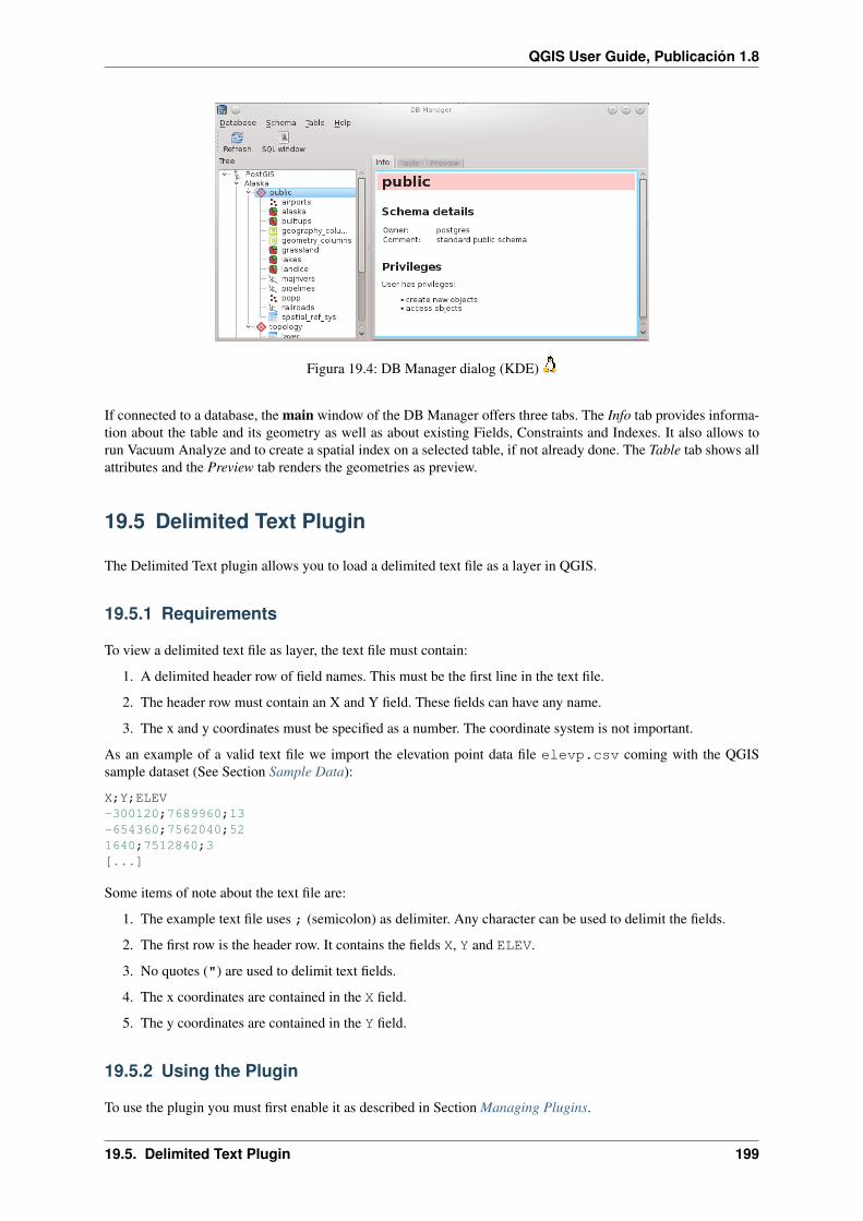
QGIS User Guide, Publicación 1.8
Figura 19.4: DB Manager dialog (KDE)
If connected to a database, the main window of the DB Manager offers three tabs. The Info tab provides informa-tion about the table and its geometry as well as about existing Fields, Constraints and Indexes. It also allows torun Vacuum Analyze and to create a spatial index on a selected table, if not already done. The Table tab shows allattributes and the Preview tab renders the geometries as preview.
19.5 Delimited Text Plugin
The Delimited Text plugin allows you to load a delimited text file as a layer in QGIS.
19.5.1 Requirements
To view a delimited text file as layer, the text file must contain:
1. A delimited header row of field names. This must be the first line in the text file.
2. The header row must contain an X and Y field. These fields can have any name.
3. The x and y coordinates must be specified as a number. The coordinate system is not important.
As an example of a valid text file we import the elevation point data file elevp.csv coming with the QGISsample dataset (See Section Sample Data):
X;Y;ELEV-300120;7689960;13-654360;7562040;521640;7512840;3[...]
Some items of note about the text file are:
1. The example text file uses ; (semicolon) as delimiter. Any character can be used to delimit the fields.
2. The first row is the header row. It contains the fields X, Y and ELEV.
3. No quotes (") are used to delimit text fields.
4. The x coordinates are contained in the X field.
5. The y coordinates are contained in the Y field.
19.5.2 Using the Plugin
To use the plugin you must first enable it as described in Section Managing Plugins.
19.5. Delimited Text Plugin 199
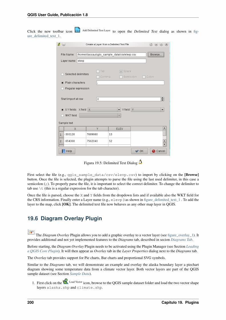
QGIS User Guide, Publicación 1.8
Click the new toolbar icon Add Delimited Text Layer to open the Delimited Text dialog as shown in fig-ure_delimited_text_1.
Figura 19.5: Delimited Text Dialog
First select the file (e.g., qgis_sample_data/csv/elevp.csv) to import by clicking on the [Browse]button. Once the file is selected, the plugin attempts to parse the file using the last used delimiter, in this case asemicolon (;). To properly parse the file, it is important to select the correct delimiter. To change the delimiter totab use \t (this is a regular expression for the tab character).
Once the file is parsed, choose the X and Y fields from the dropdown lists and if available also the WKT field forthe CRS information. Finally enter a Layer name (e.g., elevp ) as shown in figure_delimited_text_1 . To add thelayer to the map, click [OK]. The delimited text file now behaves as any other map layer in QGIS.
19.6 Diagram Overlay Plugin
The Diagram Overlay Plugin allows you to add a graphic overlay to a vector layer (see figure_overlay_1). Itprovides additional and not yet implemented features to the Diagrams tab, described in secion Diagrams Tab.
Before starting, the Diagram Overlay Plugin needs to be activated using the Plugin Manager (see Section Loadinga QGIS Core Plugin). It will then appear as Overlay tab in the Layer Properties dialog next to the Diagrams tab.
The Overlay tab provides support for Pie charts, Bar charts and proportional SVG symbols.
Similar to the Diagrams tab, we will demonstrate an example and overlay the alaska boundary layer a piechartdiagram showing some temperature data from a climate vector layer. Both vector layers are part of the QGISsample dataset (see Section Sample Data).
1. First click on the Load Vector icon, browse to the QGIS sample dataset folder and load the two vector shapelayers alaska.shp and climate.shp.
200 Capítulo 19. Plugins

QGIS User Guide, Publicación 1.8
Figura 19.6: Vector properties dialog with overlay tab
2. Double click the climate layer in the map legend to open the Layer Properties dialog.
3. Click on the Overlay tab, activate Display diagrams and select ‘Pie Chart’ from Diagram typecombobox.
4. We want to display the values of the three columns T_F_JAN, T_F_JUL and T_F_MEAN. First selectT_F_JAN as Attributes and click the [Add] button, then T_F_JUL and finally T_F_MEAN.
5. Diagram size is based on linear scaling of a classification attribute. We choose T_F_JUL, click on [Find
maximum value] and set size to 20 and Size unit to ‘Millimeter’.
6. Now click [Apply] to display the diagram in the QGIS main window.
7. You can now adapt the chart size, or change the attribute colors double clicking on the color values in theattribute field. Figure_overlay_2 gives an impression.
8. Finally click [Ok].
Figura 19.7: Pie chart diagram from temperature data overlayed on a map
Additionally in the Settings → Options dialog, there is a Overlay tab where it is possible to select the placement
19.6. Diagram Overlay Plugin 201

QGIS User Guide, Publicación 1.8
algorithm of the diagrams. The ‘Central point’ method is a generic one, the others use algorithms of the PALlibrary. They also consider diagram objects and labels in different layers.
19.7 Dxf2Shp Converter Plugin
The dxf2shape converter plugin can be used to convert vector data from DXF to Shapefile format. It requires thefollowing parameters to be specified before running:
Figura 19.8: Dxf2Shape Converter Plugin
Input DXF file: Enter path to the DXF file to be converted
Output Shp file: Enter desired name of the Shapefile to be created
Output file type: Specify the geometry type of the output Shapefile. Currently supported types are polyline,polygon, and point.
Export text labels: When this checkbox is enabled, an additional Shapefile point layer will be created, andthe associated dbf table will contain information about the “TEXT” fields found in the dxf file, and the textstrings themselves.
19.7.1 Using the Plugin
1. Start QGIS, load the Dxf2Shape plugin in the Plugin Manager (see Section Loading a QGIS Core Plugin)
and click on the Dxf2Shape Converter icon which appears in the QGIS toolbar menu. The Dxf2Shape plugindialog appears as shown in Figure_dxf2shape_1.
2. Enter input DXF file, a name for the output Shapefile and the Shapefile type.
3. Enable the Export text labels checkbox if you want to create an extra point layer with labels.
4. Click [OK].
19.8 eVis Plugin
The Biodiversity Informatics Facility at the American Museum of Natural History’s (AMNH) Center for Biodi-versity and Conservation (CBC) (this section is derived from Horning, N., K. Koy, P. Ersts. 2009. eVis (v1.1.0)User’s Guide. American Museum of Natural History, Center for Biodiversity and Conservation. Available fromhttp://biodiversityinformatics.amnh.org/, and released under the GNU FDL.) has developed the Event Visualiza-tion Tool (eVis), another software tool to add to the suite of conservation monitoring and decision support tools forguiding protected area and landscape planning. This plugin enables users to easily link geocoded (i.e., referencedwith latitude and longitude or X and Y coordinates) photographs, and other supporting documents, to vector datain QGIS.
202 Capítulo 19. Plugins

QGIS User Guide, Publicación 1.8
eVis is now automatically installed and enabled in new versions of QGIS, and as with all plugins, it can be disabledand enabled using the Plugin Manager (See Managing Plugins).
The eVis plugin is made up of three modules: the ‘Database Connection tool’, ‘Event ID tool’, and the ‘EventBrowser’. These work together to allow viewing of geocoded photographs and other documents that are linked tofeatures stored in vector files, databases, or spreadsheets.
19.8.1 Event Browser
The Event Browser module provides the functionality to display geocoded photographs that are linked to vectorfeatures displayed in the QGIS map window. Point data, for example, can be from a vector file that can be inputusing QGIS or it can be from the result of a database query. The vector feature must have attribute informationassociated with it to describe the location and name of the file containing the photograph and, optionally, thecompass direction the camera was pointed when the image was acquired. Your vector layer must be loaded intoQGIS before running the Event Browser.
Launch the Event Browser module
To launch the Event browser module either click on the eVis Event Browser icon or click on Database → eVis →eVis Event Browser. This will open the Generic Event Browser window.
The Generic Event Browser window has three tabs displayed at the top of the window. The Display tab is usedto view the photograph and its associated attribute data. The Options tab provides a number of settings that canbe adjusted to control the behavior of the eVis plugin. Lastly, the Configure External Applications tab is used tomaintain a table of file extensions and their associated application to allow eVis to display documents other thanimages.
Understanding the Display window
To see the Display window click on the Display tab in the Generic Event Browser window. The Display windowis used to view geocoded photographs and their associated attribute data.
1. Display window: A window where the photograph will appear.
2. Zoom in button: Zoom in to see more detail. If the entire image cannot be displayed in the display window,scroll bars will appear on the left and bottom sides of the window to allow you to pan around the image.
3. Zoom out button: Zoom out to see more area.
4. Zoom to full extent button: Displays the full extent of the photograph.
5. Attribute information window: All of the attribute information for the point associated with the photo-graph being viewed is displayed here. If the file type being referenced in the displayed record is not animage but is of a file type defined in the Configure External Applications tab then when you double-clickon the value of the field containing the path to the file the application to open the file will be launched toview or hear the contents of the file. If the file extension is recognized the attribute data will be displayed ingreen.
6. Navigation buttons: Use the Previous and Next buttons to load the previous or next feature when more thanone feature is selected.
7. Feature indicator: This heading indicates which feature is being displayed and how many features areavailable for display.
Understanding the Options window
1. File path: A dropdown list to specify the attribute field that contains the directory path or URL for thephotographs or other documents being displayed. If the location is a relative path then the checkbox mustbe clicked. The base path for a relative path can be entered in the Base Path text box below. Information
19.8. eVis Plugin 203
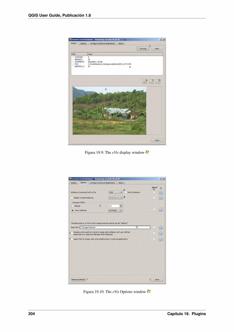
QGIS User Guide, Publicación 1.8
Figura 19.9: The eVis display window
Figura 19.10: The eVis Options window
204 Capítulo 19. Plugins
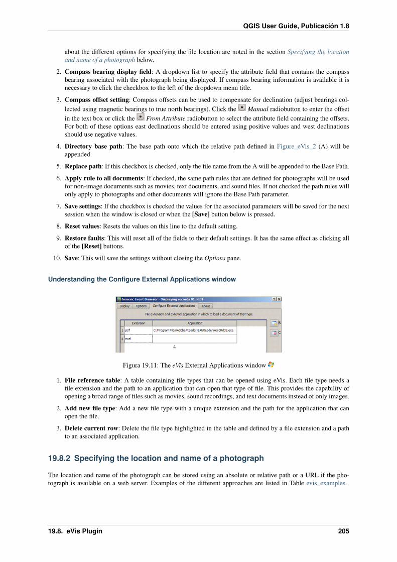
QGIS User Guide, Publicación 1.8
about the different options for specifying the file location are noted in the section Specifying the locationand name of a photograph below.
2. Compass bearing display field: A dropdown list to specify the attribute field that contains the compassbearing associated with the photograph being displayed. If compass bearing information is available it isnecessary to click the checkbox to the left of the dropdown menu title.
3. Compass offset setting: Compass offsets can be used to compensate for declination (adjust bearings col-lected using magnetic bearings to true north bearings). Click the Manual radiobutton to enter the offsetin the text box or click the From Attribute radiobutton to select the attribute field containing the offsets.For both of these options east declinations should be entered using positive values and west declinationsshould use negative values.
4. Directory base path: The base path onto which the relative path defined in Figure_eVis_2 (A) will beappended.
5. Replace path: If this checkbox is checked, only the file name from the A will be appended to the Base Path.
6. Apply rule to all documents: If checked, the same path rules that are defined for photographs will be usedfor non-image documents such as movies, text documents, and sound files. If not checked the path rules willonly apply to photographs and other documents will ignore the Base Path parameter.
7. Save settings: If the checkbox is checked the values for the associated parameters will be saved for the nextsession when the window is closed or when the [Save] button below is pressed.
8. Reset values: Resets the values on this line to the default setting.
9. Restore faults: This will reset all of the fields to their default settings. It has the same effect as clicking allof the [Reset] buttons.
10. Save: This will save the settings without closing the Options pane.
Understanding the Configure External Applications window
Figura 19.11: The eVis External Applications window
1. File reference table: A table containing file types that can be opened using eVis. Each file type needs afile extension and the path to an application that can open that type of file. This provides the capability ofopening a broad range of files such as movies, sound recordings, and text documents instead of only images.
2. Add new file type: Add a new file type with a unique extension and the path for the application that canopen the file.
3. Delete current row: Delete the file type highlighted in the table and defined by a file extension and a pathto an associated application.
19.8.2 Specifying the location and name of a photograph
The location and name of the photograph can be stored using an absolute or relative path or a URL if the pho-tograph is available on a web server. Examples of the different approaches are listed in Table evis_examples.
19.8. eVis Plugin 205

QGIS User Guide, Publicación 1.8
X Y FILE BEARING780596 1784017 C:\Workshop\eVis_Data\groundphotos\DSC_0168.JPG 275780596 1784017 /groundphotos/DSC_0169.JPG 80780819 1784015 http://biodiversityinform.org/testdata/DSC_0170.JPG 10780596 1784017 pdf:http://www.test.com/attach.php?attachment_id-12 76
19.8.3 Specifying the location and name of other supporting documents
Supporting documents such as text documents, videos, and sound clips can also be displayed or played by eVis. Todo this it is necessary to add an entry in the file reference table that can be accessed from the Configure ExternalApplications window in the Generic Event Browser that matches the file extension to an application that can beused to open the file. It is also necessary to have the path or URL to the file in the attribute table for the vectorlayer. One additional rule that can be used for URLs that don’t contain a file extension for the document you wantto open is to specify the file extension before the URL. The format is — file extension:URL. The URLis preceded by the file extension and a colon, and is particularly useful for accessing documents from Wikis andother web sites that use a database to manage the web pages (see Table evis_examples).
19.8.4 Using the Generic Event Browser
When the Event Browser window opens a photograph will appear in the display window if the document refer-enced in the vector file attribute table is an image and if the file location information in the Options window isproperly set. If a photograph is expected and it does not appear it will be necessary to adjust the parameters in theOptions window.
If a supporting document (or an image that does not have a file extension recognized by eVis) is referenced in theattribute table the field containing the file path will be highlighted in green in the attribute information window ifthat file extension is defined in the file reference table located in the Configure External Applications window. Toopen the document double-click on the green-highlighted line in the attribute information window. If a supportingdocument is referenced in the attribute information window and the file path is not highlighted in green then itwill be necessary to add an entry for the file’s filename extension in the Configure External Applications window.If the file path is highlighted in green but does not open when double-clicked it will be necessary to adjust theparameters in the Options window so the file can be located by eVis.
If no compass bearing is provided in the Options window a red asterisk will be displayed on top of the vectorfeature that is associated with the photograph being displayed. If a compass bearing is provided then an arrowwill appear pointing in the direction indicated by the value in the compass bearing display field in the GenericEvent Browser window. The arrow will be centered over the point that is associated with the photograph or otherdocument.
To close the Generic Event Browser window click on the [Close] button from the Display window.
19.8.5 Event ID Tool
The ‘Event ID’ module allows you to display a photograph by clicking on a feature displayed in the QGIS mapwindow. The vector feature must have attribute information associated with it to describe the location and name ofthe file containing the photograph and optionally the compass direction the camera was pointed when the imagewas acquired. This layer must be loaded into QGIS before running the ‘Event ID’ tool.
Launch the Event ID module
To launch the ‘Event ID’ module either click on the Event ID icon or click on Plugins → eVis → Event ID Tool.This will cause the cursor to change to an arrow with an ‘i’ on top of it signifying that the ID tool is active.
To view the photographs linked to vector features in the active vector layer displayed in the QGIS map window,move the Event ID cursor over the feature and then click the mouse. After clicking on the feature, the GenericEvent Browser window is opened and the photographs on or near the clicked locality are available for display
206 Capítulo 19. Plugins

QGIS User Guide, Publicación 1.8
in the browser. If more than one photograph is available, you can cycle through the different features using the[Previous] and [Next] buttons. The other controls are described in the ref:evis_browser section of this guide.
19.8.6 Database connection
The ‘Database Connection’ module provides tools to connect to and query a database or other ODBC resource,such as a spreadsheet.
eVis can directly connect to four types of databases: Microsoft Access, PostgreSQL, MySQL, SQLite, and canalso read from ODBC connections. When reading from an ODBC database (such as an Excel spreadsheet) it isnecessary to configure your ODBC driver for the operating system you are using.
Launch the Database Connection module
To launch the ‘Database Connection’ module either click on the appropriate icon eVis Database Connection or clickon Plugins → eVis → Database Connection. This will launch the Database Connection window. The window hasthree tabs: Predefined Queries, Database Connection, and SQL Query. The Output Console window at the bottomof the window displays the status of actions initiated by the different sections of this module.
Connect to a database
Click on the Database Connection tab to open the database connection interface. Next, use the Database Type
combobox to select the type of database that you want to connect to. If a password or username isrequired, that information can be entered in the Username and Password textboxes.
Enter the database host in the Database Host textbox. This option is not available if you selected “MS Access” asthe database type. If the database resides on your desktop you should enter “localhost”.
Enter the name of the database in the Database Name textbox. If you selected “ODBC” as the database type, youneed to enter the data source name.
When all of the parameters are filled in, click on the [Connect] button. If the connection is successful, a messagewill be written in the Output Console window stating that the connection was established. If a connection was notestablished you will need to check that the correct parameters were entered above.
1. Database Type: A dropdown list to specify the type of database that will be used.
2. Database Host: The name of the database host.
3. Port The port number if a MySQL or PostgreSQL database type is selected.
4. Database Name The name of the database.
5. Connect A button to connect to the database using the parameters defined above.
6. Output Console The console window where messages related to processing are displayed.
7. Username: Username for use when a database is password protected.
8. Password: Password for use when a database is password protected.
9. Predefined Queries: Tab to open the “Predefined Queries” window.
10. Database Connection: Tab to open the “Database Connection” window.
11. SQL Query: Tab to open the “SQL Query” window.
12. Help: Displays the on line help.
13. OK: Close the main “Database Connection” window.
19.8. eVis Plugin 207

QGIS User Guide, Publicación 1.8
Figura 19.12: The eVis Database connection window
Running SQL queries
SQL queries are used to extract information from a database or ODBC resource. In eVis the output from thesequeries is a vector layer added to the QGIS map window. Click on the SQL Query tab to display the SQL queryinterface. SQL commands can be entered in this text window. A helpful tutorial on SQL commands is available athttp://www.w3schools.com/sql. For example, to extract all of the data from a worksheet in an Excel file, select* from [sheet1$] where sheet1 is the name of the worksheet.
Click on the [Run Query] button to execute the command. If the query is successful a Database File Selectionwindow will be displayed. If the query is not successful an error message will appear in the Output Consolewindow.
In the Database File Selection window, enter the name of the layer that will be created from the results of thequery in the Name of New Layer textbox.
1. SQL Query Text Window: A screen to type SQL queries.
2. Run Query: Button to execute the query entered in the SQL Query Window.
3. Console Window: The console window where messages related to processing are displayed.
4. Help: Displays the on line help.
5. OK: Closes the main Database Connection window.
Use the X Coordinate and Y Coordinate comboboxes to select the field from the database thatstore the X (or longitude) and Y (or latitude) coordinates. Clicking on the [OK] button causes the vector layercreated from the SQL query to be displayed in the QGIS map window.
To save this vector file for future use, you can use the QGIS ‘Save as...’ command that is accessed by right clickingon the layer name in the QGIS map legend and then selecting ‘Save as...’
Truco: Creating a vector layer from a Microsoft Excel Worksheet
208 Capítulo 19. Plugins
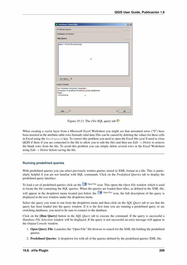
QGIS User Guide, Publicación 1.8
Figura 19.13: The eVis SQL query tab
When creating a vector layer from a Microsoft Excel Worksheet you might see that unwanted zeros (“0”) havebeen inserted in the attribute table rows beneath valid data.This can be caused by deleting the values for these cellsin Excel using the Backspace key. To correct this problem you need to open the Excel file (you’ll need to closeQGIS if there if you are connected to the file to allow you to edit the file) and then use Edit → Delete to removethe blank rows from the file. To avoid this problem you can simply delete several rows in the Excel Worksheetusing Edit → Delete before saving the file.
Running predefined queries
With predefined queries you can select previously written queries stored in XML format in a file. This is partic-ularly helpful if you are not familiar with SQL commands. Click on the Predefined Queries tab to display thepredefined query interface.
To load a set of predefined queries click on the Open File icon. This opens the Open File window which is usedto locate the file containing the SQL queries. When the queries are loaded their titles, as defined in the XML file,will appear in the dropdown menu located just below the Open File icon, the full description of the query isdisplayed in the text window under the dropdown menu.
Select the query you want to run from the dropdown menu and then click on the SQL Query tab to see that thequery has been loaded into the query window. If it is the first time you are running a predefined query or areswitching databases, you need to be sure to connect to the database.
Click on the [Run Query] button in the SQL Query tab to execute the command. If the query is successful aDatabase File Selection window will be displayed. If the query is not successful an error message will appear inthe Output Console window.
1. Open Query File: Launches the “Open File” file browser to search for the XML file holding the predefinedqueries.
2. Predefined Queries: A dropdown list with all of the queries defined by the predefined queries XML file.
19.8. eVis Plugin 209

QGIS User Guide, Publicación 1.8
Figura 19.14: The eVis Predefined queries tab
3. Query description: A short description of the query. This description is from the predefined queries XMLfile.
4. Console Window: The console window where messages related to processing are displayed.
5. Help: Displays the on line help.
6. OK: Closes the main “Database Connection” window.
XML format for eVis predefined queries
The XML tags read by eVis
210 Capítulo 19. Plugins

QGIS User Guide, Publicación 1.8
Tag Descriptionquery Defines the beginning and end of a query statement.shortde-scription
A short description of the query that appears in the eVis dropdown menu.
descrip-tion
A more detailed description of the query displayed in the Predefined Query text window.
database-type
The database type as defined in the Database Type dropdown menu in the Database Connectiontab.
database-port
The port as defined in the Port textbox in the Database Connection tab.
database-name
The database name as defined in the Database Name textbox in the Database Connection tab.
databaseuser-name
The database username as defined in the Username textbox in the Database Connection tab.
databasep-assword
The database password as defined in the Password textbox in the Database Connection tab.
sqlstate-ment
The SQL command.
autocon-nect
A flag (“true”” or “false”) to specify if the above tags should be used to automatically connect todatabase without running the database connection routine in the Database Connection tab.
A complete sample XML file with three queries is displayed below:
<?xml version="1.0"?><doc><query><shortdescription>Import all photograph points</shortdescription><description>This command will import all of the data in the SQLite database to QGIS
</description><databasetype>SQLITE</databasetype><databasehost /><databaseport /><databasename>C:\textbackslash Workshop/textbackslash
eVis\_Data\textbackslash PhotoPoints.db</databasename><databaseusername /><databasepassword /><sqlstatement>SELECT Attributes.*, Points.x, Points.y FROM Attributes LEFT JOIN
Points ON Points.rec_id=Attributes.point_ID</sqlstatement><autoconnect>false</autoconnect>
</query><query><shortdescription>Import photograph points "looking across Valley"</shortdescription><description>This command will import only points that have photographs "looking across
a valley" to QGIS</description><databasetype>SQLITE</databasetype><databasehost /><databaseport /><databasename>C:\Workshop\eVis_Data\PhotoPoints.db</databasename><databaseusername /><databasepassword /><sqlstatement>SELECT Attributes.*, Points.x, Points.y FROM Attributes LEFT JOIN
Points ON Points.rec_id=Attributes.point_ID where COMMENTS=’Looking acrossvalley’</sqlstatement>
<autoconnect>false</autoconnect></query><query>
<shortdescription>Import photograph points that mention "limestone"</shortdescription><description>This command will import only points that have photographs that mention
"limestone" to QGIS</description><databasetype>SQLITE</databasetype><databasehost /><databaseport />
19.8. eVis Plugin 211

QGIS User Guide, Publicación 1.8
<databasename>C:\Workshop\eVis_Data\PhotoPoints.db</databasename><databaseusername /><databasepassword /><sqlstatement>SELECT Attributes.*, Points.x, Points.y FROM Attributes LEFT JOIN
Points ON Points.rec_id=Attributes.point_ID where COMMENTS like ’%limestone%’</sqlstatement>
<autoconnect>false</autoconnect></query>
</doc>
19.9 fTools Plugin
The goal of the fTools python plugin is to provide a one-stop resource for many common vector-based GIS tasks,without the need for additional software, libraries, or complex workarounds. It provides a growing suite of spatialdata management and analysis functions that are both fast and functional.
fTools is now automatically installed and enabled in new versions of QGIS, and as with all plugins, it can bedisabled and enabled using the Plugin Manager (See Section Loading a QGIS Core Plugin). When enabled, thefTools plugin adds a Vector menu to QGIS, providing functions ranging from Analysis and Research Tools toGeometry and Geoprocessing Tools, as well as several useful Data Management Tools.
19.9.1 Analysis tools
Icon Tool Purpose
DistanceMatrix
Measure distances between two point layers, and output results as a) Square distancematrix, b) Linear distance matrix, or c) Summary of distances. Can limit distances tothe k nearest features.
Sum linelength
Calculate the total sum of line lengths for each polygon of a polygon vector layer.
Points inpolygon
Count the number of points that occur in each polygon of an input polygon vector layer.
List uniquevalues
List all unique values in an input vector layer field
Basicstatistic
Compute basic statistics (mean, std dev, N, sum, CV) on an input field.
NearestNeighboranalysis
Compute nearest neighbor statistics assess the level of clustering in a point vector layer
Meancoordinate(s)
Compute either the normal or weighted mean center of an entire vector layer, ormultiple features based on a unique ID field.
Lineintersections
Locate intersections between lines, and output results as a point shapefile. Useful forlocating road or stream intersections, ignores line intersections with length > 0.
Table Ftools 1: fTools Analysis tools
212 Capítulo 19. Plugins

QGIS User Guide, Publicación 1.8
19.9.2 Research tools
Icon Tool Purpose
Random selection Randomly select n number of features, or n percentage of features
Random selectionwithin subsets
Randomly select features within subsets based on a unique ID field.
Random points Generate pseudo-random points over a given input layer.
Regular points Generate a regular grid of points over a specified region and export them as apoint shapefile.
Vector grid Generate a line or polygon grid based on user specified grid spacing.
Select by location Select features based on their location relative to another layer to form a newselection, or add or subtract from the current selection.
Polygon from layerextent
Create a single rectangular polygon layer from the extent of an input raster orvector layer.
Table Ftools 2: fTools Research tools
19.9.3 Geoprocessing tools
Icon Tool Purpose
Convex hull(s) Create minimum convex hull(s) for an input layer, or based on an ID field.
Buffer(s) Create buffer(s) around features based on distance, or distance field.
Intersect Overlay layers such that output contains areas where both layers intersect.
Union Overlay layers such that output contains intersecting and non-intersecting areas.
Symmetricaldifference
Overlay layers such that output contains those areas of the input and differencelayers that do not intersect.
Clip Overlay layers such that output contains areas that intersect the clip layer.
Difference Overlay layers such that output contains areas not intersecting the clip layer.
Dissolve Merge features based on input field. All features with identical input values arecombined to form one single feature.
Table Ftools 3: fTools Geoprocessing tools
19.9. fTools Plugin 213

QGIS User Guide, Publicación 1.8
19.9.4 Geometry tools
Icon Tool Purpose
Check geometry Check polygons for intersections, closed-holes, and fix node ordering.
Export/Addgeometry columns
Add vector layer geometry info to point (XCOORD, YCOORD), line(LENGTH), or polygon (AREA, PERIMETER) layer.
Polygon centroids Calculate the true centroids for each polygon in an input polygon layer.
Delaunaytriangulation
Calculate and output (as polygons) the delaunay triangulation of an input pointvector layer.
Voronoi Polygons Calculate voronoi polygons of an input point vector layer.
Simplify geometry Generalize lines or polygons with a modified Douglas-Peucker algorithm.Densify geometry Densify lines or polygons by adding vertices
Multipart tosingleparts
Convert multipart features to multiple singlepart features. Creates simplepolygons and lines.
Singleparts tomultipart
Merge multiple features to a single multipart feature based on a unique ID field.
Polygons to lines Convert polygons to lines, multipart polygons to multiple singlepart lines.
Lines to polygons Convert lines to polygons, multipart lines to multiple singlepart polygons.
Extract nodes Extract nodes from line and polygon layers and output them as points.
Table Ftools 4: fTools Geometry tools
Nota: The Simplify geometry tool can be used to remove duplicate nodes in line and polygon geometries, just setthe Simplify tolerance parameter to 0 and this will do the trick.
19.9.5 Data management tools
Icon Tool Purpose
Defineprojection
Specify the CRS for shapefiles whose CRS has not been defined.
Joinattributes bylocation
Join additional attributes to vector layer based on spatial relationship. Attributes fromone vector layer are appended to the attribute table of another layer and exported as ashapefile.
Split vectorlayer
Split input layer into multiple separate layers based on input field.
Mergeshapefiles toone
Merge several shapefiles within a folder into a new shapefile based on the layer type(point, line, area).
Createspatial index
Create a spatial index for OGR supported formats.
Table Ftools 5: fTools Data management tools
214 Capítulo 19. Plugins

QGIS User Guide, Publicación 1.8
19.10 GDAL Tools Plugin
19.10.1 What is GDALTools?
The GDAL Tools plugin offers a GUI to the collection of tools in the Geospatial Data Abstraction Library,http://gdal.osgeo.org . These are raster management tools to query, re-project, warp and merge a wide varietyof raster formats. Also included are tools to create a contour (vector) layer, or a shaded relief from a raster DEM,and to make a vrt (Virtual Raster Tile in XML format) from a collection of one or more raster files. These toolsare available when the plugin is installed and activated.
The GDAL Library
The GDAL library consists of a set of command line programs, each with a large list of options. Users comfortablewith running commands from a terminal may prefer the command line, with access to the full set of options. TheGDALTools plugin offers an easy interface to the tools, exposing only the most popular options.
19.10.2 List of GDAL tools
Figura 19.15: The GDALTools menu list
Projections
Warp(Reproject)
This utility is an image mosaicing, reprojection and warping utility. The program can reprojectto any supported projection, and can also apply GCPs stored with the image if the image is“raw” with control information. For more information you can read on the GDAL websitehttp://www.gdal.org/gdalwarp.html
Assignprojection
This tool allows to assign projection to rasters that already georeferenced but miss projectioninformation. Also with it help it is possible to alter existing projection definition. Both singlefile and batch mode are supported. For more information please visit utility page at GDAL sitehttp://www.gdal.org/gdalwarp.html
Extractprojection
This utility helps you to extract projection information from an input file. If you want toextract projection from a whole directory you can use the Batch mode. It creates both .prjand .wld files.
19.10. GDAL Tools Plugin 215

QGIS User Guide, Publicación 1.8
Conversion
RasterizeThis program burns vector geometries (points, lines and polygons) into the raster band(s) of araster image. Vectors are read from OGR supported vector formats. Note that the vector datamust in the same coordinate system as the raster data; on the fly reprojection is not provided. Formore information see http://www.gdal.org/gdal_rasterize.html
Poly-gonize
This utility creates vector polygons for all connected regions of pixels in the raster sharing acommon pixel value. Each polygon is created with an attribute indicating the pixel value of thatpolygon. The utility will create the output vector datasource if it does not already exist,defaulting to ESRI shapefile format. See also http://www.gdal.org/gdal_polygonize.html
TranslateThis utility can be used to convert raster data between different formats, potentially performingsome operations like subsettings, resampling, and rescaling pixels in the process. For moreinformation you can read on http://www.gdal.org/gdal_translate.html
RGBto PCT
This utility will compute an optimal pseudo-color table for a given RGB image using a mediancut algorithm on a downsampled RGB histogram. Then it converts the image into apseudo-colored image using the color table. This conversion utilizes Floyd-Steinberg dithering(error diffusion) to maximize output image visual quality. The utility is also desribed athttp://www.gdal.org/rgb2pct.html
PCTto RGB
This utility will convert a pseudocolor band on the input file into an output RGB file of thedesired format. For more information see http://www.gdal.org/pct2rgb.html
Extraction
Con-tour
This program generates a vector contour file from the input raster elevation model (DEM). Onhttp://www.gdal.org/gdal_contour.html you can find more information.
Clip-per
This utility allows to clip (extract subset) raster using selected extent or based on mask layerbounds. More information can be found at http://www.gdal.org/gdal_translate.html.
216 Capítulo 19. Plugins
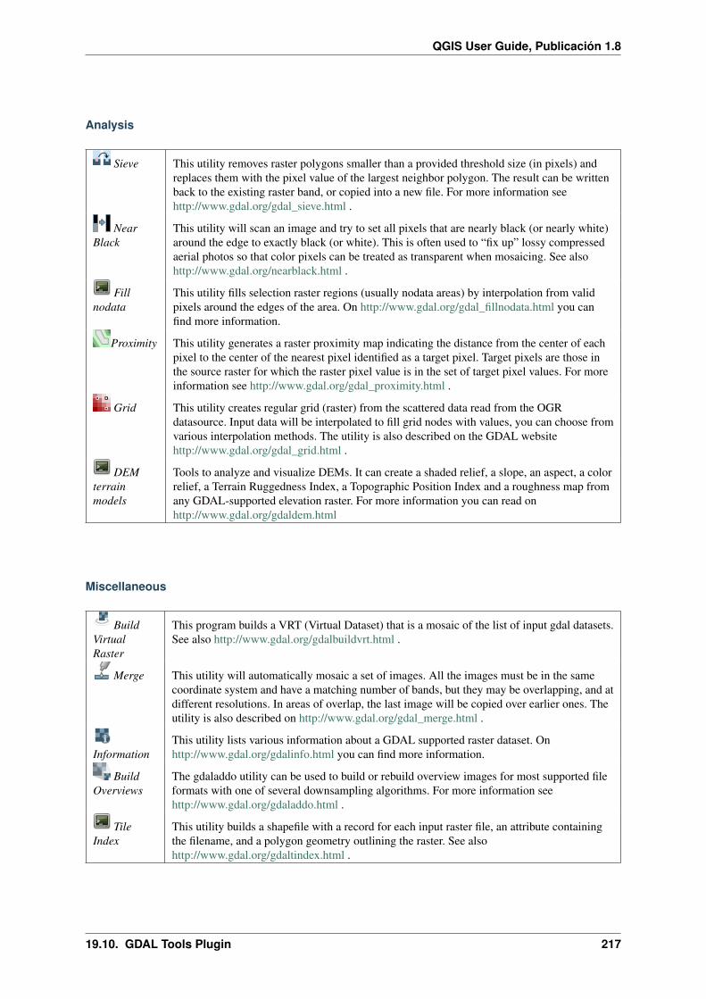
QGIS User Guide, Publicación 1.8
Analysis
Sieve This utility removes raster polygons smaller than a provided threshold size (in pixels) andreplaces them with the pixel value of the largest neighbor polygon. The result can be writtenback to the existing raster band, or copied into a new file. For more information seehttp://www.gdal.org/gdal_sieve.html .
NearBlack
This utility will scan an image and try to set all pixels that are nearly black (or nearly white)around the edge to exactly black (or white). This is often used to “fix up” lossy compressedaerial photos so that color pixels can be treated as transparent when mosaicing. See alsohttp://www.gdal.org/nearblack.html .
Fillnodata
This utility fills selection raster regions (usually nodata areas) by interpolation from validpixels around the edges of the area. On http://www.gdal.org/gdal_fillnodata.html you canfind more information.
Proximity This utility generates a raster proximity map indicating the distance from the center of eachpixel to the center of the nearest pixel identified as a target pixel. Target pixels are those inthe source raster for which the raster pixel value is in the set of target pixel values. For moreinformation see http://www.gdal.org/gdal_proximity.html .
Grid This utility creates regular grid (raster) from the scattered data read from the OGRdatasource. Input data will be interpolated to fill grid nodes with values, you can choose fromvarious interpolation methods. The utility is also described on the GDAL websitehttp://www.gdal.org/gdal_grid.html .
DEMterrainmodels
Tools to analyze and visualize DEMs. It can create a shaded relief, a slope, an aspect, a colorrelief, a Terrain Ruggedness Index, a Topographic Position Index and a roughness map fromany GDAL-supported elevation raster. For more information you can read onhttp://www.gdal.org/gdaldem.html
Miscellaneous
BuildVirtualRaster
This program builds a VRT (Virtual Dataset) that is a mosaic of the list of input gdal datasets.See also http://www.gdal.org/gdalbuildvrt.html .
Merge This utility will automatically mosaic a set of images. All the images must be in the samecoordinate system and have a matching number of bands, but they may be overlapping, and atdifferent resolutions. In areas of overlap, the last image will be copied over earlier ones. Theutility is also described on http://www.gdal.org/gdal_merge.html .
InformationThis utility lists various information about a GDAL supported raster dataset. Onhttp://www.gdal.org/gdalinfo.html you can find more information.
BuildOverviews
The gdaladdo utility can be used to build or rebuild overview images for most supported fileformats with one of several downsampling algorithms. For more information seehttp://www.gdal.org/gdaladdo.html .
TileIndex
This utility builds a shapefile with a record for each input raster file, an attribute containingthe filename, and a polygon geometry outlining the raster. See alsohttp://www.gdal.org/gdaltindex.html .
19.10. GDAL Tools Plugin 217
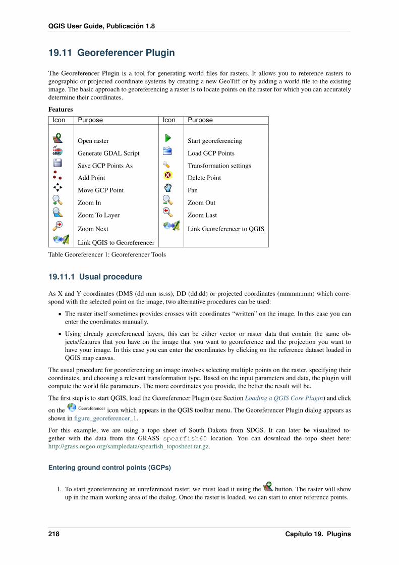
QGIS User Guide, Publicación 1.8
19.11 Georeferencer Plugin
The Georeferencer Plugin is a tool for generating world files for rasters. It allows you to reference rasters togeographic or projected coordinate systems by creating a new GeoTiff or by adding a world file to the existingimage. The basic approach to georeferencing a raster is to locate points on the raster for which you can accuratelydetermine their coordinates.
FeaturesIcon Purpose Icon Purpose
Open raster Start georeferencing
Generate GDAL Script Load GCP Points
Save GCP Points As Transformation settings
Add Point Delete Point
Move GCP Point Pan
Zoom In Zoom Out
Zoom To Layer Zoom Last
Zoom Next Link Georeferencer to QGIS
Link QGIS to Georeferencer
Table Georeferencer 1: Georeferencer Tools
19.11.1 Usual procedure
As X and Y coordinates (DMS (dd mm ss.ss), DD (dd.dd) or projected coordinates (mmmm.mm) which corre-spond with the selected point on the image, two alternative procedures can be used:
The raster itself sometimes provides crosses with coordinates “written” on the image. In this case you canenter the coordinates manually.
Using already georeferenced layers, this can be either vector or raster data that contain the same ob-jects/features that you have on the image that you want to georeference and the projection you want tohave your image. In this case you can enter the coordinates by clicking on the reference dataset loaded inQGIS map canvas.
The usual procedure for georeferencing an image involves selecting multiple points on the raster, specifying theircoordinates, and choosing a relevant transformation type. Based on the input parameters and data, the plugin willcompute the world file parameters. The more coordinates you provide, the better the result will be.
The first step is to start QGIS, load the Georeferencer Plugin (see Section Loading a QGIS Core Plugin) and click
on the Georeferencer icon which appears in the QGIS toolbar menu. The Georeferencer Plugin dialog appears asshown in figure_georeferencer_1.
For this example, we are using a topo sheet of South Dakota from SDGS. It can later be visualized to-gether with the data from the GRASS spearfish60 location. You can download the topo sheet here:http://grass.osgeo.org/sampledata/spearfish_toposheet.tar.gz.
Entering ground control points (GCPs)
1. To start georeferencing an unreferenced raster, we must load it using the button. The raster will showup in the main working area of the dialog. Once the raster is loaded, we can start to enter reference points.
218 Capítulo 19. Plugins
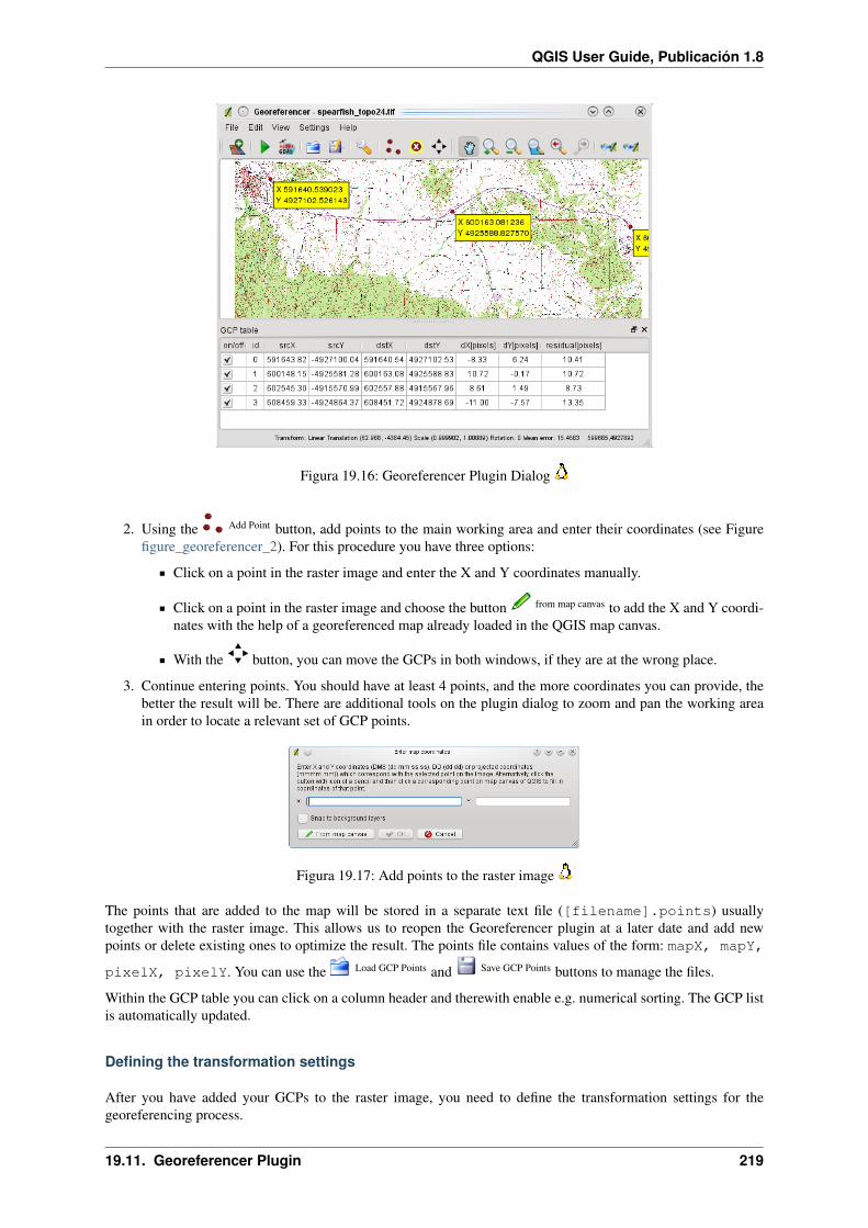
QGIS User Guide, Publicación 1.8
Figura 19.16: Georeferencer Plugin Dialog
2. Using the Add Point button, add points to the main working area and enter their coordinates (see Figurefigure_georeferencer_2). For this procedure you have three options:
Click on a point in the raster image and enter the X and Y coordinates manually.
Click on a point in the raster image and choose the button from map canvas to add the X and Y coordi-nates with the help of a georeferenced map already loaded in the QGIS map canvas.
With the button, you can move the GCPs in both windows, if they are at the wrong place.
3. Continue entering points. You should have at least 4 points, and the more coordinates you can provide, thebetter the result will be. There are additional tools on the plugin dialog to zoom and pan the working areain order to locate a relevant set of GCP points.
Figura 19.17: Add points to the raster image
The points that are added to the map will be stored in a separate text file ([filename].points) usuallytogether with the raster image. This allows us to reopen the Georeferencer plugin at a later date and add newpoints or delete existing ones to optimize the result. The points file contains values of the form: mapX, mapY,
pixelX, pixelY. You can use the Load GCP Points and Save GCP Points buttons to manage the files.
Within the GCP table you can click on a column header and therewith enable e.g. numerical sorting. The GCP listis automatically updated.
Defining the transformation settings
After you have added your GCPs to the raster image, you need to define the transformation settings for thegeoreferencing process.
19.11. Georeferencer Plugin 219
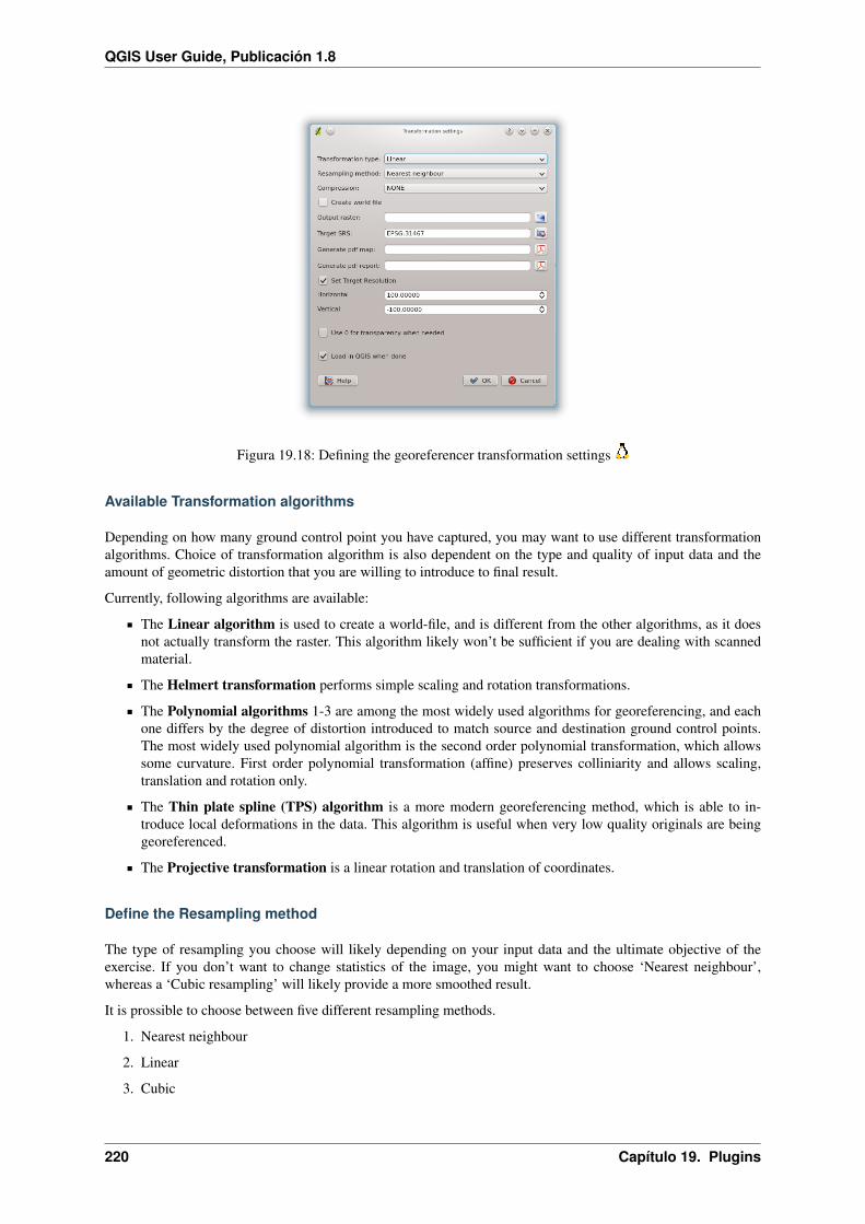
QGIS User Guide, Publicación 1.8
Figura 19.18: Defining the georeferencer transformation settings
Available Transformation algorithms
Depending on how many ground control point you have captured, you may want to use different transformationalgorithms. Choice of transformation algorithm is also dependent on the type and quality of input data and theamount of geometric distortion that you are willing to introduce to final result.
Currently, following algorithms are available:
The Linear algorithm is used to create a world-file, and is different from the other algorithms, as it doesnot actually transform the raster. This algorithm likely won’t be sufficient if you are dealing with scannedmaterial.
The Helmert transformation performs simple scaling and rotation transformations.
The Polynomial algorithms 1-3 are among the most widely used algorithms for georeferencing, and eachone differs by the degree of distortion introduced to match source and destination ground control points.The most widely used polynomial algorithm is the second order polynomial transformation, which allowssome curvature. First order polynomial transformation (affine) preserves colliniarity and allows scaling,translation and rotation only.
The Thin plate spline (TPS) algorithm is a more modern georeferencing method, which is able to in-troduce local deformations in the data. This algorithm is useful when very low quality originals are beinggeoreferenced.
The Projective transformation is a linear rotation and translation of coordinates.
Define the Resampling method
The type of resampling you choose will likely depending on your input data and the ultimate objective of theexercise. If you don’t want to change statistics of the image, you might want to choose ‘Nearest neighbour’,whereas a ‘Cubic resampling’ will likely provide a more smoothed result.
It is prossible to choose between five different resampling methods.
1. Nearest neighbour
2. Linear
3. Cubic
220 Capítulo 19. Plugins

QGIS User Guide, Publicación 1.8
4. Cubic Spline
5. Lanczos
Define the transformation settings
There are several options that need to be defined for the georeferenced output raster.
The checkbox Create world file is only available, if you decide to use the linear transformation type,because this means that the raster image actually won’t be transformed. In this case, the field Output rasteris not activated, because only a new world-file will be created.
For all other transformation type you have to define an Output raster. As default a new file ([file-name]_modified) will be created in the same folder together with the original raster image.
As a next step you have to define the Target SRS (Spatial Reference System) for the georeferenced raster(see section Working with Projections).
If you like, you can generate a pdf map and also a pdf report. The report includes information about theused transformation parameters. An image of the residuals and a list with all GCPs and their RMS errors.
Furthermore you can activate the Set Target Resolution checkbox and define pixel resolution of theoutput raster. Default horizontal and vertical resolution is 1,
The Use 0 for transparency when needed can be activated, if pixels with the value 0 shall be visualizedtransparent. In our example toposheet all white areas would be transparent.
Finally Load in QGIS when done loads the output raster automatically into the QGIS map canvas whenthe transformation is done.
Show and adapt raster properties
Clicking on the Raster properties dialog in the Settings menu opens the raster properties of the layer that you wantto georeference.
Configure the georeferencer
You can define if you want to show GCP coordiniates and/or IDs.
As residual units pixels and map units can be chosen.
For the PDF report a left and right margin can be defined and you can also set the paper size for the PDFmap.
Finally you can activate to show georeferencer window docked.
Running the transformation
After all GCPs have been collected and all transformation settings are defined, just press the buttonStart georeferencing to create the new georeferenced raster.
19.12 Interpolation Plugin
The Interplation plugin can be used to generate a TIN or IDW interpolation of a point vector layer. It is verysimple to handle and provides an intuitive graphical user interface for creating interpolated raster layers (SeeFigure_interpolation_1). The plugin requires the following parameters to be specified before running:
19.12. Interpolation Plugin 221

QGIS User Guide, Publicación 1.8
Input vector layer: Specify the input point vector layer(s) from a list of loaded point layers. If severallayers are specified, then data from all layers is used for interpolation. Note: It is possible to insert lines orpolygons as constraints for the triangulation, by specifying either “points”, “structure lines” or “break lines”
in the Type combobox.
Interpolation attribute: Select attribute column to be used for interpolation or enable the Use Z-Coordinate checkbox to use the layers stored Z values.
Interpolation Method: Select interpolation method. This can be either ‘Triangulated Irregular Network(TIN)’ or ‘Inverse Distance Weighted (IDW)’.
Number of columns/rows: Specify the number row and colums for the output raster file.
Output file: Specify a name for the output raster file.
Figura 19.19: Interpolation Plugin
19.12.1 Using the plugin
1. Start QGIS and load a point vector layer (e.g., elevp.csv).
2. Load the Interpolation plugin in the Plugin Manager (see Section Loading a QGIS Core Plugin) and click
on the Interpolation icon which appears in the QGIS toolbar menu. The Interpolation plugin dialog appearsas shown in Figure_interpolation_1.
3. Select an input layer (e.g., elevp ) and column (e.g., ELEV) for interpolation.
4. Select an interpolation method (e.g. ‘Triangulated Irregular Network (TIN)’), and specify a cellsize of 5000as well as the raster output filename (e.g., elevation_tin).
5. Click [OK].
6. For the current example, double click elevation_tin in the layer list to open the raster Layer Properties
dialog and select ‘Pseudocolor’ as Color Map in the Symbology tab. Or you can define a new colortable as described in section Working with Raster Data.
19.13 MapServer Export Plugin
You can use QGIS to ‘compose’ your map by adding and arranging layers, symbolizing them, customizing thecolors and then creating a map file for MapServer.
Nota: Currently the plugin only works when you use ‘Old Symbology’ in QGIS. ‘New Symbology’ is not yetsupported.
222 Capítulo 19. Plugins

QGIS User Guide, Publicación 1.8
19.13.1 Creating the Project File
The MapServer Export Plugin operates on a saved QGIS project file and not on the current contents of the mapcanvas and legend. This has been a source of confusion for a number of users. As described below, before you startusing the MapServer Export Plugin, you need to arrange the raster and vector layers you want to use in MapServerand save this status in a QGIS project file.
Figura 19.20: Arrange raster and vector layers for QGIS project file
In this example, we demonstrate the four steps required to create a simple project file which can be used to createthe MapServer map file. We use raster and vector files from the QGIS sample dataset Sample Data.
1. Add the raster layer landcover.tif clicking on the Add Raster Layer icon.
2. Add the vector Shapefiles lakes.shp, majrivers.shp and airports.shp from the QGIS sample
dataset clicking on the Add Vector Layer icon.
3. Change the colors and symbolize the data as you like (for example see figure_mapserver_export_1)
4. Save a new project named mapserverproject.qgs using File → Save Project.
19.13.2 Creating the Map File
To use the Mapserver Export plugin from within QGIS, you need to enable the MapServer Export Plugin firstusing the Plugin Manager (see Loading a QGIS Core Plugin).
19.13. MapServer Export Plugin 223
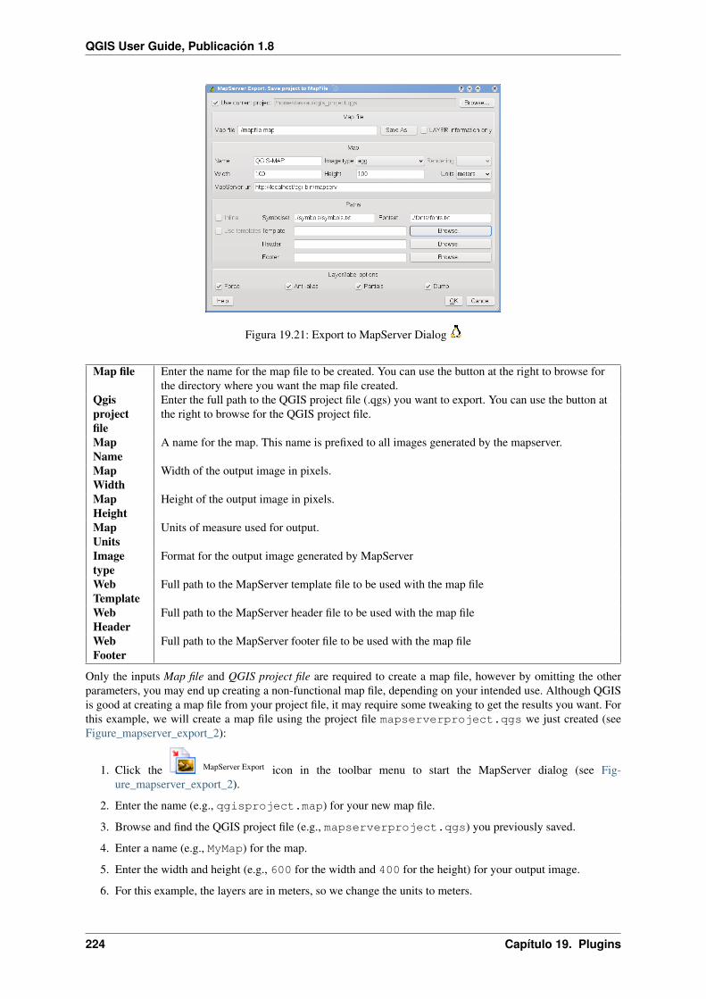
QGIS User Guide, Publicación 1.8
Figura 19.21: Export to MapServer Dialog
Map file Enter the name for the map file to be created. You can use the button at the right to browse forthe directory where you want the map file created.
Qgisprojectfile
Enter the full path to the QGIS project file (.qgs) you want to export. You can use the button atthe right to browse for the QGIS project file.
MapName
A name for the map. This name is prefixed to all images generated by the mapserver.
MapWidth
Width of the output image in pixels.
MapHeight
Height of the output image in pixels.
MapUnits
Units of measure used for output.
Imagetype
Format for the output image generated by MapServer
WebTemplate
Full path to the MapServer template file to be used with the map file
WebHeader
Full path to the MapServer header file to be used with the map file
WebFooter
Full path to the MapServer footer file to be used with the map file
Only the inputs Map file and QGIS project file are required to create a map file, however by omitting the otherparameters, you may end up creating a non-functional map file, depending on your intended use. Although QGISis good at creating a map file from your project file, it may require some tweaking to get the results you want. Forthis example, we will create a map file using the project file mapserverproject.qgs we just created (seeFigure_mapserver_export_2):
1. Click the MapServer Export icon in the toolbar menu to start the MapServer dialog (see Fig-ure_mapserver_export_2).
2. Enter the name (e.g., qgisproject.map) for your new map file.
3. Browse and find the QGIS project file (e.g., mapserverproject.qgs) you previously saved.
4. Enter a name (e.g., MyMap) for the map.
5. Enter the width and height (e.g., 600 for the width and 400 for the height) for your output image.
6. For this example, the layers are in meters, so we change the units to meters.
224 Capítulo 19. Plugins

QGIS User Guide, Publicación 1.8
7. Choose png for the image type.
8. Click [OK] to generate the new map file qgisproject.map. QGIS displays the success of your efforts.
Figura 19.22: Export to MapServer Succesfull Dialog
You can view the map file in any text editor or visualizer. If you take a look, you’ll notice that the export tool addsthe metadata needed to enable our map file for WMS.
19.13.3 Troubleshooting
If you get error messages from mapserver like:
loadSymbolSet(): Unable to access file. (./symbols/symbols.txt)
or:
msLoadFontset(): Unable to access file. Error opening fontset ./fonts/fonts.txt.
This means that that the map file is requesting for fonts or symbol definition files but that Mapserver cannot findthose.
Either comment the lines containing those names in the map file (this is possible if you do not have labels or usestyles from the symbols.txt). Or create those files (see below).
The most simple fonts.txt file (because arial is used in the QGIS generated map files) contains the followingline
# either relative to the map file or a full path:arial /usr/share/fonts/truetype/msttcorefonts/arial.ttf
The most simple symbols.txt file contains the definition of a circle symbol (because a circle symbol is usedfor point layers)
SYMBOLSETSYMBOLNAME "circle"TYPE ellipseFILLED truePOINTS1 1ENDEND
END
19.13. MapServer Export Plugin 225
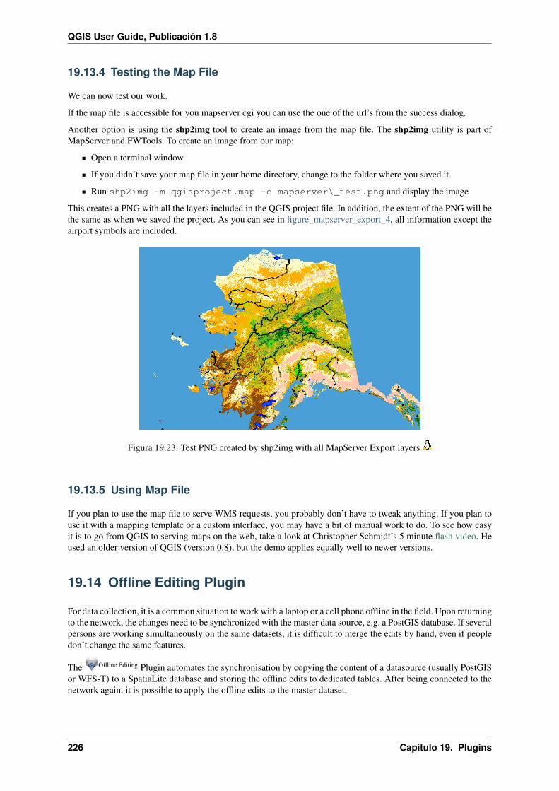
QGIS User Guide, Publicación 1.8
19.13.4 Testing the Map File
We can now test our work.
If the map file is accessible for you mapserver cgi you can use the one of the url’s from the success dialog.
Another option is using the shp2img tool to create an image from the map file. The shp2img utility is part ofMapServer and FWTools. To create an image from our map:
Open a terminal window
If you didn’t save your map file in your home directory, change to the folder where you saved it.
Run shp2img -m qgisproject.map -o mapserver\_test.png and display the image
This creates a PNG with all the layers included in the QGIS project file. In addition, the extent of the PNG will bethe same as when we saved the project. As you can see in figure_mapserver_export_4, all information except theairport symbols are included.
Figura 19.23: Test PNG created by shp2img with all MapServer Export layers
19.13.5 Using Map File
If you plan to use the map file to serve WMS requests, you probably don’t have to tweak anything. If you plan touse it with a mapping template or a custom interface, you may have a bit of manual work to do. To see how easyit is to go from QGIS to serving maps on the web, take a look at Christopher Schmidt’s 5 minute flash video. Heused an older version of QGIS (version 0.8), but the demo applies equally well to newer versions.
19.14 Offline Editing Plugin
For data collection, it is a common situation to work with a laptop or a cell phone offline in the field. Upon returningto the network, the changes need to be synchronized with the master data source, e.g. a PostGIS database. If severalpersons are working simultaneously on the same datasets, it is difficult to merge the edits by hand, even if peopledon’t change the same features.
The Offline Editing Plugin automates the synchronisation by copying the content of a datasource (usually PostGISor WFS-T) to a SpatiaLite database and storing the offline edits to dedicated tables. After being connected to thenetwork again, it is possible to apply the offline edits to the master dataset.
226 Capítulo 19. Plugins
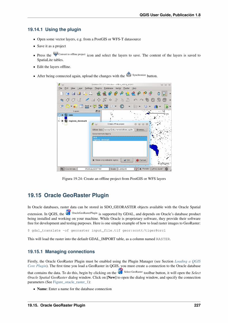
QGIS User Guide, Publicación 1.8
19.14.1 Using the plugin
Open some vector layers, e.g. from a PostGIS or WFS-T datasource
Save it as a project
Press the Convert to offline project icon and select the layers to save. The content of the layers is saved toSpatiaLite tables.
Edit the layers offline.
After being connected again, upload the changes with the Synchronize button.
Figura 19.24: Create an offline project from PostGIS or WFS layers
19.15 Oracle GeoRaster Plugin
In Oracle databases, raster data can be stored in SDO_GEORASTER objects available with the Oracle Spatial
extension. In QGIS, the OracleGeoRasterPlugin is supported by GDAL, and depends on Oracle’s database productbeing installed and working on your machine. While Oracle is proprietary software, they provide their softwarefree for development and testing purposes. Here is one simple example of how to load raster images to GeoRaster:
$ gdal_translate -of georaster input_file.tif geor:scott/tiger@orcl
This will load the raster into the default GDAL_IMPORT table, as a column named RASTER.
19.15.1 Managing connections
Firstly, the Oracle GeoRaster Plugin must be enabled using the Plugin Manager (see Section Loading a QGISCore Plugin). The first time you load a GeoRaster in QGIS, you must create a connection to the Oracle database
that contains the data. To do this, begin by clicking on the Select GeoRaster toolbar button, it will open the SelectOracle Spatial GeoRaster dialog window. Click on [New] to open the dialog window, and specify the connectionparameters (See Figure_oracle_raster_1):
Name: Enter a name for the database connection
19.15. Oracle GeoRaster Plugin 227

QGIS User Guide, Publicación 1.8
Database instance: Enter the name of the database that you will connect to
Username: Specify your own username that you will use to access the database
Password: The password associated with your username that is required to access the database
Figura 19.25: Create Oracle connection dialog
Now, back on the main Oracle Spatial GeoRaster dialog window (see Figure_oracle_raster_2), use the drop-downlist to choose one connection, and use the [Connect] button to establish a connection. You may also [Edit] theconnection by opening the previous dialog and making changes to the connection information, or use the [Delete]button to remove the connection from the drop-down list.
19.15.2 Selecting a GeoRaster
Once a connection has been established, the sub-datasets window will show the names of all the tables that containsGeoRaster columns in that database in the format of a GDAL subdataset name.
Click on one of the listed subdatasets and then click on [Select] to choose the table name. Now another list ofsubdatasets will show with the names of GeoRaster columns on that table. This is usually a short list, since mostusers will not have more than one or two GeoRaster columns on the same table.
Click on one of the listed subdatasets and then click on [Select] to choose one of the the table/column combination.The dialog will now show all the rows that contains GeoRaster objects. Note that the subdataset list will now showthe Raster Data Table and Raster Id’s pairs.
At anytime the Selection entry can be edited in order to go directly to a known GeoRaster or to go back to thebeginning and select another table name.
The Selection data entry can also be used to enter a Where clause at the end of the iden-tification string, e.g. geor:scott/tiger@orcl,gdal_import,raster,geoid=. Seehttp://www.gdal.org/frmt_georaster.html for more information.
19.15.3 Displaying GeoRaster
Finally, by selecting a GeoRaster from the list of Raster Data Table and Raster Id’s, the raster image will be loadedinto QGIS.
The Select Oracle Spatial GeoRaster dialog can be closed now and next time it opens it will keep the sameconnection, and will show the same previous list of subdataset making it very easy to open up another image fromthe same context.
Nota: GeoRasters that contains pyramids will display much faster but the pyramids need to be generated outsideof QGIS using Oracle PL/SQL or gdaladdo.
The following is example using gdaladdo:
228 Capítulo 19. Plugins

QGIS User Guide, Publicación 1.8
Figura 19.26: Select Oracle GeoRaster dialog
gdaladdo georaster:scott/tiger@orcl,georaster\_table,georaster,georid=6 \-r nearest 2 4 6 8 16 32
This is an example using PL/SQL:
$ sqlplus scott/tigerSQL> DECLAREgr sdo_georaster;
BEGINSELECT image INTO gr FROM cities WHERE id = 1 FOR UPDATE;sdo_geor.generatePyramid(gr, ’rLevel=5, resampling=NN’);UPDATE cities SET image = gr WHERE id = 1;COMMIT;
END;
19.16 Raster Terrain Analysis Plugin
The Raster Terrain Analysis Plugin can be used to calculate the slope, aspect, hillshade, ruggedness indexand relief for digital elevation models (DEM). It is very simple to handle and provides an intuitive graphical userinterface for creating new raster layers (See Figure_raster_terrain_1).
Description of the analysis:
Slope: Calculates slope angle for each cell in degrees (based on first order derivative estimation).
Aspect: Exposition (starting with 0 for north direction, in degrees counterclockwise).
Hillshade: Create shaded map using light and shadow to provide a more three-dimensional appearance fora shaded relief map.
Ruggedness Index: A quantitative measurement of terrain heterogeneity as described by Riley et al. (1999).It is calculated for every location, by summarizing the change in elevation within the 3x3 pixel grid.
Relief: Creating a shaded relief map from digital elevation data. Implemented is a method to choose theelevation colors analysing the frequency distribution.
19.16. Raster Terrain Analysis Plugin 229
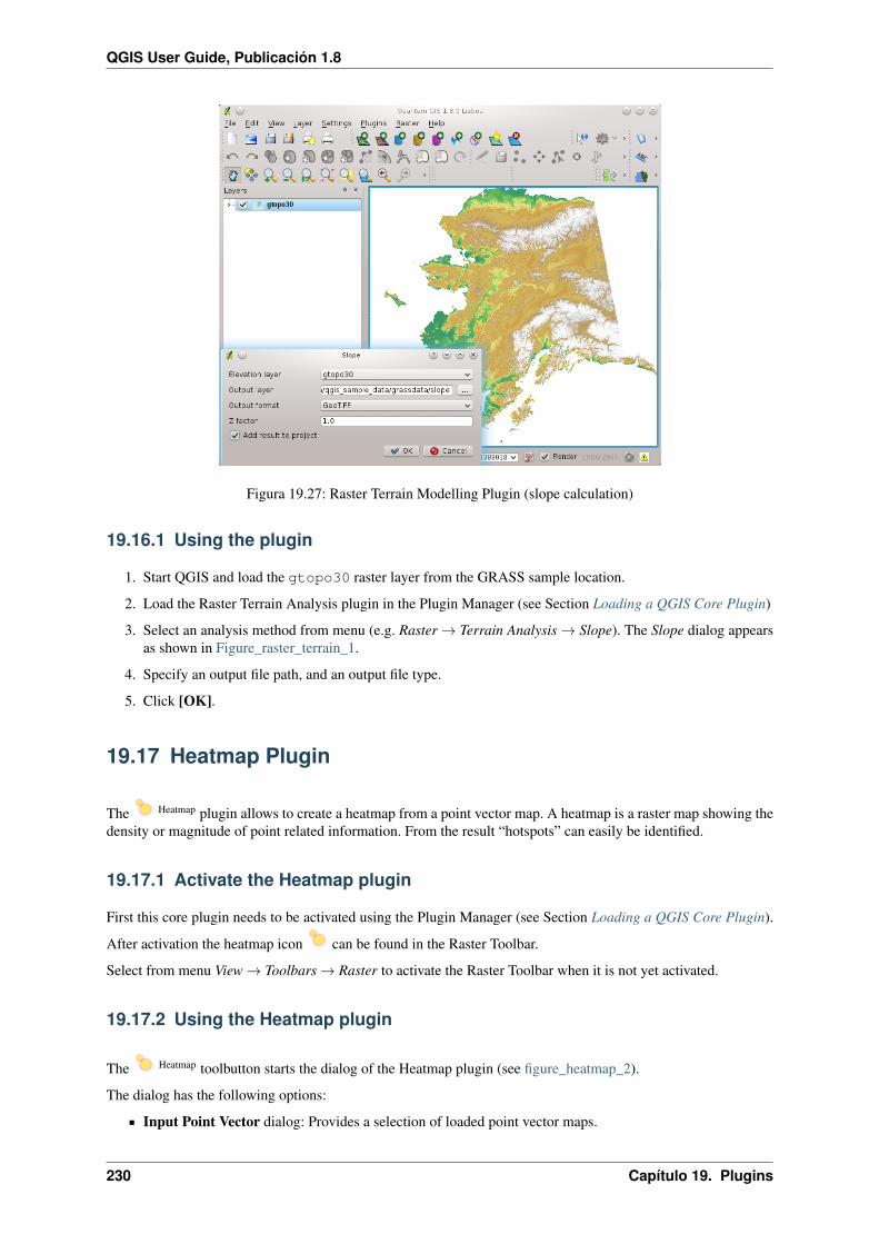
QGIS User Guide, Publicación 1.8
Figura 19.27: Raster Terrain Modelling Plugin (slope calculation)
19.16.1 Using the plugin
1. Start QGIS and load the gtopo30 raster layer from the GRASS sample location.
2. Load the Raster Terrain Analysis plugin in the Plugin Manager (see Section Loading a QGIS Core Plugin)
3. Select an analysis method from menu (e.g. Raster → Terrain Analysis → Slope). The Slope dialog appearsas shown in Figure_raster_terrain_1.
4. Specify an output file path, and an output file type.
5. Click [OK].
19.17 Heatmap Plugin
The Heatmap plugin allows to create a heatmap from a point vector map. A heatmap is a raster map showing thedensity or magnitude of point related information. From the result “hotspots” can easily be identified.
19.17.1 Activate the Heatmap plugin
First this core plugin needs to be activated using the Plugin Manager (see Section Loading a QGIS Core Plugin).
After activation the heatmap icon can be found in the Raster Toolbar.
Select from menu View → Toolbars → Raster to activate the Raster Toolbar when it is not yet activated.
19.17.2 Using the Heatmap plugin
The Heatmap toolbutton starts the dialog of the Heatmap plugin (see figure_heatmap_2).
The dialog has the following options:
Input Point Vector dialog: Provides a selection of loaded point vector maps.
230 Capítulo 19. Plugins

QGIS User Guide, Publicación 1.8
Output Raster: Using the button you select the folder and the name of the output raster the Heatmapplugin will generate. It is not necessary to give a file extension
Output Format: Selection of the output format. Although all formats supported by GDAL can be choosen,GeoTIFF is most in cases the best format to choose.
Radius: can be used to give the radius in meters or mapunit. When the radius is choosen too small you willnot get a nice heatmap. In places where more circles around points overlap eachother the brighter hotspotswill occur!
Decay Ratio: is used to show with which ratio the heat dies out from the center.
• When 0 is given (=minimum) the heat will be concentrated in the centre of given radius and be com-pletely extinguished at the edge.
• When 10 is given (=maximum) the heat is concentrated at the edge and in the centre it is completelyextinguished. Higher given values are allowed but have no effect.
• When 1 is given the heat is spread evenly over the whole circle.
• When a negative Decay Ratio is given you will create a Coolmap instead of a Heatmap!
When the Advanced checkbox is checked it will give acces to additional advanced options.
Row and Column, can be used to change the pixelsize of the output raster. More rows and colums meansa smaller pixelsize and the size of the output file will become bigger and processing a bit slower. Whendoubling the number of rows this will automatically double the size of Columns and the cell sizes will alsobe halved. The area of the output raster will remain the same!
Cell Size X and Cell Size Y influence the pixelsize of the output raster and will also change the rows andcolumns.
The point vector layer may have attribute fields that can be used to create a heatmap:
Use Radius from Field: the radius set from an attribute field.
Use Weight from field: the weight factor set from an attribute field.
When the output raster is given, the [OK] button can be used to create a heatmap. The first result is a grey surfacethat still needs to be given additional treatment to make it a heatmap.
Advertencia: Changing the raster size propertiesWhen changing the raster size properties, this also changes the resulting output. The hotspot areas will becomebigger.
19.17.3 Creating a Heatmap
For the following example, we will use the airports vector point layer from the QGIS sample dataset (see Sam-ple Data). Another exellent QGIS tutorial on making heatmaps can be found on http://qgis.spatialthoughts.com.
In Figure_Heatmap_1 the airports of Alaska are shown.
1. Select the Heatmap toolbutton. The heatmap dialog starts (see Figure_Heatmap_2).
2. In field Input Point Vector select airpoirt from the list of point layers loaded in current project.
3. In field Output Raster give the name and location using the button of the output raster. Give the outputraster file the name heatmap_airports to give an file extension is not necessary.
4. In field Output Format choose GeoTIFF.
5. In the field Radius give 1000000 meters.
6. The original Decay Ratio of 0.1 is fine.
19.17. Heatmap Plugin 231

QGIS User Guide, Publicación 1.8
Figura 19.28: Airports of Alaska
7. Click on [OK] to create and load the new raster map (see Figure_Heatmap_3).
Figura 19.29: The Heatmap Dialog
The result after loading the heatmap is probably not the result which was expected. It is still a grey even surfacenot showing any variation. First some additional configuration of this layer needs to be done to make the heatmappresent itself.
1. Open the properties dialog of layer heatmap_airports (select the layer heatmap_airports, opencontext menu with right mouse button and select Properties).
2. Select the Symbology tab.
3. Change Color map from ‘Grayscale’ to ‘Pseudocolor’.
4. Press the [Apply] button.
5. Switch to the Transparency tab and set Global transparency to 40 %.
6. Select [OK]
The final result is shown in Figure_Heatmap_4.
19.18 Road Graph Plugin
The Road Graph Plugin is a C++ plugin for QGIS, that calculates the shortest path between two points on anypolyline layer and plots this path over the road network.
Main features:
232 Capítulo 19. Plugins
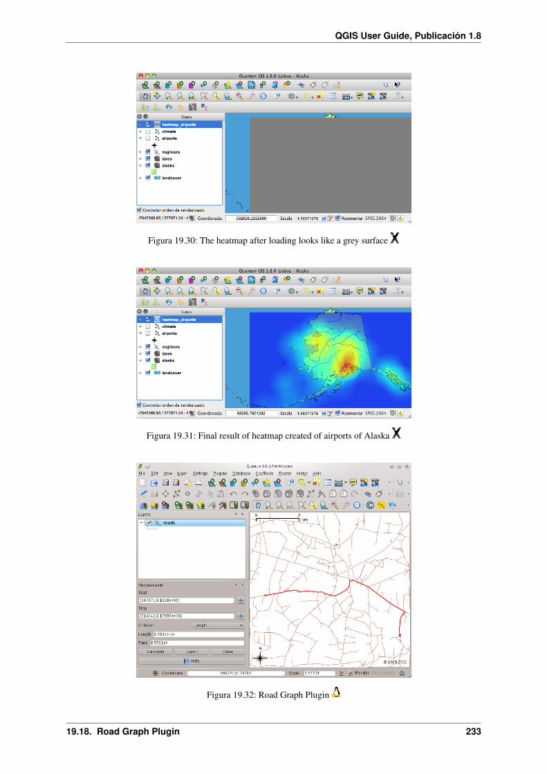
QGIS User Guide, Publicación 1.8
Figura 19.30: The heatmap after loading looks like a grey surface
Figura 19.31: Final result of heatmap created of airports of Alaska
Figura 19.32: Road Graph Plugin
19.18. Road Graph Plugin 233

QGIS User Guide, Publicación 1.8
calculate path, it’s length and travel time
optimize by length or by travel time
export path to a vector layer
highlight roads directions (this is slow and used mainly for debug purposes and for the settings testing)
As a roads layer you can use any polyline vector layer in any QGIS supported format. Two lines with a commonpoint are considered connected. Please note, it is required to use layer CRS as project CRS while editing roadslayer. This is due to the fact that recalculation of the coordinates between different CRS introduce some errors thatcan result in discontinuities, even when ‘snapping’ is used.
In the layer attribute table the following fields can be used:
speed on road section — numeric field;
direction — any type, that can be casted to string. Forward and reverse directions are correspond to theone-way road, both directions — two-way road
If some fields don’t have any value or do not exist — default values are used. You can change defaults and someplugin settings in plugin settings dialog.
19.18.1 Using the plugin
After plugin activation you will see an additional panel on the left side of the main QGIS window. Now makesome definitions to the Road graph plugin settings dialog in the menu Vector → Road Graph.
Select a Start and a Stop point in the road network layer and click on [Calculate].
19.19 Spatial Query Plugin
The Spatial Query plugin allows to make a spatial query (select features) in a target layer with reference to anotherlayer. The functionality is based on the GEOS library and depends on the selected source feature layer.
Possible operators are:
Contains
Equals
Overlap
Crosses
Intersects
Is disjoint
Touches
Within
19.19.1 Using the plugin
As an example we want to find regions in the Alaska dataset that contain airports. Following steps are necessary:
1. Start QGIS and load the vector layers regions.shp and airports.shp.
2. Load the Spatial Query plugin in the Plugin Manager (see Section Loading a QGIS Core Plugin) and click
on the Spatial Query icon which appears in the QGIS toolbar menu. The plugin dialog appears.
3. Select layer regions as source layer and airports as reference feature layer.
234 Capítulo 19. Plugins

QGIS User Guide, Publicación 1.8
4. Select ‘Contains’ as operator and click [Apply].
Now you get a list of feature IDs from the query and you have several options as shown in figure_spatial_query_1.
Click on the Create layer with list of items
Select an ID from the list and click on Create layer with selected
Select the ‘Remove from current selection’ in the field And use the result to .
Additionally you can Zoom to item or display Log messages.
Figura 19.33: Spatial Query analysis - regions contain airports
19.20 SPIT Plugin
QGIS comes with a plugin named SPIT (Shapefile to PostGIS Import Tool). SPIT can be used to load multipleshapefiles at one time and includes support for schemas. To use SPIT, open the Plugin Manager from the Plugins
menu, check the box next to the SPIT plugin and click [OK]. The SPIT icon will be added to the plugin toolbar.
To import a shapefile, click on the SPIT tool in the toolbar to open the SPIT - Shapefile to PostGIS ImportTool dialog. Select the PostGIS database you want to connect to and click on [Connect]. If you want, you candefine or change some import options. Now you can add one or more files to the queue by clicking on the [Add]button. To process the files, click on the [OK] button. The progress of the import as well as any errors/warningswill be displayed as each shapefile is processed.
Truco: Importing Shapefiles Containing PostgreSQL Reserved WordsIf a shapefile is added to the queue containing fields that are reserved words in the PostgreSQL database a dialogwill popup showing the status of each field. You can edit the field names prior to import and change any that arereserved words (or change any other field names as desired). Attempting to import a shapefile with reserved wordsas field names will likely fail.
19.20. SPIT Plugin 235

QGIS User Guide, Publicación 1.8
Figura 19.34: Using SPIT Plugin to import Shape files to PostGIS
19.21 SQL Anywhere Plugin
SQL Anywhere is a proprietary relational database management system (RDBMS) from Sybase. SQL Anywhereincludes spatial support including OGC, shape files etc. and built in functions to export to KML, GML and SVGformats.
Figura 19.35: SQL Anywhere dialog (KDE)
The SQL Anywhere allows to connect to spatialy enabled SQL Anywhere databases. The Add SQL Anywherelayer dialog is similar in functionality to the dialogs for PostGIS and SpatiaLite.
19.22 Zonal Statistics Plugin
With the Zonal Statistics Plugin you can analyze the results of a thematic classification. It allows to calculate severalvalues of the pixels of a raster layer with the help of a polygonal vector layer (see figure_zonal_statistics). You cancalculate the sum, the mean value and the total count of the pixels that are within a polygon. The plugin generatesoutput columns in the vector layer with a user-defined prefix.
236 Capítulo 19. Plugins

QGIS User Guide, Publicación 1.8
Figura 19.36: Zonal statistics dialog (KDE)
19.22. Zonal Statistics Plugin 237

QGIS User Guide, Publicación 1.8
238 Capítulo 19. Plugins
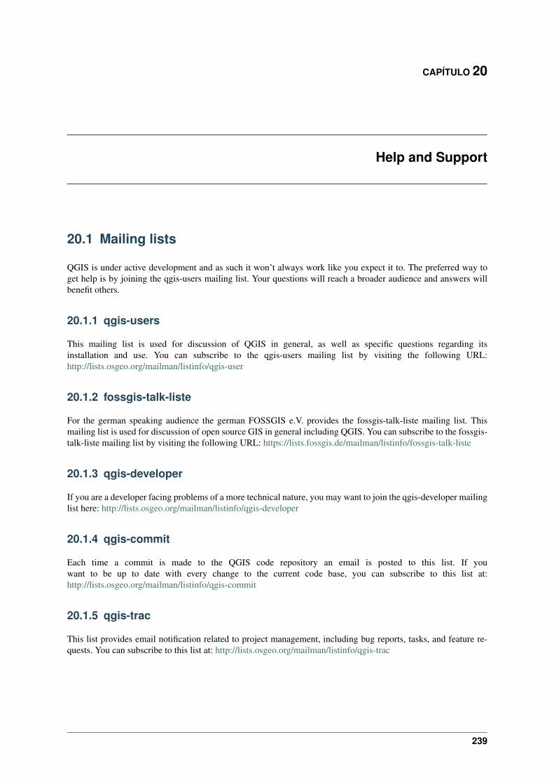
CAPÍTULO 20
Help and Support
20.1 Mailing lists
QGIS is under active development and as such it won’t always work like you expect it to. The preferred way toget help is by joining the qgis-users mailing list. Your questions will reach a broader audience and answers willbenefit others.
20.1.1 qgis-users
This mailing list is used for discussion of QGIS in general, as well as specific questions regarding itsinstallation and use. You can subscribe to the qgis-users mailing list by visiting the following URL:http://lists.osgeo.org/mailman/listinfo/qgis-user
20.1.2 fossgis-talk-liste
For the german speaking audience the german FOSSGIS e.V. provides the fossgis-talk-liste mailing list. Thismailing list is used for discussion of open source GIS in general including QGIS. You can subscribe to the fossgis-talk-liste mailing list by visiting the following URL: https://lists.fossgis.de/mailman/listinfo/fossgis-talk-liste
20.1.3 qgis-developer
If you are a developer facing problems of a more technical nature, you may want to join the qgis-developer mailinglist here: http://lists.osgeo.org/mailman/listinfo/qgis-developer
20.1.4 qgis-commit
Each time a commit is made to the QGIS code repository an email is posted to this list. If youwant to be up to date with every change to the current code base, you can subscribe to this list at:http://lists.osgeo.org/mailman/listinfo/qgis-commit
20.1.5 qgis-trac
This list provides email notification related to project management, including bug reports, tasks, and feature re-quests. You can subscribe to this list at: http://lists.osgeo.org/mailman/listinfo/qgis-trac
239
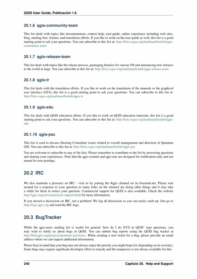
QGIS User Guide, Publicación 1.8
20.1.6 qgis-community-team
This list deals with topics like documentation, context help, user-guide, online experience including web sites,blog, mailing lists, forums, and translation efforts. If you like to work on the user-guide as well, this list is a goodstarting point to ask your questions. You can subscribe to this list at: http://lists.osgeo.org/mailman/listinfo/qgis-community-team
20.1.7 qgis-release-team
This list deals with topics like the release process, packaging binaries for various OS and announcing new releasesto the world at large. You can subscribe to this list at: http://lists.osgeo.org/mailman/listinfo/qgis-release-team
20.1.8 qgis-tr
This list deals with the translation efforts. If you like to work on the translation of the manuals or the graphicaluser interface (GUI), this list is a good starting point to ask your questions. You can subscribe to this list at:http://lists.osgeo.org/mailman/listinfo/qgis-tr
20.1.9 qgis-edu
This list deals with QGIS education efforts. If you like to work on QGIS education materials, this list is a goodstarting point to ask your questions. You can subscribe to this list at: http://lists.osgeo.org/mailman/listinfo/qgis-edu
20.1.10 qgis-psc
This list is used to discuss Steering Committee issues related to overall management and direction of QuantumGIS. You can subscribe to this list at: http://lists.osgeo.org/mailman/listinfo/qgis-psc
You are welcome to subscribe to any of the lists. Please remember to contribute to the list by answering questionsand sharing your experiences. Note that the qgis-commit and qgis-trac are designed for notification only and notmeant for user postings.
20.2 IRC
We also maintain a presence on IRC - visit us by joining the #qgis channel on irc.freenode.net. Please waitaround for a response to your question as many folks on the channel are doing other things and it may takea while for them to notice your question. Commercial support for QGIS is also available. Check the websitehttp://qgis.org/en/commercial-support.html for more information.
If you missed a discussion on IRC, not a problem! We log all discussion so you can easily catch up. Just go tohttp://logs.qgis.org and read the IRC-logs.
20.3 BugTracker
While the qgis-users mailing list is useful for general ‘how do I do XYZ in QGIS’ type questions, youmay wish to notify us about bugs in QGIS. You can submit bug reports using the QGIS bug tracker athttp://hub.qgis.org/projects/quantum-gis/issues. When creating a new ticket for a bug, please provide an emailaddress where we can request additional information.
Please bear in mind that your bug may not always enjoy the priority you might hope for (depending on its severity).Some bugs may require significant developer effort to remedy and the manpower is not always available for this.
240 Capítulo 20. Help and Support

QGIS User Guide, Publicación 1.8
Feature requests can be submitted as well using the same ticket system as for bugs. Please make sure to select thetype Feature.
If you have found a bug and fixed it yourself you can submit this patch also. Again, the lovely redmine ticketsystemat http://hub.qgis.org/projects/quantum-gis/issues has this type as well. Check Patch supplied checkbox andattach your patch before submitting bug. Someone of the developers will review it and apply it to QGIS. Pleasedon’t be alarmed if your patch is not applied straight away — developers may be tied up with other committments.
20.4 Blog
The QGIS-community also runs a weblog at http://www.qgis.org/planet which has some interesting articles forusers and developers as well provided by other blogs in the community. You are invited to contribute your ownQGIS blog!
20.5 Plugins
The website http://plugins.qgis.org provides the official QGIS plugins web portal. Here you find a list of all stableand experimental QGIS plugins available via the ‘Official QGIS Plugin Repository’.
20.6 Wiki
Lastly, we maintain a WIKI web site at http://hub.qgis.org/projects/quantum-gis/wiki where you can find a varietyof useful information relating to QGIS development, release plans, links to download sites, message translation-hints and so on. Check it out, there are some goodies inside!
20.4. Blog 241

QGIS User Guide, Publicación 1.8
242 Capítulo 20. Help and Support

CAPÍTULO 21
Appendix
21.1 GNU General Public License
Version 2, June 1991
Copyright (C) 1989, 1991 Free Software Foundation, Inc. 59 Temple Place - Suite 330, Boston, MA 02111-1307,USA
Everyone is permitted to copy and distribute verbatim copies of this license document, but changing it is notallowed.
Preamble
The licenses for most software are designed to take away your freedom to share and change it. By contrast,the GNU General Public License is intended to guarantee your freedom to share and change free software–tomake sure the software is free for all its users. This General Public License applies to most of the Free SoftwareFoundation’s software and to any other program whose authors commit to using it. (Some other Free SoftwareFoundation software is covered by the GNU Library General Public License instead.) You can apply it to yourprograms, too.
When we speak of free software, we are referring to freedom, not price. Our General Public Licenses are designedto make sure that you have the freedom to distribute copies of free software (and charge for this service if youwish), that you receive source code or can get it if you want it, that you can change the software or use pieces ofit in new free programs; and that you know you can do these things.
To protect your rights, we need to make restrictions that forbid anyone to deny you these rights or to ask you tosurrender the rights. These restrictions translate to certain responsibilities for you if you distribute copies of thesoftware, or if you modify it.
For example, if you distribute copies of such a program, whether gratis or for a fee, you must give the recipientsall the rights that you have. You must make sure that they, too, receive or can get the source code. And you mustshow them these terms so they know their rights.
We protect your rights with two steps: (1) copyright the software, and (2) offer you this license which gives youlegal permission to copy, distribute and/or modify the software.
Also, for each author’s protection and ours, we want to make certain that everyone understands that there is nowarranty for this free software. If the software is modified by someone else and passed on, we want its recipientsto know that what they have is not the original, so that any problems introduced by others will not reflect on theoriginal authors’ reputations.
Finally, any free program is threatened constantly by software patents. We wish to avoid the danger that redis-tributors of a free program will individually obtain patent licenses, in effect making the program proprietary. Toprevent this, we have made it clear that any patent must be licensed for everyone’s free use or not licensed at all.
The precise terms and conditions for copying, distribution and modification follow. TERMS AND CONDITIONSFOR COPYING, DISTRIBUTION AND MODIFICATION
0. This License applies to any program or other work which contains a notice placed by the copyright holdersaying it may be distributed under the terms of this General Public License. The “Program”, below, refers to
243

QGIS User Guide, Publicación 1.8
any such program or work, and a “work based on the Program” means either the Program or any derivativework under copyright law: that is to say, a work containing the Program or a portion of it, either verbatimor with modifications and/or translated into another language. (Hereinafter, translation is included withoutlimitation in the term “modification”.) Each licensee is addressed as “you”.
Activities other than copying, distribution and modification are not covered by this License; they are outsideits scope. The act of running the Program is not restricted, and the output from the Program is covered onlyif its contents constitute a work based on the Program (independent of having been made by running theProgram). Whether that is true depends on what the Program does.
1. You may copy and distribute verbatim copies of the Program’s source code as you receive it, in any medium,provided that you conspicuously and appropriately publish on each copy an appropriate copyright noticeand disclaimer of warranty; keep intact all the notices that refer to this License and to the absence of anywarranty; and give any other recipients of the Program a copy of this License along with the Program.
You may charge a fee for the physical act of transferring a copy, and you may at your option offer warrantyprotection in exchange for a fee.
2. You may modify your copy or copies of the Program or any portion of it, thus forming a work based on theProgram, and copy and distribute such modifications or work under the terms of Section 1 above, providedthat you also meet all of these conditions:
a) You must cause the modified files to carry prominent notices stating that you changed the files and thedate of any change.
b) You must cause any work that you distribute or publish, that in whole or in part contains or is derivedfrom the Program or any part thereof, to be licensed as a whole at no charge to all third parties underthe terms of this License.
c) If the modified program normally reads commands interactively when run, you must cause it, whenstarted running for such interactive use in the most ordinary way, to print or display an announcementincluding an appropriate copyright notice and a notice that there is no warranty (or else, saying thatyou provide a warranty) and that users may redistribute the program under these conditions, and tellingthe user how to view a copy of this License. (Exception: if the Program itself is interactive but doesnot normally print such an announcement, your work based on the Program is not required to print anannouncement.)
These requirements apply to the modified work as a whole. If identifiable sections of that work are notderived from the Program, and can be reasonably considered independent and separate works in themselves,then this License, and its terms, do not apply to those sections when you distribute them as separate works.But when you distribute the same sections as part of a whole which is a work based on the Program, thedistribution of the whole must be on the terms of this License, whose permissions for other licensees extendto the entire whole, and thus to each and every part regardless of who wrote it.
Thus, it is not the intent of this section to claim rights or contest your rights to work written entirely by you;rather, the intent is to exercise the right to control the distribution of derivative or collective works based onthe Program.
In addition, mere aggregation of another work not based on the Program with the Program (or with a workbased on the Program) on a volume of a storage or distribution medium does not bring the other work underthe scope of this License.
3. You may copy and distribute the Program (or a work based on it, under Section 2) in object code or exe-cutable form under the terms of Sections 1 and 2 above provided that you also do one of the following:
a) Accompany it with the complete corresponding machine-readable source code, which must be dis-tributed under the terms of Sections 1 and 2 above on a medium customarily used for software inter-change; or,
b) Accompany it with a written offer, valid for at least three years, to give any third party, for a charge nomore than your cost of physically performing source distribution, a complete machine-readable copyof the corresponding source code, to be distributed under the terms of Sections 1 and 2 above on amedium customarily used for software interchange; or,
244 Capítulo 21. Appendix
QGIS User Guide, Publicación 1.8
c) Accompany it with the information you received as to the offer to distribute corresponding sourcecode. (This alternative is allowed only for noncommercial distribution and only if you received theprogram in object code or executable form with such an offer, in accord with Subsection b above.)
The source code for a work means the preferred form of the work for making modifications to it. For anexecutable work, complete source code means all the source code for all modules it contains, plus any asso-ciated interface definition files, plus the scripts used to control compilation and installation of the executable.However, as a special exception, the source code distributed need not include anything that is normally dis-tributed (in either source or binary form) with the major components (compiler, kernel, and so on) of theoperating system on which the executable runs, unless that component itself accompanies the executable.
If distribution of executable or object code is made by offering access to copy from a designated place, thenoffering equivalent access to copy the source code from the same place counts as distribution of the sourcecode, even though third parties are not compelled to copy the source along with the object code.
4. You may not copy, modify, sublicense, or distribute the Program except as expressly provided under thisLicense. Any attempt otherwise to copy, modify, sublicense or distribute the Program is void, and willautomatically terminate your rights under this License. However, parties who have received copies, or rights,from you under this License will not have their licenses terminated so long as such parties remain in fullcompliance.
5. You are not required to accept this License, since you have not signed it. However, nothing else grants youpermission to modify or distribute the Program or its derivative works. These actions are prohibited by lawif you do not accept this License. Therefore, by modifying or distributing the Program (or any work basedon the Program), you indicate your acceptance of this License to do so, and all its terms and conditions forcopying, distributing or modifying the Program or works based on it.
6. Each time you redistribute the Program (or any work based on the Program), the recipient automaticallyreceives a license from the original licensor to copy, distribute or modify the Program subject to these termsand conditions. You may not impose any further restrictions on the recipients’ exercise of the rights grantedherein. You are not responsible for enforcing compliance by third parties to this License.
7. If, as a consequence of a court judgment or allegation of patent infringement or for any other reason (notlimited to patent issues), conditions are imposed on you (whether by court order, agreement or otherwise)that contradict the conditions of this License, they do not excuse you from the conditions of this License.If you cannot distribute so as to satisfy simultaneously your obligations under this License and any otherpertinent obligations, then as a consequence you may not distribute the Program at all. For example, if apatent license would not permit royalty-free redistribution of the Program by all those who receive copiesdirectly or indirectly through you, then the only way you could satisfy both it and this License would be torefrain entirely from distribution of the Program.
If any portion of this section is held invalid or unenforceable under any particular circumstance, the balanceof the section is intended to apply and the section as a whole is intended to apply in other circumstances.
It is not the purpose of this section to induce you to infringe any patents or other property right claimsor to contest validity of any such claims; this section has the sole purpose of protecting the integrity ofthe free software distribution system, which is implemented by public license practices. Many people havemade generous contributions to the wide range of software distributed through that system in reliance onconsistent application of that system; it is up to the author/donor to decide if he or she is willing to distributesoftware through any other system and a licensee cannot impose that choice.
This section is intended to make thoroughly clear what is believed to be a consequence of the rest of thisLicense.
8. If the distribution and/or use of the Program is restricted in certain countries either by patents or by copy-righted interfaces, the original copyright holder who places the Program under this License may add anexplicit geographical distribution limitation excluding those countries, so that distribution is permitted onlyin or among countries not thus excluded. In such case, this License incorporates the limitation as if writtenin the body of this License.
9. The Free Software Foundation may publish revised and/or new versions of the General Public License fromtime to time. Such new versions will be similar in spirit to the present version, but may differ in detail toaddress new problems or concerns.
21.1. GNU General Public License 245

QGIS User Guide, Publicación 1.8
Each version is given a distinguishing version number. If the Program specifies a version number of thisLicense which applies to it and “any later version”, you have the option of following the terms and conditionseither of that version or of any later version published by the Free Software Foundation. If the Program doesnot specify a version number of this License, you may choose any version ever published by the FreeSoftware Foundation.
10. If you wish to incorporate parts of the Program into other free programs whose distribution conditions aredifferent, write to the author to ask for permission. For software which is copyrighted by the Free SoftwareFoundation, write to the Free Software Foundation; we sometimes make exceptions for this. Our decisionwill be guided by the two goals of preserving the free status of all derivatives of our free software and ofpromoting the sharing and reuse of software generally.
NO WARRANTY
11. BECAUSE THE PROGRAM IS LICENSED FREE OF CHARGE, THERE IS NO WARRANTY FORTHE PROGRAM, TO THE EXTENT PERMITTED BY APPLICABLE LAW. EXCEPT WHEN OTH-ERWISE STATED IN WRITING THE COPYRIGHT HOLDERS AND/OR OTHER PARTIES PROVIDETHE PROGRAM “AS IS” WITHOUT WARRANTY OF ANY KIND, EITHER EXPRESSED OR IM-PLIED, INCLUDING, BUT NOT LIMITED TO, THE IMPLIED WARRANTIES OF MERCHANTABIL-ITY AND FITNESS FOR A PARTICULAR PURPOSE. THE ENTIRE RISK AS TO THE QUALITY ANDPERFORMANCE OF THE PROGRAM IS WITH YOU. SHOULD THE PROGRAM PROVE DEFEC-TIVE, YOU ASSUME THE COST OF ALL NECESSARY SERVICING, REPAIR OR CORRECTION.
12. IN NO EVENT UNLESS REQUIRED BY APPLICABLE LAW OR AGREED TO IN WRITING WILLANY COPYRIGHT HOLDER, OR ANY OTHER PARTY WHO MAY MODIFY AND/OR REDIS-TRIBUTE THE PROGRAM AS PERMITTED ABOVE, BE LIABLE TO YOU FOR DAMAGES, IN-CLUDING ANY GENERAL, SPECIAL, INCIDENTAL OR CONSEQUENTIAL DAMAGES ARISINGOUT OF THE USE OR INABILITY TO USE THE PROGRAM (INCLUDING BUT NOT LIMITED TOLOSS OF DATA OR DATA BEING RENDERED INACCURATE OR LOSSES SUSTAINED BY YOUOR THIRD PARTIES OR A FAILURE OF THE PROGRAM TO OPERATE WITH ANY OTHER PRO-GRAMS), EVEN IF SUCH HOLDER OR OTHER PARTY HAS BEEN ADVISED OF THE POSSIBILI-TY OF SUCH DAMAGES.
Quantum GIS Qt exception for GPL
In addition, as a special exception, the QGIS Development Team gives permission to link the codeof this program with the Qt library, including but not limited to the following versions (both freeand commercial): Qt/Non-commerical Windows, Qt/Windows, Qt/X11, Qt/Mac, and Qt/Embedded(or with modified versions of Qt that use the same license as Qt), and distribute linked combinationsincluding the two. You must obey the GNU General Public License in all respects for all of the codeused other than Qt. If you modify this file, you may extend this exception to your version of the file,but you are not obligated to do so. If you do not wish to do so, delete this exception statement fromyour version.
21.2 GNU Free Documentation License
Version 1.3, 3 November 2008
Copyright 2000, 2001, 2002, 2007, 2008 Free Software Foundation, Inc
<http://fsf.org/>
Everyone is permitted to copy and distribute verbatim copies of this license document, but changing it is notallowed.
Preamble
The purpose of this License is to make a manual, textbook, or other functional and useful document “free” in thesense of freedom: to assure everyone the effective freedom to copy and redistribute it, with or without modifyingit, either commercially or noncommercially. Secondarily, this License preserves for the author and publisher a wayto get credit for their work, while not being considered responsible for modifications made by others.
246 Capítulo 21. Appendix
QGIS User Guide, Publicación 1.8
This License is a kind of “copyleft”, which means that derivative works of the document must themselves be freein the same sense. It complements the GNU General Public License, which is a copyleft license designed for freesoftware.
We have designed this License in order to use it for manuals for free software, because free software needs freedocumentation: a free program should come with manuals providing the same freedoms that the software does.But this License is not limited to software manuals; it can be used for any textual work, regardless of subject matteror whether it is published as a printed book. We recommend this License principally for works whose purpose isinstruction or reference.
1. APPLICABILITY AND DEFINITIONS
This License applies to any manual or other work, in any medium, that contains a notice placed by the copyrightholder saying it can be distributed under the terms of this License. Such a notice grants a world-wide, royalty-freelicense, unlimited in duration, to use that work under the conditions stated herein. The Document, below, refersto any such manual or work. Any member of the public is a licensee, and is addressed as “you”. You accept thelicense if you copy, modify or distribute the work in a way requiring permission under copyright law.
A “Modified Version” of the Document means any work containing the Document or a portion of it, either copiedverbatim, or with modifications and/or translated into another language.
A “Secondary Section” is a named appendix or a front-matter section of the Document that deals exclusivelywith the relationship of the publishers or authors of the Document to the Document’s overall subject (or to relatedmatters) and contains nothing that could fall directly within that overall subject. (Thus, if the Document is in parta textbook of mathematics, a Secondary Section may not explain any mathematics.) The relationship could be amatter of historical connection with the subject or with related matters, or of legal, commercial, philosophical,ethical or political position regarding them.
The “Invariant Sections” are certain Secondary Sections whose titles are designated, as being those of InvariantSections, in the notice that says that the Document is released under this License. If a section does not fit theabove definition of Secondary then it is not allowed to be designated as Invariant. The Document may containzero Invariant Sections. If the Document does not identify any Invariant Sections then there are none.
The “Cover Texts” are certain short passages of text that are listed, as Front-Cover Texts or Back-Cover Texts, inthe notice that says that the Document is released under this License. A Front-Cover Text may be at most 5 words,and a Back-Cover Text may be at most 25 words.
A “Transparent” copy of the Document means a machine-readable copy, represented in a format whose specifi-cation is available to the general public, that is suitable for revising the document straightforwardly with generictext editors or (for images composed of pixels) generic paint programs or (for drawings) some widely availabledrawing editor, and that is suitable for input to text formatters or for automatic translation to a variety of formatssuitable for input to text formatters. A copy made in an otherwise Transparent file format whose markup, or ab-sence of markup, has been arranged to thwart or discourage subsequent modification by readers is not Transparent.An image format is not Transparent if used for any substantial amount of text. A copy that is not “Transparent” iscalled Opaque.
Examples of suitable formats for Transparent copies include plain ASCII without markup, Texinfo input format,LaTeX input format, SGML or XML using a publicly available DTD, and standard-conforming simple HTML,PostScript or PDF designed for human modification. Examples of transparent image formats include PNG, XCFand JPG. Opaque formats include proprietary formats that can be read and edited only by proprietary word pro-cessors, SGML or XML for which the DTD and/or processing tools are not generally available, and the machine-generated HTML, PostScript or PDF produced by some word processors for output purposes only.
The “Title Page” means, for a printed book, the title page itself, plus such following pages as are needed to hold,legibly, the material this License requires to appear in the title page. For works in formats which do not have anytitle page as such, “Title Page” means the text near the most prominent appearance of the work’s title, precedingthe beginning of the body of the text.
The “publisher” means any person or entity that distributes copies of the Document to the public.
A section “Entitled XYZ” means a named subunit of the Document whose title either is precisely XYZ or containsXYZ in parentheses following text that translates XYZ in another language. (Here XYZ stands for a specificsection name mentioned below, such as “Acknowledgements”, “Dedications”, “Endorsements”, or “History”.)
21.2. GNU Free Documentation License 247

QGIS User Guide, Publicación 1.8
To “Preserve the Title” of such a section when you modify the Document means that it remains a section “EntitledXYZ” according to this definition.
The Document may include Warranty Disclaimers next to the notice which states that this License applies to theDocument. These Warranty Disclaimers are considered to be included by reference in this License, but only asregards disclaiming warranties: any other implication that these Warranty Disclaimers may have is void and hasno effect on the meaning of this License.
2. VERBATIM COPYING
You may copy and distribute the Document in any medium, either commercially or noncommercially, providedthat this License, the copyright notices, and the license notice saying this License applies to the Document arereproduced in all copies, and that you add no other conditions whatsoever to those of this License. You may notuse technical measures to obstruct or control the reading or further copying of the copies you make or distribute.However, you may accept compensation in exchange for copies. If you distribute a large enough number of copiesyou must also follow the conditions in section 3.
You may also lend copies, under the same conditions stated above, and you may publicly display copies.
3. COPYING IN QUANTITY
If you publish printed copies (or copies in media that commonly have printed covers) of the Document, numberingmore than 100, and the Document’s license notice requires Cover Texts, you must enclose the copies in coversthat carry, clearly and legibly, all these Cover Texts: Front-Cover Texts on the front cover, and Back-Cover Textson the back cover. Both covers must also clearly and legibly identify you as the publisher of these copies. Thefront cover must present the full title with all words of the title equally prominent and visible. You may add othermaterial on the covers in addition. Copying with changes limited to the covers, as long as they preserve the title ofthe Document and satisfy these conditions, can be treated as verbatim copying in other respects.
If the required texts for either cover are too voluminous to fit legibly, you should put the first ones listed (as manyas fit reasonably) on the actual cover, and continue the rest onto adjacent pages.
If you publish or distribute Opaque copies of the Document numbering more than 100, you must either includea machine-readable Transparent copy along with each Opaque copy, or state in or with each Opaque copy acomputer-network location from which the general network-using public has access to download using public-standard network protocols a complete Transparent copy of the Document, free of added material. If you use thelatter option, you must take reasonably prudent steps, when you begin distribution of Opaque copies in quantity, toensure that this Transparent copy will remain thus accessible at the stated location until at least one year after thelast time you distribute an Opaque copy (directly or through your agents or retailers) of that edition to the public.
It is requested, but not required, that you contact the authors of the Document well before redistributing any largenumber of copies, to give them a chance to provide you with an updated version of the Document.
4. MODIFICATIONS
You may copy and distribute a Modified Version of the Document under the conditions of sections 2 and 3 above,provided that you release the Modified Version under precisely this License, with the Modified Version filling therole of the Document, thus licensing distribution and modification of the Modified Version to whoever possessesa copy of it. In addition, you must do these things in the Modified Version:
1. Use in the Title Page (and on the covers, if any) a title distinct from that of the Document, and from those ofprevious versions (which should, if there were any, be listed in the History section of the Document). Youmay use the same title as a previous version if the original publisher of that version gives permission.
2. List on the Title Page, as authors, one or more persons or entities responsible for authorship of the modifi-cations in the Modified Version, together with at least five of the principal authors of the Document (all ofits principal authors, if it has fewer than five), unless they release you from this requirement.
3. State on the Title page the name of the publisher of the Modified Version, as the publisher.
4. Preserve all the copyright notices of the Document.
5. Add an appropriate copyright notice for your modifications adjacent to the other copyright notices.
6. Include, immediately after the copyright notices, a license notice giving the public permission to use theModified Version under the terms of this License, in the form shown in the Addendum below.
248 Capítulo 21. Appendix
QGIS User Guide, Publicación 1.8
7. Preserve in that license notice the full lists of Invariant Sections and required Cover Texts given in theDocument’s license notice.
8. Include an unaltered copy of this License.
9. Preserve the section Entitled “History”, Preserve its Title, and add to it an item stating at least the title, year,new authors, and publisher of the Modified Version as given on the Title Page. If there is no section Entitled“History” in the Document, create one stating the title, year, authors, and publisher of the Document asgiven on its Title Page, then add an item describing the Modified Version as stated in the previous sentence.
10. Preserve the network location, if any, given in the Document for public access to a Transparent copy of theDocument, and likewise the network locations given in the Document for previous versions it was basedon. These may be placed in the “History” section. You may omit a network location for a work that waspublished at least four years before the Document itself, or if the original publisher of the version it refersto gives permission.
11. For any section Entitled “Acknowledgements” or “Dedications”, Preserve the Title of the section, and pre-serve in the section all the substance and tone of each of the contributor acknowledgements and/or dedica-tions given therein.
12. Preserve all the Invariant Sections of the Document, unaltered in their text and in their titles. Section numbersor the equivalent are not considered part of the section titles.
13. Delete any section Entitled “Endorsements”. Such a section may not be included in the Modified Version.
14. Do not retitle any existing section to be Entitled “Endorsements” or to conflict in title with any InvariantSection.
15. Preserve any Warranty Disclaimers.
If the Modified Version includes new front-matter sections or appendices that qualify as Secondary Sections andcontain no material copied from the Document, you may at your option designate some or all of these sections asinvariant. To do this, add their titles to the list of Invariant Sections in the Modified Version’s license notice. Thesetitles must be distinct from any other section titles.
You may add a section Entitled “Endorsements”, provided it contains nothing but endorsements of your ModifiedVersion by various parties—for example, statements of peer review or that the text has been approved by anorganization as the authoritative definition of a standard.
You may add a passage of up to five words as a Front-Cover Text, and a passage of up to 25 words as a Back-CoverText, to the end of the list of Cover Texts in the Modified Version. Only one passage of Front-Cover Text and oneof Back-Cover Text may be added by (or through arrangements made by) any one entity. If the Document alreadyincludes a cover text for the same cover, previously added by you or by arrangement made by the same entity youare acting on behalf of, you may not add another; but you may replace the old one, on explicit permission fromthe previous publisher that added the old one.
The author(s) and publisher(s) of the Document do not by this License give permission to use their names forpublicity for or to assert or imply endorsement of any Modified Version.
5. COMBINING DOCUMENTS
You may combine the Document with other documents released under this License, under the terms defined insection 4 above for modified versions, provided that you include in the combination all of the Invariant Sectionsof all of the original documents, unmodified, and list them all as Invariant Sections of your combined work in itslicense notice, and that you preserve all their Warranty Disclaimers.
The combined work need only contain one copy of this License, and multiple identical Invariant Sections maybe replaced with a single copy. If there are multiple Invariant Sections with the same name but different contents,make the title of each such section unique by adding at the end of it, in parentheses, the name of the original authoror publisher of that section if known, or else a unique number. Make the same adjustment to the section titles inthe list of Invariant Sections in the license notice of the combined work.
In the combination, you must combine any sections Entitled “History” in the various original documents, formingone section Entitled “History”; likewise combine any sections Entitled “Acknowledgements”, and any sectionsEntitled “Dedications”. You must delete all sections Entitled “Endorsements”.
6. COLLECTIONS OF DOCUMENTS
21.2. GNU Free Documentation License 249

QGIS User Guide, Publicación 1.8
You may make a collection consisting of the Document and other documents released under this License, andreplace the individual copies of this License in the various documents with a single copy that is included in thecollection, provided that you follow the rules of this License for verbatim copying of each of the documents in allother respects.
You may extract a single document from such a collection, and distribute it individually under this License, pro-vided you insert a copy of this License into the extracted document, and follow this License in all other respectsregarding verbatim copying of that document.
7. AGGREGATION WITH INDEPENDENT WORKS
A compilation of the Document or its derivatives with other separate and independent documents or works, inor on a volume of a storage or distribution medium, is called an “aggregate” if the copyright resulting from thecompilation is not used to limit the legal rights of the compilation’s users beyond what the individual works permit.When the Document is included in an aggregate, this License does not apply to the other works in the aggregatewhich are not themselves derivative works of the Document.
If the Cover Text requirement of section 3 is applicable to these copies of the Document, then if the Documentis less than one half of the entire aggregate, the Document’s Cover Texts may be placed on covers that bracketthe Document within the aggregate, or the electronic equivalent of covers if the Document is in electronic form.Otherwise they must appear on printed covers that bracket the whole aggregate.
8. TRANSLATION
Translation is considered a kind of modification, so you may distribute translations of the Document under theterms of section 4. Replacing Invariant Sections with translations requires special permission from their copyrightholders, but you may include translations of some or all Invariant Sections in addition to the original versions ofthese Invariant Sections. You may include a translation of this License, and all the license notices in the Document,and any Warranty Disclaimers, provided that you also include the original English version of this License and theoriginal versions of those notices and disclaimers. In case of a disagreement between the translation and theoriginal version of this License or a notice or disclaimer, the original version will prevail.
If a section in the Document is Entitled “Acknowledgements”, “Dedications”, or “History”, the requirement (sec-tion 4) to Preserve its Title (section 1) will typically require changing the actual title.
9. TERMINATION
You may not copy, modify, sublicense, or distribute the Document except as expressly provided under this License.Any attempt otherwise to copy, modify, sublicense, or distribute it is void, and will automatically terminate yourrights under this License.
However, if you cease all violation of this License, then your license from a particular copyright holder is reinstated(a) provisionally, unless and until the copyright holder explicitly and finally terminates your license, and (b)permanently, if the copyright holder fails to notify you of the violation by some reasonable means prior to 60 daysafter the cessation.
Moreover, your license from a particular copyright holder is reinstated permanently if the copyright holder notifiesyou of the violation by some reasonable means, this is the first time you have received notice of violation of thisLicense (for any work) from that copyright holder, and you cure the violation prior to 30 days after your receiptof the notice.
Termination of your rights under this section does not terminate the licenses of parties who have received copiesor rights from you under this License. If your rights have been terminated and not permanently reinstated, receiptof a copy of some or all of the same material does not give you any rights to use it.
10. FUTURE REVISIONS OF THIS LICENSE
The Free Software Foundation may publish new, revised versions of the GNU Free Documentation License fromtime to time. Such new versions will be similar in spirit to the present version, but may differ in detail to addressnew problems or concerns. See http://www.gnu.org/copyleft/.
Each version of the License is given a distinguishing version number. If the Document specifies that a particularnumbered version of this License “or any later version” applies to it, you have the option of following the termsand conditions either of that specified version or of any later version that has been published (not as a draft) by theFree Software Foundation. If the Document does not specify a version number of this License, you may chooseany version ever published (not as a draft) by the Free Software Foundation. If the Document specifies that a
250 Capítulo 21. Appendix

QGIS User Guide, Publicación 1.8
proxy can decide which future versions of this License can be used, that proxy’s public statement of acceptanceof a version permanently authorizes you to choose that version for the Document.
11. RELICENSING
“Massive Multiauthor Collaboration Site” (or “MMC Site”) means any World Wide Web server that publishescopyrightable works and also provides prominent facilities for anybody to edit those works. A public wiki thatanybody can edit is an example of such a server. A “Massive Multiauthor Collaboration” (or “MMC”) containedin the site means any set of copyrightable works thus published on the MMC site.
“CC-BY-SA” means the Creative Commons Attribution-Share Alike 3.0 license published by Creative CommonsCorporation, a not-for-profit corporation with a principal place of business in San Francisco, California, as well asfuture copyleft versions of that license published by that same organization.
“Incorporate” means to publish or republish a Document, in whole or in part, as part of another Document.
An MMC is “eligible for relicensing” if it is licensed under this License, and if all works that were first publishedunder this License somewhere other than this MMC, and subsequently incorporated in whole or in part into theMMC, (1) had no cover texts or invariant sections, and (2) were thus incorporated prior to November 1, 2008.
The operator of an MMC Site may republish an MMC contained in the site under CC-BY-SA on the same site atany time before August 1, 2009, provided the MMC is eligible for relicensing.
ADDENDUM: How to use this License for your documents
To use this License in a document you have written, include a copy of the License in the document and put thefollowing copyright and license notices just after the title page:
Copyright © YEAR YOUR NAME. Permission is granted to copy, distribute and/or modify thisdocument under the terms of the GNU Free Documentation License, Version 1.3 or any later versionpublished by the Free Software Foundation; with no Invariant Sections, no Front-Cover Texts, and noBack-Cover Texts. A copy of the license is included in the section entitled “GNU Free DocumentationLicense”.
If you have Invariant Sections, Front-Cover Texts and Back-Cover Texts, replace the “with ... Texts.” line withthis:
with the Invariant Sections being LIST THEIR TITLES, with the Front-Cover Texts being LIST, andwith the Back-Cover Texts being LIST.
If you have Invariant Sections without Cover Texts, or some other combination of the three, merge those twoalternatives to suit the situation.
If your document contains nontrivial examples of program code, we recommend releasing these examples inparallel under your choice of free software license, such as the GNU General Public License, to permit their usein free software.
21.2. GNU Free Documentation License 251

QGIS User Guide, Publicación 1.8
252 Capítulo 21. Appendix

CAPÍTULO 22
Literature and Web References
GDAL-SOFTWARE-SUITE. Geospatial data abstraction library. htt://www.gdal.org, 2012.
GRASS-PROJECT. Geographic ressource analysis support system. http://grass.osgeo.org , 2012.
MITCHELL, T. Web mapping illustrated, 2005.
NETELER, M., AND MITASOVA, H. Open source gis: A grass gis approach, 2008.
OGR-SOFTWARE-SUITE. Geospatial data abstraction library. http://www.gdal.org/ogr , 2012.
OPEN-GEOSPATIAL-CONSORTIUM. Web map service (1.1.1) implementation specification.http://portal.opengeospatial.org, 2002.
OPEN-GEOSPATIAL-CONSORTIUM. Web map service (1.3.0) implementation specification.http://portal.opengeospatial.org, 2004.
POSTGIS-PROJECT. Spatial support for postgresql. http://postgis.refractions.net/ , 2012.
253

QGIS User Guide, Publicación 1.8
254 Capítulo 22. Literature and Web References

Índice
% %, 77
Actions, 77Analysis tools, 212annotation, 38apache, 112apache2, 112Arc/Info_ASCII_Grid, 99Arc/Info_Binary_Grid, 99ArcInfo_Binary_Coverage, 57attribute table, 91Attribute_Actions, 77Attribute_Table_Selection, 92Avoid_Intersections_Of_Polygons, 84
bookmarks, 39Browse_Maps, 52
Calculator_Field, 95CAT, 105Categorized_Renderer, 65Centroid_fill, 64CGI, 111Chain, 72change the symbology, 70Colliding_Labels, 72Color_interpolation, 102Color_Ramp, 66Color_ramps, 64ColorBrewer, 66Colormap, 102command line options, 17Common_Gateway_Interface, 111Compose_Maps, 178Composer_Manager, 191Composer_Template, 179Connection_Manager, 58Context help, 33Contrast_enhancement, 101Coordinate_Reference_System, 49, 108crashes, 193Create_Maps, 178Create_New_Layers, 90crossing the 180 degrees longitude line, 61CRS, 49, 108
CSV, 86Custom_Color_Ramp, 66Custom_CRS, 52
data providers, 196DB_Manager, 62Debian_Squeeze, 112default_CRS, 49define an action, 77Derived_Fields, 95Digitizing, 84Discrete, 102Displacement_plugin, 67documentation, 5
editing, 82EPSG, 49Equal_Interval, 66Erdas Imagine, 99ESRI, 55European_Petroleom_Search_Group, 49example actions, 77Export_as_image, 190Export_as_PDF, 190Export_as_SVG, 190
FALP, 72FastCGI, 111Field_Calculator, 95Field_Calculator_Functions, 96Fill_Color, 70Fill_Style, 70Font_Marker, 64Freak_out, 100FWTools, 225
GDAL, 99Georeferencer tools, 218GeoTIFF, 99GeoTiff, 99GiST (Generalized Search Tree) index, 61GML, 105Gradient_Color_Ramp, 66Graduated_Renderer, 66GRASS, 120, véase Creating new vec-
tors;editing;creating a new layer
255

QGIS User Guide, Publicación 1.8
attribute linkage, 126attribute storage, 126category settings, 127digitizing, 125digitizing tools, 126display results, 130, 133loading data, 122region, 129region display, 129region editing, 129snapping tolerance, 128Start Plugin, 121symbology settings, 128table editing, 128toolbox, 133topology, 125vector data model, 125
GRASS toolbox, 129Browser, 136customize, 136
Grayscale, 100Grid
Map_Grid, 182
Histogram, 103
IGNF, 49Import_Maps, 52Institut_Geographique_National_de_France, 49InteProxy, 110
join a loaded attribute table to a loaded vector layer, 80join layer, 80
Keyboard shortcuts, 33
Label_Engine_Settings, 72Labeling_Engine, 70Labeling_New, 70Labeling_Old, 70layer visibility, 27layout toolbars, 27Layout_Maps, 178legend, 27license
GPL, 243Line_decoration, 64load a shapefile, 55loading_raster, 99
Manage_Color_Ramps, 70Manage_Symbols, 70Map overview, 41Map_Legend, 185Map_Navigation, 83Map_Template, 179MapInfo, 57Mapserver_Export_Plugin, 222Marker_line, 64
measure, 35angles, 35areas, 35line length, 35
menus, 22merge attributes of features, 90Merge_Attributes_of_Selected_Features, 90Merge_Selected_Features, 90Metadata, 103msexport, 223Multi_Band_Raster, 100multipolygon, 89
Natural_Breaks_(Jenks), 66nesting projects, 40New_Labeling, 71New_Shapefile_Layer, 90New_Spatialite_Layer, 91New_Symbology, 63Node_Tool, 85Nodes, 86Non_Spatial_Attribute_Tables, 93
OGC, 105OGR, 55OGR Simple Feature Library, 55ogr2ogr, 60Old_Symbology, 69Old_Symbology_Renderers, 70Open_Geospatial_Consortium, 105Outline_Options, 70output save as image, 19
Pan, 83pan arrow keys, 30pgsql2shp, 60Picture_database, 184plugins, 193
installing, 195manager, 193Python Plugin Installer, 195types, 193upgrading, 195
Point_Displacement_Renderer, 67Popmusic_Chain, 72Popmusic_Tabu, 72Popmusic_Tabu_Chain, 72PostGIS, 58PostGIS spatial index, 61PostgreSQL, 58Pretty_Breaks, 66print composer quick print, 19print_composer
tools, 179Printing
Export_Map, 190Proj.4, 52Proj4, 50Proj4_text, 50
256 Índice

QGIS User Guide, Publicación 1.8
Projections, 49Proxy, 106proxy-server, 106Pseudocolor, 100Publish_to_Web_plugin, 111Pyramids, 103
QGIS_mapserver, 110QGIS_Server, 111QSpatiaLite, 62Quantile, 66Query_Builder, 94
Raster, 99Raster_Calculator, 103Renderer_Categorized, 65Renderer_Graduated, 66Renderer_Point_Displacement, 67Renderer_Single_Symbol, 65Renderers, 64Renderers_Old_Symbology, 70Rendering, 33Rendering halting, 34rendering quality, 35Rendering scale dependent, 34rendering update during drawing, 35Rendering_Rule-based, 67Research tools, 212Revert_Layout_Actions, 188ring polygons, 89Rotate_Point_symbols, 90Rotated_North_Arrow, 184Rule-based_Rendering, 67
Scale, 34scale calculate, 30Scalebar
Map_Scalebar, 186Search_Radius, 83Secured_OGC_Authentication, 110Select_using_Query, 95SFS, 105Shapefile, 55Shapefile_to_Postgis_Import_Tool, 235Shared_Polygon_Boundaries, 84shp2img, 225shp2pgsql, 60Simple_fill, 64Simple_line, 64Simple_Marker, 64Single_Band_Raster, 100Single_Symbol_Renderer, 65SLD, 111SLD/SE, 111Smart_Labeling, 71Snapping, 82Snapping_Tolerance, 82spatial bookmarks
see bookmarks, 39
Spatialite, 62Spatialite_Manager, 62SPIT, 235Split_Features, 89SQLite, 62SRS, 108ST_Shift_Longitude, 61Style_Manager, 70SVG_fill, 64SVG_Marker, 64Symbol_Properties, 68Symbology, 100Symbology_New, 63Symbology_Old, 69
Three_Band_Color_Raster, 100Tiger_Format, 57Toggle Editing, 84toolbar, 27Topological_Editing, 84Transparency, 101Transparency_Vector, 70
UK_National_Transfer_Format, 57US_Census_Bureau, 57
Vector_Transparency, 70Vertex, 86Vertices, 86
WCS, 105WFS, 105, 110WFS-T, 110WFS_Transactional, 110WKT, 49, 86WMS, 105WMS-C, 109WMS_1.3.0, 110WMS_client, 105WMS_identify, 109WMS_layer_transparency, 108WMS_metadata, 109WMS_properties, 109WMS_tiles, 109Work_with_Attribute_Table, 91
zoom mouse wheel, 29Zoom_In Zoom_Out, 83
Índice 257
Related Documents