ERDC/CHL TR-06-20 Coastal Inlets Research Program, Dredging Operations and Environmental Research Program PTM: Particle Tracking Model Report 1: Model Theory, Implementation, and Example Applications Neil J. MacDonald, Michael H. Davies, Alan K. Zundel, John D. Howlett, Zeki Demirbilek, Joseph Z. Gailani, Tahirih C. Lackey, and Jarrell Smith September 2006 Coastal and Hydraulics Laboratory Approved for public release; distribution is unlimited.

Welcome message from author
This document is posted to help you gain knowledge. Please leave a comment to let me know what you think about it! Share it to your friends and learn new things together.
Transcript

ERD
C/CH
L TR
-06
-20
Coastal Inlets Research Program, Dredging Operations and Environmental Research Program
PTM: Particle Tracking Model Report 1: Model Theory, Implementation, and Example Applications
Neil J. MacDonald, Michael H. Davies, Alan K. Zundel, John D. Howlett, Zeki Demirbilek, Joseph Z. Gailani, Tahirih C. Lackey, and Jarrell Smith
September 2006
Coa
stal
an
d H
ydra
ulic
s La
bor
ator
y
Approved for public release; distribution is unlimited.
Coastal Inlets Research Program, and Dredging Operations and Environmental Research Program
ERDC/CHL TR-06-20 September 2006
PTM: Particle Tracking Model Report 1: Model Theory, Implementation, and Example Applications
Neil J. MacDonald and Michael H. Davies
Pacific International Engineering 260 Centrum Blvd., Suite 220 Ottawa, ON K1E 3P4 Canada
Alan K. Zundel and John D. Howlett
Brigham Young University Civil and Environmental Engineering Department 240 Clyde Building Provo, UT 84602
Zeki Demirbilek, Joseph Z. Gailani, Tahirih C. Lackey, and Jarrell Smith
Coastal and Hydraulics Laboratory U.S. Army Engineer Research and Development Center 3909 Halls Ferry Road Vicksburg, MS 39180-6199
Final report
Approved for public release; distribution is unlimited.
Prepared for U.S. Army Corps of Engineers Washington, DC 20314-1000
ERDC/CHL TR-06-20 ii
Abstract: This report introduces a Lagrangian-based Particle Tracking Model (PTM) developed by the Coastal Inlets Research Program (CIRP) and the Dredging Operations and Environmental Research Program (DOER) being conducted at the U.S. Army Engineer Research and Development Center. The PTM’s Lagrangian framework is one in which the sediment being modeled is discretized into a finite number of particles that are followed as they are transported by the flow. Lagrangian modeling is insightful for modeling transport from specified sources. Many particles are modeled such that transport patterns are representative of all particle movement from the sources. The model operates in the Surface-water Modeling System (SMS) interface and allows the user to simulate particle transport processes to determine particle fate and pathways. Waves and currents used in the PTM as forcing functions are developed through other models and input directly to the PTM. PTM Version 1.0 input files are from the ADCIRC or M2-D depth-averaged hydrodynamic models and STWAVE and WABED wave models. Other models can be used as input by first converting their output to ADCIRC, M2-D, or STWAVE and WABED formats.
The general features, formulation, and capabilities of PTM Version 1.0 are described in this report, including the basic components of the model, model input and output, and application guidelines. Other chapters of this report provide detailed information about the PTM’s theory, numerical implementation, and examples that demonstrate the model’s potential usage in practical applications. Sediment pathways are readily identified within the Lagrangian modeling framework of the PTM for conditions with sharp gradients in suspended solids (plumes, for example), where numerical diffusion in Eulerian models would require very small grid spacing to provide reliable solutions. The Lagrangian framework of the PTM is computationally advantageous, and the model can be run with a fraction of the computer execution time required by Eulerian models. Each particle in the PTM represents a given mass of sediment (not an individual sediment particle or grain), and each particle has its own unique set of characteristics. As a minimum, a particle must be defined with certain physical properties (e.g., grain size and specific gravity) and an initial position. The particles can also be given other characteristics that may be independent of the solution, and particles can be static or dynamic. Particles from sources being modeled (as opposed to the local, or native, bed sediment) are introduced, or released, into the domain from specified source locations. These sources are designed to permit modeling of a wide range of natural or anthropogenic processes in coastal and environmental studies.
DISCLAIMER: The contents of this report are not to be used for advertising, publication, or promotional purposes. Citation of trade names does not constitute an official endorsement or approval of the use of such commercial products. All product names and trademarks cited are the property of their respective owners. The findings of this report are not to be construed as an official Department of the Army position unless so designated by other authorized documents. DESTROY THIS REPORT WHEN NO LONGER NEEDED. DO NOT RETURN IT TO THE ORIGINATOR.

ERDC/CHL TR-06-20 iii
Contents Figures and Tables..................................................................................................................................v
Preface..................................................................................................................................................viii
List of Symbols ........................................................................................................................................x
1 Introduction..................................................................................................................................... 1
2 Model Design.................................................................................................................................. 4 Basic structure ......................................................................................................................... 4
SMS interface............................................................................................................................... 4 Bathymetric, hydrodynamic, and wave data .............................................................................. 4 Eulerian calculations.................................................................................................................... 5 Source releases............................................................................................................................ 6 Lagrangian calculations .............................................................................................................. 7
Modes of operation .................................................................................................................. 8 2-D mode ....................................................................................................................................10 Q3-D mode..................................................................................................................................10 3-D mode ....................................................................................................................................11 Neutrally-buoyant option............................................................................................................12
3 Model Physical Processes...........................................................................................................13 Eulerian transport calculations .............................................................................................13
Roughness characterization......................................................................................................13 Shear stress ...............................................................................................................................14 Threshold for initiation of motion ..............................................................................................15 Transport mobility ......................................................................................................................17 Bed form calculation..................................................................................................................18 Potential transport rate..............................................................................................................20
Particle transport calculations ..............................................................................................21 Particle position..........................................................................................................................21 Advection velocity.......................................................................................................................22 Diffusion velocity ........................................................................................................................31 Turbulent bed shear stress formulation ...................................................................................33 Hiding and exposure function ...................................................................................................34 Probabilistic particle-bed interactions ......................................................................................37 Particle deposition .....................................................................................................................41 Particle re-entrainment..............................................................................................................41 Boundary conditions ..................................................................................................................45
4 Model Operation...........................................................................................................................46 Model setup and input files...................................................................................................46
Program control file....................................................................................................................47

ERDC/CHL TR-06-20 iv
Sediment source file ..................................................................................................................53 Native sediments file .................................................................................................................59 Geometry file ..............................................................................................................................59 Neighbor data files.....................................................................................................................60 Hydrodynamic data files ............................................................................................................60 Wave input files ..........................................................................................................................61 Trap file structures .....................................................................................................................61
Output files .............................................................................................................................62 Particle file..................................................................................................................................62 Map file .......................................................................................................................................64
Model execution .....................................................................................................................65 Output window............................................................................................................................65 Number of particles ...................................................................................................................67 Output visualization ...................................................................................................................68
5 Model Application ........................................................................................................................69 Example 1: Straight flume .....................................................................................................70
Objective .....................................................................................................................................70 PTM setup...................................................................................................................................70 PTM results.................................................................................................................................71
Example 2: Flow over a trench ..............................................................................................73 Objective .....................................................................................................................................73 PTM setup...................................................................................................................................73 PTM results.................................................................................................................................75
Example 3: Concentration plume..........................................................................................77 Objective .....................................................................................................................................77 PTM setup...................................................................................................................................77 PTM results.................................................................................................................................77
Example 4: Flow in an idealized inlet ....................................................................................78 Objective .....................................................................................................................................78 Background ................................................................................................................................79 PTM input....................................................................................................................................81 PTM results.................................................................................................................................85
Example 5: Dredging application, Brunswick, GA................................................................. 87 Objective .....................................................................................................................................87 Background ................................................................................................................................87 Fluorescent tracer study............................................................................................................88 PTM setup...................................................................................................................................89 PTM results.................................................................................................................................91
Example 6: Suspended sediment transport in Northern Cook Inlet and Knik Arm, AK............................................................................................................................................93
Objective .....................................................................................................................................93 Background ................................................................................................................................93 PTM input....................................................................................................................................95 PTM results.................................................................................................................................98
6 Concluding Remarks................................................................................................................. 101

ERDC/CHL TR-06-20 v
References......................................................................................................................................... 102
Appendix A: Model Flow Diagram................................................................................................... 105
Appendix B: Particle Tracking Model (PTM) in the SMS: I. Graphical Interface ........................107
Appendix C: Particle Tracking Model (PTM): II. Overview of Features and Capabilities .......... 122
Appendix D: Particle Tracking Model (PTM) in the SMS: III. Tutorial with Examples ............... 137
Report Documentation Page
Figures and Tables
Figures
Figure 1. Sediment transport threshold under currents. ..................................................................... 17 Figure 2. Van Rijn (1984c) prediction of bed form height as a function of relative depth
for several mobility levels. ........................................................................................................19 Figure 3. Rouse concentration distribution after Yalin (1977). Lines are labeled by ws/κu*
value........................................................................................................................................... 24 Figure 4. Relationship used to determine height of centroid of suspended particle
load transport............................................................................................................................ 24 Figure 5. Fall velocity for sediments. ......................................................................................................25 Figure 6. Ratio of suspended to total load............................................................................................. 27 Figure 7. Advection paths for conditions for bed-particle interaction..................................................28 Figure 8. Velocity deficit model for horizontal particle advection. .......................................................30 Figure 9. Variation in range of instantaneous (turbulent) shear stress with expected shear
stress..........................................................................................................................................34 Figure 10. Comparison of Shields and hiding and exposure functions for D50 = 0.1 mm
bed material. .............................................................................................................................35 Figure 11. Comparison of Shields and hiding and exposure functions for D50 = 1 mm bed
material......................................................................................................................................36 Figure 12. Comparison of Shields and hiding and exposure functions for D50 = 10 mm
bed material. .............................................................................................................................36 Figure 13. Variation of frequency of pickup with grain size and mobility............................................39 Figure 14. Example of Rouse-type random number generator output. ..............................................43 Figure 15. Influence of particle-bed interaction on sediment advection............................................44 Figure 16. Comparison of sediment advection for a range of grain sizes. .........................................45 Figure 17. Initiating a PTM simulation. ................................................................................................... 47 Figure 18. Selecting the PTM model control. ........................................................................................ 47 Figure 19. PTM model control window at initialization.........................................................................48 Figure 20. Example completed Hydro, Sediment, and Source Input page. .......................................49 Figure 21. Example completed Time Control page...............................................................................50

ERDC/CHL TR-06-20 vi
Figure 22. Example completed Computational Parameters page. ..................................................... 51 Figure 23. Example completed Output Options page...........................................................................52 Figure 24. Example completed Waves page..........................................................................................52 Figure 25. Example Traps page showing default values (i.e., traps not active). ................................53 Figure 26. Conversion of source coverage type to PTM. ......................................................................54 Figure 27. Example source control box...................................................................................................55 Figure 28. Example source release schedule. ......................................................................................56 Figure 29. Example source release properties window........................................................................56 Figure 30. Selection of source coverage in PTM model control box. ..................................................58 Figure 31. Create PTM External Input Files page..................................................................................60 Figure 32. Apparent path of particle (red line) from particle file with output every 10 steps...........64 Figure 33. Executing a PTM simulation..................................................................................................65 Figure 34. Output window at the start of a PTM simulation. ...............................................................66 Figure 35. Output window at the end of a PTM simulation..................................................................67 Figure 36. Display options page for particle visualization....................................................................68 Figure 37. Example 1 geometry. .............................................................................................................70 Figure 38. Sediment source description for Example 1. ...................................................................... 71 Figure 39. Particles released in a straight channel at 1-min intervals (elevation view). Red
particles are deposited. Blue particles are active. ................................................................72 Figure 40. Path of a single particle (elevation view). ............................................................................72 Figure 41. Example 2 geometry. .............................................................................................................73 Figure 42. Source property pages for Example 2.................................................................................. 74 Figure 43. PTM Time Control................................................................................................................... 74 Figure 44. PTM Computational Parameters..........................................................................................75 Figure 45. Snapshot of particles passing over trench..........................................................................75 Figure 46. Streamlines of selected particles passing over trench. ..................................................... 76 Figure 47. Particles crossing trench. Particles are colored according to their source. Each
frame is separated by 10 min.................................................................................................. 76 Figure 48. Diffusion modeled by PTM compared to analytic solution. ...............................................78 Figure 49. Comparison of pure diffusion at two distances from point source...................................78 Figure 50. Schematic of laboratory experiment for idealized inlet......................................................80 Figure 51. Laboratory arrangement for idealized inlet tests................................................................ 81 Figure 52. Example 4 mesh and bathymetry. .......................................................................................82 Figure 53. Flow field at t = 8 sec. ...........................................................................................................82 Figure 54. Source input property page. .................................................................................................83 Figure 55. Create PTM External Input Files SMS dialogue box. ..........................................................84 Figure 56. PTM Wave Model Control in SMS.........................................................................................85 Figure 57. Particle positions at t = 1 sec................................................................................................86 Figure 58. Particle positions at t = 60 sec.............................................................................................86 Figure 59. Map of Brunswick dredge material mound region. ............................................................88

ERDC/CHL TR-06-20 vii
Figure 60. ADCIRC and PTM computational mesh, bathymetry (depth in meters relative to mean tide level), and position of Sites C and JN....................................................................90
Figure 61. Properties of sediment sources............................................................................................ 91 Figure 62. PTM predictions for sediment at Site JN after 21 days. Particles are colored
according to grain size..............................................................................................................92 Figure 63. ADCIRC and PTM grid for Cook Inlet. Horizontal scale indicated in meters. ....................94 Figure 64. Knik Arm and POA, including ADCIRC mesh. Note fine mesh spacing near POA............95 Figure 65. ADCIRC/PTM hydrodynamic mesh of upper Cook Inlet and lower Knik Arm near
Anchorage, Alaska. Locations of Port MacKenzie and Port of Anchorage are indicated. ...................................................................................................................................96
Figure 66. Location of two particle release sources in Cook Inlet/Knik Arm model. A line source is indicated approximately 5,000 m north of POA. A series of point sources is indicated south of Susitna River mouth. .............................................................. 97
Figure 67. (a) Knik Arm horizontal line source and (b) sample Susitna River vertical line source....................................................................................................................98
Figure 68. Particle positions in Knik Arm region at 23 July 2005 (12 p.m.). Blue particles indicate suspended sediment and red particles indicate sediment resting on bed. ............................................................................................................................................99
Figure 69. Particle positions in Susitna River region. Blue represents suspended particles and red represents deposited particles. ..............................................................................100
Tables
Table 1. Guidelines for selecting maximum time-step for various grain sizes...................................... 9 Table 2. Tracer characteristics. ...............................................................................................................89
ERDC/CHL TR-06-20 viii
Preface
This report describes a modeling system being developed by the Coastal Inlets Research Program (CIRP) and the Dredging Operations and Environmental Research (DOER) Program. A corresponding interface in the Surface-water Modeling System (SMS) is also being developed. The PTM has application to dredging and coastal projects, including dredged material dispersion and fate, sediment pathway and fate, and constituent transport. This technical report describes theory and numerical implementation aspects of the PTM and includes five examples that demonstrate application of the PTM in engineering studies. Subsequent reports in the PTM series will provide model validation with field data from various U.S. Army Corps of Engineers (USACE) dredging-related studies.
The CIRP and DOER Programs are administered by Headquarters, USACE. Research and Development activities of the PTM are being conducted at the U.S. Army Engineer Research and Development Center (ERDC), Coastal and Hydraulics Laboratory (CHL), Vicksburg, MS. The CHL Technical Director for CIRP and DOER was James E. Clausner. Program Managers for CIRP and DOER were Dr. Nicholas C. Kraus and Dr. Todd S. Bridges, respectively.
Model development was performed by Drs. Neil J. MacDonald and Michael H. Davies, of Pacific International (PI) Engineering, Ottawa, Canada, under contract to CHL. Interface development was performed by Dr. Alan K. Zundel and John D. Howlett. Principal Investigators and contract monitors for this work were Dr. Zeki Demirbilek, Coastal Entrances and Structures Branch (HN-HH), and Dr. Joseph Z. Gailani, Coastal Processes Branch (HF-CT), CHL. They were responsible for providing direction for and assembling, editing and reviewing this report. Drs. Zeki Demirbilek and Tahirih C. Lackey, and Jarrell Smith, HF-CT, provided examples for this report.
Work at CHL was performed under the general supervision of Jose E. Sanchez, Chief of Coastal Entrances and Structures Branch(HN-H); Dr. Rose M. Kress, Chief of Navigation Division; Ty V. Wamsley, Chief of Coastal Processes Branch (HF-C); Bruce A. Ebersole, Chief Flood and

ERDC/CHL TR-06-20 ix
Storm Protection Division; Dr. William D. Martin, Deputy Director, CHL; and Thomas W. Richardson, Director, CHL. This report was formatted by J. Holley Messing, Coastal Engineering and Geomorphology Branch, CHL.
COL Richard B. Jenkins was Commander and Executive Director of ERDC. Dr. James R. Houston was Director.

ERDC/CHL TR-06-20 x
List of Symbols
sA , ssA , sbA Coefficients
Δc Velocity deficit coefficient
C Concentration
0C Reference concentration
C ′′ Dimensionless Chézy coefficient
DC Drag coefficient
dt Time-step
D Characteristic grain size
D Mean grain size
35D Thirty-fifth-percentile surficial grain size (35% finer)
50D Median surficial sediment grain size
90D Ninetieth-percentile surficial grain size (90% finer)
grD Dimensionless grain size
tE Turbulent diffusion coefficient
vE Vertical diffusion coefficient
mintE Minimum turbulent diffusion coefficient
ef Frequency of particle entrainment
pf Frequency of particle pickup
g Gravitational acceleration
h Flow depth
activeh Thickness of the active transport layer of the bed
burialh Depth of burial of a particle
sk′ Skin (or grain) roughness height
sk ′′ Bed form roughness height
burialK Reduction factor to account for the possible burial of the particle
tEK Scale factor for the turbulent diffusion coefficient
vEK Scale factor for the vertical diffusion coefficient
mixingK Reduction factor to account for mixing within the active sediment transport layer

ERDC/CHL TR-06-20 xi
M Mobility
bM Mixing enhancement coefficient for wave breaking
n Sediment porosity
Pe Probability of particle entrainment
Pp Probability of particle pickup
pq Transport pickup or entrainment rate
sq Suspended transport rate
tq Total transport rate
s Relative density ratio ( ρρ= s )
t Time
ft Fall time of a particle
pt Time required to pick up one full layer of material of particle grain size
wt Expected wait time between entrainment events for a particle on the bed
T Transport parameter ( 1−= M )
Au Horizontal advection velocity for particles
Au′ Advection velocity for particles at time-step 21+n
bu Advection velocity in the bed load layer
cu Advection velocity of the total load (i.e., centroid)
su Advection velocity for suspended particles
Du Dispersion velocity for particles
Du′ Dispersion velocity for particles at time-step 21+n
*u Shear velocity
*u′ Shear velocity associated with skin friction only
*u ′′ Shear velocity associated with form drag only
czu Particle velocity when entrained at the centroid height
U Depth-averaged velocity
crU Critical velocity
sw Particle fall velocity
Aw Vertical advection velocity
Dw Vertical diffusion velocity
x Coordinate dimension
ERDC/CHL TR-06-20 xii
nx x position of particle at time-step n
1+nx x position of particle at time-step 1+n
x′ x position of particle at time-step 21+n
z Vertical coordinate
bz Thickness of the bed load transport layer
cz Height of the centroid of the total load transport distribution above the bed
pz Particle height above the bed
sz Height of the centroid of the suspended load transport distribution above the bed
0z Reference elevation
β Dimensionless scale factor for Rouse concentration profiles
γ Ratio of turbulent shear stress standard deviation to its mean
ζ Free-surface elevation
η Bed form height
bη Equilibrium bed form height
κ Von Karman constant (≈0.4)
τμ Mean of the turbulent shear stress
θ Shields parameter
crθ Critical Shields parameter
crθ& Critical Shields parameter adjusted for hiding/exposure effects
ν Kinematic viscosity of the fluid
ξ Hiding and exposure correction factor
Π Random number uniformly distributed between 0 and 1 ρ Fluid density
sρ Sediment density
σ Relative height above the bed ( hz /= )
oσ Dimensionless reference height above the bed ( hz /0= )
τσ Standard deviation of the turbulent shear stress
τ′ Combined wave-current shear due to skin friction
τ ′′ Combined wave-current shear due to form drag
cτ′ Current-induced shear stress due to skin friction

ERDC/CHL TR-06-20 xiii
cτ ′′ Current-induced shear stress due to form drag
crτ Critical shear stress
tτ Instantaneous turbulent shear stress
wτ′ Wave-induced shear stress due to skin friction
wτ ′′ Wave-induced shear stress due to form drag
φ Mobilized angle of bed shear resistance
Ψ Random number between 0 and 1 distributed according to a Rouse sediment concentration profile

ERDC/CHL TR-06-20 1
1 Introduction
Pacific International (PI) Engineering has been contracted by the U.S. Army Engineer Research and Development Center (ERDC) to develop a Lagrangian-based particle transport model. This model, the Particle Tracking Model (PTM), is funded through two ERDC research programs, the Coastal Inlets Research Program (CIRP) and the Dredging Operations and Environmental Research (DOER) Program. The model operates in the Surface-water Modeling System (SMS) interface and allows the user to simulate particle transport processes to determine particle fate and pathways. The model uses waves and currents as forcing functions. Forcing functions are developed through other models and input directly to the PTM. PTM Version 1.0 input files are from the ADCIRC or M2-D depth-averaged hydrodynamic models and STWAVE and WABED wave models. Other models can be used as input by first converting their output to ADCIRC, M2-D, or to STWAVE and WABED formats.
The present report describes the general features, formulation, and capabilities of PTM Version 1.0. It identifies the basic components of the model, model input and output, and provides application guidelines.
Most sediment transport modeling techniques are developed in an Eulerian framework, i.e., one in which the solution is obtained at a fixed point in space. Such models compute sediment transport rates over the modeling domain and, based on gradients in these rates, can also compute the morphological evolution of the bed. Eulerian modeling tools are a key component of the engineers’ analysis toolbox. A second, less frequently used but equally powerful tool is the Lagrangian modeling technique. The PTM is based upon the Lagrangian technique.
In general terms, a Lagrangian modeling framework is one that moves with the flow. The PTM’s Lagrangian framework is one in which the sediment being modeled is discretized into a finite number of particles that are followed as they are transported by the flow. In a strict sense, particles and sediments are different quantities in the context of a particle tracking model. Henceforth, we shall refer to particles in this report, and reserve the nomenclature of sediments for Eulerian models. Lagrangian modeling is especially appropriate for modeling transport from specified

ERDC/CHL TR-06-20 2
sources. Sufficient particles are modeled such that transport patterns are representative of all particle movement from the sources. In addition, sediment pathways are readily identified within the Lagrangian modeling framework. This modeling framework is appropriate for conditions with sharp gradients in suspended solids (plumes, for example), where numerical diffusion in Eulerian models would require very small grid spacing to provide reasonable solutions. Another advantage to Lagrangian frameworks is computational. Lagrangian models can be run with a fraction of the computer execution time required by Eulerian models although the circulation and wave fields must be precalculated. This makes them appropriate for simulating multiple alternatives.
Each particle in a Lagrangian transport model represents a given mass of sediment (not an individual sediment particle or grain), and each particle has its own unique set of characteristics. As a minimum, a particle must be defined with certain physical properties (e.g., grain size and specific gravity) and an initial position. The particles can also be given other characteristics that may be independent of the solution, and particles can be initially static or dynamic.
Particles from sources being modeled (as opposed to the local, or native, bed sediment) are introduced, or released, into the domain from specified source locations. These sources are designed to permit modeling of a wide range of natural or anthropogenic processes.
All particles are subjected to the hydrodynamic forcing. The complexity of the particle behavior within the flow is defined by the user. It can range from highly complex, where each particle is subjected to the same forces and exhibit the same kinematics as a single sediment particle, to simple cases where the particles are subjected to spatially-averaged forces and react more like the total mass of sediment in the water column. The material properties of the particles can also affect particle behavior.
The flow field must be prescribed as an input to the model. It can be complex or simple in resolution and dimensionality. In most applications, the input flow field will be two-dimensional (2-D) and depth-averaged, requiring approximation of the vertical structure of the flow. Waves can have a significant effect on particle transport, and these should be specified as appropriate.

ERDC/CHL TR-06-20 3
Because the sediment particles being modeled interact with the surrounding environment, Lagrangian models must also perform some Eulerian, or mesh-based, calculations in order to estimate various quantities for native sediments. Examples of these are mobility and transport of native sediments and bed form development.
ERDC/CHL TR-06-20 4
2 Model Design
Basic structure
The basic structure of the PTM is simple; a region (geometry) with bathymetric and sediment data is defined. Flow and, if applicable, wave data are supplied to the model, and particles are released into the flow. The computations then proceed through time, modeling the behavior (entrainment, advection, diffusion, settling, deposition, burial, etc.) of the released particles. There are two types of calculations performed at each time-step of PTM. Eulerian (mesh-based) calculations are required to determine the local characteristics of the environment, and Lagrangian (particle-based) calculations are required to determine the behavior of each particle. This procedure is represented in the flow diagram shown in Appendix A.
SMS interface
The PTM interface is operated in the SMS graphical user interface (Zundel 2005). The SMS interface gathers the required input file names and values, and it creates (or modifies) the program control file (.pcf), which contains all information necessary for a simulation. Program execution is initiated from the interface. A technical note describing use of the PTM within SMS (Demirbilek et al. 2005a) is included in Appendix B.
Two other technical notes have been published that describe the PTM’s general features and capabilities (Davies et al. 2005) and give tutorials in its operation (Demirbilek et al. 2005b). These are included in Appendix C and D, respectively.
Bathymetric, hydrodynamic, and wave data
The PTM has been designed to accept two-dimensional (2-D) ADCIRC (Luettich et al. 1992) files for the domain geometry, bathymetry, currents, and water levels, and STWAVE (Smith et al. 2001) files for waves. Both these models are also operated within the SMS interface. Other hydrodynamic or wave output can be used if it is first converted to ADCIRC or STWAVE file format, respectively. The hydrodynamic and wave files must be finalized prior to the start of a PTM simulation.

ERDC/CHL TR-06-20 5
The present version of the PTM requires that the mesh geometry and bathymetry file be in standard ADCIRC format (.14 or .grd). This mesh forms the solution domain. The PTM requires that these files be in the Cartesian coordinate system. Input files in geographic coordinates can be converted to Cartesian coordinates using the SMS interface. For directions on converting coordinates, one can use the Help command within SMS and review the topic: General Tools/Coordinates/Coordinate Conversions.
The PTM supports the Extensible Model Data Format (XMDF) hydrodynamic binary data format for currents and water levels in preference to the standard ADCIRC .63 and .64 format. The XMDF (.h5) format is random access and can significantly reduce run time. The SMS interface will automatically convert ADCIRC files to this file format when the user opens the files in the SMS interface.
The vertical distribution of the horizontal flow velocity is assumed to follow a logarithmic distribution with the near-bed velocity gradients being controlled by bed roughness (Yalin 1977).
The PTM accepts standard STWAVE files (.wav and .brk) for wave data input. Wave data are interpolated onto the finite element mesh by the PTM. The model can accommodate one layer of nesting, with the nested (inner) grid data used in preference to the outer grid data.
The PTM uses a calendar and clock-based time system to synchronize hydrodynamic, wave, sediment source, and simulation times. Each time-step in an ADCIRC output file includes a time stamp, but this time (in seconds) is relative to an arbitrary reference point that must be supplied to the PTM by the user. The time-steps in an STWAVE output file do not contain reference time information, so both the start time and duration between steps must be supplied to the PTM. Care should be taken in supplying these times, as well as the times for sources and simulation start and finish times.
Eulerian calculations
Various mesh-based quantities must be computed from the input flow and wave data and native sediment distribution. These Eulerian calculations are carried out over the domain defined by the finite-element mesh. Computed values include:

ERDC/CHL TR-06-20 6
1. Framework calculations – establish background data such as water depth, flow velocities, frictional information, native (bed) sediment characteristics.
2. Bed form calculations – predict sub-grid scale bed forms over the domain. 3. Shear and mobility calculations – predict the influence of the flow field on
the bed sediments over the domain. 4. Transport calculations – predict the potential sediment transport fluxes
over the domain. 5. Bed change calculations – predict the local instantaneous rates of erosion
and deposition of bed materials (expressed as the time rate of bed change, dtdz ) using the potential transport fluxes. These values characterize the
local sediment transport environment of the bed material to determine the likelihood of burial of a particle.
Source releases
The material which is to be modeled in the PTM is released from sources. The amount of material released from each source is specified as a mass, either as an instantaneously released total mass or as a mass release rate over a given time period. The PTM represents this mass by a finite number of particles.
Particles can be introduced into the system via three different types of sources as point sources, line sources and area sources. There can be any number of any source type used in a simulation, and different source types can be specified in the same simulation.
There are two types of point sources: instantaneous and varying-release. If the material to be modeled is to be released at a single point in time, then an instantaneous should be specified. An example of this type of release is an accidental spill from a vessel. This type of release occurs at a fixed location, and the full release of material occurs at the time given and with the properties specified. If the release of material occurs over a period of time, then a varying-release point source should be specified. An example of this type of release is a leak from a pipeline. The characteristics of release point sources can vary with time (e.g., release rate, three dimensional positions, etc.). Varying-release point sources can be started, stopped, re-started, moved, etc., as directed in a source release schedule, which is developed through the SMS interface. The horizontal and vertical radii of both types of point sources can be specified in the source release schedule. If either radius is greater than zero, then the initial locations of

ERDC/CHL TR-06-20 7
the individual particles are varied so as to produce a two- or three-dimensional Gaussian-distributed cloud.
Line sources must either be vertical or horizontal and are varying-release. Particles released from a line source will have a uniform distribution along the line and a two-dimensional Gaussian distribution in the plane perpendicular to the line. Line sources are specified by their end points. Line sources may move or change length, position, or discharge properties with time. Linear interpolation in time is used for most properties in a line source, but the characteristics of the release do not vary along the line source (e.g., the release rate of particles can vary with time for a line, but the rate will be the same over the length of that line). To model a line source with varying characteristics along the line, one could use a series of lines positioned end to end, each with different characteristics.
Area sources must lie on a vertical or horizontal plane and are varying-release. Area sources are polygons and are specified by the locations of their vertices. The vertices must be ordered with a counter-clockwise convention. Particles are released from an area source such that there is a uniform distribution over the area and a Gaussian distribution perpendicular to the source. Source properties within an area source are uniform across the polygon.
Lagrangian calculations
Lagrangian calculations are carried out for each particle active in the domain and include:
1. Flow calculations – interpolate the local flow and wave conditions at the particle’s location. (Vertical flow velocity is estimated using the continuity equation if the input hydrodynamics are two-dimensional. Externally computed vertical flow velocity will be included when fully-3-D hydrodynamic input is incorporated into the PTM.)
2. Mobility calculations – determine the mobility of the particle and, if deposited, the likelihood of its entrainment in the flow using the flow and wave conditions at the particle’s location.
3. Trajectory calculation – determine the position of the particle at the end of the time-step using an advection-diffusion routine with consideration of settling, deposition, and erosion. Particle inertia is not considered.
4. Boundary condition check – check that the particle’s predicted path does not violate boundary conditions.

ERDC/CHL TR-06-20 8
5. Sediment trap check – check whether the particle’s destination falls within a sediment trap.
Modes of operation
The Lagrangian calculations identified in the above list are general. The PTM offers three options for determining how these calculations are performed: 2-D, quasi-three-dimensional (Q3-D), and 3-D. At present, the 3-D mode includes 3-D particle movement capabilities based on 2-D depth-averaged hydrodynamics. Three-dimensional hydrodynamic capabilities will be incorporated in a subsequent version of the PTM. The choice of model mode may have a significant effect on the results of a simulation.
The 2-D representation of particle motion is the simplest. It provides a preliminary assessment of particle motions and pathways. A 3-D approach is required for applications where interaction with the native bed is significant, or where the vertical movement and settling of sediment particles are concerned. The PTM offers Q3-D and 3-D approaches for modeling such conditions. The Q3-D mode involves a combination of empirical particle transport functions and a 3-D advection, settling, and dispersion routine to mimic some of the key 3-D transport processes. The 3-D mode performs more comprehensive 3-D particle entrainment, deposition, and re-suspension routines. The Q3-D mode requires less execution time than 3-D, because larger time-steps can be used. Unless the vertical location of the particles is important, in which case fully 3-D mode should be used, the decision as to which 3-D mode to use depends on properties and processes influencing the transport, and requires some judgment. Test cases using 3-D and Q3-D modes can be compared to determine if the more computationally efficient Q3-D mode is sufficient for a specific application.
Although these three modes differ in some of their transport algorithms, they are fairly similar in the computational time required to execute a single time-step. They differ significantly, however, in the size of time-step required to obtain a realistic simulation of transport processes. Because the 2-D mode does not perform vertical advection computations, it can tolerate relatively large time-steps. The 3-D mode simulates vertical trajectories of particles in detail and, therefore, requires a small time-step. The Q3-D mode was developed to simulate key 3-D processes using larger time-steps. From a computational perspective, the PTM is unconditionally

ERDC/CHL TR-06-20 9
stable; however, time-steps need to be selected carefully to ensure that the vertical and horizontal movements that a particle takes during a single time-step are not out of proportion to the scale of the transport processes of interest. Table 1 provides guidelines for maximum time-steps that may be specified in each mode of operation and for different particle grain sizes.
A maximum time-step of 300 sec is provided in Table 1 for 2-D mode. This value has been demonstrated as a reasonable upper bound for many open-water coastal and fluvial applications where trajectory is not expected to deviate significantly during the time-step. For Q3-D and 3-D modes, the limiting time-step is computed as the travel time for a sediment particle with the grain size D, and particle fall velocity, sw , to cover the vertical
resolution distance shown in the table. For Q3-D mode, a resolution of between 1 and 0.1 m is typically sufficient, whereas for 3-D mode, the resolution required depends greatly on the specific physical processes being simulated. Time-step requirements for vertical resolutions of 0.1 and 0.01 m for 3-D mode are provided in Table 1 for illustration. Time-steps tΔ as short as 0.1 sec may be necessary when dealing with coarse-grained particles in cases where vertical resolution of the order of 1 mm is required. Note that these are guidelines, and actual time-step requirements need to be evaluated on a case-by-case basis. This can be done by simulating transport for a test case at several different time-steps and choosing the largest time-step that still reasonably represents the small time-step solution.
Table 1. Guidelines for selecting maximum time-step for various grain sizes.
Mode 2-D Q3-D 3-D
Vertical resolution required (m) N/A 1 0.1 0.01
Sediment D (mm) ws (m/sec) Δt (sec) Δt (sec) Δt (sec) Δt (sec)
Silts 0.01 – 0.06 0.00005 – 0.0024 300 300 45 – 300 4 – 200
Fine sand 0.07 – 0.12 0.0032 – 0.009 300 120 –300 10 – 30 1 – 3
Med sand 0.13 – 0.5 0.01 – 0.07 300 15 – 100 1.5 – 10 0.15 – 1
Coarse sand 0.5 – 1 0.07 – 0.12 300 8 – 15 1 – 1.5 0.1 – 0.15
The 2-D, Q3-D, and 3-D modes of operation of the PTM are described in the following subsections. Also discussed is a neutrally-buoyant option that can be run in conjunction with the 3-D mode. Neutrally buoyant

ERDC/CHL TR-06-20 10
particles represent dissolved constituents or fine particles or loose flocs in cases where total settling is negligible compared to simulation duration.
2-D mode
This is the simplest mode of operation of the PTM. An analogy of this technique is sand grains moving on a concrete bed. The 2-D mode gives an assessment of transport processes and pathways, and the maximum particle excursions.
In the 2-D mode, the sediment particles are independent of each other and do not interact with the native sediment. Erosion and deposition are controlled by the transport threshold (Shields curve or user-defined). This method neglects bed-particle interactions. Particles are considered to be mobile and are advected if the particle mobility, M > 1. If M < 1, the particle does not move. The mobility assessment includes a turbulent shear stress component, τt (see turbulent bed shear stress formulation in Chapter 3, “Model physical processes”). Advection velocity is based on the estimated advection velocities of bed load and suspended load (potential rates). Particles are assumed to be entrained from the bed instantaneously once the critical shear stress is exceeded. There is no vertical advection or settling; the vertical elevation of each particle is taken as the elevation of the centroid of the local sediment particle distribution. (The centroid height is unique to each particle size in the simulation, with finer particles tending to be entrained higher above the bed.) Horizontal particle advection is based on a depth-integrated interpretation of the sediment particle load.
Because there are no vertical trajectory calculations, longer time-steps can be specified in this mode than are required for the 3-D modes. This mode provides a fast and efficient model for identifying sediment pathways and zones of potential erosion or accretion. Zones of potential erosion can be identified by specification of an area source with similar characteristics to the bed sediments.
Q3-D mode
The Q3-D mode of the PTM involves more sophisticated transport processes than the 2-D mode. Stochastic characteristics of particle transport are considered.

ERDC/CHL TR-06-20 11
In the Q3-D mode, the horizontal movement of particles is determined by the elevation of the particle above the bed, and it is reduced to represent sub-grid scale processes (e.g., frequency of pickup, frequency of entrainment, burial, and mixing with bed sediments). This reduction represents the possible interaction of the particle with the bed and has the effect of slowing the net horizontal transport. The vertical velocity of the particle is comprised of the vertical flow velocity, a random dispersion component and a fall velocity component that is directed towards the transport centroid. Hence, the vertical position of a particle in Q3-D mode is used primarily to influence its horizontal movement, rather than as a true measure of the vertical distribution of the source material. In depositional areas, the particle will settle toward the bed at the fall velocity calculated from characteristic grain size and fluid conditions (temperature, salinity, etc.). Particles depositing on the bed are re-entrained into the flow by means of a probabilistic technique. The frequency of entrainment is computed considering the particle pickup rate, the mixing depth of native sediment in the active transport layer, and the likelihood of burial by native sediments.
3-D mode
Particle behavior in 3-D mode is treated as behavior of an individual sediment grain (or floc) subject to gravitational and hydrodynamic forces. If the vertical elevation of the particles is important, then fully 3-D mode should be used.
The horizontal velocity of each particle is equal to the fluid velocity at the vertical elevation of that particle. The vertical velocity consists of the vertical flow velocity, a fall velocity component and a random dispersion component. (Vertical flow velocities are estimated using continuity if the input hydrodynamics are two-dimensional. Externally-computed vertical flow velocity will be included when fully 3-D hydrodynamic input is incorporated into the PTM.) Particles depositing on the bed are re-entrained into the flow using a probabilistic technique. The frequency of entrainment is computed considering the particle pickup rate, the mixing depth of native sediment in the active transport layer, and the likelihood of burial by native sediments.

ERDC/CHL TR-06-20 12
Neutrally-buoyant option
This mode of operation of the PTM is designed to simulate particles with no fall velocity. As such, the model results should be interpreted only as representing very fine sediments or dissolved constituents. This mode can also be used to determine resident times (the cumulative amount of time that a particle spends within a given region). Neutrally-buoyant particles will be utilized more fully as the PTM is expanded to simulate dissolved contaminant transport.
Neutrally-buoyant particles are assumed to have no fall velocity and to be independent of each other. Horizontal advection velocity is based on the horizontal flow velocity at the position of the particle. There is no vertical fall velocity, but vertical position of the particle will vary because vertical flow and dispersion. (Vertical flow velocities are estimated using continuity if the input hydrodynamics are two-dimensional. Externally-computed vertical flow velocity will be included when fully 3-D hydrodynamic input is incorporated into the PTM.) Because there is less vertical movement, longer time-steps can be specified for this option than are required for the standard 3-D mode. The time-step values listed in Table 1 can be taken as a guide, but higher values might be specified.
Neutrally-buoyant particles are available only in 3-D mode, and these provide a useful tool for visualizing the behavior of flow fields generated by 2-D depth-averaged hydrodynamic models.

ERDC/CHL TR-06-20 13
3 Model Physical Processes
This chapter describes the various PTM components and is divided into two sections. The first section, “Eulerian transport calculations,” describes processes that affect the native bed sediments (e.g., sediment mobility, bed form development, etc.). The second section, “Lagrangian transport calculations,” addresses processes that determine particle motions (e.g., mobility, entrainment, advection, dispersion and settling).
Eulerian transport calculations
Regardless of the calculations performed by the PTM for sediment particle advection, erosion, and deposition, there are several basic sediment transport parameters that must be defined for the study domain. These include near-bed flow conditions, bed shear, bed forms, and sediment particle mobility.
The Eulerian calculations can be performed using more than one technique. The choice between algorithms is user-defined and is controlled in the SMS interface through the Eulerian Method control (as demonstrated in Chapters 4 and 5, “Model Operation” and “Model Application,” respectively). This selection controls a number of Eulerian calculation techniques, including bed form growth and native sediment transport rates.
Roughness characterization
Bed roughness calculations in the model are based on the surficial sediment grain size. The median, or D50, sediment grain size is used in the computation of bed forms, which produce form roughness. The ninetieth-percentile, or D90, sediment grain size is used in the computation of skin roughness. These values are input and assigned to each node in the domain and may vary across the domain. Non-erodible areas (e.g., rock outcroppings) can be specified with an effective skin roughness height, sk ′ ,
in place of a grain size. This data is specified on the Hydro, Sediment, and Source Input page of the model control within the SMS interface.

ERDC/CHL TR-06-20 14
Shear stress
Shear stress is a function of the flow and sediment bed conditions. Four shear stress components are calculated in the PTM:
1. Current-induced shear stress due to skin friction, cτ′ .
2. Current-induced shear stress due to form drag, cτ ′′ .
3. Wave-induced shear stress due to skin friction, wτ′ . 4. Wave-induced shear stress due to form drag, wτ ′′ .
For the current-induced shear stress due to form drag, cτ ′′ , the form roughness height, sk ′′ , is estimated using a combination of the bed form
length and steepness. The PTM implements methods described in van Rijn (1993) to calculate shear stress. An overview of these methods follows. The bed shear stress (Pa) can be calculated from the depth-averaged velocity, U , as:
2
2
ρτc
UC
′′ =′′
(1)
Here ρ is the water density, and C ′′ is the dimensionless Chézy coefficient,
which for rough turbulent flow is approximated by:
2.5ln 11s
hCk
⎡ ⎤′′ = ⎢ ⎥′′⎣ ⎦
(2)
where h = flow depth (m).
The bed shear velocity, *u (m/sec), is computed from:
*
τρ
c UuC
′′= =
′′ (3)
For rough turbulent flows, the bed shear velocity, *u , is dependent upon
the flow depth, h , the characteristic roughness of the flow, sk ′′ and U :
*
2.5ln 11s
Uuhk
=⎛ ⎞⎜ ⎟′′⎝ ⎠
(4)

ERDC/CHL TR-06-20 15
For the current-induced shear stress due to skin friction, cτ′ , a roughness height, sk ′ representative of the skin, or grain-size, roughness of the bed is
used. In the PTM, skin roughness is taken as 3 times the D90 of the bed material for erodible beds, where D90 is the grain size that 90 percent of the sediment is finer (by weight). The model interface can override this value with a user-specified value.
The situation becomes more complicated in the case of combined wave and current flows. Quantifying frictional effects in flows with combined waves and currents cannot be regarded as independent tasks, but should take into account the influence of the interaction of the two flows. Near-bed wave-current interaction effects have been shown by numerous authors to modify energy dissipation and bed shear stresses significantly (e.g., Bijker 1966; Kemp and Simons 1982; O’Connor and Yoo 1988). For example, detailed near bed measurements show that there is a reduction of the near-bed current velocity due to the increase in eddy viscosity resulting from the presence of waves.
The PTM incorporates two different algorithms to compute the combined wave-current shears, τ′ and τ ′′ . These are the algorithms of O’Connor and Yoo (1988) and van Rijn (1993). The techniques are complex, and the reader is referred to the original texts for a detailed description. The user selects the algorithms to use from the SMS interface through the Eulerian Method control. This selection controls a number of Eulerian calculation techniques, including growth of bed forms and native sediment transport rates. The O’Connor and Yoo (1988) technique is obtained by setting the Eulerian Method control option to “PTM,” whereas the van Rijn (1993) technique is obtained be setting it to “Van Rijn.” It should be noted that the group of techniques that comprise the “PTM” approach offer substantial computational advantages over the van Rijn techniques, especially in terms of solution speed. These techniques were assembled by members of the PTM development team at PI Engineering during the development of PTM and over the course of several studies on wave and tidally-driven transport processes including the St. Lawrence River (Davies and Watson 1997) and the North Sea (MacDonald 1998).
Threshold for initiation of motion
The threshold of motion for bed sediments and particles resting on the bed is commonly defined by the Shields curve (see Chapter 4 of Yalin (1977) for discussion), which is given by the dimensionless Shields parameter, θ as:
ERDC/CHL TR-06-20 16
( )1g s Dτθ
ρ′
=−
(5)
Here g is the gravitational acceleration, s is the relative density ratio of the particles, and D is the characteristic grain size. The dimensionless critical Shields parameter, θcr, is that value of θ at which the inception of sediment transport occurs and is given as:
( )1
crcr g s D
τθρ
=−
(6)
The shear stress at this point is the critical shear stress, τcr, corresponding to the inception of transport.
Soulsby and Whitehouse (1997) reexamined the Shields curve for predicting the inception of sediment transport as a function of the sediment dimensionless grain size, Dgr, defined as:
( )
350 2
1gr
s gD Dv−
= (7)
Here D50 is the grain size at which 50 percent of the sediment is finer (by weight), and v is the kinematic viscosity (sq m/sec) of the fluid.
Soulsby and Whitehouse (1997) presented the following analytic expression for crθ as a function of grD :
0.020.30θ 0.055 1
1 1.2grD
crgr
eD
−⎡ ⎤= + −⎣ ⎦+ (8)
The solution to Equation 8 is shown in Figure 1.
Soulsby and Whitehouse (1997) also demonstrated that the same Shields criterion is applicable for wave action provided the shear stress is the peak orbital near-bed shear stress. Although Stive et al. (2005) suggested that the use of the Shields parameter for wave-induced transport is somewhat limited by its lack of inclusion of acceleration terms, this is a shortcoming that would be most significant for coarse materials, which are affected by relatively short waves. For sand-sized materials under a wide range of

ERDC/CHL TR-06-20 17
wave conditions, the Shields curve approach provides a reasonable estimate of particle transport mobility.
Figure 1. Sediment transport threshold under currents.
Transport mobility
The dimensionless mobility, M , is the ratio of the skin shear stress acting on the bed, τ′ , to the critical shear stress, crτ , and is defined as:
τ θτ θcr cr
M′
= = (9)
The critical shear, crτ (Pa), can be determined from:
( )ρ 1cr cr s gDτ θ= − (10)
The dimensionless transport parameter, T, is also commonly used to assess sediment mobility. It is defined as:
1cr
cr
T Mτ ττ′ −
= = − (11)
From the known distributions of the native (bed surface) sediments and the flow conditions over the domain, the mobility of the bed sediments (and particles on the bed) may be determined. Spatial and temporal maps of mobility can be useful engineering tools, and the SMS interface of the
Dgr
θ cr
10-1 100 101 102 10310-2
10-1
100

ERDC/CHL TR-06-20 18
PTM supports a user-selected option to allow these maps to be saved for viewing.
Bed form calculation
Estimating bed form geometry is necessary to calculate the shear stress due to form drag, τ ′′ , and the overall flow resistance offered by the bed. The equilibrium dimensions of bed forms under waves and currents are computed using the technique of van Rijn (1984c) for currents and the technique of Mogridge et al. (1994) for combined current and wave conditions.
Van Rijn’s (1984c) bed form and roughness calculation methodology is as follows. The equilibrium bed form height, bη , is determined on the basis of
mobility, flow depth, and grain size:
( )0.3
0.5( 1)50
0 1
0.11 1 24 1 24
0 24
b
Mb
b
M
Dh e M Mh
M
η
η
η
− −
= ≤
⎛ ⎞= ⎡ − ⎤ − < ≤⎜ ⎟ ⎣ ⎦⎝ ⎠= >
(12)
These are steady-state equations, predicting no bed forms for conditions where the mobility, M, is less than unity (no transport) and for high flow conditions where bed forms would be washed out (M > 24). Equation 12 is shown graphically in Figure 2.
Bed forms do not develop for very fine materials (D50< 0.05 mm). In the PTM, it is assumed that if D50 < 0.05 mm, bed roughness is defined solely by skin friction and is as follows:
903sk D′ = (13)
The model interface can override this value with a user-specified value, if desired.
ERDC/CHL TR-06-20 19
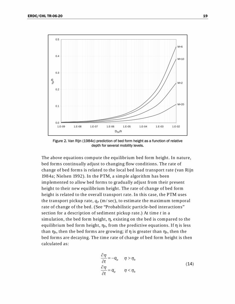
Figure 2. Van Rijn (1984c) prediction of bed form height as a function of relative depth for several mobility levels.
The above equations compute the equilibrium bed form height. In nature, bed forms continually adjust to changing flow conditions. The rate of change of bed forms is related to the local bed load transport rate (van Rijn 1984a; Nielsen 1992). In the PTM, a simple algorithm has been implemented to allow bed forms to gradually adjust from their present height to their new equilibrium height. The rate of change of bed form height is related to the overall transport rate. In this case, the PTM uses the transport pickup rate, qp (m/sec), to estimate the maximum temporal rate of change of the bed. (See “Probabilistic particle-bed interactions” section for a description of sediment pickup rate.) At time t in a simulation, the bed form height, η, existing on the bed is compared to the equilibrium bed form height, ηb, from the predictive equations. If η is less than ηb, then the bed forms are growing; if η is greater than ηb, then the bed forms are decaying. The time rate of change of bed form height is then calculated as:
p b
p b
qt
qt
η η η
η η η
∂= − >
∂∂
= <∂
(14)
M=2
M=6
M=10
M=20
0.0
0.1
0.2
0.3
0.4
0.5
1.E-09 1.E-08 1.E-07 1.E-06 1.E-05 1.E-04 1.E-03 1.E-02
D50/h
η b/h

ERDC/CHL TR-06-20 20
The bed form length is assumed to respond instantly to changes in flow conditions.
Potential transport rate
The PTM requires potential transport rates over the model domain to compute gradients in transport to estimate the potential for erosion and deposition of the native bed materials. These rates are used to determine the likelihood of burial of a sediment particle once deposited. This information, which can be output and mapped, is useful in its own right as an indicator of sediment transport conditions in the domain.
The PTM offers a choice of two techniques, Soulsby-van Rijn (Soulsby 1997) and van Rijn (1993), for the potential total load transport rate under combined wave-current conditions. The choice between algorithms is selectable in the SMS interface through the Eulerian Method control. The Soulsby-van Rijn technique is obtained by setting the Eulerian Method control to “PTM,” whereas the van Rijn technique is obtained by setting the control to “Van Rijn.” The group of techniques that comprise the PTM approach (developed by PI Engineering) offers substantial computational speed advantages over the van Rijn techniques.
The Soulsby-van Rijn total load sediment transport equation (Soulsby 1997) is:
2.412
2 20.018t s rms cr
D
q A U U U UC
⎡ ⎤⎛ ⎞⎢ ⎥= + −⎜ ⎟⎢ ⎥⎝ ⎠⎣ ⎦
(15)
where
s sb ssA A A= + (16)
[ ]
1.250
1.2
50
0.005
( 1)sb
DhhA
g s D
⎛ ⎞⎜ ⎟⎝ ⎠=
− (17)
[ ]
0.650
1.2
50
0.012
( 1)gr
ss
D DA
g s D
−
=−
(18)

ERDC/CHL TR-06-20 21
2
0
0.4
ln 1
DChz
=⎡ ⎤⎛ ⎞
−⎢ ⎥⎜ ⎟⎝ ⎠⎣ ⎦
(19)
Ucr is the critical velocity, which is given as:
0.150 10 50
90
0.650 10 50
90
40.19 log 0.5 mm
48.5 log 0.5 mm
cr
hD DD
UhD D
D
⎧ ⎛ ⎞<⎪ ⎜ ⎟
⎪ ⎝ ⎠= ⎨⎛ ⎞⎪ ≥⎜ ⎟⎪ ⎝ ⎠⎩
(20)
Particle transport calculations
In this section, the basic information necessary to enable the model to predict a particle’s transport is introduced and discussed.
Certain calculations are performed differently for each mode of operation of the model. For example, advection velocity calculations in the 2-D and Q3-D modes require computation of the suspended and bed load sediment concentration profiles, whereas the 3-D mode computes advection velocity solely from the particle’s position, independent of the local transport. Other calculations, such as for sediment fall velocity, are independent of the model’s mode of operation.
Particle position
The PTM uses a second-order predictor-corrector technique to solve for particle position at time t + dt for each of the three orthogonal dimensions x, y, and z. This is illustrated in the following example for the x dimension. The first stage of the scheme uses information at the particle’s present position and time to predict the particle’s position one-half time-step into the future, x’, as:
( )12n A Dx x u dt u dt′ = + + (21)
where uA and uD are the advection and diffusion velocities, respectively, at location x and time-step n. The second stage of the scheme uses information from this location over the full time-step:

ERDC/CHL TR-06-20 22
1n n A Dx x u dt u dt+ ′ ′= + + (22)
where Au′ and Du′ are the advection and diffusion velocities, respectively, at location x′ and time-step 2
1+n . The computation of these velocities is
dependent upon the mode of operation:
1. 2-D mode – uses the local horizontal velocity at the elevation of the centroid of the sediment transport distribution for sediment with the characteristics of the particle.
2. Q3-D mode – uses the local horizontal velocity at the elevation of the particle, which may be adjusted to account for bed-interaction (see the section Advection velocity).
3. 3-D mode – uses the local horizontal velocity at the elevation of the particle.
The calculation of the advection velocity for each mode of operation is described in the following sections.
Advection velocity
2-D mode
The 2-D and Q3-D modes require knowledge of the elevation of the centroid of the sediment transport distribution to compute horizontal advection velocities.
The particle load or concentration within the water column is the integral of the concentration, C (kg/m3), over depth:
0
( )h
z
C C z dz= ∫ (23)
The transport rate is the product of concentration and velocity, and is given by:
0
( ) ( )h
sz
q C z u z dz= ∫v v
(24)
The mean particle advection velocity, Auv , is determined from potential
transport rate divided by the sediment load as:

ERDC/CHL TR-06-20 23
0
0
( ) ( )
( )
h
zA h
z
C z u z dzu
C z dz=∫
∫
v
v (25)
This advection velocity can also be viewed as the velocity of the flow at the centroid of the particle transport rate distribution. Direct solution of this equation is too time-consuming to be implemented in the PTM. Therefore, a simpler approach has been adopted and as outlined next.
Suspended particle concentration profiles can be assumed to follow the form proposed by Rouse (1939) as:
*
00
1 11 1
swu
CC
κβ
σ
σ
⎛ ⎞−⎜ ⎟=⎜ ⎟−⎝ ⎠
(26)
where σ is the relative height above the bed ( hz /= ), κ = 0.4, β = 1, and
oC is the reference bed concentration at elevation oσ .
Rouse concentration profile shapes are considered to characterize the relative effects of particle size and shear stress on suspended concentration profile (Figure 3).
The product of the above concentration curves and assumed logarithmic velocity distribution have been integrated to determine the height of the centroid of the suspended load transport distribution, zs, for values of ws/κu*. Regression of the centroid height results in an expression for the centroid height of the suspended particle load, zs, as a function of ws/κu* (Figure 4).

ERDC/CHL TR-06-20 24
Figure 3. Rouse concentration distribution after Yalin (1977). Lines are labeled by ws/κu* value.
Figure 4. Relationship used to determine height of centroid of suspended particle load transport.
C/C0
0 0.2 0.4 0.6 0.8 10
0.2
0.4
0.6
0.8
1
0.05
0.1
0.2
0.4
0.8
1.6
3.2
6.4
12.825.6
51.2
1111
−σ
−σ
o
hzs
*uws κ

ERDC/CHL TR-06-20 25
The resulting equation for the height of the centroid of the suspended load, sz , is:
*1.08 tanh 1.2 ln 0.4
0.0398 10sw
uszh
κ⎡ ⎤⎛ ⎞
− −⎢ ⎥⎜ ⎟⎢ ⎥⎝ ⎠⎣ ⎦= ⋅ (27)
Particle fall velocity (Figure 5), sw (m/sec), is defined as a function of the dimensionless grain size, grD , and can be approximated by the following
equations proposed by Soulsby (1997), which have been adapted for extremely fine grain sizes ( grD < 0.0672) in the present work:
3
2
107.33 1.049 10.36 0.672
0.0077 0.672
gr grs
gr gr
D Dw D
D Dν
⎧ + − ≥⎪
= ⎨⎪ <⎩
(28)
Figure 5. Fall velocity for sediments.
The speed of advection of the suspended load is su (m/sec), which is the velocity at elevation sz (m) in a logarithmic profile.
*2.5 ln 30 ss
s
zu uk
⎛ ⎞′′= ⎜ ⎟′′⎝ ⎠
(29)
D (mm)
ws
(m/s
)
0 0.2 0.4 0.6 0.8 10
0.02
0.04
0.06
0.08
0.1
0.12

ERDC/CHL TR-06-20 26
Bed load is represented by a uniform layer of thickness propagating at speed, bu (m/sec). Estimates of bed load velocity have been suggested by
Yalin (1977), van Rijn (1984a), and Engelund and Fredsoe (1976). In the PTM, the bed load velocity is estimated using the relationship of Engelund and Fredsoe (1976).
*
710bu u
M⎛ ⎞′= −⎜ ⎟⎝ ⎠
(30)
The weighted average velocity of the total load is computed from the ratio of suspended load to total load, ts qq . This ratio can be determined
through integration of a predicted vertical profile of transport. However, a simpler relationship is shown as the curve superimposed on the following figure.
Figure 6 is adapted from van Rijn (1984b) and the data set of Guy et al. (1966). This curve has the following form:
*0.5 tanh 1.3 ln 0.3 0.5s
t s
q uq w
⎧ ⎫⎡ ⎤⎛ ⎞′′⎪ ⎪= − +⎨ ⎬⎢ ⎥⎜ ⎟⎝ ⎠⎪ ⎪⎣ ⎦⎩ ⎭
(31)
The advection velocity of a sediment particle is computed on the basis of the elevations of the bed load and suspended load components. The weighted advection velocity of the total load, cu (m/sec), is obtained by the
ratio of the suspended load to bed load as:
1s s
c s bt t
q qu u uq q
⎛ ⎞= + −⎜ ⎟
⎝ ⎠ (32)
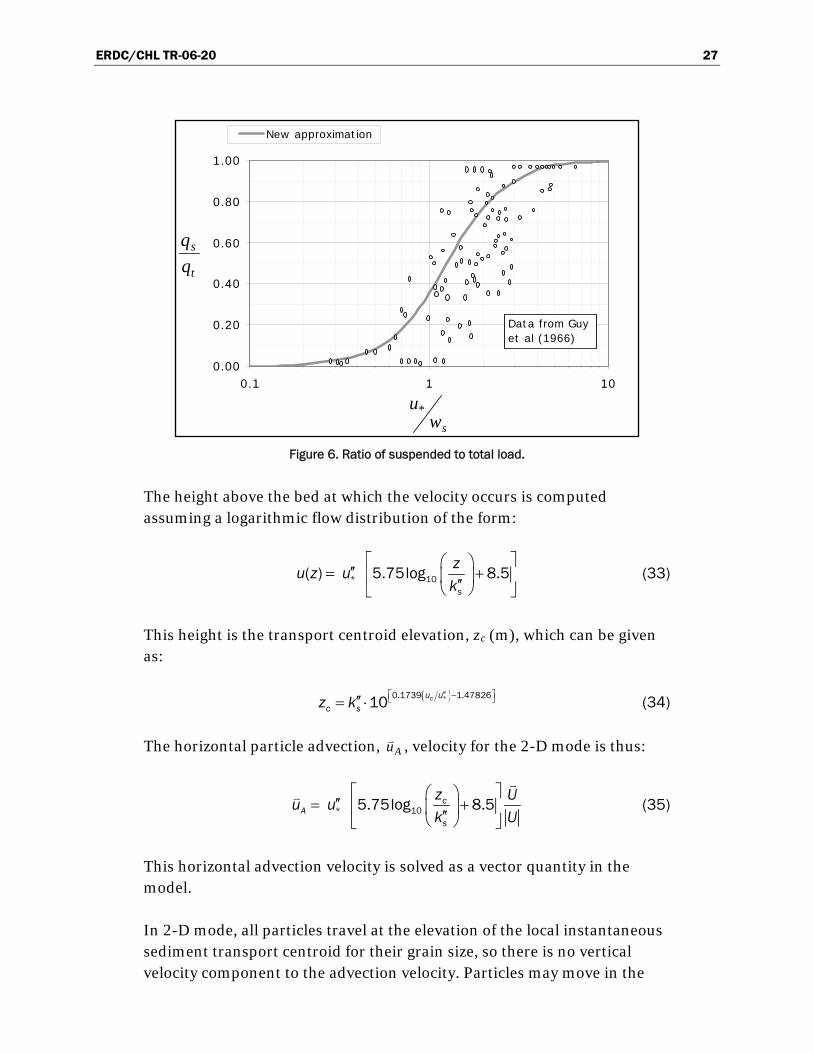
ERDC/CHL TR-06-20 27
Figure 6. Ratio of suspended to total load.
The height above the bed at which the velocity occurs is computed assuming a logarithmic flow distribution of the form:
* 10( ) 5.75log 8.5s
zu z uk
⎡ ⎤⎛ ⎞′′= +⎢ ⎥⎜ ⎟′′⎝ ⎠⎣ ⎦
(33)
This height is the transport centroid elevation, zc (m), which can be given as:
( )*0.1739 1.4782610 cu uc sz k ′′⎡ ⎤−⎣ ⎦′′= ⋅ (34)
The horizontal particle advection, Auv , velocity for the 2-D mode is thus:
* 105.75log 8.5cA
s
z Uu uk U
⎡ ⎤⎛ ⎞′′= +⎢ ⎥⎜ ⎟′′⎝ ⎠⎣ ⎦
vv
(35)
This horizontal advection velocity is solved as a vector quantity in the model.
In 2-D mode, all particles travel at the elevation of the local instantaneous sediment transport centroid for their grain size, so there is no vertical velocity component to the advection velocity. Particles may move in the
0.00
0.20
0.40
0.60
0.80
1.00
0.1 1 10
New approximation
Data from Guy et al (1966)
swu*
t
s

ERDC/CHL TR-06-20 28
vertical, however, because the centroid elevation above the bed will vary with changes in hydrodynamics.
Q3-D mode
In nature, a particle grain may be entrained upward into the flow by a burst of turbulence and then may settle back toward the bed where it may rest for some period of time before being re-entrained. This process results in net horizontal particle advection speeds that are slower than that of a continuously entrained particle. Explicit simulation of this advection retardation process is reproduced by determining the frequency of entrainment of a particle from the bed and computing the proportion of time a particle would be expected to be entrained by the flow. The advection retardation process is illustrated schematically in Figure 7.
Figure 7. Advection paths for conditions for bed-particle interaction.
In Q3-D mode, the effect of particles settling to the bed and waiting to be re-entrained is represented implicitly by computing the relative proportion of time that the particle is expected to be entrained. Particles are assumed to be continuously drawn to the bed at the fall velocity, sw .
The mean fall time, ft of a particle from the transport centroid elevation
cz (a particle’s expected vertical position) is estimated by:
cf
s
ztw
= (36)
The expected wait time between entrainments for a particle on the bed is wt :
)(zu
Mean time between entrainment events, 1/Pe
Particle entrainment height, z
Particle fall velocity, w
Time particle is entrained, t= z/w
Flow field
Bedef1

ERDC/CHL TR-06-20 29
1
we
tf
= (37)
where ef is the frequency of entrainment. A detailed description of the
methodology for the computation of ef is presented in the section
“Probabilistic particle-bed interactions.”
The proportion of the time that a particle would, therefore, be expected to be entrained in the flow is:
1
c
s c ef
w se
zw z ft
t wf= = (38)
A first-order approximation of the average advection velocity of a particle at elevation pz can be expressed as the product of the entrained particle
advection velocity, )( pzu , and the proportion of the time it is entrained. In
this approach, highly mobile particles ( sec wfz > ) will remain in motion
and move at their expected advection velocity, czu . In other words,
particles are being re-entrained before they have time to fall to the bed. Particles that have lower mobility or relatively high fall velocity are expected to spend more time on the bed prior to re-entrainment; the average advection velocity of these particles is, therefore, reduced by a velocity deficit coefficient, Δc .
1 c e s
c ec e s
s
z f wc
z f z f ww
Δ
⎧⎪ ≥⎪⎪= ⎨⎪⎪ <⎪⎩
(39)
That is, if ec fz is greater than or equal to sw , the particle stays entrained
in the flow and does not interact with the bed. However, if ec fz is less than
sw , the particle regularly settles to the bed and gets re-entrained, thereby
reducing the horizontal particle advection velocity. This difference is represented computationally by:
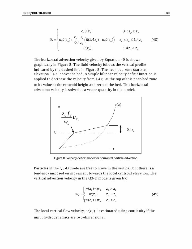
ERDC/CHL TR-06-20 30
( )
( ) 0
( ) (1.4 ) ( ) 1.40.4
( ) 1.4
p p c
p cA p c p c p c
c
p c p
c u z z zz z
u c u z u z c u z z z zz
u z z z
Δ
Δ Δ
⎧ < ≤⎪ −⎪= + − < ≤⎨⎪⎪ <⎩
v
v v v v
v
(40)
The horizontal advection velocity given by Equation 40 is shown graphically in Figure 8. The fluid velocity follows the vertical profile indicated by the dashed line in Figure 8. The near-bed zone starts at elevation 1.4 cz above the bed. A simple bilinear velocity deficit function is applied to decrease the velocity from 1.4 cz at the top of this near-bed zone
to its value at the centroid height and zero at the bed. This horizontal advection velocity is solved as a vector quantity in the model.
Figure 8. Velocity deficit model for horizontal particle advection.
Particles in the Q3-D mode are free to move in the vertical, but there is a tendency imposed on movement towards the local centroid elevation. The vertical advection velocity in the Q3-D mode is given by:
( )
( )
( )
p s p c
A p p c
p s p c
w z w z zw w z z z
w z w z z
⎧ − >⎪= =⎨⎪ + <⎩
(41)
The local vertical flow velocity, )( pzw , is estimated using continuity if the
input hydrodynamics are two-dimensional:
)(zu
cz cz4.0
( )c
s
ec zuwPz
czs
ec uwPz
czs
ec uw
fz
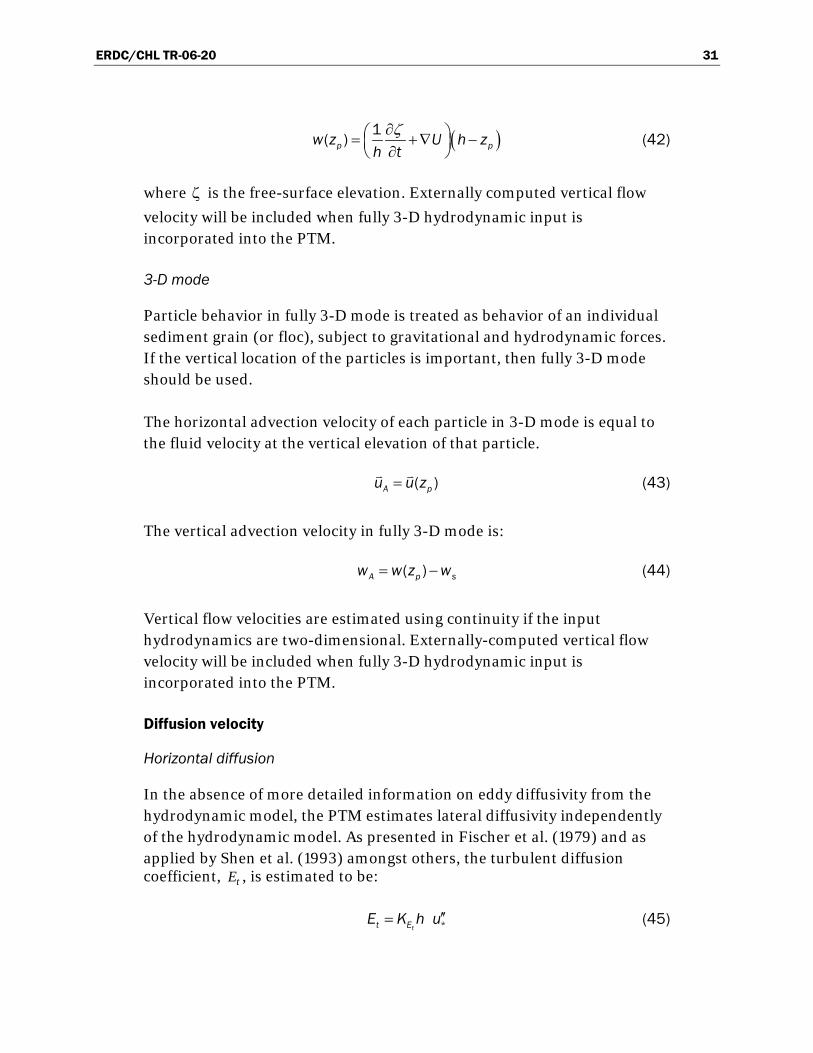
ERDC/CHL TR-06-20 31
( )1( )p pw z U h z
h tζ∂⎛ ⎞= +∇ −⎜ ⎟∂⎝ ⎠
(42)
where ζ is the free-surface elevation. Externally computed vertical flow
velocity will be included when fully 3-D hydrodynamic input is incorporated into the PTM.
3-D mode
Particle behavior in fully 3-D mode is treated as behavior of an individual sediment grain (or floc), subject to gravitational and hydrodynamic forces. If the vertical location of the particles is important, then fully 3-D mode should be used.
The horizontal advection velocity of each particle in 3-D mode is equal to the fluid velocity at the vertical elevation of that particle.
( )A pu u z=v v
(43)
The vertical advection velocity in fully 3-D mode is:
( )A p sw w z w= − (44)
Vertical flow velocities are estimated using continuity if the input hydrodynamics are two-dimensional. Externally-computed vertical flow velocity will be included when fully 3-D hydrodynamic input is incorporated into the PTM.
Diffusion velocity
Horizontal diffusion
In the absence of more detailed information on eddy diffusivity from the hydrodynamic model, the PTM estimates lateral diffusivity independently of the hydrodynamic model. As presented in Fischer et al. (1979) and as applied by Shen et al. (1993) amongst others, the turbulent diffusion coefficient, tE , is estimated to be:
*tt EE K h u′′= (45)

ERDC/CHL TR-06-20 32
The empirical coefficient tEK relates the turbulent diffusion to the local
shear velocity and water depth. Typically, tEK ranges from 0.15 to 0.6.
Two modifications are made to the method given by Equation 45 for use in the PTM. First, a coefficient, bM , which accounts for enhanced mixing due
to wave breaking is included.
*tt b EE M K h u′′= (46)
This wave breaking coefficient is defined as:
1 outside surf zone
1 inside surf zonew
bE s
MK H
⎧= ⎨ +⎩
(47)
where wEK is an empirical coefficient that relates the enhanced diffusion to
the local significant wave height, sH . Typically, wEK is set at 5. The
location of the surf zone is taken as any non-zero area in the STWAVE brk file.
Second, the formulation presented in Equation 45 produces a diffusion coefficient tE that increases proportionally with depth and shear velocity.
In coastal applications, the shear velocity drops off rapidly as depth increases. Consequently, as particles are advected into deeper and quiescent water (e.g., toward the offshore limit of an ebb shoal), the eddy diffusion drops to near zero. A user-supplied minimum value of the eddy diffusion coefficient (
mintE ) can be specified as a lower limit on diffusivity.
( )min *max ,
tt t b EE E M K h u′′= (48)
The default value of mintE is taken as 0.02 m2/sec in the PTM.
Vertical diffusion. The vertical diffusion coefficient, vE , is modeled
using a parabolic-shaped distribution:
( )2
3v
p pv b E
z h zE M K U
h
⎡ ⎤−⎢ ⎥=⎢ ⎥⎣ ⎦
(49)

ERDC/CHL TR-06-20 33
This equation is similar to Pritchard’s method (Fischer et al. 1979) if the Richardson number is taken as 0. As was done with the horizontal diffusion, the vertical diffusion is limited as:
( )
min
2
3max ,v
p pv v b E
z h zE E M K U
h
⎧ ⎫⎡ ⎤−⎪ ⎪⎢ ⎥= ⎨ ⎬⎢ ⎥⎪ ⎪⎣ ⎦⎩ ⎭
(50)
The default value of minvE is taken as 0 in the PTM.
Randon walk model. This estimate of the turbulent diffusion coefficient is used to drive a random walk diffusion model. The random walk representation of the horizontal dispersive velocities Du (and Du′ ) are
computed as:
( ) 62 0.5 t
DEu
dt= Π − (51)
where Π is a random number uniformly distributed between 0 and 1. Note that the horizontal dispersive velocities are isotropic. The vertical turbulent diffusion coefficient is taken as:
( ) 62 0.5 v
DEwdt
= Π − (52)
for a uniformly-distributed random number generator. If a Gaussian random number generator were to be used in Equations 51 and 52, the value 6 should be reduced to 4 to achieve the same dispersion.
Turbulent bed shear stress formulation
A probabilistic shear stress distribution is used to reflect the influence of turbulence on the shear stress imposed by the flow. The probability, τp , of
a given instantaneous (turbulent) shear stress is given as:
2
1exp
2 2t
ttτ
τ τ μτσ π σ
⎡ ⎤⎛ ⎞−= −⎢ ⎥⎜ ⎟
⎢ ⎥⎝ ⎠⎣ ⎦ (53)
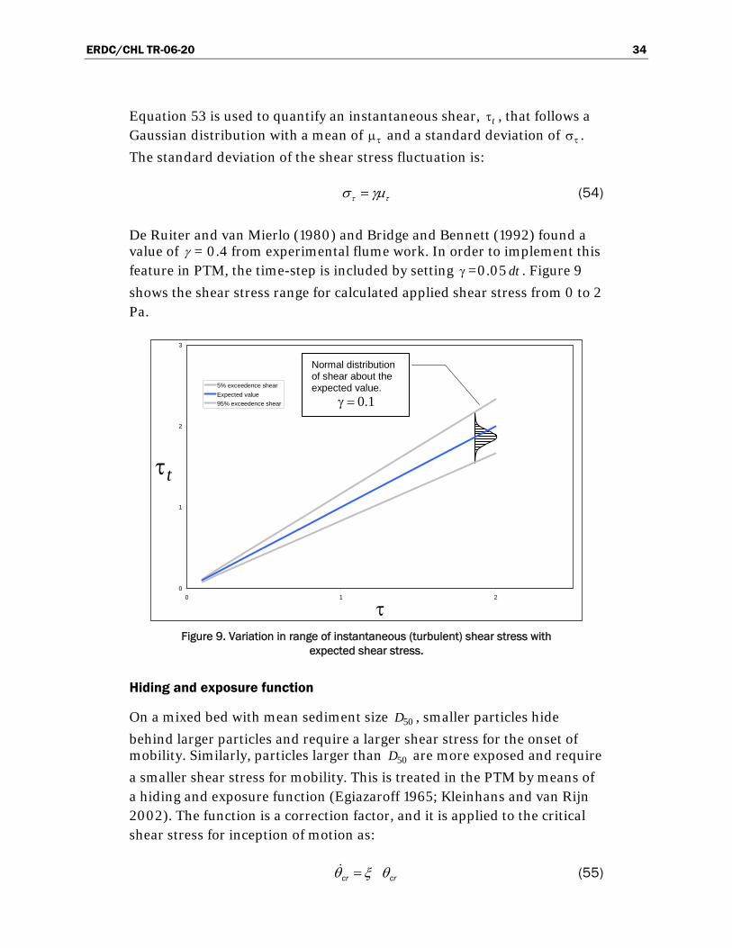
ERDC/CHL TR-06-20 34
Equation 53 is used to quantify an instantaneous shear, tτ , that follows a Gaussian distribution with a mean of τμ and a standard deviation of τσ .
The standard deviation of the shear stress fluctuation is:
τ τσ γμ= (54)
De Ruiter and van Mierlo (1980) and Bridge and Bennett (1992) found a value of γ = 0.4 from experimental flume work. In order to implement this feature in PTM, the time-step is included by setting γ =0.05 dt . Figure 9
shows the shear stress range for calculated applied shear stress from 0 to 2 Pa.
Figure 9. Variation in range of instantaneous (turbulent) shear stress with expected shear stress.
Hiding and exposure function
On a mixed bed with mean sediment size 50D , smaller particles hide
behind larger particles and require a larger shear stress for the onset of mobility. Similarly, particles larger than 50D are more exposed and require
a smaller shear stress for mobility. This is treated in the PTM by means of a hiding and exposure function (Egiazaroff 1965; Kleinhans and van Rijn 2002). The function is a correction factor, and it is applied to the critical shear stress for inception of motion as:
cr crθ ξ θ=& (55)
0
1
2
3
0 1 2
τ
ξ t
5% exceedence shearExpected value95% exceedence shear
Normal distribution of shear about expected value.
Standard deviation = 0.1 τ
Normal distribution of shear about the expected value.
1.0=γ
τ
τ′tτ

ERDC/CHL TR-06-20 35
where ξ is a dimensionless hiding and exposure correction factor. The
critical Shields parameter is a dimensionless representation of the shear stress acting on the particle and is computed using the approximation of Soulsby and Whitehouse (1997) (see the “Threshold for initiation of motion” section for discussion of the technique.) The hiding and exposure function is given by (Egiazaroff 1965):
2
50
5log 19
3D
Dξ
−⎡ ⎤⎛ ⎞
= ⎢ ⎥⎜ ⎟⎝ ⎠⎣ ⎦
(56)
This function is valid for 0.3 < 50D D < 10, and limits the particle’s mobility
threshold to be no greater than 3 times and no less than one-third of the critical Shields parameter of that particle. Note that the hiding and exposure function is only applied to particles that are deposited on the bed.
Figures 10 through 12 illustrate how the hiding and exposure function affects crθ for beds of 50D = 0.1, 1, and 10 mm.
Figure 10. Comparison of Shields and hiding and exposure functions for D50 = 0.1 mm bed material.
D (mm)
θ cr
10-1 100 101 10210-2
10-1
100
standard Shieldshiding and exposure applied

ERDC/CHL TR-06-20 36
Figure 11. Comparison of Shields and hiding and exposure functions for D50 = 1 mm bed material.
Figure 12. Comparison of Shields and hiding and exposure functions for D50 = 10 mm bed material.
D (mm)
θ cr
10-1 100 101 10210-2
10-1
100
standard Shieldshiding and exposure applied
D (mm)
θ cr
10-1 100 101 10210-2
10-1
100
standard Shieldshiding and exposure applied

ERDC/CHL TR-06-20 37
Probabilistic particle-bed interactions
One of the challenges in a Lagrangian model is how to address interactions between a deposited particle and the bed on which it deposits and mixes. Unlike Eulerian models, sediment bed dynamics are not explicitly simulated in the PTM. To include this interaction within the PTM, a probabilistic approach is used. The frequency of entrainment of a particle from the bed is computed as a function of the potential transport rate for the particle. This is combined with other factors that account for the likelihood of mixing of the particle within an active transport layer and the likelihood of burial of the particle by ambient transport processes.
Frequency of entrainment
In the PTM, particle entrainment is based on the mean shear stress and the critical shear stress for erosion as defined by the Shields curve, as well as by the following five supplemental considerations:
1. The turbulent fluctuations in the instantaneous shear stress. 2. Modifications to the critical shear stress to account for hiding and
exposure effects of graded sediment beds. 3. The transport pickup rate from the bed, pq .
4. The ambient transport conditions on the bed (erosion/deposition), leading to an estimate of the depth of burial of the particle, burialh .
5. Mixing of the particles within the active transport layer, which is based on the thickness of the active transport layer, activeh .
These have been implemented in a manner such that the frequency that a particle is picked up from the bed, ef is determined as:
e burial mixing pf K K f= (57)
In this equation, pf is the frequency of pickup based on the estimated
particle transport pickup rate for the particle. mixingK is a reduction factor
to account for the fact that the particle may lie anywhere within the thickness of the active sediment transport layer at the particle location.
burialK is a reduction factor to account for the possible burial of the particle
by ambient sediments. The units of ef are sec-1 or Hz. These processes are
discussed in the following sections.

ERDC/CHL TR-06-20 38
Pickup rate
The pickup function of van Rijn (1984b) is used to predict qp, the particle entrainment rate, as:
( ) ( )
1.5 0.13
2
10.00033 1t cr
pcr
s gDq s gDθ θθ ν
⎛ ⎞ ⎛ − ⎞−= −⎜ ⎟ ⎜ ⎟
⎝ ⎠⎝ ⎠ (58)
The units of pq are m/sec. This estimate of pq is based on the mobility
and grain size of the particle. Note that Equation 58 is modified to use the turbulent Shields parameter, tθ , which is computed using the turbulent estimate of the shear stress, tτ , as:
( )1
tt g s D
τθρ
=−
(59)
The time required to pick up one full layer of material of particle grain size, D , from the bed is pt , which is given by:
pp
Dtq
= (60)
The frequency that a particle will be picked up from the bed in any given time interval is calculated by:
pp
qf
D= (61)
This frequency, for various values of grain size diameter and mobility function, M (see Equation 9), is illustrated in Figure 13.

ERDC/CHL TR-06-20 39
Figure 13. Variation of frequency of pickup with grain size and mobility.
Active layer depth
The mechanics of the active layer of particle transport at the bed are modeled after the shear-sliding model of Wilson (1987). Once the critical shear stress for the inception of particle transport is exceeded, the shear stress applied to the bed mobilizes a thickness of particles. Frictional resistance to sliding is provided by the internal shearing resistance of the soil. The thickness of the active layer, activeh , is the depth of bed mobilized
to resist the excess shear applied at the top of the bed.
( )( )1 1 tan
t cractiveh
s n gτ τ
ρ φ−
=− −
% (62)
Here, crτ~ is the critical shear stress of the bed particles, n is the sediment
porosity, s is the relative density of the sediment, and φ is the mobilized
angle of shear resistance. The latter quantity is assumed to be equal to the dynamic angle of repose of Bagnold (1966) and is set to 18 deg, based on laboratory studies. Using standard values for the quantities in Equation 62, this can be approximated as:
( )5active t crh Dθ θ≈ − % (63)
D (mm)
f p(H
z)
10-2 10-1 100 10110-4
10-3
10-2
10-1
100
M = 1.05M = 1.2M = 1.5M = 2

ERDC/CHL TR-06-20 40
This mixing depth affects the frequency of particle entrainment; the thicker the mixing depth, the higher the number of candidate particles for removal and, hence, the lower the probability of any individual particle being removed. This relationship is expressed as the mixing factor, mixingK
as follows:
1
activeactive
mixing
active
D h Dh
Kh D
⎧ >⎪⎪⎪= ⎨⎪ ≤⎪⎪⎩
(64)
Influence of bed level change on entrainment
Total load transport under waves and currents is computed over the Eulerian mesh with the van Rijn – Soulsby technique (Soulsby 1997). Erosion and deposition potential, which is expressed as the rate of bed change, is computed from the gradients in total load. These calculations are done on an elemental scale (i.e., computed on the input finite-element mesh).
The rate of bed level change allows estimation of the erosion or deposition occurring at the bed location of any deposited particle. If a particle is resting on the bed, the rate of erosion or deposition at the particle location is integrated over time starting from the instant the particle lands on the bed. The likelihood of particle entrainment diminishes as the particle is covered by local deposition. Once the particle is below the mixing depth, the likelihood of entrainment goes to zero. If conditions at the particle location become erosional, this process is reversed: the likelihood of entrainment increases linearly from zero (when the particle is at the mixing depth or lower) to one (when the particle is exposed on the upper surface of the bed).
The erosion or deposition rate, dtdz , is used to compute the elevation of
the bed within the active layer (or below it).
0
t
burialt
dzh dtdt
= ∫ (65)

ERDC/CHL TR-06-20 41
From Equation 65, the position of the particle within the active layer can be determined and the frequency of entrainment, ef , modified
accordingly. If the value of dtdz is negative, the particle is assumed to stay
at the top of the bed with no reduction in the likelihood of entrainment. However, if the value of dtdz is positive, the particle becomes buried, and
the likelihood of entrainment diminishes with burial depth into bed. The likelihood of entrainment becomes zero if the depth of burial is equal to, or greater than, the active layer depth.
1 0 1burialburial burial
active
hK Kh
= − ≤ ≤ (66)
Particle deposition
In 2-D mode, particles are deposited if the local mobility falls below critical for that particle. In Q3-D and 3-D modes, particles are deposited on the bed once they pass below one-quarter of the skin roughness height.
particle deposits
4ifparticle remains active
4
s
ps
k
zk
′⎧ <⎪⎪⎨ ′⎪ ≥⎪⎩
(67)
If a particle becomes deposited, it will cease to move until it is re-entrained.
Particle re-entrainment
Particles that deposit on the bed can be re-entrained into the flow under certain circumstances. The PTM performs a series of checks on each deposited particle each time-step to determine whether that particle should be re-entrained. This section outlines the methods used to determine re-entrainment for each mode of operation.
2-D mode
Deposited particles are re-entrained if the local mobility is greater than critical. Particle vertical position increases in the water column with the increase in elevation of the sediment transport centroid.

ERDC/CHL TR-06-20 42
Q3-D mode
Particles deposited on the bed in the Q3-D mode are re-entrained into the flow using a probabilistic technique. The frequency of entrainment, ef , is
computed considering the particle pickup rate, the mixing depth of native sediment in the active transport layer, and the likelihood of burial by native sediments. Details of the computation of ef are presented in the
“Probabilistic particle-bed interactions” section.
If the PTM is run with particle-bed interactions active, then a test is performed each time-step on each deposited particle to determine whether the particle should be re-entrained.
particle re-entrained
ifparticle remains deposited
e
e
f dtf dt
< ⋅⎧Π ⎨≥ ⋅⎩
(68)
The entrainment elevation is set to the centroid elevation, i.e., cp zz = .
If the PTM is run with particle-bed interactions inactive, then deposited particles are assumed to be instantaneously re-entrained to the centroid elevation, if their mobility is greater than unity.
3-D mode
Particles depositing on the bed in the 3-D mode are re-entrained into the flow using a probabilistic technique. The frequency of entrainment, ef , is
computed considering the particle pickup rate, the mixing depth of native sediment in the active transport layer, and the likelihood of burial by native sediments. Details of the computation of ef are presented in the
“Probabilistic particle-bed interactions” section.
If the PTM is run with particle-bed interactions active, then the test given in Equation 68 is performed each time-step on each deposited particle.
The entrainment elevation is computed using a Rouse-type random number generator. This generator will produce random numbers that are distributed according to a Rouse sediment concentration profile for the specific sediment and flow conditions (see Equation 26). As a result, the random numbers will be biased towards 0 (taken as the bed) rather than 1

ERDC/CHL TR-06-20 43
(taken as the surface). An example of the distribution of random numbers produced by this technique is shown in Figure 14.
Figure 14. Example of Rouse-type random number generator output.
The new elevation of a re-entrained particle is taken as:
pz h= Ψ (69)
where Ψ is a random number between 0 and 1 distributed according to a Rouse sediment concentration profile.
If the PTM is run with particle-bed interactions inactive, deposited particles are assumed to be instantaneously re-entrained, and the test in Equation 68 is not performed. The elevation of entrainment is given by Equation 69.
The influence of particle-bed interaction is shown in Figure 15. This plot shows the average sediment advection velocity as a function of mean flow velocity for two simulations using the 3-D advection mode. The depth of flow is 10 m, and the particles were released 1 m above the bed. The released particles have uniform diameter of 0.1 mm. The bed is mobile and D50 = 0.2 mm. The simulation with particle-bed interaction turned off has an average sediment advection nearly equal to the flow velocity, which is
count
z p/h
0 50 100 1500
0.2
0.4
0.6
0.8
1

ERDC/CHL TR-06-20 44
to be expected for a particle of this size. With particle-bed interaction turned on, particle advection rates are decreased because the particles mix with the bed sediments.
Figure 15. Influence of particle-bed interaction on sediment advection.
Figure 16 compares sediment advection velocities for four particle sizes. All simulations have particle-bed interaction turned on; other test parameters are as described above. Larger diameter particles are advected more slowly. The reduction in transport near U = 2.0 m/sec is due to the change in bed form height and its impact on flow shear.
Dparticle=0.1 mmDparticle=0.2 mmDparticle=0.4 mmDparticle=0.8 mm
2DQ3D3D
Umean (m/sec)
UA
(m/s
ec)
0 1 2 3 4 50
1
2
3
4
5
Particle-bed interaction onParticle-bed interaction off

ERDC/CHL TR-06-20 45
Figure 16. Comparison of sediment advection for a range of grain sizes.
Boundary conditions
The PTM uses the land and open boundaries given in the ADCIRC mesh file. Particles may pass through an open boundary. If a particle passes through an open boundary, it ceases to be included in the computation.
A particle may not pass through a land boundary. The ADCIRC flow patterns should not cause particles to be directed across solid boundaries. However, if because of large time-steps, the advection-diffusion routines do predict a particle trajectory that intersects a land boundary, it should be caught by one of a number of tests performed. The particle will be placed alongside the boundary in question. The meaning of boundary in this section is mesh boundary (element on a boundary). If a particle is driven onto a dry point, it becomes stranded. Wetting and drying are included, if the original hydrodynamic model was run with this capability.
Particle-bed interaction onParticle-bed interaction off
2DQ3D3D
Umean (m/sec)
UA
(m/s
ec)
0 1 2 3 4 50
1
2
3
4
5Dparticle=0.1 mmDparticle=0.2 mmDparticle=0.4 mmDparticle=0.8 mm

ERDC/CHL TR-06-20 46
4 Model Operation
The PTM is operated through the SMS graphical user interface (Zundel 2005). The SMS interface gathers the required run-time information and file names, and creates or modifies the various input files. Program execution is initiated from within the interface. In this section, the basics of the PTM control dialogue are presented, together with the information required for each of these files. This is done to assist in their construction within the SMS. A separate technical note describing use of the PTM within the SMS (Demirbilek et al. 2005a) is included in Appendix B.
Model setup and input files
The PTM requires a number of input files depending upon the characteristics of the simulation, although all simulations must have a minimum set of files. This minimum set of files includes:
1. A program control file (.pcf) that contains run-time instructions for the model. The construction of this file constitutes the majority of the work in setting up a PTM simulation. This file is written by the SMS interface and is described in the following section.
2. A geometry file containing the bathymetry and boundary information for the model. This file must be an ADCIRC compatible three-noded triangular finite element mesh (i.e., a .14 or .grd file) in Cartesian coordinates and S.I. units.
3. An element neighbor file. The model writes this file at the time of first execution on a new mesh file. This file only needs to be regenerated if the node or element structure (e.g., number of nodes or elements, or connectivity) changes. The generation of this file can be time-consuming for very large meshes, so it is read from disk in subsequent simulations.
4. Hydrodynamic input files containing the time-varying free-surface elevation and depth-averaged velocities.
5. A native (bed) sediment file containing information about the native sediments over the domain defined by the mesh file. This file can be written by SMS if required.
6. A sediment-source file containing information about the sediment sources. This file is created in the SMS interface’s Map module.
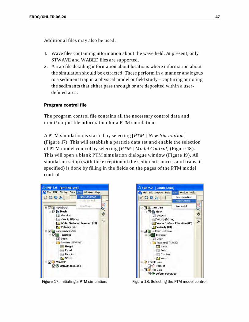
ERDC/CHL TR-06-20 47
Additional files may also be used.
1. Wave files containing information about the wave field. At present, only STWAVE and WABED files are supported.
2. A trap file detailing information about locations where information about the simulation should be extracted. These perform in a manner analogous to a sediment trap in a physical model or field study – capturing or noting the sediments that either pass through or are deposited within a user-defined area.
Program control file
The program control file contains all the necessary control data and input/output file information for a PTM simulation.
A PTM simulation is started by selecting [PTM | New Simulation] (Figure 17). This will establish a particle data set and enable the selection of PTM model control by selecting [PTM | Model Control] (Figure 18). This will open a blank PTM simulation dialogue window (Figure 19). All simulation setup (with the exception of the sediment sources and traps, if specified) is done by filling in the fields on the pages of the PTM model control.
Figure 17. Initiating a PTM simulation. Figure 18. Selecting the PTM model control.

ERDC/CHL TR-06-20 48
The program control file (with extension .pcf) is saved to disk by SMS prior to execution or by selecting [File | Save PTM] from the menu.
Figure 19. PTM model control window at initialization.
The main input files (geometry, hydrodynamics, and sediments) are identified on the Hydro, Sediment, and Source Input page. The native bed sediments file can be generated if one is required. Files are input by selecting the file browser button ( ). The initial page is shown in Figure 19 and a completed page is shown in Figure 20.
The source coverage (i.e., the location and schedule of the sediment sources) is also identified on this page. A source coverage must be created in the Map module before it can be identified on this page. The ADCIRC mesh and results file and, if required, the STWAVE input files, should be opened in the SMS environment prior to starting a PTM simulation, so that sources can be specified.
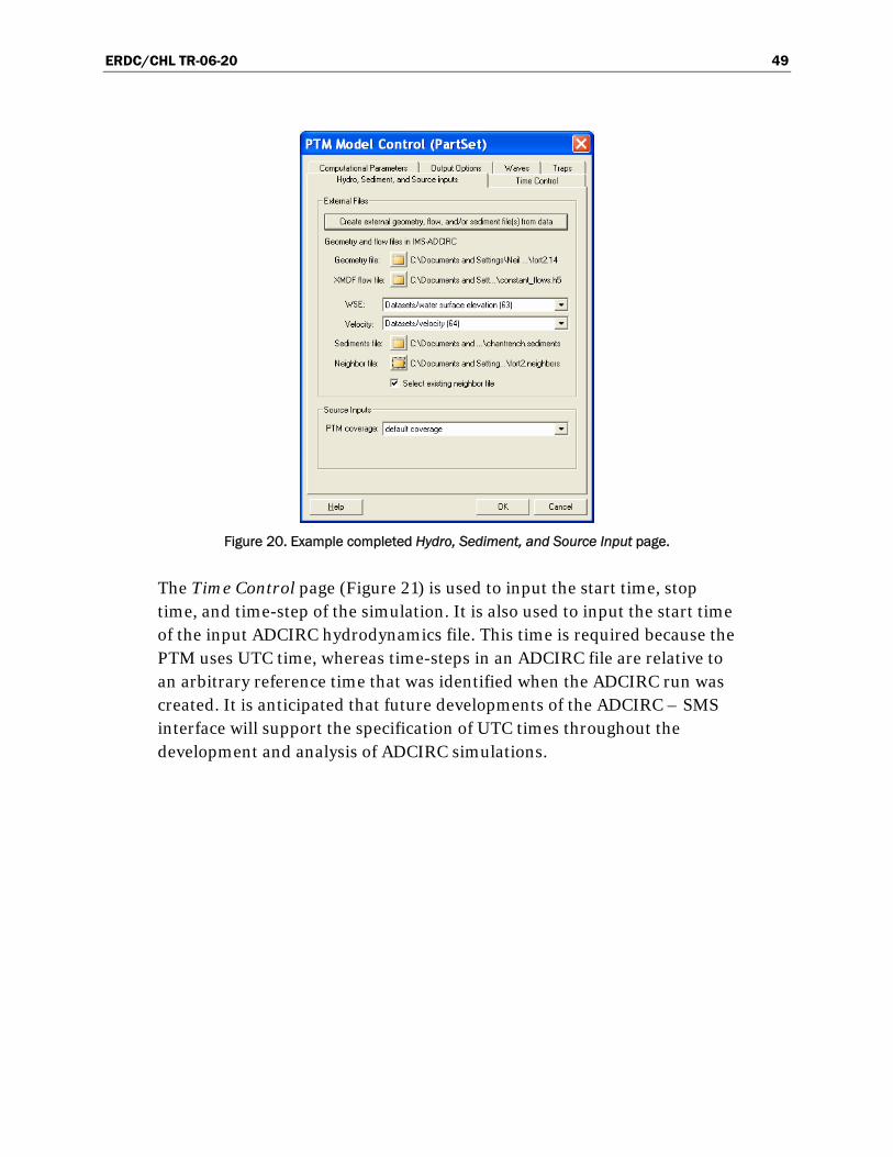
ERDC/CHL TR-06-20 49
Figure 20. Example completed Hydro, Sediment, and Source Input page.
The Time Control page (Figure 21) is used to input the start time, stop time, and time-step of the simulation. It is also used to input the start time of the input ADCIRC hydrodynamics file. This time is required because the PTM uses UTC time, whereas time-steps in an ADCIRC file are relative to an arbitrary reference time that was identified when the ADCIRC run was created. It is anticipated that future developments of the ADCIRC – SMS interface will support the specification of UTC times throughout the development and analysis of ADCIRC simulations.

ERDC/CHL TR-06-20 50
Figure 21. Example completed Time Control page.
The Computational Parameters page controls how the model performs the simulation. The Computational Methods panel controls four run-time flags:
1. The Distribution box controls whether the model synthesizes sediment particles to match the given particle size distribution by weight or by diameter (preferred). The particle size distribution characteristics are unique for each stage of each source and are given in the source file, which is created in the Map module.
2. The Centroid box controls whether the model computes the sediment transport centroid height above the bed using equations from van Rijn or from Rouse (preferred).
3. The Eulerian box controls whether the model computes a number of sediment-based parameters using equations from van Rijn or various techniques selected for PTM (preferred, see “Eulerian transport calculations” in Chapter 3 for details). These parameters are subsequently output to generate temporal and spatial maps of transport conditions.
4. The Advection box controls whether the model uses a 2-D, Q3-D or 3-D advection technique (see “Modes of operation,” Chapter 2 for details).
The Computational Parameters panel (Figure 22) controls various coefficients and three routines that influence particle interactions (see
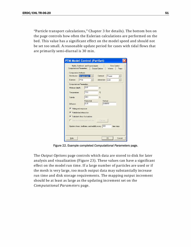
ERDC/CHL TR-06-20 51
“Particle transport calculations,” Chapter 3 for details). The bottom box on the page controls how often the Eulerian calculations are performed on the bed. This value has a significant effect on the model speed and should not be set too small. A reasonable update period for cases with tidal flows that are primarily semi-diurnal is 30 min.
Figure 22. Example completed Computational Parameters page.
The Output Options page controls which data are stored to disk for later analysis and visualization (Figure 23). These values can have a significant effect on the model run time. If a large number of particles are used or if the mesh is very large, too much output data may substantially increase run time and disk storage requirements. The mapping output increment should be at least as large as the updating increment set on the Computational Parameters page.

ERDC/CHL TR-06-20 52
Figure 23. Example completed Output Options page.
If waves are used, the Waves page needs to be completed. Wave model geometry can be obtained automatically by pressing the button (Figure 24). The wave grid file must already be open.
Figure 24. Example completed Waves page.

ERDC/CHL TR-06-20 53
Since output steps in an STWAVE/WABED output file do not contain any time information, both the start time and duration between steps must be supplied to the PTM.
If traps are in the simulation, the Traps page must be completed (Figure 25). Traps are created as closed polygons in the Map module. The SMS interface will automatically identify any active polygon coverage as the trap. If traps are not to be used, then this page can be left with its default settings, because the default dates should be outside the simulation period.
Figure 25. Example Traps page showing default values (i.e., traps not active).
Sediment source file
The sediments modeled in a PTM simulation are introduced to the model via a source file, which is generated through the Map module in the SMS. Point sources (both instantaneous and varying-release) and line sources are first created as simple point or line coverages, respectively. These coverages must have their Type set to PTM. This is performed by highlighting the coverage and following the menus available using a right-mouse click on the coverage, as is illustrated in Figure 26.

ERDC/CHL TR-06-20 54
Figure 26. Conversion of source coverage type to PTM.
After conversion to PTM type, double-clicking on the coverage will open the source’s control box (Figure 27). This box is used to enter data to specify the source’s characteristics and location data. Any number of instructions can be added to the source file (new lines are added automatically). Each instruction is identified by a unique UTC time. These instructions can be separated by any duration (minimum 1 sec). The final instruction must be beyond the end of the simulation (a zero sediment discharge rate is acceptable). In this way, complicated release schedules (e.g., dredge movement, changes in discharge rate, changes in properties of material released, intermittent releases) can be reproduced by the model.

ERDC/CHL TR-06-20 55
Figure 27. Example source control box.
Source file structure
An important point to remember about source files is that PTM will interpolate between each instruction for all data in the file. One can use this structure to build up complicated source functions.
An example source release is shown in Figure 28. Nine lines of data (instructions) would be required in the source file to enable PTM to reproduce this release schedule:
1. Time 1 is the start of the source discharge. It can be any time later than or equal to the start time of the simulation.
2. Between Time 2 and Time 3, the sediment discharge rate is to decrease. Because the model interpolates, the initial discharge (i.e., that at Time 1) is repeated at Time 2, so that the discharge is constant over the period between Time 1 and Time 2.
3. A short time later (e.g., 1 sec) the discharge is decreased to a new value (Time 3).
4. The discharge is kept constant until Time 4. Therefore, the instruction at Time 4 is a repeat of Time 3, but at a later time.
5. The next instruction is at Time 5. It has a zero discharge rate; therefore the model will linearly vary the discharge between Time 4 and Time 5.
6. A second release of sediment is desired, but at a slightly later time. Time 6 is specified to identify the start of the release, which will almost immediately increase to the rate at Time 7. If the value at Time 7 had been specified as Time 6, the model would have linearly increased the rate from zero at Time 5, rather than the step-function release desired.
7. The discharge is kept constant until Time 8. Therefore, the instruction at Time 8 is a repeat of Time 7, but at a later time.
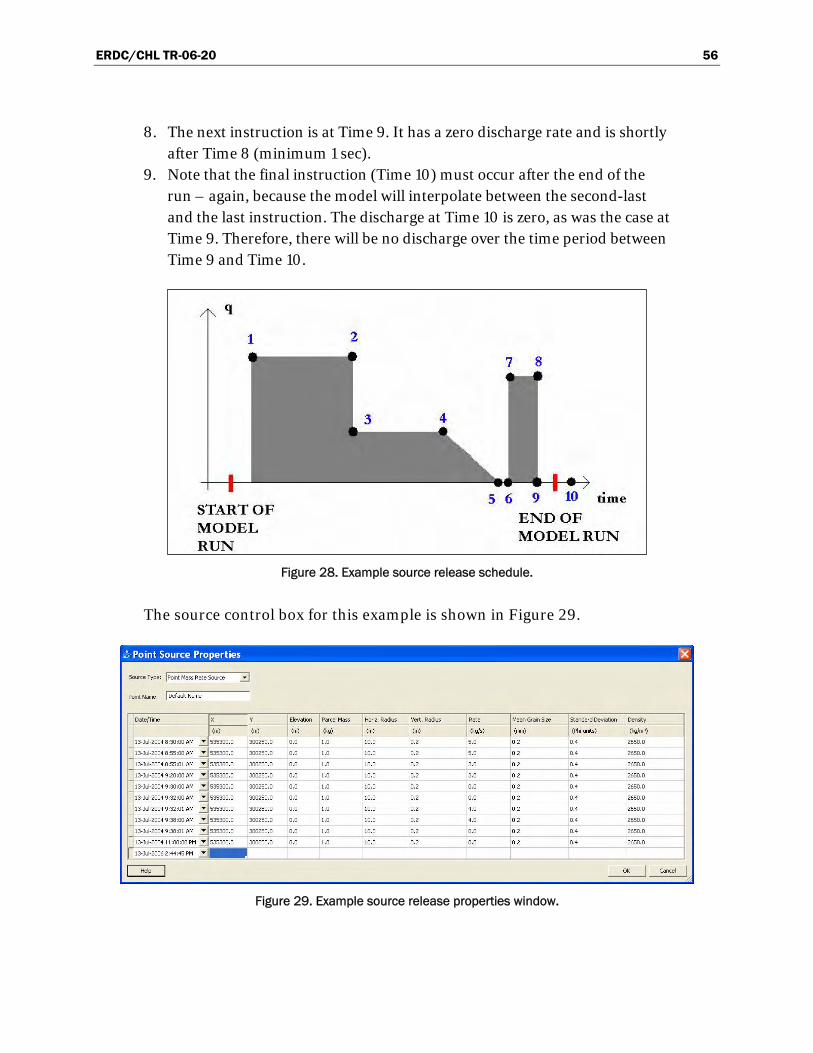
ERDC/CHL TR-06-20 56
8. The next instruction is at Time 9. It has a zero discharge rate and is shortly after Time 8 (minimum 1 sec).
9. Note that the final instruction (Time 10) must occur after the end of the run – again, because the model will interpolate between the second-last and the last instruction. The discharge at Time 10 is zero, as was the case at Time 9. Therefore, there will be no discharge over the time period between Time 9 and Time 10.
Figure 28. Example source release schedule.
The source control box for this example is shown in Figure 29.
Figure 29. Example source release properties window.

ERDC/CHL TR-06-20 57
Note that although the previous example only dealt with discharge rate, most quantities are interpolated between instructions (e.g., grain size, source location, etc.).
The particle mass can be used to control the number of particles that are generated to represent a mass release.
Instantaneous sources
These are used for instantaneous releases of sediment. These are point sources that are not interpolated; the full release of sediment occurs at the time given and with the properties specified.
Point sources
These are point sources that are interpolated. The release of sediment is variable and occurs at the times given and with the properties specified. Linear interpolation is used for most properties. A stationary, continuous point source can be specified by using two point sources with identical characteristics separated in time.
Line sources
Line sources must either be vertical or horizontal. Linear interpolation is used for most properties in the line source. Line sources may move, change length, and change discharge properties.
Area sources
The area sources are polygons. The points must be ordered using a standard counter-clockwise convention. Source properties within an area source are uniform across the polygon.
Selection of sediment sorting
The grain size associated with each particle released from a sediment source is selected by the model such that the mass of sediment released in a single instruction reproduces a user-defined particle size distribution. The form of the distribution is Gaussian and is specified by a mean grain size and a standard deviation. In order to simplify the selection, two sets of units are used; the mean grain size D is specified in millimeters, and the standard deviation σ is specified in phi-units (φ ). The phi-unit is the

ERDC/CHL TR-06-20 58
negative logarithm to the base 2 of the sediment diameter in millimeters, such that the mean phi-unit grain size is:
( )2log Dφ = − (70)
By specifying the standard deviation in phi-units, the degree of sorting of the sediment becomes independent of the mean grain size. The generally-accepted ranges are as follows:
0.5 well sorted
0.5 1.0 moderately sorted
1.0 2.0 poorly sorted
2.0 very poorly sorted
σ φ
φ σ φ
φ σ φ
φ σ
<
≤ <
≤ <
≤
(71)
After a source is created, it will become available to the model through the Source Input box on the Hydro, Sediment, and Source Input page (Figure 30).
Figure 30. Selection of source coverage in PTM model control box.

ERDC/CHL TR-06-20 59
Native sediments file
This file contains the spatially-varying grain size information for the native sediments in terms of 35D , 50D , and 90D . Frictional characteristics of the bed are computed with 90D . The 50D value is used in the prediction of bed
forms, in the determination of sediment mixing routines that influence re-entrainment of deposited particles, and in the hiding and exposure routines that influence the critical shear stress of deposited particles. The
35D value is used in the determination of the suspended sediment
transport if the van Rijn approach is selected for the centroid method.
Non-erodible areas (e.g., rock outcroppings) can be identified by a negative input grain size. This absolute value of the grain size is treated as an effective roughness height, sk′ and sk ′′ .
The native sediments file is specified on the Hydro, Sediment, and Source Input page of the PTM control box (Figure 30). A native bed sediments file can be generated by the SMS interface, if one is required, by pressing the
button. This will open the Create PTM External Input Files widow. After the geometry is selected and the native sediments option selected, the window will appear as is shown in Figure 31. A file name must be specified at this point.
Geometry file
The geometry file is used to specify the bathymetry of the domain and the boundary conditions. This is a standard ADCIRC mesh file, usually given the extension .14 or .grd. The coordinates must be in metric (or S.I.) units and must be in Cartesian coordinates. The SMS interface can convert ADCIRC files that are in curvilinear geographic coordinates (e.g., lat-long) into a plane Cartesian system (e.g., state plane).
The geometry file is specified on the Hydro, Sediment, and Source Input page of the PTM control box (Figure 20). Although the PTM can be run with this file only identified in the Hydro, Sediment, and Source Input page, it should be opened separately in the SMS interface to allow source terms to be specified graphically.

ERDC/CHL TR-06-20 60
Figure 31. Create PTM External Input Files page.
Neighbor data files
To reduce model run time, the PTM uses a list of the numbers of all neighboring elements of each element. This information can be time-consuming to obtain for large meshes, so creation of the neighbor data file is performed only once for each mesh; once computed, this additional information is written to a neighbor file (extension .neighbors). On subsequent simulations, the information is read from the neighbor file. If no neighbor file exists, the model will create one using the provided name. The neighbor file is specified on the Hydro, Sediment, and Source Input page of the PTM control box (Figure 30). This file only needs to be regenerated if there are changes to the element-node structure (e.g., addition of new nodes, changes in connectivity). Changes in node depths or locations, for example, will not necessitate a new neighbor file.
Hydrodynamic data files
At present, these files must be ADCIRC-compatible, three-noded triangular finite element mesh files in XMDF file (.h5) format. XMDF files require much less disk space than the ASCII standard ADCIRC format and, because they are random-access, can be read more quickly by the

ERDC/CHL TR-06-20 61
PTM. This can provide a significant time saving, especially if the PTM simulation starts some time after the start of the ADCIRC simulation.
The SMS interface automatically converts standard ADCIRC files (.63 and .64) to XMDF format when they are opened. The hydrodynamic file is specified on the Hydro, Sediment, and Source Input page of the PTM control box (Figure 20).
It is important to note that ADCIRC output files do not have a time stamp to identify their start. The start time must be supplied to the PTM to allow the ADCIRC flows to be converted to UTC time, so that they can be synchronized with the other input data (sources, flows, waves, etc.). This is done in the Time Control page of the program control box (Figure 21).
Wave input files
These are standard STWAVE output files. They have the extension .wav. If the steering module is used to generate the files, then each file will contain a single frame of data or snapshot of the wave field. If STWAVE is run in a stand-alone mode, then a single file will be generated with a number of frames of wave data in a single file. The wave data are supplied to the PTM in the Waves page of the program control box (Figure 24). Opening the STWAVE simulation first allows the interface to automatically obtain the grid data. This is done be pressing the button (Figure 24).
STWAVE output files do not have a time stamp to identify their start. The start time must be supplied to the PTM in the Waves page of the program control box (Figure 24).
Trap file structures
A trap is defined as an area into which particles enter and are counted. The trap may be open (particles are free to leave) or closed. A flag can also be set to control whether particles are counted once per simulation or every time they re-enter an open trap. Time limits can also be specified on the trap’s operation.
The PTM uses polygon coverages to catalogue particle activity. These coverages must be constructed in the Map module prior to their identification in the PTM model control pages. The trap data are supplied to PTM in the Traps page of the program control box (Figure 25).

ERDC/CHL TR-06-20 62
Output files
The PTM produces a number of output files depending upon the characteristics of the simulation. There are four main output files:
1. Echo file – giving a synopsis of the input for the simulation (e.g., input parameters set, default values used by PTM, mesh dimensions). This is an ASCII text file with the extension input.
2. Particle file – giving particle-based information about the source sediments introduced to the domain (e.g., particle position, user-selected properties and user-selected attributes). The default format is binary XMDF with the extension _particles.h5.
3. Map file – giving mesh-based information about the native sediments in the domain (e.g., sediment mobility, bed forms, sediment transport rate). The default format is binary XMDF with the extension _ maps.h5.
4. Error file – giving run-time error information for debugging a failed simulation. It is only produced if errors are encountered in the simulation. This is an ASCII text file with the extension err.
An additional output file(s) may be produced if traps are required:
1. Count file – giving information about any particles caught in a trap while the trap is active. This file is only produced if traps are in use. This is an ASCII file with the extension _count.out.
2. Residency file – giving information about the residency times of particles in designated areas (i.e., traps). This is an ASCII file with the extension _ residency.out.
3. Bin file – giving information about any particles in a trap at the end of the simulation. This file is only produced if traps are in use. This is an ASCII file with the extension _bin.out.
If errors are produced, then an error file is generated:
1. Error file - giving run-time error information for debugging a failed simulation. It is only produced if errors are encountered in the simulation. This is an ASCII text file with the extension err.
Particle file
As discussed in Chapter 1, each sediment particle can have a unique set of attributes and certain other properties. Properties refer to quantities that

ERDC/CHL TR-06-20 63
are invariant in a simulation (e.g., grain size), whereas attributes may vary (e.g., particle position, particle state). Certain physical attributes (e.g., particle position) are required for the solution to proceed, whereas others simply extend the capabilities of the model to provide output information. The following is a list of particle attributes in this first version of the PTM:
• position (x, y, z) • state (i.e. mobile, inactive or deposited) • mass • mobility • velocity • initial source
The desired values for output are selected on the Output Options page of the PTM model control box (Figure 23). The user must also specify the output increment. This value should be carefully selected, because it can have a significant effect on the model speed and disk storage requirements. If a large number of particles are used, a small value for this increment may result in a long run time or large disk storage requirements.
The particle file can be used for animating the movement of the particles during a simulation. Particles files give, as a minimum, the position of each particle and its ID number at a selected output frequency. Additional information (i.e., particle properties and attributes) can be written to the files if desired.
It should be noted, however, that the path of a particle taken from the particle file will always be an approximation of its actual path, unless the output increment is 1. In general, these approximations are acceptable. However, in some instances the path may appear to violate boundaries, as is shown in Figure 32. In this figure, the hollow circles represent a particle’s position at each time-step. The filled red circles represent those time-steps when the particle’s position is recorded to disk. In certain circumstances with large output increments, the model output can give the false impression that particles have crossed through boundaries. In this example, the particle has traveled around the end of the jetty, whereas the path inferred from the positions file (and the one that will appear in the paths file) implies that it passed through the jetty.

ERDC/CHL TR-06-20 64
Figure 32. Apparent path of particle (red line) from particle file with output every 10 steps.
Map file
The mapping output file presents data on the nodes of the Eulerian mesh. All data are in S.I. units, with lengths expressed in meters with the exception of grain sizes, which are specified in millimeters. The available output values in Release 1 are:
• bed forms • waves • mobility
The desired values for output are selected on the Output Options page of the PTM model control box (Figure 23). This value should be carefully selected, because it can have a significant effect on the model speed and disk storage requirements. If the mesh is very large, a small value for this increment may result in a long run time or large disk storage requirements.
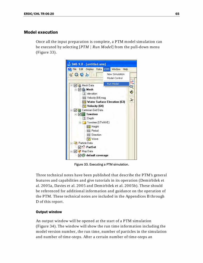
ERDC/CHL TR-06-20 65
Model execution
Once all the input preparation is complete, a PTM model simulation can be executed by selecting [PTM | Run Model] from the pull-down menu (Figure 33).
Figure 33. Executing a PTM simulation.
Three technical notes have been published that describe the PTM’s general features and capabilities and give tutorials in its operation (Demirbilek et al. 2005a, Davies et al. 2005 and Demirbilek et al. 2005b). These should be referenced for additional information and guidance on the operation of the PTM. These technical notes are included in the Appendices B through D of this report.
Output window
An output window will be opened at the start of a PTM simulation (Figure 34). The window will show the run time information including the model version number, the run time, number of particles in the simulation and number of time-steps. After a certain number of time-steps an

ERDC/CHL TR-06-20 66
estimate of the run time will be given. If desired, the simulation can be aborted during its execution from this window.
Figure 34. Output window at the start of a PTM simulation.
An update of the simulation status is given at increments of 100 time-steps (Figure 35). This includes time-step number and corresponding date and time in the simulation, and number of particles in various categories. These are as follows:
1. BORN is the number of particles that have been generated up to this point in the simulation.
2. ALIVE is the number of particles that are still within the model domain and are available for transport.
3. DEAD is the number of particles that have left the domain and are unavailable for transport.
4. ACTIVE is the number of particles that are in motion at that time-step. 5. DORMANT is the number of particles that are inactive or deposited at this
time-step.

ERDC/CHL TR-06-20 67
The symbols “=>P” or “=>M” indicate that the model is outputting data to the particle or map file, respectively.
Figure 35 shows the output window at the completion of a simulation. The solution can be loaded automatically when the window is closed if the box is checked. Pressing will close the simulation window.
Figure 35. Output window at the end of a PTM simulation.
Number of particles
The number of particles should be checked to ensure that a reasonable number of particles will be included in the simulation. This value is given at the start of a simulation (Figure 34). If too few particles are used, there may not be enough to provide the resolution required for an accurate solution, whereas too many particles may result in a simulation that takes too long to run. The simplest way to control this number is by adjusting the particle mass in the source coverage. Using a very large number of particles may result in a failure of the model to execute.
It is advised that, for new cases, a preliminary simulation be conducted with a small number of particles (e.g. a few hundred) so that the input

ERDC/CHL TR-06-20 68
values can be checked. The optimum number of particles to use in a production run requires a judgment call on the part of the user and will depend upon a number of factors, including number of sources, temporal and spatial extent of sources, duration of the simulation, required resolution of the solution, computational speed and memory size of processor and desired run time.
Output visualization
Once the simulation is complete and has been loaded, the results can be visualized. Options for visualization are set using the Particles page of the Display Options window (Figure 36).
Figure 36. Display options page for particle visualization.
The options include controls for particle path lines, particle tails and various particle settings, such as color and size. The particle visualization capabilities of the SMS interface are described in detail in (Demirbilek et al. 2005a), which in included in Appendix B.

ERDC/CHL TR-06-20 69
5 Model Application
PTM applications are presented in this chapter. Perhaps one of the most important concepts to gain from this chapter is the capability of the PTM to aid in a wide range of coastal and hydraulics projects. The applications are intended to serve as sample problems for users in their practical applications of the model. Although each case addresses the validity of results and usefulness of PTM, the applications demonstrates a specific set of processes which include: advection and diffusion, mixing within the water column, slope effects, deposition and resuspension, and the successful use of data (hydrodynamic and wave) obtained from other models. Applications are validated through both an understanding of sediment transport processes and by comparison to measurements.
Example applications considered in this chapter are:
1. Fluctuating flow through a straight flume of constant depth. 2. Uniform flow over a channel. 3. Concentration plume in a flume. 4. Combined wave and current flow in an idealized coastal inlet. 5. Wave-current co-existing flows at two field sites. 6. The effect on sediment transport of recent and proposed coastal
modifications.
Although the first three applications represent hypothetical situations, these serve to validate known sediment transport processes. The idealized inlet case is for a laboratory experiment performed by CIRP. The two field applications are for projects near Anchorage, AK, and Brunswick, GA.
Each section of this chapter focuses on one example and includes PTM application objectives. Next, PTM setup and input are discussed, including the mesh used, hydrodynamic and wave data, source information, as well as basic computational characteristics such as time-step. Finally, model results are presented. Chapter 4 is specifically dedicated to the explanation of input files. Therefore, the present chapter addresses pertinent details of input in a more general way. In the case of field applications and the idealized inlet, the project’s background is provided.
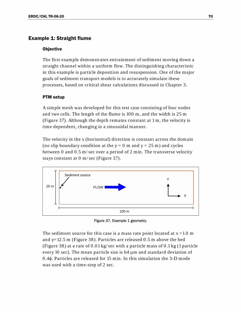
ERDC/CHL TR-06-20 70
Example 1: Straight flume
Objective
The first example demonstrates entrainment of sediment moving down a straight channel within a uniform flow. The distinguishing characteristic in this example is particle deposition and resuspension. One of the major goals of sediment transport models is to accurately simulate these processes, based on critical shear calculations discussed in Chapter 3.
PTM setup
A simple mesh was developed for this test case consisting of four nodes and two cells. The length of the flume is 100 m, and the width is 25 m (Figure 37). Although the depth remains constant at 1 m, the velocity is time dependent, changing in a sinusoidal manner.
The velocity in the x (horizontal) direction is constant across the domain (no slip boundary condition at the y = 0 m and y = 25 m) and cycles between 0 and 0.5 m/sec over a period of 2 min. The transverse velocity stays constant at 0 m/sec (Figure 37).
Figure 37. Example 1 geometry.
The sediment source for this case is a mass rate point located at x =1.0 m and y=12.5 m (Figure 38). Particles are released 0.5 m above the bed (Figure 38) at a rate of 0.01 kg/sec with a particle mass of 0.1 kg (1 particle every 10 sec). The mean particle size is 64 μm and standard deviation of 0.4φ. Particles are released for 15 min. In this simulation the 3-D mode was used with a time-step of 2 sec.
X
Y
FLOW
Sediment source
100 m
25 m

ERDC/CHL TR-06-20 71
Figure 38. Sediment source description for Example 1.
PTM results
Figure 39 shows an elevation view of the bed, water column, and particles. Particles are released 0.5 m above the bed and are advected by the flow. In the figure, blue-colored particles are active and red-colored particles are deposited.
Particles start to deposit just prior to 4 min into the simulation. More particles deposit and resuspend along the flume bed as the simulation progresses. At 7 min and 9 min, all particles have been entrained back into the flow. This example application clearly demonstrates that the PTM is capable of representing the process of sediment deposition and resuspension. Figure 40 shows the elevation view of the path of a single particle. A number of resuspension events are identified in the figure.

ERDC/CHL TR-06-20 72
Figure 39. Particles released in a straight channel at 1-min intervals (elevation view). Red particles are deposited. Blue particles are active.
Figure 40. Path of a single particle (elevation view).
t = 4 min
t = 5 min
t = 6 min
t = 7 min
t = 8 min
t = 9 min
t = 10 min
Re-suspension events
Flow speed minimum Flow speed maximum

ERDC/CHL TR-06-20 73
Example 2: Flow over a trench
Objective
The next application concerns flow over a trench. The objective of this example is to verify the capability of the PTM to correctly simulate the effect of vertical velocity change on particle movement. Presently, the PTM uses hydrodynamic input from 2-D models. A characteristic of the model is its capability to simulate the 3-D effects of particle transport given such 2-D input (see Chapter 3). This is important because the majority of hydrodynamic model data are 2-D, vertically averaged flow. Also, addressed here is the effect of slope side geometries.
PTM setup
Figure 41 shows channel geometry. The top plot is a plan view that shows the finite element mesh, the bottom plot is an elevation view (distorted vertically by a factor of 50) showing the location of the trench. The ambient depth is 2 m at the channel edge. The channel is 4 m deep and 400 m wide. The locations of the two sources are also shown. The flow moves from right to left.
Figure 41. Example 2 geometry.
Two instantaneous sources are used in this example. The property pages showing the source settings for this simulation can be seen in Figure 42. As shown in the source property pages, the first set of particles is released instantaneously on 12 August 2004 at 6:30 p.m., and the second set at 7:00 p.m. The specific positions of release points are x = 9,158 m and y = 900 m for the first and x = 9,158 m and y = 1,000 m for the second. The release point elevation for both cases is 1 m above the bed. The mass
2000 m
Elevation view (50 times vertical distortion)
Plan view
Flow direction
Source locations

ERDC/CHL TR-06-20 74
of each parcel is 0.1 kg, and the total mass of sediment is 3 kg. The mean particle size is 10 μm, and the standard deviation is 0.4φ .
Figure 42. Source property pages for Example 2.
The time control portion of the PTM Model Control input window (see Chapter 5) is shown in Figure 43. This simulation begins at 6:30 p.m. on 12 August 2004 and ends at 8:00 p.m. on the same day. The computational time-step is 1.0 sec. The hydrodynamic data also begin at 6:30 p.m. on 12 August 2004.
Figure 43. PTM Time Control.

ERDC/CHL TR-06-20 75
Figure 44 shows the Computational Parameter page of the PTM Model Control for this case. The 3-D advection modeling algorithm is chosen. This algorithm is generally most appropriate for simulation of fine-grained sediment transport. Also considered in this run are particle-bed interactions.
Figure 44. PTM Computational Parameters.
PTM results
As the particles are propelled down the channel by the flow field and then cross the channel, the expected outcome is that particles will follow the streamlines of the flow. That is, they should separate vertically as the cross-sectional area increases.
A single frame of output for the simulation is shown in Figure 45. The particles are colored according to their source. These fine particles follow the streamlines.
Figure 45. Snapshot of particles passing over trench.

ERDC/CHL TR-06-20 76
Streamlines for a number of the particles are shown in Figure 46. As particles pass across the trench, the impact of the vertical velocity distribution is obvious. The particles closer to the bed lag behind the particles higher in the water column. There is a distinct vertical separation at the higher particles also, whereas the particles close to the bed appear to cluster closer together.
Figure 46. Streamlines of selected particles passing over trench.
PTM results at 10 min intervals are presented in Figure 47.
Figure 47. Particles crossing trench. Particles are colored according to their source. Each frame is separated by 10 min.

ERDC/CHL TR-06-20 77
Example 3: Concentration plume
Objective
The objective of this example is to compare the diffusion predicted by the PTM and an exact analytical solution for diffusion (Roberts and Webster 2002).
PTM setup
The analytical solution presented in this example is based on a point release of 0.5 kg into an infinitely-wide, 2-D uniform flow of 1.0 m/sec. The diffusion coefficient is 0.25 m2/sec.
The flow and diffusion coefficients used in PTM are 3-D and unique for each particle at each time-step. In addition to vertical and horizontal diffusion coefficients, the computations take into account proximity to boundaries and depth of flow. As such, for the purposes of comparison with the analytical solution, the PTM code was modified to override these computations and use a uniform velocity field and diffusion coefficient to produce the results presented in this section.
PTM results
Figure 48 shows a comparison between the analytical and PTM predictions 50 m downstream of a continuous point source. In this example, the PTM was run with time-steps of 1 and 5 sec. Figure 49 shows the results at 250 and 500 m. The agreement between the PTM calculation and the analytical solution is excellent. By contrast, Eulerian schemes typically have difficulty obtaining an accurate diffusion solution due to inherent numerical diffusion (Vreugdenhill 1989).

ERDC/CHL TR-06-20 78
Figure 48. Diffusion modeled by PTM compared to analytic solution.
Figure 49. Comparison of pure diffusion at two distances from point source.
Example 4: Flow in an idealized inlet
Objective
In most coastal inlet applications of the PTM, coexisting flow conditions require proper handling of wave-current interactions and shear stresses that affect the movement of sediment particles. The overall capabilities of the PTM are examined in this example in the presence of waves and currents, where wave shoaling, refraction, diffraction, reflection, and breaking processes occur around an inlet protected by two jetties. This example examines the wave-current interaction at an idealized inlet to test
Distance from centerline of plume (m)
Con
cent
ratio
n(k
g/se
c)
-20 -15 -10 -5 0 5 10 15 200
0.005
0.01
0.015
0.02
0.025
0.03
0.035
0.04
0.045
0.05Analytical at 50 mPTM at 50 m (dt = 5 s)PTM at 50 m (dt = 1 s)
Distance from centerline of plume (m)
Con
cent
ratio
n(k
g/se
c)
-50 -40 -30 -20 -10 0 10 20 30 40 500
0.005
0.01
0.015
0.02Analytical at 250 mPTM at 250 mAnalytical at 500 mPTM at 500 m

ERDC/CHL TR-06-20 79
the basic processes of sediment transport. Note that this is an idealized inlet; the flow conditions are wave-dominated, and there is no tidally-induced flow through the inlet. As well, no flood or ebb delta features are represented in the bathymetry.
Wave input for this PTM simulation is obtained with STWAVE (Smith et al. 2001). The user provides the PTM with an STWAVE grid and the associated wave field file. If necessary, one can also use the SMS to convert result files from other hydrodynamic or wave models and configure necessary inputs in required formats prior to using them in a PTM application. This is illustrated in Example 3 where hydrodynamic input is obtained from M2-D (Militello et al. 2004), a 2-D finite-difference coastal circulation model. M2-D input was manually converted to ADCIRC file formats using the SMS. In a future release of SMS, this process will be automated to facilitate the usage of the PTM and its coupling with other hydrodynamic models.
Background
The CIRP conducted two laboratory experiments to investigate wave behavior and wave-induced currents around jetties of an idealized inlet (Seabergh et al. 2006). The first experiment examined refraction and diffraction at an offshore breakwater and dogleg jetty. Wave diffraction into the bay behind the inlet with and without flood currents was also studied. The second experiment involved testing two types of jetty structure, an absorbing and a reflective jetty. The highly absorbing jetty resembles a fairly porous rock rubble structure, whereas the fully reflective jetty represents a vertical sheet pile or a caisson breakwater. The laboratory model is constructed according to a 1:50 scale to replicate a medium-sized U.S. Atlantic Coast inlet. The laboratory schematic is shown in Figure 50.

ERDC/CHL TR-06-20 80
Figure 50. Schematic of laboratory experiment for idealized inlet.
Experimental conditions include both regular and irregular unidirectional waves generated at the model’s offshore boundary representing mild to moderate and high sea states. Incident wave direction was either 0 (shore-normal) or 20 deg (oblique) to shoreline. Wave and current measurements were made on a grid consisting of cross-shore and along-shore transects on the up-wave side and bay side of jetties for easy application in numerical model calibration. Wave direction was measured for some experiments by a remote-sensing video-camera system as well as analyzed from the current vector data. Wave and current measurements were also conducted within the inlet on three transects parallel to the jetties. A photograph of the model arrangement can be seen in Figure 51.
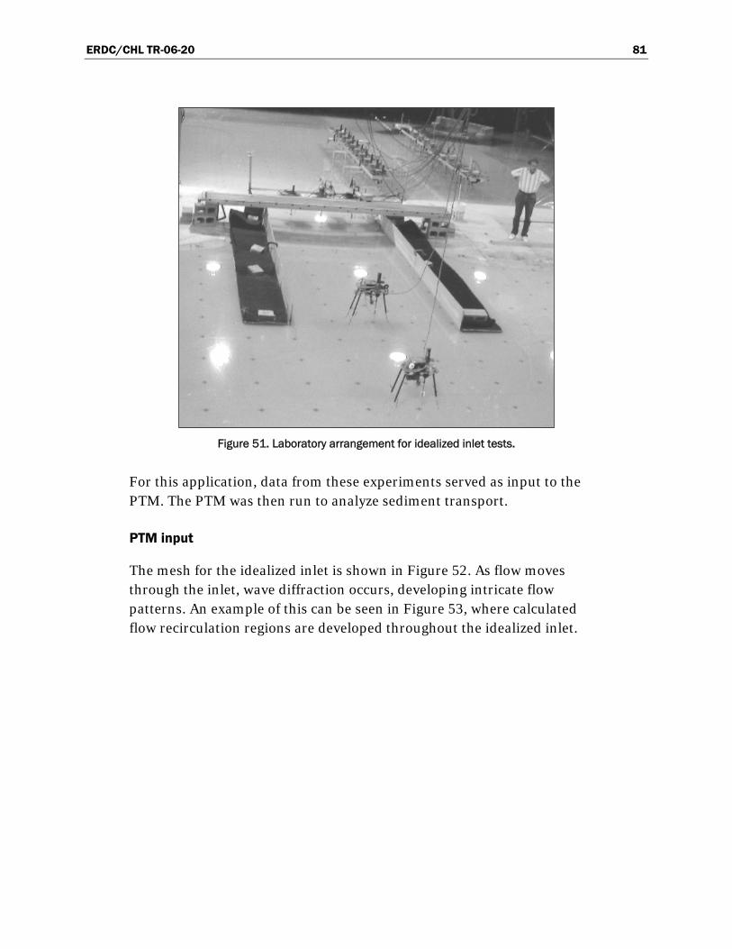
ERDC/CHL TR-06-20 81
Figure 51. Laboratory arrangement for idealized inlet tests.
For this application, data from these experiments served as input to the PTM. The PTM was then run to analyze sediment transport.
PTM input
The mesh for the idealized inlet is shown in Figure 52. As flow moves through the inlet, wave diffraction occurs, developing intricate flow patterns. An example of this can be seen in Figure 53, where calculated flow recirculation regions are developed throughout the idealized inlet.

ERDC/CHL TR-06-20 82
Figure 52. Example 4 mesh and bathymetry.
Figure 53. Flow field at t = 8 sec.
Source

ERDC/CHL TR-06-20 83
The source specified was a continuous mass point source (see Figure 53) at a rate of 10 kg/sec. The sediment size is medium sand, with median size 0.2 mm. Each particle represents 1 kg of sand (one particle released every 10 sec). The setup of the source is shown in Figure 54.
Figure 54. Source input property page.
For this case a native sediments file was created using the Create PTM External Input Files option. The 35D , 50D , and 90D are 0.1, 0.2, and
0.5 mm, respectively (Figure 55). A beneficial feature of the interface is that once this file is created, it can be used for other simulations with this grid.

ERDC/CHL TR-06-20 84
Figure 55. Create PTM External Input Files SMS dialogue box.
The simulation is set to run for 1 hr with a time-step of 1.0 sec using the Q3-D mode. As mentioned in Chapter 4, the wave option is given under the waves tab in the PTM Model Control (Figure 56). The details of the STWAVE solutions (start time, grid origin, etc.) are input into the model control.

ERDC/CHL TR-06-20 85
Figure 56. PTM Wave Model Control in SMS.
PTM results
The particle positions after 1 sec can be seen in Figure 57. Blue particles represent suspended particles, and the red particles represent currently deposited particles. The particles are transported towards the channel by the longshore currents, they then move longitudinally towards the channel due to the specified longshore boundary condition. However, they are soon forced into the channel by the tide during this portion of the simulation. Sixty seconds after the start of the simulation, particles move through the channel and deposit due to decreased wave action (Figure 58). For real applications, this information can be valuable to establish the effect of a channel configuration. As sediment enters into the channel, deposition potential is required for assessing navigation issues and dredging requirements.

ERDC/CHL TR-06-20 86
Figure 57. Particle positions at t = 1 sec.
Figure 58. Particle positions at t = 60 sec.

ERDC/CHL TR-06-20 87
Example 5: Dredging application, Brunswick, GA
Objective
This example demonstrates application of the PTM for evaluation of nearshore placement of dredged material. These PTM simulations are part of a larger study to develop a Dredged Material Management Plan that includes optimization of nearshore dredged material placement for littoral zone nourishment. Another component of the study placed fluorescent sediment tracer in the nearshore environment and monitored tracer migration over a 6-month period. The PTM simulations described here pertain to transport of sand and silt from two existing dredged material placement locations. The objective is to demonstrate a PTM application for nearshore placement of dredged material and to compare model results to fluorescent tracer study observations.
Background
The ERDC is supporting the USACE Savannah District in conducting a multi-year study to evaluate and validate numerical models for predicting dredged material transport at nearshore and open-water sites (Evans Hamilton, Inc. 2004). Nearshore transport predictions are required to address natural resource, beneficial use, and site capacity issues. Accurate predictive models are necessary for selecting and managing nearshore placement sites. PTM is applied at the Brunswick, GA, site as a diagnostic tool to judge the combined capabilities of other models, including hydrodynamic and wave models. PTM takes the results of these other models as drivers to determine fate and pathways of sediment in the modeling area and provides both qualitative and quantitative assessment of the consequences of dredging activities near Brunswick, GA.
Dredged material from the Brunswick Harbor Entrance Channel has recently been placed in a series of channel-adjacent, open-water dredged material placement sites approximately 1,200 m south of the shipping channel (Figure 59). Dredged material removed from the entrance channel is composed of approximately 80 percent sand and 20 percent silt and clay. The dredged material does not meet guidelines for direct beach placement (less than 12 percent fines). Therefore, nearshore placement is considered a promising alternative to direct beach placement for which winnowing by wave action will naturally separate sand and silt fractions. The coarser sand fraction is likely to remain in the nearshore, while fine-

ERDC/CHL TR-06-20 88
grained sediment will be suspended by high wave energy in the nearshore and transported offshore by currents.
Figure 59. Map of Brunswick dredge material mound region.
Fluorescent tracer study
Fluorescent tracer field experiments were performed in 2003 to study the transport and fate of dredge material placed at Sites C and JN (Figure 55). Fluorescent tracer was manufactured to represent silt and sand-sized
Jekyll Island

ERDC/CHL TR-06-20 89
particles characteristic of the dredged material (Table 2). Four tracer colors were manufactured (two sand-sized and two silt-sized) to distinguish particles during analysis by both sediment class (silt or sand) and initial location (C or JN). In late January 2003, fluorescent tracer was mixed with equal quantities of dredged material and placed on the mound crests at Sites C and JN. A sampling scheme was developed over the region to sample for tracer particles at 15, 60, 140, and 205 days following tracer release. The first two sampling events were performed with surface grabs, resulting in little recovery of sand tracer. The final two rounds of sampling were collected with shallow vibracore and pushcore, resulting in much higher rates of tracer recovery and indicating burial of sand tracer by as much as 0.3-0.5 m at the edge of mound C.
Table 2. Tracer characteristics.
Tracer Color Sediment Type Deployment Site D50 (mm) Standard Deviation
Violet Sand C 0.235 0.525
Yellow Silt C 0.065 0.724
UVblue Silt JN 0.045 0.898
Magenta Sand JN 0.272 0.554
Mass conservation analysis of the recovered tracer at Site C indicates that the extremely fine (10-20 m) spatial resolution of sampling was insufficient to resolve spatial variability in the tracer deposition and burial along the margins of the mound. The spatial variation at site JN was much more gradual, but mass conservation analysis indicated that only 20 percent of the particles released were recovered, suggesting that a large fraction (of particles, not necessarily mass) of sand tracer at JN was transported outside the sampling area. Analysis of silt-sized tracers deployed at C and JN indicates rapid winnowing from the deployment site, transport in suspension, and wide dispersal of tracer within and presumably beyond the study boundaries.
PTM setup
The PTM was applied for the period of tracer monitoring between 31 January and 21 February 2003. Numerical particles were specified with statistical distributions similar to each fluorescent tracer (D50 and standard deviation, see Table 2). Numerical particles were introduced as point sources on the sediment bed and made available for erosion and transport at the times and locations of the fluorescent tracer deployment.
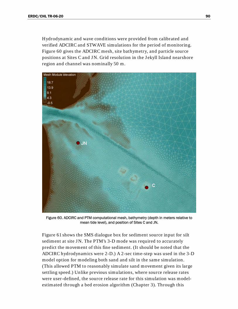
ERDC/CHL TR-06-20 90
Hydrodynamic and wave conditions were provided from calibrated and verified ADCIRC and STWAVE simulations for the period of monitoring. Figure 60 gives the ADCIRC mesh, site bathymetry, and particle source positions at Sites C and JN. Grid resolution in the Jekyll Island nearshore region and channel was nominally 50 m.
Figure 60. ADCIRC and PTM computational mesh, bathymetry (depth in meters relative to mean tide level), and position of Sites C and JN.
Figure 61 shows the SMS dialogue box for sediment source input for silt sediment at site JN. The PTM’s 3-D mode was required to accurately predict the movement of this fine sediment. (It should be noted that the ADCIRC hydrodynamics were 2-D.) A 2-sec time-step was used in the 3-D model option for modeling both sand and silt in the same simulation. (This allowed PTM to reasonably simulate sand movement given its large settling speed.) Unlike previous simulations, where source release rates were user-defined, the source release rate for this simulation was model-estimated through a bed erosion algorithm (Chapter 3). Through this

ERDC/CHL TR-06-20 91
method, particle introduction to the water column representative of bed erosion is possible. Time varying wave-current conditions were used to estimate bed shear stress and erosion (source strength) to the water column. This PTM option is described in Chapter 3.
Figure 61. Properties of sediment sources.
PTM results
The PTM simulations were performed for the tracer analysis period. In this section, results for transport of each tracer are compared to the equivalent PTM source transport.
Silt at Site JN
Similar to the fluorescent tracer study, the PTM results indicate that silt is rapidly winnowed from the site. The PTM results also indicate that the much of the silt is transported to the channel and deposited in the channel and on the channel side slopes. Although direct tracer assessment was not possible for the channel, several indicators in the tracer study support the PTM results. These include tracer detection on the sound-side of Jekyll Island and on the side slopes of the navigation channel. PTM indicates that a small fraction of silt initially moves into the Jekyll Island nearshore region and is subsequently resuspended and transported offshore by increased wave energy. The ephemeral nearshore deposition of JN silts was also observed in the tracer study. A snapshot of the PTM output after the 21-day simulation is provided in Figure 62.

ERDC/CHL TR-06-20 92
Figure 62. PTM predictions for sediment at Site JN after 21 days. Particles are colored according to grain size.
Sand at Site JN
Model data indicate that coarser sand (~0.35 mm) remains close (within 100 m) of the deployment site. Tracer data indicate that approximately 20 percent of the sand tracer remained within 100 m of the deployment site. Interestingly, if winnowing of particles is the dominant process (as indicated by the PTM simulation), 20 percent of the tracer particles are coarser than 0.250 mm, which is not greatly different from the sorting of particles in the PTM simulation. The PTM results indicate that finer sand (<0.30 mm) is transported northwest from the site, into the channel, and then transported by bi-directionally by tidal currents with a net drift in the ebb direction (Figure 62). The PTM also predicts only small quantities of the sand moving from Site JN to the Jekyll Island littoral system, a similar conclusion from the tracer study.

ERDC/CHL TR-06-20 93
Silt at Site C
The PTM predictions indicate that soon after particle seeding, silt particles rapidly winnow from the mound and are initially transported southward and deposited over the inner shelf. Later in the simulation, some of the silt particle are resuspended and transported northward, further scattering the silt-sized particles. Wide dispersal of silt particles from Site C is supported by the tracer study, but significant quantities of the yellow “silt” tracer deployed at Site C were also found in the Jekyll nearshore. This behavior may be explained by the fact that the manufactured tracer meant to represent silt at Site C also contained a large fraction of particles (by weight) in the range of 60-100 μm, or fine sand. If numerical particles in this size range are considered in this analysis, the PTM results are consistent with observations from the tracer study.
Sand at Site C
The PTM transport predictions for sandy sediments at Site C are not supported by tracer data. The suspected reason for the disagreement between tracer and numerical particle transport is the morphological behavior of the dredged material mound, by which sand tracer was transported from the mound crest and buried primarily along the southeast margin of the mound. The morphological processes involved rollover migrations are not represented in the PTM. As a result, the PTM estimated that fine and coarse sand migrated much further than actually observed.
Example 6: Suspended sediment transport in Northern Cook Inlet and Knik Arm, AK
Objective
The PTM is a versatile tool for representing sediment transport in a wide variety of aquatic systems. The primary objective of this example is to quickly and interactively investigate transport of suspended sediments in northern Cook Inlet and Knik Arm, AK.
Background
Knik Arm is a 45-km-long extension of Cook Inlet from Point Woronzof near Anchorage, to the confluence of Knik and Matanuska Rivers (Figure 63). The Port of Anchorage (POA) is situated on the southeast
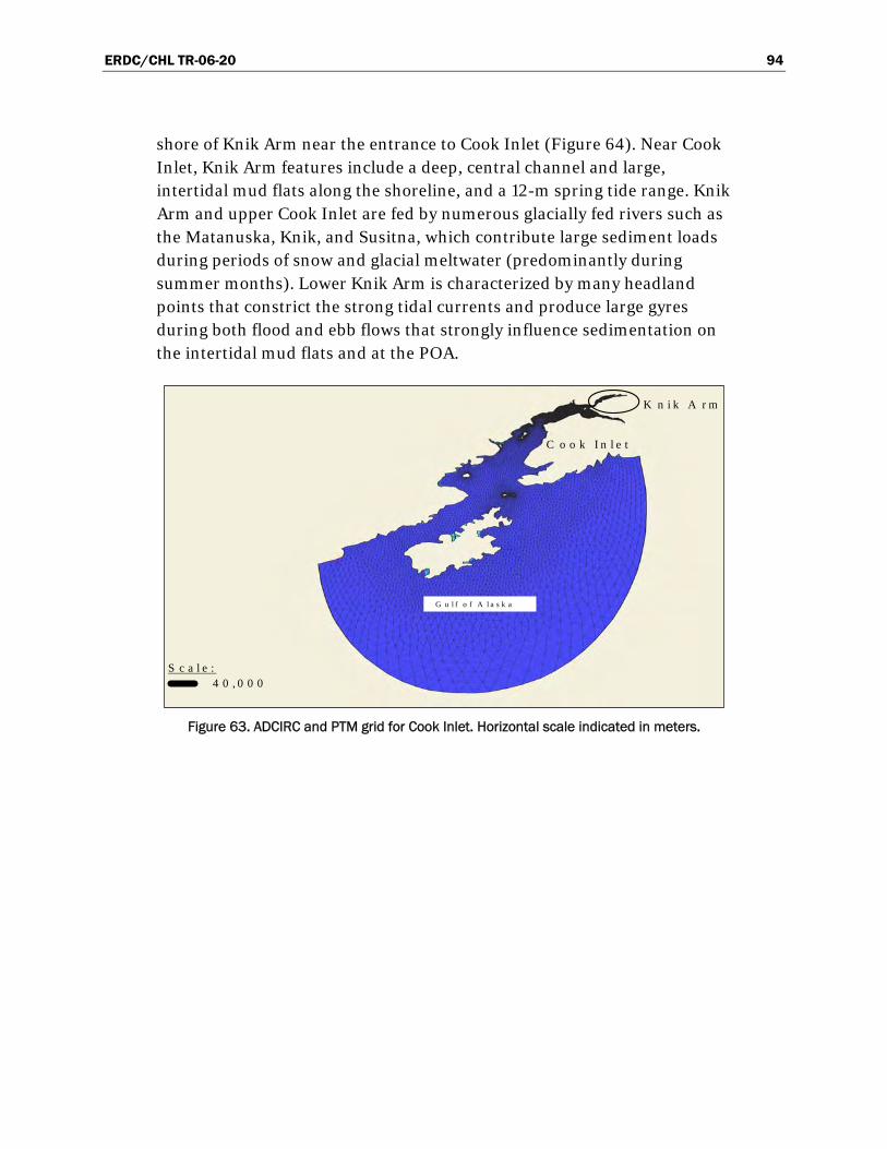
ERDC/CHL TR-06-20 94
shore of Knik Arm near the entrance to Cook Inlet (Figure 64). Near Cook Inlet, Knik Arm features include a deep, central channel and large, intertidal mud flats along the shoreline, and a 12-m spring tide range. Knik Arm and upper Cook Inlet are fed by numerous glacially fed rivers such as the Matanuska, Knik, and Susitna, which contribute large sediment loads during periods of snow and glacial meltwater (predominantly during summer months). Lower Knik Arm is characterized by many headland points that constrict the strong tidal currents and produce large gyres during both flood and ebb flows that strongly influence sedimentation on the intertidal mud flats and at the POA.
Figure 63. ADCIRC and PTM grid for Cook Inlet. Horizontal scale indicated in meters.
C o o k I n l e t
K n i k A r m
G u l f o f A l a s k a
S c a l e : 4 0 , 0 0 0

ERDC/CHL TR-06-20 95
Figure 64. Knik Arm and POA, including ADCIRC mesh. Note fine mesh spacing near POA.
Initial studies indicate that the Knik Arm Crossing may alter flow conditions and infilling at the POA, which is a Federally maintained for navigation. Due to the large riverine sediment input and sediment storage in adjacent intertidal mud flats, the POA presently requires considerable annual maintenance dredging and has, in recent years, experienced even larger shoaling rates. Consequently, the PTM was applied in upper Knik Arm to better understand sediment transport patterns in this highly dynamic system.
PTM input
A 2-D ADCIRC grid was created for the entire Cook Inlet system (Figure 63), with increasing mesh resolution provided in areas of interest (including thePOA) (Figure 64 and Figure 65). Finest resolution in the ADCIRC/PTM mesh is provided near the POA with approximately 10-m node spacing (Figure 64 and Figure 65). Field-measured tidal-elevation and current data were used to validate the hydrodynamic model. Wave-generated bed stresses in Knik Arm are negligible, and the influence of waves on sediment transport is neglected in this study.
POA
Anchorage
Port MacKenzie
Susitna River
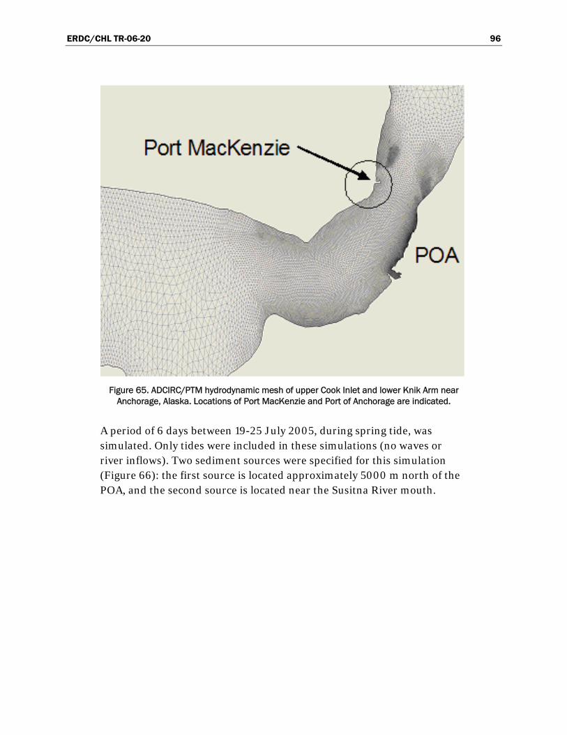
ERDC/CHL TR-06-20 96
Figure 65. ADCIRC/PTM hydrodynamic mesh of upper Cook Inlet and lower Knik Arm near Anchorage, Alaska. Locations of Port MacKenzie and Port of Anchorage are indicated.
A period of 6 days between 19-25 July 2005, during spring tide, was simulated. Only tides were included in these simulations (no waves or river inflows). Two sediment sources were specified for this simulation (Figure 66): the first source is located approximately 5000 m north of the POA, and the second source is located near the Susitna River mouth.

ERDC/CHL TR-06-20 97
Figure 66. Location of two particle release sources in Cook Inlet/Knik Arm model. A line source is indicated approximately 5,000 m north of POA. A series of point sources is indicated
south of Susitna River mouth.
For the first sediment source, north of the POA, sediment particles were introduced into the system for 10 hr at a mass rate of 1x10⁻⁴ kg/sec using a horizontal line source (see Chapter 2 for types of sediment sources available in the PTM). This source extended across the width of Knik Arm and was vertically positioned at 2-m water depth. Figure 67a shows the SMS dialogue box that provides specifics for this line source. A series of point (vertical line) sources were used for the second sediment source located near the Susitna River mouth (see Chapter 2 for details on vertical line sources). Each of the vertical line sources were configured for a uniform vertical distribution of particles released at a rate of 0.05 kg/sec. Figure 67b shows the SMS dialogue box for one of the eleven point sources. Although individual point source positions vary, the release rates and particle characteristics are identical for all 11 points. Particle characteristics for all sources are representative of coarse silt and fine sand (d50 = 0.065 mm), characteristic of suspended sediments in the study area. The 3-D PTM model option was used in this example because this example deals essentially with fine-grained sediments. Similar to Example 4, the ADCIRC simulations used here were 2-D. The PTM time-step was set to 15 sec, and the model was run for 7 days. For this example, a larger time-step than Example 4 is justified due to the slower settling velocity of silt.

ERDC/CHL TR-06-20 98
Figure 67. (a) Knik Arm horizontal line source and (b) sample Susitna River vertical line source.
PTM results
Figure 68 shows the PTM particle locations from both sources at the end of the 7-day simulation. Red particles indicate deposited sediments, and blue particles indicate sediment in suspension. Similar to observations in the natural system, deposition of silt particles is limited predominantly to the areas adjacent to the intertidal mud flats. Strong tidal flows in the main channel produce sufficiently large bed shear stresses to limit fine-sediment deposition, and more quiescent conditions in gyres shed by the numerous points in the system produce weaker bed stresses and conditions more favorable to fine-sediment deposition. Near sharp changes in geometry and bedslope, field measurements have identified 3-D hydrodynamic features. The presently applied ADCIRC 2-D hydrodynamics do not represent these hydrodynamic secondary flow features. 3-D flow characteristics would more accurately represent actual hydrodynamic conditions in the study area, and 3-D hydrodynamic modeling is planned for future applications and final analysis.

ERDC/CHL TR-06-20 99
Figure 68. Particle positions in Knik Arm region at 23 July 2005 (12 p.m.). Blue particles indicate suspended sediment and red particles indicate sediment resting on bed.
The PTM indicates that much of the sediment introduced near the Susitna River mouth deposits on the large intertidal mudflat/delta (Figure 69). No known data (other than the presence of the mudflat itself) are available to verify the modeled result. One objective of the PTM application was to assess the potential role of sediment discharge from the Susitna River as a source of sediment to lower Knik Arm. Preliminary simulations with the PTM indicate that sediments introduced near the Susitna River mouth either deposit on the surrounding mud flats or are transported with a net southward direction in upper Cook Inlet. Therefore, the Susitna River is not a significant source of sediment to lower Knik Arm.

ERDC/CHL TR-06-20 100
Figure 69. Particle positions in Susitna River region. Blue represents suspended particles and red represents deposited particles.
ERDC/CHL TR-06-20 101
6 Concluding Remarks
A new Lagrangian modeling tool, the PTM, has been developed for tracking the fate of sediments and neutrally-buoyant particles in coastal, ocean, and fluvial waters. The model requires pre-calculated hydrodynamic model results such as those from the ADCIRC circulation model and the STWAVE wave model. Operating within the SMS modeling environment, the PTM allows the user to specify detailed information about sediment sources such as sediment release locations, rates of sediment release, and grain-size characteristics.
Ongoing development of the model will further validate the algorithms employed against field and laboratory data sets and extend model applicability to other hydrodynamic models including those representing 3-D processes. Refinements to the usability of both the model and its interface are ongoing. The model is designed to provide engineers with insight into sediment transport conditions and sediment pathways.
The quality and accuracy of particle fate simulations depends directly upon the input flow conditions. It is important that the flow model results input to the PTM be an accurate representation of the site. As with any computer modeling tool, careful analysis and interpretation of the model results and comparisons to field conditions are essential to achieving accurate and meaningful simulations.

ERDC/CHL TR-06-20 102
References
Bagnold, R. A. 1966. An approach to the sediment transport problem for general physics. Washington, DC: U.S. Geological Survey Professional Paper 422-1.
Bijker, E. W. 1966. The increase of bed shear in a current due to wave motion. Proceedings 10th International Conference on Coastal Engineering 1:746-765, ASCE.
Bridge, J. S., and S. J. Bennett. 1992. A model for the entrainment and transport of sediment grains of mixed sizes, shapes and densities. Water Resources Research 28(2):337-363.
Davies, M. H., and D. A. W. Watson. 1997. Modélisation du transport sédimentaire dans l’estuaire du Saint-Laurent. Technical Report TR-HYD-033. Canada: National Research Council of Canada, March 1997, 29 pp.
Davies, M., N. MacDonald, Z. Demirbilek, J. Smith, A. Zundel, and R. Jones. 2005. Particle Tracking Model (PTM) in the SMS: II. Overview of features and capabilities. Dredging Operations and Environmental Research Technical Note Collection (ERDC-TN-DOER-D4). Vicksburg, MS: U.S. Army Engineer Research and Development Center.
Demirbilek, Z., J. Smith, A. Zundel, R. Jones, N. MacDonald, and M. Davies. 2005a. Particle Tracking Model (PTM) in the SMS: I. Graphical interface. Dredging Operations and Environmental Research Technical Note Collection (ERDC-TN-DOER-D4). Vicksburg, MS: U.S. Army Engineer Research and Development Center.
Demirbilek, Z., J. Smith, A. Zundel, R. Jones, N. MacDonald, and M. Davies. 2005b. Particle Tracking Model (PTM) in the SMS: III. Tutorial with examples. Dredging Operations and Environmental Research Technical Note Collection (ERDC-TN-DOER-D4). Vicksburg, MS: U.S. Army Engineer Research and Development Center.
De Ruiter, J. C. C., and M. C. L. M. van Mierlo. 1980. Turbulence measurements above artificial dunes. Report No. Q789-1. Delft, The Netherlands: Delft Hydraulics Laboratory.
Egiazaroff, I. V. 1965. Calculation of non-uniform sediment concentration. Journal of the Hydraulics Division 44:225-247 ASCE.
Engelund, F., and J. Fredsoe. 1976. A sediment transport model for straight alluvial channels. Nordic Hydrology 7(5):293-306.
Evans Hamilton Inc. 2004. Data report for field measurement program in support of investigation of dredged sediment movement and fate at the entrance to Brunswick Harbor, Georgia. Data Report DACW39-99-D-008. Charleston, SC.
Fischer, H. B., J. E. List, R. C. Y. Koh, J. Imberger, and N. H. Brooks. 1979. Mixing in inland and coastal waters. San Diego, CA: Academic Press, 483 pp.

ERDC/CHL TR-06-20 103
Guy, H. P., D. B. Simons, and E. V. Richardson. 1966. Summary of alluvial channel data from flume experiments, 1956-1961. U.S. Geological Survey Professional Paper 426-I, Washington, DC: U.S. Geological Survey.
Hands, E. B., M. Allison, J. Brogdon, R. Cox, P. Terell, and D. Bishop. 1992. Monitoring of Alabama berms. Dredging Research Technical Note DRP-1-08. Vicksburg, MS: U.S. Army Engineer Waterways Experiment Station, Coastal and Hydraulics Laboratory.
Kemp, P. H., and R. R. Simons. 1982. Interaction between waves and a turbulent current. Journal of Fluid Mechanics 116:227-250.
Kleinhans, M. G., and L. van Rijn. 2002. Stochastic prediction of sediment transport in sand-gravel bed rivers. Journal of Hydraulic Engineering 128(4):412-425.
Luettich, R. A., Jr., J. J. Westerink, and N. W. Scheffner. 1992. ADCIRC: An advanced three-dimensional circulation model for shelves, coasts, and estuaries. Technical Report DRP-92-6. Vicksburg, MS: U.S. Army Engineer Waterways Experiment Station, Coastal and Hydraulics Laboratory.
MacDonald, N. J. 1998. Numerical modeling of non-linear wave-induced nearshore circulation. PhD diss. Liverpool, England: University of Liverpool.
Militello, A., C. W. Reed, A. K. Zundel, and N. C. Kraus. 2004. Two-dimensional depth-averaged circulation model M2-D: Version 2.0, Report 1, technical documentation and user’s guide. Coastal Inlet Research Program Technical Report ERDC/CHL TR-04-2. Vicksburg, MS: U.S. Army Engineer Research and Development Center.
Mogridge, G. R., M. H. Davies, and D. H. Willis. 1994. Geometry prediction for wave-generated bedforms. Coastal Engineering 22:255-286, Elsevier Publishing Company.
Nielsen, P. 1992. Coastal bottom boundary layers and sediment transport. Singapore: World Scientific Publishing Co., 324 pp.
O’Connor, B.A., and D. Yoo. 1988. Mean bed friction of combined wave/current flow. Coastal Engineering 12:1-21.
Roberts, P. J. W., and D. R. Webster. 2002. Turbulent diffusion. In Environmental fluid mechanics: Theories and applications, 480 p., H. H. Shen, A. H. D. Cheng, K.-H. Wang, M. H. Teng, and C. C. K. Liu, ed., 450 pp., ASCE.
Rouse, H. 1939. Experiments on the mechanics of sediment transport. Proceedings.5th International Congress of Applied Mechanics. Cambridge, MA: Murray Printing Company, 550-554.
Seabergh, W., L. Lin, and Z. Demirbilek. 2006. Laboratory and numerical studies of hydrodynamics near inlet structures: Part 1: Laboratory studies. Submitted to Coastal Engineering.
Shen, H. T., P. D. Yapa, D. S. Wang, and X. Q. Yang. 1993. A mathematical model for oil slick transport and mixing in rivers. Special Report 93-21. Hanover, NH: U.S. Army Cold Regions Research and Engineering Laboratory, 78 pp.

ERDC/CHL TR-06-20 104
Smith, S. J., J. Z. Gailani, L. Raad, and B. Tracy. 2006 (in preparation). Monitoring and modeling of nearshore placement of dredged material at Brunswick, Georgia. Coastal and Hydraulics Laboratory Technical Report xxx. Vicksburg, MS: U.S. Army Engineer Research and Development Center.
Smith, J. M., A. R. Sherlock, and D. T. Resio. 2001. STWAVE: STeady-state spectral WAVE model: User’s manual for STWAVE Version 3.0. Supplemental Report ERDC/CHL SR-01-1, Vicksburg, MS: U.S. Army Engineer Research and Development Center.
Soulsby, R. L. 1997. Dynamics of marine sands - A manual for practical applications. ISBN 0 7277 2584 X, London, UK: Thomas Telford Publications, 249 pp.
Soulsby, R. L. and R. J. S. W. Whitehouse. 1997. Threshold of sediment motion in coastal environments. In Proceedings Pacific Coasts and Ports ’97, 149-154. Christchurch, NZ: University of Canterbury.
Stive, M. J. F., E. Terrile, A. J. H. M. Reniers, and H. J. Verhagen. 2005. Motion threshold of coarse particles under shoaling waves. Proceedings 2005 Canadian Coastal Conference (on CD-ROM). Halifax, Canada.
van Rijn, L. C. 1984a. Sediment transport, Part I: Bed load transport. Journal of Hydraulic Engineering 110(10):1431-1456.
van Rijn, L. C. 1984b. Sediment transport, Part II: Suspended load transport. Journal of Hydraulic Engineering 110(11):1613-1641.
van Rijn, L. C. 1984c. Sediment transport, Part III: Bed forms and alluvial roughness. Journal of Hydraulic Engineering 110(12):1733-1754.
van Rijn, L. C. 1993. Principles of sediment transport in rivers, estuaries and coastal seas. The Netherlands: Aqua Publications.
Vreugdenhill, C. B. 1989. Computational hydraulics, an introduction. Berlin: Springer-Verlag, 179 pp.
Wilson, K. C. 1987. Analysis of bed-load motion at high shear stress. Journal of Hydraulic Engineering 113(1):97-103.
Yalin, M. S. 1977. Mechanics of sediment transport. ISBN 0 08 021162 3, Oxford, UK: Pergamon Press, 298 pp.
Zundel, A. K. 2005. Surface-water modeling system reference manual, Version 9.0. Provo, UT: Brigham Young University Environmental Modeling Research Laboratory.

ERDC/CHL TR-06-20 105
Appendix A: Model Flow Diagram

ERDC/CHL TR-06-20 106
Read parameter file and fixed data
Read flow and wave data (if req’d)
Bathymetry Boundaries
Roughness Native sediments
Determine flow field
Release new particles
Loop through particles Transport particle
Check boundaries
No
Yes
Interpolate conditions at
particle location
Store results
Is simulation complete?
t = t0
Determine bed forms
No YesStop
Has particle left domain?
Remove from list Yes
Determine bed interactions
Check traps
Re-entrain particle?
No
Yes
t = t + Δt
Determine transport
Is particle mobile?
Compute transport rates and particle
mobility
Flows
Waves
Run controls

ERDC/CHL TR-06-20 107
Appendix B: Particle Tracking Model (PTM) in the SMS: I. Graphical Interface

ERDC/CHL TR-06-20 108

ERDC/CHL TR-06-20 109

ERDC/CHL TR-06-20 110

ERDC/CHL TR-06-20 111
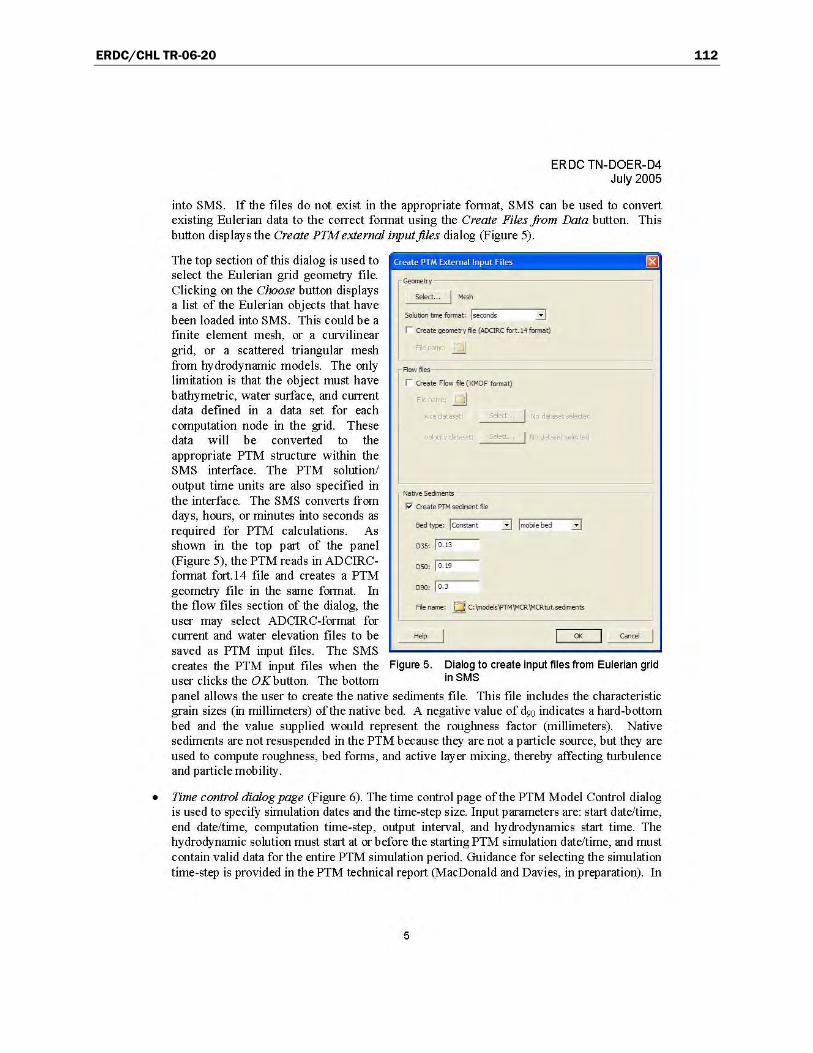
ERDC/CHL TR-06-20 112

ERDC/CHL TR-06-20 113

ERDC/CHL TR-06-20 114

ERDC/CHL TR-06-20 115

ERDC/CHL TR-06-20 116

ERDC/CHL TR-06-20 117

ERDC/CHL TR-06-20 118

ERDC/CHL TR-06-20 119

ERDC/CHL TR-06-20 120

ERDC/CHL TR-06-20 121

ERDC/CHL TR-06-20 122
Appendix C: Particle Tracking Model (PTM): II. Overview of Features and Capabilities

ERDC/CHL TR-06-20 123

ERDC/CHL TR-06-20 124

ERDC/CHL TR-06-20 125
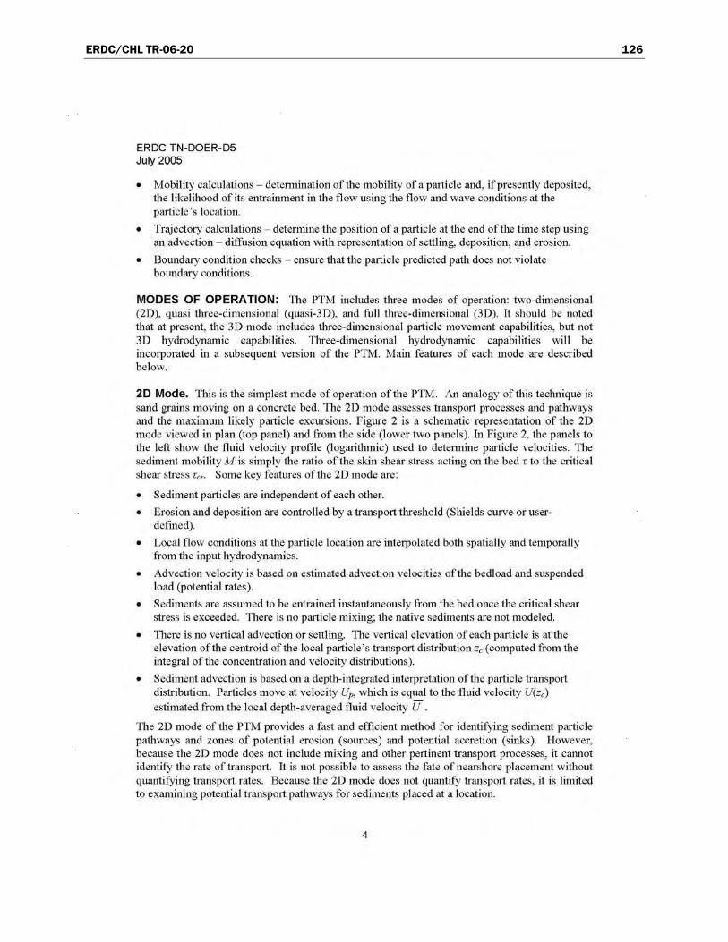
ERDC/CHL TR-06-20 126
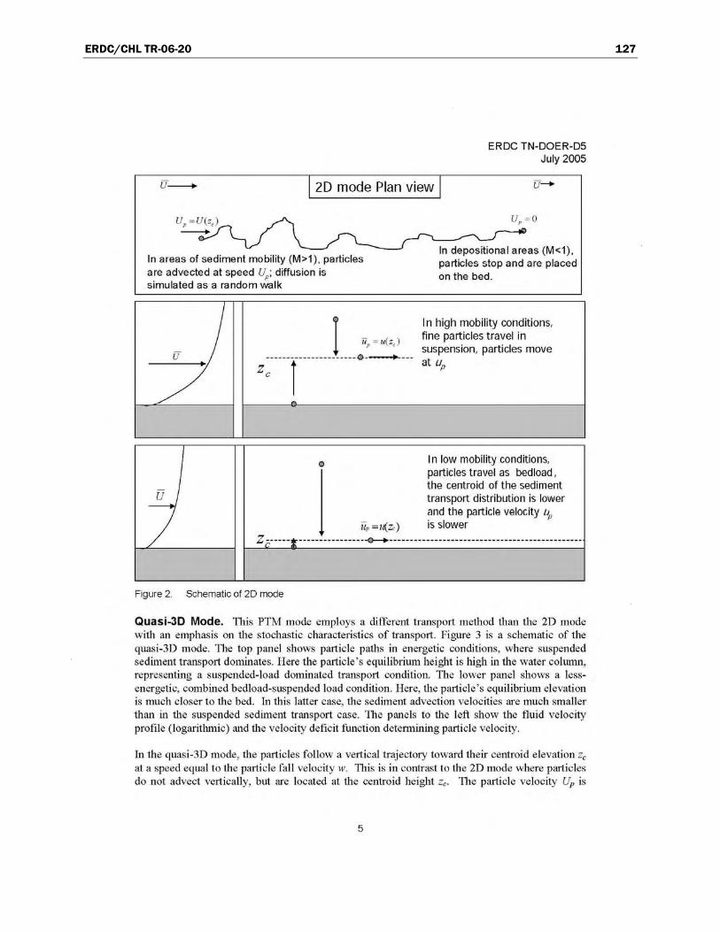
ERDC/CHL TR-06-20 127
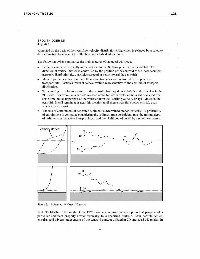
ERDC/CHL TR-06-20 128

ERDC/CHL TR-06-20 129
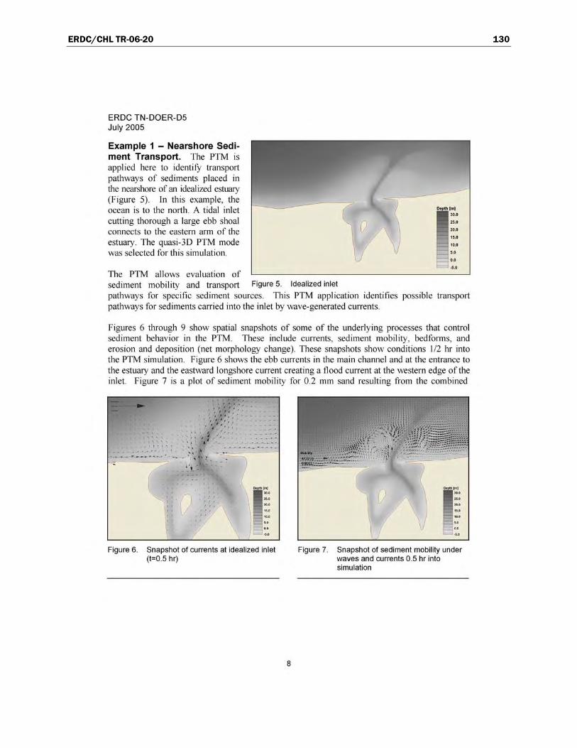
ERDC/CHL TR-06-20 130

ERDC/CHL TR-06-20 131

ERDC/CHL TR-06-20 132

ERDC/CHL TR-06-20 133

ERDC/CHL TR-06-20 134
ERDC/CHL TR-06-20 135

ERDC/CHL TR-06-20 136

ERDC/CHL TR-06-20 137
Appendix D: Particle Tracking Model (PTM) in the SMS: III. Tutorial with Examples

ERDC/CHL TR-06-20 138

ERDC/CHL TR-06-20 139

ERDC/CHL TR-06-20 140

ERDC/CHL TR-06-20 141

ERDC/CHL TR-06-20 142

ERDC/CHL TR-06-20 143

ERDC/CHL TR-06-20 144

ERDC/CHL TR-06-20 145

ERDC/CHL TR-06-20 146

ERDC/CHL TR-06-20 147

ERDC/CHL TR-06-20 148

ERDC/CHL TR-06-20 149

ERDC/CHL TR-06-20 150

ERDC/CHL TR-06-20 151

ERDC/CHL TR-06-20 152

REPORT DOCUMENTATION PAGE Form Approved
OMB No. 0704-0188 Public reporting burden for this collection of information is estimated to average 1 hour per response, including the time for reviewing instructions, searching existing data sources, gathering and maintaining the data needed, and completing and reviewing this collection of information. Send comments regarding this burden estimate or any other aspect of this collection of information, including suggestions for reducing this burden to Department of Defense, Washington Headquarters Services, Directorate for Information Operations and Reports (0704-0188), 1215 Jefferson Davis Highway, Suite 1204, Arlington, VA 22202-4302. Respondents should be aware that notwithstanding any other provision of law, no person shall be subject to any penalty for failing to comply with a collection of information if it does not display a currently valid OMB control number. PLEASE DO NOT RETURN YOUR FORM TO THE ABOVE ADDRESS.
1. REPORT DATE (DD-MM-YYYY) September 2006
2. REPORT TYPE Final report
3. DATES COVERED (From - To)
5a. CONTRACT NUMBER
5b. GRANT NUMBER
4. TITLE AND SUBTITLE
PTM: Particle Tracking Model; Report 1: Model Theory, Implementation, and Example Applications
5c. PROGRAM ELEMENT NUMBER
5d. PROJECT NUMBER
5e. TASK NUMBER
6. AUTHOR(S)
Neil J. MacDonald, Michael H. Davies, Alan K. Zundel, John D. Howlett, Zeki Demirbilek, Joseph Z. Gailani, Tahirih C. Lackey, and Jarrell Smith
5f. WORK UNIT NUMBER
7. PERFORMING ORGANIZATION NAME(S) AND ADDRESS(ES) 8. PERFORMING ORGANIZATION REPORT NUMBER
Coastal and Hydraulics Laboratory, U.S. Army Engineer Research and Development Center, 3909 Halls Ferry Road, Vicksburg, MS 39180-6199; Pacific International Engineering, 260 Centrum Blvd., Suite 220, Ottawa, ON K1E 3P4, Canada; Brigham Young University, Civil and Environmental Engineering Department, 240 Clyde Building, Provo, UT 84602
ERDC/CHL TR-06-20
9. SPONSORING / MONITORING AGENCY NAME(S) AND ADDRESS(ES) 10. SPONSOR/MONITOR’S ACRONYM(S)
11. SPONSOR/MONITOR’S REPORT NUMBER(S)
U.S. Army Corps of Engineers Washington, DC 20314-1000
12. DISTRIBUTION / AVAILABILITY STATEMENT Approved for public release; distribution is unlimited.
13. SUPPLEMENTARY NOTES
14. ABSTRACT
This report introduces a Lagrangian-based Particle Tracking Model (PTM) developed by the Coastal Inlets Research Program (CIRP) and the Dredging Operations and Environmental Research Program (DOER) being conducted at the U.S. Army Engineer Research and Development Center. The PTM’s Lagrangian framework is one in which the sediment being modeled is discretized into a finite number of particles that are followed as they are transported by the flow. Lagrangian modeling is insightful for modeling transport from specified sources. Many particles are modeled such that transport patterns are representative of all particle movement from the sources. The model operates in the Surface-water Modeling System (SMS) interface and allows the user to simulate particle transport processes to determine particle fate and pathways. Waves and currents used in the PTM as forcing functions are developed through other models and input directly to the PTM. PTM Version 1.0 input files are from the ADCIRC or M2-D depth-averaged hydrodynamic models and STWAVE and WABED wave models. Other models can be used as input by first converting their output to ADCIRC, M2-D, or STWAVE and WABED formats.
(Continued) 15. SUBJECT TERMS Coastal Inlets Research Program Dredging Operations and Environmental Research
Particle tracking model Sediment transport Hydrodynamics and waves
16. SECURITY CLASSIFICATION OF: 17. LIMITATION OF ABSTRACT
18. NUMBER OF PAGES
19a. NAME OF RESPONSIBLE PERSON
a. REPORT
UNCLASSIFIED
b. ABSTRACT
UNCLASSIFIED
c. THIS PAGE
UNCLASSIFIED 168 19b. TELEPHONE NUMBER (include area code)
Standard Form 298 (Rev. 8-98) Prescribed by ANSI Std. 239.18

14. ABSTRACT (Concluded)
The general features, formulation, and capabilities of PTM Version 1.0 are described in this report, including the basic components of the model, model input and output, and application guidelines. Other chapters of this report provide detailed information about the PTM’s theory, numerical implementation, and examples that demonstrate the model’s potential usage in practical applications. Sediment pathways are readily identified within the Lagrangian modeling framework of the PTM for conditions with sharp gradients in suspended solids (plumes, for example), where numerical diffusion in Eulerian models would require very small grid spacing to provide reliable solutions. The Lagrangian framework of the PTM is computationally advantageous, and the model can be run with a fraction of the computer execution time required by Eulerian models. Each particle in the PTM represents a given mass of sediment (not an individual sediment particle or grain), and each particle has its own unique set of characteristics. As a minimum, a particle must be defined with certain physical properties (e.g., grain size and specific gravity) and an initial position. The particles can also be given other characteristics that may be independent of the solution, and particles can be static or dynamic. Particles from sources being modeled (as opposed to the local, or native, bed sediment) are introduced, or released, into the domain from specified source locations. These sources are designed to permit modeling of a wide range of natural or anthropogenic processes in coastal and environmental studies.
Related Documents