PT 14 Rodenticides - Europa

1

CA-Jun03-Doc.8.2-PT14

Danish EPA

J. Larsen

Supplement to the methodology for risk evaluation of biocides

Emission scenario document for biocides used as rodenticides

May 2003

This report has been developed in the context of the EU project entitled "Gathering, review and development of environmental emission scenarios for biocides" (EUBEES 2).

The contents have been discussed and agreed by the EUBEES 2 working group, consisting of representatives of some Member States, CEFIC and Commission. The Commissions financial support of the project is gratefully acknowledged (Ref. ENV.C3/SER/2001/0058).

EUBEES

2

3

Foreword

This report gives a description of emission scenarios for rodenticides used in the European Union. The scenarios and assessments are dealing with the environment including the non-target mammals and birds.

This document describes a method of estimating the emission of rodenticides to the primary receiving environmental compartments (e.g. air, soil, and water). According to Annex VI of the Directive 98/8/EC (Biocidal Products Directive, BPD) the risk assessment shall cover the proposed normal use of the biocidal product together with a realistic worst-case scenario. Therefore, this report provides separate calculations for emissions under normal and realistic worst case conditions. The calculation of a normal and a realistic worst case PEC using environmental interactions is considered to be fate and behaviour modelling, and is outside the scope of this guideline. Subsequent movement of emissions to secondary environmental compartments (e.g. ground water) is considered to be subject to fate and behaviour calculations and models, and outside the scope of this guideline.

The report is based on a report prepared for the Nordic Council of Ministers in 2001 (Lodal and Hansen 2002). The original report, Human and Environmental Exposure Scenarios for Rodenticides – Focus on the Nordic Countries, was produced on behalf of the Nordic Chemicals Group and has been financed by the Nordic Council of Ministers.

Discussions in the working group for the EU project “Gathering, review and development of environmental emission scenarios for biocides (EUBEES 2)” and data supplied by some member states enabled the update presented in this report. The emission scenarios are applicable in all European Union member states.

4

5

Contents 1 Introduction.............................................................................................7 2 Exposure scenarios for the environment..................................................10

2.1 General issues and background.......................................................10 2.1.1 Further information...............................................................11 2.1.2 Bait boxes............................................................................11 2.1.3 Home range or travel distance...............................................12 2.1.4 Baiting specifications.............................................................13

2.2 Exposure scenarios ........................................................................13 2.3 Exposure scenarios for a sewer system...........................................14

2.3.1 Introduction..........................................................................14 2.3.2 Application type ...................................................................14 2.3.3 Exposed compartments.........................................................16 2.3.4 Other protection targets ........................................................18

2.4 Exposure scenarios in and around buildings.....................................18 2.4.1 Introduction..........................................................................18 2.4.2 Application type ...................................................................19 2.4.3 Exposed compartments.........................................................21 2.4.4 Other protection targets ........................................................27

2.5 Exposure scenarios open areas.......................................................27 2.5.1 Introduction..........................................................................27 2.5.2 Application type ...................................................................27 2.5.3 Exposed compartments.........................................................30 2.5.4 Other protection targets ........................................................39

2.6 Exposure scenarios waste dumps....................................................40 2.6.1 Introduction..........................................................................40 2.6.2 Application type ...................................................................40 2.6.3 Exposed compartments.........................................................41 2.6.4 Other protection targets ........................................................42

2.7 Summary.......................................................................................43 2.7.1 Environmental exposure.......... Error! Bookmark not defined.

3 Exposure scenarios for primary and secondary poisoning........................45 3.1 Introduction...................................................................................45 3.2 Exposure scenarios for primary poisoning .......................................48

3.2.1 Anticoagulant rodenticides ....................................................48 3.2.2 Non-anticoagulant rodenticides.............................................53

3.3 Exposure scenarios for secondary poisoning ...................................55 3.3.1 Anticoagulant rodenticides ....................................................56 3.3.2 Non-anticoagulant rodenticides.............................................63

4 References............................................................................................66 Appendix 1 Summary of variables in text and equations..........................71

6

7

1 Introduction

The European Parliament and the Council has adopted Directive 98/8/EC on the placing of biocidal products on the market (Biocidal Products Directive, BPD). Annex V of the Directive lists various Main Groups of biocides as well as Product Types. Under Main Group 3: Pest control, rodenticides are listed as Product Type 14. The controls of vertebrate pests are accomplished by applications indoors and outdoors. In general, all rodenticides are considered as Biocidal Products with the exclusion of products used in plant growing areas (agricultural field, greenhouse, forest) to protect plants, or to protect plant products temporarily stored in the plant growing areas which are covered by Directive 91/414/EEC. It should be noted that generally the use of rodenticides takes place as a response to an infestation, as opposed to many other biocides, which are effectively broadcast and/or used in a preventative manner.

The formats of names, parameters, variables, units and symbols used in the equations cited from EUSES and USES models and used in the exposure scenarios may have changed from their original references. This was done in order to bring the nomenclature in agreement with the proposals discussed and agreed by EUBEES working group consisting of representatives of some Member states, CEFIC and the European Commission (van der Poel 2000).

If reliable and representative measured data are available, they should be used instead of default values or modelling or included in the data used in the modelling.

Rodenticides in the present context are biocidal products used for control of rodents (rats, mice and voles). Products for controlling moles are by the mutual decision of the Competent Authorities for biocides in December 2001 deemed to be Plant Protection Products and consequently they have to be authorised according to Dir. 91/414/EEC. The non-agricultural use of rodenticides is in sewer systems, in and around buildings (e.g. houses, animal housings, commercial and industrial sites), waste dumps and landfills, lawns, golf courses, highway medians, dikes and other structures covered with vegetation and meant for e.g. protecting the coastline against erosion processes.

Professional use is a term used in order to emphasise that the general public is not allowed to use a certain compound. The term, however, is not clear and distinct. It only indicates that “professionals” are assumed to have a minimum of knowledge of the substance they are handling by training or education whereas non-professionals (or the general public) are assumed to have little or no knowledge of the substances. In the different countries the meaning of professional use may vary. For instance, the interpretation may be that the product is only to be used by pest control operators who have taken a special course on this matter. In some countries, caretakers, farmers or the staff of the pest control companies are considered professionals whereas other countries authorise professional users and some compounds are allowed to be used only by professional firms, i.e. authorised/licensed people.

In the present report it is assumed that the label instruction of a given formulated product is followed. It has to be stressed that misuse of a product is not covered by the scenarios described in this report.

8

Active substances

A list of existing active substances for rodenticides identified or notified according to the BPD can be found on the ECB Homepage: http://ecb.jrc.it/biocides/.

The main part of active substances in rodenticides belongs to the anticoagulant rodenticides. The preparations may be formulated as loose baits, pellets, and wax blocks, liquid poisons, contact dust or gel.

An important property of the first-generation anticoagulants is that they are not normally sufficiently toxic to rodents to cause death after a single exposure. Second-generation anticoagulants have been developed in response to resistance to first-generation anticoagulants. Occurrence of resistance in rats and mice is well documented to first- and some second-generation anticoagulants (Kerins et al. 2001, Lodal 2001, Lund & Lodal 1988, Pelz 2001, Myllymäki 1995).

Anticoagulant rodenticides are vitamin K antagonists. After oral administration, the major route of elimination in various species is through the faeces. The metabolic degradation of warfarin and indandiones in rats mainly involves hydroxylation. However, some second-generation anticoagulants are mainly eliminated as unchanged compounds (Lodal and Hansen 2002).

Non-anticoagulants have other modes of action. For example cholecalciferol is a fat-soluble vitamin (D3) that can be used as an acutely toxic (single feeding) and/or chronicly toxic (multiple-feeding) rodenticide. According to Buckle (1994) the mode of action of (chole)-calciferol in mammals is briefly described as a stimulation of absorption of calcium in the intestines and mobilisation of skeletal calcium. Death seems to be due to circulatory blockage, heart and renal failure. Symptoms of poisoning usually do not occur until 2-3 days after intake (Lund 1988a).

Chloralose is a narcotic with a rapid effect. Buckle (1994) describes that it slows down a number of essential metabolic processes. Therefore it is most effective against small rodents such as mice because they have a high surface to volume ratio. Cool conditions are most favourable.

Primary and secondary poisoning

Non-target vertebrates may be exposed to rodenticides primarily through consumption of bait and secondarily from consumption of poisoned rodents. Small pellets and whole grain baits are highly attractive to birds.

9

The scenarios in this report are presented in the following way:

Input

[Variable/parameter ] [Symbol] [Unit] S/D/O/P

These parameters are the input to the scenario. The S, D, O or P classification of a parameter indicates the status:

S Parameter must be present in the input data set for the calculation to be executed (there has been no method implemented in the system to estimate this parameter; no default value is set).

D Parameter has a standard value (most defaults can be changed by the user)

O Parameter is the output from another calculation (most output parameters can be overwritten by the user with alternative data).

P Parameter value can be chosen from a "pick-list" of values.

c Default or output parameter is closed and cannot be changed by the user.

Output

[Symbol] [Description]

Intermediate calculations

Parameter description (Unit)

[Parameter = equation] (Equation no.)

End calculations

[Parameter = equation] (Equation no.)

10

2 Exposure scenarios for the environment

2.1 General issues and background Environmental exposure may result from the release of rodenticides from its use and disposal. Exposure scenarios are defined as a set of conditions about sources, pathways and use patterns that quantify the release of the substance from processing, use and disposal into soil, water, air and waste.

Direct environmental exposure may take place when rodenticides are applied outdoors on public and private areas around buildings or constructions (farm buildings, railway stations, harbour areas etc.), on water banks, in and around sewer systems, waste disposal sites and waste dumps.

Indoor application may result in environmental exposure via the sewage system (e.g. during cleaning processes after a rat control operation), release of residues or carcasses to dumps.

The main formulations applied outdoors are baits, for instance wax blocks, impregnated grain and maize and contact dust (contact powder). Gassing is an outdoor activity, which may be used to control water voles and rats in burrows.

The exposure of the environmental compartments, soil, water and air is highly dependent on the formulation type, physico-chemical properties of the substance involved and the mode of application, use and disposal.

Emission scenarios relevant for rodenticides are suggested based on “realistic worst case” principles and are based on the most common application and use patterns. A few scenarios regarding less frequent uses/application methods are included, as high environmental exposures may be anticipated.

A diffuse release from target animals via urine and faeces including non-degraded active substance and its transformation and metabolic residues may be anticipated around the controlled area.

In the present paper the scenarios are categorised in the following hierarchical way:

1. Division into four main scenarios according to application surroundings,

2. Subdivision into scenarios according to application type,

3. Consideration of relevant exposed environmental compartments, and

4. Other relevant protection targets (primary and secondary poisoning, see Chapter 3)

11

In the environmental exposure assessment, emissions/releases from the processes or uses are quantified in amount released per time unit or after a campaign.

The respective emission scenarios are described as a sequence of equations so that emission rates and concentration in environmental compartments can be estimated (by calculation). The calculation depends to some degree on default values and estimations. The default values are expert judgements based on experience, measurements or evaluations. Most expert evaluations are based on personal communications with professionals and companies working with rodenticides application and the national consultants involved in rodent control. If default values are presented in the Technical Guidance Document for Risk Assessment (the revised TGD, 2003; http://ecb.jrc.it/tgdoc), they are used in this report. However, the default values can be superseded by measured values of relevant and reliable data if available.

Most rodenticides are used as either concentrates or ready-to-use products. The suggested scenarios, therefore, are based on the application, use and disposal phase. Releases from production and formulation phases are not included.

It should be noted that the report in its attempt to cover many scenarios may not include all relevant scenarios as well as not all uses are relevant to all Member States. Certain uses may not be allowed in some countries.

2.1.1 Further information

Further information should be taken into account on a case by case evaluation. Below is mentioned information that may be included in site specific exposure assessment in order to refine the basic assessment.

2.1.2 Bait boxes

Bait stations (bait boxes) are frequently used as in some member states they are considered to increase the safety of rodenticides and reduce the primary poisoning hazards of non-target animals if they are robust enough (tamper resistant). Therefore, the use of bait boxes is included in the scenarios. The degree of box resistance to tampering by rodents, humans etc. affects the default release estimates. It is assumed that a tamper proof bait box minimises environmental releases. It is also assumed that a tamper resistant bait box has much lower releases than, for example, a bait box made of cardboard. The UK expert working group RRAT (Rodenticide Risk Assessment Technical working group) states that there is experimental evidence that rats often remove bait particles from boxes and sometimes leave them where other animals can find them. The use of boxes clearly improves the safety of bait placements and permits easy retrieval of uneaten bait at the end of a treatment. However, restricting the placement of baits to inside boxes only (whether tamper-resistant or not) can impair efficacy and may prolong bait exposure periods.

Bait stations can be constructed in several ways, for example:

• It can be as simple as a flat board nailed at an angle to the bottom of a wall. The board should be long enough (e.g. 0.5 m) to keep pets, non-target animals and children from reaching the bait.

12

• It can be a length of pipe into which bait can be placed. The pipe diameter should be 5 to 8 cm for mice and 6 to 15 cm for rats. The length of the pipe should be long enough (e.g. 0.5 m) to keep pets, non-target animals and children from reaching the bait.

• More elaborate bait boxes are completely enclosed and can contain liquid as well as loose or solid baits. Bait stations for rats have normally two openings, approximately 6 cm in diameter.

• Tamper resistant bait boxes are generally those made from robust materials, such as polypropylene, that have internal dimensions that deter access to the bait by humans and non-target animals larger than rats, that have lids that are locked in place which cannot be opened without a special tool, and are capable of being anchored to the substrate.

It is important that the bait is placed out of reach of children, pets, domestic animals and non-target wildlife or in a bait station. Rats transfer all types of bait including fine particles. This occurs whether bait is placed in a box or on a tray under natural cover. However, small particles are more likely to be totally consumed, while larger particles may be partially eaten and the rest abandoned. According to the UK working group RRAT (2002),the results from research on rat behaviour at bait boxes suggest that some designs of tamper-resistant boxes may actually encourage bait transfer. Transferred bait may be abandoned in the open.

Bait boxes are placed where the rodents are active, near rodent burrows, against walls, along travel routes (runways) and preferably between the rodents’ place of shelter and their food supply.

On farms the bait boxes located outdoors, are usually placed along the building foundations or around the perimeter of the building complex.

2.1.3 Home range or travel distance

The home ranges for mice and rats vary according to season, population density, habitat, food supply etc.

Studies indicate that during its daily activities, a rat normally travels an area averaging 30 to 50 m in diameter. Rats seldom travel further away than 100 m from their burrows to obtain food or water (Lodal and Hansen, 2002). Macdonald & Fenn (1995) and Taylor (1978) have, however, shown that rats under special circumstances may move away from and around farms. They found rats having travelled distances of more than 1300 m.

During its daily activities, a mouse normally travels an area averaging 3 to 10 meters in diameter. Mice seldom travel further away than this to obtain food or water. Other references present the home range values (e.g. www.pestcon.com).

Entry holes to rodent burrows are 4 cm in diameter or less for mice and 5 cm in diameter or larger for rats.

The number of application sites and application rates vary according to both the product used and the intended target-animal. For example:

Rats: 20-50 g per application site or 1-2 wax blocks. Application sites are located 5-10 meters apart.

13

Mice: 5-15 g per application site. Application sites are located 2-5 m apart.

However, it has to be stressed that bait point sizes and distances between bait points are highly dependent on product (active ingredient, concentration and formulation type used).

A 10 meter zone around the farm building is considered the most frequented zone for the rodents. Mice typically forage in the immediate vicinity and the rats make longer foraging trips outside the location along hedgerows and the like.

2.1.4 Baiting specifications

Application methods should also be considered. For example:

Pulsed baiting: 20-50 g per application site at 7 days’ interval.

Saturation baiting: larger amounts but at longer intervals.

The average consumption per rat is estimated to be 75-100 g (total food intake) with large variation. This would approximate 3 - 4 days of bait ingestion based on the assumption that a rat weighing 250 g has a food consumption of 25 g/day (20-30 g/day/rat, P. Weile, pers. comm.). A mouse weighing 25 g has a food consumption of 3.5 g/day (3-4 g/day, P. Weile, pers. comm.). The principle of saturation baiting is to maintain a continuous supply of bait; the interval is not easy to specify and needs to be adjusted to achieve the primary objective of providing sufficient bait. However, when using the ESD manufacturers will need to insert the baiting processes specified on the label for any particular end-use product.

2.2 Exposure scenarios Basically there are four main scenarios to consider:

• Exposure scenarios for a sewer system.

• Exposure scenarios in and around buildings.

• Exposure scenarios for open areas.

• Exposure scenario for waste dumps.

The environmental exposure scenarios are developed on basis of rodenticide types and the application and disposal that are expected to result in the largest emissions to the environment.

It should be noted that according to the TGD, the local predicted environmental concentration (PEClocal) is the estimated local concentration added to the estimated regional concentration (Clocal + PEC regional). However, for rodenticides the consumption is estimated to be so low that the regional contribution is negligible. In the present document Clocal is the initial concentrations based on the emissions and have to be corrected for fate like e.g. degradation to calculate the PEC value used for the risk assessment along the principles of the TGD (2003).

In the calculation of the exposure scenarios for the soil compartment, the directly exposed area and the mixing soil depth is assumed to be 10 cm from the source. In the case of an

14

application of a rodenticide directly into a hole it is only assumed that the lower half of the hole and its surrounding environment is exposed (with the exemption of the gassing scenario). The value of 10 cm has been chosen to make the rodenticide scenarios be in agreement with the OECD emission scenario document on wood preservatives. However, it should be stated that the 10 cm is not chosen on a scientific basis.

2.3 Exposure scenarios for a sewer system

2.3.1 Introduction

The brown rat is the only mammal that can live in sewers. Depending on the structure of the sewer and the food content in the sewers the rats may often or rarely move to the surface in search for food. The structural integrity of sewers is important – damage will result in rats on the surface – if there is no damage to enclosed sewer systems then regardless of food availability, rats won´t get out. It should be noted that other animals e.g. cockroaches are known to eat rodenticides in the sewerage system (P. Weile, pers. comm.). However, cockroaches found in sewers will probably remain underground and are not significant prey items for birds.

2.3.2 Application type

2.3.2.1 Wax block Wax blocks are blocks with a matrix containing impregnated grain and wax. A typical size of a block in the Nordic countries is 12×5×4 cm and a weight of 250 to 300 g. It is noted that size and weight of wax blocks vary in the Member States. In France, wax blocks generally weigh between 20 and 100 g and the treatment frequency is 2-4 applications per year, 3-6 month apart. The amount of used product per application is often 1 block (100 g) per manhole (INERIS 2002). According to CEFIC (2002) a 300 g wax block is too large for the rest of Europe where 200g is considered a more realistic maximum. The larger ones placed on the market should be used in the realistic worst case scenario if nothing is stated in the user instruction. In the example illustrated below wax blocks of 300 g are used.

Wax blocks are applied in sewerage systems typically hanging in a wire tied to the wall a few cm above the bottom of cesspools. Residues are only occasionally removed for disposal although it occurs that whole blocks or significant residues are removed and subsequently disposed of. According to Danish rat control companies (DEPA 2001), very little if any residues are removed from the application sites.

A maximum release to the sewerage system could come directly from residues from the applied wax blocks and indirectly from the target animals’ urine, faeces and dead bodies, i.e. 100% release minus degraded/metabolised fractions.

15

The main release (70 to 90%, according to DEPA 2001) takes place in the use phase and is dominated by the intended oral ingestion by the target organism (rats) whereas significant, unintended releases are limited to spills during the rat "attacks" or ingestion by e.g. cockroaches, although the latter may be considered as almost negligible. Later in the use phase unintended releases occur which are caused by degradation and disintegration of the remains of the block.

The maximum unintended release is estimated to be 30% of the applied amount of product. However, it should be considered that a large fraction of the amount ingested by rats is assumed to be released via urine and faeces as undegraded substance depending on the rodenticide used. Rodenticides ingested by e.g. cockroaches are also assumed to be released as undegraded substance unless otherwise documented. Larger fractions of wax blocks and dead rats may be caught up in filters at the sewage treatment plant (STP), if present, or skimmed of in settling ponds.

Taking the different releases into account, 90% total release is used as default value in the realistic worst case scenario (Lodal and Hansen 2002) including releases via faeces and urine. However, information from the dossiers on metabolism of the relevant substance should be considered. When this is taken into consideration a fraction of 0.3 is assumed to be the unintended release to which should be added the non-metabolised excreted fraction (i.e. 0.6 – the metabolised amount):

Fraction of release = 0.3 + (0.6-metabolised fraction) .

A rat control operation in a heavily infected area is assumed to last 21 days. No exact data is available on how often the rat control operation will be repeated but it is assumed that the frequency is less than once in a month. The available information from a major rat control company (Helholm 2002) indicates that the usual method is application into the sewage system (manhole) at each major road crossings.

2.3.2.2 Pellets, impregnated grain Instead of wax blocks, a container with impregnated grains or pellets may be used. The container is like the wax block left hanging in a wire just above the bottom of the cesspools. In France impregnated grain may also be placed in closed plastic boxes (the amount of product depends on the area). In a rat control operation the treatment frequency is about 1-4 application per year, 3 month apart and each treatment campaign is about 10 days (INERIS, 2002).

2.3.2.3 Contact powder Not relevant.

2.3.2.4 Liquid concentrate Not relevant.

2.3.2.5 Bait box According to CEFIC (2002) bait boxes are used in sewers, secured to sewer walls and platforms where rats run. However, no further information is available and, thus, no scenario can be developed.

16

2.3.2.6 Gassing Not relevant.

2.3.3 Exposed compartments

2.3.3.1 STP According to TGD (2003), the default local sewage treatment plant (STP) receives sewage water from 10 000 person equivalents (PE). Various information on the length of sewerage systems in a typical city is available:

• DEPA (2002) report a length of 35 km sewerage per 10 000 PE based on information from a city in which the length of sewerage system of 650 km and a population of 150000 corresponding to 165000 PE.

• The size of the canal system in Berlin is about 9000 km. Berlin has 3 387 000 inhabitants and this would mean about 27 km per 10 000 PE (http://www.bwb.de).

• A mean value of 44 km sewerage per 10 000 PE is found in NL (Stichting Rio Ned 2000-2001).

Even through the length of the sewerage system in a city is highly dependent on the conditions an estimated average value of about 35 km sewerage per 10 000 PE seems to be reasonable. Rodenticides are normally applied to cesspools (manholes). The distances between cesspools are depending on their ability to keep themselves clean, (i.e. the size), with an average of 50 to 300 meters (DEPA 2002; http//www.bwb.de). A realistic average distance is set at 100 m with an enormous variation. In EU, treatment campaigns vary normally between 10 and 21 days, depending on the conditions and tradition in the country. However, for the normal use to prevent an increase of the rats in the sewer system a realistic frequency is one campaign lasting several months every three to five years (CEFIC 2002).

Two emission scenarios are relevant:

1. Normal use:

A scenario to illustrate a case where rodenticides are used to prevent an increase of the rats in the sewer system in a city. Before a rat campaign the area of the city may be divided into smaller units corresponding to e.g. 10 000 PE. Each year one or several wax blocks is applied to each cesspool in that specific area. The following year another area of the city may be selected for rat control. In Denmark the amount of formulated product used/year varies from 0 to nearly 600 kg/10 000 PE depending on the city (www.mst.dk). The mean value for Denmark is about 50 kg/10 000 PE. This value is comparable to the value of 60 kg/10 000 PE found in a German city in Baden-Württemberg (http://www.zvw.de/aktuell/2001/04/20/ratten.htm).

2. Realistic worst case:

A scenario is described to illustrate a case where rodenticides are used in a city with a serious rat problem (e.g. heavily infested areas). In this case pulsed baiting may be used.

17

Information on best practice indicates that during a control operation of 21 days the application into the cesspool/manhole may take place two to three times after demand e.g. on day 1, 7 and 14. On day 1, one wax block is applied to each cesspool. On revisiting the wells on day 7 another block is applied, if the wax block has been eaten. If the wax blocks are also eaten at the revisit on day 14, new blocks are applied.

As a realistic worst case the best guess is that 300 wax blocks are applied to 300 cesspools on day one in an area corresponding to 10 000 PE. At the revisit on day 7 100 blocks are eaten and therefore replaced. At the revisit on day 14 only 50 blocks have been eaten and are replaced and at the revisit on day 21 no blocks have been eaten. This would give a realistic worst case assumption of emission of 100 wax blocks during the first week of the 21-day´s-control operation period in the Default City. Therefore, the default amount of product used in this control operation would be 0.3 kg. x 100 = 30 kg during the first 7 days of the control-operation which corresponds to the realistic worst case situation (Qprod = weight of block x Napp).

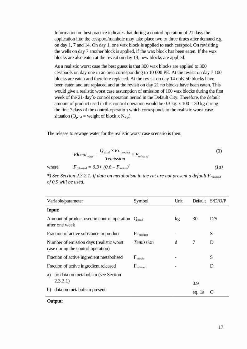
The release to sewage water for the realistic worst case scenario is then:

releasedproductprod

water FTemission

FcQElocal ×

×=

(1)

where Freleased = 0.3+ (0.6 – Fmetab)* (1a)

*) See Section 2.3.2.1. If data on metabolism in the rat are not present a default Freleased of 0.9 will be used.

Variable/parameter Symbol Unit Default S/D/O/P

Input:

Amount of product used in control operation after one week

Qprod kg 30 D/S

Fraction of active substance in product Fcproduct - S

Number of emission days (realistic worst case during the control operation)

Temission d 7 D

Fraction of active ingredient metabolised Fmetab - S

Fraction of active ingredient released

a) no data on metabolism (see Section 2.3.2.1)

b) data on metabolism present

Freleased -

0.9

eq. 1a

D

O

Output:

18

Mean local emission of active substance to waste water during episode

Elocalwater kg.d-1

It should be noted that if data on degradation and/or metabolism in the rat are present, they should be considered in the estimation.

The concentration in the sewage water can be estimated by dividing the Elocalwater by 2,000,000 l/day, which is the daily amount of sewage water to a local STP (kg/l) in a city with 10 000 PE.

2.3.4 Other protection targets

2.3.4.1 Primary poisoning There is no primary poisoning hazard to mammals or birds because no other mammals (or birds) are living or occurring in sewers.

2.3.4.2 Secondary poisoning The secondary poisoning hazard is relevant only if poisoned rats or cockroaches move to the surface. In that case the situation is similar to the one described below for rat control in and around buildings. However, according to CEFIC (2002) cockroaches are predominantly nocturnal and the species found in sewers e.g. Blatta orientalis will remain underground and are not significant prey items for birds.

2.4 Exposure scenarios in and around buildings

2.4.1 Introduction

In all EU countries baits are to be placed in bait stations or in other ways covered or hidden so as to minimise access of non-target animals. If applied properly there is a minimal risk of other mammals getting access to the poison. However, small birds and mammals may occasionally enter the bait stations (see Chapter 3).

Target animals mainly eat the bait e.g. fractionated loose bait or wax blocks in bait boxes. However, exposure of the environment (soil) besides spills etc. is also expected from urine, faeces and carcasses.

The main exposure of the environment is expected to be soil contaminated by spills during application, refilling and disposal operations. However, the contributions from disperse release of rodenticide via urine and faeces should also be considered. The rodents may disperse the

19

substance during its use period. Experiences seem to vary. Some experts are of the opinion that rats are very likely to eat wax blocks in bait boxes (e.g. Weile P., 2002), but according to the UK RRAT working group, (2002) some experts are of the opinion that rats are very unlikely to eat wax blocks in bait boxes. If the blocks are loose, they will carry them away, if secured on wires, rats will largely ignore them. However, no matter which of the two types of behavious that is dominant, the rodenticide will be spread in the surroundings either directly by rats carrying the bait away from the bait boxes or through urine and faeces. Mice normally behave different from rats, as they seem much more likely than rats to gnaw block baits.

Outdoor application directly into burrows is assumed to create a larger release to the environment. Therefore the open area exposure scenario is used to illustrate the impregnated grain and maize scenario.

See the open area scenario.

Residues from indoor use of impregnated grain and maize may reach the environment from disposal by sewerage system or cleaning. However, this emission is assumed to be insignificant and will not be addressed further.


2.4.2.1 Wax block Normally used in feeding stations. However in many countries wax blocks can also be placed on hidden places, or directly inside holes. In France a treatment campaign is about 15 days with 3-6 campaigns per year (INERIS, 2002). However, according to CEFIC (2002) the assumption that there are 3-6 campaigns per year is atypical. It exceeds the use patterns recommended by good use practices. Rodents are controlled when they become a problem. Bait is placed according to the product type, label and pattern of use. This depends on the site type and the infestation. For example for a heavy infestation, in e.g. a north German farm (typical of many European farms) there would be no more than two to three applications per year. If this fails to control the rodents, then other measures need to be taken such as physical alterations to reduce the places in which rodents live and breed.

2.4.2.2 Pellets, impregnated grain In some parts of the UK rat infestations sometimes extend along field boundaries (hedgerows, ditches) adjacent to farm buildings, but they can also occur along boundaries that are several hundred meters from buildings. These infestations occur particularly in areas of extensive cereal growing and where game birds are reared and they may act as reservoir populations that recolonise farm buildings previously cleared of rats. As a result, rodenticide baits may be applied to control such infestations, but it does not seem to be a routine procedure, probably on grounds of cost and time. According to CEFIC (2002) the use pattern for pellets should be the same as for wax blocks (the use pattern is the same for all oral baits).

See the open area scenario.

2.4.2.3 Contact powder

20

In France powder is placed in inaccessible places. Normally stripes of 20-30 cm length, 10 cm width and 1 cm thickness (one stripe = 145 g) are used. Treatment frequency is about 4 applications per year, 3-months apart. (INERIS, 2002). However, according to CEFIC (2002) a layer of 1 cm is unrealistic, 1 mm is realistic.

See also the open area scenario.

2.4.2.4 Liquid concentrate Liquid concentrates are used for preparation of poisoned food items, e.g. apple pieces and impregnated grain. In some countries farmers can buy liquid concentrate and mix it with grain and other dry rodent food materials. They present the same risks as 'impregnated grains' within the various risk scenarios that are referred to elsewhere in the document.

Liquid solutions for use as drinking poison are applied at dry places with no or limited access to other sources of water, e.g. in barns and warehouses.

Residues from the mixing with food items are discharged with sanitary wastewater whereas residues after termination of the control action are either left where they are or disposed of together with ordinary solid waste. Residues in containers are assessed to be very limited and probably not exceeding 1% of the total amount of substance used in the different application types.

Release to the sewerage system is assumed to be 0-5% (DEPA 2001). However, since the amount used is very limited and the local sewage treatment plant (STP) receives sewage water from 10 000-person equivalent the amount emitted to the STP is considered insignificant.

Apple pieces or grain mixed with liquid concentrate are placed outside and in barns and stables, e.g. under bales of straw in a bait box or on a tray. The amount of used product is about 100 to 200 g per application site. Release during application is estimated to be 5% and after application (during use) 5-10%, i.e. a total release of 10-15% to soil.

2.4.2.5 Bait box Baits are to be placed in bait stations or in other ways covered or hidden.

On a farm with a rat problem, the bait boxes (which may be filled with impregnated grain, wax blocks or other bait formulations) are assumed to be distributed around the walls of the barn, stable and fodder buildings and at the manure collection areas. For rats, bait boxes are usually placed 5 to 10 m apart and for mice 2 to 5 m apart in the Nordic countries; however in France a distance of 15-30 m is often seen. A typical number of bait boxes would be 10 to 50 each filled with 100 g rodenticide product for a typical farm, i.e. a total of 1-5 kg product/farm. According to the DEPA rat consultant in case of acute rat infestation a maximum of 10 bait stations are placed at strategic positions around the farm buildings. In case of prevention, 30 bait stations may be placed in a larger area around the farm and inspected 4 times a year (permanent baiting with wax blocks is, however, against best practice according to CEFIC, 2002). 10 bait boxes (bait points) for a seriously infested farm seem a bit low to represent UK conditions. According to Finnish rat control guidance, 10-20 bait stations should be permanently used on a farm and more bait boxes should be placed in case of an acute rat problem. About 1/3 of the bait stations are outside of buildings; the rest are inside. The length of the rat campaign depends on the active substance used: it is for most efficient

21

substances 3-4 weeks whereas for less efficient substances 5-6 weeks or up to two months (Kasvinsuojeluseura 2001).

On the basis on this data, a realistic average for a rodent infested farm would be 10 bait boxes placed around the farm buildings, with a large variation. Weight depends on product type and replenishment is on demand/use.

A farm, which has a rat problem, presents a realistic worst case example. In this case it is assumed that 10 tamper resistant bait stations is used each filled with 250 g wax blocks, inspected and replenished 5 times (day 1, 3, 7, 14, 21). It is an assumption that all of the bait has been eaten. There is a large variation of the duration of a rodenticide campaign and a 21 days period represent a realistic worst case. Estimating the direct release during application and use to the environment to be 1%, the total direct release is estimated to be 10×250×5×0.01/21= 6 g product/day, averaged over 21 days.

In a typical campaign (normal use), bait would be applied on day 1, replenished 100% on day 3, on day 7 there would be 25-50% replenishment, on day 14, 10%, on day 21 0%. Roughly the equivalent of 1.5 x 100% replenishments corresponding to a total direct release of 10 x 250 x 1.5 x 0.01/21 = 1.8 g product/day, averaged over 21 days (CEFIC 2002).



2.4.3.1 STP Relevant for the indoors application of liquid poisons, residues from mixing and cleaning. Estimation may be performed according to section 2.3. However, the pathway may be considered negligible.

2.4.3.2 Soil

Bait boxes:

The equation for the local direct release in the realistic worst-case farm scenario based on bait in bait boxes would be:

22

soilreleaserefilsitesprodprodcampaignDsoil FNNFcQElocal ,××××=−− (2)


Input:

Amount of product used at each refilling in the control operation for each bait box

Qprod g S

Fraction of active substance in product Fcprod - S

Number of application sites Nsites - 10 D

Number of refilling times Nrefil - 5 D

Fraction of product released directly to soil Frelease,soil - 0.01 D

Output:

Local direct emission rate of active substance to soil from a campaign

Elocalsoil-campaign g O

The directly exposed area is assumed to be 10 cm around the bait box (30×20 cm) with its back against the building wall and the mixing soil depth 10 cm. Thus the total soil volume is [(0.5×0.3)-(0.3×0.2)]×0.1 = 0.009 m3 per bait box. The weight of the soil around one bait box, assuming wet soil density 1700 kg.m-3 is then 15.3 kg.

The concentration in the soil around each bait box after direct release can be estimated by the equation:

23

sitessoilsoilDosed

campaignDsoilDsoil NRHODEPTHAREA

ElocalClocal

×××

×=

−

−−−

exp

310

(3)


Input:

Local emission to soil from a campaign Elocalsoil-D-campaign g eq. 2 O

Area directly exposed to rodenticide 1) AREAexposed-D m2 0.09 D

Depth of exposed soil DEPTHsoil m 0.1 D


Density of exposed soil RHOsoil kg.m-3 1700 D

Output:

Local concentration in soil due to direct release after a campaign

Clocalsoil-D mg.kg-1

1) Around the box

A calculation example of the estimated realistic worst case average soil concentration around a bait station after a campaign of 21 days is then: (250×5×0.01×1000)/15.3 = 817 mg product kg-1 soil based on direct release. This is around each of the 10 bait stations used in the scenario.

To this should be added the contribution from disperse release of rodenticide via urine and faeces. To estimate this amount it is assumed that 90% of the ingested rodenticide is released via urine and faeces as undegraded substance (information from the dossiers on metabolism of the relevant substance should be considered), that 10 bait stations placed with its back against the building are placed 5 m apart and that a 10-meter zone around the farm house is the most frequented zone for the rodents. Thus the area around the farm will be 55m long and 10m wide.

5 m X 5m X 5m X 5m X 5m X 5m X 5m X 5m X 5m X 5m X 5m

X = bait station

24

The estimated realistic worst case average soil volume due to the contribution from disperse release of rodenticide via urine and faeces after 21 days campaign is then:

[55m x 10m] x 0.1m = 55 m3 soil. The weight of the soil around the farm house where 10 bait boxes are placed, assuming wet soil density 1700 kg.m-3 is then 93500 kg.

The concentration in the soil around the bait box taking into account only disperse release can be estimated by the equation:

soilsoilIDosed

soilDreleasesoilIDreleaserefilsitesprodprodIDsoil RHODEPTHAREA

FFNNFcQClocal

××

−××××××=

−

−−−

exp

,,3 )1(10

(4)

Variable/parameter (unit) Symbol Unit Default S/D/O/P

Input:

Amount of product used at each refilling in the control operation for each bait box

Qprod g S




Fraction released indirectly to soil Frelease-ID, soil - 0.9 D

Fraction released directly to soil Frelease-D,soil - 0.01 D

Area indirectly exposed to rodenticide AREAexposed-ID m2 550 D


Density of wet soil RHOsoil kg.m-3 1700 D

Output:

Concentration in soil due to indirect (disperse) release after a campaign

Clocalsoil-ID mg.kg-1

A calculation example of the estimated realistic worst-case average soil concentration around the farm house with 10 bait stations after a campaign is then: (250×5×0.9×1000 x 10)/93500 = 120 mg product kg-1 soil.

Finally, the total concentration in the soil (Clocalsoil) around the bait box taking into account both direct and disperse releases is the sum of these and can be estimated by the equation:

25

IDsoilDsoilsoil ClocalClocalClocal −− += (5)

A calculation example of the estimated realistic worst case average total soil concentration immediately around a bait station averaged after a campaign is then: 817 + 120 = 937 mg product kg-1 soil. A majority of the soil in the use area is at an average concentration of 120 mg.kg-1. Separate risk assessments may be conducted for these areas.

Liquid concentrates:

For the local soil environment the concentration may be calculated under the bait assuming e.g. a radius of the bait applied directly on ground (worst case) of 10 cm and the exposed soil depth 10 cm and that the number of application sites per farm is 10.

The equivalent equation for the local release to soil would be:

)( ,,,, usesoilreleaseapplsoilreleaserefilsitesprodprodcampaignsoil FFNNFcQElocal +××××=−

(6)


Input:

Amount of product used at each refilling during the control operation for each application site

Qprod g S




Fraction of product released to soil during application

Frelease, soil, appl - 0.05 D

Fraction of product released to soil during use

Frelease, soil, use - 0.10 D

Output:

Local emission of active substance to soil from the emission period

Elocalsoil-campaign g

26

The local concentration in soil for each application site after the control operation (assuming no leaching and evaporation) could be estimated by the equation:

sitessoilsoilosed

campaignsoilcampaignsoil NRHODEPTHAREA

ElocalClocal

××××

= −−

exp

310

(7)


Input:

Local emission to soil after a campaign Elocalsoil-campaign g eq. 6 O

Area exposed to rodenticide: (0.1)2x π AREAexposed m2 0.0314 D



Density of wet exposed soil RHOsoil kg.m-3 1700 D

Output:

Local concentration in soil after a campaign Clocalsoil-campaign mg. kg-1 O

A detailed groundwater scenario is not considered necessary due to the limited quantities of active substances, the limited frequency and the limited contaminated area.

For the contributions from disperse release of rodenticide via urine and faeces, please see the scenario for bait boxes in this chapter. It is assumed that 85% (1 - Frelease, soil, appl - Frelease, soil,

use) of the bait is consumed by the target organism.

The total concentration in soil taking into account both direct and disperse releases is estimated by the equation.

IDsoilcampaignsoilsoil ClocalClocalClocal −− += (8)

2.4.3.3 Surface water Not relevant.

2.4.3.4 Air Not relevant.

27


2.4.4.1 Primary poisoning Regarding the possible primary hazard to non-target animals, only birds and mammals of the same size as the target rodents, i.e. rats and mice, may be able to enter the bait stations. That means in practice birds, other rodents, and possible pet animals. Small birds may be attracted by the loose bait or wax block placed in the bait station, and thereby they may be motivated to try to get access to the poison product. As documented in a Danish study of non-target poisonings (Bille & Lund 1989), the majority of the cases were caused by carelessness of the owner concerning storage of the rodenticide or attention of the animals. Detailed exposure scenarios for the assessment of primary poisoning is given in Chapter 3.2.

2.4.4.2 Secondary poisoning Secondary poisoning hazard can only be ruled out completely when the rodenticide is used in fully enclosed spaces so that rodents cannot move to outdoor areas or to (parts of) buildings where predators may have access. Predators among mammals and birds may occur inside buildings or they may hunt in the immediate vicinity of buildings, e.g. parks and gardens. Scavengers may also search for food close to buildings. Detailed exposure scenarios for the assessment of secondary poisoning is given in Chapter 3.3.

2.5 Exposure scenarios for open areas

2.5.1 Introduction

This scenario covers control of rats and water voles in open areas such as around farmland, parks and golf courses where the aim is to prevent “nuisance” from burrows or “soil heaps” or due to public hygiene reasons. Rodenticides are also used to reduce impacts on game rearing or outside food stores (potato/sugar beet clams).

The main release to the environment is expected when impregnated grain is applied into rat holes. By a spoon or a small shovel, the product is normally poured approximately 30 cm into the rat holes, depending on the slope and general accessibility of the hole. The treated holes are closed by a stone, a piece of board or similar immediately after the application to prevent unintended exposure of children or non-target organisms (e.g. birds, cats and dogs).


2.5.2.1 Wax block Wax blocks are only allowed for use in feeding stations in the Nordic countries; however, in many other countries in the EU wax blocks (100-200 g) may be placed directly inside holes. 20-30 g wax block baits are also commonly used in several countries e.g. in UK.

28

2.5.2.2 Pellets, impregnated grain There are different methods of applying rodenticides for control of voles in the open areas. Baits can be placed sub-surface, i.e. burrow baiting, and they are inaccessible to almost all non-target animals. The burrows of field, common and water voles are usually not used by other rodents or other mammals; however, non target organisms such as stoat (Mustela erminea) and weasel (Mustela nivalis) may use the burrows.

A typical initial dose for a rat hole in the Nordic countries is 100-200 g grain.hole-1; and normally application is repeated twice with an interval of 5-6 days. However, in e.g. France a typical dose for a rat hole is about 50-100 g product.

Inspection of the holes to assess the effect of the control action is usually carried out some 5-6 days after application of the poison and again with similar intervals if repeated applications are necessary.

In heavily infested areas up to 10 kg has been applied to the same rat hole during a rat control operation (DEPA 2001). However this is excessive and unrepresentative.

Though rat burrows often have their origin in and are close to eroded sewerage systems, the direct exposure of the sewerage system is assessed to be very limited, i.e. less than 1% of the applied dose.

The soil, however, is expected to be contaminated by approximately 10 to 25% of the rodenticide product during the application (0-5%) and the use phase (5-20%) (DEPA 2001).

2.5.2.3 Contact dust Contact dust (tracking powders) is applied in areas in which it is known that rodents are active. They are particularly useful where alternative rodent food is plentiful, leaving rats and mice reluctant to eat baits. The products are most often applied directly to rodent burrows. In this method, a quantity of the powder, as specified on the label, is put as far into the burrow as possible using a long-handled spoon. The back of the spoon may be used to flatten the surface of the powder. An alternative method of application is when `patches`of powder are put out in indoor areas which are accessible to rodents but not to humans and non-target animals, such as roof and wall voids. Dust blowers are sometimes used, particularly for burrow application. The general idea is that when rodents pass areas with powders, they pick up some of it on their feet and fur and later ingest it while grooming. Because the amount of material a rodent may ingest while grooming is small, the concentration of active substance in tracking powders is considerably higher than in food baits that utilise the same toxicant.

Most often contact dust is used outdoors in rat holes, though it may also be used indoors. According to a Canadian document, contact dusts are used specifically around the perimeter of the rodent nest and are used in buildings and structures (Solymar 2001).

During application, and not least when dust blowers are used where the powder is applied directly into the holes of rats and mice, the dust may be spread in the surrounding environment (indoors or outdoors). However, according to CEFIC (2002) dust blowers are not normally used anymore. If the application of powder is manually by a small shovel which puts down about 100 g of powder into the hole, the dispersal in the near environment is assumed to be high.

29

A significant risk of exposure of non-target organisms such as cats and bird species normally living or searching for food items at the same locations exists. Therefore, treated holes or surfaces are normally covered immediately after application to prevent further access.

An outdoor application of contact dust into rodent burrows is considered the situation with the highest environmental release.

When contact dust are used outdoors to control rats by application of powders into their holes, the release to the soil compartment will be large, maybe as much as 90% of the total amount. Most of this will be in the disposal phase because often it is only possible to partially re-collect the applied amount while the rest is left in the holes.

10-40% of the applied amount of contact powder is estimated to be ingested by the target organisms. For a realistic worst case example 90% may be used as a default release value.

2.5.2.4 Liquid concentrate Refer to section 2.4.2.4, scenario in and around buildings.

2.5.2.5 Bait box Baits may also be applied on the surface under some sort of cover or in bait stations.

See the corresponding scenario for in and around buildings section 2.4.2.5.

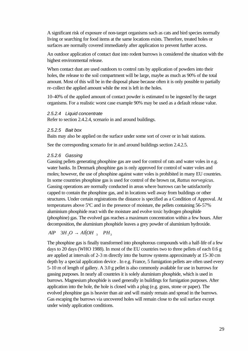
2.5.2.6 Gassing Gassing pellets generating phosphine gas are used for control of rats and water voles in e.g. water banks. In Denmark phosphine gas is only approved for control of water voles and moles; however, the use of phosphine against water voles is prohibited in many EU countries. In some countries phosphine gas is used for control of the brown rat, Rattus norvegicus. Gassing operations are normally conducted in areas where burrows can be satisfactorily capped to contain the phosphine gas, and in locations well away from buildings or other structures. Under certain registrations the distance is specified as a Condition of Approval. At temperatures above 5ºC and in the presence of moisture, the pellets containing 56-57% aluminium phosphide react with the moisture and evolve toxic hydrogen phosphide (phosphine) gas. The evolved gas reaches a maximum concentration within a few hours. After decomposition, the aluminium phosphide leaves a grey powder of aluminium hydroxide.

( ) 3323 PHOHAlOHAlP +→+

The phosphine gas is finally transformed into phosphorous compounds with a half-life of a few days to 20 days (WHO 1988). In most of the EU countries two to three pellets of each 0.6 g are applied at intervals of 2-3 m directly into the burrow systems approximately at 15-30 cm depth by a special application device . In e.g. France, 5 fumigation pellets are often used every 5-10 m of length of gallery. A 3.0 g pellet is also commonly available for use in burrows for gassing purposes. In nearly all countries it is solely aluminium phosphide, which is used in burrows. Magnesium phosphide is used generally in buildings for fumigation purposes. After application into the hole, the hole is closed with a plug (e.g. grass, stone or paper). The evolved phosphine gas is heavier than air and will mainly remain and spread in the burrows. Gas escaping the burrows via uncovered holes will remain close to the soil surface except under windy application conditions.

30

The release to the environment is estimated to be approx. 1% released to air and 99% released to soil during use.

Other metal phosphides are used in the EU, e.g. zinc phosphide in Germany and magnesium phosphide in France. The reactions and results are approximately the same (WHO 1988). However, zinc phosphide is not a gas or fumigant and is not used as such. It is mixed into an edible bait which is then consumed by the rodents. Once in the stomach of the target species it releases phosphine, which acts on the respiration pathways disrupting ADP / ATP. Zinc phosphide is not notified as an active substance under product type 14. According to CEFIC (2002) magnesium phosphide is normally not used in burrows. It is generally supplied in disc or plate form for use on large-scale fumigation in buildings for control of insects. However, magnesium phosphide is notified in product type 14.

Hilton & Robison (1972 cited in WHO 1988) introduced phosphine at 1.4 g.m-3 (1000 ppm) (as P) in the headspace of tubes containing 3 types of soil at 5 moisture levels, 0%, 25%, 50%, 75%, and 100% saturation. It was not stated whether the soils had been sterilised. Phosphine disappeared within 18 days from all air-dried soils, whereas up to 40 days was necessary for disappearance from moisture-saturated soils. Quantities of phosphorous recoverable as phosphate from the soils after incubation for 40 days varied widely with different soil types and reached about 70% of the total phosphine in a slightly acidic soil, containing 12-15% organic matter content and at 25% moisture saturation. Variation in phosphate recovery probably reflected rates of diffusion of phosphine into the soil matrix as a function of moisture content, as well as differences in the efficiency of different soils with different moisture contents as oxidising substrate for phosphine. Clearly, in time, soils are able to entrap the phosphine in the air in contact with them and oxidise it to orthophosphate.


2.5.3.1 STP Not relevant.

2.5.3.2 Soil Pellets and impregnated grain

Assuming some disturbance of the soil the equation for the local release in the farm scenario based on liquid concentrate can be modified for the impregnated grain and maize scenario and applied into one treated rat hole. Number of emission days per campaign is estimated to be 6 days during which the treatment is repeated twice. However, as previously mentioned when applying a rodenticide into a hole it is assumed that only the lower half of the hole and its surrounding environment is exposed (with the exemption of the gassing scenario). Therefore, the exposed soil volume will be divided by two.

31

Thereby the equation would be:

)( ,,,, usesoilreleaseapplsoilreleaserefilsitesprodprodcampaignsoil FFNNFcQElocal +××××=− (9)


Input:

Amount of product used at each refilling in the control operation

Qprod g S




Fraction of product released to soil during application

Frelease, soil, appl - 0.05 D

Fraction of product released to soil during use

Frelease, soil, use - 0.20 D

Output:

Local emission of active substance to soil during a campaign


The exposed soil area is assumed to be the lower half of the burrow wall surrounding an 8-cm diameter tunnel, with the mixing soil depth of 10 cm and up to 30 cm from the entrance hole. Thus the total soil volume is:

2)( 22

explrR

Vsoil osed××−

=π

(9a)


Input:

Radius of exposed soil around the hole R m 0.14 D

Radius of hole r m 0.04 D

Length of exposed hole l m 0.3 D

Output:

Soil volume exposed to rodenticide Vsoilexposed m3 0.0085

32

This corresponds to (0.142-0.042)×π×0.3 / 2 = 0.0085 m3. The weight of the soil, assuming wet soil density 1700 kg.m-3 is then 14.5 kg soil.

The local concentration in soil at each hole per control operation could be estimated by the equation:

soilosedexp

3campaignsoil

soil RHOVsoil

10ElocalClocal

×

×= −

(10)


Input:

Local emission to soil from the episode Elocalsoil-campaign g eq. 9 O

Soil volume exposed to rodenticide Vsoilexposed m3 0.0085 O


Output:

Local concentration in soil after a campaign Clocalsoil-campaign mg. kg-1

Contact powders

The exposed soil area is assumed to be the lower half of the burrow wall surrounding an 8 cm diameter tunnel, with the mixing soil depth 10 cm and 30 cm from the entrance hole. Thus the total soil volume is the same as described above for pellets and impregnated grains. The equation for the local release in the contact powder scenario would be (c.f. text 2.5.2.3):

33

soilreleasesitesprodprodcampainsoil FNFcQElocal ,×××=− (11)


Input:

Amount of product used in control operation Qprod g S



Fraction of product released to soil Frelease, soil, - 0.9 D

Output:

Local emission of active substance to soil after a campaign


The number of emission days is set to 1

The equation for soil concentration is then:

soilosedexp

3soil

soil RHOVsoil10Elocal

Clocal×

×=

(12)


Input:

Local emission rate to soil after a campaign Elocalsoil-campaign g eq. 11 O

Soil volume exposed to rodenticide Vsoilexposed m3 0.0085 D


Output:

Local concentration in soil after a campaign Clocalsoil mg.kg-1

34

Emission to soil after gassing:

The quantity used is 1 to 5 kg/field when used for agricultural purposes. However, no information on the amount per area used to protect dikes, embankments, etc. against water voles was available but this should be taken from the dossier.

The information indicates that 2 to 3 pellets are used per 2 to 3 m which gives an average of 1 pellet weighing 0.6 g m-1.

Water voles often occupy mole's burrow systems if found deserted. Thus information on both animals may be used in the scenario development. The burrows of moles are slightly oval, approx. 5 cm wide and 4 cm high, located in a depth of 5 to 100 cm of which the main parts are located in a depth of 10 to 20 cm. The area covered by the galleries is depending on the amount of food available. In areas with plenty food, a relativly small burrow system is needed.

The home range for water voles living in the Nordic countries is estimated based on a study from Sweden (Jeppsson 1987). The home ranges were observed to vary from 6 m2 to 4000 m2 per individual water vole. As water voles prefer to stay in family groups the total area may be large. A realistic gassing area is estimated to be 2 ha (20 000 m2).

The water voles entrance holes are 6-8 cm in diameter, i.e. the diameter of the burrows is set to 8 cm. The area covered by one group of voles is set at 2 ha. Controlling water voles with aluminium phosphide is comparable to controlling moles. A field trial with aluminium phosphide against moles has been carried out by Lodal (1978) and the results indicated that 1 kg per 4 ha/d may be used as a worst case: however, normally less is used.

A realistic worst case scenario is considered to be based on 0.2 kg product applied to 2 ha and repeated 5 times during a season of 3 months, i.e. 1 kg/2 ha/90 days. The diameter of the burrows is set to 8 cm, the area covered by one group of voles is set to 2 ha and the length of the burrows to 1000 m. pr. 2 ha.

The length of the burrows is based on experience that 0.2 kg product is applied to 2 ha and the average use of 1 pellet (0.6 g)/m. Thus the length of the superficial burrows is estimated to be 333 m pr. 2 ha (not including the lower galleries). To cover all burrows in a given area the length of the superficial burrows is multiplied with a factor of 3. Thus the total length is estimated to be about 1000 m pr. 2 ha.

In case of metal phosphide the phosphine gas is transformed into phosphorous compounds with a half-life of a few days to 20 days (WHO 1988). In this case it may be sufficient to estimate the local emission of active substance to soil after each application (e.g. 0.2 kg product applied to 2 ha) instead of the emission to soil per campaign.

The equivalent equation for the local release to soil in the gassing scenario would be:

35

soilreleaseappprodprodnapplicatiosoil FNFcQElocal ,×××=− (13)


Input:

Amount of product used in control operation per 2 ha*

Qprod g S

Fraction of active substance in product Fcprod - S**

Number of applications Napp - 1 D

Fraction of product released to soil Frelease, soil, - 0.99 D

Output:

Local emission of active substance to soil after a application

Elocalsoil-application g

*) A realistic gassing area is estimated to be 2 ha.

**) The scenario uses the fraction of active substance in product, Fcprod, which is a "Set"value. As 1) the active substance is formed by reaction of the rodenticide with moisture, and 2) the rodenticide consisting of aluminium phosphide usually is marketed with a purity of 56% TWO parameters might be used: Fraction of pure rodenticide Fpurity - 0.56 D

Fraction of phosphine formed Fformed - 0.585 Dc

out of rodenticde

Fformed is a closed value – i.e., it cannot be changed by the assessor – as it is based on the molecular weights of phosphine (34) and aluminium phosphide (58): Fformed = 23 / 58. In principle the emission scenario might be extended to other metal phosphides as well with a pick-list for the Fformed AlP + 3 H2O ? Al(OH)3 + PH3 58.0 34.0 Fformed = 0.586 P2Mg3 + 6 H2O ? 3 Mg(OH)2 + 2 PH3 134.86 2*34.0 Fformed = 0.504 P2Zn3 + 6 H2O ? 3 Zn(OH)2 + 2 PH3 258.1 2*34.0 Fformed = 0.263

Number of emission days per application is 1 but the exposure period is longer (see chapter 2.5.2.6).

The estimated concentration in the soil is then:

36

soilosed

napplicatiosoilsoil RHOVsoil

ElocalClocal

×

×= −

exp

310

(14)

where

l)rR(Vsoil osedexp ××−= π22 (14a)


Input:

Local emission rate to soil from a application

Elocalsoil-application g eq. 13 O

Volume of soil exposed per treated area Vsoilexposed m3 eq. 14a O

Radius of exposed soil around the hole R m 0.14 D

Radius of hole r m 0.04 D

Length of exposed hole* l m 1000 D


Output:

Local concentration in soil after a application Clocalsoil mg. kg-1

*)The total length of the burrows is estimated to be 1000 m pr. 2 ha.

The exposed area is assumed to be the whole burrow wall surrounding a tunnel of 8-cm diameter and the mixing soil depth 10-cm. Thus the total soil volume is (0.142-0.042)×π×1000 = 56.5 m3. The weight of the soil is calculated, assuming wet soil density 1700 kg.m-3.

Worst case scenario of 1 kg product per 4 ha, will result in an estimated concentration in the exposed soil of 0.005 mg product kg-1 soil (assuming 99% release to soil; see Table 2.1). A realistic worst case of 0.2 kg product per 2 ha results in 0.002 mg product kg-1 soil during emission episodes (1 day).

The effects of different scenarios are illustrated in table 2.1 below. It has to be noted that in case of using aluminium phosphide the amount of phosphine generated equals one third of the amount of product used.

Table 2.1. Estimated length of burrow tunnels and exposed soil.

Area (ha)

Area (m2) Length of exposed

tunnels (m)

Volume of exposed soil*

(m3)

Weight of exposed soil **

(kg wwt)

kg product Csoil ***

(mg prod/kg soil)

4 40,000 2,000 113 192100 1 0.005

2 20,000 1,000 56.5 96050 0.2 0.002

*: Assuming 10 cm soil depth. **: Assuming 1700 kg.m-3 and *** assuming 99% release to soil.

37

The release to groundwater is considered negligible due to the transformation into phosphine gas and further to phosphorous compounds.


2.5.3.4 Air The volatilisation of rodenticides to air based on impregnated grain and maize applied into rat holes is estimated according to the TGD (2003).

Emission to air after gassing Exposure to air is considered to take place when not all entrance holes are covered or the application takes place under windy circumstances. Usually the application takes place during calm and dry weather conditions. This mean that about 1% is assumed released to air and 99% to soil.

The fraction of emission to air is a function of vapour pressure. A relevant model of the release to air may be the one described in USES 3.0 (RIVM et al. 1999) developed for pesticides. The general total emission factors and the initial 1 hour and 24 hour averaged source strengths correspond to an application density of 1 kg.m-2/application for field use. The emission factors for the initial 1-hour averaged source strength are calculated assuming that 30% of the total emission occurs in the first hour after application. For calculation of the initial 24 hour averaged source strength, it is assumed that 90% of the total emission occurs during the first day after application which can be considered a realistic worst case. The emission factors and source strengths to air for field uses of pesticides are given in Table 2.2.

Table 2.2. Emission factors and source strength to air for field use of pesticides (RIVM et al. 1999)

Vapour pressure of a.i.

Total emission factor to air for field application

(outdoor use)

24 hour averaged source strength

Estdfield, air,24h

Pa (based on 1 kg.m-2)

>1×10-2 1 0.9

1×10-2 – 1×10-3 0.5 0.45

1×10-3 – 1×10-4 0.2 0.18

1×10-4 – 1×10-5 0.1 0.09

≤1×10-5 0.01 0.009

The standard values are recalculated using the actual dosage, i.e. by multiplying Qprod with

Estdfield, air,24h. The release to air during field use is assumed to be 1% of the applied amount as

38

realistic worst case. The emissions to air can be calculated by multiplying the local emission strength of the field at 24 hours with 1 minus the fraction of retention (Fret).

)1(24,,24,, rethairfieldprodprodhairfield FEstdFcQElocal −×××= (15)


Input:

Amount of product used pr. application in control operation

Qprod kg.m-2 S

Fraction of active substance in product* Fcprod - S

Averaged source strength Estdfield, air,24h

-

From table 2.2.

D

Fraction of retention Fret - 0.99 S/D

Output:

Local emission of the field during 24 hours Elocalfield, air, 24h kg.m-2 O * It has to be noted that in case of using aluminium phosphide the amount of phosphine generated equals one third of the amount of product used.

The local concentration in air is found by dividing the emission by the air volume considered. It is suggested to use an air height of 2 m for realistic worst case in windy situations. No scenario for this application is included in the TGD, but it is proposed that for calculation of the PEC both the photodegradation and dilution in air e.g. caused by the windy situation should be considered. The phosphine gas is heavier than air and is expected to remain below soil surface if correct application methods are followed and subsequently close to the ground if release occurs from uncovered holes or during windy weather conditions. It should be noted that the TGD does not cover this kind of exposure situation as in the TGD the Clocalair is the annual average local concentration in air and not a 24 h local air concentration which is calculated here.

The estimated concentration in air is then:

39

air

hairfieldair HEIGHT

ElocalClocal 24,,= x 106

(16)


Input:

Local emission of the field after 24 hours Elocalfield, air, 24h kg.m-2 S

Air height HEIGHTair m 2 D

Output:

Local concentration in air after 24 hours Clocalair mg.m-3

Though lethal for the target organisms (and possible non-target organisms being present in the vole galleries, e.g. toads and mice), the dose actually inhaled (and thereby removed from environmental exposure of air and soil) is assessed to be insignificant compared to the total dose applied.

Under normal circumstances there will be practically no residues for disposal (except the empty container with practically no active substance remaining in it).


2.5.4.1 Primary poisoning The bait may also attract other vertebrates and small birds. The situation in the open area scenarios is basically similar to what is mentioned for commensal rodents above regarding the risk of primary poisoning.

2.5.4.2 Secondary poisoning Secondary poisoning hazard may occur in the open area scenario but it is not assumed to be a problem after gassing. Predators among mammals and birds may occur in the immediate vicinity of buildings, e.g. parks and gardens or further away. When moving around the rats may be caught by raptors and scavengers may find dead rats. Detailed exposure scenarios for the assessment of secondary poisoning is given in Chapter 3.3.

40

2.6 Exposure scenarios for waste dumps/landfills

2.6.1 Introduction

This scenario covers control of rats and disposal of rats in waste dumps and landfills where the exposure is assumed to be higher than that described in the open area scenario.

In some instances, applications of rodenticides to refuse dumps take place. Mostly the use is limited to occasions of population outbreaks of rats. Often the rodenticides are deployed around the perimeter of the dump, more than in the disposal area itself. The bait may be placed at regular places in special feeding stations in order to prevent other animals from eating the bait. Information has been received from Finland but the scenario is included, as it may be relevant for other countries as well.

From Finland information has been received on rodenticides that are used in open refuse dumps, which have not yet been replaced by modern waste processing units. They are mostly located in some sort of pit, natural or man-made and in most cases insufficiently covered with soil. The dumps are visited 4 to 6 times per year by a rodent control service and rodenticide baits are applied to the dump. There is no detailed data available on the area of dump sites, on use of bait boxes or on collection of dead animals. Thus, it is considered as a worst case that all is left on the dump. The default exposure area is set at 1 ha.

Myllymäki (2002) mentions a case in Finland of an occasional rat population outbreak in the autumn 2000. The case was a refuse dump with an estimated rat population of 5000 rats that was closed down and thereby caused mass rat emigrations. A daily baiting programme was initiated. In less than 10 days, bait consumption decreased from more than 100 kg/day to less than 10 kg/day.

Temporary dumps or storage facilities for household waste etc. may be used as buffer at incineration facilities. If the turnover rate is too slow, application of rodenticides may be necessary. The use of contact dust in such temporary garbage storage facilities has also been described (Jensen 2002).


2.6.2.1 Wax block May be relevant in bait box or covered by available coverings. In France a typical application is 1 block (of about 20 g) for 10 m2 for each treatment. The treatment frequency may be 4-6 applications a year, 2-3 month apart (INERIS, 2002).

2.6.2.2 Pellets, impregnated grain It is assumed that available coverings are used.

2.6.2.3 Contact dust May be relevant. Information on use in rat holes at the edges of open dump sites exists.

2.6.2.4 Liquid concentrate Not relevant

2.6.2.5 Bait box

41

For control of rats in waste dumps and landfills the rodenticide may be placed in bait boxes.



2.6.3.1 STP Not relevant

2.6.3.2 Soil The soil is potentially exposed. It is assumed that available coverings are used. Apparently most of the bait is eaten and returned as urine, faeces, dead animals, etc.

Realistic worst case (rat population outbreak):

soil,releaseappprodprodcampaignsoil FNFcQElocal ×××=− (17)


Input:

Amount of product used in control operation pr. application*

Qprod kg 40 S/D


Number of applications Napp - 7 D/S

Fraction of product released to soil Frelease, soil, - 0.9 D/S

Output:

Local emission of active substance to soil from a campaign

Elocalsoil-campaign kg

*) There is enormous variation in this value.

42

The estimated concentration in the soil is then:

soilsoilosed

campaignsoilsoil RHODEPTHAREA

ElocalClocal

××

×= −

exp

610

(18)


Input:

Local emission to soil after a campaign Elocalsoil-campaign kg eq. 17 O

Area exposed to rodenticide Areaexposed m2 10000 D



Output:

Local concentration in soil after a campaign Clocalsoil mg.kg-1

The potential realistic worst case would be 90 % released to the soil, i.e. 252 kg/(10000 m2 × 0.1 × 1700) ≅ 150 mg.kg-1 soil.


2.6.3.4 Air Not relevant.


2.6.4.1 Primary poisoning Concerning the risk of primary poisoning the situation is regarded similar to that described above for vole control in the open areas.

2.6.4.2 Secondary poisoning The secondary poisoning hazard applies to predators among mammals and birds and scavengers and thus the situation is comparable to that described above for commensal

43

rodents in the open areas; however, there might be more predators around a landfill than in the open areas e.g. sea gulls, craws, etc.

2.7 Summary The environmental exposure scenarios are based on the potential releases of rodenticides from application, use and disposal to the environmental compartments water, soil, and air. The formulation types are included in the scenarios, as formulation types of the rodenticides appear to be an essential parameter determining the local releases. The exposure scenarios are suggested based on the scenarios where the highest release to the environment is expected to take place. The contribution of regional release is considered to be negligible.

It should be noted that the estimated concentrations relate to the rodenticide products since many products are available with different active substances and concentrations.

A scenario concerning the application and use of wax blocks and baits in the sewerage system is suggested.

An outdoor exposure scenario based on baits in bait boxes is suggested based on a farm scenario with releases to the local soil.

For pellets and impregnated grain and maize an open area scenario is suggested related to the application of baits into rat holes. The potential air exposure may be estimated from the potential of the rodenticides to volatilise to air.

The contact/tracking powders are estimated to have the highest release to soil when applied directly on soil in rat burrows. A scenario for estimating the soil concentration following the mixing of rodenticides into soil of a standard depth is suggested.

The release from the application and use of liquid concentrations to the soil below the mixed bait (e.g. apple pieces) is suggested.

A gassing scenario covering the use of gassing against water voles is included. The release to air is estimated as realistic worst case based on an assumption of not all exit holes covered and a windy condition. The concentration in soil is estimated based on a Danish estimation of the length of burrows within a square meter and a recent Swedish study on the home range of water voles.

A scenario for waste dumps is included for estimation of the resulting concentration of rodenticides in the local soil.

44

The following summary table can be used to give a environmental exposure summary of a given rodenticide:

Table 2.3. Environmental exposure scenarios for rodenticides.

Environmental protection targets/exposed compartments Main scenario Application type

STP Soil Surface water Air Primary poisoning

Secondary poisoning

Wax block + + + - - +

Pellets, impregnated

grain

+ + + - - +

Sewer systems

Bait box + + + - - +

Wax block + + + - + +


grain

+ + + - + +

Liquid concentrate

(-) + - - + +

In and around

buildings

Bait box - + - - + +

Wax block - + - - + +


grain

- + - - + +

Contact powder - + - - (-) +

Bait box - + - - + +

Open areas

Gassing - + - + (+) -

Wax block - + - - + +


grain

- + - - + +

Contact powder - + - - (+) +

Waste dumps

Bait box - + - - + +

45

3 Exposure scenarios for primary and secondary poisoning

3.1 Introduction The scenario for primary poisoning is also called a “direct exposure scenario” and the scenario for secondary poisoning is also called an “indirect exposure scenario”. In this report we use the terms primary and secondary poisoning.

Basically the same set of physiological processes is responsible for maintaining life for warm-blooded animals, i.e. mammals and birds. Therefore, the use of rodenticides meant for killing selected pest mammals has to be considered a general hazard to non-target mammals and birds as well. Non-target animals are potentially at risk in two ways: 1) from direct consumption of the baits (primary poisoning) and 2) through eating rodents that have taken up/accumulated the poison (secondary poisoning). Though similarities exist there are differences as to the susceptibility to or tolerance of the different rodenticides among mammals and birds. These differences may be due to differences in their normal diets, feeding habits, ecological or other factors.

The exposure scenarios and assessments presented here give a basis for evaluating the primary and secondary poisoning risk to non-target animals according to the TGD (2003). It is proposed to introduce tiered approaches for assessing the risks through both primary and secondary poisoning. These are not described in the TGD (2003) and, therefore, the principles are described here.

46

Primary poisoning Secondary poisoning

Tier 1 Risk is quantified as the ratio between the concentration in the food for the non-target organism (PECoral) and the predicted no-effect-concentration for oral intake for the non-target organism (PNECoral)

Risk is quantified as the ratio between the concentration in the rodent immediately after a last meal on day 5 (EC5) and the predicted no-effect-concentration for oral intake for the predator (PNECoral)

Tier 2 Risk is quantified as the ratio between the estimated daily intake of a compound (ETE) and the predicted no-effect-concentration for oral intake for the non-target organism (PNECoral).

For the long-term exposure the estimated concentration of the active substance in the animal can be calculated and compared with the NOAEL

Risk is quantified as the ratio between the estimated concentration in predatory mammals or birds and no-observed-adverse-effect-levels (NOAEL) for the organism

Methods for estimating the various exposure levels for tier 1 and 2 assessment for primary and secondary poisoning are described below.

As a first tier, the actual assessment (see below) is normally based on a comparison of the (predicted) concentration of the chemical in the food and the (predicted) no-effect concentration in food, which is based on studies with laboratory animals. The studies referred to furthermore emphasise that for understanding and evaluating the consequences of control operations it is of paramount importance also to have a thorough knowledge of the ecology, behaviour, feeding habits etc of the animals relevant in the geographical area to be covered by the scenarios.

Chapter 3.2.1 also describes methods to estimate daily uptake and internal body concentrations for a variety of non-target animals in case a refined exposure assessment is needed as a second tier exposure assessment option both for the primary and secondary poisoning assessment. This is because there is a element of uncertainty if PNECoral calculated according to the TGD is really very suitable for rodenticides. Based on the waiving discussions, it may be that it is not possible to do a chronic mammalian test with rodenticides, and the toxicity of many rodenticide active substances is expressed only by their acute toxicity. This is however contrary to the TGD approach which states that it is always the chronic data we should use and assigns a very high AF to acute data. It is recommended to leave further refinement to be done after we have gained experience with the ESD and know in detail the toxicology of these substances.

47

In this report the focus has been on individuals as a first step that is very important. However, equally or maybe even more important for a full understanding of the consequences of using rodenticides are the effects on populations of the animals concerned.

Primary poisoning

In addition to wild living animals domestic animals such as hens and pigs may also be considered to be among animals that are at risk of being poisoned accidentally because they prefer many types of vegetable food.

Sparrows and pigeons prefer to place their nests on or even the inside of man-made structures as buildings, or they can have their roosting sites inside the buildings. Birds with such habits are of course at greater risk of getting in contact with, find and eat or in other ways being poisoned by the rodenticides being used in their surroundings.

Secondary poisoning

Pets such as dogs and cats that live in close contact with human beings are of course also potentially at risk of being poisoned with rodenticides, particularly if they prey on poisoned rodents around buildings where rodenticides are being used. Other predatory mammals such as foxes, polecat, stone martens, stoats, racoon dog and weasels may be at risk because they often search for prey around farms, gardens, parks or other areas where rodents may be controlled.

Kestrel, buzzard, red kites, tawny owl, barn owl and eagle owl are bird species that have live rodents as their prey items. They often hunt not far away from human settlements or in areas where rodents are controlled due to their pest status. Though such birds of prey do not eat rodenticides, their risk of being victims of secondary poisoning through poisoned prey animals has to be evaluated. Also scavenger birds such as Corvidae (e.g. crows and allies) and Laridae (gulls) and other birds such as buzzards and kites which will scavenge as well may be at risk for secondary poisoning. There are clear and important differences between the group of slow-acting anticoagulant rodenticides and the group of more acute non-anticoagulant rodenticides available in the EU countries. The different groups of rodenticides are for that reason treated separately in the descriptions of scenarios given below.

Anticoagulant rodenticides are widely used in EU. Anticoagulants are used for control of rodents in sewer systems, in and around buildings and for some specific purposes also in the open field. It is evident that the primary and the secondary poisoning hazard to non-targets may vary according to the openness and accessibility of the control areas.

It should be noted that substance specific results from e.g. avoidance, feeding and animal behaviour studies, where available, could overrule the default assumptions used in the calculation formulas of the scenarios presented. The exposure scenario for secondary poisoning currently considers that predators and scavengers are exposed only by feeding on target rodents, whereas in fact it is likely that non-target species (especially small mammals) are also contaminated and this could cause an additional risk of secondary poisoning. For many species (e.g. barn owl), non-target small mammals are the main diet and might increase exposure significantly. This is, however, not considered further in this document.

48

The estimated content of active substance in some relevant non-target mammals and birds is calculated in Section 3.2.1. Further example calculations estimating uptake and internal body concentrations for a variety of predators are given in Section 3.2.2 in case a refined exposure assessment for secondary poisoning is needed as a second tier option.

A general equation describing the uptake and the expected concentration of rodenticides in selected animals is also given in Section 3.2.1 as this may be an important parameter in the evaluation of the secondary poisoning potential of a given rodenticide.

3.2 Exposure scenarios for primary poisoning

3.2.1 Anticoagulant rodenticides

When anticoagulant rodenticides are applied according to label instructions (required by the authorities), the primary poisoning hazard may be considered as small. However, small non-target rodents and small, mostly granivorous, birds may be exposed because they can pass through the entrance hole of a bait station. Another exposure of non-target animals may arise when target animals carry bait away from e.g. baits stations.

The primary poisoning of non-target animals occurs accidentally, because of carelessness or if the UK experts are right that rats carry away a fraction of the bait from the bait stations. The worst case may be considered at two levels. The first level has its limitations set by the amount of poison available. It seems reasonable to consider a portion of 600 g bait as the normal upper limit for what is available to non-target animals in several EU countries. The 600 g portion is the largest one permitted for use by non-professionals in several countries. Larger portions is permitted to be used only by professionals; however, it is assumed that professionals have knowledge of the substance they are handling and will ensure that the rodenticides are not available to non-target animals. In some member states professionals means control operators who have taken a special course on this matter; however, in others caretakers and farmers are considered as professionals. It is therefore important that the assessor checks the use conditions in a given area/country before the upper limit for what is available to non-target animals is estimated.

When larger amounts of a rodenticide are available to non-target animals, they may at worst eat as much as their full daily ration.

It is a common experience that dogs are more omnivorous than cats and that may explain why dogs are more often victims of primary poisoning (Bille & Lund 1989, KEMI 2001). Pigs are considered the most susceptible species among domestic animals. Birds eating cereal and weed seeds like sparrows, pigeons and pheasants seem reasonable to include in a worst-case scenario. The domestic hen may be comparable with the pheasant.

The risk for primary poisoning of a non-target organism, in a first tier scenario is calculated as the ratio between the concentration in their food (PECoral) and the no-effect-concentration for oral intake (PNECoral). This evaluation can be used for both short and long term exposure. It is assumed that the animal in question consumes nothing but the rodenticide (until an upper limit of 600 g) in one daily meal and therefore this is used as a default value. However, it is

49

important that the assessor checks the use conditions in a given area/country before the upper limit for what is available to non-target animals is estimated. A common concentration in the final product is 0.005% and therefore this value is used as a default value in the calculations for the scenarios. Nevertheless, the proper concentration for an active substance should be checked from its dossier and the calculations modified accordingly. Thus the concentration of the rodenticide in the food of a non-target organism (PECoral) is the concentration of the active substance in the rodenticide bait (or equivalent final a.s. concentration of the rodenticide) to be taken up by the non-target animal 600 g at maximum in one daily meal.

As a second tier evaluation, the following more detailed exposure assessment can be done. Basically the estimated daily uptake of a compound (ETE) is given by the following equation (EEC 2001):

ETE = (FIR / BW) * C * AV * PT * PD (mg.kg-1 bw/d) (19)


Input:

Food intake rate of indicator species (fresh weight)

FIR g.d-1 S/P

Body weight BW g S/P

Concentration of active compound in fresh diet (bait)

C* mg. kg-1 S/P/D

Avoidance factor (1 = no avoidance, 0 = complete avoidance)

AV - 1 S/D

Fraction of diet obtained in treated area (value between 0 and 1)

PT - 1 S/D

Fraction of food type in diet (number between 0 and 1; one type or more types)

PD - 1 S/D

Output:

Estimated daily uptake of a compound ETE mg.kg.-1d-1

*) Note that C is previously given the symbol Fcproduct

In the calculations of uptake of active substance of a rodenticide, in this first step worst case scenario AV, PT and PD are all set to 1. If no other information is available this will also be considered as a realistic worst case. A realistic worst case values AV = 0.9, PT = 0.8 and PD = 1 might be used instead as a second step, based on e.g. recommendations of the EPPO Rodent Control Panel on acceptable avoidance factors for rodenticides. These assumptions reduce exposure by 28% compared to AV=1 and PT=1, yet (a) cereal baits are highly accepted by small mammals and granivorous birds, (b) anticoagulant active ingredients have virtually no intrinsic aversive properties, (c) in at least some exposure scenarios (especially outdoors), some non-target individuals may obtain all their diet within the treated area, and (d)

50

the EPPO recommendations may not have been implemented for every product that is assessed. Using the second tier, the assessor should justify the use and check that the reductions are appropriate in each case.

It should be noted, however, that substance specific results from e.g. avoidance, feeding and animal behaviour studies, where available, can overrule the default assumptions used in the calculation formulas of the scenarios. Such studies should be included only if they are relevant and realistic. For example, a rodenticide bait may be ignored when a preferred alternative food is available, but consumed readily when presented alone (cf. discussions of avoidance testing in OECD (1996) and Leopold et al. (2001)).

Food intake can be very variable, depending on the metabolic rates of the species, the nature of their food, weather conditions, time of year, etc. If no information is available on the mean daily food intake, the following regression equations (from Nagy 1987 cited in EPPO 1993) can be used to predict dry weight intake for an animal of a particular body weight:

for all birds: log FIR = 0.651 log BW - 0.188

for songbirds: log FIR = 0.85 log BW - 0.4

for other birds: log FIR = 0.751 log BW - 0.521

for mammals: log FIR = 0.822 log BW - 0.629

(where FIR = daily food intake expressed as dry weight, BW = body weight)

The derived values on dry weight basis need to be adjusted to allow for moisture content, where this may be significant.

It has to be emphasised that the worst case scenario described above may over-estimate uptake, at least for the birds. According to the general rules in many countries all rodenticides have to be coloured in order to warn humans from eating them. In the scenario no assumption is made as to what colour the rodenticide might have.

Moran (2001) has shown that birds with their well-developed colour perception notice the different colours of scattered treated grains. When foraging in the fields they prefer natural undyed grains. For feral pigeons it was possible to rank colours as to their repelling efficiency when no undyed grains were offered, as follows: yellow > black > green and red. This means that green and red coloured grains are least repellent to feral pigeons and that grain coloured yellow are the most repellent. Blue coloured items were the least preferred by house sparrows.

Moran (2001) does not give exact figures for the effect of the different colours so it is impossible to give a value between 0 and 1 for AV in order to correct the figures calculated in Table 3.1 with a certain factor. Besides, the colour preferences vary between species and may change depending on the context (e.g. depending on the hunger of the animals). Therefore caution should be exercised before generalising from the results of Morgan or any other study. This is briefly discussed in OECD (1996). The default AV is therefore 1.

51

In Table 3.1, the content of active substance in some relevant non-target mammals and birds is calculated as examples on second tier exposure estimation of uptake and internal body concentrations relevant for primary poisoning. It is assumed that the animal in question consumes nothing but the rodenticide until an amount of 600 g at maximum has been consumed in one daily meal.

In Table 3.1, the expected content of active substance immediately after a meal (i.e. no elimination has occurred) in non-target animals has been calculated for a worst case situation. The default value for C is 50 mg.kg-1 (=0.005%). The calculation for e.g. the pheasant is as follows:

ETE = 102.7/953 * 50 * 1 * 1 * 1 = 5.4 mg.kg-1

Table 3.1. Expected content of the active substance of a rodenticide in non-target animals in the worst case situation (concentration of active substance in rodenticide bait 0.005%)

Species Body weight Daily mean food intake

Rodenticide consumption

Concen-tration of a.i. after a single meal

(one day)

(g) (g) (g) (mg/kg)

Dog Canis familiaris 10000 ? 600.0 3.0

Pig Sus scrofa 80000 ? 600.0 0.4

Pig, young Sus scrofa 25000 ? 600.0 1.2

Tree sparrow *) Passer montanus 22 7.6 7.6 17.3

Chaffinch **) Fringilla coelebs 21.4 6.42 6.42 15.0

Woodpigeon *) Columba palumbus 490 53.1 53.1 5.4

Pheasant *) Phasianus colchicus 953 102.7 102.7 5.4

*) Values for body weight and daily mean food intake from EEC (2001) **) Values for body weight and mean food intake taken from Luttik et al. (1999)

The expected concentrations of active substances in selected species of non-target animals can be summarised as seen in Table 3.2. The values are based on the calculations given in Table 3.1 but an elimination factor has been added. To illustrate this, an elimination factor of 0.3 per day has been used. This is a reasonable average default value for elimination as anticoagulant rodenticides are eliminated from the body mainly through faeces (Smith 1999). However, the elimination rates vary widely between species and between rodenticides. Therefore, the proper elimination rate for an active substance should be acquired from its dossier and the calculations modified accordingly.

52

The expected concentration of active substance in the animal after metabolism and other elimination is calculated as follows:

EC = ETE * (1 - El) (20)


Input:

Estimated daily uptake of a compound ETE mg.kg.-1d-1 Eq. 19 O

Fraction of daily uptake eliminated (number between 0 and 1)

El - S

Output:

Expected concentration of active substance in the animal

EC mg.kg-1

The calculation for e.g. the wood pigeon is as follows:

EC = 5.4 * (1 - 0.3) = 3.8 mg.kg-1, and with the comments above in mind it is a maximum value for this bird species.

It has to be remembered that the calculations are based on a rodenticide product with 0.005% active substance. E.g. brodifacoum for control of voles in Finland has a content of only 0.001% active substance. Difethialone is marketed only in 0.0025% formulations.

In a similar manner the concentrations in the relevant non-target mammals and birds can be calculated for each active substance to be assessed in second tier primary poisoning exposure assessment to show the interspecies variation due to e.g. variation in relationship between body weight and daily food ingestion rates. The choice of relevant species depends on e.g. which non-target species are most probably affected. When a bird species is relevant sparrow could be the first choice as its internal body concentration is considerably higher than in the mammals and due to its size and mobility, it seems to have better access to bait stations.

53

Table 3.2. Expected concentrations of active substance in selected non-target animals in primary poisoning scenarios after one meal followed by a 24 hour elimination period (concentration of active substance in rodenticide bait set to 0.005%)

Species (mg/kg)

Normal use Realistic worst case

Dog Canis familiaris ≅ 0 2.1

Pig Sus scrofa ≅ 0 0.3

Pig, young Sus scrofa ≅ 0 0.8

Tree sparrow *) Passer montanus ≅ 0 < 12.1

Chaffinch **) Fringilla coelebs ≅ 0 < 10.5

Woodpigeon *) Columba palumbus ≅ 0 < 3.8

Pheasant *) Phasianus colchicus ≅ 0 < 3.8

*) Values for body weight and daily mean food intake from EEC (2001)

**) Values for body weight and mean food intake taken from Luttik et al. (1999)

In second tier assessment for the long-term exposure, which also has to be taken into account in the evaluation of primary poisoning of rodenticides the ECn (expected concentration of active substance in the animal after n days) can be calculated by use of equation 21 (see part 3.3.1). However, it has to be remembered that this illustrate a worst case scenario (AV, PT, and PD are all set to 1).

If label instructions are followed, as should be the case for normal use, the primary poisoning risk should be negligible as indicated by ≅ 0 in Table 3.2. The assessor should check what the exposure would be if the label conditions are followed. The reason is to assure that label instructions are fully adequate to mitigate the high intrinsic risk that these products potentially present.

3.2.2 Non-anticoagulant rodenticides

The general approach for the assessment described in section 3.2.1 based on a comparison of the predicted concentration in the food of the non-target animal and the no-effect concentration from studies with laboratory animals can also be used for the non-anticoagulant rodenticides. Also the second tier option described there may be calculated in a similar manner for non-anticoagulant rodenticides when detailed species specific body concentrations are of interest.

Pellets containing aluminium phosphide are used against water voles living in underground tunnel systems. The animals are killed by the phosphine gas which is developed through

54

contact between aluminium phosphide and humidity in soil and air. The correct way of applying the aluminium phosphide containing pellets is to place the pellets in the tunnel system and afterwards close the hole to the tunnel system with a stone, grass or a piece of paper.

An obvious primary poisoning is considered unlikely as the water voles and moles are the only animals living in the tunnel systems when it is necessary to kill them. however, one could think that a stoat or a weasel might try to find a highly desired prey as a water vole.

Sometimes dogs are running around in the fields that have just been treated with aluminium phosphide. If a dog finds interest in digging out a hole where the pellets have been applied and eat them, the dog will be in danger of being severely intoxicated. No values regarding the toxicity of phosphine to dogs are known. According to Tomlin (1997) inhalation at 10 mg.m-3 can cause death within 6 hours. As two pellets (the dosage in one hole) generate a total of 600 mg phosphine the risk to such a dog is understandable.

Cholecalciferol (0.1%) is approved in Sweden for control of mice only. One dog has been reported poisoned by calciferol in Denmark in 1988 (Bille & Lund 1989).

The primary poisoning hazard is difficult to calculate as a dog may have access to up to 600 g poison bait at a time as 600 g in several countries is the maximum content of one package. However, the assessor must check the use conditions in a given region/country before an evaluation can be made.

A 10-kg dog consuming 600 g cholecalciferol bait gets a mean concentration of cholecalciferol in the body of 60 mg kg-1. LD50 for a dog is 88 mg kg-1, so with dogs of enormous size variations it seems reasonable that a dog now and then accidentally may be poisoned lethally by consuming a bait containing cholecalciferol.

The primary hazard of cholecalciferol to birds living close to humans should also be considered. Marshall (1984) has described non-target studies with ducks and bobwhite quails. The LD50 was 2000 mg kg-1 for mallard duck and the LC50 was 4000 ppm for mallard ducklings and 2000 ppm for bobwhite quail. There is no information about the duration of the test but it is anyway a high concentration, and all results indicate low hazard to avian species. However, UK experience does not agree that calciferol in rodenticide baits presents a low hazard to avian species. Especially small songbirds seem to be very susceptible (the UK working group RRAT, 2002). Therefore this has to be taken into consideration in the evaluation.

Chloralose (4%) is used in Denmark only for control of mice in and around buildings.

The primary poisoning hazard may be related to grain-eating birds because birds are more susceptible to this active substance than rodents and other mammals that are bigger than mice.

As an example, the chaffinch (Fringilla coelebs) can be used. According to Luttik et al. (1999) this bird has a body weight of 21.4 g and its daily food consumption in dry weight is 6.42 g.

A grain and seed eating bird is not expected to eat just the poison bait and nothing else. If the bait is as attractive as the normal food of the bird, it is considered likely to constitute 50% of the total daily food consumption as a maximum in the normal use situation. Normal situations

55

are often assumed to be less than 50% and levels of 10% and 20% are often suggested for such cases (cf. Table 3.3). However, if the normal food of the birds is limited in availability (e.g. in winter) then they might feed mainly (>>50%) on bait, at least for short periods. Therefore the realistic worst case is normally set to 100% unless the assessor has good scientific data which has to be taken into consideration.

Table 3.3. Daily intake of chloralose, mg kg-1, for the chaffinch (Fringilla coelebs)

Normal situations

Realistic Worst case

Poison bait in % of total consumption 10 20 50 100% Consumption of a.i. mg kg -1 1200 2400 6000 12000

It the case of chloralose such data exist. It has to be emphasised that it is not that likely that a bird gets such a high concentration of chloralose in the body. This is because of the narcotic effect making the bird stop feeding long before having reached the calculated amounts. The lowest known LD50 to birds of 31.6 mg kg-1 corresponds to a consumption of 0.79 g prepared bait per kg body weight. Grain eating birds may therefore succumb long before having consumed a full daily food ration.

3.3 Exposure scenarios for secondary poisoning The general rules for assessment of secondary poisoning are presented in Section 3.8 of the TGD (2003). However, the rodenticide specific issues that are to be taken into account in this exposure scenario are presented in this chapter.

The secondary poisoning risk of rodenticides may be related to the behaviour of poisoned animals if their behaviour is changed in a way that makes them an easier prey to predators. Cox & Smith (1992) studied the behaviour of brown rats that had been poisoned with anticoagulants. In enclosures they found a reduction in thigmotactic behaviour (i.e. in contact with a vertical surface) and that more than half of the rats died away from cover.

Gemmeke (1988) studied the behaviour of brown rats and house mice that had been poisoned with anticoagulants. Poisoned animals were more active in the daytime than non-poisoned and furthermore they moved more around unprotected on the surface. With such a change from normal behaviour, predatory birds and mammals may more easily take poisoned rodents. In the same study, half of the poisoned rats and mice left their burrow systems and moved up onto the surface when they were dying.

Normally non-poisoned rodents may also die on the surface. In this context, however, it is important that poisoned rodents do not always hide from scavengers and just before death some of them are easy prey to predators.

56

Commensal rodents may move to the surface when they are dying. As regards voles and their behaviour after being poisoned, Saucy et al. (2001) studied water voles being controlled with bromadiolone. In a pen experiment they found 38% of poisoned water voles dying above ground. Therefore, when controlling voles there is a comparable risk of secondary poisoning of non-target animals as mentioned for commensal rodents.

3.3.1 Anticoagulant rodenticides

It is a common experience that a rodent of the sizes occurring in the EU countries on an average consumes a daily amount of food equivalent to about 10% of its body weight. The value is based on laboratory experiences and used by several authors, e.g. Nagy (1987), EPPO (1993) and Smith (1999).

Equation 19 (cf. primary poisoning) can be used for calculating the amount of active substance being consumed by the target rodent. A reasonable value for factor PD in the equation is necessary for the full scenario.

For registration of rodenticides it is required that the consumption of the rodenticide makes up at least 20% of the total daily consumption in choice tests. The non-poisonous alternative in such tests is a type of food that is normally well accepted by and relevant for the target species under natural conditions. Therefore a value for normal use situation may be at least PD = 0.2. However, this is clearly a minimum figure and one would expect the normal case to be above the minimum. According to CEFIC (2002) evidence from efficacy trials show that the actual bait taken is never more than 60% of total food consumed in a day.

If a poisonous bait is well accepted by the target rodent, i.e. accepted to the same degree as normal food, it will make up about 50% of the daily consumption. The factor PD then becomes 0.50. This fraction may illustrate a scenario of the normal use situation.

The realistic worst case could be still higher – if a loose cereal bait is used in a situation where other food is less palatable or less accessible, then PD could be closer to 1, at least for a proportion of the rodent population.

In order to elucidate a full-scale scenario, a situation with PD = 1 (i.e. 100% of food items are poisoned bait) has to be considered as the realistic worst case. Using another value, the assessor should justify the use and check that the reduction are appropriate in each case. In the normal use it seems very unlikely that an animal should not take the normal available food within its range as the occurrence of its preferred food has been one of the factors determining its presence. Therefore, PD values 0.2, 0.5 and 1 are included in the following calculation examples.

As anticoagulant rodenticides are eliminated from the body mainly through faeces, a reasonable default value for elimination is 30% per day (Smith 1999). Therefore a default of 0.3 is used in the examples presented in this document. However, the proper elimination rate for an active substance should be checked from its dossier and the calculations modified accordingly. In addition real data from carcasses should be used wherever possible.

57

A normal susceptible rodent may eat an anticoagulant rodenticide for some days before it stops eating. For each day a new portion of the poison bait may be eaten and excretion happens every day. The feeding period has been set to a default value of 5 days, which corresponds to the feeding pattern observed in laboratory experiments. It is a characteristic element that even after having consumed a lethal dose, the rodent may continue eating until the onset of symptoms after which it eats very little or nothing until it dies. The mean time until death has been set to a default value of 7 days which corresponds very well with the value found for some rodent species by Lund & Lodal (1982).

Resistance to anticoagulant rodenticides occurs in some EU countries. Resistance in brown rats has been documented in Denmark (Lodal 2001) and resistance in house mice has been found in some places in Denmark and Sweden (Lund & Lodal 1988) and in Finland (Myllymäki 1995). Resistance in other EU countries such as e.g. UK has also been reported. Resistance seems not to be a problem in populations of other rodents.

When a resistant rodent continues eating an anticoagulant rodenticide, it may build up a higher concentration of active substance than a normal susceptible rodent is able to. Thereby, if using an anticoagulant rodenticide against resistant rodents, a greater risk may be posed to predators and scavengers feeding on the poisoned prey animals. However, it should be noted that opposite to non-resistant rodents, the behaviour of resistant rodents would probably not be altered, as the change in behaviour is caused by the toxic action of the rodenticide.

For considering the elements in a secondary poisoning scenario for resistant rodents, the concentration of active substance that may be present after a 14-day control operation has been included in the calculations. However, this is considered as a special type of a worst case scenario, which should only be considered in cases of resistens problems. It is assumed that the target rodent will eat continuously during the whole period and that the elimination of active substance is 30% per day during the whole period (worst case).

The sum of the above-mentioned considerations is expressed in Table 3.4 regarding the content of active substance in the target rodents that may be available to raptors and scavengers.

The calculations for the values in Table 3.4 are the following:

The bait consumption in % is equal to factor PD in equation 19 expressed as a factor between 0 and 1 (the default is set to 0.2, 0.5 and 1, illustrating the minimum value, normal use situation and realistic worst case; respectively); the food intake rate divided with body weight is as default set to 10% i.e. FIR/BW = 0.1 (this can be adjusted species specifically according to Table 3.1 where necessary); and the concentration of a.i. in the bait C = 50 mg.kg-1 (note that the actual value should be checked from the dossier of the substance).

Equation 19 is used for calculation of rodenticide in target animal on Day 1 immediately after first meal.

Example for 20% of total daily consumption (PD = 0.2):

ETE = 0.1 * 50 * 1 * 1 * 0.2 = 1 mg.kg-1

Equation 20 is used for calculating the value for Day 2 before new meal, and the default value for elimination is 0.3 as in Table 3.2.

58

Example for 20% of total daily consumption where EC2 is the estimated residue concentration on Day 2 before meal:

EC2 = 1 * (1 - 0.3) = 0.7 mg/kg

The principle in the calculations is for the first 5 days that the animal eats the same daily amount and eliminates 30% of its content of residues.

EC3 is the concentration of residues in the animal before new meal on Day 3 and so forth. Therefore, the concentration of residues on Day 6 is calculated stepwise this way:

EC3 = (EC2 + ETE) * (1 - 0.3) = (0.7 + 1) * 0.7 = 1.19 mg.kg-1

EC4 = (EC3 + ETE) * (1 - 0.3) = (1.19 + 1) * 0.7 = 1.533 mg.kg-1

EC5 = (EC4 + ETE) * (1 - 0.3) = (1.533 + 1) * 0.7 = 1.7731 mg.kg-1

EC6 = (EC5 + ETE) * (1 - 0.3) = (1.7731 + 1) * 0.7 = 1.94117 mg.kg-1

For the resistant rodent the calculations have been continued until Day 14 after the meal.

The general formula for calculation of ECn for animals that eats the same daily amounts is then:

∑=

−∗=1-n

1n

nn EL)(1ETEEC (21)

In the case of day 6 before meal this would be:

∑=

−∗=5

1n

n6 EL)(1ETEEC = ∑

=

−∗5

1n

n)3.0(11 = 1.94117

59

Table 3.4. Residues of active substance in target rodent in mg a.i. / kg b.w. at different times during a control operation (concentration of active substance in rodenticide bait 0.005%)

Residues of rodenticide in target animal, mg/kg

With bait consumption in % of daily consumption *as

20% 50% 100%

A normal non-resistant target rodent stops eating on day 5:

Day 1 after the first meal 1.0 2.5 5.0

Day 2 before new meal 0.7 1.8 3.5

Day 5 after the last meal 2.8 6.9 13.9

Day 6** 1.9 4.9 9.7

Day 7 (mean time to death)** 1.4 3.4 6.8

A target rodent continues eating due to resistance:

Day 14 after the meal 3.3 8.3 16.6

*) Bait consumption in % of total daily consumption is equal to factor PD in equation 19.

**) The feeding period has been set to a default value of 5 days until the onset of symptoms after which it eats nothing until its death

The assessments indicate an increased concentration in resistant rodents. Professional users should be aware of resistance problems and thereby avoid that risk by using rodenticides with no resistance problems in the area to be controlled. Non-professionals may not always know of resistance problems why they unintentionally may expose non-target animals to a greater risk than professional users do.

The above estimations with resistant rodents were based on 14-days control operations. In some countries, e.g. UK, 21 days is recommended and there is survey evidence that a large proportion of treatments is much longer or even continuous. This will increase the potential exposure in the scenario with resistant rodents. However using the assumptions presented above the concentration of a.i. in the rodents reaches equilibrium after approx. 10 to 14 days (See Fig. 3.1). The level of equilibrium depends among others highly on the intake and elimination rate, which should be included in the dossier.

60

0

2

4

6

8

10

12

14

16

18

1 3 5 7 9 11 13Day

Res

idu

es, m

g/k

g 20% before20% after50% before50% after100% before100% after

Figure3.1.Estimated accumulated concentration of active substance in resistant rodents following 20, 50 and 100% daily consumption of rodenticide (0,005% a.i.). The figure illustrates a situation in which a rat just has taken a meal and a situation where the rat has not been eating for 24 hours. The estimated accumulated concentrations are also valid for non-resistant rodents for the first 5 days.

The worst case scenario may be found with resistant rodents. However, this is considered a special type of a worst case scenario, which should only be considered in cases of resistens problems.

Regarding a control operation against normal susceptible rodents it is seen that the highest concentration of active substance is found in rodents that have just taken their last meal on the fifth day before they are going to die. The realistic worst case is considered best described when the target rodent has consumed an amount of rodenticide making up 100% of its daily food intake.

Secondary poisoning assessment according to the TGD (2003) considers the oral intake of a chemical via fish or worms only (PECoral, fish and PECoral, worm) which is compared to a PNEC for fish- or worm-eating mammals or birds. Therefore, another food chain rodenticide (bait) → rodent → rodent-eating mammal or rodent-eating bird is assessed here. A predicted environmental concentration, which corresponds to the PECoral, predator in the TGD needs to be defined. It will then be compared with the predicted no-effect concentration PNECoral according to the TGD (see Section 3.8.3.5). The time periods implied by the exposure and effects assessments should be comparable. If possible these two should be made consistent. It could be argued that both an acute and a chronic risk assessment should be done for anticoagulants, because although the mode of action is generally chronic, some anticoagulants have substantial acute toxicity. It is the general rule also for the TGD that when the assessor has good scientific data they can substitute a default value.

61

In a similar manner as in the TGD where secondary poisoning is assessed in aquatic and terrestrial food chains, it is assumed that the rodents have fed entirely on rodenticide (i.e. 100%, PD =1). In the TGD it is assumed that the non-target animals consume 50% of their daily intake on poisoned animals. However, for a one-day exposure, it is questionable whether 50%-poisoned rodents is a realistic worst case. For example, although rats are not a major part of the barn owl diet, they are taken occasionally. Even a small rat is more that 50% of a barn owl’s daily food requirement, and a moderate sized rat would be over 100% of the owl’s daily food. Therefore, on those days when a barn owl eats a rat, the figure is probably close to 100%. This is a realistic worst case, especially for scavengers such as red kite, which are likely to take poisoned rats more often. Therefore, in the case of a short-term exposure the fraction of poisoned rodents in predator’s diet might be assumed to be 1 as a realistic worst case at least for the smaller predators (e.g. all except fox).

Thus, the following calculations can be used for a first tier realistic worst case scenario. The PECoral predator is estimated to be 5 days after the last meal; see table 3.4. The PNECoral for secondary poisoning of birds and mammals is ultimately derived from the toxicity data (food basis) applying an assessment factor according to the TGD (see section 3.8.3.5). For long term exposure, which also has to be taken into account in the evaluation of secondary poisoning, it is assumed that the rodents have fed entirely on rodenticide (i.e. 100%, PD =1) and that the non-target animals consume 50% of their daily intake on poisoned rodents. As Myllymäki et al. (1999) have pointed out, there are many factors to be considered regarding the risk of secondary poisoning of predators and scavengers. In search for prey or dead animals the predators and scavengers may have very large hunting areas, and these hunting areas may cover several times the areas that have been treated with an anticoagulant rodenticide. For commensal rodents the treated area may be a single farm or building while for voles it may be the size of a few hectares. The predicted environmental concentration of an active substance in food of a rodent-eating predator is calculated as follows:

62

PECoral, predator = (ECN + ETE) * Frodent (22)


Input:

Expected concentration of active substance in the rodent on day "n" before the last meal

ECN mg.kg-1 Eq. 21 O

Number of days the rodent is eating rodenticide until caught by the predator

N - 5 D

Estimated uptake of active substance by rodent on day "n" (i.e. intake of rodenticide in the last meal, no elimination)

ETE mg.kg-1 Eq. 19 O

Fraction of poisoned rodents in predator's diet

- short-term exposure

- long-term exposure

Frodent -

1

0.5

D

Output:

Predicted environmental concentration of an active substance in food of a predator per day

PECoral, predator

mg.kg-1

As for the acute toxicity the PECoral predator has to be compared to the no-effect-concentration for oral intake (PNECoral).

In a manner similar to second tier primary poisoning calculations the concentrations in the relevant predatory mammals and birds can be calculated. This may be useful for checking if the proposed risk reduction measures are sufficient for protection of different kinds of non-target species. In Table 3.5, the expected values for uptake of active substances by a mammal predator or a bird of prey are presented after a single day of exposure and the expected concentration in the non-target animals as examples on second tier exposure estimation of secondary poisoning. It has to be remembered that the calculations are based on a rodenticide product with 0.005% active substance and that the calculations in Table 3.5 represent only a single day of exposure. As stated before, poisoned rodents are likely to be available for at least several days during a rodenticide treatment, and a locally-resident predator could therefore be exposed over several days. In principle, therefore, exposure should be estimated over several days and this is especially important given the chronic mode of action of anticoagulant rodenticides (a low dose over several days may be more toxic than a higher dose on one day). Therefore Table 3.5 is only meant as an illustrative example of the expected concentrations of active substance in non-target animals due to secondary poisoning after a single day of exposure. This does not represent a realistic worst case. In the realistic worst case situations the exposure is higher and the data presented in Table 3.5 should be combined

63

with the time of the control operations (which is described in each of the four main scenarios). Real values taken from the dossier must be used when evaluating a given active substance.

Though not occurring in all countries the selected mammal and bird species are at least to be considered representatives of closely related species. The species in the Table have been selected between those that are relevant and for which basic information was available. The final selection of relevant species depends on e.g. which predatory species are most probably affected. The most exposed example species seems to be the small weasel which could be the first choice in second tier calculations.

Table 3.5. Expected concentrations of active substance in non-target animals (predators/carnivores) due to secondary poisoning after a single day of exposure(concentration of active substance in rodenticide bait 0.005%). Rodents fed 100% on rodenticide and predators/ carnivores fed 50% on poisoned rodents

Normal susceptible rodents caught on day 5, before their last meal.

Normal susceptible rodents caught on day 5 just after their last meal

Resistant rodents caught on day 14 just after

their last meal

Species Body weight

*)

Daily mean food

intake *)

Amount a.i. consumed by

the non-target

animal**

Concen-tration in non-target

animal

Amount a.i. consumed by the non-target

animal***


animal

Amount a.i. consumed

by the non-target

animals


animal

(g) (g) (mg) (mg/kg) (mg) (mg/kg) (mg) (mg/kg)

Barn Owl Tyto alba 294 72.9 0.32 1.1 0.51 1.7 0.61 2.1

Kestrel Falco tinnunculus 209 78.7 0.35 1.7 0.55 2.6 0.65 3.1

Little owl Athene noctua 164 46.4 0.21 1.2 0.32 2.0 0.39 2.3

Tawny Owl Strix aluco 426 97.1 0.43 1.0 0.67 1.6 0.81 1.9

Fox Vulpes vulpes 5700 520.2 2.3 0.4 3.60 0.6 4.32 0.8

Polecat Mustela putorius 689 130.9 0.58 0.8 0.9 1.3 1.09 1.6

Stoat Mustela erminea 205 55.7 0.25 1.2 0.40 1.9 0.46 2.3

Weasel Mustela nivalis 63 24.7 0.11 1.7 0.17 2.7 0.21 3.3

*) all values from EEC (2001)

**) this is based on 8.9 mg a.i/kg rat (see calculation for Table 3.4) and that the non-target carnivores fed 50% on poisoned rodents.

***) this is based on 13.9 mg a.i/kg rat (see calculation for Table 3.4) and that the non-target carnivores fed 50% on poisoned rodents.

3.3.2 Non-anticoagulant rodenticides

64

Generally only a brief secondary poisoning assessment is needed for these substances unless substance specific properties (e.g. log Kow) indicate otherwise.

Aluminium phosphide: As phosphine in the target animals is metabolised to non-toxic phosphates there seems to be no risk of secondary poisoning.

As cholecalciferol as a vitamin is metabolised in the body, secondary poisoning hazard seems negligible. Marshall (1984) who also described secondary toxicity tests with beagle dogs substantiates this. During a 14-day period the dogs were fed rats that had been killed on a diet of cholecalciferol. All dogs survived and none of them had any symptoms of poisoning. Therefore, several experts assume that cholecalciferol does not pose a potential secondary risk to canine species. However, UK experience strongly suggests a secondary poisoning risk to cats (e.g. farm cats) from use of calciferol baits (UK working group RRAT, 2002). In addition, some member of this working group were aware of data apparently showing a risk of secondary poisoning to dogs and another carnivore, in contrast to other studies, which show no risk.

Chloralose: The target animals, the mice, do not eat large portions of the poison bait due to its rapid narcotic effect. Mammal predators may catch a poisoned mouse but with LD50-values no less than 100 mg kg-1 for cats and dogs, a secondary poisoning risk is considered negligible.

65

66

4 References

Bille, N. & M. Lund, 1989. Rodenticidforgiftning af husdyr i 1988. (Accidental rodenticide poisoning of domestic animals in 1988). Dansk VetTidsskr. 72, 19 1/10, 1119-1123.

Buckle, A. P., 1994. Rodent Control Methods: Chemical. In Rodent Pest and Their Control. (Edit. A. P. Buckle & R. H. Smith). CAB International, p. 127-160.

CEFIC (2002). Comments on EUBEES II Emission Scenarios for Rodenticides 30th October 2002 and during the discussion at the third EUBEES II meeting in Madrid 12-13 December 2002.

Cox, P. & R. H. Smith, 1992. Rodenticide ecotoxicology: Prelethal effects of anticoagulants on rat behaviour. In Proc. 15th Vertebrate Pest Conf. (Eds. J. E. Borecco & R. E. Marsh). Published at Univ. of Calif., Davis, Calif., p. 165-170.

DEPA (2001): Biocide use in Denmark. Phase 2. Preliminary assessment of human and environmental exposure. Final report. Prepared by Cowi and Cetox. Danish Environmental Protection Agency. Copenhagen, Denmark.

DEPA (2002): Results of the survey about rodenticides used in Denmark. Unpublished report.

ECB (1996): EUSES, the European Union System for the Evaluation of Substances. Prepared by the National Institute of Public Health and the Environment (RIVM). Bilthoven, Netherlands for the European Chemicals Bureau, Joint Research Centre. Ispra, Italy.

EEC, 2001. Guidance Document on Risk Assessment for Birds and Mammals Under Council Directive 91/414/EEC. DRAFT Working Document. SANCO/4145/2000. Draft February 2001.

EPPO, 1993. Decision-making scheme for the environmental risk assessment of plant protection products. Chapter 11 Terrestrial Vertebrates. Bulletin OEPP/EPPO Bulletin 24.

Gemmeke, H., 1988. Versuche mit Antikoagulantien zur Abschätzung des Vergiftungsrisikos bei Beutegreifern. Mitteilungen aus der Biologischen Bundesanstalt für Land- und Forstwirtschaft 245, 401.

Helholm, M., 2002. A/S Mortalin, Denmark. Personal communication.

INERIS (2002). Results of the survey about rodenticides used in France. Unpublished report. Personal communication Virginie Migné. 30 May 2002.

67

Jensen, T. F., 2002. Information on rodenticides applied as contact powders. Special advisor on rat control, Danish Environmental Protection Agency. Personal communication.

Jeppsson, B., 1987. Behavioural ecology of the water vole, Arvicola terrestris, and its implication to theories of microtine ecology. Dissertation, University of Lund, Sweden. 80 pp.

Kasvinsuojeluseura, 2001. Haittajyrsijöiden tasapainoinen torjunta elintarvikkeiden tuotantoketjussa. [Best commensal rodent control practice in the food production chain; in Finnish.] Kasvinsuojeluseuran julkaisuja no. 96, Finland. 22 pp. ISBN 952-5272-51-6.

KEMI, 2001. Information about rodenticides in Sweden. Personal communication through M. Brandhorst and L. Rosén.

Kerins, G. M., N. Dennis, H. Atterby, J. E. Gill & A. D. MacNicoll, 2001. Distribution and Resistance to Anticoagulant Rodenticides in the Norway Rat (Rattus norvegicus Berk.) in England 1995-98. In Advances in Vertebrate Pest Management II. (Eds. H.-J. Pelz, D. P. Cowan & C. J. Feare), Filander Verlag, Fürth, p. 149-159.

Leopold A, Balluff D, Barfknecht R, Chapman P, Hart A, Hawkes T, Joermann G, Luttik R. 2001. Design and interpretation of avian effects studies. In: Hart A, Balluff D, Barfknecht R, Chapman PF, Hawkes T, Joermann G, Leopold A, Luttik R. 2001. Avian effects assessment: a framework for contaminants studies. Pensacola, FL: Society of Environmental Toxicology and Chemistry (SETAC), pp. 33-44.

Lodal, J., 1978. Moles. Field trial with phosphine generating pellets. Annual Report 1977, Danish Pest Infestation Laboratory, 75-77.

Lodal, J., 2001. Distribution and levels of anticoagulant resistance in rats (Rattus norvegicus) in Denmark. In Advances in Vertebrate Pest Management II. (Eds. H.-J. Pelz, D. P. Cowan & C. J. Feare), Filander Verlag, Fürth, p. 139-148.

Lodal, J. and O.C.Hansen. 2002. Human and environmental exposure scenarios for rodenticides – Focus on the Nordic countries. TemaNord (on press). Nordic Council of Ministers.

Lund, M., 1988a. Anticogulant rodenticides. In Rodent Pest Management, (Edit. I. Prakash), CRC Press Inc. USA. (ISBN 0-8493-6726-3), p. 341-351.

Lund, M. & J. Lodal, 1982. Rat Control. Annual Report 1981, Danish Pest Infestation Laboratory, 58-63.

Lund, M. & J. Lodal, 1988. Rodents. Annual Report 1987, Danish Pest Infestation Laboratory, 81-95.

68

Luttik, R., M. A. Clook, M. R. Taylor & A. D. M. Hart, 1999. Regulatory aspects of the ecotoxicological risk assessment of rodenticides. In Advances in Vertebrate Pest Management (Eds. D. P. Cowan & C. J. Feare), Filander Verlag, Fürth, p. 369-385.

Macdonald, D. W. & M. G. P. Fenn, 1995. Rat ranges in arable land. J. Zool., Lond. 236, 349-353.

Marshall, E. F., 1984. Cholecalciferol. A unique toxicant for rodent control. In Proceedings 11th Vertebrate Pest Conference. (Editor D. O. Clark). Univ. of California, Davis, Calif., p. 95-98.

Moran, S., 2001. The Use of Dyes as Visual Deterrents to Pesticide-treated Baits and Seeds by Grain-eating Birds. In Advances in Vertebrate Pest Management II. (Eds. H.-J. Pelz, D. P. Cowan & C. J. Feare), Filander Verlag, Fürth, p. 91-102.

Myllymäki, A., 1995. Anticoagulant Resistance in Europe: Appraisal of the Data from the 1992 EPPO Questionnaire. Pestic. Sci. 43, 69-72.

Myllymäki, A., J.-M. Pihlava & H. Tuuri, 1999. Predicting the exposure and risk to predators and scavengers associated with using single-dose second-generation anticoagulants against field rodents. In Advances in Vertebrate Pest Management (Eds. D. P. Cowan & C. J. Feare), Filander Verlag, Fürth, p. 387-404.

Myllymäki, A., 2002. Information on refuse dumps in Finland. Personal communication.

Nagy, K.A. 1987. Field metabolic rate and food requirement scaling in mammals and birds. Ecol. Monogr. 57, 111-128.

OECD (1996). Testing for avoidance. Pages 63-96 in: Report of the SETAC/OECD Workshop on Avian Toxicity Testing. Series on Testing and Assessment No. 5. OECD, Paris.

Pelz, H.-J., 2001. Extensive Distribution and High Frequency of Resistance to Anticoagulant Rodenticides in Rat Populations from Northwestern Germany. In Advances in Vertebrate Pest Management II. (Eds. H.-J. Pelz, D. P. Cowan & C. J. Feare), Filander Verlag, Fürth, p. 161-170.

Rrat (2002): The UK expert working group RRAT (Rodenticide Risk Assessment Technical working group).

RIVM, VROM, VWS (1999): Uniform System for the Evaluation of Substances 3.0 (USES 3.0). RIVM report No. 601450004. National Institute of Public Health and the Environment (RIVM), Ministry of Housing, Spatial Planning and the Environment (VROM), Ministry of Health, Welfare and Sport (VWS), The Netherlands.

Saucy, F., A. Meylan & R. Poitry, 2001. Lessons From 18 Years of Use of Anticoagulants Against Fossorial Arvicola terrestris in Switzerland. In Advances in Vertebrate Pest

69

Management II. (Eds. H.-J. Pelz, D. P. Cowan & C. J. Feare), Filander Verlag, Fürth, p. 71-90.

Smith, R.H., 1999. Population biology and non-target effects of rodenticides: trying to put the eco into ecotoxicology. In Advances in Vertebrate Pest Management (Eds. D. P. Cowan & C. J. Feare), Filander Verlag, Fürth, p. 341-346.

Solymar B. 2001. Rodent management on farms and in new tree planting to prevent accidental poisoning of raptors and other non-target wildlife. Ontario barn Owl Recovery Project, Bird Studies Canada.

Stichting RioMed 2000-2001. Riool in cÿfers

Taylor, K. D., 1978. Range of movement and activity of common rats (Rattus norvegicus) on agricultural land. J. appl. Ecol. 15, 663-667.

TGD (2003): Technical Guidance Document in Support of Commission Directive 93/67/EEC on Risk Assessment for New Notified Substances, Commission Regulation (EC) No 1488/94 on Risk Assessment for Existing Substances and Directive 98/8/EC concerning the placing of biocidal products on the market. European Chemicals Bureau, Joint Research Centre. Ispra, Italy. (http://ecb.jrc.it/tgdoc)

Tomlin, C. D. S. (ed.) 1997. The Pesticide Manual. Eleventh Edition. British Crop Protection Council. . Farnham, United Kingdom.

Van der Poel P (2000): Supplement to the methodology for risk evaluation. Proposals for the formats of names, parameters, variables, units and symbols to be used in emission scenario documents. RIVM Report No. 601450007. National Institute of Public Health and the Environment (RIVM). Bilthoven, The Netherlands.

UK working group on wildlife exposure to rodenticides, 2002. Personal communications.

Weile P. (2002). Rat consultant from the Danish EPA. Personal communications.

WHO (1988): Phosphine and selected metal phosphides. Environmental Health Criteria 73. International Programme on Chemical safety. World Health Organisation, Geneva, Switzerland.

70

71

Appendix 1 Summary of variables in text and equations

Summary of variables used in the text and equations

It should be noted that the formats of names, parameters, variables, units and symbols used in the exposure scenario document may have been changed to be in agreement with the EUBEES working group (van der Poel 2000). Default values are based on TGD (2002).

Symbol Parameter Unit Default

APPLsludge Dry sludge application rate kg/m2/year Default: 0.5

AREAexposed-D Area exposed directly to rodenticide m2 Default: 0.09

AREAexposed-ID Area exposed indirectly to rodenticide m2 Default: 75

CAPACITYstp Capacity of the STP Equivalents Default: 10000

Clocal air Local concentration in air during emission episode

mg/m3

Clocaleff Concentration in the effluent mg/l

Clocalinf Concentration in untreated waste water mg/l

Clocalsoil-D Concentration in local soil due to direct release mg/kg

Clocalsoil-ID Concentration in local soil due to disperse release mg/kg

Clocalsoil Total concentration in local soil due to both direct and disperse release

mg/kg

Clocalwater Local concentration in surface water during emission episode

mg/l

Csludge Concentration in dry sewage sludge mg/kg

Csludgesoil Concentration in soil due to sludge application mg/kg

Csoilrod t0 Concentration in soil after application kg/kg ww

Csoilt Concentration in soil after t time kg/kg ww

Cstdair Concentration in air at source strength of 1 kg/d mg/m3 Default 0.000278

DEPTHsoil Depth of exposed soil m Default: 0.1

DILUTION Dilution factor Default: 10

Elocal air Local emission rate to air during episode kg/d

Elocalfield,air,xh Emission strength of the field at x hours kg/m2/d

Elocalsoil Local emission rate to soil after episode g/campaign

Elocalwater Local emission rate to waste water after episode kg/campaign

Estdfield,air,xh Standard emission strength kg/m2/d

Fairsoil Fraction of air in soil Default: 0.2

Fcprod fraction of substance in product

Fdisin Fraction of disintegration Default: 0.001

72


Finfsoil Fraction of rain water that infiltrates into soil Default: 0.25

Frelease, soil-D Fraction directly released to soil Default: 0.01

Frelease, soil-ID Fraction dispersly released to soil Default: 0.9

Freleased Fraction released

Fret Fraction of retention in goods

Fsolidsoil Fraction of solids in soil

Fstpsludge Fraction of emission directed to sludge

Fstpwater fraction of emission directed to water

Fwatersoil Fraction of water in soil Default: 0.2

HENRY Henry's Law constant Pa.m3/mol

K first order rate constant for removal from soil d-1

Kair-water Air-water partition coefficient:

HENRY/(gas constant×TEMP(ºK) = HENRY/(8.314×285)

HENRY×8.44×10-5

kaslair Partial mass transfer coefficient at air-side of the air-soil interface

m/d Default: 120

kaslsoilair Partial mass transfer coefficient at soilair-side of the air-soil interface

m/d Default: 0.48

kaslsoilwater Partial mass transfer coefficient at soilwater-side of the air-soil interface

m/d Default: 4.8×10-5

kbiosoil pseudo first order rate constant for biodegradation in soil

d-1

kdegsoil First order of biodegradation in bulk soil d-1

k leach pseudo first order rate constant for leaching from soil layer

d-1

Kpsoil Solids-water partition coefficient in soil l/kg Default: 0.2×Koc

Kpsusp Solids-water partition coefficient of suspended matter

l/kg 0.1×Koc

Ksoil-water Soil-water partitioning coefficient m3/m3

Kvolat Pseudo first order rate constant for volatilisation from soil

d-1

ln2 natural logarithm of 2 0.693

MOLW Molecular weight g/mol

N number of applications

Napp Number of application sites

PEClocalsoil Predicted concentration in soil mg/kg

Qprod Amount of product used kg

73


Qsubst Amount used kg

RAINrate Rate of precipitation (800 mm/year) m/d 2.19×10-3

RHOsoil Density of wet soil kg/m3 Default: 1700

RHOsolid Density of the solid phase kg/m3 Default: 2500

SLUDGERATE Rate of sewage sludge production kg/d Default (STP local): 710

SOL Water solubility mg/l

SUSPwater Concentration of suspended matter in the river mg/l

T Averaging time d

T½soil Half-life for biodegradation in bulk soil d

Temission number of emission days d

Tinterval Time interval for application days

VP Vapour pressure Pa

Vsoilexposed Volume of soil exposed

(R2-r2) ×π× length

m3

WASTEWinhab Amount of wastewater per inhabitants l/d/eq. Default: 200

Summary of variables used in Chapter 3 on primary and secondary poisoning


AV Avoidance factor 0: complete avoidance

1: no avoidance

BW Body weight g

C Concentration of a.i. in the compound mg/kg

ECn Estimated concentration of a.i. in the animal at day n

mg/kg (body burden)

El Fraction of daily uptake eliminated per day Default: 0.3

ETE Estimated daily uptake of a compound mg/kg bw/d

Frodent Fraction of poisoned rodents in predator's diet 0.5

FIR Food Intake Rate (in fresh weight) g/d

PD Fraction of food type in diet

PECoral, predator Predicted environmental concentration of an active substance in food of a predator

mg/kg

PT Fraction of diet obtained in treated area

74

PT 14 Rodenticides - Europa

Documents