PSO AndryPinto InesDomingues LuisRocha HugoAlves SusanaCruz

Decision Support 2010-2011

Andry Pinto Hugo Alves

Inês Domingues Luís Rocha

Susana Cruz

Introduction to Particle Swarm Optimization (PSO) • Origins • Concept • PSO Algorithm

PSO for the Bin Packing Problem (BPP)

• Problem Formulation • Algorithm • Simulation Results

Inspired from the nature social behavior and dynamic

movements with communications of insects, birds and fish

In 1986, Craig Reynolds described this process in 3

simple behaviors:

Separation

avoid crowding local flockmates

Alignment

move towards the average heading of local flockmates

Cohesion

move toward the average position of local flockmates

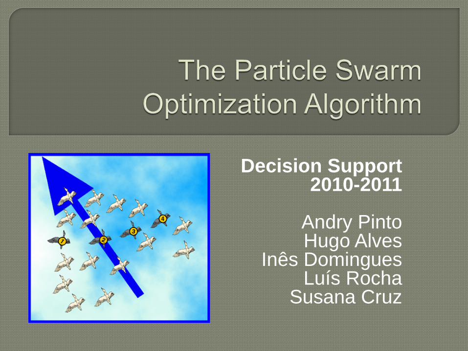
Application to optimization: Particle Swarm Optimization

Proposed by James Kennedy & Russell Eberhart (1995)

Combines self-experiences with social experiences

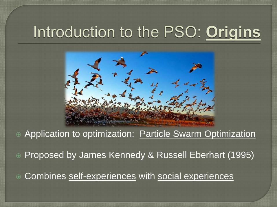
Uses a number of agents (particles)

that constitute a swarm moving

around in the search space looking for

the best solution

Each particle in search space adjusts

its “flying” according to its own flying

experience as well as the flying

experience of other particles

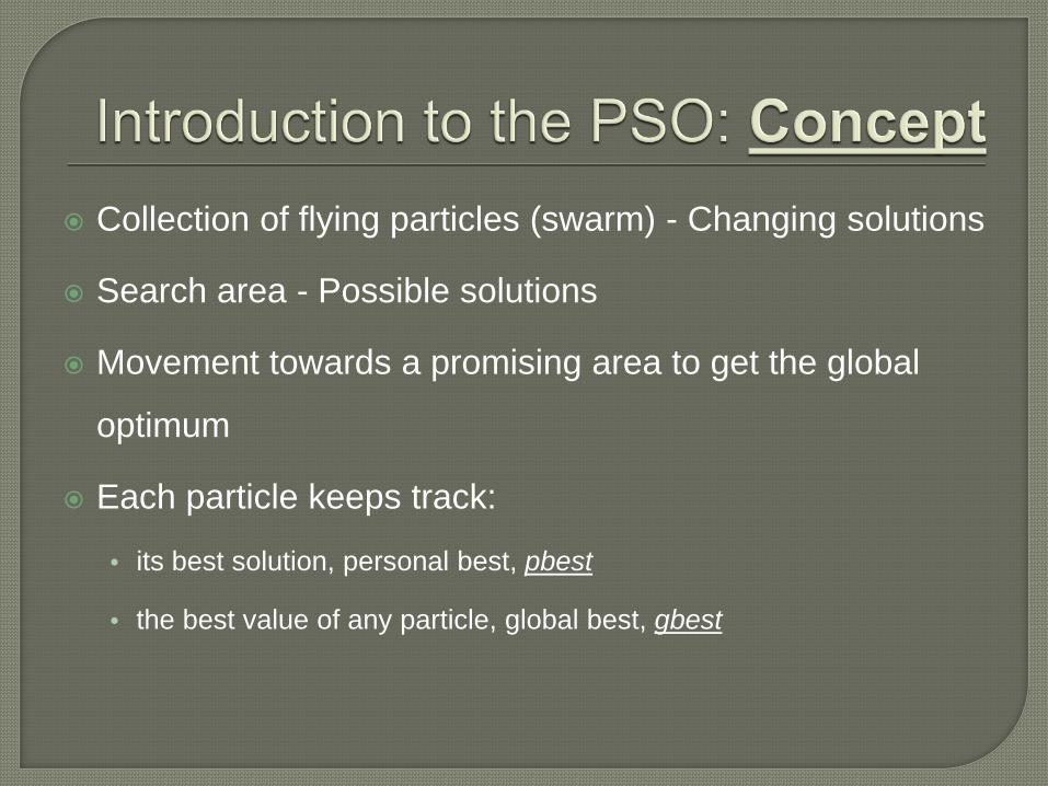
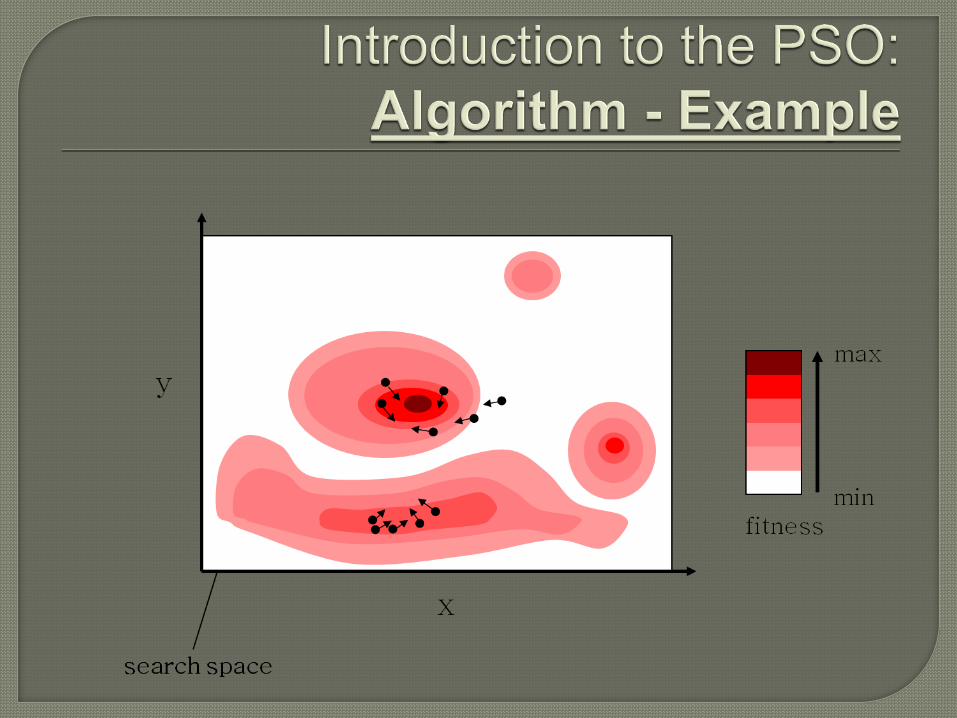
Collection of flying particles (swarm) - Changing solutions

Search area - Possible solutions

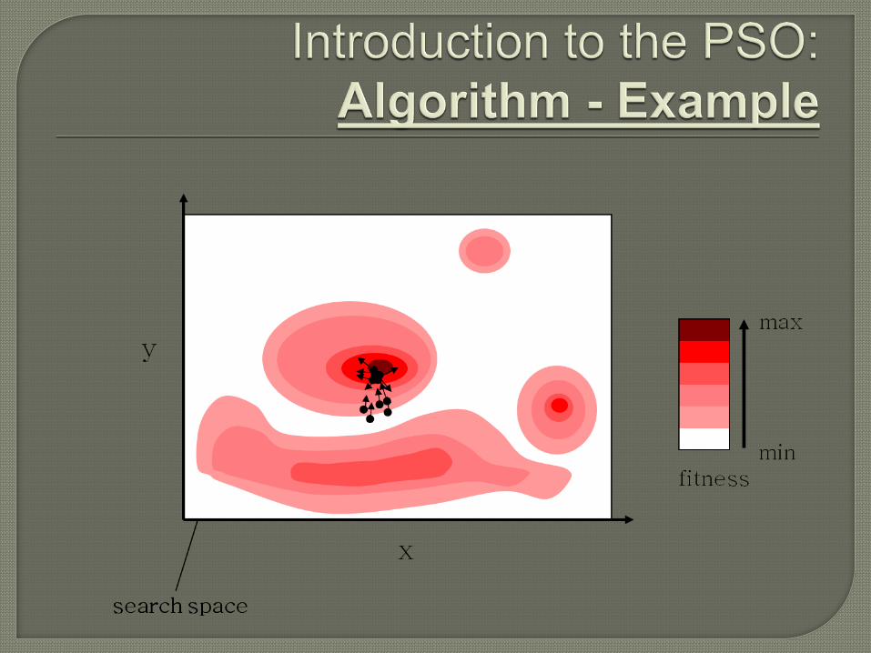
Movement towards a promising area to get the global

optimum

Each particle keeps track:

• its best solution, personal best, pbest

• the best value of any particle, global best, gbest

Each particle adjusts its travelling speed dynamically corresponding to the flying experiences of itself and its colleagues

Each particle modifies its

position according to:

• its current position

• its current velocity

• the distance between its

current position and pbest

• the distance between its

current position and gbest

geographical

social

global

Algorithm parameters

• A : Population of agents

• pi : Position of agent ai in the solution space

• f : Objective function

• vi : Velocity of agent’s ai

• V(ai) : Neighborhood of agent ai (fixed)

The neighborhood concept in PSO is not the same as the

one used in other meta-heuristics search, since in PSO

each particle’s neighborhood never changes (is fixed)

[x*] = PSO() P = Particle_Initialization(); For i=1 to it_max For each particle p in P do fp = f(p); If fp is better than f(pBest) pBest = p; end end gBest = best p in P; For each particle p in P do v = v + c1*rand*(pBest – p) + c2*rand*(gBest – p); p = p + v; end end

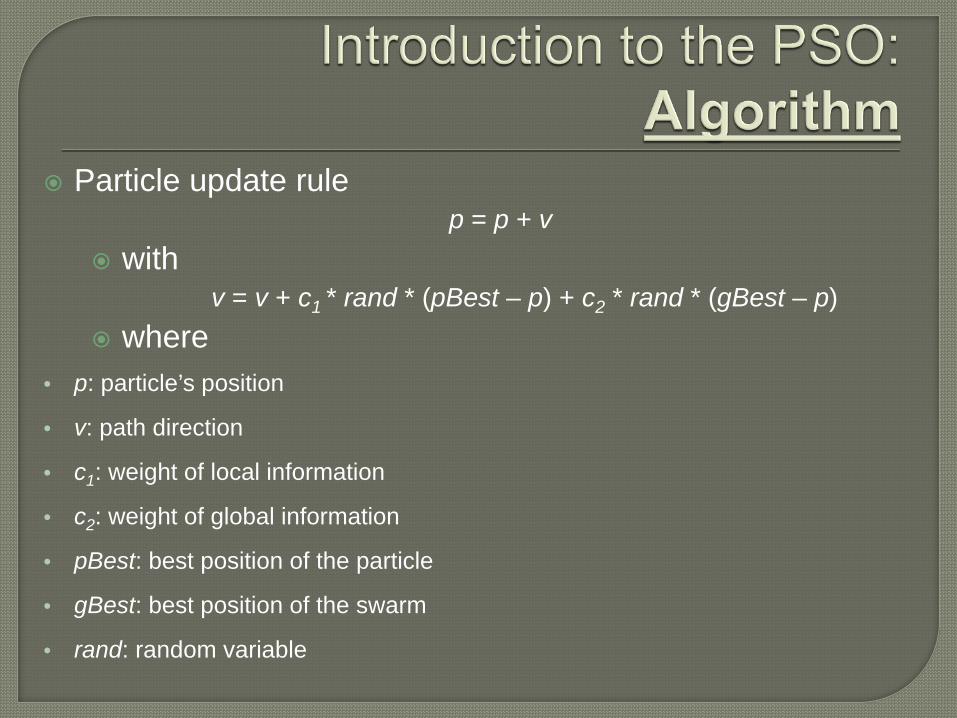
Particle update rule p = p + v

with v = v + c1 * rand * (pBest – p) + c2 * rand * (gBest – p)

where • p: particle’s position

• v: path direction

• c1: weight of local information

• c2: weight of global information

• pBest: best position of the particle

• gBest: best position of the swarm

• rand: random variable

Number of particles usually between 10 and 50

C1 is the importance of personal best value

C2 is the importance of neighborhood best value

Usually C1 + C2 = 4 (empirically chosen value)

If velocity is too low → algorithm too slow

If velocity is too high → algorithm too unstable

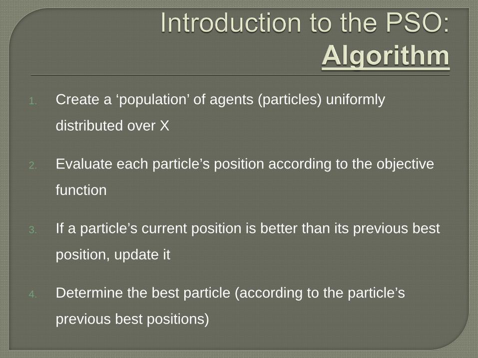
1. Create a ‘population’ of agents (particles) uniformly

distributed over X

2. Evaluate each particle’s position according to the objective

function

3. If a particle’s current position is better than its previous best

position, update it

4. Determine the best particle (according to the particle’s

previous best positions)

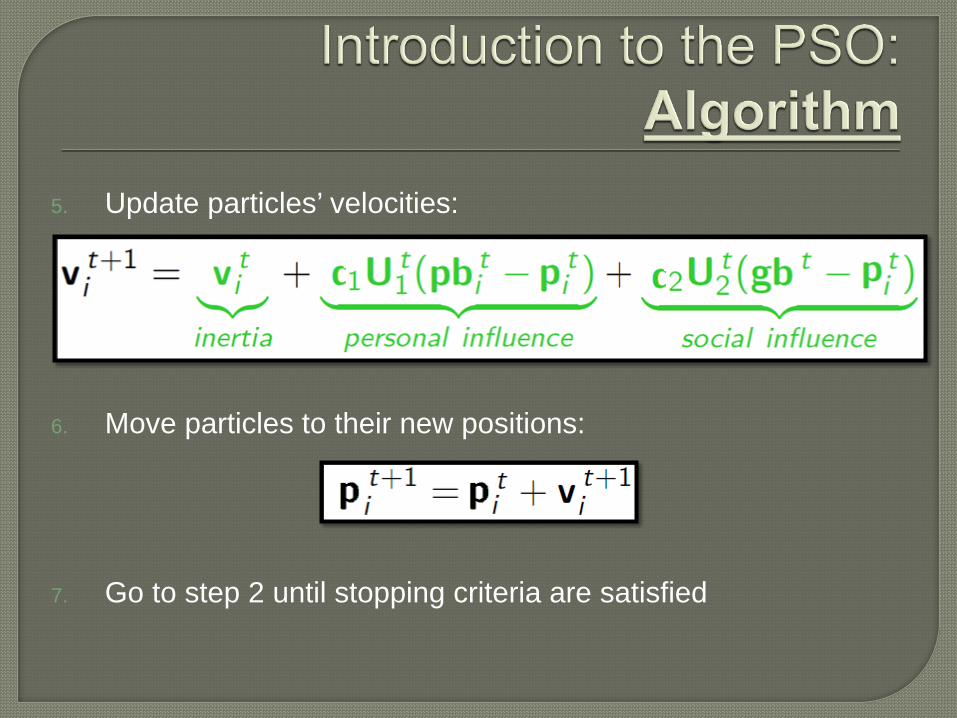
5. Update particles’ velocities:

6. Move particles to their new positions:

7. Go to step 2 until stopping criteria are satisfied

Particle’s velocity:

• Makes the particle move in the same direction and with the same velocity

1. Inertia

2. Personal Influence

3. Social Influence

• Improves the individual • Makes the particle return to a previous

position, better than the current • Conservative

• Makes the particle follow the best neighbors direction

Intensification: explores the previous solutions, finds the

best solution of a given region

Diversification: searches new solutions, finds the regions

with potentially the best solutions

In PSO:

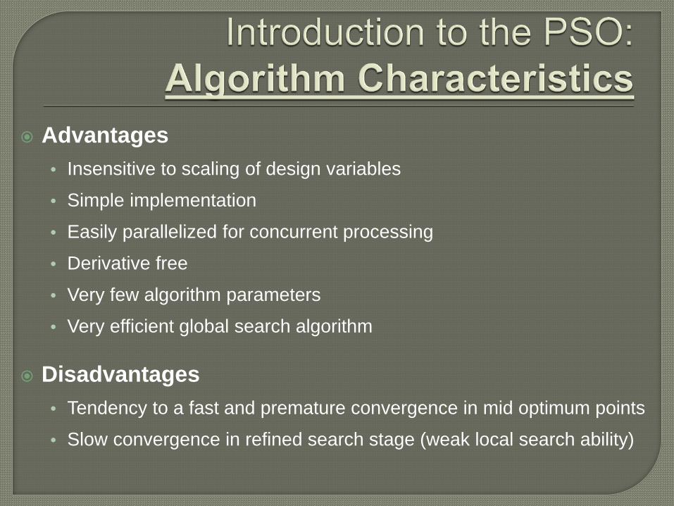
Advantages • Insensitive to scaling of design variables

• Simple implementation

• Easily parallelized for concurrent processing

• Derivative free

• Very few algorithm parameters

• Very efficient global search algorithm

Disadvantages • Tendency to a fast and premature convergence in mid optimum points

• Slow convergence in refined search stage (weak local search ability)

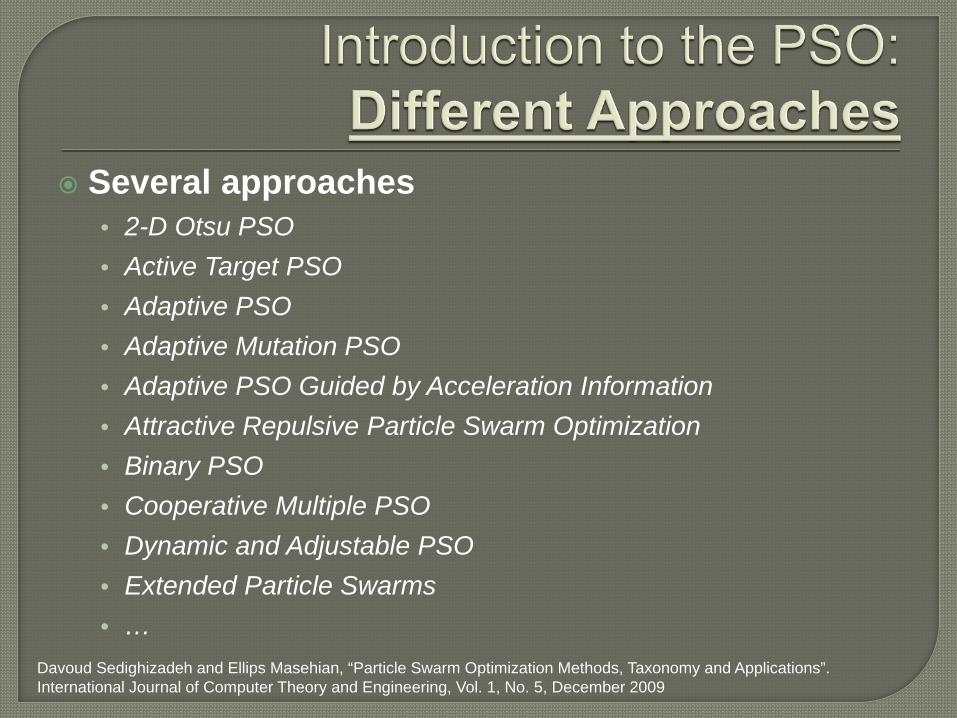
Several approaches • 2-D Otsu PSO • Active Target PSO • Adaptive PSO • Adaptive Mutation PSO • Adaptive PSO Guided by Acceleration Information • Attractive Repulsive Particle Swarm Optimization • Binary PSO • Cooperative Multiple PSO • Dynamic and Adjustable PSO • Extended Particle Swarms • …

Davoud Sedighizadeh and Ellips Masehian, “Particle Swarm Optimization Methods, Taxonomy and Applications”. International Journal of Computer Theory and Engineering, Vol. 1, No. 5, December 2009

On solving Multiobjective Bin Packing

Problem Using Particle Swarm Optimization

D.S Liu, K.C. Tan, C.K. Goh and W.K. Ho 2006 - IEEE Congress on Evolutionary Computation

First implementation of PSO for BPP

Multi-Objective 2D BPP

Maximum of I bins with width W and height H

J items with wj ≤ W, hj ≤ H and weight ψj

Objectives

• Minimize the number of bins used K

• Minimize the average deviation between the overall

centre of gravity and the desired one

Usually generated randomly In this work:

• Solution from Bottom Left Fill (BLF) heuristic

• To sort the rectangles for BLF:

Random

According to a criteria (width, weight, area, perimeter..)

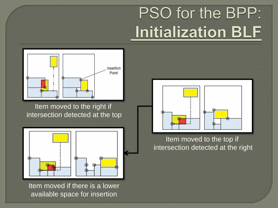
Item moved to the right if intersection detected at the top

Item moved to the top if intersection detected at the right

Item moved if there is a lower available space for insertion

Velocity depends on either pbest or gbest: never both at the same time

OR

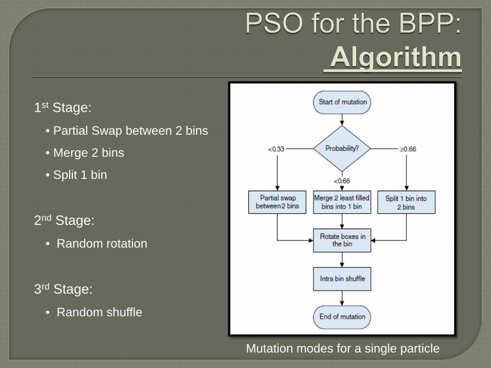
1st Stage:

• Partial Swap between 2 bins

• Merge 2 bins

• Split 1 bin

2nd Stage:

• Random rotation

3rd Stage:

• Random shuffle

Mutation modes for a single particle

The flowchart of HMOPSO

H hybrid

M multi

S swarm

O objective

P particle

O optimization

6 classes with 20 instances randomly generated

Size range:

• Class 1: [0, 100]

• Class 2: [0, 25]

• Class 3: [0, 50]

• Class 4: [0, 75]

• Class 5: [25, 75]

• Class 6: [25, 50]

Class 2: small items → more difficult to pack

Comparison with 2 other methods • MOPSO (Multiobjective PSO) from [1]

• MOEA (Multiobjective Evolutionary Algorithm) from [2]

Definition of parameters:

[1] Wang, K. P., Huang, L., Zhou C. G. and Pang, W., “Particle Swarm Optimization for Traveling Salesman Problem,” International Conference on Machine Learning and Cybernetics, vol. 3, pp. 1583-1585, 2003.

[2] Tan, K. C., Lee, T. H., Chew, Y. H., and Lee, L. H., “A hybrid multiobjective evolutionary algorithm for solving truck and trailer vehicle routing problems,” IEEE Congress on Evolutionary Computation, vol. 3, pp. 2134-2141, 2003.

Comparison on the performance of metaheuristic

algorithms against the branch and bound method (BB)

on single objective BPP

Results for each algorithm in 10 runs

Proposed method (HMOPSO) capable of evolving

more optimal solution as compared to BB in 5 out of 6

classes of test instances

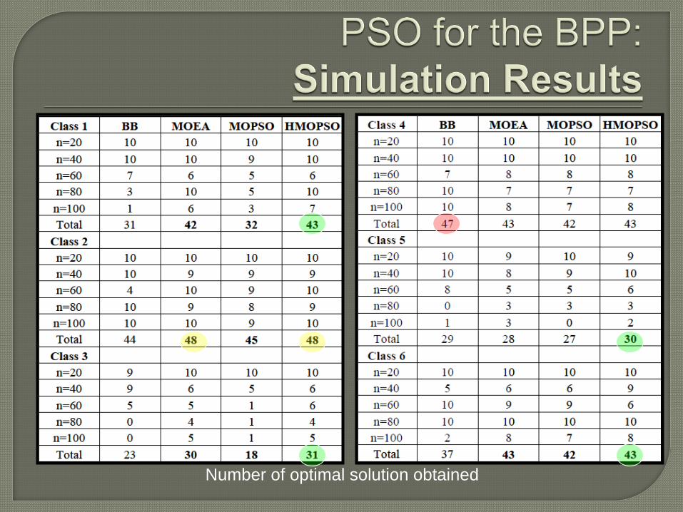
Number of optimal solution obtained

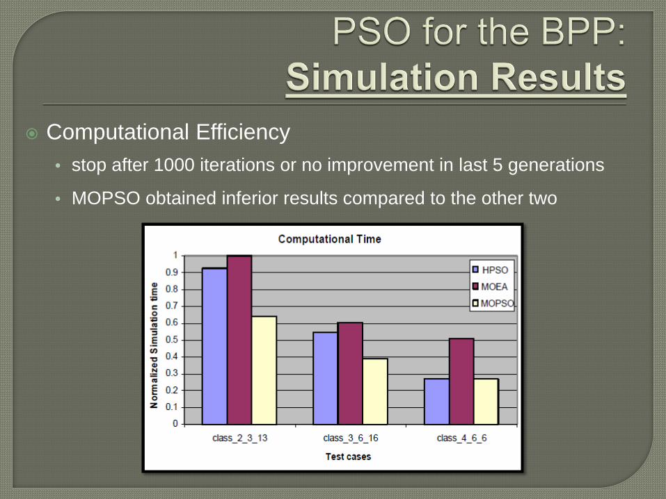
Computational Efficiency • stop after 1000 iterations or no improvement in last 5 generations

• MOPSO obtained inferior results compared to the other two

Presentation of a mathematical model for MOBPP-2D

MOBPP-2D solved by the proposed HMOPSO

BLF chosen as the decoding heuristic

HMOPSO is a robust search optimization algorithm

• Creation of variable length data structure

• Specialized mutation operator

HMOPSO performs consistently well with the best average

performance on the performance metric

Outperforms MOPSO and MOEA in most of the test cases

used in this paper