Tomislav Hengl and Robert A. MacMillan Predictive Soil Mapping with R 2019-03-17 OpenGeoHub foundation, Wageningen, Netherlands

Welcome message from author
This document is posted to help you gain knowledge. Please leave a comment to let me know what you think about it! Share it to your friends and learn new things together.
Transcript
Tomislav Hengl and Robert A. MacMillan
Predictive Soil Mapping with R
2019-03-17
OpenGeoHub foundation, Wageningen, Netherlands

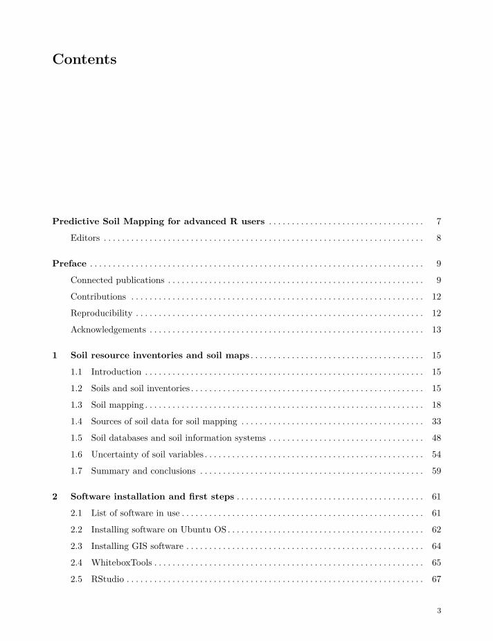
Contents
Predictive Soil Mapping for advanced R users . . . . . . . . . . . . . . . . . . . . . . . . . . . . . . . . . . 7
Editors . . . . . . . . . . . . . . . . . . . . . . . . . . . . . . . . . . . . . . . . . . . . . . . . . . . . . . . . . . . . . . . . . . . . . . 8
Preface . . . . . . . . . . . . . . . . . . . . . . . . . . . . . . . . . . . . . . . . . . . . . . . . . . . . . . . . . . . . . . . . . . . . . . . . . 9
Connected publications . . . . . . . . . . . . . . . . . . . . . . . . . . . . . . . . . . . . . . . . . . . . . . . . . . . . . . . . 9
Contributions . . . . . . . . . . . . . . . . . . . . . . . . . . . . . . . . . . . . . . . . . . . . . . . . . . . . . . . . . . . . . . . . 12
Reproducibility . . . . . . . . . . . . . . . . . . . . . . . . . . . . . . . . . . . . . . . . . . . . . . . . . . . . . . . . . . . . . . . 12
Acknowledgements . . . . . . . . . . . . . . . . . . . . . . . . . . . . . . . . . . . . . . . . . . . . . . . . . . . . . . . . . . . . 13
1 Soil resource inventories and soil maps . . . . . . . . . . . . . . . . . . . . . . . . . . . . . . . . . . . . . . 15
1.1 Introduction . . . . . . . . . . . . . . . . . . . . . . . . . . . . . . . . . . . . . . . . . . . . . . . . . . . . . . . . . . . . . 15
1.2 Soils and soil inventories . . . . . . . . . . . . . . . . . . . . . . . . . . . . . . . . . . . . . . . . . . . . . . . . . . . 15
1.3 Soil mapping . . . . . . . . . . . . . . . . . . . . . . . . . . . . . . . . . . . . . . . . . . . . . . . . . . . . . . . . . . . . . 18
1.4 Sources of soil data for soil mapping . . . . . . . . . . . . . . . . . . . . . . . . . . . . . . . . . . . . . . . . 33
1.5 Soil databases and soil information systems . . . . . . . . . . . . . . . . . . . . . . . . . . . . . . . . . . 48
1.6 Uncertainty of soil variables . . . . . . . . . . . . . . . . . . . . . . . . . . . . . . . . . . . . . . . . . . . . . . . . 54
1.7 Summary and conclusions . . . . . . . . . . . . . . . . . . . . . . . . . . . . . . . . . . . . . . . . . . . . . . . . . 59
2 Software installation and first steps . . . . . . . . . . . . . . . . . . . . . . . . . . . . . . . . . . . . . . . . . 61
2.1 List of software in use . . . . . . . . . . . . . . . . . . . . . . . . . . . . . . . . . . . . . . . . . . . . . . . . . . . . . 61
2.2 Installing software on Ubuntu OS. . . . . . . . . . . . . . . . . . . . . . . . . . . . . . . . . . . . . . . . . . . 62
2.3 Installing GIS software . . . . . . . . . . . . . . . . . . . . . . . . . . . . . . . . . . . . . . . . . . . . . . . . . . . . 64
2.4 WhiteboxTools . . . . . . . . . . . . . . . . . . . . . . . . . . . . . . . . . . . . . . . . . . . . . . . . . . . . . . . . . . . 65
2.5 RStudio . . . . . . . . . . . . . . . . . . . . . . . . . . . . . . . . . . . . . . . . . . . . . . . . . . . . . . . . . . . . . . . . . 67
3
4 Contents
2.6 plotKML and GSIF packages . . . . . . . . . . . . . . . . . . . . . . . . . . . . . . . . . . . . . . . . . . . . . . 69
2.7 Connecting R and SAGA GIS . . . . . . . . . . . . . . . . . . . . . . . . . . . . . . . . . . . . . . . . . . . . . . 71
2.8 Connecting R and GDAL . . . . . . . . . . . . . . . . . . . . . . . . . . . . . . . . . . . . . . . . . . . . . . . . . . 73
3 Soil observations and variables . . . . . . . . . . . . . . . . . . . . . . . . . . . . . . . . . . . . . . . . . . . . . . 75
3.1 Basic concepts . . . . . . . . . . . . . . . . . . . . . . . . . . . . . . . . . . . . . . . . . . . . . . . . . . . . . . . . . . . 75
3.2 Descriptive soil profile observations . . . . . . . . . . . . . . . . . . . . . . . . . . . . . . . . . . . . . . . . . 83
3.3 Chemical soil properties . . . . . . . . . . . . . . . . . . . . . . . . . . . . . . . . . . . . . . . . . . . . . . . . . . . 89
3.4 Physical and hydrological soil properties . . . . . . . . . . . . . . . . . . . . . . . . . . . . . . . . . . . . . 95
3.5 Harmonization of soil data and pedo-transfer functions . . . . . . . . . . . . . . . . . . . . . . . . 111
3.6 Soil class data . . . . . . . . . . . . . . . . . . . . . . . . . . . . . . . . . . . . . . . . . . . . . . . . . . . . . . . . . . . . 113
3.7 Importing and formatting soil data in R . . . . . . . . . . . . . . . . . . . . . . . . . . . . . . . . . . . . . 117
3.8 Using Machine Learning to build Pedo-Transfer-Functions . . . . . . . . . . . . . . . . . . . . . 127
3.9 Summary points . . . . . . . . . . . . . . . . . . . . . . . . . . . . . . . . . . . . . . . . . . . . . . . . . . . . . . . . . . 132
4 Preparation of soil covariates for soil mapping . . . . . . . . . . . . . . . . . . . . . . . . . . . . . . 135
4.1 Soil covariate data sources . . . . . . . . . . . . . . . . . . . . . . . . . . . . . . . . . . . . . . . . . . . . . . . . . 135
4.2 Preparing soil covariate layers . . . . . . . . . . . . . . . . . . . . . . . . . . . . . . . . . . . . . . . . . . . . . . 140
4.3 Summary points . . . . . . . . . . . . . . . . . . . . . . . . . . . . . . . . . . . . . . . . . . . . . . . . . . . . . . . . . . 157
5 Statistical theory for predictive soil mapping . . . . . . . . . . . . . . . . . . . . . . . . . . . . . . . 159
5.1 Aspects of spatial variability of soil variables . . . . . . . . . . . . . . . . . . . . . . . . . . . . . . . . . 159
5.2 Spatial prediction of soil variables . . . . . . . . . . . . . . . . . . . . . . . . . . . . . . . . . . . . . . . . . . 167
5.3 Accuracy assessment and the mapping efficiency . . . . . . . . . . . . . . . . . . . . . . . . . . . . . . 209
6 Machine Learning Algorithms for soil mapping . . . . . . . . . . . . . . . . . . . . . . . . . . . . . 227
6.1 Spatial prediction of soil properties and classes using MLA’s . . . . . . . . . . . . . . . . . . . 227
6.2 A generic framework for spatial prediction using Random Forest . . . . . . . . . . . . . . . . 254
6.3 Summary points . . . . . . . . . . . . . . . . . . . . . . . . . . . . . . . . . . . . . . . . . . . . . . . . . . . . . . . . . . 273
7 Spatial prediction and assessment of Soil Organic Carbon . . . . . . . . . . . . . . . . . . . 275
7.1 Introduction . . . . . . . . . . . . . . . . . . . . . . . . . . . . . . . . . . . . . . . . . . . . . . . . . . . . . . . . . . . . . 275
7.2 Measurement and derivation of soil organic carbon . . . . . . . . . . . . . . . . . . . . . . . . . . . . 275
7.3 Derivation of OCS and OCD using soil profile data . . . . . . . . . . . . . . . . . . . . . . . . . . . 278
7.4 Estimation of Bulk Density using a globally-calibrated PTF. . . . . . . . . . . . . . . . . . . . 285
Contents 5
7.5 Generating maps of OCS . . . . . . . . . . . . . . . . . . . . . . . . . . . . . . . . . . . . . . . . . . . . . . . . . . 288
7.6 Predicting OCS from point data (the 2D approach) . . . . . . . . . . . . . . . . . . . . . . . . . . . 290
7.7 Deriving OCS from soil profile data (the 3D approach) . . . . . . . . . . . . . . . . . . . . . . . . 296
7.8 Deriving OCS using spatiotemporal models . . . . . . . . . . . . . . . . . . . . . . . . . . . . . . . . . . 303
7.9 Summary points . . . . . . . . . . . . . . . . . . . . . . . . . . . . . . . . . . . . . . . . . . . . . . . . . . . . . . . . . . 308
8 Practical tips for organizing Predictive Soil Mapping . . . . . . . . . . . . . . . . . . . . . . . 311
8.1 Critical aspects of Predictive Soil Mapping . . . . . . . . . . . . . . . . . . . . . . . . . . . . . . . . . . 311
8.2 Technical specifications affecting the majority of production costs . . . . . . . . . . . . . . . 315
8.3 Final delivery of maps . . . . . . . . . . . . . . . . . . . . . . . . . . . . . . . . . . . . . . . . . . . . . . . . . . . . 323
8.4 Summary notes . . . . . . . . . . . . . . . . . . . . . . . . . . . . . . . . . . . . . . . . . . . . . . . . . . . . . . . . . . 327
9 The future of predictive soil mapping . . . . . . . . . . . . . . . . . . . . . . . . . . . . . . . . . . . . . . . 329
9.1 Introduction . . . . . . . . . . . . . . . . . . . . . . . . . . . . . . . . . . . . . . . . . . . . . . . . . . . . . . . . . . . . . 329
9.2 Past conventional terrestrial resource inventories . . . . . . . . . . . . . . . . . . . . . . . . . . . . . . 330
9.3 The future of PSM: Embracing scientific and technical advances . . . . . . . . . . . . . . . . 332
9.4 The future of PSM: Embracing new organizational and governance models . . . . . . . 346
References . . . . . . . . . . . . . . . . . . . . . . . . . . . . . . . . . . . . . . . . . . . . . . . . . . . . . . . . . . . . . . . . . . . . . . 357

Predictive Soil Mapping for advanced R users
This is the online version of the Open Access book: Predictive Soil Mapping with R1. Pullrequests and general comments are welcome. These materials are based on technical tutorialsinitially developed by the ISRIC’s2 Global Soil Information Facilities (GSIF) development teamover the period 2014–2017.
This book is continuously updated. For news and updates please refer to the github issues3.
Hard copies of this book can be ordered from www.lulu.com4. By purchasing a hard copy of thisbook from Lulu you donate $12 to the OpenGeoHub foundation.
Cite this as:
• Hengl, T., MacMillan, R.A., (2019). Predictive Soil Mapping with R. OpenGeoHub founda-tion, Wageningen, the Netherlands, 370 pages, www.soilmapper.org, ISBN: 978-0-359-30635-0.
1 https://envirometrix.github.io/PredictiveSoilMapping/2 http://isric.org/3 https://github.com/envirometrix/PredictiveSoilMapping/issues4 http://www.lulu.com/spotlight/t_hengl
7
8 Contents
Editors
Tom Hengl5 is a Senior Researcher and Vice Chair of the OpenGeoHub Foundation / technicaldirector at Envirometrix Ltd. Tom has more than 20 years of experience as an environmentalmodeler, data scientist and spatial analyst. He is a passionate advocate for, and supporter of,open data, reproducible science and career development for young scientists. He designed andimplemented the global SoilGrids6 data set, partially in response to other well known open dataprojects such as OpenStreetMap, GBIF, GlobalForestWatch and global climate mapping projects.He has taught predictive soil mapping at Wageningen University / ISRIC within the “Hands-on-GSIF” block courses. Video tutorials on predictive soil mapping with R can also be foundat http://youtube.com/c/ISRICorg and https://www.youtube.com/c/OpenGeoHubFoundation.Tom currently leads the production of a web mapping system called “LandGIS” (https://landgis.opengeohub.org) which is envisaged as “an OpenStreetMap-type system” for land-related environ-mental data. The system hosts global, fine spatial resolution data (250 m to 1 km) including varioussoil classes and soil properties, which is intended for eventual integration and use at operationalor farm-scales.
Bob MacMillan7 is a retired environmental consultant with over 40 years of experience in cre-ating, packaging, delivering and using environmental information on soils, ecosystems, landformsand hydrology. Bob spent 19 years working in public sector research with the Alberta ResearchCouncil and Agriculture and Agri-Food Canada and a second 20 years as a private sector consul-tant offering services in predictive soil and ecological mapping. Since retiring, Bob has remainedan active supporter, promoter, advocate, mentor and technical contributor to several continentalto global scale efforts to advance the science and technology of mapping soils and other ecosystemcomponents. As Science Coordinator for the GlobalSoilMap project, Bob helped to articulate thevision for the project and led initial activities aimed at achieving this, including authoring technicalspecifications, promoting the project, recruiting participants/cooperators, and liaising with repre-sentatives of national and international soil agencies. Bob continues to contribute on a voluntarybasis to OpenGeoHub and the Africa Soil Information Servicce (AfSIS) (http://africasoils.net).Throughout his career, Bob has shared his expertise and his enthusiasm freely with dozens ofyounger scientists interested in learning about, and becoming, practitioners of digital soil map-ping. Bob continues to support the next generation of digital soil mappers through his involvementwith OpenGeoHub.
5 https://opengeohub.org/people/tom-hengl6 http://journals.plos.org/plosone/article?id=10.1371/journal.pone.01697487 https://opengeohub.org/people/bob-macmillan
Preface
Predictive Soil Mapping (PSM) is based on applying statistical and/or machine learning tech-niques to fit models for the purpose of producing spatial and/or spatiotemporal predictions ofsoil variables, i.e. maps of soil properties and classes at different resolutions. It is a multidisci-plinary field combining statistics, data science, soil science, physical geography, remote sensing,geoinformation science and a number of other sciences (Scull et al, 2003; McBratney et al, 2003;Henderson et al, 2004; Boettinger et al, 2010; Zhu et al, 2015). Predictive Soil Mapping with Ris about understanding the main concepts behind soil mapping, mastering R packages that canbe used to produce high quality soil maps, and about optimizing all processes involved so thatproduction costs can also be reduced.
The main differences between predictive vs traditional expert-based soil mapping are that: (a)the production of maps is based on using state-of-the-art statistical methods to ensure objectivityof maps (including objective uncertainty assessment vs expert judgment), and (b) PSM is drivenby automation of the processes so that overall soil data production costs can be reduced andupdates of maps implemented without requirements for large investments. R, in that sense, is alogical platform to develop PSM workflows and applications, especially thanks to the vibrant andproductive R spatial interest group activities and also thanks to the increasingly professional soildata packages such as, for example: soiltexture, aqp, soilprofile, soilDB and similar.
The book is divided into sections covering theoretical concepts, preparation of covariates, modelselection and evaluation, prediction and final practical tips for operational PSM. Most of thechapters contain R code examples that try to illustrate the main processing steps and give practicalinstructions to developers and applied users.
Connected publications
Most of methods described in this book are based on the following publications:
9
10 Contents
• Hengl, T., Nussbaum, M., Wright, M. N., Heuvelink, G. B., and Gräler, B. (2018) RandomForest as a generic framework for predictive modeling of spatial and spatio-temporal variables8.PeerJ 6:e5518.
• Sanderman, J., Hengl, T., Fiske, G., (2017) The soil carbon debt of 12,000 years of human landuse9. PNAS, doi:10.1073/pnas.1706103114
• Ramcharan, A., Hengl, T., Nauman, T., Brungard, C., Waltman, S., Wills, S., & Thompson, J.(2018). Soil Property and Class Maps of the Conterminous United States at 100-Meter SpatialResolution10. Soil Science Society of America Journal, 82(1), 186–201.
• Hengl, T., Leenaars, J. G., Shepherd, K. D., Walsh, M. G., Heuvelink, G. B., Mamo, T., etal. (2017) Soil nutrient maps of Sub-Saharan Africa: assessment of soil nutrient content at 250m spatial resolution using machine learning11. Nutrient Cycling in Agroecosystems, 109(1),77–102.
• Hengl T, Mendes de Jesus J, Heuvelink GBM, Ruiperez Gonzalez M, Kilibarda M, BlagoticA, et al. (2017) SoilGrids250m: Global gridded soil information based on machine learning12.PLoS ONE 12(2): e0169748. doi:10.1371/journal.pone.0169748
• Shangguan, W., Hengl, T., de Jesus, J. M., Yuan, H., & Dai, Y. (2017). Mapping the globaldepth to bedrock for land surface modeling13. Journal of Advances in Modeling Earth Systems,9(1), 65-88.
• Hengl, T., Roudier, P., Beaudette, D., & Pebesma, E. (2015) plotKML: scientific visualizationof spatio-temporal data14. Journal of Statistical Software, 63(5).
• Gasch, C. K., Hengl, T., Gräler, B., Meyer, H., Magney, T. S., & Brown, D. J. (2015) Spatio-temporal interpolation of soil water, temperature, and electrical conductivity in 3D+ T: TheCook Agronomy Farm data set15. Spatial Statistics, 14, 70–90.
• Hengl, T., Nikolic, M., & MacMillan, R. A. (2013) Mapping efficiency and information content16.International Journal of Applied Earth Observation and Geoinformation, 22, 127–138.
• Hengl, T., Heuvelink, G. B., & Rossiter, D. G. (2007) About regression-kriging: from equationsto case studies17. Computers & geosciences, 33(10), 1301-1315.
• Hengl, T. (2006) Finding the right pixel size18. Computers & geosciences, 32(9), 1283–1298.
Some other relevant publications / books on the subject of Predictive Soil Mapping and DataScience in general include:8 https://doi.org/10.7717/peerj.55189 http://www.pnas.org/content/early/2017/08/15/1706103114.full10 https://dl.sciencesocieties.org/publications/sssaj/abstracts/82/1/18611 https://link.springer.com/article/10.1007/s10705-017-9870-x12 http://dx.doi.org/10.1371/journal.pone.016974813 https://doi.org/10.1002/2016MS00068614 https://www.jstatsoft.org/article/view/v063i0515 https://doi.org/10.1016/j.spasta.2015.04.00116 https://doi.org/10.1016/j.jag.2012.02.00517 https://doi.org/10.1016/j.cageo.2007.05.00118 https://doi.org/10.1016/j.cageo.2005.11.008
Contents 11
• Malone, B.P, Minasny, B., McBratney, A.B., (2016) Using R for Digital Soil Mapping19.Progress in Soil Science ISBN: 9783319443270, 262 pages.
• Hengl, T., & MacMillan, R. A. (2009). Geomorphometry—a key to landscape mappingand modelling20. Developments in Soil Science, 33, 433–460.
• California Soil Resource Lab, (2017) Open Source Software Tools for Soil Scientists21,UC Davis.
• McBratney, A.B., Minasny, B., Stockmann, U. (Eds) (2018) Pedometrics22. Progress in SoilScience ISBN: 9783319634395, 720 pages.
• FAO, (2018) Soil Organic Carbon Mapping Cookbook23. 2nd edt. ISBN: 9789251304402
Readers are also encouraged to obtain and study the following R books before following some ofthe more complex exercises in this book:
• Bivand, R., Pebesma, E., Rubio, V., (2013) Applied Spatial Data Analysis with R24. UseR Series, Springer, Heidelberg, 2nd Ed. 400 pages.
• Irizarry, R.A., (2018) Introduction to Data Science: Data Analysis and PredictionAlgorithms with R25. HarvardX Data Science Series.
• Kabacoff, R.I., (2011) R in Action: Data Analysis and Graphics with R26. Manningpublications, ISBN: 9781935182399, 472 pages.
• Kuhn, M., Johnson, K. (2013) Applied Predictive Modeling27. Springer Science, ISBN:9781461468493, 600 pages.
• Molnar, C. (2019) Interpretable Machine Learning: A Guide for Making Black BoxModels Explainable28, Leanpub, 251 pages.
• Lovelace, R., Nowosad, J., Muenchow, J., (2018) Geocomputation with R29. R Series, CRCPress, ISBN: 9781138304512, 338 pages.
• Reimann, C., Filzmoser, P., Garrett, R., Dutter, R., (2008) Statistical Data Analysis Ex-plained Applied Environmental Statistics with R30. Wiley, Chichester, 337 pages.
• Wilke, C.O., (2019) Fundamentals of Data Visualization31. O’Reilly, in press.19 https://www.springer.com/gp/book/978331944325620 https://doi.org/10.1016/S0166-2481(08)00019-621 https://casoilresource.lawr.ucdavis.edu/software/22 https://www.springer.com/gp/book/978331963437123 https://github.com/FAO-GSP/SOC-Mapping-Cookbook24 http://www.asdar-book.org25 https://rafalab.github.io/dsbook/26 http://www.manning.com/kabacoff/27 http://appliedpredictivemodeling.com28 https://christophm.github.io/interpretable-ml-book/29 https://geocompr.robinlovelace.net30 https://onlinelibrary.wiley.com/doi/book/10.1002/978047098760531 https://serialmentor.com/dataviz/
12 Contents
• Wikle, C.K., Zammit-Mangion, A., and Cressie, N. (2019). Spatio-Temporal Statistics withR32. Chapman & Hall/CRC, Boca Raton, FL.
For the most recent developments in the R-spatial community refer to https://r-spatial.github.io,the R-sig-geo mailing list and/or https://opengeohub.org.
Contributions
This book is designed to be constantly updated and contributions are always welcome (throughpull requests, but also through adding new chapters) provided that some minimum requirementsare met. To contribute a new chapter please contact the editors first. Some minimum requirementsto contribute a chapter are:
1. The data needs to be available for the majority of tutorials presented in a chapter. It is best ifthis is via some R package or web-source.
2. A chapter should ideally focus on implementing some computing in R (it should be written asan R tutorial).
3. All examples should be computationally efficient requiring not more than 30 secs of computingtime per process on a single core system.
4. The theoretical basis for methods and interpretation of results should be based on peer-reviewpublications. This book is not intended to report on primary research / experimental results,but only to supplement existing research publications.
5. A chapter should consist of at least 1500 words and at most 3500 words.6. The topic of the chapter must be closely connected to the theme of soil mapping, soil geograph-
ical databases, methods for processing spatial soil data and similar.
In principle, all submitted chapters should follow closely also the five pillars of Wikipedia33,especially: Verifiability, Reproducibility, No original research, Neutral point of view, Good faith,No conflict of interest, and No personal attacks.
Reproducibility
To reproduce the book, you need a recent version of R34, and RStudio35 and up-to-date packages,which can be installed with the following command (which requires devtools36):
32 https://spacetimewithr.org33 https://en.wikipedia.org/wiki/Wikipedia:Five_pillars34 https://cran.r-project.org35 http://www.rstudio.com/products/RStudio/36 https://github.com/hadley/devtools
Contents 13
devtools::install_github("Envirometrix/PSMpkg")
To build the book locally, clone or download37 the PredictiveSoilMapping repo38, load R in rootdirectory (e.g. by opening PredictiveSoilMapping.Rproj39 in RStudio) and run the following lines:
bookdown::render_book("index.Rmd") # to build the bookbrowseURL("docs/index.html") # to view it
Acknowledgements
The authors are grateful for numerous contributions from colleagues around the world, especiallyfor contributions by current and former ISRIC — World Soil Information colleagues and guestresearchers: Gerard Heuvelink, Johan Leenaars, Jorge Mendes de Jesus, Wei Shangguan, DavidG. Rossiter, and many others. The authors are also grateful to Dutch and European citizensfor financing ISRIC and Wageningen University, where work on this book was initially started.The authors acknowledge support received from the AfSIS project40, which was funded by theBill and Melinda Gates Foundation (BMGF) and the Alliance for a Green Revolution in Africa(AGRA). Many soil data processing examples in the book are based on R code developed by Dy-lan Beuadette, Pierre Roudier, Alessandro Samuel Rosa, Marcos E. Angelini, Guillermo FedericoOlmedo, Julian Moeys, Brendan Malone, and many other developers. The authors are also gratefulto comments and suggestions for improvements to the methods presented in the book by TravisNauman, Amanda Ramcharan, David G. Rossiter and Julian Moeys41.
LandGIS and SoilGrids are based on using numerous soil profile data sets kindly made availableby various national and international agencies: the USA National Cooperative Soil Survey SoilCharacterization database (http://ncsslabdatamart.sc.egov.usda.gov) and profiles from the USANational Soil Information System, Land Use/Land Cover Area Frame Survey (LUCAS) TopsoilSurvey database (Tóth et al, 2013), Repositório Brasileiro Livre para Dados Abertos do Solo(FEBR42), Sistema de Información de Suelos de Latinoamérica y el Caribe (SISLAC), AfricaSoil Profiles database (Leenaars, 2014), Australian National Soil Information by CSIRO Land andWater (Karssies, 2011; Searle, 2014), Mexican National soil profile database (Instituto Nacional deEstadística y Geografía (INEGI), 2000) provided by the Mexican Instituto Nacional de Estadísticay Geografía / CONABIO, Brazilian national soil profile database (Cooper et al, 2005) providedby the University of São Paulo, Chinese National Soil Profile database (Shangguan et al, 2013)provided by the Institute of Soil Science, Chinese Academy of Sciences, soil profile archive fromthe Canadian Soil Information System (MacDonald and Valentine, 1992) and Forest Ecosystem37 https://github.com/envirometrix/PredictiveSoilMapping/archive/master.zip38 https://github.com/envirometrix/PredictiveSoilMapping/39 https://github.com/envirometrix/PredictiveSoilMapping/blob/master/PredictiveSoilMapping.Rproj40 http://africasoils.net41 http://julienmoeys.info42 https://github.com/febr-team

14 Contents
Carbon Database (FECD), ISRIC-WISE (Batjes, 2009), The Northern Circumpolar Soil CarbonDatabase (Hugelius et al, 2013), eSOTER profiles (Van Engelen and Dijkshoorn, 2012), SPADE(Hollis et al, 2006), Unified State Register of soil resources RUSSIA (Version 1.0. Moscow —2014), National Database of Iran provided by the Tehran University, points from the Dutch SoilInformation System (BIS) prepared by Wageningen Environmental Research, and others. We arealso grateful to USA’s NASA, USGS and USDA agencies, European Space Agency Copernicusprojects, JAXA (Japan Aerospace Exploration Agency) for distributing vast amounts of remotesensing data (especially MODIS, Landsat, Copernicus land products and elevation data), andto the Open Source software developers of the packages rgdal, sp, raster, caret, mlr, ranger,SuperLearner, h2o and similar, and without which predictive soil mapping would most likely notbe possible.
This book has been inspired by the Geocomputation with R book43, an Open Access book editedby Robin Lovelace, Jakub Nowosad and Jannes Muenchow. Many thanks to Robin Lovelace forhelping with rmarkdown and for giving some initial tips for compiling and organizing this book.The authors are also grateful to the numerous software/package developers, especially EdzerPebesma, Roger Bivand, Robert Hijmans, Markus Neteler, Tim Appelhans, and Hadley Wickham,whose contributions have enabled a generation of researchers and applied projects.
We are especially grateful to Jakub Nowosad44 for helping with preparing this publication forpress and with setting up all code so that it passes automatic checks.
OpenGeoHub is a not-for-profit research foundation with headquarters in Wageningen, the Nether-lands (Stichting OpenGeoHub, KvK 71844570). The main goal of the OpenGeoHub is to promotepublishing and sharing of Open Geographical and Geoscientific Data and using and developingof Open Source Software. We believe that the key measure of quality of research in all sciences(and especially in geographical information sciences) is in transparency and reproducibility ofthe computer code used to generate results. Transparency and reproducibility increase trust ininformation so that it is eventually also the fastest path to optimal decision making.
Every effort has been made to trace copyright holders of the materials used in this publication.Should we, despite all our efforts, have overlooked contributors please contact the author and weshall correct this unintentional omission without any delay and will acknowledge any overlookedcontributions and contributors in future updates.
Data availability and Code license: All data used in this book is either available through Rpackages or is available via the github repository. If not mentioned otherwise, all code presentedis available under the GNU General Public License v2.045.
Copyright: © 2019 Authors.
This work is licensed under a Creative Commons Attribution-ShareAlike 4.0 International License.LandGIS and OpenGeoHub are registered trademarks of the OpenGeoHub Foundation (https://opengeohub.org).
43 https://geocompr.robinlovelace.net44 https://nowosad.github.io/45 https://www.gnu.org/licenses/old-licenses/gpl-2.0.en.html
Chapter 1
Soil resource inventories and soil maps
Edited by: Hengl T. & MacMillan R.A.
1.1 Introduction
This chapter presents a description and discussion of soils and conventional soil inventories framedwithin the context of Predictive Soil Mapping (PSM). Soils, their associated properties, and theirspatial and temporal distributions are the central focus of PSM. We discuss how the products andmethods associated with conventional soil mapping relate to new, and emerging, methods of PSMand automated soil mapping. We discuss similarities and differences, strengths and weaknesses ofconventional soil mapping (and its inputs and products) relative to PSM.
The universal model of soil variation presented further in detail in chapter 5 is adopted as aframework for comparison of conventional soil mapping and PSM. Our aim is to show how theproducts and methods of conventional soil mapping can complement, and contribute to, PSMand equally, how the theories and methods of PSM can extend and strengthen conventional soilmapping. PSM aims to implement tools and methods that can be supportive of growth, change andimprovement in soil mapping and that can stimulate a rebirth and reinvigoration of soil inventoryactivity globally.
1.2 Soils and soil inventories
1.2.1 Soil: a definition
Soil is a natural body composed of biota and air, water and minerals, developed from un-consolidated or semi-consolidated material that forms the topmost layer of the Earth’s surface(Chesworth, 2008). The upper limit of the soil is either air, shallow water, live plants or plantmaterials that have not begun to decompose. The lower limit is defined by the presence of hard
15
16 1 Soil resource inventories and soil maps
rock or the lower limit of biologic activity (Richter and Markewitz, 1995; Soil survey Divisionstaff, 1993). Although soil profiles up to tens of meters in depth can be found in some tropicalareas (Richter and Markewitz, 1995), for soil classification and mapping purposes, the lower limitof soil is often arbitrarily set to 2 m (http://soils.usda.gov/education/facts/soil.html). Soils arerarely described to depths beyond 2 m and many soil sampling projects put a primary focus onthe upper (0–100 cm) depths.
The chemical, physical and biological properties of the soil differ from those of unaltered (uncon-solidated) parent material, from which the soil is derived over a period of time under the influenceof climate, organisms and relief effects. Soil should show a capacity to support life, otherwise weare dealing with inert unconsolidated parent material. Hence, for purposes of developing statisticalmodels to predict soil properties using PSM, it proves useful to distinguish between actual andpotential soil areas (see further section 1.4.4).
A significant aspect of the accepted definition of soil is that it is seen as a natural body thatmerits study, description, classification and interpretation in, and of, itself. As a natural body soilis viewed as an object that occupies space, has defined physical dimensions and that is more thanthe sum of its individual properties or attributes. This concept requires that all properties of soilsbe considered collectively and simultaneously in terms of a completely integrated natural body(Soil survey Division staff, 1993). A consequence of this, is that one must generally assume thatall soil properties covary in space in lockstep with specific named soils and that different soilproperties do not exhibit different patterns of spatial variation independently.
From a management point of view, soil can be seen from at least three perspectives. It is a:
• Resource of materials — It contains quantities of unconsolidated materials, rock fragments,texture fractions, organic carbon, nutrients, minerals and metals, water and so on.
• Stabilizing medium / ecosystem — It acts as a medium that supports both global and localprocesses from carbon and nitrogen fixation to retention and transmission of water, to provisionof nutrients and minerals and so on.
• Production system — Soil is the foundation for plant growth. In fact, it is the basis of allsustainable terrestrial ecosystem services. It is also a source of livelihood for people that growcrops and livestock.
According to Frossard et al (2006) there are six key functions of soil:
1. food and other biomass production,
2. storage, filtering, and transformation of water, gases and minerals,
3. biological habitat and gene pool,
4. source of raw materials,
5. physical and cultural heritage and
6. platform for man-made structures: buildings, highways.
Soil is the Earth’s biggest carbon store containing 82% of total terrestrial organic carbon (Lal,2004).

1.2 Soils and soil inventories 17
1.2.2 Soil variables
Knowledge about soil is often assembled and catalogued through soil resource inventories. Con-ventional soil resource inventories describe the geographic distribution of soil bodies i.e. polypedons(Wysocki et al, 2005). The spatial distribution of soil properties is typically recorded and describedthrough reference to mapped soil individuals and not through separate mapping of individual soilproperties. In fact, the definition of a soil map in the US Soil Survey Manual specifically “excludesmaps showing the distribution of a single soil property such as texture, slope, or depth, alone orin limited combinations; maps that show the distribution of soil qualities such as productivity orerodibility; and maps of soil-forming factors, such as climate, topography, vegetation, or geologicmaterial” (Soil survey Division staff, 1993).
In contrast to conventional soil mapping, PSM is primarily interested in representing the spatialdistribution of soil variables — measurable or descriptive attributes commonly collected throughfield sampling and then either measured in-situ or a posteriori in a laboratory.
Soil variables can be roughly grouped into:
1. quantities of some material (𝑦 ∈ [0 → +∞]);2. transformed or standardized quantities such as pH (𝑦 ∈ [−∞ → +∞])3. relative percentages such as mass or volume percentages (𝑦 ∈ [0 → 1]);4. boolean values e.g. showing occurrence and/or non-occurrence of qualitative soil attributes or
objects (𝑦 ∈ [0, 1]);5. categories (i.e. factors) such as soil classes (𝑦 ∈ [𝑎, 𝑏, … , 𝑥]);6. probabilities e.g. probabilities of occurrence of some class or object (𝑝(𝑦) ∈ [0 → 1]).7. censored values e.g. depth to bedrock which is often observed only up to 2 m.
The nature of a soil variable determines how the attribute is modeled and presented on a map inPSM. Some soil variables are normally described as discrete entities (or classes), but classes canalso be depicted as continuous quantities on a map in the form of probabilities or memberships (deGruijter et al, 1997; McBratney et al, 2003; Kempen et al, 2009; Odgers et al, 2011). For example,a binary soil variable (e.g. the presence/absence of a specific layer or horizon) can be modeled as abinomial random variable with a logistic regression model. Spatial prediction (mapping) with thismodel gives a map depicting (continuous) probabilities in the range of 0–1. These probabilitiescan be used to determine the most likely presence/absence of a class at each prediction location,resulting, then, in a discrete representation of the soil attribute variation.
In that context, the aims of most soil resource inventories consist of the identification, mea-surement, modelling, mapping and interpretation of soil variables that represent transformed orstandardized quantities of some material, relative percentages, occurrence and/or non-occurrenceof qualitative attributes or objects, and/or soil categories.
18 1 Soil resource inventories and soil maps
1.2.3 Primary and secondary soil variables
Soil properties can be primary or inferred (see further section 3). Primary properties are propertiesthat can be measured directly in the field or in the laboratory. Inferred properties are propertiesthat cannot be measured directly (or are difficult or too expensive to measure) but can be inferredfrom primary properties, for example through pedotransfer functions (Wösten et al, 2001, 2013).Dobos et al (2006) also distinguish between primary and secondary soil properties and ‘functional’soil properties representing soil functions or soil threats. Such soil properties can be directlyused for financial assessment or for decision making. For example, soil organic carbon content ingrams per kilogram of soil is the primary soil property, while organic carbon sequestration rate inkilograms per unit area per year is a functional soil property.
1.3 Soil mapping
1.3.1 What are soil resource inventories?
Soil resource inventories describe the types, attributes and geographic distributions of soils in agiven area. They can consist of spatially explicit maps or of non-spatial lists. Lists simply itemizethe kinds and amounts of different soils that occupy an area to address questions about what soilsand soil properties occur in an area. Maps attempt to portray, with some degree of detail, thepatterns of spatial variation in soils and soil properties, within limits imposed by mapping scaleand resources.According to the USDA Manual of Soil Survey (Soil survey Division staff, 1993), a soil survey:
• describes the characteristics of the soils in a given area,• classifies the soils according to a standard system of classification,• plots the boundaries of the soils on a map, and• makes predictions about the behavior of soils.
The information collected in a soil survey helps in the development of land-use plans and evaluatesand predicts the effects of land use on the environment. Hence, the different uses of the soils andhow the response of management affects them need to be considered.This attribute of conventional soil mapping (soil individuals) represents a significant differencecompared to PSM, where the object of study is frequently an individual soil property and theobjective is to map the pattern of spatial distribution of that property (over some depth interval),and independent from consideration of the spatial distribution of soil individuals or other soilproperties.Soil maps give answers to three basic questions: (1) what is mapped? (2) what is the predictedvalue? and (3) where is it? Thematic accuracy of a map tells us how accurate predictions oftargeted soil properties are overall, while the spatial resolution helps us locate features with somespecified level of spatial precision.
1.3 Soil mapping 19
The most common output of a soil resource inventory is a soil map. Soil maps convey informationabout the geographic distribution of named soil types in a given area. They are meant to helpanswer the questions “what is here” and “where is what” (Burrough and McDonnell, 1998).
Any map is an abstraction and generalization of reality. The only perfect one-to-one representationof reality is reality itself. To fully describe reality one would need a model at 1:1 scale at which1 m2 of reality was represented by 1 m2 of the model. Since this is not feasible, we condenseand abstract reality in such a way that we hope to describe the major differences in true spaceat a much reduced scale in model (map) space. When this is done for soil maps, it needs to beunderstood that a soil map can only describe that portion of the total variation that is systematicand has structure and occurs over distances that are as large as, or larger than, the smallest areathat can be feasibly portrayed and described at any given scale. Issues of scale and resolution arediscussed in greater detail in section 4.2.2.
An important functionality of PSM is the production and distribution of maps depicting thespatial distribution of soils and, more specifically, soil attributes. In this chapter we, therefore,concentrate on describing processes for producing maps as spatial depictions of the patterns ofarrangement of soil attributes and soil types.
1.3.2 Soil mapping approaches and concepts
As mentioned previously, spatial information about the distribution of soil properties or attributes,i.e. soil maps or GIS layers focused on soil, are produced through soil resource inventories, alsoknown as soil surveys or soil mapping projects (Burrough et al, 1971; Avery, 1987; Wysocki et al,2005; Legros, 2006). The main idea of soil survey is, thus, the production and dissemination of soilinformation for an area of interest, usually to address a specific question or questions of interesti.e. production of soil maps and soil geographical databases. Although soil surveyors are usuallynot per se responsible for final use of soil information, how soil survey information is used isincreasingly important.
In statistical terms, the main objective of soil mapping is to describe the spatial variability i.e. spa-tial complexity of soils, then represent this complexity using maps, summary measures, mathe-matical models and simulations. Some known sources of spatial variability in soil variablesare:
1. Natural spatial variability in 2D (different at various scales), mainly due to climate, parentmaterial, land cover and land use;
2. Variation by depth;
3. Temporal variation due to regular or periodic changes in the ecosystem;
4. Measurement error (in situ or in lab);
5. Spatial location error;
6. Small scale variation;
20 1 Soil resource inventories and soil maps
In statistical terms, the main objective of soil mapping is to describe the spatial complexity ofsoils, then represent this complexity using maps, summary measures, mathematical models andsimulations. From the application point of view, the main application objective of soil mapping isto accurately predict response of a soil(-plant) ecosystem to various soil management strategies.
Soil mappers do their best to try to explain the first two items above and minimize, or exclude frommodelling, the remaining components: temporal variation, measurement error, spatial locationerror and small scale variation.
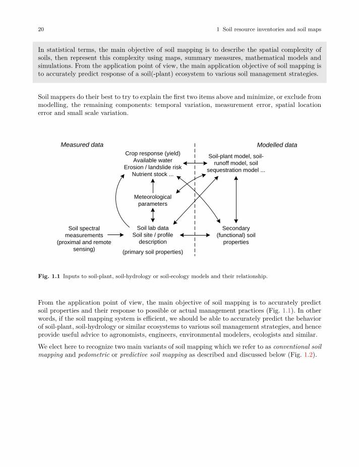
Measured data Modelled data
Meteorological parameters
Soil lab dataSoil site / profile
description
(primary soil properties)
Secondary (functional) soil
properties
Soil-plant model, soil-runoff model, soil
sequestration model ...
Crop response (yield)Available water
Erosion / landslide riskNutrient stock ...
Soil spectral measurements
(proximal and remote sensing)
Fig. 1.1 Inputs to soil-plant, soil-hydrology or soil-ecology models and their relationship.
From the application point of view, the main objective of soil mapping is to accurately predictsoil properties and their response to possible or actual management practices (Fig. 1.1). In otherwords, if the soil mapping system is efficient, we should be able to accurately predict the behaviorof soil-plant, soil-hydrology or similar ecosystems to various soil management strategies, and henceprovide useful advice to agronomists, engineers, environmental modelers, ecologists and similar.
We elect here to recognize two main variants of soil mapping which we refer to as conventional soilmapping and pedometric or predictive soil mapping as described and discussed below (Fig. 1.2).

1.3 Soil mapping 21
Soil types (soil series)
Discrete (soil bodies)
Expert knowledge / soil profile description
Soil delineations (photo-interpretation)
Averaging per polygon
Validation of soil mapping units (kappa)
Polygon maps + attribute tables
Cartographic scale
Free survey (surveyor selects sampling)
Analytical soil properties
Continuous/hybrid (quantities / probabilities)
Laboratory data / proximal soil sensing
Remote sensing images, DEM-derivatives
Automated (geo)statistics
Cross-validation (RMSE)
Gridded maps + prediction error map
Grid cell size
Statistical (design/model-based) sampling)
Data/technology-driven
soil mapping
Expert/knowledge-driven
soil mapping
Spatial data model:
Major inputs:
Spatial prediction model:
Accuracy assessment:
Data representation:
Soil sampling strategies:
Target variables:
Major technical aspect:
Important covariates:
Fig. 1.2 Matrix comparison between traditional (primarily expert-based) and automated (data-driven) soilmapping.
1.3.3 Theoretical basis of soil mapping: in context of the universalmodel of spatial variation
Stated simply, “the scientific basis of soil mapping is that the locations of soils in the landscapehave a degree of predictability” (Miller et al, 1979). According to the USDA Soil Survey Manual,“The properties of soil vary from place to place, but this variation is not random. Natural soil bodiesare the result of climate and living organisms acting on parent material, with topography or localrelief exerting a modifying influence and with time required for soil-forming processes to act. Forthe most part, soils are the same wherever all elements of these five factors are the same. Undersimilar environments in different places, soils are expected to be similar. This regularity permitsprediction of the location of many different kinds of soil” (Soil survey Division staff, 1993). Hudson(2004) considers that this soil-landscape paradigm provides the fundamental scientific basis for soilsurvey.
In the most general sense, both conventional soil mapping and PSM represent ways of applying thesoil-landscape paradigm via the universal model of spatial variation, which is explained in greaterdetail in chapter 5. Burrough and McDonnell (1998, p.133) described the universal model of soilvariation as a special case of the universal model of spatial variation. This model distinguishesbetween three major components of soil variation: (1) a deterministic component (trend), (2) aspatially correlated component and (3) pure noise.
𝑍(s) = 𝑚(s) + 𝜀′(s) + 𝜀″(s) (1.1)
where s is the two-dimensional location, 𝑚(s) is the deterministic component, 𝜀′(s) is the spatiallycorrelated stochastic component and 𝜀″(s) is the pure noise (micro-scale variation and measure-ment error).
22 1 Soil resource inventories and soil maps
The universal model of soil variation assumes that there are three major components of soil varia-tion: (1) a deterministic component (function of covariates), (2) a spatially correlated component(treated as stochastic) and (3) pure noise.
The deterministic part of the equation describes that part of the variation in soils and soil prop-erties that can be explained by reference to some model that relates observed and measuredvariation to readily observable and interpretable factors that control or influence this spatial vari-ation. In conventional soil mapping, this model is the empirical and knowledge-based soil-landscapeparadygm (Hudson, 2004). In PSM, a wide variety of statistical and machine learning models havebeen used to capture and apply the soil-landscape paradigm in a quantitative and optimal fashionusing the CLORPT model:
𝑆 = 𝑓(𝑐𝑙, 𝑜, 𝑟, 𝑝, 𝑡) (1.2)
where 𝑆 stands for soil (properties and classes), 𝑐𝑙 for climate, 𝑜 for organisms (including humans),𝑟 is relief, 𝑝 is parent material or geology and 𝑡 is time. The Eq. (1.2) is the CLORPT modeloriginally presented by Jenny (1994).
McBratney et al (2003) re-conceptualized and extended the CLORPT model via the “scorpan”model in which soil properties are modeled as a function of:
• (auxiliary) soil classes or properties,
• climate,
• organisms, vegetation, fauna or human activity,
• relief,
• parent material,
• age i.e. the time factor,
• n space, spatial context or spatial position,
Pedometric models are quantitative in that they capture relationships between observed soils,or soil properties, and controlling environmental influences (as represented by environmentalco-variates) using statistically-formulated expressions. Pedometric models are seen as optimumbecause, by design, they minimize the variance between observed and predicted values at all loca-tions with known values. So, no better model of prediction exists for that particular set of observedvalues at that specific set of locations.
Both conventional and pedometric soil mapping use models to explain the deterministic part ofthe spatial variation in soils and soil properties. These models differ mainly in terms of whetherthey are empirical and subjective (conventional) or quantitative and objective (pedometric). Bothcan be effective and the empirical and subjective models based on expert knowledge have, untilrecently, proven to be the most cost effective and widely applied for production of soil maps byconventional means.
1.3 Soil mapping 23
In its essence, the objective of PSM is to produce optimal unbiased predictions of a mean value atsome new location along with the uncertainty associated with the prediction, at the finest possibleresolution.
One way in which PSM differs significantly from conventional soil mapping in terms of the uni-versal model of soil variation is in the use of geostatistics or machine learning to quantitativelycorrect for error in predictions, defined as the difference between predicted and observed values atlocations with known values. Conventional soil mapping has no formal or quantitative mechanismfor correcting an initial set of predicted values by computing the difference between predicted andobserved values at sampled locations and then correcting initial values at all locations in responseto these observed differences. PSM uses geostatistics to determine (via the semi-variogram) if thedifferences between predicted and observed values (the residuals) exhibit spatial structure (e.g. arepredictable). If they do exhibit spatial structure, then it is useful and reasonable to interpolatethe computed error at known locations to predict the likely magnitude of error of predictions atall locations (Hengl et al, 2007a).
Neither conventional soil mapping nor PSM can do more than simply describe and quantify theamount of variation that is not predictable and has to be treated as pure noise. Conventional soilmaps can be criticized for ignoring this component of the total variation and typically treating itas if it did not exist. For many soil properties, short range, local variation in soil properties thatcannot be explained by either the deterministic or stochastic components of the universal modelof soil variation can often approach, or even exceed, a significant proportion (e.g. 30–40%) of thetotal observed range of variation in any given soil property. Such variation is simply not mappablebut it exists and should be identified and quantified. We do our users and clients a disservicewhen we fail to alert them to the presence, and the magnitude, of spatial variation that is notpredictable. In cases where the local spatial variation is not predictable (or mappable) the bestestimate for any property of interest is the mean value for that local area or spatial entity (hencenot a map).
1.3.4 Traditional (conventional) soil mapping
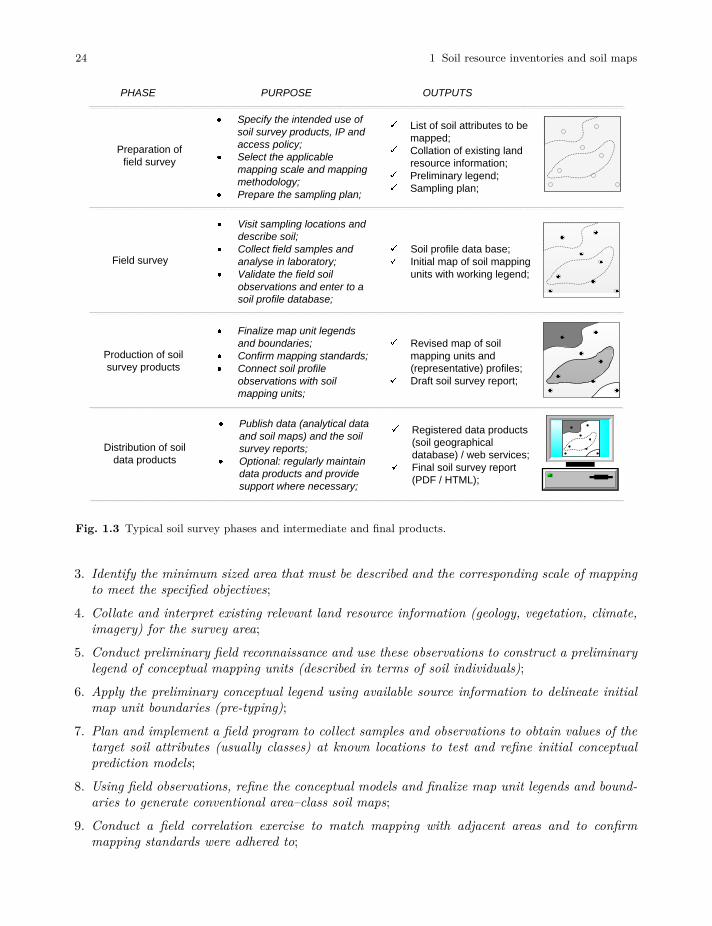
Traditional soil resource inventories are largely based on manual application of expert tacit knowl-edge through the soil-landscape paradigm (Burrough et al, 1971; Hudson, 2004). In this approach,soil surveyors develop and apply conceptual models of where and how soils vary in the landscapethrough a combination of field inspections to establish spatial patterns and photo-interpretationto extrapolate the patterns to similar portions of the landscape (Fig. 1.3). Traditional soil mappingprocedures mainly address the deterministic part of the universal model of soil variation.
Conventional (traditional) manual soil mapping typically adheres to the following sequence ofsteps, with minor variations (McBratney et al, 2003):
1. Specify the objective(s) to be served by the soil survey and resulting map;
2. Identify which attributes of the soil or land need to be observed, described and mapped to meetthe specified objectives;
24 1 Soil resource inventories and soil maps
Preparation of field survey
PHASE OUTPUTSPURPOSE
Specify the intended use of soil survey products, IP and access policy;Select the applicable mapping scale and mapping methodology;Prepare the sampling plan;
List of soil attributes to be mapped;Collation of existing land resource information;Preliminary legend;Sampling plan;
Field survey
Visit sampling locations and describe soil;Collect field samples and analyse in laboratory;Validate the field soil observations and enter to a soil profile database;
Soil profile data base;Initial map of soil mapping units with working legend;
Production of soil survey products
Finalize map unit legends and boundaries;Confirm mapping standards;Connect soil profile observations with soil mapping units;
Revised map of soil mapping units and (representative) profiles;Draft soil survey report;
Distribution of soil data products
Publish data (analytical data and soil maps) and the soil survey reports;Optional: regularly maintain data products and provide support where necessary;
Registered data products (soil geographical database) / web services;Final soil survey report (PDF / HTML);
Fig. 1.3 Typical soil survey phases and intermediate and final products.
3. Identify the minimum sized area that must be described and the corresponding scale of mappingto meet the specified objectives;
4. Collate and interpret existing relevant land resource information (geology, vegetation, climate,imagery) for the survey area;
5. Conduct preliminary field reconnaissance and use these observations to construct a preliminarylegend of conceptual mapping units (described in terms of soil individuals);
6. Apply the preliminary conceptual legend using available source information to delineate initialmap unit boundaries (pre-typing);
7. Plan and implement a field program to collect samples and observations to obtain values of thetarget soil attributes (usually classes) at known locations to test and refine initial conceptualprediction models;
8. Using field observations, refine the conceptual models and finalize map unit legends and bound-aries to generate conventional area–class soil maps;
9. Conduct a field correlation exercise to match mapping with adjacent areas and to confirmmapping standards were adhered to;
1.3 Soil mapping 25
10. Select and analyse representative soil profile site data to characterize each mapped soil type andsoil map unit;
11. Prepare final documentation describing all mapped soils and soil map units (legends) accordingto an accepted format;
12. Publish and distribute the soil information in the form of maps, geographical databases andreports;
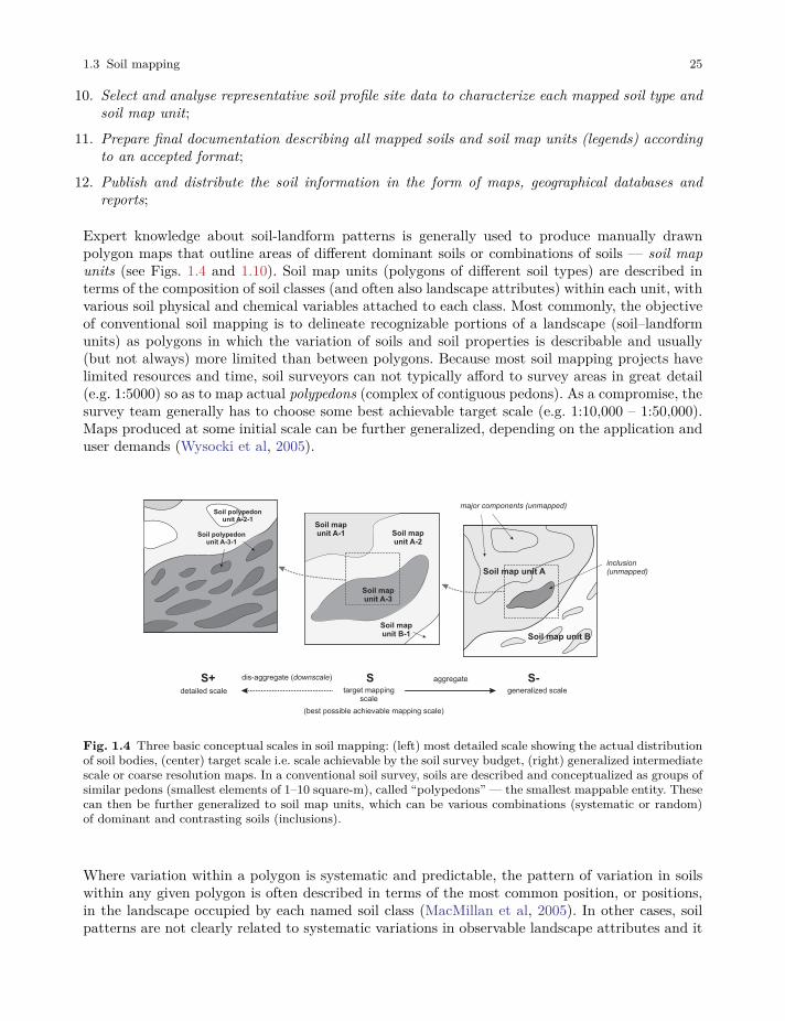
Expert knowledge about soil-landform patterns is generally used to produce manually drawnpolygon maps that outline areas of different dominant soils or combinations of soils — soil mapunits (see Figs. 1.4 and 1.10). Soil map units (polygons of different soil types) are described interms of the composition of soil classes (and often also landscape attributes) within each unit, withvarious soil physical and chemical variables attached to each class. Most commonly, the objectiveof conventional soil mapping is to delineate recognizable portions of a landscape (soil–landformunits) as polygons in which the variation of soils and soil properties is describable and usually(but not always) more limited than between polygons. Because most soil mapping projects havelimited resources and time, soil surveyors can not typically afford to survey areas in great detail(e.g. 1:5000) so as to map actual polypedons (complex of contiguous pedons). As a compromise, thesurvey team generally has to choose some best achievable target scale (e.g. 1:10,000 – 1:50,000).Maps produced at some initial scale can be further generalized, depending on the application anduser demands (Wysocki et al, 2005).
S+ S S-aggregatedis-aggregate (downscale)
inclusion(unmapped)
Soil map unit A-1 Soil map
unit A-2
Soil map unit A-3
Soil map unit B-1 Soil map unit B
major components (unmapped)
Soil polypedon unit A-3-1
Soil polypedon unit A-2-1
target mapping scale
detailed scale generalized scale
Soil map unit A
(best possible achievable mapping scale)
Fig. 1.4 Three basic conceptual scales in soil mapping: (left) most detailed scale showing the actual distributionof soil bodies, (center) target scale i.e. scale achievable by the soil survey budget, (right) generalized intermediatescale or coarse resolution maps. In a conventional soil survey, soils are described and conceptualized as groups ofsimilar pedons (smallest elements of 1–10 square-m), called “polypedons” — the smallest mappable entity. Thesecan then be further generalized to soil map units, which can be various combinations (systematic or random)of dominant and contrasting soils (inclusions).
Where variation within a polygon is systematic and predictable, the pattern of variation in soilswithin any given polygon is often described in terms of the most common position, or positions,in the landscape occupied by each named soil class (MacMillan et al, 2005). In other cases, soilpatterns are not clearly related to systematic variations in observable landscape attributes and it
26 1 Soil resource inventories and soil maps
is not possible to describe where each named soil type is most likely to occur within any polygonor why.
Conventional soil mapping has some limitations related to the fact that mapping concepts (mentalmodels) are not always applied consistently by different mappers. Application of conceptual modelsis largely manual and it is difficult to automate. In addition, conventional soil survey methodsdiffer from country to country, and even within a single region, depending largely on the scopeand level-of-detail of the inventory (Schelling, 1970; Soil Survey Staff, 1983; Rossiter, 2003). Thekey advantages of conventional soil maps, on the other hand, are that:
• they portray the spatial distribution of stable, recognizable and repeating patterns of soils thatusually occupy identifiable portions of the landscape, and
• these patterns can be extracted from legends and maps to model (predict) the most likely soil atany other location in the landscape using expert knowledge alone (Zhu et al, 2001).
Resource inventories, and in particular soil surveys, have been notoriously reluctant, or unable, toprovide objective quantitative assessments of the accuracy of their products. For example, mostsoil survey maps have only been subjected to qualitative assessments of map accuracy throughvisual inspection and subjective correlation exercises. In the very few examples of quantitativeevaluation (Marsman and de Gruijter, 1986; Finke, 2006), the assessments have typically focusedon measuring the degree with which predictions of soil classes at specific locations on a map,or within polygonal areas on a map, agreed with on-the-ground assessments of the soil class atthese same locations or within these same polygons. Measurement error can be large in assessingthe accuracy of soil class maps. MacMillan et al (2010), for example, demonstrated that expertsdisagreed with each other regarding the correct classification of ecological site types at the samelocations about as often as they disagreed with the classifications reported by a map producedusing a predictive model.
1.3.5 Variants of soil maps
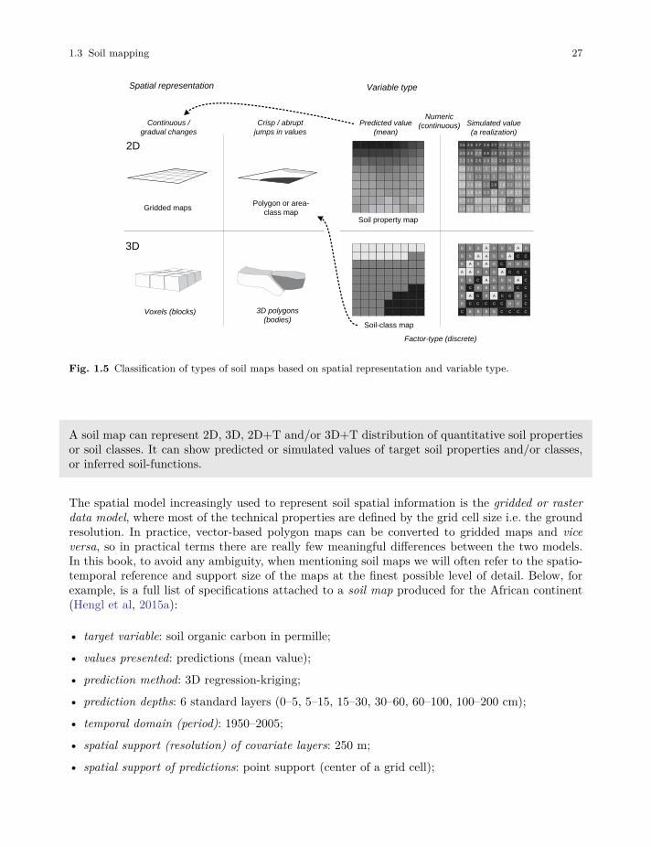
In the last 20–30 years, soil maps have evolved from purely 2D polygon maps showing the distri-bution of soil poly-pedons i.e. named soil classes, to dynamic 3D maps representing predicted orsimulated values of various primary or inferred soil properties and/or classes (Fig. 1.5). Examplesof 2D+T (2D space + time) and/or 3D+T soil maps are less common but increasingly popular(see e.g. Rosenbaum et al (2012) and Gasch et al (2015)). In general, we expect that demand forspatio-temporal soil data is likely to grow.
1.3 Soil mapping 27
Continuous /
gradual changes
Crisp / abrupt
jumps in values
2D
3D
Factor-type (discrete)
Polygon or area-
class map
Voxels (blocks) 3D polygons
(bodies)
Gridded maps
Predicted value
(mean)
Simulated value
(a realization)
Numeric
(continuous)
Soil-class map
Soil property map
Spatial representation Variable type
2.6 2.6 2.7 2.8 2.7 2.5 2.4 2.4 2.4
2.5 2.5 2.3 2.6 2.5 2.5 2.3 2.5 2.2
2.2 2.5 2.5 2.3 2.1 2.5 2.3 2.3 2.1
1.6 2.1 2.1 2 1.9 2.1 1.7 1.9 1.9
1.6 2 2.3 2.2 2 2.1 2.1 1.9 1.9
1.6 1.9 1.8 2.2 2.6 1.8 2.2 1.9 1.9
1.8 1.8 1.9 2.3 1.7 2 1.8 1.7 2.1
1.7 2.1 1.7 1.7 1.5 1.7 2.3 1.8 2
1.9 1.7 1.8 1.7 1.8 1.6 2.2 2.1 1.5
B B B A B B B A B
B B A A B B A C C
B A B A B C B B B
A A B B B A C C C
B B C A B B B A C
B C B B B B B C C
B A C B A C C B C
B C C C C C B B C
C B B B B C C C C
Fig. 1.5 Classification of types of soil maps based on spatial representation and variable type.
A soil map can represent 2D, 3D, 2D+T and/or 3D+T distribution of quantitative soil propertiesor soil classes. It can show predicted or simulated values of target soil properties and/or classes,or inferred soil-functions.
The spatial model increasingly used to represent soil spatial information is the gridded or rasterdata model, where most of the technical properties are defined by the grid cell size i.e. the groundresolution. In practice, vector-based polygon maps can be converted to gridded maps and viceversa, so in practical terms there are really few meaningful differences between the two models.In this book, to avoid any ambiguity, when mentioning soil maps we will often refer to the spatio-temporal reference and support size of the maps at the finest possible level of detail. Below, forexample, is a full list of specifications attached to a soil map produced for the African continent(Hengl et al, 2015a):
• target variable: soil organic carbon in permille;
• values presented: predictions (mean value);
• prediction method: 3D regression-kriging;
• prediction depths: 6 standard layers (0–5, 5–15, 15–30, 30–60, 60–100, 100–200 cm);
• temporal domain (period): 1950–2005;
• spatial support (resolution) of covariate layers: 250 m;
• spatial support of predictions: point support (center of a grid cell);
28 1 Soil resource inventories and soil maps
• amount of variation explained by the spatial prediction model: 45%;
Until recently, maps of individual soil properties, or of soil functions or soil interpretations, werenot considered to be true soil maps, but rather, to be single-factor derivative maps or interpretivemaps. This is beginning to change and maps of the spatial pattern of distribution of individualsoil properties are increasingly being viewed as a legitimate form of soil mapping.
1.3.6 Predictive and automated soil mapping
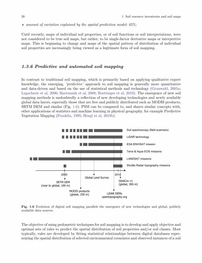
In contrast to traditional soil mapping, which is primarily based on applying qualitative expertknowledge, the emerging, ‘predictive’ approach to soil mapping is generally more quantitativeand data-driven and based on the use of statistical methods and technology (Grunwald, 2005a;Lagacherie et al, 2006; Hartemink et al, 2008; Boettinger et al, 2010). The emergence of new soilmapping methods is undoubtedly a reflection of new developing technologies and newly availableglobal data layers, especially those that are free and publicly distributed such as MODIS products,SRTM DEM and similar (Fig. 1.6). PSM can be compared to, and shares similar concepts with,other applications of statistics and machine learning in physical geography, for example PredictiveVegetation Mapping (Franklin, 1995; Hengl et al, 2018b).
SRTM DEM(near to global, 100 m)
LiDAR technology
Terra & Aqua EOS missions
MODIS products(global, 250 m)
Soil spectroscopy (field scanners)
ESA ENVISAT mission
2000 2010
GlobCov v1(global, 300 m)
Global Land Survey
LANDSAT missions
LiDAR DEMsopentopography.org
Shuttle Radar topography missions
Fig. 1.6 Evolution of digital soil mapping parallels the emergence of new technologies and global, publiclyavailable data sources.
The objective of using pedometric techniques for soil mapping is to develop and apply objective andoptimal sets of rules to predict the spatial distribution of soil properties and/or soil classes. Mosttypically, rules are developed by fitting statistical relationships between digital databases repre-senting the spatial distribution of selected environmental covariates and observed instances of a soil
1.3 Soil mapping 29
class or soil property at geo-referenced sample locations. The environmental covariate databasesare selected as predictors of the soil attributes on the basis of either expert knowledge of knownrelationships to soil patterns or through objective assessment of meaningful correlations with ob-served soil occurrences. The whole process is amenable to complete automation and documentationso that it allows for reproducible research (http://en.wikipedia.org/wiki/Reproducibility).
Pedometric soil mapping typically follows six steps as outlined by McBratney et al (2003):
1. Select soil variables (or classes) of interest and suitable measurement techniques (decide whatto map and describe);
2. Prepare a sampling design (select the spatial locations of sampling points and define a samplingintensity);
3. Collect samples in the field and then estimate values of the target soil variables at unknownlocations to test and refine prediction models;
4. Select and implement the most effective spatial prediction (or extrapolation) models and usethese to generate soil maps;
5. Select the most representative data model and distribution system;
6. Publish and distribute the soil information in the form of maps, geographical databases andreports (and provide support to users);
Differences among conventional soil mapping and digital soil mapping (or technology-driven ordata-driven mapping) relate primarily to the degree of use of robust statistical methods in devel-oping prediction models to support the mapping process.
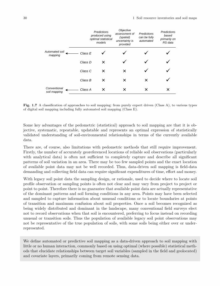
We recognize four classes of advanced soil mapping methods (B, C, D and E in Fig. 1.7) whichall belong to a continuum of digital soil mapping methods (Malone et al, 2016; McBratney et al,2018). We promote in this book specifically the Class E soil mapping approach i.e. which we referto as the predictive and/or automated soil mapping.
30 1 Soil resource inventories and soil maps
Class D
Class C
Class B
Class A
ü ü
ü
ü
ü
ü
ü
ü
ü
ü
×
Automated soil
mappingClass E
Conventional
soil mapping
Predictions
produced using
optimal statistical
models
Objective
assessment of
(spatial)
uncertainty is
provided
Predictions
can be fully
automated
Predictions
based
primarily on
RS data
×××
×
×
× ×
×
×
Fig. 1.7 A classification of approaches to soil mapping: from purely expert driven (Class A), to various typesof digital soil mapping including fully automated soil mapping (Class E).
Some key advantages of the pedometric (statistical) approach to soil mapping are that it is ob-jective, systematic, repeatable, updatable and represents an optimal expression of statisticallyvalidated understanding of soil-environmental relationships in terms of the currently availabledata.
There are, of course, also limitations with pedometric methods that still require improvement.Firstly, the number of accurately georeferenced locations of reliable soil observations (particularlywith analytical data) is often not sufficient to completely capture and describe all significantpatterns of soil variation in an area. There may be too few sampled points and the exact locationof available point data may not be well recorded. Thus, data-driven soil mapping is field-datademanding and collecting field data can require significant expenditures of time, effort and money.
With legacy soil point data the sampling design, or rationale, used to decide where to locate soilprofile observation or sampling points is often not clear and may vary from project to project orpoint to point. Therefore there is no guarantee that available point data are actually representativeof the dominant patterns and soil forming conditions in any area. Points may have been selectedand sampled to capture information about unusual conditions or to locate boundaries at pointsof transition and maximum confusion about soil properties. Once a soil becomes recognized asbeing widely distributed and dominant in the landscape, many conventional field surveys electnot to record observations when that soil is encountered, preferring to focus instead on recordingunusual or transition soils. Thus the population of available legacy soil point observations maynot be representative of the true population of soils, with some soils being either over or under-represented.
We define automated or predictive soil mapping as a data-driven approach to soil mapping withlittle or no human interaction, commonly based on using optimal (where possible) statistical meth-ods that elucidate relationships between target soil variables (sampled in the field and geolocated)and covariate layers, primarily coming from remote sensing data.
1.3 Soil mapping 31
A second key limitation of the automated approach to soil mapping is that there may be noobvious relationship between observed patterns of soil variation and the available environmentalcovariates. This may occur when a soil property of interest does, indeed, strongly covary withsome mappable environmental covariate (e.g. soil clay content with airborne radiometric data)but data for that environmental covariate are not available for an area. It may also transpire thatthe pattern of soil variation is essentially not predictable or related to any known environmentalcovariate, available or not. In such cases, only closely spaced, direct field observation and samplingis capable of detecting the spatial pattern of variation in soils because there is no, or only a veryweak, correlation with available covariates (Kondolf and Piégay, 2003).
1.3.7 Comparison of conventional and pedometric or predictive soilmapping
There has been a tendency to view conventional soil mapping and automated soil mapping ascompeting and non-complementary approaches. In fact, they share more similarities than differ-ences. Indeed, they can be viewed as end members of a logical continuum. Both rely on applyingthe underlying idea that the distribution of soils in the landscape is largely predictable (the deter-ministic part) and, where it is not predictable, it must be revealed through intensive observation,sampling and interpolation (the stochastic part).
In most cases, the basis of prediction is to relate the distribution of soils, or soil properties, inthe landscape to observable environmental factors such as topographic position, slope, aspect,underlying parent material, drainage conditions, patterns of climate, vegetation or land use andso on. This is done manually and empirically (subjectively) in conventional soil survey, while inautomated soil mapping it is done objectively and mostly in an automated fashion. At the time itwas developed, conventional soil survey lacked both the digital data sets of environmental covari-ates and the statistical tools required to objectively analyze relationships between observed soilproperties and environmental covariates. So, these relationships were, out of necessity, developedempirically and expressed conceptually as expert knowledge.
In general, we suggest that next generation soil surveyors will increasingly benefit from having asolid background in statistics and computer science, especially in Machine Learning and A.I. How-ever, effective selection and application of appropriate statistical sampling and analysis techniquescan also benefit from consideration of expert knowledge.
1.3.8 Top-down versus bottom-up approaches: subdivision versusagglomeration
There are two fundamentally different ways to approach the production of soil maps for areas oflarger extent, whether by conventional or pedometric means. For ease of understanding we refer tothese two alternatives here as “bottom-up” versus “top-down”. Rossiter (2003) refers to a syntheticapproach that he calls the “bottom-up” or “name and then group” approach versus an analyticapproach that he calls the “top-down” or “divide and then name” approach.
32 1 Soil resource inventories and soil maps
The bottom up approach is agglomerative and synthetic. It is implemented by first collecting ob-servations and making maps at the finest possible resolution and with the greatest possible levelof detail. Once all facts are collected and all possible soils and soil properties, and their respectivepatterns of spatial distribution, are recorded, these detailed data are generalized at successivelycoarser levels of generalization to detect, analyse and describe broader scale (regional to conti-nental) patterns and trends. The fine detail synthesized to extract broader patterns leads to theidentification and formulation of generalizations, theories and concepts about how and why soilsorganize themselves spatially. The bottom-up approach makes little-to-no-use of generalizationsand theories as tools to aid in the conceptualization and delineation of mapping entities. Rather,it waits until all the facts are in before making generalizations. The bottom-up approach tendsto be applied by countries and organizations that have sufficient resources (people and finances)to make detailed field surveys feasible to complete for entire areas of jurisdiction. Soil surveyactivities of the US national cooperative soil survey (NCSS) primarily adopt this bottom-up ap-proach. Other smaller countries with significant resources for field surveys have also adopted thisapproach (e.g. Netherlands, Denmark, Cuba). The bottom-up approach was, for example, used inthe development and elaboration of the US Soil Taxonomy system of classification and of the USSSURGO (1:20,000) and STATSGO (1:250,000) soil maps (Zhong and Xu, 2011).
The top-down approach is synoptic, analytic and divisive. It is implemented by first collecting justenough observations and data to permit construction of generalizations and theoretical conceptsabout how soils arrange themselves in the landscape in response to controlling environmentalvariables. Once general theories are developed about how environmental factors influence how soilsarrange themselves spatially, these concepts and theories are tested by using them to predict whattypes of soils are likely to occur under similar conditions at previously unvisited sites. The theoriesand concepts are adjusted in response to initial application and testing until such time as theyare deemed to be reliable enough to use for production mapping. Production mapping proceedsin a divisive manner by stratifying areas of interest into successively smaller, and presumablymore homogeneous, areas or regions through application of the concepts and theories to availableenvironmental data sets. The procedures begin with a synoptic overview of the environmentalconditions that characterize an entire area of interest. These conditions are then interpreted toimpose a hierarchical subdivision of the whole area into smaller, and more homogeneous subareas.This hierarchical subdivision approach owes its origins to early Russian efforts to explain soilpatterns in terms of the geographical distribution of observed soils and vegetation. The top-downapproach tends to be applied preferentially by countries and agencies that need to produce mapsfor very large areas but that lack the people and resources to conduct detailed field programseverywhere (see e.g. Henderson et al (2004) and Mansuy et al (2014)). Many of these divisivehierarchical approaches adopt principals and methods associated with the ideas of EcologicalLand Classification (Rowe and Sheard, 1981) (in Canada) or Land Systems Mapping (Gibbonset al, 1964; Rowan, 1990) (in Australia).
As observed by Rossiter (2003) “neither approach is usually applied in its pure form” and most ap-proaches to soil mapping use both approaches simultaneously, to varying degrees. Similarly, it canbe argued that PSM provides support for both approaches to soil mapping. PSM implements twoactivities that bear similarities to bottom-up mapping. Firstly, PSM uses all available soil profiledata globally as input to initial global predictions at coarser resolutions (“top-down” mapping).Secondly, PSM is set up to ingest finer resolution maps produced via detailed “bottom-up” map-ping methods and to merge these more detailed maps with initial, coarser-resolution predictions(Ramcharan et al, 2018).
1.4 Sources of soil data for soil mapping 33
1.4 Sources of soil data for soil mapping
1.4.1 Soil data sources targeted by PSM
PSM aims at integrating and facilitating exchange of global soil data. Most (global) soil mappinginitiatives currently rely on capture and use of legacy soil data. This raises several questions. Whatis meant by legacy soil data? What kinds of legacy soil data exist? What are the advantages andlimitations of the main kinds of legacy soil data?
In its most general sense, a legacy is something of value bequeathed from one generation to thenext. It can be said that global soil legacy data consists of the sum of soil data and knowledgeaccumulated since the first soil investigations 100 or more years ago (Arrouays et al, 2017). Morespecifically, the concept of a legacy is usually accompanied by an understanding that there isan obligation and duty of the recipient generation to not simply protect the legacy but to makepositive and constructive use of it.
Four main groups of legacy data of interest for global soil mapping are: (1) soil field records,(2) soil polygon maps and legends, (3) soil-landscape diagrams and sketches, (4) soil (profile)photographs.
In the context of soils, legacy soil data consist of the sum total of data, information and knowledgeabout soils accumulated since soils were first studied as independent natural objects. At its broad-est, this includes information about soil characteristics and classification, soil use and management,soil fertility, soil bio-chemistry, soil formation, soil geography and many other sub-disciplines.
In the more focused context of PSM, we are primarily interested in four main kinds of legacy soildata:
• Soil field observations and measurements — Observations and analytical data obtained forsoils at point locations represent a primary type of legacy soil data. These point source dataprovide objective evidence of observed soil characteristics at known locations that can be usedto develop knowledge and rules about how soils, or individual soil properties, vary across thelandscape. The quality and precision of these data can vary greatly. Some data points mightbe accurately located, or geo-referenced, while others might have very coarse geo-referencing(for example coordinates rounded in decimal minutes or kilometers). Some point data mightonly have a rough indication of the location obtained from a report (for example ‘2 km southof village A’), or might even lack geo-referencing. Soil profile descriptions can be obtained frompits (relatively accurate) or auger bores (less accurate). Soil attributes can be determined inthe laboratory (relatively accurate) or by hand-estimation in the field (less accurate). Legacypoint data is characterized by great variation in precision, accuracy, completeness, relevanceand age. It needs to be used with caution and with understanding of how these issues affect itspotential use.
• Soil (polygon) maps and legends — Soil maps and legends are one of the primary means bywhich information and knowledge about how soils vary spatially have been observed, distilled,recorded and presented to users. Soil maps provide lists, or inventories, of soils that occur in
34 1 Soil resource inventories and soil maps
mapped regions, illustrate the dominant spatial patterns displayed by these listed soils andprovide information to characterize the main properties of these soils. Soil maps can themselvesbe used as sources of evidence to develop knowledge and quantitative rules about how soils, orindividual soil properties, vary across the landscape. On the other hand, similar to soil observa-tions, soil maps can also exhibit significant errors with respect to measurement, classification,generalization, interpretation and spatial interpolation.
• Tacit expert soil knowledge — In the context of soils, tacit expert knowledge represents a diffusedomain of information about the characteristics and spatial distribution of soils that has notbeen captured and recorded formally or explicitly. It may reside in the minds and memories ofexperts who have conducted field and laboratory studies but have been unable to record all theirobservations in a formal way. It may be captured informally and partially in maps, legends,conceptual diagrams, block diagrams, generalized decision rules and so on. Tacit knowledgerepresents soft data, in comparison to the more hard data of point observations and maps.
• Photographs — Traditional soil survey is heavily based on use of aerial photographs. Olderaerial photographs (even if not stereoscopic) are an important resource for land degradationmonitoring and vegetation succession studies. Field photographs of soil profiles, soil sites andsoil processes are another important source of information that has been under-used for soilmapping. ISRIC for example has an archive of over 30 thousand photographs from various con-tinents. Most of these can be geo-coded and distributed via image sharing web-services such asWikiMedia, Instagram and/or Flickr. In theory, even a single photograph of a soil profile couldbe used to (automatically?) identify soil types, even extract analytical soil properties. Althoughit is very likely that prediction by using photographs-only would be fairly imprecise, such datacould potentially help fill large gaps for areas where there are simply no soil observations.
1.4.2 Field observations of soil properties
Perhaps the most significant, but certainly the most reliable, inputs to soil mapping are thefield observations (usually at point locations) of descriptive and analytical soil properties (Soilsurvey Division staff, 1993; Schoeneberger et al, 1998). This is the hard data or ground truth insoil mapping (Rossiter, 2003). Field observations are also the main input to spatial predictionmodelling and the basis for assessment of mapping accuracy. Other synthetically or empiricallygenerated estimates of values of target variables in the field are considered as soft data (data basedon qualitative information or quick observations). Soft data are less desirable as the primary inputto model estimation, but sometimes there is no alternative. It is in any case important to recognizedifferences between hard and soft data and to suggest ways to access the uncertainty of modelsthat are based on either or both.
The object of observation and description of a soil is almost always a soil profile or pedon. Officially,a soil pedon is defined as a body of soil having a limited horizontal extent of no more than 1–2 m in horizontal and a vertical dimension (𝑑) that typically extends to only 1–2 m but mayoccasionally extend to greater depths. In practice, the vast majority of soil profile data pertain tosoil observations and samples collected over very limited horizontal dimensions (10–50 cm) anddown to maximum depths of 1–2 m.
1.4 Sources of soil data for soil mapping 35
In geostatistical terms, soil observations are most commonly collected at point support, meaningthat they are representative of a point in space with very limited horizontal extent. It is relativelyrare to encounter legacy soil profile data collected over larger horizontal extents and bulked tocreate a sample representative of a larger volume of soil that can be treated as providing blocksupport for statistical purposes. On the other hand, there is an increasing interest in soil predictionsat varying support sizes e.g. 1 ha for which composite sampling can be used.
In the vertical dimension, soil profiles are usually described and sampled with respect to geneticsoil horizons, which are identifiable layers in the soil that reflect differences in soil developmentor depositional environments. Less frequently, soils are described and sampled in the verticaldimension with respect to arbitrary depth intervals or layers e.g. at fixed depths intervals e.g. 10,20, 30, 40, … cm.
A soil profile record is a set of field observations of the soil at a location — a collection of descriptiveand analytical soil properties attached to a specific location, depth and sampling support size(volume of soil body).
Soil profile descriptions in the vertical dimension are usually accompanied by additional soil sitedescriptions that describe attributes of the site in the horizontal dimension for distances of a fewmeters up to 10 m surrounding the location where the vertical profile was sampled and described.Site attributes described typically characterize the immediately surrounding landscape, includingslope gradient, aspect, slope position, surface shape, drainage condition, land use, vegetation cover,stoniness and unusual or site specific features.
Two main types of information are typically recorded for point soil profiles. The first consistsof field observations and classifications of observable profile and site characteristics. Profile at-tributes usually include the location and thickness of observably different horizons or layers, thecolor, texture, structure and consistence of each recognized horizon or layer and other observableattributes such as stone content, presence, size and abundance of roots, pores, mottles, cracks andso on. Despite their potential for subjectivity, these field observations provide much useful infor-mation at a relatively low cost, since there is no need to sample or transport the soil or analyze itat considerable cost in a distant laboratory.
The second main type of information collected to describe soil profiles consists of various types ofobjective measurements and analyses. Some objective measurements can be taken on-site, in thefield. Examples of field measurements include in-situ assessment of bulk density, infiltration rate,hydraulic conductivity, electrical conductivity, penetration resistance and, more recently, spectralanalysis of soil reflectance (Kondolf and Piégay, 2003; Gehl and Rice, 2007; Shepherd and Walsh,2007). The most frequently obtained and reported objective measurements are obtained by off-sitelaboratory analysis of soil samples collected from soil profiles at sampled locations. A wide varietyof chemical and physical laboratory analyses can be, and have been, carried out on soil samplesincluded in legacy soil profile data bases.
Within PSM we are mainly interested in a core set of laboratory analyses for e.g. pH, organiccarbon, sand, silt, clay and coarse fragment content, bulk density, available water capacity, ex-changeable cations and acidity and electrical conductivity. This core set was selected partly be-cause it is considered to represent the key soil functional properties of most interest and use forinterpretation and analysis and partly because these soil properties are the most widely analyzed
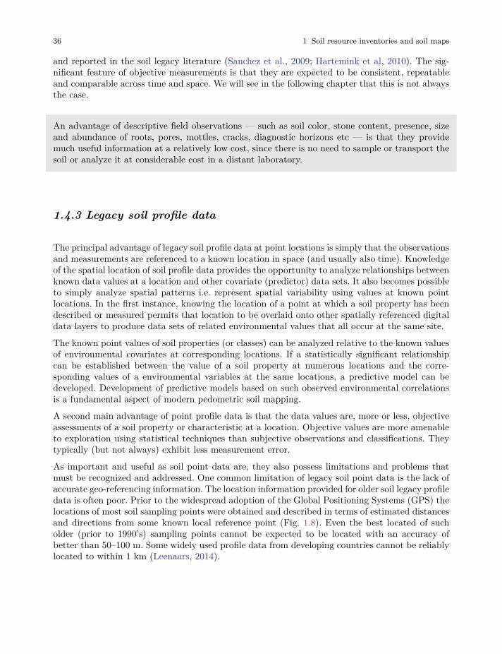
36 1 Soil resource inventories and soil maps
and reported in the soil legacy literature (Sanchez et al., 2009; Hartemink et al, 2010). The sig-nificant feature of objective measurements is that they are expected to be consistent, repeatableand comparable across time and space. We will see in the following chapter that this is not alwaysthe case.
An advantage of descriptive field observations — such as soil color, stone content, presence, sizeand abundance of roots, pores, mottles, cracks, diagnostic horizons etc — is that they providemuch useful information at a relatively low cost, since there is no need to sample or transport thesoil or analyze it at considerable cost in a distant laboratory.
1.4.3 Legacy soil profile data
The principal advantage of legacy soil profile data at point locations is simply that the observationsand measurements are referenced to a known location in space (and usually also time). Knowledgeof the spatial location of soil profile data provides the opportunity to analyze relationships betweenknown data values at a location and other covariate (predictor) data sets. It also becomes possibleto simply analyze spatial patterns i.e. represent spatial variability using values at known pointlocations. In the first instance, knowing the location of a point at which a soil property has beendescribed or measured permits that location to be overlaid onto other spatially referenced digitaldata layers to produce data sets of related environmental values that all occur at the same site.
The known point values of soil properties (or classes) can be analyzed relative to the known valuesof environmental covariates at corresponding locations. If a statistically significant relationshipcan be established between the value of a soil property at numerous locations and the corre-sponding values of a environmental variables at the same locations, a predictive model can bedeveloped. Development of predictive models based on such observed environmental correlationsis a fundamental aspect of modern pedometric soil mapping.
A second main advantage of point profile data is that the data values are, more or less, objectiveassessments of a soil property or characteristic at a location. Objective values are more amenableto exploration using statistical techniques than subjective observations and classifications. Theytypically (but not always) exhibit less measurement error.
As important and useful as soil point data are, they also possess limitations and problems thatmust be recognized and addressed. One common limitation of legacy soil point data is the lack ofaccurate geo-referencing information. The location information provided for older soil legacy profiledata is often poor. Prior to the widespread adoption of the Global Positioning Systems (GPS) thelocations of most soil sampling points were obtained and described in terms of estimated distancesand directions from some known local reference point (Fig. 1.8). Even the best located of sucholder (prior to 1990’s) sampling points cannot be expected to be located with an accuracy ofbetter than 50–100 m. Some widely used profile data from developing countries cannot be reliablylocated to within 1 km (Leenaars, 2014).
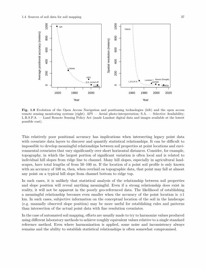
1.4 Sources of soil data for soil mapping 37
●
●
●
● ●
1920 1960 2000
020
040
060
080
010
00
Year
Ave
rage
pos
ition
al a
ccur
acy
(met
ers)
API
LORAN
GPS
S.A. turned off
Galilleo
●
●●
● ●
1960 1980 2000 2020
020
040
060
080
010
00
Year
Spa
tial r
esol
utio
n (m
eter
s)
TIROS
L.R.S.P.ALandsat 7
ASTERIkonos (Google)
GeoEye
Fig. 1.8 Evolution of the Open Access Navigation and positioning technologies (left) and the open accessremote sensing monitoring systems (right). API — Aerial photo-interpretation; S.A. — Selective Availability;L.R.S.P.A. — Land Remote Sensing Policy Act (made Landsat digital data and images available at the lowestpossible cost).
This relatively poor positional accuracy has implications when intersecting legacy point datawith covariate data layers to discover and quantify statistical relationships. It can be difficult toimpossible to develop meaningful relationships between soil properties at point locations and envi-ronmental covariates that vary significantly over short horizontal distances. Consider, for example,topography, in which the largest portion of significant variation is often local and is related toindividual hill slopes from ridge line to channel. Many hill slopes, especially in agricultural land-scapes, have total lengths of from 50–100 m. If the location of a point soil profile is only knownwith an accuracy of 100 m, then, when overlaid on topographic data, that point may fall at almostany point on a typical hill slope from channel bottom to ridge top.
In such cases, it is unlikely that statistical analysis of the relationship between soil propertiesand slope position will reveal anything meaningful. Even if a strong relationship does exist inreality, it will not be apparent in the poorly geo-referenced data. The likelihood of establishinga meaningful relationship becomes even smaller when the accuracy of the point location is ±1km. In such cases, subjective information on the conceptual location of the soil in the landscape(e.g. manually observed slope position) may be more useful for establishing rules and patternsthan intersection of the actual point data with fine resolution covariates.
In the case of automated soil mapping, efforts are usually made to try to harmonize values producedusing different laboratory methods to achieve roughly equivalent values relative to a single standardreference method. Even where harmonization is applied, some noise and inconsistency alwaysremains and the ability to establish statistical relationships is often somewhat compromised.
38 1 Soil resource inventories and soil maps
If not collected using probability sampling and with high location accuracy, soil field records areoften only marginally suitable for building spatial prediction models, especially at fine spatialresolution. Legacy data can carry significant positional and attribute error, and is possibly notrepresentative of all soil forming conditions in an area of interest. All these limitations can seriouslydegrade the final map accuracy, so that sometimes better accuracy cannot be achieved withoutcollecting new field data.
What needs to be emphasized is that much of the legacy soils profile data in the world is underused. It tends to be fragmented, non-standard between countries and often even within countries.Many original field observations are still not converted into digital format and these data arein considerable danger of being lost to effective use forever (!) as government sponsored soilinstitutions lose support and close and the current generation of experienced soil specialists retireand are not replaced. Even where these data are in digital format, it is not easy to share orexchange data across national, state or even project borders because of significant differences instandards, methods, definitions, ownership and legends (Omuto et al, 2012).
1.4.4 Soil covariates
Following the work of Jenny (White, 2009) and further McBratney et al (2011), we recognize sixmain groups of soil covariates of interest for pedometric soil mapping:
1. Raw spectral and multi-spectral images of the land surface (remote sensing bands),
2. DEM-derived covariates,
3. Climatic images,
4. Vegetation and land-cover based covariates,
5. Land survey and land use information — human-made objects, management, fertilization andtillage practice maps etc,
6. Expert-based covariates — soil delineations or delineations of soil parent material or geol-ogy (manually or semi-automatically prepared); empirical maps of soil processes and features(e.g. catena sequences etc).
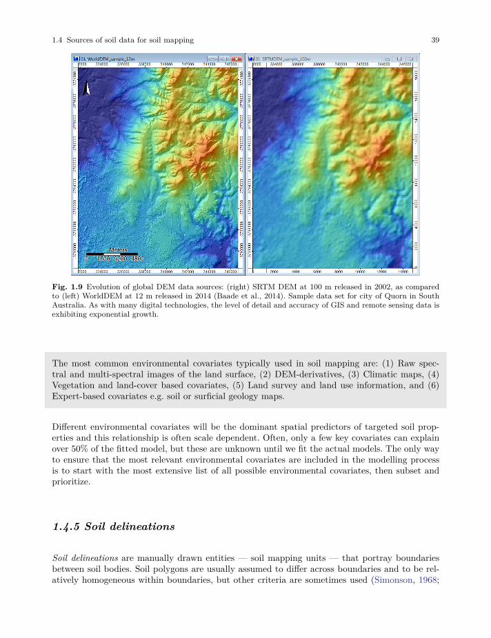
1.4 Sources of soil data for soil mapping 39
Fig. 1.9 Evolution of global DEM data sources: (right) SRTM DEM at 100 m released in 2002, as comparedto (left) WorldDEM at 12 m released in 2014 (Baade et al., 2014). Sample data set for city of Quorn in SouthAustralia. As with many digital technologies, the level of detail and accuracy of GIS and remote sensing data isexhibiting exponential growth.
The most common environmental covariates typically used in soil mapping are: (1) Raw spec-tral and multi-spectral images of the land surface, (2) DEM-derivatives, (3) Climatic maps, (4)Vegetation and land-cover based covariates, (5) Land survey and land use information, and (6)Expert-based covariates e.g. soil or surficial geology maps.
Different environmental covariates will be the dominant spatial predictors of targeted soil prop-erties and this relationship is often scale dependent. Often, only a few key covariates can explainover 50% of the fitted model, but these are unknown until we fit the actual models. The only wayto ensure that the most relevant environmental covariates are included in the modelling processis to start with the most extensive list of all possible environmental covariates, then subset andprioritize.
1.4.5 Soil delineations
Soil delineations are manually drawn entities — soil mapping units — that portray boundariesbetween soil bodies. Soil polygons are usually assumed to differ across boundaries and to be rel-atively homogeneous within boundaries, but other criteria are sometimes used (Simonson, 1968;
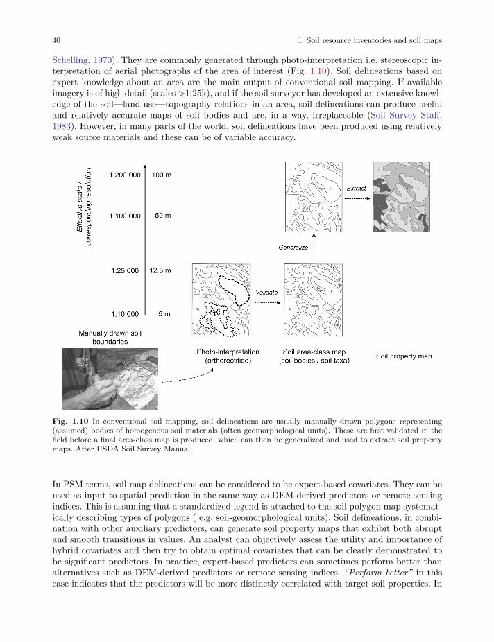
40 1 Soil resource inventories and soil maps
Schelling, 1970). They are commonly generated through photo-interpretation i.e. stereoscopic in-terpretation of aerial photographs of the area of interest (Fig. 1.10). Soil delineations based onexpert knowledge about an area are the main output of conventional soil mapping. If availableimagery is of high detail (scales >1:25k), and if the soil surveyor has developed an extensive knowl-edge of the soil—land-use—topography relations in an area, soil delineations can produce usefuland relatively accurate maps of soil bodies and are, in a way, irreplaceable (Soil Survey Staff,1983). However, in many parts of the world, soil delineations have been produced using relativelyweak source materials and these can be of variable accuracy.
Fig. 1.10 In conventional soil mapping, soil delineations are usually manually drawn polygons representing(assumed) bodies of homogenous soil materials (often geomorphological units). These are first validated in thefield before a final area-class map is produced, which can then be generalized and used to extract soil propertymaps. After USDA Soil Survey Manual.
In PSM terms, soil map delineations can be considered to be expert-based covariates. They can beused as input to spatial prediction in the same way as DEM-derived predictors or remote sensingindices. This is assuming that a standardized legend is attached to the soil polygon map systemat-ically describing types of polygons ( e.g. soil-geomorphological units). Soil delineations, in combi-nation with other auxiliary predictors, can generate soil property maps that exhibit both abruptand smooth transitions in values. An analyst can objectively assess the utility and importance ofhybrid covariates and then try to obtain optimal covariates that can be clearly demonstrated tobe significant predictors. In practice, expert-based predictors can sometimes perform better thanalternatives such as DEM-derived predictors or remote sensing indices. “Perform better” in thiscase indicates that the predictors will be more distinctly correlated with target soil properties. In
1.4 Sources of soil data for soil mapping 41
all applications of PSM methods, it is advisable to obtain and assess the utility of available soilpolygon maps.
Most legacy polygon soil maps represent a distillation and summary of expert knowledge aboutthe main spatial patterns of variation in soil types (classes) within an area. This knowledge hasbeen abstracted and generalized in order to convey dominant patterns at specific scales. Thus, itis often not reasonable to expect to be able to go to a specific point portrayed on a soil map andfind a single specific soil class or soil property value (see Fig. 1.4). Most often, soil maps providelists or inventories of soil classes that occur within a given map area and give outlines of areas(polygons) within which lists of specific soils are predicted to occur with specified frequencies orpossibilities. Soils are conceptualized as objects that belong to defined soil classes.
Soil delineations are manually drawn entities that portray boundaries between soil bodies as-sumed to be internally homogeneous. Soil delineations can be considered to be expert-based soilcovariates.
Each class of soil (often a soil series or taxonomic class) is assumed to have a limited and describ-able range of characteristics i.e. physical and chemical properties that can be used to characterizeit. Within mapped polygons, the manner in which soils vary horizontally across the landscapeis usually not explicitly portrayed (Fig. 1.4). At best, such internal polygon variation may bedescribed in conceptual terms relative to how different soils may be more likely to occupy specificlandscape positions or occur on specific parent materials or under different drainage conditions. Forexample the USDA’s Soil Survey Manual distinguishes between consociations (relatively homoge-neous polypedons), associations (heterogeneous unit with two or more similar polypedons), andcomplexes (mix of two or more contrasting polypedons), but in most cases none of the describedcomponents is actually mapped separately.
Variation of soil properties in the vertical dimension is usually described in terms of variation inthe type, thickness and arrangement of various different soil horizons. Soil horizons are themselvesa collection of class objects, with each class also expected to display a characteristic range ofattributes and soil property values. All soils do not always have the same types or sequences ofhorizons and so, most horizons are not laterally continuous and mappable. So, most legacy soilmaps portray abstract representations of how various classes of soils vary horizontally betweensoil polygons and vertically by soil horizons.
Interpretation of most maps of soil classes often requires a considerable amount of knowledgeand understanding of both underlying soil mapping concepts and of local classes of soils and soilhorizons. This restricts effective use of many soils maps to persons with the necessary backgroundknowledge.
1.4.6 Advantages and disadvantages of using soil delineations
One of the key advantages of conventional soil polygon map data is its availability. In many partsof the world, the number of instances of reliably located soil profile observations is quite low andthe spatial extent of areas for which sufficient point data are available can be small (Hartemink,
42 1 Soil resource inventories and soil maps
2008). However, many areas with only limited amounts of geo–referenced point data are coveredby soil maps of various types and scales. So, conventional soil polygon maps are often availablefor areas that lack sufficient amounts of soil point data.
For most of the last 80–100 years, conventional polygonal (area-class) soil maps have been seenas the most effective way to convey information about horizontal and vertical variation in soilsand soil properties across the landscape (Wysocki et al, 2005). Conventional soil maps do manageto achieve some partitioning of the total amount of variation in soils and soil properties in thehorizontal dimension. Soil maps have always acknowledged that they are unable to capture andexplicitly portray variation that occurs at distances shorter than some minimum sized area thatis feasible to display at any particular scale of mapping.
Since soil types and soil properties can exhibit a significant amount of variation over rather shortdistances, there is always a relatively large amount of total variation in soils and soil propertiesthat is not explicitly captured or described by polygonal soil maps. For some highly variable soilproperties, as much as 40–60% of the total variation in that soil property within a mapped areacan occur over distances of meters to tens of meters. This means that most soil maps cannotexplicitly display this portion of the variation and can only try to portray the remaining portionof the variation (60–40%) that occurs over longer distances (Heuvelink and Webster, 2001). Muchof this longer range variation is often related to observable and mappable physical or landscapefeatures such as slope gradient, slope position, landform elements, definable bodies of differentsurficial geological materials, readily apparent differences in moisture or drainage conditions orobservable changes in soil color, accumulation of surface salts or visible erosion.
Soil surveyors make use of these correlations to manually delineate soil polygon boundaries thatoutline areas that display different soil assemblages in response to observable differences in land-scape or environmental conditions. These manually drawn polygon boundaries can, and do, providemuch useful information about variation in readily observable soil and landscape attributes. So,soil maps are often one of the best sources of information on local variation in surficial geologicalmaterials, because soil surveyors have observed, recorded and mapped this variation in delineatingtheir polygons.
Likewise, soil maps are often able to be quite successful in outlining areas of significantly differentmoisture or drainage conditions, climate or vegetation related conditions, depth to bedrock, slopeor slope position, salinity or calcareousness. Where they exist, conventional soil polygon maps canact as one of the most effective sources of covariate information describing medium to long rangevariation in key environmental factors such as parent material, drainage, climate, vegetation andtopography.
In terms of automated soil mapping, one of the key advantages of conventional soil maps is thatthey provide a useful initial indication of the main soils that are likely to be encountered withinany given area (map sheet or individual polygon). This listing limits the number of soils thatneed to be considered as possible or likely to occur at any point or within any area to a muchsmaller and more manageable number than a full list of all possible soils in a region. Most soilmaps provide a hierarchical stratification of an area into smaller areas of increasing homogeneityand more limited soil and environmental conditions.
Many soil maps, or their accompanying reports, also provide some indication about how namedsoils within polygons or map units vary spatially, within the polygon, in response to changes inslope, landform position, parent material, drainage and so on (Soil survey Division staff, 1993;Wysocki et al, 2005). This information on which soils are most likely to occur within a given geo-
1.4 Sources of soil data for soil mapping 43
graphic area and under what environmental conditions (slope position, drainage, parent material)each listed soil is most likely to occur, can provide a foundation for heuristic (or expert-based)modeling of the more detailed and shorter range variation in soil types that lies at the heart ofDSM methods of soil polygon disaggregation. Disaggregation of conventional soil polygon mapsinto more detailed representations of the most likely finer scale spatial pattern of variation of thenamed component soils is an attractive and feasible method of producing more detailed estimatesof the spatial distribution of soils and soil properties for many areas for which point data arescarce and conventional soil polygon maps are available (Fig. 1.4).
The list of limitations and potential problems with using conventional soil polygon map data islong and must be acknowledged and dealt with. Two of the most serious issues are completenessand consistency. It is extremely rare to have entire regions or countries for which there is completecoverage with a consistent set of soil polygon maps of consistent scale, content and vintage. In fact,the normal situation for most regions and countries is one of incomplete coverage with patchesof maps of different scale, content, design and vintage covering portions of areas of interest withlarge gaps of unmapped areas between mapped areas.
Conventional soil polygon maps (manually-drawn delineations) are often one of the best sourcesof information on local variation in soil polypedons. On the other hand, conventional soil polygonmaps often suffer from incompleteness, inconsistency and low accuracy of thematic content, aswell as from suspect positional accuracy.
Only a few countries or regions (e.g. USA, UK, Japan, western European countries, Jamaica,Gambia etc) have achieved anywhere near complete national coverage at scales more detailedthan 1:50,000 (Rossiter, 2004; Hartemink, 2008). Most smaller scale (1:1M or smaller) nationalor continental soil maps are based on manual interpolation and extrapolation of scattered andincomplete maps that provide only partial coverage for these mapped areas. Even where coverageis complete, or nearly complete, consistency is often a significant issue.
Mapping concepts change across time and vary among different mappers and agencies. Conse-quently, the normal situation is that no two maps are entirely comparable and many collectionsof maps exhibit very marked and significant differences in what has been mapped and described,the concepts and legends used to map and describe, the classification rules and taxonomies, andthe scale and level of detail of mapping. Joining maps of different scales, vintages and legend con-cepts into consistent compilations that cover large regions is challenging and not always entirelysuccessful.
Even in the USA, where a single set of mapping guidelines and specifications is ostensibly in placefor national mapping programs, there are readily apparent differences in the concepts used toproduce maps in different areas and visible differences in the naming and description of dominantmapped soils on the same landforms and landform positions in adjoining map sheets (Lathrop Jr.et al, 1995; Zhong and Xu, 2011).
For conventional soil polygon maps to be of maximum utility for automated soil mapping, theyreally benefit from being compiled and harmonized into regional maps that have a common legend,common scale, common list of described landform and soil attributes and consistent applicationof terminologies and methods. There have been some successes in developing and demonstratingmethods for compiling harmonized soil polygon maps at regional to continental scales from scat-tered and disparate collections of available soil polygon maps (Bui, 2003; Grinand et al, 2008)
44 1 Soil resource inventories and soil maps
but these methods have not yet been formalized or widely adopted for global use. If soil polygonmaps are not harmonized to produce complete and consistent regional to national coverages, theneach map needs to be treated as a separate entity which complicates use of soil maps to buildconsistent rules for predicting soils or soil properties across large areas.
1.4.7 Accuracy of conventional soil polygon maps
The spatial accuracy of conventional soil polygon maps is also a frequent concern. Most legacy soilmaps were prepared before the advent of ortho-rectified digital base maps and GPS. Many legacymaps exist only on non-stable media (e.g. paper), are of unknown or uncertain projection anddatum and were compiled onto uncontrolled base maps, usually in paper format. Even though theboundaries of soil polygons are generally subjective and fuzzy, the correct location of many polygonboundaries on legacy soil maps is compromised by problems related to unknown or unstable geo-referencing. It is very common to encounter highly obvious discrepancies between the observedlocation of soil polygon boundaries on newly digitized soil polygon maps and the obviously intendedlocation of those same boundaries. For example, polygon boundaries clearly intended to delineatedrainage channels, are often displaced relative to the channels or cut back and forth across thechannels.
Similarly, boundaries intended to delineate an obvious break in slope are often strongly displacedrelative to the actual location of the slope break in correct geographic space. The mismatch betweenobserved geographic features and soil polygon map boundary locations is often compounded whenboundaries delineated by hand at a coarse resolution are overlain onto, and compared to, landscapefeatures observable at finer resolution on newer digital base maps and digital elevation models.
The displacements in boundary locations and level of generalization can be disturbing and reduceconfidence in the accuracy of the polygon soil map, even when the original polygon boundarieswere significant and reflected legitimate changes in soil properties at locations of likely changein soils. There are also numerous instances where boundaries on conventional soil polygons mapsdo not define locations of significant real change in soils or soil properties and simply reflect anarbitrary subdivision of the landscape.
Several soil survey cross-validation studies (Marsman and de Gruijter, 1986; Hengl and Husnjak,2006) have shown that traditional polygon-based maps can be of limited accuracy and usability.First, they are created using irreproducible methods and hence difficult to update. Second, atbroader scales, polygon maps produced by different teams are often incompatible and can notbe merged without harmonization. A non-soil scientist introduced to a continental-scale soil mapwhere soil boundaries follow country boundaries will potentially lose confidence and look foranother source of information (D’Avello and McLeese, 1998). Consider for example the HarmonizedWorld Soil Database product. On the HWSD-derived maps one can still notice numerous soilborders that match country borders (most often an artifact), but also inconsistent effective scalewithin continents. All these limitations reduce confidence in the final product and its usage.
1.4 Sources of soil data for soil mapping 45
For legacy soil maps to be of maximum possible utility for digital soil mapping they need to beharmonized with respect to thematic content and accuracy, and they need to be corrected withrespect to positional accuracy.
So, conventional soil polygon maps suffer from issues related to completeness, consistency andaccuracy of thematic content as well as from issues related to positional accuracy and relevance ofsoil polygon boundaries. If these issues are not dealt with, and corrections are not implemented,the likelihood of extracting meaningful and consistent patterns and rules for use in soil mappingis considerably compromised.
1.4.8 Legacy soil expertise (tacit knowledge)
The dominant characteristic of most legacy soil expert knowledge is that it has often not beenformalized or made explicit and systematic. Hudson (2004) refers to the vast amount of soils knowl-edge that exists in tacit form, as “unstated and unformalized rules and understanding that existsmainly in the minds and memories of the individuals who conducted field studies and mapping”.Soil maps are one mechanism by which experts try to capture and portray their understanding ofhow and why soils vary across the landscape (Bui, 2004). Other methods include:
• 2D cross sections,
• random catenas (McBratney et al, 2006),
• 3D block diagrams,
• decision trees or rules,
• mapping keys and textual descriptions of where, how and why soils have been observed to varyin particular areas or under particular conditions.
All of these methods are imperfect and all leave some portion of expert knowledge un-expressedand uncaptured. Modern methods of digital soil mapping often represent attempts to captureexpert knowledge in a systematic and formal way (Zhu et al, 2001; McBratney et al, 2003; Bui,2004; MacMillan et al, 2005).
Integration of expert pedological knowledge into soil mapping methods provides the opportunityof potentially improving both the predictions themselves and understanding of the reasons orrationale for the success (or failure) of predictions (Walter et al, 2006; Lagacherie, 1995, 2001).There is increasing realization of the benefits of incorporating both hard and soft knowledge intoprediction and decision making procedures (Christakos et al, 2001). Soft knowledge can help tosmooth out or generalize patterns that are incompletely represented by hard data or that are noisywhen assessed using hard data. A definite advantage of expert tacit knowledge is that a significantamount of it exists. Conceptual understanding of where, how and why soils and soil propertiesvary across landscapes is relatively widespread, if not always well documented or expressed.
In the absence of any hard data, in the form of point profile observations or even soil polygonmaps, expert knowledge of the main patterns of variation in soils can represent the only feasible
46 1 Soil resource inventories and soil maps
way of producing a first approximation model of soil spatial variation for an area. There will bevast tracts of the world for which both soil point data and soil maps will be lacking (e.g. remoteportions of Russia and northern Canada) but for which there is considerable expert knowledge ofthe main kinds of soils, their properties and the patterns in which they vary across the landscape,at least at a conceptual level. It may be possible to capture and apply this expert tacit knowledgein such as way as to permit creation of initial prediction rules that can subsequently be modifiedand improved upon.
As with much legacy soils data, one of the main limitations of legacy soil tacit knowledge is — itsaccessibility. By definition, tacit knowledge has not been formalized and has often not even beenwritten down. So, a challenge exists to simply locate legacy soil expert knowledge. Once located, asecond challenge is how to best capture and formalize it i.e. how to turn it into rules for a mappingalgorithm.
The first challenge to using legacy soil expert knowledge is to locate it. Once located, a secondchallenge is how to best capture and formalize it i.e. how to turn it into rules for a mappingalgorithm.
Common approaches to codifying expert knowledge about soil-landscape patterns include con-struction of decision trees (Walter et al, 2006; Zhou et al, 2004), fuzzy logic rule bases (Zhu et al,2001) or Bayesian maximum likelihood equations (Zhou et al, 2004). A less sophisticated, but moregeneralized, approach is to apply general conceptual understanding of soil-landscape relationshipsto existing databases of soils and landform data to automatically associate named soil classes withconceptual landform positions (MacMillan et al, 2005). Expert tacit knowledge is often inexactand incomplete but it can express and reveal widely recognized general patterns and can providea reasonable first approximation of soil-landscape patterns. In order to be used effectively, foractivities such as PSM, platforms and procedures need to be agreed upon, and put in place, tosupport knowledge capture and application. Agreement on such platforms and procedures is notyet widespread.
To integrate all available tacit knowledge systems into a one, all encompassing, prediction algo-rithm is probably beyond human capacities, but it could well be assisted using e.g. web crawlingapplications for legacy soils data i.e. by scanning documents, soil survey reports and books andthen extracting rules and procedures using automated methods. Alternately, different methods,using different types of expert knowledge, could be implemented regionally to locally and theresulting maps merged using harmonization procedures.
1.4.9 Pseudo-observations
When applying Statistical or Machine Learning methods to larger (global to continental) sizedareas, one thing that often limits the success of predictions is the existence of vast areas with ex-treme climatic conditions and/or very restricted access, that are consequently significantly under-sampled. This occurs largely in the following five types of areas (Hengl et al, 2017a):
1. Semi-arid and arid lands, deserts and sand dunes,
1.4 Sources of soil data for soil mapping 47
2. Mountain tops, steep slopes of mountains and similar inaccessible areas,
3. Areas covered by ice and/or snow, i.e. glaciers,
4. Inaccessible tropical forest,
5. Areas governed by totalitarian and hostile regimes, with military conflicts or war.
It might seem obvious to soil surveyors that there is no soil organic carbon on the top of the activesand dunes in the Sahara, but any model fitted without observations from the Sahara could resultin dubious extrapolation and questionable predictions. In addition, relationships across transitionalareas — from semi-arid zones to deserts — can be difficult to represent without enough pointsat both edges of the feature space. Some sand dunes in the USA have fortunately been sampledand analyzed in the laboratory. For example, Lei (1998) has shown that sand dunes in the Mojavedesert have an average pH of 8.1. Again, although it might seem obvious that deserts consistmainly of sand, and that steep slopes without vegetation are either very shallow or show bedrockat the surface, prediction models may not be aware of such expert knowledge and hence suchunsampled features need to be ‘numerically represented’ in the calibration data set.
Instead of masking out all such areas from soil mapping, one can alternatively generate a numberof pseudo-observations to fill sampling gaps in the feature space. Pseudo-observations can begenerated by photo-interpretation of high resolution imagery or by using very detailed land cover,soil or similar maps. Hengl et al (2017a) use the following data sources to delineate sand dunes,bare rock and glaciers:
• Mean annual long-term surface temperature generated from the MODIS LST data product(MOD11A2), long-term MODIS Mid-Infrared (MIR) band (MCD43A4) and slope map can beused to delineate sand dunes mask.
• The MODIS MIR band (MCD43A4) and a slope map can be used to delineate bare rock areas.Bare rock or dominantly rocky areas show high MIR surface reflectance and are associated withsteep slopes.
• Global distribution of glaciers i.e. the GLIMS Geospatial Glacier Database (Raup et al, 2007)can be used to delineate glaciers and permafrost.
For each of these three masks Hengl et al (2017a) generated randomly 100–400 points based ontheir relative global extent, and assigned soil properties and soil classes accordingly (e.g. in thecase of WRB’s Protic Arenosols for sand dunes, Lithic and Rendzic Leptosols for bare rock areas,Cryosols for areas adjacent to glaciers; in the case of USDA’s Psamments for sand dunes, Orthentsfor bare rock areas and Turbels for glaciers; for sand dunes they also inserted estimated values of0 for soil organic carbon, sand and coarse fragments).
When inserting pseudo-observations one should try to follow some basic rules (to minimize anynegative effects):
• keep the relative percentage of pseudo-points small i.e. try not to exceed 1–5% of the totalnumber of training points,
• only insert pseudo-points for which the actual ground value is known with high confidence,e.g. sand content in sand dune areas,
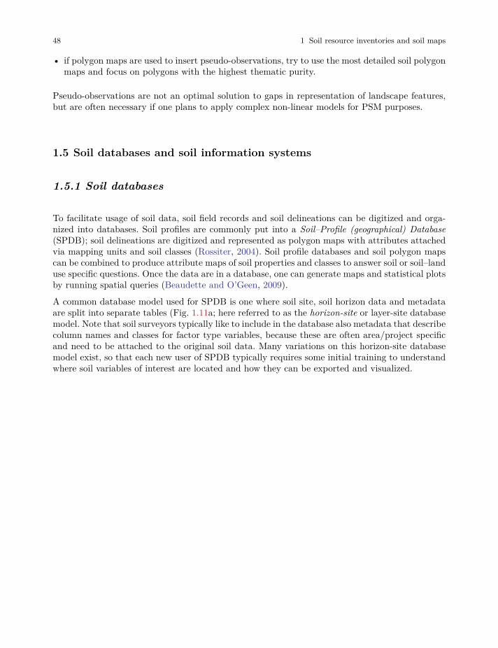
48 1 Soil resource inventories and soil maps
• if polygon maps are used to insert pseudo-observations, try to use the most detailed soil polygonmaps and focus on polygons with the highest thematic purity.
Pseudo-observations are not an optimal solution to gaps in representation of landscape features,but are often necessary if one plans to apply complex non-linear models for PSM purposes.
1.5 Soil databases and soil information systems
1.5.1 Soil databases
To facilitate usage of soil data, soil field records and soil delineations can be digitized and orga-nized into databases. Soil profiles are commonly put into a Soil–Profile (geographical) Database(SPDB); soil delineations are digitized and represented as polygon maps with attributes attachedvia mapping units and soil classes (Rossiter, 2004). Soil profile databases and soil polygon mapscan be combined to produce attribute maps of soil properties and classes to answer soil or soil–landuse specific questions. Once the data are in a database, one can generate maps and statistical plotsby running spatial queries (Beaudette and O’Geen, 2009).
A common database model used for SPDB is one where soil site, soil horizon data and metadataare split into separate tables (Fig. 1.11a; here referred to as the horizon-site or layer-site databasemodel. Note that soil surveyors typically like to include in the database also metadata that describecolumn names and classes for factor type variables, because these are often area/project specificand need to be attached to the original soil data. Many variations on this horizon-site databasemodel exist, so that each new user of SPDB typically requires some initial training to understandwhere soil variables of interest are located and how they can be exported and visualized.
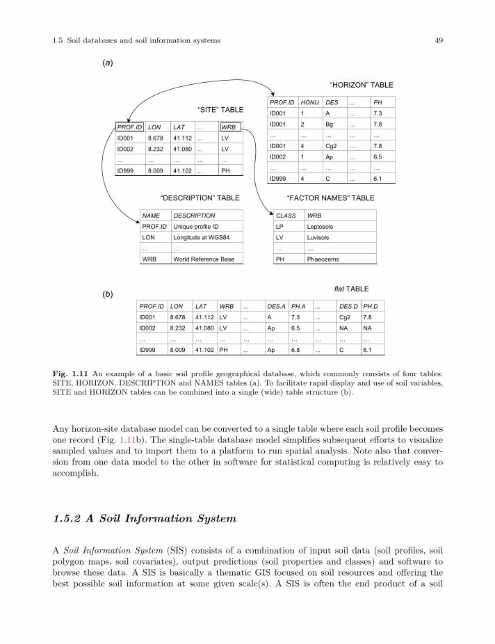
1.5 Soil databases and soil information systems 49
PROF.ID
ID001
ID002
…
ID999
“SITE” TABLE
LON
8.678
8.232
…
8.009
LAT
41.112
41.080
…
41.102
...
...
...
…
...
WRB
LV
LV
…
PH
PROF.ID
ID001
ID001
…
ID001
ID002
…
ID999
“HORIZON” TABLE
HONU
1
2
…
4
1
…
4
DES
A
Bg
…
Cg2
Ap
…
C
...
...
...
…
…
…
…
...
PH
7.3
7.8
…
7.8
6.5
…
6.1
(a)
“DESCRIPTION” TABLE
NAME
PROF.ID
LON
…
WRB
DESCRIPTION
Unique profile ID
Longitude at WGS84
…
World Reference Base
(b)
“FACTOR NAMES” TABLE
CLASS
LP
LV
…
PH
WRB
Leptosols
Luvisols
…
Phaeozems
PROF.ID
ID001
ID002
…
ID999
LON
8.678
8.232
…
8.009
LAT
41.112
41.080
…
41.102
...
...
...
…
...
WRB
LV
LV
…
PH
PH.A
7.3
6.5
…
6.8
DES.A
A
Ap
…
Ap
...
...
...
…
...
PH.D
7.8
NA
…
6.1
DES.D
Cg2
NA
…
C
flat TABLE
Fig. 1.11 An example of a basic soil profile geographical database, which commonly consists of four tables:SITE, HORIZON, DESCRIPTION and NAMES tables (a). To facilitate rapid display and use of soil variables,SITE and HORIZON tables can be combined into a single (wide) table structure (b).
Any horizon-site database model can be converted to a single table where each soil profile becomesone record (Fig. 1.11b). The single-table database model simplifies subsequent efforts to visualizesampled values and to import them to a platform to run spatial analysis. Note also that conver-sion from one data model to the other in software for statistical computing is relatively easy toaccomplish.
1.5.2 A Soil Information System
A Soil Information System (SIS) consists of a combination of input soil data (soil profiles, soilpolygon maps, soil covariates), output predictions (soil properties and classes) and software tobrowse these data. A SIS is basically a thematic GIS focused on soil resources and offering thebest possible soil information at some given scale(s). A SIS is often the end product of a soil

50 1 Soil resource inventories and soil maps
survey. In the ideal case, it should meet some common predefined soil survey specifications, forexample:
• It corresponds to a specified soil survey scale.
• It provides spatial information about a list of targeted soil variables which can be used directlyfor spatial planning and environmental modelling.
• It provides enough meta-information to allow use by a non-soil science specialist.
• It has been cross-checked and validated by an independent assessment.
• It follows national and/or international data standards.
• It has a defined information usage and access policy.
Many soil data production agencies are often unclear about where the work of a soil surveyorstops. Is a SPDB and a soil polygon map an intermediate product or can it be delivered as a soilinformation system? Does a SIS need to already hold all predictions or only inputs to predictionmodels? In this book we will adhere to a strict definition of a SIS as a complete and standardizedgeographical information system that contains both initial inputs and final outputs of spatialpredictions of soil variables, and which is fully documented and ready to be used for spatialplanning. The PSM tools described in this book, in that context, have been designed as a stepforward to producing more complete soil information systems.
A Soil Information System is an end product of soil mapping — a standardized collection of(usually gridded) soil property and class maps of an area that can be used for spatial planning,environmental modelling, agricultural engineering, land degradation studies, biodiversity assess-ment and similar. A SIS tries to provide the best possible soil information at some given scale forthe spatial domain of interest.
Another important point is that a modern SIS needs to be user-oriented. As Campbell (2008)argues: “Soil science, soil classification, mapping and monitoring systems and resources are notends in themselves, they are means to an end. The objective is more sustainable management ofsoil.” We envisage that in the near future soil surveyors will have to completely open soil infor-mation systems to users so that they can also contribute to construction and influence content.Goodchild (2008) calls this “Web 2.0” (read and write) and/or “Web 3.0” (read, write and exe-cute) approaches to content creation. We also envisage that soil information will increasingly beproduced using global vs local models and increasingly using distributed data and computing (Fig.1.12).
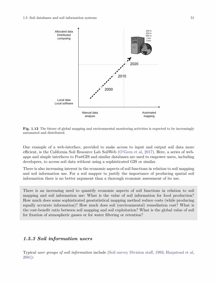
1.5 Soil databases and soil information systems 51
100 m250 m500 m1 km5 km
Manual data analysis
Automated mapping
Local dataLocal software
Allocated dataDistributed computing
Fig. 1.12 The future of global mapping and environmental monitoring activities is expected to be increasinglyautomated and distributed.
One example of a web-interface, provided to make access to input and output soil data moreefficient, is the California Soil Resource Lab SoilWeb (O’Geen et al, 2017). Here, a series of web-apps and simple interfaces to PostGIS and similar databases are used to empower users, includingdevelopers, to access soil data without using a sophisticated GIS or similar.There is also increasing interest in the economic aspects of soil functions in relation to soil mappingand soil information use. For a soil mapper to justify the importance of producing spatial soilinformation there is no better argument than a thorough economic assessment of its use.
There is an increasing need to quantify economic aspects of soil functions in relation to soilmapping and soil information use: What is the value of soil information for food production?How much does some sophisticated geostatistical mapping method reduce costs (while producingequally accurate information)? How much does soil (environmental) remediation cost? What isthe cost-benefit ratio between soil mapping and soil exploitation? What is the global value of soilfor fixation of atmospheric gasses or for water filtering or retention?
1.5.3 Soil information users
Typical user groups of soil information include (Soil survey Division staff, 1993; Harpstead et al,2001):

52 1 Soil resource inventories and soil maps
1. At local/farm level:
1. farmers and ranchers who want to maximize sustainability and/or production efficiency;
2. fertilizer dealers and agricultural consulting companies, who want to sell competitive prod-ucts and services;
3. civil engineers who plan roads, airports and similar;
4. land development agencies who must consider the soil foundations, streets, lawns and e.g. lo-cations for septic systems,
5. bankers and financial agencies who give loans, provide insurance or buy or sell land;
6. foresters who plan harvesting or reforestation operations and must know the relevant condi-tions and capabilities of the soil;
7. tax assessors who assign potential value for a given piece of farmland and/or ranch land;
2. At national level:
1. agricultural ministries and land use planning agencies (for developing and implementingpolicies and plans);
2. environmental protection agencies, who develop and enforce management plans for protectedareas or areas of special value;
3. environmental impact assessment companies and agencies, who model various managementscenarios;
4. agricultural extension agencies;
5. natural hazard (e.g. flooding or landslide) monitoring agencies;
3. At continental or global levels:
1. agricultural development organizations such as FAO, CGIAR (Consortium of InternationalAgricultural Research Centers) research institutes;
2. international environmental protection agencies, such as UNEP;
3. global financial organizations and trading entties, such as the World Bank;
4. global biogeochemical cycle modelers;
5. climate change modelers;
The future for digital soil data may well lie in task-oriented Soil Information Systems (as proposedby Gerard Heuvelink at the DSM 2010 conference in Rome), in which only input data and analyt-ical models are stored, permitting an infinite number of maps and visualizations to be generatedon-demand by users. This implies that future soil mappers will eventually evolve from people thatdraw maps to process moderators, and the maps will evolve from static to interactive, on-demandcreated maps. Likewise, if the soil mapping tools are exposed to the public, anyone will be ableto evolve from a passive user into an active soil mapper. In that sense, there is also an increasingpotential in crowd-sourcing soil mapping to a wider possible community.
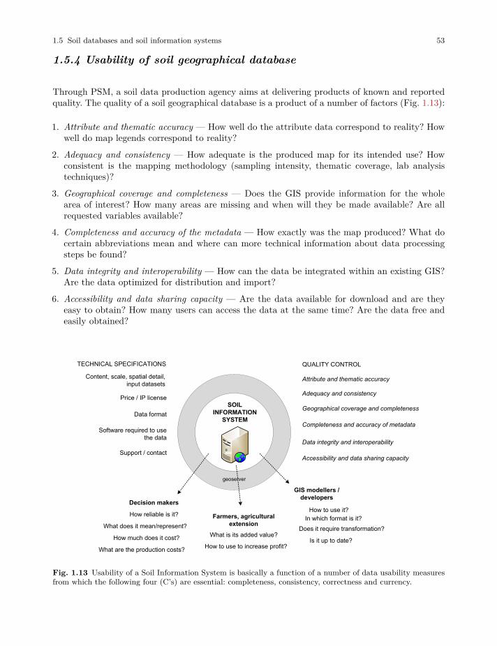
1.5 Soil databases and soil information systems 53
1.5.4 Usability of soil geographical database
Through PSM, a soil data production agency aims at delivering products of known and reportedquality. The quality of a soil geographical database is a product of a number of factors (Fig. 1.13):
1. Attribute and thematic accuracy — How well do the attribute data correspond to reality? Howwell do map legends correspond to reality?
2. Adequacy and consistency — How adequate is the produced map for its intended use? Howconsistent is the mapping methodology (sampling intensity, thematic coverage, lab analysistechniques)?
3. Geographical coverage and completeness — Does the GIS provide information for the wholearea of interest? How many areas are missing and when will they be made available? Are allrequested variables available?
4. Completeness and accuracy of the metadata — How exactly was the map produced? What docertain abbreviations mean and where can more technical information about data processingsteps be found?
5. Data integrity and interoperability — How can the data be integrated within an existing GIS?Are the data optimized for distribution and import?
6. Accessibility and data sharing capacity — Are the data available for download and are theyeasy to obtain? How many users can access the data at the same time? Are the data free andeasily obtained?
Adequacy and consistency
Geographical coverage and completeness
Completeness and accuracy of metadata
Data integrity and interoperability
Accessibility and data sharing capacity
Attribute and thematic accuracy
SOIL
INFORMATION
SYSTEM
How reliable is it?How to use it?
Does it require transformation?
In which format is it?
What does it mean/represent?
How much does it cost?What is its added value?
How to use to increase profit?
Data format
Price / IP license
Software required to use
the data
geoserver
Decision makers
Farmers, agricultural
extension
GIS modellers /
developers
What are the production costs?
TECHNICAL SPECIFICATIONS
Support / contact
Is it up to date?
Content, scale, spatial detail,
input datasets
QUALITY CONTROL
Fig. 1.13 Usability of a Soil Information System is basically a function of a number of data usability measuresfrom which the following four (C’s) are essential: completeness, consistency, correctness and currency.
54 1 Soil resource inventories and soil maps
By maximizing each of the usability measures listed above we can be confident of achieving themaximum quality for output products. In reality, we can only improve each of the listed factorsup to a certain level. Then, due to practical limits, we reach some best possible performance giventhe available funds and methods, beyond which no further improvement is feasible. For example,the capacity to serve geodata is determined by the technical capacity of the server system. Inorder to improve this performance we either have to invest more money to get better computersor re-design the data model so that it is more efficient in fulfilling some operation.
While the objective of PSM (as outlined in this book) is to increase measures such as adequacy,coverage and completeness, inherent properties of the legacy data unfortunately can not be aseasily improved. We can at least assess, and report on, the input data consistency, and evaluateand report the final accuracy of the output products. Once we have estimated the true mappingaccuracy, and under the assumption that mapping accuracy can be linearly improved by increasingthe sampling intensity, we can estimate the total number of additional samples necessary to reacha desired level of accuracy (e.g. even approaching 100% accuracy).
For Keith Shepherd (ICRAF; personal communication) the key to optimization of decision makingis to accurately account for uncertainty — to make sense out of measurements one needs to:
• Know the decision you are trying to make,
• Know the current state of uncertainty (your priors),
• Measure where it matters and only enough to make a sound decision.
The quality of a geospatial database is a function of accuracy, adequacy, consistency, complete-ness, interoperability, accessibility and serving capacity. Each of these usability measures can beoptimized up to a certain level depending on the available resources.
In practice, soil surveyors rarely have the luxury of returning to the field to collect additionalsamples to iteratively improve predictions and maps, but the concept of iterative modeling ofspatial variation is now increasingly accepted.
1.6 Uncertainty of soil variables
1.6.1 Basic concepts
An important aspect of more recent soil mapping projects, such as the GlobalSoilmap project, is acommitment to estimating and reporting the uncertainty associated with all predictions. This is arecent improvement to soil data, as uncertainty in traditional soil maps has often been reported (ifgiven at all) only using global estimates. Maps of uncertainty (confidence limits and/or predictionerror) of soil properties is a new soil data product and there is an increasing demand for suchmaps. But what is ‘uncertainty’ and how do we measure and describe it, particularly for specificpoint locations?
1.6 Uncertainty of soil variables 55
Walker et al (2003) define uncertainty as “any deviation from the unachievable ideal of completelydeterministic knowledge of the relevant system”. The purpose of measurement is to reduce deci-sion uncertainty; the purpose of planning soil sampling campaigns is to find an optimum betweenproject budget and targeted accuracy. A general framework for assessing and representing uncer-tainties in general environmental data is reviewed by Refsgaard et al (2007). In this framework, adistinction is made regarding how uncertainty can be described, i.e. whether this can be done bymeans of:
• probability distributions or upper and lower bounds,
• some qualitative indication of uncertainty,
• or scenarios, in which a partial (not exhaustive) set of possible outcomes is simulated.
Further, the methodological quality of an uncertain variable can be assessed by expert judgement,e.g. whether or not instruments or methods used are reliable and to what degree, or whetheror not an experiment for measuring an uncertain variable was properly conducted. Finally, the“longevity”, or persistence, of uncertain information can be evaluated, i.e. to what extent does theinformation on the uncertainty of a variable change over time.
Estimates of uncertainty of soil property and soil class predictions are an increasingly importantextension to soil mapping outputs. Maps of spatial variation in uncertainty can be submitted asmaps of upper and lower confidence limits, probability distributions or density functions, predictionerror maps and/or equiprobable simulations.
Heuvelink and Brown (2006) observed that soil data are rarely certain or ‘error free’, and theseerrors may be difficult to quantify in practice. Indeed, the quantification of error, defined here asa ‘departure from reality’, implies that the ‘true’ state of the environment is known, which is oftennot possible.
1.6.2 Sources of uncertainty
There are several sources of uncertainty in soil data. For soil profile data the sources of error arefor example:
1. sampling (human) bias or omission of important areas;
2. positioning error (location accuracy);
3. sampling error (at horizon level i.e. in a pit);
4. measurement error (in the laboratory);
5. temporal sampling error (changes in property value with time are ignored);
6. data input error (or typing error);
7. data interpretation error;
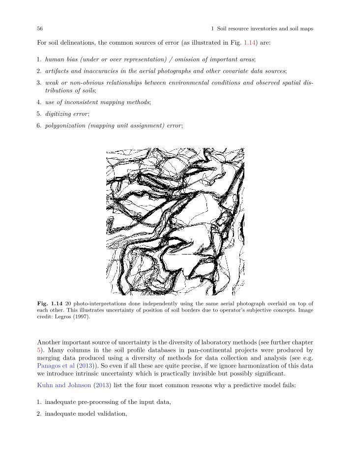
56 1 Soil resource inventories and soil maps
For soil delineations, the common sources of error (as illustrated in Fig. 1.14) are:
1. human bias (under or over representation) / omission of important areas;
2. artifacts and inaccuracies in the aerial photographs and other covariate data sources;
3. weak or non-obvious relationships between environmental conditions and observed spatial dis-tributions of soils;
4. use of inconsistent mapping methods;
5. digitizing error;
6. polygonization (mapping unit assignment) error;
Fig. 1.14 20 photo-interpretations done independently using the same aerial photograph overlaid on top ofeach other. This illustrates uncertainty of position of soil borders due to operator’s subjective concepts. Imagecredit: Legros (1997).
Another important source of uncertainty is the diversity of laboratory methods (see further chapter5). Many columns in the soil profile databases in pan-continental projects were produced bymerging data produced using a diversity of methods for data collection and analysis (see e.g.Panagos et al (2013)). So even if all these are quite precise, if we ignore harmonization of this datawe introduce intrinsic uncertainty which is practically invisible but possibly significant.
Kuhn and Johnson (2013) list the four most common reasons why a predictive model fails:
1. inadequate pre-processing of the input data,
2. inadequate model validation,
1.6 Uncertainty of soil variables 57
3. unjustified extrapolation (application of the model to data that reside in a space unknown tothe model),
4. over-fitting of the model to the existing data.
Each of these is addressed in further chapters and can often be tracked back with repeated modelingand testing.
1.6.3 Quantifying the uncertainty in soil data products
To quantify the uncertainty we must derive probability distributions. There are three main ap-proaches to achieve this (Brus et al, 2011; Heuvelink, 2014):
1. Direct uncertainty quantification through geostatistical modelling of soil properties.
2. Geostatistical modelling of the error in existing soil property maps.
3. Expert judgement/heuristic approaches.
In the first case uncertainty is directly reported by a geostatistical model. However, any model isa simplified representation of reality, and so is the geostatistical model, so that if our assumptionsare incorrect then also the estimate of the uncertainty will be poor. A model-free assessment ofuncertainty can be produced by collecting independent samples, preferably by using some pre-defined probability sampling (Brus et al, 2011). This procedure basically works the same way asfor geostatistical modelling of the soil property itself. The problem with model-free assessmentof uncertainty is that this is often the most expensive approach to quantification of uncertaintyas new soil samples need to be collected. Also, there is a difference between global assessment ofuncertainty and producing maps that depict spatial patterns of uncertainty. To assess mean errorover an entire study area we might need only 50–100 points, but to accurately map the spatialpattern of actual errors we might need an order of magnitude more points.
Uncertainty in soil data products can be quantified either via the geostatistical model, or byusing a model-free assessment of uncertainty (independent validation), or by relying on expertjudgement.
1.6.4 Common uncertainty levels in soil maps
Even small errors can compound and propagate to much larger errors, so that predictions canexceed realistic limits. In some cases, even though we spend significant amounts of money tocollect field data, we can still produce statistically insignificant predictions. For example, imagineif the location accuracy for soil profiles is ±5 km or poorer. Even if all other data collection
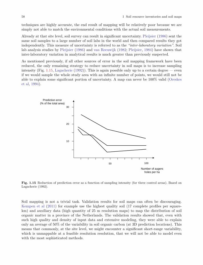
58 1 Soil resource inventories and soil maps
techniques are highly accurate, the end result of mapping will be relatively poor because we aresimply not able to match the environmental conditions with the actual soil measurements.
Already at that site level, soil survey can result in significant uncertainty. Pleijsier (1986) sent thesame soil samples to a large number of soil labs in the world and then compared results they gotindependently. This measure of uncertainty is referred to as the “inter-laboratory variation”. Soillab analysis studies by Pleijsier (1986) and van Reeuwijk (1982; Pleijsier, 1984) have shown thatinter-laboratory variation in analytical results is much greater than previously suspected.
As mentioned previously, if all other sources of error in the soil mapping framework have beenreduced, the only remaining strategy to reduce uncertainty in soil maps is to increase samplingintensity (Fig. 1.15, Lagacherie (1992)). This is again possible only up to a certain degree — evenif we would sample the whole study area with an infinite number of points, we would still not beable to explain some significant portion of uncertainty. A map can never be 100% valid (Oreskeset al, 1994).
Prediction error(% of the total area)
Number of augers holes per ha
10050
10
20
30
Fig. 1.15 Reduction of prediction error as a function of sampling intensity (for three control areas). Based onLagacherie (1992).
Soil mapping is not a trivial task. Validation results for soil maps can often be discouraging.Kempen et al (2011) for example use the highest quality soil (17 complete profiles per square-km) and auxiliary data (high quantity of 25 m resolution maps) to map the distribution of soilorganic matter in a province of the Netherlands. The validation results showed that, even withsuch high quality and density of input data and extensive modeling, they were able to explainonly an average of 50% of the variability in soil organic carbon (at 3D prediction locations). Thismeans that commonly, at the site level, we might encounter a significant short-range variability,which is unmappable at a feasible resolution resolution, that we will not be able to model evenwith the most sophisticated methods.
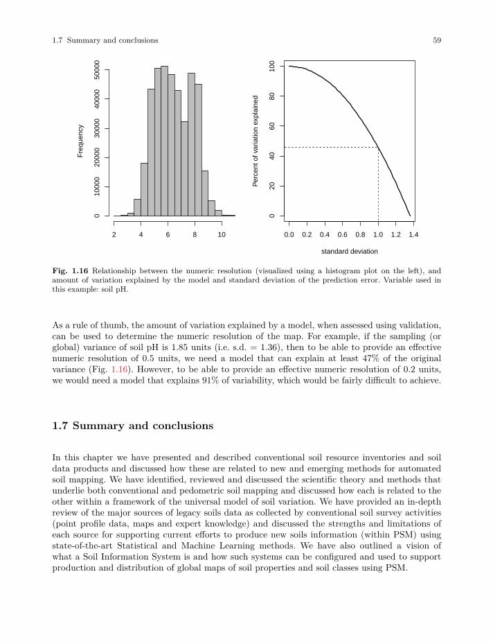
1.7 Summary and conclusions 59
Fre
quen
cy
2 4 6 8 10
010
000
2000
030
000
4000
050
000
0.0 0.2 0.4 0.6 0.8 1.0 1.2 1.4
020
4060
8010
0
standard deviationP
erce
nt o
f var
iatio
n ex
plai
ned
Fig. 1.16 Relationship between the numeric resolution (visualized using a histogram plot on the left), andamount of variation explained by the model and standard deviation of the prediction error. Variable used inthis example: soil pH.
As a rule of thumb, the amount of variation explained by a model, when assessed using validation,can be used to determine the numeric resolution of the map. For example, if the sampling (orglobal) variance of soil pH is 1.85 units (i.e. s.d. = 1.36), then to be able to provide an effectivenumeric resolution of 0.5 units, we need a model that can explain at least 47% of the originalvariance (Fig. 1.16). However, to be able to provide an effective numeric resolution of 0.2 units,we would need a model that explains 91% of variability, which would be fairly difficult to achieve.
1.7 Summary and conclusions
In this chapter we have presented and described conventional soil resource inventories and soildata products and discussed how these are related to new and emerging methods for automatedsoil mapping. We have identified, reviewed and discussed the scientific theory and methods thatunderlie both conventional and pedometric soil mapping and discussed how each is related to theother within a framework of the universal model of soil variation. We have provided an in-depthreview of the major sources of legacy soils data as collected by conventional soil survey activities(point profile data, maps and expert knowledge) and discussed the strengths and limitations ofeach source for supporting current efforts to produce new soils information (within PSM) usingstate-of-the-art Statistical and Machine Learning methods. We have also outlined a vision ofwhat a Soil Information System is and how such systems can be configured and used to supportproduction and distribution of global maps of soil properties and soil classes using PSM.
60 1 Soil resource inventories and soil maps
The main point of this chapter is to provide full documentation of, and justification for, the choicesthat have been made in designing and implementing the PSM framework (a more practical stepson how to organize PSM projects are further given in chapter 8). At present, PSM is designedto produce local to global maps of soil properties and soil classes using legacy soil data (pointprofile data, maps and expert knowledge), along with available global covariate data, as inputsto multi-scale, hierarchical, quantitative, global prediction models. At some future date, it ishoped, and expected, that PSM will be able to make increasing use of newly collected (likelycrowd-sourced) field observations and laboratory analysis data that are accurately geo-referenced,consistent, widespread and of sufficient density to support production of accurate predictions atfiner spatial resolutions (e.g. 10’s to 100’s of m). In the meantime, in order to produce interimproducts immediately, it is necessary, and desirable, to make use of existing legacy soil data andexisting covariates. It is important to acknowledge and understand the capabilities and limitationsof the existing legacy data sources at our disposal presently and of the methods that we currentlypossess to process and use these data.
Each cycle of production in PSM is also a learning cycle that should lead to improved methods,improved products and lower costs. PSM is not a static process but, rather, it is a dynamic endeavormeant to grow, evolve and improve through time. Initial products, produced using existing legacysoil information sources, will increasingly evolve into new products produced using a combinationof existing legacy data and newly collected data.
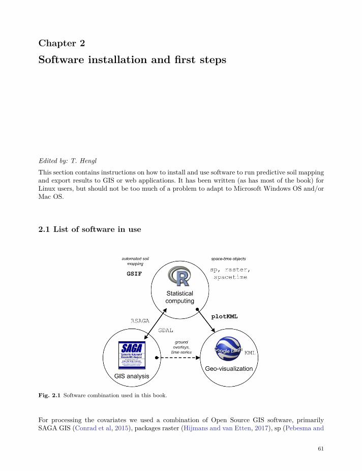
Chapter 2
Software installation and first steps
Edited by: T. HenglThis section contains instructions on how to install and use software to run predictive soil mappingand export results to GIS or web applications. It has been written (as has most of the book) forLinux users, but should not be too much of a problem to adapt to Microsoft Windows OS and/orMac OS.
2.1 List of software in use
Fig. 2.1 Software combination used in this book.
For processing the covariates we used a combination of Open Source GIS software, primarilySAGA GIS (Conrad et al, 2015), packages raster (Hijmans and van Etten, 2017), sp (Pebesma and
61
62 2 Software installation and first steps
Bivand, 2005), and GDAL (Mitchell and GDAL Developers, 2014) for reprojecting, mosaicking andmerging tiles. GDAL and parallel packages in R are highly suitable for processing large volumesof data.
Software required to run all exercises in the book includes:
• R1 or MRO2;
• RStudio3;
• R packages: GSIF, plotKML, aqp, ranger, caret, xgboost, plyr, raster, gstat, randomForest,ggplot2, e1071 (see: how to install R package4)
• SAGA GIS5 (on Windows machines run windows installer);
• Google Earth or Google Earth Pro;
• QGIS6;
• GDAL v2.x7 for Windows machines use e.g. “gdal-*-1800-x64-core.msi“8;
R script used in this tutorial can be downloaded from github9. As a gentle introduction to the Rprogramming language and to soil classes in R we recommend the section 3.7 on importing andusing soil data. Some more examples of SAGA GIS + R usage can be found in the soil covariateschapter. To visualize spatial predictions in a web-browser or Google Earth you can try usingplotKML package (Hengl et al, 2015b). As a gentle introduction to the R programming languageand spatial classes in R we recommend following the Geocomputation with R book10. Obtainingthe R reference card11 is also highly recommended.
2.2 Installing software on Ubuntu OS
On Ubuntu (often the preferred standard for the GIS community) the main required software canbe installed within 10–20 minutes. We start with installing GDAL, proj4 and some packages thatyou might need later on:
1 http://cran.r-project.org/bin/windows/base/2 https://mran.microsoft.com/download/3 http://www.rstudio.com/products/RStudio/4 http://www.r-bloggers.com/installing-r-packages/5 http://sourceforge.net/projects/saga-gis/6 https://qgis.org/en/site/forusers/download.html7 https://trac.osgeo.org/gdal/wiki/DownloadingGdalBinaries8 http://download.gisinternals.com/sdk/downloads/9 https://github.com/envirometrix/PredictiveSoilMapping10 https://geocompr.robinlovelace.net/11 https://cran.r-project.org/doc/contrib/Baggott-refcard-v2.pdf
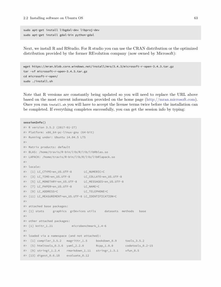
2.2 Installing software on Ubuntu OS 63
sudo apt-get install libgdal-dev libproj-devsudo apt-get install gdal-bin python-gdal
Next, we install R and RStudio. For R studio you can use the CRAN distribution or the optimizeddistribution provided by the former REvolution company (now owned by Microsoft):
wget https://mran.blob.core.windows.net/install/mro/3.4.3/microsoft-r-open-3.4.3.tar.gztar -xf microsoft-r-open-3.4.3.tar.gzcd microsoft-r-open/sudo ./install.sh
Note that R versions are constantly being updated so you will need to replace the URL abovebased on the most current information provided on the home page (http://mran.microsoft.com).Once you run install.sh you will have to accept the license terms twice before the installation canbe completed. If everything completes successfully, you can get the session info by typing:
sessionInfo()#> R version 3.5.2 (2017-01-27)#> Platform: x86_64-pc-linux-gnu (64-bit)#> Running under: Ubuntu 14.04.5 LTS#>#> Matrix products: default#> BLAS: /home/travis/R-bin/lib/R/lib/libRblas.so#> LAPACK: /home/travis/R-bin/lib/R/lib/libRlapack.so#>#> locale:#> [1] LC_CTYPE=en_US.UTF-8 LC_NUMERIC=C#> [3] LC_TIME=en_US.UTF-8 LC_COLLATE=en_US.UTF-8#> [5] LC_MONETARY=en_US.UTF-8 LC_MESSAGES=en_US.UTF-8#> [7] LC_PAPER=en_US.UTF-8 LC_NAME=C#> [9] LC_ADDRESS=C LC_TELEPHONE=C#> [11] LC_MEASUREMENT=en_US.UTF-8 LC_IDENTIFICATION=C#>#> attached base packages:#> [1] stats graphics grDevices utils datasets methods base#>#> other attached packages:#> [1] knitr_1.21 microbenchmark_1.4-6#>#> loaded via a namespace (and not attached):#> [1] compiler_3.5.2 magrittr_1.5 bookdown_0.9 tools_3.5.2#> [5] htmltools_0.3.6 yaml_2.2.0 Rcpp_1.0.0 codetools_0.2-15#> [9] stringi_1.2.4 rmarkdown_1.11 stringr_1.3.1 xfun_0.5#> [13] digest_0.6.18 evaluate_0.12
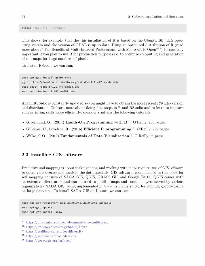
64 2 Software installation and first steps
system("gdalinfo --version")
This shows, for example, that the this installation of R is based on the Ubuntu 16.* LTS oper-ating system and the version of GDAL is up to date. Using an optimized distribution of R (readmore about “The Benefits of Multithreaded Performance with Microsoft R Open”12) is especiallyimportant if you plan to use R for production purposes i.e. to optimize computing and generationof soil maps for large numbers of pixels.
To install RStudio we can run:
sudo apt-get install gdebi-corewget https://download1.rstudio.org/rstudio-1.1.447-amd64.debsudo gdebi rstudio-1.1.447-amd64.debsudo rm rstudio-1.1.447-amd64.deb
Again, RStudio is constantly updated so you might have to obtain the most recent RStudio versionand distribution. To learn more about doing first steps in R and RStudio and to learn to improveyour scripting skills more efficiently, consider studying the following tutorials:
• Grolemund, G., (2014) Hands-On Programming with R13. O’Reilly, 236 pages.
• Gillespie, C., Lovelace, R., (2016) Efficient R programming14. O’Reilly, 222 pages.
• Wilke, C.O., (2019) Fundamentals of Data Visualization15. O’Reilly, in press.
2.3 Installing GIS software
Predictive soil mapping is about making maps, and working with maps requires use of GIS softwareto open, view overlay and analyze the data spatially. GIS software recommended in this book forsoil mapping consists of SAGA GIS, QGIS, GRASS GIS and Google Earth. QGIS comes withan extensive literature16 and can be used to publish maps and combine layers served by variousorganizations. SAGA GIS, being implemented in C++, is highly suited for running geoprocessingon large data sets. To install SAGA GIS on Ubuntu we can use:
sudo add-apt-repository ppa:ubuntugis/ubuntugis-unstablesudo apt-get updatesudo apt-get install saga
12 https://mran.microsoft.com/documents/rro/multithread13 https://rstudio-education.github.io/hopr/14 https://csgillespie.github.io/efficientR/15 https://serialmentor.com/dataviz/16 https://www.qgis.org/en/docs/
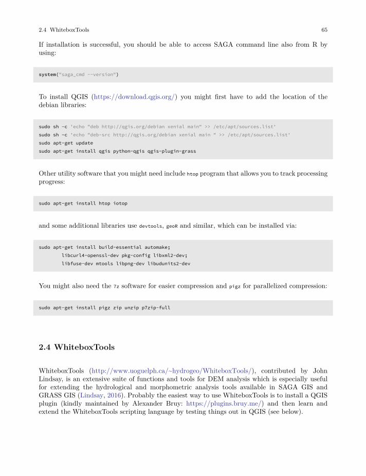
2.4 WhiteboxTools 65
If installation is successful, you should be able to access SAGA command line also from R byusing:
system("saga_cmd --version")
To install QGIS (https://download.qgis.org/) you might first have to add the location of thedebian libraries:
sudo sh -c 'echo "deb http://qgis.org/debian xenial main" >> /etc/apt/sources.list'sudo sh -c 'echo "deb-src http://qgis.org/debian xenial main " >> /etc/apt/sources.list'sudo apt-get updatesudo apt-get install qgis python-qgis qgis-plugin-grass
Other utility software that you might need include htop program that allows you to track processingprogress:
sudo apt-get install htop iotop
and some additional libraries use devtools, geoR and similar, which can be installed via:
sudo apt-get install build-essential automake;libcurl4-openssl-dev pkg-config libxml2-dev;libfuse-dev mtools libpng-dev libudunits2-dev
You might also need the 7z software for easier compression and pigz for parallelized compression:
sudo apt-get install pigz zip unzip p7zip-full
2.4 WhiteboxTools
WhiteboxTools (http://www.uoguelph.ca/~hydrogeo/WhiteboxTools/), contributed by JohnLindsay, is an extensive suite of functions and tools for DEM analysis which is especially usefulfor extending the hydrological and morphometric analysis tools available in SAGA GIS andGRASS GIS (Lindsay, 2016). Probably the easiest way to use WhiteboxTools is to install a QGISplugin (kindly maintained by Alexander Bruy: https://plugins.bruy.me/) and then learn andextend the WhiteboxTools scripting language by testing things out in QGIS (see below).
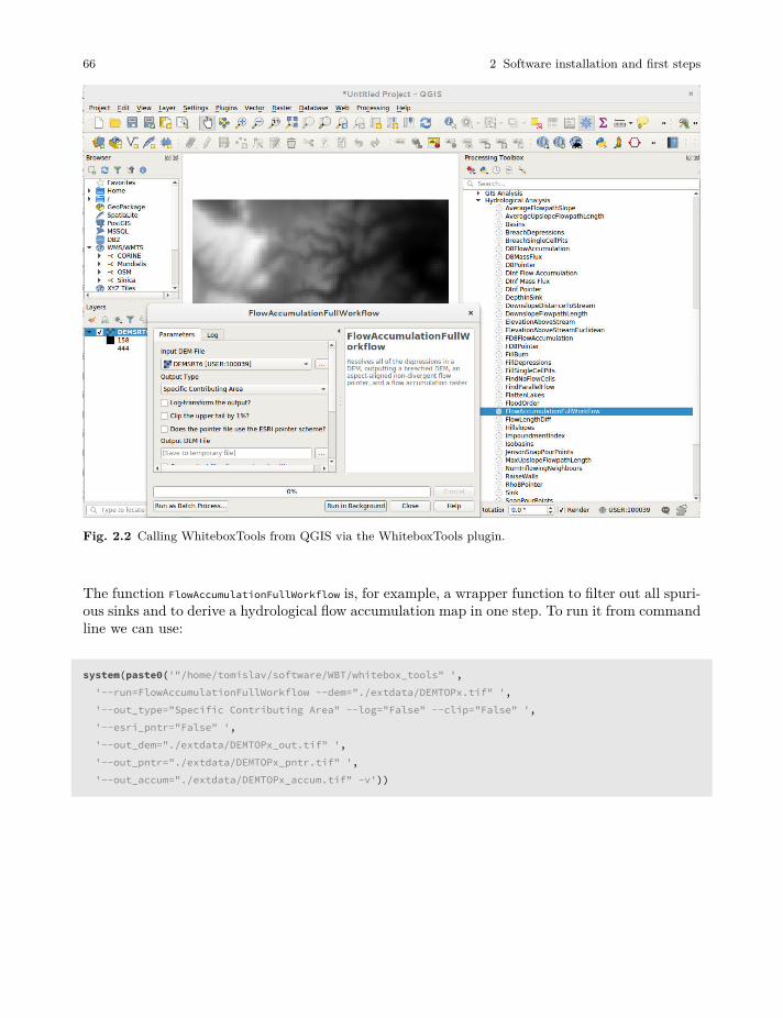
66 2 Software installation and first steps
Fig. 2.2 Calling WhiteboxTools from QGIS via the WhiteboxTools plugin.
The function FlowAccumulationFullWorkflow is, for example, a wrapper function to filter out all spuri-ous sinks and to derive a hydrological flow accumulation map in one step. To run it from commandline we can use:
system(paste0('"/home/tomislav/software/WBT/whitebox_tools" ','--run=FlowAccumulationFullWorkflow --dem="./extdata/DEMTOPx.tif" ','--out_type="Specific Contributing Area" --log="False" --clip="False" ','--esri_pntr="False" ','--out_dem="./extdata/DEMTOPx_out.tif" ','--out_pntr="./extdata/DEMTOPx_pntr.tif" ','--out_accum="./extdata/DEMTOPx_accum.tif" -v'))
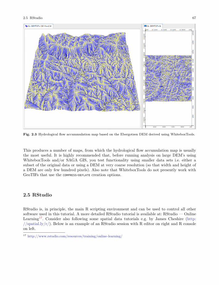
2.5 RStudio 67
Fig. 2.3 Hydrological flow accummulation map based on the Ebergotzen DEM derived using WhiteboxTools.
This produces a number of maps, from which the hydrological flow accumulation map is usuallythe most useful. It is highly recommended that, before running analysis on large DEM’s usingWhiteboxTools and/or SAGA GIS, you test functionality using smaller data sets i.e. either asubset of the original data or using a DEM at very coarse resolution (so that width and height ofa DEM are only few hundred pixels). Also note that WhiteboxTools do not presently work withGeoTIFs that use the COMPRESS=DEFLATE creation options.
2.5 RStudio
RStudio is, in principle, the main R scripting environment and can be used to control all othersoftware used in this tutorial. A more detailed RStudio tutorial is available at: RStudio — OnlineLearning17. Consider also following some spatial data tutorials e.g. by James Cheshire (http://spatial.ly/r/). Below is an example of an RStudio session with R editor on right and R consoleon left.17 http://www.rstudio.com/resources/training/online-learning/
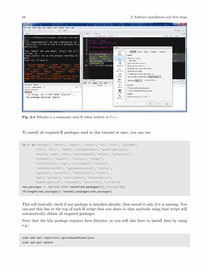
68 2 Software installation and first steps
Fig. 2.4 RStudio is a commonly used R editor written in C++.
To install all required R packages used in this tutorial at once, you can use:
ls <- c("reshape", "Hmisc", "rgdal", "raster", "sf", "GSIF", "plotKML","nnet", "plyr", "ROCR", "randomForest", "quantregForest","psych", "mda", "h2o", "h2oEnsemble", "dismo", "grDevices","snowfall", "hexbin", "lattice", "ranger","soiltexture", "aqp", "colorspace", "Cubist","randomForestSRC", "ggRandomForests", "scales","xgboost", "parallel", "doParallel", "caret","gam", "glmnet", "matrixStats", "SuperLearner","quantregForest", "intamap", "fasterize", "viridis")
new.packages <- ls[!(ls %in% installed.packages()[,"Package"])]if(length(new.packages)) install.packages(new.packages)
This will basically check if any package is installed already, then install it only if it is missing. Youcan put this line at the top of each R script that you share so that anybody using that script willautomatically obtain all required packages.
Note that the h2o package requires Java libraries, so you will also have to install Java by usinge.g.:
sudo add-apt-repository ppa:webupd8team/javasudo apt-get update
2.6 plotKML and GSIF packages 69
sudo apt-get install oracle-java8-installerjava -version
2.6 plotKML and GSIF packages
Many examples in this tutorial rely on the top 5 most commonly used packages for spatial data:(1) sp and rgdal18, (2) raster19, (3) plotKML20 and (4) GSIF21. To install the most up-to-dateversion of plotKML/GSIF, you can also use the R-Forge versions of the package:
if(!require(GSIF)){install.packages("GSIF", repos=c("http://R-Forge.R-project.org"),
type = "source", dependencies = TRUE)}#> Loading required package: GSIF#> GSIF version 0.5-5 (2019-01-04)#> URL: http://gsif.r-forge.r-project.org/
A copy of the most-up-to-date and stable versions of plotKML and GSIF is also available ongithub22. To run only some specific function from the GSIF package you can do e.g.:
source_https <- function(url, ...) {# load packagerequire(RCurl)# download:cat(getURL(url, followlocation = TRUE,
cainfo = system.file("CurlSSL", "cacert.pem", package = "RCurl")),file = basename(url))
source(basename(url))}source_https("https://raw.githubusercontent.com/cran/GSIF/master/R/OCSKGM.R")
To test if these packages work properly, create soil maps and visualize them in Google Earth byrunning the following lines of code (see also function: fit.gstatModel23):
18 https://cran.r-project.org/web/views/Spatial.html19 https://cran.r-project.org/web/packages/raster/20 http://plotkml.r-forge.r-project.org/21 http://gsif.r-forge.r-project.org/22 https://github.com/cran/GSIF23 http://gsif.r-forge.r-project.org/fit.gstatModel.html
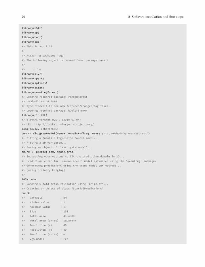
70 2 Software installation and first steps
library(GSIF)library(sp)library(boot)library(aqp)#> This is aqp 1.17#>#> Attaching package: 'aqp'#> The following object is masked from 'package:base':#>#> unionlibrary(plyr)library(rpart)library(splines)library(gstat)library(quantregForest)#> Loading required package: randomForest#> randomForest 4.6-14#> Type rfNews() to see new features/changes/bug fixes.#> Loading required package: RColorBrewerlibrary(plotKML)#> plotKML version 0.5-9 (2019-01-04)#> URL: http://plotkml.r-forge.r-project.org/demo(meuse, echo=FALSE)omm <- fit.gstatModel(meuse, om~dist+ffreq, meuse.grid, method="quantregForest")#> Fitting a Quantile Regression Forest model...#> Fitting a 2D variogram...#> Saving an object of class 'gstatModel'...om.rk <- predict(omm, meuse.grid)#> Subsetting observations to fit the prediction domain in 2D...#> Prediction error for 'randomForest' model estimated using the 'quantreg' package.#> Generating predictions using the trend model (RK method)...#> [using ordinary kriging]#>100% done#> Running 5-fold cross validation using 'krige.cv'...#> Creating an object of class "SpatialPredictions"om.rk#> Variable : om#> Minium value : 1#> Maximum value : 17#> Size : 153#> Total area : 4964800#> Total area (units) : square-m#> Resolution (x) : 40#> Resolution (y) : 40#> Resolution (units) : m#> Vgm model : Exp
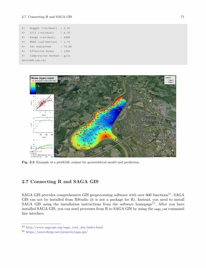
2.7 Connecting R and SAGA GIS 71
#> Nugget (residual) : 2.32#> Sill (residual) : 4.76#> Range (residual) : 2930#> RMSE (validation) : 1.75#> Var explained : 73.8%#> Effective bytes : 1202#> Compression method : gzip#plotKML(om.rk)
Fig. 2.5 Example of a plotKML output for geostatistical model and prediction.
2.7 Connecting R and SAGA GIS
SAGA GIS provides comprehensive GIS geoprocessing software with over 600 functions24. SAGAGIS can not be installed from RStudio (it is not a package for R). Instead, you need to installSAGA GIS using the installation instructions from the software homepage25. After you haveinstalled SAGA GIS, you can send processes from R to SAGA GIS by using the saga_cmd commandline interface:
24 http://www.saga-gis.org/saga_tool_doc/index.html25 https://sourceforge.net/projects/saga-gis/
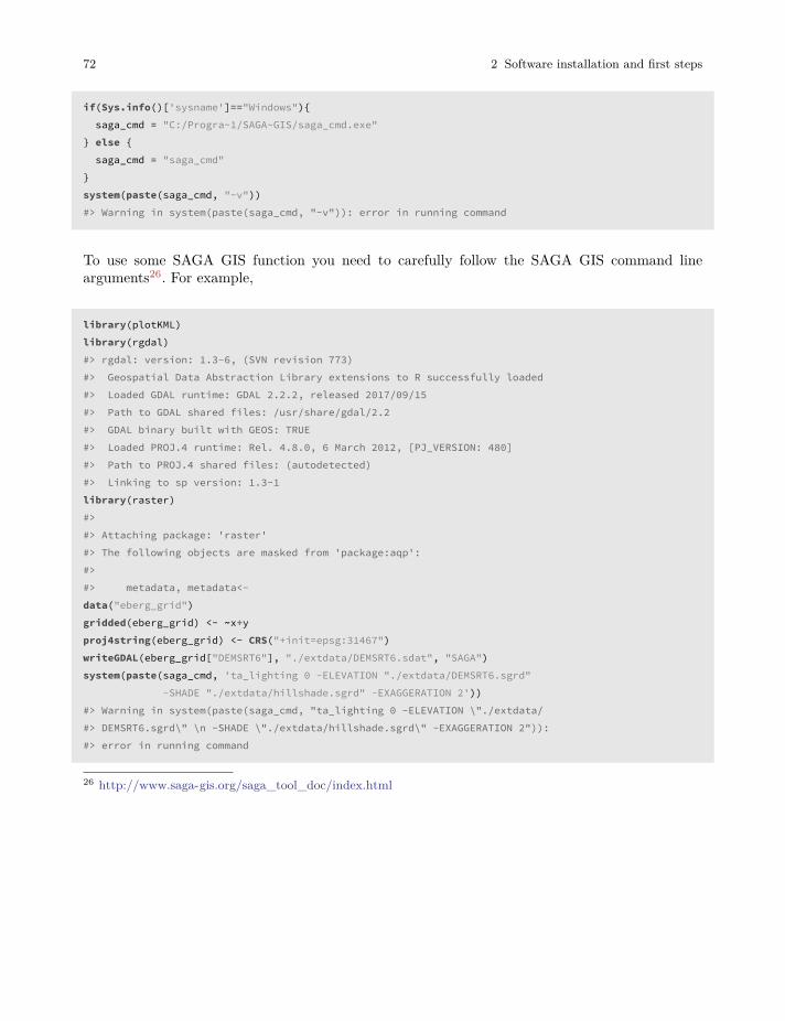
72 2 Software installation and first steps
if(Sys.info()['sysname']=="Windows"){saga_cmd = "C:/Progra~1/SAGA-GIS/saga_cmd.exe"
} else {saga_cmd = "saga_cmd"
}system(paste(saga_cmd, "-v"))#> Warning in system(paste(saga_cmd, "-v")): error in running command
To use some SAGA GIS function you need to carefully follow the SAGA GIS command linearguments26. For example,
library(plotKML)library(rgdal)#> rgdal: version: 1.3-6, (SVN revision 773)#> Geospatial Data Abstraction Library extensions to R successfully loaded#> Loaded GDAL runtime: GDAL 2.2.2, released 2017/09/15#> Path to GDAL shared files: /usr/share/gdal/2.2#> GDAL binary built with GEOS: TRUE#> Loaded PROJ.4 runtime: Rel. 4.8.0, 6 March 2012, [PJ_VERSION: 480]#> Path to PROJ.4 shared files: (autodetected)#> Linking to sp version: 1.3-1library(raster)#>#> Attaching package: 'raster'#> The following objects are masked from 'package:aqp':#>#> metadata, metadata<-data("eberg_grid")gridded(eberg_grid) <- ~x+yproj4string(eberg_grid) <- CRS("+init=epsg:31467")writeGDAL(eberg_grid["DEMSRT6"], "./extdata/DEMSRT6.sdat", "SAGA")system(paste(saga_cmd, 'ta_lighting 0 -ELEVATION "./extdata/DEMSRT6.sgrd"
-SHADE "./extdata/hillshade.sgrd" -EXAGGERATION 2'))#> Warning in system(paste(saga_cmd, "ta_lighting 0 -ELEVATION \"./extdata/#> DEMSRT6.sgrd\" \n -SHADE \"./extdata/hillshade.sgrd\" -EXAGGERATION 2")):#> error in running command
26 http://www.saga-gis.org/saga_tool_doc/index.html
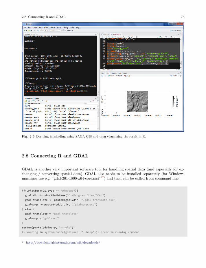
2.8 Connecting R and GDAL 73
Fig. 2.6 Deriving hillshading using SAGA GIS and then visualizing the result in R.
2.8 Connecting R and GDAL
GDAL is another very important software tool for handling spatial data (and especially for ex-changing / converting spatial data). GDAL also needs to be installed separately (for Windowsmachines use e.g. “gdal-201-1800-x64-core.msi”27) and then can be called from command line:
if(.Platform$OS.type == "windows"){gdal.dir <- shortPathName("C:/Program files/GDAL")gdal_translate <- paste0(gdal.dir, "/gdal_translate.exe")gdalwarp <- paste0(gdal.dir, "/gdalwarp.exe")
} else {gdal_translate = "gdal_translate"gdalwarp = "gdalwarp"
}system(paste(gdalwarp, "--help"))#> Warning in system(paste(gdalwarp, "--help")): error in running command
27 http://download.gisinternals.com/sdk/downloads/
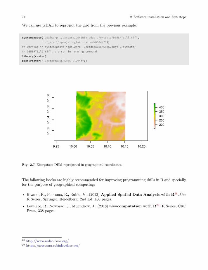
74 2 Software installation and first steps
We can use GDAL to reproject the grid from the previous example:
system(paste('gdalwarp ./extdata/DEMSRT6.sdat ./extdata/DEMSRT6_ll.tif','-t_srs \"+proj=longlat +datum=WGS84\"'))
#> Warning in system(paste("gdalwarp ./extdata/DEMSRT6.sdat ./extdata/#> DEMSRT6_ll.tif", : error in running commandlibrary(raster)plot(raster("./extdata/DEMSRT6_ll.tif"))
9.95 10.00 10.05 10.10 10.15 10.20
51.5
251
.54
51.5
651
.58
200250300350400
Fig. 2.7 Ebergotzen DEM reprojected in geographical coordinates.
The following books are highly recommended for improving programming skills in R and speciallyfor the purpose of geographical computing:
• Bivand, R., Pebesma, E., Rubio, V., (2013) Applied Spatial Data Analysis with R28. UseR Series, Springer, Heidelberg, 2nd Ed. 400 pages.
• Lovelace, R., Nowosad, J., Muenchow, J., (2018) Geocomputation with R29. R Series, CRCPress, 338 pages.
28 http://www.asdar-book.org/29 https://geocompr.robinlovelace.net/
Chapter 3
Soil observations and variables
Edited by: Hengl T., MacMillan R.A. and Leenaars J.G.B.This chapter identifies and provides comprehensive definitions and descriptions for a standardizedset of soil properties (and classes), which are commonly predicted using PSM. We first discussthe complexity of measuring and standardizing (or harmonizing) soil attributes, then focus on thekey soil properties and classes of interest for global soil mapping. The purpose of this chapter isto serve as a reference, and background, for other chapters where the focus is on generating soilmaps, interpreting accuracy results and similar.Please note that this chapter draws extensively from materials previously published as part ofthe specifications for the GlobalSoilMap project (Arrouays et al, 2014b). Large blocks of textextracted verbatum from these prevously published GlobalSoilMap specifications were, in fact,originally largely composed and written by the second author of this chapter in his former role asScience Coordinator for the GlobalSoilMap project (www.globalsoilmap.net). We acknowledge thesource of much of the content of this chapter as having originated from the previously publishedGlobalSoilMap specifications.The R tutorial at the end of the chaper reviews soil data classes and functions for R. It illustrateshow to organize and reformat soil data in R for spatial analysis, how to import soil data into R andhow to export data and plot it in Google Earth. To learn more about the Global Soil InformationFacilities (GSIF) package, visit the main documentation page (http://gsif.r-forge.r-project.org/).
3.1 Basic concepts
3.1.1 Types of soil observations
As mentioned in the previous chapter, values for soil properties or attributes are obtained throughobservation and/or measurement of a soil feature, using a specified method. We refer to observa-tions and measurements of the characteristics of soil properties and/or feature attributes as soilobservations (see also the Observation and Measurements OGC standard1; ISO/DIS 19156). From1 http://www.opengeospatial.org/standards/om
75
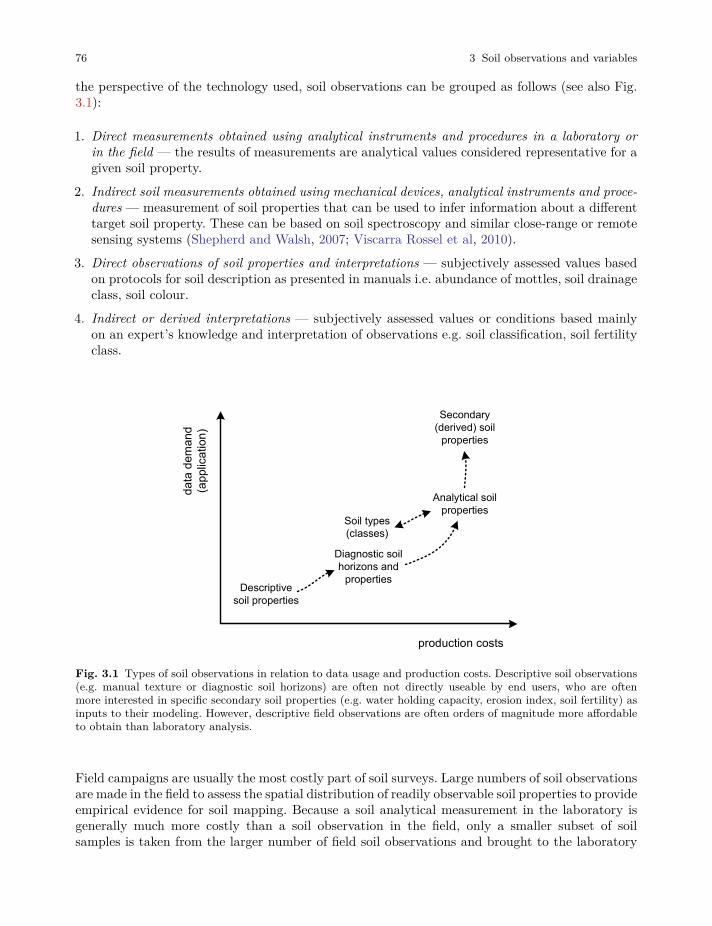
76 3 Soil observations and variables
the perspective of the technology used, soil observations can be grouped as follows (see also Fig.3.1):
1. Direct measurements obtained using analytical instruments and procedures in a laboratory orin the field — the results of measurements are analytical values considered representative for agiven soil property.
2. Indirect soil measurements obtained using mechanical devices, analytical instruments and proce-dures — measurement of soil properties that can be used to infer information about a differenttarget soil property. These can be based on soil spectroscopy and similar close-range or remotesensing systems (Shepherd and Walsh, 2007; Viscarra Rossel et al, 2010).
3. Direct observations of soil properties and interpretations — subjectively assessed values basedon protocols for soil description as presented in manuals i.e. abundance of mottles, soil drainageclass, soil colour.
4. Indirect or derived interpretations — subjectively assessed values or conditions based mainlyon an expert’s knowledge and interpretation of observations e.g. soil classification, soil fertilityclass.
Descriptive
soil properties
Diagnostic soil
horizons and
properties
Soil types
(classes)
Analytical soil
properties
data demand
(application)
production costs
Secondary
(derived) soil
properties
Fig. 3.1 Types of soil observations in relation to data usage and production costs. Descriptive soil observations(e.g. manual texture or diagnostic soil horizons) are often not directly useable by end users, who are oftenmore interested in specific secondary soil properties (e.g. water holding capacity, erosion index, soil fertility) asinputs to their modeling. However, descriptive field observations are often orders of magnitude more affordableto obtain than laboratory analysis.
Field campaigns are usually the most costly part of soil surveys. Large numbers of soil observationsare made in the field to assess the spatial distribution of readily observable soil properties to provideempirical evidence for soil mapping. Because a soil analytical measurement in the laboratory isgenerally much more costly than a soil observation in the field, only a smaller subset of soilsamples is taken from the larger number of field soil observations and brought to the laboratory
3.1 Basic concepts 77
for subsequent analysis. Ideally, every soil observation would be accompanied by correspondingsoil analytical measurements to produce the most accurate and comprehensive soil informationpossible.
Soil can be assessed quantitatively based on direct or indirect measurements using analyticaltechniques (in a laboratory or in the field) and qualitatively or descriptively based on observationsin the field that adhere to some soil description guidelines. Examples of subjective observationsare: diagnostic soil materials and horizons, soil classes, Munsell color classes, manual textureassessment (texture-by-hand), structure, compaction, root abundance and similar.
It is important to emphasize that soil properties, and the methods used to assess soil properties,are two distinctly different concepts. The two can be defined together (functional definition) or canbe defined separately, as given by numerous national and international manuals and guidelines foranalytical procedures and soil description: e.g. in Natural Resources Conservation Service (2004;Carter and Gregorich, 2007; Food and of the United Nations, 2006), and/or Van Reeuwijk (2002).In this chapter we also make a distinction between the ‘targeted variable’ (targeted soil properties)and ‘paths’ (determination methods).
Soil analytical data obtained in a laboratory are typically an order of magnitude more expensive toproduce than descriptive field observations (Burrough et al, 1971; Gehl and Rice, 2007; Kempen,2011). To reduce these high costs, surveyors collect descriptive soil observations (Fig. 3.1), whichcan subsequently be interpreted and linked to soil types and soil classes, which are then assumedto be characterised by a limited and definable range of soil properties (Bouma et al, 1998). It isalso possible to convert observed values for certain soil properties to values comparable to thosemeasured by analytical methods (albeit with unknown precision) by using various calibrationmodels or conversion functions. For example, manual texturing analysis (FAO, 1990; Soil surveyDivision staff, 1993) can be used as a basis for estimating soil texture fractions with a precisionof ±5 % at fraction of the cost of laboratory analysis.
Soils are usually sampled per depth interval or layer, generally using a genetic A-B-C-R systemi.e. corresponding to a soil horizon — a relatively homogeneous layer of soil (with upper andlower depth) that is “distinctly different from other layers and informative for the soil’s nature”(Harpstead et al, 2001). Actual soil samples are either taken from the centre of a soil horizon orare mixed samples of the material from the whole horizon (Fig. 3.2). Decades of soil survey haveshown that soil horizons can be fuzzy objects. They may be difficult for different surveyors todistinguish and delineate consistently (Burrough, 1989; de Gruijter et al, 1997). Soil correlationexercises try (not always successfully) to help different surveyors consistently recognize similar soilhorizons and assign similar codes with comparable upper and lower boundaries so as to producesimilar descriptions and classifications for any observed soil.
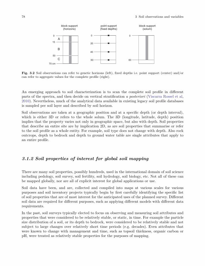
78 3 Soil observations and variables
A
B
C
0 0 0
1520
50
40
70 cm
60 60
block support(horizons)
point support(fixed depths)
block support(solum)
Fig. 3.2 Soil observations can refer to genetic horizons (left), fixed depths i.e. point support (center) and/orcan refer to aggregate values for the complete profile (right).
An emerging approach to soil characterization is to scan the complete soil profile in differentparts of the spectra, and then decide on vertical stratification a posteriori (Viscarra Rossel et al,2010). Nevertheless, much of the analytical data available in existing legacy soil profile databasesis sampled per soil layer and described by soil horizon.
Soil observations are taken at a geographic position and at a specific depth (or depth interval),which is either 3D or refers to the whole solum. The 3D (longitude, latitude, depth) positionimplies that the property varies not only in geographic space, but also with depth. Soil propertiesthat describe an entire site are by implication 2D, as are soil properties that summarise or referto the soil profile as a whole entity. For example, soil type does not change with depth. Also rockoutcrops, depth to bedrock and depth to ground water table are single attributes that apply toan entire profile.
3.1.2 Soil properties of interest for global soil mapping
There are many soil properties, possibly hundreds, used in the international domain of soil scienceincluding pedology, soil survey, soil fertility, soil hydrology, soil biology, etc. Not all of these canbe mapped globally, nor are all of explicit interest for global applications or use.
Soil data have been, and are, collected and compiled into maps at various scales for variouspurposes and soil inventory projects typically begin by first carefully identifying the specific listof soil properties that are of most interest for the anticipated uses of the planned survey. Differentsoil data are required for different purposes, such as applying different models with different datarequirements.
In the past, soil surveys typically elected to focus on observing and measuring soil attributes andproperties that were considered to be relatively stable, or static, in time. For example the particlesize distribution of a soil, or its depth to bedrock, were considered to be relatively stable and notsubject to large changes over relatively short time periods (e.g. decades). Even attributes thatwere known to change with management and time, such as topsoil thickness, organic carbon orpH, were treated as relatively stable properties for the purposes of mapping.
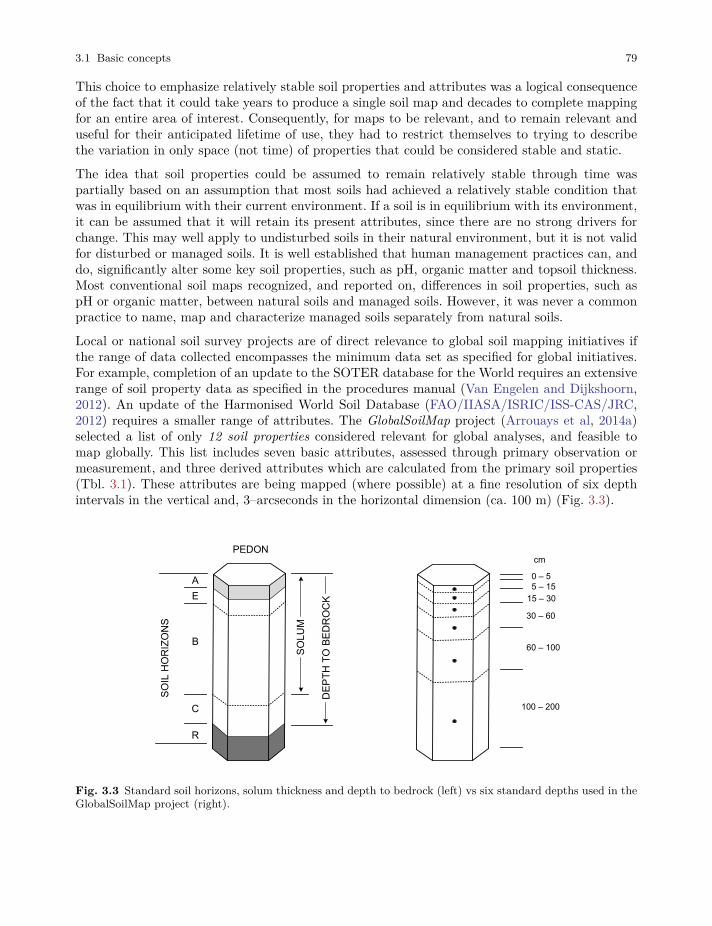
3.1 Basic concepts 79
This choice to emphasize relatively stable soil properties and attributes was a logical consequenceof the fact that it could take years to produce a single soil map and decades to complete mappingfor an entire area of interest. Consequently, for maps to be relevant, and to remain relevant anduseful for their anticipated lifetime of use, they had to restrict themselves to trying to describethe variation in only space (not time) of properties that could be considered stable and static.
The idea that soil properties could be assumed to remain relatively stable through time waspartially based on an assumption that most soils had achieved a relatively stable condition thatwas in equilibrium with their current environment. If a soil is in equilibrium with its environment,it can be assumed that it will retain its present attributes, since there are no strong drivers forchange. This may well apply to undisturbed soils in their natural environment, but it is not validfor disturbed or managed soils. It is well established that human management practices can, anddo, significantly alter some key soil properties, such as pH, organic matter and topsoil thickness.Most conventional soil maps recognized, and reported on, differences in soil properties, such aspH or organic matter, between natural soils and managed soils. However, it was never a commonpractice to name, map and characterize managed soils separately from natural soils.
Local or national soil survey projects are of direct relevance to global soil mapping initiatives ifthe range of data collected encompasses the minimum data set as specified for global initiatives.For example, completion of an update to the SOTER database for the World requires an extensiverange of soil property data as specified in the procedures manual (Van Engelen and Dijkshoorn,2012). An update of the Harmonised World Soil Database (FAO/IIASA/ISRIC/ISS-CAS/JRC,2012) requires a smaller range of attributes. The GlobalSoilMap project (Arrouays et al, 2014a)selected a list of only 12 soil properties considered relevant for global analyses, and feasible tomap globally. This list includes seven basic attributes, assessed through primary observation ormeasurement, and three derived attributes which are calculated from the primary soil properties(Tbl. 3.1). These attributes are being mapped (where possible) at a fine resolution of six depthintervals in the vertical and, 3–arcseconds in the horizontal dimension (ca. 100 m) (Fig. 3.3).
SOLUM
A
E
B
C
R
SOIL HORIZONS
PEDON
DEPTH TO BEDROCK
0 – 5
5 – 15
15 – 30
30 – 60
60 – 100
100 – 200
cm
Fig. 3.3 Standard soil horizons, solum thickness and depth to bedrock (left) vs six standard depths used in theGlobalSoilMap project (right).
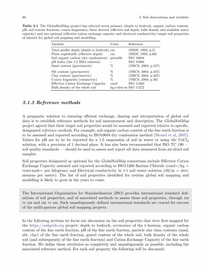
80 3 Soil observations and variables
Table 3.1 The GlobalSoilMap project has selected seven primary (depth to bedrock, organic carbon content,pH, soil texture fractions, coarse fragments), three derived (effective soil depth, bulk density and available watercapacity) and two optional (effective cation exchange capacity and electrical conductivity) target soil propertiesof interest for global soil mapping and modelling.
Variable Units ReferenceTotal profile depth (depth to bedrock) cm (SSDS, 1993; p.5)Plant exploitable (effective depth) cm (SSDS, 1993; p.60)Soil organic carbon (dry combustion) permille ISO 10694pH index (the 1:5 H2O solution) – ISO 10390Sand content (gravimetric) % (NRCS, 2004; p.347)Silt content (gravimetric) % (NRCS, 2004; p.347)Clay content (gravimetric) % (NRCS, 2004; p.347)Coarse fragments (volumetric) % (NRCS, 2004; p.36)Effective Cation Exchange Capacity cmol ISO 11260Bulk density of the whole soil kg/cubic-m ISO 11272
3.1.3 Reference methods
A pragmatic solution to ensuring efficient exchange, sharing and interpretation of global soildata is to establish reference methods for soil measurement and description. The GlobalSoilMapproject agreed that their target soil properties would be assessed and reported relative to specific,designated reference methods. For example, soil organic carbon content of the fine earth fraction isto be assessed and reported according to ISO10694 dry combustion method (Sleutel et al, 2007).Values for pH are to be be reported for a 1:5 suspension of soil in water or using the CaCl2solution, with a precision of 1 decimal place. It has also been recommended that ISO TC 190 —soil quality standards — should be used to assess and report all data measured from air-dried soilsamples.
Soil properties designated as optional for the GlobalSoilMap consortium include Effective CationExchange Capacity assessed and reported according to ISO11260 Barium Chloride (cmol+/kg =centi-mole+ per kilogram) and Electrical conductivity in 1:1 soil–water solution (dS/m = deci-siemens per metre). The list of soil properties identified for routine global soil mapping andmodelling is likely to grow in the years to come.
The International Organisation for Standardisation (ISO) provides international standard defi-nitions of soil properties, and of associated methods to assess those soil properties, through ISOTC-190 and ISO TC-345. Such unambiguously defined international standards are crucial for successof the multi-partner global soil mapping projects.
In the following sections we focus our discussion on the soil properties that were first mapped forthe https://soilgrids.org project: depth to bedrock, occurrence of the R horizon, organic carboncontent of the fine earth fraction, pH of the fine earth fraction, particle size class contents (sand,silt, clay) of the fine earth fraction, gravel content of the whole soil, bulk density of the wholesoil (and subsequently of the fine earth fraction) and Cation Exchange Capacity of the fine earthfraction. We define those attributes as completely and unambiguously as possible, including theassociated reference method. For each soil property the following will be discussed:
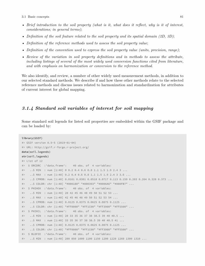
3.1 Basic concepts 81
• Brief introduction to the soil property (what is it, what does it reflect, why is it of interest,considerations; in general terms);
• Definition of the soil feature related to the soil property and its spatial domain (2D, 3D);
• Definition of the reference methods used to assess the soil property value;
• Definition of the convention used to express the soil property value (units, precision, range);
• Review of the variation in soil property definitions and in methods to assess the attribute,including listings of several of the most widely used conversion functions cited from literature,and with emphasis on harmonization or conversion to the reference method.
We also identify, and review, a number of other widely used measurement methods, in addition toour selected standard methods. We describe if and how these other methods relate to the selectedreference methods and discuss issues related to harmonization and standardization for attributesof current interest for global mapping.
3.1.4 Standard soil variables of interest for soil mapping
Some standard soil legends for listed soil properties are embedded within the GSIF package andcan be loaded by:
library(GSIF)#> GSIF version 0.5-5 (2019-01-04)#> URL: http://gsif.r-forge.r-project.org/data(soil.legends)str(soil.legends)#> List of 12#> $ ORCDRC :'data.frame': 40 obs. of 4 variables:#> ..$ MIN : num [1:40] 0 0.2 0.4 0.6 0.8 1.1 1.5 1.9 2.4 3 ...#> ..$ MAX : num [1:40] 0.2 0.4 0.6 0.8 1.1 1.5 1.9 2.4 3 3.6 ...#> ..$ CPROB: num [1:40] 0.0161 0.0301 0.0518 0.0717 0.113 0.159 0.203 0.264 0.328 0.373 ...#> ..$ COLOR: chr [1:40] "#000180" "#000393" "#0006A6" "#000FB7" ...#> $ PHIHOX :'data.frame': 40 obs. of 4 variables:#> ..$ MIN : num [1:40] 20 42 45 46 48 49 50 51 52 53 ...#> ..$ MAX : num [1:40] 42 45 46 48 49 50 51 52 53 54 ...#> ..$ CPROB: num [1:40] 0.0125 0.0375 0.0625 0.0875 0.1125 ...#> ..$ COLOR: chr [1:40] "#FF0000" "#FF1C00" "#FF3900" "#FF5500" ...#> $ PHIKCL :'data.frame': 40 obs. of 4 variables:#> ..$ MIN : num [1:40] 20 33 35 36 37 38 38.5 39 40 40.5 ...#> ..$ MAX : num [1:40] 33 35 36 37 38 38.5 39 40 40.5 41 ...#> ..$ CPROB: num [1:40] 0.0125 0.0375 0.0625 0.0875 0.1125 ...#> ..$ COLOR: chr [1:40] "#FF0000" "#FF1C00" "#FF3900" "#FF5500" ...#> $ BLDFIE :'data.frame': 40 obs. of 4 variables:#> ..$ MIN : num [1:40] 200 850 1000 1100 1150 1200 1220 1260 1300 1310 ...
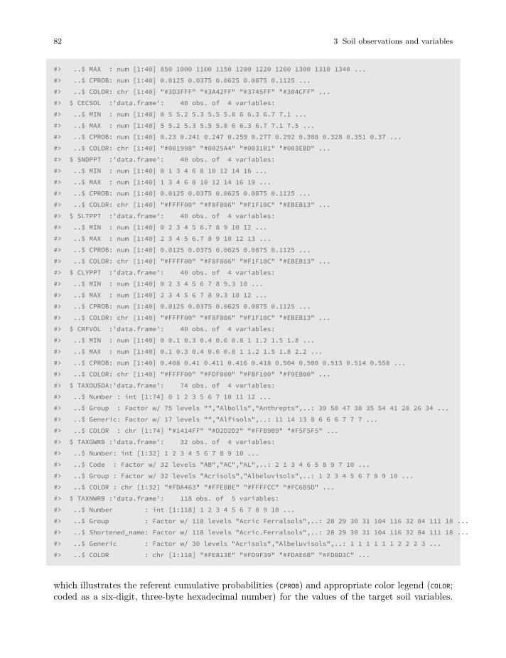
82 3 Soil observations and variables
#> ..$ MAX : num [1:40] 850 1000 1100 1150 1200 1220 1260 1300 1310 1340 ...#> ..$ CPROB: num [1:40] 0.0125 0.0375 0.0625 0.0875 0.1125 ...#> ..$ COLOR: chr [1:40] "#3D3FFF" "#3A42FF" "#3745FF" "#304CFF" ...#> $ CECSOL :'data.frame': 40 obs. of 4 variables:#> ..$ MIN : num [1:40] 0 5 5.2 5.3 5.5 5.8 6 6.3 6.7 7.1 ...#> ..$ MAX : num [1:40] 5 5.2 5.3 5.5 5.8 6 6.3 6.7 7.1 7.5 ...#> ..$ CPROB: num [1:40] 0.23 0.241 0.247 0.259 0.277 0.292 0.308 0.328 0.351 0.37 ...#> ..$ COLOR: chr [1:40] "#001998" "#0025A4" "#0031B1" "#003EBD" ...#> $ SNDPPT :'data.frame': 40 obs. of 4 variables:#> ..$ MIN : num [1:40] 0 1 3 4 6 8 10 12 14 16 ...#> ..$ MAX : num [1:40] 1 3 4 6 8 10 12 14 16 19 ...#> ..$ CPROB: num [1:40] 0.0125 0.0375 0.0625 0.0875 0.1125 ...#> ..$ COLOR: chr [1:40] "#FFFF00" "#F8F806" "#F1F10C" "#EBEB13" ...#> $ SLTPPT :'data.frame': 40 obs. of 4 variables:#> ..$ MIN : num [1:40] 0 2 3 4 5 6.7 8 9 10 12 ...#> ..$ MAX : num [1:40] 2 3 4 5 6.7 8 9 10 12 13 ...#> ..$ CPROB: num [1:40] 0.0125 0.0375 0.0625 0.0875 0.1125 ...#> ..$ COLOR: chr [1:40] "#FFFF00" "#F8F806" "#F1F10C" "#EBEB13" ...#> $ CLYPPT :'data.frame': 40 obs. of 4 variables:#> ..$ MIN : num [1:40] 0 2 3 4 5 6 7 8 9.3 10 ...#> ..$ MAX : num [1:40] 2 3 4 5 6 7 8 9.3 10 12 ...#> ..$ CPROB: num [1:40] 0.0125 0.0375 0.0625 0.0875 0.1125 ...#> ..$ COLOR: chr [1:40] "#FFFF00" "#F8F806" "#F1F10C" "#EBEB13" ...#> $ CRFVOL :'data.frame': 40 obs. of 4 variables:#> ..$ MIN : num [1:40] 0 0.1 0.3 0.4 0.6 0.8 1 1.2 1.5 1.8 ...#> ..$ MAX : num [1:40] 0.1 0.3 0.4 0.6 0.8 1 1.2 1.5 1.8 2.2 ...#> ..$ CPROB: num [1:40] 0.408 0.41 0.411 0.416 0.418 0.504 0.506 0.513 0.514 0.558 ...#> ..$ COLOR: chr [1:40] "#FFFF00" "#FDF800" "#FBF100" "#F9EB00" ...#> $ TAXOUSDA:'data.frame': 74 obs. of 4 variables:#> ..$ Number : int [1:74] 0 1 2 3 5 6 7 10 11 12 ...#> ..$ Group : Factor w/ 75 levels "","Albolls","Anthrepts",..: 39 50 47 38 35 54 41 28 26 34 ...#> ..$ Generic: Factor w/ 17 levels "","Alfisols",..: 11 14 13 8 6 6 6 7 7 7 ...#> ..$ COLOR : chr [1:74] "#1414FF" "#D2D2D2" "#FFB9B9" "#F5F5F5" ...#> $ TAXGWRB :'data.frame': 32 obs. of 4 variables:#> ..$ Number: int [1:32] 1 2 3 4 5 6 7 8 9 10 ...#> ..$ Code : Factor w/ 32 levels "AB","AC","AL",..: 2 1 3 4 6 5 8 9 7 10 ...#> ..$ Group : Factor w/ 32 levels "Acrisols","Albeluvisols",..: 1 2 3 4 5 6 7 8 9 10 ...#> ..$ COLOR : chr [1:32] "#FDA463" "#FFEBBE" "#FFFFCC" "#FC6B5D" ...#> $ TAXNWRB :'data.frame': 118 obs. of 5 variables:#> ..$ Number : int [1:118] 1 2 3 4 5 6 7 8 9 10 ...#> ..$ Group : Factor w/ 118 levels "Acric Ferralsols",..: 28 29 30 31 104 116 32 84 111 18 ...#> ..$ Shortened_name: Factor w/ 118 levels "Acric.Ferralsols",..: 28 29 30 31 104 116 32 84 111 18 ...#> ..$ Generic : Factor w/ 30 levels "Acrisols","Albeluvisols",..: 1 1 1 1 1 1 2 2 2 3 ...#> ..$ COLOR : chr [1:118] "#FE813E" "#FD9F39" "#FDAE6B" "#FD8D3C" ...
which illustrates the referent cumulative probabilities (CPROB) and appropriate color legend (COLOR;coded as a six-digit, three-byte hexadecimal number) for the values of the target soil variables.
3.2 Descriptive soil profile observations 83
The cumulative probabilities were derived using the collection of records in the WoSIS repository(Batjes et al, 2017), and can be considered as an estimate of global prior probabilities for soil pH(see further Fig. 3.7).
A general intention is to maintain a Global Soil Data Registry so that a short variable name (infurther text “variable code”) can be linked to a unique set of metadata which should include:
• Full description (text);
• Variable type (numeric, quantity, binary, factor etc);
• Determination / measurement method (unique code);
• Measurement unit (following the International System of Units);
• Biblio reference (URL or DOI);
• ISO code (if available);
• Physical limits (lower / upper);
• Detection limit (i.e. numeric resolution);
• Priority level (required, suggested or optional);
Note that MySQL has some restrictions considering column names: special characters, such asthose outside the set of alphanumeric characters from the current character set, can not be usedin the column names. Proposed abbreviations for standard method names are VOL — volumefraction, ABU — abundance or relative area cover, PCT — mass percentage, ICM — thickness incm, MHT — texture by-hand or manual hand texture and MNS — Munsell color codes, horizonsequence is coded with the capital ASCII letters e.g. A, B, C,… Z. Another option is to simply usethe US Goverment National Cooperative Soil Characterization Database column names (http://ncsslabdatamart.sc.egov.usda.gov/).
Also note that the metadata can be easily separated from the code so that the short codes (vari-able name) can be used as a shorthand (replacement) for the long description of the completemetadata. Using short codes is also important for programming because unique code names areused consistently in all scripts / functions.
3.2 Descriptive soil profile observations
3.2.1 Depth to bedrock
Soil depth (specifically depth to bedrock) is predicted because it is an important consideration fora wide variety of engineering, hydrological and agronomic interpretations. Shallow and lithic soilsare of particular interest as they impose restrictions for foundations and structures in engineering,limit infiltration and storage of moisture and produce more rapid runoff and erosion and limitgrowth of many crops by restricting rooting depth and limiting available moisture storage. Mostsoil legacy profile data do not provide any information about the soil below depths of 1 m (Richter
84 3 Soil observations and variables
and Markewitz, 1995). This characteristic of legacy soil data limits its usefulness for predictingsoil depths greater than 2 m.
Soil depth is measured from the soil surface downwards and expressed in positive values increasingwith depth. Google Earth and the KML data standard (via the altitudeMode tag) allow one tospecify if the vertical dimension refers to actual altitude (vertical distance from the land surface)or to distance from the sea level (absolute). In this case soil depths can be represented usingclampToGround and negative values. For example, a depth of 30 cm can be expressed as (Wilson,2008):
<Placemark> <Point><altitudeMode>clampToGround</altitudeMode><coordinates>17.2057,45.8851,-0.3</coordinates></Point> </Placemark>
Soil surface (depth = 0 cm) is the top of the mineral soil; or, for soils with a litter layer (O horizon),the soil surface is the top of the part of the O horizon that is at least slightly decomposed (FAO,2006). Fresh leaf or needle fall that has not undergone observable decomposition is not consideredto be part of the soil and may be described separately. For organic soils, the top of any surfacehorizon identified as an O horizon is considered the soil surface.
The depth to bedrock i.e. depth to the R horizon is measured from the soil surface downwards and isexpressed in cm with a precision of ±1 cm. Depth to bedrock deeper than e.g. 2–3 m is most oftennot recorded. Bedrock is consolidated hard rock, with only a few cracks, underlying the soil. It isnot necessarily parent material. We imagine it often as something distinct and easy to recognizein the field. In practice, depth to bedrock can be difficult to determine, and is often confused withstoniness or depth to parent material (which can be unconsolidated material). Another issue isthat, for most of the soils in the world, hard bedrock is >2 m deep so that we actually don’t knowthe correct depth to enter, other than >2 m. Rootability is physically restricted by the bedrock,whether hard or soft (see Fig. 3.4).
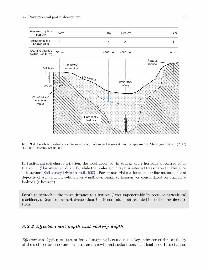
3.2 Descriptive soil profile observations 85
Soil surface
Hard rock /
bedrock
0
200 cm
Soil depth
Soil profile
description
Depth to bedrock
(within 0–200 cm)
Occurrence of R
horizon (0/1)
Absolute depth to
bedrock
Water well
drilling
Standard soil
description
depth
55 cm
1
55 cm
>200 cm
0
NA
>200 cm
0
1035 cm
0 cm
1
0 cm
Rock at
surface
Fig. 3.4 Depth to bedrock for censored and uncensored observations. Image source: Shangguan et al. (2017)doi: 10.1002/2016MS000686.
In traditional soil characterisation, the total depth of the O, A, E, and B horizons is referred to asthe solum (Harpstead et al, 2001), while the underlaying layer is referred to as parent material orsubstratum (Soil survey Division staff, 1993). Parent material can be coarse or fine unconsolidateddeposits of e.g. alluvial, colluvial or windblown origin (C horizon) or consolidated residual hardbedrock (R horizon).
Depth to bedrock is the mean distance to R horizon (layer impenetrable by roots or agriculturalmachinery). Depth to bedrock deeper than 2 m is most often not recorded in field survey descrip-tions.
3.2.2 Effective soil depth and rooting depth
Effective soil depth is of interest for soil mapping because it is a key indicator of the capabilityof the soil to store moisture, support crop growth and sustain beneficial land uses. It is often an
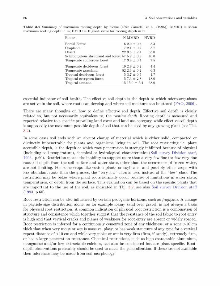
86 3 Soil observations and variables
Table 3.2 Summary of maximum rooting depth by biome (after Canadell et al. (1996)). MMRD = Meanmaximum rooting depth in m; HVRD = Highest value for rooting depth in m.
Biome N MMRD HVRDBoreal Forest 6 2.0 ± 0.3 3.3Cropland 17 2.1 ± 0.2 3.7Desert 22 9.5 ± 2.4 53.0Sclerophyllous shrubland and forest 57 5.2 ± 0.8 40.0Temperate coniferous forest 17 3.9 ± 0.4 7.5Temperate deciduous forest 19 2.9 ± 0.2 4.4Temperate grassland 82 2.6 ± 0.2 6.3Tropical deciduous forest 5 3.7 ± 0.5 4.7Tropical evergreen forest 5 7.3 ± 2.8 18.0Tropical savanna 15 15.0 ± 5.4 68.0
essential indicator of soil health. The effective soil depth is the depth to which micro-organismsare active in the soil, where roots can develop and where soil moisture can be stored (FAO, 2006).
There are many thoughts on how to define effective soil depth. Effective soil depth is closelyrelated to, but not necessarily equivalent to, the rooting depth. Rooting depth is measured andreported relative to a specific prevailing land cover and land use category, while effective soil depthis supposedly the maximum possible depth of soil that can be used by any growing plant (see Tbl.3.2).
In some cases soil ends with an abrupt change of material which is either solid, compacted ordistinctly impenetrable for plants and organisms living in soil. The root restricting i.e. plantaccessible depth, is the depth at which root penetration is strongly inhibited because of physical(including soil temperature), chemical or hydrological characteristics (Soil survey Division staff,1993, p.60). Restriction means the inability to support more than a very few fine (or few very fineroots) if depth from the soil surface and water state, other than the occurrence of frozen water,are not limiting. For some crops like cotton plants or soybeans, and possibly other crops withless abundant roots than the grasses, the “very few” class is used instead of the “few” class. Therestriction may be below where plant roots normally occur because of limitations in water state,temperatures, or depth from the surface. This evaluation can be based on the specific plants thatare important to the use of the soil, as indicated in Tbl. 3.2; see also Soil survey Division staff(1993, p.60).
Root restriction can be also influenced by certain pedogenic horizons, such as fragipans. A changein particle size distribution alone, as for example loamy sand over gravel, is not always a basisfor physical root restriction. A common indication of physical root restriction is a combination ofstructure and consistence which together suggest that the resistance of the soil fabric to root entryis high and that vertical cracks and planes of weakness for root entry are absent or widely spaced.Root restriction is inferred for a continuously cemented zone of any thickness; or a zone >10 cmthick that when very moist or wet is massive, platy, or has weak structure of any type for a verticalrepeat distance of >10 cm and while very moist or wet is very firm (firm, if sandy), extremely firm,or has a large penetration resistance. Chemical restrictions, such as high extractable aluminium,manganese and/or low extractable calcium, can also be considered but are plant-specific. Root-depth observations preferably should be used to make the generalization. If these are not availablethen inferences may be made from soil morphology.
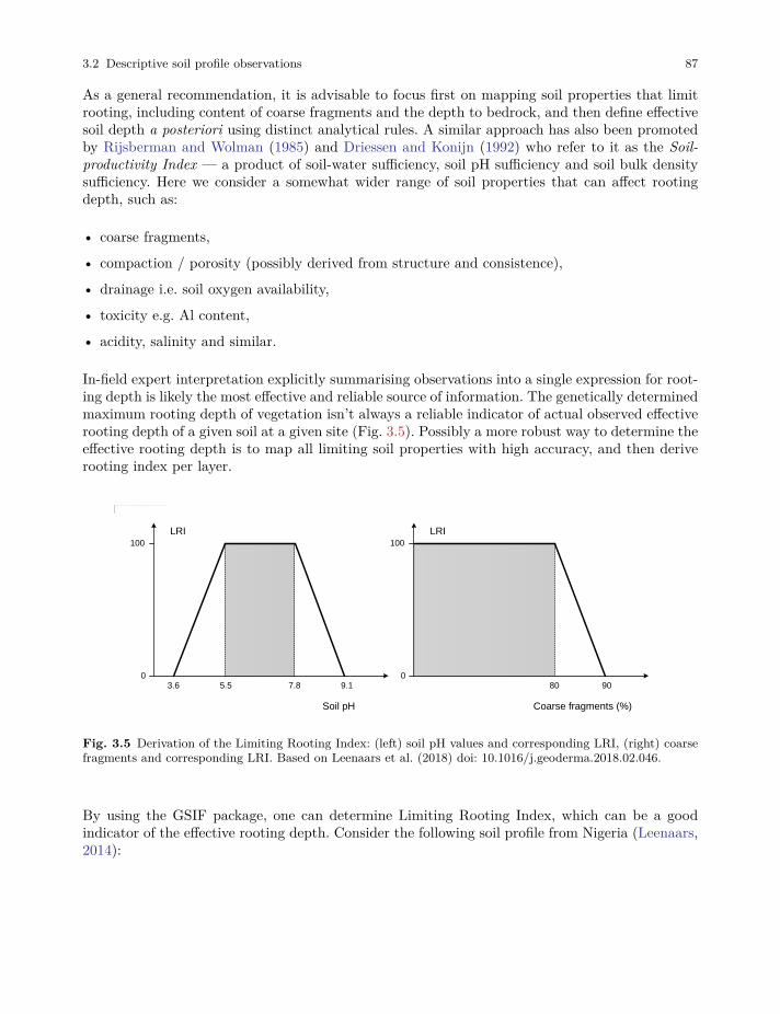
3.2 Descriptive soil profile observations 87
As a general recommendation, it is advisable to focus first on mapping soil properties that limitrooting, including content of coarse fragments and the depth to bedrock, and then define effectivesoil depth a posteriori using distinct analytical rules. A similar approach has also been promotedby Rijsberman and Wolman (1985) and Driessen and Konijn (1992) who refer to it as the Soil-productivity Index — a product of soil-water sufficiency, soil pH sufficiency and soil bulk densitysufficiency. Here we consider a somewhat wider range of soil properties that can affect rootingdepth, such as:
• coarse fragments,
• compaction / porosity (possibly derived from structure and consistence),
• drainage i.e. soil oxygen availability,
• toxicity e.g. Al content,
• acidity, salinity and similar.
In-field expert interpretation explicitly summarising observations into a single expression for root-ing depth is likely the most effective and reliable source of information. The genetically determinedmaximum rooting depth of vegetation isn’t always a reliable indicator of actual observed effectiverooting depth of a given soil at a given site (Fig. 3.5). Possibly a more robust way to determine theeffective rooting depth is to map all limiting soil properties with high accuracy, and then deriverooting index per layer.
Soil pH Coarse fragments (%)
5.5 7.8 9.13.60
100LRI
80 900
100LRI
Fig. 3.5 Derivation of the Limiting Rooting Index: (left) soil pH values and corresponding LRI, (right) coarsefragments and corresponding LRI. Based on Leenaars et al. (2018) doi: 10.1016/j.geoderma.2018.02.046.
By using the GSIF package, one can determine Limiting Rooting Index, which can be a goodindicator of the effective rooting depth. Consider the following soil profile from Nigeria (Leenaars,2014):
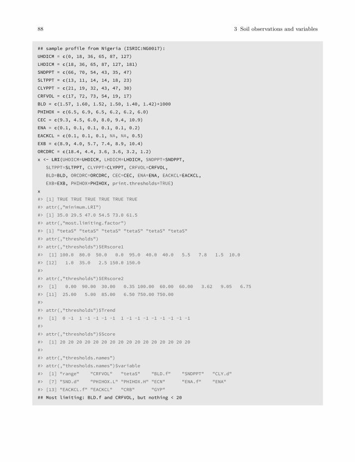
88 3 Soil observations and variables
## sample profile from Nigeria (ISRIC:NG0017):UHDICM = c(0, 18, 36, 65, 87, 127)LHDICM = c(18, 36, 65, 87, 127, 181)SNDPPT = c(66, 70, 54, 43, 35, 47)SLTPPT = c(13, 11, 14, 14, 18, 23)CLYPPT = c(21, 19, 32, 43, 47, 30)CRFVOL = c(17, 72, 73, 54, 19, 17)BLD = c(1.57, 1.60, 1.52, 1.50, 1.40, 1.42)*1000PHIHOX = c(6.5, 6.9, 6.5, 6.2, 6.2, 6.0)CEC = c(9.3, 4.5, 6.0, 8.0, 9.4, 10.9)ENA = c(0.1, 0.1, 0.1, 0.1, 0.1, 0.2)EACKCL = c(0.1, 0.1, 0.1, NA, NA, 0.5)EXB = c(8.9, 4.0, 5.7, 7.4, 8.9, 10.4)ORCDRC = c(18.4, 4.4, 3.6, 3.6, 3.2, 1.2)x <- LRI(UHDICM=UHDICM, LHDICM=LHDICM, SNDPPT=SNDPPT,
SLTPPT=SLTPPT, CLYPPT=CLYPPT, CRFVOL=CRFVOL,BLD=BLD, ORCDRC=ORCDRC, CEC=CEC, ENA=ENA, EACKCL=EACKCL,EXB=EXB, PHIHOX=PHIHOX, print.thresholds=TRUE)
x#> [1] TRUE TRUE TRUE TRUE TRUE TRUE#> attr(,"minimum.LRI")#> [1] 35.0 29.5 47.0 54.5 73.0 61.5#> attr(,"most.limiting.factor")#> [1] "tetaS" "tetaS" "tetaS" "tetaS" "tetaS" "tetaS"#> attr(,"thresholds")#> attr(,"thresholds")$ERscore1#> [1] 100.0 80.0 50.0 0.0 95.0 40.0 40.0 5.5 7.8 1.5 10.0#> [12] 1.0 35.0 2.5 150.0 150.0#>#> attr(,"thresholds")$ERscore2#> [1] 0.00 90.00 30.00 0.35 100.00 60.00 60.00 3.62 9.05 6.75#> [11] 25.00 5.00 85.00 6.50 750.00 750.00#>#> attr(,"thresholds")$Trend#> [1] 0 -1 1 -1 -1 -1 -1 1 -1 -1 -1 -1 -1 -1 -1 -1#>#> attr(,"thresholds")$Score#> [1] 20 20 20 20 20 20 20 20 20 20 20 20 20 20 20 20#>#> attr(,"thresholds.names")#> attr(,"thresholds.names")$variable#> [1] "range" "CRFVOL" "tetaS" "BLD.f" "SNDPPT" "CLY.d"#> [7] "SND.d" "PHIHOX.L" "PHIHOX.H" "ECN" "ENA.f" "ENA"#> [13] "EACKCL.f" "EACKCL" "CRB" "GYP"## Most limiting: BLD.f and CRFVOL, but nothing < 20
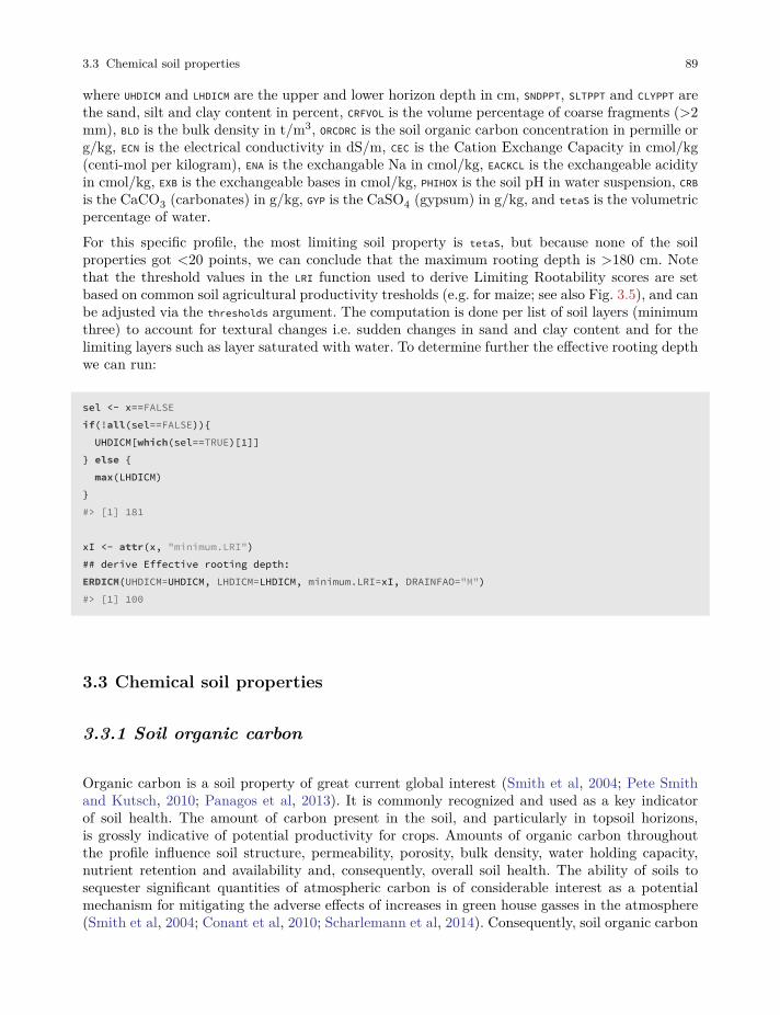
3.3 Chemical soil properties 89
where UHDICM and LHDICM are the upper and lower horizon depth in cm, SNDPPT, SLTPPT and CLYPPT arethe sand, silt and clay content in percent, CRFVOL is the volume percentage of coarse fragments (>2mm), BLD is the bulk density in t/m3, ORCDRC is the soil organic carbon concentration in permille org/kg, ECN is the electrical conductivity in dS/m, CEC is the Cation Exchange Capacity in cmol/kg(centi-mol per kilogram), ENA is the exchangable Na in cmol/kg, EACKCL is the exchangeable acidityin cmol/kg, EXB is the exchangeable bases in cmol/kg, PHIHOX is the soil pH in water suspension, CRBis the CaCO3 (carbonates) in g/kg, GYP is the CaSO4 (gypsum) in g/kg, and tetaS is the volumetricpercentage of water.For this specific profile, the most limiting soil property is tetaS, but because none of the soilproperties got <20 points, we can conclude that the maximum rooting depth is >180 cm. Notethat the threshold values in the LRI function used to derive Limiting Rootability scores are setbased on common soil agricultural productivity tresholds (e.g. for maize; see also Fig. 3.5), and canbe adjusted via the thresholds argument. The computation is done per list of soil layers (minimumthree) to account for textural changes i.e. sudden changes in sand and clay content and for thelimiting layers such as layer saturated with water. To determine further the effective rooting depthwe can run:
sel <- x==FALSEif(!all(sel==FALSE)){UHDICM[which(sel==TRUE)[1]]
} else {max(LHDICM)
}#> [1] 181
xI <- attr(x, "minimum.LRI")## derive Effective rooting depth:ERDICM(UHDICM=UHDICM, LHDICM=LHDICM, minimum.LRI=xI, DRAINFAO="M")#> [1] 100
3.3 Chemical soil properties
3.3.1 Soil organic carbon
Organic carbon is a soil property of great current global interest (Smith et al, 2004; Pete Smithand Kutsch, 2010; Panagos et al, 2013). It is commonly recognized and used as a key indicatorof soil health. The amount of carbon present in the soil, and particularly in topsoil horizons,is grossly indicative of potential productivity for crops. Amounts of organic carbon throughoutthe profile influence soil structure, permeability, porosity, bulk density, water holding capacity,nutrient retention and availability and, consequently, overall soil health. The ability of soils tosequester significant quantities of atmospheric carbon is of considerable interest as a potentialmechanism for mitigating the adverse effects of increases in green house gasses in the atmosphere(Smith et al, 2004; Conant et al, 2010; Scharlemann et al, 2014). Consequently, soil organic carbon
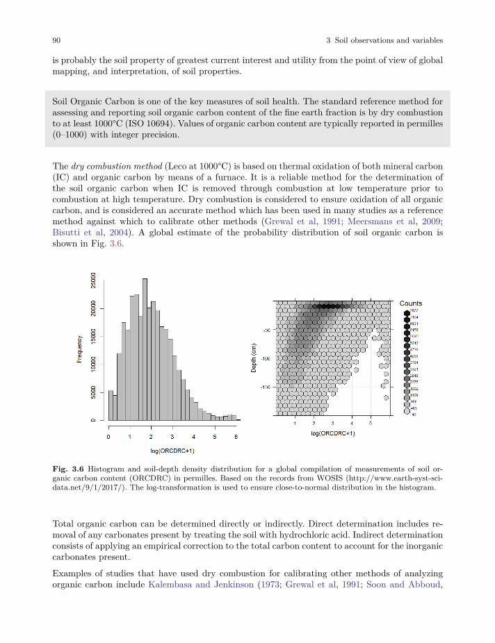
90 3 Soil observations and variables
is probably the soil property of greatest current interest and utility from the point of view of globalmapping, and interpretation, of soil properties.
Soil Organic Carbon is one of the key measures of soil health. The standard reference method forassessing and reporting soil organic carbon content of the fine earth fraction is by dry combustionto at least 1000°C (ISO 10694). Values of organic carbon content are typically reported in permilles(0–1000) with integer precision.
The dry combustion method (Leco at 1000°C) is based on thermal oxidation of both mineral carbon(IC) and organic carbon by means of a furnace. It is a reliable method for the determination ofthe soil organic carbon when IC is removed through combustion at low temperature prior tocombustion at high temperature. Dry combustion is considered to ensure oxidation of all organiccarbon, and is considered an accurate method which has been used in many studies as a referencemethod against which to calibrate other methods (Grewal et al, 1991; Meersmans et al, 2009;Bisutti et al, 2004). A global estimate of the probability distribution of soil organic carbon isshown in Fig. 3.6.
Fig. 3.6 Histogram and soil-depth density distribution for a global compilation of measurements of soil or-ganic carbon content (ORCDRC) in permilles. Based on the records from WOSIS (http://www.earth-syst-sci-data.net/9/1/2017/). The log-transformation is used to ensure close-to-normal distribution in the histogram.
Total organic carbon can be determined directly or indirectly. Direct determination includes re-moval of any carbonates present by treating the soil with hydrochloric acid. Indirect determinationconsists of applying an empirical correction to the total carbon content to account for the inorganiccarbonates present.
Examples of studies that have used dry combustion for calibrating other methods of analyzingorganic carbon include Kalembasa and Jenkinson (1973; Grewal et al, 1991; Soon and Abboud,
3.3 Chemical soil properties 91
1991; Wang et al, 1996; Konen et al, 2002; Brye and Slaton, 2003; Mikhailova et al, 2003; Bisuttiet al, 2004; Jankauskas et al, 2006; De Vos et al, 2007) and Meersmans et al (2009). It is possibleto produce regression equations to permit conversion of results for organic carbon produced byone method into equivalent values into a specified reference method (generally dry combustion).However, local calibration equations that reflect differences in soils on a regional basis are usuallyneeded. It is not possible to provide a single universal equation suitable for use everywhere toconvert organic carbon values produced using other methods of analysis to equivalent values inthe reference method of dry combustion.
3.3.2 Soil pH
Soil pH is of interest for global soil mapping because it is one of the more widely available andeasily interpreted chemical measures of the health and productivity of the soil. pH provides anindication of base status of the soil which influences nutrient availability, mobility of both ben-eficial and detrimental ions and the ecology of micro-organisms within the soil. For most cropsand agricultural uses, a pH in the range of 5.5 to 7.5 is optimal (considering the agriculturalproductivity of soil). Low pH is associated with acidic conditions and with increased mobility oftoxic ions such as aluminium iron and even acid sulphates. High pH is associated with reducedavailability of phosphorus and at higher levels with alkaline conditions that impede water uptakeby plants. A global estimate of the distribution of the soil pH is shown in Figs. 3.7 and 3.8.
PH index approximates concentration of dissolved hydrogen ions (H3O+) in a soil suspension. It isestimated as the negative decimal logarithm of the hydrogen ion activity in a soil suspension. Asa single measurement, pH describes more than relative acidity or alkalinity. It also provides infor-mation on nutrient availability, metal dissolution chemistry, and the activity of microorganisms(Miller and Kissel, 2010).

92 3 Soil observations and variables
Fig. 3.7 Histogram and soil-depth density distribution for a global compilation of measurements of soil pH(suspension of soil in H2O). Based on the records from WOSIS (http://www.earth-syst-sci-data.net/9/1/2017/).
Fig. 3.8 Histogram and soil-depth density distribution for a global compilation of measurements of soil pH(suspension of soil in KCl). Based on the records from WOSIS (http://www.earth-syst-sci-data.net/9/1/2017/).
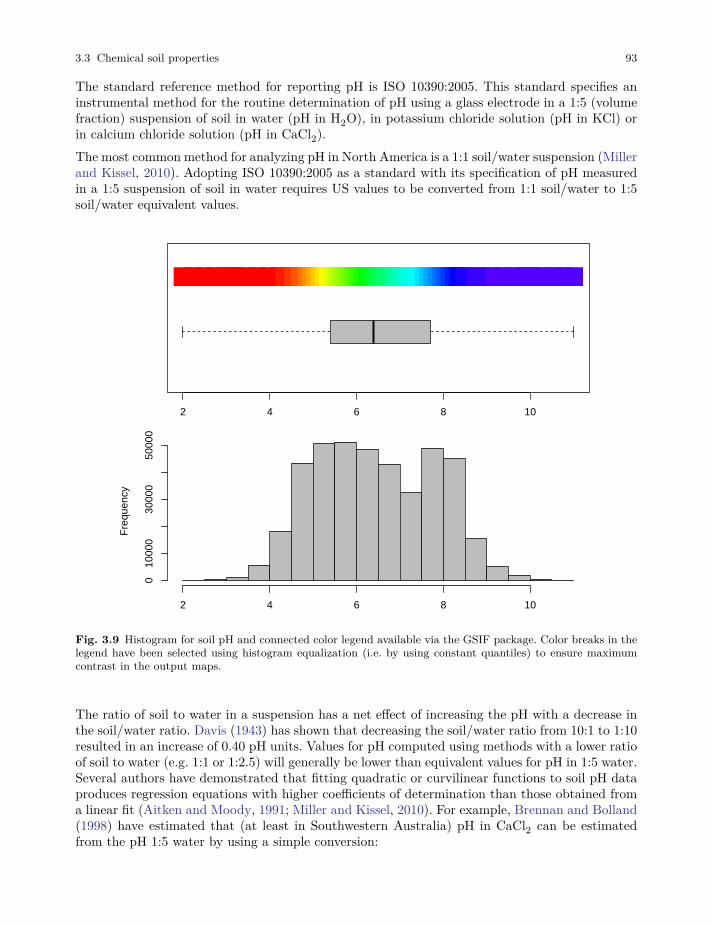
3.3 Chemical soil properties 93
The standard reference method for reporting pH is ISO 10390:2005. This standard specifies aninstrumental method for the routine determination of pH using a glass electrode in a 1:5 (volumefraction) suspension of soil in water (pH in H2O), in potassium chloride solution (pH in KCl) orin calcium chloride solution (pH in CaCl2).The most common method for analyzing pH in North America is a 1:1 soil/water suspension (Millerand Kissel, 2010). Adopting ISO 10390:2005 as a standard with its specification of pH measuredin a 1:5 suspension of soil in water requires US values to be converted from 1:1 soil/water to 1:5soil/water equivalent values.
2 4 6 8 10
Fre
quen
cy
2 4 6 8 10
010
000
3000
050
000
Fig. 3.9 Histogram for soil pH and connected color legend available via the GSIF package. Color breaks in thelegend have been selected using histogram equalization (i.e. by using constant quantiles) to ensure maximumcontrast in the output maps.
The ratio of soil to water in a suspension has a net effect of increasing the pH with a decrease inthe soil/water ratio. Davis (1943) has shown that decreasing the soil/water ratio from 10:1 to 1:10resulted in an increase of 0.40 pH units. Values for pH computed using methods with a lower ratioof soil to water (e.g. 1:1 or 1:2.5) will generally be lower than equivalent values for pH in 1:5 water.Several authors have demonstrated that fitting quadratic or curvilinear functions to soil pH dataproduces regression equations with higher coefficients of determination than those obtained froma linear fit (Aitken and Moody, 1991; Miller and Kissel, 2010). For example, Brennan and Bolland(1998) have estimated that (at least in Southwestern Australia) pH in CaCl2 can be estimatedfrom the pH 1:5 water by using a simple conversion:
94 3 Soil observations and variables
ph_h2o = 7.20.918*ph_h2o-0.3556#> [1] 6.25
This model fitted explains 94% of variation in the values of pH CaCl2 (R-square=0.9401).
Soil pH is negative decimal logarithm of the hydrogen ion activity in a soil suspension. Soil pHvalues are usually in the range 3–11, and are recorded with a precision of ±0.1. Soil pH in therange of 5.5 to 7.5 is optimal for growing crops.
Soil pH varies with season and soil moisture content, with higher pH values associated with wettersoils and winter conditions and lower pH values with drier soils and summer conditions (Miller andKissel, 2010). The effects of both temporal variation in pH and variation due to different analyticalmethods means that differences in pH of less than some specified range (e.g. ±0.3 units) may notbe meaningful in the context of predictions made using noisy legacy soils data analyzed using avariety of different analytical methods. Consequently, it is not necessary or beneficial to reportpH with a precision greater than ±0.1 unit. Natural variation of pH in soils is over a range of2–11 with a standard deviation of 1.4. Note also that pH follows a close-to-normal distribution,although it is often argued that, locally, it can show bimodal or even trimodal peaks (Fig. 3.9).
3.3.3 Soil nutrients
Nutrients are chemical elements or substances essential for the growth of plants. The most essentialelements important for the growth of plants are carbon, hydrogen and oxygen. Other essentialelements can be separated into macro-nutrients (>100 𝜇g or >100 ppm) and micro-nutrients(<100 ppm), although there is no strict border between the two (Harpstead et al, 2001; Henglet al, 2017b). Some macro-nutrients of global importance for soil management and protection are(http://en.wikipedia.org/wiki/Plant_nutrition):
• Nitrogen (N) — Nitrogen is often considered synonymous with soil fertility. Controls leafygrowth. Occurs in soil as nitrates (e.g. NO3, NO2).
• Phosphorus (P) — High phosphorus deficiency may result in the leaves becoming denaturedand showing signs of necrosis. Occurs in the form of phosphates.
• Potassium (K) — Potassium deficiency may result in higher risk of pathogens, wilting, chlorosis,brown spotting, and higher chances of damage from frost and heat.
• Sulfur (S) — Symptoms of deficiency include yellowing of leaves and stunted growth. Occursin soil in the form of sulfate salts (SO4).
• Calcium (Ca) — Calcium is involved in photosynthesis and plant structure. Calcium deficiencyresults in stunting. Occurs in the form of calcium carbonates (CaCO3).

3.4 Physical and hydrological soil properties 95
• Magnesium (Mg) — Magnesium is also an important part of chlorophyll. Magnesium deficiencycan result in interveinal chlorosis.
Nitrogen, Phosphorus and Potassium are the three relatively mobile and dynamic nutrients in soilthat are most often lacking and hence have been identified of primary interest for the fertilizerindustry. Other micro-nutrients of interest for global soil mapping would be: Iron (Fe), Zinc (Zn),Manganese (Mn), Copper (Cu), Boron (B), Chlorine (Cl), Molybdenum (Mo), Nickel (Ni) andSodium (Na).
Apart from macro- and micro-nutrients important for plant growth, there is an increasing interestin the distribution of heavy metals in soils, especially ones that are considered toxic or dangerousfor human health. Some common heavy metals of interest for soil management and soil protectionin developed industrial and / or developing countries are Lead (Pb), Arsenic (As), Zinc (Zn),Cadmium (Cd), Nickel (Ni), Copper (Cu), and Aluminium (Al) (Markus and McBratney, 2001;Reimann et al, 2011; Morel et al, 2005; Rodríguez-Lado et al, 2013; Hengl et al, 2017b).
Macro- and micro-nutrients and heavy metals are measured and mapped in parts per million or 𝜇gper kg of soil. The AfSIS project, provides a good example of mapping macro- and micro-nutrientsover a large area (Hengl et al, 2017b). The problem with mapping such chemical soil properties,however, is that they are highly dynamic. For example, nitrogen, phosphorus, and potassium arehighly mobile nutrients. Their concentration changes from month to month, even from day to dayso that space-time models (2D-T or 3D-T) need to be developed and the amount of analysis /storage needed can easily escalate.
3.4 Physical and hydrological soil properties
3.4.1 Coarse fragments
Soil texture is connected with soil granulometry or the composition of the particle sizes, typicallymeasured as volume percentages. The most common subdivision of soil granulometry is (Shiraziet al, 2001):
1. Fine earth (<2 m)
1.1 sand (coarser particles in the fine earth),
1.2 silt (medium size particles),
1.3 clay (fine particles <2 𝜇m),
2. Coarse fragments (>2 mm)
2.1 gravel (2 mm to 8 cm),
2.2 stones or boulders (>8 cm),
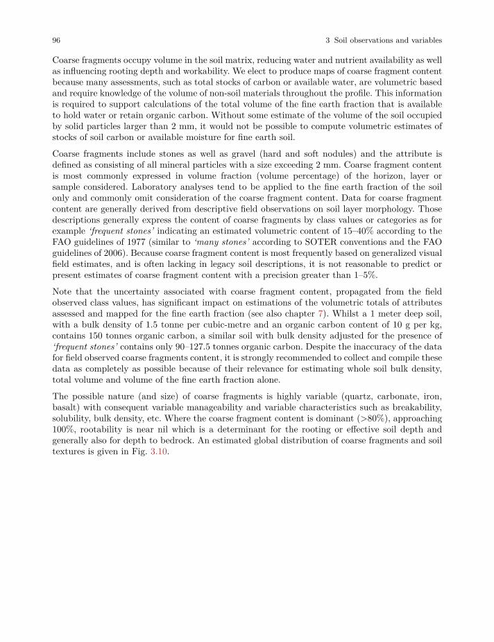
96 3 Soil observations and variables
Coarse fragments occupy volume in the soil matrix, reducing water and nutrient availability as wellas influencing rooting depth and workability. We elect to produce maps of coarse fragment contentbecause many assessments, such as total stocks of carbon or available water, are volumetric basedand require knowledge of the volume of non-soil materials throughout the profile. This informationis required to support calculations of the total volume of the fine earth fraction that is availableto hold water or retain organic carbon. Without some estimate of the volume of the soil occupiedby solid particles larger than 2 mm, it would not be possible to compute volumetric estimates ofstocks of soil carbon or available moisture for fine earth soil.
Coarse fragments include stones as well as gravel (hard and soft nodules) and the attribute isdefined as consisting of all mineral particles with a size exceeding 2 mm. Coarse fragment contentis most commonly expressed in volume fraction (volume percentage) of the horizon, layer orsample considered. Laboratory analyses tend to be applied to the fine earth fraction of the soilonly and commonly omit consideration of the coarse fragment content. Data for coarse fragmentcontent are generally derived from descriptive field observations on soil layer morphology. Thosedescriptions generally express the content of coarse fragments by class values or categories as forexample ‘frequent stones’ indicating an estimated volumetric content of 15–40% according to theFAO guidelines of 1977 (similar to ‘many stones’ according to SOTER conventions and the FAOguidelines of 2006). Because coarse fragment content is most frequently based on generalized visualfield estimates, and is often lacking in legacy soil descriptions, it is not reasonable to predict orpresent estimates of coarse fragment content with a precision greater than 1–5%.
Note that the uncertainty associated with coarse fragment content, propagated from the fieldobserved class values, has significant impact on estimations of the volumetric totals of attributesassessed and mapped for the fine earth fraction (see also chapter 7). Whilst a 1 meter deep soil,with a bulk density of 1.5 tonne per cubic-metre and an organic carbon content of 10 g per kg,contains 150 tonnes organic carbon, a similar soil with bulk density adjusted for the presence of‘frequent stones’ contains only 90–127.5 tonnes organic carbon. Despite the inaccuracy of the datafor field observed coarse fragments content, it is strongly recommended to collect and compile thesedata as completely as possible because of their relevance for estimating whole soil bulk density,total volume and volume of the fine earth fraction alone.
The possible nature (and size) of coarse fragments is highly variable (quartz, carbonate, iron,basalt) with consequent variable manageability and variable characteristics such as breakability,solubility, bulk density, etc. Where the coarse fragment content is dominant (>80%), approaching100%, rootability is near nil which is a determinant for the rooting or effective soil depth andgenerally also for depth to bedrock. An estimated global distribution of coarse fragments and soiltextures is given in Fig. 3.10.
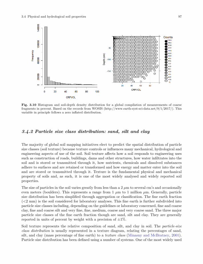
3.4 Physical and hydrological soil properties 97
Fig. 3.10 Histogram and soil-depth density distribution for a global compilation of measurements of coarsefragments in percent. Based on the records from WOSIS (http://www.earth-syst-sci-data.net/9/1/2017/). Thisvariable in principle follows a zero inflated distribution.
3.4.2 Particle size class distribution: sand, silt and clay
The majority of global soil mapping initiatives elect to predict the spatial distribution of particlesize classes (soil texture) because texture controls or influences many mechanical, hydrological andengineering aspects of use of the soil. Soil texture affects how a soil responds to engineering usessuch as construction of roads, buildings, dams and other structures, how water infiltrates into thesoil and is stored or transmitted through it, how nutrients, chemicals and dissolved substancesadhere to surfaces and are retained or transformed and how energy and matter enter into the soiland are stored or transmitted through it. Texture is the fundamental physical and mechanicalproperty of soils and, as such, it is one of the most widely analysed and widely reported soilproperties.
The size of particles in the soil varies greatly from less than a 2 𝜇m to several cm’s and occasionallyeven meters (boulders). This represents a range from 1 𝜇m to 1 million 𝜇m. Generally, particlesize distribution has been simplified through aggregation or classification. The fine earth fraction(<2 mm) is the soil considered for laboratory analyses. This fine earth is further subdivided intoparticle size classes including, depending on the guidelines or laboratory concerned, fine and coarseclay, fine and coarse silt and very fine, fine, medium, coarse and very coarse sand. The three majorparticle size classes of the fine earth fraction though are sand, silt and clay. They are generallyreported in units of percent by weight with a precision of ±1%.
Soil texture represents the relative composition of sand, silt, and clay in soil. The particle-sizeclass distribution is usually represented in a texture diagram, relating the percentages of sand,silt, and clay (mass percentage of fine earth) to a texture class (Minasny and McBratney, 2001).Particle size distribution has been defined using a number of systems. One of the most widely used
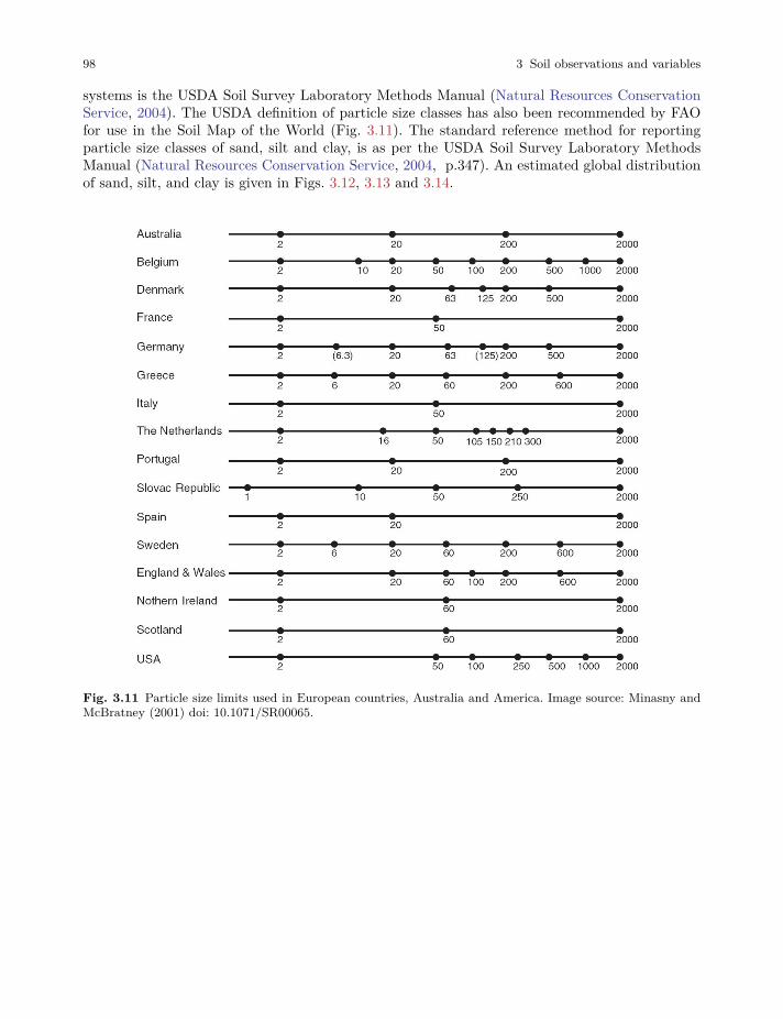
98 3 Soil observations and variables
systems is the USDA Soil Survey Laboratory Methods Manual (Natural Resources ConservationService, 2004). The USDA definition of particle size classes has also been recommended by FAOfor use in the Soil Map of the World (Fig. 3.11). The standard reference method for reportingparticle size classes of sand, silt and clay, is as per the USDA Soil Survey Laboratory MethodsManual (Natural Resources Conservation Service, 2004, p.347). An estimated global distributionof sand, silt, and clay is given in Figs. 3.12, 3.13 and 3.14.
Fig. 3.11 Particle size limits used in European countries, Australia and America. Image source: Minasny andMcBratney (2001) doi: 10.1071/SR00065.
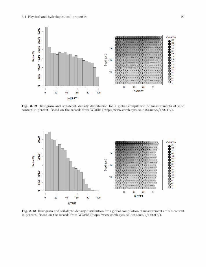
3.4 Physical and hydrological soil properties 99
Fig. 3.12 Histogram and soil-depth density distribution for a global compilation of measurements of sandcontent in percent. Based on the records from WOSIS (http://www.earth-syst-sci-data.net/9/1/2017/).
Fig. 3.13 Histogram and soil-depth density distribution for a global compilation of measurements of silt contentin percent. Based on the records from WOSIS (http://www.earth-syst-sci-data.net/9/1/2017/).
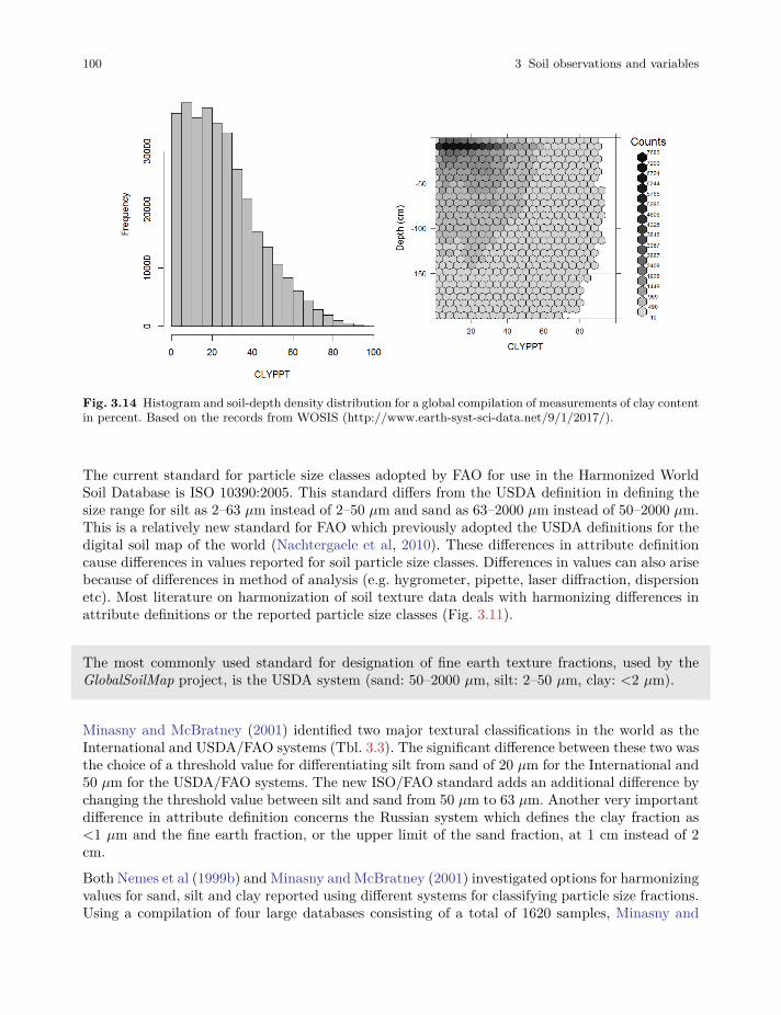
100 3 Soil observations and variables
Fig. 3.14 Histogram and soil-depth density distribution for a global compilation of measurements of clay contentin percent. Based on the records from WOSIS (http://www.earth-syst-sci-data.net/9/1/2017/).
The current standard for particle size classes adopted by FAO for use in the Harmonized WorldSoil Database is ISO 10390:2005. This standard differs from the USDA definition in defining thesize range for silt as 2–63 𝜇m instead of 2–50 𝜇m and sand as 63–2000 𝜇m instead of 50–2000 𝜇m.This is a relatively new standard for FAO which previously adopted the USDA definitions for thedigital soil map of the world (Nachtergaele et al, 2010). These differences in attribute definitioncause differences in values reported for soil particle size classes. Differences in values can also arisebecause of differences in method of analysis (e.g. hygrometer, pipette, laser diffraction, dispersionetc). Most literature on harmonization of soil texture data deals with harmonizing differences inattribute definitions or the reported particle size classes (Fig. 3.11).
The most commonly used standard for designation of fine earth texture fractions, used by theGlobalSoilMap project, is the USDA system (sand: 50–2000 𝜇m, silt: 2–50 𝜇m, clay: <2 𝜇m).
Minasny and McBratney (2001) identified two major textural classifications in the world as theInternational and USDA/FAO systems (Tbl. 3.3). The significant difference between these two wasthe choice of a threshold value for differentiating silt from sand of 20 𝜇m for the International and50 𝜇m for the USDA/FAO systems. The new ISO/FAO standard adds an additional difference bychanging the threshold value between silt and sand from 50 𝜇m to 63 𝜇m. Another very importantdifference in attribute definition concerns the Russian system which defines the clay fraction as<1 𝜇m and the fine earth fraction, or the upper limit of the sand fraction, at 1 cm instead of 2cm.
Both Nemes et al (1999b) and Minasny and McBratney (2001) investigated options for harmonizingvalues for sand, silt and clay reported using different systems for classifying particle size fractions.Using a compilation of four large databases consisting of a total of 1620 samples, Minasny and
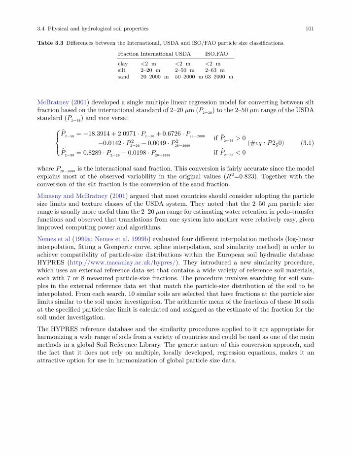
3.4 Physical and hydrological soil properties 101
Table 3.3 Differences between the International, USDA and ISO/FAO particle size classifications.
Fraction International USDA ISO.FAOclay <2 �m <2 �m <2 �msilt 2–20 �m 2–50 �m 2–63 �msand 20–2000 �m 50–2000 �m 63–2000 �m
McBratney (2001) developed a single multiple linear regression model for converting between siltfraction based on the international standard of 2–20 𝜇m (𝑃2−20) to the 2–50 𝜇m range of the USDAstandard (𝑃2−50) and vice versa:
⎧{⎨{⎩
𝑃2−50 = −18.3914 + 2.0971 ⋅ 𝑃2−20 + 0.6726 ⋅ 𝑃20−2000
−0.0142 ⋅ 𝑃 22−20 − 0.0049 ⋅ 𝑃 2
20−2000
if 𝑃2−50 > 0𝑃2−50 = 0.8289 ⋅ 𝑃2−20 + 0.0198 ⋅ 𝑃20−2000 if 𝑃2−50 < 0
(#𝑒𝑞 ∶ 𝑃250) (3.1)
where 𝑃20−2000 is the international sand fraction. This conversion is fairly accurate since the modelexplains most of the observed variability in the original values (𝑅2=0.823). Together with theconversion of the silt fraction is the conversion of the sand fraction.
Minasny and McBratney (2001) argued that most countries should consider adopting the particlesize limits and texture classes of the USDA system. They noted that the 2–50 𝜇m particle sizerange is usually more useful than the 2–20 𝜇m range for estimating water retention in pedo-transferfunctions and observed that translations from one system into another were relatively easy, givenimproved computing power and algorithms.
Nemes et al (1999a; Nemes et al, 1999b) evaluated four different interpolation methods (log-linearinterpolation, fitting a Gompertz curve, spline interpolation, and similarity method) in order toachieve compatibility of particle-size distributions within the European soil hydraulic databaseHYPRES (http://www.macaulay.ac.uk/hypres/). They introduced a new similarity procedure,which uses an external reference data set that contains a wide variety of reference soil materials,each with 7 or 8 measured particle-size fractions. The procedure involves searching for soil sam-ples in the external reference data set that match the particle-size distribution of the soil to beinterpolated. From each search. 10 similar soils are selected that have fractions at the particle sizelimits similar to the soil under investigation. The arithmetic mean of the fractions of these 10 soilsat the specified particle size limit is calculated and assigned as the estimate of the fraction for thesoil under investigation.
The HYPRES reference database and the similarity procedures applied to it are appropriate forharmonizing a wide range of soils from a variety of countries and could be used as one of the mainmethods in a global Soil Reference Library. The generic nature of this conversion approach, andthe fact that it does not rely on multiple, locally developed, regression equations, makes it anattractive option for use in harmonization of global particle size data.
102 3 Soil observations and variables
3.4.3 Bulk density
Measurement of soil Bulk Density (BLD) is often time consuming and relatively costly. For thisreason, it is not analysed and reported for legacy soil profiles as frequently or consistently as manyother, more common, soil properties. Consequently, predicting bulk density globally using digitalsoil mapping methods is fraught with difficulties and uncertainties. However, it is critical to atleast attempt to make some kind of estimate of how bulk density varies spatially because we needto know the bulk density of the soil in order to make any estimates of volumetric concentrationsof materials such as organic carbon, water or nutrients.
In practice, we need to be able to make estimates of two different types of bulk density, namely thebulk density of the whole soil and the bulk density of the fine earth fraction (particles <2 mm) only.Calculations such as those for total stocks of carbon are first applied using the bulk density of thefine earth fraction only but this value is then reduced in accordance with the volume proportionof the soil that is occupied by coarse fragments greater than 2 mm in size. Bulk density is alsoof interest for global soil mapping applications because it influences infiltration and movementof water in the soil, penetration of the soil by plant roots and mechanical workability of the soilusing farm implements.
Bulk density is the over-dry mass of soil material divided by the total volume. The standardreference method for reporting bulk density is the core method (ISO 11272): the dry bulk density(BD) is the ratio between the mass of oven dry soil material and the volume of the undisturbedfresh sample. The ISO standard defines dry bulk density as the ratio of the oven-dry mass of thesolids to the volume (the bulk volume includes the volume of the solids and of the pore space) ofthe soil. The recommended ISO method (core method) uses steel cylinders of known volume (100cm3 and/or 400 cm3) that are driven into the soil vertically or horizontally by percussion. Samplinglarge volumes results in smaller relative errors but requires heavy equipment. The method cannotbe used if stones or large roots are present or when the soil is too dry or too hard.
For soils with a high stone or root content or when the soil is too dry or too hard, methods basedon the excavation technique are used as an alternative to the core method. In the excavationmethod a hole on a horizontal surface is dug and then filled with a material with a known density(e.g. sand which packs to a calibrated volume or water separated from the soil material by anelastic membrane) to assess the volume of the hole or the sample taken. The soil obtained fromthe hole, is oven-dried to remove the water and the oven-dry mass of the total sample is weighed.The volumetric percentage of the coarse fragments needs to be determined and the weight of thecoarse fragments assessed, in order to be able to calculate the oven-dry bulk density of the fineearth separately.
The USDA handbook for analytical procedures describes various methods for assessing varioustypes of bulk density. USDA soil data report values for bulk density of the fine earth as wellas of the whole earth (including gravel), with the weight assessed oven-dry as well as at fieldcapacity e.g. including water. The latter method relates the weight of moist soil to the volumeof moist or oven-dry soil. Experience has shown that organic carbon and texture or clay contentpredominately influence soil bulk density, even though the nature of the clay (mineralogy) is asimportant as the percentage content of the clay. Organic carbon and texture information is oftenavailable in soil survey reports, while bulk density is often not reported.
Many attempts have therefore been made to estimate soil bulk densities through pedo-transferfunctions (PTFs) based on soil organic carbon and texture data (Curtis and Post, 1964; Adams,
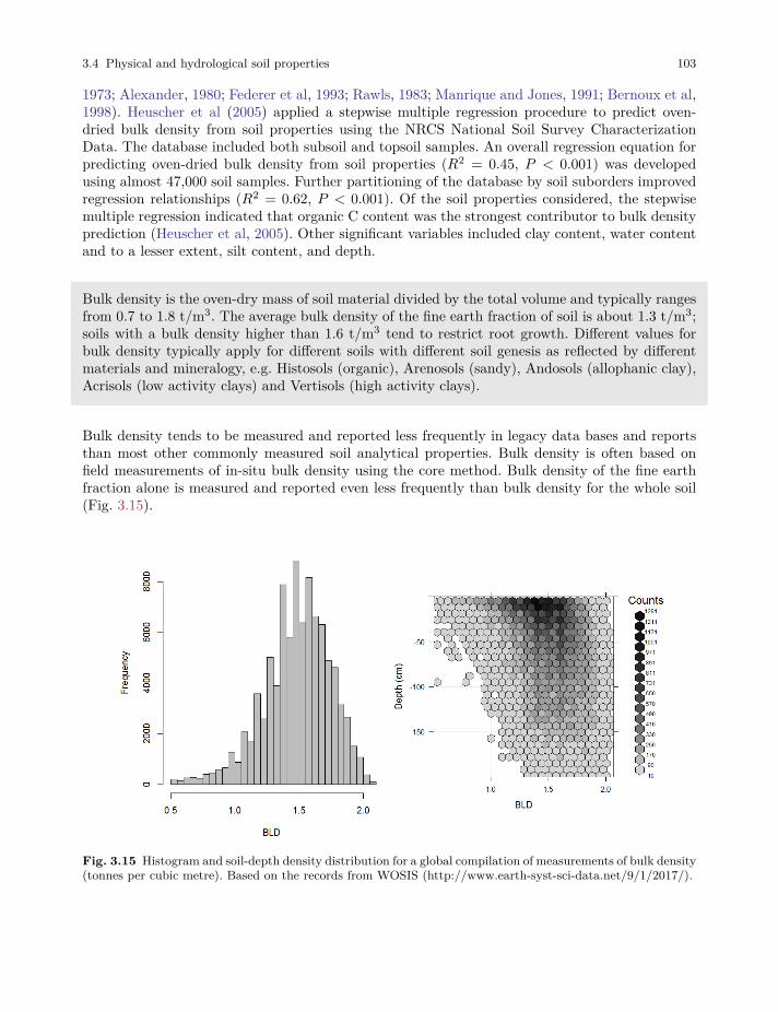
3.4 Physical and hydrological soil properties 103
1973; Alexander, 1980; Federer et al, 1993; Rawls, 1983; Manrique and Jones, 1991; Bernoux et al,1998). Heuscher et al (2005) applied a stepwise multiple regression procedure to predict oven-dried bulk density from soil properties using the NRCS National Soil Survey CharacterizationData. The database included both subsoil and topsoil samples. An overall regression equation forpredicting oven-dried bulk density from soil properties (𝑅2 = 0.45, 𝑃 < 0.001) was developedusing almost 47,000 soil samples. Further partitioning of the database by soil suborders improvedregression relationships (𝑅2 = 0.62, 𝑃 < 0.001). Of the soil properties considered, the stepwisemultiple regression indicated that organic C content was the strongest contributor to bulk densityprediction (Heuscher et al, 2005). Other significant variables included clay content, water contentand to a lesser extent, silt content, and depth.
Bulk density is the oven-dry mass of soil material divided by the total volume and typically rangesfrom 0.7 to 1.8 t/m3. The average bulk density of the fine earth fraction of soil is about 1.3 t/m3;soils with a bulk density higher than 1.6 t/m3 tend to restrict root growth. Different values forbulk density typically apply for different soils with different soil genesis as reflected by differentmaterials and mineralogy, e.g. Histosols (organic), Arenosols (sandy), Andosols (allophanic clay),Acrisols (low activity clays) and Vertisols (high activity clays).
Bulk density tends to be measured and reported less frequently in legacy data bases and reportsthan most other commonly measured soil analytical properties. Bulk density is often based onfield measurements of in-situ bulk density using the core method. Bulk density of the fine earthfraction alone is measured and reported even less frequently than bulk density for the whole soil(Fig. 3.15).
Fig. 3.15 Histogram and soil-depth density distribution for a global compilation of measurements of bulk density(tonnes per cubic metre). Based on the records from WOSIS (http://www.earth-syst-sci-data.net/9/1/2017/).
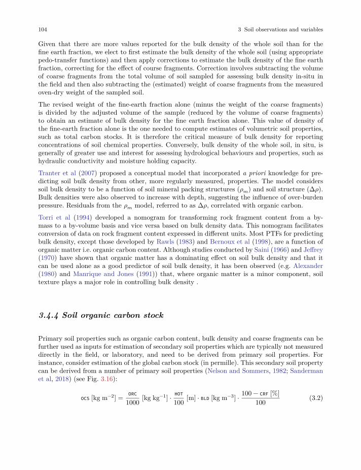
104 3 Soil observations and variables
Given that there are more values reported for the bulk density of the whole soil than for thefine earth fraction, we elect to first estimate the bulk density of the whole soil (using appropriatepedo-transfer functions) and then apply corrections to estimate the bulk density of the fine earthfraction, correcting for the effect of course fragments. Correction involves subtracting the volumeof coarse fragments from the total volume of soil sampled for assessing bulk density in-situ inthe field and then also subtracting the (estimated) weight of coarse fragments from the measuredoven-dry weight of the sampled soil.
The revised weight of the fine-earth fraction alone (minus the weight of the coarse fragments)is divided by the adjusted volume of the sample (reduced by the volume of coarse fragments)to obtain an estimate of bulk density for the fine earth fraction alone. This value of density ofthe fine-earth fraction alone is the one needed to compute estimates of volumetric soil properties,such as total carbon stocks. It is therefore the critical measure of bulk density for reportingconcentrations of soil chemical properties. Conversely, bulk density of the whole soil, in situ, isgenerally of greater use and interest for assessing hydrological behaviours and properties, such ashydraulic conductivity and moisture holding capacity.
Tranter et al (2007) proposed a conceptual model that incorporated a priori knowledge for pre-dicting soil bulk density from other, more regularly measured, properties. The model considerssoil bulk density to be a function of soil mineral packing structures (𝜌𝑚) and soil structure (Δ𝜌).Bulk densities were also observed to increase with depth, suggesting the influence of over-burdenpressure. Residuals from the 𝜌𝑚 model, referred to as Δ𝜌, correlated with organic carbon.
Torri et al (1994) developed a nomogram for transforming rock fragment content from a by-mass to a by-volume basis and vice versa based on bulk density data. This nomogram facilitatesconversion of data on rock fragment content expressed in different units. Most PTFs for predictingbulk density, except those developed by Rawls (1983) and Bernoux et al (1998), are a function oforganic matter i.e. organic carbon content. Although studies conducted by Saini (1966) and Jeffrey(1970) have shown that organic matter has a dominating effect on soil bulk density and that itcan be used alone as a good predictor of soil bulk density, it has been observed (e.g. Alexander(1980) and Manrique and Jones (1991)) that, where organic matter is a minor component, soiltexture plays a major role in controlling bulk density .
3.4.4 Soil organic carbon stock
Primary soil properties such as organic carbon content, bulk density and coarse fragments can befurther used as inputs for estimation of secondary soil properties which are typically not measureddirectly in the field, or laboratory, and need to be derived from primary soil properties. Forinstance, consider estimation of the global carbon stock (in permille). This secondary soil propertycan be derived from a number of primary soil properties (Nelson and Sommers, 1982; Sandermanet al, 2018) (see Fig. 3.16):
OCS [kg m−2] = ORC
1000 [kg kg−1] ⋅ HOT
100 [m] ⋅ BLD [kg m−3] ⋅ 100 − CRF [%]100 (3.2)
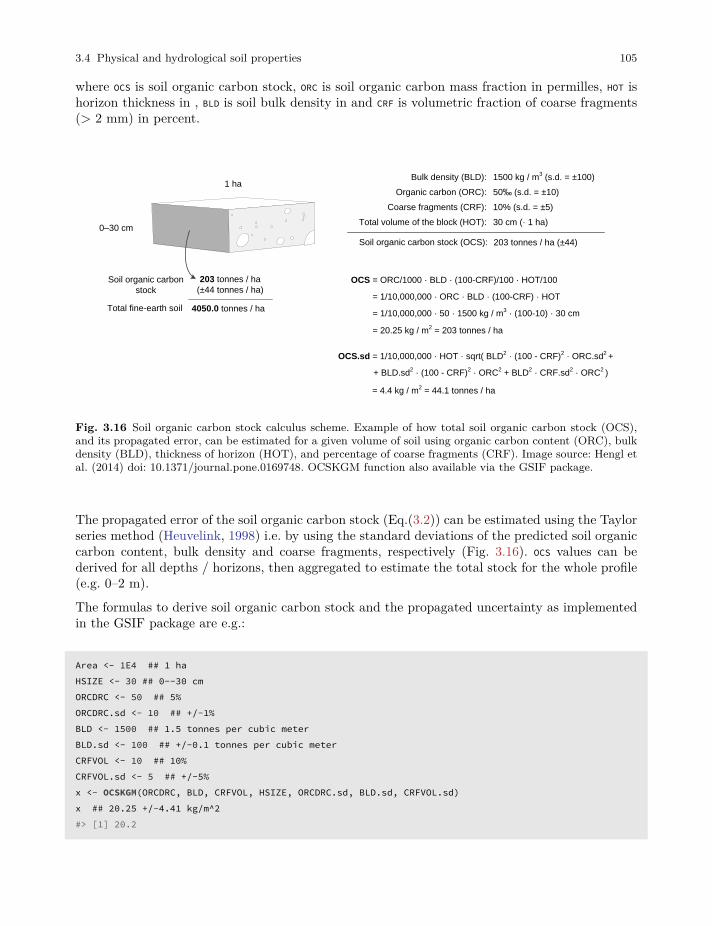
3.4 Physical and hydrological soil properties 105
where OCS is soil organic carbon stock, ORC is soil organic carbon mass fraction in permilles, HOT ishorizon thickness in , BLD is soil bulk density in and CRF is volumetric fraction of coarse fragments(> 2 mm) in percent.
1 ha
0–30 cm
Bulk density (BLD):
Organic carbon (ORC):
Coarse fragments (CRF):
Total volume of the block (HOT):
1500 kg / m3 (s.d. = ±100)
50‰ (s.d. = ±10)
10% (s.d. = ±5)
30 cm (· 1 ha)
OCS = ORC/1000 · BLD · (100-CRF)/100 · HOT/100
= 1/10,000,000 · ORC · BLD · (100-CRF) · HOT
= 1/10,000,000 · 50 · 1500 kg / m3 · (100-10) · 30 cm
Soil organic carbon stock (OCS):
= 20.25 kg / m2 = 203 tonnes / ha
203 tonnes / ha (±44)
203 tonnes / ha
(±44 tonnes / ha)
4050.0 tonnes / ha
Soil organic carbon
stock
Total fine-earth soil
OCS.sd = 1/10,000,000 · HOT · sqrt( BLD2 · (100 - CRF)
2 · ORC.sd
2 +
+ BLD.sd2 · (100 - CRF)
2 · ORC
2 + BLD
2 · CRF.sd
2 · ORC
2 )
= 4.4 kg / m2 = 44.1 tonnes / ha
Fig. 3.16 Soil organic carbon stock calculus scheme. Example of how total soil organic carbon stock (OCS),and its propagated error, can be estimated for a given volume of soil using organic carbon content (ORC), bulkdensity (BLD), thickness of horizon (HOT), and percentage of coarse fragments (CRF). Image source: Hengl etal. (2014) doi: 10.1371/journal.pone.0169748. OCSKGM function also available via the GSIF package.
The propagated error of the soil organic carbon stock (Eq.(3.2)) can be estimated using the Taylorseries method (Heuvelink, 1998) i.e. by using the standard deviations of the predicted soil organiccarbon content, bulk density and coarse fragments, respectively (Fig. 3.16). OCS values can bederived for all depths / horizons, then aggregated to estimate the total stock for the whole profile(e.g. 0–2 m).
The formulas to derive soil organic carbon stock and the propagated uncertainty as implementedin the GSIF package are e.g.:
Area <- 1E4 ## 1 haHSIZE <- 30 ## 0--30 cmORCDRC <- 50 ## 5%ORCDRC.sd <- 10 ## +/-1%BLD <- 1500 ## 1.5 tonnes per cubic meterBLD.sd <- 100 ## +/-0.1 tonnes per cubic meterCRFVOL <- 10 ## 10%CRFVOL.sd <- 5 ## +/-5%x <- OCSKGM(ORCDRC, BLD, CRFVOL, HSIZE, ORCDRC.sd, BLD.sd, CRFVOL.sd)x ## 20.25 +/-4.41 kg/m^2#> [1] 20.2
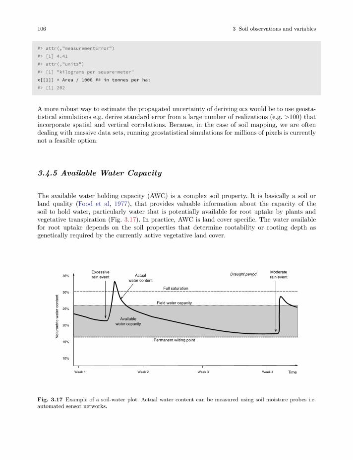
106 3 Soil observations and variables
#> attr(,"measurementError")#> [1] 4.41#> attr(,"units")#> [1] "kilograms per square-meter"x[[1]] * Area / 1000 ## in tonnes per ha:#> [1] 202
A more robust way to estimate the propagated uncertainty of deriving OCS would be to use geosta-tistical simulations e.g. derive standard error from a large number of realizations (e.g. >100) thatincorporate spatial and vertical correlations. Because, in the case of soil mapping, we are oftendealing with massive data sets, running geostatistical simulations for millions of pixels is currentlynot a feasible option.
3.4.5 Available Water Capacity
The available water holding capacity (AWC) is a complex soil property. It is basically a soil orland quality (Food et al, 1977), that provides valuable information about the capacity of thesoil to hold water, particularly water that is potentially available for root uptake by plants andvegetative transpiration (Fig. 3.17). In practice, AWC is land cover specific. The water availablefor root uptake depends on the soil properties that determine rootability or rooting depth asgenetically required by the currently active vegetative land cover.
35%
30%
25%
20%
15%
10%
Field water capacity
Excessive rain event
Moderaterain event
Availablewater capacity
Permanent wilting point
Actual water content
Vol
umet
ric w
ater
con
tent
Week 1
Full saturation
Week 2 Week 3 Week 4
Draught period
Time
Fig. 3.17 Example of a soil-water plot. Actual water content can be measured using soil moisture probes i.e.automated sensor networks.
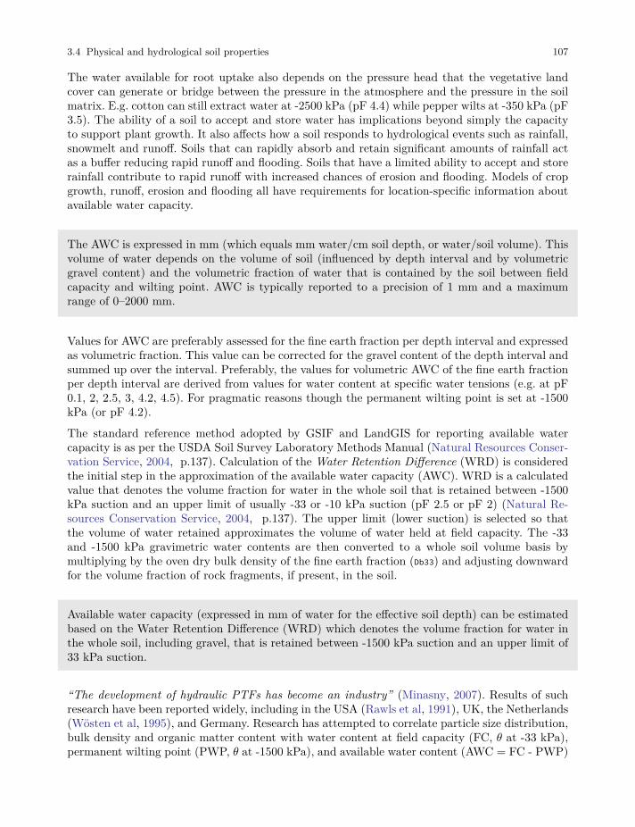
3.4 Physical and hydrological soil properties 107
The water available for root uptake also depends on the pressure head that the vegetative landcover can generate or bridge between the pressure in the atmosphere and the pressure in the soilmatrix. E.g. cotton can still extract water at -2500 kPa (pF 4.4) while pepper wilts at -350 kPa (pF3.5). The ability of a soil to accept and store water has implications beyond simply the capacityto support plant growth. It also affects how a soil responds to hydrological events such as rainfall,snowmelt and runoff. Soils that can rapidly absorb and retain significant amounts of rainfall actas a buffer reducing rapid runoff and flooding. Soils that have a limited ability to accept and storerainfall contribute to rapid runoff with increased chances of erosion and flooding. Models of cropgrowth, runoff, erosion and flooding all have requirements for location-specific information aboutavailable water capacity.
The AWC is expressed in mm (which equals mm water/cm soil depth, or water/soil volume). Thisvolume of water depends on the volume of soil (influenced by depth interval and by volumetricgravel content) and the volumetric fraction of water that is contained by the soil between fieldcapacity and wilting point. AWC is typically reported to a precision of 1 mm and a maximumrange of 0–2000 mm.
Values for AWC are preferably assessed for the fine earth fraction per depth interval and expressedas volumetric fraction. This value can be corrected for the gravel content of the depth interval andsummed up over the interval. Preferably, the values for volumetric AWC of the fine earth fractionper depth interval are derived from values for water content at specific water tensions (e.g. at pF0.1, 2, 2.5, 3, 4.2, 4.5). For pragmatic reasons though the permanent wilting point is set at -1500kPa (or pF 4.2).
The standard reference method adopted by GSIF and LandGIS for reporting available watercapacity is as per the USDA Soil Survey Laboratory Methods Manual (Natural Resources Conser-vation Service, 2004, p.137). Calculation of the Water Retention Difference (WRD) is consideredthe initial step in the approximation of the available water capacity (AWC). WRD is a calculatedvalue that denotes the volume fraction for water in the whole soil that is retained between -1500kPa suction and an upper limit of usually -33 or -10 kPa suction (pF 2.5 or pF 2) (Natural Re-sources Conservation Service, 2004, p.137). The upper limit (lower suction) is selected so thatthe volume of water retained approximates the volume of water held at field capacity. The -33and -1500 kPa gravimetric water contents are then converted to a whole soil volume basis bymultiplying by the oven dry bulk density of the fine earth fraction (Db33) and adjusting downwardfor the volume fraction of rock fragments, if present, in the soil.
Available water capacity (expressed in mm of water for the effective soil depth) can be estimatedbased on the Water Retention Difference (WRD) which denotes the volume fraction for water inthe whole soil, including gravel, that is retained between -1500 kPa suction and an upper limit of33 kPa suction.
“The development of hydraulic PTFs has become an industry” (Minasny, 2007). Results of suchresearch have been reported widely, including in the USA (Rawls et al, 1991), UK, the Netherlands(Wösten et al, 1995), and Germany. Research has attempted to correlate particle size distribution,bulk density and organic matter content with water content at field capacity (FC, 𝜃 at -33 kPa),permanent wilting point (PWP, 𝜃 at -1500 kPa), and available water content (AWC = FC - PWP)
108 3 Soil observations and variables
(Minasny, 2007). Gijsman et al (2007) reported that “many PTFs for estimating soil hydraulicproperties have been published already” (see overviews by Rawls et al (1991), Timlin et al (1996)and Wösten et al (2001)). Timlin et al (1996) reported 49 methods and estimated that these coveronly about 30% of the total. Gijsman et al (2007) compared eight methods for all the soil classesthat make up the texture triangle. They went through the triangle in steps of sand, silt and clayand determined the estimated values of wilting point or lower limit of plant extractable water (LL),field capacity or the drained upper limit (DUL), and soil saturation (SAT). They finally concludedthat none of the methods were universally good. The best method in the comparison of Gijsmanet al (2007) was Saxton et al (1986), closely followed by Rawls and Brakensiek (1982).
Alterra institute in collaboration with ISRIC validated the PTF developed by Hodnett andTomasella (2002) on the basis of the data present in the Africa Soil Profiles database (Leenaars,2014) to predict tension specific volumetric water content (Wösten et al, 2013) to assess WRD.Jagtap et al (2004) developed an approach that does not fit a mathematical equation through thedata, but rather compares the soil layer for which the key soil water contents of lower limit (LL),drained upper limit (DUL), and soil saturation (SAT), have to be estimated with all layers in adatabase of field-measured soil-water-retention data. The layer that is most similar in texture andorganic carbon concentration is considered to be the ‘nearest neighbor’ among all the layers inthe database and its soil-water-retention values are assumed to be similar to those that need tobe estimated. To avoid making estimated soil-water-retention values dependent on only one soilin the database, the six ‘nearest neighbors’ are used and weighted according to their degree ofsimilarity (Jagtap et al, 2004). This is a non-parametric procedure, in the sense that it does notassume a fixed mathematical relationship between the physical properties and the water holdingproperties of soils. The similarity method to convert soil particle size fraction data proposed byNemes et al (1999b; Nemes et al, 1999a) is a direct analogue of this similarity method of Jagtapet al (2004) for soil hydraulic properties.
Zacharias and Wessolek (2007) identified three different approaches for deriving the WRD frommore easily available parameters as:
1. Point-based estimation methods: estimating the water content of selected matric potentials frompredictors such as the percentage of sand, silt, or clay, the amount of organic matter, or thebulk density (e.g. Rawls and Brakensiek (1982)).
2. Semi-physical approach: deriving the WRD from information on the cumulative particle sizedistribution (Arya and Paris, 1981); theoretically, this approach is based on the similaritybetween cumulative particle size distribution and water retention curves. The water contentsare derived from the soil’s predicted pore volume and the hydraulic potentials are derived fromcapillarity relationships.
3. Parameter estimation methods: using multiple regression to derive the parameters of an ana-lytical closed-form equation for describing the WRD, using predictors such as the percentageof sand, silt, and clay, the amount of organic matter, or the bulk density (e.g. Van Genuchten(1980; Wösten et al, 1999; Wösten et al, 2013)).
Zacharias and Wessolek (2007) concluded that approach (1) has the disadvantage that it uses alarge number of regression parameters depending on the number of WRD sampling points, whichmakes its use in the mathematical modeling more difficult; while for approach (2) very detailedinformation about the particle size distribution is required. They therefore preferred use of (3) theparameter estimation methods.
3.4 Physical and hydrological soil properties 109
Zacharias and Wessolek (2007) also observed that pedo-transfer functions that do not considersoil organic matter are rare and gave the following examples. Hall et al (1977) developed point-based regression equations using soil texture and bulk density (only for subsoils) for British soils.Oosterveld and Chang (1980) developed an exponential regression equation for Canadian soils forfitting the relationship between clay and sand content, depth of soil, and moisture content. Equa-tions to estimate the WRC from mean particle diameter and bulk density have been proposed byCampbell and Shiozawa (1989). Williams et al (1992) analyzed Australian data sets and developedregression equations for the relationship between soil moisture and soil texture, structure informa-tion, and bulk density including variants for both the case where there is available information onsoil organic matter and where the soil organic matter is unknown. Rawls and Brakensiek (1989)reported regression equations to estimate soil water retention as a function of soil texture and bulkdensity. Canarache (1993) developed point based regression equations using clay content and bulkdensity for Romanian soils. More recently, Nemes et al (2003) developed different PTFs derivedfrom different scales of soil data (Hungary, Europe, and international data) using artificial neuralnetwork modeling including a PTF that uses soil texture and bulk density only.
Zacharias and Wessolek (2007) developed two different regression equations largely based on thepercentage of sand in a soil as follows:
⎧{{{{{{⎨{{{{{{⎩
𝜃𝑟 = 0𝜃𝑠 = 0.788 + 0.001 ⋅ clay − 0.263 ⋅ 𝐷𝑏
ln(𝛼) = −0.648 + 0.023 ⋅ sand + 0.044 ⋅ clay − 3.168 ⋅ 𝐷𝑏𝑛 = 1.392 − 0.418 ⋅ sand−0.024 + 1.212 ⋅ clay−0.704
if sand < 66.5%
𝜃𝑟 = 0𝜃𝑠 = 0.890 + 0.001 ⋅ clay − 0.332 ⋅ 𝐷𝑏
ln(𝛼) = −4.197 + 0.013 ⋅ sand + 0.076 ⋅ clay − 0.276 ⋅ 𝐷𝑏𝑛 = 2.562 − 7 ⋅ 10−9 ⋅ sand + 3.750 ⋅ clay−0.016
if sand > 66.5%
(3.3)
The regression coefficients from these models were almost identical to those reported by Vereeckenet al (1989) (i.e. 𝜃𝑠 = 0.81 + 0.001 ⋅ clay − 0.283 ⋅ 𝐷𝑏) for a different data set, adding furthercredibility to their general applicability. Zacharias and Wessolek (2007) recommended using thePTFs of Vereecken et al (1989) if data on soil organic matter were available.
Empirical equations developed by Williams et al (1992) for the prediction of the constants 𝐴 and𝐵 in the Campbell function have been widely used in Australia and elsewhere. These regressionequations require particle size distribution, field texture and bulk density inputs as follows:
𝐴 =1.996 + 0.136 ⋅ ln(clay) − 0.00007 ⋅ fsand++ 0.145 ⋅ ln(silt) + 0.382 ⋅ ln(TEXMHT) (3.4)
𝐵 = −0.192 + 0.0946 ⋅ ln(TEXMHT) − 0.00151 ⋅ fsand (3.5)
where clay (<0.002 mm), fsilt (0.02–0.20 mm), and sand (0.002–0.02 mm) are expressed in %;TEXMHT is texture group from 1–6 as defined by Northcote in Peverill et al (1999).
Cresswell et al (2006) demonstrated applicability of the Williams et al (1992) method for Frenchsoils and confirmed that the approach of assuming a Campbell SWC model and empirically pre-dicting the slope and air entry potential has merit. They concluded that the empirical regression
110 3 Soil observations and variables
equations of Campbell appeared transferable to different data sets from very different geographicallocations. They provided regression equations for all samples and stratified by horizon type thathad R-square values ranging from 0.81 to 0.91.Cresswell et al (2006) further suggested a strategy for achieving adequate coverage of soil hydraulicproperty data for France that included an efficient sampling strategy based on the use of functionalhorizons (Bouma, 1989), and a series of reference sites where soil hydraulic properties could bemeasured comprehensively. They argued that the functional horizon method recognizes the soiltexture class of the horizon rather than the profile as the individual or building block for prediction(Wösten et al, 1985; Wösten and Bouma, 1992). A significant feature of this approach is thecapacity to create a complex range of different hydrologic soil classes from simple combinations ofhorizon type, sequence, and thickness.Pedo-transfer functions for available water capacity typically have a general form of:
AWAIMM = 𝑓(organic carbon, sand, silt, clay,bulk density) (3.6)
where the total profile available water (AWAIMM) can be summed over the effective depth.By using the GSIF package, one can estimate AWAIMM using the pedo-transfer function describedby Hodnett and Tomasella (2002) and Wösten et al (2013):
SNDPPT = 30SLTPPT = 25CLYPPT = 48ORCDRC = 23BLD = 1200CEC = 12PHIHOX = 6.4x <- AWCPTF(SNDPPT, SLTPPT, CLYPPT, ORCDRC, BLD, CEC, PHIHOX)str(x)#> 'data.frame': 1 obs. of 5 variables:#> $ AWCh1: num 0.16#> $ AWCh2: num 0.122#> $ AWCh3: num 0.0999#> $ WWP : num 0.259#> $ tetaS: num 0.511#> - attr(*, "coef")=List of 4#> ..$ lnAlfa: num -2.29 0 -3.53 0 2.44 ...#> ..$ lnN : num 62.986 0 0 -0.833 -0.529 ...#> ..$ tetaS : num 81.799 0 0 0.099 0 ...#> ..$ tetaR : num 22.733 -0.164 0 0 0 ...#> - attr(*, "PTF.names")=List of 1#> ..$ variable: chr "ai1" "sand" "silt" "clay" ...attr(x, "coef")#> $lnAlfa#> [1] -2.294 0.000 -3.526 0.000 2.440 0.000 -0.076 -11.331#> [9] 0.019 0.000 0.000 0.000#>
3.5 Harmonization of soil data and pedo-transfer functions 111
#> $lnN#> [1] 62.986 0.000 0.000 -0.833 -0.529 0.000 0.000 0.593 0.000 0.007#> [11] -0.014 0.000#>#> $tetaS#> [1] 81.7990 0.0000 0.0000 0.0990 0.0000 -31.4200 0.0180#> [8] 0.4510 0.0000 0.0000 0.0000 -0.0005#>#> $tetaR#> [1] 22.7330 -0.1640 0.0000 0.0000 0.0000 0.0000 0.2350 -0.8310#> [9] 0.0000 0.0018 0.0000 0.0026
where SNDPPT, SLTPPT and CLYPPT are the measured sand, silt and clay content in percent, ORCDRC is thesoil organic carbon concentration in permille, BLD is the bulk density in kg/m3, CEC is the CationExchange Capacity, and PHIHOX is the soil pH in water suspension. The output AWCh1, AWCh2, AWCh3are the available soil water capacity (volumetric fraction) for pF 2.0, 2.3 and 2.5, WWP is the soilwater capacity (volumetric fraction) until wilting point, and tetaS is the saturated water content,respectively.
3.5 Harmonization of soil data and pedo-transfer functions
3.5.1 Basic concepts of harmonization of soil property values
A well known issue with legacy soils data is the use of different methods for analyzing soils inthe laboratory or describing them in the field. These different methods yield different values thatare not exactly equivalent or comparable. This creates a need to assess the significance of thedifferences in values arising from different methods or method-groups, and possibly the need toharmonize values produced using different methods in order to make them roughly equivalentand comparable. The process of conversion of values measured according to an original methodto values roughly equivalent to those measured according to an agreed-upon standard referencemethod is referred to as data harmonization.Note that differences in methods are not necessarily reflected in different values for a given at-tribute. The value reported is fundamentally related to the particular method used for analysis,which we correctly or incorrectly label as similar regardless of the analytical method used.When using legacy soils data for global soil mapping and analysis projects, it is important to firstdecide whether it is necessary and important to convert measurements made using various differ-ent laboratory methods into equivalent values in the specified standard reference method. Thisassessment can be made for each soil property individually. Decisions as to whether harmonizationis necessary may be influenced by the resolution of the mapping and the desired precision andaccuracy of the output predictions.The process of conversion of values measured by an original method to values roughly equivalent tothose measured by an agreed-upon standard reference method is referred to as data harmonization.
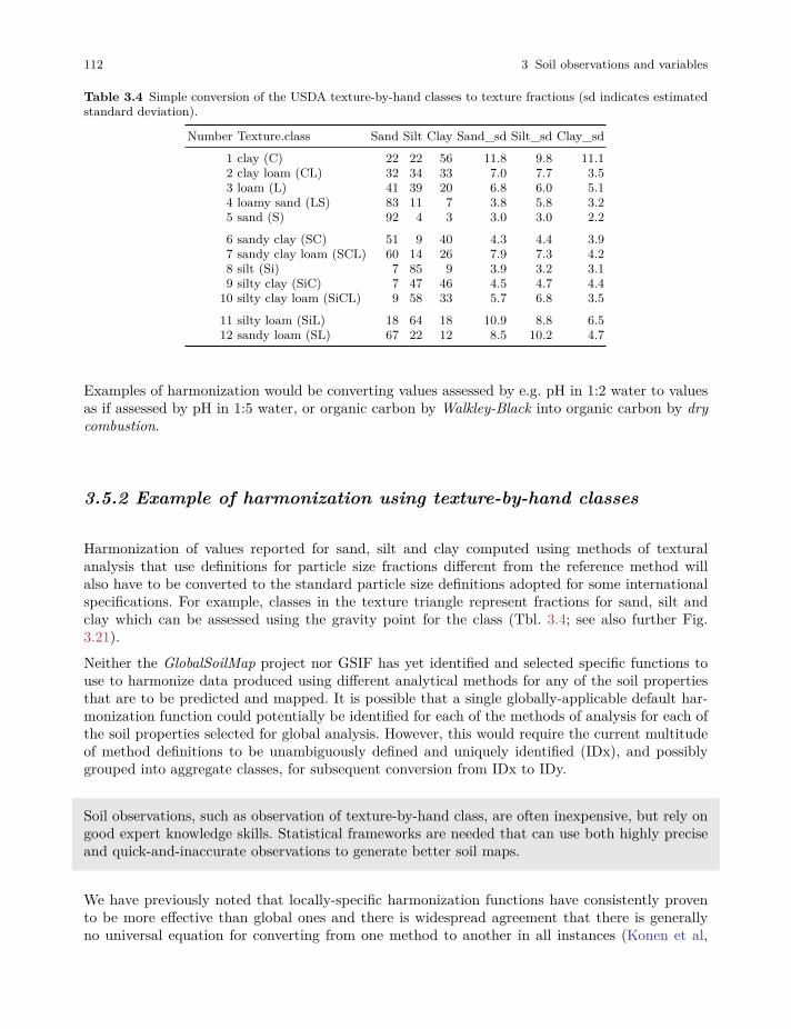
112 3 Soil observations and variables
Table 3.4 Simple conversion of the USDA texture-by-hand classes to texture fractions (sd indicates estimatedstandard deviation).
Number Texture.class Sand Silt Clay Sand_sd Silt_sd Clay_sd1 clay (C) 22 22 56 11.8 9.8 11.12 clay loam (CL) 32 34 33 7.0 7.7 3.53 loam (L) 41 39 20 6.8 6.0 5.14 loamy sand (LS) 83 11 7 3.8 5.8 3.25 sand (S) 92 4 3 3.0 3.0 2.26 sandy clay (SC) 51 9 40 4.3 4.4 3.97 sandy clay loam (SCL) 60 14 26 7.9 7.3 4.28 silt (Si) 7 85 9 3.9 3.2 3.19 silty clay (SiC) 7 47 46 4.5 4.7 4.4
10 silty clay loam (SiCL) 9 58 33 5.7 6.8 3.511 silty loam (SiL) 18 64 18 10.9 8.8 6.512 sandy loam (SL) 67 22 12 8.5 10.2 4.7
Examples of harmonization would be converting values assessed by e.g. pH in 1:2 water to valuesas if assessed by pH in 1:5 water, or organic carbon by Walkley-Black into organic carbon by drycombustion.
3.5.2 Example of harmonization using texture-by-hand classes
Harmonization of values reported for sand, silt and clay computed using methods of texturalanalysis that use definitions for particle size fractions different from the reference method willalso have to be converted to the standard particle size definitions adopted for some internationalspecifications. For example, classes in the texture triangle represent fractions for sand, silt andclay which can be assessed using the gravity point for the class (Tbl. 3.4; see also further Fig.3.21).Neither the GlobalSoilMap project nor GSIF has yet identified and selected specific functions touse to harmonize data produced using different analytical methods for any of the soil propertiesthat are to be predicted and mapped. It is possible that a single globally-applicable default har-monization function could potentially be identified for each of the methods of analysis for each ofthe soil properties selected for global analysis. However, this would require the current multitudeof method definitions to be unambiguously defined and uniquely identified (IDx), and possiblygrouped into aggregate classes, for subsequent conversion from IDx to IDy.
Soil observations, such as observation of texture-by-hand class, are often inexpensive, but rely ongood expert knowledge skills. Statistical frameworks are needed that can use both highly preciseand quick-and-inaccurate observations to generate better soil maps.
We have previously noted that locally-specific harmonization functions have consistently provento be more effective than global ones and there is widespread agreement that there is generallyno universal equation for converting from one method to another in all instances (Konen et al,
3.6 Soil class data 113
2002; Meersmans et al, 2009; Jankauskas et al, 2006; Jolivet et al, 1998; De Vos et al, 2007).Consequently, there will likely be a need to develop locally relevant harmonization functions atthe continental or regional level that apply to restricted soil-landscape domains.
McBratney et al (2002) proposed the concept of a soil inference system (SINFERS) that incorpo-rated both expert soil knowledge and statistical prediction equations. The proposed system wasintended to implement two major functions, namely:
1. Predict all soil properties using all possible (known) combinations of inputs and harmonizationfunctions.
2. Select the combination that leads to a prediction with the minimum variance.
3.6 Soil class data
3.6.1 Soil types
Soil types or soil classes are categories of soil bodies with similar soil properties and/or genesisand functions. There are three main approaches to soil classification (Eswaran et al, 2010; Buolet al, 2011):
1. Classification of soils for the purpose of engineering — Here the focus is put on predicting soilengineering properties and behaviors i.e. on physical and hydrological soil properties.
2. Descriptive classification of soil for the purpose of explaining the soil genesis — Here the focusis put on soil morphology and pedogenesis i.e. functioning of the soil as part of an ecosystem.The representative soil types derived through morphological classification are often visualizedas soil profiles or by using soil-depth functions.
3. Numerical or statistical classification of soils — This is purely data-driven soil classificationwhich can result in significant groupings of soil properties, but that then do not have anycognitive name and are difficult to memorize.
Soil classification or soil taxonomy supports the transfer of soil information from one place, orindividual, to another. Classifying soils can also often be very cost effective — if we identify the soilclass correctly, it is highly likely that we will be able to predict multiple additional soil propertiesthat co-vary by soil type, and that would otherwise require significant resources to measure in thelab.
There are two major international soil taxonomic systems of primary interest for global soil map-ping: The USDA’s Soil Taxonomy (U.S. Department of Agriculture, 2014), and the FAO’s WorldReference Base (IUSS Working Group WRB, 2006). Both KST and WRB are hierarchial, key-based morphological classification systems, but with increasingly more analytical data requiredto reach a specific, more refined, class (Krasilnikov et al, 2009). Mapping soil types, using WRBor KST or both, has been of interest for global soil mapping projects since the first developmentof the global classification systems. As a matter of interest, the term “World soil map” has been
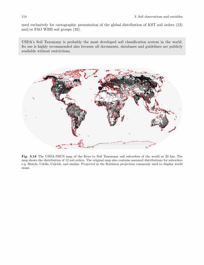
114 3 Soil observations and variables
used exclusively for cartographic presentation of the global distribution of KST soil orders (12)and/or FAO WRB soil groups (32).
USDA’s Soil Taxonomy is probably the most developed soil classification system in the world.Its use is highly recommended also because all documents, databases and guidelines are publiclyavailable without restrictions.
Fig. 3.18 The USDA-NRCS map of the Keys to Soil Taxonomy soil suborders of the world at 20 km. Themap shows the distribution of 12 soil orders. The original map also contains assumed distributions for suborderse.g. Histels, Udolls, Calcids, and similar. Projected in the Robinson projection commonly used to display worldmaps.
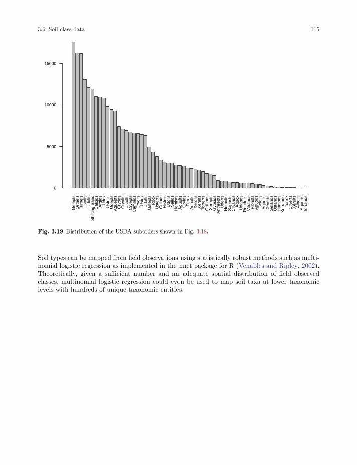
3.6 Soil class data 115
Gel
epts
Ort
hels
Turb
els
Ust
alfs
Udu
ltsS
hifti
ng S
and
Cal
cids
Arg
ids
Udo
xU
stol
lsU
dept
sA
quep
tsC
ryod
sC
ryal
fsU
stul
tsC
ryep
tsC
ambi
dsC
ryol
lsU
stox
Uda
lfsU
step
tsR
ock
Ust
erts
Gel
ods
His
tels
Udo
llsS
alid
sH
emis
tsA
quul
tsC
ryid
sP
erox
Aqu
alfs
Xer
olls
Xer
alfs
Torr
erts
Ort
hods
Xer
epts
Gyp
sids
Ant
hrep
tsU
dert
sH
umul
tsS
apris
tsC
ryan
dsA
quox
Uda
nds
Ren
dolls
Vitr
ands
Fib
rists
Aqu
ods
Gel
olls
Aqu
olls
Xer
erts
Gel
ands
Ust
ands
Hum
ods
Xer
rand
sTo
rrox
Cry
erts
Xer
ults
Alb
olls
Aqu
erts
Torr
ands
0
5000
10000
15000
Fig. 3.19 Distribution of the USDA suborders shown in Fig. 3.18.
Soil types can be mapped from field observations using statistically robust methods such as multi-nomial logistic regression as implemented in the nnet package for R (Venables and Ripley, 2002).Theoretically, given a sufficient number and an adequate spatial distribution of field observedclasses, multinomial logistic regression could even be used to map soil taxa at lower taxonomiclevels with hundreds of unique taxonomic entities.
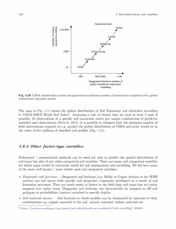
116 3 Soil observations and variables
Order
Num
ber o
f uni
que
taxo
nom
ic e
ntiti
es
Taxonomic level
Suborder
Great Group
Subgroup
Family
Series
Suggested minimum number of points needed for regression
modelling
12
>200
>15,000
100 500-1000 > 1M
Fig. 3.20 USDA classification system and approximate minimum number of observations required to fit a globalmultinomial regression model.
The map in Fig. 3.18 shows the global distribution of Soil Taxonomy soil suborders accordingto USDA-NRCS World Soil Index2. Assuming a rule of thumb that we need at least 5 and, ifpossible, 10 observations of a specific soil taxonomic entity per unique combination of predictorvariables and observations (Harrell, 2001), it is possible to estimate that the optimum number offield observations required to e.g. predict the global distribution of USDA soil series would be inthe order of few millions of classified soil profiles (Fig. 3.20).
3.6.2 Other factor-type variables
Pedometric / geostatistical methods can be used not only to predict the spatial distribution ofsoil types but also of any other categorical soil variables. There are many soil categorical variablesfor which maps would be extremely useful for soil management and modelling. We list here someof the most well known / most widely used soil categorical variables:
• Diagnostic soil horizons — Diagnostic soil horizons (e.g. Mollic or Gypsic horizon in the WRBsystem) are soil layers with specific soil properties commonly developed as a result of soilformation processes. They are much easier to detect in the field than soil types but are rarelymapped over entire areas. Diagnostic soil horizons can theoretically be mapped as 3D soilpolygons or probabilities (rasters) attached to specific depths.
• Soil material classes — Soil horizons or whole profiles can be dominated by minerals or theircombinations e.g. organic material in the soil, calcaric material, tephric material etc.
2 https://www.nrcs.usda.gov/wps/portal/nrcs/detail/soils/use/worldsoils/?cid=nrcs142p2_054010

3.7 Importing and formatting soil data in R 117
• Munsell colour classes — Soil in dry and/or wet condition can be described using some 1–2thousand Munsell colour classes. Each Munsell colour class carries a lot of information aboutthe soil (Fernandez et al, 1988), so that a map of Munsell soil colour classes could be very usefulfor soil management.
• Soil management zones —Each unique combination of soil properties or types and managementzones can be further expanded into a mixed classification system.
• Land degradation classes — Land degradation classes contain information about soil, but alsoabout land cover and land use.
As with any map, categorical, factor-type soil variables can be mapped globally (together with theuncertainty) as long as there is sufficient training field data to properly support application of theprediction algorithm. The other technical problem is the amount of storage required to save andshare all the produced predictions. Each category of a soil categorical variable must be mappedseparately, which can lead to hundreds of grids. The global land cover map for example containsonly some 35 categories, so that it is relatively easy to distribute and use it inside a GIS.
3.7 Importing and formatting soil data in R
3.7.1 Converting texture-by-hand classes to fractions
In the following example we look at how to convert texture-by-hand estimated classes to texturefractions i.e. sand, silt and clay content in %. We focus on the USDA texture-by-hand classes,which are embedded in the soiltexture package3, kindly contributed by Julien Moeys. The USDAtexture triangle can be accessed by:
library(soiltexture)#> Warning: no DISPLAY variable so Tk is not availableTT.plot(class.sys = "USDA.TT")
3 http://cran.r-project.org/web/packages/soiltexture/
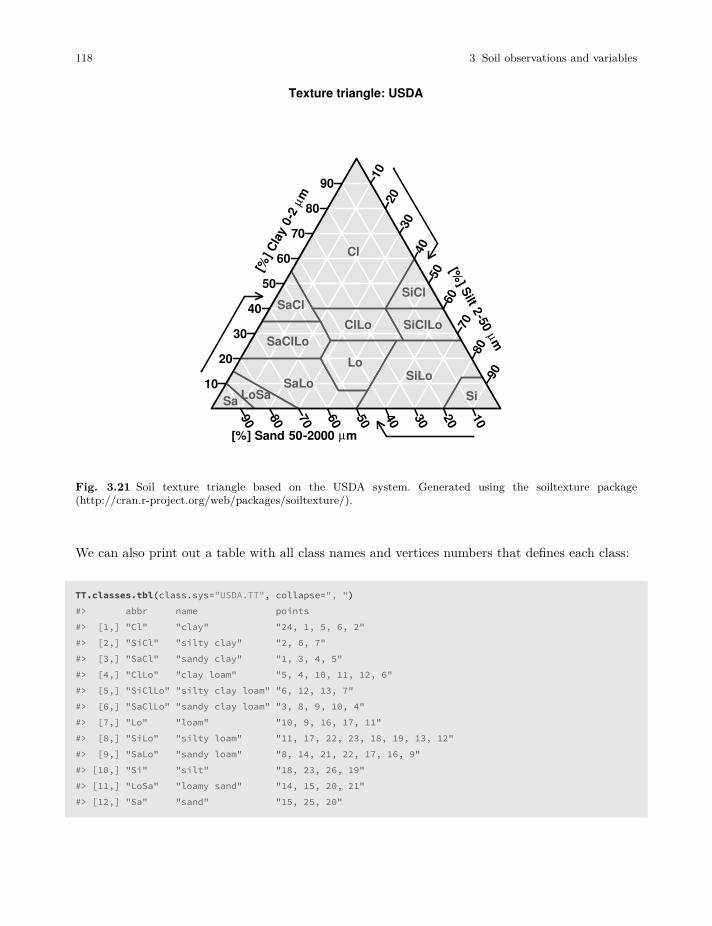
118 3 Soil observations and variables
Texture triangle: USDA
Cl
SiClSaCl
ClLo SiClLoSaClLo
LoSiLoSaLo
SiLoSaSa
102030405060708090
10
20
30
40
50
60
70
80
90
1020
3040
5060
7080
90
[%] Sand 50-2000 µm
[%] C
lay
0-2
µm
[%] Silt 2-50 µm
Fig. 3.21 Soil texture triangle based on the USDA system. Generated using the soiltexture package(http://cran.r-project.org/web/packages/soiltexture/).
We can also print out a table with all class names and vertices numbers that defines each class:
TT.classes.tbl(class.sys="USDA.TT", collapse=", ")#> abbr name points#> [1,] "Cl" "clay" "24, 1, 5, 6, 2"#> [2,] "SiCl" "silty clay" "2, 6, 7"#> [3,] "SaCl" "sandy clay" "1, 3, 4, 5"#> [4,] "ClLo" "clay loam" "5, 4, 10, 11, 12, 6"#> [5,] "SiClLo" "silty clay loam" "6, 12, 13, 7"#> [6,] "SaClLo" "sandy clay loam" "3, 8, 9, 10, 4"#> [7,] "Lo" "loam" "10, 9, 16, 17, 11"#> [8,] "SiLo" "silty loam" "11, 17, 22, 23, 18, 19, 13, 12"#> [9,] "SaLo" "sandy loam" "8, 14, 21, 22, 17, 16, 9"#> [10,] "Si" "silt" "18, 23, 26, 19"#> [11,] "LoSa" "loamy sand" "14, 15, 20, 21"#> [12,] "Sa" "sand" "15, 25, 20"
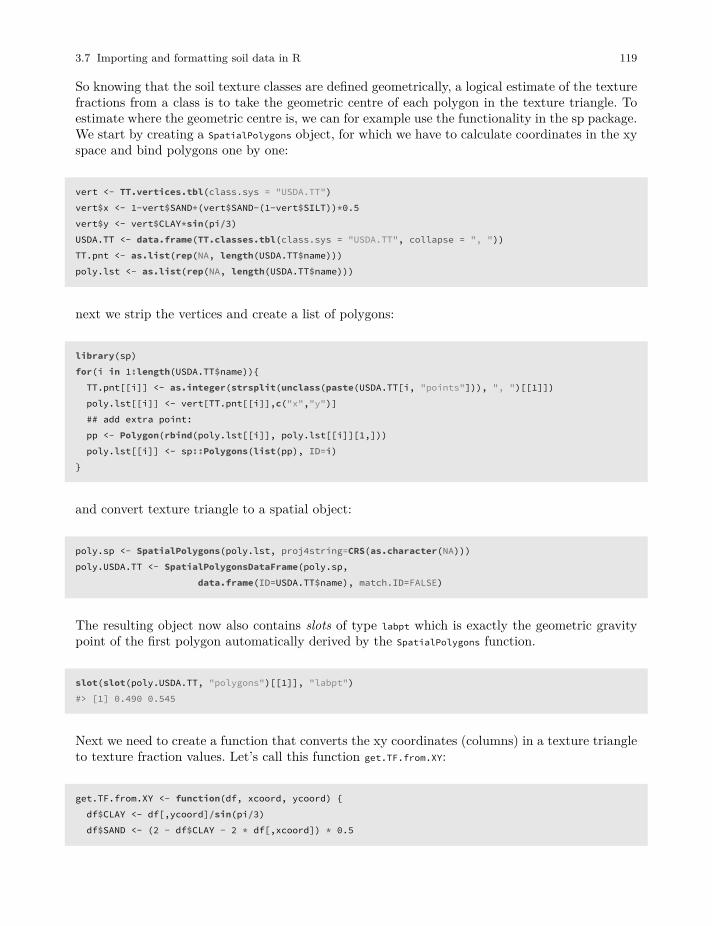
3.7 Importing and formatting soil data in R 119
So knowing that the soil texture classes are defined geometrically, a logical estimate of the texturefractions from a class is to take the geometric centre of each polygon in the texture triangle. Toestimate where the geometric centre is, we can for example use the functionality in the sp package.We start by creating a SpatialPolygons object, for which we have to calculate coordinates in the xyspace and bind polygons one by one:
vert <- TT.vertices.tbl(class.sys = "USDA.TT")vert$x <- 1-vert$SAND+(vert$SAND-(1-vert$SILT))*0.5vert$y <- vert$CLAY*sin(pi/3)USDA.TT <- data.frame(TT.classes.tbl(class.sys = "USDA.TT", collapse = ", "))TT.pnt <- as.list(rep(NA, length(USDA.TT$name)))poly.lst <- as.list(rep(NA, length(USDA.TT$name)))
next we strip the vertices and create a list of polygons:
library(sp)for(i in 1:length(USDA.TT$name)){TT.pnt[[i]] <- as.integer(strsplit(unclass(paste(USDA.TT[i, "points"])), ", ")[[1]])poly.lst[[i]] <- vert[TT.pnt[[i]],c("x","y")]## add extra point:pp <- Polygon(rbind(poly.lst[[i]], poly.lst[[i]][1,]))poly.lst[[i]] <- sp::Polygons(list(pp), ID=i)
}
and convert texture triangle to a spatial object:
poly.sp <- SpatialPolygons(poly.lst, proj4string=CRS(as.character(NA)))poly.USDA.TT <- SpatialPolygonsDataFrame(poly.sp,
data.frame(ID=USDA.TT$name), match.ID=FALSE)
The resulting object now also contains slots of type labpt which is exactly the geometric gravitypoint of the first polygon automatically derived by the SpatialPolygons function.
slot(slot(poly.USDA.TT, "polygons")[[1]], "labpt")#> [1] 0.490 0.545
Next we need to create a function that converts the xy coordinates (columns) in a texture triangleto texture fraction values. Let’s call this function get.TF.from.XY:
get.TF.from.XY <- function(df, xcoord, ycoord) {df$CLAY <- df[,ycoord]/sin(pi/3)df$SAND <- (2 - df$CLAY - 2 * df[,xcoord]) * 0.5
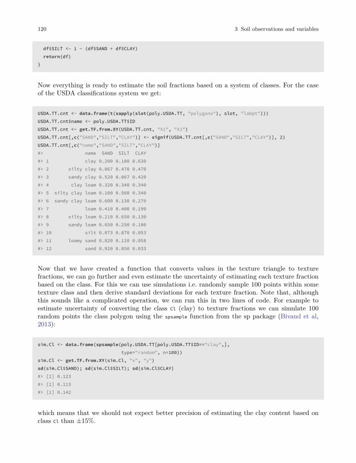
120 3 Soil observations and variables
df$SILT <- 1 - (df$SAND + df$CLAY)return(df)
}
Now everything is ready to estimate the soil fractions based on a system of classes. For the caseof the USDA classifications system we get:
USDA.TT.cnt <- data.frame(t(sapply(slot(poly.USDA.TT, "polygons"), slot, "labpt")))USDA.TT.cnt$name <- poly.USDA.TT$IDUSDA.TT.cnt <- get.TF.from.XY(USDA.TT.cnt, "X1", "X2")USDA.TT.cnt[,c("SAND","SILT","CLAY")] <- signif(USDA.TT.cnt[,c("SAND","SILT","CLAY")], 2)USDA.TT.cnt[,c("name","SAND","SILT","CLAY")]#> name SAND SILT CLAY#> 1 clay 0.200 0.180 0.630#> 2 silty clay 0.067 0.470 0.470#> 3 sandy clay 0.520 0.067 0.420#> 4 clay loam 0.320 0.340 0.340#> 5 silty clay loam 0.100 0.560 0.340#> 6 sandy clay loam 0.600 0.130 0.270#> 7 loam 0.410 0.400 0.190#> 8 silty loam 0.210 0.650 0.130#> 9 sandy loam 0.650 0.250 0.100#> 10 silt 0.073 0.870 0.053#> 11 loamy sand 0.820 0.120 0.058#> 12 sand 0.920 0.050 0.033
Now that we have created a function that converts values in the texture triangle to texturefractions, we can go further and even estimate the uncertainty of estimating each texture fractionbased on the class. For this we can use simulations i.e. randomly sample 100 points within sometexture class and then derive standard deviations for each texture fraction. Note that, althoughthis sounds like a complicated operation, we can run this in two lines of code. For example toestimate uncertainty of converting the class Cl (clay) to texture fractions we can simulate 100random points the class polygon using the spsample function from the sp package (Bivand et al,2013):
sim.Cl <- data.frame(spsample(poly.USDA.TT[poly.USDA.TT$ID=="clay",],type="random", n=100))
sim.Cl <- get.TF.from.XY(sim.Cl, "x", "y")sd(sim.Cl$SAND); sd(sim.Cl$SILT); sd(sim.Cl$CLAY)#> [1] 0.123#> [1] 0.113#> [1] 0.142
which means that we should not expect better precision of estimating the clay content based onclass Cl than ±15%.
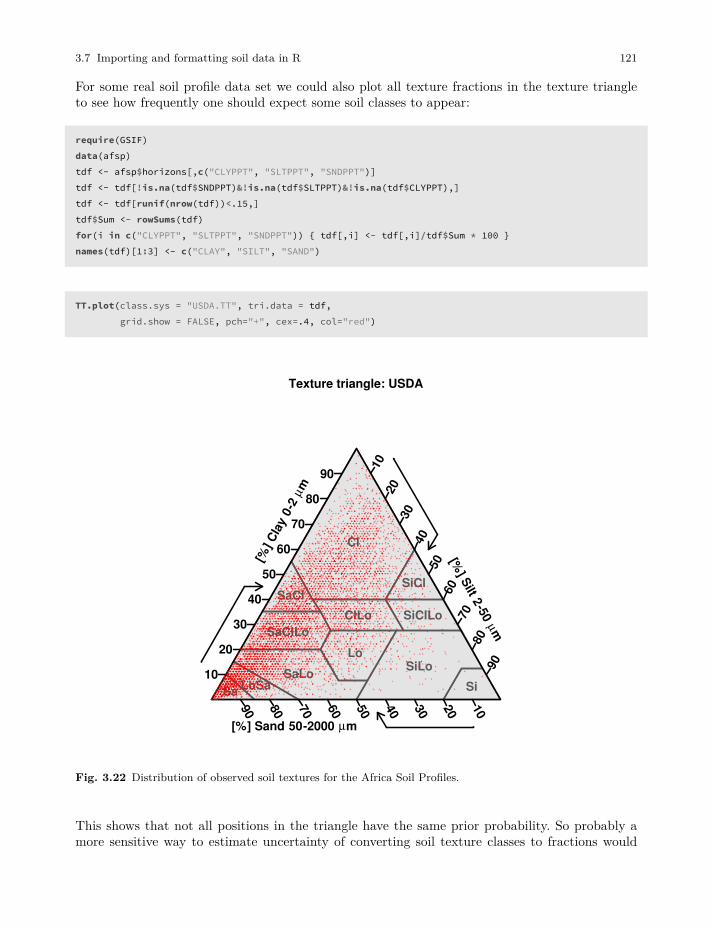
3.7 Importing and formatting soil data in R 121
For some real soil profile data set we could also plot all texture fractions in the texture triangleto see how frequently one should expect some soil classes to appear:
require(GSIF)data(afsp)tdf <- afsp$horizons[,c("CLYPPT", "SLTPPT", "SNDPPT")]tdf <- tdf[!is.na(tdf$SNDPPT)&!is.na(tdf$SLTPPT)&!is.na(tdf$CLYPPT),]tdf <- tdf[runif(nrow(tdf))<.15,]tdf$Sum <- rowSums(tdf)for(i in c("CLYPPT", "SLTPPT", "SNDPPT")) { tdf[,i] <- tdf[,i]/tdf$Sum * 100 }names(tdf)[1:3] <- c("CLAY", "SILT", "SAND")
TT.plot(class.sys = "USDA.TT", tri.data = tdf,grid.show = FALSE, pch="+", cex=.4, col="red")
Texture triangle: USDA
Cl
SiClSaCl
ClLo SiClLoSaClLo
LoSiLoSaLo
SiLoSaSa
102030405060708090
10
20
30
40
50
60
70
80
90
1020
3040
5060
7080
90
[%] Sand 50-2000 µm
[%] C
lay
0-2
µm
[%] Silt 2-50 µm
+
+
+
++
+
+
+
++
+
++
+
+ ++
+
+
+
+
+
+
+
+
+
+
+
+
+
+
+
+
++
+
+++
+
++
+
+
+
+
+
+
+
+
+
+
+
+
+
+
+
++
+
+
+++
+
+
+ +
++
+
+
+
+
++
+
+
+
+
++
+
++
+ ++
+
+
+
+
+
+
++
++
+
+
+
++
+++
++
++
+
+
+
++
++
+
+
+
+
++
+
+
+
+
+
+
++
+
+
+
+
+
+
+
+
++
+
+
+
+
+
+
+ +
+
+
+
+
+
+
+
+
+
+
+
+
++
+
+
+
+
+
+
+
+
+
+
+
+
+
+
+ ++
+
+
+
++ ++
+
+
+
+
+
+
++
+
+
++
+
+
+
+
+
+
+
+
+
+
+
+ +
+
++
+
+
+
+
+
+
+
++
+
+
+
+
+
+
+
+
+
+
+
+
+
+
+
+
+
+
+
+
+++
+
+
+
+
+
++
+
+
+
++
+
+
+
+
++
+
+
++
+
+ +
+
+
+
+
+
+
+
+
+
+
+
+
+
+
+
+
+
+
+
+
+
+
+
+ +
+
++
+
+
+
+
++
+
+
+
+
+
+
+
+
++
+
++
+
+
+
+
+
+
+
+
+
+
+
+
+
++
+
+
+
++
+
+
+
++
+
+
+
++
+
+
+
+
+
+
+
+
++
+
++
+
+
+
+
+
+
+
+
+
+
+
+++
+
+
+
+
+
+
+
+
+
+
+
+
+
++
+
+
+
+
++
++
+
+
+
++
+
++ +
+
+
+
+
+
+
++
+
++
+
+
+
+
+
+
+
+
+
+
+
++
+
+
+
+
++
++
+
+
+
+
+
+
+
++
+
+
+
+
+
+
++
+
+
++
+
+
+
+
+
+
+
+
+
+
+
+
+
+
+
+
+
+
+ +
++
++
+
+
+
+
+
+
+
+
++
+
+
+
+++
+
++
+
+
+
++
+
+
+
+
+
+
+
+
+
+
+
+
+
+
+
++
+
+
+
+
+
+
+
+
+
+
+
+++
+
+
+
++
+
+
+
+
+
+
+
+
+
+
+
+
+
+
++
+
++
+
+
+
+
+
++
+
+
+
+
+
++
++
+
++
+ ++
+
++
+
+
+
+
+
+
+
+
+
+
+
+
+
+
+
+
+
+
+
+
++
+
+
++
+
+
++
+
+
+
+
+
++
+
+
+
++
+
+
+
+ +
+
+
+
+
+
+
+
+
+
+
+
+
+
++
+
+
++
+
+++
+
+
+
+
++
+
+
+
+
+
+
++
+
+
+
+
+
+
+
+
++
+
+
+
++
+
+
+
+
+
+
+
+
+
+
+
+
+++
+
+
++
+
+
++
+
+
+
+
+
+
+
+
+
++
+
+
+
+
+
+
+
++ +
+
+
+
+
+
++
+
++
+
+
++
+
+
+
+
++
+
+
+
+
+
+
+
+
+
+
+
+
++
++
+
+
+
+
+
+
+
++
+
+
+
+
+
+
+
+
+
+ +
+
+
+
+
+
+
+
+
+
+
+
+
+
+
+
+
+
+
+
+
+
+++
++
+
+
+
+
+
+
+
+
+
+
++
+
+
+ +
+
+ +++
+
+
+
+
++
+
++
++
+
+
+
+
+
++
+
+
+
+
+
++
+
++
+
++++
+
+
++
+
+
+
+
+++
++
+
+
+
+
+
+
+
+
++
++++
+
+
+
+
+
+
+
+
++
+
+
+
+
+
+
+
+
+
+ +
+
++
+
+
+
+
+
++
++
+
+
+
+
+
+
+++
+++
+
+
+
+
+
++
+
+
+
+
+
+
+
+
+
+
+
+
+
+
+
+ +
+
+
+
+
+
+
+
+
+
+
+
+
+
+
++
+
++
+
+
+
+
+
+
+
+
+
+
+
+
+
+
+
+
+
+
+
+
+
+
+
+
+
+
+
+
+
+
+
+
+
+
+
+
+
++
++
+
+
+
+
+
+
+
+
+
+
+
+
+
+
+
+
+
++ +
+
+
+
+
+
+
++
+
+
+
+
+
+
+
+
+
+
+
+
+
+
+
+
++
+
+
+
++
+
+
+
+
+
+
+
++
+
+
+
+
+
+
+
+
+
+
+
+ +
+
+
+
+
+
+
+
+
+
+
+ +
+
+
+
+
+
+
+
+ +
+
+
+
+
+
+
+
++
+
+
+
+
+
+
++
+
++
+
+
+
+
+
+
++
+
+
+
+
+
++
+
+
+
+
+
+
+
+
+
+
+
+
+
+ +
+
+
+
+
+
+
++
+
+
+
+
+
+
+
++
++
+
++
+
+
+
+
+
++
+
+
+
+
++
++
+
+
+
+
+
+
+
+
+
+
+
+
++
++
+
+
+
+
+
+
+
+
+
++
+
+
+
+
+
+
+++
+
+
++
+
++
+
+
+
+ +
+
++
+
+
++
+
+++
+
+ ++
+
++
++
+
+
+
+++
+
++
+++
+
++
++
+++
+
++
++
+
+ +
+
+
+
+
+
+
+
+
+
+
+
+
+
+
+
+
++
+
+
+++
+
++
+
+ +
+
+
+
+
+
+
+
+
+
+
+ +
+
+
+
+
+
+
+
+
+
+
+
+
+
+
+
+
+
+
+
+
+
+
+
+
+
+
+
+
+
+
++
+
+
+
+
++
+
+
+
+
+
+
+
+
+
++
+
+
+
+
+
+
++
+
+
+
+
+
+
+
+
+
+
+
+
+
+
+
+
+
+
+
+
++
+
+
+
++
++
+
+
+
+
+
+
+
+
+
+
+
+
+
+
+
+
+
++
+
+
+
+
+
++
+
+
+
+
+
+
+
+
+
+
+
+
+
+
+
+
++
+
+
+
+
+
+
+
+
++
+
+
+
+
+
++
+
+
+
++
++
+
+
+
+
+
++
+
+
+
+
+
+
+
+
+
+
+
+
+
+++
+++
++
+
+++
+
+
+
+ +
+
+
+
+
+
++
++
+
+ +
+
+
+
+
+
+
+
+
+
+
++
+
+
+
+
+
+
++
+
+
+
+
+
++
+
+
+
++
++
+
+
++
+
+
+
+
+
+
+
+
+
++
+
+
+
+
+
+
+
+
++
++
+
+
+
+
+
++
+
+
+
++
+
+
+
+
+
+
+
+
+
+
+
+
+
+
+
+
+
+
+
+
+
+
+
+
+
+
+
+
+
+
+
++
+
+
+
+
+
+
+
+
+
+
+
+
+
+
+
+
+
+
++
+
+
+
++
+
++
++++++ ++
++
+
+
+
+
+
+
+
+
+
+
+
+
+
+
+
+
+
+
+
+
+
+
+
+
+
+
+
+
+
+
+
+
+
+
+
+
+
+
+
++
++ +
+
++
+
+ ++
+++
+
++
+
+
+
++
+
+
+
+
+
++
+
+
+
+
+
+
++
+
+
+
+
++
+
+
+
+
++
+
+
+
+
+
+
+
+
+
+++
+
+
+
+
+
++
+++
+
++
++
++
++++
++ +
++
+
+
+
+
+
+
+
+
++
+
+
+
+
+
+
+
+
++
+
+
++
+
+
+
+
+
+
+
+
+
+
++
+
+
+
+
++
+
+
+
+
+
+
+
+
+
+
+
+
+
+
+
+
+
+
+
++
+
+
+
+++
+
++++
++
+++
+ ++
+
+
+
+
+ +
+
++
++
+
+
+
+
++
++
+
+
++
+
+
+
+
+
+
+
++
++
+ +
+
+
+
+
+
+
++
+
+
+
+
+
+
+
+
+
+
+++++
++
+
+
+
+
+
+
+
+
+
+
++
+
+
++
+
+
+
+
+
+
+
+
+
+
+
+
+
++
+
+
+
+
+
+
+
+
+
+
+
+
+
+
+
+
+
++
++
+
+
+
+
+
+
++
+
+
+
+
+
+
+
+
++
+
+
+
+
+
+
+
+
+
+
+
+
++
+
++
+
+
+
+
+
+
+
+
+
+
+
+
+
+
+
+
+
+
+ ++
+
+
+
+
+
++
+
+
++
+
+
+
+
+
+
+
+
+
+
+
+
++
+
+
+ +
+
+
+
++
+
+
+
+
+
+
+
+
++
+
+
+
+
+
+
+
+
+
+
+
+
+
+
++
++
+
++
+
+
+
+
+
+
+ +
++
+
+
+
+
+
++
+
+
+
+
++
+
+
++
+
+
+
+
++
+
++
+
+
+
+
+
+
+
+
+
+
+
+
+
+
+
+
+
++
++
+
+
+
+
++
+
+
+ +
+
+
+
+
+
+
+
+
+
+
+
+
+
+
+
++
+
+
+
+
+
+
+
+
+
+
+
+
+
+
++
+++
+
+
+
+
+
+
+
+
+
+
+
++
+
+
++
+
+
+
+
+
+
+
+
+
+
++
+
+
+
+
+
+
++
+
+
++
+
+
+
+
+
+
+
+
+
++
+
+
+
+
+
++
+
+
+
+
+
+
+
++
+
+
+
+
+
+
++
+
+
+
++
+
++
+
+
+
+
+
+
++
+
+
+
+
+
++
+
+
++
+
+
+
+
+
+
+
++
+
+
+
+
+
+
+
+
+
+
+
+
+
+
+
+
+
+
+
+
++
++
+
+
+
+
+
+
+ +
+
+
+
+
+
+
+
+
+
+
+
+
+
++
+
++
+
+
++
+
+
+
+
++
+
+ +
+
+
+
++
+
+
+
+
+
++
+
+
+
+
+
+
+
+
+
+
+
+
+
+
+
+
+
+
+ +
+
+
+
+ +
+
+
+
+
+
++
+
+++
+
+
+
++
+
+
+
+
+
+
+
+
+
+
+
+
+
+
+
++
+
++
+
+
+
+
+
++
+
+
+
++ +
+ +
+
+
+
+
+
+
+
++
+
++
+
+
+
+
+
+
+
+
+
+
+
+
+
+
+
+
+
++
+
+
+
+
+
+
+
+
++
+
+
+
+
+
+
+++ +
+
+
+
+
+
+
+
+
+
+
+
++
+
++++
++
++
+
++
+
++
++
+
+
+
+
+
+
+
+
+
++
+
+
+
+
+
+
+
+
+
+
+
+
+
++
+
+
+
+
+
+
+
+
+
+
+
+
+
+
+
+
++
++
+
+
+
+
+
+
+
+
+
++
+
++
+
+
+
+
+
+
+
++
+
+
+
+
+
+
+
+
+
+
+
+
+
+
+
+
+
+
+
+
+
+
+
+
++
++
+
+
+
+
+
+
+
+
+
+
+
+
+
+
+
+
+
+
+
+
+
+
+
+
+
+
+
+
+
+
+ +
+
++
+
+
+
++
+
+
+
+
+
+
+
+
+
+
+
+
+
+
+
+
+
+
+
+
+
+
++
+
+
+
+
+
+
+
+
+
+
+
+
++
+
+
+
+
+
+
+
+
+
+
+
+ +
+
+
+
+
+
++
+
++
+
+
+
+
+
+
+
+
+
+
+
+
+
+
+
+
++
+
+
+
+
+
+
+
+
+
+
+
+
+
+
+
+
+
+
+
+
+
+
+
+
+
+
+
+
+
+
+
+
+
+
++
+
+
+
+
+
+
+
+
+
+
+
+
+
+
+
+
+
+
+
++
+
+
+
+
+++
+
+
+
+
+
+
+
+
+
+
+
+
+
+
+
+
+
+
+
+
+
+
+
+
+
+
+
++
+
+
+
+
+
+
+
++
+
+
++
++
+
++
+
+
++
+
+
+
+
+ +
+
+
++
+
+
+
+
+
+
+
+
+
+
++
++
+
+ +
+
+
+
+
+
+
+
+
+
+
+
+ +
+
+
+
++
+
+
+
+
+
++
+
++ +
+
+
+
+
+
+
++
+
+
++
+
+
+
+
+
+
+
+
+
+
+
+
+
+
+
+
+
+
+
+
++
+
+
+
+
+
+
+
+
++
+
+
+
+
++
+
+
+
+
+
+
+
+
+
+
+
+ +
+
+
++
+
+
+
+
+
+ +
+
++
+
+
++
+
+
+
+
+
+
+
+++
+
+
+
+
+
+
+
++
+
+
+
+
+
+
+
+
+
+
++
+
++
+
+
+
+
+
+
+
+
+
+
+
+
+
+
++
+
+
+
+
+
+
+
+
+
++
++
+
+
+
+
+
+
+
+
+
++
+
+
+
+
+
+
+
+
+
+
+
+
++
+
+
+
+
+
+
+
++
+
+
++
+
+++
+
++
+
++
++
++
+
+
+
+
+
+
+
+
+
+
+
+
+
+
+
+
+
+
+
+
+
+
+
++
+
++
+
+
+
+
+
+
+
+
++
+
+
+
+
+
++
+
+
+
+
+
+
+
+ +
+
+
+
+
+
+
+
+
+
++
+
+
+
+
+
+
+
++
+
+
+
+
+
++
+
+
+
+
++
+
+
+
+
+
+
+
+
++
+
+
+
+
+
++
+ +
+
+
+
++
+
+
+
+
+
+
+
+
+
+
+
+
+
+
+
+
+
+
+
+
+
+
+
+
+
+
+
+
+
+
+
+
+
++ +
+
++
+
+
+
+
+
+
+
+
+
+
+
+
+
+
+
+
+
+
+
++
+
+
+
+ +
+
+
+
+
+
++
+
+
+
+
+
+
+
+
+
+
+
++
+
+
+
+
+
+
+
+
+
+
+
+
+
+
+
+
+
+
+
+
+
+
+
+
+
+
+
+
+
+
+
+
+
+
+
+
+
+
+
+
+
+
+
+
+
+
+
++
+
+
+
+
+
+
+
+
+
+
+
+
+
+
+
+
+
+
+
+
+
+
+
++ +
+
+
+
++
+
+
+
+
+
+
+
+
+
+
+
++
+
+
+
++
+
+
+
+
+
+
+
+
+
+
+
++
+
++
+
+
+
+
+
+
+
+
+
+
++
+
++
+
+
+
+
+
+
+
+
+
+
+
+
+
++
+
+
++
+
+
+
+
++
+
+++
+
+
+
+
+
+
+
+
+
+
+
+
+
+
+
+
+
+
+
+
+
+
+
+
+
+
+
+
+
+
++
+
+
+
+
+
+
+
+
+
+
+
++
+
++
+++
+
+
+
+
+
+
+
+
+
+
+
++
+
+++
+
+
+
+
+
++
+
+
+
+
+
+
+
+
+
+
++
++
+
+
+
+
+
+
+
+
+
+
+
+
+
+
+
+
+
+
+
+
+
+
+
+
++
+
+
+
+
+
+
+
+
+
++
+
+
+
++
+
+
+
+
+
+
+
+
+
+
+
+
+
+
+
+
+
+
+
+
+
+
+
+
+
++
+
+
+
+
+ ++
+
+
+
+
+
+
+
+
+
+
+
+
+
+
+
+
+
+
+
+
+
+
+ +
+
+
++
+
+
+
+
++
+
+
+
+
+
+
+
+
+
+
+
+
+
+
+
+
+
++
+
+
+
+
+
+
++
+
+
+
+
+
+
+
+
+
+
+
+
++
+
++
+
+
+
++
+
+
+
+
++
+
+
+
+
+
+
++
+
+
+
+
+
+
+
+
+
+
+
+
+
+
+
+
++
+
+
+
+
+
+ +
+
+
+
+
+
+
+
+
+++
+
++
+
+
+
+
+
+
++
+
+
+
+
+
++
+
+
+
+
+
++
+
+
+
+
+
++
+
+
+
+
+
+
+
+
+
+
++
++
+
+
+
+
+
+
++
+
+
+
++
+
+
+
+
+
+ +
+
+
+
+ ++
++
+
+
++
+
+
++
+
+
+
+
+
+
+
+
+
+
+
+
+
+
+
+
+
+
+
+
+
+
+
++
+
+
+
+
+
+
+
+
+
++
+
++
+
+
+
+
+
+
+
++
+
++
+
++
++
++
+
+
+
++
+
+
+
+ +
+
+
+
+
+
+
+
+
+
+
+
+
++
+
+
+
++
++
+
+
+
+
+
+
+
+
+
+
+
+
+
+
+++
+
+
+
+
+
+
+
+
+
+
+
+
+
+
+
+
+
+ ++
+
+
+
++
+
+
+
+
+
+
+
+
++
+
+
+
+
+
+
+
+
+
+
+
+
+
+
++
++
+
+
+
+
+
+
+
+
+
+
+
+
+
+
+
+
+
+ +
++
++
+
+
+
++
+
+
++
+
++ +
+
+
+
+
+
+
+
+
+
+
++
+
+
+
+
+
+
+
+
+
+
+
+
+
+
+
+
+
++
+
+
+
+
+
+
+
+
+
++
+
+
+
+
+
++
+
+
+
+
+
+
+
+
+
+
+
+
+
+
+
+
+
+
+
+
+
+
+
+
+
+
+
+
+
+
+ +
+
+
+
+
+
+
+
+
+
+
+
+
+
+
+
++
+ +
+
+
++
+
+
+
+
+
+
+
+
+
+
+
+
+
+
+
++
+
+
+
+ +
+
+
+
+
++
+
+
++
+
+
+
+
+
+
++
+
+
+
++
+
+
+
+
+
+
+
+
+
+
+
++
+
+
+
+
+
+
+
+
+
+
+
++ +
+
+
+
+
+
+
++
+++
+
+
+
+
+
+
+
+
+
+
+
+
+
+
+
+
+
+
+
+
+
+
+
+
+
+
+
++
++
+
+
+
+
+
+
+
+
+
+
++
+
+
++
+
+
+
+
++
+
+
+
+
++
+
+
+
+
+
+
+
+
+
+
+
+
+
+
+
+
+
+
+
+
+
+
+
+
+
+
+
+
+
+
+
+
+
+
+
++
++
+
+
+
+
+
+
+
+
+
+
+
+
+
+
+++
+
+
+
++
+
+
+
+
+
+
++
+
+
+
+
+
+
++
+
+ +
+
+
+
++
+
+
+
+
+
++
+
+
+
+
+
+
+
+
+
+
+
+
+
++
+
+
+
+
+++
+
+
++
+
+
+
++
+
+
+
+ +
+
++
+
++
+
+
+
+
+
+
+
+
+
+
++
+
+
+
+
+
+
+
+
+
+
+
+
+ +
+
+
++
+
+
+
+
+++
+
++
+++
+
+
+
+
+
+
++
++
+
+
+
+
+
+
+
+
+
+
+
+
+
+
++
+
+
+
++
+
+
+
++
++
+
+
+
+
+
+
+
+
+
+
+
+
+
+
+
+
+
+
+
+
+
+
+
+
+ +
++
+
+
++
+
+
+
+
+
++
+
+
+
+
++
+
+
+ +
+
+
+ ++
+
+
+
+
+
+
+
+
+
+
+
+
+
+
+
+
+
+
+
+
+++
+
+
++
+
+
++
++
+
+
++
+
+
+
+
+
+
+
+++
+
+
+
+
+
+
++
+
++
+
+
+
+
+
+
+
++
++
+++
+
+
+
+
+++
++
+
+
+
+
+
+
+
+
+++
+
+
+
+
+
+
+
+
++
++
+
+
+
+
+
+
+
++
+
+
+ +
+
+
+
+
+
+
+
+
+
+++
+
+
+
+
+
+
++
+
+
+
+
+
+
+
+
++ +
+
++
+
+
+
+
+
+
+
+
+ +++
+
+
+
+
+
+
+
+
++
+
+
+
+
+
+
+
+
++
+
+
+
+
+
+
++
+
+++
+
+
+
++
+
+
+
+
+
+
+
++
+
+
+
+
+
+
+
++
+
+ +
++
+
+
+
+
+
+
+
+
+
+
+
+
+
+
+
+
+
+
+
+
+
+
+
+
+
+
+
+
+
+
+
+
+
+
+
+
+
+
+
+
+
+
+
++
+
+
+
+
+
+
++
+
+
+
+
+
+
+
+
+
+
+
+
+
+
+
+
+
+
+
+
+
+
+
++
+
++
+
+
+
+
+ +
+
+
++
+
+
+
+
++
+
+
++
+
+
+
+
+
+
+
++
+++
+
+
+
++
++
+
+
+
+
+
++
+
+
+
+
+
+
+
+
+
++
+
+
+
+
+
+
++
++
+
+
+ +
+
+
++
++
+
+
+
+
+
++
++
+
+
+
+
++
+ ++
+
+
++
+
+
+
+
+ +
++
+
+
+
+
+ +
+
+
+
+
+
+++
++
+
+
+
+ ++
++
++
+
+
+
+ ++
+
++
++
++
+
++
+
+++
+++
++
++
+
+ ++
++
++
+
+
+
+
+
++
++
+
+
+
+
+
+
+
+
+
+
+
+
+
+
+
++
+
+
+
+
+
++
+
+
++
+
+
+
+
++
+
+
+
+
+
+
+
++
+
+
+
+
+
+
+
++
+
+
+
+
+
+
+
+
+
+
+
+
+
+
+
+
++
++
++
+
+
++
+
+
+
++
+
+
+
+
+
+
+
+
+
+
+
+
+
+
+
+
+
++
+
+
+
+
+
+
+
+
+
+
+
+
++
+
++
+
+ +++
+
++
+
+ ++++++++
+
+
++
+
+
+
+
++
+
+
++
+
+
+
+
+
+
+
+
+
+
+
++ +
+
+
+ +
+
+
+
+
+
+
+ +
+
+
+
++
+
++
++
+
+
+
+
+
++
+
+
+
+
++
+
+
+
+
+
+
+
+
++
+
+
+
+
+
+
+
+
+
+
++
+
+
+
+
++
+
+
+
+
+
+
+
+
+ +
+
++
+
+
+
+
+
+
+
+
+
+
+
+
+
+
+
+
+
+
+
+
+
++
+
+
+
+
+
+
+
+
+
+
+
+
+
++
+
+
+
+
+
+
+
++
+
+
+
++
+
+
+++ +
+
+
+
+
+
+
+
++
+
+
+
+
+
+
+
+
++ +
+
+
+
+
+
+
+
+
+
+
+
+
++
+
+
+
+
+
+
+
+
++
+
+
+
+
+
+
+
+
++
++
+
+
+
++
+
+
++
+
++
+
+
++
+
+
+
++
+
+
+
+
+
++
+
+
+
+
+
+
+
+
++
+
+
++
+
+
+
+
+
++
+
+
+
+
++
+
++
+
+
+
+
+
+
+
+
+
+
+
+
+ +
+
+
+
++
+
+
+
+
+
+
+
+
+
+
+
+
+
+
+
+
+
+++
+
+ +
+
+
+
++
+
+
+
+
++
+
+
+
+
+
+
+
+
++
+
++
+
+
++
+
+
++
+
+
+
+
+
+ +
+
+
+
+
+
+
+
+
+
+
+
+
+
+
+
+
+
+
+
+
+
+
+
+
+
++
++
+
++
+
+
+
+
+
+
+
+
+
+
+
+
++
+
+
++
+
+
+
+
+
+
+
+
++
+
+
+
+++
+
+
+
+
+
+
+
+
+
+
+
++
+
+
+
+
+
+
+
+
+
+
+
++
+
+
+
++
+
++
+
++
+
+
+
+
+
+
+
+
+
+
++
+
+
+
++
++
+
+
+
+
+
+
+
+
+
+
+
+
+
+
+
+
+
+
+
+
++
++
++
+
++
+
++
+
++
+
+
+
+
+
+
++
++
+
+
+
+
+ +
+
+
+
+
+
+
+
+
+
++
+
+
+
+
+
++
+
+
++
+
+ +
+
+
++
++
+
+
+
+
+
+
+
+
+
+
+
+
+
+
+
+
+
+
+
+
+
+
+
++
+
+
+
+
+
+
+
+
+
++
+
+
+
+
+
+
+
+
+
+
+
++
+
+
+
+
+
+
+
+
+
++
+
+
+
++
+
+
+
+
+
+
+
+
+
+
+
+
++
+
+
++
+
+
+
+
+
+
+
+
++
+
+
+
+
+
+ +
+
+
+
+
+
+
+
+
+
+
+ +
+
+
+
+
+
+
+
+
++
++
+
+
+
+
++
+
+
++
+
+
+
+
+
+
+
+
+
+
+
+
+
++
+++
+
+
+
+
+
+
+
+
+
++
+
+
+
++
+
+
+
+
++
+
+
+
+
++
+
+
+
+
+
+
+
+
+
+
+
+
+
+
+
+
+
+
+
+
+
+
+
+
+
+
++
++
+
+
+
+
+
+
+
+
+
+
+
++
+ +
+
+
+
+
+
+
+
++
+
+
+
+ +
+
+
++
+
+
+
+
+
+
+
+
+
+
+
+
+
+
+
++
+
+
+
+
++
+
+
+
+
++
+
+
+
+
+
+
+
+
+
+
+
+
+
+
+
+
+
+
+
+
+
+
+
+
+
++
+
+
+
+
+
+
+
+
+
+
+
+
+
+
+
+
+
+
+
+
+
+
+
+
+
++
+
+
+
+
+
+
+
++
+
+
+
+
+
+
+
+
+
+
+
+
+
+
++
+
+++
+
+
+
+
+
+
+
+
+
+
+
++
+
+
+
+ +
+
++
+
+
+
+
+
+
+
+
++
+
+
+
+
+
+
+
++
++
+
+
+
+
++
+
+
+
+
+
+
++
+
+
+
+
+
+
+
+++
+
++++
+
+
+++
++
++ +
+
+
++++
+
+
+
++
+
+
+
+
+
+
+
+
+
+
+++
+
+
+
++
+
+
+
+
++
+
+
+
+
+
+
+
+
+
++
+
+
+
+
+
+
+
+
+
++
+
+
+
+
+
+
+
+
++
+
+
+
+
+
+++
+
+
+
+ +
+
++
++
+
+
+
+
+
+
+
+
+
+ +
+
+
+
+
++
+
+
+
+
++
++
+
+
+
+
+
+
+
+
+
+
+
+
+
+
+
+
+
++
+
+
+
+
+
+
+
+
+
+
+
+
+
+
++
+
+
+
+
+
+
+
++
+
+
+
+
+
+
++
+
+
+
+
+
+
+
+
+
+
+
++
+
+
+
+
+
+
+
+++++
+
+
+
+
+
+
+
++
+
+
++
+
+
+
+
+
+
+
+
++
++
+
+
+
+
+
+
+
+
+
+
+
+
++
+
+
+
++
+
+
+
+
+
+
+
+
+
+
+
++
+
+
+
+
+
+
+
+
++
+
+
+
+
+
+
+
+
+
+
+
+
+
+
+
+
+
++
+
+
+
+
+
++
+
+
+
+
+
+
+
+
+
+
+
+
+
+
+
+
+
+
+
+
+
+
+
++
++
+
+
+
+
++
+
++
+
+
+
+
+
+
+
+
+
++
+
+
+
+
+
+
+
+
+
+
+
+
+
+
+
+
+
++
+
+
+
+
+
+
+
++
+
+
+
+
+
+
+
+
+
+
+
+
+
+
+
+
+
+
+
+
+
++
+
+
+
++
+
+
+
++
+
++
+
+
+
+
+
+
+
++
+
+
+
+
+
+
+
+
+
+
+
+
+
+
+ +
+
+
+
+
+
+
++
+
+
+
+
+
+
+
+
+
+
++
+
+
+
+
+
+
+
+ +
++
+
+
+
++
+
+
+
+
+
+
+
+
+
+
+
++
+
+
+
+
+
+
+
+
++
+
+
+
+
+
+
+
+
+
+
+
+
+++
++
+
+
+
+
+
+
+ +
+
+
+
++
+ ++
+
++
+
+
+
+
+
+
+
+
+
+
+
+
+
+
+
+
+
+
+
+
+
+
+
+
+
+
+
+
+
+
+
++
+
+
+
+
+
+
+
+
+
+
+
++
+
+
+
+
+
+
+
+
++
+
+
+
+
+
+++
+
++
++
+
+
+
++
+
+
+
+
+
++
+
+
+
+
+
+
+
++
+
+
++
+
+
+
+
+
+
+
+
+
+
+
+
+
+
+
+
+
++
+
+
++
+
+
++
+
+
+
+
+
+
+
+
+
+
+
+
+
+
+
+
+
+
+
+
+
+
+
+
+
++
+
+
+
+
+ +
+
+
+
+
+
++
+
+
+
++
+
+
+
+++
+
+
+
+
+
+
+
++
+
+
+
+
+
+
+
+
+
+
+
+
+
+
+
+
+
++
+
+
+
+
+
+++
+
+
+
+
+
+
+
+
+
+
+
+
+
+
+
+
++
+
+
+
++
+
+ +
+
+
+
+
+
++
++
+
+
+
++
++
+
+
+
+
+
+
+
+
+
+
+
+
+
++
+
+
+
+
++
+
++
++
+
+
+
+
++
+
+
++
+
+
+
+
+
+
+
+
++
+
+
+
+
+
+
+ ++
+
+
+ +
+
+
+ +
+
++
+
+
+
+
+
+
+
+
+
+
+
+
+
+
+
+
+
++
+
+
+
+
+
+
+
+
+
+
+
+
+
+
+
+
+
+
+
+
+
+
+
+
+
++
+
+
+
+
+
+
+
+
+
++
+
+
+
+
+
+
+
+
++
+
+
++
+
+
+
+
+
+
+
+
++
+
+
+
+
+
+
+
+
+
+
++
+
+
+
++
+
+
++
+
+
+
+
+
++
+
+
++
+
+
+
+
+
+
+
+
+
+
+
+
++
+
+
+
+
+
+
+
+
+
+
+
+
+
+
++
+
+
+
+
+
+
+
+
+
+
+
++
++
+
+
+
+
+
+
+
+
+
+
+
+
+
+
+
+
+
+
+
+
+
+
+
+
+
+
+
+
+
+
+ +
+ +
+
+
+
+
+
+
++
+
+
+
+
+
+
+
+
++
+
++
++
+
+
++
+
+
+
+
+
+
+
+
+
+
+
+
+
+
+
+
+
+
+
++
+
+
+
+
+
+
+
+
+
+
+
+
+
+
++
+
+
+
+
+
++ +
+
+
+
+
+
+
+
++
+
+
+
+
+
+
+
+
+
+
+
++
+
+
++
+
+
++
+
+
+
+
+
+
+
+
+
+
+
+
+
+
++
+
+
+
+
+
+
+
+
+
+
+
+
+
+
++
+
+
+
+
+
+
+
+
+
+
+
+
+
+
+
+
+
+
+
+
++
+
+
+
+
+
+
+
+
+
+
+
+
+
++
++
+
+
+
+
+
+
+
+
+
+
+
+
+
+
+
+
+
++
+
+
+
+
+
+
+
+
++ +
+
+
+
+
++
++
+
+
+
+
+
+
+
+
+
+
+
+
+
+
+
+
+
+
+
+
+
+
+
+
+
+
++
+
+
+
+
+
+
+
+
+
++
+
+
+
+
+
+
+
+
+
+
+
+
+
+
+
+
+
+
+
+++
+
+
+
+
+
+
+
+
++
+ +
+
+
+
+
+
+
+
+
+
+
+
+
+
+
+
+
++
+
+
++
+
+
+
+ +
+
+
+
+
+
+
+
++
+
++
+
+
+
++
+
+
+
+
+
+
+
+
+
+
+
+
+
+
+
+
+
+
+
+
+
+
+
+
+
+
+
+
+
+
+
+
+
+
+
+
+
+
+
+
+
+
+
+
++
+
++
+
+
+
+
++
++
+
+
+
+
+
+
+
+
++
+
+
+
+++
++
++
+
+
+
+
++
+
+
+
+
+
+
+
+
+
+
+ +
+
+
+
+
+
++
++
++
+
+ +
+
+
+
+
+
+
+
+
+ +
+
+
+
+
+
+
+
+
+
+
+
+
+
+
+
+
+
+
++ +
+
+ +
+
+
+
+
+
+
+
+
++
+
+
++
+
+
+
+
+
+
+
+
+
+
++
+
+ +
+
+
++
+
++
+
+
+
++
+
++
+
+
+
+
++
+
++
+
++
+
++
+
+
+
+
+
+
+
+
+
+
+
+
+
+
+
+
+
+
+
+
+
+
+
+
+
+
+
+
+
+
+
+
+ +
+
+
+
++
+
+
+
+
+
+
+
+
+
++
++
+
+
+
+
+
+
+
+
++
+
+
+
+
+
+
+
+
+
+
++
+
+
+
+
+
+
+
+
+
+
++
+
+
+
+
+
+
+
+
++
+
+
+
+
+
+
+
+
+
++
+
+
+
+
+
+
+
+
+
+++++
+
+
+
+
+
+
+
+
+
+
+
+
+
+
+
+
+
+
+
++
+
+
++ +
+
+
+
+
+
+ +
++ +
+
++
++
+
+
+
+
+
+
+
+
+
+
+
+
+
++
+
+
+
+
+
+
+
+
+
+
+
+
+
+
+
+
+
++
+
+
+
+
+
+
+
++
+
+
+
++
+
+
+
+
+
+
+
+
+ +
+
+
+
+
+
+
+
+ +
+
+
+
+
+
+
+
+
+
++
+
+
++
+
+
+
+
+
+
+
+
++
+
+
+
+
+
+
+
+
+
++
+
+
++
+
+
+
+
+
+
++
+
+
+
+
+
+
++
++
+ +
+
+
+
+
+
+ +++
+
+
+
++
+
++
+ +
+
+
+
+
+
++
+
+
+
+
++
+
++
+
+
+
+
+
+
+
+
++
++
+++
+
+
++
+
+
++
+
+
+
+
+
+
+
+
++
+
+
+
+
+
+
+
+
+
++
+
+
+
++
+
++
+
+
++
+++
++
+
+
+
Fig. 3.22 Distribution of observed soil textures for the Africa Soil Profiles.
This shows that not all positions in the triangle have the same prior probability. So probably amore sensitive way to estimate uncertainty of converting soil texture classes to fractions would
122 3 Soil observations and variables
be to run simulations using a density image showing the actual distribution of classes and then,by using the rpoint function in the spatstat package4, we could also derive even more realisticconversions from texture-by-hand classes to texture fractions.
3.7.2 Converting Munsell color codes to other color systems
In the next example we look at the Munsell color codes and conversion algorithms from a code toRGB and other color spaces. Munsell color codes can be matched with RGB values via the Munsellcolor codes conversion table5. You can load a table with 2350 entries from the book repository:
load("extdata/munsell_rgb.rdata")library(colorspace)munsell.rgb[round(runif(1)*2350, 0),]#> Munsell R G B#> 2254 7.5Y_1_2 37 34 17
as(colorspace::RGB(R=munsell.rgb[1007,"R"]/255,G=munsell.rgb[1007,"G"]/255,B=munsell.rgb[1007,"B"]/255), "HSV")
#> H S V#> [1,] 3.53 0.0798 0.835
This shows that, for any given Munsell color code, it is relatively easy to convert it to any othercolor system available in R.
Within the R package aqp6 one can directly transform Munsell color codes to standard colorclasses in R (Beaudette et al, 2013). For example, to convert the Munsell color code to RGBvalues from the example above we would run:
aqp::munsell2rgb(the_hue = "10B", the_value = 2, the_chroma = 12)#> [1] "#003A7CFF"
Now the colors are coded in the hexadecimal format7, which is quite abstract but can be easilybrowsed via some web color table. To get the actual RGB values we would run:
4 http://spatstat.org5 http://www.cis.rit.edu/mcsl/online/munsell.php6 http://casoilresource.lawr.ucdavis.edu/drupal/node/2017 http://en.wikipedia.org/wiki/Web_colors#Hex_triplet

3.7 Importing and formatting soil data in R 123
grDevices::col2rgb("#003A7CFF")#> [,1]#> red 0#> green 58#> blue 124
The hex triplet format is also very similar to the color format used in the KML reference8:
plotKML::col2kml("#003A7CFF")#> [1] "#ff7c3a00"
To plot the actual colors based on an actual soil profile database we often need to prepare thecolor codes before we can run the conversion (Rossel et al, 2006). In the case of the Africa SoilProfile Database9:
data(afsp)head(afsp$horizons[!is.na(afsp$horizons$MCOMNS),"MCOMNS"])#> [1] 10YR3/3 10YR3/3 10YR3/3 10YR3/3 10YR3/3 10YR3/3#> 289 Levels: 10BG4/1 10R2.5/1 10R2/1 10R2/2 10R3/2 10R3/3 10R3/4 ... N7/0
Note that the Munsell color codes have been prepared as text. Hence we need to spend some effortto separate hue from saturation and intensity before we can derive and plot actual colors. We startby merging the tables of interest so both coordinates and Munsell color codes are available in thesame table:
mcol <- plyr::join(afsp$horizons[,c("SOURCEID","MCOMNS","UHDICM","LHDICM")],afsp$sites[,c("SOURCEID","LONWGS84","LATWGS84")])
#> Joining by: SOURCEIDmcol <- mcol[!is.na(mcol$MCOMNS),]str(mcol)#> 'data.frame': 31502 obs. of 6 variables:#> $ SOURCEID: Factor w/ 26270 levels "100902","100903",..: 974 974 974 974 974 974 975 975 975 975 ...#> $ MCOMNS : Factor w/ 289 levels "10BG4/1","10R2.5/1",..: 40 40 40 40 40 40 23 23 23 23 ...#> $ UHDICM : num 0 8 25 50 81 133 0 8 19 30 ...#> $ LHDICM : num 8 25 50 81 133 160 8 19 30 50 ...#> $ LONWGS84: num 17.6 17.6 17.6 17.6 17.6 ...#> $ LATWGS84: num -11 -11 -11 -11 -11 ...
Next we need to format all Munsell color codes to Hue_Saturation_Intensity format. We can incre-mentally replace the existing codes until all codes can be matched with the RGB table:
8 https://developers.google.com/kml/documentation/kmlreference9 http://gsif.r-forge.r-project.org/afsp.html
124 3 Soil observations and variables
mcol$Munsell <- sub(" ", "", sub("/", "_", mcol$MCOMNS))hue.lst <- expand.grid(c("2.5", "5", "7.5", "10"),
c("YR","GY","BG","YE","YN","YY","R","Y","B","G"))hue.lst$mhue <- paste(hue.lst$Var1, hue.lst$Var2, sep="")for(j in hue.lst$mhue[1:28]){mcol$Munsell <- sub(j, paste(j, "_", sep=""), mcol$Munsell, fixed=TRUE)
}mcol$depth <- mcol$UHDICM + (mcol$LHDICM-mcol$UHDICM)/2mcol.RGB <- merge(mcol, munsell.rgb, by="Munsell")str(mcol.RGB)#> 'data.frame': 11806 obs. of 11 variables:#> $ Munsell : chr "10R_2_2" "10R_2_2" "10R_2_2" "10R_2_2" ...#> $ SOURCEID: Factor w/ 26270 levels "100902","100903",..: 18724 18724 20331 18724 20331 20331 18724 9089 4859 23688 ...#> $ MCOMNS : Factor w/ 289 levels "10BG4/1","10R2.5/1",..: 4 4 4 4 4 4 4 5 5 5 ...#> $ UHDICM : num 90 35 30 10 53 0 0 18 0 0 ...#> $ LHDICM : num 135 90 53 35 98 30 10 24 15 5 ...#> $ LONWGS84: num 32.23 32.23 4.76 32.23 4.76 ...#> $ LATWGS84: num -26.15 -26.15 8.79 -26.15 8.79 ...#> $ depth : num 112.5 62.5 41.5 22.5 75.5 ...#> $ R : int 67 67 67 67 67 67 67 91 91 91 ...#> $ G : int 48 48 48 48 48 48 48 68 68 68 ...#> $ B : int 45 45 45 45 45 45 45 63 63 63 ...
Which allows us to plot the actual observed colors of the top soil (0–30 cm) for the whole of Africa:
mcol.RGB <- mcol.RGB[!is.na(mcol.RGB$R),]mcol.RGB$Rc <- round(mcol.RGB$R/255, 3)mcol.RGB$Gc <- round(mcol.RGB$G/255, 3)mcol.RGB$Bc <- round(mcol.RGB$B/255, 3)mcol.RGB$col <- rgb(mcol.RGB$Rc, mcol.RGB$Gc, mcol.RGB$Bc)mcol.RGB <- mcol.RGB[mcol.RGB$depth>0 & mcol.RGB$depth<30 & !is.na(mcol.RGB$col),]coordinates(mcol.RGB) <- ~ LONWGS84+LATWGS84
load("extdata/admin.af.rda")proj4string(admin.af) <- "+proj=longlat +datum=WGS84"#> Warning in ReplProj4string(obj, CRS(value)): A new CRS was assigned to an object with an existing CRS:#> +proj=longlat +datum=WGS84 +no_defs +ellps=WGS84 +towgs84=0,0,0#> without reprojecting.#> For reprojection, use function spTransformcountry <- as(admin.af, "SpatialLines")par(mar=c(.0,.0,.0,.0), mai=c(.0,.0,.0,.0))plot(country, col="darkgrey", asp=1)points(mcol.RGB, pch=21, bg=mcol.RGB$col, col="black")
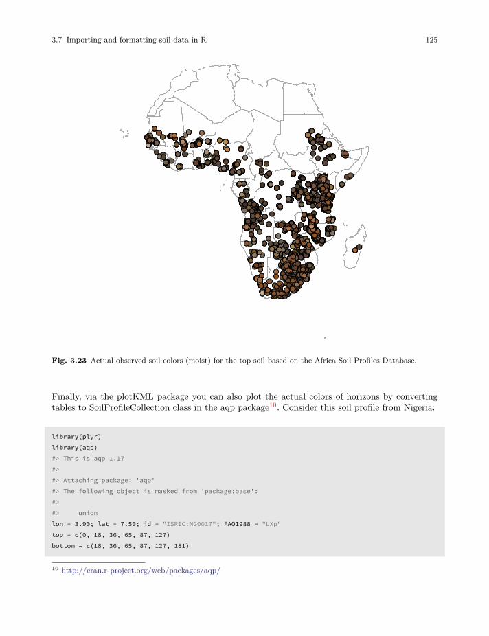
3.7 Importing and formatting soil data in R 125
Fig. 3.23 Actual observed soil colors (moist) for the top soil based on the Africa Soil Profiles Database.
Finally, via the plotKML package you can also plot the actual colors of horizons by convertingtables to SoilProfileCollection class in the aqp package10. Consider this soil profile from Nigeria:
library(plyr)library(aqp)#> This is aqp 1.17#>#> Attaching package: 'aqp'#> The following object is masked from 'package:base':#>#> unionlon = 3.90; lat = 7.50; id = "ISRIC:NG0017"; FAO1988 = "LXp"top = c(0, 18, 36, 65, 87, 127)bottom = c(18, 36, 65, 87, 127, 181)
10 http://cran.r-project.org/web/packages/aqp/
126 3 Soil observations and variables
ORCDRC = c(18.4, 4.4, 3.6, 3.6, 3.2, 1.2)hue = c("7.5YR", "7.5YR", "2.5YR", "5YR", "5YR", "10YR")value = c(3, 4, 5, 5, 5, 7); chroma = c(2, 4, 6, 8, 4, 3)## prepare a SoilProfileCollection:prof1 <- plyr::join(data.frame(id, top, bottom, ORCDRC, hue, value, chroma),
data.frame(id, lon, lat, FAO1988), type='inner')#> Joining by: idprof1$soil_color <- with(prof1, aqp::munsell2rgb(hue, value, chroma))#> Notice: converting hue to characterdepths(prof1) <- id ~ top + bottom#> Warning: converting IDs from factor to charactersite(prof1) <- ~ lon + lat + FAO1988coordinates(prof1) <- ~ lon + latproj4string(prof1) <- CRS("+proj=longlat +datum=WGS84")prof1#> Object of class SoilProfileCollection#> Number of profiles: 1#>#> Horizon attributes:#> id top bottom ORCDRC hue value chroma soil_color hzID#> 1 ISRIC:NG0017 0 18 18.4 7.5YR 3 2 #584537FF 1#> 2 ISRIC:NG0017 18 36 4.4 7.5YR 4 4 #7E5A3BFF 2#> 3 ISRIC:NG0017 36 65 3.6 2.5YR 5 6 #A96C4FFF 3#> 4 ISRIC:NG0017 65 87 3.6 5YR 5 8 #B06A32FF 4#> 5 ISRIC:NG0017 87 127 3.2 5YR 5 4 #9A7359FF 5#> 6 ISRIC:NG0017 127 181 1.2 10YR 7 3 #C4AC8CFF 6#>#> Sampling site attributes:#> id FAO1988#> 1 ISRIC:NG0017 LXp#>#> Spatial Data:#> min max#> lon 3.9 3.9#> lat 7.5 7.5#> [1] "+proj=longlat +datum=WGS84 +ellps=WGS84 +towgs84=0,0,0"
Once an object is in the format of SoilProfileCollection it can be directly plotted in Google Earthvia the generic plotKML command:
plotKML(prof1, var.name="ORCDRC", color.name="soil_color")
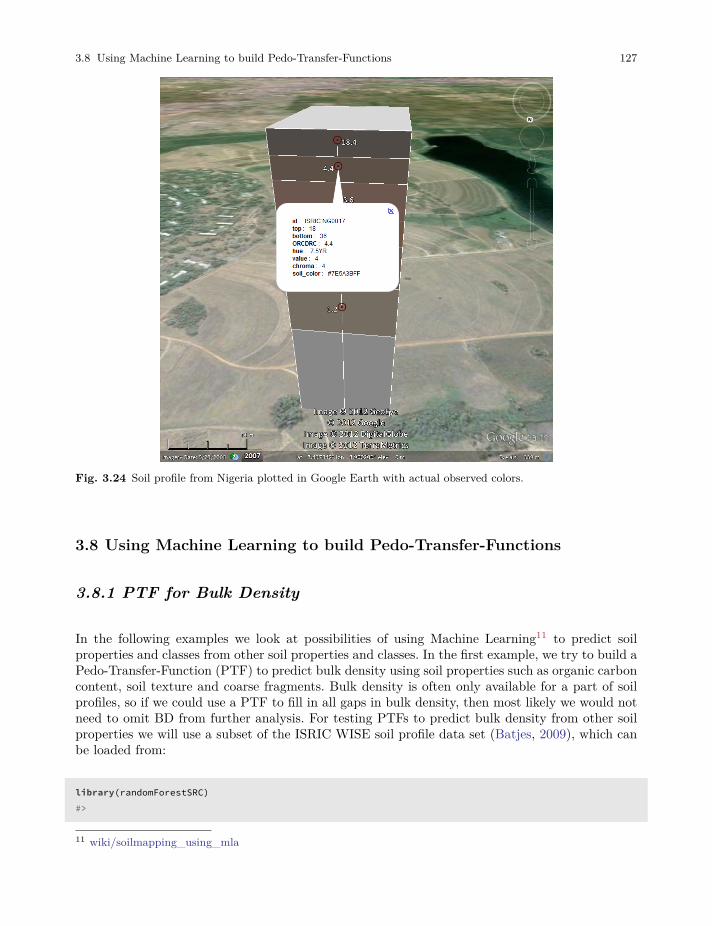
3.8 Using Machine Learning to build Pedo-Transfer-Functions 127
Fig. 3.24 Soil profile from Nigeria plotted in Google Earth with actual observed colors.
3.8 Using Machine Learning to build Pedo-Transfer-Functions
3.8.1 PTF for Bulk Density
In the following examples we look at possibilities of using Machine Learning11 to predict soilproperties and classes from other soil properties and classes. In the first example, we try to build aPedo-Transfer-Function (PTF) to predict bulk density using soil properties such as organic carboncontent, soil texture and coarse fragments. Bulk density is often only available for a part of soilprofiles, so if we could use a PTF to fill in all gaps in bulk density, then most likely we would notneed to omit BD from further analysis. For testing PTFs to predict bulk density from other soilproperties we will use a subset of the ISRIC WISE soil profile data set (Batjes, 2009), which canbe loaded from:
library(randomForestSRC)#>
11 wiki/soilmapping_using_mla
128 3 Soil observations and variables
#> randomForestSRC 2.8.0#>#> Type rfsrc.news() to see new features, changes, and bug fixes.#>library(ggRandomForests)#>#> Attaching package: 'ggRandomForests'#> The following object is masked from 'package:randomForestSRC':#>#> partial.rfsrclibrary(ggplot2)library(scales)load("extdata/sprops.wise.rda")str(SPROPS.WISE)#> 'data.frame': 47833 obs. of 17 variables:#> $ SOURCEID: Factor w/ 10253 levels "AF0001","AF0002",..: 1 1 1 2 2 2 2 3 3 3 ...#> $ SAMPLEID: chr "AF0001_1" "AF0001_2" "AF0001_3" "AF0002_1" ...#> $ UHDICM : int 0 15 60 0 20 60 110 0 20 50 ...#> $ LHDICM : int 15 60 150 20 60 110 170 20 50 110 ...#> $ DEPTH : num 7.5 37.5 105 10 40 85 140 10 35 80 ...#> $ CRFVOL : int 20 NA NA NA NA NA NA NA NA NA ...#> $ CECSUM : num NA NA NA NA NA NA NA NA NA NA ...#> $ SNDPPT : int 40 10 10 40 15 10 40 40 65 60 ...#> $ CLYPPT : int 20 35 35 20 20 35 20 20 10 25 ...#> $ BLD : num NA NA NA NA NA NA NA NA NA NA ...#> $ SLTPPT : int 40 55 55 40 65 55 40 40 25 15 ...#> $ PHIHOX : num 7.9 7.9 7.9 8.5 8.6 8.5 8.8 8.8 9.2 8.9 ...#> $ PHIKCL : num NA NA NA NA NA NA NA NA NA NA ...#> $ ORCDRC : num 7.6 2.3 0.9 12.8 6 3.9 2.7 5.9 2.4 NA ...#> $ LONWGS84: num 69.2 69.2 69.2 69.2 69.2 ...#> $ LATWGS84: num 34.5 34.5 34.5 34.5 34.5 34.5 34.5 34.5 34.5 34.5 ...#> $ SOURCEDB: chr "WISE" "WISE" "WISE" "WISE" ...
For model fitting we will use the randomForestSRC12 package, which is a robust implementationof the random forest algorithm with options for parallelization and visualization of model outputs:
bd.fm = as.formula("BLD ~ ORCDRC + PHIHOX + SNDPPT + CLYPPT + CRFVOL + DEPTH")rfsrc_BD <- rfsrc(bd.fm, data=SPROPS.WISE)rfsrc_BD#> Sample size: 3330#> Number of trees: 1000#> Forest terminal node size: 5#> Average no. of terminal nodes: 685#> No. of variables tried at each split: 2
12 https://cran.r-project.org/package=randomForestSRC
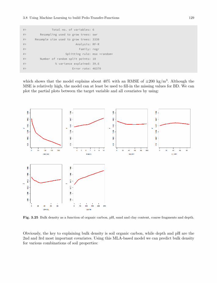
3.8 Using Machine Learning to build Pedo-Transfer-Functions 129
#> Total no. of variables: 6#> Resampling used to grow trees: swr#> Resample size used to grow trees: 3330#> Analysis: RF-R#> Family: regr#> Splitting rule: mse *random*#> Number of random split points: 10#> % variance explained: 39.6#> Error rate: 46370
which shows that the model explains about 40% with an RMSE of ±200 kg/m3. Although theMSE is relatively high, the model can at least be used to fill-in the missing values for BD. We canplot the partial plots between the target variable and all covariates by using:
Fig. 3.25 Bulk density as a function of organic carbon, pH, sand and clay content, coarse fragments and depth.
Obviously, the key to explaining bulk density is soil organic carbon, while depth and pH are the2nd and 3rd most important covariates. Using this MLA-based model we can predict bulk densityfor various combinations of soil properties:

130 3 Soil observations and variables
predict(rfsrc_BD, data.frame(ORCDRC=1.2, PHIHOX=7.6,SNDPPT=45, CLYPPT=12, CRFVOL=0, DEPTH=20))$predicted
#> [1] 1548
and for a soil with higher organic carbon content:
predict(rfsrc_BD, data.frame(ORCDRC=150, PHIHOX=4.6,SNDPPT=25, CLYPPT=35, CRFVOL=0, DEPTH=20))$predicted
#> [1] 906
3.8.2 PTF for correlating classification systems
In the second example we use ISRIC WISE data set to build a correlation function to translatesoil classes from one classification system to the other. The training data can be loaded from:
load("extdata/wise_tax.rda")str(WISE_tax)#> 'data.frame': 8189 obs. of 7 variables:#> $ SOURCEID: Factor w/ 8189 levels "AF0001","AF0002",..: 1 2 3 4 5 6 7 8 9 10 ...#> $ LATWGS84: num 34.5 34.5 34.5 34.3 32.4 ...#> $ LONWGS84: num 69.2 69.2 69.2 61.4 62.1 ...#> $ TAXNWRB : Factor w/ 146 levels "#N/A","Albic Arenosol",..: 104 9 9 72 17 16 122 49 8 9 ...#> $ TAXOUSDA: Factor w/ 1728 levels ""," Calciorthid",..: 1 1 1 1 1 1 1 1 1 1 ...#> $ LFORM : chr "LV" "LV" "LV" "LV" ...#> $ LANDUS : chr "AA4" "AA6" "AA6" "AA4" ...
For this purpose we also need to import the cleaned legend for USDA classification:
leg <- read.csv("extdata/taxousda_greatgroups.csv")str(leg)#> 'data.frame': 434 obs. of 4 variables:#> $ Great_Group: Factor w/ 434 levels "Acraquox","Acrohumox",..: 9 57 77 112 121 145 170 259 286 301 ...#> $ Suborder : Factor w/ 79 levels "Albolls","Andepts",..: 4 4 4 4 4 4 4 4 4 4 ...#> $ Order : Factor w/ 12 levels "Alfisols","Andisols",..: 1 1 1 1 1 1 1 1 1 1 ...#> $ TAX : Factor w/ 434 levels "Alfisols_Aqualfs_Albaqualfs",..: 1 2 3 4 5 6 7 8 9 10 ...
Our objective is to develop a function to translate WRB classes into USDA classes with help ofsome soil properties. We can try to add soil pH and clay content to increase the accuracy of themodel:
3.8 Using Machine Learning to build Pedo-Transfer-Functions 131
x.PHIHOX <- aggregate(SPROPS.WISE$PHIHOX,by=list(SPROPS.WISE$SOURCEID),FUN=mean, na.rm=TRUE); names(x.PHIHOX)[1] = "SOURCEID"
x.CLYPPT <- aggregate(SPROPS.WISE$CLYPPT,by=list(SPROPS.WISE$SOURCEID),FUN=mean, na.rm=TRUE); names(x.CLYPPT)[1] = "SOURCEID"
WISE_tax$PHIHOX <- plyr::join(WISE_tax, x.PHIHOX, type="left")$x#> Joining by: SOURCEIDWISE_tax$CLYPPT <- plyr::join(WISE_tax, x.CLYPPT, type="left")$x#> Joining by: SOURCEID
After that we need to clean-up the classes so that we can focus on USDA suborders only:
sel.tax = complete.cases(WISE_tax[,c("TAXNWRB","PHIHOX","CLYPPT","TAXOUSDA")])WISE_tax.sites <- WISE_tax[sel.tax,]WISE_tax.sites$TAXOUSDA.f <- NAfor(j in leg$Suborder){sel <- grep(j, WISE_tax.sites$TAXOUSDA, ignore.case=TRUE)WISE_tax.sites$TAXOUSDA.f[sel] = j
}WISE_tax.sites$TAXOUSDA.f <- as.factor(WISE_tax.sites$TAXOUSDA.f)WISE_tax.sites$TAXNWRB <- as.factor(paste(WISE_tax.sites$TAXNWRB))
and finally we can fit a model to translate WRB profiles to USDA suborders:
TAXNUSDA.rf <- rfsrc(TAXOUSDA.f ~ TAXNWRB + PHIHOX + CLYPPT, data=WISE_tax.sites)#TAXNUSDA.rf
This shows that the average accuracy is about 45%. We can test converting some classes with thehelp of additional soil properties:
newdata = data.frame(TAXNWRB=factor("Calcaric Cambisol",levels=levels(WISE_tax.sites$TAXNWRB)),PHIHOX=7.8, CLYPPT=12)
x <- data.frame(predict(TAXNUSDA.rf, newdata, type="prob")$predicted)x[,order(1/x)[1:2]]#> Ochrepts Orthids#> 1 0.288 0.154
So for example, the two most likely classes to equate to Calcaric Cambisols seem to be Ochreptsand Orthids, which is not that much different from correlation classes reported in Krasilnikov et al(2009).
132 3 Soil observations and variables
3.9 Summary points
In this chapter, we have endeavoured to provide precise and explicit descriptions of the soil prop-erties and soil classes of greatest interest to current PSM activities. For each soil property (orclass) we have provided an explanation for why that property (or class) is of interest to users andwhy it has been selected to be mapped globally, by us and by others. In many cases, the mostobvious reason is that the soil property is widely recorded and reported in legacy soil profile databases and is therefore available. But these soil properties are widely reported for good reasons,mainly because they have been found to be important to consider when managing land or makingdecisions about land capability or use. We have defined the spatial attributes of the soil propertiesmapped at various scales, defined a standard reference (analysis) method for each soil property,provided information on the units, precision and range of values used to describe each mappedsoil property and reviewed problems and opportunities related to harmonization of soil propertyvalues contained in legacy soil profile databases that have been analysed using different methodsof analysis.
It should be noted that, in this chapter, we have emphasized the use of existing, or legacy, soilprofile data to provide the evidence used to construct predicton models for PSM. This emphasisreflects the reality that, for most of the world, legacy soil profile data is all that we have to workwith, at the present time, and all that we can reasonably expect in the foreseeable future. Manyof the issues and challenges related to use and harmonization of legacy soil profile data discussedin this chapter will hopefully be of less importance as newer, contemporary data are collected inthe field and analysed in the laboratory using more robust, statistically valid and reproduceablemethods (e.g. spectroscopy). In the meantime, standardization and harmonization of legacy soilprofile data will continue to present a challenge for global to regional PSM.
One attractive option for harmonizing soil analytical data following the SINFER concept wouldbe to create and maintain a Global Soil Reference Library (GSRL). This concept is furtherdiscussed in the final chapter. Such a library would need to include data for a significant numberof soils from each continent or region. Each soil would be analysed for all properties of interestusing all commonly used methods of analysis. Values for a soil property for any soil analysed bya given method could be converted into equivalent values in any other analytical method (as longas data analysed by both methods were included in the GSRL) by developing pedo-transfer (orconversion) functions using the fully analysed samples in the conversion library. In particular,some variation of the similarity approach described by Jagtap et al (2004) for available watercapacity and Nemes et al (1999b) for harmonization of particle size data could be implemented toharmonize all types of soil property values anywhere in the world. The value of the soil property inthe desired reference method could be estimated by finding the soil or soils in the reference librarythat were most similar to the soil for which harmonization was required and then using the valueof the soil (or soils) in the desired reference method as the predicted harmonized value. If severalsimilar soils were identified, as is done by Nemes et al (1999b), then the predicted harmonizedvalue would be computed as a weighted mean, in the appropriate reference method, of all similarsoils; with weights selected according to the similarity of the soils in the conversion library to thesoil being harmonized.
What a GSRL would do, in effect, is to provide a single, centralized framework for harmonizationand conversion of soil property values. It would do this using a database of reference soils analysedfor all soil properties of interest by all major analytical methods. These fully analysed referencesoils would provide a framework for computing individualized, locally relevant conversion or pedo-

3.9 Summary points 133
transfer functions in a consistent and standardized manner. Consequently, global soil mappingwould benefit from having the best of both worlds, namely locally-specific harmonization functions(which are known to be most effective), and also ones that were computed in a single standardizedmanner using data in a single comprehensive reference database (which is desirable in terms ofsimplifying harmonization and maintaining a record of how any value was harmonized).
Over time, we expect to see progress made in developing, applying and documenting harmonizationmethods so that the values for any given soil property used to create predictive models for globalsoil property mapping are fully harmonized and roughly equivalent for all input data sets. Inthe shorter term, it is likely that the accuracy of global predictions will be reduced because ofweak, inconsistent or completely absent efforts to harmonize soil property values produced usingdifferent analytical methods. In the longer term, we hope, and expect, that data collected in thefuture, as we move forward, will benefit from adoption of methods of data collection and analysisthat are more systematic, more reproduceable, more accurate and more interchangeable. Theseimprovements should reduce the need for harmonization and standardization and should makeuse of soil observation and measurement data easier and more consistent.

Chapter 4
Preparation of soil covariates for soil mapping
Edited by: T. Hengl and R. A. MacMillan
4.1 Soil covariate data sources
4.1.1 Types of soil covariates
Soils (and vegetation + ecosystems) form under complex interactions between climate, livingorganism and anthropogenic influences, modified by relief and hydrological processes and operatingover long periods of time. This has been clearly identified first by Jenny (1994) with his CLORPTfactors of soil formation and subsequently extended by McBratney et al (2003) with the SCORPANformulation (see section 1.3.3).
The following groups of covariates are commonly considered for use in Predictive Soil Mapping:
1. Climate related covariates, which include:
• temperature maps,• precipitation maps,• snow cover maps,• potential evapotranspiration,• cloud fraction and other atmospheric images,
2. Vegetation and living organisms, which include:
• vegetation indices e.g. FAPAR (mean, median), NDVI, EVI,• biomass, Leaf Area Index,• land cover type maps,• vegetation types and communities (if mapped at high accuracy),• land cover,
135

136 4 Preparation of soil covariates for soil mapping
3. Relief and topography-related covariates, which include:
• standard window-based calculations e.g. slope, curvatures, standard deviation,• standard flow model outputs,• landform classes / landform class likelihoods,• hydrological / soil accumulation and deposition indices — MRVBFI, Wetness index, height
above channel, height below ridge, horizontal distance to channel, horizontal distance to ridge,• climatic and micro-climatic indices determined by relief e.g. incoming solar insolation and sim-
ilar,
4. Parent material / geologic material covariates, which include:
• bedrock type and age,• bedrock mineralogy (acid, basic),• surface material type, texture, age, mineralogy, thickness,• volcanic activity, historic earthquake density,• seismic activity level,• gamma ray spectroscopy grids,• gravity measurements,• electrical conductivity/resistance,
5. Estimated geological age of surface, which include:
• bedrock age / surface material age,• recent disturbance age,
6. Spatial position or spatial context, which include:
• latitude and longitude,• distance to nearest large ocean• Northing — distance to north pole,• Southing — distance to south pole,• Easting — distance to east,• Westing — distance to west,• shortest distance in any direction,• distance to nearest high mountain,• distance to nearest moderate hill,• distance to nearest major river,
7. Human or Anthropogenic Influences, which include:
• land use / land management maps,• probability / intensity of agricultural land use,• probability / intensity of pasture or grazing use,• probability / intensity of forest land management,• probability / intensity of urbanization,• soil dredging, surface sealing,
4.1 Soil covariate data sources 137
• night time illumination (nightlights) images,• probability of gullying or human-induced erosion,• soil nutrient fertilization, liming and similar maps,
In the following sections we provide some practical advice (with links to the most important datasources) on how to prepare soil covariates for use in PSM.
4.1.2 Soil covariate data sources (30–100 m resolution)
Adding relevant covariates that can help explain the distribution of soil properties increases theaccuracy of spatial predictions. Hence, prior to generating predictions of soil properties, it is agood idea to invest in preparing a list of Remote Sensing (RS), geomorphological/lithologic andDEM-based covariates that can potentially help explain the spatial distribution of soil propertiesand classes. There are now many finer resolution (30–250 m) covariates with global coverage thatare publicly available without restrictions. The spatial detail, accessibility and accuracy of RS-based products has been growing exponentially and there is no evidence that this trend is goingto slow down in the coming decades (Herold et al, 2016).The most relevant (global) publicly available remote sensing-based covariates that can be down-loaded and used to improve predictive soil mapping at high spatial resolutions are, for example:
• SRTM1 and/or ALOS W3D2 Digital Elevation Model (DEM) at 30 m and MERIT DEM3 at100 m (these can be used to derive at least 8–12 DEM derivatives of which some generally proveto be beneficial for mapping of soil chemical and hydrological properties);
• Landsat 7, 8 satellite images, either available from USGS’s GloVis4 / EarthExplorer5, or fromthe GlobalForestChange project6 repository (Hansen et al, 2013);
• Landsat-based Global Surface Water (GSW) dynamics images7 at 30 m resolution for the period1985–2016 (Pekel et al, 2016);
• Global Land Cover (GLC) maps based on the GLC30 project8 at 30 m resolution for 2000 and2010 (Chen et al, 2015) and similar land cover projects (Herold et al, 2016);
• USGS’s global bare surface images9 at 30 m resolution;• JAXA’s ALOS10 (PALSAR/PALSAR-2) radar images at 20 m resolution (Shimada et al, 2014);
radar images, bands HH: -27.7 (5.3) dB and HV: -35.8 (3.0) dB, from the JAXA’s ALOS project1 https://lta.cr.usgs.gov/SRTM1Arc2 http://www.eorc.jaxa.jp/ALOS/en/aw3d/index_e.htm3 http://hydro.iis.u-tokyo.ac.jp/~yamadai/MERIT_DEM/4 http://glovis.usgs.gov/5 http://earthexplorer.usgs.gov/6 https://earthenginepartners.appspot.com/science-2013-global-forest/download_v1.2.html7 https://global-surface-water.appspot.com/download8 http://www.globallandcover.com9 https://landcover.usgs.gov/glc/10 http://www.eorc.jaxa.jp/ALOS/en/dataset/dataset_index.htm
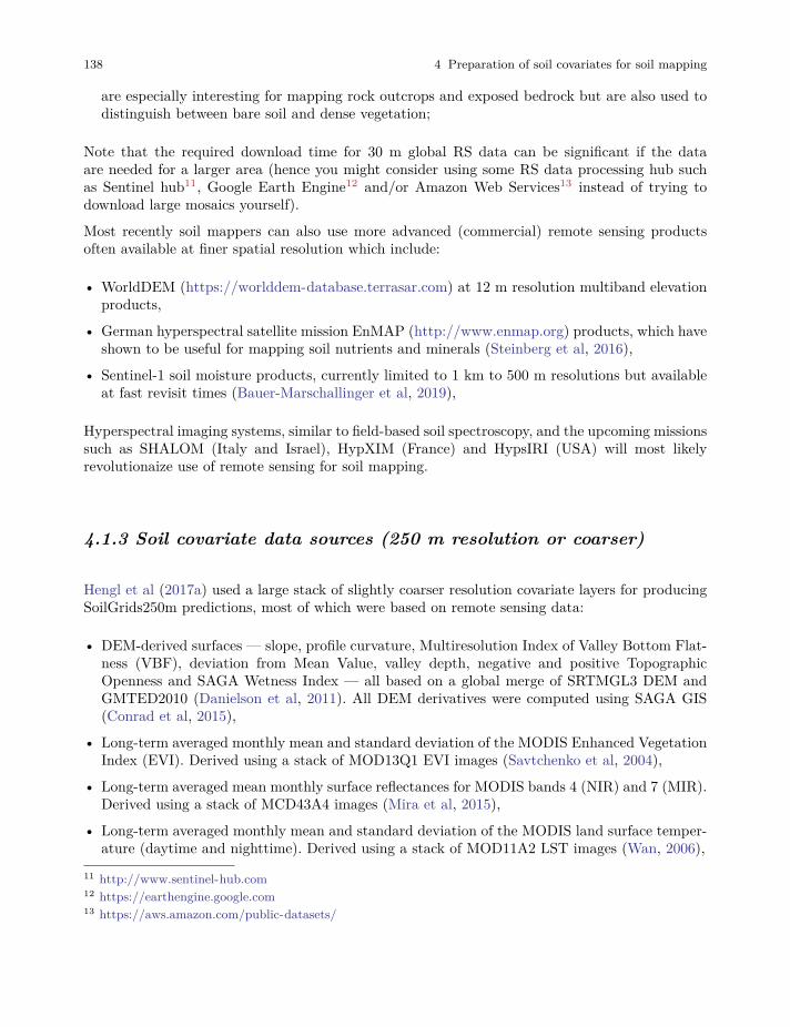
138 4 Preparation of soil covariates for soil mapping
are especially interesting for mapping rock outcrops and exposed bedrock but are also used todistinguish between bare soil and dense vegetation;
Note that the required download time for 30 m global RS data can be significant if the dataare needed for a larger area (hence you might consider using some RS data processing hub suchas Sentinel hub11, Google Earth Engine12 and/or Amazon Web Services13 instead of trying todownload large mosaics yourself).
Most recently soil mappers can also use more advanced (commercial) remote sensing productsoften available at finer spatial resolution which include:
• WorldDEM (https://worlddem-database.terrasar.com) at 12 m resolution multiband elevationproducts,
• German hyperspectral satellite mission EnMAP (http://www.enmap.org) products, which haveshown to be useful for mapping soil nutrients and minerals (Steinberg et al, 2016),
• Sentinel-1 soil moisture products, currently limited to 1 km to 500 m resolutions but availableat fast revisit times (Bauer-Marschallinger et al, 2019),
Hyperspectral imaging systems, similar to field-based soil spectroscopy, and the upcoming missionssuch as SHALOM (Italy and Israel), HypXIM (France) and HypsIRI (USA) will most likelyrevolutionaize use of remote sensing for soil mapping.
4.1.3 Soil covariate data sources (250 m resolution or coarser)
Hengl et al (2017a) used a large stack of slightly coarser resolution covariate layers for producingSoilGrids250m predictions, most of which were based on remote sensing data:
• DEM-derived surfaces — slope, profile curvature, Multiresolution Index of Valley Bottom Flat-ness (VBF), deviation from Mean Value, valley depth, negative and positive TopographicOpenness and SAGA Wetness Index — all based on a global merge of SRTMGL3 DEM andGMTED2010 (Danielson et al, 2011). All DEM derivatives were computed using SAGA GIS(Conrad et al, 2015),
• Long-term averaged monthly mean and standard deviation of the MODIS Enhanced VegetationIndex (EVI). Derived using a stack of MOD13Q1 EVI images (Savtchenko et al, 2004),
• Long-term averaged mean monthly surface reflectances for MODIS bands 4 (NIR) and 7 (MIR).Derived using a stack of MCD43A4 images (Mira et al, 2015),
• Long-term averaged monthly mean and standard deviation of the MODIS land surface temper-ature (daytime and nighttime). Derived using a stack of MOD11A2 LST images (Wan, 2006),
11 http://www.sentinel-hub.com12 https://earthengine.google.com13 https://aws.amazon.com/public-datasets/
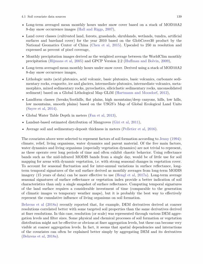
4.1 Soil covariate data sources 139
• Long-term averaged mean monthly hours under snow cover based on a stack of MOD10A28-day snow occurrence images (Hall and Riggs, 2007),
• Land cover classes (cultivated land, forests, grasslands, shrublands, wetlands, tundra, artificialsurfaces and bareland cover) for the year 2010 based on the GlobCover30 product by theNational Geomatics Center of China (Chen et al, 2015). Upscaled to 250 m resolution andexpressed as percent of pixel coverage,
• Monthly precipitation images derived as the weighted average between the WorldClim monthlyprecipitation (Hijmans et al, 2005) and GPCP Version 2.2 (Huffman and Bolvin, 2009),
• Long-term averaged mean monthly hours under snow cover. Derived using a stack of MOD10A28-day snow occurrence images,
• Lithologic units (acid plutonics, acid volcanic, basic plutonics, basic volcanics, carbonate sedi-mentary rocks, evaporite, ice and glaciers, intermediate plutonics, intermediate volcanics, meta-morphics, mixed sedimentary rocks, pyroclastics, siliciclastic sedimentary rocks, unconsolidatedsediment) based on a Global Lithological Map GLiM (Hartmann and Moosdorf, 2012),
• Landform classes (breaks/foothills, flat plains, high mountains/deep canyons, hills, low hills,low mountains, smooth plains) based on the USGS’s Map of Global Ecological Land Units(Sayre et al, 2014).
• Global Water Table Depth in meters (Fan et al, 2013),
• Landsat-based estimated distribution of Mangroves (Giri et al, 2011),
• Average soil and sedimentary-deposit thickness in meters (Pelletier et al, 2016).
The covariates above were selected to represent factors of soil formation according to Jenny (1994):climate, relief, living organisms, water dynamics and parent material. Of the five main factors,water dynamics and living organisms (especially vegetation dynamics) are not trivial to represent,as these operate over long periods of time and often exhibit chaotic behavior. Using reflectancebands such as the mid-infrared MODIS bands from a single day, would be of little use for soilmapping for areas with dynamic vegetation, i.e. with strong seasonal changes in vegetation cover.To account for seasonal fluctuation and for inter-annual variations in surface reflectance, long-term temporal signatures of the soil surface derived as monthly averages from long-term MODISimagery (15 years of data) can be more effective to use (Hengl et al, 2017a). Long-term averageseasonal signatures of surface reflectance or vegetation index provide a better indication of soilcharacteristics than only a single snapshot of surface reflectance. Computing temporal signaturesof the land surface requires a considerable investment of time (comparable to the generationof climatic images vs temporary weather maps), but it is probably the best way to effectivelyrepresent the cumulative influence of living organisms on soil formation.
Behrens et al (2018a) recently reported that, for example, DEM derivatives derived at coarserresolutions correlated better with some targeted soil properties than the same derivatives derivedat finer resolutions. In this case, resolution (or scale) was represented through various DEM aggre-gation levels and filter sizes. Some physical and chemical processes of soil formation or vegetationdistribution might not be effective or obvious at finer aggregation levels, but these can become veryvisible at coarser aggregation levels. In fact, it seems that spatial dependencies and interactionsof the covariates can often be explained better simply by aggregating DEM and its derivatives(Behrens et al, 2018a).

140 4 Preparation of soil covariates for soil mapping
4.2 Preparing soil covariate layers
Before we are able to fit spatial prediction models and generate soil maps, a significant amountof effort is first spent on preparing covariate “layers” that can be used as independent variables(i.e. “predictor variables”) in the statistical modelling. Typical operations used to generate soilcovariate layers include:
• Converting polygon maps to rasters,
• Downscaling or upscaling (aggregating) rasters to match the target resolution (i.e. preparing astack),
• Filtering out missing pixels / reducing noise and multicolinearity (data overlap) problems,
• Overlaying and subsetting raster stacks and points,
The following examples should provide some ideas about how to program these steps using themost concise possible syntax running the fastest and most robust algorithms. Raster data canoften be very large (e.g. millions of pixels) so processing large stacks of remote sensing scenes inR needs to be planned carefully. The complete R tutorial can be downloaded from the githubrepository14. Instructions on how to install and set-up all software used in this example can befound in the software installation chapter 2.
4.2.1 Converting polygon maps to rasters
Before we can attach a polygon map to other stacks of covariates, it needs to be rasterized i.e. con-verted to a raster layer defined with its bounding box (extent) and spatial resolution. Considerfor example the Ebergötzen data set15 polygon map from the plotKML package (Fig. 4.1):
library(rgdal)#> Loading required package: sp#> rgdal: version: 1.3-6, (SVN revision 773)#> Geospatial Data Abstraction Library extensions to R successfully loaded#> Loaded GDAL runtime: GDAL 2.2.2, released 2017/09/15#> Path to GDAL shared files: /usr/share/gdal/2.2#> GDAL binary built with GEOS: TRUE#> Loaded PROJ.4 runtime: Rel. 4.8.0, 6 March 2012, [PJ_VERSION: 480]#> Path to PROJ.4 shared files: (autodetected)#> Linking to sp version: 1.3-1library(raster)library(plotKML)#> plotKML version 0.5-9 (2019-01-04)
14 https://github.com/envirometrix/PredictiveSoilMapping15 http://plotkml.r-forge.r-project.org/eberg.html
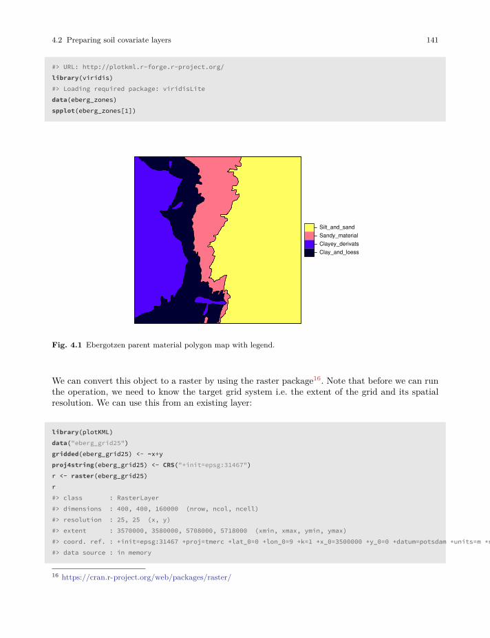
4.2 Preparing soil covariate layers 141
#> URL: http://plotkml.r-forge.r-project.org/library(viridis)#> Loading required package: viridisLitedata(eberg_zones)spplot(eberg_zones[1])
Clay_and_loessClayey_derivatsSandy_materialSilt_and_sand
Fig. 4.1 Ebergotzen parent material polygon map with legend.
We can convert this object to a raster by using the raster package16. Note that before we can runthe operation, we need to know the target grid system i.e. the extent of the grid and its spatialresolution. We can use this from an existing layer:
library(plotKML)data("eberg_grid25")gridded(eberg_grid25) <- ~x+yproj4string(eberg_grid25) <- CRS("+init=epsg:31467")r <- raster(eberg_grid25)r#> class : RasterLayer#> dimensions : 400, 400, 160000 (nrow, ncol, ncell)#> resolution : 25, 25 (x, y)#> extent : 3570000, 3580000, 5708000, 5718000 (xmin, xmax, ymin, ymax)#> coord. ref. : +init=epsg:31467 +proj=tmerc +lat_0=0 +lon_0=9 +k=1 +x_0=3500000 +y_0=0 +datum=potsdam +units=m +no_defs +ellps=bessel +towgs84=598.1,73.7,418.2,0.202,0.045,-2.455,6.7#> data source : in memory
16 https://cran.r-project.org/web/packages/raster/
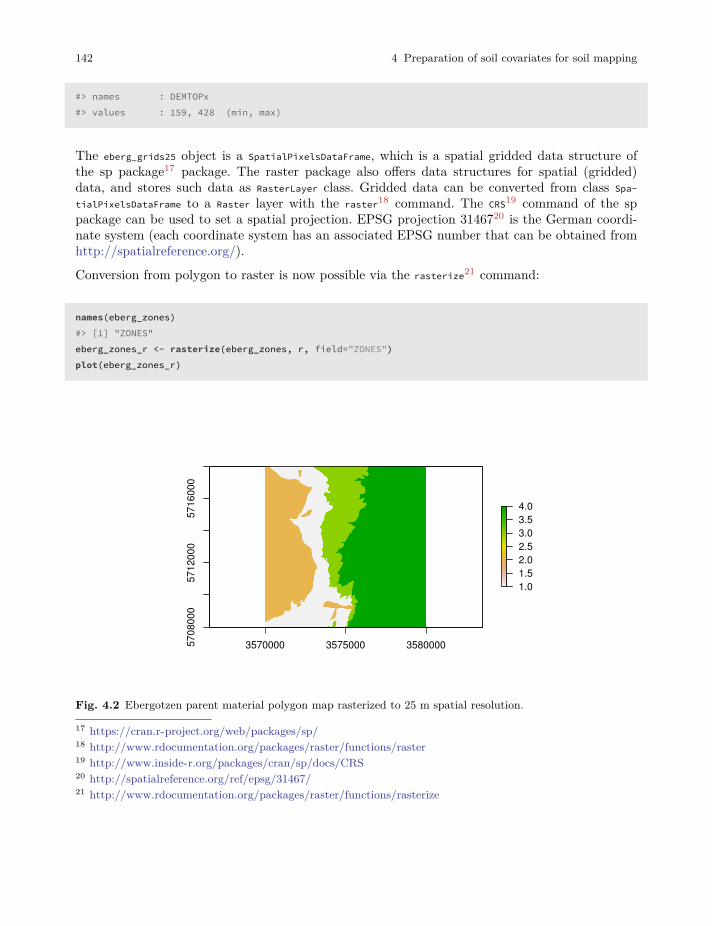
142 4 Preparation of soil covariates for soil mapping
#> names : DEMTOPx#> values : 159, 428 (min, max)
The eberg_grids25 object is a SpatialPixelsDataFrame, which is a spatial gridded data structure ofthe sp package17 package. The raster package also offers data structures for spatial (gridded)data, and stores such data as RasterLayer class. Gridded data can be converted from class Spa-tialPixelsDataFrame to a Raster layer with the raster18 command. The CRS19 command of the sppackage can be used to set a spatial projection. EPSG projection 3146720 is the German coordi-nate system (each coordinate system has an associated EPSG number that can be obtained fromhttp://spatialreference.org/).
Conversion from polygon to raster is now possible via the rasterize21 command:
names(eberg_zones)#> [1] "ZONES"eberg_zones_r <- rasterize(eberg_zones, r, field="ZONES")plot(eberg_zones_r)
3570000 3575000 35800005708
000
5712
000
5716
000
1.01.52.02.53.03.54.0
Fig. 4.2 Ebergotzen parent material polygon map rasterized to 25 m spatial resolution.
17 https://cran.r-project.org/web/packages/sp/18 http://www.rdocumentation.org/packages/raster/functions/raster19 http://www.inside-r.org/packages/cran/sp/docs/CRS20 http://spatialreference.org/ref/epsg/31467/21 http://www.rdocumentation.org/packages/raster/functions/rasterize
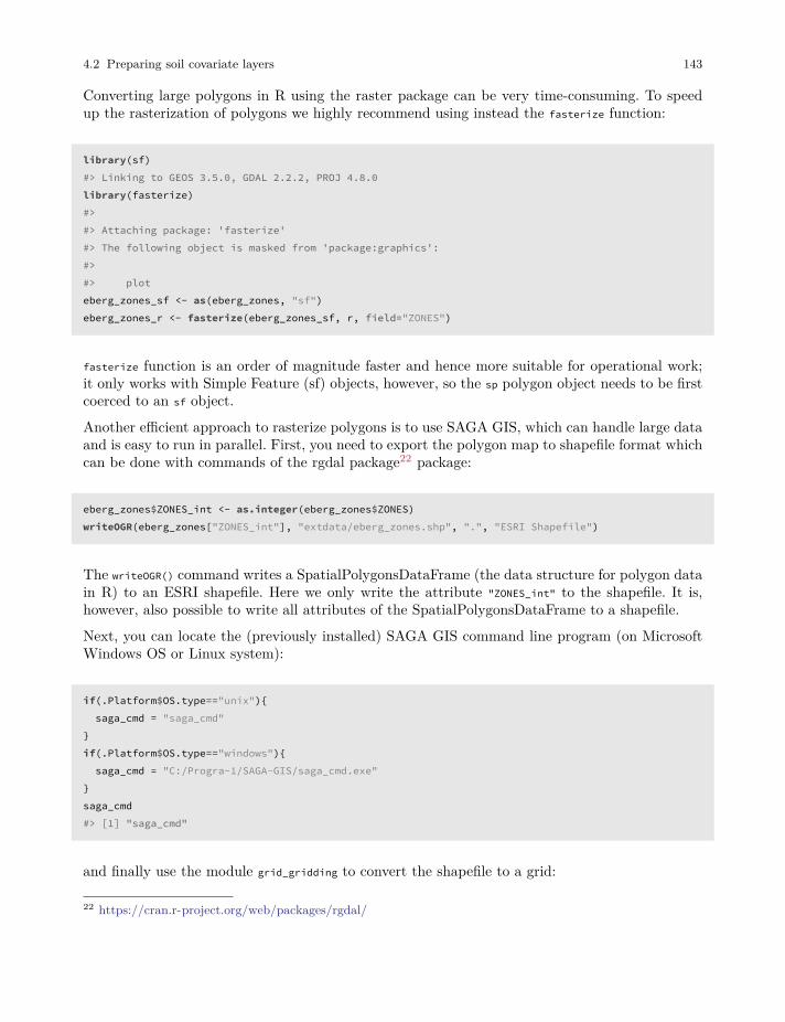
4.2 Preparing soil covariate layers 143
Converting large polygons in R using the raster package can be very time-consuming. To speedup the rasterization of polygons we highly recommend using instead the fasterize function:
library(sf)#> Linking to GEOS 3.5.0, GDAL 2.2.2, PROJ 4.8.0library(fasterize)#>#> Attaching package: 'fasterize'#> The following object is masked from 'package:graphics':#>#> ploteberg_zones_sf <- as(eberg_zones, "sf")eberg_zones_r <- fasterize(eberg_zones_sf, r, field="ZONES")
fasterize function is an order of magnitude faster and hence more suitable for operational work;it only works with Simple Feature (sf) objects, however, so the sp polygon object needs to be firstcoerced to an sf object.
Another efficient approach to rasterize polygons is to use SAGA GIS, which can handle large dataand is easy to run in parallel. First, you need to export the polygon map to shapefile format whichcan be done with commands of the rgdal package22 package:
eberg_zones$ZONES_int <- as.integer(eberg_zones$ZONES)writeOGR(eberg_zones["ZONES_int"], "extdata/eberg_zones.shp", ".", "ESRI Shapefile")
The writeOGR() command writes a SpatialPolygonsDataFrame (the data structure for polygon datain R) to an ESRI shapefile. Here we only write the attribute "ZONES_int" to the shapefile. It is,however, also possible to write all attributes of the SpatialPolygonsDataFrame to a shapefile.
Next, you can locate the (previously installed) SAGA GIS command line program (on MicrosoftWindows OS or Linux system):
if(.Platform$OS.type=="unix"){saga_cmd = "saga_cmd"
}if(.Platform$OS.type=="windows"){saga_cmd = "C:/Progra~1/SAGA-GIS/saga_cmd.exe"
}saga_cmd#> [1] "saga_cmd"
and finally use the module grid_gridding to convert the shapefile to a grid:
22 https://cran.r-project.org/web/packages/rgdal/
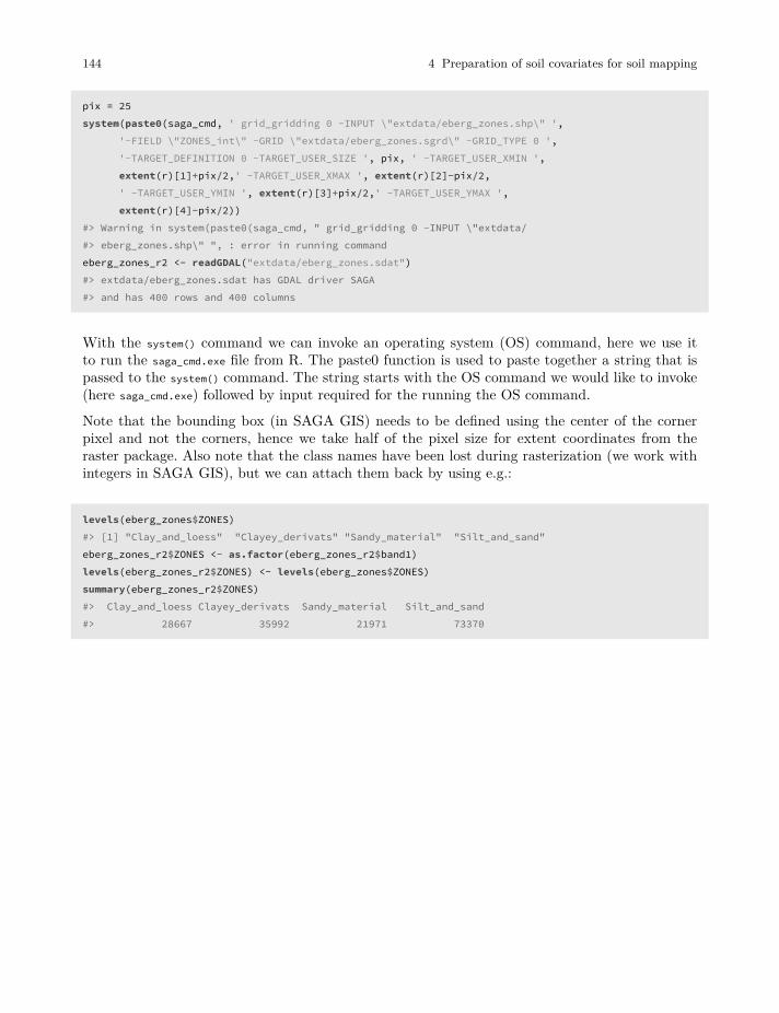
144 4 Preparation of soil covariates for soil mapping
pix = 25system(paste0(saga_cmd, ' grid_gridding 0 -INPUT \"extdata/eberg_zones.shp\" ',
'-FIELD \"ZONES_int\" -GRID \"extdata/eberg_zones.sgrd\" -GRID_TYPE 0 ','-TARGET_DEFINITION 0 -TARGET_USER_SIZE ', pix, ' -TARGET_USER_XMIN ',extent(r)[1]+pix/2,' -TARGET_USER_XMAX ', extent(r)[2]-pix/2,' -TARGET_USER_YMIN ', extent(r)[3]+pix/2,' -TARGET_USER_YMAX ',extent(r)[4]-pix/2))
#> Warning in system(paste0(saga_cmd, " grid_gridding 0 -INPUT \"extdata/#> eberg_zones.shp\" ", : error in running commandeberg_zones_r2 <- readGDAL("extdata/eberg_zones.sdat")#> extdata/eberg_zones.sdat has GDAL driver SAGA#> and has 400 rows and 400 columns
With the system() command we can invoke an operating system (OS) command, here we use itto run the saga_cmd.exe file from R. The paste0 function is used to paste together a string that ispassed to the system() command. The string starts with the OS command we would like to invoke(here saga_cmd.exe) followed by input required for the running the OS command.
Note that the bounding box (in SAGA GIS) needs to be defined using the center of the cornerpixel and not the corners, hence we take half of the pixel size for extent coordinates from theraster package. Also note that the class names have been lost during rasterization (we work withintegers in SAGA GIS), but we can attach them back by using e.g.:
levels(eberg_zones$ZONES)#> [1] "Clay_and_loess" "Clayey_derivats" "Sandy_material" "Silt_and_sand"eberg_zones_r2$ZONES <- as.factor(eberg_zones_r2$band1)levels(eberg_zones_r2$ZONES) <- levels(eberg_zones$ZONES)summary(eberg_zones_r2$ZONES)#> Clay_and_loess Clayey_derivats Sandy_material Silt_and_sand#> 28667 35992 21971 73370

4.2 Preparing soil covariate layers 145
Fig. 4.3 Ebergotzen zones rasterized to 25 m resolution and with correct factor labels.
4.2.2 Downscaling or upscaling (aggregating) rasters
In order for all covariates to perfectly stack, we also need to adjust the resolution of some covariatesthat have either too coarse or too fine a resolution compared to the target resolution. The processof bringing raster layers to a target grid resolution is also known as resampling. Consider thefollowing example from the Ebergotzen case study:
data(eberg_grid)gridded(eberg_grid) <- ~x+yproj4string(eberg_grid) <- CRS("+init=epsg:31467")names(eberg_grid)#> [1] "PRMGEO6" "DEMSRT6" "TWISRT6" "TIRAST6" "LNCCOR6"
In this case we have a few layers that we would like to use for spatial prediction in combinationwith the maps produced in the previous sections, but their resolution is 100 m i.e. about 16 timescoarser. Probably the most robust way to resample rasters is to use the gdalwarp23 function fromthe GDAL software. Assuming that you have already installed GDAL, you only need to locate theprogram on your system, and then you can again run gdalwarp24 via the system command:
23 http://www.gdal.org/gdalwarp.html24 http://www.gdal.org/gdalwarp.html
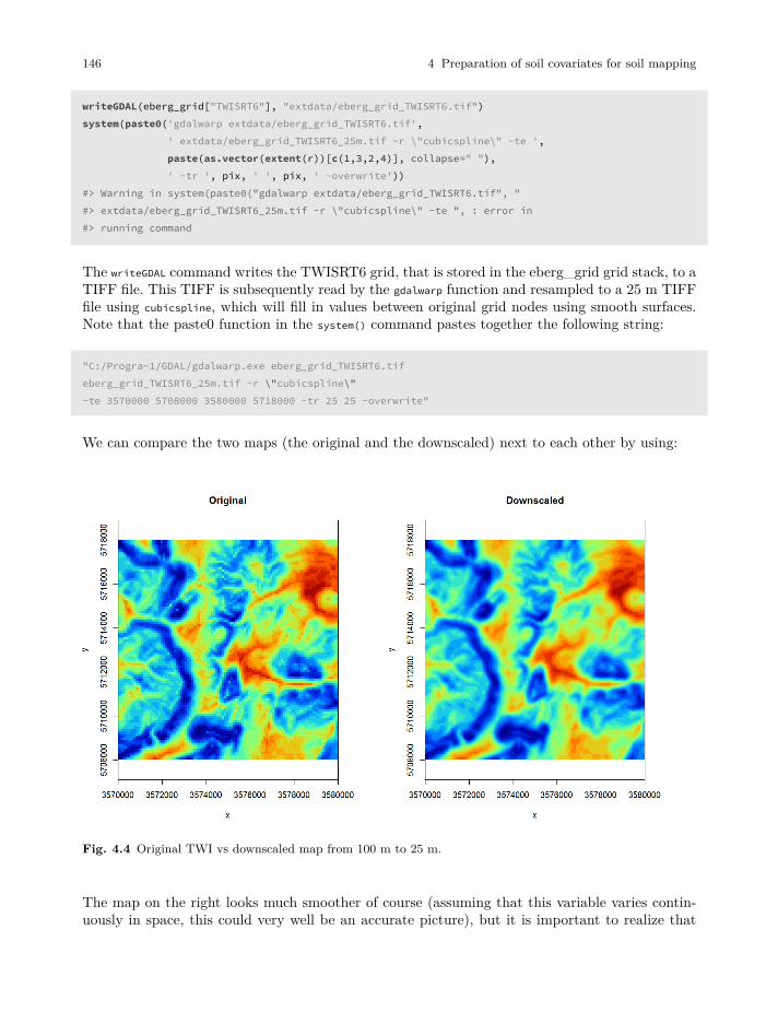
146 4 Preparation of soil covariates for soil mapping
writeGDAL(eberg_grid["TWISRT6"], "extdata/eberg_grid_TWISRT6.tif")system(paste0('gdalwarp extdata/eberg_grid_TWISRT6.tif',
' extdata/eberg_grid_TWISRT6_25m.tif -r \"cubicspline\" -te ',paste(as.vector(extent(r))[c(1,3,2,4)], collapse=" "),' -tr ', pix, ' ', pix, ' -overwrite'))
#> Warning in system(paste0("gdalwarp extdata/eberg_grid_TWISRT6.tif", "#> extdata/eberg_grid_TWISRT6_25m.tif -r \"cubicspline\" -te ", : error in#> running command
The writeGDAL command writes the TWISRT6 grid, that is stored in the eberg_grid grid stack, to aTIFF file. This TIFF is subsequently read by the gdalwarp function and resampled to a 25 m TIFFfile using cubicspline, which will fill in values between original grid nodes using smooth surfaces.Note that the paste0 function in the system() command pastes together the following string:
"C:/Progra~1/GDAL/gdalwarp.exe eberg_grid_TWISRT6.tifeberg_grid_TWISRT6_25m.tif -r \"cubicspline\"-te 3570000 5708000 3580000 5718000 -tr 25 25 -overwrite"
We can compare the two maps (the original and the downscaled) next to each other by using:
Fig. 4.4 Original TWI vs downscaled map from 100 m to 25 m.
The map on the right looks much smoother of course (assuming that this variable varies contin-uously in space, this could very well be an accurate picture), but it is important to realize that
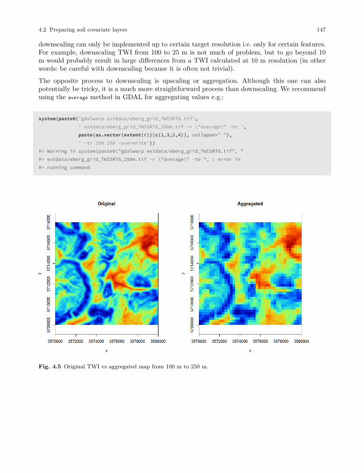
4.2 Preparing soil covariate layers 147
downscaling can only be implemented up to certain target resolution i.e. only for certain features.For example, downscaling TWI from 100 to 25 m is not much of problem, but to go beyond 10m would probably result in large differences from a TWI calculated at 10 m resolution (in otherwords: be careful with downscaling because it is often not trivial).
The opposite process to downscaling is upscaling or aggregation. Although this one can alsopotentially be tricky, it is a much more straightforward process than downscaling. We recommendusing the average method in GDAL for aggregating values e.g.:
system(paste0('gdalwarp extdata/eberg_grid_TWISRT6.tif',' extdata/eberg_grid_TWISRT6_250m.tif -r \"average\" -te ',paste(as.vector(extent(r))[c(1,3,2,4)], collapse=" "),' -tr 250 250 -overwrite'))
#> Warning in system(paste0("gdalwarp extdata/eberg_grid_TWISRT6.tif", "#> extdata/eberg_grid_TWISRT6_250m.tif -r \"average\" -te ", : error in#> running command
Fig. 4.5 Original TWI vs aggregated map from 100 m to 250 m.
148 4 Preparation of soil covariates for soil mapping
4.2.3 Deriving DEM parameters using SAGA GIS
Now that we have established a connection between R and SAGA GIS, we can also use SAGAGIS to derive some standard DEM parameters of interest to soil mapping. To automate furtherprocessing, we make the following function:
saga_DEM_derivatives <- function(INPUT, MASK=NULL,sel=c("SLP","TWI","CRV","VBF","VDP","OPN","DVM")){
if(!is.null(MASK)){## Fill in missing DEM pixels:suppressWarnings( system(paste0(saga_cmd,
' grid_tools 25 -GRID=\"', INPUT,'\" -MASK=\"', MASK, '\" -CLOSED=\"',INPUT, '\"')) )
}## Slope:if(any(sel %in% "SLP")){
try( suppressWarnings( system(paste0(saga_cmd,' ta_morphometry 0 -ELEVATION=\"',INPUT, '\" -SLOPE=\"',gsub(".sgrd", "_slope.sgrd", INPUT),'\" -C_PROF=\"',gsub(".sgrd", "_cprof.sgrd", INPUT), '\"') ) ) )
}## TWI:if(any(sel %in% "TWI")){
try( suppressWarnings( system(paste0(saga_cmd,' ta_hydrology 15 -DEM=\"',INPUT, '\" -TWI=\"',gsub(".sgrd", "_twi.sgrd", INPUT), '\"') ) ) )
}## MrVBF:if(any(sel %in% "VBF")){
try( suppressWarnings( system(paste0(saga_cmd,' ta_morphometry 8 -DEM=\"',INPUT, '\" -MRVBF=\"',gsub(".sgrd", "_vbf.sgrd", INPUT),'\" -T_SLOPE=10 -P_SLOPE=3') ) ) )
}## Valley depth:if(any(sel %in% "VDP")){
try( suppressWarnings( system(paste0(saga_cmd,' ta_channels 7 -ELEVATION=\"',INPUT, '\" -VALLEY_DEPTH=\"',gsub(".sgrd", "_vdepth.sgrd",
INPUT), '\"') ) ) )
4.2 Preparing soil covariate layers 149
}## Openness:if(any(sel %in% "OPN")){
try( suppressWarnings( system(paste0(saga_cmd,' ta_lighting 5 -DEM=\"',INPUT, '\" -POS=\"',gsub(".sgrd", "_openp.sgrd", INPUT),'\" -NEG=\"',gsub(".sgrd", "_openn.sgrd", INPUT),'\" -METHOD=0' ) ) ) )
}## Deviation from Mean Value:if(any(sel %in% "DVM")){
suppressWarnings( system(paste0(saga_cmd,' statistics_grid 1 -GRID=\"',INPUT, '\" -DEVMEAN=\"',gsub(".sgrd", "_devmean.sgrd", INPUT),'\" -RADIUS=11' ) ) )
}}
To run this function we only need DEM as input:
writeGDAL(eberg_grid["DEMSRT6"], "extdata/DEMSRT6.sdat", "SAGA")saga_DEM_derivatives("DEMSRT6.sgrd")
which processes all DEM derivatives at once. We can plot them using:
dem.lst <- list.files("extdata", pattern=glob2rx("^DEMSRT6_*.sdat"), full.names = TRUE)plot(raster::stack(dem.lst), col=rev(magma(10, alpha = 0.8)))
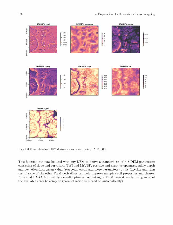
150 4 Preparation of soil covariates for soil mapping
Fig. 4.6 Some standard DEM derivatives calculated using SAGA GIS.
This function can now be used with any DEM to derive a standard set of 7–8 DEM parametersconsisting of slope and curvature, TWI and MrVBF, positive and negative openness, valley depthand deviation from mean value. You could easily add more parameters to this function and thentest if some of the other DEM derivatives can help improve mapping soil properties and classes.Note that SAGA GIS will by default optimize computing of DEM derivatives by using most ofthe available cores to compute (parallelization is turned on automatically).
4.2 Preparing soil covariate layers 151
4.2.4 Filtering out missing pixels and artifacts
After bringing all covariates to the same grid definition, remaining problems for using covariatesin spatial modelling may include:
• Missing pixels,
• Artifacts and noise,
• Multicolinearity (i.e. data overlap),
In a stack with tens of rasters, the weakest layer (i.e. the layer with greatest number of missingpixels or largest number of artifacts) could cause serious problems for producing soil maps as themissing pixels and artifacts would propagate to predictions: if only one layer in the raster stackmisses values then predictive models might drop whole rows in the predictions even though datais available for 95% of rows. Missing pixels occur for various reasons: in the case of remote sensing,missing pixels can be due to clouds or similar; noise is often due to atmospheric conditions. Missingpixels (as long as we are dealing with only a few patches of missing pixels) can be efficiently filteredby using for example the gap filling functionality25 available in the SAGA GIS e.g.:
par(mfrow=c(1,2))image(raster(eberg_grid["test"]), col=SAGA_pal[[1]], zlim=zlim, main="Original", asp=1)image(raster("test.sdat"), col=SAGA_pal[[1]], zlim=zlim, main="Filtered", asp=1)
In this example we use the same input and output file for filling in gaps. There are several othergap filling possibilities in SAGA GIS including Close Gaps with Spline, Close Gaps with StepwiseResampling and Close One Cell Gaps. Not all of these are equally applicable to all missing pixelproblems, but having <10% of missing pixels is often not much of a problem for soil mapping.
Another elegant way to filter the missing pixels, to reduce noise and to reduce data overlap is touse Principal Components26 transformation of original data. This is available also via the GSIFfunction spc:
data(eberg_grid)gridded(eberg_grid) <- ~x+yproj4string(eberg_grid) <- CRS("+init=epsg:31467")formulaString <- ~ PRMGEO6+DEMSRT6+TWISRT6+TIRAST6eberg_spc <- GSIF::spc(eberg_grid, formulaString)names(eberg_spc@predicted) # 11 components on the end;
25 http://saga-gis.org/saga_module_doc/2.2.7/grid_tools_7.html26 http://www.rdocumentation.org/packages/stats/functions/prcomp
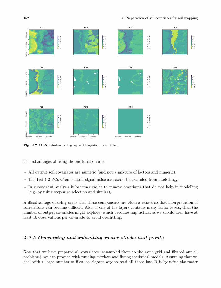
152 4 Preparation of soil covariates for soil mapping
Fig. 4.7 11 PCs derived using input Ebergotzen covariates.
The advantages of using the spc function are:
• All output soil covariates are numeric (and not a mixture of factors and numeric),
• The last 1-2 PCs often contain signal noise and could be excluded from modelling,
• In subsequent analysis it becomes easier to remove covariates that do not help in modelling(e.g. by using step-wise selection and similar),
A disadvantage of using spc is that these components are often abstract so that interpretation ofcorrelations can become difficult. Also, if one of the layers contains many factor levels, then thenumber of output covariates might explode, which becomes impractical as we should then have atleast 10 observations per covariate to avoid overfitting.
4.2.5 Overlaying and subsetting raster stacks and points
Now that we have prepared all covariates (resampled them to the same grid and filtered out allproblems), we can proceed with running overlays and fitting statistical models. Assuming that wedeal with a large number of files, an elegant way to read all those into R is by using the raster
4.2 Preparing soil covariate layers 153
package, especially the stack27 and raster28 commands. In the following example we can list allfiles of interest, and then read them all at once:
library(raster)grd.lst <- list.files(pattern="25m")grd.lstgrid25m <- stack(grd.lst)grid25m <- as(grid25m, "SpatialGridDataFrame")str(grid25m)
One could now save all the prepared covariates stored in SpatialGridDataFrame as an RDS dataobject for future use.
saveRDS(grid25m, file = "extdata/covariates25m.rds")
To overlay rasters and points and prepare a regression matrix, we can either use the over29 functionfrom the sp package, or extract30 function from the raster package. By using the raster package,one can run overlay even without reading the rasters into memory:
library(sp)data(eberg)coordinates(eberg) <- ~X+Yproj4string(eberg) <- CRS("+init=epsg:31467")ov <- as.data.frame(extract(stack(grd.lst), eberg))str(ov[complete.cases(ov),])
If the raster layers can not be stacked and if each layer is available in a different projection system,you can also create a function that reprojects points to the target raster layer projection system:
overlay.fun <- function(i, y){raster::extract(raster(i), na.rm=FALSE,
spTransform(y, proj4string(raster(i))))}
which can also be run in parallel for example by using the parallel package:
ov <- data.frame(mclapply(grd.lst, FUN=overlay.fun, y=eberg))names(ov) <- basename(grd.lst)
27 http://www.rdocumentation.org/packages/raster/functions/stack28 http://www.rdocumentation.org/packages/raster/functions/raster29 http://www.rdocumentation.org/packages/sp/functions/over30 http://www.rdocumentation.org/packages/raster/functions/extract
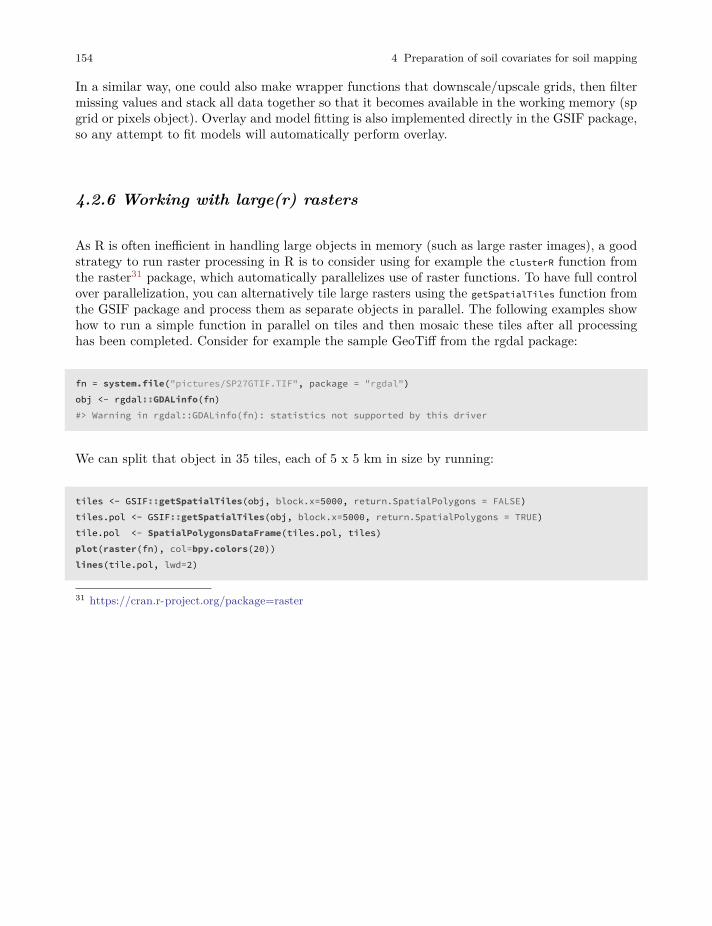
154 4 Preparation of soil covariates for soil mapping
In a similar way, one could also make wrapper functions that downscale/upscale grids, then filtermissing values and stack all data together so that it becomes available in the working memory (spgrid or pixels object). Overlay and model fitting is also implemented directly in the GSIF package,so any attempt to fit models will automatically perform overlay.
4.2.6 Working with large(r) rasters
As R is often inefficient in handling large objects in memory (such as large raster images), a goodstrategy to run raster processing in R is to consider using for example the clusterR function fromthe raster31 package, which automatically parallelizes use of raster functions. To have full controlover parallelization, you can alternatively tile large rasters using the getSpatialTiles function fromthe GSIF package and process them as separate objects in parallel. The following examples showhow to run a simple function in parallel on tiles and then mosaic these tiles after all processinghas been completed. Consider for example the sample GeoTiff from the rgdal package:
fn = system.file("pictures/SP27GTIF.TIF", package = "rgdal")obj <- rgdal::GDALinfo(fn)#> Warning in rgdal::GDALinfo(fn): statistics not supported by this driver
We can split that object in 35 tiles, each of 5 x 5 km in size by running:
tiles <- GSIF::getSpatialTiles(obj, block.x=5000, return.SpatialPolygons = FALSE)tiles.pol <- GSIF::getSpatialTiles(obj, block.x=5000, return.SpatialPolygons = TRUE)tile.pol <- SpatialPolygonsDataFrame(tiles.pol, tiles)plot(raster(fn), col=bpy.colors(20))lines(tile.pol, lwd=2)
31 https://cran.r-project.org/package=raster
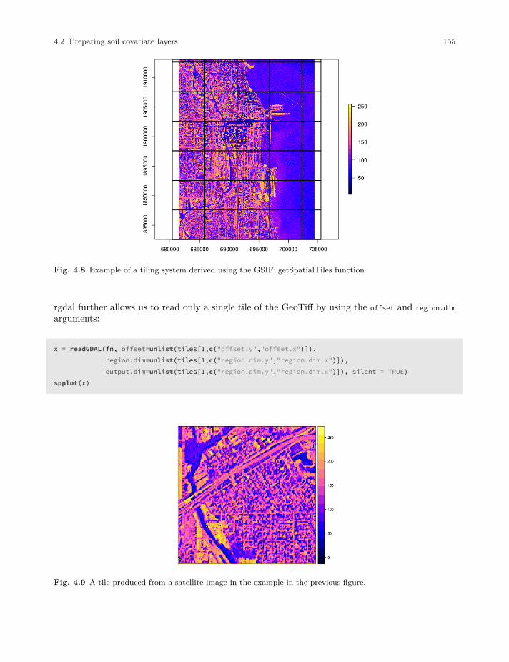
4.2 Preparing soil covariate layers 155
Fig. 4.8 Example of a tiling system derived using the GSIF::getSpatialTiles function.
rgdal further allows us to read only a single tile of the GeoTiff by using the offset and region.dimarguments:
x = readGDAL(fn, offset=unlist(tiles[1,c("offset.y","offset.x")]),region.dim=unlist(tiles[1,c("region.dim.y","region.dim.x")]),output.dim=unlist(tiles[1,c("region.dim.y","region.dim.x")]), silent = TRUE)
spplot(x)
Fig. 4.9 A tile produced from a satellite image in the example in the previous figure.
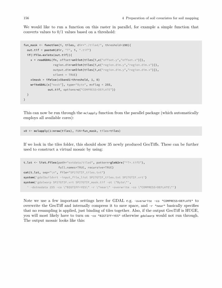
156 4 Preparation of soil covariates for soil mapping
We would like to run a function on this raster in parallel, for example a simple function thatconverts values to 0/1 values based on a threshold:
fun_mask <- function(i, tiles, dir="./tiled/", threshold=190){out.tif = paste0(dir, "T", i, ".tif")if(!file.exists(out.tif)){
x = readGDAL(fn, offset=unlist(tiles[i,c("offset.y","offset.x")]),region.dim=unlist(tiles[i,c("region.dim.y","region.dim.x")]),output.dim=unlist(tiles[i,c("region.dim.y","region.dim.x")]),silent = TRUE)
x$mask = ifelse(x$band1>threshold, 1, 0)writeGDAL(x["mask"], type="Byte", mvFlag = 255,
out.tif, options=c("COMPRESS=DEFLATE"))}
}
This can now be run through the mclapply function from the parallel package (which automaticallyemploys all available cores):
x0 <- mclapply(1:nrow(tiles), FUN=fun_mask, tiles=tiles)
If we look in the tiles folder, this should show 35 newly produced GeoTiffs. These can be furtherused to construct a virtual mosaic by using:
t.lst <- list.files(path="extdata/tiled", pattern=glob2rx("^T*.tif$"),full.names=TRUE, recursive=TRUE)
cat(t.lst, sep="\n", file="SP27GTIF_tiles.txt")system('gdalbuildvrt -input_file_list SP27GTIF_tiles.txt SP27GTIF.vrt')system('gdalwarp SP27GTIF.vrt SP27GTIF_mask.tif -ot \"Byte\"',' -dstnodata 255 -co \"BIGTIFF=YES\" -r \"near\" -overwrite -co \"COMPRESS=DEFLATE\"')
Note we use a few important settings here for GDAL e.g. -overwrite -co "COMPRESS=DEFLATE" tooverwrite the GeoTiff and internally compress it to save space, and -r "near" basically specifiesthat no resampling is applied, just binding of tiles together. Also, if the output GeoTiff is HUGE,you will most likely have to turn on -co "BIGTIFF=YES" otherwise gdalwarp would not run through.The output mosaic looks like this:
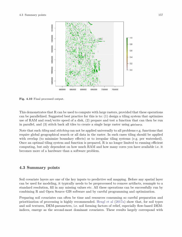
4.3 Summary points 157
Fig. 4.10 Final processed output.
This demonstrates that R can be used to compute with large rasters, provided that these operationscan be parallelized. Suggested best practice for this is to: (1) design a tiling system that optimizesuse of RAM and read/write speed of a disk, (2) prepare and test a function that can then be runin parallel, and (3) stitch back all tiles to create a single large raster using gdalwarp.
Note that such tiling and stitching can not be applied universally to all problems e.g. functions thatrequire global geographical search or all data in the raster. In such cases tiling should be appliedwith overlap (to minimize boundary effects) or to irregular tiling systems (e.g. per watershed).Once an optimal tiling system and function is prepared, R is no longer limited to running efficientcomputing, but only dependent on how much RAM and how many cores you have available i.e. itbecomes more of a hardware than a software problem.
4.3 Summary points
Soil covariate layers are one of the key inputs to predictive soil mapping. Before any spatial layercan be used for modeling, it typically needs to be preprocessed to remove artifacts, resample to astandard resolution, fill in any missing values etc. All these operations can be successfully run bycombining R and Open Source GIS software and by careful programming and optimization.
Preparing soil covariates can often be time and resources consuming so careful preparation andprioritization of processing is highly recommended. Hengl et al (2017a) show that, for soil typesand soil textures, DEM-parameters, i.e. soil forming factors of relief, especially flow-based DEM-indices, emerge as the second-most dominant covariates. These results largely correspond with

158 4 Preparation of soil covariates for soil mapping
conventional soil survey knowledge (surveyors have been using relief as a key guideline to delineatesoil bodies for decades).
Although lithology is often not in the list of the top 15 most important predictors for PSM projects,spatial patterns of lithologic classes can often be distinctly recognized in the output predictions.This is especially true for soil texture fractions and coarse fragments. In general, for predictingsoil chemical properties, climatic variables (especially precipitation) and surface reflectance seemto be the most important, while for soil classes and soil physical properties it is a combination ofrelief, vegetation dynamics and parent material. Investing extra time in preparing a better mapof soil parent material is hence often a good idea.
Other potentially useful covariates for predicting soil properties and classes could be maps of paleoi.e. pre-historic climatic conditions of soil formation, e.g. glacial landscapes and processes, pastclimate conditions and similar. These could likely become significant predictors of many currentsoil characteristics. Information on pre-historic climatic conditions and land use is unfortunatelyoften not available, especially not at detailed cartographic scales, although there are now sev-eral global products that represent, for example, dynamics of land use / changes of land cover(see e.g. HYDE data set (Klein Goldewijk et al, 2011)) through the past 1500+ years. As thespatial detail and completeness of such pre-historic maps increases, they will become potentiallyinteresting covariates for global soil modeling.
USA’s NASA and USGS, with its SRTM, MODIS, Landsat, ICESat and similar civil-applicationsmissions will likely remain the main source of spatial covariate data to support global and localsoil mapping initiatives.
Chapter 5
Statistical theory for predictive soil mapping
Edited by: Hengl T., Heuvelink G.B.M and MacMillan R. A.
5.1 Aspects of spatial variability of soil variables
In this chapter we review the statistical theory for soil mapping. We focus on models consideredmost suitable for practical implementation and use with soil profile data and gridded covariates,and we provide the mathematical-statistical details of the selected models. We start by revisitingsome basic statistical aspects of soil mapping, and conclude by illustrating a proposed frameworkfor reproducible, semi-automated mapping of soil variables using simple, real-world examples.
The code and examples are provided only for illustration. More complex predictive modeling isdescribed in chapter 6. To install and optimize all packages used in this chapter please refer tosection 2.5.
5.1.1 Modelling soil variability
Soils vary spatially in a way that is often only partially understood. The main (deterministic)causes of soil spatial variation are the well-known causal factors — climate, organisms, relief,parent material and time — but how these factors jointly shape the soil over time is a verycomplex process that is (still) extremely difficult to model mechanistically. Moreover, mechanisticmodelling approaches require large sets of input data that are realistically not available in practice.Some initial steps have been made, notably for mechanistic modelling of vertical soil variation(see e.g. Finke and Hutson (2008), Sommer et al (2008), Minasny et al (2008), and Vanwalleghemet al (2010)), but existing approaches are still rudimentary and cannot be used for operational soilmapping. Mainstream soil mapping therefore takes an empirical approach in which the relationshipbetween the soil variable of interest and causal factors (or their proxies) is modelled statistically,using various types of regression models. The explanatory variables used in regression are alsoknown as covariates (a list of common covariates used in soil mapping is provided in chapter 4).
159
160 5 Statistical theory for predictive soil mapping
Regression models explain only part of the variation (i.e. variance) of the soil variable of interest,because:
• The structure of the regression model does not represent the true mechanistic relationshipbetween the soil and its causal factors.
• The regression model includes only a few of the many causal factors that formed the soil.
• The covariates used in regression are often only incomplete proxies of the true soil formingfactors.
• The covariates often contain measurement errors and/or are measured at a much coarser scale(i.e. support) than that of the soil that needs to be mapped.
As a result, soil spatial regression models will often display a substantial amount of residualvariance, which may well be larger than the amount of variance explained by the regression itself.The residual variation can subsequently be analysed on spatial structure through a variogramanalysis. If there is spatial structure, then kriging the residual and incorporating the result of thisin mapping can improve the accuracy of soil predictions (Hengl et al, 2007a).
5.1.2 Universal model of soil variation
From a statistical point of view, it is convenient to distinguish between three major componentsof soil variation: (1) deterministic component (trend), (2) spatially correlated component and (3)pure noise. This is the basis of the universal model of soil variation (Burrough and McDonnell,1998; Webster and Oliver, 2001, p.133):
𝑍(𝑠) = 𝑚(𝑠) + 𝜀′(𝑠) + 𝜀″(𝑠) (5.1)
where 𝑠 is two-dimensional location, 𝑚(𝑠) is the deterministic component, 𝜀′(𝑠) is the spatiallycorrelated stochastic component and 𝜀″(𝑠) is the pure noise (micro-scale variation and measure-ment error). This model was probably first introduced by Matheron (1969), and has been usedas a general framework for spatial prediction of quantities in a variety of environmental researchdisciplines.
The universal model of soil variation assumes that there are three major components of soil varia-tion: (1) the deterministic component (function of covariates), (2) spatially correlated component(treated as stochastic) and (3) pure noise.
The universal model of soil variation model (Eq.(5.1)) can be further generalised to three-dimensional space and the spatio-temporal domain (3D+T) by letting the variables also dependon depth and time:
𝑍(𝑠, 𝑑, 𝑡) = 𝑚(𝑠, 𝑑, 𝑡) + 𝜀′(𝑠, 𝑑, 𝑡) + 𝜀″(𝑠, 𝑑, 𝑡) (5.2)
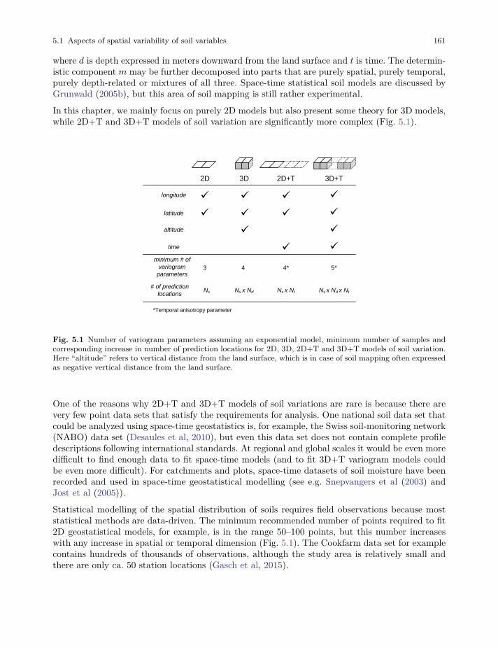
5.1 Aspects of spatial variability of soil variables 161
where 𝑑 is depth expressed in meters downward from the land surface and 𝑡 is time. The determin-istic component 𝑚 may be further decomposed into parts that are purely spatial, purely temporal,purely depth-related or mixtures of all three. Space-time statistical soil models are discussed byGrunwald (2005b), but this area of soil mapping is still rather experimental.
In this chapter, we mainly focus on purely 2D models but also present some theory for 3D models,while 2D+T and 3D+T models of soil variation are significantly more complex (Fig. 5.1).
2D 3D 2D+T 3D+T
longitude
latitude
altitude
time
minimum # of
variogram
parameters
# of prediction
locations
ü
ü
ü
ü
ü
ü
ü
ü
ü
ü
ü
ü
3 4 4* 5*
Ns Ns x Nd
*Temporal anisotropy parameter
Ns x Nt Ns x Nd x Nt
Fig. 5.1 Number of variogram parameters assuming an exponential model, minimum number of samples andcorresponding increase in number of prediction locations for 2D, 3D, 2D+T and 3D+T models of soil variation.Here “altitude” refers to vertical distance from the land surface, which is in case of soil mapping often expressedas negative vertical distance from the land surface.
One of the reasons why 2D+T and 3D+T models of soil variations are rare is because there arevery few point data sets that satisfy the requirements for analysis. One national soil data set thatcould be analyzed using space-time geostatistics is, for example, the Swiss soil-monitoring network(NABO) data set (Desaules et al, 2010), but even this data set does not contain complete profiledescriptions following international standards. At regional and global scales it would be even moredifficult to find enough data to fit space-time models (and to fit 3D+T variogram models couldbe even more difficult). For catchments and plots, space-time datasets of soil moisture have beenrecorded and used in space-time geostatistical modelling (see e.g. Snepvangers et al (2003) andJost et al (2005)).
Statistical modelling of the spatial distribution of soils requires field observations because moststatistical methods are data-driven. The minimum recommended number of points required to fit2D geostatistical models, for example, is in the range 50–100 points, but this number increaseswith any increase in spatial or temporal dimension (Fig. 5.1). The Cookfarm data set for examplecontains hundreds of thousands of observations, although the study area is relatively small andthere are only ca. 50 station locations (Gasch et al, 2015).
162 5 Statistical theory for predictive soil mapping
The deterministic and stochastic components of soil spatial variation are separately described inmore detail in subsequent sections, but before we do this, we first address soil vertical variabilityand how it can be modelled statistically.
5.1.3 Modelling the variation of soil with depth
Soil properties vary with depth, in some cases much more than in the horizontal direction. Thereis an increasing awareness that the vertical dimension is important and needs to be incorporatedin soil mapping. For example, many spatial prediction models are built using ambiguous verticalreference frames such as predicted soil property for “top-soil” or “A-horizon”. Top-soil can referto different depths / thicknesses and so can the A-horizon range from a few centimeters to overone meter. Hence before fitting a 2D spatial model to soil profile data, it is a good idea to stan-dardize values to standard depths, otherwise soil observation depth becomes an additional sourceof uncertainty. For example soil organic carbon content is strongly controlled by soil depth, socombining values from two A horizons one thick and the other thin, would increase the complexityof 2D soil mapping because a fraction of the variance is controlled by the depth, which is ignored.
The concept of perfectly homogeneous soil horizons is often too restrictive and can be betterreplaced with continuous representations of soil vertical variation i.e. soil-depth functions or curves.Variation of soil properties with depth is typically modelled using one of two approaches (Fig. 5.2):
1. Continuous vertical variation — This assumes that soil variables change continuously withdepth. The soil-depth relationship is modelled using either:
1. Parametric model — The relationship is modelled using mathematical functions such aslogarithmic or exponential decay functions.
2. Non-parametric model — The soil property changes continuously but without obvious reg-ularity with depth. Changes in values are modelled using locally fitted functions such aspiecewise linear functions or splines.
2. Abrupt or stratified vertical variation — This assumes that soil horizons are distinct and homo-geneous bodies of soil material and that soil properties are constant within horizons and changeabruptly at boundaries between horizons.
Combinations of the two approaches are also possible, such as the use of exponential decay func-tions per soil horizon (Kempen et al, 2011).
Parametric continuous models are chosen to reflect pedological knowledge e.g. knowledge of soilforming processes. For example, organic carbon usually originates from plant production i.e. litteror roots. Generally, the upper layers of the soil tend to have greater organic carbon content, whichdecreases continuously with depth, so that the soil-depth relationship can be modelled with anegative-exponential function:
ORC(𝑑) = ORC(𝑑0) ⋅ exp(−𝜏 ⋅ 𝑑) (5.3)
5.1 Aspects of spatial variability of soil variables 163
where ORC(𝑑) is the soil organic carbon content at depth (𝑑), ORC(𝑑0) is the organic carbon content atthe soil surface and 𝜏 is the rate of decrease with depth. This model has only two parameters thatmust be chosen such that model averages over sampling horizons match those of the observationsas closely as possible. Once the model parameters have been estimated, we can easily predictconcentrations for any depth interval.
Consider for example this sample profile from Nigeria:
lon = 3.90; lat = 7.50; id = "ISRIC:NG0017"; FAO1988 = "LXp"top = c(0, 18, 36, 65, 87, 127)bottom = c(18, 36, 65, 87, 127, 181)ORCDRC = c(18.4, 4.4, 3.6, 3.6, 3.2, 1.2)munsell = c("7.5YR3/2", "7.5YR4/4", "2.5YR5/6", "5YR5/8", "5YR5/4", "10YR7/3")## prepare a SoilProfileCollection:prof1 <- plyr::join(data.frame(id, top, bottom, ORCDRC, munsell),
data.frame(id, lon, lat, FAO1988), type='inner')#> Joining by: idprof1$mdepth <- prof1$top+(prof1$bottom-prof1$top)/2
we can fit a log-log model by using e.g.:
d.lm <- glm(ORCDRC ~ log(mdepth), data=prof1, family=gaussian(log))options(list(scipen=3, digits=2))d.lm$fitted.values#> 1 2 3 4 5 6#> 18.1 6.3 3.5 2.4 1.7 1.2
which shows that the log-log fit comes relatively close to the actual values. Another possibilitywould be to fit a power-law model:
ORC(𝑑) = 𝑎 ⋅ 𝑑𝑏 (5.4)
A disadvantage of a single parametric soil property-depth model along the entire soil profile is thatthese completely ignore stratigraphy and abrupt changes at the boundaries between soil horizons.For example, Kempen et al (2011) show that there are many cases where highly contrasting layersof peat can be found buried below the surface due to cultivation practices or holocene drift sand.The model given by Eq.(5.4) illustrated in Fig. 5.2 (left) will not be able to represent such abruptchanges.
Before fitting a 2D spatial prediction model to soil profile data, it is important to standardize valuesto standard depths, otherwise soil observation depth can be an additional source of uncertainty.
Non-parametric soil-depth functions are more flexible and can represent observations of soil prop-erty averages for sampling layers or horizons more accurately. One such technique that is par-ticularly interesting is equal-area or mass-preserving splines (Bishop et al, 1999; Malone et al,
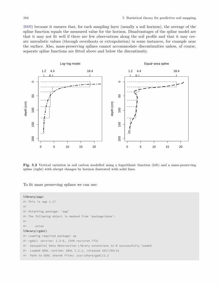
164 5 Statistical theory for predictive soil mapping
2009) because it ensures that, for each sampling layer (usually a soil horizon), the average of thespline function equals the measured value for the horizon. Disadvantages of the spline model arethat it may not fit well if there are few observations along the soil profile and that it may cre-ate unrealistic values (through overshoots or extrapolation) in some instances, for example nearthe surface. Also, mass-preserving splines cannot accommodate discontinuities unless, of course,separate spline functions are fitted above and below the discontinuity.
0 5 10 15 20
200
150
100
500
dept
h (c
m)
1.2 4.4 18.4
Log−log model
0 5 10 15 20
200
150
100
500
dept
h (c
m)
1.2 4.4 18.4
Equal−area spline
Fig. 5.2 Vertical variation in soil carbon modelled using a logarithmic function (left) and a mass-preservingspline (right) with abrupt changes by horizon ilustrated with solid lines.
To fit mass preserving splines we can use:
library(aqp)#> This is aqp 1.17#>#> Attaching package: 'aqp'#> The following object is masked from 'package:base':#>#> unionlibrary(rgdal)#> Loading required package: sp#> rgdal: version: 1.3-6, (SVN revision 773)#> Geospatial Data Abstraction Library extensions to R successfully loaded#> Loaded GDAL runtime: GDAL 2.2.2, released 2017/09/15#> Path to GDAL shared files: /usr/share/gdal/2.2
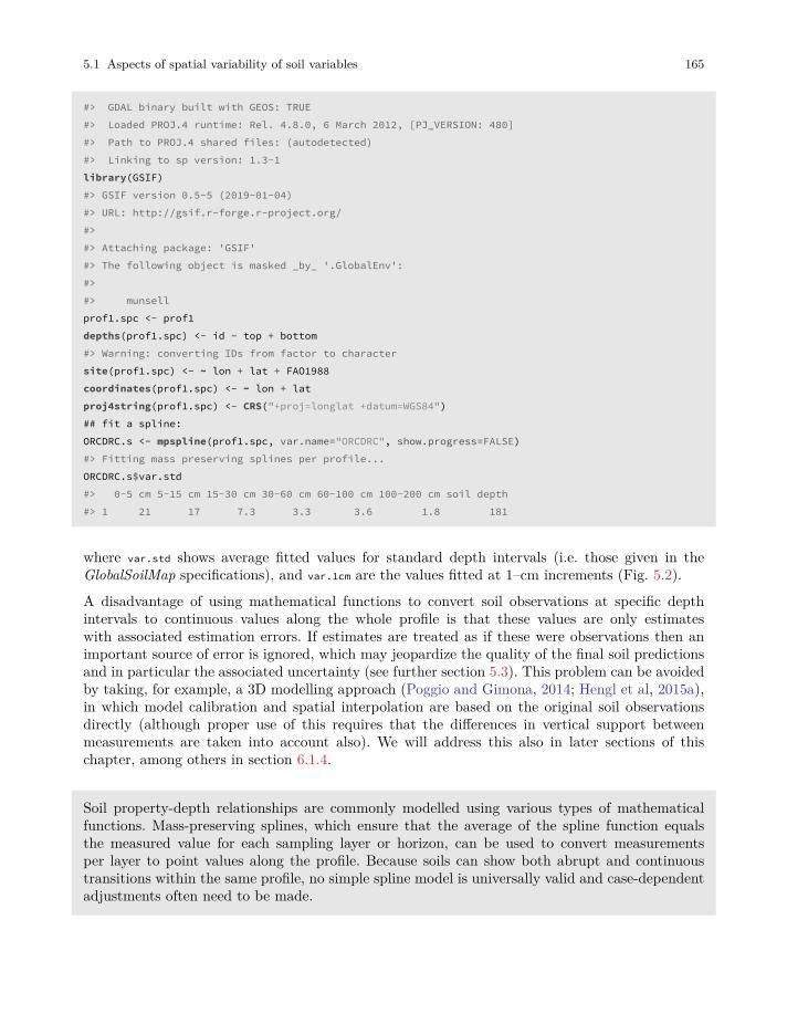
5.1 Aspects of spatial variability of soil variables 165
#> GDAL binary built with GEOS: TRUE#> Loaded PROJ.4 runtime: Rel. 4.8.0, 6 March 2012, [PJ_VERSION: 480]#> Path to PROJ.4 shared files: (autodetected)#> Linking to sp version: 1.3-1library(GSIF)#> GSIF version 0.5-5 (2019-01-04)#> URL: http://gsif.r-forge.r-project.org/#>#> Attaching package: 'GSIF'#> The following object is masked _by_ '.GlobalEnv':#>#> munsellprof1.spc <- prof1depths(prof1.spc) <- id ~ top + bottom#> Warning: converting IDs from factor to charactersite(prof1.spc) <- ~ lon + lat + FAO1988coordinates(prof1.spc) <- ~ lon + latproj4string(prof1.spc) <- CRS("+proj=longlat +datum=WGS84")## fit a spline:ORCDRC.s <- mpspline(prof1.spc, var.name="ORCDRC", show.progress=FALSE)#> Fitting mass preserving splines per profile...ORCDRC.s$var.std#> 0-5 cm 5-15 cm 15-30 cm 30-60 cm 60-100 cm 100-200 cm soil depth#> 1 21 17 7.3 3.3 3.6 1.8 181
where var.std shows average fitted values for standard depth intervals (i.e. those given in theGlobalSoilMap specifications), and var.1cm are the values fitted at 1–cm increments (Fig. 5.2).
A disadvantage of using mathematical functions to convert soil observations at specific depthintervals to continuous values along the whole profile is that these values are only estimateswith associated estimation errors. If estimates are treated as if these were observations then animportant source of error is ignored, which may jeopardize the quality of the final soil predictionsand in particular the associated uncertainty (see further section 5.3). This problem can be avoidedby taking, for example, a 3D modelling approach (Poggio and Gimona, 2014; Hengl et al, 2015a),in which model calibration and spatial interpolation are based on the original soil observationsdirectly (although proper use of this requires that the differences in vertical support betweenmeasurements are taken into account also). We will address this also in later sections of thischapter, among others in section 6.1.4.
Soil property-depth relationships are commonly modelled using various types of mathematicalfunctions. Mass-preserving splines, which ensure that the average of the spline function equalsthe measured value for each sampling layer or horizon, can be used to convert measurementsper layer to point values along the profile. Because soils can show both abrupt and continuoustransitions within the same profile, no simple spline model is universally valid and case-dependentadjustments often need to be made.
166 5 Statistical theory for predictive soil mapping
5.1.4 Vertical aggregation of soil properties
As mentioned previously, soil variables refer to aggregate values over specific depth intervals (seeFig. 5.2). For example, the organic carbon content is typically observed per soil horizon with valuesin e.g. g/kg or permilles (Conant et al, 2010; Baritz et al, 2010; Panagos et al, 2013). The SoilOrganic Carbon Storage (or Soil Organic Carbon Stock) in the whole profile can be calculated byusing Eq (7.1). Once we have determined soil organic carbon storage (OCS) per horizon, we canderive the total organic carbon in the soil by summing over all (𝐻) horizons:
OCS =𝐻
∑ℎ=1
OCSℎ (5.5)
Obviously, the horizon-specific soil organic carbon content (ORCℎ) and total soil organic carboncontent (OCS) are NOT the same variables and need to be analysed and mapped separately.In the case of pH (PHI) we usually do not aim at estimating the actual mass or quantity of hydrogenions. To represent a soil profile with a single number, we may take a weighted mean of the measuredpH values per horizon:
PHI =𝐻
∑ℎ=1
𝑤ℎ ⋅ PHIℎ;𝐻
∑ℎ=1
𝑤ℎ = 1 (5.6)
where the weights can be chosen proportional to the horizon thickness:
𝑤ℎ = HSIZEℎ𝐻∑ℎ=1
HSIZEℎ
(5.7)
Thus, it is important to be aware that all soil variables: (A) can be expressed as relative (percent-ages) or absolute (mass / quantities) values, and (B) refer to specific horizons or depth intervalsor to the whole soil profile.Similar spatial support-effects show up in the horizontal, because soil observations at point locationsare not the same as average or bulk soil samples taken by averaging a large number of pointobservations on a site or plot (Webster and Oliver, 2001).
Soil variables can refer to a specific depth interval or to the whole profile. The differences in spatialpatterns between variables representing fundamentally the same feature (e.g. soil organic carbonin of a specific soil horizon or soil layer and total organic carbon stock in of the whole profile),but at different spatial and vertical support, can be significant.
In order to avoid misinterpretation of the results of mapping, we recommend that any deliveredmap of soil properties should specify the support size in the vertical and lateral directions, theanalysis method (detection limit) and measurement units. Such information can be included inthe metadata and/or in any key visualization or plot. Likewise, any end-user of soil data shouldspecify whether estimates of the relative or total organic carbon, aggregated or at 2D/3D pointsupport are required.
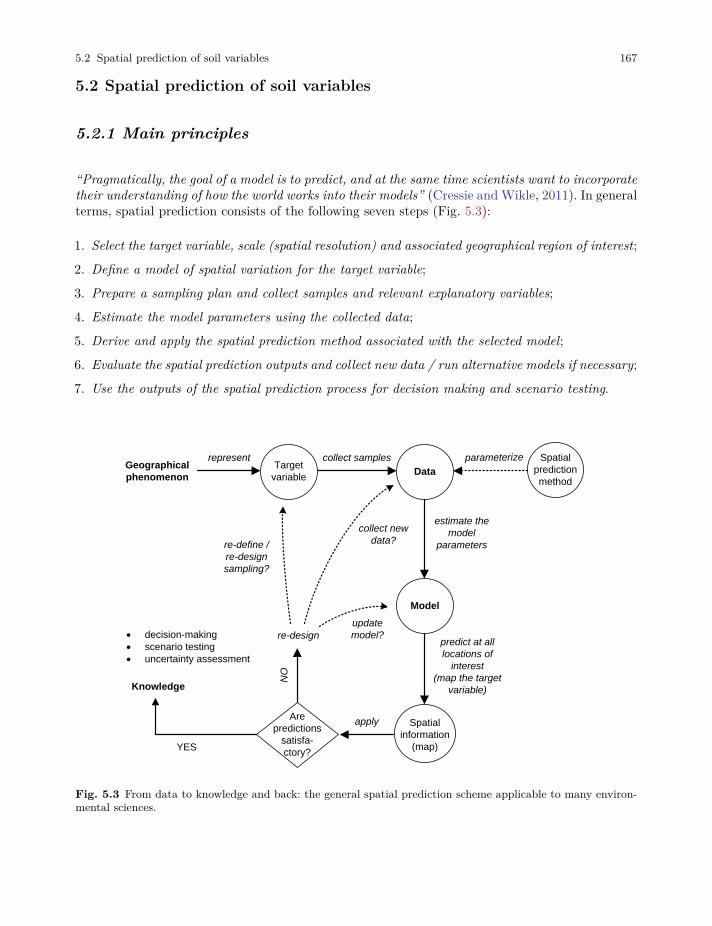
5.2 Spatial prediction of soil variables 167
5.2 Spatial prediction of soil variables
5.2.1 Main principles
“Pragmatically, the goal of a model is to predict, and at the same time scientists want to incorporatetheir understanding of how the world works into their models” (Cressie and Wikle, 2011). In generalterms, spatial prediction consists of the following seven steps (Fig. 5.3):
1. Select the target variable, scale (spatial resolution) and associated geographical region of interest;
2. Define a model of spatial variation for the target variable;
3. Prepare a sampling plan and collect samples and relevant explanatory variables;
4. Estimate the model parameters using the collected data;
5. Derive and apply the spatial prediction method associated with the selected model;
6. Evaluate the spatial prediction outputs and collect new data / run alternative models if necessary;
7. Use the outputs of the spatial prediction process for decision making and scenario testing.
representGeographical
phenomenon
Target
variable
collect samples
Data
Spatial
information
(map)
· decision-making
· scenario testing
· uncertainty assessment
Model
apply
update
model?predict at all
locations of
interest
(map the target
variable)
estimate the
model
parameters
Spatial
prediction
method
parameterize
collect new
data?
Knowledge
re-define /
re-design
sampling?
Are
predictions
satisfa-
ctory?
NO
YES
re-design
Fig. 5.3 From data to knowledge and back: the general spatial prediction scheme applicable to many environ-mental sciences.
168 5 Statistical theory for predictive soil mapping
The spatial prediction process is repeated at all nodes of a grid covering 𝐷 (or a space-time domainin case of spatiotemporal prediction) and produces three main outputs:
1. Estimates of the model parameters (e.g., regression coefficients and variogram parameters),i.e. the model;
2. Predictions at new locations, i.e. a prediction map;
3. Estimate of uncertainty associated with the predictions, i.e. a prediction error map.
It is clear from Fig. 5.3 that the key steps in the mapping procedure are: (a) choice of the samplingscheme (e.g. Ng et al (2018) and Brus (2019)), (b) choice of the model of spatial variation (e.g.Diggle and Ribeiro Jr (2007)), and (c) choice of the parameter estimation technique (e.g. Lark et al(2006)). When the sampling scheme is given and cannot be changed, the focus of optimizationof the spatial prediction process is then on selecting and fine-tuning the best performing spatialprediction method.
In a geostatistical framework, spatial prediction is estimation of values of some target variable 𝑍at a new location (𝑠0) given the input data:
𝑍(𝑠0) = 𝐸 {𝑍(𝑠0)|𝑧(𝑠𝑖), 𝑋(𝑠0), 𝑖 = 1, ..., 𝑛} (5.8)
where the 𝑧(𝑠𝑖) are the input set of observations of the target variable, 𝑠𝑖 is a geographical location,𝑛 is the number of observations and 𝑋(𝑠0) is a list of covariates or explanatory variables, availableat all prediction locations within the study area of interest (𝑠 ∈ 𝔸). To emphasise that the modelparameters also influence the outcome of the prediction process, this can be made explicit bywriting (Cressie and Wikle, 2011):
[𝑍|𝑌 , 𝜃] (5.9)
where 𝑍 is the data, 𝑌 is the (hidden) process that we are predicting, and 𝜃 is a list of modelparameters e.g. trend coefficients and variogram parameters.
There are many spatial prediction methods for generating spatial predictions from soil samples andcovariate information. All differ in the underlying statistical model of spatial variation, althoughthis model is not always made explicit and different methods may use the same statistical model.A review of currently used digital soil mapping methods is given, for example, in McBratney et al(2011), while the most extensive review can be found in McBratney et al (2003) and McBratneyet al (2018). Li and Heap (2010) list 40+ spatial prediction / spatial interpolation techniques.Many spatial prediction methods are often just different names for essentially the same thing.What is often known under a single name, in the statistical, or mathematical literature, can beimplemented through different computational frameworks, and lead to different outputs (mainlybecause many models are not written out in the finest detail and leave flexibility for actual im-plementation).
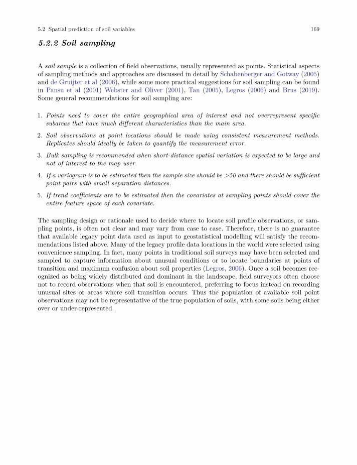
5.2 Spatial prediction of soil variables 169
5.2.2 Soil sampling
A soil sample is a collection of field observations, usually represented as points. Statistical aspectsof sampling methods and approaches are discussed in detail by Schabenberger and Gotway (2005)and de Gruijter et al (2006), while some more practical suggestions for soil sampling can be foundin Pansu et al (2001) Webster and Oliver (2001), Tan (2005), Legros (2006) and Brus (2019).Some general recommendations for soil sampling are:
1. Points need to cover the entire geographical area of interest and not overrepresent specificsubareas that have much different characteristics than the main area.
2. Soil observations at point locations should be made using consistent measurement methods.Replicates should ideally be taken to quantify the measurement error.
3. Bulk sampling is recommended when short-distance spatial variation is expected to be large andnot of interest to the map user.
4. If a variogram is to be estimated then the sample size should be >50 and there should be sufficientpoint pairs with small separation distances.
5. If trend coefficients are to be estimated then the covariates at sampling points should cover theentire feature space of each covariate.
The sampling design or rationale used to decide where to locate soil profile observations, or sam-pling points, is often not clear and may vary from case to case. Therefore, there is no guaranteethat available legacy point data used as input to geostatistical modelling will satisfy the recom-mendations listed above. Many of the legacy profile data locations in the world were selected usingconvenience sampling. In fact, many points in traditional soil surveys may have been selected andsampled to capture information about unusual conditions or to locate boundaries at points oftransition and maximum confusion about soil properties (Legros, 2006). Once a soil becomes rec-ognized as being widely distributed and dominant in the landscape, field surveyors often choosenot to record observations when that soil is encountered, preferring to focus instead on recordingunusual sites or areas where soil transition occurs. Thus the population of available soil pointobservations may not be representative of the true population of soils, with some soils being eitherover or under-represented.
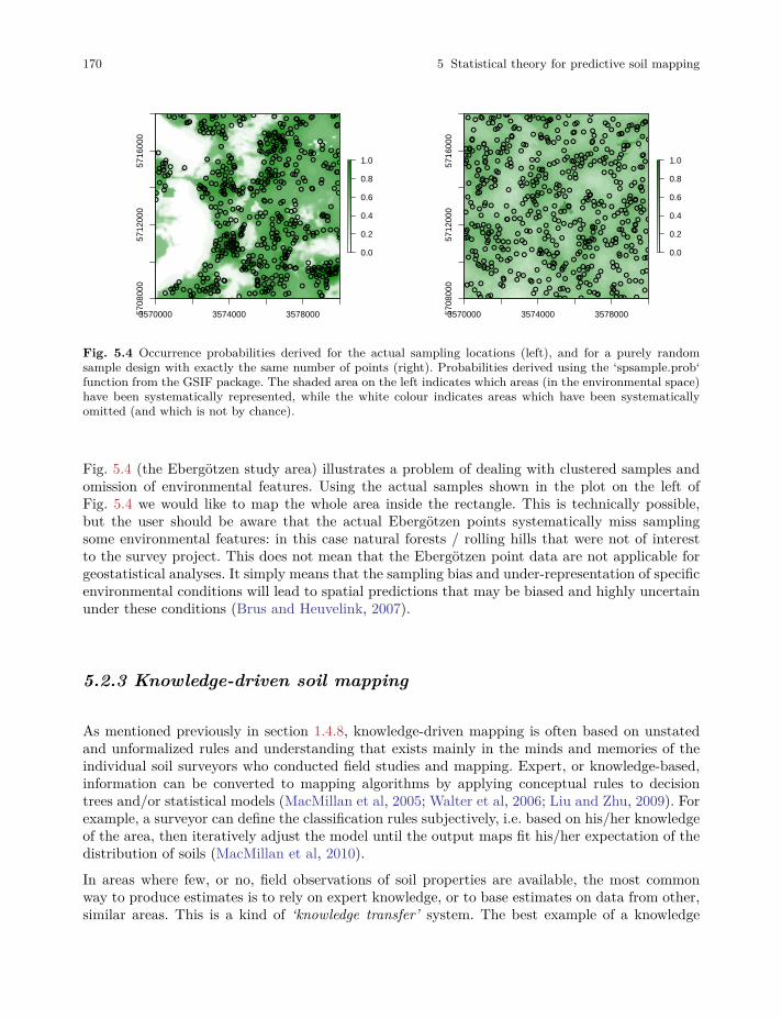
170 5 Statistical theory for predictive soil mapping
3570000 3574000 35780005708
000
5712
000
5716
000
0.0
0.2
0.4
0.6
0.8
1.0
●
●
●
●●
●
●●●
●
●
●
●
●●
●
●
●●
●●●
●
●●●
●●
●
●
●●●
●●●●
●
●
●
●
●
●
●
●
●
●
●
●
●●
●
●
●
●●
●●
●
●
●
●
●
●
●
●
●●
●
●
●
●
●
●
●●
●
●
●
●
●
●
●
●
●
●
●
●
●●●
●
●
●
●
●
●
●
●
●
●
●
●
●
●
●
●
●
●
●
●
●
●
●
●
●
●
●
●
●
●
●
●●
●●
●
●
●
●
●
●
●
●
●
●
●
●
●
●
●
●
●
●
●
●●
●
●
●
●
●●
●
●
●
●
●
●
●
●
●
●
●
●
●
●
●
●●
●
●
●
●●
●
●
●
●
●
●●
●●●
●
●
●●
●
●
●
●
●
●●
●
●
●
●
●
●●
●
●
●
●●
●
●
●●
●●
●
●
●●●
●
●
●
●
●
●
●
●
●
●
●
●●●
●
●
●●
●
●
●●
●
●●
●
●
●
●
●
●
●
●
●
●
●
●
●
●
●
●
●
●
●
●
●
●
●●
●
●
●
●
●
●
●
●
●
●
●
●
●
●
●
●●
●
●●
●
●
●
●
●
●●
●
●
●●
●
●
●
●
●
●●●
●
●
●
●
●
●
●
●●
●
●
●
●
●
●
●●
●●
●
●
●
●
●
●
●●
●
●
●
●
●
●
●
●
●
●
●●
●
●
●●
●
●
●●
●
●
●
●
●
●
●
●
●
●
●
●
●
●●●
●
●
●
●
●
●
●
●
●
●
●
●
●
●
●
●
●●
●
●
●●
●
●
●
●
●
●
●
●
●
●
●
●
●
●
●
●
●
●
●
●
●
●
●
●
●
●
●
●
●
●
●
●
●
●
●
●
●
●
●●
●
●●
●
●●
●
●
●
●
●
●
●
●
●●
●
●●
●
●●●●
●
●
●
●
●
●
●
●
●
●
●
●
●
●
●
●
●
●
●
●
●
●
●
●
●●
●
●
●
●
●
●●
●
●●
●●
●
●
●
●
●
●
●●
●●
●
●
●
●
●●●
●
●
●
●
●
●
●
●
●
●
●
●
●
●
●
●
3570000 3574000 35780005708
000
5712
000
5716
000
0.0
0.2
0.4
0.6
0.8
1.0
●
●
●
●
●
●
●
●
●
●
●
●
●
●
●●
●
●
● ●
●
●
●
●●
●
●
●
●
●
●
●● ●
●
●
●●
●
●
●
●
●
●
●
●
●
●
●
●
●
●
●
●
●
●●
●
●
●
●
●
●
●
●
●
●
●
●
●
●
●
●
●
●
●
●
●●
●
●
●
●
●
● ●●
●
●
●
●
●
●
●
●
●
●
●
●
●
●
●
●
●
●
●
●●
●
●●
●●
●
●
●
●
●
●
●
●
●
●
●
●
●
●
●
●
●
●
●
●
●
●
●
●
●
●
●
●
●●
●
●
●
●
●
●
●
●●
●
●
●
●
●
●
●
●
●
●
●
●
●●
●
●
●
●
●
●
●
●●
●
●
●
●●
●●
●
●
●
●
●
●
●
●
●
●
●●
●
●
●
● ●
●
●
●
●
●
●
●
●
●
●
●
●
●
●
●
●
●
●
●
●
●
●
●
●
●
●
●
●
●●
●
●●
●
●
●
●
●
●
●
●
●
●
●
●
●
●
●
●
●
●
●
●
●
●
●
●
●
●
●
●●
●
●
●
●
●
●
●
●
●
●
●●
●
●
●
●
●
●
●
●
●
●
●
●
●
●
●
●
●
●
●
●
●
●
●
●
●
●
●
●
●
●
●
●
●
●
●
●
●
●
●●
●
●
●
●
●
●
●
●
●
●
●
●
●
●
●
●
● ●
●
●
●
●
●
●
●
●
●
●
●
●
●●
●
●
●
●
●
●
●
●
●
●
●
●
●
●
●●
●
●
●
●
●
●
●
●
●●
●
●
●
●
●
●
●
●
●
●
●
●
●
●
●
●
●
●
●
●
●
●
●
●
●
●
●
●
●
●
●●
●
●
●
●
●
●
●
●
●
● ●
●
●
●
●
●
●●
●
●
●
●
●
●
●
●
●
●
●●
●
●
●
●
● ●
●
●
●
●
●
●
●
●
●●
●●
●
●
●
●
●
●
●
● ●
●
●
●
●
●●
●●●
●
●
●
●
●
●
●
●
●
●
●
●
●
●●
●
●
●
●
●
●
●
●
●
●
●
●
●●
●
●
●
●
●
●
●
●
●
●
●
●●
●
●
●
●
●
●●
●
●
●
●●
●
●
●
●
Fig. 5.4 Occurrence probabilities derived for the actual sampling locations (left), and for a purely randomsample design with exactly the same number of points (right). Probabilities derived using the ‘spsample.prob‘function from the GSIF package. The shaded area on the left indicates which areas (in the environmental space)have been systematically represented, while the white colour indicates areas which have been systematicallyomitted (and which is not by chance).
Fig. 5.4 (the Ebergötzen study area) illustrates a problem of dealing with clustered samples andomission of environmental features. Using the actual samples shown in the plot on the left ofFig. 5.4 we would like to map the whole area inside the rectangle. This is technically possible,but the user should be aware that the actual Ebergötzen points systematically miss samplingsome environmental features: in this case natural forests / rolling hills that were not of interestto the survey project. This does not mean that the Ebergötzen point data are not applicable forgeostatistical analyses. It simply means that the sampling bias and under-representation of specificenvironmental conditions will lead to spatial predictions that may be biased and highly uncertainunder these conditions (Brus and Heuvelink, 2007).
5.2.3 Knowledge-driven soil mapping
As mentioned previously in section 1.4.8, knowledge-driven mapping is often based on unstatedand unformalized rules and understanding that exists mainly in the minds and memories of theindividual soil surveyors who conducted field studies and mapping. Expert, or knowledge-based,information can be converted to mapping algorithms by applying conceptual rules to decisiontrees and/or statistical models (MacMillan et al, 2005; Walter et al, 2006; Liu and Zhu, 2009). Forexample, a surveyor can define the classification rules subjectively, i.e. based on his/her knowledgeof the area, then iteratively adjust the model until the output maps fit his/her expectation of thedistribution of soils (MacMillan et al, 2010).
In areas where few, or no, field observations of soil properties are available, the most commonway to produce estimates is to rely on expert knowledge, or to base estimates on data from other,similar areas. This is a kind of ‘knowledge transfer’ system. The best example of a knowledge
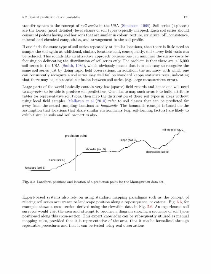
5.2 Spatial prediction of soil variables 171
transfer system is the concept of soil series in the USA (Simonson, 1968). Soil series (+phases)are the lowest (most detailed) level classes of soil types typically mapped. Each soil series shouldconsist of pedons having soil horizons that are similar in colour, texture, structure, pH, consistence,mineral and chemical composition, and arrangement in the soil profile.
If one finds the same type of soil series repeatedly at similar locations, then there is little need tosample the soil again at additional, similar, locations and, consequently, soil survey field costs canbe reduced. This sounds like an attractive approach because one can minimize the survey costs byfocusing on delineating the distribution of soil series only. The problem is that there are >15,000soil series in the USA (Smith, 1986), which obviously means that it is not easy to recognize thesame soil series just by doing rapid field observations. In addition, the accuracy with which onecan consistently recognize a soil series may well fail on standard kappa statistics tests, indicatingthat there may be substantial confusion between soil series (e.g. large measurement error).
Large parts of the world basically contain very few (sparce) field records and hence one will needto improvise to be able to produce soil predictions. One idea to map such areas is to build attributetables for representative soil types, then map the distribution of these soil types in areas withoutusing local field samples. Mallavan et al (2010) refer to soil classes that can be predicted faraway from the actual sampling locations as homosoils. The homosoils concept is based on theassumption that locations that share similar environments (e.g. soil-forming factors) are likely toexhibit similar soils and soil properties also.
hill top (soil A)
depression (soil B)
slope (soil C)
shoulder (soil D)
slope (soil C)
footslope (soil E)
prediction point
Fig. 5.5 Landform positions and location of a prediction point for the Maungawhau data set.
Expert-based systems also rely on using standard mapping paradigms such as the concept ofrelating soil series occurrance to landscape position along a toposequence, or catena . Fig. 5.5, forexample, shows a cross-section derived using the elevation data in Fig. 5.6. An experienced soilsurveyor would visit the area and attempt to produce a diagram showing a sequence of soil typespositioned along this cross-section. This expert knowledge can be subsequently utilized as manualmapping rules, provided that it is representative of the area, that it can be formalized throughrepeatable procedures and that it can be tested using real observations.
172 5 Statistical theory for predictive soil mapping
Fig. 5.6 A cross-section for the Maungawhau volcano dataset commonly used in R to illustrate DEM and imageanalysis techniques.
If relevant auxiliary information, such as a Digital Elevation Model (DEM), is available for thestudy area, one can derive a number of DEM parameters that can help to quantify landforms andgeomorphological processes. Landforms can also automatically be classified by computing variousDEM parameters per pixel, or by using knowledge from, Fig. 5.7 (a sample of the study area) toobjectively extract landforms and associated soils in an area. Such auxiliary landform informationcan be informative about the spatial distribution of the soil, which is the key principle of, forexample, the SOTER methodology (Van Engelen and Dijkshoorn, 2012).
The mapping process of knowledge-driven soil mapping can be summarized as follows (MacMillanet al, 2005, 2010):
1. Sample the study area using transects oriented along topographic cross-sections;
2. Assign soil types to each landform position and at each sample location;
3. Derive DEM parameters and other auxiliary data sets;
4. Develop (fuzzy) rules relating the distribution of soil classes to the auxiliary (mainly topographic)variables;
5. Implement (fuzzy) rules to allocate soil classes (or compute class probabi;ities) for each gridlocation;
6. Generate soil property values for each soil class using representative observations (class centers);
7. Estimate values of the target soil variable at each grid location using a weighted average ofallocated soil class or membership values and central soil property values for each soil class;
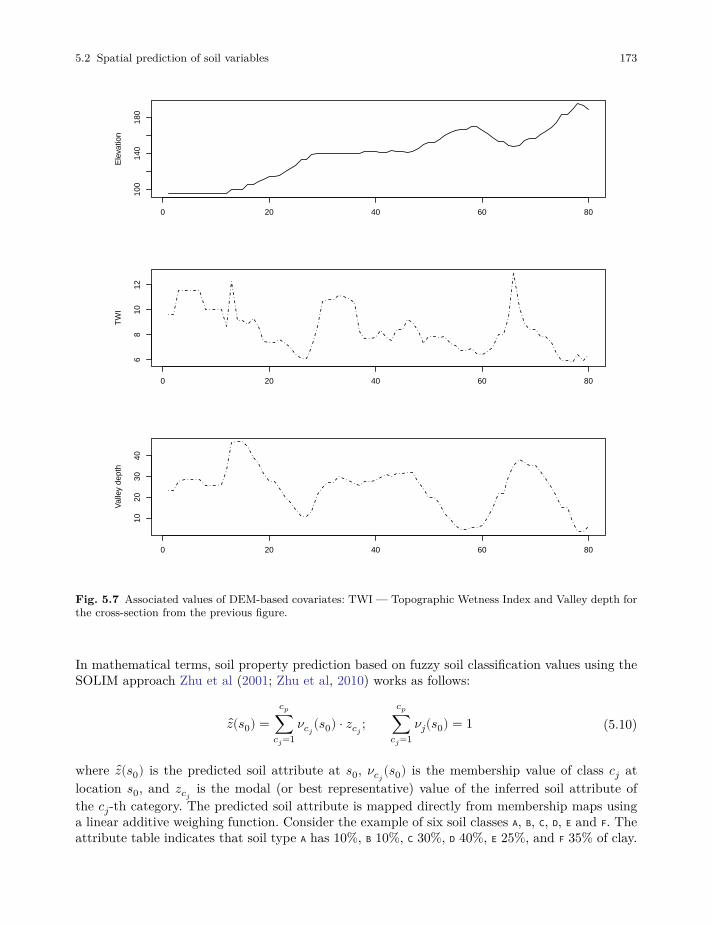
5.2 Spatial prediction of soil variables 173
0 20 40 60 80
100
140
180
Ele
vatio
n
0 20 40 60 80
68
1012
TW
I
0 20 40 60 80
1020
3040
Val
ley
dept
h
Fig. 5.7 Associated values of DEM-based covariates: TWI — Topographic Wetness Index and Valley depth forthe cross-section from the previous figure.
In mathematical terms, soil property prediction based on fuzzy soil classification values using theSOLIM approach Zhu et al (2001; Zhu et al, 2010) works as follows:
𝑧(𝑠0) =𝑐𝑝
∑𝑐𝑗=1
𝜈𝑐𝑗(𝑠0) ⋅ 𝑧𝑐𝑗
;𝑐𝑝
∑𝑐𝑗=1
𝜈𝑗(𝑠0) = 1 (5.10)
where 𝑧(𝑠0) is the predicted soil attribute at 𝑠0, 𝜈𝑐𝑗(𝑠0) is the membership value of class 𝑐𝑗 at
location 𝑠0, and 𝑧𝑐𝑗is the modal (or best representative) value of the inferred soil attribute of
the 𝑐𝑗-th category. The predicted soil attribute is mapped directly from membership maps usinga linear additive weighing function. Consider the example of six soil classes A, B, C, D, E and F. Theattribute table indicates that soil type A has 10%, B 10%, C 30%, D 40%, E 25%, and F 35% of clay.
174 5 Statistical theory for predictive soil mapping
If the membership values at a grid position are 0.6, 0.2, 0.1, 0.05, 0.00 and 0.00, then Eq.(5.10)predicts the clay content as 13.5%.
It is obvious from this work flow that the critical aspects that determine the accuracy of thefinal predictions are the selection of where we locate the cross-sections and the representativesoil profiles and the strength of the relationship between the resulting soil classes and target soilproperties. Qi et al (2006), for example, recommended that the most representative values forsoil classes can be identified, if many soil profiles are available, by finding the sampling locationthat occurs at the grid cell with highest similarity value for a particular soil class. Soil mappersare now increasingly looking for ways to combine expert systems with statistical data mining andregression modelling techniques.
One problem of using a supervised mapping system, as described above, is that it is difficult toget an objective estimate of the prediction error (or at least a robust statistical theory for thishas not yet been developed). The only possibility to assess the accuracy of such maps would be tocollect independent validation samples and estimate the mapping accuracy following the methodsdescribed in section 5.3. So, in fact, expert-based systems also depend on statistical sampling andinference for evaluation of the accuracy of the resulting map.
5.2.4 Geostatistics-driven soil mapping (pedometric mapping)
Pedometric mapping is based on using statistical models to predict soil properties, which leads us tothe field of geostatistics. Geostatistics treats the soil as a realization of a random process (Websterand Oliver, 2001). It uses the point observations and gridded covariates to predict the randomprocess at unobserved locations, which yields conditional probability distributions, whose spread(i.e. standard deviation, width of prediction intervals) explicitly characterizes the uncertaintyassociated with the predictions. As mentioned previously in section 1.3.6, geostatistics is a data-driven approach to soil mapping in which georeferenced point samples are the key input to mapproduction.
Traditional geostatistics has basically been identified with various ways of variogram modeling andkriging (Haining et al, 2010). Contemporary geostatistics extends linear models and plain krigingtechniques to non-linear and hybrid models; it also extends purely spatial models (2D) to 3D andspace-time models (Schabenberger and Gotway, 2005; Bivand et al, 2008; Diggle and Ribeiro Jr,2007; Cressie and Wikle, 2011). Implementation of more sophisticated geostatistical models forsoil mapping is an ongoing activity and is quite challenging (computationally), especially in thecase of fine-resolution mapping of large areas (Hengl et al, 2017a).
Note also that geostatistical mapping is often restricted to quantitative soil properties. Soil pre-diction models that predict categorical soil variables such as soil type or soil colour class are oftenquite complex (see e.g. Hengl et al (2007b) and Kempen et al (2009) for a discussion). Most largescale soil mapping projects also require predictions in 3D, or at least 2D predictions (layers) forseveral depth intervals. This can be done by treating each layer separately in a 2D analysis, pos-sibly by taking vertical correlations into account, but also by direct 3D geostatistical modelling.Both approaches are reviewed in the following sections.
Over the last decade statisticians have recommended using model-based geostatistics as the mostreliable framework for spatial predictions. The essence of model-based statistics is that “the sta-
5.2 Spatial prediction of soil variables 175
tistical methods are derived by applying general principles of statistical inference based on anexplicitly declared stochastic model of the data generating mechanism” (Diggle and Ribeiro Jr,2007; Brown, 2015). This avoids ad hoc, heuristic solution methods and has the advantage that ityields generic and portable solutions. Some examples of diverse geostatistical models are given inBrown (2015).
The basic geostatistical model treats the soil property of interest as the sum of a deterministictrend and a stochastic residual:
𝑍(𝑠) = 𝑚(𝑠) + 𝜀(𝑠) (5.11)
where 𝜀 and hence 𝑍 are normally distributed stochastic processes. This is the same model asthat presented in Eq.(5.1), with in this case 𝜀 = 𝜀′ + 𝜀″ being the sum of the spatially correlatedand spatially uncorrelated stochastic components. The mean of 𝜀 is taken to be zero. Note thatwe use capital letter 𝑍 because we use a probabilistic model, i.e. we treat the soil property as anoutcome of a stochastic process and define a model of that stochastic process. Ideally, the spatialvariation of the stochastic residual of Eq.(5.11) is much less than that of the dependent variable.
When the assumption of normality is not realistic, such as when the frequency distribution ofthe residuals at observation locations is very skewed, the easiest solution is to take a TransformedGaussian approach (Diggle and Ribeiro Jr, 2007, ch3.8) in which the Gaussian geostatistical modelis formulated for a transformation of the dependent variable (e.g. logarithmic, logit, square root,Box-Cox transform). A more advanced approach would drop the normal distribution approachentirely and assume a Generalized Linear Geostatistical Model (Diggle and Ribeiro Jr, 2007;Brown, 2015) but this complicates the statistical analysis and prediction process dramatically.The Transformed Gaussian approach is nearly as simple as the Gaussian approach although theback-transformation requires attention, especially when the spatial prediction includes a changeof support (leading to block kriging). If this is the case, it may be necessary to use a stochasticsimulation approach and derive the predictions and associated uncertainty (i.e. the conditionalprobability distribution) using numerical simulations.
Model-based geostatistics is based on using an explicitly declared stochastic model of the datagenerating mechanism. One basic geostatistical model of soil variation is to treat the soil propertyof interest as the sum of a deterministic trend (modelled via some regression function) and azero-mean stochastic residual.
The trend part of Eq.(5.11) (i.e. 𝑚) can take many forms. In the simplest case it would be aconstant but usually it is taken as some function of known, exhaustively available covariates. Thisis where soil mapping can benefit from other sources of information and can implement Jenny’sState Factor Model of soil formation (Jenny et al, 1968; Jenny, 1994; Heuvelink and Webster,2001; McBratney et al, 2011), which has been known from the time of Dokuchaev (Florinsky,2012). The covariates are often maps of environmental properties that are known to be related tothe soil property of interest (e.g. elevation, land cover, geology) but could also be the outcome ofa mechanistic soil process model (such as a soil acidification model, a soil nutrient leaching modelor a soil genesis model). In the case of the latter one might opt for taking 𝑚 equal to the output ofthe deterministic model, but when the covariates are related environmental properties one mustdefine a structure for 𝑚 and introduce parameters to be estimated from paired observations of the
176 5 Statistical theory for predictive soil mapping
soil property and covariates. One of the simplest approaches is to use multiple linear regression topredict values at some new location 𝑠0 (Kutner et al, 2005):
𝑚(𝑠0) =𝑝
∑𝑗=0
𝛽𝑗 ⋅ 𝑋𝑗(𝑠0) (5.12)
where 𝛽𝑗 are the regression model coefficients, 𝛽0 is the intercept, 𝑗 = 1, … , 𝑝 are covariates orexplanatory variables (available at all locations within the study area of interest 𝔸), and 𝑝 is thenumber of covariates. Eq.(5.12) can also include categorical covariates (e.g. maps of land cover,geology, soil type) by representing these by as many binary dummy variables as there are categories(minus one, to be precise, since an intercept is included in the model). In addition, transformedcovariates may also be included or interactions between covariates. The latter is achieved byextending the set of covariates with products or other mixtures of covariates. However, note thatthis will dramatically increase the number of covariates. The risk of considering a large number ofcovariates is that it may become difficult to obtain reliable estimates of the regression coefficients.Also one may run the risk of multicollinearity — the property of covariates being mutually stronglycorrelated (as indicated by Jenny et al (1968) already in (1968)).
The advantage of Eq.(5.12) is that it is linear in the unknown coefficients, which makes theirestimation relatively straightforward and also permits derivation of the uncertainty about theregression coefficients (𝛽). However, in many practical cases, the linear formulation may be toorestrictive and that is why alternative structures have been extensively developed to establishthe relationship between the dependent and covariates. Examples of these so-called ‘statisticallearning’ and/or ‘machine learning’ approaches are:
• artificial neural networks (Yegnanarayana, 2004),
• classification and regression trees (Breiman, 1993),
• support vector machines (Hearst et al, 1998),
• computer-based expert systems,
• random forests (Breiman, 2001; Meinshausen, 2006),
Statistical treatment of many of these methods is given in Hastie et al (2009) and Kuhn andJohnson (2013). Care needs to be taken when using machine learning techniques, such as randomforest, because such techniques are more sensitive to noise and blunders in the data.
Most methods listed above require appropriate levels of expertise to avoid pitfalls and incorrect usebut, when feasible and used properly, these methods should extract maximal information aboutthe target variable from the covariates (Statnikov et al, 2008; Kanevski et al, 2009).
The trend (𝑚) relates covariates to soil properties and for this it uses a soil-environment correlationmodel — the so-called CLORPT model, which was formulated by Jenny in 1941 (a (1994) reprintfrom that book is also available). McBratney et al (2003) further formulated an extension of theCLORPT model known as the “SCORPAN” model.
The CLORPT model may be written as (Jenny, 1994; Florinsky, 2012):
𝑆 = 𝑓(𝑐𝑙, 𝑜, 𝑟, 𝑝, 𝑡) (5.13)

5.2 Spatial prediction of soil variables 177
where 𝑆 stands for soil (properties and classes), 𝑐𝑙 for climate, 𝑜 for organisms (including humans),𝑟 is relief, 𝑝 is parent material or geology and 𝑡 is time. In other words, we can assume that thedistribution of both soil and vegetation (at least in a natural system) can be at least partiallyexplained by environmental conditions. Eq.(5.13) suggests that soil is a result of environmentalfactors, while in reality there are many feedbacks and soil, in turn, influences many of the factorson the right-hand side of Eq.(5.13), such as 𝑐𝑙, 𝑜 and 𝑟.Uncertainty about the estimation errors of model coefficients can fairly easily be taken into accountin the subsequent prediction analysis if the model is linear in the coefficients, such as in Eq.(5.12).In this book we therefore restrict ourselves to this case but allow that the 𝑋𝑗’s in Eq.(5.12) arederived in various ways.
Since the stochastic residual of Eq.(5.11) is normally distributed and has zero mean, only itsvariance-covariance remains to be specified:
𝐶 [𝑍(𝑠), 𝑍(𝑠 + ℎ)] = 𝜎(𝑠) ⋅ 𝜎(𝑠 + ℎ) ⋅ 𝜌(ℎ) (5.14)
where ℎ is the separation distance between two locations. Note that here we assumed that thecorrelation function 𝜌 is invariant to geographic translation (i.e., it only depends on the distanceℎ between locations and not on the locations themselves). If in addition the standard deviation 𝜎would be spatially invariant then 𝐶 would be second-order stationary. These type of simplifyingassumptions are needed to be able to estimate the variance-covariance structure of 𝐶 from theobservations. If the standard deviation is allowed to vary with location, then it could be definedin a similar way as in Eq.(5.12). The correlation function 𝜌 would be parameterised to a commonform (e.g. exponential, spherical, Matérn), thus ensuring that the model is statistically validand positive-definite. It is also quite common to assume isotropy, meaning that two-dimensionalgeographic distance ℎ can be reduced to one-dimensional Euclidean distance ℎ.Once the model has been defined, its parameters must be estimated from the data. These arethe regression coefficients of the trend (when applicable) and the parameters of the variance-covariance structure of the stochastic residual. Commonly used estimation methods are leastsquares and maximum likelihood. Both methods have been extensively described in the literature(e.g. Webster and Oliver (2001) and Diggle and Ribeiro Jr (2007)). More complex trend modelsmay also use the same techniques to estimate their parameters, although they might also needto rely on more complex parameter estimation methods such as genetic algorithms and simulatedannealing (Lark and Papritz, 2003).
Spatial prediction under the linear Gaussian model with a trend boils down to regression-krigingwhen the trend coefficients are determined prior to kriging i.e. to universal kriging or krigingwith external drift when they are estimated together with kriging weights. Both computationalapproaches — regression-kriging, kriging with external drift or universal kriging — yield exactlythe same predictions if run using the same inputs and assuming the same (global) geostatisticalmodel (Hengl et al, 2007a).
The optimal spatial prediction in the case of a model Eq.(5.11) with a linear trend Eq.(5.12) and anormally distributed residual is given by the well-kown Best Linear Unbiased Predictor (BLUP):
𝑧(𝑠0) = 𝑋𝑇0 ⋅ 𝛽 + ��𝑇
0 ⋅ (𝑧 − 𝑋 ⋅ 𝛽) (5.15)
178 5 Statistical theory for predictive soil mapping
where the regression coefficients and kriging weights are estimated using:
𝛽 = (𝑋𝑇 ⋅ 𝐶−1 ⋅ 𝑋)−1 ⋅ 𝑋𝑇 ⋅ 𝐶−1 ⋅ 𝑧��0 = 𝐶−1 ⋅ 𝑐0
and where 𝑋 is the matrix of 𝑝 predictors at the 𝑛 sampling locations, 𝛽 is the vector of estimatedregression coefficients, 𝐶 is the 𝑛𝑛 variance-covariance matrix of residuals, 𝑐0 is the vector of 𝑛1covariances at the prediction location, and 𝜆0 is the vector of 𝑛 kriging weights used to interpolatethe residuals. Derivation of BLUP for spatial data can be found in many standard statisticalbooks e.g. Stein (1999), Christensen (2001, p.277), Venables and Ripley (2002, p.425–430) and/orSchabenberger and Gotway (2005).
Any form of kriging computes the conditional distribution of 𝑍(𝑠0) at an unobserved location 𝑠0from the observations 𝑧(𝑠1), 𝑧(𝑠2), … , 𝑧(𝑠𝑛) and the covariates 𝑋(𝑠0) (matrix of size 𝑝×𝑛). From astatistical perspective this is straightforward for the case of a linear model and normally distributedresiduals. However, solving large matrices and more sophisticated model fitting algorithms such asrestricted maximum likelihood can take a significant amount of time if the number of observationsis large and/or the prediction grid dense. Pragmatic approaches to addressing constraints imposedby large data sets are to constrain the observation data set to local neighbourhoods or to take amultiscale nested approach.
Kriging not only yields optimal predictions but also quantifies the prediction error with the krigingstandard deviation. Prediction intervals can be computed easily because the prediction errors arenormally distributed. Alternatively, uncertainty in spatial predictions can also be quantified withspatial stochastic simulation. While kriging yields the ‘optimal’ prediction of the soil property atany one location, spatial stochastic simulation yields a series of possible values by sampling fromthe conditional probability distribution. In this way a large number of ‘realizations’ can be gener-ated, which can be useful when the resulting map needs to be back-transformed or when it is usedin a spatial uncertainty propagation analysis. Spatial stochastic simulation of the linear Gaussianmodel can be done using a technique known as sequential Gaussian simulation (Goovaerts, 1997;Yamamoto, 2008). It is not, in principal, more difficult than kriging but it is certainly numericallymore demanding i.e. takes significantly more time to compute.
5.2.5 Regression-kriging (generic model)
Ignoring the assumptions about the cross-correlation between the trend and residual components,we can extend the regression-kriging model and use any type of (non-linear) regression to predictvalues ( e.g. regression trees, artificial neural networks and other machine learning models), calcu-late residuals at observation locations, fit a variogram for these residuals, interpolate the residualsusing ordinary or simple kriging, and add the result to the predicted regression part. This meansthat RK can, in general, be formulated as:
prediction = trend predictedusing regression + residual predicted
using kriging (5.16)
5.2 Spatial prediction of soil variables 179
Again, statistical inference and prediction is relatively simple if the stochastic residual, or a trans-formation thereof, may be assumed normally distributed. Error of the regression-kriging model islikewise a sum of the regression and the kriging model errors.
5.2.6 Spatial Prediction using multiple linear regression
The predictor 𝑌 (𝑠0) of 𝑌 (𝑠0) is typically taken as a function of covariates and the 𝑌 (𝑠𝑖) which,upon substitution of the observations 𝑦(𝑠𝑖), yields a (deterministic) prediction 𝑦(𝑠0). In the case ofmultiple linear regression (MLR), model assumptions state that at any location in 𝐷 the dependentvariable is the sum of a linear combination of the covariates at that location and a zero-meannormally distributed residual. Thus, at the 𝑛 observation locations we have:
𝑌 = 𝑋𝑇 ⋅ 𝛽 + 𝜀 (5.17)
where 𝑌 is a vector of the target variable at the 𝑛 observation locations, 𝑋 is an 𝑛 × 𝑝 matrixof covariates at the same locations and 𝛽 is a vector of 𝑝 regression coefficients. The stochasticresidual 𝜀 is assumed to be independently and identically distributed. The paired observations ofthe target variable and covariates (𝑦 and 𝑋) are used to estimate the regression coefficients using,e.g., Ordinary Least Squares (Kutner et al, 2004):
𝛽 = (𝑋𝑇 ⋅ 𝑋)−1 ⋅ 𝑋𝑇 ⋅ 𝑦 (5.18)
once the coefficients are estimated, these can be used to generate a prediction at 𝑠0:
𝑦(𝑠0) = 𝑥𝑇0 ⋅ 𝛽 (5.19)
with associated prediction error variance:
𝜎2(𝑠0) = 𝑣𝑎𝑟 [𝜀(𝑠0)] ⋅ [1 + xT0 ⋅ (XT ⋅ X)−1 ⋅ x0] (5.20)
here, x0 is a vector with covariates at the prediction location and 𝑣𝑎𝑟 [𝜀(𝑠0)] is the variance of thestochastic residual. The latter is usually estimated by the mean squared error (MSE):
MSE =
𝑛∑𝑖=1
(𝑦𝑖 − 𝑦𝑖)2
𝑛 − 𝑝 (5.21)
The prediction error variance given by Eq.(5.20) is smallest at prediction points where the covariatevalues are in the center of the covariate (‘feature’) space and increases as predictions are madefurther away from the center. They are particularly large in case of extrapolation in feature space(Kutner et al, 2004). Note that the model defined in Eq.(5.17) is a non-spatial model becausethe observation locations and spatial-autocorrelation of the dependent variable are not taken intoaccount.
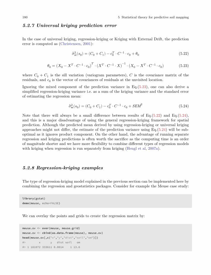
180 5 Statistical theory for predictive soil mapping
5.2.7 Universal kriging prediction error
In the case of universal kriging, regression-kriging or Kriging with External Drift, the predictionerror is computed as (Christensen, 2001):
��2UK(𝑠0) = (𝐶0 + 𝐶1) − 𝑐𝑇
0 ⋅ 𝐶−1 ⋅ 𝑐0 + 𝜃0 (5.22)
𝜃0 = (𝑋0 − 𝑋𝑇 ⋅ 𝐶−1 ⋅ 𝑐0)𝑇 ⋅ (𝑋𝑇 ⋅ 𝐶−1 ⋅ 𝑋)−1 ⋅ (𝑋0 − 𝑋𝑇 ⋅ 𝐶−1 ⋅ 𝑐0) (5.23)
where 𝐶0 + 𝐶1 is the sill variation (variogram parameters), 𝐶 is the covariance matrix of theresiduals, and 𝑐0 is the vector of covariances of residuals at the unvisited location.
Ignoring the mixed component of the prediction variance in Eq.(5.23), one can also derive asimplified regression-kriging variance i.e. as a sum of the kriging variance and the standard errorof estimating the regression mean:
��2RK(𝑠0) = (𝐶0 + 𝐶1) − 𝑐𝑇
0 ⋅ 𝐶−1 ⋅ 𝑐0 + SEM2 (5.24)
Note that there will always be a small difference between results of Eq.(5.22) and Eq.(5.24),and this is a major disadvantage of using the general regression-kriging framework for spatialprediction. Although the predicted mean derived by using regression-kriging or universal krigingapproaches might not differ, the estimate of the prediction variance using Eq.(5.24) will be sub-optimal as it ignores product component. On the other hand, the advantage of running separateregression and kriging predictions is often worth the sacrifice as the computing time is an orderof magnitude shorter and we have more flexibility to combine different types of regression modelswith kriging when regression is run separately from kriging (Hengl et al, 2007a).
5.2.8 Regression-kriging examples
The type of regression-kriging model explained in the previous section can be implemented here bycombining the regression and geostatistics packages. Consider for example the Meuse case study:
library(gstat)demo(meuse, echo=FALSE)
We can overlay the points and grids to create the regression matrix by:
meuse.ov <- over(meuse, meuse.grid)meuse.ov <- cbind(as.data.frame(meuse), meuse.ov)head(meuse.ov[,c("x","y","dist","soil","om")])#> x y dist soil om#> 1 181072 333611 0.0014 1 13.6
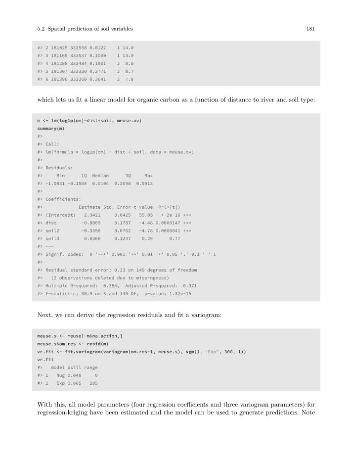
5.2 Spatial prediction of soil variables 181
#> 2 181025 333558 0.0122 1 14.0#> 3 181165 333537 0.1030 1 13.0#> 4 181298 333484 0.1901 2 8.0#> 5 181307 333330 0.2771 2 8.7#> 6 181390 333260 0.3641 2 7.8
which lets us fit a linear model for organic carbon as a function of distance to river and soil type:
m <- lm(log1p(om)~dist+soil, meuse.ov)summary(m)#>#> Call:#> lm(formula = log1p(om) ~ dist + soil, data = meuse.ov)#>#> Residuals:#> Min 1Q Median 3Q Max#> -1.0831 -0.1504 0.0104 0.2098 0.5913#>#> Coefficients:#> Estimate Std. Error t value Pr(>|t|)#> (Intercept) 2.3421 0.0425 55.05 < 2e-16 ***#> dist -0.8009 0.1787 -4.48 0.0000147 ***#> soil2 -0.3358 0.0702 -4.78 0.0000041 ***#> soil3 0.0366 0.1247 0.29 0.77#> ---#> Signif. codes: 0 '***' 0.001 '**' 0.01 '*' 0.05 '.' 0.1 ' ' 1#>#> Residual standard error: 0.33 on 149 degrees of freedom#> (2 observations deleted due to missingness)#> Multiple R-squared: 0.384, Adjusted R-squared: 0.371#> F-statistic: 30.9 on 3 and 149 DF, p-value: 1.32e-15
Next, we can derive the regression residuals and fit a variogram:
meuse.s <- meuse[-m$na.action,]meuse.s$om.res <- resid(m)vr.fit <- fit.variogram(variogram(om.res~1, meuse.s), vgm(1, "Exp", 300, 1))vr.fit#> model psill range#> 1 Nug 0.048 0#> 2 Exp 0.065 285
With this, all model parameters (four regression coefficients and three variogram parameters) forregression-kriging have been estimated and the model can be used to generate predictions. Note
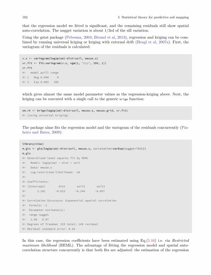
182 5 Statistical theory for predictive soil mapping
that the regression model we fitted is significant, and the remaining residuals still show spatialauto-correlation. The nugget variation is about 1/3rd of the sill variation.Using the gstat package (Pebesma, 2004; Bivand et al, 2013), regression and kriging can be com-bined by running universal kriging or kriging with external drift (Hengl et al, 2007a). First, thevariogram of the residuals is calculated:
v.s <- variogram(log1p(om)~dist+soil, meuse.s)vr.fit <- fit.variogram(v.s, vgm(1, "Exp", 300, 1))vr.fit#> model psill range#> 1 Nug 0.048 0#> 2 Exp 0.065 285
which gives almost the same model parameter values as the regression-kriging above. Next, thekriging can be executed with a single call to the generic krige function:
om.rk <- krige(log1p(om)~dist+soil, meuse.s, meuse.grid, vr.fit)#> [using universal kriging]
The package nlme fits the regression model and the variogram of the residuals concurrently (Pin-heiro and Bates, 2009):
library(nlme)m.gls <- gls(log1p(om)~dist+soil, meuse.s, correlation=corExp(nugget=TRUE))m.gls#> Generalized least squares fit by REML#> Model: log1p(om) ~ dist + soil#> Data: meuse.s#> Log-restricted-likelihood: -26#>#> Coefficients:#> (Intercept) dist soil2 soil3#> 2.281 -0.623 -0.244 -0.057#>#> Correlation Structure: Exponential spatial correlation#> Formula: ~1#> Parameter estimate(s):#> range nugget#> 2.00 0.07#> Degrees of freedom: 153 total; 149 residual#> Residual standard error: 0.34
In this case, the regression coefficients have been estimated using Eq.(5.16) i.e. via Restrictedmaximum likelihood (REML). The advantage of fitting the regression model and spatial auto-correlation structure concurrently is that both fits are adjusted: the estimation of the regression
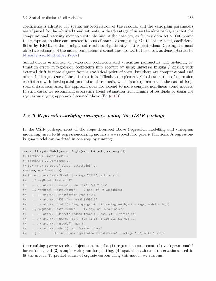
5.2 Spatial prediction of soil variables 183
coefficients is adjusted for spatial autocorrelation of the residual and the variogram parametersare adjusted for the adjusted trend estimate. A disadvantage of using the nlme package is that thecomputational intensity increases with the size of the data set, so for any data set >1000 pointsthe computation time can increase to tens of hours of computing. On the other hand, coefficientsfitted by REML methods might not result in significantly better predictions. Getting the mostobjective estimate of the model parameters is sometimes not worth the effort, as demonstrated byMinasny and McBratney (2007).Simultaneous estimation of regression coefficients and variogram parameters and including es-timation errors in regression coefficients into account by using universal kriging / kriging withexternal drift is more elegant from a statistical point of view, but there are computational andother challenges. One of these is that it is difficult to implement global estimation of regressioncoefficients with local spatial prediction of residuals, which is a requirement in the case of largespatial data sets. Also, the approach does not extend to more complex non-linear trend models.In such cases, we recommend separating trend estimation from kriging of residuals by using theregression-kriging approach discussed above (Eq.(5.16)).
5.2.9 Regression-kriging examples using the GSIF package
In the GSIF package, most of the steps described above (regression modelling and variogrammodelling) used to fit regression-kriging models are wrapped into generic functions. A regression-kriging model can be fitted in one step by running:
omm <- fit.gstatModel(meuse, log1p(om)~dist+soil, meuse.grid)#> Fitting a linear model...#> Fitting a 2D variogram...#> Saving an object of class 'gstatModel'...str(omm, max.level = 2)#> Formal class 'gstatModel' [package "GSIF"] with 4 slots#> ..@ regModel :List of 32#> .. ..- attr(*, "class")= chr [1:2] "glm" "lm"#> ..@ vgmModel :'data.frame': 2 obs. of 9 variables:#> .. ..- attr(*, "singular")= logi FALSE#> .. ..- attr(*, "SSErr")= num 0.00000107#> .. ..- attr(*, "call")= language gstat::fit.variogram(object = svgm, model = ivgm)#> ..@ svgmModel:'data.frame': 15 obs. of 6 variables:#> .. ..- attr(*, "direct")='data.frame': 1 obs. of 2 variables:#> .. ..- attr(*, "boundaries")= num [1:16] 0 106 213 319 426 ...#> .. ..- attr(*, "pseudo")= num 0#> .. ..- attr(*, "what")= chr "semivariance"#> ..@ sp :Formal class 'SpatialPointsDataFrame' [package "sp"] with 5 slots
the resulting gstatModel class object consists of a (1) regression component, (2) variogram modelfor residual, and (3) sample variogram for plotting, (4) spatial locations of observations used tofit the model. To predict values of organic carbon using this model, we can run:
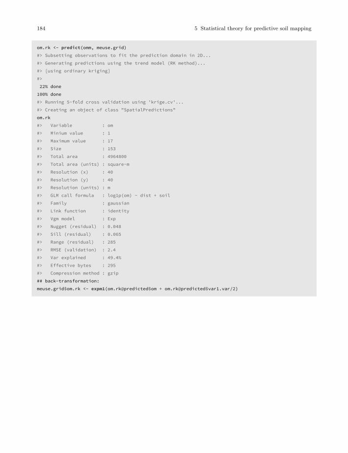
184 5 Statistical theory for predictive soil mapping
om.rk <- predict(omm, meuse.grid)#> Subsetting observations to fit the prediction domain in 2D...#> Generating predictions using the trend model (RK method)...#> [using ordinary kriging]#>22% done100% done#> Running 5-fold cross validation using 'krige.cv'...#> Creating an object of class "SpatialPredictions"om.rk#> Variable : om#> Minium value : 1#> Maximum value : 17#> Size : 153#> Total area : 4964800#> Total area (units) : square-m#> Resolution (x) : 40#> Resolution (y) : 40#> Resolution (units) : m#> GLM call formula : log1p(om) ~ dist + soil#> Family : gaussian#> Link function : identity#> Vgm model : Exp#> Nugget (residual) : 0.048#> Sill (residual) : 0.065#> Range (residual) : 285#> RMSE (validation) : 2.4#> Var explained : 49.4%#> Effective bytes : 295#> Compression method : gzip## back-transformation:meuse.grid$om.rk <- expm1(om.rk@predicted$om + om.rk@predicted$var1.var/2)
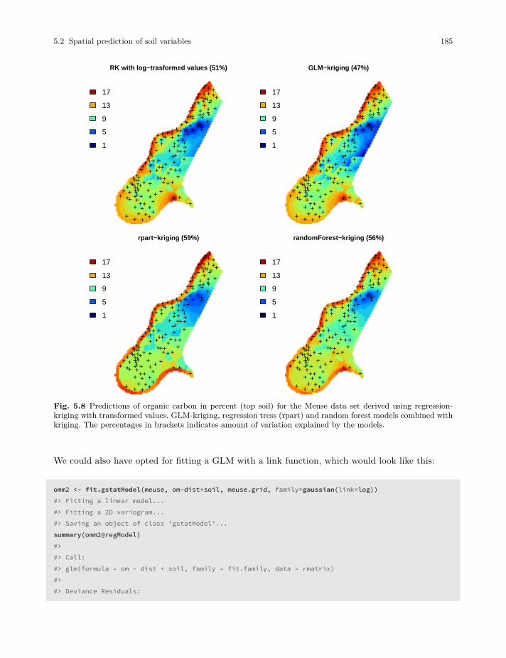
5.2 Spatial prediction of soil variables 185
RK with log−trasformed values (51%)
++ ++++++
+ +++
+++++
++
++++++++++
+
++++++++++
+++
++
++++
++
+++++++ +
++++
+++
++
++++
+++++
++++
+
+
+
++
++
++ ++
+
++
++++
+ + ++
++ +
++
+++++++
++
+
++
+++
++
++
+
++
+
+
+
+
+++
+++
+ ++
+++++ +
+ +++ ++
17
13
9
5
1
GLM−kriging (47%)
++ ++++++
+ +++
+++++
++
++++++++++
+
++++++++++
+++
++
++++
++
+++++++ +
++++
+++
++
++++
+++++
++++
+
+
+
++
++
++ ++
+
++
++++
+ + ++
++ +
++
+++++++
++
+
++
+++
++
++
+
++
+
+
+
+
+++
+++
+ ++
+++++ +
+ +++ ++
17
13
9
5
1
rpart−kriging (59%)
++ ++++++
+ +++
+++++
++
++++++++++
+
++++++++++
+++
++
++++
++
+++++++ +
++++
+++
++
++++
+++++
++++
+
+
+
++
++
++ ++
+
++
++++
+ + ++
++ +
++
+++++++
++
+
++
+++
++
++
+
++
+
+
+
+
+++
+++
+ ++
+++++ +
+ +++ ++
17
13
9
5
1
randomForest−kriging (56%)
++ ++++++
+ +++
+++++
++
++++++++++
+
++++++++++
+++
++
++++
++
+++++++ +
++++
+++
++
++++
+++++
++++
+
+
+
++
++
++ ++
+
++
++++
+ + ++
++ +
++
+++++++
++
+
++
+++
++
++
+
++
+
+
+
+
+++
+++
+ ++
+++++ +
+ +++ ++
17
13
9
5
1
Fig. 5.8 Predictions of organic carbon in percent (top soil) for the Meuse data set derived using regression-kriging with transformed values, GLM-kriging, regression tress (rpart) and random forest models combined withkriging. The percentages in brackets indicates amount of variation explained by the models.
We could also have opted for fitting a GLM with a link function, which would look like this:
omm2 <- fit.gstatModel(meuse, om~dist+soil, meuse.grid, family=gaussian(link=log))#> Fitting a linear model...#> Fitting a 2D variogram...#> Saving an object of class 'gstatModel'...summary(omm2@regModel)#>#> Call:#> glm(formula = om ~ dist + soil, family = fit.family, data = rmatrix)#>#> Deviance Residuals:
186 5 Statistical theory for predictive soil mapping
#> Min 1Q Median 3Q Max#> -7.066 -1.492 -0.281 1.635 7.401#>#> Coefficients:#> Estimate Std. Error t value Pr(>|t|)#> (Intercept) 10.054 0.348 28.88 < 2e-16 ***#> dist -8.465 1.461 -5.79 4e-08 ***#> soil2 -2.079 0.575 -3.62 0.00041 ***#> soil3 0.708 1.021 0.69 0.48913#> ---#> Signif. codes: 0 '***' 0.001 '**' 0.01 '*' 0.05 '.' 0.1 ' ' 1#>#> (Dispersion parameter for gaussian family taken to be 7.2)#>#> Null deviance: 1791.4 on 152 degrees of freedom#> Residual deviance: 1075.5 on 149 degrees of freedom#> (2 observations deleted due to missingness)#> AIC: 742.6#>#> Number of Fisher Scoring iterations: 2om.rk2 <- predict(omm2, meuse.grid)#> Subsetting observations to fit the prediction domain in 2D...#> Generating predictions using the trend model (RK method)...#> [using ordinary kriging]#>8% done
100% done#> Running 5-fold cross validation using 'krige.cv'...#> Creating an object of class "SpatialPredictions"
or fitting a regression tree:
omm3 <- fit.gstatModel(meuse, log1p(om)~dist+soil, meuse.grid, method="rpart")#> Fitting a regression tree model...#> Estimated Complexity Parameter (for prunning): 0.09396#> Fitting a 2D variogram...#> Saving an object of class 'gstatModel'...
or a random forest model:
omm4 <- fit.gstatModel(meuse, om~dist+soil, meuse.grid, method="quantregForest")#> Fitting a Quantile Regression Forest model...#> Fitting a 2D variogram...#> Saving an object of class 'gstatModel'...
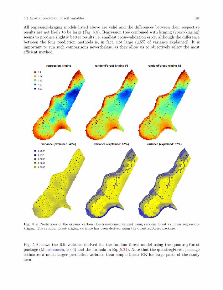
5.2 Spatial prediction of soil variables 187
All regression-kriging models listed above are valid and the differences between their respectiveresults are not likely to be large (Fig. 5.8). Regression tree combined with kriging (rpart-kriging)seems to produce slightly better results i.e. smallest cross-validation error, although the differencebetween the four prediction methods is, in fact, not large (±5% of variance explained). It isimportant to run such comparisons nevertheless, as they allow us to objectively select the mostefficient method.
Fig. 5.9 Predictions of the organic carbon (log-transformed values) using random forest vs linear regression-kriging. The random forest-kriging variance has been derived using the quantregForest package.
Fig. 5.9 shows the RK variance derived for the random forest model using the quantregForestpackage (Meinshausen, 2006) and the formula in Eq.(5.24). Note that the quantregForest packageestimates a much larger prediction variance than simple linear RK for large parts of the studyarea.
188 5 Statistical theory for predictive soil mapping
5.2.10 Regression-kriging and polygon averaging
Although many soil mappers may not realize it, many simpler regression-based techniques can beviewed as a special case of RK, or its variants. Consider for example a technique commonly used togenerate predictions of soil properties from polygon maps: weighted averaging. Here the principalcovariate available is a polygon map (showing the distribution of mapping units). In this modelit is assumed that the trend is constant within mapping units and that the stochastic residual isspatially uncorrelated. In that case, the Best Linear Unbiased Predictor of the values is simpleaveraging of soil properties per unit (Webster and Oliver, 2001, p.43):
𝑧(𝑠0) = 𝜇𝑝 = 1𝑛𝑝
𝑛𝑝
∑𝑖=1
𝑧(𝑠𝑖) (5.25)
The output map produced by polygon averaging will exhibit abrupt changes at boundaries betweenpolygon units. The prediction variance of this area-class prediction model is simply the sum ofthe within-unit variance and the estimation variance of the unit mean:
��2(𝑠0) = (1 + 1𝑛𝑝
) ⋅ 𝜎2𝑝 (5.26)
From Eq.(5.26), it is evident that the accuracy of the prediction under this model depends on thedegree of within-unit variation. The approach is advantageous if the within-unit variation is smallcompared to the between-unit variation. The predictions under this model can also be expressedas:
𝑧(𝑠0) =𝑛
∑𝑖=1
𝑤𝑖 ⋅ 𝑧(𝑠𝑖); 𝑤𝑖 = { 1/𝑛𝑝 for 𝑠𝑖 ∈ 𝑝0 otherwise (5.27)
where 𝑝 is the unit identifier. So, in fact, weighted averaging per unit is a special version ofregression-kriging where spatial autocorrelation is ignored (assumed zero) and all covariates arecategorical variables.
Going back to the Meuse data set, we can fit a regression model for organic matter using soil typesas predictors, which gives:
omm <- fit.gstatModel(meuse, log1p(om)~soil-1, meuse.grid)#> Fitting a linear model...#> Fitting a 2D variogram...#> Saving an object of class 'gstatModel'...summary(omm@regModel)#>#> Call:#> glm(formula = log1p(om) ~ soil - 1, family = fit.family, data = rmatrix)#>#> Deviance Residuals:#> Min 1Q Median 3Q Max
5.2 Spatial prediction of soil variables 189
#> -1.0297 -0.2087 -0.0044 0.2098 0.6668#>#> Coefficients:#> Estimate Std. Error t value Pr(>|t|)#> soil1 2.2236 0.0354 62.9 <2e-16 ***#> soil2 1.7217 0.0525 32.8 <2e-16 ***#> soil3 1.9293 0.1006 19.2 <2e-16 ***#> ---#> Signif. codes: 0 '***' 0.001 '**' 0.01 '*' 0.05 '.' 0.1 ' ' 1#>#> (Dispersion parameter for gaussian family taken to be 0.12)#>#> Null deviance: 672.901 on 153 degrees of freedom#> Residual deviance: 18.214 on 150 degrees of freedom#> (2 observations deleted due to missingness)#> AIC: 116.6#>#> Number of Fisher Scoring iterations: 2
and these regression coefficients for soil classes 1, 2, 3 are equal to the mean values per class:
aggregate(log1p(om) ~ soil, meuse, mean)#> soil log1p(om)#> 1 1 2.2#> 2 2 1.7#> 3 3 1.9
Note that this equality can be observed only if we remove the intercept from the regression model,hence we use:
log1p(om) ~ soil-1
and NOT:
log1p(om) ~ soil
The RK model can also be extended to fuzzy memberships, in which case MU values are binaryvariables with continuous values in the range 0–1. Hence also the SOLIM model Eq.(5.10) is infact just a special version of regression on mapping units:
𝑧(𝑠0) =𝑐𝑝
∑𝑐𝑗=1
𝜈𝑐𝑗(𝑠0) ⋅ 𝑧𝑐𝑗
=𝑝
∑𝑗=1
MU𝑗 ⋅ 𝑏𝑗 for 𝑧𝑐𝑗= 1
𝑛𝑝
𝑛𝑝
∑𝑖=1
𝑧(𝑠𝑖) (5.28)
where MU is the mapping unit or soil type, 𝑧𝑐𝑗is the modal (or most representative) value of
some soil property 𝑧 for the 𝑐𝑗 class, and 𝑛𝑝 is total number of points in some mapping unit MU.
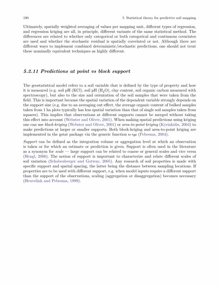
190 5 Statistical theory for predictive soil mapping
Ultimately, spatially weighted averaging of values per mapping unit, different types of regression,and regression kriging are all, in principle, different variants of the same statistical method. Thedifferences are related to whether only categorical or both categorical and continuous covariatesare used and whether the stochastic residual is spatially correlated or not. Although there aredifferent ways to implement combined deterministic/stochastic predictions, one should not treatthese nominally equivalent techniques as highly different.
5.2.11 Predictions at point vs block support
The geostatistical model refers to a soil variable that is defined by the type of property and howit is measured (e.g. soil pH (KCl), soil pH (H2O), clay content, soil organic carbon measured withspectroscopy), but also to the size and orientation of the soil samples that were taken from thefield. This is important because the spatial variation of the dependent variable strongly depends onthe support size (e.g. due to an averaging out effect, the average organic content of bulked samplestaken from 1 ha plots typically has less spatial variation than that of single soil samples taken fromsquares). This implies that observations at different supports cannot be merged without takingthis effect into account (Webster and Oliver, 2001). When making spatial predictions using krigingone can use block-kriging (Webster and Oliver, 2001) or area-to-point kriging (Kyriakidis, 2004) tomake predictions at larger or smaller supports. Both block-kriging and area-to-point kriging areimplemented in the gstat package via the generic function krige (Pebesma, 2004).
Support can be defined as the integration volume or aggregation level at which an observationis taken or for which an estimate or prediction is given. Support is often used in the literatureas a synonym for scale — large support can be related to coarse or general scales and vice versa(Hengl, 2006). The notion of support is important to characterize and relate different scales ofsoil variation (Schabenberger and Gotway, 2005). Any research of soil properties is made withspecific support and spatial spacing, the latter being the distance between sampling locations. Ifproperties are to be used with different support, e.g. when model inputs require a different supportthan the support of the observations, scaling (aggregation or disaggregation) becomes necessary(Heuvelink and Pebesma, 1999).
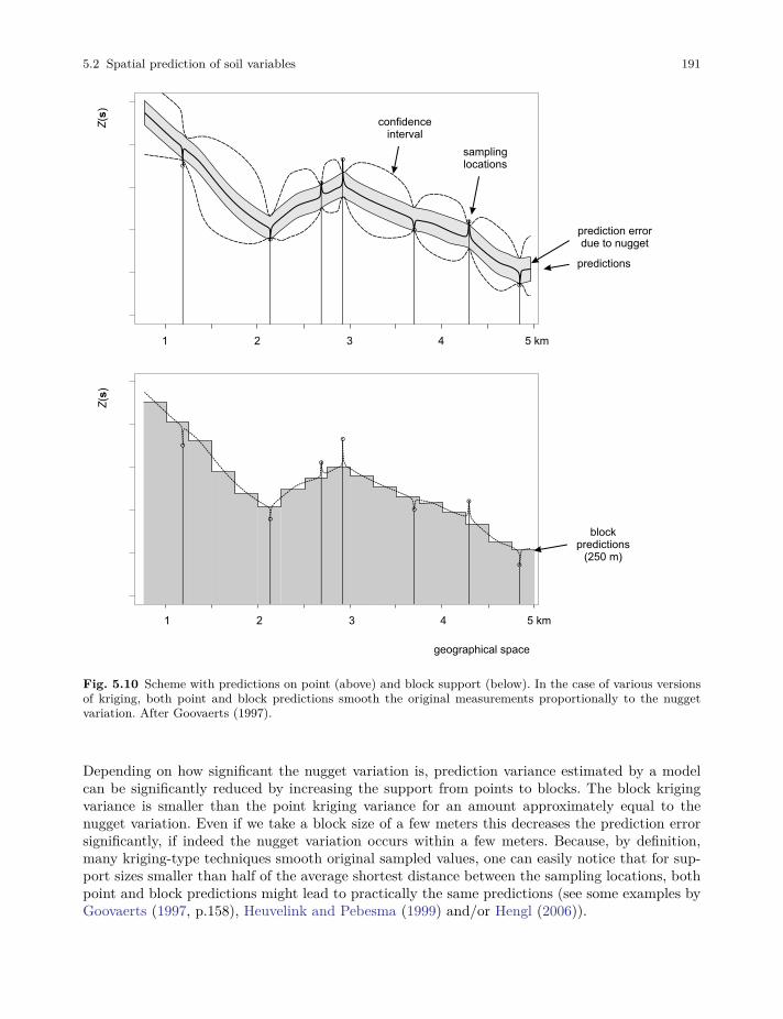
5.2 Spatial prediction of soil variables 191
Fig. 5.10 Scheme with predictions on point (above) and block support (below). In the case of various versionsof kriging, both point and block predictions smooth the original measurements proportionally to the nuggetvariation. After Goovaerts (1997).
Depending on how significant the nugget variation is, prediction variance estimated by a modelcan be significantly reduced by increasing the support from points to blocks. The block krigingvariance is smaller than the point kriging variance for an amount approximately equal to thenugget variation. Even if we take a block size of a few meters this decreases the prediction errorsignificantly, if indeed the nugget variation occurs within a few meters. Because, by definition,many kriging-type techniques smooth original sampled values, one can easily notice that for sup-port sizes smaller than half of the average shortest distance between the sampling locations, bothpoint and block predictions might lead to practically the same predictions (see some examples byGoovaerts (1997, p.158), Heuvelink and Pebesma (1999) and/or Hengl (2006)).
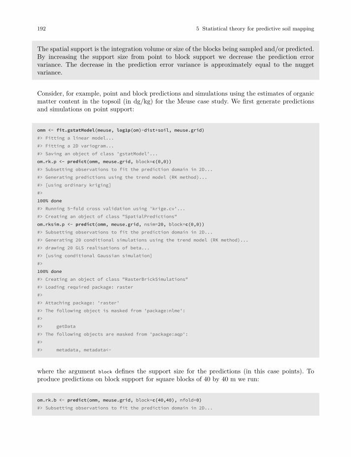
192 5 Statistical theory for predictive soil mapping
The spatial support is the integration volume or size of the blocks being sampled and/or predicted.By increasing the support size from point to block support we decrease the prediction errorvariance. The decrease in the prediction error variance is approximately equal to the nuggetvariance.
Consider, for example, point and block predictions and simulations using the estimates of organicmatter content in the topsoil (in dg/kg) for the Meuse case study. We first generate predictionsand simulations on point support:
omm <- fit.gstatModel(meuse, log1p(om)~dist+soil, meuse.grid)#> Fitting a linear model...#> Fitting a 2D variogram...#> Saving an object of class 'gstatModel'...om.rk.p <- predict(omm, meuse.grid, block=c(0,0))#> Subsetting observations to fit the prediction domain in 2D...#> Generating predictions using the trend model (RK method)...#> [using ordinary kriging]#>100% done#> Running 5-fold cross validation using 'krige.cv'...#> Creating an object of class "SpatialPredictions"om.rksim.p <- predict(omm, meuse.grid, nsim=20, block=c(0,0))#> Subsetting observations to fit the prediction domain in 2D...#> Generating 20 conditional simulations using the trend model (RK method)...#> drawing 20 GLS realisations of beta...#> [using conditional Gaussian simulation]#>100% done#> Creating an object of class "RasterBrickSimulations"#> Loading required package: raster#>#> Attaching package: 'raster'#> The following object is masked from 'package:nlme':#>#> getData#> The following objects are masked from 'package:aqp':#>#> metadata, metadata<-
where the argument block defines the support size for the predictions (in this case points). Toproduce predictions on block support for square blocks of 40 by 40 m we run:
om.rk.b <- predict(omm, meuse.grid, block=c(40,40), nfold=0)#> Subsetting observations to fit the prediction domain in 2D...
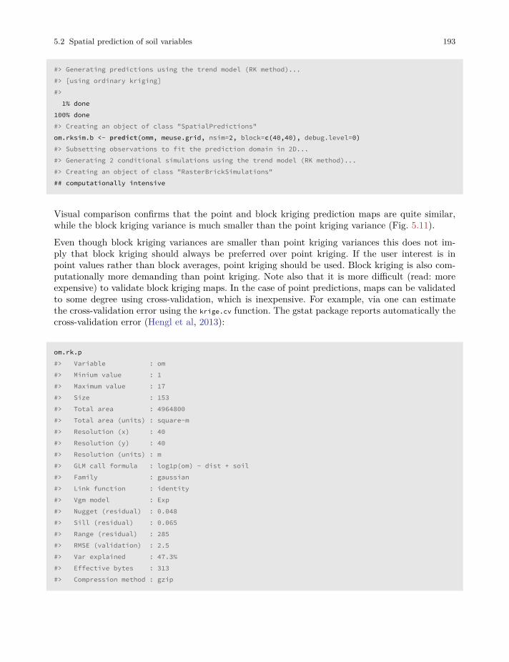
5.2 Spatial prediction of soil variables 193
#> Generating predictions using the trend model (RK method)...#> [using ordinary kriging]#>1% done
100% done#> Creating an object of class "SpatialPredictions"om.rksim.b <- predict(omm, meuse.grid, nsim=2, block=c(40,40), debug.level=0)#> Subsetting observations to fit the prediction domain in 2D...#> Generating 2 conditional simulations using the trend model (RK method)...#> Creating an object of class "RasterBrickSimulations"## computationally intensive
Visual comparison confirms that the point and block kriging prediction maps are quite similar,while the block kriging variance is much smaller than the point kriging variance (Fig. 5.11).
Even though block kriging variances are smaller than point kriging variances this does not im-ply that block kriging should always be preferred over point kriging. If the user interest is inpoint values rather than block averages, point kriging should be used. Block kriging is also com-putationally more demanding than point kriging. Note also that it is more difficult (read: moreexpensive) to validate block kriging maps. In the case of point predictions, maps can be validatedto some degree using cross-validation, which is inexpensive. For example, via one can estimatethe cross-validation error using the krige.cv function. The gstat package reports automatically thecross-validation error (Hengl et al, 2013):
om.rk.p#> Variable : om#> Minium value : 1#> Maximum value : 17#> Size : 153#> Total area : 4964800#> Total area (units) : square-m#> Resolution (x) : 40#> Resolution (y) : 40#> Resolution (units) : m#> GLM call formula : log1p(om) ~ dist + soil#> Family : gaussian#> Link function : identity#> Vgm model : Exp#> Nugget (residual) : 0.048#> Sill (residual) : 0.065#> Range (residual) : 285#> RMSE (validation) : 2.5#> Var explained : 47.3%#> Effective bytes : 313#> Compression method : gzip
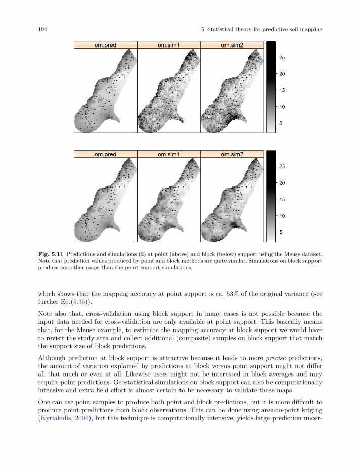
194 5 Statistical theory for predictive soil mapping
Fig. 5.11 Predictions and simulations (2) at point (above) and block (below) support using the Meuse dataset.Note that prediction values produced by point and block methods are quite similar. Simulations on block supportproduce smoother maps than the point-support simulations.
which shows that the mapping accuracy at point support is ca. 53% of the original variance (seefurther Eq.(5.35)).
Note also that, cross-validation using block support in many cases is not possible because theinput data needed for cross-validation are only available at point support. This basically meansthat, for the Meuse example, to estimate the mapping accuracy at block support we would haveto revisit the study area and collect additional (composite) samples on block support that matchthe support size of block predictions.
Although prediction at block support is attractive because it leads to more precise predictions,the amount of variation explained by predictions at block versus point support might not differall that much or even at all. Likewise users might not be interested in block averages and mayrequire point predictions. Geostatistical simulations on block support can also be computationallyintensive and extra field effort is almost certain to be necessary to validate these maps.
One can use point samples to produce both point and block predictions, but it is more difficult toproduce point predictions from block observations. This can be done using area-to-point kriging(Kyriakidis, 2004), but this technique is computationally intensive, yields large prediction uncer-
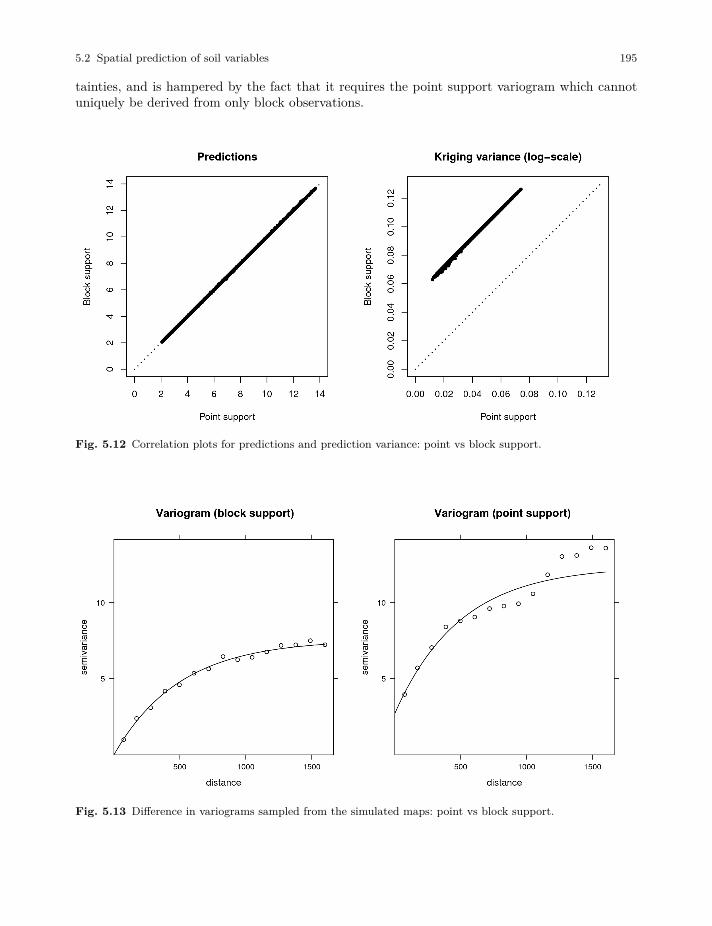
5.2 Spatial prediction of soil variables 195
tainties, and is hampered by the fact that it requires the point support variogram which cannotuniquely be derived from only block observations.
Fig. 5.12 Correlation plots for predictions and prediction variance: point vs block support.
Fig. 5.13 Difference in variograms sampled from the simulated maps: point vs block support.
196 5 Statistical theory for predictive soil mapping
What confuses non-geostatisticians is that both point and block predictions are normally visualizedusing raster GIS models, hence one does not see that the point predictions refer to the centres ofthe grid cells (Hengl, 2006). In the case of soil survey, the available soil profile data most typicallyrefer to point locations (1 × 1 meter or smaller horizontal blocks) because soil samples have smallsupport. In some cases surveyors mix soil samples from several different profle locations to producecomposite estimates of values. Nevertheless, we can assume that the vast majority of soil profilesthat are collected in the world refer to (lateral) point support. Hence the most typical combinationof support size that we work with is: point support for soil property observations, block support forcovariates and point or block support for soil property predictions. Modelling at full point support(both soil samples, covariates and outputs at point support) is in fact very rare. Soil covariatesare often derived from remote sensing data, which is almost always delivered at block support.
In principle, there is no problem with using covariates at block support to predict the soil at pointsupport, except the strength of the relationship between the covariate and target soil propertymay be weakened by a mismatch in the support. Ideally, one should always try to collect all inputdata at the finest support possible, then aggregate based on the project requirements. This isunfortunately not always possible, as most inputs are often bulked already and our knowledgeabout the short range variation is often very limited.
Figs. 5.12 and 5.13 (correlation plots for Meuse data set) confirms that: (1) predictions on blockand point support show practically no differences and (2) the difference in the prediction errorvariance for point and block kriging effectively equals the nugget variance.
The targeted support size for the GlobalSoilMap project, for example, is 3–arcsecond (ca. 100 m)horizontal dimensions of the SRTM and other covariate data layers used to support predictionof spatial variation in soil properties. This project probably needs predictions at both point andblock support at the target resolution, and then also provide aggregated values at coarser resolutionblocks (250, 500, 1000 m etc). In any case, understanding consequences of aggregating spatial dataand converting from point to block support is important.
In geostatistics, one needs to consider that any input / output spatial layer refers to some support.In soil mapping, there are three main support sizes: support size of the soil samples (samplingsupport; can refer to point locations or blocks of land), support size of the covariates (oftenequivalent to the grid cell size), and support size of predictions (again point locations or blocks ofland).
5.2.12 Geostatistical simulations
In statistical terms, the assessment of the uncertainty of produced maps is equally important asthe prediction of values at all locations. As shown in the previous section, uncertainty of soilvariables can be assessed in several ways. Three aspects, however, appear to be important for anytype of spatial prediction model:
• What are the conditional probability distribution functions (PDFs) of the target variable at eachlocation?
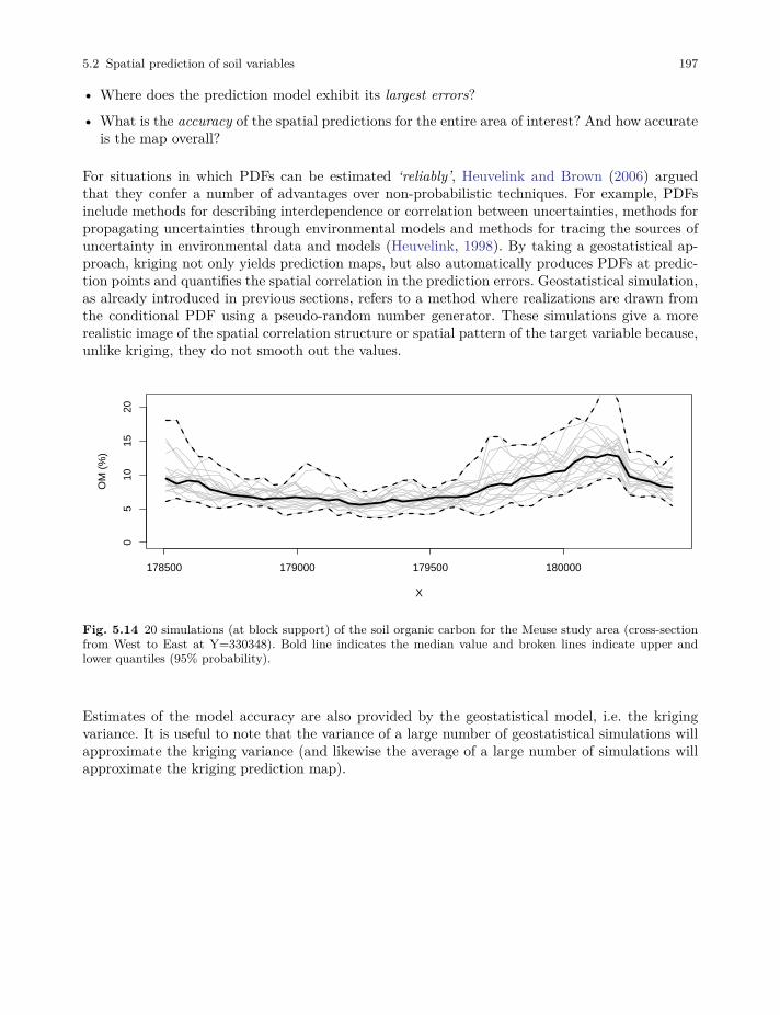
5.2 Spatial prediction of soil variables 197
• Where does the prediction model exhibit its largest errors?
• What is the accuracy of the spatial predictions for the entire area of interest? And how accurateis the map overall?
For situations in which PDFs can be estimated ‘reliably’, Heuvelink and Brown (2006) arguedthat they confer a number of advantages over non-probabilistic techniques. For example, PDFsinclude methods for describing interdependence or correlation between uncertainties, methods forpropagating uncertainties through environmental models and methods for tracing the sources ofuncertainty in environmental data and models (Heuvelink, 1998). By taking a geostatistical ap-proach, kriging not only yields prediction maps, but also automatically produces PDFs at predic-tion points and quantifies the spatial correlation in the prediction errors. Geostatistical simulation,as already introduced in previous sections, refers to a method where realizations are drawn fromthe conditional PDF using a pseudo-random number generator. These simulations give a morerealistic image of the spatial correlation structure or spatial pattern of the target variable because,unlike kriging, they do not smooth out the values.
178500 179000 179500 180000
05
1015
20
X
OM
(%
)
Fig. 5.14 20 simulations (at block support) of the soil organic carbon for the Meuse study area (cross-sectionfrom West to East at Y=330348). Bold line indicates the median value and broken lines indicate upper andlower quantiles (95% probability).
Estimates of the model accuracy are also provided by the geostatistical model, i.e. the krigingvariance. It is useful to note that the variance of a large number of geostatistical simulations willapproximate the kriging variance (and likewise the average of a large number of simulations willapproximate the kriging prediction map).
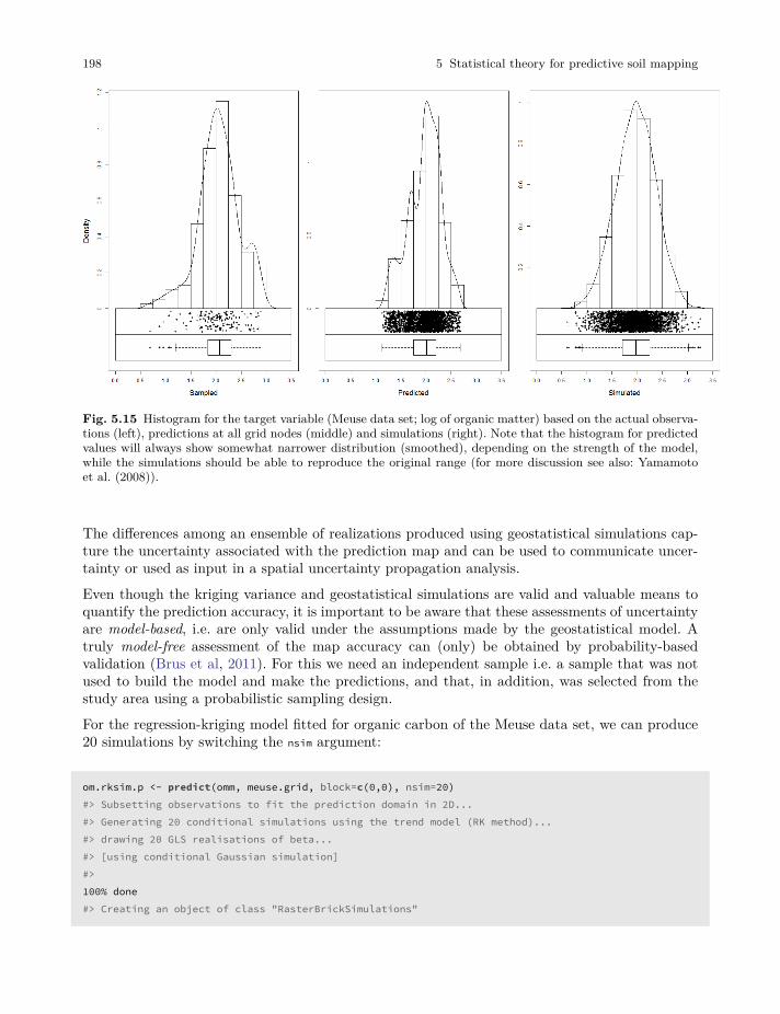
198 5 Statistical theory for predictive soil mapping
Fig. 5.15 Histogram for the target variable (Meuse data set; log of organic matter) based on the actual observa-tions (left), predictions at all grid nodes (middle) and simulations (right). Note that the histogram for predictedvalues will always show somewhat narrower distribution (smoothed), depending on the strength of the model,while the simulations should be able to reproduce the original range (for more discussion see also: Yamamotoet al. (2008)).
The differences among an ensemble of realizations produced using geostatistical simulations cap-ture the uncertainty associated with the prediction map and can be used to communicate uncer-tainty or used as input in a spatial uncertainty propagation analysis.
Even though the kriging variance and geostatistical simulations are valid and valuable means toquantify the prediction accuracy, it is important to be aware that these assessments of uncertaintyare model-based, i.e. are only valid under the assumptions made by the geostatistical model. Atruly model-free assessment of the map accuracy can (only) be obtained by probability-basedvalidation (Brus et al, 2011). For this we need an independent sample i.e. a sample that was notused to build the model and make the predictions, and that, in addition, was selected from thestudy area using a probabilistic sampling design.
For the regression-kriging model fitted for organic carbon of the Meuse data set, we can produce20 simulations by switching the nsim argument:
om.rksim.p <- predict(omm, meuse.grid, block=c(0,0), nsim=20)#> Subsetting observations to fit the prediction domain in 2D...#> Generating 20 conditional simulations using the trend model (RK method)...#> drawing 20 GLS realisations of beta...#> [using conditional Gaussian simulation]#>100% done#> Creating an object of class "RasterBrickSimulations"
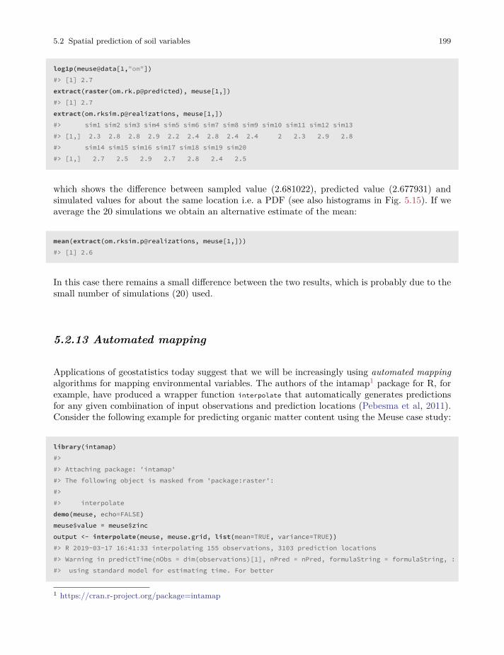
5.2 Spatial prediction of soil variables 199
log1p(meuse@data[1,"om"])#> [1] 2.7extract(raster(om.rk.p@predicted), meuse[1,])#> [1] 2.7extract(om.rksim.p@realizations, meuse[1,])#> sim1 sim2 sim3 sim4 sim5 sim6 sim7 sim8 sim9 sim10 sim11 sim12 sim13#> [1,] 2.3 2.8 2.8 2.9 2.2 2.4 2.8 2.4 2.4 2 2.3 2.9 2.8#> sim14 sim15 sim16 sim17 sim18 sim19 sim20#> [1,] 2.7 2.5 2.9 2.7 2.8 2.4 2.5
which shows the difference between sampled value (2.681022), predicted value (2.677931) andsimulated values for about the same location i.e. a PDF (see also histograms in Fig. 5.15). If weaverage the 20 simulations we obtain an alternative estimate of the mean:
mean(extract(om.rksim.p@realizations, meuse[1,]))#> [1] 2.6
In this case there remains a small difference between the two results, which is probably due to thesmall number of simulations (20) used.
5.2.13 Automated mapping
Applications of geostatistics today suggest that we will be increasingly using automated mappingalgorithms for mapping environmental variables. The authors of the intamap1 package for R, forexample, have produced a wrapper function interpolate that automatically generates predictionsfor any given combiination of input observations and prediction locations (Pebesma et al, 2011).Consider the following example for predicting organic matter content using the Meuse case study:
library(intamap)#>#> Attaching package: 'intamap'#> The following object is masked from 'package:raster':#>#> interpolatedemo(meuse, echo=FALSE)meuse$value = meuse$zincoutput <- interpolate(meuse, meuse.grid, list(mean=TRUE, variance=TRUE))#> R 2019-03-17 16:41:33 interpolating 155 observations, 3103 prediction locations#> Warning in predictTime(nObs = dim(observations)[1], nPred = nPred, formulaString = formulaString, :#> using standard model for estimating time. For better
1 https://cran.r-project.org/package=intamap
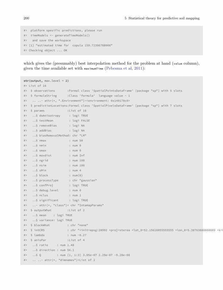
200 5 Statistical theory for predictive soil mapping
#> platform spesific predictions, please run#> timeModels <- generateTimeModels()#> and save the workspace#> [1] "estimated time for copula 159.72396788006"#> Checking object ... OK
which gives the (presumably) best interpolation method for the problem at hand (value column),given the time available set with maximumTime (Pebesma et al, 2011):
str(output, max.level = 2)#> List of 16#> $ observations :Formal class 'SpatialPointsDataFrame' [package "sp"] with 5 slots#> $ formulaString :Class 'formula' language value ~ 1#> .. ..- attr(*, ".Environment")=<environment: 0x140178c0>#> $ predictionLocations:Formal class 'SpatialPixelsDataFrame' [package "sp"] with 7 slots#> $ params :List of 18#> ..$ doAnisotropy : logi TRUE#> ..$ testMean : logi FALSE#> ..$ removeBias : logi NA#> ..$ addBias : logi NA#> ..$ biasRemovalMethod: chr "LM"#> ..$ nmax : num 50#> ..$ nmin : num 0#> ..$ omax : num 0#> ..$ maxdist : num Inf#> ..$ ngrid : num 100#> ..$ nsim : num 100#> ..$ sMin : num 4#> ..$ block : num(0)#> ..$ processType : chr "gaussian"#> ..$ confProj : logi TRUE#> ..$ debug.level : num 0#> ..$ nclus : num 1#> ..$ significant : logi TRUE#> ..- attr(*, "class")= chr "IntamapParams"#> $ outputWhat :List of 2#> ..$ mean : logi TRUE#> ..$ variance: logi TRUE#> $ blockWhat : chr "none"#> $ intCRS : chr "+init=epsg:28992 +proj=sterea +lat_0=52.15616055555555 +lon_0=5.38763888888889 +k=0.9999079 +x_0=155000 +y_0=46"| __truncated__#> $ lambda : num -0.27#> $ anisPar :List of 4#> ..$ ratio : num 1.48#> ..$ direction : num 56.1#> ..$ Q : num [1, 1:3] 3.05e-07 2.29e-07 -9.28e-08#> .. ..- attr(*, "dimnames")=List of 2
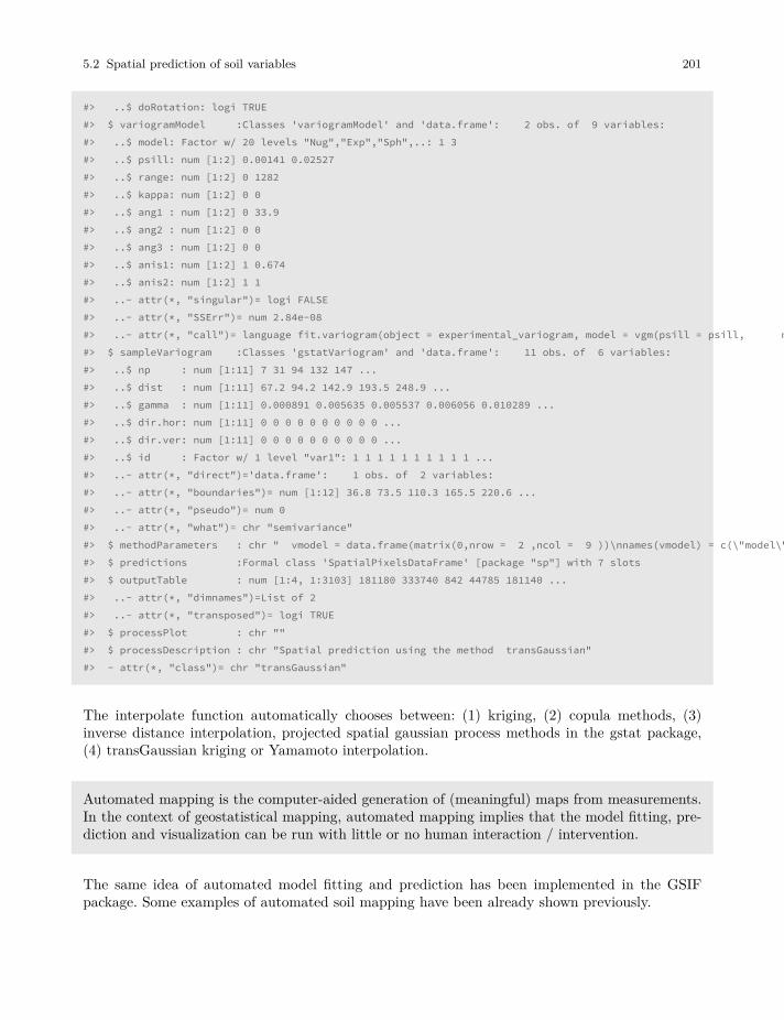
5.2 Spatial prediction of soil variables 201
#> ..$ doRotation: logi TRUE#> $ variogramModel :Classes 'variogramModel' and 'data.frame': 2 obs. of 9 variables:#> ..$ model: Factor w/ 20 levels "Nug","Exp","Sph",..: 1 3#> ..$ psill: num [1:2] 0.00141 0.02527#> ..$ range: num [1:2] 0 1282#> ..$ kappa: num [1:2] 0 0#> ..$ ang1 : num [1:2] 0 33.9#> ..$ ang2 : num [1:2] 0 0#> ..$ ang3 : num [1:2] 0 0#> ..$ anis1: num [1:2] 1 0.674#> ..$ anis2: num [1:2] 1 1#> ..- attr(*, "singular")= logi FALSE#> ..- attr(*, "SSErr")= num 2.84e-08#> ..- attr(*, "call")= language fit.variogram(object = experimental_variogram, model = vgm(psill = psill, model = model, range = range, nugg| __truncated__ ...#> $ sampleVariogram :Classes 'gstatVariogram' and 'data.frame': 11 obs. of 6 variables:#> ..$ np : num [1:11] 7 31 94 132 147 ...#> ..$ dist : num [1:11] 67.2 94.2 142.9 193.5 248.9 ...#> ..$ gamma : num [1:11] 0.000891 0.005635 0.005537 0.006056 0.010289 ...#> ..$ dir.hor: num [1:11] 0 0 0 0 0 0 0 0 0 0 ...#> ..$ dir.ver: num [1:11] 0 0 0 0 0 0 0 0 0 0 ...#> ..$ id : Factor w/ 1 level "var1": 1 1 1 1 1 1 1 1 1 1 ...#> ..- attr(*, "direct")='data.frame': 1 obs. of 2 variables:#> ..- attr(*, "boundaries")= num [1:12] 36.8 73.5 110.3 165.5 220.6 ...#> ..- attr(*, "pseudo")= num 0#> ..- attr(*, "what")= chr "semivariance"#> $ methodParameters : chr " vmodel = data.frame(matrix(0,nrow = 2 ,ncol = 9 ))\nnames(vmodel) = c(\"model\",\"psill\",\"range\",\"kappa"| __truncated__#> $ predictions :Formal class 'SpatialPixelsDataFrame' [package "sp"] with 7 slots#> $ outputTable : num [1:4, 1:3103] 181180 333740 842 44785 181140 ...#> ..- attr(*, "dimnames")=List of 2#> ..- attr(*, "transposed")= logi TRUE#> $ processPlot : chr ""#> $ processDescription : chr "Spatial prediction using the method transGaussian"#> - attr(*, "class")= chr "transGaussian"
The interpolate function automatically chooses between: (1) kriging, (2) copula methods, (3)inverse distance interpolation, projected spatial gaussian process methods in the gstat package,(4) transGaussian kriging or Yamamoto interpolation.
Automated mapping is the computer-aided generation of (meaningful) maps from measurements.In the context of geostatistical mapping, automated mapping implies that the model fitting, pre-diction and visualization can be run with little or no human interaction / intervention.
The same idea of automated model fitting and prediction has been implemented in the GSIFpackage. Some examples of automated soil mapping have been already shown previously.
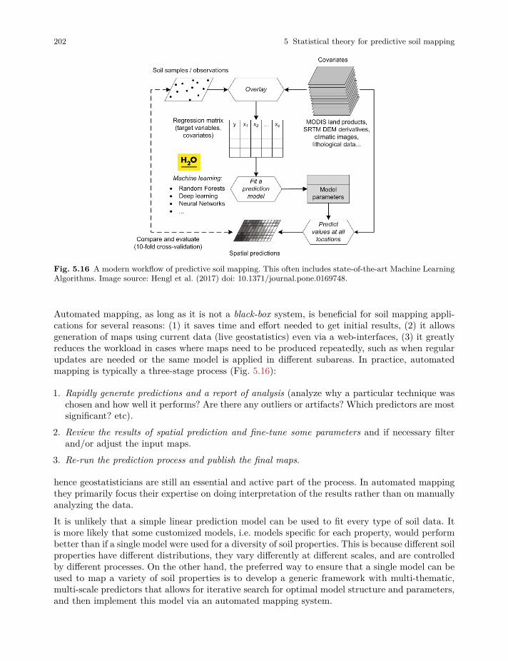
202 5 Statistical theory for predictive soil mapping
Fig. 5.16 A modern workflow of predictive soil mapping. This often includes state-of-the-art Machine LearningAlgorithms. Image source: Hengl et al. (2017) doi: 10.1371/journal.pone.0169748.
Automated mapping, as long as it is not a black-box system, is beneficial for soil mapping appli-cations for several reasons: (1) it saves time and effort needed to get initial results, (2) it allowsgeneration of maps using current data (live geostatistics) even via a web-interfaces, (3) it greatlyreduces the workload in cases where maps need to be produced repeatedly, such as when regularupdates are needed or the same model is applied in different subareas. In practice, automatedmapping is typically a three-stage process (Fig. 5.16):
1. Rapidly generate predictions and a report of analysis (analyze why a particular technique waschosen and how well it performs? Are there any outliers or artifacts? Which predictors are mostsignificant? etc).
2. Review the results of spatial prediction and fine-tune some parameters and if necessary filterand/or adjust the input maps.
3. Re-run the prediction process and publish the final maps.
hence geostatisticians are still an essential and active part of the process. In automated mappingthey primarily focus their expertise on doing interpretation of the results rather than on manuallyanalyzing the data.It is unlikely that a simple linear prediction model can be used to fit every type of soil data. Itis more likely that some customized models, i.e. models specific for each property, would performbetter than if a single model were used for a diversity of soil properties. This is because different soilproperties have different distributions, they vary differently at different scales, and are controlledby different processes. On the other hand, the preferred way to ensure that a single model can beused to map a variety of soil properties is to develop a generic framework with multi-thematic,multi-scale predictors that allows for iterative search for optimal model structure and parameters,and then implement this model via an automated mapping system.
5.2 Spatial prediction of soil variables 203
5.2.14 Selecting spatial prediction models
The purpose of spatial prediction is to (a) produce a map showing spatial distribution of the vari-able of interest for the area of interest, and (b) to do this in an unbiased way. A comprehensivepath to evaluating spatial predictions is the caret2 approach (Kuhn and Johnson, 2013), whichwraps up many of the standard processes such as model training and validation, method compar-ison and visualization. Consider, for example, organic matter % in the topsoil in the meuse dataset:
library(caret); library(rgdal)#> Loading required package: lattice#> Loading required package: ggplot2#>#> Attaching package: 'caret'#> The following object is masked from 'package:intamap':#>#> preProcessdemo(meuse, echo=FALSE)meuse.ov <- cbind(over(meuse, meuse.grid), meuse@data)meuse.ov$x0 = 1
We can quickly compare performance of using GLM vs random forest vs no model for predictingorganic matter (om) by using the caret package functionality:
fitControl <- trainControl(method="repeatedcv", number=2, repeats=2)mFit0 <- caret::train(om~x0, data=meuse.ov, method="glm",
family=gaussian(link=log), trControl=fitControl,na.action=na.omit)
mFit1 <- caret::train(om~soil, data=meuse.ov, method="glm",family=gaussian(link=log), trControl=fitControl,na.action=na.omit)
mFit2 <- caret::train(om~dist+soil+ffreq, data=meuse.ov, method="glm",family=gaussian(link=log), trControl=fitControl,na.action=na.omit)
mFit3 <- caret::train(om~dist+soil+ffreq, data=meuse.ov, method="ranger",trControl=fitControl, na.action=na.omit)
This will run repeated Cross-validation with 50% : 50% splits training and validation, which meansthat, in each iteration, models will be refitted from scratch. Next we can compare performance ofthe three models by using:
2 http://topepo.github.io/caret/index.html
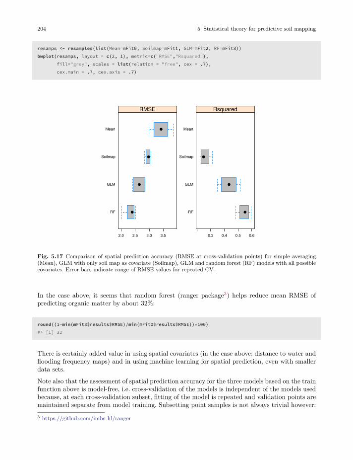
204 5 Statistical theory for predictive soil mapping
resamps <- resamples(list(Mean=mFit0, Soilmap=mFit1, GLM=mFit2, RF=mFit3))bwplot(resamps, layout = c(2, 1), metric=c("RMSE","Rsquared"),
fill="grey", scales = list(relation = "free", cex = .7),cex.main = .7, cex.axis = .7)
RF
GLM
Soilmap
Mean
2.0 2.5 3.0 3.5
RMSE
RF
GLM
Soilmap
Mean
0.3 0.4 0.5 0.6
Rsquared
Fig. 5.17 Comparison of spatial prediction accuracy (RMSE at cross-validation points) for simple averaging(Mean), GLM with only soil map as covariate (Soilmap), GLM and random forest (RF) models with all possiblecovariates. Error bars indicate range of RMSE values for repeated CV.
In the case above, it seems that random forest (ranger package3) helps reduce mean RMSE ofpredicting organic matter by about 32%:
round((1-min(mFit3$results$RMSE)/min(mFit0$results$RMSE))*100)#> [1] 32
There is certainly added value in using spatial covariates (in the case above: distance to water andflooding frequency maps) and in using machine learning for spatial prediction, even with smallerdata sets.
Note also that the assessment of spatial prediction accuracy for the three models based on the trainfunction above is model-free, i.e. cross-validation of the models is independent of the models usedbecause, at each cross-validation subset, fitting of the model is repeated and validation points aremaintained separate from model training. Subsetting point samples is not always trivial however:3 https://github.com/imbs-hl/ranger
5.2 Spatial prediction of soil variables 205
in order to consider cross-validation as completely reliable, the samples ought to be representativeof the study area and preferably collected using objective sampling such as simple random samplingor similar (Brus et al, 2011; Brus, 2019). In cases where the sampling locations are clustered ingeographical space i.e. if some parts of the study area are completely omitted from sampling,then also the results of cross-validation will reflect that sampling bias / poor representation. In allthe following examples we will assume that cross-validation gives a reliable measure of mappingaccuracy and we will use it as the basis of accuracy assessment i.e. mapping efficiency. In reality,cross-validation might be tricky to implement and could often lead to somewhat over-optimisticresults if either sampling bias exists or/and if there are too few points for model validation. Forexample, in the case of soil profile data, it is highly recommended that entire profiles are removedfrom CV because soil horizons are too strongly correlated (as discussed in detail in Gasch et al(2015) and Brenning (2012)).
The whole process of spatial prediction of soil properties could be summarized in 5 steps:
1. Initial model comparison (comparison of prediction accuracy and computing time).2. Selection of applicable model(s) and estimation of model parameters i.e. model fitting.3. Predictions i.e. generation of maps for all areas of interest.4. Objective accuracy assessment using independent (cross-)validation.5. Export and sharing of maps and summary documentation explaining all processing steps.
Studying the caret package tutorial4 and/or the mlr tutorials5 is highly recommended for anyonelooking for a systematic introduction to predictive modelling.
5.2.15 3D regression-kriging
Measurements of soil properties at point support can be thought of as describing explicit 3Dlocations (easting, northing and depth), and are amenable to being dealt with using 3D geostatis-tics (e.g. 3D kriging). Application of 3D kriging to soil measurements is cumbersome for severalreasons:
1. The differences between sampling intervals and spatial correlation in the horizontal and verticaldimensions are very large (<10 in the vertical v.s. 100’s to 1000’s of in the horizontal). Theresulting strong anisotropy must be accounted for when the geostatisitcal model is derived.Estimation of the anisotropy may be hampered by the relatively small number of observationsalong the vertical profile, although under a stationarity assumption it can benefit from themany repetitions of profile data for all profile locations.
2. Soil property values refer to vertical block support (usually because they are composite samples,i.e. the average over a soil horizon), hence some of the local variation (in the vertical dimension)has been smoothed out.
3. Soil surveyors systematically under-represent lower depths — surveyors tend to systematicallytake fewer samples as they assume that deeper horizons are of less importance for management
4 http://topepo.github.io/caret/index.html5 https://mlr-org.github.io
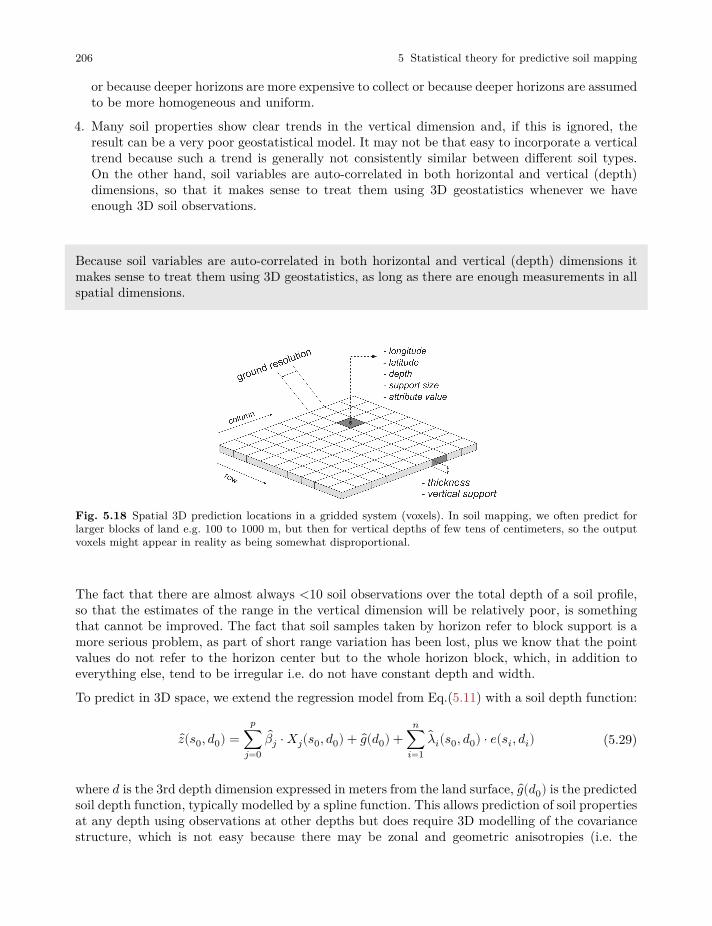
206 5 Statistical theory for predictive soil mapping
or because deeper horizons are more expensive to collect or because deeper horizons are assumedto be more homogeneous and uniform.
4. Many soil properties show clear trends in the vertical dimension and, if this is ignored, theresult can be a very poor geostatistical model. It may not be that easy to incorporate a verticaltrend because such a trend is generally not consistently similar between different soil types.On the other hand, soil variables are auto-correlated in both horizontal and vertical (depth)dimensions, so that it makes sense to treat them using 3D geostatistics whenever we haveenough 3D soil observations.
Because soil variables are auto-correlated in both horizontal and vertical (depth) dimensions itmakes sense to treat them using 3D geostatistics, as long as there are enough measurements in allspatial dimensions.
Fig. 5.18 Spatial 3D prediction locations in a gridded system (voxels). In soil mapping, we often predict forlarger blocks of land e.g. 100 to 1000 m, but then for vertical depths of few tens of centimeters, so the outputvoxels might appear in reality as being somewhat disproportional.
The fact that there are almost always <10 soil observations over the total depth of a soil profile,so that the estimates of the range in the vertical dimension will be relatively poor, is somethingthat cannot be improved. The fact that soil samples taken by horizon refer to block support is amore serious problem, as part of short range variation has been lost, plus we know that the pointvalues do not refer to the horizon center but to the whole horizon block, which, in addition toeverything else, tend to be irregular i.e. do not have constant depth and width.
To predict in 3D space, we extend the regression model from Eq.(5.11) with a soil depth function:
𝑧(𝑠0, 𝑑0) =𝑝
∑𝑗=0
𝛽𝑗 ⋅ 𝑋𝑗(𝑠0, 𝑑0) + 𝑔(𝑑0) +𝑛
∑𝑖=1
��𝑖(𝑠0, 𝑑0) ⋅ 𝑒(𝑠𝑖, 𝑑𝑖) (5.29)
where 𝑑 is the 3rd depth dimension expressed in meters from the land surface, 𝑔(𝑑0) is the predictedsoil depth function, typically modelled by a spline function. This allows prediction of soil propertiesat any depth using observations at other depths but does require 3D modelling of the covariancestructure, which is not easy because there may be zonal and geometric anisotropies (i.e. the

5.2 Spatial prediction of soil variables 207
variance and correlation lengths may differ between vertical and horizontal directions). Also, thevertical support of observations becomes important and it should be realized that observationsare the averages over depth intervals and not values at points along the vertical axis (Fig. 5.18).Spline functions have been proposed and used as mass-preserving curve fitting methods to derivepoint and block values along the vertical axis from observations at given depth intervals, but thedifficulty is that these yield estimates (with uncertainties) that should not be confused with realobservations.
A 3D variogram, e.g. modelled using an exponential model with three standard parameters (nugget𝑐0, partial sill 𝑐1, range parameter 𝑟):
𝛾 (ℎ) = { 0 if ℎ = 0𝑐0 + 𝑐1 ⋅ [1 − 𝑒−( ℎ
𝑟 )] if ℎ > 0 ℎ = [ℎ𝑥, ℎ𝑦, ℎ𝑑] (5.30)
where the scalar ‘distance’ ℎ is calculated by scaling horizontal and vertical separation distancesusing three anisotropy parameters:
ℎ =√√⎷
(ℎ𝑥𝑎𝑥
)2
+ (ℎ𝑦𝑎𝑦
)2
+ (ℎ𝑑𝑎𝑑
)2
(5.31)
Typically, in the case of soil data, the anisotropy ratio between horizontal and vertical distancesis high — spatial variation observed in a few depth changes may correspond with several ormore in horizontal space, so that the initial settings of the anisotropy ratio (i.e. the ratio of thehorizontal and vertical variogram ranges) are between 3000–8000, for example. Variogram fittingcriteria can then be used to optimize the anisotropy parameters. In our case we assumed nohorizontal anisotropy and hence assumed 𝑎𝑥 = 𝑎𝑦 = 1, leaving only 𝑎𝑑 to be estimated. Oncethe anisotropy ratio is obtained, 3D variogram modelling does not meaningfully differ from 2Dvariogram modelling.
The 3D RK framework explained above can be compared to the approach of Malone et al (2009),who first fit an equal-area spline function to estimate the soil properties at standard depths, andnext fit regression and variogram models at each depth. A drawback of the approach by Maloneet al (2009), however, is that the separate models for each depth ignore all vertical correlations. Inaddition, the equal-area spline is not used to model soil-depth relationships but only to estimatethe values at standard depths for sampling locations i.e. it is implemented for each soil profile(site) separately. In the 3D RK framework explained above, a single model is used to generatepredictions at any location and for any depth, and this takes into account both horizontal andvertical relationships simultaneously. The 3D RK approach is both easier to implement, and allowsfor incorporating all (vertical) soil-depth relationships including the spatial correlations.
5.2.16 Predicting with multiscale and multisource data
Fig. 5.3 indicates that spatial prediction is a linear processes with one line of inputs and oneline of outputs. In some cases soil mappers have to use methods that can work with multi-scaleand/or multi-source data i.e. data with different extents, resolution and uncertainty. Here bymultiscale data we imply covariates used for geostatistical mapping that are available at two or
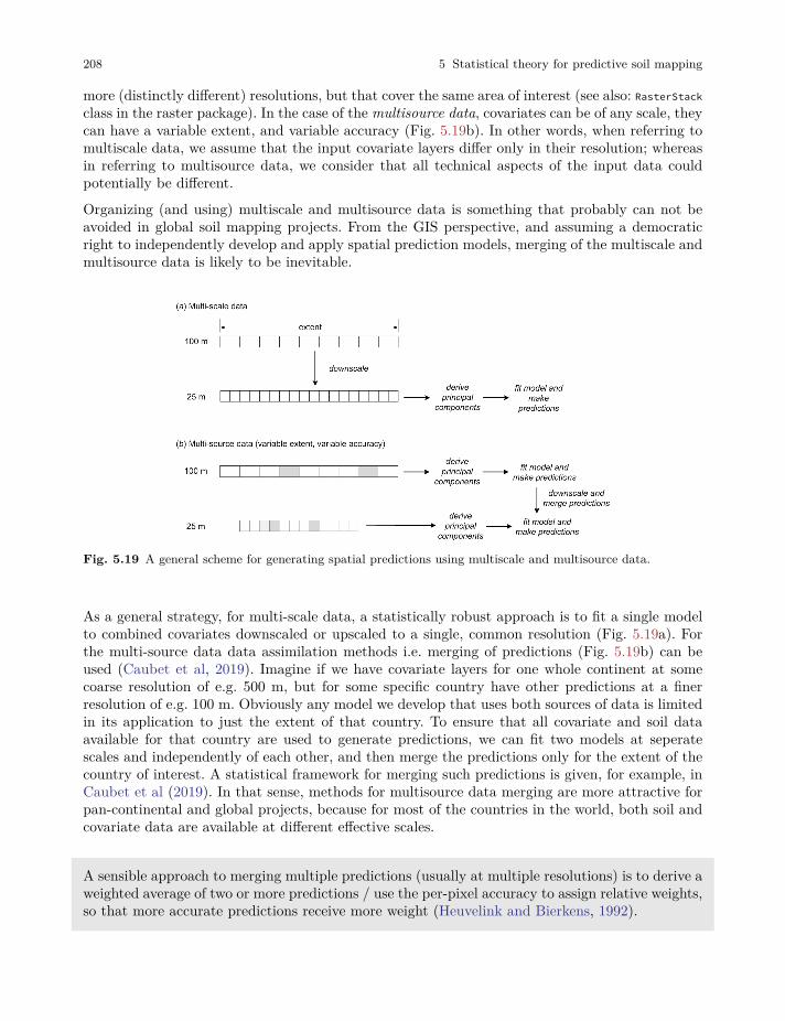
208 5 Statistical theory for predictive soil mapping
more (distinctly different) resolutions, but that cover the same area of interest (see also: RasterStackclass in the raster package). In the case of the multisource data, covariates can be of any scale, theycan have a variable extent, and variable accuracy (Fig. 5.19b). In other words, when referring tomultiscale data, we assume that the input covariate layers differ only in their resolution; whereasin referring to multisource data, we consider that all technical aspects of the input data couldpotentially be different.
Organizing (and using) multiscale and multisource data is something that probably can not beavoided in global soil mapping projects. From the GIS perspective, and assuming a democraticright to independently develop and apply spatial prediction models, merging of the multiscale andmultisource data is likely to be inevitable.
Fig. 5.19 A general scheme for generating spatial predictions using multiscale and multisource data.
As a general strategy, for multi-scale data, a statistically robust approach is to fit a single modelto combined covariates downscaled or upscaled to a single, common resolution (Fig. 5.19a). Forthe multi-source data data assimilation methods i.e. merging of predictions (Fig. 5.19b) can beused (Caubet et al, 2019). Imagine if we have covariate layers for one whole continent at somecoarse resolution of e.g. 500 m, but for some specific country have other predictions at a finerresolution of e.g. 100 m. Obviously any model we develop that uses both sources of data is limitedin its application to just the extent of that country. To ensure that all covariate and soil dataavailable for that country are used to generate predictions, we can fit two models at seperatescales and independently of each other, and then merge the predictions only for the extent of thecountry of interest. A statistical framework for merging such predictions is given, for example, inCaubet et al (2019). In that sense, methods for multisource data merging are more attractive forpan-continental and global projects, because for most of the countries in the world, both soil andcovariate data are available at different effective scales.
A sensible approach to merging multiple predictions (usually at multiple resolutions) is to derive aweighted average of two or more predictions / use the per-pixel accuracy to assign relative weights,so that more accurate predictions receive more weight (Heuvelink and Bierkens, 1992).
5.3 Accuracy assessment and the mapping efficiency 209
It is important to emphasize, however, that, in order to combine various predictors, we do needto have an estimate of the prediction uncertainty e.g. derived using cross-validation, otherwisewe are not able to assign the weights. In principle, a linear combination of statistical techniquesusing the equation above should be avoided if a theoretical basis exists that incorporates such acombination.
Combined predictions are especially interesting for situations where:
• predictions are produced using different inputs i.e. data with different coverage,
• there are several prediction methods which are equally applicable,
• where no theory exists that describes a combination of spatial prediction methods,
• where fitting and prediction of individual models is faster and less problematic than fitting ofa hybrid model.
Estimation of the prediction variance and confidence interval of combined or merged predictionsis more complex than estimation of the mean value.
5.3 Accuracy assessment and the mapping efficiency
5.3.1 Mapping accuracy and numeric resolution
Every time a digital soil mapper produces soil maps, soil GIS and soil geographical databases thoseproducts can be evaluated using independent validation studies. Unfortunately, much evaluationof soil maps in the world is still done using subjective ‘look-good’ assessments and the inherentuncertainty of the product is often underreported. In this book, we promote objective assessmentof mapping accuracy, i.e. based on statistical testing using ground truth data.
Mapping accuracy can be defined as the difference between an estimated value and the “true” value,i.e. a value of the same target variable arrived at using a significantly more accurate method. In themost simple terms, accuracy is the error component of the perfectly accurate map (Mowrer andCongalton, 2000). Although we know that soils form under systematic environmental conditionsand probably much of the variation is deterministic (Eq.(5.1)), we do not yet have tools that allowus to model soil formation and evolution processes perfectly (see also section 1.6.2). The best wecan do is to calibrate some spatial prediction model using field records, and then generate (thebest possible) predictions. The resulting soil property map, i.e. what we know about soils, is thena sum of two signals:
𝑧map(𝑠) = 𝑍(𝑠) + 𝜀(𝑠) (5.32)
where 𝑍(𝑠) is the true variation, and 𝜀(𝑠) is the error component i.e. what we do not know. Theerror component, also known as the error budget, consists of two parts: (1) the unexplained partof soil variation, and (2) the pure noise (sampling and measurement errors described in section1.6.2).
210 5 Statistical theory for predictive soil mapping
The unexplained part of soil variation is the variation we somehow failed to explain because weare not using all relevant covariates and/or due to the limited sampling intensity. For example,the sampling plan might fail to sample some hot-spots or other important local features. Theunexplained part of variation also includes short-range variation, which is possibly deterministicbut often not of interest or is simply not feasible to describe at common mapping scales.
The way to determine the error part in Eq.(5.32) is to collect additional samples and then de-termine the average error or the Root Mean Square Error (Goovaerts, 2001; Finke, 2006; Li andHeap, 2010):
RMSE =√√√⎷
1𝑙 ⋅
𝑙∑𝑖=1
[ 𝑧(𝑠𝑖) − 𝑧(𝑠𝑖)]2 (5.33)
where 𝑙 is the number of validation points, and the expected estimate of prediction error atsampling locations is equal to the nugget variation (𝐸{RMSE} = 𝜎(ℎ = 0)). In addition to RMSE,it is often interesting to see also whether the errors are, on average, positive (over-estimation) ornegative (under-estimation) i.e. whether there is possibly any clear bias in our predictions:
ME = 1𝑚
𝑚∑𝑗=1
( 𝑦(𝑠𝑗) − 𝑦(𝑠𝑗)) (5.34)
To see how much of the global variation budget has been explained by the model we can use:
Σ% = [1 − SSESSTO] = [1 − RMSE2
𝜎2𝑧] [0 − 100%] (5.35)
where SSE is the sum of squares for residuals at cross-validation points (i.e. MSE ⋅ 𝑛), and SSTOis the total sum of squares. Σ% is a global estimate of the map accuracy, valid only under theassumption that the validation points are spatially independent from the calibration points, rep-resentative and large enough (e.g. 𝑙 > 50), and that the error component is normally distributedaround the zero value (𝐸 { 𝑧(𝑠𝑖) − 𝑧(𝑠𝑖)} = 0).Once we have estimated RMSE, we can also determine the effective numeric resolution for thepredictions (Hengl et al, 2013). For example, assuming that the original sampling variance is 1.85and that RMSE=1 (i.e. Σ%=47%), the effective numeric resolution for predictions is then 0.5(as shown previously in Fig. 1.16). There is probably no need to code the values with a betterprecision than 0.5 units.
5.3.2 Accuracy assessment methods
There are three possibilities for estimating the RMSE (Fig. 5.20):
1. Run cross-validation using the same input data used for model fitting.
2. Collect new samples using a correct probability sampling design to ensure an unbiased estimateof accuracy.

5.3 Accuracy assessment and the mapping efficiency 211
3. Compare predicted values with more detailed maps for small study areas produced at much higheraccuracy, usually also at much finer level of detail.
Original data
(original survey)
Independent data
(new survey)
Model fitting and
spatial prediction
Spatial
prediction
1 ×
Full cross-
validation
Cross-validation
of predictions
N ×
1 × N × 1 × N ×
Independent
validation
Fig. 5.20 General types of validation procedures for evaluating accuracy of spatial prediction models.
Although the prediction variance already indicates what the potential accuracy of the maps is,only by independent validation can we determine the true accuracy of the maps. Brus et al (2011)further show that, actually, only if the validation points are selected using some probability-basedsampling, like simple random sampling or stratified sampling, can one determine the true accuracyof any produced gridded maps. In practice, we can rarely afford to collect new samples, so thatcross-validation is often the only viable option.
5.3.3 Cross-validation and its limitations
Because collecting additional (independent) samples is often impractical and expensive, validationof prediction models is commonly done by using cross-validation i.e. by subsetting the originalpoint set into two data sets — calibration and validation — and then repeating the analysis. Thereare several types of cross-validation methods (Bivand et al, 2008, pp.221–226):
• the 𝑘–fold cross-validation — the original sample is split into 𝑘 equal parts and then each isused for cross-validation;
• leave-one-out cross-validation (LOO) — each sampling point is used for cross-validation;
• Jackknifing — similar to LOO, but aims at estimating the bias of statistical analysis and notof predictions;
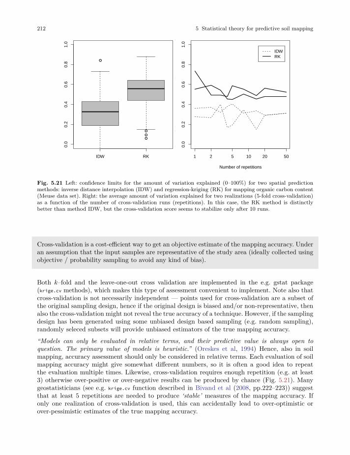
212 5 Statistical theory for predictive soil mapping
●
●
●
●
●
●
IDW RK
0.0
0.2
0.4
0.6
0.8
1.0
1 2 5 10 20 50
0.0
0.2
0.4
0.6
0.8
1.0
Number of repetitionsx_
a$T
var[
x_a$
Met
hod
==
"ID
W"
& x
_a$R
ealiz
atio
n =
= 1
]
IDWRK
Fig. 5.21 Left: confidence limits for the amount of variation explained (0–100%) for two spatial predictionmethods: inverse distance interpolation (IDW) and regression-kriging (RK) for mapping organic carbon content(Meuse data set). Right: the average amount of variation explained for two realizations (5-fold cross-validation)as a function of the number of cross-validation runs (repetitions). In this case, the RK method is distinctlybetter than method IDW, but the cross-validation score seems to stabilize only after 10 runs.
Cross-validation is a cost-efficient way to get an objective estimate of the mapping accuracy. Underan assumption that the input samples are representative of the study area (ideally collected usingobjective / probability sampling to avoid any kind of bias).
Both 𝑘–fold and the leave-one-out cross validation are implemented in the e.g. gstat package(krige.cv methods), which makes this type of assessment convenient to implement. Note also thatcross-validation is not necessarily independent — points used for cross-validation are a subset ofthe original sampling design, hence if the original design is biased and/or non-representative, thenalso the cross-validation might not reveal the true accuracy of a technique. However, if the samplingdesign has been generated using some unbiased design based sampling (e.g. random sampling),randomly seleced subsets will provide unbiased estimators of the true mapping accuracy.
“Models can only be evaluated in relative terms, and their predictive value is always open toquestion. The primary value of models is heuristic.” (Oreskes et al, 1994) Hence, also in soilmapping, accuracy assessment should only be considered in relative terms. Each evaluation of soilmapping accuracy might give somewhat different numbers, so it is often a good idea to repeatthe evaluation multiple times. Likewise, cross-validation requires enough repetition (e.g. at least3) otherwise over-positive or over-negative results can be produced by chance (Fig. 5.21). Manygeostatisticians (see e.g. krige.cv function described in Bivand et al (2008, pp.222–223)) suggestthat at least 5 repetitions are needed to produce ‘stable’ measures of the mapping accuracy. Ifonly one realization of cross-validation is used, this can accidentally lead to over-optimistic orover-pessimistic estimates of the true mapping accuracy.
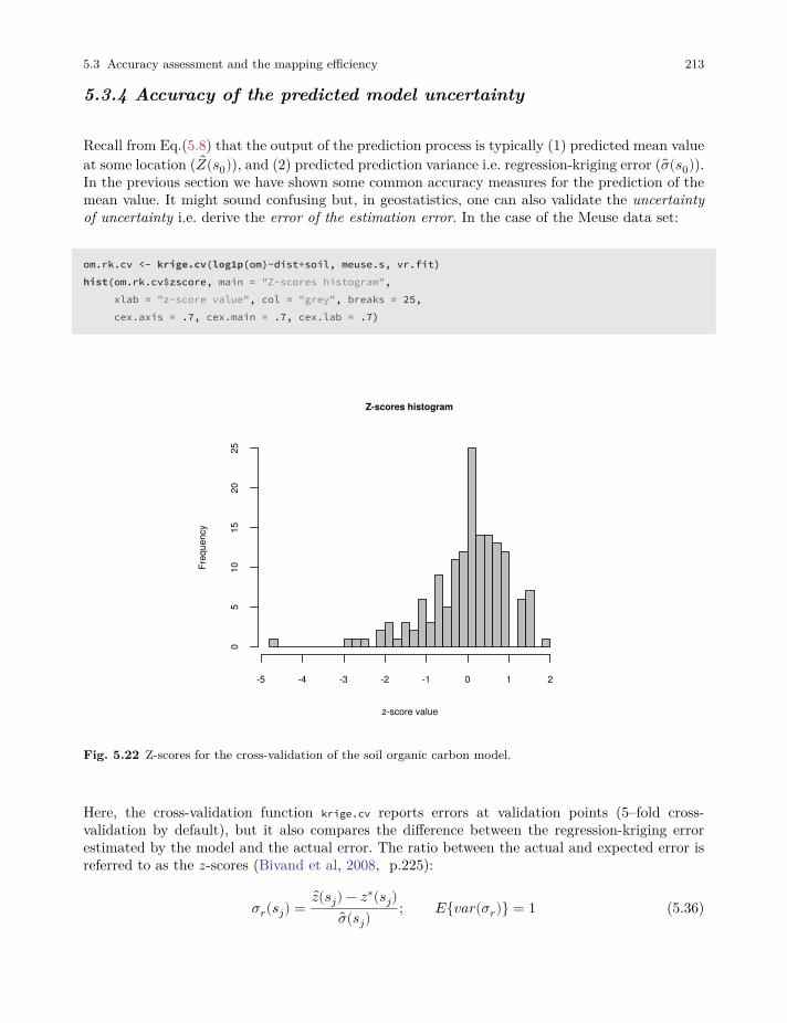
5.3 Accuracy assessment and the mapping efficiency 213
5.3.4 Accuracy of the predicted model uncertainty
Recall from Eq.(5.8) that the output of the prediction process is typically (1) predicted mean valueat some location ( 𝑍(𝑠0)), and (2) predicted prediction variance i.e. regression-kriging error (��(𝑠0)).In the previous section we have shown some common accuracy measures for the prediction of themean value. It might sound confusing but, in geostatistics, one can also validate the uncertaintyof uncertainty i.e. derive the error of the estimation error. In the case of the Meuse data set:
om.rk.cv <- krige.cv(log1p(om)~dist+soil, meuse.s, vr.fit)hist(om.rk.cv$zscore, main = "Z-scores histogram",
xlab = "z-score value", col = "grey", breaks = 25,cex.axis = .7, cex.main = .7, cex.lab = .7)
Z-scores histogram
z-score value
Freq
uenc
y
-5 -4 -3 -2 -1 0 1 2
05
1015
2025
Fig. 5.22 Z-scores for the cross-validation of the soil organic carbon model.
Here, the cross-validation function krige.cv reports errors at validation points (5–fold cross-validation by default), but it also compares the difference between the regression-kriging errorestimated by the model and the actual error. The ratio between the actual and expected error isreferred to as the 𝑧-scores (Bivand et al, 2008, p.225):
𝜎𝑟(𝑠𝑗) = 𝑧(𝑠𝑗) − 𝑧∗(𝑠𝑗)��(𝑠𝑗)
; 𝐸{𝑣𝑎𝑟(𝜎𝑟)} = 1 (5.36)
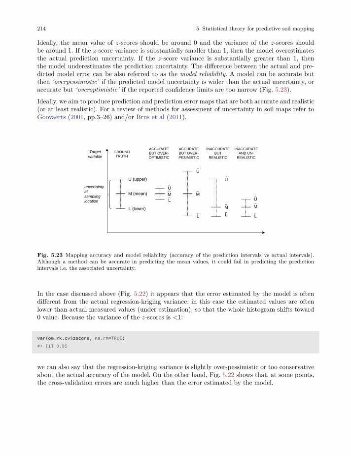
214 5 Statistical theory for predictive soil mapping
Ideally, the mean value of 𝑧-scores should be around 0 and the variance of the 𝑧-scores shouldbe around 1. If the 𝑧-score variance is substantially smaller than 1, then the model overestimatesthe actual prediction uncertainty. If the 𝑧-score variance is substantially greater than 1, thenthe model underestimates the prediction uncertainty. The difference between the actual and pre-dicted model error can be also referred to as the model reliability. A model can be accurate butthen ‘overpessimistic’ if the predicted model uncertainty is wider than the actual uncertainty, oraccurate but ‘overoptimistic’ if the reported confidence limits are too narrow (Fig. 5.23).
Ideally, we aim to produce prediction and prediction error maps that are both accurate and realistic(or at least realistic). For a review of methods for assessment of uncertainty in soil maps refer toGoovaerts (2001, pp.3–26) and/or Brus et al (2011).
U (upper)
M (mean)
L (lower)
Target
variable
GROUND
TRUTH
U
M
L
ACCURATE
BUT OVER-
OPTIMISTIC
ACCURATE
BUT OVER-
PESIMISTIC
INACCURATE
BUT
REALISTIC
INACCURATE
AND UN-
REALISTIC
U
M
L
U
M
L
U
M
L
uncertainty
at
sampling
location
Fig. 5.23 Mapping accuracy and model reliability (accuracy of the prediction intervals vs actual intervals).Although a method can be accurate in predicting the mean values, it could fail in predicting the predictionintervals i.e. the associated uncertainty.
In the case discussed above (Fig. 5.22) it appears that the error estimated by the model is oftendifferent from the actual regression-kriging variance: in this case the estimated values are oftenlower than actual measured values (under-estimation), so that the whole histogram shifts toward0 value. Because the variance of the 𝑧-scores is <1:
var(om.rk.cv$zscore, na.rm=TRUE)#> [1] 0.95
we can also say that the regression-kriging variance is slightly over-pessimistic or too conservativeabout the actual accuracy of the model. On the other hand, Fig. 5.22 shows that, at some points,the cross-validation errors are much higher than the error estimated by the model.
5.3 Accuracy assessment and the mapping efficiency 215
5.3.5 Derivation and interpretation of prediction interval
Another important issue for understanding the error budget is derivation of prediction intervali.e. upper and lower values of the target variable for which we assume that our predictions willfall within, with a high probability (e.g. 19 out of 20 times or the 95% probability). Predictioninterval or confidence limits are commonly well accepted by users as the easiest way to communicateuncertainty (Brodlie et al, 2012). For example, organic carbon in Meuse study area (based on 153samples of organic matter) has a 95% interval of 2–16%:
signif(quantile(meuse$om, c(.025, .975), na.rm=TRUE), 2)#> 2.5% 98%#> 2 16
We have previously fitted a geostatistical model using two covariates, which can now be used togenerate predictions:
om.rk <- predict(omm, meuse.grid)#> Subsetting observations to fit the prediction domain in 2D...#> Generating predictions using the trend model (RK method)...#> [using ordinary kriging]#>100% done#> Running 5-fold cross validation using 'krige.cv'...#> Creating an object of class "SpatialPredictions"
and which allows us to estimate the confidence limits for organic matter (assuming normal distri-bution) at any location within the study area e.g.:
pt1 <- data.frame(x=179390, y=330820)coordinates(pt1) <- ~x+yproj4string(pt1) = proj4string(meuse.grid)pt1.om <- over(pt1, om.rk@predicted["om"])pt1.om.sd <- over(pt1, om.rk@predicted["var1.var"])signif(expm1(pt1.om-1.645*sqrt(pt1.om.sd)), 2)#> om#> 1 4.6signif(expm1(pt1.om+1.645*sqrt(pt1.om.sd)), 2)#> om#> 1 8.9
where 4.6–8.9 are the upper and lower confidence limits. This interval can also be expressed as:
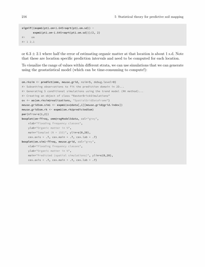
216 5 Statistical theory for predictive soil mapping
signif((expm1(pt1.om+1.645*sqrt(pt1.om.sd)) -expm1(pt1.om-1.645*sqrt(pt1.om.sd)))/2, 2)
#> om#> 1 2.1
or 6.3 ± 2.1 where half the error of estimating organic matter at that location is about 1 s.d. Notethat these are location specific prediction intervals and need to be computed for each location.
To visualize the range of values within different strata, we can use simulations that we can generateusing the geostatistical model (which can be time-consuming to compute!):
om.rksim <- predict(omm, meuse.grid, nsim=5, debug.level=0)#> Subsetting observations to fit the prediction domain in 2D...#> Generating 5 conditional simulations using the trend model (RK method)...#> Creating an object of class "RasterBrickSimulations"ov <- as(om.rksim@realizations, "SpatialGridDataFrame")meuse.grid$om.sim1 <- expm1(ov@data[,1][[email protected]])meuse.grid$om.rk <- expm1(om.rk@predicted$om)par(mfrow=c(1,2))boxplot(om~ffreq, omm@regModel$data, col="grey",
xlab="Flooding frequency classes",ylab="Organic matter in %",main="Sampled (N = 153)", ylim=c(0,20),cex.axis = .7, cex.main = .7, cex.lab = .7)
boxplot(om.sim1~ffreq, meuse.grid, col="grey",xlab="Flooding frequency classes",ylab="Organic matter in %",main="Predicted (spatial simulations)", ylim=c(0,20),cex.axis = .7, cex.main = .7, cex.lab = .7)
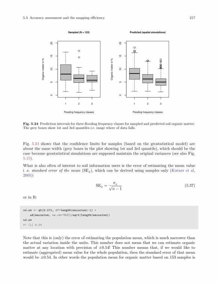
5.3 Accuracy assessment and the mapping efficiency 217
1 2 3
05
1015
20
Sampled (N = 153)
Flooding frequency classes
Org
anic
mat
ter i
n %
1 2 3
05
1015
20
Predicted (spatial simulations)
Flooding frequency classesO
rgan
ic m
atte
r in
%
Fig. 5.24 Prediction intervals for three flooding frequency classes for sampled and predicted soil organic matter.The grey boxes show 1st and 3rd quantiles i.e. range where of data falls.
Fig. 5.24 shows that the confidence limits for samples (based on the geostatistical model) areabout the same width (grey boxes in the plot showing 1st and 3rd quantile), which should be thecase because geostatistical simulations are supposed maintain the original variances (see also Fig.5.15).
What is also often of interest to soil information users is the error of estimating the mean valuei .e. standard error of the mean (SE��), which can be derived using samples only (Kutner et al,2005):
SE�� = 𝜎𝑥√𝑛 − 1 (5.37)
or in R:
sd.om <- qt(0.975, df=length(meuse$om)-1) *sd(meuse$om, na.rm=TRUE)/sqrt(length(meuse$om))
sd.om#> [1] 0.54
Note that this is (only) the error of estimating the population mean, which is much narrower thanthe actual variation inside the units. This number does not mean that we can estimate organicmatter at any location with precision of ±0.54! This number means that, if we would like toestimate (aggregated) mean value for the whole population, then the standard error of that meanwould be ±0.54. In other words the population mean for organic matter based on 153 samples is
218 5 Statistical theory for predictive soil mapping
7.48 ± 0.54, but if we would know the values of organic matter at specific, individual locations,then the confidence limits are about 7.48 ± 3.4 (where 3.4 is the standard error).The actual variation within the units based on simulations is:
lapply(levels(meuse.grid$ffreq), function(x){sapply(subset(meuse.grid@data, ffreq==x,
select=om.sim1), sd, na.rm=TRUE)})#> [[1]]#> om.sim1#> 3#>#> [[2]]#> om.sim1#> 2.4#>#> [[3]]#> om.sim1#> 1.9
This can be confusing especially if the soil data producer does not clearly report if the confidencelimits refer to the population mean, or to individual values. In principle, most users are interestedin the confidence limits of measuring some value at an individual location, which are alwaysconsiderably wider than the confidence limits of estimating the population mean.Assessment of the confidence limits should be best considered as a regression problem, in fact. Itcan easily be shown that, by fitting a regression model on strata, we automatically get an estimateof confidence limits for the study area:
omm0 <- lm(om~ffreq-1, omm@regModel$data)om.r <- predict(omm0, meuse.grid, se.fit=TRUE)meuse.grid$se.fit <- om.r$se.fitsignif(mean(meuse.grid$se.fit, na.rm=TRUE), 3)#> [1] 0.48
This number is similar to 0.54, which we derived directly from the simulations. The difference inthe values is because the regression model estimates the prediction intervals for the whole studyarea based on the covariate data (and not only for the sampling locations). The value is alsodifferent than the previously derived 0.54 because we use ffreq stratification as a covariate, sothat, as long as the strata is relatively homogenous, the confidence limits get narrower.
Prediction intervals (upper and lower ranges of expected values with some high probability) arepossibly the most accepted way to communicate uncertainty. Users are commonly interested inwhat the probability confidence limits are of measuring some value at a specific location, or thehigh probability prediction range.
5.3 Accuracy assessment and the mapping efficiency 219
To estimate the actual prediction intervals of estimating individual values (estimation error) weneed to add the residual scale value which is a constant number:
aggregate(sqrt(meuse.grid$se.fit^2+om.r$residual.scale^2),by=list(meuse.grid$ffreq), mean, na.rm=TRUE)
#> Group.1 x#> 1 1 3.3#> 2 2 3.3#> 3 3 3.3
and if we compare these limits to the confidence bands for the values predicted by the geostatisticalmodel fitted above:
aggregate(meuse.grid$om.sim1, by=list(meuse.grid$ffreq), sd, na.rm=TRUE)#> Group.1 x#> 1 1 3.0#> 2 2 2.4#> 3 3 1.9
we can clearly see that the geostatistical model has helped us narrow down the confidence limits,especially for class 3.
5.3.6 Universal measures of mapping accuracy
In the examples above, we have seen that mapping accuracy can be determined by running cross-validation and determining e.g. RMSE and R-square. In addition to R–square, a more universalmeasure of prediction success is the Lin’s Concordance Correlation Coefficient (CCC) (Steichenand Cox, 2002):
𝜌𝑐 = 2 ⋅ 𝜌 ⋅ 𝜎 𝑦 ⋅ 𝜎𝑦𝜎2
𝑦 + 𝜎2𝑦 + (𝜇 𝑦 − 𝜇𝑦)2 (5.38)
where 𝑦 are the predicted values and 𝑦 are actual values at cross-validation points, 𝜇 𝑦 and 𝜇𝑦are predicted and observed means and 𝜌 is the correlation coefficient between predicted andobserved values. CCC correctly quantifies how far the observed data deviate from the line ofperfect concordance (1:1 line in Fig. 5.25). It is usually equal to or somewhat lower than R–square, depending on the amount of bias in predictions.
CCC and variance or standard deviation of the z-scores are two universal / scale-free parametersthat can be used to assign multiple spatial prediction algorithms to work on multiple soil variables.Two additional measures of the predictive performance of a mapping algoritm are the spatial de-pendence structure in the cross-validation residuals and so called “accuracy plots” i.e. (Goovaerts,1999) (Fig. 5.25). Ideally, a variogram of the residuals should show no spatial dependence (i.e.
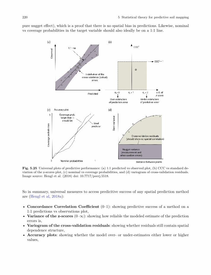
220 5 Statistical theory for predictive soil mapping
pure nugget effect), which is a proof that there is no spatial bias in predictions. Likewise, nominalvs coverage probabilities in the target variable should also ideally be on a 1:1 line.
Fig. 5.25 Universal plots of predictive performance: (a) 1:1 predicted vs observed plot, (b) CCC vs standard de-viation of the z-scores plot, (c) nominal vs coverage probabilities, and (d) variogram of cross-validation residuals.Image source: Hengl et al. (2018) doi: 10.7717/peerj.5518.
So in summary, universal measures to access predicitive success of any spatial prediction methodare (Hengl et al, 2018a):
• Concordance Correlation Coefficient (0–1): showing predictive success of a method on a1:1 predictions vs observations plot,
• Variance of the z-scores (0–∞): showing how reliable the modeled estimate of the predictionerrors is,
• Variogram of the cross-validation residuals: showing whether residuals still contain spatialdependence structure,
• Accuracy plots: showing whether the model over- or under-estimates either lower or highervalues,
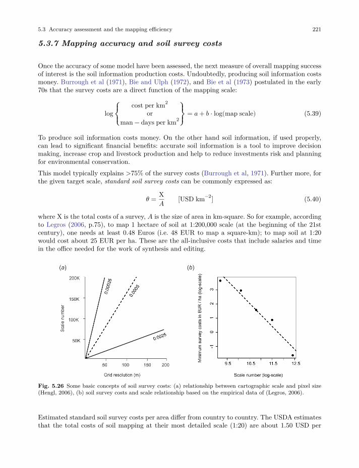
5.3 Accuracy assessment and the mapping efficiency 221
5.3.7 Mapping accuracy and soil survey costs
Once the accuracy of some model have been assessed, the next measure of overall mapping successof interest is the soil information production costs. Undoubtedly, producing soil information costsmoney. Burrough et al (1971), Bie and Ulph (1972), and Bie et al (1973) postulated in the early70s that the survey costs are a direct function of the mapping scale:
log⎧{⎨{⎩
cost per km2
orman − days per km2
⎫}⎬}⎭
= 𝑎 + 𝑏 ⋅ log(map scale) (5.39)
To produce soil information costs money. On the other hand soil information, if used properly,can lead to significant financial benefits: accurate soil information is a tool to improve decisionmaking, increase crop and livestock production and help to reduce investments risk and planningfor environmental conservation.This model typically explains >75% of the survey costs (Burrough et al, 1971). Further more, forthe given target scale, standard soil survey costs can be commonly expressed as:
𝜃 = X𝐴 [USD km−2] (5.40)
where X is the total costs of a survey, 𝐴 is the size of area in km-square. So for example, accordingto Legros (2006, p.75), to map 1 hectare of soil at 1:200,000 scale (at the beginning of the 21stcentury), one needs at least 0.48 Euros (i.e. 48 EUR to map a square-km); to map soil at 1:20would cost about 25 EUR per ha. These are the all-inclusive costs that include salaries and timein the office needed for the work of synthesis and editing.
Fig. 5.26 Some basic concepts of soil survey costs: (a) relationship between cartographic scale and pixel size(Hengl, 2006), (b) soil survey costs and scale relationship based on the empirical data of (Legros, 2006).
Estimated standard soil survey costs per area differ from country to country. The USDA estimatesthat the total costs of soil mapping at their most detailed scale (1:20) are about 1.50 USD per
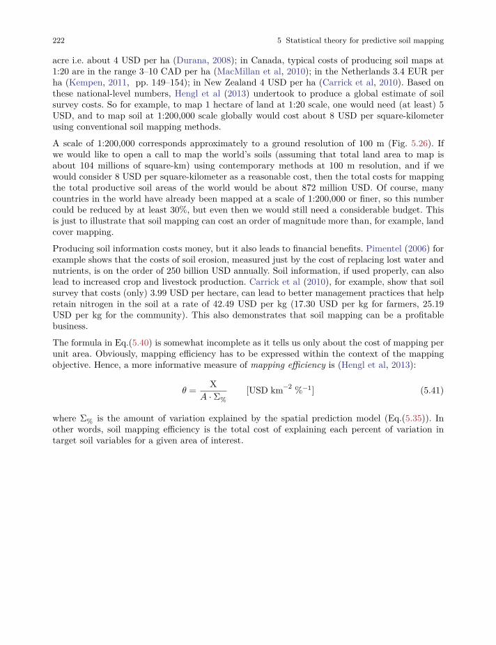
222 5 Statistical theory for predictive soil mapping
acre i.e. about 4 USD per ha (Durana, 2008); in Canada, typical costs of producing soil maps at1:20 are in the range 3–10 CAD per ha (MacMillan et al, 2010); in the Netherlands 3.4 EUR perha (Kempen, 2011, pp. 149–154); in New Zealand 4 USD per ha (Carrick et al, 2010). Based onthese national-level numbers, Hengl et al (2013) undertook to produce a global estimate of soilsurvey costs. So for example, to map 1 hectare of land at 1:20 scale, one would need (at least) 5USD, and to map soil at 1:200,000 scale globally would cost about 8 USD per square-kilometerusing conventional soil mapping methods.
A scale of 1:200,000 corresponds approximately to a ground resolution of 100 m (Fig. 5.26). Ifwe would like to open a call to map the world’s soils (assuming that total land area to map isabout 104 millions of square-km) using contemporary methods at 100 m resolution, and if wewould consider 8 USD per square-kilometer as a reasonable cost, then the total costs for mappingthe total productive soil areas of the world would be about 872 million USD. Of course, manycountries in the world have already been mapped at a scale of 1:200,000 or finer, so this numbercould be reduced by at least 30%, but even then we would still need a considerable budget. Thisis just to illustrate that soil mapping can cost an order of magnitude more than, for example, landcover mapping.
Producing soil information costs money, but it also leads to financial benefits. Pimentel (2006) forexample shows that the costs of soil erosion, measured just by the cost of replacing lost water andnutrients, is on the order of 250 billion USD annually. Soil information, if used properly, can alsolead to increased crop and livestock production. Carrick et al (2010), for example, show that soilsurvey that costs (only) 3.99 USD per hectare, can lead to better management practices that helpretain nitrogen in the soil at a rate of 42.49 USD per kg (17.30 USD per kg for farmers, 25.19USD per kg for the community). This also demonstrates that soil mapping can be a profitablebusiness.
The formula in Eq.(5.40) is somewhat incomplete as it tells us only about the cost of mapping perunit area. Obviously, mapping efficiency has to be expressed within the context of the mappingobjective. Hence, a more informative measure of mapping efficiency is (Hengl et al, 2013):
𝜃 = X𝐴 ⋅ Σ%
[USD km−2 %−1] (5.41)
where Σ% is the amount of variation explained by the spatial prediction model (Eq.(5.35)). Inother words, soil mapping efficiency is the total cost of explaining each percent of variation intarget soil variables for a given area of interest.
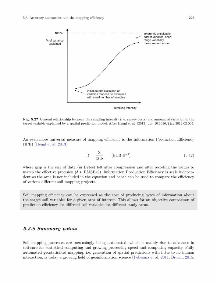
5.3 Accuracy assessment and the mapping efficiency 223
sampling intensity
% of varianceexplained
inherently unsolvable part of variation: short range variability, measurement errors
initial deterministic part of variation that can be explained with small number of samples
100 %
Fig. 5.27 General relationship between the sampling intensity (i.e. survey costs) and amount of variation in thetarget variable explained by a spatial prediction model. After Hengl et al. (2013) doi: 10.1016/j.jag.2012.02.005.
An even more universal measure of mapping efficiency is the Information Production Efficiency(IPE) (Hengl et al, 2013):
Υ = Xgzip [EUR B−1] (5.42)
where gzip is the size of data (in Bytes) left after compression and after recoding the values tomatch the effective precision (𝛿 ≈ RMSE/2). Information Production Efficiency is scale indepen-dent as the area is not included in the equation and hence can be used to compare the efficiencyof various different soil mapping projects.
Soil mapping efficiency can be expressed as the cost of producing bytes of information aboutthe target soil variables for a given area of interest. This allows for an objective comparison ofprediction efficiency for different soil variables for different study areas.
5.3.8 Summary points
Soil mapping processes are increasingly being automated, which is mainly due to advances insoftware for statistical computing and growing processing speed and computing capacity. Fullyautomated geostatistical mapping, i.e. generation of spatial predictions with little to no humaninteraction, is today a growing field of geoinformation science (Pebesma et al, 2011; Brown, 2015;

224 5 Statistical theory for predictive soil mapping
Hengl et al, 2014). Some key advantages of using automated soil mapping versus more conventional,traditional expert-based soil mapping are (Heuvelink et al, 2010; Bivand et al, 2013):
1. All rules required to produce outputs are formalized. The whole procedure is documented (thestatistical model and associated computer script), enabling reproducible research.
2. Predicted surfaces can make use of various information sources and can be optimized relativeto all available quantitative point and covariate data.
3. There is more flexibility in terms of the spatial extent, resolution and support of requestedmaps.
4. Automated mapping is more cost-effective: once the system is operational, maintenance andproduction of updates are an order of magnitude faster and cheaper. Consequently, predictionmaps can be updated and improved at shorter and shorter time intervals.
5. Spatial prediction models typically provide quantitative measures of prediction uncertainty (foreach prediction location), which are often not provided in the case of conventional soil mapping.
A disadvantage of automated soil mapping is that many statistical and machine learning techniquesare sensitive to errors and inconsistencies in the input data. A few typos, misaligned spatialcoordinates or misspecified models can create serious artifacts and reduce prediction accuracy,more so than with traditional methods. Also, fitting models using large and complex data sets canbe time consuming and selection of the ‘best’ model is often problematic. Explicit incorporation ofconceptual pedological (expert) knowledge, which can be important for prediction in new situationsto address the above issues, can be challenging as well.
In contemporary soil mapping, traditional concepts such as soil map scale and size of delineationsare becoming increasingly dated or secondary. The focus of contemporary soil mapping is onminimizing costs required to explain variation in the target variable, while support size of theoutput maps can be set by the user. The amount of variation explained by a given statisticalmodel gradually increases with sampling intensity, until it reaches some physical limit and doesnot result in any further improvements. Short-range variability and measurement error, e.g. theportion of the variation that cannot be captured or expressed by the model, for many soil variablescan be as great as 10–40% (Fig. 5.27).
A useful thing for soil mapping teams is to compare a list of valid competing models and plot thedifferences for comparison studies using what we call “predictograms” (as illustrated in Fig. 5.28).Such comparison studies permit us to determine the best performing, and most cost effective,pedometric method for an area of interest and a list of target variables.

5.3 Accuracy assessment and the mapping efficiency 225
Fig. 5.28 An schematic example of a performance plot (‘predictogram’) for comparing spatial prediction models.For more details see: Hengl et al. (2013) doi: 10.1016/j.jag.2012.02.005.
In summary, gauging the success of soil mapping basically boils down to the amount of variationexplained by the spatial prediction model i.e. quantity of effective bytes produced for the datausers. The survey costs are mainly a function of sampling intensity i.e. field work and laboratorydata analysis. As we collect more samples for an area of interest we explain more and more ofthe total variance, until we reach some maximum feasible locked variation (Fig. 5.28). For a giventotal budget and a list of target variables an optimal (most efficient) prediction method can bedetermined by deriving the mapping efficiency described in Eq.(5.41) or even better Eq.(5.42).
Modern soil mapping is driven by the objective assessment of accuracy — emphasis is put on usingmethods and covariate layers that can produce the most accurate soil information given availableresources, and much less on expert opinion or preference.
By reporting on the RMSE, effective precision, information production efficiency, and by plottingthe prediction variance estimated by the model, one gets a fairly good idea about the overall addedinformation value in a given map. In other words, by assessing the accuracy of a map we canboth recommend ways to improve the predictions (i.e. collect additional samples), and estimatethe resources needed to reach some target accuracy. By assessing how the accuracy of variousmethods changes for various sampling intensities (Fig. 5.28), we can distinguish between methodsthat are more suited for particular regions, data sets or sizes of area and optimum methods thatoutperform all alternatives.

Chapter 6
Machine Learning Algorithms for soil mapping
Edited by: T. Hengl
6.1 Spatial prediction of soil properties and classes using MLA’s
This chapter reviews some common Machine learning algorithms (MLA’s) that have demonstratedpotential for soil mapping projects i.e. for generating spatial predictions (Brungard et al, 2015;Heung et al, 2016; Behrens et al, 2018b). In this tutorial we especially focus on using tree-basedalgorithms such as random forest1, gradient boosting2 and Cubist3. For a more in-depth overviewof machine learning algorithms used in statistics refer to the CRAN Task View on Machine Learn-ing & Statistical Learning4. As a gentle introduction to Machine and Statistical Learning werecommend:
• Irizarry, R.A., (2018) Introduction to Data Science: Data Analysis and PredictionAlgorithms with R5. HarvardX Data Science Series.
• Kuhn, M., Johnson, K. (2013) Applied Predictive Modeling6. Springer Science, ISBN:9781461468493, 600 pages.
• Molnar, C. (2019) Interpretable Machine Learning: A Guide for Making Black BoxModels Explainable7, Leanpub, 251 pages.
Some other examples of how MLA’s can be used to fit Pedo-Transfer-Functions can be found insection 3.8.1 https://en.wikipedia.org/wiki/Random_forest2 https://en.wikipedia.org/wiki/Gradient_boosting3 https://cran.r-project.org/package=Cubist4 https://cran.r-project.org/web/views/MachineLearning.html5 https://rafalab.github.io/dsbook/6 http://appliedpredictivemodeling.com7 https://christophm.github.io/interpretable-ml-book/
227
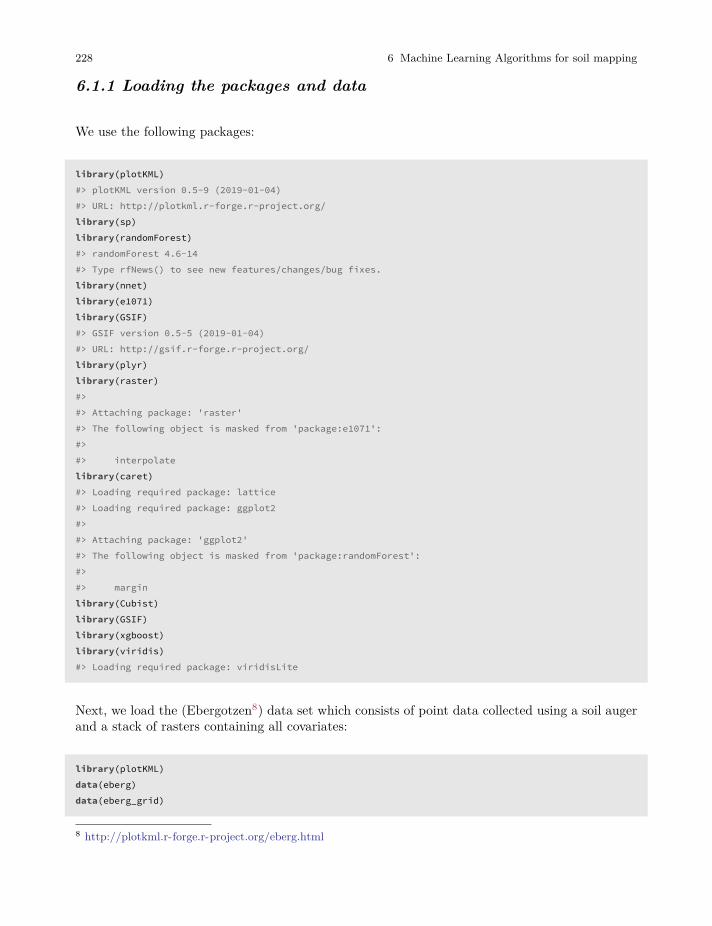
228 6 Machine Learning Algorithms for soil mapping
6.1.1 Loading the packages and data
We use the following packages:
library(plotKML)#> plotKML version 0.5-9 (2019-01-04)#> URL: http://plotkml.r-forge.r-project.org/library(sp)library(randomForest)#> randomForest 4.6-14#> Type rfNews() to see new features/changes/bug fixes.library(nnet)library(e1071)library(GSIF)#> GSIF version 0.5-5 (2019-01-04)#> URL: http://gsif.r-forge.r-project.org/library(plyr)library(raster)#>#> Attaching package: 'raster'#> The following object is masked from 'package:e1071':#>#> interpolatelibrary(caret)#> Loading required package: lattice#> Loading required package: ggplot2#>#> Attaching package: 'ggplot2'#> The following object is masked from 'package:randomForest':#>#> marginlibrary(Cubist)library(GSIF)library(xgboost)library(viridis)#> Loading required package: viridisLite
Next, we load the (Ebergotzen8) data set which consists of point data collected using a soil augerand a stack of rasters containing all covariates:
library(plotKML)data(eberg)data(eberg_grid)
8 http://plotkml.r-forge.r-project.org/eberg.html
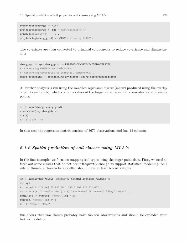
6.1 Spatial prediction of soil properties and classes using MLA’s 229
coordinates(eberg) <- ~X+Yproj4string(eberg) <- CRS("+init=epsg:31467")gridded(eberg_grid) <- ~x+yproj4string(eberg_grid) <- CRS("+init=epsg:31467")
The covariates are then converted to principal components to reduce covariance and dimension-ality:
eberg_spc <- spc(eberg_grid, ~ PRMGEO6+DEMSRT6+TWISRT6+TIRAST6)#> Converting PRMGEO6 to indicators...#> Converting covariates to principal components...eberg_grid@data <- cbind(eberg_grid@data, eberg_spc@predicted@data)
All further analysis is run using the so-called regression matrix (matrix produced using the overlayof points and grids), which contains values of the target variable and all covariates for all trainingpoints:
ov <- over(eberg, eberg_grid)m <- cbind(ov, eberg@data)dim(m)#> [1] 3670 44
In this case the regression matrix consists of 3670 observations and has 44 columns.
6.1.2 Spatial prediction of soil classes using MLA’s
In the first example, we focus on mapping soil types using the auger point data. First, we need tofilter out some classes that do not occur frequently enough to support statistical modelling. As arule of thumb, a class to be modelled should have at least 5 observations:
xg <- summary(m$TAXGRSC, maxsum=(1+length(levels(m$TAXGRSC))))str(xg)#> Named int [1:14] 71 790 86 1 186 1 704 215 252 487 ...#> - attr(*, "names")= chr [1:14] "Auenboden" "Braunerde" "Gley" "HMoor" ...selg.levs <- attr(xg, "names")[xg > 5]attr(xg, "names")[xg <= 5]#> [1] "HMoor" "Moor"
this shows that two classes probably have too few observations and should be excluded fromfurther modeling:
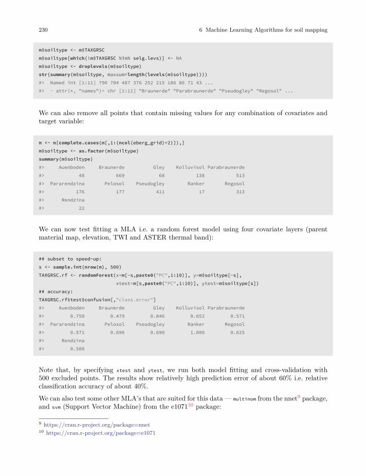
230 6 Machine Learning Algorithms for soil mapping
m$soiltype <- m$TAXGRSCm$soiltype[which(!m$TAXGRSC %in% selg.levs)] <- NAm$soiltype <- droplevels(m$soiltype)str(summary(m$soiltype, maxsum=length(levels(m$soiltype))))#> Named int [1:11] 790 704 487 376 252 215 186 86 71 43 ...#> - attr(*, "names")= chr [1:11] "Braunerde" "Parabraunerde" "Pseudogley" "Regosol" ...
We can also remove all points that contain missing values for any combination of covariates andtarget variable:
m <- m[complete.cases(m[,1:(ncol(eberg_grid)+2)]),]m$soiltype <- as.factor(m$soiltype)summary(m$soiltype)#> Auenboden Braunerde Gley Kolluvisol Parabraunerde#> 48 669 68 138 513#> Pararendzina Pelosol Pseudogley Ranker Regosol#> 176 177 411 17 313#> Rendzina#> 22
We can now test fitting a MLA i.e. a random forest model using four covariate layers (parentmaterial map, elevation, TWI and ASTER thermal band):
## subset to speed-up:s <- sample.int(nrow(m), 500)TAXGRSC.rf <- randomForest(x=m[-s,paste0("PC",1:10)], y=m$soiltype[-s],
xtest=m[s,paste0("PC",1:10)], ytest=m$soiltype[s])## accuracy:TAXGRSC.rf$test$confusion[,"class.error"]#> Auenboden Braunerde Gley Kolluvisol Parabraunerde#> 0.750 0.479 0.846 0.652 0.571#> Pararendzina Pelosol Pseudogley Ranker Regosol#> 0.571 0.696 0.690 1.000 0.625#> Rendzina#> 0.500
Note that, by specifying xtest and ytest, we run both model fitting and cross-validation with500 excluded points. The results show relatively high prediction error of about 60% i.e. relativeclassification accuracy of about 40%.
We can also test some other MLA’s that are suited for this data — multinom from the nnet9 package,and svm (Support Vector Machine) from the e107110 package:
9 https://cran.r-project.org/package=nnet10 https://cran.r-project.org/package=e1071
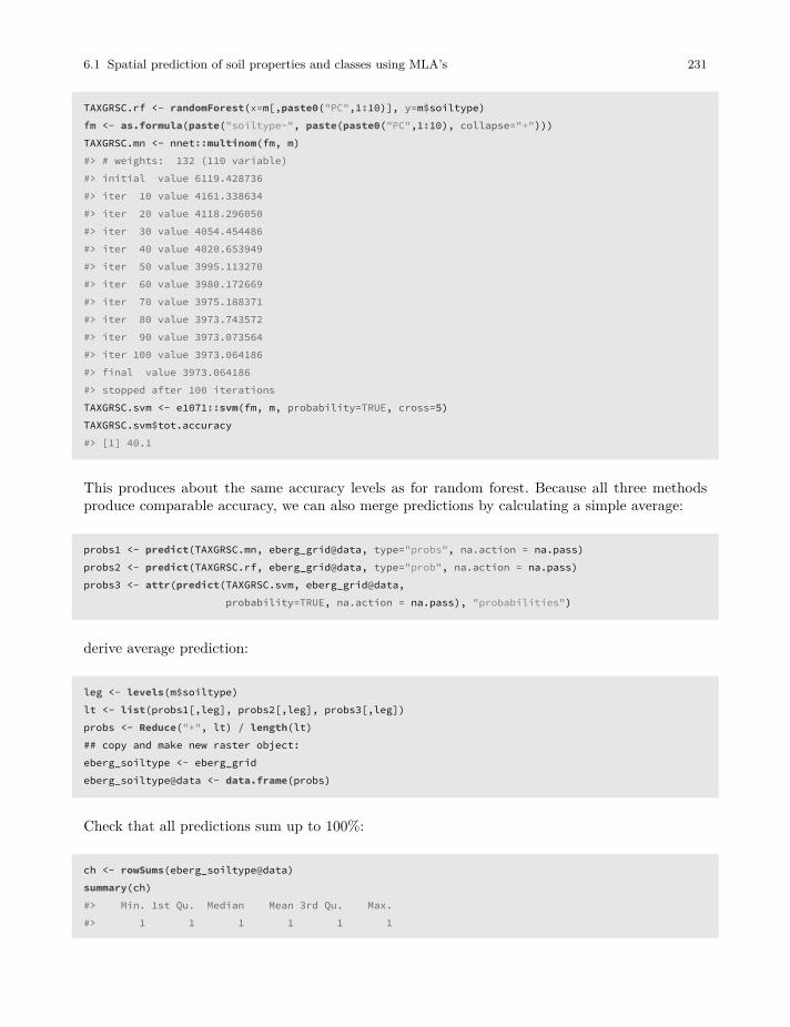
6.1 Spatial prediction of soil properties and classes using MLA’s 231
TAXGRSC.rf <- randomForest(x=m[,paste0("PC",1:10)], y=m$soiltype)fm <- as.formula(paste("soiltype~", paste(paste0("PC",1:10), collapse="+")))TAXGRSC.mn <- nnet::multinom(fm, m)#> # weights: 132 (110 variable)#> initial value 6119.428736#> iter 10 value 4161.338634#> iter 20 value 4118.296050#> iter 30 value 4054.454486#> iter 40 value 4020.653949#> iter 50 value 3995.113270#> iter 60 value 3980.172669#> iter 70 value 3975.188371#> iter 80 value 3973.743572#> iter 90 value 3973.073564#> iter 100 value 3973.064186#> final value 3973.064186#> stopped after 100 iterationsTAXGRSC.svm <- e1071::svm(fm, m, probability=TRUE, cross=5)TAXGRSC.svm$tot.accuracy#> [1] 40.1
This produces about the same accuracy levels as for random forest. Because all three methodsproduce comparable accuracy, we can also merge predictions by calculating a simple average:
probs1 <- predict(TAXGRSC.mn, eberg_grid@data, type="probs", na.action = na.pass)probs2 <- predict(TAXGRSC.rf, eberg_grid@data, type="prob", na.action = na.pass)probs3 <- attr(predict(TAXGRSC.svm, eberg_grid@data,
probability=TRUE, na.action = na.pass), "probabilities")
derive average prediction:
leg <- levels(m$soiltype)lt <- list(probs1[,leg], probs2[,leg], probs3[,leg])probs <- Reduce("+", lt) / length(lt)## copy and make new raster object:eberg_soiltype <- eberg_grideberg_soiltype@data <- data.frame(probs)
Check that all predictions sum up to 100%:
ch <- rowSums(eberg_soiltype@data)summary(ch)#> Min. 1st Qu. Median Mean 3rd Qu. Max.#> 1 1 1 1 1 1
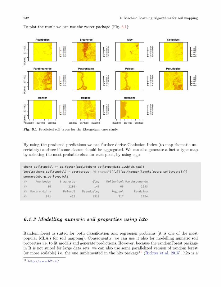
232 6 Machine Learning Algorithms for soil mapping
To plot the result we can use the raster package (Fig. 6.1):
5708
000
5714
000
Auenboden
0.00.20.40.60.81.0
Braunerde
0.00.20.40.60.81.0
Gley
0.00.20.40.60.81.0
Kolluvisol
0.00.20.40.60.81.0
5708
000
5714
000
Parabraunerde
0.00.20.40.60.81.0
Pararendzina
0.00.20.40.60.81.0
Pelosol
0.00.20.40.60.81.0
Pseudogley
0.00.20.40.60.81.0
3568000 3574000 35800005708
000
5714
000
Ranker
0.00.20.40.60.81.0
3568000 3574000 3580000
Regosol
0.00.20.40.60.81.0
3568000 3574000 3580000
Rendzina
0.00.20.40.60.81.0
Fig. 6.1 Predicted soil types for the Ebergotzen case study.
By using the produced predictions we can further derive Confusion Index (to map thematic un-certainty) and see if some classes should be aggregated. We can also generate a factor-type mapby selecting the most probable class for each pixel, by using e.g.:
eberg_soiltype$cl <- as.factor(apply(eberg_soiltype@data,1,which.max))levels(eberg_soiltype$cl) = attr(probs, "dimnames")[[2]][as.integer(levels(eberg_soiltype$cl))]summary(eberg_soiltype$cl)#> Auenboden Braunerde Gley Kolluvisol Parabraunerde#> 36 2286 146 68 2253#> Pararendzina Pelosol Pseudogley Regosol Rendzina#> 821 439 1310 317 2324
6.1.3 Modelling numeric soil properties using h2o
Random forest is suited for both classification and regression problems (it is one of the mostpopular MLA’s for soil mapping). Consequently, we can use it also for modelling numeric soilproperties i.e. to fit models and generate predictions. However, because the randomForest packagein R is not suited for large data sets, we can also use some parallelized version of random forest(or more scalable) i.e. the one implemented in the h2o package11 (Richter et al, 2015). h2o is a11 http://www.h2o.ai/
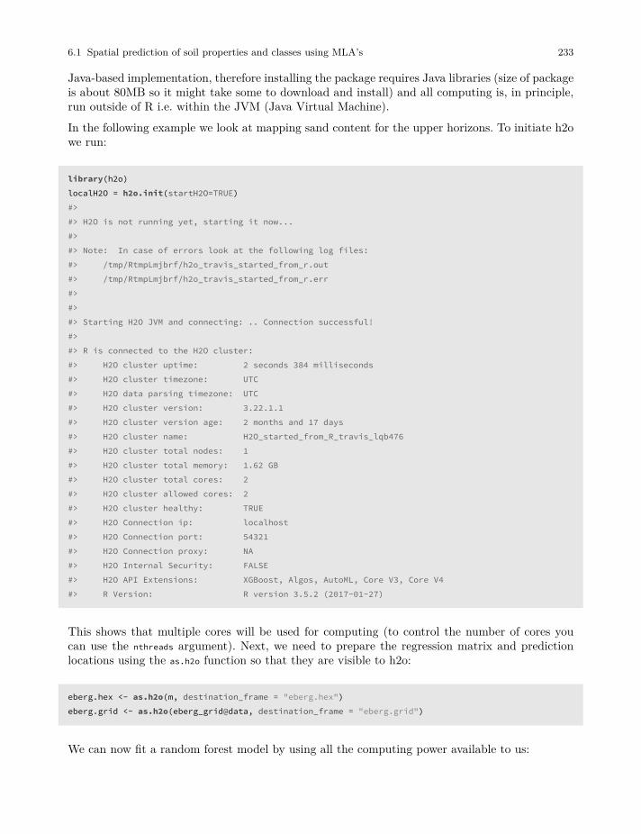
6.1 Spatial prediction of soil properties and classes using MLA’s 233
Java-based implementation, therefore installing the package requires Java libraries (size of packageis about 80MB so it might take some to download and install) and all computing is, in principle,run outside of R i.e. within the JVM (Java Virtual Machine).In the following example we look at mapping sand content for the upper horizons. To initiate h2owe run:
library(h2o)localH2O = h2o.init(startH2O=TRUE)#>#> H2O is not running yet, starting it now...#>#> Note: In case of errors look at the following log files:#> /tmp/RtmpLmjbrf/h2o_travis_started_from_r.out#> /tmp/RtmpLmjbrf/h2o_travis_started_from_r.err#>#>#> Starting H2O JVM and connecting: .. Connection successful!#>#> R is connected to the H2O cluster:#> H2O cluster uptime: 2 seconds 384 milliseconds#> H2O cluster timezone: UTC#> H2O data parsing timezone: UTC#> H2O cluster version: 3.22.1.1#> H2O cluster version age: 2 months and 17 days#> H2O cluster name: H2O_started_from_R_travis_lqb476#> H2O cluster total nodes: 1#> H2O cluster total memory: 1.62 GB#> H2O cluster total cores: 2#> H2O cluster allowed cores: 2#> H2O cluster healthy: TRUE#> H2O Connection ip: localhost#> H2O Connection port: 54321#> H2O Connection proxy: NA#> H2O Internal Security: FALSE#> H2O API Extensions: XGBoost, Algos, AutoML, Core V3, Core V4#> R Version: R version 3.5.2 (2017-01-27)
This shows that multiple cores will be used for computing (to control the number of cores youcan use the nthreads argument). Next, we need to prepare the regression matrix and predictionlocations using the as.h2o function so that they are visible to h2o:
eberg.hex <- as.h2o(m, destination_frame = "eberg.hex")eberg.grid <- as.h2o(eberg_grid@data, destination_frame = "eberg.grid")
We can now fit a random forest model by using all the computing power available to us:
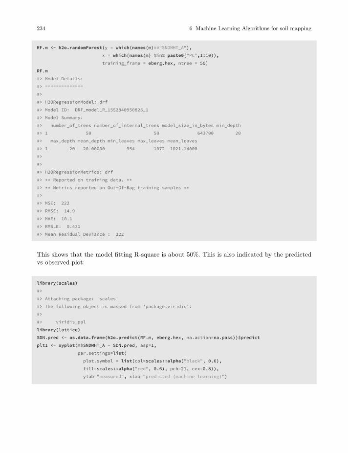
234 6 Machine Learning Algorithms for soil mapping
RF.m <- h2o.randomForest(y = which(names(m)=="SNDMHT_A"),x = which(names(m) %in% paste0("PC",1:10)),training_frame = eberg.hex, ntree = 50)
RF.m#> Model Details:#> ==============#>#> H2ORegressionModel: drf#> Model ID: DRF_model_R_1552840950825_1#> Model Summary:#> number_of_trees number_of_internal_trees model_size_in_bytes min_depth#> 1 50 50 643700 20#> max_depth mean_depth min_leaves max_leaves mean_leaves#> 1 20 20.00000 954 1072 1021.14000#>#>#> H2ORegressionMetrics: drf#> ** Reported on training data. **#> ** Metrics reported on Out-Of-Bag training samples **#>#> MSE: 222#> RMSE: 14.9#> MAE: 10.1#> RMSLE: 0.431#> Mean Residual Deviance : 222
This shows that the model fitting R-square is about 50%. This is also indicated by the predictedvs observed plot:
library(scales)#>#> Attaching package: 'scales'#> The following object is masked from 'package:viridis':#>#> viridis_pallibrary(lattice)SDN.pred <- as.data.frame(h2o.predict(RF.m, eberg.hex, na.action=na.pass))$predictplt1 <- xyplot(m$SNDMHT_A ~ SDN.pred, asp=1,
par.settings=list(plot.symbol = list(col=scales::alpha("black", 0.6),fill=scales::alpha("red", 0.6), pch=21, cex=0.8)),ylab="measured", xlab="predicted (machine learning)")

6.1 Spatial prediction of soil properties and classes using MLA’s 235
Fig. 6.2 Measured vs predicted sand content based on the Random Forest model.
To produce a map based on these predictions we use:
eberg_grid$RFx <- as.data.frame(h2o.predict(RF.m, eberg.grid, na.action=na.pass))$predict
10
20
30
40
50
60
70
80
90
Fig. 6.3 Predicted sand content based on random forest.
h2o has another MLA of interest for soil mapping called deep learning (a feed-forward multilayerartificial neural network). Fitting the model is equivalent to using random forest:
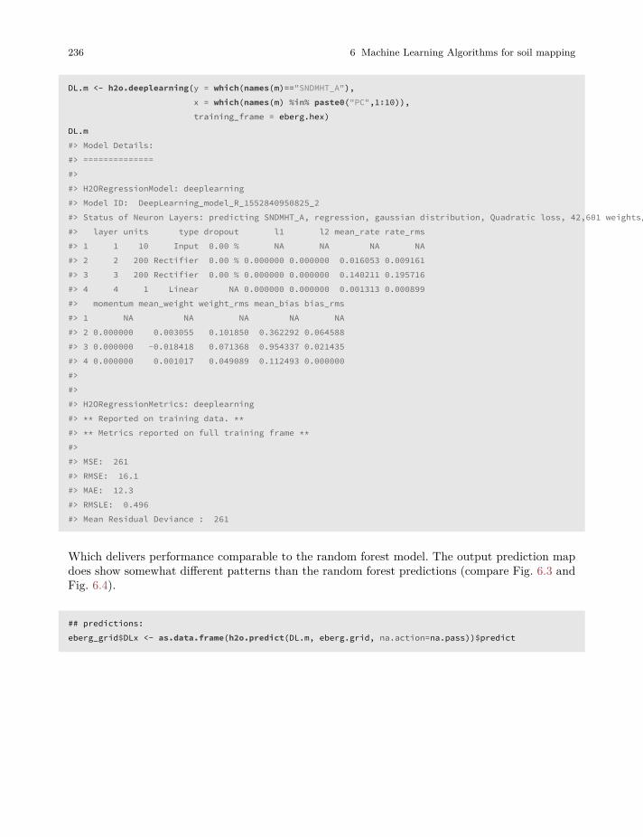
236 6 Machine Learning Algorithms for soil mapping
DL.m <- h2o.deeplearning(y = which(names(m)=="SNDMHT_A"),x = which(names(m) %in% paste0("PC",1:10)),training_frame = eberg.hex)
DL.m#> Model Details:#> ==============#>#> H2ORegressionModel: deeplearning#> Model ID: DeepLearning_model_R_1552840950825_2#> Status of Neuron Layers: predicting SNDMHT_A, regression, gaussian distribution, Quadratic loss, 42,601 weights/biases, 508.3 KB, 25,520 training samples, mini-batch size 1#> layer units type dropout l1 l2 mean_rate rate_rms#> 1 1 10 Input 0.00 % NA NA NA NA#> 2 2 200 Rectifier 0.00 % 0.000000 0.000000 0.016053 0.009161#> 3 3 200 Rectifier 0.00 % 0.000000 0.000000 0.140211 0.195716#> 4 4 1 Linear NA 0.000000 0.000000 0.001313 0.000899#> momentum mean_weight weight_rms mean_bias bias_rms#> 1 NA NA NA NA NA#> 2 0.000000 0.003055 0.101850 0.362292 0.064588#> 3 0.000000 -0.018418 0.071368 0.954337 0.021435#> 4 0.000000 0.001017 0.049089 0.112493 0.000000#>#>#> H2ORegressionMetrics: deeplearning#> ** Reported on training data. **#> ** Metrics reported on full training frame **#>#> MSE: 261#> RMSE: 16.1#> MAE: 12.3#> RMSLE: 0.496#> Mean Residual Deviance : 261
Which delivers performance comparable to the random forest model. The output prediction mapdoes show somewhat different patterns than the random forest predictions (compare Fig. 6.3 andFig. 6.4).
## predictions:eberg_grid$DLx <- as.data.frame(h2o.predict(DL.m, eberg.grid, na.action=na.pass))$predict
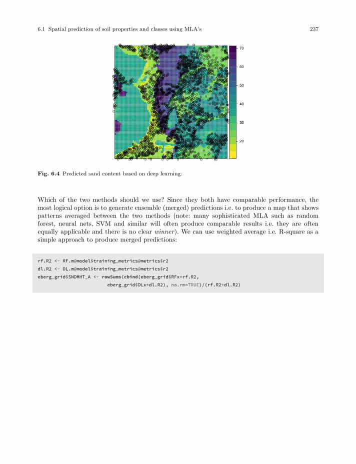
6.1 Spatial prediction of soil properties and classes using MLA’s 237
20
30
40
50
60
70
Fig. 6.4 Predicted sand content based on deep learning.
Which of the two methods should we use? Since they both have comparable performance, themost logical option is to generate ensemble (merged) predictions i.e. to produce a map that showspatterns averaged between the two methods (note: many sophisticated MLA such as randomforest, neural nets, SVM and similar will often produce comparable results i.e. they are oftenequally applicable and there is no clear winner). We can use weighted average i.e. R-square as asimple approach to produce merged predictions:
rf.R2 <- RF.m@model$training_metrics@metrics$r2dl.R2 <- DL.m@model$training_metrics@metrics$r2eberg_grid$SNDMHT_A <- rowSums(cbind(eberg_grid$RFx*rf.R2,
eberg_grid$DLx*dl.R2), na.rm=TRUE)/(rf.R2+dl.R2)
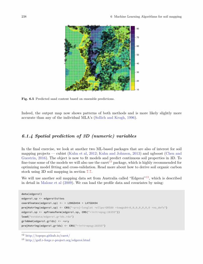
238 6 Machine Learning Algorithms for soil mapping
10
20
30
40
50
60
70
80
Fig. 6.5 Predicted sand content based on ensemble predictions.
Indeed, the output map now shows patterns of both methods and is more likely slightly moreaccurate than any of the individual MLA’s (Sollich and Krogh, 1996).
6.1.4 Spatial prediction of 3D (numeric) variables
In the final exercise, we look at another two ML-based packages that are also of interest for soilmapping projects — cubist (Kuhn et al, 2012; Kuhn and Johnson, 2013) and xgboost (Chen andGuestrin, 2016). The object is now to fit models and predict continuous soil properties in 3D. Tofine-tune some of the models we will also use the caret12 package, which is highly recommended foroptimizing model fitting and cross-validation. Read more about how to derive soil organic carbonstock using 3D soil mapping in section 7.7.We will use another soil mapping data set from Australia called “Edgeroi”13, which is describedin detail in Malone et al (2009). We can load the profile data and covariates by using:
data(edgeroi)edgeroi.sp <- edgeroi$sitescoordinates(edgeroi.sp) <- ~ LONGDA94 + LATGDA94proj4string(edgeroi.sp) <- CRS("+proj=longlat +ellps=GRS80 +towgs84=0,0,0,0,0,0,0 +no_defs")edgeroi.sp <- spTransform(edgeroi.sp, CRS("+init=epsg:28355"))load("extdata/edgeroi.grids.rda")gridded(edgeroi.grids) <- ~x+yproj4string(edgeroi.grids) <- CRS("+init=epsg:28355")
12 http://topepo.github.io/caret/13 http://gsif.r-forge.r-project.org/edgeroi.html
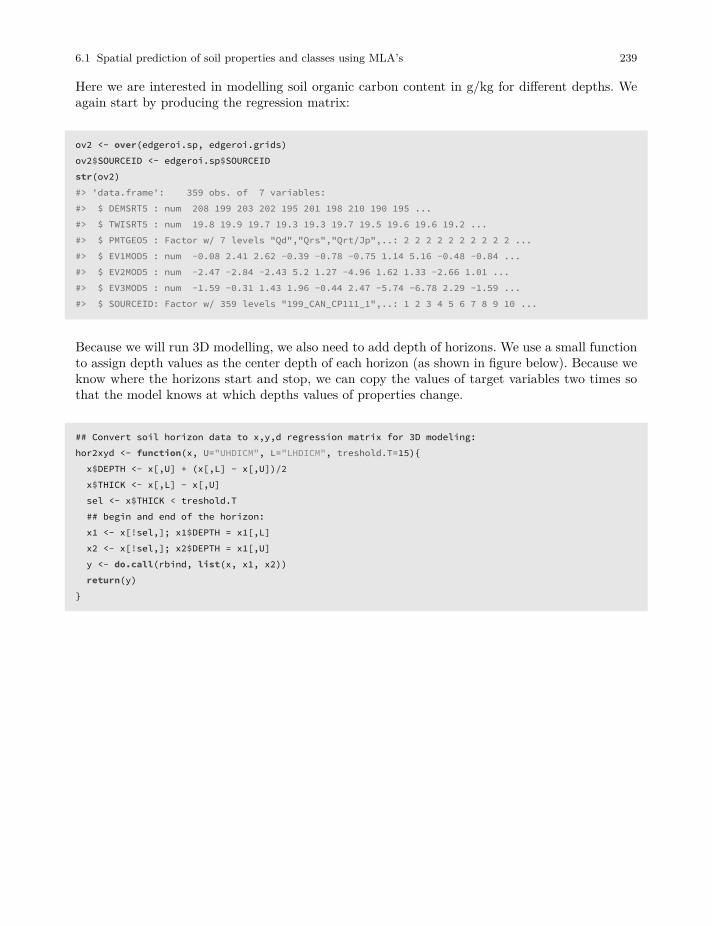
6.1 Spatial prediction of soil properties and classes using MLA’s 239
Here we are interested in modelling soil organic carbon content in g/kg for different depths. Weagain start by producing the regression matrix:
ov2 <- over(edgeroi.sp, edgeroi.grids)ov2$SOURCEID <- edgeroi.sp$SOURCEIDstr(ov2)#> 'data.frame': 359 obs. of 7 variables:#> $ DEMSRT5 : num 208 199 203 202 195 201 198 210 190 195 ...#> $ TWISRT5 : num 19.8 19.9 19.7 19.3 19.3 19.7 19.5 19.6 19.6 19.2 ...#> $ PMTGEO5 : Factor w/ 7 levels "Qd","Qrs","Qrt/Jp",..: 2 2 2 2 2 2 2 2 2 2 ...#> $ EV1MOD5 : num -0.08 2.41 2.62 -0.39 -0.78 -0.75 1.14 5.16 -0.48 -0.84 ...#> $ EV2MOD5 : num -2.47 -2.84 -2.43 5.2 1.27 -4.96 1.62 1.33 -2.66 1.01 ...#> $ EV3MOD5 : num -1.59 -0.31 1.43 1.96 -0.44 2.47 -5.74 -6.78 2.29 -1.59 ...#> $ SOURCEID: Factor w/ 359 levels "199_CAN_CP111_1",..: 1 2 3 4 5 6 7 8 9 10 ...
Because we will run 3D modelling, we also need to add depth of horizons. We use a small functionto assign depth values as the center depth of each horizon (as shown in figure below). Because weknow where the horizons start and stop, we can copy the values of target variables two times sothat the model knows at which depths values of properties change.
## Convert soil horizon data to x,y,d regression matrix for 3D modeling:hor2xyd <- function(x, U="UHDICM", L="LHDICM", treshold.T=15){x$DEPTH <- x[,U] + (x[,L] - x[,U])/2x$THICK <- x[,L] - x[,U]sel <- x$THICK < treshold.T## begin and end of the horizon:x1 <- x[!sel,]; x1$DEPTH = x1[,L]x2 <- x[!sel,]; x2$DEPTH = x1[,U]y <- do.call(rbind, list(x, x1, x2))return(y)
}
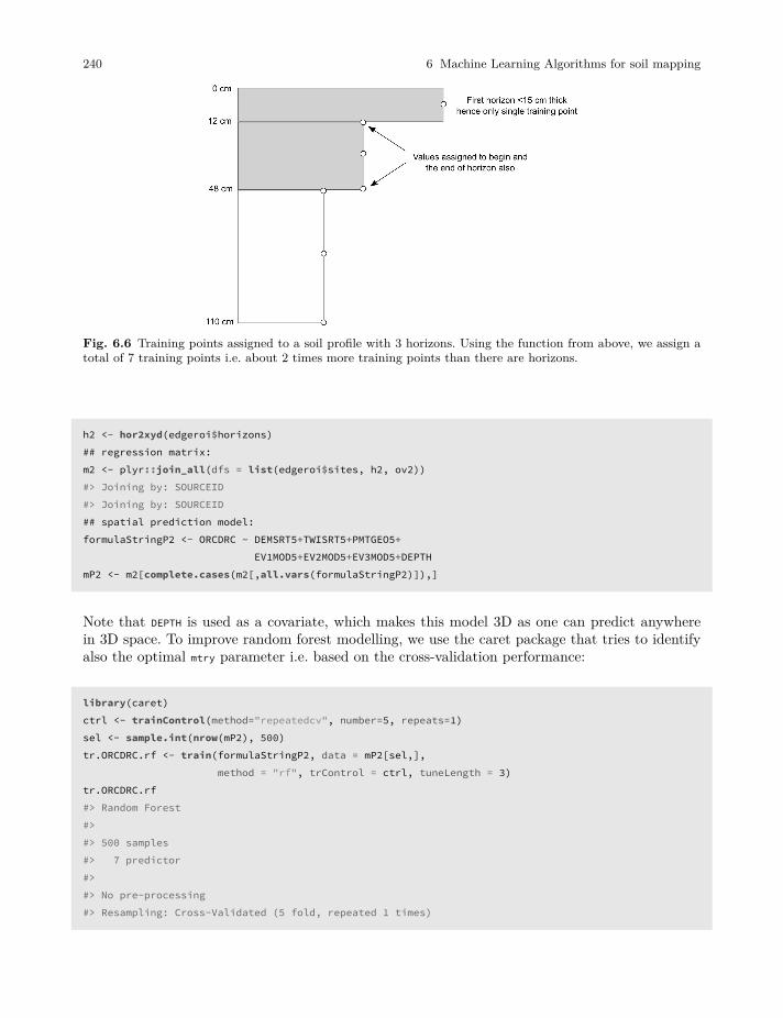
240 6 Machine Learning Algorithms for soil mapping
Fig. 6.6 Training points assigned to a soil profile with 3 horizons. Using the function from above, we assign atotal of 7 training points i.e. about 2 times more training points than there are horizons.
h2 <- hor2xyd(edgeroi$horizons)## regression matrix:m2 <- plyr::join_all(dfs = list(edgeroi$sites, h2, ov2))#> Joining by: SOURCEID#> Joining by: SOURCEID## spatial prediction model:formulaStringP2 <- ORCDRC ~ DEMSRT5+TWISRT5+PMTGEO5+
EV1MOD5+EV2MOD5+EV3MOD5+DEPTHmP2 <- m2[complete.cases(m2[,all.vars(formulaStringP2)]),]
Note that DEPTH is used as a covariate, which makes this model 3D as one can predict anywherein 3D space. To improve random forest modelling, we use the caret package that tries to identifyalso the optimal mtry parameter i.e. based on the cross-validation performance:
library(caret)ctrl <- trainControl(method="repeatedcv", number=5, repeats=1)sel <- sample.int(nrow(mP2), 500)tr.ORCDRC.rf <- train(formulaStringP2, data = mP2[sel,],
method = "rf", trControl = ctrl, tuneLength = 3)tr.ORCDRC.rf#> Random Forest#>#> 500 samples#> 7 predictor#>#> No pre-processing#> Resampling: Cross-Validated (5 fold, repeated 1 times)

6.1 Spatial prediction of soil properties and classes using MLA’s 241
#> Summary of sample sizes: 399, 401, 399, 401, 400#> Resampling results across tuning parameters:#>#> mtry RMSE Rsquared MAE#> 2 4.36 0.525 2.83#> 7 4.17 0.552 2.45#> 12 4.36 0.527 2.51#>#> RMSE was used to select the optimal model using the smallest value.#> The final value used for the model was mtry = 7.
In this case, mtry = 12 seems to achieve the best performance. Note that we sub-set the initial matrixto speed up fine-tuning of the parameters (otherwise the computing time could easily become toogreat). Next, we can fit the final model by using all data (this time we also turn cross-validationoff):
ORCDRC.rf <- train(formulaStringP2, data=mP2,method = "rf", tuneGrid=data.frame(mtry=7),trControl=trainControl(method="none"))
w1 <- 100*max(tr.ORCDRC.rf$results$Rsquared)
The variable importance plot indicates that DEPTH is by far the most important predictor:
PMTGEO5TsPMTGEO5Qrt/RnPMTGEO5QrsPMTGEO5Qrt/TvPMTGEO5Qrt/JpPMTGEO5TvTWISRT5EV1MOD5EV2MOD5EV3MOD5DEMSRT5DEPTH
0 20000 40000 60000 80000
IncNodePurity
Fig. 6.7 Variable importance plot for predicting soil organic carbon content (ORC) in 3D.
We can also try fitting models using the xgboost package and the cubist packages:
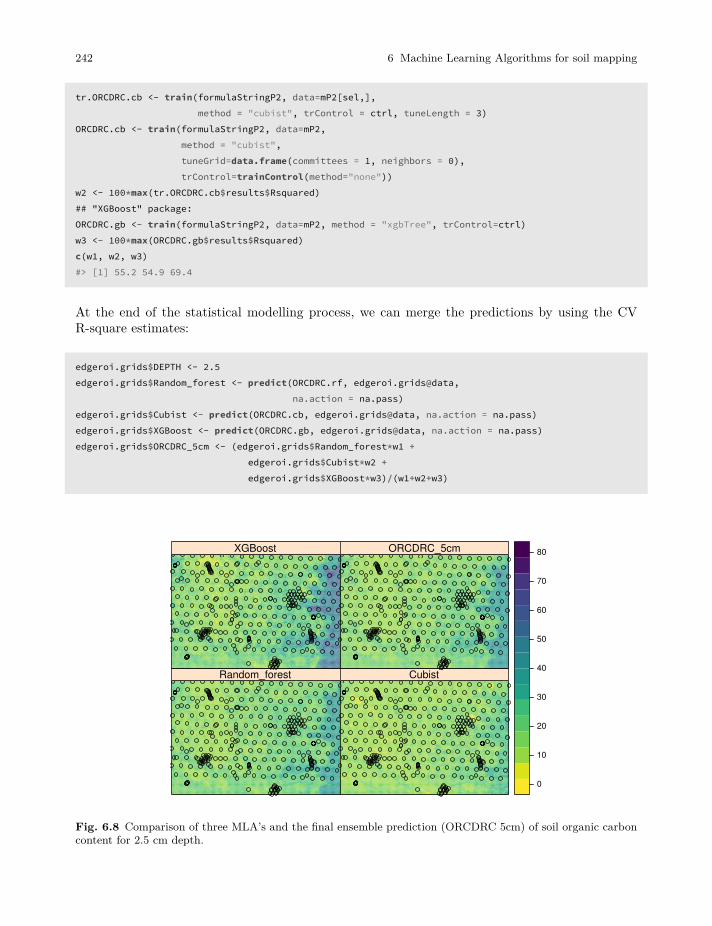
242 6 Machine Learning Algorithms for soil mapping
tr.ORCDRC.cb <- train(formulaStringP2, data=mP2[sel,],method = "cubist", trControl = ctrl, tuneLength = 3)
ORCDRC.cb <- train(formulaStringP2, data=mP2,method = "cubist",tuneGrid=data.frame(committees = 1, neighbors = 0),trControl=trainControl(method="none"))
w2 <- 100*max(tr.ORCDRC.cb$results$Rsquared)## "XGBoost" package:ORCDRC.gb <- train(formulaStringP2, data=mP2, method = "xgbTree", trControl=ctrl)w3 <- 100*max(ORCDRC.gb$results$Rsquared)c(w1, w2, w3)#> [1] 55.2 54.9 69.4
At the end of the statistical modelling process, we can merge the predictions by using the CVR-square estimates:
edgeroi.grids$DEPTH <- 2.5edgeroi.grids$Random_forest <- predict(ORCDRC.rf, edgeroi.grids@data,
na.action = na.pass)edgeroi.grids$Cubist <- predict(ORCDRC.cb, edgeroi.grids@data, na.action = na.pass)edgeroi.grids$XGBoost <- predict(ORCDRC.gb, edgeroi.grids@data, na.action = na.pass)edgeroi.grids$ORCDRC_5cm <- (edgeroi.grids$Random_forest*w1 +
edgeroi.grids$Cubist*w2 +edgeroi.grids$XGBoost*w3)/(w1+w2+w3)
Random_forest Cubist
XGBoost ORCDRC_5cm
0
10
20
30
40
50
60
70
80
Fig. 6.8 Comparison of three MLA’s and the final ensemble prediction (ORCDRC 5cm) of soil organic carboncontent for 2.5 cm depth.
6.1 Spatial prediction of soil properties and classes using MLA’s 243
The final plot shows that xgboost possibly over-predicts and that cubist possibly under-predictsvalues of ORCDRC, while random forest is somewhere in-between the two. Again, merged predic-tions are probably the safest option considering that all three MLA’s have similar measures ofperformance.
We can quickly test the overall performance using a script on github prepared for testing perfor-mance of merged predictions:
source_https <- function(url, ...) {require(RCurl)if(!file.exists(paste0("R/", basename(url)))){
cat(getURL(url, followlocation = TRUE,cainfo = system.file("CurlSSL", "cacert.pem", package = "RCurl")),
file = paste0("R/", basename(url)))}source(paste0("R/", basename(url)))
}wdir = "https://raw.githubusercontent.com/ISRICWorldSoil/SoilGrids250m/"source_https(paste0(wdir, "master/grids/cv/cv_functions.R"))#> Loading required package: RCurl#> Loading required package: bitops
We can hence run 5-fold cross validation:
mP2$SOURCEID = paste(mP2$SOURCEID)test.ORC <- cv_numeric(formulaStringP2, rmatrix=mP2,
nfold=5, idcol="SOURCEID", Log=TRUE)#> Running 5-fold cross validation with model re-fitting method ranger ...#> Subsetting observations by unique location#> Loading required package: snowfall#> Loading required package: snow#> Warning in searchCommandline(parallel, cpus = cpus, type = type,#> socketHosts = socketHosts, : Unknown option on commandline: --file#> R Version: R version 3.5.2 (2017-01-27)#> snowfall 1.84-6.1 initialized (using snow 0.4-3): parallel execution on 2 CPUs.#> Library plyr loaded.#> Library plyr loaded in cluster.#> Library ranger loaded.#> Library ranger loaded in cluster.#>#> Attaching package: 'ranger'#> The following object is masked from 'package:randomForest':#>#> importance#>#> Stopping cluster
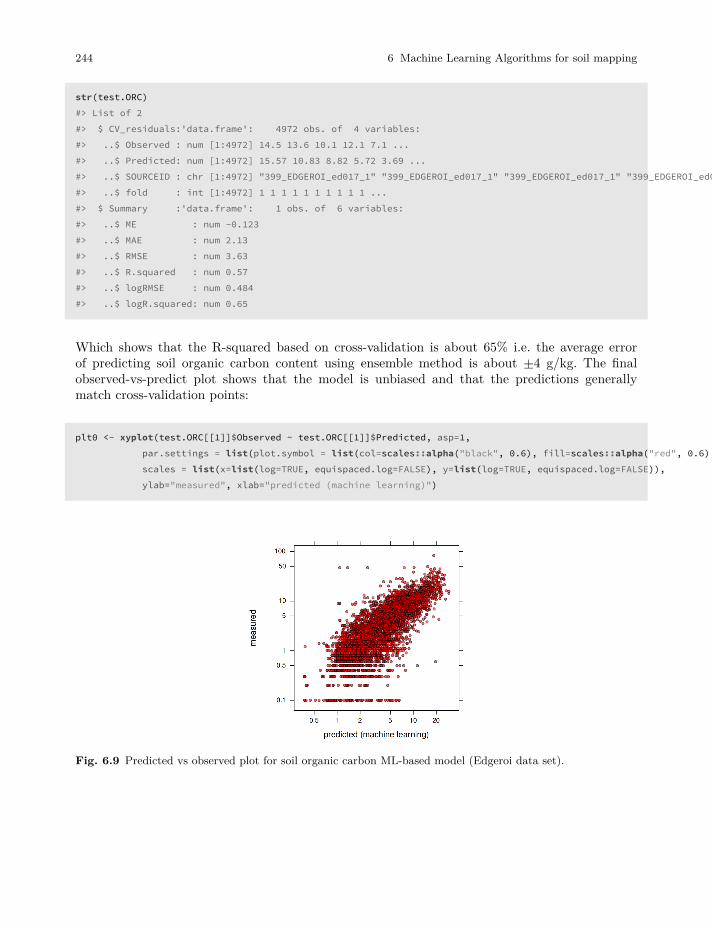
244 6 Machine Learning Algorithms for soil mapping
str(test.ORC)#> List of 2#> $ CV_residuals:'data.frame': 4972 obs. of 4 variables:#> ..$ Observed : num [1:4972] 14.5 13.6 10.1 12.1 7.1 ...#> ..$ Predicted: num [1:4972] 15.57 10.83 8.82 5.72 3.69 ...#> ..$ SOURCEID : chr [1:4972] "399_EDGEROI_ed017_1" "399_EDGEROI_ed017_1" "399_EDGEROI_ed017_1" "399_EDGEROI_ed017_1" ...#> ..$ fold : int [1:4972] 1 1 1 1 1 1 1 1 1 1 ...#> $ Summary :'data.frame': 1 obs. of 6 variables:#> ..$ ME : num -0.123#> ..$ MAE : num 2.13#> ..$ RMSE : num 3.63#> ..$ R.squared : num 0.57#> ..$ logRMSE : num 0.484#> ..$ logR.squared: num 0.65
Which shows that the R-squared based on cross-validation is about 65% i.e. the average errorof predicting soil organic carbon content using ensemble method is about ±4 g/kg. The finalobserved-vs-predict plot shows that the model is unbiased and that the predictions generallymatch cross-validation points:
plt0 <- xyplot(test.ORC[[1]]$Observed ~ test.ORC[[1]]$Predicted, asp=1,par.settings = list(plot.symbol = list(col=scales::alpha("black", 0.6), fill=scales::alpha("red", 0.6), pch=21, cex=0.6)),scales = list(x=list(log=TRUE, equispaced.log=FALSE), y=list(log=TRUE, equispaced.log=FALSE)),ylab="measured", xlab="predicted (machine learning)")
Fig. 6.9 Predicted vs observed plot for soil organic carbon ML-based model (Edgeroi data set).
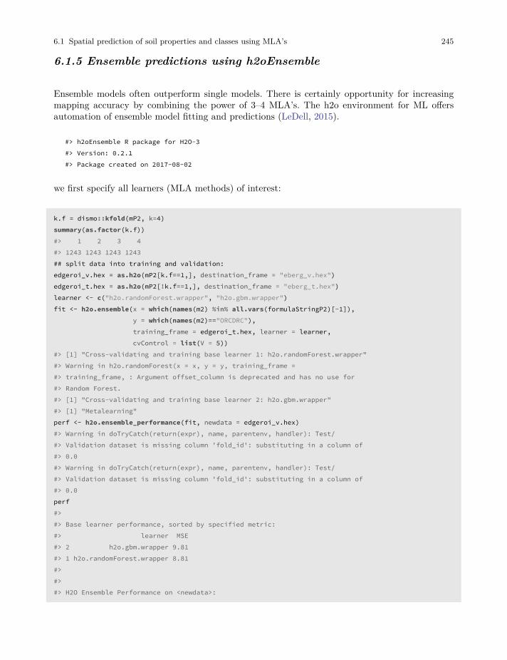
6.1 Spatial prediction of soil properties and classes using MLA’s 245
6.1.5 Ensemble predictions using h2oEnsemble
Ensemble models often outperform single models. There is certainly opportunity for increasingmapping accuracy by combining the power of 3–4 MLA’s. The h2o environment for ML offersautomation of ensemble model fitting and predictions (LeDell, 2015).
#> h2oEnsemble R package for H2O-3#> Version: 0.2.1#> Package created on 2017-08-02
we first specify all learners (MLA methods) of interest:
k.f = dismo::kfold(mP2, k=4)summary(as.factor(k.f))#> 1 2 3 4#> 1243 1243 1243 1243## split data into training and validation:edgeroi_v.hex = as.h2o(mP2[k.f==1,], destination_frame = "eberg_v.hex")edgeroi_t.hex = as.h2o(mP2[!k.f==1,], destination_frame = "eberg_t.hex")learner <- c("h2o.randomForest.wrapper", "h2o.gbm.wrapper")fit <- h2o.ensemble(x = which(names(m2) %in% all.vars(formulaStringP2)[-1]),
y = which(names(m2)=="ORCDRC"),training_frame = edgeroi_t.hex, learner = learner,cvControl = list(V = 5))
#> [1] "Cross-validating and training base learner 1: h2o.randomForest.wrapper"#> Warning in h2o.randomForest(x = x, y = y, training_frame =#> training_frame, : Argument offset_column is deprecated and has no use for#> Random Forest.#> [1] "Cross-validating and training base learner 2: h2o.gbm.wrapper"#> [1] "Metalearning"perf <- h2o.ensemble_performance(fit, newdata = edgeroi_v.hex)#> Warning in doTryCatch(return(expr), name, parentenv, handler): Test/#> Validation dataset is missing column 'fold_id': substituting in a column of#> 0.0#> Warning in doTryCatch(return(expr), name, parentenv, handler): Test/#> Validation dataset is missing column 'fold_id': substituting in a column of#> 0.0perf#>#> Base learner performance, sorted by specified metric:#> learner MSE#> 2 h2o.gbm.wrapper 9.81#> 1 h2o.randomForest.wrapper 8.81#>#>#> H2O Ensemble Performance on <newdata>:
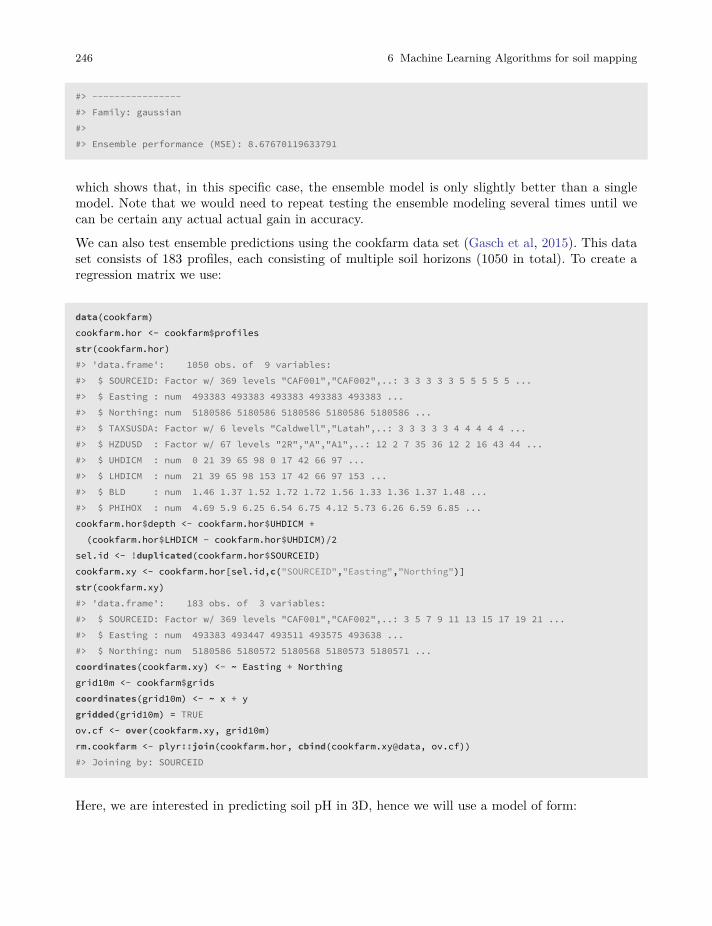
246 6 Machine Learning Algorithms for soil mapping
#> ----------------#> Family: gaussian#>#> Ensemble performance (MSE): 8.67670119633791
which shows that, in this specific case, the ensemble model is only slightly better than a singlemodel. Note that we would need to repeat testing the ensemble modeling several times until wecan be certain any actual actual gain in accuracy.
We can also test ensemble predictions using the cookfarm data set (Gasch et al, 2015). This dataset consists of 183 profiles, each consisting of multiple soil horizons (1050 in total). To create aregression matrix we use:
data(cookfarm)cookfarm.hor <- cookfarm$profilesstr(cookfarm.hor)#> 'data.frame': 1050 obs. of 9 variables:#> $ SOURCEID: Factor w/ 369 levels "CAF001","CAF002",..: 3 3 3 3 3 5 5 5 5 5 ...#> $ Easting : num 493383 493383 493383 493383 493383 ...#> $ Northing: num 5180586 5180586 5180586 5180586 5180586 ...#> $ TAXSUSDA: Factor w/ 6 levels "Caldwell","Latah",..: 3 3 3 3 3 4 4 4 4 4 ...#> $ HZDUSD : Factor w/ 67 levels "2R","A","A1",..: 12 2 7 35 36 12 2 16 43 44 ...#> $ UHDICM : num 0 21 39 65 98 0 17 42 66 97 ...#> $ LHDICM : num 21 39 65 98 153 17 42 66 97 153 ...#> $ BLD : num 1.46 1.37 1.52 1.72 1.72 1.56 1.33 1.36 1.37 1.48 ...#> $ PHIHOX : num 4.69 5.9 6.25 6.54 6.75 4.12 5.73 6.26 6.59 6.85 ...cookfarm.hor$depth <- cookfarm.hor$UHDICM +(cookfarm.hor$LHDICM - cookfarm.hor$UHDICM)/2
sel.id <- !duplicated(cookfarm.hor$SOURCEID)cookfarm.xy <- cookfarm.hor[sel.id,c("SOURCEID","Easting","Northing")]str(cookfarm.xy)#> 'data.frame': 183 obs. of 3 variables:#> $ SOURCEID: Factor w/ 369 levels "CAF001","CAF002",..: 3 5 7 9 11 13 15 17 19 21 ...#> $ Easting : num 493383 493447 493511 493575 493638 ...#> $ Northing: num 5180586 5180572 5180568 5180573 5180571 ...coordinates(cookfarm.xy) <- ~ Easting + Northinggrid10m <- cookfarm$gridscoordinates(grid10m) <- ~ x + ygridded(grid10m) = TRUEov.cf <- over(cookfarm.xy, grid10m)rm.cookfarm <- plyr::join(cookfarm.hor, cbind(cookfarm.xy@data, ov.cf))#> Joining by: SOURCEID
Here, we are interested in predicting soil pH in 3D, hence we will use a model of form:
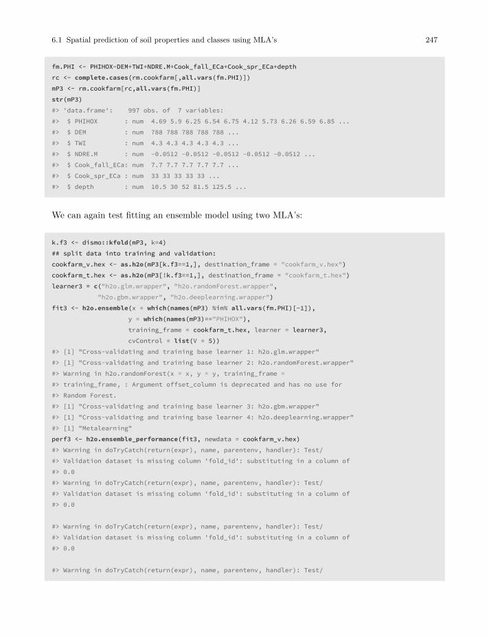
6.1 Spatial prediction of soil properties and classes using MLA’s 247
fm.PHI <- PHIHOX~DEM+TWI+NDRE.M+Cook_fall_ECa+Cook_spr_ECa+depthrc <- complete.cases(rm.cookfarm[,all.vars(fm.PHI)])mP3 <- rm.cookfarm[rc,all.vars(fm.PHI)]str(mP3)#> 'data.frame': 997 obs. of 7 variables:#> $ PHIHOX : num 4.69 5.9 6.25 6.54 6.75 4.12 5.73 6.26 6.59 6.85 ...#> $ DEM : num 788 788 788 788 788 ...#> $ TWI : num 4.3 4.3 4.3 4.3 4.3 ...#> $ NDRE.M : num -0.0512 -0.0512 -0.0512 -0.0512 -0.0512 ...#> $ Cook_fall_ECa: num 7.7 7.7 7.7 7.7 7.7 ...#> $ Cook_spr_ECa : num 33 33 33 33 33 ...#> $ depth : num 10.5 30 52 81.5 125.5 ...
We can again test fitting an ensemble model using two MLA’s:
k.f3 <- dismo::kfold(mP3, k=4)## split data into training and validation:cookfarm_v.hex <- as.h2o(mP3[k.f3==1,], destination_frame = "cookfarm_v.hex")cookfarm_t.hex <- as.h2o(mP3[!k.f3==1,], destination_frame = "cookfarm_t.hex")learner3 = c("h2o.glm.wrapper", "h2o.randomForest.wrapper",
"h2o.gbm.wrapper", "h2o.deeplearning.wrapper")fit3 <- h2o.ensemble(x = which(names(mP3) %in% all.vars(fm.PHI)[-1]),
y = which(names(mP3)=="PHIHOX"),training_frame = cookfarm_t.hex, learner = learner3,cvControl = list(V = 5))
#> [1] "Cross-validating and training base learner 1: h2o.glm.wrapper"#> [1] "Cross-validating and training base learner 2: h2o.randomForest.wrapper"#> Warning in h2o.randomForest(x = x, y = y, training_frame =#> training_frame, : Argument offset_column is deprecated and has no use for#> Random Forest.#> [1] "Cross-validating and training base learner 3: h2o.gbm.wrapper"#> [1] "Cross-validating and training base learner 4: h2o.deeplearning.wrapper"#> [1] "Metalearning"perf3 <- h2o.ensemble_performance(fit3, newdata = cookfarm_v.hex)#> Warning in doTryCatch(return(expr), name, parentenv, handler): Test/#> Validation dataset is missing column 'fold_id': substituting in a column of#> 0.0#> Warning in doTryCatch(return(expr), name, parentenv, handler): Test/#> Validation dataset is missing column 'fold_id': substituting in a column of#> 0.0
#> Warning in doTryCatch(return(expr), name, parentenv, handler): Test/#> Validation dataset is missing column 'fold_id': substituting in a column of#> 0.0
#> Warning in doTryCatch(return(expr), name, parentenv, handler): Test/
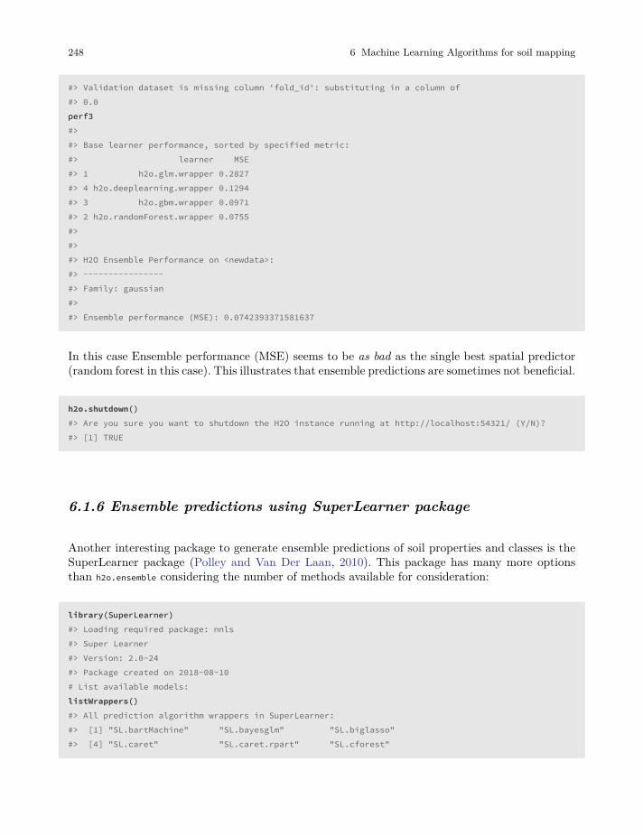
248 6 Machine Learning Algorithms for soil mapping
#> Validation dataset is missing column 'fold_id': substituting in a column of#> 0.0perf3#>#> Base learner performance, sorted by specified metric:#> learner MSE#> 1 h2o.glm.wrapper 0.2827#> 4 h2o.deeplearning.wrapper 0.1294#> 3 h2o.gbm.wrapper 0.0971#> 2 h2o.randomForest.wrapper 0.0755#>#>#> H2O Ensemble Performance on <newdata>:#> ----------------#> Family: gaussian#>#> Ensemble performance (MSE): 0.0742393371581637
In this case Ensemble performance (MSE) seems to be as bad as the single best spatial predictor(random forest in this case). This illustrates that ensemble predictions are sometimes not beneficial.
h2o.shutdown()#> Are you sure you want to shutdown the H2O instance running at http://localhost:54321/ (Y/N)?#> [1] TRUE
6.1.6 Ensemble predictions using SuperLearner package
Another interesting package to generate ensemble predictions of soil properties and classes is theSuperLearner package (Polley and Van Der Laan, 2010). This package has many more optionsthan h2o.ensemble considering the number of methods available for consideration:
library(SuperLearner)#> Loading required package: nnls#> Super Learner#> Version: 2.0-24#> Package created on 2018-08-10# List available models:listWrappers()#> All prediction algorithm wrappers in SuperLearner:#> [1] "SL.bartMachine" "SL.bayesglm" "SL.biglasso"#> [4] "SL.caret" "SL.caret.rpart" "SL.cforest"
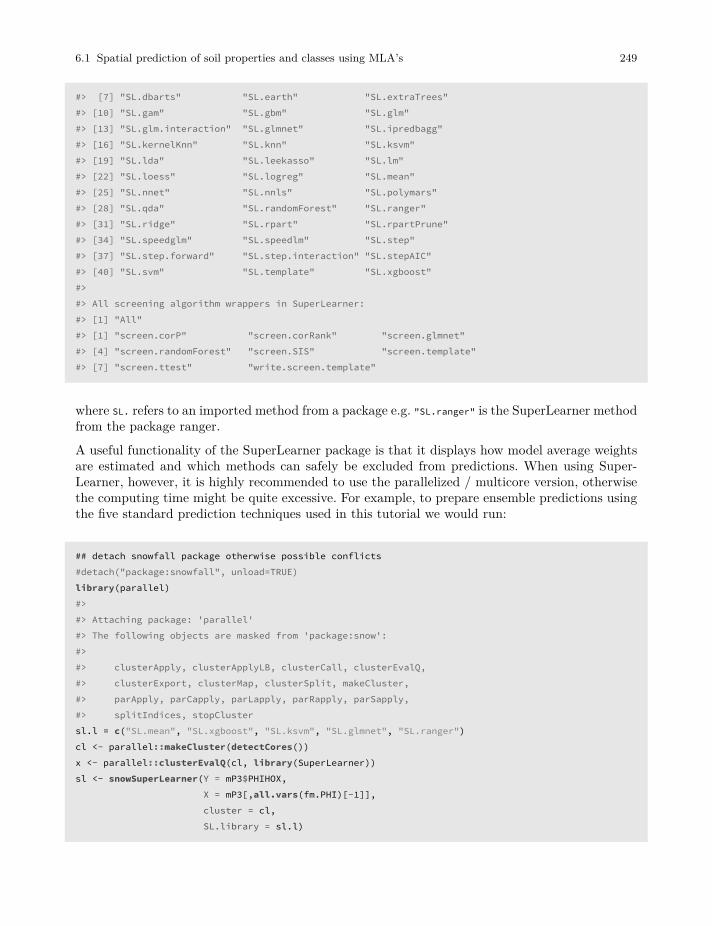
6.1 Spatial prediction of soil properties and classes using MLA’s 249
#> [7] "SL.dbarts" "SL.earth" "SL.extraTrees"#> [10] "SL.gam" "SL.gbm" "SL.glm"#> [13] "SL.glm.interaction" "SL.glmnet" "SL.ipredbagg"#> [16] "SL.kernelKnn" "SL.knn" "SL.ksvm"#> [19] "SL.lda" "SL.leekasso" "SL.lm"#> [22] "SL.loess" "SL.logreg" "SL.mean"#> [25] "SL.nnet" "SL.nnls" "SL.polymars"#> [28] "SL.qda" "SL.randomForest" "SL.ranger"#> [31] "SL.ridge" "SL.rpart" "SL.rpartPrune"#> [34] "SL.speedglm" "SL.speedlm" "SL.step"#> [37] "SL.step.forward" "SL.step.interaction" "SL.stepAIC"#> [40] "SL.svm" "SL.template" "SL.xgboost"#>#> All screening algorithm wrappers in SuperLearner:#> [1] "All"#> [1] "screen.corP" "screen.corRank" "screen.glmnet"#> [4] "screen.randomForest" "screen.SIS" "screen.template"#> [7] "screen.ttest" "write.screen.template"
where SL. refers to an imported method from a package e.g. "SL.ranger" is the SuperLearner methodfrom the package ranger.
A useful functionality of the SuperLearner package is that it displays how model average weightsare estimated and which methods can safely be excluded from predictions. When using Super-Learner, however, it is highly recommended to use the parallelized / multicore version, otherwisethe computing time might be quite excessive. For example, to prepare ensemble predictions usingthe five standard prediction techniques used in this tutorial we would run:
## detach snowfall package otherwise possible conflicts#detach("package:snowfall", unload=TRUE)library(parallel)#>#> Attaching package: 'parallel'#> The following objects are masked from 'package:snow':#>#> clusterApply, clusterApplyLB, clusterCall, clusterEvalQ,#> clusterExport, clusterMap, clusterSplit, makeCluster,#> parApply, parCapply, parLapply, parRapply, parSapply,#> splitIndices, stopClustersl.l = c("SL.mean", "SL.xgboost", "SL.ksvm", "SL.glmnet", "SL.ranger")cl <- parallel::makeCluster(detectCores())x <- parallel::clusterEvalQ(cl, library(SuperLearner))sl <- snowSuperLearner(Y = mP3$PHIHOX,
X = mP3[,all.vars(fm.PHI)[-1]],cluster = cl,SL.library = sl.l)
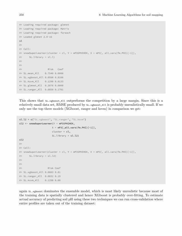
250 6 Machine Learning Algorithms for soil mapping
#> Loading required package: glmnet#> Loading required package: Matrix#> Loading required package: foreach#> Loaded glmnet 2.0-16sl#>#> Call:#> snowSuperLearner(cluster = cl, Y = mP3$PHIHOX, X = mP3[, all.vars(fm.PHI)[-1]],#> SL.library = sl.l)#>#>#> Risk Coef#> SL.mean_All 0.7540 0.0000#> SL.xgboost_All 0.0598 0.8166#> SL.ksvm_All 0.1290 0.0133#> SL.glmnet_All 0.3076 0.0000#> SL.ranger_All 0.0850 0.1701
This shows that SL.xgboost_All outperforms the competition by a large margin. Since this is arelatively small data set, RMSE produced by SL.xgboost_All is probably unrealistically small. If weonly use the top three models (XGboost, ranger and ksvm) in comparison we get:
sl.l2 = c("SL.xgboost", "SL.ranger", "SL.ksvm")sl2 <- snowSuperLearner(Y = mP3$PHIHOX,
X = mP3[,all.vars(fm.PHI)[-1]],cluster = cl,SL.library = sl.l2)
sl2#>#> Call:#> snowSuperLearner(cluster = cl, Y = mP3$PHIHOX, X = mP3[, all.vars(fm.PHI)[-1]],#> SL.library = sl.l2)#>#>#> Risk Coef#> SL.xgboost_All 0.0603 0.81#> SL.ranger_All 0.0832 0.19#> SL.ksvm_All 0.1298 0.00
again SL.xgboost dominates the ensemble model, which is most likely unrealistic because most ofthe training data is spatially clustered and hence XGboost is probably over-fitting. To estimateactual accuracy of predicting soil pH using these two techniques we can run cross-validation whereentire profiles are taken out of the training dataset:
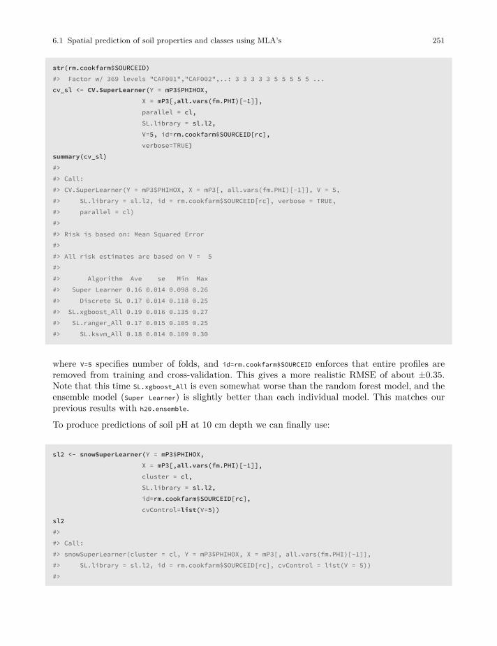
6.1 Spatial prediction of soil properties and classes using MLA’s 251
str(rm.cookfarm$SOURCEID)#> Factor w/ 369 levels "CAF001","CAF002",..: 3 3 3 3 3 5 5 5 5 5 ...cv_sl <- CV.SuperLearner(Y = mP3$PHIHOX,
X = mP3[,all.vars(fm.PHI)[-1]],parallel = cl,SL.library = sl.l2,V=5, id=rm.cookfarm$SOURCEID[rc],verbose=TRUE)
summary(cv_sl)#>#> Call:#> CV.SuperLearner(Y = mP3$PHIHOX, X = mP3[, all.vars(fm.PHI)[-1]], V = 5,#> SL.library = sl.l2, id = rm.cookfarm$SOURCEID[rc], verbose = TRUE,#> parallel = cl)#>#> Risk is based on: Mean Squared Error#>#> All risk estimates are based on V = 5#>#> Algorithm Ave se Min Max#> Super Learner 0.16 0.014 0.098 0.26#> Discrete SL 0.17 0.014 0.118 0.25#> SL.xgboost_All 0.19 0.016 0.135 0.27#> SL.ranger_All 0.17 0.015 0.105 0.25#> SL.ksvm_All 0.18 0.014 0.109 0.30
where V=5 specifies number of folds, and id=rm.cookfarm$SOURCEID enforces that entire profiles areremoved from training and cross-validation. This gives a more realistic RMSE of about ±0.35.Note that this time SL.xgboost_All is even somewhat worse than the random forest model, and theensemble model (Super Learner) is slightly better than each individual model. This matches ourprevious results with h20.ensemble.
To produce predictions of soil pH at 10 cm depth we can finally use:
sl2 <- snowSuperLearner(Y = mP3$PHIHOX,X = mP3[,all.vars(fm.PHI)[-1]],cluster = cl,SL.library = sl.l2,id=rm.cookfarm$SOURCEID[rc],cvControl=list(V=5))
sl2#>#> Call:#> snowSuperLearner(cluster = cl, Y = mP3$PHIHOX, X = mP3[, all.vars(fm.PHI)[-1]],#> SL.library = sl.l2, id = rm.cookfarm$SOURCEID[rc], cvControl = list(V = 5))#>
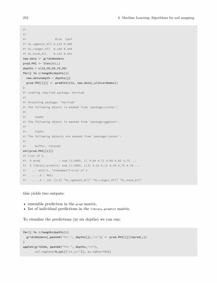
252 6 Machine Learning Algorithms for soil mapping
#>#>#> Risk Coef#> SL.xgboost_All 0.215 0.000#> SL.ranger_All 0.166 0.459#> SL.ksvm_All 0.163 0.541new.data <- [email protected] <- list(NULL)depths = c(10,30,50,70,90)for(j in 1:length(depths)){new.data$depth = depths[j]pred.PHI[[j]] <- predict(sl2, new.data[,sl2$varNames])
}#> Loading required package: kernlab#>#> Attaching package: 'kernlab'#> The following object is masked from 'package:scales':#>#> alpha#> The following object is masked from 'package:ggplot2':#>#> alpha#> The following objects are masked from 'package:raster':#>#> buffer, rotatedstr(pred.PHI[[1]])#> List of 2#> $ pred : num [1:3865, 1] 4.64 4.71 4.85 4.82 4.75 ...#> $ library.predict: num [1:3865, 1:3] 4.15 4.11 4.45 4.75 4.78 ...#> ..- attr(*, "dimnames")=List of 2#> .. ..$ : NULL#> .. ..$ : chr [1:3] "SL.xgboost_All" "SL.ranger_All" "SL.ksvm_All"
this yields two outputs:
• ensemble prediction in the pred matrix,• list of individual predictions in the library.predict matrix,
To visualize the predictions (at six depths) we can run:
for(j in 1:length(depths)){grid10m@data[,paste0("PHI.", depths[j],"cm")] <- pred.PHI[[j]]$pred[,1]
}spplot(grid10m, paste0("PHI.", depths,"cm"),
col.regions=R_pal[["pH_pal"]], as.table=TRUE)
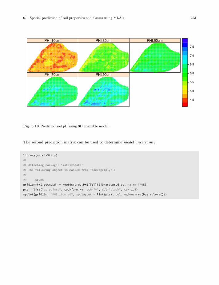
6.1 Spatial prediction of soil properties and classes using MLA’s 253
PHI.10cm PHI.30cm PHI.50cm
PHI.70cm PHI.90cm
4.5
5.0
5.5
6.0
6.5
7.0
7.5
Fig. 6.10 Predicted soil pH using 3D ensemble model.
The second prediction matrix can be used to determine model uncertainty:
library(matrixStats)#>#> Attaching package: 'matrixStats'#> The following object is masked from 'package:plyr':#>#> countgrid10m$PHI.10cm.sd <- rowSds(pred.PHI[[1]]$library.predict, na.rm=TRUE)pts = list("sp.points", cookfarm.xy, pch="+", col="black", cex=1.4)spplot(grid10m, "PHI.10cm.sd", sp.layout = list(pts), col.regions=rev(bpy.colors()))
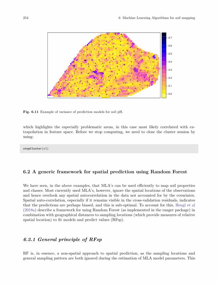
254 6 Machine Learning Algorithms for soil mapping
+ + + + + + + ++ ++ + + + + +
+ + + ++ + + + + + + + + ++ + +
++ + + + + +
+ + + + + ++
+ + + + + + + ++
+ + + ++ + + + + + + +
++ + + +
+ + + + + ++ + + + + + +
+ + + + + ++ + + + + +
+ + + + ++ + + + + + +
++ + + + + + +
+ + + ++ + + + + +
++ + + + +
+ + + ++
+ + + + + +
+ + + ++ + + + + +
+ + + + ++
+ ++ + +
+ + ++ + ++
+ ++ +
+ ++ + + +
0.0
0.1
0.2
0.3
0.4
0.5
0.6
0.7
Fig. 6.11 Example of variance of prediction models for soil pH.
which highlights the especially problematic areas, in this case most likely correlated with ex-trapolation in feature space. Before we stop computing, we need to close the cluster session byusing:
stopCluster(cl)
6.2 A generic framework for spatial prediction using Random Forest
We have seen, in the above examples, that MLA’s can be used efficiently to map soil propertiesand classes. Most currently used MLA’s, however, ignore the spatial locations of the observationsand hence overlook any spatial autocorrelation in the data not accounted for by the covariates.Spatial auto-correlation, especially if it remains visible in the cross-validation residuals, indicatesthat the predictions are perhaps biased, and this is sub-optimal. To account for this, Hengl et al(2018a) describe a framework for using Random Forest (as implemented in the ranger package) incombination with geographical distances to sampling locations (which provide measures of relativespatial location) to fit models and predict values (RFsp).
6.2.1 General principle of RFsp
RF is, in essence, a non-spatial approach to spatial prediction, as the sampling locations andgeneral sampling pattern are both ignored during the estimation of MLA model parameters. This
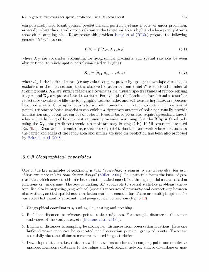
6.2 A generic framework for spatial prediction using Random Forest 255
can potentially lead to sub-optimal predictions and possibly systematic over- or under-prediction,especially where the spatial autocorrelation in the target variable is high and where point patternsshow clear sampling bias. To overcome this problem Hengl et al (2018a) propose the followinggeneric “RFsp” system:
𝑌 (s) = 𝑓 (X𝐺, X𝑅, X𝑃 ) (6.1)
where X𝐺 are covariates accounting for geographical proximity and spatial relations betweenobservations (to mimic spatial correlation used in kriging):
X𝐺 = (𝑑𝑝1, 𝑑𝑝2, … , 𝑑𝑝𝑁) (6.2)
where 𝑑𝑝𝑖 is the buffer distance (or any other complex proximity upslope/downslope distance, asexplained in the next section) to the observed location 𝑝𝑖 from s and 𝑁 is the total number oftraining points. X𝑅 are surface reflectance covariates, i.e. usually spectral bands of remote sensingimages, and X𝑃 are process-based covariates. For example, the Landsat infrared band is a surfacereflectance covariate, while the topographic wetness index and soil weathering index are process-based covariates. Geographic covariates are often smooth and reflect geometric composition ofpoints, reflectance-based covariates can exhibit a significant amount of noise and usually provideinformation only about the surface of objects. Process-based covariates require specialized knowl-edge and rethinking of how to best represent processes. Assuming that the RFsp is fitted onlyusing the XG, the predictions would resemble ordinary kriging (OK). If All covariates are usedEq. (6.1), RFsp would resemble regression-kriging (RK). Similar framework where distances tothe center and edges of the study area and similar are used for prediction has been also proposedby Behrens et al (2018c).
6.2.2 Geographical covariates
One of the key principles of geography is that “everything is related to everything else, but nearthings are more related than distant things” (Miller, 2004). This principle forms the basis of geo-statistics, which converts this rule into a mathematical model, i.e., through spatial autocorrelationfunctions or variograms. The key to making RF applicable to spatial statistics problems, there-fore, lies also in preparing geographical (spatial) measures of proximity and connectivity betweenobservations, so that spatial autocorrelation can be accounted for. There are multiple options forvariables that quantify proximity and geographical connection (Fig. 6.12):
1. Geographical coordinates 𝑠1 and 𝑠2, i.e., easting and northing.2. Euclidean distances to reference points in the study area. For example, distance to the center
and edges of the study area, etc (Behrens et al, 2018c).3. Euclidean distances to sampling locations, i.e., distances from observation locations. Here one
buffer distance map can be generated per observation point or group of points. These areessentially the same distance measures as used in geostatistics.
4. Downslope distances, i.e., distances within a watershed: for each sampling point one can deriveupslope/downslope distances to the ridges and hydrological network and/or downslope or ups-
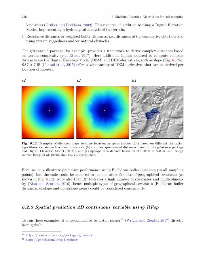
256 6 Machine Learning Algorithms for soil mapping
lope areas (Gruber and Peckham, 2009). This requires, in addition to using a Digital ElevationModel, implementing a hydrological analysis of the terrain.
5. Resistance distances or weighted buffer distances, i.e., distances of the cumulative effort derivedusing terrain ruggedness and/or natural obstacles.
The gdistance14 package, for example, provides a framework to derive complex distances basedon terrain complexity (van Etten, 2017). Here additional inputs required to compute complexdistances are the Digital Elevation Model (DEM) and DEM-derivatives, such as slope (Fig. 6.12b).SAGA GIS (Conrad et al, 2015) offers a wide variety of DEM derivatives that can be derived perlocation of interest.
Fig. 6.12 Examples of distance maps to some location in space (yellow dot) based on different derivationalgorithms: (a) simple Euclidean distances, (b) complex speed-based distances based on the gdistance packageand Digital Elevation Model (DEM), and (c) upslope area derived based on the DEM in SAGA GIS. Imagesource: Hengl et al. (2018) doi: 10.7717/peerj.5518.
Here, we only illustrate predictive performance using Euclidean buffer distances (to all samplingpoints), but the code could be adapted to include other families of geographical covariates (asshown in Fig. 6.12). Note also that RF tolerates a high number of covariates and multicolinear-ity (Biau and Scornet, 2016), hence multiple types of geographical covariates (Euclidean bufferdistances, upslope and downslope areas) could be considered concurrently.
6.2.3 Spatial prediction 2D continuous variable using RFsp
To run these examples, it is recommended to install ranger15 (Wright and Ziegler, 2017) directlyfrom github:
14 https://cran.r-project.org/package=gdistance15 https://github.com/imbs-hl/ranger
6.2 A generic framework for spatial prediction using Random Forest 257
if(!require(ranger)){ devtools::install_github("imbs-hl/ranger") }
Quantile regression random forest and derivation of standard errors using Jackknifing is availablefrom ranger version >0.9.4. Other packages that we use here include:
library(GSIF)library(rgdal)#> rgdal: version: 1.3-6, (SVN revision 773)#> Geospatial Data Abstraction Library extensions to R successfully loaded#> Loaded GDAL runtime: GDAL 2.2.2, released 2017/09/15#> Path to GDAL shared files: /usr/share/gdal/2.2#> GDAL binary built with GEOS: TRUE#> Loaded PROJ.4 runtime: Rel. 4.8.0, 6 March 2012, [PJ_VERSION: 480]#> Path to PROJ.4 shared files: (autodetected)#> Linking to sp version: 1.3-1library(raster)library(geoR)#> Warning: no DISPLAY variable so Tk is not available#> --------------------------------------------------------------#> Analysis of Geostatistical Data#> For an Introduction to geoR go to http://www.leg.ufpr.br/geoR#> geoR version 1.7-5.2.1 (built on 2016-05-02) is now loaded#> --------------------------------------------------------------library(ranger)
#>#> Attaching package: 'gridExtra'#> The following object is masked from 'package:randomForest':#>#> combine
If no other information is available, we can use buffer distances to all points as covariates to predictvalues of some continuous or categorical variable in the RFsp framework. These can be derivedwith the help of the raster16 package (Hijmans and van Etten, 2017). Consider for example themeuse data set from the sp package:
demo(meuse, echo=FALSE)
We can derive buffer distance by using:
16 https://cran.r-project.org/package=raster
258 6 Machine Learning Algorithms for soil mapping
grid.dist0 <- GSIF::buffer.dist(meuse["zinc"], meuse.grid[1], as.factor(1:nrow(meuse)))
which requires a few seconds, as it generates 155 individual gridded maps. The value of the targetvariable zinc can be now modeled as a function of these computed buffer distances:
dn0 <- paste(names(grid.dist0), collapse="+")fm0 <- as.formula(paste("zinc ~ ", dn0))fm0#> zinc ~ layer.1 + layer.2 + layer.3 + layer.4 + layer.5 + layer.6 +#> layer.7 + layer.8 + layer.9 + layer.10 + layer.11 + layer.12 +#> layer.13 + layer.14 + layer.15 + layer.16 + layer.17 + layer.18 +#> layer.19 + layer.20 + layer.21 + layer.22 + layer.23 + layer.24 +#> layer.25 + layer.26 + layer.27 + layer.28 + layer.29 + layer.30 +#> layer.31 + layer.32 + layer.33 + layer.34 + layer.35 + layer.36 +#> layer.37 + layer.38 + layer.39 + layer.40 + layer.41 + layer.42 +#> layer.43 + layer.44 + layer.45 + layer.46 + layer.47 + layer.48 +#> layer.49 + layer.50 + layer.51 + layer.52 + layer.53 + layer.54 +#> layer.55 + layer.56 + layer.57 + layer.58 + layer.59 + layer.60 +#> layer.61 + layer.62 + layer.63 + layer.64 + layer.65 + layer.66 +#> layer.67 + layer.68 + layer.69 + layer.70 + layer.71 + layer.72 +#> layer.73 + layer.74 + layer.75 + layer.76 + layer.77 + layer.78 +#> layer.79 + layer.80 + layer.81 + layer.82 + layer.83 + layer.84 +#> layer.85 + layer.86 + layer.87 + layer.88 + layer.89 + layer.90 +#> layer.91 + layer.92 + layer.93 + layer.94 + layer.95 + layer.96 +#> layer.97 + layer.98 + layer.99 + layer.100 + layer.101 +#> layer.102 + layer.103 + layer.104 + layer.105 + layer.106 +#> layer.107 + layer.108 + layer.109 + layer.110 + layer.111 +#> layer.112 + layer.113 + layer.114 + layer.115 + layer.116 +#> layer.117 + layer.118 + layer.119 + layer.120 + layer.121 +#> layer.122 + layer.123 + layer.124 + layer.125 + layer.126 +#> layer.127 + layer.128 + layer.129 + layer.130 + layer.131 +#> layer.132 + layer.133 + layer.134 + layer.135 + layer.136 +#> layer.137 + layer.138 + layer.139 + layer.140 + layer.141 +#> layer.142 + layer.143 + layer.144 + layer.145 + layer.146 +#> layer.147 + layer.148 + layer.149 + layer.150 + layer.151 +#> layer.152 + layer.153 + layer.154 + layer.155
Subsequent analysis is similar to any regression analysis using the ranger package17. First weoverlay points and grids to create a regression matrix:
ov.zinc <- over(meuse["zinc"], grid.dist0)rm.zinc <- cbind(meuse@data["zinc"], ov.zinc)
17 https://github.com/imbs-hl/ranger

6.2 A generic framework for spatial prediction using Random Forest 259
to estimate also the prediction error variance i.e. prediction intervals we set quantreg=TRUE whichinitiates the Quantile Regression RF approach (Meinshausen, 2006):
m.zinc <- ranger(fm0, rm.zinc, quantreg=TRUE, num.trees=150, seed=1)m.zinc#> Ranger result#>#> Call:#> ranger(fm0, rm.zinc, quantreg = TRUE, num.trees = 150, seed = 1)#>#> Type: Regression#> Number of trees: 150#> Sample size: 155#> Number of independent variables: 155#> Mtry: 12#> Target node size: 5#> Variable importance mode: none#> Splitrule: variance#> OOB prediction error (MSE): 67501#> R squared (OOB): 0.499
This shows that, using only buffer distance explains almost 50% of the variation in the targetvariable. To generate predictions for the zinc variable and using the RFsp model, we use:
q <- c((1-.682)/2, 0.5, 1-(1-.682)/2)zinc.rfd <- predict(m.zinc, grid.dist0@data,
type="quantiles", quantiles=q)$predictionsstr(zinc.rfd)#> num [1:3103, 1:3] 257 257 257 257 257 ...#> - attr(*, "dimnames")=List of 2#> ..$ : NULL#> ..$ : chr [1:3] "quantile= 0.159" "quantile= 0.5" "quantile= 0.841"
this will estimate 67% probability lower and upper limits and median value. Note that “median”can often be different from the “mean”, so, if you prefer to derive mean, then the quantreg=FALSEneeds to be used as the Quantile Regression Forests approach can only derive median.To be able to plot or export the predicted values as maps, we add them to the spatial pixels object:
meuse.grid$zinc_rfd = zinc.rfd[,2]meuse.grid$zinc_rfd_range = (zinc.rfd[,3]-zinc.rfd[,1])/2
We can compare the RFsp approach with the model-based geostatistics approach (see e.g. geoRpackage18), where we first decide about the transformation, then fit the variogram of the targetvariable (Diggle and Ribeiro Jr, 2007; Brown, 2015):18 http://leg.ufpr.br/geoR/geoRdoc/geoRintro.html

260 6 Machine Learning Algorithms for soil mapping
zinc.geo <- as.geodata(meuse["zinc"])ini.v <- c(var(log1p(zinc.geo$data)),500)zinc.vgm <- likfit(zinc.geo, lambda=0, ini=ini.v, cov.model="exponential")#> kappa not used for the exponential correlation function#> ---------------------------------------------------------------#> likfit: likelihood maximisation using the function optim.#> likfit: Use control() to pass additional#> arguments for the maximisation function.#> For further details see documentation for optim.#> likfit: It is highly advisable to run this function several#> times with different initial values for the parameters.#> likfit: WARNING: This step can be time demanding!#> ---------------------------------------------------------------#> likfit: end of numerical maximisation.zinc.vgm#> likfit: estimated model parameters:#> beta tausq sigmasq phi#> " 6.1553" " 0.0164" " 0.5928" "500.0001"#> Practical Range with cor=0.05 for asymptotic range: 1498#>#> likfit: maximised log-likelihood = -1014
where likfit function fits a log-likelihood based variogram. Note that here we need to manuallyspecify log-transformation via the lambda parameter. To generate predictions and kriging varianceusing geoR we run:
locs <- [email protected] <- krige.conv(zinc.geo, locations=locs, krige=krige.control(obj.model=zinc.vgm))#> krige.conv: model with constant mean#> krige.conv: performing the Box-Cox data transformation#> krige.conv: back-transforming the predicted mean and variance#> krige.conv: Kriging performed using global neighbourhoodmeuse.grid$zinc_ok <- zinc.ok$predictmeuse.grid$zinc_ok_range <- sqrt(zinc.ok$krige.var)
in this case geoR automatically back-transforms values to the original scale, which is a recom-mended feature. Comparison of predictions and prediction error maps produced using geoR (or-dinary kriging) and RFsp (with buffer distances and using just coordinates) is given in Fig. 6.13.
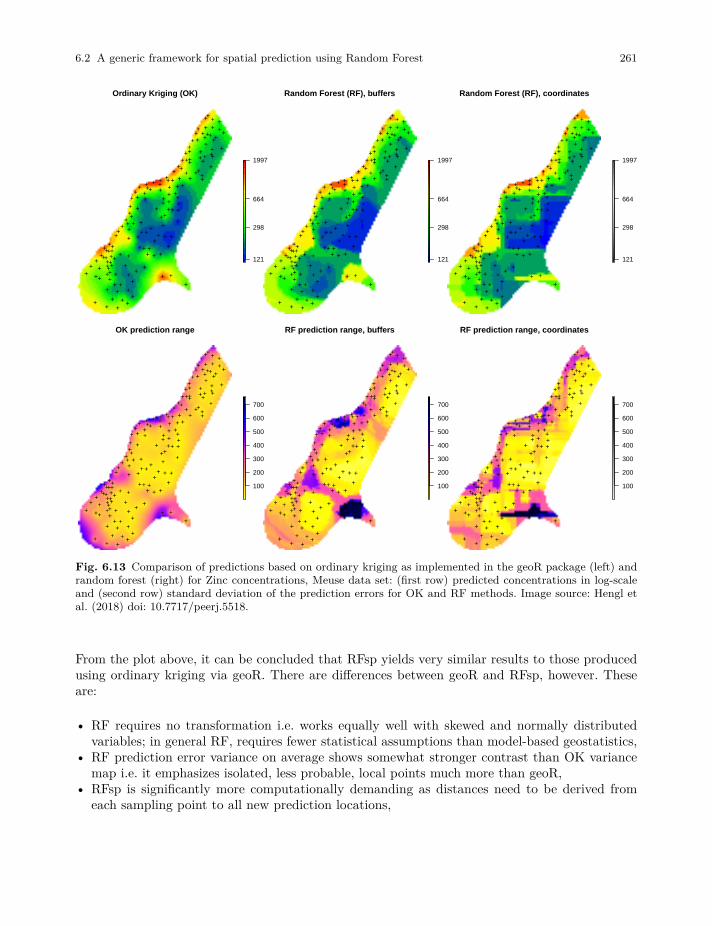
6.2 A generic framework for spatial prediction using Random Forest 261
Ordinary Kriging (OK)
121
298
664
1997
++ + +++
+++ +++
+++
++
++
++++
++++
++
+
+++ +
+++
++++++
+
+++++
++
++++++
++
++++
++
++
++
+++
+ ++++
+++
+
+
+
+
++
++
++ ++
+
++
+
+++
+ ++
+
+
++
+
++
++
++
+++
+
+
++
+++
+
+++
+
+
+
+
+
+
+
++
+
+++
+ ++
++++
+ ++
+++ +
+
Random Forest (RF), buffers
121
298
664
1997
++ + +++
+++ +++
+++
++
++
++++
++++
++
+
+++ +
+++
++++++
+
+++++
++
++++++
++
++++
++
++
++
+++
+ ++++
+++
+
+
+
+
++
++
++ ++
+
++
+
+++
+ ++
+
+
++
+
++
++
++
+++
+
+
++
+++
+
+++
+
+
+
+
+
+
+
++
+
+++
+ ++
++++
+ ++
+++ +
+
Random Forest (RF), coordinates
121
298
664
1997
++ + +++
+++ +++
+++
++
++
++++
++++
++
+
+++ +
+++
++++++
+
+++++
++
++++++
++
++++
++
++
++
+++
+ ++++
+++
+
+
+
+
++
++
++ ++
+
++
+
+++
+ ++
+
+
++
+
++
++
++
+++
+
+
++
+++
+
+++
+
+
+
+
+
+
+
++
+
+++
+ ++
++++
+ ++
+++ +
+
OK prediction range
100
200
300
400
500
600
700
++ + +++
+++ +++
+++
++
++
++++
++++
++
+
+++ +
+++
++++++
+
+++++
++
++++++
++
++++
++
++
++
+++
+ ++++
+++
+
+
+
+
++
++
++ ++
+
++
+
+++
+ ++
+
+
++
+
++
++
++
+++
+
+
++
+++
+
+++
+
+
+
+
+
+
+
++
+
+++
+ ++
++++
+ ++
+++ +
+
RF prediction range, buffers
100
200
300
400
500
600
700
++ + +++
+++ +++
+++
++
++
++++
++++
++
+
+++ +
+++
++++++
+
+++++
++
++++++
++
++++
++
++
++
+++
+ ++++
+++
+
+
+
+
++
++
++ ++
+
++
+
+++
+ ++
+
+
++
+
++
++
++
+++
+
+
++
+++
+
+++
+
+
+
+
+
+
+
++
+
+++
+ ++
++++
+ ++
+++ +
+
RF prediction range, coordinates
100
200
300
400
500
600
700
++ + +++
+++ +++
+++
++
++
++++
++++
++
+
+++ +
+++
++++++
+
+++++
++
++++++
++
++++
++
++
++
+++
+ ++++
+++
+
+
+
+
++
++
++ ++
+
++
+
+++
+ ++
+
+
++
+
++
++
++
+++
+
+
++
+++
+
+++
+
+
+
+
+
+
+
++
+
+++
+ ++
++++
+ ++
+++ +
+
Fig. 6.13 Comparison of predictions based on ordinary kriging as implemented in the geoR package (left) andrandom forest (right) for Zinc concentrations, Meuse data set: (first row) predicted concentrations in log-scaleand (second row) standard deviation of the prediction errors for OK and RF methods. Image source: Hengl etal. (2018) doi: 10.7717/peerj.5518.
From the plot above, it can be concluded that RFsp yields very similar results to those producedusing ordinary kriging via geoR. There are differences between geoR and RFsp, however. Theseare:
• RF requires no transformation i.e. works equally well with skewed and normally distributedvariables; in general RF, requires fewer statistical assumptions than model-based geostatistics,
• RF prediction error variance on average shows somewhat stronger contrast than OK variancemap i.e. it emphasizes isolated, less probable, local points much more than geoR,
• RFsp is significantly more computationally demanding as distances need to be derived fromeach sampling point to all new prediction locations,
262 6 Machine Learning Algorithms for soil mapping
• geoR uses global model parameters and, as such, prediction patterns are also relatively uniform,RFsp on the other hand (being tree-based) will produce patterns that match the data as muchas possible.
6.2.4 Spatial prediction 2D variable with covariates using RFsp
Next, we can also consider adding additional covariates that describe soil forming processes orcharacteristics of the land to the list of buffer distances. For example, we can add covariates forsurface water occurrence (Pekel et al, 2016) and elevation (AHN19):
f1 = "extdata/Meuse_GlobalSurfaceWater_occurrence.tif"f2 = "extdata/ahn.asc"meuse.grid$SW_occurrence <- readGDAL(f1)$band1[[email protected]]#> extdata/Meuse_GlobalSurfaceWater_occurrence.tif has GDAL driver GTiff#> and has 104 rows and 78 columnsmeuse.grid$AHN = readGDAL(f2)$band1[[email protected]]#> extdata/ahn.asc has GDAL driver AAIGrid#> and has 104 rows and 78 columns
to convert all covariates to numeric values and fill in all missing pixels we use Principal Componenttransformation:
grids.spc <- GSIF::spc(meuse.grid, as.formula("~ SW_occurrence + AHN + ffreq + dist"))#> Converting ffreq to indicators...#> Converting covariates to principal components...
so that we can fit a ranger model using both geographical covariates (buffer distances) and envi-ronmental covariates imported previously:
nms <- paste(names(grids.spc@predicted), collapse = "+")fm1 <- as.formula(paste("zinc ~ ", dn0, " + ", nms))fm1#> zinc ~ layer.1 + layer.2 + layer.3 + layer.4 + layer.5 + layer.6 +#> layer.7 + layer.8 + layer.9 + layer.10 + layer.11 + layer.12 +#> layer.13 + layer.14 + layer.15 + layer.16 + layer.17 + layer.18 +#> layer.19 + layer.20 + layer.21 + layer.22 + layer.23 + layer.24 +#> layer.25 + layer.26 + layer.27 + layer.28 + layer.29 + layer.30 +#> layer.31 + layer.32 + layer.33 + layer.34 + layer.35 + layer.36 +#> layer.37 + layer.38 + layer.39 + layer.40 + layer.41 + layer.42 +#> layer.43 + layer.44 + layer.45 + layer.46 + layer.47 + layer.48 +
19 http://ahn.nl
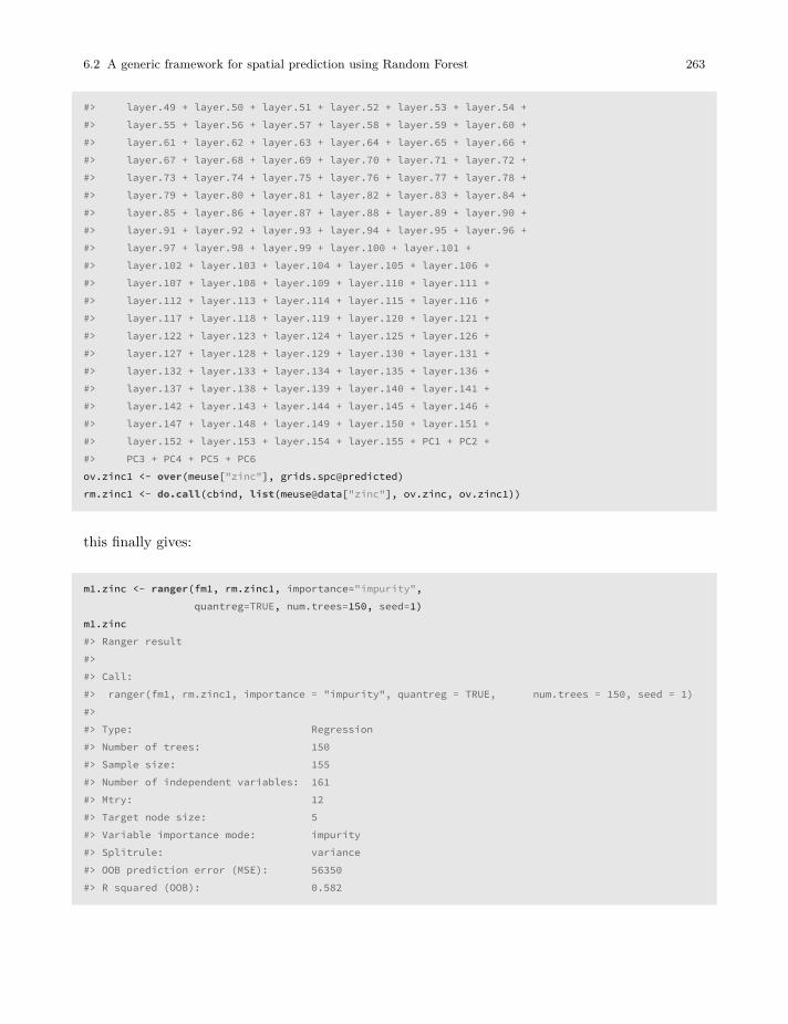
6.2 A generic framework for spatial prediction using Random Forest 263
#> layer.49 + layer.50 + layer.51 + layer.52 + layer.53 + layer.54 +#> layer.55 + layer.56 + layer.57 + layer.58 + layer.59 + layer.60 +#> layer.61 + layer.62 + layer.63 + layer.64 + layer.65 + layer.66 +#> layer.67 + layer.68 + layer.69 + layer.70 + layer.71 + layer.72 +#> layer.73 + layer.74 + layer.75 + layer.76 + layer.77 + layer.78 +#> layer.79 + layer.80 + layer.81 + layer.82 + layer.83 + layer.84 +#> layer.85 + layer.86 + layer.87 + layer.88 + layer.89 + layer.90 +#> layer.91 + layer.92 + layer.93 + layer.94 + layer.95 + layer.96 +#> layer.97 + layer.98 + layer.99 + layer.100 + layer.101 +#> layer.102 + layer.103 + layer.104 + layer.105 + layer.106 +#> layer.107 + layer.108 + layer.109 + layer.110 + layer.111 +#> layer.112 + layer.113 + layer.114 + layer.115 + layer.116 +#> layer.117 + layer.118 + layer.119 + layer.120 + layer.121 +#> layer.122 + layer.123 + layer.124 + layer.125 + layer.126 +#> layer.127 + layer.128 + layer.129 + layer.130 + layer.131 +#> layer.132 + layer.133 + layer.134 + layer.135 + layer.136 +#> layer.137 + layer.138 + layer.139 + layer.140 + layer.141 +#> layer.142 + layer.143 + layer.144 + layer.145 + layer.146 +#> layer.147 + layer.148 + layer.149 + layer.150 + layer.151 +#> layer.152 + layer.153 + layer.154 + layer.155 + PC1 + PC2 +#> PC3 + PC4 + PC5 + PC6ov.zinc1 <- over(meuse["zinc"], grids.spc@predicted)rm.zinc1 <- do.call(cbind, list(meuse@data["zinc"], ov.zinc, ov.zinc1))
this finally gives:
m1.zinc <- ranger(fm1, rm.zinc1, importance="impurity",quantreg=TRUE, num.trees=150, seed=1)
m1.zinc#> Ranger result#>#> Call:#> ranger(fm1, rm.zinc1, importance = "impurity", quantreg = TRUE, num.trees = 150, seed = 1)#>#> Type: Regression#> Number of trees: 150#> Sample size: 155#> Number of independent variables: 161#> Mtry: 12#> Target node size: 5#> Variable importance mode: impurity#> Splitrule: variance#> OOB prediction error (MSE): 56350#> R squared (OOB): 0.582
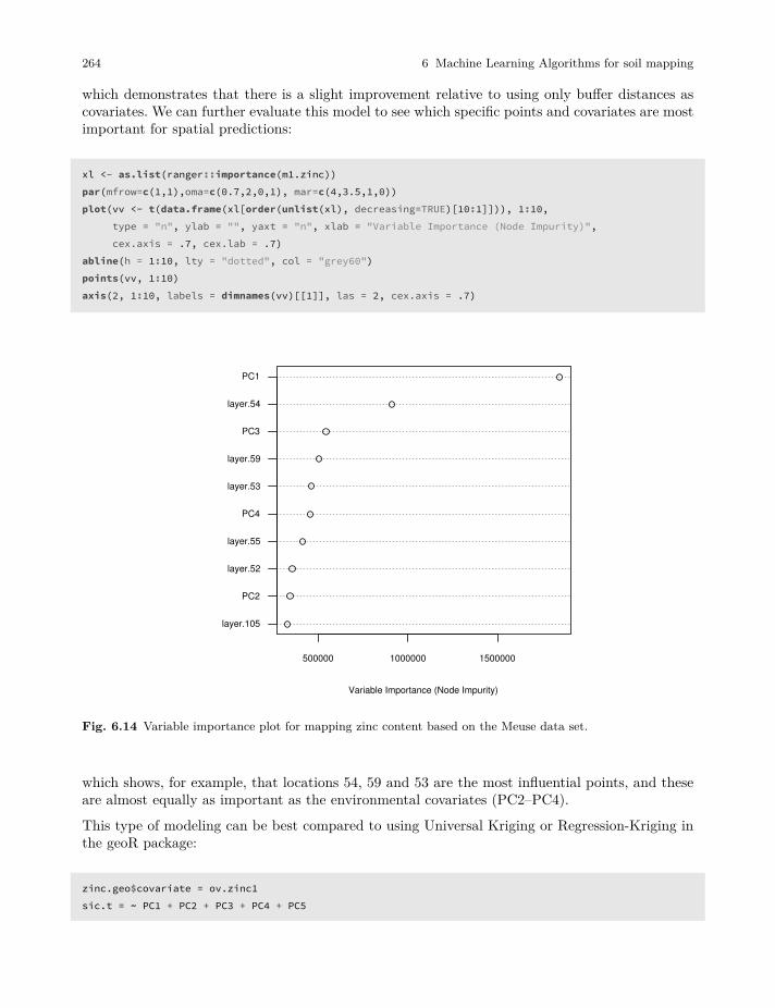
264 6 Machine Learning Algorithms for soil mapping
which demonstrates that there is a slight improvement relative to using only buffer distances ascovariates. We can further evaluate this model to see which specific points and covariates are mostimportant for spatial predictions:
xl <- as.list(ranger::importance(m1.zinc))par(mfrow=c(1,1),oma=c(0.7,2,0,1), mar=c(4,3.5,1,0))plot(vv <- t(data.frame(xl[order(unlist(xl), decreasing=TRUE)[10:1]])), 1:10,
type = "n", ylab = "", yaxt = "n", xlab = "Variable Importance (Node Impurity)",cex.axis = .7, cex.lab = .7)
abline(h = 1:10, lty = "dotted", col = "grey60")points(vv, 1:10)axis(2, 1:10, labels = dimnames(vv)[[1]], las = 2, cex.axis = .7)
500000 1000000 1500000
Variable Importance (Node Impurity)
layer.105
PC2
layer.52
layer.55
PC4
layer.53
layer.59
PC3
layer.54
PC1
Fig. 6.14 Variable importance plot for mapping zinc content based on the Meuse data set.
which shows, for example, that locations 54, 59 and 53 are the most influential points, and theseare almost equally as important as the environmental covariates (PC2–PC4).
This type of modeling can be best compared to using Universal Kriging or Regression-Kriging inthe geoR package:
zinc.geo$covariate = ov.zinc1sic.t = ~ PC1 + PC2 + PC3 + PC4 + PC5
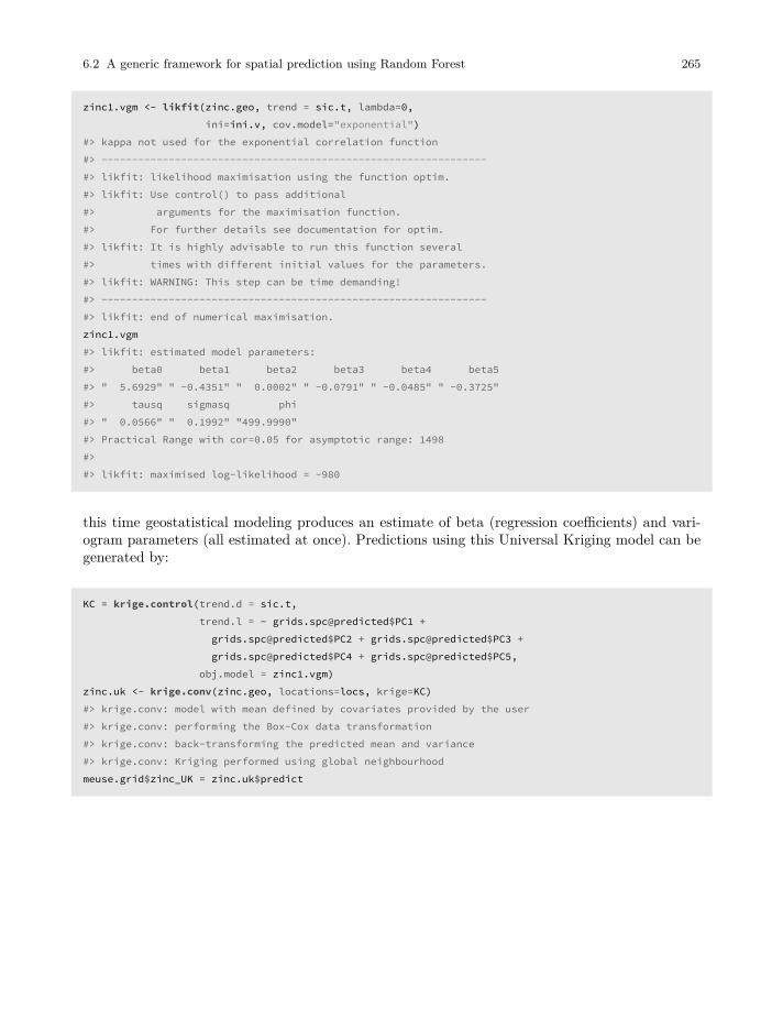
6.2 A generic framework for spatial prediction using Random Forest 265
zinc1.vgm <- likfit(zinc.geo, trend = sic.t, lambda=0,ini=ini.v, cov.model="exponential")
#> kappa not used for the exponential correlation function#> ---------------------------------------------------------------#> likfit: likelihood maximisation using the function optim.#> likfit: Use control() to pass additional#> arguments for the maximisation function.#> For further details see documentation for optim.#> likfit: It is highly advisable to run this function several#> times with different initial values for the parameters.#> likfit: WARNING: This step can be time demanding!#> ---------------------------------------------------------------#> likfit: end of numerical maximisation.zinc1.vgm#> likfit: estimated model parameters:#> beta0 beta1 beta2 beta3 beta4 beta5#> " 5.6929" " -0.4351" " 0.0002" " -0.0791" " -0.0485" " -0.3725"#> tausq sigmasq phi#> " 0.0566" " 0.1992" "499.9990"#> Practical Range with cor=0.05 for asymptotic range: 1498#>#> likfit: maximised log-likelihood = -980
this time geostatistical modeling produces an estimate of beta (regression coefficients) and vari-ogram parameters (all estimated at once). Predictions using this Universal Kriging model can begenerated by:
KC = krige.control(trend.d = sic.t,trend.l = ~ grids.spc@predicted$PC1 +
grids.spc@predicted$PC2 + grids.spc@predicted$PC3 +grids.spc@predicted$PC4 + grids.spc@predicted$PC5,
obj.model = zinc1.vgm)zinc.uk <- krige.conv(zinc.geo, locations=locs, krige=KC)#> krige.conv: model with mean defined by covariates provided by the user#> krige.conv: performing the Box-Cox data transformation#> krige.conv: back-transforming the predicted mean and variance#> krige.conv: Kriging performed using global neighbourhoodmeuse.grid$zinc_UK = zinc.uk$predict
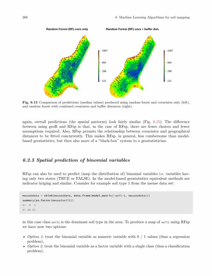
266 6 Machine Learning Algorithms for soil mapping
Random Forest (RF) covs only
121
298
664
1997
++ + +++
+++ +++
+++++
++
++++
++++++
+
+++ +++++++
+++
+
+++++
++
+++++++
++
+++
++
++
++
++++++++
++++
+
+
+
++
++
++ ++
+
++
++++
+ + ++
++ +
++
+++
++++
++
+
++
+++
++
++
+
++
+
+
+
+
+++
+++
+ ++
+++++ +
++
++ ++
Random Forest (RF) covs + buffer dist.
121
298
664
1997
++ + +++
+++ +++
+++++
++
++++
++++++
+
+++ +++++++
+++
+
+++++
++
+++++++
++
+++
++
++
++
++++++++
++++
+
+
+
++
++
++ ++
+
++
++++
+ + ++
++ +
++
+++
++++
++
+
++
+++
++
++
+
++
+
+
+
+
+++
+++
+ ++
+++++ +
++
++ ++
Fig. 6.15 Comparison of predictions (median values) produced using random forest and covariates only (left),and random forest with combined covariates and buffer distances (right).
again, overall predictions (the spatial patterns) look fairly similar (Fig. 6.15). The differencebetween using geoR and RFsp is that, in the case of RFsp, there are fewer choices and fewerassumptions required. Also, RFsp permits the relationship between covariates and geographicaldistances to be fitted concurrently. This makes RFsp, in general, less cumbersome than model-based geostatistics, but then also more of a “black-box” system to a geostatistician.
6.2.5 Spatial prediction of binomial variables
RFsp can also be used to predict (map the distribution of) binomial variables i.e. variables hav-ing only two states (TRUE or FALSE). In the model-based geostatistics equivalent methods areindicator kriging and similar. Consider for example soil type 1 from the meuse data set:
meuse@data = cbind(meuse@data, data.frame(model.matrix(~soil-1, meuse@data)))summary(as.factor(meuse$soil1))#> 0 1#> 58 97
in this case class soil1 is the dominant soil type in the area. To produce a map of soil1 using RFspwe have now two options:
• Option 1: treat the binomial variable as numeric variable with 0 / 1 values (thus a regressionproblem),
• Option 2: treat the binomial variable as a factor variable with a single class (thus a classificationproblem),
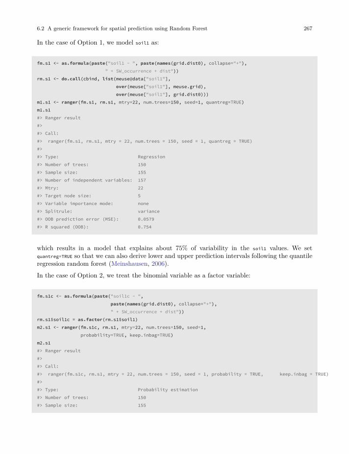
6.2 A generic framework for spatial prediction using Random Forest 267
In the case of Option 1, we model soil1 as:
fm.s1 <- as.formula(paste("soil1 ~ ", paste(names(grid.dist0), collapse="+")," + SW_occurrence + dist"))
rm.s1 <- do.call(cbind, list(meuse@data["soil1"],over(meuse["soil1"], meuse.grid),over(meuse["soil1"], grid.dist0)))
m1.s1 <- ranger(fm.s1, rm.s1, mtry=22, num.trees=150, seed=1, quantreg=TRUE)m1.s1#> Ranger result#>#> Call:#> ranger(fm.s1, rm.s1, mtry = 22, num.trees = 150, seed = 1, quantreg = TRUE)#>#> Type: Regression#> Number of trees: 150#> Sample size: 155#> Number of independent variables: 157#> Mtry: 22#> Target node size: 5#> Variable importance mode: none#> Splitrule: variance#> OOB prediction error (MSE): 0.0579#> R squared (OOB): 0.754
which results in a model that explains about 75% of variability in the soil1 values. We setquantreg=TRUE so that we can also derive lower and upper prediction intervals following the quantileregression random forest (Meinshausen, 2006).
In the case of Option 2, we treat the binomial variable as a factor variable:
fm.s1c <- as.formula(paste("soil1c ~ ",paste(names(grid.dist0), collapse="+")," + SW_occurrence + dist"))
rm.s1$soil1c = as.factor(rm.s1$soil1)m2.s1 <- ranger(fm.s1c, rm.s1, mtry=22, num.trees=150, seed=1,
probability=TRUE, keep.inbag=TRUE)m2.s1#> Ranger result#>#> Call:#> ranger(fm.s1c, rm.s1, mtry = 22, num.trees = 150, seed = 1, probability = TRUE, keep.inbag = TRUE)#>#> Type: Probability estimation#> Number of trees: 150#> Sample size: 155
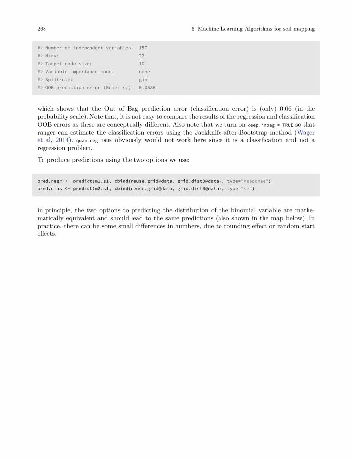
268 6 Machine Learning Algorithms for soil mapping
#> Number of independent variables: 157#> Mtry: 22#> Target node size: 10#> Variable importance mode: none#> Splitrule: gini#> OOB prediction error (Brier s.): 0.0586
which shows that the Out of Bag prediction error (classification error) is (only) 0.06 (in theprobability scale). Note that, it is not easy to compare the results of the regression and classificationOOB errors as these are conceptually different. Also note that we turn on keep.inbag = TRUE so thatranger can estimate the classification errors using the Jackknife-after-Bootstrap method (Wageret al, 2014). quantreg=TRUE obviously would not work here since it is a classification and not aregression problem.
To produce predictions using the two options we use:
pred.regr <- predict(m1.s1, cbind(meuse.grid@data, grid.dist0@data), type="response")pred.clas <- predict(m2.s1, cbind(meuse.grid@data, grid.dist0@data), type="se")
in principle, the two options to predicting the distribution of the binomial variable are mathe-matically equivalent and should lead to the same predictions (also shown in the map below). Inpractice, there can be some small differences in numbers, due to rounding effect or random starteffects.
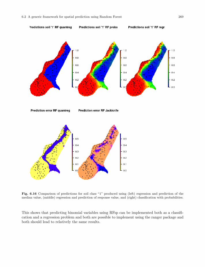
6.2 A generic framework for spatial prediction using Random Forest 269
Fig. 6.16 Comparison of predictions for soil class “1” produced using (left) regression and prediction of themedian value, (middle) regression and prediction of response value, and (right) classification with probabilities.
This shows that predicting binomial variables using RFsp can be implemented both as a classifi-cation and a regression problem and both are possible to implement using the ranger package andboth should lead to relatively the same results.
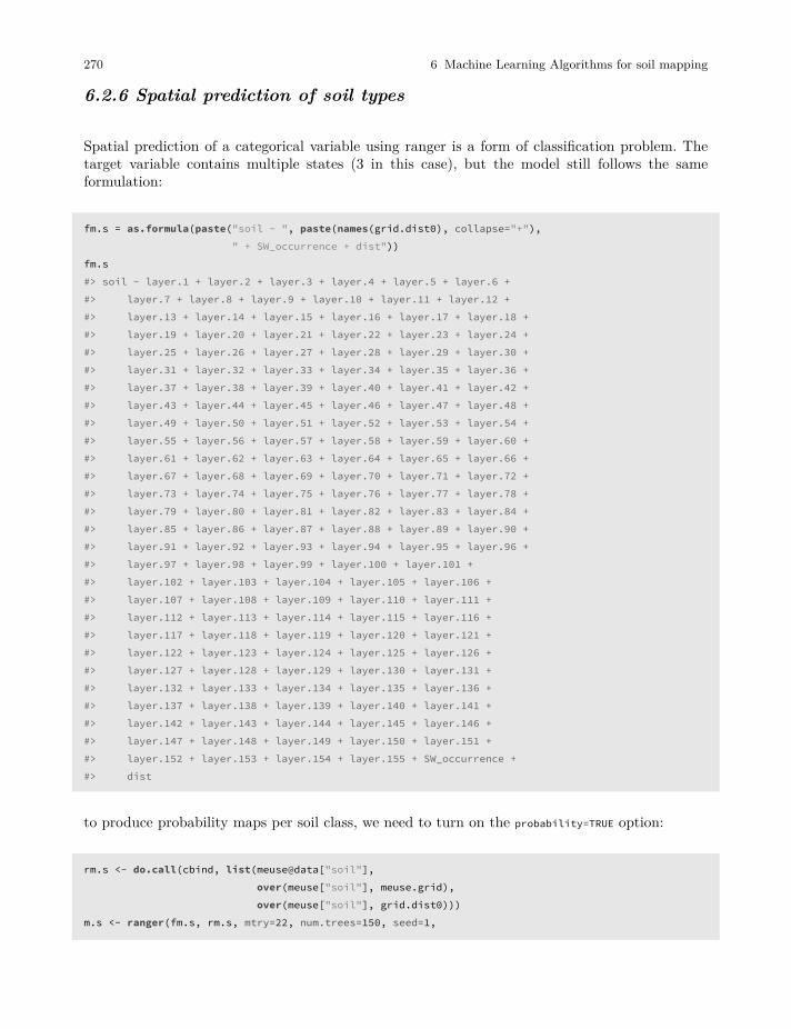
270 6 Machine Learning Algorithms for soil mapping
6.2.6 Spatial prediction of soil types
Spatial prediction of a categorical variable using ranger is a form of classification problem. Thetarget variable contains multiple states (3 in this case), but the model still follows the sameformulation:
fm.s = as.formula(paste("soil ~ ", paste(names(grid.dist0), collapse="+")," + SW_occurrence + dist"))
fm.s#> soil ~ layer.1 + layer.2 + layer.3 + layer.4 + layer.5 + layer.6 +#> layer.7 + layer.8 + layer.9 + layer.10 + layer.11 + layer.12 +#> layer.13 + layer.14 + layer.15 + layer.16 + layer.17 + layer.18 +#> layer.19 + layer.20 + layer.21 + layer.22 + layer.23 + layer.24 +#> layer.25 + layer.26 + layer.27 + layer.28 + layer.29 + layer.30 +#> layer.31 + layer.32 + layer.33 + layer.34 + layer.35 + layer.36 +#> layer.37 + layer.38 + layer.39 + layer.40 + layer.41 + layer.42 +#> layer.43 + layer.44 + layer.45 + layer.46 + layer.47 + layer.48 +#> layer.49 + layer.50 + layer.51 + layer.52 + layer.53 + layer.54 +#> layer.55 + layer.56 + layer.57 + layer.58 + layer.59 + layer.60 +#> layer.61 + layer.62 + layer.63 + layer.64 + layer.65 + layer.66 +#> layer.67 + layer.68 + layer.69 + layer.70 + layer.71 + layer.72 +#> layer.73 + layer.74 + layer.75 + layer.76 + layer.77 + layer.78 +#> layer.79 + layer.80 + layer.81 + layer.82 + layer.83 + layer.84 +#> layer.85 + layer.86 + layer.87 + layer.88 + layer.89 + layer.90 +#> layer.91 + layer.92 + layer.93 + layer.94 + layer.95 + layer.96 +#> layer.97 + layer.98 + layer.99 + layer.100 + layer.101 +#> layer.102 + layer.103 + layer.104 + layer.105 + layer.106 +#> layer.107 + layer.108 + layer.109 + layer.110 + layer.111 +#> layer.112 + layer.113 + layer.114 + layer.115 + layer.116 +#> layer.117 + layer.118 + layer.119 + layer.120 + layer.121 +#> layer.122 + layer.123 + layer.124 + layer.125 + layer.126 +#> layer.127 + layer.128 + layer.129 + layer.130 + layer.131 +#> layer.132 + layer.133 + layer.134 + layer.135 + layer.136 +#> layer.137 + layer.138 + layer.139 + layer.140 + layer.141 +#> layer.142 + layer.143 + layer.144 + layer.145 + layer.146 +#> layer.147 + layer.148 + layer.149 + layer.150 + layer.151 +#> layer.152 + layer.153 + layer.154 + layer.155 + SW_occurrence +#> dist
to produce probability maps per soil class, we need to turn on the probability=TRUE option:
rm.s <- do.call(cbind, list(meuse@data["soil"],over(meuse["soil"], meuse.grid),over(meuse["soil"], grid.dist0)))
m.s <- ranger(fm.s, rm.s, mtry=22, num.trees=150, seed=1,

6.2 A generic framework for spatial prediction using Random Forest 271
probability=TRUE, keep.inbag=TRUE)m.s#> Ranger result#>#> Call:#> ranger(fm.s, rm.s, mtry = 22, num.trees = 150, seed = 1, probability = TRUE, keep.inbag = TRUE)#>#> Type: Probability estimation#> Number of trees: 150#> Sample size: 155#> Number of independent variables: 157#> Mtry: 22#> Target node size: 10#> Variable importance mode: none#> Splitrule: gini#> OOB prediction error (Brier s.): 0.0922
this shows that the model is successful with an OOB prediction error of about 0.09. This numberis rather abstract so we can also check the actual classification accuracy using hard classes:
m.s0 <- ranger(fm.s, rm.s, mtry=22, num.trees=150, seed=1)m.s0#> Ranger result#>#> Call:#> ranger(fm.s, rm.s, mtry = 22, num.trees = 150, seed = 1)#>#> Type: Classification#> Number of trees: 150#> Sample size: 155#> Number of independent variables: 157#> Mtry: 22#> Target node size: 1#> Variable importance mode: none#> Splitrule: gini#> OOB prediction error: 10.32 %
which shows that the classification or mapping accuracy for hard classes is about 90%. We canproduce predictions of probabilities per class by running:
pred.soil_rfc = predict(m.s, cbind(meuse.grid@data, grid.dist0@data), type="se")pred.grids = meuse.grid["soil"]pred.grids@data = do.call(cbind, list(pred.grids@data,
data.frame(pred.soil_rfc$predictions),
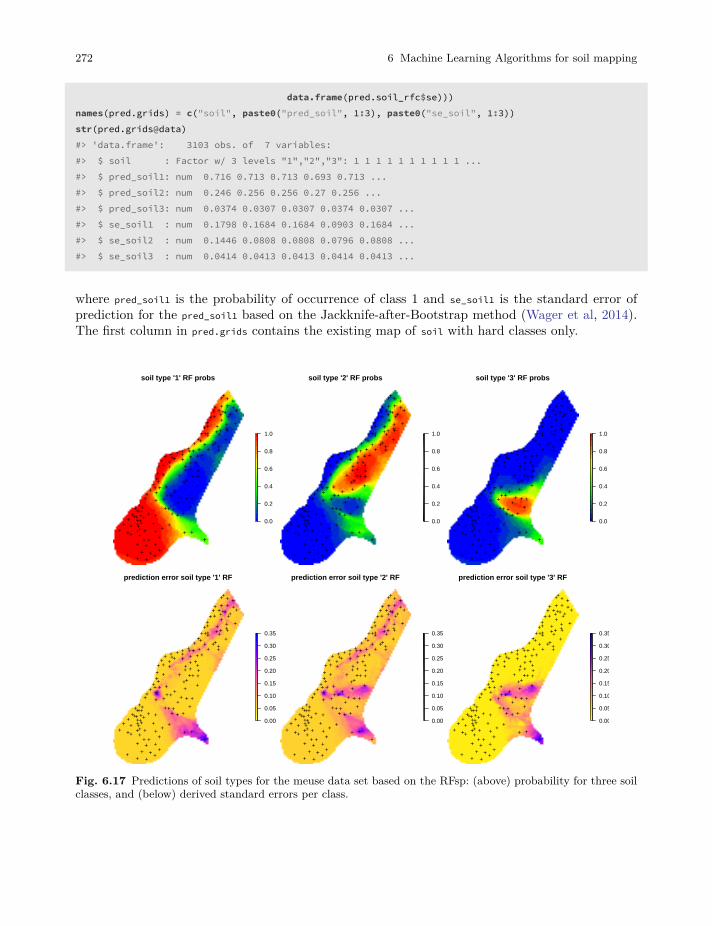
272 6 Machine Learning Algorithms for soil mapping
data.frame(pred.soil_rfc$se)))names(pred.grids) = c("soil", paste0("pred_soil", 1:3), paste0("se_soil", 1:3))str(pred.grids@data)#> 'data.frame': 3103 obs. of 7 variables:#> $ soil : Factor w/ 3 levels "1","2","3": 1 1 1 1 1 1 1 1 1 1 ...#> $ pred_soil1: num 0.716 0.713 0.713 0.693 0.713 ...#> $ pred_soil2: num 0.246 0.256 0.256 0.27 0.256 ...#> $ pred_soil3: num 0.0374 0.0307 0.0307 0.0374 0.0307 ...#> $ se_soil1 : num 0.1798 0.1684 0.1684 0.0903 0.1684 ...#> $ se_soil2 : num 0.1446 0.0808 0.0808 0.0796 0.0808 ...#> $ se_soil3 : num 0.0414 0.0413 0.0413 0.0414 0.0413 ...
where pred_soil1 is the probability of occurrence of class 1 and se_soil1 is the standard error ofprediction for the pred_soil1 based on the Jackknife-after-Bootstrap method (Wager et al, 2014).The first column in pred.grids contains the existing map of soil with hard classes only.
soil type '1' RF probs
0.0
0.2
0.4
0.6
0.8
1.0
++ + +++
+++ +++
+++
++
++
++++
++++
+++
+++ ++++
++++++
+
+++++
++
++++++ +
++
+++
++
++
++
+++
+ ++++
++++
+
+
+
++
++
++ ++
+
++
+++
+
+ ++
+
++
+
++
+++
++++
++
+
++
+++
++
++
+
+
+
+
+
+
+
++
+
+++
+ ++
++++
+ ++
+++ +
+
soil type '2' RF probs
0.0
0.2
0.4
0.6
0.8
1.0
++ + +++
+++ +++
+++
++
++
++++
++++
+++
+++ ++++
++++++
+
+++++
++
++++++ +
++
+++
++
++
++
+++
+ ++++
++++
+
+
+
++
++
++ ++
+
++
+++
+
+ ++
+
++
+
++
+++
++++
++
+
++
+++
++
++
+
+
+
+
+
+
+
++
+
+++
+ ++
++++
+ ++
+++ +
+
soil type '3' RF probs
0.0
0.2
0.4
0.6
0.8
1.0
++ + +++
+++ +++
+++
++
++
++++
++++
+++
+++ ++++
++++++
+
+++++
++
++++++ +
++
+++
++
++
++
+++
+ ++++
++++
+
+
+
++
++
++ ++
+
++
+++
+
+ ++
+
++
+
++
+++
++++
++
+
++
+++
++
++
+
+
+
+
+
+
+
++
+
+++
+ ++
++++
+ ++
+++ +
+
prediction error soil type '1' RF
0.00
0.05
0.10
0.15
0.20
0.25
0.30
0.35
++ + +++
+++ +++
+++
++
++
++++
++++
+++
+++ ++++
++++++
+
+++++
++
++++++ +
++
+++
++
++
++
+++
+ ++++
++++
+
+
+
++
++
++ ++
+
++
+++
+
+ ++
+
++
+
++
+++
++++
++
+
++
+++
++
++
+
+
+
+
+
+
+
++
+
+++
+ ++
++++
+ ++
+++ +
+
prediction error soil type '2' RF
0.00
0.05
0.10
0.15
0.20
0.25
0.30
0.35
++ + +++
+++ +++
+++
++
++
++++
++++
+++
+++ ++++
++++++
+
+++++
++
++++++ +
++
+++
++
++
++
+++
+ ++++
++++
+
+
+
++
++
++ ++
+
++
+++
+
+ ++
+
++
+
++
+++
++++
++
+
++
+++
++
++
+
+
+
+
+
+
+
++
+
+++
+ ++
++++
+ ++
+++ +
+
prediction error soil type '3' RF
0.00
0.05
0.10
0.15
0.20
0.25
0.30
0.35
++ + +++
+++ +++
+++
++
++
++++
++++
+++
+++ ++++
++++++
+
+++++
++
++++++ +
++
+++
++
++
++
+++
+ ++++
++++
+
+
+
++
++
++ ++
+
++
+++
+
+ ++
+
++
+
++
+++
++++
++
+
++
+++
++
++
+
+
+
+
+
+
+
++
+
+++
+ ++
++++
+ ++
+++ +
+
Fig. 6.17 Predictions of soil types for the meuse data set based on the RFsp: (above) probability for three soilclasses, and (below) derived standard errors per class.
6.3 Summary points 273
Spatial prediction of binomial and factor-type variables is straightforward with ranger / RFsp:buffer distance and spatial-autocorrelation can be incorporated simultaneously as opposed togeostatistical packages, where link functions and/or indicator kriging would need to be used, andwhich require that variograms are fitted per class.
6.3 Summary points
In summary, MLA’s represent an increasingly attractive option for soil mapping and soil modellingproblems in general, as they often perform better than standard linear models (as previouslyrecognized by Moran and Bui (2002) and Henderson et al (2004)) Some recent comparisons ofMLA’s performance for operational soil mapping can be found in Nussbaum et al (2018)). MLA’soften perform better than linear techniques for soil mapping; possibly for the following threereasons:
1. Non-linear relationships between soil forming factors and soil properties can be more efficientlymodeled using MLA’s,
2. Tree-based MLA’s (random forest, gradient boosting, cubist) are suitable for representing localsoil-landscape relationships, nested within a hierarchy of larger areas, which is often importantfor achieving accuracy of spatial prediction models,
3. In the case of MLA, statistical properties such as multicolinearity and non-Gaussian distributionare dealt with inside the models, which simplifies statistical modeling steps,
On the other hand, MLA’s can be computationally very intensive and consequently require carefulplanning, especially when the number of points goes beyond a few thousand and the number ofcovariates beyond a dozen. Note also that some MLA’s, such as for example Support VectorMachines (SVM), are computationally very intensive and are probably not well suited for verylarge data sets.Within PSM, there is increasing interest in doing ensemble predictions, model averages or modelstacks. Stacking models can improve upon individual best techniques, achieving improvements ofup to 30%, with the additional demands consisting of only higher computation loads (Michailidis,2017). In the example above, the extensive computational load from derivation of models andproduct predictions already achieved improved accuracies, making increasing computing loadsfurther a matter of diminishing returns. Some interesting Machine Learning Algorithms for soilmapping based on regression include: Random Forest (Biau and Scornet, 2016), Gradient BoostingMachine (GBM) (Hastie et al, 2009), Cubist (Kuhn et al, 2014), Generalized Boosted RegressionModels (Ridgeway, 2018), Support Vector Machines (Chang and Lin, 2011), and the ExtremeGradient Boosting approach available via the xgboost package (Chen and Guestrin, 2016). Noneof these techniques is universally recognized as the best spatial predictor for all soil variables.Instead, we recommend comparing MLA’s using robust cross-validation methods as explainedabove. Also combining MLA’s into ensemble predictions might not be beneficial in all situations.Less is better sometimes.The RFsp method seems to be suitable for generating spatial and spatiotemporal predictions.Computing time, however, can be demanding and working with data sets with >1000 point lo-cations (hence 1000+ buffer distance maps) is probably not yet feasible or recommended. Also

274 6 Machine Learning Algorithms for soil mapping
cross-validation of accuracy of predictions produced using RFsp needs to be implemented usingleave-location-out CV to account for spatial autocorrelation in data. The key to the success of theRFsp framework might be the training data quality — especially quality of spatial sampling (tominimize extrapolation problems and any type of bias in data), and quality of model validation(to ensure that accuracy is not effected by over-fitting). For all other details about RFsp refer toHengl et al (2018a).
Chapter 7
Spatial prediction and assessment of Soil OrganicCarbon
Edited by: Hengl T. & Sanderman J.
7.1 Introduction
This chapter was prepared as supplementary material for the Sanderman et al (2018) article. Itexplains how to map Soil Organic Carbon Stocks (OCS) using soil samples (point data). It alsodemonstrates derivation of values at both the site level (per profile) and by using raster calculus(per pixel). We then illustrate how to estimate total OCS for any area of interest (which can be afield plot, farm and/or administrative region). For an introduction to soil mapping using MachineLearning Algorithms refer to chapter 6. To access the ISRIC global compilation of soil profilesreferenced here please refer to: http://www.isric.org/explore/wosis
7.2 Measurement and derivation of soil organic carbon
Carbon below ground can be organic or non-organic/ mineral (usually carbonates and bicarbon-ates) i.e. CaCO3 in the rocks. Organic carbon stocks below ground (0–2 m) in terrestrial ecosystemsconsist of two major components:
1. Living organism biomass i.e. mainly:
• Plant roots,• Microbial biomass (Xu et al, 2013),
2. Plant and animal residues at various stages of decomposition (organic matter).
Xu et al (2013) estimated that total global microbial biomass is about 17 Pg C, which is onlyabout 2% of the total for organic matter. Therefore, the amounts of C in microbial biomass can
275
276 7 Spatial prediction and assessment of Soil Organic Carbon
reasonably be considered negligible, in comparison to the total C stock. However, if one includesall living organisms, and especially tree roots, then the portion of total C found in living organismscould be more significant, especially in areas under dense forests.
Soil Organic Carbon Stock (OCS) is the mass of soil organic carbon per standard area and fora specific depth interval, usually expressed in kg/m2 or t/ha. It can be derived using (laboratoryand/or field) measurement of soil organic carbon content (ORC; expressed in % or g/kg of <2mmmineral earth), then taking into account bulk density (BLD), thickness of the soil layer, andvolume percentage of coarse fragments (CRF) (Nelson and Sommers, 1982; Poeplau et al, 2017):
OCS[kg/m2] = ORC[%]/100 ⋅ BLD[kg/m3] ⋅ (1 − CRF[%]/100) ⋅ HOT[𝑚] (7.1)
Note that if one has soil organic carbon content measured in g/kg then one should divide by 1000instead of 100. A correction for gravel content is necessary because only material less than 2 mmis analyzed for ORC concentration. Ignoring the gravel content can result in an overestimation ofthe organic carbon stock. Note also that OCS always refers to a specific depth interval or horizonthickness (HOT), e.g.:
• kg/m2 for depth 0–30 cm (Berhongaray and Alvarez, 2013),
Values of OCS in kg/m2 can also be expressed in tons/ha units, in which case a simple conversionformula can be applied:
1 ⋅ kg/m2 = 10 ⋅ tons/ha (7.2)
Total OCS for an area of interest can be derived by multiplying OCS by total area e.g.:
120tons/ha ⋅ 1km2 = 120 ⋅ 100 = 12, 000tons (7.3)
Another way to express soil organic carbon is through soil organic carbon density (OCD inkg/m3), which is in fact equivalent to OCS divided by the horizon thickness:
OCD[kg/m3] = ORC[%]/100 ⋅ BLD[kg/m3] ⋅ (1 − CRF[%]/100) = OCS/HOT (7.4)
While OCS is a summary measure of SOC, always associated with a specific depth interval, OCD isa relative measure of soil organic carbon distribution and can be associated with any support sizei.e. to an arbitrary depth. In principle, OCD (kg/m3) is strongly correlated with ORC (g/kg) asindicated in the figure below. However, depending on soil mineralogy and coarse fragment content,OCD can be lower or higher than what the smoothed line indicates (notice the range of valuesaround the smoothed line is relatively wide). It is important to understand, however, that, as longas ORC, BLD and CRF are known, one can convert the values from ORC to OCD and OCS andvice versa, without loosing any information about the soil organic carbon stock.
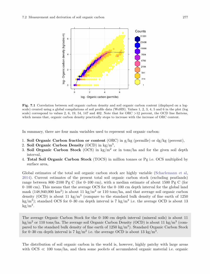
7.2 Measurement and derivation of soil organic carbon 277
Fig. 7.1 Correlation between soil organic carbon density and soil organic carbon content (displayed on a log-scale) created using a global compilations of soil profile data (WoSIS). Values 1, 2, 3, 4, 5 and 6 in the plot (logscale) correspond to values 2, 6, 19, 54, 147 and 402. Note that for ORC >12 percent, the OCD line flattens,which means that, organic carbon density practically stops to increase with the increase of ORC content.
In summary, there are four main variables used to represent soil organic carbon:
1. Soil Organic Carbon fraction or content (ORC) in g/kg (permille) or dg/kg (percent),2. Soil Organic Carbon Density (OCD) in kg/m3,3. Soil Organic Carbon Stock (OCS) in kg/m2 or in tons/ha and for the given soil depth
interval,4. Total Soil Organic Carbon Stock (TOCS) in million tonnes or Pg i.e. OCS multiplied by
surface area,
Global estimates of the total soil organic carbon stock are highly variable (Scharlemann et al,2014). Current estimates of the present total soil organic carbon stock (excluding peatlands)range between 800–2100 Pg C (for 0–100 cm), with a median estimate of about 1500 Pg C (for0–100 cm). This means that the average OCS for the 0–100 cm depth interval for the global landmask (148,940,000 km2) is about 11 kg/m2 or 110 tons/ha, and that average soil organic carbondensity (OCD) is about 11 kg/m3 (compare to the standard bulk density of fine earth of 1250kg/m3); standard OCS for 0–30 cm depth interval is 7 kg/m2 i.e. the average OCD is about 13kg/m3.
The average Organic Carbon Stock for the 0–100 cm depth interval (mineral soils) is about 11kg/m2 or 110 tons/ha. The average soil Organic Carbon Density (OCD) is about 11 kg/m3 (com-pared to the standard bulk density of fine earth of 1250 kg/m3). Standard Organic Carbon Stockfor 0–30 cm depth interval is 7 kg/m2 i.e. the average OCD is about 13 kg/m3.
The distribution of soil organic carbon in the world is, however, highly patchy with large areaswith OCS ≪ 100 tons/ha, and then some pockets of accumulated organic material i.e. organic
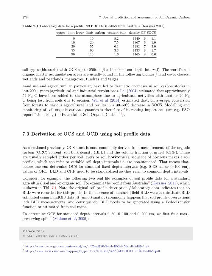
278 7 Spatial prediction and assessment of Soil Organic Carbon
Table 7.1 Laboratory data for a profile 399 EDGEROI ed079 from Australia (Karssies 2011).
upper_limit lower_limit carbon_content bulk_density CF SOCS0 10 8.2 1340 6 1.1
10 20 7.5 1367 6 1.020 55 6.1 1382 7 3.055 90 3.3 1433 8 1.790 116 1.6 1465 8 0.6
soil types (histosols) with OCS up to 850tons/ha (for 0–30 cm depth interval). The world’s soilorganic matter accumulation areas are usually found in the following biomes / land cover classes:wetlands and peatlands, mangroves, tundras and taigas.
Land use and agriculture, in particular, have led to dramatic decreases in soil carbon stocks inlast 200+ years (agricultural and industrial revolutions). Lal (2004) estimated that approximately54 Pg C have been added to the atmosphere due to agricultural activities with another 26 PgC being lost from soils due to erosion. Wei et al (2014) estimated that, on average, conversionfrom forests to various agricultural land results in a 30–50% decrease in SOCS. Modelling andmonitoring of soil organic carbon dynamics is therefore of increasing importance (see e.g. FAOreport “Unlocking the Potential of Soil Organic Carbon”1).
7.3 Derivation of OCS and OCD using soil profile data
As mentioned previously, OCS stock is most commonly derived from measurements of the organiccarbon (ORC) content, soil bulk density (BLD) and the volume fraction of gravel (CRF). Theseare usually sampled either per soil layers or soil horizons (a sequence of horizons makes a soilprofile), which can refer to variable soil depth intervals i.e. are non-standard. That means that,before one can determine OCS for standard fixed depth intervals (e.g. 0–30 cm or 0–100 cm),values of ORC, BLD and CRF need to be standardized so they refer to common depth intervals.
Consider, for example, the following two real life examples of soil profile data for a standardagricultural soil and an organic soil. For example the profile from Australia2 (Karssies, 2011), whichis shown in Tbl. 7.1. Note the original soil profile description / laboratory data indicates that noBLD were recorded for this profile. In the absence of measured field BLD we can substitute BLDestimated using LandGIS data. It (unfortunately) commonly happens that soil profile observationslack BLD measurements, and consequently BLD needs to be generated using a Pedo-Transferfunction or estimated from soil maps.
To determine OCS for standard depth intervals 0–30, 0–100 and 0–200 cm, we first fit a mass-preserving spline (Malone et al, 2009):
library(GSIF)#> GSIF version 0.5-5 (2019-01-04)
1 http://www.fao.org/documents/card/en/c/25eaf720-94e4-4f53-8f50-cdfc2487e1f8/2 http://www.asris.csiro.au/mapping/hyperdocs/NatSoil/399%5EEDGEROI%5Eed079.pdf
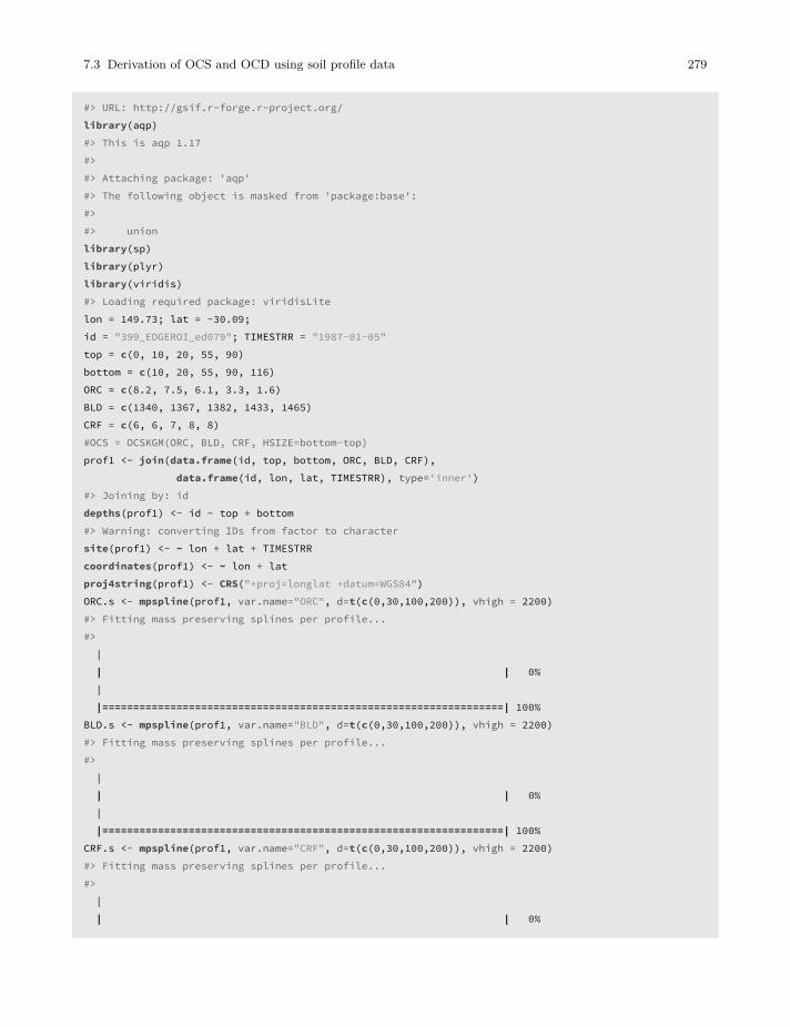
7.3 Derivation of OCS and OCD using soil profile data 279
#> URL: http://gsif.r-forge.r-project.org/library(aqp)#> This is aqp 1.17#>#> Attaching package: 'aqp'#> The following object is masked from 'package:base':#>#> unionlibrary(sp)library(plyr)library(viridis)#> Loading required package: viridisLitelon = 149.73; lat = -30.09;id = "399_EDGEROI_ed079"; TIMESTRR = "1987-01-05"top = c(0, 10, 20, 55, 90)bottom = c(10, 20, 55, 90, 116)ORC = c(8.2, 7.5, 6.1, 3.3, 1.6)BLD = c(1340, 1367, 1382, 1433, 1465)CRF = c(6, 6, 7, 8, 8)#OCS = OCSKGM(ORC, BLD, CRF, HSIZE=bottom-top)prof1 <- join(data.frame(id, top, bottom, ORC, BLD, CRF),
data.frame(id, lon, lat, TIMESTRR), type='inner')#> Joining by: iddepths(prof1) <- id ~ top + bottom#> Warning: converting IDs from factor to charactersite(prof1) <- ~ lon + lat + TIMESTRRcoordinates(prof1) <- ~ lon + latproj4string(prof1) <- CRS("+proj=longlat +datum=WGS84")ORC.s <- mpspline(prof1, var.name="ORC", d=t(c(0,30,100,200)), vhigh = 2200)#> Fitting mass preserving splines per profile...#>|| | 0%||=================================================================| 100%
BLD.s <- mpspline(prof1, var.name="BLD", d=t(c(0,30,100,200)), vhigh = 2200)#> Fitting mass preserving splines per profile...#>|| | 0%||=================================================================| 100%
CRF.s <- mpspline(prof1, var.name="CRF", d=t(c(0,30,100,200)), vhigh = 2200)#> Fitting mass preserving splines per profile...#>|| | 0%
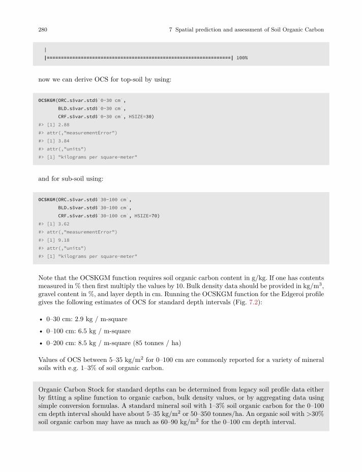
280 7 Spatial prediction and assessment of Soil Organic Carbon
||=================================================================| 100%
now we can derive OCS for top-soil by using:
OCSKGM(ORC.s$var.std$`0-30 cm`,BLD.s$var.std$`0-30 cm`,CRF.s$var.std$`0-30 cm`, HSIZE=30)
#> [1] 2.88#> attr(,"measurementError")#> [1] 3.84#> attr(,"units")#> [1] "kilograms per square-meter"
and for sub-soil using:
OCSKGM(ORC.s$var.std$`30-100 cm`,BLD.s$var.std$`30-100 cm`,CRF.s$var.std$`30-100 cm`, HSIZE=70)
#> [1] 3.62#> attr(,"measurementError")#> [1] 9.18#> attr(,"units")#> [1] "kilograms per square-meter"
Note that the OCSKGM function requires soil organic carbon content in g/kg. If one has contentsmeasured in % then first multiply the values by 10. Bulk density data should be provided in kg/m3,gravel content in %, and layer depth in cm. Running the OCSKGM function for the Edgeroi profilegives the following estimates of OCS for standard depth intervals (Fig. 7.2):
• 0–30 cm: 2.9 kg / m-square
• 0–100 cm: 6.5 kg / m-square
• 0–200 cm: 8.5 kg / m-square (85 tonnes / ha)
Values of OCS between 5–35 kg/m2 for 0–100 cm are commonly reported for a variety of mineralsoils with e.g. 1–3% of soil organic carbon.
Organic Carbon Stock for standard depths can be determined from legacy soil profile data eitherby fitting a spline function to organic carbon, bulk density values, or by aggregating data usingsimple conversion formulas. A standard mineral soil with 1–3% soil organic carbon for the 0–100cm depth interval should have about 5–35 kg/m2 or 50–350 tonnes/ha. An organic soil with >30%soil organic carbon may have as much as 60–90 kg/m2 for the 0–100 cm depth interval.
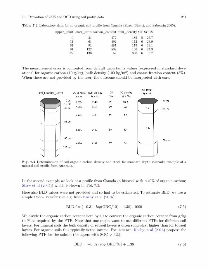
7.3 Derivation of OCS and OCD using soil profile data 281
Table 7.2 Laboratory data for an organic soil profile from Canada (Shaw, Bhatti, and Sabourin 2005).
upper_limit lower_limit carbon_content bulk_density CF SOCS0 31 472 185 5 25.7
31 61 492 172 6 23.961 91 487 175 6 24.191 122 502 166 6 24.3
122 130 59 830 6 3.7
The measurement error is computed from default uncertainty values (expressed in standard devi-ations) for organic carbon (10 g/kg), bulk density (100 kg/m3) and coarse fraction content (5%).When these are not provided by the user, the outcome should be interpreted with care.
Fig. 7.2 Determination of soil organic carbon density and stock for standard depth intervals: example of amineral soil profile from Australia.
In the second example we look at a profile from Canada (a histosol with >40% of organic carbon;Shaw et al (2005)) which is shown in Tbl. 7.2.
Here also BLD values were not provided and so had to be estimated. To estimate BLD, we use asimple Pedo-Transfer rule e.g. from Köchy et al (2015):
BLD.f = (−0.31 ⋅ 𝑙𝑜𝑔(ORC/10) + 1.38) ⋅ 1000 (7.5)
We divide the organic carbon content here by 10 to convert the organic carbon content from g/kgto % as required by the PTF. Note that one might want to use different PTFs for different soillayers. For mineral soils the bulk density of subsoil layers is often somewhat higher than for topsoillayers. For organic soils this typically is the inverse. For instance, Köchy et al (2015) propose thefollowing PTF for the subsoil (for layers with SOC > 3%):
BLD = −0.32 ⋅ 𝑙𝑜𝑔(ORC[%]) + 1.38 (7.6)
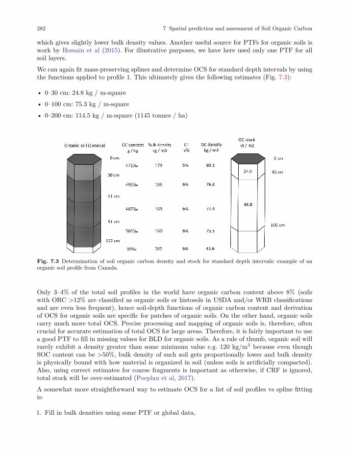
282 7 Spatial prediction and assessment of Soil Organic Carbon
which gives slightly lower bulk density values. Another useful source for PTFs for organic soils iswork by Hossain et al (2015). For illustrative purposes, we have here used only one PTF for allsoil layers.We can again fit mass-preserving splines and determine OCS for standard depth intervals by usingthe functions applied to profile 1. This ultimately gives the following estimates (Fig. 7.3):
• 0–30 cm: 24.8 kg / m-square• 0–100 cm: 75.3 kg / m-square• 0–200 cm: 114.5 kg / m-square (1145 tonnes / ha)
Fig. 7.3 Determination of soil organic carbon density and stock for standard depth intervals: example of anorganic soil profile from Canada.
Only 3–4% of the total soil profiles in the world have organic carbon content above 8% (soilswith ORC >12% are classified as organic soils or histosols in USDA and/or WRB classificationsand are even less frequent), hence soil-depth functions of organic carbon content and derivationof OCS for organic soils are specific for patches of organic soils. On the other hand, organic soilscarry much more total OCS. Precise processing and mapping of organic soils is, therefore, oftencrucial for accurate estimation of total OCS for large areas. Therefore, it is fairly important to usea good PTF to fill in missing values for BLD for organic soils. As a rule of thumb, organic soil willrarely exhibit a density greater than some minimum value e.g. 120 kg/m3 because even thoughSOC content can be >50%, bulk density of such soil gets proportionally lower and bulk densityis physically bound with how material is organized in soil (unless soils is artificially compacted).Also, using correct estimates for coarse fragments is important as otherwise, if CRF is ignored,total stock will be over-estimated (Poeplau et al, 2017).A somewhat more straightforward way to estimate OCS for a list of soil profiles vs spline fittingis:
1. Fill in bulk densities using some PTF or global data,

7.3 Derivation of OCS and OCD using soil profile data 283
2. Use information about the depth to bedrock to correct for shallow soils,3. Use information on CRF to correct stocks for stony / skeletoidal component,4. Aggregate non-standard horizon depth values using some simple rules (Fig. 7.4).

284 7 Spatial prediction and assessment of Soil Organic Carbon
Fig. 7.4 Estimation of OCS values 0–30 cm using some typical soil profile data without fitting splines.
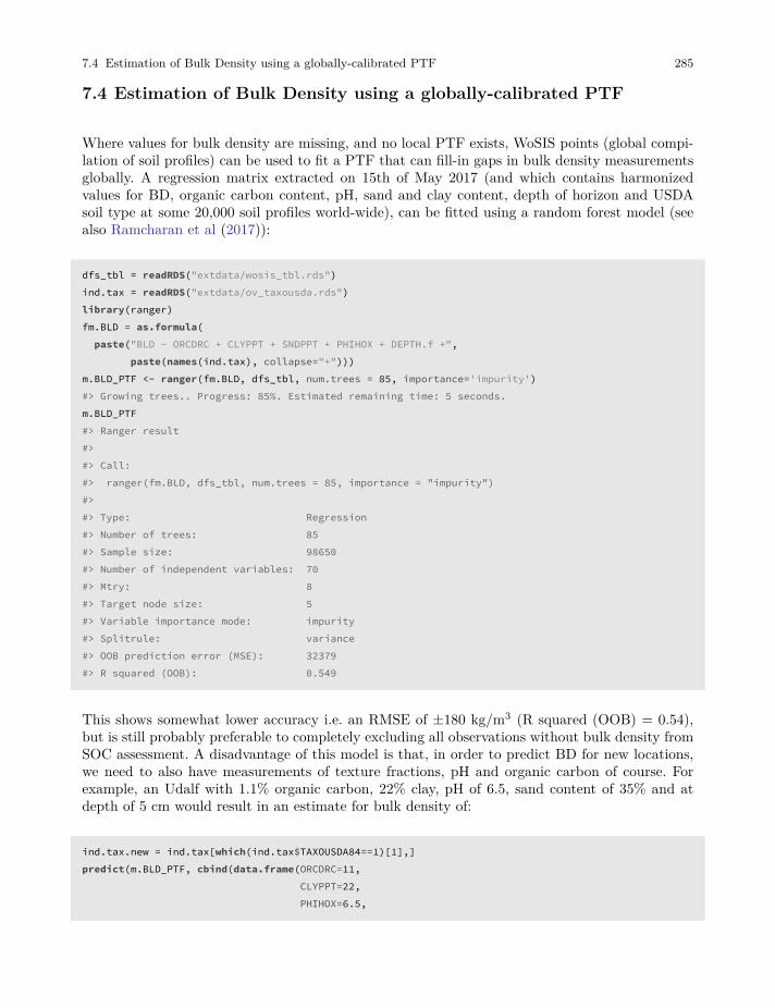
7.4 Estimation of Bulk Density using a globally-calibrated PTF 285
7.4 Estimation of Bulk Density using a globally-calibrated PTF
Where values for bulk density are missing, and no local PTF exists, WoSIS points (global compi-lation of soil profiles) can be used to fit a PTF that can fill-in gaps in bulk density measurementsglobally. A regression matrix extracted on 15th of May 2017 (and which contains harmonizedvalues for BD, organic carbon content, pH, sand and clay content, depth of horizon and USDAsoil type at some 20,000 soil profiles world-wide), can be fitted using a random forest model (seealso Ramcharan et al (2017)):
dfs_tbl = readRDS("extdata/wosis_tbl.rds")ind.tax = readRDS("extdata/ov_taxousda.rds")library(ranger)fm.BLD = as.formula(paste("BLD ~ ORCDRC + CLYPPT + SNDPPT + PHIHOX + DEPTH.f +",
paste(names(ind.tax), collapse="+")))m.BLD_PTF <- ranger(fm.BLD, dfs_tbl, num.trees = 85, importance='impurity')#> Growing trees.. Progress: 85%. Estimated remaining time: 5 seconds.m.BLD_PTF#> Ranger result#>#> Call:#> ranger(fm.BLD, dfs_tbl, num.trees = 85, importance = "impurity")#>#> Type: Regression#> Number of trees: 85#> Sample size: 98650#> Number of independent variables: 70#> Mtry: 8#> Target node size: 5#> Variable importance mode: impurity#> Splitrule: variance#> OOB prediction error (MSE): 32379#> R squared (OOB): 0.549
This shows somewhat lower accuracy i.e. an RMSE of ±180 kg/m3 (R squared (OOB) = 0.54),but is still probably preferable to completely excluding all observations without bulk density fromSOC assessment. A disadvantage of this model is that, in order to predict BD for new locations,we need to also have measurements of texture fractions, pH and organic carbon of course. Forexample, an Udalf with 1.1% organic carbon, 22% clay, pH of 6.5, sand content of 35% and atdepth of 5 cm would result in an estimate for bulk density of:
ind.tax.new = ind.tax[which(ind.tax$TAXOUSDA84==1)[1],]predict(m.BLD_PTF, cbind(data.frame(ORCDRC=11,
CLYPPT=22,PHIHOX=6.5,
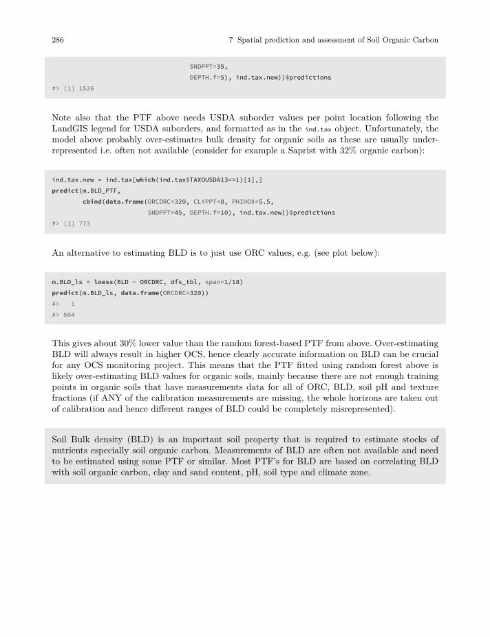
286 7 Spatial prediction and assessment of Soil Organic Carbon
SNDPPT=35,DEPTH.f=5), ind.tax.new))$predictions
#> [1] 1526
Note also that the PTF above needs USDA suborder values per point location following theLandGIS legend for USDA suborders, and formatted as in the ind.tax object. Unfortunately, themodel above probably over-estimates bulk density for organic soils as these are usually under-represented i.e. often not available (consider for example a Saprist with 32% organic carbon):
ind.tax.new = ind.tax[which(ind.tax$TAXOUSDA13==1)[1],]predict(m.BLD_PTF,
cbind(data.frame(ORCDRC=320, CLYPPT=8, PHIHOX=5.5,SNDPPT=45, DEPTH.f=10), ind.tax.new))$predictions
#> [1] 773
An alternative to estimating BLD is to just use ORC values, e.g. (see plot below):
m.BLD_ls = loess(BLD ~ ORCDRC, dfs_tbl, span=1/18)predict(m.BLD_ls, data.frame(ORCDRC=320))#> 1#> 664
This gives about 30% lower value than the random forest-based PTF from above. Over-estimatingBLD will always result in higher OCS, hence clearly accurate information on BLD can be crucialfor any OCS monitoring project. This means that the PTF fitted using random forest above islikely over-estimating BLD values for organic soils, mainly because there are not enough trainingpoints in organic soils that have measurements data for all of ORC, BLD, soil pH and texturefractions (if ANY of the calibration measurements are missing, the whole horizons are taken outof calibration and hence different ranges of BLD could be completely misrepresented).
Soil Bulk density (BLD) is an important soil property that is required to estimate stocks ofnutrients especially soil organic carbon. Measurements of BLD are often not available and needto be estimated using some PTF or similar. Most PTF’s for BLD are based on correlating BLDwith soil organic carbon, clay and sand content, pH, soil type and climate zone.
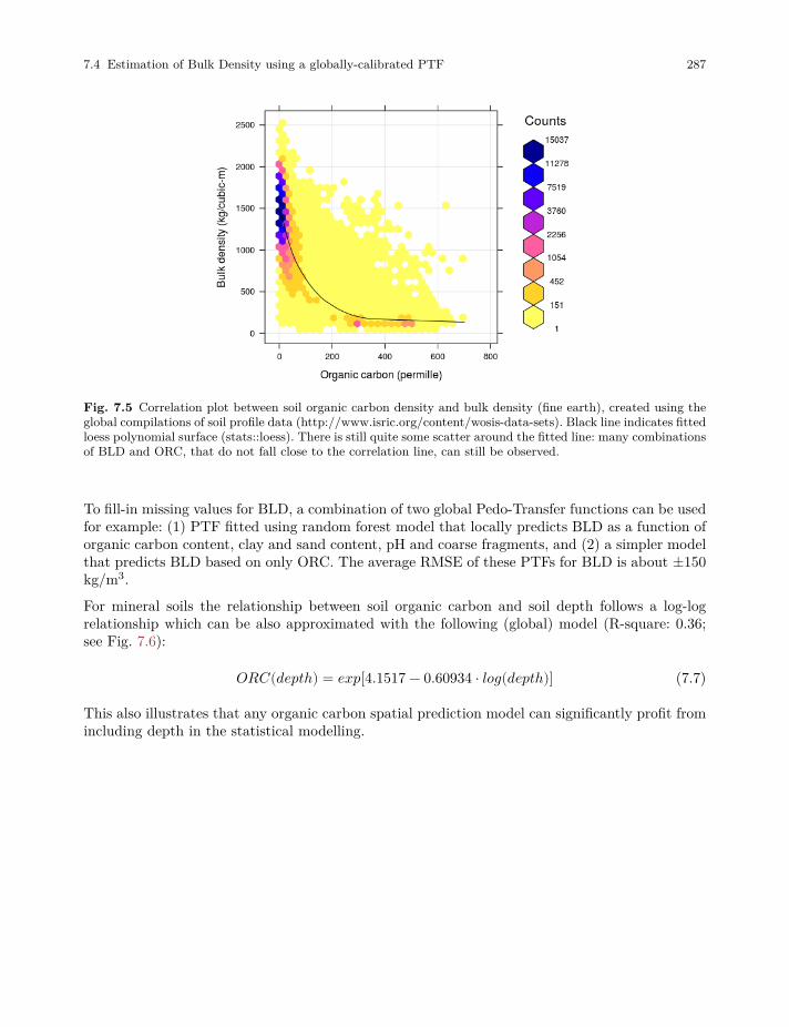
7.4 Estimation of Bulk Density using a globally-calibrated PTF 287
Fig. 7.5 Correlation plot between soil organic carbon density and bulk density (fine earth), created using theglobal compilations of soil profile data (http://www.isric.org/content/wosis-data-sets). Black line indicates fittedloess polynomial surface (stats::loess). There is still quite some scatter around the fitted line: many combinationsof BLD and ORC, that do not fall close to the correlation line, can still be observed.
To fill-in missing values for BLD, a combination of two global Pedo-Transfer functions can be usedfor example: (1) PTF fitted using random forest model that locally predicts BLD as a function oforganic carbon content, clay and sand content, pH and coarse fragments, and (2) a simpler modelthat predicts BLD based on only ORC. The average RMSE of these PTFs for BLD is about ±150kg/m3.
For mineral soils the relationship between soil organic carbon and soil depth follows a log-logrelationship which can be also approximated with the following (global) model (R-square: 0.36;see Fig. 7.6):
𝑂𝑅𝐶(𝑑𝑒𝑝𝑡ℎ) = 𝑒𝑥𝑝[4.1517 − 0.60934 ⋅ 𝑙𝑜𝑔(𝑑𝑒𝑝𝑡ℎ)] (7.7)
This also illustrates that any organic carbon spatial prediction model can significantly profit fromincluding depth in the statistical modelling.
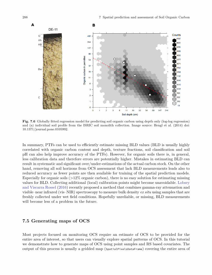
288 7 Spatial prediction and assessment of Soil Organic Carbon
Fig. 7.6 Globally fitted regression model for predicting soil organic carbon using depth only (log-log regression)and (a) individual soil profile from the ISRIC soil monolith collection. Image source: Hengl et al. (2014) doi:10.1371/journal.pone.0105992.
In summary, PTFs can be used to efficiently estimate missing BLD values (BLD is usually highlycorrelated with organic carbon content and depth, texture fractions, soil classification and soilpH can also help improve accuracy of the PTFs). However, for organic soils there is, in general,less calibration data and therefore errors are potentially higher. Mistakes in estimating BLD canresult in systematic and significant over/under-estimations of the actual carbon stock. On the otherhand, removing all soil horizons from OCS assessment that lack BLD measurements leads also toreduced accuracy as fewer points are then available for training of the spatial prediction models.Especially for organic soils (>12% organic carbon), there is no easy solution for estimating missingvalues for BLD. Collecting additional (local) calibration points might become unavoidable. Lobseyand Viscarra Rossel (2016) recently proposed a method that combines gamma-ray attenuation andvisible–near infrared (vis–NIR) spectroscopy to measure bulk density ex situ using samples that arefreshly collected under wet field conditions. Hopefully unreliable, or missing, BLD measurementswill become less of a problem in the future.
7.5 Generating maps of OCS
Most projects focused on monitoring OCS require an estimate of OCS to be provided for theentire area of interest, so that users can visually explore spatial patterns of OCS. In this tutorialwe demonstrate how to generate maps of OCS using point samples and RS based covariates. Theoutput of this process is usually a gridded map (SpatialPixelsDataFrame) covering the entire area of
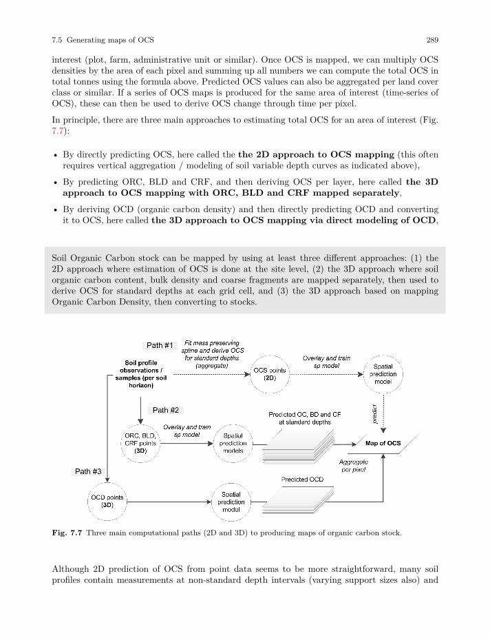
7.5 Generating maps of OCS 289
interest (plot, farm, administrative unit or similar). Once OCS is mapped, we can multiply OCSdensities by the area of each pixel and summing up all numbers we can compute the total OCS intotal tonnes using the formula above. Predicted OCS values can also be aggregated per land coverclass or similar. If a series of OCS maps is produced for the same area of interest (time-series ofOCS), these can then be used to derive OCS change through time per pixel.
In principle, there are three main approaches to estimating total OCS for an area of interest (Fig.7.7):
• By directly predicting OCS, here called the the 2D approach to OCS mapping (this oftenrequires vertical aggregation / modeling of soil variable depth curves as indicated above),
• By predicting ORC, BLD and CRF, and then deriving OCS per layer, here called the 3Dapproach to OCS mapping with ORC, BLD and CRF mapped separately,
• By deriving OCD (organic carbon density) and then directly predicting OCD and convertingit to OCS, here called the 3D approach to OCS mapping via direct modeling of OCD,
Soil Organic Carbon stock can be mapped by using at least three different approaches: (1) the2D approach where estimation of OCS is done at the site level, (2) the 3D approach where soilorganic carbon content, bulk density and coarse fragments are mapped separately, then used toderive OCS for standard depths at each grid cell, and (3) the 3D approach based on mappingOrganic Carbon Density, then converting to stocks.
Fig. 7.7 Three main computational paths (2D and 3D) to producing maps of organic carbon stock.
Although 2D prediction of OCS from point data seems to be more straightforward, many soilprofiles contain measurements at non-standard depth intervals (varying support sizes also) and
290 7 Spatial prediction and assessment of Soil Organic Carbon
therefore 2D modeling of OCS can often be a cumbersome. In most situations where legacy soilprofile data are used, 3D modeling of OCD is probably the most elegant solution to mapping OCSbecause:
• No vertical aggregation of values via spline fitting or similar is needed to standardize valuesper standard depths,
• No additional uncertainty is introduced (in the case of the 2D approach splines likely introducesome extra uncertainty in the model),
• Predictions of OCD/OCS can be generated for any depth interval using the same model (i.e. pre-dictions are based on a single 3D model),
A disadvantage of doing 3D modeling of OCD is, however, that correlation with covariate layerscould be less clear than if separate models are built for ORC, BLD and CRF. Because OCD is acomposite variable, it can often be difficult to distinguish whether the values are lower or higherdue to differences in ORC, BLD or CRF. We leave it to users to compare various approaches toOCS mapping and then select the method that achieves the best accuracy and/or is most suitablefor use for their applications.
7.6 Predicting OCS from point data (the 2D approach)
The geospt package3 contains 125 samples of OCS from Colombia already at standard depthintervals, hence this data set is suitable and ready for 2D mapping of OCS. The data set consistsof tabular values for points and a raster map containing the borders of the study area:
load("extdata/COSha10.rda")load("extdata/COSha30.rda")str(COSha30)#> 'data.frame': 118 obs. of 10 variables:#> $ ID : Factor w/ 118 levels "S1","S10","S100",..: 1 44 61 89 100 110 2 9 15 21 ...#> $ x : int 669030 669330 670292 669709 671321 670881 670548 671340 671082 670862 ...#> $ y : int 448722 448734 448697 448952 448700 448699 448700 448969 448966 448968 ...#> $ DA30 : num 1.65 1.6 1.5 1.32 1.41 1.39 1.51 1.39 1.55 1.63 ...#> $ CO30 : num 0.99 1.33 1.33 1.09 1.04 1.19 1.21 1.36 1.09 1.19 ...#> $ COB1r : Factor w/ 6 levels "Az","Ci","Cpf",..: 5 5 2 5 2 5 2 2 2 5 ...#> $ S_UDS : Factor w/ 19 levels "BJa1","BQa1",..: 12 5 12 5 11 12 12 12 12 12 ...#> $ COSha30 : num 49.2 64 59.8 43.1 44.2 ...#> $ Cor4DAidep: num 43.3 56.3 54 37.9 39.9 ...#> $ CorT : num 1.37 1.39 1.38 1.36 1.36 ...
where COSha10 = 0–10 cm, COSha30 = 0–30 cm in tons / ha are values for OCS aggregated to standardsoil depth intervals, so there is no need to do any spline fitting and/or vertical aggregation. Wecan also load the raster map for the area by using (Fig. 7.8):3 https://cran.r-project.org/package=geospt
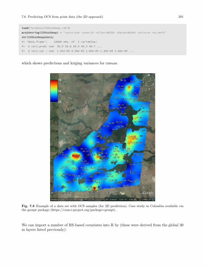
7.6 Predicting OCS from point data (the 2D approach) 291
load("extdata/COSha30map.rda")proj4string(COSha30map) = "+proj=utm +zone=18 +ellps=WGS84 +datum=WGS84 +units=m +no_defs"str(COSha30map@data)#> 'data.frame': 10000 obs. of 2 variables:#> $ var1.pred: num 39.9 39.8 39.9 40.3 40.7 ...#> $ var1.var : num 1.91e-05 6.39e-05 1.05e-04 1.39e-04 1.66e-04 ...
which shows predictions and kriging variances for COSha30.
Fig. 7.8 Example of a data set with OCS samples (for 2D prediction). Case study in Colombia available viathe geospt package (https://cran.r-project.org/package=geospt).
We can import a number of RS-based covariates into R by (these were derived from the global 30m layers listed previously):
292 7 Spatial prediction and assessment of Soil Organic Carbon
covs30m = readRDS("extdata/covs30m.rds")proj4string(covs30m) = proj4string(COSha30map)names(covs30m)#> [1] "SRTMGL1_SRTMGL1.2_cprof"#> [2] "SRTMGL1_SRTMGL1.2_devmean"#> [3] "SRTMGL1_SRTMGL1.2_openn"#> [4] "SRTMGL1_SRTMGL1.2_openp"#> [5] "SRTMGL1_SRTMGL1.2_slope"#> [6] "SRTMGL1_SRTMGL1.2_twi"#> [7] "SRTMGL1_SRTMGL1.2_vbf"#> [8] "SRTMGL1_SRTMGL1.2_vdepth"#> [9] "SRTMGL1_SRTMGL1.2"#> [10] "COSha30map_var1pred_"#> [11] "GlobalForestChange2000.2014_first_NIRL00"#> [12] "GlobalForestChange2000.2014_first_REDL00"#> [13] "GlobalForestChange2000.2014_first_SW1L00"#> [14] "GlobalForestChange2000.2014_first_SW2L00"#> [15] "GlobalForestChange2000.2014_treecover2000"#> [16] "GlobalSurfaceWater_extent"#> [17] "GlobalSurfaceWater_occurrence"#> [18] "Landsat_bare2010"
This contains a number of covariates from SRTM DEM derivatives, to Global Surface Wateroccurrence values and similar (see section 4.1.2 for more details). All these could potentially proveuseful for mapping OCS. We can also derive buffer distances from observations points and usethese (as measures of spatial context) to improve predictions (Hengl et al, 2018a):
proj4string(COSha30map) = "+proj=utm +zone=18 +ellps=WGS84 +datum=WGS84 +units=m +no_defs"coordinates(COSha30) = ~ x+yproj4string(COSha30) = proj4string(COSha30map)covs30mdist = GSIF::buffer.dist(COSha30["COSha30"], covs30m[1],
as.factor(1:nrow(COSha30)))
We can convert the original covariates to Principal Components, also to fill in all missing pixels:
covs30m@data = cbind(covs30m@data, covs30mdist@data)sel.rm = c("GlobalSurfaceWater_occurrence", "GlobalSurfaceWater_extent",
"Landsat_bare2010", "COSha30map_var1pred_")rr = which(names(covs30m@data) %in% sel.rm)fm.spc = as.formula(paste(" ~ ", paste(names(covs30m)[-rr], collapse = "+")))proj4string(covs30m) = proj4string(COSha30)covs30m.spc = GSIF::spc(covs30m, fm.spc)#> Converting covariates to principal components...ov.COSha30 = cbind(as.data.frame(COSha30), over(COSha30, covs30m.spc@predicted))

7.6 Predicting OCS from point data (the 2D approach) 293
By using the above listed covariates, we can fit a spatial prediction 2D model using an availablemodel, such as ranger4 (Wright and Ziegler, 2017), xgboost5 and/or gamboost6:
library(caret)#> Loading required package: lattice#> Loading required package: ggplot2library(ranger)fm.COSha30 = as.formula(paste("COSha30 ~ ",
paste(names(covs30m.spc@predicted), collapse = "+")))fm.COSha30#> COSha30 ~ PC1 + PC2 + PC3 + PC4 + PC5 + PC6 + PC7 + PC8 + PC9 +#> PC10 + PC11 + PC12 + PC13 + PC14 + PC15 + PC16 + PC17 + PC18 +#> PC19 + PC20 + PC21 + PC22 + PC23 + PC24 + PC25 + PC26 + PC27 +#> PC28 + PC29 + PC30 + PC31 + PC32 + PC33 + PC34 + PC35 + PC36 +#> PC37 + PC38 + PC39 + PC40 + PC41 + PC42 + PC43 + PC44 + PC45 +#> PC46 + PC47 + PC48 + PC49 + PC50 + PC51 + PC52 + PC53 + PC54 +#> PC55 + PC56 + PC57 + PC58 + PC59 + PC60 + PC61 + PC62 + PC63 +#> PC64 + PC65 + PC66 + PC67 + PC68 + PC69 + PC70 + PC71 + PC72 +#> PC73 + PC74 + PC75 + PC76 + PC77 + PC78 + PC79 + PC80 + PC81 +#> PC82 + PC83 + PC84 + PC85 + PC86 + PC87 + PC88 + PC89 + PC90 +#> PC91 + PC92 + PC93 + PC94 + PC95 + PC96 + PC97 + PC98 + PC99 +#> PC100 + PC101 + PC102 + PC103 + PC104 + PC105 + PC106 + PC107 +#> PC108 + PC109 + PC110 + PC111 + PC112 + PC113 + PC114 + PC115 +#> PC116 + PC117 + PC118 + PC119 + PC120 + PC121 + PC122 + PC123 +#> PC124 + PC125 + PC126 + PC127 + PC128 + PC129 + PC130 + PC131 +#> PC132rf.tuneGrid <- expand.grid(.mtry = seq(2, 60, by=5),
.splitrule = "maxstat",
.min.node.size = c(10, 20))gb.tuneGrid <- expand.grid(eta = c(0.3,0.4),
nrounds = c(50,100),max_depth = 2:3, gamma = 0,colsample_bytree = 0.8,min_child_weight = 1, subsample=1)
fitControl <- trainControl(method="repeatedcv", number=4, repeats=1)mFit1 <- train(fm.COSha30, data=ov.COSha30, method="ranger",
trControl=fitControl, importance='impurity',tuneGrid=rf.tuneGrid)
mFit1#> Random Forest#>#> 118 samples#> 132 predictors
4 https://cran.r-project.org/package=ranger5 https://cran.r-project.org/package=xgboost6 https://cran.r-project.org/package=GAMBoost
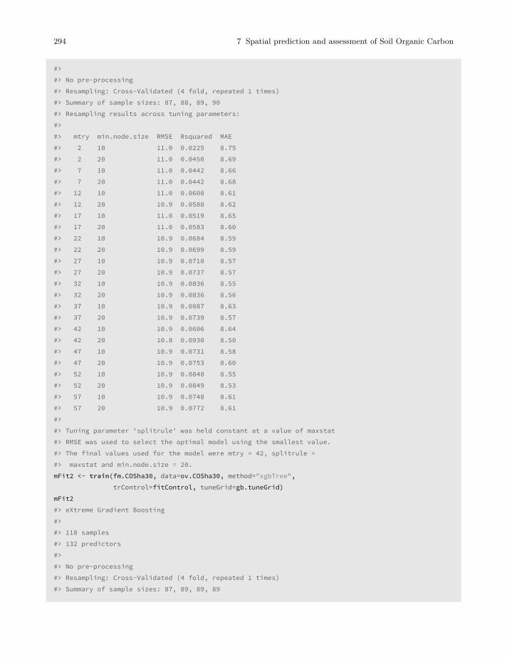
294 7 Spatial prediction and assessment of Soil Organic Carbon
#>#> No pre-processing#> Resampling: Cross-Validated (4 fold, repeated 1 times)#> Summary of sample sizes: 87, 88, 89, 90#> Resampling results across tuning parameters:#>#> mtry min.node.size RMSE Rsquared MAE#> 2 10 11.0 0.0225 8.75#> 2 20 11.0 0.0450 8.69#> 7 10 11.0 0.0442 8.66#> 7 20 11.0 0.0442 8.68#> 12 10 11.0 0.0608 8.61#> 12 20 10.9 0.0588 8.62#> 17 10 11.0 0.0519 8.65#> 17 20 11.0 0.0583 8.60#> 22 10 10.9 0.0684 8.59#> 22 20 10.9 0.0699 8.59#> 27 10 10.9 0.0710 8.57#> 27 20 10.9 0.0737 8.57#> 32 10 10.9 0.0836 8.55#> 32 20 10.9 0.0836 8.56#> 37 10 10.9 0.0887 8.63#> 37 20 10.9 0.0739 8.57#> 42 10 10.9 0.0606 8.64#> 42 20 10.8 0.0930 8.50#> 47 10 10.9 0.0731 8.58#> 47 20 10.9 0.0753 8.60#> 52 10 10.9 0.0848 8.55#> 52 20 10.9 0.0849 8.53#> 57 10 10.9 0.0748 8.61#> 57 20 10.9 0.0772 8.61#>#> Tuning parameter 'splitrule' was held constant at a value of maxstat#> RMSE was used to select the optimal model using the smallest value.#> The final values used for the model were mtry = 42, splitrule =#> maxstat and min.node.size = 20.mFit2 <- train(fm.COSha30, data=ov.COSha30, method="xgbTree",
trControl=fitControl, tuneGrid=gb.tuneGrid)mFit2#> eXtreme Gradient Boosting#>#> 118 samples#> 132 predictors#>#> No pre-processing#> Resampling: Cross-Validated (4 fold, repeated 1 times)#> Summary of sample sizes: 87, 89, 89, 89

7.6 Predicting OCS from point data (the 2D approach) 295
#> Resampling results across tuning parameters:#>#> eta max_depth nrounds RMSE Rsquared MAE#> 0.3 2 50 11.9 0.0547 9.20#> 0.3 2 100 11.9 0.0558 9.22#> 0.3 3 50 11.6 0.0305 9.14#> 0.3 3 100 11.6 0.0305 9.14#> 0.4 2 50 12.0 0.0443 9.60#> 0.4 2 100 12.0 0.0439 9.60#> 0.4 3 50 11.5 0.0776 9.19#> 0.4 3 100 11.5 0.0777 9.19#>#> Tuning parameter 'gamma' was held constant at a value of 0#> 0.8#> Tuning parameter 'min_child_weight' was held constant at a value of#> 1#> Tuning parameter 'subsample' was held constant at a value of 1#> RMSE was used to select the optimal model using the smallest value.#> The final values used for the model were nrounds = 100, max_depth = 3,#> eta = 0.4, gamma = 0, colsample_bytree = 0.8, min_child_weight = 1#> and subsample = 1.
This example illustrates that no significant spatial prediction models (with an R-square exceeding10%) can be fitted using these data. It is very common in soil mapping projects for models toexplain only low amounts of the total variation, resulting in large average errors of predictionand/or wide prediction intervals. This can occur because of high measurement errors, and/orbecause there are missing covariates, but it could also happen because the natural complexity ofsoils in the area is simply high.
Note that the absolute values of our predictions of OCS are somewhat different than those pro-duced by the geospt package7 authors, although the main patterns are comparable.7 https://cran.r-project.org/package=geospt
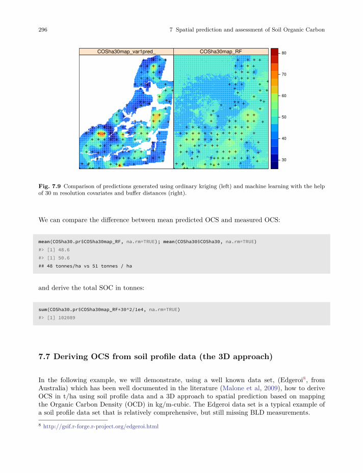
296 7 Spatial prediction and assessment of Soil Organic Carbon
+ + ++
++++++ +++++
+ + + + + ++
+ + + + +
+++
++
++
+++++
+
++++
+
+
++++
+ ++
+ +
+
++
+ + + +++++
+ + + +++++
++++++
+++
+ +
+++++
+ +
++ + +
++
+ +
++
+++++
+
+++
++
+++
+
+
COSha30map_var1pred_
+ + ++
++++++ +++++
+ + + + + ++
+ + + + +
+++
++
++
+++++
+
++++
+
+
++++
+ ++
+ +
+
++
+ + + +++++
+ + + +++++
++++++
+++
+ +
+++++
+ +
++ + +
++
+ +
++
+++++
+
+++
++
+++
+
+
COSha30map_RF
30
40
50
60
70
80
Fig. 7.9 Comparison of predictions generated using ordinary kriging (left) and machine learning with the helpof 30 m resolution covariates and buffer distances (right).
We can compare the difference between mean predicted OCS and measured OCS:
mean(COSha30.pr$COSha30map_RF, na.rm=TRUE); mean(COSha30$COSha30, na.rm=TRUE)#> [1] 48.6#> [1] 50.6## 48 tonnes/ha vs 51 tonnes / ha
and derive the total SOC in tonnes:
sum(COSha30.pr$COSha30map_RF*30^2/1e4, na.rm=TRUE)#> [1] 102089
7.7 Deriving OCS from soil profile data (the 3D approach)
In the following example, we will demonstrate, using a well known data set, (Edgeroi8, fromAustralia) which has been well documented in the literature (Malone et al, 2009), how to deriveOCS in t/ha using soil profile data and a 3D approach to spatial prediction based on mappingthe Organic Carbon Density (OCD) in kg/m-cubic. The Edgeroi data set is a typical example ofa soil profile data set that is relatively comprehensive, but still missing BLD measurements.8 http://gsif.r-forge.r-project.org/edgeroi.html

7.7 Deriving OCS from soil profile data (the 3D approach) 297
Fig. 7.10 Edgeroi data set: locations of soil profiles and Australian soil classification codes. For more detailssee Malone et al. (2009).
The Edgeroi data set can be loaded from the GSIF package:
library(GSIF)data(edgeroi)edgeroi.sp = edgeroi$sitescoordinates(edgeroi.sp) <- ~ LONGDA94 + LATGDA94proj4string(edgeroi.sp) <- CRS("+proj=longlat +ellps=GRS80 +towgs84=0,0,0,0,0,0,0 +no_defs")edgeroi.sp <- spTransform(edgeroi.sp, CRS("+init=epsg:28355"))
This data set comes with a list of covariate layers which can be used to model the distribution ofsoil organic carbon:
load("extdata/edgeroi.grids.rda")gridded(edgeroi.grids) <- ~x+yproj4string(edgeroi.grids) <- CRS("+init=epsg:28355")names(edgeroi.grids)#> [1] "DEMSRT5" "TWISRT5" "PMTGEO5" "EV1MOD5" "EV2MOD5" "EV3MOD5"
Because some of the covariate layers are factors e.g. PMTGEO5 (parent material map) and becauserandom forest requires numeric covariates, we can convert factors to numeric PCs by using:
298 7 Spatial prediction and assessment of Soil Organic Carbon
edgeroi.spc = spc(edgeroi.grids, ~DEMSRT5+TWISRT5+PMTGEO5+EV1MOD5+EV2MOD5+EV3MOD5)#> Converting PMTGEO5 to indicators...#> Converting covariates to principal components...
The Edgeroi completely lacks any BLD values, therefore before we can compute OCD values, weneed to estimate BLD values for each corresponding horizon. Here the easiest option is probablyto use BLD values sourced from LandGIS predictions (and which you can download from https://landgis.opengeohub.org).
landgis.bld = list.files("/mnt/DATA/LandGIS/predicted250m",pattern=glob2rx("sol_bulkdens.fineearth_usda.4a1h_m_*.tif$"),full.names=TRUE)
for(j in 1:length(landgis.bld)){system(paste0('gdalwarp ', landgis.bld[j], ' extdata/edgeroi_',
basename(landgis.bld[j]), ' -t_srs \"', proj4string(edgeroi.grids),'\" -tr 250 250 -co \"COMPRESS=DEFLATE\"',' -te ', paste(as.vector(edgeroi.grids@bbox), collapse = " ")))
}
Matching between the irregularly distributed soil horizons and LandGIS bulk density at standarddepths can be implemented in three steps. First, we overlay the points and LandGIS GeoTIFFsto get the BLD values in kg / cubic-m at standard depths:
sg <- list.files("extdata", "edgeroi_sol_bulkdens.fineearth", full.names = TRUE)ov <- as.data.frame(raster::extract(stack(sg), edgeroi.sp)*10)ov.edgeroi.BLD = ov[,c(grep("b0..", names(ov),
fixed = TRUE), grep("b10..", names(ov), fixed = TRUE),grep("b30..", names(ov),
fixed = TRUE), grep("b60..", names(ov), fixed = TRUE),grep("b100..", names(ov),
fixed = TRUE), grep("b200..", names(ov), fixed = TRUE))]
Second, we derive averaged estimates of BLD for standard depth intervals:
ov.edgeroi.BLDm <- data.frame(BLD.f = as.vector(sapply(2:ncol(ov.edgeroi.BLD),function(i){rowMeans(ov.edgeroi.BLD[,c(i-1,i)])})),
DEPTH.c = as.vector(sapply(1:5, function(i){rep(paste0("sd",i),nrow(edgeroi$sites))})), SOURCEID = rep(edgeroi$sites$SOURCEID, 5))
str(ov.edgeroi.BLDm)#> 'data.frame': 1795 obs. of 3 variables:#> $ BLD.f : num 1370 1335 1310 1500 1490 ...#> $ DEPTH.c : Factor w/ 5 levels "sd1","sd2","sd3",..: 1 1 1 1 1 1 1 1 1 1 ...#> $ SOURCEID: Factor w/ 359 levels "199_CAN_CP111_1",..: 1 2 3 4 5 6 7 8 9 10 ...
7.7 Deriving OCS from soil profile data (the 3D approach) 299
Third, we match BLD values by matching horizon depths (center of horizon) with the standarddepth intervals sd1 to sd5:
edgeroi$horizons$DEPTH = edgeroi$horizons$UHDICM +(edgeroi$horizons$LHDICM - edgeroi$horizons$UHDICM)/2
edgeroi$horizons$DEPTH.c = cut(edgeroi$horizons$DEPTH, include.lowest = TRUE,breaks = c(0,10,30,60,100,1000), labels = paste0("sd",1:5))
summary(edgeroi$horizons$DEPTH.c)#> sd1 sd2 sd3 sd4 sd5#> 391 379 408 391 769edgeroi$horizons$BLD.f = plyr::join(edgeroi$horizons[,c("SOURCEID","DEPTH.c")],
ov.edgeroi.BLDm)$BLD.f#> Joining by: SOURCEID, DEPTH.c
which shows relatively equal distribution of soil horizons within the standard depths. Now thatwe have a rough estimate of the bulk density for all horizons, we can derive OCD in kg/m-cubicby using:
edgeroi$horizons$OCD = edgeroi$horizons$ORCDRC/1000 * edgeroi$horizons$BLD.fsummary(edgeroi$horizons$OCD)#> Min. 1st Qu. Median Mean 3rd Qu. Max. NA's#> 0.1 2.4 7.2 9.5 13.2 124.9 262
This shows that OCD values range from 0–110 kg/m-cubic, with an average of 9.5 kg/m-cubic(this corresponds to an average organic carbon content of about 0.8%).
For further 3D spatial prediction of OCD we use the ranger package, which fits a random forestmodel to this 3D data. We start by overlaying points and rasters so that we can create a regressionmatrix:
ov2 <- over(edgeroi.sp, edgeroi.spc@predicted)ov2$SOURCEID = edgeroi.sp$SOURCEIDh2 = hor2xyd(edgeroi$horizons)m2 <- plyr::join_all(dfs = list(edgeroi$sites, h2, ov2))#> Joining by: SOURCEID#> Joining by: SOURCEID
The spatial prediction model can be fitted using:
fm.OCD = as.formula(paste0("OCD ~ DEPTH + ", paste(names(edgeroi.spc@predicted),collapse = "+")))
fm.OCD#> OCD ~ DEPTH + PC1 + PC2 + PC3 + PC4 + PC5 + PC6 + PC7 + PC8 +#> PC9 + PC10 + PC11 + PC12
300 7 Spatial prediction and assessment of Soil Organic Carbon
m.OCD <- ranger(fm.OCD, m2[complete.cases(m2[,all.vars(fm.OCD)]),],quantreg = TRUE, importance = "impurity")
m.OCD#> Ranger result#>#> Call:#> ranger(fm.OCD, m2[complete.cases(m2[, all.vars(fm.OCD)]), ], quantreg = TRUE, importance = "impurity")#>#> Type: Regression#> Number of trees: 500#> Sample size: 4972#> Number of independent variables: 13#> Mtry: 3#> Target node size: 5#> Variable importance mode: impurity#> Splitrule: variance#> OOB prediction error (MSE): 18.4#> R squared (OOB): 0.697
Which shows that the average error with Out-of-bag training points is ±4.2 kg/m-cubic. Note thatsetting quantreg = TRUE allows us to derive also a map of the prediction errors (Fig. 7.11), followingthe method of Meinshausen (2006).
To derive OCS in tons/ha we can compute OCD at two depths (0 and 30 cm) and then take themean value to produce a more representative value:
for(i in c(0,30)){edgeroi.spc@predicted$DEPTH = iOCD.rf <- predict(m.OCD, edgeroi.spc@predicted@data)nm1 = paste0("OCD.", i, "cm")edgeroi.grids@data[,nm1] = OCD.rf$predictionsOCD.qrf <- predict(m.OCD, edgeroi.spc@predicted@data,
type="quantiles", quantiles=c((1-.682)/2, 1-(1-.682)/2))nm2 = paste0("OCD.", i, "cm_se")edgeroi.grids@data[,nm2] = (OCD.qrf$predictions[,2] - OCD.qrf$predictions[,1])/2
}
so that the final Organic carbon stocks in t/ha is:
#> Min. 1st Qu. Median Mean 3rd Qu. Max.#> 20.3 39.1 48.0 48.8 57.6 112.1
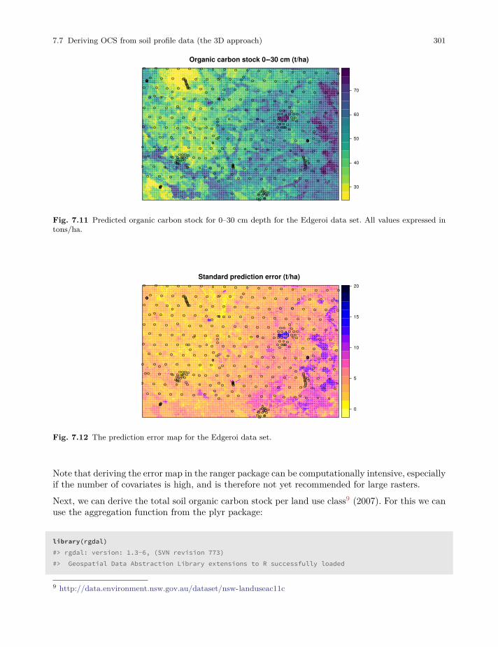
7.7 Deriving OCS from soil profile data (the 3D approach) 301
Organic carbon stock 0‒30 cm (t/ha)
30
40
50
60
70
Fig. 7.11 Predicted organic carbon stock for 0–30 cm depth for the Edgeroi data set. All values expressed intons/ha.
Standard prediction error (t/ha)
0
5
10
15
20
Fig. 7.12 The prediction error map for the Edgeroi data set.
Note that deriving the error map in the ranger package can be computationally intensive, especiallyif the number of covariates is high, and is therefore not yet recommended for large rasters.
Next, we can derive the total soil organic carbon stock per land use class9 (2007). For this we canuse the aggregation function from the plyr package:
library(rgdal)#> rgdal: version: 1.3-6, (SVN revision 773)#> Geospatial Data Abstraction Library extensions to R successfully loaded
9 http://data.environment.nsw.gov.au/dataset/nsw-landuseac11c
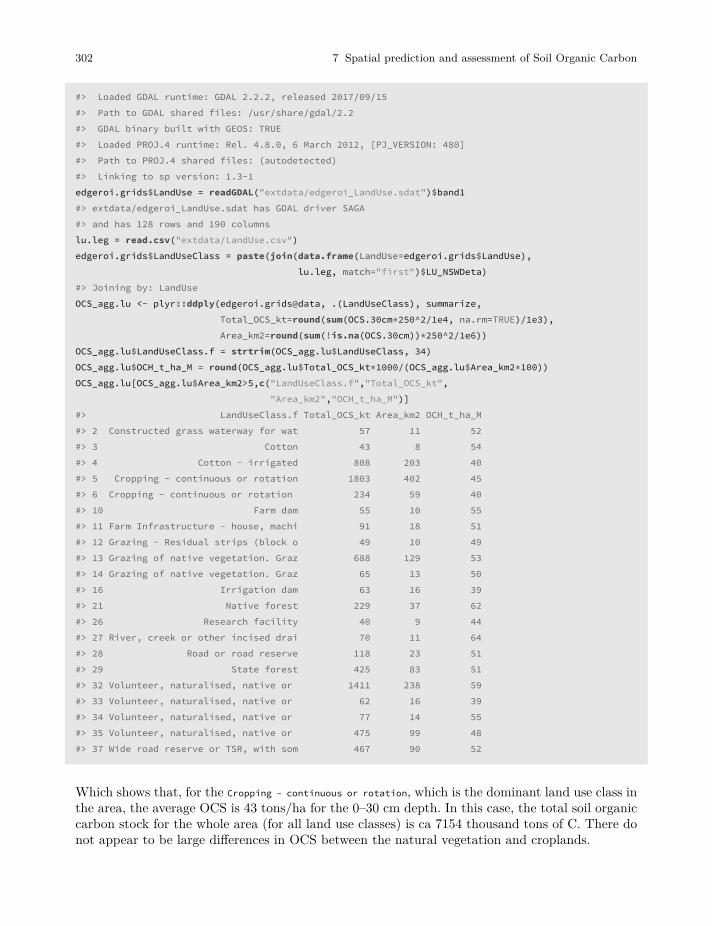
302 7 Spatial prediction and assessment of Soil Organic Carbon
#> Loaded GDAL runtime: GDAL 2.2.2, released 2017/09/15#> Path to GDAL shared files: /usr/share/gdal/2.2#> GDAL binary built with GEOS: TRUE#> Loaded PROJ.4 runtime: Rel. 4.8.0, 6 March 2012, [PJ_VERSION: 480]#> Path to PROJ.4 shared files: (autodetected)#> Linking to sp version: 1.3-1edgeroi.grids$LandUse = readGDAL("extdata/edgeroi_LandUse.sdat")$band1#> extdata/edgeroi_LandUse.sdat has GDAL driver SAGA#> and has 128 rows and 190 columnslu.leg = read.csv("extdata/LandUse.csv")edgeroi.grids$LandUseClass = paste(join(data.frame(LandUse=edgeroi.grids$LandUse),
lu.leg, match="first")$LU_NSWDeta)#> Joining by: LandUseOCS_agg.lu <- plyr::ddply(edgeroi.grids@data, .(LandUseClass), summarize,
Total_OCS_kt=round(sum(OCS.30cm*250^2/1e4, na.rm=TRUE)/1e3),Area_km2=round(sum(!is.na(OCS.30cm))*250^2/1e6))
OCS_agg.lu$LandUseClass.f = strtrim(OCS_agg.lu$LandUseClass, 34)OCS_agg.lu$OCH_t_ha_M = round(OCS_agg.lu$Total_OCS_kt*1000/(OCS_agg.lu$Area_km2*100))OCS_agg.lu[OCS_agg.lu$Area_km2>5,c("LandUseClass.f","Total_OCS_kt",
"Area_km2","OCH_t_ha_M")]#> LandUseClass.f Total_OCS_kt Area_km2 OCH_t_ha_M#> 2 Constructed grass waterway for wat 57 11 52#> 3 Cotton 43 8 54#> 4 Cotton - irrigated 808 203 40#> 5 Cropping - continuous or rotation 1803 402 45#> 6 Cropping - continuous or rotation 234 59 40#> 10 Farm dam 55 10 55#> 11 Farm Infrastructure - house, machi 91 18 51#> 12 Grazing - Residual strips (block o 49 10 49#> 13 Grazing of native vegetation. Graz 688 129 53#> 14 Grazing of native vegetation. Graz 65 13 50#> 16 Irrigation dam 63 16 39#> 21 Native forest 229 37 62#> 26 Research facility 40 9 44#> 27 River, creek or other incised drai 70 11 64#> 28 Road or road reserve 118 23 51#> 29 State forest 425 83 51#> 32 Volunteer, naturalised, native or 1411 238 59#> 33 Volunteer, naturalised, native or 62 16 39#> 34 Volunteer, naturalised, native or 77 14 55#> 35 Volunteer, naturalised, native or 475 99 48#> 37 Wide road reserve or TSR, with som 467 90 52
Which shows that, for the Cropping - continuous or rotation, which is the dominant land use class inthe area, the average OCS is 43 tons/ha for the 0–30 cm depth. In this case, the total soil organiccarbon stock for the whole area (for all land use classes) is ca 7154 thousand tons of C. There donot appear to be large differences in OCS between the natural vegetation and croplands.
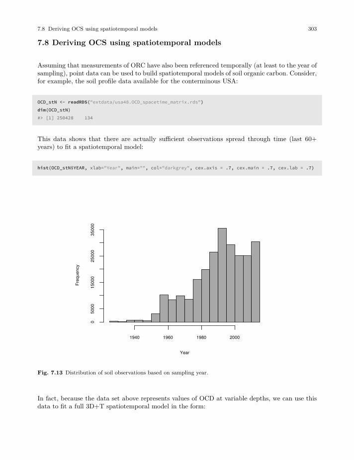
7.8 Deriving OCS using spatiotemporal models 303
7.8 Deriving OCS using spatiotemporal models
Assuming that measurements of ORC have also been referenced temporally (at least to the year ofsampling), point data can be used to build spatiotemporal models of soil organic carbon. Consider,for example, the soil profile data available for the conterminous USA:
OCD_stN <- readRDS("extdata/usa48.OCD_spacetime_matrix.rds")dim(OCD_stN)#> [1] 250428 134
This data shows that there are actually sufficient observations spread through time (last 60+years) to fit a spatiotemporal model:
hist(OCD_stN$YEAR, xlab="Year", main="", col="darkgrey", cex.axis = .7, cex.main = .7, cex.lab = .7)
Year
Freq
uenc
y
1940 1960 1980 2000
050
0015
000
2500
035
000
Fig. 7.13 Distribution of soil observations based on sampling year.
In fact, because the data set above represents values of OCD at variable depths, we can use thisdata to fit a full 3D+T spatiotemporal model in the form:
304 7 Spatial prediction and assessment of Soil Organic Carbon
OCD(𝑥𝑦𝑑𝑡) = 𝑑 + 𝑋1(𝑥𝑦) + … + 𝑋𝑘(𝑥𝑦) + … + 𝑋𝑝(𝑥𝑦𝑡) (7.8)
where 𝑑 is the depth, 𝑋𝑘(𝑥𝑦) are static covariates i.e. the covariates that do not change in time,and 𝑋𝑝(𝑥𝑦𝑡) are spatiotemporal covariates i.e. covariates that change with time. Here we canassume that the static covariates are mainly landform and lithology: these have probably notchanged significantly in the last 100 years. Land cover, land use and climate, on the other hand,have probably changed drastically in the last 100 years and have to be represented with a time-series of images. There are, indeed, several time-series data sets now available that can be used torepresent land cover dynamics:
• HYDE 3.2 Historic land use data set10 (Klein Goldewijk et al, 2011): portrays the distribution ofmajor agricultural systems from 10,000 BC (pre-historic no land-use condition) to the presenttime. 10 categories of land use have been represented: total cropping, total grazing, pasture(improved grazing-land), rangeland (unimproved grazing-land), total rainfed cropping, totalirrigated cropping, with further subdivisions for rice and non-rice cropping systems for bothrainfed and irrigated cropping.
• CRU TS2.1 climatic surfaces11 for period 1960–1990 (Harris et al, 2014).
• UNEP-WCMC Generalized Original and Current Forest cover map12 showing global dynamicsof forest cover.
All these layers are available only at a relatively coarse resolution of 10 km, but then cover longertime spans. Note also that, since these are time-series images, spatiotemporal overlay can taketime as spatial overlay must be repeated for each time period. The spatiotemporal matrix filealready contains the results of overlay, so that we can focus directly on building spatiotemporalmodels of OCD e.g.:
pr.lst <- names(OCD_stN)[-which(names(OCD_stN) %in% c("SOURCEID", "DEPTH.f", "OCDENS","YEAR", "YEAR_c", "LONWGS84","LATWGS84"))]
fm0.st <- as.formula(paste('OCDENS ~ DEPTH.f + ', paste(pr.lst, collapse="+")))sel0.m = complete.cases(OCD_stN[,all.vars(fm0.st)])## takes >2 minsrf0.OCD_st <- ranger(fm0.st, data=OCD_stN[sel0.m,all.vars(fm0.st)],
importance="impurity", write.forest=TRUE, num.trees=120)
the most important covariates being:
xl <- as.list(ranger::importance(rf0.OCD_st))print(t(data.frame(xl[order(unlist(xl), decreasing=TRUE)[1:10]])))
10 ftp://ftp.pbl.nl/hyde/hyde3.2/11 http://www.ipcc-data.org/observ/clim/12 http://www.unep-wcmc.org/resources-and-data/generalised-original-and-current-forest
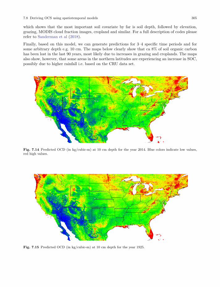
7.8 Deriving OCS using spatiotemporal models 305
which shows that the most important soil covariate by far is soil depth, followed by elevation,grazing, MODIS cloud fraction images, cropland and similar. For a full description of codes pleaserefer to Sanderman et al (2018).
Finally, based on this model, we can generate predictions for 3–4 specific time periods and forsome arbitrary depth e.g. 10 cm. The maps below clearly show that ca 8% of soil organic carbonhas been lost in the last 90 years, most likely due to increases in grazing and croplands. The mapsalso show, however, that some areas in the northern latitudes are experiencing an increase in SOC,possibly due to higher rainfall i.e. based on the CRU data set.
Fig. 7.14 Predicted OCD (in kg/cubic-m) at 10 cm depth for the year 2014. Blue colors indicate low values,red high values.
Fig. 7.15 Predicted OCD (in kg/cubic-m) at 10 cm depth for the year 1925.
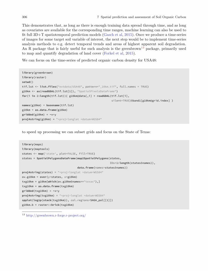
306 7 Spatial prediction and assessment of Soil Organic Carbon
This demonstrates that, as long as there is enough training data spread through time, and as longas covariates are available for the corresponding time ranges, machine learning can also be used tofit full 3D+T spatiotemporal prediction models (Gasch et al, 2015). Once we produce a time-seriesof images for some target soil variable of interest, the next step would be to implement time-seriesanalysis methods to e.g. detect temporal trends and areas of highest apparent soil degradation.An R package that is fairly useful for such analysis is the greenbrown13 package, primarily usedto map and quantify degradation of land cover (Forkel et al, 2015).
We can focus on the time-series of predicted organic carbon density for USA48:
library(greenbrown)library(raster)setwd()tif.lst <- list.files("extdata/USA48", pattern="_10km.tif", full.names = TRUE)g10km <- as(readGDAL(tif.lst[1]), "SpatialPixelsDataFrame")for(i in 2:length(tif.lst)){ g10km@data[,i] = readGDAL(tif.lst[i],
silent=TRUE)$band1[[email protected]] }names(g10km) = basename(tif.lst)g10km = as.data.frame(g10km)gridded(g10km) = ~x+yproj4string(g10km) = "+proj=longlat +datum=WGS84"
to speed up processing we can subset grids and focus on the State of Texas:
library(maps)library(maptools)states <- map('state', plot=FALSE, fill=TRUE)states = SpatialPolygonsDataFrame(map2SpatialPolygons(states,
IDs=1:length(states$names)),data.frame(names=states$names))
proj4string(states) = "+proj=longlat +datum=WGS84"ov.g10km = over(y=states, x=g10km)txg10km = g10km[which(ov.g10km$names=="texas"),]txg10km = as.data.frame(txg10km)gridded(txg10km) = ~x+yproj4string(txg10km) = "+proj=longlat +datum=WGS84"spplot(log1p(stack(txg10km)), col.regions=SAGA_pal[[1]])g10km.b = raster::brick(txg10km)
13 http://greenbrown.r-forge.r-project.org/
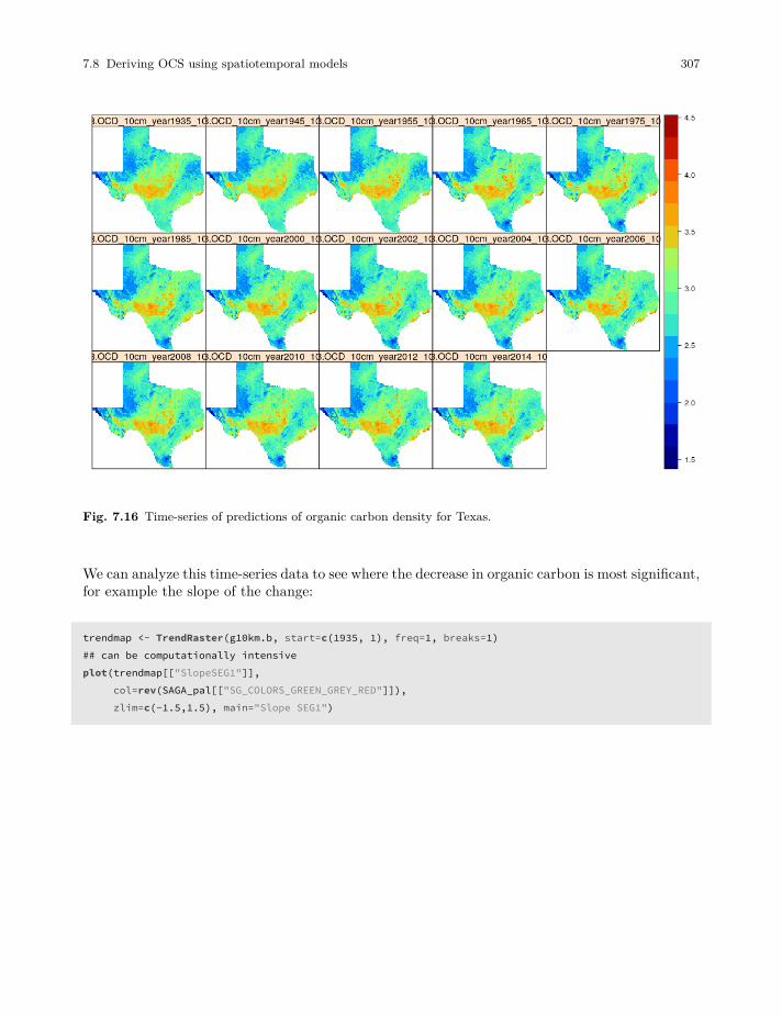
7.8 Deriving OCS using spatiotemporal models 307
Fig. 7.16 Time-series of predictions of organic carbon density for Texas.
We can analyze this time-series data to see where the decrease in organic carbon is most significant,for example the slope of the change:
trendmap <- TrendRaster(g10km.b, start=c(1935, 1), freq=1, breaks=1)## can be computationally intensiveplot(trendmap[["SlopeSEG1"]],
col=rev(SAGA_pal[["SG_COLORS_GREEN_GREY_RED"]]),zlim=c(-1.5,1.5), main="Slope SEG1")

308 7 Spatial prediction and assessment of Soil Organic Carbon
Fig. 7.17 Predicted slope of change of soil organic carbon density for Texas for the period 1935–2014. Negativevalues indicate loss of soil organic carbon.
which shows that loss of soil organic carbon is especially distinct in the southern part of Texas. Theslope coefficient map is, on average, negative, which indicates that most of the state has lost organiccarbon for the period of interest. Note that running such time-series analysis is not trivial as asufficient number of observations in time (if possible: repetitions) is needed to be able to extractsignificant patterns. Also TrendRaster function can be quite computationally intensive, hence somecareful planning of the processing steps / processing infrastructure is usually recommended.
7.9 Summary points
Based on all the examples and discussion above, the following key points can be emphasized:
1. OCS for an area of interest can be derived either using 2D or 3D approaches. 3D approachestypically include modeling ORC, BLD and CRF separately (and then deriving OCS per pixel),or modeling OCD for standard depths and then converting to OCS.
2. Publicly available RS-based covariates (SRTM / ALOS DEM, Landsat, Sentinel satellites) areavailable for improving the mapping accuracy of OCS. Improving the accuracy of OCS maps isbecoming less expensive, given the increasing availability of RS data.
3. PT (Pedo-Transfer) rules can be used to fill in (estimate) missing BLD values and to estimateORC for deeper soil depths. Also global maps with predictions of BLD and CRF can be usedto supply missing values, if there are no other alternatives.
4. Machine learning techniques such as Random Forest, neural nets, gradient boosting and sim-ilar, can be used to predict soil organic carbon in 2D, 3D and in spatiotemporal modeling
7.9 Summary points 309
frameworks. The accuracy of these predictions is improved relative to linear statistical models,especially where the relationship between soil organic carbon distribution and climatic, landcover, hydrological, relief and similar covariates is complex (i.e. non-linear).
5. Global estimates of ORC, BLD and CRF can be used as covariates so that consistent predictionscan be produced (as explained in Ramcharan et al (2018)).
6. By producing spatial predictions of OCS for specific time periods, one can derive estimates ofOCS change (loss or gain).
7. Most of the statistical / analytical tools required for running spatial analysis, time series anal-ysis, export and visualization of soil carbon data are available in R, especially thanks to thecontributed packages: aqp, caret, ranger, xgboost, GSIF, greenbrown and similar.
8. Accurate measurements of bulk density (BLD) by horizon or depth interval for described soilprofiles are critical for producing accurate calculations of soil carbon stock. Unfortunately,BLD data are often missing or not reported for many legacy soil profile descriptions and arefrequently unreliable even when reported. Future efforts to sample and describe soil profilesshould emphasise the collection and publication of accurate measurements of BLD by horizonor depth interval for all described soil profiles.

Chapter 8
Practical tips for organizing Predictive Soil Mapping
Edited by: T. Hengl, R. A. MacMillan and I. Wheeler
8.1 Critical aspects of Predictive Soil Mapping
Previous chapters in this book have reviewed many of the technical aspects of PSM. For a statisti-cian, following the right procedures and applying the right statistical frameworks will are the keyelements of success for a PSM project. In practice, it is really a combination of all elements andaspects that determines a success of a PSM project. In this chapter we provide some practical tipson how to organize work and what to be especially careful about. We refer to these as the criticalaspects of PSM projects.
At the end of the chapter we also try to present additional practical tips in the form of check-listsand simple economic analysis, to help readers avoid making unrealistic plans or producing mapsthat may not find effective use.
8.1.1 PSM main steps
Based on previously presented theory, we can summarize the usual PSM processes as:
1. Preparation of point data (training data).
2. Preparation of covariate data (the explanatory variables).
3. Model fitting and validation (building rules by overlay, model fitting and cross-validation).
4. Prediction and generation of (currently best-possible) final maps (applying the rules).
5. Archiving and distribution of maps (usually via soil geographical databases and/or web ser-vices).
6. Updates and improvements (support).
311
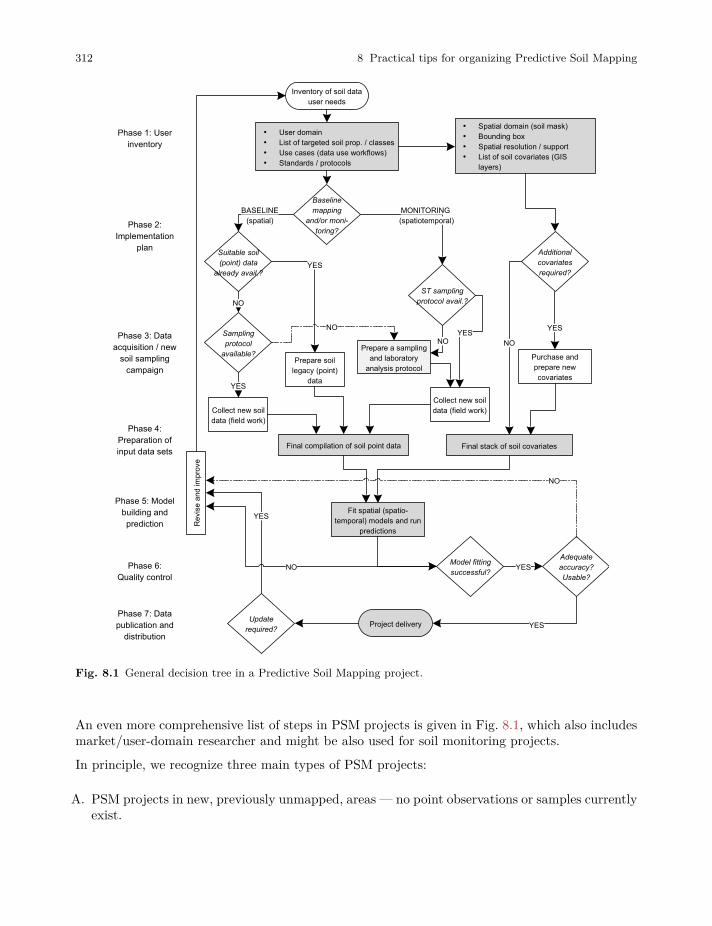
312 8 Practical tips for organizing Predictive Soil Mapping
Phase 1: User inventory
Phase 2: Implementation
plan
Phase 3: Data acquisition / new
soil sampling campaign
Phase 4: Preparation of input data sets
Phase 5: Model building and prediction
Phase 6: Quality control
Phase 7: Data publication and
distribution
Baseline mapping
and/or moni-toring?
Inventory of soil data user needs
Prepare soil legacy (point)
data
Suitable soil (point) data
already avail.?
Collect new soil data (field work)
Sampling protocol
available?
Adequate accuracy?Usable?
Re
vise
and
impr
ove
Final compilation of soil point data Final stack of soil covariates
Additional covariates required?
• User domain• List of targeted soil prop. / classes• Use cases (data use workflows)• Standards / protocols
BASELINE(spatial)
ST sampling protocol avail.?
Collect new soil data (field work)
YES
Prepare a sampling and laboratory
analysis protocol
Purchase and prepare new covariates
YES
NO
Project delivery
YES
MONITORING (spatiotemporal)
NO
YES
NO
Model fitting successful?
Fit spatial (spatio-temporal) models and run
predictions
YESNO
YES
NO
NO
• Spatial domain (soil mask)• Bounding box• Spatial resolution / support• List of soil covariates (GIS
layers)
Update required?
YES
Fig. 8.1 General decision tree in a Predictive Soil Mapping project.
An even more comprehensive list of steps in PSM projects is given in Fig. 8.1, which also includesmarket/user-domain researcher and might be also used for soil monitoring projects.
In principle, we recognize three main types of PSM projects:
A. PSM projects in new, previously unmapped, areas — no point observations or samples currentlyexist.

8.1 Critical aspects of Predictive Soil Mapping 313
B. PSM projects using legacy points — sufficient point data to support PSM exist and are available,but no previous PSM modelling has been implemented for this area.
C. PSM projects aimed at optimizing predictions and usability — Previous PSM models havealready been completed but previous results can still be improved / optimized.
If point data are not available, then collecting new point data, via field work and laboratoryanalysis will usually consume a majority of any PSM project budget (PSM projects type A).Otherwise, if point data are already available (and only need to be imported and harmonized),the most time consuming part of PSM will likely be preparation of covariate data layers (PSMprojects type B). Predictions can also take a long time and computing costs per update can besignificant (see further sections). Personnel costs can be more significant than server costs asprogramming can require weeks of staff time. However, if programming is done at a high level(e.g. through generic functions and objects), subsequent updates should require less personneltime as predictions can be increasingly automated.
Another aspect of PSM is the time dimension i.e. will maps be continuously updated or do theyneed to produced only once and then remain relevant and useful for years (often up to decades),so that PSM projects can also be classified into:
I. PSM projects for the purpose of mapping static (stable) spatial patterns only.
II. PSM projects for the purpose of one-time change detection (e.g. two time intervals).
III. PSM projects for the purpose of monitoring soil conditions / status (continuous updates atregular intervals).
To date, almost all conventional soil mapping ignores time and change and instead tries to assumethat soil properties are static and persist through time virtually unaltered. Increasingly, however,new generation PSM projects aim to monitor changes in soil resources, with special focus given tochanges in soil organic carbon, soil nutrients, soil moisture and similar (Fig. 8.2). For PSM projecttype III spatio-temporal prediction models can be used (as in meteorology for example), but thenthis requires that sufficient training data are available in both the space and time domains e.g. atleast five measurement intervals / repetitions.
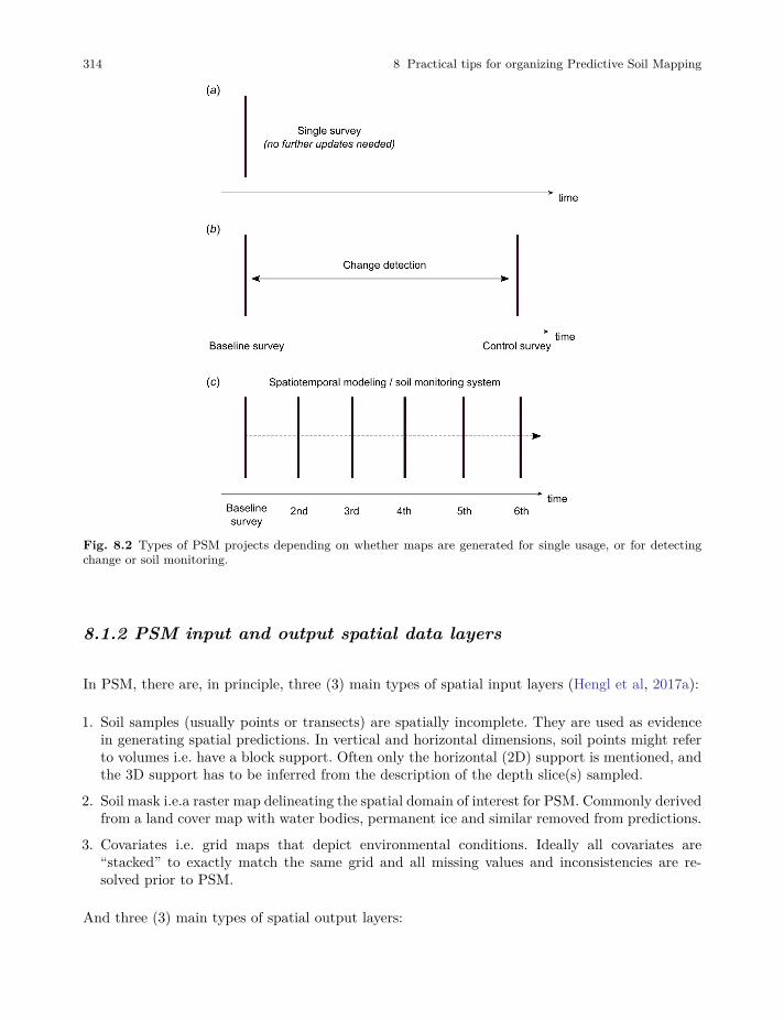
314 8 Practical tips for organizing Predictive Soil Mapping
Fig. 8.2 Types of PSM projects depending on whether maps are generated for single usage, or for detectingchange or soil monitoring.
8.1.2 PSM input and output spatial data layers
In PSM, there are, in principle, three (3) main types of spatial input layers (Hengl et al, 2017a):
1. Soil samples (usually points or transects) are spatially incomplete. They are used as evidencein generating spatial predictions. In vertical and horizontal dimensions, soil points might referto volumes i.e. have a block support. Often only the horizontal (2D) support is mentioned, andthe 3D support has to be inferred from the description of the depth slice(s) sampled.
2. Soil mask i.e.a raster map delineating the spatial domain of interest for PSM. Commonly derivedfrom a land cover map with water bodies, permanent ice and similar removed from predictions.
3. Covariates i.e. grid maps that depict environmental conditions. Ideally all covariates are“stacked” to exactly match the same grid and all missing values and inconsistencies are re-solved prior to PSM.
And three (3) main types of spatial output layers:
8.2 Technical specifications affecting the majority of production costs 315
4. Spatial predictions of (primary) soil variables that are spatially complete i.e. are produced andavailable for the entire extent of the soil mask.
5. Maps of (secondary) soil variables which are derived using calculations applied to combinationsof the primary predicted soil variables. These are usually less expensive to produce, by an orderof magnitude, than spatial predictions of primary soil variables.
6. Maps quantifying uncertainty in terms of prediction error, prediction interval, confusion indexor similar metrics. These may be derived at the same time as predictions are made or can bemade completely independently of predictions.
Each element of the map types listed above needs to have a consistent spatio-temporal reference,which typically includes:
• Geographic location in local or geographic coordinates (for global modelling we usually preferinitial georeferencing that uses longitude and latitude in the WGS84 coordinate system);
• Depth interval expressed in cm from the land surface (upper and lower depth) for layers andpoint depth for point predictions;
• Support size or referent soil volume (or voxel) i.e. the horizontal sampling area multiplied bythe thickness of the sampling block e.g. 30 × 30 × 0.3 m.
• Temporal reference i.e. a begin and an end date/time of the period of measure-ments/estimations. Specifying exact spatial and temporal references in the metadatacan is vital for optimal production and use of maps.
Spatial predictions of primary soil properties can be used to:
• Derive spatial aggregates (upscaling to coarser resolution).
• Derive vertical aggregates e.g. mean pH in 0–100 cm of soil (for this we usually recommendusing the trapezoidal rule as explained in Hengl et al (2017a)).
• Derive secondary soil properties e.g. available water capacity, organic carbon stock etc.
Spatial predictions of primary soil variables and derived soil variables are meant to be used fordecision making and further modeling i.e. they are used to construct a Soil Information Systemonce all values of all variables are known for all pixels within the soil mask. A SIS should ideallyprovide information that can directly support input to modeling, planning and decision-making.
8.2 Technical specifications affecting the majority of production costs
The majority of the costs of a PSM project are controlled by the following:
1. Spatial resolution (commonly 30 m, 100 m or 250 m): Spatial resolution is crucial in deter-mining the total costs of PSM, especially in terms of computing, storage, network traffic andhardware requirements. Changing the spatial resolution from 100 to 30 m means that about 10
316 8 Practical tips for organizing Predictive Soil Mapping
times more pixels will need to be produced, stored and shared via the network. This does notalways imply that the costs of PSM will also be 10 times greater than for a 100 m resolutionproject, but the increase in costs is often going to follow a quadratic function. Also note that,for even finer resolutions e.g. 5 m, very limited free public covariate data are available andadditional purchases of commercial RS products will typically be required. For example thelatest 12 m resolution WorldDEM (https://worlddem-database.terrasar.com/) can cost up to10 USD per square km, which can increase PSM costs significantly.
2. List of target variables and their complexity: Some PSM projects focus on mapping 1–2soil variables only, and as such can be rather straightforward to implement. Any PSM projectthat requires creation of a complete Soil Information System (tens of quantitative soil variablesand soil types), will definitely demand more effort and hence potentially significantly increasecosts. Typically, evaluation and quality control of maps in a SIS requires an analyst to openand visually compare patterns from different maps and to make use of considerable empir-ical knowledge of soils. Costs of production can also be significantly increased depending onwhether lower and upper prediction intervals are required. As with increasing spatial resolution,requesting lower and upper prediction intervals means that two times more pixels will need tobe produced.
3. Targeted accuracy/quality levels: Often the agencies that order spatial soil informationexpect that predictions will achieve some desired accuracy targets. Accuracy of predictions can,indeed, often be improved (but only up to a certain level), by simply improving the modellingframework (PSM projects type C). In practice, if a contractor requires significant improvementsin accuracy, then this often means that both additional point records and improved covariatedata (for example at finer spatial resolution) will need to be collected and/or purchased. Thiscan often mean that the original budget will have to be increased until the required accuracylevel can be reached.
4. List of targeted services / user domain: Is the goal of the PSM project to produce dataonly, or to serve this data for a number of applications (use-cases)? How broad is the userdomain? Is the data being made for a few targeted clients or for the widest possible user base?Is high traffic expected and, if so, how will the costs of hosting and serving the data andprocesses be met? Producing a robust, scalable web-system that can serve thousands of usersat the same time requires considerable investments in programming and maintenance.
5. Commercialization options: Commercialization of data and services can also significantlyincrease costs, since the development team needs to prepare also workflows where invoicesand bills are generated on demand, or where efficient support and security are now criticallyimportant. Even though many companies exist that offer outsourcing of this functionality, manyorganizations and companies prefer to have full control of the commercialization steps, hencesuch functionality needs to be then developed internally within the project or organization.
8.2.1 Field observations and measurements
Observations and measurements (O&M) are at the heart of all advances in scientific endeavor.One cannot describe, or attempt to understand, what one cannot see, or measure. Great leapsin scientific understanding have always followed from major improvements in the ability to see,
8.2 Technical specifications affecting the majority of production costs 317
and measure, phenomenon or objects. Think of the telescope and astronomy, the microscope andmicrobiology, the X-ray and atomic structure or crystallography and so on.
In the area of resource inventories, observations and measurements carried out in the field (fielddata) provide the evidence critical to developing the understanding of spatial patterns and spatialprocesses that underpins all models that predict the spatial distribution of properties or classes.This applies equally to subjective, empirical mental, or conceptual, models and objective, quan-titative statistical models. The more and better the observations and measurements we obtain,the better will be our ability to understand and predict spatial patterns of soils and other naturalphenomena. Consider here some general observations on how to maximize efficiency of O&M:
• For maximum utility, field data should be objective and reproducible.
• They should be collected using some kind of unbiased sampling design that supports repro-ducibility and return sampling (Brus, 2019; Malone et al, 2019).
• They should be located as accurately as possible in both space (geolocation) and time (temporallocation).
• They should describe and measure actual conditions in their present state (and current landuse) and not in some assumed natural, climax or equilibrium condition.
• They should capture and permit description of spatial and temporal variation across multiplespatial scales and time frames.
It is widely assumed that collecting new field data to produce new and improved inventory prod-ucts is prohibitively expensive and will never be possible or affordable in the foreseeable future.Consequently, most current projects or programs that aim to produce new maps of soils or otherterrestrial entities have explicitly embraced the assumption that the only feasible way to pro-duce new soil maps is to locate, and make use of, existing legacy data consisting of previouslyreported field observations or existing laboratory analysed field samples. However, recent activitiesin Africa (www.Africasoils.net), for example, have demonstrated conclusively that it is feasible,affordable and beneficial to collect new field observations and samples and to analyse new soilsamples affordably and to a high standard (Shepherd and Walsh, 2007).
8.2.2 Preparation of point data
Import of basic O&M field data (e.g. soil point data) can be time consuming and require intensive,often manual, checking and harmonization. Communicating with the original data producers ishighly recommended to reduce errors during import. Getting original data producers involved canbe best achieved by inviting them to become full participants ( e.g. join in joint publications) orby at least providing adequate and visible acknowledgement (e.g. listing names and affiliations inmetadata or on project websites).
Documenting all import, filtering and translation steps applied to source data is highly recom-mended, as these steps can then be communicated to the original field data producers to helpfilter out further bugs. We typically generate a single tabular object with the following propertiesas our final output of point data preparation :
318 8 Practical tips for organizing Predictive Soil Mapping
• Consistent column names are used; metadata explaining column names is provided,
• All columns contain standardized data (same variable type, same measurement units) withharmonized values (no significant bias in values from sub-methods),
• All artifacts, outliers and typos have been identified and corrected to the best of our ability,
• Missing values have been imputed (replaced with estimated values) as much as possible,
• Spatial coordinates, including depths, (x,y,z) are available for all rows (point locations).
8.2.3 Preparation of covariates
As mentioned previously, preparation of covariate layers can require significant effort, even if RSdata is publicly available and well documented. For example, MODIS land products are amongthe most used RS layers for global to regional PSM. Using raw reflectance data, such as themid-infrared MODIS bands from a single day can, however, be of limited use for soil mappingin areas with dynamic vegetation, i.e. with strong seasonal changes in vegetation cover. To ac-count for seasonal fluctuation and for inter-annual variations in surface reflectance, we insteadadvise using long-term temporal signatures of the soil surface derived as monthly averages fromlong-term MODIS imagery (18+ years of data). We assume here that, for each location in theworld, long-term average seasonal signatures of surface reflectance or vegetation index provide abetter indication of site environmental characteristics than just a single day snapshot of surfacereflectance. Computing temporal signatures of the land surface requires a large investment of time(comparable to the generation of climatic images vs temporary weather maps), but it is possiblythe only way to effectively represent the cumulative influence of living organisms on soil formation(Hengl et al, 2017a).
Typical operations to prepare soil covariates for PSM thus include:
• Downloading the original source RS data,
• Filtering missing pixels using neighborhood filters and/or simple rules,
• Running aggregation functions (usually via some tiling system),
• Running hydrological and morphological analysis on source DEM data
• Calculation of a Gaussian pyramid, for some relevant covariates, at multiple coarser resolutions,in order to capture multi-scale variation at appropriate (longer range) process scales.
• Preparing final mosaics to be used for PSM (e.g. convert to GeoTIFFs and compress usinginternal compression "COMPRESS=DEFLATE" or similar),
For processing the covariates we currently use a combination of Open Source GIS software, pri-marily SAGA GIS, GRASS GIS, Whitebox tools, R packages raster, sp, GSIF and GDAL for re-projecting, mosaicking and merging tiles. SAGA GIS and GDAL were found to be highly suitablefor processing massive data sets, as parallelization of computing was relatively easy to implement.
Preparation of covariate layers is completed once:
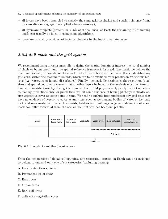
8.2 Technical specifications affecting the majority of production costs 319
• all layers have been resampled to exactly the same grid resolution and spatial reference frame(downscaling or aggregation applied where necessary),
• all layers are complete (present for >95% of the soil mask at least; the remaining 5% of missingpixels can usually be filled-in using some algorithm),
• there are no visibly obvious artifacts or blunders in the input covariate layers,
8.2.4 Soil mask and the grid system
We recommend using a raster mask file to define the spatial domain of interest (i.e. total numberof pixels to be mapped), and the spatial reference framework for PSM. The mask file defines themaximum extent, or bounds, of the area for which predictions will be made. It also identifies anygrid cells, within the maximum bounds, which are to be excluded from prediction for various rea-sons (e.g. water, ice or human disturbance). Finally, the mask file establishes the resolution (pixelsize) and spatial coordinate system that all other layers included in the analysis must conform to,to ensure consistent overlay of all grids. In most of our PSM projects we typically restrict ourselvesto making predictions only for pixels that exhibit some evidence of having photosynthetically ac-tive vegetative cover at some point in time. We tend to exclude from prediction any grid cells thathave no evidence of vegetative cover at any time, such as permanent bodies of water or ice, barerock and man made features such as roads, bridges and buildings. A generic definition of a soilmask can differ somewhat from the one we use, but this has been our practice.
Fig. 8.3 Example of a soil (land) mask scheme.
From the perspective of global soil mapping, any terrestrial location on Earth can be consideredto belong to one and only one of six categories (excluding oceans):
A. Fresh water (lakes, rivers)
B. Permanent ice or snow
C. Bare rocks
D. Urban areas
E. Bare soil areas
F. Soils with vegetation cover
320 8 Practical tips for organizing Predictive Soil Mapping
This gives the following formulas:
F = Land mask - ( A + B + C + D + E )
Soil mask = D + E + F
Hence the values in the soil mask can be typically coded as:
• 0 = NA or non-soil
• 1 = soils with vegetation cover
• 2 = urban areas
• 3 = bare soil areas
If no other layers are available, global maps of land cover can be used to produce a soil mask file(following the simple formula from above). Some known global land cover layers are:
• 300 m resolution: ESA CCI Land cover — 300 m annual global land cover time series from 1992to 2015 (https://www.esa-landcover-cci.org/),
• 100 m resolution: ESA PROBA-V 100 m land cover map (http://land.copernicus.eu/global),
• 30 m resolution: Chinese GLC data product (GlobeLand30) with 10 classes for the years 2000and 2010 (http://www.globallandcover.com),
Using widely accepted, published, global land cover maps to define a soil mask is highly recom-mended. This allows users to validate the maps and also ensures future consistency in case thereis a need in the future to merge multiple maps covering larger areas.
Another important technical consideration for a PSM project is the grid system. The grid systemis defined by the bounding box, pixel size and number of rows and columns:
• Xmin, Xmax, Ymin, Ymax,• Spatial resolution in m (projected),• Spatial resolution in DD,• Number of rows (X) and columns (Y),
Maps referenced by geographical coordinates (EPSG:43261; used by the GPS satellite navigationsystem and for NATOmilitary geodetic surveying) have spatial resolution given in abstract decimaldegrees (which do not relate 1:1 with metric resolution). Some standard spatial resolutions (indecimal degrees) can be derived using the following simple rules of thumb (d.d. = decimal degrees):
• 30 m � 1/4000 d.d. = 0.00025
• 100 m � 1/1200 d.d. = 0.0008333333
• 250 m � 1/480 d.d. = 0.002083333
• 500 m � 1/240 d.d. = 0.0041666671 http://spatialreference.org/ref/epsg/wgs-84/
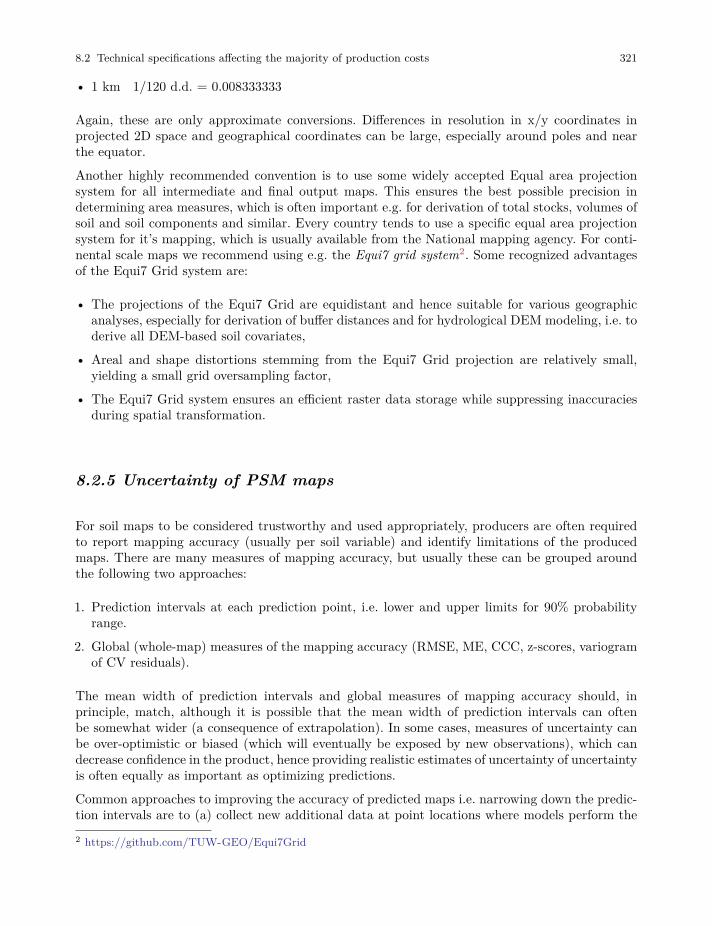
8.2 Technical specifications affecting the majority of production costs 321
• 1 km � 1/120 d.d. = 0.008333333
Again, these are only approximate conversions. Differences in resolution in x/y coordinates inprojected 2D space and geographical coordinates can be large, especially around poles and nearthe equator.
Another highly recommended convention is to use some widely accepted Equal area projectionsystem for all intermediate and final output maps. This ensures the best possible precision indetermining area measures, which is often important e.g. for derivation of total stocks, volumes ofsoil and soil components and similar. Every country tends to use a specific equal area projectionsystem for it’s mapping, which is usually available from the National mapping agency. For conti-nental scale maps we recommend using e.g. the Equi7 grid system2. Some recognized advantagesof the Equi7 Grid system are:
• The projections of the Equi7 Grid are equidistant and hence suitable for various geographicanalyses, especially for derivation of buffer distances and for hydrological DEM modeling, i.e. toderive all DEM-based soil covariates,
• Areal and shape distortions stemming from the Equi7 Grid projection are relatively small,yielding a small grid oversampling factor,
• The Equi7 Grid system ensures an efficient raster data storage while suppressing inaccuraciesduring spatial transformation.
8.2.5 Uncertainty of PSM maps
For soil maps to be considered trustworthy and used appropriately, producers are often requiredto report mapping accuracy (usually per soil variable) and identify limitations of the producedmaps. There are many measures of mapping accuracy, but usually these can be grouped aroundthe following two approaches:
1. Prediction intervals at each prediction point, i.e. lower and upper limits for 90% probabilityrange.
2. Global (whole-map) measures of the mapping accuracy (RMSE, ME, CCC, z-scores, variogramof CV residuals).
The mean width of prediction intervals and global measures of mapping accuracy should, inprinciple, match, although it is possible that the mean width of prediction intervals can oftenbe somewhat wider (a consequence of extrapolation). In some cases, measures of uncertainty canbe over-optimistic or biased (which will eventually be exposed by new observations), which candecrease confidence in the product, hence providing realistic estimates of uncertainty of uncertaintyis often equally as important as optimizing predictions.
Common approaches to improving the accuracy of predicted maps i.e. narrowing down the predic-tion intervals are to (a) collect new additional data at point locations where models perform the2 https://github.com/TUW-GEO/Equi7Grid

322 8 Practical tips for organizing Predictive Soil Mapping
poorest (e.g. exhibit the widest prediction intervals), and (b) invest in preparing more meaningfulcovariates, especially finer resolution covariates. Technical specifications, however, influence theproduction costs and have to be considered carefully as production costs can significantly increasewith e.g. finer pixel size. Aiming at 30% lower RMSE might seem trivial but the costs of suchimprovement could exceed the original budget by several times (Hengl et al, 2013).
8.2.6 Computing costs
To achieve efficient computing, experienced data scientists understand the importance of utilizingthe full capacity of the available hardware to its maximum potential (100%). This usually impliesthat:
• the most up-to-date software is used for all computing tasks,
• the software is installed in such a way that it can achieve maximum computing capacity,
• any function, or process, that can be parallelized in theory is also parallelized in practice,
• running functions on the system will not result in system shutdowns, failures or artifacts,
As mentioned previously, applying PSM for large areas at finer resolutions (billions of pixels)benefits from use of a high performance computing (HPC) server to run overlay, model fitting andpredictions and to then generate mosaics. The current code presented in this PSM with R book ismore or less 90% optimized so that running of the most important functions can be easily scaledup. The total time required to run one global update on a single dedicated HPC server (e.g. viaAmazon AWS) for a soil mask that contains >100 million pixels can require weeks of computingtime. Copying and uploading files can also be a lengthy process.
A configuration we adopt, and recommend, for processing large stacks of grids with a large numberof evidence points is e.g. the OVH server3:
• EG-512-H4 (512GB RAM takes 3 weeks of computing; costs ca € 950,00 per month)
An alternative to using OVH is the Amazon AWS (Fig. 8.4). Amazon AWS server, with a similarconfiguration, might appear to cost much more than an OVH server (especially if used continuouslyover a month period), but Amazon permits computing costs to be paid by the hour, which providesmore flexibility for less intensive users. As a rule of thumb, a dedicated server at Amazon AWS,if used continuously 100% for the whole month, could cost up to 2.5 times more than an OVHserver.
The recommended server for running PSM on Amazon AWS to produce predictions for billions ofpixels is:
• AWS m4.16xlarge5 ($3.84 per Hour);3 https://www.ovh.nl/dedicated_servers/HG/4 https://www.ovh.nl/dedicated_servers/infrastructure/1801eg08.xml5 https://aws.amazon.com/ec2/pricing/on-demand/
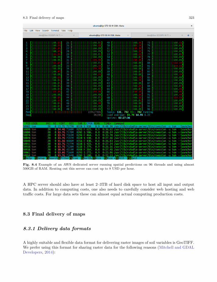
8.3 Final delivery of maps 323
Fig. 8.4 Example of an AWS dedicated server running spatial predictions on 96 threads and using almost500GB of RAM. Renting out this server can cost up to 8 USD per hour.
A HPC server should also have at least 2–3TB of hard disk space to host all input and outputdata. In addition to computing costs, one also needs to carefully consider web hosting and webtraffic costs. For large data sets these can almost equal actual computing production costs.
8.3 Final delivery of maps
8.3.1 Delivery data formats
A highly suitable and flexible data format for delivering raster images of soil variables is GeoTIFF.We prefer using this format for sharing raster data for the following reasons (Mitchell and GDALDevelopers, 2014):
324 8 Practical tips for organizing Predictive Soil Mapping
• It is GDAL’s default data format and much functionality for subsetting, reprojecting, readingand writing GeoTIFFs already exists (see GDAL utils6).
• It supports internal compression via creation options (e.g. COMPRESS=DEFLATE).
• Extensive overlay, subset, index, translate functionality is available via GDAL and other opensource software. Basically, the GeoTIFF format functions as a raster DB.
By exporting spatial data to GeoTiffs, one can create a soil spatial DB or a soil information system.This does not necessarily mean that its targeted users will be able to find all information withoutproblems and/or questions. The usability and popularity of a data set reflect many considerationsin addition to data quality.
Another useful aspect of final delivery of maps is compression of the GeoTIFFs. To avoid large filesizes, we recommend always using integers inside GeoTIFF formats because floating point formatscan result in increases in file sizes of up four times (with no increase in accuracy). This mightrequire multiplication of original values of the soil property of interest by 10 or 100, in order tomaintain precision and accuracy (e.g. multiply pH values by 10 before exporting your raster intointeger GeoTIFF format).
8.3.2 General recommendations
Even maps of perfect quality might still not attract users, if they are not properly designed. Somethings to consider to increase both use and usability of map data are:
1. Make a landing page for your map data that includes: (a) simple access/download instructions,(b) screenshots of your data in action (people prefer visual explanations with examples), (c)links to key documents explaining how the data were produced, and (d) workflows explaininghow to request support (who to contact and how).
2. Make data accessible from multiple independent systems e.g. via WCS, FTP and through amirror site (in case one of the access sites goes offline). This might be inefficient consideringthere will be multiple copies of the same data, but it can quadruple data usage.
3. Explain the data formats used to share data, and provide tutorials, for both beginners andadvanced users, that instruct how to access and use the data.
4. Consider installing and using a version control system (or simply use github or a similar repos-itory) so that the users can track earlier versions of map data.
5. Consider closely following principles of reproducible research7 (all processing steps, inputs andoutputs are accessible). For example, making the R code available via github so that anyone istheoretically able to reproduce all examples shown in the text. Transparency increases trust.
6 http://www.gdal.org/gdal_utilities.html7 https://ropensci.org/blog/2014/06/09/reproducibility/

8.3 Final delivery of maps 325
8.3.3 Technical specifications PSM project
A way to improve planning of a PSM project is to spend more time on preparing the technicalaspects of data production. This includes listing the general specifications of the study area,listing target variables and their collection methods, listing covariate layers of interest to be usedto improve mapping accuracy and listing targeted spatial prediction algorithms to be compared.
General specifications of the study area include:
• G.1 Project title:• G.2 PSM project type:
– PSM project in a new area– PSM project using legacy points– PSM project aiming at optimizing predictions and usability
• G.3 Target spatial resolution:
– 10 m– 30 m– 100 m– 250 m– 1000 m
• G.4 Target temporal span (period of interest):
– Begin date,– End date,
• G.5 Soil mask:
– raster image or land cover classes in the referent land cover map covering the study area
• G.6 Grid definition:
– Xmin,– Ymin,– Xmax,– Ymax,
• G.7 Target projection system:
– proj48 code,
• G.8 Total area:
– in square-km,
• G.9 Inspection density (observations per square-km):
– Detailed soil profiles,8 https://proj4.org/
326 8 Practical tips for organizing Predictive Soil Mapping
– Soil semi-profiles,– Top-soil / sub-soil samples (with laboratory analysis),– Quick observations (no lab data),
• G.10 Total budget (planned):• G.11 Total pixels in millions:
– amount of pixels for all predictions
• G.12 Total planned production costs per 1M pixels (divide G.10 by G.11):• G.13 Target data license:• G.14 Target user groups and workflows (targeted services):• G.15 Further updates of maps:
– Continuous updates in regular intervals,– Two prediction time intervals (start, end period),– No updates required except fixes and corrections,
• G.16 Commercialization of the PSM outputs:
– No commercial data nor services,– Commercial data products,– Commercial services,
• G.17 Support options:
– Dedicated staff / live contact,– Mailing list,– Github / code repository issues,
8.3.4 Standard soil data production costs
Standard production costs can be roughly split into three main categories:
• Fixed costs (e.g. project initiation, equipment, materials, workshops etc),• Variable data production costs expressed per:
– M (million) of pixels of data produced,– Number of points samples,– Number of variables modeled,
• Data maintenance and web-serving costs, usually expressed as monthly/yearly costs,
Although in the introduction chapter we mentioned that the production costs are mainly a functionof grid resolution i.e. cartographic scale, in practice several other factors determine the total costs.Standard soil data production costs (approximate estimates) per soil data quality category (seebelow) are connected to the quality level of the output maps. Consider that there are four mainquality levels:
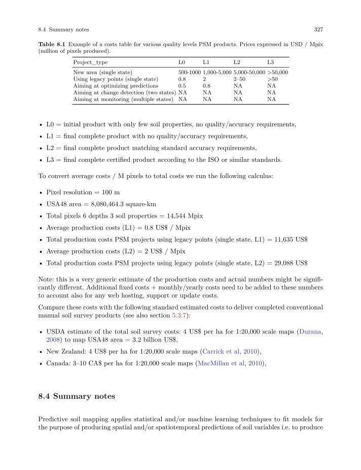
8.4 Summary notes 327
Table 8.1 Example of a costs table for various quality levels PSM products. Prices expressed in USD / Mpix(million of pixels produced).
Project_type L0 L1 L2 L3New area (single state) 500-1000 1,000-5,000 5,000-50,000 >50,000Using legacy points (single state) 0.8 2 2–50 >50Aiming at optimizing predictions 0.5 0.8 NA NAAiming at change detection (two states) NA NA NA NAAiming at monitoring (multiple states) NA NA NA NA
• L0 = initial product with only few soil properties, no quality/accuracy requirements,• L1 = final complete product with no quality/accuracy requirements,• L2 = final complete product matching standard accuracy requirements,• L3 = final complete certified product according to the ISO or similar standards.
To convert average costs / M pixels to total costs we run the following calculus:
• Pixel resolution = 100 m• USA48 area = 8,080,464.3 square-km• Total pixels 6 depths 3 soil properties = 14,544 Mpix• Average production costs (L1) = 0.8 US$ / Mpix• Total production costs PSM projects using legacy points (single state, L1) = 11,635 US$• Average production costs (L2) = 2 US$ / Mpix• Total production costs PSM projects using legacy points (single state, L2) = 29,088 US$
Note: this is a very generic estimate of the production costs and actual numbers might be signifi-cantly different. Additional fixed costs + monthly/yearly costs need to be added to these numbersto account also for any web hosting, support or update costs.Compare these costs with the following standard estimated costs to deliver completed conventionalmanual soil survey products (see also section 5.3.7):
• USDA estimate of the total soil survey costs: 4 US$ per ha for 1:20,000 scale maps (Durana,2008) to map USA48 area = 3.2 billion US$,
• New Zealand: 4 US$ per ha for 1:20,000 scale maps (Carrick et al, 2010),• Canada: 3–10 CA$ per ha for 1:20,000 scale maps (MacMillan et al, 2010),
8.4 Summary notes
Predictive soil mapping applies statistical and/or machine learning techniques to fit models forthe purpose of producing spatial and/or spatiotemporal predictions of soil variables i.e. to produce

328 8 Practical tips for organizing Predictive Soil Mapping
maps of soil properties or soil classes at various resolutions. This chapter identifies and discussessome of the key technical specifications users need to consider to prepare for data production andto obtain realistic estimates of workloads and production costs.
The key technical specifications of a PSM project are considered to consist of defining the following:a soil mask, a spatial resolution, a list of target variables and standard depth intervals (for 3D soilvariables), prediction intervals (if required), any secondary soil variables (and how they will bederived) and required accuracy levels. Technical specifications determine the production costs andneed to be considered carefully as production costs are sensitive to specifications, (e.g. 3 times finerpixel size can increase production costs up to 10 times, or setting targets such as 30% lower RMSEcan increase costs as either more points or more covariates, or both, need to be included. Generalforms at the end of the chapter provide an example of detailed list of technical specifications inrelation to target variables and covariate layers typically used in PSM projects to date.

Chapter 9
The future of predictive soil mapping
Edited by: R. A. MacMillan and T. Hengl
9.1 Introduction
This chapter presents some opinions and speculation about how predictive soil mapping (PSM)may evolve, develop and improve in the near term future. These thoughts were originally preparedfor a discussion document about whether national to provincial scale soil inventory programs inCanada could, or indeed should, be reinvented and reinvigorated and, if so, how this reinventionmight be best designed and accomplished.
The solutions proposed for reinvigorating presently moribund soil inventory programs in Canadawere largely based on adopting new methods and ideas associated with PSM within a new collab-orative, collective and open operational framework. These earlier thoughts were considered to berelevant to the more general topic of the future of predictive soil mapping (PSM). As such, theoriginal discussion document was slightly modified, extended and included as a chapter in thisbook.
This chapter addresses the following two main issues:
• What caused past national to state level conventional soil, and other terrestrial resource, in-ventory programs to anthropy and disappear globally and can they now be renewed and resur-rected?
• How can the methods and ideas behind PSM be adopted and applied to accomplish the goalof renewing and reviving conventional soil and terrestrial resource inventory programs?
329
330 9 The future of predictive soil mapping
9.2 Past conventional terrestrial resource inventories
9.2.1 Why have most national resource inventories been discontinued?
Historically, almost all past terrestrial resource inventory agencies were slow, expensive to maintainand failed to produce complete, consistent, current and correct map coverage (4Cs) for entire areasof political jurisdiction or interest. Most national agencies were unable to completely map an entireadministrative area affordably at any useful scale using a single consistent methodology appliedover a relatively short time span to produce a single wall to wall map product. Instead almost allpast inventory efforts have been piecemeal and incomplete.
This resulted in what we consider to be “the embarrassment of the index map”. Virtually everyjurisdiction produced an index map to illustrate which parts of the jurisdiction had been mappedat all, which different mapping methods were used to map different parts, which eras or years eachbit of mapping represented and what scale of mapping had been carried out in any part. Thisindex map was often proudly displayed and circulated to illustrate how much progress had beenmade towards mapping an entire jurisdiction of interest. In actual fact, the index map representeda powerful demonstration of all that was wrong with mapping and mapping progress in thatjurisdiction.
The first thing that index maps clearly demonstrated was that there was no complete map coveragefor the area at any scale. The second thing highlighted was that there was no consistency in scale,methods or legend across even areas that had been mapped. Different areas had been mapped atdifferent scales, over different times, using different concepts and legends and no effort had beenexpended to achieve consistency across the entire area. The third thing that would also becomeimmediately obvious was that, at current rates, complete mapping of any jurisdiction would neverbe achieved in anyone’s lifetime. Not particularly encouraging information to impart. And yet,every agency maintained an index map and loved to share it.
Another significant historical misjudgement was the failure to make the information and servicesprovided by terrestrial inventory service agencies critically important and absolutely necessary toat least one essential decision making process, preferably a legally mandated one. Where inventoryagencies still survive, they have linked their products and services intimately to one or moreclearly defined, and legally mandated, decision making processes that involve the expenditure ofconsiderable sums of (usually public) money. Soil survey survives in the USA (at least for now)largely because county scale soil maps are a critical requirement for calculating eligibility forfinancial support payments for many agricultural subsidy and support payment programs. Youcannot apply for, or obtain, a subsidy payment unless you have a soil survey map to justify youreligibility for the payment and to document where and how the required supported activity willbe implemented.
It can be argued that many terrestrial resource inventory programs failed (and disappeared) be-cause they viewed themselves as their own primary customer and designed and delivered productsand services meant to satisfy their own desires and expectations and not those of real, downstreamusers. They became convinced of the rightness, value and importance of their maps and databasesthe way they wanted to make them and did not effectively listen to, or respond to, criticism ofthese products. Users would criticize conventional soil polygon maps and reports filled with com-plicated jargon and impenetrable legends and be dismissed as simply not being able to understand

9.2 Past conventional terrestrial resource inventories 331
a soil map and to appreciate how complicated and complex it was to portray the spatial variationin soils in a simple way. Rather than trying to design and make simpler representations of moreeasily understood spatial patterns, terrestrial inventory agencies would suggest that an expert inmaking the maps was required to assist users in interpretation and use of any map.
9.2.2 Is there a future for conventional terrestrial inventoryprograms?
We have asked ourselves, “can conventional comprehensive soil and similar terrestrial inventoryprograms be saved or renewed?” The short answer is: probably no, at least not in their presentformat. Conventional resource inventory programs have become too expensive, too slow to deliverneeded outputs and too slow to change to produce innovative and needed products. There is nowprobably insufficient will, money, demand or benefit to support continuation, or re-establishment,of conventional, government-funded, comprehensive inventory programs as we have known themin the past. However, that does not mean that all needs and benefits previously provided bycomprehensive inventory programs are being met now or that they do not need to be met. Thereare a large number of benefits associated with the existence of comprehensive inventories and weask if these may not be important to continue to service and if they might still be provided undersome newly redesigned framework.
9.2.3 Can terrestrial inventory programs be renewed and revived?
One of our key hopes (which we especially try to achieve through the OpenGeoHub Foundation),is to contribute to a discussion of how comprehensive terrestrial resource inventory programs(or equivalent frameworks) might be re-imagined, re-designed, re-invented, re-implemented andrenewed at regional to national to global scales, for the next generation, and by whom.
We consider here that we are now at a nexus where it has become possible to address and re-dress many of the past inconsistencies and oversights in terrestrial resource mapping. It is nowcompletely feasible to aspire to affordably and expeditiously produce new predictive maps thatachieve the 4 Cs and are:
• Complete (e.g. cover entire areas of interest),
• Consistent (e.g. are made using a single methodology, applied at a single scale and over asingle short period of time),
• Current (e.g. represent conditions as they are today, at a specific moment in time),
• Correct (e.g. are as accurate as is possible to achieve given available data and methods),
We consider that it is also now possible to redesign any new output maps so that they are capableof acting directly as inputs to well established processes and programs for planning and decisionmaking at national to regional to operational scales. And we consider that we have a unique
332 9 The future of predictive soil mapping
opportunity to work collaboratively with numerous actual and potential users of spatial inventorydata to ensure that new output products directly meet their spatial data needs.
9.2.4 How can terrestrial inventory programs be renewed and revivedand by whom?
In light of developments in science, technology, methods of societal interaction and new modelsof funding and cooperative action, we suggest that looking back at how things were done in thepast no longer provides the most appropriate model for how inventory activities ought to bedesigned and conducted in the future. We argue that it is preferable to re-imagine an entirely newframework for cooperation, which takes advantage of new scientific and organizational advancesand within which many of the acknowledged benefits of previous, government-funded, programscan be delivered within a new model of cooperative, collective action and sharing.
In this age of Facebook and Twitter and Wikipedia and Google Earth, it is no longer the purview,or responsibility, of any single, government funded, agency to collect, produce, maintain anddistribute comprehensive information about the spatial distribution of soils, eco-systems, terrainunits, wetlands or any other terrestrial attributes. We believe that it should instead becomea collective responsibility, for a large variety of overlapping groups and institutions, to create,maintain and share spatial information of common interest. It is incumbent on these diverseinterest groups to identify mechanisms by which willing collaborators can join together to produce,maintain and distribute basic levels of spatially distributed land resource information jointly andcollectively.
9.3 The future of PSM: Embracing scientific and technical advances
9.3.1 Overview
We consider that any new, future collaborative PSM activity should take advantage of recentscientific and technical advances in the following areas:
• Collection of field observations and samples:
– Collating and harmonizing existing legacy soils data,
– New field sampling designs and programs and new data collection strategies,
• Characterization of soils in the field and in the laboratory:
– New field sensors for characterizing soils in situ,
– New faster, cheaper and more accurate methods of laboratory analysis,
9.3 The future of PSM: Embracing scientific and technical advances 333
• Creation, collation and distribution of comprehensive sets of environmental covariates:
– Introduce new covariate data sets based on new remote, air and space sensors,
– Include new varieties and resolutions of DEM and other environmental covariate data,
– Maximize use and relevance of existing data sets of environmental covariates,
• Automated spatial prediction models:
– Replace previous qualitative and subjective mental models with new quantitative and objec-tive statistical models,
– Adopt new methods of automated space-time modelling and prediction,
• New options for hosting, publishing, sharing and using spatial data via cloud services:
– Develop new platforms for collaborative data sharing and geo-publishing,
– Develop open services to deliver on-demand, real time online mapping,
9.3.2 Collection of field observations and samples
We can improve how we locate and obtain data on field observations and measurements. TheseO&M field data provide the evidence that is essential for developing all spatial prediction modelsand outputs. First consider the challenges and opportunities associated with identifying, obtainingand using existing, or legacy, field observations and measurements.
Legacy field data refers to any field observations or measurements that were collected in thepast and that remain discoverable and available for present use. Typically, these legacy fielddata consist of either field observations and classifications made at point locations to supportthe development of conventional, manually prepared maps or of laboratory analysed samples,collected to support characterization of point locations considered to be typical or representativeof a particular soil class or individual. Legacy field data may already be in digital format andstored in digital databases. More often, legacy data are found in paper reports, manuals, scientificpublications and other hard copy formats that require the data to first be transformed into digitalformat and then harmonized into a standardized format before they can be used effectively.
Legacy field data typically possess several characteristics which can make their use for producingnew inventory map products problematic. Some common limitations of legacy field data are:
• They are rarely collected using any kind of rigorous, statistically valid, sampling design,
• Their locations in space (geolocations) are often not measured or reported accurately,
• Their locations in time (sampling dates) are often unknown or are spread over decades,
• The methods used in description or analysis can vary greatly by source, location or time,
• They can be difficult and costly to find, to obtain, to digitize and to harmonize,
334 9 The future of predictive soil mapping
Despite these limitations, legacy field data have other attributes that make them valuable andworth assembling, collating, harmonizing and using. The advantages associated with using legacyfield data can be summarized as follows:
• Legacy point data provide the only source of baseline information about past time periods:
– We can’t go back in time to collect new samples or make new observations applicable to pasttime periods,
– They establish prior probabilities which are essentially starting points that describe what weknow now before we start making new predictions and new maps using new data,
• Legacy point data are all we have initially to work with until new field data can be obtained:
– Use of legacy field data can help us to learn and to improve methods and approaches,
– Working through the full cycle required to produce predictive maps using legacy data letsus learn a lot about how to do it and, more importantly, how we might do it better the nexttime around,
– They give us something to work with to provide real-world, worked examples, for ourselvesand for potential users, of the kinds of maps and other products that can now be producedusing modern automated prediction methods,
• Legacy point data help us to illustrate problems, weaknesses and opportunities for improvement:
– Gaps in existing legacy data (missing data in space and time) help to illustrate the need tohave samples that comprehensively cover all areas of space and time of interest,
– Errors and uncertainties in initial predictive maps based on legacy field data provide a clearillustration of the need for more and better field data to improve future mapping,
– The spatial distribution of uncertainties computed for initial maps created using legacydata can identify locations where new observations and samples are most needed and willcontribute most to improving subsequent predictions,
Legacy point data can be surprisingly difficult and costly to find, obtain, harmonize and digitize(Arrouays et al, 2017). One can only imagine how many hundreds of thousands, even millions,of site observations may have been made by field personnel undertaking many different types ofinventories for many different agencies over the years. Similarly, laboratories have definitely ana-lyzed millions of soil samples over the years for samples collected by government agencies, privatesector consulting companies, NGOs, advocacy groups, farmers or landowners. Unfortunately, veryfew of these observations or samples have survived to enter the public domain where they can nowbe easily located and obtained.
In an ideal world, it would be possible to identify and obtain hundreds of thousands to perhapseven millions of laboratory analysed results for point locations globally. These samples surelywere taken and analysed but they no longer remain accessible. Instead, best efforts to date haveresulted in rescuing some 300,000 to 350,000 records globally for which soil analytical data existfor geolocated point locations. What has happened to all of the thousands to millions of other
9.3 The future of PSM: Embracing scientific and technical advances 335
analysed samples that were undeniably collected and analysed? Essentially they may be consideredto be lost in the mists of time, victims of lack of will and lack of resources to support maintaining aviable archive of observation and sample results over the years. Unfortunately, no entity or agencyhad the mandate to maintain such a comprehensive global archive and no one had the vision orresources to take on such a challenge.
The world can do a much better job of locating, harmonizing, archiving and sharing global legacyfield and laboratory data than it has done to date (Arrouays et al, 2017). It is incumbent onagencies, companies, organizations and individuals that hold, or are aware of, collections of legacyfield data to step forward to offer to contribute such data to a comprehensive and open repositoryof field observations and laboratory measurements. We would hope that the evidence of beneficialuse of legacy point data by OpenGeoHub to produce concrete examples of needed and useful spatialoutputs would encourage entities that hold field O&M data that are not currently publicly availableto contribute them for future use by a community of global mappers. Techniques developed byOpenGeoHub to collate and harmonize legacy point data could be applied to any new, previouslyoverlooked, data sets contributed, in the future, by interested parties.
9.3.3 Collecting new field O&M data
The Africa Soil Information Service (AfSIS) project (http://www.africasoils.net) provides a pow-erful example of how new field observations and laboratory analysed field data can be collected ina manner that is reliable, feasible and affordable. AfSIS is one of the very few global examples ofan entity that has not accepted that collection of new field data is too difficult and too expensiveto contemplate. Instead, AfSIS asked the question “how can we make it feasible and affordable tocollect new, high quality, field data?” And then AfSIS (and several partner countries) went aheadand collected new field data using modern, robust and affordable methods of field sampling andlaboratory analysis.
Following the example of AfSIS, we can identify the following major considerations for how thecollection of new field O&M data can be made both more affordable and more effective.
• Select locations for field sampling using a formal, rigorous sampling design (Brown et al, 2015;Stumpf et al, 2017; Brus, 2019),
– Design based sampling schemes:
· Random sampling,
· Stratified random sampling,
· Systematic sampling (confluence point or grid sampling),
· Nested, multi-scale hierarchical sampling,
· Spatially-based sampling,
– Model based sampling schemes:
· Conditioned Latin Hypercube (cLHC) sampling (Malone et al, 2019),
336 9 The future of predictive soil mapping
· Multi-stage sampling at locations of maximum uncertainty,
• Systematize and automate all field sampling and recording procedures as much as possible,
– Create custom tools and apps to support:
· Locating sample sites and recording observations,
· Assigning unique identifier sample numbers to all locations and samples,
· Tracking progress of samples from the field through the lab to the database,
Adopting formal sampling designs to identify where to best collect new field O&M samples offersseveral significant advantages.
Firstly, statistically valid sampling schemes ensure that the fewest number of samples are requiredto achieve the most correct and representative values to characterize any area of interest. Thisminimizes field data collection costs while maximizing usefulness of the samples. Secondly, thereis rapidly growing interest in, and need for, measuring and monitoring of changes in environmen-tal conditions through time (e.g. carbon sequestration or losses, fertility changes). Quantitativestatements can only be made about the accuracy of changes in values for any given area if thereis an ability to replicate those values with a subsequent comparable sampling effort. The abilityto return to any given area at some later time to collect a second set of statistically representa-tive field samples is essential to any effort to quantify and monitor changes through time. Onlystatistically based sampling frameworks support repeat sampling.
Design based sampling schemes generally require little to no advance knowledge about the patternsof spatial variation within an area to be sampled. They are best used for situations where there islittle existing knowledge about spatial variation and where there is a need to collect a representativesample with the fewest possible sample points.
Of the design based options available a nested, multiscale sampling design based on a stratifiedrandom sample framework or spatially-based sampling appears as a suitable option. In these nestedsampling approaches, explicit attention is given to ensuring that multiple samples are collectedat a succession of point locations with increasingly large interpoint separation distances (e.g. 1m, 10 m, 100 m, 1 km). These multiple points support construction of semi-variograms thatquantify the amounts of variation in any attribute that occur across different distances. Knowinghow much of the total observed variation occurs across different distances can be very helpful foridentifying and selecting the most appropriate grid resolution(s) to use for predictive mapping.If 100% of the observed variation occurs over distances shorter than the minimum feasible gridresolution, then there is really no point in trying to map the attribute spatially at that resolution.Similarly, if most of the observed variation occurs across longer distances, there is really littlepoint in using a very fine resolution grid for prediction. Most past purposive sampling undertakenfor conventional inventories was not particularly well suited to supporting geostatistics and theproduction of semi-variograms.
Model based sampling frameworks are recommended for situations where there is some existing(a-priori) knowledge about the spatial pattern of distribution of properties or classes of interest.Conditioned Latin Hypercube (cLHC) sampling is based on first identifying all significant com-binations of environmental conditions that occur in an area based on overlay and intersection ofgrid maps that depict the spatial distribution of environmental covariates (Stumpf et al, 2016;
9.3 The future of PSM: Embracing scientific and technical advances 337
Malone et al, 2019). Potential point sample locations are then identified and selected in such away that they represent all significant combinations of environmental conditions in an area. Pointsamples are typically selected so that the numbers of samples taken are more or less proportionalto the frequency of occurrence of each significant combination of environmental covariates. Thisensures that samples cover the full range of combinations of environmental conditions (e.g. thecovariate space) in an area and sample numbers are proportional to the relative extent of eachmajor combination of environmental conditions in an area.
Field sampling programs can also be designed to collect new point samples at locations of maximumuncertainty or error in a current set of spatial predictions (Stumpf et al, 2017). The spatiallylocated measures of uncertainty computed as one output of a prediction model can be used toprovide an indication of the locations where it may be most beneficial to collect new samples toreduce uncertainty to the maximum extent possible. This type of sampling approach can proceedsequentially, with predictions updated for both estimated values and computed uncertainty at alllocations after any new point sample data have been included in a new model run. It is oftennot efficient to collect just one new point sample prior to rerunning a model and updating allpredictions of values and uncertainties. So, it is often recommended to collect a series of newpoint observations at a number of locations that exhibit the largest estimates of uncertainty andthen update all predictions based on this series of new field point data. Collecting a series ofnew multistage samples can be repeated as many times as is deemed necessary to achieve somespecified maximum acceptable level of uncertainty everywhere.
Field sampling can also be made more efficient, and less expensive, by creating and adoptingmore systematic and automated procedures to support field description and sampling. Customapps can be developed to help to choose, and then locate, sampling points in the field rapidlyand accurately. These field apps can be extended to automate and systematize most aspects ofmaking and recording observations in the field, thereby increasing speed and accuracy and reducingcosts. Unique sample numbers can be generated to automatically assign unique and persistentidentifiers to every site and to every soil sample collected in the field. This can reduce costs anderrors associated with assigning different sample IDs at different stages in a sampling campaign (e.g. field, lab, data entry). Persistent and unique machine readable identifiers can help to supportcontinuous, real-time tracking of the progress of field descriptions and soil samples from initialcollection in the field through laboratory analysis to final collation in a soil information system.This consistency and reliability of tracking can also improve efficiency, decrease errors and reducecosts for field description and laboratory analysis. Taken all together, improvements that automateand systematize field descriptions and field sampling can make it much more affordable and feasibleto collect new field data through new field sampling programs.
Brus (2019) provides a systematic overview of sampling techniques and how to implement themin R1. The author also recongizes that “further research is recommended on sampling designs formapping with machine learning techniques, designs that are robust against deviations of modelingassumptions”.1 https://github.com/DickBrus/TutorialSampling4DSM
338 9 The future of predictive soil mapping
9.3.4 Characterization of soils in the field and the laboratory
Characterization of field profiles and samples can be made more affordable and feasible again bymaking maximum use of new technologies that enable field descriptions and laboratory analysesto be completed more rapidly, more affordably and more accurately.
Field characterizations can be improved by making use of a number of new technologies. Simplytaking geotagged digital photos of soil profiles and sample sites can provide effective informationthat is located with accuracy in both space and time. New sensors based on handheld spec-trophotometers are just beginning to become available. These may soon support fast, efficient andaccurate characterization of many soil physical and chemical attributes directly in the field. Otherfield instruments such as ground penetrating radar (Gerber et al, 2010), electrical conductivityand gamma ray spectroscopy (Rouze et al, 2017) are also becoming increasingly available anduseful. Field sensors for monitoring soil moisture and soil temperature in real time and transmit-ting these data to a central location are also becoming increasingly common and affordable todeploy. Portable MIR scanners achieve almost the same accuracy as laboratories (Hutengs et al,2018). Simple field description protocols based on using mobile phones to crowdsource a set ofbasic observations and measurements could enable massive public participation in collecting newfield data.
Recent developments in the use of new, rapid and accurate pharmaceutical grade analytical deviceshave reduced the costs of typical laboratory analyses dramatically, while, at the same time, signif-icantly improving on reproducibility and accuracy (Shepherd and Walsh, 2002, 2007). A modernsoil laboratory now entails making use of mid and near infrared spectrophotometers, X-ray diffrac-tion and X-Ray diffusion and laser based particle size analysis. Using these new instruments, ithas been demonstrated that total costs for running a complete set of common soil analyses on afull soil profile can be reduced from a current cost of US$ 2,000 to as little as US$ 2–10 per profile(Shepherd and Walsh, 2007; Rossel et al, 2016). This reduction in cost, along with the associatedimprovement in reproducibility is a game changer. It makes it, once again, feasible and affordableto consider taking new field soil samples and analyzing them in the laboratory.
9.3.5 Creation, collation and distribution of effective environmentalcovariates
Any future soil inventory activities will inevitably be largely based on development and applica-tion of automated predictive soil mapping (PSM) methods. These methods are themselves basedon developing statistical relationships between environmental conditions that have been mappedextensively, over an entire area of interest (e.g. environmental covariates), and geolocated pointobservations that provide objective evidence about the properties or classes of soils (or any otherenvironmental attribute of interest) at specific sampled locations.
The quality of outputs generated by predictive mapping models is therefore highly dependent onthe quality of the point evidence and also on the environmental covariates available for use in anymodel. For environmental covariates to be considered effective and useful, they must capture anddescribe spatial variation in the most influential environmental conditions accurately and at theappropriate level of spatial resolution (detail) and spatial abstraction (generalization). They must
9.3 The future of PSM: Embracing scientific and technical advances 339
also describe those specific environmental conditions that exhibit the most direct influence on thedevelopment and distribution of soils or soil properties (or of whatever else one wishes to predict).The degree to which available environmental covariates can act as reliable and accurate proxies forthe main (scorpan) soil forming factors has a profound influence on the success of PSM methods.If available covariates describe the environment comprehensively, accurately and correctly, it islikely that predictive models will also achieve high levels of prediction accuracy and effectiveness,if provided with sufficient suitable point training data.
Fortunately, advances in remote sensing and mapping continue to provide us with more and betterinformation on the global spatial distribution of many key (scorpan) environmental conditions.Climate data (c) is becoming increasingly detailed, accurate and available. Similarly, many cur-rently available kinds of remotely sensed imagery provide increasingly useful proxies for describingspatial patterns of vegetation (o) and land use. Topography, or relief (r), is being described withincreasing detail, precision and accuracy by ever finer resolution global digital elevation models(DEMs).
Unfortunately, several key environmental conditions are still not as well represented, by currentlyavailable environmental covariates, as one would wish. Improvements need to be made in acquiringglobal covariates that describe parent material (p), age (a) and spatial context or spatial position(n) better than they currently are. In addition, the scorpan model recognizes that available infor-mation about some aspect of the soil (s) can itself be used as a covariate in predicting some other(related) aspect of the soil. Only recently have we begun to see complete and consistent globalmaps of soil classes and soil properties emerge that can be used as covariates to represent the soil(s) factor in prediction models based on the scorpan concept.
Advances are being made in developing new covariates that provide improved proxies for describingparent material (p). Perhaps the best known of these, and the most directly relevant, is airbornegamma ray spectroscopy (Wilford et al, 1997; Viscarra Rossel et al, 2007; Rouze et al, 2017).This sensor can provide very direct and interpretable information from which inferences can bemade about both the mineralogy and the texture of the top few centimeters of the land surface.A number of countries (e.g. Australia, Uganda, Ireland) already possess complete, country-widecoverage of gamma ray spectroscopy surveys. More are likely to follow. Similarly, advances arebeing made in interpreting satellite based measurements of spatio-temporal variations in groundsurface temperature and near surface soil moisture to infer properties of the parent material suchas texture, and to a lesser extent, mineralogy (Liu et al, 2012). These act as very indirect proxiesbut they do help to distinguish warmer and more rapidly drying sands, for example, from colderand slower drying wet clays. Identifying and acquiring more detailed and more accurate covariatesfrom which parent material type and texture can be inferred is a major ongoing challenge forwhich progress has been slow.
Only recently have a number of investigators begun to suggest a variety of covariates that can becalculated and used as proxies to describe spatial context or spatial position (n) in the scorpanmodel (Behrens et al, 2018c). These measures of spatial context or position can help to account forthe effects of spatial autocorrelation in prediction models for many soil properties and attributes.They also help to coax out effects related to spatial context and spatial scale. The old adage that“what you see depends upon how closely you look” certainly applies to predictive soil mapping.If one only looks at the finest detail, one overlooks the broader context and broader patterns.Similarly, if one only looks at broad patterns (coarser resolutions) one can easily miss seeing, andpredicting, important shorter range variation. Soils are known to form in response to a numberof different soil forming processes and these processes are themselves known to operate over quite
340 9 The future of predictive soil mapping
different ranges of process scales (or distances). So, if one looks only at the most detailed scales(e.g. finest spatial resolution) one can easily fail to observe, describe and account for importantinfluences that operate across longer distances and larger scales. Increasingly, it is becoming evidentthat prediction models generate more accurate results when they incorporate consideration of ahierarchical pyramid of environmental covariates computed across a wide range of resolutions torepresent a wide range of process scales and formative influences (Behrens et al, 2018c,b).
A final, and very significant, consideration, for environmental covariates is one of degree of avail-ability and ease of use. For covariates to be effective, they must be relatively easy to identify,locate and use. Many existing spatial data sets need some form of preprocessing or transformationin order to become useful inputs as environmental covariates in predictive mapping. Difficultiesand costs involved in locating, downloading and transforming these source data sets can severelyrestrict their effective use. Equally, many of these same covariates are often located, downloadedand processed multiple times by multiple entities for use in isolated projects and then archived(or disposed of) and not made easily available for subsequent use and reuse. A mentality of “pro-tecting my data” leads to limitations on sharing and reuse of spatial data with large resultingcosts from redoing the same work over and over for each new project. Significant improvementscould be realized if spatial data sets, once assembled, corrected and preprocessed, could be widelyshared and widely used.
In many PSM projects, as much as 80% of the time and effort expended can go into preparingand collating the environmental covariates used in the modelling process. If modelers could workcollectively and collaboratively to share entire collections of relevant covariates at global to re-gional to national scales, considerable efficiencies could be realized. Time and effort now spent inassembling covariates could instead be devoted to locating and assembling more and better pointO&M data and on discovering and applying improved models. So, one key way in which futureinventory activities could be made much more efficient and cost-effective would be to developmechanisms and platforms whereby comprehensive stacks of environmental covariates, coveringentire regions of interest, could be jointly created, collated and freely shared. OpenGeoHub aimsto provide a fully worked example of such a platform for sharing geodata.
9.3.6 Automated spatial prediction models (PSM)
Rapid adoption of new, automated, spatial prediction methods is the most fundamental changeenvisaged as being central to all efforts to redesign land resource inventories such that they can,once again, become affordable and feasible to conduct. These models are quantitative, objective,repeatable and updateable. They capture and codify understanding of how soils are arrangedspatially in the landscape, and why, in ways that are systematic, rigorous and verifiable. Resultsof models can be updated regularly and easily, as new O&M point data, new covariates, or evennew modelling algorithms become available. The time and costs associated with constructingprediction models is minimal in comparison with traditional manual mapping methods. Evenmore dramatically, once constructed, models can be rerun, against improved data, to updatepredictions regularly or to track changes in conditions through time.
Prediction models have changed, and improved, quite substantially, over the last few years. Mostinitial PSM models were linear (simple) and universal (applied equally to entire areas). Newer PSMmodels are increasingly non-linear and hierarchical with different mathematical combinations of
9.3 The future of PSM: Embracing scientific and technical advances 341
predictors operating in different ways under different regional combinations of environmental con-ditions. More powerful methods involving Deep Learning and Artificial Intelligence have recentlydemonstrated improved prediction accuracies, compared to earlier, more simple, linear regressionor tree models.
Automated prediction models have several other clear advantages over conventional manual map-ping methods. Consider again, the previously discussed manual approaches of top-down versusbottom up mapping. Up until now, almost all previous manual (or indeed automated) mappingprograms have been bottom up approaches applicable to bounded areas of some defined and lim-ited extent such as individual farm fields, map sheets, counties, provinces, states or, at a maximum,entire countries. Any project that applies only to a bounded area of limited extent will, as a con-sequence, only collect, analyse and use observations and data that exist within the boundaries ofthe defined map extent.
Automated mapping methods have the advantage that they can be truly global. That is, they canuse, and consider, all available point data, everywhere in the world, as evidence when constructingprediction rules. This means that all possible point data get used and no data go to waste.Global models, that use all available global point data are, in fact, an elegant and simple wayof implementing the concept of Homosoil that has been advanced by Mallavan et al (2010). TheHomosol concept suggests that, if O&M data are not available for any particular point of interestin the world, then one should search to identify and locate a point somewhere else in the world thathas the most similar possible combination of environmental conditions as the current unsampledpoint but that has also been sampled. Data for this sampled site are then used to characterizethe current unsampled site. Global models simply reverse this search process by 180 degrees whileat the same time making it much more efficient and simpler to implement. Global models takeall available point data and then identify all other locations anywhere in the world that possesssimilar combinations of environmental conditions. All these similar locations are then assigned,via application of the prediction model, values for soil properties or soil classes that are similar tothose observed at the sampled reference location, or multiple similar locations.
Global models not only make use of all available point data to develop rules, they also capture andquantify variation in soil classes and soil properties that operates over longer distances (10s to 100sof km) and coarser scales. This longer range variation is usually related to soil forming processesthat themselves operate over longer distances, such as gradual, long distance variation in climate,vegetation or even topography (at the level of regional physiography). Long range variation mayrequire consideration of patterns that express themselves over very large distances that may existpartially, or entirely, outside the boundaries of some current bounded area of interest. Local,bounded studies can easily fail to observe and quantify this long range variation.
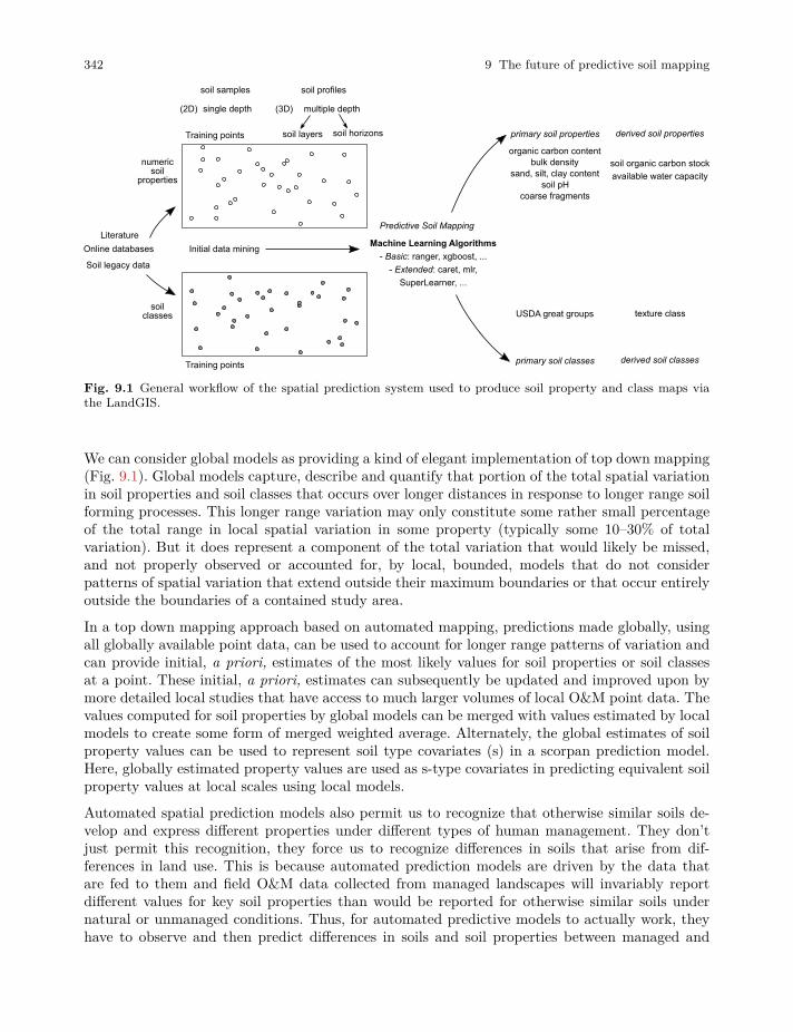
342 9 The future of predictive soil mapping
soil samples soil profiles
single depth
soil layers soil horizons
multiple depth
Predictive Soil Mapping
Training points
Machine Learning Algorithms
- Basic: ranger, xgboost, ...
- Extended: caret, mlr,
SuperLearner, ...
USDA great groups
primary soil properties
primary soil classes
derived soil properties
derived soil classes
Initial data mining
organic carbon contentbulk density
sand, silt, clay contentsoil pH
coarse fragments
texture class
soil organic carbon stock
available water capacity
Literature
Online databases
Soil legacy data
(2D) (3D)
numericsoil
properties
Training points
soilclasses
Fig. 9.1 General workflow of the spatial prediction system used to produce soil property and class maps viathe LandGIS.
We can consider global models as providing a kind of elegant implementation of top down mapping(Fig. 9.1). Global models capture, describe and quantify that portion of the total spatial variationin soil properties and soil classes that occurs over longer distances in response to longer range soilforming processes. This longer range variation may only constitute some rather small percentageof the total range in local spatial variation in some property (typically some 10–30% of totalvariation). But it does represent a component of the total variation that would likely be missed,and not properly observed or accounted for, by local, bounded, models that do not considerpatterns of spatial variation that extend outside their maximum boundaries or that occur entirelyoutside the boundaries of a contained study area.
In a top down mapping approach based on automated mapping, predictions made globally, usingall globally available point data, can be used to account for longer range patterns of variation andcan provide initial, a priori, estimates of the most likely values for soil properties or soil classesat a point. These initial, a priori, estimates can subsequently be updated and improved upon bymore detailed local studies that have access to much larger volumes of local O&M point data. Thevalues computed for soil properties by global models can be merged with values estimated by localmodels to create some form of merged weighted average. Alternately, the global estimates of soilproperty values can be used to represent soil type covariates (s) in a scorpan prediction model.Here, globally estimated property values are used as s-type covariates in predicting equivalent soilproperty values at local scales using local models.
Automated spatial prediction models also permit us to recognize that otherwise similar soils de-velop and express different properties under different types of human management. They don’tjust permit this recognition, they force us to recognize differences in soils that arise from dif-ferences in land use. This is because automated prediction models are driven by the data thatare fed to them and field O&M data collected from managed landscapes will invariably reportdifferent values for key soil properties than would be reported for otherwise similar soils undernatural or unmanaged conditions. Thus, for automated predictive models to actually work, theyhave to observe and then predict differences in soils and soil properties between managed and
9.3 The future of PSM: Embracing scientific and technical advances 343
natural landscapes. This was never something that was considered feasible to do with manual soilmapping. Consequently managed soils were usually named and mapped as if they were identicalto their natural (unmanaged) equivalents. Differences might be described in reports or tables oflaboratory analyses, but the two variations of the same soil (managed and natural) were rarely, ifever, mapped as separately described entities.
In a similar way, automated prediction methods force us to recognize and account for tempo-ral variations that arise from changes in soil conditions or soil attributes at the same locationsover time. The models will predict values similar to those provided to them as input from fieldobservations and measurements. If we have point O&M data for the same point location that isseparated in time and that reflects changes in soil property values through time, we need to beable to recognize this and adapt to it. We need to recognize that all predictions apply to a specifictime period and that different predictions (maps) need to be produced for different time periods,if the available point O&M data reference widely different time periods.
In the context of automated mapping and High Performance Computing, opportunities for pro-ducing high quality soil maps using Open Source software are becoming more and more attractive.However, not all Open Source Machine Learning packages are equally applicable for processinglarge national or international data sets at resolutions of 250 m or better. LandGIS predictionsare, for example, possible only thanks to the following packages that can be fully parallelized andare ready for upscaling predictions (all written in C++ in fact):
• ranger (https://github.com/imbs-hl/ranger),
• xgboost (https://xgboost.readthedocs.io/en/latest/),
• liquidSVM (https://github.com/liquidSVM/liquidSVM),
these can be further efficiently combined with accuracy assessment and fine-tuning packages (alsoready for parallelization):
• SuperLearner (https://cran.r-project.org/web/packages/SuperLearner/),
• caret (https://topepo.github.io/caret/),
• mlr (https://mlr.mlr-org.com/),
Beyond that it is not trivial to use R for production of large rasters where millions of pointswith hundreds of covariates are used for model building. So it is important to realize that OpenSource does not have out-of-box solutions for PSM projects, but requires active involvement anddevelopment.
9.3.7 Hosting, publishing, sharing and using spatial data
Finally, we need to consider how future inventory activities can benefit from improved approachesfor hosting, publishing, sharing and using spatial data, with special attention paid to predictionsof soil properties or soil classes.
344 9 The future of predictive soil mapping
The value of data is in its use. Thus, we only get full value for our data if we can maximizeits distribution and use. Developments in mechanisms and communities for sharing digital dataonline provide promise of greatly improved access to, and use of, new digital data sets, includingpredictive soil maps. Major developments in hosting and delivering spatial data online includenew and increased interest in, and adherence to, principles of FAIR Data, FAST Data and, mostimportantly, OPEN Data.
FAIR Data principles aim to make data findable, accessible, interoperable and reusable (Wilkinsonet al, 2016). The easier data are to locate and access, the greater the use is likely to be. Similarly,data that are interoperable are easier to ingest into end user applications, and so, will receivegreater use. Data that are reusable also ensure maximum benefit by facilitating regular use andreuse.
FAST data is the application of big data analytics to smaller data sets in near-real or real-time inorder to solve a problem or create business value. The goal of fast data is to quickly gather and minestructured and unstructured data so that action can be taken (https://whatis.techtarget.com/definition/fast-data). Fast data is fundamentally different from Big Data in many ways. Big Datais most typically data at rest, hundreds of terabytes or even petabytes of it, taking up lots of spaceon disk drives. Fast data is data in motion (https://www.voltdb.com/why-voltdb/big-data/).OpenGeoHub aims to use Big Data analytics to rapidly and affordably turn static and unstructureddata into easily used, and widely used information. The objective should be to rapidly generateagile, flexible and user oriented data.
Future soil inventory projects based on application of predictive soil modelling will also bene-fit from adopting the following principles of OPEN Data based on the Sunlight Foundation’s“Ten Principles for Opening up Government Information” (https://open.canada.ca/en/open-data-principles#toc95):
1. CompletenessData sets should be as complete as possible, reflecting the entirety of what is recordedabout a particular subject. All raw information from a data set should be released to thepublic, unless there are Access to Information or Privacy issues. Metadata that defines andexplains the raw data should be included, along with explanations for how the data was calculated.
2. PrimacyData sets should come from a primary source. This includes the original information collected bythe original sources and available details on how the data was collected. Public dissemination willallow users to verify that information was collected properly and recorded accurately.
3. TimelinessData sets released should be made available to the public in a timely fashion. Whenever feasible,information collected by original entities should be released as quickly as it is gathered andcollected. Priority should be given to data whose utility is time sensitive.
4. Ease of Physical and Electronic AccessData sets released by their producers should be as accessible as possible, with accessibility definedas the ease with which information can be obtained. Barriers to electronic access include makingdata accessible only via submitted forms or systems that require browser-oriented technologies(e.g., Flash, Javascript, cookies or Java applets). By contrast, providing an interface for users
9.3 The future of PSM: Embracing scientific and technical advances 345
to make specific calls for data through an Application Programming Interface (API) make datamuch more readily accessible.
5. Machine readabilityMachines can handle certain kinds of inputs much better than others. Data sets should bereleased in widely-used file formats that easily lend themselves to machine processing (e.g. CSV,XML). These files should be accompanied by documentation related to the format and how touse it in relation to the data.
6. Non-discriminationNon-discrimination refers to who can access data and how they must do so. Barriers to use ofdata can include registration or membership requirements. Released data sets should have as fewbarriers to use as possible. Non-discriminatory access to data should enable any person to accessthe data at any time without having to identify him/herself or provide any justification for doingso.
7. Use of Commonly Owned StandardsCommonly owned standards refer to who owns the format in which data is stored. For example, ifonly one company manufactures the program that can read a file where data is stored, access tothat information is dependent upon use of that company’s program. Sometimes that program isunavailable to the public at any cost, or is available, but for a fee. Removing this cost makes thedata available to a wider pool of potential users. Released data sets should be in freely availablefile formats as often as possible.
8. LicencingAll data sets should be released under a recognized Open Data Licence. Such licences are designedto increase openness and minimize restrictions on the use of the data.
9. PermanenceThe capability of finding information over time is referred to as permanence. For best use by thepublic, information made available online should remain online, with appropriate version-trackingand archiving over time.
10. Usage CostsAll open data should be provided free of charge.
A preferred way of achieving FAIR, FAST and OPEN data distribution is to develop and maintainnew, online platforms that support collaborative compilation, sharing and geopublishing. Open-GeoHub aims to provide a viable, worked example of how a new, open and collaborative web-basedplatform can deliver soil spatial information on-demand and in nearly real time.

346 9 The future of predictive soil mapping
9.3.8 New visualization and data analysis tools
Terrestrial resource inventories, and indeed spatial inventories of almost all environmental con-ditions, will increasingly benefit from adopting and using new tools and platforms that enhanceinteractive, real time data visualization and data analysis.Spatial data increasingly needs to be presented in ways that support interactive, real time visual-ization of 3 dimensions plus time. What is increasingly being referred to as 4D or 3D+ time. Weneed to help users visualize, and appreciate, how soils vary with depth as well as in horizontalspace. And, also increasingly, we need to be able to help users visualize and understand how soilscan vary through time. OpenGeoHub is attempting to demonstrate newly available facilities forvisualizing, and interacting with, 3D and 3D+ time spatio-temporal data.Every effort needs to be made to facilitate easy use of terrestrial resource inventory spatial data.This should entail releasing spatial data that has both the content and the format required forimmediate ingestion into, and use in, critical end user applications. Users should be able to linktheir applications to data supplier platforms and simple call up needed data.
9.4 The future of PSM: Embracing new organizational and governancemodels
9.4.1 Overview
In the same way that new scientific and technological advances can be embraced to improvefuture PSM any new, future, PSM activities should also take advantage of newer organizationalmodels that improve how collective activities can be organized and managed collaboratively andcooperatively through innovations such as (Hengl et al, 2018c):
• Open data and platforms and procedures for acquiring and sharing data,• Open, cloud-based, processing capabilities,• Collaborative production of inputs and new outputs,• Crowdsourcing and voluntary collaboration,• Crowdfunding and blockchain funding systems,• Web-based sponsorship and revenue opportunities,
9.4.2 Open data and platforms and procedures for acquiring andsharing it
Open data is, of course, the key requirement for enabling maximum access to, and use of, point andcovariate data required to support collaborative PSM. Firewalls, paywalls and data silos typically
9.4 The future of PSM: Embracing new organizational and governance models 347
act to restrict access to, and use of, valuable point and covariate data, Open data can be usedand reused, multiple times, often for unanticipated applications. Data need to be not only openbut also easily discoverable and accessible. This is where open platforms, such as OpenGeoHub,come in. They can facilitate easy and effective access to, and use of, shared open data.
9.4.3 Open cloud-based processing capabilities
At the moment, most PSM activities take place on local computers using local processors. AsPSM proceeds and increasingly deals with much larger data sets at much finer spatial resolutions,it may become less and less viable to download all data for local processing. Imagine trying todownload 5 to 10 m resolution raster data for an entire continent, or even the entire world, fortens to perhaps hundreds of layers of covariate data. We may rapidly arrive at a situation whereit could take months to years to simply download such large volumes of data before any analysescould take place. It such a situation, it no longer makes sense to try to download covariate datasets to work with them locally.
Similarly, many big data applications have now accepted that it is far more efficient and affordableto conduct their processing and analysis in the cloud using services such as Amazon cloud ser-vices, Google Earth Engine or Microsoft cloud services. It has become too costly to assemble andmaintain the massive amounts of processing power, and memory, in house that are increasinglyrequired to process massive data sets using big data analytics.
Modelers can easily obtain and download all available covariate data for all point locations forwhich they possess point observations or measurements. Typically, entire stacks of covariate datacan be identified and downloaded for thousands of point locations within just a few seconds ofsubmitting a query. This covariate data is all that is needed to create the matrices required tosupport development, evaluation and finalization of multiple predictive models for PSM. Once anoptimum model (or models) has been developed, the model itself can be uploaded to a cloud basedprocessing service and the model can be run against all covariate data stored in the cloud, usingcloud based memory and processing capabilities. This is perhaps a preferable and more practicalway to implement PSM modelling for very large data sets.
9.4.4 Collaborative production of inputs and new outputs
It is likely that it will increasingly only be possible to produce next generation national to statelevel PSM inventory products through some form of collaborative effort. It is very unusual forany one agency or entity to have both the mandate and the resources to assume responsibilityfor producing maps for entire countries or even entire provinces or states. Mapping and fielddata collection activities tend to be fragmented in response to various jurisdictional mandatesand operational responsibilities. Agricultural departments are responsible for agricultural lands,forestry for forested areas, parks departments for public parklands and environmental departmentsfor conservation areas. No one entity ever seems to have responsibility for mapping an entirecountry or state. In addition, a majority of mapping and field data collection programs are now
348 9 The future of predictive soil mapping
typically undertaken by private engineering and environmental consulting companies on contractto industry or government clients. The people charged with collecting the field data seldom haveany responsibility or mandate for ongoing custodianship and preservation of the collected data. Thecompanies or government agencies that contracted to have the data collected themselves typicallylack the resources, expertise or motivation to conserve and maintain the field data delivered tothem, let alone to share it widely with others.
So, how can a situation be achieved where a large proportion of point data collected in the field, oranalysed in a lab, are collated, stored and maintained for widespread distribution, use and reuse inPSM?We believe that what is required are both physical (or virtual) platforms where collaborationand sharing can be facilitated and legal and organisational protocols that encourage, and indeedrequire, saving, maintaining and sharing of point observation data collectively and collaboratively.
What is required is a change in attitude that is reflected by equivalent changes in regulationsand procedures. Governments and private sector industries that require, or commission, field datacollection activities need to adopt procedures and rules that require any new data to be depositedin an open repository where it can be widely and easily accessed and shared. Similarly, laboratoriesthat undertake analysis of field collected samples need to be encouraged, or even obliged, to submitanalytical results for samples from point locations to some shared and open repository. If this wereto occur, then anyone interested in producing maps for any area would have access to all potentiallyavailable and useful point data to inform and drive their predictive models. We offer OpenGeoHubas an example of a physical platform where all of point data, covariate data and output predictivemaps can be widely and freely published, archived and shared.
The production of output maps can also be undertaken as a collective and collaborative exercise.Individuals and agencies can work together to create and share input data sets (point data andcovariates) and models and to jointly produce maps for areas of common interest. The more peoplethat get involved in producing new maps using common, open databases, the greater the number,variety and utility of maps we are likely to see produced.
9.4.5 Crowdsourcing and voluntary collaboration,
There is a role in PSM for crowdsourcing and voluntary contributions from citizen scientists(Hengl et al, 2018c). Sampling plans can be developed and volunteers can be encouraged to goto identified sampling locations to collect a series of easy to make observations using a providedtemplate. One active example of this approach is the Degree Confluence Project. This projectaims to have people visit each of the exact integer degree intersections of latitude and longitudeon Earth, posting photographs and a narrative of each visit online (https://en.wikipedia.org/wiki/Degree_Confluence_Project). The project describes itself as “an organized sampling of the world”and is purely based on enthusiasm.
Monitoring programs can vary significantly, ranging from community based monitoring on a localscale, to large-scale collaborative global monitoring programs such as those focused on climatechange (Lovett et al, 2007). There is a global recognition that “environmental issues are besthandled with the participation of all concerned citizens”, a principal first articulated in the UnitedNation’s Earth Summit Agenda 21 (UN, 1992). This principle was strengthened further in July,2009, with the formal ratification of the Aarhus Convention which mandates participation by the
9.4 The future of PSM: Embracing new organizational and governance models 349
public in environmental decision-making and access to justice in environmental matters (UNECE,2008).
If volunteers can be advised where to go and what to observe, or collect, at sample locationsfollowing a defined format or template, much useful data can be collected for use in PSM. Forexample, it is relatively easy to make very useful field observations about whether a location isa wetland organic soil or an upland mineral soil. This, in itself, is very useful to know. Similarly,citizen scientists can be instructed to obtain valuable measurements such as depth of a soil tobedrock, thickness of a topsoil horizon, color of a topsoil or subsoil horizon or presence or absenceof bare rock, water, stones or gullies. It is even possible to provide detailed instructions that permitvolunteers to estimate soil texture by application of manual hand texture assessments. Increasingly,apps are likely to be developed for mobile phones that will support quantitative assessments ofsoil color or structure and, possibly very soon, spectroscopic analysis of soil properties on-site.So, future PSM activities should look for opportunities to engage citizen volunteers in collectingfield observations and measurements to extend what PSM is able to accomplish now using datacollected data by professionals.
9.4.6 Sponsorship, subscription, crowdfunding and blockchain fundingsystems
Someone has to pay to finance the collection of new field and laboratory point data, the assembly,storage and distribution of databases of relevant point data or environmental covariates at relevantresolutions and the production, publication, maintenance and distribution of any models, outputmaps or other end products. We can imagine several possible revenue streams that could beadopted to fund a collaborative platform in a sustainable way. These include:
• Sponsorship,
• Subscriptions by participating partners,
• Crowdfunding,
• Blockchain funding,
• Advertising revenue,
Sponsors are those who provide funds willingly to support operations and activities that theyconsider to be beneficial, possibly to themselves but, more importantly, to wider society. Sponsorstypically regard the services and products provided by the funded entity as delivering a desirablepublic good or public service and to therefore be worthy of their financial support. Sponsorstypically do not dictate what gets done, or how, but sponsors do have some expectations that theirfunding will ensure that the public good activities they support will continue to be undertakenand delivered by the funding recipient in a consistent and responsible manner.
We can imagine that an open collaborative for natural resource inventory products might attractsponsorship from philanthropic donors who elect to fund environmental activities undertaken insupport of the broader public interest. Some government agencies, or even commercial companies,might also elect to offer ongoing sponsorship funding. The main role of sponsorship funding ought

350 9 The future of predictive soil mapping
to be to provide some minimum base level of income that can pay for the ongoing costs associatedwith maintaining basic operational capabilities. Examples of basic operational costs include ongo-ing charges for paying for website development and maintenance, online storage, web traffic andweb based processing arising from user activity and system administration. These are basicallyjust the costs associated with keeping the lights on and the doors open. They ensure continuityfrom year to year but do not usually fund major expansions or annual production activities.
Active contributors to, and users of, the products and services generated by a consortium orcollective of partners can help to self-fund the collective’s activities by agreeing to contributefunds via some sort of continuing subscription. Partners may be able to justify paying an annualsubscription to sustain the collective activity because they, themselves, obtain benefits or reduceinternal expenditures they would otherwise normally pay for the same sets of services or activitiesinternally and individually. Sharing platforms for collecting, creating, hosting, publishing and dis-seminating spatial environmental data could be more cost effective than building and maintainingmultiple separate platforms and functionalities individually (Fig. 9.2). These reduced, or avoided,costs could justify contributing some funds to pay for, and sustain, the operations of the collective.Sustaining subscriptions are a more stable and reliable way to fund the ongoing development andmaintenance of the collective’s activities and infrastructure because they can be more reliablyestimated and counted on. These funds can also help pay for new work and new data.
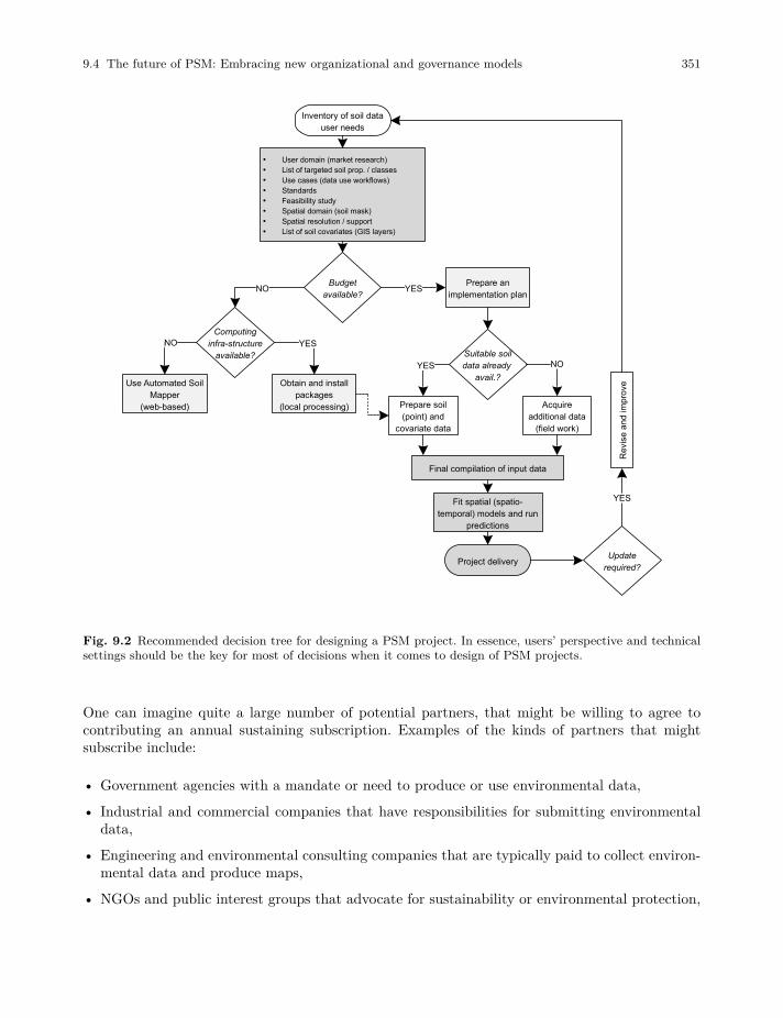
9.4 The future of PSM: Embracing new organizational and governance models 351
Budget available?
Inventory of soil data user needs
Computing infra-structure
available?
NO YES
• User domain (market research)• List of targeted soil prop. / classes• Use cases (data use workflows)• Standards• Feasibility study• Spatial domain (soil mask)• Spatial resolution / support• List of soil covariates (GIS layers)
Prepare an implementation plan
Prepare soil (point) and
covariate data
Suitable soil data already
avail.?
Acquire additional data
(field work)
NOYES
Use Automated Soil Mapper
(web-based)
Obtain and install packages
(local processing)
NO YES
Final compilation of input data
Project delivery
Fit spatial (spatio-temporal) models and run
predictions
Rev
ise
and
imp
rove
Update required?
YES
Fig. 9.2 Recommended decision tree for designing a PSM project. In essence, users’ perspective and technicalsettings should be the key for most of decisions when it comes to design of PSM projects.
One can imagine quite a large number of potential partners, that might be willing to agree tocontributing an annual sustaining subscription. Examples of the kinds of partners that mightsubscribe include:
• Government agencies with a mandate or need to produce or use environmental data,
• Industrial and commercial companies that have responsibilities for submitting environmentaldata,
• Engineering and environmental consulting companies that are typically paid to collect environ-mental data and produce maps,
• NGOs and public interest groups that advocate for sustainability or environmental protection,
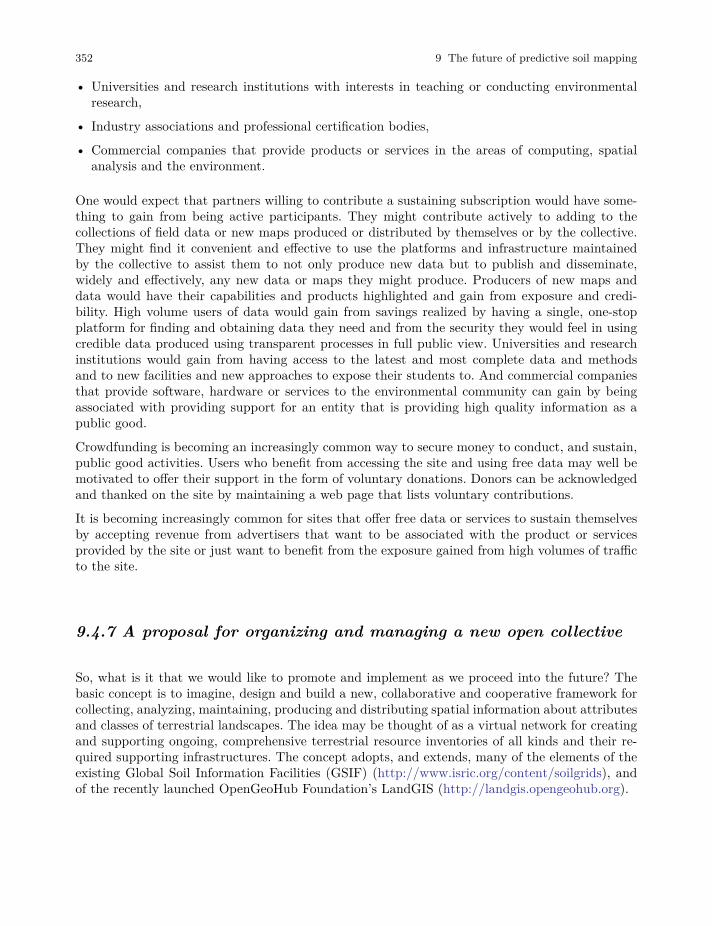
352 9 The future of predictive soil mapping
• Universities and research institutions with interests in teaching or conducting environmentalresearch,
• Industry associations and professional certification bodies,
• Commercial companies that provide products or services in the areas of computing, spatialanalysis and the environment.
One would expect that partners willing to contribute a sustaining subscription would have some-thing to gain from being active participants. They might contribute actively to adding to thecollections of field data or new maps produced or distributed by themselves or by the collective.They might find it convenient and effective to use the platforms and infrastructure maintainedby the collective to assist them to not only produce new data but to publish and disseminate,widely and effectively, any new data or maps they might produce. Producers of new maps anddata would have their capabilities and products highlighted and gain from exposure and credi-bility. High volume users of data would gain from savings realized by having a single, one-stopplatform for finding and obtaining data they need and from the security they would feel in usingcredible data produced using transparent processes in full public view. Universities and researchinstitutions would gain from having access to the latest and most complete data and methodsand to new facilities and new approaches to expose their students to. And commercial companiesthat provide software, hardware or services to the environmental community can gain by beingassociated with providing support for an entity that is providing high quality information as apublic good.
Crowdfunding is becoming an increasingly common way to secure money to conduct, and sustain,public good activities. Users who benefit from accessing the site and using free data may well bemotivated to offer their support in the form of voluntary donations. Donors can be acknowledgedand thanked on the site by maintaining a web page that lists voluntary contributions.
It is becoming increasingly common for sites that offer free data or services to sustain themselvesby accepting revenue from advertisers that want to be associated with the product or servicesprovided by the site or just want to benefit from the exposure gained from high volumes of trafficto the site.
9.4.7 A proposal for organizing and managing a new open collective
So, what is it that we would like to promote and implement as we proceed into the future? Thebasic concept is to imagine, design and build a new, collaborative and cooperative framework forcollecting, analyzing, maintaining, producing and distributing spatial information about attributesand classes of terrestrial landscapes. The idea may be thought of as a virtual network for creatingand supporting ongoing, comprehensive terrestrial resource inventories of all kinds and their re-quired supporting infrastructures. The concept adopts, and extends, many of the elements of theexisting Global Soil Information Facilities (GSIF) (http://www.isric.org/content/soilgrids), andof the recently launched OpenGeoHub Foundation’s LandGIS (http://landgis.opengeohub.org).
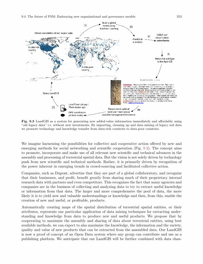
9.4 The future of PSM: Embracing new organizational and governance models 353
Fig. 9.3 LandGIS as a system for generating new added-value information immediately and affordably using“old legacy data” i.e. without new investments. By importing, cleaning up and data mining of legacy soil datawe promote technology and knowledge transfer from data-rich countries to data-poor countries.
We imagine harnessing the possibilities for collective and cooperative action offered by new andemerging methods for social networking and scientific cooperation (Fig. 9.3). The concept aimsto promote, incorporate and make use of all relevant new scientific and technical advances in theassembly and processing of terrestrial spatial data. But the vision is not solely driven by technologypush from new scientific and technical methods. Rather, it is primarily driven by recognition ofthe power inherent in emerging trends in crowd-sourcing and facilitated collective action.
Companies, such as Dupont, advertise that they are part of a global collaboratory, and recognizethat their businesses, and profit, benefit greatly from sharing much of their proprietary internalresearch data with partners and even competitors. This recognizes the fact that many agencies andcompanies are in the business of collecting and analyzing data to try to extract useful knowledgeor information from that data. The larger and more comprehensive the pool of data, the morelikely it is to yield new and valuable understandings or knowledge and then, from this, enable thecreation of new and useful, or profitable, products.
Automatically creating maps of the spatial distribution of terrestrial spatial entities, or theirattributes, represents one particular application of data mining techniques for extracting under-standing and knowledge from data to produce new and useful products. We propose that bycooperating to maximize the assembly and sharing of data about terrestrial entities, using bestavailable methods, we can expect to also maximize the knowledge, the information and the variety,quality and value of new products that can be extracted from the assembled data. Our LandGISis now a proof of concept of an Open Data system where any group can contribute and use as apublishing platform. We anticipate that our LandGIS will be further combined with data chan-
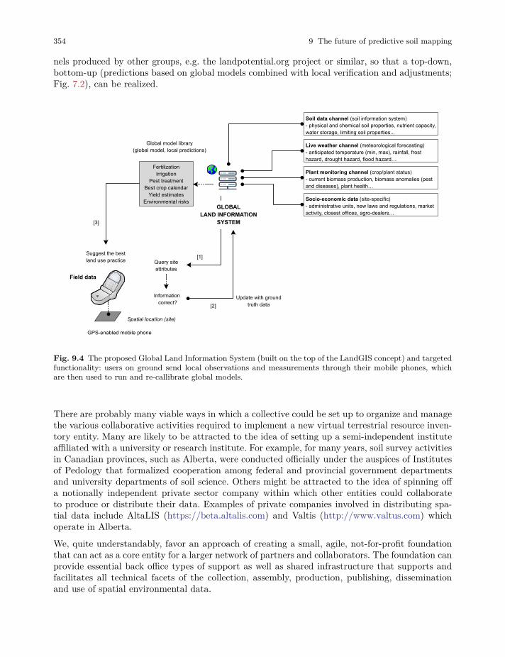
354 9 The future of predictive soil mapping
nels produced by other groups, e.g. the landpotential.org project or similar, so that a top-down,bottom-up (predictions based on global models combined with local verification and adjustments;Fig. 7.2), can be realized.
GLOBALLAND INFORMATION
SYSTEM
Soil data channel (soil information system)- physical and chemical soil properties, nutrient capacity, water storage, limiting soil properties...
Live weather channel (meteorological forecasting)- anticipated temperature (min, max), rainfall, frost hazard, drought hazard, flood hazard…
Plant monitoring channel (crop/plant status)- current biomass production, biomass anomalies (pest and diseases), plant health…
Socio-economic data (site-specific)- administrative units, new laws and regulations, market activity, closest offices, agro-dealers…
Spatial location (site)
Query siteattributes
Information correct?
Update with ground truth data
FertilizationIrrigation
Pest treatmentBest crop calendar
Yield estimatesEnvironmental risks
Suggest the bestland use practice
Global model library(global model, local predictions)
GPS-enabled mobile phone
[1]
[2]
[3]
Field data
Fig. 9.4 The proposed Global Land Information System (built on the top of the LandGIS concept) and targetedfunctionality: users on ground send local observations and measurements through their mobile phones, whichare then used to run and re-callibrate global models.
There are probably many viable ways in which a collective could be set up to organize and managethe various collaborative activities required to implement a new virtual terrestrial resource inven-tory entity. Many are likely to be attracted to the idea of setting up a semi-independent instituteaffiliated with a university or research institute. For example, for many years, soil survey activitiesin Canadian provinces, such as Alberta, were conducted officially under the auspices of Institutesof Pedology that formalized cooperation among federal and provincial government departmentsand university departments of soil science. Others might be attracted to the idea of spinning offa notionally independent private sector company within which other entities could collaborateto produce or distribute their data. Examples of private companies involved in distributing spa-tial data include AltaLIS (https://beta.altalis.com) and Valtis (http://www.valtus.com) whichoperate in Alberta.
We, quite understandably, favor an approach of creating a small, agile, not-for-profit foundationthat can act as a core entity for a larger network of partners and collaborators. The foundation canprovide essential back office types of support as well as shared infrastructure that supports andfacilitates all technical facets of the collection, assembly, production, publishing, disseminationand use of spatial environmental data.
9.4 The future of PSM: Embracing new organizational and governance models 355
This is the concept behind the newly formed OpenGeoHub Foundation (https://opengeohub.org).We see OpenGeoHub as an entity that can build, operate and maintain a core set of functionalitiesand infrastructure required to support a wide variety of inventory type activities. This core func-tionality can provide back office facilities and support that can be made use of by any entity thatdesires to be actively involved in the collection, production or distribution of spatial environmentalinformation. Just as many companies and agencies have increasingly begun to outsource their datastorage, data processing and even key functions such as payroll and human resources, so too couldentities involved in the production or use or spatial data outsource many of their functions toOpenGeoHub. It is expensive and time consuming to build and maintain custom functionality inhouse to support the production and distribution of inventory spatial data. Why not build it wellonce and make this functionality available to everyone? If some desired functionality is missing,then build it inside the foundation so that all can benefit from using the new functionality. Whyspend money and time building multiple versions of systems with equivalent functionality andpurpose when one will do for all? Then the partner entities can concentrate on doing what theirmandates instruct them to do, and not on building and maintaining separate spatial analysis andspatial distribution systems and infrastructures.
We would hope that OpenGeoHub can act as a fully functional, worked example of how collabo-ration and collective action in the area of production and delivery of environmental spatial datacould be organized and implemented efficiently and effectively. Once the concept has been demon-strated and accepted, it might well prove useful to replicate or clone the concept, including allof its functionalities, for use at national, state or regional levels. As with any other concept thatworks, cloning to set up franchise operations is widely accepted. It is not necessary to reinventthe wheel to set up a cloned franchise operation. Most of the design and functionality can simplybe replicated for use at the local franchise level. We envisage OpenGeoHub as a test case and anincubator that, if successful, could form a template for many other successful spin-offs.

References
Adams WA (1973) The effect of organic matter on the bulk and true density of some uncultivated podzolic soils.Journal of Soil Science 24:10 – 17
Aitken R, Moody P (1991) Interrelations between Soil pH Measurements in Various Electrolytes and Soil SolutionpH in Acidic Soils. Australian Journal of Soil Research 29:483 – 491
Alexander E (1980) Bulk density of Californian soils in relation to other soil properties. Soil Science Society ofAmerica Journal 44:689–692
Arrouays D, Grundy MG, Hartemink AE, Hempel JW, Heuvelink GB, Young Hong S, Lagacherie P, Lelyk G,McBratney AB, McKenzie NJ, Mendonça-Santos Md, Minasny B, Montanarella L, Odeh IO, Sanchez PA,Thompson JA, Zhang GL (2014a) Chapter Three — GlobalSoilMap: Toward a Fine-Resolution Global Gridof Soil Properties. In: Sparks DL (ed) Soil carbon, Advances in Agronomy, vol 125, Academic Press, pp 93 –134, DOI 10.1016/B978-0-12-800137-0.00003-0
Arrouays D, McKenzie N, de Forges A, Hempel J, McBratney A (2014b) GlobalSoilMap: basis of the globalspatial soil information system. CRC press, Boca Raton, USA
Arrouays D, Leenaars JG, Richer-de Forges AC, Adhikari K, Ballabio C, Greve M, Grundy M, Guerrero E,Hempel J, Hengl T, et al (2017) Soil legacy data rescue via GlobalSoilMap and other international andnational initiatives. GeoResJ 14:1–19
Arya L, Paris J (1981) A physico-empirical approach to predict the soil water moisture characteristic fromparticle size distribution and bulk density data. Soil Science Society of America Journal 45:1023–1030
Avery B (1987) Soil survey methods: a review. Technical Monograph No. 18, Soil Survey & Land ResourceCentre, Silsoe
Baritz R, Seufert G, Montanarella L, Van Ranst E (2010) Carbon concentrations and stocks in forest soils ofeurope. Forest Ecology and Management 260:262 – 277, DOI 10.1016/j.foreco.2010.03.025
Batjes N, Ribeiro E, van Oostrum A, Leenaars JG, Hengl T, Mendes de Jesus J (2017) WoSIS: Providingstandardised soil profile data for the world. Earth System Science Data 9:1–14
Batjes NH (2009) Harmonized soil profile data for applications at global and continental scales: Updates to theWISE database. Soil Use and Management 25(2):124–127, DOI 10.1111/j.1475-2743.2009.00202.x
Bauer-Marschallinger B, Freeman V, Cao S, Paulik C, Schaufler S, Stachl T, Modanesi S, Massari C, CiabattaL, Brocca L, Wagner W (2019) Toward Global Soil Moisture Monitoring With Sentinel-1: Harnessing Assetsand Overcoming Obstacles. IEEE Transactions on Geoscience and Remote Sensing 57(1):520–539, DOI10.1109/TGRS.2018.2858004
Beaudette D, O’Geen A (2009) Soil-web: An online soil survey for California, Arizona, and Nevada. Computers& Geosciences 35:2119–2128
Beaudette D, Roudier P, O’Geen A (2013) Algorithms for quantitative pedology: A toolkit for soil scientists.Computers & Geosciences 52(0):258 – 268, DOI 10.1016/j.cageo.2012.10.020
Behrens T, Schmidt K, MacMillan R, Viscarra Rossel R (2018a) Multiscale contextual spatial modelling withthe gaussian scale space. Geoderma 310:128 – 137, DOI 10.1016/j.geoderma.2017.09.015
Behrens T, Schmidt K, MacMillan RA, Rossel RAV (2018b) Multi-scale digital soil mapping with deep learning.Scientific reports 8:15244, DOI 10.1038/s41598-018-33516-6
Behrens T, Schmidt K, Viscarra Rossel R, Gries P, Scholten T, MacMillan R (2018c) Spatial modelling withEuclidean distance fields and machine learning. European journal of soil science 69(5):757–770
357

358 References
Berhongaray G, Alvarez R (2013) The ipcc tool for predicting soil organic carbon changes evaluated for thepampas, argentina. Agriculture, ecosystems & environment 181:241–245
Bernoux M, Arrouays D, Cerri C, Valkoff B, Jolivet C (1998) Bulk densities of Brazilian Amazon soils relatedto other soil properties. Soil Science Society of America Journal 62:743–749
Biau G, Scornet E (2016) A random forest guided tour. TEST 25(2):197–227, DOI 10.1007/s11749-016-0481-7Bie S, Ulph A (1972) The economic value of survey information. Journal of Agricultural Economics 13:285–297Bie S, Uph A, Beckett PT (1973) Calculating the economic benefits of soil survey. Journal of Soil Science
24:429–435Bishop T, McBratney AB, Laslett G (1999) Modelling soil attribute depth functions with equal-area quadratic
smoothing splines. Geoderma 91(1-2):27–45Bisutti I, Hilke I, Raessler M (2004) Determination of total organic carbon — an overview of current methods.
Trends in Analytical Chemistry 23(10-11):716–726Bivand R, Pebesma E, Rubio V (2008) Applied Spatial Data Analysis with R. Use R Series, Springer, HeidelbergBivand R, Pebesma E, Rubio V (2013) Applied Spatial Data Analysis with R, 2nd edn. Use R Series, Springer,
HeidelbergBoettinger JL, Howell DW, Moore AC, Hartemink AE, Kienast-Brown S (eds) (2010) Digital Soil Mapping:
Bridging Research, Environmental Application, and Operation, Progress in Soil Science, vol 2. SpringerBouma J (1989) Land qualities in space and time. In: Bouma J, Bregt A (eds) Proceedings of a symposium
organized by the International Society of Soil Science, Wageningen University, Wageningen, pp 3–13Bouma J, Batjes NH, Groot JJR (1998) Exploring land quality effects on world food supply. Geoderma 86(1):43–
59Breiman L (1993) Classification and regression trees. CRC pressBreiman L (2001) Random forests. Machine learning 45(1):5–32Brennan R, Bolland M (1998) Relationship between ph measured in water and calcium chloride for soils of
southwestern australia. Communications in Soil Science and Plant Analysis 29(17-18):2683–2689, DOI 10.1080/00103629809370143
Brenning A (2012) Spatial cross-validation and bootstrap for the assessment of prediction rules in remotesensing: The R package sperrorest. In: 2012 IEEE International Geoscience and Remote Sensing Symposium,pp 5372–5375, DOI 10.1109/IGARSS.2012.6352393
Brodlie K, Osorio RA, Lopes A (2012) A review of uncertainty in data visualization. In: Expanding the Frontiersof Visual Analytics and Visualization, Springer, pp 81–109
Brown J, Robertson B, McDonald T (2015) Spatially balanced sampling: application to environmental surveys.Procedia Environmental Sciences 27:6–9
Brown PE (2015) Model-Based Geostatistics the Easy Way. Journal of Statistical Software 63(12), URL http://www.jstatsoft.org/v63/i12
Brungard CW, Boettinger JL, Duniway MC, Wills SA, Edwards Jr TC (2015) Machine learning for predictingsoil classes in three semi-arid landscapes. Geoderma 239:68–83
Brus D (2019) Sampling for digital soil mapping: A tutorial supported by R scripts. Geoderma 338:464 – 480,DOI 10.1016/j.geoderma.2018.07.036
Brus D, Kempen B, Heuvelink G (2011) Sampling for validation of digital soil maps. European Journal of SoilScience 62(3):394–407, DOI 10.1111/j.1365-2389.2011.01364.x
Brus DJ, Heuvelink GBM (2007) Optimization of sample patterns for universal kriging of environmental vari-ables. Geoderma 138(1-2):86–95
Brye K, Slaton N (2003) Carbon and Nitrogen Storage in a Typic Albaqualf as Affected by Assessment Method.Communications in Soil Science and Plant Analysis 34:1637–1655
Bui E (2003) A strategy to fill gaps in soil survey over large spatial extents: an example from the murray-darlingbasin of australia. Geoderma 111:21–44, DOI 10.1016/S0016-7061(02)00238-0
Bui E (2004) Soil survey as a knowledge system. Geoderma 120:17–26, DOI 10.1016/j.geoderma.2003.07.006Buol S, Southard R, Graham R, McDaniel PA (2011) Soil Genesis and Classification. WileyBurrough PA (1989) Fuzzy mathematical methods for soil survey and land evaluation. Journal of Soil Science
40(3):477–492, DOI 10.1111/j.1365-2389.1989.tb01290.xBurrough PA, McDonnell RA (1998) Principles of Geographical Information Systems, 2nd edn. Oxford University
Press, OxfordBurrough PA, Beckett PT, Jarvis M (1971) The relation between cost and utility in soil survey (i–iii). Journal
of Soil Science 22(3):359–394, DOI 10.1111/j.1365-2389.1971.tb01624.xCampbell A (2008) Managing Australia’s Soils: A policy discussion paper. CSIRO, Canberra
References 359
Campbell G, Shiozawa S (1989) Prediction of hydraulic properties of soils using particle-size distribution andbulk density data. In: van Genuchten, MTh et al (ed) Proc. Int. Worksh. On Indirect Methods for Estimatingthe Hydraulic Properties of Unsaturated Soils, Univ. of California, Riverside, Riverside, CA, pp 317–328
Canarache A (1993) Physical-technological soil maps — A possible product of soil survey for direct use inagriculture. Soil Technology 6:3–15
Carrick S, Vesely ET, Hewitt A (2010) Economic value of improved soil natural capital assessment: a case studyon nitrogen leaching. In: 19th World Congress of Soil Science, IUSS, Brisbane, Australia, pp 1–6
Carter M, Gregorich E (2007) Soil Sampling and Methods of Analysis. CRC PRESSCaubet M, Dobarco MR, Arrouays D, Minasny B, Saby NP (2019) Merging country, continental and global
predictions of soil texture: Lessons from ensemble modelling in france. Geoderma 337:99 – 110, DOI 10.1016/j.geoderma.2018.09.007
Chang CC, Lin CJ (2011) LIBSVM: a library for support vector machines. ACM transactions on intelligentsystems and technology (TIST) 2(3):27
Chen J, Chen J, Liao A, Cao X, Chen L, Chen X, He C, Han G, Peng S, Lu M, Zhang W, Tong X, Mills J(2015) Global land cover mapping at 30 m resolution: A POK-based operational approach. ISPRS Journalof Photogrammetry and Remote Sensing 103:7–27, DOI 10.1016/j.isprsjprs.2014.09.002
Chen T, Guestrin C (2016) XGBoost: A Scalable Tree Boosting System. ArXiv e-prints 1603.02754Chesworth W (2008) Encyclopedia of soil science. Encyclopedia of earth sciences series, SpringerChristakos G, Bogaert P, Serre M (2001) Temporal GIS: advanced functions for field-based applications. v. 1,
SpringerChristensen R (2001) Linear Models for Multivariate, Time Series, and Spatial Data, 2nd edn. Springer Verlag,
New YorkConant RT, Ogle SM, Paul EA, Paustian K (2010) Measuring and monitoring soil organic carbon stocks in
agricultural lands for climate mitigation. Frontiers in Ecology and the Environment 9(3):169–173, URLhttp://dx.doi.org/10.1890/090153
Conrad O, Bechtel B, Bock M, Dietrich H, Fischer E, Gerlitz L, Wehberg J, Wichmann V, Böhner J (2015)System for automated geoscientific analyses (saga) v. 2.1.4. Geoscientific Model Development 8(7):1991–2007,DOI 10.5194/gmd-8-1991-2015
Cooper M, Mendes LMS, Silva WLC, Sparovek G (2005) A national soil profile database for brazil available tointernational scientists. Soil Science Society of America Journal 69(3):649–652
Cressie NC, Wikle C (2011) Statistics for Spatio-Temporal Data. Wiley Series in Probability and Statistics,Wiley
Cresswell H, Coquet Y, Bruand A, McKenzie N (2006) The transferability of Australian pedotransfer functionsfor predicting water retention characteristics of French soils. Soil Use and Management 22:62–70
Curtis R, Post B (1964) Estimating bulk density from organic matter content in some Vermont forest soils. SoilScience Society of America Proceedings 28:285–286
Danielson J, , Gesch D (2011) Global multi-resolution terrain elevation data 2010 (GMTED2010). Open-FileReport 2011-1073, U.S. Geological Survey
D’Avello T, McLeese R (1998) Why are those lines placed where they are? an investigation of soil map recom-pilation methods. Soil Survey Horiz 39:119–126
Davis L (1943) Measurements of ph with the glass electrode as affected by soil moisture. Soil Science 56(6):405–422
de Gruijter J, Brus D, Bierkens M, Knotters M (2006) Sampling for Natural Resource Monitoring. Springer,London
de Gruijter JJ, Walvoort DJJ, van Gaans PFM (1997) Continuous soil maps — a fuzzy set approach to bridgethe gap between aggregation levels of process and distribution models. Geoderma 77(2-4):169–195
De Vos B, Lettens S, Muys B, Deckers J (2007) Walkley-Black analysis of forest soil organic carbon: Recov-ery,limitations and uncertainty. Soil Use and Management 23:221–229
Desaules A, Ammann S, Schwab P (2010) Advances in long-term soil-pollution monitoring of switzerland. Journalof Plant Nutrition and Soil Science 173(4):525–535, DOI 10.1002/jpln.200900269
Diggle PJ, Ribeiro Jr PJ (2007) Model-based Geostatistics. Springer Series in Statistics, SpringerDobos E, Carré F, Hengl T, Reuter HI, Tóth G (2006) Digital soil mapping: as a support to production of
functional maps. Office for Official Publications of the European Communities, LuxemburgDriessen PM, Konijn NT (1992) Land-use systems analysis. Wageningen Agricultural UniversityDurana PJ (2008) Appendix A: Chronology of the U.S. Soil Survey. In: Profiles in the History of the U.S. Soil
Survey, Iowa State Press, pp 315–320, DOI 10.1002/9780470376959.app1Eswaran H, Ahrens R, Rice T, Stewart B (2010) Soil Classification: A Global Desk Reference. Taylor & Francis
360 References
Fan Y, Li H, Miguez-Macho G (2013) Global patterns of groundwater table depth. Science 339(6122):940–943FAO (1990) Guidelines for soil profile description, 3rd edn. Food and Agriculture Organization of the United
Nations, RomeFAO (2006) Guidelines for soil profile description, 4th edn. Food and Agriculture Organization of the United
Nations, RomeFAO/IIASA/ISRIC/ISS-CAS/JRC (2012) Harmonized World Soil Database (version 1.2). FAO, RomeFederer C, Turcotte D, Smith C (1993) The organic- bulk-density relationship and the expression of nutrient
content in forest soils. Canadian Journal of Forest Research 23:1026–1032Fernandez R, Schulze D, Coffin D, Van Scoyoc G (1988) Color, organic matter, and pesticide adsorption rela-
tionships in a soil landscape. Soil Science Society of America Journal 52(4):1023–1026Finke P (2006) Quality assessment of digital soil maps: producers and users perspectives. In: Lagacherie P,
McBratney AB, Voltz M (eds) Digital Soil Mapping: An Introductory Perspective, Developments in SoilScience, Elsevier, Amsterdam, pp 523–541
Finke PA, Hutson JL (2008) Modelling soil genesis in calcareous loess. Geoderma 145(3-4):462 – 479, DOI10.1016/j.geoderma.2008.01.017
Florinsky IV (2012) The dokuchaev hypothesis as a basis for predictive digital soil mapping (on the 125thanniversary of its publication). Eurasian Soil Science 45(4):445–451, DOI 10.1134/S1064229312040047
Food, of the United Nations AO (2006) Guidelines for Soil Description. Food and Agriculture Organization ofthe United Nations
Food, Agriculture Organization of the United Nations Soil Resources D, Service C (1977) A framework forland evaluation. Publication (International Institute for Land Reclamation and Improvement), InternationalInstitute for Land Reclamation and Improvement
Forkel M, Migliavacca M, Thonicke K, Reichstein M, Schaphoff S, Weber U, Carvalhais N (2015) Codominantwater control on global interannual variability and trends in land surface phenology and greenness. Globalchange biology 21(9):3414–3435
Franklin J (1995) Predictive vegetation mapping: geographic modelling of biospatial patterns in relation toenvironmental gradients. Progress in Physical Geography 19(4):474–499
Frossard E, Blum W, Warkentin B, of London GS (2006) Function of soils for human societies and the environ-ment. Special publication — Geological Society of London, Geological Society
Gasch C, Hengl T, Gräler B, Meyer H, Magney T, Brown D (2015) Spatio-temporal interpolation of soil water,temperature, and electrical conductivity in 3D+T: The Cook Agronomy Farm data set. Spatial Statistics14(Part A):70–90, DOI 10.1016/j.spasta.2015.04.001
Gehl R, Rice C (2007) Emerging technologies for in situ measurement of soil carbon. Climatic Change 80(1-2):43–54, DOI 10.1007/s10584-006-9150-2
Gerber R, Felix-Henningsen P, Behrens T, Scholten T (2010) Applicability of ground-penetrating radar as a toolfor nondestructive soil-depth mapping on pleistocene periglacial slope deposits. Journal of Plant Nutritionand Soil Science 173(2):173–184
Gibbons FR, Downes RG, et al (1964) A study of the land in south-western Victoria. Soil Conservation AuthorityMelbourne
Gijsman A, Thornton P, Hoogenboom G (2007) Using the WISE database to parameterize soil inputs for cropsimulation models. Computers and Electronics in Agriculture 56:85–100
Giri C, Ochieng E, Tieszen LL, Zhu Z, Singh A, Loveland T, Masek J, Duke N (2011) Status and distributionof mangrove forests of the world using earth observation satellite data. Global Ecology and Biogeography20(1):154–159
Goodchild M (2008) Spatial accuracy 2.0. In: Wan, Y et al (ed) Proceedings of the 8th International Symposiumon Spatial Accuracy Assessment in Natural Resources and Environmental Sciences, World Academic Union(Press), pp 1–7
Goovaerts P (1997) Geostatistics for Natural Resources Evaluation (Applied Geostatistics). Oxford UniversityPress, New York
Goovaerts P (1999) Geostatistics in soil science: state-of-the-art and perspectives. Geoderma 89(1):1–45Goovaerts P (2001) Geostatistical modelling of uncertainty in soil science. Geoderma 103(1):3–26Grewal K, Buchan G, Sherlock R (1991) A comparison of three methods of organic carbon determination in
some New Zealand soils. Journal of Soil Science 42:251–257Grinand C, Arrouays D, Laroche B, Martin M (2008) Extrapolating regional soil landscapes from an existing soil
map: Sampling intensity, validation procedures, and integration of spatialcontext. Geoderma 143:180–190,DOI 10.1016/j.geoderma.2007.11.004
References 361
Gruber S, Peckham S (2009) Chapter 7 land-surface parameters and objects in hydrology. In: Hengl T, ReuterHI (eds) Geomorphometry, Developments in Soil Science, vol 33, Elsevier, pp 171 – 194, DOI 10.1016/S0166-2481(08)00007-X
Grunwald S (2005a) Environmental Soil-Landscape Modeling: Geographic Information Technologies and Pedo-metrics. Books in Soils, Plants, and the Environment Series, Taylor & Francis
Grunwald S (2005b) What do we really know about the space-time continuum of soil-landscapes. In: Grunwald S(ed) Environmental Soil-Landscape Modeling: Geographic Information Technologies and Pedometrics, CRCPress, Boca Raton, Florida, pp 3–36
Haining RP, Kerry R, Oliver MA (2010) Geography, spatial data analysis, and geostatistics: An overview.Geographical Analysis 42(1):7–31, DOI 10.1111/j.1538-4632.2009.00780.x, URL http://dx.doi.org/10.1111/j.1538-4632.2009.00780.x
Hall D, Reeve M, Thomasson A, Wright V (1977) Water Retention, Porosity and Density of Field Soils. SoilSurvey of England and Wales, Transport and Road Research Laboratory, Harpenden, technical MonographNo. 9
Hall DK, Riggs GA (2007) Accuracy assessment of the MODIS snow products. Hydrological Processes21(12):1534–1547
Hansen MC, Potapov PV, Moore R, Hancher M, Turubanova SA, Tyukavina A, Thau D, Stehman SV, GoetzSJ, Loveland TR, et al (2013) High-resolution global maps of 21st-century forest cover change. Science342(6160):850–853
Harpstead M, Sauer T, Bennett W (2001) Soil Science Simplified. WileyHarrell F (2001) Regression Modeling Strategies: With Applications to Linear Models, Logistic Regression, and
Survival Analysis. Graduate Texts in Mathematics, SpringerHarris I, Jones P, Osborn T, Lister D (2014) Updated high-resolution grids of monthly climatic observations–the
cru ts3. 10 dataset. International Journal of Climatology 34(3):623–642Hartemink A (2008) Soil Map Density and a Nation’s Wealth and Income. In: Hartemink A, McBratney A,
Mendonça-Santos ML (eds) Digital Soil Mapping with Limited Data, Springer Netherlands, pp 53–66, DOI10.1007/978-1-4020-8592-5_1
Hartemink AE, McBratney A, Mendonça-Santos MdL (eds) (2008) Digital Soil Mapping with Limited Data,Progress in Soil Science, vol 1. Springer
Hartemink AE, Hempel J, Lagacherie P, McBratney AB, McKenzie N, MacMillan RA, Minasny B, MontanarellaL, Mendoça Santos M, Sanchez P, Walsh M, Zhang GL (2010) GlobalSoilMap.net — A New Digital Soil Mapof the World. In: Boettinger JL, Howell DW, Moore AC, Hartemink AE, Kienast-Brown S (eds) Digital SoilMapping: Bridging Research, Environmental Application, and Operation, Progress in Soil Science, vol 2,Springer, chap 33, pp 423–427
Hartmann J, Moosdorf N (2012) The new global lithological map database GLiM: A representation of rockproperties at the Earth surface. Geochemistry, Geophysics, Geosystems 13(12):n/a–n/a, DOI 10.1029/2012GC004370
Hastie T, Tibshirani R, Friedman J (2009) The Elements of Statistical Learning: Data Mining, Inference, andPrediction. Springer series in statistics, Springer-Verlag New York
Hearst MA, Dumais S, Osman E, Platt J, Scholkopf B (1998) Support vector machines. Intelligent Systems andtheir Applications, IEEE 13(4):18–28
Henderson BL, Bui EN, Moran CJ, Simon DAP (2004) Australia-wide predictions of soil properties using decisiontrees. Geoderma 124(3-4):383–398
Hengl T (2006) Finding the right pixel size. Computers & Geosciences 32(9):1283–1298Hengl T, Husnjak S (2006) Evaluating Adequacy and Usability of Soil Maps in Croatia. Soil Science Society of
America Journal 70(3):920–929, DOI 10.2136/sssaj2004.0141Hengl T, Heuvelink G, Rossiter D (2007a) About regression-kriging: from equations to case studies. Computers
& Geosciences 33(10):1301–1315Hengl T, Toomanian N, Reuter HI, Malakouti MJ (2007b) Methods to interpolate soil categorical variables from
profile observations: Lessons from iran. Geoderma 140(4):417 – 427, DOI 10.1016/j.geoderma.2007.04.022Hengl T, Nikolić M, MacMillan RA (2013) Mapping efficiency and information content. International Journal
of Applied Earth Observation and Geoinformation 22:127–138, DOI 10.1016/j.jag.2012.02.005Hengl T, Mendes de Jesus J, MacMillan RA, Batjes NH, Heuvelink GB, Ribeiro E, Samuel-Rosa A, Kempen
B, Leenaars JG, Walsh MG, Ruiperez Gonzalez M (2014) SoilGrids1km — Global Soil Information Basedon Automated Mapping. PLoS ONE 9(e105992), DOI 10.1371/journal.pone.0105992
Hengl T, Heuvelink GB, Kempen B, Leenaars JG, Walsh MG, Shepherd KD, Sila A, MacMillan RA, Mendes deJesus J, Tamene L, Tondoh JE (2015a) Mapping Soil Properties of Africa at 250 m Resolution: Random
362 References
Forests Significantly Improve Current Predictions. PLoS ONE 10(e0125814), DOI 10.1371/journal.pone.0125814
Hengl T, Roudier P, Beaudette D, Pebesma E (2015b) plotkml: Scientific visualization of spatio-temporal data.Journal of Statistical Software 63(5):1–25, URL http://www.jstatsoft.org/v63/i05/
Hengl T, Mendes de Jesus J, Heuvelink GBM, Ruiperez Gonzalez M, Kilibarda M, Blagotic A, Shangguan W,Wright MN, Geng X, Bauer-Marschallinger B, Guevara MA, Vargas R, MacMillan RA, Batjes NH, LeenaarsJG, Ribeiro E, Wheeler I, Mantel S, Kempen B (2017a) Soilgrids250m: Global gridded soil information basedon machine learning. PLoS One 12(2):e0169,748
Hengl T, Leenaars J, Shepherd K, Walsh M, Heuvelink G, Mamo T, Tilahun H, Berkhout E, Cooper M, FegrausE (2017b) Soil nutrient maps of Sub-Saharan Africa: assessment of soil nutrient content at 250 m spatialresolution using machine learning. Nutrient Cycling in Agroecosystems 109(1):77–102
Hengl T, Nussbaum M, Wright M, Heuvelink G, Gräler B (2018a) Random forest as a generic framework forpredictive modeling of spatial and spatio-temporal variables. PeerJ 6:e5518, DOI 10.7717/peerj.5518
Hengl T, Walsh M, Sanderman J, Wheeler I, Harrison S, Prentice I (2018b) Global mapping of potential naturalvegetation: an assessment of machine learning algorithms for estimating land potential. PeerJ 6:e5457, DOI10.7717/peerj.5457
Hengl T, Wheeler I, MacMillan RA (2018c) A brief introduction to Open Data, Open Source Software andCollective Intelligence for environmental data creators and users. PeerJ Preprints 6:e27,127v2, DOI 10.7287/peerj.preprints.27127v2
Herold M, See L, Tsendbazar NE, Fritz S (2016) Towards an integrated global land cover monitoring andmapping system. Remote Sensing 8(12), DOI 10.3390/rs8121036
Heung B, Ho HC, Zhang J, Knudby A, Bulmer CE, Schmidt MG (2016) An overview and comparison ofmachine-learning techniques for classification purposes in digital soil mapping. Geoderma 265:62–77
Heuscher S, Brandt C, Jardine P (2005) Using Soil Physical and Chemical Properties to Estimate Bulk Density.Soil Science Society of America Journal 69:1–7
Heuvelink G (1998) Error propagation in environmental modelling with GIS. Taylor & Francis, London, UKHeuvelink G, Bierkens M (1992) Combining soil maps with interpolations from point observations to predict
quantitative soil properties. Geoderma 55(1-2):1–15, DOI 10.1016/0016-7061(92)90002-OHeuvelink G, Brown J (2006) Towards a soil information system for uncertain soil data. In: Lagacherie P,
McBratney AB, Voltz M (eds) Digital Soil Mapping: An Introductory Perspective, Developments in SoilScience, Elsevier, Amsterdam, pp 112–118
Heuvelink G, Webster R (2001) Modelling soil variation: past, present, and future. Geoderma 100(3-4)Heuvelink G, Brus D, De Vries F, Vašát R, Walvoort D, Kempen B, Knotters M (2010) Implications of digital
soil mapping for soil information systems. In: 4th Global Workshop on Digital Soil Mapping, Rome, pp 24–26Heuvelink GB (2014) Uncertainty quantification of globalsoilmap products. In: Arrouays D, McKenzie N, Hempel
J, de Forges A, McBratney A (eds) GlobalSoilMap: Basis of the global spatial soil information system, Taylor& Francis, pp 327–332
Heuvelink GBM, Pebesma EJ (1999) Spatial aggregation and soil process modelling. Geoderma 89(1-2):47–65Hijmans RJ, van Etten J (2017) raster: Geographic data analysis and modeling. URL http://CRAN.R-project.
org/package=raster, r package version 2.6-7Hijmans RJ, Cameron SE, Parra JL, Jones PG, Jarvis A (2005) Very high resolution interpolated climate
surfaces for global land areas. International Journal of Climatology 25:1965–1978Hodnett M, Tomasella J (2002) Marked differences between van Genuchten soil water-retention parameters
for temperate and tropical soils: a new water-retention pedo-transfer functions developed for tropical soils.Geoderma 108(3):155–180
Hollis J, Jones R, Marshall C, Holden A, Van de Veen J, Montanarella L (2006) SPADE-2: The soil profileanalytical database for Europe, version 1.0. Office for official publications of the European Communities,Luxembourg, eUR22127EN
Hossain M, Chen W, Zhang Y (2015) Bulk density of mineral and organic soils in the canada’s arctic andsub-arctic. Information processing in agriculture 2(3-4):183–190
Hudson BD (2004) The soil survey as a paradigm-based science. Soil Science Society of America Journal 56:836–841
Huffman GJ, Bolvin DT (2009) GPCP version 2 combined precipitation data set documentation, vol 1. Labo-ratory for Atmospheres, NASA Goddard Space Flight Center and Science Systems and Applications
Hugelius G, Tarnocai C, Broll G, Canadell JG, Kuhry P, Swanson DK (2013) The northern circumpolar soilcarbon database: spatially distributed datasets of soil coverage and soil carbon storage in the northernpermafrost regions. Earth System Science Data 5(1):3–13, DOI 10.5194/essd-5-3-2013
References 363
Hutengs C, Ludwig B, Jung A, Eisele A, Vohland M (2018) Comparison of Portable and Bench-Top Spectrom-eters for Mid-Infrared Diffuse Reflectance Measurements of Soils. Sensors 18(4), DOI 10.3390/s18040993
Instituto Nacional de Estadística y Geografía (INEGI) (2000) Conjunto de Datos de Perfiles de Suelos, Escala1: 250 000 Serie II. (Continuo Nacional), INEGI, Aguascalientes, Ags. México
IUSS Working Group WRB (2006) World reference base for soil resources 2006: a framework for internationalclassification, correlation and communication. World soil resources reports No. 103, Food and AgricultureOrganization of the United Nations, Rome
Jagtap S, Lal U, Jones J, Gijsman A, Ritchie J (2004) A dynamic nearest-neighbor method for estimating soilwater parameters. Trans ASAE 47:1437–1444
Jankauskas B, Jankauskiene G, Slepetiene A, Fullen M, Booth C (2006) International Comparison of AnalyticalMethods of Determining the Soil Organic Matter Content of Lithuanian Eutric Albeluvisols. Communicationsin Soil Science and Plant Analysis 37:707–720
Jeffrey DW (1970) A note on the use of ignition loss as a means for the approximate estimation of soil bulkdensity. Journal of Ecology 58:297–299
Jenny H (1994) Factors of soil formation: a system of quantitative pedology. Dover books on Earth sciences,Dover Publications
Jenny H, Salem AE, Wallis JR (1968) Organic Matter and Soil Fertility, Pontif. Acad. Sci. Scripta varia, vol 32,North Holland Publishing Co., Amsterdam, & Wiley Interscience Division, John Wiley & Sons, Inc., NewYork, chap Interplay of soil organic matter and soil fertility with state factors and soil properties, pp 5–36
Jolivet C, Arrouays D, Bernoux M (1998) Comparison between analytical methods for organic carbon andorganic matter determination in sandy Spodosols of France. Communications in Soil Science and PlantAnalysis 29:2227–2233
Jost G, Heuvelink GBM, Papritz A (2005) Analysing the space–time distribution of soil water storage of a forestecosystem using spatio-temporal kriging. Geoderma 128(3):258–273
Kalembasa S, Jenkinson D (1973) A Comparative Study of Titrimetric and Gravimetric Methods for the De-termination of Organic Carbon in Soil. Journal of the Science of Food and Agriculture 24:1085–1090
Kanevski M, Timonin V, Pozdnukhov A (2009) Machine Learning for Spatial Environmental Data: Theory,Applications, and Software. Environmental sciences, EFPL Press
Karssies L (2011) CSIRO National Soil Archive and the National Soil Database (NatSoil). No. v1 in DataCollection, CSIRO, Canberra
Kempen B (2011) Updating soil information with digital soil mapping. Phd thesis, Wageningen University,Wageningen, URL http://edepot.wur.nl/187198, p. 215
Kempen B, Brus D, Heuvelink G, Stoorvogel J (2009) Updating the 1:50,000 Dutch soil map using legacysoil data: A multinomial logistic regression approach. Geoderma 151(3-4):311–326, DOI 10.1016/j.geoderma.2009.04.023
Kempen B, Brus D, Stoorvogel J (2011) Three-dimensional mapping of soil organic matter content using soiltype-specific depth functions. Geoderma 162(1-2):107 – 123, DOI 10.1016/j.geoderma.2011.01.010
Klein Goldewijk K, Beusen A, Van Drecht G, De Vos M (2011) The hyde 3.1 spatially explicit database of human-induced global land-use change over the past 12,000 years. Global Ecology and Biogeography 20(1):73–86
Köchy M, Hiederer R, Freibauer A (2015) Global distribution of soil organic carbon–part 1: Masses and frequencydistributions of soc stocks for the tropics, permafrost regions, wetlands, and the world. Soil 1(1):351–365
Kondolf G, Piégay H (2003) Tools in fluvial geomorphology. WileyKonen M, Jacobs P, Burras C, Talaga B, Mason J (2002) Equations for Predicting Soil Organic Carbon Using
Loss-on-Ignitionfor North Central U.S. Soils. Soil Science Society of America Journal 66:1878–1881Krasilnikov P, Marti J, Arnold R, Shoba S (eds) (2009) A Handbook of Soil Terminology, Correlation and
Classification. Earthscan LLCKuhn M, Johnson K (2013) Applied predictive modeling, vol 810. SpringerKuhn M, Weston S, Keefer C, Coulter N (2012) Cubist models for regression. URL https://cran.r-project.org/
package=cubist, r package Vignette R package version 1.0Kuhn M, Weston S, Keefer C, Coulter N, Quinlan R (2014) Cubist: rule-and instance-based regression modeling.
URL http://CRAN.R-project.org/package=Cubist, r package version 0.0Kutner M, Neter J, Nachtsheim C, Li W (2005) Applied Linear Statistical Models. Operations and decision
sciences series, McGraw-Hill IrwinKutner MH, Nachtsheim CJ, Neter J, Li W (eds) (2004) Applied Linear Statistical Models, 5th edn. McGraw-HillKyriakidis PC (2004) A geostatistical framework for area-to-point spatial interpolation. Geographical Analysis
36(3):259–289, DOI 10.1111/j.1538-4632.2004.tb01135.x
364 References
Lagacherie P (1992) Formalisation des lois de distribution des sols pour automatiser la cartographie pédologiqueà partir d’un secteur pris comme référence. cas de la petite région “moyenne vallée de l’hérault”. Phd thesis,Université des Sciences et Techniques du Languedoc, Montpellier
Lagacherie P (1995) A soil survey procedure using the knowledge of soil pattern established on a previouslymapped reference area. Geoderma 65:283–301, DOI 10.1016/0016-7061(94)00040-H
Lagacherie P (2001) Mapping of reference area representativity using a mathematical soilscape distance. Geo-derma 101:105–118, DOI 10.1016/S0016-7061(00)00101-4
Lagacherie P, McBratney AB, Voltz M (eds) (2006) Digital Soil Mapping: An Introductory Perspective. Devel-opments in Soil Science, Elsevier, Amsterdam
Lal R (2004) Soil Carbon Sequestration Impacts on Global Climate Change and Food Security. Science304(5677):1623–1627, DOI 10.1126/science.1097396
Lark R, Papritz A (2003) Fitting a linear model of coregionalization for soil properties using simulated annealing.Geoderma 115(3):245–260
Lark R, Cullis B, Welham S (2006) On spatial prediction of soil properties in the presence of a spatial trend: theempirical best linear unbiased predictor (E-BLUP) with REML. European Journal of Soil Science 57(6):787–799
Lathrop Jr RG, Aber JD, Bognar JA (1995) Spatial variability of digital soil maps and its impact on regionalecosystem modeling. Ecological Modelling 82(1):1 – 10, DOI 10.1016/0304-3800(94)00068-S
LeDell EE (2015) Scalable Ensemble Learning and Computationally Efficient Variance Estimation. Universityof California, Berkeley
Leenaars JG (2014) Africa Soil Profiles Database, Version 1.2. A compilation of geo-referenced and standardizedlegacy soil profile data for Sub Saharan Africa (with dataset). Africa Soil Information Service (AfSIS) projectand ISRIC — World Soil Information, Wageningen, the Netherlands, iSRIC report 2014/01
Legros JP (2006) Mapping of the soil, 1st edn. Science Publishers, Enfield, New HampshireLei SA (1998) Soil properties of the kelso sand dunes in the mojave desert. The Southwestern Naturalist 43(1):47–
52Li J, Heap AD (2010) A review of comparative studies of spatial interpolation methods in environmental sciences:
Performance and impact factors. Ecological Informatics 6(3):228–241, DOI 10.1016/j.ecoinf.2010.12.003Lindsay JB (2016) Whitebox GAT: A case study in geomorphometric analysis. Computers & Geosciences 95:75–
84Liu F, Geng X, Zhu AX, Fraser W, Waddell A (2012) Soil texture mapping over low relief areas using land
surface feedback dynamic patterns extracted from MODIS. Geoderma 171:44–52Liu J, Zhu AX (2009) Mapping with words: A new approach to automated digital soil survey. International
Journal of Intelligent Systems 24(3):293–311, DOI 10.1002/int.20337, URL http://dx.doi.org/10.1002/int.20337
Lobsey C, Viscarra Rossel R (2016) Sensing of soil bulk density for more accurate carbon accounting. EuropeanJournal of Soil Science 67(4):504–513
Lovett GM, Burns DA, Driscoll CT, Jenkins JC, Mitchell MJ, Rustad L, Shanley JB, Likens GE, Haeuber R(2007) Who needs environmental monitoring? Frontiers in Ecology and the Environment 5(5):253–260
MacDonald KB, Valentine KWG (1992) CanSIS/NSDB. A general description. Centre for Land and BiologicalResources Research, Research Branch, Agriculture Canada, Ottawa
MacMillan R, Moon D, Coupé R, Phillips N (2010) Predictive ecosystem mapping (pem) for 8.2 million ha offorestland,british columbia, canada. In: JL Boettinger et al (ed) Digital Soil Mapping: Bridging Research,Environmental Application, and Operation, Progress in Soil Science, vol 2, Springer, pp 335–354, DOI10.1007/978-90-481-8863-5_27
MacMillan RA, Pettapiece WW, Brierley JA (2005) An expert system for allocating soils to landforms throughthe application of soil survey tacit knowledge. Canadian Journal of Soil Science pp 103–112
Mallavan B, Minasny B, McBratney AB (2010) Homosoil, a Methodology for Quantitative Extrapolation ofSoil Information Across the Globe, Progress in Soil Science, vol 2, Elsevier, chap 12, pp 137–149. DOI10.1007/978-90-481-8863-5_12
Malone B, McBratney AB, Minasny B, Laslett G (2009) Mapping continuous depth functions of soil carbonstorage and available water capacity. Geoderma 154(1-2):138–152, DOI 10.1016/j.geoderma.2009.10.007
Malone B, Minasny B, McBratney A (2016) Using R for Digital Soil Mapping. Progress in Soil Science, SpringerInternational Publishing
Malone BP, Minansy B, Brungard C (2019) Some methods to improve the utility of conditioned latin hypercubesampling. PeerJ 7:e6451, DOI 10.7717/peerj.6451

References 365
Manrique L, Jones C (1991) Bulk-density of soils in relation to soil physical and chemical properties. Soil ScienceSociety of America Journal 55:476–481
Mansuy N, Thiffault E, Pare D, Bernier P, Guindon L, Villemaire P, Poirier V, Beaudoin A (2014) Digitalmapping of soil properties in canadian managed forests at 250 m of resolution using the k-nearest neighbormethod. Geoderma 235-236(0):59–73, DOI 10.1016/j.geoderma.2014.06.032
Markus J, McBratney AB (2001) A review of the contamination of soil with lead: Ii. spatial distribution andrisk assessment of soil lead. Environment International 27(5):399 – 411, DOI 10.1016/S0160-4120(01)00049-6
Marsman B, de Gruijter J (1986) Quality of soil maps: A comparison of soil survey methods in a sandyarea,Soil Survey Papers, vol 15. Netherlands Soil Survey Institute, Wageningen
Matheron G (1969) Le krigeage universel, vol 1. Cahiers du Centre de Morphologie Mathématique, École desMines de Paris, Fontainebleau
McBratney A, Mendonça Santos M, Minasny B (2003) On digital soil mapping. Geoderma 117(1):3–52, DOI10.1016/S0016-7061(03)00223-4
McBratney A, Odgers N, Minasny B (2006) Random catena sampling for establishing soil-landscape rulesfordigital soil mapping. In: 18th World Congress of Soil Science, IUSS, Philadelphia, Pennsylvania, p 4
McBratney A, Minasny B, Stockmann U (2018) Pedometrics. Progress in Soil Science, Springer InternationalPublishing
McBratney AB, Minasny B, Cattle S, Vervoort R (2002) From pedotransfer functions to soil inference systems.Geoderma 109:41–73
McBratney AB, Minasny B, MacMillan RA, Carré F (2011) Digital soil mapping. In: Li H, Sumner M (eds)Handbook of Soil Science, vol 37, CRC Press, pp 1–45
Meersmans J, Van Wesemael B, Van Molle M (2009) Determining soil organic carbon for a agricultural soils: Acomparison between the Walkley & Black and the dry combustion methods (north Belgium). Soil Use andManagement 25:346–353
Meinshausen N (2006) Quantile regression forests. The Journal of Machine Learning Research 7(Jun):983–999Michailidis M (2017) Investigating machine learning methods in recommender systems. PhD thesis, UCL (Uni-
versity College London)Mikhailova E, Noble R, Post C (2003) Comparison of Soil Organic Carbon Recovery by Walkley-Black andDry
Combustion Methods in the Russian Chernozem. Communications in Soil Science and Plant Analysis 34:1853–1860
Miller FP, McCormack DE, Talbot JR (1979) The Mechanics of Track Support, Piles and Geotechnical Data,Board. Natl. Acad. Sci., Washington D.C., chap Soil Surveys: Review of Data Collection Methodologies,Confidence Limits and Uses, pp 57–65. No. Trans. Res. Record 733 in Symposium
Miller HJ (2004) Tobler’s first law and spatial analysis. Annals of the Association of American Geographers94(2):284–289
Miller R, Kissel D (2010) Comparison of Soil pH Methods on Soils of North America. Soil Science Society ofAmerica Journal 74:310–316
Minasny B (2007) Predicting soil properties. Jurnal Ilmu Tanah dan Lingkungan 7(1):54–67Minasny B, McBratney A (2001) The Australian soil texture boomerang: A comparison of the Australian and
USDA/FAO soil particle-size classification systems. Australian Journal of Soil Research 39:1443–1451Minasny B, McBratney A (2007) Spatial prediction of soil properties using EBLUP with Matérn covariance
function. Geoderma 140:324–336Minasny B, McBratney AB, Salvador-Blanes S (2008) Quantitative models for pedogenesis — a review. Geo-
derma 144(1-2):140 – 157, DOI 10.1016/j.geoderma.2007.12.013Mira M, Weiss M, Baret F, Courault D, Hagolle O, Gallego-Elvira B, Olioso A (2015) The modis (collection
v006) brdf/albedo product mcd43d: temporal course evaluated over agricultural landscape. Remote Sensingof Environment 170:216–228
Mitchell T, GDAL Developers (2014) Geospatial Power Tools: GDAL Raster & Vector Commands. Locate PressMoran C, Bui E (2002) Spatial data mining for enhanced soil map modelling. International Journal of Geo-
graphical Information Science 16(6):533–549Morel JL, Schwartz C, Florentin L, de Kimpe C (2005) Urban soils. In: Hillel D (ed) Encyclopedia of Soils in
the Environment, Elsevier, Oxford, pp 202 – 208, DOI 10.1016/B0-12-348530-4/00305-2Mowrer HT, Congalton R (2000) Quantifying spatial uncertainty in natural resources: theory and applications
for GIS and remote sensing. Ann Arbor PressNachtergaele FO, Van Engelen V, Batjes NH (2010) Qualitative and quantitative aspects of world and regional
soildatabases and maps. In: Li Y, Sumner M (eds) Handbook of Soil Science, 2nd edn, CRC Press, Taylorand Francis Group, p in press
366 References
Natural Resources Conservation Service (2004) Soil Survey Laboratory Methods Manual Version 4.0. Soil SurveyInvestigations Report No. 42, United States Department of Agriculture
Nelson DW, Sommers L (1982) Total carbon, organic carbon, and organic matter. In: Page A, Miller R, KeeneyD (eds) Methods of soil analysis, Part 2, 2nd edn, Agron. Monogr. 9, ASA and SSSA, Madison, WI, pp539–579
Nemes A, Schaap M, Leij F (1999a) The UNSODA unsaturated soil hydraulic database Version 2.0. US SalinityLaboratory, Riverside, CA
Nemes A, Wösten J, Lilly A, Oude Voshaar J (1999b) Evaluation of different procedures to interpolate particle-size distributions to achieve compatibility within soil databases. Geoderma 90:187–202
Nemes A, Schaap M, Wösten J (2003) Functional evaluation of pedotransfer functions derived from differentscales of data collection. Soil Science Society of America Journal 67:1093–1102
Ng W, Minasny B, Malone B, Filippi P (2018) In search of an optimum sampling algorithm for prediction ofsoil properties from infrared spectra. PeerJ 6:e5722, DOI 10.7717/peerj.5722
Nussbaum M, Spiess K, Baltensweiler A, Grob U, Keller A, Greiner L, Schaepman ME, Papritz A (2018)Evaluation of digital soil mapping approaches with large sets of environmental covariates. Soil 4(1):1
Odgers NP, McBratney AB, Minasny B (2011) Bottom-up digital soil mapping. ii. soil series classes. Geoderma163(1-2):30 – 37, DOI 10.1016/j.geoderma.2011.03.013
Omuto C, Nachtergaele F, Vargas Rojas R (2012) State of the Art Report on Global and Regional Soil Infor-mation: Where are we? Where to go? Global Soil Partnership technical report, FAO, Rome
Oosterveld M, Chang C (1980) Empirical relationship between laboratory determinations of soil texture andmoisture retention. Can Agric Eng 22:149–151
Oreskes N, Shrader-Frechette K, Belitz K (1994) Verification, validation, and confirmation of numerical modelsin the earth sciences. Science 263(5147):641–646, DOI 10.1126/science.263.5147.641
O’Geen A, Walkinshaw M, Beaudette D (2017) SoilWeb: A Multifaceted Interface to Soil Survey Information.Soil Science Society of America Journal 81(4):853–862
Panagos P, Hiederer R, Liedekerke MV, Bampa F (2013) Estimating soil organic carbon in Europe based ondata collected through an European network. Ecological Indicators 24(0):439 – 450, DOI 10.1016/j.ecolind.2012.07.020
Pansu M, Gautheyrou J, Loyer J (2001) Soil Analysis: Sampling, Instrumentation and Quality Control. A.A.Balkema Publishers
Pebesma E, Cornford D, Dubois G, Heuvelink GB, Hristopulos D, Pilz J, Stöhlker U, Morin G, Skøien JO (2011)INTAMAP: The design and implementation of an interoperable automated interpolation web service. Com-puters & Geosciences 37(3):343 – 352, DOI 10.1016/j.cageo.2010.03.019, geoinformatics for EnvironmentalSurveillance
Pebesma EJ (2004) Multivariable geostatistics in S: the gstat package. Computers & Geosciences 30(7):683–691Pebesma EJ, Bivand RS (2005) Classes and methods for spatial data in r. R news 5(2):9–13Pekel JF, Cottam A, Gorelick N, Belward AS (2016) High-resolution mapping of global surface water and its
long-term changes. Nature 504:418–422Pelletier JD, Broxton PD, Hazenberg P, Zeng X, Troch PA, Niu GY, Williams Z, Brunke MA, Gochis D (2016) A
gridded global data set of soil, immobile regolith, and sedimentary deposit thicknesses for regional and globalland surface modeling. Journal of Advances in Modeling Earth Systems 8, DOI 10.1002/2015MS000526
Pete Smith PF, Kutsch WL (2010) The role of soils in the Kyoto Protocol. In: Bahn M (ed) Soil CarbonDynamics, Cambridge University Press, pp 245–256, DOI 10.1017/CBO9780511711794.014
Peverill K, Sparrow L, Reuter D (1999) Soil analysis: an interpretation manual. CSIRO PublishingPimentel D (2006) Soil Erosion: A Food and Environmental Threat. Environment, Development and Sustain-
ability 8(1):119–137, DOI 10.1007/s10668-005-1262-8Pinheiro J, Bates D (2009) Mixed-Effects Models in S and S-PLUS. Statistics and Computing, SpringerPleijsier L (1984) Laboratory methods and data quality. Program for soil characterization: a report on the pilot
round. Part II. Exchangeable bases, base saturation and pH. International Soil Reference and InformationCentre, Wageningen
Pleijsier L (1986) The laboratory methods and data exchange programme. Interim report on the ExchangeRound 85-2, International Soil Reference and Information Centre, Wageningen
Poeplau C, Vos C, Axel D (2017) Soil organic carbon stocks are systematically overestimated by misuse of theparameters bulk density and rock fragment content. Soil 3(1):61
Poggio L, Gimona A (2014) National scale 3D modelling of soil organic carbon stocks with uncertainty propa-gation — An example from Scotland. Geoderma 232:284–299

References 367
Polley EC, Van Der Laan MJ (2010) Super learner in prediction. Working Paper Series, U.C. Berkeley Divisionof Biostatistics
Qi F, Zhu AX, Harrower M, Burt JE (2006) Fuzzy soil mapping based on prototype category theory. Geoderma136(3-4):774 – 787, DOI 10.1016/j.geoderma.2006.06.001
Ramcharan A, Hengl T, Beaudette D, Wills S (2017) A Soil Bulk Density Pedotransfer Function Based onMachine Learning: A Case Study with the NCSS Soil Characterization Database. Soil Science Society ofAmerica Journal 81(6):1279–1287
Ramcharan A, Hengl T, Nauman T, Brungard C, Waltman S, Wills S, Thompson J (2018) Soil property andclass maps of the conterminous united states at 100-meter spatial resolution. Soil Science Society of AmericaJournal 82:186–201, DOI 10.2136/sssaj2017.04.0122
Raup B, Racoviteanu A, Khalsa SJS, Helm C, Armstrong R, Arnaud Y (2007) The GLIMS geospatial glacierdatabase: a new tool for studying glacier change. Global and Planetary Change 56(1):101–110
Rawls W (1983) Estimating soil bulk-density from particle-size analysis and organic matter content. Soil Science135:123–125
Rawls W, Brakensiek D (1982) Estimating soil water retention from soil properties. J Irrig Drainage Div AmSoc Civ Eng 108:166–171
Rawls W, Brakensiek D (1989) Estimation of soil water retention and hydraulic properties. In: Morel-SeytouxH (ed) Unsaturated flow in hydrologic modeling; theory and practice, Proc. NATO Adv. Res. Worksh.Hydrology, Kluwer Acad. Publ., Dordrecht, the Netherlands, pp 275–300
Rawls W, Gish T, Brakensiek D (1991) Estimating soil water retention from soil physical properties and char-acteristics. Advances in Agronomy 16:213–234
Refsgaard JC, van der Sluijs JP, Højberg AL, Vanrolleghem PA (2007) Uncertainty in the environmental mod-elling process — A framework and guidance. Environ Model Softw 22:1543–1556, DOI 10.1016/j.envsoft.2007.02.004
Reimann C, Filzmoser P, Garrett R, Dutter R (2011) Statistical Data Analysis Explained: Applied Environ-mental Statistics with R. Wiley
Richter AN, Khoshgoftaar TM, Landset S, Hasanin T (2015) A multi-dimensional comparison of toolkits formachine learning with big data. In: Information Reuse and Integration (IRI), 2015 IEEE International Con-ference, IEEE, pp 1–8
Richter DD, Markewitz D (1995) How deep is soil? BioScience 45(9):600–609, URL http://www.jstor.org/stable/1312764
Ridgeway G (2018) gbm: generalized boosted regression models. URL http://CRAN.R-project.org/package=gbm, r package version 2.1.3
Rijsberman FR, Wolman MG (1985) Effect of erosion on soil productivity: an international comparison. Journalof soil and water conservation 40(4):349–354
Rodríguez-Lado L, Sun G, Berg M, Zhang Q, Xue H, Zheng Q, Johnson CA (2013) Groundwater ArsenicContamination Throughout China. Science 341(6148):866–868, DOI 10.1126/science.1237484, URL http://www.sciencemag.org/content/341/6148/866.abstract
Rosenbaum U, Bogena HR, Herbst M, Huisman JA, Peterson TJ, Weuthen A, Western AW, Vereecken H (2012)Seasonal and event dynamics of spatial soil moisture patterns at the small catchment scale. Water ResourcesResearch 48(10):1–22, DOI 10.1029/2011WR011518
Rossel RV, Minasny B, Roudier P, McBratney A (2006) Colour space models for soil science. Geoderma133(3):320 – 337, DOI https://doi.org/10.1016/j.geoderma.2005.07.017
Rossel RV, Behrens T, Ben-Dor E, Brown D, Demattê J, Shepherd KD, Shi Z, Stenberg B, Stevens A, AdamchukV (2016) A global spectral library to characterize the world’s soil. Earth-Science Reviews 155:198–230, DOI10.1016/j.earscirev.2016.01.012
Rossiter D (2003) Methodology for Soil Resource Inventories, 3rd edn. ITC Lecture Notes SOL.27, ITC, En-schede, the Netherlands
Rossiter D (2004) Digital soil resource inventories: status and prospects. Soil Use and Management 20(3):296–301, DOI 10.1111/j.1475-2743.2004.tb00372.x
Rouze G, Morgan C, McBratney A (2017) Understanding the utility of aerial gamma radiometrics for mappingsoil properties through proximal gamma surveys. Geoderma 289:185–195
Rowan JN (1990) Land systems of Victoria. Land Protection DivisionRowe JS, Sheard JW (1981) Ecological land classification: a survey approach. Environmental Management
5(5):451–464Saini G (1966) Organic matter as a measure of bulk density of soil. Nature 210:1295Sanchez et al (2009) Digital Soil Map of the World. Science 325:680–681
368 References
Sanderman J, Hengl T, Fiske GJ (2018) Soil carbon debt of 12,000 years of human land use. PNAS 115(7):E1700–E1700
Savtchenko A, Ouzounov D, Ahmad S, Acker J, Leptoukh G, Koziana J, Nickless D (2004) Terra and AquaMODIS products available from NASA GES DAAC. Advances in Space Research 34(4):710–714, DOI 10.1016/j.asr.2004.03.012
Saxton K, Rawls W, Romberger J, Papendick R (1986) Estimating generalized soil-water characteristics fromtexture. Soil Science Society of America Journal 50:1031–1036
Sayre R, Dangermond J, Frye C, Vaughan R, Aniello P, Breyer S, Cribbs D, Hopkins D, Nauman R, DerrenbacherW, et al (2014) A new map of global ecological land units—an ecophysiographic stratification approach. USGS/ Association of American Geographers, Washington, DC
Schabenberger O, Gotway CA (2005) Statistical methods for spatial data analysis. Texts in statistical science,Chapman & Hall/CRC
Scharlemann JPW, Tanner EVJ, Hiederer R, Kapos V (2014) Global soil carbon: understanding and managingthe largest terrestrial carbon pool. Carbon Management 5(1):81–91, DOI 10.4155/cmt.13.77
Schelling J (1970) Soil genesis, soil classification and soil survey. Geoderma 4(3):165–193, DOI 10.1016/0016-7061(70)90002-9
Schoeneberger P, Wysocki D, Benham E, Broderson W (1998) Field book for describing and sampling soils.Natural Resources Conservation Service, USDA, National Soil Survey Centre, Lincoln, Nebraska
Scull P, Franklin J, Chadwick OA, McArthur D (2003) Predictive soil mapping: a review. Progress in PhysicalGeography 27(2):171–197
Searle R (2014) The australian site data collation to support the globalsoilmap. GlobalSoilMap: Basis of theglobal spatial soil information system p 127
Shangguan W, Dai Y, Liu B, Zhu A, Duan Q, Wu L, Ji D, Ye A, Yuan H, Zhang Q, Chen D, Chen M, ChuJ, Dou Y, Guo J, Li H, Li J, Liang L, Liang X, Liu H, Liu S, Miao C, Zhang Y (2013) A china data setof soil properties for land surface modeling. Journal of Advances in Modeling Earth Systems 5(2):212–224,DOI 10.1002/jame.20026
Shaw C, Bhatti J, Sabourin K (2005) An Ecosystem Carbon Database for Canadian Forests. Information report,Canadian Forest Service, Northern Forestry Centre, Edmonton, Alberta
Shepherd K, Walsh M (2007) Infrared spectroscopy — enabling an evidence based diagnostic survellance ap-proach to agricultural and environmental management in developing countries. Journal of Near InfraredSpectroscopy 15:1–19
Shepherd KD, Walsh MG (2002) Development of reflectance spectral libraries for characterization of soil prop-erties. Soil Science Society of America Journal 66(3):988–998
Shimada M, Itoh T, Motooka T, Watanabe M, Shiraishi T, Thapa R, Lucas R (2014) New global forest/non-forest maps from alos palsar data (2007–2010). Remote Sensing of Environment 155:13–31
Shirazi M, Boersma L, Johnson C (2001) Particle size distributions: comparing texture systems, adding rock,and predicting soil properties. Soil Science Society of America Journal 65:300–310
Simonson RW (1968) Concept of soil. In: Norman A (ed) Prepared under the Auspices of the American Society ofAgronomy, Advances in Agronomy, vol 20, Academic Press, pp 1 – 47, DOI 10.1016/S0065-2113(08)60853-6
Sleutel S, De Neve S, Singier B, Hofman G (2007) Quantification of Organic Carbon in Soils: A Comparison ofMethodologies and Assessment of the Carbon Content of Organic Matter. Communications in Soil Scienceand Plant Analysis 38:2647–2657
Smith G (1986) The Guy Smith interviews: Rationale for Concepts in Soil Taxonomy. SMSS Technical Mono-graph No.11, Soil Management Support Services, USDA, Cornell University
Smith P, Falloon P, Kutsch L (2004) Soils as carbon sinks: the global context. Soil Use and Management20(2):212–218, DOI 10.1111/j.1475-2743.2004.tb00361.x
Snepvangers JJJC, Heuvelink GBM, Huisman JA (2003) Soil water content interpolation using spatio-temporalkriging with external drift. Geoderma 112(3):253–271
Soil survey Division staff (1993) Soil survey manual, vol Handbook 18. United States Department of Agriculture,Washington
Soil Survey Staff (1983) Soil Survey Manual, vol Handbook 18, rev. edn. United States Agriculture, USDA,Washington
Sollich P, Krogh A (1996) Learning with ensembles: How over-fitting can be useful. In: Advances in NeuralInformation Processing Systems, vol 8, p 190
Sommer M, Gerke H, Deumlich D (2008) Modelling soil landscape genesis — a “time split” approach forhummocky agricultural landscapes. Geoderma 145(3-4):480 – 493, DOI 10.1016/j.geoderma.2008.01.012
References 369
Soon Y, Abboud S (1991) A comparison of some methods for soil organic carbon determination. Communicationsin Soil Science and Plant Analysis 22:943–954
Statnikov A, Wang L, Aliferis C (2008) A comprehensive comparison of random forests and support vectormachines for microarray-based cancer classification. BMC Bioinformatics 9(1):319, DOI 10.1186/1471-2105-9-319
Steichen TJ, Cox NJ (2002) A note on the concordance correlation coefficient. Stata J 2(2):183–189Stein ML (1999) Interpolation of Spatial Data: Some Theory for Kriging. Series in Statistics, Springer, New
YorkSteinberg A, Chabrillat S, Stevens A, Segl K, Foerster S (2016) Prediction of Common Surface Soil Properties
Based on Vis-NIR Airborne and Simulated EnMAP Imaging Spectroscopy Data: Prediction Accuracy andInfluence of Spatial Resolution. Remote Sensing 8(7), DOI 10.3390/rs8070613, URL http://www.mdpi.com/2072-4292/8/7/613
Stumpf F, Schmidt K, Behrens T, Schönbrodt-Stitt S, Buzzo G, Dumperth C, Wadoux A, Xiang W, ScholtenT (2016) Incorporating limited field operability and legacy soil samples in a hypercube sampling design fordigital soil mapping. Journal of Plant Nutrition and Soil Science 179(4):499–509
Stumpf F, Schmidt K, Goebes P, Behrens T, Schönbrodt-Stitt S, Wadoux A, Xiang W, Scholten T (2017)Uncertainty-guided sampling to improve digital soil maps. Catena 153:30–38
Tan K (2005) Soil Sampling, Preparation, And Analysis. Books in Soils, Plants, and the Environment, Taylor& Francis/CRC Press
Timlin D, Pachepsky Y, Acock B, Whisler F (1996) Indirect estimation of soil hydraulic properties to predictsoybeanyield using GLYCIM. Agricultural Systems 52:331–353
Torri D, Poesen J, Monaci F, Busoni E (1994) Rock fragment content and fine soil bulk density. Catena 23:65–71Tóth G, Jones A, Montanarella L (eds) (2013) LUCAS Topsoil Survey. Methodology, data and results. JRC
Technical Reports EUR 26102, Publications Office of the European Union, LuxembourgTranter G, Minasny B, McBratney AB, Murphy B, McKenzie N, Grundy M, Brough D (2007) Building and
testing conceptual and empirical models for predicting soil bulk density. Soil Use and Management pp 1–6US Department of Agriculture (2014) Keys to Soil Taxonomy, 12th edn. U.S. Government Printing OfficeVan Engelen V, Dijkshoorn J (eds) (2012) Global and National Soils and Terrain Digital Databases (SOTER),
Procedures Manual, version 2.0. ISRIC Report 2012/04, ISRIC - World Soil Information, Wageningen, theNetherlands
van Etten J (2017) R Package gdistance: Distances and Routes on Geographical Grids. Journal of StatisticalSoftware 76(13):1–21
Van Genuchten MT (1980) A closed-form equation for predicting the hydraulic conductivity of unsaturated soils.Soil Science Society of America Journal 44(5):892–898
van Reeuwijk L (1982) Laboratory methods and data quality. program for soil characterization: a report on thepilot round. part i. cec and texture. In: Proceedings of 5th International Classification Workshop, ISRIC,Khartoum, Sudan
Van Reeuwijk L (ed) (2002) Procedures for Soil Analysis. Technical paper 9, ISRIC - World Soil Information,Wageningen, the Netherlands
Vanwalleghem T, Poesen J, McBratney A, Deckers J (2010) Spatial variability of soil horizon depth in naturalloess-derived soils. Geoderma 157(1):37–45
Venables WN, Ripley BD (2002) Modern applied statistics with S, 4th edn. Springer-Verlag, New YorkVereecken H, Maes J, Feyen P (1989) Estimating the Soil Moisture Retention Characteristic from Texture,Bulk
Density, and Carbon Content. Soil Science 148(6):389–403Viscarra Rossel R, Taylor H, McBratney A (2007) Multivariate calibration of hyperspectral gamma-ray energy
spectra for proximal soil sensing. European Journal of Soil Science 58(1):343–353Viscarra Rossel RA, McBratney AB, Minasny B (eds) (2010) Proximal Soil Sensing. Progress in Soil Science,
SpringerWager S, Hastie T, Efron B (2014) Confidence intervals for random forests: the jackknife and the infinitesimal
jackknife. Journal of Machine Learning Research 15(1):1625–1651Walker W, Harremoës P, Rotmans J, van der Sluijs J, van Asselt M, Janssen P, von Krauss M (2003) Defining
Uncertainty: A Conceptual Basis for Uncertainty Management in Model-Based Decision Support. IntegratedAssessment 4(1):5–17
Walter C, Lagacherie P, Follain S (2006) Integrating pedological knowledge into digital soil mapping. In: La-gacherie P, McBratney AB, Voltz M (eds) Digital Soil Mapping — An Introductory Perspective, Develop-ments in Soil Science, vol 31, Elsevier, pp 281 – 300, 615, DOI 10.1016/S0166-2481(06)31022-7
Wan Z (2006) MODIS land surface temperature products users’ guide. ICESS, University of California
370 References
Wang X, Smethurst P, Herbed A (1996) Relationships between three measures of organic matter or carbon insoils of eucalypt plantations in Tasmania. Australian Journal of Soil Research 34:545–553
Webster R, Oliver M (2001) Geostatistics for Environmental Scientists. Statistics in Practice, Wiley, ChichesterWei X, Shao M, Gale W, Li L (2014) Global pattern of soil carbon losses due to the conversion of forests to
agricultural land. Scientific reports 4:4062White R (2009) Principles and Practice of Soil Science: The Soil as a Natural Resource. WileyWilford J, Bierwirth P, Craig M (1997) Application of airborne gamma-ray spectrometry in soil/regolith mapping
and applied geomorphology. AGSO Journal of Australian Geology and Geophysics 17(2):201–216Wilkinson MD, Dumontier M, Aalbersberg IJ, Appleton G, Axton M, Baak A, Blomberg N, Boiten JW,
da Silva Santos LB, Bourne PE, et al (2016) The FAIR Guiding Principles for scientific data managementand stewardship. Scientific data 3
Williams J, Ross P, Bristow K (1992) Prediction of the Campbell water retention function from texture, structureand organic matter. In: van Genuchten M, Leij F, Lund L (eds) Proceedings of the International Workshopon Indirect Methods for Estimating the Hydraulic Properties of Unsaturated Soils, University of California,Riverside, Riverside, CA, pp 427–441
Wilson T (2008) OGC KML. OGC Standard OGC 07-147r2, Open Geospatial Consortium Inc.Wösten J, Bouma J (1992) Applicability of soil survey data to estimate hydraulic properties of unsaturated soils.
In: van Genuchten M, Leij F, Lund L (eds) Proceedings of an International Workshop on Indirect Methodsfor Estimating the Hydraulic Properties of Unsaturated Soils, University of California, Riverside, pp 463–472
Wösten J, Bouma J, Stoffelsen G (1985) Use of soil survey data for regional soil water simulation models. SoilScience Society of America Journal 49:1238–1244
Wösten J, Fi PA, Jansen M (1995) Comparison of class and continuous pedotransfer functions to generate soilhydraulic characteristics. Geoderma 66:227–237
Wösten J, Lilly A, Nemes A, Le Bas C (1999) Development and use of a database of hydraulic properties ofEuropean soils. Geoderma 90:169–185
Wösten J, Pachepsky Y, Rawls W (2001) Pedotransfer functions: Bridging the gap between available basic soildata and missing soil hydraulic functions. Journal of Hydrology 251:123–150
Wösten J, Verzandvoort S, Leenaars J, Hoogland T, Wesseling J (2013) Soil hydraulic information for riverbasin studies in semi-arid regions. Geoderma 195:79–86, DOI 10.1016/j.geoderma.2012.11.021
Wright MN, Ziegler A (2017) ranger: A Fast Implementation of Random Forests for High Dimensional Data inC++ and R. Journal of Statistical Software 77(1):1–17
Wysocki D, Schoeneberger P, LaGarry H (2005) Soil surveys: A window to the subsurface. Geoderma 126:167–180Xu X, Thornton PE, Post WM (2013) A global analysis of soil microbial biomass carbon, nitrogen and phos-
phorus in terrestrial ecosystems. Global Ecology and Biogeography 22(6):737–749Yamamoto J (2008) Estimation or simulation? that is the question. Computational Geosciences 12(4):573–591,
DOI 10.1007/s10596-008-9096-8Yegnanarayana B (2004) Artificial neural networks. PHI Learning Pvt. Ltd.Zacharias S, Wessolek G (2007) Excluding Organic Matter Content from Pedotransfer Predictors of Soil Water
Retention. Soil Science Society of America Journal 71:43–50Zhong B, Xu Y (2011) Scale effects of geographical soil datasets on soil carbon estimation in louisiana, usa: A
comparison of statsgo and ssurgo. Pedosphere 21(4):491 – 501, DOI 10.1016/S1002-0160(11)60151-3Zhou B, Zhang Xg, Wang Rc (2004) Automated soil resources mapping based on decision tree and bayesian
predictive modeling. Journal of Zhejiang University Science 5:782–795, DOI 10.1631/jzus.2004.0782Zhu A, Hudson B, Burt J, Lubich K, Simonson D (2001) Soil mapping using gis, expert knowledge, and fuzzy
logic. Soil Science Society of America Journal 65:1463–1472Zhu A, Liu J, Du F, Zhang S, Qin C, Burt J, Behrens T, Scholten T (2015) Predictive soil mapping with limited
sample data. European Journal of Soil Science 66(3):535–547, DOI 10.1111/ejss.12244Zhu AX, Qi F, Moore A, Burt JE (2010) Prediction of soil properties using fuzzy membership values. Geoderma
158(3-4):199 – 206, DOI 10.1016/j.geoderma.2010.05.001
Related Documents