PRX QUANTUM 1, 020319 (2020) - Physical Review Journals

PRX QUANTUM 1, 020319 (2020)

Exploring Entanglement and Optimization within the Hamiltonian VariationalAnsatz

Roeland Wiersema,1,2,*,‡ Cunlu Zhou ,3,1,†,‡ Yvette de Sereville,2,4 Juan Felipe Carrasquilla,1,2

Yong Baek Kim,5 and Henry Yuen6

1Vector Institute, MaRS Centre, Toronto, Ontario M5G 1M1, Canada

2Department of Physics and Astronomy, University of Waterloo, Ontario N2L 3G1, Canada

3Department of Computer Science, University of Toronto, Ontario M5T 3A1, Canada

4Institute for Quantum Computing, University of Waterloo, Ontario N2L 3G1, Canada

5Department of Physics, University of Toronto, Ontario M5S 1A7, Canada

6Department of Computer Science and Department of Mathematics, University of Toronto, Ontario M5T 3A1,

Canada

(Received 10 August 2020; accepted 16 November 2020; published 8 December 2020)

Quantum variational algorithms are one of the most promising applications of near-term quantumcomputers; however, recent studies have demonstrated that unless the variational quantum circuits areconfigured in a problem-specific manner, optimization of such circuits will most likely fail. In this paper,we focus on a special family of quantum circuits called the Hamiltonian variational ansatz (HVA), whichits takes inspiration from the quantum approximate optimization algorithm and adiabatic quantum com-putation. Through the study of its entanglement spectrum and energy-gradient statistics, we find that theHVA exhibits favorable structural properties such as mild or entirely absent barren plateaus and a restrictedstate space that eases their optimization in comparison to the well-studied “hardware-efficient ansatz.” Wealso numerically observe that the optimization landscape of the HVA becomes almost trap free, i.e., thereare no suboptimal minima, when the ansatz is overparametrized. We observe a size-dependent “compu-tational phase transition” as the number of layers in the HVA circuit is increased where the optimizationcrosses over from a hard to an easy region in terms of the quality of the approximations and the speed ofconvergence to a good solution. In contrast to the analogous transitions observed in the learning of ran-dom unitaries, which occur at a number of layers that grows exponentially with the number of qubits, ourvariational-quantum-eigensolver experiments suggest that the threshold to achieve the overparametriza-tion phenomenon scales at most polynomially in the number of qubits for the transverse-field Ising andXXZ models. Lastly, as a demonstration of its entangling power and effectiveness, we show that the HVAcan find accurate approximations to the ground states of a modified Haldane-Shastry Hamiltonian on aring, which has long-range interactions and has a power-law entanglement scaling.

DOI: 10.1103/PRXQuantum.1.020319

I. INTRODUCTION

With the advent of noisy intermediate-scale quantum(NISQ) computers [1], near-term quantum algorithms,such as variational quantum eigensolvers (VQEs), mayoffer computational capabilities beyond those of the best

*[email protected]†[email protected]‡These authors contributed equally to this work.

Published by the American Physical Society under the terms ofthe Creative Commons Attribution 4.0 International license. Fur-ther distribution of this work must maintain attribution to theauthor(s) and the published article’s title, journal citation, andDOI.

current classical computers and algorithms for approxi-mating ground states of quantum many-body systems. AVQE algorithm contains three ingredients: a variational-quantum-circuit ansatz specified by a set of parametersθ ; an energy function given by the expectation value ofa local Hamiltonian H , composed of local measurementson the variational circuit state; and a classical optimizer.A natural first approach is the random-quantum-circuitansatz [2–4], which is capable of expressing a wide varietyof states. However, this has been shown to be ineffec-tive for gradient-based optimization strategies due to thebarren-plateau phenomenon [5–8], which causes the opti-mization of randomly initialized circuits to get stuck on flatareas in the cost landscape, where gradients are exponen-tially small. These observations suggest that an effective

2691-3399/20/1(2)/020319(14) 020319-1 Published by the American Physical Society

ROELAND WIERSEMA et al. PRX QUANTUM 1, 020319 (2020)

ansatz for a VQE requires a circuit that is problem spe-cific, such that the optimization landscape of the problem isnot hindered by barren plateaus. For quantum many-bodyproblems, Ref. [9] suggests a novel variational circuit thatis now called the Hamiltonian variational ansatz (HVA).While there is no rigorous proof that the HVA will be aneffective ansatz, recent work has demonstrated that it israther effective for several one- and two-dimensional (1Dand 2D, respectively) quantum many-body models [10,11].It is thus an intriguing question to further understand theempirically observed effectiveness of the HVA.

For the purpose of understanding the effectiveness ofsuch Ansätze, it is useful to note that quantum entangle-ment provides a window into the capabilities of severalfamilies of numerical techniques and algorithms aimedat understanding the properties of quantum many-bodystates, as well as helping us delineate the boundarybetween quantum states that can be simulated classicallyand those that call for quantum simulators and quantumcomputers for their accurate description. For instance, fora 1D gapped local Hamiltonian, the entanglement entropyof the ground state obeys an area law, i.e., the entanglemententropy grows proportional to the boundary area of the sys-tem instead of the system size [12]. This remarkable resultallows us to combat the exponential scaling of the Hilbertspace, since this area law provides evidence that the rele-vant physics of a system only takes place in a restrictedpart of the full state space. These observations haveinspired a variety of variational numerical methods, mostnotably, tensor-network approaches such as the matrix-product state (MPS), multiscale entanglement renormal-ization, and projected entangled pair states [13] but alsodeep-learning-inspired variational approaches, which havebeen successful at representing quantum many-body states[14–17].

In this paper, we study various entanglement propertiesof the HVA and present several results on the favorablefeatures of the HVA that shed light on the underlyingreasons for its effectiveness for solving natural many-body problems. Our findings suggest that the HVA ishighly expressive but yet structured enough to allow forefficient optimization. Through the study of two prototyp-ical models in condensed-matter physics, namely the 1Dtransverse-field Ising model (TFIM) and the XXZ model,we find that entanglement entropy and entanglement spec-trum can shed light on the initialization and optimizationproperties of the HVA in the context of the VQE algorithm.Whereas the HVA provides a restricted and effective statespace for the TFIM, which yields ground-state approxi-mations largely insensitive to the circuit initialization, the1D-XXZ-model ansatz requires a careful parameter initial-ization for its successful optimization. Through the studyof the dynamics of the entanglement spectrum during theoptimization of the XXZ model, we find that initializingthe HVA near the identity operator enables a restricted and

effective subspace during optimization that yields accurateapproximations to the ground state with fast convergence.Furthermore, we show evidence that the gradient vanishingproblem in the HVA, especially if the HVA is initial-ized near the identity operator, is mild or entirely absentin comparison to the random circuit ansatz, where bar-ren plateaus in the energy landscape cause gradients todecay exponentially with increasing system size. We alsoexplore the overparametrization phenomena in the HVAand observe a “computational phase transition” betweenan underparametrized and an overparametrized regime,where the optimization landscape of the HVA crosses overto a regime with faster convergence and an absence oflow-quality solutions. Lastly, as a demonstration of theentangling power and effectiveness of the HVA, we studya modified Haldane-Shastry (MHS) Hamiltonian, whichhas long-range interactions and a power-law scaling entan-glement entropy [18]. We observe that the HVA can findapproximations to the ground state of the MHS Hamil-tonian reaching fidelities > 99% for system sizes N = 4,N = 8, N = 12, and N = 16 and circuit depths p = N .Our findings point to important features of the HVA thatwill lead to a deeper understanding of its effectiveness andpoint the way to developing more sophisticated Ansätze forother many-body problems, as well as more informed opti-mization strategies. Moreover,we establish a substantialconnection between quantum entanglement and the effi-cacy of the HVA and show how entanglement propertiessuch as the entanglement spectrum can be used to studyvariational quantum circuits. Furthermore, the surprisingphenomenon of overparametrization in the HVA signalsa nontrivial connection with deep neural networks, whichmerits further investigation.

In Sec. II, we introduce the basic concepts of the VQEand the HVA. In Sec. III, we introduce two paradigmaticquantum many-body models that we use in our study, theTFIM and the XXZ model, as well as their respectiveAnsätze. We also introduce the necessary entanglementconcepts used in this paper. Our main results are presentedin Sec. IV and we conclude in Sec. V. In the appen-dices, we include the computational details in Appendix A,some additional numerical results in Appendix B, andextra results on the dynamics of entanglement entropy inAppendix C.

II. VARIATIONAL QUANTUM EIGENSOLVERAND HAMILTONIAN VARIATIONAL ANSATZ

The VQE [19] is a hybrid classical-quantum algorithmfor finding eigenstates of a quantum many-body Hamil-tonian. According to the variational principle of quantummechanics, a parametrized wave function |ψ(θ)〉 providesan upper bound on the ground-state energy,

Eground ≤ 〈ψ(θ)| H |ψ(θ)〉 = E(θ), (1)

020319-2

EXPLORING ENTANGLEMENT AND OPTIMIZATION. . . PRX QUANTUM 1, 020319 (2020)

where H is a k-local lattice Hamiltonian. Hence, we canapproximate the ground state by minimizing E(θ) withrespect to the parameters θ . In the case of the VQE, thewave function |ψ(θ)〉 corresponds to a depth-p quantumcircuit specified by a unitary matrix U(θ), i.e., |ψ(θ)〉 =U(θ) |0〉, where a number of m parameters specify the uni-tary θ ∈ R

m. We can estimate the variational energy E(θ)p ,where E(θ)p denotes the energy at the p-level circuit,by measuring the observables that compose the Hamilto-nian of the system over the quantum state U(θ) |0〉. Weuse a classical optimization procedure to find the optimalparameters θ∗ that minimize the energy.

As with other variational methods for approximatingthe ground state, a key ingredient in the success of themethod is finding a good parametrization scheme for thewave function. Ideally, the manifold of states parametrizedby the ansatz of choice contains the ground state ofinterest and this ground state can be reached using anumerical optimization. The HVA [9] is a quantum circuitansatz inspired by the quantum approximate optimizationalgorithm (QAOA) [20] and adiabatic computation [21].Instead of using only two (noncommuting) operators asin QAOA, the HVA uses more terms of the Hamiltonian.More specifically,

H =∑

s

Hs, (2)

where we assume that each pair of Hs and Hs′ does notcommute, i.e., [Hs, Hs′] �= 0. A depth-p HVA is given by

|ψp〉 =p∏

l=1

(∏

s

exp −iθs,lHs

)|ψ0〉 , (3)

where |ψ0〉 is the ground state of one of the terms in Eq. (2),i.e., Hs0 . When ordering the unitaries, we make sure thatHs0 is not the first Hs acting on |ψ0〉. Note that due to theperiodicity of the complex exponent, we can restrict theparameters to [0, 2π ], although in the case of certain sym-metries, this restriction can be made tighter without losingexpressive power [10]. Since these circuits are model spe-cific, the properties of the circuit can vary per problem.We give some concrete examples of the HVA in the nextsection.

III. METHODS AND MODELS

A. Models

1. Transverse-field Ising model

The TFIM is a paradigmatic model for studies of quan-tum magnetism. The Hamiltonian for the 1D chain is

given by

HTFIM = −N∑

i=1

[σ z

i σzi+1 + gσ x

i

] = Hzz + gHx, (4)

with Hzz = −∑Ni=1 σ

zi σ

zi+1 and Hx = −∑N

i=1 σxi , where

we assume that g > 0 and use periodic boundary condi-tions σ z

N+1 ≡ σ z1 . Here, σαi corresponds to a Pauli matrix

α = x, y, z acting on a site i, where the Pauli matrices aredefined as follows:

σx ≡(

0 11 0

), σy ≡

(0 −ii 0

), σz ≡

(1 00 −1

).

The Hamiltonian has a Z2 symmetry, so it is invariantunder the operation of flipping all spins.

For g < 1, the system is in a ferromagnetic phase inwhich the Hamiltonian favors spin alignment along the zdirection. For g > 1, the system transitions to a disorderedparamagnetic phase. In the limit as g → ∞, the σ x termdominates the Hamiltonian and the ground state becomes|+〉⊗N . At g = 1, there is a critical point and the systembecomes gapless in the thermodynamic limit.

A depth-p HVA circuit for the TFIM corresponds to

UTFIM(β, γ ) =p∏

l=1

exp{−iβl

2Hzz

}exp

{−iγl

2Hx

}. (5)

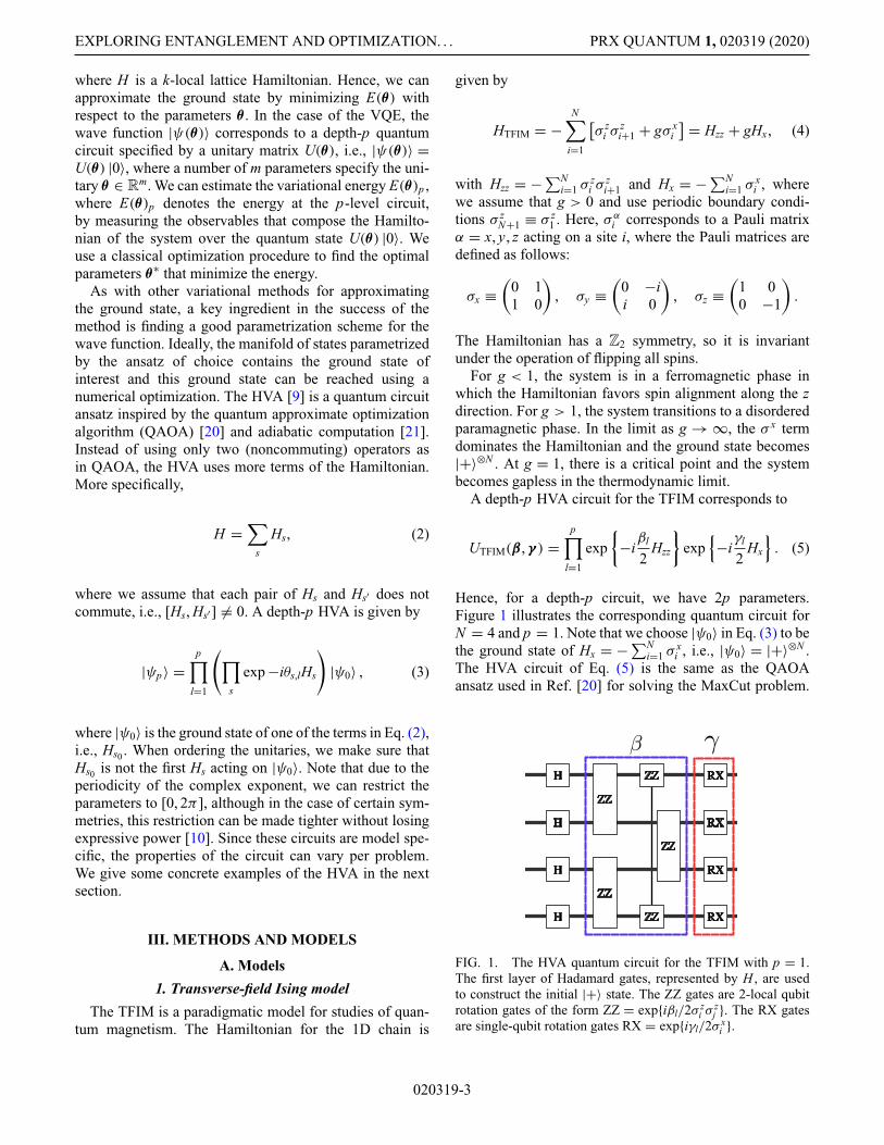
Hence, for a depth-p circuit, we have 2p parameters.Figure 1 illustrates the corresponding quantum circuit forN = 4 and p = 1. Note that we choose |ψ0〉 in Eq. (3) to bethe ground state of Hx = −∑N

i=1 σxi , i.e., |ψ0〉 = |+〉⊗N .

The HVA circuit of Eq. (5) is the same as the QAOAansatz used in Ref. [20] for solving the MaxCut problem.

FIG. 1. The HVA quantum circuit for the TFIM with p = 1.The first layer of Hadamard gates, represented by H , are usedto construct the initial |+〉 state. The ZZ gates are 2-local qubitrotation gates of the form ZZ = exp{iβl/2σ z

i σzj }. The RX gates

are single-qubit rotation gates RX = exp{iγl/2σ xi }.

020319-3

ROELAND WIERSEMA et al. PRX QUANTUM 1, 020319 (2020)

By using the Jordan-Wigner transformation, it has beenshown that the ground state can be represented accuratelywith a depth p = N/2 circuit for the case in which g = 0[22]. For the case in which g �= 0, there is only numeri-cal evidence to support this claim [10,23]. In Appendix B,we confirm that for the TFIM, one can consistently findthe ground state for g ∈ {0.5, 0.52, . . . , 1.5} with a depthp = N/2 circuit.

2. XXZ model

Another prototypical model for studying quantum mag-netism is the XXZ model. For the 1D XXZ model, theHamiltonian is given by

HXXZ =N∑

i=1

[σ x

i σxi+1 + σ

yi σ

yi+1 +σ z

i σzi+1

]

= Hxx + Hyy +Hzz, (6)

with Hxx = ∑Ni=1 σ

xi σ

xi+1, Hyy = ∑N

i=1 σyi σ

yi+1 and Hzz =∑N

i=1 σzi σ

zi+1. Again, we assume periodic boundary condi-

tions. The parameter controls the spin anisotropy in themodel. For = 1, this model has an SU(2) symmetry andis equivalent to the Heisenberg chain. For �= 1, this sym-metry gets reduced to a U(1)× Z2 symmetry. For 1 < ||,the system is in the XY quasi-long-range ordered state andbecomes gapless in the thermodynamic limit. At || = 1,there is a phase transition to the Néel ordered state. Thismodel can be solved exactly using the Bethe ansatz forN → ∞ [24].

Inspired by Ref. [10], we decompose the 1D chain intoeven and odd links and separate the Hamiltonian into twoparts,

H even = H evenxx + H even

yy + H evenzz ,

H odd = H oddxx + H odd

yy + H oddzz ,

where the indices only run over nonoverlapping bonds:

H evenαα =

N/2∑

i=1

σα2i−1σα2i and H odd

αα =N/2∑

i=1

σα2iσα2i+1

for α = x, y, z. Our numerical experiments indicate thatseparately parametrizing these bonds gives better per-formance when studying the anisotropic system �= 1.Additionally, we parametrize the Hxx, Hyy and Hzz termswith their own respective parameters. The reason for thisis that for �= 1, the anisotropy in the model cannotbe accounted for by a single parameter. A depth-p HVA

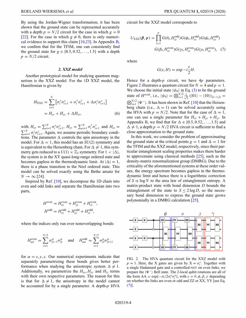
circuit for the XXZ model corresponds to

UXXZ(β, γ ) =p∏

l=1

G(θl, H oddzz )G(φl, H odd

xx )G(φl, H oddyy )

G(βl, H evenzz )G(γl, H even

xx )G(γl, H evenyy ), (7)

where

G(x, H) = exp −ix2

H .

Hence for a depth-p circuit, we have 4p parameters.Figure 2 illustrates a quantum circuit for N = 4 and p = 1.We choose the initial state |ψ0〉 in Eq. (3) to be the groundstate of H even, i.e., |ψ0〉 = ⊗N/2

i=11√2(|01〉 − |10〉)2i−1,2i =

⊗N/2i=1 |�−〉. It has been shown in Ref. [10] that the Heisen-

berg chain (i.e., = 1) can be solved accurately usingthe HVA with p = N/2. Note that for the case of = 1,one can use a single parameter for Hxx + Hyy + Hzz. InAppendix B, we find that for ∈ {0.5, 0.52, . . . , 1.5} and �= 1, a depth p = N/2 HVA circuit is sufficient to find aclose approximation to the ground state.

In this work, we consider the problem of approximatingthe ground state at the critical points g = 1 and = 1 forthe TFIM and the XXZ model, respectively, since their par-ticular entanglement scaling properties makes them harderto approximate using classical methods [25], such as thedensity-matrix renormalization group (DMRG). Due to thecriticality of the aforementioned systems at these order val-ues, the energy spectrum becomes gapless in the thermo-dynamic limit and hence there is a logarithmic correctionof S ∝ log N to the area law of entanglement entropy. Amatrix-product state with bond dimension D bounds theentanglement of the state to S ≤ 2 log D, so the neces-sary bond dimension to express the ground state growspolynomially in a DMRG calculation [25].

FIG. 2. The HVA quantum circuit for the XXZ model withp = 1. Here, the X gates are given by X = σ x

i . Together witha single Hadamard gate and a controlled-NOT on even links, weprepare the |�−〉 Bell state. The 2-local qubit rotations are all ofthe form AA = exp{−ix/2σ a

i σaj }, with x = θ ,φ,β, γ depending

on whether the links are even or odd and ZZ or XX, YY [see Eq.(7)].

020319-4

EXPLORING ENTANGLEMENT AND OPTIMIZATION. . . PRX QUANTUM 1, 020319 (2020)

3. Performance metrics

We use the fidelity F between the VQE optimized state|ψ(θ∗)〉 and the true ground state |ψground〉 obtained fromexact diagonalization:

F = |〈ψ(θ∗)|ψground〉|.

Note that for the models studied in this work, |ψground〉is always nondegenerate. If the fidelity is > 99.9%, weassume that we have successfully found the ground state.When assessing the quality of an optimized HVA circuit,the fidelity is a strong indicator of the success for solvingthe ground-state problem, since the infidelity upper boundsthe difference between the ground state and variationalexpectation value of any observable. Letting 1 − F < ε,

|〈O〉ground − 〈O〉θ | ≤ 2c√ε(1 − ε)+ ε,

where c is the operator norm of O [26].

B. Entanglement

In the context of quantum many-body physics, quantumcorrelations play a central role in our current understand-ing of the equilibrium and out-of-equilibrium propertiesof several systems in condensed matter. The source ofthese correlations is inherently nonlocal and can be tracedback to the presence of entanglement in the quantumstate. In this section, we introduce several commonly usedentanglement quantities in quantum many-body physics.

In classical systems, one uses entropy to quantify thelack of knowledge of the state of the system due to ther-mal fluctuations. However, for a quantum system at zerotemperature, the entropy of a subsystem has a differentorigin: entanglement. To quantify it, we use the bipartiteentanglement entropy [12], which is defined as the vonNeumann entropy of the reduced density matrix ρA. Toobtain this reduced density matrix, we divide the systeminto two subsystems A and B and trace out subsystem B,

ρA(|ψ〉) = TrB(|ψ〉 〈ψ |), (8)

where |ψ〉 is a pure state. For example, for an eight-spinmodel on a ring, a typical bipartition is given in Fig. 3.

FIG. 3. The division of the full system into two subsystems A(blue) and B (red) on a 1D chain.

The von Neumann entropy generalizes the concept ofShannon entropy to quantum states and is given by

S(ρA) � −(ρA log ρA). (9)

Since a bipartite quantum state can always be rewrittenusing the Schmidt decomposition,

|ψ〉 =K∑

k=0

e−(1/2)ξk |ψkA〉 ⊗ |ψk

B〉 , (10)

with 〈ψkA|ψm

A 〉 = 〈ψkB|ψm

B 〉 = δkm and where K is the size ofthe smallest subsystem, the von Neumann entropy reducesto [27]

S(ρA) =K∑

k=0

ξk exp −ξk. (11)

In recent years, the importance of entanglement incondensed-matter physics has been elucidated in severalsystems through the study of the scaling behavior of theentanglement entropy, which has enabled the identifica-tion and characterization of exotic phases of matter such astopological quantum states [28] and quantum spin liquids[29,30].

Full characterization of the entanglement properties ofa system cannot be done by looking solely at the entan-glement entropy [27,31,32]. The so-called entanglementspectrum has a much richer structure and has been usedto study many-body localization [31], observable thermal-ization [33], irreversibility in quantum circuits [32], andpreparation of ground states of nonintegrable quantummodels [34]. In addition, the entanglement spectrum hasbeen used to study the properties of variational methodssuch as the restricted Boltzmann machine [18]. The entan-glement spectrum is defined as the eigenvalue spectrum ofthe entanglement Hamiltonian

Hent � − log ρA. (12)

From Eq. (10), it follows directly that this Hamiltonianhas eigenvalues ξk. For random quantum states distributedaccording to the Haar measure, the entanglement spectrumfollows the Marchenko-Pastur distribution [35,36]. Thisdistribution describes the asymptotic average density ofeigenvalues of Wishart matrices, i.e., matrices of the formXX ∗, where the X are m × n random matrices.

Finally, the Page entropy [37] describes the averageentanglement entropy over randomly drawn pure states in

020319-5

ROELAND WIERSEMA et al. PRX QUANTUM 1, 020319 (2020)

the entire Hilbert space, and is given by

SPage = −dA − 12dB

+dAdB∑

k=dB+1

1k

≈ log(dA)− dA

2dB, (13)

where dA and dB are the dimensions of subsystems A andB, respectively.

IV. MAIN RESULTS

A. The ansatz space through the lens of entanglementspectrum

The effectiveness of a VQE optimization is determinedby two factors. First, one requires an expressive enoughansatz space that contains the ground state. The ansatzspace of a specific model H and depth p refers to the set ofall possible quantum states that can be reached by applyinga depth-p HVA circuit corresponding to H to a fixed initialstate |ψ0〉, which depends on the model. Second, the non-convex cost landscape induced by the variational energy ofEq. (1) must be favorable, in the sense that the optimiza-tion does not get stuck in local minima and can reliablyreach the ground state.

Here, we investigate the properties of the ansatz spaceby examining the entanglement spectra of HVA quantumstates generated with random parameters sampled uni-formly in the range [0,π ] for the TFIM and [0, 2π ] forthe XXZ model. For each model, we sample 5000 sets ofparameters and calculate the entanglement spectrum of theresulting state. If the spectrum of the sampled states fol-lows a distribution close to the Marchenko-Pastur (MP)distribution, a random HVA state has an entanglementspectrum that resembles that of a Haar random state. Onthe contrary, a distribution far away from the MP distri-bution indicates a restricted manifold of states that has anonrandom structure. We hypothesize that the shape of theaverage entanglement spectrum can give an insight intothe performance of the VQE optimization by revealing thestructure of the ansatz space.

Figure 4 shows the average entanglement spectrum fora state in the ansatz space of circuits with depths rang-ing from 1, 2, . . . , N for the N = 16 qubit TFIM and theXXZ model. From the insets, we see that both Ansätzehave enough entangling power to express the ground state,even for low-depth circuits. For the TFIM with 16 qubits[Fig. 4(a)], we see that for all p , the HVA spectrum is fur-ther away from the MP distribution and the HVA spacecorresponding to the TFIM appears to be a manifold ofstates with a restricted entanglement structure. In contrast,for the XXZ model, we see that the average spectra getscloser to the MP distribution as p increases. This suggeststhat the HVA space for the XXZ model is not as restrictedas for the TFIM. This can be understood directly by look-ing at the circuit complexity, which for the XXZ model

(a)

(b)

FIG. 4. The average entanglement spectrum of HVA quantumstates from layer p = 1 (bottom line in purple) to p = N (top linein yellow) over 5000 random parameter initializations: (a) TFIM;(b) XXZ model. ξk denotes the kth eigenvalue of Hent. The eigen-values are arranged in descending order and cut off at ξk = −30.The black lines in the insets show how close the average entan-glement entropy is to the Page entropy (purple dashed line) as afunction of the increasing circuit depth. The lower blue dashedline in the inset indicates the entanglement entropy of the groundstate. We see that the average HVA state is more entangled thanthe ground states of interest.

contains more gates and parameters per layer. However,this is necessary because the XXZ model is inherently amuch richer model in terms of physics and it may be nec-essary for the HVA space to accommodate a greater varietyof states.

We now turn to examining the entanglement featuresof the XXZ-model HVA states explored during optimiza-tion. For the variational minimization of Eq. (1), we use agradient-descent algorithm (for details, see Appendix A).Since the cost function is nonconvex, the quality of the

020319-6

EXPLORING ENTANGLEMENT AND OPTIMIZATION. . . PRX QUANTUM 1, 020319 (2020)

solution will vary significantly between different start-ing points in parameter space. We compare the followinginitialization strategies:

1. A completely random-state initialization, where allparameters are sampled as θ ∼ U(0, 2π).

2. An identity initialization. We set all parametersequal to π , so that our circuit is equal to the identitycircuit and a global phase i.

Our approach of starting close to the identity is similarto the block-identity initialization strategy discussed inRef. [38]; however, we study a simpler version by settingall parameters equal to π . For both parameter initializa-tions, we extract the final layer state from the circuit atmultiple times during the optimization and calculate itsentanglement spectrum using Eq. (12). Not surprisingly,our experiments indicate that a random start is prone togetting stuck in a local minimum, due to our local opti-mization strategies combined with a nonconvex energylandscape. The identity start, on the other hand, allows usto consistently find a high-fidelity state for both systemswith a depth p = N/2 circuit (see Appendix B).

To study this finding in more detail, we investigatethe dynamics of the entanglement spectrum for differ-ent initialization strategies. In Fig. 5(a), we see that anidentity-state initialization stays far away from the MPdistribution at all times, indicating that we are accessinga highly structured restricted subspace of the full HVAspace. Additionally, this initialization reaches a state witha > 99.9% fidelity state. On the contrary, the random-stateinitialization in Fig. 5(b) starts close to the MP distribu-tion and then moves to a more structured local minimumwith 70% fidelity. We conclude that even though the shapeof the entanglement spectrum from Fig. 4(b) indicates apossible large unstructured ansatz space, a local optimiza-tion is still capable of finding the ground state if we choosea suitable parameter initialization. We further investigatethe qualitative properties of the optimization dynamics inAppendix C. In the next section, we will see that the disad-vantage of starting at a bad initial point can be overcomeby making the circuit sufficiently deep, a process known asoverparametrization.

B. Overparametrization in the HVA

Overparametrization is a phenomenon in certain typesof nonconvex optimization problems. For an over-parametrized model, the optimization landscape becomesdramatically better (e.g., almost trap free or almost con-vex) as the number of parameters reaches some threshold.In most cases, the rate of convergence also becomes bet-ter, sometimes even exponentially faster after passing thisthreshold.

Overparametrization has been studied extensively inthe classical deep-neural-network literature [39–42]. For

(a)

(b)

FIG. 5. The change of the entanglement spectrum of the finallayer during the optimization. Both figures are for a 16-qubitXXZ model with a depth p = N/2 circuit and the times arepercentages of the total optimization time: (a) corresponds to aconverged state of fidelity, whereas (b) corresponds to an approx-imately 70% fidelity state. (a) The identity-state initializationremains far away from the MP distribution at all times duringthe optimization and convergence to state with > 99.9% withthe ground state. Since this initialization strategy starts with theidentity circuit, we find the t = 0% state to be a product state,as indicated by the single eigenvalue. (b) The random initializa-tion starts close to the MP distribution and converges to a localminimum with approximately 70% fidelity.

example, in Ref. [40], it has been shown that under certainmild assumptions, the optimization landscape of a deepneural network is almost convex in a large neighborhoodof a random starting point. As a consequence, the stochas-tic gradient-descent algorithm can almost always find anaccurate solution.

Although for VQE algorithms it is clear that we havemin E(θ)p+1 ≤ min E(θ)p , it is not clear if this minimumcan be found consistently due to the nonconvexity of theenergy landscape. Hence, a deeper understanding of theenergy landscape with increasing depth is required. Thereis some work on overparametrization in the context ofcontrollable quantum systems with unconstrained time-varying controls [43–45], where the authors show thatthere are no suboptimal local minima in the optimiza-tion landscape. For the case of a constrained controllablequantum system, a recent work [46] considers the prob-lem of learning d-dimensional Haar random unitaries U(d)

020319-7

ROELAND WIERSEMA et al. PRX QUANTUM 1, 020319 (2020)

by gradient descent using a general alternating-operatoransatz of the form e−iγp Ae−iβp B · · · e−iγ1Ae−iβ1B, where Aand B are matrices sampled from the Gaussian unitaryensemble [47]. The authors show that gradient descentalways converges to an accurate solution when the num-ber of parameters is d2 or greater and that a “compu-tational phase transition” is observed between an under-parametrization (< d2) and an overparametrization (> d2)regime.

Since the HVA also has the form of an alternating-operator ansatz and the problem of finding the groundstates can also be seen as a constrained quantum controlproblem, we expect a similar overparametrization phe-nomenon in our setting. To investigate this, we randomlysample 100 initial parameters θ (uniformly drawn fromthe interval [0,π ] for the TFIM and [0, 2π ] for the XXZmodel) and perform the optimization for increasing valuesof p . Here, we set the stopping criterion for the optimiza-tion to εres = E(θ)p − Eground < 1e − 4 and the maximumnumber of iterations to 3000. Indeed, Fig. 6 shows that theoverparametrization phenomenon also occurs in the HVA

(a)

(b)

Iterations

Iterations

FIG. 6. Overparametrization in the HVA: (a) TFIM; (b) XXZmodel. Each line corresponds to the VQE optimization at depthp that takes the most iterations to converge out of 100 randominitializations. Both figures are for N = 12 qubits. The rapidoscillations in (b) are artifacts of the ADAM optimizer and areless severe as the circuit depth increases. Due to our stoppingcriterion, we know that if the number of iterations is smaller than3000, then εres ≤ 1e − 4 and so the model does converge to agood ground-state approximation.

for the 12-qubit TFIM and the XXZ model. We find thatfor both the TFIM and the XXZ model, gradient descentfrom all 100 random starting points converges to an accu-rate solution once the depth p reaches a certain thresholdp(N ).

Moreover, we also observe a “computational phase tran-sition” around this threshold where the convergence speedbecomes exponentially fast, i.e., the decrease of the residueenergy as a function of the number of iterations. However,this threshold p(N ) is not tight, i.e., for depth p < p(N ),it is possible that the gradient descent still converges toa high-fidelity state. This indicates that in the setting offinding ground states using the HVA, the problem is morestructured and gradient descent is effective. In Fig. 7, wesee that for all system sizes, the mean number of iter-ations eventually converges to about 100 iterations. Inaddition, we can find the overparametrization thresholdsp(N ) in Table I for the TFIM and the XXZ model withdifferent system sizes. Our data suggest that p(N ) has atmost a polynomial scaling, which is compatible with the

(a)

(b)

Itera

tions

Itera

tions

FIG. 7. The mean iteration time to convergence as a functionof depth: (a) TFIM; (b) XXZ model. The error bars indicatethe standard deviation over 100 different initializations. For bothmodels, there is a clear cutoff where the number of iterations sat-urates. Note that if the number of iterations is smaller than 3000,then we know that εres ≤ 1e − 4, indicating that the optimiza-tion has converged to a good ground-state approximation. Wesee that the error bars decrease systematically with depth. Forboth models, there is a critical p after which all random initializa-tions converge to a good ground-state approximation. Moreover,for depth p = 34 and p = 52 for the TFIM and the XXZ model,respectively, the number of iterations to find the ground state isof the order of 100 iterations for every starting point.

020319-8

EXPLORING ENTANGLEMENT AND OPTIMIZATION. . . PRX QUANTUM 1, 020319 (2020)

TABLE I. The overparametrization threshold p(N ) for theTFIM and the XXZ model with different system sizes N . By“threshold,” we mean that when p ≥ p(N ), all the randominitializations converge to an accurate solution.

TFIM XXZ modelN p(N ) p(N )

4 6 46 6 48 8 810 10 1212 14 36

analogous parameter count required to express critical 1Dground states with an MPS. A more detailed view of thesedata can be found in Fig. 11 in the Appendix, which showsthat all random initializations converge to the ground stateafter a certain threshold p(N ).

This is a striking difference compared with Ref. [46],where the number of parameters to achieve over-parametrization is (2N )2. From Fig. 7, we can also see thatthe iteration time decreases substantially as p increases,saturating to around 100 iterations after a certain p forall N .

The overparametrization phenomenon in the HVAshows a clear difference between the HVA and parametrizedrandom quantum circuits (RQC), because there is no indi-cation or evidence that the landscape of RQC gets betteras one increases the depth. On the contrary, in our exper-iments with random circuits of comparable depths to ourHVA circuits, we are unable to observe the same over-parametrization phenomenon. This can be explained fromthe barren-plateau point of view and the lack of structurein the ansatz space.

C. Ameliorated barren plateaus in the HVA

In Ref. [5], a barren-plateau phenomenon has beenobserved for the VQE on random quantum circuits, whereall gradients are exponentially close to zero with over-whelmingly high probability, making local optimizationwithin the ansatz space extremely challenging. The barren-plateau phenomenon is due to the fact that RQCs consist-ing of single- and two-qubit gates form a 2-design, whichmeans that the gradients of the energy objective functionwill obey the same concentration of measure properties asif the circuits are Haar random unitaries.

In contrast to the RQC ansatz, we show that the opti-mization landscape of the HVA is much more favorable.This is clearly illustrated when optimizing the HVA cor-responding to the TFIM: to begin with, as discussedin Sec. IV A, the manifold of states has a much morerestricted entanglement structure than a typical Haar ran-dom state—this already indicates that the HVA circuits donot form 2-designs and thus do not obey the same kind of

concentration-of-measure phenomenon as RQCs. On theother hand, the entanglement spectrum of the ansatz spacecorresponding to the XXZ model does not immediatelyrule out the same barren-plateau behavior as exhibited byRQCs.

Nonetheless, we determine that the barren-plateau prob-lem is significantly ameliorated in the TFIM and mild inthe XXZ model. In Fig. 8, we calculate the variance ofgradients as a function of the number of qubits N andthe depth p over 20 random points per N and per p .For the TFIM, the flatness of the variance curve indi-cates no barren-plateau problem. However, for the XXZmodel, we see an exponential decay, but this decay is notas strong as in RQCs [5]. The scaling of the mean-gradientmagnitudes follows a similar pattern. Nonetheless, wecan reliably find an accurate solution when choosing anidentity start (see Appendix B), where the barren-plateauproblem is absent. Indeed, sampling gradients close to theidentity initialization gives a constant gradient variance forall N . This indicates that the vanishing-gradient problemcan be circumvented by choosing a suitable initializationstrategy.

(a)

(b)

FIG. 8. The variance of the gradients of a single Z1Z2 termwith respect to θ0 as a function of the number of qubits at ini-tialization. The number of samples used per N for each p is 20.(a) For the TFIM, the gradient-variance decay is almost constantfor all N . (b) The XXZ-model gradient variance is still exponen-tial, although the effect is not as pronounced as for the RQCs ofRef. [5], where the N = 16 variance is 2 orders of magnitudesmaller.

020319-9

ROELAND WIERSEMA et al. PRX QUANTUM 1, 020319 (2020)

D. The entangling power of HVA circuits

For a 1D gapped quantum system, the entanglemententropy of the ground state obeys an area law [48–50],i.e., the entanglement entropy grows proportionally to theboundary area ∂I of the subsystem ρA:

S(ρA) = O(|∂I |).

In 1D, the boundary area ∂I is either 1 (for an open chain)or 2 (for a closed chain) and the area law simply saysthat the entanglement entropy should be constant as Nincreases. For a 1D conformally invariant gapless (criti-cal) system, the entanglement entropy of the ground statehas a logarithmic scaling instead [51], i.e.,

S(ρA) = O(log(n)).

The entangling power is an important factor for charac-terizing the expressiveness and efficiency of many varia-tional Ansätze in condensed-matter physics. It character-izes how much entanglement (measured by the entangle-ment entropy) can be generated by the variational circuit.For example, in the matrix-product state representation,the entangling power is limited by the so-called bonddimension D, which affects the expressive power and com-putational cost of the ansatz. For a 1D gapped systemwith energy gap ε, the ground state can be approximatedwell by an MPS with sublinear bond dimension D =exp[O(log3/4 n/ε1/4)] [52]. In the case of the HVA, theamount of entanglement generated by the circuit dependson the depth p of the circuit. Indeed, we observe numeri-cally in Fig. 4 that the HVA circuits for the TFIM and the

FIG. 9. The infidelities found after optimization for the MHSHamiltonian. The circuit is initialized with an identity start. Forthe four-qubit case, we get close to machine precision and hencethe fidelities are unstable.

XXZ model have enough entangling power to express theground states.

As a demonstration that the full entangling power of theHVA can be utilized effectively, we solve for the groundstate of the so-called modified Haldane-Shastry (MHS)Hamiltonian. This model has long-range interactions andis expected to have power-law entanglement scaling in theground state [53,54]. The MHS Hamiltonian is given by

HMHS =N∑

j<k

1d2

jk(−σ j

x σkx − σ j

y σky + σ j

z σkz ),

where djk = Nπ|sin(π(j − k)/N )|. Due to the form of the

Hamiltonian, we can use the same HVA, given in Eq. (7),as for the XXZ model. In Fig. 9, we see that it is possible tofind the ground state with > 99.7% fidelity using a depthp = N circuit for N = 4, N = 8, N = 12, and N = 16.

V. CONCLUSION

In this work, we shed light on some of the desir-able properties of the HVA as a critical ingredient in thevariational quantum eigensolver algorithm. In particular,we show evidence that there are only mild or entirelyabsent barren plateaus in the HVA. This is strikingly dif-ferent from the commonly used random quantum circuits.Moreover, we also observe an overparametrization phe-nomenon in the HVA. Similar to what has been observedin deep neural networks, the optimization landscape ofthe HVA becomes increasingly better as the ansatz isoverparametrized and eventually becomes trap free as theoverparametrization reaches a certain threshold. In con-trast to the case of learning Haar random unitaries, weobserve that such threshold in the HVA scales at mostpolynomially with the system size. Finally, we providenumerical evidence that the HVA can be used to find theground state of the MHS Hamiltonian, which has a power-law scaling entanglement. We believe that our findingspoint to important features of the HVA that will lead toa deeper understanding of its effectiveness and that pointthe way to the development of more sophisticated Ansätzefor other many-body problems, as well as better-informedoptimization and/or initialization strategies.

As for future work, since most 1D quantum many-body systems can be simulated efficiently using classicalmethods, the crucible for the HVA will be 2D systems.If low-depth circuits are capable of reproducing nontriv-ial 2D quantum states, then one can start thinking aboutwhen a quantum advantage can be reached for systemswhere classical methods are computationally expensive oreven ineffective. The effectiveness of the identity initial-ization, both in terms of the absence of vanishing gradientsand the reliability of finding a good ground-state approx-imation, is striking. Scrutinizing the mechanism for why

020319-10

EXPLORING ENTANGLEMENT AND OPTIMIZATION. . . PRX QUANTUM 1, 020319 (2020)

this is the case will require a deeper understanding of theenergy landscape of the HVA. Our preliminary results forthe XXZ model and the TFIM on rectangular lattices showthat this initialization strategy remains effective even for2D systems.

Lastly, the overparametrized regime is a double-edgedsword. On the one hand, it implies that we can improvethe energy landscape by increasing the depth of the circuit,ameliorating the effects of local minima. On the other hand,the growth in circuit depth may well nullify this increasein performance due to the longer coherence times requiredand multiplicative gate errors. In order to assess how use-ful this regime is for hardware implementations, we wouldrequire an understanding of the effect that noise has on theoptimization in the overparametrized regime. The recentwork of Wang et al.[55] indicates that for a class ofVQE Ansätze, including the quantum alternating-operatoransatz, there could be severe noise-induced barren plateauswhen the number of layers scales polynomially. However,for the practical performance of the general HVA, a morecareful analysis of the trade-off between the benefits ofoverparametrization and the detrimental effects of noise-induced barren plateaus is needed. Moreover, research onthe design of more effective variational quantum circuitsbased on the HVA should also be pursued.

ACKNOWLEDGMENTS

H.Y. is supported by the Natural Sciences and Engineer-ing Research Council (NSERC) Discovery Grant 2019-06636 and a Google Quantum Research Award. Y.B.K.is supported by the NSERC of Canada and the KillamResearch Fellowship from the Canada Council of theArts. J.C. acknowledges support from NSERC, the SharedHierarchical Academic Research Computing Network

(SHARCNET), Compute Canada, a Google QuantumResearch Award, and the CIFAR AI chair program. Theresources used in preparing this research were provided, inpart, by the Province of Ontario, Government of Canadathrough the Canadian Institute for Advanced Research(CIFAR) and by companies sponsoring the Vector Insti-tute www.vectorinstitute.ai/#partners. C.Z. acknowledgespartial support from the Postgraduate Affiliate Award fromthe Vector Institute.

APPENDIX A: COMPUTATIONAL DETAILS

For the implementation of our quantum circuits, weuse ZYGLROX [56], a powerful TensorFlow-based quan-tum simulator. For the classical optimization process, weuse ADAM (adaptive moment estimation) [57], a gradient-descent-based optimizer, which is widely used in themachine-learning community. Compared to vanilla gra-dient descent and its other variants, ADAM updates thelearning rates adaptively on a per-parameter basis by usingestimates of the first and second moments of the gradients.In our own investigation for solving the ground-energyproblem with the HVA, ADAM outperforms all the otheroptimizers available in TensorFlow, with respect to fidelityand convergence times.

Unless stated otherwise, the stopping criterion for ouroptimization is defined as |E(θ t)− E(θ t+1)| < 1 × 10−13,where t is the iteration number. The maximum number ofiterations is set to 15 000. We use an initial learning rateof r = 0.01 for ADAM, which gives reasonably consistentresults across all the models. Through our own investiga-tion into initial ADAM learning rates, we find a learningrate of 1 × 10−3 ≤ r ≤ 4 × 10−2 to be a good choice forthe optimization for both the TFIM and the XXZ model,

(a) (b)

FIG. 10. The infidelities as a function of the order values g and for (a) the TFIM and (b) the XXZ model, respectively. For theseresults, we use the identity initialization combined with a depth p = N/2 circuit. The dashed black line indicates the cutoff for 99.9%fidelity. (a) For the TFIM, we can obtain machine-precision results, except in the region g > 1.24 for N = 16. In this region, theoptimization has not fully converged but is stopped after 15 000 iterations. We note that for increasing N , the time until convergenceis polynomial in N (not shown here), similar to what has been observed in Ref. [23]. Additionally, we observe a worsening of thisscaling with increased g. (b) For the XXZ model, we are unable to consistently reach machine-precision fidelities. In addition, thefidelities that we find become worse as N increases. However, except for a couple of outliers, we are able to obtain > 99.9% fidelitiesfor N ≤ 16 or all order values.

020319-11

ROELAND WIERSEMA et al. PRX QUANTUM 1, 020319 (2020)

(a) (b)Ra

tio c

onve

rged

Ratio

con

verg

ed

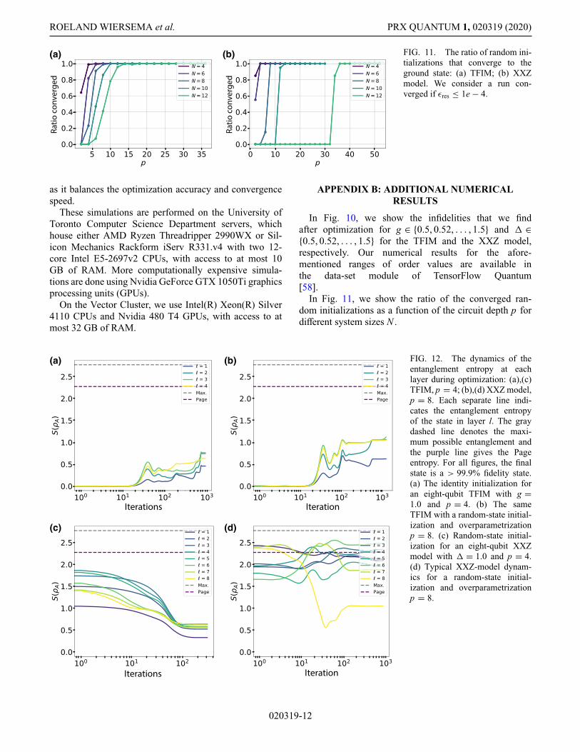
FIG. 11. The ratio of random ini-tializations that converge to theground state: (a) TFIM; (b) XXZmodel. We consider a run con-verged if εres ≤ 1e − 4.

as it balances the optimization accuracy and convergencespeed.

These simulations are performed on the University ofToronto Computer Science Department servers, whichhouse either AMD Ryzen Threadripper 2990WX or Sil-icon Mechanics Rackform iServ R331.v4 with two 12-core Intel E5-2697v2 CPUs, with access to at most 10GB of RAM. More computationally expensive simula-tions are done using Nvidia GeForce GTX 1050Ti graphicsprocessing units (GPUs).

On the Vector Cluster, we use Intel(R) Xeon(R) Silver4110 CPUs and Nvidia 480 T4 GPUs, with access to atmost 32 GB of RAM.

APPENDIX B: ADDITIONAL NUMERICALRESULTS

In Fig. 10, we show the infidelities that we findafter optimization for g ∈ {0.5, 0.52, . . . , 1.5} and ∈{0.5, 0.52, . . . , 1.5} for the TFIM and the XXZ model,respectively. Our numerical results for the afore-mentioned ranges of order values are available inthe data-set module of TensorFlow Quantum[58].

In Fig. 11, we show the ratio of the converged ran-dom initializations as a function of the circuit depth p fordifferent system sizes N .

(a) (b)

(c) (d)

Iterations Iteration

IterationIterations

FIG. 12. The dynamics of theentanglement entropy at eachlayer during optimization: (a),(c)TFIM, p = 4; (b),(d) XXZ model,p = 8. Each separate line indi-cates the entanglement entropyof the state in layer l. The graydashed line denotes the maxi-mum possible entanglement andthe purple line gives the Pageentropy. For all figures, the finalstate is a > 99.9% fidelity state.(a) The identity initialization foran eight-qubit TFIM with g =1.0 and p = 4. (b) The sameTFIM with a random-state initial-ization and overparametrizationp = 8. (c) Random-state initial-ization for an eight-qubit XXZmodel with = 1.0 and p = 4.(d) Typical XXZ-model dynam-ics for a random-state initial-ization and overparametrizationp = 8.

020319-12

EXPLORING ENTANGLEMENT AND OPTIMIZATION. . . PRX QUANTUM 1, 020319 (2020)

(a) (b) (c)

FIG. 13. The scaling of the entanglement entropy of the converged state after p/2 and p layers: (a) TFIM, g = 1.0; (b) TFIM,g = 0.5; (c) XXZ model, = 1.0. (a) For the TFIM at the critical point, the ground-state entanglement entropy has a logarithmiccorrection with increasing N . The entanglement halfway through the circuit is larger than in the final layer. (b) For a noncriticalpoint, the ground-state entanglement entropy is constant but the entanglement entropy halfway through the circuit scales linearly withsystem size. (c) For the XXZ model, in addition to the logarithmic scaling of the entanglement entropy, the final layer entanglement isconsistently higher than in the p/2 depth layer.

APPENDIX C: DYNAMICS OF ENTANGLEMENTENTROPY DURING OPTIMIZATION

To further elucidate the difference in initialization strate-gies, we qualitatively study the dynamics of the entangle-ment entropy during optimization. In Fig. 12, we calculatethe entanglement entropy of ρA at each layer of the cir-cuit during the optimization. Although not much can besaid about the intermediate states for the random-stateinitialization, except that they are highly entangled, theentanglement entropy dynamics for the identity initial-ization have a distinct structure that is consistent as weincrease the system size. In Fig. 13, we compare the scalingof the entanglement entropy for the identity start halfwaythrough the circuit for different system sizes.

[1] J. Preskill, Quantum computing in the NISQ era andbeyond, Quantum 2, 79 (2018).

[2] A. Kandala, A. Mezzacapo, K. Temme, M. Takita, M.Brink, J. M. Chow, and J. M. Gambetta, Hardware-efficientvariational quantum eigensolver for small molecules andquantum magnets, Nature 549, 242 (2017).

[3] S. Sim, P. D. Johnson, and A. Aspuru-Guzik, Express-ibility and entangling capability of parameterized quan-tum circuits for hybrid quantum-classical algorithms, Adv.Quantum Technol. 2, 1900070 (2019).

[4] C. Bravo-Prieto, J. Lumbreras-Zarapico, L. Tagliacozzo,and J. I. Latorre, Scaling of variational quantum circuitdepth for condensed matter systems, Quantum 4, 272(2020).

[5] J. R. McClean, S. Boixo, V. N. Smelyanskiy, R. Babbush,and H. Neven, Barren plateaus in quantum neural networktraining landscapes, Nat. Commun. 9, 4812 (2018).

[6] K. Sharma, M. Cerezo, L. Cincio, and P. J. Coles, Train-ability of dissipative perceptron-based quantum neural net-works, arXiv:2005.12458 (2020).

[7] T. Volkoff and P. J. Coles, Large gradients via correlation inrandom parameterized quantum circuits, arXiv:2005.12200(2020).

[8] M. Cerezo, A. Sone, T. Volkoff, L. Cincio, and P. J.Coles, Cost-function-dependent barren plateaus in shallowquantum neural networks, arXiv:2001.00550 (2020).

[9] D. Wecker, M. B. Hastings, and M. Troyer, Progresstowards practical quantum variational algorithms, Phys.Rev. A 92, 042303 (2015).

[10] W. W. Ho and T. H. Hsieh, Efficient variational simulationof non-trivial quantum states, SciPost Phys. 6, 29 (2019).

[11] C. Cade, L. Mineh, A. Montanaro, and S. Stanisic, Strate-gies for solving the Fermi-Hubbard model on near-termquantum computers, arXiv:1912.06007 (2019).

[12] J. Eisert, M. Cramer, and M. B. Plenio, Colloquium: Arealaws for the entanglement entropy, Rev. Mod. Phys. 82, 277(2010).

[13] J. Eisert, in Autumn School on Correlated Electrons:Emergent Phenomena in Correlated Matter, edited by E.Pavarini, E. Koch, and U. Schollwöck (ForschungszentrumJülich Zentralbibliothek, Verlag, Germany, 2013).

[14] G. Carleo and M. Troyer, Solving the quantum many-bodyproblem with artificial neural networks, Science 355, 602(2017).

[15] O. Sharir, Y. Levine, N. Wies, G. Carleo, and A. Shashua,Deep Autoregressive Models for the Efficient VariationalSimulation of Many-Body Quantum Systems, Phys. Rev.Lett. 124, 020503 (2020).

[16] J. Carrasquilla, G. Torlai, R. G. Melko, and L. Aolita,Reconstructing quantum states with generative models,Nat. Mach. Intell. 1, 155 (2019).

[17] M. Hibat-Allah, M. Ganahl, L. E. Hayward, R. G. Melko,and J. Carrasquilla, Recurrent neural network wavefunc-tions, Phys. Rev. Res. 2, 023358 (2020).

[18] D.-L. Deng, X. Li, and S. D. Sarma, Quantum Entangle-ment in Neural Network States, Phys. Rev. X 7, 021021(2017).

[19] A. Peruzzo, J. McClean, P. Shadbolt, M.-H. Yung, X.-Q.Zhou, P. J. Love, A. Aspuru-Guzik, and J. L. O’Brien,

020319-13

ROELAND WIERSEMA et al. PRX QUANTUM 1, 020319 (2020)

A variational eigenvalue solver on a photonic quantumprocessor, Nat. Commun. 5, 4213 (2014).

[20] E. Farhi, J. Goldstone, and S. Gutmann, A quantum approx-imate optimization algorithm, arXiv:1411.4028 (2014).

[21] E. Farhi, J. Goldstone, S. Gutmann, and MichaelSipser, Quantum computation by adiabatic evolution,arXiv:quant-ph/0001106 (2000).

[22] G. Bigan Mbeng, R. Fazio, and G. Santoro, Quantumannealing: A journey through digitalization, control, andhybrid quantum variational schemes, arXiv:1906.08948(2019).

[23] D. Wierichs, C. Gogolin, and M. Kastoryano, Avoidinglocal minima in variational quantum eigensolvers withthe natural gradient optimizer, Phys. Rev. Res. 2, 043246(2020).

[24] F. Franchini, An Introduction to Integrable Techniquesfor One-Dimensional Quantum Systems (Springer Interna-tional, Cham, Switzerland, 2017).

[25] R. Orús, Tensor networks for complex quantum systems,Nat. Rev. Phys. 1, 538 (2019).

[26] M. J. S. Beach, R. G. Melko, T. Grover, and T. H. Hsieh,Making trotters sprint: A variational imaginary time ansatzfor quantum many-body systems, Phys. Rev. B 100, 094434(2019).

[27] H. Li and F. D. M. Haldane, Entanglement Spectrum asa Generalization of Entanglement Entropy: Identificationof Topological Order in Non-Abelian Fractional QuantumHall Effect States, Phys. Rev. Lett. 101, 010504 (2008).

[28] A. Kitaev and J. Preskill, Topological EntanglementEntropy, Phys. Rev. Lett. 96, 110404 (2006).

[29] S. V. Isakov, M. B. Hastings, and R. G. Melko, Topologicalentanglement entropy of a Bose-Hubbard spin liquid, Nat.Phys. 7, 772 (2011).

[30] Y. Zhang, T. Grover, and A. Vishwanath, EntanglementEntropy of Critical Spin Liquids, Phys. Rev. Lett. 107,067202 (2011).

[31] Z.-C. Yang, C. Chamon, A. Hamma, and E. R. Mucciolo,Two-Component Structure in the Entanglement Spectrumof Highly Excited States, Phys. Rev. Lett. 115, 267206(2015).

[32] D. Shaffer, C. Chamon, A. Hamma, and E. R. Mucci-olo, Irreversibility and entanglement spectrum statistics inquantum circuits, J. Stat. Mech.: Theory Exp. 2014, P12007(2014).

[33] S. D. Geraedts, R. Nandkishore, and N. Regnault, Many-body localization and thermalization: Insights from theentanglement spectrum, Phys. Rev. B 93, 174202 (2016).

[34] G. Matos, S. Johri, and Z. Papic, Quantifying the efficiencyof state preparation via quantum variational eigensolvers(2020).

[35] M. Žnidaric, Entanglement of random vectors, J. Phys. A:Math. Theor. 40, F105 (2006).

[36] V. A. Marcenko and L. A. Pastur, Distribution of eigenval-ues for some sets of random matrices, Math. USSR-Sbornik1, 457 (1967).

[37] D. N. Page, Average Entropy of a Subsystem, Phys. Rev.Lett. 71, 1291 (1993).

[38] E. Grant, L. Wossnig, M. Ostaszewski, and M. Benedetti,An initialization strategy for addressing barren plateaus inparametrized quantum circuits, Quantum 3, 214 (2019).

[39] Z. Allen-Zhu, Y. Li, and Y. Liang, Learning and generaliza-tion in overparameterized neural networks, going beyondtwo layers (2018).

[40] Z. Allen-Zhu, Y. Li, and Z. Song, A convergence theory fordeep learning via over-parameterization (2018).

[41] Z. Chen, Y. Cao, D. Zou, and Q. Gu, How much over-parameterization is sufficient to learn deep ReLU networks?(2019).

[42] Z. Chen, Y. Cao, Q. Gu, and T. Zhang, Mean-field analy-sis of two-layer neural networks: Non-asymptotic rates andgeneralization bounds (2020).

[43] H. A. Rabitz, M. M. Hsieh, and C. M. Rosenthal, Quantumoptimally controlled transition landscapes, Science 303,1998 (2004).

[44] H. Rabitz, M. Hsieh, and C. Rosenthal, Landscape foroptimal control of quantum-mechanical unitary transforma-tions, Phys. Rev. A 72, 052337 (2005).

[45] B. Russell, H. Rabitz, and R.-B. Wu, Control landscapes arealmost always trap free: A geometric assessment, J. Phys.A: Math. Theor. 50, 205302 (2017).

[46] B. T. Kiani, S. Lloyd, and R. Maity, Learning unitaries bygradient descent (2020).

[47] M. L. Mehta, Random Matrices, Pure and Applied Mathe-matics (Academic Press, 2004), 3rd ed.

[48] M. B. Hastings, An area law for one-dimensional quan-tum systems, J. Stat. Mech.: Theory Exp. 2007, P08024(2007).

[49] I. Arad, Z. Landau, and U. Vazirani, Improved one-dimensional area law for frustration-free systems, Phys.Rev. B 85, 195145 (2012).

[50] I. Arad, A. Kitaev, Z. Landau, and U. Vazirani, Anarea law and sub-exponential algorithm for 1D systems(2013).

[51] P. Calabrese and J. Cardy, Entanglement entropy and quan-tum field theory, J. Stat. Mech.: Theory Exp. 2004, P06002(2004).

[52] S. Gharibian, Y. Huang, Z. Landau, and S. W. Shin,Quantum Hamiltonian complexity, Found. Trendso Theor.Comp. Sci. 10, 159 (2015).

[53] F. D. M. Haldane, Exact Jastrow-Gutzwiller Resonating-Valence-Bond Ground State of the Spin- 1

2 Antiferromag-netic Heisenberg Chain with 1/r2 Exchange, Phys. Rev.Lett. 60, 635 (1988).

[54] B. S. Shastry, Exact Solution of an s = 1/2 HeisenbergAntiferromagnetic Chain with Long-Ranged Interactions,Phys. Rev. Lett. 60, 639 (1988).

[55] S. Wang, E. Fontana, M. Cerezo, K. Sharma, A. Sone, L.Cincio, and P. J. Coles, Noise-induced barren plateaus invariational quantum algorithms (2020).

[56] R. C. Wiersema, Zyglrox. https://github.com/therooler/zyglrox (2020).

[57] D. Kingma and J. Ba, in International Conference onLearning Representations, edited by Y. Bengio and Y.LeCun (ICLR, San Diego, CA, USA, 2015).

[58] M. Broughton, G. Verdon, T. McCourt, A. J. Martinez, J.H. Yoo, S. V. Isakov, P. Massey, M. Y. Niu, R. Halavati, E.Peters, M. Leib, A. Skolik, M. Streif, D. Von Dollen, J. R.McClean, S. Boixo, D. Bacon, A. K. Ho, H. Neven, and M.Mohseni, TensorFlow Quantum: A software framework forquantum machine learning (2020).

020319-14