PROXIMAL THRESHOLDING ALGORITHM FOR MINIMIZATION OVER …plc/siopt2.pdf · 2017-05-09 · PROXIMAL THRESHOLDING ALGORITHM FOR MINIMIZATION OVER ORTHONORMAL BASES∗ PATRICK L. COMBETTES†

SIAM J. Optim. to appear

PROXIMAL THRESHOLDING ALGORITHM FOR MINIMIZATION

OVER ORTHONORMAL BASES∗

PATRICK L. COMBETTES† AND JEAN-CHRISTOPHE PESQUET‡

Abstract. The notion of soft thresholding plays a central role in problems from various areasof applied mathematics, in which the ideal solution is known to possess a sparse decomposition insome orthonormal basis. Using convex-analytical tools, we extend this notion to that of proximalthresholding and investigate its properties, providing in particular several characterizations of suchthresholders. We then propose a versatile convex variational formulation for optimization over or-thonormal bases that covers a wide range of problems, and establish the strong convergence of aproximal thresholding algorithm to solve it. Numerical applications to signal recovery are demon-strated.

Key words. convex programming, deconvolution, denoising, forward-backward splitting al-gorithm, Hilbert space, orthonormal basis, proximal algorithm, proximal thresholding, proximityoperator, signal recovery, soft-thresholding, strong convergence

AMS subject classifications. 90C25, 65K10, 94A12

PII. XXXX

1. Problem formulation. Throughout this paper, H is a separable infinite-dimensional real Hilbert space with scalar product 〈· | ·〉, norm ‖ · ‖, and distance d.Moreover, Γ0(H) denotes the class of proper lower semicontinuous convex functionsfrom H to ]−∞,+∞], and (ek)k∈N is an orthonormal basis of H.

The standard denoising problem in signal theory consists of recovering the originalform of a signal x ∈ H from an observation z = x+ v, where v ∈ H is the realizationof a noise process. In many instances, x is known to admit a sparse representationwith respect to (ek)k∈N and an estimate x of x can be constructed by removing thecoefficients of small magnitude in the representation (〈z | ek〉)k∈N of z with respectto (ek)k∈N. A popular method consists of performing a so-called soft thresholding ofeach coefficient 〈z | ek〉 at some predetermined level ωk ∈ ]0,+∞[, namely

(1.1) x =∑

k∈N

soft[−ωk,ωk] (〈z | ek〉)ek,

where (see Fig. 2.1)

(1.2) soft[−ωk,ωk] : ξ 7→ sign(ξ)max|ξ| − ωk, 0.

This approach has received considerable attention in various areas of applied mathe-matics ranging from nonlinear approximation theory to statistics, and from harmonicanalysis to image processing; see for instance [2, 7, 9, 21, 23, 29, 33] and the references

∗Received by the editors XXX XX, 2006; accepted for publication XXX XX, 2007; publishedelectronically DATE.

http://www.siam.org/journals/mms/x-x/XXXX.html†Laboratoire Jacques-Louis Lions – UMR CNRS 7598, Faculte de Mathematiques, Universite

Pierre et Marie Curie – Paris 6, 75005 Paris, France ([email protected]).‡Institut Gaspard Monge and UMR CNRS 8049, Universite de Marne la Vallee, 77454 Marne la

Vallee Cedex 2, France ([email protected]).

1

2 PATRICK L. COMBETTES AND JEAN-CHRISTOPHE PESQUET

therein. From an optimization point of view (see Remark 2.8), the vector x exhibitedin (1.1) is the solution to the variational problem

(1.3) minimizex∈H

1

2‖x− z‖2 +

∑

k∈N

ωk |〈x | ek〉| .

Attempts have been made to extend this formulation to the more general inverseproblems in which the observation assumes the form z = Tx+v, where T is a nonzerobounded linear operator from H to some real Hilbert space G, and where v ∈ G is therealization of a noise process. Thus, the variational problem

(1.4) minimizex∈H

1

2‖Tx− z‖2 +

∑

k∈N

ωk |〈x | ek〉|

has been considered and, since it admits no closed-form solution, the soft thresholdingalgorithm

(1.5) x0 ∈ H and (∀n ∈ N) xn+1 =∑

k∈N

soft[−ωk,ωk]

(〈xn + T ∗(z − Txn) | ek〉

)ek

has been proposed to solve it [5, 19, 20, 24] (see also [36] and the references thereinfor related work). The strong convergence of this algorithm was formally establishedin [18].

Proposition 1.1. [18, Theorem 3.1] Suppose that infk∈N ωk > 0 and that ‖T ‖ <1. Then the sequence (xn)n∈N generated by (1.5) converges strongly to a solution to(1.4).

In [16], (1.4) was analyzed in a broader framework and the following extensionof Proposition 1.1 was obtained by bringing into play tools from convex analysisand recent results from constructive fixed point theory (Proposition 1.2 reduces toProposition 1.1 when ‖T ‖ < 1, γn ≡ 1, and λn ≡ 1).

Proposition 1.2. [16, Corollary 5.19] Let (γn)n∈N be a sequence in ]0,+∞[ andlet (λn)n∈N be a sequence in ]0, 1]. Suppose that the following hold: infk∈N ωk > 0,infn∈N γn > 0, supn∈N γn < 2/‖T ‖2, and infn∈N λn > 0. Then the sequence (xn)n∈N

generated by the algorithm

(1.6) x0 ∈ H and (∀n ∈ N) xn+1 = xn+

λn

(∑

k∈N

soft[−γnωk,γnωk]

(〈xn + γnT

∗(z − Txn) | ek〉)ek − xn

)

converges strongly to a solution to (1.4).In denoising and approximation problems, various theoretical, physical, and

heuristic considerations have led researchers to consider alternative thresholdingstrategies in (1.1); see, e.g., [1, 33, 34, 35, 39]. However, the questions of whetheralternative thresholding rules can be used in algorithms akin to (1.6) and of identify-ing the underlying variational problems remain open. These questions are significantbecause the current theory of iterative thresholding, as described by Proposition 1.2,can tackle only variational problems of the form (1.4), which offers limited flexibility inthe penalization of the coefficients (〈x | ek〉)k∈N and which is furthermore restrictedto standard linear inverse problems. The aim of the present paper is to bring outgeneral answers to these questions. Our analysis will revolve around the followingvariational formulation, where σΩ denotes the support function of a set Ω (see (2.2)).

PROXIMAL THRESHOLDING ALGORITHM 3

Problem 1.3. Let Φ ∈ Γ0(H), let K ⊂ N, let L = N r K, let (Ωk)k∈K bea sequence of closed intervals in R, and let (ψk)k∈N be a sequence in Γ0(R). Theobjective is to

(1.7) minimizex∈H

Φ(x) +∑

k∈N

ψk(〈x | ek〉) +∑

k∈K

σΩk(〈x | ek〉),

under the following standing assumptions:(i) the function Φ is differentiable on H, inf Φ(H) > −∞, and ∇Φ is 1/β-

Lipschitz continuous for some β ∈ ]0,+∞[ ;(ii) for every k ∈ N, ψk ≥ ψk(0) = 0;(iii) the functions (ψk)k∈N are differentiable at 0;(iv) if L 6= ∅, the functions (ψk)k∈L are finite and twice differentiable on Rr0,

and

(1.8) (∀ρ ∈ ]0,+∞[)(∃ θ ∈ ]0,+∞[) infk∈L

inf0<|ξ|≤ρ

ψ′′k (ξ) ≥ θ;

(v) if L 6= ∅, the function ΥL : ℓ2(L) → ]−∞,+∞] : (ξk)k∈L 7→∑k∈L

ψk(ξk) iscoercive;

(vi) (∃ω ∈ ]0,+∞[) [−ω, ω] ⊂⋂k∈K

Ωk.Let us note that Problem 1.3 reduces to (1.4) when Φ: x 7→ ‖Tx− z‖2/2, K = N,

and, for every k ∈ N, Ωk = [−ωk, ωk] and ψk = 0. It will be shown (Proposition 4.1)that Problem 1.3 admits at least one solution. While assumption (i) on Φ may seemoffhand to be rather restrictive, it will be seen in Section 5.1 to cover importantscenarios. In addition, it makes it possible to employ a forward-backward splittingstrategy to solve (1.7), which consists essentially of alternating a forward (explicit)gradient step on Φ with a backward (implicit) proximal step on

(1.9) Ψ: H → ]−∞,+∞] : x 7→∑

k∈N

ψk(〈x | ek〉) +∑

k∈K

σΩk(〈x | ek〉).

Our main convergence result (Theorem 4.5) will establish the strong convergence of aninexact forward-backward splitting algorithm (Algorithm 4.3) for solving Problem 1.3.Another contribution of this paper will be to show (Remark 3.4) that, under ourstanding assumptions, the function displayed in (1.9) is quite general in the sensethat the operators on H that perform nonexpansive (as required by our convergenceanalysis) and increasing (as imposed by practical considerations) thresholdings on theclosed intervals (Ωk)k∈K of the coefficients (〈x | ek〉)k∈K of a point x ∈ H are preciselythose of the form proxΨ, i.e., the proximity operator of Ψ. Furthermore, we show(Proposition 3.6 and Lemma 2.3) that such an operator, which provides the proximalstep of our algorithm, can be conveniently decomposed as

(1.10) proxΨ : H → H : x 7→∑

k∈K

proxψk

(softΩk

〈x | ek〉)ek +

∑

k∈L

proxψk〈x | ek〉 ek,

where we define the soft thresholder relative to a nonempty closed interval Ω ⊂ R as

(1.11) softΩ : R → R : ξ 7→

ξ − ω, if ξ < ω;

0, if ξ ∈ Ω;

ξ − ω, if ξ > ω,

with

ω = inf Ω,

ω = sup Ω.


The remainder of the paper is organized as follows. In Section 2, we provide abrief account of the theory of proximity operators, which play a central role in ouranalysis. In Section 3, we introduce and study the notion of a proximal thresholder.Our algorithm is presented in Section 4 and its strong convergence to a solution toProblem 1.3 is demonstrated. Signal recovery applications are discussed in Section 5,where numerical results are presented.

2. Proximity operators. Let us first introduce some basic notation (for a de-tailed account of convex analysis, see [41]). Let C be a subset of H. The indicatorfunction of C is

(2.1) ιC : H → 0,+∞ : x 7→

0, if x ∈ C;

+∞, if x /∈ C,

its support function is

(2.2) σC : H → [−∞,+∞] : u 7→ supx∈C

〈x | u〉,

and its distance function is dC : H → [0,+∞] : x 7→ inf ‖C − x‖. If C is nonempty,closed, and convex then, for every x ∈ H, there exists a unique point PCx ∈ C,called the projection of x onto C, such that ‖x− PCx‖ = dC(x). A function f : H →[−∞,+∞] is proper if −∞ /∈ f(H) 6= +∞, and coercive if lim‖x‖→+∞ f(x) =

+∞. The domain of f : H → [−∞,+∞] is dom f =x ∈ H

∣∣ f(x) < +∞, its

set of global minimizers is denoted by Argmin f , and its conjugate is the functionf∗ : H → [−∞,+∞] : u 7→ supx∈H 〈x | u〉 − f(x); if f is proper, its subdifferential isthe set-valued operator

(2.3) ∂f : H → 2H : x 7→u ∈ H

∣∣ (∀y ∈ dom f) 〈y − x | u〉 + f(x) ≤ f(y).

If f : H → ]−∞,+∞] is convex and Gateaux differentiable at x ∈ dom f with gradient∇f(x), then ∂f(x) = ∇f(x).

Example 2.1. Let Ω ⊂ R be a nonempty closed interval, let ω = inf Ω, letω = sup Ω, and let ξ ∈ R. Then the following hold.

(i) σΩ(ξ) =

ωξ, if ξ < 0;

0, if ξ = 0;

ωξ, if ξ > 0.

(ii) ∂σΩ(ξ) =

ω ∩ R, if ξ < 0;

Ω, if ξ = 0;

ω ∩ R, if ξ > 0.

The infimal convolution of two functions f, g : H → ]−∞,+∞] is denoted by f g.Finally, an operator R : H → H is nonexpansive if (∀(x, y) ∈ H2) ‖Rx−Ry‖ ≤ ‖x−y‖and firmly nonexpansive if (∀(x, y) ∈ H2) ‖Rx−Ry‖2 ≤ 〈x− y | Rx−Ry〉.

Proximity operators (sometimes called “proximal mappings”) were introduced byMoreau [30] and their use in signal theory goes back to [11] (see also [8, 16] for recentdevelopments). We briefly recall some essential facts below and refer the reader to[16] and [31] for more details. Let f ∈ Γ0(H). The proximity operator of f is theoperator proxf : H → H which maps every x ∈ H to the unique minimizer of thefunction y 7→ f(y) + ‖x− y‖2/2. It is characterized by

(2.4) (∀x ∈ H)(∀p ∈ H) p = proxf x ⇔ x− p ∈ ∂f(p).

Lemma 2.2. Let f ∈ Γ0(H). Then the following hold.


(i) (∀x ∈ H)[x ∈ Argmin f ⇔ 0 ∈ ∂f(x) ⇔ proxf x = x

].

(ii) proxf∗ = Id − proxf .(iii) proxf is firmly nonexpansive.(iv) If f is even, then proxf is odd.The next result provides a key decomposition property with respect to the or-

thonormal basis (ek)k∈N.Lemma 2.3. [16, Example 2.19] Set

(2.5) f : H → ]−∞,+∞] : x 7→∑

k∈N

φk(〈x | ek〉),

where (φk)k∈N are functions in Γ0(R) that satisfy (∀k ∈ N) φk ≥ φk(0) = 0. Thenf ∈ Γ0(H) and (∀x ∈ H) proxf x =

∑k∈N

proxφk〈x | ek〉 ek.

The remainder of this section is dedicated to proximity operators on the real line,the importance of which is underscored by Lemma 2.3.

Proposition 2.4. Let be a function defined from R to R. Then is the prox-imity operator of a function in Γ0(R) if and only if it is nonexpansive and increasing.

Proof. Let ξ and η be real numbers. First, suppose that = proxφ, whereφ ∈ Γ0(R). Then it follows from Lemma 2.2(iii) that is nonexpansive and that0 ≤ |(ξ)− (η)|2 ≤ (ξ − η)((ξ) − (η)), which shows that is increasing since ξ − ηand (ξ) − (η) have the same sign. Conversely, suppose that is nonexpansive andincreasing and, without loss of generality, that ξ ≤ η. Then, 0 ≤ (ξ)−(η) ≤ ξ−η andtherefore |(ξ)−(η)|2 ≤ (ξ−η)((ξ)−(η)). Thus, is firmly nonexpansive. However,every firmly nonexpansive operator R : H → H is of the form R = (Id +A)−1, whereA : H → 2H is a maximal monotone operator [6]. Since the only maximal monotoneoperators in R are subdifferentials of functions in Γ0(R) [32, Section 24], we musthave = (Id +∂φ)−1 = proxφ for some φ ∈ Γ0(R).

Corollary 2.5. Suppose that 0 is a minimizer of φ ∈ Γ0(R). Then

(2.6) (∀ξ ∈ R)

0 ≤ proxφ ξ ≤ ξ, if ξ > 0;

proxφ ξ = 0, if ξ = 0;

ξ ≤ proxφ ξ ≤ 0, if ξ < 0.

This is true in particular when φ is even, in which case proxφ is an odd operator.Proof. Since 0 ∈ Argminφ, Lemma 2.2(i) yields proxφ 0 = 0. In turn, since

proxφ is nonexpansive by Lemma 2.2(iii), we have (∀ξ ∈ R) | proxφ ξ| = | proxφ ξ −proxφ 0| ≤ |ξ − 0| = |ξ|. Altogether, since Proposition 2.4 asserts that proxφ isincreasing, we obtain (2.6). Finally, if φ is even, its convexity yields (∀ξ ∈ domφ)φ(0) = φ

((ξ − ξ)/2

)≤(φ(ξ) + φ(−ξ)

)/2 = φ(ξ). Therefore 0 ∈ Argminφ, while the

oddness of proxφ follows from Lemma 2.2(iv).Let us now provide some elementary examples (Example 2.6 is illustrated in

Fig. 2.1 in the case when Ω = [−1, 1]).Example 2.6. Let Ω ⊂ R be a nonempty closed interval, let ω = inf Ω, let

ω = sup Ω, and let ξ ∈ R. Then the following hold.

(i) proxιΩ ξ = PΩ ξ =

ω, if ξ < ω;

ξ, if ξ ∈ Ω;

ω, if ξ > ω.

(ii) proxσΩξ = softΩ ξ, where softΩ is the soft thresholder defined in (1.11).

Proof. (i) is clear and, since σ∗Ω = ιΩ, (ii) follows from (i) and Lemma 2.2(ii).


−5 −4 −3 −2 −1 1 2 3 4 5

−4

−3

−2

−1

1

2

3

4

Fig. 2.1. Graphs of proxφ = soft[−1,1] (solid line) and proxφ∗ = P[−1,1] (dashed line), whereφ = | · | and φ∗ = ι[−1,1] (see Example 2.6).

Example 2.7. [8, Examples 4.2 and 4.4] Let p ∈ [1,+∞[, let ω ∈ ]0,+∞[, letφ : R → R : η 7→ ω|η|p, let ξ ∈ R, and set π = proxφ ξ. Then the following hold.

(i) π = soft[−ω,ω] (ξ) = sign(ξ)max|ξ| − ω, 0, if p = 1;

(ii) π = ξ +4ω

3 · 21/3

((ρ − ξ)1/3 − (ρ + ξ)1/3

), where ρ =

√ξ2 + 256ω3/729, if

p = 4/3;(iii) π = ξ + 9ω2 sign(ξ)

(1 −

√1 + 16|ξ|/(9ω2)

)/8, if p = 3/2;

(iv) π = ξ/(1 + 2ω), if p = 2;(v) π = sign(ξ)

(√1 + 12ω|ξ| − 1

)/(6ω), if p = 3;

(vi) π =

(ρ+ ξ

8ω

)1/3

−

(ρ− ξ

8ω

)1/3

, where ρ =√ξ2 + 1/(27ω), if p = 4.

Remark 2.8. The variational problem described in (1.3) is equivalent to mini-mizing over H the function x 7→ f(x) + ‖z − x‖2/2, where f : H → ]−∞,+∞] : x 7→∑

k∈Nωk |〈x | ek〉|. In view of Lemma 2.3 and Example 2.7(i), its solution is proxf z =∑

k∈Nsoft[−ωk,ωk] (〈z | ek〉)ek, as displayed in (1.1).

Proposition 2.9. Let ψ be a function in Γ0(R), and let ρ and θ be real numbersin ]0,+∞[ such that:

(i) ψ ≥ ψ(0) = 0;(ii) ψ is differentiable at 0;(iii) ψ is twice differentiable on [−ρ, ρ] r 0 and inf0<|ξ|≤ρ ψ

′′(ξ) ≥ θ.

Then (∀ξ ∈ [−ρ, ρ])(∀η ∈ [−ρ, ρ]) | proxψ ξ − proxψ η| ≤ |ξ − η|/(1 + θ).

Proof. Set R = [−ρ, ρ] r 0 and ϕ : R → R : ζ 7→ ζ + ψ′(ζ). We first infer from(iii) that

(2.7) (∀ζ ∈ R) ϕ′(ζ) = 1 + ψ′′(ζ) ≥ 1 + θ.

Moreover, (2.4) yields (∀ζ ∈ R) proxψ ζ = ϕ−1(ζ). Note also that, in the light of(2.4), (ii), and (i), we have (∀ζ ∈ R) proxψ ζ = 0 ⇔ ζ ∈ ∂ψ(0) = ψ′(0) = 0.


Hence, proxψ vanishes only at 0 and we derive from Lemma 2.2(iii) that

(2.8) (∀ζ ∈ R) 0 < |ϕ−1(ζ)| = | proxψ ζ − proxψ 0| ≤ |ζ − 0| ≤ ρ.

In turn, we deduce from (2.7) that

(2.9) supζ∈R

prox′ψ ζ =1

infζ∈R

ϕ′(ϕ−1(ζ)

) ≤1

infζ∈R

ϕ′(ζ)≤

1

1 + θ.

Now fix ξ and η in R. First, let us assume that either ξ < η < 0 or 0 < ξ < η. Then,since proxψ is increasing by Proposition 2.4, it follows from the mean value theoremand (2.9) that there exists µ ∈ ]ξ, η[ such that

(2.10) 0 ≤ proxψ η − proxψ ξ = (η − ξ) prox′ψ µ ≤ (η − ξ) supζ∈R

prox′ψ ζ ≤η − ξ

1 + θ.

Next, let us assume that ξ < 0 < η. Then the mean value theorem asserts that thereexist µ ∈ ]ξ, 0[ and ν ∈ ]0, η[ such that

(2.11) proxψ 0 − proxψ ξ = −ξ prox′ψ µ and proxψ η − proxψ 0 = η prox′ψ ν.

Since proxψ is increasing and proxψ 0 = 0, we obtain

(2.12) 0 ≤ proxψ η− proxψ ξ = η prox′ψ ν − ξ prox′ψ µ ≤ (η− ξ) supζ∈R

prox′ψ ζ ≤η − ξ

1 + θ.

Altogether, we have shown that, for every ξ and η in R, | proxψ ξ − proxψ η| ≤|ξ − η|/(1 + θ). We conclude by observing that, due to the continuity of proxψ(Lemma 2.2(iii)), this inequality holds for every ξ and η in [−ρ, ρ].

3. Proximal thresholding. The standard soft thresholder of (1.2), which wasextended to closed intervals in (1.11), was seen in Example 2.6(ii) to be a proximityoperator. As such, it possesses attractive properties (see Lemma 2.2(i)&(iii)) thatprove extremely useful in the convergence analysis of iterative methods [13]. Thisremark motivates the following definition.

Definition 3.1. Let R : H → H and let Ω be a nonempty closed convex subsetof H. Then R is a proximal thresholder on Ω if there exists a function f ∈ Γ0(H)such that

(3.1) R = proxf and (∀x ∈ H) Rx = 0 ⇔ x ∈ Ω.

The next proposition provides characterizations of proximal thresholders.Proposition 3.2. Let f ∈ Γ0(H) and let Ω be a nonempty closed convex subset

of H. Then the following are equivalent.(i) proxf is a proximal thresholder on Ω.(ii) ∂f(0) = Ω.(iii) (∀x ∈ H)

[proxf∗ x = x ⇔ x ∈ Ω

].

(iv) Argmin f∗ = Ω.In particular, (i)–(iv) hold when

(v) f = g + σΩ, where g ∈ Γ0(H) is Gateaux differentiable at 0 and ∇g(0) = 0.


Proof. (i)⇔(ii): Fix x ∈ H. Then it follows from (2.4) that[proxf x = 0 ⇔

x ∈ Ω]⇔[x ∈ ∂f(0) ⇔ x ∈ Ω

]⇔ ∂f(0) = Ω. (i)⇔(iii): Fix x ∈ H. Then it follows

from Lemma 2.2(ii) that[proxf x = 0 ⇔ x ∈ Ω

]⇔[x − proxf∗ x = 0 ⇔ x ∈ Ω

].

(iii)⇔(iv): Since f ∈ Γ0(H), f∗ ∈ Γ0(H) and we can apply Lemma 2.2(i) to f∗.(v)⇒(ii): Since (v) implies that 0 ∈ core dom g, we have 0 ∈ (core dom g) ∩ domσΩ

and it follows from [41, Theorem 2.8.3] that

(3.2) ∂f(0) = ∂(g + σΩ)(0) = ∂g(0) + ∂σΩ(0) = ∂g(0) + Ω,

where the last equality results from the observation that, for every u ∈ H, Fenchel’sidentity yields u ∈ ∂σΩ(0) ⇔ 0 = 〈0 | u〉 = σΩ(0) + σ∗

Ω(u) ⇔ 0 = σ∗Ω(u) = ιΩ(u) ⇔

u ∈ Ω. However, since ∂g(0) = ∇g(0) = 0, we obtain ∂f(0) = Ω, and (ii) istherefore satisfied.

The following theorem is a significant refinement of a result of Proposition 3.2 inthe case when H = R, that characterizes all the functions φ ∈ Γ0(R) for which proxφis a proximal thresholder.

Theorem 3.3. Let φ ∈ Γ0(R) and let Ω ⊂ R be a nonempty closed interval.Then the following are equivalent.

(i) proxφ is a proximal thresholder on Ω.(ii) φ = ψ + σΩ, where ψ ∈ Γ0(R) is differentiable at 0 and ψ′(0) = 0.Proof. In view of Proposition 3.2, it is enough to show that ∂φ(0) = Ω ⇒ (ii). So

let us assume that ∂φ(0) = Ω, and set ω = inf Ω and ω = sup Ω. Since ∂φ(0) 6= ∅,we deduce from (2.3) that 0 ∈ domφ and that

(3.3) (∀ξ ∈ R) σΩ(ξ) = supν∈Ω

(ξ − 0)ν ≤ φ(ξ) − φ(0).

Consequently,

(3.4) domφ ⊂ domσΩ.

Thus, in the case when Ω = R, Example 2.1(i) yields domφ = domσΩ = 0 and weobtain φ = φ(0) + ι0 = φ(0) + σΩ, hence (ii) with ψ ≡ φ(0). We henceforth assumethat Ω 6= R and set

(3.5) (∀ξ ∈ R) ϕ(ξ) =

φ(ξ) − φ(0) − ω ξ, if ξ > 0 and ω < +∞;

φ(ξ) − φ(0) − ω ξ, if ξ < 0 and ω > −∞;

0, otherwise.

Then Example 2.1(i) and (3.3) yield

(3.6) ϕ ≥ 0 = ϕ(0),

which also shows that ϕ is proper. In addition, we derive from Example 2.1(i) and(3.5) the following three possible expressions for ϕ.

(a) If ω > −∞ and ω < +∞, then σΩ is a finite continuous function and

(3.7) (∀ξ ∈ R) ϕ(ξ) = φ(ξ) − φ(0) − σΩ(ξ).

(b) If ω = −∞ and ω < +∞, then

(3.8) (∀ξ ∈ R) ϕ(ξ) =

φ(ξ) − φ(0) − ω ξ, if ξ > 0;

0, otherwise.


(c) If ω > −∞ and ω = +∞, then

(3.9) (∀ξ ∈ R) ϕ(ξ) =

φ(ξ) − φ(0) − ω ξ, if ξ < 0;

0, otherwise.

Let us show that ϕ is lower semicontinuous. In case (a), this follows at once from thelower semicontinuity of φ and the continuity of σΩ. In cases (b) and (c), ϕ is clearlylower semicontinuous at every point ξ 6= 0 and, by (3.6), at 0 as well. Next, let usestablish the convexity of ϕ. To this end, we set

(3.10) (∀ξ ∈ R) ϕ(ξ) =

φ(ξ) − φ(0) − ω ξ, if ξ > 0 and ω < +∞;

0, otherwise,

and

(3.11) (∀ξ ∈ R) ϕ(ξ) =

φ(ξ) − φ(0) − ω ξ, if ξ < 0 and ω > −∞;

0, otherwise.

By inspecting (3.5), (3.10), and (3.11) we learn that ϕ coincides with ϕ on [0,+∞[and with ϕ on ]−∞, 0]. Hence, (3.6) yields

(3.12) ϕ ≥ 0 and ϕ ≥ 0,

and

(3.13) ϕ = maxϕ,ϕ.

Furthermore, since φ is convex, so are the functions ξ 7→ φ(ξ) − φ(0) − ω ξ andξ 7→ φ(ξ)−φ(0)−ω ξ, when ω < +∞ and ω > −∞, respectively. Therefore, it followsfrom (3.10), (3.11), and (3.12) that ϕ and ϕ are convex, and hence from (3.13) that ϕis convex. We have thus shown that ϕ ∈ Γ0(R). We now claim that, for every ξ ∈ R,

(3.14) φ(ξ) = ϕ(ξ) + φ(0) + σΩ(ξ).

We can establish this identity with the help of Example 2.1(i). In case (a), (3.14)follows at once from (3.7) since σΩ is finite. In case (b), (3.14) follows from (3.8)when ξ ≥ 0, and from (3.3) when ξ < 0 since, in this case, σΩ(ξ) = +∞. Likewise,in case (c), (3.14) follows from (3.9) when ξ ≤ 0, and from (3.3) when ξ > 0 since, inthis case, σΩ(ξ) = +∞. Next, let us show that

(3.15) 0 ∈ int(domφ− domσΩ).

In case (a), we have Ω = [ω, ω ]. Therefore domσΩ = R and (3.15) trivially holds.In case (b), we have Ω = ]−∞, ω] and, therefore, domσΩ = [0,+∞[. This implies,via (3.4), that domφ ⊂ [0,+∞[. Therefore, there exists ν ∈ domφ ∩ ]0,+∞[ sinceotherwise we would have domφ = 0, which, in view of (2.3), would contradictthe current working assumption that ∂φ(0) = Ω 6= R. By convexity of φ, it followsthat [0, ν] ⊂ domφ and, therefore, that ]−∞, ν] ⊂ domφ − domσΩ. We thus obtain(3.15) in case (b); case (c) can be handled analogously. We can now appeal to [32,Theorem 23.8] to derive from (3.14), (3.15), and Example 2.1(ii) that

(3.16) Ω = ∂φ(0) = ∂ϕ(0) + ∂σΩ(0) = ∂ϕ(0) + Ω.

Now fix ν ∈ ∂ϕ(0). Then (3.16) yields ν + Ω ⊂ Ω. There are three possible cases tostudy.


−10 −8 −6 −4 −2 2 4 6 8 10

−1.0

−0.8

−0.6

−0.4

−0.2

0.2

0.4

0.6

0.8

1.0

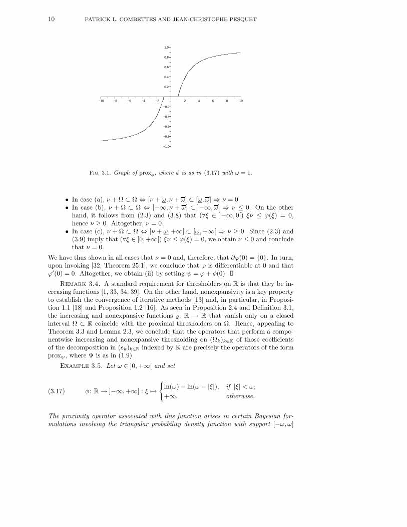
Fig. 3.1. Graph of proxφ, where φ is as in (3.17) with ω = 1.

• In case (a), ν + Ω ⊂ Ω ⇔ [ν + ω, ν + ω] ⊂ [ω, ω] ⇒ ν = 0.• In case (b), ν + Ω ⊂ Ω ⇔ ]−∞, ν + ω] ⊂ ]−∞, ω] ⇒ ν ≤ 0. On the other

hand, it follows from (2.3) and (3.8) that (∀ξ ∈ ]−∞, 0[) ξν ≤ ϕ(ξ) = 0,hence ν ≥ 0. Altogether, ν = 0.

• In case (c), ν + Ω ⊂ Ω ⇔ [ν + ω,+∞[ ⊂ [ω,+∞[ ⇒ ν ≥ 0. Since (2.3) and(3.9) imply that (∀ξ ∈ ]0,+∞[) ξν ≤ ϕ(ξ) = 0, we obtain ν ≤ 0 and concludethat ν = 0.

We have thus shown in all cases that ν = 0 and, therefore, that ∂ϕ(0) = 0. In turn,upon invoking [32, Theorem 25.1], we conclude that ϕ is differentiable at 0 and thatϕ′(0) = 0. Altogether, we obtain (ii) by setting ψ = ϕ+ φ(0).

Remark 3.4. A standard requirement for thresholders on R is that they be in-creasing functions [1, 33, 34, 39]. On the other hand, nonexpansivity is a key propertyto establish the convergence of iterative methods [13] and, in particular, in Proposi-tion 1.1 [18] and Proposition 1.2 [16]. As seen in Proposition 2.4 and Definition 3.1,the increasing and nonexpansive functions : R → R that vanish only on a closedinterval Ω ⊂ R coincide with the proximal thresholders on Ω. Hence, appealing toTheorem 3.3 and Lemma 2.3, we conclude that the operators that perform a compo-nentwise increasing and nonexpansive thresholding on (Ωk)k∈K of those coefficientsof the decomposition in (ek)k∈N indexed by K are precisely the operators of the formproxΨ, where Ψ is as in (1.9).

Example 3.5. Let ω ∈ ]0,+∞[ and set

(3.17) φ : R → ]−∞,+∞] : ξ 7→

ln(ω) − ln(ω − |ξ|), if |ξ| < ω;

+∞, otherwise.

The proximity operator associated with this function arises in certain Bayesian for-mulations involving the triangular probability density function with support [−ω, ω]


[8]. Let us set

(3.18) ψ : R → ]−∞,+∞] : ξ 7→

ln(ω) − ln(ω − |ξ|) − |ξ|/ω, if |ξ| < ω;

+∞, otherwise

and Ω = [−1/ω, 1/ω]. Then ψ ∈ Γ0(R) is differentiable at 0, ψ′(0) = 0, and φ =ψ + σΩ. Therefore, Theorem 3.3 asserts that proxφ is a proximal thresholder on[−1/ω, 1/ω]. Actually (see Fig. 3.1), for every ξ ∈ R, we have [8, Example 4.12]

(3.19) proxφ ξ =

sign(ξ)

|ξ| + ω −

√∣∣|ξ| − ω∣∣2 + 4

2, if |ξ| > 1/ω;

0 otherwise.

Next, we provide a convenient decomposition rule for implementing proximalthresholders.

Proposition 3.6. Let φ = ψ + σΩ, where ψ ∈ Γ0(R) and Ω ⊂ R is a nonemptyclosed interval. Suppose that ψ is differentiable at 0 with ψ′(0) = 0. Then proxφ =proxψ softΩ .

Proof. Fix ξ and π in R. We have 0 ∈ domσΩ and, since ψ is differentiable at 0,0 ∈ int domψ. It therefore follows from (2.4) and [32, Theorem 23.8] that

π = proxφ ξ ⇔ ξ − π ∈ ∂φ(π) = ∂ψ(π) + ∂σΩ(π)

⇔ (∃ ν ∈ ∂ψ(π)) ξ − (π + ν) ∈ ∂σΩ(π).(3.20)

Let us observe that, if ν ∈ ∂ψ(π), then, since 0 ∈ Argminψ, (2.3) implies that(0 − π)ν + ψ(π) ≤ ψ(0) ≤ ψ(π) < +∞ and, in turn, that πν ≥ 0. This shows that,if ν ∈ ∂ψ(π) and π 6= 0, then either π > 0 and ν ≥ 0, or π < 0 and ν ≤ 0; in turn,Lemma 2.1(ii) yields ∂σΩ(π) = ∂σΩ(π + ν). Consequently, if π 6= 0, we derive from(3.20) and Example 2.6(ii) that

π = proxφ ξ ⇒ (∃ ν ∈ ∂ψ(π)) ξ − (π + ν) ∈ ∂σΩ(π + ν)

⇔ (∃ ν ∈ ∂ψ(π)) π + ν = proxσΩξ = softΩ ξ

⇔ softΩ ξ − π ∈ ∂ψ(π)

⇔ π = proxψ(softΩ ξ

).(3.21)

On the other hand, if π = 0, since ∂ψ(0) = ψ′(0) = 0, we derive from (3.20),Example 2.1(ii), (1.11), and Lemma 2.2(i) that

(3.22) π = proxφ ξ ⇒ ξ ∈ ∂σΩ(0) = Ω ⇒ softΩ ξ = 0 ⇒ proxψ(softΩ ξ

)= 0 = π.

The proof is now complete.In view of Proposition 3.6 and (1.11), the computation of the proximal thresholder

proxψ+σΩreduces to that of proxψ . By duality, we obtain a decomposition formula

for those proximal operators that coincide with the identity on a closed interval Ω.Proposition 3.7. Let φ = ψ ιΩ, where ψ ∈ Γ0(R) and Ω ⊂ R is a nonempty

closed interval. Suppose that ψ∗ is differentiable at 0 with ψ∗′(0) = 0. Then thefollowing hold.

(i) proxφ = PΩ + proxψ softΩ .(ii) (∀ξ ∈ R) proxφ ξ = ξ ⇔ ξ ∈ Ω.


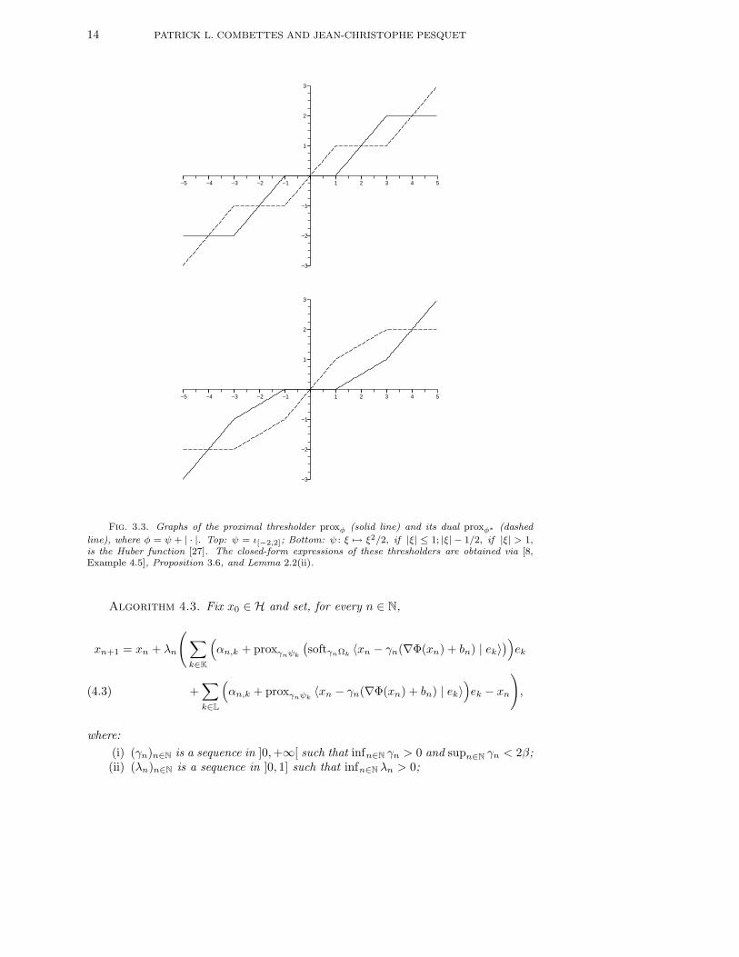
−5 −4 −3 −2 −1 1 2 3 4 5

−3

−2

−1

1

2

3

−5 −4 −3 −1 1 2 3 4 5

−3

−2

−1

1

2

3

Fig. 3.2. Graphs of the proximal thresholder proxφ (solid line) and its dual proxφ∗ (dashed line),where φ = τ | · |p + | · |. Top: τ = 0.05 and p = 4; Bottom: τ = 0.9 and p = 4/3. Explicit expressionsfor these thresholders are provided by Example 2.7(ii)&(vi), Proposition 3.6, and Lemma 2.2(ii).

Proof. It follows from [32, Theorem 16.4] that

(3.23) φ∗ = ψ∗ + ι∗Ω = ψ∗ + σΩ.

Note also that, since ψ ∈ Γ0(R), we have ψ∗ ∈ Γ0(R) [32, Theorem 12.2]. (i): Fix


ξ ∈ R. Then, by Lemma 2.2(ii), (3.23), Proposition 3.6, and Example 2.6,

proxφ ξ = ξ − proxφ∗ ξ(3.24)

= ξ − proxψ∗+σΩξ

= ξ − proxψ∗

(proxσΩ

ξ)

= ξ − proxσΩξ + proxψ

(proxσΩ

ξ)

= proxσ∗

Ωξ + proxψ

(proxσΩ

ξ)

= proxιΩ ξ + proxψ(proxσΩ

ξ)

= PΩξ + proxψ(softΩ ξ

).(3.25)

(ii): It follows from (3.23) and Theorem 3.3 that proxφ∗ is a proximal thresholder onΩ. Hence, we derive from (3.24) and (3.1) that (∀ξ ∈ R) proxφ ξ = ξ ⇔ proxφ∗ ξ = 0⇔ ξ ∈ Ω.

Examples of proximal thresholders (see Proposition 3.6) and their duals (seeProposition 3.7) are provided in Figs. 3.2 and 3.3 (see also Fig. 2.1) in the casewhen Ω = [−1, 1].

4. Iterative proximal thresholding. Let us start with some basic propertiesof Problem 1.3.

Proposition 4.1. Problem 1.3 possesses at least one solution.

Proof. Let Ψ be as in (1.9). We infer from the assumptions of Problem 1.3 andLemma 2.3 that Ψ ∈ Γ0(H) and, in turn, that Φ + Ψ ∈ Γ0(H). Hence, it sufficesto show that Φ + Ψ is coercive [41, Theorem 2.5.1(ii)], i.e., since inf Φ(H) > −∞ byassumption (i) in Problem 1.3, that Ψ is coercive. For this purpose, let x = (ξk)k∈N

denote a generic element in ℓ2(N), and let

(4.1) Υ: ℓ2(N) → ]−∞,+∞] : x 7→∑

k∈N

ψk(ξk) +∑

k∈K

σΩk(ξk).

Then, by Parseval’s identity, it is enough to show that Υ is coercive. To this end, setxK = (ξk)k∈K and xL = (ξk)k∈L, and denote by ‖ · ‖K and ‖ · ‖L the standard norms onℓ2(K) and ℓ2(L), respectively. Using (4.1), assumptions (ii) and (vi) in Problem 1.3,and Example 2.1(i), we obtain

(∀ x ∈ ℓ2(N)) Υ(x) ≥∑

k∈K

σΩk(ξk) +

∑

k∈L

ψk(ξk)

≥ ω∑

k∈K

|ξk| + ΥL(xL)

≥ ω‖xK‖K + ΥL(xL),(4.2)

where ΥL is defined in Problem 1.3(v). Now suppose that ‖x‖ =√‖xK‖2

K+ ‖xL‖2

L→

+∞. Then (4.2) and assumption (v) in Problem 1.3 yield Υ(x) → +∞, as desired.

Proposition 4.2. Let Ψ be as in (1.9), let x ∈ H, and let γ ∈ ]0,+∞[. Then xis a solution to Problem 1.3 if and only if x = proxγΨ(x− γ∇Φ(x)).

Proof. Since Problem 1.3 is equivalent to minimizing Φ + Ψ, this is a standardcharacterization, see for instance [16, Proposition 3.1(iii)].

Our algorithm for solving Problem 1.3 will be the following.


−5 −4 −3 −2 −1 1 2 3 4 5

−3

−2

−1

1

2

3

−5 −4 −3 −2 −1 1 2 3 4 5

−3

−2

−1

1

2

3

Fig. 3.3. Graphs of the proximal thresholder proxφ (solid line) and its dual proxφ∗ (dashed

line), where φ = ψ + | · |. Top: ψ = ι[−2,2]; Bottom: ψ : ξ 7→ ξ2/2, if |ξ| ≤ 1; |ξ| − 1/2, if |ξ| > 1,is the Huber function [27]. The closed-form expressions of these thresholders are obtained via [8,Example 4.5], Proposition 3.6, and Lemma 2.2(ii).

Algorithm 4.3. Fix x0 ∈ H and set, for every n ∈ N,

xn+1 = xn + λn

(∑

k∈K

(αn,k + proxγnψk

(softγnΩk

〈xn − γn(∇Φ(xn) + bn) | ek〉))ek

+∑

k∈L

(αn,k + proxγnψk

〈xn − γn(∇Φ(xn) + bn) | ek〉)ek − xn

),(4.3)

where:

(i) (γn)n∈N is a sequence in ]0,+∞[ such that infn∈N γn > 0 and supn∈N γn < 2β;(ii) (λn)n∈N is a sequence in ]0, 1] such that infn∈N λn > 0;


(iii) for every n ∈ N, (αn,k)k∈N is a sequence in ℓ2(N) such that

∑

n∈N

√∑

k∈N

|αn,k|2 < +∞;

(iv) (bn)n∈N is a sequence in H such that∑n∈N

‖bn‖ < +∞.Remark 4.4. Let us highlight some features of Algorithm 4.3.• The set K contains the indices of those coefficients of the decomposition in

(ek)k∈N that are thresholded.• The terms αn,k and bn stand for some numerical tolerance in the implemen-

tation of proxγnψkand the computation of ∇Φ(xn), respectively.

• The parameters λn and γn provide added flexibility to the algorithm and canbe used to improve its convergence profile.

• The operator softγnΩkis given explicitly in (1.11).

Our main convergence result can now be stated.Theorem 4.5. Every sequence generated by Algorithm 4.3 converges strongly to

a solution to Problem 1.3.Proof. Hereafter, (xn)n∈N is a sequence generated by Algorithm 4.3 and we define

(4.4) (∀k ∈ N) φk =

ψk + σΩk

, if k ∈ K;

ψk, if k ∈ L.

It follows from the assumptions on (ψk)k∈N in Problem 1.3 that (∀k ∈ N) ψ′k(0) = 0.

Therefore, for every n in N, Theorem 3.3 implies that

(4.5) for every k in K, proxγnφkis a proximal thresholder on γnΩk,

while Proposition 3.6 supplies(4.6)(∀k ∈ K) proxγnφk

= proxγnψk+γnσΩk= proxγnψk+σ(γnΩk)

= proxγnψk softγnΩk

.

Thus, (4.3) can be rewritten as

(4.7) xn+1 = xn +λn

(∑

k∈N

(αn,k +proxγnφk

〈xn − γn(∇Φ(xn) + bn) | ek〉)ek− xn

).

Now let Ψ be as in (1.9), i.e., Ψ =∑

k∈Nφk(〈· | ek〉), and set (∀n ∈ N) an =∑

k∈Nαn,kek. Then it follows from (4.4) and Lemma 2.3 that Ψ ∈ Γ0(H) and that

(4.7) can be rewritten as

(4.8) xn+1 = xn + λn

(proxγnΨ

(xn − γn(∇Φ(xn) + bn)

)+ an − xn

).

Consequently, since Proposition 4.1 asserts that Φ + Ψ possesses a minimizer, wederive from assumptions (i)–(iv) in Algorithm 4.3 and [16, Theorem 3.4] that

(4.9) (xn)n∈N converges weakly to a solution x to Problem 1.3

and that(4.10)∑

n∈N

‖xn−proxγnΨ

(xn−γn∇Φ(xn)

)‖2 < +∞ and

∑

n∈N

‖∇Φ(xn)−∇Φ(x)‖2 < +∞.


Hence, it follows from Lemma 2.2(iii) and assumption (i) in Algorithm 4.3 that

(4.11)1

2

∑

n∈N

‖xn − proxγnΨ

(xn − γn∇Φ(x)

)‖2

≤∑

n∈N

‖xn − proxγnΨ

(xn − γn∇Φ(xn)

)‖2

+∑

n∈N

‖ proxγnΨ


)− proxγnΨ

(xn − γn∇Φ(x)

)‖2

≤∑

n∈N

‖xn − proxγnΨ


)‖2 +

∑

n∈N

γ2n‖∇Φ(xn) −∇Φ(x)‖2

≤∑

n∈N

‖xn − proxγnΨ


)‖2 + 4β2

∑

n∈N

‖∇Φ(xn) −∇Φ(x)‖2

< +∞.

Now define

(4.12) (∀n ∈ N) vn = xn − x and hn = x− γn∇Φ(x).

On the one hand, we derive from (4.9) that

(4.13) (vn)n∈N converges weakly to 0

and, on the other hand, from (4.11) and Proposition 4.2 that

∑

n∈N

‖vn − proxγnΨ(vn + hn) + proxγnΨ hn‖2 =

∑

n∈N

‖xn − proxγnΨ

(xn − γn∇Φ(x)

)‖2

< +∞.(4.14)

By Parseval’s identity, to establish that ‖vn‖ = ‖xn−x‖ → 0, we must show that

(4.15)∑

k∈K

|νn,k|2 → 0 and

∑

k∈L

|νn,k|2 → 0,

where (∀n ∈ N)(∀k ∈ N) νn,k = 〈vn | ek〉. To this end, let us set, for every n ∈ N andk ∈ N, ηn,k = 〈hn | ek〉 and observe that (4.14), Parseval’s identity, and Lemma 2.3imply that

(4.16)∑

k∈N

|νn,k − proxγnφk(νn,k + ηn,k) + proxγnφk

ηn,k|2 → 0.

In addition, let us set r = 2β∇Φ(x) and, for every k ∈ N, ξk = 〈x | ek〉 and ρk =〈r | ek〉. Then we derive from (4.12) and assumption (i) in Algorithm 4.3 that

(4.17) (∀n ∈ N)(∀k ∈ N) |ηn,k|2/2 ≤ |ξk|

2 + γ2n |〈∇Φ(x) | ek〉|

2 ≤ |ξk|2 + |ρk|

2.

To establish (4.15), let us first show that∑

k∈K|νn,k|

2 → 0. For this purpose,set δ = γω, where γ = infn∈N γn and where ω is supplied by assumption (vi) inProblem 1.3. Then it follows from assumption (i) in Algorithm 4.3 that δ > 0 andthat

(4.18) [−δ, δ] ⊂⋂

n∈N

⋂

k∈K

γnΩk.


On the other hand, (4.17) yields

(4.19)∑

k∈K

supn∈N

|ηn,k|2/2 ≤

∑

k∈N

(|ξk|

2 + |ρk|2)

= ‖x‖2 + ‖r‖2 < +∞.

Hence, there exists a finite set K1 ⊂ K such that

(4.20) (∀n ∈ N)∑

k∈K2

|ηn,k|2 ≤ δ2/4, where K2 = K r K1.

In view of (4.13), we have∑

k∈K1|νn,k|

2 → 0. Let us now show that∑

k∈K2|νn,k|

2 →0. Note that (4.18) and (4.20) yield

(4.21) (∀n ∈ N)(∀k ∈ K2) ηn,k ∈ [−δ/2, δ/2] ⊂ γnΩk.

Therefore, (4.5) implies that

(4.22) (∀n ∈ N)(∀k ∈ K2) proxγnφkηn,k = 0.

Let us define

(4.23) (∀n ∈ N) K21,n =k ∈ K2

∣∣ νn,k + ηn,k ∈ γnΩk.

Then, invoking (4.5) once again, we obtain

(4.24) (∀n ∈ N)(∀k ∈ K21,n) proxγnφk(νn,k + ηn,k) = 0

which, combined with (4.22), yields

(∀n ∈ N)∑

k∈K21,n

|νn,k|2 =

∑

k∈K21,n


ηn,k|2

≤∑

k∈N


ηn,k|2.(4.25)

Consequently, it results from (4.16) that∑

k∈K21,n|νn,k|

2 → 0. Next, let us set

(4.26) (∀n ∈ N) K22,n = K2 r K21,n

and show that∑

k∈K22,n|νn,k|

2 → 0. It follows from (4.26), (4.23), and (4.18) that

(4.27) (∀n ∈ N)(∀k ∈ K22,n) νn,k + ηn,k /∈ γnΩk ⊃ [−δ, δ].

Hence, appealing to (4.21), we obtain

(4.28) (∀n ∈ N)(∀k ∈ K22,n) |νn,k + ηn,k| ≥ δ ≥ |ηn,k| + δ/2.

Now take n ∈ N and k ∈ K22,n. We derive from (4.22) and Lemma 2.2(ii) that

(4.29) |νn,k − proxγnφk(νn,k + ηn,k) + proxγnφk

ηn,k|

= |(νn,k + ηn,k) − proxγnφk(νn,k + ηn,k) − ηn,k|

= | prox(γnφk)∗(νn,k + ηn,k) − ηn,k|.


However, it results from (4.18), (4.5), and Proposition 3.2 that prox(γnφk)∗(±δ) = ±δ.We consider two cases. First, if νn,k + ηn,k ≥ 0 then, since prox(γnφk)∗ is increasingby Proposition 2.4, (4.28) yields νn,k + ηn,k ≥ δ and

(4.30) prox(γnφk)∗(νn,k + ηn,k) ≥ prox(γnφk)∗ δ = δ ≥ ηn,k + δ/2.

Likewise, if νn,k + ηn,k ≤ 0, then (4.28) yields νn,k + ηn,k ≤ −δ and

(4.31) prox(γnφk)∗(νn,k + ηn,k) ≤ prox(γnφk)∗(−δ) = −δ ≤ ηn,k − δ/2.

Altogether, we derive from (4.30) and (4.31) that

(4.32) (∀n ∈ N)(∀k ∈ K22,n) | prox(γnφk)∗(νn,k + ηn,k) − ηn,k| ≥ δ/2.

In turn, (4.29) yields(4.33)

(∀n ∈ N)∑

k∈K22,n


ηn,k|2 ≥ card(K22,n)δ

2/4.

However, it follows from (4.16) that, for n sufficiently large,

(4.34)∑

k∈N


ηn,k|2 ≤ δ2/5.

Thus, for n sufficiently large, K22,n = ∅. We conclude from this first part of the proofthat

∑k∈K

|νn,k|2 → 0.

In order to obtain (4.15), we must now show that∑k∈L

|νn,k|2 → 0. We infer

from (4.13) that (vn)n∈N is bounded, hence

(4.35) supn∈N

∑

k∈L

|νn,k|2 ≤ sup

n∈N

‖vn‖2 ≤ ρ2/4,

for some ρ ∈ ]0,+∞[. Now define

(4.36) L1 =k ∈ L

∣∣ (∃n ∈ N) |ηn,k| ≥ ρ/2.

Then we derive from (4.17) that

(4.37) (∀k ∈ L1)(∃n ∈ N) |ξk|2 + |ρk|

2 ≥ |ηn,k|2/2 ≥ ρ2/8.

Consequently, we have

(4.38) +∞ > ‖x‖2 + ‖r‖2 ≥∑

k∈L1

(|ξk|

2 + |ρk|2)≥ (cardL1)ρ

2/8

and therefore card(L1) < +∞. In turn, it results from (4.13) that∑

k∈L1|νn,k|

2 → 0.

Hence, to obtain∑

k∈L|νn,k|

2 → 0, it remains to show that∑

k∈L2|νn,k|

2 → 0, whereL2 = L r L1. In view of (4.36) and (4.35), we have

(4.39) (∀n ∈ N)(∀k ∈ L2) |ηn,k| < ρ/2 and |νn,k + ηn,k| ≤ |νn,k| + |ηn,k| < ρ.

On the other hand, assumption (iv) in Problem 1.3 asserts that there exists θ ∈]0,+∞[ such that

(4.40) infn∈N

infk∈L2

inf0<|ξ|≤ρ

(γnψk)′′(ξ) ≥ γ inf

k∈L2

inf0<|ξ|≤ρ

ψ′′k (ξ) ≥ γθ.


It therefore follows from assumptions (ii) and (iii) in Problem 1.3, Proposition 2.9,and (4.4) that

(∀n ∈ N)(∀k ∈ L2) |νn,k| ≤ |νn,k − proxγnψk(νn,k + ηn,k) + proxγnψk

ηn,k|

+ | proxγnψk(νn,k + ηn,k) − proxγnψk

ηn,k|

≤ |νn,k − proxγnψk(νn,k + ηn,k) + proxγnψk

ηn,k|

+ |νn,k|/(1 + γθ)

= |νn,k − proxγnφk(νn,k + ηn,k) + proxγnφk

ηn,k|

+ |νn,k|/(1 + γθ).(4.41)

Consequently, upon setting µ = 1 + 1/(γθ), we obtain

(4.42) (∀n ∈ N)(∀k ∈ L2) |νn,k| ≤ µ|νn,k − proxγnφk(νn,k + ηn,k) + proxγnφk

ηn,k|.

In turn,

(4.43) (∀n ∈ N)∑

k∈L2

|νn,k|2 ≤ µ2

∑

k∈L2

|νn,k−proxγnφk(νn,k+ηn,k)+proxγnφk

ηn,k|2.

Hence, (4.16) forces∑

k∈L2|νn,k|

2 → 0, as desired.Remark 4.6. An important aspect of Theorem 4.5 is that it provides a strong

convergence result. Indeed, in general, only weak convergence can be claimed forforward-backward methods [16, 38] (see [3], [4], [16, Remark 5.12], and [25] for explicitconstructions in which strong convergence fails). In addition, the standard sufficientconditions for strong convergence in this type of algorithm (see [13, Remark 6.6]and [16, Theorem 3.4(iv)]) are not satisfied in Problem 1.3. Further aspects of therelevance of strong convergence in proximal methods are discussed in [25, 26].

Remark 4.7. Let T be a nonzero bounded linear operator from H to a realHilbert space G, let z ∈ G, and let τ and ω be in ]0,+∞[. Specializing Theorem 4.5to the case when Φ: x 7→ ‖Tx− z‖2/2 and either

(4.44) K = ∅ and (∀k ∈ L) ψk = τk|·|p, where p ∈ ]1, 2] and τk ∈ [τ,+∞[ ,

or(4.45)

L = ∅ and (∀k ∈ K) ψk = 0 and Ωk = [−ωk, ωk], where ωk ∈ [ω,+∞[ ,

yields [16, Corollary 5.19]. If we further impose λn ≡ 1, ‖T ‖ < 1, γn ≡ 1, αn,k ≡ 0,and bn ≡ 0, we obtain [18, Theorem 3.1].

5. Applications to sparse signal recovery.

5.1. A special case of Problem 1.3. In (1.4), a single observation z of theoriginal signal x is available. In certain problems, q such noisy linear observations areavailable, say zi = Tix + vi (1 ≤ i ≤ q), which leads to the weighted least-squaresdata fidelity term x 7→

∑qi=1 µi‖Tix − zi‖

2; see [12] and the references therein. Fur-thermore, signal recovery problems are typically accompanied with convex constraintsthat confine x to some closed convex subsets (Si)1≤i≤m of H. The violation of theseconstraints can be penalized via the cost function x 7→

∑mi=1 ϑid

2Si

(x); see [10, 28]and the references therein. On the other hand, power functions are frequently usedas cost functions in variational models for determining the coefficients of orthonormal


basis decompositions, e.g., [1, 7, 8, 18]. Moreover, we aim at promoting sparsity of asolution x ∈ H with respect to (ek)k∈N in the sense that, for every k in K, we wish toset to 0 the coefficient 〈x | ek〉 if it lies in the interval Ωk. The following formulationis consistent with these considerations.

Problem 5.1. For every i ∈ 1, . . . , q, let µi ∈ ]0,+∞[, let Ti be a nonzerobounded linear operator from H to a real Hilbert space Gi, and let zi ∈ Gi. For everyi ∈ 1, . . . ,m, let ϑi ∈ ]0,+∞[ and let Si be a nonempty closed and convex subset ofH. Furthermore, let (pk,l)0≤l≤Lk

be distinct real numbers in ]1,+∞[, let (τk,l)0≤l≤Lk

be real numbers in [0,+∞[, and let lk ∈ 0, . . . , Lk satisfy pk,lk = min0≤l≤Lkpk,l,

where (Lk)k∈N is a sequence in N. Finally, let K ⊂ N, let L = N r K, and let (Ωk)k∈K

be a sequence of closed intervals in R. The objective is to

(5.1) minimizex∈H

1

2

q∑

i=1

µi‖Tix− zi‖2 +

1

2

m∑

i=1

ϑid2Si

(x)

+∑

k∈N

Lk∑

l=0

τk,l|〈x | ek〉|pk,l +

∑

k∈K

σΩk(〈x | ek〉),

under the following assumptions:(i) infk∈L τk,lk > 0;(ii) infk∈L pk,lk > 1;(iii) supk∈L pk,lk ≤ 2;(iv) 0 ∈ int

⋂k∈K

Ωk.Proposition 5.2. Problem 5.1 is a special case of Problem 1.3.Proof. First, we observe that (5.1) corresponds to (1.7) where

(5.2)

Φ: x 7→1

2

q∑

i=1

µi‖Tix−zi‖2 +

1

2

m∑

i=1

ϑid2Si

(x) and (∀k ∈ N) ψk : ξ 7→

Lk∑

l=0

τk,l|ξ|pk,l .

Hence, Φ is a finite positive continuous convex function with Frechet gradient

(5.3) ∇Φ: x 7→

q∑

i=1

µiT∗i (Tix− zi) +

m∑

i=1

ϑi(x− Pix),

where Pi is the projection operator onto Si. Therefore, since the operators(Id −Pi)1≤i≤m are nonexpansive, it follows that assumption (i) in Problem 1.3 issatisfied with 1/β =

∑qi=1 µi‖Ti‖

2 +∑mi=1 ϑi. Moreover, the functions (ψk)k∈N are in

Γ0(R) and satisfy assumptions (ii) and (iii) in Problem 1.3.Let us now turn to assumption (iv) in Problem 1.3. Fix ρ ∈ ]0,+∞[ and set

τ = infk∈L τk,lk , p = infk∈L pk,lk , and θ = τp(p− 1)min1, 1/ρ. Then it follows from(i), (ii), and (iii) that θ > 0 and that

infk∈L

inf0<|ξ|≤ρ

ψ′′k (ξ) = inf

k∈L

inf0<|ξ|≤ρ

Lk∑

l=0

τk,lpk,l(pk,l − 1)|ξ|pk,l−2

≥ infk∈L

τk,lkpk,lk(pk,lk − 1) inf0<ξ≤ρ

ξpk,lk−2

≥ τp(p− 1) infk∈L

inf0<ξ≤ρ

ξpk,lk−2

≥ τp(p− 1) infk∈L

(1/ρ)2−pk,lk

≥ θ,(5.4)


0 200 400 600 800 1000

0

1

2

3

4

5

6

7

8

9

Fig. 5.1. Original signal – first example.

which shows that (1.8) is satisfied.It remains to check assumption (v) in Problem 1.3. To this end, let ‖ · ‖L denote

the standard norm on ℓ2(L), take x = (ξk)k∈L ∈ ℓ2(L) such that ‖x‖L ≥ 1, and set(ηk)k∈L = x/‖x‖L. Then, for every k ∈ L, |ηk| ≤ 1 and, since pk,lk ∈ ]1, 2], we have|ηk|

pk,lk ≥ |ηk|2. Consequently,

(5.5)

ΥL(x) =∑

k∈L

Lk∑

l=0

τk,l|ξk|pk,l ≥

∑

k∈L

τk,lk |ξk|pk,lk

≥ τ∑

k∈L

|ξk|pk,lk = τ

∑

k∈L

‖x‖pk,lk

L|ηk|

pk,lk

≥ τ∑

k∈L

‖x‖pk,lk

L|ηk|

2 = τ∑

k∈L

‖x‖pk,lk

−2

L|ξk|

2

≥ τ‖x‖−1L

∑

k∈L

|ξk|2 = τ‖x‖L.

We conclude that ΥL(x) → +∞ as ‖x‖L → +∞.

5.2. First example. Our first example concerns the simulated X-ray fluores-cence spectrum x displayed in Fig. 5.1, which is often used to test restoration meth-ods, e.g., [14, 37]. The measured signal z shown in Fig. 5.2 has undergone blurring bythe limited resolution of the spectrometer and further corruption by addition of noise.In the underlying Hilbert space H = ℓ2(N), this process is modeled by z = Tx + v,where T : H → H is the operator of convolution with a truncated Gaussian kernel.The noise samples are uncorrelated and drawn from a Gaussian population with meanzero and standard deviation 0.15. The original signal x has support 0, . . . , N − 1(N = 1024), takes on positive values, and possesses a sparse structure. These featurescan be promoted in Problem 5.1 by letting (ek)k∈N be the canonical orthonormal basisof H, and setting K = N, τk,l ≡ 0, and

(5.6) (∀k ∈ N) Ωk =

]−∞, ω] , if 0 ≤ k ≤ N − 1;

R, otherwise,

where the one-sided thresholding level is set to ω = 0.01. On the other hand, us-ing the methodology described in [37], the above information about the noise can


0 200 400 600 800 1000

0

1

2

3

4

5

6

7

8

9

Fig. 5.2. Degraded signal – first example.

0 200 400 600 800 1000

0

1

2

3

4

5

6

7

8

9

Fig. 5.3. Signal restored by Algorithm 4.3 – first example.

be used to construct the constraint sets S1 =x ∈ H

∣∣ ‖Tx− z‖ ≤ δ1

and S2 =⋂N−1l=1

x ∈ H

∣∣ |T x(l/N) − z(l/N)| ≤ δ2, where a : ν 7→

∑+∞k=0 〈a | ek〉 exp(−ı2πkν)

designates the Fourier transform of a ∈ H. The bounds δ1 and δ2 have been deter-mined so as to guarantee that x lies in S1 and in S2 with a 99 percent confidence level(see [15] for details). Finally, we set q = 0, m = 2, and ϑ1 = ϑ2 = 1 in (5.1) (thecomputation of the projectors P1 and P2 required in (5.3) is detailed in [37]). Thesolution produced by Algorithm 4.3 is shown in Fig. 5.3. It is of much better qualitythan the restorations obtained in [14] and [37] via alternative methods.

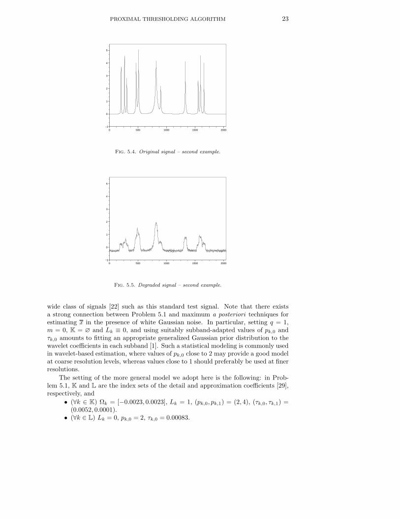
5.3. Second example. We provide a wavelet deconvolution example in H =L

2(R). The original signal x is the classical “bumps” signal [40] displayed in Fig. 5.4.The degraded version shown in Fig. 5.5 is z1 = T1x+v1, where T1 models convolutionwith a uniform kernel and v1 is a realization of a zero-mean white Gaussian noise.

The basis (ek)k∈N is an orthonormal wavelet symlet basis with 8 vanishing mo-ments [17]. Such wavelet bases are known to provide sparse representations for a


0 500 1000 1500 2000−1

0

1

2

3

4

5

Fig. 5.4. Original signal – second example.

0 500 1000 1500 2000−1

0

1

2

3

4

5

Fig. 5.5. Degraded signal – second example.

wide class of signals [22] such as this standard test signal. Note that there existsa strong connection between Problem 5.1 and maximum a posteriori techniques forestimating x in the presence of white Gaussian noise. In particular, setting q = 1,m = 0, K = ∅ and Lk ≡ 0, and using suitably subband-adapted values of pk,0 andτk,0 amounts to fitting an appropriate generalized Gaussian prior distribution to thewavelet coefficients in each subband [1]. Such a statistical modeling is commonly usedin wavelet-based estimation, where values of pk,0 close to 2 may provide a good modelat coarse resolution levels, whereas values close to 1 should preferably be used at finerresolutions.

The setting of the more general model we adopt here is the following: in Prob-lem 5.1, K and L are the index sets of the detail and approximation coefficients [29],respectively, and

• (∀k ∈ K) Ωk = [−0.0023, 0.0023], Lk = 1, (pk,0, pk,1) = (2, 4), (τk,0, τk,1) =(0.0052, 0.0001).

• (∀k ∈ L) Lk = 0, pk,0 = 2, τk,0 = 0.00083.


0 500 1000 1500 2000−1

0

1

2

3

4

5

Fig. 5.6. Signal restored by Algorithm 4.3 – second example.

0 500 1000 1500 2000−1

0

1

2

3

4

5

Fig. 5.7. Signal restored by solving (1.4) – second example.

For each k, the integer Lk and the exponents (pk,l)0≤l≤Lkare imposed, while the set

Ωk and the coefficients (τk,l)0≤l≤Lkare chosen empirically. In addition, we set q = 1,

µ1 = 1, m = 1, ϑ1 = 1, and S1 =x ∈ H

∣∣ x ≥ 0

(pointwise positivity constraint).The solution x produced by Algorithm 4.3 is shown in Fig. 5.6. The estimation erroris ‖x−x‖ = 8.33. For comparison, the signal x restored via (1.4) with Algorithm (1.5)is displayed in Fig. 5.7. In Problem 5.1, this corresponds to q = 1, m = 0, K = N,τk,l ≡ 0, Ωk ≡ [−2.9, 2.9] for the detail coefficients, and Ωk ≡ [−0.0062, 0.0062] forthe approximation coefficients. This setup yields a worse error of ‖x − x‖ = 14.14(the sets (Ωk)k∈N have been adjusted so as to mininize this error). The above resultshave been obtained with a discrete implementation of the wavelet decomposition over4 resolution levels using 2048 signal samples [29].

REFERENCES

[1] A. Antoniadis, D. Leporini, and J.-C. Pesquet, Wavelet thresholding for some classes of


non-Gaussian noise, Statist. Neerlandica, 56 (2002), pp. 434–453.[2] S. Bacchelli and S. Papi, Filtered wavelet thresholding methods, J. Comput. Appl. Math.,

164/165 (2004), pp. 39–52.[3] H. H. Bauschke, J. V. Burke, F. R. Deutsch, H. S. Hundal, and J. D. Vanderwerff, A

new proximal point iteration that converges weakly but not in norm, Proc. Amer. Math.Soc., 133 (2005), pp. 1829–1835.

[4] H. H. Bauschke, E. Matouskova, and S. Reich, Projection and proximal point methods:Convergence results and counterexamples, Nonlinear Anal., 56 (2004), pp. 715–738.

[5] J. Bect, L. Blanc-Feraud, G. Aubert, and A. Chambolle, A ℓ1 unified variational frame-work for image restoration, in Proc. Eighth Europ. Conf. Comput. Vision, Prague, 2004,T. Pajdla and J. Matas, eds., Lecture Notes in Comput. Sci. 3024, Springer-Verlag, NewYork, 2004, pp 1–13.

[6] R. E. Bruck and S. Reich, Nonexpansive projections and resolvents of accretive operatorsin Banach spaces, Houston J. Math., 3 (1977), pp. 459–470.

[7] A. Chambolle, R. A. DeVore, N. Y. Lee, and B. J. Lucier, Nonlinear wavelet image pro-cessing: Variational problems, compression, and noise removal through wavelet shrinkage,IEEE Trans. Image Process., 7 (1998), pp. 319–335.

[8] C. Chaux, P. L. Combettes, J.-C. Pesquet, and V. R. Wajs, A variational formulation forframe-based inverse problems, Inverse Problems, to appear.

[9] S. Chen, D. Donoho, and M. Saunders, Atomic decomposition by basis pursuit, SIAM Rev.,43 (2001), pp. 129–159.

[10] P. L. Combettes, Inconsistent signal feasibility problems: Least-squares solutions in a productspace, IEEE Trans. Signal Process., 42 (1994), pp. 2955–2966.

[11] P. L. Combettes, Convexite et signal, in Actes du Congres de Mathematiques Appliquees etIndustrielles SMAI’01, Pompadour, France, May 28–June 1, 2001, pp. 6–16.

[12] P. L. Combettes, A block-iterative surrogate constraint splitting method for quadratic signalrecovery, IEEE Trans. Signal Process., 51 (2003), pp. 1771–1782.

[13] P. L. Combettes, Solving monotone inclusions via compositions of nonexpansive averagedoperators, Optimization, 53 (2004), pp. 475–504.

[14] P. L. Combettes and H. J. Trussell, Method of successive projections for finding a commonpoint of sets in metric spaces, J. Optim. Theory Appl., 67 (1990), pp. 487–507.

[15] P. L. Combettes and H. J. Trussell, The use of noise properties in set theoretic estimation,IEEE Trans. Signal Process., 39 (1991), pp. 1630–1641.

[16] P. L. Combettes and V. R. Wajs, Signal recovery by proximal forward-backward splitting,Multiscale Model. Simul., 4 (2005), pp. 1168–1200.

[17] I. Daubechies, Ten Lectures on Wavelets, SIAM, Philadelphia, PA, 1992.[18] I. Daubechies, M. Defrise, and C. De Mol, An iterative thresholding algorithm for linear

inverse problems with a sparsity constraint, Comm. Pure Appl. Math., 57 (2004), pp.1413–1457.

[19] I. Daubechies and G. Teschke, Variational image restoration by means of wavelets: Si-multaneous decomposition, deblurring, and denoising, Appl. Comput. Harmon. Anal., 19(2005), pp. 1–16.

[20] C. de Mol and M. Defrise, A note on wavelet-based inversion algorithms, Contemp. Math.,313 (2002), pp. 85–96.

[21] D. Donoho and I. Johnstone, Ideal spatial adaptation via wavelet shrinkage, Biometrika, 81(1994), pp. 425–455.

[22] D. L. Donoho and I. M. Johnstone, Adapting to unknown smoothness via wavelet shrinkage,J. Amer. Stat. Assoc., vol. 90, pp. 1200–1224, 1995.

[23] D. L. Donoho, I. M. Johnstone, G. Kerkyacharian, and D. Picard, Wavelet shrinkage:Asymptopia?, J. R. Statist. Soc. B., 57 (1995), pp. 301–369.

[24] M. A. T. Figueiredo and R. D. Nowak, An EM algorithm for wavelet-based image restora-tion, IEEE Trans. Image Process., 12 (2003), pp. 906–916.

[25] O. Guler, On the convergence of the proximal point algorithm for convex minimization, SIAMJ. Control Optim., 29 (1991), pp. 403–419.

[26] O. Guler, Convergence rate estimates for the gradient differential inclusion, Optim. MethodsSoftw., 20 (2005), pp. 729–735.

[27] P. J. Huber, Robust regression: Asymptotics, conjectures, and Monte Carlo, Ann. Statist., 1(1973), pp. 799–821.

[28] T. Kotzer, N. Cohen, and J. Shamir, A projection-based algorithm for consistent and in-consistent constraints, SIAM J. Optim., 7 (1997), pp. 527–546.

[29] S. G. Mallat, A Wavelet Tour of Signal Processing, 2nd ed, Academic Press, New York, 1999.[30] J.-J. Moreau, Fonctions convexes duales et points proximaux dans un espace hilbertien, C. R.


Acad. Sci. Paris Ser. A Math., 255 (1962), pp. 2897–2899.[31] J.-J. Moreau, Proximite et dualite dans un espace hilbertien, Bull. Soc. Math. France, 93

(1965), pp. 273–299.[32] R. T. Rockafellar, Convex Analysis, Princeton University Press, Princeton, NJ, 1970.[33] G. Steidl, J. Weickert, T. Brox, P. Mrazek, and M. Welk, On the equivalence of soft

wavelet shrinkage, total variation diffusion, total variation regularization, and SIDEs,SIAM J. Numer. Anal., 42 (2004), pp. 686–713.

[34] T. Tao and B. Vidakovic, Almost everywhere behavior of general wavelet shrinkage operators,Appl. Comput. Harmon. Anal., 9 (2000), pp. 72–82.

[35] V. N. Temlyakov, Universal bases and greedy algorithms for anisotropic function classes,Constr. Approx., 18 (2002), pp. 529–550.

[36] J. A. Tropp, Just relax: Convex programming methods for identifying sparse signals in noise,IEEE Trans. Inform. Theory, 52 (2006), pp. 1030–1051.

[37] H. J. Trussell and M. R. Civanlar, The feasible solution in signal restoration, IEEE Trans.Acoust., Speech, Signal Process., 32 (1984), pp. 201–212.

[38] P. Tseng, Applications of a splitting algorithm to decomposition in convex programming andvariational inequalities, SIAM J. Control Optim., 29 (1991), pp. 119–138.

[39] B. Vidakovic, Nonlinear wavelet shrinkage with Bayes rules and Bayes factors, J. Amer.Statist. Assoc., 93 (1998), pp. 173–179.

[40] WaveLab Toolbox, Stanford University, http://www-stat.stanford.edu/~wavelab/.[41] C. Zalinescu, Convex Analysis in General Vector Spaces, World Scientific, River Edge, NJ,

2002.

PROXIMAL THRESHOLDING ALGORITHM FOR MINIMIZATION OVER …plc/siopt2.pdf · 2017-05-09 · PROXIMAL THRESHOLDING ALGORITHM FOR MINIMIZATION OVER ORTHONORMAL BASES∗ PATRICK L. COMBETTES†

Documents