Provided for non-commercial research and educational use. …arnoldo/ftp/papers/ESCO_00… · · 2012-04-06Not for reproduction, distribution or commercial use. ... 2010). This

Provided for non-commercial research and educational use.Not for reproduction, distribution or commercial use.

This chapter was originally published in Treatise on Estuarine and CoastalScience, published by Elsevier, and the attached copy is provided by Elsevier for

the author's benefit and for the benefit of the author's institution, for non-commercial research and educational use including without limitation use in

instruction at your institution, sending it to specific colleagues who you know, andproviding a copy to your institution's administrator.

All other uses, reproduction and distribution, including without limitationcommercial reprints, selling or licensing copies or access, or posting on open

internet sites, your personal or institution's website or repository, are prohibited.For exceptions, permission may be sought for such use through Elsevier's

permissions site at:

http://www.elsevier.com/locate/permissionusematerial

Valle-Levinson A (2011) Classification of Estuarine Circulation. In: Wolanski E andMcLusky DS (eds.) Treatise on Estuarine and Coastal Science, Vol 1, pp. 75–86.

Waltham: Academic Press.

© 2011 Elsevier Inc. All rights reserved.

Author's personal copy

1.05 Classification of Estuarine Circulation A Valle-Levinson, University of Florida, Gainesville, FL, USA

© 2011 Elsevier Inc. All rights reserved.

1.05.1 Introduction 75
1.05.2 Classification of Gravitational Circulation According to Estuarine Origin/Geomorphology 78 1.05.2.1 Coastal Plain/Drowned River Valley Estuaries 78 1.05.2.2 Tectonic Estuaries 78 1.05.2.3 Fjords 80 1.05.2.4 Bar-Built Estuaries 81 1.05.3 Classification of Gravitational Circulation According to Water Balance 81 1.05.4 Classification of Gravitational Circulation According to the Competition between Tidal Flow
and River Discharge 82
1.05.5 Estuarine Circulation 83 References 86
Abstract

In the absence of the Earth’s rotation effects, estuarine circulation represents the interaction among the contributions from gravitational circulation, tidal residual circulation, and circulation driven by tidally asymmetric vertical mixing. In turn, gravitational circulation is driven by river discharge and density gradients. Gravitational circulation tends to be dominant in many estuaries and can be classified according to the basin’s morphology or origin, to its water balance, or to the competition between tidal forcing and river discharge. Such classification as well as the circumstances under which the residual circulation induced by tidal flows and tidally asymmetric mixing are discussed in this chapter.

1.05.1 Introduction

Throughout the years, several schemes have been proposed to classify estuaries on the basis of their definition as semi-enclosed coastal bodies of water where ocean water is diluted by land-derived freshwater discharges. Traditional approaches to categorize estuaries have dealt with (1) their origin or geomorphology, (2) their water balance, (3) the competition between tidal flow and river discharge, and (4) the stratification and water-circulation characteristics of the system. An overview of such classification, of estuaries as basin entities, may be found elsewhere (e.g., Valle-Levinson, 2010). This chapter seeks to describe the circulation in estuaries, not necessarily as basin entities but as dynamic entities, but still, following similar schemes that have been used in the past.

It is necessary to point out, however, that fitting a given estuary or coastal basin into any type of classification is a risky undertaking. This is because most estuaries will show characteristics of different categories according to intra-tidal (ebb or flood) and sub-tidal (springs or neaps) phases, buoyancy conditions (dry or wet season), and atmospheric forcing (cooling/ heating and wind direction). According to the phasing of the forcing, a given estuary will be stratified or destratified and will exhibit different circulation patterns. Therefore, classifications of estuaries should be used cautiously. In any case, a discussion of several approaches is presented next.

In order to classify the along-estuary (in the x direction) non-tidal, or sub-tidal, circulation ue, it is essential to acknowledge the contribution from four basic flows: (1) density-driven flow, ud; (2) tidally rectified flow, ut; (3) river-driven flow, ur; and (4) flow induced by tidally asymmetric mixing, ua (Cheng et al., 2011):

ue ¼ ud þ ut þ ur þ ua ½1�

Treatise on Estuarine and Coastal Science, 2011, Vol.

We begin with, and concentrate mostly in this chapter on, a description of the typical gravitational circulation, as proposed by Pritchard (1956). Herein, we refer to gravitational circulation ug as the combined flow produced by density gradients ud and by the water-level slope associated with river discharge ur. In any basin where fresh/riverine and salty/oceanic waters interact, the long-term circulation should consist of lighter, riverine water moving at the surface toward the ocean and heavier, oceanic water flowing near the bottom toward the river source (Figure 1). This presumed two-layer circulation is vertically sheared, bidirectional, and also known as baroclinic circulation. The various appellations describe flow resulting from the adjustment of the density gradient under the influence of gravity. The density-driven flow reverses direction with depth and the river-driven flow is unidirectional with depth.

It is important to note that the direct observation of gravitational circulation in nature may or may not be possible because of typical masking of instantaneous flow by tides. When possible, the observation of estuarine circulation requires persistent measurements throughout one or several tidal cycles. This is because coastal basins are normally affected by forcing from tides, the atmosphere (winds, barometric pressure, cooling/heating, and evaporation/precipitation), and the adjacent ocean (coastally trapped waves and planetary waves with periods greater than the tidal period). Therefore, at any given time, the circulation profile may show unidirectional flow throughout the water column. The gravitational circulation should then be extracted from data of flow profiles after averaging over one, or several, or many tidal cycles (Figure 2). The result of averaging flow profiles represents the interaction between waters of different densities. Even then, the average flow may have influence from tidally asymmetric mixing (e.g., Stacey et al.,

75 1, 75-86, DOI: 10.1016/B978-0-12-374711-2.00106-6

Author's personal copy76 Classification of Estuarine Circulation

River Ocean

0.0

ug ud

–0.2 ur

Non

dim

ensi

onal

dep

th

–0.4

–0.6

–0.8

–1.0 –1.0 –0.5 0.0 0.5 1.0

Nondimensional flow

Figure 1 Representation of gravitational circulation ug (in blue), illustrating seaward flow at the surface and landward flow at the bottom. The red line is the density-driven circulation ud and the orange line is the river-induced circulation ur.

Figure 2 Time series of principal-axis flow profiles during one tidal cycle at the entrance to the Chesapeake Bay. The tidally averaged flow profile appears on the right panel (seaward flow is positive).

2008) causing ua, which will be discussed in Section 1.05.4. In many cases, however, the gravitational circulation may be observed instantaneously during periods of slack tidal currents (e.g., around hour 7 in Figure 2), when only density gradients drive the circulation observed.

The gravitational circulation ug often results from a dynamic balance between pressure gradient and stress divergence (frictional effects):

Z0 � � 1 ∂p ∂η g ∂ρ ∂ ∂ug¼ g þ dz ¼ Az ½2� ρ ∂x ∂x ρ ∂x ∂z ∂z

− H

Treatise on Estuarine and Coastal Science, 2011, Vol. 1

where Az is an eddy viscosity coefficient with units m2 s−1, ρ is a reference density of seawater, and z is the vertical coordinate, positive upward. The pressure gradient ∂ρ/∂x has a contribution from the density difference ∂ρ/∂x between riverine and oceanic waters, and a contribution from the water-level slope ∂η/∂x that develops between the river and the ocean. Riverine waters, being less dense than oceanic waters, stand taller and are forced to flow seaward. Heavier oceanic waters flow near the bottom toward the freshwater source. The stress divergence that balances the pressure gradient arises mainly from the interaction between flows and the bottom of the basin (bottom

, 75-86, DOI: 10.1016/B978-0-12-374711-2.00106-6

Author's personal copyClassification of Estuarine Circulation 77

friction). This interaction causes vertical shears that allow transfer of horizontal momentum in the vertical direction, the stress divergence. The analytical solution to eqn [2] for ug can be obtained by integrating it twice and applying boundary conditions of no stress at the surface, no flow at the bottom, and net transport provided by river discharge per unit width R (in m2 s−1), as in Officer (1976)

� � � � ��2 3g ∂ρ=∂x H3 z zugðzÞ ¼ 9 1 − − 8 1 þ

48 ρAz H2 H3 |fflfflfflfflfflfflfflfflfflfflfflfflfflfflfflfflfflfflfflfflfflfflfflfflfflfflfflfflfflfflfflfflfflfflfflfflfflffl{zfflfflfflfflfflfflfflfflfflfflfflfflfflfflfflfflfflfflfflfflfflfflfflfflfflfflfflfflfflfflfflfflfflfflfflfflfflffl}ud � 2 �

3 R zþ 1 − ½3� 2 H H2

|fflfflfflfflfflfflfflfflfflfflfflffl{zfflfflfflfflfflfflfflfflfflfflfflffl}ur

This velocity profile is presented in Figure 1 with both ud and ur contributions. Notice that ud is a third-degree polynomial, a hyperbola with two inflection points, which has a zero vertical average. Its amplitude is proportional to the density gradient (∂ρ/∂x) and the cube of the water-column depth (H3), and inversely proportional to mixing (as prescribed by Az). In turn, ur is a second-degree polynomial with a parabolic profile that represents seaward flow throughout the entire water column. Its magnitude is proportional to R and inversely proportional to H. Other forms of this solution can be obtained with a different boundary condition at the bottom (e.g., no stress instead of no slip) and express it as a function of ∂ρ/∂x:

� 3 2 � g ∂ρ=∂x H3 z z

udðzÞ ¼ 1 − 4 − 6 ½4� 24 ρAz H3 H2

2

4

6

8

10

12

14

16

15 20 25 30 Salinity

2

4

6

8

10

12

14

16

12 14 16 18 20 22 –3)Density anomaly (kg m

2

4

6

8

10

12

14

16

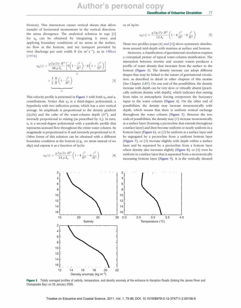
Figure 3 Tidally averaged profiles of salinity, temperature, and density anomChesapeake Bay) on 26 January 2005.


or of ∂η/∂x:

� 3 2 � g ∂η=∂x H2 z z

udðzÞ ¼ 1 − 4 − 6 ½5� 12Az H3 H2

These two profiles (eqns [4] and [5]) show symmetric distributions around mid-depth with maxima at surface and bottom.

Moreover, a classification of gravitational circulation requires a conceptual picture of typical water-column stratification. The interaction between riverine and oceanic waters produces a profile of water density that increases from the surface to the bottom (Figure 3). The density increase can adopt different shapes that may be linked to the nature of gravitational circulation, as described in detail in other chapters of this treatise (See Chapter 2.07). On one end of the possibilities, the density increase with depth can be very slow or virtually absent (practically uniform density with depth), which indicates that mixing from tides or atmospheric forcing overpowers the buoyancy input to the water column (Figure 4). On the other end of possibilities, the density may increase monotonically with depth, which means that there is uniform vertical exchange throughout the water column (Figure 5). Between the two ends of possibilities, the density may (1) increase monotonically at a surface layer (forming a pycnocline that extends throughout a surface layer) and then become uniform or nearly uniform in a bottom layer (Figure 6), or (2) be uniform at a surface layer and be segregated by a pycnocline from a uniform bottom layer (Figure 7), or (3) increase slightly with depth within a surface layer and be separated by a pycnocline from a bottom layer where density also increases slightly (Figure 8), or (4) even be uniform in a surface layer that is separated from a monotonically increasing bottom layer (Figure 9). It is the vertically sheared

2.0 2.5 3.0 3.5 4.0 Temperature (°C)

aly at the entrance to Hampton Roads (linking the James River and

1, 75-86, DOI: 10.1016/B978-0-12-374711-2.00106-6


Figure 4 Tidally averaged profiles of salinity, temperature, and density anomaly at St. Augustine Inlet, Florida, on 2 February 2006. Profiles illustrate essentially vertically mixed conditions.

gravitational circulation, as well as the vertical density distribution, that will be described for different types of basins in the discussions of this chapter.

Figure 5 Generic tidally averaged density profile illustrating uniformly stratif


1.05.2 Classification of Gravitational Circulation According to Estuarine Origin/Geomorphology

1.05.2.1 Coastal Plain/Drowned River Valley Estuaries

These are found mostly in temperate climates and are the most studied of all estuaries. Extensive studies have been reported in coastal plain, temperate estuaries in Japan, Australia, Europe, and North America. The gravitational circulation is typically well developed and vertically sheared, although it may be influenced by bathymetry (see Chapter 2.07). In these systems, the stress divergence that balances the pressure gradient arises mostly from tidal flows interacting with the bottom. Such interaction represents the main agent for vertical mixing of momentum and mass. In some cases, it is possible that mixing at the pycnocline, from internal stresses (or stresses within the water column around the pycnocline region), also contributes to balance the pressure gradient. Moreover, advective accelerations could influence the dynamics of the exchange flow. The density profile may acquire any of the configurations described in the previous paragraph (Figures 3–9).

1.05.2.2 Tectonic Estuaries

These estuaries operate dynamically in many ways that are similar to coastal plain estuaries. For instance, the processes and dynamics described in coastal plain estuaries apply, for the most part, to San Francisco Bay, a tectonic estuary. There are tectonic estuaries, however, like some rias in the northwest coast of Spain (e.g., Gilcoto et al., 2007), where the gravitational circulation is not as well developed as in coastal plain estuaries. This is because the circulation forced from the coast, typically during upwelling conditions, masks the gravitational circulation. Moreover, rias are deeper than coastal plain estuaries and therefore tidal currents tend to be weaker. This means that the bottom stress divergence is less effective in balancing the pressure gradient and the wind stress, together with Coriolis and advective accelerations, enter the dynamic picture. Depending on the season, the density profile may exhibit (1) a monotonically increasing

ied water column.

, 75-86, DOI: 10.1016/B978-0-12-374711-2.00106-6


Figure 6 Salinity, temperature, and density profiles at Reloncavi Fjord, Chile, on 10 March 2002, illustrating a surface stratified layer on top of a homogeneous water column (profiles extended to >100 m but density did not change appreciably below 20 m).

Figure 7 Generic tidally averaged density profile illustrating weakly stratified surface and bottom layers, separated by a pycnocline.

Treatise on Estuarine and Coastal Science, 2011, Vol. 1, 75-86, DOI: 10.1016/B978-0-12-374711-2.00106-6


Figure 8 Generic tidally averaged density profile illustrating mixed surface and bottom layers, separated by a pycnocline.

Figure 9 Generic tidally averaged density profile illustrating a mixed surface layer separated by a continuously stratified water column underneath.

density within a surface layer that is separated from a homogeneous bottom layer, or (2) a weakly varying distribution. This pattern that develops in rias is similar to what happens in fjords.

1.05.2.3 Fjords

These estuaries are the deepest and among the most stratified during the season of largest buoyancy input. The residual (or long-term) circulation may be interpreted as a gravitational circulation consisting of a thin (typically <0.3 of the water-column depth) surface layer flowing seaward and a sluggish, thick (often >0.7 of the water-column depth) bottom layer flowing landward. On the other hand, the residual circulation may also be interpreted as the result of a thin lens of seaward-flowing freshwater that overlays a rather sluggish basin. In the sluggish basin, underneath the freshwater lens,


the residual circulation arises from the rectification (nonlinear modification) of the tidal wave reflecting at the end of the fjord (e.g., Ianniello, 1977). This tidal distortion yields a two-layer or three-layer (depending on the specific geometry of the basin) residual flow, as observed in several fjords and channels of southern Chile (e.g., Valle-Levinson et al., 2007). The alternative interpretations of the residual circulation in fjords require further studies to resolve whether the residual circulation is driven by density gradients throughout the water column. Regardless of whether the residual circulation is density driven (gravitational) throughout the water column or not, it is likely that in fjords the pressure gradient is balanced mainly by advective accelerations with some contribution from Coriolis accelerations. It is also likely that internal friction becomes dynamically important in regions of geometry variations, where vertical excursions of the pycnocline will cause increased drag and energy

, 75-86, DOI: 10.1016/B978-0-12-374711-2.00106-6


dissipation. The density profile will typically exhibit a monotonically increasing density within a thin surface layer, separated from a homogeneous bottom layer that occupies most of the water column.

1.05.2.4 Bar-Built Estuaries

These estuaries tend to be shallow (a few meters deep) with weak river discharge and rapid dissipation of tidal energy as the tidal wave enters the estuary. They are mostly found in subtropical and temperate low-lying areas with little area for a well-developed river basin, that is, with small watershed areas. The gravitational circulation may be restricted to the area proximate to the source of freshwater but may not be vertically sheared in the rest of the system. Tidal currents and mixing are typically relevant at the transition with the ocean but become weak inside the basin. These systems are mostly driven by wind forcing but the dynamics remains between pressure gradient and friction, except that friction acts both at the surface, through wind stress, and at the bottom, through stresses produced by wind-driven currents. The density profile tends to be homogeneous or with weak vertical structure, as compared to the other types of estuaries.

1.05.3 Classification of Gravitational Circulation According to Water Balance

In the most generic way, estuarine circulation may be classified according to whether the net volume outflow, associated with the gravitational circulation, is larger or smaller than the net volume inflow. In positive or normal estuaries, there is a net

Land Ocean La

Dep

th

ρ ρ

Inverse

Land Ocean La

Dep

th

ρ ρ

Salt plug

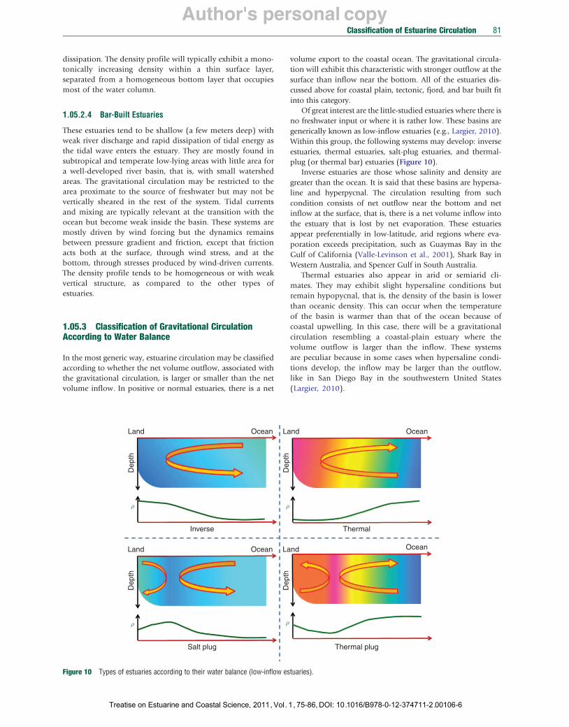
Figure 10 Types of estuaries according to their water balance (low-inflow es


volume export to the coastal ocean. The gravitational circulation will exhibit this characteristic with stronger outflow at the surface than inflow near the bottom. All of the estuaries discussed above for coastal plain, tectonic, fjord, and bar built fit into this category.

Of great interest are the little-studied estuaries where there is no freshwater input or where it is rather low. These basins are generically known as low-inflow estuaries (e.g., Largier, 2010). Within this group, the following systems may develop: inverse estuaries, thermal estuaries, salt-plug estuaries, and thermal-plug (or thermal bar) estuaries (Figure 10).

Inverse estuaries are those whose salinity and density are greater than the ocean. It is said that these basins are hypersaline and hyperpycnal. The circulation resulting from such condition consists of net outflow near the bottom and net inflow at the surface, that is, there is a net volume inflow into the estuary that is lost by net evaporation. These estuaries appear preferentially in low-latitude, arid regions where evaporation exceeds precipitation, such as Guaymas Bay in the Gulf of California (Valle-Levinson et al., 2001), Shark Bay in Western Australia, and Spencer Gulf in South Australia.

Thermal estuaries also appear in arid or semiarid climates. They may exhibit slight hypersaline conditions but remain hypopycnal, that is, the density of the basin is lower than oceanic density. This can occur when the temperature of the basin is warmer than that of the ocean because of coastal upwelling. In this case, there will be a gravitational circulation resembling a coastal-plain estuary where the volume outflow is larger than the inflow. These systems are peculiar because in some cases when hypersaline conditions develop, the inflow may be larger than the outflow, like in San Diego Bay in the southwestern United States (Largier, 2010).

nd Ocean

Dep

th

Thermal

nd Ocean

Dep

th

Thermal plug

tuaries).

1, 75-86, DOI: 10.1016/B978-0-12-374711-2.00106-6


Salt-plug estuaries are a combination of inverse and positive estuaries. These develop in relatively shallow basins of semiarid or strongly seasonal climates where a river reaches the coast. During the dry season, the river discharge is low but a positive estuary is still present around the area where the river enters the estuary. In the rest of the basin, hypersaline and inverse conditions develop, creating a region of maximum salinity within the estuary. This region of maximum salinity acts as a salt plug that separates a zone of positive gravitational circulation near the river/estuary area and a zone of inverse gravitational circulation between the salt plug and the coastal ocean. The salt plug should have important water-quality conditions as it effectively acts as a barrier for the flushing of the estuarine region. Examples of systems similar to this one are found in Alligator River, Northern Territory of Australia, and the Gulf of Fonseca in the Pacific side of Central America (Valle-Levinson and Bosley, 2003).

Thermal-plug estuaries are analogous to salt-plug estuaries. They may develop transitionally from a thermal estuary that becomes hypersaline and inverse near its landward end. Thus, the landward portion of the estuary will exhibit inflow at surface and outflow near the bottom, whereas the seaward portion will exhibit outflow at the surface and inflow at depth. The convergence of bottom flows toward the landward end of the estuary will represent a thermal plug that also acts as a barrier for flushing. These systems are much less documented, but San Diego Bay is thought to show these properties (Largier, 2010).

1.05.4 Classification of Gravitational Circulation According to the Competition between Tidal Flow and River Discharge

Traditionally, estuaries may be classified as vertically homogeneous, weakly stratified or partially mixed, and highly stratified. This classification has been proposed on the basis of the competition between tidal forcing and buoyancy forcing. The key of this classifying idea is how to characterize tidal and buoyancy forcing. One way of assessing tidal forcing is through the tidal prism volume, and a way of evaluating buoyancy forcing in estuaries dominated by freshwater input is by the volume of the river discharged. Tidal prism is the volume of water that enters the estuary with every tidal cycle. It equals the tidal range multiplied by the surface area of the basin. Therefore, much larger tidal prisms than freshwater volumes, more than one order of magnitude larger, will result in weakly stratified or vertically homogeneous estuaries. In these estuaries, the gravitational circulation may be vertically sheared or horizontally sheared, depending on the geometry of the basin (see Chapter 2.07).

When the tidal prism is of the order of the freshwater volume or slightly larger, the estuary will be partially mixed. These estuaries support the strongest longitudinal density gradients because of the active mixing, albeit not sufficiently energetic to homogenize the basin. In this case, the gravitational circulation is most robust because of the strength of the horizontal density gradients. Many temperate estuaries may fit into this category.

Finally, when the freshwater volume overwhelms the tidal prism, by one or more orders of magnitude, strong stratification will ensue. This will cause well-developed gravitational


circulation but not as robust as in partially mixed estuaries because the longitudinal density gradients will be weaker. Moreover, the vertical exchange of properties is hindered by the presence of a pycnocline. These estuaries are found in wet climates.

Once again, it is pertinent to raise caution about this type of classification. Any given estuary may show every characteristic or type as seasonal forcing changes. It may also change from spring to neap tides or even from flood to ebb phases of the tidal cycle.

In the widely used classification of estuaries based on a circulation/stratification diagram (Hansen and Rattray, 1966), the nature of both the gravitational circulation and the water stratification are used to classify an estuary. This classification does not describe the gravitational circulation but uses it to characterize the estuary. A detailed explanation of this classification is presented in most texts that deal with estuaries and the reader is referred to those explanations (e.g., Valle-Levinson, 2010). In essence, the gravitational circulation is described as a circulation parameter uf, which is the ratio between the net surface outflow speed us and the cross-sectional average of the net flow uc. When the gravitational circulation is well developed, the net outflow will be similar to the net inflow in such a way that uc tends to zero. In this case of well-developed gravitational circulation, the circulation parameter uf will tend to infinity, that is, it becomes a large number. When the gravitational circulation is weak, the net surface outflow is nearly representative of the entire cross-sectional average flow in which case uf tends to 1.

The stratification of the estuary is characterized by the stratification parameter Sp, which is the ratio between the top-tobottom salinity difference ΔS and the cross-sectional mean of salinity S0. The values of Sp range from nearly zero for a mixed estuary to near 1, for a highly stratified estuary. On the basis of its values of uf and Sp, an estuary may be strongly stratified, partially mixed, mixed, or salt wedge. However, in order to characterize the estuary, these diagnostic parameters are needed. In other words, by the time the values of uf and Sp

are determined, the type of estuary is already known. Arguably, a more useful approach is a prognostic scheme in

which simple estuarine properties such as the tidal current amplitude and the river discharge velocity are used to characterize the estuary and the nature of the circulation. This approach has been proposed independently by Prandle (2009) and Geyer (2010). In essence, Geyer’s approach predicts the stratification of the estuary ΔS, normalized by a reference salinity S0, as a function of tidal current amplitude UT and river velocity Ur:

ΔS Ur4=5

¼ 10 ½6� S0

2=5U ðβgS0hÞ1=5 T

where β is the coefficient of haline contraction (7.7 � 10−4), g is the acceleration caused by gravity, and h is the water-column depth. Contours of normalized stratification are shown in Figure 11 for a range of commonly observable Ur and UT. The upper right corner of the parameter space characterizes estuaries that are short and flush quickly, such as salt-wedge estuaries with strong tidal forcing (e.g., Columbia River in Washington/Oregon and Merrimack River in Massachusetts, both in the United States). The lower left corner of Figure 11 includes long- and slow-flushing estuaries. Moreover, the upper part of the parameter space in the ordinate, that of

, 75-86, DOI: 10.1016/B978-0-12-374711-2.00106-6


Long slow flushing

Partially mixed

Highly stratified 1.000

0.100

0.010

0.001

Short rapid flushing

Well mixed

U

r (m

s−1

) 1

UT (m s−1)

Figure 11 Stratification contours obtained from the relation that includes the influence of tidal flows (abscissa) and river flows (ordinate). Only the contours that approximately separate stratified from mixed estuaries are shown. Modified from Geyer, R.W., 2010. Estuarine salinity structure and circulation. In: Valle-Levinson, A. (Ed.), Contemporary Issues in Estuarine Physics. Cambridge University Press, Cambridge, pp. 12–26.
large river velocities, characterizes highly stratified estuaries such as the Mississippi River for weak tidal currents. The lower part of the ordinate illustrates vertically homogeneous estuaries, such as the Delaware River, and the middle portion of the ordinate includes partially mixed estuaries such as the James River and the Hudson River. This approach provides a rough characterization of processes in estuaries but does not take into account temporal or spatial variations in the particular systems. Further research is needed to determine other variables that should enter this scheme.
1.05.5 Estuarine Circulation

The introductory part of this chapter mentions that estuarine circulation ue can be regarded as the sum of the gravitational circulation ug, the tidal residual circulation ut, and the

(a) (b)

0 5 6

4 3 7

2 8 1 10 12

9 11

Dep

th (

m)

−5

911 1 812

7 −10

−1 −0.5 0 0.5 1 1.5 0 1010−

u (m s−1) Az

Figure 12 Numerical results from an idealized flat bottom estuary for which laContinuous lines are for flood phases. (a) Evolution of tidal velocity profiles thviscosity profiles through the tidal cycle. (c) Evolution of the stress profiles thro2011. A numerical study of residual circulation induced by asymmetric tidal mC01017, doi:10.1029/2010JC006137.


circulation induced by asymmetric tidal mixing ua. Up tothis point, discussions have concentrated on ug but ut and ua

will now be presented for idealized vertically mixed, weakly stratified, and strongly stratified estuaries, following the results of Cheng et al. (2010). Tidal residual flows develop from distortions on the tidal signal as it enters semi-enclosed systems. The distortions cause stronger floods than ebbs, or vice versa, which result in residual flows. In turn, tidal asymmetries in vertical mixing are illustrated in Figure 12. Asymmetric distributions from flood to ebb of eddy viscosity and stress (therefore stress divergence) profiles show larger values in flood than in ebb. The stronger mixing in flood than ebb is also related to asymmetric velocity profiles at both phases of the tidal cycle. These asymmetries produce a residual flow that can either enhance or compete against gravitational circulation. In a vertically well-mixed estuary with a horizontal density gradient, ug is

(c)

56 3 42

10

12 1034 2 5 1 6 7 8 11 9

20 −10 −5 0 5 10 3 (m2 s−1) Shear stress 10−4 (Pa)

teral variations are neglected. Numbers indicate hours after the end of ebb. roughout the tidal cycle. Positive is seaward. (b) Evolution of the eddy ughout the tidal cycle. From Cheng, P., Valle-Levinson, A., de Swart, H.E., ixing in tidally dominated estuaries, Journal of Geophysical Research 116,

1, 75-86, DOI: 10.1016/B978-0-12-374711-2.00106-6


1.2 1.6

0.8

0

−2

−2

−2

4

8

8

35

15

10

25

5

0

−5

−5

15

5

0

20

30

12 12 12

2

4 8

4 8

4

0

2016

12

−4

8−

−8 −4

2015

10

−5

−5

0

−10

3025 10 5

0 6

ud 8 6

ur

0−4

0 D

epth

(m

) D

epth

(m

)D

epth

(m

)

−8 0.8

0.4 0

uaut

−4

−8 4

0 35

+ ud + ut + uur ua

−4 5 0

−8

240 260 280 240 260 280 x (km) x (km)

84 Classification of Estuarine Circulation

Figure 13 Along-estuary distributions, derived from a numerical model, of the different mechanisms that produce estuarine circulation and of tidally averaged flow in an idealized vertically mixed estuary. Shaded contours indicate negative flows (inflows) cm s−1. The bottom right panel is the straight tidal average, whereas the bottom left panel is the sum of each individual contribution. From Cheng, P., Valle-Levinson, A., de Swart, H.E., 2011. A numerical study of residual circulation induced by asymmetric tidal mixing in tidally dominated estuaries, Journal of Geophysical Research 116, C01017, doi:10.1029/2010JC006137.

as expected, with surface outflow and bottom inflow (Figure 13). The strongest gravitational circulation occurs at the region of the estuary with largest horizontal density gradient, which is near the estuary mouth. Tidal residual flows ut indicate net outflow throughout the water column with a similar distribution to ur, indicating that tidal residual flows enhance the gravitational outflow but oppose the gravitational inflow. By contrast, tidal asymmetries in mixing produce a residual circulation ua that reinforces gravitational circulation. It even has a larger magnitude than ug and is strongest at the mouth, where the asymmetries in mixing and tidal currents are largest in the estuary. The sum of all contributions to ue, as in eqn [1], is essentially the same as the straight tidal average of tidal flows along the idealized estuary. Therefore, in a vertically mixed estuary, the estuarine circulation can be reliably represented as the linear combination of the four contributors discussed.

In a weakly stratified estuary, the main driver of estuarine circulation that is markedly modified is the circulation produced by tidal asymmetries in mixing (Figure 14). In this case, ua exhibits a three-layered structure in the estuarine region (where the density driven flow is most robust), representing


inflow at surface and bottom. Therefore, ua competes with gravitational circulation in portions of the water column but reinforces ug in others. The magnitude of ua is similar to that of ud and therefore it is still relevant. Once again, in a weakly stratified estuary, the estuarine circulation can be dependably represented as the linear superposition of different mechanisms.

In a strongly stratified estuary (Figure 15), ut and ua are different from the other two types of estuaries. The tidal residual flow shows a two-layered pattern that opposes the density-driven flow. Similarly, the flow driven by tidal asymmetries in mixing opposes the density-driven flow in most of the water column but reinforces it near the bottom. It can be seen that the linear superposition of the four mechanisms is a good representation of the estuarine circulation. There is no doubt that the mechanism that drives ua should be important in estuaries and its influence requires more detailed observational scrutiny. A relevant concept advanced in this chapter is that estuarine circulation ue is not necessarily the same as gravitational circulation ug. As discussed above, ue and ug will be the same only if the flows produced by tidal rectification and tidally asymmetric mixing are negligible.

, 75-86, DOI: 10.1016/B978-0-12-374711-2.00106-6


0

ur ud

uaut

ur + ud + ut + ua u

Dep

th (

m)

Dep

th (

m)

Dep

th (

m)

−4

−8

0

−4

−8

0

−4

−8

220 240 260 280 220 240 260 280 x (km) x (km)

Classification of Estuarine Circulation 85

Figure 14 Same as Figure 13 but for a weakly stratified estuary. From Cheng, P., Valle-Levinson, A., de Swart, H.E., 2011. A numerical study of residual circulation induced by asymmetric tidal mixing in tidally dominated estuaries, Journal of Geophysical Research 116, C01017, doi:10.1029/ 2010JC006137.

Figure 15 Same as Figure 13 but for a strongly stratified estuary. From Cheng, P., Valle-Levinson, A., de Swart, H.E., 2011. A numerical study of residual circulation induced by asymmetric tidal mixing in tidally dominated estuaries, Journal of Geophysical Research 116, C01017, doi:10.1029/ 2010JC006137.

Dep

th (

m)

Dep

th (

m)

Dep

th (

m)

0

ur ud

uaut

ur + ud + ut + ua

−4

−8

0

−4

−8

−4

−8

240 260 280x (km) x (km)

260 280240

0

0

u

1

2

4 8 1616

12

4

4

3026

10

5

20

15

25

20

20

3

5

0

−5

−5−5

0

−5

−5−10

−5

05

5

10 1520

253035

−50

5 55

0

5101

5

20−15

−3

−3

−3

−50−5−10

0

036

8

0

1518 1215

Treatise on Estuarine and Coastal Science, 2011, Vol. 1, 75-86, DOI: 10.1016/B978-0-12-374711-2.00106-6


References

Cheng, P., Valle-Levinson, A., de Swart, H.E., 2011. A numerical study of residual circulation induced by asymmetric tidal mixing in tidally dominated estuaries, Journal of Geophysical Research 116, C01017, doi:10.1029/2010JC006137.

Geyer, R.W., 2010. Estuarine salinity structure and circulation. In: Valle-Levinson, A. (Ed.), Contemporary Issues in Estuarine Physics. Cambridge University Press, Cambridge, pp. 12–26.

Gilcoto, M., Pardo, P.C., Álvarez-Salgado, X.A., Pérez, F.F., 2007. Exchange fluxes between the Rı´a de Vigo and the shelf: a bidirectional flow forced by remote wind. Journal of Geophysical Research 112, C06001. doi: 10.1029/2005JC003140.

Hansen, D.V., Rattray, M., Jr., 1966. New dimensions in estuary classification. Limnology and Oceanography 11, 319–325.

Ianniello, J.P., 1977. Tidally induced residual currents in estuaries of constant breadth and depth. Journal of Marine Research 35, 755–786.

Largier, J., 2010. Low-inflow estuaries: hypersaline, inverse and thermal scenarios. In: Valle-Levinson, A. (Ed.), Contemporary Issues in Estuarine Physics. Cambridge University Press, Cambridge, pp. 247–272.

Officer, C.B., 1976. Physical Oceanography of Estuaries (and Associated Coastal Waters). Wiley, New York, NY, 465 pp.


Prandle, D., 2009. Estuaries: Dynamics, Mixing, Sedimentation and Morphology. Cambridge University Press, Cambridge, 246 pp.

Pritchard, D.W., 1956. The dynamic structure of a coastal plain estuary. Journal of Marine Research 15, 33–42.

Stacey, M.T., Fram, J.P., Chow, F.K., 2008. Role of tidally periodic density stratification in the creation of estuarine subtidal circulation. Journal of Geophysical Research 113, C08016. doi: 10.1029/2007JC004581.

Valle-Levinson, A. (Ed.), 2010. Definition and classification of estuaries. In: Contemporary Issues in Estuarine Physics. Cambridge University Press, Cambridge, pp. 1–11.

Valle-Levinson, A., Bosley, K.T., 2003. Reversing circulation patterns in a tropical estuary. Journal of Geophysical Research 108 (C10), 3331. doi: 10.1029/ 2003JC001786.

Valle-Levinson, A., Delgado, J.A., Atkinson, L.P., 2001. Reversing water exchange patterns at the entrance to a Semiarid Coastal Lagoon. Estuarine, Coastal and Shelf Science 53, 825–838.

Valle-Levinson, A., Sarkar, N., Sanay, R., Soto, D., León, J., 2007. Spatial structure of hydrography and flow in a Chilean Fjord, Estuario Reloncaví. Estuaries and Coasts 30 (1), 113–126.

, 75-86, DOI: 10.1016/B978-0-12-374711-2.00106-6

Provided for non-commercial research and educational use. …arnoldo/ftp/papers/ESCO_00… · · 2012-04-06Not for reproduction, distribution or commercial use. ... 2010). This

Documents