Monographs of the School of Doctoral Studies in Environmental Engineering Doctoral School in Environmental Engineering Building skin as energy supply: Prototype development of a wooden prefabricated BiPV wall Laura Maturi Department of Civil, Environmental and Mechanical Engineering in cooperation with Institute for Renewable Energy 2013 Supervisors: Prof. Paolo Baggio, Ing. Roberto Lollini, Ing. Wolfram Sparber

Welcome message from author
This document is posted to help you gain knowledge. Please leave a comment to let me know what you think about it! Share it to your friends and learn new things together.
Transcript

Monographs of the School of Doctoral Studies in Environmental Engineering
Doctoral School in Environmental Engineering
Building skin as energy supply:
Prototype development of a wooden prefabricated BiPV wall
Laura Maturi
Department of Civil,
Environmental and Mechanical Engineering
in cooperation with
Institute for Renewable Energy
2013
Supervisors: Prof. Paolo Baggio, Ing. Roberto Lollini, Ing. Wolfram Sparber

Doctoral thesis in Environmental Engineering, XXV cycle
Faculty of Engineering, University of Trento
Academic year 2012/13
Supervisors: Prof. Paolo Baggio, University of Trento
Ing. Roberto Lollini, Eurac
Ing. Wolfram Sparber, Eurac
University of Trento
Trento, Italy
2013


To Francesco
and Agostino
-With love-


Acknowledgements
The author would like to thank the following people for their assistance and
contribution during the course of this study:
My promoters Prof. Paolo Baggio, Ing. Roberto Lollini, Ing. Wolfram Sparber
who have supported and guided my activities.
The Network Chi Quadrato with FESR for the realization of the prototype, and
IEA Task 41 “Solar Energy and Architecture” experts.
My colleagues at EuracTec, who contributed actively in supporting my
activities, without whom this work would not exist: Roberto Lollini again, for
his constant and active presence during all the thesis development, Paolo
Baldracchi for his essential help in all fields (energy simulations, test in
laboratory, data elaboration), David Moser for the precious support to improve
the results of this work and for revising the thesis in a very effective way [see
Lollini-Moser plot], Stefano Avesani and Alessia Giovanardi for their
contribution during the test and for all interesting discussions, Ludwig
Kronthaler for his smart way to always find proper solutions to any problem
during the test in SoLaRE-PV lab, Walter Bresciani for the nice electrical
cabinet, Giorgio Belluardo for the “ABD data”, Ulrich Filippi for the
“mathematical discussions”, Radko Brock for the experiments suggestions,
David Cennamo for the software elaboration, Matteo Del Buono for his inputs
and suggestions, Siegfried from Stahlbau Pichler for the precious technical
support, Alessandra Colli for her enthusiasm in encouraging me and for the
many international contacts she managed to create and bring in our group,
Lorenzo Fanni for the help with resistors and many issues, Miglena Dimitrova for
the discussions and support. All my colleagues and former colleagues at Eurac,
who have created a warm and friendly working environment: Francesco2 of
course, Patrizia, Gabriella, Cristiana, Alexa, Francesca, Chiara, Giulia,
Annamaria, Elisabetta, Marco, Roberto V., Hannes, Davide, Matteo D., Dagmar,
Federico, Monika, Marina, Alexandra, Filippo, Roberto F., Daniele, Adriano,
Philip, Simon, Anton, Alice, Alessio, Florian, Markus.
My special friends Federica, Silvia, Maria, Serena and Michele.
Finally, special thanks to my parents, to Francesca with Roberto and Fabiano
with Claudia. Grazie!


i
TABLE OF CONTENTS
TABLE OF CONTENTS ...................................................................... i
LIST OF FIGURES ........................................................................... vi
LIST OF TABLES .......................................................................... xiii
LIST OF SYMBOLS ......................................................................... xv
ABSTRACT ................................................................................ xvii
CHAPTER 1 Introduction ................................................................. 1
1.1 Introduction ..................................................................... 3
1.2 Thesis structure ................................................................ 5
References ............................................................................. 7
CHAPTER 2 State of the art ............................................................. 9
2.1 PV technological integration into the envelope .......................... 11
2.2 PV topological integration into the envelope ............................ 13
2.2.1 Roof integration ...................................................... 13
2.2.2 Façade integration ................................................... 16
2.2.3 Façade vs roof integration .......................................... 18
2.3 Limitations, needs and IEA Task 41 recommendations .................. 19
References ............................................................................ 21
CHAPTER 3 Prototype development .................................................. 23
3.1 Introduction .................................................................... 25
3.2 Development process methodology ........................................ 26
ii
3.3 Concept ......................................................................... 28
3.3.1 Integration concept .................................................. 29
3.3.2 Multi-functionality concept ........................................ 30
3.3.3 Sustainability concept ............................................... 31
3.3.4 Prefabrication concept .............................................. 32
3.4 Theoretical study ............................................................. 33
3.4.1 PV technology and integration issues ............................. 33
3.4.2 PV performance ...................................................... 41
3.4.3 Building performance ............................................... 53
3.5 Prototype design .............................................................. 63
3.6 Prototype application ........................................................ 64
References ............................................................................ 68
CHAPTER 4 Experimental campaign .................................................. 73
4.1 Introduction .................................................................... 75
4.2 INTENT Lab ..................................................................... 77
4.2.1 Measurement sensors ................................................ 79
4.3 SoLaRE-PV Lab ................................................................. 80
4.3.1 Measurement sensors ................................................ 81
4.4 The use of INTENT and SoLaRE-PV Labs (phase 2&3) .................... 82
4.5 The specimen .................................................................. 83
4.5.1 Specimen construction drawing ................................... 83
4.5.2 Specimen construction: the industrial collaboration ........... 84
4.6 Phase 1: “Bi” characterization .............................................. 85
4.6.1 Aim of the test ....................................................... 85
4.6.2 Experimental setup .................................................. 87

iii
4.6.3 Results ................................................................. 88
4.7 Phase 2: “PV” characterization ............................................. 89
4.7.1 Aim of the test ....................................................... 89
4.7.2 Experimental setup .................................................. 90
4.7.3 PV module preconditioning ......................................... 90
4.7.4 Results ................................................................. 93
4.8 Phase 3: “PV in Bi” characterization ...................................... 97
4.8.1 Aim of the test ....................................................... 97
4.8.2 Experimental setup .................................................. 98
4.8.3 Results ............................................................... 102
References .......................................................................... 111
CHAPTER 5 Test results and discussion ............................................ 113
5.1 Introduction .................................................................. 115
5.2 “Bi” performance ........................................................... 116
5.3 PV” performance ............................................................ 117
5.3.1 BiPV façade system: Ex-Post Building........................... 117
5.3.2 BiPV roof system: Milland Church ............................... 120
5.3.3 Ground mounted PV system: ABD PV plant .................... 123
5.3.4 BiPV wall prototype................................................ 127
5.3.5 Performance comparison with BiPV wall prototype .......... 129
5.3.6 Generalization of results over one year time period ......... 132
5.4 Further PV performance improvement due to fins application ...... 137
5.4.1 Generalization of results to other PV technologies........... 139
5.4.2 Generalization of results over one year time period ......... 145
References .......................................................................... 149

iv
CHAPTER 6 Summary, conclusions and future development ................. 151
6.1 Summary ...................................................................... 153
6.1.1 Concept .............................................................. 153
6.1.2 Theoretical study .................................................. 154
6.1.3 Prototype design and application ............................... 156
6.1.4 Experimental campaign ........................................... 156
6.2 Conclusions ................................................................... 160
6.2.1 General achievement .............................................. 160
6.2.2 Experimental approach ........................................... 160
6.2.3 “Bi” performance .................................................. 161
6.2.4 Effectiveness of the BiPV prototype configuration ........... 161
6.2.5 Influence of “PV” on “Bi” and of “Bi” on “PV” ............... 163
6.2.6 Explicit correlation for façade integrated PV operating
temperature ................................................................. 164
6.2.7 NOCT model vs experimental data .............................. 165
6.2.8 Factors influencing effectiveness of fins application ........ 165
6.2.9 Effectiveness of fins application in the prototype ............ 166
6.2.10 Estimated effectiveness of fins application for different PV
technologies ................................................................. 167
6.3 Research limitations and future developments ........................ 168
BIBLIOGRAPHY .......................................................................... 171
ANNEXES ................................................................................. 181
Annex A .............................................................................. 183
Drawing of INTENT calorimeter ........................................... 186
Sensors positioning –phase 1- ............................................. 187

v
Sensors positioning –phase 3- ............................................. 189
Measurements of phase 2 .................................................. 191
Annex B .............................................................................. 195
Outdoor temperature coefficients of six different technologies .... 197
Annex C .............................................................................. 199
IEA Task 41 project “Solar Energy and Architecture” ................. 201
FP7 project “Solar Design - On-the-fly alterable thin-film solar
modules for design driven applications” ................................ 207

vi
LIST OF FIGURES
Figure 2.1: Solar laminate integrated into metal roof system. .................... 13
Figure 2.2: Left: Schüco façade SCC 60 and its application. Right: Schüco
façade module ProSol TF and its application, © Schüco ..................... 13
Figure 2.3: roof systems: Solar tile © SRS Sole Power Tile, Solar slate ©
Megaslate, Solar slate © Sunstyle Solaire France ............................. 14
Figure 2.4: Left: special rack system for flexible laminate on stainless steel
substrate, © Unisolar. Centre: Powerply monocrystalline module with
plastic substrate © Lumeta, Right: Biohaus, Germany, plastic
substrate, © Flexcell. ............................................................. 15
Figure 2.5: semi-transparent skylights. Left: Community Center Ludesch,
Austria, Herman Kaufmann: semi-transparent modules with crystalline
cells © Kaufmann. Right: Würth Holding GmbH HQ: semi-transparent
thin film modules © Würth Solar. ............................................... 16
Figure 2.6: PV facade cladding solutions. Left: Soltecture Solartechnik
GmbH, Berlin, Germany, © Soltecturel. Right: Paul-Horn Arena,
Tübingen, Germany, Alman-Sattler-Wappner, © Sunways. ................. 17
Figure 2.7: warm façade solution. Zara Fashion Store, Cologne, Germany,
Architekturbüro Angela und Georg Feinhals: opaque monocrystalline
cells combined with transparent glazing in post-beam curtain wall
structure, © Solon. ................................................................ 17
Figure 2.8: Left: Schott Headquarter Mainz, translucent thin film module, ©
Schott; right: GreenPix Media Wall, Beijing, China, Simone Giostra &
Partners, frameless modules with spider glazing system, © Simone
Giostra & Partners/Arup. ......................................................... 18
Figure 2.9: How the orientation affects BiPV installation in Europe [2.1] ....... 19
Figure 2.10: Comparison of the monthly sun radiation available on a 33°
south exposed optimal tilted surface vs. a vertical south exposed
surface in Zurich, Switzerland (Middle Europe latitude). ................... 19
Figure 3.1: Process that guided the development of the BiPV prototype, from
the concept to the construction. ................................................ 27

vii
Figure 3.2: Conceptual schema of the four key concepts that originated the
prototype development. .......................................................... 28
Figure 3.3: multi-layering concept: the prototype is conceived as a wall
package made of several layers with several functions. .................... 30
Figure 3.4: Conceptual schema: the building envelope could be conceived
not only as a passive component which provides protection from the
outside conditions, but also as an active system able to produce
energy. .............................................................................. 31
Figure 3.5: Example of prefabricated wooden panels during manufacturing
phase (on the left) and installation on site (on the right, [source:
Promolegno]) ....................................................................... 32
Figure 3.6: Colour palette for monocrystalline cells, © System Photonics ...... 38
Figure 3.7: Multicrystalline silicon wafers; first the blue antireflective
standard color with the best efficiency, the second is the original
wafer without reflective layer, then cells with other colours that have
different anti-reflective layers, © Sunways ................................... 38
Figure 3.8: Coloured thin film modules in reddish brown, chocolate-brown,
hepatic and sage green colour, © Rixin ........................................ 38
Figure 3.9: Different PV module typologies, which originate different
textures [source: Eurac, ABD experimental PV plant] ....................... 39
Figure 3.10: Horizontal section of three wooden prefabricate wall types ...... 40
Figure 3.11: multifunctional characteristics of the BiPV prototype, based on
[3.13] reccomandations ........................................................... 41
Figure 3.12: Vertical section of the specimen with the schema of the natural
ventilation concept: the air in the gap cools the PV modules .............. 44
Figure 3.13: examples of CPU heat-sinks. On the right: a fan-cooled heat sink
on the processor of a personal computer with a smaller heat sink
cooling another integrated circuit of the motherboard ..................... 45
Figure 3.14: different geometry configurations of the air gap behind the PV
module, as investigated by Friling et al. [3.28] and Tonui et al. [3.14] .. 46
Figure 3.15: the zoom shows the L shape of the aluminium fin attached to
the back side of the PV modules ................................................ 47
Figure 3.16: The pictures show the fins applied on a 6mm glass. ................ 48

viii
Figure 3.17: temperature distribution of the PV module simulated with the
FEM software THERM (developed by Lawrence Berkeley National
Laboratory). ........................................................................ 49
Figure 3.18: temperature distribution of the PV module simulated with the
FEM software THERM (developed by Lawrence Berkeley National
Laboratory) ......................................................................... 51
Figure 3.19: The images show the temperature distribution of the PV module
with and without attached metal fin, simulated with the FEM software
THERM (developed by Lawrence Berkeley National Laboratory) in
average summer conditions (as described in Table 3.2). .................... 52
Figure 3.20: The images show the temperature distribution of the PV module
with and without attached metal fin, simulated with the FEM software
THERM (developed by Lawrence Berkeley National Laboratory) in
average winter conditions (as described in Table 3.2). ..................... 52
Figure 3.21: the U-value (i.e. thermal transmittance) calculated considering
the prototype with and without PV modules. ................................. 56
Figure 3.22: dimensions of each layer of the prototype ............................ 58
Figure 3.23: schema of the considered sections a, b, c and d ..................... 59
Figure 3.24: Schema of the considered resistances to calculate the upper
limit of the total thermal resistance ........................................... 59
Figure 3.25: schema of the considered layers of the prototype ................... 61
Figure 3.26: Schema of the considered resistances to calculate the lower
limit of the total thermal resistance ........................................... 61
Figure 3.27: design of the frontal view and horizontal section of the
prototype. The horizontal section is made of the following layers : ...... 63
Figure 3.28: preliminary hypothesis for the BiPV wall prototype positioning. .. 65
Figure 3.29: Visibility: module aesthetical perception vs observer position. ... 66
Figure 3.30: Rendering of the elementary school that was designed as a
prototypal building within the project “Chi Quadrato” ..................... 66
Figure 3.31: architectural drawings and details of the BiPV wall prototype
integrated in the elementary school design. .................................. 67
Figure 4.1: The diagram shows the organization of the experimental
campaign, which is divided into three phases................................. 76

ix
Figure 4.2: INTENT Lab at Eurac: the calorimeter with the sun simulator and
the hydraulic circuit ............................................................... 78
Figure 4.3: general schema of INTENT lab, which is made of. .................... 78
Figure 4.4: PV-SoLaRE Lab at Eurac: the sun simulator and the climatic
chamber ............................................................................. 81
Figure 4.5: The diagram shows the concept behind the organization of the
experimental campaign related to phase 2 and 3. ........................... 82
Figure 4.6: frontal view and horizontal section of the specimen (see annex A
for further details) ................................................................. 83
Figure 4.7: The specimen built by two enterprises belonging to the network
Chi-Quadrato. ...................................................................... 84
Figure 4.8: guarded hot box as foreseen by the UNI EN ISO 8990 [3.1], where:
1 is the metering box, 2 is the guarded box, 3 is the cold chamber and
4 is the specimen. ................................................................. 85
Figure 4.9: calibration and surrounding panel in the frame of the guarded
hot-box .............................................................................. 86
Figure 4.10: drawing of the calorimeter with the specimen during test of
phase 1. ............................................................................. 87
Figure 4.11: Normalized Pmax (i.e. normalized to the value of Pmax at M1,
before light soaking) against light-soaking cycles referred to the no-fins
CIGS module (NF) and the CIGS module with fins (WF). ..................... 92
Figure 4.12: Surface that interpolate the measured maximum power point
values of the module without fins (NF) at different temperature and
Irradiance conditions. ............................................................. 94
Figure 4.13: Measured maximum power point values of the module with fins
(WF) at different temperature and Irradiance conditions. .................. 94
Figure 4.14: Pmppt values of the module no fins at 1000W/sqm (AM 1.5) as
function of the device temperature (over a range of 50°C) with a least-
squares-fit curve through the set of data. ..................................... 95
Figure 4.15: γ and γrel of the NF and WF modules are plotted for each
irradiance value (AM 1.5) from the measured Pmppt values ............... 97
Figure 4.16: test devices used during experiments of phase 3 .................. 100
Figure 4.17: Positioning of the temperature, air velocity and irradiance
sensors during the third phase of the experimental campaign ........... 101

x
Figure 4.18: Measured average values of modules temperature (NF and WF)
at twenty different set point conditions of air temperature and
irradiance. ........................................................................ 102
Figure 4.19: I-V characteristic curve of the WF module (above, on the left),
the NF module (above, on the right) and of both modules connected in
series (below) measured with a peak power measuring device with I-V-
Curve tracer at an irradiance of 797W/sqm. ................................ 103
Figure 4.20: Measured average values of modules temperature (NF and WF)
and resulting ΔT between them at twenty different set point
conditions of air temperature and irradiance, after applying the
filtering procedure to eliminate transient points. .......................... 104
Figure 4.21: test boundary conditions of air velocity, air temperature and
irradiance kept in the calorimeter cold chamber during the
experiment. ....................................................................... 105
Figure 4.22: test boundary conditions of air temperature and air velocity
measured in the air gap between the modules and the wooden wall
during the experiment. ......................................................... 105
Figure 4.23: Approximated surface through the average T measured values of
the two modules depending on Tair and Irradiance. ....................... 106
Figure 4.24: Approximated surface through the ΔT measured data depending
on Tair and Irradiance. .......................................................... 108
Figure 4.25: AM1.5 spectrum and corresponding spectral response of
different solar cell materials. The spectral response of various
materials is indicated by the boxes [4.12] ................................... 109
Figure 5.1: Schema linking the two test phases. .................................. 115
Figure 5.2: Pictures of Ex Post Building with a schema of the building plant
showing the pictures point of view [source of pictures: www.expost.it] 117
Figure 5.3: mounting system of the modules integrated in the Ex Post
building façade [source: Elpo] ................................................. 118
Figure 5.4: Module (Tmod) and air (Tair) temperature difference against
Irradiance values and least-squares-fit line through the set of data
(with additional constraint Tmod-Tair=0 when Irr=0), referred to Ex-Post
BiPV system ....................................................................... 119

xi
Figure 5.5: Picture of the roof integrated PV system of the Milland Church in
Bressanone (North of Italy) ..................................................... 120
Figure 5.6: On the left: picture of the BiPV system highlighting the inlet and
outlet air gap sections. On the right: zoom which shows the reduced
air gap section .................................................................... 121
Figure 5.7: Module (Tmod) and air (Tair) temperature difference against
Irradiance values and least-squares-fit line through the set of data
(with additional constraint Tmod-Tair=0 when Irr=0), referred to Milland
Church BiPV system. ............................................................. 122
Figure 5.8: ABD PV Plant. Experimental plant on the left and commercial
part on right ...................................................................... 123
Figure 5.9: meteo station at ABD PV Plant ......................................... 124
Figure 5.10: The analysed PV systems at ABD: mono-crystalline back-contact
technology [source:Eurac]. ..................................................... 125
Figure 5.11: schema of the positioning of the two PT100 on the back side of
the modules [source:Eurac]. ................................................... 125
Figure 5.12: Module (Tmod) and air (Tair) temperature difference against
Irradiance values and least-squares-fit line through the set of data
(with additional constraint Tmod-Tair=0 when Irr=0), referred to the
mono-crystalline back-contact technology at ABD plant. ................. 126
Figure 5.13: Module (Tmod) and air (Tair) temperature difference against
Irradiance values and least-squares-fit line through the set of data
(with additional constraint Tmod-Tair=0 when Irr=0), referred to the NF
module of the BiPV wall prototype. .......................................... 127
Figure 5.14: Module (Tmod) and air (Tair) temperature difference against
Irradiance values and least-squares-fit line through the set of data
(with additional constraint Tmod-Tair=0 when Irr=0), referred to the WF
module of the BiPV wall prototype. .......................................... 128
Figure 5.15: plots of Equation 5.1, Equation 5.2, Equation 5.4 and Equation
5.5. ................................................................................. 129
Figure 5.16: plots of Equation 5.3, Equation 5.4 and Equation 5.5 ............. 131
Figure 5.17: plots of Equation 5.1, Equation 5.2, Equation 5.3, Equation 5.4
and Equation 5.5. ................................................................ 132

xii
Figure 5.18: average monthly values of irradiance onto a vertical south
facing façade for the two locations Agrigento and Bolzano. .............. 134
Figure 5.19: Schema of the reference South facing BiPV façade simulated
with the commercial software PV-SOL. ...................................... 135
Figure 5.20: interpolation surface of ΔPNF-WF (as absolute value) in different
condition of Tair and Irr, as calculated by Equation 5.10 ................. 138
Figure 5.21: Outdoor temperature coefficients evaluated with the
methodology explained in the previous paragraph, referred to a-Si (on
the left, Module 3) and a-Si/μc-Si (on the right, Module 5)
technologies. ..................................................................... 143
Figure 5.22: ΔPNF-WF distribution over 1 year referred to the prototype
positioned South facing (azimuth = 0°, tilt = 90°) in Bolzano. ........... 146
Figure 5.23: ΔPNF-WF distribution over 1 year referred to the prototype
positioned South facing (azimuth = 0°, tilt = 90°) in Agrigento. ......... 147
Figure 6.1: (from chapter 3) Process that guided the development of the
BiPV prototype, from the concept to the experimental campaign. ..... 153
Figure 6.2: energy yield and module life-time, normalized by values referred
to integration type 1 referred to the climate of Agrigento. .............. 163

xiii
LIST OF TABLES
Table 3.1: some examples of the cell types available on the market for the
two main PV types, i.e. crystalline silicon and thin film. ................... 36
Table 3.2: the table shows average values at 12 o’clock for the city of
Bolzano (North of Italy) of: global irradiation on a vertical South-
oriented surface, air temperature and air velocity. ......................... 51
Table 3.3: Coefficient of thermal conductivity of each layer (W/mK),
referred to numbered items of Figure 3.27. ................................... 56
Table 3.4: L is the reference number of each layer referred to Figure 3.25, s
is the thickness (m), λ is the thermal conductivity (W/m K), Ri is the
resistance of each homogeneous layer (sqm K/W) ........................... 57
Table 3.5: indoor and outdoor surface resistance calculation ..................... 57
Table 3.6: Calculation of the upper limit of the total thermal resistance ...... 60
Table 3.7: Calculation of the lower limit of the total thermal resistance ....... 61
Table 4.1: Technical characteristics of the calorimeter of INTENT Lab ......... 78
Table 4.2: Technical characteristics of the climatic chamber of SoLaRE-PV
Lab ................................................................................... 81
Table 4.3: Measured values registered during the test, required by the UNI
EN ISO12567-1 [4.2] for the assessment of the thermal transmittance. .. 88
Table 4.4: this table summarizes the main average values measured during
the steady conditions used for the thermal transmittance calculation
according to the UNI EN ISO12567-1 [4.2] ..................................... 88
Table 4.5: no fins module: power temperature coefficients (γ )and relative
power temperature coefficients (γrel), calculated for each irradiance
value (AM 1.5) from the measured Pmppt values at different
temperatures over a range of 50°C (25°C-75°C) ............................. 96
Table 4.6: with fins module: power temperature coefficients (γ )and relative
power temperature coefficients (γrel), calculated for each irradiance
value (AM 1.5) from the measured Pmppt values at different
temperatures over a range of 45°C (30°C-75°C) ............................. 96

xiv
Table 4.7: Isc values of the two modules connected in series for different
conditions. The values are taken from the measurements of the NF
module. .............................................................................. 99
Table 4.8: Voc values of the two modules connected in series for different
conditions. The values are calculated multiplying by two the
measurements of the NF module. ............................................... 99
Table 5.1: outdoor temperature coefficients as function of irradiance for
each PV technology, referred to the installed nominal power Pn ........ 142

xv
LIST OF SYMBOLS
Symbol Definiton
NF No Fins (refers to the module without fins) WF With Fins (refers to the module with fins) Pmppt Power at the maximum power point Isc Short circuit current Voc Open circuit voltage γ Temperature coefficient of Pmppt γrel Relative temperature coefficient of Pmppt Tmod PV module temperature Tair Air temperature Irr Irradiance Vair Air velocity C-Si Crystalline silicon m-Si Mono-crystalline silicon p-Si Poly-crystalline silicon a-Si Amorphous silicon a-Si/a-Si Single junction amorphous silicon a-Si/μc-Si amorphous/microcrystalline hcv i Convective coefficient in the air gap – PV module side- hcv out Outdoor convective coefficient –PV module external side- Ti Air temperature in the air gap Tout Outdoor air temperature εi PV module emissivity - air gap side εo PV module emissivity - outdoor side
ΔTNF-WF Average working temperature difference between NF and WF modules [°C]
ΔPNF-WF Power production difference between NF and WF modules, according to ΔTNF-WF [W]
ΔTEX-POST-WF Average working temperature difference between Ex-Post modules and WF module [°C]
ΔPEX-POST-WF Power production difference between Ex-Post modules and WF modules, according to ΔTEX-POST-WF [W]
ΔENF-WF Annual energy production difference between NF and WF modules due to ΔTNF–WF [kWh/(kWp y)]
ΔEEX-POST-WF Annual energy production difference between Ex-Post and WF modules due to ΔTEX-POST-WF [kWh/(kWp y)]
Tmod,Ex-Post Average temperature of the back side of the Ex-Post module Tmod,Milland Average temperature of the back side of the Milland Church module Tmod,m-Si Average temperature of the back side of the m-Si module at ABD-PV Plant Tmod,CIGS Average temperature of the back side of the CIGS module at ABD-PV Plant
Tmod,NF Average temperature of the back side of the NF module integrated in the prototype
Tmod,WF Average temperature of the back side of WF module integrated in the prototype

xvi

xvii
ABSTRACT
In the perspective of “nearly zero energy buildings” as foreseen in the EPBD
2010/31/EU [1.3], herein a prototype of a wooden prefabricated BiPV wall is
conceived, designed, built and tested.
The prototype key concepts, identified according to the recommendations of
the IEA Task 41 project [see annex C], are: multi-functionality, prefabrication,
sustainability and integration.
The prototype design is the result of a theoretical study which takes into
account both architectural integration aspects and energy performance issues.
The latter in particular, is based on the evaluation and improvement of both PV
and building-related aspects, through the investigation and implementation of
low-cost passive strategies to improve the overall BiPV performance.
A modular specimen of the prototype was built thanks to an industrial
collaboration and tested through an experimental approach, based on the
combination of several phases performed in two test facilities (i.e. INTENT lab
and SoLaRE-PV lab) by means of original experimental set-up.
The effectiveness of the proposed BiPV prototype configuration is proven by
comparing the results of the experiments with monitored data of two BiPV
systems (a roof and a façade system) located in South Tyrol (North of Italy).
The experimental results are then generalized, providing significant data and
experimental expressions for a deeper understanding of BiPV systems energy
performance.

xviii

CHAPTER 1 Introduction
1
CHAPTER 1
Introduction

CHAPTER 1 Introduction
2

CHAPTER 1 Introduction
3
1.1 Introduction
Present European energy demand is growing continuously, together with the
related CO2 gas emissions in the atmosphere resulting from the use of non-
renewable energies.
The building sector accounts for over 40% of the European total primary energy
use and 24% of greenhouse gas emissions [1.1],[1.2].
A combination of making buildings more energy-efficient and using a larger
fraction of renewable energy is therefore a key issue to reduce the non-
renewable energy use and greenhouse gas emissions.
European policy is fostering the use of renewable energies in buildings, setting
ambitious goals for the next coming years as foreseen in two strategic
directives: the EPBD (energy performance building directive) recast
2010/31/EU [1.3], which states that all new buildings after 2021 will have to be
nearly zero-energy and the RES Directive (Renewable Energy Sources)
2009/28/CE [1.4], that requires minimum levels of RES use in all new buildings
after 2015.
The essential role of the renewable energies in the building sector is also part
of the national (Italian) strategy which recently implemented the RES European
Directive in the “RES national action plan” (June 2010) [1.5], foreseeing to
introduce a minimum requirement of electric power from RES in the building
sector after 2011.
A recent study by the Italian Association Confartigianato [1.6] shows that in
2009 all the residential electrical demand was covered by RES in Italy,
underlining the importance of this sector which is growing despite the current
economic crisis.
Among renewables in particular, solar energy is an enormous resource
considering that the sun is a clean, unlimited and almost infinite energy source,
providing each hour on earth as much energy as the whole world needs in a
year [1.1].
Within solar technologies, the greatest role is played by photovoltaic systems
and promising developments are expected in the BiPV (Building Integrated
Photovoltaic) sector (J. Bloem 2008). Numerous market studies (e.g. BIPV
Report Global Data, 2011, Frost and Sullivan) suggest that BiPV will be the

CHAPTER 1 Introduction
4
fastest growing segment of the whole PV market for the next years. Base case
scenarios project that the BiPV market in Europe alone will jump over 2,5
billion Euros until 2015. Furthermore, many European countries are altering
their feed-in tariffs in favour of BiPV.
On the other hand, a large portion of the potential to utilize PV systems in
buildings still remains unused and it is clear that solar energy use can be an
important part of the building design and the building’s energy balance to a
much higher extent than it is today [1.10].
The reasons for this condition can be ascribed to several aspects: economic
factors (such as investment costs and maintenance costs), technical knowledge
factors (such as lack of knowledge among decision makers and architects, as
well as a general reluctance to “new” technologies) and architectural-aesthetic
factors (solar technologies for building use have an important impact on the
building’s architecture).
An international survey among architects and designers carried out in the
context of IEA Task 41 [1.10] (see annex C on IEA Task 41 Project) underlines
that one of the main barriers which obstacle the spread of PV systems
integrated in buildings is the lack of suitable products developed to satisfy the
architects and engineers needs for high quality, formal and conceptual
architectonical integration.
In this context, the concept of an innovative BiPV prototype has been
conceived and developed, with the aim to make available to engineers,
architects, manufacturers and clients a new multifunctional façade component
able to provide both passive and active functions.
It is a prefabricated wooden façade component with integrated PV, conceived
as a multifunctional component able to provide mechanical resistance, thermal
insulation, water-tightness and to produce electricity.
The prototype has been designed as a multifunctional prefabricated product, as
encouraged by the Task 7 of the IEA PV Power Systems Program [1.7], which
identified in standardisation, prefabrication and “low cost” the greatest
opportunities for new product developments.
The design of the prototype has been driven by considering both architectural
integration aspects and energy performance issues.

CHAPTER 1 Introduction
5
The latter in particular regarded both energy saving (i.e. thermal
characteristics related to the building envelope) and producing aspects (i.e.
electricity production); In fact, the concurrent consideration of these two
aspects (saving and producing) is a crucial point for BiPV concept, to evaluate
the overall energy performance (considering the “Bi” and “PV” part).
The prototype of such a component has been developed, built with the
collaboration of a network of enterprises (Chi Quadrato [1.8]) and tested at the
EURAC laboratory (INTENT Lab and SoLaRE Lab [1.9]).
1.2 Thesis structure
Chapter 2 gives an overview on the state of the art regarding BiPV systems and
presents several examples of current products available on the market.
After this review, the main limitations of current BiPV products are highlighted
and the related recommendations for new product development defined in IEA
Task 41 project are reported.
Chapter 3 presents the development process which, according to the above
mentioned recommendations, lead to the prototype design of a BiPV
prefabricated wooden wall. The methodology used and all the steps needed to
reach this aim are described: from the definition of the concept, through a
theoretical study, to the final prototype design. The possible application of this
prototype in the design of a prototypical elementary school is also presented.
Chapter 4 describes the experimental campaign performed on a sample of the
designed BiPV wooden wall, which was built thanks to an industrial
collaboration with a network of enterprises.
A new experimental approach (based on three phases) is applied and new test
set-ups are defined to explore the overall energy performance of the BiPV
prototype (both “Bi”, i.e. building and “PV”, i.e. photovoltaic characteristics).
Each one of the three experimental phases is described and the single results
are reported in this chapter.
In chapter 5, the results obtained from the whole experimental campaign are
analysed and discussed. The output of all test phases are linked together and
general outcomes are provided regarding the “Bi” and the “PV” performance.

CHAPTER 1 Introduction
6
The last chapter, summarizes the main steps of the prototype development
process and presents the main related outcomes and conclusions.
Finally, the research limitations, which could represent the starting point for
future developments of this work, are highlighted.

CHAPTER 1 Introduction
7
References
[1.1] Oliver Morton, 2006. Solar energy: A new day dawning?: Silicon Valley
sunrise. Nature 443, 19-22. doi:10.1038/443019a
[1.2] IEA Promoting Energy Efficiency Investments – case studies in the
residential sector, Paris 2008. ISBN 978-92-64-04214-8
[1.3] Directive 2010/31/EU of the European Parliament and of the Council of 19
May 2010 on the Energy Performance of Buildings (EPBD)
[1.4] Directive 2009/28/CE the European Parliament and of the Council of 23
April 2009 on renewable energy sources (RES)
[1.5] Piano di Azione Nazionale per le Energie Rinnovabili (with reference to
Directive 2009/28/CE), Ministero dello sviluppo economico
[1.6] http://www.ecologiae.com/energie-rinnovabili/18808/
[1.7] T. Schoen, et al, 2001. Task 7 of the IEA PV power systems program–
achievements and outlook, Proceedings of the 17th European Photovoltaic Solar
Conference.
[1.8] http://www.chiquadrato.org/
[1.9]
http://www.eurac.edu/en/research/institutes/renewableenergy/default.html
[1.10] K. Farkas, M. Horvat et al., 2012. Report T.41.A.1: Building Integration
of Solar Thermal and Photovoltaics – Barriers, Needs and Strategies.
(available at: http://members.iea-shc.org/publications/task.aspx?Task=41)

CHAPTER 2 State of the art
8

CHAPTER 2 State of the art
9
CHAPTER 2
State of the art
Abstract
This chapter gives an overview on the state of the art regarding BiPV systems.
Many examples of products currently available on the market are presented and
categorized according to their technological and topological integration
characteristics.
After this review, which includes both roof and façade systems, the main
limitations of the current systems are highlighted and the related
recommendations for new product development defined in IEA Task 41 project
are reported.

CHAPTER 2 State of the art
10
CHAPTER 2 State of the art
11
2.1 PV technological integration into the envelope
According to a technological integration classification, PV systems can be
divided in two main groups: BaPV (i.e. Building Added Photovoltaics), and BiPV
systems (i.e. Building Integrated Photovoltaics).
In the first case, PV modules are simply applied on top of the building skin and
they are thus commonly considered just as technical devices added to the
building, without any specific technical or architectural function. An example
of add-on system could be a typical frame-mounted system attached above an
existing roof without any architectonical design and not providing any
additional function to the existing roof.
As for BiPV systems instead, the PV modules are integrated into the envelope
constructive system, being an integral part of the building. PV modules in this
case, replace traditional building components and are able to fulfill other
functions required by the building envelope (e.g. providing weather protection,
heat insulation, sun protection, noise protection, modulation of daylight and
security).
BiPV products could be thus seen as multifunctional building components able
to produce energy rather than dissipating it.
Concept of gradual levels of integration
Three progressive levels of integrability can be defined according to IEA Task 41
guidelines for BiPV system developments (see annex C on IEA Task 41 project)
[2.3]: basic, medium and advanced, which are defined as follows:
Basic level of integrability (module formal flexibility)
The “basic level” refers to solar systems which are conceived to be adaptive to
specific contexts and buildings (both new and retrofits), being able to provide
flexibility on a maximum of module characteristics affecting building
appearance, such as module shape and size (i.e. offer of a maximum
dimensional freedom to cope with the great variability of building dimensional
constraints), jointing (i.e. offer of an appropriate selection of jointing to
interact correctly with the building envelope), colours and surface finishing.
Medium level of integrability (non-active elements)

CHAPTER 2 State of the art
12
The further integration step refers to the possibility to associate to the PV
modules, some non-active elements (called “dummies”), similar to the
modules, but fulfilling only the added envelope function; they are conceived to
help position and dimension of the whole system field according to building
composition needs.
Advanced level of integrability (complete roof/façade system)
The maximum integrability is reached when a complete active envelope system
is offered by providing also all the needed complementary elements
(jointing/finishing/building functions).
According to [2.3], to develop such integral solar roof/façade systems, two
approaches can be considered:
- Start from the module and complete the system by designing all the
interface elements around it. This path gives the maximum freedom to
designers and might offer some additional functionality to the non-
active elements, but at the extensive cost of developing a whole
roof/façade concept.
- Start from the roof/façade system. This approach means to adapt the
new multifunctional module to an already existing roof/façade system.
This option can require some modifications to the module’s initial
design and to the original roof/façade system, but in most cases it will
be quicker to develop and more cost effective, while offering access to
an existing market.
The second approach was recently taken by the several façade and roof
manufacturers, i.e. Rheinzink and Schüco. The former, developed a Solar PV
Standing Steam and Click Roll Cap roof system using flexible Unisolar thin film
laminates, conceived to be compatible with the already existing Rheinzink
Standing Steam and Click Roll Cap roof covering system (Figure 2.1). The
curtain wall manufacturer Schüco integrated thin film PV into their glazing to
be used in ventilated cladding (Façade SCC 60, Figure 2.2) and in thermal
insulated glass of windows and curtain wall façades (ProSol TF, Figure 2.2).

CH
FiLeSy
Fim
2
Th
th
in
th
pr
sh
Be
ca
ro
2
Ac
pa
ex
HAPTER 2
gure 2.1: Soeft: Click rolystem on a c
gure 2.2: Leodule ProSol
.2 PV to
he topologi
he building
ntegrated in
hem into tw
roducts, spa
hingles, stan
etween the
ase of man
oof and faça
.2.1 Roo
ccording to
aragraph 2.
xternal lay
lar laminatel cap jointinurved roof, ©
ft: Schüco fal TF and its a
opologica
cal integrat
envelope.
nto differen
wo macro-ca
andrel pane
nding seam
ese two cate
y contemp
ade do not
of integra
o differen
1, a PV com
yer of the
e integrated g, Center: S© Rheinzink
açade SCC 60application,
al integra
tion concep
. According
nt parts of
ategories: f
els, glazing
products,
egories, mi
orary archi
exists anym
ation
t levels o
mponent ca
roof syste
13
into metal rotanding seam
0 and its app © Schüco
ation into
pt refers to
g to this c
the buildin
facade syste
gs etc.) and
skylights et
xed configu
itectures, w
more.
of technolo
an be added
em (i.e. PV
oof system. m jointing, R
plication. Rig
o the env
the placem
classificatio
g fabric an
ems (which
d roof syste
tc.).
urations are
where a cle
ogical inte
d on the ro
V as a cla
Sta
Right: Standi
ght: Schüco
velope
ment of the
on, PV mod
nd it is poss
include cu
ms (which
e also possi
ear distinct
egration as
oof, it can s
adding), or
ate of the a
ng Seam
façade
e PV system
dules can
sible to gro
rtain wall
include tile
ble, as in t
tion betwe
s defined
substitute t
r it can al
art
in
be
up
es,
he
en
in
he
lso

CHAPTER 2 State of the art
14
substitute the whole technological sandwich (i.e. semitransparent glass-glass
modules as skylights). Depending on the layer(s) the PV component substitutes,
it has to meet different requirements that influence the choice of the most
suitable PV component.
In the following a general overview of the way PV can be used in roofs will be
presented, according to the review performed by IEA Task 41 experts [2.5].
Opaque – Tilted roof
Building added PV systems have been very common on tilted roofs especially in
case of integration into existing buildings. Using this solution there is a need for
an additional mounting system and in most cases the reinforcement of the roof
structure due to the additional loads.
Figure 2.3: roof systems: Solar tile © SRS Sole Power Tile, Solar slate © Megaslate, Solar slate © Sunstyle Solaire France
The building added PV systems systems on roof have been highly criticized for
their aesthetics that urged the market to provide building integrated products
replacing all types of traditional roof claddings. There are products both with
crystalline and thin film technologies for roof tiles, shingles and slates that
formally match with common roof products (Figure 2.3). Several metal roof
system manufacturers (standing seam, click-roll-cap, corrugated sheets)
developed their own PV products with the integration of thin film solar
laminates (Figure 2.1). Moreover there are also prefabricated roofing systems
(insulated panels) with integrated thin film laminates available [2.5].
Depending on the insulating features, these PV “sandwiches” can be suitable
for any kind of building (i. e. industrial or residential).

CHAPTER 2 State of the art
15
Opaque – Flat roof
In the case of flat opaque roofs, the most commonly used systems are: added
systems with rack supporting standard glass-Tedlar modules, or specific tilted
rack system with thin film laminates (Figure 2.4, on the left).
Figure 2.4: Left: special rack system for flexible laminate on stainless steel substrate, © Unisolar. Centre: Powerply monocrystalline module with plastic substrate © Lumeta, Right: Biohaus, Germany, plastic substrate, © Flexcell. There is also a possibility to use crystalline modules with plastic substrates
allowing a seamless integration on the roof with an adhesive backing (Figure
2.4, in the centre). Thin film technologies also offer different flexible
laminates, with plastic or stainless steel substrates, that can be easily mounted
on flat roofs (Figure 2.4, on the right). A recent trend for flat roof is using the
waterproof membrane as a support on which flexible amorphous laminates are
glued, providing a simple and economic integration possibility.
Semi-transparent roofs
The PV system can also become the complete roof covering, fulfilling all its
functions. Most commonly semi-transparent crystalline or thin film panels are
used in skylights (Figure 2.5). These solutions provide controlled day lighting
for the interior, while simultaneously generating electricity. Semi-transparent
crystalline modules are sometimes custom-made. In this case it could happen
that the architect have no technical information and data about the
performance of the component from the manufacturer. A simulation or a
special test or measurement should then be asked for [2.6],[2.7].
However standard semi-transparent modules have more detailed datasheets
with this information.

CHAPTER 2 State of the art
16
Figure 2.5: semi-transparent skylights. Left: Community Center Ludesch, Austria, Herman Kaufmann: semi-transparent modules with crystalline cells © Kaufmann. Right: Würth Holding GmbH HQ: semi-transparent thin film modules © Würth Solar.
2.2.2 Façade integration
According to different levels of technological integration as defined in
paragraph 2.1, a PV component can substitute the external layer of the facade
(i.e. PV as a cladding of a cold facade), or it can substitute the whole façade
system (i.e. curtain walls – opaque or translucent) [2.8]. Depending on the
layer(s) the PV component substitutes, it has to meet different requirements
that influence the choice of the most suitable PV component.
In the following a general overview of the way PV can be used in facades will
be presented, according to the review performed by IEA Task 41 experts [2.5].
Opaque - cold facade
Photovoltaic modules can be used in all types of façade structures. In opaque
cold facades, the PV panel is usually used as a cladding element, mounted on
an insulated load-bearing wall.
In these cases, the PV integration should be carefully evaluated since PV
performance could be affected by temperature increasing if the design do not
foresee adequate retro-ventilation.
Some fastening systems have been developed for façade cladding, for specific
PV modules (Figure 2.6).

CHAPTER 2 State of the art
17
Figure 2.6: PV facade cladding solutions. Left: Soltecture Solartechnik GmbH, Berlin, Germany, © Soltecturel. Right: Paul-Horn Arena, Tübingen, Germany, Alman-Sattler-Wappner, © Sunways.
Opaque – non-insulated glazing and warm facade
Curtain wall systems with single glazing (for non-insulated facades) or double
glazing modules (Figure 2.7) also offer opportunities for PV integration. These
can be either opaque or semi-transparent/translucent. In these cases, the PV
integration should be carefully evaluated since problems with indoor comfort
and overheating could occur.
Figure 2.7: warm façade solution. Zara Fashion Store, Cologne, Germany, Architekturbüro Angela und Georg Feinhals: opaque monocrystalline cells combined with transparent glazing in post-beam curtain wall structure, © Solon.
Semi-transparent and translucent façade parts
Semi-transparent PV modules can be integrated in translucent parts of the
façade. With crystalline cells, the distance among each cell inside the module
can be freely defined, controlling transparency and aesthetical effect (Figure
2.8, on the right).
Also a single crystalline cell can be semi-transparent (due to grooved holes in
the cell), but this solution is rarely used for its costs.
With thin-film modules, transparency is created by additional grooves
perpendicular to the cell strip, creating a finely checked pattern that gives the

CHAPTER 2 State of the art
18
thin-film modules a neutrally coloured transparency (Figure 2.8, on the left).
Figure 2.8: Left: Schott Headquarter Mainz, translucent thin film module, © Schott; right: GreenPix Media Wall, Beijing, China, Simone Giostra & Partners, frameless modules with spider glazing system, © Simone Giostra & Partners/Arup.
When working with a semi-transparent PV in façades, the PV integration should
be carefully evaluated since problems with indoor comfort and overheating
could occur.
2.2.3 Façade vs roof integration
The great majority of BiPV systems have been developed and used for roof
integration (see product review in [2.5]).
Roof is in fact considered as the natural location for PV integrated systems in
order to optimize the energy efficiency due to the system tilt (see Figure 2.9
and Figure 2.10) and to minimize the aesthetic disturbance.
In fact Figure 2.9 and Figure 2.10 show that in central Europe (e.g. Zurich,
Switzerland) the annual solar irradiation of a PV system placed in a south
vertical surface is almost constant, and it is reduced by about 30% compared to
optimal slope.
However, in the near future, exploitation of roof surface for capturing solar
irradiance won’t be enough to meet the ambitious goals set by the European
policy as for nearly zero energy buildings [2.9],[2.10].
Many studies ([2.12],[2.13],[2.14],[2.15],[2.16]) show that it is crucial to start
looking at façade surfaces, which represent a huge potential for solar
technologies integration, considering that, as shown in [2.2] about ¼ of the
total EU BiPV area potential is attributed to façades.

CHAPTER 2 State of the art
19
Figure 2.9: How the orientation affects BiPV installation in Europe [2.1]
Figure 2.10: Comparison of the monthly sun radiation available on a 33° south exposed optimal tilted surface vs. a vertical south exposed surface in Zurich, Switzerland (Middle Europe latitude). Data elaborated on monthly database of PVGIS [2.1]
2.3 Limitations, needs and IEA Task 41 recommendations
Despite the variety of special PV components available on the market to match
building integration needs (see previous paragraphs and a BiPV products review
in [2.5]), only very few among architects, engineers and designers are using PV
technologies in their current architectural practice on a regular basis [2.11].
In order to identify the reasons for this situation and to investigate architects’
needs for increased/better use of active solar in their architecture, an
international survey was conducted within IEA Task 41 project.
The web-based survey involved about 600 architects/engineers from 14
different countries and it was translated into 10 languages.

CHAPTER 2 State of the art
20
According to the survey results, three main topics are here highlighted and are
considered as main recommendations for this thesis development:
- Barriers and needs of using active solar systems in architecture:
The results of the survey showed that economic issues are the main
driving forces for photovoltaic integration issue: 73% of the interviewed
architects identified in high cost the main barrier to overcome and
consequently in cost reduction the most important strategy to consider
for new product development.
- Satisfaction with actual product offers:
the overall results of this survey regarding the current offer of products
that are suitable for successful architectural integration that, although
considerable advancements have been made in the development of
innovative BiPV systems, there is still quite a lot of room for
improvements for new products especially, as architects are still finding
it difficult to find suitable products on the current market.
According to what discussed in paragraph 2.2.3, there is a lack of
available products especially with regard façade systems despite the
huge potential offered by facades for PV integration.
- Integration level requirements:
Regarding the integration level, the survey results showed that building
integration is becoming of increasing interest, especially in Europe.
Accordingly, IEA Task 41 experts developed possible approaches (as
presented in paragraph 2.1) for the development of innovative integral
solar roof/façade systems (advanced level of integration concept) [2.3].
These main aspects, resulting from IEA Task 41 project, lead to the definition
of the concept for the new prototype developed in this thesis.
The concept is presented in detail in the next chapter.

CHAPTER 2 State of the art
21
References
[2.1] A. Giovanardi, 2012. Integrated solar thermal facade component for
building energy retrofit. PhD thesis, Doctoral School in Environmental
Engineering Universitá degli Studi di Trento.
[2.2] Marcel Gutschner et al., 2002. Report IEA-PVPS T7-4, Potential for
building integrated photovoltaic. IEA Task 7 PVPS “Photovoltaic Power Systems
in the Built Environment”
[2.3] Report T.41.A.3, 2013. Designing photovoltaic systems for architectural
integration -Criteria and guidelines for product and system developers, in
press.
[2.4] A. Scognamiglio, P. Bosisio, V. Di Dio, 2009. Fotovoltaico negli edifici,
Edizioni Ambiente, ISBN 978-88-96238-14-1.
[2.5] MC Munari Probst, C Roecker et al., 2012. Report T.41.A.2: IEA SHC Task
41 Solar energy and Architecture. Solar energy systems in architecture –
Integration criteria and guidelines. (available at: http://members.iea-
shc.org/publications/task.aspx?Task=41)
[2.6] F. Frontini, 2009. Daylight and Solar Control in Buildings: General
Evaluation and Optimization of a New Angle Selective Glazing, PhD Thesis,
Politecnico di Milano, Fraunhofer Verlag, ISBN 978-3839602386.
[2.7] F. Frontini, T.E. Kuhn, 2010. A new angle-selective, see-through BiPV
façade for solar control. In proceedings of Eurosun Conference 2010, Graz.
[2.8] C. Schittich et al., 2001. Building Skins – Concepts, Layers, Materials,
Birkhauser (2001) Edition Detail, pp.8-27.
[2.9] Karsten Voss, Eike Musall, 2012. Net zero energy buildings, Detail Green
Book, ISBN 978-3-920034-80-5.
[2.10] Directive 2010/31/EU of the European Parliament and of the Council of
19 May 2010 on the Energy Performance of Buildings (EPBD)
[2.11] K. Farkas, M. Horvat et al., 2012. Report T.41.A.1: Building Integration
of Solar Thermal and Photovoltaics – Barriers, Needs and Strategies.
(available at: http://members.iea-shc.org/publications/task.aspx?Task=41)
[2.12] T.T. Chow et al., 2007. An experimental study of façade-integrated
photovoltaic/water-heating system. Applied Thermal Engineering 27 (1), 37-45.
DOI: 10.1016/j.applthermaleng.2006.05.015
CHAPTER 2 State of the art
22
[2.13] G. Quesada et al., 2012. A comprehensive review of solar facades.
Transparent and translucent solar facades. Renewable and Sustainable Energy
Reviews 16, 2643–2651.
[2.14] A. Guardo et al., 2009. CFD approach to evaluate the influence of
construction and operation parameters on the performance of Active
Transparent Facades in Mediterranean climates. Energy and Buildings 41, 534–
42.
[2.15] S.P. Corgnati et al., 2007. Experimental assessment of the performance
of an active transparent facade during actual operating conditions. Solar Energy
81,993–1013.
[2.16] D.Infield D et al., 2004. Thermal performance estimation for ventilated
PV facades. Solar Energy 76, 93–8.

CHAPTER 3 Prototype development
23
CHAPTER 3
Prototype development
Abstract
This chapter presents the development process which lead to the prototype
design of a BiPV prefabricated wooden wall.
The methodology and all the steps needed to reach this aim are described:
from the definition of the concept, through a theoretical study involving
architectonical integration issues as well as photovoltaic and building
performance, to the final prototype design.
The last paragraph presents the possible integration of this prototype in a real
case study for the design of a prototypical elementary school following an IDP
approach (integrated design process).

CHAPTER 3 Prototype development
24

CHAPTER 3 Prototype development
25
3.1 Introduction
Given the recommendations provided by the IEA Task 41 project for the
development of new BiPV products related to architects and designers’ needs
(as highlighted from the results of an international survey which involved about
600 architects/designers [3.1]), an innovative BIPV façade component is
conceived and developed.
This chapter describes the development process which lead to the configuration
of such a prototype, from the concept to its realization.
The development process starts with the identification of the main concepts
which constitute the motivation and background for this prototype
development. After that, a theoretical study is carried out to define the
prototype configuration. The theoretical study is based on the evaluation of
both photovoltaic and building energy performance.
This approach, focussed on the contemporary consideration of both “PV” and
“Bi” aspects, is essential for a successful development of BiPV systems.
Often in the actual practice, one or the other aspects are under-evaluated
[3.7].
In addition, a FEM energy simulation campaign is carried out to assist the design
phase in order to improve the thermal behaviour of the prototype.
The formal architectural integration issue is also an essential factor which was
taken into account during the design phase, as described in detail in paragraph
3.4.1.

CHAPTER 3 Prototype development
26
3.2 Development process methodology
The process that guided the development of the prototype, from the concept
to the construction, is synthetically shown in Figure 3.1 and described below.
- Analysis of the context: European and National policies
As already mentioned in the first chapter, two important European
Directives such as the Energy Performance Building Directive
(2010/31/EU) and the Renewable Energy Sources Directive
(2009/28/CE), are paving the way for the development of new ways to
conceive the building envelope: from a merely passive system to an
active multi-functional system.
At national level, Italy is also supporting and promoting the use of
renewable energies in buildings through the Renewable Energy Sources
national action plan and the special incentives foreseen for innovative
PV integrated systems in the scheme of “conto energia” (5th conto
energia, DM 507 agosto 2012, at the time of the thesis writing. Also in
former Conto Energia, special incentives were foreseen for building
integrated PV)
- State of the art: existing BIPV products and limitations
A review of the state of the art of BIPV systems, their problematic and
opportunities, is described in the second chapter.
- Concept
The above mentioned steps lead to the definition of the concept, which
is described in the next paragraph.
- From theoretical study to experimental campaign
The theoretical study, as described in paragraph 3.4, leads to the
configuration of the prototype which is improved through an energy
simulation campaign and preliminary tests until the complete definition
of the prototype characteristics in the executive design.
Based on the executive design, a specimen of the prototype is then
built, thanks to an industrial collaboration, by a network of enterprises
called “Chi Quadrato”, that is a consortium gathered together through a
local research project (province of Trento L. 6 scheme) entitled “CHI
QUADRATO - costruire strutture in bioedilizia certificate per attività

CHAPTER 3 Prototype development
27
formative” (“Chi Quadrato: construction building of certified green
buildings designed for training activities”).
The last step of the development project is an experimental campaign
on the specimen, carried out with the Eurac testing facilities, to
characterise through experimental data the BiPV system performance
and to identify its limits and suggestions for future adjustments, needed
before facing an industrialization phase.
Figure 3.1: Process that guided the development of the BiPV prototype, from the concept to the construction.

CH
3
Th
th
co
-
bu
-
te
au
de
-
an
-
ef
Ea
Fide
HAPTER 3
.3 Conce
he analysis
he state of
oncepts whi
multi-func
uilding requ
sustainabi
echnology, w
utochthono
eveloped;
integration
n additiona
prefabrica
ffectiveness
ach concept
gure 3.2: Coevelopment.
ept
of the con
f the art o
ich are liste
tionality co
uirements a
lity concep
which expl
us materia
n concept: t
l layer to th
ation conc
s, lean cons
t is describe
onceptual sch
ntext (in te
on BiPV sy
ed below:
oncept: th
and to prod
pt: the pr
oits a rene
al consider
the PV syst
he building
cept: to
struction si
ed in more
hema of the
28
erms of Eur
ystems, lea
e prototyp
uce electric
rototype fo
wable ener
ring the A
tem is not c
envelope,
allow a c
te and qual
detail in th
four key con
ropean poli
ad to the
pe is conce
city;
oresees th
rgy source,
Alpine regio
conceived a
but as a pa
costs redu
lity enhanc
he next par
ncepts that o
Prototype
icies and tr
definition
eived to sa
he coupling
with wood
on where
as an elem
art of it;
uction, im
ement.
ragraphs.
originated th
developme
rends) and
of the ma
atisfy sever
g of the
d, which is
it has be
ent added
plementati
he prototype
ent
of
ain
ral
PV
an
en
as
on
e

CHAPTER 3 Prototype development
29
3.3.1 Integration concept
As already mentioned in paragraph 2.3, three progressive levels of integrability
can be defined according to Task 41 guidelines for BiPV system developments
[3.6]: basic, medium and advanced.
- Basic level of integrability (module formal flexibility)
The “basic level” refers to solar systems which are conceived to be
adaptive to specific contexts and buildings (both new and retrofits),
being able to provide flexibility on a maximum of module characteristics
affecting building appearance, such as module shape and size (i.e. offer
of a maximum dimensional freedom to cope with the great variability of
building dimensional constraints), jointing (i.e. offer of an appropriate
selection of jointing to interact correctly with the building envelope),
colours and surface finishing.
- Medium level of integrability (non-active elements)
The further integration step refers to the possibility to associate to the
PV modules, some non-active elements (called “dummies”), similar to
the modules, but fulfilling only the added envelope function; they are
conceived to help position and dimension of the whole system field
according to building composition needs.
- Advanced level of integrability (complete roof/façade system)
The maximum integrability is reached when a complete active envelope
system is offered by providing also all the needed complementary
elements (jointing/finishing/building functions).
Because the prototype developed in this thesis is conceived from the beginning
as a “BiPV” system, it aims to reach the “advanced level of integrability”,
developing a “multi-functional façade system” which allows
architects/designers to use a complete system where the “integration” issues
are already solved and which is characterized both from the building and the
photovoltaic point of view.

CHAPTER 3 Prototype development
30
3.3.2 Multi-functionality concept
The commonly shared definition of “BiPV system” states that the main
characteristic of such a system is the multi-functionality.
The acronym BiPV in fact refers to systems and concepts in which the
photovoltaic element takes, in addition to the function of producing electricity,
the role of a building element. This concept opposes to the definition of BaPV
(i.e. Building added PV) systems, which refers instead to applications where the
PV module is simply added to the building envelope as an additional layer
which do not substitute any building material (see BiPV and BaPV definitions in
chapter 2).
Figure 3.3: multi-layering concept: the prototype is conceived as a wall package made of several layers with several functions. Within this wall package, the PV modules provide the double function to produce electricity and to provide weather protection (replacing the traditional cladding)
This BIPV prototype is conceived as a “multilayer façade system”, in which
each layer provides part of the building required functions.
Within this wall package, the PV modules provide the double function to
produce electricity and to provide weather protection, thus replacing the
traditional cladding.
The final multi-layer package provides the “traditional” functions related to
building requirements such as mechanical resistance, thermal insulations, air

CH
an
w
Cu
en
op
In
bu
us
ye
EP
th
Di
le
Fipaan
Th
in
re
3
Th
m
Tr
ec
ne
is
fib
Eu
HAPTER 3
nd water ti
ell as the “
urrently, p
nvelope com
ption to cov
n the future
uildings wil
sing renewa
ears to pro
PBD (energy
hat all new
irective (Re
evels of RES
gure 3.4: Coassive compon active syste
he prototy
ncorporates
equirements
.3.3 Sus
he main pa
material in t
rentino Alto
conomy bec
eighbouring
made of
bres. All m
uropean qua
ghtness, w
“additional”
roduction o
mponents,
ver part of
e in fact, a
ll have to b
able energie
omote the
y performa
buildings b
enewable
S use in all n
onceptual schonent which em able to p
ype is thus
several f
s.
stainabili
art of the p
the Alpine
o Adige in
cause of its
g areas such
wood and
materials w
ality mark
eather prot
” function o
of energy i
but in the
a building e
new appro
be able to
es. Europe
use of ren
ance buildin
by 2021 wil
Energy Sou
new buildin
hema: the bu provides proproduce ener
s conceive
functions a
ity conce
prototype i
region wh
fact, wood
s copious p
h as Tyrol, V
the select
which const
“Natureplu
31
tection, mo
of producing
is not cons
next futur
energy cons
oach will be
produce a
is setting a
newable en
ng directive
ll have to b
urces) 2009
ngs after 20
uilding enveotection fromrgy.
ed as a p
able to fu
ept
s made by
ere it has
d represent
presence in
Vorarlberg
ted insulati
titute the
s” [3.33] an
oisture/con
g electricity
idered a re
re this conc
sumption.
e required f
part of th
ambitious go
ergies in t
e) recast 20
be nearly z
9/28/CE [3
15.
lope could bm the outsid
passive and
ulfil curren
wood, whi
been deve
ts a leadin
the territo
and Bavaria
ion materia
prototype
nd “FSC” ce
Prototype
ndensation
y.
equirement
cept could
for building
he energy t
oals for the
the building
010/31/EU
zero-energy
3.37] requir
be conceivede conditions
d active sy
nt and fut
ich is an a
eloped. In t
ng resource
ory (the sam
a). The stru
als are bas
are certif
ertification
developme
protection
t for buildi
represent
g design sin
they consum
e next comi
g sector: t
[3.36] stat
y and the R
res minimu
d not only as s, but also as
ystem whi
ture buildi
utochthono
the region
of the loc
me is for t
uctural fram
sed on wo
ied with t
[3.34] [3.3
ent
as
ng
an
ce
me
ng
he
tes
RES
um
a s
ich
ng
ous
of
cal
he
me
od
he
38]

CH
[3
lim
3
An
th
th
of
ex
re
Th
re
ar
Th
en
id
op
Al
av
m
th
au
qu
th
fa
co
Fith
HAPTER 3
3.39] which
mited natur
.3.4 Pre
n internatio
he context
hat costs ar
f PV system
xpected in
epresent sti
he prefabric
educe the
rchitectural
he prototyp
ncouraged b
dentified in
pportunities
ll the cons
vailable, w
market pene
he factory
utomation
uality. The
he construc
arm site), m
ompletion.
gure 3.5: Exhe left) and i
h guarante
ral resource
efabricat
onal survey
of IEA Task
re still ident
ms in archi
n the inte
ll a barrier
cation of an
installation
l quality an
pe has thu
by the Task
n standard
s for new p
tituting co
hich could
etration. Th
under cont
and high le
“prefabric
ction site c
making cos
xample of preinstallation o
ee environm
es and suita
ion conc
y carried ou
k 41 projec
tified as on
itecture. In
gration of
for the use
n envelope
n costs an
nd the energ
us been con
k 7 of the I
isation, pr
product dev
mponents a
enhance t
he BiPV pro
trolled and
evel of acc
cation conce
carried out
ts reductio
efabricated won site (on th
32
mentally-fr
ability of ap
cept
ut among a
ct (as descr
ne of the m
n fact, eve
PV techn
e of PV as a
component
d, at the
gy performa
nceived as
IEA PV Pow
refabricatio
elopments.
are in fact
the product
oduct has b
industrial
curacy, in
ept” also im
t by less ac
on possible
wooden panehe right, [so
riendly pro
pplication.
about 600
ribed in cha
ain barriers
en if prom
nology in
a common b
t that integ
same time
ance.
a prefabri
wer Systems
on and “lo
t standard
tion efficie
been concei
conditions,
order to g
mplies less
ctors (mov
and reduc
els during murce: Promo
Prototype
oduction, p
architects/
apter 2) [3
s which obs
ising devel
buildings
building mat
grates a PV
e, enhance
icated prod
Program [
ow cost”
ized produ
ency and ac
ived to be
, with a hi
guarantee h
and faster
ving comple
cing the wh
manufacturingolegno])
developme
protection
designers
.7] highligh
stacle the u
lopments a
[3.10], cos
terial [3.9]
system cou
e the over
duct, as al
3.11] , whi
the greate
ucts current
ccelerate t
assembled
gh degree
high standa
r activities
exity towar
hole times
g phase (on
ent
of
in
hts
use
are
sts
.
uld
all
lso
ch
est
tly
he
in
of
ard
at
rds
of

CHAPTER 3 Prototype development
33
3.4 Theoretical study
The configuration of the prototype is the result of a theoretical study which
takes into account both architectural integration aspects (as described in
paragraph 3.4.1) and energy performance issues (paragraph 3.4.2 and 3.4.3).
The latter in particular, is based on the evaluation and improvement of both PV
and building-related aspects.
In fact, since it is a BiPV prototype, its energy behaviour regards both the
energy production of electricity (paragraph 3.4.2) and the thermal
characteristics related to the building envelope (paragraph 3.4.3).
The “Bi” and the “PV” performances are investigated through four main
factors: ventilation of the air gap, thickness of the air gap, heat exchange
features and materials applied.
The “PV” performance is improved taking into consideration passive strategies
to keep the module temperature as low as possible and the “Bi” performance is
evaluated taking into account the thermal transmittance value of the whole
BiPV system, which is assessed in accordance with the UNI EN ISO 6946 [3.1].
3.4.1 PV technology and integration issues
Three main aspects are taken into account for the choice of the PV technology:
formal-architectural integration issues, cost and energy performance.
Following these criteria, a standard module based on thin film technology
(CIGS) was selected.
The choice of this PV module is the result of the considerations described in
this paragraphs, including the above mentioned three criteria, but where the
main role is played by formal-architectural concerns.
The latter influences in an essential way the public acceptance of such a
prototype, which, being part of a building, is supposed to have an important
impact on the building architecture.
The international project IEA Task 41 [3.4] highlights how public acceptance of
solar energy systems integrated in architecture is one of the main obstacles to
their diffusion and underlines, as a provocation, that a “less performing” solar
device installed (or integrated) is better than an “optimal performing” solar

CHAPTER 3 Prototype development
34
device not installed (or integrated). Thus, the public acceptance of these
systems, is one of the main obstacles that need to be overcome.
Cost considerations
Since the prototype is planned to be a prefabricated component and the price
reduction plays an important role, it was decided to use a “standard” module,
rather than a custom-made product in order to be coherent with the concept of
standardization to reduce costs.
Dimensions were thus a key point for the selection of the most suitable module,
which had to fit the standard measures foreseen by the structural prefabricated
part of the prototype, composed itself by standardised components.
Energy performance considerations
It is not possible to assess which is the “optimal” choice of PV technology for a
specific application just from an energy perspective, but some general
concerns can be considered.
The use of a thin film technology was preferred to a crystalline one as, in
general, they fit better for BiPV applications. This is due to their lower
temperature coefficient (see definition below) and their often reported better
low light response, which are positive aspects considering the operating
conditions of the modules integrated in the façade.
The relative temperature coefficient γPmppt is defined as follows:
γ1
P
∂P
∂T
Equation 3.1
Where, Pmppt is the power at the maximum power point and T is the
temperature. The temperature coefficient γPmppt indicates how the value of
Pmppt behaves by changing the temperature.
Considering the datasheets temperature coefficients, the selected module
presents a relative temperature coefficient of -0,36%/°C, which is lower
compared with a crystalline module (typically around -0,5%/°C) [3.40] [3.42]
[3.41].

CHAPTER 3 Prototype development
35
Architectural integration and PV module
The PV module aesthetical appearance is an essential aspect for a successful
formal-architectural integration of a PV system, and the architectural
(aesthetic) integration is an essential issue for the public acceptance of every
BiPV system, considering that it has an important impact on the building
architecture.
Several PV solutions based on different cell technologies are available on the
market, offering a variety of design possibilities, as described below. Table 3.1
lists some examples of the cell types available on the market for the two main
PV types, i.e. crystalline silicon and thin film.
The main characteristics of the two main PV types are described below.
Crystalline silicon
Crystalline silicon (c-Si) modules, which account for about 85% of the cells used
worldwide [3.32], are subdivided in two main categories: single crystalline (sc-
Si) and multi-crystalline (mc-Si).
Crystalline silicon cells are typically produced in a complex manufacturing
process. Mono-crystalline cells are produced from silicon wafers; these wafers
are cut from an ingot of single crystal silicon, resulting in slices of
approximately 0.2 mm thick. This produces square (most common, even if also
circular and quadrilateral exist) cells of 100 to 150 mm sides with a
homogeneous structure and a dark blue / blackish colour appearance.
For poly-crystalline cells, the melted silicon is cast into square ingots where it
solidifies into a multitude of crystals with different orientations (frost-like
structure), which gives the cells their spotted and shiny surface (see Table
3.1).
Crystalline modules present front contacts (usually visible) constituted by
several thin individual lines (contact fingers, about 0.1 mm to 0.2 mm thick)
and two collector contact lines (busbars, about 1.5mm to 2.5 mm thick), which
run across the thin contact fingers.

CH
Th
Th
ca
te
(C
In
w
to
CRYS
TALL
INE
SIL
ICO
N
CEL
LS
THIN
FI
LM
CEL
LS
Taty
HAPTER 3
hin film
hin-film sol
ategorized
echnologies
CIS or CIGS)
n general, t
ith respect
o purple and
C
CRYS
TALL
INE
SIL
ICO
N
CEL
LS Mon
Si
PolySi
Polysem
Si
THIN
FI
LM
CEL
LS
Amor
Copdise
CadmCe
able 3.1: somypes, i.e. cry
lar cells (a
according
being amo
and Cadmi
thin-film m
to wafer b
d black, wit
Cell type
nocrystallineilicon Cell
ycrystallineilicon Cell
ycrystallineitransparenilicon Cell
rphous silicoCell
pper indiumelenide Cel
(CIS)
mium telluriell (CdTe)
me examplesystalline silic
also called
to the ph
orphous silic
ium Tellurid
modules hav
based crysta
th parallel
e Stand
Cuscolour
e cuscolour
e nt The
on R
m l
de Dark
s of the cell con and thin
36
“second ge
hotovoltaic
con (a-Si), C
de (CdTe).
ve a more
alline techn
lines more
Appearan
ard: Dark bluetom-made: Dirs available (s
3.6)
Standard: bltom-made: Dirs available (F
same as abovtransparenc
Red-brown to b
Black/dark b
k red/brown t
types availa film.
eneration”
c material
Copper Indi
homogeneo
nology, rang
or less mar
ce
e to black ifferent see Figure
lue ifferent Figure 3.7)
ve (with cy)
black
blue
to black
ble on the m
Prototype
solar cells
used, the
um Gallium
ous surface
ging from b
rked (see Ta
I
market for th
developme
s) are usua
three ma
m (Di)Seleni
e appearan
brown/oran
able 3.1).
mage
he two main
ent
lly
ain
de
nce
ge
PV

CHAPTER 3 Prototype development
37
An analysis of the standard products available on the market was carried out
and a thin film module based on CIGS technology was selected. The aim was in
fact to find a PV module presenting an homogenous surface, as coherent as
possible with the common building cladding materials, taking into consideration
guidelines and criteria provided by the IEA project Task 41 “Solar Energy and
Architecture” [3.5]. In particular, the IEA Task 41 project reports three main
criteria for the evaluation of architectural integration of solar systems (as
proposed for the selection of the best case studies that are uploaded on the
Task 41 web-site [3.5]), i.e. the overall global composition, the detailed
composition of surface and materials (e.g. PV colour and PV pattern/texture)
as well as the added values and function. The first criteria (i.e. overall global
composition) is not eligible for this analysis since it refers to the global
composition of a whole architecture and thus cannot be used for the evaluation
of a single building component (i.e. the prototype of the BiPV wall). This
criteria has to be taken into consideration by the architects who would use this
prototype as part of their composition.
The other two criteria (i.e. surface and materials, added values and function)
were instead considered during the prototype development and are described
below.
Surface and materials: PV colour considerations
Most of standard PV modules are in the dark range of colours (black, blue,
purple, green).
The use of coloured cells is also possible for almost all kind of PV technologies,
as shown in Figure 3.6, Figure 3.7 and Figure 3.8.
Despite the widely-spread idea that the possibility to choose among different
cell colours would push architects to make a larger use of PV systems in their
architectures, it seems that these options were not so appreciated so far and
“coloured modules” seem not to be the key solution for the use of solar
systems in architecture.
Of course this is primary due to their low efficiency and high cost but,
surprisingly, other reasons may exist which are directly connected to the
formal quality.

CHAPTER 3 Prototype development
38
Results of a web survey conducted among European architects (1500
distributed, 170 fully completed questionnaires) with the aim to objectively
define the formal quality of building integrated solar technologies [3.2],
surprisingly shows that architects prefer black/dark solar modules for many
examples of integration better than coloured modules.
This does not imply that architects in general do not like coloured modules, but
it demonstrates that the latter do not necessarily represent a key solution to
increase the formal quality of a system integrating solar energy systems.
Given these considerations, together with the economical aspect, it was
decided to use a standard black module for the prototype integration. The
chosen module also has an anodized-aluminium black frame and a black cells
background which provide an homogeneous appearance to the whole PV
module.
Figure 3.6: Colour palette for monocrystalline cells, © System Photonics
Figure 3.7: Multicrystalline silicon wafers; first the blue antireflective standard color with the best efficiency, the second is the original wafer without reflective layer, then cells with other colours that have different anti-reflective layers, © Sunways
Figure 3.8: Coloured thin film modules in reddish brown, chocolate-brown, hepatic and sage green colour, © Rixin
Surface and materials: PV pattern/texture considerations
Contrarily to crystalline silicon modules, the most of which present an
inhomogeneous surface due to the “pixelling effect” of the strict quadratic grid
of cells connected by visible metal contacts, the pattern of thin film modules

CH
pr
“p
Th
su
Th
cr
Th
la
as
ac
as
FiEuFrfinwi
Ad
Gi
Bi
HAPTER 3
resent a m
pixelling eff
hin-film sol
ubstrates, s
hin films m
rystalline te
hin film lam
ateral areas
s in the cas
ctive mater
s possible w
gure 3.9: Difurac, ABD exrom top left ngers, s-Si without frame
dded value
iven the dif
iPV (buildin
much more
fect” [3.3].
lar cells an
uch as glass
module surfa
echnology.
minates cur
s where the
e of this pr
rial, guaran
with a tradit
fferent PV mxperimental P to bottom ri
with back cone, CIGS (i.e.
and functio
fferent def
ng integrate
homogene
.
nd their co
s, metal or
ace have a
rrently have
e substrate
rototype, w
ntees a com
tional build
module typoloPV plant] ight: m-Si wintact techno the selected
on
finition betw
ed photovol
39
eous aspect
ontacts are
polymeric
more homo
e a particu
is visible.
with a subst
mplete hom
ding claddin
ogies, which
ith visible cology, s-Si ond module for
ween BAPV
ltaic) syste
t without v
e deposited
panels.
ogeneous a
lar surface
The choice
rate having
ogeneous a
ng.
h originate di
ontact finger dark substra
r the prototy
V (building a
ms, it is cle
Prototype
visible cell
d directly o
appearance
texture an
e of a thin
g the same
appearance
ifferent text
rs, s-Si with ate without
ype), a-Si/a-
added phot
ear that a P
developme
l contacts
on large ar
with respe
nd two emp
film modul
colour as t
, as cohere
tures [source
visible conta frame, a-Si Si.
tovoltaic) a
PV system,
ent
or
rea
ect
pty
le,
he
ent
e:
act
nd
in

CH
or
pr
in
bu
w
Fi
pr
pr
m
tr
Fi1.2.3.4.5.6.7. OP8.9.10 OP8. OP8.9.10
HAPTER 3
rder to be
rovide an
ntegrated in
uilding pref
ooden pref
gure 3.10
refabricate
rototype (o
module is c
raditional cl
gure 3.10: H Gypsum fib thermal ins Vapor retar OSB thermal ins OSB (Orient Thermal ins
PTION 1 –tra Waterproof Air gap
0. wooden pl
PTION 2 –tra finishing co
PTION 3 –inn Waterproof Air gap
0. PV module
considere
additional
n this prot
fabricated
abricated w
shows the
wall type
option 3). I
conceived
ladding (op
Horizontal seer panels
sulation (betwrder
sulation (betwted Strand Bsulation
ditional- f barrier
lanking
ditional- oat
novative- f barrier
e
d as “inte
function t
totype is co
wall, subs
walls.
e schemati
es (option
t is clearly
as a mult
tion 1 and 2
ction of thre
ween the wo
ween the wooard)
40
egrated” an
to the buil
onceived fr
tituting the
c horizont
1 and 2)
y visible th
tifunctional
2).
ee wooden p
ooden frame
ooden frame
nd not jus
lding comp
rom the be
e tradition
tal section
and of the
at, accordi
element,
prefabricate
e)
e)
OPT
OPT
OPT
Prototype
t as “adde
ponent. Th
eginning as
al externa
of traditi
e conceive
ing to opti
which sub
wall types
TION 1
TION 2
TION 3
developme
ed”, has
e PV syste
s part of t
l cladding
onal wood
ed innovati
on 3, the
bstitutes t
ent
to
em
he
of
en
ive
PV
he

CH
Th
bu
pr
In
pr
in
fr
a
in
Fire Th
co
3
Ve
An
en
PV
HAPTER 3
he BiPV pre
uilding com
rotection, i
n particular
rovided by
n building se
rom researc
BiPV system
ncluding mu
gure 3.11: meccomandatio
he BiPV p
onceived to
- Weat
resist
- Therm
config
- Aesth
- Electr
buildi
.4.2 PV
entilation
n essential
nvelope is t
V modules’
efabricated
mponent, a
nsulation a
r, the prot
the outcom
ervices eng
ch institutio
m should pr
ultifunctiona
multifunctionons
prototypal
o provide th
her protec
tance agains
mal insulat
guration as
hetics desig
rical energ
ing or to fe
perform
of the air
aspect for
the presenc
back surfac
prototype
able to fu
nd to also p
totype is co
mes of the
ineering [3
ons industry
rovide with
ality [Figure
nal character
prefabrica
he following
ction, inclu
st weather
tion, achie
well as the
n, as shown
gy producti
ed into the
mance
r gap
r the corre
ce of an air
ce and the
41
as a whole
ulfil the b
produce ele
onfigured a
research pr
.13]. This p
y and econo
h the aim to
e 3.11].
ristics of the
ated wall,
g functions:
ding imper
changes (se
eved throu
e thermal in
n in the pre
on, genera
e grid.
ct integrat
r gap to gu
building en
e is conceiv
building ne
ectricity.
according t
roject MULT
project, wh
omy, define
o reduce th
e BiPV protot
as recom
rmeability
ee Figure 3
gh the m
nsulation of
evious parag
ating powe
tion of PV m
uarantee a v
nvelope stru
Prototype
ved as a mu
eeds, such
to the reco
TIELEMENT
ich involve
ed several f
e cost by s
type, based o
mmended i
against rai
.31);
ulti-layered
f the woode
graphs;
r for direc
modules in
ventilation
ucture.
developme
ultifunction
as weath
ommendati
-PV elemen
d 15 partne
functions th
ystematica
on [3.13]
n [3.13],
in and win
d of modu
en structure
ct use in t
the buildi
between t
ent
nal
her
on
nts
ers
hat
lly
is
nd,
ule
e;
he
ng
he

CHAPTER 3 Prototype development
42
In fact, when the module is integrated, the increase of the operating
temperature, as already mentioned in chapter 2, is one of the critical points
with regard of BiPV systems performance [3.14].
B.V. Kampen [3.24] shows that a BiPV façade system without ventilation can
reach temperature peaks of 85°C (at max ambient temperatures of 40°C, in
Lugano -Switzerland- ), which could affect the PV power output up to 30% with
respect to PV temperature conditions of 25°C, depending on the PV technology.
Other experiences in monitoring of BIPV façades in Northern Italy show that,
without ventilation, peaks of around 60°C are easily reached causing losses of
15.4 % in power production [3.29].
Especially it has to be underlined that it is during the most productive hours
that the PV temperature is the highest, i.e. when the PV surface is reached by
the peak irradiance. In fact, the maximum production conditions (MPC, i.e. the
ambient conditions in which the most power production occurs) appear usually
at high temperature levels, as shown in [3.25] for two PV plants in Central and
South Italy (MPC Bolzano: 50°C, MPC Catania: 45°C), which means that most of
the energy is produced when the PV system operates at high temperatures
(high with respect to STC conditions, which are never met).
In order to avoid significant PV power losses, it is thus crucial to properly
design and to carefully consider the integration characteristics. This aspect is
in fact very often underestimated by designers and architects.
Air circulation in the air gap to cool the PV array can be triggered either by
forced or natural flow. Forced circulation is more efficient than natural
circulation owing to increase convective heat transfer, but the required fan
power reduces the net electricity gain [3.15].
Moreover, natural air circulation constitutes a simpler and lower cost method
to remove heat from PV modules and to keep the electrical efficiency at an
acceptable level [3.16], representing an opportunity for the development of a
prefabricated BIPV component where the cost is an issue. In addition,
considering that the BIPV component has to fulfil also the building standards,
the maintenance aspects represent another key point.
Henceforth, natural ventilation instead than the mechanical one was preferred
for this prototype.

CHAPTER 3 Prototype development
43
Natural ventilation foresees that the movement of the air in the gap behind the
PV module is governed by a combination of natural convection (or stack
effects, i.e. the warming of the air in the duct induces an upward flow), and
wind induced flow (i.e. local wind at the inlet and outlet apertures of the air
gap causes pressure differences between those two points, which induce a flow
that can assist or oppose to the stack effect) [3.18].
Design for natural ventilation behind the BIPV elements can enable a
temperature reduction of up to 20°C [3.17].
B.J. Brinkworth & M.Sandberg [3.19] found that, even for moderate solar
irradiance (i.e. 600W/sqm), the average temperature rise of a PV array
integrated into a façade specimen, is reduced by the presence of an air gap
behind the modules by 11°C in still air and by 14°C when the wind speed is
just 2 m/s.
Natural ventilation could thus enhance the PV performance and it could also
provide other advantages from the building point of view, as shown by Ji et al.
[3.22]: they studied numerically the energy performance of a BIPV façade with
a ventilating air gap behind the PV modules in a high-rise building of Hong
Kong. In this case it was found that the provision of the free airflow gap affects
not only the electrical performance but it is also able to reduce the heat gains
through the PV façade during the summer, helping to avoid the internal space
overheating. Yang et al. [3.23] carried out a similar study based on the weather
conditions of three cities in China: Hong Kong (at 22.3_N), Shanghai (at 31.2_N)
and Beijing (at 39.9_N). It was found that the ratio of space cooling load
reduction owing to the airflow behind the PV modules ranges from 33% to 52%
on typical days.
The literature review led thus to the choice to include a naturally ventilated air
gap in the prototype with the main aim to cool the PV operating temperature.
In addition the air gap could lead to other advantages such as avoiding
overheating of the building during summer, as shown in [3.22] [3.23].
The characteristics of this air gap are discussed in the following paragraphs.
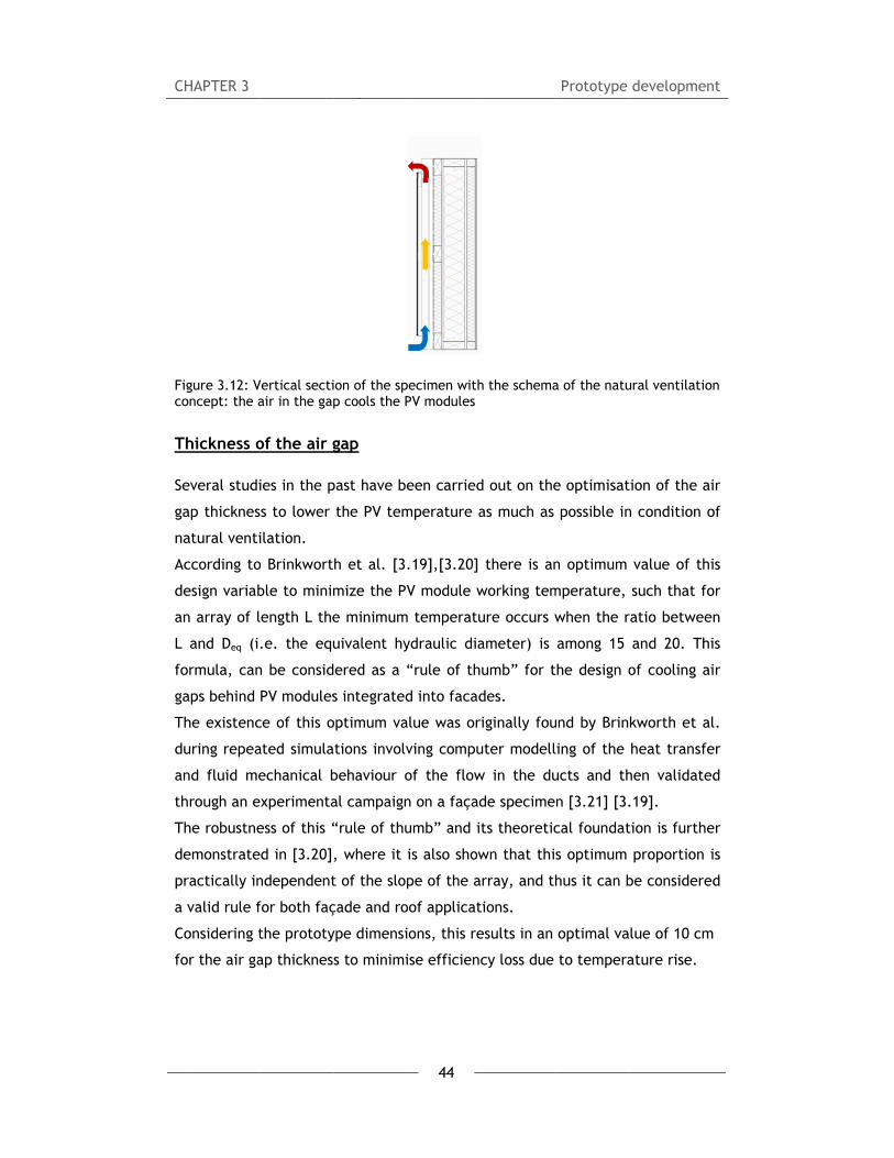
CH
Fico
Th
Se
ga
na
Ac
de
an
L
fo
ga
Th
du
an
th
Th
de
pr
a
Co
fo
HAPTER 3
gure 3.12: Voncept: the a
hickness o
everal studi
ap thicknes
atural venti
ccording to
esign variab
n array of l
and Deq (i
ormula, can
aps behind
he existenc
uring repea
nd fluid me
hrough an e
he robustne
emonstrate
ractically in
valid rule f
onsidering t
or the air ga
Vertical sectiair in the gap
of the air g
ies in the p
ss to lower
ilation.
o Brinkwort
ble to minim
length L the
.e. the equ
n be consid
PV modules
ce of this o
ated simula
echanical b
experimenta
ess of this “
ed in [3.20]
ndependent
for both faç
the prototy
ap thickness
ion of the spp cools the P
gap
past have be
the PV tem
h et al. [3.
mize the PV
e minimum
uivalent hy
ered as a “
s integrated
optimum va
tions involv
behaviour o
al campaign
“rule of thu
, where it i
t of the slop
çade and ro
ype dimensi
s to minimi
44
ecimen withPV modules
een carried
mperature a
.19],[3.20]
V module w
temperatu
ydraulic dia
“rule of th
d into facad
lue was ori
ving compu
of the flow
n on a façad
umb” and it
is also show
pe of the a
oof applicat
ons, this re
ise efficienc
h the schema
d out on the
as much as
there is an
working tem
ure occurs w
ameter) is
umb” for t
des.
iginally fou
uter modell
w in the du
de specime
ts theoretic
wn that this
rray, and th
ions.
esults in an
cy loss due
Prototype
a of the natu
e optimisat
possible in
n optimum
mperature,
when the r
among 15
he design o
und by Brin
ing of the
ucts and th
n [3.21] [3.
cal foundat
s optimum
hus it can b
optimal va
to tempera
developme
ural ventilati
ion of the a
n condition
value of th
such that f
ratio betwe
and 20. Th
of cooling a
kworth et a
heat transf
hen validat
.19].
tion is furth
proportion
be consider
lue of 10 cm
ature rise.
ent
ion
air
of
his
for
en
his
air
al.
fer
ed
her
is
red
m

CHAPTER 3 Prototype development
45
Heat exchange improvement
As stated in the paragraph above, temperature increase of the PV operating
temperature causes significant power production drops that, for a correct
integration into building, has to be minimized as much as possible.
Therefore, it is crucial to develop strategies and solutions to reduce the
working module temperature.
In this thesis, a passive low-cost strategy is experimented and investigated,
with the aim to further enhance the advantages provided to the PV module
performance by the ventilation in terms of PV temperature decreasing.
The idea rises from the necessity to develop a technique as passive, low cost
and simple as possible (for coherency with the prototype prefabrication
concept), implementing in the PV sector a strategy which is very often used in
the ICT sector for electronic device cooling.
In fact, in electronic systems it is a very common practice to include a heat
sink which works as passive heat exchanger to cool a device by dissipating heat
into the surrounding air.
For example, in computers, heat sinks are used to cool central processing units
(CPU) or graphics processors.
In general, heat sinks are often used with high-power semiconductor devices,
such as power transistors and optoelectronic devices, such as lasers and light
emitting diodes (LEDs), wherever the heat dissipation ability of the basic device
package is insufficient to control its temperature.
Figure 3.13: examples of CPU heat-sinks. On the right: a fan-cooled heat sink on the processor of a personal computer with a smaller heat sink cooling another integrated circuit of the motherboard This concept is scaled up to the PV module dimensions, resulting in a proposed
solution which is first evaluated through FEM simulations, then measured and
quantified through an experimental campaign presented in the next chapter.

CHAPTER 3 Prototype development
46
The concept results in a technical modification of the PV module, foreseeing
the applications of metal fins attached on the back side of the module itself (as
shown in Figure 3.15).
The heat coming from the PV module is transferred to the heat sink (i.e. the
fins) by conduction and from the heat sink to the ambient air by natural
convection [3.26][3.1].
The role of the metal fins is to increase the heat transfer surface area in the air
channel, working as a heat sink and thus dissipating an higher quantity of heat
produced by the PV modules.
Furthermore, Tonui & Tripanagnostopoulos [3.14] showed that presence of fins
in a naturally ventilated duct behind the PV modules create an higher stack
effect leading to a better PV cooling. Similar results were found by Friling et al.
[3.28]. In those cases, the fins were attached on the wall to the opposite side
of the PV modules [as shown in Figure 3.14], but the same concept could be
extended for the case of fins attached on the module.
Figure 3.14: different geometry configurations of the air gap behind the PV module, as investigated by Friling et al. [3.28] and Tonui et al. [3.14]
No much literature was found by the author about experimental data regarding
the application of heat sinks directly on the PV module. Some data are
reported for a module with aluminium finned substrate in [3.31] but no
information are provided about the characteristics of the fins and their
application on the module. This configuration is thus investigated in this thesis
to evaluate and quantify its effectiveness, also through an experimental
campaign (as reported in chapters 4 and 5).
In order to define the configuration of the system module-heat sink, because no
much experimental data or examples are available, several energy simulations
with finite elements method are carried out.

CH
Th
fa
pr
co
Fiof
Th
ro
he
co
di
Fi
Me
di
It
fin
th
co
Se
an
Tw
fin
m
co
HAPTER 3
he materia
açade syste
roperties,
orrosion eff
gure 3.15: thf the PV mod
he next pa
ough experi
eat sink on
ompound l
imensions.
n-module h
etal fins a
irection.
is necessa
ns and the
he presenc
onduction f
everal kind
nd economi
wo options
ns through
mechanical j
onsidering o
l chosen fo
ems), since
and it is th
fects.
he zoom shodules
aragraphs re
iments that
the modul
ayer betw
heat transfe
re attache
ary to inclu
module to
ce of any
rom the PV
of such the
cal solution
are in par
h a therma
joint with a
only the pre
or the fins
it is a che
he same ma
ows the L sha
eport the
t were carr
le, and in p
ween the f
er: the ther
ed on the b
ude a therm
o guarantee
air) and
V module to
ermal comp
n for this ap
rticular com
al conduct
additional f
esence of a
47
is aluminiu
eap and lig
aterial as th
ape of the al
results of s
ried out to
particular:
fins and t
rmal compo
back side o
mal conduc
e a perfect
to permit
the fins.
pound are e
pplication.
mpared: on
tive (non-a
ixing to the
thermo co
um (i.e. a m
ht material
he module
luminium fin
some energ
define the
the charac
the module
ound layer
of the PV
tive compo
t contact b
t the heat
evaluated t
ne foresees
adhesive) c
e module fr
nductive ad
Prototype
material la
l with high
frame to a
n attached to
gy simulati
way to inc
cteristics of
e as well
module in
ound layer
between th
t transmis
o find the
s the applic
compound
rame, and t
dhesive.
developme
rgely used
conductivi
avoid possib
o the back si
ons and fir
corporate t
f the therm
as the fi
the vertic
between t
em (avoidi
sion throu
most suitab
cation of t
ensuring t
the other o
ent
in
ity
ble
de
rst
he
mal
ins
cal
he
ng
gh
ble
the
he
ne

CHAPTER 3 Prototype development
48
Both options are tested through first rough experiments: two fins are applied
on a 6mm glass (the same thickness as the PV module which is a glass-glass
kind) through one commercially available thermal compound and one
commercially available thermal adhesive, as shown in the following pictures.
Figure 3.16: The pictures show the fins applied on a 6mm glass. The right-hand image, which shows the backside of the glass, displays the air holes (as marked in the red circles) in the thermal compound used to attach the fin on the right. The fin on the left is instead attached with a thermo conductive adhesive, which gives better results from the contact point of view. Therefore, the alternative with the adhesive is selected as the best, since it
allows to avoid additional mechanical fixing thus reducing time in the
component construction and also because it presents better characteristics in
its distribution, avoiding air holes between the glass and the fins (as shown in
Figure 3.16) which could significantly affect the thermal transmittance.
Among the commercially available thermal conductive adhesives, two different
kinds are considered: a thermal compound based on Epoxy technology (with a
thermal conductivity coefficient of 1.4 W/mK, based on ISO 8302) and a
thermal compound based on Silver technology (with a thermal conductivity
coefficient of 8.89 W/mK).
The latter presents an higher value of conductivity and thus could be
considered as best option, nevertheless it has a much higher price.
Some energy simulations are thus carried out to quantify the different
performances of the two compounds to evaluate the best option balancing
between performance and costs.
The FEM energy simulations results reported in Figure 3.17 show that there is
no need of an higher thermal conductivity coefficient, since there is no
significant change in the module temperature distribution considering the two
thermal compound types. This can be due to the fact that the thermal

CHAPTER 3 Prototype development
49
conductivity of the first compound, even if it is lower than the second, is higher
than that of the module glass where it is applied (which is 1 W/mK).
The first image of Figure 3.17 plots the isotherms expressed in °C, considering
the thermal compound based on Epoxy technology (with a thermal conductivity
coefficient of 1,4 W/mK) between the module and the fin; the second one
considers a thermal compound based on Silver technology (with a thermal
conductivity coefficient of 8,89 W/mK).
The considered boundary conditions for the simulations are:
Ti= 30°C, hcv i= 2.5 W/(sqmK), εi= 0.84, Tout= 25°C, hcv out= 8 W/(sqmK), εo =
0.84, constant heat flux= 1000W/sqm, hp of black body radiation. hcv
coefficients (i.e. convective coefficients) are calculated according to UNI EN
ISO 6946.
Considering the results of the simulations, the cheapest solution (a structural
adhesive based on epoxy technology with a coefficient of thermal conductivity
(ISO 8302) of 1.4 W/(mK)) is thus selected as the best option for this
application.
Figure 3.17: temperature distribution of the PV module simulated with the FEM software THERM (developed by Lawrence Berkeley National Laboratory). The first image plots the isotherms expressed in °C, referred to the epoxy technology compound; the second one considers a thermal compound based on Silver technology
It is important to underline that these simulations are focussed on the heat sink
thermal performance of different possible configurations.
The considered boundary conditions in fact refer to hypothetic conditions (no
measured data are available at this stage) and thus, the temperatures shown in
Figure 3.17 have to be considered significant not as absolute values but as
relative values, which are of interest for this study.
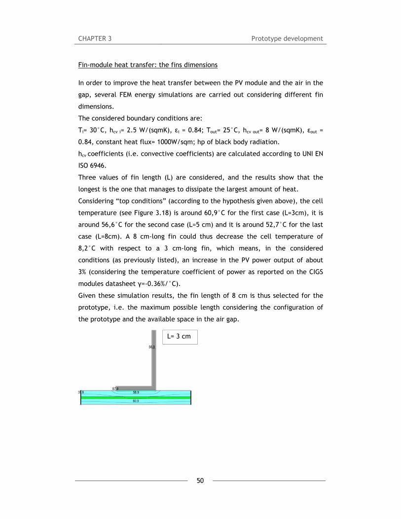
CHAPTER 3 Prototype development
50
Fin-module heat transfer: the fins dimensions
In order to improve the heat transfer between the PV module and the air in the
gap, several FEM energy simulations are carried out considering different fin
dimensions.
The considered boundary conditions are:
Ti= 30°C, hcv i= 2.5 W/(sqmK), εi = 0.84; Tout= 25°C, hcv out= 8 W/(sqmK), εout =
0.84, constant heat flux= 1000W/sqm; hp of black body radiation.
hcv coefficients (i.e. convective coefficients) are calculated according to UNI EN
ISO 6946.
Three values of fin length (L) are considered, and the results show that the
longest is the one that manages to dissipate the largest amount of heat.
Considering “top conditions” (according to the hypothesis given above), the cell
temperature (see Figure 3.18) is around 60,9°C for the first case (L=3cm), it is
around 56,6°C for the second case (L=5 cm) and it is around 52,7°C for the last
case (L=8cm). A 8 cm-long fin could thus decrease the cell temperature of
8,2°C with respect to a 3 cm-long fin, which means, in the considered
conditions (as previously listed), an increase in the PV power output of about
3% (considering the temperature coefficient of power as reported on the CIGS
modules datasheet γ=-0.36%/°C).
Given these simulation results, the fin length of 8 cm is thus selected for the
prototype, i.e. the maximum possible length considering the configuration of
the prototype and the available space in the air gap.
L= 3 cm

CHAPTER 3 Prototype development
51
Figure 3.18: temperature distribution of the PV module simulated with the FEM software THERM (developed by Lawrence Berkeley National Laboratory), given the boundary conditions listed above. The first image plots the isotherms expressed in °C, considering respectively: a 3 cm-long fin, a 5 cm-long fin and a 8 cm-long fin.
Preliminary evaluation of the fins effect
Several FEM simulations are carried out to evaluate the effect of the fins
application on the PV module temperature distribution.
The simulation results reported in Figure 3.19 and in Figure 3.20 show how the
PV temperature changes considering the situation with and without fins in
average meteorological conditions referred to the city of Bolzano (North of
Italy) at 12:00 for summer and winter (as described in Table 3.2).
Average Values at 12:00
global irradiation air temperature air velocity
W/sqmK °C m/s
WINTER 358 6 1,2
SUMMER 340 25 2,5
Table 3.2: the table shows average values at 12 o’clock for the city of Bolzano (North of Italy) of: global irradiation on a vertical South-oriented surface, air temperature and air velocity. The values were calculated considering the meteorological data base
L= 5 cm
L= 8 cm

CHAPTER 3 Prototype development
52
of the Swiss software Meteonorm. Values are divided in winter conditions (December 21st-March 21st ) and summer conditions (June 21st – September 21st )
Figure 3.19: The images show the temperature distribution of the PV module with and without attached metal fin, simulated with the FEM software THERM (developed by Lawrence Berkeley National Laboratory) in average summer conditions (as described in Table 3.2).
Figure 3.19 shows that, in the considered conditions (Ti= 30°C, hcv i=2.5 W/(sqm
K), εi= 0.84; Tout= 25°C, εout= 0,84, constant heat flux= 340W/sqm, hcv out=14
W/(sqm K), which was evaluated in accordance with the UNI EN ISO 6946
considering the air velocity of 2.5 m/s; hp of black body radiation), the
presence of the fins allows a decrease of around 3.5 °C in the cell
temperature, which would mean an increase of the PV power output of 1.3%,
considering a constant power temperature coefficient of -0.36 %/°C (as
reported on the module datasheet).
Figure 3.20: The images show the temperature distribution of the PV module with and without attached metal fin, simulated with the FEM software THERM (developed by Lawrence Berkeley National Laboratory) in average winter conditions (as described in Table 3.2).

CHAPTER 3 Prototype development
53
Figure 3.20 shows that, in the considered conditions (Ti= 11°C, hcv i=2.5 W/(sqm
K), εi= 0.84; Tout= 6°C, εout= 0.84, constant heat flux= 358W/m2, hcv out=8.8
W/(sqm K), which was evaluated in accordance with the UNI EN ISO 6946
considering the air velocity of 1.2 m/s; hp of black body radiation), the
presence of the fins leads to a decrease of around 6 °C in the cell temperature,
which would mean an increase of the PV power ouput of 2.2%, considering a
constant power temperature coefficient of -0.36 %/°C (as reported on the
module datasheet). According to these simulations, application of fins leads to
a slight enhancement of the PV power production (+1.3% in typical summer
conditions, +2.2% in typical winter conditions) in the considered average
working conditions.
These values are expected to be higher during peak working conditions, i.e.
when the power production is at the top, providing an increase in the PV power
production up to 6.2% [3.27].
These simulations show that application of fins on the PV module has a positive
influence on the PV performance and could thus represent a passive and low
cost strategy to further improve the performance of BiPV systems.
However, in order to comprehensively quantify the influence of fins on the
performance of the PV module integrated in a façade, further investigation
were carried out. An experimental campaign was thus performed as described
in chapter 4, providing monitored data to describe this phenomena in an
exhaustive and reliable way.
3.4.3 Building performance
The prototype energy performance, in terms of “building performance” is
strictly linked with two main variables: the choice of materials (i.e. their
thermal characteristics) and the thickness of each material layer.
The latter is mainly related to the fact that the prefabricated prototype is
supposed to have adequate resistance to static and dynamic loads and safety
against structural collapse and inadmissible deformations.
The thickness of the prototype frame is thus a fixed parameter, which is given
by structural requirements.

CHAPTER 3 Prototype development
54
Accordingly, the thickness of the main insulation layer becomes a fixed
parameter because it is inserted in the same plane of the structural frame.
The only design variable is thus related to the choice of insulation materials,
which is discussed in the next paragraph.
Materials
Four commercially available insulation materials, which are typically used in
the light wooden buildings, are considered and compared:
1) Flexible thermal insulation made from natural wood fibres (λ= 0.042
W/mK)
2) Flexible thermal insulation made from hemp (λ= 0.044 W/mK)
3) Mineral wool thermal insulation (λ= 0.042 W/mK)
4) Extruded polystyrene (λ= 0.039 W/mK)
All insulation materials present similar thermal conductivity values. In order to
quantify the influence of the choice of the different materials on the overall
prototype thermal transmittance, the total prototype resistance is evaluated
for the four options, according to the UNI EN ISO 6946.
The calculated resistance values, considering the four materials are
respectively:
1) R= 5.31 sqm*K/W
2) R= 5.23 sqm*K/W
3) R= 5.31 sqm*K/W
4) R= 5.44 sqm*K/W
Extruded polystyrene is the material which provides the highest thermal
resistance (R= 5.44 sqm*K/W), while insulation made from hemp is the one
which perform in the poorest way (R= 5.23 sqm*K/W).
However, it has to be considered that the extruded polystyrene is a synthetic
polymer made from the monomer styrene, a liquid petrochemical, which does
not fit very well with the overall prototype concept of sustainability and use of
natural local materials.
The other two materials (based respectively on natural wood fibres and mineral
wool) provide a resistance which do not differ in a significant way from the
extruded polystyrene (i.e. 2% less).

CHAPTER 3 Prototype development
55
Given these considerations, the flexible thermal insulation made from natural
wood fibres is selected as the best option for this prototype because, even if its
performance in terms of thermal resistance is slightly lower compared to the
best performing option, the use of this material is coherent with the overall
concept used for the prototype configuration.
The prototype is thus largely made of wood or wood-based materials (the
structural frame is made of local wood).
The selected insulation material is based on wood fibres, and all of them are
certified with the European quality mark “Natureplus” [3.33] and “FSC”
certification [3.34] [3.38] [3.39], which guarantee environmentally-friendly
production, protection of limited natural resources and suitability of
application.
Moreover, from an LCA (life cycle assessment) perspective, several studies have
shown that buildings with wooden structures require less energy and emit less
CO2 during their life cycle, than buildings with other types of structures [3.43]
[3.45]. For example, in a Canadian office building, the embodied energy in a
steel structure is 1.61 times greater than that in a concrete structure, which in
turn is 1.27 times greater than that of a wooden structure [3.45]. Also in
Northern European countries various life cycle studies have been carried out
that indicate the advantages of wooden structures [3.46].
Prototype thermal characteristics
In order to understand the influence of the presence of PV on the building
envelope, the value of the thermal transmittance of the prototype is calculated
in accordance with the UNI EN ISO 6946 [3.1] considering two situations: the
building component with and without the PV system.
The International Standard UNI EN ISO 6946 provides in fact a simplified
calculation method to assess the value of thermal transmittance and thermal
resistance of building components.
The calculation is based on combining the individual thermal resistance of each
thermally homogeneous layer to obtain the total thermal resistance of the
component including the effect of surface resistances.
The air gap included in the prototype is treated in accordance with the
Standard definitions as a well-ventilated air layer: the total thermal

CHAPTER 3 Prototype development
56
transmittance is thus obtained by disregarding the thermal resistance of the air
layer and all other layers between the air layer and external environment, and
including an external surface resistance corresponding to still air, which is
calculated in accordance to Annex A.
Table 3.3 summarizes the values of thermal conductivity which were used for
each layer.
λ: Coefficient of thermal conductivity of each layer (W/mK)
1 2 3 4 5 6 7 8
0,352 0,042 0,22 0,13 0,042 0,13 0,043 0,2
Table 3.3: Coefficient of thermal conductivity of each layer (W/mK), referred to numbered items of Figure 3.27.
Following the calculation schema of the standard (as described in the next
paragraph) the results show that the presence of PV do not affect in a
significant way the total thermal resistance of the component: the thermal
transmittance of the component with the integrated PV system (which is 0.188
W/sqm K) is slightly lower than the one without it (which is 0.191 W/sqm K)
(Figure 3.21).
Therefore, according to this calculation schema, the PV system does not affect
the building envelope performance in a negative way.
Figure 3.21: the U-value (i.e. thermal transmittance) calculated considering the prototype with and without PV modules.
U = 0,188 W/sqm K
U = 0,191 W/sqm K

CHAPTER 3 Prototype development
57
Prototype thermal transmittance - calculation method-
This paragraph describes the calculation method, as foreseen by the UNI EN ISO
6946 [3.1], for the evaluation of the prototype thermal transmittance.
The first step foresees the calculation of the thermal resistance of the
homogeneous layers resulting from the thermal conductivity values which are
taken from generic values given by the UNI EN ISO 10456:2008 [3.30] (for layers
1, 2b, 3, 4, 5b, 6, 7b and 8) and from the manufacturer datasheets, worsened
for an amount of 10% as suggested by the standard (for layers 2a, 5a and 7a).
Ri: resistance value of each homogeneous layer (sqm K/W) L 1 2a 2b 3 4 5a 5b 6 7a 7b 8
s 0.012 0.06 0.06 0.0003 0.015 0.16 0.16 0.012 0.06 0.06 0.0003
λ 0.352 0.042 0.13 0.22 0.13 0.042 0.13 0.13 0.043 0.13 0.2
Ri 0.035 1.428 0.461 0.001 0.115 3.809 1.230 0.092 1.395 0.461 0.001
Table 3.4: L is the reference number of each layer referred to Figure 3.25, s is the thickness (m), λ is the thermal conductivity (W/m K), Ri is the resistance of each homogeneous layer (sqm K/W)
Surface resistances
In the second step, the surface resistances are calculated according to the
appendix A of the standard, as illustrated in Table 3.5.
Rs: Surface resistances
hci Convection coefficient-inside W/(m^2)K 2.5
hce Convection coefficient-outside W/(m^2)K 2.5
hri Radiative coefficient -inside W/(m^2)K 5.04
hre Radiative coefficient -outside W/(m^2)K 3.28
εi Surface emissivity-inside 0.8
εe Surface emissivity-outside 0.8
σ Stefan-Boltzmann constant W/(mq*K^4) 5.67E-08
Heat flux horizontal
hro i Black body radiative coefficient-inside W/(m^2)K 6.3
hro e Black body radiative coefficient-outside W/(m^2)K 4.1
Ti Temperature-inside °C 30
Te Temperature-inside °C -10
Rsi Surface resistance-inside sqm*K/W 0.13 Rse Surface resistance-outside sqm*K/W 0.17 Table 3.5: indoor and outdoor surface resistance calculation

CH
To
As
Th
ho
ca
re
w
R’
R’
Ca
co
di
pr
4,
Th
ha
th
ar
Th
fa
Fi
HAPTER 3
otal therma
s last step,
he total the
omogeneou
alculated a
esistance:
here:
’T is the upp
’’ T is the lo
alculation o
omponent s
ivided into
rototype is
, 5, 6, 7, 8
he section
as a fractio
hickness dj.
rea fm and t
he fraction
+ fb + fc+ fd
gure 3.22:
al resistance
the total th
ermal resist
s and ther
as the arit
per limit of
ower limit o
of the upp
split into se
parts, mj
considered
(see Figure
m (m =a, b
nal area fm
The part m
thermal res
al area of
= 1 (see Ta
dimensions
e
hermal resi
tance (RT)
rmally inho
thmetic me
RT=
f the total t
of the total
er and low
ections and
, which ar
d divided in
3.23 and F
b, c, d) per
. The layer
mj has a the
sistance Rmj
a section is
able 3.6 and
s of each lay
58
stance is ev
of the prot
mogeneous
ean of the
= (R’T+ R’’T
thermal res
thermal re
wer limits a
layers, in
re themsel
nto sections
Figure 3.25)
rpendicular
j (j =1, 2,
ermal cond
.
s its propor
d Table 3.7
yer of the p
valuated.
totype, whi
s layers par
e upper an
T)/2
istance
esistance
are carried
such a way
lves therma
s a, b, c, d
)
to the sur
... 8) paral
uctivity lmj,
rtion of the
7).
prototype
Prototype
ch consists
rallel to th
nd lower l
out by co
y that the c
ally homog
and into la
rfaces of th
llel to the s
, thickness
e total area
developme
s of therma
he surface,
limits of t
nsidering t
component
geneous. T
ayers 1, 2,
he compone
surfaces has
dj, fraction
a. Therefor
ent
lly
is
he
he
t is
The
3,
ent
s a
nal
re,
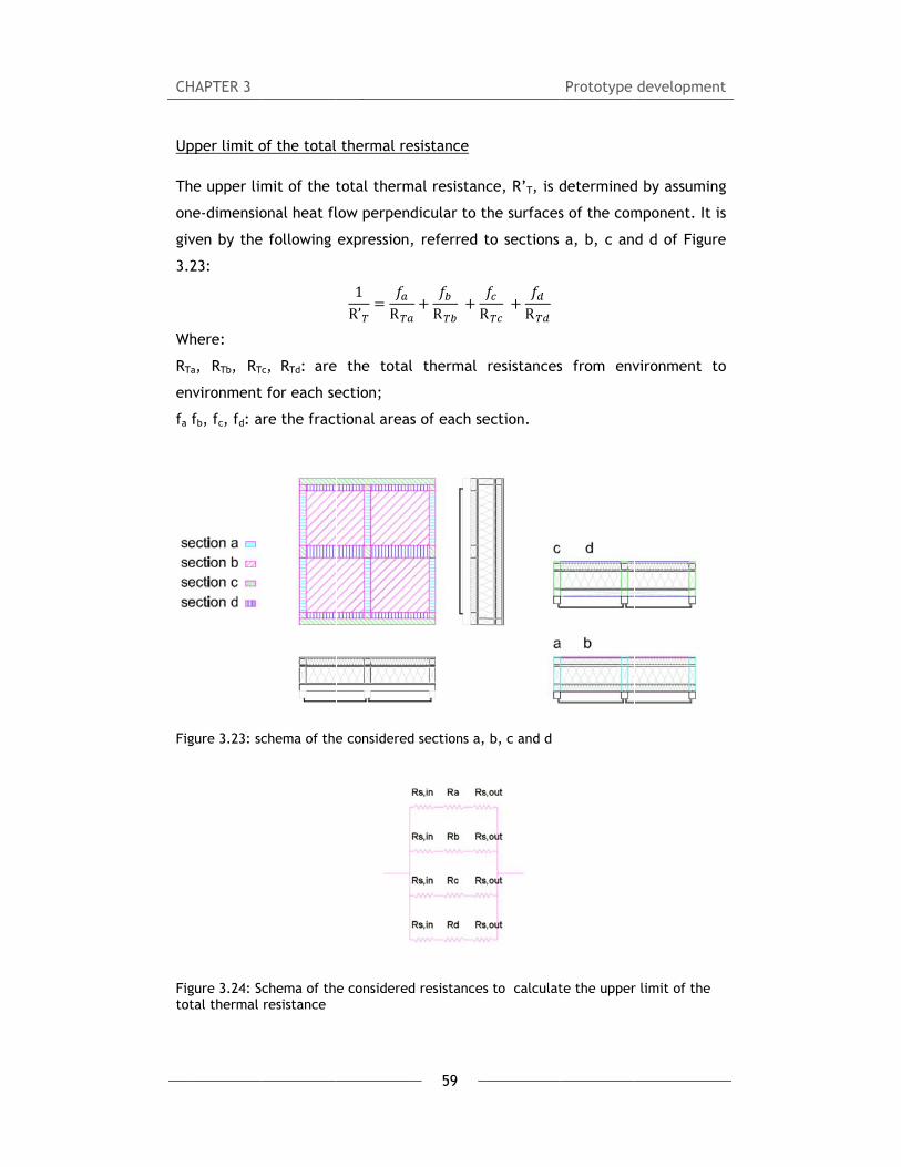
CH
Up
Th
on
gi
3.
W
RT
en
fa
Fi
Fito
HAPTER 3
pper limit o
he upper lim
ne-dimensio
ven by the
.23:
Where:
Ta, RTb, RT
nvironment
fb, fc, fd: a
gure 3.23: sc
gure 3.24: Sotal thermal
of the total
mit of the t
onal heat fl
e following
c, RTd: are
for each se
re the fract
chema of the
chema of th resistance
thermal re
total therm
low perpend
expression,
1R’ R
the total
ection;
tional areas
e considered
e considered
59
esistance
mal resistan
dicular to t
, referred t
R
R
l thermal
s of each se
d sections a,
d resistances
ce, R’T, is d
the surfaces
to sections
R
R
resistances
ection.
b, c and d
s to calculat
Prototype
determined
s of the com
a, b, c an
s from env
te the upper
developme
d by assumi
mponent. It
d d of Figu
vironment
r limit of the
ent
ng
t is
ure
to
e

CHAPTER 3 Prototype development
60
Upper limit of the total thermal resistance, R'T Atot total wall area mq 1,84055
f (fa+fb +fc+fc+fc)*f
Aa area of section a mq 0,1881
Ab area of section b mq 1,18085
Ac area of section c mq 0,2004
Ad area of section d mq 0,2712
fa fractional area of section a - 0,102198
fb fractional area of section b - 0,641575
fc fractional area of section c - 0,10888
fd fractional area of section d - 0,147347
RTa total thermal resistance of section a mq*K/W 3,65
RTb total thermal resistance of section b mq*K/W 7,19
RTc total thermal resistance of section c mq*K/W 2,71
RTd total thermal resistance of section d mq*K/W 6,26
R'T Upper limit of the total thermal resistance mq*K/W 5,53 Table 3.6: Calculation of the upper limit of the total thermal resistance
Lower limit of the total thermal resistance
The lower limit of the total thermal resistance, R’’T, is determined by assuming
That all planes parallel to the surfaces of the component are isothermal
surfaces.
Calculating an equivalent thermal resistance, Rj, for each thermally
inhomogeneous layer given by this expression:
1R R R
R
R
The lower limit is then determined by the following expression, referred to the
layers shown in Figure 3.25:
R′′ R R R R R R R R R R

CH
Fi
Fito
R
R
R
R
R
R
R
R
R'
R'Ta
HAPTER 3
gure 3.25: sc
gure 3.26: Sotal thermal
R1
R2
R3
R4
R5
R6
R7
R8
''T somma
''T Loweable 3.7: Cal
chema of the
chema of th resistance
Lower limtotal the
total the
total the
total the
total the
total the
total the
total the
delle 8 resis
er limit oflculation of t
e considered
e considered
mit of the termal resista
ermal resista
ermal resista
ermal resista
ermal resista
ermal resista
ermal resista
ermal resista
stenze (da R1
f the total the lower lim
61
d layers of th
d resistances
total therance of layer
ance of layer
ance of layer
ance of layer
ance of layer
ance of layer
ance of layer
ance of layer
1 a R8) in se
thermal rmit of the to
he prototype
s to calculat
mal resistr 1
r 2
r 3
r 4
r 5
r 6
r 7
r 8
rie + Rsi + Rs
resistancetal thermal
Prototype
e
te the lower
ance, R''T
mq*K/W
mq*K/W
mq*K/W
mq*K/W
mq*K/W
mq*K/W
mq*K/W
mq*K/W
se W/mq*K
mq*K/resistance
developme
limit of the
W 0,03551
W 0,9905
W 0,001
W 0,11538
W 2,64135
W 0,09230
W 0,91895
W 0,001
K 5,1
/W 5,1
ent
11
51
15
85
59
08
51
15
11
1

CHAPTER 3 Prototype development
62
Resulting total thermal resistance
The resulting total thermal resistance of the whole prototype is:
U= 0.188 W/(sqm*K)
And the corresponding total thermal resistance is
RT= 5.32 (sqm*K)/W
The calculated thermal transmittance values can be considered a satisfying
result in terms of building energy performance, and it is index of a well-
insulated wall as its thermal transmittance is below, for an extent of 23%, the
limit of 0.26 W/(sqm*K) required by the actual Italian law referring to the
worst case scenario (“zona climatica F”) [5.1].
In fact, the concept that lead to the development of this BiPV prototype
foresees the idea of a building component which is first of all “energy saving”
and only afterwards “energy producing”. Energy saving is considered the first
inescapable step toward an energy efficient BiPV system.
In addition, it is evaluated that the PV modules themselves do not affect in a
significant way the value of thermal transmittance of the whole component, as
calculated in the previous paragraphs according to the Standard UNI EN ISO
6946.

CHAPTER 3 Prototype development
63
3.5 Prototype design
The final prototype design is the result of the theoretical study carried out as
described in the previous paragraph.
The prototype [Figure 3.27] is conceived as a standardized modular unit with
dimensions of 442 x 1310 x 1240 mm, characterized by a nominal power of
160Wp and with a calculated thermal transmittance value of 0,188 W/sqm K.
Figure 3.27: design of the frontal view and horizontal section of the prototype. The horizontal section is made of the following layers : 1. Gypsum fiber panels 2a. Wooden fiber thermal insulation 2b. Wooden frame 3. Vapor retarder 4. OSB 5a. Wooden fiber thermal insulation 5b. Wooden frame 6. OSB (Oriented Strand Board) 7. Thermal insulation 8. Waterproof barrier 9. Air gap 10. Metal fins 11. Thermoconductive glue 12. PV module (thin film technology)

CHAPTER 3 Prototype development
64
3.6 Prototype application
The BiPV prototype of this thesis was developed within a wider research
project entitled “Chi Quadrato: building construction of certified green
buildings designed for training activities”, which aim was to design a
prototypical elementary school of 200 sqm located in Condino (Province of
Trento, North of Italy), entirely realized with prefabricated wood framed
panels with high energy efficiency standard, developing innovative
technological solutions, innovative processes (off-site construction) and
promoting and enhancing the value of wood as a sustainable building material.
The consortium “Chi Quadrato” is constituted by eight SME’s (small medium
enterprises), coordinated by five research Institutions: Università IUAV di
Venezia, Università degli Studi di Trento, CNR Ivalsa (National Research Council
of Italy-Trees and Timber Institute-), Libera Università di Bolzano and Eurac.
The partners of the consortium worked together following an integrated design
process (IDP), i.e. a design process based on close multidisciplinary cooperation
and iterative design loops.
The IDP includes the organization of several workshops during the entire design
phase, in which all stakeholders involved in the project collaborate (architects,
clients, solar energy consultants, specific contractors and manufacturers) to
guarantee a more holistic approach to building design. These workshops were
carried out for the project duration to clarify, after each design loop,
architectural and technical target criteria and constraints.
At the beginning of the project, several hypothesis were considered for the PV
integration, together with the architects and electricians. Figure 3.28 shows
some of the considered preliminary hypothesis elaborated before the
development of the BiPV wall prototype.
The BiPV wall prototype developed in this thesis is thus conceived as a
“prototype in the prototype” (i.e. a BiPV wall prototype in a wooden
prefabricated prototypal building).

CHAPTER 3 Prototype development
65
Figure 3.28: preliminary hypothesis for the BiPV wall prototype positioning, elaborated by the architects belonging to the “Chi Quadrato” Consortium at the beginning of the project (from the top left to the bottom right: solutions 1,2,3,4).
Among the considered hypothesis, as shown in Figure 3.28, the most suitable
“place” for PV integration was selected using the IDP approach, together with
architects, technicians and manufacturers, on the basis of two groups of
criteria (according to the criteria identified by Wittkopf et al. [3.35]):
- Climatic and site characteristics
- Architectural characteristics
The first group of criteria considers: tilt, orientation and shading effect.
The first (tilt) is not applicable as an option as it is already fixed at 90°, being
a façade application. In terms of orientation (azimuth) and shading, the South-
West (azimuth=+20) façade is, by evidence, the one with the highest solar
radiation potential considering the morphological configuration of the
surrounding East and North-West mountains of the place (i.e. Condino, Province
of Trento, Italy). All solutions of Figure 3.28 refer to that façade.
The second group of criteria considers: position, visibility from outside the
building, accessibility, function and aesthetics.
According to these criteria, option number 2 was selected as the most suitable,
for the following reasons:
1 2
3 4

CH
Fipihoap
Fibu[re
HAPTER 3
- In op
during
shown
- Positi
public
space
This c
aesth
- In op
techn
least
buildi
gure 3.29: Vcture is takeomogeneous ppears marke
gure 3.30: Ruilding withine-arrangeme
ption 4 the
g the day,
n in the sec
ioning the
c accessibi
e where also
could repre
etic percep
ption 2 the
nicians but
3 meters
ing [see Fig
Visibility: moen at a dista pattern; theed by vertica
Rendering of n the projecent L. Maturi
PV module
is shadowe
ction drawin
modules a
lity to the
o children o
esent a pro
ption [as sh
e PV modu
not for pu
and in ar
gure 3.30].
odule aesthetnce of 3 mete other pictual lines, whic
the elementct “Chi Quadi from rende
66
es are in a
ed by an ad
ng of Figure
as foreseen
PV system
of the schoo
oblem in te
own in Figu
ules are in
blic, visible
chitectural
tical perceptters and the ure is taken ach are the ce
tary school trato”, includ
ering Studio A
a position w
djacent proj
e 3.28)
n in option
m: the adja
ol are allow
erms both o
ure 3.29]
n a positio
e to the pu
coherence
tion vs obser modules surat a distanceell connectio
that was desding the BiPVArch. Frate]
Prototype
which, for
jecting buil
ns 1 and 3
cent groun
wed to walk
of safety a
on easily a
ublic at a d
e with the
rver positionrface appeare of 50 cm: tons
igned as a pV prototype
developme
some peri
lding part (
, would gi
nd is a pub
k through.
and also fro
accessible f
distance of
e rest of t
n. The first rs as an the pattern
rototypal on the left.
ent
od
(as
ive
lic
om
for
at
he

CHAPTER 3 Prototype development
67
Figure 3.30 shows a preliminary rendering of the elementary school to pre-
evaluate the visual impact and the architectural coherence of the BiPV
prototype with the whole architecture composition.
This rendering and the preliminary positioning hypothesis of Figure 3.28, were
elaborated in the first phase of the project, when the design of the BiPV wall
prototype (as described in paragraph 3.5) was not defined yet.
The BiPV wall prototype was in fact developed as a parallel task within the
whole project.
The final design completed with architectural details, which was elaborated
after the “BiPV wall prototype” development as described in this chapter, is
shown in Figure 3.31.
Figure 3.31: architectural drawings and details of the BiPV wall prototype integrated in the elementary school design.

CHAPTER 3 Prototype development
68
References
[3.1] UNI EN ISO 6946:2007, Building component and building elements –
thermal resistance and thermal transmittance – calculation method
[3.2] MC.Munari Probst, 2008. Architectural Integration and Design of Solar
Thermal Systems. École Polytechnique Fédérale de Lausanne, doctoral thesis n.
4258
[3.3] K. Farkas, 2011. The Perception of Formal and Symbolic Aesthetics of
Photovoltaics. Proceedings of ISES Solar World Congress 2011, ISBN 978
39814659 0 7
[3.4] M. Wall et al., 2008. IEA Task 41-Solar Energy and Architecture-Annex
Plan. (available at: http://members.iea-
shc.org/publications/task.aspx?Task=41)
[3.5] MC Munari Probst, C Roecker et al., 2012. Report T.41.A.2: IEA SHC Task
41 Solar energy and Architecture. Solar energy systems in architecture –
Integration criteria and guidelines. (available at: http://members.iea-
shc.org/publications/task.aspx?Task=41)
[3.6] Report T.41.A.3, in press: Designing photovoltaic systems for architectural
integration -Criteria and guidelines for product and system developers, 2013.
[3.7] K. Farkas, M. Horvat et al., 2012. Report T.41.A.1: Building Integration of
Solar Thermal and Photovoltaics – Barriers, Needs and Strategies.
(available at: http://members.iea-shc.org/publications/task.aspx?Task=41)
[3.8] R. Gottschalg et al., 2003. Experimental study of variations of the solar
spectrum of relevance to thin film solar cells. Solar Energy Materials & Solar
Cells 79, 527–537
[3.9] Energy-efficient buildings ppp – Multi-annual roadmap and longer term
strategy-, prepared by the Ad-hoc Industrial Advisory Group, European
Commission
[3.10] J.J. Bloem, 2008. Evaluation of a PV-integrated building application in a
well-controlled outdoor test environment. Building and Environment 43, 205–
216
[3.11] T. Schoen et al., 2001. Task 7 of the IEA PV power systems program –
achievements and outlook, Proceedings of the 17th European Photovoltaic Solar
Conference.

CHAPTER 3 Prototype development
69
[3.12] I. Bergmann, W.Weiss, 2002. Fassadenintegration von thermischen
Sonnenkollektoren ohne Hinterlüftung. AEE Intec, Arbeitsgemeinschaft
ERNEUERBARE ENERGIE, Institut für Nachhaltige Technologien
[3.13] P. Funtan et al., 2009. MULTIELEMENT project-PV Elements in Building
Services Engineering, (http://www.pv-multielement.de/)
[3.14] J.K. Tonui & Y. Tripanagnostopoulos, 2008. Performance improvement of
PV/T solar collectors with natural air flow operation. Solar Energy 82(1) 1-12
[3.15] T.T. Chow, 2010. A review on photovoltaic/thermal hybrid solar
technology, Applied Energy, 87(2) 365-379
[3.16] Y. Tripanagnostopoulos et al., 2002. Hybrid photovoltaic/thermal solar
systems, Solar Energy 72(3) 217-234
[3.17] B. Norton et al., 2011. Enhancing the performance of building integrated
photovoltaics, Solar Energy 85(8) 1629-1664
[3.18] P. Batagiannis, C. Gibbons, 2001. Thermal assessment of silicon-based
composite materials used in photovoltaics, Conference proceedings of
Renewable Energy in Maritime Island Climates, Belfast, 151–157
[3.19] B.J. Brinkworth & M.Sandberg, 2006. Design procedure for cooling ducts
to minimise efficiency loss due to temperature rise in PV arrays, Solar Energy
80(1) 89-103
[3.20] B.J. Brinkworth, 2006. Optimum depth for PV cooling ducts, Solar Energy
80, 1131–1134
[3.21] Brinkworth, B.J. et al, 2000. A validated model of naturally ventilated
PV cladding. Solar Energy 69, 67–81
[3.22] Ji Jie et al., 2002. The annual analysis of the power output and heat gain
of a PV-wall with different integration mode in Hong Kong, Solar Energy
Materials and Solar Cells, Vol 71 Issue 4 435-448
[3.23] H. Yang et al., 2001. Building-integrated photovoltaics: effect on the
cooling load component of building facades, Building Serv Eng Res Technol 22
(3), 157–165
[3.24] B. van Kampen, 2008. Actual Temperatures of Building Integrated PV
Modules. Study in the framework of the EU IP Performance project, September
2008 (available at: www.pv-performance.org)
CHAPTER 3 Prototype development
70
[3.25] L. Fanni et al., 2011. Maximum production conditions of a c-Si module in
three different Italian locations. Proceedings of the 26th European Photovoltaic
Solar Energy Conference and Exhibition. 3446 - 3449
[3.26] Y. A. Cengel, 2006. Heat and Mass Transfer -A Practical Approach- 517-
518
[3.27] L. Maturi, R. Lollini, P. Baldracchi, W. Sparber, 2011. Building skin as
electricity source: the prototype of a wooden BiPV façade component.
Proceedings of the 26th European Photovoltaic Solar Energy Conference and
Exhibition. 3991 - 3999
[3.28] N. Friling et al., 2009. Modelling the heat dynamics of building
integrated and ventilated photovoltaic modules. Energy and Buildings 41 (10),
1051–1057
[3.29] L. Maturi et al., 2010. Analysis and monitoring results of a BiPV system in
Northern Italy. Proceedings of the 25th European Photovoltaic Solar Energy
Conference and Exhibition, 5131-5134
[3.30] UNI EN ISO 10456:2008. Materiali e prodotti per edilizia - Proprietà
igrometriche - Valori tabulati di progetto e procedimenti per la determinazione
dei valori termici dichiarati e di progetto.
[3.31] Flat-Plate Solar Array Project Final Report, 1986. Volume VI: Engineering
Sciences and Reliability, JPL Publication 86-31.
[3.32] B. Weller et al., 2010. Detail Practice: Photovoltaics, ed. Detail, ISBN
978-3-0346-0369-0.
[3.33] www.natureplus.org
[3.34] www.fsc.org
[3.35] S. Wittkopf et al., 2011. Testing a design methodology for building
integration of photovoltaics (PV) using a PV demonstration site in Singapore.
Architectural Science review 54, 192-205.
[3.36] Directive 2010/31/EU of the European Parliament and of the Council of
19 May 2010 on the Energy Performance of Buildings (EPBD)
[3.37] RES Directive 2009/28/CE the European Parliament and of the Council of
23 April 2009 on renewable energy sources

CHAPTER 3 Prototype development
71
[3.38] Graeme Auld et al., 2008. Certification Schemes and the Impacts on
Forests and Forestry, Annual Review of Environment and Resources. Vol. 33:
187-211. DOI: 10.1146
[3.39] V.A. Sample, 2003. Certification on Public and University Lands:
Evaluations of FSC and SFI by the Forest Managers. Journal of Forestry, Volume
101 (8), 21-25(5)
[3.40] G. Makrides et al., 2009. Temperature behaviour of different
photovoltaic systems installed in Cyprus and Germany. Solar Energy Materials
and Solar Cells 93, 1095–1099.
[3.41] E. Skoplaki, J.A. Palyvos, 2009. On the temperature dependence of
photovoltaic module electrical performance: A review of efficiency/power
correlations. Solar Energy 83, 614–624.
[3.42] P. Trinuruk et al., 2009. Estimating operating cell temperature of BIPV
modules in Thailand. Renewable Energy 34, 2515–2523.
[3.43] A. Buchanan A, B. Levine, 1999. Wood-based building materials and
atmospheric carbon emissions. Environmental Science and Policy 2, 427-37.
[3.44] L. Gustavsson et al, 2006. Carbon dioxide balance of wood substitution:
comparing concrete- and wood-framed buildings. Mitigation and Adaptation.
Strateg for Glob Change 11, 667-91.
[3.45] R.J. Cole, P.C. Kernan, 1996. Life-cycle energy use in office buildings.
Building and Environment 31(4), 307-17.
[3.46] A.K. Petersen, B. Solberg, 2005. Environmental and economic impacts of
substitution between wood products and alternative materials: a review of
micro-level analyses from Norway and Sweden. Forest Policy and Economics 7,
249-59.

CHAPTER 4 Experimental campaign
72

CHAPTER 4 Experimental campaign
73
CHAPTER 4
Experimental campaign
Abstract
This chapter describes the experimental campaign performed on a sample of
the designed BiPV wooden wall. The tests are organized in three phases with
the aim to explore the overall energy performance of the BiPV prototype (both
“Bi”, i.e. building and “PV”, i.e. photovoltaic characteristics).
The first part of the chapter presents the two laboratories where the tests
were carried out, including an overview on the measurements sensors, as well
as a description of the tested specimen, which was built thanks to an industrial
collaboration with a network of enterprises.
The second part of the chapter deals with the three experimental phases,
explaining the aim, the experimental setup and the obtained results of each
single phase.

CHAPTER 4 Experimental campaign
74

CHAPTER 4 Experimental campaign
75
4.1 Introduction
The double “core” of BiPV systems (Bi+PV), requires the need to use different
facilities with different features to test together their “passive” (e.g. thermal
transmission properties) and “active”(e.g. electrical production) performance
and to understand the interaction between the active and passive layers.
A new experimental approach, based on three phases with the combination of
different test facilities (i.e. INTENT lab and SoLaRE-PV lab), and original
experimental set-ups, were defined and applied to properly test the BiPV
prototype.
The experimental campaign is divided into three phases which aim at exploring
the overall energy performance of the BiPV prototype. Since the energy
behaviour of a BiPV system is defined by the synergy between the thermal “Bi”
side (i.e. the building) and the energy “PV” side (i.e. the photovoltaic system),
both aspects are considered in this experimental campaign.
The organization of the tests in three phases is essential for the evaluation of
the two aspects: in the first two phases each feature is treated separately in
detail, while the last phase helps to merge both aspects and their interaction
together so to come out with an overall overview of the energy behaviour.
The first phase focuses on the characteristics related to the “Bi” side, and in
particular on the thermal characterization of the prototype with the
measurement of its thermal transmittance; the second phase deals with the
“PV” side, and in particular with the electrical characterization of the modules
through the measurements of the I-V characteristic curve at different
conditions. The goal of the last phase is to merge together the “Bi” and the
“PV” sides, and it focuses on the thermal-energy characterization of the
integrated PV modules.

CHAPTER 4 Experimental campaign
76
Figure 4.1: The diagram shows the organization of the experimental campaign, which is divided into three phases
The double “core” of BiPV systems entails the need to use different facilities
with different features to test together “passive” (e.g. thermal transmission
properties) and “active”(e.g. electrical production) performances and to
understand the energy interaction between the active and passive layers. The
tests carried out in this experimental campaign are performed in two
laboratories at the Institute for Renewable Energy of Eurac: INTENT Lab and
SoLaRE-PV Lab [1.9]. The first laboratory is a test facility for building systems
that allows the performance analysis of passive and active building envelope
systems, while the second one is an indoor test facility for PV module
characterisation according to relative IEC standards. The features of the two
test facilities are described in the next paragraphs.

CHAPTER 4 Experimental campaign
77
4.2 INTENT Lab
INTENT (INTegrated ENergy walls Test facility) is a laboratory that can
evaluate, either in dynamic or static mode, the thermal and energy
performance of building envelope systems, such as walls and floors that
integrate active solar systems for energy production or radiant circuits for
heating/cooling.
The laboratory includes:
- a calorimeter, which has been designed and planned on the basis of the
International standards UNI EN ISO 8990 [3.1] and UNI EN ISO 12567-1
[4.2] with some technical changes. The calorimeter is composed by a
cold chamber, a metering box and a guard chamber (see Figure 4.2),
which simulate respectively the outdoor and indoor conditions by
controlling temperature, humidity and air velocity;
- a steady-state sun simulator, that varies in a range of irradiance from
400 W/m² to 1000 W/m², class BBB as reported in the standard IEC
60904-9 [4.3]: spectral match, spatial uniformity, temporal stability,
referred to a maximum irradiated surface of 1.5m x 2.0m;
- an hydraulic measurement circuit to assess the performance of possible
thermal active systems integrated in the envelope;
- a detailed monitoring system made of sensors and data acquisition
instruments that measure significant physical parameters with the aim
of determining the characteristics of the test sample.
During the tests, the prototype is inserted into a frame surrounded by thermal
insulation, located between the cold and a hot box which is constituted of a
guard chambers.
The solar simulator reproduces the irradiation conditions on the external
surface of the test sample. The glazed panel at the bottom of the cold-box
allows us to keep the desired climatic conditions in the cold chamber and at
the same time guarantees the needed transparency for the irradiation of the
sample.
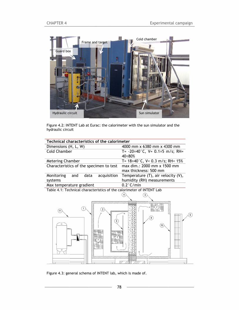
CH
Fihy
TeDiCo
MeCh
MosyMaTa
Fi
HAPTER 4
gure 4.2: INTydraulic circu
echnical chimensions (old Chambe
etering Chaharacteristi
onitoring ystems ax temperaable 4.1: Tec
gure 4.3: ge
Hydraulic ci
Guard box
TENT Lab at uit
haracteristiH, L, W)
er
amber ics of the sp
and dat
ature gradiechnical chara
neral schem
ircuit
x
Fram
Eurac: the c
ics of the c
pecimen to
ta acquis
ent acteristics of
ma of INTENT
e and target
78
calorimeter
calorimeter4000T= -40÷8T= 1
test maxmax
sition Temhum0.2°
f the calorim
lab, which i
with the sun
r 0 mm x 638-20÷40°C, V80%
18÷40°C, V<x dim.: 2000x thickness:mperature (Tmidity (RH) m°C/min meter of INTE
is made of.
Sun sim
Cold cha
Experimen
n simulator a
80 mm x 430V= 0.1÷5 m
< 0.3 m/s; R0 mm x 150 500 mm T), air velomeasureme
ENT Lab
mulator
amber
ntal campai
and the
00 mm
m/s; RH=
RH< 15% 00 mm
ocity (V), ents
gn

CHAPTER 4 Experimental campaign
79
Numbers of Figure 4.3 refer to: (1) Guard chamber (3,36x2,23x3,48 m LxTxH);
(2) Metering Chamber (2,00x1,00x2,50 m LxTxH); (3) Cold Chamber
(3,36x2,09x3,48 m LxTxH); (4) Fixed sample frame; (5) Wall samples; (6) Sun
simulator; (7) Air conditioning devices; (8) Opaque panel to control air flux; (9)
Transparent panel to control air flux; (10) Tempered glass; (11) Hydraulic
circuit.
4.2.1 Measurement sensors
The temperature values are acquired with 70 surface thermocouples (Type T)
and 40 air thermocouples (Type T). The metering box is equipped with an
heating device. The guard and the cold chambers have air conditioning
systems. The ambient temperature within the three climatic chambers (guard,
metering and cold), is controlled using PT100 temperature sensors distributed
within them. The air velocity can either be mechanically regulated by varying
the dimensions of the channels in which the air is conveyed or automatically by
regulating the speed of the installed fans. The air velocity is measured by two
fixed anemometer (velocity transmitters EE75, uncertainty of measurement:
0.02m/s, accuracy in air at 25°C at 45% RH and 1013hPa: ±0.03m/s from 0.06
to 2 m/s; uncertainty of factory calibration: ±1% of measuring value,
temperature dependence electronics type:-0.005% of measuring value/°C,
dependence of angle of inflow <3% for α<20°, dependence of direction of
inflow: <3%, calibrated respectively at 1.5-9.5 m/s and 0.5-1.9 m/s) and one
moveable hot-wire anemometer (air velocity hand-probe 0-20 m/s FV A935-
TH5K2; relative measurement uncertainty: 5%). The moveable anemometer
allows us to check the air velocity field within the air stream channels.
The irradiance is measured with a pyranometer placed on the same plane of
the PV modules (Kipp&Zonen CMP 21, inaccuracy: ±0.05%, estimated total
instrument calibration uncertainty: ±1.5%, sensivity: 9.29 µV/W/sqm at normal
incidence on horizontal pyranometer). All measured values are continuously
controlled and acquired, with 1 minute interval. In addition to this
instrumentation which is integrated into the fixed experimental station, other
portable measuring instruments were used for the experimental campaign of
this thesis, and they are described in the next chapters.

CHAPTER 4 Experimental campaign
80
4.3 SoLaRE-PV Lab
SoLaRE-PV (South Tyrol Laboratory for Renewable Energy-PV) is a laboratory for
the assessment of the characteristics and performance of photovoltaic modules
based on different technologies. The laboratory includes:
- one solar simulator with a range of irradiance from 100 W/m² to 1200
W/m², classified as “AAA” class according to the international standard IEC
60904-9 [4.3] (i.e. Non-uniformity of irradiance≤1%, Pulse instability ≤1%,
Spectral irradiance distribution ≤±12.5%) with 10 ms as maximum usable
duration of the pulse;
- one climatic chamber for the execution of thermal and humidity
accelerated cycles;
- a detailed monitoring system that includes sensors and acquisition tools to
measure the physical parameters that characterise the DUT (device under
test).
The PASAN SunSim 3b solar simulator [Figure 4.4] is equipped with 4 Xenon
flash tubes to generate a pulsed, calibrated light. The light travels through a
black tunnel and illuminates the module, which is positioned at a 8 meters
distance on an uniformly illuminated 3x3 meters surface. Different irradiance
levels can be reproduced by attenuating the light with special masks (100, 200,
400, 700 W/m2) placed in front of the lamps. A tracer records the electrical
response of the module measuring up to 4000 points of the I-V curve, along
with other electrical parameters.
The Angelantoni PV4500 climatic chamber [Figure 4.4] is equipped with a
heating, cooling, humidification and dehumidification system for the complete
control of temperature and humidity conditions. The tests can be performed
according to international standards IEC 61215 (crystalline silicon modules) and
IEC 61646 (thin film modules), and simulate the environmental conditions under
which a module is normally exposed to during its life cycle, accelerating the
process of natural degradation. For the purpose of this thesis, the climatic
chamber was used to decrease the modules temperature at the desired levels
to perform the Pmppt matrix.

CH
Fi
TeInTeMa
Ma Ta
4
In
ac
In
Pt
m
Th
m
HAPTER 4
gure 4.4: PV
echnical chnternal dimeemperatureax capacity
ax tempera
able 4.2: Tec
.3.1 Mea
n the climat
cquired wit
n the solar
t1000 and
measured wi
he tempera
minute interv
V-SoLaRE Lab
haracteristiensions (L, e and r.humy
ature gradie
chnical chara
asureme
tic chambe
h seven Pt1
simulator,
the modu
th two mon
ature value
val.
b at Eurac: th
ics of the c W, H)
midity range
ent
acteristics of
ent senso
er, the amb
100.
the ambien
ule tempe
nocrystallin
es are con
81
he sun simul
climatic cha1300 mm
e T= -50÷910 modu
1.7°C/m
f the climati
ors
bient and th
nt tempera
rature wit
e silicon re
ntinuously
lator and the
amber m x 1520 mm90°C; RH= 2ules
min (1.0 °C/m
ic chamber o
he module
ature values
th one Pt1
eference ce
controlled
Experimen
e climatic ch
m x 2200 m20÷95%
min from 0°C t
of SoLaRE-PV
temperatu
s are acqui
100. The
lls.
and acqu
ntal campai
hamber
m
to -40°C)
V Lab
re values a
ired with o
irradiance
ired, with
gn
are
ne
is
1

CHAPTER 4 Experimental campaign
82
4.4 The use of INTENT and SoLaRE-PV Labs (phase 2&3)
As mentioned in the introduction of this paragraph, the double “core” of BiPV
systems (Bi+PV), requires the need to use different facilities with different
features to test together their “passive” (e.g. thermal transmission properties)
and “active”(e.g. electrical production) performance and to understand the
interaction between the active and passive layers.
The coupled use of INTENT and SoLaRE-PV Labs provides a great opportunity to
focus on the building thermal performance and on the PV energy output at the
same time.
The experimental results obtained as an output in INTENT Lab are used, for this
experimental campaign, as an input for the test performed in SoLaRE-PV Lab.
The concept for the test phases 2&3 is thus to use separately the two labs
merging then together the results to characterize the BiPV component as a
whole.
Figure 4.5: The diagram shows the concept behind the organization of the experimental campaign related to phase 2 and 3.
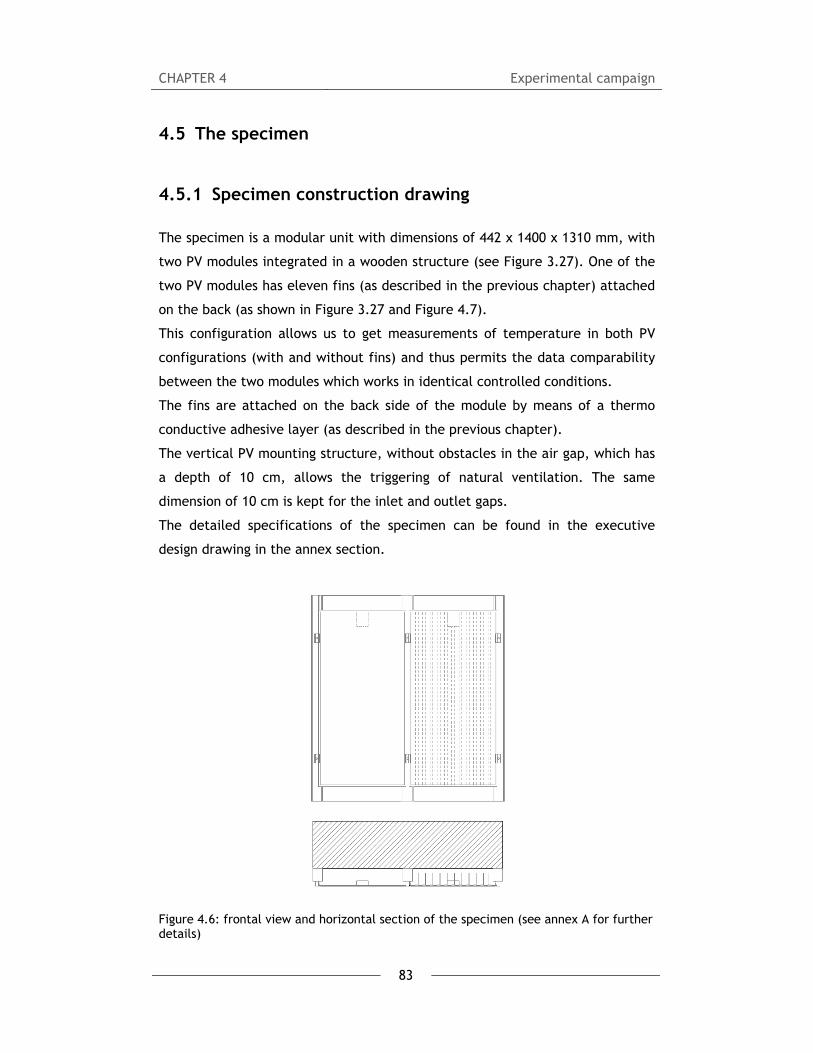
CHAPTER 4 Experimental campaign
83
4.5 The specimen
4.5.1 Specimen construction drawing
The specimen is a modular unit with dimensions of 442 x 1400 x 1310 mm, with
two PV modules integrated in a wooden structure (see Figure 3.27). One of the
two PV modules has eleven fins (as described in the previous chapter) attached
on the back (as shown in Figure 3.27 and Figure 4.7).
This configuration allows us to get measurements of temperature in both PV
configurations (with and without fins) and thus permits the data comparability
between the two modules which works in identical controlled conditions.
The fins are attached on the back side of the module by means of a thermo
conductive adhesive layer (as described in the previous chapter).
The vertical PV mounting structure, without obstacles in the air gap, which has
a depth of 10 cm, allows the triggering of natural ventilation. The same
dimension of 10 cm is kept for the inlet and outlet gaps.
The detailed specifications of the specimen can be found in the executive
design drawing in the annex section.
Figure 4.6: frontal view and horizontal section of the specimen (see annex A for further details)

CHAPTER 4 Experimental campaign
84
4.5.2 Specimen construction: the industrial collaboration
The specimen was built by a network of enterprises sited in province of Trento
called “Chi Quadrato”, that is a consortium gathered together through a local
project entitled “CHI QUADRATO - costruire strutture in bioedilizia certificate
per attività formative” (“Chi Quadrato: construction building of certified green
buildings designed for training activities”), co-financed from the Autonomous
Province of Trento in the framework of the Program FESR 2007-2013 Obiettivo 2
(Bando 1/2008 –“Promozione di progetti di ricerca applicata inerenti il Distretto
Tecnologico Energia ed Ambiente”).
General aim of the project was to design a prototypical elementary school of
200 m2 entirely realized with prefabricated wood framed panels with high
energy efficiency standard, developing innovative technological solutions and
promoting and enhancing the value of wood as a sustainable building material.
The BiPV wall prototype developed in this thesis is part of this project and it is
conceived as a “prototype in the prototype”.
In particular the specimen was built by two enterprises which work in the field
of wooden sustainable buildings (Legno Piú Case s.p.a.) and in the electricity
sector (G&G Impianti Elettrici s.r.l) belonging to Chi Quadrato consortium.
Figure 4.7: The specimen built by two enterprises belonging to the network Chi-Quadrato. The picture on the left shows the modular specimen; The other picture shows one of the two PV modules which has eleven fins attached on the back side.

CHAPTER 4 Experimental campaign
85
4.6 Phase 1: “Bi” characterization
4.6.1 Aim of the test
The first test phase was carried out to measure the steady-state thermal
transmission properties of the prototype and to assess its global thermal
transmittance in accordance with the UNI EN ISO 8990 [3.1] and UNI EN ISO
12567-1 [4.2]. The standard UNI EN ISO 8990 regards the determination of
steady-state thermal transmission properties in calibrated and guarded hot box,
and shows the heat fluxes through all parts of the apparatus. For the guarded
hot box, an overview of the heat fluxes is given by Figure 4.8: the metering
chamber is surrounded by the guard chamber with controlled conditions to
minimize the lateral heat flux in the specimen (Φ2) and the heat flux through
the metering chamber envelope (Φ3). Ideally, when the specimen is
homogenous, the temperatures are uniform both internally and externally to
the metering box, as well as when the hot side temperatures and the surface
heat transfer coefficients are uniform, a thermal balance for the air (both
internally and externally to the metering box), would imply a balance on the
specimen surface and the other way round, e.g. Φ2= Φ3=0. The total heat flux
through the specimen is the same as the one provided in the metering box (Φp).
Φp is the sum of the thermal power provided by the fans and by the heater,
which is made of five electrical resistances: 4 x 120W “on-off” resistances and
1 x 100W “continuously-variable” resistance.
Figure 4.8: guarded hot box as foreseen by the UNI EN ISO 8990 [3.1], where: 1 is the metering box, 2 is the guarded box, 3 is the cold chamber and 4 is the specimen.

CHAPTER 4 Experimental campaign
86
According to the standard UNI EN ISO 12567-1 [4.2], the determination of the
thermal transmittance involves two stages. Firstly, measurements are made on
two calibration panels with known thermal proprieties, from which the surface
coefficient of the heat transfer (radiative and convective components) on both
sides of the calibration panel with surface emissivity on average similar to
those of the specimen to be tested and the thermal resistance of the surround
panel are determined. Secondly, measurements are made with the specimen
and the hot-box apparatus is used with the same fan settings on the cold side
as during the calibration procedure [4.2].
The principal heat fluxes through the surrounding panel, which provides
thermal insulation around the specimen, and through the test specimen are
shown in Figure 4.9: Φsur is heat transfer through the surround panel, Φcal is the
heat transfer through the calibration panel, Φedge is the boundary edge heat
transfer. Φedge is equal to zero for the considered BiPV specimen.
Figure 4.9: calibration and surrounding panel in the frame of the guarded hot-box as foreseen by the UNI EN ISO 12567 [4.2], where: 1 is the surround panel, 2 is the boundary effect, 3 is the cold side, 4 is the warm side, 5 is the calibration panel.

CH
4
IN
si
ca
ex
St
ca
ch
77
th
pa
FiThx x x o A
HAPTER 4
.6.2 Exp
NTENT lab a
mulator, a
alorimeter
xpanded po
teady state
alorimeter,
hambers: th
7 thermoco
hermocoupl
anels, 16 su
gure 4.10: dhe temperat= surface the= air thermo= surface the= air thermo clearer draw
periment
apparatus i
as required
of INTENT
olystyrene E
e conditio
with a ΔT
he cold cha
ouples type
es on the
urface therm
rawing of thure sensors aermocouple
ocouple ermocouple ocouple of thwing can be f
tal setup
is used for
d by the
Lab and
EPS (thickne
ns are re
T of approx
mber is set
T are used
specimen
mocouples
he calorimeteare shown as
on the wall he chambersfound in the
87
p
this test p
standard.
is surround
ess=44.3cm
eached and
ximately 40
t to -10°C, t
d during the
, 18 surfa
on the surr
er with the ss follows:
behind the P annex secti
phase witho
The speci
ded by fou
, density=3
d kept fo
0°C betwee
the hot one
e test and i
ace thermo
ounding pa
specimen du
PV modules
on.
Experimen
out the use
men is pl
ur pre-shap
0 kg/cm).
r three h
en the hot
e to 30°C.
in particula
ocouples o
nel.
ring test of
ntal campai
e of the sol
laced in t
ped blocks
hours in t
and the co
ar: 25 surfa
n the baff
phase 1.
gn
lar
he
of
he
old
ace
fle

CHAPTER 4 Experimental campaign
88
4.6.3 Results
The thermal transmittance measured by the hot box method according to UNI
EN ISO 12567 [4.2], results to be 0.204 W/(m²K). The discrepancy between the
measured and calculated values (which is 0.188 W/(m²K), as reported in the
previous chapter) lies within the 8.5% measurements error.
Specimen measurement results
Cold temperatures - measured
θce Air °C -9.97
θse,b Baffle °C -10.38
θse,p Reveal temperature °C ---
θse,sur Sorround panel temperature °C -10.19
Warm temperatures - measured
θci Air °C 29.97
θsi,b Baffle °C 29.95
θsi,sur Sorround panel temperature °C 29.71
Φin Input power in hot box W 23.80
Vi Air flow warm, down m/s 0.16
Ve Air flow cold, up m/s 0.13
Table 4.3: Measured values registered during the test, required by the UNI EN ISO12567-1 [4.2] for the assessment of the thermal transmittance.
Thermal transmittance calculation θme,sur Mean temp. of surround panel °C Rsur Surround panel thermal resistance m²K/W 12.63 λsur Conductivity of surround panel W/(mK) 0.04 ψedge for w=20 mm / d=150 mm W/(mK) 0.00 Δθs,sur Temp. Difference of surround panel K 39.89 Δθc Air temperature difference K 39.94 Φin Input power to hot box W 23.80 Φsur surround panel heat flow W 8.78 Φedge Edge zone heat flow W 0.00 qsp Heat flow density of specimen W/m² 8.16 Fci Convective fraction - warmside - 0.52 Fce Convective fraction - coldside - 0.81 Rs,t Total superficial thermal resistance m²K/W 0.15 θri Radiant temperature - warmside °C 29.95 θre Radiant temperature - coldside °C -10.38 θni environmental temp. - warmside °C 29.96 θne environmental temp. - coldside °C -10.05 Δθn environmental temp. difference K 40.01 Um Measured thermal transmittance W/(m²K) 0.204 Δum Uncertainty of the measurement W/(m²K) ± 0.08
Table 4.4: this table summarizes the main average values measured during the steady conditions used for the thermal transmittance calculation according to the UNI EN ISO12567-1 [4.2]

CHAPTER 4 Experimental campaign
89
4.7 Phase 2: “PV” characterization
4.7.1 Aim of the test
The second test phase was carried out to measure the PV-related
characteristics of the CIGS modules (I-V characteristic curve, Voc, Isc, Pmppt
values at different conditions) and in particular to plot a “Pmppt matrix” which
provides the Pmppt value at each condition of irradiance and temperature. From
the matrix it is possible to evaluate the value of the temperature coefficient γ
at different irradiance values (AM 1.5) according to the International Standard
IEC 61646 [4.4] and IEC 60891 [4.5]. The two standards contain the apparatus
description and the procedures to determine the temperature coefficients of
current (α), voltage (β) and peak power (γ) from module measurements
referred to one Irradiance value.
The procedure specified in the standard requires to [4.5]:
a) Heat or cool the module to the temperature of interest until its temperature
is uniform within ±2 °C. Once the module temperature has stabilized, set the
irradiance to the desired level, using the reference device (IEC 60904-2).
b) Record the current-voltage characteristic and temperature of the specimen
and take the values of ISC, Voc and Pmax.
c) Change the module temperature in steps of approximately 5 °C over a range
of interest of at least 30 °C and repeat steps a) and b).
This procedure is repeated for 11 Irradiance values (from 100W/sqm to
1100W/sqm) over a range of 70°C (from 5°C to 75°C) in order to build the
“Pmppt matrix” of the CIGS module.
CHAPTER 4 Experimental campaign
90
4.7.2 Experimental setup
The apparatus used to control and measure the test conditions meets the
requirements foreseen by the IEC 61646 [4.4], and includes:
- a radiant source which is a solar simulator, class AAA in accordance with
IEC 60904-9 [4.3];
- a PV reference device with a known short-circuit current versus
irradiance characteristic determined by calibrating against an absolute
radiometer in accordance with IEC 60904-2;
- equipment necessary to control the temperature of the test specimen
over the range of interest. For this purpose, two different devices are
used: a thermal blanket placed on the back side of the module to heat
it up and the climatic chamber (see paragraph 4.3) to cool it down. With
regard to the latter, in order to guarantee the temperature stability
after the refrigeration in the climatic chamber, a thermal insulation
together with an high thermal inertia material were applied to the back
side of the module;
- a suitable mount for supporting the test specimen and the reference
device in the same plane normal to the radiant beam;
- an electronic load to measure the I-V curve in accordance with IEC
60904-1.
4.7.3 PV module preconditioning
Thin-film module technologies are known for their metastability and thus it is
recommended [4.4] to stabilize their electrical characteristics before each
measurement. In particular, CIGS modules are subject to light-induced change
of the module efficiency and, as a consequence, an appropriate pre-
conditioning treatment needs to be applied to ensure that the performance
measurements are representative of those expected in normal operation.
The CIGS modules are in fact affected by “dark ageing” phenomenon, which
means that if they are stored in the dark, fill factor and Voc decrease
considerably (especially at high temperatures), while Isc is affected only to a
minor extent (reflecting changes of the spectral quantum efficiency) [4.7].

CHAPTER 4 Experimental campaign
91
This phenomenon is reversible by light-soaking (LS), although the recovery is
not always complete. In general, the improvement is greater for poorer
performing devices, but even high efficiency modules can show significant
gains. Light soaking in general can strongly influence the performance, even
within very short time intervals (from seconds to hours). On the other hand,
Kenny et al. [4.6] have shown that these module technologies may degrade
with light exposure. It is difficult to predict how a given CI(G)S material will
behave and each device is somehow unique. The behaviour is, in general, very
dependent on the deposition and exact material composition: the material’s
actual composition or stoichiometry, the deposition temperature and thickness
of the CdS buffer layer, the presence of gallium or sulphur in the quaternary
(Cu(In,Ga)Se2) and the different deposition processes can all influence the
meta-stable state [4.7].
However, in general, these modules exhibit a short-term meta-stable behaviour
modulated by light but for long-term light exposure, CIS/CIGS devices appear to
be very stable [4.8]. Moreover, [4.6] shows that the IEC 61646 stabilization
procedure could be considered a valid one for CIS and CIGS modules as long as
the measurement is made immediately following the LS in order to minimize
the relaxation effect of dark storage. The CIGS modules are thus pre-
conditioned, as required by the International Standard IEC 61646 [4.4] through
controlled Light-Soaking by means of simulated solar irradiation, and measured
immediately after.
Apparatus used for preconditioning
INTENT lab is used as apparatus for the module preconditioning, since it
complies with the standard IEC 61646 requirements and includes:
- a class BBB solar simulator in accordance with the IEC 60904-9, which is
the sun simulator part of INTENT lab;
- a suitable reference device (Kipp&Zonen CMP 21, as described in
paragraph 4.2), for monitoring the irradiation;
- means to mount the modules (the frame in Figure 4.2), co-planar with
the reference device.

CH
Pr
Th
pe
co
St
le
be
<
af
48
48
45
m
w
FisoCI
Th
fo
se
HAPTER 4
- mean
±1 °C
modu
- a resi
will o
rocedure f
he procedu
eriods at 6
onnected t
tabilization
east 43 kW
etween 40
2 %. The st
fter three
8°C, Energy
8°C, Energy
5°C, Energ
measuremen
ithin ±2 °C
gure 4.11: Noaking) againGS module w
he measur
ollowing th
ensitivity of
ns for measu
C (three th
ule)
istor sized
operate nea
for precon
re describe
600-1000 W
to the re
occurs wh
Wh/m2 eac
°C and 60 °
tabilization
light soakin
y = 46.150
y = 46.475
gy = 51
ts were pe
.
Normalized Pnst light-soakwith fins (WF
rements of
e light soa
f these devi
uring the te
hermocoupl
such that a
ar their max
nditioning
ed in the IEC
W/m2 and
esistor, unt
hen measur
h integrate
°C, meet th
for the tw
ng periods
0 kWh/m2;
kWh/m2;
1.600 kWh
erformed at
Pmax (i.e. noking cycles reF).
f I-V char
aking in or
ices to shor
92
emperature
es Type T
at STC (sta
ximum powe
g
C 61646 [4.
40-60°C m
til the m
rements fro
ed over p
he following
wo CIGS mod
(LS1: Irrad
LS2: Irradi
LS3: Irradi
h/m2). All
t module t
ormalized to eferred to th
racteristic
rder to min
rt term dark
e of the mo
placed on
andard test
er point (re
4] foresees
module tem
aximum p
om two co
eriods whe
g criteria: (
dules conne
diation = 65
iation = 65
iation = 60
intermed
temperature
the value ofhe no-fins CI
curves we
nimise the
k ageing eff
Experimen
odules to an
the back
condition)
esistance of
s a series of
mperature w
ower valu
nsecutive p
en the tem
(Pmax – Pm
ected in ser
50W/m2, T
50W/m2, T
00W/m2, T
diate maxi
e of 30.5°C
f Pmax at M1GS module (
ere made
effects re
fects.
ntal campai
n accuracy
side of ea
the modul
f 33 ohm).
f light soaki
with modul
e stabilize
periods of
mperature
min)/Pavera
ries, occurr
Tmod = 45°
mod = 45°
mod = 40°
imum pow
C reproduc
1, before lig(NF) and the
immediate
elated to t
gn
of
ach
les
ing
les
es.
at
is
age
red
C-
C-
C-
wer
ed
ht
ely
the

CHAPTER 4 Experimental campaign
93
4.7.4 Results
Pmppt matrices
The values of Pmppt is measured at different conditions of temperature and
Irradiation with a step respectively of 5°C and 100 W/sqm. Measurements are
performed for both modules, with and without fins. The module without fins
(NF) will be used as reference module for the discussion in next chapters. The
matrix for the module without fins is assembled in two following stages, due to
a practical convenience of heating the module up with the heating blanket in
stage 1 and cooling the module down with the climatic chamber in stage 2: in
the first stage, the I-V curve measurements are taken at each irradiance value
(steps of 100W/sqm, from 100W/sqm to 1100W/sqm) starting from a
temperature of 25°C±2°C to a temperature of 75°C±2°C with a step of
approximately 5°C. In the second stage the I-V curve measurements are taken
at some irradiance values (100-200-400-700-800-1000W/smq: the remaining
irradiance values were not measured because of the difficulty to keep stable
temperatures for a longer period required to flash for all irradiances values)
from a temperature of 5°C ±2°C to a temperature of 20°C ±2°C with a step of
approximately 5°C. The matrix for the module with fins is performed through
measurements taken at each irradiance value (steps of 100W/sqm, from
100W/sqm to 1100W/sqm) starting at 25°C ±2°C to 75°C ±2°C with a step of
approximately 5°C. Measurements for temperatures below 25°C were not
performed, considering that this module is not taken as a reference for the
following chapters.

CH
FimvaW
Fidi
Du
Pm
ca
ex
ep
is
As
th
Th
ph
Eq
m
HAPTER 4
gure 4.12: Sodule withou
alues in the gW/sqm, are in
gure 4.13: Mfferent temp
uring the l
mppt matrix,
aused by t
xpansion co
poxy adhes
around thr
s a consequ
he second p
hus, only t
hases.
quation 4.1
method and
urface that iut fins (NF) agraph from 5nterpolated v
Measured maperature and
ast measur
, some crac
he therma
oefficient
ive and the
ree times th
uence, the
phase measu
he NF mod
is the fun
considerin
interpolate tat different 5°C to 20°C fvalues since
ximum powed Irradiance
rements (i.
cks on the
l stress es
among the
e glass (the
he glass one
power outp
urements.
dule is used
nction that
g Pmppt line
94
the measuretemperaturefor Irradianc they have n
er point valu conditions.
e. measure
glass of th
specially at
e aluminium
ermal expan
e).
put of the W
d as refere
approxima
ear to both
ed maximum e and Irradiaces of 1100, ot been mea
ues of the mo
ements at
he WF mod
t 75°C and
m fins, the
nsion coeff
WF module
nce module
ates, using
h irradiance
Experimen
power pointance conditio900, 600, 50asured.
odule with fi
Tmod=75°C
dule appear
d the diffe
e thermally
ficient of th
slightly de
e for the f
the least e
e and temp
ntal campai
t values of thons. The 00, 300
ins (WF) at
C) of the W
red. This w
rent therm
y conducti
he aluminiu
ecreases aft
following te
error squar
perature, t
gn
he
WF
was
mal
ive
um
ter
est
res
he

CH
m
Irr
Te
Fo
th
Ac
de
da
Pm
(s
Fithth
Th
bo
re
co
HAPTER 4
measured m
radiance an
emperatu
or each Irra
he measure
ccording to
evice tempe
ata is const
mppt are d
ee Figure 4
gure 4.14: Phe device temhe set of data
he power te
oth the m
espectively,
ondition are
maximum p
nd module t
Pm
re coeffic
adiance valu
ments prese
o the Standa
erature is p
tructed. Fro
drawn and
4.14 as an e
Pmppt valuesmperature (oa.
emperature
modules (w
, of 45°C (3
e inserted i
ower point
temperatur
mmpt,NF=0.081
ient meas
ue, the rela
ented in th
ard IEC 616
plotted and
om the slop
the temper
example).
s of the modover a range
e coefficien
with and
30°C-75°C)
n the annex
95
t values o
re.
18*Irr-0.108
surements
ative tempe
e previous
646 [4.4], v
d a least-sq
pes of the
rature coef
ule no fins a of 50°C) wi
nts are mea
without fi
and 50°C (
x section.
of the NF
85*Tmod [
s
erature coe
paragraph
alues of Pm
uares-fit cu
least squar
fficient of
at 1000W/sqmth a least-sq
asured at e
ns) over
25°C-75°C)
Experimen
module, d
[W]
efficient is a
for both CIG
mppt as fun
urve throug
res fit, stra
Pmppt (γ)
m (AM 1.5) aquares-fit cu
ach irradia
a tempera
), and the p
ntal campai
depending
Equation 4
assessed fro
GS modules
nctions of t
gh each set
aight lines f
is calculat
as function orve through
nce value f
ature rang
plots for ea
gn
on
4.1
om
s.
he
of
for
ed
of
for
ge,
ach

CHAPTER 4 Experimental campaign
96
In addition, the relative power temperature coefficients expressed as
percentages are determined for each irradiance value by dividing the
calculated γ by the value of peak power at 25 °C (see Table 4.5).
The measured temperature coefficients refer to AM 1.5.
NF module
G/[W/sqm] γ/ [W/°C] measured Pmppt at 25°C/[W]
γrel/ [%/°C]
1100 -0.36 89.81 -0.40 1000 -0.33 81.93 -0.41 900 -0.30 73.88 -0.41 800 -0.27 65.73 -0.42 700 -0.24 57.43 -0.43 600 -0.21 49.12 -0.43 500 -0.18 40.75 -0.44 400 -0.14 32.16 -0.45 300 -0.11 23.77 -0.46 200 -0.07 15.35 -0.47 100 -0.04 7.12 -0.50
Table 4.5: no fins module: power temperature coefficients (γ )and relative power temperature coefficients (γrel), calculated for each irradiance value (AM 1.5) from the measured Pmppt values at different temperatures over a range of 50°C (25°C-75°C)
WF module G/[W/sqm] γ/ [W/°C] calculated Pmppt
at 25°C/[W] γrel/ [%/°C]
1100 -0.37 93.65 -0.40 1000 -0.34 85.44 -0.40 900 -0.31 77.10 -0.40 800 -0.28 68.63 -0.40 700 -0.25 60.15 -0.41 600 -0.21 51.48 -0.42 500 -0.18 42.78 -0.42 400 -0.15 33.92 -0.43 300 -0.11 25.12 -0.44 200 -0.07 16.26 -0.45 100 -0.04 7.64 -0.47
Table 4.6: with fins module: power temperature coefficients (γ )and relative power temperature coefficients (γrel), calculated for each irradiance value (AM 1.5) from the measured Pmppt values at different temperatures over a range of 45°C (30°C-75°C)
Finally, the values of the relative temperature coefficient of Pmppt (γrel) for the
two modules are plotted for each irradiance (Figure 4.15).

CH
Fi(A50
As
Irr
ac
Th
th
ex
4
4
Ma
th
ev
th
te
th
to
HAPTER 4
gure 4.15: γAM 1.5) from 0°C (25°C-75
s shown in
radiance, f
ccordance w
he resulting
he NF modu
xpressed by
.8 Phase
.8.1 Aim
ain aims of
he two mod
valuate the
he two mo
emperature
he measure
o:
γ and γrel of t the measure5°C) for the
Figure 4.1
for both mo
with [4.9], w
g dependen
ule, which
y the follow
γ = - 0
e 3: “PV
m of the t
f the third
dules (NF a
e averaged
odules) ope
and irradi
d data are
the NF and Wed Pmppt vaNF module a
5, the rela
odules, has
where a cry
ncy of the
is taken a
wing equatio
.0003*Irr - 0
in Bi” ch
test
phase are
and WF) in
ΔTNF-WF (i.
erating in
ance). The
then assess
97
WF modules aalues at diffeand 45°C (30
ative tempe
s a logarith
ystalline sil
temperatu
as a refere
on:
0.0123 (R2=
haracteri
to measur
ntegrated i
e. average
different e
e mathemat
sed through
are plotted ferent temper0°C-75°C) fo
erature coe
hmic regres
licon modul
ure coeffici
nce for the
=0.998)
ization
re the tem
in the woo
e temperatu
environmen
tical equat
h the exper
Experimen
for each irraratures over
or the WF mo
efficient of
ssion trend
le is tested.
ent γ on i
e following
[W/°C]
perature d
oden wall a
ure differe
ntal conditi
ions which
rimental re
ntal campai
adiance value a range of:
odule.
Pmppt again
d, which is
.
rradiance f
g chapters,
Equation 4
istribution
as well as
nce betwe
ions (i.e. a
approxima
sults in ord
gn
e
nst
in
for
is
4.2
of
to
en
air
ate
der

CHAPTER 4 Experimental campaign
98
- understand the dependency of the working module temperatures on the
environmental conditions (i.e. air temperature and irradiance), and thus
to evaluate the effectiveness of the proposed BiPV configuration;
- understand the dependency of the ΔTNF-WF between the two modules on
the environmental conditions (i.e. air temperature and irradiance), and
thus to evaluate the contribution provided by the fins to decrease the
module temperature in each condition of irradiance and air
temperature.
The modules temperature distribution and ΔTNF-WF between the two modules
are measured for irradiance and air temperature conditions over an irradiance
range of 600 W/sqm in steps of 200W/sqm and over a temperature range of
40°C in steps of 10°C.
4.8.2 Experimental setup
Measurements of this experimental phase are carried out in INTENT lab. In this
third phase, unlike the phase 1, also the steady state sun simulator is used (see
paragraph 4.2 for the lab description). In addition, in order to guarantee the
correct functioning of the two modules close to their maximum power point
value, a “stand-alone system” with an mppt tracer is set up. The stand-alone
system includes:
- a maximum power point tracking solar charge controller (max. PV input
voltage of 150 VDC, rated load current 10A, max. PV input power of 260W,
system voltage 12 / 24VDC);
- four loads (two DC lamps of 60 W and two DC lamps of 40 W) to dissipate
the produced energy depending on the working condition;
- two AGM batteries 12V-26Ah connected in series;
- cables (4mm2) to connect the system;
- an electric panel with safety devices and switches.
To size the solar charge controller considering the test conditions, the
measured values of Isc and Voc of the two modules connected in series are
verified according to the device requirements (max. PV input voltage of 150
VDC, rated load current 10A, max. PV input power of 260W).

CHAPTER 4 Experimental campaign
99
Isc [A], two modules in series 1100 1000 900 800 700 600 500 400 300 200 100
5 2.91* 2.70 2.39* 2.17 1.89 1.60* 1.33* 1.08 0.80* 0.54 0.27 10 2.91* 2.70 2.39* 2.16 1.89 1.60* 1.34* 1.08 0.80* 0.54 0.27 15 2.92* 2.66 2.39* 2.14 1.87 1.60* 1.34* 1.07 0.80* 0.54 0.27 20 2.92* 2.66 2.40* 2.13 1.87 1.60* 1.34* 1.07 0.80* 0.54 0.27 25 2.92 2.66 2.40 2.14 1.87 1.60 1.34 1.07 0.81 0.54 0.27 30 2.93 2.67 2.40 2.14 1.87 1.61 1.34 1.07 0.81 0.54 0.27 35 2.93 2.67 2.41 2.14 1.87 1.61 1.35 1.07 0.81 0.54 0.27 40 2.93 2.67 2.41 2.14 1.88 1.61 1.35 1.07 0.81 0.54 0.27 45 2.93 2.67 2.41 2.14 1.88 1.61 1.35 1.08 0.81 0.54 0.27 50 2.94 2.68 2.41 2.15 1.88 1.61 1.35 1.08 0.81 0.54 0.27 55 2.94 2.68 2.41 2.15 1.88 1.62 1.35 1.08 0.81 0.54 0.27 60 2.94 2.68 2.42 2.15 1.88 1.62 1.35 1.08 0.81 0.54 0.27 65 2.95 2.69 2.42 2.16 1.89 1.62 1.35 1.08 0.81 0.54 0.27 70 2.95 2.69 2.42 2.16 1.89 1.62 1.36 1.08 0.81 0.54 0.27 75 2.96 2.69 2.43 2.16 1.89 1.63 1.36 1.09 0.82 0.54 0.27 *calculated value (extrapolation)
Table 4.7: Isc values of the two modules connected in series for different conditions. The values are taken from the measurements of the NF module.
Voc [V], two modules in series 1100 1000 900 800 700 600 500 400 300 200 100
5 93.68* 93.33 92.98* 92.09 91.27 91.18* 90.34* 88.31 87.93* 84.62 80.81 10 92.39* 91.94 91.64* 90.71 89.98 89.78* 88.91* 87.07 86.44* 83.33 79.54 15 91.10* 90.52 90.31* 89.35 88.65 88.38* 87.49* 85.72 84.96* 82.06 78.28 20 89.81* 88.56 88.97* 87.41 86.73 86.98* 86.07* 83.79 83.48* 80.09 76.32 25 88.27 87.91 87.36 86.73 86.08 85.23 84.24 83.09 81.51 79.39 75.58 30 87.13 86.77 86.25 85.65 85.02 84.22 83.27 82.16 80.61 78.51 74.79 35 86.24 85.78 85.22 84.56 83.86 83.00 82.02 80.86 79.30 77.11 73.07 40 84.78 84.30 83.73 83.03 82.33 81.47 80.46 79.21 77.60 75.43 71.56 45 83.99 83.45 82.78 82.07 81.33 80.40 79.34 78.10 76.44 74.19 70.26 50 81.43 80.96 80.38 79.73 79.07 78.18 77.16 75.96 74.32 72.08 68.08 55 81.09 80.51 79.85 79.12 78.35 77.39 76.30 74.99 73.27 70.86 66.80 60 79.34 78.77 78.10 77.36 76.49 75.55 74.66 73.37 71.63 69.24 65.11 65 77.92 77.34 76.69 75.95 75.20 74.22 73.11 71.77 70.02 67.58 63.42 70 77.18 76.55 75.80 75.02 74.21 73.17 72.03 70.64 68.79 66.33 62.03 75 75.67 74.96 74.27 73.42 72.56 71.50 70.19 68.81 66.94 64.37 60.07 *calculated value (extrapolation)
Table 4.8: Voc values of the two modules connected in series for different conditions. The values are calculated multiplying by two the measurements of the NF module.
Considering Table 4.7 and Table 4.8, the maximum PV output current is 2.96 A,
and the maximum PV output voltage is 93.68 V. The two values lie below the
requirements foreseen by solar charge controller and they are thus verified.
Other devices are used during the third phase experiments, and in particular:
- a current probe and a tester to double check the correct working
conditions at mppt of the two modules during the experiment

CHAPTER 4 Experimental campaign
100
- a peak power measuring device with I-V-curve tracer (PVPM 1000C), to
double check the I-V curve of each module at some conditions (e.g. see
Figure 4.19), with the following characteristics: Peak power measurement:
±5%, duration of single measurement: 2s, reference cell Phox sensor with
integrated Pt1000 sensor (Solar Radiation Sensor SOZ-03, calibrated on the
17.04.2012, calibration value: 96,0 mv at 1000W/sqm)
- an additional hot wire anemometer (air velocity handprobe 0-20 m/s FV
A935-TH5K2; relative measurement uncertainty: 5%) to measure the air
velocity speed in different points .
Figure 4.16: test devices used during experiments of phase 3: a current probe with a tester, a peak power measuring device with I-V-curve tracer and a stand-alone system with mppt tracer connected to the two modules. The image on the right shows the experimental setup connected to the specimen placed in the INTENT calorimeter.
The BiPV specimen is placed in INTENT calorimeter (see Figure 4.17) and the
two PV modules (NF and WF) are connected in series to the stand alone system
placed close to the calorimeter. The temperature distribution of the two
modules is measured with twelve surface thermocouples (type T) placed on the
back side of each module (see Figure 4.17). Moreover, to identify the boundary
conditions of the heat transfer problem, the following data are acquired:
- the irradiation of the modules, measured with a pyranometer (as described
in paragraph 4.2) placed vertically next to the modules (see Figure 4.17);
- the cold chamber air velocity, measured with a hot-wire anemometer
placed at the top of the cold chamber next to the target to get the vertical
value of the air velocity (see Figure 4.17);
- the cold chamber air temperature, measured with eight air thermocouples
(Type T) placed next to the target (Figure 4.17);
- the surface wall temperature behind the two modules, measured with
eight surface thermocouples (Type T) (see Figure 4.17);
- the air temperature in the middle of the air gap between the modules and
the wall (see Figure 4.17), measured with four air thermocouples (Type T);

CH
-
Th
irr
10
of
40
“o
to
Ea
ke
Du
en
Fithdex bean
HAPTER 4
the air v
the wall
he tests a
radiance o
000W/sqm)
f the calori
0°C). For e
outdoor” ai
o the target
ach conditi
ept for at le
uring each
nvironment
gure 4.17: Phe third phasetailed draw= surface theehind the PVnemometer;
velocity (ve
, measured
are repeate
over a rang
and varyin
imeter cold
each conditi
ir velocity t
t as shown i
on (which
east two ho
h test co
al condition
Positioning ofse of the exp
wing). The seermocouple;
V modules; o o = pyranom
ertical direc
with a hot
ed for twe
ge of 600
ng the ambi
d chamber)
ion, the co
tangent to
in Figure 4.
is a combi
ours after re
ondition, t
ns to ensure
f the temperperimental cansors are sho; x = air ther = air thermo
meter
101
ction) in th
t-wire anem
enty enviro
W/sqm in
ent air tem
over a ran
old chamber
the PV mo
17) is kept
ination of a
eaching the
the two
e the comp
rature, air veampaign (seeown as followrmocouple; xocouple of th
e gap betw
mometer (se
onmental c
steps of
mperature (
nge of 40°C
r air veloci
dules and w
constant w
air tempera
e steady-ste
modules o
parability of
elocity and ie the annex ws: x = surface the chambers
Experimen
ween the NF
ee Figure 4.
conditions:
200W/sqm
i.e. the air
C in steps o
ty (which r
which is me
with a value
ature and i
ead conditio
operate in
f the data.
rradiance se section for a
hermocouples; □ = hot wi
ntal campai
F module a
.17).
varying t
(400W/sqm
temperatu
of 10°C (0°
represent t
easured clo
e of 2m/s.
irradiance)
ons.
n the sam
ensors duringa more
e on the walre
gn
nd
he
m-
ure
C-
the
ose
is
me
g
ll

CHAPTER 4 Experimental campaign
102
4.8.3 Results
The temperature distribution of each module is measured for each
environmental condition with twelve thermocouples attached on the back side
of each module.
Figure 4.18 shows the average temperature (i.e. the average of the values
measured by the twelve thermocouples) of the two PV modules (NF and WF)
and the resulting ΔTNF-WF at each environmental condition. During each test
condition, the irradiance and air temperature values are kept in steady state
conditions for at least two hours with a constancy over time, respectively, of
±2% and ±0.2°C (as shown in Figure 4.20). The air velocity in the cold chamber
is kept at a constant value of 2m/s (±0,1m/s over time) in the vertical
direction, as measured by the anemometer close to the PV modules surface
(see Figure 4.17).
Figure 4.18: Measured average values of modules temperature (NF and WF) at twenty different set point conditions of air temperature and irradiance. The purple line shows the resulting temperature difference between the two modules.
Test 4 Test 1
Test 2 Test 3
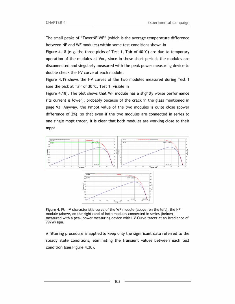
CHAPTER 4 Experimental campaign
103
The small peaks of “TaverNF-WF” (which is the average temperature difference
between NF and WF modules) within some test conditions shown in
Figure 4.18 (e.g. the three picks of Test 1, Tair of 40°C) are due to temporary
operation of the modules at Voc, since in those short periods the modules are
disconnected and singularly measured with the peak power measuring device to
double check the I-V curve of each module.
Figure 4.19 shows the I-V curves of the two modules measured during Test 1
(see the pick at Tair of 30°C, Test 1, visible in
Figure 4.18). The plot shows that WF module has a slightly worse performance
(its current is lower), probably because of the crack in the glass mentioned in
page 93. Anyway, the Pmppt value of the two modules is quite close (power
difference of 2%), so that even if the two modules are connected in series to
one single mppt tracer, it is clear that both modules are working close to their
mppt.
Figure 4.19: I-V characteristic curve of the WF module (above, on the left), the NF module (above, on the right) and of both modules connected in series (below) measured with a peak power measuring device with I-V-Curve tracer at an irradiance of 797W/sqm.
A filtering procedure is applied to keep only the significant data referred to the
steady state conditions, eliminating the transient values between each test
condition (see Figure 4.20).
0
10
20
30
40
50
60
70
80
90
0
0,2
0,4
0,6
0,8
1
1,2
1,4
1,6
1,8
2
0 5 10 15 20 25 30 35 40 45Voltage in V
Cu
rren
t in
A
Po
wer
in
W
MPP: 60.4W
34.52 V
1.75 A
1.96 A
0
10
20
30
40
50
60
70
80
90
0
0,2
0,4
0,6
0,8
1
1,2
1,4
1,6
1,8
2
0 5 10 15 20 25 30 35 40 45Voltage in V
Cu
rren
t in
A
Po
wer
in
W
MPP: 61.9W
34.07 V
1.82 A
1.99 A
0
20
40
60
80
100
120
140
160
180
0
0,2
0,4
0,6
0,8
1
1,2
1,4
1,6
1,8
2
0 10 20 30 40 50 60 70 80 90Voltage in V
Cu
rre
nt
in A
Po
we
r in
W
MPP: 122.3W
69.02 V
1.77 A
87.25 V
1.99 A

CHAPTER 4 Experimental campaign
104
Figure 4.20: Measured average values of modules temperature (NF and WF) and resulting ΔT between them at twenty different set point conditions of air temperature and irradiance, after applying the filtering procedure to eliminate transient points.
Figure 4.21 and Figure 4.22 show, respectively, the test boundary conditions
measured in the cold chamber and in the air gap of the specimen (between the
PV modules and the wooden wall), where: “Pyranometer” is the measured
irradiance on the PV modules plane; “TaverAircold” is the average temperature
of eight thermocouples in the calorimeter cold chamber (see Figure 4.17);
“VelocityAirColdChamber” is the vertical component of the velocity tangent to
the modules in the cold chamber (see Figure 4.17);
“VelocityAirGap_anenometer” is the measured air velocity in the middle of the
air gap; “AirGap TNF” is the average temperature of two thermocouples in the
air gap behind the NF module (see Figure 4.17); “AirGap TWF” is the average
temperature of two thermocouples in the air gap behind the WF module (see
Figure 4.17).
During the experiments, the air temperature of the hot chamber is kept
constant at 20°C.
Test 4 Test 1
Test 2 Test 3

CHAPTER 4 Experimental campaign
105
Figure 4.21: test boundary conditions of air velocity, air temperature and irradiance kept in the calorimeter cold chamber during the experiment.
Figure 4.22: test boundary conditions of air temperature and air velocity measured in the air gap between the modules and the wooden wall during the experiment.
Expression of TNF and TWF as function of Tair and Irr
After filtering the data as shown in Figure 4.20, the function which
approximate the measured modules temperature values (NF module and WF
module) depending on Irradiance and air temperature values is assessed using
the least error squares method (Equation 4.3 and Equation 4.4).

CHAPTER 4 Experimental campaign
106
Figure 4.23 shows the surface which approximate the measured average
temperature values of the two modules depending on the cold chamber air
temperature and the irradiance values, where: “T mod” is the average
temperature of the NF module (on the left) and of the WF module (on the
right); “Tair” is the average temperature of the air in the calorimeter cold
chamber; “Irr” is the sun simulator irradiance on the modules plane.
Figure 4.23: Approximated surface through the average T measured values of the two modules depending on Tair and Irradiance.
TNF= 1.0122*Tair + 0.0250*Irr [°C]
Equation 4.3
TWF= 1.0071*Tair + 0.0206*Irr [°C]
Equation 4.4
NOCT model vs experimental data
The resulting Equation 4.3 can be compared with one of the most commonly
used prediction model of the operating module temperature, e.g. the nominal
operating cell temperature (NOCT) model [4.10] [4.11].
According to this model, the module operating temperature can be retrieved by
Equation 4.5, as give below:
Tmod=Tair + Irr* (NOCT-20)/800 [°C]
Equation 4.5
Where: Tmod, is the module temperature; Tair is the ambient temperature; Irr
is the solar irradiation; NOCT is the Nominal Operating Cell Temperature

CHAPTER 4 Experimental campaign
107
defined as the temperature reached by open circuited cells in a module under
the conditions of: Irradiance on cell surface = 800 W/sqm; Air Temperature =
20°C; Wind Velocity = 1 m/s; Mounting = open back side.
For the considered CIGS module, which has an NOCT value of 47°C ±3°C (data
from the datasheet), Equation 4.5 would be:
Tmod=Tair + 0.0338* Irr [°C]
Equation 4.6
The coefficients of the resulting Equation 4.6 differ from the coefficients of
Equation 4.3 of 1% with regard the Tamb and between 17% and 33% (according
to the NOCT value uncertainty given in the module datasheet: NOCT=47°C±3°C)
with regard the Irr. Significant errors of predictions by this model are thus
found with regard this application. In fact, the NOCT approach is based on the
more common scenario where both sides of the PV module see the same
ambient temperature and wind conditions. Instead, the two sides of the
modules integrated in the prototype, are subjected to significantly different
environmental conditions, as it is for most BiPV applications
[4.10],[4.11],[4.13],[4.14]. Other studies [4.10] [4.11] confirm that significant
errors of prediction by this model are found when the conditions of installation
are different from the standard conditions as regards mounting configuration,
loading and environmental conditions.
It is thus suggested not to rely on this model, even if it is a very handy and
simple one, when dealing with these kind of BiPV applications, but to use more
accurate techniques, such as:
- Expressions which include a parameter for BiPV situations depending on
the level of integration and (ventilation) gap size, such as the one
developed by Nordmann and Clavadetscher [4.15], or the one developed
by Krauter [4.16];
- Expressions which include wind velocity as a parameter, such as
[4.17],[4.18],[4.19],[4.20];
- A more complex, one-dimensional heat transfer model developed by
Davis et al. [4.11], which includes forced and natural convection
relations.

CHAPTER 4 Experimental campaign
108
Other more complex models can be found in [4.14], which report several
implicit equations for the evaluation of Tmod.
Expression of ΔTNF-WF as function of Tair and Irr
As last step, the function which approximate the measured ΔTNF-WF values (i.e.
ΔT between NF module and WF module) depending on Irradiance and air
temperature values is assessed using the least error squares method (Equation
4.7). Figure 4.24 shows the ΔTNF-WF linear relation with air temperature and
Irradiance, where: ΔT is the temperature difference between the average
temperature of NF module and of WF module; “Tair” is the average
temperature of the air in the calorimeter cold chamber; “Irradiance” is the sun
simulator irradiance on the modules plane.
Figure 4.24: Approximated surface through the ΔT measured data depending on Tair and Irradiance.
ΔTNF-WF= 0.0051*Tair + 0.0044*Irr [°C]
Equation 4.7
RMS (root mean squared) of residuals= 0.0874202; R2=0.989102
Equation 4.7 refers to the measured conditions of:
- Irradiance ranging from 400W/sqm to 1000W/sqm

CHAPTER 4 Experimental campaign
109
- Air temperature ranging from 0 to 40°C
- Velocity of the air adjacent to the PV modules kept constant at 2m/s (as
shown in Figure 4.21)
- Air gap velocity ranging between 1.1 m/s and 1.5m/s (as measured, see
Figure 4.22)
- Irradiation referred to the spectrum AM 1.5
Regarding the last point, it has to be underlined that, since all measured data
of irradiance refer to the spectrum AM 1.5, the spectral effects are not
considered. However, this simplification is justified by the fact that the
spectral effect for CIGS technology is negligible [4.12]. CIGS in fact is one of
the materials which present the highest range of spectral response (as shown in
Figure 4.25).
Figure 4.25: AM1.5 spectrum and corresponding spectral response of different solar cell materials. The spectral response of various materials is indicated by the boxes [4.12]
Figure 4.1 and Equation 4.7 show that the influence of Tair on ΔTNF-WF is much
lower than the irradiance’s one, considering the typical ambient conditions on
the Earth (Irr is typically an order of magnitude higher than Tair).
For instance, a peak temperature of 50°C would affect the value of ΔTNF-WF for
an extent of 0.25°C, while a peak irradiance of 1100W/sqm would affect the
value of ΔTNF-WF for an extent of 4.8°C, i.e. around 19 times the value due to
Tair.
Considering the city of Aswan in Egypt as a limit example, the highest
irradiance on a best oriented module (i.e. azimuth of 0° and tilt of 23°) is 1172
W/sqm and the corresponding Tair is 28.8°C, happening on the 7th of March at

CHAPTER 4 Experimental campaign
110
noon referring to the meteorological database of the commercial software PV-
SOL.
In these peak conditions (Irr=1172 W/sqm and Tair=28.8°C), the resulting ΔTNF-
WF would be 5.3°C. This number can be considered as a limit value of the
maximum contribution that can be provided by the fins to decrease the module
temperature in the considered conditions (as listed below the Equation 4.7).

CHAPTER 4 Experimental campaign
111
References
[4.1] International Standard UNI EN ISO 8990, 1999. Thermal Insulation –
Determination of steady-state thermal transmission properties – Calibrated and
guarded hot box.
[4.2] International Standard UNI EN ISO 12567, 2002. Thermal performance of
windows and doors – Determination of thermal transmittance by hot box
method.
[4.3] International Standard IEC 60904-9, 2007. Photovoltaic devices –Part 9:
Solar simulator performance requirements.
[4.4] International Standard IEC 61646, 2008. Thin film terrestrial photovoltaic
(PV) modules – Design qualification and type approval.
[4.5] International Standard IEC 60891, 2009-12. Photovoltaic devices –
Procedures for temperature and irradiance corrections to measured I-V
characteristics.
[4.6] Robert P. Kenny, Anatoli I. Chatzipanagi and Tony Sample, 2012.
Preconditioning of thin-film PV module technologies for calibration. Progress in
Photovoltaic: research and applications, DOI: 10.1002/pip.2234.
[4.7] N. Taylor et al., April 2011. Guidelines for PV Power Measurement in
Industry. Report of Performance FP6 Integrated Project.
[4.8] M. Gostein & L. Dunn, 2011. Light Soaking Effects on Photovoltaic
Modules: Overview and Literature Review. Proceedings of the 37th IEEE
Photovoltaic Specialists Conference (PVSC), Seattle, Washington. 003126-
003131.
[4.9] D. L. King, J. A. Kratochvil and William E. Boyson, 1997. Temperature
Coefficients for PV Modules and Arrays: Measurement, Methods, Difficulties and
Results. Proceedings of the 26th IEEE Photovoltaic Specialists Conference,
Anaheim, California, 1183-1186.
[4.10] P. Trinuruk, C. Sorapipatana, D. Chenvidhya, 2009. Estimating operating
cell temperature of BIPV modules in Thailand. Renewable Energy 34, 2515–
2523.
[4.11] M.W. Davis, B.P. Dougherty, A.H. Fanney, 2001. Prediction of Building
integrated Photovoltaic Cell Temperatures. ASME Transactions the journal of
Solar Energy Engineering, Vol. 123, No.2, 200-2010.

CHAPTER 4 Experimental campaign
112
[4.12] R. Gottschalga et al., 2003. Experimental study of variations of the solar
spectrum of relevance to thin film solar cells. Solar Energy Materials & Solar
Cells 79. 527–537.
[4.13] E. Skoplaki et al., 2008. A simple correlation for the operating
temperature of photovoltaic modules of arbitrary mounting. Solar Energy
Materials & Solar Cells 92, 1393-1402.
[4.14] E. Skoplaki et al., 2008. Operating temperature of photovoltaic modules:
a survey of pertinent correlations. Renewable Energy 34, 23-29.
[4.15] T. Nordmann T, L. Clavadetscher, 2003. Understanding temperature
effects on PV system performance. In Proceedings of the third world
conference on photovoltaic energy conversion, Osaka, Japan. 2243–6.
[4.16] S.C.W. Krauter, 2004. Development of an integrated solar home system.
Solar Energy Materials and Solar Cells 82, 119–30.
[4.17] R. Chenni et al., 2007. A detailed modelling method for photovoltaic
cells. Energy 32, 1724–30.
[4.18] V.V. Risser, M.K. Fuentes, 1983. Linear regression analysis of flat-plate
photovoltaic system performance data. In: Proceedings of the fifth E.C.
photovoltaic solar energy conference, Athens. 623–7.
[4.19] D.L. King, 1997. Photovoltaic module and array performance
characterization methods for all system operating conditions. In Proceedings of
the NREL/SNL photovoltaic program review meeting, Lakewood, CO, 1–22.
[4.20] J.M. Servant, 1985. Calculation of the cell temperature for photovoltaic
modules from climatic data. In Proceedings of the 9th biennial congress of ISES –
Intersol 85, Montreal, Canada, extended abstracts, p. 370.

CHAPTER 5 Test results and discussion
113
CHAPTER 5
Test results and discussion
Abstract
In this chapter the results obtained from the whole experimental campaign are
analysed and discussed.
The output of all test phases are linked together and general outcomes are
provided regarding the “Bi” and the “PV” performance.
In order to evaluate the effectiveness of the proposed BiPV prototype
configuration, in terms of PV performance related to the integration
characteristics, the results measured for the BiPV wall prototype are compared
with:
- monitored data of two BiPV systems (one façade and one roof integrated
PV system) located in South Tyrol (North of Italy);
- monitored data of two ground mounted PV systems located in Bolzano
(North of Italy).
Afterwards, the further improvement of the prototype PV performance due to
fins application, is investigated: the expression of ΔPNF-WF (defined as the
additional power produced by the PV module thanks to the influence of the fins
that work as heat sinks) as a function of ambient temperature and irradiance is
provided. These results are then extended to the behaviour of other PV
technologies at outdoor conditions (mc-Si, a-Si, a-Si/a-Si, a-Si/μc-Si), using
monitored data collected for one year period at the ABD PV plant of Bolzano
(North of Italy).
Finally, the results are extended to one year time period considering two
different locations in Italy (in the North and the South).

CHAPTER 5 Test results and discussion
114

CHAPTER 5 Test results and discussion
115
5.1 Introduction
In chapter 4, the results are presented in separate ways for each experimental
phase, while chapter 5 aims at linking together the output of each part to
generalize and further discuss the outcomes of the whole experimental
campaign.
In particular, while phase 1 is strictly connected to the “building performance”
and provides data which are independent by the other tests, phase 2 and 3 are
strongly connected together and, as shown in chapter 4, the output of phase 3
is used as an input for phase 2.
The expression of “ΔTNF-WF” (mean temperature difference between NF and WF
modules) found in phase 3, is merged here together with the output of phase 2,
which provides information on the dependence of the PV module performance
on its operating temperature. Hence, an expression of “ΔPNF-WF”, which is
defined as the Pmppt difference between NF and WF modules, is derived. This
expression of ΔPNF-WF as function of Tair (air temperature) and Irr (Irradiance),
allows us to generalize the results obtained in the experimental campaign to
evaluate the influence of the fins on the back side of the module, considering
different scenarios presented in the next paragraphs.
Figure 5.1: Schema linking the two test phases. Phase 3 reports the values of ΔT (mean temperature difference between NF and WF modules) for each condition of ambient temperature (Tair) and Irradiance (Irr). Values of ΔP (i.e. additional power produced by the PV module thanks to the influence of the fins that work as heat sinks) are consequently derived thanks to the data provided by phase 2 tests.
The same approach is used to evaluate the effectiveness of the proposed BiPV
prototype configuration, in terms of PV performance related to the integration
characteristics. The results measured for the BiPV wall prototype are compared
with monitored data of two BiPV systems (one façade and one roof integrated
PV system) located in South Tyrol (North of Italy).

CHAPTER 5 Test results and discussion
116
In particular, the BiPV wall prototype performance is compared with the
monitored façade BiPV system (Ex-Post building) and the expression of ΔP Ex-Post –
WF is formulated. ΔP Ex-Post – WF is defined as the additional power (Pmppt) that the
WF module produces being integrated as it is, with respect the hypothetical
power that it would produce if it was integrated in the same way as the Ex-Post
building modules (according to ΔT Ex-Post – WF).
5.2 “Bi” performance
The thermal transmittance measured by the hot box method according to UNI
EN ISO 12567, is 0.204 W/(m²K).
This value can be considered as a satisfying result in terms of building energy
performance, and it is index of a well-insulated wall as its thermal
transmittance is below, by an extent of 23%, the limit of 0.26 W/(sqm*K)
required by the actual Italian law referring to the worst case scenario (“zona
climatica F”) [5.1].
In fact, the concept that lead to the development of this BiPV prototype, as
explained in the previous chapters, foresees the idea of a building component
which is first of all “energy saving” and only afterwards “energy producing”.
Energy saving is considered the first inescapable step toward an energy
efficient BiPV system.
The measured value of thermal transmittance resulting from the test is
coherent with that calculated according to the Standard UNI EN ISO 6946.
In fact, the discrepancy between the measured and calculated value (which is
0.188 W/(m²K)) falls within the accepted uncertainty (8,5%).
In addition, it is evaluated that the PV modules themselves do not affect in a
significant way the value of thermal transmittance of the whole component, as
calculated in the previous chapters according to the calculation method of the
Standard UNI EN ISO 6946.

CH
5
In
co
ch
ch
So
po
in
ar
te
5
Bi
Th
en
De
th
pr
fa
Fipi
HAPTER 5
.3 PV” p
n order to
onfiguration
haracteristi
hapter 4) a
outh Tyrol
ost buildin
ntegration (
re then ca
echnologies
.3.1 BiPV
iPV system
he three-st
nlarged wit
epartment.
he rail stat
rocess and
ace South Ea
gure 5.2: Picctures point
performa
o evaluate
n, in term
cs, the re
are compare
(North of I
g, Bolzano
(Milland Ch
arried out
installed a
V façade
m descript
torey Post
th two new
It is locate
tion. Energ
a retrofit
ast and Sou
ctures of Ex t of view [sou
ance
the effec
ms of PV
esults of t
ed with mo
taly). The
o-South Ty
hurch, Bres
with grou
at the ABD P
e system:
tion
building w
w storey in 2
ed in the ci
gy efficienc
BIPV system
uth West [Fi
Post Buildinurce of pictu
117
ctiveness o
performa
the prototy
onitored da
e first syste
yrol), while
ssanone-Sou
und mount
PV plant (de
: Ex-Post
was built in
2006 for th
ity centre o
cy has bee
m has been
igure 5.2].
g with a scheures: www.e
Te
of the pro
nce relate
ype experi
ata of two
em is a faç
e the seco
uth Tyrol).
ted PV sys
escribed in
t Building
n 1954 and
he relocatio
of Bolzano
n a key po
n integrated
ema of the bxpost.it]
est results a
oposed BiP
ed to the
ments (as
BiPV system
çade PV int
ond one is
Additional
stems, con
paragraph
g
refurbishe
on of the E
(North of It
oint for th
d into two
building plan
and discussi
PV prototy
e integrati
reported
ms located
tegration (E
s a PV ro
compariso
nsidering tw
5.3.3).
ed as well
Environment
taly), next
he renovati
façades th
nt showing th
on
pe
on
in
in
Ex-
oof
ons
wo
as
tal
to
on
hat
he

CHAPTER 5 Test results and discussion
118
The PV modules have been applied on the existing façade through a metallic
structure as a cladding of the wall [as shown in Figure 5.3]. The modules are
not retro-ventilated and even if there is a 15 cm gap between the modules and
the wall, a frame surrounding the PV system obstructs the air flow in the gap.
Consequences of this lack of ventilation on the PV performance are discussed
and analysed by L. Maturi et al. [5.7], which shows that, as for many BiPV
façade applications, the PV module temperature increase is one critical aspect
causing losses in PV power production: it was calculated that, with reference to
one single day, the power production could be enhanced of 3.5% if the system
was ventilated.
Figure 5.3: mounting system of the modules integrated in the Ex Post building façade [source: Elpo]
BiPV system monitored data
Eurac is monitoring this BiPV system since 2010. The monitoring system is
divided in two main parts: one for the collection of meteorological data and
the other one for the registration of the PV system output.
The meteorological data system includes one reference cell mounted vertically
on the SE façade and one thermocouple Pt100-M positioned on the back side of
a module next to the reference cell.
Monitoring data are registered with 15 minutes intervals. Figure 5.4 shows the
monitored values of the difference between Tmod (i.e. PV module working
temperature) and Tair (i.e. ambient temperature) against irradiation. The
difference between Tmod and Tair is a parameter very often used to evaluate,
against irradiance values, the module working conditions.
The plotted set of data in Figure 5.4 refers to three months monitoring (April-
June 2012). A reference cell were installed to measure irradiance and air
temperature but data were acquired only for a limited period due to an

CHAPTER 5 Test results and discussion
119
electrical fault. An alternative method to provide values of irradiance and Tair
was therefore sought and it is described in details by Moser et al. [5.10] where
the validity of satellite derived irradiance and the translational algorithm to
the module plane is studied: shading correction was applied using measured on
site shading diagrams.
Tmod is measured with one thermocouple Pt100-M positioned on the back side of
a module next to the reference cell placed on the SE façade.
Figure 5.4: Module (Tmod) and air (Tair) temperature difference against Irradiance values and least-squares-fit line through the set of data (with additional constraint Tmod-Tair=0 when Irr=0), referred to Ex-Post BiPV system
The least-squares-fit line through the set of data (see Equation 5.1 and Figure
5.4) is evaluated with an additional constraint, such as Tmod-Tair=0 when Irr=0,
for the physical meaning related to the thermal equilibrium, in steady state
conditions, when no irradiance is present. The resulting equation follows:
Tmod,Ex-Post-Tair= 0.0437*Irr [°C]
Equation 5.1
degrees of freedom (FIT_NDF): 8732
rms of residuals (FIT_STDFIT) = sqrt(WSSR/ndf): 6.58062
variance of residuals (reduced chisquare) = WSSR/ndf: 43.3046

CHAPTER 5 Test results and discussion
120
5.3.2 BiPV roof system: Milland Church
BiPV system description
The Millan Church was designed by Arch. O. Treffer and built in 1984-85 and it
is located in the city of Bressanone (South Tyrol, North of Italy). In 2008, a PV
plant has been integrated into the roof. Respecting the original building shape,
composition and main colours, this BiPV system is an interesting example of
retrofit solution.
The PV system is integrated into the South-West facing roof, and it is made of
87 monocrystalline modules (17.83 kWp) based on monocrystalline technology
with black rear side base in order to keep homogeneity in surface and colours.
The PV modules are installed on the existing metal roof, and are placed about
14 cm far from the outside roof layer, allowing a slight ventilation.
On the other hand, some obstacles are present in the inlet and outlet of the air
gap reducing its section (as shown in Figure 5.6). In addition the air gap section
on the top (see Figure 5.6) is quite small compared with the section on the
bottom (it is around 1/3 of section 2 dimensions), and this could obstacle the
proper ventilation of the whole PV system.
Figure 5.5: Picture of the roof integrated PV system of the Milland Church in Bressanone (North of Italy)

CHAPTER 5 Test results and discussion
121
Figure 5.6: On the left: picture of the BiPV system highlighting the inlet and outlet air gap sections. On the right: zoom which shows the reduced air gap section
BiPV system monitored data
Eurac is monitoring this BiPV system since 2010. The monitoring system includes
a meteorological station (1 minute interval averaged over 15 minutes) and a
data logger for the registration of the PV system output (15 minutes interval).
The former includes one humidity and temperature sensor, one c-Si reference
cell (installed in August 2011) and two thermocouples (type K) which are
positioned on the back side of two modules placed in the right side of the PV
system.
Figure 5.7 shows the monitored values of the difference between Tmod (i.e. PV
module working temperature) and Tair (i.e. ambient temperature) against
irradiation.
Values plotted in Figure 5.7 refer to averaged 15 minutes values. The plotted
set of data refers to nine months monitoring (September 2011-May 2012). The
considered irradiance is measured on the module plane with a c-Si reference
cell. Tair is measured with a dedicated humidity/temperature weather station.
Tmod is measured with two Pt100 (type K) positioned on the back side of two PV
modules placed in the right side of the PV system.

CHAPTER 5 Test results and discussion
122
Figure 5.7: Module (Tmod) and air (Tair) temperature difference against Irradiance values and least-squares-fit line through the set of data (with additional constraint Tmod-Tair=0 when Irr=0), referred to Milland Church BiPV system.
Following the same procedure as for the BiPV system of paragraph 5.3.1, the
least-squares-fit line through the set of data (see Equation 5.2) is evaluated
with an additional constraint, such as Tmod-Tair=0 when Irr=0, for the physical
meaning related to the thermal equilibrium, in steady state conditions, when
no irradiance is present. The resulting equation follows:
Tmod,Milland-Tair= 0.0375*Irr [°C]
Equation 5.2
degrees of freedom (FIT_NDF) : 24844
rms of residuals (FIT_STDFIT) = sqrt(WSSR/ndf) : 3.77109
variance of residuals (reduced chisquare) = WSSR/ndf : 14.2211

CHAPTER 5 Test results and discussion
123
5.3.3 Ground mounted PV system: ABD PV plant
PV system description: PV plant at ABD
The ABD (AeroportoBolzanoDolomiti) PV plant is located in the South of the city
of Bolzano (North of Italy) at the airport “Aereoporto Bolzano Dolomiti” (ABD)
and it is operating since August 2010. The European Academy of Bozen/Bolzano
(EURAC) is the scientific responsible for monitoring and performance and
degradation evaluation of the plant, owned by ABD and developed with a co-
financing of the European Regional Development Fund (ERDF) [5.2]. On an area
of 205 m x 92 m = 18860 sqm the plant contains 10 different PV technologies
subdivided into 24 different types of modules. The whole PV plant (Figure 5.8)
is divided into a commercial field and an experimental field. The commercial
field is made of 8538 CdTe-modules (662 kWp), which are installed on a rack
with a fixed inclination of 30°. The experimental field contains 24 different
types of modules (about 1kWp for each type), most of the which are installed
on a rack with a fixed tilt of 30°. Some types are also installed on a monoaxial
and a biaxial tracker.
Figure 5.8: ABD PV Plant. Experimental plant on the left and commercial part on right
Measurement sensors at the ABD plant
Characteristic data regarding PV modules and meteorological parameters are
acquired and logged automatically every 15 min. In fact, besides the
parameters from the module, such as the current Impp, voltage Vmpp or power
Pmpp at the maximum power point (mpp), also data from a meteo station
installed at the airport are collected [5.3].

CHAPTER 5 Test results and discussion
124
The meteo station at ABD include a number of quite accurate tools to measure
irradiance, ambient temperature, module temperature and wind values.
Irradiance values are acquired with:
- Two pyranometers (Kipp & Zonen CMP) to measure the diffuse and the
global horizontal radiation. To measure the diffuse radiation one
pyranometer is shadowed by a sphere (Figure 5.9, on the left). The
system is mounted on a 2-axis sun tracker;
- a pyrheliometer (Kipp & Zonen CHP1) (Figure 5.9, on the left);
- an additional pyranometer (Kipp & Zonen CMP) for measuring the global
irradiance at tilt of 30° (same plane as the modules) (Figure 5.9, in the
centre);
- four reference cells for measuring the global irradiance: one c-Si
reference cell on the horizontal plane, one c-Si reference cell at tilt of
30, one KG5 on the horizontal plane, one KG5 at tilt of 30°(Figure 5.9,
in the centre);
- one albedometer to determine the albedo (αalbedo= Irrrefl/Irrglobal,0). It
consists of two pyranometer: one facing the sky and measuring the
global radiation (Irrglobal,0) and the other one facing the ground and
measuring the reflected radiation (Irrrefl) (Figure 5.9, on the right).
Figure 5.9: meteo station at ABD PV Plant, respectively: two pyranometers with a pyrheliometer; a pyranometer and four reference cells (KG5 on the left and c-Si ref. cell on the right); one albedometer on the left, one anemometer on the top, a PT100 covered by a weather and radiation protection on the right.
The modules and the air temperature are acquired with PT100 resistance
temperature sensors. The PT100 that measures the air temperature is covered
by a weather and radiation protection (Figure 5.9, on the right); while the
PT100 that measure the modules temperature is attached on the back side of
the modules (at least one PT100 for each module type).

CHAPTER 5 Test results and discussion
125
The wind velocity and direction are measured with a sonic anemometer (Figure
5.9, on the right).
PV system monitored data
Among the PV technologies at ABD plant, there is the same module technology
which is the same as the one integrated in the system described in paragraph
5.3.2, i.e. mono-crystalline back contact technology (same technology and
manufacturer of the Milland Church roof integrated system) (Figure 5.10).
This paragraph thus presents the monitored parameter Tmod-Tair against
irradiance, referred to this technology installed on a fixed rack in an open
field.
This allows to compare the monitored working conditions of integrated and not-
integrated PV modules.
Figure 5.10: The analysed PV systems at ABD: mono-crystalline back-contact technology [source:Eurac].
Figure 5.11: schema of the positioning of the two PT100 on the back side of the modules [source:Eurac].
Figure 5.12 shows the monitored values of the difference between Tmod (i.e. PV
module working temperature) and Tair (i.e. ambient temperature) against
irradiation referred to the considered technology.
Values plotted in Figure 5.12 refers to averaged 15 minutes values. The plotted
set of data refers to one year monitoring (January-December 2012). The
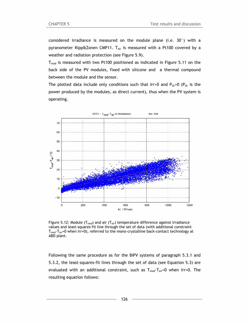
CHAPTER 5 Test results and discussion
126
considered irradiance is measured on the module plane (i.e. 30°) with a
pyranometer Kipp&Zonen CMP11. Tair is measured with a Pt100 covered by a
weather and radiation protection (see Figure 5.9).
Tmod is measured with two Pt100 positioned as indicated in Figure 5.11 on the
back side of the PV modules, fixed with silicone and a thermal compound
between the module and the sensor.
The plotted data include only conditions such that Irr>0 and Pdc>0 (Pdc is the
power produced by the modules, as direct current), thus when the PV system is
operating.
Figure 5.12: Module (Tmod) and air (Tair) temperature difference against Irradiance values and least-squares-fit line through the set of data (with additional constraint Tmod-Tair=0 when Irr=0), referred to the mono-crystalline back-contact technology at ABD plant.
Following the same procedure as for the BiPV systems of paragraph 5.3.1 and
5.3.2, the least-squares-fit lines through the set of data (see Equation 5.3) are
evaluated with an additional constraint, such as Tmod-Tair=0 when Irr=0. The
resulting equation follows:

CH
De
va
5
Th
re
Fi
be
te
m
Va
co
be
FivaTm
HAPTER 5
egrees of fr
ariance of r
.3.4 BiPV
his paragra
eferred to t
gure 5.13
etween Tmo
emperature
modules inte
alues plott
onditions ar
elow Equati
gure 5.13: Malues and leamod-Tair=0 wh
reedom = 16
residuals (re
V wall pr
aph present
he BiPV wa
and Figur
od (i.e. PV
) against
egrated in t
ed in Figu
re describe
ion 4.7).
Module (Tmod)ast-squares-fen Irr=0), re
Tmod,m-Si-Ta
6581; rms o
educed chis
rototype
ts the mea
all prototype
e 5.14 sho
module w
irradiation
he BiPV wa
re 5.13 an
ed in detail
) and air (Tai
fit line throueferred to th
127
air= 0.0230*
of residuals
square) = W
sured para
e develope
ow the me
working tem
referred
all prototype
d Figure 5
in chapter
r) temperatuugh the set oe NF module
Te
Irr [°C]
= sqrt(WSS
WSSR/ndf =
meter Tmod
d in this the
easured va
mperature)
respective
e.
5.14 refer t
r 4 (see bo
ure differencof data (with e of the BiPV
est results a
SR/ndf) = 3.
11.5523
d-Tair agains
esis.
alues of th
and Tair (
ly to the
to indoor m
undary con
ce against Irr additional c
V wall protot
and discussi
Equation 5
.39886
st irradianc
he differen
(i.e. ambie
NF and W
measureme
nditions list
radiance constraint type.
on
5.3
ce,
ce
ent
WF
ent
ed

CH
FivaTm
Th
Eq
w
Co
Eq
Co
Eq
HAPTER 5
gure 5.14: Malues and leamod-Tair=0 wh
he least-sq
quation 5.5
hen Irr=0. T
oefficient o
quation 5.4
oefficient o
quation 5.4
Module (Tmod)ast-squares-fen Irr=0), re
quares-fit l
5) are evalu
The resultin
of determin
refers to t
of determin
refers to t
) and air (Tai
fit line throueferred to th
ines throu
uated with
ng equation
Tmod,NF-Ta
ation (R2)=
he NF modu
Tmod,WF-Ta
ation (R2)=
he WF mod
128
r) temperatuugh the set oe WF module
gh the set
the additio
ns follow:
ir= 0.0253*I
0.9950
ule integrat
air= 0.0208*I
0.9932
dule integra
Te
ure differencof data (with e of the BiPV
t of data
onal constr
rr [°C]
ted in the B
rr [°C]
ated in the
est results a
ce against Irr additional cV wall protot
(see Equat
raint, such
BiPV wall pr
BiPV wall p
and discussi
radiance constraint type.
tion 5.4 a
as Tmod-Tair
Equation 5
rototype.
Equation 5
prototype.
on
nd
r=0
5.4
5.5

CH
5
Co
Ex
w
an
Fo
in
to
Th
Ch
fo
to
Th
(a
m
Eq
co
Fi
Fi
be
HAPTER 5
.3.5 Per
omparison
x-Post and
hich offer
nd roof inte
or many ap
n the buildi
o the achiev
he perform
hurch roof s
ocused on t
o the PV pe
he paramet
as describe
measured for
quation 5.1
ompared in
gure 5.15: p
gure 5.15 sh
etween the
formanc
n Prototyp
Milland C
examples o
egrated syst
plications i
ng envelop
vement of h
mance comp
system and
the PV work
rformance
ters Tmod-Ta
ed in parag
r the BiPV w
1, Equatio
Figure 5.15
plots of Equa
hows the c
two analyz
e compa
pe-BiPV mo
hurch BiPV
of typical p
tems.
in fact, it i
e without f
higher PV m
parison am
the BiPV w
king tempe
as explaine
ir against ir
graph 5.3.
wall prototy
n 5.2, Eq
5.
tion 5.1, Equ
comparison
zed BiPV sy
129
arison wit
onitored s
V systems,
problems re
s a commo
foreseeing
module temp
ong the Ex
wall prototy
erature con
ed in the pre
rradiance, e
1 and 5.3
ype (as des
uation 5.4
uation 5.2, E
of the par
stems and t
Te
th BiPV w
systems
are two i
elated, res
n practice
a proper ve
peratures.
x-Post faca
ype develop
ditions, wh
evious para
evaluated f
.2), are co
cribed in pa
4, Equation
Equation 5.4
rameter Tm
the BiPV wa
est results a
wall prot
nteresting
pectively,
to integrat
entilation a
ade system,
ped in this t
hich is relat
agraphs and
or the two
ompared w
aragraph 5.
n 5.5 are
and Equatio
od-Tair again
all prototyp
and discussi
totype
case studi
to PV faça
te PV system
and this lea
, the Milla
thesis, is th
ted of cour
d chapters.
BiPV system
with the o
.3.4).
plotted a
on 5.5.
nst irradian
pe.
on
ies
de
ms
ads
nd
hus
rse
ms
ne
nd
ce

CHAPTER 5 Test results and discussion
130
It is clearly visible that, as expected, the Ex-Post BiPV system is the worst
performing while the WF module of the wall prototype is the best performing.
Modules integrated in the Ex-Post building in fact (as shown in paragraph 5.3.1)
are not retro-ventilated and this of course affects the module operating
temperatures. On the contrary, the WF module of the wall prototype is very
well retro-ventilated and in addition it was specifically designed with the heat-
sink system to additionally decrease its temperature.
According to the monitored data, the PV modules integrated in the Ex-Post
building are operating at a temperature which is 2.3%*Irr higher with respect
the best performing WF module integrated into the BiPV wall prototype.
This means that, e.g. at a top irradiance of 1000W/sqm, the Ex-Post PV
modules would work at a temperature which is 23°C higher with respect the
BiPV wall prototype WF module.
This temperature difference is quite significant and thus affects the PV
performance in a significant way. This would be particularly emphasized for
those PV technologies which present important temperature coefficients (e.g.
crystalline technology, for which the power temperature coefficient γrel is
typically around -0.5%/°C).
This confirms that different integration configurations can strongly influence
the working module temperatures and thus the PV performance.
It also confirms the importance to design for proper ventilation behind the BiPV
elements, which, as demonstrated, can enable a temperature reduction of up
to 23°C to be achieved. Similar values were found by Norton et al. in [5.11],
which formulated a possible temperature reduction up to around 20°C to be
achieved thanks to natural ventilation.
Figure 5.15 also shows that the PV modules integrated in the Milland Church roof
present working temperature conditions which are in between the not-
ventilated Ex-Post building and the well ventilated BiPV wall prototype.
This result is also in agreement with expectations: in fact the modules in this
case are retro-ventilated but still some obstacles and problems are present as
shown in paragraph 5.3.2. The Milland Church PV modules operate at a
temperature which is 1.2%*Irr higher with respect the NF module integrated in
the BiPV wall prototype.

CH
Th
m
pr
sig
an
0.
NF
co
Th
ap
PV
Co
An
th
pa
te
cl
an
an
sy
th
ou
Fi
HAPTER 5
his means
modules wor
rototype N
gnificant as
nd WF modu
. The WF m
F module,
onditions of
his confirm
pplied heat
V power pe
omparison
n additiona
he BiPV wa
aragraph 5
emperature
ose with t
nalysis is gi
nd in Figure
ystem) and
hus compar
utdoor mon
gure 5.16: p
that, e.g.
rk at a temp
F module.
s in the pre
ules of the
module oper
which me
f 1000W/sq
ms that, as
t sink syste
rformance.
n Prototyp
al comparis
all prototyp
5.3.3) is c
s of the m
the ones of
ven by the
e 5.15 refe
to indoor
ring indoor
nitored data
plots of Equa
at a top
perature wh
The temp
evious case.
BiPV wall m
rates at a t
eans a dec
m.
already d
m (i.e. the
pe-PV grou
son betwee
pe and of
arried out
modules inte
f the groun
fact that t
er to outdo
experiment
r measured
a.
tion 5.3, Equ
131
irradiance
hich is 12°C
perature di
. The tempe
modules is e
emperature
crease of
discussed in
e fins) provi
und mount
en the PV w
a ground m
. Figure 5
egrated in
nd mounte
the plotted
oor monitor
tal data (fo
d data (w
uation 5.4 an
Te
e of 1000W
C higher wi
fference in
erature diff
extensively
e which is 0
around 4.
n paragraph
ide an addi
ted system
working tem
mounted P
5.16 shows
the BiPV w
d PV syste
d equations
red data (f
or the BiPv
ith constan
nd Equation
est results a
W/sqm, the
th respect
n this case
ference bet
discussed i
0.45%*Irr lo
5°C at to
hs 5.3 an
itional sligh
m
mperature
PV system
s that the
wall prototy
em. A limit
reported i
for the gro
v prototype
nt wind ve
5.5
and discussi
e Milland
the BiPV w
e is not th
tween the
in paragrap
ower than t
op irradian
nd 5.4.2, t
ht increase
conditions
(described
PV worki
ype are qui
tation to th
n Figure 5.
und-mount
) and we a
elocity) wi
on
PV
all
hat
NF
phs
he
ce
he
in
of
in
ng
ite
his
16
ed
are
ith

CH
Co
Co
te
th
at
sy
Th
co
ch
FiEq
5
Re
w
tim
No
Ac
th
op
By
of
fu
HAPTER 5
omparison
oncluding,
emperature
he condition
t ABD plant
ystem (i.e.
hese result
onfiguration
haracteristi
gure 5.17: pquation 5.5.
.3.6 Gen
esults repor
all prototy
me period
orthern and
ccording to
he WF mod
perating tem
y subtractin
f Tair and I
unction of T
n conclusio
Figure 5.17
working c
ns reported
t) than the
Ex-Post bui
ts highligh
n, in term
cs.
plots of Equa
neralizat
rted in para
pe and the
considering
d Southern
o Figure 5.15
ule of the
mperatures
ng Equation
rr) to Equa
Tair and Irr),
ons
7, which su
conditions o
d for the gro
ones repor
lding).
t the effe
ms of PV
tion 5.1, Equ
ion of re
agraph 5.3.
e Ex Post b
g the ambi
Italy, i.e. B
5, the Ex-Po
wall proto
s.
n 5.5 (whic
ation 5.1 (
the value
132
mmarizes a
of the BiPV
ound-moun
rted for the
ectiveness
performa
uation 5.2, E
esults ove
5 regarding
building, ar
ient condit
Bolzano and
ost BiPV sys
otype is the
h provides
which prov
of ΔT Ex-Post –
Te
all results t
V prototype
ted PV syst
e BiPV not
of the pro
nce relate
Equation 5.3
er one ye
g the compa
re here gen
tions of tw
d Agrigento.
stem is the
e best perf
the values
vides the v
– WF is obtain
est results a
ogether, sh
e modules
tems (i.e. C
retro-vent
oposed BiP
ed to the
, Equation 5
ear time
arison betw
neralized o
wo different
.
worst perf
forming, in
of Tmod,WF
values of T
ned:
and discussi
hows that t
are closer
CIGS and m
ilated faça
PV prototy
e integrati
.4 and
period
ween the Bi
over one ye
t locations
forming wh
terms of
as a functi
mod,Ex-Post as
on
he
to
-Si
de
pe
on
PV
ear
in
ile
PV
on
s a

CHAPTER 5 Test results and discussion
133
ΔT Ex-Post – WF= 0.0229*Irr [°C]
Equation 5.6
ΔT Ex-Post – WF is defined as the working temperature difference, as function of
Irradiance, between the WF module integrated in the BiPV wall prototype and
the modules integrated in the Ex-Post façade, according to measured and
monitored data as explained in paragraphs 5.3.4 and 5.3.1.
By multiplying Equation 4.2 (i.e. the value of the CIGS module power
temperature coefficient as function of irradiance) with Equation 5.6, the value
of ΔP Ex-Post – WF, for each condition of Irradiance, is evaluated.
ΔP Ex-Post – WF is defined as the additional power (Pmppt) that the WF module
produces being integrated as it is, with respect the hypothetical power that it
would produce if it was integrated in the same way as the Ex-Post building
modules (according to ΔT Ex-Post – WF).
ΔP Ex-Post – WF = (0.0229*Irr)*( - 0.0003*Irr - 0.0123) [W]
Equation 5.7
Equation 5.7 allows to calculate the value of ΔP Ex-Post – WF for each ambient
condition, according to the measured data of Tmod,WF (see Equation 5.5, and
measurement boundary conditions listed below Equation 4.7) and to the
monitored data of Tmod,Ex-Post (see Equation 5.1).
Considering the ambient conditions of two different locations in Northern and
Southern Italy, i.e. Bolzano and Agrigento, the hourly based values of ΔP Ex-Post –
WF are evaluated for one reference year. The final value of the annual ΔE Ex-Post –
WF (i.e. the annual energy production difference due to ΔT Ex-Post – WF) is then
assessed.
Meteo data
The data of ambient temperature and Irradiance used in this analysis are taken
from the CTI (Comitato Termotecnico Italiano) database which provides the
characteristic climate year of all the Italian provinces, referred to the
calculation model of the UNI EN ISO 15927 - 4:2005 "Hygrothermal performance

CH
of
da
Ev
fr
ye
th
ho
Th
ve
SO
irr
an
it
su
Fifo
Re
Th
tw
Bo
Ba
pr
HAPTER 5
f buildings
ata for Asse
very charac
rom a datab
ears and co
here is the
orizontal pl
he values o
ertical plan
OL Expert.
radiance on
nd Bolzano.
would hap
urface facin
gure 5.18: aor the two lo
esults
he results r
wo compare
olzano
ased on ho
roduction Δ
- Calculati
essing the a
cteristic yea
base of wea
ontains hou
e ambient
lane.
of irradianc
e through t
Figure 5
nto a vertic
. As expect
ppen for an
ng South.
average moncations Agrig
reported in
ed systems o
urly calcula
ΔE Ex-Post – WF,
ion and pre
annual ener
ar data-set
ather data
urly record
temperatu
ce on the h
the algorith
.18 shows
cal south f
ted, the pea
n horizontal
nthly values gento and Bo
this paragr
on a vertica
ation, the
due to ΔT
134
esentation
gy use for h
is made of
actually me
ds of meteo
ure and th
horizontal
hm of the c
the resul
acing façad
ak of solar
l surface, b
of irradiancolzano.
raph refers
al plane (ti
total annua
Ex-Post – WF, re
Te
of climatic
heating and
f 12 charact
easured for
orological v
e global s
plane are
commercial
lting avera
de for the
radiation is
because it i
ce onto a ve
to an hypo
lt=90°) Sou
al amount
esults to be
est results a
c data - Pa
d cooling".
teristic mo
r a period o
variables, a
solar irradi
then transp
l software V
age month
two locatio
s not durin
is referred
ertical south
thetic posit
uth facing (a
of differen
e 43.70 kWh
and discussi
art 4: Hour
nths select
of at least
among whi
ance on t
posed on t
Valentine P
ly values
ons Agrigen
g summer,
to a vertic
facing faça
tioning of t
azimuth=0°
nce of ener
h/(kWp y) f
on
rly
ed
10
ch
he
he
PV-
of
nto
as
cal
ade
he
).
rgy
for

CHAPTER 5 Test results and discussion
135
the city of Bolzano. This value is evaluated summing the ΔE Ex-Post – WF calculated
for each hour, over the whole year.
The reference specific annual yield of a BiPV façade system of Wuerth CIGS
modules South facing [Figure 5.19], is calculated through the commercial
dynamic simulation software PV-SOL and results to be 818.2 kWh/kWp.
Considering this reference yield, the ΔE Ex-Post – WF, as related to the integration
characteristics, accounts thus for 5.34% of the annual energy production.
Figure 5.19: Schema of the reference South facing BiPV façade simulated with the commercial software PV-SOL.
Moreover, the average working temperature difference between the WF
module and the Ex-Post modules (average calculated on hourly values over one
year when Irr>100W/sqm) results to be 8.2°C (WF module:23.8°C, Ex-Post
module:32°C).
Reliability research states that the PV degradation rate doubles for every 10°C
increase in temperature [5.9], implying that an array design that ran e.g. 10°C
hotter than another could be expected to last only half as long.
Hypothesizing a direct linear correlation for the degradation rate, a first
estimation would thus lead to the consideration that in the climate of Bolzano,
the “best integrated” WF module could potentially last around 4/5 longer than
the “worst integrated” Ex-Post modules.
Agrigento
For the city of Agrigento, the total annual amount of difference of energy
production ΔE Ex-Post – WF, due to ΔT Ex-Post – WF, results to be 59.60 kWh/(kWp y),
i.e. 15.9 kWh/(kWp y) more than the value referred to Bolzano.
The reference specific annual yield of a BiPV façade system of Wuerth CIGS
modules South facing [the same reference system shown in Figure 5.19], is
calculated also for the city of Agrigento through the commercial dynamic
simulation software PV-SOL and results to be 993.8 kWh/kWp.
Considering this reference yield, the ΔE Ex-Post – WF, due to ΔT Ex-Post – WF, accounts
thus for 6.00% of the annual energy production.
10
5
50 x Würth Solar GmbH & Co.
WSG0036E080 80 W
90°; 0°
1 x SMA America, Inc.
Sunny Boy 3800US (USA/240V/60Hz)
3,8kW

CHAPTER 5 Test results and discussion
136
Moreover, the average working temperature difference between the WF
module and the Ex-Post modules (average calculated on hourly values over one
year when Irr>100W/sqm) results to be 11.4°C (WFmodule:30°C, Ex-Post
module:41.4°C).
According to [5.9] as mentioned for the city of Bolzano, a first estimation leads
to the consideration that in the climate of Agrigento, the “best integrated” WF
module could potentially last more than twice longer than the “worst
integrated” Ex-Post modules.
Conclusions
The module working temperature difference ΔT Ex-Post – WF, which is related to
the integration characteristics, leads to an energy production difference ΔE Ex-
Post – WF which accounts for the 6.00% of the annual energy production in the
Agrigento climate (South of Italy) and for the 5.34% of the annual energy
production in the Bolzano climate (North of Italy).
This means that a proper design for natural ventilation in a BiPV system, leads
to an energy gain which can be considered as significant.
In addition, it has also to be taken into account that decreasing the module
temperature could also lead to other positive effects, i.e. the opportunity to
prolong the life time of an operating PV array due to lower thermal stress.
This effect has been roughly estimated for the two cities: the “well integrated”
WF module could potentially last around 4/5 longer than the “bad integrated”
Ex-Post modules in Bolzano and more than twice longer in Agrigento.
These results highlight the importance of a proper design for integration of PV
systems in the building envelope.

CHAPTER 5 Test results and discussion
137
5.4 Further PV performance improvement due to fins
application
The results of the experimental phases 2 and 3 are discussed in this paragraph
in order to evaluate the influence of the fins applied on one module of the
specimen, on the PV performance.
Test carried out in phase 3, provides the ΔTNF-WF value (i.e. the average
temperature difference between the module NF and WF) for each condition of
ambient temperature (Tair) and irradiance (Irr), as given below:
ΔTNF-WF= 0.0051*Tair + 0.0044*Irr [°C]
Equation 5.8
Equation 5.8 refers to the measured conditions listed in the previous chapter
(see boundary conditions listed below Equation 4.7).
Equation 5.9, as found in chapter 4 (i.e. Equation 4.2), provides the γ value
(i.e. the temperature coefficient of Pmppt) of the NF module, which is taken as
reference module, for each condition of irradiance (Irr), as given below:
γ = - 0.0003*Irr - 0.0123 [W/°C]
Equation 5.9 By multiplying Equation 5.8 and Equation 5.9, the value of “ΔPNF-WF”, for each
condition of Tair and Irr, is evaluated. “ΔPNF-WF” is defined as the additional
power (Pmppt) produced by the PV module thanks to the influence of the fins
that work as heat sinks.
The resulting equation is thus:
ΔPNF-WF= (0.0051*Tair + 0.0044*Irr)*( - 0.0003*Irr - 0.0123) [W]
ΔPNF-WF=-1.32E-06*Irr2 -5.412E-05*Irr -6.273E-05*Tair -1.53E-06*Tair*Irr
Equation 5.10
Equation 5.10, refers to the measured conditions listed in the previous chapter
(see boundary conditions listed below Equation 4.7).

CHAPTER 5 Test results and discussion
138
Figure 5.20 shows the interpolation surface of ΔPNF-WF in different condition of
Tair and Irr, as calculated by Equation 5.10.
Figure 5.20: interpolation surface of ΔPNF-WF (as absolute value) in different condition of Tair and Irr, as calculated by Equation 5.10 Equation 5.10 can be simplified by fitting the measured data referred to that
formula, with a planar surface and thus obtaining the following equation:
ΔPNF-WF= 0.001192*Irr-0.001925*Tair [W]
RMS (root mean squared) of residuals= 0.1657855; R2= 0.819689
Equation 5.11
Equation 5.10 provides the value of ΔPNF-WF for each condition of ambient
temperature and irradiance.
Figure 5.20 and Equation 5.10, in agreement with what discussed in chapter 4
for the equation 4.7, show that the influence of Tair on ΔPNF-WF is much lower
than the irradiance’s one.
Reporting again the example discussed in chapter 4 for equation 4.7, a peak
temperature of 50°C would affect the value of ΔPNF-WF for an extent of 0.003W,
while a peak irradiance of 1100 W/sqm would affect the value of ΔPNF-WF for an
extent of 1.657 W, i.e. more than 500 times the value due to Tair.
Thus, the influence of Tair on ΔPNF-WF can be considered as negligible.
Considering the city of Aswan in Egypt as a limit example, the highest
irradiance on a best oriented module (i.e. azimuth of 0° and tilt of 23°) is 1172

CHAPTER 5 Test results and discussion
139
W/sqm and the corresponding Tair is 28.8°C, happening on the 7th of March at
noon referring to the meteorological database of the commercial software PV-
SOL.
In these peak conditions (Irr=1172 W/sqm and Tair=28.8°C), the resulting ΔTNF-
WF evaluated in chapter 4 was 5.3°C, which was considered as a limit value of
the maximum contribution that can be provided by the fins to decrease the
module temperature in the considered conditions (as listed below the Equation
5.10). According to Equation 5.10, the corresponding ΔPNF-WF at these peak
conditions results to be 1.93 W (as absolute value) referred to one module.
Normalizing this value to the module nominal power Pn, it results to be 0.024
W/Wp. This means that, in these conditions, the presence of fins leads to an
increase in power of the 2.4% of the nominal power installed.
This number can be considered as a limit value of the maximum contribution
that can be provided by the fins, to increase the module power in the
considered conditions (as listed below the Equation 4.7).
5.4.1 Generalization of results to other PV technologies
The results obtained for the prototype, which is made of two Würth CIGS
modules, are generalized taking into consideration other PV technologies.
Among the 24 types of modules monitored by Eurac at ABD-PV plant (as
described in paragraph 5.3.3), 6 of them are selected for this analysis as they
present a similar section, in terms of materials and thickness, compared with
the Würth CIGS module tested in the prototype.
In fact, the generalization of the results is based on the hypothesis that the
presence of fins on the module would affect the module temperature with the
same extent of the tested CIGS modules, and thus the ΔT values resulting from
the phase 2 tests are assumed to be the same as for the selected PV
technologies.
The selection of 6 glass-glass module types (see Table 5.1), which present
similar characteristics of materials and thickness as the Würth CIGS modules, is
meant to be as coherent as possible with the above mentioned hypothesis.

CHAPTER 5 Test results and discussion
140
The dependence of the Pmppt on the module temperature is evaluated, for each
of the 6 analyzed technologies, through monitored data acquired in the outdoor
ABD-PV field (see description in paragraph 5.3.3).
Outdoor temperature characterization
Values of outdoor temperature coefficient for the 6 selected technologies at
different irradiances are evaluated from the data monitored at the ABD plant.
The considered time period for the following results starts with January 2012
and ends with December 2012, i.e. one entire year to avoid overestimating or
underestimating the role of a season. On the other side, by measuring every 15
min, this long time period provides a huge amount of data, which includes all
possible outdoor conditions. To exclude the non-reliable and non-comparable
data, a filtering method, which was applied by M. Pichler et al. [5.3], is
implemented.
The filtering method considers of three parameters: turbidity, performance
ratio and wind speed.
Turbidity
The turbidity (t) is a measure for the clearness of the sky for a single day. It is
defined as the ratio of the sum of the diffuse (Iday diff) and of the global (Iday global)
irradiance over one day [5.4]. Days with a low turbidity tend to be at clear sky
condition, while increasing the turbidity leads to more cloudy days. The
problem with cloudy days is the fact that clouds can shadow the module but
not the pyranometer, or vice versa. In such a case the data is not coherent.
Additionally, the spectrum during days with a high turbidity or high diffuse
irradiance can be different to the spectrum of bright days, which are closer to
AM1.5 (definition of STC). This difference is hard to determine and therefore
overcast days have to be excluded. In the results reported in this paragraph, a
turbidity of t < 0.25 is used for the sorting procedure. The choice of t < 0.25
leads to the selection of days at clear sky condition.
Performance Ratio
The Performance Ratio (PR) is the ratio of the normalized value of the
produced energy and the normalized value of the incoming solar energy:

CHAPTER 5 Test results and discussion
141
, ,
Equation 5.12
where Yf is the final PV system yield, Yr is the reference yield, E is the net
energy output in a certain period of time, Pn is the nominal power of the PV
array, Gsum is the total in-plane irradiance over time, Gn is the PV’s reference
irradiance.
The turbidity is not enough to exclude the points coming from shading effects.
Also on days with clear sky it can happen that the module is producing no
energy while the pyranometer is measuring some irradiance or that the
pyranometer is measuring very low irradiance while the module is still
producing energy. These situations arise in the morning and in the afternoon,
i.e. at sunrise and at sunset. The reason for shading at these times is due to the
mountains around the PV-plant and the fact that the plant has only one
pyranometer and not one per array. To exclude these points, the performance
ratio at a 15 min-interval PR15min is used. Due to the definition from Equation
5.12, PR is too small when only the module is shadowed and too high when only
the pyranometer is shadowed. To have an adequate range for all modules for
the sorting by PR15min, the average ( 15min) and the standard deviation of
PR15min (σ PR15min) are calculated as follows:
1
11
where N is the number of the data points. The sorting range is then given by
PR σ . This method ensures that 68 % of the data points are in
this range.
Wind speed
The PT100 used for measuring the module temperature are not sufficiently
insulated against influences of the weather and therefore the wind has an

CHAPTER 5 Test results and discussion
142
effect on the measured temperature. Too windy days have to be sorted out to
ensure the assumption that Tmod≈TBoM (where Tmod is the module temperature
and TBoM is the temperature measured on the back side of the module).
For the following results, a wind speed of Vwind < 2 m/s is used for the sorting
procedure. Vwind < 2 m/s decreases the influence of the cooling effect of the
wind on the measured module temperature.
Results
The outdoor temperature coefficients for the selected PV technologies are
evaluated for each irradiance value (from 500 W/sqm to 900 W/sqm, with a
step of 100W/sqm) and the expression γout as function of irradiance is then
derived through the least-squares-fit method (all graphs are reported in annex
A). By multiplying the equation of γout of each technology (as reported in Table
5.1) with Equation 5.8, the expression of ΔP can be derived as follows:
ΔP= (0.0051*Tair + 0.0044*Irr)* γout [W]
Equation 5.13
It has to be underlined that the calculated temperature coefficients γout are
still subjected to various external effects such as LS, TA, spectrum etc. which
are not considered by the methodology used for their calculation (as proposed
by [5.3]), thus care must be taken in the consideration of the following
outcomes.
Reference nr.
Technology γout [W/°C] R2 Pn [kW]
1 mc-Si -0.0143*Irr + 7.4975 0.8225 1.98
2 mc-Si -0.0112*Irr + 5.8644 0.7600 1.96
3 a-Si -0.0024*Irr + 5.0136 0.5286 1.00
4 a-Si/a-Si -0.0034*Irr + 4.8651 0.6169 0.97
5 a-Si/μc-Si -0.0045*Irr + 5.3529 0.5972 1.15
6 a-Si/μc-Si -0.0047*Irr + 5.0143 0.8049 1.10
Table 5.1: outdoor temperature coefficients as function of irradiance for each PV technology, referred to the installed nominal power Pn

CH
Am
FiexSi
Fi
co
te
a-
irr
In
st
in
Th
pr
Th
co
of
ty
ef
th
m
Th
co
ch
Th
ac
in
HAPTER 5
morphous s
gure 5.21: Oxplained in t/μc-Si (on th
gure 5.21
onsidered r
emperature
-Si module
radiance of
ndoor measu
tandard [4
ncreasing, t
his phenom
rocedure fo
he tempera
onsideration
f a-Si modu
ypical beha
ffect. Anne
he higher th
module [5.5]
his phenom
oefficients
hapter.
he positive
ccording to
nfluence of
ilicon techn
Outdoor temphe previous he right, Mod
shows that
range of ir
coefficien
= -0.19%/°C
f 1000W/sq
urements o
.4]) are i
the PV ener
mena is imm
or temperat
ature coeff
ns other ph
les and whi
avior of a-S
ealing in pa
he tempera
].
mena may e
(as shown
e value of
Equation 5
the fins att
nology
perature coe paragraph, rdule 5) techn
t the tempe
rradiances.
t reported
C and a-Si/
m and are m
of temperat
n fact alw
rgy gap (Eg
mediate and
ture coeffic
icient whic
enomena, s
ich leads in
Si module
articular, m
ature, the m
explain the
in Figure 5
f the tem
5.13, would
tached on t
143
efficients evareferred to anologies.
erature coe
On the ot
on the mo
μc-Si Modu
measured in
ture coeffic
ways nega
g) decrease
d can be m
cient evalua
ch is evalua
such as the
nstead to po
is part of
mainly depe
more effect
e positive v
5.21), evalu
mperature c
d result in
the module.
Te
aluated witha-Si (on the l
efficients γ
ther hand,
odule datas
le 5 = -0.25
ndoor.
cients (mea
ative becau
es and thus
easured ac
ation [4.4].
ated in this
e thermal an
ower recove
the well-k
ends on th
tive the def
value of th
uated as ex
coefficients
a positive
.
est results a
h the methodleft, Module
γout are pos
the value
heets are n
5%/°C). The
asured acco
use, with
s the voltag
ccording to
s way, do n
nnealing wh
ery of the m
known Stae
e module
fects recov
he outdoor
xplained in
s for a-Si
ΔP, meanin
and discussi
dology 3) and a-
sitive for t
es of relati
negative (i.
ey refer to
ording to t
temperatu
ge decrease
the standa
not take in
hich is typic
modules. Th
ebler–Wrons
temperatur
very in the
temperatu
the previo
technolog
ng a negati
on
he
ive
.e.
an
he
ure
es.
ard
nto
cal
his
ski
re:
PV
ure
ous
gy,
ive
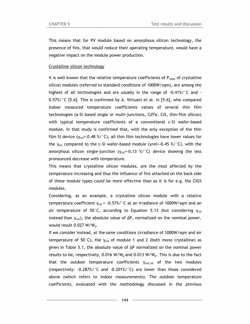
CHAPTER 5 Test results and discussion
144
This means that for PV module based on amorphous silicon technology, the
presence of fins, that would reduce their operating temperature, would have a
negative impact on the module power production.
Crystalline silicon technology
It is well known that the relative temperature coefficients of Pmppt of crystalline
silicon modules (referred to standard conditions of 1000W/sqm), are among the
highest of all technologies and are usually in the range of -0.41%/°C and -
0.57%/°C [5.6]. This is confirmed by A. Virtuani et al. in [5.6], who compared
indoor measured temperature coefficients values of several thin film
technologies (a-Si based single or multi-junctions, CdTe, CIS, thin-film silicon)
with typical temperature coefficients of a conventional c-Si wafer-based
module. In that study is confirmed that, with the only exception of the thin
film Si device (γrel=-0.48 %/°C), all thin film technologies have lower values for
the γrel compared to the c-Si wafer-based module (γrel=-0.45 %/°C), with the
amorphous silicon single-junction (γrel=-0.13 %/°C) device showing the less
pronounced decrease with temperature.
This means that crystalline silicon modules, are the most affected by the
temperature increasing and thus the influence of fins attached on the back side
of these module types could be more effective than as it is for e.g. the CIGS
modules.
Considering, as an example, a crystalline silicon module with a relative
temperature coefficient γrel = -0.57%/°C at an irradiance of 1000W/sqm and an
air temperature of 50°C, according to Equation 5.13 (but considering γrel
instead than γout), the absolute value of ΔP, normalized on the nominal power,
would result 0.027 W/Wp.
If we consider instead, at the same conditions (irradiance of 1000W/sqm and air
temperature of 50°C), the γout of module 1 and 2 (both mono crystalline) as
given in Table 5.1, the absolute value of ΔP normalized on the nominal power
results to be, respectively, 0.016 W/Wp and 0.013 W/Wp. This is due to the fact
that the outdoor temperature coefficients γout,rel of the two modules
(respectively: -0.287%/°C and -0.201%/°C) are lower than those considered
above (which refers to indoor measurements). The outdoor temperature
coefficients, evaluated with the methodology discussed in the previous

CHAPTER 5 Test results and discussion
145
paragraph, result in fact to be lower than the values reported on the
datasheets which refer to indoor measurements: for an extent of 43% for
Module 1 and of 62% for Module 2.
Reporting again the limit example of a best tilted module at Aswan, already
discussed in paragraph 5.3, and considering the outdoor temperature
coefficients γout of module 1 and 2, the resulting absolute value of ΔP
normalized on the nominal power would be, respectively, 0.024 W/Wp and
0.019 W/Wp.
5.4.2 Generalization of results over one year time period
Equation 5.10 allows to calculate the value of ΔPNF-WF (i.e. the power
production difference of WF and NF module, due to the ΔTNF-WF between them)
for each ambient condition (i.e. air temperature and irradiance), according to
the settings listed below Equation 4.7 (which means that spectral effects, angle
of incidence, reflection losses and wind velocity variations are not considered).
Considering the ambient conditions of two different locations in Northern and
Southern Italy, i.e. Bolzano and Agrigento, the hourly based values of ΔPNF-WF
are evaluated for one reference year. The final value of the annual ΔENF-WF (i.e.
the annual energy production difference of WF and NF module, due to the ΔTNF-
WF between them) is then assessed.
The results reported in this paragraph refers to the prototype positioned on a
vertical plane (tilt=90°) South facing (azimuth=0°).
Bolzano
Based on hourly calculation, the total annual amount of difference of energy
production ΔENF-WF between the WF and NF modules, due to their ΔTNF-WF,
results to be 8.82 kWh/(kWp y) for the city of Bolzano (see meteo data
description in paragraph 5.3.6). This value is evaluated by summing the ΔENF-WF
calculated for each hour over the whole year.
Considering the reference specific annual yield of a BiPV façade system in
Bolzano (as described in paragraph 5.3.6 and shown in [Figure 5.19]), the ΔENF-
WF due to the presence of fins accounts thus for 1.08% of the annual energy
production.

CHAPTER 5 Test results and discussion
146
Figure 5.22: ΔPNF-WF distribution over 1 year referred to the prototype positioned South facing (azimuth = 0°, tilt = 90°) in Bolzano. ΔPNF-WF is the hourly energy production difference of the WF and NF module, due to the ΔTNF-WF between them; T air is the ambient temperature and Irradiance is the irradiance on the vertical plane of the modules. The average working temperature of the NF module is 25.5°C (average
calculated on hourly values over one year when Irr>100W/sqm), while the
average working temperature of the WF module is 23.8°C (average calculated
on hourly values over one year when Irr>100W/sqm). This means that in
operative conditions (considered as Irr>100W/sqm) the WF module operates
with an average temperature which is 1.7°C lower than the NF module.
As already mentioned in paragraph 5.3.6, reliability research states that the PV
degradation rate doubles for every 10°C increase in temperature [5.9],
implying that an array design that ran e.g. 10°C hotter than another could be
expected to last only half as long.
Hypothesizing a direct linear correlation for the degradation rate, a first
estimation would thus lead to the consideration that the WF module could
potentially last around 1/6 longer than the NF module in Bolzano.
Agrigento
For the city of Agrigento (see meteo data description in paragraph 5.3.6), the
total annual amount of difference of energy production ΔENF-WF between the WF
CHAPTER 5 Test results and discussion
147
and NF modules, due to their ΔTNF-WF, results to be 12.12 kWh/(kWp y), which is
3.3 kWh more than the value referred to Bolzano.
Considering the reference specific annual yield of a BiPV façade system in
Agrigento (as described in paragraph 5.3.6 and shown in [Figure 5.19]), the
ΔENF-WF due to the presence of fins accounts thus for 1.22% of the annual energy
production.
Figure 5.23: ΔPNF-WF distribution over 1 year referred to the prototype positioned South facing (azimuth = 0°, tilt = 90°) in Agrigento. ΔPNF-WF is the hourly energy production difference of the WF and NF module, due to the ΔTNF-WF between them; T air is the ambient temperature and Irradiance is the irradiance on the vertical plane of the modules.
The average working temperature of the NF module is 31.9°C (average
calculated on hourly values over one year when Irr>100W/sqm), while the
average working temperature of the WF module is 30.0°C (average calculated
on hourly values over one year when Irr>100W/sqm). This means that in
operative conditions (considered as Irr>100W/sqm) the WF module operates
with an average temperature which is 1.9°C lower than the NF module.
According to [5.9] as mentioned for the city of Bolzano, a first estimation leads
to the consideration that in the climate of Agrigento the WF module could
potentially last around 1/5 longer than the NF module.

CHAPTER 5 Test results and discussion
148
Conclusions
Concluding, the presence of fins on the CIGS module for the considered
prototype, would slightly enhance the PV output energy production over one
year time: for an extent of 1.08% in the climate of Bolzano and for an extent of
1.22% in the climate of Agrigento.
Consequently, even if the cost of the proposed heat sink system (metal fins +
thermal adhesive) is marginal, the net energy gain they would provide in the
considered conditions results probably to be too low to be an interesting
solution for the market.
On the other hand, it has also to be taken into account that decreasing the
module temperature could also lead to other positive effects, i.e. the
opportunity to prolong the life time of an operating PV array due to lower
thermal stress, considering that presence of fins would ensure a lower working
module temperature over time.
This effect has been roughly estimated for the two cities: the WF module could
potentially last around 1/5 longer than the NF module in Agrigento and it could
potentially last around 1/6 longer in Bolzano.

CHAPTER 5 Test results and discussion
149
References
[5.1] Decreto Ministeriale 26 gennaio 2010. Aggiornamento del decreto 11
marzo 2008 in material di riqualificazione energetica degli edifici. G.U. n. 35,
12/01/2010
[5.2] A.Colli, W.Sparber, M. Armani, B. Kofler and L.Maturi, 2010. Performance
monitoring of different PV technologies at a PV field in Northern Italy.
Proceedings of the 25th European Photovoltaic Solar Energy Conference and
Exhibition / 5th World Conference on Photovoltaic Energy Conversion, Valencia,
Spain. 4344 - 4349
[5.3] M. Pichler, 2012. Outdoor temperature coefficient of different PV module
technologies at ABD-plant in a one-year period. Master Thesis at the Vienna
University of Technology.
[5.4] S. Krauter and A. Preiss, 2010. Performance comparison of aSi, a-Si, c-si
as a function of air mass and turbidity. Proceedings of the 25th European
Photovoltaic Solar Energy Conference and Exhibition / 5th World Conference on
Photovoltaic Energy Conversion, Valencia, Spain.3141 – 3144.
[5.5] L. Fanni, A. Virtuani, D. Chianese, 2011. A detailed analysis of gains and
losses of a fully-integrated flat roof amorphous silicon photovoltaic plant. Solar
Energy 85, 2360–2373.
[5.6] A. Virtuani, D. Pavanello, G. Friesen, 2010. Overview of Temperature
Coefficients of Different Thin Film Photovoltaic Technologies. Proceedings of
the 25th European Photovoltaic Solar Energy Conference and Exhibition / 5th
World Conference on Photovoltaic Energy Conversion, Valencia, Spain. 4248 –
4252.
[5.7] L. Maturi et al., 2010. Analysis and monitoring results of a BiPV system in
Northern Italy. Proceedings of the 25th European Photovoltaic Solar Energy
Conference and Exhibition / 5th World Conference on Photovoltaic Energy
Conversion, Valencia, Spain.3141 – 3144.
[5.8] R. Gottschalga et al., 2003. Experimental study of variations of the solar
spectrum of relevance to thin film solar cells. Solar Energy Materials & Solar
Cells 79. 527–537.
[5.9] Flat-Plate Solar Array Project Final Report, 1986. Volume VI: Engineering
Sciences and Reliability, report prepared by JPL (Jet Propulsion Laboratory,

CHAPTER 5 Test results and discussion
150
California Institute of Technology, Pasadena) for U.S. Department of Energy
with NASA, JPL Publication 86-31.
[5.10] D. Moser et at., 2012. Evaluation of the performance of façade mounted
photovoltaic modules. Do we need a sensor when we have satellite derived
irradiance?. Proceedings of the 27th European Photovoltaic Solar Energy
Conference and Exhibition 3723 – 3726.
[5.11] B. Norton et al., 2011. Enhancing the performance of building integrated
photovoltaics, Solar Energy 85(8) 1629-1664.

CHAPTER 6 Summary, conclusions and future development
151
CHAPTER 6
Summary, conclusions and future development
Abstract
The prototype of a wooden prefabricated BIPV wall has been conceived,
designed, built and finally tested.
This chapter summarizes the main steps of the prototype development process
and presents the main related outcomes and conclusions.
The last paragraph highlights the research limitations, which could represent
the starting point for future developments of this work.

CHAPTER 6 Summary, conclusions and future development
152

CHAPTER 6 Summary, conclusions and future development
153
6.1 Summary
This paragraph summarizes the main step of the prototype development
process and presents the main related outcomes, according to each step of
Figure 6.1.
Figure 6.1: (from chapter 3) Process that guided the development of the BiPV prototype, from the concept to the experimental campaign.
6.1.1 Concept
Given the recommendations provided by the IEA Task 41 project for the
development of new BiPV products related to architects and designers’ needs
(as highlighted from the results of an international survey which involved about
600 architects/designers [3.1]), an innovative BIPV façade component is
conceived and developed.
According to these recommendations, four main concepts have been identified
as key-points for the prototype development:
- multi-functionality concept: the prototype is conceived to satisfy several
building requirements and to produce electricity;
- sustainability concept: the prototype foresees the coupling of the PV
technology, which exploits a renewable energy source, with wood, which is an
autochthonous material considering the Alpine region where it has been
developed;

CHAPTER 6 Summary, conclusions and future development
154
- integration concept: the PV system is not conceived as an element added as
an additional layer to the building envelope, but as a part of it;
- prefabrication concept: to allow a costs reduction, implementation
effectiveness, lean construction site and quality enhancement.
Identification of these concepts constitute the motivation and background for
the prototype development.
6.1.2 Theoretical study
The configuration of the prototype is the result of a theoretical study which
takes into account both architectural integration aspects (as described in
paragraph 3.4.1) and energy performance issues.
The latter in particular, is based on the evaluation and improvement of both PV
and building-related aspects.
The “PV” performance is improved taking into consideration passive strategies
to keep the module temperature as low as possible (thus increasing the PV
efficiency) and the “Bi” (i.e. building) performance is evaluated, considering
different possible materials, taking into account the thermal transmittance
value of the whole BiPV system.
“PV” Performance
The prototype has been designed foreseeing an air gap for the natural
ventilation of the modules.
This is a crucial aspect for the correct integration of PV modules, since the
increase of the operating temperature is one of the critical points which affect
the BiPV systems performance [see literature review: 3.9, 3.12, 3.14, 3.17,
3.21].
The optimal thickness of the air gap to keep the operating module temperature
as low as possible, has been calculated to be 10 cm, according to a procedure
formulated by Brinkworth et al. [3.19, 3.20, 3.21].
In order to further minimise efficiency loss due to temperature rise, a passive
low-cost strategy is experimented and investigated, with the aim to further

CHAPTER 6 Summary, conclusions and future development
155
enhance the advantages provided to the PV module performance by the
ventilation.
A strategy which is very often used in the ICT sector for electronic device
cooling, is implemented in the prototype: metal fins are applied on the back
side of the PV module to work as a heat sink (see Figure 3.15).
In order to define the configuration of the system module-heat sink, because no
much experimental data or examples are available, preliminary tests on a small
sample and several energy simulations with finite elements method are carried
out. The main results of the energy FEM simulations regarding the fins
application show that:
- There is no significant improvement in using Silver based technology
(l=8.89 W/mK) as thermal compound between fin and module instead
than Epoxy based technology (l=1.4 W/mK), which is cheaper;
- A 8 cm-long fin could decrease the cell temperature of 8.2°C with respect
to a 3 cm-long fin, which means, in the considered conditions (see
paragraph 3.4.2), an increase in the PV power output of about 3%;
- The effect of the fins application on the PV module is beneficial and
could lead to a slight enhancement of the PV power production (+1.3% in
typical summer conditions, +2.2% in typical winter conditions referred to
Northern Italy latitudes).
These energy simulations were carried out to support the prototype design
phase. However, in order to comprehensively quantify the influence of fins on
the performance of the PV module integrated in a façade, further experimental
investigation were carried out, providing monitored data to describe this
phenomena in an exhaustive and reliable way.
“Bi” Performance
The “Bi” (i.e. building) performance is evaluated taking into account the
thermal transmittance value of the whole BiPV system.
Four different thermal insulation materials are compared and among them, a
natural wood fibres insulation was selected as the best option for this
prototype.

CHAPTER 6 Summary, conclusions and future development
156
Moreover, in order to understand the impact of the PV system on the energy
performance of the building envelope in steady-state conditions, the value of
the thermal transmittance of the prototype was calculated in accordance with
the UNI EN ISO 6946 [3.1] considering two situations: the building component
with and without the PV system.
The results show that the presence of PV do not affect in a significant way the
total thermal resistance of the component: the thermal transmittance of the
component with the integrated PV system (which is 0.188 W/sqm K) is slightly
lower than the one without it (which is 0.191 W/sqm K).
Therefore, according to this calculation schema, the PV system does not affect
the building envelope performance in a negative way.
6.1.3 Prototype design and application
The final prototype design is the result of the theoretical study carried out as
described in the previous paragraph. The prototype [see Figure 3.27] is
conceived as a standardized modular unit with dimensions of 442 x 1310 x 1240
mm, characterized by a nominal power of 160Wp and with a calculated thermal
transmittance value of 0,188 W/sqm K.
This BiPV wall prototype was used in the design of an elementary school of 200
sqm entirely made of prefabricated wood framed panels (within a wider
research project entitled “Chi Quadrato: building construction of certified
green buildings designed for training activities”), providing an example of
possible application of the BiPV prototype in a building design.
6.1.4 Experimental campaign
A specimen of the designed prototype was built by a network of enterprises
called “Chi Quadrato” (see paragraph 4.5.2). The specimen is a modular unit
with dimensions of 442 x 1400 x 1310 mm, with two PV modules integrated in a
wooden structure (see Figure 4.6). One of the two PV modules has eleven fins
attached on the back side (as shown in Figure 4.6 and Figure 4.7).

CHAPTER 6 Summary, conclusions and future development
157
This configuration allows us to get measurements of temperature in both PV
configurations (with and without fins) and thus permits the data comparability
between the two modules which works in identical controlled conditions.
A new experimental approach, based on three phases and combining different
test facilities (i.e. INTENT lab and SoLaRE-PV lab), was defined to properly test
this BiPV prototype.
The experimental campaign is divided into three phases to evaluate both the
“Bi” (i.e. the building) and the “PV” (i.e. the photovoltaic system)
performance: the first phase focuses on the characteristics related to the “Bi”
side and in particular on the thermal characterization of the prototype with the
measurement of its thermal transmittance; the second phase deals with the
“PV” side, and in particular with the electrical characterization of the modules
through the measurements of the I-V characteristic curve at different
conditions; the goal of the last phase is to merge together the “Bi” and the
“PV” sides, focusing on the thermal-energy characterization of the integrated
PV modules.
Phase 1 results: “Bi” characterization
In the first test phase the steady-state thermal transmission properties of the
prototype are measured and its global thermal transmittance is assessed in
accordance with the UNI EN ISO 8990 [4.1] and UNI EN ISO 12567-1 [4.2].
The thermal transmittance of the whole BiPV wall prototype measured by the
hot box method results to be 0.204 W/(m²K). The discrepancy between the
measured and calculated values (which is 0.188 W/(m²K), as reported in the
previous paragraph) lies in the 8.5% measurements error.
Phase 2 results: “PV” characterization
The second test phase is carried out to measure the PV-related characteristics
of the CIGS modules (I-V characteristic curve, Voc, Isc, Pmppt values at
different conditions).
Before carrying out the measurements, the modules were pre-conditioned,
through controlled Light-Soaking by means of simulated solar irradiation, to
stabilize their electrical features. Preconditioning is in fact strongly

CHAPTER 6 Summary, conclusions and future development
158
recommended for CIGS technology, which is known for its metastability and
light-induced change behaviour [4.4, 4.6, 4.7, 4.8].
According to the procedure of the International Standard IEC 61646 [4.4], the
stabilization for the two CIGS modules, occurred after three light soaking
periods (as shown in Figure 4.11).
The values of Pmppt of the NF module, which is used as reference module, are
measured in SoLaRE-PV lab, at different conditions of temperature and
irradiation with a step respectively of 5°C and 100 W/sqm, over a range of
70°C and 1100W/sqm.
From these measured data, a mathematical expression (i.e. Equation 4.1) is
derived, using the least error squares method and considering Pmppt linear to
both irradiance and temperature, which provides the values of Pmppt as a
function of irradiance and module temperature.
Pmmpt,NF=0.0818*Irr-0.1085*Tmod [W]
Equation 4.1
After that, the power temperature coefficients (γ) of the NF module are
assessed at each irradiance value from the measured data (according to IEC
61646 [4.4] and IEC 60891 [4.5]), and the mathematical expression (i.e.
Equation 4.2) which provides the values of γ as a function of irradiance is
derived, using the least error squares method.
γ = - 0.0003*Irr - 0.0123 [W/°C]
Equation 4.2
Phase 3 results: “PV in Bi” characterization
The temperature distribution of the two modules (NF and WF) integrated in the
wooden wall is measured, in INTENT Lab, in different environmental conditions
(i.e. air temperature from 0°C to 40°C with a step of 10°C and irradiance from
400 W/sqm to 1000 W/sqm with a step of 200 W/sqm) and the averaged ΔTNF-WF
(temperature difference) between the two modules is assessed for each
condition.

CHAPTER 6 Summary, conclusions and future development
159
From these measured data, two mathematical expressions (i.e. Equation 4.3
and 4.4) are derived, using the least error squares method and considering Tmod
linear to both irradiance and air temperature, which provide the values of TNF
(i.e. average NF module working temperature) and TWF (i.e. average WF module
working temperature) as a function of irradiance and air temperature.
TNF= 1.0122*Tair + 0.0250*Irr [°C]
Equation 4.3
TWF= 1.0071*Tair + 0.0206*Irr [°C]
Equation 4.4
Consequently, the mathematical expression of ΔTNF-WF between the two
modules is derived, as a function of irradiance and air temperature (Equation
4.7).
ΔTNF-WF= 0.0051*Tair + 0.0044*Irr [°C]
Equation 4.7
Equation 4.7 allows to evaluate the contribution provided by the fins to
decrease the module temperature in each condition of irradiance and air
temperature.
Phase 2 and 3 results: further outcomes
By multiplying Equation 4.2 and Equation 4.7, the value of ΔPNF-WF, for each
condition of Tair and Irr, is evaluated. ΔPNF-WF is defined as the additional
power (Pmppt) produced by the PV module thanks to the influence of the fins
that work as heat sinks. The resulting equation is thus:
ΔPNF-WF= (0.0051*Tair + 0.0044*Irr)*( - 0.0003*Irr - 0.0123) [W]
Equation 5.3

CHAPTER 6 Summary, conclusions and future development
160
6.2 Conclusions
6.2.1 General achievement
The prototype of a wooden prefabricated BiPV wall was conceived, designed,
built and tested. It is a standardized modular unit with dimensions of 442 x
1310 x 1240 mm, characterized by a nominal power of 160 Wp and with a
measured thermal transmittance value of 0.2 W/sqm K.
Designed according to the recommendations developed by the IEA Task 41
“Solar Energy and Architecture” project, this prototype is intended to make
available to architects, engineers and designers a multifunctional product
which is characterized both from the “Bi” and the “PV” point of view and
which is able to provide both passive and active functions to the building
envelope.
6.2.2 Experimental approach
The development of such multifunctional building component entails the need
for innovative experimental approaches to be developed in order to properly
evaluate its energy performance. In fact, there is a need to monitor and test
together its “passive” (e.g. thermal transmission properties) and “active”(e.g.
electrical and thermal production) performance and to understand the energy
interaction between the active and passive layers.
In this thesis, a new experimental approach, based on three phases with the
combination of different test facilities (i.e. INTENT lab and SoLaRE-PV lab) and
original experimental set-ups, is defined and applied. Figure 4.1 shows the
organization of the experimental campaign in three phases and Figure 4.5
shows the concept behind the coupled use of two different test facilities (i.e.
INTENT and SoLaRE-PV Labs): the experimental results obtained as an output in
INTENT Lab are used as an input for the test performed in SoLaRE-PV Lab. By
coupling the two test facilities together and defining original experimental set-
ups (as described in chapter 4) it was possible to characterize the BiPV
component as a whole.

CH
6
Th
m
Th
pe
tr
re
cl
Th
co
In
0.
6
Th
pe
co
Bi
Po
Fi
HAPTER 6
.2.3 “B
he thermal
method acco
his value ca
erformance
ransmittanc
equired by
imatica F”)
he measur
oherent wit
n fact, the
.188 W/(m²
.2.4 Effe
he effective
erformance
omparing th
iPV systems
ost) located
gure 5.15: p
Bi” perfo
transmitta
ording to UN
an be consi
e, and it
ce is below
the actual
) [5.1].
ed value
th that calc
discrepancy
²K)) falls wi
ectivene
eness of the
e related
he results o
s (a roof sy
d in South T
plots of Equa
S
rmance
nce of the
NI EN ISO 12
idered as a
is index
w, for an e
Italian law
of therma
ulated acco
y between
ithin the ac
ess of the
e proposed
to the in
of the proto
ystem, i.e.
Tyrol (North
tion 5.1, Equ
Summary, c
161
BiPV wall p
2567, result
a satisfying
of a wel
extent of 2
w referring
l transmitt
ording to th
the measu
ccepted unc
e BiPV pr
BiPV proto
ntegration
otype exper
Milland Chu
h of Italy).
uation 5.2, E
onclusions
prototype m
ts to be 0,2
result in t
ll-insulated
3%, the li
to the wor
tance resu
he Standard
red and ca
certainty (8
rototype
otype confi
characteris
riments with
urch and a
Equation 5.4
and future
measured by
204 W/(m²K
erms of bu
d wall as
imit of 0.2
rst case sce
lting from
d UNI EN ISO
lculated va
8,5%).
configur
guration, in
stics, is e
h monitored
façade sys
and Equatio
developme
y the hot b
K).
uilding ener
its therm
26 W/(sqm*
enario (“zo
the test
O 6946.
alue (which
ration
n terms of
evaluated
d data of tw
stem, i.e. E
on 5.5.
ent
box
rgy
mal
*K)
ona
is
is
PV
by
wo
Ex-

CHAPTER 6 Summary, conclusions and future development
162
General remarks
Results reported in Figure 5.23 highlight the effectiveness of the proposed BiPV
prototype configuration in comparison with the other analyzed BiPV systems: in
particular the WF module of the wall prototype results to be the best
performing, operating at a temperature which is 2.3%*Irr lower with respect the
worst performing modules integrated in the Ex-Post building (which are not
retroventilated).
This means that, e.g. at a top irradiance of 1000W/sqm, the Ex-Post PV
modules work at a temperature which is 23°C higher with respect the BiPV wall
prototype WF modules.
This confirms that different integration configurations can strongly influence
the working module temperatures and thus the PV performance.
It also confirms the importance to design for proper ventilation behind the BiPV
elements, which, as demonstrated, could enable a temperature reduction of up
to 23°C to be achieved. Similar values were found by Norton et al. in [5.10],
which formulated a possible temperature reduction up to around 20°C to be
achieved thanks to a proper design.
Energy gain over one year time period
The module working temperature difference ΔT Ex-Post – WF, which is related to
the integration characteristics, leads to an energy production difference ΔE Ex-
Post – WF which accounts for the 6.00% of the annual energy production in the
Agrigento climate (South of Italy) and for the 5.34% of the annual energy
production in the Bolzano climate (North of Italy).
In addition, it has also to be taken into account that decreasing the module
temperature could lead to other positive effects, i.e. the opportunity to
prolong the life time of an operating PV array due to lower thermal stress.
This effect has been roughly estimated for the two cities: the “well integrated”
WF module could potentially last around 4/5 longer than the “bad integrated”
Ex-Post modules in Bolzano and more than twice longer in Agrigento (see Figure
6.2).

CHAPTER 6 Summary, conclusions and future development
163
These results confirm that different integration configurations can strongly
influence the PV performance and highlight the importance to design for proper
ventilation behind the BiPV elements.
Figure 6.2: energy yield and module life-time, normalized by values referred to integration type 1 referred to the climate of Agrigento. Integration types refer to (1) Ex-Post modules, (2) NF prototype module, (3) WF prototype module.
6.2.5 Influence of “PV” on “Bi” and of “Bi” on “PV”
The influence of “Bi” on “PV” is evaluated in terms of PV working temperature
conditions. Experimental data obtained for the BiPV wall prototype, are also
compared with monitored data of one ground mounted PV system placed at the
ABD PV plant (in Bolzano, North of Italy). According to Figure 5.17, the
temperature working conditions of the BiPV prototype modules are closer to
the conditions reported for the ground-mounted PV system than the ones
reported for the BiPV systems (i.e. Ex-Post building and Milland Church system,
as described in the paragraph above). Consequently, according to these data,
the working temperature conditions of the modules integrated in the BiPV wall
prototype, are not significantly affected by the “Bi” side because of the well
retro-ventilation of the PV modules.
The influence of “PV” on “Bi” is evaluated in terms of steady-state thermal
transmission properties, calculating the thermal transmittance of the prototype
considering two situations: the building component with and without the PV
system. The results show that the presence of PV do not affect in a significant
way the total thermal resistance of the component: the thermal transmittance
CHAPTER 6 Summary, conclusions and future development
164
of the component with the integrated PV system (which is 0.188 W/sqm K) is
slightly lower than the one without it (which is 0.191 W/sqm K).
Therefore, according to this calculation schema, the PV system does not affect
the building envelope performance in any significant way.
The resulting negligible influence of “Bi” on “PV” and of “PV” on “Bi”, can be
mainly ascribed to a proper PV integration design.
6.2.6 Explicit correlation for façade integrated PV
operating temperature
The expression of Tmod,NF as function of Tair and Irr is formulated (Equation 5.4)
according to the experimental data. This expression can be generally used to
easily predict the operating temperature of façade integrated PV modules,
which present similar integration characteristics as the prototype ones (i.e.
well retro-natural-ventilation, see boundary conditions listed below).
Tmod,NF = Tair + 0.0253*Irr
Equation 5.4
Coefficient of determination (R2)= 0.9950
Equation 5.4 refers to the NF module integrated in the BiPV wall prototype. It
is the least-squares-fit line evaluated through the set of data measured at the
following boundary conditions:
- Irradiance ranging from 400W/sqm to 1000W/sqm;
- Air temperature ranging from 0 to 40°C;
- Velocity of the air adjacent to the PV modules kept constant at 2m/s (as
shown in Figure 4.21);
- Air gap velocity ranging between 1.1 m/s and 1.5m/s (as measured, see
Figure 4.22);
- Irradiation referred to the spectrum AM 1.5;
- Additional constraint: Tmod-Tair=0 when Irr=0.

CHAPTER 6 Summary, conclusions and future development
165
6.2.7 NOCT model vs experimental data
The NOCT model is a very commonly used approach to estimate the cell
temperature based on the ambient temperature and the solar irradiance [4.10]
[4.11].
According to this model, the module operating temperature can be retrieved by
Equation 4.5 (i.e.: Tmod=Tair + Irr* (NOCT-20)/800).
Comparing the results predicted by this model with measured data resulting
from the BiPV wall prototype experimental campaign (described by Equation
4.3), significant errors of prediction by this model (without wind corrections)
are found: the coefficients of Equation 4.3 (from measured data) differ from
the coefficients of Equation 4.6 (from NOCT model) of 1% with regard the Tair
and between 17% and 33% (according to the NOCT value uncertainty given in
the module datasheet: NOCT=47°C±3°C) with regard the Irr.
These results show that there are significant limitations in using the NOCT
approach (without wind corrections) for predicting cell temperature in BiPV
applications as the tested one, i.e. when the two sides of the module are
subjected to significantly different environmental conditions due to the
mounting characteristics.
It is thus recommended not to rely on this model without wind correction, even
if it a very simple and handy one, when dealing with these kind of BiPV
applications, but to use more accurate techniques, such as:
- Expressions which include a parameter for BiPV situations depending on the
level of integration and (ventilation) gap size, e.g. [4.15],[4.16];
- Expressions which include wind velocity as a parameter, e.g.
[4.17],[4.18],[4.19],[4.20];
- More complex heat transfer models, e.g. [4.11], [4.14].
6.2.8 Factors influencing effectiveness of fins application
The influence of Tair on ΔPNF-WF is much lower than the irradiance’s one (as
shown in Figure 4.18).
For example, a peak temperature of 50°C would affect the value of ΔPNF-WF for
an extent of 0.003W, while a peak irradiance of 1100 W/sqm would affect the

CHAPTER 6 Summary, conclusions and future development
166
value of ΔPNF-WF for an extent of 1.657 W, i.e. more than 500 times the value
due to Tair. Thus, the influence of Tair on ΔPNF-WF can be considered as
negligible. The dominating factor which influence ΔPNF-WF (i.e. the fins
effectiveness in increasing the PV efficiency) is the irradiance. This means that
application of fins is more effective for those systems which are exposed to
high irradiance levels (i.e. PV modules on movable tracking systems).
6.2.9 Effectiveness of fins application in the prototype
Limit conditions (upper limits of effectiveness)
Considering a limit example (i.e. the city of Aswan in Egypt, top irradiance of
1172 W/sqm and corresponding Tair of 28.8°C), the maximum contribution that
can be provided by the fins to decrease the module temperature in the
prototype is evaluated according to the experimental results. In these “limit
conditions”, the resulting ΔTNF-WF is 5.3°C (see paragraph 4.8.3), and the
resulting ΔPNF-WF (according to paragraph 5.3) is 1.93 W (as absolute value
referred to one module), i.e. 0.024 W/Wp (as normalized value on the module
nominal power Pn). This means that, in these “limit conditions”, the presence of
fins leads to an increase in power of the 2.4% of the nominal installed power.
Energy gain over one year time period
Considering the ambient conditions of two different locations in Northern and
Southern Italy, i.e. Bolzano and Agrigento, the hourly based values of ΔPNF-WF
are evaluated for one reference year. The final value of the annual ΔENF-WF (i.e.
the annual energy production difference of WF and NF module, due to the ΔTNF-
WF between them) is then assessed.
According to the experimental results, it is proven that the presence of fins on
the CIGS module for the considered prototype, would slightly enhance the PV
output energy production over one year time: for an extent of 1.08% in the
climate of Bolzano and for an extent of 1.22% in the climate of Agrigento.
Consequently, even if the cost of the proposed heat sink system (metal fins +
thermal adhesive) is marginal, the net energy gain they would provide in the

CHAPTER 6 Summary, conclusions and future development
167
considered conditions results probably to be too low to be an interesting
solution for the market.
On the other hand, it has also to be taken into account that decreasing the
module temperature could also lead to other positive effects, i.e. the
opportunity to prolong the life time of an operating PV array due to lower
thermal stress, considering that presence of fins would ensure a lower working
module temperature over time.
This effect has been roughly estimated for the two cities: the WF module could
potentially last around 1/5 longer than the NF module in Agrigento and it could
potentially last around 1/6 longer in Bolzano.
6.2.10 Estimated effectiveness of fins application for
different PV technologies
The effectiveness of fins application on different PV technologies is estimated
under the hypothesis that the presence of fins on the module would affect the
module temperature with the same extent of the tested CIGS modules, and
thus the ΔTNF-WF values resulting from the phase 2 tests are assumed to be the
same as for the selected PV technologies (modules with similar sections to the
tested CIGS Würth modules are selected in order to be as coherent as possible
with this hypothesis).
Based on the above mentioned hypothesis, two main conclusions can be
derived:
- For amorphous silicon modules, according to the measured outdoor
temperature coefficients (see paragraph 5.4), the presence of fins would
have a negative impact on the module power production. Application of fins
is thus a strategy to avoid for this technology.
- For crystalline silicon modules, the influence of fins results to be more
effective than as it is for the tested CIGS modules: considering “extreme
conditions” (i.e. irradiance of 1000W/sqm and air temperature of 50°C), the
power increase due to the influence of fins results to be 1.8% of the nominal
power for the CIGS module, and up to 2.7% of the nominal power for a
crystalline silicon module (i.e. 0.9% more effective at extreme conditions).

CHAPTER 6 Summary, conclusions and future development
168
6.3 Research limitations and future developments
The research work has been carried out under some significant hypotheses
which of course influence and restrict the effectiveness of the obtained results.
Nevertheless, such bounds can represent the starting point for future
developments of this work.
With regard the experimental results, the major limitations concern the test
boundary conditions (as listed in paragraph 4.8.3) which do not take into
consideration angle of incidence, spectral effects (that could be neglected as
shown in paragraph 5.3) as well as, most important, wind effects. As for the
latter in particular, tests were carried out with a constant air velocity value
(i.e. 2 m/s, which is an annual average value in the city of Bolzano-North of
Italy). Consequently, equations 4.3 (TNF), 4.4 (TWF), 4.7 (ΔTNF-WF) and 5.10 (ΔPNF-
WF) which are derived from the experimental data, are express as a function of
only ambient temperature and irradiance. Further investigations could be
carried out to extend those equations with a third parameter, i.e. the wind
velocity.
Other possible future developments could regard:
1) Experimental evaluation of different prototype configurations
Because of reasons of time and funding, one single prototype was
developed and built within this thesis. Anyway, some aspects could be
further improved (i.e. from the technological point of view) and other
prototype configurations could be investigated, going again through the
development procedure as illustrated in Figure 6.1.
Two new configurations are proposed:
- Option 1: development of a system to recover the heat of the air gap,
using it to contribute to the building heating demand instead than
dissipating it as for the actual prototype configuration.
- Option 2: development and optimization of a mechanical ventilation
system for the air gap to further decrease the modules temperature and
evaluation of the ΔT (temperature difference between NF and WF
module) values according to different air gap velocities
2) Further investigation of identified research topics:

CHAPTER 6 Summary, conclusions and future development
169
- Detailed analysis of module-life duration according to working
temperature conditions. As such activity did not fall within the major
goals of this thesis, this topic was just briefly treated according to
general values found in literature, but it could be interesting to consider
a more detailed analysis about the correlation between PV working
temperature conditions and module life-time.
- Evaluation of dynamic performance to further investigate the energy
influence between the photovoltaic system and the building envelope,
considering a whole façade-building approach.
In this thesis the influence of the photovoltaic system on the building
envelope performance was mainly evaluated with respect to steady-
state parameters. In case of different prototype configurations (such as
the one suggested above with air gap heat recovery), it could be of
interest to also analyze dynamic parameters.
Despite the mentioned restrictions, the goal to conceive, design, build and test
the prototype of a BiPV wall, was achieved.
Along such a development process, many problems were addressed and solved
and significant experimental data are finally provided, contributing to a deeper
understanding of BIPV systems energy performance.
The impact of this work related to the contributions provided to the IEA Task
41 project “Solar Energy and Architecture” (see annex section) and in the
definition of the newly accepted FP7 project “Solar Design - On-the-fly
alterable thin-film solar modules for design driven applications” (see annex
section), is a further confirmation of the relevance of this thesis outcomes.

CHAPTER 6 Summary, conclusions and future development
170

171
BIBLIOGRAPHY
[1.1] Oliver Morton, 2006. Solar energy: A new day dawning?: Silicon Valley
sunrise. Nature 443, 19-22. doi:10.1038/443019a
[1.2] IEA Promoting Energy Efficiency Investments – case studies in the
residential sector, Paris 2008. ISBN 978-92-64-04214-8
[1.3] Directive 2010/31/EU of the European Parliament and of the Council of
19 May 2010 on the Energy Performance of Buildings (EPBD)
[1.4] Directive 2009/28/CE the European Parliament and of the Council of 23
April 2009 on renewable energy sources (RES)
[1.5] Piano di Azione Nazionale per le Energie Rinnovabili (with reference to
Directive 2009/28/CE), Ministero dello sviluppo economico
[1.6] http://www.ecologiae.com/energie-rinnovabili/18808/
[1.7] T. Schoen, et al, 2001. Task 7 of the IEA PV power systems program–
achievements and outlook, Proceedings of the 17th European
Photovoltaic Solar Conference.
[1.8] http://www.chiquadrato.org/
[1.9]
http://www.eurac.edu/en/research/institutes/renewableenergy/defa
ult.html
[1.10] K. Farkas, M. Horvat et al., 2012. Report T.41.A.1: Building
Integration of Solar Thermal and Photovoltaics – Barriers, Needs and
Strategies.
[2.1] A. Giovanardi, 2012. Integrated solar thermal facade component for
building energy retrofit. PhD thesis, Doctoral School in Environmental
Engineering Universitá degli Studi di Trento.
[2.2] Marcel Gutschner et al., 2002. Report IEA-PVPS T7-4, Potential for
building integrated photovoltaic. IEA Task 7 PVPS “Photovoltaic Power
Systems in the Built Environment”
[2.3] Report T.41.A.3, 2013. Designing photovoltaic systems for architectural
integration -Criteria and guidelines for product and system developers,
in press.

172
[2.4] A. Scognamiglio, P. Bosisio, V. Di Dio, 2009. Fotovoltaico negli edifici,
Edizioni Ambiente, ISBN 978-88-96238-14-1.
[2.5] MC Munari Probst, C Roecker et al., 2012. Report T.41.A.2: IEA SHC
Task 41 Solar energy and Architecture. Solar energy systems in
architecture –Integration criteria and guidelines. (available at:
http://members.iea-shc.org/publications/task.aspx?Task=41)
[2.6] F. Frontini, 2009. Daylight and Solar Control in Buildings: General
Evaluation and Optimization of a New Angle Selective Glazing, PhD
Thesis, Politecnico di Milano, Fraunhofer Verlag, ISBN 978-3839602386.
[2.7] F. Frontini, T.E. Kuhn, 2010. A new angle-selective, see-through BiPV
façade for solar control. In proceedings of Eurosun Conference 2010,
Graz.
[2.8] C. Schittich et al., 2001. Building Skins – Concepts, Layers, Materials,
Birkhauser (2001) Edition Detail, pp.8-27.
[2.9] Karsten Voss, Eike Musall, 2012. Net zero energy buildings, Detail
Green Book, ISBN 978-3-920034-80-5.
[2.10] Directive 2010/31/EU of the European Parliament and of the Council
of 19 May 2010 on the Energy Performance of Buildings (EPBD)
[2.11] K. Farkas, M. Horvat et al., 2012. Report T.41.A.1: Building
Integration of Solar Thermal and Photovoltaics – Barriers, Needs and
Strategies.
[2.12] T.T. Chow et al., 2007. An experimental study of façade-integrated
photovoltaic/water-heating system. Applied Thermal Engineering 27
(1), 37-45. DOI: 10.1016/j.applthermaleng.2006.05.015
[2.13] G. Quesada et al., 2012. A comprehensive review of solar facades.
Transparent and translucent solar facades. Renewable and Sustainable
Energy Reviews 16, 2643–2651.
[2.14] A. Guardo et al., 2009. CFD approach to evaluate the influence of
construction and operation parameters on the performance of Active
Transparent Facades in Mediterranean climates. Energy and Buildings
41, 534–42.
[2.15] S.P. Corgnati et al., 2007. Experimental assessment of the
performance of an active transparent facade during actual operating
conditions. Solar Energy 81,993–1013.
173
[2.16] D.Infield D et al., 2004. Thermal performance estimation for
ventilated PV facades. Solar Energy 76, 93–8.
[3.1] UNI EN ISO 6946:2007, Building component and building elements –
thermal resistance and thermal transmittance – calculation method
[3.2] MC.Munari Probst, 2008. Architectural Integration and Design of Solar
Thermal Systems. École Polytechnique Fédérale de Lausanne, doctoral
thesis n. 4258
[3.3] K. Farkas, 2011. The Perception of Formal and Symbolic Aesthetics of
Photovoltaics. Proceedings of ISES Solar World Congress 2011, ISBN 978
39814659 0 7
[3.4] M. Wall et al., 2008. IEA Task 41-Solar Energy and Architecture-Annex
Plan. (available at: http://members.iea-
shc.org/publications/task.aspx?Task=41)
[3.5] MC Munari Probst, C Roecker et al., 2012. Report T.41.A.2: IEA SHC
Task 41 Solar energy and Architecture. Solar energy systems in
architecture –Integration criteria and guidelines. (available at:
http://members.iea-shc.org/publications/task.aspx?Task=41)
[3.6] Report T.41.A.3, in press: Designing photovoltaic systems for
architectural integration -Criteria and guidelines for product and
system developers, 2013.
[3.7] K. Farkas, M. Horvat et al., 2012. Report T.41.A.1: Building Integration
of Solar Thermal and Photovoltaics – Barriers, Needs and Strategies.
[3.8] R. Gottschalg et al., 2003. Experimental study of variations of the solar
spectrum of relevance to thin film solar cells. Solar Energy Materials &
Solar Cells 79, 527–537
[3.9] Energy-efficient buildings ppp – Multi-annual roadmap and longer term
strategy-, prepared by the Ad-hoc Industrial Advisory Group, European
Commission
[3.10] J.J. Bloem, 2008. Evaluation of a PV-integrated building application in
a well-controlled outdoor test environment. Building and Environment
43, 205–216
[3.11] T. Schoen et al., 2001. Task 7 of the IEA PV power systems program –
achievements and outlook, Proceedings of the 17th European
Photovoltaic Solar Conference.

174
[3.12] I. Bergmann, W.Weiss, 2002. Fassadenintegration von thermischen
Sonnenkollektoren ohne Hinterlüftung. AEE Intec, Arbeitsgemeinschaft
ERNEUERBARE ENERGIE, Institut für Nachhaltige Technologien
[3.13] P. Funtan et al., 2009. MULTIELEMENT project-PV Elements in Building
Services Engineering, (http://www.pv-multielement.de/)
[3.14] J.K. Tonui & Y. Tripanagnostopoulos, 2008. Performance improvement
of PV/T solar collectors with natural air flow operation. Solar Energy
82(1) 1-12
[3.15] T.T. Chow, 2010. A review on photovoltaic/thermal hybrid solar
technology, Applied Energy, 87(2) 365-379
[3.16] Y. Tripanagnostopoulos et al., 2002. Hybrid photovoltaic/thermal
solar systems, Solar Energy 72(3) 217-234
[3.17] B. Norton et al., 2011. Enhancing the performance of building
integrated photovoltaics, Solar Energy 85(8) 1629-1664
[3.18] P. Batagiannis, C. Gibbons, 2001. Thermal assessment of silicon-based
composite materials used in photovoltaics, Conference proceedings of
Renewable Energy in Maritime Island Climates, Belfast, 151–157
[3.19] B.J. Brinkworth & M.Sandberg, 2006. Design procedure for cooling
ducts to minimise efficiency loss due to temperature rise in PV arrays,
Solar Energy 80(1) 89-103
[3.20] B.J. Brinkworth, 2006. Optimum depth for PV cooling ducts, Solar
Energy 80, 1131–1134
[3.21] Brinkworth, B.J. et al, 2000. A validated model of naturally ventilated
PV cladding. Solar Energy 69, 67–81
[3.22] Ji Jie et al., 2002. The annual analysis of the power output and heat
gain of a PV-wall with different integration mode in Hong Kong, Solar
Energy Materials and Solar Cells, Vol 71 Issue 4 435-448
[3.23] H. Yang et al., 2001. Building-integrated photovoltaics: effect on the
cooling load component of building facades, Building Serv Eng Res
Technol 22 (3), 157–165
[3.24] B. van Kampen, 2008. Actual Temperatures of Building Integrated PV
Modules. Study in the framework of the EU IP Performance project,
September 2008 (available at: www.pv-performance.org)

175
[3.25] L. Fanni et al., 2011. Maximum production conditions of a c-Si
module in three different Italian locations. Proceedings of the 26th
European Photovoltaic Solar Energy Conference and Exhibition. 3446 -
3449
[3.26] Y. A. Cengel, 2006. Heat and Mass Transfer -A Practical Approach-
517-518
[3.27] L. Maturi, R. Lollini, P. Baldracchi, W. Sparber, 2011. Building skin as
electricity source: the prototype of a wooden BiPV façade component.
Proceedings of the 26th European Photovoltaic Solar Energy Conference
and Exhibition. 3991 - 3999
[3.28] N. Friling et al., 2009. Modelling the heat dynamics of building
integrated and ventilated photovoltaic modules. Energy and Buildings
41 (10), 1051–1057
[3.29] L. Maturi et al., 2010. Analysis and monitoring results of a BiPV
system in Northern Italy. Proceedings of the 25th European
Photovoltaic Solar Energy Conference and Exhibition, 5131-5134
[3.30] UNI EN ISO 10456:2008. Materiali e prodotti per edilizia - Proprietà
igrometriche - Valori tabulati di progetto e procedimenti per la
determinazione dei valori termici dichiarati e di progetto.
[3.31] Flat-Plate Solar Array Project Final Report, 1986. Volume VI:
Engineering Sciences and Reliability, JPL Publication 86-31.
[3.32] B. Weller et al., 2010. Detail Practice: Photovoltaics, ed. Detail, ISBN
978-3-0346-0369-0.
[3.33] www.natureplus.org
[3.34] www.fsc.org
[3.35] S. Wittkopf et al., 2011. Testing a design methodology for building
integration of photovoltaics (PV) using a PV demonstration site in
Singapore. Architectural Science review 54, 192-205.
[3.36] Directive 2010/31/EU of the European Parliament and of the Council
of 19 May 2010 on the Energy Performance of Buildings (EPBD)
[3.37] RES Directive 2009/28/CE the European Parliament and of the Council
of 23 April 2009 on renewable energy sources

176
[3.38] Graeme Auld et al., 2008. Certification Schemes and the Impacts on
Forests and Forestry, Annual Review of Environment and Resources.
Vol. 33: 187-211. DOI: 10.1146
[3.39] V.A. Sample, 2003. Certification on Public and University Lands:
Evaluations of FSC and SFI by the Forest Managers. Journal of Forestry,
Volume 101 (8), 21-25(5)
[3.40] G. Makrides et al., 2009. Temperature behaviour of different
photovoltaic systems installed in Cyprus and Germany. Solar Energy
Materials and Solar Cells 93, 1095–1099.
[3.41] E. Skoplaki, J.A. Palyvos, 2009. On the temperature dependence of
photovoltaic module electrical performance: A review of
efficiency/power correlations. Solar Energy 83, 614–624.
[3.42] P. Trinuruk et al., 2009. Estimating operating cell temperature of
BIPV modules in Thailand. Renewable Energy 34, 2515–2523.
[3.43] A. Buchanan A, B. Levine, 1999. Wood-based building materials and
atmospheric carbon emissions. Environmental Science and Policy 2,
427-37.
[3.44] L. Gustavsson et al, 2006. Carbon dioxide balance of wood
substitution: comparing concrete- and wood-framed buildings.
Mitigation and Adaptation. Strateg for Glob Change 11, 667-91.
[3.45] R.J. Cole, P.C. Kernan, 1996. Life-cycle energy use in office buildings.
Building and Environment 31(4), 307-17.
[3.46] A.K. Petersen, B. Solberg, 2005. Environmental and economic impacts
of substitution between wood products and alternative materials: a
review of micro-level analyses from Norway and Sweden. Forest Policy
and Economics 7, 249-59.
[4.1] International Standard UNI EN ISO 8990, 1999. Thermal Insulation –
Determination of steady-state thermal transmission properties –
Calibrated and guarded hot box.
[4.2] International Standard UNI EN ISO 12567, 2002. Thermal performance
of windows and doors – Determination of thermal transmittance by hot
box method.
[4.3] International Standard IEC 60904-9, 2007. Photovoltaic devices –Part 9:
Solar simulator performance requirements.

177
[4.4] International Standard IEC 61646, 2008. Thin film terrestrial
photovoltaic (PV) modules – Design qualification and type approval.
[4.5] International Standard IEC 60891, 2009-12. Photovoltaic devices –
Procedures for temperature and irradiance corrections to measured I-V
characteristics.
[4.6] Robert P. Kenny, Anatoli I. Chatzipanagi and Tony Sample, 2012.
Preconditioning of thin-film PV module technologies for calibration.
Progress in Photovoltaic: research and applications, DOI:
10.1002/pip.2234.
[4.7] N. Taylor et al., April 2011. Guidelines for PV Power Measurement in
Industry. Report of Performance FP6 Integrated Project.
[4.8] M. Gostein & L. Dunn, 2011. Light Soaking Effects on Photovoltaic
Modules: Overview and Literature Review. Proceedings of the 37th IEEE
Photovoltaic Specialists Conference (PVSC), Seattle, Washington.
003126-003131.
[4.9] D. L. King, J. A. Kratochvil and William E. Boyson, 1997. Temperature
Coefficients for PV Modules and Arrays: Measurement, Methods,
Difficulties and Results. Proceedings of the 26th IEEE Photovoltaic
Specialists Conference, Anaheim, California, 1183-1186.
[4.10] P. Trinuruk, C. Sorapipatana, D. Chenvidhya, 2009. Estimating
operating cell temperature of BIPV modules in Thailand. Renewable
Energy 34, 2515–2523.
[4.11] M.W. Davis, B.P. Dougherty, A.H. Fanney, 2001. Prediction of Building
integrated Photovoltaic Cell Temperatures. ASME Transactions the
journal of Solar Energy Engineering, Vol. 123, No.2, 200-2010.
[4.12] R. Gottschalga et al., 2003. Experimental study of variations of the
solar spectrum of relevance to thin film solar cells. Solar Energy
Materials & Solar Cells 79. 527–537.
[4.13] E. Skoplaki et al., 2008. A simple correlation for the operating
temperature of photovoltaic modules of arbitrary mounting. Solar
Energy Materials & Solar Cells 92, 1393-1402.
[4.14] E. Skoplaki et al., 2008. Operating temperature of photovoltaic
modules: a survey of pertinent correlations. Renewable Energy 34, 23-
29.

178
[4.15] T. Nordmann T, L. Clavadetscher, 2003. Understanding temperature
effects on PV system performance. In Proceedings of the third world
conference on photovoltaic energy conversion, Osaka, Japan. 2243–6.
[4.16] S.C.W. Krauter, 2004. Development of an integrated solar home
system. Solar Energy Materials and Solar Cells 82, 119–30.
[4.17] R. Chenni et al., 2007. A detailed modelling method for photovoltaic
cells. Energy 32, 1724–30.
[4.18] V.V. Risser, M.K. Fuentes, 1983. Linear regression analysis of flat-
plate photovoltaic system performance data. In: Proceedings of the
fifth E.C. photovoltaic solar energy conference, Athens. 623–7.
[4.19] D.L. King, 1997. Photovoltaic module and array performance
characterization methods for all system operating conditions. In
Proceedings of the NREL/SNL photovoltaic program review meeting,
Lakewood, CO, 1–22.
[4.20] J.M. Servant, 1985. Calculation of the cell temperature for
photovoltaic modules from climatic data. In Proceedings of the 9th
biennial congress of ISES – Intersol 85, Montreal, Canada, extended
abstracts, p. 370.
[5.1] Decreto Ministeriale 26 gennaio 2010. Aggiornamento del decreto 11
marzo 2008 in material di riqualificazione energetica degli edifici. G.U.
n. 35, 12/01/2010
[5.2] A.Colli, W.Sparber, M. Armani, B. Kofler and L.Maturi, 2010.
Performance monitoring of different PV technologies at a PV field in
Northern Italy. Proceedings of the 25th European Photovoltaic Solar
Energy Conference and Exhibition / 5th World Conference on
Photovoltaic Energy Conversion, Valencia, Spain. 4344 - 4349
[5.3] M. Pichler, 2012. Outdoor temperature coefficient of different PV
module technologies at ABD-plant in a one-year period. Master Thesis
at the Vienna University of Technology.
[5.4] S. Krauter and A. Preiss, 2010. Performance comparison of aSi, a-Si, c-
si as a function of air mass and turbidity. Proceedings of the 25th
European Photovoltaic Solar Energy Conference and Exhibition / 5th
World Conference on Photovoltaic Energy Conversion, Valencia,
Spain.3141 – 3144.

179
[5.5] L. Fanni, A. Virtuani, D. Chianese, 2011. A detailed analysis of gains
and losses of a fully-integrated flat roof amorphous silicon photovoltaic
plant. Solar Energy 85, 2360–2373.
[5.6] A. Virtuani, D. Pavanello, G. Friesen, 2010. Overview of Temperature
Coefficients of Different Thin Film Photovoltaic Technologies.
Proceedings of the 25th European Photovoltaic Solar Energy
Conference and Exhibition / 5th World Conference on Photovoltaic
Energy Conversion, Valencia, Spain. 4248 – 4252.
[5.7] L. Maturi et al., 2010. Analysis and monitoring results of a BiPV system
in Northern Italy. Proceedings of the 25th European Photovoltaic Solar
Energy Conference and Exhibition / 5th World Conference on
Photovoltaic Energy Conversion, Valencia, Spain.3141 – 3144.
[5.8] R. Gottschalga et al., 2003. Experimental study of variations of the
solar spectrum of relevance to thin film solar cells. Solar Energy
Materials & Solar Cells 79. 527–537.
[5.9] Flat-Plate Solar Array Project Final Report, 1986. Volume VI:
Engineering Sciences and Reliability, report prepared by JPL (Jet
Propulsion Laboratory, California Institute of Technology, Pasadena)
for U.S. Department of Energy with NASA, JPL Publication 86-31.
[5.10] D. Moser et at., 2012. Evaluation of the performance of façade
mounted photovoltaic modules. Do we need a sensor when we have
satellite derived irradiance?. Proceedings of the 27th European
Photovoltaic Solar Energy Conference and Exhibition 3723 – 3726.
[5.11] B. Norton et al., 2011. Enhancing the performance of building
integrated photovoltaics, Solar Energy 85(8) 1629-1664.

180

ANNEXES
181
ANNEXES

ANNEXES
182

ANNEXES
183
Annex A
Annex A includes:
- construction drawings of the prototype
- drawing of the INTENT calorimeter
- sensors positioning –phase 1-
- sensors positioning –phase 3-
- measurements of phase 2
A

ANNEXES
184

ANNEXES
185
Construction drawings of the prototype

AN
D
NNEXES
Drawing oof INTENTT calorim
186
meter
INTE
NT
calo
rim
eter
:
1. G
uard
cha
mbe
r (3
,36x
2,23
x3,4
8 m
LxT
xH);
h
b
7. A
ir c
ondi
tion
ing
devi
ces;
l
lfl
2. M
eter
ing
Cha
mbe
r (2
,00x
1,00
x2,5
0 m
LxT
xH);
3.
C
old
Cha
mbe
r (3
,36x
2,09
x3,4
8 m
LxT
xH);
4.
F
ixed
sam
ple
fram
e;
5. W
all sa
mpl
es;
6.
S
un s
imul
ator
;
8. O
paqu
e pa
nel to
con
trol
air
flu
x;
9. T
rans
pare
nt p
anel
to
cont
rol ai
r fl
ux;
10
. T
empe
red
glas
s;
11.
Hyd
raul
ic c
ircu
it
6. S
un s
imul
ator
;

AN
Se
NNEXES
ensors positioninng –phase
187
e 1-
Dra
win
g of
the
cal
orim
eter
(co
ld s
ide)
wit
h th
e sp
ecim
en d
urin
g te
st o
f ph
ase
1.
The
tem
pera
ture
sen
sors
are
sho
wn
as f
ollo
ws:
x
= su
rfac
e th
erm
ocou
ple
x =
air
ther
moc
oupl
e x
= su
rfac
e th
erm
ocou
ple
on t
he w
all be
hind
the
PV m
odul
es
o =
air
ther
moc
oupl
e of
the
cha
mbe
rs
o =
air
ther
moc
oupl
e of
the
cha
mbe
rs

AN
NNEXES
188
Dra
win
g of
the
cal
orim
eter
(w
arm
sid
e) w
ith
the
spec
imen
dur
ing
test
of
phas
e 1
D
raw
ing
of t
he c
alor
imet
er (
war
m s
ide)
wit
h th
e sp
ecim
en d
urin
g te
st o
f ph
ase
1.
The
tem
pera
ture
sen
sors
are
sho
wn
as f
ollo
ws:
x
= su
rfac
e th
erm
ocou
ple
x =
air
ther
moc
oupl
e x
= su
rfac
e th
erm
ocou
ple
on t
he w
all be
hind
the
PV m
odul
es
o =
air
ther
moc
oupl
e of
the
cha
mbe
rs

AN
Se
NNEXES
ensors positioninng –phase
189
e 3-
Posi
tion
ing
of t
he t
empe
ratu
re,
air
velo
city
and
irr
adia
nce
sens
ors
duri
ng t
he t
hird
pha
se o
f th
e ex
peri
men
ts (
cold
sid
e of
the
cal
orim
eter
).
The
sen
sors
are
sho
wn
as f
ollo
ws:
x
= su
rfac
e th
erm
ocou
ple;
x
= ai
r th
erm
ocou
ple;
x
= su
rfac
e th
erm
ocou
ple
on t
he w
all be
hind
the
PV m
odul
es;
o
= ai
r th
erm
ocou
ple
of t
he c
ham
bers
; o
air
the
rmoc
oupl
e of
the
cha
mbe
rs;
□ =
hot
wir
e an
emom
eter
;
o =
pyra
nom
eter

AN
NNEXES
190
Posi
tion
ing
of t
he t
empe
ratu
re,
air
velo
city
and
irr
adia
nce
sens
ors
duri
ng
the
thir
d ph
ase
of t
he e
xper
imen
ts (
war
m s
ide
of t
he c
alor
imet
er).
The
sen
sors
are
sho
wn
as f
ollo
ws:
x
= su
rfac
e th
erm
ocou
ple;
x
= ai
r th
erm
ocou
ple;
x
= su
rfac
e th
erm
ocou
ple
on t
he w
all be
hind
the
PV m
odul
es;
o
= ai
r th
erm
ocou
ple
of t
he c
ham
bers
; o
air
the
rmoc
oupl
e of
the
cha
mbe
rs;
□ =
hot
wir
e an
emom
eter
;
o =
pyra
nom
eter

ANNEXES
191
Measurements of phase 2
Measurements carried out in phase 2, include:
- Measured Pmppt values at different Irradiances and module
temperatures (module no fins);
- Measured Pmppt values at different Irradiances and module
temperatures (module with fins):

AN
Me
(m
NNEXES
easured Pm
module no f
mppt value
fins):
es at diffe
192
erent Irrad
iances andd module ttemperatur
res

AN
Me
(m
NNEXES
easured Pm
module with
mppt value
h fins):
es at diffe
193
erent Irrad
iances andd module ttemperatur
res

ANNEXES
194

ANNEXES
195
Annex B
Outdoor temperature coefficients of six different technologies
B

ANNEXES
196

AN
O
te
Th
irr
co
“A
Re
NNEXES
Outdoor t
echnolog
he graphs s
radiance f
ollected ove
Aereoporto
eference nr
Module 1
Module 2
Module 3 Module 4
Module 5
Module 6
temperat
gies
show the d
or each m
er one year
Bolzano Do
. Technolo
mc-Si
mc-Si
a-Si a-Si/a-Si
a-Si/μc-S
a-Si/μc-S
ture coef
dependence
module typ
r time perio
olomiti” of
ogy
Si
Si
197
fficients
e of the ou
pology. The
od at the ex
Bolzano.
of six di
tdoor temp
e data ref
xperimenta
ifferent
perature co
fer to mo
al PV plant o
oefficients
nitored da
of the airpo
on
ata
ort

ANNEXES
198

ANNEXES
199
Annex C
Annex C includes:
- IEA Task 41 project “Solar Energy and Architecture”
- FP7 project “Solar Design - On-the-fly alterable thin-film solar modules
for design driven applications”
C

ANNEXES
200

ANNEXES
201
IEA Task 41 project “Solar Energy and Architecture”
IEA Task 41 “Solar Energy and Architecture” is an international research project
of the International Energy Agency carried out in the Framework of the SHC
(Solar Heating and Cooling) Programme. It started in May 2009 and finished in
April 2012, involving around 70 experts coming from 14 different countries (for
more details visit IEA Task 41 website: http://members.iea-
shc.org/task41/index.html).
Main goals of this project were to help achieving high quality architecture for
buildings integrating solar energy systems, improving the qualifications of the
architects, their communications and interactions with engineers,
manufactures and clients, making architectural design a driving force for the
use of solar energy.
The author of this thesis was member of Task 41 project, and she contributed
in the following publications:
- Report T.41.B.1 of IEA-SHC Task 41, State-of-the-art of digital tools
used by architects for solar design, published on the IEA-SHC Task 41
web site [http://www.iea-shc.org/publications/task.aspx?Task=41],
September 2010.
Abstract of the report: This report presents a review of existing digital
tools widely used today, as part of the Subtask B: Methods and Tools for
Solar Design of the IEA SHC Task 41 “Solar Energy and Architecture”.
The review covers a total of 56 computer programs, classified according
to three categories: 1) CAAD (computer-aided architectural design), 2)
visualization, 3) simulation tools. The aim of this review is to analyse
the current software landscape for building projects with a focus on
early design phase (EDP).
- Report T.41.B.2. of IEA-SHC Task 41, International Survey About Digital
Tools Used by Architects for Solar Design, published on the IEA-SHC Task
41 web site [http://www.iea-shc.org/publications/task.aspx?Task=41],
July 2011.
Abstract of the report: This report forms part of IEA‐SHC Task 41: Solar
Energy and Architecture, specifically Subtask B: Methods and Tools for
Solar Design. After a literature review of former studies made between

ANNEXES
202
1993 and 2011, the international survey Design Process for Solar
Architecture, conducted in 2010 within Task 41 is presented and
analyzed. Professionals in 14 countries were contacted and questioned
about their use of digital tools for solar design and related themes, such
as, barriers for the use of digital tools or their design process. In
addition, general data concerning the firm (size, type of buildings) and
personal facts (age, experience, profession) was collected. The response
rate was less than hoped; nevertheless, this report points out that there
is a high awareness of the importance of solar energy use in buildings,
but that there are still a number of barriers to the widespread
application of digital tools during the design process. The survey affirms
results of former investigations by others presented in literature review
that widely accepted solar design software packages adequate for use
by architects in the early design phase are still lacking. The
identification of opportunities and obstacles, special requirements
expressed by professionals and suggestions for improvements will help
formulate the next program of work, which will involve the
development of guidelines for both professionals and software tool
developers in order to support design methods and enhance the use of
solar energy in building projects.
- Report T.41.A.1 of IEA-SHC Task 41, Building Integration of Solar
Thermal and Photovoltaics – Barriers, Needs and Strategies, published
on the IEA-SHC Task 41 web site [http://www.iea-
shc.org/publications/task.aspx?Task=41], May 2012.
Abstract of the report: This report describes the results of a large
international survey on the reasons why architects do not use or rarely
use solar technologies, and gives proposals to help overcome these
barriers by identifying the architect’s needs in this area.
- Report T.41.C.1 of IEA-SHC Task 41,Communication Guideline,
published on the IEA-SHC Task 41 web site [http://www.iea-
shc.org/publications/task.aspx?Task=41], July 2012.
Abstract of the report: In order to stimulate an increased use of solar in
energy conscious building design, the Task 41 participants have
developed a Communication Guideline as a tool to support architects in

ANNEXES
203
their communication process with especially clients, authorities and
contractors. Today the energy performance of solar solutions is well
documented and well known especially in the “technical environment”.
This knowledge, however, needs to be communicated in a convincing
way to the decision makers in order to ensure a broad implementation
of sustainable solar solutions in future building design. The
Communication Guideline includes convincing arguments and facts
supporting the implementation of solar based design solutions. The
Communication Guideline is divided in three main parts:
- Part 1: Convincing clients to request and commission solar buildings
- Part 2: Communication strategies at the design/ construction team
level
- Part 3: Tools and References
- Contributor in Report T.41.C.2 of IEA-SHC Task 41, Product
Developments and Dissemination Activities, published on the IEA-SHC
Task 41 web site [http://www.iea-
shc.org/publications/task.aspx?Task=41], September 2012.
Abstract of the report: This document shows product developments and
dissemination activities carried out within the framework of, or in close
relation to, the project IEA SHC Task 41 Solar Energy and Architecture.
This Task gathered researchers and practicing architects from 14
countries in the three year project whose aim was to identify the
obstacles architects are facing when incorporating solar design in their
projects, to provide resources for overcoming these barriers and to help
improving architects’ communication with other stakeholders in the
design of solar buildings. Participating countries were Australia, Austria,
Belgium, Canada, Denmark, Germany, Italy, Norway, Portugal, Republic
of Korea, Singapore, Spain, Sweden and Switzerland. The report gives
not a complete list of activities, but shows the different types of
activities to spread the findings in Task 41 and to initiate product
developments in participating countries.
- Contributor in Report T.41.A.2 of IEA-SHC Task 41, Solar energy systems
in architecture –Integration criteria and guidelines, published on the

ANNEXES
204
IEA-SHC Task 41 web site [http://www.iea-
shc.org/publications/task.aspx?Task=41], September 2012.
Abstract of the report: This document is conceived for architects and
intended to be as clear and practical as possible. It summarizes the
knowledge needed to integrate active solar technologies (solar thermal
and photovoltaics) into buildings, handling at the same time
architectural integration issues and energy production requirements.
Solar thermal and photovoltaics are treated separately, but the
information is given following the same structure: 1- Main technical
information; 2- Constructive/functional integration possibilities in the
envelope layers; 3- System sizing and positioning criteria; 4- Good
integration examples; 5- Formal flexibility offered by standard products;
6 - Innovative market products. To complete the information the manual
ends with a short section dedicated to the differences and similarities
between solar thermal and photovoltaic systems, with the purpose to
help architects make an energetic and architecturally optimized use of
the sun exposed surfaces of their buildings.
In order to further disseminate IEA Task 41 outcomes and to help increasing
public awareness with regard the use of solar energy in architecture, the
author of this thesis contributed in the scientific organization of several events
and workshops (see Fig. 1, Fig. 2, Fig. 3, Fig. 4):
1. “Progettazione integrata e architettura solare - Verso edifici a bilancio energetico nullo”, 19/3/2010, Bolzano;
2. “Forms of Energy”, 10/6/2010, Roma, in collaboration with ENEA;
3. “Energia solare ed architettura – casi studio nazionali di edifici ed aree urbane”, in the context of Klimaenergy fair 2010, 23/9/2010, Bolzano;
4. “Fotovoltaico integrato: la sfida per gli edifici del futuro”, in the context of Klimahouse fair 2012, 26/01/2012, Bolzano.

ANNEXES
205
Fig. 1: Flayer of the workshop “Progettazione integrata e architettura solare - Verso edifici a bilancio energetico nullo” held in Bolzano on the 19th of March 2010
Fig. 2: Flayer of the launch of initiative “Forms of Energy”, Rome, held on the 10th of June 2010

AN
Fied23
Fifu20
NNEXES
g. 3: Flayer difici ed aree3rd of Septem
g. 4: Flayer uturo” organi012
of the semine urbane” ormber 2010
of the seminized in the c
nar “Energia rganized in t
nar “FOTOVOcontext of Kl
206
solare ed arhe context o
OLTAICO INTimahouse fa
rchitettura –of Klimaener
EGRATO: la air in Bolzano
casi studio rgy fair in Bo
sfida per gli o on the 26th
nazionali di olzano on the
edifici del of January
e

ANNEXES
207
FP7 project “Solar Design - On-the-fly alterable thin-film
solar modules for design driven applications”
Objective of the project:
The demand for aesthetically integrated photovoltaic materials is increasing
steadily in many industries. A growing number of designers, architects and
industrial manufacturers across the world share a common interest in using
Photovoltaics (PV) as a decentralized and sustainable source of energy in their
product designs. Developing markets such as sustainable housing, temporary
building structures, outdoor activities, electro-mobility and mobile computing
will drive the demand for decentralized, attractive energy solutions.
For solar powered products are customisable shapes, sizes, colours,
transparencies or specific electrical properties required, which have a decisive
influence on the acceptance on the market. Therefore a new breed of solar
technologies is necessary. To achieve this goal new flexible production
processes and materials need to be developed.
A novel manufacturing process will enable the adjustment of all properties of a
thin-film module on-the-fly and facilitate the production of customized
photovoltaic modules with the desired voltage, size and shape. Combined with
the material characteristics given by the underlying thin-film solar cell
technology a new-breed of design-led, sustainable and decentralised energy
solutions can be realized. Furthermore the designer or architect who wants to
incorporate solar electricity into his work needs a service environment to be
assisted in the creative process. Tools should support the designer in
conceiving, planning and producing the solar design products. This project will
address the above mentioned challenges by exploring and developing new
materials, manufacturing and business processes in PV powered product design
and architecture.
Project duration:
1.1.2013- 31.12.2015
Project participants:
Technische Universitaet Wien (Austria), Sunplugged - Solare Energiesysteme
Gmbh (Austria), Faktor 3 (Denmark), Innovatec Sensorizacion Y Comunicacion
(Spain), Studio Itinerante Arquitectura (Spain), Rhp-Technology Gmbh & Co

ANNEXES
208
(Austria), Euskal Herriko Elektronika Eta Informazio Gaia (Spain),
Fachhochschule Munchen (Germany), Accademia Europea Bolzano (Italy),
Universita' Degli Studi Di Milano-Bicocca (Italy), Commissariat a l Energie
Atomique et aux Energies Alternatives.
Further information available at:
http://cordis.europa.eu/search/index.cfm?fuseaction=proj.document&PJ_RCN
=13384701
Related Documents