Protostellar evolution during time-dependent anisotropic collapse

arX

iv:a

stro

-ph/

0108

454v

1 2

8 A

ug 2

001

Mon. Not. R. Astron. Soc. 000, 1–11 (2000) Printed 5 February 2008 (MN LATEX style file v1.4)

Protostellar Evolution during Time Dependent,

Anisotropic Collapse

Mahmoud Aburihan1 ⋆, Jason D. Fiege2†, Richard N. Henriksen1‡, and Thibaut Lery3§1Queen’s University, Kingston, Ontario,Canada2Canadian Institute for Theoretical Astrophysics, McLennan Labs, University of Toronto 60 St. George Street, Toronto, Ontario, M5S 3H83 DIAS, School of Cosmic Physics, 5 Merrion Square, Dublin 2 Ireland

5 February 2008

ABSTRACT

The formation and collapse of a protostar involves the simultaneous infall and outflowof material in the presence of magnetic fields, self-gravity, and rotation. We use self-similar techniques to self-consistently model the anisotropic collapse and outflow by aset of angle-separated self-similar equations. The outflow is quite strong in our model,with the velocity increasing in proportion to radius, and material formally escapingto infinity in the finite time required for the central singularity to develop.

Analytically tractable collapse models have been limited mainly to sphericallysymmetric collapse, with neither magnetic field nor rotation. Other analyses usuallyemploy extensive numerical simulations, or either perturbative or quasistatic tech-niques. Our model is unique as an exact solution to the non-stationary equations ofself-gravitating MHD, which features co-existing regions of infall and outflow.

The velocity and magnetic topology of our model is quadrupolar, although dipolarsolutions may also exist. We provide a qualitative model for the origin and subsequentevolution of such a state. However, a central singularity forms at late times, andwe expect the late time behaviour to be dominated by the singularity rather thanto depend on the details of its initial state. Our solution may, therefore, have thecharacter of an attractor among a much more general class of self-similarity.

Key words: stars: formation–MHD–ISM: magnetic fields–ISM: clouds

1 INTRODUCTION

It is clear that outflows often co-exist with infall as proto-stars form within the collapsing cores of molecular clouds(Bertout 1989; Andre et al. 1993). Infall and outflow bothappear to be present for much of the protostellar “main se-quence,” from rapidly accreting embedded Class 0 objectsto fully formed T Tauri stars. This suggests that the dy-namics leading to the formation of a protostar are morecomplex than simple radial infall, and are dominated bystrongly anisotropic motions. We present a new model forthe anisotropic collapse of a molecular cloud core, which self-consistently treats the effects due to self-gravity, magnetic

⋆ This paper developed from an insightful MSc. thesis by Mah-moud Aburihan whose accidental death on Dec. 20, 1999 is greatlyregretted by his colleagues and many friends. His co-authorswould like to dedicate this work to his memory and to his family.† [email protected]‡ [email protected]§ [email protected]

fields, and rotation, as the central protostellar core growsand a bipolar outflow develops.

Self-gravitating models of protostellar collapse haveusually been limited to the classical solutions with spher-ical symmetry (Larson, 1969; Penston, 1969; Shu, 1977), in-cluding the elaborations and clarifications in related works(Hunter, 1977; Whitworth and Summers, 1985; Henriksen,Andre and Bontemps, 1997, hereafter HAB1997). Galli andShu (1993, hereafter GS) presented a very interesting calcu-lation, which included the effects of anisotropy as a per-turbation about the classical Shu (1977) inside-out col-lapse solution. Subsequently, Li and Shu (1996) presenteda quasi-static calculation. An approximate analytic self-similar treatment based on a dynamic termination of theambipolar diffusion models has also been given recently anddeveloped to the point of comparison with observations (e.g.Basu, 1997). However the bipolar outflow was not integralto any of these papers, as it is in the case of the presentwork.

We have previously studied steady-state solutions forsimultaneous infall and outflow late in the evolutionary se-quence, after the dominant central mass had already formed

c© 2000 RAS

http://arXiv.org/abs/astro-ph/0108454v1

2 Mahmoud Aburihan, J.D. Fiege, R.N. Henriksen & T. Lery

(Henriksen and Valls-Gabaud, 1994; Fiege & Henriksen1996, hereafter FH1; Lery, Henriksen, & Fiege 1999, here-after LHF). Thus, our previous models apply only to verylate times in the formation of a protostar. The philosophyof these articles was that bipolarity could be studied usingscale free solutions near the central singularity without wor-rying too much about the initial state of the flow. This issimilar in spirit to the development of the Larson-Penstonself-similar solution from non-self-similar initial conditions.

The model presented in this paper takes quite a dif-ferent approach by treating the time-dependent problem ofaccretion and simultaneous outflow in a dynamically collaps-ing and self-gravitating core. Thus, we study an early stageof stellar formation when the star has not yet formed, andmost of the gas still resides in the surroundings. A limit tothe self-gravitating regime is certainly set when the mass ofthe central object dominates that of the surroundings. Thusour present solution is a natural complement to our earlierstudies.

The present model is best described as an inner “set-tling” solution, which follows the assembly of the protostarin detail. It is limited to smaller spatial scales than our pre-vious work, but the flow structure that we predict wouldpresumably be embedded within a larger collapsing region.This larger region might include nearly steady-state outflowsand an accretion region of the self-similar type that we havepreviously discussed in FH1 and LHF (See Section 5).

Numerical simulations have also been used tostudy non-isotropic self-gravitating collapse. For example,Tomisaka (1998) used a multi-grid MHD code to study thegravitational collapse of a segment of a magnetized andslowly rotating filament. His simulation resulted in a rotat-ing pseudo-disc, which produced an outflow as the centralobject grew. Most interesting, from our point of view, isthat the late stages of the calculation were dominated bya quadrupolar velocity field. Such quadrupolarity can de-velop in super-Alfvenic flows when infalling material nearthe midplane is deflected up the axis due to a combinationof pressure gradients, magnetic fields, and the centrifugalbarrier. Our present calculation shows that this mechanismcan operate on smaller scales between the growing boundaryof the hydrostatic core and the pressure dominated regionexternal to the region of self-similarity. The development ofquadrupolar structure and the connection of our model tothe exterior region is discussed in Section 5.

Our central assumption is that this early stage of starformation is dynamic rather than quasi-static. This is sug-gested by various lines of evidence (Basu, 1997; Foster andChevalier, 1993; HAB, 1997), although this assumption can-not be regarded as certain (Basu and Mouschovias 1995a;Basu and Mouschovias 1995b; Galli and Shu, 1993; Li andShu,1997). In any case, the central regions must ultimatelybecome hydrostatic to allow for the growth of the naissantprotostar. Thus, we expect and do indeed find “settling”solutions, in which the radial velocity goes to zero near thecentre, where the infalling material actually forms the stellarcore.

In the following section, we derive our basic self-similarequations from self-gravitating MHD, under the assumptionof self-similar flow. We show, in Section 4, that our equationsadmit an exact and completely analytic class of solutions.We use these solutions to derive several interesting analytic

results, which illustrate and constrain the properties of themodel. Our most important result is that substantial out-flow velocities can be obtained without resorting to heatingthe material, as in FHI and LHF. The axial outflow veloc-ity is never more than twice the equatorial inflow velocityon a sphere of some given radius, at some instant of time.However, we find that the outflow velocity increases linearlywith distance, so that substantial velocities are obtained farfrom the origin. By following the motion of individual fluidelements, we find that all such fluid elements escape to ra-dial infinity in the finite time required for the central sin-gularity to develop. This escaping gas would presumably in-teract with the external medium in a complicated manner,which we discuss in Section 5. Our Discussion section alsopresents a simple, qualitative model to provide one possi-ble way in which the quadrupolar structure might arise. Wealso note that models with dipolar geometry are also possi-ble, although we do not find them explicitly in the presentcalculation.

Finally, we note that a preliminary account of this workwas presented at the Cracow meeting on ”Plasma Turbu-lence and Energetic Particles in Astrophysics”(1999, M. Os-trowski and R. Schlickeiser, eds.).

2 SELF-SIMILAR ACCRETION AND

OUTFLOW

We assume that the protostellar development begins withthe primarily radial collapse of a cold molecular core. In re-ality, cores are not really expected to be spherical (Tomisakaet al. 1988, Myers et al. 1991, Ryden 1996, Fiege & Pudritz2000a), but all that is really required is that there be asubstantial collapse in a plane perpendicular to the initialmagnetic and rotation axes (assumed to be parallel for sim-plicity). The core may have been in equilibrium initially asa singular isothermal sphere (SIS) as in GS, or it may havehad a more complicated internal structure as suggested byHAB. The initial conditions provide a set of characteristicscales, which suggest the set of conserved quantities used todefine the class of self-similar symmetry. For example, theobvious constants for an unbounded SIS are the sound speedcs and Newton’s constant G. GS used these constants to de-fine a “class” of self-similarity obeyed during the collapse.On the other hand, a constant external pressure boundinga truncated self-gravitating sphere, together with G, woulddefine a different class of self-similarity. Yet another similar-ity class would be appropriate if there were a characteristictime due to rotation.

Carter and Henriksen (1991) developed a mathemat-ical formalism for determining the most general class ofself-similarity possible, which naturally includes all possi-ble initial states. This method has been used successfully instudying the evolution of collisionless n-body systems (seee.g. Henriksen, 1997), but is equally well-suited for study-ing the dynamical collapse of a magnetized, self-gravitatingcore. This technique can be used to demonstrate the exis-tence of the separable (in radius, poloidal angle, and time)“settling” solution presented here, as a special case within amore general class of self-similarity. It is possible that theseseparable solution might represent an “attractor” within this

c© 2000 RAS, MNRAS 000, 1–11

Protostellar Evolution during Time Dependent, Anisotropic Collapse 3

larger class of self-similar models (Aburihan, 1999), but wedo not prove this here.

It is important to address the question of how thequadrupolar magnetic and flow structure assumed by ourmodel might originate. Such questions are really beyondthe scope of our self-similar treatment, since self-similar so-lutions are often intermediate, in the sense that they aredisconnected from their boundary conditions in space ortime (see discussion in FH1). Thus, our ideas regarding theorigin of our self-similar model are somewhat speculative.Nevertheless, we suggest a reasonable scenario in Section 5,by which a rotating and magnetized cloud could evolve aquadrupolar flow and magnetic field structure during col-lapse. This would arise as a consequence of poloidal pres-sure gradients, the centrifugal barrier encountered by thecollapsing cloud, and magnetic reconnection effects whichchange the topology of the field in regions where localizedfield reversals occur. We discuss the details of this scenarioin Section 5, and turn now to a derivation of the basic equa-tions.

2.1 Equations

The basic non-dimensional quantities from which we con-struct our self-similar model are given by the poloidal angleθ and the variable

X ≡ − r

cs t, (1)

where r is spherical radius, t is time, and cs is a fiducial

sound speed. The local sound speed need not be constant;the constant cs in equation 1 is only meant to be typical ofthe initial conditions. The minus sign is included to makeX positive definite, since our model starts with t large andnegative, evolving toward a singularity at t = 0. Note thatour X is essentially the same as the self-similar variableused by Shu (1977) and more recently by GS in the con-text of collapsing isothermal spheres, although their modelis strictly isothermal. We provide a self-similar frameworkin this section which would, in principle, allow one to followthe collapse of a SIS.

Our treatment admits considerable freedom in choos-ing the equation of state (EOS). One particularly simplenon-isothermal choice, which we discuss later in this sectionand use extensively throughout this paper, makes the par-tial differential equations separable, which allows us to find asingular and completely analytic solution to our self-similarequations. Unfortunately, this particular solution does notmatch on to the SIS at early times. A more complete treat-ment of the collapse problem would solve (with greater ef-fort) the general self-similar PDEs directly, beginning withrealistic initial conditions, such as a SIS threaded by a mag-netic field, rather than seeking out special separable forms.However, our singular solution might represent an “attrac-tor” among the more general class of self-similarity, whichwould make it a valid end state for a wide variety of initialconditions. This possibility is further explored in Section 5.

The actual temperature and sound speed in our modelvary as functions of r, θ, and t in a way that is uniquely de-termined by the self-similarity. Generally speaking, the gasheats up during collapse in our model, although with sig-nificant temperature structure in θ. Isothermality in cores

is maintained primarily by the efficient cooling providedby molecular lines. An anisotropically collapsing core wouldlikely evolve toward a more complex temperature structureonce the dynamical timescale r/cs becomes shorter than thecooling time. Thus, we expect the self-similarity to developfrom the inside out, with the central regions of the collapsingcore evolving more rapidly toward a self-similar flow pattern,while the outer layers remain nearly isothermal until laterin the collapse.

The most general class of self-similarity based on X andθ is expressed by writing all physical quantities as functionsof these variables:

ρ =c2s

4πGr2µ(X, θ) (2)

v = csW(X, θ) (3)

B =

√

c4sG

b(X, θ)

r(4)

Φ = c2sψ(X, θ) (5)

P =c4s

4πG

(

p0(t)

r20+p(X, θ)

r2

)

. (6)

The notation for the dimensional magnetohydrodynamic(MHD) quantities on the left land side of these equationsis standard, and the quantities µ, W, b, ψ, and p on theright hand side are dimensionless forms of the density, veloc-ity, magnetic field, gravitational potential, and “dynamical”pressure respectively. Note that we separate the pressureinto a “dynamical” pressure term p, and a background pres-sure term p0(t). The term involving p0(t) has no dynamicalconsequences whatsoever, since it does not contribute to thepressure gradient. It is necessary because realistic solutionsare obtained only when the “dynamical” part of the pres-sure p < 0, as we shall further discuss in Section 4.1. Finally,note that the overbars distinguish these quantities from theseparated forms of these variables, presented later in thissection.

We now use the preceding ansatz of self-similarity ineach of the equations of self-gravitating MHD to obtain ourgeneral set of self-similar equations. Poisson’s equation, thecontinuity equation, and the condition that there are nomagnetic monopoles are written respectively as follows:Poisson’s Equation

X2∂2Xψ + 2X∂X ψ +

1

sin θ∂θ(sin θ∂θψ) = µ ; (7)

Continuity

(Wr +X)X∂X µ+ µX∂XWr +1

sin θ∂θ(µWθ sin θ) = 0; (8)

No Magnetic Poles

∂X(Xbr) +1

sin θ∂θ(sin θbθ) = 0. (9)

The 3 components of the MHD induction equation are givenby the following:Induction Equation - r

−X2∂X br =1

sin θ∂θ(sin θEφ) ; (10)

Induction Equation - θ

−X∂X bθ + ∂XEφ = 0 ; (11)

c© 2000 RAS, MNRAS 000, 1–11


Induction Equation - φ

−X∂X bφ = ∂XEθ − 1

X∂θEr, (12)

where Er, Eθ, and Eφ are related to the electric field andgiven by

Eφ ≡ −(Wr bθ − Wθ br), (13)

Eθ ≡ −(Wφbr − Wr bφ), (14)

Er ≡ −(Wθ bφ − Wφbθ). (15)

Finally, the 3 components of the momentum equation aregiven as follows:Momentum - r

X(Wr +X)∂XWr + Wθ∂θWr − (W 2θ + W 2

φ)

=2p

µ− 1

µX∂X p−X∂X ψ +

1

µbθ∂θ br

− 1

2µX∂X(b2θ + b2φ) ; (16)

Momentum - θ

X(Wr +X)∂XWθ + Wθ∂θWθ + WrWθ − W 2φ cot θ

= − 1

µ∂θp− ∂θψ +

1

µbrX∂X bθ − 1

µb2φ cot θ

− 1

2µ∂θ(b

2r + b2φ); (17)

Momentum - φ

X(Wr +X)∂XWφ +1

sin θWθ∂θ(sin θWφ) + WφWr

=1

µbrX∂X bφ +

1

µ sin θbθ∂θ(sin θbφ). (18)

Note that the self-similar forms presented in equations2 to 6 would represent a SIS if µ = 2 and W = 0. A completetreatment of the self-similar problem would involve solv-ing the (X,θ) partial differential equations presented above,starting from a slightly perturbed SIS at some initial time t0(t0 = −∞ for an infinitestimal perturbation). In principle,this approach would allow us to follow the entire anisotropicdevelopment of the SIS all the way to the development ofthe singularity at t = 0. This could be done under variousassumptions regarding the initial conditions for the rotationand magnetic field, resulting in a very complete model ofprotostellar collapse. This ambitious project will be left forfuture work. Instead, we take a more modest approach inthis paper, by solving the restricted problem where all ofthe variables fi written with overbars in equations 2 to 6can be written in the separable form

fi(X, θ) = kiXαifi(θ), (19)

where the ki are appropriate normalizing constants. In thecase of µ and p these constants are each 4π,. They are equalto +1 elsewhere. The factor that depends on X is eliminatedby carefully balancing powers of αi, resulting in the followingsystem of ordinary differential equations in θ, written herein the same order as in equations 7 to 12 and 16 to 18.

6Ψ +1

sin θdθ(sin θdθΨ) = 4πµ, (20)

3Wr + 2 +1

sin θdθ(sin θWθ) +Wθdθ lnµ = 0, (21)

3br +1

sin θdθ(sin θbθ) = 0, (22)

− 2br +1

sin θdθ [sin θ(Wrbθ −Wθbr)] = 0, (23)

2bθ − 3(Wθbr −Wrbθ) = 0, (24)

− 2bφ + 3(Wφbr −Wrbφ) + dθ(Wφbθ −Wθbφ) = 0, (25)

Wr +W 2r +WθdθWr − (W 2

θ +W 2φ)

= −2p

µ− 2Ψ +

1

4πµ

[

(bθdθbr − 2(b2θ + b2φ)]

, (26)

Wθ +WθdθWθ + 2WrWθ −W 2φ cot θ = −dθp

µ− dθΨ

+1

4πµ

[

2brbθ − 1

2dθ(b

2r + b2φ) − b2φ cot θ

]

(27)

Wφ + 2WrWφ +Wθ

sin θdθ(sin θWφ)

=1

4πµ

[

2brbφ +bθ

sin θdθ(sin θbφ)

]

. (28)

Equations 20 to 28 are the final equations, whose solutionswe study for the remainder of this paper.

The physical variables are given explicity by the follow-ing forms, in which we have replaced X by r and t, usingthe definition of X given in equation 1:

v = −rtW(θ), (29)

B =r√Gt2

b(θ), (30)

ρ =1

Gt2µ(θ), (31)

p =1

Gt4

[

r20p∗

0 + r2p(θ)]

(32)

Φ =r2

t2Ψ(θ). (33)

Note that we have replaced the term involving p0(t) in equa-tion 6 with one involving only the constant p∗0, which canbe chosen a posteriori to keep the total pressure positivethroughout the region of interest. Formally we have setpo(t) = 4π

c4st4r4op

∗o.

One should realize that our final set of equations canalso be obtained by using these physical forms directly inthe equations of self-gravitating MHD, without ever writ-ing down the (X, θ) forms of the equations (equations 7 to18). However, our treatment has the advantage of provid-ing the equations within the context of a broader class ofself-similarity, which may be useful for future analysis. Itis important to realize that cs has disappeared from theseequations, as would any dimensional constant used in equa-tion 1. Thus there is a “route” to these equations from quitegeneral initial conditions, which is the main reason for oursuspicion that it may be an attractor.

The nature of our model as an internal settling solu-tion is clear from the self-similar forms in equations 29 to33, before we even solve the equations. We observe that allvelocity components go to zero proportionally to r, whichalso implies that there is rigid rotation on each cone definedby θ = const. Of course, the angular velocity is allowed tovary between cones, and material flows between them.

c© 2000 RAS, MNRAS 000, 1–11


A difficulty arises when one tries to solve the self-similarform of Poisson’s equation given in equation 20. Any solutionto equation 20 must satisfy the boundary conditions Ψ′(0) =0 and Ψ′(π/2) = 0, so that there is no θ component of thegravitational acceleration at either boundary. The solutionto the homogeneous form of the equation (µ = 0) whichsatisfies these boundary conditions, is the following:

Ψhom = cP2(cos θ) = c1

2(3 cos2 θ − 1), (34)

where P2(cos θ) is the second order Legendre polynomialand c is an arbitrary constant. Note that the homogeneoussolution, with arbitrary c may be added to any particularsolution of equation 20, which produces an additional termin the gravitational acceleration. The solution to Poisson’sequation is non-unique for our system, since any such so-lution satisfies the boundary conditions at the polar andequatorial boundaries. This non-uniqueness originates fromthe self-similarity. Poisson’s equation has a unique solutionprovided that appropriate boundary conditions can be spec-ified everywhere on a surface enclosing the region of interest.However, there is no unique way to specify the potential atradial infinity for our distribution of matter, which in prin-ciple extends to infinity. In practice our solution must behalted at some surface R(θ, t) whose form depends on thematching to an external medium. The best that we can dois to limit ourselves to the special case where µ(θ) is con-stant and the density distribution is spherically symmetricat all times. In that case, Ψ should be contant on physicalgrounds, so that the isopotential surfaces are spherical aswell. Poisson’s equation (20) is then trivially solved:

Ψ =2

3πµ. (35)

We use this equation and the underlying assumptions ofconstant µ and Ψ for the remainder of the analysis in thispaper.

Note that the restriction that µ = const implies a sortof “poloidal incompressibility” on our system, which takesthe place of a thermodynamic equation of state (EOS) in oursystem, in the same way that true incompressibility replacesa thermodynamic EOS in incompressible fluid dynamics. Itis generally not possible to impose any additional EOS di-rectly relating p(θ) to µ(θ) or any other variable, withoutimposing complete boundary conditions on Poisson’s equa-tion.

We commented in Section 2 that our solution must onlybe valid near the centre of a collapsing core, where the dy-namical timescale is much shorter than the cooling time ofthe molecular gas. Realistically, our settling solution must beembedded within a nearly isothermal exterior region, whichwould remain nearly isothermal, as a result of the efficientcooling provided by molecular lines and the longer dynami-cal timescale outside of the collapsing region. The boundaryjoining our model to such a region would undoubtedly becomplex in both shape and internal structure, with shocksarising near the outflow axis. A more complete model, whichexplicitly includes this external region would be very difficultto treat analytically. The equatorial region is expected tocontain both acretion discs and magnetically neutral pointsas suggested above, while there may be more violent activ-ity (including shocks in super Alfvenic flow) near the axes.None of this can appear in the simple asymptotic forms that

we study here. The only effect of the external region in thepresent calculation is through the background pressure p0(t)in equation 32, which has no effect on the dynamics what-soever.

The self-similar forms given by equations 29 to 33 be-come singular at t = 0 over the entire domain of validity,and they cannot be continued beyond this singularity. Thisis unlike the usual point singularity (i.e. a “core” of finitemass) that forms at t = r = 0 in the spherically symmetriccollapse models, across which the solution may be contin-ued into the core accretion phase. Such a solution (but withappropriate asymmetry) would be external to the solutionpresented here.

The inner boundary of our solution is the growing hy-drostatic core and realistically, we expect the self-similar so-lution to vanish altogether before t = 0. This can happen ifthe outer boundary is shrinking in time as the inner bound-ary grows. We can make this plausible near the equatorialplane by observing that outside the transition region we canexpect a mass flux ∝ c3s/G, as given by Shu (1977). At the“boundary” R of our inner region equations (3) and (2) showthat the mass flux scales as R3/t3 and thus by equating thetwo expressions we obtain R ∝ cst. Consequently the outerboundary of our solution may be expected to shrink onto thehydrostatic core before t→ 0, thus removing the mathemat-ical singularity from the domain over which our solution isvalid.

We turn in the next section to an analysis of these equa-tions.

3 INTEGRALS

There is considerable redundancy in our equations. We notethat equation 22 can be derived from equations 23 and 24by simple algebra. There are also several integrals that canbe derived from our equations. Equation 24 is already in theform of an integral. Combined with equations 22 and 21, weeasily find the following two integrals, in simplified form:

bθ = qWθ, (36)

br = q(

Wr +2

3

)

, (37)

where q is a constant. A third integral can be obtainedby inserting the first two into equations 20 to 28 and seekinga relation between bφ and Wφ:

bφ = qWφ + Ωsin θ, (38)

where Ω is another constant. Note that these integrals allowus to remove the self-similar magnetic field b entirely fromthe equations to be solved.

Although it is not essential to the arguments of thepresent paper we might reflect a little on the general signif-icance of these integrals. They are likely to be more generalin fact than our particular solution. In their present physicalform they read:

Br =q√Gt

(

2

3

r

t− vr

)

,

Bθ = − q√Gtvθ ,

Bφ =Ωr sin θ√Gt2

− q√Gtvφ.

c© 2000 RAS, MNRAS 000, 1–11


If we rearrange these equations into vector form as

v − 2

3

r

t=

−√Gt

qB +

Ω

qt× r,

where Ω is along the axis of symmetry, then we can recognizea kind of Ferraro’s theorem (in the form v = const.×B+ω×r

where ω is the angular velocity of the field line) with timedependence. The constants are time-dependent here and thematerial velocity is relative to a freely-falling, zero-energy,Keplerian observer. One might expect the time dependenceto be different for different self-similar symmetries.

4 ANALYTIC SOLUTION AND ANALYSIS

4.1 Boundary Conditions and Method of Solution

We now turn to the task of actually solving the self-similarequations presented in the previous section, subject to allappropriate boundary conditions. With the help of the in-tegrals given in equations 36 to 38, equations 21 to 35 canbe reduced to a system of equations involving only the self-similar velocity components W, pressure p, and their deriva-tives with respect to θ. Solving for the derivatives, the equa-tions can be written as a dynamical system in standard form,which specifies a boundary value problem in four variableson the interval θǫ[0, π/2].

The boundary conditions at the symmetry axis andequatorial plane are as follows. The self-similar velocity com-ponents Wθ and Wφ must vanish at θ = 0, where we alsorequire that Wr > 0 for an outflow solution. The velocitycomponent Wθ must vanish at the equatorial plane θ = π/2for quadrupolar symmetry. The “dynamical” component ofthe pressure p must be negative everywhere, since the pres-sure would increase radially outward otherwise, accordingto the self-similar form for the pressure given by equation32. The total pressure can be made positive throughout theregion of interest, which is bounded on the inside by theforming hydrostatic core and on the outside by the externalmolecular gas that provides the source of the backgroundpressure p0(t) in our model. Note that we have demandedstrict analyticity everywhere on the angular domain for thesolutions presented in this paper. This restriction could, inprinciple, be relaxed by allowing a singular radial velocityalong the axis, in the spirit of FH1 and LHF.

The following symmetry conditions allow us to extendour solutions from [0, π/2] to the full sphere [0, π]. Underreflection about the midplane (θ → π − θ), we assume thatWθ → −Wθ, br → −br, and bφ → −bφ. All other quantitiesremain unchanged upon reflection. Note that the reversal ofthe magnetic field at the midplane requires the existence of acurrent sheet in the equatorial plane, which is in accordancewith the scenario discussed in Section 5 for the generationof the quadrupolar field. Note that the symmetry assumedhere differs from our previous work, where we assumed thatWθ → −Wθ and bθ → −bθ, with all other quantities un-changed upon reflection. In this case, continuity requiresthat both Wθ and bθ must vanish on the midplane, thusrequiring quadrupolar symmetry for all solutions. This isnot required in general for the present model, which admitssolutions with dipolar symmetry in principle. Different equa-torial boundary conditions are required, notably bθ 6= 0 and

continuous, but this is permitted in principle by the time de-pendence. We will, however, concentrate on the quadrupolarclass of solutions in this paper.

We proceeded first with a numerical survey of the solu-tions in an extended region of parameter space. However, itgradually became clear from the extremely simple appear-ance of the solutions and one extremely robust result (seeequation 52 below), that an underlying analytical solutionwas at play. Once we realized this, it was relatively easy todiscover the form of the analytical solution. Given the pa-rameters µ, q, and Ω, we assume a solution of the followingform and solve for the constants c1 through c6 in the result-ing algebraic set of equations, which are derived from thereduced system of equations involving only the self-similarvelocity components and pressure:

Wr(θ) = c1 + c2 cos2 θ (39)

Wθ(θ) = c3 sin(2θ) (40)

Wφ(θ) = c4 sin θ (41)

p(θ) = c5 + c6 sin2 θ. (42)

After straightforward but tedious algebraic manipulations,it turns out that the constants c2 through c6 can all beexpressed in terms of c1 and the other three parametersmentioned above:

c2 = −2 − 3c1 (43)

c3 = − c22

(44)

c4 = − c2qΩ

6πµ(1 + 2c1) + q2c2(45)

c5 = −2

3πµ2 − µ(1 + 2c1)(1 + c1) (46)

c6 =1

4π

−(c4q + Ω)2 + 2πµ[

c24 − c2(1 + c1)]

(47)

The parameter space is four-dimensional, with solutions toour boundary value problem completely specified by choos-ing µ, q, Ω, and c1.

This solution clearly possesses quadrupolar symmetry,as defined above. We have checked this solution numeri-cally for many values of the parameters. In addition, ournumerical analysis did not find any other classes of solution.Thus, it appears that the analytic solution given above is theunique solution to our boundary value problem. We suspectthat other classes of solutions, including singular solutionsand solutions with dipolar symmetry, may exist if differentboundary conditions are allowed.

Not all of the solutions given by equations 39 to 47correspond to protostellar collapse and outflow solutions.¿From equation 39, we note that outflow solutions requirec1 < 0 and c2 > |c1|, so that material falls in near theequatorial plane and is ejected near the symmetry axis. Withthe help of equation 43, this restriction implies that c1 <−1. The opposite conditions provide us with solutions inwhich the flow is reversed, with infall near the polar axis andexpulsion near the equatorial plane. The maximum valueof the self-similar dynamical pressure is c5 + c6. Thus, werequire c5+c6 < 0, which keeps both the dynamical pressureand the outward pressure gradient negative, as discussed inSection 2.1. There are, in fact, solutions with p > 0 so thatthe pressure increases with radius. Such solutions might bephysically interpreted as anisotropic collapse solutions that

c© 2000 RAS, MNRAS 000, 1–11


are driven primarily by a sudden increase in the externalpressure. This sort of collapse might be reasonable in regionswhere star formation is initiated by a strong external shock.However, we restrict ourselves to less exotic cases in thispaper, where the pressure decreases radially outward.

4.2 Characteristics of the Model and Exploration

of the Parameter Space

In this section, we discuss the general properties of the ana-lytical solution given by equations 39 to 47. We supplementthis discussion by a rather complete exploration of the pa-rameter space, in which we allow the parameters q, Ω, andc1 to vary within pre-defined ranges given by

0 ≤ µ ≤ 103 −103 ≤ q ≤ 103

−103 ≤ Ω ≤ 103 −103 ≤ c1 ≤ −1. (48)

We sampled these ranges normally in each parameter pi

when |pi| ≤ 1 and log-normally when |pi| > 1. We findacceptable solutions right up to the edges of our parameterspace given by equation 48. In principle, we could expandthe region of our parameter space search even further thanthe ranges given above. However, our choice to limit our pa-rameter space is consistent with the spirit of our self-similaranalysis, where non-dimensional parameters are not usuallyexpected to be too many orders of magnitude greater or lessthan unity.

The Alfven singularity in our self-similar equations oc-curs when mA,θ = 1, where

m2A,θ ≡ 4πµW 2

θ

b2θ. (49)

Note that the usual Alfvenic singularity is modified byour self-similarity ansatz so that only the θ components ofthe velocity and magnetic field are involved (eg. Tsinganoset al. 1996, LHF). This can be simplified with the help ofequation 36:

m2A,θ =

4πµ

q2. (50)

The Alfvenic mach number has a constant value for eachsolution, which does not vary with either radius or angle.Both super-Alfvenic and sub-Alfvenic models are allowed,although there are no models where material passes throughan Alfven point. Not, however, that the special solutionwhere mA,θ = 1 everywhere is allowed. Somewhat arbitrar-ily, we eliminate any solution for which mA,θ < 0.1, whichcorresponds to magnetic energy densities in bθ greater than50 times the kinetic energy density in Wθ. This providesus with a convenient way to exclude strongly sub-Alfvenicmodels with unrealistically high magnetic field strengths.

There are several important conclusions that can bedrawn directly from equations 39 to 47. ¿From equation 39,and with the help of equation 44, the ratio of the outflowvelocity to the infall velocity is given by

Wr(0)

Wr(π/2)= −2 − 2

c1. (51)

The ratio Wr(0)/|Wr(π/2)| < 2 for all models, since c1 isnegative. This upper limit on the net acceleration of the gasmeans that the axial outflow velocity is at most twice theequatorial inflow velocity on a sphere of some given radius,

0 0.5 1 1.5−4

−2

0

2

4

6

θ

Wr

0 0.5 1 1.5

−5

−4

−3

−2

−1

0

θ

Wθ

0 0.5 1 1.5

0

5

10

θ

Wφ

0 0.5 1 1.5−60

−40

−20

θ

p

0 0.5 1 1.5

2

4

6

8

10

θ

ψ

0 0.5 1 1.5

1

2

3

4

θ

µ

0 0.5 1 1.5

−20

0

20

40

60

θ

b r

0 0.5 1 1.5

−40

−30

−20

−10

0

θ

b θ

0 0.5 1 1.5−20

0

20

40

θ

b φ

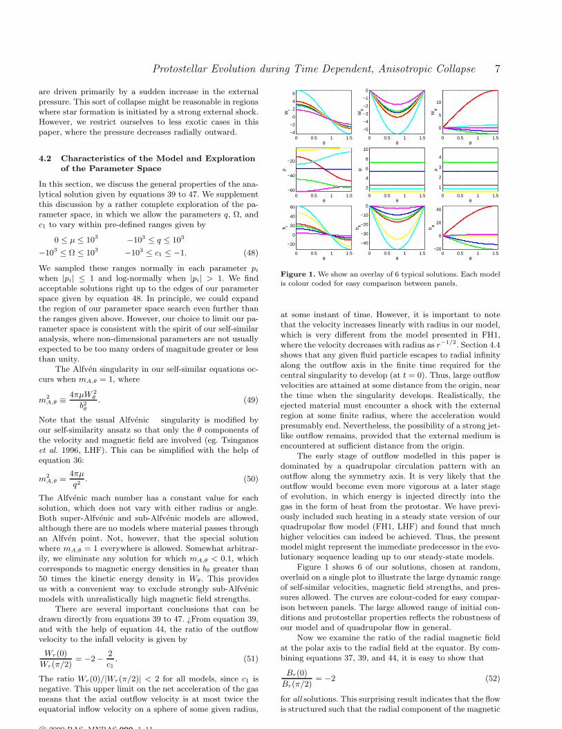
Figure 1. We show an overlay of 6 typical solutions. Each modelis colour coded for easy comparison between panels.

at some instant of time. However, it is important to notethat the velocity increases linearly with radius in our model,which is very different from the model presented in FH1,where the velocity decreases with radius as r−1/2. Section 4.4shows that any given fluid particle escapes to radial infinityalong the outflow axis in the finite time required for thecentral singularity to develop (at t = 0). Thus, large outflowvelocities are attained at some distance from the origin, nearthe time when the singularity develops. Realistically, theejected material must encounter a shock with the externalregion at some finite radius, where the acceleration wouldpresumably end. Nevertheless, the possibility of a strong jet-like outflow remains, provided that the external medium isencountered at sufficient distance from the origin.

The early stage of outflow modelled in this paper isdominated by a quadrupolar circulation pattern with anoutflow along the symmetry axis. It is very likely that theoutflow would become even more vigorous at a later stageof evolution, in which energy is injected directly into thegas in the form of heat from the protostar. We have previ-ously included such heating in a steady state version of ourquadrupolar flow model (FH1, LHF) and found that muchhigher velocities can indeed be achieved. Thus, the presentmodel might represent the immediate predecessor in the evo-lutionary sequence leading up to our steady-state models.

Figure 1 shows 6 of our solutions, chosen at random,overlaid on a single plot to illustrate the large dynamic rangeof self-similar velocities, magnetic field strengths, and pres-sures allowed. The curves are colour-coded for easy compar-ison between panels. The large allowed range of initial con-ditions and protostellar properties reflects the robustness ofour model and of quadrupolar flow in general.

Now we examine the ratio of the radial magnetic fieldat the polar axis to the radial field at the equator. By com-bining equations 37, 39, and 44, it is easy to show that

Br(0)

Br(π/2)= −2 (52)

for all solutions. This surprising result indicates that the flowis structured such that the radial component of the magnetic

c© 2000 RAS, MNRAS 000, 1–11


field is always compressed to precisely the same extent. It isinteresting that we first noticed this result in outflow solu-tions obtained numerically using a shooting code. This wasone of the key results that suggested the existence of a gen-eral analytic solution to our boundary value problem, andled us to the solution presented in equations 21 to 35.

A careful examination of Figure 1 reveals that most ofour models have a low pressure region near the symmetryaxis, but some demonstrate the opposite behaviour. Thiseffect can be explained by consulting equations 42, 38, 41,and 47. Note that c6 is the self-similar pressure differencebetween the midplane and the polar axis:

c6 = p(π/2) − p(0). (53)

Note also that the term (c4q+Ω) in equation 47 is the maxi-mum value of the self-similar toroidal field bφ. Thus, a strongtoroidal field tends to make c6 negative, so that the pressureis highest at the polar axis. Clearly, this compression is dueto the radial pinch of the toroidal field toward the polaraxis (e.g. Fiege & Pudritz 2000a,b). On the other hand, theconstant c4 in the second term is equal to the maximumrotational velocity, which acts in the opposite sense to pushmaterial away from the axis. This centrifugal barrier pro-duces a low pressure region near the axis when the toroidalfield is not sufficiently strong to counter its effect. We referto these models as “tornado” solutions, while we often referto bφ dominated models as magnetically pinched. A usefulparameter to investigate these two types of behaviour is theratio of the dynamical pressure at the the symmetry axisdivided by the pressure at the midplane:

p(0)

p(π/2)=

c5c5 + c6

. (54)

Since p < 0, tornado-type solutions correspond top(0)/p(π/2) > 1, while magnetically pinched solutions havethe opposite behaviour, with p(0)/p(π/2) < 1. In Figure 2,we plot this quantity against the magnetic pressure ratiobr(θ0)

2/bpol(θ0)2, where br(θ0) and bpol(θ0) are respectively

the self-similar toroidal field and poloidal field (defined by

bpol =√

b2r + b2θ) components, evaluated at the angle

θ0 = cos−1[

√

−c1/c2]

, (55)

which divides the equatorial infall zone from the polar out-flow zone (See equation 39). Since c1 < −1, equation 43 im-

plies that θ0 has a maximum possible value of cos−1√

1/3 ≈54.7. Note that the transition between tornado and mag-netically pinched solutions occurs when b2φ,max/b

2r,max ≈ 1,

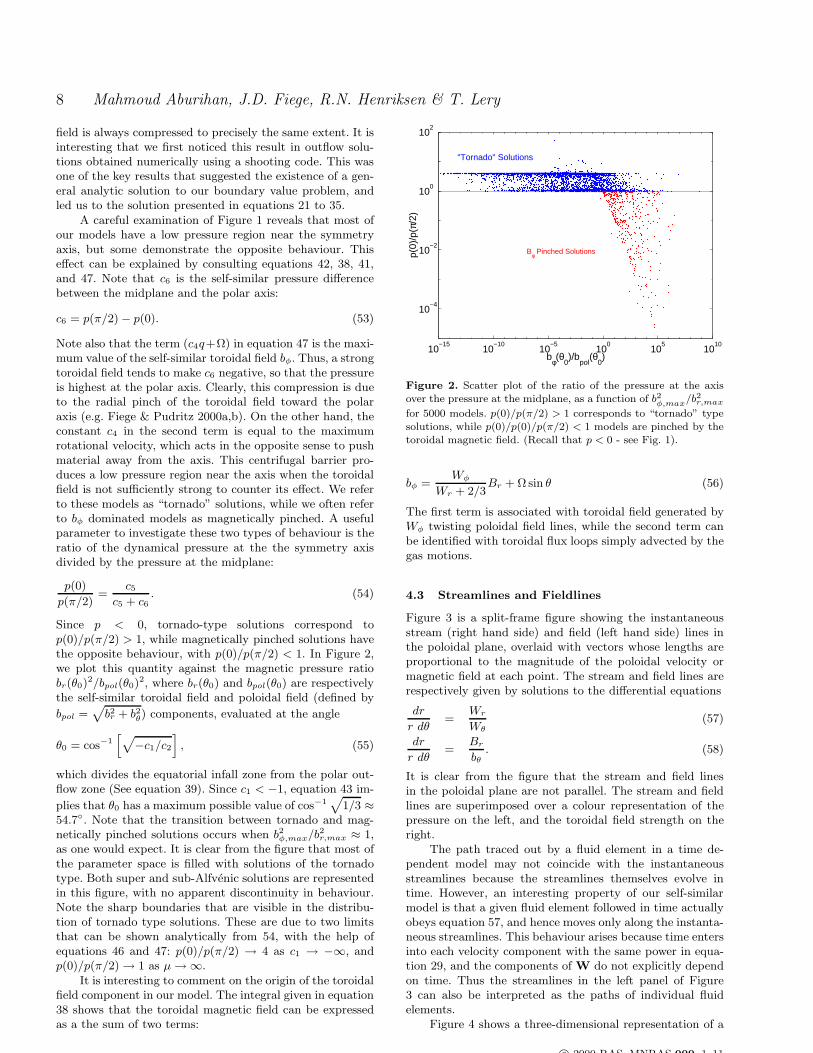
as one would expect. It is clear from the figure that most ofthe parameter space is filled with solutions of the tornadotype. Both super and sub-Alfvenic solutions are representedin this figure, with no apparent discontinuity in behaviour.Note the sharp boundaries that are visible in the distribu-tion of tornado type solutions. These are due to two limitsthat can be shown analytically from 54, with the help ofequations 46 and 47: p(0)/p(π/2) → 4 as c1 → −∞, andp(0)/p(π/2) → 1 as µ→ ∞.

It is interesting to comment on the origin of the toroidalfield component in our model. The integral given in equation38 shows that the toroidal magnetic field can be expressedas a the sum of two terms:

10−15

10−10

10−5

100

105

1010

10−4

10−2

100

102

"Tornado" Solutions

Bφ Pinched Solutions

bφ(θ

0)/b

pol(θ

0)

p(0)

/p(π

/2)

Figure 2. Scatter plot of the ratio of the pressure at the axisover the pressure at the midplane, as a function of b2φ,max/b2r,max

for 5000 models. p(0)/p(π/2) > 1 corresponds to “tornado” typesolutions, while p(0)/p(0)/p(π/2) < 1 models are pinched by thetoroidal magnetic field. (Recall that p < 0 - see Fig. 1).

bφ =Wφ

Wr + 2/3Br + Ωsin θ (56)

The first term is associated with toroidal field generated byWφ twisting poloidal field lines, while the second term canbe identified with toroidal flux loops simply advected by thegas motions.

4.3 Streamlines and Fieldlines

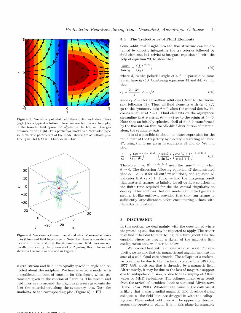
Figure 3 is a split-frame figure showing the instantaneousstream (right hand side) and field (left hand side) lines inthe poloidal plane, overlaid with vectors whose lengths areproportional to the magnitude of the poloidal velocity ormagnetic field at each point. The stream and field lines arerespectively given by solutions to the differential equations

dr

r dθ=

Wr

Wθ(57)

dr

r dθ=

Br

bθ. (58)

It is clear from the figure that the stream and field linesin the poloidal plane are not parallel. The stream and fieldlines are superimposed over a colour representation of thepressure on the left, and the toroidal field strength on theright.

The path traced out by a fluid element in a time de-pendent model may not coincide with the instantaneousstreamlines because the streamlines themselves evolve intime. However, an interesting property of our self-similarmodel is that a given fluid element followed in time actuallyobeys equation 57, and hence moves only along the instanta-neous streamlines. This behaviour arises because time entersinto each velocity component with the same power in equa-tion 29, and the components of W do not explicitly dependon time. Thus the streamlines in the left panel of Figure3 can also be interpreted as the paths of individual fluidelements.

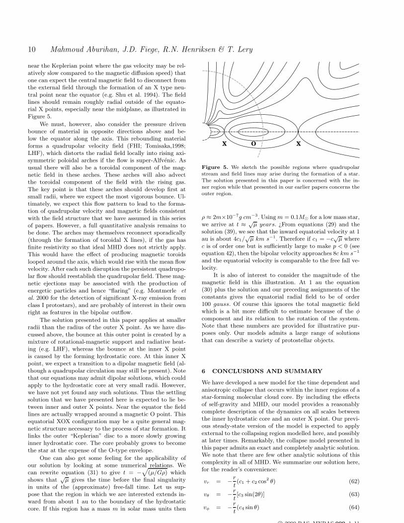
Figure 4 shows a three-dimensional representation of a

c© 2000 RAS, MNRAS 000, 1–11


−5 0 5−5

0

5

x

z

Figure 3. We show poloidal field lines (left) and streamlines(right) for a typical solution. These are overlaid on a colour plotof the toroidal field “pressure” b2

φ/8π on the left, and the gas

pressure on the right. This particular model is a “tornado” typesolution. The parameters of the model shown are as follows: µ =1.77, q = −6.11, Ω = −14.56, c1 = −4.33.

−20

0

20

−20

0

20

−20

−10

0

10

20

xy

z

Figure 4. We show a three-dimensional view of several stream-lines (blue) and field lines (green). Note that there is considerablerotation in flow, and that the streamline and field lines are notparallel, indicating the presence of a Poynting flux. The modelshown is the same as the one in Figure 3.

several stream and field lines equally spaced in angle and re-flected about the midplane. We have selected a model witha significant amount of rotation for this figure, whose pa-rameters given in the caption of figure 3). The stream andfield lines wraps around the origin as pressure gradients de-flect the material out along the symmetry axis. Note thesimilarity to the corresponding plot (Figure 5) in FH1.

4.4 The Trajectories of Fluid Elements

Some additional insight into the flow structure can be ob-tained by directly integrating the trajectories followed byfluid elements. It is trivial to integrate equation 40, with thehelp of equation 29, to show that

tan θ

tan θ0=

(

t

t0

)−2c3

, (59)

where θ0 is the poloidal angle of a fluid particle at someinitial time t0 < 0. Combining equations 43 and 44, we findthat

c3 =2 + 3c1

2< −1/2 (60)

since c1 < −1 for all outflow solutions (Refer to the discus-sion following 47). Thus, all fluid elements with θ0 < π/2go to the symmetry axis θ = 0 when the central density be-comes singular at t = 0. Fluid elements on the asymptoticstreamline that starts at θ0 = π/2 go to the origin at t = 0.Note that an initially spherical shell of fluid is transformedby the flow into an thin “needle-like” distribution of materialalong the symmetry axis.

It is also possible to obtain an exact expression for theradial part of the trajectory by directly integrating equation57, using the forms given in equations 39 and 40. We findthat

r

r0=

(

tan θ

tan θ0

)c1/(2c3) [(

sin θ

sin θ0

)(

cos θ0 + 1

cos θ + 1

)]c2/(2c3)

.(61)

Therefore, r ∝ θ(c1+c2)/(2c3) near the time t = 0, whenθ → 0. The discussion following equation 47 demonstratedthat c1 + c2 > 0 for all outflow solutions, and equation 60indicates that c3 < 1. Thus, we find the intriguing resultthat material escapes to infinity for all outflow solutions inthe finite time required for the the central singularity todevelop. This confirms that our model can indeed generatestrong, jet-like outflows, provided that they can escape tosufficiently large distances before encountering a shock withthe external medium.

5 DISCUSSION

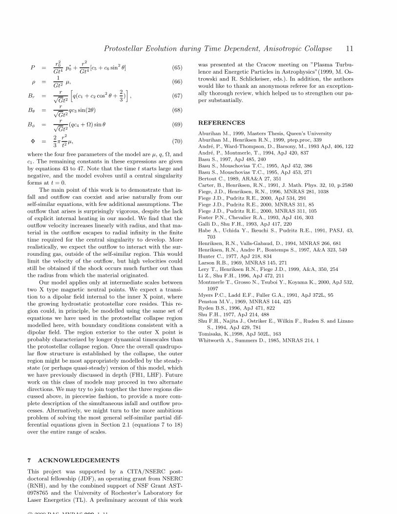
In this section, we deal mainly with the question of wherethe preceding solution may be expected to apply. The readermay find it helpful to refer to Figure 5 throughout this dis-cussion, where we provide a sketch of the magnetic fieldconfiguration that we describe below.

We proceed first with a qualitative discussion. For sim-plicity, we assume that the magnetic and angular momentumaxes of a cold cloud core coincide. The collapse of a molecu-lar core may be due to the inside-out collapse of a SIS (Shu1977; GS), albeit one that is threaded by a magnetic field.Alternatively, it may be due to the loss of magnetic supportdue to ambipolar diffusion, or due to the damping of Alfvenwaves or MHD turbulence. The collapse might even resultfrom the arrival of a sudden shock or torsional Alfven wave(Habe et al. 1991). Whatever the cause of the collapse, itis likely that a nearly radial magnetic field develops duringcollapse, as the field lines are dragged in with the collaps-ing gas. These radial field lines will be oppositely directedacross the equatorial plane. It is in this plane (presumably

c© 2000 RAS, MNRAS 000, 1–11


near the Keplerian point where the gas velocity may be rel-atively slow compared to the magnetic diffusion speed) thatone can expect the central magnetic field to disconnect fromthe external field through the formation of an X type neu-tral point near the equator (e.g. Shu et al. 1994). The fieldlines should remain roughly radial outside of the equato-rial X points, especially near the midplane, as illustrated inFigure 5.

We must, however, also consider the pressure drivenbounce of material in opposite directions above and be-low the equator along the axis. This rebounding materialforms a quadrupolar velocity field (FHI; Tomisaka,1998;LHF), which distorts the radial field locally into rising axi-symmetric poloidal arches if the flow is super-Alfvenic. Asusual there will also be a toroidal component of the mag-netic field in these arches. These arches will also advectthe toroidal component of the field with the rising gas.The key point is that these arches should develop first atsmall radii, where we expect the most vigorous bounce. Ul-timately, we expect this flow pattern to lead to the forma-tion of quadrupolar velocity and magnetic fields consistentwith the field structure that we have assumed in this seriesof papers. However, a full quantitative analysis remains tobe done. The arches may themselves reconnect sporadically(through the formation of toroidal X lines), if the gas hasfinite resistivity so that ideal MHD does not strictly apply.This would have the effect of producing magnetic toroidslooped around the axis, which would rise with the mean flowvelocity. After each such disruption the persistent quadrupo-lar flow should reestablish the quadrupolar field. These mag-netic ejections may be associated with the production ofenergetic particles and hence “flaring” (e.g. Montmerle et

al. 2000 for the detection of significant X-ray emission fromclass I protostars), and are probably of interest in their ownright as features in the bipolar outflow.

The solution presented in this paper applies at smallerradii than the radius of the outer X point. As we have dis-cussed above, the bounce at this outer point is created by amixture of rotational-magnetic support and radiative heat-ing (e.g. LHF), whereas the bounce at the inner X pointis caused by the forming hydrostatic core. At this inner Xpoint, we expect a transition to a dipolar magnetic field (al-though a quadrupolar circulation may still be present). Notethat our equations may admit dipolar solutions, which couldapply to the hydrostatic core at very small radii. However,we have not yet found any such solutions. Thus the settlingsolution that we have presented here is expected to lie be-tween inner and outer X points. Near the equator the fieldlines are actually wrapped around a magnetic O point. Thisequatorial XOX configuration may be a quite general mag-netic structure necessary to the process of star formation. Itlinks the outer “Keplerian” disc to a more slowly growinginner hydrostatic core. The core probably grows to becomethe star at the expense of the O-type envelope.

One can also get some feeling for the applicability ofour solution by looking at some numerical relations. Wecan rewrite equation (31) to give t = −

√

(µ/Gρ) whichshows that

√µ gives the time before the final singularity

in units of the (approximate) free-fall time. Let us sup-pose that the region in which we are interested extends in-ward from about 1 au to the boundary of the hydrostaticcore. If this region has a mass m in solar mass units then

X XO

Figure 5. We sketch the possible regions where quadrupolarstream and field lines may arise during the formation of a star.The solution presented in this paper is concerned with the in-ner region while that presented in our earlier papers concerns theouter region.

ρ ≈ 2m×10−7g cm−3. Usingm = 0.1M⊙ for a low mass star,we arrive at t ≈ √

µ years. ¿From equations (29) and thesolution (39), we see that the inward equatorial velocity at 1au is about 4c1/

√µ km s−1. Therefore if c1 = −c√µ where

c is of order one but is sufficiently large to make p < 0 (seeequation 42), then the bipolar velocity approaches 8c km s−1

and the equatorial velocity is comparable to the free fall ve-locity.

It is also of interest to consider the magnitude of themagnetic field in this illustration. At 1 au the equation(30) plus the solution and our preceding assignments of theconstants gives the equatorial radial field to be of order100 gauss. Of course this ignores the total magnetic fieldwhich is a bit more difficult to estimate because of the φcomponent and its relation to the rotation of the system.Note that these numbers are provided for illustrative pur-poses only. Our models admits a large range of solutionsthat can describe a variety of protostellar objects.

6 CONCLUSIONS AND SUMMARY

We have developed a new model for the time dependent andanisotropic collapse that occurs within the inner regions of astar-forming molecular cloud core. By including the effectsof self-gravity and MHD, our model provides a reasonablycomplete description of the dynamics on all scales betweenthe inner hydrostatic core and an outer X point. Our previ-ous steady-state version of the model is expected to applyexternal to the collapsing region modelled here, and possiblyat later times. Remarkably, the collapse model presented inthis paper admits an exact and completely analytic solution.We note that there are few other analytic solutions of thiscomplexity in all of MHD. We summarize our solution here,for the reader’s convenience:

vr = −rt(c1 + c2 cos2 θ) (62)

vθ = −rt[c3 sin(2θ)] (63)

vφ = −rt(c4 sin θ) (64)

c© 2000 RAS, MNRAS 000, 1–11


P =r20Gt4

p∗0 +r2

Gt4[c5 + c6 sin2 θ] (65)

ρ =1

Gt2µ, (66)

Br =r√Gt2

[

q(c1 + c2 cos2 θ +2

3)]

, (67)

Bθ =r√Gt2

qc3 sin(2θ) (68)

Bφ =r√Gt2

(qc4 + Ω) sin θ (69)

Φ =2

3πr2

t2µ, (70)

where the four free parameters of the model are µ, q, Ω, andc1. The remaining constants in these expressions are givenby equations 43 to 47. Note that the time t starts large andnegative, and the model evolves until a central singularityforms at t = 0.

The main point of this work is to demonstrate that in-fall and outflow can coexist and arise naturally from ourself-similar equations, with few additional assumptions. Theoutflow that arises is surprisingly vigorous, despite the lackof explicit internal heating in our model. We find that theoutflow velocity increases linearly with radius, and that ma-terial in the outflow escapes to radial infinity in the finitetime required for the central singularity to develop. Morerealistically, we expect the outflow to interact with the sur-rounding gas, outside of the self-similar region. This wouldlimit the velocity of the outflow, but high velocities couldstill be obtained if the shock occurs much further out thanthe radius from which the material originated.

Our model applies only at intermediate scales betweentwo X type magnetic neutral points. We expect a transi-tion to a dipolar field internal to the inner X point, wherethe growing hydrostatic protostellar core resides. This re-gion could, in principle, be modelled using the same set ofequations we have used in the protostellar collapse regionmodelled here, with boundary conditions consistent with adipolar field. The region exterior to the outer X point isprobably characterized by longer dynamical timescales thanthe protostellar collapse region. Once the overall quadrupo-lar flow structure is established by the collapse, the outerregion might be most appropriately modelled by the steady-state (or perhaps quasi-steady) version of this model, whichwe have previously discussed in depth (FH1, LHF). Futurework on this class of models may proceed in two alternatedirections. We may try to join together the three regions dis-cussed above, in piecewise fashion, to provide a more com-plete description of the simultaneous infall and outflow pro-cesses. Alternatively, we might turn to the more ambitiousproblem of solving the most general self-similar partial dif-ferential equations given in Section 2.1 (equations 7 to 18)over the entire range of scales.

7 ACKNOWLEDGEMENTS

This project was supported by a CITA/NSERC post-doctoral fellowship (JDF), an operating grant from NSERC(RNH), and by the combined support of NSF Grant AST-0978765 and the University of Rochester’s Laboratory forLaser Energetics (TL). A preliminary account of this work

was presented at the Cracow meeting on ”Plasma Turbu-lence and Energetic Particles in Astrophysics”(1999, M. Os-trowski and R. Schlickeiser, eds.). In addition, the authorswould like to thank an anonymous referee for an exception-ally thorough review, which helped us to strengthen our pa-per substantially.

REFERENCES

Aburihan M., 1999, Masters Thesis, Queen’s UniversityAburihan M., Henriksen R.N., 1999, ptep.proc, 339Andre, P., Ward-Thompson, D., Barsony, M., 1993 ApJ, 406, 122Andre, P., Montmerle, T., 1994, ApJ 420, 837Basu S., 1997, ApJ 485, 240Basu S., Mouschovias T.C., 1995, ApJ 452, 386Basu S., Mouschovias T.C., 1995, ApJ 453, 271Bertout C., 1989, ARA&A 27, 351Carter, B., Henriksen, R.N., 1991, J. Math. Phys. 32, 10, p.2580Fiege, J.D., Henriksen, R.N., 1996, MNRAS 281, 1038Fiege J.D., Pudritz R.E., 2000, ApJ 534, 291Fiege J.D., Pudritz R.E., 2000, MNRAS 311, 85Fiege J.D., Pudritz R.E., 2000, MNRAS 311, 105Foster P.N., Chevalier R.A., 1993, ApJ 416, 303Galli D., Shu F.H., 1993, ApJ 417, 220Habe A., Uchida Y., Ikeuchi S., Pudritz R.E., 1991, PASJ, 43,

703Henriksen, R.N., Valls-Gabaud, D., 1994, MNRAS 266, 681Henriksen, R.N., Andre P., Bontemps S., 1997, A&A 323, 549Hunter C., 1977, ApJ 218, 834Larson R.B., 1969, MNRAS 145, 271Lery T., Henriksen R.N., Fiege J.D., 1999, A&A, 350, 254Li Z., Shu F.H., 1996, ApJ 472, 211Montmerle T., Grosso N., Tsuboi Y., Koyama K., 2000, ApJ 532,

1097Myers P.C., Ladd E.F., Fuller G.A., 1991, ApJ 372L, 95Penston M.V., 1969, MNRAS 144, 425Ryden B.S., 1996, ApJ 471, 822Shu F.H., 1977, ApJ 214, 488Shu F.H., Najita J., Ostriker E., Wilkin F., Ruden S. and Lizano

S., 1994, ApJ 429, 781Tomisaka, K.,1998, ApJ 502L, 163Whitworth A., Summers D., 1985, MNRAS 214, 1

c© 2000 RAS, MNRAS 000, 1–11

Protostellar evolution during time-dependent anisotropic collapse

Documents