PROTEINS, INTERACTIONS, AND COMPLEXES: A COMPUTATIONAL APPROACH A DISSERTATION SUBMITTED TO THE DEPARTMENT OF COMPUTER SCIENCE AND THE COMMITTEE ON GRADUATE STUDIES OF STANFORD UNIVERSITY IN PARTIAL FULFILLMENT OF THE REQUIREMENTS FOR THE DEGREE OF DOCTOR OF PHILOSOPHY Haidong Wang December 2008

Welcome message from author
This document is posted to help you gain knowledge. Please leave a comment to let me know what you think about it! Share it to your friends and learn new things together.
Transcript

PROTEINS, INTERACTIONS, AND COMPLEXES: A
COMPUTATIONAL APPROACH
A DISSERTATION
SUBMITTED TO THE DEPARTMENT OF COMPUTER SCIENCE
AND THE COMMITTEE ON GRADUATE STUDIES
OF STANFORD UNIVERSITY
IN PARTIAL FULFILLMENT OF THE REQUIREMENTS
FOR THE DEGREE OF
DOCTOR OF PHILOSOPHY
Haidong Wang
December 2008

c© Copyright by Haidong Wang 2009
All Rights Reserved
ii

I certify that I have read this dissertation and that, in my opinion, it
is fully adequate in scope and quality as a dissertation for the degree
of Doctor of Philosophy.
(Daphne Koller) Principal Adviser
I certify that I have read this dissertation and that, in my opinion, it
is fully adequate in scope and quality as a dissertation for the degree
of Doctor of Philosophy.
(Jean-Claude Latombe)
I certify that I have read this dissertation and that, in my opinion, it
is fully adequate in scope and quality as a dissertation for the degree
of Doctor of Philosophy.
(Andrew Ng)
Approved for the University Committee on Graduate Studies.
iii

To Zhiqing and Rirong.
iv

Abstract
Proteins play a major role in cellular processes; therefore, it is important to under-
stand how they perform their functions. Proteins, however, do not act alone; they
work together to create various biological processes in a hierarchical fashion. First,
multiple proteins physically bind together to form stoichiometrically stable complexes.
These complexes interact with each other to form functional modules and pathways
that carry out most cellular processes. Although large amounts of proteomic data are
available, extracting biological insights about proteins and complexes is a challenging
task because most high throughput data are noisy and indirect, and thus only weakly
correlate with the objective we seek.
In this thesis, we try to understand the hierarchical structure of protein dynamics
by applying computational algorithms that deal effectively with the noise and in-
completeness in our data. At the lowest level of the hierarchy, we use unsupervised
learning to predict the binding sites where the interaction between two proteins occur.
At the middle level, we identify a set of stoichiometrically stable complexes. With
the availability of labeled data and high quality measurement, we used supervised
learning combined with a specifically designed clustering algorithm. Finally, at the
highest level, we predict interactions between stoichiometrically stable complexes that
belong to the same pathway.
Our methods are validated as more accurate than previous approaches, and they
reveal important biological insights. For example, diseases related to certain mu-
tations are shown to involve proteins that are predicted to bind to the sites where
the mutations occur, suggesting possible mechanisms where the mutations disrupt
the bindings and thus lead to the diseases. Another finding shows that proteins in
v

larger predicted complexes are more likely to be essential, which explains previous
observation that ‘hub’ proteins are more likely to be essential.
vi

Acknowledgement
First of all, I would like to thank my advisor, Daphne Koller, for her guidance through
my entire PhD process. From the beginning when I first entered the Stanford and
knew little about the field, she guided me at each step of the research process. With
her, I learned how to select interesting problems, how to download and analyze data,
how to come up with a model and implement it, how to evaluate the results and
possibly repeat to the whole process to gain further improvement, and finally how to
present the findings in professional settings. Although Daphne has a busy schedule
and many other PhD students, she has spent a lot of time with me to make sure I
am on the right track at each step. Whenever I have any questions, she is able to
respond promptly with her insights.
I would also like to thank other members of my reading committee, Jean-Claude
Latombe and Andrew Ng, and other members of my oral committee, Doug Brutlag
and Serafim Batzoglou. Their feedback and thought-provoking suggestions helps me
improve my research, oral presentation, and the thesis. In particular, I discussed the
clustering problem with Andrew and gained a lot of understanding of the problem
from his knowledge in the field.
Through the many days and nights working in the Gates Computer Science build-
ing, I am lucky to share office with Pieter Abbeel and Su-In Lee. Research is a lonely
business, but working with Pieter and Su-In made it enjoyable. Our endless talk
involves both personal interests and PhD research, where I learned a lot from their
insights and am inspired by their hard-working spirit. I am also lucky to be among
Daphne’s large group of smart students, whose names are too long to list. I enjoyed
the numerous conversations with them during lunch time and retreat.
vii

I would not be able to do what I have done if it is not because of many of
my collaborators. In the earlier collaborations, I worked with Eran Segal and Asa
Ben-Hur, from whom I learned a lot about research so I was able to start working
independently. In the later collaborations, I was blessed to work with many biologists
— Qianru Li, Marc Vidal, Sean Collins, and Nevan Krogan — who provided me with
data, explained me the biological ideas, and did the web-lab experiments. They spent
a lot of time going through my predictions, which made the paper much more relevant
to the actual biology.
Last but not least, I am profoundly grateful to my parents for making me who I
am. Although they could not be here with me during my PhD process, they always
paid great attention to every little aspect of my life and research. They are always
there to give me encouragement when I met difficulties. I would also like to thank
many of the new friends I met in Stanford. They made here a home away from home
and my Stanford life exciting.
viii

Contents
Abstract v
Acknowledgement vii
1 Introduction 1
1.1 Biological background . . . . . . . . . . . . . . . . . . . . . . . . . . 3
1.2 Overview of the thesis . . . . . . . . . . . . . . . . . . . . . . . . . . 7
1.3 Our contribution . . . . . . . . . . . . . . . . . . . . . . . . . . . . . 12
2 Protein-protein interaction sites 14
2.1 Introduction . . . . . . . . . . . . . . . . . . . . . . . . . . . . . . . . 14
2.2 Related work . . . . . . . . . . . . . . . . . . . . . . . . . . . . . . . 21
2.3 Sources of data . . . . . . . . . . . . . . . . . . . . . . . . . . . . . . 23
2.3.1 S. cerevisiae . . . . . . . . . . . . . . . . . . . . . . . . . . . . 23
2.3.2 Human . . . . . . . . . . . . . . . . . . . . . . . . . . . . . . . 26
2.4 Methods . . . . . . . . . . . . . . . . . . . . . . . . . . . . . . . . . . 26
2.4.1 Probabilistic model . . . . . . . . . . . . . . . . . . . . . . . . 26
2.4.2 Learning . . . . . . . . . . . . . . . . . . . . . . . . . . . . . . 32
2.4.3 Binding confidence estimation . . . . . . . . . . . . . . . . . . 35
2.4.4 Model initialization . . . . . . . . . . . . . . . . . . . . . . . . 36
2.5 Results . . . . . . . . . . . . . . . . . . . . . . . . . . . . . . . . . . . 38
2.5.1 Overview . . . . . . . . . . . . . . . . . . . . . . . . . . . . . 38
2.5.2 Predicting physical interactions . . . . . . . . . . . . . . . . . 40
2.5.3 Predicting binding sites . . . . . . . . . . . . . . . . . . . . . 41
ix

2.5.4 Understanding disease-causing mutations in human . . . . . . 49
2.6 Discussion . . . . . . . . . . . . . . . . . . . . . . . . . . . . . . . . . 56
2.7 Conclusions . . . . . . . . . . . . . . . . . . . . . . . . . . . . . . . . 59
3 MRFs: modeling interaction and complex 60
3.1 Introduction . . . . . . . . . . . . . . . . . . . . . . . . . . . . . . . . 60
3.2 Related work . . . . . . . . . . . . . . . . . . . . . . . . . . . . . . . 63
3.3 Background . . . . . . . . . . . . . . . . . . . . . . . . . . . . . . . . 65
3.3.1 Markov Random Field (MRF) . . . . . . . . . . . . . . . . . . 65
3.4 Methods . . . . . . . . . . . . . . . . . . . . . . . . . . . . . . . . . . 73
3.5 MRF for the triplet model . . . . . . . . . . . . . . . . . . . . . . . . 78
3.5.1 Representation . . . . . . . . . . . . . . . . . . . . . . . . . . 78
3.5.2 Learning and inference . . . . . . . . . . . . . . . . . . . . . . 79
3.5.3 Experiment setup . . . . . . . . . . . . . . . . . . . . . . . . . 80
3.5.4 Results . . . . . . . . . . . . . . . . . . . . . . . . . . . . . . . 80
3.6 MRF for the complex model . . . . . . . . . . . . . . . . . . . . . . . 83
3.6.1 Representation . . . . . . . . . . . . . . . . . . . . . . . . . . 83
3.6.2 Learning and identifying complexes . . . . . . . . . . . . . . . 84
3.6.3 Experiment setup . . . . . . . . . . . . . . . . . . . . . . . . . 84
3.6.4 Results . . . . . . . . . . . . . . . . . . . . . . . . . . . . . . . 85
3.7 Discussion . . . . . . . . . . . . . . . . . . . . . . . . . . . . . . . . . 86
4 Stoichiometrically Stable Complexes 88
4.1 Introduction . . . . . . . . . . . . . . . . . . . . . . . . . . . . . . . . 88
4.2 Related work . . . . . . . . . . . . . . . . . . . . . . . . . . . . . . . 92
4.3 Constructing a set of reference complexes . . . . . . . . . . . . . . . . 96
4.4 Pairwise signals for predicting complexes . . . . . . . . . . . . . . . . 97
4.5 Methods . . . . . . . . . . . . . . . . . . . . . . . . . . . . . . . . . . 100
4.5.1 Complexness model . . . . . . . . . . . . . . . . . . . . . . . . 100
4.5.2 Protein-complex model . . . . . . . . . . . . . . . . . . . . . . 102
4.5.3 Protein-protein model . . . . . . . . . . . . . . . . . . . . . . 104
4.6 Experiment setup . . . . . . . . . . . . . . . . . . . . . . . . . . . . . 108
x
4.6.1 Training and test regime . . . . . . . . . . . . . . . . . . . . . 108
4.6.2 Evaluation metrics . . . . . . . . . . . . . . . . . . . . . . . . 109
4.7 Results . . . . . . . . . . . . . . . . . . . . . . . . . . . . . . . . . . . 110
4.7.1 Coverage and sensitivity of predicted complexes . . . . . . . . 110
4.7.2 Contribution of each data source . . . . . . . . . . . . . . . . 116
4.7.3 Biological coherence of predicted complexes . . . . . . . . . . 119
4.7.4 Essentiality and complex size . . . . . . . . . . . . . . . . . . 122
4.8 Discussion . . . . . . . . . . . . . . . . . . . . . . . . . . . . . . . . . 126
5 Complex-complex interactions 129
5.1 Introduction . . . . . . . . . . . . . . . . . . . . . . . . . . . . . . . . 129
5.2 Related work . . . . . . . . . . . . . . . . . . . . . . . . . . . . . . . 131
5.3 Reference list of positive and negative complex-complex interactions . 131
5.4 Protein-level signals for predicting complex-complex interactions . . . 132
5.5 Aggregating signals into features between complexes . . . . . . . . . . 134
5.6 Methods . . . . . . . . . . . . . . . . . . . . . . . . . . . . . . . . . . 136
5.7 Results . . . . . . . . . . . . . . . . . . . . . . . . . . . . . . . . . . . 139
5.7.1 Accuracy of complex-complex interaction predictions . . . . . 139
5.7.2 Functional coherence of interacting complexes . . . . . . . . . 141
5.7.3 Accuracy of unified interaction network . . . . . . . . . . . . . 141
5.7.4 Conditions when two complexes interact . . . . . . . . . . . . 141
5.8 Discussion . . . . . . . . . . . . . . . . . . . . . . . . . . . . . . . . . 144
6 Conclusions 145
6.1 Summary . . . . . . . . . . . . . . . . . . . . . . . . . . . . . . . . . 145
6.2 Future directions . . . . . . . . . . . . . . . . . . . . . . . . . . . . . 147
6.2.1 Identifying pathways . . . . . . . . . . . . . . . . . . . . . . . 147
6.2.2 Different types of interactions . . . . . . . . . . . . . . . . . . 147
6.2.3 Interacting regions between complexes . . . . . . . . . . . . . 148
A Aggregating functions for creating complex-level features 149
xi

Bibliography 151
xii

List of Tables
2.1 Top binding site predictions in human . . . . . . . . . . . . . . . . . 51
3.1 Representing a pairwise term . . . . . . . . . . . . . . . . . . . . . . 68
3.2 Decomposition of a pairwise term . . . . . . . . . . . . . . . . . . . . 68
3.3 Representing a triplet term . . . . . . . . . . . . . . . . . . . . . . . . 69
3.4 Decomposition of a triplet term . . . . . . . . . . . . . . . . . . . . . 69
3.5 Decomposition of a triplet term . . . . . . . . . . . . . . . . . . . . . 71
3.6 Rewrite a non-regular pairwise term . . . . . . . . . . . . . . . . . . . 72
5.1 List of aggregating functions chosen . . . . . . . . . . . . . . . . . . . 135
5.2 Parametric family in the model for the complex-complex interaction
network . . . . . . . . . . . . . . . . . . . . . . . . . . . . . . . . . . 137
5.3 Parametric family in the model for the unified interaction network . . 138
xiii

List of Figures
1.1 Protein sequence and its folding . . . . . . . . . . . . . . . . . . . . . 4
2.1 Example illustrating the intuition behind our approach . . . . . . . . 17
2.2 Overview of our automated procedure . . . . . . . . . . . . . . . . . . 19
2.3 Protein-protein interaction assays . . . . . . . . . . . . . . . . . . . . 25
2.4 Our Bayesian Network model . . . . . . . . . . . . . . . . . . . . . . 28
2.5 Schematic illustration of our EM-based learning algorithm . . . . . . 34
2.6 Perturbation analysis for binding site prediction . . . . . . . . . . . . 37
2.7 Motif coverage of protein sequences and binding sites . . . . . . . . . 39
2.8 Verification of protein-protein interaction predictions . . . . . . . . . 42
2.9 Binding site predictions within the RNA Polymerase II complex . . . 44
2.10 Distribution of motif coverage . . . . . . . . . . . . . . . . . . . . . . 45
2.11 Global verification of binding site predictions . . . . . . . . . . . . . . 46
2.12 Number of motif pair occurrences . . . . . . . . . . . . . . . . . . . . 48
2.13 Illustrations of human binding site predictions . . . . . . . . . . . . . 52
2.14 3-D structure of one of our top predictions . . . . . . . . . . . . . . . 55
2.15 Contribution of indirect evidence . . . . . . . . . . . . . . . . . . . . 58
3.1 Mincut graph for a triplet term without pairwise components . . . . . 70
3.2 Sensitivity of the three MRF models in predicting protein-protein in-
teractions . . . . . . . . . . . . . . . . . . . . . . . . . . . . . . . . . 81
3.3 Computational time for learning three MRF models . . . . . . . . . . 82
3.4 Verification of complex predictions using MRF . . . . . . . . . . . . . 85
xiv

4.1 Illustration of the HACO intuition . . . . . . . . . . . . . . . . . . . . 106
4.2 Metrics for overlap between two complexes . . . . . . . . . . . . . . . 109
4.3 Size distribution of reference and predicted complexes . . . . . . . . . 111
4.4 Prediction accuracy of our different models . . . . . . . . . . . . . . . 113
4.5 Accuracy in reconstructing reference complexes . . . . . . . . . . . . 114
4.6 Coverage and sensitivity of predicted complexes . . . . . . . . . . . . 115
4.7 Contribution of each data source . . . . . . . . . . . . . . . . . . . . 118
4.8 Coherence of our predicted complexes . . . . . . . . . . . . . . . . . . 120
4.9 Proportion of essential proteins across complexes . . . . . . . . . . . 123
4.10 Relationship between complex size and essentiality . . . . . . . . . . 124
4.11 Explaining essentiality using complex size vs. hubness . . . . . . . . . 125
5.1 Verification of complex-complex interactions . . . . . . . . . . . . . . 140
5.2 Functional coherence of interacting complexes . . . . . . . . . . . . . 142
5.3 Verification of our unified interaction network . . . . . . . . . . . . . 143
xv

Chapter 1
Introduction
The central dogma of molecular biology states that genetic information is stored in
DNA, which is a linear sequence of four nucleotides. When needed, DNA is tran-
scribed into RNA, which in turn is translated into proteins, which are the main cell
machinery. The large amount of data produced by many genome projects and ten
years of computational analysis of those genomic data provided us with a relatively
complete set of genes and their proteins. Analysis of the microarray data produced
a picture of when and how much a gene is transcribed, which is a rough estimate of
protein abundance. Therefore, the natural next step would be the study of how these
proteins perform their functions.
The functions of proteins are as complicated as if not more complicated than DNA
or RNA. They work with each other to form various biological processes and pathways
in a hierarchical fashion. First, the primary sequence of the protein, which is a linear
sequence of 20 amino acids, dictates the folding of the protein into some 3-D structure.
Protein properties such as 3-D structure of the protein, the chemical properties of its
amino acids, and its localization decide which other proteins or small molecules it
physically binds to. Usually the binding happens at places of complementary 3-
D structure. This kind of physical association enables multiple proteins to form
stoichiometrically stable complexes. At the next level, the complexes interact with
individual proteins or other complexes to form functional modules and pathways that
carry out most cellular processes. Through this hierarchical structure, the limited
1

CHAPTER 1. INTRODUCTION 2
number of proteins are able to combine with each other to perform exponentially
diverse kinds of cellular function.
Recent advances in technology provided us with many types of high throughput
proteomic data, such as yeast two-hybrid and tandem affinity purification for mea-
suring protein-protein interaction, GFP for measuring protein localization, ChIP-chip
for measuring transcriptional regulation, and double knockout for measuring genetic
interaction. This, combined with high throughput data from DNA and RNA such as
sequence motifs and measurement of mRNA levels of entire genomes under various
conditions, provided us with vast amount of information to understand the protein
interaction and function at different levels of the hierarchical structure.
However, extracting biological insights from these data is a challenging task be-
cause most high throughput data are noisy and many types of data provide indirect
evidence, which only weakly correlate with the biological objective we seek. Fortu-
nately, algorithms in computer sciences, statistics, and machine learning have been
developed to extract patterns from large amount of data while dealing with the above
issues. Therefore, the key to success lies in using the right algorithm among the large
number of possible alternatives, and tailor it to the specific biological data and the
problem we want to solve.
In this thesis, we try to gain understanding of the hierarchical structure of the
protein dynamics by applying a diverse range of computational algorithms, adapted
to the specific problem we want to solve and the characteristics of available data.
At the lowest level, we try to predict binding sites of protein-protein interaction. We
applied the framework of probabilistic graphical model to encode our prior knowledge
about the relationship between different entities. Due to the lack of labeled data and
direct evidence, we used unsupervised learning, which also takes into consideration
the structure of unlabeled parts. At the middle level, we try to predict the protein
composition of stoichiometrically stable complexes. Here we have a reference set of
complexes from small-scale experiments and large amount of direct evidence from
high throughput experiments of relatively high quality. Therefore, we use supervised
learning to combine the evidence and then tackle the complex reconstruction using
a specifically designed clustering algorithm that allows overlap. In the end, at the

CHAPTER 1. INTRODUCTION 3
highest level, we try to predict interactions between the stoichiometrically stable
complexes we just constructed in the previous part. Here again we lack enough
labeled data and direct evidence so we used semi-supervised learning. Here we focus
on feature construction to extract and aggregate information between two complexes.
One useful feature is the protein-protein interactions we predicted in the first part.
Therefore, the work of the previous two parts serves as the foundation for the last
part, which deals with the highest level of interactions. The common theme across
all parts of the thesis is the task of integrating heterogeneous types of noisy data.
1.1 Biological background
Here we go through some basic concepts of molecular biology that are essential in un-
derstanding this thesis. We refer the reader to general molecular biology textbook [7]
for more information.
Cells are fundamental units of living organisms. The genetic information for
making an individual is stored in and replicated through DNA, which is located
inside the nucleus. DNA is a sequence of four different types of nucleotides. Certain
segments of the DNA correspond to genes, which under appropriate condition would
be used to make a molecule called mRNA, whose sequence directly corresponds to the
DNA sequence. This process is called transcription. The resulting mRNA migrates
out of the nucleus into cell cytoplasm. There, a protein is synthesized in a process
called translation using the mRNA as template. A protein is a sequence of 20 different
kinds of amino acids. Each amino acid is uniquely determined by three nucleotides
on the DNA or RNA. Therefore, once we know the sequence of a gene, we also know
the sequence of the corresponding protein.
Different amino acids have different structures and chemical properties. For exam-
ple, hydrophobicity is how much an amino acid wants to avoid water, i.e. it would be
in a high energy (unstable) state when in contact with water molecule. Therefore, a
sequence of amino acid in the cell will fold into a specific 3-D structure that minimizes
its energy. The hydrophobic, also called non-polar, amino acids will tend to be buried
inside while the hydrophilic (polar) ones will be more likely on the surface (Fig. 1.1).

CHAPTER 1. INTRODUCTION 4
Figure 1.1: A protein is a sequence of amino acids, some of which are hydrophobic (non-polar,green ones) and some of which are hydrophilic (polar, blue ones). It folds into some 3-D configurationin the cell based on the properties of the amino acid with hydrophobic ones buried inside. The 3-Dshape of the protein is important to the its function.
Amino acids of opposite charge will tend to be close to each other while ones of the
same charge are likely to be farther away. The size of the amino acid also puts a
constraint on the possible configuration. In general, a protein will adopt certain 3-D
structure based on its amino acid sequence although it is difficult to computationally
decide its structure based on the sequence.
Proteins do not function in isolation. They physically interact with each other
or small molecules (ligands) to mediate biological processes or pathways. The in-
teractions happen when the surface patches of the proteins or ligands complement
to each other and form a number of non-covalent bonds such as hydrogen bond,
ionic interactions, Van der Waal’s forces, and hydrophobic packing. Therefore, pro-
tein structure, esp. its complementarity with other surface patch, plays an important
role in facilitating protein-protein interactions. Those contacting surface patches, i.e.
protein-protein interaction sites would be an important target when designing a drug
to disrupt the interaction.

CHAPTER 1. INTRODUCTION 5
Computational approaches in predicting the details of protein-protein interac-
tions have not been satisfactory. Docking methods try to find interaction sties by
matching two protein structures to find the best sites on both structures [51]. These
methods only apply to solved protein structures, which are currently available only for
a small number of proteins. We propose an algorithm that identifies protein-protein
interaction sites only based on high-throughput data, without explicitly knowing the
structures.
Many binary protein-protein interactions comes from proteins within the same
complex or from proteins between two interacting complexes, where a complex is a
stoichiometrically stable set of proteins that permanently associate with each other
to play its cellular role as a single unit. For example, the 20S Proteasome complex is
consisted of four stacked heptameric ring structures [80] with a total of 28 subunits.
The number of unique proteins in the complex varies based on the organism because
some subunits share the same protein. The 20S proteasome is the place where proteins
are degraded, an important step in many biological processes. In general, complexes
are the basic functional units in the cell. Therefore, a faithful reconstruction of the
entire set of complexes is essential in understanding the function of individual proteins
and the higher level organization of the cell, to which the complexes serve as building
blocks.
Fortunately in this case, unlike predicting protein-protein interaction sites de-
scribed previously or predicting complex-complex interactions described below where
we have few labeled data and direct measurement, a new technology called tandem-
affinity purification followed by mass spectrometry (TAP-MS) produced large amount
of high quality data that measures protein complexes directly [45, 59, 44, 79]. In this
assay, a protein, called bait, is fused with a TAP tag. The fusion protein is then
introduced into the host and would be able to interact with other proteins under
normal physiological conditions. Subsequently, after breaking the cells, the fusion
protein is retrieved, together with other constituents attached to it (prey proteins),
through affinity selection by means of an IgG matrix. The identity of the bait and
prey proteins can be resolved by mass spectrometry. TAP-MS identifies the direct or
indirect interaction partners of the bait, which constitute the same complex together

CHAPTER 1. INTRODUCTION 6
with the bait. It works under native condition and is able to detect low number of
protein copies. The stringent affinity selection method resulted in the identification
of mostly stable interactions. Therefore, the assay provides the main signals for our
task of predicting stoichiometrically stable complexes.
However, like all high-throughput assays, there are still false positives and neg-
atives in TAP-MS. A tag added to a protein might obscure binding of the bait to
its interacting partners. On the other hand, the bait proteins might also retrieve
contaminants that is attached non-specifically. Therefore, we might want to consider
other data sets, such expression correlation and co-localization, that give signals to
as whether two proteins are in the same complex.
The functional roles of protein complexes can be further organized into pathways
and processes, where sets of complexes coordinate to achieve a specific goal. For
example in a signaling pathway, a protein or complex, which receives signals from up-
stream entities, interacts with a downstream protein or complex to activate or inhibit
its function. Once activated or inhibited, the downstream entity passes the signal fur-
ther down through more interactions. Therefore, some extra-cellular or environmental
perturbation can be amplified into a strong signal in the nucleus. The interactions
between upstream and downstream entities usually involves post-translational mod-
ification of the downstream entity such as phosphorylation and methylation, which
triggers the change of its 3-D configuration and provide energy for its activities. In
such cases, the interaction happens only when an upstream signal is received and it
ends as soon as the downstream entity is modified. In some other cases, a complex,
though an important functional unit, is not able to perform a biological role by itself.
Instead, it needs to assemble with other complexes into a bigger body. For example,
One copy of 20S proteasome assembles with two copies of 19S proteasomes into a 26S
proteasome which performs the protein degradation where the 19S proteasome regu-
lates the entry of the proteins into 20S proteasome, where the protein is destructed.
In this example, the 26S proteasome is assembled only when needed and the assembly
requires the binding of ATP to the 19S ATP-binding sites. In general, complexes in
the same pathway interact with each other to coordinate the execution of certain
biological processes. These interactions tend to be transient. They happen in specific

CHAPTER 1. INTRODUCTION 7
time, condition, and cellular localization. Once the process is done, their association
may disappear.
Understanding the behavior of different biological pathways leads us to the ulti-
mate goal of biology — predicting the phenotype. On the way from DNA (genotype)
to phenotype, there are a lot of other important biology we need to understand such
as the number of mRNA copies that are produced and phosphorylation, methylation,
and other post-translational modification of the proteins. However we refer the read-
ers to the textbooks since those contents are not directly related to this thesis. Here
we focus on the part that goes from the underlying mechanism of interaction between
two proteins, to the interactions between two complexes, with the main theme around
protein complexes.
1.2 Overview of the thesis
Following is an overview of of the rest of the chapters in this thesis:
Chapter 2: Protein-protein interaction sites: Protein-protein interactions hap-
pen at specific places on the protein sequences. A mutation occurring inside
the interaction site can disrupt the particular protein-protein interaction and
thus leads to some disease. Drugs has been designed to specifically target the
interaction sites in order to disrupt harmful protein-protein interactions. In this
chapter, we predict interactions between proteins, as well as the location of the
interaction sites. Our method takes the following input:
1. protein motifs, which are conserved patterns on protein sequences that
recur in many proteins. There are many existing motif databases that are
derived from high throughput sequence data. Longer motifs are sometimes
called domains, which is usually a functional unit.
2. evidence for protein-protein interactions, such as yeast two-hybrid or TAP-
MS, and indirect evidence like co-expression.
3. evidence for motif-motif interactions such as domain fusion.

CHAPTER 1. INTRODUCTION 8
The output are predicted interaction probability for a pair of proteins and the
confidence that the interaction occurs at a specific site.
We use a probabilistic graphical model, Bayesian networks [107], to encode the
relationships between the inputs and outputs. Probabilistic models are a pow-
erful framework that provides a principled integration of heterogeneous types
of data and deals with noise effectively. One challenge is that few known inter-
action sites are available as true labels, especially outside the model organism
of Saccharomyces cerevisiae; there are no high-throughput assays and individ-
ual experiments using co-crystallization are costly and time-consuming [13].
Therefore in this unsupervised setting, instead of training the Bayesian net-
work discriminatively, we trained it generatively by maximizing the likelihood
of the observed data while summing over the missing labels. Such likelihood
function, however, is non-convex and direct optimization is difficult. We solve
this problem by applying Expectation Maximization algorithm (EM), which is
guaranteed to find a local optimum.
Our predictions on protein-protein interactions and interaction sites are shown
to have better accuracy than other state-of-the-art methods in terms of correctly
predicting reliable protein-protein interactions and the interaction sites from
co-crystallized data in PDB. Diseases related to certain mutations are shown
to involve proteins that are predicted to bind to the sites where the mutations
occur, suggesting possible mechanisms where the mutations disrupt the bindings
and thus lead to the diseases.
Chapter 3. MRF for protein-protein interactions and complexes: Many of
the protein-protein interactions we observe in the previous chapter are derived
from proteins in the same complex: if protein A interacts with B and B inter-
acts with C, it is likely that A, B, and C are in the same complex and thus
A also interacts with C. This transitivity relationship suggests that instead of
predicting the interaction between each pair of proteins independently, we can
try to predict all of them ‘collectively’ at the same time by exploiting the cor-
relation among them; we can also take into account relationships that involve

CHAPTER 1. INTRODUCTION 9
other types of data such as if A transcriptionally regulates both B and C, then
B and C are more likely to interact. We demonstrate how to do this to improve
the accuracy on protein-protein interactions in the first half of this chapter.
The task of ‘collective classification’, where a set of labels are predicted to-
gether while considering their dependencies, fits well into the framework of
Markov Random Fields (MRF). The MRF, like the Bayesian Network, is a kind
of probabilistic graphical model. It is a powerful framework and a principle way
to encode prior domain knowledge about the relationships between different en-
tities. It allows us to collectively predict all the unknown variables while taking
into consideration the correlation between those predictions, such as the tran-
sitivity relationship. There are vast amount of research devoted to the efficient
learning and inference of probabilistic graphical models in general, and MRF in
particular. However, most approaches are still too slow or only approximate,
which severely limit the application of MRF. Therefore, we extended one class
of inference algorithm, which is fast and exact but limited to a special class
of MRF. The new algorithm, while still being fast, can be applied to a wide
range of MRF, including ones that represent interesting problems in biology.
We applied the model to the problems of predicting all interactions between
proteins. We demonstrate the significant speedup of the new algorithm and
show the collective predictions are more accurate than a flat model where each
prediction is made independently based on its own features.
The transitivity relationship we use is largely a result of multiple proteins as-
sociating with each other to form a complex. So why not predict the complex
directly? With the recent availability of large amount of high quality measure-
ment of co-complexed proteins, it becomes possible for a genome-wide recon-
struction of complexes. MRF, which is a flexible framework, can be readily
applied to construct a model for this task. In the second half of this chapter,
we apply the above fast inference algorithm to the new MRF for the task of
predicting protein complexes.

CHAPTER 1. INTRODUCTION 10
Chapter 4. Stoichiometrically stable complexes: The previous approach of us-
ing an MRF for predicting complexes has low coverage. In this chapter, we
construct a comprehensive set of stoichiometrically stable complexes in Saccha-
romyces cerevisiae. The goal here is to improve the accuracy by integrating
heterogeneous types of data and train the model carefully so as to predict at
the level of protein complexes, instead of functional modules.
We use supervised learning for this problem because there are large amounts of
direct measurements and enough labeled training data derived from a reference
set of complexes. Here our choices are over which algorithm to use and what
features to construct. In the case of MRF, the likelihood of a set of proteins be-
ing a complex depends on the sum of the affinities for all pairs of proteins within
the set. This limits the possible types of features we can construct. Therefore,
we tried alternative methods which create a rich set of features directly from
the multiple types of evidence between all pairs of proteins, instead of first com-
bining them into pairwise affinities protein pair by protein pair. Classification
algorithms such as Boosting, logistic regression, and Support Vector Machine
(SVM) are based on a flat model where each prediction is made independently;
this limitation is offset by the rich features these methods can incorporate and
the fast and powerful learning methods. We tried different algorithms on the
problem. The winner turns out to be a two-stage approach combining Logit-
Boost, a variant of Boosting, and an extension of hierarchical agglomerative
clustering (HAC) that allows overlap (HACO). LogitBoost is first used to pre-
dict co-complex likelihood (affinity) between two proteins from multiple types
of evidence; then HACO is used to cluster the resulting pairwise affinity graph.
This approach worked the best because LogitBoost is able to select important
and complementary features automatically from large amount of heterogeneous
biological data. The list of features selected helps us understand the relationship
among and relative strength of the many types of evidence.
Our set of predicted complexes is shown to be more accurate and biologically
more coherent than the predictions from other state-of-the-art methods. We

CHAPTER 1. INTRODUCTION 11
are able to identify novel complexes, which are consistent with other sources
of evidence. Finally, our predicted set of complexes allows us to better under-
stand the essentiality of the genes. Previous studies have found the relationship
between essentiality and the degree of the protein in the protein-protein inter-
action network. We show, however, that the size of the complex to which the
protein belongs is a better predictor of the protein’s essentiality than its degree.
Chapter 5. interactions between complexes: A pathway usually involves a set
of stoichiometrically stable complexes that work together to achieve a specific
biological task. In the process, complexes interact with each other to coordinate
their activities for different purposes.
Interaction brings two complexes physically close to each other so they can
work together on some substrate. In some cases, one complex processes the
substrate to produce some intermediary, and the other complex processes the
intermediary to produce the final product; by interacting and being in physical
proximity, the two-step process can be completed efficiently. In other cases, a
bigger body needs to be assembled from several complexes, which play related
roles to achieve a task.
Interaction also brings closer two complexes so one complex modifies the other,
such as phosphorylation and methylation. The modification either activates or
inhibits the other complex by altering its 3-D configuration and providing it
with energy.
These interactions, however, happen only when they are needed for the specific
biological task, such as in response to the change in the environment. Therefore,
they are more transient in nature, as they occur only under specific condition,
and at specific time and location. In this chapter, we predict interactions be-
tween the set of high quality complexes we constructed in the previous chapter.
There are few known complex-complex interactions because their transient na-
ture makes experimental detection difficult. On the other hand, computational
studies on interactions between complexes are limited by the lack of a compre-
hensive set of known complexes. To address the lack of labeled data, i.e. known

CHAPTER 1. INTRODUCTION 12
complex-complex interactions, we apply a Naive Bayes model with hidden vari-
ables for unknown interaction status and train it generatively using EM. Most
signals for complex-complex interactions are defined over protein pairs, while
our prediction task is between two complexes. Therefore, we aggregate the sig-
nals between these two multi-protein complexes to construct rich features that
are used to predict the interactions between these two complexes.
Using cross-validation, we show that the interactions we predict have high ac-
curacy. They are enriched for complexes in the same pathway or functional
categories. We annotate each pair of interactions with the transcription factors
that regulate them and the condition in which they are activated. This helps bi-
ologists to understand the specific condition, time, and location the interaction
happens and what biological processes and pathways it is involved in.
We also applied the same model to the protein-complex interactions. With the
high-quality protein-protein interaction predictions from Chapter 2, we pro-
duced a unified interaction network involving both proteins and complexes.
Chapter 6. Conclusions and future directions: We summarize this thesis by
talking about its contribution and limitations. We also discuss challenges and
future directions.
1.3 Our contribution
In this thesis, we provide a machine learning framework that can be applied to a
wide range of problems related to the hierarchical organization of proteins into high
level entities. Its flexibility makes it possible to integrate in heterogeneous types of
data and deals with noise effectively, which are the two main challenges given the
large amount but noisy data in the field of proteomics. Here is a list of our specific
contributions:
Biological:
1. High quality and genome-wide predictions of protein-protein interactions and
their binding sites.

CHAPTER 1. INTRODUCTION 13
2. A set of reference complexes that is merged from different sources with higher
coverage.
3. High quality and genome-wise predictions of protein complexes.
4. A better way to process time-series expression data. Among many ways to
process the data, this correlates the best with interactions between complexes.
5. High quality and genome-wide predictions of interactions between complexes
and proteins.
All the above predictions can be downloaded from our website for further analysis
by biologists.
Computational:
1. An algorithm that allows us to do fast MAP inference in MRF.
2. An extension to the popular hierarchical agglomerative clustering (HAC) algo-
rithm to allow overlaps (HACO) in the resulting clustering. Since HAC is shown
to be useful in many tasks [34], we expect HACO to be also widely applicable.
All the above novel algorithms as well as the code that generated our biological
predictions can be downloaded from our website. They are general-purpose and can
be applied to a wide range of problems.

Chapter 2
Protein-protein interaction sites
In this chapter, We propose InSite, a computational method that integrates high-
throughput protein and sequence data to predict protein-protein interactions and infer
the specific binding regions of interacting protein pairs. We compared our predictions
with binding sites in Protein Data Bank and found significantly more binding events
occur at sites we predicted. Several regions containing disease-causing mutations or
cancer polymorphisms in human are predicted to be binding for protein pairs related
to the disease, which suggests novel mechanistic hypotheses for several diseases.
2.1 Introduction
Much recent work focuses on generating proteome-wide protein-protein interaction
maps for both model organisms and human, using high-throughput biological assays
such as affinity purification [45, 59, 44, 79] and yeast two-hybrid [123, 115, 48, 132,
127, 63]. However, even the highest-quality interaction map does not directly reveal
the mechanism by which two proteins interact. Interactions between proteins arise
from physical binding between small regions on the surface of the proteins [21]. By
understanding the sites at which binding takes place, we can obtain insights into the
mechanism by which different proteins fulfill their role. In particular, when mutations
alter amino acids in binding sites they can disrupt the interactions, often changing the
behavior of the corresponding pathway and leading to a change in phenotype. This
14

CHAPTER 2. PROTEIN-PROTEIN INTERACTION SITES 15
mechanism has been associated with several human diseases [68]. Thus, a detailed
understanding of the binding sites at which an interaction takes place can provide
both scientific insight into the causes of human disease and a starting point for drug
and protein design.
We propose an automated method, called InSite (for Interaction Site), for predict-
ing the specific regions where protein-protein interactions take place. InSite assumes
no knowledge of the 3-D protein structure, nor of the sites at which binding occurs. It
takes as input a library of conserved sequence motifs [39, 38], a heterogeneous data set
of protein-protein interactions, obtained from multiple assays [44, 79, 127, 63, 96, 134],
and any available indirect evidence on protein-protein interactions and motif-motif
interactions, such as expression correlation, Gene Ontology (GO) annotation [9], and
domain fusion. It integrates these data sets in a principled way and generates pre-
dictions in the form of ‘motif M on protein A binds to protein B’.
InSite is based on several key assumptions. The first is that protein-protein inter-
actions are induced by interactions between pairs of high-affinity sites on the protein
sequences. Second, we assume that most binding sites are covered and character-
ized by motifs or domains. (For simplicity, we use the word ‘motif’ to refer to both
motifs and domains, except in cases where we wish to refer specifically to domains.)
Although an approximation, this assumption is supported in the literature, as in-
teraction sites tend to be more conserved than the rest of the protein surface [19].
These motifs can correspond to any conserved pattern recurring on protein sequences,
whether short regions or entire domains. Finally, we assume that the same motifs
participate in mediating multiple interactions. Therefore, we can study a motif’s
binding affinity with other motifs by examining multiple protein-protein interactions
that involve the motif.
InSite is structured in two phases. In the first phase, the algorithm searches
for a set of affinity parameters between pairs of motif types that provides a good
explanation of the interaction data, roughly speaking: (a) every pair of interacting
proteins contains a high-affinity motif pair, (b) non-interacting proteins do not contain
such motif pairs, and (c) motif pairs with supporting evidence such as from domain
fusion should be more likely to have high affinity. There may be multiple assignments

CHAPTER 2. PROTEIN-PROTEIN INTERACTION SITES 16
to the affinity parameters that explain the data well; our method tends to select
sparser explanations, where fewer motif pairs have high affinity, thereby incorporating
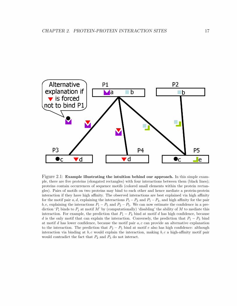
a natural bias towards simplicity. A simple example of this phase is illustrated in
Fig. 2.1; here, the observed interactions are best explained via high affinity for the
motif pair a, d, explaining the interactions P1 − P3 and P1 − P4, and high affinity
for the pair b, e, explaining the interactions P1 − P5 and P2 − P5. By contrast, the
motif pair c, d is not as good an explanation, because the motif pair also appears
in the non-interacting protein pair P3, P5. We note that the motif pair a, c is also a
candidate hypothesis, as it predicts the interactions P1−P3 and P1−P5 and does not
incorrectly predict any other interaction. However, it leaves the interaction P1 − P4
unexplained, therefore leading to a less parsimonious model that also contains the
motif pair a, d.
A set of estimated affinities provides us with a way of predicting, for each pair of
proteins, which motif pair is most likely to have produced the binding. In the second
phase, we use this ability to produce specific hypotheses of the form ‘Motif M on
protein A binds to protein B’. In a naive approach, we can simply take the most
likely set of binding sites for the estimated set of affinity parameters. However, in some
cases, there may be multiple models that are equally consistent with our observed
interaction pattern, but that give rise to different binding predictions. In the second
phase of InSite, we therefore assess the confidence in each binding prediction by
‘disallowing’ the A−B binding at the predicted motif M , re-estimating the affinities,
and computing the overall score of the resulting model (its ability to explain the
observed interactions). The reduction in score relative to our original model is an
estimate of our confidence in the prediction. This phase serves two purposes: it
increases the robustness of our predictions to noise, and also reduces the confidence
in cases where there is an alternative explanation of the interaction using a different
motif. For example, in Fig. 2.1, the prediction that ‘motif d on P4 binds to P1’
has higher confidence, because d is the only motif that can explain the interaction.
Conversely, the prediction that ‘motif d on P3 binds to P1’ has lower confidence,
because the motif pair a, c can provide an alternative explanation to the interaction.
The prediction that ‘motif e on P5 binds to P2’ also has high confidence: although
CHAPTER 2. PROTEIN-PROTEIN INTERACTION SITES 17
Figure 2.1: Example illustrating the intuition behind our approach. In this simple exam-ple, there are five proteins (elongated rectangles) with four interactions between them (black lines);proteins contain occurrences of sequence motifs (colored small elements within the protein rectan-gles). Pairs of motifs on two proteins may bind to each other and hence mediate a protein-proteininteraction if they have high affinity. The observed interactions are best explained via high affinityfor the motif pair a, d, explaining the interactions P1−P3 and P1−P4, and high affinity for the pairb, e, explaining the interactions P1 − P5 and P2 − P5. We can now estimate the confidence in a pre-diction ‘Pi binds to Pj at motif M ’ by (computationally) ‘disabling’ the ability of M to mediate thisinteraction. For example, the prediction that P1 − P4 bind at motif d has high confidence, becaused is the only motif that can explain the interaction. Conversely, the prediction that P1 − P3 bindat motif d has lower confidence, because the motif pair a, c can provide an alternative explanationto the interaction. The prediction that P2 − P5 bind at motif e also has high confidence: althoughinteraction via binding at b, c would explain the interaction, making b, c a high-affinity motif pairwould contradict the fact that P2 and P3 do not interact.
CHAPTER 2. PROTEIN-PROTEIN INTERACTION SITES 18
interaction via binding at b, c would explain the interaction, making b, c a high-affinity
motif pair would contradict the fact that P2 and P3 do not interact.
We provide a formal foundation for this type of intuitive argument within an auto-
mated procedure (Fig. 2.2), based on the principled framework of probability theory
and Bayesian networks [107]. At a high level, the InSite model contains three compo-
nents, which are trained together to optimize a single likelihood objective. The first
component, inspired by the work of Deng et al. [31] and Riley et al. [112], formalizes
the binding model described above, whereby motif pairs have binding affinities, and
an interaction between two protein pairs is induced by binding at some pair of motifs
in their sequence. The second and third components, novel to our approach, formu-
late the evidence models for protein-protein interactions and motif-motif interactions
respectively. They address both the noise in high-throughput assays [83, 130], and in
the case of protein-protein interactions, the fact that many of the relevant assays are
based on affinity purification, which detects protein complexes instead of the pairwise
physical interactions that are the basis for inferring direct binding sites. To integrate
many assays coherently, InSite uses a naive Bayes model [83, 100, 65], where the
assays are a ‘noisy observation’ of an underlying ‘true interaction’.
Our entire model is trained using the expectation maximization (EM) algorithm in
a unified way (see Section 2.4 and Fig. 2.5), to maximize the overall probability of the
observed protein-protein interactions. This type of training differs significantly from
most previous methods that aggregate multiple assays to produce a unified estimate of
protein-protein interactions. These methods [65, 143] generally train the parameters
of the unified model using only a small set of ‘gold positives’, typically obtained from
the MIPS database [96]. This form of training has the disadvantages of training the
parameters on a relatively small set of interactions, and also of potentially biasing
the learned parameters towards the type of interactions that were tested in small-
scale experiments. By contrast, the use of the EM algorithm allows us to train the
model using all of the protein interactions in any data set, increasing the amount of
available data by orders of magnitude, and reducing the potential for bias. The same
EM algorithm also trains the affinity parameters for the different motif pairs, so as
to best explain the observed protein-protein interactions.

CHAPTER 2. PROTEIN-PROTEIN INTERACTION SITES 19
Figure 2.2: Overview of our automated procedure. Our automated procedure (InSite), whichhas two main phases, takes as input protein sequences and multiple evidences on protein-proteininteractions and motif-motif interactions.(a) Motifs, downloaded from Prosite or Pfam database, were generated based on conservation inprotein sequences. Protein-protein interactions are obtained from a variety of assays, including: asmall set of ‘reliable’ interactions, which recurred in multiple experiments or were verified in low-throughput experiments; a set of interactions from yeast two-hybrid assays; and a set of interactionsfrom the co-affinity precipitation assays of Krogan et al. [79] and Gavin et al. [44].(b) The first phase (Fig. 2.4 and Fig. 2.5) uses a Bayesian network to estimate both the motif pairbinding affinities and the parameters governing the evidence models of protein-protein interactionsand motif-motif interactions, where the model is trained to maximize the likelihood of the inputdata. Note that the affinity learned in this phase only depends on the type of motifs, regardless ofwhich protein pair they occur on.(c) In the second phase (Fig. 2.6), we do a protein-specific binding site prediction based on the modellearned in the previous phase. For each protein pair, we compute the confidence score for a motifto be the binding site between them. Note that the confidence scores computed here are proteinspecific and can be different for the same motif depending on the context it appears in.

CHAPTER 2. PROTEIN-PROTEIN INTERACTION SITES 20
These estimated affinities allow us to predict, for each pair of proteins, which
motif pair is most likely to have produced the binding. In the second phase, we use
these predictions, augmented with a procedure aimed at estimating the confidence in
each such prediction, to produce specific hypotheses of the form ‘Motif M on protein
A binds to protein B’. In this phase, InSite modifies the model so as to enforce that
binding between A and B does not occur at motif M . We then compute the loss in
the likelihood of the data, and use it as our estimate of the confidence in the binding
hypothesis.
As an initial validation of the InSite method, we first show that it provides high-
quality predictions of direct physical binding for held-out protein interactions that
were not used in training. These integrated predictions, which utilize both binding
sites and multiple types of protein-protein interaction data, provide high precision and
higher coverage than previous methods. As the primary validation of our approach,
we compare the specific binding site predictions made by InSite to the co-crystallized
protein pairs in the Protein Data Bank (PDB) [13], whose structures are solved and
thus binding sites can be inferred. In our results, 90.0% of the top 50 Pfam-A domains
that are predicted to be binding sites are indeed verified by PDB structures. InSite
significantly out-performs several state-of-the-art methods: In particular, only 82.0%
of the top 50 predictions by Lee et al. [82] and 80.0% of the top 50 predictions by
Riley et al. [112] and of Guimaraes et al. [53] are verified in PDB.
We also examined the functional ramifications of our predictions. If protein A
interacts with protein B via the motif M on A, a mutation at motif M may have
a significant effect on the interaction. If the interaction is critical in some pathway,
this mutation may result in a deleterious phenotype, which may lead to disease [119].
We applied InSite to human protein-protein interaction data, and considered those
predicted binding motifs M that contain a mutation in the OMIM human disease
database [54] or identified as a potential driver mutation in the recent cancer poly-
morphism data [52]. We then investigated the hypothesis that the mutation at M
leads to the disease by disrupting the binding of the protein pair. A literature search
validated many of these disease-related predictions, whereas others are unknown but
provide plausible hypotheses. Therefore, our predictions provide us with significant

CHAPTER 2. PROTEIN-PROTEIN INTERACTION SITES 21
insights into the underlying mechanism of the disease processes, which may help
future study and drug design.
We have made our predictions and our code publicly available for download [1].
Our algorithm is general, and can be applied to any organism, any protein-protein
interaction data set, and any type of motifs or domains.
2.2 Related work
Deng et al. [31] constructed a Bayesian Network that tries to best explain the ob-
served protein-protein interactions by motif-motif interactions. Their simple Bayesian
Network, however, does not take into account indirect evidence. Instead, it only uses
motifs and observed protein-protein interactions, with the goal of better predicting
the interactions, not the interaction sites. Liu et al. [88] used the same Bayesian
Network but incorporated protein-protein interactions from three organisms to gain
better accuracy at predicting protein-protein interactions. Gomez et al. [50] used a
model, in which a motif pair can be repulsive — reducing the interaction probability
of a protein pair containing the motif pair. Again, their goal is to use the protein
sequence information to help better predict protein-protein interactions.
Our approach is most similar to previous work that tries to predict motif-motif or
domain-domain interactions [53, 82, 112, 102]. A key difference between InSite and
previous methods is that InSite makes predictions at the level of individual protein
pairs, in a way that takes into consideration the various alternatives for explaining
the binding between this particular protein pair. By contrast, other methods predict
affinities between motif types; these predictions are independent of the proteins on
which the motifs occur. For example, Guimaraes et al. tries to explain protein-protein
interactions using as fewer motif-motif interactions as possible. They formulate the
problem using linear programming where the variables to be solved are potential
interactions between two motif types. Lee et al. proposed a new measure, the expected
number of interactions between two motif types, and used a Bayesian approach to
integrate it with information on motif pairs such as domain fusion and GO similarity.
Whereas the above methods aim to compute the general affinity between two motif

CHAPTER 2. PROTEIN-PROTEIN INTERACTION SITES 22
types, InSite also explicitly computes the confidence that a specific motif occurrence
mediates the binding of a specific interacting protein pair. It may give the same
motif pair different binding confidences in the context of explaining different protein-
protein interactions. These finer-grained predictions allow us to identify the specific
mechanism for their interaction, whereas other methods that make predictions by only
looking at motif types would not be as appropriate for this purpose. For example,
the DPEA method by Riley et al. [112] also uses a Bayesian Network that tries to
best explain protein-protein interactions by motif-motif interactions. Besides some of
the algorithmic problems, which we will discuss in the Methods section, it treats all
observed protein-protein interactions as gold positives and thus neglects the noises in
those assays. No indirect evidence is integrated either for protein-protein interactions
or for motif-motif interactions.
Most importantly, DPEA computes the confidence score between a pair of motif
types by forcing them to have affinity 0. In contrast, InSite aims to compute predic-
tions for a specific motif occurrence on an interacting protein pair, and thus forces a
particular motif occurrence on a particular protein to be non-binding to another pro-
tein. The more global perturbation used by Riley et al. would not be as appropriate
for this purpose: It may well be the case that a good alternative binding hypothesis
exists for the interaction at a particular protein pair, but disallowing all interactions
between a pair of motif types causes significant reduction to the likelihood in other
protein pairs. Indeed, our method outperforms DPEA, and other state-of-the-art
methods like the parsimony approach by Guimaraes et al. and the integrative ap-
proach by Lee et al., at identifying binding regions between an interacting protein
pair. To our knowledge, InSite is the first method that does protein specific binding
site predictions. This capability allows us to use InSite to understand specific disease-
causing mechanisms that may arise from a mutation that disrupts a protein-protein
interaction.
Some other work [103, 67] infers motif-motif interaction using other types of infor-
mation. Jothi et al. [67] observed that interacting domain pairs for a given interaction
exhibit higher level of co-evolution than the non-interacting domain pairs. Motivated
by this finding, they developed a computational method to test the generality of

CHAPTER 2. PROTEIN-PROTEIN INTERACTION SITES 23
the observed trend, and to predict large-scale domain-domain interactions. Given
a protein-protein interaction, their method predicts the domain pairs that are most
likely to mediate the interaction. They applied the method to yeast and its predic-
tions has been shown to have little overlap with InSite-style methods [67], and thus
can be combined with InSite to gain wider coverage.
InSite also provides a unified framework for integrating evidence from multiple
assays, some of which are noisy and some of which are indirect. Unlike other methods,
our approach uses all available evidence for both protein-protein interactions and
motif-motif interactions, and it does not assume the existence of a large data set of
gold positives.
2.3 Sources of data
We extracted signals from multiple sources of data and integrated them using our
Bayesian Network model.
2.3.1 S. cerevisiae
We constructed a ‘gold standard’ set of S. cerevisiae protein-protein interactions
from MIPS [96] and DIP [134], downloaded on March 21st, 2006. We extracted from
MIPS those physical interactions that are non-high-throughput yeast two-hybrid or
affinity chromatography. For DIP, we picked non-genetic interactions that are derived
from small-scale experiments or verified by multiple experiments. We use this set of
reliable interactions as ‘gold standard’ interactions in our model. For ‘gold standard’
non-interactions, we picked 20,000 random pairs [12] and removed those that appear
in any interaction assays. For these gold standard pairs, we fixed the value of the
‘actual interaction’ variable accordingly. In all other protein pairs, we leave the actual
interaction variables as unobserved.
We constructed ‘observed interaction’ variables for each of the assays, as follows.
For the yeast two-hybrid data sets of Uetz et al. [127] and Ito et al. [63], these variables
are binary-valued. They take the value true if the pair is observed to interact in the

CHAPTER 2. PROTEIN-PROTEIN INTERACTION SITES 24
assay, and the value false if both of the two proteins appeared in the assay but the
pair was not observed to interact. However, as the number of unobserved interactions
grows quadratically in the number of proteins assayed, this procedure would result in
too many non-interacting pairs; we therefore keep only those pairs that appeared in
some other high-throughput data set, to allow evidence integration. For the TAP-MS
assays, we selected the interactions with confidence score above 0.2 from Krogan et
al. [79] and all interactions from Gavin et al. [44], using their confidence scores as
continuous observation values.
This procedure results in a data set of 101,065 protein pairs, of which 4,200 were
gold standard interactions and 18,666 gold standard non-interactions, and a total of
108,924 observations. See Fig. 2.3.
We computed expression correlation using a compendium of time series data ob-
tained in different environmental conditions [139, 95, 20, 81, 106, 43, 42, 32, 70]. The
compendium has 76 different conditions with a total of 403 time points. For each
pair of proteins, we computed the Pearson correlation coefficient across all the time
points. We also annotated our proteins with biological process from GO. For each
pair of proteins, we computed the GO distance as the log size of the smallest com-
mon category shared by the two proteins. The smaller the value, the more specific
category the two proteins belong to, and thus they are more likely to interact [111].
In one run, we used sequence motifs from the Prosite database [38] excluding the
non-specific motifs, mostly post-translational modification motifs that appears across
many proteins. We removed motifs that are annotated as ‘Compositionally biased’
or ‘DNA or RNA associated’. This gives us 708 different types of motifs with a total
of 2,808 motif occurrences. In another run, we used sequence motifs from the Pfam
domain database [11], which results in 8,089 different types of domains with a total
of 11,767 domain occurrences.
We construct a ‘domain fusion’ variable for each pair of Prosite motifs or Pfam
domains. Its value is 1 if the two motifs ever co-occur on the same protein in any
species whose proteins are sequenced and annotated in the motif databases. Its value
is 0 otherwise. Note that we use the term ‘domain fusion’ here although it can also
refer to motifs. We also looked at whether the two motifs appear together in any

CHAPTER 2. PROTEIN-PROTEIN INTERACTION SITES 25
Figure 2.3: Protein-protein interaction assays. A total of 101,065 pairs are used, amongwhich 4,200 are reliable interactions and 18,666 are gold non-interactions (see Methods). Each ofthe remaining pairs is associated with observations from one or more of the four high-throughputassays. The size of the four circles represents the number of pairs in each of the experimental assays.The red slice within each circle represents the overlap with reliable interactions, while the blueslice represents the overlap with gold non-interactions. In Gavin’s and Krogan’s assays, each pair isassociated with a confidence score. In Ito’s and Uetz’s assays, we have either observed interactingpairs (3,938 for Ito and 821 for Uetz) or non-interacting pairs, which are between the proteins usedin the assay but not identified as interacting. The number on the line between two circles is thenumber of pairs that overlap between the two assays, with only positive interactions consideredin the case of the Ito and Uetz assays. Following is a breakdown of the number of pairs in each assay:
Assay Gold PPI Other observed PPI Gold non-PPI Other observed non-PPIGavin 1157 69,140 N.A. N.A.
Krogan 847 6,591 N.A. N.A.Ito 1,542 2,396 7,362 16,343
Uetz 599 222 706 2,019

CHAPTER 2. PROTEIN-PROTEIN INTERACTION SITES 26
biological process category based on the mapping table from Pfam to GO [9]. If they
do, we assign the ‘shared GO’ variable to be 1 and we assign it to be 0 otherwise.
2.3.2 Human
We used a high confidence yeast two-hybrid assay [115] and the Human Protein Refer-
ence Database (HPRD), a resource that contains known protein-protein interactions
manually curated from the literature by expert biologists [108] (downloaded on Jan.
24th, 2006). The union of these data sets gives us 6,688 reliable interactions. We
also used a yeast two-hybrid assay from Stelzl et al. [123] and an assay that iden-
tify co-complex proteins [37] with its confidence score as our observation value. This
gives us 5,723 observations. As in yeast, we picked 20,000 random pairs as our gold
non-interactions [12] and removed those that appear in any interaction assays. We
used the same Prosite motifs, which gives us 687 different types of motifs with a total
of 3,034 motif occurrences.
2.4 Methods
2.4.1 Probabilistic model
Our probabilistic model has three components. The first (Fig. 2.4, black box) for-
malizes the binding model described above: for each protein pair in our model, and
each pair of motifs on the two proteins, we have a variable indicating whether binding
took place at this motif pair. The prior probability that a specific motif pair binds
is the affinity of the corresponding motif types. The overall interaction of the pro-
teins is a disjunction of these binding events, and of an additional ‘spurious binding’
variable that accounts both for noise in some interaction data sets and for binding
outside of motifs in our database. The second component of our model (Fig. 2.4,
red box) addresses the problem that very few protein interactions are known with
certainty. Yeast two-hybrid assays can be noisy [83, 130], with a non-trivial fraction
of both false positives and false negatives, while affinity purification detects protein
complexes instead of the pairwise physical interactions that are the basis for inferring

CHAPTER 2. PROTEIN-PROTEIN INTERACTION SITES 27
direct binding sites. Moreover, indirect evidence such as co-expression, though use-
ful, only weakly correlates with the actual interactions. Therefore, to integrate many
assays coherently, we use a naive Bayes model [83, 100, 65]. In this model, we have an
‘Interaction variable’ for each protein pair, whose value is ‘true’ only when the pair
actually interacts. This variable is unobserved in most cases, but serves to aggregate
information from a set of partial and noisy assays, which are viewed as ‘noisy sensors’
for the interaction variable. The quantitative dependencies of these sensors are mod-
eled differently for different assays, to allow for variations in false positive and false
negative rate [130, 86], and for confidence scores accompanying certain assays [44, 79].
The parametric families of the dependency relationships are picked by examining the
data and their parameters are fitted when the model is learned. There may be mul-
tiple observation variables attached to a protein pair, whose interaction probability
summarizes the signal from all the assays and is used to learn the binding affinity.
The third component of our model (Fig. 2.4, blue box) takes into consideration the
noisy evidence on motif-motif interactions. A binding variable between two motifs
may have multiple evidences, all of which serve as noisy sensors for the binding vari-
able and are integrated using a naive Bayes model in the same way as in the second
component. Note parameters of the evidence models for motif-motif interactions are
all also learned from the data. Some of the learned values are illustrated in Fig. 2.4.
More formally, each interacting or non-interacting pair of proteins Pi, Pj is de-
scribed by an entity Tij. A pair of motifs in two proteins can potentially bind and
induce an interaction between the corresponding proteins. We encode this assump-
tion by introducing a variable Tij.Bab for each pair of motifs a in Pi and b in Pj, which
represents whether the pair of motif occurrences actually binds. The probability that
they bind depends on the affinity between the motifs. Therefore, we define:
P (Tij.Bab = true) = θab
and
P (Tij.Bab = false) = 1− θab

CHAPTER 2. PROTEIN-PROTEIN INTERACTION SITES 28
Figure 2.4: Our Bayesian Network model. The first phase of InSite, shown here, uses aBayesian network to estimate the affinities between motif pairs and evidence models for protein-protein interactions and motif-motif interactions. The Bayesian network is trained so as to maximizethe likelihood of the observed protein-protein interaction and motif-motif interaction pattern. Anillustrative fragment of the Bayesian network, for the protein pair P1−P3 of Fig. 2.1, is shown insidethe box. The variable B represents the actual binding of a protein pair at a particular motif pair,which is never observed, but is shown to correlate with information such as domain fusion and GeneOntology. We use them as noisy indicators (E), which take binary values — whether two motifs everappear in the same protein and whether they share the same GO biological process category. Thevariable S represents ‘spurious’ binding, which occurs at a region not represented in our set of motifpairs. An actual interaction between the proteins, represented by the variable I, occurs whenever anytype of binding occurs. Importantly, not all of the data represent high-reliability physical bindingbetween protein pairs: some data sets could be noisy, and the affinity precipitation assays captureentire complexes. We therefore assign the variable I the value true in the training data only if theprotein pair is a high-reliability physical interaction and assign the value false if it is among therandomly picked 20,000 pairs. If the pair occurs in high-throughput assays or has some indirectevidence, it is treated as a noisy indicator (O). For the binary interaction assays, this indicatoris a binary-valued variable; the protein-complex assays of Gavin and Krogan are associated with anumerical score, and are treated as continuous-valued indicators, whose parametric form was derivedby examining the data. Indirect evidence such as expression correlation and Gene Ontology, which isshown to correlate with protein-protein interaction, are also used as noisy indicators. Arrows in theBayesian network represents the variable downstream is probabilistically dependent on its parentvariable. The observed variables are colored in orange and stripes are used for partially observedvariables. Both the motif binding affinities and the parameters governing the evidence models arelearned together using the expectation maximization algorithm, to maximize the likelihood of theobserved data. Some examples of the evidence models learned are shown in the call-out boxes.

CHAPTER 2. PROTEIN-PROTEIN INTERACTION SITES 29
where θab is the affinity between motifs a and b. Note that this affinity is a feature of
the motif pair and does not depend on the proteins in which they appear. We place
a Dirichlet prior distribution over the value of θab, which is the same for θ across
all motif pairs. We must also account for interactions that are not explained by our
set of motifs, such as the binding between amino acids not included in our motif
set. Thus, we add a spurious binding variable Tij.S. The probability that spurious
binding occurs is given by:
P (Tij.S = true) = θs(m) = 1− (1− θs)m
where m is proportional to the average (geometrical) number of amino acids not
covered by any motif in the two proteins. It represents the fact that the more amino
acids we have outside the motif set, the more likely the interaction is induced by
something other than binding between motifs. Two proteins interact if and only if
some form of binding occurs, whether by a motif pair or by spurious binding. Thus, we
define a variable Tij.I, which represents whether protein Pi interacts with protein Pj,
to be a deterministic OR of all the binding variables Tij.S and Tij.Bab. We note that
Riley et al. [112] did not include a spurious interaction variable in their model, but
rather used 0.001, regardless of the protein length, as the probability of interaction
when there is no motif pair between two proteins.
To account for the fact that our experimental assays are not direct and reliable
measurements of physical protein-protein interactions, we define the observation vari-
ables Tij.O to be the interactions observed in the experimental assays and indirect
evidence like co-expression and GO distance, which are noisy sensors for the actual
interaction variable Tij.I. Note that an actual interaction variable may have several
observation variables if the pair appears in multiple assays. For those assays with bi-
nary observations, Tij.On is a binary variable and the probability it is true depends on
Tij.I and the type of assay. Therefore, we can account for the different false positive
and false negative rates in different assays. For Gavin et al. [44], we assume her con-
fidence score Tij.Og to be Gaussian distributions, whose mean and variance depends
on the Tij.I. For Krogan et al., we assume the confidence score Tij.Ok has a uniform

CHAPTER 2. PROTEIN-PROTEIN INTERACTION SITES 30
distribution if Tij.I is false (non-interacting) and has an exponential distribution
if Tij.I is true (interacting). For co-expression, we assume the Pearson correlation
coefficient Tij.Oe to have a Gaussian distribution, whose mean and variance depends
on the Tij.I. For GO distance, we assume its value Tij.Oo to be an exponential distri-
bution when Tij.I is false and a mixture of Gaussian and uniform distribution when
Tij.I is true (interacting). In the case of human confidence score Tij.Ow from Ewing
et al., we use a mixture of Gaussian and indicator functions with different parameters
depending on the value of Tij.I.
We use Rab to describe a pair of motif a and motif b. We introduce a variable
Rab.Eg to represent whether they share the same GO biological process category and
another variable Rab.Ef for whether they appear together in a domain fusion event.
Both variables are probabilistically dependent on the binding variable Tij.Bab and
serve as its noisy sensors. Note that Rab is the same regardless which protein pair Tij
it appears in. We use different models for domain fusion and GO distance to account
for their different correlation with the actual motif-motif interactions.
An instantiation of our probabilistic model is illustrated in Fig. 2.4 and the con-
ditional probabilities involved are summarized below:

CHAPTER 2. PROTEIN-PROTEIN INTERACTION SITES 31
P (θab = x) = P (θs = x)
=1
B(α, β)xα−1(1− x)β−1
P (Tij.Bab = true|θab = x) = x
P (Tij.S = true|θs = x) = θs(m)
= 1− (1− x)m
Tij.I = OR(Tij.B, Tij.S)
P (Tij.On|Tij.I) = ρn(Tij.I)
P (Tij.Og|Tij.I = false) = N(µg0, σ2g0)
P (Tij.Og|Tij.I = true) = N(µg1, σ2g1)
P (Tij.Ok|Tij.I = false) = 1
P (Tij.Ok|Tij.I = true) = λk exp(−λk(1− Tij.Ok))
P (Tij.Oe|Tij.I = false) = N(µe0, σ2e0)
P (Tij.Oe|Tij.I = true) = N(µe1, σ2e1)
P (Tij.Oo|Tij.I = false) = λ0 exp(−λ0(8.68− Tij.Oo))
P (Tij.Oo|Tij.I = true) = wo1N(µo1, σ2o1) + wo2U(7, 8.68)
P (Tij.Ow|Tij.I = false) = ww1N(µw0, σ2w0) + ww2I(Tij.Ow = 0)
+ww3I(Tij.Ow = NA)
P (Tij.Ow|Tij.I = true) = ww4N(µw1, σ2w1) + ww5I(Tij.Ow = 0)
+ww6I(Tij.Ow = NA)
P (Tij.O|Tij.I) =∏
Tij .O∈Tij .O
P (Tij.O|Tij.I)
P (Rab.Eg|Tij.Bab) = ρg(Tij.Bab)
P (Rab.Ef |Tij.Bab) = ρf (Tij.Bab)
P (Tij.E|Tij.Bab) = P (Rab.Eg|Tij.Bab)P (Rab.Ef |Tij.Bab)
where α, β are the hyper-parameters in the Dirichlet distribution, which encodes our

CHAPTER 2. PROTEIN-PROTEIN INTERACTION SITES 32
prior belief about the evidence model before seeing any data, 8.68 is the maximum
value of the GO distance, ρ represents binary functions. n enumerates the different
type of yeast two-hybrid assays, Og is Gavin et al.’s assay, Ok is Krogan et al.’s
assay, Oe is co-expression, Oo is GO distance, Ow is Ewing’s confidence score, Eg is
shared GO motif function, Ef is domain fusion, U() is uniform distribution, and I()
is indicator function. The observation parameter vector η is the union of ρ, µ, σ, w,
λ.
2.4.2 Learning
The model defines a joint probability over the entire set of attributes, which is the
product of all local conditional probability models shown above. Our learning ob-
jective is to find affinities between motifs θ, probability of spurious binding θs, and
the parameters for the observation models η, which maximize the probability over
observed evidence on protein-protein interactions T.O, the partial assignment to the
actual interactions T.I, and the observed evidence on motif-motif interactions R.E.
Our algorithm uses an iterative procedure based on the Expectation-Maximization
(EM) algorithm [30] to find the local maximum. In the E-step, we compute the con-
ditional probabilities for the binding variables T.B, T.S, and the actual interaction
variables T.I, given θ, θs, η, T.O, R.E, and use those as the soft assignments to the
variables. Define:
P (Tij.Bab = true|Rab.E) = θ′ab =θabP (Rab.E|Tij.Bab = true)
P (Rab.E)
to be the binding probability given the evidences on motif-motif interactions, where:
P (Rab.E) = P (Tij.Bab = true)P (Rab.E|Tij.Bab = true)
+(1− P (Tij.Bab = true))P (Rab.E|Tij.Bab = false)
By Bayes’ rule, we have:

CHAPTER 2. PROTEIN-PROTEIN INTERACTION SITES 33
P (Tij.Bab = true|T.O; θ, η) =θ′abP (Tij.O|Tij.I = true)
P (Tij.O)
P (Tij.S = true|T.O; θ, η) =θs(m)P (Tij.O|Tij.I = true)
P (Tij.O = true)
P (Tij.I = true|T.O; θ, η) =P (Tij.I = true)P (Tij.O|Tij.I = true)
P (Tij.O)
where
P (Tij.I = true) = 1− (1− θs(m))∏
Tij .Bab∈Tij .B
(1− θ′ab)
P (Tij.O) = P (Tij.I = true)P (Tij.O|Tij.I = true)
+(1− P (Tij.I = true))P (Tij.O|Tij.I = false)
In the M-step, we compute relevant expected sufficient statistics using the com-
puted soft marginal probabilities as soft assignments. We use maximum a posteriori
(MAP) inference to re-estimate the parameters θ, θs, η. This step can be executed
efficiently in closed form, using standard methods, for the parameters θ, η. To esti-
mate θs, we need to decompose it into m variables and apply EM to this approximate
form. In detail, the probability that a spurious binding occurs between a protein pair
is given by:
P (Tij.S = true) = θs(Tij.m) = 1− (1− θs)Tij .m
where Tij.m is proportional to the average (geometrical) number of amino acids not
covered by any motif in the two proteins. This is equivalent to having m variables
Tij.sk, k = 1, . . . ,m, each of which has probability θs of being true, and Tij.S is the
deterministic OR of these m variables.
To learn θs, in E-step, we compute the posterior marginal probabilities for Tij.sk:

CHAPTER 2. PROTEIN-PROTEIN INTERACTION SITES 34
Figure 2.5: Schematic illustration of our EM-based learning algorithm. It estimates themotif affinities (θ) and parameters in the evidence model (η) based on the InSite model illustratedin Fig. 2.4.

CHAPTER 2. PROTEIN-PROTEIN INTERACTION SITES 35
P (Tij.sk = true|T.O; θ, η) =θsP (Tij.O|Tij.I = true)
P (Tij.O = true)
In M-step, we re-estimate θs by:
θs =
∑i,j
∑Tij .mk=1 P (Tij.sk = true|T.O; θ, η)∑
i,j Tij.m
Note that we would not have a closed-form solution if we do not decompose Tij.S
into Tij.sk and instead try to re-estimate θs directly from:
P (Tij.S = true|T.O; θ, η) =θs(Tij.m)P (Tij.O|Tij.I = true)
P (Tij.O = true)
We repeat the E-step and M-step until the change of likelihood is less than a
threshold. Since, in the next phase, we force each motif-protein pair to be non-binding
and compare the change of likelihood Liaj, we have to makes sure the threshold used
here for convergence is at least a magnitude smaller than Liaj, so the noise would
not overwhelm the signal. Here we set the threshold to be 0.01 in terms of change
of log-likelihood. Note that DPEA of Riley et al. [112] used the change in expected
log-likelihood to test for convergence. This does not optimize the joint likelihood,
which may not always increase over the EM steps. On the other hand, InSite used
joint likelihood, which is the measure we try to optimize and is guaranteed to increase
after each EM iteration.
To estimate the two hyper-parameters, α, β of the Dirichlet distribution, we used
two-fold cross-validation on the PDB data set. In this regime, we select the hyper-
parameters so as to optimize performance on one PDB fold, and evaluate performance
on the other fold; thus, no data in the test set was used to estimate any of the
parameters or hyper-parameters in the model.
2.4.3 Binding confidence estimation
Since we explicitly model the binding events between a pair of motifs and between
amino acid pairs outside the motif set, it gives us a way to compute the confidence that

CHAPTER 2. PROTEIN-PROTEIN INTERACTION SITES 36
a motif on a protein binds to another protein. Here the intuition is that if a motif is
non-binding for a particular interaction, it is dispensable from the model. We first run
our model until convergence. To predict whether motif a on protein i is the binding
site to protein j, we force a not to bind with any motif on protein j (Fig. 2.6). We
rerun our algorithm with the above constraint and use the change in likelihood as the
confidence score of our prediction, which we denote to be Liaj. A high score indicates
that forcing a not to be the binding site for proteins i and j induces a big change
in likelihood and is unfavorable. A low score suggests the binding site is dispensable
from the model with competing hypotheses that can explain the observed interactions,
and thus the prediction is questionable. Unlike the motif affinities θab learned from
the previous step, here our confidence score Liaj depends on both proteins i and j
and is different for different proteins.
Note Riley et al. force a pair of motif types to have affinity 0 and thus, unlike
us, their prediction is not specific to each individual protein pair. Also, their change
of likelihood is computed only based on the interacting protein pairs while throwing
away information that can be gained from non-interacting pairs. In contrast, InSite
uses the likelihood of the entire model, which forces us to explain both interactions
and non-interactions.
2.4.4 Model initialization
If a motif pair does not appear between any pair of interacting proteins, we set its
affinity to be 0, an assignment guaranteed to maximize the joint likelihood; this helps
simplify our model structure. We set the initial affinity for the remaining motif pairs
based on the frequency they appear between interacting protein pairs [121]. The
observation parameters η for the evidence models are initialized based on empirical
counts for the ‘gold standard’ interactions and non-interactions.
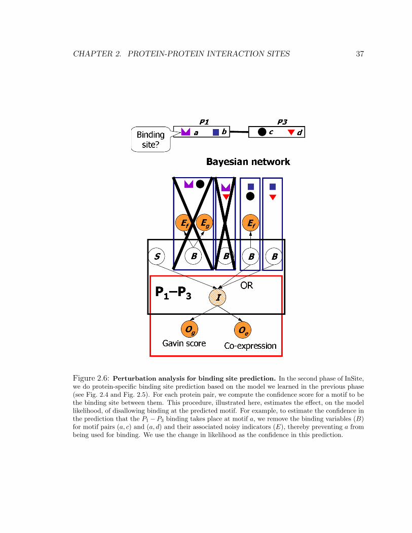
CHAPTER 2. PROTEIN-PROTEIN INTERACTION SITES 37
Figure 2.6: Perturbation analysis for binding site prediction. In the second phase of InSite,we do protein-specific binding site prediction based on the model we learned in the previous phase(see Fig. 2.4 and Fig. 2.5). For each protein pair, we compute the confidence score for a motif to bethe binding site between them. This procedure, illustrated here, estimates the effect, on the modellikelihood, of disallowing binding at the predicted motif. For example, to estimate the confidence inthe prediction that the P1−P3 binding takes place at motif a, we remove the binding variables (B)for motif pairs (a, c) and (a, d) and their associated noisy indicators (E), thereby preventing a frombeing used for binding. We use the change in likelihood as the confidence in this prediction.

CHAPTER 2. PROTEIN-PROTEIN INTERACTION SITES 38
2.5 Results
2.5.1 Overview
We applied InSite to data from both S. cerevisiae and human. For S. cerevisiae, we
compiled 4,200 reliable protein-protein interactions as our gold standard and 108,924
observations of pairwise protein-protein interactions from high-throughput yeast two-
hybrid assays of Ito and Uetz [63, 127] and assays of Gavin and Krogan that iden-
tify complexes [44, 79]. We also computed expression correlation and GO distance
between every pair of proteins, data which have been shown to be useful in predict-
ing protein-protein interactions [111]. Altogether, these measurements involve 4,669
proteins and 82,399 protein pairs. We also constructed a set of fairly reliable non-
interactions as our gold standard by selecting 20,000 random protein pairs [12], and
eliminating those pairs that appeared in any interaction assay. In the case of human,
we used two sets of training data for our analysis. First, we focused on high-confidence
pairwise interactions, all of which were modeled as gold positive interactions. These
interactions were obtained both from high-quality yeast two-hybrid assays [115] and
from the Human Protein Reference Database (HPRD), a resource that contains pub-
lished protein-protein interactions, manually curated from the literature [108]. In
the second case, we additionally incorporated into our evidence model the yeast two-
hybrid interactions from Stelzl et al. [123] and the assay from Ewing et al. [37] that
identifies complexes. Overall, we obtained 12,411 protein interactions involving 2,926
proteins, and selected 18,745 random pairs as our gold non-interactions, as for yeast.
The InSite method can be applied to any set of sequence motifs. Different sets
offer different trade-offs in terms of coverage of binding sites; we can estimate this
coverage by comparing residues covered by a particular set of motifs to residues found
to be binding sites in some interaction in PDB, One option is Prosite motifs [38],
where we excluded non-specific motifs, such as those involved in post-translational
modification, which are short and match many proteins. These motifs cover 9.6% of
all residues in the protein sequences in our data set (Fig. 2.7(a)). Of residues that are
found to be binding sites in PDB, 37.8% are covered by these Prosite motifs. This
enrichment is significant, but many actual binding motifs are omitted in this analysis.

CHAPTER 2. PROTEIN-PROTEIN INTERACTION SITES 39
Figure 2.7: Motif coverage of protein sequences and binding sites. Motif (domain) coverageof protein sequences compared with coverage of the protein-protein interaction binding sites in yeast.The outer circle represents all residues in all 4,669 protein sequences we used in our data set andthe light blue is the portion that is covered by our motifs (domains). The inner circle representsresidues that are identified to be binding sites in PDB. It only includes the 268 proteins in our dataset that are crystallized in PDB and thus whose binding sites we can infer. The dark blue is theportion that is covered by our motifs (domains).(a) Prosite motifs. 9.6% of the residues in our data set are covered by Prosite motifs, 37.8% of thebinding residues in PDB-included proteins are covered by Prosite.(b) Pfam domains. 73.9% of the residues in our data set are covered by Pfam domains, 70.9% ofthe binding residues in PDB-included proteins are covered by Pfam.(c) Pfam-A domains. 38.1% of the residues in our data set are covered by Pfam-A domains, 70.3%of the binding residues in PDB-included proteins are covered by Pfam-A.

CHAPTER 2. PROTEIN-PROTEIN INTERACTION SITES 40
An alternative option is to use Pfam domains [11], which cover 73.9% of all the
residues; however, PDB binding sites are not enriched in Pfam (Fig. 2.7(b)). Pfam-A
domains (Fig. 2.7(c)), which are accurate, human crafted multiple alignments, appear
to provide a better compromise: Pfam-A domains contain only 38.1% of the residues
in our dataset, but cover 70.3% of the PDB binding sites. One regime that seems
to work best, which is also used by Riley et al., is to train on all Pfam domains
(providing a larger training set) and to evaluate the predictions only on the more
reliable Pfam-A domains. For each motif set, we used evidence from domain fusion
and whether two motifs share common GO category as noisy indicators for motif-motif
interactions [35, 92].
We experimented with different data sets and different motif sets. In each case,
we trained our algorithm on these data; then, for each interacting protein pair, we
compute the binding confidences for all their motifs, and generate a set of binding
site predictions, which we rank in order of the computed confidence.
2.5.2 Predicting physical interactions
The actual protein-protein interactions are mostly unobserved in our probabilistic
model. However, we can compute the probability of interaction between two proteins
based on our learned model, which integrates evidences on protein-protein interac-
tions and motif-motif interactions as well as the motif composition of the proteins.
As a preliminary validation, we first evaluate if InSite is able to identify direct phys-
ical interactions. We compare our results to those obtained by using the confidence
scores computed by Gavin and Krogan, which are derived from their TAP-MS assays
and quantify the propensity of proteins to be in the same complex. Using standard
ten-fold cross-validation, we divide our gold interactions and high-throughput inter-
actions into ten sets; for each of ten trials, we hide one set and train on the remaining
nine sets together with our gold non-interactions. We then compute the probability of
physical interaction for each protein pair in the hidden set, and rank them according
to their predicted interaction probabilities. We define a predicted interaction to be
true only if it appears in our gold interactions, and false if it appears only in the
CHAPTER 2. PROTEIN-PROTEIN INTERACTION SITES 41
high-throughput interactions; we then count the number of true and false predictions
in the top pairs, for different thresholds. Although this evaluation may miss some
true physical interactions that appear in the high-throughput data set but not in our
gold set, it provides an unbiased estimate of our ability to identify direct physical
interactions. We separately perform this procedure by ranking the interactions ac-
cording to the scores computed by Gavin and by Krogan. We also compared with a
method that combines all evidences on protein-protein interactions in a naive Bayes
model where motifs are not used.
Our results (Fig. 2.8(a)) show that InSite is better able to identify direct physical
interactions within the top pairs. The area under the ROC curve are 0.855 and 0.916
for Prosite and Pfam respectively, while it is 0.806 for the naive Bayes model, which
integrates different evidences on protein-protein interactions without using any motifs.
This shows the motif based formulation is better able to provide higher rankings
to the reliable direct interactions (Fig. 2.8(a)). When comparing with Gavin’s and
Krogan’s scores, our model covers more positive interactions because it integrates
multiple assays. However, even if we restrict only to pairs appearing in a single assay,
such as Gavin’s or Krogan’s, InSite (Fig. 2.8(b,c)) is able to achieve better accuracy
with either Prosite or Pfam. These results illustrate the power of using both an
integrated data set and the information present in the sequence motifs in reliably
predicting protein-protein interactions. A list of all protein pairs ranked by their
interaction probabilities estimated by training on the full data set is available from
our website [1].
2.5.3 Predicting binding sites
The key feature of InSite is its ability to predict not only that two proteins interact
directly, but also the specific region at which they interact. As an example, we
considered the RNA polymerase II (Pol II) complex, which is responsible for all mRNA
synthesis in eukaryotes. Its 3-D structure is solved at 2.8A resolution [27], so that
its internal structure is well-characterized (Fig. 2.9(a,b)), allowing for a comparison
of our predictions to the actual binding sites. When using Pfam-A domains, the

CHAPTER 2. PROTEIN-PROTEIN INTERACTION SITES 42
Figure 2.8: Verification of protein-protein interaction predictions. Verification of protein-protein interaction predictions relative to reliable interactions. Protein pairs in the hidden set in aten-fold cross validation are ranked based on their predicted interaction probabilities (green, red,and black curves for Prosite, Pfam, and naive Bayes respectively). Each point corresponds to adifferent threshold, giving rise to a different number of predicted interactions. The value on theX-axis is the number of pairs not in the reliable interactions but predicted to interact. The value onthe Y-axis is the number of reliable interactions that are predicted to interact. The blue and browncurves (as relevant) are for pairs ranked by Gavin’s and Krogan’s scores respectively.(a) Predictions for all protein pairs in our data set. As we can see, InSite with Pfam is better thanInSite with Prosite, which is in turn better than the naive Bayes model. All those three modelsintegrate multiple data sets and thus have higher coverage than other methods using a single assayalone. The cross and circle are the accuracies for interacting pairs based on Ito’s and Uetz’s Y2Hassays respectively.(b) Predictions only for pairs in Gavin’s assay, providing a direct comparison of our predicted prob-ability with Gavin’s confidence score on the same set of protein pairs. The InSite model outperformsthe Gavin’s score.(c) Predictions only for pairs in Krogan’s assay, providing a direct comparison of our predictedprobability with Krogan’s confidence score on the same set of protein pairs. Our InSite modeloutperforms the Krogan’s score.

CHAPTER 2. PROTEIN-PROTEIN INTERACTION SITES 43
complex gives rise to 123 potential binding site predictions: one for each direct protein
interaction in the complex and each motif on each of the two proteins. Among the
123 potential predictions, 68 (55.3%) are actually binding according to the solved 3-D
structure. We rank these 123 potential predictions based on our computed binding
confidences. All of the top 26 predictions are actually binding (Fig. 2.9(d)). As one
detailed example (Fig. 2.9(c)), Rpb10 interacts with Rpb2 and Rpb3 through its motif
PF01194. We correctly predicted this motif as the binding site for the two proteins
(ranked 3rd and 4th). On the other hand, there are 9 motifs on the two partner
proteins that could be the possible binding sites to Rpb10. Among them, 4 are
actually binding, and were all ranked among the top half of the total 123 predictions,
while the other 5 non-binding motifs were ranked below 100th with low confidence
score. Overall, the 6 binding sites in this example all have higher confidence scores
than the 5 non-binding sites.
We performed this type of binding site evaluation for all of the co-crystallized
protein pairs in PDB that also appeared in our set of gold interactions. We extracted
structures from PDB that have at least two co-crystallized chains, and whose chains
are nearly identical to S. cerevisiae proteins. We define two residues to be in contact
if the closest distance between their two respective heavy atoms is less than 5A. This
definition is similar to that of Koike and Takagi [73]. A motif is said to bind to a
protein if they contain a residue pair that is in contact.
While the PDB data is scarce, it provides the ultimate evaluation of our predic-
tions. We applied our method separately in two regimes. In the first, we train on
Prosite motifs and evaluate on those motifs that cover less than half of the protein
length (Fig. 2.10(a)); we pruned the motif set in this way because short motifs pro-
vide us with more information about the binding site location. In the second regime,
we followed the protocol of Riley et al., and trained on Pfam domains and evaluated
PDB binding sites on the more reliable Pfam-A domains; we also tried to both train
and evaluate on Pfam-A domains but the result is worse in comparison to training
on all Pfam domains (data not shown).
Overall, the PDB co-crystallized structures contain 96 potential binding sites cov-
ered by Prosite motifs, of which 50 (52.1%) are verified as actually binding, and the

CHAPTER 2. PROTEIN-PROTEIN INTERACTION SITES 44
Figure 2.9: Binding site predictions within the RNA Polymerase II complex.(a) A schematic illustration of interactions within the RNA Polymerase II complex revealed by its3-D structure. Each circle with number k corresponds to the protein ‘Rpbk’ (e.g., Rpb1).(b) One of our top predictions is ‘Pfam-A domain PF01096 on Rpb9 binds to Rpb1’. Both Rpb9and Rpb1 are part of the co-crystallized RNA Polymerase II complex in PDB (1I50). Rpb9 is shownas the light green chain with the surface accessible area of the domain rendered in white; Rpb1is shown as the light orange chain with its residues that are in contact with the domain shown inorange, which verifies our prediction.(c) Binding site predictions for interactions involving Rpb10. A red arrow connects a motif to aprotein it binds to as revealed by its 3-D structure. A dashed black arrow represents a non-bindingsite. The numbers on the arrow are the ranks based on our predicted binding confidences. Weassigned confidence values to a total of 123 motif-protein pairs in this complex. In this case, all sixPDB verified binding sites (red arrows) are ranked among the top half, while all five non-bindingsites have low confidence values with ranks below 100.(d) ROC curve for our motif-protein binding sites predictions within the RNA Polymerase II complex.There are 123 possible binding sites within the complex that involves the Pfam-A domains in ourdata set, out of which 68 (55.3%) are actually binding according to its 3-D structure. The possiblebinding sites are ranked by our predicted binding confidences. The X-axis is the number of non-binding sites within the complex that are predicted to be binding. The Y-axis is the number of PDBverified binding sites that are also predicted to be binding. The purple line is what we expect bychance.

CHAPTER 2. PROTEIN-PROTEIN INTERACTION SITES 45
Figure 2.10: Distribution of motif coverage.(a) For each motif occurrence, we compute its coverage as the ratio of its length to the length ofthe protein it occurs on. The x-axis is the bin for the coverage. The y-axis is the number of motifoccurrences that fall into this coverage bin. As we can see, most of Prosite motifs cover a smallfraction of the protein while Pfam-A domains are usually longer.(b) For each protein, we compute the fraction of its length that is covered by motif in our data set.The x-axis is the bin for the fraction. The y-axis is the number of proteins that fall into this bin. Weexclude those proteins that are not covered by any motif. As we can see, if we use Prosite motifs,most proteins will have majority of their residues not covered by any motif.

CHAPTER 2. PROTEIN-PROTEIN INTERACTION SITES 46
Figure 2.11: Global verification of binding site predictions. Verification of motif-proteinbinding site predictions relative to solved PDB structures. Possible binding sites are ranked basedon our predicted binding confidences. The X-axis is the number of sites that are non-binding inPDB that are predicted to be binding. The Y-axis is the number of PDB verified binding sitesthat are also predicted to be binding. The green and red curve are for our InSite with Prosite andPfam respectively, which is tailored to binding site prediction and explicitly models the noise in thedifferent experimental assays. The brown curve is for the DPEA score as in Riley et al.. The graycurve is for the score derived from the parsimony approach of Guimaraes et al.. The black curveis for the integrative approach by Lee et al.. The purple curve is what we expect from randompredictions.(a) Result using Prosite motifs. The area under the curve if we normalize both axes to interval [0,1]are 0.680, 0.601, 0.5 for InSite, DPEA by Riley et al., and random prediction respectively.(b) Result when we train on Pfam domains and evaluate the PDB binding sites only on Pfam-Adomains, as in the protocol of Riley et al.. The area under the curve if we normalize both axes tointerval [0,1] are 0.786, 0.745, 0.619, 0.620 for InSite, integrative approach by Lee et al., DPEA byRiley et al., and parsimony approach by Guimaraes et al. respectively.
remaining 46 are verified to be non-binding. Similarly, PDB contained 317 possible
bindings between a Pfam-A domain and a protein, of which 167 (52.7%) are verified
in PDB. We ranked all possible bindings according to their predicted binding confi-
dences. With Prosite motifs (Fig. 2.11(a)), the area under ROC curve (AUC) is 0.68;
note that random predictions are expected to have AUC of 0.5. For Pfam-A, when
trained on all Pfam domains, we achieved an AUC of 0.786 (Fig. 2.11(b)).
We compared our results to those obtained by the DPEA method of Riley et
al. [112], the parsimony approach of Guimaraes et al. [53], and an integrated ap-
proach of Lee et al. [82]. DPEA computes confidence scores between two motif types

CHAPTER 2. PROTEIN-PROTEIN INTERACTION SITES 47
by forcing them to be nonbinding, and computing the change of likelihood after
re-converging the model with this change. InSite differs from DPEA in two main
characteristics: its confidence evaluation method, which is designed to evaluate the
likelihood of binding between two particular proteins at a particular site; and the in-
tegration of multiple sources of noisy data. Guimaraes et al. use linear programming
to find the confidence scores to a most parsimonious set of motif pairs that explains
the protein-protein interactions. Lee et al. use the expected of number of motif-motif
interactions for a pair of Pfam-A domain types across four species, and integrate them
with GO annotation and domain fusion to generate a final ranking on pairs of motif
types.
All of these methods generate confidence scores on pairs of motif types, regardless
of what protein pairs they occur on. To use these predictions for the task of estimating
specific binding regions, we define the confidence that motif M on Protein A binds
to Protein B as the maximum confidence score between motif type M and all the
motif types that appear on protein B. For Guimaraes et al. and Lee et al., only the
confidence scores between Pfam-A domains are available so we only compared their
results with our Pfam-A predictions. We re-implemented DPEA and compared with
both our Prosite and Pfam-A predictions. As we can see, in both Prosite and Pfam
evaluations (Fig. 2.11), the AUC obtained by InSite are the highest (0.786 and 0.680
for Pfam and Prosite respectively) while Lee et al. (0.745 for Pfam only) comes second
(Kolmogorov-Smirnov p-value < 0.0002). InSite is able to reduce the error rate (1 -
AUC) by 16.2% compared with Lee et al.. For Pfam, the AUC values are 0.619 and
0.620 for Riley et al. and Guimaraes et al. respectively. For Prosite, the AUC value
for Riley et al. is 0.601. Compared to these two methods, InSite achieves a significant
error reduction of 43.7% and 19.8% for Pfam and Prosite respectively.
If we consider the top 50 predictions made by InSite, 33 (66.0%) are correct
for Prosite and 45 (90.0%) are correct for Pfam-A. In comparison, only 52.1% and
52.7% are expected to be correct using random predictions for Prosite and Pfam-A,
respectively. The enrichment of known binding sites in our top predictions indicates
that InSite is able to distinguish actual binding sites from non-binding sites. In
comparison, the proportion of top 50 predictions verified are 82.0% (Pfam-A) for Lee

CHAPTER 2. PROTEIN-PROTEIN INTERACTION SITES 48
Figure 2.12: Number of motif pair occurrences.(a) Same pair of motif types may occur between multiple pairs of proteins. Here the x-axis is thenumber of protein pairs, n. The y-axis is the number of Prosite motif pairs that occur betweenexactly n pairs of proteins in our data set.(b) Same as (a), except this is for Pfam-A domains.
et al., 80.0% (Pfam-A) for Guimaraes et al., and 80.0% (Pfam-A) and 58.9% (Prosite)
for Riley et al.. Note that, in the case of Pfam-A, Riley et al. predicted all top 24 pairs
correctly because they are derived from the binding of PF00227 (Proteasome) with
itself. This motif pair has the highest score and it appears in 24 binding events, all
of which are correctly verified by PDB. The lack of granularity (i.e. pairs mediated
by the same motif types have the same score) in Riley et al. helped in those top
predictions, but hurt it in the remaining predictions, thus resulting in overall lower
performance.

CHAPTER 2. PROTEIN-PROTEIN INTERACTION SITES 49
More generally, a pair of motif types may have multiple occurrences over differ-
ent protein pairs (Fig. 2.12). The previous methods [53, 82, 112] assign the same
confidence score to all of them. In order to demonstrate that InSite is able to make
different predictions even when both motifs involved are the same, we ran InSite by
forcing a pair of motif occurrences between two proteins to be non-binding and use its
change of likelihood as how confident we are about whether these two motifs bind to
each other. As an example, transcription factor S-II (PF01096) and RNA polymerase
Rpb1 domain 4 (PF05000) are predicted to be more likely to bind when occurring
between Rpb9 and Rpo31 than when occurring between Dst1 and Rpo21. This hap-
pens because there are fewer motifs on Rpb9 than on Dst1 and the motifs on Rpo31
is a subset of motifs on Rpo21. Although some alternative motif pairs between Rpb9
and Rpo31 have high affinity, overall they provide fewer alternative binding sites than
those between Dst1 and Rpo21. Furthermore, Rpb9 and Rpo31 are more likely to
interact than Dst1 and Rpo21. Therefore our final confidence score combines the
affinity between the two motifs, the presence of other motifs on the proteins, and the
interaction probability between the two proteins. Indeed, PDB verifies PF01096 and
PF05000 to bind between Rpb9 and Rpo31, but not between Dst1 and Rpo21. The
same reasoning applies to binding site predictions between a motif and a protein.
2.5.4 Understanding disease-causing mutations in human
While a systematic validation is not possible in human, due to the very low cover-
age of known protein-protein interactions or binding sites, we performed an anecdotal
evaluation that focuses on interactions of particular interest for human disease. Many
genetic diseases in human have been mapped to a single amino-acid mutation and
cataloged in the Online Mendelian Inheritance in Man (OMIM) database [54]. The
exact pathway that leads to the disease is unknown for many of the mutations. As
disrupting protein-protein interaction is one way by which a mutation causes dis-
ease [119], our binding site predictions can suggest one possible mechanism for such
diseases: If a mutation in protein A occurs on a motif M that is predicted to be the
binding site to a protein B, and B is involved in pathways related to the disease, it is
CHAPTER 2. PROTEIN-PROTEIN INTERACTION SITES 50
likely that the mutation disrupts the binding and thus leads to the disease. We ran
InSite with two different experimental setups: one using only reliable protein-protein
interactions, and the other using both reliable and high-throughput protein-protein
interactions. To relate our predictions to mutations that cause human genetic dis-
eases, we extracted the allelic variants from OMIM [54], which describes where the
mutations occur and their related diseases. We get a total of 737 mutations covering
131 motifs in 97 proteins of our training data.
Table 2.1 lists our top ten predictions from each experiment with relevant litera-
ture references. As in yeast, we exclude those motifs that cover more than half the
length of the protein, so we focus on short motifs that provide us with more infor-
mation about the binding site. Note that eight predictions are among the top ten in
both experiments, showing the robustness of our method to different protein-protein
interaction data. A full list of our predictions is available from our website [1].
Some of our predictions are directly validated in the literature. One of the top
ten predictions involves Vitamin K-dependent protein C precursor PROC, which is
predicted to bind to Vitamin K-dependent protein S precursor PROS1. There are
four regions on PROC — Gla domain, EGF-like domain 1, EGF-like domain 2, and
Serine proteases domain. Prosite has ten motifs on the protein, covering those four
regions. InSite predicted two of the motifs (PS01187 and PS50026), which correspond
to EGF-like domain 1, to be the binding site to PROS. Ohlin et al. [105] showed that
antibody binding to the region of the EGF-like domain 1 reduces the anticoagulant
activity of PROC, apparently by interfering with the interaction between activated
protein C and its cofactor PROS1. Therefore, they propose the domain to be the
binding site on PROC with PROS, thus validating our prediction. A mutation in the
domain causes thromboembolic disease due to protein C deficiency [2], matching the
fact that defects in PROS1 are also associated with an increased risk of thrombotic
disease (Uniprot:P07225). These facts support a hypothesis in which the mutation
on PROC leads to the disease by disrupting the interaction with PROS1.
Another of our highest-confidence binding site predictions is: ‘the BH3 motif on
BAX binds to BCL2L1’ (Fig. 2.13). BCL2 has inhibitory effect on programmed cell

CHAPTER 2. PROTEIN-PROTEIN INTERACTION SITES 51
Protein Partner Binding site OMIM disease PubmedPROC PROS1 PS01187 Protein C deficiency 1615482PROC PROS1 PS50026 Protein C deficiency 1615482BAX BCL2L1 PS01259 Leukemia 9531611
MMP2 BCAN PS00142 Winchester syndrome 10986281STAT1 SRC PS50001 STAT1 deficiency 9344858VAPB VAMP2 PS50202 Amyotrophic lateral sclerosis 9920726VAPB VAMP1 PS50202 Amyotrophic lateral sclerosis 9920726MMP2 BCAN PS00546 Multicentric osteolysis, . . . 10986281PLAU PLAT PS50070 Alzheimer disease 7721771
UCHL1 S100A7 PS00140 Parkinson disease 12032852
Protein Partner Binding site OMIM disease PubmedPROC PROS1 PS01187 Protein C deficiency 1615482PROC PROS1 PS50026 Protein C deficiency 1615482BAX BCL2L1 PS01259 Leukemia 9531611
MMP2 BCAN PS00142 Winchester syndrome 10986281PTPN11 TIE1 PS50055 Noonan syndrome 1 10949653VAPB VAMP2 PS50202 Amyotrophic lateral sclerosis 9920726MMP2 BCAN PS00546 Multicentric osteolysis, . . . 10986281EFNB1 SRC PS01299 Craniofrontonasal syndrome 8878483PLAU PLAT PS50070 Alzheimer disease 7721771
UCHL1 S100A7 PS00140 Parkinson disease 12032852PS01259 BH3 motif PS50055 PTP type protein phosphatasePS50001 SH2 domain PS01187 Calcium-binding EGF-like domainPS50070 Kringle domain PS50202 Major sperm protein (MSP) domainPS00546 cysteine switch PS00142 metallopeptidase zinc-binding regionPS50026 EGF-like domain PS00140 Ubiquitin C-terminal hydrolase cysteine active-sitePS01299 Ephrins signature
Table 2.1: Top binding site predictions in human. We list the top 10 binding site predictionsin human that contain disease causing mutation. The top panel is the predictions when using onlyreliable protein-protein interactions. The bottom panel is the predictions when integrating high-throughput interactions. Eight predictions appear in both panels, showing our method is robustto the change in the input data. Shown are the protein, its interacting partner, the motif that ispredicted to be the binding sites to its partner, the disease caused by the mutations inside the motif,and the Pubmed reference to the interaction. Three of top predictions are verified by literature (boldand italic), four in the top panel and three in the bottom panel are supported by existing evidence(bold), one in the top panel and two in the bottom panel are confirmed to be wrong (italic), andthe remaining two predictions do not have literature information. In some cases, it is possible thatthe mutations at the binding site disrupt the interaction, and thus lead to the disease.

CHAPTER 2. PROTEIN-PROTEIN INTERACTION SITES 52
Figure 2.13: Illustrations of human binding site predictions. Schematic representation ofour top prediction and its validation by literature. BAX has four motifs: BH3 motif (PS01259),BH1 (PS01080), BH2 (PS01258), and BCL2-like apoptosis inhibitors family profile (PS50062). BH3(in red) has the highest change in log-likelihood among those motifs, and is among one of our toppredictions (1.9%). Reed et al. (1996) confirmed that BH3 on BAX is involved in binding withBCL2. On the other hand, the binding site on BCL2 involves portions where all of BH1, BH2, andBH3 reside. Interestingly, none of these motifs on BCL2L1 have high confidence to be binding site,with the highest one also being BH3 and ranked in the top 8.7%. Mutations in BAX (in positionshown by the black bar) cause leukemia.

CHAPTER 2. PROTEIN-PROTEIN INTERACTION SITES 53
death (anti-apoptotic) [62] while BAX is a tumor suppressor that promotes apop-
tosis. Approximately 21% of lines of human hematopoietic malignancies possessed
mutations in BAX, perhaps most commonly in the acute lymphoblastic leukemia sub-
set [94]. There are four motifs on BAX (Fig. 2.13) and we predict BH3 to be the
binding site to BCL2 with high confidence (top 1.9%). By searching the literature,
we found that Zha et al. [141] showed that the BH3 motif on BAX is involved in
binding with BCL2, thus validating our binding site prediction. However, BH3 is
also required for homo-oligomerization of BAX, which is necessary for the apoptotic
function [46]; thus, the BH3 mutation may cause the disease by disrupting the BAX
homo-oligemorization. From the BCL2 side, the associated binding site involves the
portion where three motifs — BH1, BH2, and BH3 — reside [110]. If we examine the
InSite binding site predictions on BCL2, none of the motifs is predicted to have high
confidence, with the best one — BH3 — ranked at the 8.7th percentile. Therefore,
InSite has the flexibility to predict the binding site in one direction, but not the other
direction.
Some of our predictions (Table 2.1) are not directly verified but are consistent
with existing literature evidence, and provide biologists with testable hypotheses for
possible further investigation. As one example, a mutation at codon 404 in MMP2
causes Winchester syndrome [2]. However, it is not well understood how diminished
MMP2 activity leads to the changes observed in the disease [140]. InSite predicted
the zinc-binding peptidase region on MMP2, which contains codon 404, to be the
binding site to BCAN. As BCAN is degraded by MMP2 [101], the peptidase region
we predicted is likely to be the binding site that catalyzes the degradation of BCAN.
Codon 404 is believed to be essential for the peptidase activity [2], consistent with
our hypothesis that its mutation might disrupt the interaction between MMP2 to
BCAN. Our binding site prediction provides one possible hypothesis that implicates
BCAN in the process of pathogenesis.
We also listed all top predictions are that are confirmed to be wrong (Table 2.1).
In one case, the prediction involves the Ephrins signature, which is an example of
a ‘signature motif’. Such motifs represent the most conserved region of a protein
family or a longer domain, and are used by Prosite to conveniently identify the longer

CHAPTER 2. PROTEIN-PROTEIN INTERACTION SITES 54
domain. InSite cannot distinguish the behavior of the signature from the domain.
Therefore, when the signature motif is predicted to be the binding site, the actual
binding could take place in the longer domain. In the case of the Ephrins signature,
Prosite uses the motif to identify the Ephrins protein family. Therefore, we would
not generally expect a binding site to overlap the motif.
In a similar validation to our OMIM analysis, we considered a recent data set by
Greenman et al. [52] produced by screening protein kinases for mutations associated
with cancer. However, in many cases, it is unknown whether a mutation is a driver
mutation that causes the cancer, or whether it is a passenger mutation that occurs
by chance in the cancer cell. Even for driver mutations, the mechanism by which it
leads to cancer is often unknown. To relate our predictions to mutations in cancer,
we extracted more than 1,000 somatic mutations found in 274 megabases (Mb) of
DNA corresponding to the coding exons of 518 protein kinase genes in 210 diverse
human cancers [52]. We focused only on those proteins that are predicted to contain
a driver mutation. This results in a total of 652 mutations covering 489 motifs in 249
proteins of our training set.
We considered those mutations that fall in InSite predicted binding sites. Among
all the potential driver mutations identified by Greenman et al., the one most likely
to be a binding site according to the InSite predictions is the SH2 domain of FYN
in SRC family (Fig. 2.14), which is predicted to bind to proto-oncogene vav (VAV1).
Greenman et al. found three mutations on FYN and predicted with 0.985 probability
that at least one of them is a driver mutation [52]. This finding suggests the hypothesis
that the mutation disrupts the binding of SH2 domain to VAV1, and thus causes
cancer. Indeed, a literature search shows that the SH2 domain on FYN is known to
bind to VAV1 [99], thereby validating our binding site prediction. Moreover, VAV1
was discovered when DNA from five esophageal carcinomas were tested for their
transforming activity [5], which is compatible with the fact that FYN is implicated
in squamous cell carcinoma [52]. These observations support the disruption of the
FYN-VAV1 binding as the cause for the disease in this case.

CHAPTER 2. PROTEIN-PROTEIN INTERACTION SITES 55
Figure 2.14: 3-D structure of one of our top predictions. A fragment of FYN with SH2 andSH3 domain is crystallized in PDB (ID: 1G83) and is visualized here. The fragment accounts forabout 30% of the total protein length and is rendered in a ribbon representation. The SH2 domain,which is colored in green, is predicted to be the binding site to VAV1. The position of the potentialdriver mutation found in somatic cancer cell is highlighted by the white balls.

CHAPTER 2. PROTEIN-PROTEIN INTERACTION SITES 56
2.6 Discussion
Obtaining computational models for the mechanism of protein-protein interactions
is an important but challenging task. Other computational methods for discovering
protein-protein interaction sites fall into two broad categories. The first are dock-
ing methods that try to match two protein structures to find the best sites on both
structures [51]. These methods only apply to solved protein structures, which are
currently available only for a small number of proteins. To enlarge the set of appli-
cable proteins, some methods [69, 90, 8, 93] use homology to proteins with known
structures, but many proteins do not, as yet, have any homologous with solved struc-
ture, necessitating the use of other techniques. The second class of methods use local
sequence information to predict interaction sites [104, 73]. These methods typically
train a machine learning algorithm (such as a neural network) to identify interaction
sites, and therefore require solved complexes to provide examples of interaction sites
as training data. As such examples are relatively scarce, the available data might not
sufficiently capture the sequence variability found in interaction sites, which can lead
these methods to have low sensitivity. Our approach uses only the widely-available
sequence information and raw protein-protein interaction data, and therefore offers
the promise of identifying binding sites on a genome-wide scale.
InSite is able to integrate different sources of assays in a principled way and learn
a different observation model for each assay. InSite explicitly models the noise from
high-throughput assays and the possibility that two proteins in the same complex
do not physically interact. This allows us to use the noisy data as well as assays
aimed at identifying complexes, so our interaction data set is much bigger than any
that have been used before, providing both higher coverage and increased robust-
ness. Our data integration method is unique in not utilizing a ‘gold standard’ set of
interactions (such as ones obtained from low-throughput experiments) for training,
thereby greatly increasing the size of the training set and avoiding possible biases in
the training set. InSite also easily accommodates other types of indirect evidence,
such as co-expression, GO annotation, and domain fusion, on both protein-protein
interactions and motif-motif interactions. This type of integration may be useful in

CHAPTER 2. PROTEIN-PROTEIN INTERACTION SITES 57
other settings as well (see Section 5). We note that the evidence model, although
an important component in our approach, is not the main factor in its performance.
Indeed, if we remove the indirect evidence like co-expression, GO annotation, and
domain fusion from our model, the AUC values decreases by only 0.033 and 0.019 for
Pfam and Prosite respectively (Fig. 2.15). Therefore our result using protein-protein
interactions alone is still significantly better than the methods of Guimaraes et al. and
Riley et al., which also only rely on protein-protein interaction, and it beats Lee et al.,
which uses multiple types of data including indirect evidences. On the other hand, if
we add our evidence model onto the model of Riley et al., the AUC values increase
by only 0.017 and 0.009 for Pfam and Prosite respectively. Therefore, the main com-
ponent in the performance of our model is the construction of predictions that are
targeted at specific protein pairs and take their particular context into account.
There are several limitations to the ability of our approach to identify correct
binding sites. Not all motifs mediate protein interactions through direct binding.
Some motifs help shape the structure of the proteins. Mutations in the motifs would
alter the structure of the protein and disrupt the bindings at some other places. Other
motifs are signatures that are markers for longer domains. It is the longer domain,
and not the signature motif, that serves as the actual binding site. InSite will not
be able to distinguish these cases. One approach would be to classify motifs into
either structural or binding motifs by using partially supervised learning with labeled
binding sites from PDB or prior biological knowledge. A motif may appear multiple
times in a protein, but InSite is unable to distinguish between them, and therefore
cannot predict which copy is the actual binding site. Most importantly, some binding
sites may not be covered by any motif in our set of conserved motifs (Fig. 2.7 and
Fig. 2.10(b)), and thus our current model has no way to predict interactions involving
them. Clearly, we can apply InSite to a larger set of motifs, e.g., eMotifs [125, 60],
but there may still be motifs that cannot be identified by conservation. Thus, the
most significant extension of our method would be to allow it to search for a motif
in cases where there is no pre-existing motif that provides a good explanation for the
observed interactions. One possible approach may be an integration of InSite with
approaches that use sequence to predict binding sites directly [104, 73].

CHAPTER 2. PROTEIN-PROTEIN INTERACTION SITES 58
Figure 2.15: Contribution of indirect evidence. Verification of motif-protein binding sitepredictions relative to solved PDB structures. Possible binding sites are ranked based on our pre-dicted binding confidences. The X-axis is the number of sites that are non-binding in PDB thatare predicted to be binding. The Y-axis is the number of PDB verified binding sites that are alsopredicted to be binding. The green (Prosite) and red (Pfam) curve are for our InSite applied toboth protein-protein interaction assays and indirect evidences on protein-protein interactions andmotif-motif interactions, such as co-expression, GO distance, and domain fusion. The blue curve isfor InSite applied to only protein-protein interaction assays. The purple curve is what we expectfrom random predictions.(a) Result using Prosite motifs. The area under the curve if we normalize both axes to interval[0,1] are 0.680, 0.661, 0.500 for InSite applied to all data, InSite applied only to protein-proteininteractions, and random predictions respectively.(b) Result when we train on Pfam domains and evaluate the PDB binding sites only on Pfam-Adomains, as in the protocol of Riley et al.. The area under the curve if we normalize both axesto interval [0,1] are 0.786, 0.754, and 0.500 for InSite applied to all data, InSite applied only toprotein-protein interactions, and random predictions respectively.
CHAPTER 2. PROTEIN-PROTEIN INTERACTION SITES 59
2.7 Conclusions
In the past few years, there is a growing suite of methods that successfully utilize
large amounts of available data and sophisticated machine learning methods to solve
problems in structural biology for which experimental methods are difficult and time-
consuming. These tasks include protein structure prediction [15], RNA structure
prediction [33, 113], side-chain prediction [136], protein surface prediction, and more.
Following in this tradition, we have developed InSite, a novel probabilistic method for
predicting regions at which two interacting proteins bind to each other. InSite makes
use of three types of data sets: direct protein-protein interaction assays; indirect
evidence on protein-protein interactions such as co-expression; and indirect evidence
on motif-motif interactions such as domain fusion. It provides a principled integration
of these data sets, which may be noisy, and may not correspond to direct physical
interaction. In future work, the flexibility of the framework would allow us to easily
extend it to include more types of information, including structural information. For
example, we can use motif-motif bindings in PDB to construct a more informed prior
for the motif-motif affinity.
InSite makes targeted, testable predictions for specific binding regions in an in-
teracting protein pair. As we have shown, these predictions can be used to generate
hypotheses regarding the mechanism by which certain mutations in a protein can
disrupt interactions, and give rise to phenotypic changes, including human disease
such as cancer. We put all predictions with cancer annotation or OMIM mutation
online, allowing a more comprehensive analysis by experts and follow-on wet-lab ex-
periments. We have also made the InSite software publicly available via the web to
allow this tool to be used by researchers. Due to the universal mechanisms underly-
ing biochemical interactions, the tool can be applied to any organisms, and even to
protein-protein interaction data generated from multiple organisms.

Chapter 3
MRFs: modeling interaction and
complex
Many protein-protein interactions occur between proteins in the same complex. In
this chapter, we exploit that relationship to improve the prediction accuracy of
protein-protein interactions and to predict complexes directly. We use the frame-
work of Markov Random Fields (MRFs), which enables us to encode the relationship
between different entities and make predictions on all of them at the same time. We
develop an algorithm for fast inference in MRF so we can apply our model to the
entire proteome.
3.1 Introduction
Many of the protein-protein interactions we observe in the previous chapter are de-
rived from proteins in the same complex: if protein A interacts with B and B interacts
with C, it is likely A, B, and C are in the same complex and thus A also interacts
with C. This transitivity relationship suggests that instead of predicting the interac-
tion between each pair of proteins independently, we can try to predict all of them
‘collectively’ at the same time by exploiting the correlation among them, as Jaimovich
et al. [64] did using an MRF model. We built on the work of Jaimovich et al. to also
60

CHAPTER 3. MRFS: MODELING INTERACTION AND COMPLEX 61
take into account relationships that involve other type of data; for example, if A tran-
scriptionally regulates both B and C, then B and C are more likely to interact. We
demonstrate how to do this and improve the prediction accuracy on protein-protein
interactions in the first part of this chapter.
The task of ‘collective classification’, where a set of labels are predicted together
while considering their dependencies, fits well into the framework of MRFs. An
MRF, like a Bayesian Network, is a kind of probabilistic graphical model. It is a
powerful framework and a principle way to encode prior domain knowledge about
the relationship between different entities. It allows us to collectively predict all
the unknown entities while taking into consideration the correlation between the
predictions, such as the transitivity relationship.
In particular, we applied the MRF model to the problems of predicting all in-
teractions between proteins. We construct an MRF that consists of nodes represent-
ing transcriptional regulation, protein-protein interactions, localization, and observed
values for these underlying biological entities based on high-throughput experimental
assays. Edges and cliques in the network encodes the transitivity relationship among
protein-protein interactions and between protein-protein interactions and transcrip-
tional regulation. The MRF model is also able to effectively deal with the noise in the
experimental assays, and correlate the protein-protein interaction with co-localization.
The transitivity relationship we use is largely a result of multiple proteins associ-
ating with each other to form a complex. So instead of focusing on protein-protein
interactions, why not directly predicting the underlying biological entity — protein
complexes? This would also avoid an intrinsic bias with the triplet model described
in Section 3.2. A complex, which is stoichiometrically stable, is a basic biological unit
that has its own properties and serves as the building block of high level structures.
Therefore, identifying a list of complexes is a key middle step for our understand-
ing of the mechanism from proteins to functions. The recent technology of tandem
affinity purification followed by mass spectrometry (TAP-MS) provided us with large
amounts and high quality measurements of co-complexed proteins. With the TAP-
MS scores, it becomes possible for a genome-wide reconstruction of complexes. The
MRF, which is a flexible framework, can be readily applied to construct a model for

CHAPTER 3. MRFS: MODELING INTERACTION AND COMPLEX 62
protein complexes, as we demonstrate in the second part of this chapter. We will
later design better methods for the same task in the next chapter.
In this case, the node in the MRF is a protein-complex pair, (P,C), where the
node has value 1 if protein P is in complex C and has value 0 if P is not in C. We then
connect nodes for the same complex and use the potential function to encode whether
we prefer those two proteins to be both in that particular complex. The potential
function depends on the pairwise features between those two proteins and the weights
of those features. The pairwise features come from different types of evidence, such
as the TAP-MS score and co-localization, between the two proteins. They provide
signals to whether these two proteins are likely to be in the same complex or not.
The potential function is a linear combination of the features, weighted to account for
their relative contribution appropriately. The larger the potential, the more likely the
two proteins are both in the same complex. We learn those weights by maximizing
the joint likelihood of the MRF, which is instantiated on the reference complexes. We
use maximum a posteriori (MAP) inference to identify new complexes.
There is a vast amount of research devoted to efficient learning and inference in
probabilistic graphical models in general, and MRFs in particular. However, most
approaches are slow and approximate, which severely limits the applications of MRF.
In recent years, a new algorithm is developed that converts the inference problem in
an MRF into a minimum cut (mincut) problem in a directed graph, which can be
solved efficiently using the maxflow algorithm [75]. The inference algorithm based on
mincut is fast and exact but is only limited to a special class of MRF that has all
regular (submodular) potentials, which require neighboring nodes to be more likely
to have the same value. For the triplet model, all the potentials are close to being
regular. Therefore, we constrain them to be regular during the learning so that we
can apply the fast and exact mincut inference. The results show that we improve
prediction accuracy of protein-protein interactions by incorporating more types of
evidence and doing collective classification so the correlations between all entities
are taken into consideration. For the complex model, however, the edge potential
between two proteins would not be regular if the proteins are less likely to be in the
same complex based on their features. Therefore, we extended the mincut inference

CHAPTER 3. MRFS: MODELING INTERACTION AND COMPLEX 63
to accommodate non-regular potentials. The new algorithm, while still being fast,
can be applied to a wide range of MRFs, including ones that represent interesting
problems in biology. We applied it to our complex models and its predictions of
complexes achieved high sensitivity. For both the triplet model and complex model,
the speedup of the inference enables us to work on the entire genome.
3.2 Related work
Kolmogorov and Zabih [75] applied mincut/maxflow algorithms to solve the problem
of MAP inference. It is fast and exact. However, it only applies to a special class of
MRFs that have all binary variables with regular potentials. To deal with variables
of more than two values, Boykov et al. [17] developed an α-expansion algorithm that
converts a non-binary MRF into solving a series of binary MRFs, where the energy
of the original MRF is guaranteed to increase at each iteration. To deal with MRFs
with non-regular potentials, Kolmogorov and Rother [74] described a method called
QPBO that extends the mincut inference. However, its output is only a partial
assignment and there may be variables that remain unresolved. In order to get a full
assignment to all the variables, Cremers and Grady [28] dealt with non-regular terms
by throwing away potential functions that do not satisfy the regularity constraint
Eq. (3.2). The resulting MRF would be regular, and efficient exact inference can
be performed. However as shown in [74], the performance degrades when many
non-regular potentials are needed for the problem. Rother et al. [114] proposed to
‘truncate’ the non-regular terms, i.e. replacing them with regular approximations,
so that at each iteration of the α-expansion algorithm, which solves the multi-class
labeling problem, the energy is guaranteed to decrease. We propose an algorithm
that combines limited ‘truncation’, i.e. replacing a subset of non-regular potentials
with regular approximations, with the QPBO method that does partial inference.
This procedure resolves more variables than QPBO, and in certain cases produces a
provably correct assignment. We also propose a procedure that gives an approximate
assignment to unresolved variables if there are any left.
The MAP inference can also be formulated and solved as an integer programming

CHAPTER 3. MRFS: MODELING INTERACTION AND COMPLEX 64
problem, whose LP relaxation was first proposed by [116], and then subsequently
rediscovered independently by several researchers. Komodakis and colleagues [76, 77]
make use of the dual of the LP relaxation in the context of graph cut methods, where
it corresponds to the well-known duality between min-cut and max-flow. They use
this approach to derive primal-dual methods that speed up and extend the alpha-
expansion method in several ways.
Jaimovich et al. [64] proposed several MRF models for protein-protein interactions,
which use observed and hidden localization and interaction variables to capture the
transitivity properties described above. There is, however, an intrinsic bias with his
models. The protein-protein interaction nodes belong to two groups: those with value
1 are pairs of proteins that are known to interact; those with value 0 are randomly
picked protein pairs that are assumed to be non-interacting. If we only randomly pick
the same number of non-interacting nodes as known interactions, like what Jaimovich
et al. did, we end up with a sparse set of protein pairs. It is unlikely that any three
nodes in the set would form a triplet. On the other hand, a known interaction, such
as A−B, is often part of a larger complex, say (A,B,C). It is likely to form triplets
with other known interactions in the complex, such as A−C and B−C. In general,
the nodes with value 1, representing known interactions, are likely to form triplets
with each other. Therefore, our model only needs to learn a simple classifier that
predicts a node to be 1 (interacting) if it is part of a triplet and 0 (non-interacting)
if it is not. We address this problem by picking many more non-interacting nodes
than known interactions so there are enough triplets involving both types of nodes:
non-interacting pairs and known interactions.
In order to perform ‘collective classification’ over a set of protein pairs, Jaimovich
et al. [64] used Loopy Belief Propagation (LBP) [107, 137] to do the inference, which
is approximate and slow. Due to the long running time of LBP, they were limited
to predicting interactions between a small subset of all proteins: 543 of the approxi-
mately 6000 proteins in yeast. We extend their model to include regulation variables
and use fast inference to reduce the running time.
There are other works that apply MRFs to protein-protein interaction network.
For example, works by Letovsky and Kasif [87] and Segal et al. [118] used MRFs to

CHAPTER 3. MRFS: MODELING INTERACTION AND COMPLEX 65
encode the fact that interacting proteins are more likely to share the same function
or be in the same functional module, i.e. neighbors in a protein-protein interaction
network should be more likely to have the same functional assignment. Therefore,
they made accurate predictions of protein functions or functional module assignments
by doing inference in the network.
There are many works on reconstructing complexes. For a detailed review, see
the Related Work section of the next chapter (Section 4.2).
3.3 Background
3.3.1 Markov Random Field (MRF)
In many biological problems, the correlation between the labels is important. In those
cases, it is helpful to make predictions on all the instances at the same time while
taking into considerations the correlations. For example, when predicting protein-
protein interactions, if our evidence strongly indicates that proteins A and B interact
and proteins B and C interact, we are more likely to believe that proteins A and C
also interact based on transitivity. This kind of structure or other domain knowledge
can be encoded in a principled way through an MRF.
An MRF, also called Markov network, is an undirected probabilistic graphical
model, as opposed to a Bayesian network, which is a directed model. It is a way to
compactly define a joint distribution over a set of random variables. It encodes the
conditional independence relationships by the structure of the graph and its parame-
ters are associated with the local neighborhoods of the graph. Algorithms have been
developed to learn both the structure of the graph, which defines the conditional in-
dependences, and the parameters, which quantitative the joint distribution. Given a
learned model and some observed variables, we can obtain the marginal distribution
or the most likely assignment to the unobserved variables.
Representation of MRF
An MRF is defined as:

CHAPTER 3. MRFS: MODELING INTERACTION AND COMPLEX 66
1. an undirected graph G = (V,E), where each node X ∈ V represents a random
variable and edges between the nodes represent probabilistic dependencies.
2. a set of potential functions defined over the cliques (complete subgraphs) in G.
A potential function φc(Xc), where Xc are the variables in clique c, maps every
assignment to Xc to a non-negative real number.
The joint distribution defined by the above Markov network is:
P (x) =1
Z
∏c∈C
φc(xc)
where x is a particular assignment to all variables X, C is the set of all the cliques,
xc is the assignment to the variables in clique c induced by the joint assignment x,
and Z is the normalizing constant to make sure P (X) is a probability distribution:
Z =∑x
∏c∈C
φc(xc)
If two variables are connected in the graph, they are dependent on each other, and
their dependency is specified in the potential function. On the other hand, if they
are not connected, they are conditionally independent given all the other variables.
Inference in MRF
There are two main types of inference tasks. Marginal inference computes the marginal
distribution for variables. Maximum a posteriori (MAP) inference computes the most
likely assignment of a set of variables. For a general network, these inference tasks are
NP-hard. Algorithms based on belief propagation (BP) [107, 137] have shown good
promise in doing marginal inference. However, the BP algorithm can still be compu-
tationally intensive and is not guaranteed to converge. Recently, there has been great
progress in MAP inference by using mincut and maxflow algorithms. However until
recently, they can only be applied to MRFs with special type of potential functions.
In this thesis, we extend the algorithm to do approximate MAP inference over any
MRF. It is shown to be fast and achieved good accuracy.

CHAPTER 3. MRFS: MODELING INTERACTION AND COMPLEX 67
The basic concept of MAP inference using graph cut is to convert a MRF into an
specialized graph such that the most likely assignment in the MRF corresponds to the
minimum cut (mincut) in the graph. We then solve the mincut problem using maxflow
algorithm, which is very efficient. The resulting solution can be easily mapped back
to the MAP assignment in the MRF. However, the conversion is only possible for a
special class of potential function.
In particular, our MAP inference objective is:
argmaxx
P (x)
= argmaxx
∏c∈C
φc(xc)
= argminx
∑c∈C
ψc(xc)
= argminx
Energy(x) (3.1)
where ψc = − log φc. In order to maximize the likelihood, we just need to minimize
the energy.
We only consider MRFs where every clique c involves no more than three variables,
which covers most MRFs we encounter in biological domains. The corresponding
mincut graph is a directed graph with positive edge weights. It has a vertex vi for
each node xi in the MRF, in addition to two terminal vertices: source s and sink t.
A cut of the graph is a partition of the vertices into S and T , where s ∈ S and t ∈ T .
The cost of the cut is the sum of all edges going from S to T . Next we describe
how we convert the potential functions of the MRF to the edges in the mincut graph
based on Kolmogorov and Zabih [75].
Node clique: one variable For each node term in Eq. (3.1), ψi(xi), we compute
δi = ψi(xi = 0) − ψi(xi = 1). We add an edge from s to vi of weight −δi if
δi < 0 and an edge from vi to t of δi if δi > 0.
Pairwise clique: two variables For each pairwise term in Eq. (3.1), ψi,j(xi, xj), we
decompose it into two node terms and a pairwise term with only one non-zero
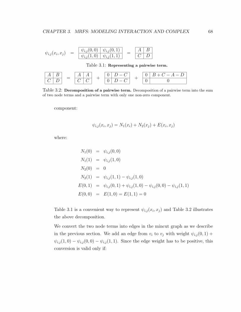
CHAPTER 3. MRFS: MODELING INTERACTION AND COMPLEX 68
ψi,j(xi, xj) =ψi,j(0, 0) ψi,j(0, 1)ψi,j(1, 0) ψi,j(1, 1)
=A BC D
Table 3.1: Representing a pairwise term.
A BC D
=A AC C
+0 D − C0 D − C +
0 B + C − A−D0 0
Table 3.2: Decomposition of a pairwise term. Decomposition of a pairwise term into the sumof two node terms and a pairwise term with only one non-zero component.
component:
ψi,j(xi, xj) = N1(xi) +N2(xj) + E(xi, xj)
where:
N1(0) = ψi,j(0, 0)
N1(1) = ψi,j(1, 0)
N2(0) = 0
N2(1) = ψi,j(1, 1)− ψi,j(1, 0)
E(0, 1) = ψi,j(0, 1) + ψi,j(1, 0)− ψi,j(0, 0)− ψi,j(1, 1)
E(0, 0) = E(1, 0) = E(1, 1) = 0
Table 3.1 is a convenient way to represent ψi,j(xi, xj) and Table 3.2 illustrates
the above decomposition.
We convert the two node terms into edges in the mincut graph as we describe
in the previous section. We add an edge from vi to vj with weight ψi,j(0, 1) +
ψi,j(1, 0) − ψi,j(0, 0) − ψi,j(1, 1). Since the edge weight has to be positive, this
conversion is valid only if:

CHAPTER 3. MRFS: MODELING INTERACTION AND COMPLEX 69
ψi,j,k(xi, xj, xk) =
ψi,j,k(0, 0, 0) ψi,j,k(0, 0, 1)ψi,j,k(0, 1, 0) ψi,j,k(0, 1, 1)ψi,j,k(1, 0, 0) ψi,j,k(1, 0, 1)ψi,j,k(1, 1, 0) ψi,j,k(1, 1, 1)
=
A BC DE FG H
Table 3.3: Representing a triplet term.
A BC DE FG H
=
A AC CE EG G
+
0 B − A0 B − A0 F − E0 F − E
+
0 00 A+D −B − C0 00 A+D −B − C
+
0 00 00 00 P
Table 3.4: Decomposition of a triplet term. Decomposition of a triplet term into the sum ofthree pairwise terms and a triplet term with only one non-zero component.
ψi,j(0, 1) + ψi,j(1, 0)− ψi,j(0, 0)− ψi,j(1, 1) ≥ 0
⇐⇒
ψi,j(0, 1) + ψi,j(1, 0) ≥ ψi,j(0, 0) + ψi,j(1, 1)
⇐⇒
φi,j(0, 0)φi,j(1, 1) ≥ φi,j(0, 1)φi,j(1, 0) (3.2)
We call potential functions satisfying the above condition regular.
Triplet clique: three variables We conveniently represent the triplet term in Eq. (3.1),
ψi,j,k(xi, xj, xk), as in Table 3.3. We define:
P = B + C + E +H − A−D − F −G
If P ≤ 0, we decompose the triplet term as shown in Table 3.4. The first box
on the right side is a pairwise term independent of xk. The second and third
boxes are pairwise terms independent of xj and xi respectively. They can be
converted into the edges in the mincut graph as we described earlier as long as

CHAPTER 3. MRFS: MODELING INTERACTION AND COMPLEX 70
Figure 3.1: Mincut graph for a triplet term without pairwise components. Any tripletterm can be decomposed into the sum of three pairwise terms plus a residue triplet term, which canbe converted to one of the above mincut graph:(a) Edge weights are all −P . The cost of the minimum cut is 0 if xi = xj = xk = 1 and −Potherwise.(b) Edge weights are all P . The cost of the minimum cut is 0 if xi = xj = xk = 0 and P otherwise.
they satisfy the regularity condition:
C + E ≥ A+G
B + E ≥ A+ F
B + C ≥ A+D
To represent the last box, we will add an auxiliary vertex uijk and four edges
of weight −P : vi → uijk, vj → uijk, vk → uijk, and uijk → t (Fig. 3.1(a)). It is
easy to verify that the cost of the minimum cut is 0 if xi = xj = xk = 1 and P
otherwise, which is equivalent to the last box by a constant.
In the case of P > 0, we decompose it as shown in Table 3.5.

CHAPTER 3. MRFS: MODELING INTERACTION AND COMPLEX 71
A BC DE FG H
=
B BD DF FH H
+
C −D 0C −D 0G−H 0G−H 0
+
E +H − F −G 00 0
E +H − F −G 00 0
+
−P 00 00 00 0
Table 3.5: Decomposition of a triplet term. Decomposition of a triplet term into the sum ofthree pairwise terms and a triplet term with only one non-zero component.
The first three boxes on the right side are pairwise terms, which can be converted
into the edges in the mincut graph as we described earlier as long as they satisfy
the regularity condition:
D + F ≥ B +H
D +G ≥ C +H
F +G ≥ E +H
To represent the last box, we will add an auxiliary vertex uijk and four edges
of weight P : uijk → vi, uijk → vj, uijk → vk, s → uijk (Fig. 3.1(b)). It is easy
to verify that the cost of the minimum cut is 0 if xi = xj = xk = 0 and P
otherwise, which is equivalent to the last box by a constant.
It is easy to verify that the cost of any cut S, T would equal to the energy of
the MRF, up to a constant, if we assign xi = 0 for vi ∈ S and xi = 1 for vi ∈ T .
Therefore, our problem becomes finding the minimum cost cut for the graph, which
can be efficiently solved by using the maximum flow algorithm (maxflow) [6].
Kolmogorov and Rother [74] described a method called QPBO that extends the
mincut inference and deals with MRFs with non-regular potentials. According to the
QPBO method, in addition to the terminal vertices s and t, there are two vertices
vi and wi for each node xi in MRF. The edges involving vi would be constructed
exactly the same way as described above, except all the weights are halved. The
edges involving wi’s are reversed from those of the vi’s:
• If there is an edge from vi to vj, we add an edge from wj to wi.
• If there is an edge from vi to t, we add an edge from s to wi.
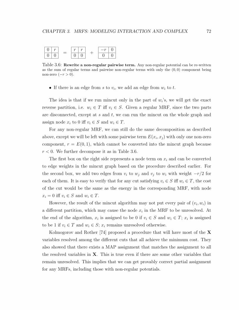
CHAPTER 3. MRFS: MODELING INTERACTION AND COMPLEX 72
0 r0 0
=r r0 0
+−r 00 0
Table 3.6: Rewrite a non-regular pairwise term. Any non-regular potential can be re-writtenas the sum of regular terms and pairwise non-regular terms with only the (0, 0) component beingnon-zero (−r > 0).
• If there is an edge from s to vi, we add an edge from wi to t.
The idea is that if we run mincut only in the part of wi’s, we will get the exact
reverse partition, i.e. wi ∈ T iff vi ∈ S. Given a regular MRF, since the two parts
are disconnected, except at s and t, we can run the mincut on the whole graph and
assign node xi to 0 iff vi ∈ S and wi ∈ T .
For any non-regular MRF, we can still do the same decomposition as described
above, except we will be left with some pairwise term E(xi, xj) with only one non-zero
component, r = E(0, 1), which cannot be converted into the mincut graph because
r < 0. We further decompose it as in Table 3.6.
The first box on the right side represents a node term on xi and can be converted
to edge weights in the mincut graph based on the procedure described earlier. For
the second box, we add two edges from vi to wj and vj to wi with weight −r/2 for
each of them. It is easy to verify that for any cut satisfying vi ∈ S iff wi ∈ T , the cost
of the cut would be the same as the energy in the corresponding MRF, with node
xi = 0 iff vi ∈ S and wi ∈ T .
However, the result of the mincut algorithm may not put every pair of (vi, wi) in
a different partition, which may cause the node xi in the MRF to be unresolved. At
the end of the algorithm, xi is assigned to be 0 if vi ∈ S and wi ∈ T ; xi is assigned
to be 1 if vi ∈ T and wi ∈ S; xi remains unresolved otherwise.
Kolmogorov and Rother [74] proposed a procedure that will have most of the X
variables resolved among the different cuts that all achieve the minimum cost. They
also showed that there exists a MAP assignment that matches the assignment to all
the resolved variables in X. This is true even if there are some other variables that
remain unresolved. This implies that we can get provably correct partial assignment
for any MRFs, including those with non-regular potentials.
CHAPTER 3. MRFS: MODELING INTERACTION AND COMPLEX 73
Learning in MRFs
Learning algorithms have been developed that takes either the marginal inference
or MAP inference as a subroutine. Therefore, it is important to have a fast and
accurate inference algorithm that can be applied to any kind of MRF. Maximum
likelihood learning, which optimize the likelihood by gradient descent, uses marginal
inference to compute the gradient. The marginal inference is usually done with loopy
belief propagation, which is slow and approximate. Max-Margin Markov Network
learning [126], which tries to maximize the margin between the true labels and all
the other labels, uses MAP inference to generate constraints in its QP optimization
problem.
In this thesis, we first used maximum likelihood learning, but with the MAP as-
signment as the gradient, which approximates the marginals but is a magnitude faster
than computing the marginals using LBP. Since the gradient is no longer continuous,
our optimization algorithm would stop earlier before reaching the actual global max-
imum. We then tried the perceptron learning with voting [24], which also takes MAP
inference as a subroutine. In both cases, we used our fast MAP inference algorithm,
which greatly speeds up the learning. In particular, the perceptron learning, when
combined with the less efficient message-passing MAP inference algorithm, is still
shown to faster than maximum likelihood learning [24]. Now combined with our fast
inference algorithm, the perceptron learning is able to speed up more.
3.4 Methods
We propose an inference algorithm that combines limited ‘truncation’, i.e. replacing a
subset of non-regular potentials with regular approximations, with the QPBO method
that does partial inference. This procedure resolve more variables than QPBO, and
in some cases provably more correct assignments. We also propose a procedure that
gives approximate assignment to unresolved variables if there are any left.
As we described earlier, the terms in the energy formulation Eq. (3.1) can be
decomposed into node terms, regular pairwise terms, non-regular pairwise terms with

CHAPTER 3. MRFS: MODELING INTERACTION AND COMPLEX 74
only one non-zero component, and triplet terms with only one non-zero component:
Energy(X)
=∑
Ni(Xi) +∑
Ti,j,k(Xi, Xj, Xk) +∑
Eij(Xi, Xj) +∑{i,j}∈M
Fij(Xi, Xj)
= Regular(X) + F(X)
where Eij(Xi, Xj) is the regular pairwise term, Fij(Xi, Xj) is the non-regular pairwise
term with only one non-zero component as in Table 3.6: Fij(0, 0) > 0, and M is the
set of variable pairs in all non-regular pairwise terms.
The intuition is that, the fewer non-regular terms, the more variables we can
resolve. If we drop all the non-regular terms, we can get a complete assignment.
However, what is the relationship between the assignment we get from this ‘truncated’
MRF and the true MAP assignment? We have the following theorem:
Theorem 1. Assume Energy(X) consists of only node terms and pairwise terms.
Given its truncation:
Energy′(X) = Regular(X)
Assume x′∗ is the MAP assignment to Energy′(X), which can be computed effi-
ciently and exactly by mincut inference. There exists an assignment x∗ that is the
MAP assignment to Energy(X) and satisfies x∗i = 1 if x′∗i = 1.
The theorem follows the intuition that if we drop the non-regular terms, which
disfavors the (0, 0) pair, we will end up with more 0’s in the MAP assignment and
those assigned to be 1 are guaranteed to be correct.
Proof. Let Y denote to be those variables in x′∗ that are assigned to be 0 and Z to
be those variables that are assigned to be 1.
The MRF Energy′(X) can be converted into a mincut graph with a node vi for
each variable Xi plus two terminal vertices s and t. The maxflow algorithm that
solves the mincut problem pushes as much flow from s to t as possible. The mincut
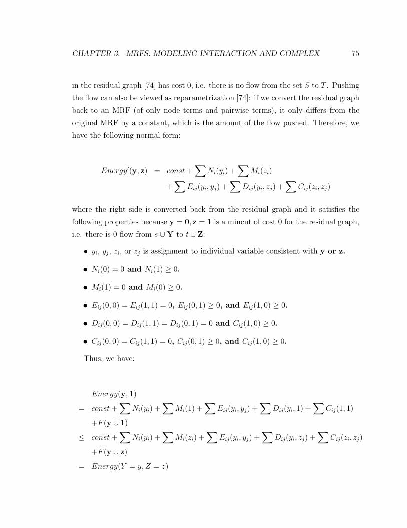
CHAPTER 3. MRFS: MODELING INTERACTION AND COMPLEX 75
in the residual graph [74] has cost 0, i.e. there is no flow from the set S to T . Pushing
the flow can also be viewed as reparametrization [74]: if we convert the residual graph
back to an MRF (of only node terms and pairwise terms), it only differs from the
original MRF by a constant, which is the amount of the flow pushed. Therefore, we
have the following normal form:
Energy′(y, z) = const+∑
Ni(yi) +∑
Mi(zi)
+∑
Eij(yi, yj) +∑
Dij(yi, zj) +∑
Cij(zi, zj)
where the right side is converted back from the residual graph and it satisfies the
following properties because y = 0, z = 1 is a mincut of cost 0 for the residual graph,
i.e. there is 0 flow from s ∪Y to t ∪ Z:
• yi, yj, zi, or zj is assignment to individual variable consistent with y or z.
• Ni(0) = 0 and Ni(1) ≥ 0.
• Mi(1) = 0 and Mi(0) ≥ 0.
• Eij(0, 0) = Eij(1, 1) = 0, Eij(0, 1) ≥ 0, and Eij(1, 0) ≥ 0.
• Dij(0, 0) = Dij(1, 1) = Dij(0, 1) = 0 and Cij(1, 0) ≥ 0.
• Cij(0, 0) = Cij(1, 1) = 0, Cij(0, 1) ≥ 0, and Cij(1, 0) ≥ 0.
Thus, we have:
Energy(y,1)
= const+∑
Ni(yi) +∑
Mi(1) +∑
Eij(yi, yj) +∑
Dij(yi, 1) +∑
Cij(1, 1)
+F (y ∪ 1)
≤ const+∑
Ni(yi) +∑
Mi(zi) +∑
Eij(yi, yj) +∑
Dij(yi, zj) +∑
Cij(zi, zj)
+F (y ∪ z)
= Energy(Y = y, Z = z)

CHAPTER 3. MRFS: MODELING INTERACTION AND COMPLEX 76
The inequality are based on the inequalities for the corresponding terms. Most
of them are obvious based on the properties of the normal form. For example,
Dij(yi, 1) ≤ Dij(yi, zj) because Dij(yi, 1) is always 0 no matter what yi is, while
Dij(yi, zj) ≥ 0. Finally, the inequality involving F () is due to the (0, 0) pairs in
y ∪ 1 is a subset of those in y ∪ z, and (0, 0) pairs are the only non-zero (positive)
components in Fij(), whose sum is F ().
We conclude there always exists a MAP assignment where we have z = 1.
In practice, we also consider the partial truncation: Energy′′(x) = Regular(x) +∑{i,j}∈M0
Fij(xi,xj) where M0 ⊂ M . We use the QPBO method to get a partial
assignment to Energy′′(). The intuition is that since the partially ‘truncated’ MRF
disfavors the (0, 0) pair, our assignment of 1 is more conservative and is likely to be
correct for the original Energy().
Therefore, our algorithm starts with Regular(x). At each step, it incrementally
adds in one non-regular term Fij(). We apply the QPBO method on this partial
truncation and produce the partial assignment. We repeat the steps until all non-
regular terms are added. We pick among all the partial assignments the one that has
the most variables assigned to be 1. We fix those variables to be 1, and repeat the same
procedure on the remaining variables at the next iteration. We are guaranteed to fix
the correct variables if we pick the partial assignment corresponding to the complete
truncation, Regular(X) at the beginning of the iteration, due to our Theorem 1. On
the other hand, it is also guaranteed to be correct if we pick the partial assignment
corresponding to the original MRF at the end of the iteration when all non-regular
pairwise terms are added due to the correctness of the QPBO algorithm. Note that the
0 and 1 labels are symmetrical. Therefore at each iteration, we can also decompose
the non-regular terms so that Fij(1, 1) > 0 is the only non-zero component, and
conservatively fix some variables to be 0 at each iteration. We repeat the iterations
until no more variables could be fixed.
During each iteration, we need to run mincut multiple times, each time with
one more non-regular term. Using the dynamic graph cuts algorithm by Kohli and

CHAPTER 3. MRFS: MODELING INTERACTION AND COMPLEX 77
Torr [71], the time complexity of repeatedly running the mincut for each of the non-
regular terms within a certain iteration is on the same level of magnitude as running
one single mincut on the original energy function. Therefore, our method is still
guaranteed to be fast.
If there are still unresolved variables at the end of the algorithm, we use an
approximation method to complete their assignment. In the mincut graph constructed
by the QPBO method, the two vertices for an unresolved variable, p and p, are in the
same strongly connected component [74]. We compare the maximum amount of flow
we can push from p to p to the amount we can push from p to p. This can be shown
to be equivalent to the procedure used by Kohli and Torr [72] to compute the max-
marginals, but extended to this non-regular case. In the case when all variables are
resolved, the amount of flow pushed is proportional to the max-marginal. Therefore
if we can push more flow from p to p, the corresponding variable would have a higher
max-marginal when assigned to 1 than when it is assigned to 0. In the case involving
unresolved variables, it is no longer guaranteed to be true, but we still use it as an
approximation. Thus, here is our procedure for assigning an unresolved variable: if we
can push more flow from p to p than from p to p, we assign the corresponding variable
to 1; otherwise, we assign it to 0. We fix this variable and repeat the procedure for
the next unresolved variable. We can do this for all unresolved variables efficiently
using the dynamic graph cuts algorithm [71].
To summarize, we proposed a fast inference algorithm that works on any kind of
MRF. We applied it to the protein-protein interaction data, which we will describe
in details below. We also applied it to object recognition in computer vision. It is
shown to have comparable accuracy to loopy belief propagation, while being almost
10 times faster.

CHAPTER 3. MRFS: MODELING INTERACTION AND COMPLEX 78
3.5 MRF for the triplet model
3.5.1 Representation
We extend the model of Jaimovich et al. [64]. We have four types of nodes in the
MRF for predicting protein-protein interactions:
• Actual protein-protein interactions Iij. They have value 1 if protein i and
protein j interact and 0 otherwise.
• Observed protein-protein interactions IAij. They have value 1 if protein i and
protein j are observed to interact in a particular assay and 0 otherwise. We
used four interaction assays: Ito, Uetz, DIP, and MIPS and thus have four IA
nodes for each protein pair.
• Actual protein localization Li. They have value 1 if protein i locates in the par-
ticular cellular component, and 0 otherwise. We use GFP experimental data,
which distinguishes between four different cellular components: nucleus, cyto-
plasm, mitochondrion, and endoplasmic reticulum [61] so we have four nodes
for each protein.
• Transcriptional regulation node Rij. Rij is 1 if protein i transcriptionally reg-
ulates protein j, and 0 otherwise. We use data from ChIP-Chip experiments
by [85] as the actual regulation.
During the training, all nodes are observed. During test, we do inference on the
actual protein-protein interaction nodes given all the other nodes.
The MRF has four types of cliques:
• Directed edges between actual protein-protein interactions Iij and observed
protein-protein interactions IAij to deal with the noise in the protein inter-
action assays.
• Triplets between actual protein-protein interactions Iij and their corresponding
actual localizations Li and Lj to represent the intuition that interacting proteins
should be co-localized.

CHAPTER 3. MRFS: MODELING INTERACTION AND COMPLEX 79
• Triplets for three actual protein-protein interaction nodes: Iij, Ijk, and Iik to
represent the transitivity relationship between them.
• Triplets for Rij, Rik, and Ijk to represent the intuition that if two proteins are
co-regulated by the some other protein, they are more likely to interact with
each other.
3.5.2 Learning and inference
We maximize the joint likelihood of the data using gradient ascent. We tried two
training methods: generative where we maximize P (I, IA, L,R) and discriminative
where we maximize P (I|IA, L,R). We used the MAP assignment computed by the
efficient mincut inference to approximate the gradient.
The MAP assignment for P (I, IA, L,R) in the generative case is:
argmaxI,IA,L,R
P (I, IA, L,R)
where IA, L, and R are not fixed.
The MAP assignment for P (I|IA, L,R) in the discriminative case is
(I, IA, L,R) s.t. I = argmaxI
P (I|IA, L,R)
where IA, L, and R are fixed to the observed values.
We use the exact mincut inference during test time because we want to apply
the learned model to entire proteome and belief propagation is too slow for that.
Mincut inference, though efficient and exact, requires the potentials to be regular.
Therefore, at each step of the gradient ascent during the learning, we use the log-
barrier method [16] to force the parameters to stay in the regularity constraints.
Although this limits the class of potentials we can learn, it speeds up both inference
and learning, which uses MAP inference as a subroutine to compute the approximate
gradient. Since our potentials are close enough to be regular, the approximation is
accurate enough to generate good results.

CHAPTER 3. MRFS: MODELING INTERACTION AND COMPLEX 80
3.5.3 Experiment setup
We evaluated our model on a S. cerevisiae data set compiled by von Mering et al. [130]
who ranked 80,000 protein-protein interactions by their reliability. We picked the top
1,000 interactions and considered them as the ‘true’ interactions. Those 1000 in-
teractions involve 543 unique proteins. From those proteins, we generated the ‘true’
non-interactions by randomly selecting 10,000 protein pairs that do not appear on the
the list of 80,000 interactions. We used 10 times as many non-interactions as inter-
actions so we have roughly the same number of triplets involving non-interactions as
triplets involving interactions. This avoids the intrinsic bias in the model of Jaimovich
et al. Section 3.2. We used four interaction assays [127, 63, 98, 122] and one localiza-
tion assay with four cellular components [61]. We also used transcription regulation
data from [85], which resulted in 113 transcription factors each regulating 39 target
genes on average. We used standard four-fold cross validation, where we learn the
model using 750 interactions and 7,500 non-interactions and test it on the remaining
held-out protein pairs.
3.5.4 Results
We compare our model with the two best-performing models used by [64]. The so-
called ‘Triplet’ model includes both the interaction and localization variables and
cliques. As such, it is a strict subset of the ‘Regulation’ model described earlier. The
so-called ‘Full’ model extends the ‘Triplet’ model by hiding the actual localization
variables Li, and adding respective observed variables LAi corresponding to the ex-
perimental GFP results. The hidden variable is handled by EM during the learning,
where we iteratively assign values to the Li’s given the current parameters and then
optimize the parameters based on the complete assignment.
As we can see from Fig. 3.2, in the generative learning regime originally used by
Jaimovich et al. [64], we are able to improve the accuracy of the ‘Triplet’ model by inte-
grating the regulation data and reach accuracy comparable to the ‘Full’ model. More-
over, our discriminative learning regime yields significantly improved cross-validation
performance for all models.

CHAPTER 3. MRFS: MODELING INTERACTION AND COMPLEX 81
Figure 3.2: Sensitivity of the three MRF models in predicting protein-protein inter-actions. We cut off our predictions and compute the sensitivity at a level where we achieve 99.5%specificity, where sensitivity is the proportion of labeled positives that we actually predicted to bepositive, and specificity is the proportion of labeled negatives that we actually predicted to be neg-ative. The ‘Regulation’ model is our extension to the ‘Triplet’ model and the ‘Full’ model is by [64].The red bar is for generative training where we maximize the likelihood all data while the blue bar isfor discriminative training where we maximize the likelihood of the labels given other observations.

CHAPTER 3. MRFS: MODELING INTERACTION AND COMPLEX 82
Figure 3.3: Computational time for learning three MRF models. Computational time forapplying our learning algorithm, which is based on efficient MAP inference, to the three MRF modelsare shown in red and blue for generative and discriminative training respectively. In comparison,computational time for the original maximum likelihood learning algorithm by Jaimovich et al. [64],which is based on loopy belief propagation inference, is shown in green.

CHAPTER 3. MRFS: MODELING INTERACTION AND COMPLEX 83
As shown in Fig. 3.3, our learning algorithm, which is based on efficient MAP
inference, reduces the training time of the two original models significantly compare
to that based on loopy belief propagation by Jaimovich et al. [64]. It allows us to
learn our new ‘Regulation’ model with thousands of co-regulation triplets efficiently.
Moreover, efficient inference would enable us to expand our MRF to cover more
proteins in the genome.
3.6 MRF for the complex model
3.6.1 Representation
To construct complexes, we try to decide for each protein j, whether it belongs to a
particular complex i or not. We build an MRF to represent the relationship between
proteins and complexes. For each protein j and complex i, we create a node Vji,
whose value 1 if protein j is in complex i and 0 if protein j is not in complex i. Then
we associate two types of cliques with the Markov Network:
• Each node has a singleton clique with a potential function that is b when the
node value is 1 and 0 when the node value is 0. This node potential represents
the prior probability that a protein is in a particular complex.
• For any two nodes for the same complex i, Vij and Vik, we create an edge
between them: Eijk. The potential for this edge is wTf if both nodes have
values 1, and is 0 otherwise, where f are the features between protein i and
protein j such as TAP-MS score and co-localization. See next chapter for a
complete list of features we use. w is the vector of weights we need to learn; it
weighs the different feature appropriately so wTf , which is the affinity between
the two proteins, corresponds to the likelihood the two proteins being in the
same complex. Ideally, wTf should be large for a pair of proteins in the same
complex, and small otherwise. Our learning tries to find the b and weights
w that best explains our reference complexes. Using the learned model, our
inference tries to identify new complexes that have high likelihood, i.e. the sum
of affinities between all pairs of proteins in the complex.

CHAPTER 3. MRFS: MODELING INTERACTION AND COMPLEX 84
3.6.2 Learning and identifying complexes
We use the same training and test set as in the next chapter (Section 4.3 and Sec-
tion 4.6). We ended up having 340 reference complexes, four-fifth of which are used
during training in a five-fold cross validation. We maximize the likelihood of the
MRF constructed from the training set. All nodes in the MRF are labeled. The
gradient for the maximum likelihood optimization is approximately computed using
belief propagation.
To identify a new complex C, we construct an MRF that for each protein, it has a
node that associates the protein with the complex C. We connected all pairs of nodes
into pairwise cliques as described earlier. We then do inference in the MRF using
the learned weights. However, the potentials for some edges would be non-regular
because, for a pair of proteins not likely to be in the same complex, we would have
a negative value of wTf , which means the 1-1 configuration is less likely between the
nodes representing the pair of proteins. To deal with such an MRF with non-regular
potentials, we use our efficient inference algorithm described earlier, which is shown
to work well empirically in the object recognition in computer vision. The resulting
assignment to the nodes tells us whether the proteins belong to the new complex C.
In order to avoid repeatedly identifying the same complex, we find two proteins,
Pi and Pj, not in any of the same complex discovered so far and fix their value to be 1.
Therefore, the new complex would always include Pi and Pj and thus be different from
the complexes already discovered. However, the new complex may involve proteins
that have high affinity with each other but have low affinity with Pi or Pj, which
are included because they are fixed. Therefore in a post-processing stage, we run
the inference a second time only on the proteins in the complex discovered in the
previous stage, but this time we do not fix Pi and Pj. The complex resulting after the
post-processing is considered to be our predicted complex, which may be redundant
to our previously predicted complexes.
3.6.3 Experiment setup
Refer to the experiment setup in the next chapter (Section 4.6).

CHAPTER 3. MRFS: MODELING INTERACTION AND COMPLEX 85
(a) (b)
Figure 3.4: Verification of complex predictions using MRF.We use five-fold cross-validation to predict reference complexes in the held-out set that is not used intraining. The blue bar shows the reference complex that exactly matches certain predicted complex.The green and red bars shows the reference complex that differs with certain predicted complex byone and two proteins respectively. We collectively call those reference complexes well-predicted. Seenext chapter for exact definition. We compare our MRF model with the state-of-the-art methods ofHart et al. and Pu et al..(a) The total number of reference complexes that are well predicted.(b) The number of reference complexes well predicted divided by number of predicted complexes.This corresponds to the sensitivity of the predictions. Our MRF model is able to achieve highersensitivity with fewer predicted complexes.
3.6.4 Results
We constructed a reference set of reliable complexes. See next chapter for details
on how we construct the reference complexes. We did five-fold cross-validation to
evaluate the accuracy of our complex reconstruction.
we compare our method with the state-of-the-art methods of Hart et al. [57] and
Pu et al. [109]. As we can see from Fig. 3.4(a), Hart et al. and Pu et al. are able
to well predict more reference complexes than our MRF model. However, this is
mostly due to the fact that our method predicts much fewer complexes (182) than
Hart et al. (337) and Pu et al. (396). For each predicted complexes, our method is
able to perfectly predict 0.264 reference complex on average, compared to 0.199 and
0.164 reference complex by Hart et al. and Pu et al. respectively (Fig. 3.4(b)). If we

CHAPTER 3. MRFS: MODELING INTERACTION AND COMPLEX 86
define the sensitivity of the predictions to be the number of reference complexes well
predicted divided by the number of predicted complex, our method is able to achieve
higher sensitivity than Hart et al. and Pu et al..
A shortcoming of our method is that it predicts fewer complexes because many
of the complexes it found are redundant. Therefore, fewer total number of reference
complexes are well predicted Fig. 3.4(a), resulting in low coverage of our method.
We will present new methods in the next chapter to expand the coverage of our
predictions.
3.7 Discussion
There are many work on predicting protein-protein interactions. Some of them [14]
use flat models where predictions on protein-protein interactions are made indepen-
dently. Others, such as our InSite model of the last chapter, use a graphical model
so the interaction predictions are correlated indirectly through the affinities between
motifs.
In this chapter, we extend the model of Jaimovich et al. [64]. It takes into account
the transitivity relationship among protein-protein interactions. Therefore, predic-
tions in one part of the protein-protein interaction network give signals to predictions
in another part of the interaction network, which in turn give signals to predictions
in yet another part of the network. We use the framework of MRF to encode such
transitivity relationship and make predictions on all protein-protein interactions at
the same time using an efficient inference algorithm we developed. With the flexible
framework of MRF and our efficient inference algorithm, we also encode the rela-
tionships that interacting proteins are more likely to be located in the same cellular
component and they are more likely to be regulated by the same transcription factors.
Our results show that we are able to better predict protein-protein interactions with
those additional features.
There are many other types of relationships between proteins that are related to
protein-protein interactions [142]. For example, interacting proteins are more likely
to be phosphorylated by the same kinase. With our MRF framework, it is easy to

CHAPTER 3. MRFS: MODELING INTERACTION AND COMPLEX 87
encode those additional relationships. In the case we do not know, a priori, whether
certain relationship exists, we can still put it into our MRF and use L1 regularization
to do feature selection and remove those relationships that do not exist [82].
Many protein-protein interactions and their transitivity relationship are the results
of multiple proteins in the same complex. In the second part of this chapter, we try
to reconstruct complexes directly. Our MRF model picks a set of proteins that has
the highest sum of affinity between the member proteins. Therefore, it tends to pick
the same set at different iterations, resulting in complexes that are exactly the same
as each other. After removing this redundancy, we ended up with few predicted
complexes. Therefore, our model has low coverage despite its high sensitivity. We
address this problem in the next chapter with methods based on supervised learning
and clustering. Another solution would be to reduce the affinities between proteins
that already appear in any of the same complex, as Gavin et al. [44] did. This way,
it is less likely to predict the same complex again because the affinities within that
complex are reduced.

Chapter 4
Stoichiometrically Stable
Complexes
4.1 Introduction
Biological processes exhibit a hierarchical structure in which the basic working units,
proteins, physically associate to form stoichiometrically stable complexes. Complexes
interact with individual proteins or other complexes to form functional modules and
pathways that carry out most cellular processes. Such higher level interactions are
more transient than those within complexes and are highly dependent on temporal
and spatial context. The function of each protein or complex depends on its interac-
tion partners. Therefore, a faithful reconstruction of the entire set of complexes in the
cell is essential to identifying the function of individual proteins and complexes, as
well as serving as a building block for understanding the higher level organization of
the cell, such as the interactions of complexes and proteins within cellular pathways.
In this chapter, we describe a novel method for reconstruction of complexes from a
variety of biological assays.
Our reconstruction effort focuses on the yeast Saccharomyces cerevisiae, both
as the prototypical case study for the reconstruction of protein-protein interaction
networks; importantly, the yeast complexes often have conserved orthologs in other
organisms, including human, and are therefore of interest in their own right. Several
88

CHAPTER 4. STOICHIOMETRICALLY STABLE COMPLEXES 89
studies [45, 59, 44, 79], using a variety of assays, have generated high-throughput data
that directly measure protein-protein interactions. Most notably, two high-quality
data sets [44, 79] used tandem affinity purification followed by mass-spectrometry
(TAP-MS) to provide a proteome-wide measurement of protein complexes. These
data provide the basis for attempting a comprehensive reconstruction of a large frac-
tion of the protein complexes in this organism.
Despite the fairly high quality of these networks and the agreement between them,
they still contain many false positives and negatives. False negatives can arise, for ex-
ample, from the difficulty in detecting interactions involving low-abundance proteins
or membrane proteins; or from cases where the tag added to the bait protein during
TAP-MS prevents binding of the bait to its interacting partners. False positives can
arise, for example, from complexes that share components; or from the contaminants
that bind to the bait non-specifically. Therefore, the set of complexes derived from
the protein-protein interaction network alone has limited accuracy. Less than 20% of
the MIPS complexes [97], which are derived from reliable small-scale experiments, are
exactly captured by the predictions of Pu et al. [109] or by those of Hart et al. [57].
In this chapter, we construct a method that generates a set of complexes with
higher sensitivity and coverage by integrating multiple sources of data, including
mRNA gene expression data, cellular localization, and yeast 2-hybrid data. These
evidences, however, only provide weak signals to co-complexness and they also corre-
late with other relationship between two proteins such as being in the same pathway.
Therefore, we develop a data integration approach that is aimed directly at the prob-
lem of predicting stoichiometrically stable complexes.
In the previous chapter, we used an MRF model to identify complexes, which
has high sensitivity but low coverage. It is equivalent to finding the subgraph that
has the maximum sum of affinities between all the pairs in the subgraph, where
the affinity is the result of combining the learned weights with the features between
a pair of proteins. To avoid this restricted form of defining cluster coherence, we
try new models that learn a cluster coherence measure directly from raw evidences,
such as TAP-MS score, instead of collapsing them into affinities for pairs of proteins
first. This allows us to use richer features across protein pairs to define the cluster

CHAPTER 4. STOICHIOMETRICALLY STABLE COMPLEXES 90
coherence, and a more flexible way to combine the affinities for all protein pairs.
We began by creating a comprehensive set of reference complexes from the litera-
ture. Unlike other methods, which generally used only the MIPS [97] complexes, we
extracted complexes from both MIPS (225 complexes) and SGD [23] (195 complexes),
and combined them with a large set of (164) hand-curated complexes constructed
from our own prior knowledge. We then applied an unbiased procedure to unify these
(sometimes inconsistent) sets into a large set of 340 reference complexes that we used
both for training our learning method and for evaluating the quality of its predictions
(in a hold-out regime). The merging process creates complexes that are supported by
multiple sources, and whose protein members appear in strict majority of the sources.
Therefore, the resulting reference set has both higher sensitivity and coverage than
those used by previous studies [57, 109]. This set of high-quality reference complexes
can be downloaded from our website [4].
Based on this set, we tried three different algorithms: a complexness model, a
protein-complex model, and a protein-protein model.
The complexness model tries to learn a ranking between two sets of proteins based
on the features between all pairs of proteins in each set. The ranking tells us which
set of proteins looks more like a complex. We identify complexes by doing greed hill
climbing to find a set of proteins that is a local maximum of the ranking function.
The protein-complex model tries to learn a classification that decides whether a
protein should belong to the same complex with a set of proteins based on the features
between the protein and every protein in the set. Starting with a set of proteins, we
then use a procedure that iteratively adds proteins with positive score to the set and
removes an existing protein from the set if it has negative score.
The protein-protein model works the best and is the focus of this chapter. It, like
others, has two phases. In the first, we use boosting [24], a state-of-the-art machine
learning method, to train an affinity function that is specifically aimed at predicting
whether two proteins are co-complexed. Unlike most other learning methods, boosting
is capable of inducing useful features by combining different aspects of the raw data,
making it particularly well-suited to a data-integration setting. Once we generate the
learned affinity graph over pairs of proteins, we predict complexes by using a novel
CHAPTER 4. STOICHIOMETRICALLY STABLE COMPLEXES 91
clustering algorithm. Our initial experiments showed that hierarchical agglomerative
clustering (HAC), which progressively merges sets of proteins with strongest affinity,
produces the best results for complex reconstruction if trained to optimize for that
task. However, HAC has several significant limitations. First, it does not allow
clusters to overlap, whereas actual complexes do share subunits. Second, it uses a
single cutoff to decide the granularity of the complexes constructed. A cluster near
the cutoff in the dendrogram can be formed even if it is the result of merging two
relatively weakly connected sub-clusters A and B. Such a cluster, although of lower
confidence, still excludes both A and B from being predicted as a complex; this
occurs even if A and B are strong candidates for being a complex. Finally, once a set
of proteins is merged with another set, it cannot merge with anything else even if the
affinity is only slightly lower. Therefore an incorrect decision cannot be fixed later in
the process.
To address these limitations, we constructed a novel clustering algorithm called
HACO (HAC with Overlap) that allows a set of proteins to be merged with multiple
other sets with which it has comparably strong affinity. HACO addresses all of the
limitations above: It produces clusters that can overlap. Second, when merging A
and B into a single cluster C, it also has the option of leaving A and/or B as candidate
complexes, avoiding a wrong decision because of an arbitrary cutoff. Finally, as it
allows the same cluster to be used in multiple places, it avoids many mistakes that
arise from an almost-arbitrary breaking of near-ties. Both our boosting algorithm
and the HACO code are made freely available on our project webpage [4], allowing
them to be used for predicting complexes with other forms of data. Moreover, the
HACO algorithm is a simple and elegant extension of HAC, which can be applied
to any setting where HAC is applied; given the enormous usefulness of HAC for the
analysis of biological data sets of many different types (e.g., [34]), we believe that
HACO may be applicable in a broad range of other tasks.
To validate our approaches, we show that we are able to predict more reference
complexes in the held-out set that is not used in training. By integrating multi-
ple sources of data, we recover more reference complexes than other state-of-the-art
methods [57, 109], even when we use simple HAC for the clustering. We further

CHAPTER 4. STOICHIOMETRICALLY STABLE COMPLEXES 92
improve both the coverage and sensitivity of our predictions when we use HACO. In
particular, Hart et al. [57] and Pu et al. [109] are only able to predict 67 and 65 com-
plexes respectively that exactly matches some reference complex. On the other hand,
HACO is able to predict 95 complexes perfectly. We also validated our predicted
set of complexes against external data sources that are not used in the training. In
all cases, our predictions are shown to be more coherent than methods of Hart et
al. and Pu et al.. Interestingly in two of the four cases, our predictions are even more
coherent than the reference set of complexes: proteins in the same predicted complex
share more transcription regulators and they have similar abundance levels.
Our predicted set of complexes provides us with some new insight on the global
structure of the protein complex network. In the past, Jeong et al. [66] have sug-
gested that the degree of a protein in an interaction network is positively correlated
with its essentiality, and have argued that ‘hubs’ in the network are more likely to
be essential because they are involved in more interactions. Our analysis shows that
this phenomenon is much better understood once we understand the protein network
in terms of complexes. Hart et al. [57] recently showed that complexes are either
‘essential’ — have a large fraction of essential components — or inessential — having
a small fraction of such components. We show here that large complexes are preferen-
tially comprised of essential proteins: the larger the complex, the larger the fraction
of essential proteins. Indeed, the size of the (largest) complex to which a protein
belongs is a significantly better predictor of its essentiality than its overall network
connectivity.
4.2 Related work
A number of works [57, 109] have attempted a comprehensive reconstruction of a
large fraction of the protein complexes in Yeast. Generally speaking, all use the
same general procedure: one or more data sources are used to estimate a set of
affinities between pairs of proteins, essentially measuring the likelihood of that pair
to participate together in a complex; these affinities induce a weighted graph, whose
nodes are proteins and whose edges encode the affinities; a clustering algorithm is

CHAPTER 4. STOICHIOMETRICALLY STABLE COMPLEXES 93
then used to construct complexes C sets of proteins that have high affinity in the
graph. Although similar at a high level, the different methods differ significantly on
the design choices made for the key steps in the process.
Recent works (since 2006) all focus on processing the proteome-wide TAP-MS data
and using the results to define complexes. Gavin et al. [44], Collins et al. [25], and
Hart et al. [57] all use probabilistic models that compare the number of interactions
observed between proteins in the data versus the number expected in some null model.
Collins et al. and Hart et al.both used all three of the available high-throughput data
sets [59, 44, 79], in an attempt to provide a unified interaction network. The two
unified networks resulting from these studies were shown to have large overlap and to
achieve comparable agreement with the set of co-complex interactions in the MIPS
data set [97], which are collated from previous small-scale studies. The interaction
graphs resulting from the computed affinity scores are then clustered to produce a
set of identified complexes. Gavin et al. [44], Hart et al. [57], and Pu et al. [109] all
use a Markov clustering [36] (MCL) procedure; Collins et al. [25] use a hierarchical
agglomerative clustering (HAC) procedure, but do not suggest a computational pro-
cedure for using the resulting clustergram to produce specific complex predictions.
Following are the details of several complex reconstruction methods.
• Bader et al. [10] used a novel clustering algorithm called Molecular Complex
Detection (MCODE) to detect densely connected regions in an earlier data set
of protein-protein interactions. It starts by assigning a weight to each protein
based on its neighborhood density. Then it picks the top-weighted protein as a
seed and traverse out from it to include neighboring proteins whose weights are
above a threshold. Once it stops, all the proteins picked along the way form
a complex, which is then excluded from the network in the following rounds
that start from the next highest weighted protein. However, Brohee et al. [18]
showed that the Markov clustering algorithm (MCL) works better than MCODE
on protein-protein interaction network.
• Gavin et al. [44] first computed a socio-affinity score between each pair of pro-
teins to be the log-odds of the number of times the two proteins are observed

CHAPTER 4. STOICHIOMETRICALLY STABLE COMPLEXES 94
together in some purifications relative to what is expected by chance based
on their frequencies. It takes into account both bait-prey and prey-prey in-
formation and is unbiased toward known complexes. The pairwise network of
socio-affinity scores is then subjected to a procedure that produces overlapping
clusters. This clustering procedure is repeatedly performed with different pa-
rameters. Similar clusters resulted from different parameters are grouped to
form ‘complex isoforms’. Proteins in each complex are divided into core, which
appears in most of the isoforms, and attachment, which only appears in some
of them. Two or more proteins in some attachment that also appear in other
complexes comprise a module.
• Krogan et al. [79] used a machine learning approach, trained on MIPS reference
complexes, to predict the confidence score for a pair of proteins to be in the
same complex. It only uses bait-prey relationship. It then applied a Markov
Clustering (MCL) algorithm to the pairwise network of confidence scores to
produce a list of non-overlapping clusters.
• Hart et al. [57] defined a p-value by comparing observed relative to expected
number of interactions in both bait-prey and prey-prey relationship. It is ap-
plied to three sets of purifications [59, 44, 79] and the combined score is derived
from multiplying their p-values. It then applied MCL to produce a list of non-
overlapping clusters.
• Pu et al. [109] applied MCL directly to the purification enrichment (PE) score [25],
which is derived from two sets of purifications [44, 79]. The clusters from MCL
were post-processed to identify proteins that are likely to be recruited by multi-
ple complexes. This resulted in a list of overlapping complexes. Pu et al. [109]
showed using PE score to combine Gavin’s and Krogan’s purifications gets bet-
ter accuracy than using either purification alone and MCL produces state-of-
the-art complexes.
• Collins et al. [25] applied a hierarchical agglomerative clustering (HAC) proce-
dure to the PE score. However, they do not suggest a computational procedure

CHAPTER 4. STOICHIOMETRICALLY STABLE COMPLEXES 95
for using the resulting clustergram to produce specific complex predictions. In-
stead, biologists look for potential complexes as regions of dense connections in
the clustergram.
Unlike the above methods, we generate a set of complexes with higher sensitivity
and coverage by integrating multiple sources of data, including mRNA gene expression
data, cellular localization, and yeast 2-hybrid data. The data integration approach
was used in some early works on predicting protein-protein interactions [65, 143], but
was not revisited in recent years. They tried, however, only to predict whether two
proteins belong to the same complex without reconstructing the set of proteins that
constitutes a complex. Jansen et al. [65] used a full Bayesian Network to integrate
four different high-throughput experiments of protein-protein interactions. The com-
plexity of a full Bayesian Network grows exponentially with the number of features,
and thus it is unlikely to be extended to deal with more features. Zhang et al. [143]
used a probabilistic decision tree to decide whether a protein pair belongs to the same
complex or not. A decision tree, though easily interpretable by biologists, fragments
the data with the addition of each layer of the tree.
Many recent studies [22, 84, 92, 117, 124, 129, 131, 135, 138] have successfully
integrated multiple types of data to predict functional linkage between proteins, con-
structing a graph whose pairwise affinity score summarizes the information from dif-
ferent sources of data. In particular, Chen and Yuan [22] integrated protein-protein
interactions and expression data to build a weighted graph. The resulting clusters,
however, are functional modules, which are larger units and sometimes are supersets
of complexes. Lee et al. [84] and Marcotte et al. [92] integrates multiple sources of
genomic data, such as genetic interactions, co-evolution, co-expression, and domain
fusion to predict pairwise functional relationship, which is used to assign protein
functions.
However, since the data integration is not trained toward predicting complexes,
the high-affinity pairs contain transient binding partners, and even protein pairs that
never interact directly but merely function in the same pathways. When these graphs
are clustered, the clusters correspond to a variety of cellular entities, including path-
ways, functional modules, or co-expression clusters. We develop a data integration

CHAPTER 4. STOICHIOMETRICALLY STABLE COMPLEXES 96
approach that is aimed directly at the problem of predicting stoichiometrically stable
complexes.
4.3 Constructing a set of reference complexes
We compiled a reference set of complexes by combining literature-derived results from
small-scale experiments in MIPS [97] and SGD [23] with a hand-curated list (see our
supporting website [4]) that we generated. The MIPS, SGD, and hand-curated set
contain 225, 195, and 164 complexes respectively. Below we describe our method
for establishing correspondence between the three lists and combining them into a
high-confidence reference set suitable for training our method and for evaluating the
accuracy of its predictions.
Our approach consisted of five processing steps. First, we merged similar com-
plexes from the original lists (see below), resulting in a list of 543 complexes. Second,
we removed 112 redundant complexes which were proper subsets of other complexes.
Third, we removed the five largest complexes: the four ribosomal subunits and the
small nucleolar ribonucleoprotein complex; these complexes are so large that they
greatly overwhelm the signal, both in training the method and in evaluating the
results. Fourth, we restricted the complexes to the set of 2195 proteins that have
adequate amount of experimental evidence (see below). Finally, we removed single-
protein complexes, arriving at the final list of 340 complexes. With at least 2 and
on average 4.9 proteins per complex, this set of complexes contained 1100 unique
proteins and a total of 1661 protein members, showing that the reference complexes
contain notable overlap (proteins that are shared by multiple complexes).
In the first step of this merging process, we define each candidate complex from
the three curated lists as a node in an undirected graph (or network). Two complexes
are connected by an edge if they overlap significantly, i.e., their Jaccard coefficient is
greater than 0.7 (see JC metric below), with an edge weight equal to the JC value. We
found 422 isolated nodes in the graph, corresponding to unique complexes that do not
overlap significantly with any other complexes in the list. The task of merging similar
complexes is equivalent to that of finding several types of connected components in

CHAPTER 4. STOICHIOMETRICALLY STABLE COMPLEXES 97
this graph. A complete subgraph with average edge weight of 1 is equivalent to a
group of complexes with identical protein content that appear under multiple names
in at least two of the curated lists. We found 66 such groups, which correspond to
complexes that we regard as very high-confidence because of multiple corroborating
evidence. A complete subgraph in the rest of the network with average edge weight
less than 1 (but greater than 0.7) is equivalent to a group of complexes whose protein
contents are reported differently by the different curated lists. We found 45 such
groups and produced a consensus complex for each, resolving conflicts by a majority
vote: a protein was included in the resulting complex only if it was found in more
than half of the candidate complexes from the conflicted group. The remaining 18
nodes formed 4 connected components but no complete subgraphs, each component
indicating non-transitive overlaps between three or more candidate complexes (e.g.
A overlaps with B, and B overlaps with C, but A does not overlap significantly with
C). Manual inspection and consultation with experts resulted in 10 unique complexes
being added to the reference list.
4.4 Pairwise signals for predicting complexes
We extracted pairwise signals from five different data sources: the purification en-
richment (PE) score from the consolidated network of Collins et al. [25], a cellular
component from a truncated version of the Gene Ontology (GO) [9], trans-membrane
proteins [23], co-expression [49], and yeast two-hybrid (Y2H) interactions [63, 127].
Our highest-coverage source regarding direct physical interaction comes from high-
throughput TAP-MS data of the Gavin [44] and Krogan [79] data sets. The recent
work of Collins et al. [25] provides a coherent and systematic way of integrating the
data from these separate assays into a high-quality score that measures the probability
of a protein pair to be co-complexed. The recent work of Hart et al. [57] provides
a different integration method, but the results are quite similar, providing support
for both of these procedures. We derived five signals from the PE analysis: the
direct score is computed based only on bait-prey information in the purifications; the
indirect score is computed based on prey-prey information; the actual PE score is

CHAPTER 4. STOICHIOMETRICALLY STABLE COMPLEXES 98
the sum of direct and indirect scores; the scaled score maps the PE score to a value
between 0 and 1 to approximate the confidence value that the pair represents a true
interaction; finally each protein is represented by a vector of its scaled PE scores with
all the other proteins (where we assign its interaction with itself a score of 1), and
we define our PE-distance signal as the cosine distance between the vectors of two
proteins.
As the PE score provides most of the signals in predicting complexes (See Re-
sults section), we only kept the 2390 proteins that have at least one scaled PE score
above 0.2 with some other protein. Although this set only covers about 40% of the
approximately 6000 yeast genes, it covers 81% of all protein members in the lists of
high-quality complexes that comprised our reference set. As noted earlier, we exclude
proteins that appear exclusively in the four ribosomal subunits and the small nucle-
olar ribonucleoprotein complex. This resulted in the final list of 2195 proteins, on
which we performed our complex prediction.
The Gene Ontology (GO) cellular component hierarchy [9] was downloaded on
June 25, 2007. An examination of the hierarchy showed that many of the smaller
categories (lower in the hierarchy) refer to particular complexes whose information is
derived from the same small-scale experiment that inform our reference set. Thus,
in order to achieve a fair evaluation using the reference set, we remove categories of
size less than 120 that can potentially contain the answer. The remaining 44 out of
564 categories represent high-level cellular localization information, much of which is
obtained through high-throughput experiments [61]. Some sample categories include
‘endoplasmic reticulum part’, ‘nuclear chromosome part’, ‘mitochondrial membrane’,
and ‘cytoplasm’.
We derived two pairwise localization signals from the GO cellular component. One
is the semantic distance measure [89], which is the log size of the smallest category that
contains both proteins. However, this signal is a pessimistic assessment regarding the
co-localization of the two proteins, as lack of annotation of a protein in some category,
particularly one that is a subset of its most specific category, does not necessarily
mean that it cannot belong to this category. Therefore, we construct a second signal,
which is the log size of the smallest possible group that could contain both proteins

CHAPTER 4. STOICHIOMETRICALLY STABLE COMPLEXES 99
(given the current evidence). It is computed in the following way between protein A
and protein B, whose most specific categories are X and Y respectively. If X is a
sub-category of Y , then the two proteins might belong together to any group if they
were to be annotated with enough detail. Therefore, we use log of 120, the size of
the smallest category, as our second signal. On the other hand, if X and Y are not
sub-categories of each other, we denote Z to be the smallest common super-category
of X and Y . We then denote X ′ (resp. Y ′) to be the category one level down the path
from Z to X (resp. Y ). Thus, assuming that A and B belong to the two different
categories at X ′ and Y ′, the smallest semantic category that we can form that may
contain them both is X ′ ∪ Y ′. Thus, our second signal is log(|X ′ ∪ Y ′|).A list of membrane proteins are obtained by parsing the trans-membrane anno-
tations in SGD [23]. A pair of proteins is considered to be membrane if at least one
of the proteins is found in the membrane. The first membrane signal is 1 if the pair
is membrane and 0 otherwise. The second and third signals are the product of the
first signal with the direct and indirect PE score of the two proteins, respectively.
This allows our boosting model to take into account the known fact that TAP-MS
purifications work differently on membrane proteins from non-membrane proteins.
Yeast two-hybrid protein-protein interactions are obtained from the assays of Ito
et al. [63] and Uetz et al. [127]. Interacting pairs are assigned signal value 1. Pairs of
proteins that appeared in the assay but not observed to interact are assigned signal
value -1. All other pairs have 0 as their signal values.
Microarray data were downloaded from Stanford Microarray Database (SMD) [49]
on Dec. 5th, 2006, which contains a total of 902 experiments for Yeast divided into
19 categories. The data were normalized to mean 0 and standard deviation 1. We
construct a signal by computing the mean-centered Pearson correlation coefficient
between the expression profiles of two proteins.
A final signal is obtained from small-scale physical interactions. We downloaded
protein-protein interactions from MIPS [96] and DIP [134] on 21 March 2006. We
extracted from MIPS those physical interactions that are non-high-throughput yeast
two-hybrid or affinity chromatography. For DIP, we picked non-genetic interactions
that are derived from small-scale experiments or verified by multiple experiments.

CHAPTER 4. STOICHIOMETRICALLY STABLE COMPLEXES 100
This signal has value 1 for observed interactions, and signal value 0 for all other pairs.
Importantly, there is a risk of cyclicity between these small-scale interactions and the
reference complexes. Therefore, to avoid a positive bias in our results, we omitted
this signal in the cross-validation runs, which are evaluated against the reference
complexes. For those runs that are trained on the entire set of reference complexes,
this cyclicity is not a concern, so this signal was included.
There are a total of 12 signals for cross-validation runs and 13 signals for runs
that are trained on the entire reference set.
4.5 Methods
4.5.1 Complexness model
In the complexness model, we try to learn the coherence for a set of proteins, which
measures how the set is like a complex.
Feature construction
Denote Sj(P,Q) to be the jth signal between protein P and protein Q. For each j,
we construct features for a set of proteins C by aggregating signals between proteins
in the set:
fij(C) = Ai({Sj(P,Q)|P ∈ C,Q ∈ C,P ≺ Q})
where Ai is the ith aggregation function that combines the jth signals for all pairs of
proteins in the set. ≺ can be any ordering among the proteins, such as alphabetical, to
avoid a pair appearing twice in both orders. We used the list of aggregating functions
in Appendix A.
Besides the pairwise data, we also use the GFP localization data, which give us the
localization of a protein in five cellular components: cytoplasm, nucleus, nucleolus,
mitochondrion, and ER. Denote L(P ) to be the set of cellular components protein P
belongs to. We construct the following aggregation features:

CHAPTER 4. STOICHIOMETRICALLY STABLE COMPLEXES 101
Nk = |{P,Q|k ∈ L(P ), k ∈ L(Q), P ≺ Q}|
where k is a cellular component. Nk the number of protein pairs in the set where
both proteins localizes to k. We also use the fraction of such protein pairs among all
pairs, Nk/C(n, 2) as another feature. We also count the number of protein pairs in
the set where the two proteins appear in none of the cellular components together
and the fraction of such pairs among all protein pairs as two features.
Finally, we include the number of proteins and number of protein pairs in the set
as two global features, which are independent of the signals and data sources. We
end up with a total of 134 features, which are richer and are not simply the linear
combination of the signals.
Learning with RankBoost
RankBoost [40] tries to learn a mapping g() from a set of proteins to a coherence
value, such that A should be more coherent than B if g(A) > g(B). Each training
instance (A � B) is associated with a loss function logit(g(B)− g(A)). Our learning
algorithm tries to minimize total loss, which is the sum of the loss functions over
all training instances. In our work, g() is a weighted sum of decision stumps, which
are incorporated one at a time to minimize the total loss. In detail, we start with
g(0)() = 0. At each iteration, we pick a decision stump dt():
dt() =
{0 if fi ≤ s
1 if fi > s(4.1)
where fi is a feature and s is the threshold of the decision stump. We pick the feature
and the threshold to minimize the loss function with the current g(t)() = g(t−1)()+dt()
over the training set. We repeat the iterations 100 times: g() = g(100)(), and use this
final classifier to predict how much a protein set looks like a complex.

CHAPTER 4. STOICHIOMETRICALLY STABLE COMPLEXES 102
Constructing the training set
Since we use RankBoost (see below) to do the learning, each of our training instances
involves two sets of proteins with one set ranked higher to the other. For each reference
complex C in the training set, we construct the following training instances:
C � C ∪ Pi, ∀i, s.t.Pi /∈ C
C � C\Pi, ∀i, s.t.Pi ∈ C
This is based on the intuition that a reference complex is ranked higher than any
protein set that is one-away from the complex. We end up with 746,300 training
instances.
Identifying complexes
We use greedy hill climbing over the surface of the coherence function g() until it
stops at some local maximum, which we use as our predicted complexes.
In particular, we start with a pair of proteins as the current set. At each step, we
consider all the candidate sets that are one-away from the current set — either by
adding one outside protein or by removing one existing protein. Among those sets,
we pick the one with the highest coherence and use it as the current set. We repeat
the steps until the current set has the highest coherence among all the candidate sets,
at which point we use the current set as our predicted complex.
4.5.2 Protein-complex model
In the protein-complex model, we try to learn the coherence between a protein Q and
a set of proteins C, which measures how likely the protein Q is to belong to the same
complex as the set C.
CHAPTER 4. STOICHIOMETRICALLY STABLE COMPLEXES 103
Feature construction
We construct the same set of features as in the complexness model (Section 4.5.1)
except that we consider pairs of proteins between Q and every protein in C. In
contrast, the complexness model considers all pairs of proteins within a set. Also,
instead of having two global features, we use number of proteins in C as our only
global feature that does not depend on any data source.
Learning with LogitBoost
Boosting [41, 24] is a class of algorithms that iteratively combines weak learners to
give an ensemble for our classification task. Each weak learner is a simple classi-
fier, such as a decision stump (Eq. (4.1)), that may only weakly correlate with the
labels. After a weak learner is trained, we add it to the ensemble with appropriate
weight. In the next iteration, the algorithm puts more weights on the data points
that are classified incorrectly by the current ensemble, which the next weak learner
will focus on. Boosting is able to perform automatic feature selection and has better
or comparable accuracy with other state-of-the-art classifiers such as support vector
machines (SVMs) [128] in many domains. We implemented a version of boosting
algorithms called LogitBoost [24] that uses decision stumps as weak learners and the
logit function as the loss function. This variant is shown to be more robust to outliers
and overfitting than the standard AdaBoost variant [41]. Our experiments (data not
shown) showed that this method performs well on our data, compared to other ver-
sions of Boosting and other classification algorithms such as logistic regression and
SVMs.
We applied the LogitBoost to the training set and learned a classifier that com-
putes an affinity value between a protein and a set of proteins. The higher the affinity,
the more likely the protein should belong to the same complex as the set of proteins.
Constructing the training set
For each reference complex C in the training set, we construct the following training
instances:

CHAPTER 4. STOICHIOMETRICALLY STABLE COMPLEXES 104
Positive instances. (P,C\P )|P ∈ C
negative instances. (P,C)|P /∈ C
This is based on the intuition that the pair that consists of a protein P in the
complex C and the set of remaining proteins in the complex should be in the positive
set because both the protein and the set belong to the same complex. On the other
hand, a protein P outside a complex C and the complex should be in the negative set
because the protein and the the set (complex C) do not belong to the same complex.
We end up with 746,300 positive and negative training instances.
Identifying complexes
We start with a pair of proteins as the current set. At each step, we consider each
protein outside the current set and use the learned boosting classifier to compute the
affinity between the protein and the current set. We add the protein to the current
set if the affinity is positive. We also compute the affinity between each protein in
the current set with the rest of the proteins and remove the protein from the current
set if the affinity is negative. We repeat the steps until no protein can be added or
removed, or when a cycle is detected such that we end up with a current set that is
identical to the set in some previous iteration.
4.5.3 Protein-protein model
Constructing co-complex protein pairs
The set of positive co-complexed protein pairs consists of all protein pairs that appear
in the same complex in the reference set. For the negative set, we first consider all
protein pairs (P,Q) such that P is in a reference complex and Q outside any version
of that complex, in any of the three hand-curated set; we then exclude any pair that
is within some other reference complex. The result of this process is 5065 positive
pairs and about 1 million negative pairs. Since there are too many negative pairs, for
computational expediency, we randomly sample one tenth of the negative pairs to be

CHAPTER 4. STOICHIOMETRICALLY STABLE COMPLEXES 105
used in training while setting each negative pair to have ten times the weight of the
positive pairs.
Integrating multiple features using LogitBoost
We applied LogitBoost to our training set of positives and negatives. We used the
12 signals from various data sources as our 12 features for the cross-validation runs
where we train on four-fifth of the reference complexes and test on the remaining
ones. We used the signal from small-scale interactions as our additional feature for
the run trained on the entire set of reference complexes. The prediction of the learned
ensemble classifier on a given protein pair is taken to be the pair’s affinity in the
clustering algorithm below. A high-affinity pair is predicted to be more likely to
appear in the same complex.
HAC with Overlap (HACO)
The HAC algorithm does not allow overlap between predicted complexes. To address
the limitation, we extend it to allow overlap. We started with standard HAC algo-
rithm using average linkage [120], which maintains a pool of merging candidate sets
where the distance between two non-overlapping sets is:
d(A,B) =1
|A||B|∑
P∈A,Q∈B
d(P,Q)
In our setting, we take d(P,Q) as the negative of the affinity between protein P and
protein Q. Note that d(A,B) is the average of the edge distance between proteins in
A and proteins in B.
In HAC, at each step, we pick the two non-overlapping sets with the closest
distance, A and B, and merge them to create a new set, M . M is added to the pool,
while the sets A and B are removed. Therefore, in later steps, we could only consider
the superset M , and would never be able to use A or B again to merge with some
other set. Assume that there is another set C whose distance to A is only slightly
larger than d(A,B). In this case, the decision to merge A with B rather than with C is
arbitrary and unstable. When the actual clusters overlap, a more appropriate solution
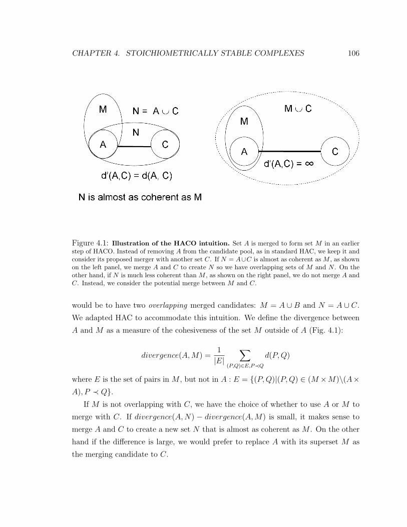
CHAPTER 4. STOICHIOMETRICALLY STABLE COMPLEXES 106
Figure 4.1: Illustration of the HACO intuition. Set A is merged to form set M in an earlierstep of HACO. Instead of removing A from the candidate pool, as in standard HAC, we keep it andconsider its proposed merger with another set C. If N = A∪C is almost as coherent as M , as shownon the left panel, we merge A and C to create N so we have overlapping sets of M and N . On theother hand, if N is much less coherent than M , as shown on the right panel, we do not merge A andC. Instead, we consider the potential merge between M and C.
would be to have two overlapping merged candidates: M = A ∪ B and N = A ∪ C.
We adapted HAC to accommodate this intuition. We define the divergence between
A and M as a measure of the cohesiveness of the set M outside of A (Fig. 4.1):
divergence(A,M) =1
|E|∑
(P,Q)∈E,P≺Q
d(P,Q)
where E is the set of pairs in M , but not in A : E = {(P,Q)|(P,Q) ∈ (M ×M)\(A×A), P ≺ Q}.
If M is not overlapping with C, we have the choice of whether to use A or M to
merge with C. If divergence(A,N) − divergence(A,M) is small, it makes sense to
merge A and C to create a new set N that is almost as coherent as M . On the other
hand if the difference is large, we would prefer to replace A with its superset M as
the merging candidate to C.
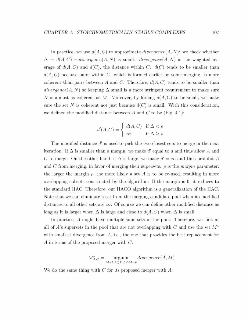
CHAPTER 4. STOICHIOMETRICALLY STABLE COMPLEXES 107
In practice, we use d(A,C) to approximate divergence(A,N): we check whether
∆ = d(A,C) − divergence(A,N) is small. divergence(A,N) is the weighted av-
erage of d(A,C) and d(C), the distance within C. d(C) tends to be smaller than
d(A,C) because pairs within C, which is formed earlier by some merging, is more
coherent than pairs between A and C. Therefore, d(A,C) tends to be smaller than
divergence(A,N) so keeping ∆ small is a more stringent requirement to make sure
N is almost as coherent as M . Moreover, by forcing d(A,C) to be small, we make
sure the set N is coherent not just because d(C) is small. With this consideration,
we defined the modified distance between A and C to be (Fig. 4.1):
d′(A,C) =
{d(A,C) if ∆ < ρ
∞ if ∆ ≥ ρ
The modified distance d′ is used to pick the two closest sets to merge in the next
iteration. If ∆ is smaller than a margin, we make d′ equal to d and thus allow A and
C to merge. On the other hand, if ∆ is large, we make d′ = ∞ and thus prohibit A
and C from merging, in favor of merging their supersets. ρ is the margin parameter:
the larger the margin ρ, the more likely a set A is to be re-used, resulting in more
overlapping subsets constructed by the algorithm. If the margin is 0, it reduces to
the standard HAC. Therefore, our HACO algorithm is a generalization of the HAC.
Note that we can eliminate a set from the merging candidate pool when its modified
distances to all other sets are ∞. Of course we can define other modified distance as
long as it is larger when ∆ is large and close to d(A,C) when ∆ is small.
In practice, A might have multiple supersets in the pool. Therefore, we look at
all of A’s supersets in the pool that are not overlapping with C and use the set M∗
with smallest divergence from A, i.e., the one that provides the best replacement for
A in terms of the proposed merger with C:
M∗A,C = argmin
Ms.t.A⊂M,C∩M=∅divergence(A,M)
We do the same thing with C for its proposed merger with A:

CHAPTER 4. STOICHIOMETRICALLY STABLE COMPLEXES 108
M∗C,A = argmin
M ′s.t.C⊂M ′,A∩M ′=∅divergence(C,M ′)
The smaller of divergence(A,M∗A,C) and divergence(C,M∗
C,A) is used to compute the
modified distance.
The algorithm terminates when there are no more non-overlapping sets to merge.
The output is a cluster-lattice, where the same cluster can be a child of multiple
parents in the lattice. The lattice is cut at a certain threshold to generate a set
of overlapping clusters. These predicted clusters are the sets that are still in the
candidate pool when the distance in the merging process reaches the threshold.
Learning and inference
We applied the HACO algorithm on the pairwise affinity network learned using Log-
itBoost. We use the same training set in all steps of our pipeline and evaluate the
final predictions on complexes in a separate test set which is hidden during all steps
of the training process.
We select the threshold that cuts the cluster-lattice in HACO by maximizing the
coverage (see Section 4.6.2) on the training set. To pick the margin ρ in HACO, we
cannot use coverage alone because our model would always prefer a bigger margin
that keeps more sets in the pool. Therefore, we choose ρ by maximizing the product of
coverage and sensitivity (see Section 4.6.2) on the training set. This approach trades
off between the match with the reference set and the number of predicted complexes.
4.6 Experiment setup
4.6.1 Training and test regime
To evaluate our prediction accuracy against the reference set, we divide the 340
reference complexes into five disjoint subsets, or folds. For each fold in the five-fold
cross validation, we hide one set and use the remaining four sets to train the model.
We then evaluate our predictions on the held-out set, which is not seen during the

CHAPTER 4. STOICHIOMETRICALLY STABLE COMPLEXES 109
Figure 4.2: Metrics for overlap between two complexes. Rj is a reference complex and Ci
is our predicted complex. The overlap between the two complexes can be quantified by the Jaccardcoefficient and the Hamming distance as illustrated in the figure. The better the overlap, the greaterthe Jaccard coefficient and the smaller the Hamming distance, with perfect match has a Jaccardcoefficient 1 and Hamming distance 0.
training process. We use the same training-test divide in all steps of our three models:
complexness model, protein-complex model, and protein-protein model.
To evaluate our predictions against external data sources, such as biological co-
herence and essentiality, we augment our model with a signal constructed from small-
scale physical interactions and train it on the entire set of 340 reference complexes. To
avoid circularity between signals and evaluation, we do not evaluate the predictions
from such runs against the reference complexes.
4.6.2 Evaluation metrics
To evaluate the matching between reference complexes and predictions, we quantify
the overlap between a reference complex R and a predicted complex C in several
ways [78] (Fig. 4.2):
Jaccard coefficient (JC): |R ∩ C|/|R ∪ C|

CHAPTER 4. STOICHIOMETRICALLY STABLE COMPLEXES 110
Hamming distance: |R ∪ C| − |R ∩ C|
Two complexes that overlap well will have a large Jaccard coefficient and a small
Hamming distance, with a perfect match has a Jaccard coefficient 1 and Hamming
distance 0.
We define the coverage and sensitivity of a set of predictions so we can system-
atically evaluate genome-wide predictions. For each reference complex, we find the
prediction that has the highest Jaccard coefficient. We define the scaled Jaccard co-
efficient: SJC(R,C) = max{0, 2JC(R,C)− 1}. We truncate the value at 0 because
it may represent random overlap. We define the coverage as the average Jaccard
coefficient per reference complex:
1
m
m∑i=1
nmaxj=1
SJC(Ri, Cj)
where m is the number of reference complexes and n is the number of predicted
complexes.
For sensitivity, we sum the Jaccard coefficients of all the overlapping (reference,
prediction) complex pairs, and normalize by the total number of predicted complexes:
1
m
m∑i=1
n∑j=1
SJC(Ri, Cj)
4.7 Results
4.7.1 Coverage and sensitivity of predicted complexes
We compiled a reference set of complexes from MIPS [97], SGD [23], and hand-
curation, which is more comprehensive than previous studies [57, 109]. Although
it still contains noise and bias, it provides us with the ultimate evaluation of our
predictions. There are 340 complexes in our reference set with an average of 4.9
proteins per complex.
We tested our approach using a standard 5-fold cross-validation regime, training
on 80% of the complexes and testing on the remaining 20%; the test set was not
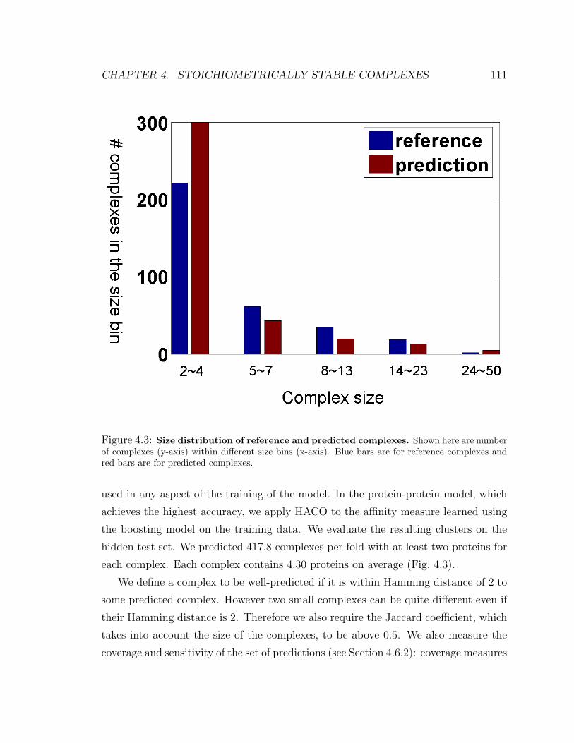
CHAPTER 4. STOICHIOMETRICALLY STABLE COMPLEXES 111
Figure 4.3: Size distribution of reference and predicted complexes. Shown here are numberof complexes (y-axis) within different size bins (x-axis). Blue bars are for reference complexes andred bars are for predicted complexes.
used in any aspect of the training of the model. In the protein-protein model, which
achieves the highest accuracy, we apply HACO to the affinity measure learned using
the boosting model on the training data. We evaluate the resulting clusters on the
hidden test set. We predicted 417.8 complexes per fold with at least two proteins for
each complex. Each complex contains 4.30 proteins on average (Fig. 4.3).
We define a complex to be well-predicted if it is within Hamming distance of 2 to
some predicted complex. However two small complexes can be quite different even if
their Hamming distance is 2. Therefore we also require the Jaccard coefficient, which
takes into account the size of the complexes, to be above 0.5. We also measure the
coverage and sensitivity of the set of predictions (see Section 4.6.2): coverage measures
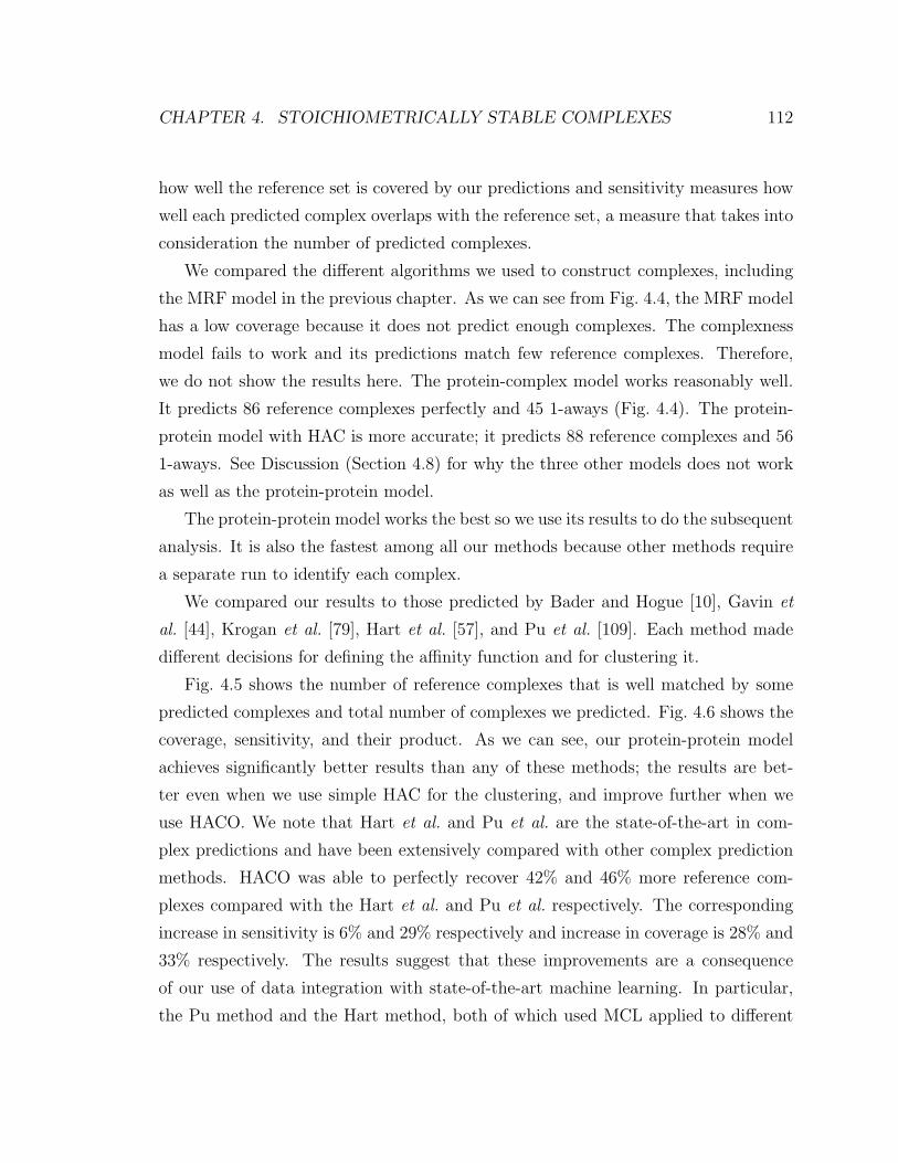
CHAPTER 4. STOICHIOMETRICALLY STABLE COMPLEXES 112
how well the reference set is covered by our predictions and sensitivity measures how
well each predicted complex overlaps with the reference set, a measure that takes into
consideration the number of predicted complexes.
We compared the different algorithms we used to construct complexes, including
the MRF model in the previous chapter. As we can see from Fig. 4.4, the MRF model
has a low coverage because it does not predict enough complexes. The complexness
model fails to work and its predictions match few reference complexes. Therefore,
we do not show the results here. The protein-complex model works reasonably well.
It predicts 86 reference complexes perfectly and 45 1-aways (Fig. 4.4). The protein-
protein model with HAC is more accurate; it predicts 88 reference complexes and 56
1-aways. See Discussion (Section 4.8) for why the three other models does not work
as well as the protein-protein model.
The protein-protein model works the best so we use its results to do the subsequent
analysis. It is also the fastest among all our methods because other methods require
a separate run to identify each complex.
We compared our results to those predicted by Bader and Hogue [10], Gavin et
al. [44], Krogan et al. [79], Hart et al. [57], and Pu et al. [109]. Each method made
different decisions for defining the affinity function and for clustering it.
Fig. 4.5 shows the number of reference complexes that is well matched by some
predicted complexes and total number of complexes we predicted. Fig. 4.6 shows the
coverage, sensitivity, and their product. As we can see, our protein-protein model
achieves significantly better results than any of these methods; the results are bet-
ter even when we use simple HAC for the clustering, and improve further when we
use HACO. We note that Hart et al. and Pu et al. are the state-of-the-art in com-
plex predictions and have been extensively compared with other complex prediction
methods. HACO was able to perfectly recover 42% and 46% more reference com-
plexes compared with the Hart et al. and Pu et al. respectively. The corresponding
increase in sensitivity is 6% and 29% respectively and increase in coverage is 28% and
33% respectively. The results suggest that these improvements are a consequence
of our use of data integration with state-of-the-art machine learning. In particular,
the Pu method and the Hart method, both of which used MCL applied to different

CHAPTER 4. STOICHIOMETRICALLY STABLE COMPLEXES 113
Figure 4.4: Prediction accuracy of our different models. We compare our predicted com-plexes with the reference complexes. x-axis are the different models we tried. MRF is the model weconstructed in the last chapter. Protein-complex model tries to learn an affinity function on howlikely a protein should belong to the same complex with a set of proteins. Protein-protein model isour two-stage approach where we first learn an affinity function on how likely two proteins belong tothe same complex. Then, we cluster the pairwise affinity network using HAC and treat the resultingclusters as our predicted complexes. The y-axis is the number of reference complexes that are wellmatched by our predictions. Blue bars are for reference complexes that are perfectly matched by ourpredictions. Green bars are for reference complexes that differ with some of our predicted complexesby one protein, either one extra or one fewer. Red bars are for reference complexes that differ withsome of our predicted complexes by two proteins. As we can see, the protein-protein model performsthe best. The complexness model has low accuracy so the result is not shown here.
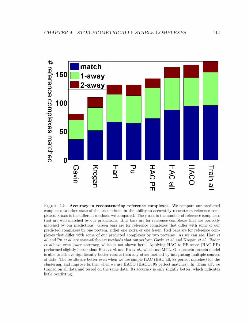
CHAPTER 4. STOICHIOMETRICALLY STABLE COMPLEXES 114
Figure 4.5: Accuracy in reconstructing reference complexes. We compare our predictedcomplexes to other state-of-the-art methods in the ability to accurately reconstruct reference com-plexes. x-axis is the different methods we compared. The y-axis is the number of reference complexesthat are well matched by our predictions. Blue bars are for reference complexes that are perfectlymatched by our predictions. Green bars are for reference complexes that differ with some of ourpredicted complexes by one protein, either one extra or one fewer. Red bars are for reference com-plexes that differ with some of our predicted complexes by two proteins. As we can see, Hart etal. and Pu et al. are state-of-the-art methods that outperform Gavin et al. and Krogan et al.. Baderet al.have even lower accuracy, which is not shown here. Applying HAC to PE score (HAC PE)performed slightly better than Hart et al. and Pu et al., which use MCL. Our protein-protein modelis able to achieve significantly better results than any other method by integrating multiple sourcesof data. The results are better even when we use simple HAC (HAC all, 88 perfect matches) for theclustering, and improve further when we use HACO (HACO, 95 perfect matches). In ‘Train all’, wetrained on all data and tested on the same data. Its accuracy is only slightly better, which indicateslittle overfitting.

CHAPTER 4. STOICHIOMETRICALLY STABLE COMPLEXES 115
Figure 4.6: Coverage and sensitivity of predicted complexes. x-axis is the sensitivity of ourpredictions, which quantifies how likely a prediction matches some reference complexes. y-axis isthe coverage of our predictions, which quantifies how many reference complexes are matched by ourpredictions. See text for the exact definition. All the results are based on cross-validation except for’Train all’, which is trained and tested on all data using Boosting and HACO. Our protein-proteinmodel (HAC all or HACO) has higher sensitivities and coverages than other methods. HACO hasthe highest product of sensitivity and coverage, except for ‘Train all’.

CHAPTER 4. STOICHIOMETRICALLY STABLE COMPLEXES 116
affinities obtained from the TAP-MS data, performed very similarly. Interestingly,
HAC applied to the PE score performed slightly better than MCL applied to the PE
score (HAC-PE vs. Pu et al.). These three methods performed better than Bader et
al., Gavin et al., and Krogan et al., which can be explained by the fact that these
earlier methods used only a single set of purifications. These results demonstrate the
importance of combining data from multiple data sources, integrated appropriately.
The HACO algorithm helps address several of the limitations of the HAC ap-
proach. First, it reduces the sensitivity of the complex definitions to a single uni-
versal threshold in the hierarchy. One such example involves the 15-protein SAGA
complex. Here, HAC predicts a 24-protein superset of the SAGA complex. This
cluster is a much weaker cluster than SAGA itself: the average affinity between the
SAGA proteins is 0.35, as compared to the average affinity, -1.19, for pairs within the
23 proteins excluding pairs of SAGA proteins. By comparison, HACO, by keeping
multiple hypotheses relative to the cutoff, predicted both a 23 protein cluster (similar
to the HAC prediction), but also predicted the subcluster that corresponds perfectly
to the SAGA complex. The second limitation addressed by HACO is that it avoids an
early commitment to incorrect outcomes. For example, the affinity between RAD23
and PNG1 is slightly higher than that between RAD23 and RAD4. HAC incorrectly
merges RAD23 and PNG1, and now cannot reuse RAD23 in any other complex.
HACO can reuse RAD23, merging it with RAD4 to create a complex that perfectly
matches the NEF2 (nucleotide-excision repair factor 2) complex in the reference set.
4.7.2 Contribution of each data source
Given the importance of data integration, it is useful to see which data sources play
the most important role in our results. We first considered the contribution of each
feature to our learned affinity function. Our approach uses LogitBoost [24], which
defines the affinity function as the weighted sum of many weak learners, each of which
is a decision stump on one of the features. The top weak learners involve features
that are deemed to be most predictive. The top weak learners in the order of their
importance use: correlation of PE score (weight 3.84); semantic similarity in the

CHAPTER 4. STOICHIOMETRICALLY STABLE COMPLEXES 117
truncated GO cellular component categories (-2.2); directed PE score (0.58); small-
scale physical interactions (0.55); and co-expression (0.16). It is interesting to note
that the correlation of the PE score is deemed more informative than the PE score
itself. One explanation is that the pairwise PE score between proteins P and Q is
still a noisy measure for co-complexness, but if two proteins are truly co-complexed,
they are likely to have similar interactions with other proteins.
To assess the contribution of each data source, we successively applied our pipeline
with HAC to the data source alone and to all data sources except that data source.
As we can see from Fig. 4.7, the PE score plays the dominant role and by itself
predicts most of the complexes. Importantly, our method here combines different
variations of PE score (direct, indirect, scaled, total, and correlation) using boosting,
generating an affinity score that is quite a bit better at predicting complexes than the
original scaled PE score (73/54/16 perfect matches/1-away/2-aways for ‘HAC PE’
in Fig. 4.5 versus 81/50/19 for the PE-based features alone in Fig. 4.7). This result
demonstrates the value of applying machine learning methods specifically optimized
for the problem of complex identification. Nevertheless, we still get a significant
improvement by integrating in other data sources.
Localization and expression have a similar effect. By itself, neither predicts any
complexes at all; this is not surprising, as both are features with low precision. How-
ever, removing each of them decreases the accuracy, suggesting that they provide a
signal that is independent of the PE score, and can help resolve some of its ambigui-
ties and errors. The yeast two-hybrid feature has the opposite behavior: In isolation,
it predicts a reasonable number of complexes; however, removing it does not decrease
accuracy at all. This behavior can be explained by the hypothesis that yeast two-
hybrid data largely correlates with PE score; thus, although it is predictive, it does
not add much given the PE score data. This last hypothesis is further verified by the
fact that localization and expression features appear within the top 5 weak learners
whereas the yeast two-hybrid feature does not.

CHAPTER 4. STOICHIOMETRICALLY STABLE COMPLEXES 118
Figure 4.7: Contribution of each data source. To assess the contribution of each data source,we successively applied our pipeline with HAC to the data source alone and to all data sourcesexcept that data source. The x-axis shows the runs with interesting observations. The y-axis is thenumber of reference complexes that are well matched by our predictions. Blue bars are for referencecomplexes that are perfectly matched by our predictions. Green bars are for reference complexesthat differ with some of our predicted complexes by one protein, either one extra or one fewer. Redbars are for reference complexes that differ with some of our predicted complexes by two proteins.As we can see, the PE score by itself predicts most of the complexes. Nevertheless, we still geta significant improvement by integrating other data sources. Localization or expression by itselfdoes not predict any complexes at all, but removing it decreases the accuracy. On the other hand,the yeast two-hybrid by itself predicts a reasonable number of complexes, but removing it does notdecrease accuracy at all.
CHAPTER 4. STOICHIOMETRICALLY STABLE COMPLEXES 119
4.7.3 Biological coherence of predicted complexes
We also evaluated the validity of our predicted complexes by comparing to external
data sources not used in the training and not directly related to reference complexes.
Here, we train on all reference complexes with the additional feature from the small-
scale experiments and predicted 383 complexes. For all biological coherence valida-
tions, we compute the coherence for each complex as the average of the coherence
measure for all pairs in the complex. Then, we take the average across all complexes
predicted. We compare to the methods of Hart et al. [57], and Pu et al. [109], which
consistently out-performed all previous methods. As a different benchmark, we also
compare to the coherence for the highest-affinity protein pairs (those that are most
likely to belong to the same complex).
We validate our predictions by looking at various measures of biological coherence
(Fig. 4.8): similarity of GO biological process; similarity in the level of protein abun-
dance for different complex components; correlation of growth defect profiles across a
broad range of conditions; and co-regulation, as measured by sharing of transcription
factors. For all measures, HACO with our affinity function considerably outperformed
all other approaches, with the method of Hart et al. being the closest competitor.
• GO data were downloaded on 25 June 2007. We compute the semantic distance
between two proteins as the log size of their smallest common category [89] in
the Biological Process hierarchy.
Our complexes have a semantic distance 8% and 17% lower than the methods
of Hart et al. and Pu et al. respectively. Conversely, they are 21% less coherent
than the reference complexes.
• We downloaded the protein abundance data from [47]. We use log of measured
protein levels in terms of molecules per cell as the protein abundance value.
The improvement in coherence of protein abundance is 5%, 10%; notably, here
our predicted complexes outperform the reference complexes by 2% on this
metric. However, our complexes are 12% less coherent than the top affinity
pairs, suggesting that proteins with lower affinity scores can be members of the

CHAPTER 4. STOICHIOMETRICALLY STABLE COMPLEXES 120
Figure 4.8: Coherence of our predicted complexes. We computed the functional coherencebetween proteins in the same complex against external data sources that are not used in training.More coherent proteins have a smaller difference in protein abundance and a smaller distance in GObiological process. On the other hand, more coherent proteins share more transcriptional regulatorsand have a higher growth fitness correlation. The y-axis shows the values for above measurementsof functional coherence. The highest point of the y-axis is the coherence for random protein pairsin the case of protein abundance and GO biological process. The lowest point of the y-axis is thecoherence for random pairs in the case of regulator overlap and growth correlation. As we can see,our predicted set of complexes is able to outperform other state-of-the-art methods. It is even betterthan the reference set of complexes in two cases and only marginally worse in another case. For theremaining case regarding GO biological process, we are worse only because the reference complexesand GO annotation are derived (at least partly) from similar data sources.
CHAPTER 4. STOICHIOMETRICALLY STABLE COMPLEXES 121
complex, but also play other roles in the cell, reducing their correlation with
other proteins in the same complex.
• The growth phenotype data was obtained from [58]. For each gene, its homozy-
gous deletion strain is grown in 418 experiments with different drug treatments.
The log ratio of the deletion strain’s growth in no-drug control to its growth
with the drug treatment is used to define the growth phenotype in that partic-
ular condition. For each pair of genes, we compute the Pearson correlation of
the growth phenotypes across all 418 conditions. Based on this measure, our
predicted complexes are 19%, 31% more coherent than Hart et al. and Pu et
al. respectively, a very significant improvement. They are 4% worse than the
reference complexes.
• We downloaded the transcriptional regulation data from [91, 56]. We used
p-value cutoff at 0.001 and required conservation across species to define the
transcription factors for each protein. Protein pairs within our complexes on
average share 30%, 59% more transcription factors then those in Hart et al. and
Pu et al. respectively. They share 17% more transcription factors than those in
the reference complexes.
The comparison to the reference complexes is also interesting: Our complexes are
17% more coherent than the reference complexes on regulator overlap, and perform
similarly on correlation of abundance and growth phenotype (within ±4%). Con-
versely, our complexes are 21% less coherent than the reference complexes on GO
biological process annotations; this is not surprising, as the reference complexes and
GO annotations are derived (at least partly) from similar data sources, such as litera-
ture and small scale experiments. Overall. when comparing to data sources that were
not used in constructing the reference complexes, our predictions seem to perform as
well or better than the reference set, suggesting that our predictions provide a strong
set of complexes that can be used as a new reference.

CHAPTER 4. STOICHIOMETRICALLY STABLE COMPLEXES 122
4.7.4 Essentiality and complex size
Much discussion has occurred regarding the relationship between essentiality and the
structure of the protein-protein interaction network. Early work of Jeong et al. and
Han et al. [66, 55] found that hub proteins in a protein-protein interaction network
are more likely to be encoded by essential genes. However, a much deeper insight
on the relationship between the protein network and essentiality can be obtained by
considering the network at the level of complexes rather than pairwise interactions.
Such an analysis was recently performed by Hart et al. [57], who showed that essential
proteins are concentrated in certain complexes, a phenomenon also found in our
predicted complexes (Fig. 4.9). Thus, we have a dichotomy of essential and non-
essential complexes. However, that finding does not explain why ‘hubs’ in the network
are more likely to be essential. We therefore looked into the distribution of essential
proteins in complexes of different sizes. As we can see from Fig. 4.10, the larger
the complex, the greater the proportion of essential proteins among its components.
This finding suggests that ‘hubs’ in the protein interaction network are generally
components in a large complex, and the finding regarding the essentiality of hubs
arises from the fact that large complexes are more likely to have a much higher ratio
of essential genes.
Indeed, we found that essentiality is better explained by complex size than hub-
ness. We rank every protein based on the size of the largest complex to which it
belongs, and for the K top-ranked proteins (for different values of K), plot the num-
ber of essential vs. non-essential proteins (Fig. 4.11). We plotted a similar curve
by using the hubness of the protein — the degree in the yeast two-hybrid protein-
protein interaction network [63, 127]. As we can see, complex size is a much better
predictor for essentiality than hubness. We note that if we use the scaled PE score (at
threshold ¿ 0.5) to define a protein-interaction network, the hubness becomes a strong
predictor of protein essentiality. However, PE score is more related to co-complexness
than interaction, and thus this metric of hubness is directly related to complex size.
Nevertheless, using complex size directly is still better than using scaled PE score.
Interestingly, if we use the size of the largest enclosing reference complex to rank each
protein, the result is slightly less predictive than using our predicted complexes, or

CHAPTER 4. STOICHIOMETRICALLY STABLE COMPLEXES 123
Figure 4.9: Proportion of essential proteins across complexes. For each complex, wecompute the proportion of its protein members that are essential. The x-axis is a specific bin andthe y-axis is the number of complexes whose proportion of essential proteins falls into that bin.As we can see, most complexes have either few essential proteins (< 10%) or almost all essentialproteins (> 90%).
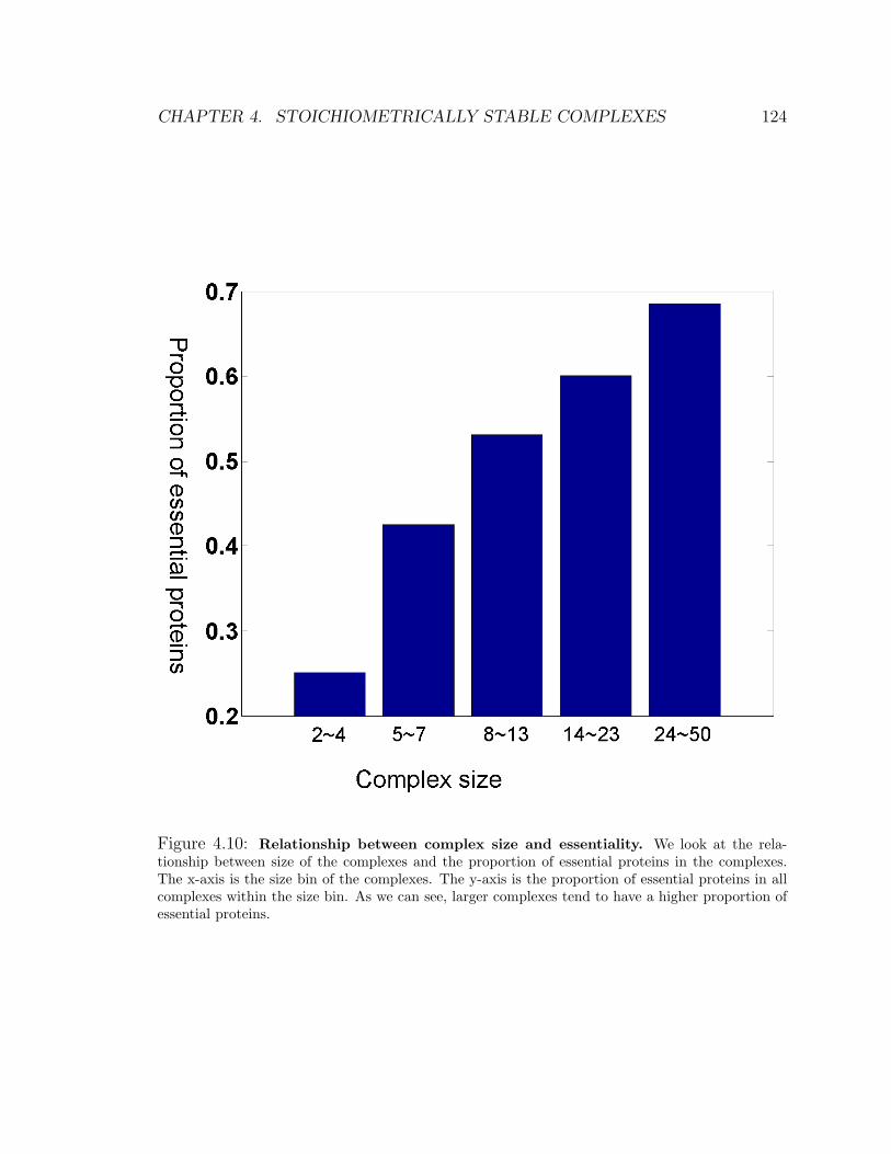
CHAPTER 4. STOICHIOMETRICALLY STABLE COMPLEXES 124
Figure 4.10: Relationship between complex size and essentiality. We look at the rela-tionship between size of the complexes and the proportion of essential proteins in the complexes.The x-axis is the size bin of the complexes. The y-axis is the proportion of essential proteins in allcomplexes within the size bin. As we can see, larger complexes tend to have a higher proportion ofessential proteins.

CHAPTER 4. STOICHIOMETRICALLY STABLE COMPLEXES 125
Figure 4.11: Explaining essentiality using complex size vs. hubness. We try to explain theessentiality of a protein by using the size of the largest enclosing complex vs. by using its hubnessin the protein-protein interaction network. We rank the proteins based either on complex size or onhubness. The x-axis is the number of essential proteins in the K top-ranked proteins (for differentvalues of K) and the y-axis is the number of non-essential proteins. For the red curve, we use thesize of the predicted complexes while the light blue curve uses the size of the reference complexes.For the blue curve, we use the hubness — degree in the yeast two-hybrid protein-protein interactionnetwork. The green curve also uses the hubness but in a network whose edges have scaled PE score> 0.5. As we can see, complex size is a much better predictor for essentiality than hubness (bluecurve). Since the PE score is more related to co-complexness than interaction, the hubness based onPE score (green curve) is directly related to complex size. Nevertheless, using the size of predictedcomplexes directly (red curve) is still better than using the PE score. Interestingly, using the size ofreference complexes (light blue curve) is slightly less predictive than using the size of our predictedcomplexes, or even the PE score directly.
CHAPTER 4. STOICHIOMETRICALLY STABLE COMPLEXES 126
even the scaled PE score directly.
4.8 Discussion
Identifying a comprehensive set of protein complexes in yeast is an important but
challenging task. The high-quality and high-throughput TAP-MS data, which directly
measures co-complexness, provides a starting point for accurately reconstructing these
complexes. Indeed, two recent studies [57, 109] used the TAP-MS data to produce
a set of complexes with the state-of-the-art performances. Both methods applied a
simple clustering algorithm to a score derived directly from the TAP-MS data.
In this chapter, we tried four different methods and the protein-protein model
is able to significantly improve the accuracy of the complex reconstruction in three
ways. First, we carefully constructed a large set of reference complexes and trained our
model so it specifically predicts co-membership in stoichiometrically stable complexes.
Second, we integrated multiple sources of heterogeneous data so our predictions are
more robust to noise and incomplete coverage in the TAP-MS data. Finally, we ex-
tended the highly effective hierarchical agglomerative clustering (HAC) algorithm to
allow reconstruction of clusters with overlap, a flexibility that allows it to circumvent
many of the limitations of the standard HAC algorithm. We show that the resulting
set of predicted complexes (available from our website [4]) has significantly higher
accuracy and is more biologically coherent than that of other recent methods. In
many cases, it is even more coherent than the reference set, indicating it is of high
quality and can be used as a new reference set. When combined with our comprehen-
sive, hand-curated reference set (also available from our website), our work provides
a significant new resource to the research community.
The other three methods we tried to reconstruct complexes all seems to have
reasonable intuition behind them. It turns out, however, both the Markov Network
model and complexness model has low accuracy. We looked more carefully into
the reasons why they do not work. After a certain number of complexes predicted,
the Markov Network model mostly constructs complexes that are identical to the
ones discovered before. Therefore, we end up with a limited number of complexes

CHAPTER 4. STOICHIOMETRICALLY STABLE COMPLEXES 127
predicted. As for the complexness model, it tries to compute a coherence value for
a set of proteins based on how coherent its features are such as PE score and co-
expression. However, if a complex is coherent, its subsets, especially those closely
connected components, are also likely to be coherent. Therefore, our RankBoost
model is unable to distinguish a complex from its subsets, which severely limits its
ability in identifying complexes.
Both the protein-complex model and protein-protein model achieved good accu-
racy, with the latter being unequivocally better. One problem for the protein-complex
model is that at each iteration, it considers every protein outside the current complex
to be a possible candidate to be added. Since there are thousands of proteins outside
the complex, the chances that at least one of them would have a positive affinity with
the current set is high, even if we have low false positive rate. Therefore, even if the
current set is already a complex, we are still likely to add in extra proteins, which
causes the prediction to be not perfect. On the other hand, in the protein-protein
model, at each step of the HAC, we consider merging two sets instead of individual
proteins. So if some set in the current pool is already a complex, it will be considered
to merge with other sets in the pool only, which is a relatively small number, and since
we use average linkage, one false high affinity between the two sets would be averaged
out by other pairs with low affinities. Therefore, our set is less likely to be merged
with other sets that are not in the same complex, and thus the prediction would be
perfect. As for HACO, we prefer to use the superset as the merging candidate unless
the subset satisfy some stringent criteria. This also limits the choices a set has as its
merging candidate.
There are still many reference complexes that are not matched by our predicted
complexes. Many of them fall into roughly two categories. In the first category,
proteins in the reference complex have high affinities with each other, and are grouped
as a set during the HACO procedure. However, they are not selected in our predictions
because they are not at the granularity where we cut our HACO cluster-lattice. They
then become subsets or supersets of some predicted complexes. In fact, if we use all
the sets generated during our HACO procedure as predicted complexes, 136 reference
complexes would be perfectly predicted and 243 would be well matched by some

CHAPTER 4. STOICHIOMETRICALLY STABLE COMPLEXES 128
predicted complexes, in comparison to 95 perfect matches and 189 well matched by our
current predictions. However, this approach would result in far too many predictions
(3478), greatly reducing sensitivity. This fact highlights the limitations in defining
a universal level of affinity at which one determines that a group of proteins form a
stable complex, and suggests that a more flexible technique may be a useful direction
for future work. In the second category, the proteins in the reference complex do not
have high affinities with each other. This situation arises when the signal in the data
is not sufficiently strong to indicate that two proteins are likely to interact. As most of
our signal comes from the TAP-MS data, such ‘blind spots’ can arise from limitations
of this assay, such as complexes of low abundance or that are membrane-bound. In
particular, we note that the TAP-MS data was all acquired in a single condition (rich
media), and some complexes may simply not be present in the cell in that condition.
Our inability to recover such complexes arises not from computational limitations,
but from limitations in the data. New experimental assays are needed before these
complexes can be reconstructed.
Like other previous approaches, our method was developed in the context of S.
cerevisiae, where we have the most data relevant to protein-protein interactions. Hav-
ing a high-quality set of predicted complexes is of significant value even in yeast, as
many key complexes are conserved from yeast to human. Moreover, our method is
general-purpose, and can easily be applied more broadly. With the increasing amount
of high-throughput protein-protein interaction data, both TAP-MS [37] and other as-
says [108, 123], we should soon be able to provide a high-quality reconstruction of
protein complexes in other organisms, including human.

Chapter 5
Complex-complex interactions
In this chapter, we use the complexes we predicted in the previous chapter as basic
units, and predict interactions between them. Complexes that interact with each
other are more likely to be involved in the same biological pathway. This puts proteins
or complexes into a larger context for us to understand how they influence cellular
processes. In the end, we create a unified network of interactions between core cellular
units — complexes and proteins.
5.1 Introduction
Complexes and individual proteins that act alone are the basic entities, or building
blocks, from which the protein interaction network in the cell is comprised. Given
the set of complexes we predicted in the previous chapter, which is high-quality and
comprehensive, we now try to reconstruct the network of interactions between these
entities. Interactions between entities usually happen when they try to coordinate
their activities to achieve a certain biological task. For example in a signaling path-
way, an entity (a protein or complex) receives signals from an upstream entity, and
interacts with a downstream entity to activate or inhibit its function. Once activated
or inhibited, the downstream entity passes the signal further down through more
interactions. The interactions between upstream and downstream entities usually
129

CHAPTER 5. COMPLEX-COMPLEX INTERACTIONS 130
involve post-translational modification of the downstream entity, such as phosphory-
lation or methylation, which triggers a change in its 3D configuration and enables its
activities. In general, unlike the interactions between proteins within the same com-
plex, the interactions between complexes are more transient. They happen only in a
certain context, involving a specific time, location, or condition. Understanding such
interactions is important for understanding cellular interactions and for providing a
higher level view of cellular processes.
In this chapter, we reformulate the task of reconstructing the protein interaction
network, which is the focus of much prior work. Rather than predicting interac-
tions between individual proteins — a somewhat confusing network that confounds
interactions within complexes and interactions between complexes — we tackle the
novel task of predicting a comprehensive protein interaction network that involves
both individual proteins and larger complexes. We argue that these entities are the
right building blocks in reconstructing cellular processes, providing a view of cellu-
lar interaction networks that is both easier to interpret than the complex network
of interactions between individual proteins, and more faithful to biological reality.
Moreover, a complex, which is a stable collection of many proteins that act together,
provides a more robust basis for predicting interactions, as we can combine signals
for all its constituent proteins, reducing sensitivity to noise.
To accomplish this goal, we construct a reference set of complex-complex inter-
actions, considering two complexes to interact if they are significantly enriched for
reliable interactions between their components. We further augmented this set with
a hand-curated list of established complex-complex interactions. We then use a ma-
chine learning approach to detect the ‘signature’ of such interactions from a large
set of assays that are likely to be indicative. We explore different machine learning
methods, and show that a partially supervised naive Bayes model, where we learn the
model from both labeled and unlabeled interactions, provides the best performance.
This model is applied both to our predicted complexes and to individual proteins,
providing a new, comprehensive reconstruction of the S. cerevisiae interaction net-
work, which can be downloaded from our webpage [3]. We show that entities that
are predicted to interact are more likely to share the same functional categories.

CHAPTER 5. COMPLEX-COMPLEX INTERACTIONS 131
5.2 Related work
Much work has focused on predicting interactions, possibly transient, between pro-
teins. For example, Deng et al. [31] and Liu et al. [88] tried to predict protein-protein
interactions by building a graphical model that takes into consideration the protein
sequence motifs and observed protein-protein interactions. Bock and Gough [14] used
Support Vector Machines (SVM), a supervised learning approach, to predict inter-
actions based on the physicochemical properties of the amino acids on the protein
sequence. Importantly, our work predicts interactions between complexes instead of
just between proteins. Computationally, this enables us to combine the signals from
all the constituent proteins in the complexes, which reduces the sensitivity to noise
so the result is more robust. Biologically, this gives a more interpretable interaction
network.
Some other approaches mentioned earlier [22, 84, 92, 117, 124, 129, 131, 135, 138]
integrate multiple sources of data to predict whether two proteins are functionally
related: act in the same complex, pathway, or functional module. By comparison, our
work focuses specifically on predicting transiently interacting pairs, which is the first
step in identifying co-pathway complexes. It also provide us with a way to understand
the internal structure, with which complexes coordinate with each other to execute a
pathway.
5.3 Reference list of positive and negative complex-
complex interactions
We use the same set of reliable interactions as in Section 2.3.1. We compute the
number of reliable interactions between proteins of two complexes, and compared it
to what we expect if the reliable interactions are distributed randomly. We define the
two complexes to be interacting if the enrichment of reliable interactions is more than
20 standard deviations above the mean. This gives us a list of 82 interactions between
the set of 383 complexes we just predicted. To augment this list, we generated a list
of 59 additional known interactions between 81 named complexes. Both lists are

CHAPTER 5. COMPLEX-COMPLEX INTERACTIONS 132
available from our website [3]. To avoid the redundancy between those 81 named
complexes and our 383 predicted complexes, we replace a predicted complex by a
named complex if they overlap with Jaccard coefficient > 0.5. This process gives
us a total of 421 complexes with 133 unique interactions between them, which is
used as our positive reference set. The named complexes are better known and more
thoroughly studied so if a pair of named complexes is not known to interact, they
are more likely to be non-interacting. Therefore, we create a negative reference set
of 3173 non-interactions by using all pairs of named complexes that are not in our
positive set. The interaction status of all the remaining pairs of complexes, named or
predicted, is treated as unknown.
We also apply our model to predict a unified interaction network involve both
proteins and complexes. In this case, we have both the interaction between two
complexes and the interaction between a protein and a complex. We create the
positive set using the same procedure as above. As for the negative set, in addition
to the above negative reference set between complexes, we randomly sampled 6560
protein-complex pairs that are not in the positive set and added them to our negative
reference set. The number 6560 is chosen so the ratio of positive to negative pairs for
protein-complex interactions is the same the ratio for complex-complex interactions.
All our reference lists are available from our website [3].
5.4 Protein-level signals for predicting complex-
complex interactions
Since there is no direct measurement of complex-complex interactions, we try to use
as much indirect evidence as possible. Besides all data sources used for identifying
complexes, we added four additional data sources based on correlation of growth fit-
ness, correlation of transcription factor profile, protein-protein interaction prediction,
and condition specific expression correlation.
The correlation of growth fitness profile [58] is computed as described in Sec-
tion 4.7.3.
CHAPTER 5. COMPLEX-COMPLEX INTERACTIONS 133
For each protein, we create a transcription factor (TF) profile vector, where each
position in the vector represents a TF and its value is 1 if the TF is found to regulate
the protein [91] and 0 if it is not. We used the same transcription regulation data
as described in Section 4.7.3. For any pair of proteins, we compute the mutual
information between the profile vectors of the two proteins using the method described
in Date et al. [29].
There are many works on integrating multiple sources of data to predict protein-
protein interactions. In particular, the InSite method [133] in Chapter 2 integrates
protein sequence motifs, evidence for protein-protein interactions, and evidence for
motif-motif interactions in a principled probabilistic framework to make high-quality
predictions of protein-protein interactions. Here, we use the InSite method, but
trained without the reliable interactions between complexes in our positive reference
set. We use the predicted probabilities that two proteins interact as one more data
source.
We processed the expression data in accordance with our intuition that transient
interactions occur under specific conditions, and we should only expect expression
profiles of interacting proteins to be correlated only when at least one of the pair
is active. Specifically, we divided our expression data into 76 conditions [139, 95,
20, 81, 106, 43, 42, 32, 70], each of which represents a particular time course. In
accordance with convention, we quantify a proteins activity under certain condition
according to its maximum deviation from norm, or in other words the maximum
absolute expression (assuming norm to be 0). For each condition, we define a protein
to be differentially expressed, or active, if its maximum absolute expression is above
a cutoff, which we specify to be 1.0. For each pair of proteins, we compute Pearson
Correlation Coefficient (PCC) separately in each condition. If a protein in the pair is
inactive under a condition, the PCC value for the condition is assumed to be 0. We
use the PCC value, averaged across all conditions under which at least one protein
out of the pair is active, as our last signal. Initial investigation showed that this
signal is better correlated with the reference complex-complex interactions than the
overall PCC across all conditions. We note that, for the task of predicting when two
proteins are co-complexed, the simple correlation performed better (data not shown),

CHAPTER 5. COMPLEX-COMPLEX INTERACTIONS 134
consistent with the fact that the activity of two members of a stable complex is likely
to be similar across a wide range of conditions.
5.5 Aggregating signals into features between com-
plexes
All forms of signals in our analysis involve a pair of proteins. To predict interactions
between two complexes, C and D, we aggregate the signals for all protein pairs
between C and D and produce the following features:
fij = Ai({Sj(P,Q)|P ∈ C,Q ∈ D})
where Ai() is some aggregating function, such as: sum, max, mean, min, decayed
max, decayed min, etc. We use the same list of aggregating functions as in Appendix
A. Sj() represents the j’th signal type between a pair of proteins. We also use four
global features, independent of the data sources: size of the first complex, size of the
second complex, number of protein pairs between the two complexes, and number of
overlapping proteins between the two complexes.
The Naive Bayes model that we use assumes all features to be conditionally in-
dependent of each other given the status of whether two complexes interact or not.
Therefore for each data source, we pick only the best aggregating function in order
to reduce the conditional dependencies between the features. To do this, we define
rij to be the area under the ROC curve if we use the feature fij alone to predict
complex-complex interactions. The greater the rij, the stronger correlation between
the feature and the complex-complex interactions. Therefore, for Naive Bayes, we
use the following features in addition to one of the four global features:
fj = fij where i = argmaxi
rij
The aggregating functions chosen for our signals and the global feature are listed
in Table 5.1.

CHAPTER 5. COMPLEX-COMPLEX INTERACTIONS 135
Direct PE score MaxIndirect PE score MaxScaled PE score SumPE score correlation SumGO distance MinTrans-membrane SumCo-expression (SMD) Average of top three valuesInSite Decayed minFitness correlation Average of top three valuesTF Mutual information SumTime-series correlation MaxGFP localization Number of pairs with different localizationGlobal Number of protein pairs
Direct PE score MaxIndirect PE score MaxScaled PE score SumPE score correlation SumGO distance Decayed minTrans-membrane SumCo-expression (SMD) Average of top three valuesInSite Decayed minFitness correlation Average of top three valuesTF Mutual information SumTime-series correlation MaxGFP localization Fraction of pairs with different localizationGlobal Number of protein pairs
Table 5.1: List of aggregating functions chosen. We plot the ROC curve of each aggregatingfunction, applied to a data source, in predicting interactions and pick the aggregating function thathas the maximum area under the curve. The data source is listed in the first column and thecorresponding best aggregating function is listed in the second column. Among all global features,we also pick the one that has the maximum area under the ROC curve. The first table is for thecomplex-complex interaction network and the second table is for the unified interaction networkinvolving both proteins and complexes.

CHAPTER 5. COMPLEX-COMPLEX INTERACTIONS 136
5.6 Methods
We experimented with different machine learning algorithms for making our predic-
tions: (1) a simple Naive Bayes model, where the effects of different feature types
are assumed to be independent; (2) a discriminative boosting algorithm, as we used
in predicting co-complexed affinities between protein pairs above; (3) a Naive Bayes
model where the unlabeled complex-complex interactions are taken to be unobserved
variables, and the model is trained via the Expectation Maximization (EM) algo-
rithm. This last approach is based on the fact that the amount of labeled training
data is quite limited in this task, but the unlabeled data also provides us with useful
information about the behavior of different features in interacting and non-interacting
pairs. A variant of this same approach was used with success in the InSite model [133]
in Chapter 2.
More formally, for each pair of complexes, we construct an ‘interaction variable’,
whose value is 1 if the two complexes are in the positive reference set of interacting
complexes, 0 if they are in the negative reference set, and unobserved otherwise. Each
feature of the complex pair is associated with two conditional distributions: one for
the case of an interacting and the other for the case of a non-interacting pair. These
distributions are defined via some parametric classes (Table 5.2), which are picked
by examining the empirical distributions. The distributions for the different features
are taken to be independent of each other within each of the two cases. The model
is trained via the following EM procedure. We initialize the model parameters to
those that would be obtained from MLE estimation using the pairs in our reference
set alone. We then iteratively repeat the following two steps until convergence. In
the E-step, we use our current model to compute the marginal probability of each
unobserved interaction variable given the features associated with the pair. We use
the computed probability as a soft assignment to the interaction variable. In the M-
step, we learn the parameters for the distributions using the inferred soft assignment
to all interaction variables; the variables in the reference set are always fixed to their
known value. We use the model obtained at convergence to predict, for each pair of
complexes not in our reference set, the probability with which the pair interacts.
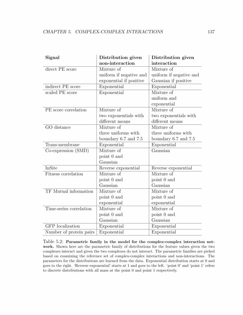
CHAPTER 5. COMPLEX-COMPLEX INTERACTIONS 137
Signal Distribution given Distribution givennon-interaction interaction
direct PE score Mixture of Mixture ofuniform if negative and uniform if negative andexponential if positive Gaussian if positive
indirect PE score Exponential Exponentialscaled PE score Exponential Mixture of
uniform andexponential
PE score correlation Mixture of Mixture oftwo exponentials with two exponentials withdifferent means different means
GO distance Mixture of Mixture ofthree uniforms with three uniforms withboundary 6.7 and 7.5 boundary 6.7 and 7.5
Trans-membrane Exponential ExponentialCo-expression (SMD) Mixture of Gaussian
point 0 andGaussian
InSite Reverse exponential Reverse exponentialFitness correlation Mixture of Mixture of
point 0 and point 0 andGaussian Gaussian
TF Mutual information Mixture of Mixture ofpoint 0 and point 0 andexponential exponential
Time-series correlation Mixture of Mixture ofpoint 0 and point 0 andGaussian Gaussian
GFP localization Exponential ExponentialNumber of protein pairs Exponential Exponential
Table 5.2: Parametric family in the model for the complex-complex interaction net-work. Shown here are the parametric family of distributions for the feature values given the twocomplexes interact and given the two complexes do not interact. The parametric families are pickedbased on examining the reference set of complex-complex interactions and non-interactions. Theparameters for the distributions are learned from the data. Exponential distribution starts at 0 andgoes to the right. ‘Reverse exponential’ starts at 1 and goes to the left. ‘point 0’ and ‘point 1’ refersto discrete distributions with all mass at the point 0 and point 1 respectively.

CHAPTER 5. COMPLEX-COMPLEX INTERACTIONS 138
Signal Distribution given Distribution givennon-interaction interaction
direct PE score Mixture of Mixture oftwo exponentials with exponential anddifferent means Gaussian
indirect PE score Mixture of Mixture ofpoint 0 and point 0 andGaussian Gaussian
scaled PE score Mixture of Mixture ofpoint 0 and point 0 andexponential exponential
PE score correlation Mixture of Mixture oftwo exponentials with two exponentials withdifferent means different means
GO distance Mixture of Mixture ofthree uniforms with three uniforms withboundary 6.7 and 8.4 boundary 6.7 and 8.4
Trans-membrane Exponential ExponentialCo-expression (SMD) Mixture of Gaussian
point 0 andGaussian
InSite Reverse exponential Reverse exponentialFitness correlation Mixture of Mixture of
point 0 and point 0 andGaussian Gaussian
TF Mutual information Mixture of Mixture ofpoint 0 and point 0 andexponential exponential
Time-series correlation Mixture of Gaussianpoint 0 andGaussian
GFP localization Mixture of Mixture ofpoint 0, point 1, and point 0, point 1, andGaussian Gaussian
Number of protein pairs Exponential Exponential
Table 5.3: Parametric family in the model for the unified interaction network. Same asTable 5.2 except here the parametric families are picked based on examining the reference set forthe unified interaction network involving both proteins and complexes.

CHAPTER 5. COMPLEX-COMPLEX INTERACTIONS 139
When training using the LogitBoost model, we are not making independence
assumptions between the different features. Hence, there we include all features fij,
instead of just picking the best aggregating function for each feature type.
We used the same naive Bayes + EM procedure for the protein-complex interaction
predictions, although the best aggregating functions picked and the set of parametric
classes used for the feature distributions was a little different. (See Table 5.1 and
Table 5.3.)
5.7 Results
5.7.1 Accuracy of complex-complex interaction predictions
We compiled a reference set of complex-complex interactions from reliable protein-
protein interactions and hand-curation. There are 133 interactions in the positive
reference set and 3173 non-interactions in the negative reference set.
We used ten-fold cross-validation to evaluate the ability of our model in accurately
predicting complex-complex interactions. We randomly divide our reference interac-
tions into ten sets. In each fold, we hide one set and train on the remaining nine sets.
We then make predictions on the held-out set using the learned model. We compare
three methods (see Methods): simple Naive Bayes, a discriminative Boosting method,
and Naive Bayes with EM (NB+EM) that also makes use of the data for pairs that
are not in our reference set. As we can see from Fig. 5.1, ‘NB+EM’ performs better
than both other methods, achieving very high performance: 44 of the top 50 predic-
tions (88%) are in the positive reference set. We also compared these results to two
state-of-the-art methods for predicting protein-protein interactions: the PE score and
the InSite probabilities. As we can see, by integrating multiple sources of data, we
are able to improve the accuracy to 0.88 (area under the ROC curve) from 0.85 and
0.79 for PE score and InSite probabilities respectively. The PE score provides the
strongest signal; using it alone or combining it with other subsets of data sources is
able to predict complex-complex interaction with an accuracy that is slightly lower
than our integrated model (Fig. 5.1).
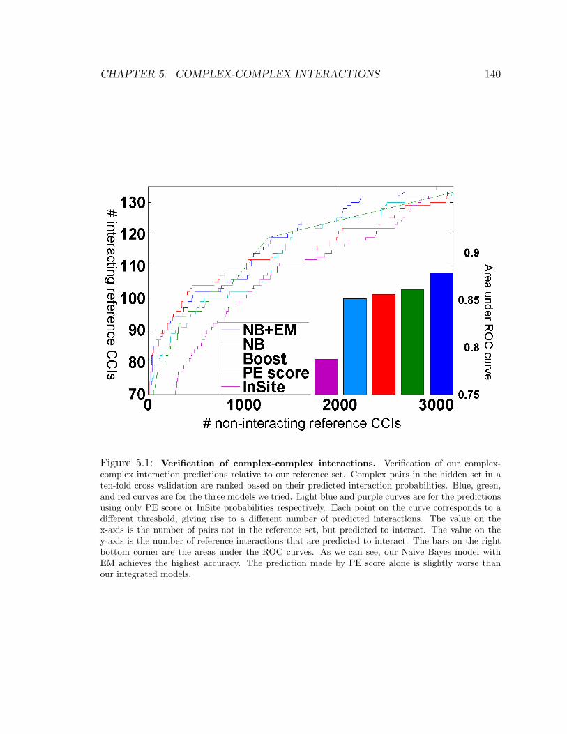
CHAPTER 5. COMPLEX-COMPLEX INTERACTIONS 140
Figure 5.1: Verification of complex-complex interactions. Verification of our complex-complex interaction predictions relative to our reference set. Complex pairs in the hidden set in aten-fold cross validation are ranked based on their predicted interaction probabilities. Blue, green,and red curves are for the three models we tried. Light blue and purple curves are for the predictionsusing only PE score or InSite probabilities respectively. Each point on the curve corresponds to adifferent threshold, giving rise to a different number of predicted interactions. The value on thex-axis is the number of pairs not in the reference set, but predicted to interact. The value on they-axis is the number of reference interactions that are predicted to interact. The bars on the rightbottom corner are the areas under the ROC curves. As we can see, our Naive Bayes model withEM achieves the highest accuracy. The prediction made by PE score alone is slightly worse thanour integrated models.

CHAPTER 5. COMPLEX-COMPLEX INTERACTIONS 141
5.7.2 Functional coherence of interacting complexes
We evaluate whether two interacting complexes are more likely to share the same
functional category, which is not used in our training. We used functional categories
from MIPS [97], which has 18 functional categories with average 684 proteins per
category. A complex is assigned to a particular functional category if more than half of
its components belong to the functional category. We only perform our evaluation on
complex pairs where both complexes are assigned to some MIPS functional category.
We trained our model on the entire reference set of complex-complex interactions
and perform the evaluation on the top 500 predicted pairs of interacting complexes.
Among them, as we can see from Fig. 5.2, 59.2% consist of complexes that share the
same MIPS functional category, compare to only 35.2% among the random complex
pairs. Therefore, our predicted set of interacting complexes is functionally more
coherent.
5.7.3 Accuracy of unified interaction network
We also apply our model to predict a unified network involving both proteins and
complexes. In this case, we have both the interactions between two complexes and
the interactions between a protein and a complex. As we can see from Fig. 5.3, by
integrating multiple data sources, our Naive Bayes model with EM is able to achieve
higher accuracy than using PE score alone. We generated predictions for all protein-
complex pairs and complex-complex pairs by training on the entire reference set (see
our supporting website for the complete list of the predictions [3]). Combined with
high-quality protein-protein interaction predictions [133], we provide biologists with
a unified interaction network involving both proteins and complexes.
5.7.4 Conditions when two complexes interact
Due to our use of condition-specific time-series expression data as a cue for determin-
ing interaction, our analysis can also provide hypotheses regarding the condition in
which two complexes interact. Between each pair of interacting complexes, we find
the two proteins with the highest correlation. We then list the condition when the
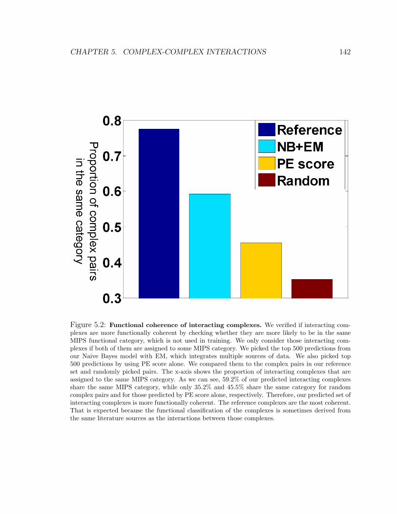
CHAPTER 5. COMPLEX-COMPLEX INTERACTIONS 142
Figure 5.2: Functional coherence of interacting complexes. We verified if interacting com-plexes are more functionally coherent by checking whether they are more likely to be in the sameMIPS functional category, which is not used in training. We only consider those interacting com-plexes if both of them are assigned to some MIPS category. We picked the top 500 predictions fromour Naive Bayes model with EM, which integrates multiple sources of data. We also picked top500 predictions by using PE score alone. We compared them to the complex pairs in our referenceset and randomly picked pairs. The x-axis shows the proportion of interacting complexes that areassigned to the same MIPS category. As we can see, 59.2% of our predicted interacting complexesshare the same MIPS category, while only 35.2% and 45.5% share the same category for randomcomplex pairs and for those predicted by PE score alone, respectively. Therefore, our predicted set ofinteracting complexes is more functionally coherent. The reference complexes are the most coherent.That is expected because the functional classification of the complexes is sometimes derived fromthe same literature sources as the interactions between those complexes.

CHAPTER 5. COMPLEX-COMPLEX INTERACTIONS 143
Figure 5.3: Verification of our unified interaction network. Verification of our predictionsinvolving both protein-complex interactions and complex-complex interactions against the referenceset. Complex pairs in the hidden set of a ten-fold cross validation are ranked based on their predictedinteraction probabilities. Blue curve is for our Nave Bayes model with EM. Green curve is for thepredictions using only PE score. Each point on the curve corresponds to a different threshold, givingrise to a different number of predicted interactions. The value on the x-axis is the number of pairsnot in the reference set, but predicted to interact. The value on the y-axis is the number of referenceinteractions that are predicted to interact. The area under the blue curve is 0.82 and the area underthe green curve is 0.73. Therefore, our data integration is able to achieve better accuracy than usinga single data source alone.

CHAPTER 5. COMPLEX-COMPLEX INTERACTIONS 144
two proteins are most correlated (see our supporting website [3]). This list provides
the biologists with a clue about when the interaction occurs.
5.8 Discussion
With our high-quality set of predicted complexes from Chapter 4, we are able to take
a higher-level perspective on the protein-protein interaction network, viewing it in
terms of interactions between atomic units — whether individual proteins or stable
complexes. There has been much work on predicting protein-protein interactions.
However, these pairwise interactions are often induced by higher-level relationships:
those within a complex and those between complexes. Interactions within a com-
plex give rise to densely connected subgraphs in the interaction network; interactions
between complexes can give rise to a network of interconnections involving different
members of the two complexes. Viewing the network in terms of its atomic units
can help clarify its structure and its basic properties. We therefore defined the novel
problem of predicting interactions between complexes and other complexes or pro-
teins, and constructed a new, high-accuracy method for making such predictions.
The result of our analysis is a unified interaction network involving both proteins and
complexes. We can now analyze the properties of this network, such as its connectiv-
ity and hierarchical structure, which better captures the true interactions underlying
cellular processes.
Our work takes a step towards a more hierarchical view of the protein-protein
interaction network, moving up from individual proteins to complexes as the basic
interacting units. The next level of the hierarchy is the pathways that comprise
cellular pathways. Although the notion of a ‘pathway’ is not as well-defined, it would
nevertheless be very useful to reconstruct pathways that are comprised of interacting
complexes and proteins. We can then move even higher in the cellular hierarchy,
and study the interactions between pathways. This type of analysis will give us a
unified perspective on the underlying hierarchical organization of the cell, and provide
significant insight.

Chapter 6
Conclusions
In this final chapter, we summarize the contributions of this thesis and outline some
future direction.
6.1 Summary
In this thesis, we try to gain understanding of the hierarchical structure of the protein
dynamics by applying a diverse range of computational algorithms, adapted to the
specific problem we want to solve and the characteristics of available data. At the
lowest level, we try to predict binding sites of protein-protein interaction. We ap-
plied the framework of probabilistic graphical models to encode our prior knowledge
about the relationship between different entities. Due to the lack of labeled data and
direct evidence, we used unsupervised learning, which also takes into consideration
the unlabeled data. At the middle level, we try to reconstruct a comprehensive set
of stoichiometrically stable complexes. Here we have a reference set of complexes
from small-scale experiments and large amount of direct evidence from high through-
put experiments of relatively high quality. Therefore, we use supervised learning to
combine the evidence and then tackle the complex reconstruction using a specifically
designed clustering algorithm that allows overlap. In the end, at the highest level,
we try to predict interactions between the stoichiometrically stable complexes we just
constructed in the previous part. Here again we lack enough labeled data and direct
145
CHAPTER 6. CONCLUSIONS 146
evidence so we used semi-supervised learning. Here we focus on feature construction
to extract and aggregate information between two complexes. One useful feature is
the protein-protein interactions we predicted in the first part. Therefore, the work
of the previous two parts serves as the foundation for the last part, which deals with
the highest level of interactions. The common theme across all parts of the thesis is
the task of integrating heterogeneous types of noisy data.
Here is a list of our specific contributions:
Biological:
1. High quality and genome-wide predictions of protein-protein interactions and
their binding sites.
2. A set of reference complexes that is merged from different sources with higher
coverage.
3. High quality and genome-wide predictions of protein complexes.
4. A better way to process time-series expression data. Among many ways to
process the data, this correlates the best with interactions between complexes.
5. High quality and genome-wide predictions of interactions between complexes
and proteins.
All the above predictions can be downloaded from our website for further analysis
by biologists.
Computational:
1. An algorithm that allows us to do fast MAP inference in MRF. [26]
2. An extension to the popular hierarchical agglomerative clustering (HAC) al-
gorithm to allow overlaps (HACO) in the resulting clustering. Since HAC is
shown to be useful in many tasks [34, 25, 26], we expect HACO to be also
widely applicable.
All the above novel algorithms as well as the code that generated our biological
predictions can be downloaded from our website. They are general-purpose and can
be applied to a wide range of problems.

CHAPTER 6. CONCLUSIONS 147
6.2 Future directions
6.2.1 Identifying pathways
In the last chapter, we found interacting complexes are more likely to share the same
functional category. This is partly due to the fact that complexes interact with each
other in the same pathway to achieve a certain biological task. Therefore, instead of
predicting interactions between complexes, we can try to directly predict complexes
that are within the same pathway. This is similar to what we did in Chapter 4 where
we predicted complexes, instead of predicting interactions between proteins, which
are partly a result of proteins belonging to the same complex.
To predict pathways, we may use the clustering algorithm that groups complexes
into coherent sets, which are predicted to be our pathways. However unlike the task
of identifying complexes, here we lack enough labeled data and high-quality direct
measurement of complexes in the same pathway.
6.2.2 Different types of interactions
In this thesis, we try to predict interactions between biological entities: proteins
and complexes. We view an interaction as a binary attribute: a pair of proteins
or complexes either interact or not. In real biology, however, there are different
types of interactions such as phosphorylation, methylation, or permanent binding. So
instead of simply predicting the binary relationship, we can try to predict the exact
type of interactions, which would provide biologists with much richer information.
There are some preliminary study of the relationship between those different types of
interactions. In particular, Zhang et al. [142] discovered motifs, which are different
types of interactions arranged in certain patterns occur repeatedly in the interaction
network. Those motifs suggest that there exists strong correlation between those types
of interactions. Therefore, we may use a probabilistic graphical model to encode and
learn those correlations. Once learned, we may use the model to make collective
predictions on all types of interactions.

CHAPTER 6. CONCLUSIONS 148
6.2.3 Interacting regions between complexes
In this thesis, we predicted whether two complexes interact or not. In the future, we
can also try to predict which proteins on the complexes actually bind to each other,
which, combined with our InSite model in Chapter 2, will gives the exact location
where a complex-complex interaction occurs. This will help us design drugs that
specifically target the interaction sites and disable the complex-complex interaction.

Appendix A
Aggregate to create complex-level
features
For each protein-level pairwise signal, we create the complex-level features using the
following aggregation functions:
• Summation of all values.
• Maximum of all values.
• Average of all values.
• Minimum of all values.
• Number of values above a certain cutoff where the cutoff for different data
sources are listed below.
• ‘number above cutoff’ divided by total number of values.
• ‘number above cutoff’ divided by square root of total number of values.
• Average of top three values.
• Decayed max: weighted average with the largest value has weight 1, second
largest weight 1/2, and each subsequent one reducing the weight by half.
149

APPENDIX A. AGGREGATE TO CREATE COMPLEX-LEVEL FEATURES150
• Decayed min: weighted average with the smallest value has weight 1, second
smallest weight 1/2, and each subsequent one reducing the weight by half.
Here are the cutoffs used in the aggregating functions:
3 for direct PE score.
3 for indirect PE score.
0.5 for scaled PE score.
0.2 for PE score correlation.
7.5 for semantic distance of GO cell component.
7.5 for log size of the smallest possible GO group that could contain both proteins.
0.5 for trans-membrane proteins.
3 for the product of trans-membrane and direct PE score.
3 for the product of trans-membrane and indirect PE score.
0.5 for the product of trans-membrane and scaled PE score.
0.5 for expression correlation.
0.5 for Yeast two-hybrid.

Bibliography
[1] Insite [http://dags.stanford.edu/insite/].
[2] Omim [http://www.ncbi.nlm.nih.gov/omim/].
[3] Supporting website, cci [http://dags.stanford.edu/cci/].
[4] Supporting website, complex [http://dags.stanford.edu/complex/].
[5] Vav1 [http://atlasgeneticsoncology.org/genes/vav1id195ch19p13.html].
[6] RK. Ahuja, TL. Magnanti, and JB. Orlin. Network Flows: Theory, Algorithms,
and Applications. Prentice Hall, 1993.
[7] B. Alberts, A. Johnson, J. Lewis, M. Raff, K. Roberts, and P. Walter. Molecular
Biology of the Cell. Garland publishing, 2002.
[8] P. Aloy and R. B. Russell. Interrogating protein interaction networks through
structural biology. Proc Natl Acad Sci U S A, 99(9):5896–901, 2002. 0027-8424
(Print) Journal Article.
[9] M. Ashburner, C. A. Ball, J. A. Blake, D. Botstein, H. Butler, J. M. Cherry,
A. P. Davis, K. Dolinski, S. S. Dwight, J. T. Eppig, M. A. Harris, D. P. Hill,
L. Issel-Tarver, A. Kasarskis, S. Lewis, J. C. Matese, J. E. Richardson, M. Ring-
wald, G. M. Rubin, and G. Sherlock. Gene ontology: tool for the unification of
biology. the gene ontology consortium. Nat Genet, 25(1):25–9, 2000. 1061-4036
Journal Article.
151
BIBLIOGRAPHY 152
[10] G. D. Bader and C. W. Hogue. An automated method for finding molecular
complexes in large protein interaction networks. BMC Bioinformatics, 4:2, 2003.
1471-2105 (Electronic) Evaluation Studies Journal Article Research Support,
Non-U.S. Gov’t.
[11] A. Bateman, L. Coin, R. Durbin, R. D. Finn, V. Hollich, S. Griffiths-Jones,
A. Khanna, M. Marshall, S. Moxon, E. L. Sonnhammer, D. J. Studholme,
C. Yeats, and S. R. Eddy. The pfam protein families database. Nucleic Acids
Res, 32(Database issue):D138–41, 2004. 1362-4962 (Electronic) Journal Article
Research Support, Non-U.S. Gov’t.
[12] A. Ben-Hur and W. S. Noble. Choosing negative examples for the predic-
tion of protein-protein interactions. BMC Bioinformatics, 7 Suppl 1:S2, 2006.
1471-2105 (Electronic) Journal Article Research Support, N.I.H., Extramural
Research Support, Non-U.S. Gov’t Research Support, U.S. Gov’t, Non-P.H.S.
[13] H. M. Berman, J. Westbrook, Z. Feng, G. Gilliland, T. N. Bhat, H. Weissig,
I. N. Shindyalov, and P. E. Bourne. The protein data bank. Nucleic Acids Res,
28(1):235–42, 2000. 0305-1048 Journal Article.
[14] J. R. Bock and D. A. Gough. Predicting protein–protein interactions from pri-
mary structure. Bioinformatics, 17(5):455–60, 2001. 1367-4803 (Print) Journal
Article.
[15] R. Bonneau, J. Tsai, I. Ruczinski, D. Chivian, C. Rohl, C. E. Strauss, and
D. Baker. Rosetta in casp4: progress in ab initio protein structure prediction.
Proteins, Suppl 5:119–26, 2001. 0887-3585 (Print) Journal Article Research
Support, Non-U.S. Gov’t Research Support, U.S. Gov’t, Non-P.H.S.
[16] S. Boyd and L. Vandenberghe. Convex Optimization. Cambridge University
Press, 2004.
[17] Y. Boykov, O. Veksler, and R. Zabih. Fast approximate energy minimization via
graph cuts. In Proc. IEEE Trans. Pattern Analysis and Machine Intelligence,
volume 23, pages 1222–1239, 2001.

BIBLIOGRAPHY 153
[18] S. Brohee and J. van Helden. Evaluation of clustering algorithms for protein-
protein interaction networks. BMC Bioinformatics, 7:488, 2006. 1471-2105
(Electronic) Comparative Study Evaluation Studies Journal Article Research
Support, Non-U.S. Gov’t.
[19] D. R. Caffrey, S. Somaroo, J. D. Hughes, J. Mintseris, and E. S. Huang. Are
protein-protein interfaces more conserved in sequence than the rest of the pro-
tein surface? Protein Sci, 13(1):190–202, 2004. 0961-8368 Journal Article.
[20] H. C. Causton, B. Ren, S. S. Koh, C. T. Harbison, E. Kanin, E. G. Jen-
nings, T. I. Lee, H. L. True, E. S. Lander, and R. A. Young. Remodeling
of yeast genome expression in response to environmental changes. Mol Biol
Cell, 12(2):323–37, 2001. 1059-1524 (Print) Journal Article Research Support,
Non-U.S. Gov’t Research Support, U.S. Gov’t, P.H.S.
[21] P. Chakrabarti and J. Janin. Dissecting protein-protein recognition sites. Pro-
teins, 47(3):334–43, 2002. 1097-0134 Journal Article.
[22] J. Chen and B. Yuan. Detecting functional modules in the yeast protein-protein
interaction network. Bioinformatics, 22(18):2283–90, 2006. 1460-2059 (Elec-
tronic) Journal Article.
[23] J. M. Cherry, C. Adler, C. Ball, S. A. Chervitz, S. S. Dwight, E. T. Hester,
Y. Jia, G. Juvik, T. Roe, M. Schroeder, S. Weng, and D. Botstein. Sgd: Sac-
charomyces genome database. Nucleic Acids Res, 26(1):73–9, 1998. 0305-1048
(Print) Journal Article Research Support, U.S. Gov’t, P.H.S.
[24] M. Collins. Discriminative training methods for hidden markov models: Theory
and experiments with perceptron algorithms. In EMNLP, 2002.
[25] S. R. Collins, P. Kemmeren, X. C. Zhao, J. F. Greenblatt, F. Spencer, F. C.
Holstege, J. S. Weissman, and N. J. Krogan. Toward a comprehensive atlas
of the physical interactome of saccharomyces cerevisiae. Mol Cell Proteomics,
6(3):439–50, 2007. 1535-9476 (Print) Journal Article Research Support, Non-
U.S. Gov’t.

BIBLIOGRAPHY 154
[26] S. R. Collins, K. M. Miller, N. L. Maas, A. Roguev, J. Fillingham, C. S. Chu,
M. Schuldiner, M. Gebbia, J. Recht, M. Shales, H. Ding, H. Xu, J. Han, K. Ing-
varsdottir, B. Cheng, B. Andrews, C. Boone, S. L. Berger, P. Hieter, Z. Zhang,
G. W. Brown, C. J. Ingles, A. Emili, C. D. Allis, D. P. Toczyski, J. S. Weissman,
J. F. Greenblatt, and N. J. Krogan. Functional dissection of protein complexes
involved in yeast chromosome biology using a genetic interaction map. Na-
ture, 446(7137):806–10, 2007. 1476-4687 (Electronic) Journal Article Research
Support, N.I.H., Extramural Research Support, Non-U.S. Gov’t.
[27] P. Cramer, D. A. Bushnell, and R. D. Kornberg. Structural basis of transcrip-
tion: Rna polymerase ii at 2.8 angstrom resolution. Science, 292(5523):1863–76,
2001. 0036-8075 (Print) Journal Article Research Support, Non-U.S. Gov’t Re-
search Support, U.S. Gov’t, P.H.S.
[28] D. Cremers and L. Grady. Statistical priors for efficient combinatorial opti-
mization via graph cuts. In ECCV, volume 3953. Springer Berlin / Heidelberg,
2006.
[29] S. V. Date and E. M. Marcotte. Discovery of uncharacterized cellular systems
by genome-wide analysis of functional linkages. Nat Biotechnol, 21(9):1055–62,
2003. 1087-0156 (Print) Evaluation Studies Journal Article Research Support,
Non-U.S. Gov’t Research Support, U.S. Gov’t, Non-P.H.S. Validation Studies.
[30] AP. Dempster, NM. Laird, and DB. Rubin. Maximum likelihood from incom-
plete data via the em algorithm. J. Royal Stat. Soc., 39:1–38, 1977.
[31] M. Deng, S. Mehta, F. Sun, and T. Chen. Inferring domain-domain interactions
from protein-protein interactions. Genome Res, 12(10):1540–8, 2002. 22253763
1088-9051 Journal Article.
[32] J. L. DeRisi, V. R. Iyer, and P. O. Brown. Exploring the metabolic and genetic
control of gene expression on a genomic scale. Science, 278(5338):680–6, 1997.
0036-8075 (Print) Journal Article Research Support, Non-U.S. Gov’t Research
Support, U.S. Gov’t, P.H.S.
BIBLIOGRAPHY 155
[33] C. B. Do, D. A. Woods, and S. Batzoglou. Contrafold: Rna secondary structure
prediction without physics-based models. Bioinformatics, 22(14):e90–8, 2006.
1460-2059 (Electronic) Journal Article Research Support, N.I.H., Extramural
Research Support, Non-U.S. Gov’t Research Support, U.S. Gov’t, Non-P.H.S.
[34] M. B. Eisen, P. T. Spellman, P. O. Brown, and D. Botstein. Cluster analysis
and display of genome-wide expression patterns. Proc Natl Acad Sci U S A,
95(25):14863–8, 1998. 0027-8424 (Print) Journal Article Research Support, U.S.
Gov’t, P.H.S.
[35] A. J. Enright, I. Iliopoulos, N. C. Kyrpides, and C. A. Ouzounis. Protein
interaction maps for complete genomes based on gene fusion events. Nature,
402(6757):86–90, 1999. 0028-0836 Journal Article.
[36] A. J. Enright, S. Van Dongen, and C. A. Ouzounis. An efficient algorithm
for large-scale detection of protein families. Nucleic Acids Res, 30(7):1575–84,
2002. 1362-4962 (Electronic) Journal Article.
[37] R. M. Ewing, P. Chu, F. Elisma, H. Li, P. Taylor, S. Climie, L. McBroom-
Cerajewski, M. D. Robinson, L. O’Connor, M. Li, R. Taylor, M. Dharsee, Y. Ho,
A. Heilbut, L. Moore, S. Zhang, O. Ornatsky, Y. V. Bukhman, M. Ethier,
Y. Sheng, J. Vasilescu, M. Abu-Farha, J. P. Lambert, H. S. Duewel, II Stewart,
B. Kuehl, K. Hogue, K. Colwill, K. Gladwish, B. Muskat, R. Kinach, S. L.
Adams, M. F. Moran, G. B. Morin, T. Topaloglou, and D. Figeys. Large-scale
mapping of human protein-protein interactions by mass spectrometry. Mol
Syst Biol, 3:89, 2007. 1744-4292 (Electronic) Journal Article Research Support,
Non-U.S. Gov’t.
[38] L. Falquet, M. Pagni, P. Bucher, N. Hulo, C. J. Sigrist, K. Hofmann, and
A. Bairoch. The prosite database, its status in 2002. Nucleic Acids Res,
30(1):235–8, 2002. 1362-4962 Journal Article.
[39] R. D. Finn, J. Mistry, B. Schuster-Bockler, S. Griffiths-Jones, V. Hollich,
T. Lassmann, S. Moxon, M. Marshall, A. Khanna, R. Durbin, S. R. Eddy,

BIBLIOGRAPHY 156
E. L. Sonnhammer, and A. Bateman. Pfam: clans, web tools and services.
Nucleic Acids Res, 34(Database issue):D247–51, 2006. 1362-4962 (Electronic)
Journal Article Research Support, Non-U.S. Gov’t.
[40] Y. Freund, R. Iyer, RE. Schapire, and Y. Singer. An efficient boosting algorithm
for combining preferences. Journal of Machine Learning Research, 4:933–969,
2003.
[41] Y. Freund and RE. Schapire. A decision-theoretic generalization of on-line
learning and an application to boosting. Journal of Computer and System
Sciences, 55(1):119–139, 1997.
[42] A. P. Gasch, M. Huang, S. Metzner, D. Botstein, S. J. Elledge, and P. O. Brown.
Genomic expression responses to dna-damaging agents and the regulatory role
of the yeast atr homolog mec1p. Mol Biol Cell, 12(10):2987–3003, 2001. 1059-
1524 (Print) Comparative Study Journal Article Research Support, Non-U.S.
Gov’t Research Support, U.S. Gov’t, P.H.S.
[43] A. P. Gasch, P. T. Spellman, C. M. Kao, O. Carmel-Harel, M. B. Eisen, G. Storz,
D. Botstein, and P. O. Brown. Genomic expression programs in the response
of yeast cells to environmental changes. Mol Biol Cell, 11(12):4241–57, 2000.
1059-1524 Journal Article.
[44] A. C. Gavin, P. Aloy, P. Grandi, R. Krause, M. Boesche, M. Marzioch, C. Rau,
L. J. Jensen, S. Bastuck, B. Dumpelfeld, A. Edelmann, M. A. Heurtier, V. Hoff-
man, C. Hoefert, K. Klein, M. Hudak, A. M. Michon, M. Schelder, M. Schirle,
M. Remor, T. Rudi, S. Hooper, A. Bauer, T. Bouwmeester, G. Casari,
G. Drewes, G. Neubauer, J. M. Rick, B. Kuster, P. Bork, R. B. Russell, and
G. Superti-Furga. Proteome survey reveals modularity of the yeast cell machin-
ery. Nature, 440(7084):631–6, 2006. 1476-4687 (Electronic) Journal Article.
[45] A. C. Gavin, M. Bosche, R. Krause, P. Grandi, M. Marzioch, A. Bauer,
J. Schultz, J. M. Rick, A. M. Michon, C. M. Cruciat, M. Remor, C. Hofert,
M. Schelder, M. Brajenovic, H. Ruffner, A. Merino, K. Klein, M. Hudak,
BIBLIOGRAPHY 157
D. Dickson, T. Rudi, V. Gnau, A. Bauch, S. Bastuck, B. Huhse, C. Leutwein,
M. A. Heurtier, R. R. Copley, A. Edelmann, E. Querfurth, V. Rybin, G. Drewes,
M. Raida, T. Bouwmeester, P. Bork, B. Seraphin, B. Kuster, G. Neubauer, and
G. Superti-Furga. Functional organization of the yeast proteome by system-
atic analysis of protein complexes. Nature, 415(6868):141–7, 2002. 0028-0836
Journal Article.
[46] N. M. George, J. J. Evans, and X. Luo. A three-helix homo-oligomerization
domain containing bh3 and bh1 is responsible for the apoptotic activity of bax.
Genes Dev, 21(15):1937–48, 2007. 0890-9369 (Print) Journal Article.
[47] S. Ghaemmaghami, W. K. Huh, K. Bower, R. W. Howson, A. Belle, N. De-
phoure, E. K. O’Shea, and J. S. Weissman. Global analysis of protein expres-
sion in yeast. Nature, 425(6959):737–41, 2003. 1476-4687 (Electronic) Journal
Article Research Support, Non-U.S. Gov’t.
[48] L. Giot, J. S. Bader, C. Brouwer, A. Chaudhuri, B. Kuang, Y. Li, Y. L. Hao,
C. E. Ooi, B. Godwin, E. Vitols, G. Vijayadamodar, P. Pochart, H. Machineni,
M. Welsh, Y. Kong, B. Zerhusen, R. Malcolm, Z. Varrone, A. Collis, M. Minto,
S. Burgess, L. McDaniel, E. Stimpson, F. Spriggs, J. Williams, K. Neurath,
N. Ioime, M. Agee, E. Voss, K. Furtak, R. Renzulli, N. Aanensen, S. Car-
rolla, E. Bickelhaupt, Y. Lazovatsky, A. DaSilva, J. Zhong, C. A. Stanyon,
Jr. R. L. Finley, K. P. White, M. Braverman, T. Jarvie, S. Gold, M. Leach,
J. Knight, R. A. Shimkets, M. P. McKenna, J. Chant, and J. M. Rothberg. A
protein interaction map of drosophila melanogaster. Science, 302(5651):1727–
36, 2003.
[49] J. Gollub, C. A. Ball, G. Binkley, J. Demeter, D. B. Finkelstein, J. M. Hebert,
T. Hernandez-Boussard, H. Jin, M. Kaloper, J. C. Matese, M. Schroeder, P. O.
Brown, D. Botstein, and G. Sherlock. The stanford microarray database: data
access and quality assessment tools. Nucleic Acids Res, 31(1):94–6, 2003. 1362-
4962 (Electronic) Journal Article.

BIBLIOGRAPHY 158
[50] S. M. Gomez, S. H. Lo, and A. Rzhetsky. Probabilistic prediction of unknown
metabolic and signal-transduction networks. Genetics, 159(3):1291–8, 2001.
0016-6731 Journal Article.
[51] J. J. Gray, S. Moughon, C. Wang, O. Schueler-Furman, B. Kuhlman, C. A.
Rohl, and D. Baker. Protein-protein docking with simultaneous optimization of
rigid-body displacement and side-chain conformations. J Mol Biol, 331(1):281–
99, 2003. 0022-2836 Journal Article.
[52] C. Greenman, P. Stephens, R. Smith, G. L. Dalgliesh, C. Hunter, G. Bignell,
H. Davies, J. Teague, A. Butler, C. Stevens, S. Edkins, S. O’Meara, I. Vastrik,
E. E. Schmidt, T. Avis, S. Barthorpe, G. Bhamra, G. Buck, B. Choudhury,
J. Clements, J. Cole, E. Dicks, S. Forbes, K. Gray, K. Halliday, R. Harri-
son, K. Hills, J. Hinton, A. Jenkinson, D. Jones, A. Menzies, T. Mironenko,
J. Perry, K. Raine, D. Richardson, R. Shepherd, A. Small, C. Tofts, J. Varian,
T. Webb, S. West, S. Widaa, A. Yates, D. P. Cahill, D. N. Louis, P. Gold-
straw, A. G. Nicholson, F. Brasseur, L. Looijenga, B. L. Weber, Y. E. Chiew,
A. DeFazio, M. F. Greaves, A. R. Green, P. Campbell, E. Birney, D. F. Easton,
G. Chenevix-Trench, M. H. Tan, S. K. Khoo, B. T. Teh, S. T. Yuen, S. Y.
Leung, R. Wooster, P. A. Futreal, and M. R. Stratton. Patterns of somatic
mutation in human cancer genomes. Nature, 446(7132):153–8, 2007. 1476-4687
(Electronic) Journal Article Research Support, N.I.H., Extramural Research
Support, Non-U.S. Gov’t.
[53] K. S. Guimaraes, R. Jothi, E. Zotenko, and T. M. Przytycka. Predict-
ing domain-domain interactions using a parsimony approach. Genome Biol,
7(11):R104, 2006. 1465-6914 (Electronic) Journal Article Research Support,
N.I.H., Intramural.
[54] A. Hamosh, A. F. Scott, J. S. Amberger, C. A. Bocchini, and V. A. McKusick.
Online mendelian inheritance in man (omim), a knowledgebase of human genes
and genetic disorders. Nucleic Acids Res, 33(Database issue):D514–7, 2005.
1362-4962 (Electronic) Journal Article.

BIBLIOGRAPHY 159
[55] J. D. Han, N. Bertin, T. Hao, D. S. Goldberg, G. F. Berriz, L. V. Zhang,
D. Dupuy, A. J. Walhout, M. E. Cusick, F. P. Roth, and M. Vidal. Evidence
for dynamically organized modularity in the yeast protein-protein interaction
network. Nature, 430(6995):88–93, 2004. 1476-4687 (Electronic) Journal Article
Research Support, Non-U.S. Gov’t Research Support, U.S. Gov’t, Non-P.H.S.
Research Support, U.S. Gov’t, P.H.S.
[56] C. T. Harbison, D. B. Gordon, T. I. Lee, N. J. Rinaldi, K. D. Macisaac, T. W.
Danford, N. M. Hannett, J. B. Tagne, D. B. Reynolds, J. Yoo, E. G. Jennings,
J. Zeitlinger, D. K. Pokholok, M. Kellis, P. A. Rolfe, K. T. Takusagawa, E. S.
Lander, D. K. Gifford, E. Fraenkel, and R. A. Young. Transcriptional regulatory
code of a eukaryotic genome. Nature, 431(7004):99–104, 2004. 1476-4687 (Elec-
tronic) Journal Article Research Support, Non-U.S. Gov’t Research Support,
U.S. Gov’t, P.H.S.
[57] G. T. Hart, I. Lee, and E. R. Marcotte. A high-accuracy consensus map of yeast
protein complexes reveals modular nature of gene essentiality. BMC Bioinfor-
matics, 8:236, 2007. 1471-2105 (Electronic) Comparative Study Journal Article
Research Support, Non-U.S. Gov’t Research Support, U.S. Gov’t, Non-P.H.S.
[58] M. E. Hillenmeyer, E. Fung, J. Wildenhain, S. E. Pierce, S. Hoon, W. Lee,
M. Proctor, R. P. St Onge, M. Tyers, D. Koller, R. B. Altman, R. W. Davis,
C. Nislow, and G. Giaever. The chemical genomic portrait of yeast: uncovering a
phenotype for all genes. Science, 320(5874):362–5, 2008. 1095-9203 (Electronic)
Journal Article Research Support, N.I.H., Extramural Research Support, Non-
U.S. Gov’t Research Support, U.S. Gov’t, Non-P.H.S.
[59] Y. Ho, A. Gruhler, A. Heilbut, G. D. Bader, L. Moore, S. L. Adams, A. Mil-
lar, P. Taylor, K. Bennett, K. Boutilier, L. Yang, C. Wolting, I. Donaldson,
S. Schandorff, J. Shewnarane, M. Vo, J. Taggart, M. Goudreault, B. Muskat,
C. Alfarano, D. Dewar, Z. Lin, K. Michalickova, A. R. Willems, H. Sassi, P. A.
Nielsen, K. J. Rasmussen, J. R. Andersen, L. E. Johansen, L. H. Hansen,
H. Jespersen, A. Podtelejnikov, E. Nielsen, J. Crawford, V. Poulsen, B. D.

BIBLIOGRAPHY 160
Sorensen, J. Matthiesen, R. C. Hendrickson, F. Gleeson, T. Pawson, M. F.
Moran, D. Durocher, M. Mann, C. W. Hogue, D. Figeys, and M. Tyers. Sys-
tematic identification of protein complexes in saccharomyces cerevisiae by mass
spectrometry. Nature, 415(6868):180–3, 2002. 0028-0836 Journal Article.
[60] J. Y. Huang and D. L. Brutlag. The emotif database. Nucleic Acids Res,
29(1):202–4, 2001. 1362-4962 (Electronic) Journal Article Research Support,
U.S. Gov’t, P.H.S.
[61] W. K. Huh, J. V. Falvo, L. C. Gerke, A. S. Carroll, R. W. Howson, J. S.
Weissman, and E. K. O’Shea. Global analysis of protein localization in budding
yeast. Nature, 425(6959):686–91, 2003. 1476-4687 (Electronic) Journal Article
Research Support, Non-U.S. Gov’t.
[62] N. Inohara, L. Ding, S. Chen, and G. Nunez. harakiri, a novel regulator of cell
death, encodes a protein that activates apoptosis and interacts selectively with
survival-promoting proteins bcl-2 and bcl-x(l). Embo J, 16(7):1686–94, 1997.
0261-4189 (Print) Journal Article Research Support, U.S. Gov’t, Non-P.H.S.
Research Support, U.S. Gov’t, P.H.S.
[63] T. Ito, T. Chiba, R. Ozawa, M. Yoshida, M. Hattori, and Y. Sakaki. A com-
prehensive two-hybrid analysis to explore the yeast protein interactome. Proc
Natl Acad Sci U S A, 98(8):4569–74, 2001. 0027-8424 Journal Article.
[64] A. Jaimovich, G. Elidan, H. Margalit, and N. Friedman. Towards an integrated
protein-protein interaction network: a relational markov network approach. J
Comput Biol, 13(2):145–64, 2006. 1066-5277 (Print) Journal Article Research
Support, Non-U.S. Gov’t Research Support, U.S. Gov’t, Non-P.H.S. Research
Support, U.S. Gov’t, P.H.S.
[65] R. Jansen, H. Yu, D. Greenbaum, Y. Kluger, N. J. Krogan, S. Chung, A. Emili,
M. Snyder, J. F. Greenblatt, and M. Gerstein. A bayesian networks ap-
proach for predicting protein-protein interactions from genomic data. Science,

BIBLIOGRAPHY 161
302(5644):449–53, 2003. 1095-9203 (Electronic) Evaluation Studies Journal Ar-
ticle.
[66] H. Jeong, S. P. Mason, A. L. Barabasi, and Z. N. Oltvai. Lethality and centrality
in protein networks. Nature, 411(6833):41–2, 2001. 0028-0836 (Print) Journal
Article.
[67] R. Jothi, P. F. Cherukuri, A. Tasneem, and T. M. Przytycka. Co-evolutionary
analysis of domains in interacting proteins reveals insights into domain-domain
interactions mediating protein-protein interactions. J Mol Biol, 362(4):861–75,
2006. 0022-2836 (Print) Journal Article Research Support, Non-U.S. Gov’t.
[68] M. G. Kann. Protein interactions and disease: computational approaches to
uncover the etiology of diseases. Brief Bioinform, 2007. 1467-5463 (Print)
Journal article.
[69] P. M. Kim, L. J. Lu, Y. Xia, and M. B. Gerstein. Relating three-
dimensional structures to protein networks provides evolutionary insights. Sci-
ence, 314(5807):1938–41, 2006. 1095-9203 (Electronic) Journal Article Research
Support, N.I.H., Extramural Research Support, Non-U.S. Gov’t.
[70] E. Kitagawa, K. Akama, and H. Iwahashi. Effects of iodine on global gene ex-
pression in saccharomyces cerevisiae. Biosci Biotechnol Biochem, 69(12):2285–
93, 2005. 0916-8451 (Print) Journal Article.
[71] P. Kohli and P. H. Torr. Dynamic graph cuts for efficient inference in markov
random fields. IEEE Trans Pattern Anal Mach Intell, 29(12):2079–88, 2007.
0162-8828 (Print) Journal Article Research Support, Non-U.S. Gov’t.
[72] P. Kohli and P.H.S. Torr. Measuring uncertainty in graph cut solutions. ECCV
2006, 2006.
[73] A. Koike and T. Takagi. Prediction of protein-protein interaction sites using
support vector machines. Protein Eng Des Sel, 17(2):165–73, 2004. 1741-0126
(Print) Journal Article.

BIBLIOGRAPHY 162
[74] V. Kolmogorov and C. Rother. Minimizing nonsubmodular functions with graph
cuts - a review. IEEE Trans Pattern Anal Mach Intell, 29(7):1274–9, 2007.
0162-8828 (Print) Journal Article Review.
[75] V. Kolmogorov and R. Zabih. What energy functions can be minimized via
graph cuts? IEEE Trans Pattern Anal Mach Intell, 26(2):147–59, 2004. 0162-
8828 (Print) Comparative Study Evaluation Studies Journal Article Research
Support, Non-U.S. Gov’t Research Support, U.S. Gov’t, Non-P.H.S. Validation
Studies.
[76] N. Komodakis and G. Tziritas. A new framework for approximate labeling via
graph-cuts.
[77] N. Komodakis, G. Tziritas, and N. Paragios. Fast, approximately optimal
solutions for single and dynamic MRFs.
[78] R. Krause, C. von Mering, and P. Bork. A comprehensive set of protein com-
plexes in yeast: mining large scale protein-protein interaction screens. Bioinfor-
matics, 19(15):1901–8, 2003. 1367-4803 (Print) Comparative Study Evaluation
Studies Journal Article Validation Studies.
[79] N. J. Krogan, G. Cagney, H. Yu, G. Zhong, X. Guo, A. Ignatchenko, J. Li, S. Pu,
N. Datta, A. P. Tikuisis, T. Punna, J. M. Peregrin-Alvarez, M. Shales, X. Zhang,
M. Davey, M. D. Robinson, A. Paccanaro, J. E. Bray, A. Sheung, B. Beattie,
D. P. Richards, V. Canadien, A. Lalev, F. Mena, P. Wong, A. Starostine, M. M.
Canete, J. Vlasblom, S. Wu, C. Orsi, S. R. Collins, S. Chandran, R. Haw, J. J.
Rilstone, K. Gandi, N. J. Thompson, G. Musso, P. St Onge, S. Ghanny, M. H.
Lam, G. Butland, A. M. Altaf-Ul, S. Kanaya, A. Shilatifard, E. O’Shea, J. S.
Weissman, C. J. Ingles, T. R. Hughes, J. Parkinson, M. Gerstein, S. J. Wodak,
A. Emili, and J. F. Greenblatt. Global landscape of protein complexes in the
yeast saccharomyces cerevisiae. Nature, 440(7084):637–43, 2006. 1476-4687
(Electronic) Journal Article.

BIBLIOGRAPHY 163
[80] E. Kruger, P. M. Kloetzel, and C. Enenkel. 20s proteasome biogenesis.
Biochimie, 83(3-4):289–93, 2001. 0300-9084 (Print) Comparative Study Journal
Article Research Support, Non-U.S. Gov’t Review.
[81] L. C. Lai, A. L. Kosorukoff, P. V. Burke, and K. E. Kwast. Dynamical re-
modeling of the transcriptome during short-term anaerobiosis in saccharomyces
cerevisiae: differential response and role of msn2 and/or msn4 and other factors
in galactose and glucose media. Mol Cell Biol, 25(10):4075–91, 2005. 0270-7306
(Print) Journal Article Research Support, N.I.H., Extramural Research Sup-
port, U.S. Gov’t, P.H.S.
[82] H. Lee, M. Deng, F. Sun, and T. Chen. An integrated approach to the prediction
of domain-domain interactions. BMC Bioinformatics, 7:269, 2006. 1471-2105
(Electronic) Journal Article Research Support, N.I.H., Extramural Research
Support, Non-U.S. Gov’t Research Support, U.S. Gov’t, Non-P.H.S.
[83] I. Lee, S. V. Date, A. T. Adai, and E. M. Marcotte. A probabilistic functional
network of yeast genes. Science, 306(5701):1555–8, 2004. 1095-9203 (Electronic)
Journal Article.
[84] I. Lee, Z. Li, and E. M. Marcotte. An improved, bias-reduced probabilistic
functional gene network of baker’s yeast, saccharomyces cerevisiae. PLoS ONE,
2(10):e988, 2007. 1932-6203 (Electronic) Journal Article.
[85] T. I. Lee, N. J. Rinaldi, F. Robert, D. T. Odom, Z. Bar-Joseph, G. K. Gerber,
N. M. Hannett, C. T. Harbison, C. M. Thompson, I. Simon, J. Zeitlinger, E. G.
Jennings, H. L. Murray, D. B. Gordon, B. Ren, J. J. Wyrick, J. B. Tagne, T. L.
Volkert, E. Fraenkel, D. K. Gifford, and R. A. Young. Transcriptional regulatory
networks in saccharomyces cerevisiae. Science, 298(5594):799–804, 2002. 1095-
9203 (Electronic) Journal Article Research Support, Non-U.S. Gov’t Research
Support, U.S. Gov’t, Non-P.H.S. Research Support, U.S. Gov’t, P.H.S.
BIBLIOGRAPHY 164
[86] P. Legrain and L. Selig. Genome-wide protein interaction maps using two-hybrid
systems. FEBS Lett, 480(1):32–6, 2000. 20437401 0014-5793 Journal Article
Review Review, Tutorial.
[87] S. Letovsky and S. Kasif. Predicting protein function from protein/protein
interaction data: a probabilistic approach. Bioinformatics, 19 Suppl 1:i197–
204, 2003. 1367-4803 (Print) Comparative Study Evaluation Studies Journal
Article Research Support, U.S. Gov’t, Non-P.H.S. Validation Studies.
[88] Y. Liu, N. Liu, and H. Zhao. Inferring protein-protein interactions through
high-throughput interaction data from diverse organisms. Bioinformatics,
21(15):3279–85, 2005. 1367-4803 (Print) Evaluation Studies Journal Article Re-
search Support, U.S. Gov’t, Non-P.H.S. Research Support, U.S. Gov’t, P.H.S.
[89] P. W. Lord, R. D. Stevens, A. Brass, and C. A. Goble. Investigating semantic
similarity measures across the gene ontology: the relationship between sequence
and annotation. Bioinformatics, 19(10):1275–83, 2003. 1367-4803 (Print) Com-
parative Study Evaluation Studies Journal Article Research Support, Non-U.S.
Gov’t Validation Studies.
[90] L. Lu, A. K. Arakaki, H. Lu, and J. Skolnick. Multimeric threading-based
prediction of protein-protein interactions on a genomic scale: application to the
saccharomyces cerevisiae proteome. Genome Res, 13(6A):1146–54, 2003. 1088-
9051 (Print) Comparative Study Journal Article Research Support, U.S. Gov’t,
P.H.S.
[91] K. D. MacIsaac, T. Wang, D. B. Gordon, D. K. Gifford, G. D. Stormo, and
E. Fraenkel. An improved map of conserved regulatory sites for saccharomyces
cerevisiae. BMC Bioinformatics, 7:113, 2006. 1471-2105 (Electronic) Jour-
nal Article Research Support, N.I.H., Extramural Research Support, Non-U.S.
Gov’t.

BIBLIOGRAPHY 165
[92] E. M. Marcotte, M. Pellegrini, H. L. Ng, D. W. Rice, T. O. Yeates, and D. Eisen-
berg. Detecting protein function and protein-protein interactions from genome
sequences. Science, 285(5428):751–3, 1999. 0036-8075 Journal Article.
[93] M. A. Marti-Renom, A. Rossi, F. Al-Shahrour, F. P. Davis, U. Pieper,
J. Dopazo, and A. Sali. The annolite and annolyze programs for compara-
tive annotation of protein structures. BMC Bioinformatics, 8 Suppl 4:S4, 2007.
1471-2105 (Electronic) Journal Article Research Support, Non-U.S. Gov’t.
[94] J. P. Meijerink, E. J. Mensink, K. Wang, T. W. Sedlak, A. W. Sloetjes,
T. de Witte, G. Waksman, and S. J. Korsmeyer. Hematopoietic malignan-
cies demonstrate loss-of-function mutations of bax. Blood, 91(8):2991–7, 1998.
0006-4971 (Print) Journal Article.
[95] G. Mercier, N. Berthault, N. Touleimat, F. Kepes, G. Fourel, E. Gilson, and
M. Dutreix. A haploid-specific transcriptional response to irradiation in sac-
charomyces cerevisiae. Nucleic Acids Res, 33(20):6635–43, 2005. 1362-4962
(Electronic) Journal Article Research Support, Non-U.S. Gov’t.
[96] H. W. Mewes, D. Frishman, U. Gdener, G. Mannhaupt, K. Mayer, M. Mokrejs,
B. Morgenstern, M. Msterkotter, S. Rudd, and B. Weil. Mips: a database for
genomes and protein sequences. Nucleic Acids Res, 30(1):31–4, 2002.
[97] H. W. Mewes, D. Frishman, K. F. Mayer, M. Munsterkotter, O. Noubibou,
P. Pagel, T. Rattei, M. Oesterheld, A. Ruepp, and V. Stumpflen. Mips: anal-
ysis and annotation of proteins from whole genomes in 2005. Nucleic Acids
Res, 34(Database issue):D169–72, 2006. 1362-4962 (Electronic) Journal Article
Research Support, Non-U.S. Gov’t.
[98] H. W. Mewes, J. Hani, F. Pfeiffer, and D. Frishman. Mips: a database for
protein sequences and complete genomes. Nucleic Acids Res, 26(1):33–7, 1998.
0305-1048 (Print) Journal Article Research Support, Non-U.S. Gov’t.
[99] F. Michel, L. Grimaud, L. Tuosto, and O. Acuto. Fyn and zap-70 are required
for vav phosphorylation in t cells stimulated by antigen-presenting cells. J
BIBLIOGRAPHY 166
Biol Chem, 273(48):31932–8, 1998. 0021-9258 (Print) Journal Article Research
Support, Non-U.S. Gov’t.
[100] C. L. Myers, D. Robson, A. Wible, M. A. Hibbs, C. Chiriac, C. L. Theesfeld,
K. Dolinski, and O. G. Troyanskaya. Discovery of biological networks from
diverse functional genomic data. Genome Biol, 6(13):R114, 2005. 1465-6914
(Electronic) Journal Article.
[101] H. Nakamura, Y. Fujii, I. Inoki, K. Sugimoto, K. Tanzawa, H. Matsuki,
R. Miura, Y. Yamaguchi, and Y. Okada. Brevican is degraded by matrix met-
alloproteinases and aggrecanase-1 (adamts4) at different sites. J Biol Chem,
275(49):38885–90, 2000. 0021-9258 (Print) Journal Article Research Support,
Non-U.S. Gov’t.
[102] S. K. Ng, Z. Zhang, and S. H. Tan. Integrative approach for computationally
inferring protein domain interactions. Bioinformatics, 19(8):923–9, 2003. 1367-
4803 (Print) Comparative Study Evaluation Studies Journal Article Validation
Studies.
[103] T. M. Nye, C. Berzuini, W. R. Gilks, M. M. Babu, and S. A. Teichmann.
Statistical analysis of domains in interacting protein pairs. Bioinformatics,
21(7):993–1001, 2005. 1367-4803 (Print) Evaluation Studies Journal Article.
[104] Y. Ofran and B. Rost. Predicted protein-protein interaction sites from local
sequence information. FEBS Lett, 544(1-3):236–9, 2003. 0014-5793 (Print)
Journal Article.
[105] A. K. Ohlin, G. Landes, P. Bourdon, C. Oppenheimer, R. Wydro, and J. Sten-
flo. Beta-hydroxyaspartic acid in the first epidermal growth factor-like domain
of protein c. its role in ca2+ binding and biological activity. J Biol Chem,
263(35):19240–8, 1988. 0021-9258 (Print) Journal Article Research Support,
Non-U.S. Gov’t.
[106] S. M. O’Rourke and I. Herskowitz. A third osmosensing branch in saccha-
romyces cerevisiae requires the msb2 protein and functions in parallel with the
BIBLIOGRAPHY 167
sho1 branch. Mol Cell Biol, 22(13):4739–49, 2002. 0270-7306 (Print) Journal
Article Research Support, Non-U.S. Gov’t Research Support, U.S. Gov’t, P.H.S.
[107] J. Pearl. Probabilistic Reasoning in Intelligent Systems. Morgan Kaufmann,
1988.
[108] S. Peri, J. D. Navarro, R. Amanchy, T. Z. Kristiansen, C. K. Jonnalagadda,
V. Surendranath, V. Niranjan, B. Muthusamy, T. K. Gandhi, M. Gronborg,
N. Ibarrola, N. Deshpande, K. Shanker, H. N. Shivashankar, B. P. Rashmi,
M. A. Ramya, Z. Zhao, K. N. Chandrika, N. Padma, H. C. Harsha, A. J.
Yatish, M. P. Kavitha, M. Menezes, D. R. Choudhury, S. Suresh, N. Ghosh,
R. Saravana, S. Chandran, S. Krishna, M. Joy, S. K. Anand, V. Madavan,
A. Joseph, G. W. Wong, W. P. Schiemann, S. N. Constantinescu, L. Huang,
R. Khosravi-Far, H. Steen, M. Tewari, S. Ghaffari, G. C. Blobe, C. V. Dang,
J. G. Garcia, J. Pevsner, O. N. Jensen, P. Roepstorff, K. S. Deshpande, A. M.
Chinnaiyan, A. Hamosh, A. Chakravarti, and A. Pandey. Development of hu-
man protein reference database as an initial platform for approaching systems
biology in humans. Genome Res, 13(10):2363–71, 2003. 1088-9051 (Print)
Journal Article.
[109] S. Pu, J. Vlasblom, A. Emili, J. Greenblatt, and S. J. Wodak. Identifying func-
tional modules in the physical interactome of saccharomyces cerevisiae. Pro-
teomics, 7(6):944–60, 2007. 1615-9853 (Print) Journal Article Research Support,
Non-U.S. Gov’t.
[110] J. C. Reed, H. Zha, C. Aime-Sempe, S. Takayama, and H. G. Wang. Structure-
function analysis of bcl-2 family proteins. regulators of programmed cell death.
Adv Exp Med Biol, 406:99–112, 1996. 0065-2598 (Print) Journal Article Review.
[111] D. R. Rhodes, S. A. Tomlins, S. Varambally, V. Mahavisno, T. Barrette,
S. Kalyana-Sundaram, D. Ghosh, A. Pandey, and A. M. Chinnaiyan. Probabilis-
tic model of the human protein-protein interaction network. Nat Biotechnol,
23(8):951–9, 2005. 1087-0156 (Print) Comparative Study Evaluation Studies
BIBLIOGRAPHY 168
Journal Article Research Support, N.I.H., Extramural Research Support, Non-
U.S. Gov’t Research Support, U.S. Gov’t, P.H.S. Validation Studies.
[112] R. Riley, C. Lee, C. Sabatti, and D. Eisenberg. Inferring protein domain inter-
actions from databases of interacting proteins. Genome Biol, 6(10):R89, 2005.
1465-6914 (Electronic) Journal Article.
[113] E. Rivas and S. R. Eddy. A dynamic programming algorithm for rna structure
prediction including pseudoknots. J Mol Biol, 285(5):2053–68, 1999. 0022-2836
(Print) Journal Article Research Support, U.S. Gov’t, P.H.S.
[114] C. Rother, S. Kumar, V. Kolmogorov, and A. Blake. Digital tapestry. In CVPR,
San Diego, USA, 2005.
[115] J. F. Rual, K. Venkatesan, T. Hao, T. Hirozane-Kishikawa, A. Dricot, N. Li,
G. F. Berriz, F. D. Gibbons, M. Dreze, N. Ayivi-Guedehoussou, N. Klitgord,
C. Simon, M. Boxem, S. Milstein, J. Rosenberg, D. S. Goldberg, L. V. Zhang,
S. L. Wong, G. Franklin, S. Li, J. S. Albala, J. Lim, C. Fraughton, E. Llamosas,
S. Cevik, C. Bex, P. Lamesch, R. S. Sikorski, J. Vandenhaute, H. Y. Zoghbi,
A. Smolyar, S. Bosak, R. Sequerra, L. Doucette-Stamm, M. E. Cusick, D. E.
Hill, F. P. Roth, and M. Vidal. Towards a proteome-scale map of the human
protein-protein interaction network. Nature, 437(7062):1173–8, 2005. 1476-4687
(Electronic) Journal Article.
[116] M. Schlesinger. Sintaksicheskiy analiz dvumernykh zritelnikh singnalov v
usloviyakh pomekh (syntactic analysis of two-dimensional visual signals in noisy
conditions). Kibernetika, 4:113–130, 1976.
[117] T. Schlitt, K. Palin, J. Rung, S. Dietmann, M. Lappe, E. Ukkonen, and
A. Brazma. From gene networks to gene function. Genome Res, 13(12):2568–76,
2003. 1088-9051 (Print) Comparative Study Journal Article Research Support,
Non-U.S. Gov’t.
[118] E. Segal, H. Wang, and D. Koller. Discovering molecular pathways from pro-
tein interaction and gene expression data. Bioinformatics, 19 Suppl 1:i264–71,
BIBLIOGRAPHY 169
2003. 1367-4803 (Print) Comparative Study Evaluation Studies Journal Article
Research Support, Non-U.S. Gov’t Research Support, U.S. Gov’t, Non-P.H.S.
Validation Studies.
[119] J. Siemens, P. Kazmierczak, A. Reynolds, M. Sticker, A. Littlewood-Evans,
and U. Muller. The usher syndrome proteins cadherin 23 and harmonin form
a complex by means of pdz-domain interactions. Proc Natl Acad Sci U S A,
99(23):14946–51, 2002. 0027-8424 (Print) Journal Article.
[120] RR. Sokal and CD. Michener. A statistical method for evaluating systematic
relationships. Univ. Kans. Sci. Bull., 38:1409–1438, 1958.
[121] E. Sprinzak and H. Margalit. Correlated sequence-signatures as markers of
protein-protein interaction. J Mol Biol, 311(4):681–92, 2001. 21410059 0022-
2836 Journal Article.
[122] E. Sprinzak, S. Sattath, and H. Margalit. How reliable are experimental protein-
protein interaction data? J Mol Biol, 327(5):919–23, 2003. 22549834 0022-2836
Journal Article.
[123] U. Stelzl, U. Worm, M. Lalowski, C. Haenig, F. H. Brembeck, H. Goehler,
M. Stroedicke, M. Zenkner, A. Schoenherr, S. Koeppen, J. Timm, S. Mintzlaff,
C. Abraham, N. Bock, S. Kietzmann, A. Goedde, E. Toksoz, A. Droege, S. Kro-
bitsch, B. Korn, W. Birchmeier, H. Lehrach, and E. E. Wanker. A human
protein-protein interaction network: a resource for annotating the proteome.
Cell, 122(6):957–68, 2005. 0092-8674 (Print) Journal Article.
[124] M. Strong, P. Mallick, M. Pellegrini, M. J. Thompson, and D. Eisenberg. In-
ference of protein function and protein linkages in mycobacterium tuberculo-
sis based on prokaryotic genome organization: a combined computational ap-
proach. Genome Biol, 4(9):R59, 2003. 1465-6914 (Electronic) Journal Article
Research Support, U.S. Gov’t, P.H.S.

BIBLIOGRAPHY 170
[125] Q. J. Su, L. Lu, S. Saxonov, and D. L. Brutlag. eblocks: enumerating conserved
protein blocks to achieve maximal sensitivity and specificity. Nucleic Acids Res,
33(Database issue):D178–82, 2005. 1362-4962 (Electronic) Journal Article.
[126] B. Taskar, C. Guestrin, and D. Koller. Max margin markov networks. In NIPS,
2003.
[127] P. Uetz, L. Giot, G. Cagney, T. A. Mansfield, R. S. Judson, J. R. Knight,
D. Lockshon, V. Narayan, M. Srinivasan, P. Pochart, A. Qureshi-Emili, Y. Li,
B. Godwin, D. Conover, T. Kalbfleisch, G. Vijayadamodar, M. Yang, M. John-
ston, S. Fields, and J. M. Rothberg. A comprehensive analysis of protein-protein
interactions in saccharomyces cerevisiae. Nature, 403(6770):623–7, 2000. 0028-
0836 Journal Article.
[128] V. Vapnik. The Nature of Statistical Learning Theory. Springer Verlag, 2nd
edition, 1999.
[129] C. von Mering, M. Huynen, D. Jaeggi, S. Schmidt, P. Bork, and B. Snel. String:
a database of predicted functional associations between proteins. Nucleic Acids
Res, 31(1):258–61, 2003. 1362-4962 (Electronic) Journal Article Research Sup-
port, Non-U.S. Gov’t.
[130] C. von Mering, R. Krause, B. Snel, M. Cornell, S. G. Oliver, S. Fields, and
P. Bork. Comparative assessment of large-scale data sets of protein-protein
interactions. Nature, 417(6887):399–403, 2002. 22022100 0028-0836 Evaluation
Studies Journal Article.
[131] C. von Mering, E. M. Zdobnov, S. Tsoka, F. D. Ciccarelli, J. B. Pereira-Leal,
C. A. Ouzounis, and P. Bork. Genome evolution reveals biochemical networks
and functional modules. Proc Natl Acad Sci U S A, 100(26):15428–33, 2003.
0027-8424 (Print) Journal Article Research Support, Non-U.S. Gov’t.
[132] A. J. Walhout, R. Sordella, X. Lu, J. L. Hartley, G. F. Temple, M. A. Brasch,
N. Thierry-Mieg, and M. Vidal. Protein interaction mapping in c. elegans using

BIBLIOGRAPHY 171
proteins involved in vulval development. Science, 287(5450):116–22, 2000. 0036-
8075 (Print) Journal Article.
[133] H. Wang, E. Segal, A. Ben-Hur, Q. R. Li, M. Vidal, and D. Koller. Insite: a
computational method for identifying protein-protein interaction binding sites
on a proteome-wide scale. Genome Biol, 8(9):R192, 2007. 1465-6914 (Elec-
tronic) Journal Article Research Support, Non-U.S. Gov’t Research Support,
U.S. Gov’t, Non-P.H.S.
[134] I. Xenarios, L. Salwinski, X. Q. J. Duan, P. Higney, S. M. Kim, and D. Eisen-
berg. Dip ; the database of interacting proteins: a research tool for studying
cellular networks of protein interactions. Nucleic Acids Research, 30(1):303–305,
2002. (c) 2002 Inst. For Sci. Info.
[135] I. Yanai and C. DeLisi. The society of genes: networks of functional links
between genes from comparative genomics. Genome Biol, 3(11):research0064,
2002. 1465-6914 (Electronic) Comparative Study Journal Article Research Sup-
port, Non-U.S. Gov’t.
[136] C. Yanover and Y. Weiss. Approximate inference and protein folding. In Ad-
vances in Neural Information Processing Systems (NIPS), Vancouver, Canada,
2002.
[137] J. Yedidia, W. Freeman, and Y. Weiss. Generalized belief propagation. In
NIPS, 2000.
[138] S. Yellaboina, K. Goyal, and S. C. Mande. Inferring genome-wide functional
linkages in e. coli by combining improved genome context methods: comparison
with high-throughput experimental data. Genome Res, 17(4):527–35, 2007.
1088-9051 (Print) Comparative Study Journal Article Research Support, Non-
U.S. Gov’t.
BIBLIOGRAPHY 172
[139] A. Zakrzewska, A. Boorsma, S. Brul, K. J. Hellingwerf, and F. M. Klis.
Transcriptional response of saccharomyces cerevisiae to the plasma membrane-
perturbing compound chitosan. Eukaryot Cell, 4(4):703–15, 2005. 1535-9778
(Print) Journal Article Research Support, Non-U.S. Gov’t.
[140] A. Zankl, L. Bonafe, V. Calcaterra, M. Di Rocco, and A. Superti-Furga. Winch-
ester syndrome caused by a homozygous mutation affecting the active site of
matrix metalloproteinase 2. Clin Genet, 67(3):261–6, 2005. 0009-9163 (Print)
Case Reports Journal Article Research Support, Non-U.S. Gov’t.
[141] H. Zha, C. Aime-Sempe, T. Sato, and J. C. Reed. Proapoptotic protein bax
heterodimerizes with bcl-2 and homodimerizes with bax via a novel domain
(bh3) distinct from bh1 and bh2. J Biol Chem, 271(13):7440–4, 1996. 0021-
9258 (Print) Comparative Study Journal Article.
[142] L. V. Zhang, O. D. King, S. L. Wong, D. S. Goldberg, A. H. Tong, G. Lesage,
B. Andrews, H. Bussey, C. Boone, and F. P. Roth. Motifs, themes and thematic
maps of an integrated saccharomyces cerevisiae interaction network. J Biol,
4(2):6, 2005. 1475-4924 (Electronic) Journal Article Research Support, Non-
U.S. Gov’t Research Support, U.S. Gov’t, Non-P.H.S.
[143] L. V. Zhang, S. L. Wong, O. D. King, and F. P. Roth. Predicting co-complexed
protein pairs using genomic and proteomic data integration. BMC Bioinfor-
matics, 5:38, 2004. 1471-2105 (Electronic) Journal Article Research Support,
Non-U.S. Gov’t Validation Studies.
Related Documents