Protective Measurement and the Meaning of the Wave Function

Protective Measurement and the Meaning of the

Wave Function

Shan Gao∗

January 6, 2013

Abstract

This article analyzes the implications of protective measurement for themeaning of the wave function. According to protective measurement,the mass and charge of a charged quantum system are distributed inspace, and the mass and charge density in each position is proportionalto the modulus squared of the wave function of the system there. It isargued that the mass and charge distributions are not real but effective;they are formed by the ergodic motion of a localized particle with thetotal mass and charge of the system. Moreover, the ergodic motion isarguably discontinuous and random. Based on this result, we suggestthat the wave function in quantum mechanics describes the state ofrandom discontinuous motion of particles, and at a deeper level, itrepresents the property of the particles that determines their randomdiscontinuous motion. In particular, the modulus squared of the wavefunction (in position space) gives the probability density of the particlesbeing in certain positions in space.

1 Introduction

The physical meaning of the wave function is an important interpretativeproblem of quantum mechanics. Notwithstanding more than eighty years’developments of the theory, however, this is still a debated issue. It has beenwidely argued that the probability interpretation is not wholly satisfactorybecause of resorting to the vague concept of measurement - though it is stillthe standard interpretation in textbooks nowadays (Bell 1990). On the otherhand, the meaning of the wave function is also in dispute in the alternativesto quantum mechanics such as the de Broglie-Bohm theory and the many-worlds interpretation (de Broglie 1928; Bohm 1952; Everett 1957; De Wittand Graham 1973). In view of this unsatisfactory situation, it seems that

∗Institute for the History of Natural Sciences, Chinese Academy of Sciences, Beijing100190, P. R. China. E-mail: [email protected].

1

we need a new starting point to solve this fundamental interpretive problemof quantum mechanics.

The meaning of the wave function is often analyzed in the context ofconventional impulsive measurements, for which the coupling interactionbetween the measured system and the measuring device is of short dura-tion and strong. Even though the wave function of a quantum system is ingeneral extended over space, an ideal position measurement will collapse thewave function and can only detect the system in a random position in space.Then it is unsurprising that the wave function is assumed to be related tothe probabilities of these random measurement results by the standard prob-ability interpretation. However, it has been known that there exists anotherkind of measurement that is less directly related to the collapse of the wavefunction, namely the protective measurement (Aharonov and Vaidman 1993;Aharonov, Anandan and Vaidman 1993; Aharonov, Anandan and Vaidman1996). Protective measurement also uses a standard measuring procedure,but with a weak and long duration coupling interaction and an appropriateprocedure to protect the measured wave function from collapsing. Thesedifferences permit protective measurement to be able to gain more informa-tion about the measured quantum system and its wave function, and thusit may help to unveil more physical content of the wave function. In thispaper, we will analyze the possible implications of protective measurementfor the meaning of the wave function.

The plan of this paper is as follows. In Section 2, we first introduce theprinciple of protective measurement. It is stressed that protective measure-ment can measure the expectation values of observables for a single quantumsystem, and these expectation values are physical properties of the system,not properties of an ensemble of identical systems. Section 3 gives a typi-cal example of such properties, the mass and charge density. According toprotective measurement, the mass and charge of a charged quantum sys-tem are distributed throughout space, and the mass and charge density ineach position is proportional to the modulus squared of the wave functionof the system there. In Section 4, the physical origin of the mass and chargedensity is then investigated. It is argued that the mass and charge densityof a quantum system is not real but effective; it is formed by the ergodicmotion of a localized particle with the total mass and charge of the system.Moreover, the ergodic motion is discontinuous and random. Based on thisresult, we suggest in Section 5 that the wave function in quantum mechan-ics describes the state of random discontinuous motion of particles, and ata deeper level, it represents the property of the particles that determinestheir random discontinuous motion. According to this interpretation, themodulus squared of the wave function (in position space) not only givesthe probability density of the particles being found in certain locations asthe probability interpretation holds, but also gives the objective probabilitydensity of the particles being there. Conclusions are given in the last section.

2

2 Protective measurements

Protective measurement is a method to measure the expectation values ofobservables on a single quantum system. A general scheme is to let themeasured system be in a nondegenerate eigenstate of the whole Hamilto-nian using a suitable protective interaction, and then make the measurementadiabatically so that the state of the system neither changes nor becomesentangled with the measuring device appreciably. In this way, protectivemeasurement can measure the expectation value of an observable on a singlequantum system. In the following, we will introduce the principle of protec-tive measurement in more detail (Aharonov and Vaidman 1993; Aharonov,Anandan and Vaidman 1993)1.

2.1 Measurements with natural protection

As a typical example, we consider a quantum system in a discrete nonde-generate energy eigenstate |En〉. In this case, the system itself supplies theprotection of the state due to energy conservation and no artificial protectionis needed.

The interaction Hamiltonian for a protective measurement of an ob-servable A in this state involves the same interaction Hamiltonian as thestandard measuring procedure:

HI = g(t)PA, (1)

where P is the momentum conjugate to the pointer variable X of an ap-propriate measuring device. Let the initial state of the pointer at t = 0 be|φ(x0)〉, which is a Gaussian wave packet of eigenstates of X with width w0,centered around the eigenvalue x0. The time-dependent coupling strengthg(t) is also a smooth function normalized to

∫dtg(t) = 1. But different

from conventional impulsive measurements, for which the interaction is verystrong and almost instantaneous, protective measurements make use of theopposite limit where the interaction of the measuring device with the systemis weak and adiabatic, and thus the free Hamiltonians cannot be neglected.Let the Hamiltonian of the combined system be

H(t) = HS +HD + g(t)PA, (2)

where HS and HD are the Hamiltonians of the measured system and themeasuring device, respectively. The interaction lasts for a long time T ,and g(t) is very small and constant for the most part, and it goes to zerogradually before and after the interaction.

1Although there appeared numerous objections to the validity of protective measure-ments (see, e.g. Unruh 1994; Rovelli 1994; Ghose and Home 1995; Uffink 1999), these ob-jections have been answered (Aharonov, Anandan and Vaidman 1996; Dass and Qureshi1999; Vaidman 2009; Gao 2012).

3

The state of the combined system after T is given by

|t = T 〉 = e−i~∫ T0 H(t)dt |En〉 |φ(x0)〉 . (3)

By ignoring the switching on and switching off processes2, the full Hamilto-nian (with g(t) = 1/T ) is time-independent and no time-ordering is needed.Then we obtain

|t = T 〉 = e−i~HT |En〉 |φ(x0)〉 , (4)

where H = HS +HD + PAT . We further expand |φ(x0)〉 in the eigenstate of

HD,∣∣∣Edj ⟩, and write

|t = T 〉 = e−i~HT

∑j

cj |En〉∣∣∣Edj ⟩ , (5)

Let the exact eigenstates of H be |Ψk,m〉 and the corresponding eigenvaluesbe E(k,m), we have

|t = T 〉 =∑j

cj∑k,m

e−i~E(k,m)T 〈Ψk,m|En, Edj 〉|Ψk,m〉. (6)

Since the interaction is very weak, the Hamiltonian H of Eq.(2) can bethought of as H0 = HS +HD perturbed by PA

T . Using the fact that PAT is a

small perturbation and that the eigenstates of H0 are of the form |Ek〉∣∣Edm⟩,

the perturbation theory gives

|Ψk,m〉 = |Ek〉∣∣∣Edm⟩+O(1/T ),

E(k,m) = Ek + Edm +1

T〈A〉k〈P 〉m +O(1/T 2). (7)

Note that it is a necessary condition for Eq.(7) to hold that |Ek〉 is a non-degenerate eigenstate of HS . Substituting Eq.(7) in Eq.(6) and taking thelarge T limit yields

|t = T 〉 ≈∑j

e−i~ (EnT+Edj T+〈A〉n〈P 〉j)cj |En〉

∣∣∣Edj ⟩ . (8)

For the special case when P commutes with the free Hamiltonian of the

device, i.e., [P,HD] = 0, the eigenstates∣∣∣Edj ⟩ of HD are also the eigenstates

of P , and thus the above equation can be rewritten as

|t = T 〉 ≈ e−i~EnT−

i~HDT−

i~ 〈A〉nP |En〉 |φ(x0)〉 . (9)

2The change in the total Hamiltonian during these processes is smaller than PA/T ,and thus the adiabaticity of the interaction will not be violated and the approximatetreatment given below is valid. For a more strict analysis see Dass and Qureshi (1999).

4

It can be seen that the third term in the exponent will shift the center ofthe pointer |φ(x0)〉 by an amount 〈A〉n:

|t = T 〉 ≈ e−i~EnT−

i~HDT |En〉 |φ(x0 + 〈A〉n)〉. (10)

This shows that at the end of the interaction, the center of the pointer hasshifted by the expectation value of the measured observable in the measuredstate.

For the general case when [P,HD] 6= 0, we can introduce an operator

Y =∑

j〈P 〉j∣∣∣Edj ⟩ 〈Edj | and rewrite Eq.(8) as

|t = T 〉 ≈ e−i~EnT−

i~HDT−

i~ 〈A〉nY |En〉 |φ(x0)〉 . (11)

Then by rechoosing the state of the device so that it is peaked around avalue x′0 of the pointer variable X ′ conjugate to Y , i.e., [X ′, Y ] = i~,3 wecan obtain

|t = T 〉 ≈ e−i~EnT−

i~HDT−

i~ 〈A〉nY |En〉

∣∣φ(x′0)⟩

= e−i~EnT−

i~HDT |En〉 |φ(x′0+〈A〉n)〉.

(12)Thus the center of the pointer also shifts by 〈A〉n at the end of the inter-action. This demonstrates the generic possibility of the protective measure-ment of 〈A〉n.

It is worth noting that since the position variable of the pointer doesnot commute with its free Hamiltonian, the pointer wave packet will spreadduring the long measuring time. For example, the kinematic energy termP 2/2M in the free Hamiltonian of the pointer will spread the wave packetwithout shifting the center, and the width of the wave packet at the endof interaction will be w(T ) = [1

2(w20 + T 2

M2w20)]

12 (Dass and Qureshi 1999).

However, the spreading of the pointer wave packet can be made as smallas possible by increasing the mass M of the pointer, and thus it will notinterfere with resolving the shift of the center of the pointer in principle.

As in conventional impulsive measurements, there is also an issue of re-trieving the information about the center of the wave packet of the pointer(Dass and Qureshi 1999). One strategy is to consider adiabatic coupling ofa single quantum system to an ensemble of measuring devices and make im-pulsive position measurements on the ensemble of devices to determine thepointer position. For example, the ensemble of devices could be a beam ofatoms interacting adiabatically with the spin of the system. Although suchan ensemble approach inevitably carries with it uncertainty in the knowl-edge of the position of the device, the pointer position, which is the average

3Note that it may not always be possible to physically realize the operator Y , and anoperator canonically conjugate to Y need not always exist either. For further discussionssee Dass and Qureshi (1999).

5

of the result of these position measurements, can be determined with arbi-trary accuracy. Another approach is to make repeated measurements (e.g.weak quantum nondemolition measurements) on the single measuring device(Dass and Qureshi 1999). This issue does not affect the principle of pro-tective measurements. In particular, retrieving the information about theposition of the pointer only depends on the Born rule and is independent ofwhether the wave function collapses or not during a conventional impulsivemeasurement.

2.2 Measurements with artificial protection

Protective measurements can not only measure the discrete nondegenerateenergy eigenstates of a single quantum system, which are naturally protectedby energy conservation, but also measure the general quantum states byadding an artificial protection procedure in principle (Aharonov and Vaid-man 1993). For this case, the measured state needs to be known beforehandin order to arrange a proper protection.

For degenerate energy eigenstates, the simplest way is to add a poten-tial (as part of the measuring procedure) to change the energies of the otherstates and lift the degeneracy. Then the measured state remains unchanged,but is now protected by energy conservation like nondegenerate energy eigen-states. Although this protection does not change the state, it does changethe physical situation. This change can be brought to a minimum by addingstrong protection potential for a dense set of very short time intervals. Thenmost of the time the system has not only the same state, but also the originalpotential.

The superposition of energy eigenstates can be measured by a similarprocedure. One can add a dense set of time-dependent potentials actingfor very short periods of time such that the state at all these times is thenondegenerate eigenstate of the Hamiltonian together with the additionalpotential. Then most of the time the system also evolves under the originalHamiltonian. A stronger protection is needed in order to measure all detailsof the time-dependent state. One way is via the quantum Zeno effect. Thefrequent impulsive measurements can test and protect the time evolution ofthe quantum state. For measurement of any desired accuracy of the state,there is a density of the impulsive measurements which can protect the statefrom being changed due to the measuring interaction. When the time scaleof intervals between consecutive protections is much smaller than the timescale of the original state evolution, the system will evolve according to itsoriginal Hamiltonian most of the time, and thus what’s measured is still theproperty of the system and not of the protection procedure (Aharonov andVaidman 1993).

Lastly, we note that the scheme of protective measurement can also beextended to a many-particle system (Anandan 1993). If the system is in a

6

product state, then this is easily done by protectively measuring each stateof the individual systems. But this is impossible when the system is in anentangled state because neither particle is then in a unique state that can beprotected. If a protective measurement is made only on one of the particles,then this would also collapse the entangled state into one of the eigenstatesof the protecting Hamiltonian. The right method is by adding appropriateprotection procedure to the whole system so that the entangled state is anondegenerate eigenstate of the total Hamiltonian of the system togetherwith the added potential. Then the entangled state can be protectivelymeasured. Note that the additional protection usually contains a nonlo-cal interaction for separated particles. However, this measurement may beperformed without violating causality by having the entangled particles suf-ficiently close to each other so that they have this protective interaction.Then when the particles are separated they would still be in the same en-tangled state which has been protectively measured.

2.3 Further discussions

According to the standard view, the expectation values of observables arenot the physical properties of a single system, but the statistical propertiesof an ensemble of identical systems. This seems reasonable if there existonly conventional impulsive measurements. An impulsive measurement canonly obtain one of the eigenvalues of the measured observable, and thusthe expectation value can only be defined as a statistical average of theeigenvalues for an ensemble of identical systems. However, as we have seenabove, there exist other kinds of quantum measurements, and in particular,protective measurements can measure the expectation values of observablesfor a single system, using an adiabatic measuring procedure. Therefore,the expectation values of observables should be considered as the physicalproperties of a single quantum system, not those of an ensemble (Aharonov,Anandan and Vaidman 1996)4.

It is worth pointing out that a realistic protective measurement (wherethe measuring time T is finite) can never be performed on a single quantumsystem with absolute certainty because of the tiny unavoidable entanglementin the final state5. For example, we can only obtain the exact expectationvalue 〈A〉 with a probability very close to one, and the measurement mayalso result in collapse and its result be the expectation value 〈A〉⊥ with a

4Anandan (1993) and Dickson (1995) gave some primary analyses of the implicationsof this result for quantum realism. According to Anandan (1993), protective measure-ment refutes an argument of Einstein in favor of the ensemble interpretation of quantummechanics. Dickson’s (1995) analysis was more philosophical. He argued that protectivemeasurement provides a reply to scientific empiricism about quantum mechanics, but itcan neither refute that position nor confirm scientific realism, and the aim of his argumentis to place realism and empiricism on an even score in regards to quantum mechanics.

5This point was discussed and stressed by Dass and Qureshi (1999).

7

probability proportional to ∼ 1/T 2, where ⊥ refers to a normalized statein the subspace normal to the initial state as picked out by the first-orderperturbation theory(Dass and Qureshi 1999). Therefore, a small ensembleis still needed for a realistic protective measurement, and the size of theensemble is in inverse proportion to the duration of measurement. However,the limitation of a realistic protective measurement does not influence theabove conclusion. The key point is that the effects of entanglement andcollapse can be made arbitrarily small, and a protective measurement canmeasure the expectation values of observables on a single quantum systemwith certainty in principle (when the measuring time T approaches infi-nite). Thus the expectation values of observables should be regarded as thephysical properties of a quantum system.

In addition, we can also provide an argument against the standard view,independently of the above analysis of protective measurement. First ofall, although the expectation values of observables can only be obtained bymeasuring an ensemble of identical systems in the context of conventionalimpulsive measurements, this fact does not necessarily entail that they canonly be the statistical properties of the ensemble. Next, if each system inthe ensemble is indeed identical as the standard view holds (this meansthat the quantum state is a complete description of a single system), thenobviously the expectation values of observables will be also the properties ofeach individual system in the ensemble. Thirdly, even if the quantum stateis not a complete description of a single system and additional variables areneeded as in the de Broglie-Bohm theory (de Broglie 1928; Bohm 1952), thequantum state of each system in an ensemble of identical systems is still thesame, and thus the expectation values of observables, which are calculatedin terms of the quantum state, are also the same for every system in theensemble. As a result, the expectation values of observables can still beregarded as the properties of individual systems.

Lastly, we stress that the expectation values of observables are instanta-neous properties of a quantum system (Aharonov, Anandan and Vaidman1996). Although the measured state may be unchanged during a protec-tive measurement and the duration of measurement may be very long, foran arbitrarily short period of time the measuring device always shifts byan amount proportional to the expectation value of the measured observ-able in the state according to quantum mechanics (see Eq. (9)). Therefore,the expectation values of observables are not time-averaged properties of aquantum system defined during a finite period of time, but instantaneousproperties of the system defined during an infinitesimal period of time or ata precise instant.

8

3 On the mass and charge distributions of a quan-tum system

According to protective measurement, the expectation values of observablesare properties of a single quantum system. Two examples of such propertiesare the mass and charge distributions of a quantum system. In this section,we will present a detailed analysis of these properties.

3.1 A general argument

Consider a quantum system in a discrete nondegenerate energy eigenstateψ(x). We take the measured observable An to be (normalized) projectionoperators on small spatial regions Vn having volume vn:

An =

{1vn, if x ∈ Vn,

0, if x 6∈ Vn.(13)

The protective measurement of An then yields

〈An〉 =1

vn

∫Vn

|ψ(x)|2dv = |ψn|2, (14)

where |ψn|2 is the average of the density ρ(x) = |ψ(x)|2 over the small regionVn. Then when vn → 0 and after performing measurements in sufficientlymany regions Vn we can measure ρ(x) everywhere in space.

Since the measured state ψ(x) is not changed during the above protec-tive measurement (in the limit T → ∞), the measurement result, namelythe density ρ(x), reflects (one part of) the actual physical state of the mea-sured system. What density, then, is ρ(x)? If the observable An and thecorresponding interaction Hamiltonian are physically realized by the elec-tromagnetic or gravitational interaction between the measured system andthe measuring device, then the measured density ρ(x) (multiplied by thetotal charge or mass of the measured system) will be the charge density ormass density of the measured system6. In other words, the measurementresult will show that the mass and charge of a quantum system such as anelectron is distributed throughout space, and the mass and charge densityof the system in each position x is proportional to the modulus squared ofits wave function there, namely the density ρ(x). In the following, we willgive a more specific example to illustrate this important result.

6Strictly speaking, the mass density is m|ψ(x)|2 + ψ∗Hψ/c2 in the non-relativisticdomain, but the second term is very small compared with the first term and can beomitted.

9

3.2 A specific example

Consider the spatial wave function of a single quantum system with negativecharge Q (e.g. Q = −e)

ψ(x, t) = aψ1(x, t) + bψ2(x, t), (15)

where ψ1(x, t) and ψ2(x, t) are two normalized wave functions respectivelylocalized in their ground states in two small identical boxes 1 and 2, and|a|2 + |b|2 = 1. An electron, which initial state is a Gaussian wave packetnarrow in both position and momentum, is shot along a straight line nearbox 1 and perpendicular to the line of separation between the boxes. Theelectron is detected on a screen after passing by box 1. Suppose the sepa-ration between the boxes is large enough so that a charge Q in box 2 hasno observable influence on the electron. Then if the system were in box2, namely |a|2 = 0, the trajectory of the electron wave packet would be astraight line as indicated by position “0” in Fig.1. By contrast, if the systemwere in box 1, namely |a|2 = 1, the trajectory of the electron wave packetwould be deviated by the electric field of the system by a maximum amountas indicated by position “1” in Fig.1.

We first suppose that ψ(x, t) is unprotected, then the wave function ofthe combined system after interaction will be

ψ(x, x′, t) = aϕ1(x′, t)ψ1(x, t) + bϕ2(x′, t)ψ2(x, t), (16)

where ϕ1(x′, t) and ϕ2(x′, t) are the wave functions of the electron influencedby the electric fields of the system in box 1 and box 2, respectively, the tra-jectory of ϕ1(x′, t) is deviated by a maximum amount, and the trajectory ofϕ2(x′, t) is not deviated and still a straight line. When the electron is de-tected on the screen, the above wave function will collapse to ϕ1(x′, t)ψ1(x, t)or ϕ2(x′, t)ψ2(x, t). As a result, the detected position of the electron willbe either “1” or “0” in Fig.1, indicating that the system is in box 1 or 2after the detection. This is a conventional impulsive measurement of theprojection operator on the spatial region of box 1, denoted by A1. A1 hastwo eigenstates corresponding to the system being in box 1 and 2, respec-tively, and the corresponding eigenvalues are 1 and 0, respectively. Since themeasurement is accomplished through the electrostatic interaction betweentwo charges, the measured observable A1, when multiplied by the chargeQ, is actually the observable for the charge of the system in box 1, and itseigenvalues are Q and 0, corresponding to the charge Q being in boxes 1 and2, respectively. Such a measurement cannot tell us the charge distributionof the system in each box before the measurement.

10

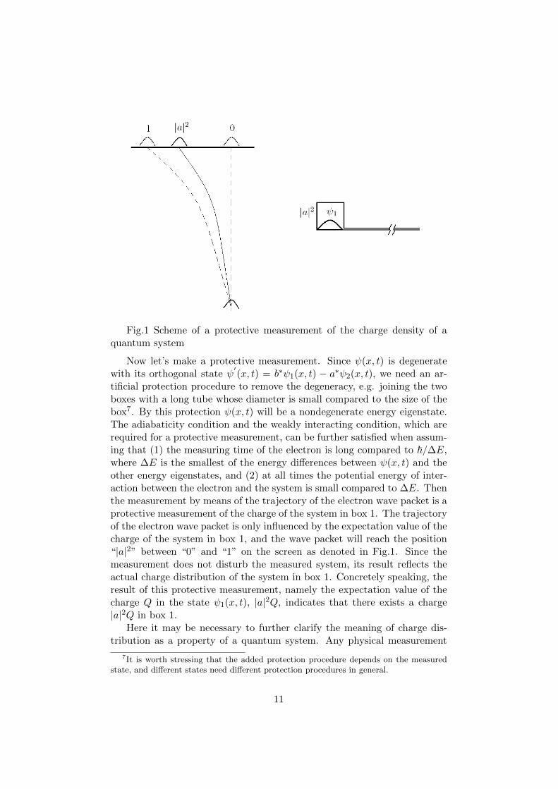
Fig.1 Scheme of a protective measurement of the charge density of aquantum system

Now let’s make a protective measurement. Since ψ(x, t) is degeneratewith its orthogonal state ψ

′(x, t) = b∗ψ1(x, t) − a∗ψ2(x, t), we need an ar-

tificial protection procedure to remove the degeneracy, e.g. joining the twoboxes with a long tube whose diameter is small compared to the size of thebox7. By this protection ψ(x, t) will be a nondegenerate energy eigenstate.The adiabaticity condition and the weakly interacting condition, which arerequired for a protective measurement, can be further satisfied when assum-ing that (1) the measuring time of the electron is long compared to ~/∆E,where ∆E is the smallest of the energy differences between ψ(x, t) and theother energy eigenstates, and (2) at all times the potential energy of inter-action between the electron and the system is small compared to ∆E. Thenthe measurement by means of the trajectory of the electron wave packet is aprotective measurement of the charge of the system in box 1. The trajectoryof the electron wave packet is only influenced by the expectation value of thecharge of the system in box 1, and the wave packet will reach the position“|a|2” between “0” and “1” on the screen as denoted in Fig.1. Since themeasurement does not disturb the measured system, its result reflects theactual charge distribution of the system in box 1. Concretely speaking, theresult of this protective measurement, namely the expectation value of thecharge Q in the state ψ1(x, t), |a|2Q, indicates that there exists a charge|a|2Q in box 1.

Here it may be necessary to further clarify the meaning of charge dis-tribution as a property of a quantum system. Any physical measurement

7It is worth stressing that the added protection procedure depends on the measuredstate, and different states need different protection procedures in general.

11

is necessarily based on some interaction between the measured system andthe measuring system. One basic form of interaction is the electrostaticinteraction between two electric charges as in the above example, and theexistence of this interaction during a measurement, which is indicated bythe deviation of the trajectory of the charged measuring system such as anelectron, means that the measured system also has the charge responsiblefor the interaction8. Then at least in the sense that any part of a physicalentity has electrostatic interaction with another charged system such as an-other electron, we can say that the physical entity has charge distribution inspace9. In the above example, the definite deviation of the trajectory of theelectron will reflect that there exists a definite amount of charge in box 1,and the extent of the deviation will further indicate how much charge thereis there.

It should be noted that the existence of such a charge distribution doesnot imply that two quantum systems interact directly by way of their chargedistributions as in classical mechanics. In other words, the existence of thecharge distribution can be consistent with quantum mechanics, in whichthe interaction between two quantum systems is always described by theinteraction potentials in the Schrodinger equation. As we will see in thenext section, however, the consistency will restrict and even determine theexisting form of the charge distribution of a quantum system.

4 The physical origin of the mass and charge dis-tributions

We have argued that the mass and charge of a quantum system are dis-tributed throughout space, and the mass and charge density in each position

8If one denies this point, then it seems that one cannot obtain any information aboutthe measured system by the measurement. Note that the arguments against the naiverealism about operators and the eigenvalue realism in the quantum context are irrelevanthere (Daumer et al 1997; Valentini 2010).

9This is consistent with the anti-Humean position about laws of nature in contemporaryphilosophy. According to this view, laws are grounded in the ontology, and the theoreticalterms (expressed in the language of mathematics) connect to the entities existing in thephysical world. It is essential for a property to induce a certain behaviour of the objectsthat instantiate the property in question, while the law expresses that behaviour. Forexample, the parameter we call “charge” in the Schrodinger equation refers to a propertyof quantum systems. This property is not a pure quality, but a disposition whose manifes-tation is the electromagnetic interaction between the systems as expressed qualitativelyand quantitatively by the Schrodinger equation. In this way, laws are suitable to figure inexplanations answering why-questions, and they reveal the real connections that there arein nature. By contrast, according to Humeanism, the laws are mere means of economicaldescription, and they do not have any explanatory function. They sum up what has hap-pened in the world; but they do not answer the question why what has happened did infact happen, given certain initial conditions. Note that there are a number of substantialphilosophical objections against Humeanism (see e.g. Mumford 2004).

12

is proportional to the modulus squared of the wave function of the systemthere. In this section, we will further investigate the physical origin of themass and charge distributions. As we will see, the answer may provide animportant clue to the meaning of the wave function.

Historically, the charge density interpretation for electrons was originallysuggested by Schrodinger when he introduced the wave function and foundedwave mechanics (Schrodinger 1926). Schrodinger clearly realized that thecharge distribution cannot be of classical nature because his equation doesnot include the usual classical interaction between the distributions. Pre-sumably since people thought that the charge distribution could not bemeasured and also lacked a consistent physical picture, this initial inter-pretation of the wave function was soon rejected and replaced by Born’sprobability interpretation (Born 1926). Now protective measurement re-endows the charge distribution of an electron with reality. The question isthen how to find a consistent physical explanation for it10. Our followinganalysis can be regarded as a further development of Schrodinger’s idea tosome extent. The twist is that the charge distribution is not classical doesnot imply its non-existence; rather, its existence points to a non-classicalpicture of quantum reality hiding behind the wave function.

4.1 The mass and charge distributions are effective

As noted earlier, the expectation values of observables are the properties ofa quantum system defined either at a precise instant or during an infinites-imal time interval. Correspondingly, the mass and charge distributions ofa quantum system, which can be protectively measured as the expectationvalues of certain observables, have two possible existent forms: it is eitherreal or effective. The distribution is real means that it exists throughoutspace at the same time. The distribution is effective means that at everyinstant there is only a localized, point-like particle with the total mass andcharge of the system, and its motion during an infinitesimal time intervalforms the effective distribution. Concretely speaking, at a particular instantthe mass and charge density of the particle in each position is either zero (ifthe particle is not there) or singular (if the particle is there), while the timeaverage of the density during an infinitesimal time interval gives the effectivemass and charge density. Moreover, the motion of the particle is ergodic inthe sense that the integral of the formed mass and charge density in anyregion is required to be equal to the expectation value of the total mass andcharge in the region. In the following, we will determine the existent formof the mass and charge distributions of a quantum system.

10Note that the proponents of protective measurement did not give an analysis of theorigin of the charge distribution. According to them, this type of measurement impliesthat the wave function of a single quantum system is ontological, i.e., that it is a realphysical wave (Aharonov, Anandan and Vaidman 1993).

13

If the mass and charge distributions are real, then any two parts of thedistributions, e.g. the two wavepackets in box 1 and box 2 in the examplegiven in the last section, will have gravitational and electrostatic interactionsdescribed by the interaction potential terms in the Schrodinger equation11.The existence of such gravitational and electrostatic self-interactions for in-dividual quantum systems is inconsistent with the superposition principleof quantum mechanics (at least for microscopic systems such as electrons).Moreover, the existence of the electrostatic self-interaction for the chargedistribution of an electron also contradicts experimental observations. Forexample, for the electron in the hydrogen atom, since the potential of theelectrostatic self-interaction is of the same order as the Coulomb potentialproduced by the nucleus, the energy levels of hydrogen atoms will be remark-ably different from those predicted by quantum mechanics and confirmed byexperiments if there exists such electrostatic self-interaction. By contrast,if the mass and charge distributions are effective, then there will be onlya localized particle at every instant, and thus there will exist no gravita-tional and electrostatic self-interactions of the effective distributions. Thisis consistent with the superposition principle of quantum mechanics and theSchrodinger equation.

Since this argument is pivotal for our later discussions, we will give amore detailed analysis here. It can be seen that the existence of the massand charge distributions poses a puzzle. According to quantum mechanics,two charge distributions such as two electrons, which exist in space at thesame time, have electrostatic interaction described by the interaction po-tential term in the Schrodinger equation, but in the example given in thelast section, the two charges in box 1 and box 2 have no such electrostaticinteraction. This puzzle is not so much dependent on the existence of massand charge distributions as properties of a quantum system. It is essen-tially that according to quantum mechanics, the wavepacket ψ1 in box 1has interaction with any test electron (e.g. deviating the trajectory of theelectron wavepacket), so does the wavepacket ψ2 in box 2, but these twowavepackets, unlike two electrons, have no interaction.

Facing this puzzle one may have two choices. The first one is simplyadmitting that this is a distinct feature of the laws of quantum mechanics,but insisting that the laws are what they are and no further explanationis needed. In our opinion, this choice seems to beg the question and isunsatisfactory in the final analysis. A more reasonable choice is to try toexplain this puzzling feature of the evolution of the wave function, which isgoverned by the Schrodinger equation12. After all, there is only one actual

11According to quantum mechanics, two real mass and charge distributions such as twoelectrons have gravitational and electrostatic interactions described by the interactionpotential terms in the Schrodinger equation. Moreover, these two distributions will beentangled and their wave function will be defined in a six-dimensional configuration space.

12An immediate explanation may be that why the two wavepackets with charges have no

14

form of the mass and charge distributions, while there are two possible formsas given above, and we need to determine which possible form is the actualone.

The above argument provides an answer to this question13. The reasonwhy two wavepackets of an electron, each of which has part of the electron’scharge, have no electrostatic interaction is that these two wavepackets do notexist at the same time, and their charges are not real but effective, formedby the motion of a localized particle with the total charge of the electron.If the two wavepackets with charges, like two electrons, existed at the sametime, then they would also have the same form of electrostatic interactionas that between two electrons. The lack of such interaction then indicatesthat the two wavepackets of an electron exist in a way of time division, andtheir charges are effectively formed by the motion of a localized particle withthe total charge of the electron. Since in this case there is only a localizedparticle at every instant, there exist no electrostatic self-interactions of theeffective charge distribution formed by the motion of the particle. Note thatthis argument does not assume that real charges that exist at the same timeare classical charges and they have classical interaction14.

To sum up, we have argued that the superposition principle of quantummechanics requires that the mass and charge distributions of a quantumsystem such as an electron are not real but effective; at every instant thereis only a localized particle with the total mass and charge of the system,while during an infinitesimal time interval the ergodic motion of the particleforms the effective mass and charge distributions, and the mass and chargedensity in each position is proportional to the modulus squared of the wavefunction of the system there.

4.2 The ergodic motion of a particle is discontinuous

Which sort of ergodic motion? This is a further question. If the ergodicmotion of a particle is continuous, then it can only form the effective massand charge density during a finite time interval. But according to quantummechanics, the effective mass and charge density is required to be formedby the ergodic motion of the particle during an infinitesimal time interval(not during a finite time interval) near a given instant. Thus it seems thatthe ergodic motion of the particle cannot be continuous. This is at least

electrostatic interaction is because they belong to one quantum system such as an electron,and if they belong to two charged quantum systems such as two electrons, then they willhave electrostatic interaction. However, this explanation seems still unsatisfactory, andone may further ask why two wavepackets of a charged quantum system such as an electron,each of which has charge, have no electrostatic interaction.

13In some sense, this argument provides an explanation of why there is no gravitationaland electrostatic self-interaction terms in the Schrodinger equation.

14By contrast, the Schrodinger-Newton equation, which was proposed by Diosi (1984)and Penrose (1998), describes the gravitational self-interaction of classical mass density.

15

what the existing theory says. However, there may exist a possible loopholehere. Although the classical ergodic models that assume continuous motionare inconsistent with quantum mechanics due to the existence of a finiteergodic time, they may be not completely precluded by experiments if onlythe ergodic time is extremely short. After all quantum mechanics is only anapproximation of a more fundamental theory of quantum gravity, in whichthere may exist a minimum time scale such as the Planck time. Therefore,we need to investigate the classical ergodic models more thoroughly.

Consider an electron in a one-dimensional box in the first excited stateψ(x) (Aharonov and Vaidman 1993). Its wave function has a node at thecenter of the box, where its charge density is zero. Assume the electronperforms a very fast continuous motion in the box, and during a very shorttime interval its motion generates an effective charge distribution. Let’s seewhether this distribution can assume the same form as e|ψ(x)|2, which isrequired by protective measurement15. Since the effective charge density isproportional to the amount of time the electron spends in a given position,the electron must be in the left half of the box half of the time and in theright half of the box half of the time. But it can spend no time at the centerof the box where the effective charge density is zero; in other words, it mustmove at infinite velocity at the center. Certainly, the appearance of velocitiesfaster than light or even infinite velocities may be not a fatal problem, as ourdiscussion is entirely in the context of non-relativistic quantum mechanics,and especially the infinite potential in the example is also an ideal situation.However, it seems difficult to explain why the electron speeds up at the nodeand where the infinite energy required for the acceleration comes from.

Let’s further consider an electron in a superposition of two energy eigen-states in two boxes ψ1(x) + ψ2(x). In this example, even if one assumesthat the electron can move with infinite velocity (e.g. at the nodes), it can-not continuously move from one box to another due to the restriction ofbox walls. Therefore, any sort of continuous motion cannot generate theeffective charge distribution e|ψ1(x) + ψ2(x)|2. One may still object thatthis is merely an artifact of the idealization of infinite potential. However,even in this ideal situation, the model should also be able to generate theeffective charge distribution by means of some sort of ergodic motion ofthe electron; otherwise it will be inconsistent with quantum mechanics. Onthe other hand, it is very common in quantum optics experiments that asingle-photon wave packet is split into two branches moving along two well

15Note that in Nelson’s stochastic mechanics, the electron, which is assumed to undergoa Brownian motion, moves only within a region bounded by the nodes (Nelson 1966).This ensures that the theory can be equivalent to quantum mechanics in a limited sense.Obviously this sort of motion is not ergodic and cannot generate the required chargedistribution. This conclusion also holds true for the motion of particles in some variantsof stochastic mechanics (Bell 1986; Vink 1993), as well as in the de Broglie-Bohm theory(de Broglie 1928; Bohm 1952).

16

separated paths in space. The wave function of the photon disappears out-side the two paths for all practical purposes. Moreover, the experimentalresults are not influenced by the environment and experimental setup be-tween the two paths of the photon. Thus it seems impossible that the photonperforms a continuous ergodic motion back and forth in the space betweenits two paths.

In view of these drawbacks of the classical ergodic models and theirinconsistency with quantum mechanics, we conclude that the ergodic motionof particles cannot be continuous. If the motion of a particle is essentiallydiscontinuous, then the particle can readily appear throughout all regionswhere the wave function is nonzero during an arbitrarily short time intervalnear a given instant. Furthermore, if the probability density of the particleappearing in each position is proportional to the modulus squared of itswave function there at every instant, the discontinuous motion can alsogenerate the right mass and charge distributions. This will solve the aboveproblems plagued by the classical ergodic models. The discontinuous ergodicmotion requires no existence of a finite ergodic time. Moreover, a particleundergoing discontinuous motion can also “jump” from one region to anotherspatially separated region, no matter whether there is an infinite potentialwall between them, and such discontinuous motion is not influenced by theenvironment and experimental setup between these regions either.

4.3 An argument for random discontinuous motion

We have argued that the ergodic motion of a particle is discontinuous. How-ever, the argument doesn’t require that the discontinuous motion must berandom. It is possible that the randomness of the result of a quantum mea-surement is only apparent. In order to know whether the motion of particlesis random or not, we need to analyze the cause of motion. For example, ifmotion has no deterministic cause, then it will be random, only determinedby a probabilistic cause. This may also be the right way to find how particlesmove. Since motion involves change in position, if we can find the cause orinstantaneous condition determining the change16, we will be able to findhow particles move.

Let’s consider the simplest states of motion of a free particle, for whichthe instantaneous condition determining the change of its position is a con-stant during the motion. The instantaneous condition can be deterministicor indeterministic. That the instantaneous condition is deterministic meansthat it leads to a deterministic change of the position of the particle at agiven instant. That the instantaneous condition is indeterministic meansthat it only determines the probability of the particle appearing in each

16The word “cause” used here only denotes a certain instantaneous condition deter-mining the change of position, which may appear in the laws of motion. Our analysis isindependent of whether the condition has causal power or not.

17

position in space at a given instant. If the instantaneous condition is deter-ministic, then the simplest states of motion of the free particle will have twopossible forms. The first one is continuous motion with constant velocity,and the equation of motion of the particle is x(t + dt) = x(t) + vdt, wherethe deterministic instantaneous condition v is a constant17. The second oneis discontinuous motion with infinite average velocity; the particle performsa finite jump along a fixed direction at every instant, where the jump dis-tance is a constant, determined by the constant instantaneous condition18.On the other hand, if the instantaneous condition is indeterministic, thenthe simplest states of motion of the free particle will be random discontinu-ous motion with even position probability distribution. At each instant theprobability density of the particle appearing in every position is the same.

In order to know whether the instantaneous condition is deterministicor not, we need to determine which sort of simplest states of motion arethe solutions of the equation of free motion in quantum mechanics (i.e. thefree Schrodinger equation). According to the analysis in the last subsection,the momentum eigenstates of a free particle, which are the solutions ofthe free Schrodinger equation, describe the ergodic motion of the particlewith even position probability distribution in space. Therefore, the simpleststates of motion with a constant probabilistic instantaneous condition arethe solutions of the equation of free motion, while the simplest states ofmotion with a constant deterministic instantaneous condition are not.

When assuming that (1) the simplest states of motion of a free particleare the solutions of the equation of free motion; and (2) the instantaneouscondition determining the position change of a particle is always determinis-tic or indeterministic for any state of motion, the above result then impliesthat motion, no matter whether it is free or forced, has no deterministiccause, and thus it is random and discontinuous, only determined by a prob-abilistic cause. The argument may be improved by further analyzing thesetwo seemingly reasonable assumptions, but we will leave this for future work.

5 The wave function as a description of randomdiscontinuous motion of particles

In classical mechanics, we have a clear physical picture of motion. It is wellunderstood that the trajectory function x(t) in classical mechanics describesthe continuous motion of a particle. In quantum mechanics, the trajectoryfunction x(t) is replaced by a wave function ψ(x, t). If the particle ontology

17This deterministic instantaneous condition is often called intrinsic velocity (Tooley1988).

18In discrete space and time, the motion will be a discrete jump across space along afixed direction at each time unit, and thus it will become continuous motion with constantvelocity in the continuous limit.

18

is still viable in the quantum domain, then it seems natural that the wavefunction should describe some sort of more fundamental motion of particles,of which continuous motion is an approximation in the classical domain,as quantum mechanics is a more fundamental theory of the physical world,of which classical mechanics is an approximation. The analysis in the lastsection provides a strong support for this conjecture. It suggests that aquantum system such as an electron is a localized particle that undergoesrandom discontinuous motion, and the probability density of the particleappearing in each position is proportional to the modulus squared of itswave function there. As a result, the wave function in quantum mechanicscan be regarded as a description of the more fundamental motion of particles,which is arguably discontinuous and random. In this section, we will give amore detailed analysis of random discontinuous motion and the meaning ofthe wave function (Gao 2011).

5.1 An analysis of random discontinuous motion of particles

Let’s first make clearer what we mean when we say a quantum system suchas an electron is a particle. The picture of particles appears from our analysisof the mass and charge density of a quantum system. As we have arguedin the last section, the mass and charge density of an electron, which ismeasurable by protective measurement and proportional to the modulussquared of its wave function, is not real but effective; it is formed by theergodic motion of a localized particle with the total mass and charge of theelectron. If the mass and charge density is real, i.e., if the mass and chargedistributions at different locations exist at the same time, then there willexist gravitational and electrostatic interactions between the distributions,the existence of which not only contradicts experiments but also violates thesuperposition principle of quantum mechanics. It is this analysis that leadsus to the basic existent form of a quantum system such as an electron in spaceand time; an electron is a particle19. Here the concept of particle is used inits usual sense. A particle is a small localized object with mass and charge,and it is only in one position in space at an instant. However, as we haveargued above, the motion of an electron described by its wave function is notcontinuous but discontinuous and random in nature. We may say that anelectron is a quantum particle in the sense that its motion is not continuousmotion described by classical mechanics, but random discontinuous motiondescribed by quantum mechanics.

Next, let’s analyze the random discontinuous motion of particles. From alogical point of view, for the random discontinuous motion of a particle, theparticle must have an instantaneous property (as a probabilistic instanta-neous condition) that determines the probability density to appear in every

19However, the analysis cannot tell us the precise size and possible structure of electron.

19

position in space; otherwise the particle would not “know” how frequentlyit should appear in each position in space. This property is usually calledindeterministic disposition or propensity in the literature20, and it can berepresented by %(x, t), which satisfies the nonnegative condition %(x, t) > 0and the normalization relation

∫ +∞−∞ %(x, t)dx = 1. As a result, the position

of the particle at every instant is random, and its trajectory formed by therandom position series is also discontinuous at every instant21.

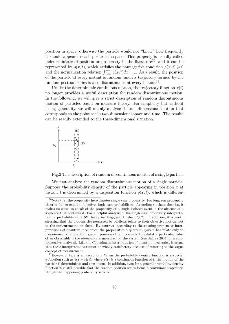
Unlike the deterministic continuous motion, the trajectory function x(t)no longer provides a useful description for random discontinuous motion.In the following, we will give a strict description of random discontinuousmotion of particles based on measure theory. For simplicity but withoutlosing generality, we will mainly analyze the one-dimensional motion thatcorresponds to the point set in two-dimensional space and time. The resultscan be readily extended to the three-dimensional situation.

Fig.2 The description of random discontinuous motion of a single particle

We first analyze the random discontinuous motion of a single particle.Suppose the probability density of the particle appearing in position x atinstant t is determined by a disposition function %(x, t), which is differen-

20Note that the propensity here denotes single case propensity. For long run propensitytheories fail to explain objective single-case probabilities. According to these theories, itmakes no sense to speak of the propensity of a single isolated event in the absence of asequence that contains it. For a helpful analysis of the single-case propensity interpreta-tion of probability in GRW theory see Frigg and Hoefer (2007). In addition, it is worthstressing that the propensities possessed by particles relate to their objective motion, notto the measurements on them. By contrast, according to the existing propensity inter-pretations of quantum mechanics, the propensities a quantum system has relate only tomeasurements; a quantum system possesses the propensity to exhibit a particular valueof an observable if the observable is measured on the system (see Suarez 2004 for a com-prehensive analysis). Like the Copenhagen interpretation of quantum mechanics, it seemsthat these interpretations cannot be wholly satisfactory because of resorting to the vagueconcept of measurement.

21However, there is an exception. When the probability density function is a specialδ-function such as δ(x− x(t)), where x(t) is a continuous function of t, the motion of theparticle is deterministic and continuous. In addition, even for a general probability densityfunction it is still possible that the random position series forms a continuous trajectory,though the happening probability is zero.

20

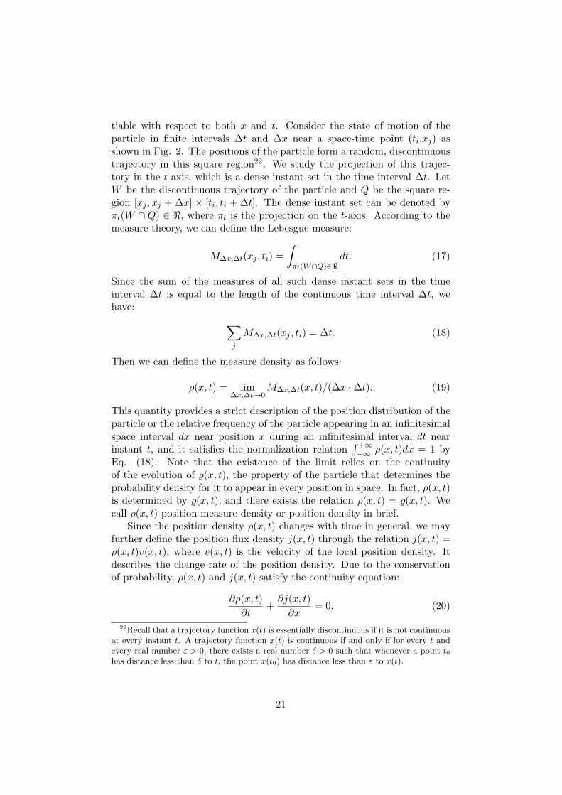
tiable with respect to both x and t. Consider the state of motion of theparticle in finite intervals ∆t and ∆x near a space-time point (ti,xj) asshown in Fig. 2. The positions of the particle form a random, discontinuoustrajectory in this square region22. We study the projection of this trajec-tory in the t-axis, which is a dense instant set in the time interval ∆t. LetW be the discontinuous trajectory of the particle and Q be the square re-gion [xj , xj + ∆x] × [ti, ti + ∆t]. The dense instant set can be denoted byπt(W ∩ Q) ∈ <, where πt is the projection on the t-axis. According to themeasure theory, we can define the Lebesgue measure:

M∆x,∆t(xj , ti) =

∫πt(W∩Q)∈<

dt. (17)

Since the sum of the measures of all such dense instant sets in the timeinterval ∆t is equal to the length of the continuous time interval ∆t, wehave: ∑

j

M∆x,∆t(xj , ti) = ∆t. (18)

Then we can define the measure density as follows:

ρ(x, t) = lim∆x,∆t→0

M∆x,∆t(x, t)/(∆x ·∆t). (19)

This quantity provides a strict description of the position distribution of theparticle or the relative frequency of the particle appearing in an infinitesimalspace interval dx near position x during an infinitesimal interval dt nearinstant t, and it satisfies the normalization relation

∫ +∞−∞ ρ(x, t)dx = 1 by

Eq. (18). Note that the existence of the limit relies on the continuityof the evolution of %(x, t), the property of the particle that determines theprobability density for it to appear in every position in space. In fact, ρ(x, t)is determined by %(x, t), and there exists the relation ρ(x, t) = %(x, t). Wecall ρ(x, t) position measure density or position density in brief.

Since the position density ρ(x, t) changes with time in general, we mayfurther define the position flux density j(x, t) through the relation j(x, t) =ρ(x, t)v(x, t), where v(x, t) is the velocity of the local position density. Itdescribes the change rate of the position density. Due to the conservationof probability, ρ(x, t) and j(x, t) satisfy the continuity equation:

∂ρ(x, t)

∂t+∂j(x, t)

∂x= 0. (20)

22Recall that a trajectory function x(t) is essentially discontinuous if it is not continuousat every instant t. A trajectory function x(t) is continuous if and only if for every t andevery real number ε > 0, there exists a real number δ > 0 such that whenever a point t0has distance less than δ to t, the point x(t0) has distance less than ε to x(t).

21

The position density ρ(x, t) and position flux density j(x, t) provide a com-plete description of the state of random discontinuous motion of a singleparticle23.

The description of the motion of a single particle can be extended to themotion of many particles. At each instant a quantum system of N particlescan be represented by a point in an 3N -dimensional configuration space.Then, similar to the single particle case, the state of the system can berepresented by the joint position density ρ(x1, x2, ...xN , t) and joint positionflux density j(x1, x2, ...xN , t) defined in the configuration space. They alsosatisfy the continuity equation:

∂ρ(x1, x2, ...xN , t)

∂t+

N∑i=1

∂j(x1, x2, ...xN , t)

∂xi= 0. (21)

The joint position density ρ(x1, x2, ...xN , t) represents the probability den-sity of particle 1 appearing in position x1 and particle 2 appearing in positionx2, , and particle N appearing in position xN . When these N particles areindependent, the joint position density can be reduced to the direct prod-uct of the position density for each particle, namely ρ(x1, x2, ...xN , t) =∏Ni=1 ρ(xi, t). Note that the joint position density ρ(x1, x2, ...xN , t) and

joint position flux density j(x1, x2, ...xN , t) are not defined in the real three-dimensional space, but defined in the 3N-dimensional configuration space.

5.2 Interpreting the wave function

Although the motion of particles is essentially discontinuous and random,the discontinuity and randomness of motion are absorbed into the stateof motion, which is defined during an infinitesimal time interval and rep-resented by the position density ρ(x, t) and position flux density j(x, t).Therefore, the evolution of the state of random discontinuous motion of par-ticles may obey a deterministic continuous equation. By assuming that thenonrelativistic equation of random discontinuous motion is the Schrodingerequation in quantum mechanics, both ρ(x, t) and j(x, t) can be expressedby the wave function in a unique way24:

ρ(x, t) = |ψ(x, t)|2, (22)

23It is also possible that the position density ρ(x, t) alone provides a complete descriptionof the state of random discontinuous motion of a particle. Which one is right dependson the laws of motion. As we will see later, quantum mechanics requires that a completedescription of the state of random discontinuous motion of particles includes both theposition density and the position flux density.

24Note that the relation between j(x, t) and ψ(x, t) depends on the concrete evolutionunder an external potential such as electromagnetic vector potential. By contrast, therelation ρ(x, t) = |ψ(x, t)|2 holds true universally, independently of the concrete evolution.

22

j(x, t) =~

2mi[ψ∗(x, t)

∂ψ(x, t)

∂x− ψ(x, t)

∂ψ∗(x, t)

∂x]. (23)

Correspondingly, the wave function ψ(x, t) can be uniquely expressed byρ(x, t) and j(x, t) (except for a constant phase factor):

ψ(x, t) =√ρ(x, t)e

im∫ x−∞

j(x′,t)ρ(x′,t)dx

′/~. (24)

In this way, the wave function ψ(x, t) also provides a complete descriptionof the state of random discontinuous motion of particles. For the motionof many particles, the joint position density and joint position flux densityare defined in the 3N-dimensional configuration space, and thus the many-particle wave function, which is composed of these two quantities, is alsodefined in the 3N-dimensional configuration space.

Interestingly, we can reverse the above logic in some sense, namely by as-suming the wave function is a complete objective description for the motionof particles, we can also reach the random discontinuous motion of parti-cles, independently of our previous analysis. If the wave function ψ(x, t) isa complete description of the state of motion for a single particle, then thequantity |ψ(x, t)|2dx will not only give the probability of the particle beingfound in an infinitesimal space interval dx near position x at instant t (asrequired by quantum mechanics), but also give the objective probability ofthe particle being there at the instant. This accords with the common-senseassumption that the probability distribution of the measurement results ofa property is the same as the objective distribution of the values of theproperty in the measured state. Then at instant t the particle will be ina random position where the probability density |ψ(x, t)|2 is nonzero, andduring an infinitesimal time interval near instant t it will move throughoutthe whole region where the wave function ψ(x, t) spreads. Moreover, itsposition density in each position is equal to the probability density there.Obviously this kind of motion is random and discontinuous.

One important point needs to be pointed out here. Since the wave func-tion in quantum mechanics is defined at instants, not during an infinitesimaltime interval, it should be regarded not simply as a description of the state ofrandom discontinuous motion of particles, but more suitably as a descriptionof the property of the particles that determines their random discontinuousmotion at a deeper level25. In particular, the modulus squared of the wavefunction represents the property that determines the probability density ofthe particles appearing in certain positions in space at a given instant (thismeans %(x, t) ≡ |ψ(x, t)|2). By contrast, the position density and positionflux density, which are defined during an infinitesimal time interval near agiven instant, are only a description of the state of the resulting random

25For a many-particle system in an entangled state, this property is possessed by thewhole system.

23

discontinuous motion of particles, and they are determined by the wavefunction. In this sense, we may say that the motion of particles is “guided”by their wave function in a probabilistic way.

5.3 On momentum, energy and spin

We have been discussing random discontinuous motion of particles in realspace. Does the picture of random discontinuous motion exist for otherdynamical variables such as momentum and energy? Since there are alsowave functions of these variables in quantum mechanics, it seems tempting toassume that the above interpretation of the wave function in position spacealso applies to the wave functions in momentum space etc26. This meansthat when a particle is in a superposition of the eigenstates of a variable,it also undergoes random discontinuous motion among the correspondingeigenvalues of this variable. For example, a particle in a superposition ofenergy eigenstates also undergoes random discontinuous motion among allenergy eigenvalues. At each instant, the energy of the particle is definite,randomly assuming one of the energy eigenvalues with probability givenby the modulus squared of the wave function at this energy eigenvalue,and during an infinitesimal time interval, the energy of the particle spreadsthroughout all energy eigenvalues. Since the values of two noncommutativevariables (e.g. position and momentum) at every instant may be mutuallyindependent, the objective value distribution of every variable can be equalto the modulus squared of its wave function and consistent with quantummechanics27.

However, there is also another possibility, namely that the picture of ran-dom discontinuous motion exists only for position, while momentum, energyetc do not undergo random discontinuous change among their eigenvalues.This is a minimum formulation in the sense that the ontology of the theoryonly includes the wave function and the particle position. A heuristic argu-ment for this possibility is as follows. In quantum mechanics, the definitionsof momentum and energy relate to spacetime translation. The momentumoperator and energy operator are defined as the generators of space trans-lation and time translation, respectively. By these definitions momentumand energy seem distinct from position. For random discontinuous motionof particles, the position of a particle is its primary property defined at in-stants, while momentum and energy are secondary properties relating onlyto its state of motion (e.g. momentum and energy eigenstates), which is

26Under this assumption, the ontology of the theory will not only include the wavefunction and the particle position, but also include momentum and energy.

27Note that for random discontinuous motion a property (e.g. position) of a quantumsystem in a superposed state of the property is indeterminate in the sense of usual hiddenvariables, though it does have a definite value at each instant. This makes the theoremsthat restrict hidden variables such as the Kochen-Specker theorem (Kochen and Specker1967) irrelevant.

24

formed by the motion of the particle. In other words, position is an in-stantaneous property of a particle, while momentum and energy are onlymanifestations of its state of motion during an infinitesimal time interval.Note that the particle position here is different from the position propertydescribed by the position operator in quantum mechanics, and the latter isalso a secondary property relating only to the state of motion of the particlesuch as position eigenstates. Certainly, we can still talk about momentumand energy on this view. For example, when a particle is in an eigenstate ofthe momentum or energy operator, we can say that the particle has definitemomentum or energy, whose value is the corresponding eigenvalue. More-over, when the eigenstates of the momentum or energy operator are wellseparated in space, we can still say that the particle has definite momentumor energy in certain local regions.

Lastly, we note that spin is a more distinct property. Since the spin ofa free particle is always definite along one direction, the spin of the particledoes not undergo random discontinuous motion, though a spin eigenstatealong one direction can always be decomposed into two different spin eigen-states along another direction. But if the spin state of a particle is entangledwith its spatial state due to interaction and the branches of the entangledstate are well separated in space, the particle in different branches will havedifferent spin, and it will also undergo random discontinuous motion be-tween these different spin states. This is the situation that usually happensduring a spin measurement.

6 Conclusions

In this paper, we have argued that protective measurement may have im-portant implications for the physical meaning of the wave function. Thereare three key steps in the argument. First of all, the results of protectivemeasurements as predicted by quantum mechanics show that the mass andcharge of a charged quantum system are distributed throughout space, andthe mass and charge density in each position is proportional to the modulussquared of the wave function of the system there. Next, the superpositionprinciple of quantum mechanics requires that the mass and charge distri-butions are effective, that is, they are formed by the ergodic motion of alocalized particle with the total mass and charge of the system. Lastly, theconsistency of the formed distribution with that predicted by quantum me-chanics requires that the ergodic motion of the particle is discontinuous, andthe probability density of the particle appearing in every position is equalto the modulus squared of its wave function there. Based on this analy-sis, we suggest that the wave function in quantum mechanics describes thestate of random discontinuous motion of particles, and at a deeper level, itrepresents the property of the particles that determines their random dis-

25

continuous motion. In particular, the modulus squared of the wave function(in position space) gives the probability density of the particles being incertain positions in space.

Acknowledgments

I am very grateful to Dean Rickles, Huw Price, Hans Westman, AntonyValentini, and Lev Vaidman for helpful comments and suggestions. I amalso grateful for stimulating discussions with participants in the PIAF Work-shop in Foundations, held at the Griffith University, Brisbane, December1-3, 2010. This work was supported by the Postgraduate Scholarship inQuantum Foundations provided by the Unit for History and Philosophy ofScience and Centre for Time of the University of Sydney.

References

[1] Aharonov, Y., Anandan, J. and Vaidman, L. (1993). Meaning of thewave function, Phys. Rev. A 47, 4616.

[2] Aharonov, Y., Anandan, J. and Vaidman, L. (1996). The meaning ofprotective measurements, Found. Phys. 26, 117.

[3] Aharonov, Y. and Vaidman, L. (1993). Measurement of the Schrodingerwave of a single particle, Phys. Lett. A 178, 38.

[4] Anandan, J. (1993). Protective Measurement and Quantum Reality.Found. Phys. Lett., 6, 503-532.

[5] Bell, J. S. (1986). Beables for quantum field theory. Phys. Rep. 137,49-54.

[6] Bell, J. S. (1990). Against measurement, in A. I. Miller (ed.), Sixty-Two Years of Uncertainty: Historical Philosophical and Physics En-quiries into the Foundations of Quantum Mechanics. Berlin: Springer,17-33.

[7] Bohm, D. (1952). A suggested interpretation of quantum theory interms of “hidden” variables, I and II. Phys. Rev. 85, 166-193.

[8] Born, M. (1926). Quantenmechanik der Stoβvorgange. Z. Phys. 38,803; English translation in Ludwig, G., eds., 1968, Wave Mechanics,Oxford: Pergamon Press: 206.

[9] Dass, N. D. H. and Qureshi, T. (1999). Critique of protective mea-surements. Phys. Rev. A 59, 2590.

26

[10] Daumer, M., Durr, D., Goldstein, S., and Zangh, N. (1997). NaiveRealism About Operators, Erkenntnis 45, 379-397.

[11] de Broglie, L. (1928). in: Electrons et photons: Rapports et discus-sions du cinquime Conseil de Physique Solvay, eds. J. Bordet. Paris:Gauthier-Villars. pp.105. English translation: G. Bacciagaluppi andA. Valentini (2009), Quantum Theory at the Crossroads: Reconsid-ering the 1927 Solvay Conference. Cambridge: Cambridge UniversityPress.

[12] Dickson, M. (1995). An empirical reply to empiricism: protective mea-surement opens the door for quantum realism. Philosophy of Science62, 122.

[13] Diosi, L. (1984). Gravitation and the quantum-mechanical localizationof macro-objects. Phys. Lett. A 105, 199-202.

[14] Everett, H. (1957). Relative state formulation of quantum mechanics.Rev. Mod. Phys. 29, 454-462.

[15] Frigg, R and Hoefer, C. (2007). Probability in GRW Theory. Studiesin the History and Philosophy of Modern Physics 38, 371-389.

[16] Gao, S. (2011). Interpreting Quantum Mechanics in Terms of RandomDiscontinuous Motion of Particles. http://philsci-archive.pitt.edu/9057/.

[17] Gao, S. (2012). On Uffink’s alternative interpretation of protectivemeasurements. http://philsci-archive.pitt.edu/9447/.

[18] Ghose, P. and Home, D. (1995). An analysisi of Aharonov-Anandan-Vaidman model, Found. Phys. 25, 1105.

[19] Kochen, S. and Specker, E. (1967). The Problem of Hidden Variablesin Quantum Mechanics, J. Math. Mech. 17, 59-87.

[20] Mumford, S. (2004). Laws in nature. London: Routledge.

[21] Nelson, E. (1966). Derivation of the Schrodinger equation from New-tonian mechanics. Phys. Rev. 150, 10791085.

[22] Penrose, R. (1998). Quantum computation, entanglement and statereduction. Phil. Trans. R. Soc. Lond. A 356, 1927.

[23] Rovelli, C. (1994). Meaning of the wave function - Comment, Phys.Rev. A 50, 2788.

[24] Schrodinger, E. (1926). Quantizierung als Eigenwertproblem (VierteMitteilung). Ann. d. Phys. (4) 81, 109-139. English translation:Quantisation as a Problem of Proper Values. Part IV, Reprint in

27

Schrodinger, E. (1982). Collected Papers on Wave Mechanics. NewYork: Chelsea Publishing Company, pp. 102-123.

[25] Suarez, M. (2004), Quantum Selections, Propensities and the Problemof Measurement, British Journal for the Philosophy of Science, 55(2),219-55.

[26] Tooley, M. (1988). In defence of the existence of states of motion.Philosophical Topics 16, 225-254.

[27] Uffink, J. (1999). How to protect the interpretation of the wave func-tion against protective measurements. Phys. Rev. A 60, 3474-3481.

[28] Unruh, W. G. (1994). Reality and measurement of the wave functionPhys. Rev. A 50, 882.

[29] Vaidman, L. (2009) Protective measurements, in Greenberger, D.,Hentschel, K., and Weinert, F. (eds.), Compendium of Quantum Physics:Concepts, Experiments, History and Philosophy. Springer-Verlag, Berlin.pp.505-507.

[30] Valentini, A. (2010). De Broglie-Bohm Pilot-Wave Theory: ManyWorlds in Denial? in Saunders, S., Barrett, J., Kent, A. and Wallace,D. (eds.). Many Worlds? Everett, Quantum Theory, and Reality.Oxford: Oxford University Press.

[31] Vink, J. C. (1993). Quantum mechanics in terms of discrete beables.Phys. Rev. A 48, 1808.

28