Protecting Against Low Probability Disasters: A Large Stakes Experiment

Protecting against Low Probability Disasters: The Role of Worry

Christian Schade Humboldt-Universität

zu Berlin

Howard Kunreuther The Wharton School

University of Pennsylvania

Philipp Koellinger Erasmus University Rotterdam

Netherlands

Klaus Peter Kaas Goethe-University

Frankfurt

December 2009 Working Paper # 2009-03-23

Submission to the

Journal of Behavioral Decision Making

_____________________________________________________________________ Risk Management and Decision Processes Center The Wharton School, University of Pennsylvania 3730 Walnut Street, Jon Huntsman Hall, Suite 500

Philadelphia, PA, 19104 USA

Phone: 215‐898‐4589 Fax: 215‐573‐2130

http://opim.wharton.upenn.edu/risk/ ___________________________________________________________________________

THE WHARTON RISK MANAGEMENT AND DECISION PROCESSES CENTER

Established in 1984, the Wharton Risk Management and Decision Processes Center develops and promotes effective corporate and public policies for low‐probability events with potentially catastrophic consequences through the integration of risk assessment, and risk perception with risk management strategies. Natural disasters, technological hazards, and national and international security issues (e.g., terrorism risk insurance markets, protection of critical infrastructure, global security) are among the extreme events that are the focus of the Center’s research.

The Risk Center’s neutrality allows it to undertake large‐scale projects in conjunction with other researchers and organizations in the public and private sectors. Building on the disciplines of economics, decision sciences, finance, insurance, marketing and psychology, the Center supports and undertakes field and experimental studies of risk and uncertainty to better understand how individuals and organizations make choices under conditions of risk and uncertainty. Risk Center research also investigates the effectiveness of strategies such as risk communication, information sharing, incentive systems, insurance, regulation and public‐private collaborations at a national and international scale. From these findings, the Wharton Risk Center’s research team – over 50 faculty, fellows and doctoral students – is able to design new approaches to enable individuals and organizations to make better decisions regarding risk under various regulatory and market conditions.

The Center is also concerned with training leading decision makers. It actively engages multiple viewpoints, including top‐level representatives from industry, government, international organizations, interest groups and academics through its research and policy publications, and through sponsored seminars, roundtables and forums.

More information is available at http://opim.wharton.upenn.edu/risk.

Protecting against Low Probability Disasters: The Role of Worry

Christian Schade Howard Kunreuther Philipp Koellinger Klaus Peter Kaas*

We conducted a large stakes insurance experiment with small probabilities of losses and a

realistic form of ambiguity. Our results demonstrate that worry plays a more important role in the

decision to consider insurance against high losses that are rare than does subjective probability

estimates. For those who do have an interest in buying insurance, worry is also positively related

to the willingness to pay (WTP) for coverage. If faced with an ambiguous risk, an individual is

more willing to consider insurance and pay higher amounts than when the probability of a loss is

specified precisely. An approximately 1,000-fold increase in the ambiguous probability did not

change the percentage of those who consider insurance and had a very small positive impact on

WTP. Our results provide insights into the low probability insurance puzzle where some

individuals are willing to pay too much and others nothing for coverage in relation to the risk

associated with the specific event.

Professor Christian Schade is Director of the Institute for Entrepreneurial Studies and

Innovation Management, School of Business and Economics, Humboldt-Universität zu Berlin, Germany, email: [email protected]

Professor Howard Kunreuther is Director of the Risk Management and Decision Processes Center, Wharton School, University of Pennsylvania, Philadelphia, USA, email: [email protected]

Philipp Koellinger is assistant professor at the Erasmus School of Economics, Erasmus University Rotterdam, the Netherlands, email: [email protected]

* Professor Klaus Peter Kaas, Marketing Department, Faculty of Business and Economics, Goethe-University, Frankfurt/M., Germany, email: [email protected]

2

Introduction

Imagine you are facing a risk that is characterized by a very small probability of

occurrence but, if it occurs, will cause significant damage relative to your total wealth. Examples

of such risks are floods and earthquakes, as well as fire and theft. If you were offered insurance

coverage against such a risk would you try to estimate the probability and multiply this figure by

the value or utility of the potential loss? What role would affect or emotional factors such as

worry play in your decision with respect to specific outcomes?

Understanding insurance decisions with respect to low-probability disasters has been a

challenge for psychologists as well as economists. Field studies and controlled laboratory

experiments have posed the following low probability insurance puzzle: (1) many individuals do

not voluntarily purchase coverage even when premiums are highly subsidized (Kunreuther, 1978;

Slovic, Fischhoff, Lichtenstein, Corrigan, & Combs, 1978). (2) In a controlled experiment con-

sistent with these earlier studies, McClelland, Schulze, and Coursey (1993) showed that most

individuals are either unwilling to pay a penny for low-probability insurance or far too much

when compared with the expected loss from the event. The early version of prospect theory

(Kahneman & Tversky, 1979) takes this feature into account by having a discontinuity in the

probability weighting function close to zero.

Most earlier studies in decision making including the above-mentioned ones have focused

on explaining deviations from the predictions derived from normative models of choice such as

(subjective) expected utility theory (Savage, 1954; von Neumann & Morgenstern, 1947). Only

recently has behavioral decision theory concerned itself with the impact that affect and emotion

have on decision making with respect to protective measures (see, e.g., Hogarth & Kunreuther,

1995; Baron, Hershey & Kunreuther, 2000; Hsee & Kunreuther, 2000; Rottenstreich & Hsee,

3

2001; Slovic, Finucane, Peters, & MacGregor, 2002; Loewenstein, Weber, Hsee, & Welsh,

2001). Affect and emotions seem to be especially important with respect to decisions involving

uncertain outcomes with large consequences (Slovic et al., 2002; Loewenstein et al., 2001).

This paper analyzes how individuals’ willingness to pay (WTP) for insurance against real

high-stakes losses is related to calculations based on probabilities and/or emotional factors such

as a person’s worry regarding the outcome. Caplin and Leahy (2001) suggest that worry is a

plausible anticipatory emotion associated with potential losses. MacLeod, Williams, and

Bekerian (1991, p. 478) note that “worry is […being] concerned with future events where there is

uncertainty about the outcome, the future being thought about is a negative one, and this is

accompanied by feelings of anxiety”. Both of these definitions of worry are relevant to the

feeling someone may have when considering whether to purchase insurance coverage and if so

how much to pay for a policy.

Krantz and Kunreuther (2007) have argued that an important goal that individuals pursue

when making decisions on whether to buy insurance is peace of mind. The importance of this

type of non-monetary utility has also been demonstrated in an earlier empirical study by Hogarth

and Kunreuther (1995). When individuals where asked to report on the arguments they ‘had with

themselves’ in deciding whether or not to buy a warranty, peace of mind proved to be the most

important reason. Equating peace of mind with the absence of worry, we contend that the more

worried an individual may be, the greater the interest is in purchasing insurance and the more one

should be willing to pay as a way of reducing her worries and obtaining peace of mind in the

process.

We examine these issues through a controlled experiment using an incentive-compatible,

real payments mechanism: Individuals are asked to state their maximum willingness to pay for

4

insurance facing an unknown selling price that is concealed in an envelope. Such a mechanism is

expected to elicit a price that is equal to the utility of insurance for the individual because it is

mathematically equivalent to a random-price mechanism (Becker, DeGroot, & Marschak, 1964).

The probability of a loss is very low and it is either specified precisely or there is ambiguity

regarding the estimate (i.e., number of rainy days in a particular city during a prespecified time

period). By eliciting the degree of worry, our investigation enables one to take a small but

important step towards solving the low probability insurance puzzle. Understanding why some

people would not pay anything for insurance while others volunteer an amount far greater than

their expected loss requires one to look at the two stages of the decision: (1) whether one has an

interest in purchasing insurance (i.e. WTP> 0) and if so (2) how much one is willing to pay.

Kunreuther (1978) has also referred to a two-stage decision when interpreting behavior with

small probability disasters. Slovic and Lichtenstein (1968) demonstrate the existence of a two-

stage process where individuals determine the general attractiveness of a lottery in the first stage

and then decide on their exact bid or rating of the lottery in the second stage.

Two-stage explanations have also been suggested in consumer behavior where the

decision on whether to purchase an item is influenced by different variables than the decision on

how much to spend (Jones, 1989; Melenberg & van Soest, 1996). In analyzing individuals’

cigarette consumption in the UK, Jones (1989) finds that the decision to smoke is qualitatively

different from the decision on how much to smoke. Individuals who believe that smoking is more

harmful than drinking are less likely to start smoking; for those who do smoke, this belief

regarding the dangers of smoking relative to alcohol consumption does not significantly reduce

average cigarette consumption. In a similar spirit, Melenberg and van Soest (1996) analyze

5

vacation expenditures of Dutch families and find that a person’s income level has a different

effect on whether to take a vacation than on how much to spend if one decides to take a vacation.

Our results are consistent with earlier findings on decisions with respect to low

probability disasters. A substantial percentage of individuals are not willing to pay anything for

insurance. Those who consider buying coverage are willing to pay significantly more than the

expected loss whether the likelihood of a loss of given amount is specified precisely or is

ambiguous. We show that under conditions of ambiguity, worry is more important than

subjective probability estimates for determining those individuals who are willing to pay a

positive amount for insurance. For those who are interest in buying insurance, worry is the most

important driver for understanding how much one is willing to pay for coverage. If we increase

the ambiguous probability by a factor of approximately 1,000, the percentage of those who

consider insurance does not change, and we observe only a minimal positive impact on their

WTP, whilst worry remains an important driver of behavior. Finally, worry is an important factor

when considering insurance and specifying WTP if the probability of a loss is specified precisely.

Our study thus provides additional evidence on the impact of emotional factors as drivers of

choices under conditions of risk and ambiguity. Moreover, the extreme behaviors positing the

low probability insurance puzzle defined above can be partially attributed to differences in

individuals’ worry with respect to the possibility of a loss. When the probability is ambiguous

rather than well-specified, an individual is more likely to consider insurance and be willing to pay

a large amount for coverage.

The paper is organized as follows. The next section offers a detailed explanation of our

experimental design. The following section reports our results. The last two sections contain a

general discussion and implications of our findings for policy makers.

6

Experimental design and sample

Sample

A total of 263 students from a major German university participated in the experiment.

They were recruited via email, posters, and short presentations in classrooms. They were told that

the experiment would take 90 minutes, that all participants would receive 10 DM for sure, and

that there was a small chance (not specified) that they would earn 2,000 DM at the end of the

experiment.1 The study was carried out in groups of six to ten students each of whom was

situated in a separate booth. Nine of the 263 subjects had to be excluded because of nonsensical

responses.2,3

Basic features and experimental conditions

Objects at stake: Participants were told that they had inherited either a painting or a

sculpture and each received a small photo of the art object with an individual identification

number. It was announced that only one painting and one sculpture were originals, worth 2,000

DM; if it was a forgery then it had zero value. All participants learned that one person in the

1 At the time of the experiment, the 2,000 DM was worth US $1,086.48.

2 Of the 254 usable responses, 54.5% were female, 45.5% male. The largest groups were psychology

(29.9%) and business (28.7%) majors followed by economics (5.1%), pedagogic sciences (4.7%), law and German

(each group 3.9%), and sociology (3.5%) students. The remaining 20.3% of the subjects were majoring in 18

different fields of study. The average age of the participants was 25.6.

3 Subjects were excluded from the analysis mostly because they wanted to pay more for insurance than the

value of the object to be insured – an (inherited) painting or sculpture (see below) – or because they clearly

misunderstood the experimental situation (derived from open-ended questions) i.e. assumed they were paying for the

(inherited) painting (or sculpture) rather than the insurance policy.

7

experiment would have the original painting and one would have the original sculpture. These

individuals would be determined by random draws. This is an extreme form of the random pay

mechanism suggested and investigated by Bolle (1990).

Nature of the risks, experimental conditions, and timing: The original painting or

sculpture was threatened by fire and theft. Participants were offered insurance protection against

a potential loss of 2,000 DM. It was made clear that the insurer would only sell a policy to the

owner of the original art object, and that insurance purchased by others would be hypothetical

and not affect their final wealth level. In other words only the owner of the original painting or

sculpture would have to pay for coverage. We made it clear that it was in everyone’s best interest

to anticipate being the owner of the respective original art object when determining the maximum

amount they would be willing to pay for an insurance policy. In addition to providing written

instructions a flow diagram was presented to subjects describing the key variables and the

decisions they had to make. All questions were answered, and the procedure was explained again

when necessary. The Appendix contains the most significant part of the instructions.4

In part A of the experiment each participant inherited a painting. The original was

threatened by the following ambiguous risk: The painting was declared to be stolen if it would

rain exactly 24 days in July in the current year at the Frankfurt Airport; a fire occurs and destroys

the painting if it would rain exactly 23 days in August.5 Subjects knew that the actual outcome

would only be determined after data on the number of days with precipitation in July and August

were obtained from the Frankfurt airport. The experiment was carried out in the spring of 1999.

4 The complete set of instructions is available from the authors upon request

5 Students were informed that a day is defined as a rain day by the weather station in Frankfurt if there is

more than one millimeter of rain that day.

8

We define ambiguity as a state of mind in which the decision maker perceives difficulties

in estimating the relevant probabilities.6 Whereas rain frequencies may be precisely estimated by

meteorologists, they will be ambiguous for most if not all the participants in the experiment. This

situation was designed to resemble a real-life risk (e.g. of a fire or theft in one’s home) where

insurers estimate annual loss probabilities across all policyholders but the individual homeowner

views these risks as ambiguous.

On the basis of actual Frankfurt weather data from the year 1870 to the present, we

estimated the probability of each of these events occurring to be approximately 1 in 10,000.7 In

Group 1, respondents were informed about both hazards threatening the original painting: theft

and fire, but were not told the chances that either theft or fire would occur except that it was

equal to the chance of the above rain frequencies in July and August in Frankfurt respectively .

Respondents were then asked to state their maximum WTP first for theft insurance and then for

fire coverage. Group 2 differed only in that respondents were asked to state their maximum WTP

for one insurance policy covering both fire and theft damage. Risks were however still presented

separately.

6 Ambiguity is defined as a subjective phenomenon in the spirit of work on comparative ignorance by Fox

and Tversky (1995) and Fox and Weber (2002).

7 Rain frequencies were analyzed for consistency with different distribution forms for random events, e.g.

normal, binomial. Rain frequencies were consistent with a Poisson distribution (KS-test of deviation: not

significant.). Lousy weather like this was fortunately never experienced in the period from 1870 to today in

Frankfurt. Since the ‘base rate’ for rain in July and August is different, 24 days of rain in July have the same

probability of occurrence than 23 days of rain in August.

9

In Group 3 respondents were informed that the risk of theft was based on 24 rainy days in

July. They then had to state their maximum WTP for theft insurance. They only learned

afterwards that a second risk, fire, was also threatening the painting and went through the same

procedure with respect to this risk (based on 23 rainy days in August). This experimental

manipulation between the three groups (bundling, unbundling, and stepwise selling) was

designed to increase our understanding as to how insurance against very low-probability events

might be marketed. It was unrelated to the research questions motivating this paper and will not

be analyzed here.8

In part B of the experiment the participants in Groups 1 and 2 were subject to the same

treatments as in Part A. The only difference was that a sculpture (instead of a painting) was

threatened by theft and fire, each of which was specified as having a probability of 1 in 10,000 of

occurring. To determine whether a fire had occurred two random draws with replacement were

taken from a bingo cage containing 100 balls. The same procedure was followed to determine

whether a theft occurred.9 Group 3 had a 1 in 10 ambiguous chance of either fire or theft in part

B. (i.e., theft occurs if there is rain during exactly 12 days in July; fire occurs if there is rain

during exactly 11 days in August). We used this relatively high value to see whether or not there

were differences in people’s decision processes between this situation and the case where the

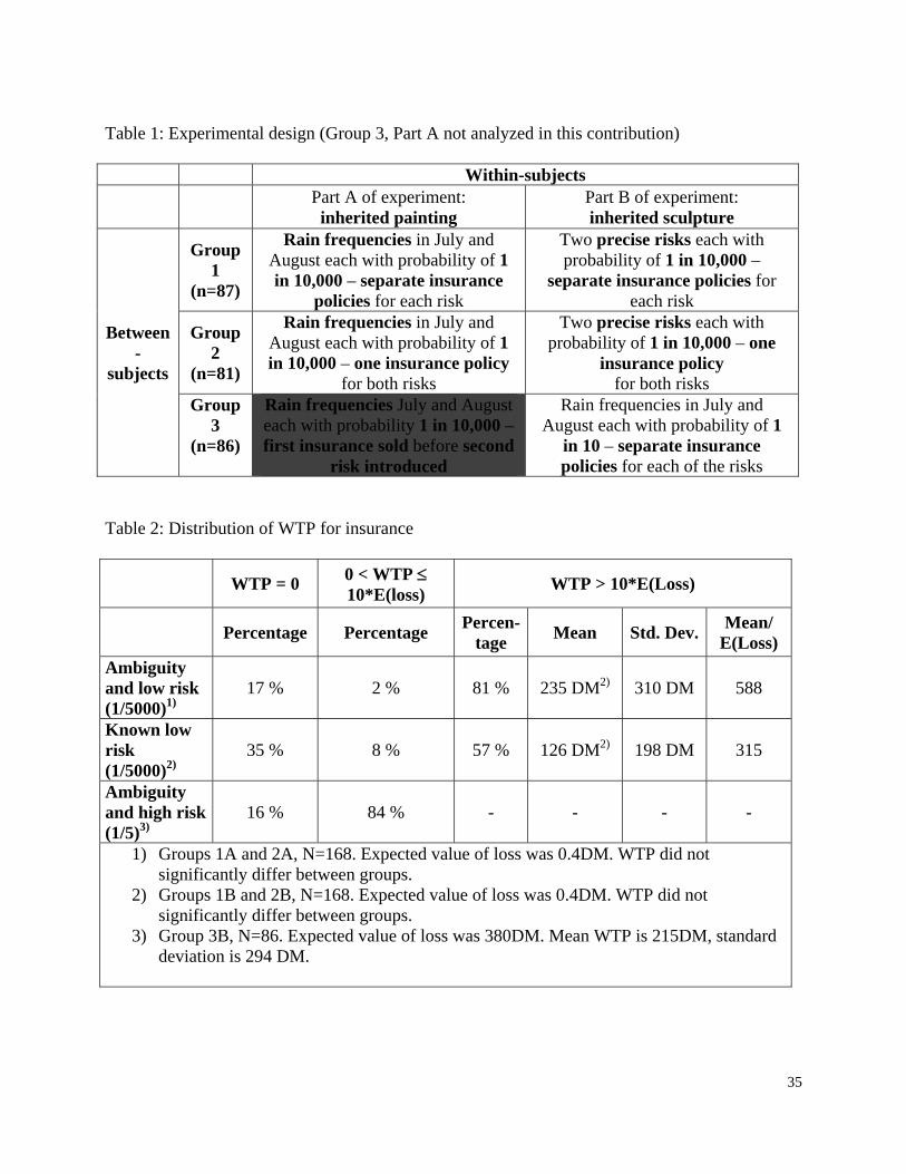
probability was 1 in 10,000. The experimental design is depicted in Table 1.

8 The individuals in Group 3A only learned about a second risk after stating WTP for the first risk in

contrast to Groups 1A and 2A where the individuals learned about both risks before stating their WTP. In group 3A,

individuals were willing to pay a large amount for the first risk but then reduced their WTP for the second risk. The

sum of WTP was significantly below what was observed in groups 1A and 2A. Hence it was inappropriate to merge

group 3A with groups 1A and 2A.

9 A theft or fire was assumed to occur if the number 1 was pulled out twice from the bingo cage.

10

Insert table 1 about here

Note that the ambiguous low-probability situation is always presented first. If we had

initially presented the exact probabilities scenario to some of the respondents, they might have

anchored on this figure when estimating the likelihood of rain in Frankfurt, potentially distorting

our results on ambiguity. There was no feedback at all between parts A and B of the experiment

so that respondents could not learn anything from the situation presented in A when they made a

decision in B.

Eliciting WTP for insurance: There were no fixed selling prices for the insurance

policies. Instead, we utilized a modified Becker, DeGroot and Marschak (BDM) (1964) mecha-

nism for eliciting maximum WTP values. This modified mechanism was first introduced in

laboratory research by Schade and Kunreuther (2001) and has recently been used in the

marketing literature to reveal reservation prices at the point of purchase (Wang, Venkatesh, &

Chatterjee, 2007). Reservation prices reflect an individual’s highest willingness to pay such that

the net utility of purchasing is zero. In the original BDM-procedure, respondents face a random

draw of selling prices for the respective object and are informed about the distribution of these

prices. In theory it is incentive-compatible to state prices as being equal to reservation prices

under these conditions, but there are practical problems in utilizing this method (Becker et al.,

1964).

When utilizing the standard BDM procedure for eliciting reservation prices for insurance

against our risky prospect, decision makers might have treated the resulting two-stage as a one-

11

stage lottery but in an erroneous way as discussed by Safra, Segal, & Spivak (1990).10 Pre-

specified intervals of WTP in the original BDM may also serve as anchors, thus biasing

individuals’ estimates (Bohm, Lindén, & Sonnegard, 1997). Such a bias is precluded by our

procedure since the actual selling prices for each of the insurance policies were inserted in sealed

envelopes to be opened only after the experiment was conducted. This undisclosed price was

selected before the start of the experiment on the basis of pretest results with respect to WTP, so

that about one half of the respondent’s bids could be expected to be higher than the pre-

determined price.

The mechanism was carefully explained to the subjects so that they understood that it was

designed to elicit their maximum willingness to pay. We noted that if they bid too high they

might actually pay that price for insurance should they be the owner of the original art object and

regret having made such a high offer. If they bid too low they may not qualify for insurance even

though they would have been willing to purchase coverage at a higher price than their stated

value. Respondents were then asked to write their maximum willingness to pay for the respective

insurance policy on a piece of paper and place it in an envelope.

Eliciting subjective probability estimates: After stating maximum buying prices for

insurance, respondents were then asked to estimate the probability of each of the ambiguous

risks. We distributed tables with likelihoods of a loss ranging from certainty to 1 in 10,000,000.

Respondents were first asked to mark the probability of a fire or theft causing a loss in one of 15

intervals (e.g. the chance was between 1 in 5,000 and 1 in 10,000). Respondents could also

10 According to standard expected utility theory, respondents are allowed to reduce a two-stage to a one-

stage lottery by multiplying through the probabilities. However, individuals are known to make errors when doing

this. In addition, behavior towards a two-stage lottery might differ from behavior towards a one-stage lottery.

12

indicate that the risk was less than 1 in 10,000,000. After they checked one of the intervals, they

were then asked for their best point estimate of a probability of a loss. The probability table is

included in the Appendix.

Eliciting the level of worry: As part of the experiment all subjects were asked the

following question for parts A and B of the experiment:

“How worried were you to be the owner of the original painting (sculpture) and then lose

the money again?”11

Worry was not defined, specified or decomposed into elements of the problem such as

magnitude of loss or likelihood of loss. We kept the question more general so as to elicit the

emotional state of the respondent – and hence indirectly measuring the importance of peace of

mind when the person faced a given scenario. Answers were based on a 10-point rating scale with

1= not worried at all, to 10= very worried.

11 This is a translation of the following question in German: “Wie besorgt waren Sie, der Besitzer des

echten Gemäldes zu sein und das Geld wieder zu verlieren?”

13

Experimental results

Basic considerations

We begin with a descriptive analysis of WTP for insurance for ambiguous and well-

specified loss probabilities. We continue with descriptive and regression analyses of the impact

of subjective probabilities and individuals’ worry on their choices.

Distribution of WTP: inconsistent with expected utility maximization?

To determine the proportion of subjects who state a maximum WTP that is consistent with

expected utility maximization, we divided the responses into three groups: (1) WTP = 0, (2)

responses clearly consistent with what would be expected if individuals maximized expected

utility: 0 < WTP 10 E(loss), and (3) WTP > 10 E(loss). With exact probabilities, the last group

would have to be extremely risk averse to be consistent with an expected utility model. With

ambiguity, individuals could also be overestimating the loss probability (see below). E(loss) is

approximately 0.40 DM in our experiment for the small probabilities.12 Therefore, the cutoff

point between intervals (2) and (3) is 4.00 DM. With large ambiguous probabilities, E(loss) is

approximately 380 DM.13

When the likelihood of the event was ambiguous, only 2 individuals (1.2% of N) were

located in the interval between .5 and 5 E(Loss) and 137 individuals (81.5% of N) were willing to

pay more than 5 times E(Loss). The values of WTP varied between 0 DM and 1690 DM.

12 The exact value is 0.39998 DM since the aggregate probability of a loss of 2,000DM is 0.00019999 or 1

in 5000.25.

13 The aggregate probability of a loss of 2,000 DM is approximately 0.19 or 1 in 5.26.

14

The findings for ambiguous and exact loss probabilities (Groups 1 and 2) are reported in

table 2. When the probability of the two events was 1 in 5,000, most respondents either do not

want to pay anything for insurance or are willing to pay incredibly high premiums. For those

individuals having a WTP greater than 10 times E(loss), the mean premium is approximately 588

times the E(loss) if probabilities are ambiguous and approximately 315 times the E(loss) if

probabilities are known exactly. For Group B with a known risk of 1/5000, we can conclude that

most respondents’ behavior is highly inconsistent with expected utility [E(U)] theory.


The picture changes when the ambiguous risk is 1/5. There was still a group of individuals

who had no interest in purchasing insurance (i.e. WTP =0) and this is hard to explain on the basis

of expected utility theory. However, the remaining 84% all specified prices that were consistent

with an E(U) theory. Note from Table 2 that with small probabilities, the mean WTP for

insurance is more than double if the probability information is ambiguous rather than well-

specified. In the same vein for the low probability case, only 17 percent of those with ambiguous

probability information had WTP= 0 compared to 35 percent when the risk was specified. The

differences in absolute WTP and proportion who were unwilling to pay anything for insurance

differ significantly between ambiguous and precise probabilities (the t-values are 4.6 and 3.8,

respectively).

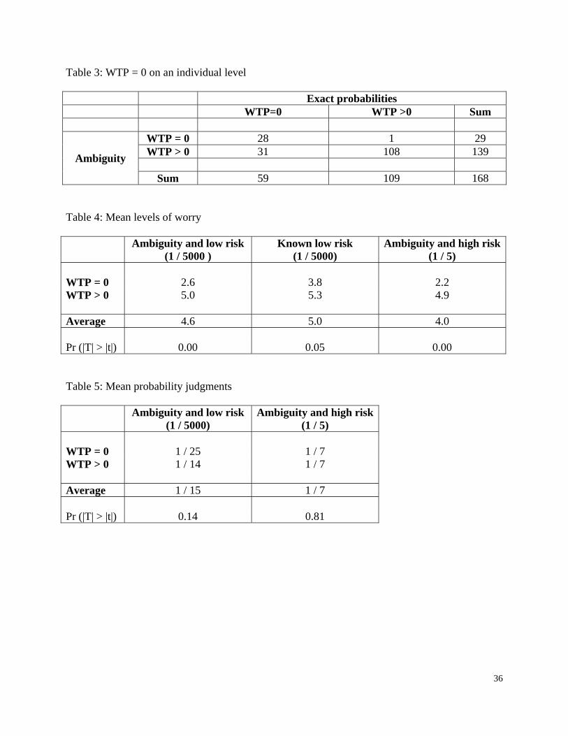
We now analyze whether respondents in Groups 1 or 2 who specified WTP = 0 for at least

one scenario differed when they were presented with ambiguous and exact probabilities. Each

individual can only be situated in one of the four cells of table 3: WTP = 0 for ambiguous and

exact probabilities; WTP = 0 for ambiguous probabilities and WTP > 0 for exact probabilities,

15

WTP = 0 for exact probabilities and WTP > 0 for ambiguous probabilities and WTP > 0 in both

situations.

As shown in Table 3, approximately twice as many individuals (59 versus 29) do not want

to pay anything for insurance if the risk is precisely specified than if the risk is perceived to be

ambiguous. Furthermore, only one person who specified WTP = 0 for an ambiguous risk has a

WTP>0 for insurance with exact probabilities. The other 28 individuals in this group also specify

WTP = 0 for the risk with exact probabilities. On the other hand, 31 of the 59 individuals with

WTP = 0 for an exact probability specify WTP > 0 if the risk is ambiguous. Stated another way,

having a positive WTP with exact probabilities implies (with one exception) having a positive

WTP with ambiguous probabilities. On the other hand, WTP > 0 when the risk is ambiguous does

not imply having WTP>0 with exact probabilities. This finding suggests that respondents are

ambiguity averse.

Impact of loss probabilities versus worry on WTP for insurance

Descriptive analysis of the impact of worry and subjective probabilities: Can one ascribe

the difference between individuals not interested in buying insurance (i.e. WTP=0) and those who

want coverage (i.e. WTP>0) to differences between their subjective probability judgments and/or

their level of worry? Table 4 reports on mean worry ratings for ambiguous and exact probabilities

when the actual risk is very low and for ambiguous probabilities when the risk is high. Mean

subjective probability judgments are compared between small and large ambiguous risks in Table

5.

Insert tables 4 and 5 about here

16

On average, worry is significantly higher for those individuals who are willing to

purchase insurance (WTP>0) than those who had no interest in coverage (WTP =0) for both large

and small perceived probabilities as well as for exact probabilities (Table 4). With respect to the

ambiguous risks, probability judgments are higher for those with WTP>0, but this difference is

only marginally significant (one-sided) when the ambiguous risk is low and almost identical

when the ambiguous risk is high.14 (Table 5). These findings already suggest that worry is more

important than probability of a loss in determining whether a person is willing to purchase

insurance. Furthermore, probability judgments are not significantly correlated with the decision

of people to consider insurance15 and only weakly correlated with their WTP, provided they

consider insurance16.

Table 5 also shows the immense difficulties people have in judging small probabilities.

The low ambiguous risk of 1 / 5000 was on average believed to be a risk of 1 / 15. This is an

overestimation by a factor of 333. The high ambiguous risk of 1 / 5 was, however, slightly

underestimated with 1 / 7 on average. Although probability judgments are higher in the high risk

treatment than in the low risk treatment by a factor of 2 on average, the actual risks differed by a

factor of 1,000. Clearly, the subjects did a particularly poor job in judging the likelihood of a very

small risk and were much better calibrated in estimating the high risk.

14 The mean probabilities for the ambiguity high risk case was 15.3% when WTP=0 and 16.6% when

WTP>0.

15 We constructed a dummy variable that takes a value of one if people have a WTP>0 and a value of zero

otherwise. The Pearson correlation coefficient between this dummy and the subjective probability judgments is 0.08

(78% significance with N=243)

16 The Pearson correlation coefficient between subjective probability judgments and WTP for those

subjects with WTP>0 is 0.14 (96% significant with N=208).

17

This pattern is consistent with Einhorn and Hogarth’s (1985) ambiguity model that is

based on the anchoring-and-adjustment heuristic and mental simulations. With very small

probabilities, there is no room for downward adjustments but considerable room for

overestimating probability. With large subjective ambiguous probabilities, however, downwards

as well as upwards mental simulations are feasible, which is likely to produce a more accurate

estimate of the probability.

Another explanation for this difference could be a person’s past experience. Individuals

should be better in estimating a probability when they have experienced the respective part of the

distribution – 11 or 12 days of monthly precipitation in the summer is a normal event whereas 23

or 24 days would require an individual to have a lifespan (on average) of some 10,000 years to

experience the event just once.

To be consistent with an E(U) model one could contend that individuals having a positive

WTP significantly overestimate the probabilities for very low probability events that are

ambiguous and actually use these estimates in their decisions. For large ambiguous probabilities

individuals would also have to base their WTP for insurance partially on their subjective

probability estimates of a loss to be consistent with expected utility theory and again use these

estimates to determine WTP. We will examine whether individuals behave in this way by

undertaking regression analyses with respect to their decisions regarding their interest in

purchasing insurance and the amount they are willing to pay for coverage.

Comparing the impact of probabilities and worry using regression analysis

Before undertaking these regression analyses we checked to make sure that there was no

multicollinearity between worry and subjective probabilities (i.e. worry could be the consequence

18

of subjective probabilities or subjective probabilities could be influenced by different levels of

worry). Table 6 reveals that neither of these relationships noted above is statistically significant

for the group of individuals having a positive WTP for insurance and for individuals with

WTP=0. The overall correlation between worry and subjective probability judgments is 0.08

(0.19 significance level with N=243).


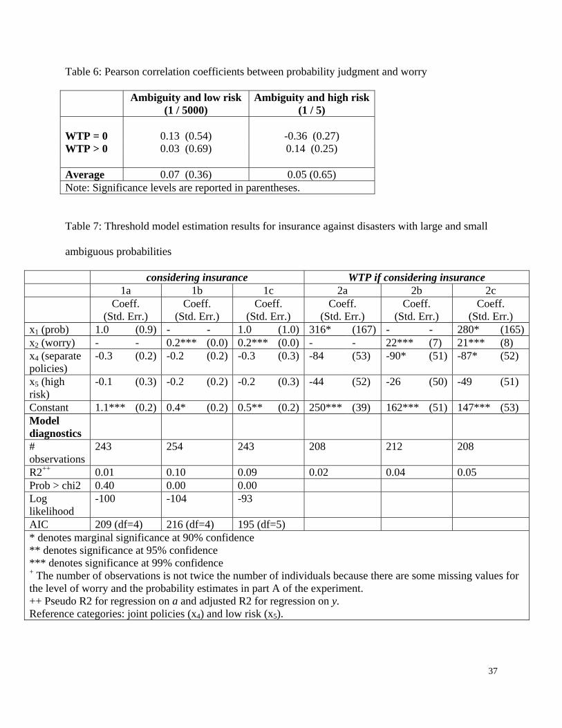
In undertaking the regression analysis, we used so-called threshold models that separately

analyze whether respondents consider insurance at all (i.e. if their WTP=0) and the magnitude of

their WTP if they do consider insurance (i.e. regression on WTP for those with WTP >0). A

simple OLS regression is not suitable because WTP is truncated at 0, and many observations are

located at this extreme point. In practice, our strategy corresponds to estimating a Probit model

for the participation decision with a binary dependent variable taking on a value of 0 if WTP=0

and a value of 1 if WTP>0. We then undertake an OLS regression on WTP for those subjects

who consider insurance. Under certain plausible assumptions17, this approach is consistent with

the more general class of threshold models that are, in turn, based on the so-called Tobit model

(Tobin, 1956; see also Melenberg & van Soest, 1996; Jones, 1989). Threshold models are more

general than Tobit models because they allow parameters to have different effects on the two

17 One can estimate the two equations of a threshold model separately if the error term in the OLS

regression is independent from the participation decision. The general requirement for the identification of both

regression equations is that the error term has a mean of zero and is strictly independent of the variables on the right

hand side of the equation. Our robustness checks using panel methods, for which these assumptions are not critical,

lead to qualitatively identical results.

19

parts of the model. We choose this approach because we wanted to allow for different decision

processes in each stage of the person’s decision process.18

We are particularly interested in comparing the relative effects of probability judgments

and worry. Hence, we estimated three different model specifications for each the binary probits

and the OLS regressions. Model (1) only includes probability judgments (values range from

2/10,000,000 to 4/5). Model (2) only includes worry (values ranging from 1 to 9). Model (3)

includes both probability judgments and worry. We always added a dummy labeled separate

policies to control for the effect of our bundling manipulation and a high risk dummy which

reflects the difference between high and low ambiguous risks. The results of the six regressions

are reported in Table 7.19


18 We ran Tobit models – not discriminating between the two stages – as a benchmark and found that they

do not compare favorably with the more general threshold models in terms of model fit and explanatory power.

Using the same parameters as in Table 7 (below), the R2 of the Tobit models ranged from 0.00 to 0.02 and the

Akaike Information Criterion (AIC) ranged from 1,974 to 3,122. Both measures are very poor fits compared to the

separate regressions. Without separating between the ‘considering insurance’ and WTP stages one loses most of the

explanatory power with respect to characterizing the decision on whether to purchase insurance and how much to

pay for coverage.

19 We also ran a random effects threshold model on Group 1 and Group 2, simultaneously analyzing the

ambiguity and exact probability for the low risk treatments within-subjects. Such a model can be criticized on the

grounds that exact probabilities provided by the experimenter and subjective probabilities provided by the

respondents are treated as the same type of variable. This analysis, on the other hand, controls for unobserved

heterogeneity of the individuals and confirms the findings reported here.

20

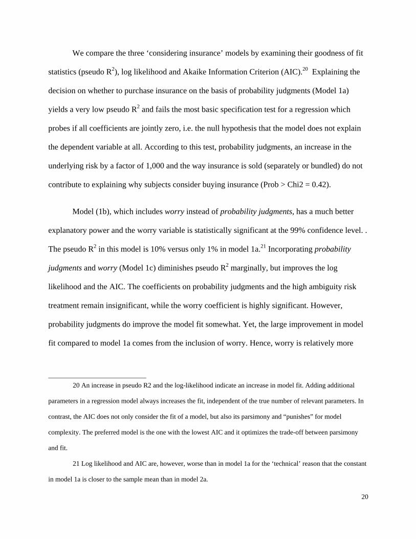
We compare the three ‘considering insurance’ models by examining their goodness of fit

statistics (pseudo R2), log likelihood and Akaike Information Criterion (AIC).20 Explaining the

decision on whether to purchase insurance on the basis of probability judgments (Model 1a)

yields a very low pseudo R2 and fails the most basic specification test for a regression which

probes if all coefficients are jointly zero, i.e. the null hypothesis that the model does not explain

the dependent variable at all. According to this test, probability judgments, an increase in the

underlying risk by a factor of 1,000 and the way insurance is sold (separately or bundled) do not

contribute to explaining why subjects consider buying insurance (Prob > Chi2 = 0.42).

Model (1b), which includes worry instead of probability judgments, has a much better

explanatory power and the worry variable is statistically significant at the 99% confidence level. .

The pseudo R2 in this model is 10% versus only 1% in model 1a.21 Incorporating probability

judgments and worry (Model 1c) diminishes pseudo R2 marginally, but improves the log

likelihood and the AIC. The coefficients on probability judgments and the high ambiguity risk

treatment remain insignificant, while the worry coefficient is highly significant. However,

probability judgments do improve the model fit somewhat. Yet, the large improvement in model

fit compared to model 1a comes from the inclusion of worry. Hence, worry is relatively more

20 An increase in pseudo R2 and the log-likelihood indicate an increase in model fit. Adding additional

parameters in a regression model always increases the fit, independent of the true number of relevant parameters. In

contrast, the AIC does not only consider the fit of a model, but also its parsimony and “punishes” for model

complexity. The preferred model is the one with the lowest AIC and it optimizes the trade-off between parsimony

and fit.

21 Log likelihood and AIC are, however, worse than in model 1a for the ‘technical’ reason that the constant

in model 1a is closer to the sample mean than in model 2a.

21

important for determining insurance decisions than probability judgments or variations in the

actual probability of a loss from 1/5000 to 1/5.

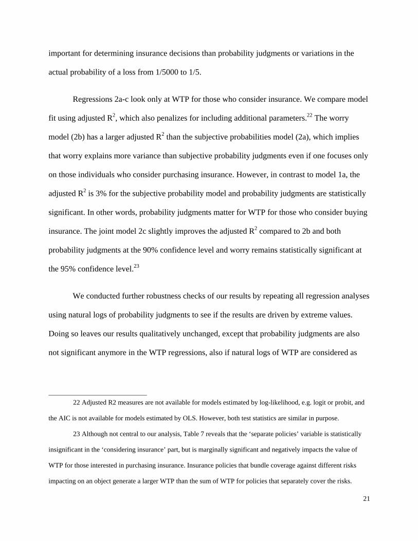
Regressions 2a-c look only at WTP for those who consider insurance. We compare model

fit using adjusted R2, which also penalizes for including additional parameters.22 The worry

model (2b) has a larger adjusted R2 than the subjective probabilities model (2a), which implies

that worry explains more variance than subjective probability judgments even if one focuses only

on those individuals who consider purchasing insurance. However, in contrast to model 1a, the

adjusted R2 is 3% for the subjective probability model and probability judgments are statistically

significant. In other words, probability judgments matter for WTP for those who consider buying

insurance. The joint model 2c slightly improves the adjusted R2 compared to 2b and both

probability judgments at the 90% confidence level and worry remains statistically significant at

the 95% confidence level.23

We conducted further robustness checks of our results by repeating all regression analyses

using natural logs of probability judgments to see if the results are driven by extreme values.

Doing so leaves our results qualitatively unchanged, except that probability judgments are also

not significant anymore in the WTP regressions, also if natural logs of WTP are considered as

22 Adjusted R2 measures are not available for models estimated by log-likelihood, e.g. logit or probit, and

the AIC is not available for models estimated by OLS. However, both test statistics are similar in purpose.

23 Although not central to our analysis, Table 7 reveals that the ‘separate policies’ variable is statistically

insignificant in the ‘considering insurance’ part, but is marginally significant and negatively impacts the value of

WTP for those interested in purchasing insurance. Insurance policies that bundle coverage against different risks

impacting on an object generate a larger WTP than the sum of WTP for policies that separately cover the risks.

22

dependent variable. Apparently, the explanatory power of probability judgments is very limited

while worry is positively related to considering insurance and WTP.

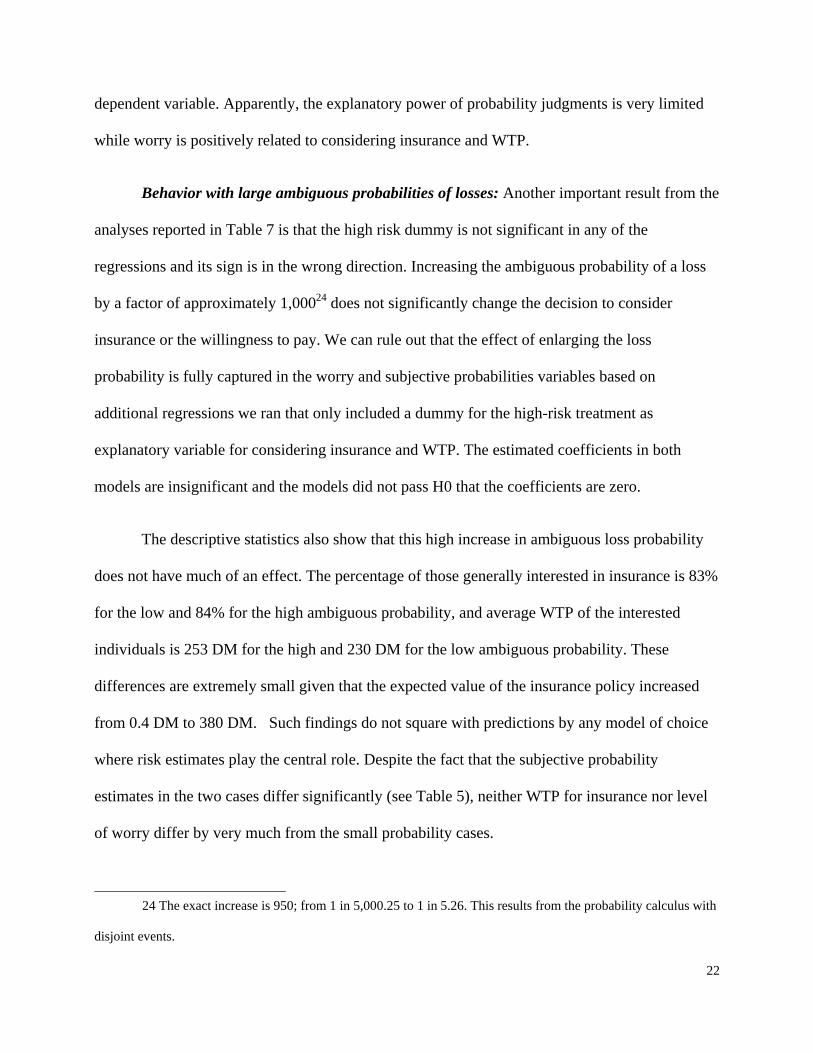
Behavior with large ambiguous probabilities of losses: Another important result from the

analyses reported in Table 7 is that the high risk dummy is not significant in any of the

regressions and its sign is in the wrong direction. Increasing the ambiguous probability of a loss

by a factor of approximately 1,00024 does not significantly change the decision to consider

insurance or the willingness to pay. We can rule out that the effect of enlarging the loss

probability is fully captured in the worry and subjective probabilities variables based on

additional regressions we ran that only included a dummy for the high-risk treatment as

explanatory variable for considering insurance and WTP. The estimated coefficients in both

models are insignificant and the models did not pass H0 that the coefficients are zero.

The descriptive statistics also show that this high increase in ambiguous loss probability

does not have much of an effect. The percentage of those generally interested in insurance is 83%

for the low and 84% for the high ambiguous probability, and average WTP of the interested

individuals is 253 DM for the high and 230 DM for the low ambiguous probability. These

differences are extremely small given that the expected value of the insurance policy increased

from 0.4 DM to 380 DM. Such findings do not square with predictions by any model of choice

where risk estimates play the central role. Despite the fact that the subjective probability

estimates in the two cases differ significantly (see Table 5), neither WTP for insurance nor level

of worry differ by very much from the small probability cases.

24 The exact increase is 950; from 1 in 5,000.25 to 1 in 5.26. This results from the probability calculus with

disjoint events.

23

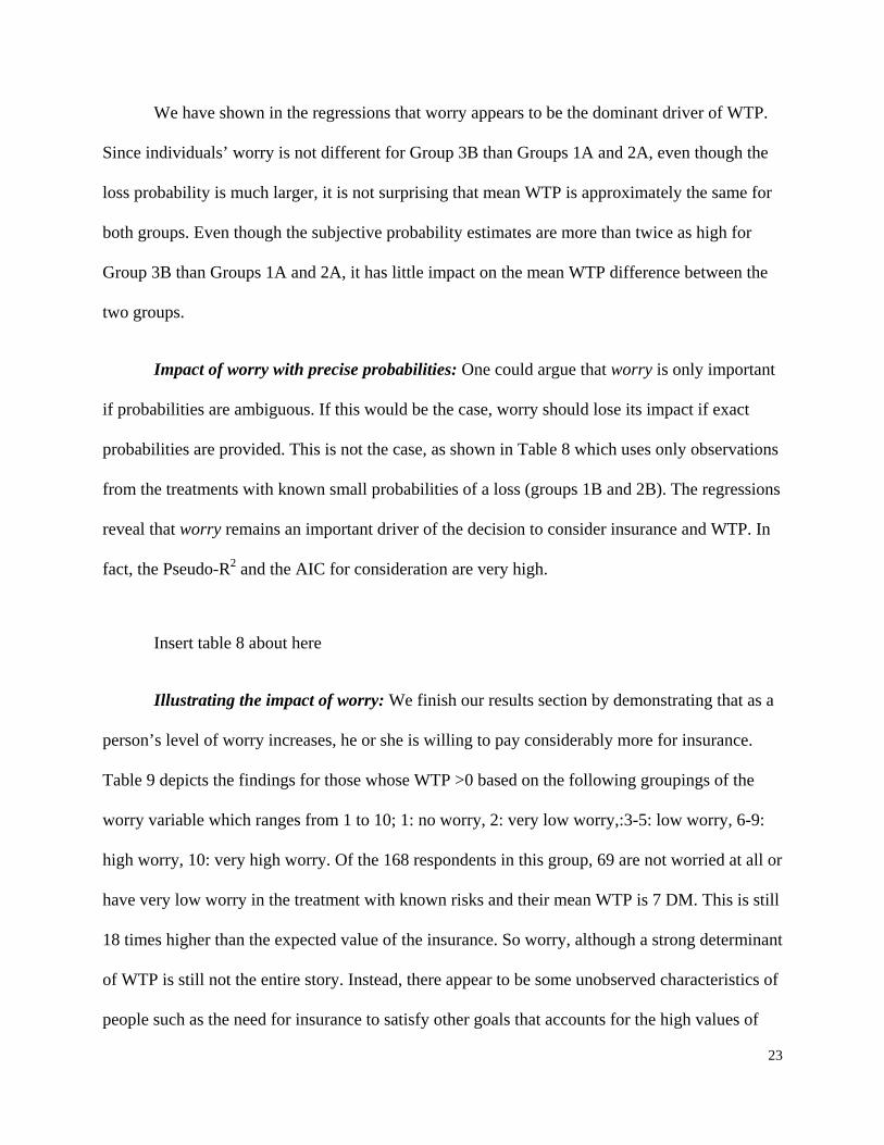
We have shown in the regressions that worry appears to be the dominant driver of WTP.

Since individuals’ worry is not different for Group 3B than Groups 1A and 2A, even though the

loss probability is much larger, it is not surprising that mean WTP is approximately the same for

both groups. Even though the subjective probability estimates are more than twice as high for

Group 3B than Groups 1A and 2A, it has little impact on the mean WTP difference between the

two groups.

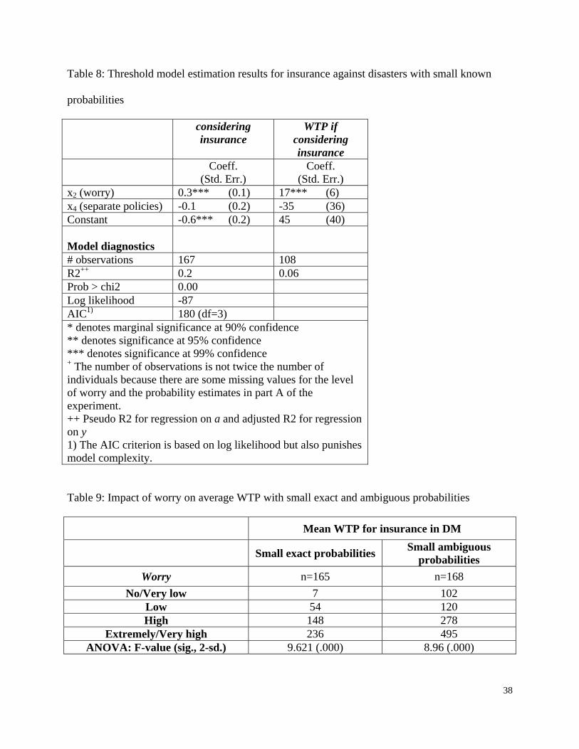
Impact of worry with precise probabilities: One could argue that worry is only important

if probabilities are ambiguous. If this would be the case, worry should lose its impact if exact

probabilities are provided. This is not the case, as shown in Table 8 which uses only observations

from the treatments with known small probabilities of a loss (groups 1B and 2B). The regressions

reveal that worry remains an important driver of the decision to consider insurance and WTP. In

fact, the Pseudo-R2 and the AIC for consideration are very high.


Illustrating the impact of worry: We finish our results section by demonstrating that as a

person’s level of worry increases, he or she is willing to pay considerably more for insurance.

Table 9 depicts the findings for those whose WTP >0 based on the following groupings of the

worry variable which ranges from 1 to 10; 1: no worry, 2: very low worry,:3-5: low worry, 6-9:

high worry, 10: very high worry. Of the 168 respondents in this group, 69 are not worried at all or

have very low worry in the treatment with known risks and their mean WTP is 7 DM. This is still

18 times higher than the expected value of the insurance. So worry, although a strong determinant

of WTP is still not the entire story. Instead, there appear to be some unobserved characteristics of

people such as the need for insurance to satisfy other goals that accounts for the high values of

24

WTP. Turning to the worry variable, the mean WTP estimates for those in the high and extremely

high worry groups are respectively 20 and 30 times higher than the mean WTP for the no and low

worry group. Similarly, under ambiguous probabilities the group with the highest level of worry

is willing to pay almost 5 times more for insurance than the group with no or very low worry.


General Discussion

The above experiments suggest that subjective estimates of ambiguous probabilities play

a minor role in explaining when individuals may be interested in buying insurance and the

amount they are willing to pay for coverage. Other authors have reported on findings that are

consistent with this result. Huber, Wider, and Huber (1997) have experimentally demonstrated

that in naturalistic decision tasks, probabilities are used far less than expected from classical

decision theory. In their experiments, most individuals do not request probability information

before making their decisions even though they could have obtained this information.

With small probabilities, there is strong evidence from the experimental literature that

with very small exact probabilities, individuals have a hard time understanding their meaning and

are considerably insensitive to variations of their level (Kunreuther, Novemsky, & Kahneman,

2001). In their experiments, individuals’ perception of the safety of a chemical facility did not

differ when the risks of a serious industrial accident varied between 1 in 100,000, 1 in 1,000,000,

and 1 in 10,000,000 (Kunreuther et al., 2001). We extend this finding and demonstrate that at

least for ambiguous risks, even large probabilities such as 1 in 5 may not lead to different

25

insurance decisions than probabilities of 1 in 5,000. We cannot judge from our experiments,

however, whether this would still hold for known probabilities of 1 in 5 vs. 1 in 5,000 since we

did not vary known probabilities. With respect to the consideration of insurance and WTP for

coverage, we would expect that variations of known probabilities in this interval would make a

large difference in behavior.

Sunstein (2003) has coined the term probability neglect. He refers to a number of

experimental studies where people are quite insensitive to changes of probabilities (with an

overlap with those referenced, here) and adds evidence from a study on cancer risk he had carried

out at the University of Chicago. In this study, individuals’ WTP to eliminate the cancer risk only

increased by a factor of about two when the probability was ten times higher. He also reports on

anecdotal evidence for peoples’ strong emotional reactions after terrorist acts; individuals seem to

focus on the potential event rather than its likelihood. In his opinion, this is the main reason why

the public demands a substantial governmental response to terrorist acts. Our results indicate that

his view might also hold in settings were the stakes are high but clearly far below the potential

consequences of a terrorist act.

Our results suggest that the low probability insurance puzzle can be explained by focusing

on the role that worry plays in people’s decisions. More specifically the data indicate that those

who are more worried about suffering a loss will be more likely to purchase insurance and pay

more for coverage than those who are less worried. Obtaining peace of mind is worth a lot if one

is highly worried.

The effect of ambiguity on behavior has been studied systematically since Daniel

Ellsberg’s classic study (Ellsberg, 1961). However, to the best of our knowledge, we demonstrate

26

for the first time that ambiguity has a remarkably different effect on behavior than known

probabilities in a realistic high-stakes scenario where probabilities are very small. In our

experiments individuals exhibit a stronger aversion to ambiguous than precise probabilities with

more individuals considering insurance and indicating a larger WTP for coverage when the risk is

ambiguous than when probabilities are specified precisely. Probabilities were not the primary

driver of this behavior. Rather we believe that people are cognizant of their difficulties in judging

probabilities of very rare events and hence tend to ignore their own probability judgments when

deciding about the purchase of insurance. An alternative explanation that ambiguity leads to

higher worry can be ruled out by looking at table 4. Worry is not higher on average in our

treatments with ambiguity than with known probabilities.

Implications, limitations, and future research

We ran a laboratory experiment with the aim of implementing a real-life risk with high-

stakes monetary consequences. Although we feel that our experimental design has the advantage

of coming quite close to an actual protective decision for a low-probability-high consequence

event, we are aware that generalizations based on laboratory evidence must be qualified even

though our findings of extreme responses with many individuals having a WTP = 0 and many

having a large WTP are supported by McClelland et al. (1993) in the laboratory and Kunreuther

(1978) in the field.

Another potential limitation of our design is that individuals did not lose their own money

and had the potential of gaining additional funds. We did our best to ensure that the loss was

perceived as a real one: Individuals received pictures of the painting and the sculpture; there was

27

real money at stake that was ‘attached’ to those objects and the person had the option to purchase

insurance against a large loss. We also discussed the situation with each group after the

experiment and their comments indicated that they had framed the problem as a potential loss

rather than as a lottery. Hence, we feel that we have been successful in implementing a large

stakes insurance experiment.

Our findings suggest that insurers can charge a premium considerably in excess of

expected loss when probabilities are extremely low and still generate considerable demand for

coverage. Interest in terrorism insurance coverage at extremely high prices supports this finding

(General Accounting Office, 2002). For low-probability-high consequence events, consumer

unions or financial test magazines might consider informing people about how to compute the

expected loss so that comparisons between the actual premium and an actuarially fair one could

be made.

Insurers could also be expected to take advantage of their knowledge that ambiguous

probabilities lead to higher WTP than well-specified estimates when the likelihood of the event

occurring is very small. This may be a principal reason why one rarely learns about the chances

of making a claim at the time one purchases a policy. Future research might also want to look at a

comparison of large known and ambiguous probabilities in a realistic large stakes scenario to

complete the picture.

Not only insurers but also other companies or institutions such as politicians and the

media who are interested in changing behavior may find ways to stir up individuals’ worries,

sometimes for their own benefit but also for the benefit of those at risk. One current example

where generating worry by the media has changed behavior is the swine flu concerns of 2009

28

where the probability of an infection was originally highly uncertain and one rarely obtained

estimates of the probabilities and consequences of the illness. In the early phase of pandemic, the

media succeeded in stirring up worries by those residing in many countries (e.g., BBC News, July

19, 2009), leading to calls for and large stake government purchases of vaccinations against the

swine flu. Later, however, the risks of the swine flu became more transparent but there was now

increasing uncertainty and worry about the side effects of the vaccinations, again stirred by the

media (Focus Online, November 11, 2009). As a result, many people decided against vaccination

and there was an oversupply of vaccinations in some countries such as Germany. Stirring up

worry by the media apparently had a strong influence on the behavior of people.

Future research would benefit not only from manipulating the degree of worry in the

laboratory but also by measuring the different dimensions of worry that are evoked by exposing

individuals to different scenarios. In this way we would increase our understanding as to what

makes individuals worry about one risk but not another. Future research might also want to look

more closely at ‘trait’-like concepts such as optimism and pessimism etc. (Einhorn & Hogarth,

1985).

Special consideration should also be given to the decision processes of individuals who

decide not to even consider insurance. As Slovic, Fischhoff, & Lichtenstein (1981) noted "people

often attempt to reduce the anxiety generated in the face of uncertainty by denying the

uncertainty, thus making the risk seem so small it can safely be ignored […]." (p.160). Although

we would expect that worry is an even more accurate term for the emotion invoked with respect

to potential high-stakes losses, the rationale and findings of the experiments reported in this paper

are consistent with their view. Individuals with low levels of worry have a high propensity not to

protect themselves. For these individuals, there is no monetary incentive for purchasing

29

insurance. Hence, subsidies reducing the insurance premium may not be expected to work since

they are not willing to even pay a penny for insurance. However, for those individuals deserving

special treatment such as low income individuals, insurance stamps (like food stamps) might be

provided for equity reasons; and for risks that have negative externalities when people fail to

purchase insurance, such as disaster relief provided to uninsured flood victims, it may be

necessary to require coverage for all those residing in these hazard-prone areas. (Kunreuther &

Michel-Kerjan, in press).

30

References

Baron, J., Hershey, J. C., & Kunreuther, H. (2000). Determinants of priority for risk reduction:

The role of worry. Risk Analysis, 20(4), 413–427. doi:10.1111/0272-4332.204041.

BBC News (2009). Swine flu: how the numbers add up. July 19, 2009.

http://news.bbc.co.uk/2/hi/health/8159488.stm

Becker, G. M., DeGroot, M. H., & Marschak, J. (1964). Measuring utility by a single-response

sequential method. Behavioral Science, 9, 226–232. doi:10.1002/bs.3830090304

Bohm, P., Lindén, J., & Sonnegard, J. (1997). Eliciting reservation prices: Becker-DeGroot-

Marschak mechanisms vs. markets. Economic Journal, 107(443), 1079–1089.

Bolle, F. (1990). High reward experiments without high expenditure for the experimenter?

Journal of Economic Psychology, 11(2), 157-167.

Caplin, A. & Leahy, J. (2001). Psychological expected utility and anticipatory feelings. Quarterly

Journal of Economics, 116(1), 55-79.

Einhorn, H., & Hogarth, R. M. (1985). Ambiguity and uncertainty in probabilistic inference.

Psychological Review, 92, 433–461.

Ellsberg, D. (1961). Risk, Ambiguity, and the Savage Axioms. Quarterly Journal of Economics,

75(4), 643–669.

Focus Online (2009). Neue Grippe - die Nebenwirkungen der Impfung. November 8, 2009.

http://www.focus.de/gesundheit/ratgeber/schweinegrippe/neue-grippe-die-nebenwirkungen-

der-impfung_aid_451821.html.

31

Fox, C. R., & Tversky, A. (1995). Ambiguity aversion and comparative ignorance. Quarterly

Journal of Economics, 110(3), 585–603.

Fox, C. R., & Weber, M. (2002). Ambiguity aversion, comparative ignorance, and decision

context. Organizational behavior and human decision process, 88(1), 476-498.

doi:10.1006/obhd.2001.2990

General Accounting Office (2002). Terrorism insurance: Rising uninsured exposure to attacks

heightens potential economic vulnerabilities. Testimony of Richard J. Hillman Before the

Subcommittee on Oversight and Investigations.

Hogarth, R. &, Kunreuther, H. (1995). Decision making under ignorance: Arguing with yourself.

Journal of Risk and Uncertainty, 10(1), 15–36.

Hsee, C., & Kunreuther, H. (2000). The affection effect in insurance decisions. Journal of Risk

and Uncertainty, 20(2), 141–159.

Huber, O., Wider, R., & Huber, O. (1997). Active information search and complete information

presentation in naturalistic risky decision tasks. Acta Psychologica, 95(1), 15–29.

Jones, A. M. (1989). A double-hurdle model of cigarette consumption. Journal of Applied

Econometrics, 4(1), 23-39.

Kahneman, D., & Tversky, A. (1979). Prospect theory: An Analysis of Decision under Risk.

Econometrica, 47(1), 263-291.

Krantz, D. and Kunreuther, H. (2007). Goals and plans in decision making. Judgment and

Decision Making, 2(3), 137-168.

Kunreuther, H. C. (1978). Disaster insurance protection. Public Policy Lessons, New York, NY:

32

Wiley.

Kunreuther, Howard and Erwann Michel-Kerjan (in press), “From Market to Government Failure

in Insuring U.S. Natural Catastrophes: How Can Long-Term Contracts Help”. In Private

Markets and Public Insurance Programs. J. Brown (ed). Washington, D.C., American

Enterprise Institute Press.

Kunreuther, H., Novemsky, N., & Kahneman, D. (2001). Making low probabilities useful.

Journal of Risk and Uncertainty, 23(2), 103–120.

Loewenstein, G., Weber, E., Hsee, C., & Welch, N. (2001). Risk as feelings. Psychological

Bulletin, 127(2), 267–286.

MacLeod, A. K., Williams, J., & Bekerian, D. (1991). Worry is reasonable: The role of

explanations in pessimism about future events. Journal of Abnormal Psychology, 100, 478–

486.

McClelland, G. H., Schulze, W. D., & Coursey, D. L. (1993). Insurance for low-probability

hazards; a bimodal response to unlikely events. Journal of Risk and Uncertainty, 7(1), 95–116.

doi:10.1007/BF01065317

Melenberg, B. & Soest, A. van (1996). Parametric and semi-parametric modeling of vacation

expenditures. Journal of Applied. Econometrics, 11(1), 59-76.

Neumann, J. von, & Morgenstern, O. (1947). Theory of games and economic behavior. Princeton,

NJ: Princeton University Press.

Rottenstreich, Y., & Hsee, C. (2001). Money, kisses, and electric shocks: On the affective

psychology of risk. Psychological Science, 12(3), 185–190.

33

Safra, Z., Segal, U., & Spivak, A. (1990). The Becker-DeGroot-Marshak mechanism and

nonexpected utility; a testable approach. Journal of Risk and Uncertainty, 3(2), 177–190.

doi:10.1007/BF00056371

Savage, L. J. (1954). The foundations of statistics. New York, NY: Wiley.

Schade, C. & Kunreuther, H. (2001): Worry and mental accounting with protective measures.

Working paper, Wharton School, University of Pennsylvania.

Slovic, P., Fischhoff, B., Lichtenstein, S., Corrigan, & Combs, B. (1978). Controlled laboratory

experiments. In H. Kunreuther et al. (Eds.), Disaster insurance protection: Public Policy

Lessons (pp. 165-186). New York, NY: Wiley.

Slovic, P., Finucane, M., Peters, E., & MacGregor, D. G. (2002). The affect heuristic. In T.

Gilovich, D. Griffin, & D. Kahneman (Eds.), Heuristics and biases: The psychology of

intuitive judgment (pp. 397-420). New York, NY: Cambridge University Press.

Slovic, P. & Lichtenstein, S. (1968). The relative importance of probabilities and payoffs in risk

taking. Journal of Experimental Psychology Monographs, 78, 1-18.

Slovic, P., Fischhoff, B. & Lichtenstein, S. (1981). Perception and acceptability of risk from

energy systems. In A. Baum and J. Singer (Eds.), Advances in environmental psychology, 3

(pp. 157-169). Hillsdale, NJ: Erlbaum.

Sunstein, C. (2003). Terrorism and probability neglect. Journal of Risk and Uncertainty, 26, 121–

136. doi:10.1023/A:1024111006336

Tobin, J. (1956). Estimation of relationships for limited dependent variables. Econometrica,

26(1), 24-36.

34

Wang, Tuo., R. Venkatesh, & Chatterjee, R. (2007). Reservation price as a range: An incentive-

compatible measurement approach. Journal of Marketing Research, 44(2), 200-213, DOI:

10.1509/jmkr.44.2.200.

35

Table 1: Experimental design (Group 3, Part A not analyzed in this contribution)

Within-subjects

Part A of experiment: inherited painting

Part B of experiment: inherited sculpture

Between-

subjects

Group 1

(n=87)

Rain frequencies in July and August each with probability of 1 in 10,000 – separate insurance

policies for each risk

Two precise risks each with probability of 1 in 10,000 –

separate insurance policies for each risk

Group 2

(n=81)

Rain frequencies in July and August each with probability of 1 in 10,000 – one insurance policy

for both risks

Two precise risks each with probability of 1 in 10,000 – one

insurance policy for both risks

Group 3

(n=86)

Rain frequencies July and August each with probability 1 in 10,000 – first insurance sold before second

risk introduced

Rain frequencies in July and August each with probability of 1

in 10 – separate insurance policies for each of the risks

Table 2: Distribution of WTP for insurance

WTP = 0 0 < WTP 10*E(loss)

WTP > 10*E(Loss)

Percentage Percentage Percen-

tage Mean Std. Dev.

Mean/ E(Loss)

Ambiguity and low risk (1/5000)1)

17 % 2 % 81 % 235 DM2) 310 DM 588

Known low risk (1/5000)2)

35 % 8 % 57 % 126 DM2) 198 DM 315

Ambiguity and high risk (1/5)3)

16 % 84 % - - - -

1) Groups 1A and 2A, N=168. Expected value of loss was 0.4DM. WTP did not significantly differ between groups.

2) Groups 1B and 2B, N=168. Expected value of loss was 0.4DM. WTP did not significantly differ between groups.

3) Group 3B, N=86. Expected value of loss was 380DM. Mean WTP is 215DM, standard deviation is 294 DM.

36

Table 3: WTP = 0 on an individual level

Exact probabilities WTP=0 WTP >0 Sum

Ambiguity

WTP = 0 28 1 29 WTP > 0 31 108 139

Sum 59 109 168

Table 4: Mean levels of worry

Ambiguity and low risk (1 / 5000 )

Known low risk (1 / 5000)

Ambiguity and high risk(1 / 5)

WTP = 0 2.6 3.8 2.2 WTP > 0 5.0 5.3 4.9 Average 4.6 5.0 4.0 Pr (|T| > |t|) 0.00 0.05 0.00 Table 5: Mean probability judgments

Ambiguity and low risk(1 / 5000)


WTP = 0 1 / 25 1 / 7 WTP > 0 1 / 14 1 / 7 Average 1 / 15 1 / 7 Pr (|T| > |t|) 0.14 0.81

37

Table 6: Pearson correlation coefficients between probability judgment and worry

Ambiguity and low risk(1 / 5000)


WTP = 0 0.13 (0.54) -0.36 (0.27) WTP > 0 0.03 (0.69) 0.14 (0.25) Average 0.07 (0.36) 0.05 (0.65) Note: Significance levels are reported in parentheses. Table 7: Threshold model estimation results for insurance against disasters with large and small

ambiguous probabilities

considering insurance WTP if considering insurance 1a 1b 1c 2a 2b 2c Coeff.

(Std. Err.) Coeff.

(Std. Err.) Coeff.

(Std. Err.) Coeff.

(Std. Err.) Coeff.

(Std. Err.) Coeff.

(Std. Err.) x1 (prob) 1.0 (0.9) - - 1.0 (1.0) 316* (167) - - 280* (165)x2 (worry) - - 0.2*** (0.0) 0.2*** (0.0) - - 22*** (7) 21*** (8) x4 (separate policies)

-0.3 (0.2) -0.2 (0.2) -0.3 (0.3) -84 (53) -90* (51) -87* (52)

x5 (high risk)

-0.1 (0.3) -0.2 (0.2) -0.2 (0.3) -44 (52) -26 (50) -49 (51)

Constant 1.1*** (0.2) 0.4* (0.2) 0.5** (0.2) 250*** (39) 162*** (51) 147*** (53) Model diagnostics

# observations

243 254 243 208 212 208

R2++ 0.01 0.10 0.09 0.02 0.04 0.05 Prob > chi2 0.40 0.00 0.00 Log likelihood

-100 -104 -93

AIC 209 (df=4) 216 (df=4) 195 (df=5) * denotes marginal significance at 90% confidence ** denotes significance at 95% confidence *** denotes significance at 99% confidence + The number of observations is not twice the number of individuals because there are some missing values for the level of worry and the probability estimates in part A of the experiment. ++ Pseudo R2 for regression on a and adjusted R2 for regression on y. Reference categories: joint policies (x4) and low risk (x5).

38

Table 8: Threshold model estimation results for insurance against disasters with small known

probabilities

considering insurance

WTP if considering insurance

Coeff. (Std. Err.)

Coeff. (Std. Err.)

x2 (worry) 0.3*** (0.1) 17*** (6) x4 (separate policies) -0.1 (0.2) -35 (36) Constant -0.6*** (0.2) 45 (40) Model diagnostics

# observations 167 108 R2++ 0.2 0.06 Prob > chi2 0.00 Log likelihood -87 AIC1) 180 (df=3) * denotes marginal significance at 90% confidence ** denotes significance at 95% confidence *** denotes significance at 99% confidence + The number of observations is not twice the number of individuals because there are some missing values for the level of worry and the probability estimates in part A of the experiment. ++ Pseudo R2 for regression on a and adjusted R2 for regression on y 1) The AIC criterion is based on log likelihood but also punishes model complexity. Table 9: Impact of worry on average WTP with small exact and ambiguous probabilities

Mean WTP for insurance in DM

Small exact probabilities Small ambiguous

probabilities

Worry n=165 n=168

No/Very low 7 102 Low 54 120 High 148 278

Extremely/Very high 236 495 ANOVA: F-value (sig., 2-sd.) 9.621 (.000) 8.96 (.000)

39

Appendix

A.1 Experimental Instructions (translations of parts A and B of the experiment)

Group 1 (separate policies)

Part A: Ambiguity

You inherited a small painting and have received a photograph of it. The photo carries an

individual identification number. You do not know if the painting is an original or a

reproduction. If it is an original it is worth 2,000 DM. If it is a reproduction it is worth

nothing.

One person in the entire group of respondents participating in our experiment (about 260 to

280 people) has an original painting. All others have reproductions. Which one of the

paintings is the original will be determined by a random draw symbolizing the decision of an

art appraiser at the end of the entire experiment. The person who has the original painting will

actually receive the value of the painting: 2,000 DM (in real bills!).

Theft and fire threaten your painting.

Whether or not the painting will be stolen will be determined by the weather conditions in

July. If it will rain on 24 days in July (not more but also not less), a theft will occur. More

precisely, the painting will be stolen if the weather station at the Frankfurt Airport will report

on exactly 24 days of rain. A day is defined as a rainy day if there is at least 1 mm of rain on

this day.

The weather conditions in August determine if a fire will destroy the painting. If it will rain on

23 days in August (not more but also not less), a fire will occur. More precisely, a fire will

40

destroy the painting if the weather station at the Frankfurt Airport will report exactly 23 days

of rain. Here again a day is defined as a rainy day if there is at least 1 mm of rain on this day.

You can buy insurance policies against either each or both of these risks. If you have an

insurance policy against theft or fire and the painting will be stolen or destroyed by fire,

respectively, the insurance will reimburse you for the loss of 2,000 DM. If you have an

insurance policy against fire and the painting will be destroyed by fire, the insurance will

reimburse you for the value of 2,000 DM.

The insurance company will sell the insurance policy and charge the money for it only in case

an art appraiser, represented by the random draw of the experimenter, finds out that your

painting is an original. Thus, for all respondents having the reproduction the payments for the

insurance policies will remain hypothetical. However, for the one having the original painting

they will become true and have to be paid from his or her own money.

The selling procedure for the theft insurance policy is organized in the following way:

Before the experiment, the experimenter selected a secret selling price for the theft insurance

policy. He or she wrote it on a piece of paper and put it into the envelope on the front desk.

You are now required to write a buying price equal to your maximum willingness to pay for

the theft insurance policy on the form in front of you and to put it in the respective envelope.

After the experiment, the experimenter will open the envelope with the selling price. If your

buying price is equal to or higher than the secret selling price you will have bought or are able

to buy the theft insurance policy should you be the person with the original painting.(if you are

the one who has the original painting). If your buying price is lower than the secret price, you

are not able to buy the theft insurance policy.

41

Note that you have no information about the selling price for the theft insurance policy. The

experimenter changes this price every time.

In this situation, the best you can do is to state your true value, your maximum willingness to

pay for the theft insurance policy.

It does not make sense to state a buying price higher than your maximum willingness to pay

since you may end up paying this high price.

It does also not make sense to state a price lower than your maximum willingness to pay. If

your stated price is lower than the selling price but you, in fact, would have been willing to

pay that price you may end up without the theft insurance policy even if you would have liked

to buy it for that price if you are the one who has the original painting.

If you do not want to buy the theft insurance policy please state 0 DM on the respective form.

Please do not announce your buying price to the others and do not raise questions that allow

the other participants to guess your buying price.

Again, note that you only have to actually pay the price for the insurance policy if you are the

one who has the original painting. This is because the insurance company will only sell the

insurance policy if the painting is verified as the original. In this case, the person who has the

original painting is able to buy insurance. He or she has to pay for the coverage of the

insurance policies from his or her own money.

Basically, that means that you are buying insurance for the original and that you only pay for it

in case you have it.

Now, please put the form with your maximum buying price in the appropriate envelope and

hand it over to the experimenter.

42

The selling procedure for the fire insurance policy is organized the following way:

The selling procedure of the fire insurance policy is organized in exactly the same way as the

selling procedure for the theft insurance policy, i.e. again there is a secret selling price in an

envelope, and you again are supposed to state your maximum buying price.



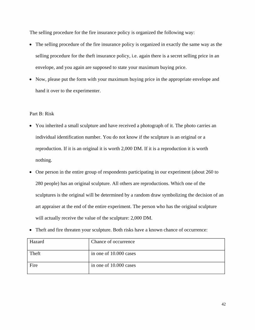
Part B: Risk

You inherited a small sculpture and have received a photograph of it. The photo carries an

individual identification number. You do not know if the sculpture is an original or a

reproduction. If it is an original it is worth 2,000 DM. If it is a reproduction it is worth

nothing.

One person in the entire group of respondents participating in our experiment (about 260 to

280 people) has an original sculpture. All others are reproductions. Which one of the

sculptures is the original will be determined by a random draw symbolizing the decision of an

art appraiser at the end of the entire experiment. The person who has the original sculpture

will actually receive the value of the sculpture: 2,000 DM.

Theft and fire threaten your sculpture. Both risks have a known chance of occurrence:

Hazard Chance of occurrence

Theft in one of 10.000 cases

Fire in one of 10.000 cases

43

A bingo cage with 100 balls will be used to determine whether or not the sculpture will be

stolen and whether or not it will be destroyed by fire.

- Whether or not the sculpture will be stolen will be determined by the following two-stage

procedure: If a ball with a number between 2 and 100 is drawn, no theft will have

occurred. We will continue drawing of the bingo cage with 100 balls after the first draw

only if a ball carrying the number 1 is drawn. Otherwise nothing happened. In a second

draw, another ball from the bingo cage with 100 balls will be taken. Theft occurs if the ball

with the number 1 is drawn in the second stage. The chance that both these events occur is

exactly 1 in 10,000.

- Secondly we will determine the case if fire occurs. We will proceed with the same two-

stage procedure as used for the theft situation.

You can buy insurance policies against either each or both of these risks. If you have an

insurance policy against theft or fire and the sculpture will be stolen or destroyed by fire,

respectively, the insurance will reimburse you for the loss of 2,000 DM. If you have an

insurance policy against fire and the fire destroys the sculpture, the insurance will reimburse

you for the value of 2,000 DM.

The insurance company will sell the insurance policy and charge the money for it only in case

an art appraiser, represented by the random draw of the experimenter, finds out that the

sculpture is an original. Thus, for all respondents having the reproduction, the payments for

the insurance policies will remain hypothetical. However, for the one having the original

sculpture they will become true and have to be paid from his or her own money.

44

The selling procedure for the theft insurance policy is organized the following way:

The selling procedure of the theft insurance policy is organized in exactly the same way as the

selling procedure for the theft and fire insurance policies in the first part of the experiment, i.e.

there again is a secret selling price in an envelope, and you again are supposed to state your

maximum buying price.



The selling procedure for the fire insurance policy is organized the following way:

The selling procedure of the fire insurance policy is organized in exactly the same way as the

selling procedure for the theft and fire insurance policy in the first and the theft insurance

policy in the second part of the experiment, i.e. there again is a secret selling price in an

envelope, and you again are supposed to state your maximum buying price.



45

Group 2 (one policy)

The only difference between groups 1 and 2 was that in group 2 we sold bundled rather than

separate insurance in both parts A and B.

Therefore, the part of the instructions dealing with insurance was written up as follows in part A

(B) of the experiment:

You can buy an insurance policy against each of these two risks. If you have an insurance

policy and your painting (sculpture) will be stolen or destroyed by fire, the insurance will

reimburse you for the loss of 2,000 DM.

Moreover, the selling procedure was described in the following way in part A (B) of the

experiment:

Before the experiment, the experimenter selected a secret selling price for the insurance

policy. He or she wrote it on a piece of paper and put it into the envelope on the front desk.

In the following you are required to write a buying price equaling your maximum willingness

to pay for the insurance policy on the form in front of you and to put it in the respective

envelope.

After the experiment, the experimenter will open the envelope with the selling price. If your

buying price is equal to or higher than the secret selling price, you are able to buy the

insurance policy (in case you are the one who has the original painting (sculpture)). If your

buying price is lower than the secret price, you are not able to buy the insurance policy.

Note that you have no information about the selling price for the insurance policy. The

experimenter changes this price every time.

46

In this situation, the best you can do is to state the true value of your maximum willingness to

pay for the insurance policy.

It does not make sense to state a buying price higher than your maximum willingness to pay

since you may end up paying this high price.

It does also not make sense to state a price lower than your maximum willingness to pay. If

your stated price is lower than the selling price but you in fact would have been willing to pay

that price you may end up without the insurance policy even if you would have liked to buy it

for that price if you are the one who has the original painting (sculpture).

If you do not want to buy the insurance policy please state 0 DM on the respective form.

Please do not announce your buying price to the other participants and do not raise questions

that allow others to guess your buying price.

Again, note that you only have to actually pay the price for the insurance policy if you are the

one who has the original painting. This is because the insurance company will only sell the

insurance policy if the painting is verified as the original. In this case, the person who has the

original painting is able to buy insurance. He or she has to pay for the coverage of the

insurance policies from his or her own money.

Basically that means that you are buying insurance for the original and that you only pay for it

in case you have it.



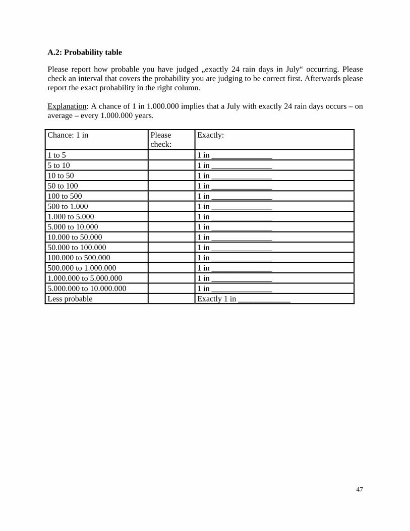
47

A.2: Probability table Please report how probable you have judged „exactly 24 rain days in July“ occurring. Please check an interval that covers the probability you are judging to be correct first. Afterwards please report the exact probability in the right column. Explanation: A chance of 1 in 1.000.000 implies that a July with exactly 24 rain days occurs – on average – every 1.000.000 years. Chance: 1 in Please

check: Exactly:

1 to 5 1 in _______________ 5 to 10 1 in _______________ 10 to 50 1 in _______________ 50 to 100 1 in _______________ 100 to 500 1 in _______________ 500 to 1.000 1 in _______________ 1.000 to 5.000 1 in _______________ 5.000 to 10.000 1 in _______________ 10.000 to 50.000 1 in _______________ 50.000 to 100.000 1 in _______________ 100.000 to 500.000 1 in _______________ 500.000 to 1.000.000 1 in _______________ 1.000.000 to 5.000.000 1 in _______________ 5.000.000 to 10.000.000 1 in _______________ Less probable Exactly 1 in _____________

Protecting Against Low Probability Disasters: A Large Stakes Experiment

Documents