PROSPECT THEORY AND UTILITY THEORY: …pluto.mscc.huji.ac.il/~mswiener/research/PTandUT.pdf · prospect theory and utility theory: temporary versus permanent attitude ... temporary

PROSPECT THEORY AND UTILITY THEORY: TEMPORARY VERSUS

PERMANENT ATTITUDE TOWARDS RISK

Haim Levy* and Zvi Wiener*

October 2002

ABSTRACT

Prospect Theory (PT), which relies on subjects' behavior as observed in laboratory

experiments contradicts the behavior predicted by the Expected Utility (EU) paradigm. In this

study, we introduce the concept of Temporary Attitude Towards Risk (TATR) and Permanent

Attitude Towards Risk (PATR). Using these concepts, we build a model that merges both the PT

and the EU paradigms. The TATR and PATR concepts explain recent experimental findings and

the observed stock price overreaction. We relate the properties of PT to some well-known

financial and economic results. We show that a positive risk premium with decreasing absolute

risk aversion (DARA) can be consistent with the S-shaped value function used in PT. Finally, we

introduce the Prospect Stochastic Dominance (PSD) rule for partial ordering of uncertain

prospects for all S-shaped value functions.

JEL Classification Codes: D81, G0

Keywords: Utility Theory, Prospect Theory, value function, risk attitude

* School of Business, The Hebrew University of Jerusalem, Jerusalem, Israel.

Tel: 972-2-588-3101, e-mail: [email protected] (corresponding author)

Tel: 972-2-588-3049, e-mail: [email protected]

The authors wish to thank B. Barlev, A. Cohen, M. Levy, Z. Shapira, and S. Yitzhaki for their

helpful comments. Financial support from the Krueger Center of Finance is appreciated.

1

PROSPECT THEORY AND UTILITY THEORY: TEMPORARY VERSUS

PERMANENT ATTITUDE TOWARDS RISK

Theories of decision making under uncertainty and, in particular, portfolio selection,

assume (explicitly or implicitly) expected utility (EU) maximization. Yet, EU is criticized on

several grounds. Probably the most well known criticism was made by the French economist,

Maurice Allais (1953, 1988, 1990), who showed that preferences are non-linear. According to

Allais, an increase in the probability of receiving an amount w from .99 to 1.00 has more impact

on individuals than an increase in the probability of receiving w from .10 to .11. This contradicts

the expected utility theory that predicts an equal increase, of 0.01U(w) in both cases, U being the

utility function.

Markowitz (1952) also pointed out possible contradictions to the expected utility theory

as early as 1952. Markowitz proposes a utility function that explains gambling and insurance

which differs significantly from Friedman and Savage’s (1948) utility function. To the best of

our knowledge, Markowitz was the first to raise a few important issues, later on confirmed by

experimental studies. First, he claims that not only total wealth but also change of wealth

may be a factor in the decision making process, and second, that "temporary" changes in the

utility function might take place and therefore a distinction should be made between

"customary" wealth and present wealth. Moreover, he also suggested that the inflection point

temporarily “travels” along the utility function:

"So far I have assumed that the second inflection corresponds to present wealth. There

are reasons for believing that this is not always the case. For example, suppose that our

hypothetical stranger, rather than offering to give you $X or a chance of $Y, had instead first

given you the $X and then had offered you a fair bet which if lost would cost you -$X and if won

2

would net you $(Y - X). These two situations are essentially the same, and it is plausible to expect

the chooser to act in the same manner in both situations. But this will not always be the

implication of our hypotheses if we insist that the second inflection point always corresponds to

present wealth. We can resolve this dilemma by assuming that in the case of recent windfall

gains or losses, the second inflection point may temporarily deviate from present wealth. The

level of wealth which corresponds to the second inflection point will be called "customary

wealth." (See Markowitz (1952), p. 154−155 and also Mosteller and Nogee (1951)).

In a very well cited article Kahneman and Tversky (1979) suggested a new model which

competes with the expected utility paradigm. They conducted a series of experiments showing

that subjects make decisions based on change in wealth rather than total wealth; and that subjects

tend to subjectively overweight low probabilities. The combination of these two factors (together

with a few more ingredients to be spelled out later in the paper) served to create a new

explanatory framework of investor’s behavior which was coined Prospect Theory (PT) by

Kahneman and Tversky. PT competes with the von Neumann and Morgenstern (NM) expected

utility theory. It is based on the experimental results that do not confirm with the expected utility

theory. In a further development Tversky and Kahneman (T&K (1992)) propose Cumulative

Prospect Theory (CPT) which preserves the main ingredients of PT without violating first degree

stochastic dominance. The main difference between PT and CPT is that the subjective decision

weights are assigned to the cumulative probabilities rather than to the probabilities themselves.1

Before we turn to the objectives of our paper let us summarize the main findings of PT:

1) Most subjects violate expected utility exactly as shown by Allais.

2) Subjects are commonly concerned with changes in wealth rather than total

wealth, in contradiction to the expected utility paradigm.

3) Subjects act to maximize the expected value function Vw(x), which is S-shaped,

3

(concave for gains - risk aversion, and convex for losses - risk seeking). The

value function is steeper for losses than it is for gains.

4) Subjective decision weights are assigned to probability and are employed in

calculating expectations (alternatively the cumulative probability is subjectively

changed).

Our model is motivated by the hypothesis that it takes time to investors to adjust to

changes, in particular in their wealth. This hypothesis is not new. For example, Rabin (1998)

asserts:

“Overwhelming evidence shows that humans are often more sensitive to how their

current situation differs from some reference level than to the absolute characteristics of the

situation (Harry Helson 1964). For instance, the same temperature that feels cold when we are

adapted to hot temperatures may appear hot when we are adapted to cold temperatures.

Understanding that people are often more sensitive to changes than to absolute levels suggests

that we ought incorporate into utility analysis such factors as habitual levels of consumption.

Instead of utility at time t depending solely on present consumption, ct, it may also depend on a

“reference level,” rt, determined by factors like past consumption or expectations of future

consumption. Hence, instead of a utility function of the form ut(ct), utility should be written in a

more general form , ut(rt; ct).

The objective of this paper is threefold:

a. First we integrate prospect theory with expected utility theory. Based on

Markowitz’s hypothesis and the experimental findings that change of wealth, x and

the initial wealth w, are important factors in the decision making process, we

define a two-dimensional utility function U(w,x) (without restricting ourselves to a

particular shape apart from the condition that the marginal utilities of w and of x

4

are positive). Thus we treat w and x as two different commodities which generally

can not be combined. This is very similar to formulation given by Kihlstrom and

Mirman (1974, 1981), Levhari, Paroush and Peleg (1975), Levy and Paroush

(1974), and Levy (1976), where the utility function is defined on many

commodities. The experimental findings reveal that w and x can not be combined,

at least not in a short run, because the investment decisions of a person who had

wealth of w=$90,000 and just suddenly won another x=$10,000 is different from

the investment decisions of a person who’s wealth was $100,000 and did not

change. Recall that if U(w,x)=U(w+x) we come back to the classic one-

dimensional EU utility function. We focus in the paper in particular on another

specific case2 U(w,x)=U(w)+Vw(x), which corresponds to the prospect theory

framework. Here w and x are not combined, and the value function Vw(x) travels

along the utility function U(w). We emphasize that not only the inflection point

travels (see Markowitz (1952)), but also the value function may change shape as w

changes. In this framework we decompose U(w, x) to its two major components –

one (V) responsible for short run and sudden or unexpected effects, another (U)

responsible for the long run effects. To be more specific, the decision making

based on changes in wealth reflects temporary attitude towards risk (TATR),

whereas decision making based on total wealth reflects permanent attitude towards

risk (PATR). However, note that even temporary attitude towards risk may depend

on wealth (w); hence, we have a value function with two arguments which can be

written as Vw(x), where the changes in wealth x are emphasized. If an investor

holds w and faces a change of wealth x, he ends up with w1=w + x. Yet, the utility

from this new wealth w1 is path-time dependent: It is path-dependent because the

5

way w1 was achieved affects utility and it is path-time dependent because the time

affects utility. To be more specific in the long run the path by which the wealth

was achieved becomes less important and only the level of wealth determines

utility. This structure of preference confirms experimental findings. Moreover, we

show that the combination of TATR and PATR can explain some of the

experimental results and, in particular, the results obtained by Thaler and Johnson

(1990) and the well-known phenomenon of short-term overreaction of stock prices.

3

b. It is well documented in the literature that the risk premium is (generally) positive.

Moreover, Pratt (1964) and Arrow (1965) show that the risk premium decreases

with wealth (DARA-decreasing absolute risk aversion). We analyze the concept of

risk premium in the PT framework and show that positive risk premium is

consistent with the experimental results asserting that the convex segment of the

value function is steeper than the concave segment. From the fact that the risk

premium decreases with wealth, we conclude that under certain conditions, the

value function Vw(x) rotates about x=0, in a clockwise direction as w increases.

By the same argument also the reversed S-shaped utility function suggested by

Markowitz (1952) is consistent with the existence of positive risk premium

(because Markowitz requires that the concave part is steeper then the convex

part.

c. Assuming that the value function is an S-shaped function as implied by PT, we

establish a stochastic dominance rule, called PSD (Prospect Stochastic

Dominance), specifying the conditions for dominance of one prospect over

another for all S-shaped value functions Vw(x). Finally, in this paper, we focus

6

on the relationship between the value function and the utility function, and not

on probabilities and weights and, therefore, we do not distinguish between PT

and CPT, and simply refer to PT.4

I. Temporary and Permanent Attitude Towards Risk

The following notations will be used throughout the paper:

w – initial wealth

x – change in wealth (in absolute terms)

f(x) – the density function of x with a cumulative distribution F(x).

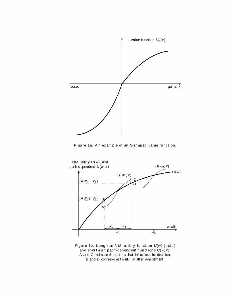
Vw(x) – a value function measuring additional value due to changes in x, with zero as

a reference point. Thus, if x=0, Vw(0) = 0. The shape of the function depends on w, hence

the subscript w. This is the value function suggested by K&T (1979).

U(w) – the NM utility function. In the rest of the paper, U(w) is referred to as the utility

function.

U(w, x) – the two dimensional utility function, and generally U(w, x)≠U(w+x)

because in the short term in a sudden and unexpected change in wealth, w is different from its

long-term and expected effect. However when w and x can be added to a total sum we are

back in the one-dimensional NM utility paradigm. In this study we focus on the following

specific form of the two-dimensional utility function,

U(w, x)=U(w) + Vw(x) (1)

where U(w) is the classic NM utility function which can take any (reasonable) form, see

Figures1 and 2.

(Insert Figures 1a and 1b here)

7

As explained in the introduction U(w, x) is a path-time-dependent utility function. We

adopt the path-time-dependent utility function because it confirms with most experimental

findings and in particular with the S-shaped value function suggested by Kahneman and Tversky

(1979).

Let us elaborate on the "surprise effect" of x, and its importance for the two-dimensional

utility function. Suppose that you have wealth of w and you hold in addition n units of a long-

term government bond with market value nPB. You know and expect market fluctuations in PB

due to possible changes in interest rate. Suppose that you expect possible changes in interest rate

in the range ±0.25% and therefore expect the corresponding fluctuations in PB. If there are no

changes in interest rate, then you expect PB to grow over time due to the continuous accumulated

interest. Thus, with no surprises the utility is U(w + nPB). Due to September 2001 terrorist attack

on the U.S. and its impact on the market, the Federal Reserve Bank cuts substantially the interest

rate in a very short period of time. In such a case, a holder of long-term government bonds has an

unexpected gain, because the sharp cut in interest rates as well as the terrorist attack were a

complete surprise to the investors. In such a case, the investor's utility is U(w + nPB, n∆PB),

where ∆PB is the unexpected gain due to the sharp unexpected cut in interest rates. Similarly, the

holder of United Airlines stocks has a wealth of (w + P0) and utility of U(w + P0) where P0 is the

value of the stocks of United Airlines. As a result of the terrorist attacks the value P0 dropped by

about 40% in one day. Because this was unexpected, the damage in utility terms was much larger

than the expected drop of 40% in P0. Thus, the investor's utility in this case is

U(w + P0, –0.4 P0) < U(w + 0.6P0)

Let us go to the other, albeit artificial, example. Suppose that a firm's CEO holds stocks

of his company and he is not allowed to sell them in the next five years. He knows that due to

insider information accumulated in his firm, bad news will emerge and the stock price will drop

8

by about 40%. When the news was released, it indeed dropped by 40%. This one-day drop in

stock price is not a surprise to the CEO, hence his utility will be U(w + 0.6p) (where 0.6p is the

value of equity after the drop in price). On the other hand, for investors who did not possess the

private information, the utility will drop to U(w + p, –0.4p), where for simplicity we assume that

utility function, wealth and stocks held by the CEO and the investor are identical. Therefore, the

investor is worse off relative to the CEO in utility terms because U(w + 0.6p) > U(w + p, –0.4p).

In the rest of the paper when we relate to short-run or temporary effect, we implicitly or

explicitly mean that it also contains a "surprise" or unexpected effect. If you invest in Treasury

Bills and get every week x = r/52 where r is the annual interest rate, though x corresponds to

short-run effect, it does not contain a surprise effect and the wealth increases every week by x

and the NM one-dimensional utility function is relevant.

To sum up when an unexpected change occurs we require that for x > 0 the following holds:

U(w, 0) < U(w–x, x) ≡ U(w-x) + Vw-x(x)

U(w, 0) > U(w+x, –x) ≡ U(w+x) + Vw+x(–x),

where x is short-run surprise change of wealth.

Our specific two-dimensional utility function is also time dependent, because in the long

run both U(w-x, x) and U(w+x, –x) become closer to each other and approach U(w,0)=U(w).

The experimental studies do not provide a unique answer of how long does it take to converge to

the NM utility.

This approach allows us to incorporate the Prospect Theory (PT) as a specific case of

two-dimensional utility function. PT emphasizes changes of wealth and not total wealth.

However, PT does not ignore initial wealth. K&T claim that the initial wealth serves as a

reference point5:

"The emphasis on changes as the carriers of value should not be taken to imply that the

9

value of a particular change is independent of initial position. Strictly speaking, value should be

treated as a function of two arguments: the asset position that serves as a reference point, and

the magnitude of the change (positive or negative) from the reference point," (see K&T, 1979, p.

277).

K&T realize that initial wealth affects the value function but they do not investigate its

effects further, nor do they address the relationship between value function, utility function and

wealth. Based on experimental results, K&T claim that the value function V is S-shaped with

V'> 0 for all x≠0, and V" > 0 for x < 0 and V" < 0 for x > 0 (in this paper, prime denotes the

derivative with respect to a change in wealth, x, if no confusion arises we omit the subscript w).

Markowitz (1952) suggests a reversed S-shaped form for the utility function with and

V" < 0 for x < 0 and V" > 0 for x > 0. Most of our analysis refers to K&T S-shaped function but

as we shall see below the stock overreaction phenomena can be better explained with

Markowitz’s reversed S-shaped function.

Figure 1a demonstrates K&T value function with w=0 as a reference point. Figure 1b

shows NM utility function of wealth U(w) and two utility functions U(w1, x) and U(w2, x),

i.e. two-dimensional utility functions which can be interpreted also as two value functions for

two levels of wealth w1 and w2. Experiments show that in the short run the subjects make

decisions due to unexpected change in wealth based on U(w, x), namely, according to the S-

shaped value function. However, in the long run the utility of the new wealth (resulting from

the subject’s decisions) approaches the NM utility U(w). Thus, the utility derived from a

given outcome is dynamic over time. The satisfaction from unexpected gain and the sorrow

from an unexpected loss decay with time, hence the time-dependent utility function

terminology.

Another hypothesis of PT is that subjects behave differently immediately after a loss (or

10

gain) than later on, after adjusting to the loss (or gain). Though K&T do not further analyze the

implications of this hypothesis, it seems that the value function Vw(x) reflects short-term

overreaction of subjects to a sudden change in wealth (like winning in a lottery), where

overreaction is defined relative to the behavior predicted by the expected utility paradigm. Note

that the overreaction includes both adjust of beliefs and risk attitude in face of recent gain or loss.

In particular, a sharp overreaction occurs in the case of unexpected losses. After some time

period has elapsed (which may vary in length among investors), complete adaptation to the loss

is expected. However, if there is incomplete adaptation to the loss, the investor will become a

risk seeker, choosing investments which otherwise would be rejected. This short-term

overreaction is suggested by K&T:

"This analysis suggests that a person who has not made peace with his losses is likely to

accept gambles that would be unacceptable to him otherwise." (See K&T, 1979, p. 287).

The model that we suggest in this paper assumes that investors are myopic in that they make

investment decisions by the utility function with short-term memory U(w, x). This has a direct

impact on short-term price changes of risky assets, to be elaborated later on in the paper.

Figure 2 illustrates the two-dimensional utility function U(w, x). Here we draw it in line

of equation (1), thus we have the specific additive shape of U(w, x). Note that for a given x,

when w changes, utility is always concave, and for any given w the function U(w, x) is S-shaped

in x.

(Insert Figure 2 here)

Using the relationship, U(w, x) = U(w) + Vw(x), Figure 2 illustrates the shape of the path-

dependent utility function U(w, x), and the relationship between TATR and PATR. The TATR is

measured along the vertical axis U(w, x) for a given w for various values x. For example, for w =

11

50 we obtain an S-shaped curve with 0),( >∂∂ xwUx

for all x≠0 and 0),(2

2

<∂∂ xwUx

for x > 0

and 0),(2

2

>∂∂ xwUx

for x<0.6 The slope of the S-shaped value function changes with w, but it

remains S-shaped. This can be clearly seen in Figure 2 by comparing the S-shaped functions

corresponding to low and high values of w. In Figure 2, U(w, x) is assumed to be concave in w

(for a fixed x). Similar curves are drawn for various values of x which are held constant along

each curve, when w changes. Facing an uncertain investment, investors will make decisions by

U(w, x), based on two variables. Thus, the surface of Figure 2 can be employed to measure the

investor’s TATR for various reference points w, and for various random variables x. The curves

along a given x simply measure the change in the function U(w, x) when w changes (and x is

held constant). Thus, U(w, x)|x=const is similar to the NM utility function U(w+x) where x is

constant and w changes. Obviously, the precise shape of the surface in Figure 2 may vary from

one investor to another. The two components, U(w) and Vw(x) of U(w, x) are important for

decision making and both affect the prices of risky assets. The U(w) part affects the long-run

behavior of the prices of risky assets (corresponding to NM utility function). The Vw(x) part

affects the short-run behavior of prices of risky assets. In section III we develop a dominance

decision rule for one prospect over another for all surfaces of the type given in Figure 2.

We show below the relationship between the path-dependent function U(w, x), the

overreaction effect and the NM utility function, U(x). However, before we present our

analysis, let us discuss briefly an important experimental result that directly addresses the

influence of time on attitude towards risk (TATR and PATR). A series of experiments

conducted by Thaler and Johnson (1990) produced several interesting results. Of particular

importance to our analysis is their experiment involving a two-week gap between payments.

In a series of three experiments Thaler and Johnson asked 65 participants whether they

12

prefer two events to occur on the same day or two weeks apart (see Table 2 in their paper).

In the first experiment the events are:

(i) win $25 in an office lottery

(ii) win $50 in an office lottery

25% of participants preferred the two events to occur on the same day; 63% preferred the events

to be two weeks apart; and 12% were indifferent.

In the second experiment the events are:

(i) receive a letter from the federal income tax authority saying that due to an arithmetical

mistake $100 must be paid.

(ii) receive a letter from the state income tax authority saying that due to an arithmetical mistake

$50 must be paid.

34% of participants preferred the two events to occur on the same day; 57% preferred the events

to be two weeks apart; and 9% were indifferent.

In the third experiment the events are:

(i) receive a $20 parking ticket

(ii) receive a bill for $25 from the registrar because a form was filled in improperly

17% of participants preferred the two events to occur on the same day; 75% preferred the events

to be two weeks apart; and 7% were indifferent.

Summarizing this experiment, Thaler and Johnson state:

"The responses to question 1 reveal that for pairs of gains subjects did respond in the

way suggested by the hedonic editing hypothesis. Subjects preferred to spread out the arrival

of pleasant events, presumably to help segregate the pleasures experienced. Using the same

logic, subjects should prefer to have pairs of losses occur on the same day, to facilitate their

integration. However, subjects did not express this preference. Rather, in questions 2 and 3

13

subjects indicated that they prefer to experience the losses separately. We have obtained this

result repeatedly, for small or large losses, for nonmonetary as well as monetary losses, and

for unrelated and related pairs of events. This result is a severe blow to the hedonic editing

hypothesis." (See Thaler and Johnson 1990, p.649). These results emphasize that the utility is

not only path-dependent it is also time-dependent. Also winning in a lottery or being told that

there was a mistake in your income tax calculation constitutes a “suprize” or unexpected

change in income. We will show below that the results of the above three experiments can be

explained by temporary risk attitude, TATR, (value function) and permanent risk attitude,

PATR, (utility function) and the difference between them. Actually, the results of these

experiments are in line with our suggestion regarding the relationship between Vw(x), the

path-time-dependent utility function U(w, x), and the NM utility function U(w+x), to which

we turn next. However, before explaining Thaler and Johnson results in our framework we

need first to explain further the TATR and PATR.

The value function Vw(x) represents the Temporary Attitude Towards Risk (TATR). In

particular, if we have wealth w1 and we receive an unexpected income x1, our path-dependent

utility is U(w1, x1), (see point C in Figure 1b), and if we need to pay (or we lose) an unexpected

amount y1, our value function will be U(w1, -y1) (see point A). Namely, in the short run, it hurts

both economically and psychologically when the wealth is unexpecedly decreased from w1 to w1

– y1; hence, the value function U(w1, -y1) will be lower than U(w1–y1). To illustrate, suppose that

we invest all our wealth, say $10,000, in the stock market and the stock price suddenly goes

down by 20%, like in October 1987 or in September 2001. Even though we will have a wealth of

$8,000 left, the blow of a sudden loss of $2,000 will leave us feeling as if we have less than

$8,000 left. However, this feeling will be temporary. After a short time period (hours, days, or

weeks) we adapt to the new wealth; in other words, we will feel that we have $8,000 and not less

14

(and behave appropriately). This means that we will have “made peace” with our loss (see K&T,

1979, p.287). Then, after a complete adjustment is achieved, we move to a new value, which

coincides with U(8,000). Thus, the utility is a function of the path the wealth is achieved and the

time it takes to adopt to the new wealth.

Thus, when the investor “makes peace” with the changes of wealth, there is a shift from

point A to point B, and from point C to point D (in a case of gain), reflecting the Permanent

Attitude Towards Risk (PATR). However, decisions are made by the S-shaped function U(w, x)

which reflects the investor's view of utility at the time of making the decision. Only after a time

period long enough to guarantee a complete adjustment, the investor will adapt to the new wealth

position, as indicated by a shift from the path-dependent utility U(w, x) to the NM utility

U(w+x). Many experiments reveal, that investors make decisions based on U(w, x) rather than

on utility U(w+x). This implies that investors are myopic: they consider short-term values and

ignore the effect of the future move back to the utility function U(w+x) which takes place when

the overreaction (to loss or gain) subsides. For each decision, the path dependent utility, U(w, x),

is employed. After the overreaction to changes of wealth subsides, investors turn back to the base

utility function U(w+x), ready to make a new myopic decision. For example, if the investor's

wealth changes from w1 to w2>w1 and enough time passes the investor will consider a new

investment according to U(w2) but react to unexpected changes in wealth according to the new

function U(w2, x) (see Figure 1b). Note that U(w2, x) has the same general S-shape but the slope

and higher derivatives may differ, reflecting the fact that U(w, x) is a function of x and w, and

not of x alone.

As mention before, K&T do not analyze the impact of reference point w on decision-

making, but merely state that it affects the decision. We will analyze the effect of the reference

point on the shape of the value function. Moreover, as we shall see below, U(w, x) and U(w+x)

15

together can explain stock price overreaction to an unexpected new information, and results of

Thaler and Johnson’s experiment.

Thus, we argue that there are three important factors in the decision making process:

a) Investors maximize the expected value of a two dimensional path-time-dependent

utility function U(w, x).

b) Investors are myopic, and when an unexpected change in wealth occurs they ignore

the utility that will be obtained after full adjustment to the change in wealth is achieved.

Therefore when they are faced with an uncertain prospect an error in the decision making

process is made.

c) After enough time elapses the utility U(w,x) becomes equal to the utility value

U(w+x), reflecting the time dependence.

Using TATR and PATR, let us analyze Thaler and Johnson's results discussed above as

well as stock market overreaction.

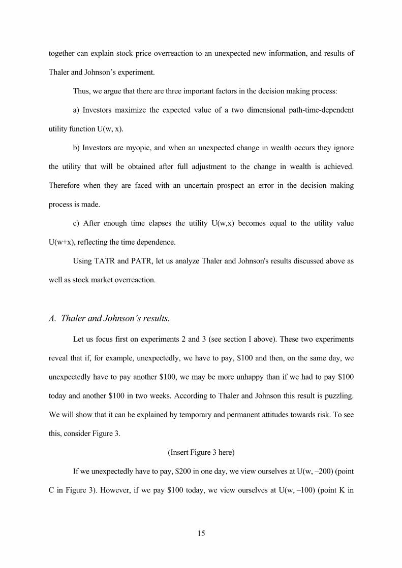
A. Thaler and Johnson’s results.

Let us focus first on experiments 2 and 3 (see section I above). These two experiments

reveal that if, for example, unexpectedly, we have to pay, $100 and then, on the same day, we

unexpectedly have to pay another $100, we may be more unhappy than if we had to pay $100

today and another $100 in two weeks. According to Thaler and Johnson this result is puzzling.

We will show that it can be explained by temporary and permanent attitudes towards risk. To see

this, consider Figure 3.

(Insert Figure 3 here)

If we unexpectedly have to pay, $200 in one day, we view ourselves at U(w, –200) (point

C in Figure 3). However, if we pay $100 today, we view ourselves at U(w, –100) (point K in

16

Figure 3). After two weeks, most subjects "make peace" with such a loss, implying that they

move to the point corresponding to U(w-100) on the permanent utility curve (point A in Figure

3). The overreaction to the loss is over. Then, the subjects pay an additional $100, moving to

U(w-100, –100), from point A to B. Because point B is above point C, subjects will be more

unhappy with one payment of $200 today rather than with two payments of $100 each. This

explains the results of experiments 2 and 3 of Thaler and Johnson.

We suspect that the period needed to adjust to the loss varies from one investor to

another and that it is also a function of the size of the loss: the larger the loss, presumably the

longer the time needed to accept it. In Thaler and Johnson’s experiment, for most subjects, two

weeks is enough to complete this transition of a relatively small monetary loss; hence, with a

two-week separation between payments, they end up at point B, which is above point C.

The above experimental results, which seem to contradict intuition, perfectly fit our

temporary and permanent attitude towards risk, or the existence of short-term value functions

Vw(x) and a long-term utility function U(w+x).

Let us turn now to the results of experiment of Thaler and Johnson cited above. Most

investors are happier receiving two gains separated by two weeks than receiving the sum of the

two gains on the same day. Figure 4 explains why this preference also fits our model. To see this,

consider two gains of $100 each and compare them to one gain of $200.

(Insert Figure 4 here)

Receiving $200 on one day, the investor moves to U(w, 200), corresponds to point A

which is above B corresponding to U(w + 200). If only $100 is received, we move along the

curve U(w, x) up to point D. When the overreaction effect is over, we move back to point E on

the utility function. Now, another payment of $100 is received, and the investor moves along

U(w+100, x) up to point C. In cases where C is above A, two gains of $100 two weeks apart are

17

better than one gain of $200 (this occurs with 63% of subjects).

Obviously, positions of points C and A depend on the slopes of functions V and U. For

some investors, point C may be below point A. However, if subjects do not adjust completely to

the new wealth after the first payment, a fortiori they will prefer the two payments over the one

large payment. In such a case, they move from the new reference point, D to point C* which is

higher than C. Thus, there may be subjects who prefer two separate payments (see experiment of

Thaler and Johnson) and adjust to their new wealth within two weeks. For them, point C is above

point A, (as illustrated in Figure 4). For those subjects who do not adjust to their new wealth,

point C* is above point C.

Finally, note that for those investors who prefer one payment and do not overreact to

losses and gains, or know that they simply move back in the future to U(w+x), the value function

is identical to the utility function U(w, x) = U(w+x) and indeed there is no need to represent

preferences of those investors by two separate variables if only their sum matters. K&T show

that this is not the usual case and most investors go through two steps in the evaluation of x,

implying short-term overreaction. Such short-term overreactions are probably less severe for

institutional investors than for individual investors.

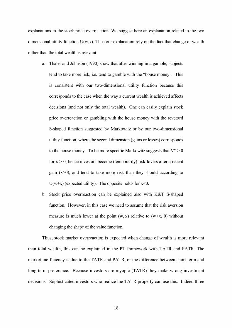
B. Stock Price Overreaction

Event studies are usually employed to measure stock market reaction to new and

unexpected information. The information can be of any kind: dividends, earnings, mergers,

spinoffs, replacement of a firm's chief executive officer, etc. Stock prices have been found to

overreact to unexpected new information, at least in the short run. Therefore, some researchers

postulate the "stock market overreaction" hypothesis. It asserts that stock prices temporary swing

away from their fundamental values due to short-term optimism or pessimism.7 There are several

18

explanations to the stock price overreaction. We suggest here an explanation related to the two

dimensional utility function U(w,x). Thus our explanation rely on the fact that change of wealth

rather than the total wealth is relevant:

a. Thaler and Johnson (1990) show that after winning in a gamble, subjects

tend to take more risk, i.e. tend to gamble with the “house money”. This

is consistent with our two-dimensional utility function because this

corresponds to the case when the way a current wealth is achieved affects

decisions (and not only the total wealth). One can easily explain stock

price overreaction or gambling with the house money with the reversed

S-shaped function suggested by Markowitz or by our two-dimensional

utility function, where the second dimension (gains or losses) corresponds

to the house money. To be more specific Markowitz suggests that V" > 0

for x > 0, hence investors become (temporarily) risk-lovers after a recent

gain (x>0), and tend to take more risk than they should according to

U(w+x) (expected utility). The opposite holds for x<0.

b. Stock price overreaction can be explained also with K&T S-shaped

function. However, in this case we need to assume that the risk aversion

measure is much lower at the point (w, x) relative to (w+x, 0) without

changing the shape of the value function.

Thus, stock market overreaction is expected when change of wealth is more relevant

than total wealth, this can be explained in the PT framework with TATR and PATR. The

market inefficiency is due to the TATR and PATR, or the difference between short-term and

long-term preference. Because investors are myopic (TATR) they make wrong investment

decisions. Sophisticated investors who realize the TATR property can use this. Indeed three

19

mutual funds named Behavioral Value, Behavioral Growth and Behavioral Long/Short,

which implicitly employ the difference between TATR and PATR8 have been recently

established. A description of a positive behavioral portfolio theory can be found in Shefrin

and Statman (2000).

II. Risk Premium and Prospect Theory

In this section we show that the value function with a convex segment steeper than its

concave part, as observed in laboratory experiments, is consistent with the observed positive risk

premium.

Friedman and Savage (1948) and Markowitz (1952) claim that the risk premium can be

negative or positive because utility function has both concave and convex segments.

Nevertheless, there is virtually consensus in the financial and economic literature that the risk

premium is positive. A firm’s cost of capital is larger than the risk-free interest rate indicating

risk aversion and a positive risk premium. Similarly, the long-run (1926–2000) average annual

rate of return on equity in the U.S. is about 13 % while the average annual rate of return on the

riskless asset (Treasury bills) is only about 3.9%.9

Arrow (1965) and Pratt (1964) developed a risk premium measure, which is a function of

−UU

"'. Arrow (1965) and others10 claim that absolute risk aversion (DARA) decreases with

wealth: the larger the wealth, the less premium one is willing to give up to get rid of a given risk.

11

In this section, we analyze the existence of a positive risk premium and DARA in the PT

framework. Because, the PT value function is S-shaped, some of its properties differ from the

concave-shaped utility function. For example, the risk premium can be positive or negative

20

depending on the distribution of the payoff. Because the value function is concave in the positive

domain, we can easily conclude that for a prospect with positive outcomes only, there will be a

positive risk premium. Similarly for a prospect with negative outcomes only, the risk premium

will be negative because the value function is convex.

The interesting question, of course, is “What is the risk premium when an investor can

either lose or win?” In other words, what is the risk premium in a realistic case where both

positive and negative outcomes are possible. In PT, the S-shaped value function has an inflection

point at the reference point w; therefore Arrow's approach to measuring risk premium is not

applicable because an S-shaped function is not differentiable at the inflection point. With Pratt's

approach, the derivatives are taken at )~( xEw + , where U' and U" are defined (if E~x 0≠ ), and

the risk premium can be derived. We confine ourselves to the realistic case where E~x > 0 (for

the unrealistic case where E~x 0< the results are inconclusive).

Theorem 1. Risk aversion in the small: Assume that there is a value function Vw(x) with Vw’ >0,

and Vw"<0 for x>0 and Vw">0 for x<0. If the convex segment is steeper than the concave

segment (as found by K&T (1979)), there will be a positive risk premium for all small prospects

with positive expected value.

Proof. Using the Taylor expansion of the value function around zero we obtain:

where β>α because the convex segment is steeper. Here we use the standard notation of o(x) to

denote a function of higher order than x (for small x).

Take a random prospect ~x where all possible outcomes are close to zero (between a < 0

and b > 0), and there is a positive expected value E~x = xf(x) dx > 0a

b

∫ where f is the density

<+≥+

=0),(0),(

)(xifxoxxifxox

xVw βα

,

21

function of ~x . Denote by e- and e+ the negative and positive parts of this expectation

− +∫ ∫e = xf(x) dx < 0, e = xf(x) dx > 0.a

0

0

b

Note that |e–| < |e+| because E~x = e–+ e+ > 0 by

assumption. Then the value of this expected payoff )x~(EVw will be α ( + e )+e− up to terms of

higher order. The expected value function will be:

Because β>α and |e–|< e+, we conclude that for small enough prospects )x~(EV<)x~(EV ww

implying positive risk premium in the small. 12

Actually, the argument can be reversed to support K&T’s observation regarding the

steepness of the two segments of the value function: If there is a positive risk premium in the

small, then β ≥ α which implies that the value function is steeper (in the weak sense) for x < 0

than for x > 0.13 Thus, the existence of a positive risk premium in the small can be taken as

further validation of the experimental results of K&T regarding the shape of the value function

Vw.

The risk premium in PT is confined to small prospects; hence, the extension of the results

to risk premium "in the large" as performed by Pratt, is impossible. Because the value function V

has a convex segment, and such an extension may imply that the risk premium is negative rather

than positive. To show that this theorem cannot be extended for risk premium in the large we use

the following example:

Take the following (S-shaped) value function (which is steeper for x<0, than for x>0):

<−

≥−=

−

0,10,1

)(3 xife

xifexV

x

x

w

)(+e+e=dxf(x)))(x+(dx+f(x)))(x+(=dxf(x)(x)V=)x~(EV +

b

0

0

a

b

a

xoxoxoww αβαβ −∫∫∫ .

22

This function is drawn in Figure 5a

(Insert Figure 5a here)

Consider the prospect (x1, p; x2, (1–p)) = (1, 0.7; –2, 0.3) which means a gain of 1 with

a probability of 0.7 and a loss of 2 with a probability of 0.3. In this case, the expected payoff is

0.7 – 0.6 = 0.1 > 0 and the value of the expected payoff is: 0951626.01)( 1.0 =−= −eExVw .

However, the expected value function will be (1–e–1)0.7 + (e–6–1) 0.3 = 0.143228. Figure 5b

shows that at the expected outcome (0.1) point A on the Vw function (0.095) is below point B

(0.1432) on the straight line connecting two extreme payoffs.

(Insert Figure 5b here)

This example demonstrates the existence of a negative risk premium for a prospect with a

positive expected payoff. Note that "in the small", the risk premium is positive even for this

function, because we have proved above that the risk premium in the small is positive for β>α

and |e–|< e+ which holds true in our example. This implies that )x~(EV<)x~(EV ww for small

enough prospects with a positive expected value, which is equivalent to the assumption that a

positive risk premium prevails. In the above example, the condition "in the small" is violated,

hence, we obtained a negative risk premium "in the large."

Decreasing absolute risk aversion (DARA)

In order to analyze DARA in the utility theory framework, we investigate the change in

U"/U' as w changes. In PT, the decisions are made by the value function Vw(x); hence, we have

to check the relevant derivatives along Vw(x) as w changes.

We introduce below the concept of DARA in PT. To investigate changes in the absolute

risk aversion as a function of wealth, we repeat the basic steps from Pratt (1964) for the case

where the path-dependent utility function depends on both current wealth and possible change in

23

wealth U(w, x). We will show that if there is DARA with U(w, x), there will be DARA with the

K&T value function Vw(x).

With a path-dependent utility function, the risk premium is defined by )x~(w,π given by,

)x~(w,=))x~(w,-x~E(w, EUU π (2)

where ))x~(w,-x~E(w, π is the two-dimensional certainty equivalent.

Using the Taylor expansion around the point (w,E~x )14 in the second variable, for the right side

we obtain:

)x~E-x~(+)x~E-x~E()x~E(w,21+)x~E-x~E()x~E(w,+)x~E(w,=)x~(w, 22 oUUUEU xxx (3)

where Ux is the first partial derivative of the value function with respect to its second argument

and Uxx is the second derivative. Following Pratt’s procedure, for the left side of equation (2) we

can write:

( ))x~(w,+)x~(w,)x~E(w,-)x~E(w,=))x~(w,-x~E(w, πππ oUUU x . (4)

Using equations (2), (3) and (4), for the path-dependent utility risk premium π we obtain:

)o(+2)x~E(w,

)x~E(w,=)x~(w, 2

2

σσπx

xx

UU

− ,

which is very similar to Pratt’s definition adjusted to the two-dimensional utility function.

Denoting the risk premium in the utility theory by π, DARA implies that ∂π/∂w < 0

(where w is the investor's wealth). In prospect theory, we have a somewhat different formulation:

There is a two-dimensional utility function U(w, x) which depends on two arguments, w and x.

The investor makes decisions based on the impact of x; therefore, we look at the derivatives 'wV

and "wV with respect to x. These derivatives determine the risk premium. However, to test for the

existence of DARA, we need to analyze how these derivatives at point Ex≠0 change when w

changes.

24

Let Ux(w, x), Uxx(w, x) denote the first two derivatives with respect to x. The effect of

change in these derivatives as a function of w can be measured by the mixed derivatives Uxw and

Uxxw We claim below that any path-dependent utility function of this type with

0)/(<

∂∂

−w

UU xxx is consistent with DARA in PT. To see this, recall that

(x)V'=x)(w, wxU and )(V"=x)(w, xU wxx . Therefore, Pratt's risk aversion is given by:

and, if 0<w/)/( ∂∂− xxx UU , we have the same property for the value function, V, and DARA

prevails also with the K&T value function Vw(x).

(Insert Figures 6a, 6b here)

Figures 6a and 6b demonstrate the concept of DARA in PT. Figure 6a is given in K&T

framework. We have two S-shaped hypothetical functions for an individual investor,

corresponding to different levels of wealth. DARA exists if the derivatives satisfy

− −V" (E~x) / V' (E~x) < V" (E~x) / V' (E~x)w w w w2 2 1 1 when w2 > w1 (and w2 is close enough to

w1). Figure 6b demonstrates the same idea with the path-dependent utility function. The same

relation should hold for the ratio of the derivatives at points A and B. This differs from the utility

theory risk premium when a movement along U(w) is involved. Actually, here we measure the

slope on two value functions corresponding to two wealth levels: hence DARA in PT is

expressed by moving from one value function to another.

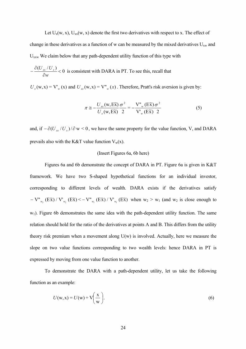
To demonstrate the DARA with a path-dependent utility, let us take the following

function as an example:

wxV+(w)=x)(w, UU . (6)

2)x~(EV'

)x~(EV"=

2)x~E(w,)x~E(w, 22 σσπ

w

w

x

xx

UU

−−≅ (5)

25

This function has the following desired property: the larger the wealth, the smaller the effect of

given change x on the value function. The benefit of x=1 (or the loss due to x = –1) is much

smaller for w = 1,000 than for w = 10.

It is easy to verify that for this function, ∂π/∂w < 0:

This formula clearly shows that the risk premium (its absolute value) decreases when wealth

increases. Thus, for this specific function, we have two properties: DARA holds and the value

function Vw(x) changes in a clockwise directions as w increases (see Figure 6a).

III. Prospect Stochastic Dominance (PSD)

It is very important for the choice by prospect theory not to violate First Degree

Stochastic Dominance (FSD) (see K&T (1979) and T&K (1992)). Indeed, in CPT (unlike PT),

T&K ensure that the probability weight function is such that if there are two prospects, F and G,

and if F dominates G by FSD, such dominance will be found also in the PT framework. Thus, the

transformation of cumulative probability does not violate FSD. In this section, we assume that

the utility function is path-dependent U(w, x), as before, and that Vw(x) is an S-shaped value

function (see eq. (1)). With no constraints on the relationship between Vw(x) and w (as long as it

remains S-shaped), we derive the conditions for dominance of F over G for all S-shaped value

functions. We first assume a Vw(x) function as advocated by K&T (see Figure 1a), and then

show that the results also hold for U(w, x). Under certain conditions, the results also hold for the

NM utility function U(w+x). To be more specific, we find a condition for dominance of one

prospect over another for all possible surfaces U(w, x) given in Figure 2, as long as the S-shaped

2w

1)x~(EV')x~(EV"

=2)x~E(w,

)x~E(w,)x~E(w,

22 σσπw

w

x

xx

UU

−−≅ (7)

26

feature is maintained along x for a constant w.

Like K&T (1979) let us focus on the value function, assuming first that there are no

subjective transformations of probabilities. Suppose that there are two uncertain options with

density functions f(x) and g(x) and that the corresponding cumulative distribution functions are

F(x) and G(x), where x is the change in wealth (gains or losses). Then, by PT, F will be preferred

to G if and only if the following holds:

F w w w G wE V (x) = V (x) dF(x) V (x) dG(x) = E V (x)∫ ≥ ∫ (8)

where Vw(x) is the K&T value function (S-shaped) whose precise shape depends on current

wealth w (see Figure 1a). In the following theorem, we provide necessary and sufficient

conditions for preference of F over G for all value functions Vw(⋅) of this type.

Theorem 2. Let Vw(⋅) be an S-shaped value function with V' ≥ 0, where V"≤ 0 for gains

and V" ≥0 for losses. Then F will dominate G by PSD if and only if for any pair y < 0 < x,

( )y

x

G(t) - F(t) dt 0∫ ≥ (9)

where F and G are the cumulative distribution functions of f and g, respectively.

Proof. We consider the case in which all possible gains/losses are in a bounded domain [a,b]. 15

a) Sufficiency:

Define by ∆≡EF V(x) – EG V(x) and assume that x is always in [a,b]. Then

∆ = − = −∫ ∫∫V V Vw w w( ) ( ) ( ) ( ) ( ) ( ( ) ( ))x dF x x dG x x d F x G xa

b

a

b

a

b

.

Integrating by parts we obtain:

[ ] dx(x)V'G(x))-(F(x)-G(x)-F(x)(x)V= w

b

a

b

aw | ∫∆ .

27

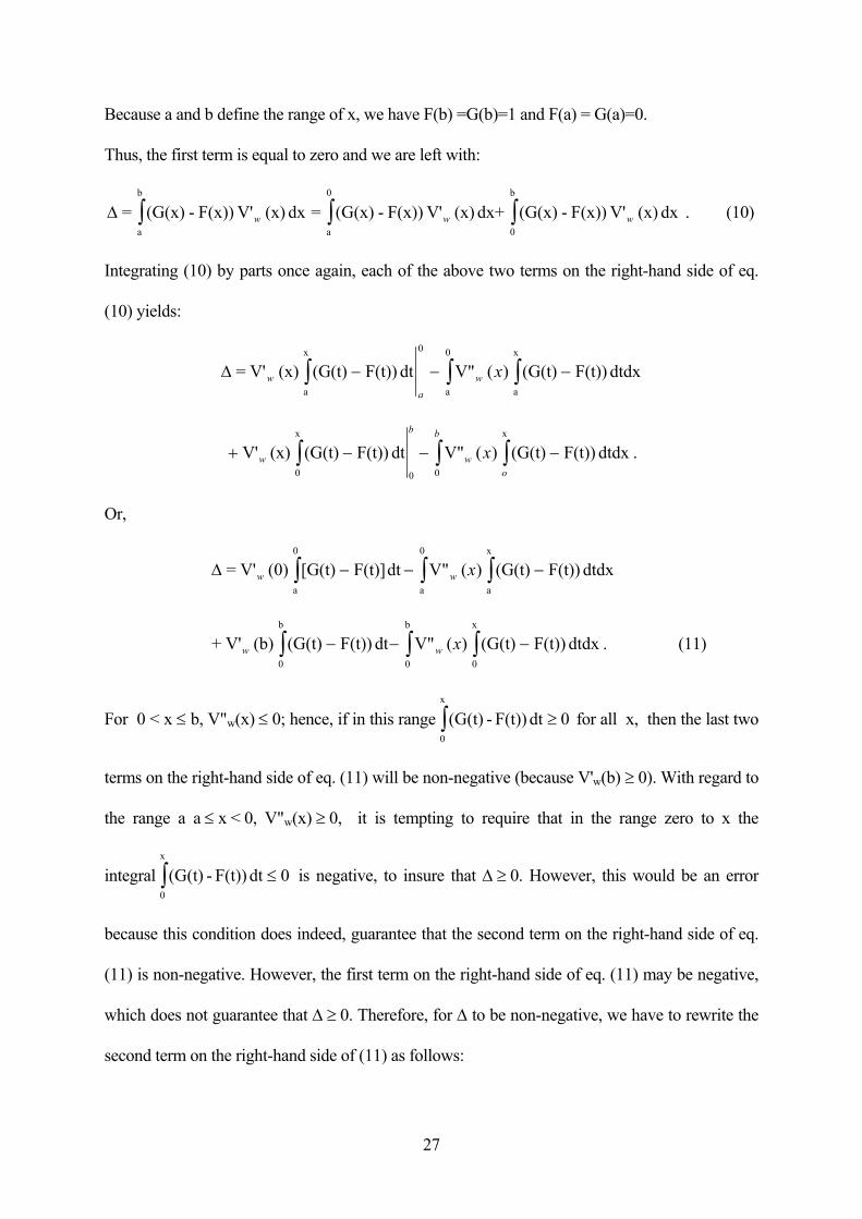
Because a and b define the range of x, we have F(b) =G(b)=1 and F(a) = G(a)=0.

Thus, the first term is equal to zero and we are left with:

∆ = (G(x) - F(x)) V' (x) dxa

b

∫ w = (G(x) - F(x)) V' (x) dx+ (G(x) - F(x)) V' (x) dxa

0

0

b

∫ ∫w w . (10)

Integrating (10) by parts once again, each of the above two terms on the right-hand side of eq.

(10) yields:

∆ = V' (x) (G(t) F(t)) dt V" ( ) (G(t) F(t)) dtdxa

x

a

0

a

x

wa

w x∫ ∫ ∫− − −0

+ − − −∫ ∫ ∫V' (x) (G(t) F(t)) dt V" ( ) (G(t) F(t)) dtdxx x

w

b b

wo

x0 0 0

.

Or,

∆ = V' (0) [G(t) F(t)]dt V" ( ) (G(t) F(t)) dtdxa

0

a

0

a

x

w w x∫ ∫ ∫− − −

+ V' (b) (G(t) F(t)) dt V" ( ) (G(t) F(t)) dtdx0

b

0

b

0

x

w w x∫ ∫ ∫− − − . (11)

For 0 < x ≤ b, V"w(x) ≤ 0; hence, if in this range0

x

(G(t) - F(t)) dt 0∫ ≥ for all x, then the last two

terms on the right-hand side of eq. (11) will be non-negative (because V'w(b) ≥ 0). With regard to

the range a a ≤ x < 0, V"w(x) ≥ 0, it is tempting to require that in the range zero to x the

integral0

x

(G(t) - F(t)) dt 0∫ ≤ is negative, to insure that ∆ ≥ 0. However, this would be an error

because this condition does indeed, guarantee that the second term on the right-hand side of eq.

(11) is non-negative. However, the first term on the right-hand side of eq. (11) may be negative,

which does not guarantee that ∆ ≥ 0. Therefore, for ∆ to be non-negative, we have to rewrite the

second term on the right-hand side of (11) as follows:

28

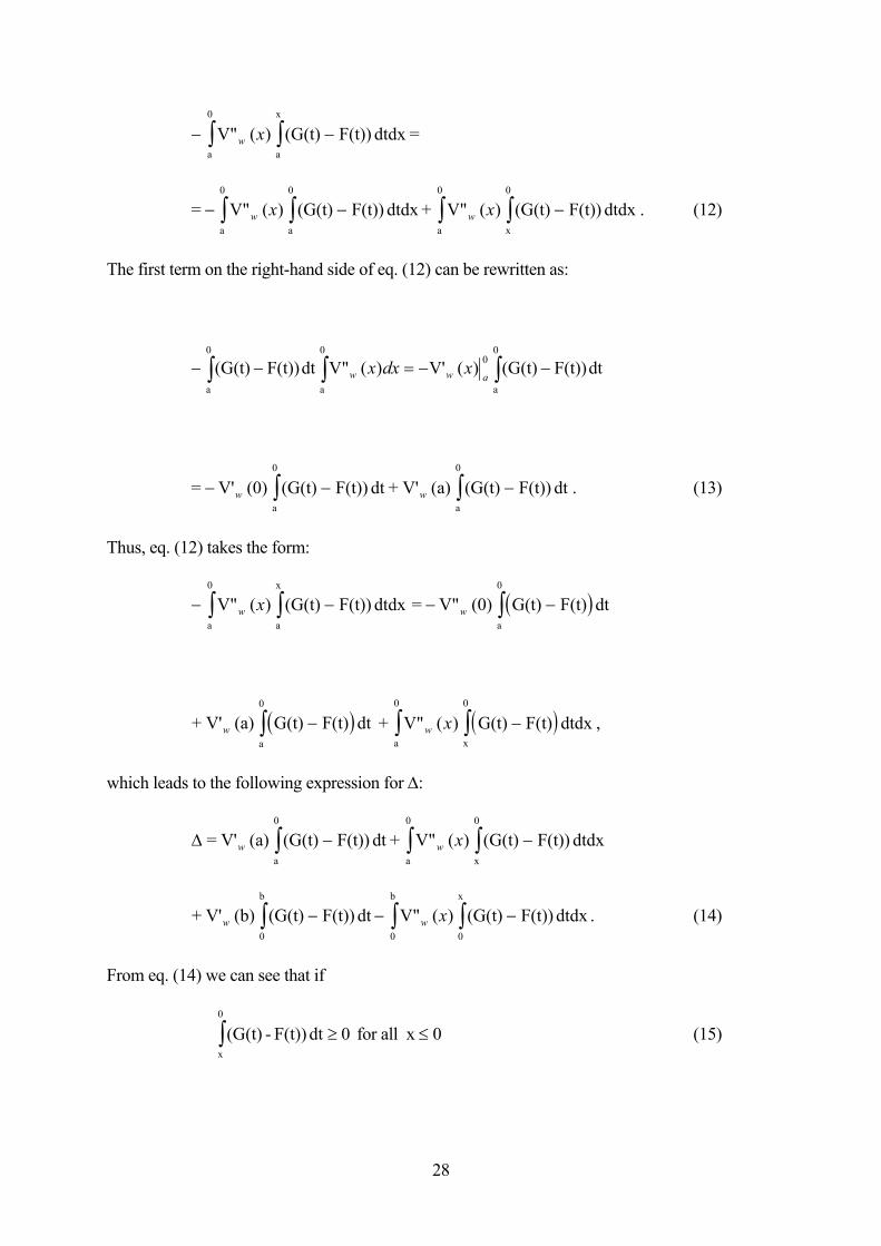
− −∫ ∫a

0

a

x

V" ( ) (G(t) F(t)) dtdx =w x

= V" ( ) (G(t) F(t)) dtdx + V" ( ) (G(t) F(t)) dtdxa

0

a

0

a

0

x

0

− − −∫ ∫ ∫ ∫w wx x . (12)

The first term on the right-hand side of eq. (12) can be rewritten as:

dtF(t))(G(t))(V')(V"dtF(t))(G(t)0

a

00

a

0

a

−−=−− ∫∫∫ aww xdxx

= V' (0) (G(t) F(t)) dt + V' (a) (G(t) F(t)) dta

0

a

0

− − −∫ ∫w w . (13)

Thus, eq. (12) takes the form:

− −∫ ∫a

0

a

x

V" ( ) (G(t) F(t)) dtdxw x ( )= V" (0) G(t) F(t) dta

0

− −∫w

( )+ V' (a) G(t) F(t) dta

0

w ∫ − ( )+ V" ( ) G(t) F(t) dtdxa

0

x

0

∫ ∫ −w x ,

which leads to the following expression for ∆:

∆ = V' (a) (G(t) F(t)) dt + V" ( ) (G(t) F(t)) dtdxa

0

a

0

x

0

w w x∫ ∫ ∫− −

+ V' (b) (G(t) F(t)) dt V" ( ) (G(t) F(t)) dtdx0

b

0

b

0

x

w w x∫ ∫ ∫− − − . (14)

From eq. (14) we can see that if

x

0

(G(t) - F(t)) dt 0∫ ≥ for all x ≤ 0 (15)

29

and ( )0

x

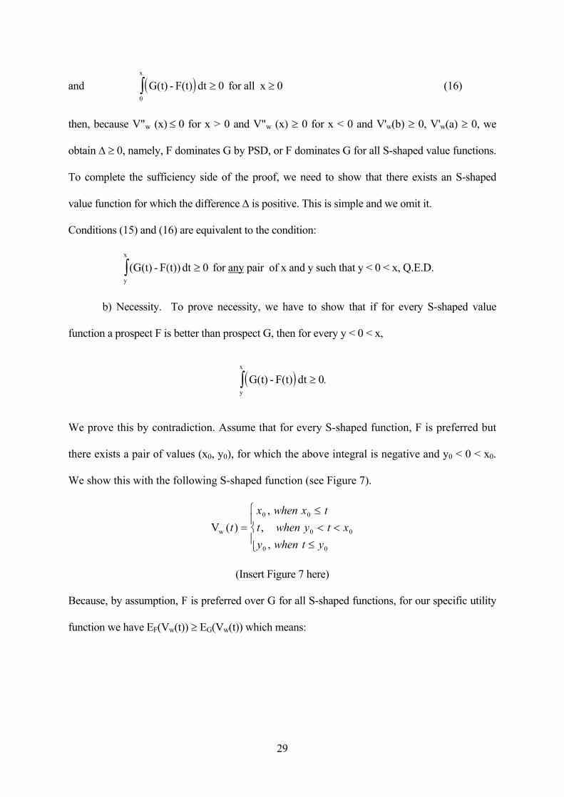
G(t) - F(t) dt 0∫ ≥ for all x ≥ 0 (16)

then, because V"w (x) ≤ 0 for x > 0 and V"w (x) ≥ 0 for x < 0 and V'w(b) ≥ 0, V'w(a) ≥ 0, we

obtain ∆ ≥ 0, namely, F dominates G by PSD, or F dominates G for all S-shaped value functions.

To complete the sufficiency side of the proof, we need to show that there exists an S-shaped

value function for which the difference ∆ is positive. This is simple and we omit it.

Conditions (15) and (16) are equivalent to the condition:

y

x

(G(t) - F(t)) dt 0∫ ≥ for any pair of x and y such that y < 0 < x, Q.E.D.

b) Necessity. To prove necessity, we have to show that if for every S-shaped value

function a prospect F is better than prospect G, then for every y < 0 < x,

We prove this by contradiction. Assume that for every S-shaped function, F is preferred but

there exists a pair of values (x0, y0), for which the above integral is negative and y0 < 0 < x0.

We show this with the following S-shaped function (see Figure 7).

Vw ( ),

,,

tx when x tt when y t xy when t y

=≤< <

≤

0 0

0 0

0 0

(Insert Figure 7 here)

Because, by assumption, F is preferred over G for all S-shaped functions, for our specific utility

function we have EF(Vw(t)) ≥ EG(Vw(t)) which means:

( )y

x

G(t) - F(t) dt 0∫ ≥ .

30

Because F(a)=G(a)=0 and F(b)=G(b)=1 (because F and G are cumulate distribution functions),

and using the fact that V'w is zero below y0 and above x0, the previous expression can be written

as:

which contradicts the assumption that the integral is negative for all pairs x, y such that y<0<x.

Corollary. F dominates G by PSD if and only if F dominates G for all path-dependent utility

functions U(w, x) given by eq. (1).

The proof is straightforward. To see this, note that because U(w, x) = U(w) + Vw(x) and

U'(w, x) = V′w(x), U"(w, x) = V"w(x), (all derivations are with respect to x). Thus, the PSD proof

with U(w, x) is the same as in Theorem 2: simply substitute U for Vw everywhere.

A. Discussion

In expected utility theory, the main parameter is total wealth w + x and not change in wealth, x,

which is the main parameter in prospect theory. Thus, it would seem that the results of Theorem

2 do not apply to utility theory. However this is not the case, and the results of Theorem 2 hold

for all S-shaped value functions Vw(x) as well as for all NM utility functions of the form U(w+x)

such that U"(0) for all x < 0 and U"< 0 for x > 0. U" is a function of w just as V"w(x) depends

on w. Similarly, in utility theory, F and G should be defined on terminal wealth w+x and not on x

as shown in the proof of Theorem 2. However, because

( ) ( )∆ = − = − − − ≥∫∫∫ V V V V V'w w w w w( ) ( ) ( ) ( ) ( ) ( ) ( ) ( ) ( )t dF t dG t F t t G t t F t G t dta

b

a

b

a

b

a

b

0 .

( ) ( ) 0)()()()()(V'=y

x

b

a

0

0

= ≥−−∆ ∫∫ dttFtGdttFtGtw ,

31

y

x

y-w

x-w

(G(t) F(t)) dt > 0 (G(w+ t) F(w+ t)) dt > 0∫ ∫− ⇔ − ,

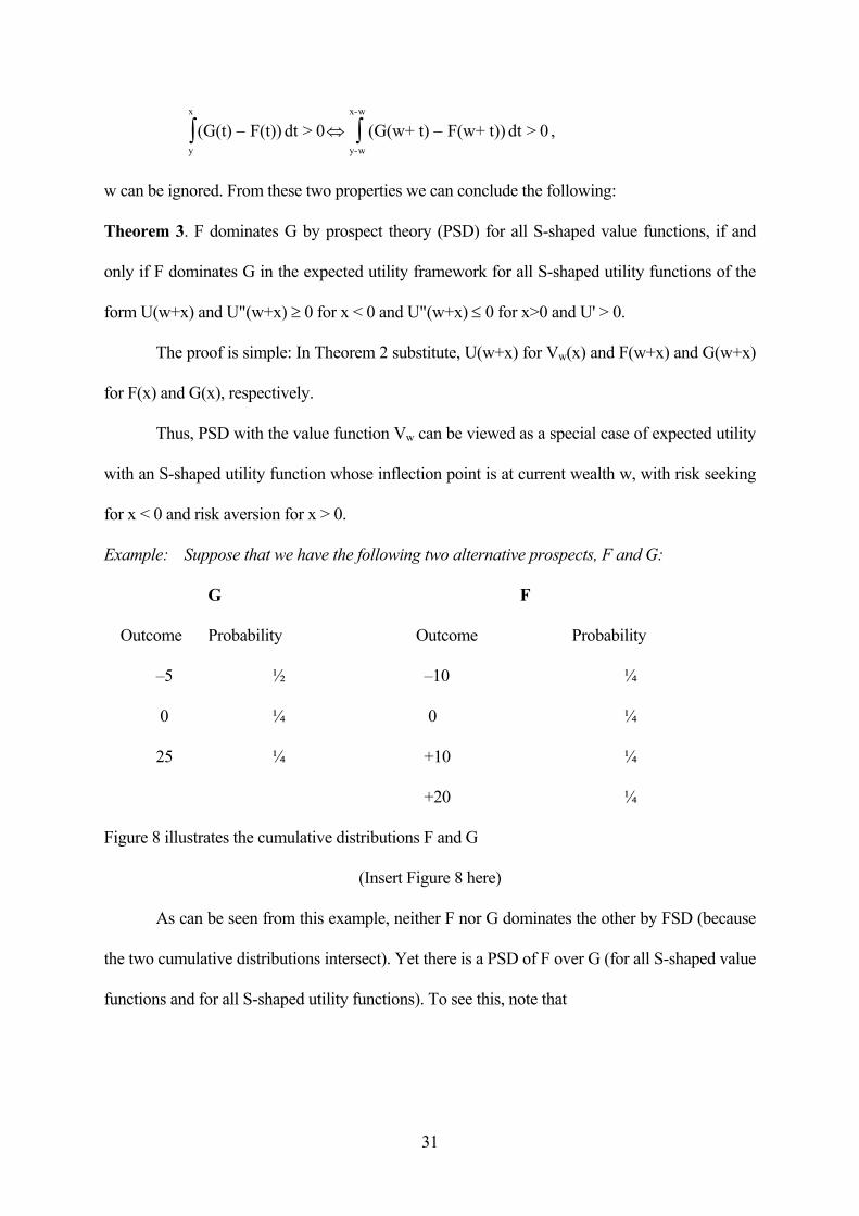
w can be ignored. From these two properties we can conclude the following:

Theorem 3. F dominates G by prospect theory (PSD) for all S-shaped value functions, if and

only if F dominates G in the expected utility framework for all S-shaped utility functions of the

form U(w+x) and U"(w+x) ≥ 0 for x < 0 and U"(w+x) ≤ 0 for x>0 and U' > 0.

The proof is simple: In Theorem 2 substitute, U(w+x) for Vw(x) and F(w+x) and G(w+x)

for F(x) and G(x), respectively.

Thus, PSD with the value function Vw can be viewed as a special case of expected utility

with an S-shaped utility function whose inflection point is at current wealth w, with risk seeking

for x < 0 and risk aversion for x > 0.

Example: Suppose that we have the following two alternative prospects, F and G:

G F

Outcome Probability Outcome Probability

–5 ½ –10 ¼

0 ¼ 0 ¼

25 ¼ +10 ¼

+20 ¼

Figure 8 illustrates the cumulative distributions F and G

(Insert Figure 8 here)

As can be seen from this example, neither F nor G dominates the other by FSD (because

the two cumulative distributions intersect). Yet there is a PSD of F over G (for all S-shaped value

functions and for all S-shaped utility functions). To see this, note that

32

0dtF(t))-(G(t)0

x

≥∫ for all 0x ≤ , and 0dtF(t))-(G(t)x

0

≥∫ for all 0x ≥ (and there is at least

one strict inequality). Alternatively, for any pair y ≤ 0, x ≥ 0, the integral 0dtF(t))-(G(t)x

y

≥∫ is

positive implying that F dominates G by PSD.

It is interesting to note that in the above example, neither F nor G dominates the other by

second degree stochastic dominance (SSD), because F dominates G by SSD if and only if:

a

x

(G(t) - F(t)) dt > 0∫

for all values x (with at least one strict inequality). This condition does not hold for x < –5.

Hence, F does not dominate G by SSD. It is easy to show that G also does not dominate F by

SSD (for x = 10, the integral is negative: a

10

(F(t) - G(t)) dt < 0)∫ .

Finally, if F dominates G by FSD, it implies that F dominates G by PSD. To see this,

recall that FSD dominance implies that,

F (w+x) ≤ G (w+x) for all x,

which is the same as F(x) ≤ G(x) for all x. However, because V"(x) ≥ 0, from equation (10), it is

obvious that if F dominates G by FSD, ∆ ≥ 0 for all value functions Vw with V′w(⋅) ≥ 0; hence F

dominates G by PSD. It is easy to show that SSD, unlike FSD, does not imply PSD.

B. Weight Function

In proving PSD, we assume that F and G are the original distributions and no

transformation on the probabilities is made. However, if a transformation on the cumulative

distributions is made (as advocated by CPT, in Tversky and Kahneman (1992), with F* = T(F)

33

and G* = T(G), T being a monotonous non-decreasing transformation used by all investors), then

PSD will hold but, this time, the condition will be ( )x

y* *G (t) - F (t) dt = 0∫ for all y < 0 and x > 0.

IV. Conclusions

Most equilibrium models and criteria for decision making under uncertainty (e.g.,

equilibrium prices of risky assets, portfolio theory, risk premium and stochastic dominance rules)

were developed within the expected utility paradigm. Markowitz (1952) and Allais (1953)

suggested that investors do not make choices in accordance to EU. Moreover, experiments

conducted with and without real money show that subjects violate the expected utility paradigm

and, in particular, the independence axiom. Following Markowitz (1952) and Edwards (1953,

1954), Kahneman and Tversky’s (1979). Prospect Theory shows that a high proportion of

subjects maximize their expected value function, Vw(x), where x is the unexpected change in

wealth (gains or losses) rather than total wealth. This runs counter to the assertion of expected

utility that investors maximize the expected value of the function U(w+x), where w+x is the total

wealth.

In this paper, we bridge the gap between prospect theory and expected utility theory. We

first define a two-dimensional utility function U(w, x) and show that investors make decisions

according to these two variables, exactly as claimed by prospect theory. In comparison to NM

utility function U(w,x) is a path-dependent: ending up with a wealth w+x may provide in the

short run a different utility, depending on the path by which w+x was achieved. The function

U(w,x) is also time-dependent because the utility may change with time. Hence U(w,x) is path-

time dependent utility function. This function reflects the Temporary Attitude Towards Risk

(TATR). If one observes a continuous process of gain accumulation or wealth loss, then the

34

behavior will be according to the one-dimensional utility function. However, when the change in

wealth x is sudden and unexpected (e.g. October 1987 or September 2001 crashes) then the

psychological effects come to play and investors act according to the two dimensional utility

function U(w,x), i.e. according to Markowitz or Kahneman and Tversky’s PT utility (or value)

functions. When the subjects adjust to the gain or loss, there is a shift from the function U(w, x)

to the NM utility function U(w+x), and the utility function U(w+x) reflects the Permanent

Attitude Towards Risk (PATR). This two-dimensional utility function together with the

conventional NM utility function U(w+x) can explain Thaler and Johnson’s (1990) experimental

results as well as short-run stock price overreaction to unexpected bad or good news. Because

investors make decisions based on a change in wealth rather then terminal wealth, these

decisions are myopic and often not optimal. In the long run investors return to the NM expected

utility framework. Behavioral mutual funds can make abnormal profits due to these errors.

Next we analyze the impact of the empirically found positive risk premium and a

decreasing absolute risk aversion on the shape of the value function advocated by prospect

theory. We find that positive risk premium is consistent with Kahneman and Tversky's value

function (as well as with Markowitz utility function) indicating that the convex part of the value

function is steeper than the concave part, and decreasing risk premium under certain conditions

implies that the value function shifts in a clockwise direction as wealth increases.

According to prospect theory, the value function by which investors make investment

decisions is an S-shaped function that varies from one investor to another, depending on his/her

preference and their wealth, but preserves its S-shape. Moreover, the value function of the same

investor may not be the same for different levels of hypothetical wealth. In the final part of this

study, we develop an investment decision rule called Prospect Stochastic Dominance (PSD)

deriving the conditions under which one prospect x will dominate another prospect y for all S-

35

shaped Kahneman and Tversky value functions. We show that PSD holds if and only if such

dominance holds for the path-dependent utility function U(w, x) as well as for the NM utility

function U(w+x), which is also S-shaped with a reference point w. We also show that First

Degree Stochastic Dominance (FSD) implies PSD but not vice versa.

36

REFERENCES

Allais, M. “Le comportement de l’homme rationnel devant le risque: Critique des postulates et

axioms de l’ecole Americaine”, Econometrica, 21 (1953), 503-546.

Allais, M. “The General Theory of Random Choices in Relation to the Invariant Cardinal Utility

Function and the Specific Probability Function. The (U, Θ) Model. A General Overview”, in B.

Munier (ed.) Risk, Decision and Rationality, (Dordrecht, Reidel), (1988), 231-289.

Allais, M. “Allais Paradox”, in The New Palgrave: Utility and Probability, The Macmillan Press,

(1990), 3–9.

Arrow, K. Aspects of the Theory of Risk-Bearing, Helsinki, Yrjö Jahnssonin Säätiö, (1965).

Barberis, N., Huang, M. Santos, T. “Prospect Theory and Asset Prices”, The Quarterly Journal

of Economics, 116:1 (2001), 1-53.

Benartzi, S. and Thaler, R. “Myopic Loss Aversion and the Equity Premium Puzzle”, The

Quarterly Journal of Economics, 110:1 (1995), 73-92.

Conrad, J. and Gautam K., “Long-Term Market Overreaction or Biases in Computed Returns?”,

Journal of Finance, 48:1 (1993), 39–63.

Conrad, J. and Gautam K., “Mean Reversion in Short-Horizon Expected Returns”, Review of

Financial Studies, 2:2 (1989), 225–240.

De Bondt, W. and Thaler, R. “Does the stock market overreact?”, Journal of Finance, 42:3

(1985), 793–808.

De Bondt, W. and Thaler, R. “Further evidence on investor overreaction and stock market

seasonability”, Journal of Finance, 42:3 (1987), 557–581.

Edwards, W. “Probability-preferences in gambling”, American Journal of Psychology, 66

(1953), 349-364.

Edwards, W. “Probability-preferences among bets with differing expected values”, American

37

Journal of Psychology, 67 (1954), 56-67.

Friedman, M. and Savage, L. “The Utility Analysis of Choices Involving Risk”, Journal of

Political Economy, 56:4 (1948), 279–304.

Hanoch, G. and Levy, H. “The Efficiency Analysis of Choices Involving Risk”, Review of

Economic Studies, 36:107 (1969), 335–346.

Handa, J. “Risk, Probabilities, and a New Theory of Cardinal Utility”, Journal of Political

Economy, 85:1 (1977), 97-122.

Ibbotson Associates, Stocks, Bonds, Bills and Inflation, Chicago, various issues.

Kahneman, D. and Tversky, A. “Prospect Theory of Decisions Under Risk”, Econometrica, 47:2

(1979), 263–291.

Kihlstrom, R. and Mirman, L. “Risk Aversion with Many Commodities”, Journal of Economic

Theory 8:3 (1974), 361-388.

Kihlstrom, R. and Mirman, L. “Constant Increasing and Decreasing Risk Aversion with Many

Commodities”, Review of Economic Studies, 48:2 (1981), 271-280.

Lehmann, B. “Fads, Martingales and Market Efficiency”, Quarterly Journal of Economics, 105

(1990), 1–28.

Levhari, D., Paroush, J. and Peleg, B. “Efficiency Analysis for Multivariate Distributions”,

Review of Economic Studies, 42:1 (1975), 87-91.

Levy, H. “Multi-period Consumption Decisions Under Conditions of Uncertainty”, Management

Science, 22:11 (1976), 1258-1267.

Levy, H. “Stochastic Dominance: Survey and Analyses”, Management Science,

38:4 (1992), 555–593.

Levy, H. “Absolute and Relative Risk Aversion: An Experimental Study”, Journal of Risk and

Uncertainty, 8 (1994), 289–302.

38

Levy, H. and Paroush, J. “Toward Multivariate Efficiency Criteria”, Journal of Economic

Theory, 7 (1974), 129-142.

Levy, H. and Wiener, Z. “Stochastic Dominance and Prospect Dominance with Subjective

Weighting Functions”, Journal of Risk and Uncertainty, 16 (1998), 147-164.

Lo, A. and Mackinlay, C. “Stock Market Prices Do Not Follow Random Walks: Evidence from a

Simple Specification Test”, Review of Financial Studies, 1 (1988), 41–66.

Markowitz, H., “The Utility of Wealth”, Journal of Political Economy, 60 (1952), 151–156.

March, J. and Shapira, Z. “Variable Risk Preferences and the Focus of Attention”, Psychological

Review, 99:1 (1992), 172–183.

Machina, M. “Choice Under Uncertainty: Problems Solved and Unsolved”, Economic

Perspectives, 1:1 (1987), 121-154.

Mosteller, F. and Nogee, P. “An experimental measurement of utility”, Journal of Political

Economy, 59 (1951), 371-404.

Pratt, J. “Risk Aversion in the Small and in the Large”, Econometrica, 32:1–2 (1964), 122–136.

Samuelson, W., and Zeckhauser, R. “Status Quo Bias in Decision Making”, Journal of Risk and

Uncertainty, 1 (1988), 7–59.

Rabin, M. “Psychology and Economics”, Journal of Economic Literature, 36 (1998), 11-46.

Shefrin, H., and M. Statman. "Behavioral Portfolio Theory", Journal of Financial and

Quantitative Analysis, 35:2 (2000), 127-151.

Shefrin, H., and Statman, M. “The Disposition to Sell Winners Too Early and Ride Losers Too

Long: Theory and Evidence”, The Journal of Finance, 41:3 (1985), 777–782.

Starmer, C. “Developments in Non-Expected Utility Theory: The Hunt for a Descriptive Theory

of Chioce under Risk”, Journal of Economic Literature, 38 (2000), 332-382.

Thaler, R. and Johnson, E. “Gambling with the House Money and Trying to Break Even: the

39

Effects of Prior Outcomes on Risky Choice”, Management Science, 36:3 (1990), 643–660.

Tversky, A. and Kahneman, D. “Advances in Prospect Theory: Cumulative Representation of

Uncertainty”, Journal of Risk and Uncertainty, 5 (1992), 297–323.

Tversky, A. and Wakker, P. “Risk Attitudes and Decision Weights”, Econometrica, 63:6 (1995),

1255–1280.

Varey, C. and Kahneman, D. “Experiences Extended Over Time: Evaluation of Moments and

Episodes”, Journal of Behavioral Decision Making, 5 (1992), 169–185.

Quiggin, J. “A Theory of Anticipated Utility”, Journal of Economic Behavior and Organization,

3 (1982), 323-343.

Quiggin, J. “Decision Weights in Anticipated Utility Theory: Response”, Journal of Economic

Behavior and Organization, 8:4 (1987), 641-45.

Yaari, M. “The Dual Theory of Choice Under Risk”, Econometrica, 55:1 (1987), 95–115.

40

Footnotes

1 An attempt to combine Prospect Theory and market forces is made in Barberis, Huang,

and Santos (1999). Various methods of distortion of probabilities are described in Edwards

(1953, 1954) and Handa (1977). Distortion of cumulative probabilities is described in Quiggin

(1982, 1987) and Yaari (1987). Levy and Wiener (1998) analyze the effect of various

transformations on FSD as well as other stochastic dominance rules. For stochastic

dominance rules see Levy (1992).

2 The function U(w) in the right-hand side is the standard NM utility and the Vw(x) part

represents the temporarily shift from the long-term utility caused by the recent gains/losses.

3 It is difficult to obtain precise information about the time needed for investors to adjust to

their new wealth and to consider the sum of the old wealth and its change as their new

endowment. However, based on results of Lo and MacKinley (1988) and Conrad and Kaul

(1989), we conclude that this period is approximately 1–2 weeks. See also footnote 7.

4 See Machina (1987), Benartzi and Thaler (1995) and Starmer (2000) for excellent

reviews of PT and myopic behavior.

5 Some studies claim that there are two reference points, see Samuelson and

Zeckhauser (1988), March and Shapira (1992), Varey and Kahneman (1992).

6 Friedman and Savage (1948) and Markowitz (1952) suggest an explanation for the

combination of risk seeking and risk aversion using NM utility function U(w).

7 See, for example, De Bondt and Thaler (1985, 1987), Lehmann (1990), Shefrin and

Statman (1985) and Conard and Kaul (1993). Some studies claim that long-term overreaction

41

also exists, but Conard and Kaul (1993) show that the overreaction disappears when various

biases are corrected.

8 See Gene Epstein, “Efficient Market Humbug”, Barron’s, February 1, 1999, p. 44.

9 See Ibbotson Associate, “Stocks, Bonds, Bills and Inflation,” Chicago, 1999 yearbook.

10 Levy (1994), in an experimental study, (with real money gains and losses), finds

decreasing absolute risk aversion.

11 Tversky and Wakker (1995) introduced the notion of sub-additivity (SA), and show that

the relation "more-SA-than" between the weighting functions of different individuals is

analogous to the Arrow-Pratt analysis of "more risk averse than". In this paper, we do not deal

with the weighting functions but focus on value function and expected utility.

12 Note that Markowitz (1952) claims that the utility function is a reversed S-shaped with

risk-seeking part for x>0 and risk averse for x<0 (see also Mosteller and Nogee (1951)).

However, he also claims that the segment corresponding to x<0 is steeper than the segment x>0.

We use in the proof only that β > α, thus the same proof also works for the reversed S-shaped

function as long as β > α. In the case when β = α, a similar result is obtained involving second-

order derivatives of the value function. However, the case β > α is the most important one, as

noted in K&T (1979).

13 Actually, β > α implies π > 0, however, π > 0 only implies that β ≥ α because even when

β = α, higher derivatives can force π to be positive.

14 We assume E~x 0.≠

15 For the unbounded case, see Hanoch and Levy (1969).

losses gains, x

Value function Vw (x)

................................................

.......

........

..................

...............

.........................................................................................................

..........................................................

...........................................................................................................................................................................................................................................................................................................................................................................................................................................................................................................................

..........................................................

...............................................................................

........................................................

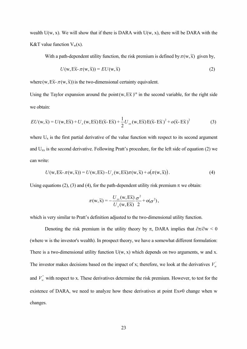
Figure 1a. An example of an S-shaped value function.

w1 w2

NM utility U (w), andpath-dependent U(w; x)

U (w)

wealth

U (w1; x)

U(w2; x)

..................................... ...............

......

........

.......

................

...............

.............................................................................................................................................................................................................. ....................... ......... ................................ ....................... .......

..y1 x1

A

B

CD

²

²

²

²

²

²

.

.

.

.

.

.

.

.

.

.

.

.

.

.

.

.

.

.

.

.

.

.

.

.

.

.

.

.

.

.

.

.

.

.

.

.

.

.

.

.

.

.

.

.

.

.

.

.

.

.

.

.

.

.

.

.

.

.

.

.

.

.

.

.

.

.

.

.

.

.

.

. . . . . . . . . . . . . . . . . . . . . . . .

. . . . . . . . . . . . . . . . . . . . . . . . . . . . . . . . . . . . . . . . . . . . . . .

U(w1 ¡ y1)

U(w1 + x1)

.................................................................................................................................................................................................................................................

..............

....................................................................................................................................................................

...............................................

.............................................................................................................................................................................................................................................................................

.........................................................

.................................................................

.........................................................................

...........................................................................................

................................................................................................................................

...........................................................

Figure 1b. Long-run NM utility function U(w) (bold)and short-run path-dependent functions U(w; x).A and C indicate the points that in°uence the decision,

B and D correspond to utility after adjustment.

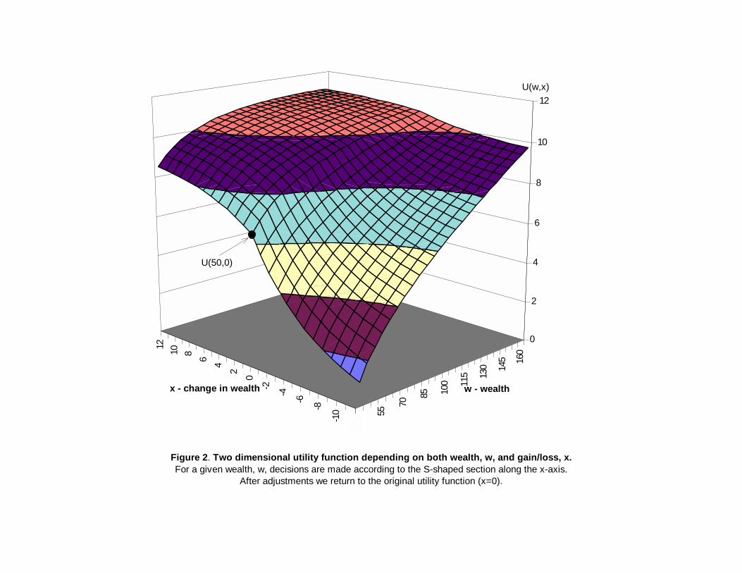
40

55

70

85 100 11

5 130 14

5 160

-12-1

0-8

-6

-4

-2

0

2

4

6

810

12

0

2

4

6

8

10

12

U(50,0)

Figure 2. Two dimensional utility function depending on both wealth, w, and gain/loss, x.For a given wealth, w, decisions are made according to the S-shaped section along the x-axis.

After adjustments we return to the original utility function (x=0).

U(w,x)

w - wealthx - change in wealth

U (w;¡200)

U (w;¡100)

U (w ¡ 100)

w ¡ 200 w ¡ 100 w

NM utility U (w), andpath-dependent U (w; x)

U (w)

wealth

U (w; x)

U (w ¡ 100; x)

..................................... ...............

.......

.......

.......................

...............

K

A

B

C

²

²²²

²

. . . . . .. . . . . . . . . . . .

. . . . . .. . . . . . . . . . . . . . . . . . . . . . . . . . . . .

. . . . . .. . . . . . . . . . . . . . . . . . . . . . . . . . . . .

.

.

.

.

.

.

.

.

.

.

.

.

.

.

.

.

.

.

.

.

.

.

.

.

.

.

.

.

.

.

.

.

.

.

.

.

.

.

.

.

.

.

.

.

..

.

.

.

.

.

.

.

.

. . . . . .. . . . . . . . . . . . . . . . . . . . . . . . . . . . .

.

.

.

.

.

.

.

.

.

.

.

.

.

.

.

.

.

.

.

.

.

.

.

.

.

.

.

.

.

.

.

.

.

.

.

...............................................................................................................................................................................................................................................................................................................

.......

............................................

................................

................................................................................................................................................................................................................................................................................................................................................................................................

.....................

..............................................................................................................................................................................................................................................................................

..........................................................

................................................................

..........................................................................

...........................................................................................

..................................................................................................................................

.......................................................

Figure 3. This ¯gure explains why a large loss may beworse than two smaller losses separated in time.

w w + 100 w + 200

NM utility U (w), andpath-dependent U (w; x)

U (w)

wealth

U(w; x)

U (w + 100; x)

..................................... ...............

.......

.......

.......................

...............

A

B

C

C¤

D

E

²

²

²²

² ²

²

.

.

.

.

.

.

.

.

.

.

.

.

.

.

.

.

.

.

..

.

.

.

.

.

.

.

.

.

.

.

.

.

.

.

.

.

.

.

.

.

.

.

.

.

.

.

.

.

.

.

.

.

.

.

.

.

.

.

.

.

.

.

.

.

.

.

.

.

.

.

.

.

.

.

.

.

.

.

.

.

.

.

.

.

.

.

.

.

.

.

.

.

.

.

.

.

.

.

.

.

.

.

.

.

.

.

.

.

.

.

..

.

.

.

.

.

.

.

.

.

.

.

.

.

.

.

.

.

.

.

.

.

.

.

.

.

.

.

.

.

.......................

... .

. .. .

.....................................................................................................................................................................................................................................................................................................................................................................................

...................................

.................................................

.....................................................

..........................................................................................................................................................................................................................................................................................................................................

.................................

.......................

..............................................................................................................................................................................................................................................................................

..........................................................

................................................................

...........................................................................

...........................................................................................

.................................................................................................................................

.......................................................

Figure 4. This ¯gure explains why two smaller gains separatedin time may be better than a larger one-time gain.

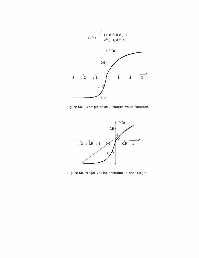
Vw(x) =

(1 ¡ e¡x ; if x ¸ 0

e3x ¡ 1; if x < 0

¡1

¡0:5

0:5

¡3 ¡2 ¡1 1 2 3

............................................................................

........

.................

............... V (w)

x

.....................................................................................................................................................................................................................................

.................................................................................................................................................................................................................................................................................................................................

.......................................................................................

..........................................................................................

Figure 5a. Example of an S-shaped value function.

¡1

¡0:5

0:5

1

¡2 ¡1:5 ¡1 ¡0:5 0:5 1................................................................................... ..............

.

......

...................

............... V (w)

x

B

A

......................................................................................................................................................................................................................................................................................................................................................................................................................................................................................................................

........................................................................................................................................................................................................

...........................................................................................................................................................................................................................................................................................................

...................................................

²²

Figure 5b. Negative risk premium in the "large."

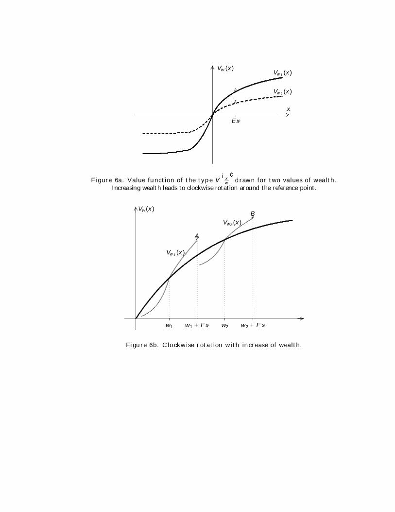
E~x............................................................. ..............

.

......

...................

............... Vw (x)Vw1(x)

Vw2(x)

x......................................................................................................................

.................................................................................

.........................................................................................................................

......................................................................................................................................................................................................................

.........................................................................................................................................................

.....................................................

.................................................................................

................................................................................................................................

................................

²²

Figure 6a. Value function of the type V¡

xw

¢drawn for two values of wealth.

Increasing wealth leads to clockwise rotation around the reference point.

w1 w1 + E~x w2 w2 + E~x

..................................... ...............

.......

.......

.......................

............... Vw(x)

Vw1(x)

Vw2(x)

A

B

²

²

.

.

.

.

.

.

.

.

.

.

.

.

.

.

.

.

.

.

.

.

.

.

.

.

.

.

.

.

.

.

.

.

.

.

.

.

.

.

.

.

.

.

.

.

.

.

.

.

.

.

.

.

.

.

.

.

.

.

.

.

.

..

.

.

.

.

.

.

.

.

.

.

.

.

.

.

.

.

.

.

.

.

.

.

.

.

.

.

.

.

.

.

.

.

.

.

.

.

.

.

.

..

.

.

.

.

.

.

.

.

.

.

.

.

.

.

.

.

.

.

.

.

.

.

.

.

.

.

.

.

.

.

.

.

.

.

.

.

.

.

.

..

.

.

.

.

.

.

.

.

.

.

.

.

......................................................................................................................................................................................................................................................................................................................................................................................

...................................

....................................................................................................................................................................................................................................................

...

...................................................................................................................................................................................................................................................

.......................................................

.............................................................

.....................................................................

.................................................................................

.........................................................................................................

................................................................................................................................

Figure 6b. Clockwise rotation with increase of wealth.

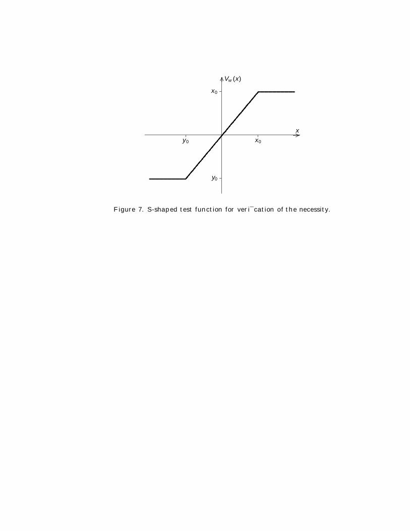
y0

x0

y0 x0

...................................... ...............

........

.......

.................

............... Vw (x)

x

........................................................................................................................................................................................................................................................................................................................................................................................................................................................................................................................................................................................................................................................................................................................

Figure 7. S-shaped test function for veri¯cation of the necessity.

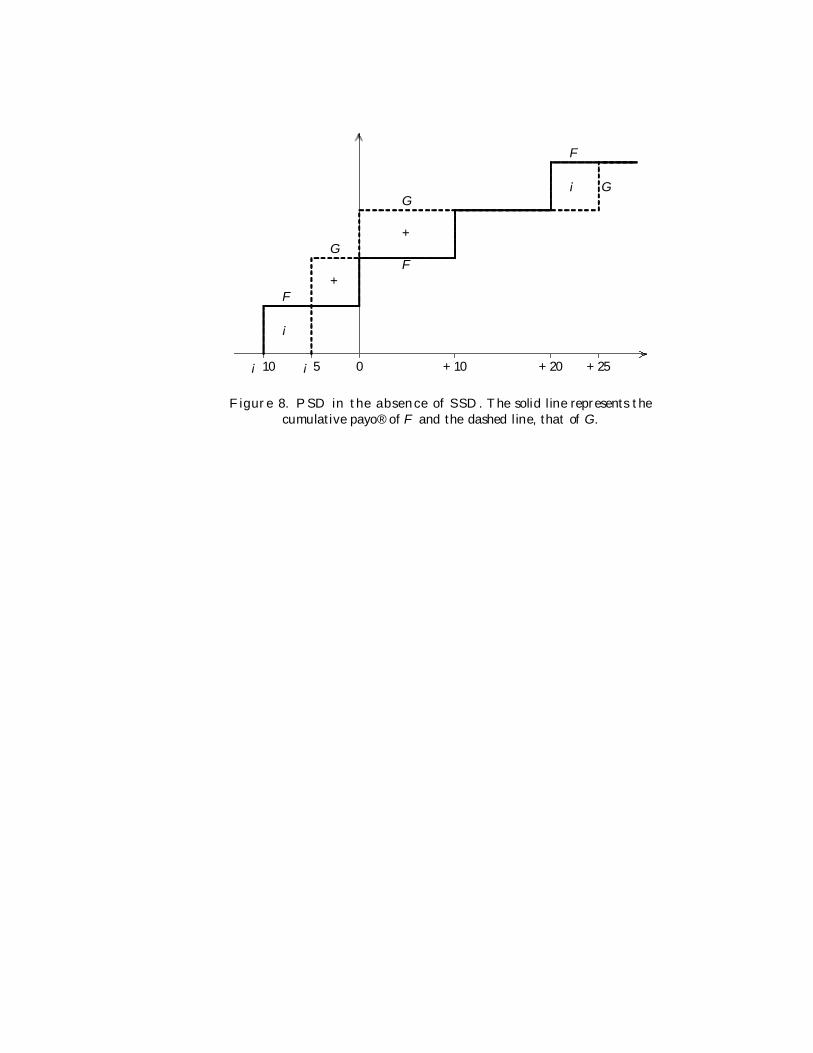
¡10 ¡5 0 +10 +20 +25

F

G

F

G

F

G

¡

+

+

¡

......................... ...............

.......

..................

...............

.................

.................

.................

................

.................

..................................................................................................................................................................................................................................................................................................................................................................................................................................................................................

................

.................

.................

.................

.................

....................................................................................................................................................................................................................................................................................................................................................................................................................................................

...........

..........

............

.........

............

.........

............

.........

............

.............................................................................................................................................................................................................................................................................................................................................................................

........

...........

..........

............

.............................................

Figure 8. PSD in the absence of SSD. The solid line represents thecumulative payo® of F and the dashed line, that of G.