U.S. Department Of Transportation National Highway Traffic Safety Administration PRELIMINARY REGULATORY IMPACT ANALYSIS PROPOSED FMVSS No. 126 Electronic Stability Control Systems Office of Regulatory Analysis and Evaluation National Center for Statistics and Analysis August 2006 People Saving People

Welcome message from author
This document is posted to help you gain knowledge. Please leave a comment to let me know what you think about it! Share it to your friends and learn new things together.
Transcript

U.S. Department Of Transportation
National Highway Traffic Safety Administration
PRELIMINARY REGULATORY IMPACT ANALYSIS
PROPOSED FMVSS No. 126 Electronic Stability Control Systems
Office of Regulatory Analysis and Evaluation National Center for Statistics and Analysis
August 2006
People Saving People

TABLE OF CONTENTS EXECUTIVE SUMMARY ---------------------------------------------------- E-1
I. INTRODUCTION --------------------------------------------------- I-1 II. PROPOSED REQUIREMENTS ---------------------------------- II-1
A. Definition of ESC ------------------------------------------- II-2 B. Functional Requirements ----------------------------------- II-3 C. Performance Requirements ---------------------------------II-4
1. Oversteering Test Maneuver --------------------------- II-5 2. Lateral Stability Criteria -------------------------------- II-7 3. Responsiveness Criteria -- ----------------------------- II-8
D. ESC Malfunction Telltale and Symbol ------------------- II-10 E. ESC Off Switch, Telltale and Symbol -------------------- II-11
III. HOW ESC WORKS ------------------------------------------------ III-1
A. ESC Systems ------------------------------------------------ III-1 B. How ESC Prevents Loss of Control ------------------- III-2 C. Additional Features of Some ESC Systems ------------ III-8 D. ESC Effectiveness ------------------------------------------ III-11
1. The Agency’s Real World Crash Data Analysis ---- III-11 2. Global Studies Of ESC Effectiveness ---------------- III-17 3. Laboratory Studies of ESC ---------------------------- III-18
IV. BENEFITS ----------------------------------------------------------- IV-1
A. Target Population ------------------------------------------- IV-3 B. Projected Target Population ------------------------------- IV-13 C. Benefits ------------------------------------------------------ IV-18 D. Travel Delay and Property Damage Savings ------------ IV-26 E. Summary ----------------------------------------------------- IV-31
V. ESC COSTS --------------------------------------------------------- V-1
A. Technology Costs ------------------------------------------- V-1 B. Fuel Economy Impacts ------------------------------------- V-8 C. Summary ----------------------------------------------------- V-20

VI. COST EFFECTIVENESS AND BENEFIT-COST ------------ VI-1 A. Fatal Equivalents -------------------------------------------- VI-3 B. Net Costs ----------------------------------------------------- VI-6 C. Cost-Effectiveness ------------------------------------------ VI-7 D. Net Benefits -------------------------------------------------- VI-7 E. Summary ----------------------------------------------------- VI-8
VII. ALTERNATIVES -------------------------------------------------- VII-1 VIII. PROBABILISTIC UNCERTAINTY ANALYSIS ------------- VIII-1
A. Simulation Models ------------------------------------------ VIII-3 B. Uncertainty Factors ------------------------------------------VIII-8 C. Quantifying Uncertainty Factors -------------------------- VIII-13 D. Simulation Results ------------------------------------------ VIII-22
IX. REGULATORY FLEXIBILITY ACT AND ------------------- IX-1 UNFUNDED MANDATES REFORM ACT ANALYSIS
A. Regulatory Flexibility Act -------------------------------- IX-1 B. Unfunded Mandates Reform Act ------------------------- IX-8

E-1
EXECUTIVE SUMMARY
This Preliminary Regulatory Impact Analysis examines the impact of the proposal to establish
Federal Motor Vehicle Safety Standard (FMVSS) No. 126, Electronic Stability Control Systems
(ESC). ESC has been found to be highly effective in preventing single-vehicle loss-of-control,
run-off-the road crashes, of which a significant portion are rollover crashes. ESC has also been
found to reduce some multi-vehicle crashes. Based on this analysis, the proposal is highly cost-
effective.
Proposed Requirements
The proposal would require passenger cars, multipurpose passenger vehicles (MPVs), trucks, and
buses that have a gross vehicle weight rating (GVWR) of 4,536 kg (10,000 pounds) or less to be
equipped with an ESC system. We assume throughout this analysis that an ESC system
combines two basic technologies: Anti-lock Brakes (ABS) and Electronic Stability Control. The
proposal would require an ESC system to meet a definition, as well as meet the functional and
performance requirements specified in FMVSS No. 126. The proposal would require
manufacturers to install an ESC malfunction telltale and would allow manufacturers to provide
an optional ESC Off switch (and associated telltale) to temporarily disable the ESC system. In
addition, the proposal would require specific symbols to be used for the malfunction telltale and
ESC Off switch.

E-2
Technical Feasibility/Baseline
ESC is increasingly being offered as standard or optional equipment in new model year
passenger vehicles. An estimated 29 percent of the 2006 model year (MY) passenger vehicles
will be equipped with ESC, compared to 10 percent in MY 2003 vehicles. Based on
manufacturers’ product plans submitted to the agency, 71 percent of the MY 2011 light vehicles
will be equipped with ESC. The agency believes that these ESC systems will meet the proposed
definition since the vast majority of the 2006 ESC systems already met the proposed
performance test. The projected MY 2011 installation rates serve as the baseline voluntary
compliance rates. The analysis estimates the incremental benefits and costs of the proposal,
which would require manufacturers to increase ESC installations from 71 percent of the fleet to
100 percent of the fleet.
Benefits1
Based upon our analysis, we estimate that the proposal would save 1,536 – 2,211 lives and
reduce 50,594 – 69,630 MAIS 1-5 injuries annually once all passenger vehicles have ESC.
Fatalities and injuries associated with rollovers are a significant portion of this total; we estimate
that the proposal would reduce 1,161 to 1,445 fatalities and 43,901 to 49,010 MAIS 1-5 injuries
associated with single-vehicle rollovers.
1 Benefits of the proposal are measured from a baseline of 71% ESC installation to 100% installation. However, the overall benefits of ESC could be measured from “no ESC” to 100% penetration rate. Overall, ESC would save a total of 5,252 – 10,292 lives and eliminate 167,949 – 251,566 MAIS 1-5 injuries annually. Of these benefits, 4,194 – 5,425 lives and 155,849 – 178,062 MAIS 1-5 injuries would be associated with single-vehicle rollovers.

E-3
Low Range of Benefits High Range of Benefits Single
Vehicle Crashes
Multi- Vehicle Crashes
Total
Single Vehicle Crashes
Multi- Vehicle Crashes
Total Fatalities 1,536 0 1,536 2,066 145 2,211 Injuries (AIS 1-5)
50,594 0 50,594 62,212 7,418 69,630
Technology Costs
Vehicle costs are estimated to be $368 (in 2005 dollars) for anti-lock brakes and an additional
$111 for electronic stability control for a total system cost of $479 per vehicle. The total
incremental cost of the proposal (over the MY 2011 installation rates and assuming 17 million
passenger vehicles sold per year) are estimated to be $985 million to install antilock brakes,
electronic stability control, and malfunction lights. The average incremental cost per passenger
vehicle is estimated to be $58 ($90 for the average passenger car and $29 for the average light
truck), a figure which reflects the fact that many baseline MY 2011 vehicles are projected to
already come equipped with ESC components (particularly ABS).
Summary of Vehicle Costs ($2005)
Average Vehicle Costs Total Costs Passenger Cars $ 90.3 $ 722.5 mill. Light Trucks $ 29.2 $ 262.7 mill. Total $ 58.0 $ 985.2 mill.

E-4
Other Impacts
Property Damage and Travel Delay
The proposal would prevent crashes and thus reduce property damage costs and travel delay
associated with those crashes avoided. The proposal would save $453 million at a 3 percent
discount rate to $260 million at a 7 percent discount rate in property damage and travel delay.
Fuel Economy
The proposal would add weight to vehicles and consequently would increase their lifetime use of
fuel. Most of the added weight is for ABS components and very little is for the ESC
components. Since 99 percent of the light trucks are predicted to have ABS in MY 2011, the
weight increase for light trucks is less than one pound and is considered negligible. The average
weight gain for a passenger car is estimated to be 2.1 pounds, resulting in 2.6 more gallons of
fuel being used over their lifetime. The present discounted value of the added fuel cost over the
lifetime of the average passenger car is estimated to be $3.35 at a 3 percent discount rate and
$2.73 at a 7 percent discount rate.

E-5
Net Cost Per Equivalent Life Saved
The net cost per equivalent life saved, discounted at a 3 percent and 7 percent discount rate, is
less than $450,000.
Cost Per Equivalent Life Saved (2005 dollars)
3% Discount Rate 7% Discount Rate Low High Low High Net Cost per Equivalent Life Saved
$188,014 $315,051 $272,742 $427,665
Net Benefits
A net benefit analysis differs from a cost effectiveness analysis in that it requires that benefits be
assigned a monetary value. This value is compared to the monetary value of costs to derive a net
benefit. The high end of the net benefits is $10.6 billion using a 3 percent discount rate and the
low end is $5.8 billion using a 7 percent discount rate. Both of these are based on a $3.75
million comprehensive value for preventing a fatality.
Net Benefits With $3.75 M Cost Per Life (in billions of 2005 dollars)
At 3% Discount At 7% Discount Low High Low High Net Benefits $7.5 Bill. $10.6 Bill. $5.8 Bill. $8.2 Bill.

E-6
Leadtime
The agency is proposing a phase-in requirement for vehicle manufacturers excluding multi-stage
manufacturers, alterers, and small volume manufacturers (i.e., manufacturers producing less than
5,000 vehicles for sale in the U.S. market in one year). Vehicle manufacturers are permitted to
use carryover credits. The phase-in schedule for vehicle manufacturers is:
Model Year Production Beginning Date Requirement 2009 September 1, 2008 30% with carryover credit 2010 September 1, 2009 60% with carryover credit 2011 September 1, 2010 90% with carryover credit 2012 September 1, 2011 Fully effective
Instead of complying with the proposed phase-in requirement, the proposal would allow multi-
stage manufacturers and alterers to fully comply with the standard on September 1, 2012, which
is a one-year extension from full compliance of the phase-in schedule. The proposal would also
permit small volume manufacturers to be excluded from the phase-in but to fully comply with
the standard on September 1, 2011.
I-1
CHAPTER I. INTRODUCTION
This preliminary regulatory impact analysis (PRIA) accompanies NHTSA’s proposal to establish
Federal Motor Vehicle Safety Standard (FMVSS) No. 126, Electronic Stability Control Systems,
which would require passenger cars, multipurpose passenger vehicles (MPVs), trucks, and buses
that have a gross vehicle weight rating (GVWR) of 4,536 kg (10,000 pounds) or less to be
equipped with an electronic stability control (ESC) system. An ESC system is an active-safety
technology designed to proactively help drivers to maintain control of their vehicles in situations
where the vehicle is beginning to lose directional stability. Typically, an ESC system intervenes
by utilizing computers to control individual wheel brakes, thereby keeping the vehicle headed in
the direction intended by drivers. Keeping the vehicle on the road prevents run-off-road crashes,
which are the circumstances that lead to most single-vehicle rollovers.
Several studies from Europe and Japan have shown significant reduction in crashes by ESC,
specifically in single-vehicle crashes (see Chapter III). The agency’s studies and a study by the
Insurance Institute for Highway Safety (IIHS) also concluded that the ESC systems would
eliminate a substantial number of crashes. Based on 2004 Fatality Analysis Reporting Systems
(FARS) and 2000-2004 National Automotive Sampling System (NASS) Crashworthiness Data
System (CDS), the agency estimates that there were 34,314 police-reported passenger vehicle
fatal crashes2 and over 2.5 million serious non-fatal crashes (defined as at least one involved
passenger vehicle was towed away) annually. About 33,907 passenger vehicle occupant
fatalities and 2,182,460 non-fatal injuries were associated with these crashes. Single-vehicle
crashes, which frequently include roadway departure, accounted for about 53 percent (18,321 2 Not all passenger vehicle fatal crashes result in fatalities to passenger vehicle occupants, some result in fatalities to pedestrians, motorcyclists, etc.
I-2
fatal crashes) of the fatal crashes and 33 percent (820,218 crashes) of the towaway crashes. A
total of 15,611 occupant fatalities and 516,500 non-fatal injuries were associated with these
single-vehicle crashes. Rollovers comprised a large share of these single-vehicle crashes and
were responsible for a disproportionate number of fatalities. Rollovers accounted for 42 percent
(or 7,734 crashes) of the single-vehicle fatal crashes and 56 percent (8,487 fatalities) of the
occupant fatalities3. ESC would potentially prevent many of these crashes from occurring and
thus would reduce associated fatalities and injuries. Based on the agency’s ESC effectiveness
study, which found that ESC is highly effective against rollovers (Chapter III), a large portion of
these benefits would be from rollovers.
Since the early 1990’s, the agency has been actively engaged in finding ways to address the
rollover safety problem. The agency has explored several options. However, due to feasibility
and practicability issues, the agency ultimately chose a consumer-information-based-approach to
the rollover problem. In 2001, the agency added a rollover resistance rating to our New Car
Assessment Program (NCAP) consumer information. The rollover resistance rating, based on
the height of the center of gravity and the track width of a vehicle, measures the likelihood of a
vehicle would rollover in a crash. The agency believes that the NCAP rollover resistance rating
information allows consumers to make an informed decision when they purchase a new vehicle.
In addition, the agency believes that the NCAP rollover information also encourages vehicle
manufacturers to increase their vehicles’ geometric stability and rollover resistance through
market-based incentives.
In response to NCAP rollover resistance information, vehicle manufacturers have modified many
of their new model vehicles, especially those with a higher center of gravity such as SUVs and 3 An additional 1,971 rollover occupant fatalities were recorded in multi-vehicle crashes.

I-3
trucks. Examples of their changes include utilizing a wider track platform for newer sport utility
vehicles (SUVs) and/or equipping SUVs with roll stability control technology. However, the
impact of this consumer-information-based-approach has been offset by a continuous demand
from consumers for vehicles with a greater carrying capacity and a higher ground clearance.
In recent years, the maturation of ESC technologies has created an opportunity to establish
performance criteria and reduce the occurrence of rollovers in new vehicles. This opportunity
led to today’s proposal. This proposal is consistent with recent congressional legislation
contained in section 10301 of the Safe, Accountable, Flexible, Efficient Transportation Equity
Act: A Legacy for Users of 2005 (SAFETEA-LU).4 The provision requires the Secretary of
Transportation to “establish performance criteria to reduce the occurrence of rollovers consistent
with stability enhancing technology” and to “issue a proposed rule … by October 1, 2006, and a
final rule by April 1, 2009.”
This PRIA estimates the benefits, cost, cost-effectiveness, benefit-cost of the proposal, and the
following outlines the structure of the balance of this document. The PRIA first describes the
proposed requirements in Chapter II. After describing the proposal, the PRIA discusses current
ESC systems, their functional capability, and their effectiveness in Chapter III. Chapter IV of
the PRIA estimates the benefits. Chapter V discusses the costs and leadtime. Chapter VI
provides cost-effectiveness and benefit-cost analysis. Chapter VII discusses alternatives.
Chapter VIII provides the uncertainty analysis to address variations of the estimated benefits.
And finally, Chapter IX examines the impacts of the rule on small business entities
4 Pub. L. 109-59, 119 Stat. 1144 (2005).
II-1
CHAPTER II. PROPOSED REQUIREMENTS
The proposal would establish Federal Motor Vehicle Safety Standard (FMVSS) No. 126,
Electronic Stability Control System, which would require passenger cars, multipurpose
passenger vehicles (MPVs), light trucks and buses that have a gross vehicle weight rating
(GVWR) of 4,536 kg (10,000 pounds) or less to be equipped with an ESC system that meets the
requirements of the standard. The proposed standard specifies: (a) the Definition of ESC, (b) the
Functional Requirements of ESC, (c) the Performance Requirements of ESC, (d) ESC
Malfunction Telltale and Symbol Requirements, and (e) ESC Off Switch, Telltale and Symbol
Requirements (if provided). The following sections summarize these requirements. Interested
parties should consult the preamble of the notice of proposed rulemaking (NPRM) for the
detailed proposal. Comprehensive technical background for deriving the proposed requirements
can be found in the following agency research reports:
a. Forkenbrock, G.J., Elsasser, D.H., O’Harra, B., and Jones, R.E., “Development of Criteria for Electronic Stability Control Performance Evaluation,” DOT HS 809 974, December 2005
b. Mazzae, E.N., Papelis, Y.E., Watson, G.S., and Ahmad, O., “The Effectiveness of ESC
and Related Telltales: NADS Wet Pavement Study,” DOT HS 809 978, December 2005
II-2
A. DEFINITION OF ESC
The agency proposes to adopt the ESC definition based on the Society of Automotive Engineers
(SAE) Surface Vehicle Information Report J2564 (revised June 2004). The ESC is defined as a
system that has all of the following attributes:
(a) ESC augments vehicle directional stability by applying and adjusting the vehicle brakes
individually to induce correcting yaw torques to the vehicle.
(b) ESC is a computer-controlled system, which uses a close-loop algorithm to limit
understeer and oversteer of the vehicle when appropriate. [The close-loop algorithm is a
cycle of operations followed by a computer that includes automatic adjustments based on
the result of previous operations or other changing conditions.]
(c) ESC has a means to determine vehicle yaw rate and to estimate its sideslip. [Yaw rate
means the rate of change of the vehicle’s heading angle about a vertical axis through the
vehicle center of gravity. Sideslip is the arctangent of the ratio of the lateral velocity to
the longitudinal velocity of the center of gravity.]
(d) ESC has a means to monitor driver steering input.
(e) ESC is operational over the full speed range of the vehicle (except below a low –speed
threshold where loss of control is unlikely).

II-3
B. FUNCTIONAL REQUIREMENTS
The proposed ESC is required to comply with following functional requirements:
(a) The ESC system must have the means to apply all four brakes individually and a control
algorithm that utilizes this capability.
(b) The ESC must be operational during all phases of driving including acceleration,
coasting, and deceleration (including braking).
(c) The ESC system must stay operational when the antilock brake system (ABS) or Traction
Control is activated.
With the ESC definition and the functional requirements, the agency basically adopts the SAE
definition and attributes for the 4-wheel ESC system without engine control5. This system would
have oversteering and understeering intervention capabilities. Oversteering and understeering
are typically cases of loss-of-control where vehicles move in a direction different from the
driver’s intended direction. Oversteering is a situation where a vehicle turns more than driver’s
input because the rear end of the vehicle is spinning out or sliding out. Understeering is a
situation where a vehicle turns less than the driver’s input and departs from its intended course
because the front wheels do not have sufficient traction. Chapter III details how ESC functions
during these situations. The agency proposed this ESC standard to balance the necessary ESC
intervention capabilities and the complexity of the technologies, which generally are associated
with significant costs. Also, the proposed standard does not conflict with the 4-wheel ESC
system with engine control. An ESC system with engine control may control the throttle and
5 Engine control refers to the ability of the vehicle’s ESC to remove or apply driver torque to one or more wheels. Such intervention is intended to augment, but not replace, the benefits offered by brake intervention.
II-4
reduce the amount of fuel going into the engine to slow the vehicle down, in addition to braking
one wheel.
Furthermore, the proposed ESC definition and functional requirements would require
manufacturers to implement an ABS-equivalent braking technology in their vehicles. If
manufacturers choose to equip their vehicles with the ABS technology, the ABS would be
required to comply with FMVSS No. 135.
C. PERFORMANCE REQUIREMENTS
As proposed, the ESC-equipped vehicle must satisfy a performance test criteria to ensure
sufficient oversteer intervention (i.e., mitigate the tendency for the vehicle to spinout). A
“spinout” is defined as vehicle final heading angle of more than 90 degrees from the initial
heading after a symmetric steering maneuver in which the amount of right and left steering is
equal. During the proposed test, the vehicle is not permitted to lose lateral stability. A
quantifiable definition of lateral stability is proposed and is discussed later in this chapter.
In addition to being required to satisfy the standard’s lateral stability criteria, the standard
proposes an ESC-equipped vehicle also must satisfy a responsiveness criterion to preserve the
ability of the vehicle to adequately respond to a driver’s steering inputs during ESC intervention.
These criteria ensure that an ESC achieves an optimal stability performance, but not at the
expense of responsiveness. Note that the agency is still conducting research to establish an
appropriate understeering intervention test.
II-5
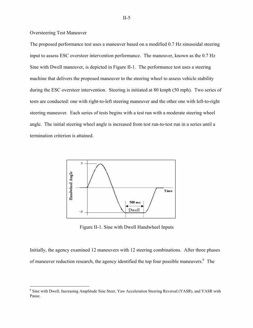
Oversteering Test Maneuver
The proposed performance test uses a maneuver based on a modified 0.7 Hz sinusoidal steering
input to assess ESC oversteer intervention performance. The maneuver, known as the 0.7 Hz
Sine with Dwell maneuver, is depicted in Figure II-1. The performance test uses a steering
machine that delivers the proposed maneuver to the steering wheel to assess vehicle stability
during the ESC oversteer intervention. Steering is initiated at 80 kmph (50 mph). Two series of
tests are conducted: one with right-to-left steering maneuver and the other one with left-to-right
steering maneuver. Each series of tests begins with a test run with a moderate steering wheel
angle. The initial steering wheel angle is increased from test run-to-test run in a series until a
termination criterion is attained.
Figure II-1. Sine with Dwell Handwheel Inputs
Initially, the agency examined 12 maneuvers with 12 steering combinations. After three phases
of maneuver reduction research, the agency identified the top four possible maneuvers.6 The
6 Sine with Dwell, Increasing Amplitude Sine Steer, Yaw Acceleration Steering Reversal (YASR), and YASR with Pause.
Dwell

II-6
proposed Sine with Dwell maneuver was selected over three other maneuvers due to its
objectivity, practicability, repeatability, and representativeness.
The proposed maneuver is highly objective because it will initiate oversteer intervention for
every tested ESC system and because it will discriminate strongly between vehicles with and
without ESC (or ESC disabled). The maneuver is practicable because it can easily be
programmed into the steering machine and because it simplifies the instrumentation required to
perform the test due to its lack of acceleration feedback. It is repeatable due to the use of a
steering machine thereby minimizing drive effects. In addition, the maneuver is representative
of steering inputs produced by human drivers in an emergency obstacle avoidance situation.
The agency also explored the possibility of using a Sine with Dwell curve with a different
frequency (i.e., the 0.5 Hz curve) as the steering maneuver. However, the Alliance of
Automobile Manufacturers (Alliance) presented data, which cast doubt on the practicability of
this approach, as discussed in their presentation to the agency on December 3, 2004 (Docketed at
NHTSA-2004-19951-1). Specifically, the Alliance reported that the 0.5 Hz Sine with Dwell did
not correlate as well with the responsiveness versus controllability ratings made by its
professional test drivers in a subjective evaluation (the same vehicles evaluated with the Sine
with Dwell maneuvers were also driven by the test drivers), and it provided less input energy
than the 0.7 Hz Sine with Dwell.

II-7
Lateral Stability Criteria
“Lateral stability” is defined as the ratio of vehicle yaw rate at a specified time and the peak yaw
rate generated by the 0.7 Hz Sine with Dwell steering reversal. The performance limit (i.e., the
maximum value of the ratio) establishes a 5 percent spinout threshold when ESC intervenes. In
other words, an ESC-equipped vehicle has a less than 5 percent probability of spinout if the
vehicle meets the proposed lateral criteria. Under the proposed performance test, ESC would be
required to meet the following two lateral stability criteria:
(1) One second after completion of the steering input for the 0.7 Hz Sine with Dwell maneuver,
the yaw rate of the vehicle has to be less than or equal to 35 percent of the peak yaw rate
(Criterion #1).
(2) 1.75 seconds after completion of the steering input, the yaw rate of the vehicle has to be less
than or equal to 20 percent of the peak yaw rate (Criterion #2).
The lateral stability criteria can be represented in the mathematical notations as follows:
%35100)00.1( 0 <=×+
Peak
t
ψψ&
& (Criterion #1), and
%20100)75.1( 0 <=×+
Peak
t
ψψ&
& (Criterion #2)
Where,
inputsteering of completiontotimerecersal sterring Dwell with Sine Hz 0.7 by the generated rateyawPeak
seconds)(in t timeatrateYaw
0 ===
tPeak
t
ψψ
&
&
II-8
Based on the agency’s analysis, we anticipate that an ESC system meeting these lateral stability
criteria would have at least a 95 percent probability of preventing a spinout.
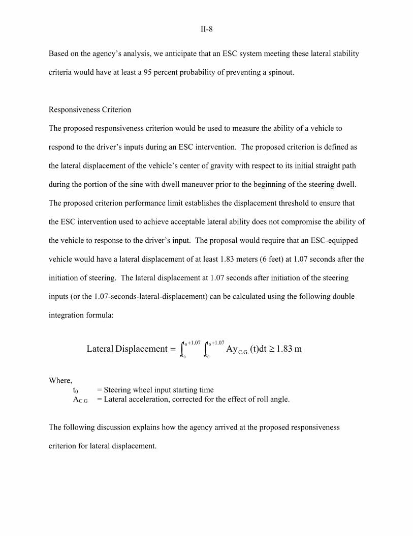
Responsiveness Criterion
The proposed responsiveness criterion would be used to measure the ability of a vehicle to
respond to the driver’s inputs during an ESC intervention. The proposed criterion is defined as
the lateral displacement of the vehicle’s center of gravity with respect to its initial straight path
during the portion of the sine with dwell maneuver prior to the beginning of the steering dwell.
The proposed criterion performance limit establishes the displacement threshold to ensure that
the ESC intervention used to achieve acceptable lateral ability does not compromise the ability of
the vehicle to response to the driver’s input. The proposal would require that an ESC-equipped
vehicle would have a lateral displacement of at least 1.83 meters (6 feet) at 1.07 seconds after the
initiation of steering. The lateral displacement at 1.07 seconds after initiation of the steering
inputs (or the 1.07-seconds-lateral-displacement) can be calculated using the following double
integration formula:
Where, t0 = Steering wheel input starting time
AC.G = Lateral acceleration, corrected for the effect of roll angle.
The following discussion explains how the agency arrived at the proposed responsiveness
criterion for lateral displacement.
m 1.83(t)dtAyntDisplaceme Lateral1.07t
t
1.07t
t C.G.0
0
0
0
≥= ∫ ∫+ +

II-9
The 1.07 seconds is chosen because it is the starting point of the dwell period and can easily be
identified. Most importantly, 1.07 seconds is short enough to assure accuracy of the double
integration and long enough to induce a discernable lateral displacement.
The 1.83 meters (6 feet) is based on the responsiveness, measured by the 1.07-seconds-lateral-
displacement, of 61 vehicles tested by the agency and eleven vehicle manufacturers using the 0.7
Hz Sine with Dwell maneuver with steering angles of 180 degrees or greater. These 61 vehicles
include passenger cars (PCs), sport utility vehicles (SUVs), pick-up trucks, and vans and range
from high performance sports cars to 15-passenger vans. All of the 61 vehicles but one achieved
the 1.83 meters (6 feet) lateral displacement at 1.07 seconds.
The double integration technique for deriving the lateral displacement was presented by the
Alliance on September 7, 2005.7 The technique is an indefinite double integral. Strictly
speaking, it means Ay GC .. (the vehicle’s lateral acceleration data) analytically is integrated
twice; first to obtain lateral velocity, and a second time to produce lateral displacement from the
vehicle’s initial heading. The result is an approximation for lateral displacement as a function of
time. The technique was adapted after the agency validated the integration displacement results
and concluded that they are in good agreement with the global positioning sensor (GPS)
measurements for vehicles tested by the agency, provided there is no offset to the lateral
acceleration data channel and calculated data no longer than 1.07 seconds after initiation of the
Sine with Dwell steering inputs are considered. The Alliance stated that there would be a
7 Docket Number NHTSA-2005-19951

II-10
substantial cost savings to the industry with no loss of technical validity if double integration was
used instead of GPS measurements.
During the development of the responsiveness criterion, the agency also considered several other
metrics, such as lateral speed and lateral acceleration, to measure the responsiveness of the
vehicle. However, the agency concluded that the lateral displacement and maximum
displacement are the most obvious and relevant responsiveness measurements. The 1.07-
seconds-lateral-displacement was chosen over the maximum lateral displacement for several
reasons. The maximum displacement occurs later in the steering maneuver and at different times
for different vehicles. Therefore, the maximum displacement is subject to greater measurement
error from the double integration process. Such errors could be systematically greater for certain
type of vehicles than others. Most importantly, the 1.07-seconds-lateral-displacement
establishes a standardized baseline for every vehicle since it is measured uniformly at the same
traveling distance from the initiation of steering.
D. ESC Malfunction Telltale and Symbol
The proposal would require a yellow ESC malfunction telltale identified by the following
symbol:

II-11
We propose to include this symbol in Table 1 of FMVSS No. 101, Controls and Displays. The
malfunction telltale would be required to be mounted inside the occupant compartment in front
of and in clear view of the driver. The malfunction telltale would be required to illuminate not
more than two minutes after the occurrence of one or more ESC malfunctions. Such telltale
would be required to remain continuously illuminated for as long as the malfunction exists,
whenever the ignition locking system in “On” (“Run”) position. The ESC malfunction telltale is
permitted to flash in order to indicate ESC operation. A flashing telltale can not be used to
indicate a malfunction.
E. ESC Off Switch, Telltale and Symbol
The proposal would permit (but not require) vehicle manufacturers to install a driver-selectable
switch to temporarily disable or limit the ESC functions. This would allow drivers to disengage
ESC or limit the ESC intervention capability in certain circumstances when the full ESC
intervention might not be appropriate. Examples include circumstances such as when a vehicle
is stuck in sand/gravel or when the vehicle is being operated within the controlled confines of a
racetrack for maximum performance.
If vehicles manufacturers choose this option, the proposal would require that the ESC system
return to a mode that satisfies the requirements of the standard at the initiation of each new
ignition cycle. In addition, vehicle manufacturers would be required to provide a yellow “ESC
OFF” telltale identified by the following symbol:
II-12
We propose to include this symbol in Table 1 of FMVSS No 101, Controls and Displays. The
telltale would be required to be mounted inside the occupant compartment in front of and in clear
view of the driver. Such telltales must remain continuously illuminated for as long as the ESC is
in a mode that makes it unable to meet the performance requirements of the standard, whenever
the ignition locking system is in the “On” (“Run”) position.

III-1
CHAPTER III. HOW ESC WORKS
A. ESC SYSTEMS
ESC is known by many different trade names such as AdvanceTrac, Dynamic Stability Control
(DSC), Dynamic Stability and Traction Control (DSTC), Electronic Stability Program (ESP),
Vehicle Dynamic Control (VDC), Vehicle Stability Assist (VSA), Vehicle Stability Control
(VSC), Vehicle Skid Control (VSC), Vehicle Stability Enhancement (VSE), StabiliTrak, and
Porsche Stability Management (PSM). An ESC system utilizes computers to control individual
wheel brakes and assists the driver in maintaining control of the vehicle by keeping the vehicle
headed in the direction the driver is steering even when the vehicle nears or reaches the limits of
road traction.
When a driver attempts a sudden maneuver (for example, to avoid a crash or because he
misjudged the severity of a curve), he may lose control if the vehicle responds differently as it
nears the limits of road traction than it does in ordinary driving. The driver’s loss of control can
result in either the rear of the vehicle “spinning out" or the front of the vehicle "plowing out." As
long as there is sufficient road traction, a professional race driver could maintain control in many
spinout or plowout conditions by using countersteering (momentarily turning away from the
intended direction) and other techniques. However, in a panic situation with the vehicle
beginning to spin out, for example, average drivers would be unlikely to countersteer like a race
driver and regain control.

III-2
In contrast, ESC uses automatic braking of individual wheels to adjust the vehicle’s heading if it
departs from the direction the driver is steering. Thus, it prevents the heading from changing too
quickly (spinning out) or not quickly enough (plowing out). Although it cannot increase the
available traction, ESC affords the driver the maximum possibility of keeping the vehicle under
control and on the road in an emergency maneuver using just the natural reaction of steering in
the intended direction.
Keeping the vehicle on the road prevents single-vehicle crashes, which are the circumstances that
lead to most rollovers. However, if the speed is simply too great for the available road traction,
the vehicle will unavoidably drift (without spinning) off the road. And, of course, ESC cannot
prevent road departures due to driver inattention or drowsiness rather than loss of control.
B. How ESC Prevents Loss of Control
The following explanation of ESC systems illustrates the basic principle of yaw stability control,
but actual systems include countless refinements and proprietary algorithms that make them
practical for the range of circumstances and roadway conditions encountered by drivers. For
example, actual ESC systems augment the yaw rate control strategy described below with the
consideration of vehicle sideslip (lateral sliding that may not alter yaw rate) to determine the
optimal intervention.
An ESC system maintains what is known as “yaw” (or heading) control by determining the
driver’s intended heading, measuring the vehicle’s actual response, and automatically turning the

III-3
vehicle if its response does not match the driver’s intention. However, with ESC, turning is
accomplished by counter torques from the braking system rather than from steering input. Speed
and steering angle measurements are used to determine the driver’s intended heading. The
vehicle response is measured in terms of lateral acceleration and yaw rate by onboard sensors. If
the vehicle is responding properly to the driver, the yaw rate will be in balance with the speed
and lateral acceleration.
The concept of “yaw rate” can be illustrated by imagining the view from above of a car
following a large circle painted on a parking lot. One is looking at the top of the roof of the
vehicle and seeing the circle. If the car starts in a heading pointed north and drives half way
around circle, its new heading is south. Its yaw angle has changed 180 degrees. If it takes 10
seconds to go half way around the circle, the “yaw rate” is 180 degrees per 10 seconds (deg/sec)
or 18 deg/sec. If the speed stays the same, the car is constantly rotating at a rate of 18 deg/sec
around a vertical axis that can be imagined as piercing its roof. If the speed is doubled, the yaw
rate increases to 36 deg/sec.
While driving in a circle, the driver notices that he must hold the steering wheel tightly to avoid
sliding toward the passenger seat. The bracing force is necessary to overcome the lateral
acceleration that is caused by the car following the curve. The lateral acceleration is also
measured by the ESC system. When the speed is doubled, the lateral acceleration increases by a
factor of four if the vehicle follows the same circle. There is a fixed physical relationship
between the car’s speed, the radius of its circular path, and its lateral acceleration. Since the ESC
system measures the car’s speed and its lateral acceleration, it can compute the radius of the

III-4
circle. Since it then has the radius of the circle and the car’s speed, the ESC system can compute
the correct yaw rate for a car following the path. Of course, the system includes a yaw rate
sensor, and it compares the actual measured yaw rate of the car to that computed for the path the
car is following. If the computed and measured yaw rates begin to diverge as the car that is
trying to follow the circle speeds up, it means the driver is beginning to lose control, even if he
cannot yet sense it. Soon, an unassisted vehicle would have a heading significantly different
from the desired path and would be out of control either by oversteering (spinning out) or
understeering.
When the ESC system detects an imbalance between the measured yaw rate of a vehicle and the
path defined by its speed and lateral acceleration (as measured by the steering angle), it
automatically intervenes to turn the vehicle. The automatic turning of the vehicle is
accomplished by uneven brake application rather than by steering wheel movement. If only one
wheel is braked, the uneven brake force will cause the vehicle’s heading to change. Figure III-1
shows the action of ESC using single wheel braking to correct the onset of oversteering or
understeering.
• Oversteering. In Figure III-1 to the right, the vehicle has entered a left curve that is
extreme for the speed it is traveling. The rear of the vehicle begins to slide which
would lead to a non-ESC vehicle turning sideways (or “spinning out”) unless the driver
expertly countersteers. In a vehicle equipped with ESC, the system immediately
detects that the vehicle’s heading is changing more quickly than appropriate for the
driver’s intended path (the yaw rate is too high). It momentarily applies the right front
brake to turn the heading of the vehicle back to the correct path. The intervention

III-5
action happens quickly and smoothly and thus most of the time will go undetected by
the drivers. Even if the driver brakes because the curve is sharper than anticipated, the
system is still capable of generating uneven braking if necessary to correct the heading.
• Understeering. Figure III-1 to the left shows a similar situation faced by a vehicle
whose response as it nears the limits of road traction is first sliding at the front
(“plowing out” or understeering) rather than oversteering. In this vehicle, ESC rapidly
detects that the vehicle’s heading is changing less quickly than appropriate for the
driver’s intended path (the yaw rate is too low). It momentarily applies the left rear
brake to turn the heading of the vehicle back to the correct path.
While Figure III-1 may suggest that particular vehicles go out of control due to either oversteer
or vehicles prone to understeer, it is quite possible a vehicle could require both understeer and
oversteer interventions during progressive phases of a complex avoidance maneuver like a
double lane change.

III-6
Understeering (“plowing out”) Oversteering (“spinning out”)
Figure III-1. ESC Interventions for Understeering and Oversteering
Although ESC cannot change the tire/road friction conditions the driver is confronted with in a
critical situation, there are clear reasons to expect it can reduce loss-of-control crashes.
In vehicles without ESC, the response of the vehicle to steering inputs changes as the vehicle
nears the limits of road traction. Generally speaking, most drivers operate with their “linear
range” skills, the range of lateral acceleration in which a given steering wheel movement
produces a proportional change in the vehicle’s heading. The driver merely turns the wheel the
expected amount to produce the desired heading. Adjustments in heading are easy to achieve
because the vehicle’s response is proportional to the driver’s steering input, and there is very
little lag time between input and response. The car is traveling in the direction it is pointed, and
the driver feels in control. However, at lateral accelerations above about one half g on dry
pavement for ordinary vehicles, the relationship between the driver’s steering input and the

III-7
vehicle’s response changes (oversteer or understeer), and the lag time of the vehicle response can
lengthen. When a driver encounters these changes during a panic situation, it adds to the
likelihood that the driver will lose control and crash because the familiar actions learned by
driving in the linear range would not be correct.
However, ordinary linear range driving skills are much more likely to be adequate for a driver of
a vehicle with ESC to avoid loss of control in a panic situation. By monitoring yaw rate and
sideslip, ESC can intervene early in the impending loss-of–control situation with the appropriate
brake forces to restore yaw stability before the driver would attempt an over-correction or other
error. The net effect of ESC is that the driver’s ordinary driving actions learned in linear range
driving are the correct actions to control the vehicle in an emergency. Also, the vehicle will not
change its heading from the desired path in a way that would induce further panic in a driver
facing a critical situation. Studies using a driving simulator, discussed in Section III,
demonstrate that ordinary drivers are much less likely to lose control of a vehicle with ESC when
faced with a critical situation.
Besides allowing drivers to cope with potentially dangerous situations and slippery pavement
using only “linear range” skills, ESC provides more complete control interventions than those
available to expert drivers of non-ESC vehicles. For all practical purposes, the yaw control
actions with non-ESC vehicles are limited to steering. However, as the tires approach the
maximum lateral force sustainable under the available pavement friction, the yaw moment
generated by a given increment of steering angle is much less than at the low lateral forces

III-8
occurring in regular driving8. This means that as the vehicle approaches its maximum cornering
capability, the ability of the steering system to turn the vehicle is greatly diminished even in the
hands of an expert. ESC creates the yaw moment to turn the vehicle using braking at an
individual wheel rather than the steering system. This intervention remains powerful even at
limits of tire traction because both the braking force of the individual tire and the reduction of
lateral force that accompanies the braking force act to create the desired yaw moment.
Therefore, ESC can be especially beneficial on slippery surfaces. The possibility of a vehicle
staying on the road in any maneuver is ultimately limited by the tire/pavement friction. ESC
maximizes an ordinary driver’s ability to use the tire/pavement friction available.
C. Additional Features of Some ESC Systems
In addition to the basic operation of “yaw stability control”, many systems include additional
features. Most ESC systems reduce engine power during intervention to slow the vehicle and to
give it a better chance of being able to stay on the intended path after its heading has been
corrected.
Other ESC systems may go beyond reducing engine power to slow the vehicle by performing
high deceleration automatic braking at all four wheels. Of course, the braking would be
performed unevenly side to side so that the same net yaw torque or “turning force” would be
applied to the vehicle as in the basic case of single wheel braking.
8 Liebemann et al, Safety and Performance Enhancement: The Bosch Electronic Stability Control (ESP), 2005 ESV Conference, Washington, DC
III-9
Some ESC systems used on vehicles with a high center of gravity (c.g.), such as SUVs, are
programmed for an additional function known as roll stability control. Roll stability control is a
direct countermeasure for on-pavement rollover crashes of high c.g. vehicles. Some systems
measure the roll angle of the vehicle using an additional roll rate sensor to determine if the
vehicle is in danger of tipping up. Other systems rely on the existing ESC sensors for steering
angle, speed, and lateral acceleration along with knowledge of vehicle-specific characteristics to
estimate whether the vehicle is in danger of tipping up.
Regardless of the method of detecting the risk of tip-up, the various types of roll stability control
intervene in the same way. They intervene by reducing the lateral acceleration that is causing the
roll motion of the vehicle on its suspension and preventing the possibility of it rolling so much
that the inside wheels lift off the pavement. The principal way of accomplishing this
intervention is by applying hard braking to either the outside front wheel or to both outside front
wheels. In either case, the braking force generated must be large enough to cause high
longitudinal wheel slip for the outside front wheel(s). This dramatically reduces the lateral
forces being produced by the outside front tire(s) and straightens the path of the vehicle. Greatly
reducing the lateral forces being produced by the outside front tire(s) lowers the lateral
acceleration of the vehicle. Since lateral acceleration is the driving force that causes untripped
rollover, greatly reducing it makes untripped rollover less likely to happen. Also, whereas the
primary objective of conventional ESC intervention is increased path-following capability, the
roll stability control endeavors to prevent on-road untripped rollver; often at the expense of path-
following.

III-10
Another difference between a roll stability control intervention and oversteer intervention by the
ESC system operating in the basic yaw stability control mode is the triggering circumstance.
The oversteer intervention occurs when the vehicle’s excessive yaw rate indicates that its
heading is departing from the driver’s intended path, but the roll stability control intervention
occurs when there is an appreciable risk the vehicle could roll over. The roll stability control
intervention may occur when the vehicle is still following the driver’s intended path. The
obvious trade-off of roll stability control is that the vehicle must depart to some extent from the
driver’s intended path in order to reduce the lateral acceleration from the level that could cause
rollover.
If the determination of impending rollover that triggers the roll stability intervention is very
certain, then the possibility of the vehicle leaving the roadway as a result of the roll stability
intervention represents a lower relative risk to the driver. Obviously, systems that intervene only
when absolutely necessary and produce the minimum loss of lateral acceleration to prevent
rollover are the most effective. However, roll stability control is a new technology that is still
evolving. Roll stability control is not a subject of this rulemaking because there are not enough
vehicles with roll stability for actual crash statistics to demonstrate its practical effect on crash
reduction.

III-11
D. ESC Effectiveness
The Agency’s Real World Crash Data Analysis
In 2004, an agency study found that ESC is approximately 30 percent effective in preventing
fatal single-vehicle crashes for passenger cars (PCs) and 63 percent for sport utility vehicles
(SUVs). For all single-vehicle crashes, the corresponding effectiveness rates are 35 and 67
percent.9 These results were statistically significant at the 0.05 level. The 2004 study deployed a
before-after, case-control approach to derive these effectiveness rates. The approach attempted
to control factors other than presence and absence of ESCs that could be associated with crash
scenarios. Basically, the approach compared the number of case crashes (and control crashes)
involving make-models equipped with ESCs (after) to their earlier models without ESCs
(before). The case crashes contain crashes that would be affected by ESCs and the control
crashes would not. In the agency approach, the case crashes were single-vehicle crashes
excluding pedestrians, pedalcyclists, and animals, and the control crashes were multi-vehicle
crashes. The effectiveness of ESC was derived by the following formula:
Control ESC, No
Control ESC,
Case ESC, No
Case ESC,
ff
ff
1−
Where,
fESC, Case = the number of case crashes (i.e., single vehicle) involving vehicles with ESCs,
fNo ESC, Case = the number of case crashes (i.e., single vehicle) involving vehicles without ESCs,
fESC, Control = the number of control crashes (i.e., multi-vehicle crashes) involving
9 Dang, J., Preliminary Results Analyzing Effectiveness of Electronic Stability Control (ESC) Systems, September 2004, DOT HS 809 790

III-12
vehicles with ESCs, and fNo ESC, Control = the number of control crashes (i.e., multi-vehicle crashes) involving
vehicles without ESCs.
Data from 1997 to 2003 FARS were used to examine the effectiveness of ESCs in reducing fatal
single vehicle crashes. For nonfatal single-vehicle crashes, 1997 to 2002 State data from five
States were used. The five States are Florida, Illinois, Maryland, Missouri, and Utah. These five
States were chosen because they consistently have a high percentage of Vehicle Identification
Numbers (VINs), which were used to identify vehicle make/models with ESCs. A high
percentage of VIN coded among these five States allowed the agency to establish a larger sample
and minimize variations among States.
We acknowledge that the NHTSA study was not without it limitations. Since ESC is considered
a fairly new technology in the U.S. market, only specific make/models were equipped with ESC
each year. Vehicle make/models that offered ESC as optional equipment were excluded from
the sample in order to clearly differentiate vehicles with ESC and without. Thus, the passenger
car sample included mainly Mercedes-Benz, BMW, and GM luxury models. The SUV sample
included certain Mercedes-Benz, Toyota, and Lexus models. Since vehicles included were from
a few manufacturers and were mostly high-end luxury models, the estimated effectiveness of
ESC derived from these vehicles might not be representative of an overall fleet of vehicles.
Furthermore, the effectiveness of ESC for SUVs was derived from a small sample, so a large
estimation error is expected. In addition, vehicle type obviously is a factor that influences the
effectiveness of ESC. Thus, the effectiveness of ESC for SUVs might not be comparable to that
of pick-up trucks and vans.

III-13
The 2004 study also used logistic regression to verify the effect of passenger car ESC on crash
involvements by controlling factors such as vehicle age, make/model, driver age, and gender.
The produced effectiveness estimates are similar to those derived from the before-after
comparison approach.
Recently, the agency extended the 2004 study to examine ESC effectiveness on multi-vehicle
crashes (publication pending).10 There were three major changes in the updated study. First, the
updated study included one more year of newly available crash data, i.e., 2004 FARS and 2003
State Data, in the analysis. In addition, a total of 7 State data11 were used as apposed to 5 States
used in the 2004 study. Second, the updated study refined the control crashes. It used a set of
ESC-insensitive multi-vehicle crashes on dry roadways as the control crashes, as opposed to all
multi-vehicle crashes used in the 2004 study. The refined control crashes were called the non-
culpable crashes on dry roadways. These crashes included, for example, a vehicle rear-ended by
the front of another vehicle. Third, the updated study examined the effect of ESC on several
types of case crashes including: (a) single-vehicle crashes excluding pedestrians/cyclists/animals,
(b) single-vehicle rollover crashes, (c) culpable multi-vehicle crashes, and (d) non-culpable
multi-vehicle crashes on wet roadways. Culpable multi-vehicle crashes include, for example,
head-on crashes involving a vehicle that failed to stop or yield or crashes where the driver was
charged with reckless driving or where the driver was inattentive.
10 Dang, J., Statistical Analysis of the Effectiveness of Electronic Stability Control (ESC) Systems, --- 2006, DOT HS --- --- (currently under external peer review) 11 California, Florida, Illinois, Kentucky, Missouri, Pennsylvania, and Wisconsin

III-14
The updated study found that ESC is effective in preventing single-vehicle crashes including
rollovers and culpable multi-vehicle crashes. The results are statistically significant, except for
the passenger car (PC) effectiveness rate against culpable multi-vehicle crashes. Table III-1 lists
these ESC effectiveness rates by crash types (single vs. multi-vehicle) and vehicle types [PCs vs.
light trucks/vans (LTVs)]. These effectiveness rates, if statistically significant, are used later to
derive the benefits of the proposal. ESC effectiveness rates that are not statistically significant
are treated as zero, i.e., no effect. For example, the ESC effectiveness rates in preventing non-
culpable crashes on wet roadways are very small (not shown in Table III-1) and not statistically
significant. Therefore, this analysis assumes that ESC has no effect on these non-culpable multi-
vehicle crashes regardless of the roadway surface conditions on which they occurred. Also, the
effectiveness rates for PCs in preventing culpable multi-vehicle crashes are not statistically
significant, and thus are also treated as zero.
As shown in Table III-1, for fatal crashes, ESC is 35 percent effective in preventing single-
vehicle crashes (excluding pedestrians, cyclists, and animals) for PCs and 67 percent for LTVs.
If limited to single vehicle rollovers, the ESC effectiveness rates are generally higher than those
assessed for fatal single-vehicle crashes as a whole. ESC is 69 percent effective in preventing
single-vehicle PC rollover crashes and 88 percent for single-vehicle LTV rollover crashes. For
culpable multi-vehicle crashes, the corresponding effectiveness rates are 19 and 38 percent for
PCs and LTVs, respectively. The 19 percent effectiveness for PCs in multi-vehicle crashes is not
statistically significant.

III-15
For all crash severity levels, ESC is 34 percent effective against single-vehicle crashes for PCs
and 59 percent for LTVs. For rollovers, ESC is 71 percent effective in preventing single-vehicle
passenger car rollover crashes and 84 percent for single-vehicle LTV rollover crashes. For
culpable multi-vehicle crashes, the ESC effectiveness rate is 11 percent for PCs (not statistically
significant) and 16 percent for LTVs. Note that these ESC effectiveness rates are the mean
results among the seven States.
Table III-1 Effectiveness of ESC by Crash Type and Vehicle Type
Fatal Crashes PCs LTVs Single Vehicle Excluding Pedestrians, Bicyclist, and Animal Rollover
35 (20 – 51)
69
(52 – 87)
67 (55 – 78)
88
(81 – 95) Culpable Multi-Vehicle 19*
(-2 – 39) 38
(16 – 60) All Fatal Crashes 14
(3 – 25) 29
(21 – 38) All Crash Severity Levels Single Vehicle Excluding Pedestrians, Bicyclist, and Animal Rollover
34 (20 – 46)
71
(60 – 78)
59 (47 – 68)
84
(75 – 90) Culpable Multi-Vehicle
11* (4 – 18)
16 (7 – 24)
All Crashes 8 (5 – 11)
13 (9 – 16)
*not statistically significant PC: passenger cars, LTV: light trucks and vans Note: numbers in parentheses represent the 90 percent confidence bounds for the mean
Overall, the updated study found that ESC is estimated to reduce all fatal crashes by 14 percent
for PCs and 29 percent for LTVs. When considering all police-reported crash involvements
based on the seven State data, ESC is estimated to reduce all crashes by 8 percent for passenger
cars and 13 percent for LTVs. These effectiveness rates are statistically significant.
III-16
The updated study further examined the effectiveness for two types of ESC systems that have
been installed in vehicles: 2-wheel and 4-wheel systems. The 2-wheel systems are no longer
being produced by any manufacturer. The 2-wheel ESC system is designed to apply an
intervention force only to the two front wheels of a vehicle, while the 4-wheel ESC system is
capable of intervening by applying braking force individually to all four wheels. The updated
study used a chi-square statistic to test the difference between their effectiveness rates. Due to
small sample sizes and no LTVs in the sample were equipped with a 2-wheel system, the
updated study only examined single-PC run-off-road crashes.
For fatal single-PC run-off-road crashes, the updated study found that the effectiveness rate for
each individual system compared to no ESC is statistically significant. However, the vehicle
sample with ESC systems in FARS was too small to test the difference in these two effectiveness
rates for 2-wheel and 4-wheel ESC systems.
For all crash severity levels, based on means of the reductions in crashes in six states12, the 4-
wheel system was found to be 46 percent effective in preventing single-PC run-off-road crashes;
while for the 2-wheel system, the effectiveness rate was 32 percent. The difference between
these two systems was found to be statistically significant at the 0.05 level. In addition, if all the
state crash data were treated as one sample, the 4-wheel system was found to be 48 percent
effective in preventing single-PC run-off-road crashes; while for the 2-wheel system, the
effectiveness rate was 33 percent. The difference was also statistically significant at the 0.05
level.
12 California (CA) was excluded from the 2- v.s. 4-channel analysis since Mercedes-Benz was the only manufacturer included in the California crash data and all the Mercedes-Benz models, if equipped, were equipped with a 4-channel ESC.

III-17
Global Studies of ESC Effectiveness
Several studies from Europe and Japan concluded that ESC is highly effective in preventing
crashes. In the U.S., the IIHS’s 2004 study also confirmed that ESC is effective. The following
summarizes some results from these global studies:
• Germany: ESC would prevent 80 percent of skidding crashes (Volkswagen and Audi
ESP) and 35 percent of all vehicle fatalities (Rieger et al, 2005).13
• Sweden: ESC would prevent 16.7 percent of all injury crashes excluding rear-end and
21.6 percent of serious and fatal crashes (Lie et al, 2005).14
• Japan: ESC would prevent 35 percent of single-vehicle crashes and 50 percent of fatal
single-vehicle crashes. In addition, ESC would prevent 30 percent of head-on crashes
and 40 percent of fatal head-on crashes (Aga, 2003).15
• U.S., IIHS: ESC would prevent 41 percent of the single vehicle crashes and 56 percent of
the fatal single vehicle crashes (Farmer, 2004).16 The study also found a small but not
statistically significant reduction in multi-vehicle crashes.
• U.S., University of Michigan: ESC would reduce the odds of fatal single-SUV crashes by
50 percent and fatal single-PC crashes by 30 percent. Corresponding reductions for non-
13 Rieger, G., Scheef, J., Becker, H., Stanzel, M., Zobel, R., Active Safety Systems Change Accident Environment of Vehicles Significantly – A Challenge for Vehicle Design, Paper Number 05-0052, Proceedings of the 19th International Technical Conference on the Enhanced Safety of Vehicle (CD-ROM), National Highway Traffic Safety Administration, Washington DC, 2005 14 Lie A., Tingvall, C., Krafft, M., Kullgren, A., The Effectiveness of ESC (Electronic Stability Control) in Reducing Real Life Crashes and Injuries, Paper Number 05-0135, Proceedings of the 19th International Technical Conference on the Enhanced Safety of Vehicle (CD-ROM), National Highway Traffic Safety Administration, Washington DC, 2005 15 Aga, M, Okada, A., Analysis of Vehicle Stability Control (VSC)’s Effectiveness from Accident Data, paper Number 541, Proceedings of the 18th International Technical Conference on the Enhanced Safety of Vehicle (CD-ROM), National Highway Traffic Safety Administration, Washington DC, 2003 16 Farmer, C., Effect of Electronic Stability Control on Automobile Crash Risk, Traffic Injury Prevention, 5:317-325, 2004

III-18
fatal single-vehicle crashes are 70 percent for SUVs and 55 percent for PCs (UMTRI,
2006).17
Note that the summary serves only as a reference in assessing ESC global effects. It is not meant
to be comprehensive. Interested parties can consult Bosch’s 2005 review18 for a more complete
list of studies on ESC effectiveness.
Laboratory Studies of ESC
The University of Iowa has performed two studies looking at the effectiveness of ESC in
assisting drivers to maintain control of their vehicle in certain critical situations. For both of
these studies, the University used the National Advanced Driving Simulator (NADS) to simulate
real world driving conditions. A variety of critical events were simulated and driver/vehicle
reactions studied.
The first study19 examined drivers’ ability to avoid crashes with ESC versus without ESC on a
dry pavement. This experiment had five factors: critical event, ESC presence (between-
subjects), vehicle type (mid-size sedan versus SUV, between-subjects), gender (male/female),
and participant age. Three driver age groups: Younger (18-25), Middle (30-40), and Older (55-
65) were included to assess effects of ESC on loss of control by age group. A total of 120
drivers were used in this study. Each participant drove a single vehicle with ESC either “On” or 17 Green, P., Woodrooffe, J. , The Effect of Electronic Stability Control on Motor Vehicle Crash Prevention, UMTRI-2006-12, Transportation Research Institute, University of Michigan, April 2006 18 Bosch, 2005, 10 Years of ESP® from Bosch: More Driving Safety with the Electronic Stability Program, http://www.bosch-press.de, February 2005. 19 Papelis, Y.E., Brown, T., Watson, G.S., Holz, D., and Pan, W., “Study of ESC Assisted Driver Performance Using a Driver Simulator,” University of Iowa, March 2004

III-19
“Off” in three critical event scenarios: an intersection incursion from the right, a deceptively
decreasing radius curve, and a sudden lateral wind gust. A total of 360 data points were
collected during this testing, 180 each for “ESC On” and for “ESC Off.” This study found that
drivers lost control in 6 out of 180 cases with “ESC On” compared to 50 out of 180 cases for
“ESC Off.” This study demonstrated that, for these three maneuvers, ESC is 88 percent effective
in assisting drivers in maintaining control of their vehicles.
The second study20 examined drivers’ ability to avoid crashes with ESC versus without ESC on a
wet, slippery pavement and assessed the effects of alerting the driver of ESC operation. Alerting
the driver of ESC activation may not be advisable, since it could divert the attention of the driver
away from the event at a critical time. Such an alert might also startle the driver. The study used
the ISO J.14 icon with the text “ACTIVE” beneath it.
The experiment focused on the effects of ESC presence/icon (between-subjects) and participant
age. One fifth of participants drove with ESC off and the remaining participants drove with ESC
on. To assess whether presentation of a visual indication of ESC activation affects the outcome
of a crash-imminent event, some participants were presented with an ESC icon during ESC
activation. Participants in the “ESC on” condition were broken into four groups: one receiving
visual ESC activation indication via a steadily illuminated telltale, one receiving visual ESC
activation indication via a flashing telltale, another receiving no visual ESC activation indication,
and lastly a group that received an auditory only indication of ESC operation. Four age groups
[between-subjects; Novice (16-17, licensed 1-6 months), Younger (18-25), Middle (30-45), and
20 Mazzae, E.N., Papelis, Y.E., Watson, G.S., and Ahmad, O., “The Effectiveness of ESC and Related Telltales: NADS Wet Pavement Study,” DOT HS 809 978, December 2005

III-20
Older (50-60)] were included to assess effects of ESC on crashes, loss of control, and road
departures by age group. In addition to the three critical events used in the first study, two
additional events, an oncoming vehicle incursion and an object-in-the-lane avoidance were added
for this study.
To achieve the most direct comparison of event outcome as a function of ESC presence, the
results of participants in the “no ESC” condition were compared to participants in the ESC
condition that were not presented with an ESC activation indication. Participants in the ESC
condition that did not receive an activation indication experienced loss of control significantly
( (1) = 84.06, p<.0001) less frequently (2%) across all five of the scenarios than those without
ESC (38%). For road departures, participants in the ESC condition that did not receive an
activation indication were found to have had significantly fewer overall road departures than
those without ESC (p=0.0071). The number of crashes did not differ significantly as a function
of ESC. However, it should be noted that scenarios were designed such that with the proper
timing and magnitude of steering inputs, participants could steer around any obstacles present.
The trend of fewer loss of control incidents for participants with ESC continued to be evident
when examining all ESC icon conditions combined for individual scenario events.
Participants in the ESC condition that received a notification of ESC activation did not lose
control of the vehicle or depart the roadway significantly less than those that did not receive a
notification. In fact, participants in the condition in which only auditory ESC activation
indications were presented experienced significantly more road departures (15%) than
participants receiving visual only (steady 8%, flashing 8%) or no ESC activation indications

III-21
(7%). Results suggest that providing the driver with a visual indication of ESC activation does
not improve the outcome of a critical, loss of control situation. While this study did not provide
statistically significant results that would justify requiring or forbidding the presentation of a
telltale during ESC activation, glance results suggest that presenting a flashing telltale during
ESC activation may draw the drivers’ eyes away from the roadway. Presentation of an auditory
indication of ESC activation was shown to increase the likelihood of road departure, particularly
for older drivers. As a result, use of an auditory indication of ESC activation that is presented
during the ESC activation is not recommended.
When examining road departure results by age group, the finding of increased departures for
participants in the auditory indication condition was revealed to be most evident for the older
driver group who experienced significantly more road departure events with the auditory ESC
indication than with the other three conditions (p<0.0001). Younger drivers also showed an
increased road departure rate with the auditory ESC indication, although not at a statistically
significant level (p=0.071). Other age groups’ results with respect to road departures were
unremarkable.

IV-1
CHAPTER IV. BENEFITS
This chapter estimates the benefits of the proposal. ESC is a crash avoidance countermeasure
that would prevent crashes from occurring. Preventing a crash not only would save lives and
reduce injuries, it also would alleviate crash-related travel delays and property damage.
Therefore, the estimated benefits include both injury and non-injury components. The “injury
benefits” discussed in this chapter are the estimated fatalities and injuries that would be
eliminated by the proposal. The non-injury benefits include the travel delay and property
damage savings from crashes that were avoided by ESC.
Basically, the size of the benefits depends on two elements: (1) target population (P) and (2) the
ESC effectiveness (e) against that population. The overall injury benefit of the proposal is equal
to the product of these two elements and can be expressed mathematically by the following
generic formula:
B = P * e
Where, B = Benefit of the proposal
P = Target population, and
e = Effectiveness of ESC.

IV-2
The following three sections discuss these two elements and the benefit estimation process,
specifically for the injury benefits. The non-injury benefits are estimated by MAIS level and
property damage only (PDO) crashes and are discussed in Section D following the injury
benefits.
The element “e”, the effectiveness of ESC, was discussed in detail in Chapter III and thus is not
repeated here. For clarity, this chapter only provides a table summarizing the ESC effectiveness
rates that are used for the benefit assessment.
Table IV-1 lists the effectiveness rates of ESC, which are used for deriving benefits. The
analysis uses a range of ESC effectiveness for LTVs, with the effectiveness derived from SUVs
as the upper bound and PCs as the lower bound. The range is used to address the uncertainties
inherent in the ESC effectiveness estimate for LTVs. For instance, the data sample used in
deriving the effectiveness for LTVs contains mostly SUVs. The effectiveness of SUVs might
not be comparable to that of all LTVs, including minivans and pickup trucks. Furthermore, the
sample size with ESC is very small, so a large estimation error for LTV effectiveness is
expected. In any case, the lower bound provides a conservative benefit estimate. Note that the
analysis uses only the statistically significant effectiveness rates and treats those non-statistically
significant results as zero as shown in Table IV-1. In other words, the analysis assumes that ESC
has no effect against a population, such as culpable multi-vehicle crashes for passenger cars,
against which the impact of ESC was not measured to be statistically significant.

IV-3
Table IV-1 Effectiveness of ESC by Crash Type and Vehicle Type
Fatal Crashes PCs LTVs*
Single Vehicle Excluding Pedestrians, Bicyclist, and Animal (Rollover)
35
(69)
35 – 67
(69 – 88) Culpable Multi-Vehicle 0** 0 – 38
All Crash Severity Levels
Single Vehicle Excluding Pedestrians, Bicyclist, and Animal (Rollover)
34
(71)
34 – 59
(71 – 84) Culpable Multi-Vehicle 0** 0 – 16 *Lower bound effectiveness = effectiveness of PCs ** Treated as 0 since it was not statistically significant PC: passenger cars, LTV: light trucks and vans
A. Target Population
The target population is derived in a manner consistent with the crash population that was used
in deriving effectiveness. Accordingly, the base target population for benefit estimates includes
all occupant fatalities and MAIS 1+ non-fatal injuries21 in: (a) single vehicles crashes excluding
crashes involving pedestrians, pedalcyclists, and animals and (b) multi-vehicle crashes that might
be prevented if the subject vehicle were equipped with an ESC. For this analysis, the subject
vehicle, specifically in multi-vehicle crashes, is defined as the at-fault vehicle or striking vehicle.
The inclusion criteria for these single- and multi-vehicle crashes are consistent with or
comparable to that used by the agency in deriving the effectiveness of ESCs.22,23 The target
21 MAIS (Maximum Abbreviated Injury Scale) represents the maximum injury severity of an occupant at an Abbreviated Injury Scale (AIS) level. AIS ranks individual injuries by body region on a scale of 1 to 6: 1=minor, 2=moderate, 3=serious, 4=severe, 5=critical, and 6=maximum (untreatable). 22 Dang, J., Preliminary Results Analyzing Effectiveness of Electronic Stability Control (ESC) Systems, September 2004, DOT HS 809 790 23 Dang, J., Statistical Analysis of the Effectiveness of Electronic Stability Control (ESC) Systems, --- 2006, DOT HS --- --- (currently under external peer review)

IV-4
single vehicle crashes were further segregated by rollover status to identify the target rollover
population.
The base target fatalities and non-fatal injuries were limited to crashes where ESC was not
already a standard safety device in any of the involved subject vehicles. In other words, fatalities
and injuries that occurred in ESC-equipped vehicles were excluded from the target population.
Some of these ESC systems were 2-wheel systems that did not meet the proposal. However, the
numbers are too small to make a significant impact. In addition, the industry is already moving
towards more advanced ESC technologies.
The 2004 Fatality Analysis Reporting System (FARS) and 2000 – 2004 Crashworthiness Data
System (CDS) were used to derive the base target population. FARS is a census of fatalities that
occurred in fatal crashes. Therefore, FARS was used to derive the incidence of fatal crashes and
associated fatalities and non-fatal injuries. CDS is a sampling system limited to the police-
reported passenger vehicle towaway crashes. CDS was used to derive the MAIS 1+ injuries in
non-fatal passenger vehicle crashes. MAIS injuries in the CDS-based fatal crashes were also
used but only as a tool to translate KABCO24-based, non-fatal injuries in FARS to MAIS
injuries. We chose CDS over the nationally representative sample, General Estimates System
(GES), for its in-depth crash information, its use of the MAIS injury scale, and its applicability.
In-depth crash information allows crashes to be categorized more accurately. We also believe
that crashes collected in CDS are more applicable to ESC, since under its tow-away crash
conditions ESC would likely intervene. Nevertheless, CDS might underestimate the injuries and
24 KABCO is a policed-reported injury severity scale. K: fatal injury, A: incapacitating injury, B: non-incapacitating injury, C: possible injury, O: no injury.

IV-5
provide a conservative estimate of target non-fatal injuries since in the past GES has estimated
consistently more than CDS on an annual basis.
FARS is the crash data source used in deriving the ESC effectiveness against fatal crashes.
Thus, the definition used to derive the target fatal population, which is based on FARS, is
consistent with that used in the agency’s ESC effectiveness studies. CDS data, on the other
hand, were not the source for deriving ESC effectiveness. Besides, variables and structures in
CDS are different from those in the FARS and State Data (the other data source used in the ESC
effectiveness analysis). Therefore, the analysis cannot define the crashes as precisely as defined
in FARS and State Data. Instead, the analysis derives a comparable definition by mapping the
CDS-variables closely to those in the FARS and State Data. The CDS variables used to define
the target multi-vehicle crashes include accident type, driver distraction, roadway condition,
roadway alignment, weather condition, pre-crash stability, pre-crash movement, crash avoidance
maneuver, rollover type, rollover initiation objects contacted, and crash event sequence. The
accident type variable defined single-vehicle or multi-vehicle crashes. This variable was also
used to identify pedestrian/cyclist/animal-related single-vehicle crashes. The remaining chosen
variables were used to further refine certain aspects of multi-vehicle crashes such as driver
inattention (the driver distraction variable), crashes on wet roadway (roadway condition and
weather), or curved roadway (roadway alignment), or loss-of-control not due to flat tires and
vehicle mechanical failure (pre-crash stability), or with certain pre-crash movement (e.g.,
negotiating a curve), or with certain steering or braking input (avoidance maneuver). They are
also used to identify the subject vehicles.
IV-6
For rollovers, rollover occurrence sequence is the factor used for establishing a rollover
population comparable to that used in generating the ESC effectiveness rates against rollover.
CDS does not have a specific code to indicate whether the rollover is the first harmful event or a
subsequent event as does FARS. Therefore, the analysis uses three variables to identify the first
event and subsequent event rollovers: (1) rollover type, (2) rollover initiation objects contacted,
and (3) crash event sequence. The first event rollover crashes in CDS are those for which the
rollover crash event sequence is the initial event, and no rollover initiation objects were coded
other than “turn-over”, “end-to-end”, “jackknife”, or “ground”.
In total, there were 25,365 target fatal crashes (13,711 single-vehicle crashes; 11,594 multi-
vehicle crashes) and 1,374,119 target non-fatal crashes (662,877 single-vehicle crashes; 711,242
multi-vehicle crashes). About 28,25225 fatalities (15,007 in single-vehicle crashes; 13,234 in
multi-vehicle crashes) and 1,088,977 MAIS1-5 injuries (493,670 in single-vehicle crashes;
595,307 in multi-vehicle crashes) were associated with these target crashes. Table IV-2 shows
these base target crashes by crash type (single, multi-vehicles), crash severity (fatal, nonfatal),
and subject vehicle type (PCs, LTVs). A parallel table, Table IV-3, shows the associated target
fatalities and MAIS 1-5 injuries.
25 Compared to the 33,907 passenger vehicle occupant fatalities in 2004, this estimate excludes fatalities in (1) single-vehicle crashes where drivers were involved with or were avoiding pedestrians/cyclists/animals and a passenger vehicle occupant died (2) multi-vehicle crashes such as rear-end crashes, back-up crashes, etc., where ESC could not have been a factor, and (3) crashes where the subject vehicle, striking vehicle, was not a light passenger vehicle, but a passenger vehicle occupant died.

IV-7
Table IV-2 Base Target Crashes
by Crash Type, Crash Severity, Injury Severity, and Vehicle Type
All Target Crashes Crash Fatal Crashes Nonfatal Crashes Fatal + Nonfatal Crashes
Type PC LTV Total PC LTV Total PC LTV Total Single 7,147 6,624 13,771 419,099 243,788 662,877 426,246 250,402 676,648
Rollover 3,306 4,401 7,707 97,857 100,334 198,209 101,181 104,735 205,916Multi 6,341 5,253 11,594 470,914 240,328 711,242 477,255 245,581 722,836Total 13,488 11,877 25,365 890,013 484,106 1,374,119 903,501 495,983 1,399,484Source: 2004 FARS, 2000-2004 CDS PC: passenger cars, LTV: light trucks/vans Single: single vehicle crashes, Multi: multi-vehicle crashes.
Note that the target crashes and injuries (fatalities and MAIS 1-5 injuries) were organized by
subject vehicle type instead of the actual vehicle type where injuries occurred. This
categorization corresponds to how the effectiveness rates should apply. For example, in a multi-
vehicle crash, if the subject vehicle is a PC and if it were equipped with an ESC, the crash might
be prevented. The chance that this crash would be prevented depends on its ESC effectiveness
for the subject vehicle, not the partner vehicle. In this case, ESC effectiveness for PCs would
apply to all associated injuries, including those in the partner vehicle.

IV-8
Table IV-3 Base Target Fatalities and Non-Fatal Injuries
by Crash Type, Crash Severity, Injury Severity, and Vehicle Type
Target Single Vehicle Crashes Injury
Severity Fatal Crashes Nonfatal Crashes Fatal + Nonfatal Crashes MAIS PC LTV Total PC LTV Total PC LTV Total
1 1,863 2,815 4,678 235,484 159,254 394,738 237,347 162,069 399,4162 884 861 1,745 28,077 23,788 51,865 28,961 24,649 53,6103 982 1,445 2,427 16,415 8,396 24,811 17,397 9,841 27,2384 408 429 837 6,617 2,731 9,348 7,025 3,160 10,1855 260 144 404 2,191 626 2,817 2,451 770 3,221
Fatalities 7,807 7,200 15,007 0 0 0 7,807 7,200 15,0071-5 4,397 5,694 10,091 288,784 194,795 483,579 293,181 200,489 493,670
Target Multi-Vehicle Crashes
Injury Severity Fatal Crashes Nonfatal Crashes Fatal + Nonfatal Crashes
MAIS PC LTV Total PC LTV Total PC LTV Total 1 6,769 5,071 11,840 347,737 166,302 514,039 354,506 171,373 525,8792 2,417 1,152 3,569 26,487 15,166 41,653 28,904 16,318 45,2223 3,048 1,683 4,731 8,046 4,946 12,992 11,094 6,629 17,7234 1,241 527 1,768 1,289 931 2,220 2,530 1,458 3,9885 687 121 808 1,058 629 1,687 1,745 750 2,495
Fatalities 8,220 5,025 13,245 0 0 0 8,220 5,025 13,2451-5 14,162 8,554 22,716 384,617 187,974 572,591 398,779 196,528 595,307
Total Target Crashes (Single and Multi-Vehicle Crashes Combined)
Injury Severity Fatal Crashes Nonfatal Crashes Fatal + Nonfatal Crashes
MAIS PC LTV Total PC LTV Total PC LTV Total 1 8,632 7,886 16,518 583,221 325,556 908,777 591,853 333,442 925,2952 3,301 2,013 5,314 54,564 38,954 93,518 57,865 40,967 98,8323 4,030 3,128 7,158 24,461 13,342 37,803 28,491 16,470 44,9614 1,649 956 2,605 7,906 3,662 11,568 9,555 4,618 14,1735 947 265 1,212 3,249 1,255 4,504 4,196 1,520 5,716
Fatalities 16,027 12,225 28,252 0 0 0 16,027 12,225 28,2521-5 18,559 14,248 32,807 673,401 382,769 1,056,170 691,960 397,017 1,088,977
Source: 2004 FARS, 2000-2004 CDS PC: passenger cars, LTV: light trucks/vans

IV-9
Target Single-Vehicle Crashes
As shown in Tables IV-2 and IV-3, there were a total of 676,648 target single-vehicle crashes, of
which, 13,771 were fatal crashes and 662,877 were non-fatal crashes. A total of 15,007 fatalities
and 493,670 MAIS 1-5 injuries were associated with these crashes. Of the 15,007 fatalities,
about 52 percent (7,807 fatalities) were PC occupants and 48 percent (7,200 fatalities) were LTV
occupants. While for MAIS 1-5 injuries, 59 percent (293,181 MAIS 1-5 injuries) were PC
occupants and 41 percent (200,489) were LTV occupants.
Target Multi-Vehicle Crashes
Based also on Tables IV-2 and IV-3, there were a total of 722,836 target multi-vehicle crashes,
of which 11,594 were fatal crashes and 711,242 were non-fatal crashes. About 13,245 fatalities
and 595,307 MAIS 1-5 injuries were associated with these target multi-vehicle crashes. Of these
13,245 fatalities, 62 percent (8,220 fatalities) occurred in crashes where PC is the subject vehicle
(i.e., at fault or striking vehicle) and 38 percent (5,025 fatalities) where the LTV is the subject
vehicle. While for MAIS 1-5 injuries, 67 percent (398,779 MAIS 1-5 injuries) occurred in
crashes where a PC is the subject vehicle, while 33 percent (196,528 MAIS 1-5 injuries) were in
crashes where a LTV was the subject vehicle.

IV-10
Single-Vehicle Rollovers
Among the 676,648 target single vehicle crashes, 205,916 were rollovers. Of these rollovers,
7,707 were fatal rollover crashes (3,306 – PCs; 4,401 – LTVs), and 198,209 were non-fatal
rollover crashes (97,875 – PCs; 100,334 - LTVs). Overall, rollovers comprised 56 percent of
the target fatal single-vehicle crashes and 30 percent of the all target single-vehicle crashes.
Rollover crashes were further segregated by rollover occurrence sequence (i.e., the first harmful
event vs. a subsequent event). Table IV-4 shows rollover crashes by rollover occurrence
sequence. As shown in Table IV-4, 3,254 of the target rollover fatal crashes and 156,585 of the
non-fatal crashes were first event rollovers.
Table IV-4 Base Target Single Vehicle Rollover Crashes*
by Crash Type, Crash Severity, Injury Severity, and Vehicle Type Rollover Fatal Crashes Nonfatal Crashes Fatal + Nonfatal Crashes Type PC LTV Total PC LTV Total PC LTV Total First 1,034 2,220 3,254 77,321 79,264 156,585 78,355 81,484 159,839Sub 2,272 2,181 4,453 20,554 21,070 41,624 22,826 23,251 46,077Total 3,306 4,401 7,707 97,875 100,334 198,206 101,181 104,735 205,916* Part of the target single vehicle crashes Source: 2004 FARS, 2000-2004 CDS PC: passenger cars, LTV: light trucks/vans First: first harmful event, Sub: the subsequent event.
As discussed previously, rollover occurrence sequence was used to establish a rollover
population comparable to that used to generate the ESC effectiveness rates. These first event
rollovers are equivalent to those used to derive the ESC effectiveness against rollovers. Thus,
the rollover effectiveness would apply directly to these first event rollovers. The ESC
IV-11
effectiveness rate for single-vehicle crashes would apply to the remaining rollovers, i.e., the
subsequent event rollovers.
Table IV-5 shows the target rollover fatalities and non-fatal injuries. As shown in Table IV-5,
there were about 8,460 rollover fatalities26, which account for about 56 percent (=8,460/15,007
from Table IV-2) of the fatalities in single-vehicle crashes. There were 247,498 rollover MAIS
1-5 injuries, which account for 24 percent (=247,498/1,016,858) of MAIS 1+ injuries in target
single-vehicle crashes. About 3,624 fatalities and 193,897 MAIS 1-5 injuries were associated
with the first-event rollovers. The remaining 4,836 fatalities and 53,601 MAIS 1-5 injuries were
associated with the subsequent rollovers. Similar to crashes, the rollover effectiveness rate
would be applied to fatalities and non-fatal injuries in the first-event rollovers while ESC
effectiveness for single-vehicle crashes would be applied to the subsequent-event rollovers to
derive the overall rollover benefits.
26 In 2004, there were 10,458 rollover fatalities in PCs and LTVs. Of these, 1,998 fatalities were excluded from our base target population: 27 were in vehicles already equipped with ESC and 1,971 were in multi-vehicle crashes.

IV-12
Table IV-5 Based Target Fatalities and Non-Fatal Injuries in Single-Vehicle Rollover Crashes
by Crash Type, Crash Severity, Injury Severity, and Vehicle Type
The First-Event Rollovers Injury
Severity Fatal Crashes Nonfatal Crashes Fatal + Nonfatal Crashes MAIS PC LTV Total PC LTV Total PC LTV Total
1 403 1,549 1,952 69,102 89,207 158,309 69,505 90,756 160,2612 179 424 603 8,048 12,216 20,264 8,227 12,640 20,8673 113 643 756 3,445 4,109 7,554 3,558 4,752 8,3104 71 108 179 1,568 1,697 3,265 1,639 1,805 3,4445 36 78 114 373 528 901 409 606 1,015
Fatalities 1,116 2,508 3,624 0 0 0 1,116 2,508 3,6241-5 802 2,802 3,604 82,536 107,757 190,293 83,338 110,559 193,897
The Subsequent-Event Rollovers
Injury Severity Fatal Crashes Nonfatal Crashes Fatal + Nonfatal Crashes
MAIS PC LTV Total PC LTV Total PC LTV Total 1 712 884 1,596 18,369 23,712 42,081 19,081 24,596 43,6772 317 242 559 2,139 3,247 5,386 2,456 3,489 5,9453 200 367 567 915 1,092 2,007 1,115 1,459 2,5744 125 62 187 417 451 868 542 513 1,0555 64 45 109 100 141 241 164 186 350
Fatalities 2,476 2,360 4,836 0 0 0 2,476 2,360 4,8361-5 1,418 1,600 3,018 21,940 28,643 50,583 23,358 30,243 53,601
Rollovers Total
Injury Severity Fatal Crashes Nonfatal Crashes Fatal + Nonfatal Crashes
MAIS PC LTV Total PC LTV Total PC LTV Total 1 1,115 2,433 3,548 87,471 112,919 200,390 88,586 115,352 203,9382 496 666 1,162 10,187 15,463 25,650 10,683 16,129 26,8123 313 1,010 1,323 4,360 5,201 9,561 4,673 6,211 10,8844 196 170 366 1,985 2,148 4,133 2,181 2,318 4,4995 100 123 223 473 669 1,142 573 792 1,365
Fatalities 3,592 4,868 8,460 0 0 0 3,592 4,868 8,4601-5 2,220 4,402 6,622 104,476 136,400 240,876 106,696 140,802 247,498
Source: 2004 FARS, 2000-2004 CDS PC: passenger cars, LTV: light trucks/vans

IV-13
B. Projected Target Population
The base target population is derived from a crash population for a fleet of vehicles where most
of them were equipped without ESC. There is a difference between the percent of the on-road
fleet in our crash data with ESC and the percent of the MY 2011 new vehicle fleet with ESC (see
Chapter V for a discussion of using MY 2011 as the baseline). For example, less than 0.5
percent of the vehicles involved in the target fatal crashes were equipped with ESC. However,
the agency estimates that about 71 percent of the MY 2011 vehicles will be equipped with ESC.
Thus, using the base target population shown in Tables IV-2 and IV-3 would overestimate the
benefit of ESC. To overcome this, the analysis adjusts the base target population to a level that
reflects the penetration rate of the 2011 model vehicles. This adjustment is appropriate to derive
the projected target population for benefit estimates. The following discussion leads to a
projected target population.
The projected target population essentially is equal to the potential target population multiplied
by the non-penetration portion (No-ESC portion), i.e., discounting the ESC penetration portion
from the potential target population. The potential target population is an estimated population
for a fleet of vehicles without ESCs, which contains two subpopulations: (1) base target
population (i.e., No-ESC portion) and (2) all injuries in ESC-portion including those saved by
ESC (i.e., ESC portion plus saved population). The potential target population is derived by the
following formula:
e1PPP ESC
bt −+=
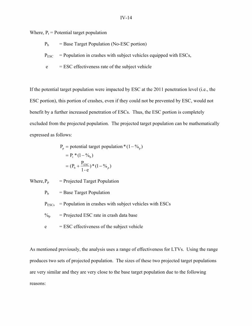
IV-14
Where, Pt = Potential target population
Pb = Base Target Population (No-ESC portion)
PESC = Population in crashes with subject vehicles equipped with ESCs,
e = ESC effectiveness rate of the subject vehicle
If the potential target population were impacted by ESC at the 2011 penetration level (i.e., the
ESC portion), this portion of crashes, even if they could not be prevented by ESC, would not
benefit by a further increased penetration of ESCs. Thus, the ESC portion is completely
excluded from the projected population. The projected target population can be mathematically
expressed as follows:
)%1(*)e-1
P P(
)%1(*P
)%(1*populationtargetpotentialP
ESCb
t
pp
p
b
−+=
−=
−=
Where, Pp = Projected Target Population
Pb = Base Target Population
PESCs = Population in crashes with subject vehicles with ESCs
%p = Projected ESC rate in crash data base
e = ESC effectiveness of the subject vehicle
As mentioned previously, the analysis uses a range of effectiveness for LTVs. Using the range
produces two sets of projected population. The sizes of these two projected target populations
are very similar and they are very close to the base target population due to the following
reasons:
IV-15
1) Less than 0.5 percent of fatalities were in ESC-equipped vehicles, i.e., PESC is relatively
small for fatal crashes,
2) All vehicles in CDS were non-ESC equipped vehicles, i.e., PESC = 0 for MAIS 1-5
injuries in non-fatal crashes, and
3) The majority of the crashes were multi-vehicle crashes against which ESC had a lower
effectiveness than against single-vehicle crashes.
Therefore, for simplicity, this analysis uses the base target population, instead of the potential
target population, for adjustment. The above formula for the projected target population formula
can be simplified as:
)%(1PP pbp −=
The impact of this simplified approach on target population is minimal (less than 0.01 percent of
overall target population and less than 0.5 percent of the fatalities). In addition, using the
simplified formula generally produces a smaller projected population than the original formula
because the base target crash population is smaller than the potential crash population.
The agency estimates that about 65 percent of PCs and 77 percent of LTVs in model year 2011
vehicles will be equipped with ESCs. Thus, %p = 0.65 for PCs and %p = 0.77 for LTVs. The
projected target population for PC is the product of the base target population for PCs (Tables
IV-2 and IV-3) and 0.35 (1-0.65). Similarly, the projected target population for LTVs is the
product of the base target population for LTVs and 0.23. Tables IV-6 and IV-7 list the projected
target crashes and injuries separately for benefit estimates. Tables IV-8 and IV-9 show the

IV-16
projected rollover crashes and associated injuries. Note that the analysis does not adjust the
projected baseline population further to account for the effects of current finalized safety
regulations and those that have not been fully phased in. Current finalized safety regulations or
consumer information that the agency anticipates will have an influence on fatalities from run-
off-the-road crashes include FMVSS No. 208 advanced air bags and rear-center seat lap/shoulder
belt requirements, FMVSS No. 138 Tire Pressure Monitoring Systems, FMVSS No. 139, New
Pneumatic Tires for Light Vehicles, and the Static Stability Ratings for new vehicles. The
agency believes that the impact of these safety standards on the proposed ESC rule is not
significant enough to make specific adjustments. Similarly, the analysis does not adjust the
baseline to account for possible increases in vehicle miles traveled (VMT) that could increase the
target population of fatalities and injuries.
As shown in Tables IV-6 and IV-7, the proposal would impact 430,301 crashes and the
associated 5,725 fatalities and 330,571 MAIS 1-5 injuries. For rollovers, the proposal would
impact 59,503 rollover crashes and the 2,378 fatalities and 69,730 MAIS 1-5 injuries that were
associated with rollovers (Tables IV-8 and IV-9).
Table IV-6
Projected Target Crashes for MY 2011 ESC Level by Crash Type, Crash Severity, Injury Severity, and Vehicle Type
Crash Fatal Crashes Nonfatal Crashes Fatal + Nonfatal Crashes Type PC LTV Total PC LTV Total PC LTV Total Single 2,501 1,524 4,025 146,685 56,069 202,754 149,186 57,593 206,779
Rollover 1,157 1,013 2,170 34,256 23,077 57,333 35,413 24,090 59,503Multi 2,219 1,208 3,427 164,820 55,275 220,095 167,039 56,483 223,522Total 4,720 2,732 7,452 311,505 111,344 422,849 316,225 114,076 430,301Source: 2004 FARS, 2000-2004 CDS; PC: passenger cars, LTV: light trucks/vans Single: single vehicle crashes, Multi: multi-vehicle crashes.

IV-17
Table IV-7 Projected Target Fatalities and Injuries for MY 2011 ESC Level by Crash Type, Crash Severity, Injury Severity, and Vehicle Type
Target Single Vehicle Crashes
Injury Severity Fatal Crashes Nonfatal Crashes Fatal + Nonfatal Crashes
MAIS PC LTV Total PC LTV Total PC LTV Total 1 652 647 1,299 82,419 36,628 119,047 83,071 37,275 120,3462 309 198 507 9,827 5,471 15,298 10,136 5,669 15,8053 344 332 676 5,745 1,931 7,676 6,089 2,263 8,3524 143 99 242 2,316 628 2,944 2,459 727 3,1865 91 33 124 767 144 911 858 177 1,035
Fatalities 2,732 1,656 4,388 0 0 0 2,732 1,656 4,3881-5 1,539 1,309 2,848 101,074 44,802 145,876 102,613 46,111 148,724
Target Multi-Vehicle Crashes
Injury Severity Fatal Crashes Nonfatal Crashes Fatal + Nonfatal Crashes
MAIS PC LTV Total PC LTV Total PC LTV Total 1 2,369 1,166 3,535 121,708 38,249 159,957 124,077 39,415 163,4922 108 46 154 9,270 3,488 12,758 9,378 3,534 12,9123 120 76 196 2,816 1,138 3,954 2,936 1,214 4,1504 50 23 73 451 214 665 501 237 7385 32 8 40 370 145 515 402 153 555
Fatalities 956 381 1,337 0 0 0 956 381 1,3371-5 2,679 1,319 3,998 134,615 43,234 177,849 137,294 44,553 181,847
Total Target Crashes (Single and Multi-Vehicle Crashes Combined)
Injury Severity Fatal Crashes Nonfatal Crashes Fatal + Nonfatal Crashes
MAIS PC LTV Total PC LTV Total PC LTV Total 1 3,021 1,813 4,834 204,127 74,877 279,004 207,148 76,690 283,8382 417 244 661 19,097 8,959 28,056 19,514 9,203 28,7173 464 408 872 8,561 3,069 11,630 9,025 3,477 12,5024 193 122 315 2,767 842 3,609 2,960 964 3,9245 123 41 164 1,137 289 1,426 1,260 330 1,590
Fatalities 3,688 2,037 5,725 0 0 0 3,688 2,037 5,7251-5 4,218 2,628 6,846 235,689 88,036 323,725 239,907 90,664 330,571
Source: 2004 FARS, 2000-2004 CDS PC: passenger cars, LTV: light trucks/vans

IV-18
Table IV-8 Projected Target Single-Vehicle Rollover Crashes for MY 2011 ESC Level
by Rollover Type, Crash Severity, Injury Severity, and Vehicle Type Rollover Fatal Crashes Nonfatal Crashes Fatal + Nonfatal Crashes Type PC LTV Total PC LTV Total PC LTV Total First 362 511 873 27,062 18,231 45,293 27,424 18,742 46,166Sub 795 502 1,297 7,194 4,846 12,040 7,989 5,348 13,337Total 1,157 1,013 2,170 34,256 23,077 57,333 35,413 24,090 59,503Source: 2004 FARS, 2000-2004 CDS PC: passenger cars, LTV: light trucks/vans First: the first-event rollovers, Sub: the subsequent-event rollovers
C. Benefits
Applying the effectiveness rates of ESCs (Table IV-1) to the projected target population (crashes
and injuries) derived in the previous section provides the benefits of the proposal. Table IV-10
lists the crashes that would be prevented by the proposal. Table IV-11-A shows the estimated
overall benefits for the proposal by crash severity (fatal and non-fatal), injury severity level
(MAIS), and vehicle type (PCs and LTVs). As shown in Tables IV-10, the proposal would
prevent 70,344 – 90,153 crashes (1,408 – 2,355 fatal crashes, 68,936 – 91,798 non-fatal crashes).
As a result, the proposal would save 1,536 – 2,211 fatalities and reduce 50,594 – 69,630 MAIS
1-5 injuries (Table IV-11-A).

IV-19
Table IV-9 Projected Target Fatalities and Injuries in
Single-Vehicle Rollover Crashes for MY 2011 ESC Level by Rollover Type, Crash Severity, Injury Severity, and Vehicle Type
First Event Rollovers
Injury Severity Fatal Crashes Nonfatal Crashes Fatal + Nonfatal Crashes
MAIS PC LTV Total PC LTV Total PC LTV Total 1 141 356 497 24,186 20,518 44,704 24,327 20,874 45,2012 63 98 161 2,817 2,810 5,627 2,880 2,908 5,7883 40 148 188 1,206 945 2,151 1,246 1,093 2,3394 25 25 50 549 390 939 574 415 9895 13 18 31 131 121 252 144 139 283
Fatalities 391 577 968 0 0 0 391 577 9681-5 282 645 927 28,889 24,784 53,673 29,171 25,429 54,600
Subsequent Event Rollovers
Injury Severity Fatal Crashes Nonfatal Crashes Fatal + Nonfatal Crashes
MAIS PC LTV Total PC LTV Total PC LTV Total 1 249 203 452 6,429 5,454 11,883 6,678 5,657 12,3352 111 56 167 749 747 1,496 860 803 1,6633 70 84 154 320 251 571 390 335 7254 44 14 58 146 104 250 190 118 3085 22 10 32 35 32 67 57 42 99
Fatalities 867 543 1,410 0 0 0 867 543 1,4101-5 496 367 863 7,679 6,588 14,267 8,175 6,955 15,130
Rollovers Total
Injury Severity Fatal Crashes Nonfatal Crashes Fatal + Nonfatal Crashes
MAIS PC LTV Total PC LTV Total PC LTV Total 1 390 559 949 30,615 25,972 56,587 31,005 26,531 57,5362 174 154 328 3,566 3,557 7,123 3,740 3,711 7,4513 110 232 342 1,526 1,196 2,722 1,636 1,428 3,0644 69 39 108 695 494 1,189 764 533 1,2975 35 28 63 166 153 319 201 181 382
Fatalities 1,258 1,120 2,378 0 0 0 1,258 1,120 2,3781-5 778 1,012 1,790 36,568 31,372 67,940 37,346 32,384 69,730
Source: 2004 FARS, 2000-2004 CDS PC: passenger cars, LTV: light trucks/vans

IV-20
Table IV-10 Estimated Crashes Prevented
by Crash Type, Crash Severity, Injury Severity, and Vehicle Type
Lower Bound* Crash Fatal Crashes Nonfatal Crashes Fatal + Nonfatal Crashes
Type PC LTV Total PC LTV Total PC LTV Total Single 875 533 1,408 49,873 19,063 68,936 50,748 19,596 70,344
Rollover 528 529 1,057 21,660 14,592 36,252 22,188 15,121 37,309Multi 0 0 0 0 0 0 0 0 0Total 875 533 1,408 49,873 19,063 68,936 50,748 19,596 70,344
Higher Bound Crash Fatal Crashes Nonfatal Crashes Fatal + Nonfatal Crashes
Type PC LTV Total PC LTV Total PC LTV Total Single 875 1,021 1,896 49,873 33,081 82,954 50,748 34,102 84,850
Rollover 528 786 1,314 21,660 18,173 39,833 22,188 18,959 41,147Multi 0 459 459 0 8,844 8,844 0 9,303 9,303Total 875 1,480 2,355 49,873 41,925 91,798 50,748 43,405 94,153Source: 2004 FARS, 2000-2004 CDS PC: passenger cars, LTV: light trucks/vans Single: single-vehicle crashes, Multi: multi-vehicle crashes * Assuming ESC effectiveness of LTVs = PCs
Table IV-11-B also shows the overall benefits for the proposal but benefits are tabulated by crash
type (single-vehicle, multi-vehicles crashes) instead of by crash severity as are shown in Table
IV-11-A. As shown in Table IV-11-B, of the 1,536 – 2,211 estimated fatalities saved by the
proposal, 1,536 – 2,066 are from the prevention of single-vehicle crashes and up to 145 are from
the reduction of multi-vehicle crashes. The proposal would eliminate 50,594 to 62,212 MAIS 1-
5 injuries from single-vehicle crashes and up to 7,418 MAIS 1-5 injuries from multi-vehicle
crashes.

IV-21
Table IV-11-A Estimated Benefits of the Proposal
Occupant Fatalities and Injuries Reduced by Crash Severity, Injury Severity, and Vehicle Type
Lower Bound*
Injury Severity Fatal Crashes Nonfatal Crashes Fatal + Nonfatal Crashes
MAIS PC LTV Total PC LTV Total PC LTV Total 1 228 226 454 28,022 12,454 40,476 28,250 12,680 40,9302 108 69 177 3,341 1,860 5,201 3,449 1,929 5,3783 120 116 236 1,953 657 2,610 2,073 773 2,8464 50 35 85 787 214 1,001 837 249 1,0865 32 12 44 261 49 310 293 61 354
Fatalities 956 580 1,536 0 0 0 956 580 1,5361-5 538 458 996 34,364 15,234 49,598 34,902 15,692 50,594
Higher Bound
Injury Severity Fatal Crashes Nonfatal Crashes Fatal + Nonfatal Crashes
MAIS PC LTV Total PC LTV Total PC LTV Total 1 228 876 1,104 28,022 27,731 55,753 28,250 28,607 56,8572 108 150 258 3,341 3,786 7,127 3,449 3,936 7,3853 120 251 371 1,953 1,321 3,274 2,073 1,572 3,6454 50 75 125 787 405 1,192 837 480 1,3175 32 25 57 261 108 369 293 133 426
Fatalities 956 1,255 2,211 0 0 0 956 1,255 2,2111-5 538 1,377 1,915 34,364 33,351 67,715 34,902 34,728 69,630
Source: 2004 FARS, 2000-2004 CDS PC: passenger cars, LTV: light trucks/vans * Assuming ESC effectiveness of LTVs = PCs

IV-22
Table IV-11-B Estimated Benefits of the Proposal
Occupant Fatalities and Injuries Reduced by Crash Type, Injury Severity, and Vehicle Type
Lower Bound*
Injury Severity Single-Vehicle Crashes Multi-Vehicle Crashes
Single- + Multi-Vehicle Crashes
MAIS PC LTV Total PC LTV Total PC LTV Total 1 28,250 12,680 40,930 0 0 0 28,250 12,680 40,9302 3,449 1,929 5,378 0 0 0 3,449 1,929 5,3783 2,073 773 2,846 0 0 0 2,073 773 2,8464 837 249 1,086 0 0 0 837 249 1,0865 293 61 354 0 0 0 293 61 354
Fatalities 956 580 1,536 0 0 0 956 580 1,5361-5 34,902 15,692 50,594 0 0 0 34,902 15,692 50,594
Higher Bound
Injury Severity Single-Vehicle Crashes Multi-Vehicle Crashes
Single- + Multi-Vehicle Crashes
MAIS PC LTV Total PC LTV Total PC LTV Total 1 28,250 22,044 50,294 0 6,563 6,563 28,250 28,607 56,8572 3,449 3,361 6,810 0 575 575 3,449 3,936 7,3853 2,073 1,361 3,434 0 211 211 2,073 1,572 3,6454 837 437 1,274 0 43 43 837 480 1,3175 293 107 400 0 26 26 293 133 426
Fatalities 956 1,110 2,066 0 145 145 956 1,255 2,2111-5 34,902 27,310 62,212 0 7,418 7,418 34,902 34,728 69,630
Source: 2004 FARS, 2000-2004 CDS PC: passenger cars, LTV: light trucks/vans * Assuming ESC effectiveness of LTVs = PCs
Similarly, applying the projected rollover population to its corresponding ESC effectiveness rates
derives the rollover portion of benefits. Tables IV-12 and IV-13 list the rollover crashes that
would be prevented and injuries that would be eliminated separately by this proposal. As shown
in these two tables, the proposal would prevent 37,309 to 41,147 single-vehicle rollover crashes,
including 1,057 – 1,314 fatal crashes and 36,252 – 39,833 non-fatal single-vehicle rollover

IV-23
crashes. In preventing these rollover crashes, the proposal would save 1,161 to 1,445 lives and
eliminate 43,901 – 49,010 MAIS 1-5 injuries.
Note that the range of benefits basically is a reflection of the range of effectiveness rates that
were used for LTVs in the analysis. The lower range of the benefits was derived by assuming
that the ESC effectiveness rates for LTVs are equal to those of the PCs. ESC is designed to
prevent loss-of-control crashes including rollovers. Logically, ESC would be expected to be
more beneficial to LTVs specifically for rollover crashes. However, the agency also
acknowledges that ESC effectiveness estimates for LTVs might have a greater estimating
variation due to the small sample size of LTVs with an ESC and the predominance of SUVs
within the sample. Therefore, the analysis provides the lower bound estimates as a conservative
benefit estimate.
The rollover benefits were derived using different ESC effectiveness estimates based on whether
the rollover is the first or subsequent harmful event. For first-event rollovers, the ESC
effectiveness rates against rollovers were used. For the subsequent event rollovers, the ESC
effectiveness rates against all crashes were used. The differentiation is made to ensure that the
rollover target population is consistent with or comparable to that used in deriving the rollover
effectiveness rates.
Although the effectiveness rates are crash-based (i.e., against crashes), these rates are applied
directly to fatalities and injuries to derive benefits. The effectiveness rates for fatal crashes are
applied to the fatalities and nonfatal injuries associated with the fatal target crashes. Similarly,

IV-24
the effectiveness rates for nonfatal crashes are uniformly applied to those nonfatal injuries
associated with the nonfatal target crashes, regardless of MAIS severity levels. This approach is
appropriate since preventing a crash would prevent all injuries that resulted from that crash.
Table IV-12 Single-Vehicle Rollover Crashes Prevented
by Rollover Type, Crash Severity, Injury Severity, and Vehicle Type
Lower Bound* Rollover Fatal Crashes Nonfatal Crashes Fatal + Nonfatal Crashes Type PC LTV Total PC LTV Total PC LTV Total First 250 353 603 19,214 12,944 32,158 19,464 13,297 32,761Sub 278 176 454 2,446 1,648 4,094 2,724 1,824 4,548Total 528 529 1,057 21,660 14,592 36,252 22,188 15,121 37,309
Higher Bound* Rollover Fatal Crashes Nonfatal Crashes Fatal + Nonfatal Crashes Type PC LTV Total PC LTV Total PC LTV Total First 250 450 700 19,214 15,314 34,528 19,464 15,764 35,228Sub 278 336 614 2,446 2,859 5,305 2,724 3,195 5,919Total 528 786 1,314 21,660 18,173 39,833 22,188 18,959 41,147Source: 2004 FARS, 2000-2004 CDS PC: passenger cars, LTV: light trucks/vans First: the first-event rollovers, Sub: the subsequent-event rollovers * Assuming ESC effectiveness of LTVs = PCs
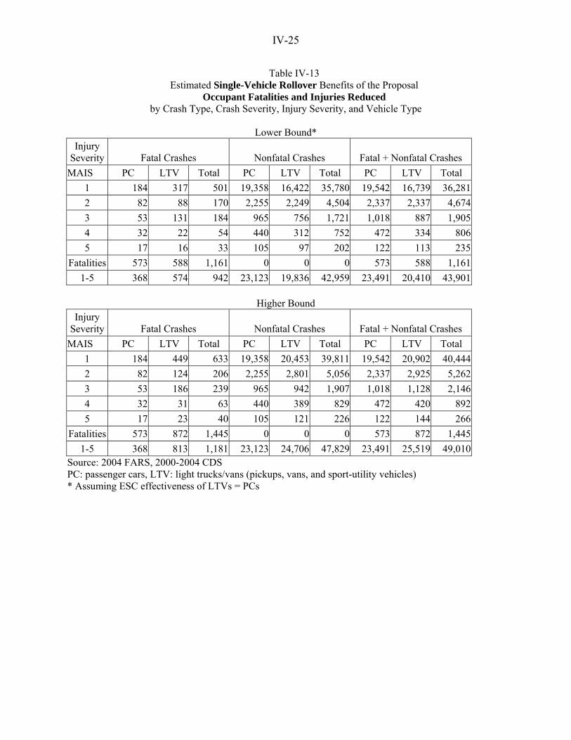
IV-25
Table IV-13 Estimated Single-Vehicle Rollover Benefits of the Proposal
Occupant Fatalities and Injuries Reduced by Crash Type, Crash Severity, Injury Severity, and Vehicle Type
Lower Bound*
Injury Severity Fatal Crashes Nonfatal Crashes Fatal + Nonfatal Crashes
MAIS PC LTV Total PC LTV Total PC LTV Total 1 184 317 501 19,358 16,422 35,780 19,542 16,739 36,2812 82 88 170 2,255 2,249 4,504 2,337 2,337 4,6743 53 131 184 965 756 1,721 1,018 887 1,9054 32 22 54 440 312 752 472 334 8065 17 16 33 105 97 202 122 113 235
Fatalities 573 588 1,161 0 0 0 573 588 1,1611-5 368 574 942 23,123 19,836 42,959 23,491 20,410 43,901
Higher Bound
Injury Severity Fatal Crashes Nonfatal Crashes Fatal + Nonfatal Crashes
MAIS PC LTV Total PC LTV Total PC LTV Total 1 184 449 633 19,358 20,453 39,811 19,542 20,902 40,4442 82 124 206 2,255 2,801 5,056 2,337 2,925 5,2623 53 186 239 965 942 1,907 1,018 1,128 2,1464 32 31 63 440 389 829 472 420 8925 17 23 40 105 121 226 122 144 266
Fatalities 573 872 1,445 0 0 0 573 872 1,4451-5 368 813 1,181 23,123 24,706 47,829 23,491 25,519 49,010
Source: 2004 FARS, 2000-2004 CDS PC: passenger cars, LTV: light trucks/vans (pickups, vans, and sport-utility vehicles) * Assuming ESC effectiveness of LTVs = PCs
IV-26
D. Travel Delay and Property Damage Savings
The non-injury component of benefits includes savings from the elimination of crash-related
travel delays and vehicle property damage. Unit costs for both travel delay and property damage
are represented on a per person basis for all MAIS injury levels, and per vehicle basis for
property damage only (PDO) crashes. These unit costs were developed from a 2002 NHTSA
report27 based on 2000 economics. These costs were adjusted to 2005 dollars using a factor of
1.121 (=112.145/100), which was derived using the implicit price deflator for gross domestic
product28.
The total travel delay and property damage cost for each MAIS and PDO level is equal to the
product of the individual unit cost and the corresponding incidences that would be prevented by
the proposal. The MAIS incidences prevented by the proposal were estimated previously in this
section (Tables IV-11 and IV-13). For PDO crashes, the incidence is the total number of PDO
vehicles for which crashes were eliminated. At this time, there is no available ESC effectiveness
rate against PDO crashes for us to precisely estimate the PDO crashes that would be prevented
by ESC. As an alternative, the number of PDO crashes was prorated from the total non-fatal
crashes prevented according to their proportion reported in the 2000-2004 CDS.
27 Table 2, Blincoe, L., et al, The Economic Impact of Motor Vehicle Crashes 2000, Washington, DC, DOT HS 809 446, May 2002
(in 2000 $) MAIS 1 MAIS 2 MAIS 3 MAIS 4 MAIS 5 Fatality PDO Travel Delay $777 $846 $940 $999 $9,148 $9,148 $803 Property Damage $3,844 $3,954 $6,799 $9,833 $9,446 $10,273 $1,484
28 Published by Bureau of Economic Analysis, U.S. Department of Commerce, December 2005.

IV-27
Based on 2000-2004 CDS, PDO crashes accounted for about 43 percent of the target single-
vehicle crashes and 49 percent of the target multi-vehicle crashes. Therefore, 43 percent of the
single-vehicle crashes and 49 percent of the multi-vehicle crashes prevented by the proposal
would be PDO crashes, i.e.,
PDOs = 0.43 * Cs, and
PDOm = 0.49 * Cm
Where, PDOs = Single vehicle PDO crashes prevented
PDOm = Multi-vehicle PDO crashes prevented
Cs = Single vehicle non-fatal crashes prevented, and
Cm = Multi-vehicle non-fatal crashes prevented.
Cs and Cm can be found in Table IV-10 for all non-fatal crashes and in Table IV-12 for rollovers.
Also, based on 2000-2004 CDS, on average, about 2.2 vehicles were involved in a multi-vehicle
crash. Thus, the total number of vehicles in prevented PDO crashes is equal to the sum of the
total single-vehicle PDO crashes prevented and 2.2 times the multi-vehicle PDO crashes, i.e.,
PDOV = PDOs + 2.2* PDOm
= 0.43 * Cs + 2.2 * 0.49 * Cm
Where, PDOV = Property-damage-only-vehicles in PDO crashes prevented
PDOs = Single-vehicle PDO crashes prevented
PDOm = Multi-vehicle PDO crashes prevented
Cs = Single-vehicle non-fatal crashes prevented, and

IV-28
Cm = Multi-vehicle non-fatal crashes prevented.
Table IV-14 lists the travel delay and property damage unit costs, MAIS and PDO incidences,
and the total costs. All the costs reported in Table IV-14 are in 2005 dollars. As shown in Table
IV-14, the proposal would save undiscounted $396 to $555 million from travel delay and
property damage associated with the crashes that would be prevented by the proposal.

IV-29
Table IV-14 Total Travel Delay and Property Damage Savings
(Undiscounted 2005 $)
Lower Bound* Unit Cost Total Costs Total MAIS
Travel Delay
Property Damage
Incidents Prevented
Travel Delay
Property Damage
Travel Delay +Property Damage
1 $871 $4,309 40,930 $35,650,030 $176,367,370 $212,017,4002 $948 $4,432 5,378 $5,098,344 $23,835,296 $28,933,6403 $1,054 $7,622 2,846 $2,999,684 $21,692,212 $24,691,8964 $1,120 $11,023 1,086 $1,216,320 $11,970,978 $13,187,2985 $10,255 $10,589 354 $3,630,270 $3,748,506 $7,378,776Fatal $10,255 $11,516 1,536 $15,751,680 $17,688,576 $33,440,256PDO** $900 $1,664 29,642 $26,677,800 $49,324,288 $76,002,088Total $91,024,128 $304,627,226 $395,651,354
Higher Bound Unit Cost Total Costs Total MAIS
Travel Delay
Property Damage
Incidents Prevented
Travel Delay
Property Damage
Travel Delay +Property Damage
1 $871 $4,309 56,857 $49,522,447 $244,996,813 $294,519,2602 $948 $4,432 7,385 $7,000,980 $32,730,320 $39,731,3003 $1,054 $7,622 3,645 $3,841,830 $27,782,190 $31,624,0204 $1,120 $11,023 1,317 $1,475,040 $14,517,291 $15,992,3315 $10,255 $10,589 426 $4,368,630 $4,510,914 $8,879,544Fatal $10,255 $11,516 2,211 $22,673,805 $25,461,876 $48,135,681PDO** $900 $1,664 45,205 $40,684,320 $75,220,787 $115,905,107Total $129,567,052 $425,220,191 $554,787,243Source: Table 2 of “The Economic Impact of Motor Vehicle Crashes 2000”, NHTSA Report; 2004 FARS, 2000-2004 CDS PDO: property damage only *Assuming ESC effectiveness of LTVs = PCs; ** PDO vehicles
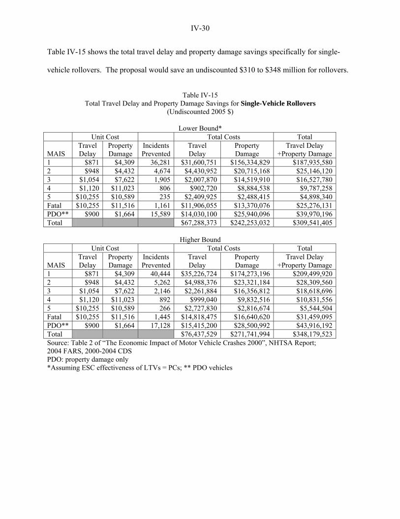
IV-30
Table IV-15 shows the total travel delay and property damage savings specifically for single-
vehicle rollovers. The proposal would save an undiscounted $310 to $348 million for rollovers.
Table IV-15
Total Travel Delay and Property Damage Savings for Single-Vehicle Rollovers (Undiscounted 2005 $)
Lower Bound*
Unit Cost Total Costs Total MAIS
Travel Delay
Property Damage
Incidents Prevented
Travel Delay
Property Damage
Travel Delay +Property Damage
1 $871 $4,309 36,281 $31,600,751 $156,334,829 $187,935,5802 $948 $4,432 4,674 $4,430,952 $20,715,168 $25,146,1203 $1,054 $7,622 1,905 $2,007,870 $14,519,910 $16,527,7804 $1,120 $11,023 806 $902,720 $8,884,538 $9,787,2585 $10,255 $10,589 235 $2,409,925 $2,488,415 $4,898,340Fatal $10,255 $11,516 1,161 $11,906,055 $13,370,076 $25,276,131PDO** $900 $1,664 15,589 $14,030,100 $25,940,096 $39,970,196Total $67,288,373 $242,253,032 $309,541,405
Higher Bound Unit Cost Total Costs Total MAIS
Travel Delay
Property Damage
Incidents Prevented
Travel Delay
Property Damage
Travel Delay +Property Damage
1 $871 $4,309 40,444 $35,226,724 $174,273,196 $209,499,9202 $948 $4,432 5,262 $4,988,376 $23,321,184 $28,309,5603 $1,054 $7,622 2,146 $2,261,884 $16,356,812 $18,618,6964 $1,120 $11,023 892 $999,040 $9,832,516 $10,831,5565 $10,255 $10,589 266 $2,727,830 $2,816,674 $5,544,504Fatal $10,255 $11,516 1,445 $14,818,475 $16,640,620 $31,459,095PDO** $900 $1,664 17,128 $15,415,200 $28,500,992 $43,916,192Total $76,437,529 $271,741,994 $348,179,523Source: Table 2 of “The Economic Impact of Motor Vehicle Crashes 2000”, NHTSA Report; 2004 FARS, 2000-2004 CDS PDO: property damage only *Assuming ESC effectiveness of LTVs = PCs; ** PDO vehicles

IV-31
E. Summary
The following summarizes the estimated benefits of the proposal. These are incremental benefits
over a projected baseline of 71 percent ESC installations in the model year 2011 fleet. These are
the annual benefits that would accrue once all vehicles in the fleet are equipped with ESC.
Overall Benefits of the Proposal
• Prevent 70,344 – 95,153 crashes
▪ 1,408 – 2,355 fatal crashes
▪ 68,936 – 91,798 non-fatal crashes
• Save 1,536 – 2,211 lives
• Eliminate 50,594 – 69,630 MAIS 1-5 injuries
• Save $396 – $555 million (undiscounted) from travel delay and property damage.
Single-Vehicle Rollover Benefits (these are included in the overall benefits above)
• Prevent 37,309 – 41,147 rollover crashes
▪ 1,057 – 1,314 fatal crashes
▪ 36,252 – 39,833 non-fatal crashes
• Save 1,161 – 1,445 lives
• Eliminate 43,901 – 49,010 MAIS 1-5 injuries.
• Save $310 – $348 million (undiscounted) from travel delay and property damage.

IV-32
Note that the estimated injury benefits and property damage and travel delay savings of the
proposal are measured from a baseline of 71 percent ESC installation rate to 100 percent
installation. The benefits of the ESC system itself, which are measured from a baseline of no
ESC installation to 100 percent installation, are summarized below.
ESC Benefits (0% to 100% ESC Installation)
• Prevent 230,198 – 333,710 crashes
▪ 4,819 – 8,935 fatal crashes
▪ 225,379 – 324,775 non-fatal crashes
• Save 5,252 – 10,292 lives
• Eliminate 167,949 – 251,566 MAIS 1-5 injuries
• Save $1,310 – $2,056 million (undiscounted) from travel delay and property damage.
ESC Benefits for Single-Vehicle Rollovers (these are included in the ESC benefits above)
• Prevent 129,130 – 145,822 rollover crashes
▪ 3,803 – 4,923 fatal crashes
▪ 125,327 – 140,899 non-fatal crashes
• Save 4,194 – 5,425 lives
• Eliminate 155,849 – 178,062 MAIS 1-5 injuries.
• Save $1,096 – $1,264 million (undiscounted) from travel delay and property damage.

V-1
CHAPTER V. ESC COSTS
The cost of the proposal comprises technology costs and fuel economy impacts. The
components add weight to vehicles and increase fuel consumption over the lifetime of the
vehicles. The analysis examines the economic and environmental impacts resulting from
increases in fuel consumption. These future impacts are discounted to represent their present
value, using a 3 and 7 percent discount rate.
A. Technology Costs
A contractor did a tear-down study of the incremental technology cost and weight to equip
vehicles with ABS, traction control, ESC, and a telltale light. Ten different make/models were
analyzed. In addition, a cost tear-down study of a 2-channel system was completed in order to
be able to compare it to a 4-channel system in the same make/model. In order to estimate the
cost of the additional components required to equip every vehicle in future model years with an
ESC system, a determination had to be made about the relationship between equipment found in
anti-lock brake systems (ABS), traction control, and ESC systems. Almost every ESC system in
production today has ABS, traction control, and ESC. We assumed that ABS is a prerequisite
for an ESC system. However, we assumed that traction control is a convenience feature and is
not a safety feature required to provide the safety benefits found in ESC systems. Thus, the cost
of traction control is not included in the cost of an ESC system. Thus, if a passenger car or light
truck had none of those systems, it would require the cost of an ABS plus the additional
incremental costs of ESC to comply with an ESC standard. We estimated a future annual

V-2
production volume of 17 million light vehicles, consisting of 9 million light trucks and 8 million
passenger cars.
The Baseline for ESC compliance
The installation rate for ESC in the new model year fleet has been rapidly increasing (from 10
percent in MY 2003, to 16 percent in MY 2004, to 19 percent in MY 2005, to 29 percent in MY
2006)29. In order to get a better estimate of the market penetration of ESC with a requirement,
the agency requested product plan information from seven manufacturers to establish a baseline
voluntary installation rate of ABS and ESC. From these product plans and the current MY 2006
installation rates of ABS and ESC for those manufacturers that were not asked for production
plans, estimates were made of the planned progress of ABS and ESC. MY 2011 was chosen as
the baseline voluntary installation rate for ESC, because it was the last year for which available
data indicated changes in the planned percentages of ESC. MY 2011 serves as the baseline
against which both costs and benefits are measured. In other words, the ESC penetration rate for
each new model of vehicles beyond MY 2011 is assumed to be at the MY 2011 level of 71
percent. Thus, the cost of the standard is the incremental cost of going from the MY 2011
planned installations to 100 percent installation of ABS and ESC. The estimated model year
(MY) planned installation rates are shown in Table V-1. The weighted average reflects the
relative unit sales of passenger cars and light trucks noted above.
29 Based on NHTSA estimates.

V-3
Table V-1 Estimated Installations
(% of the fleet) MY 2007 MY 2008 MY 2009 MY 2010 MY 2011 Neither ABS nor ESC Passenger Cars 22 18 16 14 14 Light Trucks 4 1 2 1 1 Weighted Ave 12 9 8 7 7 ABS alone Passenger Cars 49 46 39 33 21 Light Trucks 42 35 27 25 22 Weighted Ave 45 40 32 29 22 ABS + ESC Passenger Cars 29 36 44 52 65 Light Trucks 54 64 72 74 77 Weighted Ave 42 52 60 64 71
Based on the assumptions above and the data provided in Table V-1, the percent of the MY 2011
fleet that needs these specific technologies in order to reach 100 percent of the fleet with ESC are
shown in the Table V-2.
Table V-2
Percent of Fleet Needing Technology to Achieve 100% ESC None ABS + ESC ESC only Passenger Cars 65 14 21 Light Trucks 77 1 22 Weighted Ave. 71 7 22
The cost estimates developed for this analysis were taken from tear down studies that a
contractor has performed for NHTSA30. The total average incremental cost for ABS and ESC in
these vehicles is estimated at $479 (see Table V-3). This process resulted in estimates of the
consumer cost of ABS at $368, and the incremental cost of ESC at $111, for a total cost of $479.
30 In order to abide with our confidentiality agreements with the manufacturers, the particular make/models will not be disclosed. However, a representative sample of passenger cars, light trucks, vans, and SUVs designed in the U.S., Europe, and Japan were analyzed.

V-4
Table V-3 Incremental Cost and Weights for ABS and ESC
ABS ESC ABS/ESC Combined Costs $368 $111 $479 Weights 4.85 kg. 0.82 kg. 5.67 kg. 10.7 lbs. 1.8 lbs. 12.5 lbs.
We included, in these costs above, the costs and weights for two malfunction warning telltales,
one for ABS and one for ESC systems, at $2.52 per telltale (which includes the malfunction
electronics) and 0.02 pounds. We assumed that existing ABS systems and existing ESC systems
already had a malfunction warning telltale.
The agency and its contractor had a very difficult time determining the parts that made up the
ABS and ESC systems, and separating out the traction control systems. Each manufacturer
provided the contractor with a confidential list of parts that comprised their systems. However,
some manufacturers included everything in the brake system (down to the nuts and bolts),
including parts from the non-ABS hydraulic brake systems, and other manufacturers provided
only the new big ticket items (new sensors and integrated control unit). Each manufacturer has
different names for their systems, uses different parts, and the systems are quickly changing.
The agency took the contractor’s data and tried to make a consistent set of incremental parts for
each manufacturer and averaged these data, as shown in Table V-4. Costs and weights were very
similar between passenger cars and light trucks and are assumed to be the same for all vehicles.
Further complicating the task was changing technology. For example, when we compared some
ABS systems to ABS/ESC systems for the same make/models, we found that the integrated
control unit doing both functions (ABS and ESC) was cheaper than the previous integrated

V-5
control unit handling only ABS. In this case we assumed that the ABS integrated control unit
could have been made less expensive if it were redesigned after the learning curve of technology
costs. In essence, we have a cost estimate from a slice in time (MY 2005).
Table V-4 Average Incremental Costs and Weights
($2005 and lbs.) ABS System Components Incremental Costs Incremental Weight Speed Sensors $60.32 3.22 lbs. Integrated Control Unit/Hydraulic Control
Unit 290.03 6.78
Wires/Telltale/Hardware 17.52 0.70 Subtotal $367.87 10.70 ESC System Components Yaw Rate/Lateral Acceleration Sensors $60.24 0.78 Steering Wheel Sensor 27.55 0.35 Integrated Control Unit (over ABS) 17.58 0.61 Wires/Telltale 5.52 0.08 Subtotal $110.89 1.82 Total $478.76 12.52 lbs. Note: Most ESC systems include a manual Off switch to allow the driver to turn off the ESC in some situations. The contractor’s estimate of the cost of an Off switch averaged $5.93 and weighed 0.08 lbs. An Off switch is not required by the standard and has not been included in the average cost of the rule. Combining the technology needs in Table V-2 with the cost above and the assumed production
volume yields the cost in Table V-5 for the proposed standard.

V-6
Table V-5
Total Costs for the Proposal ($2005)
Passenger Cars None ABS + ESC ESC only % Needing Improvements 65% 14% 21% 8 million sales estimated 1.12 M 1.68 M Costs per vehicle 0 $479 $111 Total costs 0 $536 M $186 M Light Trucks
% Needing Improvements 77% 1% 22% 9 million sales estimated 0.09 M 1.98 M Costs per vehicle 0 $479 $111 Total costs 0 $43 M $ 220 M M: million
Table V-6 Summary of Vehicle Costs
($2005) Average Vehicle Costs Total Costs Passenger Cars $ 90.3 $ 722.5 mill. Light Trucks $ 29.2 $ 262.7 mill. Total $ 58.0 $ 985.2 mill.
In summary, Table V-6 shows that the incremental vehicle costs of providing electronic stability
control and antilock brakes compared to manufacturer’s planned production for MY 2011 fleet
will add $985 million to new light vehicles at a cost averaging $58 per vehicle.
Predicting MY 2011 Installations for Manufacturers without their production plans
Because we have different effectiveness estimates for SUVs versus passenger cars, we broke out
sales estimates into light trucks (pickups, vans, and SUVs) and passenger cars separately. At
this time, our tear-down costs data do not indicate that an ABS or ESC system costs more or less
for a light truck than for a passenger car. We assume they are the same cost. The basis for
predicting MY 2011 installations for manufacturers without their production plans starts with

V-7
data provided in the 2005 Wards Automotive Yearbook. This provides sales of MY 2004
vehicles by make/model, which includes actual rates of installations for standard equipment as
well as factory-installed optional equipment.
From these MY 2004 sales data, and from make/model data provided in “Buying a Safer Car” by
NHTSA for MY 2006, which provides information as to whether such equipment is provided as
standard equipment or optional equipment, an estimate was made regarding predicted
installations of ESC-related equipment for MY 2006. Assumptions made in the analysis
included:
1) That the optional equipment installation rate for a specific make/model in MY 2004
would be the same optional equipment installation rate for that make/model in MY 2006.
(This may well be a conservative assumption, given the level of media coverage of the
benefits of ESC over this time period.)
2) When a MY 2004 make/model was replaced by another make/model by MY 2006, and
both had optional equipment, the optional equipment installation rate would be the same
for the new MY 2006 make/model.
3) When a totally new make/model was introduced by MY 2006 that had optional
equipment, the sales level and the optional equipment installation rate from a similar
vehicle in its class were used to estimate the sales and optional equipment installation
rates for the new make/model.

V-8
Obviously, there are a number of assumptions that must be made in this estimation process for
MY 2006; however, this will give us a closer estimate of current compliance with the ESC
proposal than if we just relied on known MY 2006 installation rates.
B. Fuel Economy Impacts
Going through the same averaging technique we used for costs in Tables V-5 and V-6 and
applying it to weights, we find that the proposal would add an additional 2.13 pounds to an
average PC and 0.52 pounds to a LTV. The added weight would reduce vehicle fuel economy
[measured by miles per gallon (mpg)] and consequently increase vehicle lifetime gasoline
consumption and fuel economy costs. Lifetime fuel economy cost is the cost of additional
gasoline used over the vehicles’ life and is estimated on a per vehicle basis. Applying the
estimated lifetime fuel economy cost per vehicle to every vehicle derives the fuel economy cost
of the proposal. The cost is accrued throughout the vehicles’ life and is discounted to reflect its
present value (2005 $ value). The analysis uses a 3 percent and a 7 percent discount rate. The
discounting procedures for future benefits and costs in regulatory impact analyses are based on
the guidelines published in Appendix V of the "Regulatory Program of the United States
Government", April 1, 1990 - March 31, 1991.
The process of deriving the lifetime fuel economy cost per vehicle can be represented by the
following generic formula:
ii
N
1iij d*(j)G*FCLFEV ∑
=
=
Where, LFEVj = lifetime fuel economy cost per vehicle

V-9
j = added weight
N = vehicle life
FCi = fuel price per gallon
Gi (j) = additional gallons used per vehicle
di = discount factors at 3 or 7 percent
Within this formula, Vehicle life, N, is determined by the age at which 98 percent of the vehicles
originally produced in a model year are no longer registered using Polk data (mainly because
they have been scrapped). Based on this criterion and the vehicle operation data in the National
Vehicle Population Profile (NVPP)31, the agency concludes that PCs are expected to last an
average of about 25 years and LTVs will last 36 years. Therefore, N = 25 for PCs and N=36 for
LTVs.
Fuel prices per gallon, FCi, are adapted from those (in 2003 dollar) published in the 2006 final
rule for corporate average fuel economy (CAFE) standards for light trucks32, but are presented in
2005 dollars. The adjustment factor from 2003 dollars to 2005 dollars is 1.055
(=112.145/106.305), which is the ratio of 2005 and 2003 gross domestic product (GDP) implicit
price deflector33. Fuel taxes of $0.40 are already excluded from these unit prices since taxes are
transfer payments and not a cost to society. These fuel prices are further adjusted to account for
externalities that are associated with U.S. oil consumption but not reflected in the projected
31 Annual census of passenger cars and light trucks vans in operation, as July 1 of each year, compiled by R.L. Polk and Company. 32 Final Regulatory Impact Analysis, Corporate Average Fuel Economy and CAFE Reform for MY 2008-2011 Light Trucks, March 2006 33 Published by U.S. Department of Commerce, Bureau of Economic Analysis, May 25, 2006

V-10
market oil price. Externalities considered here include the monopsony effect of the oil market,
oil price shock impacts, environmental impacts, and other impacts from rebound effects. Costs
for these externalities are also adopted from those published in the 2006 CAFE final rule or
revisions derived after the publication of the final rule. Detailed discussions about these external
economic costs are available in the 2006 CAFE final rule.
Monopsony costs are related to oil supplier-demand and the anticompetitive nature of the global
oil market. For the supplier side, the Organization of Petroleum Exporting Countries (OPEC)
operates as a cartel that restricts oil production to escalate the price of oil far above its marginal
cost. For the demand side, an increase in U.S. petroleum demand also can cause the world oil
price to rise. Since the higher oil price is applied to all oil imported to the U.S., not just limited
to the increased oil use, the actual cost for purchasing the increased amount would exceed their
market payment. In addition, an increase in monopsony payment to foreign oil suppliers
represents a net loss to U.S. oil purchasers and thus has a downward impact on the U.S.
economy. Overall, the monopsony cost is estimated to be $0.142 per gallon34.
The effects of oil price shocks account for the impacts on oil price that were triggered by a
disruption in world oil supplies. The increased oil price reduces the level of U.S. economic
output using its available resource. Also, a sudden disruption requires a rapid adjustment in oil
use and the use of other energy sources and would impose an additional societal cost. The
agency estimates that the cost is about $0.047 per gallon35.
34 Derived from a revised value of $0.135 (2003 $) which is slightly different from $0.122 that was published in the 2006 CAFÉ final rule for light trucks. 35 Adjusted from the $0.045 (2003 $) published in the 2006 CAFE final rule.
V-11
Environmental impacts include the economic and environmental consequence of increased
emissions directly from vehicles (combustion emissions) and emissions associated with fuel’s
exploration, production, processing, and distribution (pre-combustion emissions). These
emissions include carbon dioxide (CO2), carbon monoxide (CO), hydrocarbons (HC), nitrous
oxides nitrogen (NOx) and other airborne particulates. At this moment, the administration has
not taken a position on combustion emission related costs. Also, the cost on a per vehicle basis
is extremely small if based on estimates in the literature. Thus the cost for combustion emissions
is not included in the analysis. As for pre-combustion emission related cost, the agency
estimates its marginal cost is $0.084 per gallon36.
This cost is adjusted downward to account for the emission impact due to the rebound effect.
Rebound effect refers to drivers’ compensatory behavior in response to the rising cost of driving
due to lower fuel economy and increased oil prices. Drivers might reduce their driving by
combining short trips and/or driving less to control the rising cost of driving. Driving less miles
reduces emissions. The estimated emission impact due to the rebound effect is $0.030 per
gallon37. Overall, the economic and environmental impact is estimated to be $0.054 per gallon
(= $0.084 - $0.030)
Furthermore, the compensatory behavior due to the rebound effect, in turn, would generate other
benefits to drivers and society such as reducing traffic congestion, motor vehicle crashes, and
noise. The agency estimates that the combined benefit is about $0.07 per gallon, of which
36 Adjusted from the $0.080 (2003 $) estimated in the 2006 CAFE final rule 37 Adjusted form the $0.028 (2003 $) estimated in the 2006 CAFE final rule
V-12
$0.045 is from the mitigation of traffic congestion, $0.024 from the reduction of crashes, and
$0.001 from the elimination of noise38.
Collectively, the net cost for these externalities is $0.173 per gallon (= $0.042 + 0.047 + $0.054 -
$0.070). Note that the real impact of relatively small increase in vehicle weight on these
externalities is unclear. The inclusion of estimates for these externalities nevertheless provides a
comprehensive assessment of the costs and produces relatively conservative cost-effectiveness
and net benefit estimates.
Additional gasoline use per vehicle, Gi(j), is the difference in fuel consumption (in gallons)
between an average baseline vehicle (i.e., 2011 MY) with added weight and without. Fuel
consumption of a vehicle generally is a function of average vehicle miles traveled, the survival
probability of the vehicle, its fuel economy, and vehicle weight. Specifically, some vehicles are
gradually scrapped or retired each year after their initial production. As vehicles age, the actual
miles traveled tend to decline. Therefore, the average vehicle miles traveled are discounted by
the vehicle’s survival probability to reflect the actual average miles traveled in each year.
Dividing the actually vehicle miles traveled by the fuel economy derives the total gallons of fuel
used. Fuel economy is determined according to procedures established by the Environmental
Protection Agency (EPA). However, the EPA estimates that actual on-road fuel economy is
overall 15 percent less than the EPA’s derived fuel economy. Therefore, the EPA fuel economy
values are discounted by 15 percent.
In essence, Gi(j) can be noted as:
38 Adjusted separately from the $0.043 (traffic congestion), $0.023 (crashes), and $0.001 (noise) estimated in the 2006 CAFÉ final rule

V-13
)MPG
1MPG
1(0.85
Suv*VMTMPG*0.85
Suv*VMTMPG*0.85
Suv*VMT(j)G
w0jw0
ii
w0
ii
jw0
iii
−=
−=
+
+
Where Gi = gasoline use per vehicle
j = added weigh
VMTi = average miles traveled
Suvi = vehicle survival probability
MPGw0 = fuel economy that is associated with vehicle test weight w0
0.85 = EPA factor to reflect the on-road driving fuel economy
The average vehicle miles traveled and survival probability are derived from the agency report
on vehicle survivability and travel mileage schedules39. Fuel economy value for PCs is based on
EPA fuel economy of 29.50 mpg achieved by the 2006 model year PCs40. The 2006 level CAFE
standard of 22.50 mpg is used for the fuel economy value for LTVs. These fuel economy values
are associated with their base vehicle test weights: 3,564 pounds for PCs and 4,750 pounds for
LTVs. In other words, MPGw0 = MPG3,564 = 29.50 mpg for PCs and MPGw0 = MPG4,750 = 22.50
mpg for LTVs.
Furthermore, j represents the added weight, i.e., j = 2.13 pounds for PCs and j = 0.52 pounds for
LTVs. A study by the National Research Council projected a fuel consumption of 3 to 4 percent
39 Lu, S., “Vehicle Survivability and Travel Mileage Schedules”, NHTSA Technical Report, January 2006, DOT 809 952 40 Current the CAFE standard for PCs is 27.5 mpg.

V-14
for each 5 percent weight reduction while maintaining the same acceleration performance41. If
an average is used, the projection means that every 1 percent reduction (or increase) in vehicle
weight would reduce (or increase) fuel consumption by 0.7 percent (=3.5/5). Based in this
projection, the new fuel consumption per mile, i.e.,jw0MPG
1
+
, can be transformed to be a
function of base weight (w0), added weight (j pounds), and base fuel consumption w0MPG
1 :
w0
w0jw0
MPG1
w00.7jw0
MPG1)
w00.7j(1
MPG1
+=
+=+
Substituting this formula to that in Gi(j), Gi(j) can be rewritten as
w0
ii
w0w0
ii
w0jw0
iii
MPG1*
w00.7j*
0.85Suv*VMT
)MPG
1MPG
1w0
0.7jw0(0.85
Suv*VMT
)MPG
1MPG
1(0.85
Suv*VMT(j)G
=
−+
=
−=+
Lastly, the discount factors (di) are factors corresponding to mid-year 3 and 7 discount rates.
The discount factors (di) corresponding a discount rate can be represented as:
0.5ii d)(11d −+
=
Where, d = 3 percent or 7 percent
41 Effectiveness and Impact of Corporate Average Fuel Economy (CAFE) Standards, National Research Council, National Academy Press, Washington DC, 2002

V-15
Substitute the above detailed formulas back into the generic LFEVj, the LFEVj can be refined as:
0.5iii
N
1ii
w0
0.5iw0
ii
N
1ii
ii
N
1iij
d)(11*Suv*VMT*FC
MPG*0.850.7j
d)(11*)
MPG*0.850.7j*Suv*(VMT*FC
d*(j)G*FCLFE
−=
−=
=
+=
+=
=
∑
∑
∑
Tables V-7 to V-10 illustrate the process of deriving LFEVi. These tables list the unit fuel
prices, vehicle miles traveled, survival probability, fuel consumption in gallons, and present
discounted values of fuel costs by vehicle age. Tables V-7 and V-8 show the present discounted
values of fuel costs at 3 percent discount for PCs and LTVs, respectively. In parallel, Tables V-9
and V-10 show the present discounted values of the fuel costs at 7 percent discount.
As shown, the average weight gain of 2.13 pounds for every PC results in an additional 2.6
gallons of fuel being used over its lifetime. The present discounted value of the added fuel cost
over the lifetime of an average passenger car is estimated to be $3.35 at a 3 percent discount rate
and $2.73 at a 7 percent discount rate. The average weight increase for every light truck is
estimated to be 0.52 pounds. The incremental fuel cost for LTVs is negligible.
Applying the per vehicle based fuel costs and fuel consumption to the total vehicles derives the
total fuel impacts of the proposal. Table V-11 summarizes the estimated fuel economy impact of
the proposal. As shown, the proposal would increase the lifetime fuel consumption by a total of
20.8 million gallons. The estimated added fuel consumption cost is estimated to be $26.8 million
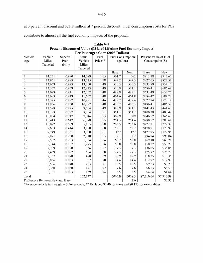
V-16
at 3 percent discount and $21.8 million at 7 percent discount. Fuel consumption costs for PCs
contribute to almost all the fuel economy impacts of the proposal.
Table V-7 Present Discounted Value @3% of Lifetime Fuel Economy Impact
Per Passenger Car* (2005 Dollars) Vehicle Age
Vehicle Miles
Traveled
Survival Prob-ability
Actual Vehicle Miles
Traveled
Fuel Price**
Fuel Consumption (gallon)
Present Value of Fuel Consumption ($)
Base New Base New 1 14,231 0.990 14,089 1.65 561.7 562 $913.18 $913.67 2 13,961 0.983 13,725 1.58 547.2 547.5 $827.05 $827.51 3 13,669 0.973 13,300 1.49 530.3 530.5 $733.89 $734.17 4 13,357 0.959 12,813 1.49 510.9 511.1 $686.41 $686.68 5 13,028 0.941 12,262 1.48 488.9 489.1 $633.49 $633.75 6 12,683 0.919 11,652 1.48 464.6 464.8 $584.47 $584.72 7 12,325 0.892 10,991 1.46 438.2 438.4 $527.94 $528.18 8 11,956 0.860 10,287 1.48 410.2 410.3 $486.41 $486.52 9 11,578 0.825 9,554 1.49 380.9 381.1 $441.43 $441.67 10 11,193 0.787 8,804 1.51 351.1 351.2 $400.38 $400.49 11 10,804 0.717 7,746 1.53 308.9 309 $346.52 $346.63 12 10,413 0.612 6,378 1.55 254.3 254.4 $280.57 $280.68 13 10,022 0.509 5,105 1.58 203.5 203.6 $222.21 $222.32 14 9,633 0.414 3,990 1.60 159.1 159.2 $170.81 $170.92 15 9,249 0.331 3,060 1.61 122 122 $127.95 $127.95 16 8,871 0.260 2,310 1.63 92.1 92.2 $94.94 $95.04 17 8,502 0.203 1,724 1.64 68.7 68.8 $69.18 $69.28 18 8,144 0.157 1,275 1.66 50.8 50.8 $50.27 $50.27 19 7,799 0.120 936 1.67 37.3 37.3 $36.05 $36.05 20 7,469 0.092 684 1.68 27.3 27.3 $25.77 $25.77 21 7,157 0.070 498 1.69 19.9 19.9 $18.35 $18.35 22 6,866 0.053 362 1.70 14.4 14.4 $12.97 $12.97 23 6,596 0.040 263 1.71 10.5 10.5 $9.23 $9.23 24 6,350 0.030 191 1.72 7.6 7.6 $6.53 $6.53 25 6,131 0.023 139 1.74 5.5 5.5 $4.64 $4.64 Total 152,137 6065.9 6068.5 $7,710.64 $7,713.99 Difference Between New and Base 2.6 $3.35 *Average vehicle test weight = 3,564 pounds; ** Excluded $0.40 for taxes and $0.173 for externalities

V-17
Table V-8 Present Discounted Value @3% of Lifetime Fuel Economy Impact
Per Light Truck/Van* (2005 Dollars) Vehicle Age
Vehicle Miles
Traveled
Survival Prob-ability
Actual Vehicle Miles
Traveled
Fuel Price**
Fuel Consumption (gallon)
Present Value of Fuel Consumption ($)
Base New Base New 1 16,085 0.974 15,668 1.65 819.0 819.0 $1,331.49 $1,331.492 15,782 0.960 15,155 1.58 792.2 792.2 $1,197.35 $1,197.353 15,442 0.942 14,547 1.49 760.4 760.4 $1,052.33 $1,052.334 15,069 0.919 13,849 1.49 723.9 723.9 $972.58 $972.585 14,667 0.891 13,072 1.48 683.3 683.3 $885.38 $885.386 14,239 0.859 12,230 1.48 639.3 639.3 $804.24 $804.247 13,790 0.823 11,343 1.46 592.9 592.9 $714.32 $714.328 13,323 0.783 10,428 1.48 545.1 545.1 $646.37 $646.379 12,844 0.740 9,506 1.49 496.9 496.9 $575.87 $575.8710 12,356 0.696 8,595 1.51 449.3 449.3 $512.36 $512.3611 11,863 0.650 7,712 1.53 403.1 403.1 $452.20 $452.2012 11,369 0.604 6,870 1.55 359.1 359.1 $396.19 $396.1913 10,879 0.552 6,002 1.58 313.7 313.7 $342.54 $342.5414 10,396 0.501 5,207 1.60 272.2 272.2 $292.23 $292.2315 9,924 0.452 4,488 1.61 234.6 234.6 $246.04 $246.0416 9,468 0.406 3,846 1.63 201.1 201.1 $207.30 $207.3017 9,032 0.363 3,281 1.64 171.5 171.5 $172.69 $172.6918 8,619 0.324 2,790 1.66 145.8 145.8 $144.27 $144.2719 8,234 0.287 2,366 1.67 123.7 123.7 $119.57 $119.5720 7,881 0.254 2,004 1.68 104.7 104.7 $98.84 $98.8421 7,565 0.224 1,697 1.69 88.7 88.7 $81.79 $81.7922 7,288 0.198 1,440 1.70 75.2 75.2 $67.72 $67.7223 7,055 0.174 1,224 1.71 64.0 64.0 $56.27 $56.2724 6,871 0.152 1,046 1.72 54.7 54.7 $46.98 $46.9825 6,739 0.133 898 1.74 46.9 46.9 $39.55 $39.5526 6663 0.116 776 1.75 40.6 40.6 $33.44 $33.4427 6648 0.102 676 1.77 35.3 35.3 $28.55 $28.5528 6648 0.089 590 1.78 30.8 30.8 $24.32 $24.3229 6648 0.077 514 1.79 26.9 26.9 $20.74 $20.7430 6648 0.067 448 1.81 23.4 23.4 $17.71 $17.7131 6648 0.059 389 1.82 20.4 20.4 $15.07 $15.0732 6648 0.051 339 1.84 17.7 17.7 $12.84 $12.8433 6648 0.044 294 1.85 15.4 15.4 $10.90 $10.9034 6648 0.038 256 1.86 13.4 13.4 $9.26 $9.2635 6648 0.033 222 1.88 11.6 11.6 $7.87 $7.8736 6648 0.029 193 1.89 10.1 10.1 $6.68 $6.68Total 179,957 9,406.9 9,406.9 $11,643.85 $11,643.85Difference Between New and Base 0.00*** $0.00****Average vehicle test weight = 4,750 pounds; ** Excluded $0.40 for taxes and $0.173 for externalities; *** Insignificant difference

V-18
Table V-9 Present Discounted Value @7% of Lifetime Fuel Economy Impact
Per Passenger Car* (2005 Dollars) Vehicle Age
Vehicle Miles
Traveled
Survival Prob-ability
Actual Vehicle Miles
Traveled
Fuel Price**
Fuel Consumption (gallon)
Present Value of Fuel Consumption ($)
Base New Base New 1 14,231 0.990 14,089 1.65 561.7 562 $895.94 $896.42 2 13,961 0.983 13,725 1.58 547.2 547.5 $781.14 $781.57 3 13,669 0.973 13,300 1.49 530.3 530.5 $667.20 $667.45 4 13,357 0.959 12,813 1.49 510.9 511.1 $600.70 $600.93 5 13,028 0.941 12,262 1.48 488.9 489.1 $533.63 $533.85 6 12,683 0.919 11,652 1.48 464.6 464.8 $473.97 $474.17 7 12,325 0.892 10,991 1.46 438.2 438.4 $412.14 $412.33 8 11,956 0.860 10,287 1.48 410.2 410.3 $365.47 $365.56 9 11,578 0.825 9,554 1.49 380.9 381.1 $319.30 $319.47 10 11,193 0.787 8,804 1.51 351.1 351.2 $278.76 $278.84 11 10,804 0.717 7,746 1.53 308.9 309 $232.24 $232.32 12 10,413 0.612 6,378 1.55 254.3 254.4 $181.04 $181.11 13 10,022 0.509 5,105 1.58 203.5 203.6 $138.00 $138.07 14 9,633 0.414 3,990 1.60 159.1 159.2 $102.13 $102.19 15 9,249 0.331 3,060 1.61 122 122 $73.64 $73.64 16 8,871 0.260 2,310 1.63 92.1 92.2 $52.60 $52.66 17 8,502 0.203 1,724 1.64 68.7 68.8 $36.90 $36.95 18 8,144 0.157 1,275 1.66 50.8 50.8 $25.80 $25.80 19 7,799 0.120 936 1.67 37.3 37.3 $17.82 $17.82 20 7,469 0.092 684 1.68 27.3 27.3 $12.26 $12.26 21 7,157 0.070 498 1.69 19.9 19.9 $8.40 $8.40 22 6,866 0.053 362 1.70 14.4 14.4 $5.72 $5.72 23 6,596 0.040 263 1.71 10.5 10.5 $3.92 $3.92 24 6,350 0.030 191 1.72 7.6 7.6 $2.67 $2.67 25 6,131 0.023 139 1.74 5.5 5.5 $1.82 $1.82 Total 152,137 6065.9 6068.5 $6,223.21 $6,225.94 Difference Between New and Base 2.6 $2.73 *Average vehicle test weight = 3,564 pounds; ** Excluded 0.40 taxes and $0.173 for externalities

V-19
Table V-10 Present Discounted Value @7% of Lifetime Fuel Economy Impact
Per Light Truck/Van* (2005 Dollars) Vehicle Age
Vehicle Miles
Traveled
Survival Prob-ability
Actual Vehicle Miles
Traveled
Fuel Price**
Fuel Consumption (gallon)
Present Value of Fuel Consumption ($)
Base New Base New 1 16,085 0.974 15,668 1.65 819.0 819.0 $1,306.35 $1,306.352 15,782 0.960 15,155 1.58 792.2 792.2 $1,130.89 $1,130.893 15,442 0.942 14,547 1.49 760.4 760.4 $956.70 $956.704 15,069 0.919 13,849 1.49 723.9 723.9 $851.13 $851.135 14,667 0.891 13,072 1.48 683.3 683.3 $745.82 $745.826 14,239 0.859 12,230 1.48 639.3 639.3 $652.19 $652.197 13,790 0.823 11,343 1.46 592.9 592.9 $557.64 $557.648 13,323 0.783 10,428 1.48 545.1 545.1 $485.66 $485.669 12,844 0.740 9,506 1.49 496.9 496.9 $416.54 $416.5410 12,356 0.696 8,595 1.51 449.3 449.3 $356.73 $356.7311 11,863 0.650 7,712 1.53 403.1 403.1 $303.07 $303.0712 11,369 0.604 6,870 1.55 359.1 359.1 $255.65 $255.6513 10,879 0.552 6,002 1.58 313.7 313.7 $212.73 $212.7314 10,396 0.501 5,207 1.60 272.2 272.2 $174.73 $174.7315 9,924 0.452 4,488 1.61 234.6 234.6 $141.60 $141.6016 9,468 0.406 3,846 1.63 201.1 201.1 $114.86 $114.8617 9,032 0.363 3,281 1.64 171.5 171.5 $92.11 $92.1118 8,619 0.324 2,790 1.66 145.8 145.8 $74.06 $74.0619 8,234 0.287 2,366 1.67 123.7 123.7 $59.08 $59.0820 7,881 0.254 2,004 1.68 104.7 104.7 $47.02 $47.0221 7,565 0.224 1,697 1.69 88.7 88.7 $37.45 $37.4522 7,288 0.198 1,440 1.70 75.2 75.2 $29.85 $29.8523 7,055 0.174 1,224 1.71 64.0 64.0 $23.88 $23.8824 6,871 0.152 1,046 1.72 54.7 54.7 $19.18 $19.1825 6,739 0.133 898 1.74 46.9 46.9 $15.55 $15.5526 6663 0.116 776 1.75 40.6 40.6 $12.65 $12.6527 6648 0.102 676 1.77 35.3 35.3 $10.40 $10.4028 6648 0.089 590 1.78 30.8 30.8 $8.53 $8.5329 6648 0.077 514 1.79 26.9 26.9 $7.00 $7.0030 6648 0.067 448 1.81 23.4 23.4 $5.76 $5.7631 6648 0.059 389 1.82 20.4 20.4 $4.72 $4.7232 6648 0.051 339 1.84 17.7 17.7 $3.87 $3.8733 6648 0.044 294 1.85 15.4 15.4 $3.16 $3.1634 6648 0.038 256 1.86 13.4 13.4 $2.58 $2.5835 6648 0.033 222 1.88 11.6 11.6 $2.11 $2.1136 6648 0.029 193 1.89 10.1 10.1 $1.73 $1.73Total 179,957 9,406.9 9,406.9 $9,122.98 $9,122.98Difference Between New and Base 0.00*** $0.00****Average vehicle test weight = 4,750 pounds; ** Excluded $0.40 for taxes and $0.173 for externalities; *** Insignificant difference

V-20
Table V-11 Fuel Economy Impacts
by Vehicle Type and Discount Rate (2005 Dollars)
At 3% Discount
Added Weights
Per Vehicle (pounds)
Total Vehicles
Additional Fuel Use
Per Vehicle (gallon)
Fuel Economy
Per Vehicle ($)
Total Additional Fuel Use (gallon)
Present Value of Total Fuel
Economy ($)
PCs 2.13 8,000,000 2.6 $3.35 20,800,000 $26,800,000LTVs 0.52 9,000,000 0.0* $0.00* 0* $0*Total 17,000,000 20,800,000 $26,800,000
At 7% Discount
Added Weights
Per Vehicle (pounds)
Total Vehicles
Additional Fuel Use
Per Vehicle (gallon)
Fuel Economy
Per Vehicle ($)
Total Additional Fuel Use (gallon)
Present Value of Total Fuel
Economy ($)
PCs 2.13 8,000,000 2.6 $2.73 20,800,000 $21,840,000LTVs 0.52 9,000,000 0.0* $0.00* 0* $0*Total 17,000,000 20,800,000 $21,840,000* Extremely small numbers
C. Summary
The following summarizes the estimated cost and fuel economy impacts of the proposal:
• Technology cost: $985 million
▪ Cost per vehicle: $58.0 ($90.3 per PC; $29.2 per LTV)
▪ Number of vehicles: 17 million (8 million PCs and 9 million LTVs)
• Fuel economy impacts
▪ Added weight per vehicle: 2.13 lbs per PC; 0.52 lbs per LTV
▪ Additional fuel consumption per vehicle: 2.6 gallons per PC; < 0.001 gallons per LTV
▪ Total additional fuel consumption: 20.8 million gallons
▪ Fuel cost: $26.8 million at 3 percent; $21.8 million at 7 percent

VI-1
CHAPTER VI. COST-EFFECTIVENESS AND BENEFIT-COST
This chapter provides cost-effectiveness and benefit-cost analysis for the ESC proposal. The
Office of Management and Budget (OMB) requires all agencies to perform both analyses in
support of rules, effective January 1, 2004.42
The cost-effectiveness measures the net cost per equivalent life saved (i.e., per equivalent
fatality), while the benefit-cost measures the net benefit which is the difference between benefits
and net costs in monetary values. The net cost is equal to the technology and fuel costs for the
vehicles minus the savings from the prevention of crash-related travel delays and property
damage. Thus, these two analyses require four primary components: injury benefits, travel
delays and property damage savings, vehicle costs, and fuel costs. Injury benefits are expressed
in fatal equivalents in cost-effectiveness analysis and are further translated into monetary value
in benefit-cost analysis. Fatal equivalents and travel delays and property damage savings
represent the savings throughout the vehicle life and are discounted to reflect their present values
(2005 $ value). The discounting procedures for future benefits and costs in regulatory impact
analyses are based on the guidelines published in Appendix V of the "Regulatory Program of the
United States Government", April 1, 1990 - March 31, 1991. The guidelines state, "An attempt
should be made to quantify all potential real incremental benefits to society in monetary terms to
the maximum extent possible."
There is general agreement within the economic community that the appropriate basis for
determining discount rates is the marginal opportunity costs of lost or displaced funds. When 42 See OMB Circular A-4.

VI-2
these funds involve capital investment, the marginal, real rate of return on capital must be
considered. However, when these funds represent lost consumption, the appropriate measure is
the rate at which society is willing to trade-off future for current consumption. This is referred to
as the "social rate of time preference," and it is generally assumed that the consumption rate of
interest, i.e., the real, after-tax rate of return on widely available savings instruments or
investment opportunities, is the appropriate measure of its value.
Estimates of the social rate of time preference have been made by a number of authors. Robert
Lind43 estimated that the social rate of time preference is between zero and six percent, reflecting
the rates of return on Treasury bills and stock market portfolios. Kolb and Sheraga44 put the rate
at between one and five percent, based on returns to stocks and three-month Treasury bills.
Moore and Viscusi45 calculated a two percent real time rate of time preference for health, which
they characterize as being consistent with financial market rates for the period covered by their
study. Moore and Viscusi's estimate was derived by estimating the implicit discount rate for
deferred health benefits exhibited by workers in their choice of job risk. OMB Circular A-4
recommends agencies use both 3 percent and 7 percent as the “social rate of time preference.”
Safety benefits can occur at any time during the vehicle's lifetime. For this analysis, the agency
assumes that the distribution of weighted yearly vehicle miles traveled is an appropriate proxy
43 Lind, R.C., "A Primer on the Major Issues Relating to the Discount Rate for Evaluating National Energy Options," in Discounting for Time and Risks in Energy Policy, 1982, (Washington, D.C., Resources for the Future, Inc.). 44 J. Kolb and J.D. Sheraga, "A Suggested Approach for Discounting the Benefits and Costs of Environmental Regulations,: unpublished working papers. 45 Moore, M.J. and Viscusi, W.K., "Discounting Environmental Health Risks: New Evidence and Policy Implications," Journal of Environmental Economics and Management, V. 18, No. 2, March 1990, part 2 of 2.

VI-3
measure for the distribution of such crashes over the vehicle's lifetime. This measure takes into
account both vehicle survival rates and changes over time in annual average vehicle miles
traveled (VMT). Multiplying the percent of a vehicle's total lifetime mileage that occurs in each
year by the discount factor and summing these percentages over the years of the vehicle's
operating life, results in a factor of 0.8304 for PCs and 0.8022 for LTVs under a 3 percent
discounted rate. For the 7 percent discounted rate, these factors are 0.6700 and 0.6300 for PCs
and LTVs, respectively. For example, the present value of the benefits for PCs at the 3 percent
discounted rate is equivalent to a 0.8304 of the initial estimates.
A. Fatal Equivalents
To calculate a cost per equivalent fatality, nonfatal injuries must be expressed in terms of
fatalities. This is done by comparing the values of preventing nonfatal injuries to the value of
preventing a fatality. Comprehensive values, which include both economic impacts and loss of
quality (or value) of life considerations, will be used to determine the relative value of nonfatal
injuries to fatalities. Value-of-life measurements inherently include a value for lost quality of
life plus a valuation of lost material consumption that is represented by measuring consumers’
after-tax lost productivity. In addition to these factors, preventing a motor vehicle fatality will
reduce costs for medical care, emergency services, insurance administrative costs, workplace
costs, and legal costs. If the countermeasure is one that also prevents a crash from occurring,
property damage and travel delay would be prevented as well. The sum of both value-of-life and
economic cost impacts is referred to as the comprehensive cost savings from reducing fatalities.
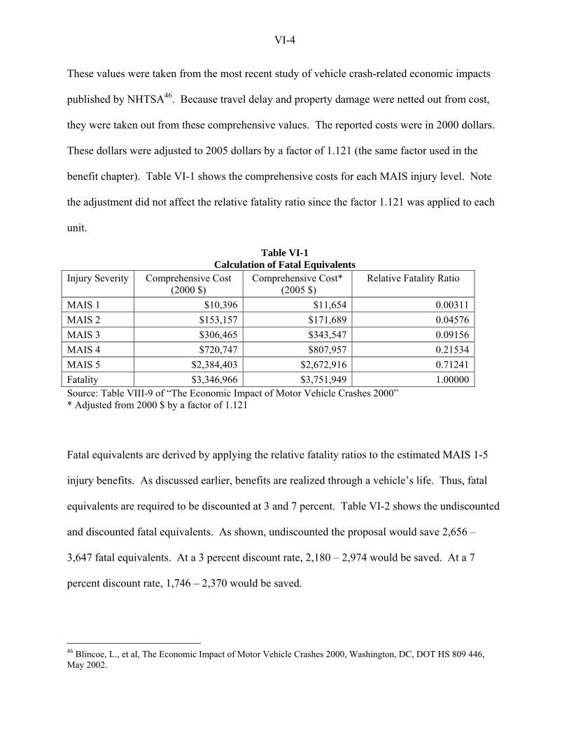
VI-4
These values were taken from the most recent study of vehicle crash-related economic impacts
published by NHTSA46. Because travel delay and property damage were netted out from cost,
they were taken out from these comprehensive values. The reported costs were in 2000 dollars.
These dollars were adjusted to 2005 dollars by a factor of 1.121 (the same factor used in the
benefit chapter). Table VI-1 shows the comprehensive costs for each MAIS injury level. Note
the adjustment did not affect the relative fatality ratio since the factor 1.121 was applied to each
unit.
Table VI-1 Calculation of Fatal Equivalents
Injury Severity Comprehensive Cost (2000 $)
Comprehensive Cost* (2005 $)
Relative Fatality Ratio
MAIS 1 $10,396 $11,654 0.00311 MAIS 2 $153,157 $171,689 0.04576 MAIS 3 $306,465 $343,547 0.09156 MAIS 4 $720,747 $807,957 0.21534 MAIS 5 $2,384,403 $2,672,916 0.71241 Fatality $3,346,966 $3,751,949 1.00000 Source: Table VIII-9 of “The Economic Impact of Motor Vehicle Crashes 2000” * Adjusted from 2000 $ by a factor of 1.121
Fatal equivalents are derived by applying the relative fatality ratios to the estimated MAIS 1-5
injury benefits. As discussed earlier, benefits are realized through a vehicle’s life. Thus, fatal
equivalents are required to be discounted at 3 and 7 percent. Table VI-2 shows the undiscounted
and discounted fatal equivalents. As shown, undiscounted the proposal would save 2,656 –
3,647 fatal equivalents. At a 3 percent discount rate, 2,180 – 2,974 would be saved. At a 7
percent discount rate, 1,746 – 2,370 would be saved.
46 Blincoe, L., et al, The Economic Impact of Motor Vehicle Crashes 2000, Washington, DC, DOT HS 809 446, May 2002.

VI-5
Table VI-2 Fatal Equivalents
Lower Bound* Injury
Severity No Discount At 3 Percent Discount At 7 Percent Discount MAIS PC LTV Total PC LTV Total PC LTV Total
1 88 39 127 73 31 104 59 25 842 158 88 246 131 71 202 106 55 1613 190 71 261 158 57 215 127 45 1724 180 54 234 149 43 192 121 34 1555 209 43 252 174 34 208 140 27 167
Fatalities 956 580 1,536 794 465 1,259 641 366 1,007Total 1,781 875 2,656 1,479 701 2,180 1,194 552 1,746
Higher Bound
Injury Severity No Discount At 3 Percent Discount At 7 Percent Discount
MAIS PC LTV Total PC LTV Total PC LTV Total 1 88 89 177 73 71 144 59 56 1152 158 180 338 131 145 276 106 113 2193 190 144 334 158 115 273 127 91 2184 180 103 283 149 82 231 121 65 1865 209 95 304 174 76 250 140 60 200
Fatalities 956 1,255 2,211 794 1,006 1,800 641 791 1,432Total 1,781 1,866 3,647 1,479 1,495 2,974 1,194 1,176 2,370
PC: passenger cars, LTV: light trucks/vans * Assuming the effectiveness of LTVs = PCs

VI-6
B. Net Costs
The net cost is the difference between the technology and fuel economy costs and the savings
from travel delays and property damage. The total technology cost of the proposal as estimated
in the cost chapter is $985 million. The technology cost represents the investments paid now for
future benefits and thus no discounting is needed.
By contrast, the travel delay and property damage savings and fuel economy costs are realized
through vehicle’s life, thus are required to be discounted at 3 and 7 percent. At a 3 percent
discount, the travel delay and property damage savings range from $325 to $453 million. At a 7
percent discount, the savings are estimated to range $260 to $361 million. The fuel economy
costs are estimated be $26.8 and $21.8 million at 3 percent and 7 percent discount, respectively.
Subtracting the travel delay and property damage savings from vehicle technology and fuel
economy costs derives the net cost. The net cost is estimated to range from $559 to $687 million
at a 3 percent discount and $646 to $747 million at a 7 percent discount. Table VI-3 lists the
vehicle technology cost, travel delays and property damage savings, fuel economy costs, and the
net costs by discount rate,
Table VI-3 Net Costs by Discount Rate
(2005 $) At 3% Discount At 7% Discount
Vehicle Cost (a)* $985 M $985 MSavings from Property Damage and Travel Delay (b) $325 - $453 M $260 - $361 M
Fuel Economy Impact (c) $26.8 M $21.8 MNet Costs (= a – b + c) $559 -$687 M $646 - $747 M* Vehicle costs are not discounted, since they occur when the vehicle is purchased, whereas benefits occur over the vehicle’s lifetime and are discounted back to the time of purchase. M: million
VI-7
C. Cost-Effectiveness
The cost-effectiveness analysis derives the cost per equivalent life saved (i.e., cost per equivalent
fatality), which is equal to the net cost divided by the fatal equivalents. As show in Table VI-3,
the net cost is estimated to be $559 to $687 million at a 3 percent discount and $646 to $747
million at a 7 percent discount. Dividing these costs to the responding fatal equivalents derives
the net cost per equivalent fatality. The net cost per equivalent fatality would range from $0.19
to $0.32 million at a 3 percent discount, and $0.27 - $0.43 million at a 7 percent discount.
D. Net Benefits
Benefit-cost analysis derives the net benefits which is the difference between the injury benefits
and the net costs of the proposal in monetary values. Thus, benefit-cost analysis differs from
cost-effectiveness analysis in that it requires that benefits be assigned a monetary value, and that
this value be compared to the monetary value of costs to derive a net benefit. As shown in Table
VI-5, a fatality was valued at $3,751,949 in 2005 dollars. Multiplying this unit cost by the total
fatal equivalents (Table VI-2) derives the monetary values for the injury benefits of the proposal.
As results, the injury benefit is estimated to range from $8.2 to $11.2 billion at a 3 percent
discount and $6.6 to $8.9 billion at a 7 percent discount.
After translating the injury benefits into monetary values and deriving the net cost (Table VI-3),
the net benefits simply is the difference of these values. Table IV-4 shows the discounted injury

VI-8
benefits, net costs, and net benefits. As shown, the net benefits would range from $7.5 to $10.6
billion at a 3 percent discount rate and $5.8 to $8.2 billion at a 7 percent discount rate.
E. Summary
In summary, this proposal would save 1,536 to 2,211 lives and eliminate 50,594 to 69,630 MAIS
1-5 injuries. These fatalities and injuries translate to a total of 2,656 to 3,467 undiscounted fatal
equivalents, 2,180 to 2,974 fatal equivalent at a 3 percent discount, and 1,746 to 2,730 fatal
equivalents at a 7 percent discount rate.
The cost per equivalent life saved would range from $0.19 to $0.32 million at a 3 percent
discount and $0.27 to $0.43 million at a 7 percent discount. The net benefit is estimated to range
from $7.5 to $10.6 billion at a 3 percent discount and $5.8 to $8.2 billion at a 7 percent discount.
Table VI-4 summarizes the fatal equivalents, cost-effectiveness, and net benefit statistics. The
low and high figures correspond to the low and high bounds of injury benefits. Based on these
cost/benefit statistics, the proposal is extremely cost-effective. The cost per life saved, at both 3
and 7 discount, is estimated to be less than a $450,000. At both 3 and 7 discount, the proposal
would generate over $5.5 billion in net benefits.
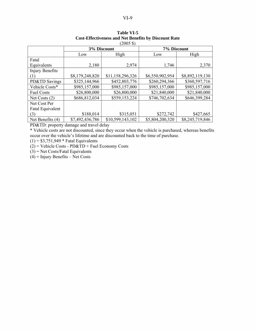
VI-9
Table VI-5 Cost-Effectiveness and Net Benefits by Discount Rate
(2005 $) 3% Discount 7% Discount Low High Low High Fatal Equivalents 2,180 2,974 1,746 2,370Injury Benefits (1) $8,179,248,820 $11,158,296,326 $6,550,902,954 $8,892,119,130PD&TD Savings $325,144,966 $452,803,776 $260,294,366 $360,597,716Vehicle Costs* $985,157,000 $985,157,000 $985,157,000 $985,157,000Fuel Costs $26,800,000 $26,800,000 $21,840,000 $21,840,000Net Costs (2) $686,812,034 $559,153,224 $746,702,634 $646,399,284Net Cost Per Fatal Equivalent (3) $188,014 $315,051 $272,742 $427,665Net Benefits (4) $7,492,436,786 $10,599,143,102 $5,804,200,320 $8,245,719,846PD&TD: property damage and travel delay * Vehicle costs are not discounted, since they occur when the vehicle is purchased, whereas benefits occur over the vehicle’s lifetime and are discounted back to the time of purchase. (1) = $3,751,949 * Fatal Equivalents (2) = Vehicle Costs - PD&TD + Fuel Economy Costs (3) = Net Costs/Fatal Equivalents (4) = Injury Benefits – Net Costs
VII-1
CHAPTER VII. ALTERNATIVES
The agency considered two alternatives to the proposal. The first was to limit the ESC
standard’s applicability only to LTVs. The second alternative was to not require a 4-wheel
system, which would allow a 2-wheel system to be used by manufacturers.
Alternative 1, Limiting the Applicability to LTVs
The agency considered this alternative for two reasons: (a) the ESC effectiveness rates for LTVs
against single-vehicle crashes were almost twice as high of the effectiveness rates for passenger
cars (PCs), and (b) LTVs generally had a higher propensity for rollover than PCs. The
alternative would address the core rollover issue and target the high-risk rollover vehicle
population. However, after examining the safety impact and the cost-effectiveness of the
alternative, the agency determined that an excellent opportunity to reduce passenger car crashes
would be lost if PCs were excluded from the proposal.
We examined this alternative by looking at the impacts of requiring ESC for passenger cars.
Requiring ESC for passenger cars would save 956 lives and reduce 34,902 non-fatal injuries.
Following this analysis through the cost-effectiveness equations, the cost-effectiveness analysis
shows that ESC is highly cost-effective for PCs alone. For PCs, the cost per equivalent life
saved is estimated to be $0.35 million at a 3 percent discount rate and $0.47 million at a 7
percent discount rate. The net benefit would be $4.8 billion at a 3 percent discount rate and $3.8
billion at a 7 percent discount rate.

VII-2
Given the fact that ESC is highly cost-effective and that extending the ESC applicability to PCs
would save a large number of additional lives (956) and reduce a large number of additional
injuries (34,902), the agency is not proposing this alternative.
Alternative 2, Two-Wheel System
2-Wheel vs. 4-Wheel systems
General Motors utilized a 2-wheel ESC system in most of its ESC-equipped passenger cars
through MY 2005, but has changed over to a 4-wheel system in MY 2006. All other
manufacturers have utilized a 4-wheel ESC system in their vehicles. The agency’s tests on the
track indicate that the 4-wheel systems tend to exhibit more oversteer mitigation capability than
GM’s earlier 2-wheel systems.
Statistical analyses comparing 2-wheel to 4-wheel ESC systems were shown in Chapter III. The
effectiveness estimates show a potentially enhanced benefit of 4-wheel ESC systems over 2-
wheel ESC systems in reducing single-vehicle run-off-road crashes (significant at the 0.05 level),
although the benefit could not be shown in a separate analysis of fatal-only crashes, likely due to
the small sample size.
The agency’s contractor has performed a teardown study to determine the difference in costs
between a 2-wheel and 4-wheel system, and the 2-wheel system is about $10.00 less expensive.
However, it is not intuitively obvious that the difference need be this much, and with a sample of
one, it is possible that other changes in design for other reasons may be affecting this estimate.

VII-3
Since the industry has moved away from the 2-wheel system on its own, and it appears that the
difference in cost of $10 or less will be insignificant as compared to the additional benefits
achieved with 4-wheel ESC, we are not providing a full analysis of this alternative at this time.
Based on the available information, the agency is proposing the 4-wheel system. The agency’s
decision is based on our and the industry’s engineering judgment that the 4-wheel system is more
effective, the effectiveness study showing that the 4-wheel system is more effective than the 2-
wheel system in reducing crashes, the industry trend towards installing the 4-wheel system in
their vehicles, and the estimated cost differences between 2-wheel and 4-wheel ESC systems.
VIII-1
VIII. PROBABILISTIC UNCERTAINTY ANALYSIS
This chapter identifies and quantifies the major uncertainties in the cost-effectiveness and net
benefit (benefit-cost) analyses and examines the impacts of these uncertainties. Throughout the
course of these analyses, many assumptions were made, diverse data sources were used, and
different statistical processes were applied. The variability of these assumptions, data sources,
and statistical processes potentially would influence the estimated regulatory outcomes. Thus,
all these assumptions, data sources, and derived statistics can be considered as uncertainty
factors for the regulatory analysis. The purpose of this uncertainty analysis is to identify the
uncertainty factors with appreciable variability, quantify these uncertainty factors by appropriate
probability distributions, and induce the probabilistic outcomes accompanied with degrees of
probability or plausibility. This facilitates a more informed decision-making process.
A Monte Carlo statistical simulation technique47 is used to accomplish the process. The
technique is to first randomly select values for those uncertainty factors from their pre-
established probability distributions. The selected values then are fed back to the cost-
effectiveness and net benefit analysis process to generate all possible outcomes. The process is
run repeatedly. Each complete run is a trial. Crystal Ball®48, a spreadsheet-based risk analysis
and forecasting software package which includes the Monte Carlo simulation technique tool, was
chosen to automate the process. In addition to simulation results, Crystal Ball® also provides
47 a: Robert, C.P. & Casella, G., Monte Carlo Statistical Methods, Springer-Verlag New York, Inc., 1999
b: Liu, J.S., Monte Carlo Strategies in Scientific Computing, Springer-Verlag New York, Inc., 2001 (Or any statistics books describing the Monte Carlo simulation theory are good references for understanding the technique.)
48 A registered trademark of Decisioneering, Inc.

VIII-2
the degree of certainty (or confidence, or credibility) that is associated with the simulated results.
The degree of certainty provides the decision-makers an additional piece of important
information to evaluate the outcomes.
The analysis starts by establishing mathematical models that imitate the actual processes in
deriving cost-effectiveness and net benefits, as shown in previous chapters. The formulation of
the models also allows analysts to conveniently identify and categorize uncertainty factors. In
the mathematical model, each variable (e.g., cost of technology) represents an uncertainty factor
that would potentially alter the model outcomes if its value were changed. Variations of these
uncertainty factors are described by appropriate probability distribution functions. These
probability distributions are established based on available data. If data are not sufficient or not
available, professional judgments are used to estimate the distribution of these uncertainty
factors.
After defining and quantifying the uncertainty factors, the next step is to simulate the model to
obtain probabilistic results rather than single-value estimates. The simulation repeats the trials
until certain pre-defined criteria49 are met and a probability distribution of results is generated.
49 The pre-defined criteria may change with each uncertainty analysis. In this case, we require a 99 percent precision in mean for each simulated outcome such as total costs, cost-effectiveness, and net benefits as described later.
VIII-3
A. Simulation Models
Mathematical models were built to imitate the process used in deriving cost-effectiveness and net
benefits as developed in previous chapters. Both the cost-effectiveness and net benefit models
comprise four principal components: injury benefits, travel delay and property damage savings,
vehicle technology costs, and fuel economy cost. These four components are discussed
separately in the following sections.
A.1 Benefit Component
In the cost-effectiveness model, injury benefits are represented by fatal equivalents (FEs)
reduced. In the net benefit model, injury benefits are represented by their monetary value, which
is the product of comprehensive cost per life saved and FEs. Since benefits (fatalities and
injuries reduced) were already expressed as FEs in the cost-effectiveness model, the net benefit
model is just one step removed from the cost-effectiveness model. Therefore, the FE model is
discussed first.
The overall FEs are derived from eight mutually exclusive target crash populations that were
categorized by three attributes: crash type (single vehicle crashes, multi-vehicle crashes), crash
severity (non-fatal, fatal), and vehicle type (PC, LTV). For example, one crash type is single-
vehicle, non-fatal PC crashes. Each of these FEs is derived through the following steps:
(1) estimating initial crash benefits (i.e., crashes avoided by ESC)

VIII-4
(2) deriving corresponding injury benefits (i.e., fatalities and MAIS 1-5 injuries eliminated
by ESC),
(3) deriving FEs by multiplying the injury benefits by their corresponding injury-to-fatality
ratios, and
(4) discounting FEs to derive the discounted net benefits over the vehicle’s life.
Therefore, FEs can be represented by the following mathematical formula:
d*)r*p*e*TC(FEs8
1i
6
1jjijii∑∑
= =
=
Where TCi= target crash population
ei = effectiveness of ESC against the ith target crash population
pij = MAIS j injuries per crash for ith target crash population, with j=6 as fatalities
rj = MAIS j injury-to-fatality ratio with j=6 as fatalities.
d = cumulative lifetime discount factor, either at 3 or 7 percent discount rate.
Of the notation and processes, the product of the ith target crash (TCi) and the corresponding ESC
effectiveness rate (ei ) represents the crash benefits from the ith target crash population (=
TCi*ei). The product of the resulted crash benefits and severity j injuries per crash (pij)
represents the injury benefits for severity j injuries (= TCi*ei * pij). Multiplying the injury
severity j benefits by its corresponding injury-to-fatality ratio (= TCi*ei * pij *rj) derives its FEs.
Summed over the injury severity (indexed by j) and target crash population (indexed by i) thus
will derive the total FEs. Finally, the total FEs are discounted either at a 3 or 7 percent rate to
reflect the net benefits of the proposal over a vehicle’s life.

VIII-5
As described, FEs is the basic benefit measurement for estimating cost-effectiveness. For net
benefits, FEs is translated into monetary value. If M denotes the cost per fatality, benefit in the
net benefit calculation is equal to M*FEs. Hence, the benefit component for net benefits is:
d*)r*p*e*TC(*MFEs*M8
1i
6
1jjijii∑∑
= =
=
A.2 Traveling Delay and Property Damage Savings
Travel delay and property damage savings (S) can be represented by the following mathematical
formula:
d*)o*u(S7
1jjj∑
=
=
Where,
uj= unit cost for travel delays and property damage by MAIS injury severity levels and
PDOV, with j=6 as fatalities and j=7 as PDOV
oj = incidents by MAIS severity levels and PDOV
d = cumulative lifetime discount factors, either at 3 or 7 percent discount rate.
Incidents, oi, represent injuries, fatalities, and PDOV that would be prevented by ESC. As
described in the FE model and the benefit chapter, these incidents can be derived from target
crashes avoided. Injuries and fatalities were derived by multiplying injuries per crash (noted as
pij in the FE model) by the number of corresponding target crashes avoided (i.e., TCi*ei ).

VIII-6
Similarly, PDOV is the product of PDOV per crash and the number of corresponding target
crashes avoided. Thus, the S model can be further expanded as:
d*)p*e*TC*u(S8
1i
7
1jijiii∑∑
= =
=
Note that pij represents severity j injuries per crash with j ≤ 6 and PDOV per crash for j = 7.
A.3 Vehicle Technology Cost Component
Vehicle technology cost (VC) is the product of technology cost per vehicle and the number of
vehicles. The technology cost per vehicle varies depending upon whether vehicles are required
to install ABS and ESC or just ESC. As discussed in the cost chapter, the manufacturers’
product plan for PCs is different from that of LTVs. Thus, the vehicle technology cost per
vehicle differs between these two groups of vehicles. The vehicle technology cost of the
proposal can be represented as:
∑=
=2
1iii v*cVC
Where, VC = vehicle technology cost
ci = technology cost per vehicle, i=1 for PCs and i=2 for LTVs
vi = vehicle population corresponding to ci.

VIII-7
A.4 Fuel Economy Cost Component
The total lifetime fuel economic cost (LFE) model of the proposal can be represented by the
following simplified formula:
∑=
=2
1iii v*LFEVLFE
Where, LFEVi = present value of lifetime fuel economy per vehicle at 3 or 7 percent discount,
with i=1 for PCs and i=2 for LTVs
vi = number of vehicles
A.5 Cost-Effectiveness Model and Net Benefit Model
After the fatal equivalent, travel delay and property damage savings, vehicle technology cost,
and fuel economy cost models were established, the cost-effectiveness model (CE) is calculated
as the ratio of net costs (NC) to fatal equivalents (FEs) where net cost is equal to vehicle
technology cost (VC) plus lifetime fuel economy cost (LFE) minus savings from travel delay and
property damage (S). The cost-effectiveness model (CE) has the format:
∑∑
∑∑∑
= =
= ==
−+=
−+=
=
8
1i
6
1jiijii
8
1i
7
1jijiij
2
1iiii
d*)r*p*e*TC(
d*)p*e*TC*u(v*)LFEV(c
FEsSLFEVC
FEsNCCE

VIII-8
The net benefit is the difference between benefits expressed in monetary value and the net cost.
The net benefit model (NB) has the format:
∑∑∑∑∑== == =
+−+=
−+=−=
2
1iiii
8
1i
7
1jijiij
8
1i
6
1jjijii v*)LFEV(cd*)p*e*TC*u(d*)r*p*e*TC(*M
LFE - VCSFEs*MNCFEs*MNB
Where, M is the cost per fatality.
B. Uncertainty Factors
Each parameter in the above cost-effectiveness and net benefit model represents a major
category of uncertainty factors. Therefore, there are nine categories of uncertainty factors that
would impact the cost-effectiveness: (1) target crash population, TCi, (2) effectiveness, ei, (3)
injuries or PDOV per crash, pij, (4) injury-to-fatality ratios, ri, (5) cumulative lifetime discount
factors, d, (6) unit costs for travel delays and property damage, ui, (7) cost per vehicle, ci, (8)
lifetime fuel economic cost per vehicle, LEFVi, and (9) number of vehicles, vi. The net benefit
model has one additional uncertainty factor (10) cost per life, M, in addition to those eight for the
cost-effectiveness model.
Target crash population, TCi, is important to benefit estimates because it defines the crash
population of risk without the rule. The major uncertainties in this factor arise from sources such
as demographic projections, driver/occupant behavioral changes (e.g., shifts in safety belt use),
increased roadway travel, new Government safety regulations, and survey errors in NHTSA’s
data sampling system NASS-CDS.

VIII-9
The impact of demographic and driver/occupant behavior changes, roadway traveling, and new
automobile safety regulations are reflected in the crash database. Thus, the analysis examined
the historic FARS and CDS to determine whether variations resulting from these uncertainty
sources would warrant further adjustment to the future target crash population. Based on 1995 to
2004 FARS, there is no definitive trend in total incidents for this period of time. The changes in
fatal crashes and fatalities among years were small with a variation within +2.0 percent. Data
from 1995-2004 CDS yields a similar result for non-fatal crashes and MAIS 1-5 injuries.
Therefore, the analysis does not further adjust the target crash population to account for
variations associated with these uncertainty sources. Only survey errors from CDS are
considered here. In other words, fatal crashes (and fatalities) are treated as constants. In
contrast, non-fatal crashes (and MAIS 1-5 injuries) have variations and are treated as normally
distributed. Survey errors for CDS are used as the proxy for standard deviation to establish the
normal distribution for non-fatal target population. Standard errors (SE) form CDS were derived
using SUDAAN50.
Effectiveness of countermeasures, ei, is by far the parameter with the greatest uncertainty. The
sources of its uncertainty include the estimation errors inherent in the statistical processes, the
variability of the data systems (i.e., FARS and State Data Systems), and the representativeness of
the data samples (i.e., SUVs representing LTVs). Two types of probability distributions are used
to describe the variations for these effectiveness rates. For PCs, the ESC effectiveness rates are
treated as normally distributed. Their confidence bounds are used as the proxy for standard
deviations for establishing the normal distribution. For LTVs, the ESC effectiveness rates are 50 Software for the Statistical Analysis of Correlated Data, Release 9.0.1, Research Triangle Institute, NC

VIII-10
treated as minimum extreme value distribution (also known as the Gumbel distribution) with its
initial confidence bounds as the proxy for standard deviations. As described in the benefit
chapter, the lower range of the ESC effectiveness for LTVs is bounded by the mean effectiveness
for PCs. Due to this constraint, distributions for ESC in LTVs tend to be negatively skewed if its
mean is preserved, i.e., a distribution with a longer tail towards the lower end of values.
Therefore, a minimum extreme value distribution, a skewed distribution bounded by its
minimum and maximum values, is more appropriate to describe the effectiveness for LTVs than
a normal distribution with a similar mean and standard deviation.
MAIS injuries and PDOV per crash, pij, is obviously important to benefit estimates because it is
used to derive the at-risk injury and PDOV population. The major uncertainties for these factors
arise from sources similar to those for crash population. Similarly, only survey errors from CDS
are considered. However, variations for these factors are highly correlated with those of crash
population and are already described by the probability distributions for crash population (TCi).
Furthermore, based on 1995-2004 FARS and CDS, no specific trend existed in number of
occupants per vehicle and in injury profile (i.e., the make-up of all injury severity levels or the
relative proportion of each injury severity) would influence these factors. Based on these
historic data, the fatalities per crash fluctuated between 1.12 and 1.13. Injuries per crash range
from 0.8 to 1.0 over the years with the majority at a constant level of 0.9. These statistics
indicate that changes in number of occupants per vehicle and injury profile are insignificant and
are not considered here. Similarly, the number of PDOV per crash stays almost constant over the
same period. Therefore, these factors are not described by separate distributions and are treated
as constants.

VIII-11
Injury-to-fatality ratios, ri, reflect the relative economic impact of injuries compared to fatalities
based on their estimated comprehensive unit costs. They were derived based on the most current
2002 crash cost assessment51. The crash cost assessment itself is a complex analysis with an
associated degree of uncertainty. At this time, these uncertainties are also unknowns. Thus, the
variation in these ratios is unknown and the analysis treats these ratios as constants.
Cumulative lifetime discount factors, d, represent the present discount factor over the vehicle’s
life. These factors are derived based on the agency study on vehicle miles traveled and vehicle
survivability52. Variation of these factors comes from vehicle mileage surveys, national vehicle
population, and statistical process. These uncertainties cannot be quantified at this time. Thus,
the analysis treats these factors as constants.
Technology cost per vehicle, ci, is a concern. The sources of cost uncertainties arise from, but
are not limited to, maturity of the technologies/countermeasures and potential fluctuation in labor
and material costs (e.g., due to economics from production volume). According to professional
judgments of NHTSA cost analysts and contractors, the cost (for MY 2005 designs) will fall
within 10 percent of the point estimate shown in the cost chapter. Any cost in this range would
have equal chance to be the true cost. Thus, the analysis treats the cost is uniformly distributed.
Lifetime fuel economy cost per vehicle, LFEVi, is expected to have certain level of variability.
Its variation comes from many sources: fuel price projections, vehicle lifespan, annual vehicle
51 The Economic Impact of Motor Vehicle Crashes 2000, NHTSA DOT HS 809 446, May 2002 52 Vehicle Survivability and Travel Mileage Schedules, Technical Report, DOT HS 809 952, January 2006 (Docket No. 22223-2218)

VIII-12
miles traveled, survival probability, and discount rate. Variations for these sources are unknown
at this time. Therefore, the uncertainty for LFEVi is also unknown. However, due to the
importance of the fuel economy impacts, the analysis treats LFEVi as normally distributed to
monitor the potential fuel economic impact of the proposal. The standard deviation is set to be
10 percent of the mean cost.
Number of vehicles, vi, is an uncertainty factor that would impact the cost estimates. Although,
vehicle sales have gradually increased over time, they are subject to annual variation due to
changes in economic conditions, which are difficult to predict. Thus, the number of vehicles (vi)
is treated as a constant.
The nine factors discussed above would impact the cost-effectiveness outcome. The net benefit
model has an additional factor, cost of statistical life, M.
Cost per statistical life, M, is an uncertainty factor for net benefits. The cost is based on recent
meta-analyses of the wage-risk value of statistical life (VSL). These meta-analyses deployed
different statistical methodologies and assumptions. But, generally, these studies show that an
individual’s willingness-to-pay (WTP) for reduction in premature fatalities is from $1 million to
$10 million53. Thus, the agency uses this as the range for M and assumes the value of M is
normally distributed.
53 a: Mrozek, J.R. and L.O. Taylor, What determines the value of a life? A Meta Analysis, Journal of Policy Analysis and Management 21 (2), pp. 253-270. b: Viscusi , W. K., The Value of Life: Estimates with Risks by Occupation and Industry, Economic Inquiry, Oxford University Press, vol. 42(1), pages 29-48, January, 2004.

VIII-13
C. Quantifying the Uncertainty Factors
This section establishes the appropriate probability distributions for the uncertainty factors that
come with appreciable variations (i.e., target crash population and effectiveness) and quantifies
the constant values for other factors.
Target Crashes, TCi. As discussed in the previous section, the size of the target fatal crashes is
treated as constant and the size of the target non-fatal crashes is treated as normally distributed.
Means and standard deviations are provided here to establish the normal distributions. The
standard deviation for the target non-fatal crashes is set to be equivalent to the survey errors of
the CDS. PROC CROSSTAB54 procedure in SUDAAN is used to derive the survey errors for
the base target crash population. Then, standard errors for the projected crash population (e.g.,
2011 based adjustment) are prorated from the overall standard errors based on its size relative to
the base population. In other words, if SEBC represents the standard errors for the base crash
population BC, the standard errors for the individual projected target population (i.e., 2011
adjusted crash population) TCj,, j = 1 to 8, is equal to SEIC * TCj / BC. Figure VIII-1 depicts the
probability distribution for projected target crash population by crash type, crash severity, and
subject vehicle type. Note that target fatal crashes are treated as constants.
c: Viscusi, W. K. & Aldy, J.E., The Value of a Statistical Life: A Critical Review of Market Estimates through Out the World, Journal of Risk and Uncertainty, Kluwer Academic Publishers, vol. 27(1), pages 5-76, August, 2003. 54 SUDAAN User’s Manual, Research Triangle Institute

VIII-14
Single-Vehicle Crashes Fatal
PC LTV
(TC1)
Constant: 2,501
(TC2)
Constant: 1,524
Non-Fatal
(TC3)
Mean: 146,685
SD: 42,479
(TC4)
Mean: 56,069 SD: 16,237
Multi-Vehicle Crashes
Fatal PC LTV
(TC5)
Constant: 2,219
(TC6)
Constant: 1,208
Non-Fatal
(TC7)
Mean: 164,820
SD: 47,731
(TC8)
Mean: 55,275 SD: 16,007
Source: 2004 FARS, 2000-2004 CDS PC: passenger cars, LTV: light trucks/vans
Figure VIII-1
Probability Distributions for Target Crashes

VIII-15
ESC Effectiveness, ei. The analysis treats ESC effectiveness for PCs as normally distributed
with its standard errors as the proxy for standard deviation. The effectiveness for LTVs is
described by a minimum extreme value distribution with the standard deviation set to be equal to
the standard error derived from the statistical process. Two parameters, mode and scale, are also
required to establish the minimum extreme value distribution. Figures VIII-2-A and Figure VIII-
2-B depict these two types of distributions against single-vehicle and multi-vehicle crashes,
respectively. Note that mean and standard deviation are required for establishing the normal
distributions. Mode and scale are required for minimum extreme value distributions.

VIII-16
Fatal Single-Vehicle Crashes PC LTV
(e1)
Mean: 35% SD: 10%
(e2)
Mode: 67% Scale: 6%
Non-Fatal Single-Vehicle Crashes
PC LTV
(e3)
Mean: 34%
SD: 8%
(e4)
Mode: 59% Scale: 4%
Figure VIII-2-A Parameters for Probability Distributions
ESC Effectiveness (in Percent) Against Single-Vehicle Crashes

VIII-17
Fatal Multi-Vehicle Crashes PC LTV
(e5)
Constant: 0%
(e6)
Mode: 38% Scale: 6%
Non-Fatal Multi-Vehicle Crashes
PC LTV
(e7)
Constant: 0%
(e8)
Mode: 16% Scale: 3%
Figure VIII-2-B Parameters for Probability Distributions
ESC Effectiveness (in Percent) Against Multi-Vehicle Crashes
Injuries and PDOV Per Crash (pi,j). The index j of these factors represents injury severity with
j=1 as MAIS 1 injuries, j=6 as fatalities, and j=7 as PDOV. The index i represents the eight
target crash types that were defined by crash type (single vehicle crashes, multi-vehicle crashes),
crash severity (fatal, non-fatal), and vehicle type (PCs, LTVs). These factors are treated as
constants. For injuries, i.e., pij, j ≤ 6, their values are represented by the mean injuries per crash
that is derived from the FARS and CDS. Basically, their values are equal to the number of

VIII-18
injuries shown in Table IV-3 (mean injuries) divided by the number of corresponding crashes
shown in Table IV-2 (mean crashes). For example, fatalities per single fatal PC crash (p1,6) is
equal to 1.0924 which is equal to 2,732/2,501.
As for PDOVs per crash, pij, j=7, it is equal to 0.43 per single-vehicle crash (= 1 PDOV per
single-vehicle PDO crash * 0.43 of the single-vehicle crashes) and 1.08 per multi-vehicle crash
(= 2.2 PDOV per multi-vehicle PDO crash * 0.49 of the multi-vehicle crashes). In other words,
pi7 = 0.43 for 1 ≤ i ≤ 4 (single-vehicle crash types)
= 1.08 for 5 ≤ i ≤ 8 (multi-vehicle crash types)
Table VIII-1 summarizes these constants for pij.
Table VIII-1 Constant Values for Injuries per Crash (pij)
Injury Severity Fatal Crashes Non-Fatal Crashes By Crash Type PC LTV PC LTV Single Vehicle (i=1) (i=2) (i=3) (i=4) MAIS 1 (j=1) 0.2607 0.4245 0.5619 0.6533 MAIS 2 (j=2) 0.1236 0.1299 0.0670 0.0976 MAIS 3 (j=3) 0.1375 0.2178 0.0392 0.0344 MAIS 4 (j=4) 0.0572 0.0650 0.0158 0.0112 MAIS 5 (j=5) 0.0364 0.0217 0.0052 0.0026 Fatality (j=6) 1.0924 1.0866 0.0000 0.0000 PDOV (j=7) 0.4300 0.4300 0.4300 0.4300 Multi-Vehicle (i=5) (i=6) (i=7) (i=8) MAIS 1 (j=1) 1.0676 0.9652 0.7384 0.6920 MAIS 2 (j=2) 0.0487 0.0381 0.0562 0.0631 MAIS 3 (j=3) 0.0541 0.0629 0.0171 0.0206 MAIS 4 (j=4) 0.0225 0.0190 0.0027 0.0039 MAIS 5 (j=5) 0.0144 0.0066 0.0022 0.0026 Fatality (j=6) 0.4308 0.3154 0.0000 0.0000 PDOV (j=7) 1.0800 1.0800 1.0800 1.0800 Source: 2004 FARS, 2000-2004 CDS PC: passenger cars, LTV: light trucks/vans, PDOV: property damage only vehicles

VIII-19
Injury-to-fatality equivalent ratios (ri). These factors are treated as constants. Table VIII-2 lists
the injury-to-fatality equivalent ratios which are used to translate non-fatal injuries to fatal
equivalents.
Table VIII-2
Injury-To-Fatality Equivalence Ratios* Injury-To-Fatality Equivalence Ratios
MAIS 1 (r1) 0.0031 MAIS 2 (r2) 0.0458 MAIS 3 (r3) 0.0916 MAIS 4 (r4) 0.2153 MAIS 5 (r5) 0.7124 Fatality (r6) 1.0000
Cumulative lifetime discount factors (d). These factors are treated as constants. At a 3 percent
discount, d = 0.8304 for PCs and d = 0.8022 for LTVs. A at 7 percent discount, d = 0.6700 for
PCs and d = 6303 for LTVs.
Unit costs for travel delays and property damage, ui, are represented as per person based for all
MAIS injury levels, and per vehicle based for PDO crashes. Same as injury-to-fatality ratios,
these unit costs were also developed from the NHTSA 2000 crash cost report. Similarly,
uncertainties associated with these unit costs are unknown. These unit costs are treated as
constants. Table VIII-3 lists these unit costs in 2005 dollar. The combined cost of travel delay
and property damage is used for uj.
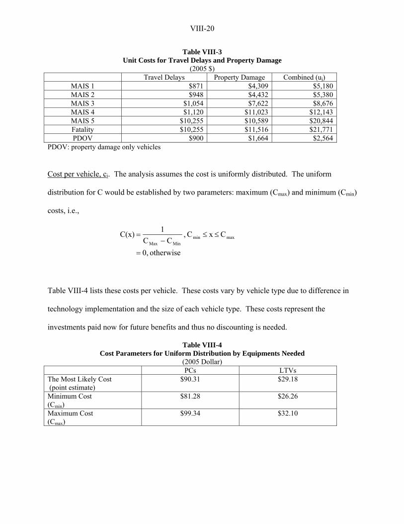
VIII-20
Table VIII-3 Unit Costs for Travel Delays and Property Damage
(2005 $) Travel Delays Property Damage Combined (uj)
MAIS 1 $871 $4,309 $5,180MAIS 2 $948 $4,432 $5,380MAIS 3 $1,054 $7,622 $8,676MAIS 4 $1,120 $11,023 $12,143MAIS 5 $10,255 $10,589 $20,844Fatality $10,255 $11,516 $21,771PDOV $900 $1,664 $2,564
PDOV: property damage only vehicles
Cost per vehicle, ci. The analysis assumes the cost is uniformly distributed. The uniform
distribution for C would be established by two parameters: maximum (Cmax) and minimum (Cmin)
costs, i.e.,
otherwise 0,
C x C ,CC
1C(x) maxminMinMax
=
≤≤−
=
Table VIII-4 lists these costs per vehicle. These costs vary by vehicle type due to difference in
technology implementation and the size of each vehicle type. These costs represent the
investments paid now for future benefits and thus no discounting is needed.
Table VIII-4 Cost Parameters for Uniform Distribution by Equipments Needed
(2005 Dollar) PCs LTVs The Most Likely Cost (point estimate)
$90.31 $29.18
Minimum Cost (Cmin)
$81.28 $26.26
Maximum Cost (Cmax)
$99.34 $32.10
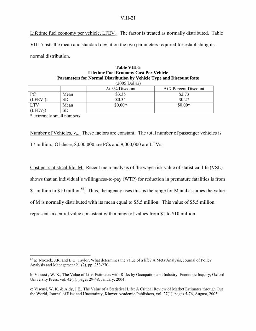
VIII-21
Lifetime fuel economy per vehicle, LFEVi. The factor is treated as normally distributed. Table
VIII-5 lists the mean and standard deviation the two parameters required for establishing its
normal distribution.
Table VIII-5 Lifetime Fuel Economy Cost Per Vehicle
Parameters for Normal Distribution by Vehicle Type and Discount Rate (2005 Dollar)
At 3% Discount At 7 Percent Discount PC (LFEV1)
Mean SD
$3.35 $0.34
$2.73 $0.27
LTV (LFEV2)
Mean SD
$0.00* $0.00*
* extremely small numbers
Number of Vehicles, vi,. These factors are constant. The total number of passenger vehicles is
17 million. Of these, 8,000,000 are PCs and 9,000,000 are LTVs.
Cost per statistical life, M. Recent meta-analysis of the wage-risk value of statistical life (VSL)
shows that an individual’s willingness-to-pay (WTP) for reduction in premature fatalities is from
$1 million to $10 million55. Thus, the agency uses this as the range for M and assumes the value
of M is normally distributed with its mean equal to $5.5 million. This value of $5.5 million
represents a central value consistent with a range of values from $1 to $10 million.
55 a: Mrozek, J.R. and L.O. Taylor, What determines the value of a life? A Meta Analysis, Journal of Policy Analysis and Management 21 (2), pp. 253-270. b: Viscusi , W. K., The Value of Life: Estimates with Risks by Occupation and Industry, Economic Inquiry, Oxford University Press, vol. 42(1), pages 29-48, January, 2004. c: Viscusi, W. K. & Aldy, J.E., The Value of a Statistical Life: A Critical Review of Market Estimates through Out the World, Journal of Risk and Uncertainty, Kluwer Academic Publishers, vol. 27(1), pages 5-76, August, 2003.

VIII-22
D. Simulation Results
The Monte Carlo simulation first randomly selects a value for each of the significant factors
based on their probability distributions. Then, the selected values are fed into the model to
forecast the results. Each process is a trial. The simulation repeats the process until a pre-
defined accuracy has been accomplished. Since Crystal Ball is a spreadsheet based simulation
software, the simulation model actually is a step-wise process, i.e., the simulation estimates gross
benefits, the net benefits (after redistribution of gross benefits through the injury redistribution
process), fatal equivalents, cost-effectiveness, and net benefits. Therefore, each of these
forecasted results had certainty bounds. This uncertainty analysis conducted a total of 10,000
trials before the forecasted mean results reached 99 percent precision. Even if the later criterion
was reached first, the trial numbers generally are very close to 10,000. These criteria were
chosen to ensure the simulation errors (000,101
≈ ) would be very close to 0. Therefore, the
results would truly reflect the probabilistic nature of the uncertainty factors.
Table VIII-6 summarizes the simulated injury benefit results including travel delay and property
damage savings at no discount level after about 10,000 trials. As shown, undiscounted, the
proposal would prevent 28,405 to 207,207 crashes. Reducing theses crashes results in
eliminating 922 to 3,201 fatalities and 21,068 to 150,851 MAIS 1-5 injuries. These fatalities and
injuries equate to 1,808 – 5,590 equivalent lives.

VIII-23
TABLE VIII-6 Simulated Injury Benefits
No Discount
Crashes Prevented Mean 91,822
Range 28,405 – 207,20790% Certainty 58,712 – 129,493
Fatalities Reduced Mean 2,146
Range 922 – 3,20190% Certainty 1,644 – 2,633
MAIS Injuries Eliminated Mean 67,754
Range 21,068 – 150,85190% Certainty 44,017 – 94,456
Equivalent Lives Saved Mean 3,551
Range 1,808 – 5,59090% Certainty 2,807 – 4,310
Table VIII-7 summarizes the simulated cost-effectiveness and net benefit results at 3 and 7
percent discount. As shown, at a 3 percent discount rate, the proposal rule would save 2,285 –
3,529 equivalent lives with a 90 percent certainty. In addition, with the same 90 percent
certainty, the proposal would save $299 - $599 million from travel delay and property damage
that is associated with the crashes that would be prevented by the proposal. However, the
proposal would increase fuel economy cost by $22.4 - $31.3 million. Nevertheless, the proposal
is extremely cost effective. At this discount level, the proposal would produce a cost per
equivalent fatality of no more than $3.75 million and a positive net benefit with a 100 percent
certainty. At a 90 percent certainty, the net benefits would range from $8.2 to $23.4 billion.

VIII-24
At a 7 percent discount rate, the proposal rule would save 1,816 – 2,815 equivalent lives and
$237 - $477 million from travel delay and property damage with a 90 percent certainty. The fuel
economy cost would be increased by $18.3 - $25.5 million with a 90 percent certainty. At this
discount level, the proposal would produce a cost per equivalent fatality of no more than $3.75
million and a positive net benefit with a 100 percent certainty. At a 90 percent certainty, the net
benefits would range from $6.3 to $18.5 billion

VIII-25
Table VIII-7 Simulated Cost-Effectiveness and Net Benefits by Discount Rate
(2005 Dollar) Discount Rate Costs* At 3% At 7% Mean $985 M $985 M Total Range $889 – $1,082 M $889 – $1,082 M 90% Certainty Range $914 – $1,056 M $914 – $1,056 MEquivalent Lives Saved Mean 2,899 2,309 Total Range 1,468 – 4,579 1,164 – 3,656 90% Certainty Range 2,285 – 3,529 1,816 – 2,815Property Damage and Travel Delay Savings Mean $440 M $351 M Total Range $175 – $938 M $139 – $749 M 90% Certainty Range $299 – $599 M $237 – $477 MFuel Economy Mean $26.8 M $21.9 M Total Range $16.3 – $37.2 M $12.8 – $30.9 M 90% Certainty Range $22.4 – $31.3 M $18.3 – $25.5 MCost-Effectiveness (CE) Mean $0.20 M $0.29 M Total Range $0.02 – $0.52 M $0.07 – $0.69 M 90% Certainty Range $0.12 – $0.31 M $0.19 – $0.42 M Certainty that CE ≤ $3.75 M 100% 100% Certainty that CE ≤ $5.5 M 100% 100%Net Benefit (NB) Mean $15.4 B $12.0 B Total Range $2.3 – $38.9 B $1.7 – $30.8 B 90% Certainty Range $8.2 – $23.4 B $6.3 – $18.5 B Certainty that NB > $0 100% 100%B: billion; M: million * same for all discount rates
IX-1
CHAPTER IX. REGULATORY FLEXIBILITY ACT AND UNFUNDED MANDATES REFORM ACT ANALYSIS
A. Regulatory Flexibility Act
The Regulatory Flexibility Act of 1980 (5 U.S.C. §601 et seq.), as amended by the Small
Business Regulatory Enforcement Fairness Act (SBREFA) of 1996, requires agencies to evaluate
the potential effects of their proposed and final rules on small businesses, small organizations,
and small governmental jurisdictions in the United States.
5 U.S.C. §603 requires agencies to prepare and make available for public comment an initial
and a final regulatory flexibility analysis (RFA) describing the impact of proposed and final rules
on small entities if the agency decides that the proposal may have a significant economic impact
on a substantial number of small entities. Each RFA must contain:
(1) A description of the reasons why action by the agency is being considered;
(2) A succinct statement of the objectives of, and legal basis for, a proposal or final rule;
(3) A description of and, where feasible, an estimate of the number of small entities to which
the proposal or final rule will apply;
(4) A description of the projected reporting, record keeping and other compliance
requirements of a proposal or final rule including an estimate of the classes of small
entities which will be subject to the requirement and the type of professional skills
necessary for preparation of the report or record;
(5) An identification, to the extent practicable, of all relevant Federal rules which may
duplicate, overlap, or conflict with the proposal or final rule;

IX-2
(6) Each final regulatory flexibility analysis shall also contain a description of any significant
alternatives to the final rule which accomplish the stated objectives of applicable statutes
and which minimize any significant economic impact of the final rule on small entities.
1. Description of the reasons why action by the agency is being considered
NHTSA is considering this action to require an ESC system in light vehicles in order to reduce
the number of automobile crashes and associated fatalities and injuries. ESC has been found to
be highly effective in reducing single-vehicle run-off-road crashes, a large percentage of which
involve vehicle rollover.
2. Objectives of, and legal basis for, the proposal or final rule
Under 49 U.S.C. 322(a), the Secretary of Transportation (the “Secretary”) has authority to
prescribe regulations to carry out the duties and powers of the Secretary. One of the duties of the
Secretary is to administer the National Traffic and Motor Vehicle Safety Act, as amended (49
U.S.C. 30101 et seq.). The Secretary is authorized to issue Federal motor vehicle safety
standards (FMVSS) that are practicable, meet the need for motor vehicle safety, and are stated in
objective terms56. The Secretary has delegated the responsibility for carrying out the National
Traffic and Motor Vehicle Safety Act to NHTSA57. NHTSA is proposing this rule under the
Authority of 49 U.S.C. 322, 30111, 30115, 30117, and 30166; delegation of authority at 49 CFR
1.50.
56 49 U.S.C. 30111(a). 57 49 U.S.C. 105 and 322; delegation of authority at 49 CFR 1.50.

IX-3
3. Description and estimate of the number of small entities to which the proposal or final rule
will apply
The proposal would apply to motor vehicle manufacturers, second-stage or final-stage
manufacturers and alterers, and manufacturers of ESC systems. Business entities are defined as
small businesses using the North American Industry Classification System (NAICS) code, for
the purposes of receiving Small Business Administration assistance. One of the criteria for
determining size, as stated in 13 CFR 121.201, is the number of employees in the firm. Affected
business categories include: (a) To qualify as a small business in Automotive Manufacturing
(NAICS 336111), the firm must have fewer than 1000 employees, (b) In Light Truck and Utility
Vehicle Manufacturing (NAICS 336112), the firm must have fewer than 1000 employees, (c) In
Motor Vehicle Body Manufacturing (NAICS 336211), the firm must have fewer than 1000
employees, and (d) In All Other Motor Vehicle Parts Manufacturing (NAICS 336399), the firm
must have fewer than 750 employees.
Small volume motor vehicle manufacturers
There are four vehicle manufacturers that would qualify as a small business under the definitions
of (a), (b), and (c) above. Table IX-1 provides information about the 4 small domestic
manufacturers in MY 2005.
Table IX-1 Small Vehicle Manufacturers
Manufacturer Employees Estimated Sales Sale Price Range Est. Revenues* Avanti 22 150 $75,000 to $125,000 $15,000,000 Panoz 50 150 $90,000 to $130,000 $16,500,000 Saleen 150 1,300 $42,000 to $75,000 $76,000,000 Shelby 44 60 $42,000 to $135,000 $5,310,000
* Assuming an average sales price from the sales price range

IX-4
Based on information available at various web sites58, Table IX-2 shows the current status of
compliance with the proposal.
Table IX-2 Small Volume Vehicle Manufacturer Compliance Status
ABS Traction Control ESC Avanti Yes Yes No Panoz Yes Yes No
Saleen S7 ? ? No Saleen
Mustang and Focus Based Models
Optional Optional No
Shelby Optional Optional No
ESC would cost at least $111 for the models that need only ESC and $479 for the models that
need ABS and ESC. Consumer costs for the more exotic models may be much higher than this.
Compared to the least expensive vehicle in Table IX-1, the cost could range from less than one-
half of one percent ($111/$42,000 = .0026) to 1.1 percent ($479/42,000 = .0114). Compared to
a weighted average sales price ($68,000), the cost could range from less than two tenths of one
percent ($111/$68,000 = .0016) to 0.7 percent ($479/$68,000 = .0070).
We believe that the market for the products of these small manufacturers is highly inelastic.
Purchasers of these products are enticed by the desire to have an unusual vehicle. Furthermore,
the price of competitor’s models will also need to be raised by a similar amount, since all light
vehicles must pass the standards. Thus, we do not believe that raising the price to include the
value of ESC will have much, if any, affect on sales of these vehicle. We expect that these price
increases will be passed on to the final customer. Based on this analysis, the agency believes
that the proposal will not have a significant economic impact on these four small domestic
vehicle manufacturers. 58 Avantimotors.com, panozauto.com, saleen.com, shelbyamerican.com, Edmunds.com

IX-5
Final-stage manufacturers and alterers
There are a significant number (several hundred) of second-stage or final-stage manufacturers
and alterers that could be impacted by the proposed rule. Some of these manufacturers buy
incomplete vehicles. Many of these vehicles are van conversions, but there are a variety of
vehicle types affected. Typically, none of these second-stage manufacturers or alterers changes
the brake system of the vehicle. Even the incomplete vehicles typically are delivered with
brakes. The brake system contains the central components for the ESC system. Thus, the
original manufacturer’s certification should apply for all of these vehicles as long as the brake
system is not disturbed. Thus, while there are a significant number of second-stage and final
stage manufacturers impacted by the proposed rule, we do not believe the impact will be
economically significant, since a pass-through certification process should apply to these
manufacturers.
Based on this analysis, although the proposal will impact about 100 percent of the small vehicle
manufacturers, final-stage manufacturers, and alterers, the proposal is not anticipated to have a
significant economic impact on these entities.
Small ESC system manufacturers
There are no ESC system manufacturers that would qualify as a small business under the
definition (d) above (i.e., all other motor vehicle parts manufacturing). ESC manufacturers
include Bosch, TRW, Continental-Teves, FTE, Automotive GmbH, Delphi, Mando America
Corp (Korean), Advics Co. Ltd (was Denso Japan), Nissin Kogyo Co., Ltd, Hitachi, and AISIN

IX-6
SEIKI Co., LTD. All of these are large corporations. The proposal is expected to have positive
economic impacts on ESC manufacturers.
4. Description of the projected reporting, record keeping and other compliance requirements for
small entities
The proposed rule would require manufacturers to equip their vehicles with ESC and to certify
that their products comply with the standard. There are record keeping requirements for those
manufacturers that comply using the phase-in schedule. However, the proposal would require
the multi-stage manufacturers, alterers, and small volume manufacturers to fully comply with the
standard on September 1, 2012, which is a one-year extension from full compliance of the phase-
in schedule. Thus, for these manufacturers there are no new reporting or record keeping
requirements, because they are not required to report during the phase-in period.
5. Duplication with other Federal rules
There are no relevant Federal regulations that duplicate, overlap, or conflict with the proposed
rule.
6. Description of any significant alternatives to the proposed rule
The agency considered two alternatives. One alternative was to limit applicability of the
standard to just light trucks, since ESC effectiveness for SUVs was much higher than ESC
effectiveness for passenger cars. The agency decided not to propose this alternative since there
were significant benefits from equipping passenger cars with ESC and requiring ESC for

IX-7
passenger cars was very cost-effective. Extending the ESC applicability to PCs would save an
additional 956 lives and reduce an additional 34,902 injuries.
The other alternative is to require a 2-wheel ESC system. A 2-wheel system is a less complex
system than the proposed ESC system. Based on an agency study, the 2-wheel ESC system is
less effective in preventing crashes than the proposed system. Thus, the proposed system would
potentially save more lives and reduce more injuries than the 2-wheel system. In addition, the
industry is already moving towards the proposed system for many of its vehicles. The agency
believes that all the 2011ESC systems will meet the proposed performance test.
In summary, the proposal requires for vehicle manufacturers to install ESC in their light vehicles.
There are 18 vehicle manufacturers. Four of them are considered to be small businesses.
However, purchasers of these high-end products are enticed by the desire to have an unusual
vehicle. These price increases will be passed on to the final customers. Most importantly, many
vehicles produced by these four companies already are equipped with ABS. The cost increase
per vehicle would be less than three tenths to 0.7 percent of their average sales price. We believe
this price increase will not affect their vehicle sales, given that all other vehicles will be required
to provide the same equipment.
As for the final stage manufacturers and alterers, typically these small businesses adhere to
original equipment manufacturers’ instructions in manufacturing modified and altered vehicles.
Based on our knowledge, original equipment manufacturers do not permit a final stage
manufacturer or alterer to modify or alter sophisticated devices such as air bags, event-data

IX-8
recorders (EDRs), or ESC. Therefore, multistage manufacturers and alterers would be able to
rely on the certification and information provided by the original equipment manufacturer. For
the above reasons, we have concluded that this proposal would not result in a significant
economic impact on small business, small organizations, or small governmental units.
B. Unfunded Mandates Reform Act
The Unfunded Mandates Reform Act of 1995 (Public Law 104-4) requires agencies to prepare a
written assessment of the costs, benefits, and other effects of proposed or final rules that include
a Federal mandate likely to result in the expenditures by State, local or tribal governments, in the
aggregate, or by the private sector, of more than $100 million annually (adjusted annually for
inflation with base year of 1995). Adjusting this amount by the implicit gross domestic product
price deflator for the year 2005 results in $122 million (112.145/92.106 = 1.22). The assessment
may be included in conjunction with other assessments, as it is here.
This proposal is not estimated to result in expenditures by State, local or tribal governments of
more than $122 million annually. However, it would result in an expenditure of much more than
that magnitude by the automobile manufacturers and/or their suppliers. The estimated annual
cost would be $985 million annually. These effects have been discussed previously in this
Preliminary Regulatory Impact Analysis (see Chapter V, Costs).
Related Documents