Properties Relevant for Inferring Provenance

Properties Relevant for InferringProvenance

Author:Abdul GhaniRajput

Supervisors:Dr. Andreas Wombacher

Rezwan Huq, M.Sc

Master Thesis

University of Twentethe Netherlands

August 16, 2011

Properties Relevant for InferringProvenance

A thesis submitted to the faculty of Electrical Engineering, Mathematics andComputer Science, University of Twente, the Netherlands in partial fulfillment

of the requirements for the degree of

Master of Sciences in Computer Science

with specialization in

Information System Engineering

Department of Computer Science,

University of Twentethe Netherlands

August 16, 2011

Contents

Abstract v

Acknowledgment vii

List of Figures ix

1 Introduction 11.1 Motivating Scenarios . . . . . . . . . . . . . . . . . . . . . . . . . 2

1.1.1 Supervisory Control and Data Acquisition . . . . . . . . . 21.1.2 SwissEX RECORD . . . . . . . . . . . . . . . . . . . . . . 3

1.2 Workflow Description . . . . . . . . . . . . . . . . . . . . . . . . 31.3 Objectives of Thesis . . . . . . . . . . . . . . . . . . . . . . . . . 41.4 Research Questions . . . . . . . . . . . . . . . . . . . . . . . . . . 51.5 Thesis Outline . . . . . . . . . . . . . . . . . . . . . . . . . . . . 6

2 Related work 72.1 Existing Stream Processing Systems . . . . . . . . . . . . . . . . 72.2 Data Provenance . . . . . . . . . . . . . . . . . . . . . . . . . . . 82.3 Existing Data Provenance Techniques . . . . . . . . . . . . . . . 82.4 Provenance in Stream Data Processing . . . . . . . . . . . . . . . 9

3 Formal Stream Processing Model 133.1 Syntactic Entities of Formal Model . . . . . . . . . . . . . . . . . 143.2 Discrete Time Signal . . . . . . . . . . . . . . . . . . . . . . . . . 143.3 General Definitions . . . . . . . . . . . . . . . . . . . . . . . . . . 183.4 Simple Stream Processing . . . . . . . . . . . . . . . . . . . . . . 223.5 Representation of Multiple Output Streams . . . . . . . . . . . . 223.6 Representation of Multiple Input Streams . . . . . . . . . . . . . 243.7 Formalization . . . . . . . . . . . . . . . . . . . . . . . . . . . . . 243.8 Continuity . . . . . . . . . . . . . . . . . . . . . . . . . . . . . . . 25

4 Transformation Properties 294.1 Classification of Operations . . . . . . . . . . . . . . . . . . . . . 294.2 Mapping of Operations . . . . . . . . . . . . . . . . . . . . . . . . 31

iii

4.3 Input Sources . . . . . . . . . . . . . . . . . . . . . . . . . . . . . 314.4 Contributing Sources . . . . . . . . . . . . . . . . . . . . . . . . . 324.5 Input Tuple Mapping . . . . . . . . . . . . . . . . . . . . . . . . . 324.6 Output Tuple Mapping . . . . . . . . . . . . . . . . . . . . . . . 33

5 Case Studies 355.1 Case 1: Project Operation . . . . . . . . . . . . . . . . . . . . . . 35

5.1.1 Transformation . . . . . . . . . . . . . . . . . . . . . . . . 355.1.2 Properties . . . . . . . . . . . . . . . . . . . . . . . . . . . 38

5.2 Case 2: Average Operation . . . . . . . . . . . . . . . . . . . . . 405.2.1 Transformation . . . . . . . . . . . . . . . . . . . . . . . . 405.2.2 Properties . . . . . . . . . . . . . . . . . . . . . . . . . . . 42

5.3 Case 3: Interpolation . . . . . . . . . . . . . . . . . . . . . . . . . 435.3.1 Transformation . . . . . . . . . . . . . . . . . . . . . . . . 435.3.2 Properties . . . . . . . . . . . . . . . . . . . . . . . . . . . 46

5.4 Case 4: Cartesian Product . . . . . . . . . . . . . . . . . . . . . . 475.4.1 Transformation . . . . . . . . . . . . . . . . . . . . . . . . 475.4.2 Properties . . . . . . . . . . . . . . . . . . . . . . . . . . . 50

5.5 Provenance Example . . . . . . . . . . . . . . . . . . . . . . . . . 51

6 Conclusion 556.1 Answers to Research Questions . . . . . . . . . . . . . . . . . . . 556.2 Contributions . . . . . . . . . . . . . . . . . . . . . . . . . . . . . 576.3 Future Work . . . . . . . . . . . . . . . . . . . . . . . . . . . . . 57

References 59

iv

AbstractProvenance is an important requirement for real-time applications, especiallywhen sensors act as a source of streams for large-scale, automated process con-trol and decision control applications. Provenance provides important informa-tion that is essential to identify the origin of data, to reproduce the results inreal-time applications as well as to interpret and validate the associated scien-tific results. The term provenance documents the origin of data by explicatingthe relationship among the input samples, the transformation and the outputsamples. In this thesis, we present a formal stream processing model based ondiscrete time signal processing. We use the formal stream processing model toinvestigate different data transformations and the provenance relevant charac-teristics of these transformations. The validity of the formal stream processingmodel and transformation properties is demonstrated by providing the four casestudies.

v

AcknowledgmentOver the last two years, I have received a lot of help and support by manypeople whom I would like to thank here.

I would not have been able to successfully complete this thesis without thesupport of supervisors during past seven months. My sincere thanks to Dr.Andreas Wombacher, Dr. Brahmananda Sapkota and Rezwan Huq. They havebeen a source of inspiration for me throughout the process of the research andwriting. Their feedback and insights were always valuable, and never wentunused.

I owe my deep gratitude to all of my teachers, who have taught me at Twente.Their wonderful teaching methods enhanced my knowledge of the respectivesubject and enabled me to complete my studies in time. I also like to extendmy sincere thanks to the staff of international office. Special thanks go to JanSchut because without his support it is not possible for me to come here andcomplete my studies.

My roommates at the third floor at Zilverling provided a great working environ-ment. I thank them for the laughs and talks we had. I would like to thank thefollowing colleagues and friends whose help in the study period has contributedto achieve this dream. Thanks to Fiazan Ahmed, Fiaza Ahemd, Irfan Ali, IrfanZafar, M.Aamir, Martin, Klifman, T.Tamoor and Mudassir.

Of course, this acknowledgment would not complete without thanking my mother,brother and sister. Having supported me throughout my university study, I can-not express my gratitude enough. I hope this achievement will cheer them upduring these stressful times.

My family (Nida, Fatin and Abdullah) more than deserves to be named heretoo. Throughout the process of my studies and my graduation research, theyhave been loving and supportive.

ABDUL GHANI RAJPUT

August 16, 2011.

vii

List of Figures

1.1 Workflow model based on RECORD project scenario . . . . . . . 4

2.1 Taxonomy of Provenance . . . . . . . . . . . . . . . . . . . . . . 10

3.1 Logical components of the formal model and the idea of figure istaken from [18] . . . . . . . . . . . . . . . . . . . . . . . . . . . . 15

3.2 The generic Transformation function . . . . . . . . . . . . . . . . 163.3 Unit impulse sequence . . . . . . . . . . . . . . . . . . . . . . . . 173.4 Unit step Sequence . . . . . . . . . . . . . . . . . . . . . . . . . . 173.5 Example of a Sequence . . . . . . . . . . . . . . . . . . . . . . . . 183.6 Sensor Signal Produces an Input Sequence . . . . . . . . . . . . . 193.7 Input Sequence . . . . . . . . . . . . . . . . . . . . . . . . . . . . 203.8 Window Sequence . . . . . . . . . . . . . . . . . . . . . . . . . . 213.9 Simple stream processing . . . . . . . . . . . . . . . . . . . . . . 223.10 Multiple outputs based on the same window sequence . . . . . . 233.11 Example of increasing chain of sequences . . . . . . . . . . . . . . 26

4.1 Types of Transfer Function . . . . . . . . . . . . . . . . . . . . . 34

5.1 Transformation Process of Project Operation . . . . . . . . . . . 365.2 Input Sequence and Window Sequence . . . . . . . . . . . . . . . 375.3 Several Transfer Functions is Executed in Parallel . . . . . . . . . 385.4 Average Transformation . . . . . . . . . . . . . . . . . . . . . . . 415.5 Interpolation Transformation . . . . . . . . . . . . . . . . . . . . 445.6 Distance based interpolation . . . . . . . . . . . . . . . . . . . . . 465.7 Cartesian Product Transformation . . . . . . . . . . . . . . . . . 485.8 Example for overlapping windows . . . . . . . . . . . . . . . . . . 525.9 Example for non-overlapping windows . . . . . . . . . . . . . . . 53

ix

Chapter 1

Introduction

Stream data processing has been a hot topic in the database community inthis decade. The research on stream data processing has resulted in severalpublications, formal systems and commercial products.

In this digital era, there are many real-time applications of stream data process-ing such as location based services (LBSs identify a location of a person) basedon user’s continuously changing location, e-health care monitoring systems formonitoring patient medical conditions and many more. Most of the real-timeapplications collect data from source. The source (sensor) produces data con-tinuously. The real-time applications also connect with multiple sources thatare spread over wide geographic locations (also called data collection points).The examples of sources are scientific data, sensor data, wireless and sensornetworks. These sources are called data streams [11].

A data stream is an infinite sequence of tuples with the timestamps. A tuple isan ordered list of elements in the sequence and the timestamp is used to definethe total order over the tuples. Real-time applications are specialized forms ofstream data processing. In real-time applications, a large amount of sensor datais processed and transformed in various steps.

In real-time applications, reproducibility is a key requirement and reproducibil-ity means the ability to reproduce the data items. In order to reproduce thedata items, data provenance is important. Data provenance [23] documentsthe origin of data by explicating the relationship among the input data, thealgorithm and the processed data. It can be used to identify data because itprovides the key facts about the origin of the data.

The research on data provenance has focused on static databases and also instream data processing, which are discussed in Chapter 2. But there is still a lotto be investigated such as reproducibility in real-time applications. Suppose in astream processing setup, we have a transformation process T . It is executed on

1

CHAPTER 1. INTRODUCTION

an input stream X at time n and produces output stream Y . We can re-executethe same transformation process T at any later point in time n0 (with n0 > n)on the same input stream X and generate exactly the same output stream Y [1].The ability to reproduce the transformation process for a particular data item ina stream requires transformation properties. The transformation has a numberof properties for instance constant mapping. For example, if a user wants totrace back the problem to the corresponding data stream then he needs to havea constant rate of output tuple otherwise user can not handle that. Thereforeone important property for inferring provenance is constant mapping or fixedmapping and we have more properties which are discussed in Chapter 4. Thesetransformation properties are used to infer data provenance.

To this end, this thesis will present a formal stream processing model based ondiscrete time signal processing theory. The formal stream processing model isused to investigate different data transformations and transformation propertiesrelevant for inferring data provenance to ensure reproducibility of data items inreal-time applications.

This chapter is organized as follows. In Section 1.1, two motivating scenariosare presented. In Section 1.2, we give a detailed description of a workflow modelwhich is based on a motivating scenario Section 1.1.2. In Section 1.3, we presentthe objectives of the thesis. In Section 1.4, we state our research questions andsub research questions followed by Section 1.5 that states the complete thesisoutline.

1.1 Motivating Scenarios

Due to the growth in technology, the use of real-time application is increasingday-by-day in many domains such as environmental research and medical re-search. In most of these domains, the real-time applications are designed tocollect and process the real-time data which is produced by sensor. In these ap-plications, provenance information is required. In order to show the importanceof data provenance in stream data processing we will present two motivatingscenarios in the following subsections.

1.1.1 Supervisory Control and Data Acquisition

The Supervisory Control And Data Acquisition (SCADA) application is a real-time application. The SCADA application collects data from multiple sensorsand these sensors produce data continuously. The SCADA is a data-acquisition-oriented and an event-driven application [4]. The SCADA is a centralized systemwhich performs process control activities. It also controls entire sites (electri-cal power transmission and distribution station) from a remote location. Forinstance, the SCADA electrical system contains up to 50,000 data collection

2


points and over 3,000 public/ private electric utilities. In that system, failureof any single data collection point can disrupt the entire process flow and causefinancial losses to all the customers that receive electricity from the source, dueto a blackout [4].

When a blackout event occurs, the actual measured sensor data can be com-pared with the observed source data. In case of a discrepancy, the SCADAsystem analysts need to understand what caused the discrepancy and have tounderstand the data processed on the basis of the streamed sensor data. Thus,analysts must have a mechanism to reproduce the same processing result frompast sensor data so that they can find the cause of the discrepancy.

1.1.2 SwissEX RECORD

Another data stream based application is the RECORD project [28]. It is aproject of the Swiss Experiment (SwissEx) platform [6]. The SwissEX platformprovides a large scale sensor network for environmental research in Switzerland.One of the objectives of the RECORD project is to identify how river restorationaffects water quality, both in the river itself and in the groundwater.

In order to collect the environmental changes data due to river restoration,SwissEX deployed several sensors at the weather station. One of them is thesensorscope Meteo station [6]. At the weather station, the deployed sensorsmeasure water temperature, air temperature, wind speed and some other factorsrelated to the experiment like electric conductivity of water [28]. These sensorsare deployed in a distributed environment and send the data as streaming datato the data transformation element through a wireless sensor network.

At the research centre, the researchers can collect and use the sensor data toproduce graphs and tables for various purposes. For instance, a data transfor-mation element may produce several graphs and tables of an experiment. Ifresearchers want to publish these graphs and tables in scientific journals thanthe reproducibility of these graphs and tables from original data is required to beable to validate the result afterwards. Therefore, one of the main requirementsof the RECORD project is the reproducibility of results.

1.2 Workflow Description

In the previous section, a motivating scenario SwissEX RECORD has beenintroduced. In which the researchers want to identify how river restorationaffects the quality of water. To achieve this objective, a streaming workflowmodel is required. This section illustrates how the streaming workflow modelworks. Figure 1.1 shows a workflow model which is based on the RECORDproject scenario.

3


Figure 1.1: Workflow model based on RECORD project scenario

In Figure 1.1, three sensors are collecting the real-time data. These sensorsare deployed in three different geographic location of a known region of theriver and the region is divided into 3 × 3 cells of a grid. These sensors sendreadings of electric conductivity of water to a data transformation element. Inorder to convert the sensor data in a streaming processing system, we proposea wrapper called source processing element. Each sensor is associated with aprocessing element named PE1, PE2 and PE3 which provides the data tuplesin a sequence x1[n], x2[n] and x3[n] respectively. A sequence is an infinite setof tuples/data with timestamps. These sequences are combined together (by aunion operation) which generates a sequence xunion[n] as output. It containsall data tuples sent from all the three sensors. The sequence xunion[n] will workas input to the transformation element. The transformation element processesthe tuples of the input sequence and produces an output sequence or multipleoutput sequences y[n], depending on the transformation operations used.

Let us look at a concrete example, at the transformation element (as shownin Figure 1.1), an average operation is configured. The average operation ac-quires tuple from xunion[n] and computing last 10 tuples/time space of theinput sequence and it executed every 5 seconds. The tuples/time space whichis configured for the average operation is called a window and how often aver-age operation is executed, we call a trigger. The details of the trigger and thewindow are discussed in Chapter 3.

For the rest of the thesis, the example workflow model is used to define thetransformation of any operation and answer the potential research questions.

1.3 Objectives of Thesis

The following are the objectives of the thesis.

4


• Define a formal stream processing model to do calculations over streamprocessing which is based on an existing stream processing model [9].

• Investigate the data transformations of SQL operations such as Project,Average, Interpolation and Cartesian product using the formal streamprocessing model.

• Define the formal definitions of data transformation properties.

• Prove the continuity property of the formal stream processing model.

F (∪χ) = ∪F (χ)

1.4 Research Questions

In order to achieve the objectives of the thesis, the following main researchquestions are addressed.

• What are the formal definitions of the basic elements of a stream process-ing model that can be applied to any stream processing systems?

• What are the suitable definitions of transformation properties for inferringprovenance?

In order to answers the main research questions, the following sub questionshave been defined.

• What is the mathematical formulation of a simple stream processing model?

• What are the mathematical definitions of Project, Average, Interpolationand Cartesian product transformations?

• What are the suitable properties of the data transformations?

• What are the formulas of the data transformation properties?

The formal stream processing model is a mathematical model and an importantproperty of this mathematical model is the continuity property. It is used toprovide a constructive procedure for finding the one unique behavior of thetransformation. Therefore, we have another research question which is:

• How to prove the continuity property for formal stream processing model?

The answers of these sub-questions provide the answer to the main researchquestions.

5


1.5 Thesis Outline

The thesis is organized as follows

• Chapter 2 gives a short review of existing stream data processing systems.It will describe what provenance metadata is, why it is essential in streamdata processing and how this can be recorded and retrieved. Chapter 2also provides the review of provenance in streaming processing.

• To derive the transfer functions of the operations, we need an existingsimple stream processing model. In Chapter 3, we presented a short in-troduction to discrete time signal processing for the formalization of theformal stream processing model. Based on discrete time signal, we providethe definitions of basic elements of the formal stream processing model anddiscrete time representation of the stream processing.

• Chapter 4 provides the details of transformation properties and formaldefinitions of properties relevant for tracing provenance.

• In Chapter 5, four case studies are described where the formal streamprocessing model has been used and tested. At the end of the chapter,two examples are given for the case of overlapping and non-overlappingwindows.

• Finally in Chapter 6, conclusions are drawn and future work is discussed.

6

Chapter 2

Related work

This chapter introduces preliminary concepts which is used throughout thisthesis. Section 2.1 starts with a brief discussion on existing stream processingsystems. This includes discussions on how stream processing systems handleand process continuous data streams. Section 2.2 introduces the concept ofdata provenance and the importance of data provenance in stream processingsystems. Section 2.3 introduces existing data provenance techniques. This chap-ter is concluded in Section 2.4, which discusses the data provenance in streamprocessing system.

2.1 Existing Stream Processing Systems

Stream data processing systems are more and more supporting the execution ofcontinuous tasks. These tasks can be defined as database queries [12]. In [12]data stream processing system is defined as follows:

Data stream processing systems take continuous streams of input data, processthat data in certain ways, and produce ongoing results.

Stream data processing systems are used in decision making, process controland real-time applications. Several stream data processing systems have beendeveloped in the research as well as in the commercial sector. Some of whichare described below.

STREAM [16] is a stream data processing system. The main objective of theSTREAM project was memory management and computing approximate queryresults. It is an all purpose stream processing system but this system can notsupport reproducibility of query results.

TelegraphCQ at UC Berkeley [17] is a dataflow system for processing continuesqueries over data streams. The primary objective of the Telegraph project is

7

CHAPTER 2. RELATED WORK

to design for adaptive query processing and shared query evaluation of sensordata. CACQ is an improved form of the Telegraph project and it has the abilityto execute multiple queries concurrently [14].

Another popular system in the field of stream data processing is the Aurora sys-tem. Aurora system allows users to create the query plans by visually arrangingquery operators using boxes (corresponding to query operators) and links (cor-responding to data flow) paradigm [18]. The extended version of Aurora systemis the Borealis [21] system. It supports distributed functionality as well.

IBM delivers a System S [19] solution for the commercial sector. The System Sis a stream data processing system (it is also called stream computing system).The System S is designed specifically to handle and process massive amountsof incoming data streams. It supports structured as well as unstructured datastream processing. It can be scaled form one to thousands of computer nodes.For instance, System S can analyze hundreds or thousands of simultaneous datastreams (such as stock prices, retail sales, weather reports) and deliver nearlyinstantaneous analysis to users who need to make split-second decisions [20].

The System S does not support the data provenance functionality and in thissystem data provenance is important, because later on users may want to trackhow data are derived as they flow through the system.

All of the above approaches do not provide the functionality of data provenanceand cannot regenerate the results. Therefore, a provenance subsystem is neededto collect and store metadata, in order to support reproducibility of results.

2.2 Data Provenance

Provenance means, where is the particular tuple/data item coming from or theorigin of data item or the source of a data item. In [7] provenance also definedas the history of ownership of a valued object or work of art or literature. Itwas originated in the field of Art and it is also called metadata. Provenance canalso help to determine the quality of a data item or the authenticity of a dataitem [13]. In stream data processing , data provenance is important because itnot only ensures the integrity of a data item but also identifies the source ororigin of a data tuple. In decision support applications, data provenance can beused to validate the decision made by application.

2.3 Existing Data Provenance Techniques

In the domain of information/data processing, [27] is one the first to use thenotion of provenance. In [27], authors introduce two ideas of data provenancei.e. where and why provenance. When executing a query, a set of input data

8


items is used to produce a set of output data items. To reproduce the outputdata set, one needs the query as well as the input data items. The set of inputdata items are referred to as Why-provenance. Where-provenance refers to thelocation(s) in the source database from which the data was extracted [27]. In[27], authors did not address how to deal with streaming data and associatedoverlapping windows. It only shows case studies for traditional data.

In [29], authors proposed a method for recording and reasoning over data prove-nance in web and grid services. The proposed method captures all informationon workflow, activities and all datasets to provide provenance data. They cre-ated a service oriented architecture (SOA), where they use a specific web servicefor the recording and querying of provenance data. The method is only worksfor coarse grained data provenance (the coarse grained data provenance can bedefined on relation-level) ; therefore this method cannot achieve reproducibilityof results.

In [30], authors recognized a specific class of workflow called data driven work-flows. In data driven workflows, data items are first class input parametersto processes that consume and transform the input to generate derived outputdata. They proposed a framework called Karma2 that records the provenanceinformation on processes as well as on data items. While their proposed frame-work is closer to the stream processing system than the majority of the researchpapers on workflows, it does not address the problem, specifically related tostream data processing.

To design a standard provenance model, a series of workshops and conferenceshave been arranged. During these workshops and conferences participants havediscussed a standard provenance model, which is called the Open ProvenanceModel (OPM)[31]. The OPM is a model for provenance which allows provenanceinformation to be exchanged between systems, by means of a compatibilitylayer based on a shared provenance model [1]. The OPM define a notion ofgraphs. The provenance graph is used to identify the casual relationship betweenartifacts, processes and agents. A limitation of the OPM is that it primarilyfocuses on the workflow aspect. It is not possible to define what exactly a processdoes. It also has an advantage that it might to be working with interoperabilityof different systems [31].

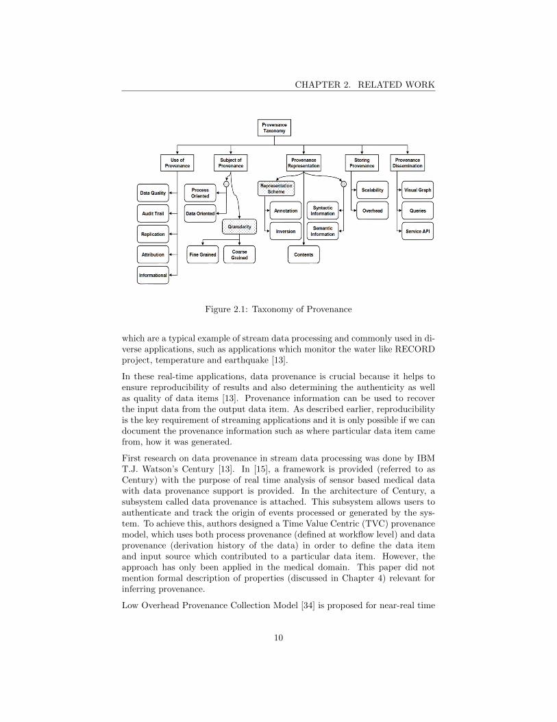
In [32] authors did a survey on data provenance techniques that were used indifferent projects. On the bases of their survey, they provide a taxonomy ofprovenance as shown in Figure 2.11.

2.4 Provenance in Stream Data Processing

In this era, lots of real-time applications have been developed. Most of the ap-plications are based on mobile networks or sensors networks. Sensor networks,

1Figure 2.1 is taken from [32].

9


Figure 2.1: Taxonomy of Provenance

which are a typical example of stream data processing and commonly used in di-verse applications, such as applications which monitor the water like RECORDproject, temperature and earthquake [13].

In these real-time applications, data provenance is crucial because it helps toensure reproducibility of results and also determining the authenticity as wellas quality of data items [13]. Provenance information can be used to recoverthe input data from the output data item. As described earlier, reproducibilityis the key requirement of streaming applications and it is only possible if we candocument the provenance information such as where particular data item camefrom, how it was generated.

First research on data provenance in stream data processing was done by IBMT.J. Watson’s Century [13]. In [15], a framework is provided (referred to asCentury) with the purpose of real time analysis of sensor based medical datawith data provenance support is provided. In the architecture of Century, asubsystem called data provenance is attached. This subsystem allows users toauthenticate and track the origin of events processed or generated by the sys-tem. To achieve this, authors designed a Time Value Centric (TVC) provenancemodel, which uses both process provenance (defined at workflow level) and dataprovenance (derivation history of the data) in order to define the data itemand input source which contributed to a particular data item. However, theapproach has only been applied in the medical domain. This paper did notmention formal description of properties (discussed in Chapter 4) relevant forinferring provenance.

Low Overhead Provenance Collection Model [34] is proposed for near-real time

10


provenance collection in sensor based environmental data stream. In this paper,authors focus on identifying properties that represent provenance of data itemfrom real time environmental data streams. The three main challenges describedin [34] are given below:

• Identifying the small unit (data item), for which provenance informationis collected.

• Capturing the provenance history of streams and transformation states.

• Tracing the input source of a data stream after the transformation iscompleted.

A low overhead provenance collection model has been proposed for a meteorol-ogy forecasting application.

In [5], authors report their initial idea of achieving fine-grained data provenanceusing a temporal data model. They theoretically explain the application of thetemporal data model to achieve the database state at a given point in time.

Recently [1], proposed an algorithm for inferring fine grained provenance in-formation by applying a temporal data model and using coarse grained dataprovenance. The algorithm is based on four steps; first step is to identify thecoarse grained data provenance (it contains information about the transforma-tion process performed by that particular processing element). Second step is toretrieve the database state. Third step is to reconstruct the processing windowbased on information provided by the first two steps. The final step is to inferthe fine grained data provenance information. In order to infer fine grained dataprovenance, authors have provided the classification of transformation proper-ties of processing elements, i.e., operations only for constant mapping opera-tions. Such properties are the input sources, contributing sources, input tuplemapping and output tuple mapping. Authors have implemented the algorithminto a real time stream processing system and validated their algorithm.

This thesis is based on the transformation properties of processing elements de-scribed in [1]. The details and formal definitions of these properties are discussedin Chapter 4.

11

Chapter 3

Formal Stream ProcessingModel

The goal of this chapter is to provide a mathematical framework for stream dataprocessing which is based on discrete time signal processing theory. It can benamed as formal stream processing model.

The discrete time signal processing is the theory of representation, transforma-tion and manipulation of signals and the information they contain [22]. Thediscrete time signal can be represented as a sequence of numbers. The discretetime transformation is a process that maps an input sequence into an outputsequence. There are a number of reasons to choose discrete time signal pro-cessing to formalize the stream data processing. One important reason is that,the discrete time signal processing allows for the system to be event-triggered,which is often the case in stream data processing. Another reason is that, one ofthe objectives of the stream data processing is to perform real-time processingon real-time data. Therefore, the discrete time signal processing is common toprocess real-time data in communication systems, radar, video encoding andstream data processing [22].

This chapter is organized as follows. Section 3.1 provides an overview of thesyntactic entities, their graphical representation and symbols used in the formalstream processing model. Section 3.2 introduces the basic concepts of discretetime signal processing theory. This theory can be used to solve the researchquestions stated in the previous chapter. Section 3.3 provides the general defi-nitions of the input sequence, transformation, window function and the triggerrate. Based on these general definitions, the simplest data stream processingis defined in Section 3.4. The representation of multiple outputs and multipleinputs is illustrated in Section 3.5 and Section 3.6 respectively. Section 3.7 pro-vides the formalization of the model with and without considering the complexdata structure. Finally in Section 3.8, a proof of continuity property of formal

13

CHAPTER 3. FORMAL STREAM PROCESSING MODEL

stream processing model is given.

3.1 Syntactic Entities of Formal Model

The symbols, formulas and interpretation used in formal stream processingmodel are syntactic entities [24]. The syntactic entities are the basic require-ments to design a formal model [24]. Figure 3.1 shows that the formal streamprocessing model is based on symbols, string of symbols, well-formed formulas,interpretation of the formulas and theorems. In order to define a trasformationelement, syntactic entities of the formal stream processing model are requiredbecause syntactic entities are used to define the transformation element.

The list of symbols, used in our formal stream processing model, and theirdescription [25] are given in Table 3.1.

S.No Symbols Description1 x[n] Represents an input sequence, generated by

an input source.2 y[n] Represents the output of the transformation.3 n Particular point in time in the input sequence.4 w(n, x[n]) Represents a window function.5 nw Is used to represent the window size of the

window sequence.6 τ Is used to represent the trigger in the formal

model.7 o Used to represent the offset.8 I Represents the number of input sources.9 T{.} Shows a transformation function T, that maps

an input to an output.10 m Shows the total number of transformation or

output11 j′ Represents the particular output and it value

goes to 1,2,3...,m.12 l Represents the particular transformation and

it value goes to 1,2,3,...,m.

Table 3.1: List of Symbols used in FSPM

3.2 Discrete Time Signal

The formal stream processing model is based on discrete time signal theory,which is a theory of representing discrete time signals by a sequence of number

14


Figure 3.1: Logical components of the formal model and the idea of figure istaken from [18]

15


and the transformation of these signals [22]. The mathematical representationof the discrete time signal is defined below:

Discrete time signal : n ∈ Z→ x[n]

Where

index n represents the sequential values of time,

x[n], the nth number in the sequence, is called a sample.

the complete sequence is represented as {x[n]}.

In the used stream processing model, a stream is called a sequence. The formalmodel is process stream or set of streams. Therefore we can say that, a streamis simply a discrete time sequence or discrete time signal.

A transformation is a discrete time system. A discrete time system maps an in-put sequence {x [n]} to an output sequence {y[n]}; An equivalent block diagramis shown in Figure 3.2.

Figure 3.2: The generic Transformation function

In order to define a transformation of an operation, some basic sequences andsequence of operations are required.

Unit Impulse

The unit impulse or unit sample sequence (Figure 3.3) is a generalized functiondepending on n such that it is zero for all values of n except when the value ofn is zero.

δ[n] =

{1 n = 00 otherwise

16


Figure 3.3: Unit impulse sequence

Unit Step

The unit step response or unit step sequence (Figure 3.5) is given by

u[n] =

{1 n ≥ 00 n ≤ 0

The unit step response is simply an on-off switch which is very useful in discretetime signal processing.

Figure 3.4: Unit step Sequence

Delay or shift by integer k

y[n] = x[n− k] - ∞ < n <∞

when, k ≥ 0, sequence of x[n] shifted by k units to the right.

k < 0, sequence of x[n] shifted by k units to the left.

Any sequence can be represented as a sum of scaled, delayed impulses. Forexample the sequence x[n] in Figure 3.5 can be expressed as:

x[n] = a−3δ[n+ 3] + a1δ[n− 1] + a2δ[n− 2] + a5δ[n− 5]

17


Figure 3.5: Example of a Sequence

More generally, any sequence can be represented as:

y[n] =

∞∑k=−∞

x[k]δ[n− k]

Finally, these concepts of discrete time signal theory help us to represent theformal definitions of stream processing model. The formal model will allow usto define the properties relevant for inferring provenance.

3.3 General Definitions

The fundamental elements of any stream processing system are data streams,transformation element, window, trigger and offset. There are number of defini-tions available in the literature for these fundamental elements. In this thesis wetry to provide the formal definition of these elements. The element definitionsare as follows.

Input Sequence

In our model, the input data arrives from one or more continuous data streams.Normally, these data streams are produced by sensors. These data streams arerepresented as input sequences in our model. The input sequence representsthe measurement/record of a sensor. The input sequence contains more thanone element. Each of these elements is called a sample which represents onemeasurement [22].

Definition 1 Input Sequence: An input sequence is a data stream used by atransformation function. It is a sequence of number x, where the nth numberin the input sequence is denoted as x[n]:

x = {x[n]} −∞ < n <∞ (3.1)

18


Figure 3.6: Sensor Signal Produces an Input Sequence

Where n is an integer number which represents the measurement/record of asensor.

Note that from this definition, an input sequence is defined only for integervalues of n and refers to the complete sequence simply by {x[n]}. For example,the infinite length sequence as shown in Figure 3.6 is represented by the followingsequence of numbers.

x = {..., x[1], x[2], x[3]......}

Transformation

The transformation is a transfer function which takes finitely many input se-quences as input and gives finitely many sequences as output. The numberof input and output depends on an operation. The formal definition of thetransformation is given as:

Definition 2 Transformation: Let {xi[n]} be the input sequences and {yj′ [n]}be the output sequences for 1 ≤ i ≤ I and 1 ≤ j

′ ≤ m. A transformation is atransfer function T defined as:

m∏j′=1

yj′ [n] = T{I∏i=1

xi[n]}.

Where m is the total number of output and I is the total number of input se-quence.

Window

For the processing of sensor data, most of the real-time applications are in-terested in the most recent samples of the input sequences. Therefore, a time

19


window is defined to select the most recent samples of the input sequence. Awindow always consists of two end-points and a window size. The end-pointsare moving or fixed. Windows are either time based or tuple based [1]. In thisthesis, we used time based window. Why we used time based window? Becausewe have a model that supports only time instead of tuple which is based onIDs. The formal stream processing model supports time based sliding windowbecause a time stamp is associated with each sample of the input sequence. Thesliding window is a window type in which both end-points move. In the slidingwindow, the window size is always constant. To represent the window in ourformal model, we have defined a window function. The formal definition is givenas follows:

Definition 3 Window Function: A window function is applied on the inputsequence (Definition 1) in order to select a subset of the input sequence {x[n]}.This function selects subset of nw elements in the sequence where nw is thewindow size. Window function is defined as:

w(n, {x[n]}) =

nw−1∑k=0

x[n′]δ[n− n′ − k] −∞ < n′, n <∞

which is also equivalent to:

w(n, {x[n]}) =

n∑k=n−nw+1

x[n′]δ[n′ − k] −∞ < n′, n <∞ (3.2)

The output of the window function w(n, {x[n]}) is called the window sequence.The window sequence is nothing more than a sum of delayed impulses (definedin Section 3.2) multiplied by the corresponding samples of the sequence {x[n]}at the particular point in time n. The resulting sequence can be represented interms of time. Example 3.1, describing the working of window function.

Example 3.1 Suppose we have an input sequence {x[n]} as shown in the Figure3.7. To select subset of the sequence, window function is applied on the inputsequence.

Figure 3.7: Input Sequence

20


The samples involved in computation of the window sequence are k = 3 to 5with window size nw = 3 and n = 5. The result of the window function is shownin Figure 3.8. By putting these parameters to the window function formula, weget:

Figure 3.8: Window Sequence

w(5, {x[n]}) =

5∑k=5−3+1

x[n′]δ[n′ − k]

w(5, {x[n]}) =

5∑k=3

x[n′]δ[n′ − 3]

w(5, {x[n]}) = x[n′]δ[n′ − 3] + x[n′]δ[n′ − 4] + x[n′]δ[n′ − 5]

when n′ is 3 from replicated sequence therefore, we get:

w(5, {x[n]}) = x[3]

Similarly the output of the w(5, {x[n]}) = x[4],when n′ = 4 and w(5, {x[n]}) =x[5],when n′ = 5.

Trigger Rate

A trigger rate represents the data driven control flow of the data workflow. Data-driven workflows are executed in an order determined by conditional expressions[8]. Triggers are important in a stream processing. It is used to specify whena transformation element should execute. In general, there are two types oftriggers, namely time based triggers and tuple based triggers. A time basedtrigger executes at fixed intervals, while a tuple based trigger executes when anew tuple arrives [1]. The formal model is based on time based triggers sincethe formal model is based only for time (we do not have a model for IDs).

Definition 4 Trigger Rate: τ is a trigger rate over a sequence which specifieswhen a transformation element is executed. It is defined for all values of n andapplied again with a unit impulse function. The Trigger Offset, (o) determines

21


how many samples are skipped at the beginning of the total record before samplesare transferred to the window. Which is defined as:

δ[n%τ − o]

The transformation element is defined for all values of n, based on the triggerthe transformation element is only supposed to be defined at the moments wherethe trigger is enabled. Thus, for a transformation T{.}, a trigger is applied witha unit sample(i.e. δ[n%τ − o] = 1).

3.4 Simple Stream Processing

The simple stream processing is based on a transformation function that mapsinput data contained in a window sequence producing an output sequence, wherethe transformation function is executed after arrival of every τ elements of theinput sequence. It shows how to process and integrate the input sequence toproduce the output sample as shown in Figure 3.9.

Figure 3.9: Simple stream processing

Based on the above definition, the simple possible stream processing can bedefined mathematically as,

y[n] = δ[n%τ − o]T {w(n, {x[n]})} −∞ < n <∞ (3.3)

with window size nw, trigger offset o and trigger rate τ.

3.5 Representation of Multiple Output Streams

Equation 3.3 shows that when we execute a transformation function based onthe same window sequence (where window size is one) that contained a singlesample, it produces a single output value. The window sequence contains morethan one sample, the transformation element produces different outputs. Allthese outputs must be associated with the same time index n. Since it is notpossible, it is modeled as several transformation functions performed in parallelthereby producing several output sequences [9]. Thus,

22


y1[n] = δ[n%τ − o]T1{w(n, {x[n]})}

:

yl[n] = δ[n%τ − o]Tl{w(n, {x[n]})}

To represent the multiple outputs of the transformation element, we used theconcept of the direct product. The direct product is defined on two algebras Xand Y, giving a new one. It can be represented as infix notation ×, or prefix

notation∏

. The direct product of X ×Y is given by the Cartesian product of

X,Y together with a properly defined formation on the product set.

Definition 5 Multiple outputs: Let y1[n], y2[n], y3[n]......ym[n] be the outputs ofT1{.}, T2{.}, T3{.}, ......Tm{.} based on the same window sequence w(n, {x[n]})of input sequence for all values of n, then multiple output can be represented by

m∏j′=1

yi[n] =

m∏l=1

Tl{.}

m∏j′=1

yi[n] =

m∏l=1

δ[n%τ − o]Tl{w(n, {x[n]})}

where m is the total number of output.

Figure 3.10 shows the graphical representation of multiple outputs based onthe same window sequence. The direct product of the output sequence can beinterpreted as a sequence of output tuples. In definition 5, we assumed that thenumber of output is fixed to m.

Figure 3.10: Multiple outputs based on the same window sequence

23


3.6 Representation of Multiple Input Streams

The concept of multiple input streams is common in stream data processingand in mathematics. For instance, union and Cartesian Product can take morethan one sequence as input. In order to carry out the transformation of theseprocessing elements, we have to extend the simple stream processing model tosupport multiple input streams.

Definition 6 Multiple input streams: Let us we have multiple window sequencesw(n1, {x1[n]}), ....w(ni, {xi[n]}) and each window has a different window sizenw1

...nwi. Let these windows are input to a transformation function such as:

y[n] = δ[n%τ − o]T{w(n1, {x1[n]}), ....w(ni, {xi[n]})} −∞ < n′, n <∞

Multiple input streams can also be defined in terms of a direct product again,that is:

y[n] = δ[n%τ − o]T{I∏i=1

w(ni, {xi[n]})} −∞ < n <∞

where I is the total number of input stream/source.

3.7 Formalization

This section combines the definitions introduced before in order to define theformal stream processing model. Equation 3.4 shows the mathematical descrip-tion of the formal stream processing model. This formal model will be used todo calculations over stream processing. In Equation 3.4, the structure of theinput sequence and the output sequence is not considered. It is, therefore, pos-sible to include the more complex data structure of yj′ [n] and xi[n] in Equation3.4. The resulting formal stream processing which includes more complex datastructure is given in Equation 3.5.

m∏j′=1

yj′ [n] = δ[n%τ − o]m∏l=1

Tl{I∏i=1

w(ni, {xi[n]})} −∞ < n <∞ (3.4)

m∏j′=1

dj′,yj′∏

j′′=1

yj′,j′′ [n] = δ[n%τ−o]m∏l=1

Tl{I∏i=1

w(ni,

dxi∏ji=1

{xi,ji [n]})} −∞ < n <∞

(3.5)Where,

24


j′and l = 1, 2, 3...m, where m being the maximum number of outputsof the processing element

dj′,yj′ is the dimensionality of the data structure of the j′th outputsequence yj′

I is the number of input sequences

dxiis the dimensionality of the data structure of the ith input se-

quence xi

In this thesis, dimensionality of the input data is not considered because thedata structure information of the input data is not available in advance. Theformal model (without considering the complex data structure) Equation 3.4is used to identify the data transformation and transformation properties forinferring provenance, which are discussed in next chapter.

3.8 Continuity

In this section, we provide a simple proof of a continuity property of the formalstream processing model. The proof of the method is essentially the same asin [26] but the contribution here the proof of continuity property using thenotations of formal stream processing model.

As per the Kahn Process Network [26], let {x[n]} denotes the sequence of valuesin the stream, which is itself totally ordered set. In our formal stream processingmodel, the order relationship is not present because every sequence is definedfrom −∞ to ∞, as shown in Figure 3.11.

To define a partial order relatioship in our formal model, let us consider a prefixordering of sequences, where x1[n] v x2[n], if x1[n] is a prefix of x2[n] (i.e., ifthe first values of x2[n] are exactly those in x1[n]) in X. Where X denotes theset of finite and infinite sequences as shown in Equation 3.6.

X = {x1[n], x2[n], x3[n], ...} =

∞⋃i=1

{xi[n]} 1 ≤ i ≤ ∞ (3.6)

In Equation 3.6, X is a complete partial order set, if it holds the followingrelationship between sequences.

xi[n] v xj [n]⇔ xi[n] = xj [n] · u[−i]

The above relationship is defined as the complete partial order (CPO) in ourformal stream processing model. Therefore, the set X is a complete partial orderwith the prefix order defining the ordering. A complete partial order is a partialorder with a bottom element where every chain has a least upper bound (LUB)

25


Figure 3.11: Example of increasing chain of sequences

[26]. A least upper bound (LUB), written tX, is an upper bound that is aprefix of every other upper bound. The term (xj [n] · u[−i]) indicates that whenxj [n] is multiplied with the unit step sequence then we get the xi[n] sequence.

In our formal stream processing model, usually T is executed on a sequence.Now we can extend the definition of T in order to execute and support chain ofsequences such as:

T (X) =⋃

x[n]εX

T{x[n]}

Definition: Let X and Y be the CPO’s. A transformation T : X → Y iscontinuous if for each directed subset x[n] of X, we have T (tX) = tT (X).We denote the set of all continuous transformation from X to Y by [X → Y ].

In our formal stream processing model, a transformation takes m input and noutputs such as T : Xm → Y n. Let a transformation is defined as below:

T (x[n]) =

{y[n], if x[n] v X0 otherwise

Theorem: The above transformation is Continuous.

Proof. Consider a chain of sequences X = {x1[n], x2[n], x3[n], ...}, we need to

show that T (tX) = tT (X). Write T (X) =⋃

x[n]εX

T{x[n]}.

26


Taking R.H.S:

tT (X) = t{T (x1[n]), T (x2[n]), ...}

Since X is an increasing chain, it has a least upper bound as per the partialorder relationship defined above. Suppose the LUB is x[n], then output is:

tT (X) = t{T (x1[n]), T (x2[n]), ..., T (x[n])}tT (X) = x[n] = y[n]

Similarly for L.H.S:

T (tX) = T (t{x1[n], x2[n], ..., x[n]}T (tX) = x[n] = y[n]

Thus, in both cases, T (tX) = tT (X), so T is continuous.

27

Chapter 4

Transformation Properties

The goal of this chapter is to provide the formal definitions of transformationproperties for inferring provenance. In Section 1.2, a workflow model was de-scribed, in which transformation is an important element. The transformationhas a number of properties that makes it useful for inferring provenance. Thesetransformation properties are: input sources, contributing sources, input tuplemapping, output tuple mapping and mapping of operations. These are classifiedand discussed in [1] as required for reproducibility of results in e-science applica-tions. Based on this classification, the formal definitions of the transformationproperties are provided in this chapter.

The remainder of the chapter is organized as follow. Section 4.1 provides theclassification of operation. Section 4.2 explains the mapping of operationsand provides the formal definition of mapping. Section 4.3 describes the in-put sources property and its formal definition. Section 4.4 discusses about thecontributing sources property and provides the formal definition. Section 4.5 ex-plains and defines the formal definition of input tuple mapping. Finally, Section4.6 defines the output tuple mapping and its formal definition.

4.1 Classification of Operations

To formalize the definitions of transformation properties, the data transfor-mation of four SQL operations are considered. These are: Project, Average,Interpolation and Cartesian product. Each of these data transformations havea set of properties, such as the ratio of mapping from input to output tuples isa transformation property. The explanation of all these properties is describedin Table 4.1.

In Figure 4.1, the graphical representation of considered transformation is pro-vided. The transformation of Project, Average, Interpolation and Cartesian

29

CHAPTER 4. TRANSFORMATION PROPERTIES

product are constant mapping operations, which are separated by black solidline. The Select operation is a variable mapping operation which is not consid-ered in this thesis.

Figure 4.1 shows that the Project, Average and Interpolation operation aresingle input source operations. The Cartesian product operation is a multipleinput source operation.

It also shows that Project transformation takes a single element of the inputsequence and produces a single element at the output sequence. Thus, the ratiois 1 : 1. The Average transformation takes three input elements of the inputsequence and produced single output, therefore the ratio is 3 : 1.

Since the Cartesian product is a multiple input source operation it takes oneinput element from each source and produces one output element as shown inFigure 4.1. Therefore, the ratio of Cartesian product is (1,1) : 1. These ratiosare again reflected in the input and output tuple mapping criteria in Table 4.2.

30


4.2 Mapping of Operations

Based on the classification of operations described in Section 4.1, the formaldefinition of a mapping is defined in this section. The two types of transfor-mations are possible: constant mapping and variable mapping transformations.The constant mapping transformations have a fixed ratio. The variable map-ping transformations do not maintain a fixed ratio of input to output mappingas described in Table 4.1. Let us give the formal definition.

Definition 7 Constant Mapping Transfer Function: T : {w(n, {x[n]})} → {y[n]}is called constant mapping transfer function if the mapping ratio of {w(n, {x[n]})}to {y[n]} is fixed for all values of n. If it is not fixed, then it is a variable map-ping.

4.3 Input Sources

In our formal stream processing model, one of the important transformationproperties is input sources. This property is used to find the number of inputsources that contribute to produce an output tuple.

The input sources are input sequences (see Definition 1). The transfer functionstakes one or more input sources, processes them and produces one or morederived output sequences. The single input source transfer functions do havea single input sequence, while multiple input source transfer functions havemultiple input sequences as inputs. Let us give a formal definition.

Definition 8 Input Sources: Let y[n] be an output sequence of a transfer func-tion T, where T is applied on one or more input sequences as per Definition 6,then:

y[n] = δ[n%τ − o]T{I∏i=1

w(ni, {xi[n]})} −∞ < n <∞

31


where I is used to denote the number of input sources contributing to T toproduce the output, I ∈ N, where N is the natural number. Therefore:

Input sources =

{Multiple if I > 1Single else

4.4 Contributing Sources

The formal definition of this property will be used to find the creation of anoutput sample is based on samples from a single or multiple input sequences.This property is only applicable for those transformations which takes I > 1input sequences as an input. The formal definition of the property is givenbelow.

Definition 9 Contributing Sources: Let T be a transfer function which havemultiple input sources as input, such as w(n1, {x1[n]}) × ... × w(n′i, {xi[n′]}),then contributing sources property defined as:

T {w(n1, {x1[n]})× ...× w(n′i, {xi[n′]})} = T

{I∏i=1

w(ni, {xi[n]})

}

Contributing sources =

Multiple For I > 1 and

each I is contributed in TSingle For I > 1 and

only a single source is contributed in TNot Applicable For I = 1

4.5 Input Tuple Mapping

The input tuple mapping property is used to find a given sample, related to theinput source that is used by the transfer function. The formal definition is asfollows:

Definition 10 Input Tuple Mapping (ITM): Let T be a transfer function andapplied on a window (see definition 3) {w(n, {x[n]})},which is equivalent to:

T {w(n, {x[n]})} = T

{n∑

k=n−nw+1

x[n′]δ[n′ − k]

}−∞ < n′, n <∞

If the output of the transfer function is an accumulated sum of the value at indexn and all previous values of the input sequence {x[n]} then input tuple mappingis multiple else input tuple mapping is single.

32


4.6 Output Tuple Mapping

The most important and difficult property is the output tuple mapping forinferring provenance data. It depends on input tuple mapping as well as on aninput source. In this property, dimensionality of input data is important beacusethe output data dimensionality is different from the input data dimensionality.But In this thesis, we did not consider the dimensionality of the input data.Output tuple mapping distinguishes whether the execution of a transformationproduces a single or multiple output tuple per input tuple mapping [1]. Theoutput tuple mapping is a decimal or a fractional number when it is calculated.The formal definition is given as:

Definition 11 Output Tuple Mapping (OTM): Let T be a transformation thatmaps the nw(window size) samples per source to produce the m number of outputsamples, then the output tuple mapping is defined as:

OTM = r ×I∑i=1

ITMi

{Multiple OTM > 1Single otherwise

where OTM = output tuple mapping

ITMi = input tuple mapping per source

r =m

I∑i=1

nwi

where I is the total number of input sources

33


Figure 4.1: Types of Transfer Function

34

Chapter 5

Case Studies

The primary goal of this chapter is to derive the transformation of the Project,Average, Interpolation and Cartesian product to exemplify the formal streamprocessing model and formal definitions of transformation properties describedin the previous chapters.

5.1 Case 1: Project Operation

5.1.1 Transformation

This section derives the transformation definition of Project operation using theformal stream processing model. We begin by explaining the concept of Projectoperation.

The Project operation is a SQL operation which is also called projection. Aproject is an unary transformation that can be applied on a single input se-quence. The transformation process takes the input sequence (see Definition 1)and computes the sub-samples of the input sequence. In other words, it reducesthe nth sample from the input sequence. Similarly in the databases, projectionof a relational database table is a new table containing a subset of the originalcolumns.

Figure 5.1 shows the graphical representation of the project transformationprocess and also shows that the sensor produces an input sequence which isx[n]. The input sequence is passed to the project transformation (in Figure5.1, big square box represents the project transformation process). The windowfunction (see Definition 2) is applied on the input sequence to cover the mostrecent samples of the input sequence since the sensor is producing the datacontinuously. The output of the window function is the window sequence. Basedon the window size of the sequence, the multiple outputs are produced by project

35

CHAPTER 5. CASE STUDIES

transformation i.e. Y1[n], Y2[n] and Ym[n] as shown in Figure 5.1. All outputsare associated with the same time n.

Figure 5.1: Transformation Process of Project Operation

Now using the concept of project operation which is defined above, the transferfunction of project can be derived using the formalization Equation 3.4 whichis:

m∏j′=1

yj′ [n] = δ[n%τ − o]m∏l=1

Tl{I∏i=1

w(ni, {xi[n]})} −∞ < n <∞

Put the value of I = 1 in the above equation, because the project is an unaryoperation. we get:

m∏j′=1

yj′ [n] = δ[n%τ − o]m∏l=1

Tl{1∏i=1

w(ni, {xi[n]})} −∞ < n <∞

As we have described earlier that the total number of outputs for the projectoperation is equal to the window size which is m = nw, therefore the aboveequation becomes:

nw∏j′=1

yj′ [n] = δ[n%τ−o]nw∏l=1

Tl

{1∏i=1

(n∑

k=n−nw+1

xil [n′]δ[n′ − k]

)}−∞ ≤ n′, n ≤ ∞

The project transformation simply takes the input sequence {x[n]} to the rightby l − nw samples to form the output where Tl denotes the total number oftransformation. Therefore, the final transformation of the project is defined by:

36


nw∏j′=1

yj′ [n] = δ[n%τ − o]nw∏l=1

1∏i=1

xil [n− nw + l] −∞ < n <∞ (5.1)

where

xil is the input sequence, where the value of i = 1 which means thatsingle input source is participating and l represents the particularpoint sample in time.

nw is the window size and being the maximum number of outputsby the project operation.

o is the offset value initially we consider offset to be zero and τ is atrigger rate.

Example 5.1 Suppose an input sequence (as shown in Figure 5.2) is appliedon a project transformation. The window function is applied on input sequencewith nw = 3 at the point in time n = 5. The transfer function is executed afterarrival of every 3 elements in the sequence and the trigger offset is 2.

Figure 5.2: Input Sequence and Window Sequence

By putting the values nw = 3, I = 1, τ = 3 and o = 2 in Equation 5.1, we get:

3∏j′=1

yj′ [n] = δ[n%τ − o]3∏l=1

x1l [n− nw + l]

The output of the above equation is multiple as per the Definition 5. It can bemodeled as transformations in parallel producing several outputs as shown inFigure 5.3.

In Figure 5.3, Tl takes the window sequence as an input sequence and it pro-duces multiple outputs which are T1, T2 and T3. Therefore, the general outputis described by:

37


Figure 5.3: Several Transfer Functions is Executed in Parallel

3∏j′=1

yj′ [n] = x11 [n− nw + 1]× x12 [n− nw + 2]× x13 [n− nw + 3]

Let us start with the definition of T1. It takes window sequence with the fol-lowing parameters nw = 3, l = 1 and n = 5 and translate it in the followingsteps.

y1[n] = x11 [n− nw + 1]y1[n] = x11 [5− 3 + 1]y1[n] = x11 [3] = T1

The transformation function T2 executes the next sample with the followingparameters nw = 3, l = 2 and n = 5, the output becomes:

y2[n] = x12 [n− nw + 2]y2[n] = x12 [5− 3 + 2]y2[n] = x12 [4] = T2

This process is performed continuously until all the transformations are exe-cuted.

5.1.2 Properties

In the previous section, the project transformation is defined to test the formaldefinitions of transformation properties (as we have defined in Chapter 4). Wehave to test the following properties:

• Input Sources

• Contributing Sources

• Input Tuple Mapping

• Output Tuple Mapping

38


Input Sources

This property checks that transfer functions take single or multiple input sourcesas input that contributes to produce an output sample. According to Definition8, the value of I in our formal model is used to identify the number of inputsources that contribute to produce the output. The derived project transforma-tion is:

nw∏j′=1

yj′ [n] = δ[n%τ − o]nw∏l=1

1∏i=1

xil [n− nw + l] −∞ < n <∞

Now compare the project transformation definition with the formal stream pro-cessing model, which is

m∏j′=1

yj′ [n] = δ[n%τ − o]m∏l=1

Tl{I∏i=1

w(ni, {xi[n]})} −∞ < n <∞

As we can see, the value of I in the project transformation is equal to 1, thereforethe project transformation is a single input source operation.

Contributing Sources

According to Definition 9, the contributing sources property is only applica-ble for those transformations which have multiple input sources. In case ofthe project transformation this property is not applicable because the projecttransformation has a single input source as shown in Equation 5.1.

Input Tuple Mapping

According to Definition 10, the input tuple mapping of the project transfor-mation is single. The project transformation Equation 5.1 indicates that theoutput of the project transformation is a single sample i.e. xil [n−nw+l] insteadof accumulated sum of the value at index n and all previous values of the inputsequence {x[n]}.

Output Tuple Mapping

It distinguishes whether the execution of a transformation produces a single ormultiple output tuples per input tuple mapping. To check this, a formula isdefined (see Definition 11) to calculate the output tuple mapping. The generalformula is:

39


OTM = r ×I∑i=1

ITMi

{Multiple OTM > 1Single otherwise

where OTM = output tuple mapping

ITMi = Input tuple mapping per source

r =m

I∏i=1

nwi

where I is the total number of input sources

Therefore to calculate the output tuple mapping of the project transformation,the value of m and the value of the input tuple mapping is required. The inputtuple mapping has been already calculated in previous section. The input tuplemapping is one. The total number of output can easily derived from the projecttransformation equation:

nw∏j′=1

yj′ [n] = δ[n%τ − o]nw∏j′=1

1∏i=1

xil [n− nw + l] −∞ < n <∞

The above equation indicates that the total number of output produced by theproject transformation is m = nw, therefore by putting the values in the outputtuple mapping formula. we get:

OTM = r ×I∑i=1

ITMi

OTM =m

1∏i=1

nwi

×1∑i=1

ITMi

OTM =nwnw× 1 = 1

The result of Definition 11 is interpreted that the output tuple mapping ofproject transformation is 1.

5.2 Case 2: Average Operation


The goal of this section is to derive the transformation of average operationusing the formal stream processing model given in Equation 3.4. The average is

40


a SQL aggregate operation and returns a single value, using the values in a tablecolumn [35]. Figure 5.4 shows the generic process of the average transformation.It also shows that the average is calculated by combining the values from a setof input and computing a single number as being the average of the set.

Figure 5.4: Average Transformation

From the concept of the average operation, the average transformation can bederived using the following equation:

m∏j′=1

yj′ [n] = δ[n%τ − o]m∏l=1

Tl{I∏i=1

w(ni, {xi[n]})} −∞ < n <∞

In the above equation, we can put the value of I = 1 and the value of m = 1since the average returns a single sample, using samples in an input sequence.So, the resulting equation is:

1∏j′=1

yj′ [n] = δ[n%τ − o]1∏l=1

Tl{1∏i=1

w(ni, {xi[n]})} −∞ < n <∞

1∏j′=1

yj′ [n] = δ[n%τ − o]1∏l=1

Tl

{1∏i=1

(n∑

k=n−nw+1

xil [n′]δ[n′ − k]

)}−∞ ≤ n′, n ≤ ∞

In mathematics, the average of n numbers is given as 1/n

n∑i=1

ai where ai are

numbers with i = 1, 2, 3...n. Similarly, the average transformation is defined as:

41


1∏j′=1

yj′ [n] = δ[n%τ − o]1∏l=1

1∏i=1

1

nw

(n∑

k=n−nw+1

x1[k]

)−∞ < n <∞ (5.2)

where

x1 is the input sequence and yj′ [n] is the output sequence where j′

is the number of output which is equal to 1.

nw is the window size and n is the point in time at which we areinterested to start calculating the average.

o is the offset value, initially it is considered to be zero and τ is atrigger rate.

5.2.2 Properties

Input Sources

The input sources property checks whether the average transformation takessingle or multiple input sources as input (as per Definition 8). The propertycan be checked by looking at the average transformation Equation 5.2. InEquation 5.2, the value of I = 1. Therefore, average is a single input sourcetransformation.


Same as the project transformation, the contributing sources property is notapplicable on the average transformation because Equation 5.2 indicates thatthe average transformation has a single input source as input.

Input Tuple Mapping

The input tuple mapping property of the average transformation is multiplesince output of the average transformation is the accumulated sum of the valueat index n and all previous values of the input sequence x[n] that is:

n∑k=n−nw+1

x1[k] = x1[n− nw + 1] + x1[n− nw + 2] + ...+ x1[k]

The value of k goes to n, therefore

42


k = (n− n+ nw + 1)− 1

k = nw

So, the average transformation has multiple input tuple mapping i.e. nw.


To calculate the output tuple mapping of the average transformation, Definition11 is used. The formula for output tuple mapping is:

OTM = r ×I∑i=1

ITMi

OTM =m

1∏i=1

nwi

×1∑i=1

ITMi

OTM =1

nw× nw = 1

The result of the OTM formula is 1 which means that the output tuple mappingof the average transformation is 1.

5.3 Case 3: Interpolation


The Interpolation is an important function in many real-time applications suchas the RECORD project (described in Section 1.2) and has been used for yearsto estimate the value at an unsampled location. It is important for visualizationsuch as generation of contours.

There exist many different methods of interpolation. The most common ap-proaches are weighted average distance and natural neighbors. The deatialsof these approaches are available in [36]. In this thesis only weighted distancebased interpolation transformation is described.

In Section 1.2, we described how the streaming workflow model use sensor dataand combine them into a grid and how transformation element, interpolationare used to construct new samples. The RECORD case (defined in Section 1.2)

43


is used to derive the transformation of interpolation operation using the formalstream processing model.

Figure 5.5 shows the generic process of the interpolation transformation. Itshows that the interpolation transformation takes a number of input samplesfrom an input sequence and produces a set of output samples. In Figure 5.5,the interpolation takes 2 input samples and produces 6 output samples. Sim-ilarly, if it takes 3 input samples then it produces 9 output samples thereforeinterpolation is a constant mapping operation (as we have described in Section4.1).

Figure 5.5: Interpolation Transformation

To derive the interpolation transformation, we can use the formal model Equa-tion 3.4:

m∏j′=1

yj′ [n] = δ[n%τ − o]m∏l=1

Tl{I∏i=1

w(ni, {xi[n]})} −∞ < n <∞

As we know that the interpolation transformation takes a single input sequenceas input, therefore we can put the value of I = 1 in the above equation, theresulting equation is:

44


m∏j′=1

yj′ [n] = δ[n%τ − o]m∏l=1

Tl{1∏i=1

w(ni, {xi[n]})} −∞ < n <∞

m∏j′=1

yj′ [n] = δ[n%τ − o]m∏l=1

Tl

{1∏i=1

(n∑

k=n−nw+1

xi[n′]δ[n′ − k]

)}−∞ < n.n′ <∞

Suppose that we have an input sequence {x[n]} and we can apply the windowfunction on the input sequence to select a subset of the samples (of window sizenw) at the given point in time n, therefore the above equation become,

m∏j′=1

yj′ [n] = δ[n%τ − o]m∏l=1

1∏i=1

(n∑

k=n−nw+1

x1[k]

)

Given a set of samples to which a point P(x,y) is attached as shown in Figure 5.6.The point P is user-defined. In Figure 5.6, black circles are samples involved inthe interpolation and gray circle is a new sample which is being esitmated. Theweight assigned to each sample is typically based on the square of the distancefrom the black to gray circle. Therefore the above equation becomes:

m∏j′=1

yj′ [n] = δ[n%τ − o]m∏l=1

1∏i=1

(n∑

k=n−nw+1

λi,l · x1[k]

)

where

λi,l =1/C+d2n,l∑n

k′=n−nw+11/C+d2n,l

λi,l the weight of each sample (with respect to the interpolationsample i.e. gray circle) used in the interpolation process,

d2i,l is the distance between sample n and the location being esti-mated

C is the small constant for avoiding ∞ condition

So, the interpolation transformation is defined as,

m∏j′=1

yj′ [n] = δ[n%τ − o]m∏l=1

1∏i=1

(n∑

k=n−nw+1

1/C + d2n,l∑nk′=n−nw+1 1/C + d2n,l

· xi[k]

)(5.3)

45


Figure 5.6: Distance based interpolation

5.3.2 Properties

Input Sources

The input sources property is a transformation property which is used to find thenumber of input sequences participating in the transformation process. The in-terpolation transformation Equation 5.3 shows that the value of I = 1 therefore,the interpolation is a single source transformation. The interpolation transfor-mation can take multiple input sources as input but with some assumption suchas window size is one for each input sources. The alternative of the interpolationtransformation is not chosen because it depends on the window size. On theother hand, all the case studies are independent of the window size.


The contributing sources property is not applicable to the interpolation trans-formation because the value of I = 1 in Equation 5.3.

Input Tuple Mapping

Same as the average transformation, the input tuple mapping property of theinterpolation transformation is multiple since the output of the transformationis the accumulated sum of the value at index n and all previous values of theinput sequence x[n] that is:

46


n∑k=n−nw+1

x1[k] = λ1,l · x1[n− nw + 1] + λ1,l · x1[n− nw + 2] + ...+ λ1,l · x1[k]

The value of k goes to n, therefore

k = (n− n+ nw + 1)− 1

k = nw

The input tuple mapping of interpolation transformation is nw which is multiple.


The output tuple mapping of the interpolation transformation is multiple asper Definition 11. Equation 5.3 shows that the number of outputs is m. Theinput tuple mapping property defines that the interpolation transformation hasmultiple input tuple. Therefore, the output tuple mapping is:

OTM = r ×I∑i=1

ITMi

OTM =m

1∏i=1

nwi

×1∑i=1

ITMi

OTM =m

nw× nw = m

As a result of the OTM formula, the output tuple mapping of the interpolationtransformation is multiple.

5.4 Case 4: Cartesian Product


The Cartesian product is the direct product of two or more sources. It is alsocalled the product set. Suppose we have two input sources {x1[n]} and {x2[n]},the Cartesian product of these sources is defined as the set of all ordered pairswhose first sample is an element of source x1[n], and whose second sample is

47


an element of source x2[n]. The Cartesian product is written as (x1[n]×x2[n]).The order of the input sources can not be changed because the ordered pairs isreversed. Although its elements remain the same but their pairing gets reversed.

In the workflow model described in Chapter 1, the Cartesian product operationis considered a transformation element. Figure 5.7 shows the Cartesian producttransformation process. It takes two input sequences as input and produces fouroutput samples i.e. T1..4. Figure 5.7 also shows that the Cartesian product hasa ratio of (1, 1) : 1 which means it takes one input sample from each source andthen produces one output tuple. Therefore, it belongs to the constant mappingoperations.

Figure 5.7: Cartesian Product Transformation

We can define the Cartesian product transformation using the formal modelequation which is:

m∏j′=1

yj′ [n] = δ[n%τ − o]m∏l=1

Tl{I∏i=1

w(ni, {xi[n]})} −∞ < n <∞

The above equation also equal to:

48


m∏j′=1

yj′ [n] = δ[n%τ − o]m∏l=1

Tl

n∑k=n−nw1

+1

x1[n′]δ[n·′ − k]

× n∑k=n−nw2

+1

x2[n′]δ[n·′ − k]

× ...×

n∑k=n−nwi

+1

xi[n′]δ[n·′ − k]

Now suppose we have 2 input sources, therefore the value of I = 2 and eachsource has constant window size i.e. nw1, nw2 = 2. The number of output (m =nw1×nw2 = 4) is fixed which is a multiple of each source window size. Therefore,the above equation becomes:

m∏j′=1

yj′ [n] = δ[n%τ − o]m∏l=1

Tl

n∑k=n−nw1

+1

x1[n′]δ[n·′ − k]

× n∑k=n−nw2

+1

x2[n′]δ[n·′ − k]

The Cartesian product of two input sequences {x1[n]} and {x2[n]} with windowsize nw1, nw2 is the set of all possible combinations of ( x1[n−nw1 + 1] , x2[n−nw2 + 1] ) where x1[n − nw1 + 1] is a sample of input sequence {x1[n]} atthe particular point in time and x2[n − nw2 + 1] is a sample of {x2[n]} at theparticular point in time. We can define the Cartesian product of two inputsequences as follows:

m∏j′=1

yj′ [n] = δ[n%τ − o]m∏l=1

{(x1[n− nw1 + l])× (x2[n− nw2 + l])}

The generalized form of Cartesian product for I number of input sources is givenas:

m∏j′=1

yj′ [n] = δ[n%τ − o]m∏l=1

(I∏i=1

xi[n− nwi + li]

)(5.4)

Where

m is the total number of output i.e. m = nw1 × nw2 × ...nwi.

I is the total number of input sources.

li shows the position of a sample in the ith source window which isli = 1, 2, ...nwi

49


5.4.2 Properties

Input Sources

According to Definition 8, the transformation of the Cartesian product takesmultiple input sources i.e. I as input to produce an output as shown in Equation5.4. The value of I ε N where N is the natural number. Therefore, the Cartesianproduct is a multiple input sources operation.


The contributing sources property is applicable on the Cartesian product trans-formation since the value of I > 1 in Equation 5.4. According to Definition 9, Ifthe value of I > 1 and each I is contributed to produce an output sample thenthe contributing sources property is multiple. In the Cartesian product trans-formation each source is participating to produce an output sample, such astwo input sequences {x1[n]} and {x2[n]} are contributed to produce an output.Therefore the contributing sources property of Cartesian product transforma-tion is multiple.

Input Tuple Mapping

From the definition of the Cartesian product transformation, the input tuplemapping is single per input source. The derived transformation of Cartesianproduct is:

m∏j′=1

yj′ [n]= δ[n%τ − o]m∏l=1

(I∏i=1

xi[n− nwi + li]

)m∏j′=1

yj′ [n]= δ[n%τ − o]m∏l=1

(x1[n− nwi + l1]× x2[n− nwi + l2]...× xi[n− nwi + li])

The above equation shows that each source is contributing a sample to exactlyproduce the multiple output samples. Which means that each source is con-tributing a single sample and those samples are combined together to producemultiple output samples. So, the input tuple mapping is one per input sourceas per Definition 10.


When the transformation of the Cartesian product is executed, it producesmultiple output tuples as define by [1]. Now, we can prove it easily by using

50


Definition 11, which is:

OTM = r ×I∑i=1

ITMi

OTM =m

I∏i=1

nwi

×I∑i=1

ITMi

The value of the input tuple mapping is 1 per input source and the total numberof output m = nw1 × nw2 × ...nwi. Therefore, the above formula becomes:

OTM =nw1 × nw2 × ...nwinw1 + nw2 + ...nwi

× (1 + 1 + 1 + ...1i)

OTM =

(nw1 × nw2 × ...nwinw1 + nw2 + ...nwi

× (1 + 1 + 1 + ...1i)

)> 1

OTM = Multiple

As a result, the output tuple mapping of Cartesian product is multiple.

5.5 Provenance Example

In this section, we provide two examples for inferring provenance of a givensample for the case of overlapping windows and non-overlapping windows. Theidea of the examples is taken from [1]. We can use transformation propertiesto infer provenance information for any particular output sample at a specficpoint in time n.

Example 1: Case of Overlapping Windows

For this case, we have considered a simple workflow where a project transfor-mation takes one input sequence as input and produces an output sequence. InFigure 1, we considered that the window size is 3 and the transformation willbe executed after arrival of every single sample (i.e. τ = 1). In Figure 5.8,the starting time is 1 and 2,3,... are different points in time. For overlappingwindows, we get the same type of output sequence.

Now, we have to choose the output sample for which the provenance informationis inferred. Assume y3[4] (point in time 4) sample of the output sequence ischosen for inferring provenance information as shown in Figure 5.8. In Figure

51


5.8, the project transformation processess 3 samples (which are x1[2],x1[3] andx1[4]) of the window sequence as input and produces the multiple outputs . Afterthat the transformation processes the next window sequence (from x1[3], x1[4]and x1[5]) and produces the next outputs.

Figure 5.8: Example for overlapping windows

According to the transformatin properties, first we have to get the total numberof input sources using input sources property (see Definition 8). Here, singleinput sources is contributing, which is x1. Now, we check the value of inputtuple mapping. In this example, the input tuple mapping is 1 as per the ITMproperty. At last, we have to check which input sample is contributing frominput source at a point in time 4. In order to check the input sample, we haveto reconstruct the processing window. As we know that the window size is 3and trigger rate is 1, so y3[4] (point in time 4) sample should be produced frominput samples x1[2] to x1[4]. We are interested in provenance information of y3at point in time 4. Now, we can count 3 samples of the input sequence which isstarted from x1[2] to x1[4] as shown in Figure 5.8. Therefore, the input samplex1[4] contributed to produce y3[4] at the output sequence.

Example 2: Case of Non-Overlapping Windows

For this case, we consider the project transformation to process the non-overlappingwindows. Figure 5.9 shows an input sequence with 2 windows (in dark smallsquare box), each window contains three samples and the project transformationis executed after arrival of every three samples.

The output sample, i.e. y3[7] is chosed for which provenance data is inferred.The project transformation processes first window and produces three outputas the output sequence. Similarly, it processess second window and producessthree more output, as shown in Figure 5.9.

Same as the first example, the single input sources x1 is contributing and theinput tuple mapping is also one as per the definition of ITM porperty. Now inferrthe provenance information of y3[7], since we know the window size and triggerrate. The samples y3[7] is produced from input sample x1[5] to x1[7]. Frompoint in time 7 of the input sequence, subtract three samples since window size

52


Figure 5.9: Example for non-overlapping windows

is 3, we get the desired window. The desired window sequence (x1[5] to x1[7]) isprocessed by the project transformation to produce y3[7]. So, the input samplex1[7] contributed to produce y3[7] at the output sequence as shown in Figure5.9.

53

Chapter 6

Conclusion

This chapter summarizes the thesis by briefly discussing the conclusions of theprevious chapters followed by discussing the contributions and the most impor-tant directions for future work.

This chapter is structured as follows: Section 6.1 gives answers to researchquestions, Section 6.2 explains the scientific contribution of this research andSection 6.3 identifies some potential research issues for future work.

6.1 Answers to Research Questions

This thesis discusses the properties relevant for inferring provenance in streamdata processing. It introduced the formal definitions of the input sequence,transformation, window function, trigger rate and representation of multiple in-put and output streams using discrete time signal processing. Based on thesedefinitions, a formal stream processing model and data transformation prop-erties are given. These data transformation properties are one of our maincontributions with regard to inference of provenance.

Now, we reflect on the results of our research by explicitly answering each re-search question presented in Chapter 1.

What are the formal definitions of the basic elements of a stream pro-cessing model that can be applied to any stream processing systems?

In Chapter 2, several stream processing systems have been summarized withtheir advantages and drawbacks. We identified that most of the data streammodels consist of the input streams, stream transformer, trigger and windows.

55

CHAPTER 6. CONCLUSION

There are many definitions of these elements available in the literature. Wetried to provide the most general definitions of these elements.

In Chapter 3, the formal definitions of the basic elements for any stream pro-cessing model were defined. In the following Chapters 4,5 it was shown thatthese definitions are suitable to derive the definition of any transformation.

What are the formal definitions of transformation properties for in-ferring provenance?

In Chapter 1, a streaming workflow model was described. One of the importantelements of the model is the transformation element. The transformation ele-ment has a number of properties that are useful for inferring provenance, suchas a transformation consists of one or more input sequence as input and one ormore output sequence as outputs. An input sequence can be an input sourcewhich originates and provides data to transformation element. A transformationelement processes the input source and produces the output sequence. Basedon the number of input sources, a classification of operations are provided inChapter 4.

In Chapter 4, data transformation properties are introduced for tracking prove-nance. In this chapter, the formal stream processing model was used to providethe formal definitions of input sources, contributing sources, input tuple map-ping, output tuple mapping and mapping type. These definitions were presentedonly for constant mapping operation.

What is the mathematical formulation of a simple stream processingmodel?

In Chapter 3, a simple stream processing model formula is introduced. In thismodel, we did not consider the dimension of the input data because we do nothave any infromation about the input data in advance. For instance, when weapply m×n matrix as an input to a transformation. The output of the transfor-mation has different dimensionality as compare to the input data dimensional-ity. Therefore the input and output data structure has an impact output tuplemapping property. In the later chapters, it was shown that this mathemati-cal formula of stream processing model is suitable to derive any transformationdefinition.

What are the mathematical definitions of Project, Average, Interpo-lation and Cartesian product transformations?

Four case studies were presented in Chapter 5. The case studies were a very im-portant part of this research. First, case studies proved that the formal stream

56


processing model can be used to derive any transformation such as Project, Av-erage, Interpolation and Cartesian product. Second, the derived transformationis used to test the formal definitions of transformation properties.

In Chapter 5, transformation definitions of Project, Average, Interpolation andCartesian product are provided.

Can we prove the continuity property for formal stream processingmodel?

In Chapter 3, we have proved that our formal stream processing model is con-tinuous by given the proof of continuity theorem.

6.2 Contributions

This section summarizes the contributions of the thesis in the field of streamdata processing and data provenance.

The main contribution of this master project is to formalize the transformationproperties for inferring provenance information in stream processing. The for-malization of transformation properties was done using the formal definitionsof stream processing model. These properties allow scientists to reproduce theresults in real-time applications. The generic properties can then be used inmany domains such as monitoring systems, control systems and in academicsettings.

The second contribution and difficult task of this thesis is to provide the defi-nition of Project, Average, Interpolation and Cartesian product transformationto test the formal stream processing model. It has been shown that the formal-ization Equation 3.4 could be used to analyze and derive the definition of anytransformation element for any streaming processing.

The third contribution is to prove the continuity property of the formal streamprocessing model using the notation of the discrete time signal processing.

We believe that the proposed formalism of transformation properties is a firststep towards a unique theory for inferring provenance in stream processing.

6.3 Future Work

In this section, we provide a couple of interesting oppourtinities for data trans-formation properties that are left out from this thesis due to time constraints.The directions for future resarch are given below.

57


More research can be done by considering the input and output data structurein the formal stream processing model. In the output tuple mapping property,the dimensionality of input and output data structure is important, for instancewhen the average transformation is executed it combines multiple elements intoone element in the output by reducing the dimension of the input data structure.Therefore, it would be interesting to add a dimensionality factor in the formaldefinitions of transformation properties.

The formalization of data transformation is not completed yet. More trans-formation elements could be distinguished, like variable mapping operations.Those operations which do not maintain a fixed ratio of output to input map-ping are called variable mapping operations such as Select and Join operations.The Select operation may map an input sample to an output sample dependingon the Select criteria, these operations have no fixed ratio. Therefore, futurework could entail to find out how to derive the variable mapping transformationusing the formal stream processing model.

58

References

[1] Mohammad Rezwanul Huq, Andreas Wombacher, Peter M. G. Apers: ”In-ferring Fine-grained Data Provenance in Stream Data Processing: ReducedStorage Cost, High Accuracy”. In DEXA 2011, Toulouse, France. Lecturenotes in Computer Science (LNCS), Vol: 6861, part II, pp. 118-127.

[2] P. Buneman and W. C. Tan, “Provenance in databases,” in SIGMOD ’07:Proceedings of the 2007 ACM SIGMOD international conference on Man-agement of data. New York, NY, USA: ACM, 2007, pp. 1171– 1173.

[3] http://en.wikipedia.org/wiki/Syntax %28logic%29, Retrieved on16/05/2011.

[4] J. D. Fernandez and A. E. Fernandez, SCADA Systems: Vulnerabilities andRemediation,” Journal of Computing Sciences in Colleges, Vol. 20, No. 4,pp. 160-168, Apr. 2005.

[5] Mohammad Rezwanul Huq, Andreas Wombacher, Peter M. G. Apers: ”Fa-cilitating fine-grained data provenance using temporal data model”. In:Proceedings of the Seventh International Workshop on Data Managementfor Sensor Networks, DMSN 2010, 13 Sep 2010, Singapore. pp. 8-13. ACM.ISBN 978-1-4503-0416-0.

[6] http://www.swiss-experiment.ch/index.php/Main:Home, Retrieved on12/07/2011.

[7] M.Webster Online - The Language Center. http://www.m-w.com/home.htm, Retrieved on 18/05/2011.

[8] A. Wombacher, “Data workflow - a workflow model for continuous dataprocessing,” http://eprints.eemcs.utwente.nl/17743/, Centre for Telemat-ics and Information Technology University of Twente, Enschede, TechnicalReport TR-CTIT-10-12, 2010.

[9] A.Wombacher, M.R.Huq and J.Amiguet, ”Formal stream processingmodel”, Database group, University of Twente, Enschede The Netherlands.

[10] http://en.wikipedia.org/wiki/Direct product, Retrieved on 08/04/2011.

[11] http://moa-datastream.posterous.com/, Retrieved on 10/07/2011.

59

REFERENCES

[12] M. Branson, F. Douglis, B. Fawcett, Z. Liu, A. Riabov, and F. Ye, “CLASP:Collaborating, autonomous stream processing systems,” in Proc. ACMMiddleware, 2007.

[13] H.Lim, Y.Moon and E.Bertino, ”Research issues in data provenance forstreaming environments” Proceedings of the 2009 ACM SPRINGL, Novem-ber 3, 2009, Seattle, WA, USA, pp. 58 - 62.

[14] S. Madden, M. Shah, J. Hellerstein, and V. Raman: ”Continuously adap-tive continuous queries over streams”, in Proceedings of the 2002 ACMSIGMOD international conference on Management of data. ACM, 2002,pp. 49,60.

[15] Blount, M., Davis II, J.S., Ebling, M., Kim, J.H., Kim, K.H., Lee, K.,Misra, A., Park, S., Sow, D.M., Tak, Y.J., Wang, M., Witting, K. ”Cen-tury: Automated Aspects of Patient Care” In Proc. of the 13th IEEE Int’lConf. on Embedded and Real-Time Computing Systems and Applications(RTCSA 2007), Daegu, Korea, pp.504-509, August 21-24, 2007.

[16] B. Babcock, S. Babu, M. Datar, R. Motwani, and J. Widom, “Models andissues in data stream systems,” in Proceedings of the twenty-first ACMSIGMOD-SIGACT-SIGART symposium on Principles of database systems.ACM, 2002, pp. 1–16.

[17] S. Chandrasekar an, O. Cooper, A. Deshpande, M. Franklin, J. Heller-stein,W. Hong, S. Krishnamurthy, S. Madden, F. Reiss, and M. Shah,“TelegraphCQ: continuous dataflow processing,” in Proceedings of the 2003ACM SIGMOD international conference on Management of data. ACM,2003, p. 668.

[18] L. Golab and T. Ozsu: ”Processing sliding window multi-joins in continuousqueries over data streams”, In Proc. of the 2003 Intl. Conf. on Very LargeData Bases, Sept. 2003.

[19] http://public.dhe.ibm.com/software/data/sw-library/ii/whitepaper/SystemS 2008-1001.pdf, Retrieved on 18/07/11

[20] http://www.eweek.com/c/a/IT-Infrastructure/IBM-Debuts-System-S-Stream-Computing-Platform-614980/, Retrieved on 18/07/11

[21] D. Abadi, Y. Ahmad, M. Balazinska, U. Cetintemel, M. Cherniack, J.Hwang, W. Lindner, A. Maskey, A. Rasin, E. Ryvkina et al., “The designof the borealis stream processing engine,” in Second Biennial Conferenceon Innovative Data Systems Research (CIDR 2005), Asilomar, CA, 2005,pp. 277–289.

[22] A. V. Oppenheim. (1999). Introduction. In: T. Robbins Discrete-Time Sig-nal Processing. 2nd ed. USA: Prentice-Hall, Inc. p1-70.

[23] Y. L. Simmhan, B. Plale, and D. Gannon, ”A survey of data provenancein e-science,” SIGMOD Rec., vol. 34, no. 3, pp. 31-36, 2005.

60

REFERENCES

[24] D. Miller. (1992). Abstract Syntax and Logic Programming. Logic Pro-gramming. Volume 592/1992, (2), p322-337.

[25] http://en.wikipedia.org/wiki/Syntax %28logic%29#cite note-1, Retrievedon 18/05/2011.

[26] E. A. Lee, “A Denotational semantics for dataflowwith firing,” Electron.Res. Lab., Univ. of Cal., Berkeley, Tech. Rep. No. UCB/ERL M97/3, 1997.

[27] P. Buneman, S. Khanna, and T. Wang-Chiew, “Why and where: A char-acterization of data provenance,” in Database Theory – ICDT 2001, 2001,pp. 316–330.

[28] Website: Record project http://www.swissexperiment.ch/index.php/Record:Home,Retrieved on 10/03/2011.

[29] Szomszor, M., Moreau, L.: Recording and reasoning over data provenancein web and grid services. In: On The Move to Meaningful Internet Systems2003: CoopIS, DOA, and ODBASE. (2003), pages 603 - 620.

[30] Y. L. Simmhan, B. Plale, and D. Gannon, “Karma2: Provenance man-agement for data driven workflows,” International Journal of Web ServicesResearch, Idea Group Publishing, vol. 5, pp. 1–23, 2008.

[31] L. Moreau, J. Freire, J. Futrelle, R. McGrath, J. Myers, and P. Paulson,“The open provenance model: An overview,” Provenance and Annotationof Data and Processes, pp. 323–326, 2008.

[32] Y. Simmhan, B. Plale, D.G. (2005). A Survey of Data Provenance Tech-niques. Technical Report IUB-CS-TR618, Indiana University.

[33] M. Stonebraker, U. Cetintemel, and S. Zdonik, ”The 8 Requirements ofRealtime Stream Processing.” SIGMOD Record, 34(4):42–47, 2005.

[34] N. Vijayakumar and B. Plale, ”Towards low overhead provenance trackingin near real-time stream filtering”. Lecture Notes in Computer Science, vol.4145, I. Moreau and I. T. Foster Eds, Springer, pp.46-54.

[35] http://en.wikipedia.org/wiki/Average, Retrieved on 22/06/2011.

[36] I. Amidror. Scattered data interpolation methods for electronic imagingsystems: A survey. Journal of Electronic Imaging, 2(11):157–176, 2002.

[37] http://www.tutornext.com/cartesian-product-two-sets/729, Retrieved on9/07/11.

61

Properties Relevant for Inferring Provenance

Documents