Properties of randomly distributed sparse acoustic sensors for ground vehicle tracking and localization

Properties of Randomly Distributed Sparse Acoustic Sensorsfor Ground Vehicle Tracking and Localization

M. R. Azimi-Sadjadi∗a, Y. Jiang b and G. Wichern c †

aInformation System Technologies, Inc.Fort Collins, CO, 80521

bDepartment of Electrical and Computer EngineeringUniversity of Colorado, Boulder, CO 80309

cElectrical and Computer Engineering DepartmentColorado State University, Fort Collins, CO, 80523

ABSTRACT

In order to resolve multiple closely spaced sources moving in a tight formation using unattended acoustic sensors,the array aperture must be extended using a sparse array geometry. Traditional sparse array algorithms relyon the spatial invariance property often leading to inaccurate Direction of Arrival (DOA) estimates due to thelarge side-lobes present in the power spectrum. Many problems of traditional sparse arrays can be alleviatedby forming a sparse array using randomly distributed single microphones. The power spectrum of a randomsparse array will almost always exhibit low side-lobes, thus increasing the ability of the beamforming algorithmto accurately separate and localize sources. This paper examines the robustness of randomly distributed sparsearray beamforming in situations where the exact sensor location is unknown and benchmark its performance withthat of traditional baseline sparse arrays. We will also use a realistic acoustic propagation model to study fadingeffects as a function of range and its effects on the beamforming process for various sparse array configurations.

Keywords: Distributed Acoustic Sensor Networks, Sparse Array Processing, Capon Beamforming, Sensor Lo-cation Uncertainty, Acoustic Transmission Loss

1. INTRODUCTION

The emergence of small, low cost and low-power sensor technologies that possess on-board signal processing andwireless communication capabilities has stimulated great interests in utilization of distributed sensor networks in awide variety of applications. These distributed sensor networks offer a new and promising paradigm for militarysurveillance, reconnaissance and situation awareness such as military operations in urban terrain (MOUT).1

Additionally, there has been considerable attention to develop miniature sensitive microphones for many newindustrial and military applications that require acoustic data collection over larger bandwidths for proper signaldetection and identification. These microphones can operate in harsh environments and measure a wide rangeof sound pressure levels.

In distributed sensor processing a group of sensor nodes form a cluster responsible to detect and recognizea locally occurring event recorded by most of, if not all, the nodes in the cluster. Some preliminary detection,feature extraction and lossy compression is often carried out at node-level and only the essential informationis broadcast to the gateway or the master station at which the high level decisions such as target localization,tracking and classification takes place. In this framework, intra-cluster communication among nodes is possibledue to small distances between the nodes within a cluster. This allows for collaborative signal processing amongcertain nodes in a cluster. However, this requires complicated sensor management strategies. Clearly, thereare several advantages of distributed versus centralized processing that include reduce bandwidth and powerrequirements, reduced computations at the master station, and hence reduced costs. Nevertheless, the maindisadvantage is that the master station has access to only partial information transmitted by the sensor nodes,which may result in loss of performance.

∗[email protected]; phone: 1 970 224 2556; http://www.infsyst.com.†Y. Jiang and and G. Wichern are consultants at Information System Technologies, Inc.

In2 we investigated several important properties of the randomly distributed acoustic sensors for detection,tracking and localization of moving sources namely vehicles. More specifically, direction of arrival (DOA) esti-mation accuracy and resolution for separating multiple closely spaced sources, robustness to noise, and effects ofnode/array placement on the beampattern and bearing response of the Capon beamformer for these sparse arrayswere carefully studied and benchmarked against baseline 5-element wagon-wheel sensor arrays. Although thesestudies were conducted using synthetically generated narrowband sources, the results can directly be applicableto wideband sources as well. The results of these experiments led to several intriguing conclusions. As far asDOA resolution is concerned sparse distributed arrays provide much better ability in separating closely spacedsources than a single baseline array. However, sparse arrays formed of multiple baseline arrays exhibit dramaticdeterioration in DOA accuracy when the sources are near-field. That is, the effect of array steering mismatch(actual versus presumed) caused by near-field or wavefront perturbation effects has more dramatic impact onthe baseline arrays due to prominent and regular side-lobe structure of these arrays.

In this paper, we further investigate the properties of the distributed sensor arrays in terms of their robustnessto array mismatch caused by sensor location errors and acoustic transmission loss. Comparison with sparse arraysmade of several baseline arrays is also made. Simulation results are also provided to further evaluate the varioussparse array configurations.

2. SPARSE ARRAY CONFIGURATIONS AND PROPERTIES

In this section, two different sparse array configurations are considered and thoroughly studied. These are: sparsearrays consisting of several 5-element wagon-wheel nodes and sparse randomly distributed single microphonesthat exhibit frequency diversity. In the following subsection, we first review the sparse DOA processing for theregular 5-element sparse configuration.

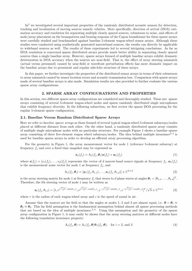
2.1. Baseline Versus Random Distributed Sparse ArraysHere we refer to baseline sparse arrays as those formed of several typical wagon-wheel 5-element subarrays/nodesplaced at different distance from each other. On the other hand, a randomly distributed sparse array consistsof multiple single microphone nodes with no particular structure. For example Figure 1 shows a baseline sparsearray consisting of three five-element wagon wheel subarrays/nodes. The idea behind multiple invariance3, 4 isused for baseline sparse arrays in order to develop an efficient array processing algorithm.

For the geometry in Figure 1, the array measurement vector for node 1 (reference 5-element subarray) atfrequency fj and over a fixed time snapshot may be expressed as

x1(fj) = A1(fj , θ1)s(fj) + n1(fj) (1)

where s(fj) = [s1(fj), . . . , sd(fj)] represents the vector of d narrow-band source signals at frequency fj , n1(fj)is the measurement noise vector for node 1 at frequency fj , and

A1(fj ,θi) = [a1(fj , θ1,1), . . . ,a1(fj , θ1,d)] ∈ C5×d (2)

is the array steering matrix for node 1 at frequency fj that steers to d plane-waves at angles θ1 = [θ1,1, . . . , θ1,d]T .Therefore, the lth steering vector of node 1 may be written as

a1(fj , θ1,l) = [1, ej2πfjr

c sin(θ1,l), ej2πfjr

c cos(θ1,l), e−j2πfjr

c sin(θ1,l), e−j2πfjr

c cos(θ1,l)]T /√

5 ∈ C5×1 (3)

where r is the radius of each wagon-wheel array and c is the speed of sound in air.

Assume that the sources are far field so that the angles at nodes 1, 2 and 3 are almost equal, i.e. θ = θ1 ≈θ2 ≈ θ3. This far field assumption is the fundamental assumption behind almost all sparse processing methodsthat are based on the idea of multiple invariance.3, 4 Using this assumption and the geometry of the sparsearray configuration in Figure 1, it may easily be shown that the array steering matrices at different nodes havethe following translation invariance property:

Ai(fj , θ) = A1(fj , θ)Φi(fj , θ); for i = 2, and 3 (4)

1

2

3

4

5

Node 1

1

2

3

4

5

Node 3

1

2

3

4

5

Node 2

0 . 6

1 m

531.2 m

584.9 m

589.5 m

Figure 1. A sparse configuration with three 5-element wagon wheel subarrays.

with Φi(fj ,θ) = Diag[e−j2πfj

c (xisin(θ1)+yicos(θ1)) · · · e−j2πfj

c (xisin(θd)+yicos(θd))] where xi and yi are the distancesbetween node i and node 1 along the x− and y−axes, respectively, assuming that node 1 is positioned at the originof the coordinate system. Using this invariance property, we may define the augmented array steering matrixA(fj , θ), consisting of the array steering matrices of a subset or all the nodes, along with their correspondingaugmented array measurement vector z(fj). For the three-node array case, as shown in Figure 1, we can write

A(fj ,θ) =

A1(fj ,θ)A2(fj ,θ)A3(fj ,θ)

=

A1(fj , θ)A1(fj , θ)Φ2(fj , θ)A1(fj , θ)Φ3(fj , θ)

(5)

andx(fj) = [xH

1 (fj) xH2 (fj) xH

3 (fj)]H (6)

The augmented measurement vector x(fj) may be viewed as an array measurement vector recorded by alarger array with steering matrix A(fj , θ). In other words, x(fj) and A(fj ,θ) are regarded as the measurementvector and steering matrix for a single large array, and hence all the standard beamforming and DOA estimationmethods5 may be applied to them in order to estimate the angles θ = [θ1, . . . , θd]T . For example, we may usethe Capon beamforming method5 to estimate the angles:

PCapon(fj , θl) =1

aH(fj , θl)R−1xx (fj)a(fj , θl)

(7)

where PCapon(fj , θl) is the true Capon power spectrum, a(fj , θl) is the lth column of A(fj ,θ), and Rxx(fj) =E[x(fj)xH(fj)] is the true covariance matrix of x(fj).

In practice, however, where only a limited number of samples are available, the true covariance matrix canbe replaced by the sample covariance matrix R̂xx(fj) = 1

K

∑Kk=1 x(fj , k)x(fj , k)H where x(fj , k) is the sample

at snapshot k. This leads to the “practical” Capon power

P̂Capon(fj , θl) =1

aH(fj , θl)R̂−1

xx (fj)a(fj , θl). (8)

This practical Capon power spectrum is related to the theoretical one in (7) using

P̂Capon(f, θ) = PCapon(f, θ)η(θ) (9)

for any frequency f and angle θ. Here η(θ) is a random variable with scaled Chi square distribution:

fη(θ)(x) =KK−M+1

(K −M)!xK−Me−Kx, x ≥ 0. (10)

where M is the number of sensors in the array. The proof is omitted here. We note that although η(θ) has thedistribution independent of θ, the specific realizations of η(θ) are different for different θ. If K −M À 1, thenwith high probability, η(θ) concentrate around one. As K −M →∞, η(θ) → 1 in probability. In our numericalexperiments, M = 15 (15 sensors) and K = 1024, hence K −M À 1. Thus, in the subsequent discussions, weuse the theoretical Capon power spectrum instead of the practical one. Additionally, without loss of generality,we assume unit noise power, i.e. E[nnH ] = I.

To simplify our discussions let us now consider the case where only a single source is present with DOA θ0 andsignal power Ps. Thus, the covariance matrix of the recorded signal x(f) becomes Rxx(f) = a(f, θ0)aH(f, θ0)Ps(f)+I. Inserting this into the expression for the theoretical Capon power spectrum (7) and applying the matrix in-version lemma yields

PCapon(f, θ) =1

1− Ps(f)1+Ps(f) |aH(f, θ)a(f, θ0)|2

(11)

Clearly, the power spectrum is determined by the “Radiation Pattern” function5 PRP(f, θ) , |aH(f, θ)a(f, θ0)|.As a result, in the single source case, the study of the radiation pattern function can provide us sufficient infor-mation on the power spectrum of the Capon beamformer for a particular array configuration.

As far as the sparse arrays formed of baseline 5-element nodes are concerned, the radiation pattern can beexpressed5 as

P (f, θ) = P1(f, θ)P2(f, θ). (12)

where P1(f, θ) = |aH1 (f, θ)a1(f, θ0)| and P2(f, θ) = |aH

2 (f, θ)a2(f, θ0)| are the radiation patterns of one 5-elementnode and L-node array, respectively. For the 5-element node the steering vector is given in (3). If the sparse array

is composed of L nodes, then a2(f, θ) =[e−j2π

y1 cos θ+x1 sin θλ , . . . , e−j2π

yL cos θ+xL sin θ

λ

]T

/√

L where the center of

the lth node is assumed to be at pl = [xl, yl]T

, l = 1, . . . , L and λ = c/f is the wavelength.

To simplify the analysis we consider two different 5-element node array configurations with L = 3 as shownin Figure 2. We assume r = λ

2 and the true source DOA is at θ0 = 0. The plot of the radiation pattern P1(f, θ)is shown in Figure 3. The radiation pattern P2(f, θ) associated with the sparse array in Figure 2(a) is shownin Figure 4, where m is the number of the half-wavelength node separation distances as shown in Figure 2(a).Figure 6(a) shows the overall radiation pattern P (f, θ) as given by (12).

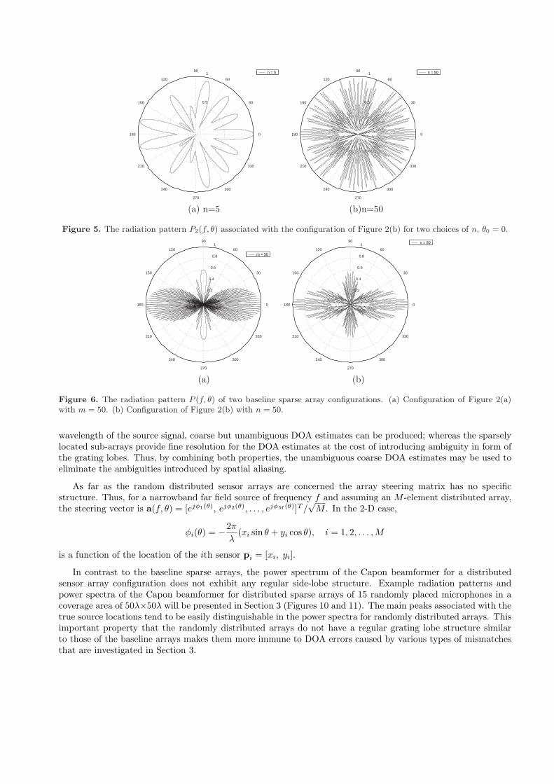
We set the center of mass of the equilateral triangle of Figure 2(b) as the origin point of Cartesian coordinate.It follows from the structure of a2(f, θ) that the steering vector associated with the sparse array configuration

of Figure 2(b) is a2(f, θ) =[e−jπ n sin θ√

3 , e−jπ

�(n cos θ

2 −n sin θ2√

3)

�, e

jπ�

(n cos θ2 + n sin θ

2√

3)

�]T

. The radiation pattern P2(f, θ)

associated with Figure 2(b) is shown in Figure 5, where n is the number of the half-wavelength node separationdistances as shown in Figure 2(b). Figure 6(b) shows the overall radiation pattern P (f, θ) for this sparse arrayconfiguration.

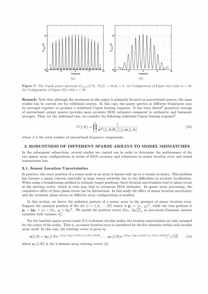
Remark: From these results we clearly notice this important property of the radiation patterns: when thenodes are far away from each other, e.g., separated by distances greater than 25λ, then for both configurationsin Figure 2 (around θ0 = 0) there are several side-lobes with amplitude near one. It follows from (11) that theCapon power spectrum also has several closely located peaks as shown in Figure 7. Clearly, the DOA estimatesgenerated using the Capon beamformer are very sensitive to the perturbations such as background noise, finite

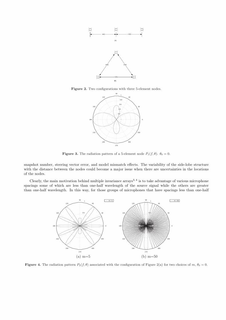
Figure 2. Two configurations with three 5-element nodes.

0.2

0.4

0.6

0.8

1

30

210

60

240

90

270

120

300

150

330

180 0

Figure 3. The radiation pattern of a 5-element node P1(f, θ). θ0 = 0.

snapshot number, steering vector error, and model mismatch effects. The variability of the side-lobe structurewith the distance between the nodes could become a major issue when there are uncertainties in the locationsof the nodes.

Clearly, the main motivation behind multiple invariance arrays3, 4 is to take advantage of various microphonespacings some of which are less than one-half wavelength of the source signal while the others are greaterthan one-half wavelength. In this way, for those groups of microphones that have spacings less than one-half

0.5

1

30

210

60

240

90

270

120

300

150

330

180 0

m = 5

0.5

1

30

210

60

240

90

270

120

300

150

330

180 0

m = 50

(a) m=5 (b) m=50

Figure 4. The radiation pattern P2(f, θ) associated with the configuration of Figure 2(a) for two choices of m, θ0 = 0.

0.5

1

30

210

60

240

90

270

120

300

150

330

180 0

n = 5

0.5

1

30

210

60

240

90

270

120

300

150

330

180 0

n = 50

(a) n=5 (b)n=50

Figure 5. The radiation pattern P2(f, θ) associated with the configuration of Figure 2(b) for two choices of n, θ0 = 0.

0.2

0.4

0.6

0.8

1

30

210

60

240

90

270

120

300

150

330

180 0

m = 50

0.2

0.4

0.6

0.8

1

30

210

60

240

90

270

120

300

150

330

180 0

n = 50

(a) (b)

Figure 6. The radiation pattern P (f, θ) of two baseline sparse array configurations. (a) Configuration of Figure 2(a)with m = 50. (b) Configuration of Figure 2(b) with n = 50.

wavelength of the source signal, coarse but unambiguous DOA estimates can be produced; whereas the sparselylocated sub-arrays provide fine resolution for the DOA estimates at the cost of introducing ambiguity in form ofthe grating lobes. Thus, by combining both properties, the unambiguous coarse DOA estimates may be used toeliminate the ambiguities introduced by spatial aliasing.

As far as the random distributed sensor arrays are concerned the array steering matrix has no specificstructure. Thus, for a narrowband far field source of frequency f and assuming an M -element distributed array,the steering vector is a(f, θ) = [ejφ1(θ), ejφ2(θ), . . . , ejφM (θ)]T /

√M . In the 2-D case,

φi(θ) = −2π

λ(xi sin θ + yi cos θ), i = 1, 2, . . . ,M

is a function of the location of the ith sensor pi = [xi, yi].

In contrast to the baseline sparse arrays, the power spectrum of the Capon beamformer for a distributedsensor array configuration does not exhibit any regular side-lobe structure. Example radiation patterns andpower spectra of the Capon beamformer for distributed sparse arrays of 15 randomly placed microphones in acoverage area of 50λ×50λ will be presented in Section 3 (Figures 10 and 11). The main peaks associated with thetrue source locations tend to be easily distinguishable in the power spectra for randomly distributed arrays. Thisimportant property that the randomly distributed arrays do not have a regular grating lobe structure similarto those of the baseline arrays makes them more immune to DOA errors caused by various types of mismatchesthat are investigated in Section 3.

−10 −5 0 5 1010

0

101

θ (degree)

PC

apon

(θ)

−10 −5 0 5 1010

0

101

θ (degree)

PC

apon

(θ)

(a) (b)

Figure 7. The Capon power spectrum PCapon(f, θ). Ps(f) = 10, θ0 = 0. (a) Configuration of Figure 2(a) with m = 50.(b) Configuration of Figure 2(b) with n = 50.

Remark: Note that although the treatment in this paper is primarily focused on narrowband sources, the samestudies can be carried out for wideband sources. In this case, the power spectra at different frequencies maybe averaged together to produce a wideband Capon bearing response. It has been shown6 geometric averageof narrowband output powers provides more accurate DOA estimates compared to arithmetic and harmonicaverages. Thus, for the wideband case, we consider the following wideband Capon bearing response6

C(f, θl) =J∏

i=1

1aH(fj , θl)R−1

xx (fj)a(fj , θl)(13)

where J is the total number of narrowband frequency components.

3. ROBUSTNESS OF DIFFERENT SPARSE ARRAYS TO MODEL MISMATCHES

In the subsequent subsections, several studies are carried out in order to determine the performance of thetwo sparse array configurations in terms of DOA accuracy and robustness to sensor location error and soundtransmission loss.

3.1. Sensor Location Uncertainties

In practice, the exact position of a sensor node in an array is known only up to a certain accuracy. This problemhas become a major concern especially in large sensor networks due to the difficulties in accurate localization.When using a beamforming method to estimate target positions, these location uncertainties lead to phase errorsin the steering vector, which in turn may lead to erroneous DOA estimates. In sparse array processing, thecumulative effect of these phase errors can be detrimental. In this study the effect of sensor location uncertaintyand the resultant phase errors on different array configurations is studied.

In this section, we derive the radiation pattern of a sensor array in the presence of sensor location error.Suppose the nominal position of the ith (i = 1, 2, . . . ,M) sensor is pi = [xi, yi]T , while the true position ispi + ∆pi = [xi + δxi, yi + δyi]T . We model the position errors {δxi, δyi}M

i=1 as zero-mean Gaussian randomvariables with variance σ2

p.

For the baseline sparse arrays made of L 5-element circular nodes, the location uncertainties are only assumedfor the center of the nodes. That is, no sensor location error is considered for the five elements within each circulararray itself. In this case, the steering vector is given by

a(f, θ) = [a1(f, θ)e−j[(y1+δy1) cos θ+(x1+δx1) sin θ], . . . ,a1(f, θ))e−j[(yL+δyL) cos θ+(xL+δxL) sin θ]]T /√

5L (14)

where a1(f, θ)) is the 5-element array steering vector (3).

For the randomly distributed microphone arrays, location uncertainties are assumed for every sensor. Thesteering vector for the random sensor configuration with location uncertainties is given by,

a(f, θ) = [e−j[(y1+δy1) cos θ+(x1+δx1) sin θ] 2πfλ , . . . , e−j[(yM+δyM ) cos θ+(xM+δxM ) sin θ] 2π

λ ]T /√

M (15)

where M is the number of sensors in the randomly distributed array.

For a narrowband source of frequency f and DOA θ0, the radiation pattern with location errors is

PRP(f, θ) =

∣∣∣∣∣M∑

i=1

ej 2πλ (xi sin θ+yi cos θ)e−j 2π

λ [(xi+δxi) sin θ0+(yi+δyi) cos θ0]

∣∣∣∣∣ . (16)

The array gain at the steering direction θ0 is

Ga =M∑

i=1

e−j 2πλ (δxi sin θ0+δyi cos θo)

If there is no sensor displacement, then Ga = M . But in presence of sensor location error, Ga is a randomvariable with mean

E [Ga] = E

[M∑

i=1

e−j 2πλ (δxi sin θ0+δyi cos θo)

]= ME

[e−j 2π

λ (δxi sin θ0+δyi cos θo)],

where

E[e−j 2π

λ (δxi sin θ0+δyi cos θo)]

=∫ ∞

−∞e−j 2π

λ x 1√2πσ2

p

e− x2

2σ2p dx = e−

2π2σ2p

λ2 . (17)

From (17), we can readily see that to make the gain loss less than 3 dB, σ2p should be no more than ln

√2

2π2 λ2 =0.0176λ2. If σp = λ, then the gain loss due to position error is more than 170 dB, and hence the array usuallywill not work at all.

In the following, we derive E{P2

RP(f, θ)}

to examine the effects of location uncertainties on the radiationpattern. According to (16),

E{P2

RP(f, θ)}

= E

{M∑

i=1

M∑

l=1

ej 2πλ (xi sin θ+yi cos θ)e−j 2π

λ [(xi+δxi) sin θ0+(yi+δyi) cos θ0]

e−j 2πλ (xl sin θ+yl cos θ)ej 2π

λ [(xl+δxl) sin θ0+(yl+δyl) cos θ0]}

(18)

=M∑

i=1

M∑

l=1

E{

ej 2πλ (xi sin θ+yi cos θ)e−j 2π

λ [(xi+δxi) sin θ0+(yi+δyi) cos θ0]

e−j 2πλ (xl sin θ+yl cos θ)ej 2π

λ [(xl+δxl) sin θ0+(yl+δyl) cos θ0]}

(19)

=M∑

i=1

M∑

l=1

ej 2πλ (xi sin θ+yi cos θ)e−j 2π

λ (xi sin θ0+yi cos θ0)e−j 2πλ (xl sin θ+yl cos θ)ej 2π

λ (xl sin θ0+yl cos θ0)

E{

ej 2πλ [(δxl sin θ0+δyl cos θ0)−(δxi sin θ0+δyi cos θ0)]

}. (20)

Denote ail = E{

ej 2πλ [(δxl sin θ0+δyl cos θ0)−(δxi sin θ0+δyi cos θ0)]

}, then

ail =

{1 i = l

e−4π2σ2

p

λ2 i 6= l. (21)

Then (20) can be shown to be5

E{P2

RP(f, θ)}

= |a(f, θ)∗a(f, θ0)|2e−4π2σ2

p

λ2 + M

(1− e−

4π2σ2p

λ2

). (22)

Equation (22) clearly shows that the effects of sensor location error on the radiation pattern is two-fold. First,

the radiation pattern is attenuated uniformly by a factor of e−4π2σ2

p

λ2 as shown in the first term of (22). Second,

the side-lobe level is increased by M

(1− e−

4π2σ2p

λ2

).

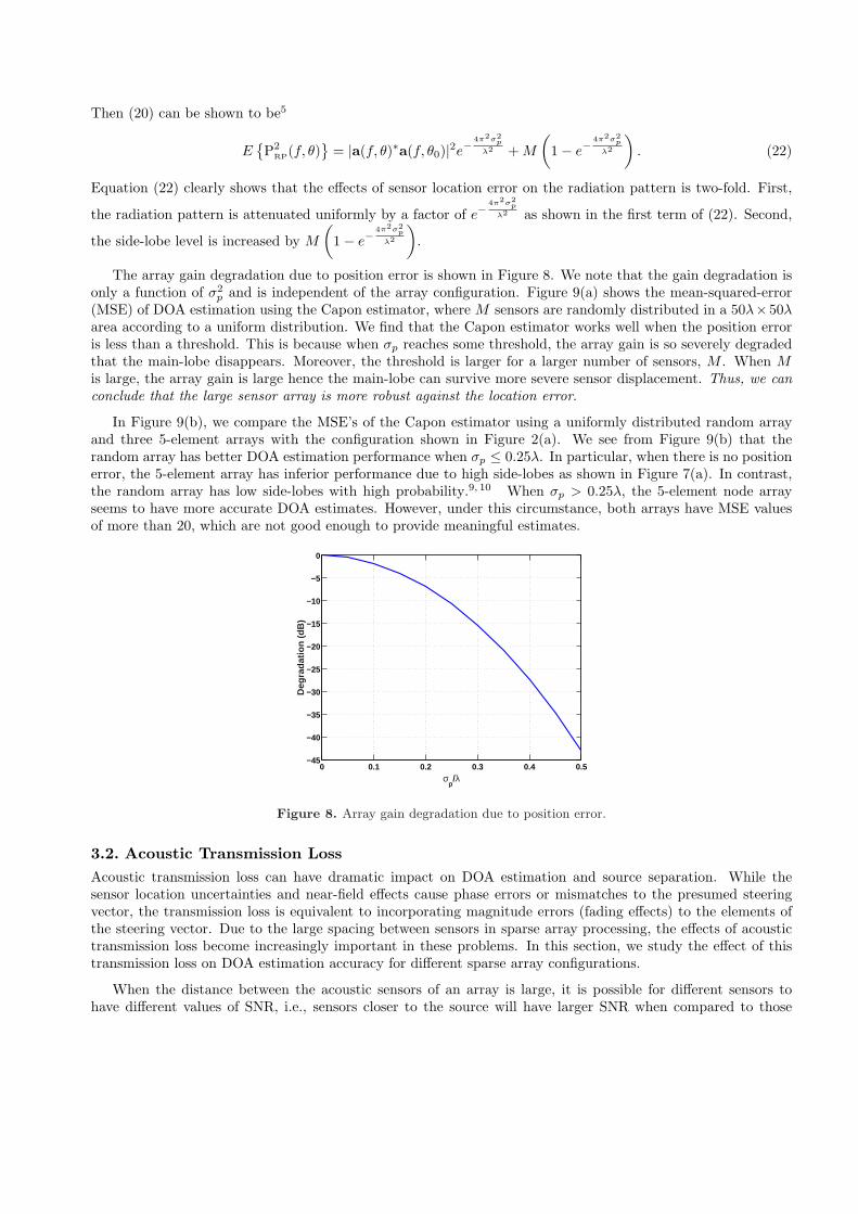
The array gain degradation due to position error is shown in Figure 8. We note that the gain degradation isonly a function of σ2

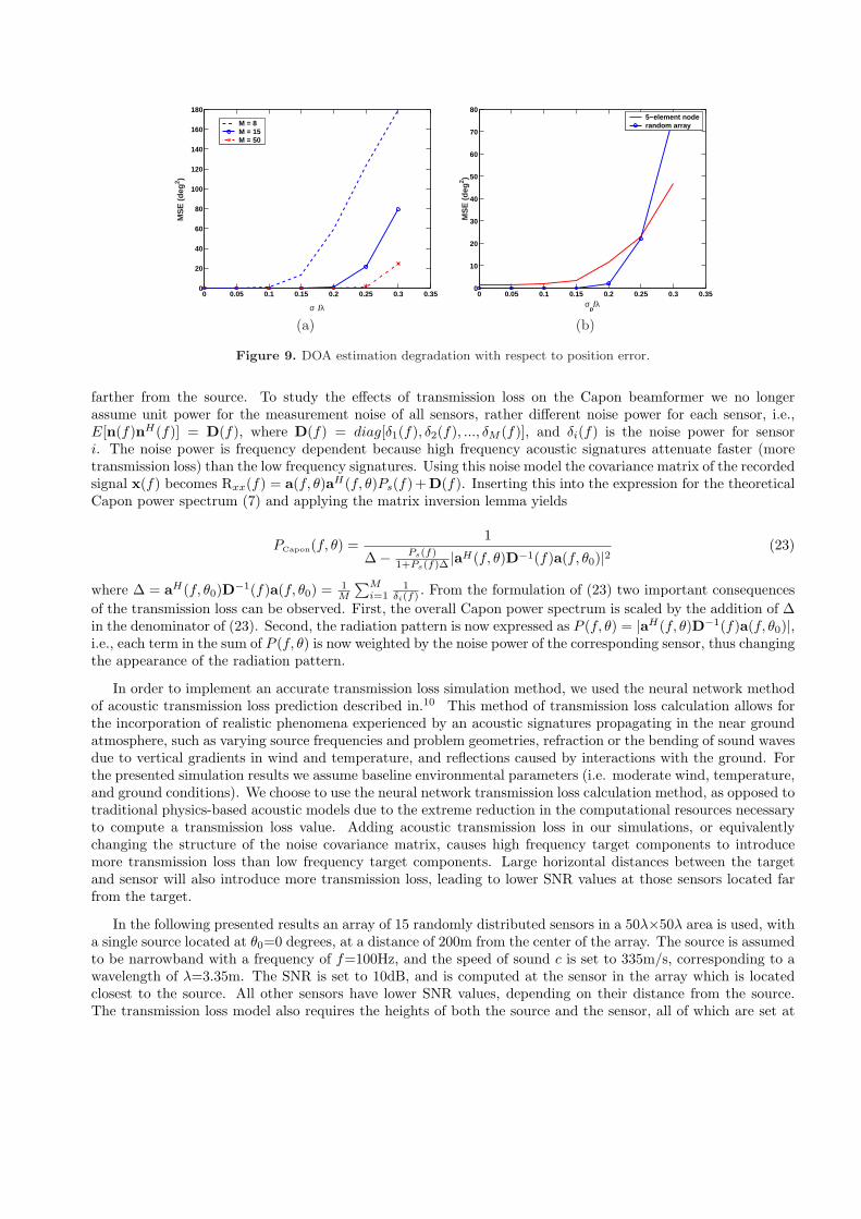
p and is independent of the array configuration. Figure 9(a) shows the mean-squared-error(MSE) of DOA estimation using the Capon estimator, where M sensors are randomly distributed in a 50λ×50λarea according to a uniform distribution. We find that the Capon estimator works well when the position erroris less than a threshold. This is because when σp reaches some threshold, the array gain is so severely degradedthat the main-lobe disappears. Moreover, the threshold is larger for a larger number of sensors, M . When Mis large, the array gain is large hence the main-lobe can survive more severe sensor displacement. Thus, we canconclude that the large sensor array is more robust against the location error.

In Figure 9(b), we compare the MSE’s of the Capon estimator using a uniformly distributed random arrayand three 5-element arrays with the configuration shown in Figure 2(a). We see from Figure 9(b) that therandom array has better DOA estimation performance when σp ≤ 0.25λ. In particular, when there is no positionerror, the 5-element array has inferior performance due to high side-lobes as shown in Figure 7(a). In contrast,the random array has low side-lobes with high probability.9, 10 When σp > 0.25λ, the 5-element node arrayseems to have more accurate DOA estimates. However, under this circumstance, both arrays have MSE valuesof more than 20, which are not good enough to provide meaningful estimates.

0 0.1 0.2 0.3 0.4 0.5−45

−40

−35

−30

−25

−20

−15

−10

−5

0

σp/λ

Deg

rada

tion

(dB

)

Figure 8. Array gain degradation due to position error.

3.2. Acoustic Transmission LossAcoustic transmission loss can have dramatic impact on DOA estimation and source separation. While thesensor location uncertainties and near-field effects cause phase errors or mismatches to the presumed steeringvector, the transmission loss is equivalent to incorporating magnitude errors (fading effects) to the elements ofthe steering vector. Due to the large spacing between sensors in sparse array processing, the effects of acoustictransmission loss become increasingly important in these problems. In this section, we study the effect of thistransmission loss on DOA estimation accuracy for different sparse array configurations.

When the distance between the acoustic sensors of an array is large, it is possible for different sensors tohave different values of SNR, i.e., sensors closer to the source will have larger SNR when compared to those

0 0.05 0.1 0.15 0.2 0.25 0.3 0.350

20

40

60

80

100

120

140

160

180

σp/λ

MS

E (

deg

2 )

M = 8M = 15M = 50

0 0.05 0.1 0.15 0.2 0.25 0.3 0.350

10

20

30

40

50

60

70

80

σp/λ

MS

E (

deg

2 )

5−element noderandom array

(a) (b)

Figure 9. DOA estimation degradation with respect to position error.

farther from the source. To study the effects of transmission loss on the Capon beamformer we no longerassume unit power for the measurement noise of all sensors, rather different noise power for each sensor, i.e.,E[n(f)nH(f)] = D(f), where D(f) = diag[δ1(f), δ2(f), ..., δM (f)], and δi(f) is the noise power for sensori. The noise power is frequency dependent because high frequency acoustic signatures attenuate faster (moretransmission loss) than the low frequency signatures. Using this noise model the covariance matrix of the recordedsignal x(f) becomes Rxx(f) = a(f, θ)aH(f, θ)Ps(f) +D(f). Inserting this into the expression for the theoreticalCapon power spectrum (7) and applying the matrix inversion lemma yields

PCapon(f, θ) =1

∆− Ps(f)1+Ps(f)∆ |aH(f, θ)D−1(f)a(f, θ0)|2

(23)

where ∆ = aH(f, θ0)D−1(f)a(f, θ0) = 1M

∑Mi=1

1δi(f) . From the formulation of (23) two important consequences

of the transmission loss can be observed. First, the overall Capon power spectrum is scaled by the addition of ∆in the denominator of (23). Second, the radiation pattern is now expressed as P (f, θ) = |aH(f, θ)D−1(f)a(f, θ0)|,i.e., each term in the sum of P (f, θ) is now weighted by the noise power of the corresponding sensor, thus changingthe appearance of the radiation pattern.

In order to implement an accurate transmission loss simulation method, we used the neural network methodof acoustic transmission loss prediction described in.10 This method of transmission loss calculation allows forthe incorporation of realistic phenomena experienced by an acoustic signatures propagating in the near groundatmosphere, such as varying source frequencies and problem geometries, refraction or the bending of sound wavesdue to vertical gradients in wind and temperature, and reflections caused by interactions with the ground. Forthe presented simulation results we assume baseline environmental parameters (i.e. moderate wind, temperature,and ground conditions). We choose to use the neural network transmission loss calculation method, as opposed totraditional physics-based acoustic models due to the extreme reduction in the computational resources necessaryto compute a transmission loss value. Adding acoustic transmission loss in our simulations, or equivalentlychanging the structure of the noise covariance matrix, causes high frequency target components to introducemore transmission loss than low frequency target components. Large horizontal distances between the targetand sensor will also introduce more transmission loss, leading to lower SNR values at those sensors located farfrom the target.

In the following presented results an array of 15 randomly distributed sensors in a 50λ×50λ area is used, witha single source located at θ0=0 degrees, at a distance of 200m from the center of the array. The source is assumedto be narrowband with a frequency of f=100Hz, and the speed of sound c is set to 335m/s, corresponding to awavelength of λ=3.35m. The SNR is set to 10dB, and is computed at the sensor in the array which is locatedclosest to the source. All other sensors have lower SNR values, depending on their distance from the source.The transmission loss model also requires the heights of both the source and the sensor, all of which are set at

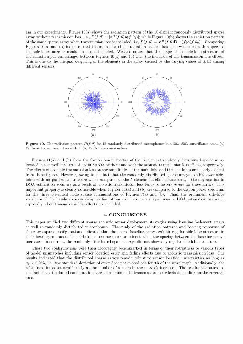
1m in our experiments. Figure 10(a) shows the radiation pattern of the 15 element randomly distributed sparsearray without transmission loss, i.e., P (f, θ) = |aH(f, θ)a(f, θ0)|; while Figure 10(b) shows the radiation patternof the same sparse array when transmission loss is included, i.e, P (f, θ) = |aH(f, θ)D−1(f)a(f, θ0)|. ComparingFigures 10(a) and (b) indicates that the main lobe of the radiation pattern has been weakened with respect tothe side-lobes once transmission loss is included. We also notice that the shape of the side-lobe structure ofthe radiation pattern changes between Figures 10(a) and (b) with the inclusion of the transmission loss effects.This is due to the unequal weighting of the elements in the array, caused by the varying values of SNR amongdifferent sensors.

0.2

30

210

60

240

90

270

120

300

150

330

180 0

0.0005

30

210

60

240

90

270

120

300

150

330

180 0

(a) (b)

Figure 10. The radiation pattern P (f, θ) for 15 randomly distributed microphones in a 50λ×50λ surveillance area. (a)Without transmission loss added. (b) With Transmission loss.

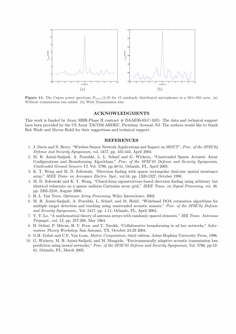
Figures 11(a) and (b) show the Capon power spectra of the 15-element randomly distributed sparse arraylocated in a surveillance area of size 50λ×50λ, without and with the acoustic transmission loss effects, respectively.The effects of acoustic transmission loss on the amplitudes of the main-lobe and the side-lobes are clearly evidentfrom these figures. However, owing to the fact that the randomly distributed sparse arrays exhibit lower side-lobes with no particular structure when compared to the 5-element baseline sparse arrays, the degradation inDOA estimation accuracy as a result of acoustic transmission loss tends to be less severe for these arrays. Thisimportant property is clearly noticeable when Figures 11(a) and (b) are compared to the Capon power spectrumfor the three 5-element node sparse configurations of Figures 7(a) and (b). Thus, the prominent side-lobestructure of the baseline sparse array configurations can become a major issue in DOA estimation accuracy,especially when transmission loss effects are included.

4. CONCLUSIONS

This paper studied two different sparse acoustic sensor deployment strategies using baseline 5-element arraysas well as randomly distributed microphones. The study of the radiation patterns and bearing responses ofthese two sparse configurations indicated that the sparse baseline arrays exhibit regular side-lobe structure intheir bearing responses. The side-lobes become more prominent when the spacing between the baseline arraysincreases. In contrast, the randomly distributed sparse arrays did not show any regular side-lobe structure.

These two configurations were then thoroughly benchmarked in terms of their robustness to various typesof model mismatches including sensor location error and fading effects due to acoustic transmission loss. Ourresults indicated that the distributed sparse arrays remain robust to sensor location uncertainties as long asσp < 0.25λ, i.e., the standard deviation of error does not exceed one fourth of the wavelength. Additionally, therobustness improves significantly as the number of sensors in the network increases. The results also attest tothe fact that distributed configurations are more immune to transmission loss effects depending on the coveragearea.

−10 −8 −6 −4 −2 0 2 4 6 8 10−2

0

2

4

6

8

10

12

θ (degree)

PC

apon

(θ)

[dB

]

−10 −8 −6 −4 −2 0 2 4 6 8 10−47

−46

−45

−44

−43

−42

−41

θ (degree)

PC

apon

(θ)

[dB

]

(a) (b)

Figure 11. The Capon power spectrum PCapon(f, θ) for 15 randomly distributed microphones in a 50λ×50λ area. (a)Without transmission loss added. (b) With Transmission loss.

ACKNOWLEDGMENTS

This work is funded by Army SBIR-Phase II contract # DAAE30-03-C-1055. The data and technical supporthave been provided by the US Army TACOM-ARDEC, Picatinny Arsenal, NJ. The authors would like to thankBob Wade and Myron Hohil for their suggestions and technical support.

REFERENCES1. J. Davis and N. Berry, “Wireless Sensor Network Applications and Impact on MOUT”, Proc. of the SPIE’04

Defense and Security Symposium, vol. 5417, pp. 435-443, April 2004.2. M. R. Azimi-Sadjadi, A. Pezeshki, L. L. Scharf and G. Wichern, “Unattended Sparse Acoustic Array

Configurations and Beamforming Algorithms,” Proc. of the SPIE’05 Defense and Security Symposium,Unattended Ground Sensors VI, Vol. 5796, pp.40-51, Orlando, FL, April 2005.

3. K. T. Wong and M. D. Zoltowski, “Direction finding with sparse rectangular dual-size spatial invariancearray,” IEEE Trans. on Aerospace Electrn. Syst., vol.34, pp. 1320-1327, October 1998.

4. M. D. Zoltowski and K. T. Wong, “Closed-form eigenstructure-based direction finding using arbitrary butidentical subarrays on a sparse uniform Cartesian array grid,” IEEE Trans. on Signal Processing, vol. 48,pp. 2205-2210, August 2000.

5. H. L. Van Trees, Optimum Array Processing, Wiley Interscience, 2002.6. M. R. Azimi-Sadjadi, A. Pezeshki, L. Scharf, and M. Hohil, “Wideband DOA estimation algorithms for

multiple target detection and tracking using unattended acoustic sensors,” Proc. of the SPIE’04 Defenseand Security Symposium., Vol. 5417, pp. 1-11, Orlando, FL, April 2004.

7. Y. T. Lo, “A mathematical theory of antenna arrays with randomly spaced elements,” IRE Trans. AntennasPropagat., vol. 12, pp. 257-268, May 1964.

8. H. Ochiai, P. Mitran, H. V. Poor, and V. Tarokh, “Collaborative beamforming in ad hoc networks,” Infor-mation Theory Workshop, San Antonio, TX, October 24-29 2004.

9. G.H. Golub and C.F. Van Loan, Matrix Computation, third edition, Johns Hopkins University Press, 1996.10. G. Wichern, M. R. Azimi-Sadjadi, and M. Mungiole, “Environmentally adaptive acoustic transmission loss

prediction using neural networks,” Proc. of the SPIE’05 Defense and Security Symposium, Vol. 5796, pp.52-61, Orlando, FL, March 2005.